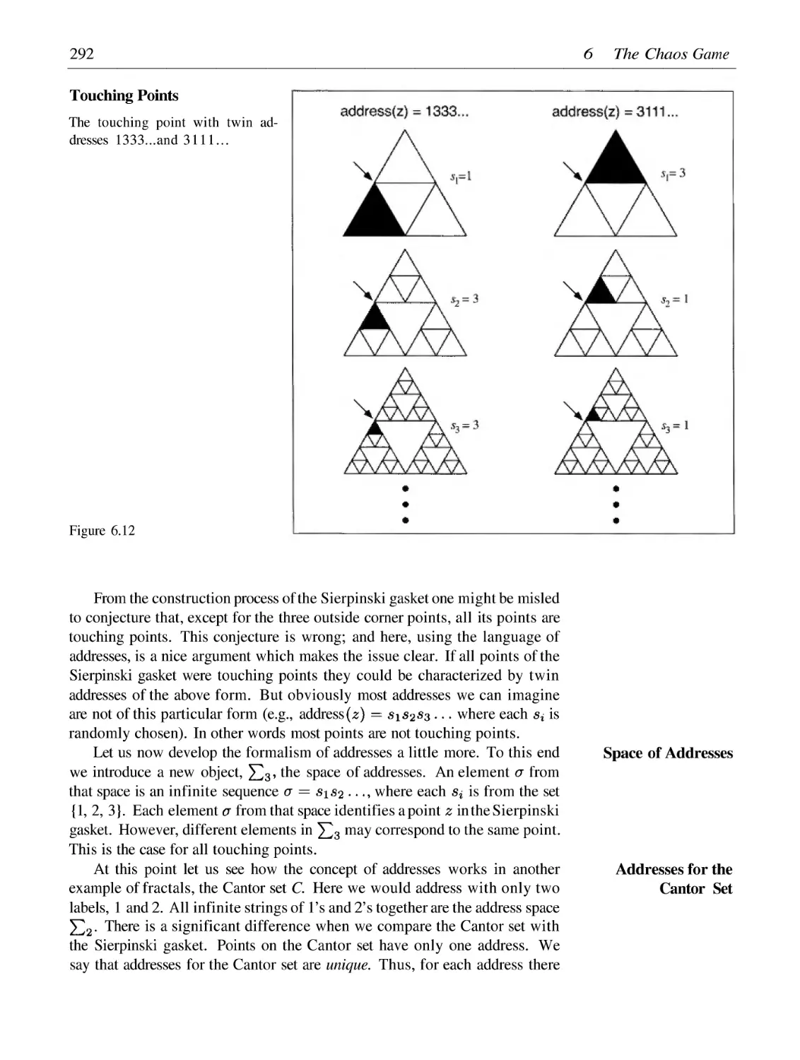
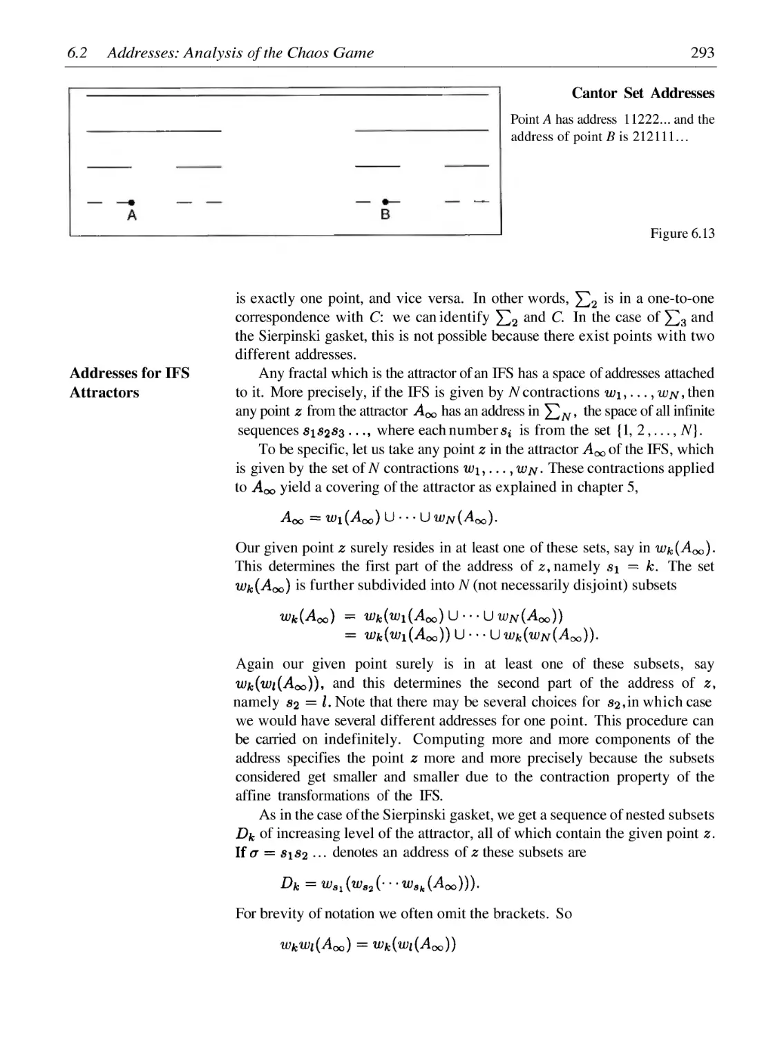
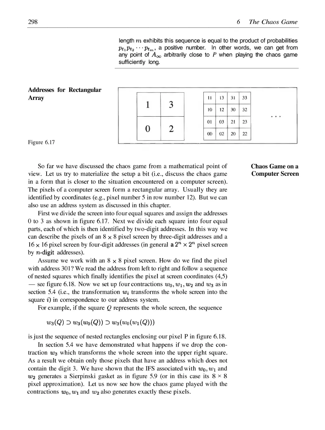
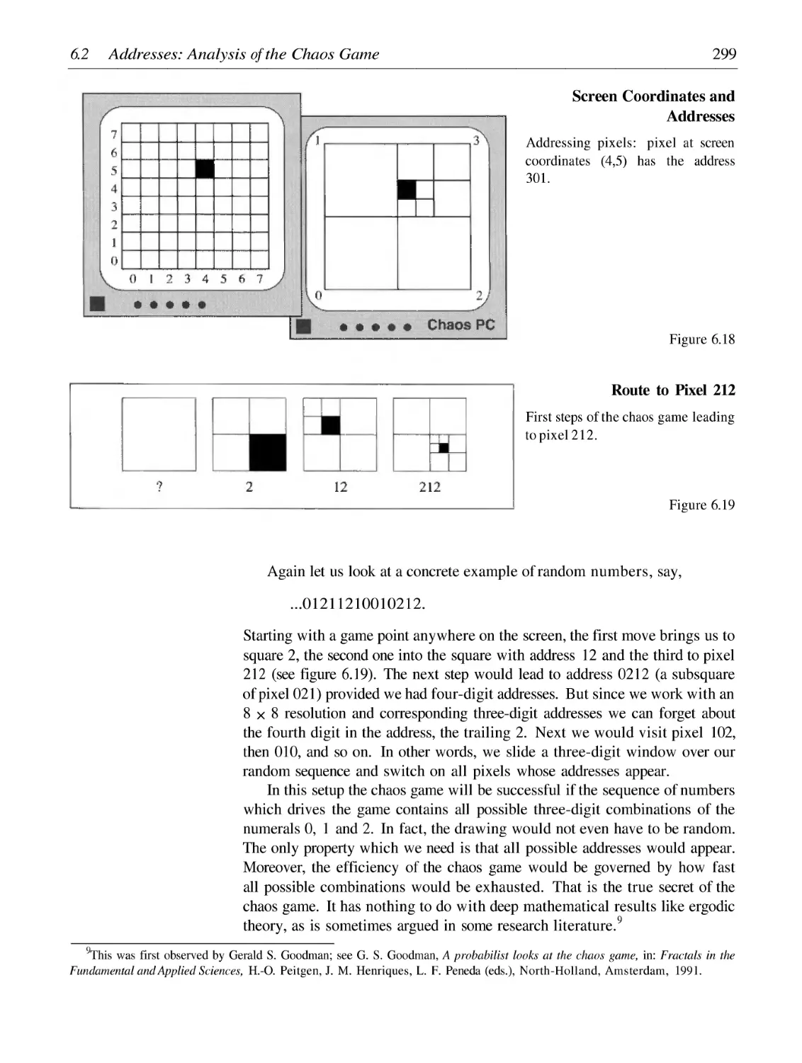
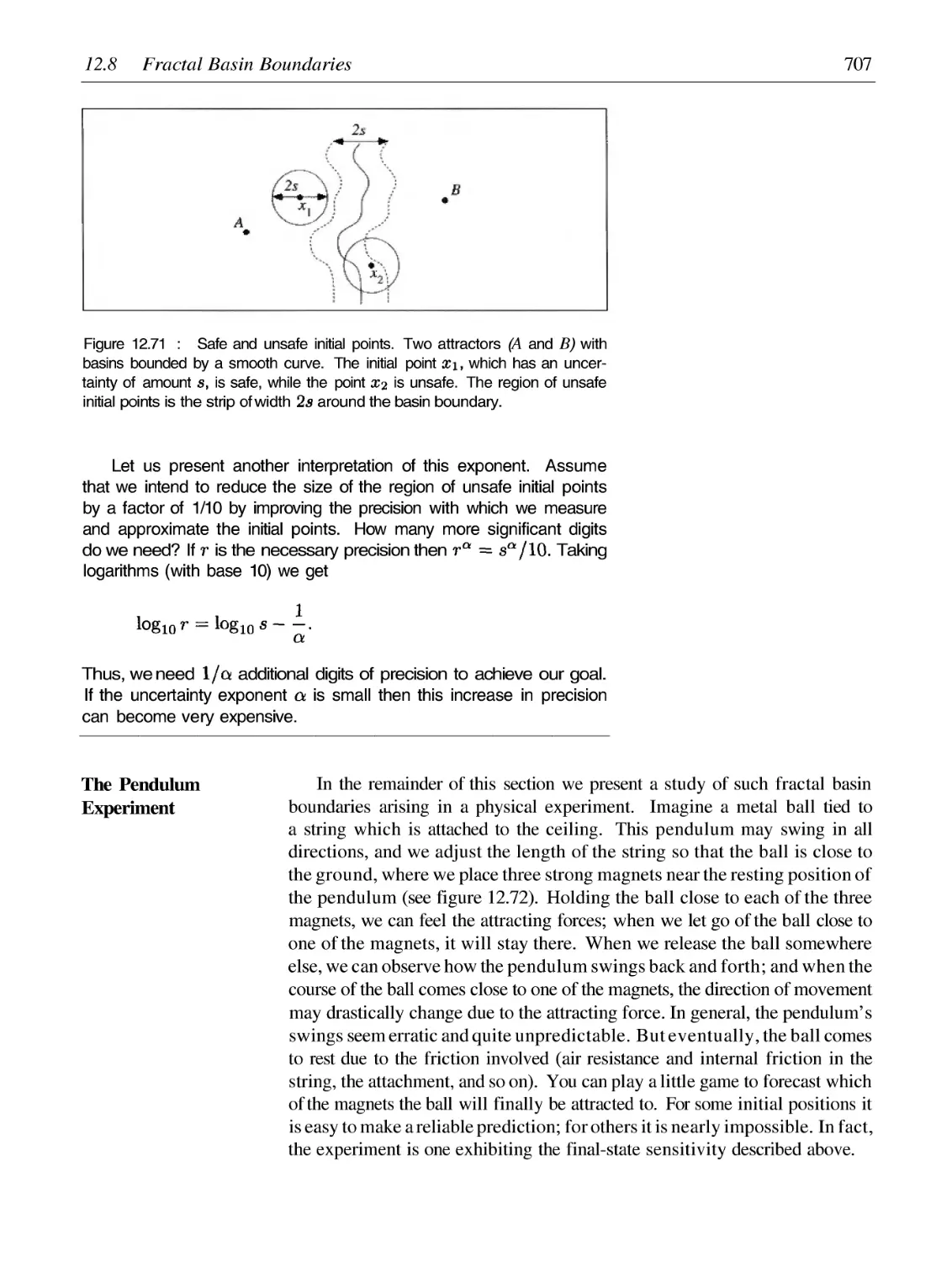
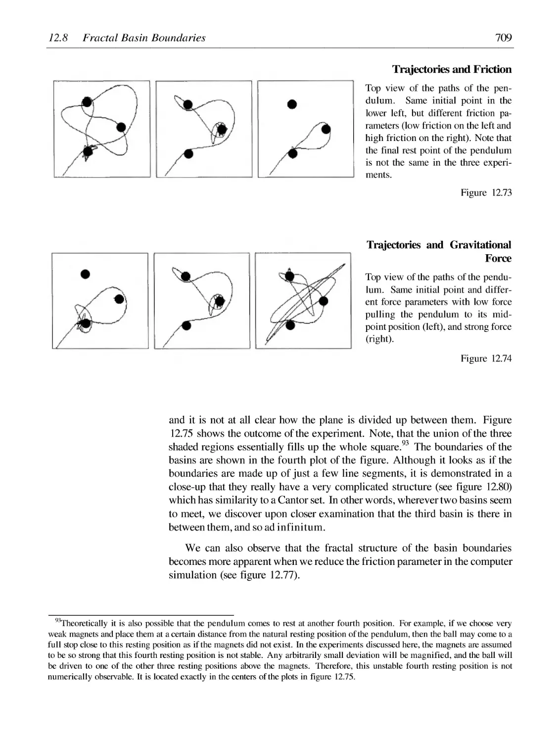
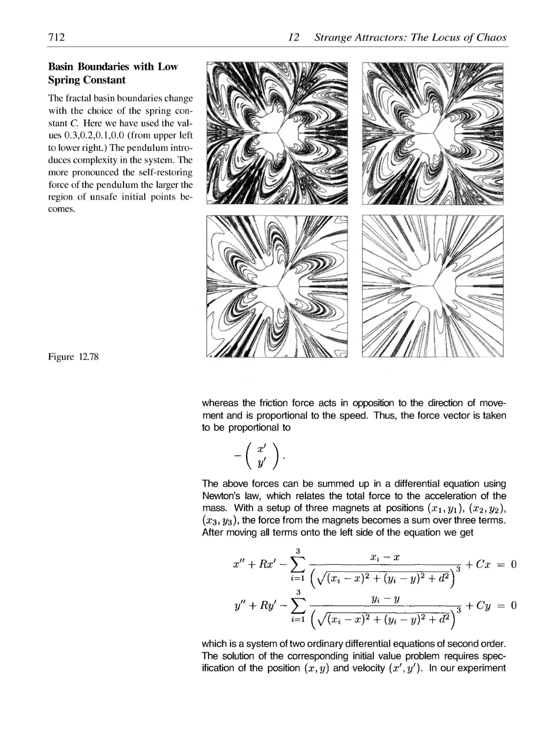
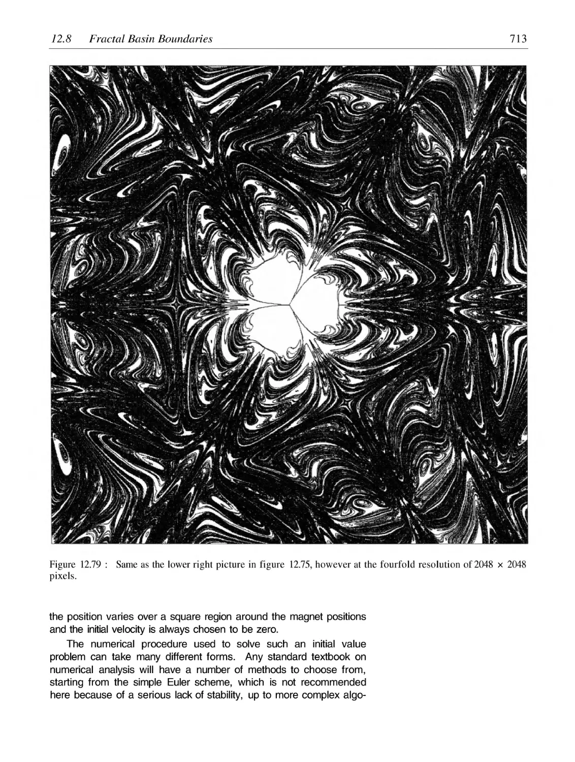
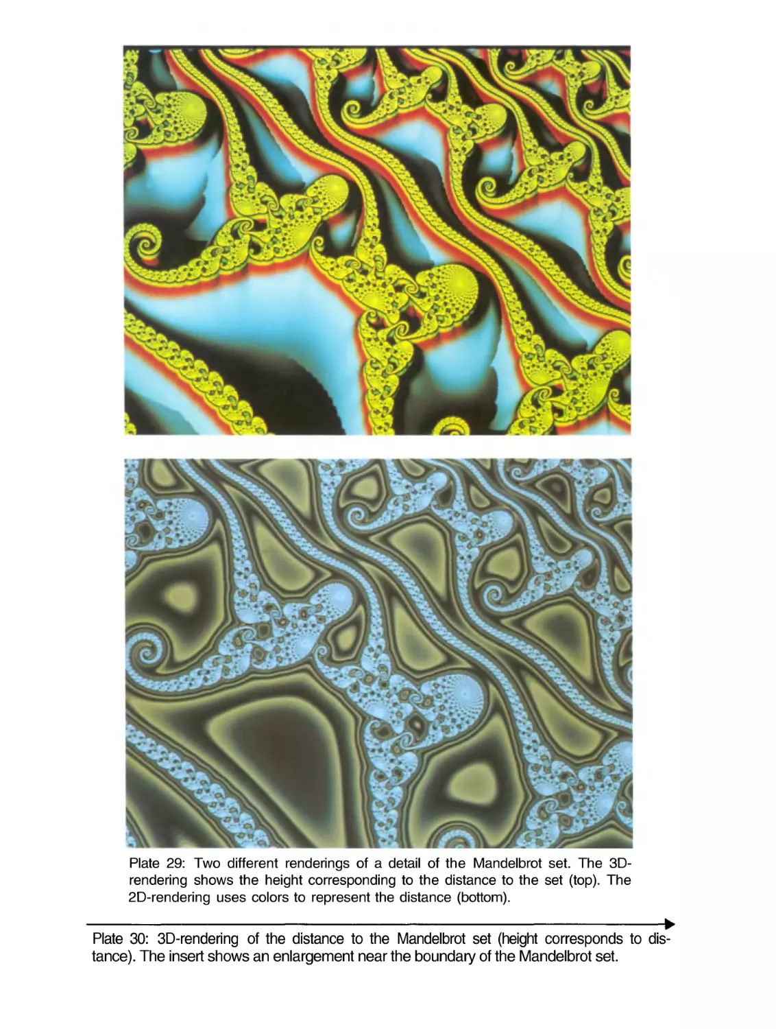
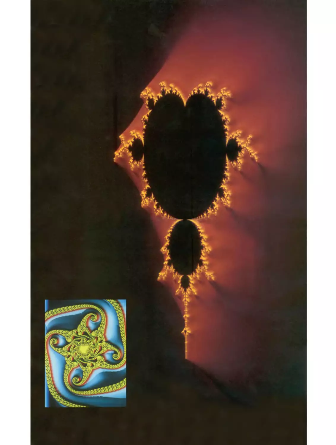
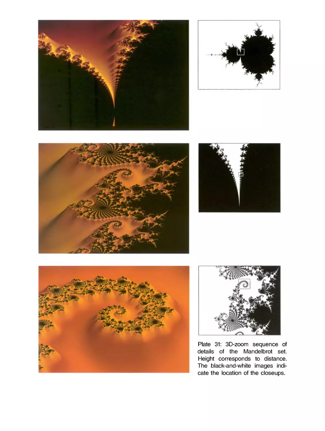
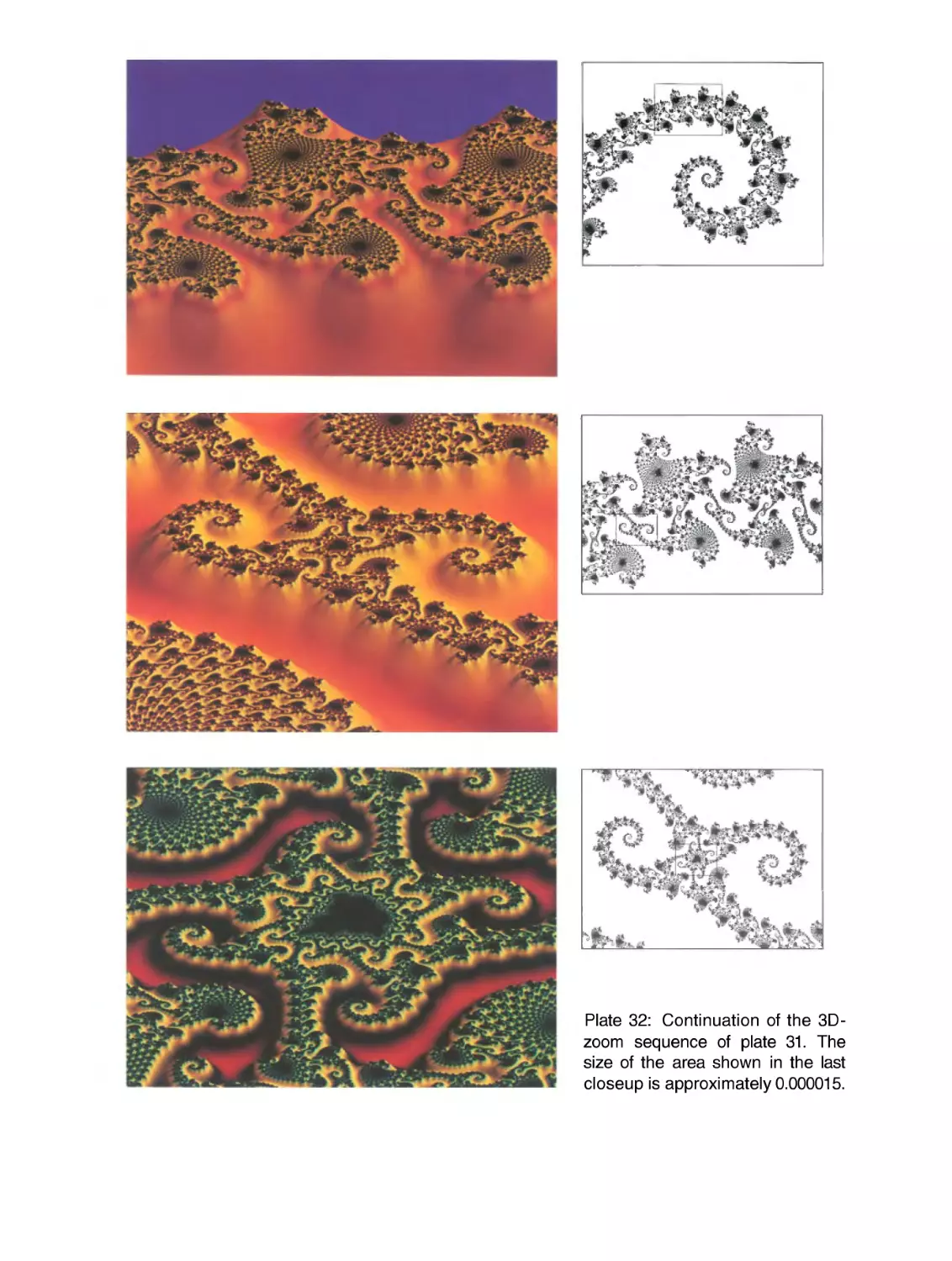
/


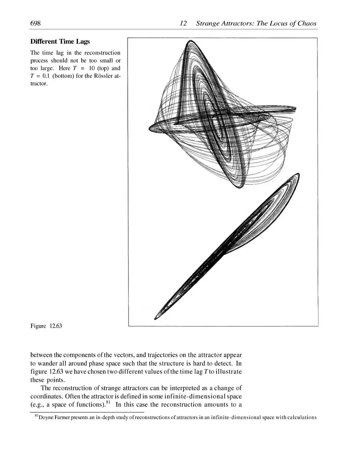


Автор: Peitgen H.-O. Juergens H. Saupe D.
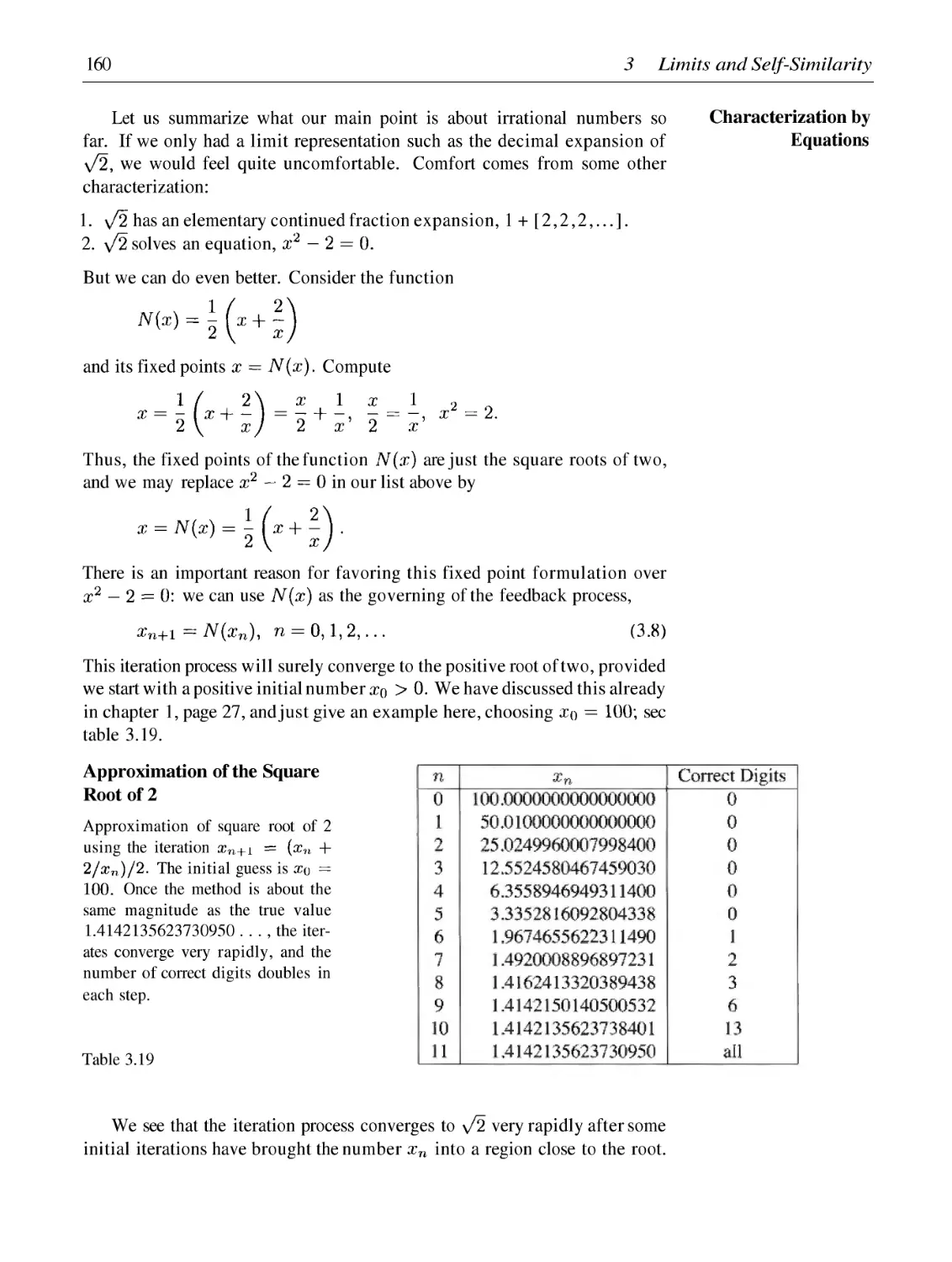
Теги: mathematics geometry fractals fractal graphics
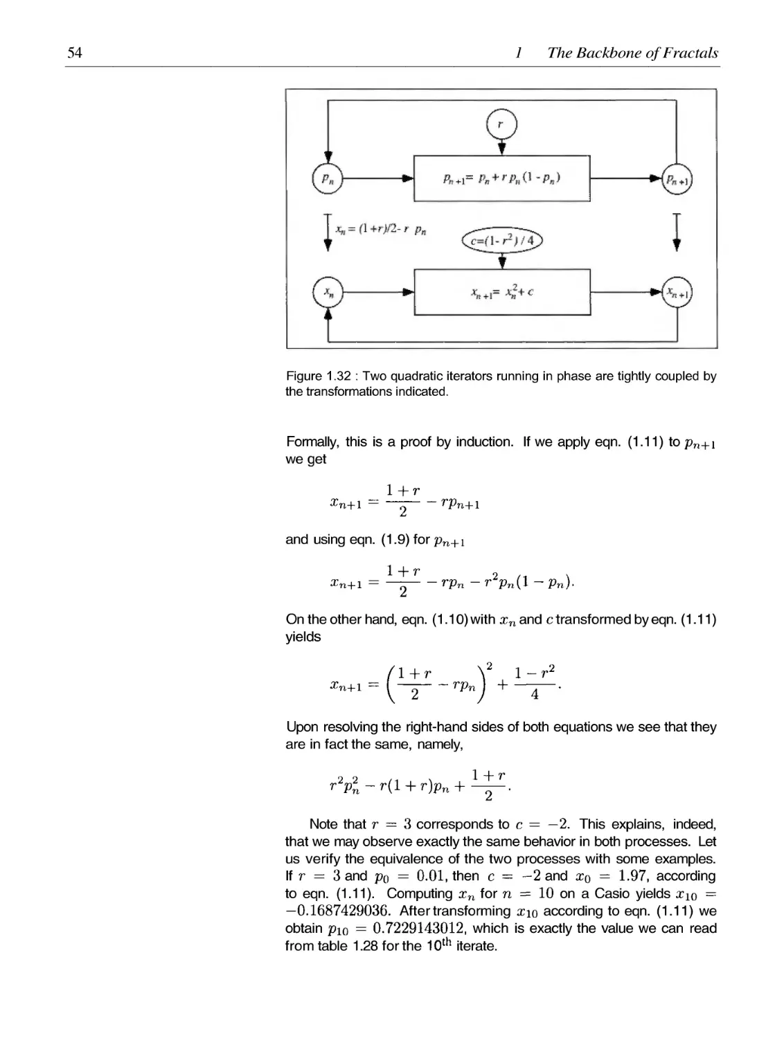
ISBN: 0-387-20229-3
Год: 2004


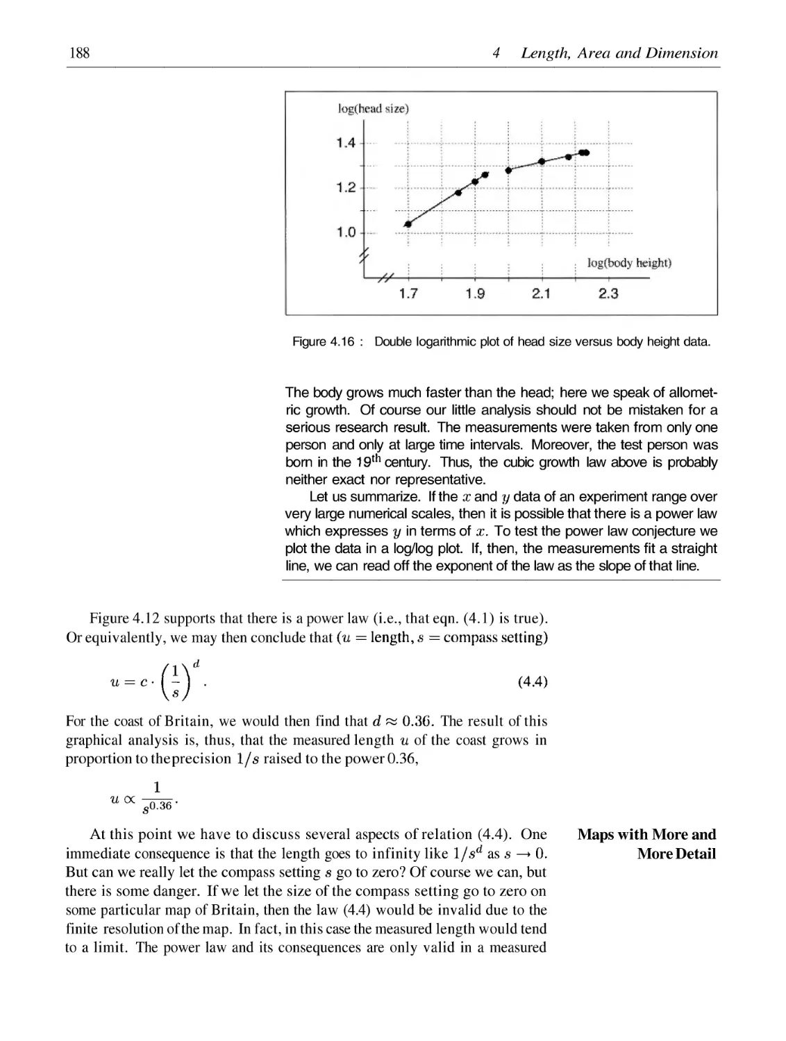
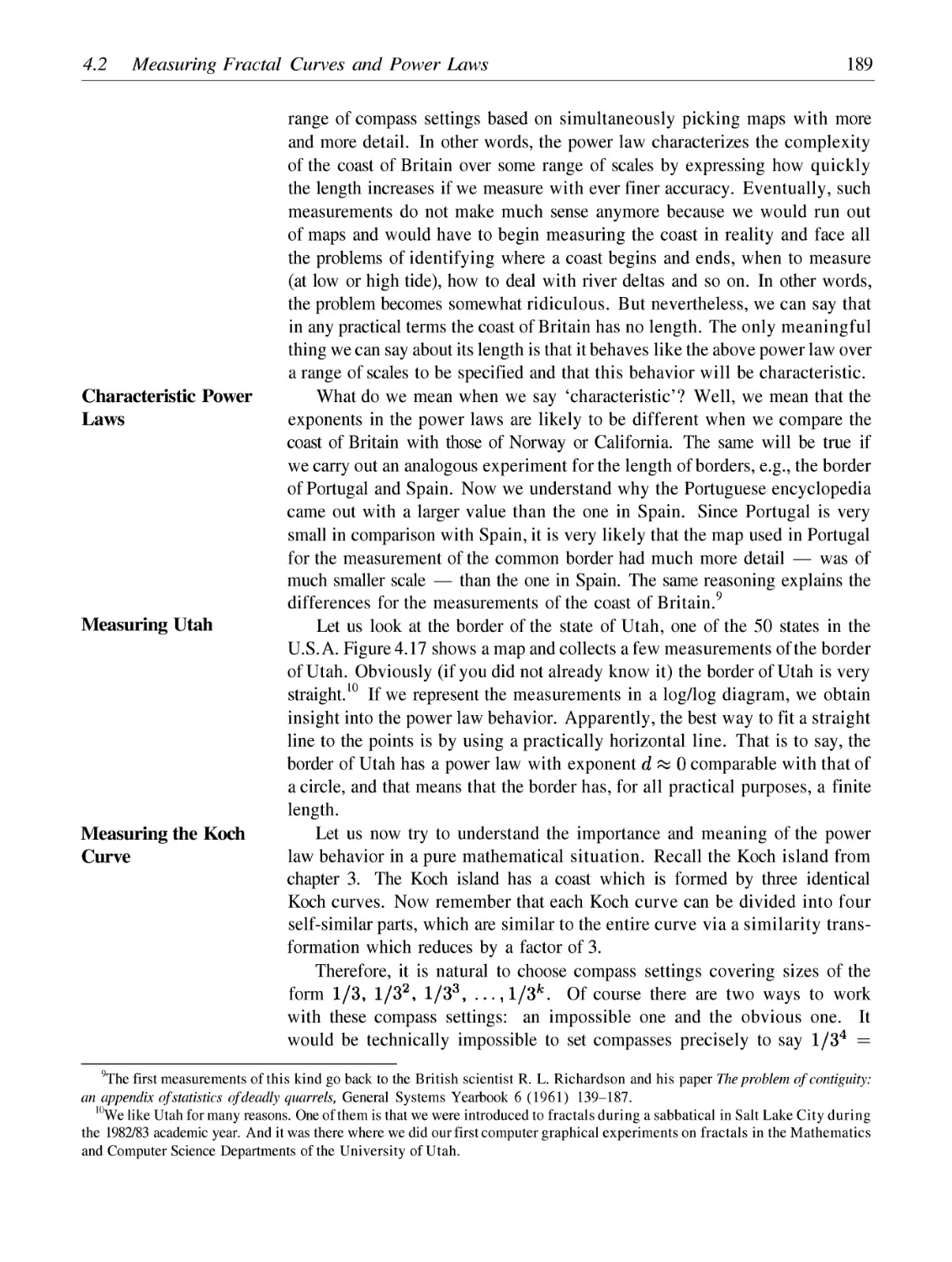
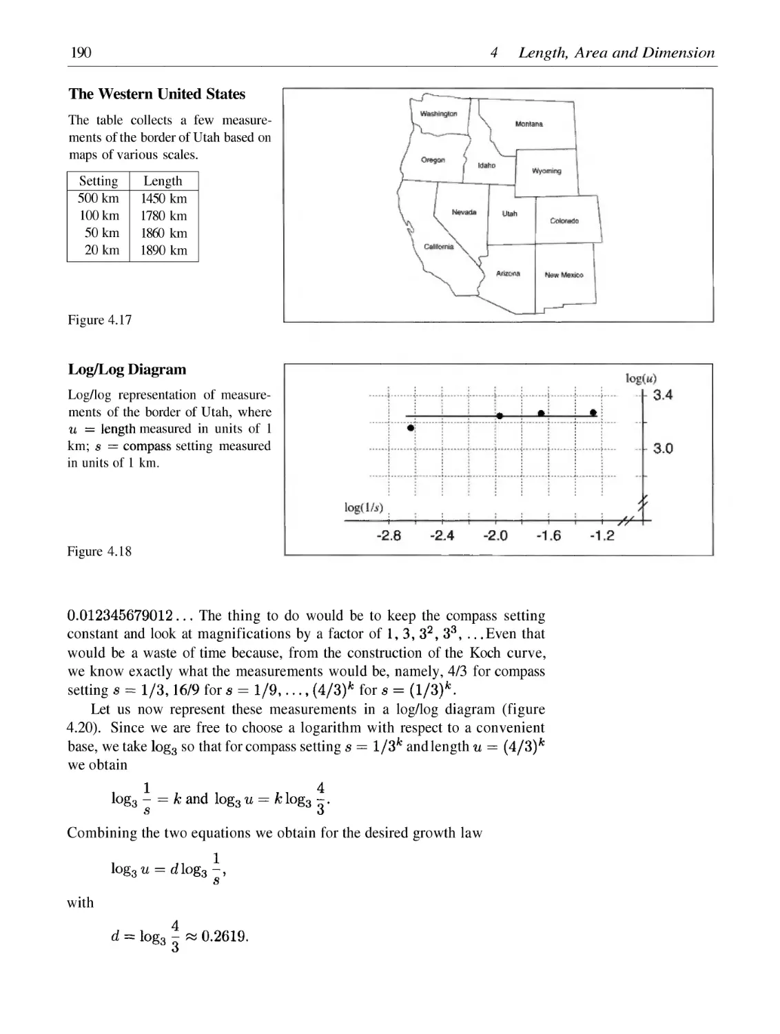
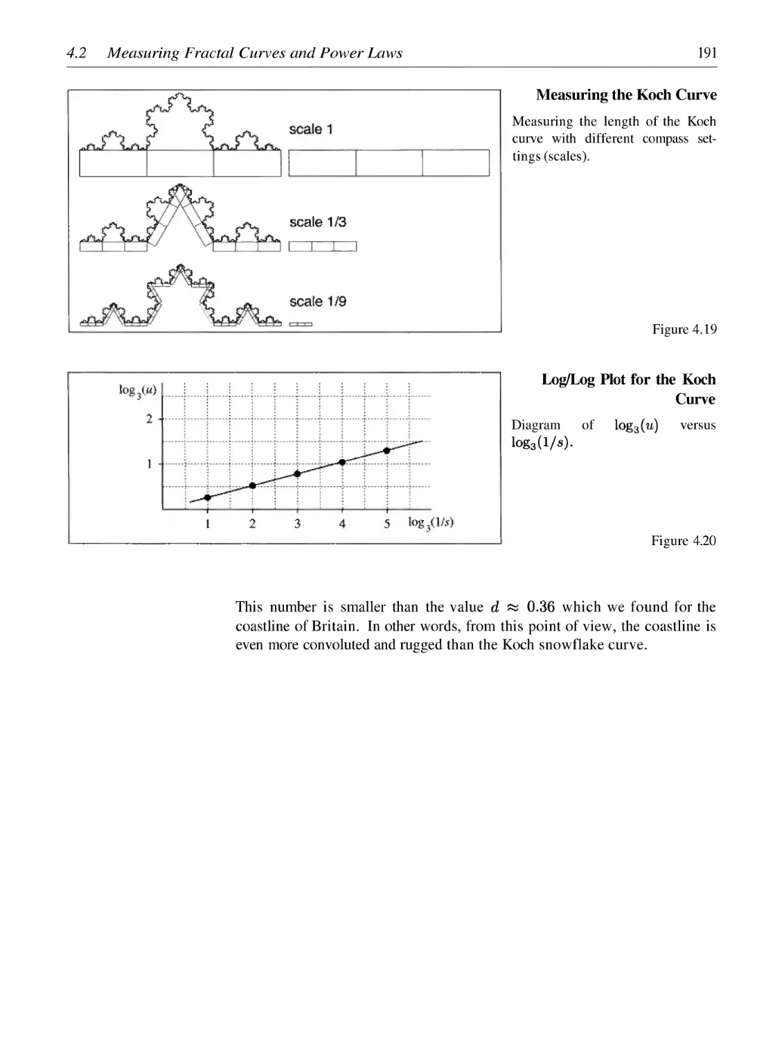
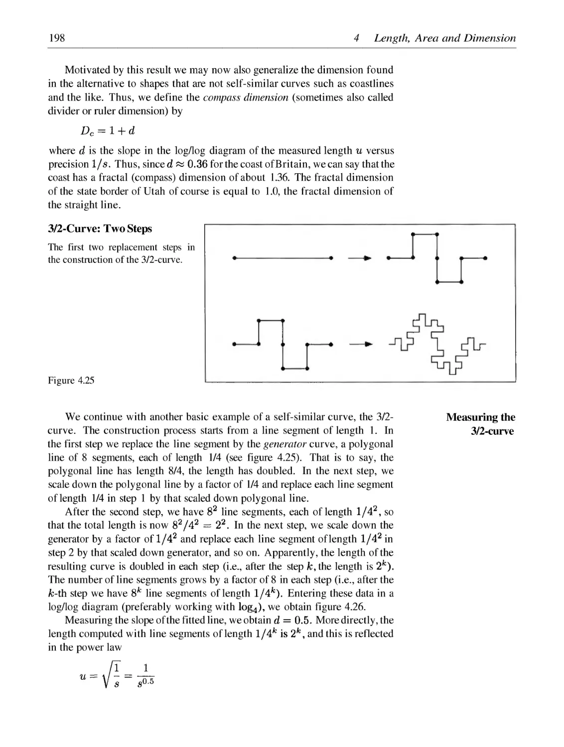
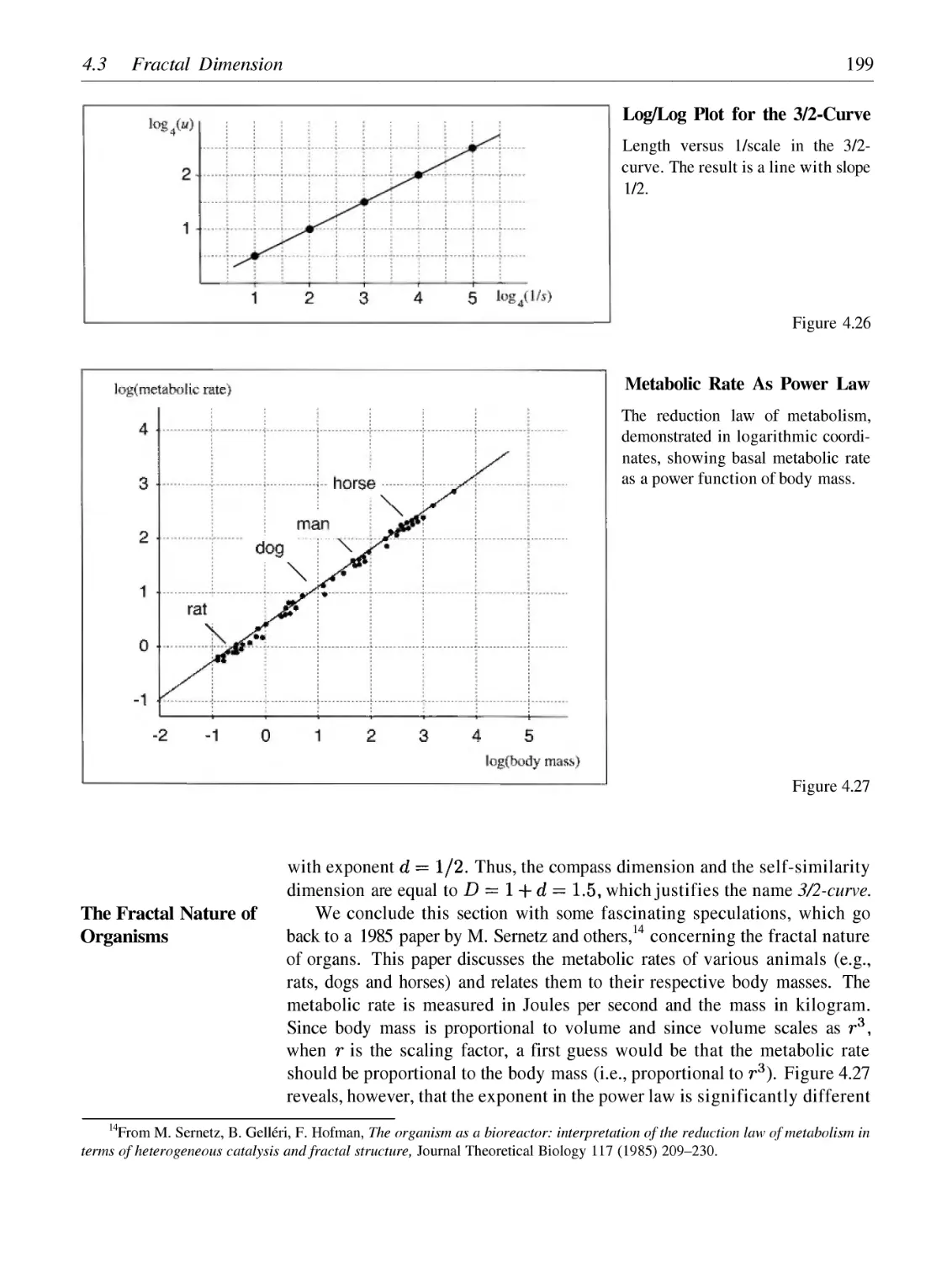
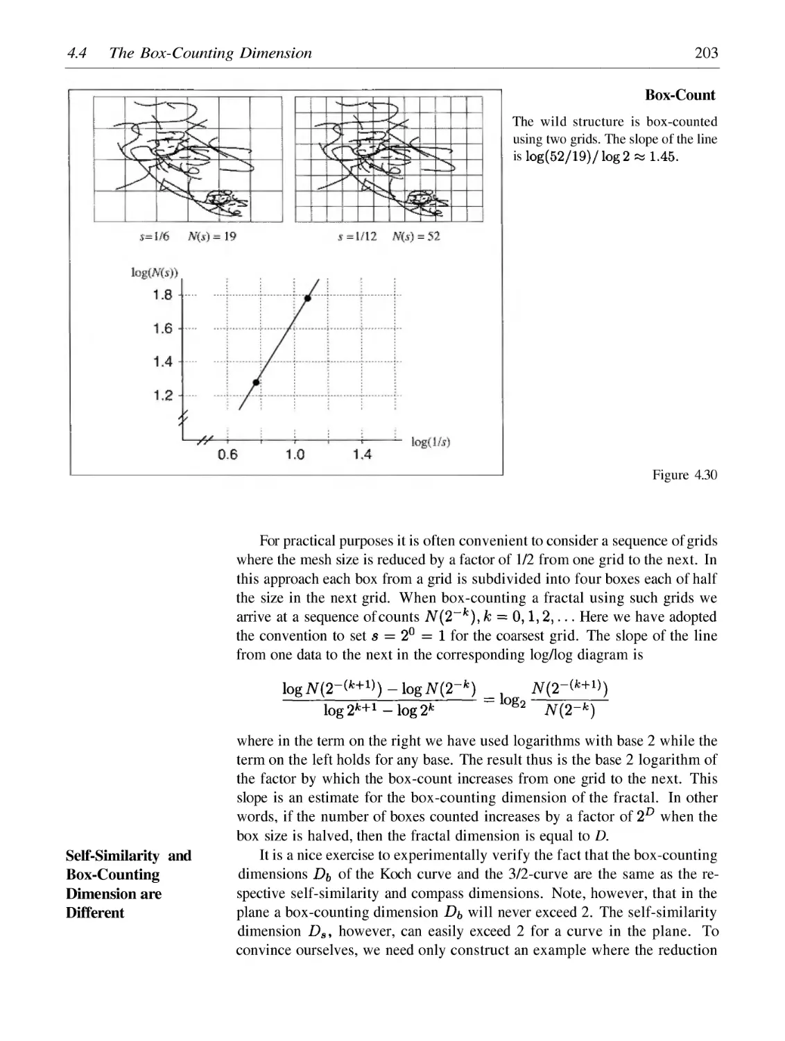
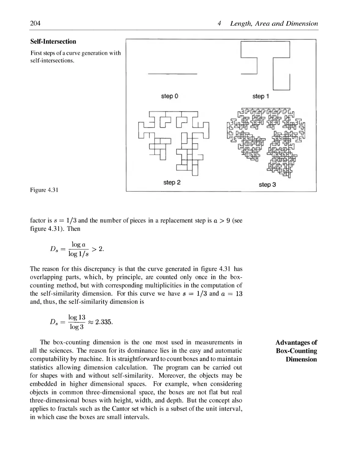
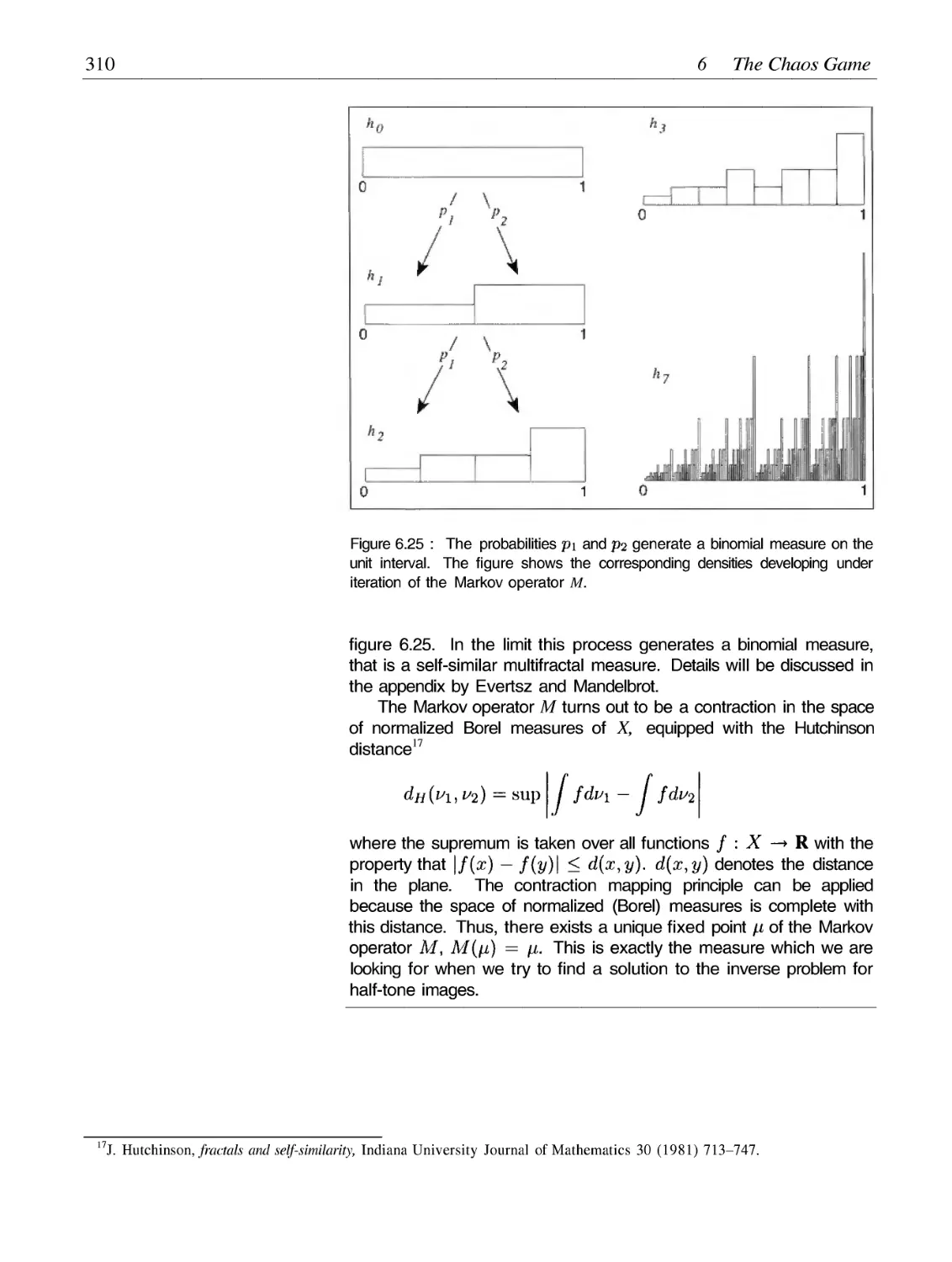
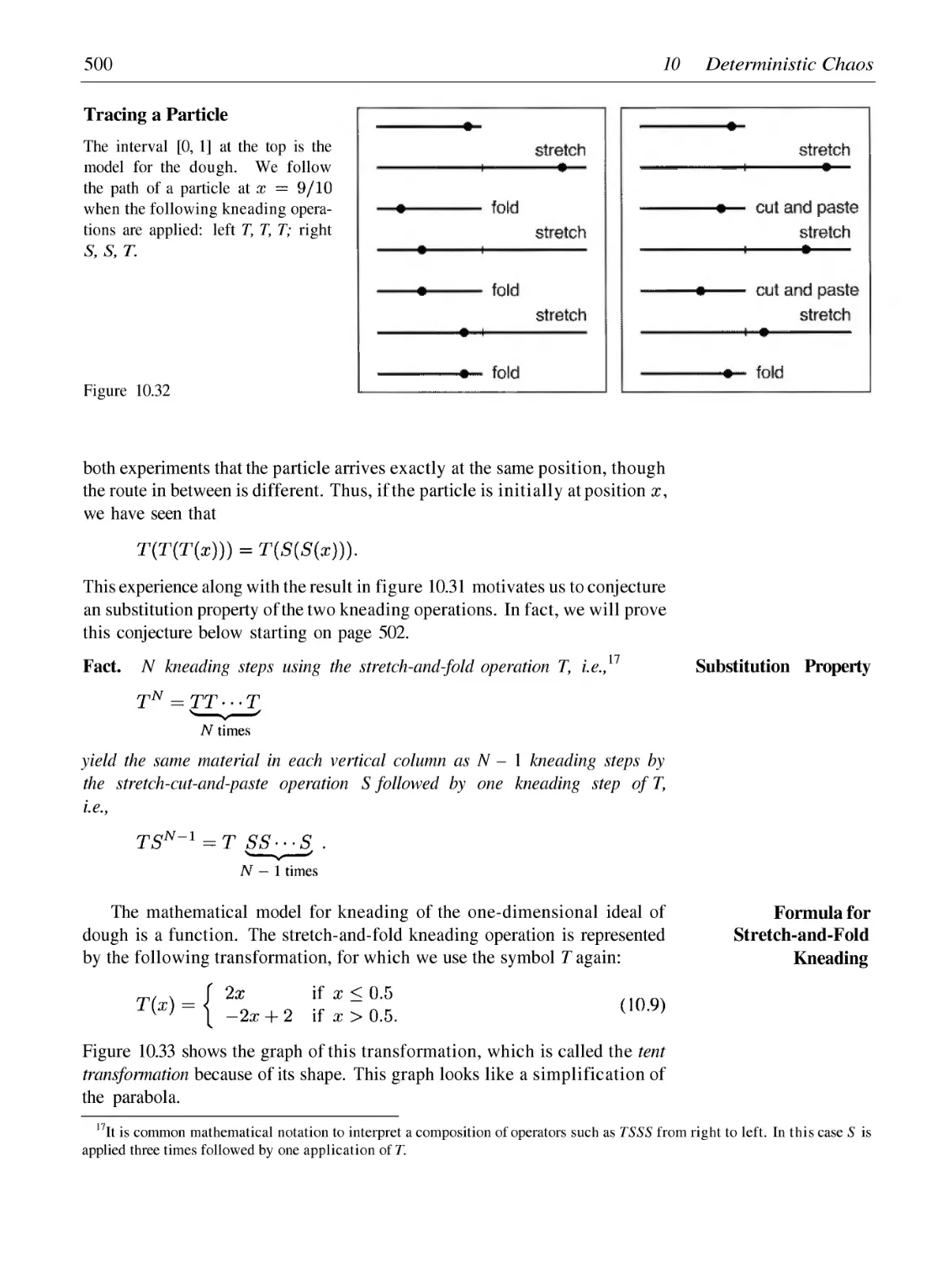
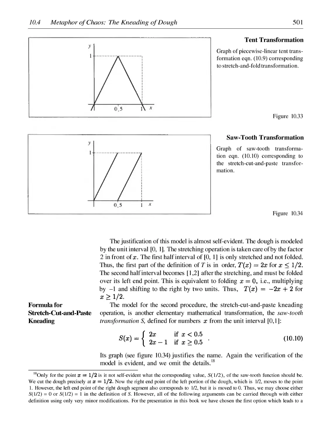
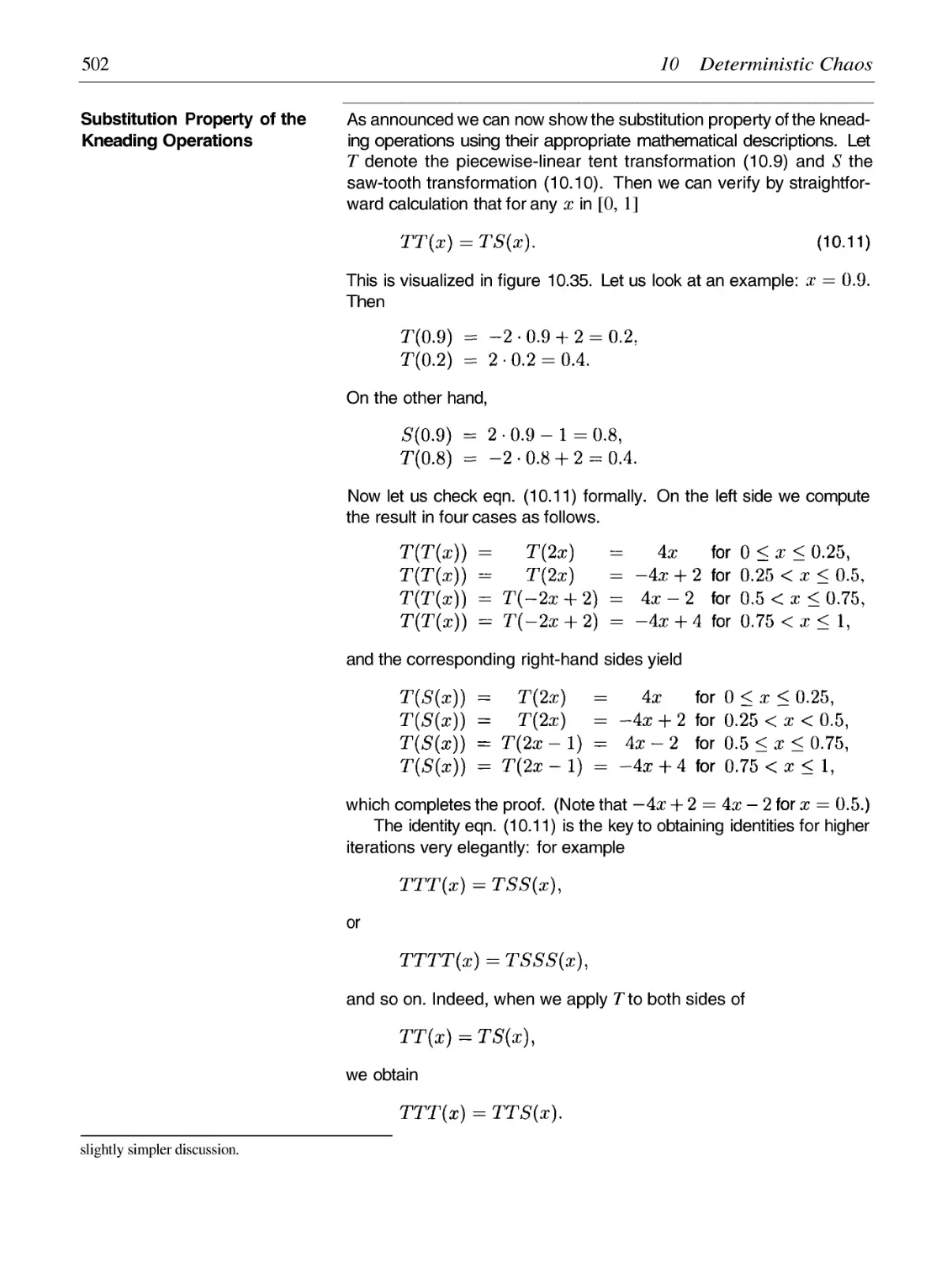
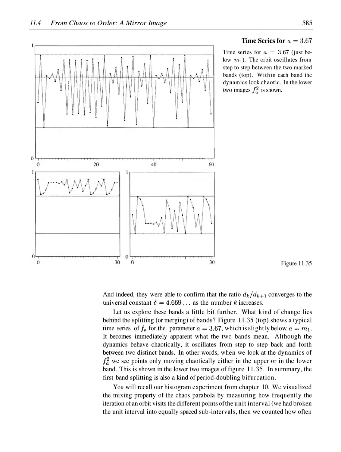
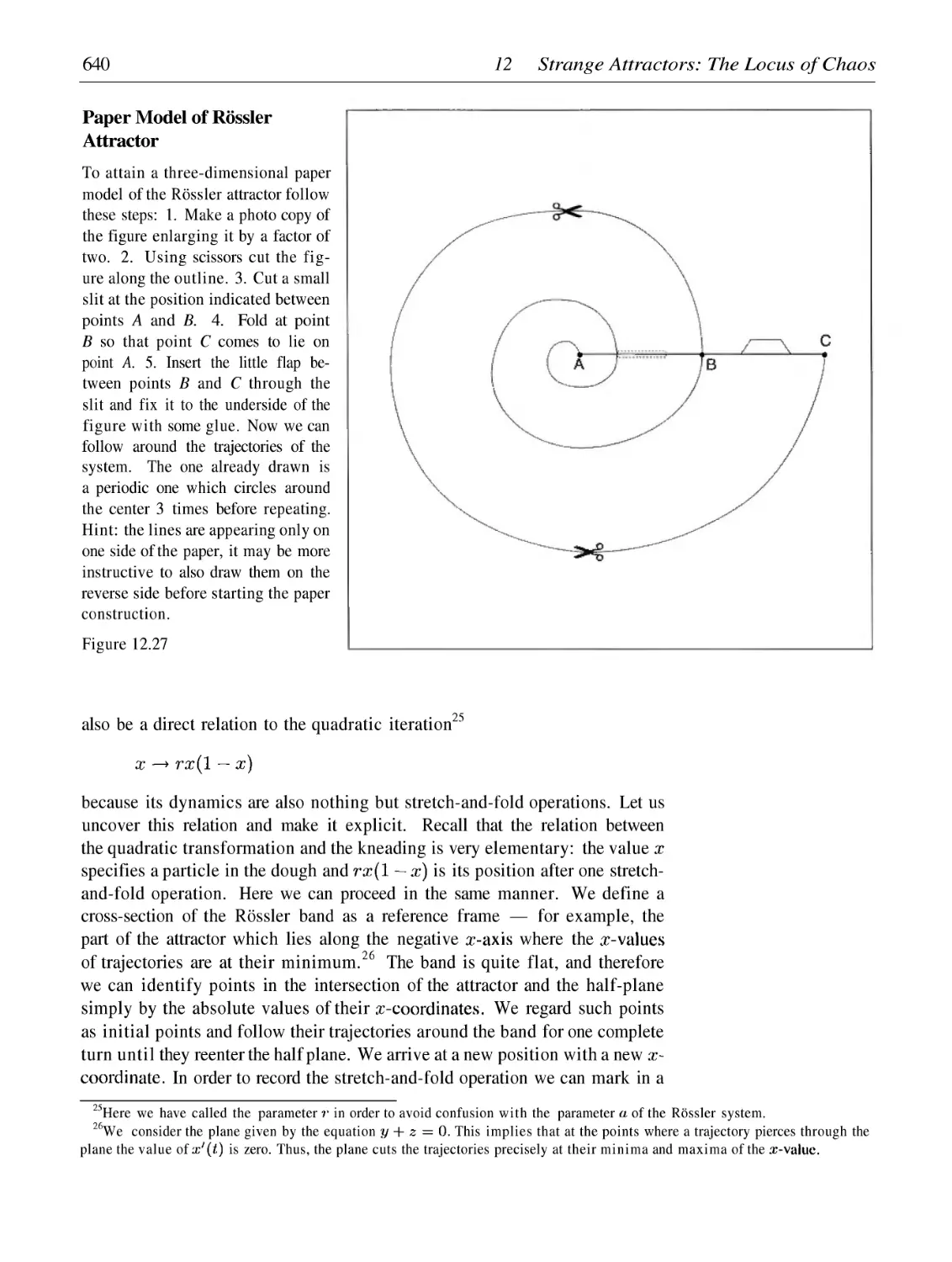
Текст
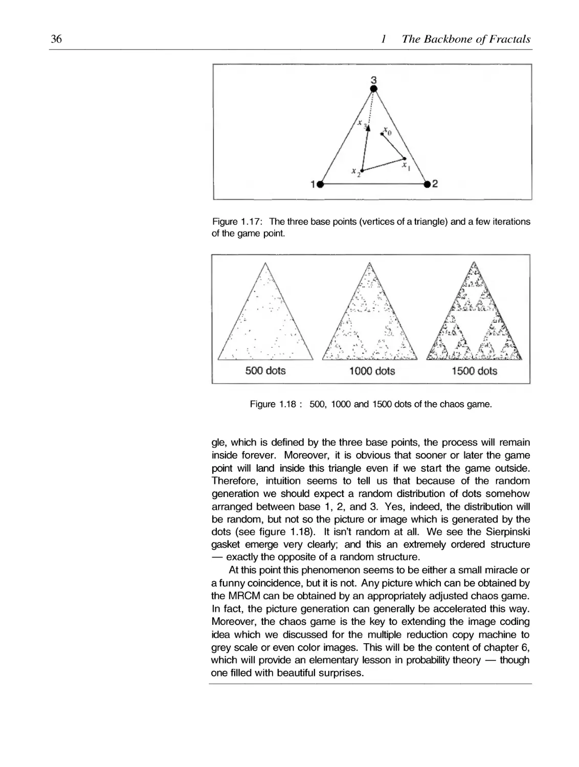
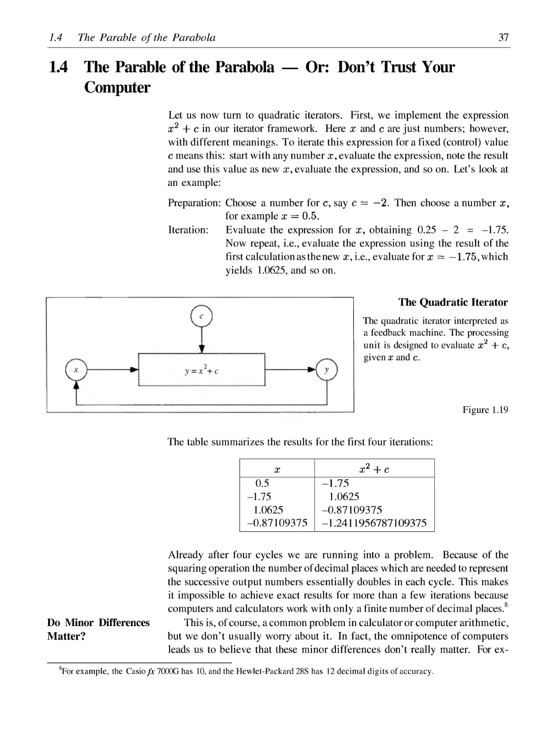
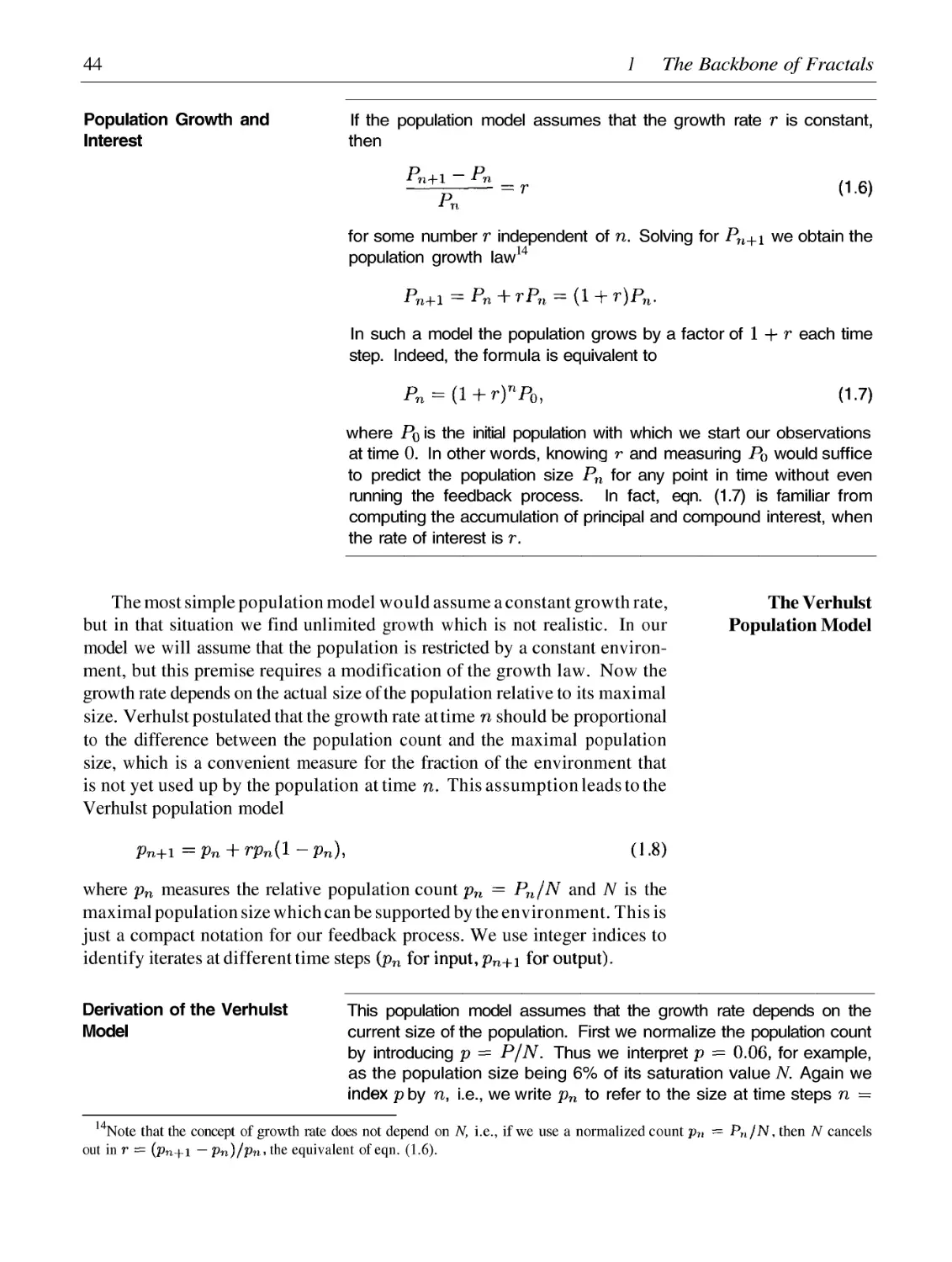
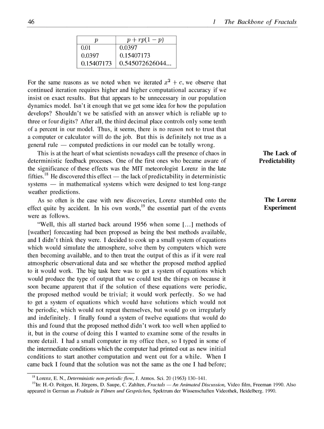
Chaos and Fractals
Springer
New York
Berlin
Heidelberg
Hong Kong
London
Milan
Paris
Tokyo
Springer
Heinz-Otto Peitgen Hartmut Jürgens Dietmar Saupe
Chaos and Fractals
New Frontiers of Science
Second Edition
With 606 illustrations, 40 in color
eBook ISBN: 0-387-21823-8
Print ISBN:
0-387-20229-3
©2004 Springer Science + Business Media, Inc.
Print ©2004 Springer-Verlag New York, Inc.
All rights reserved
No part of this eBook may be reproduced or transmitted in any form or by any means, electronic,
mechanical, recording, or otherwise, without written consent from the Publisher
Created in the United States of America
Visit Springer's eBookstore at:
http://www.ebooks.kluweronline.com
and the Springer Global Website Online at: http://www.springeronline.com
Dordrecht
Preface
Almost 12 years have passed by since we wrote Chaos and Fractals. At the time we were hoping
that our approach of writing a book which would be both accessible without mathematical sophistication
and portray these exiting new fields in an authentic manner would find an audience. Now we know it
did. We know from many reviews and personal letters that the book is used in a wide range of ways:
researchers use it to acquaint themselves, teachers use it in college and university courses, students use
it for background reading, and there is also a substantial audience of lay people who just want to know
what chaos and fractals are about.
Every book that is somewhat technical in nature is likely to have a number of misprints and errors in
its first edition. Some of these were caught and brought to our attention by our readers. One of them,
Hermann Flaschka, deserves to be thanked in particular for his suggestions and improvements.
This second edition has several changes. We have taken out the two appendices from the first edition.
At the time of the first edition Yuval Fishers contribution, which we published as an appendix was
probably the first complete expository account on fractal image compression. Meanwhile, Yuvals book
Fractal Image Compression: Theory and Application appeared and is now the publication to refer to.
Moreover, we have taken out the sections at the end of each chapter, which were devoted to a focussed
computer program in BASIC, which highlighted a fundamental construction in that respective chapter.
Instead we direct our readers to our web-site
http://www.cevis.uni-bremen.de/fractals/
where we provide 10 interactive JAVA-applets.
We also like to express our sincere gratitude to the people at Springer-Verlag, New York, who made
this whole project such a wonderful experience for us.
Heinz-Otto Peitgen, Hartmut Jürgens, Dietmar Saupe
Bremen and Konstanz, August 2003
Preface of the First Edition
Over the last decade, physicists, biologists, astronomers and economists have created a new way of
understanding the growth of complexity in nature. This new science, called chaos, offers a way of seeing
order and pattern where formerly only the random, erratic, the unpredictable --- in short, the chaotic ---
had been observed.
James Gleick1
This book is written for everyone who, even without much knowledge of technical mathematics,
wants to know the details of chaos theory and fractal geometry. This is not a textbook in the usual sense
of the word, nor is it written in a 'popular scientific' style. Rather, it has been our desire to give the
reader a broad view of the underlying notions behind fractals, chaos and dynamics. In addition, we have
wanted to show how fractals and chaos relate to each other and to many other aspects of mathematics as
well as to natural phenomena. A third motif in the book is the inherent visual and imaginative beauty in
the structures and shapes of fractals and chaos.
For almost ten years now mathematics and the natural sciences have been riding a wave which, in its
power, creativity and expanse, has become an interdisciplinary experience of the first order. For some
time now this wave has also been touching distant shores far beyond the sciences. Never before have
mathematical insights --- usually seen as dry and dusty --- found such rapid acceptance and generated so
much excitement in the public mind. Fractals and chaos have literally captured the attention, enthusiasm
and interest of a world-wide public. To the casual observer, the color of their essential structures and their
beauty and geometric form captivate the visual senses as few other things they have ever experienced in
mathematics. To the student, they bring mathematics out of the realm of ancient history into the twenty-
first century. And to the scientist, fractals and chaos offer a rich environment for exploring and modelling
the complexity of nature.
But what are the reasons for this fascination? First of all, this young area of research has created
pictures of such power and singularity that a collection of them, for example, has proven to be one of the
most successful world-wide series of exhibitions ever sponsored by the Goethe-Institute.2 More impor-
tant, however, is the fact that chaos theory and fractal geometry have corrected an outmoded conception
of the world.
The magnificent successes in the fields of the natural sciences and technology had, for many, fed
the illusion that the world on the whole functioned like a huge clockwork mechanism, whose laws were
only waiting to be deciphered step by step. Once the laws were known, it was believed, the evolution
or development of things could --- at least in principle --- be ever more accurately predicted. Captivated
by the breathtaking advances in the development of computer technology and its promises of a greater
command of information, many have put increasing hope in these machines.
But today it is exactly those at the active core of modern science who are proclaiming that this hope
is unjustified; the ability to see ever more accurately into future developments is unattainable. One
1 J. Gleick, Chaos - Making a New Science, Viking, New York, 1987.
2 Alone at the venerable London Museum of Science, the exhibition Frontiers of Chaos: Images of Complex Dynamical Systems
by H. Jürgens, H.-O. Peitgen, M. Prüfer, P. H. Richter and D. Saupe attracted more than 140,000 visitors. Since 1985 this exhibition
has travelled to more than 100 cities in more than 30 countries on all five continents.
Preface
vii
conclusion that can be drawn from the new theories, which are admittedly still young, is that stricter
determinism and apparently accidental development are not mutually exclusive, but rather that their
coexistence is more the rule in nature. Chaos theory and fractal geometry address this issue. When we
examine the development of a process over a period of time, we speak in terms used in chaos theory.
When we are more interested in the structural forms which a chaotic process leaves in its wake, then
we use the terminology of fractal geometry, which is really the geometry whose structures are what give
order to chaos.
In some sense, fractal geometry is first and foremost a new 'language' used to describe, model and
analyze the complex forms found in nature. But while the elements of the 'traditional language' --- the
familiar Euclidean geometry --- are basic visible forms such as lines, circles and spheres, those of the
new language do not lend themselves to direct observation. They are, namely, algorithms, which can
be transformed into shapes and structures only with the help of computers. In addition, the supply of
these algorithmic elements is inexhaustibly large; and they are capable of providing us with a powerful
descriptive tool. Once this new language has been mastered, we can describe the form of a cloud as
easily and precisely as an architect can describe a house using the language of traditional geometry.
The correlation of chaos and geometry is anything but coincidental. Rather, it is a witness to their
deep kinship. This kinship can best be seen in the Mandelbrot set, a mathematical object discovered by
Benoit Mandelbrot in 1980. It has been described by some scientists as the most complex --- and possibly
the most beautiful --- object ever seen in mathematics. Its most fascinating characteristic, however, has
only just recently been discovered: namely, that it can be interpreted as an illustrated encyclopedia of an
infinite number of algorithms. It is a fantastically efficiently organized storehouse of images, and as such
it is the example par excellence of order in chaos.
Fractals and modern chaos theory are also linked by the fact that many of the contemporary pace-
setting discoveries in their fields were only possible using computers. From the perspective of our in-
herited understanding of mathematics, this is a challenge which is felt by some to be a powerful renewal
and liberation and by others to be a degeneration. However this dispute over the 'right' mathematics is
decided, it is already clear that the history of the sciences has been enriched by an indispensable chapter.
Only superficially is the issue one of beautiful pictures or of perils of deterministic laws. In essence,
chaos theory and fractal geometry radically question our understanding of equilibria --- and therefore of
harmony and order --- in nature as well as in other contexts. They offer a new holistic and integral model
which can encompass a part of the true complexity of nature for the first time. It is highly probable that
the new methods and terminologies will allow us, for example, a much more adequate understanding of
ecology and climatic developments, and thus they could contribute to our more effectively tackling our
gigantic global problems.
We have worked hard in trying to reveal the elements of fractals, chaos and dynamics in a non-
threatening fashion. Each chapter can stand on its own and can be read independently from the others.
Each chapter is centered around a running 'story' typeset in Times and printed toward the outer mar-
gins. More technical discussions, typeset in Helvetica and printed toward the inner margins, have been
included to occasionally enrich the discussion by providing deeper analyses for those who may desire
them and those who are prepared to work themselves through some mathematical notations. At the end
of each chapter we offer a short BASIC program, the Program of the Chapter, which is designed to
highlight one of the most prominent experiments of the respective chapter.
This book is a close relative of the two-volume set Fractals for the Classroom which was published
by Springer-Verlag and the National Council of Teachers of Mathematics in 1991 and 1992. While
those books were originally written for an audience which is involved with the teaching or learning of
viii
Preface
mathematics, this book is intended for a much larger readership. It combines most parts of the afore-
mentioned books with many extensions and two important appendices.
The first appendix, written by Yuval Fisher, deals with aspects of image compression using funda-
mental ideas from fractal geometry. Such applications have been discussed for about five years and
hopes of new breakthrough technologies have risen very high through the work and announcements of
the group around Michael F. Barnsley. Since Barnsley has kept his work absolutely secret we still don't
know what is possible and what is not. But Fisher's contribution allows us to make a fair guess. Anybody
who is interested in the perspectives of image compression through fractals will appreciate this appendix.
The second appendix is written by Carl J. G. Evertsz and Benoit B. Mandelbrot and deals with
multifractal measures, which is one of the hottest subjects in the current scientific discussion of fractal
geometry. Usually we think of fractals as objects having some kind of self-similarity. The discussion of
multifractal measures extends this concept to the distributions of quantities (for example, the amount of
ground water found at a certain location under the surface). Furthermore, it overcomes some shortcom-
ings of the fractal dimension when used as a tool for measurement in science.
Even with these two important contributions there remain many holes in this book. However, fortu-
nately there are exceptional books already in print that can close these gaps. We list the following only
as examples: For portraits of the personalities in the field and the genesis of the subject matter, as well as
the scientific background and interrelationships, there are Chaos --- Making a New Science,3 by James
Gleick, and Does God Play Dice?,4 by Ian Stewart. For the reader who is more interested in a system-
atic mathematical exposition or who is ready to advance into the depths, there are the following titles:
An Introduction to Chaotic Dynamical Systems5 and Chaos, Fractals, and Dynamics,6 both by Robert
L. Devaney, and Fractals Everywhere,7 by Michael F. Barnsley. An adequate technical discussion of
fractal dimension can be found in the two exceptional texts, Measure, Topology and Fractal Geometry,8
by Gerald A. Edgar, and Fractal Geometry,9 by Kenneth Falconer. Readers more interested in fractals
in physics will appreciate Fractals,10 by Jens Feder, while readers who look for fractals in chemistry
should not miss The Fractal Approach to Heterogeneous Chemistry,11 by David Avnir. And last but not
least, there is the book of books about fractal geometry written by Benoit B. Mandelbrot, The Fractal
Geometry of Nature.12
We owe our gratitude to many who have assisted us during the writing of this book. Our students
Torsten Cordes and Lutz Voigt have produced most of the graphics very skillfully and with unlimited
patience. They were joined by two more of our students, Ehler Lange and Wayne Tvedt, during part of
the preparation time. Douglas Sperry has read our text very carefully at several stages of its evolution
and, in addition to helping to get our English de-Germanized, has served in the broader capacity of copy
editor. Ernst Gucker, who is working on the German edition, suggested many improvements. Friedrich
von Haeseler, Guentcho Skordev, Heinrich Niederhausen and Ulrich Krause have read several chapters
and provided valuable suggestions. We also thank Eugen Allgower, Alexander N. Charkovsky, Mitchell
J. Feigenbaum, Przemyslaw Prusinkiewicz, and Richard Voss for reading parts of the original manuscript
3Viking, 1987.
4Penguin Books, 1989.
5Second Edition, Addison Wesley, 1989.
6Addison Wesley, 1990.
7Academic Press, 1989.
8Springer-Verlag,1990
9John Wiley and Sons, 1990.
10 Plenum, 1988
11 Wiley, 1989
12 W.H. Freeman, 1982.
Preface
ix
and giving valuable advice. Gisela Gründl has helped us with selecting and organizing third-party art-
work. Claus Hösselbarth did an excellent job in designing the cover. Evan M. Maletsky, Terence H.
Perciante and Lee E. Yunker read parts of our early manuscripts and gave crucial advice concerning the
design of the book. Finally, we are most grateful to Yuval Fischer, Carl J. G. Evertsz and Benoit B.
Mandelbrot for contributing the appendices to our book, and to Mitchell Feigenbaum for his remarkable
foreword.
The entire book has been produced using the
and
typesetting systems where all figures
(except for the half-tone and color images) were integrated in the computer files. Even though it took
countless hours of sometimes painful experimentation setting up the necessary macros it must be ac-
knowledged that this approach immensely helped to streamline the writing, editing and printing.
Finally, we have been very pleased with the excellent cooperation of Springer-Verlag in New York.
Heinz-Otto Peitgen, Hartmut Jürgens, Dietmar Saupe
Bremen, May 1992
x
Authors
Authors
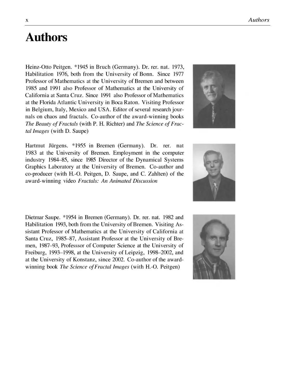
Heinz-Otto Peitgen. *1945 in Bruch (Germany). Dr. rer. nat. 1973,
Habilitation 1976, both from the University of Bonn. Since 1977
Professor of Mathematics at the University of Bremen and between
1985 and 1991 also Professor of Mathematics at the University of
California at Santa Cruz. Since 1991 also Professor of Mathematics
at the Florida Atlantic University in Boca Raton. Visiting Professor
in Belgium, Italy, Mexico and USA. Editor of several research jour-
nals on chaos and fractals. Co-author of the award-winning books
The Beauty of Fractals (with P. H. Richter) and The Science of Frac-
tal Images (with D. Saupe)
Hartmut Jürgens. *1955 in Bremen (Germany). Dr. rer. nat
1983 at the University of Bremen. Employment in the computer
industry 1984--85, since 1985 Director of the Dynamical Systems
Graphics Laboratory at the University of Bremen. Co-author and
co-producer (with H.-O. Peitgen, D. Saupe, and C. Zahlten) of the
award-winning video Fractals: An Animated Discussion
Dietmar Saupe. *1954 in Bremen (Germany). Dr. rer. nat. 1982 and
Habilitation 1993, both from the University of Bremen. Visiting As-
sistant Professor of Mathematics at the University of California at
Santa Cruz, 1985--87, Assistant Professor at the University of Bre-
men, 1987--93, Professsor of Computer Science at the University of
Freiburg, 1993--1998, at the University of Leipzig, 1998--2002, and
at the University of Konstanz, since 2002. Co-author of the award-
winning book The Science of Fractal Images (with H.-O. Peitgen)
Contents
Foreword
Introduction: Causality Principle, Deterministic Laws and Chaos
15
17
23
27
37
49
1 The Backbone of Fractals: Feedback and the Iterator
1.1
1.2
1.3
1.4
1.5
The Principle of Feedback
The Multiple Reduction Copy Machine
Basic Types of Feedback Processes
The Parable of the Parabola --- Or: Don't Trust Your Computer
Chaos Wipes Out Every Computer
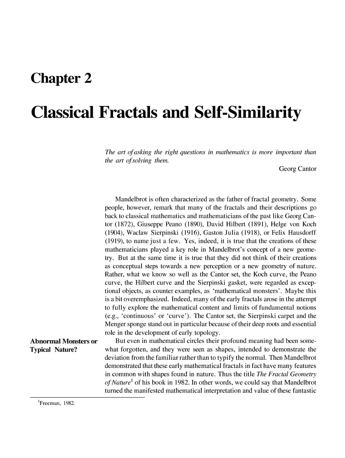
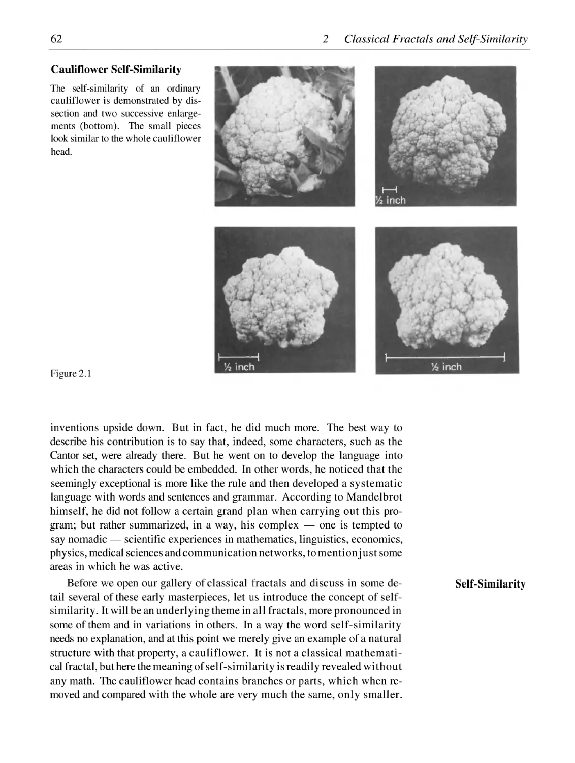
2 Classical Fractals and Self-Similarity
2.1
2.2
2.3
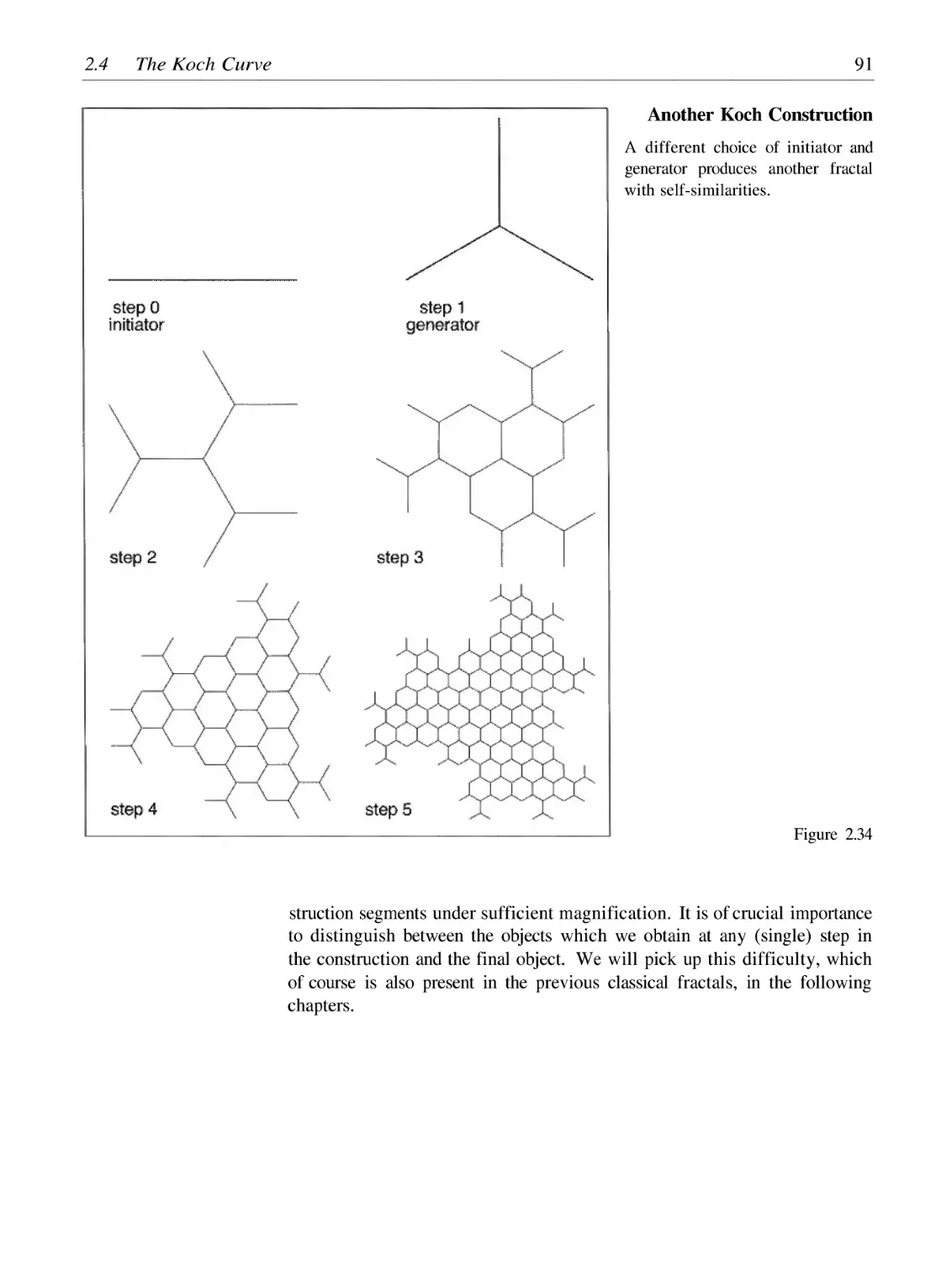
2.4
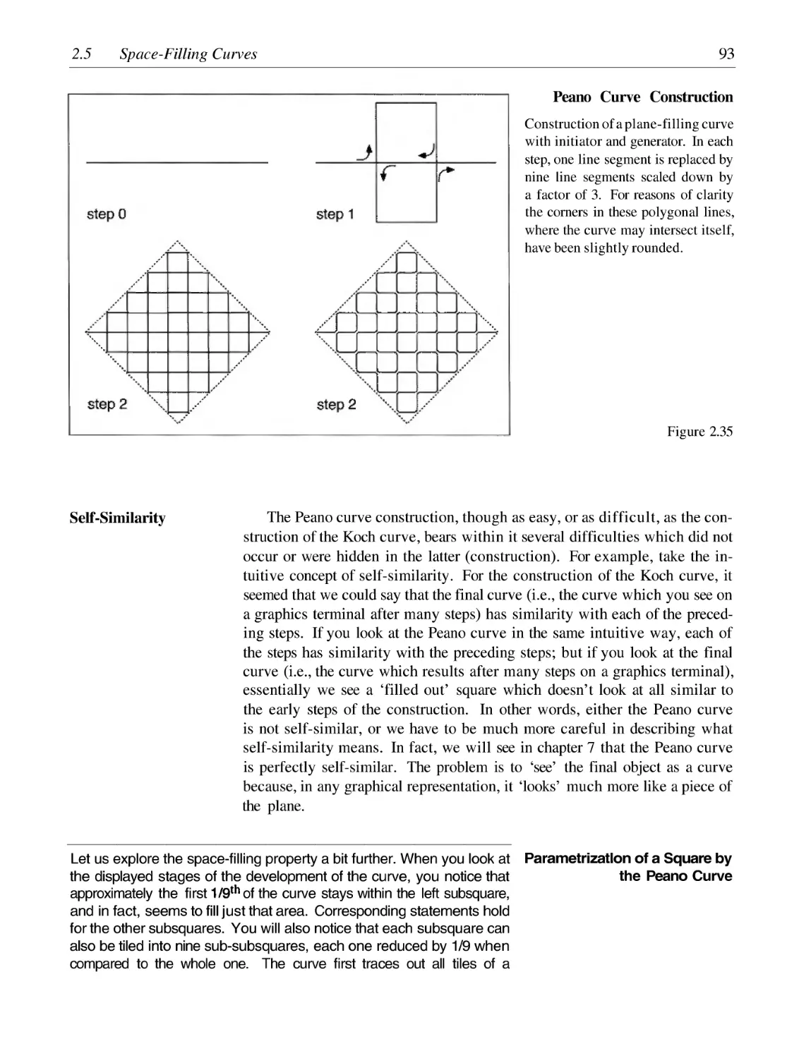
2.5
2.6
2.7
2.8
2.9
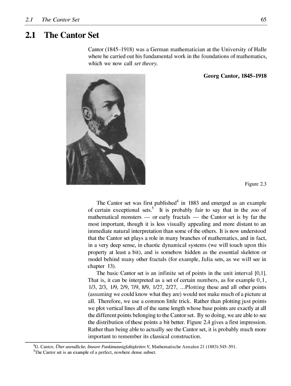
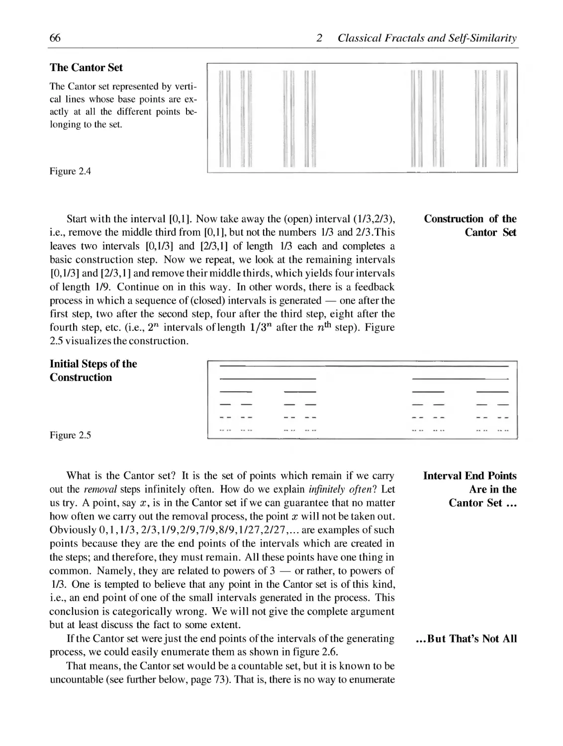
The Cantor Set
The Sierpinski Gasket and Carpet
The Pascal Triangle
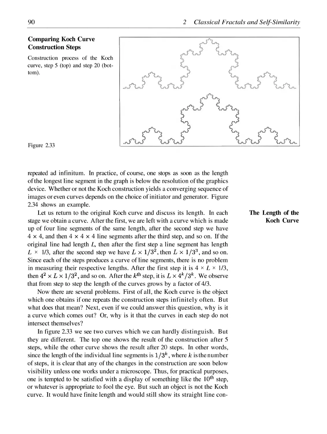
The Koch Curve
Space-Filling Curves
Fractals and the Problem of Dimension
The Universality of the Sierpinski Carpet
Julia Sets
Pythagorean Trees
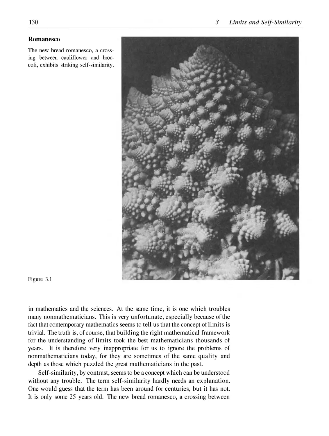
129
132
141
147
162
173
175
182
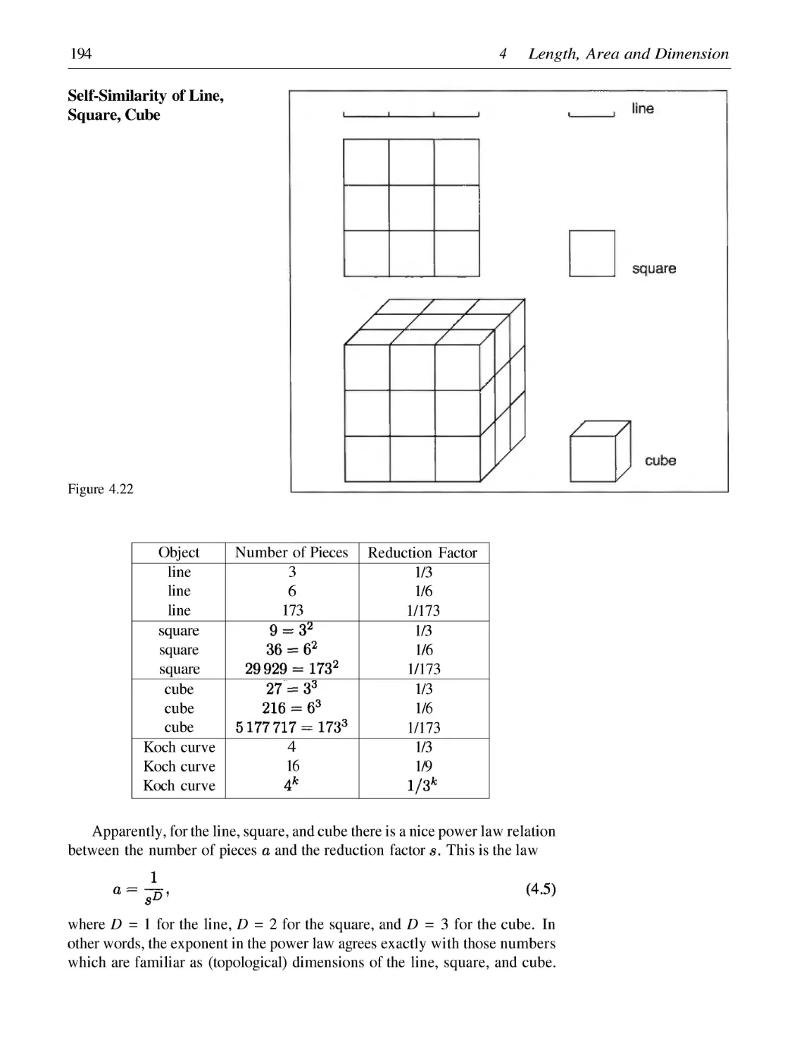
192
202
210
61
65
76
80
87
92
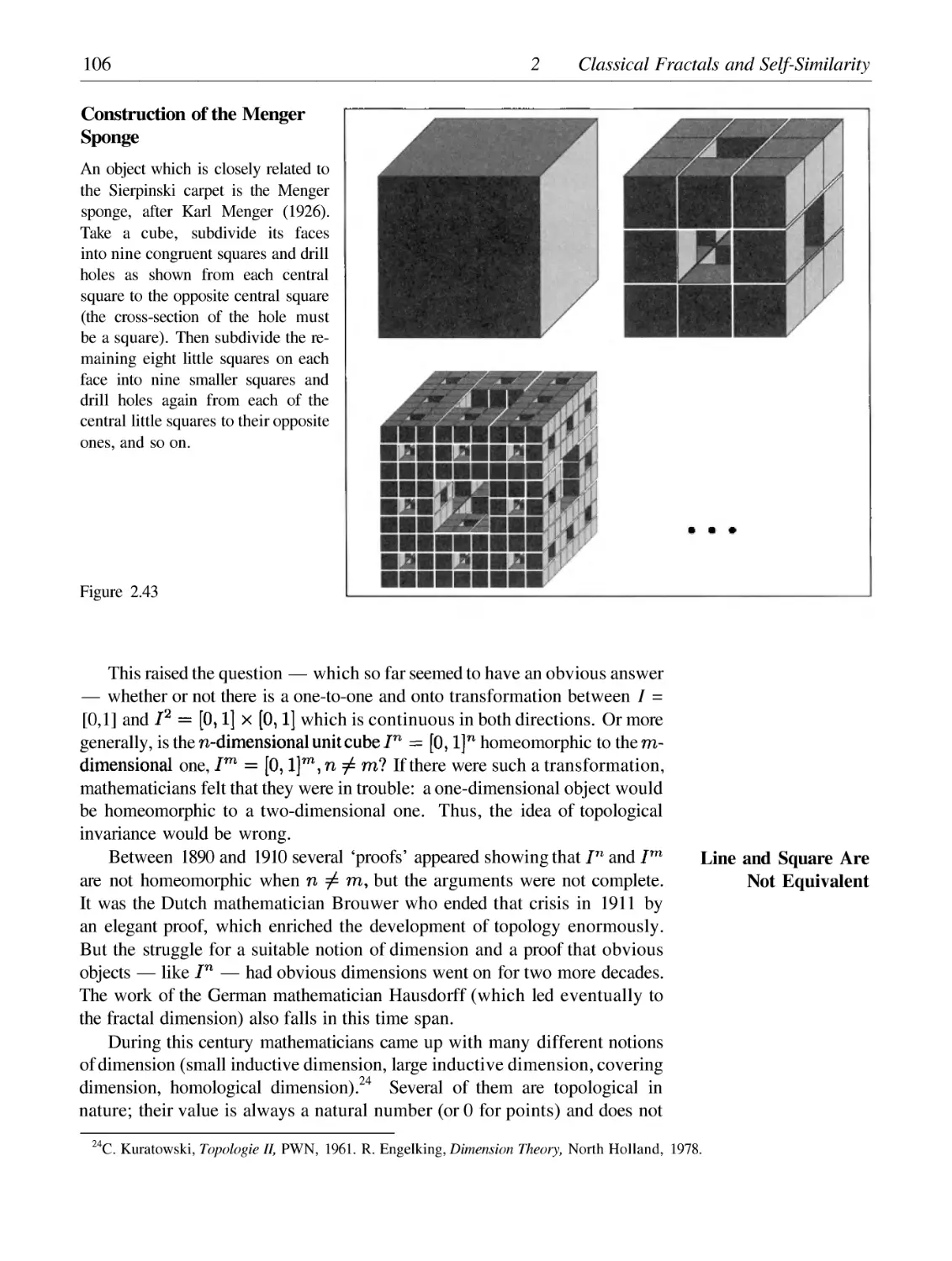
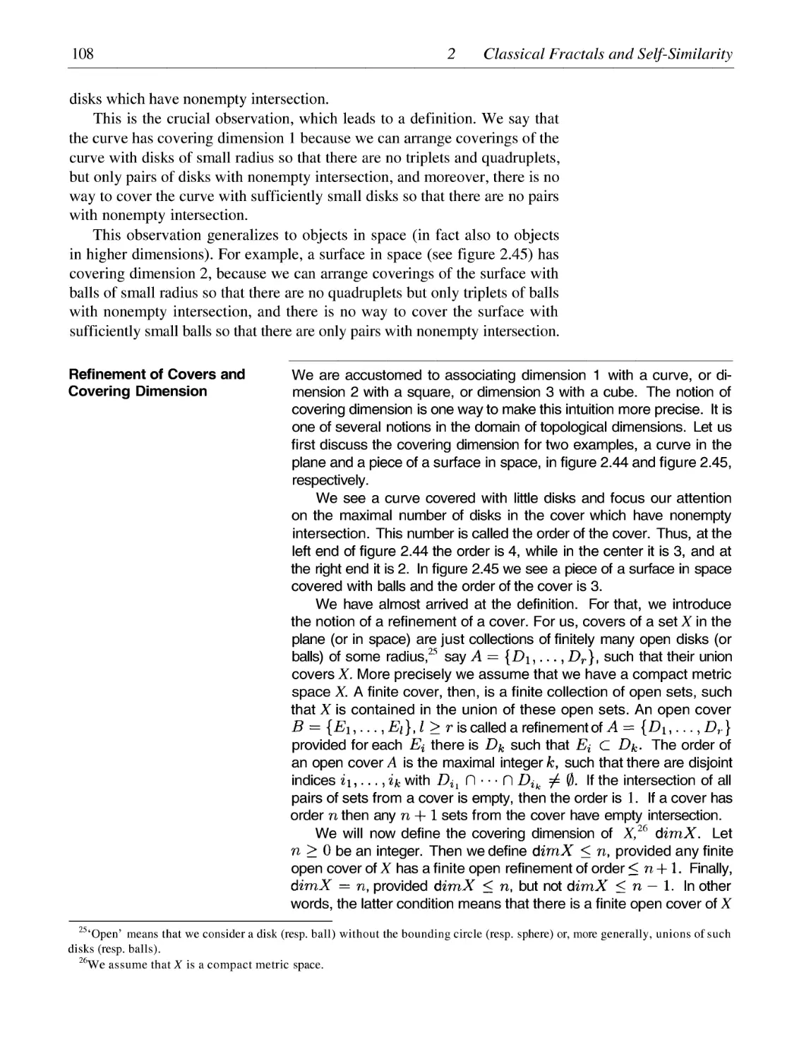
104
110
120
124
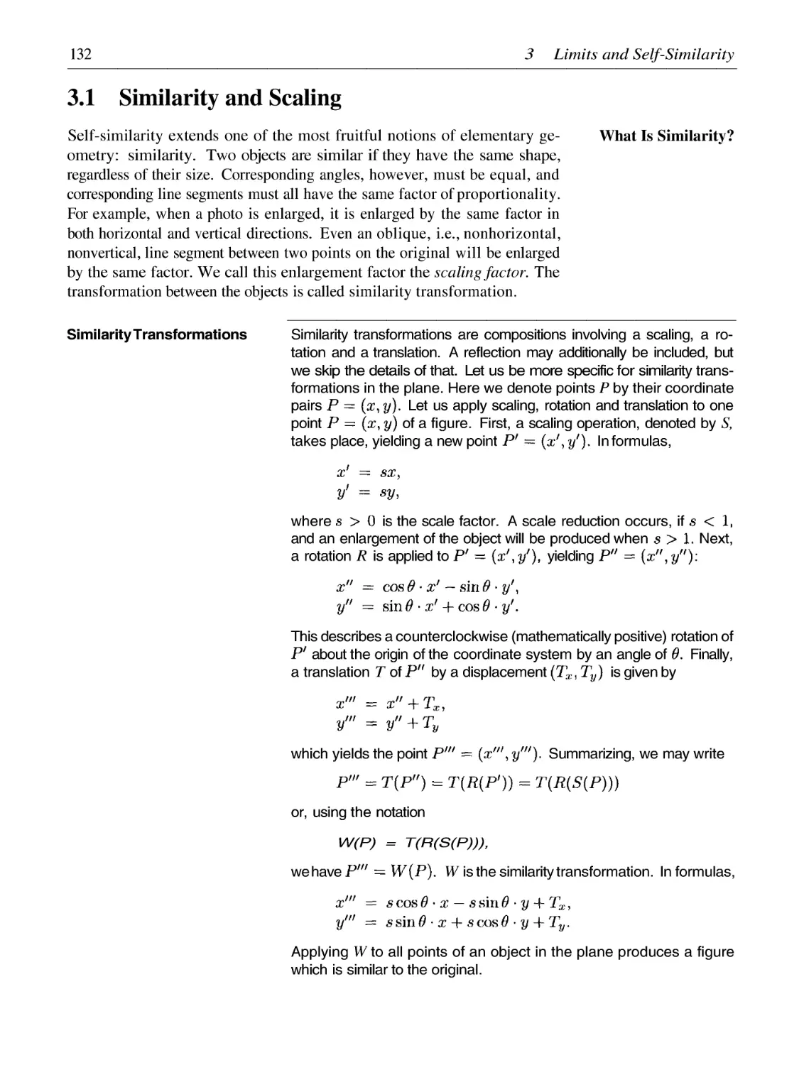
3 Limits and Self-Similarity
3.1
3.2
3.3
3.4
Similarity and Scaling
Geometric Series and the Koch Curve
Corner the New from Several Sides: Pi and the Square Root of Two
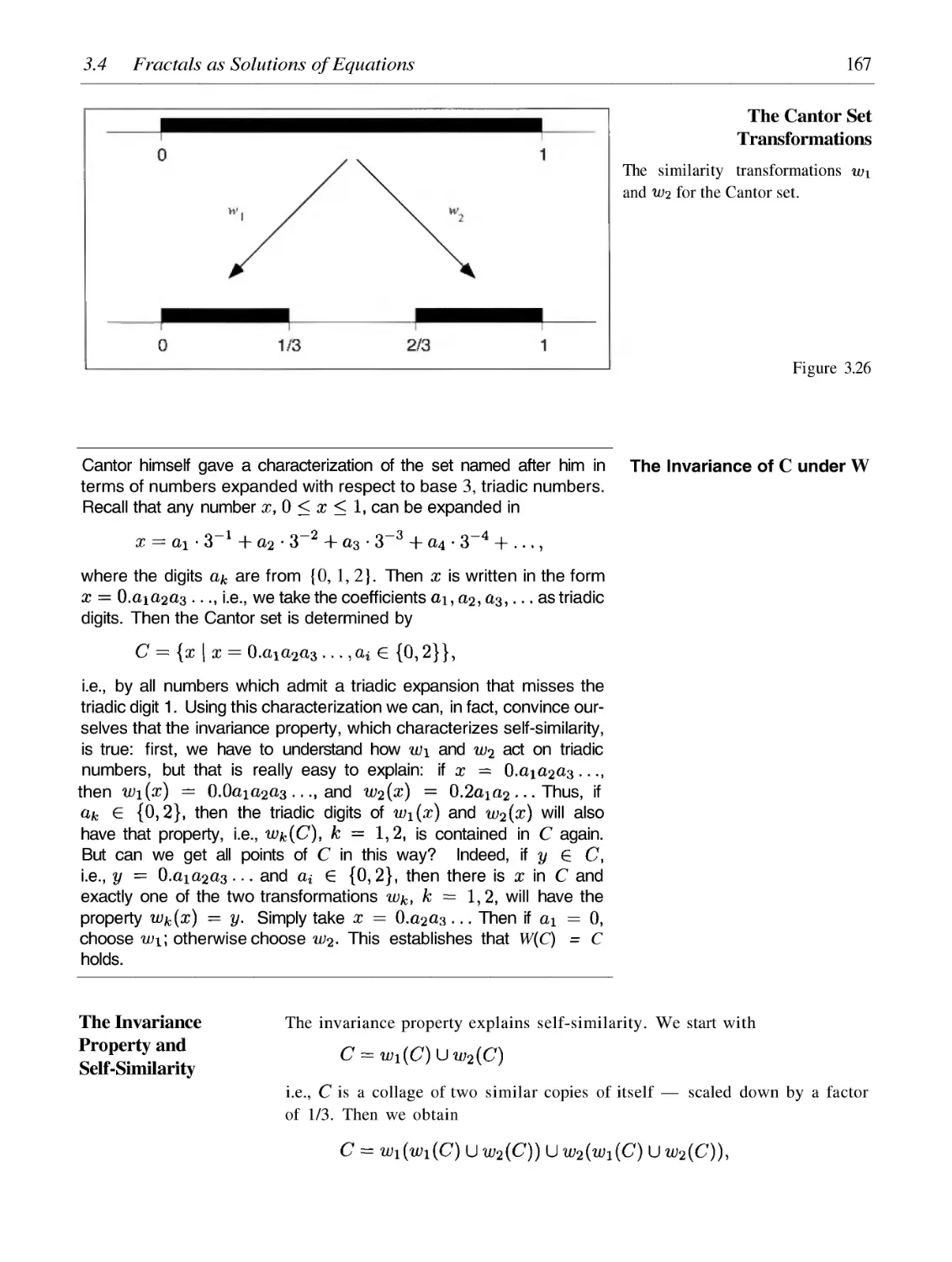
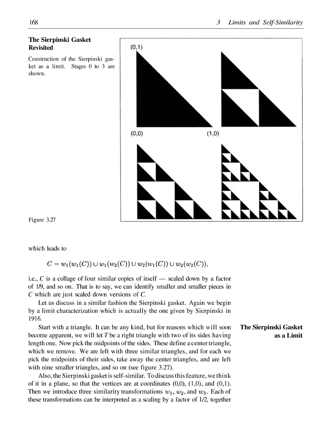
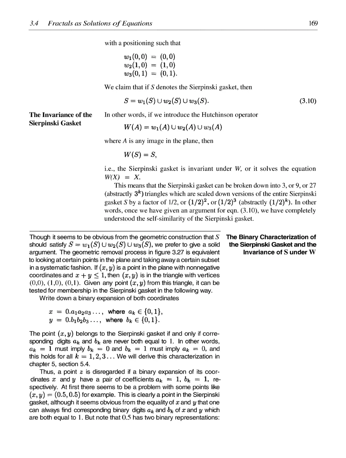
Fractals as Solutions of Equations
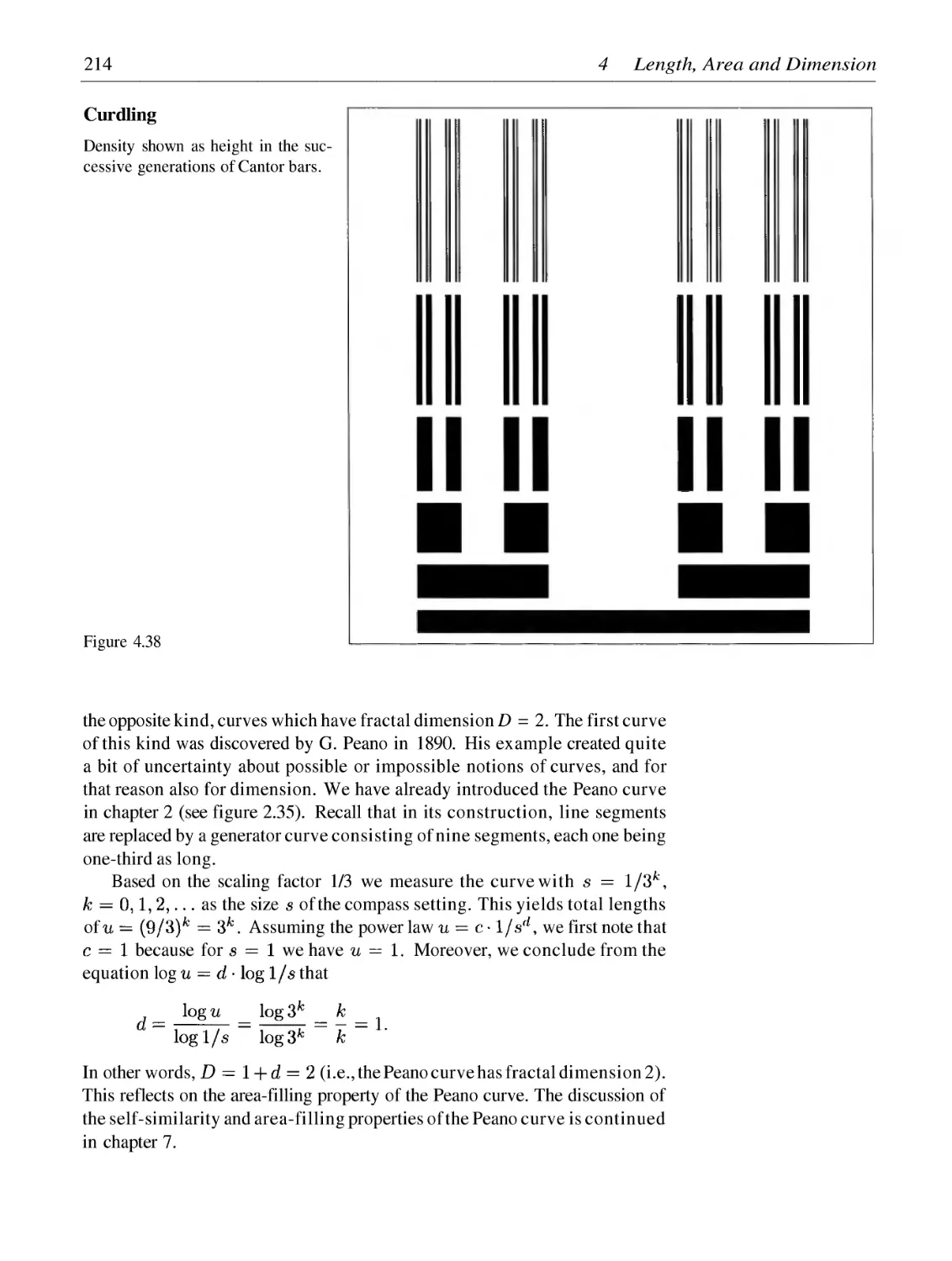
4 Length, Area and Dimension: Measuring Complexity and Scaling Properties
4.1
4.2
4.3
4.4
4.5
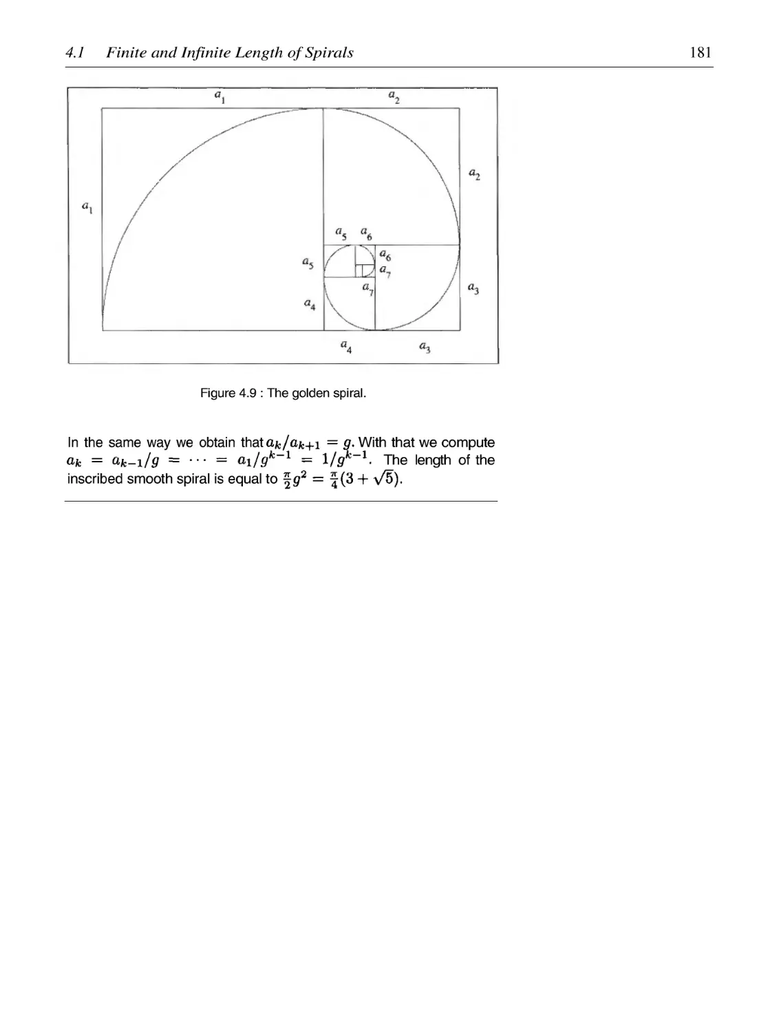
Finite and Infinite Length of Spirals
Measuring Fractal Curves and Power Laws
Fractal Dimension
The Box-Counting Dimension
Borderline Fractals: Devil's Staircase and Peano Curve
xi
1
9
xii
Table of Contents
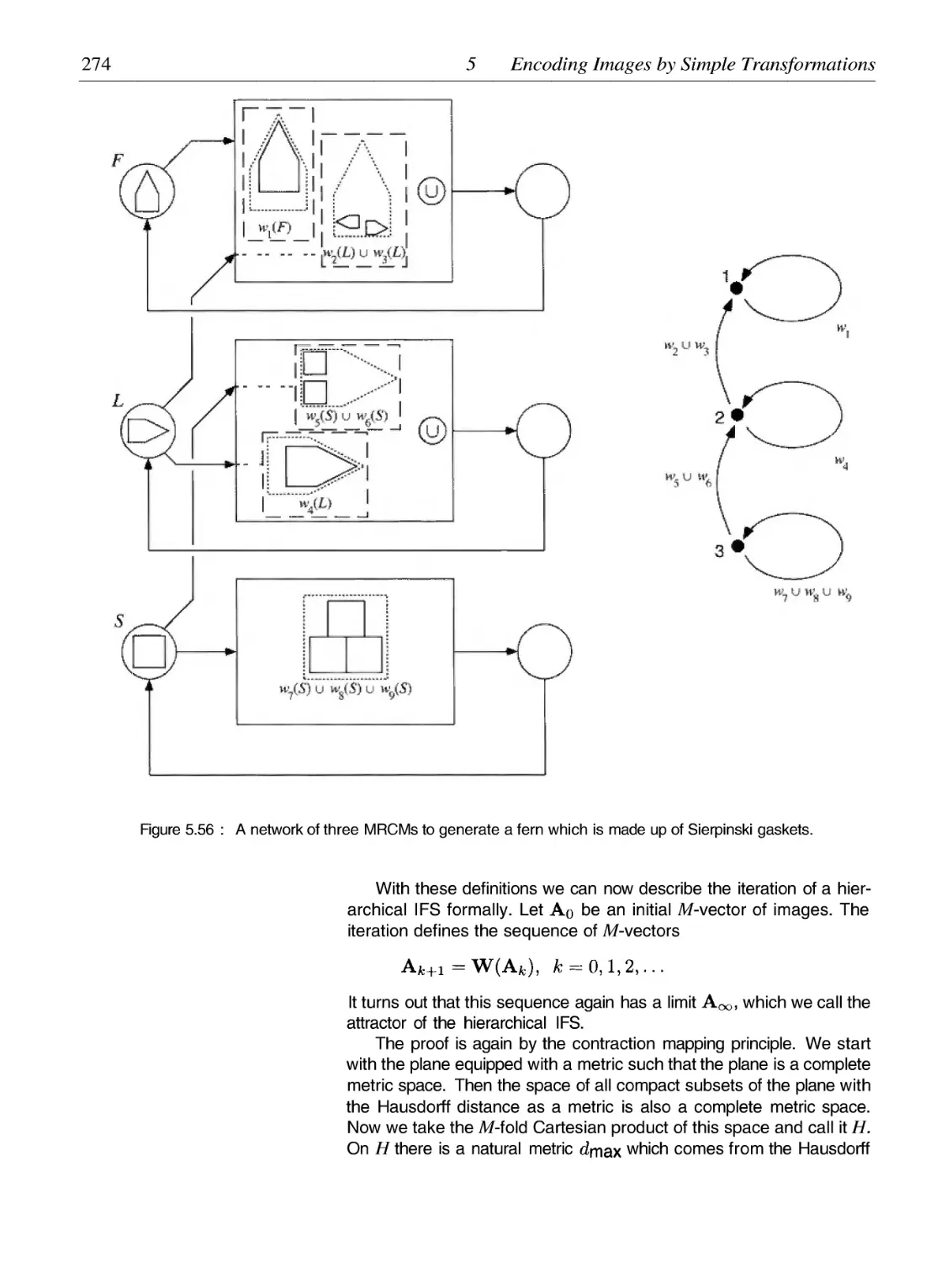
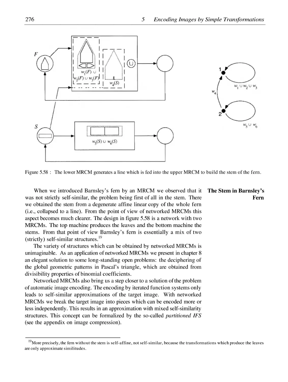
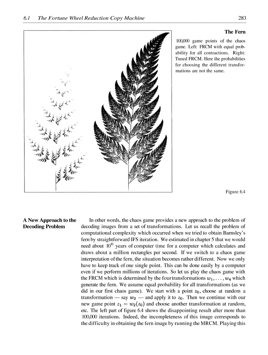
5 Encoding Images by Simple Transformations
215
5.1
5.2
5.3
5.4
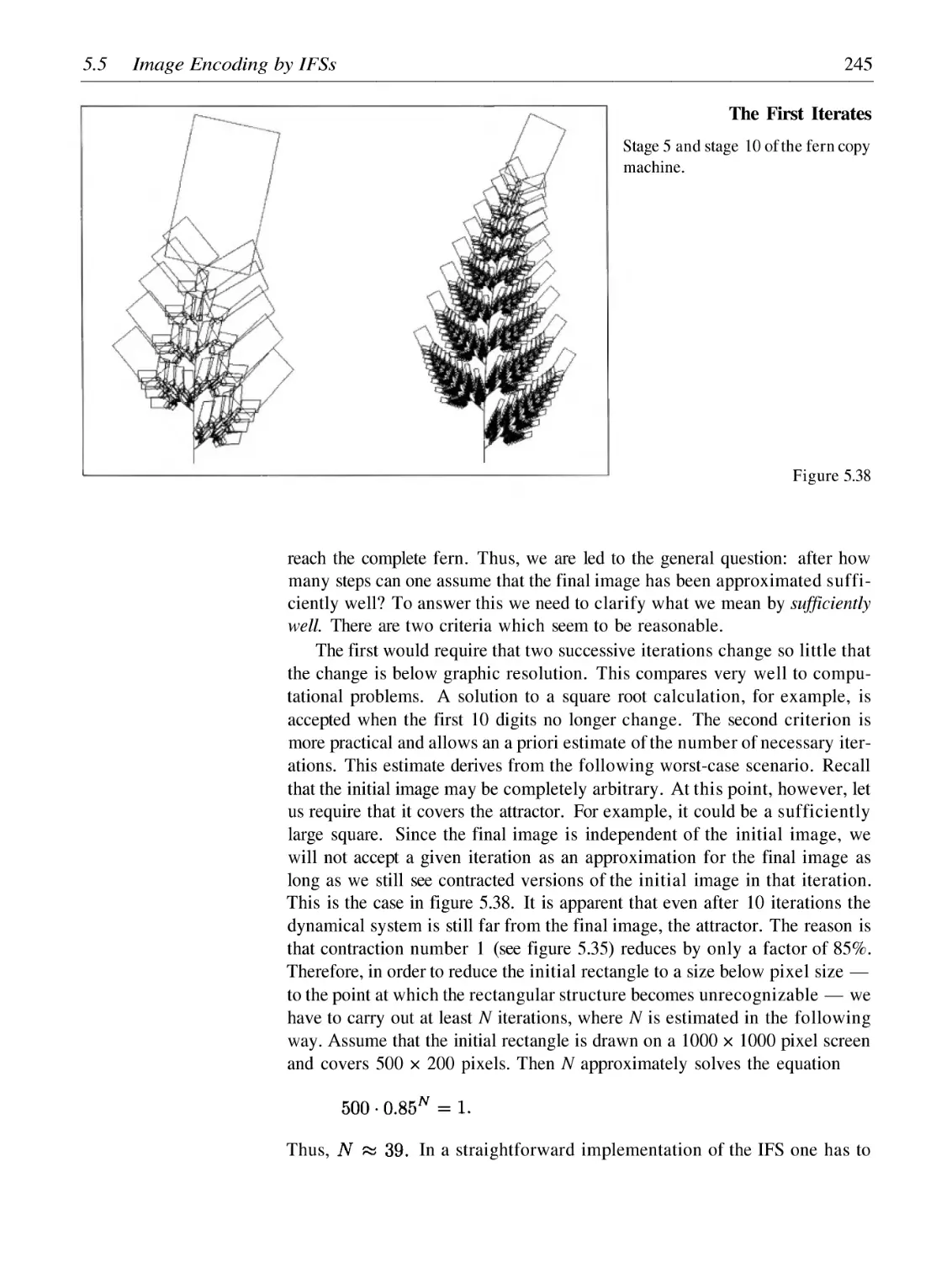
5.5
5.6
5.7
5.8
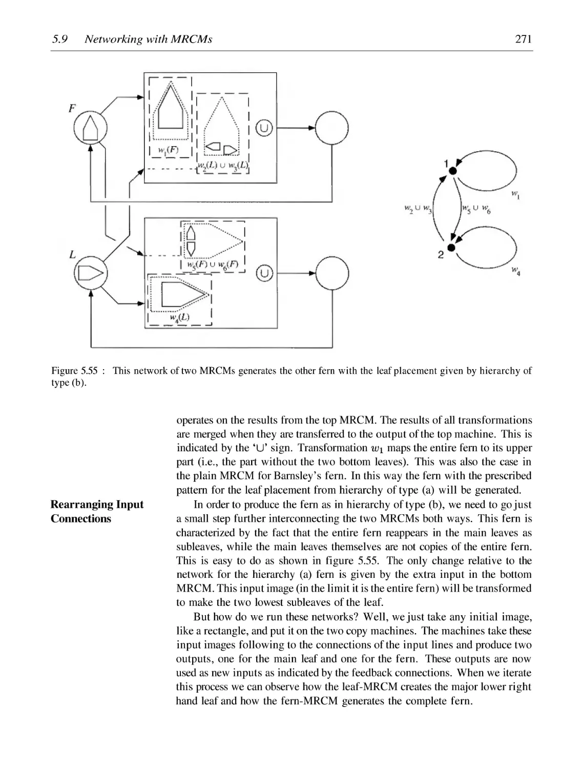
5.9
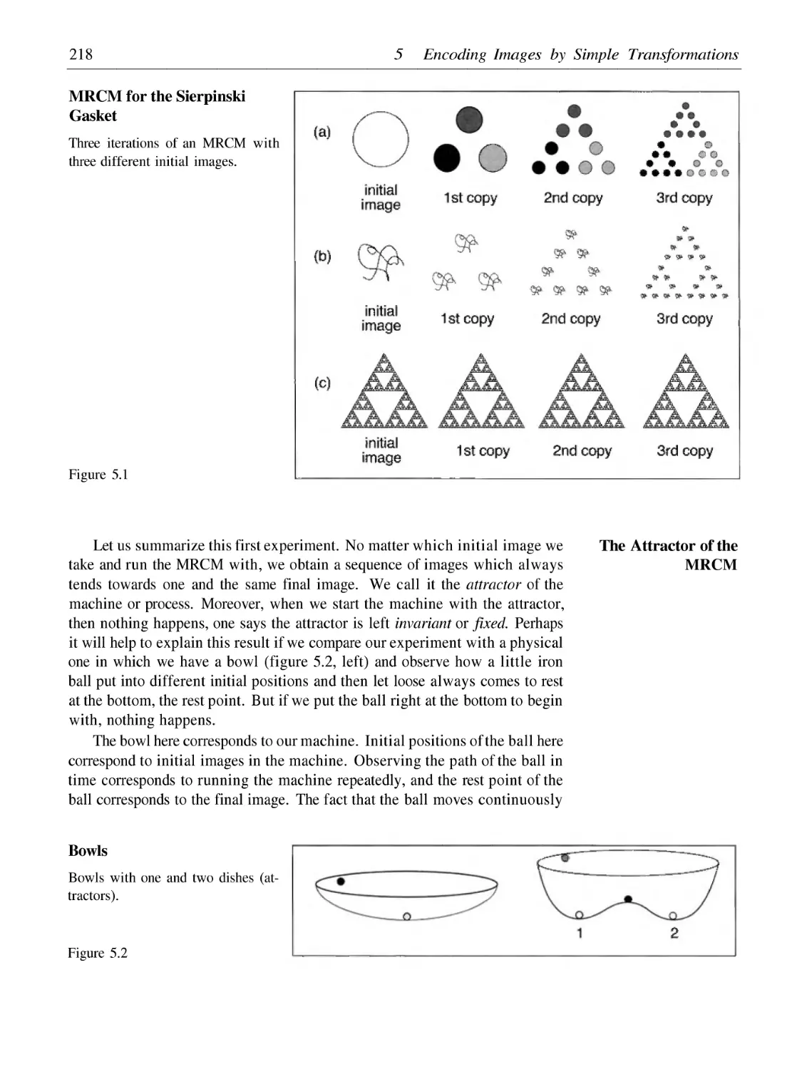
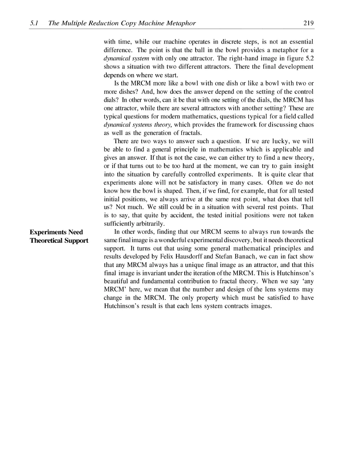
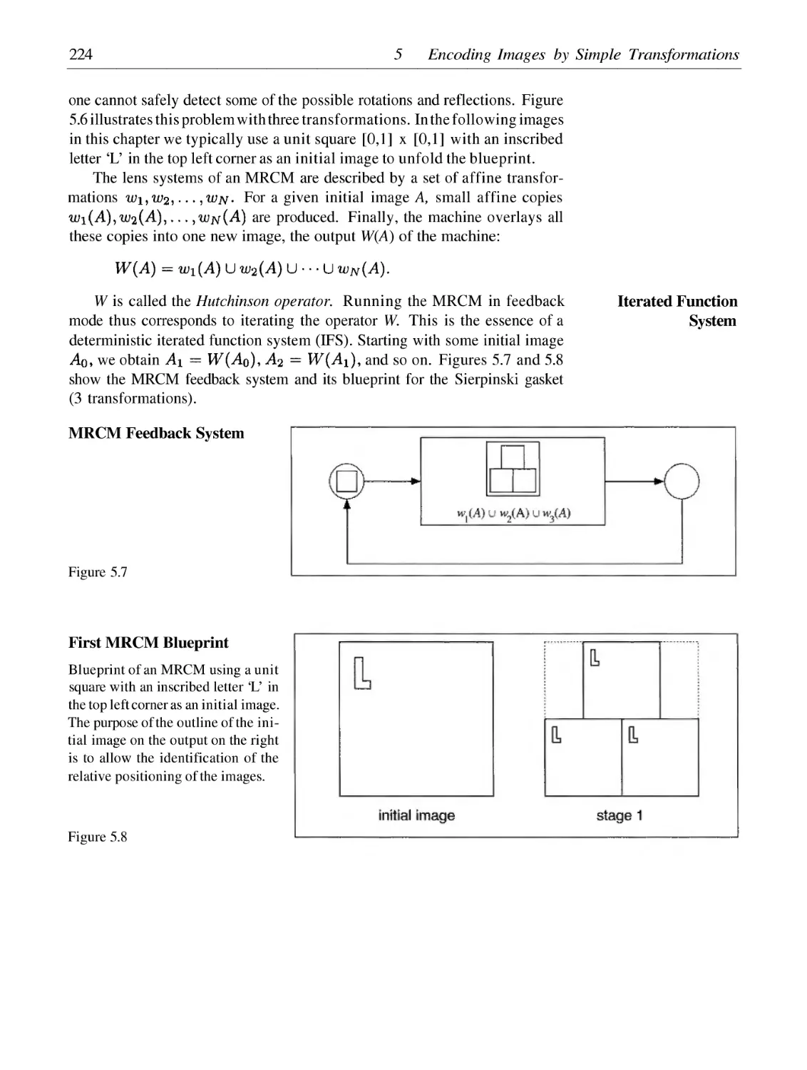
The Multiple Reduction Copy Machine Metaphor
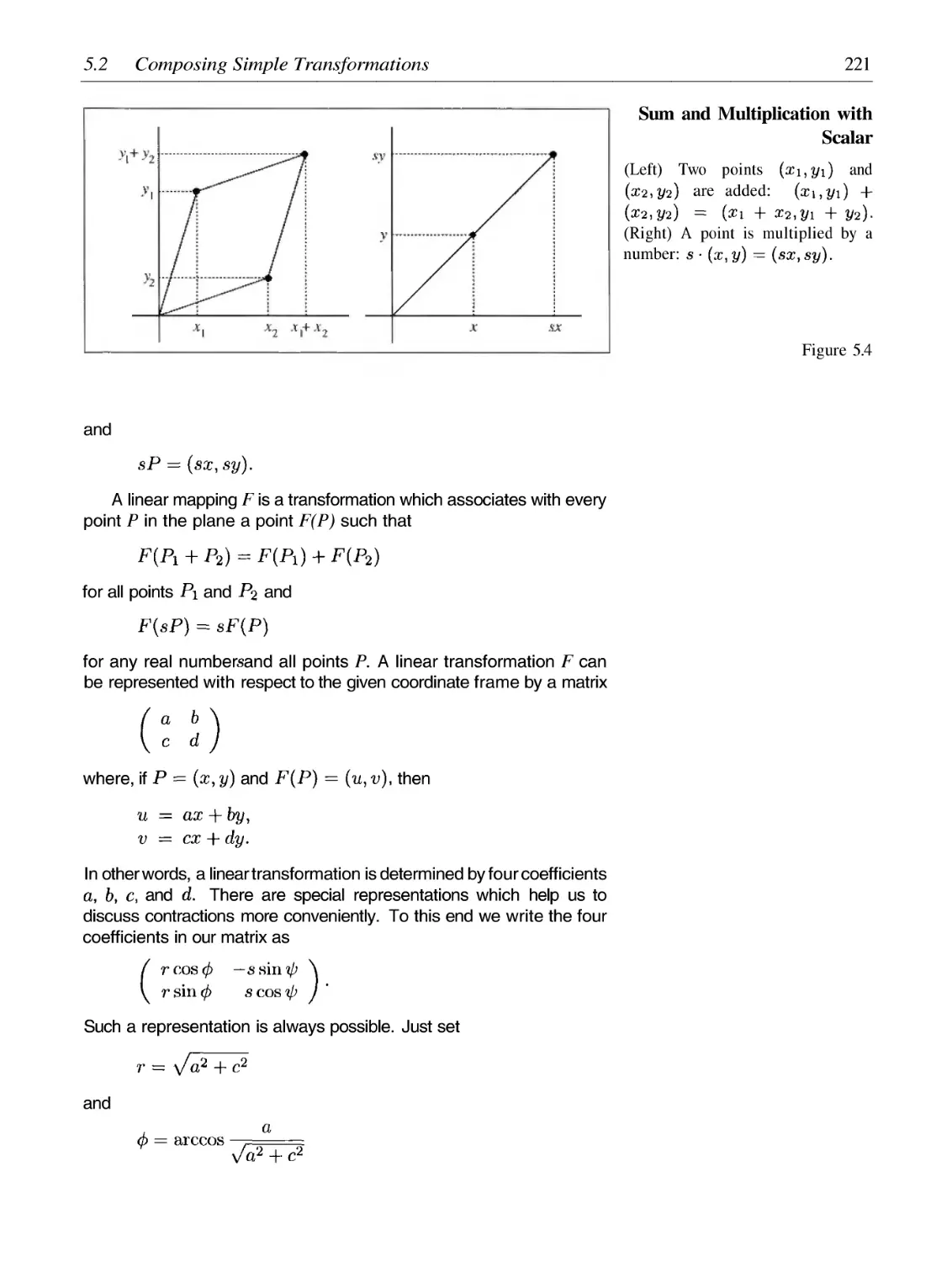
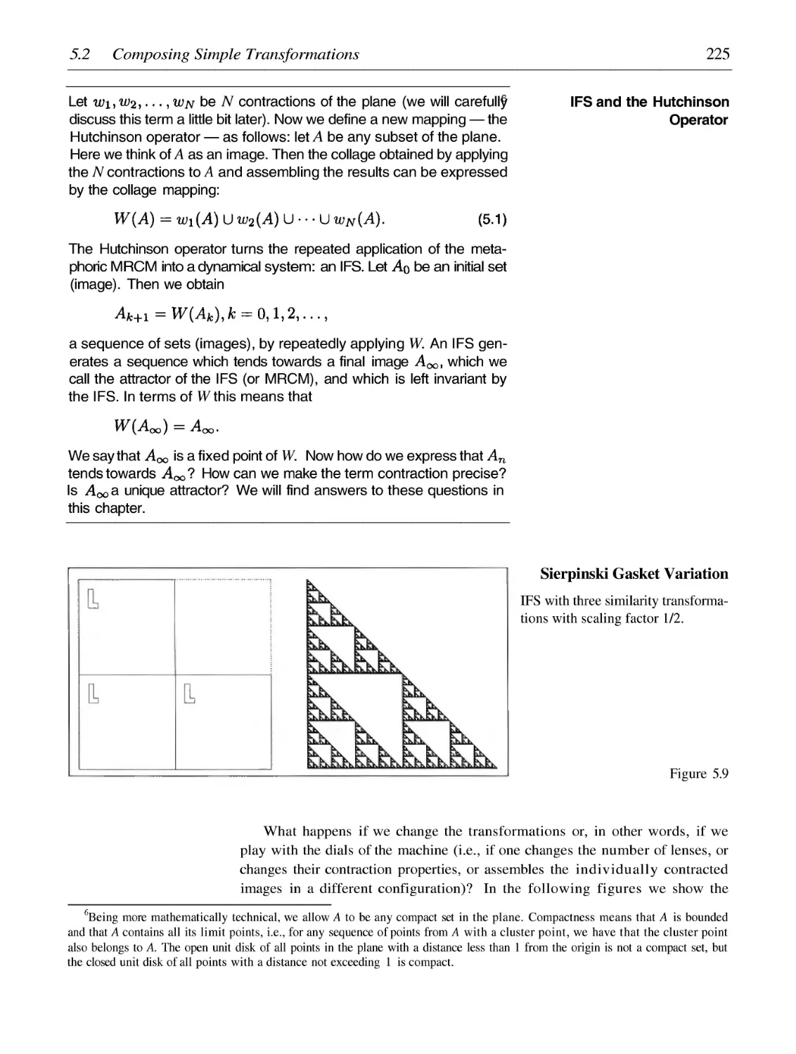
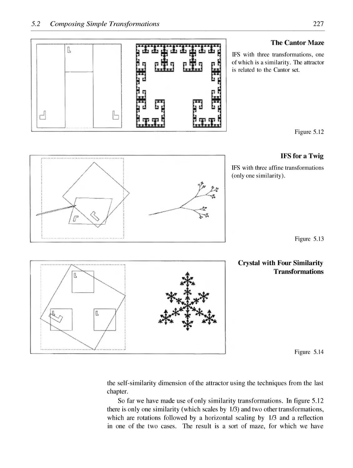
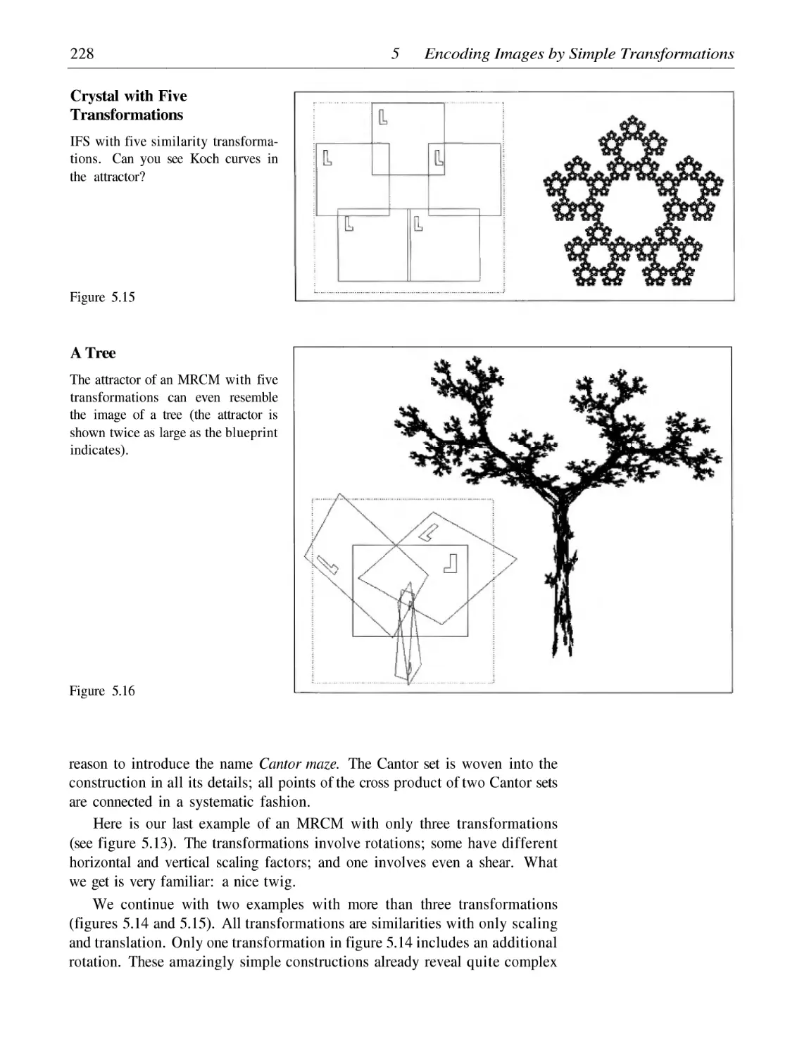
Composing Simple Transformations
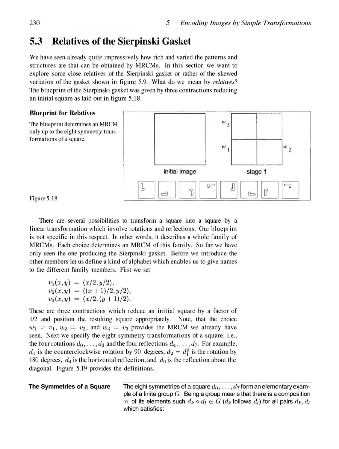
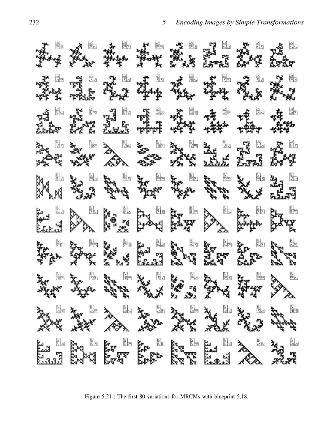
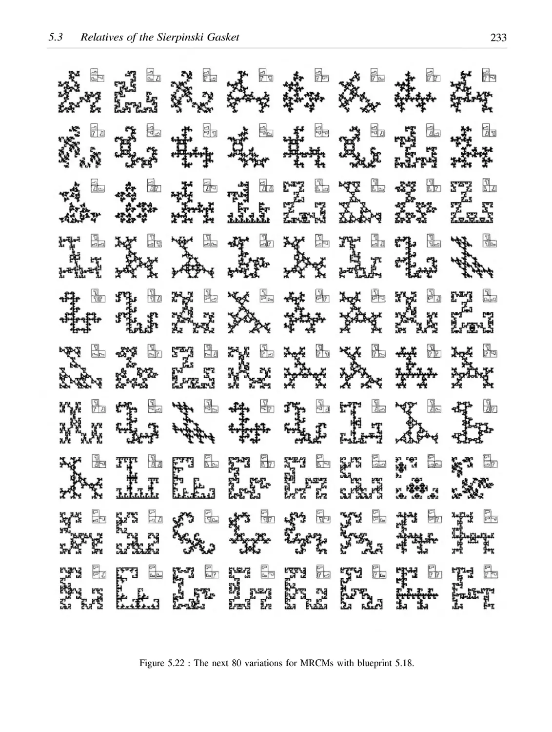
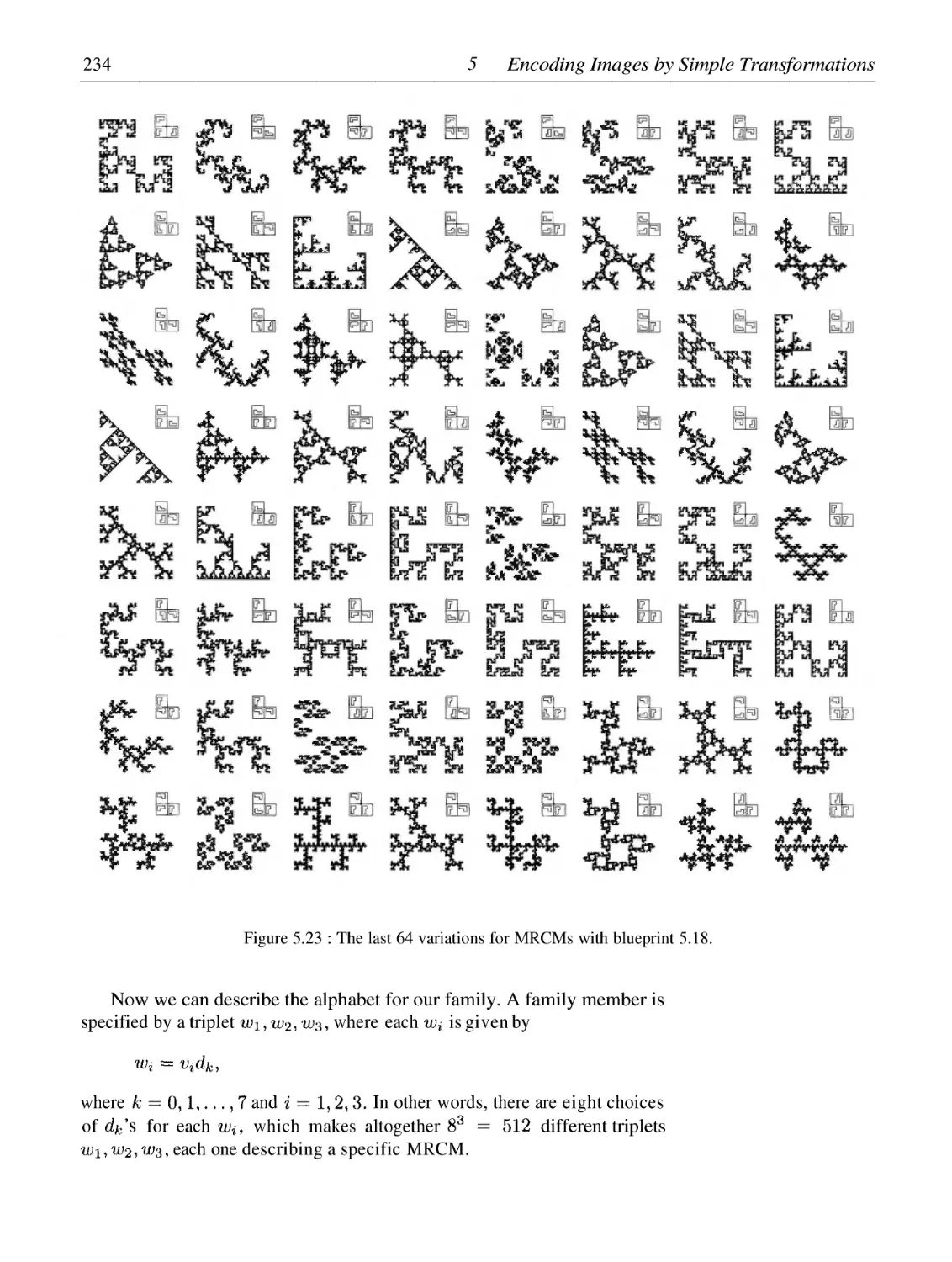
Relatives of the Sierpinski Gasket
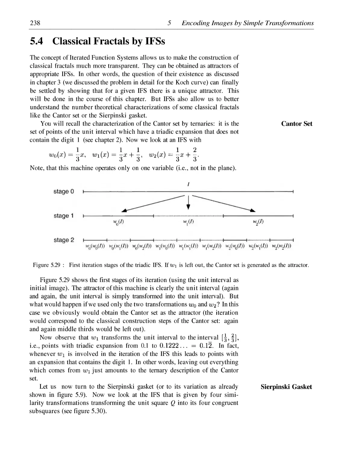
Classical Fractals by IFSs
Image Encoding by IFSs
Foundation of IFS: The Contraction Mapping Principle
Choosing the Right Metric
Composing Self-Similar Images
Breaking Self-Similarity and Self-Affinity: Networking with MRCMs
217
220
230
238
244
248
258
262
267
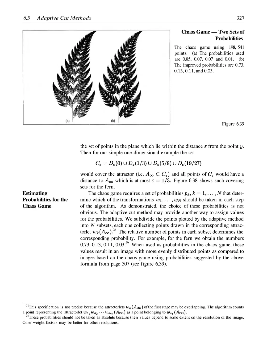
6 The Chaos Game: How Randomness Creates Deterministic Shapes
6.1
6.2
6.3
6.4
6.5
277
280
287
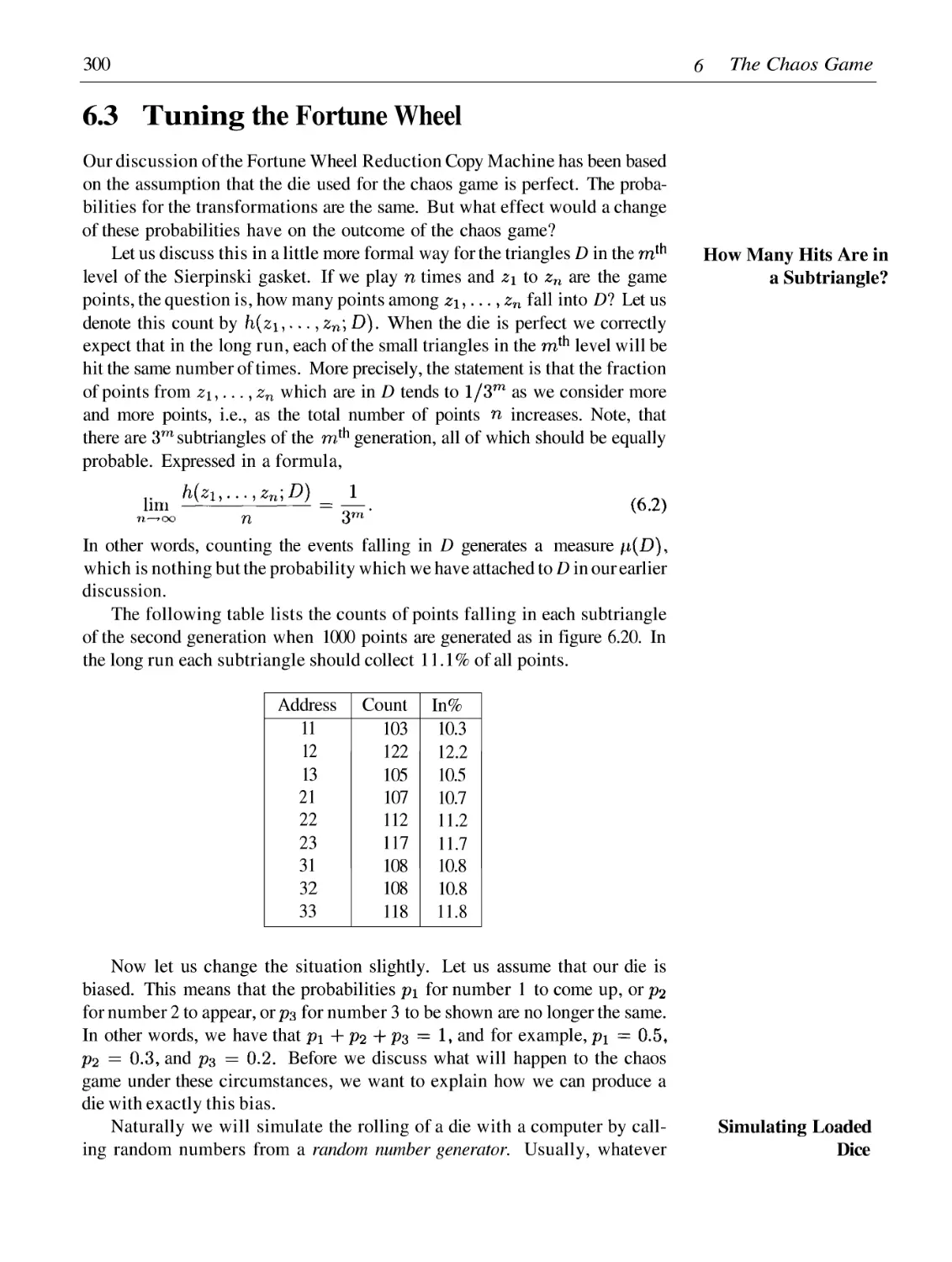
300
311
319
The Fortune Wheel Reduction Copy Machine
Addresses: Analysis of the Chaos Game
Tuning the Fortune Wheel
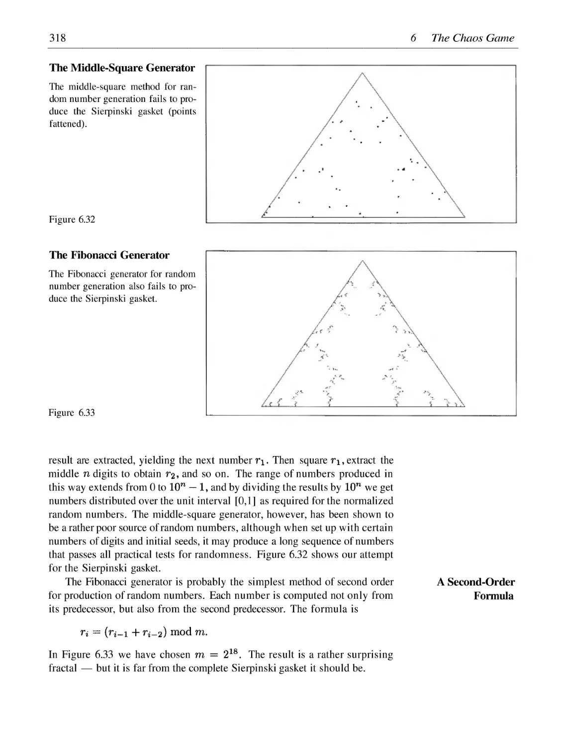
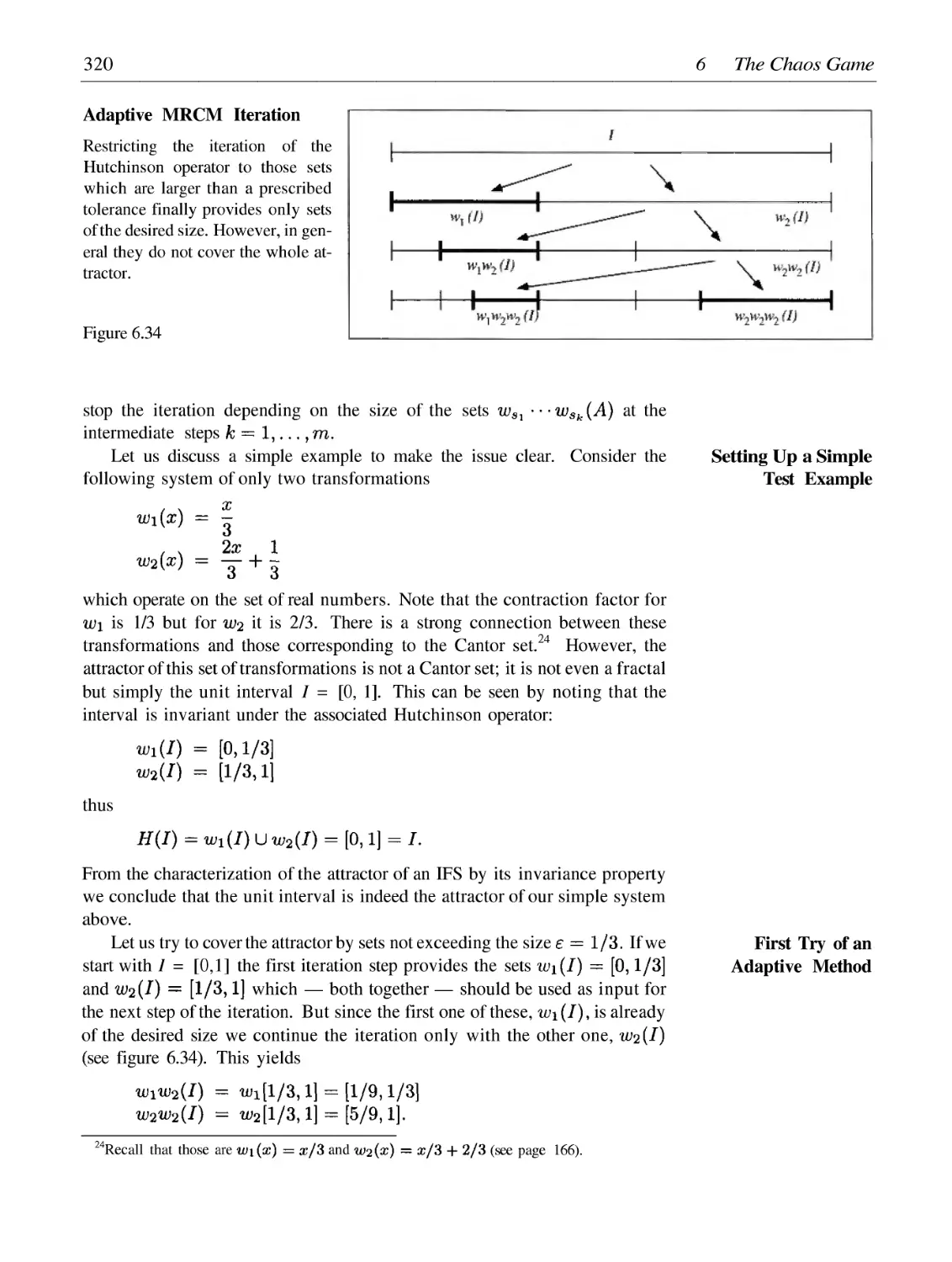
Random Number Generator Pitfall
Adaptive Cut Methods
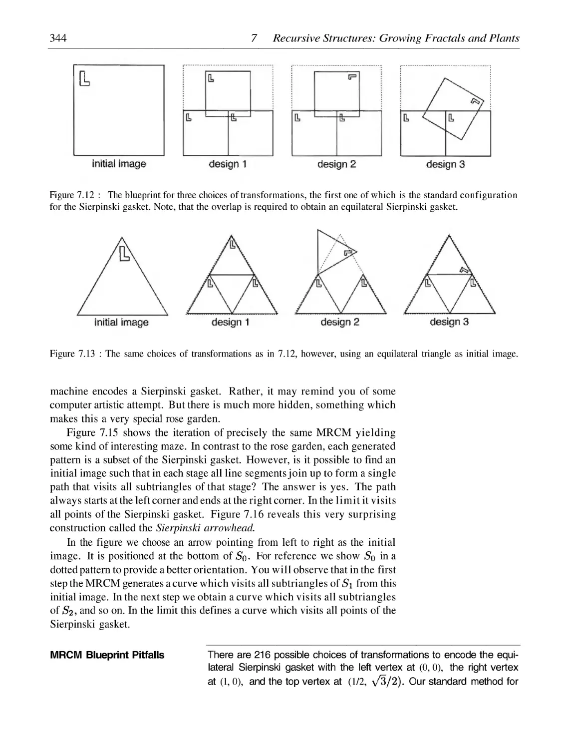
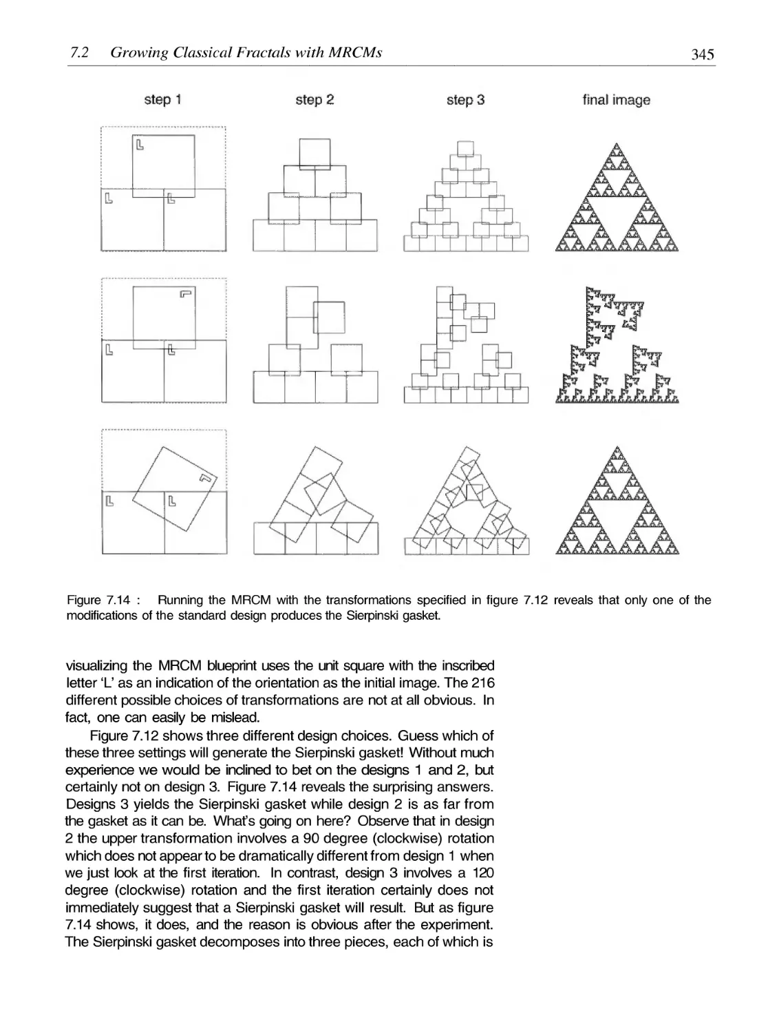
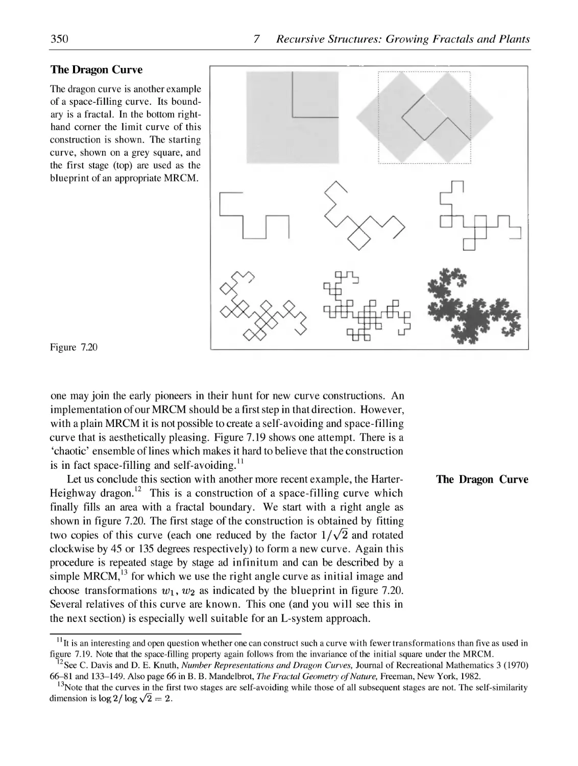
7 Recursive Structures: Growing Fractals and Plants
329
7.1
7.2
7.3
7.4
7.5
7.6
L-Systems: A Language for Modeling Growth
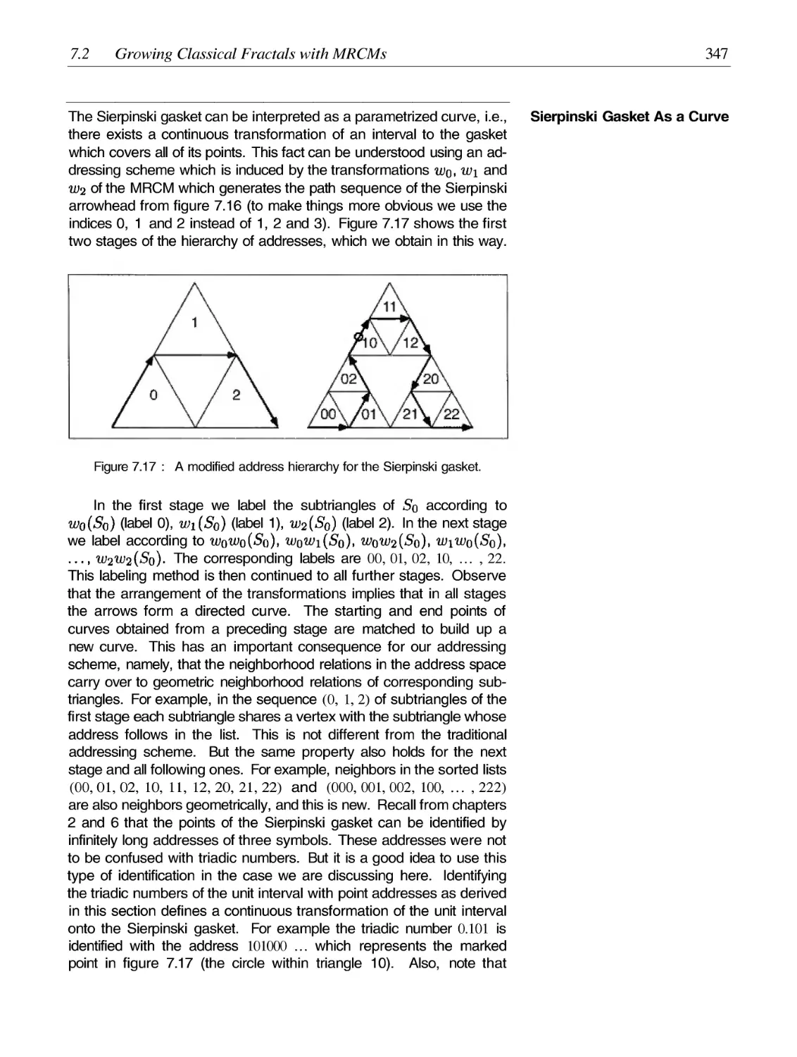
Growing Classical Fractals with MRCMs
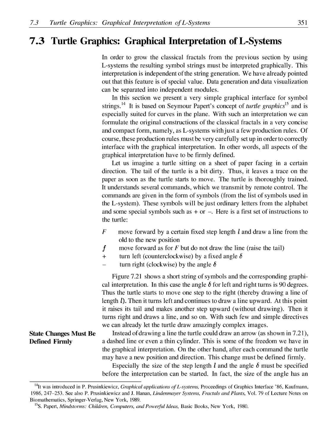
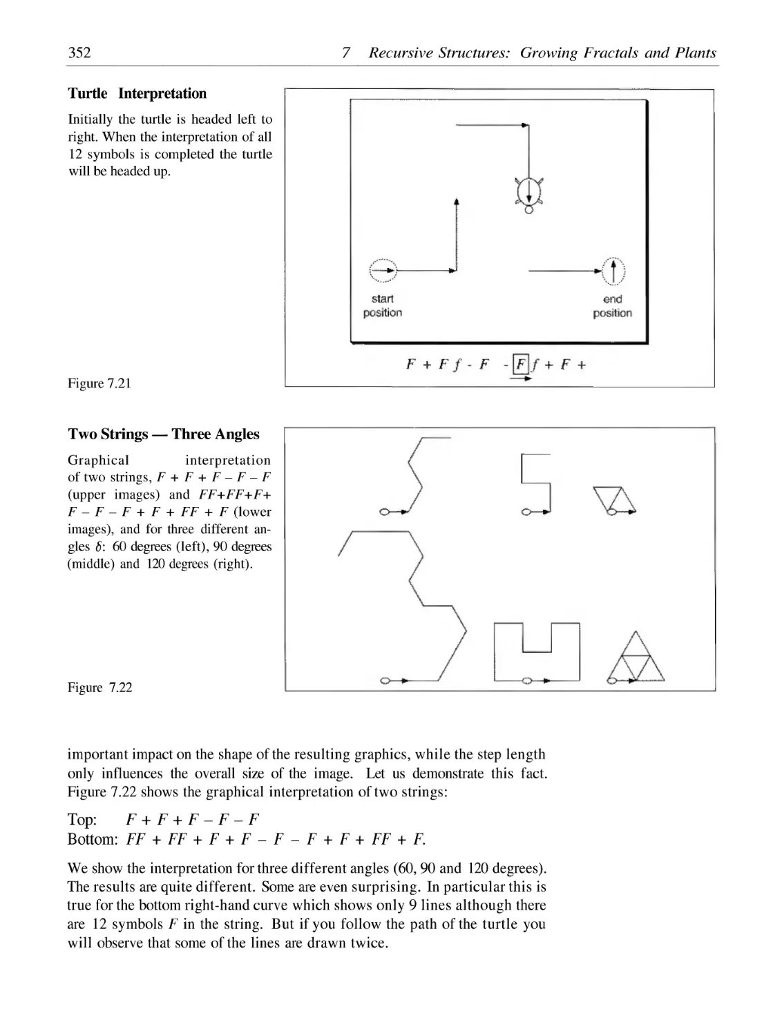
Turtle Graphics: Graphical Interpretation of L-Systems
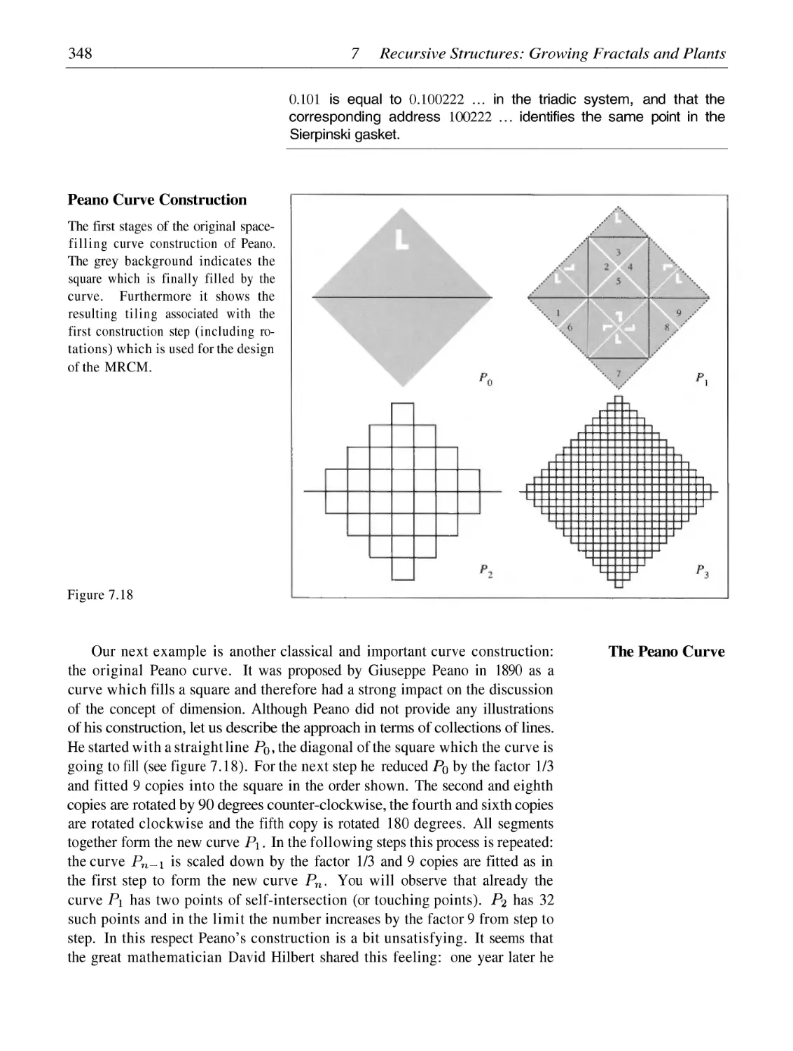
Growing Classical Fractals with L-Systems
Growing Fractals with Networked MRCMs
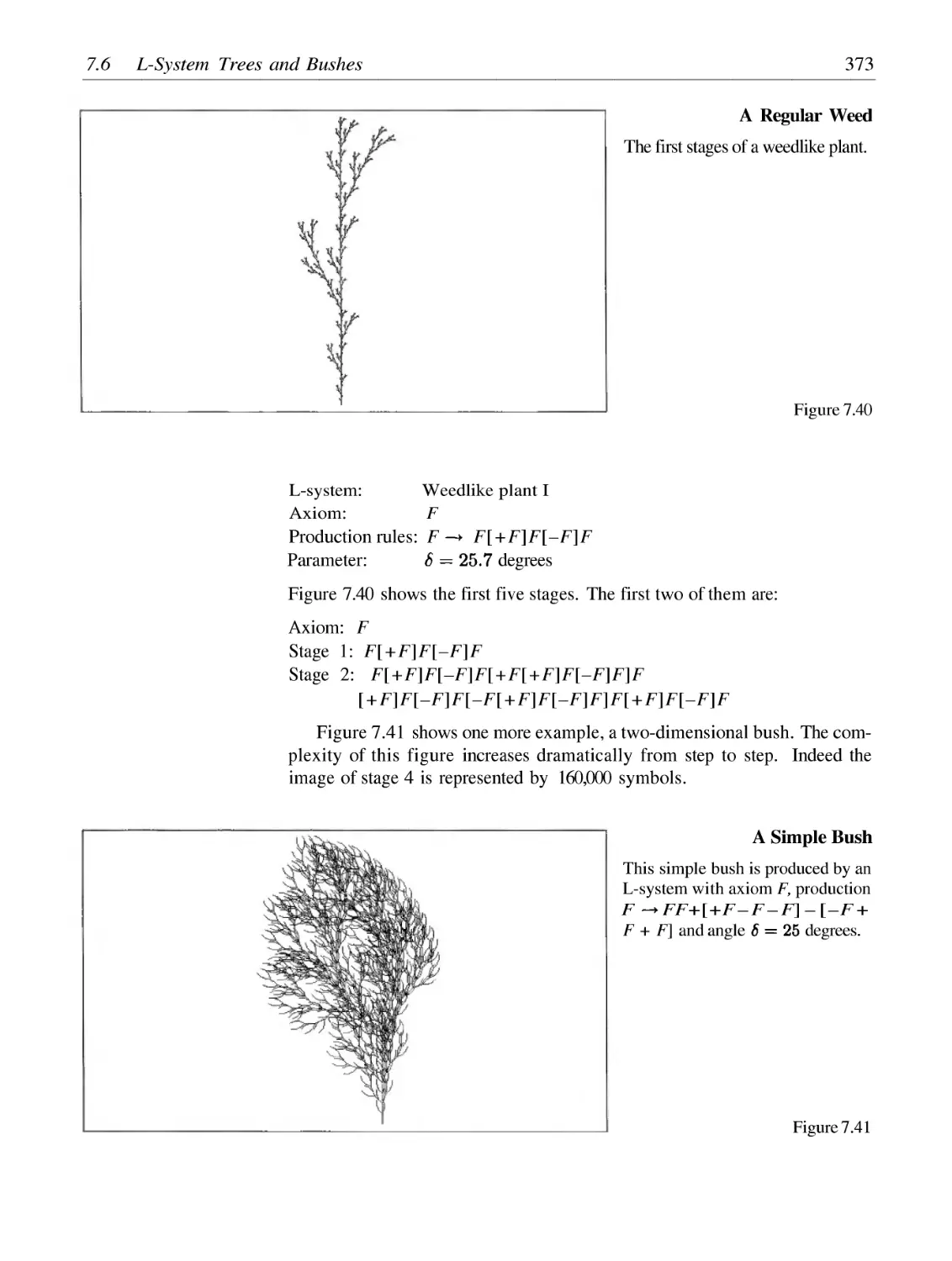
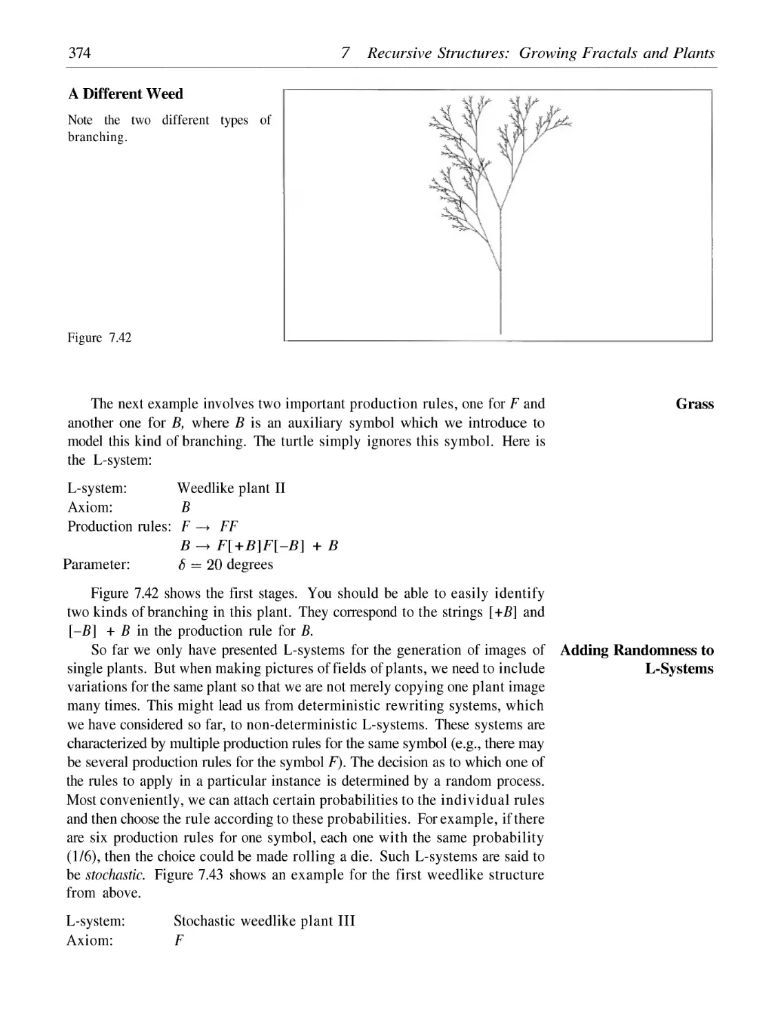
L-System Trees and Bushes
333
340
351
355
367
372
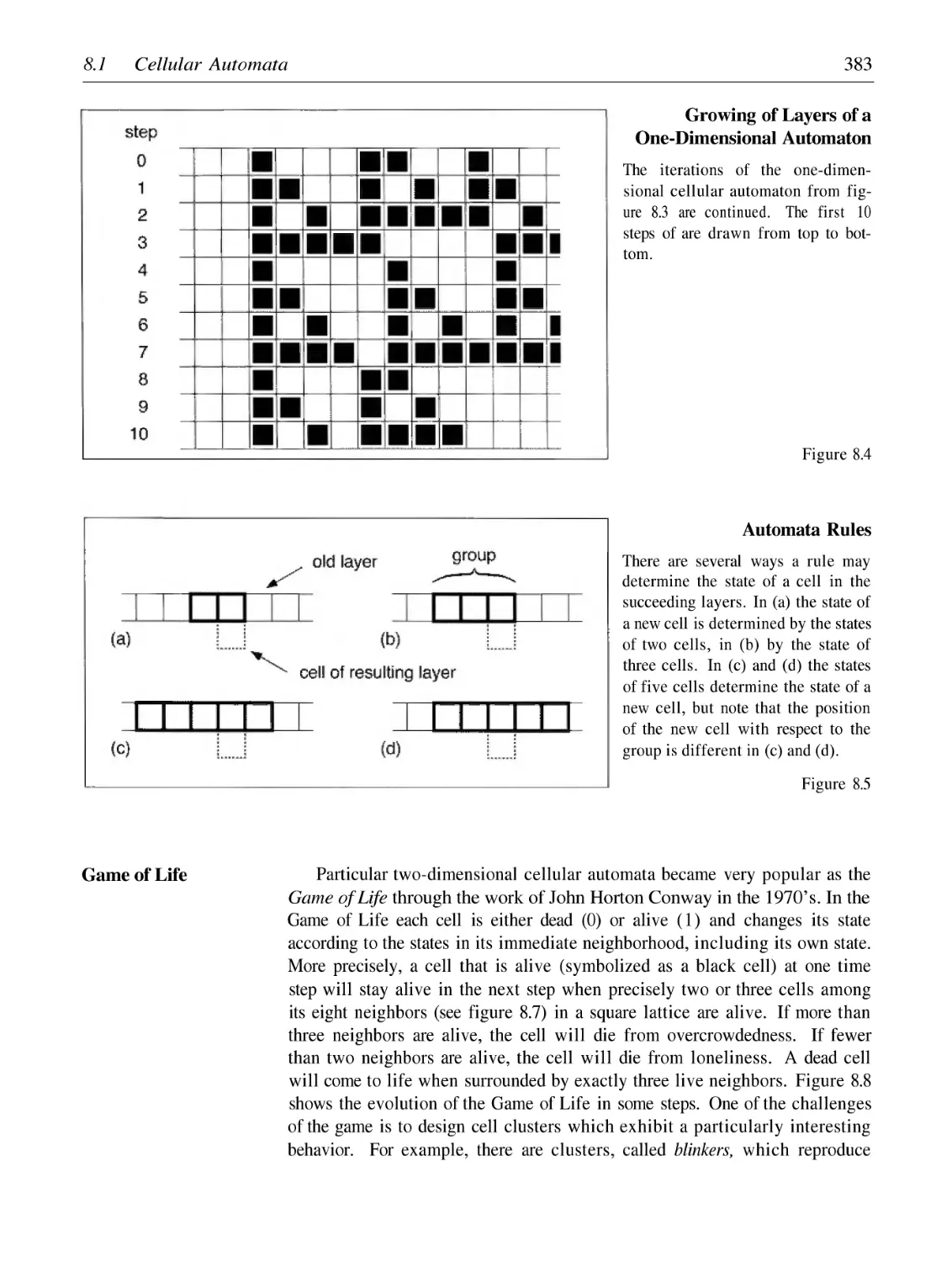
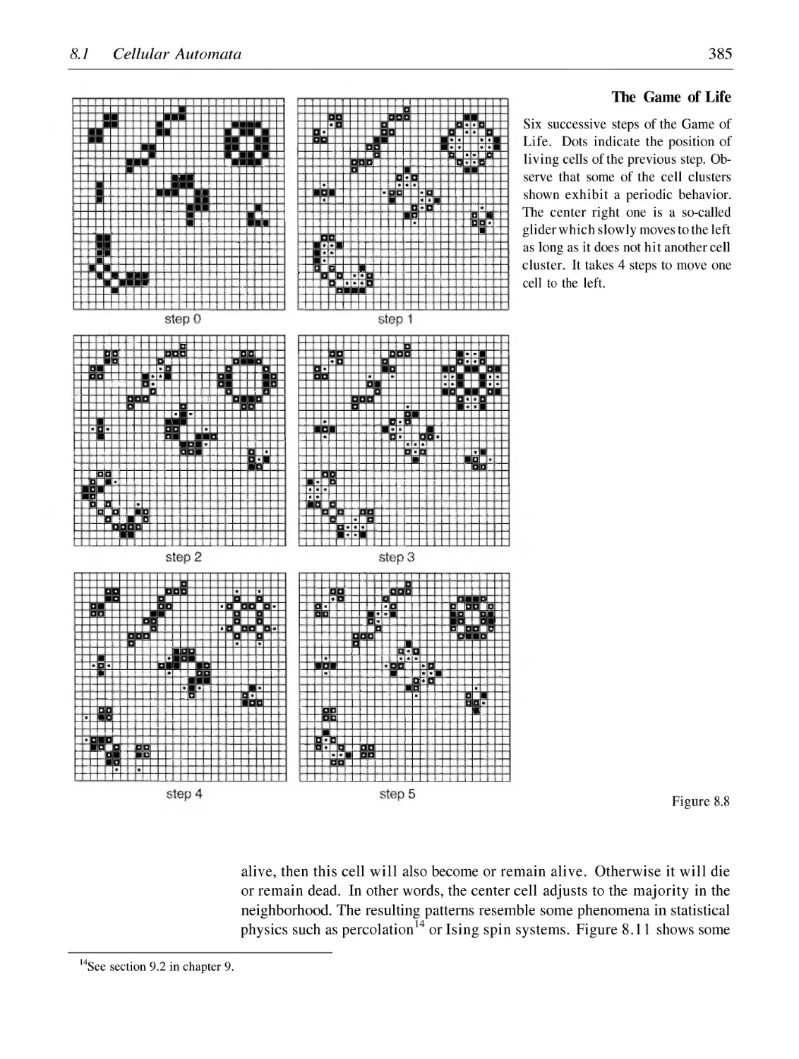
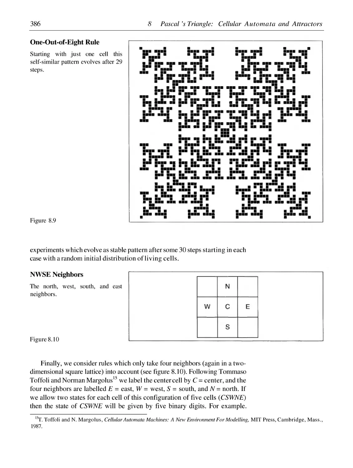
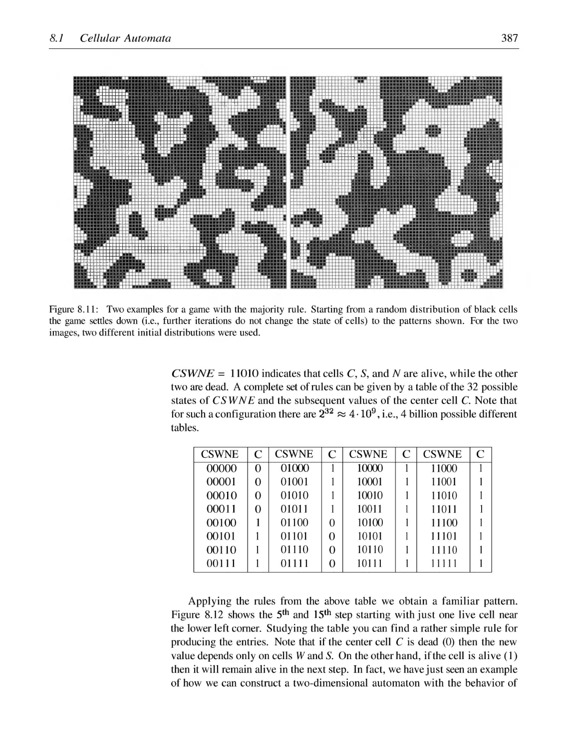
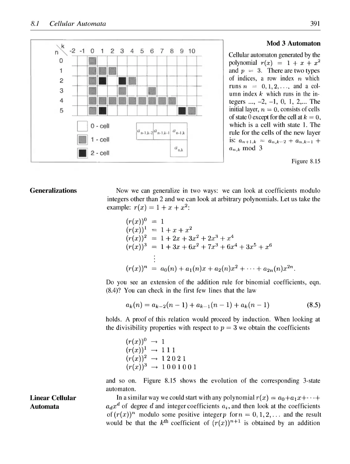
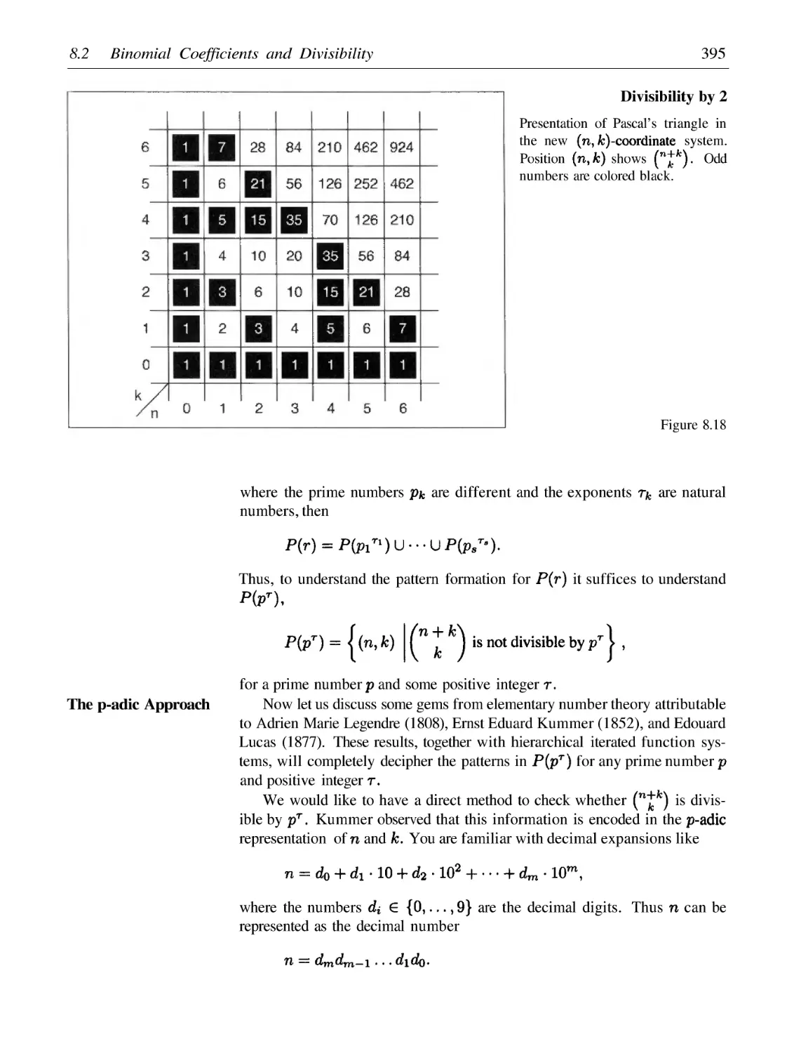
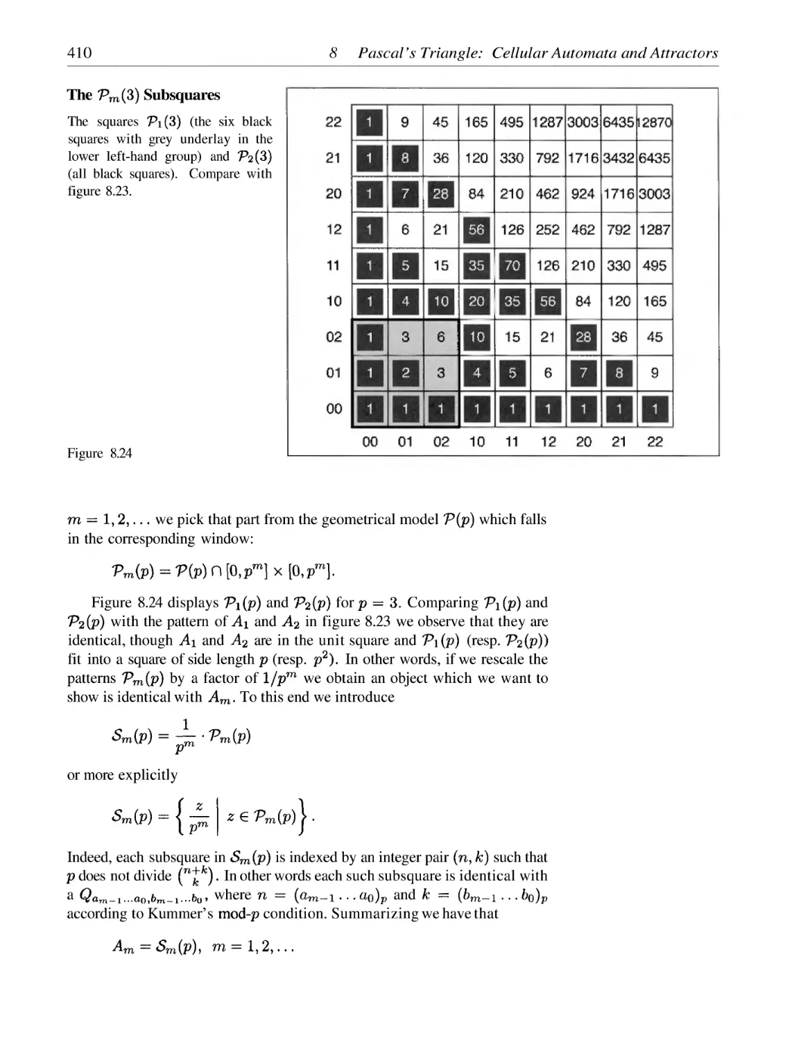
8 Pascal's Triangle: Cellular Automata and Attractors
377
8.1
8.2
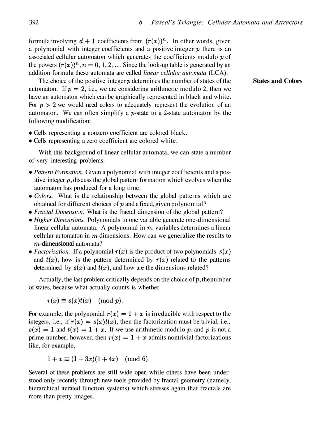
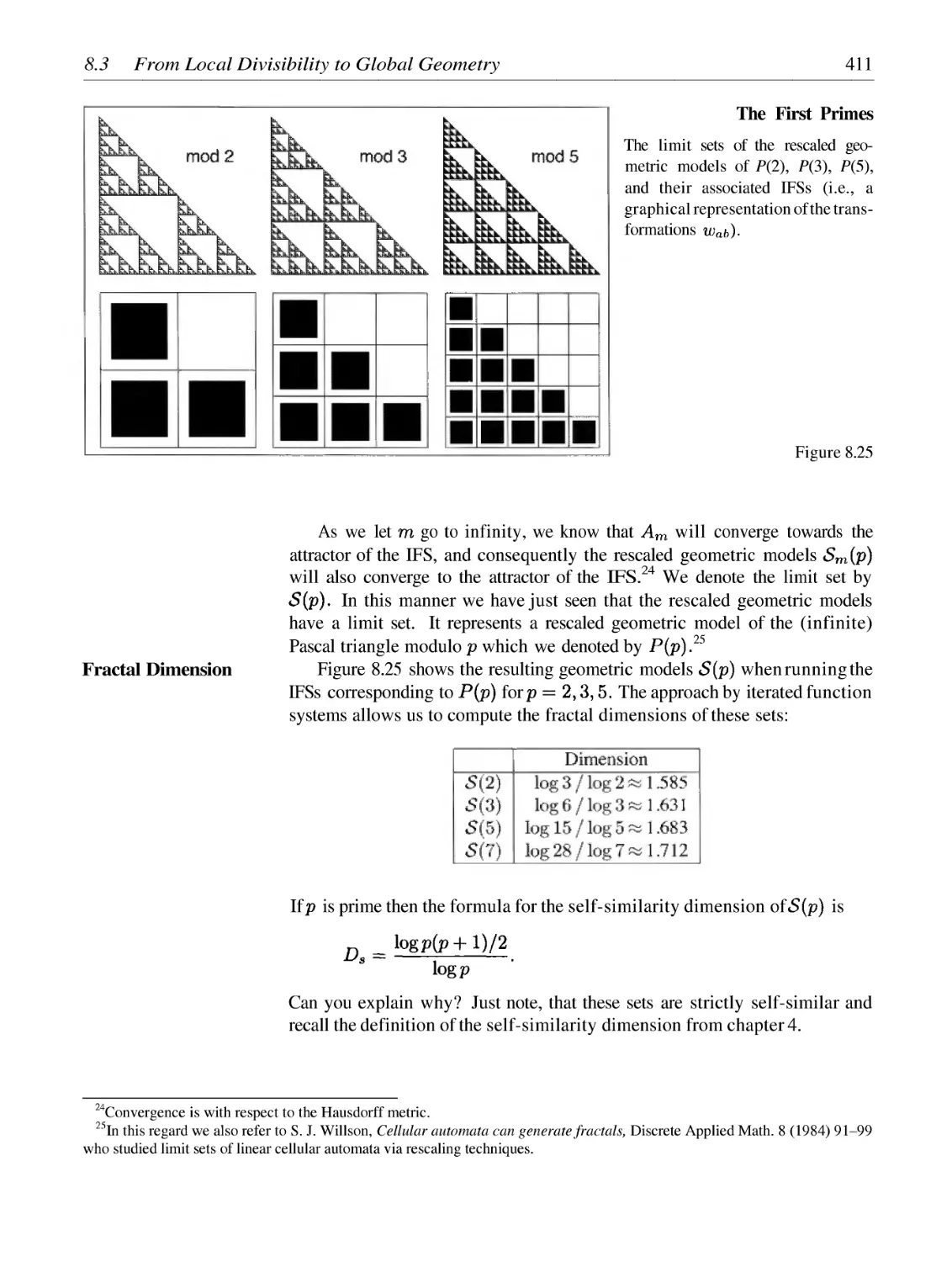
8.3
8.4
8.5
Cellular Automata
Binomial Coefficients and Divisibility
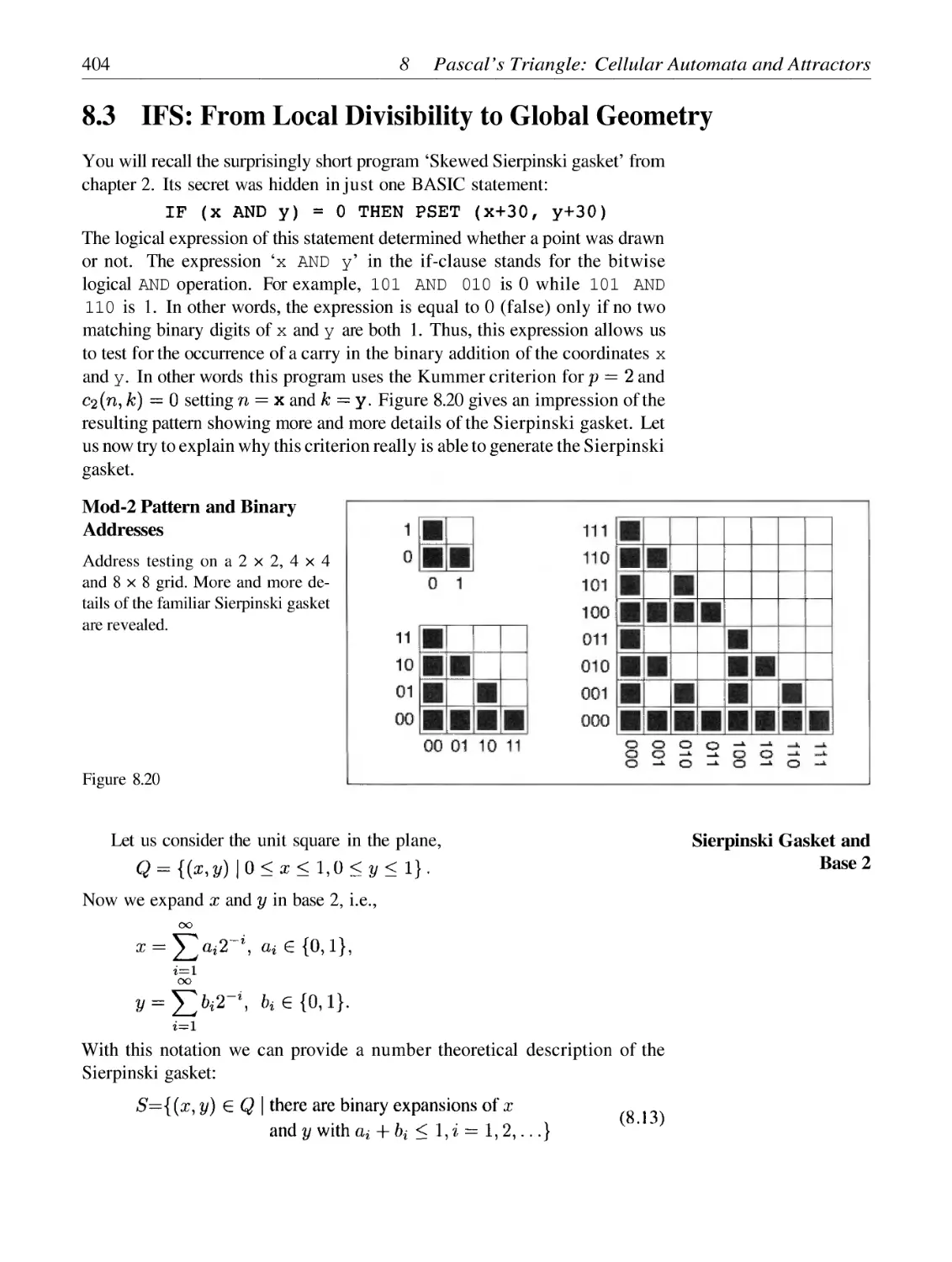
IFS: From Local Divisibility to Global Geometry
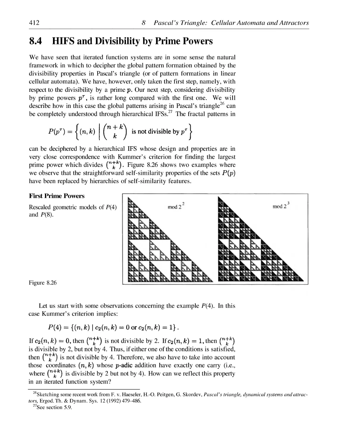
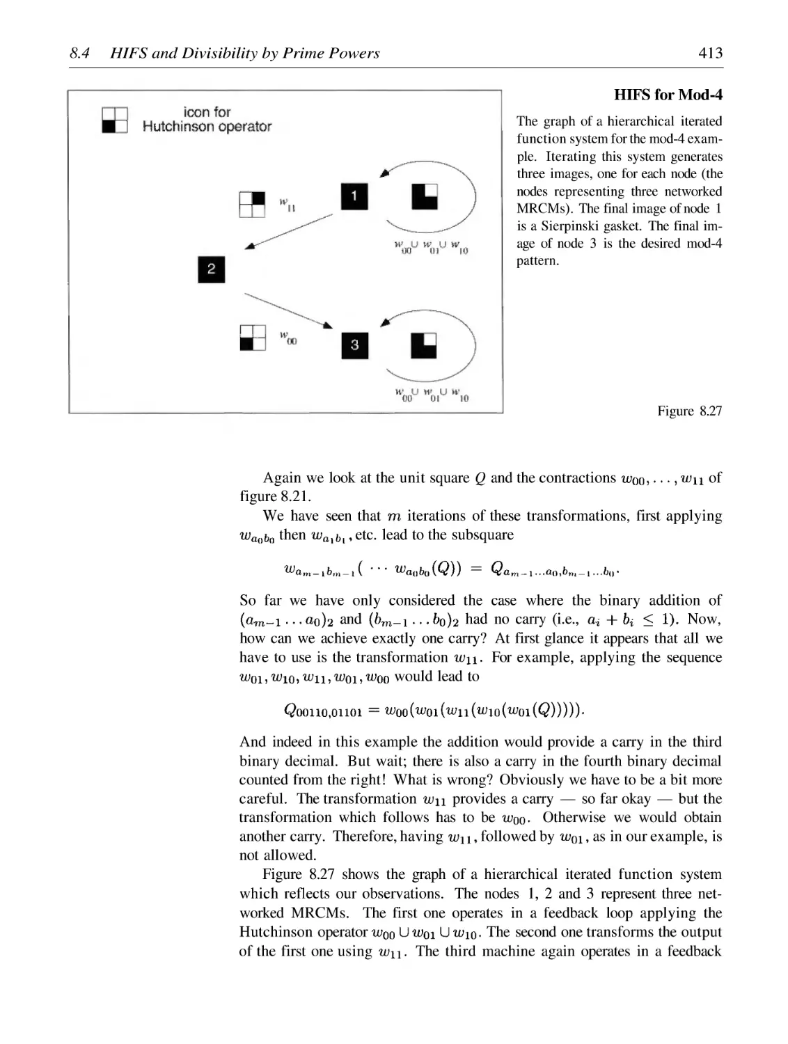
HIFS and Divisibility by Prime Powers
Catalytic Converters, or How Many Cells Are Black?
382
393
404
412
420
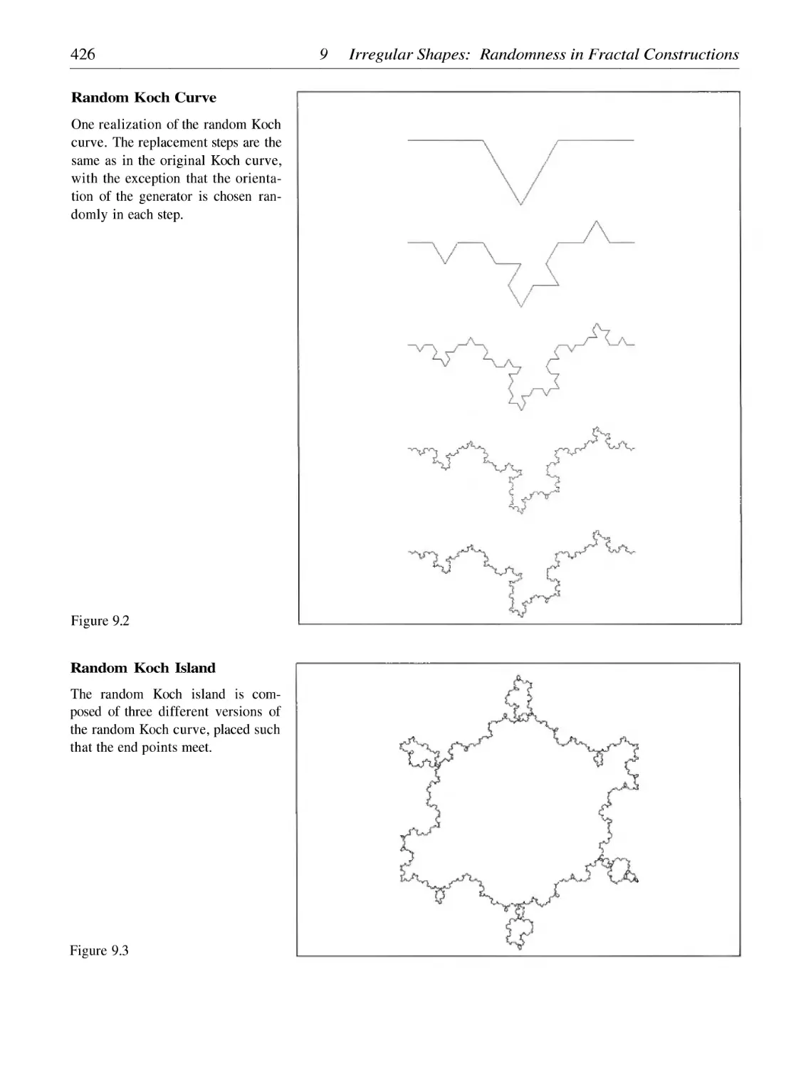
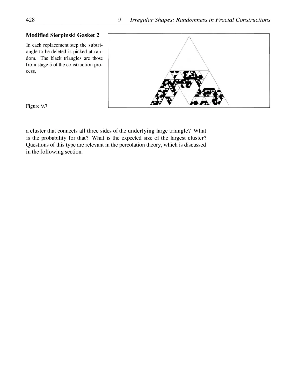
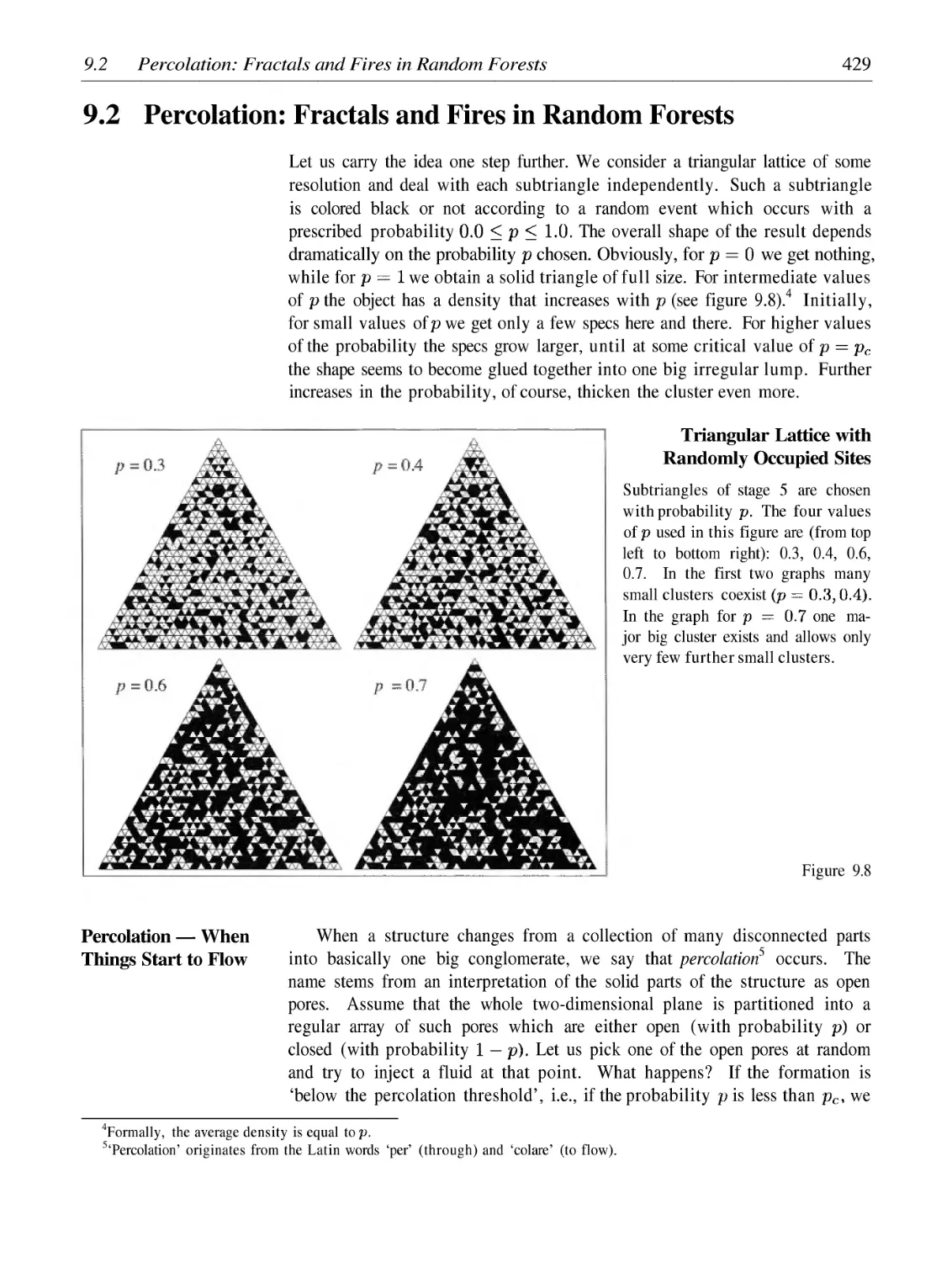
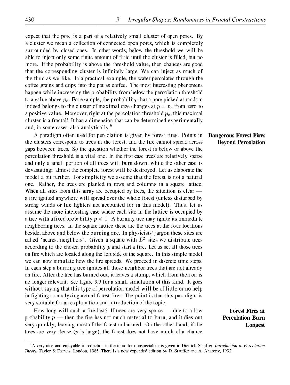
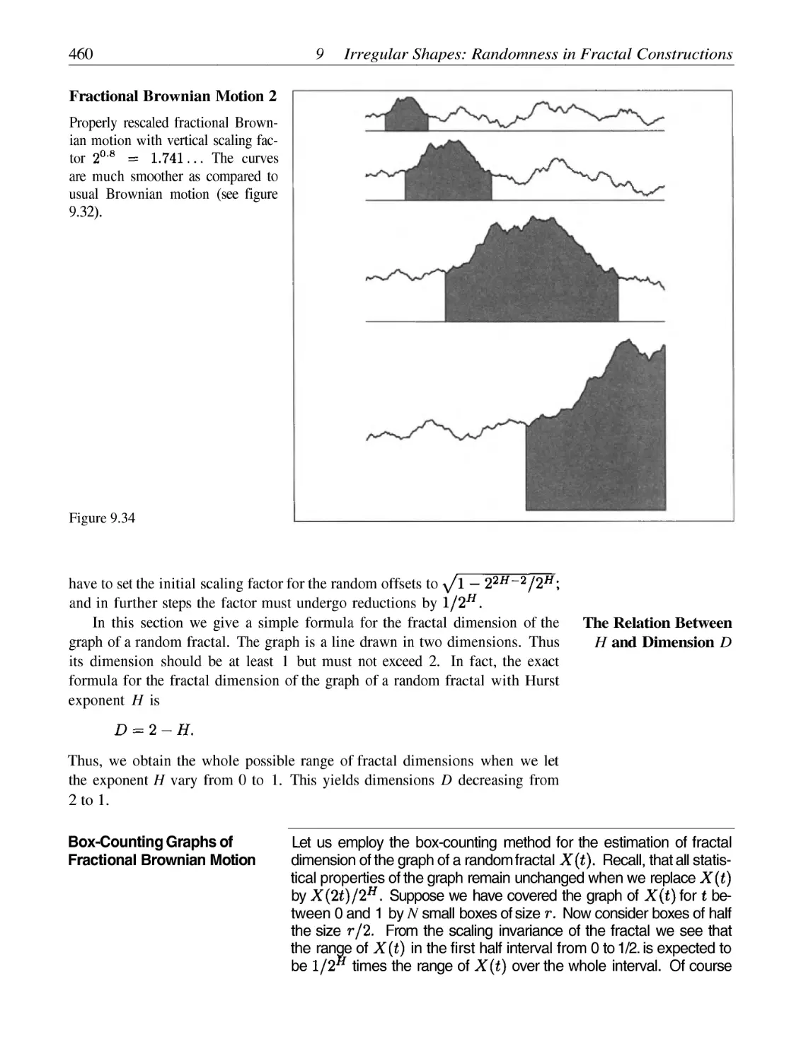
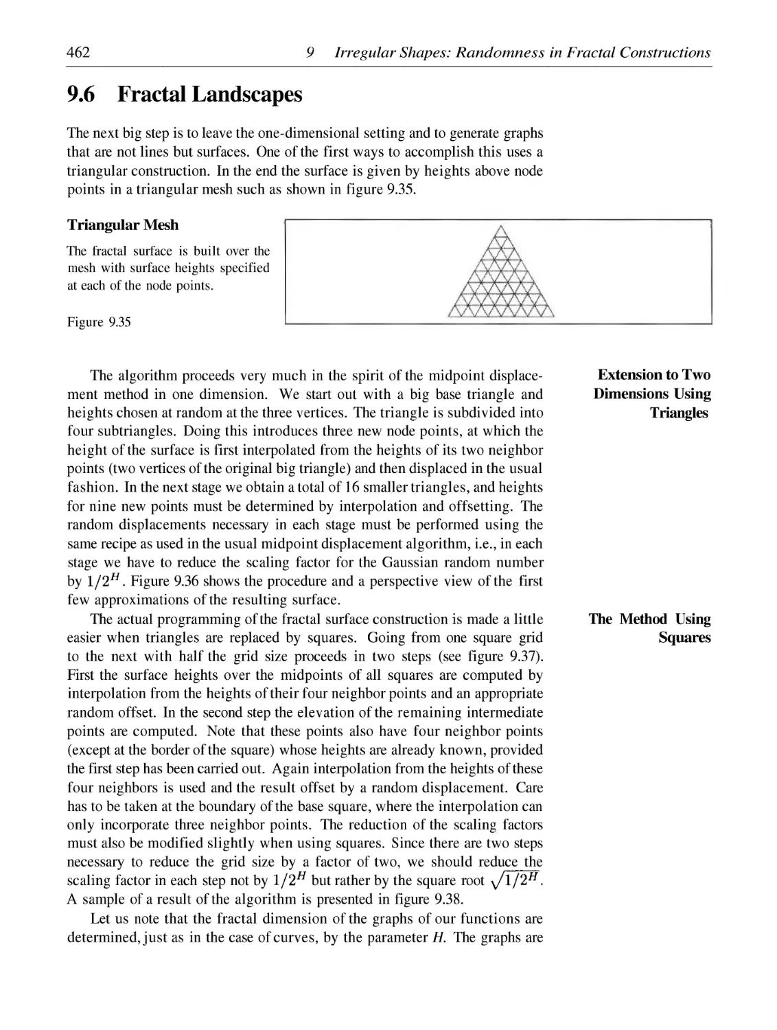
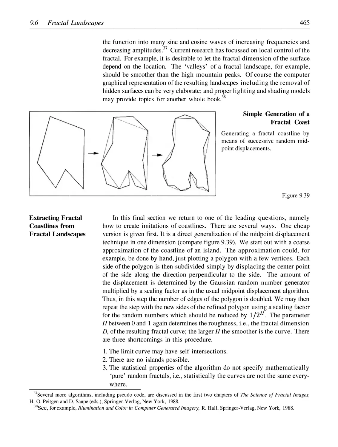
9 Irregular Shapes: Randomness in Fractal Constructions
423
9.1
9.2
9.3
9.4
9.5
9.6
Randomizing Deterministic Fractals
425
429
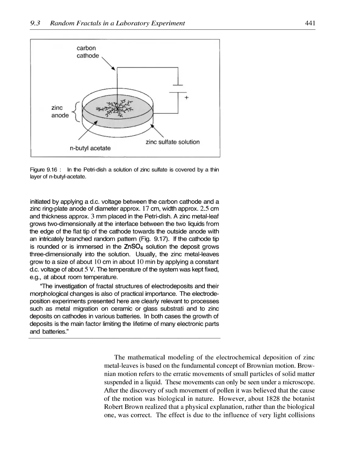
440
446
456
462
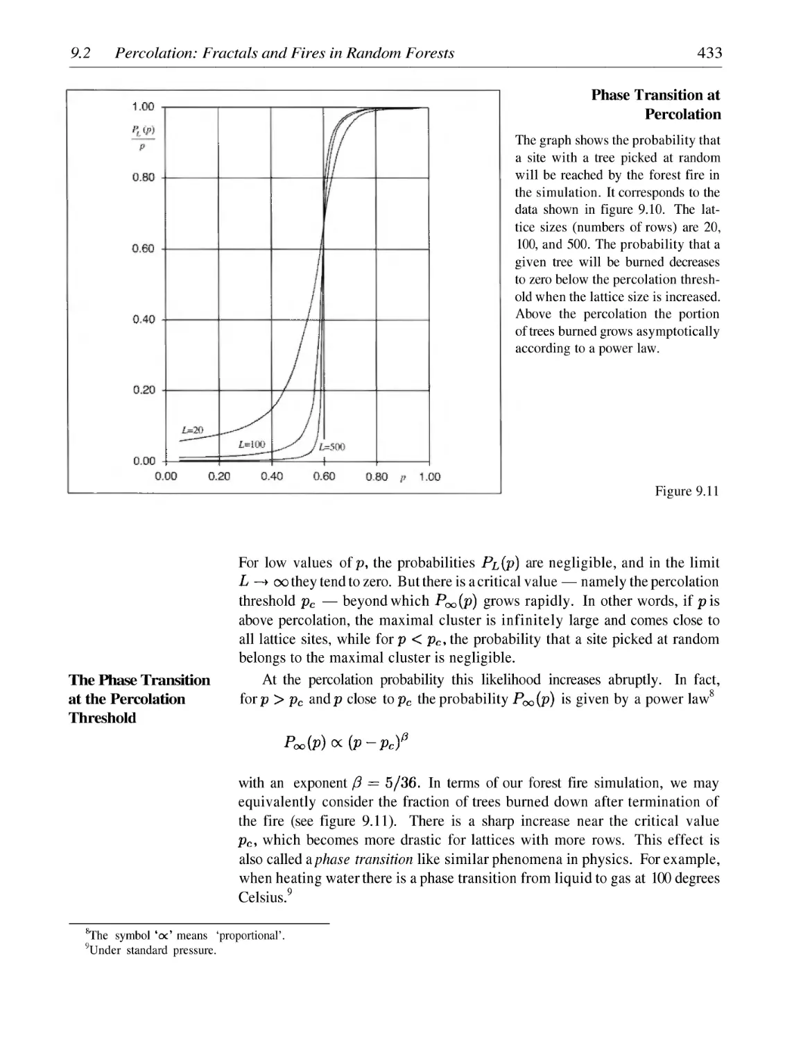
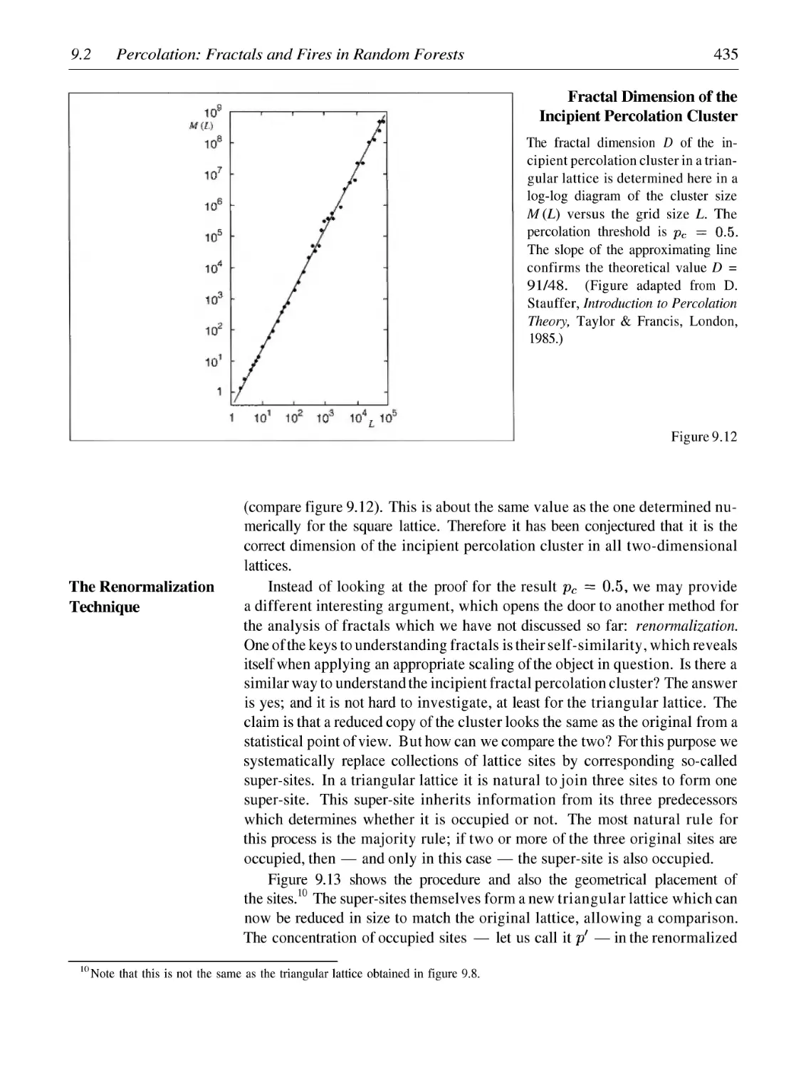
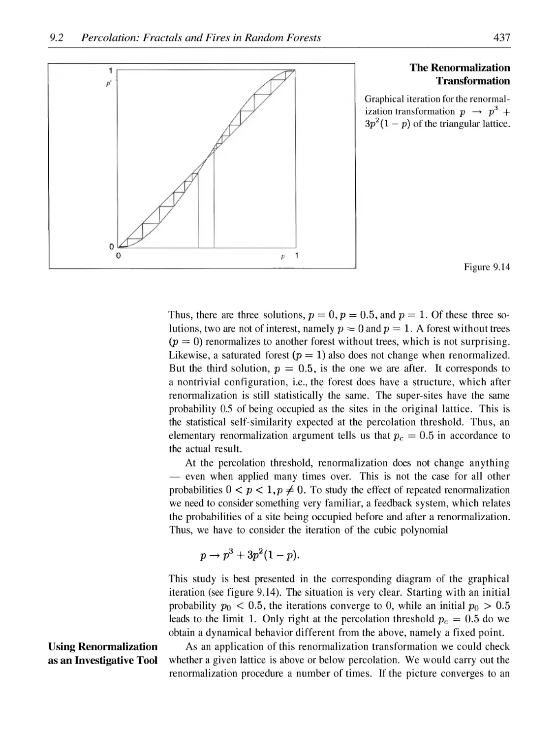
Percolation: Fractals and Fires in Random Forests
Random Fractals in a Laboratory Experiment
Simulation of Brownian Motion
Scaling Laws and Fractional Brownian Motion
Fractal Landscapes
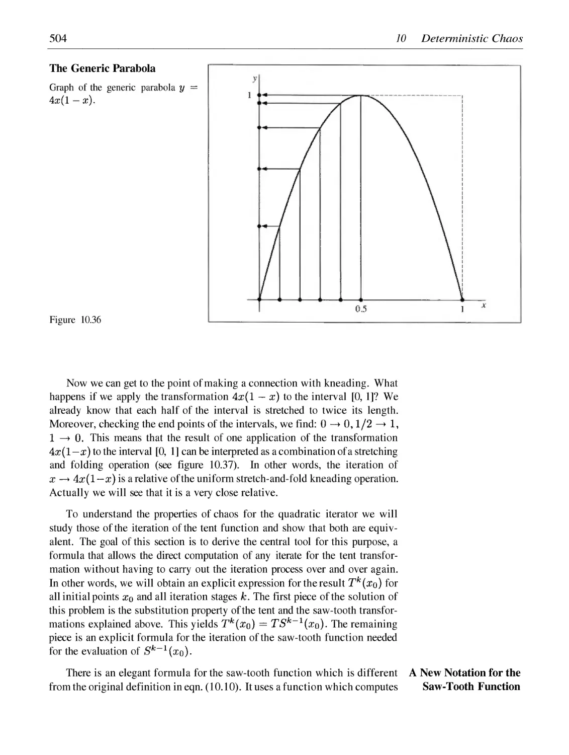
10 Deterministic Chaos: Sensitivity, Mixing, and Periodic Points
10.1
10.2
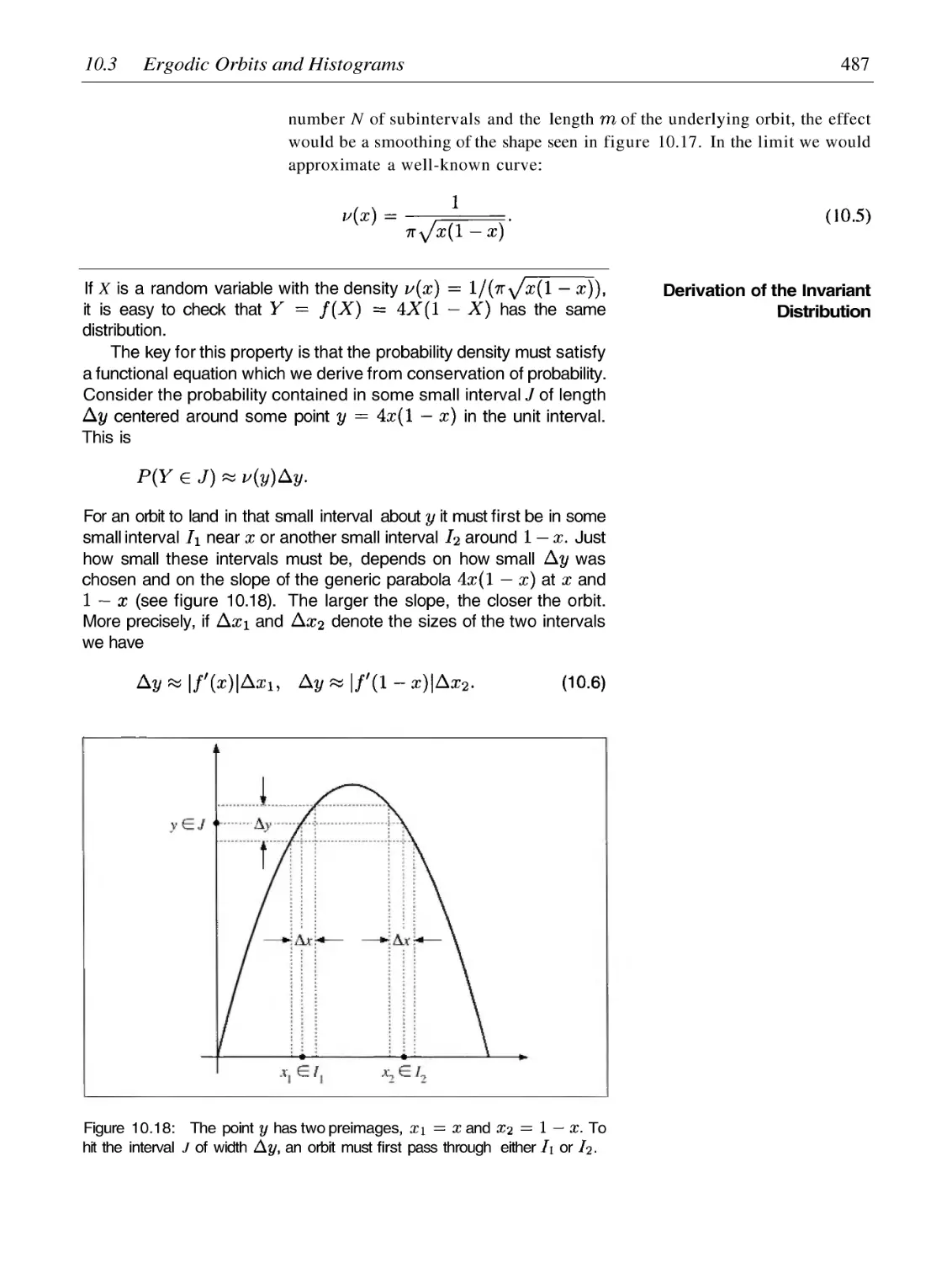
10.3
10.4
467
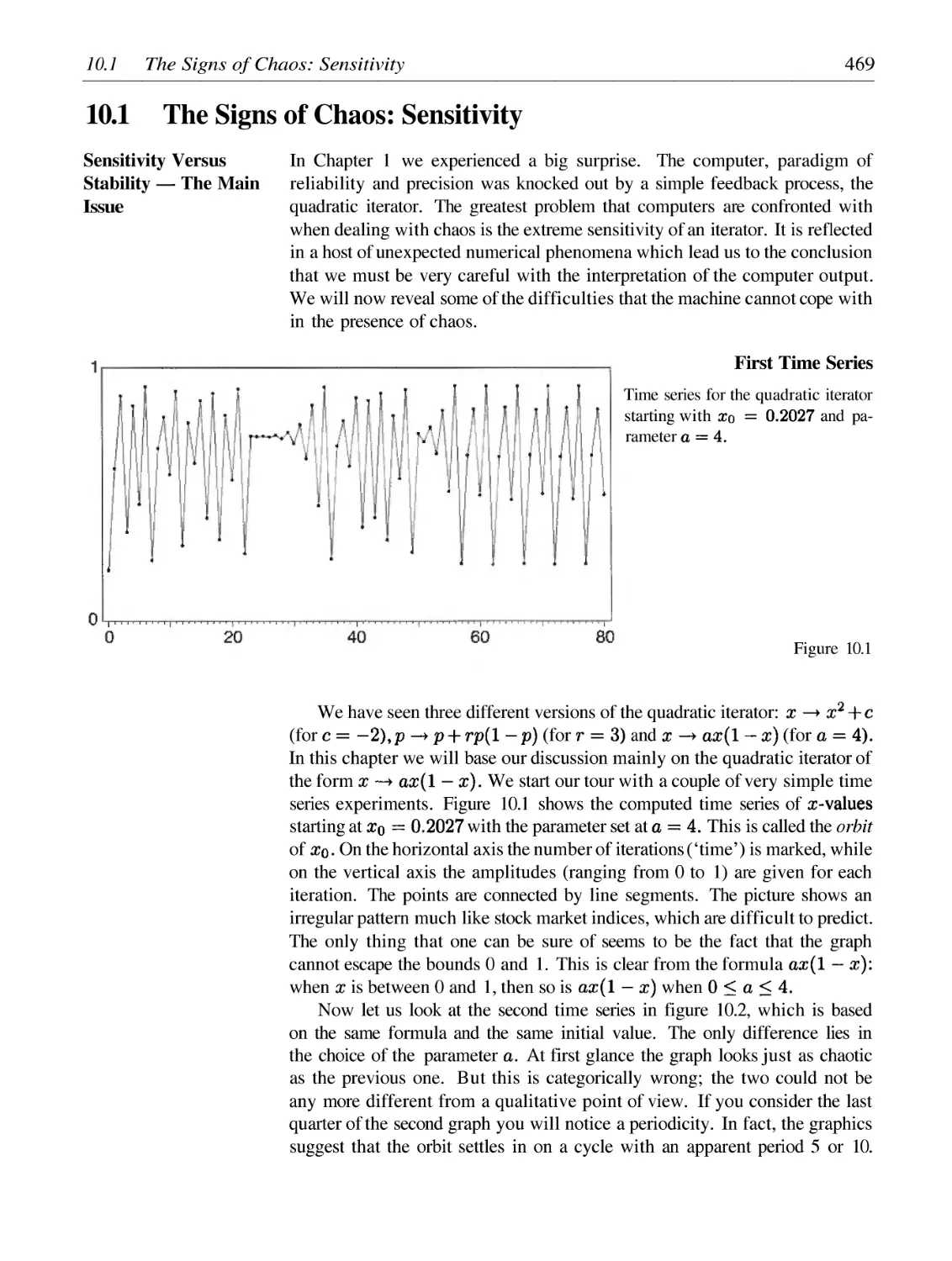
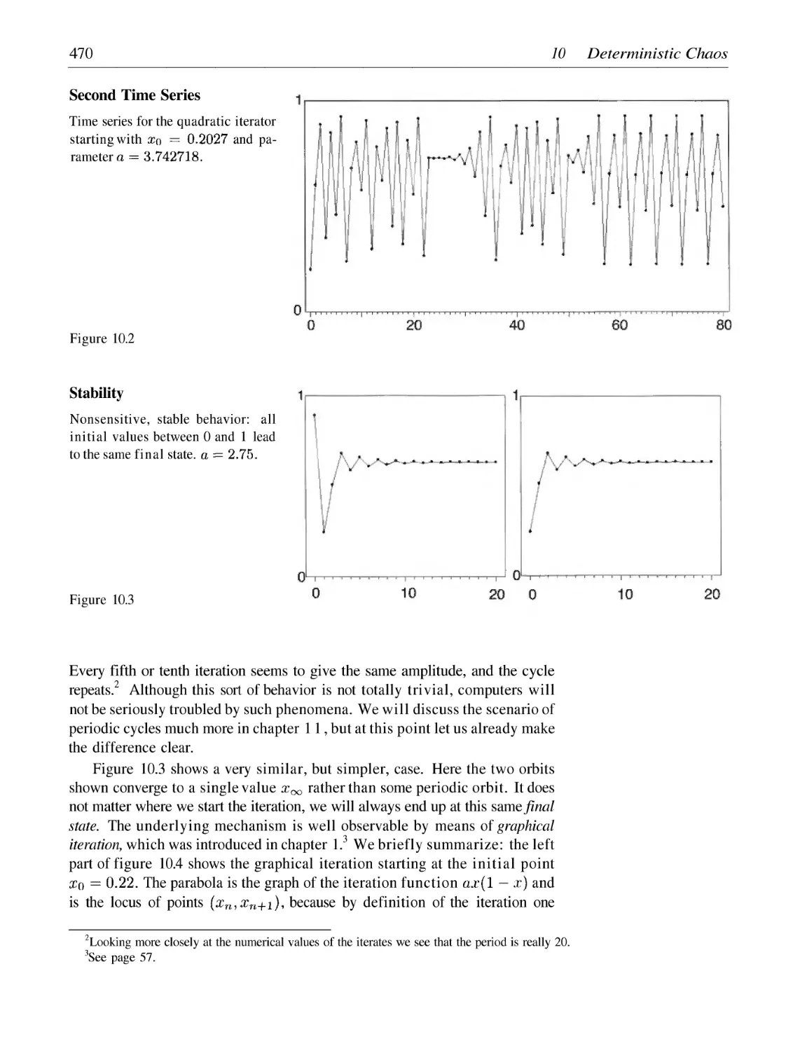
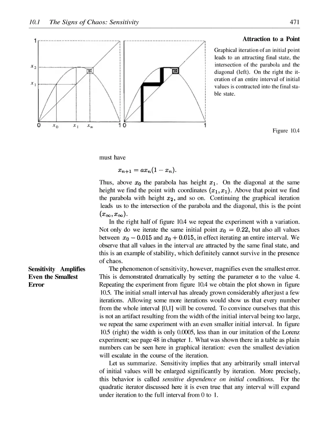
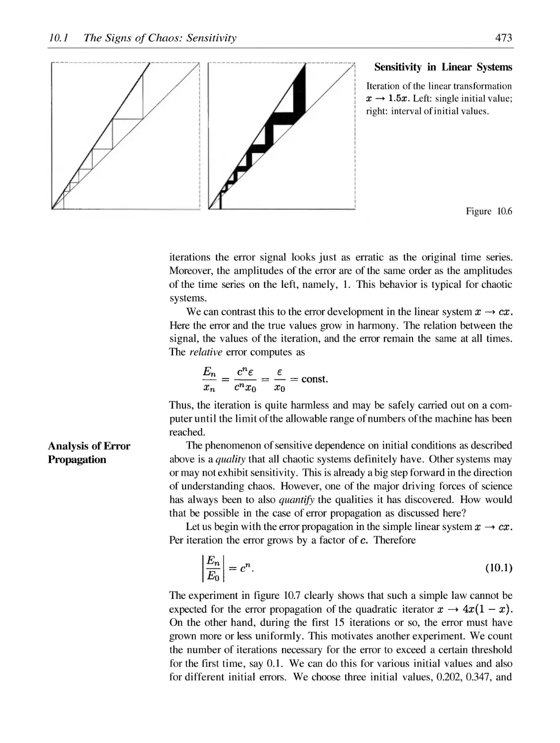
469
480
485
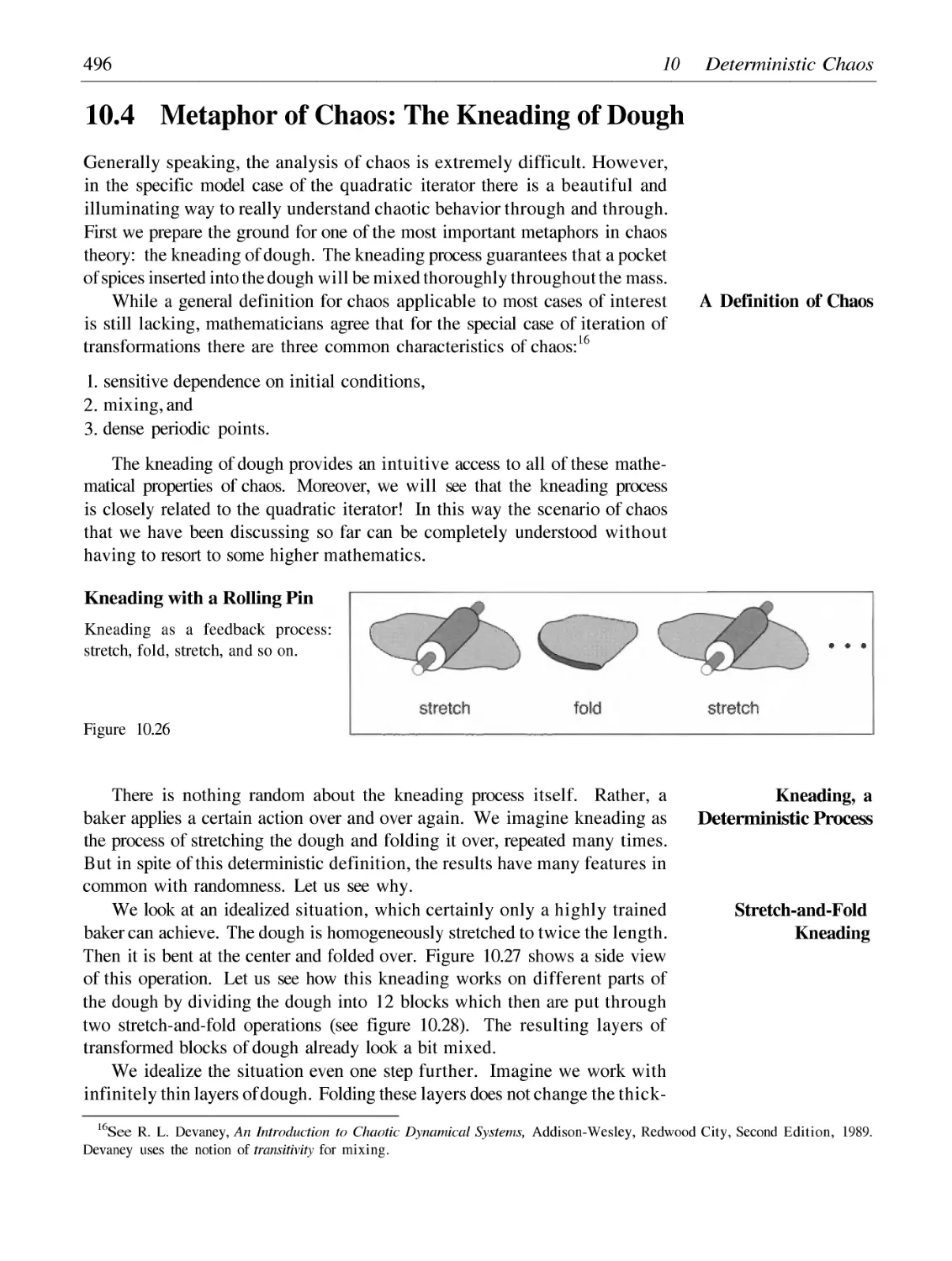
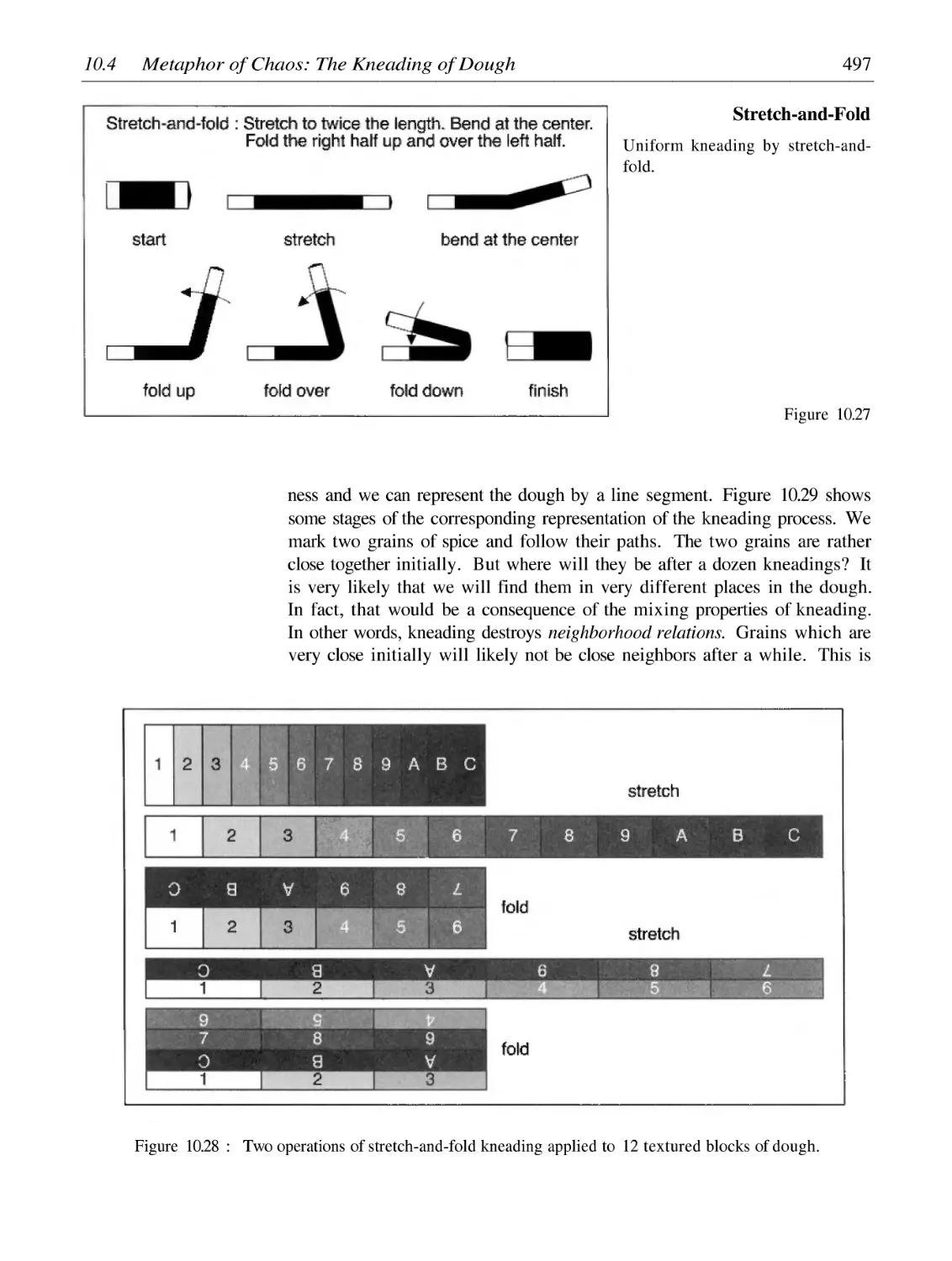
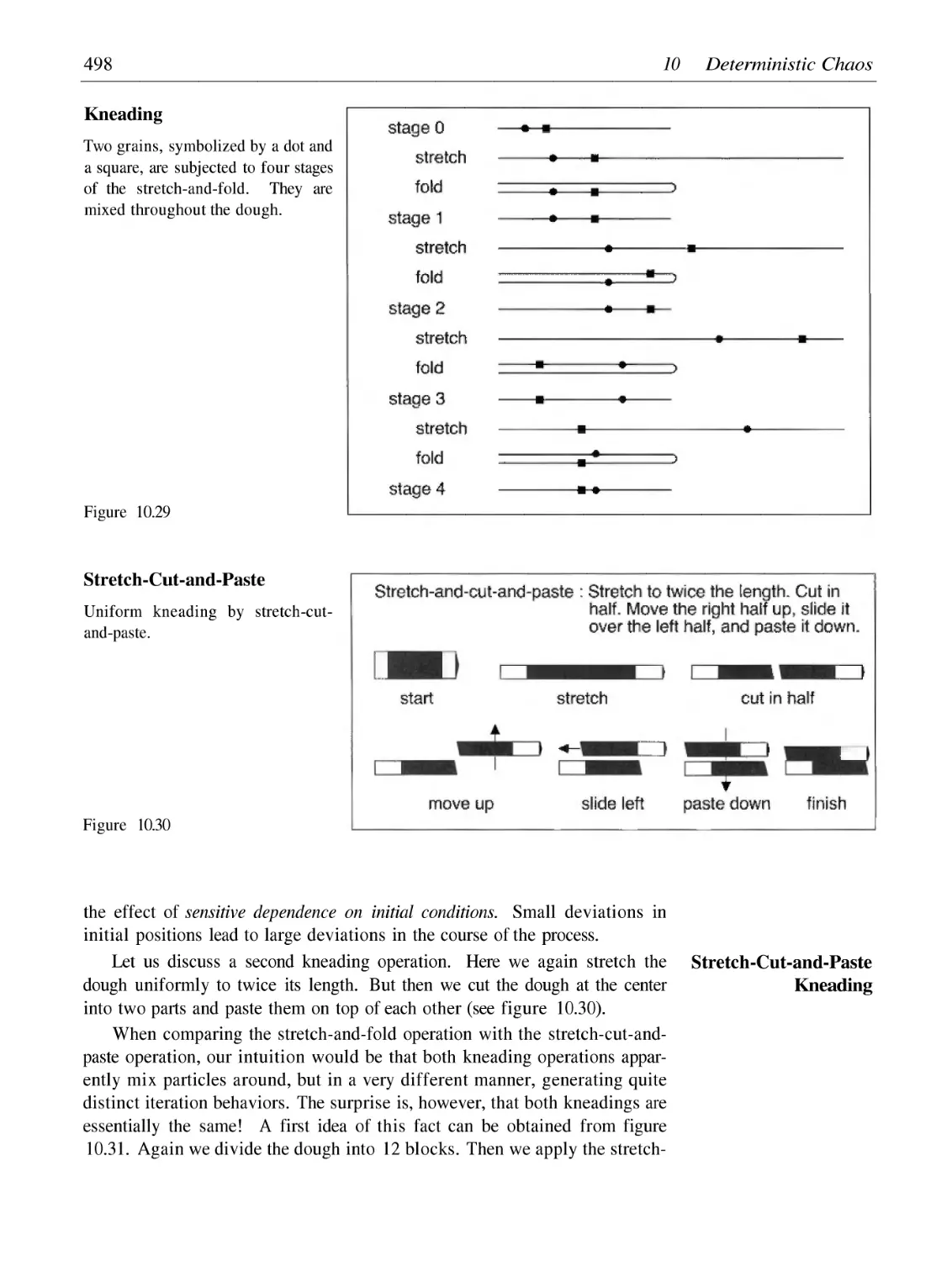
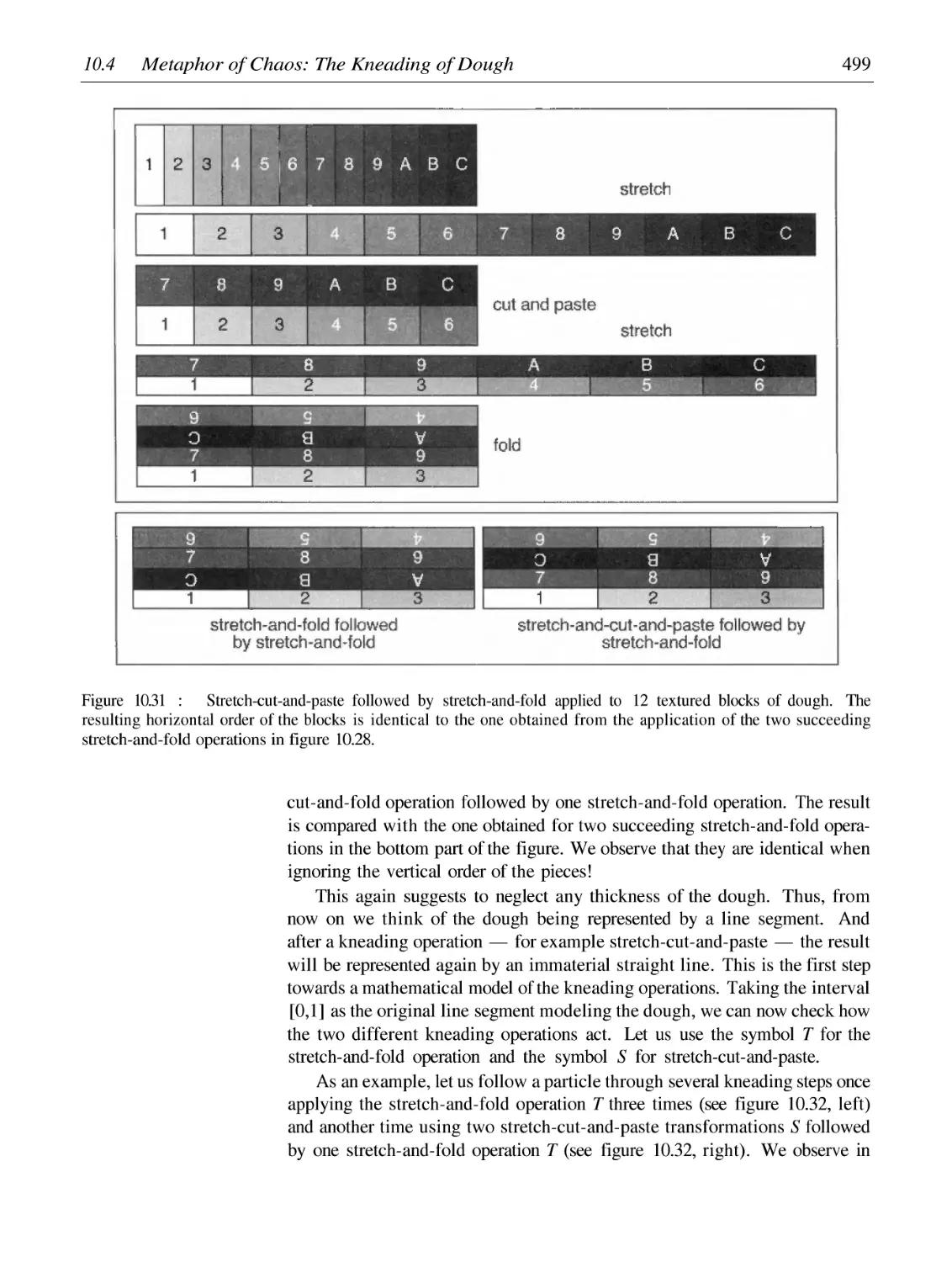
496
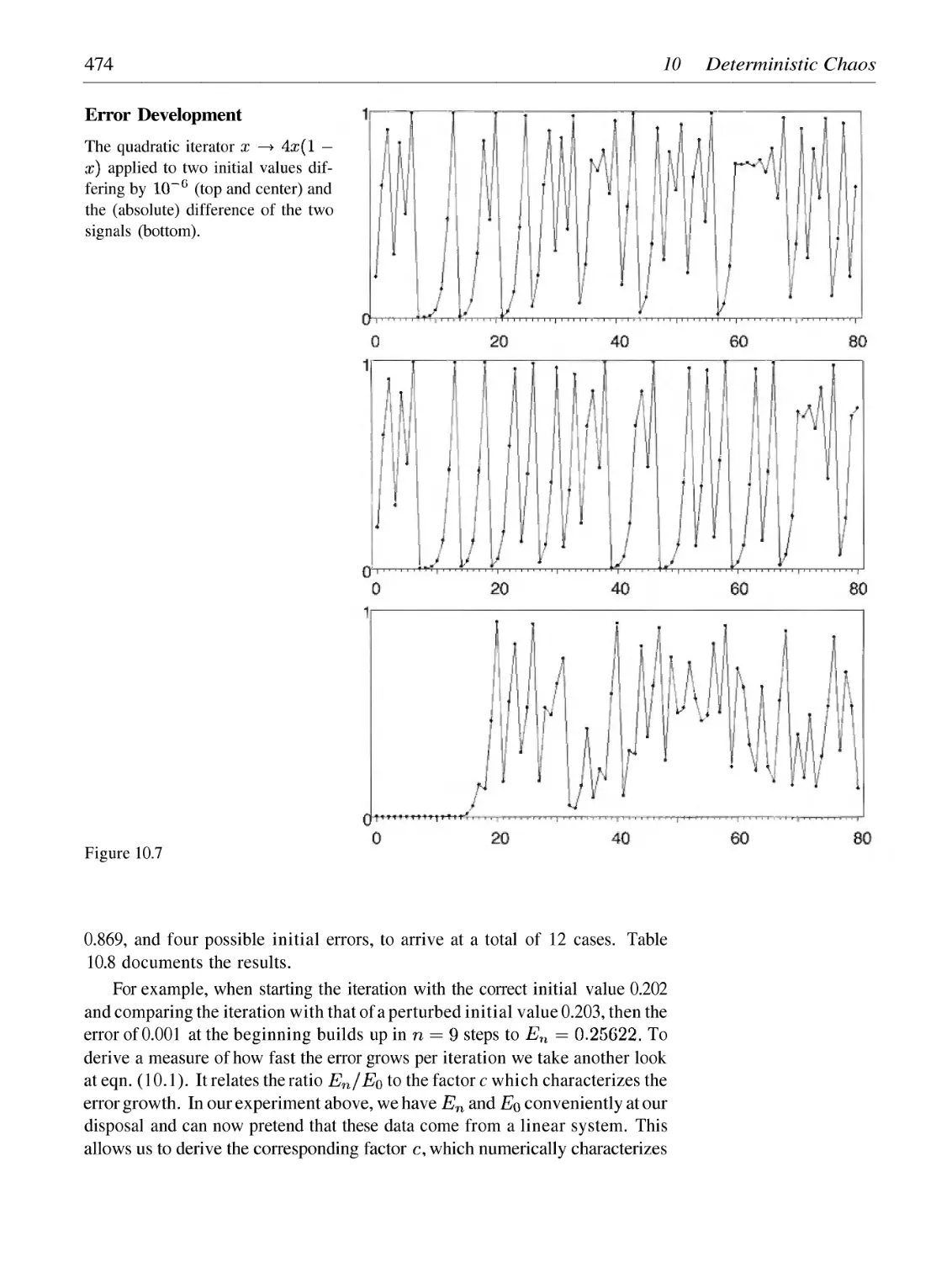
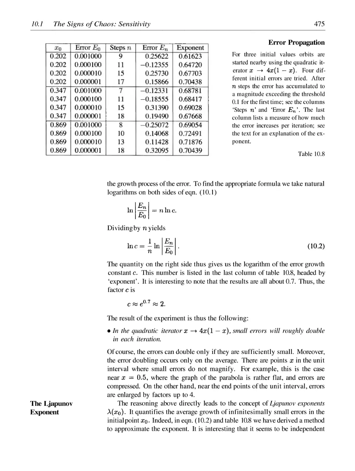
The Signs of Chaos: Sensitivity
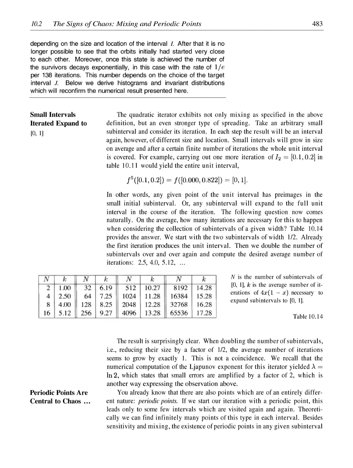
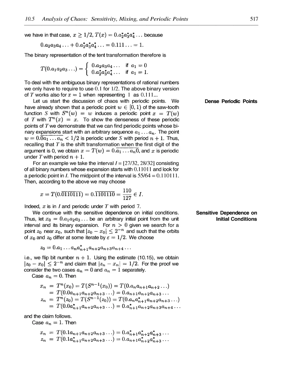
The Signs of Chaos: Mixing and Periodic Points
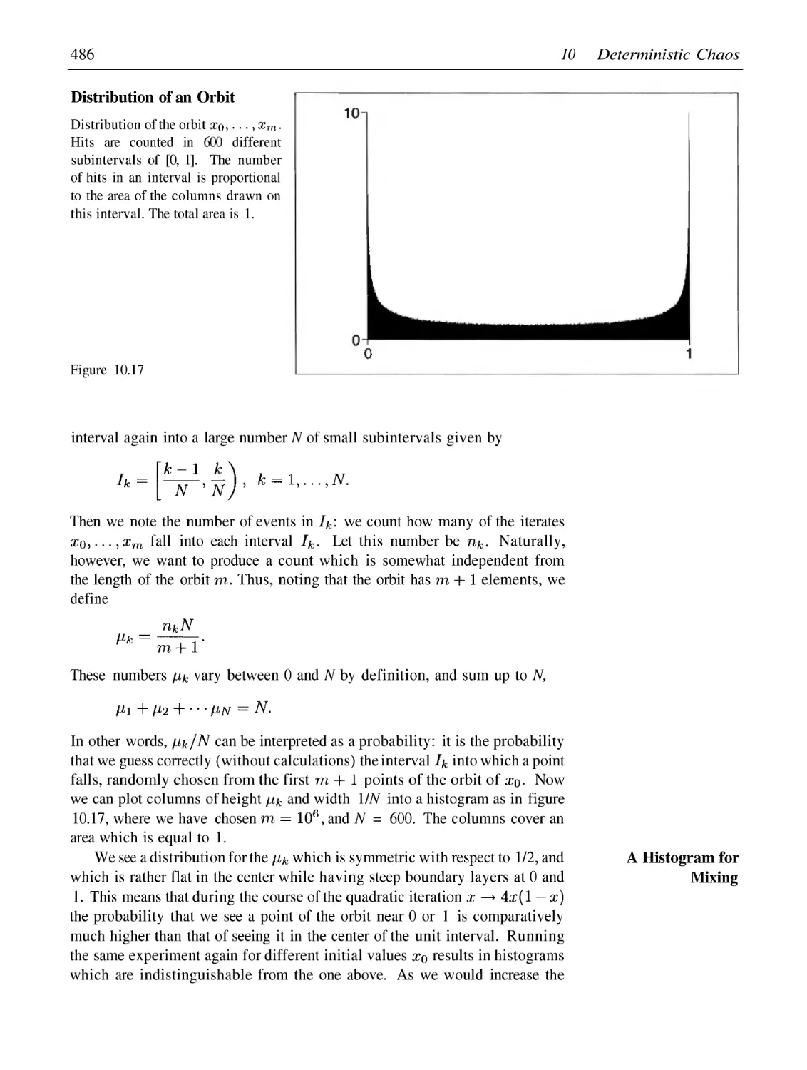
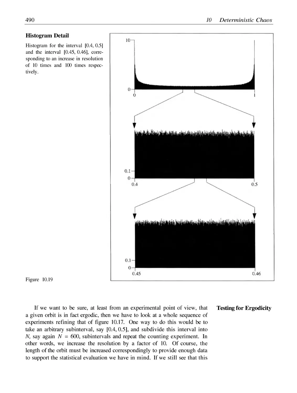
Ergodic Orbits and Histograms
Metaphor of Chaos: The Kneading of Dough
Table of Contents
xiii
10.5
10.6
10.7
10.8
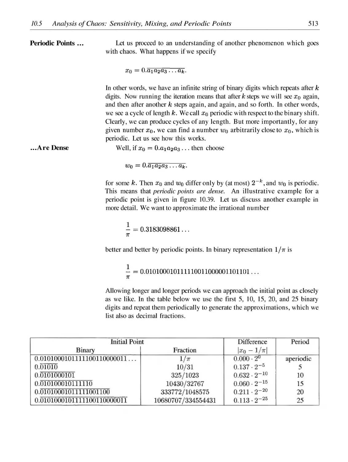
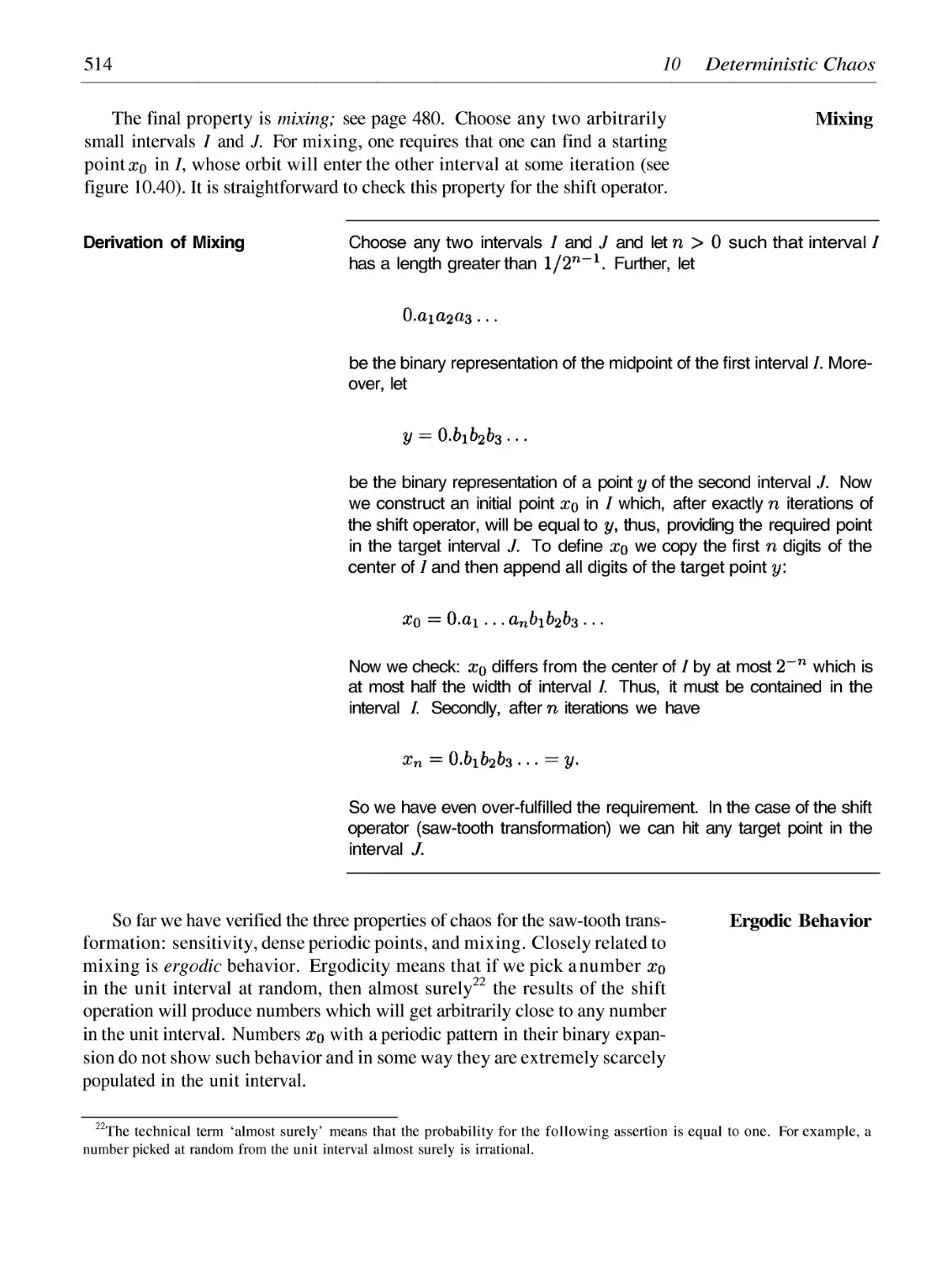
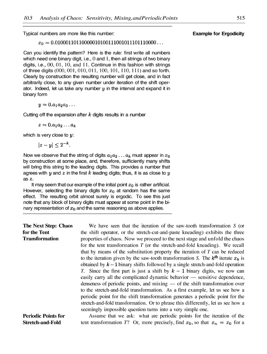
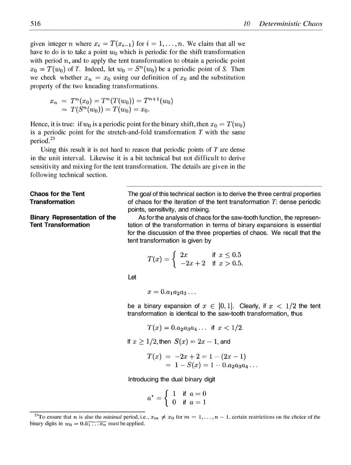
Analysis of Chaos: Sensitivity, Mixing, and Periodic Points
Chaos for the Quadratic Iterator
Mixing and Dense Periodic Points Imply Sensitivity
Numerics of Chaos: Worth the Trouble or Not?
509
520
529
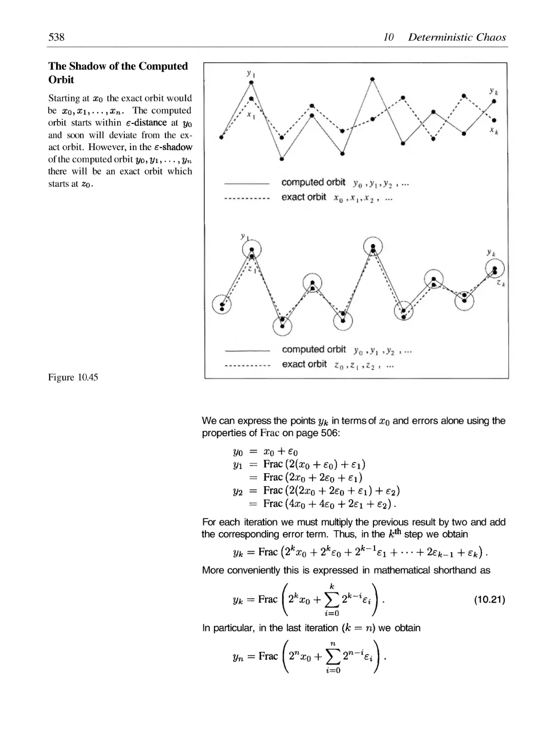
535
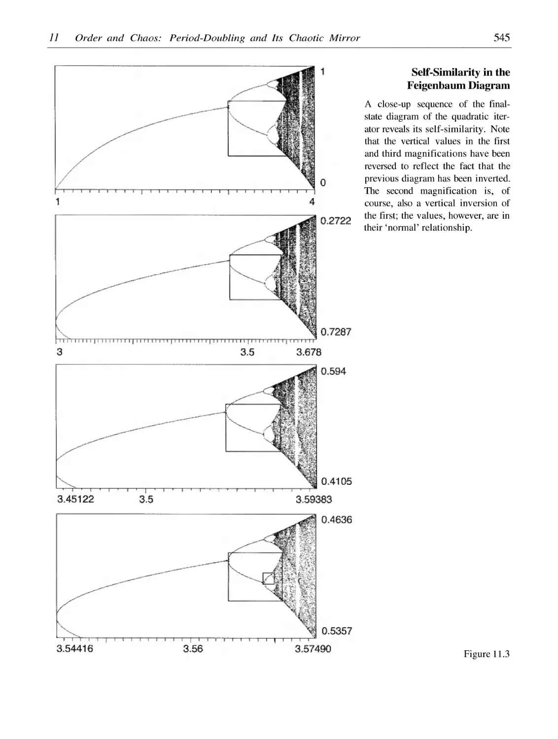
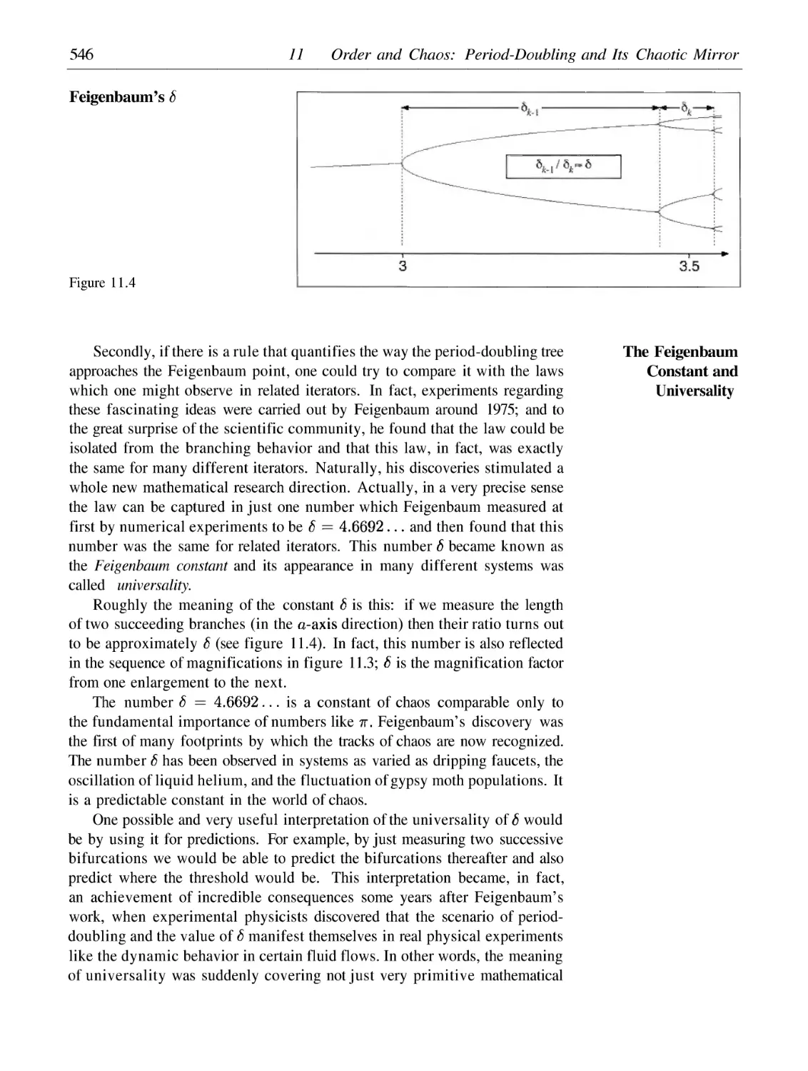
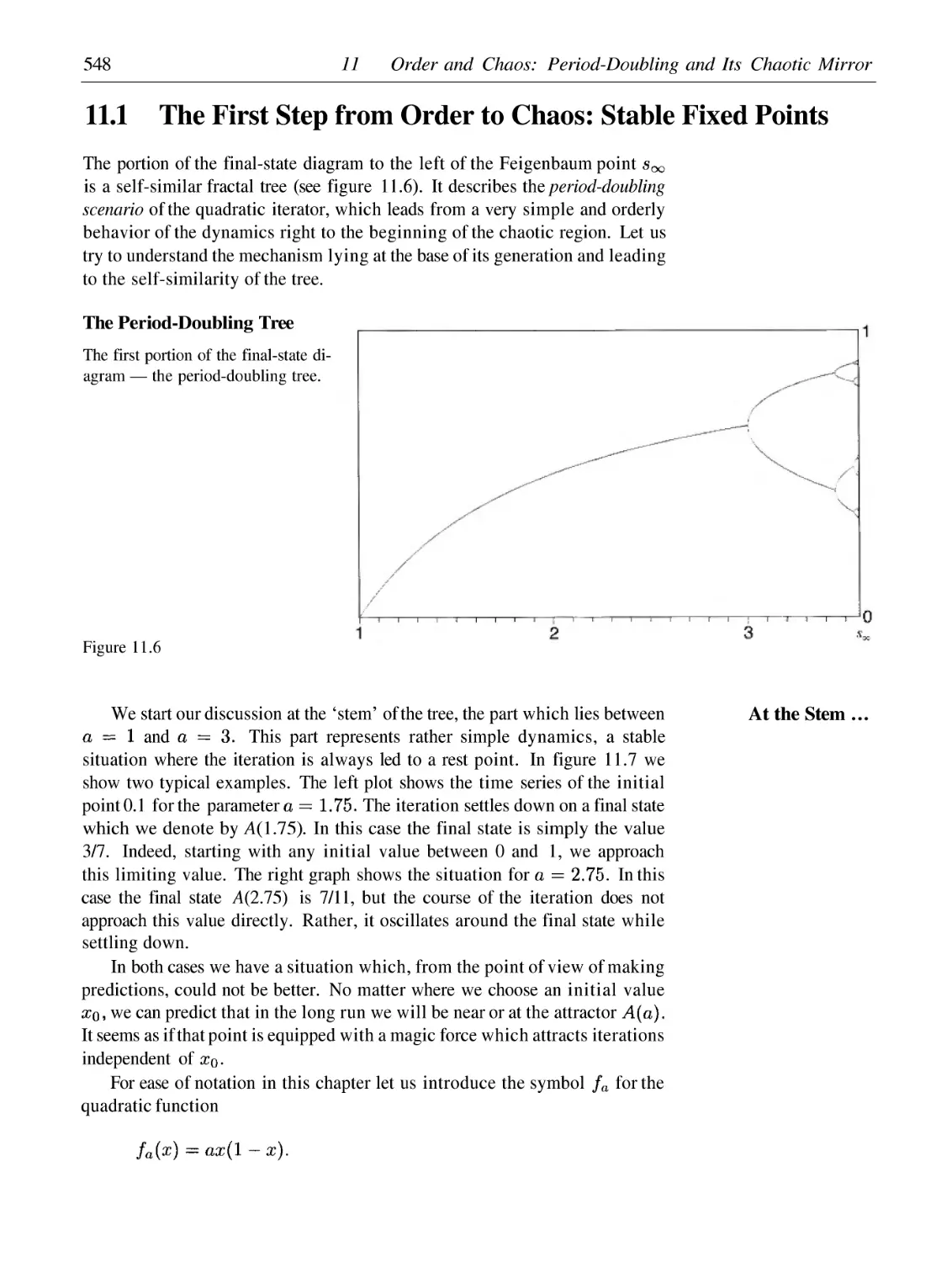
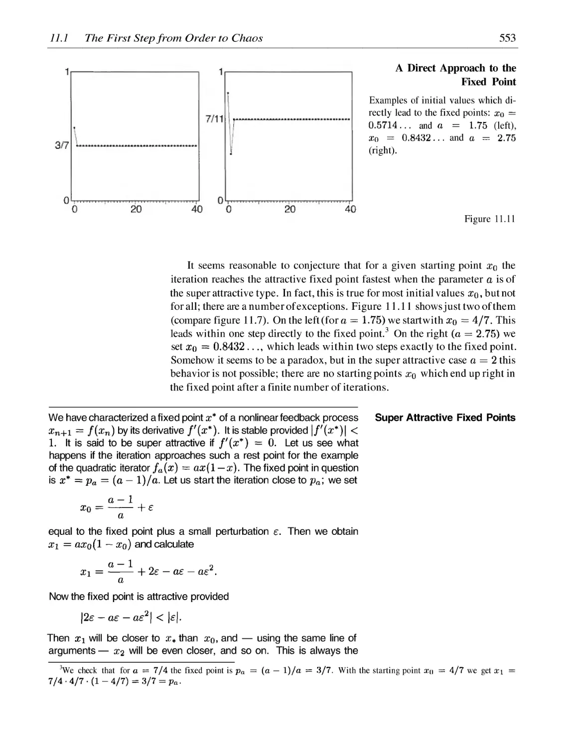
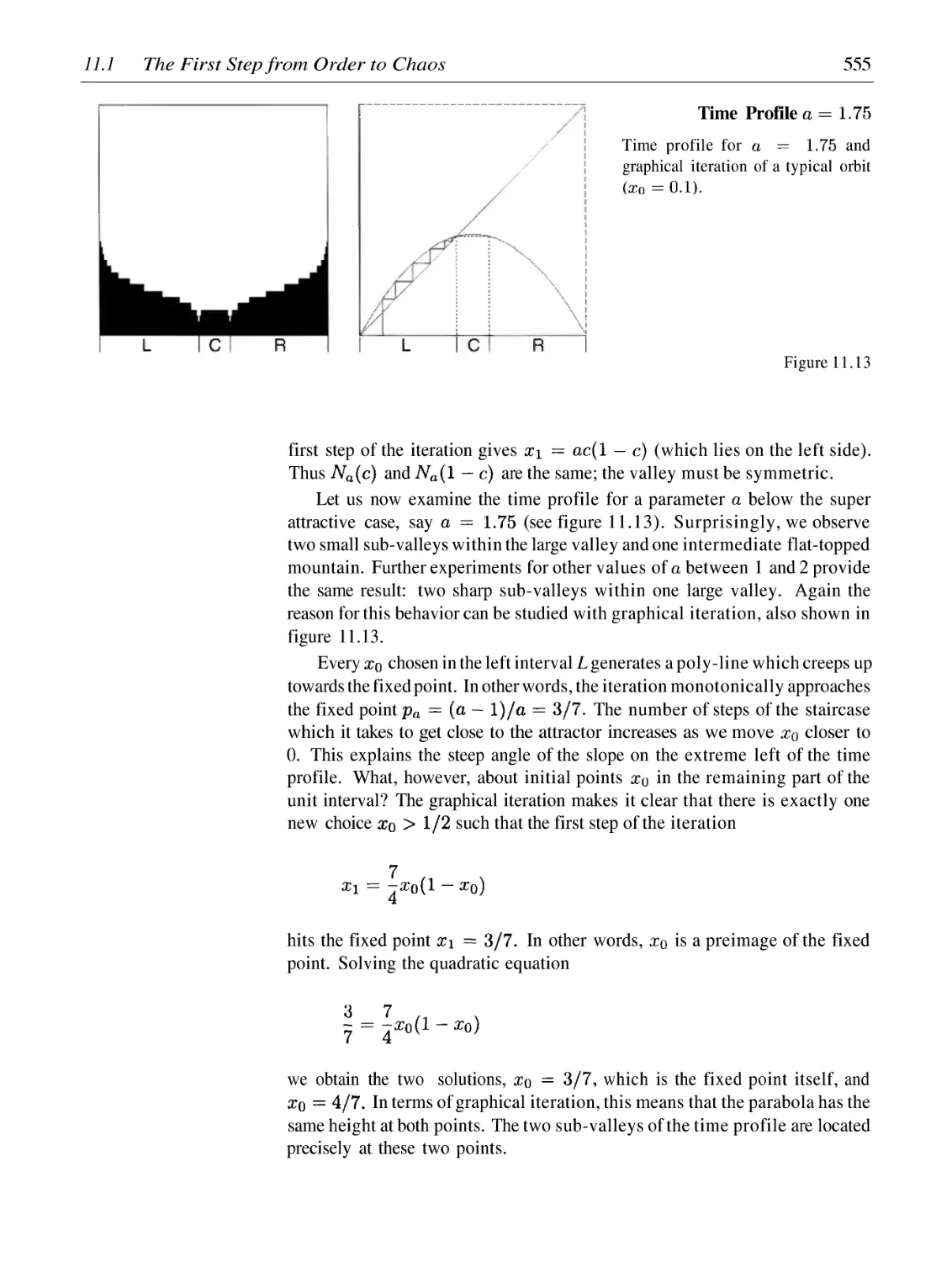
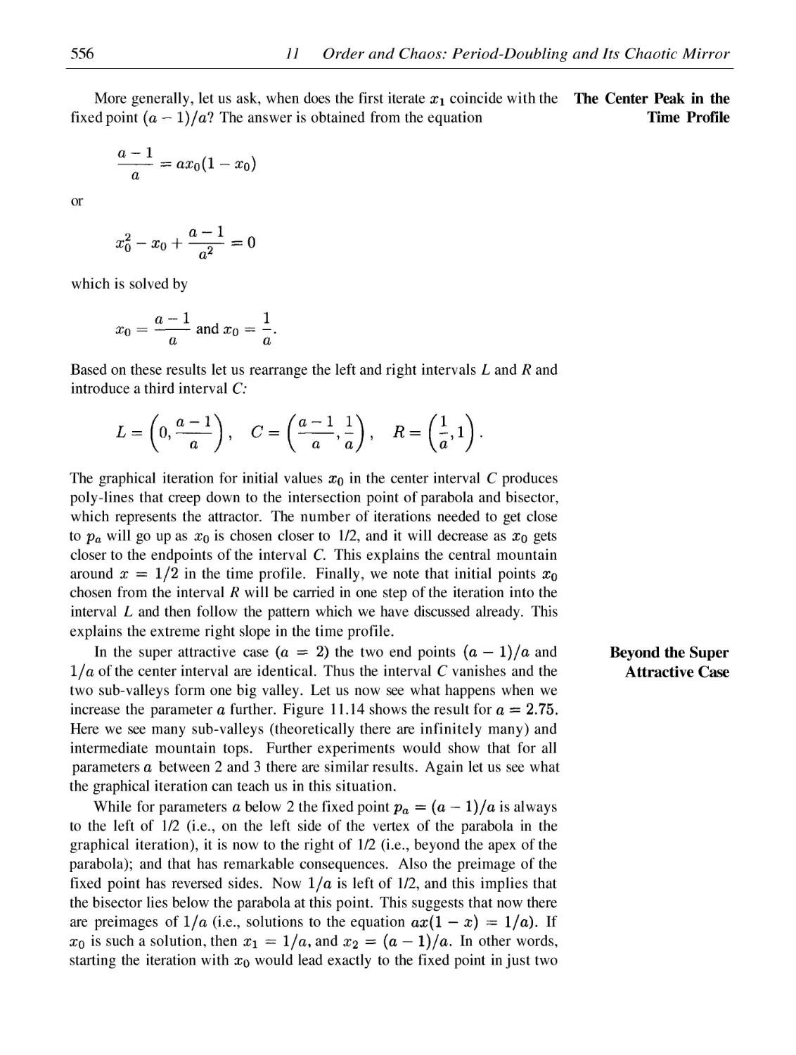
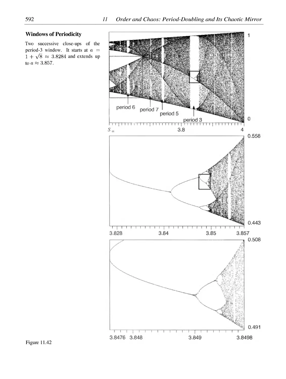
11 Order and Chaos: Period-Doubling and Its Chaotic Mirror
11.1
11.2
11.3
11.4
11.5
The First Step from Order to Chaos: Stable Fixed Points
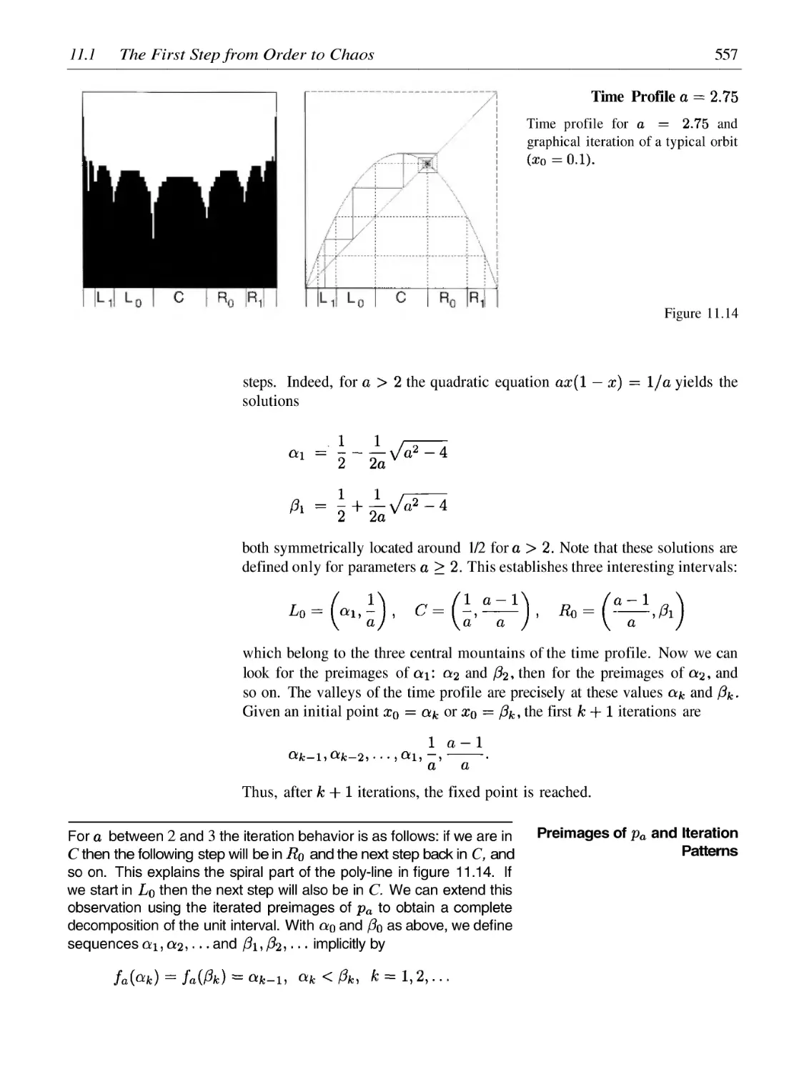
The Next Step from Order to Chaos: The Period-Doubling Scenario
The Feigenbaum Point: Entrance to Chaos
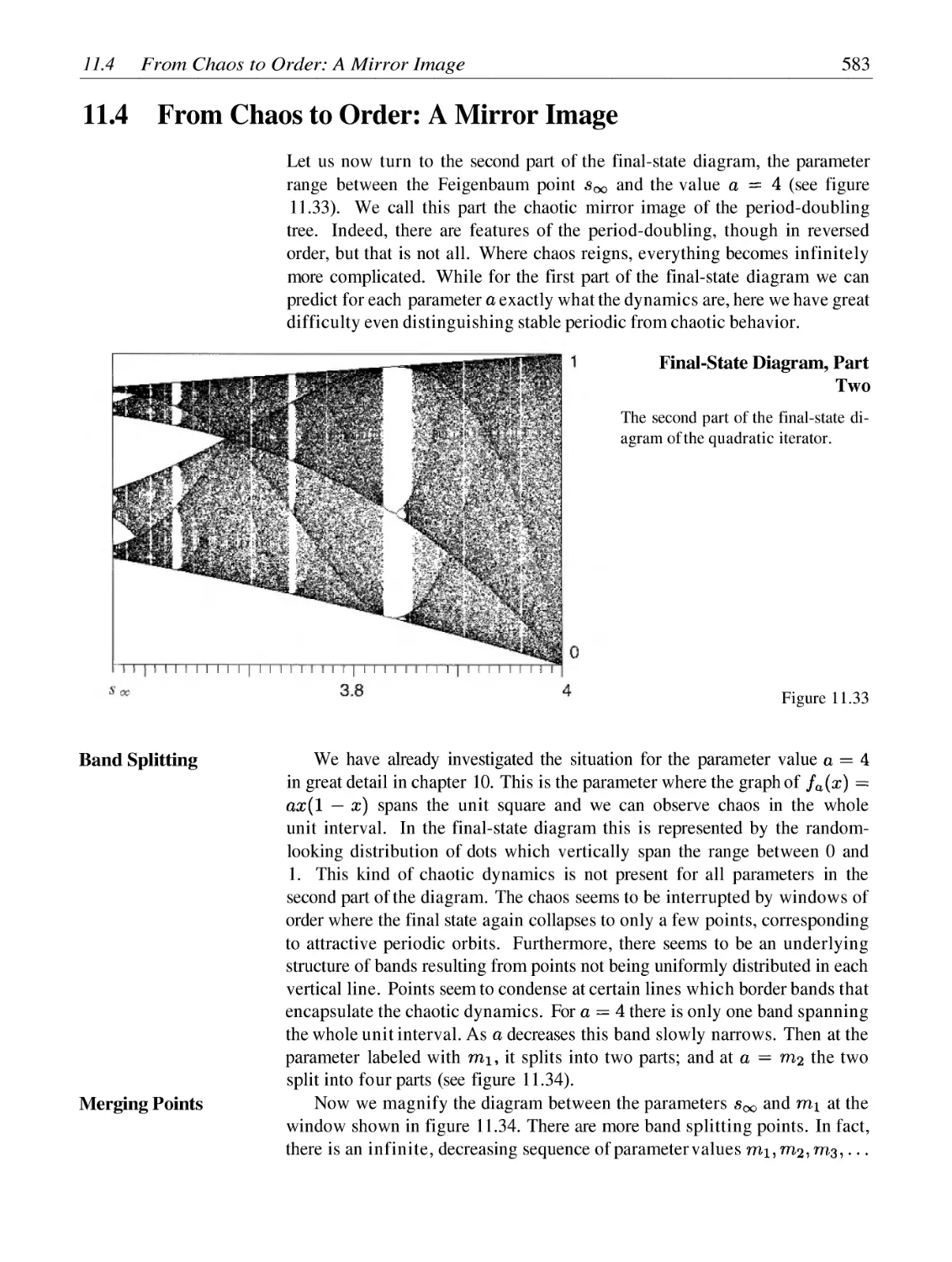
From Chaos to Order: A Mirror Image
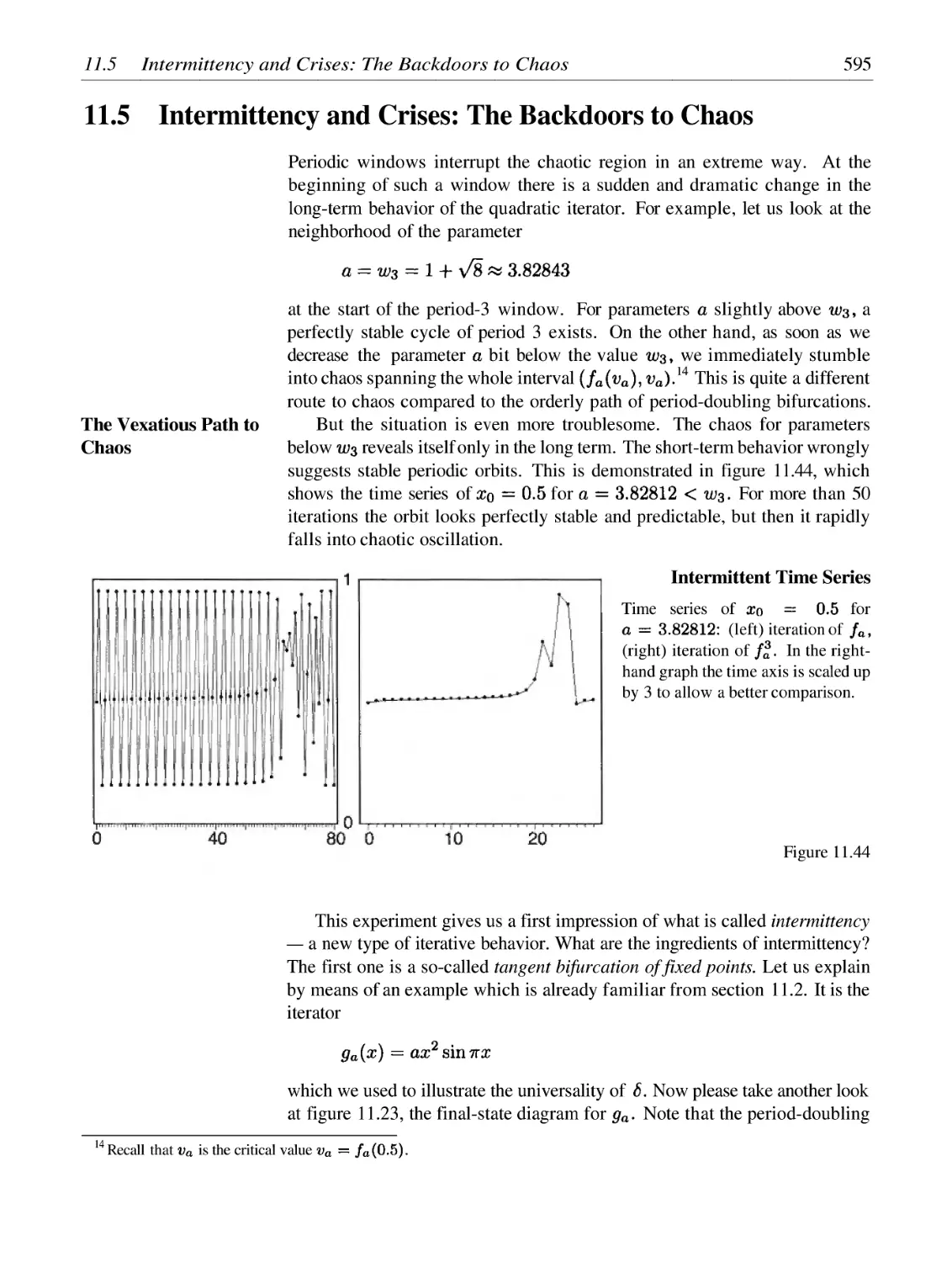
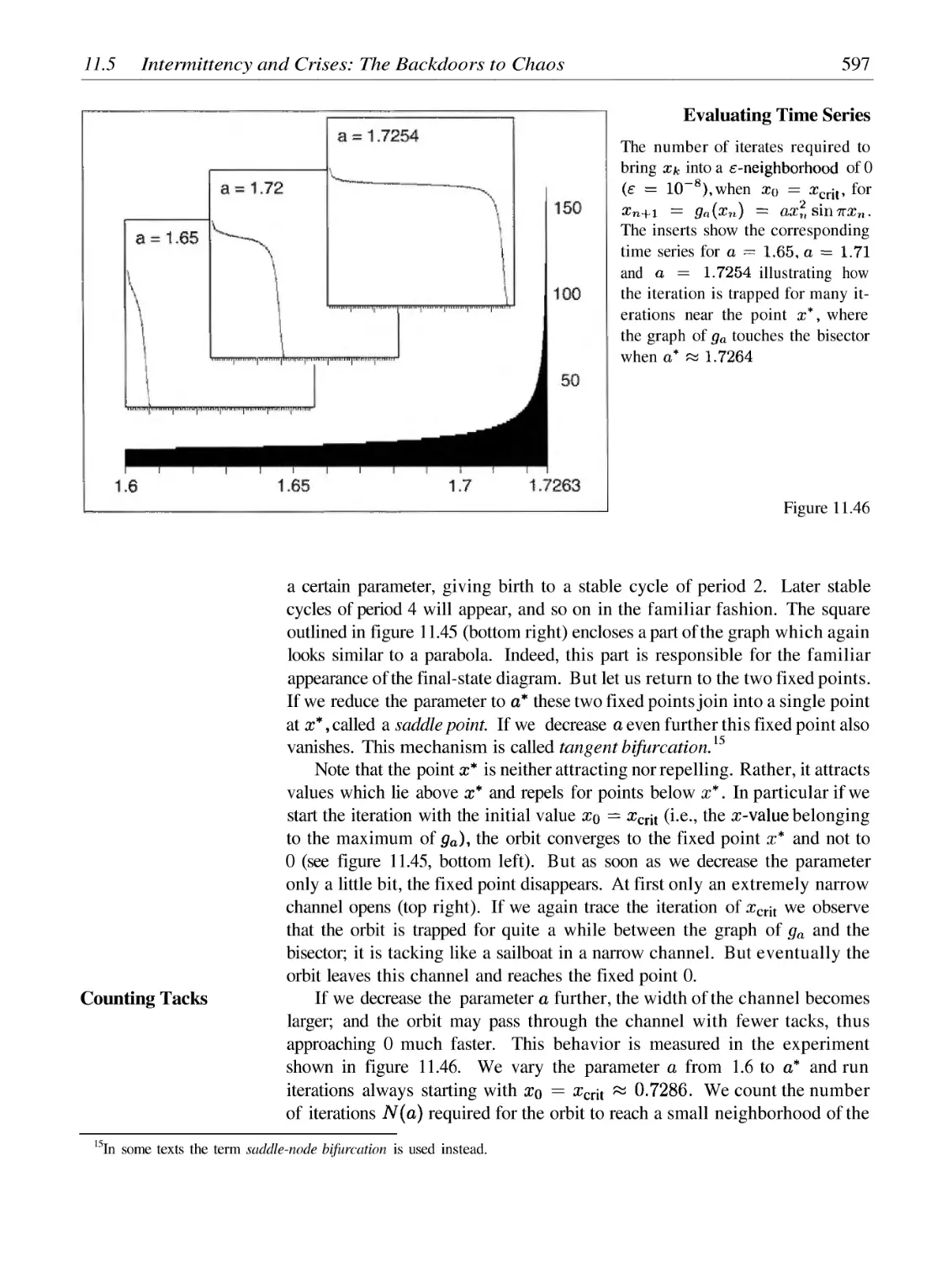
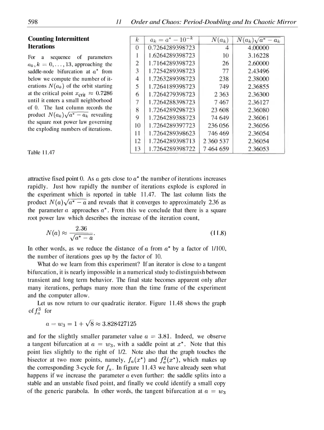
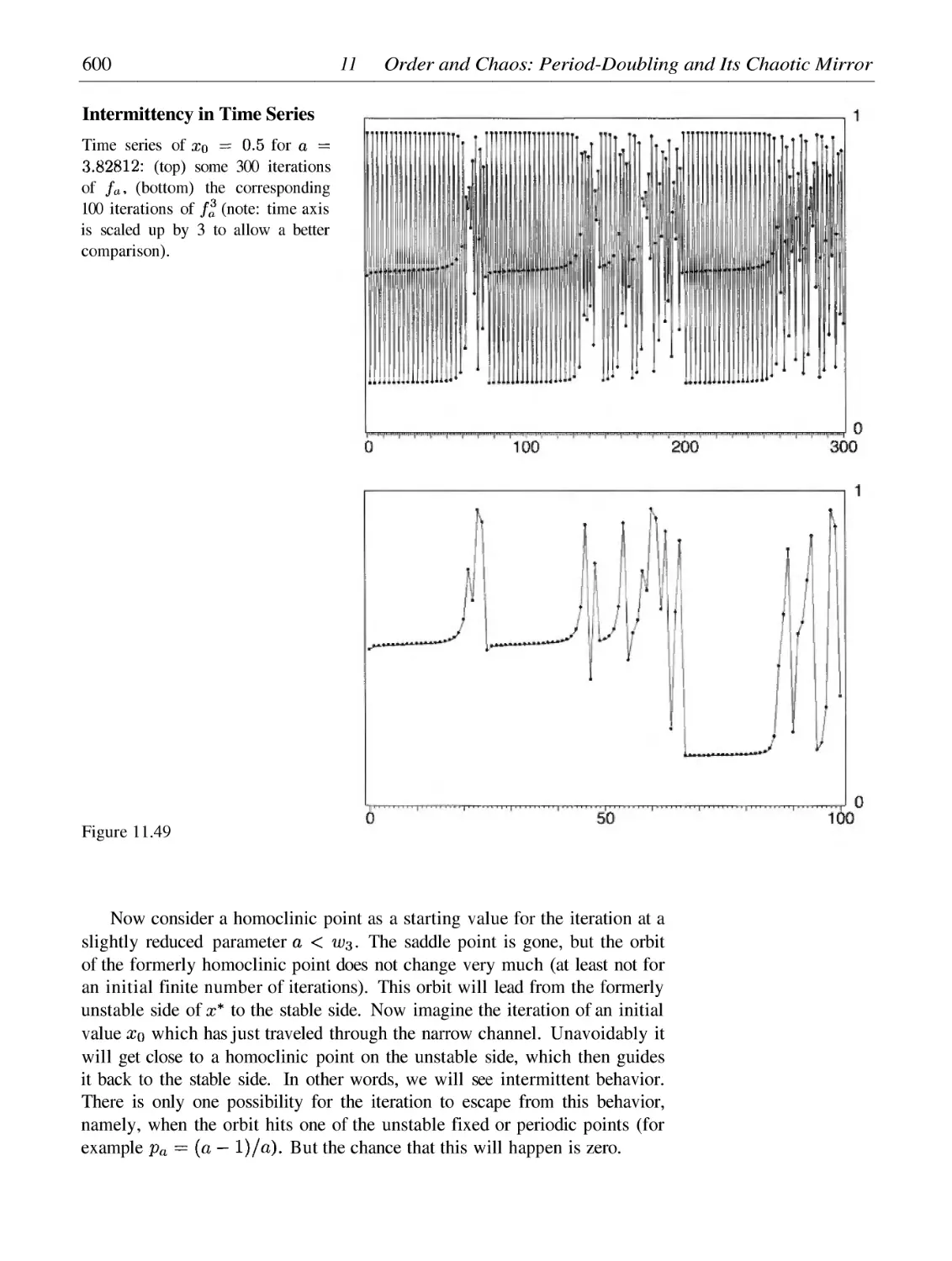
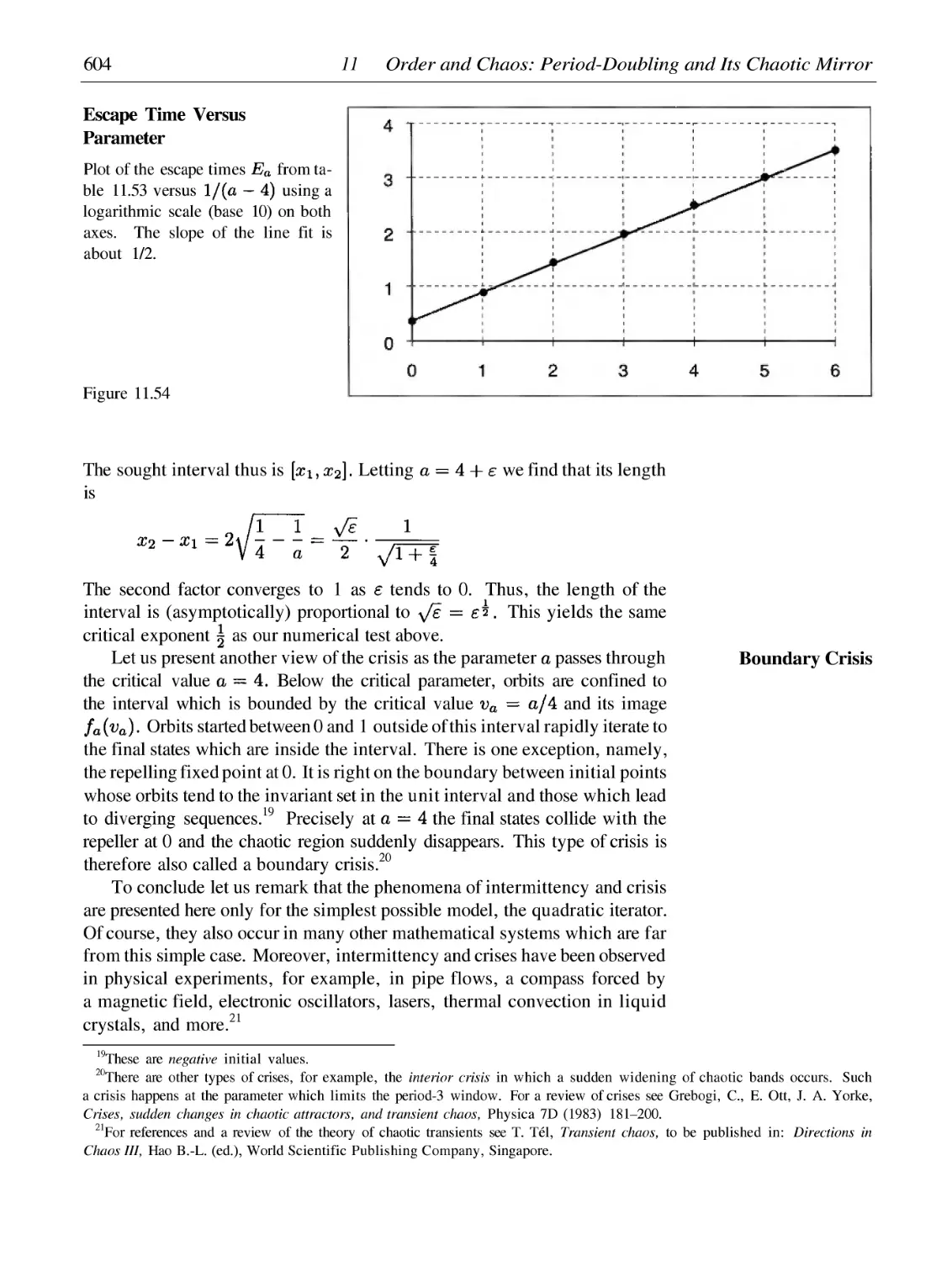
Intermittency and Crises: The Backdoors to Chaos
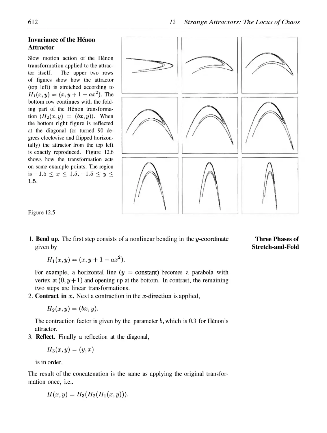
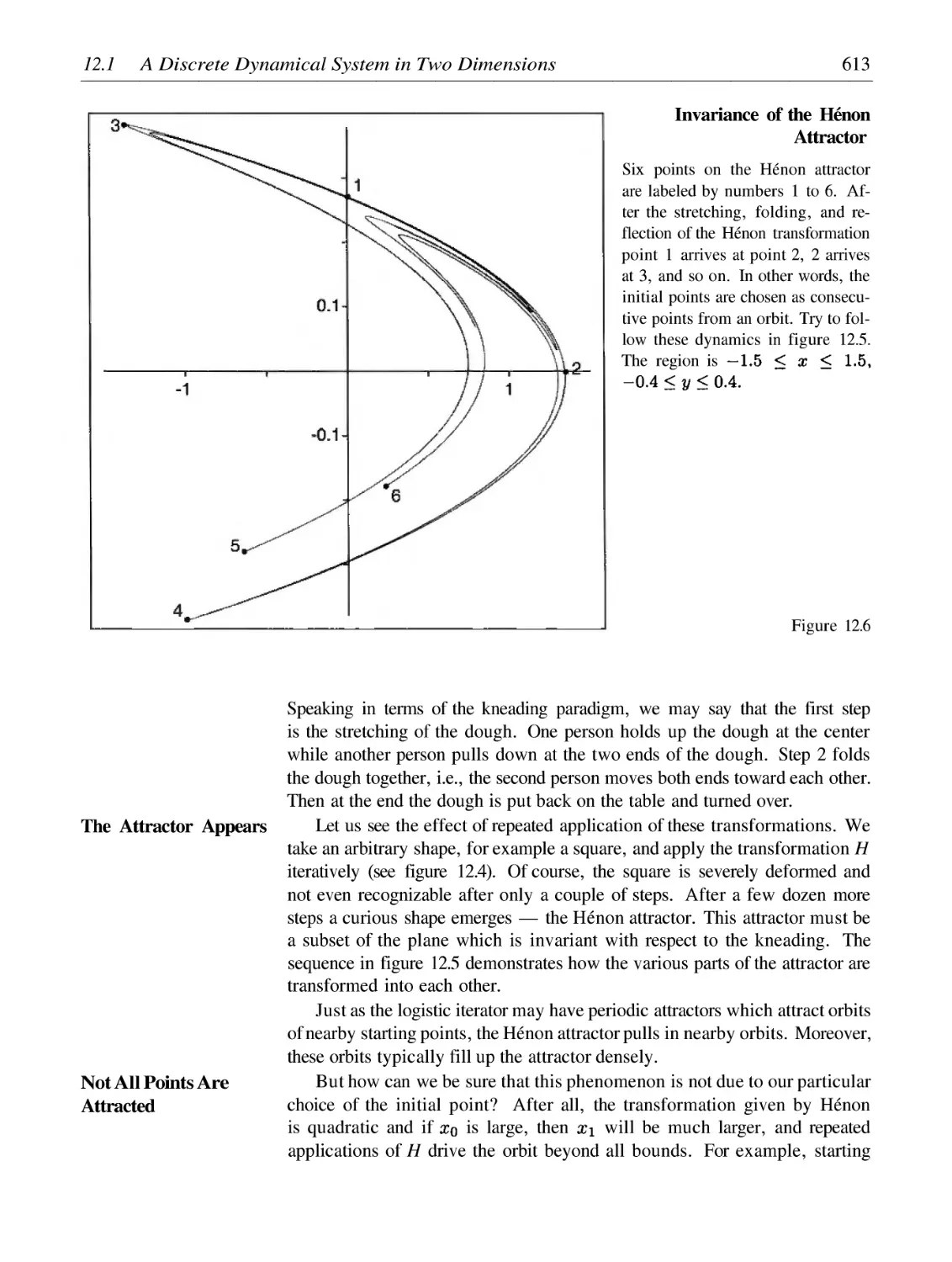
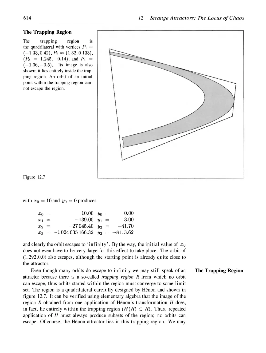
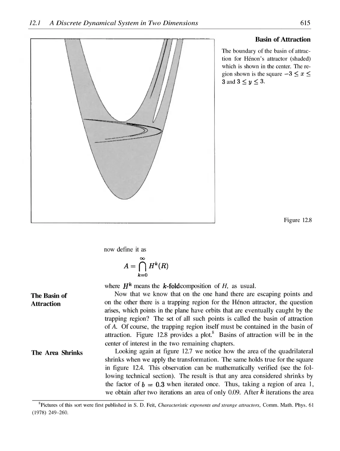
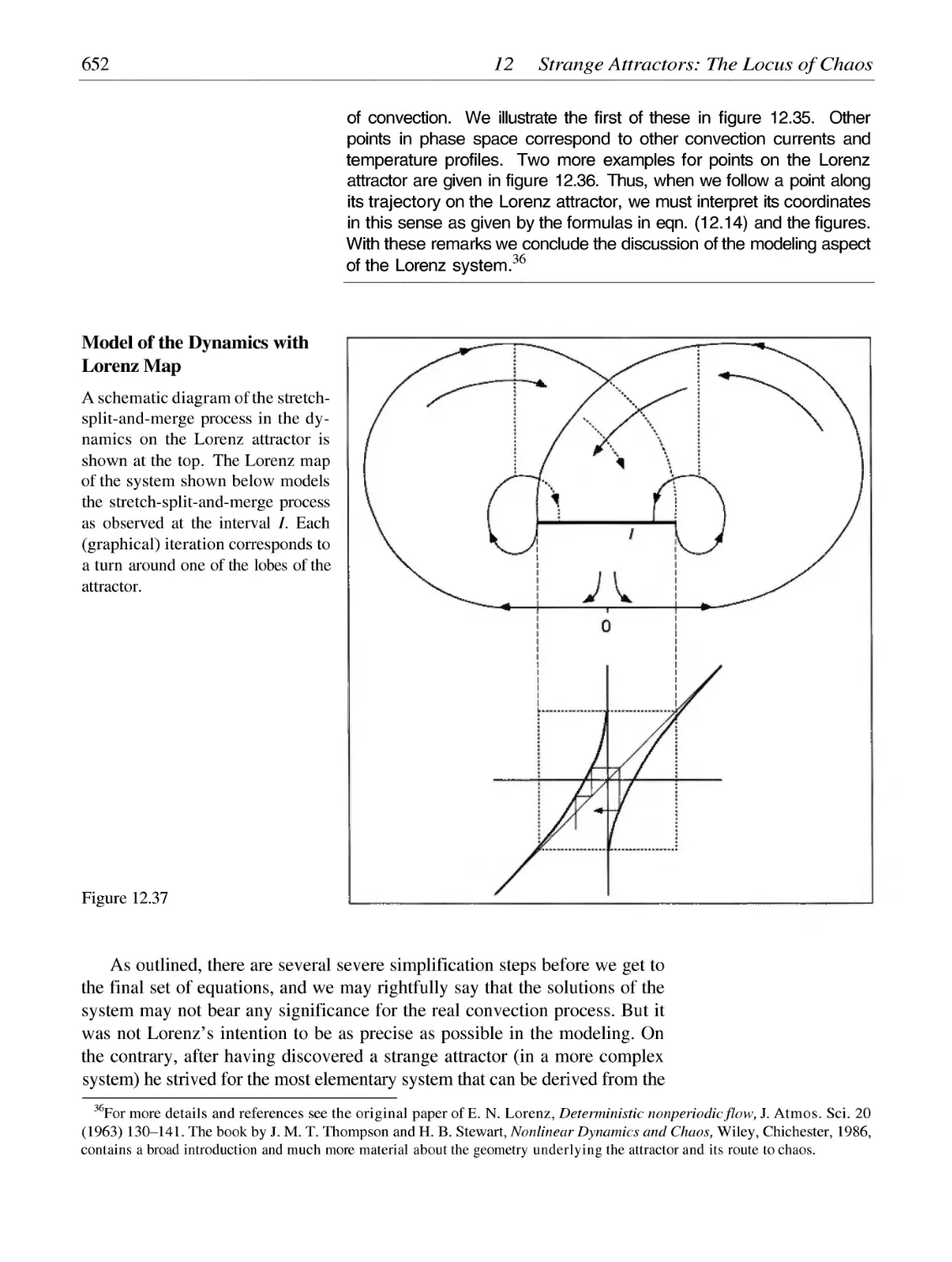
12 Strange Attractors: The Locus of Chaos
12.1
12.2
12.3
12.4
12.5
12.6
12.7
12.8
541
548
559
575
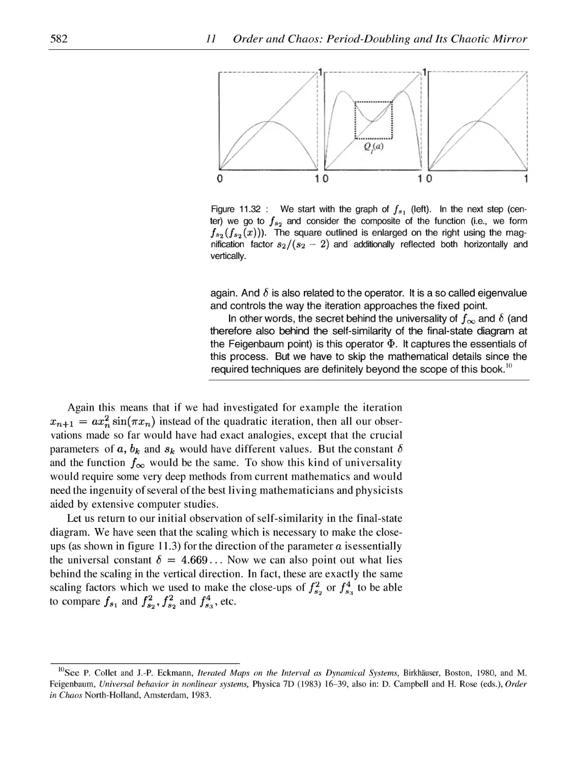
583
595
A Discrete Dynamical System in Two Dimensions: Hénon's Attractor
Continuous Dynamical Systems: Differential Equations
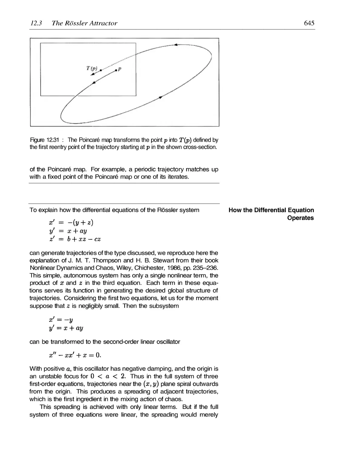
The Rössler Attractor
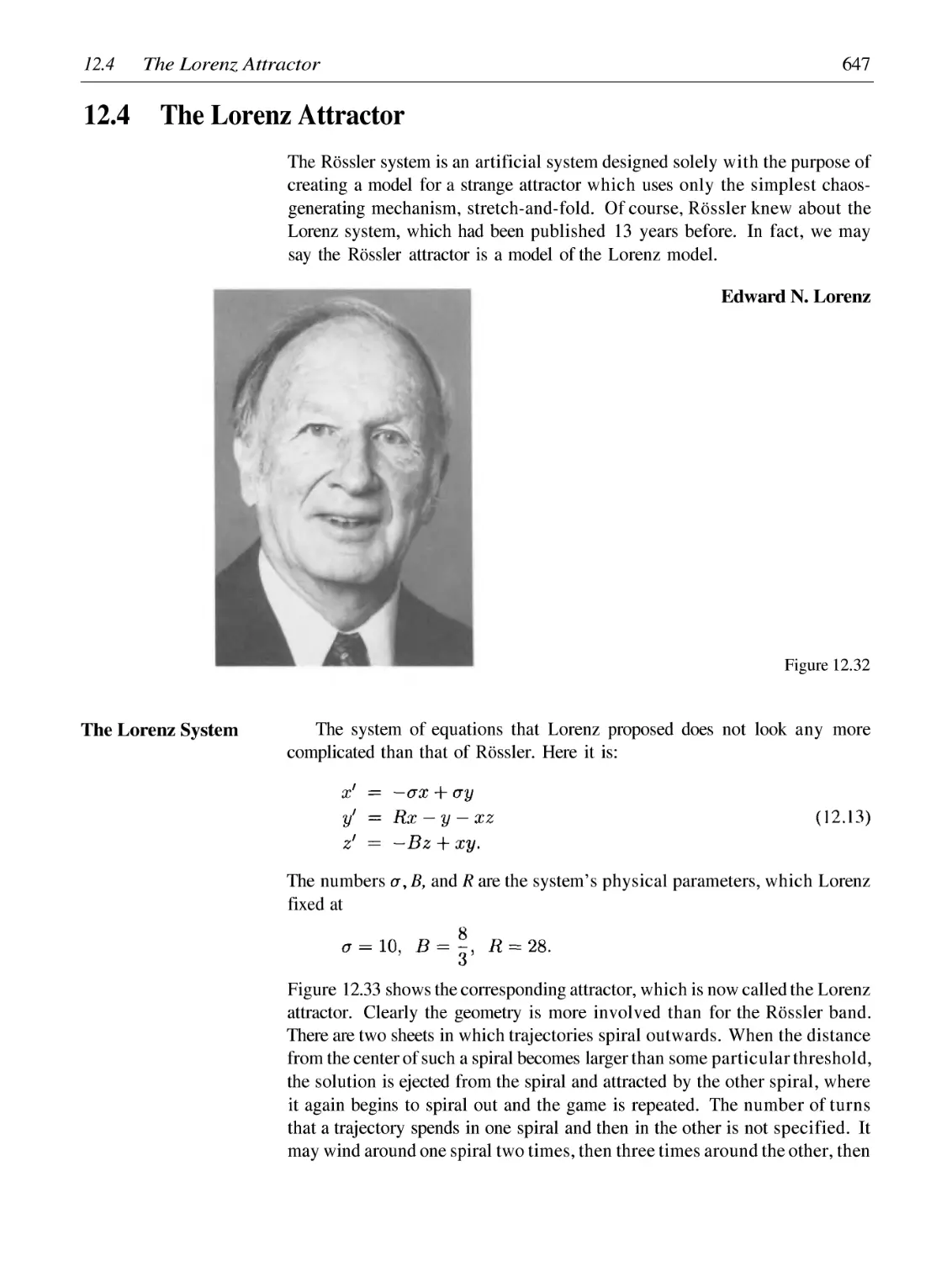
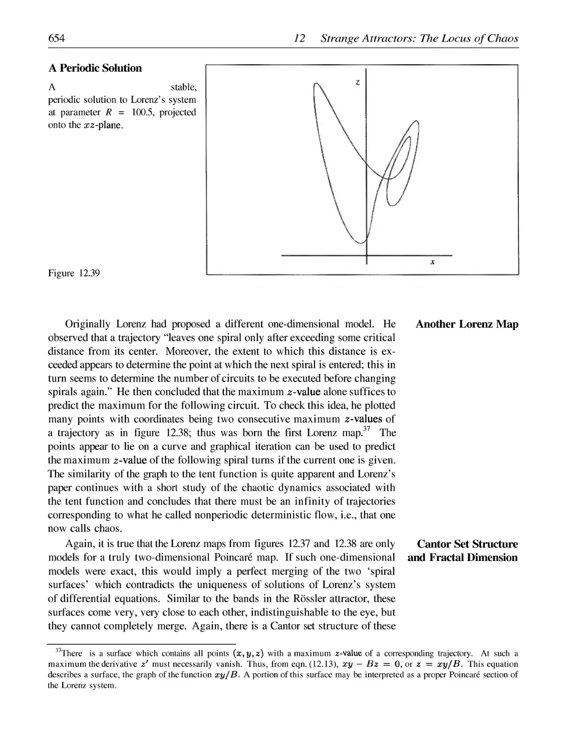
The Lorenz Attractor
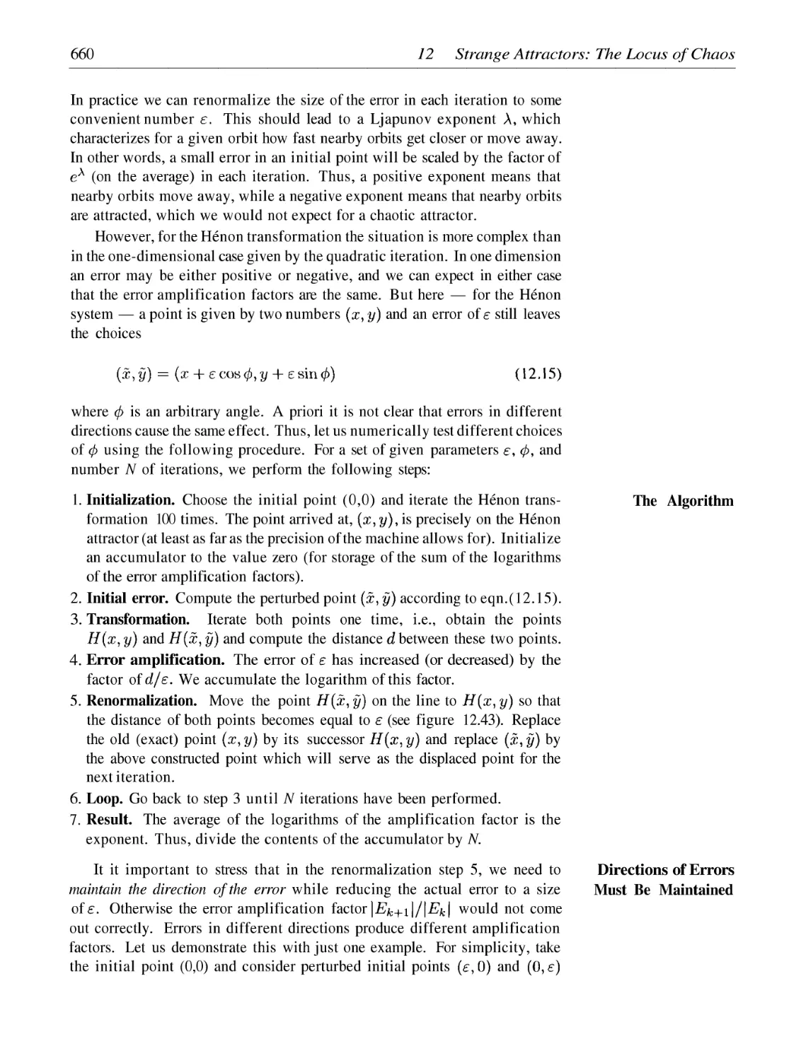
Quantitative Characterization of Strange Chaotic Attractors: Ljapunov Exponents
Quantitative Characterization of Strange Chaotic Attractors: Dimensions
The Reconstruction of Strange Attractors
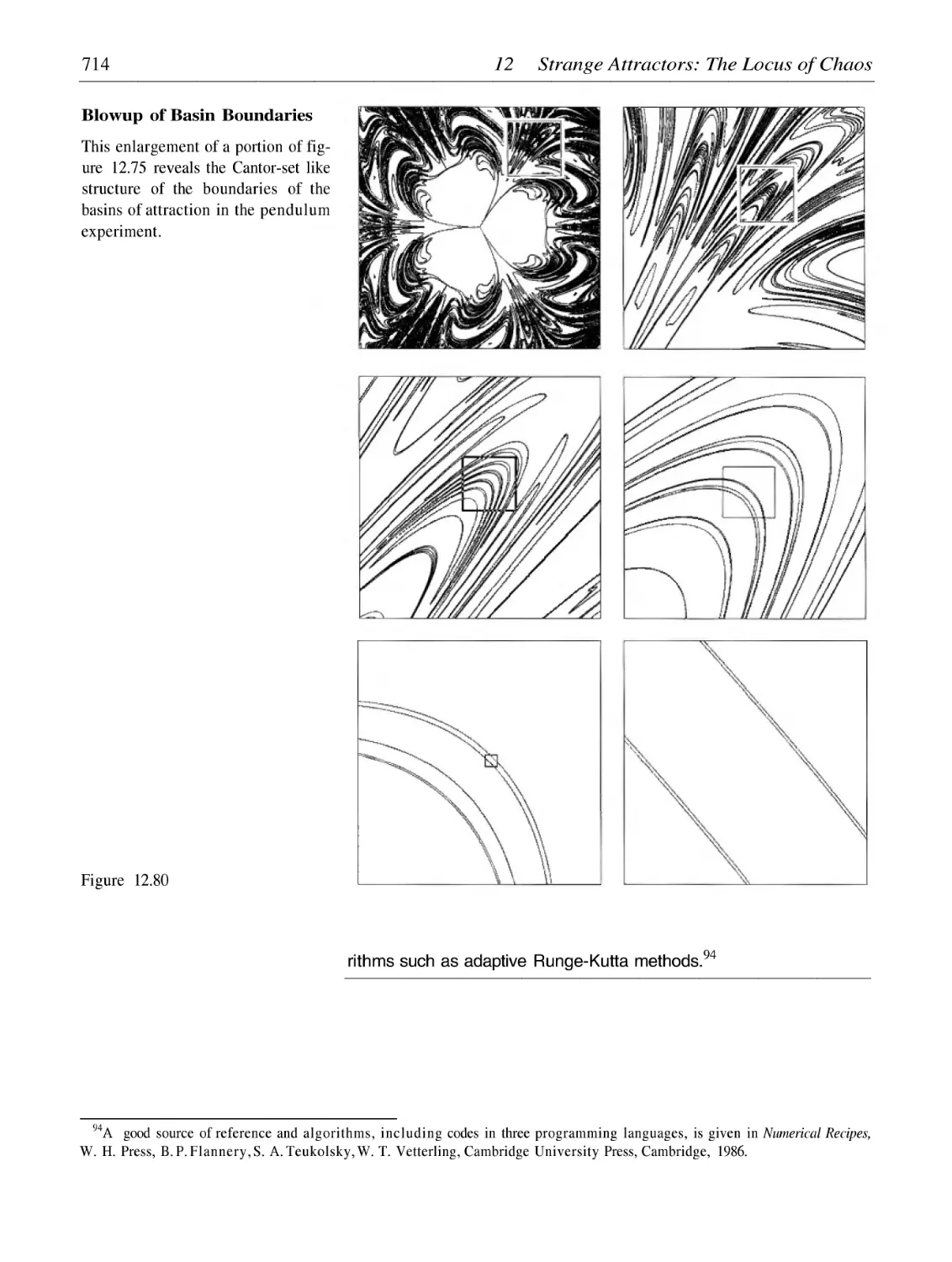
Fractal Basin Boundaries
605
609
628
636
647
659
671
694
706
13 Julia Sets: Fractal Basin Boundaries
13.1
13.2
13.3
13.4
13.5
13.6
13.7
13.8
13.9
Julia Sets as Basin Boundaries
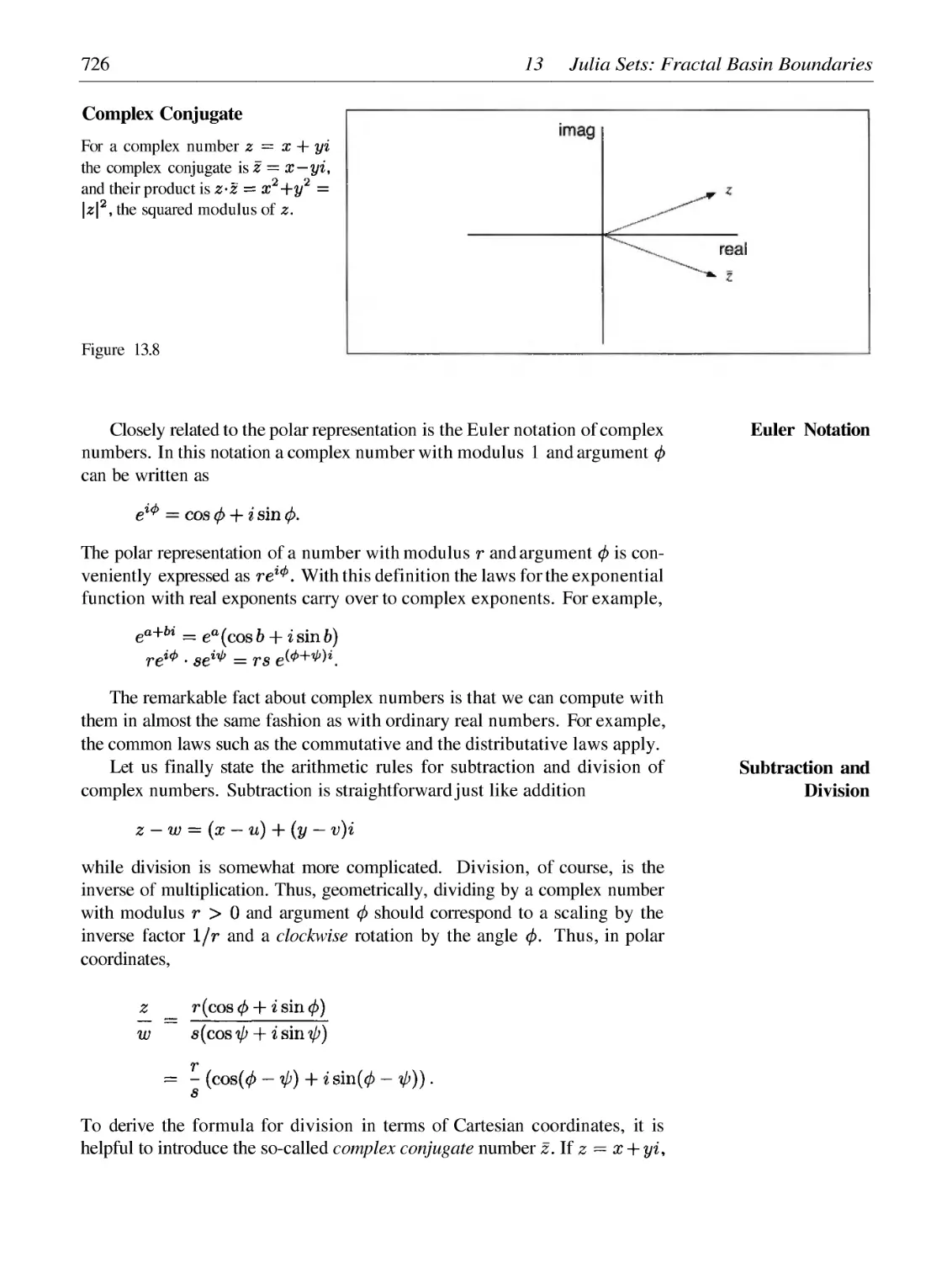
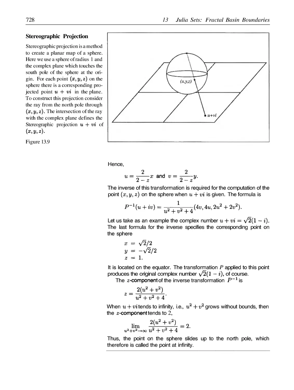
Complex Numbers --- A Short Introduction
Complex Square Roots and Quadratic Equations
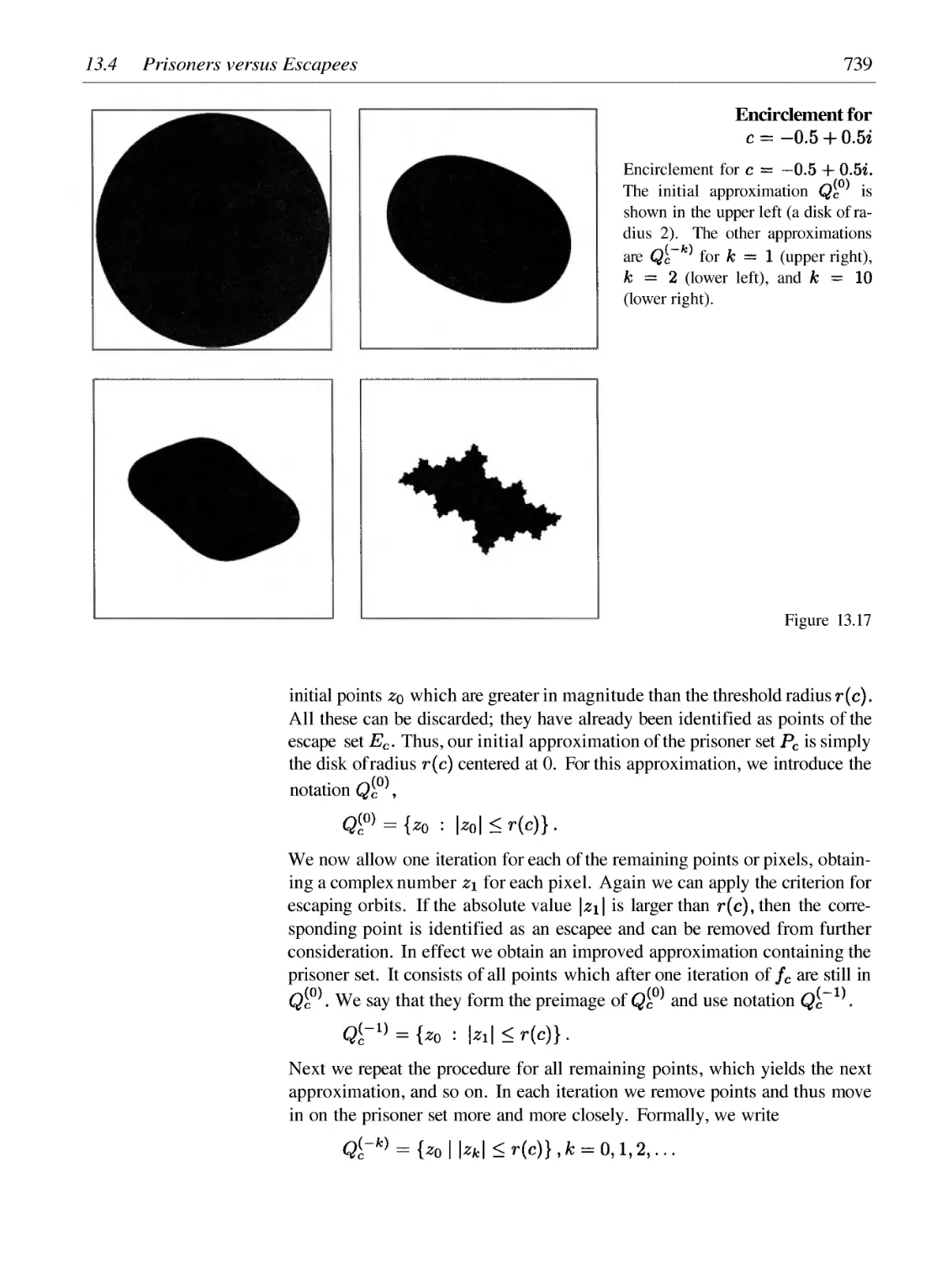
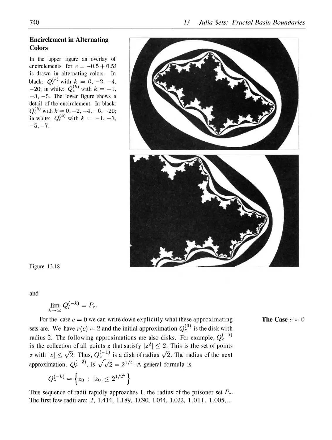
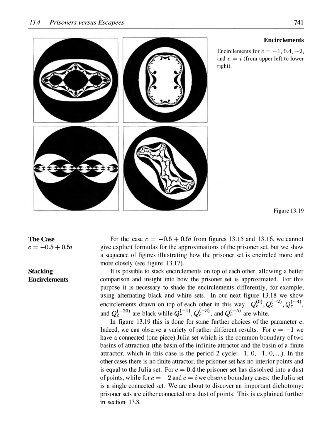
Prisoners versus Escapees
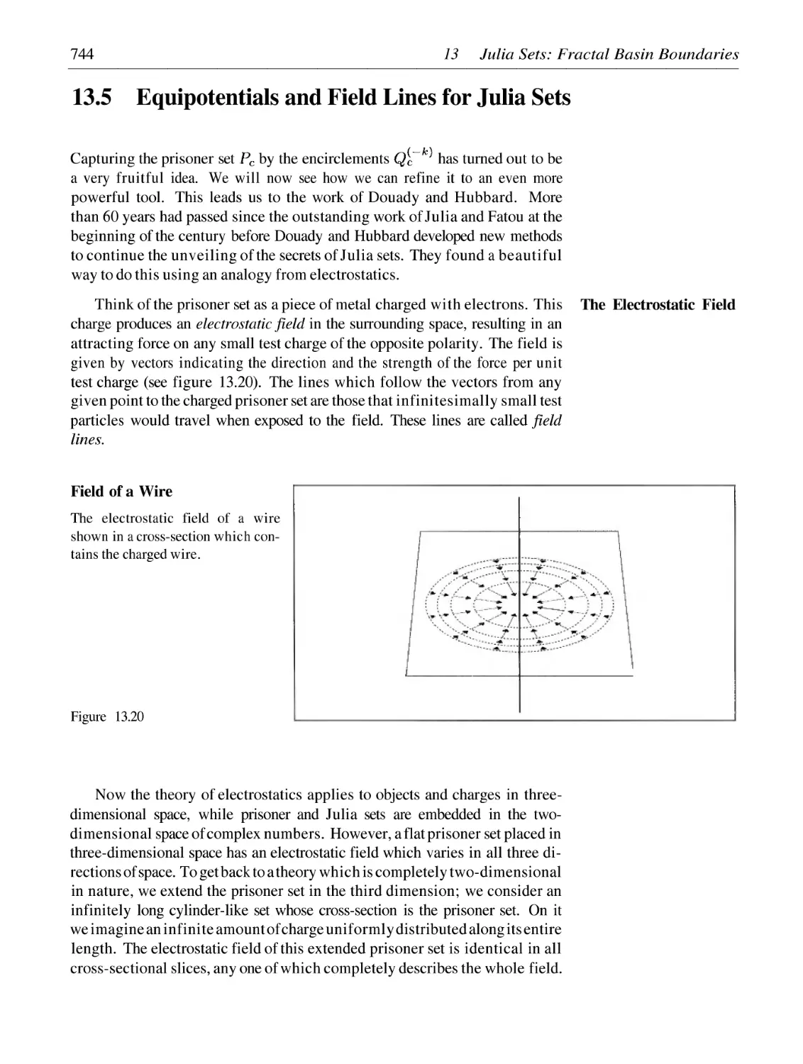
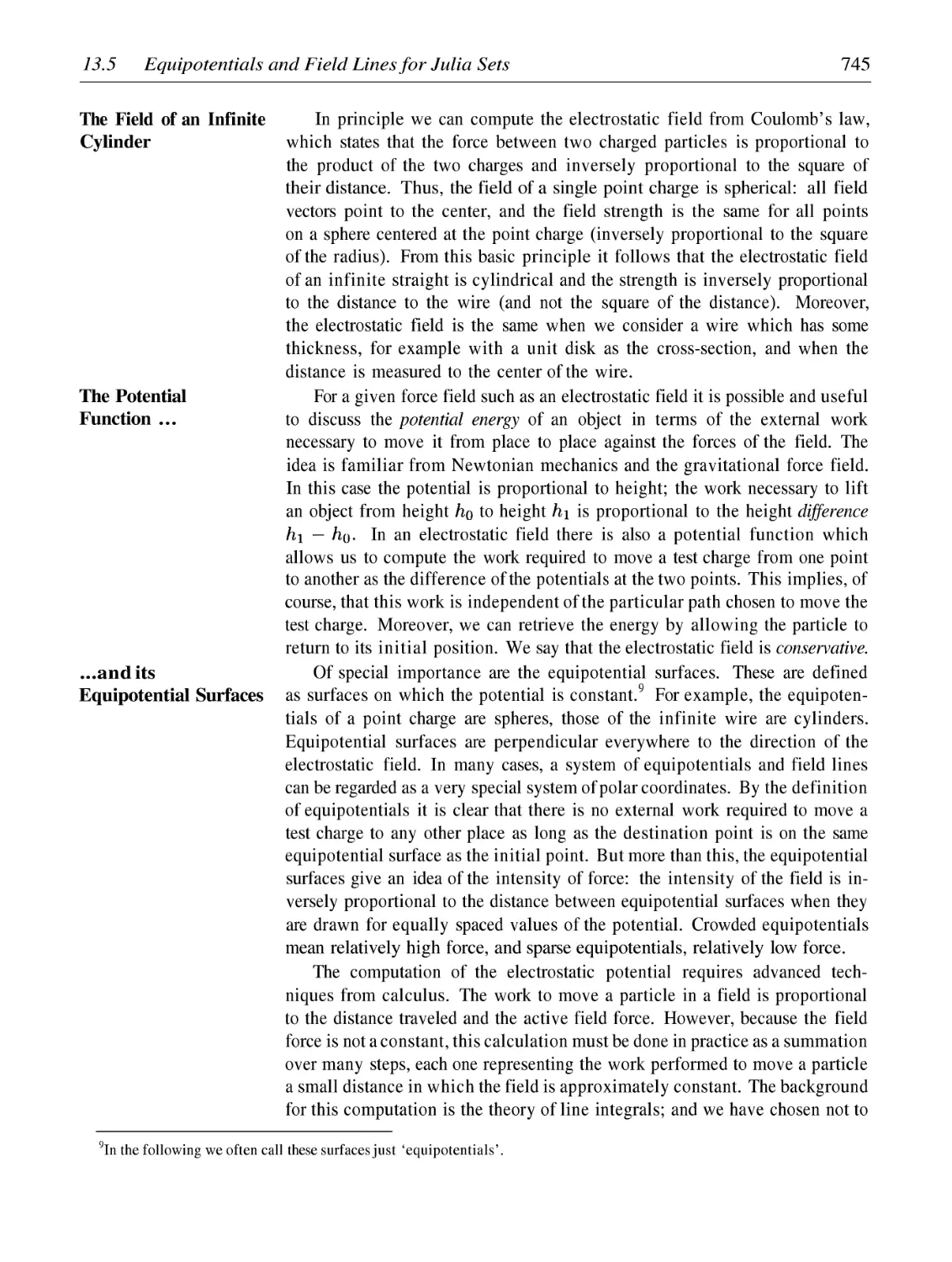
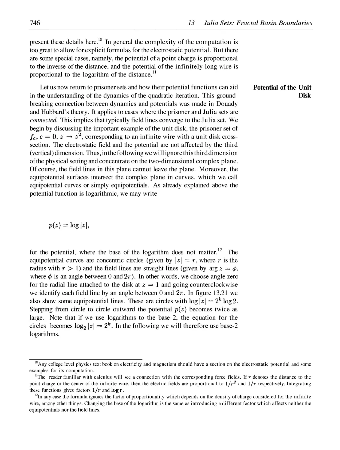
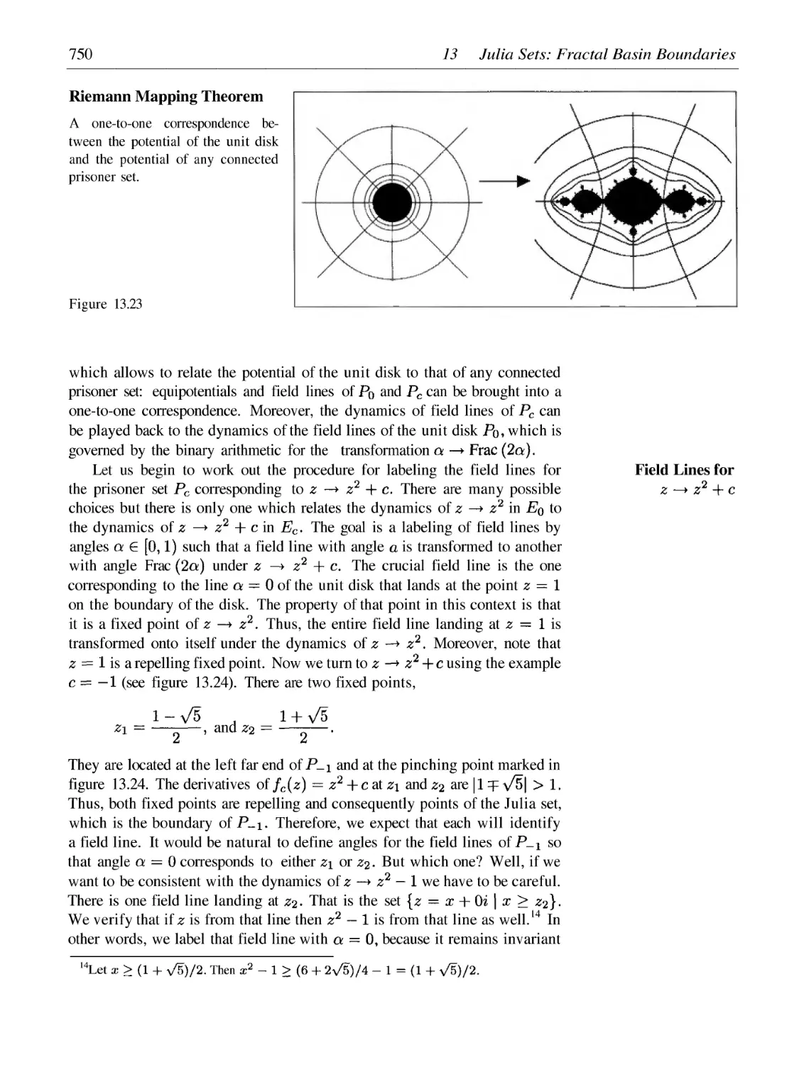
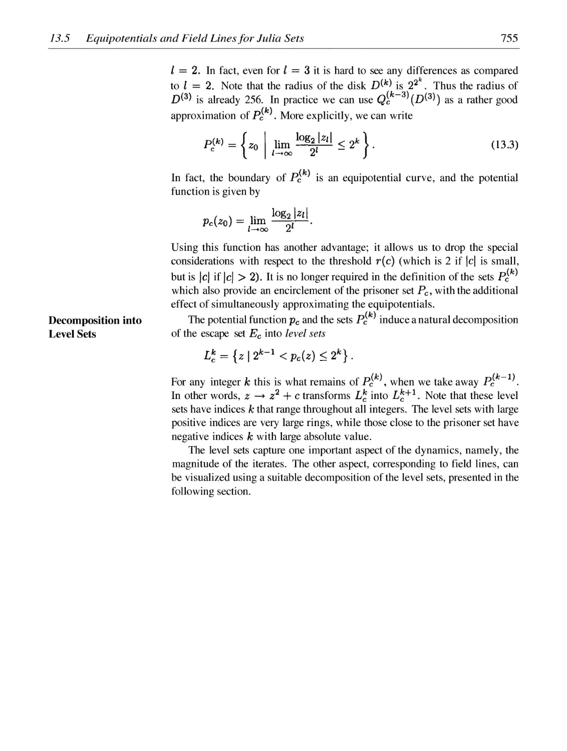
Equipotentials and Field Lines for Julia Sets
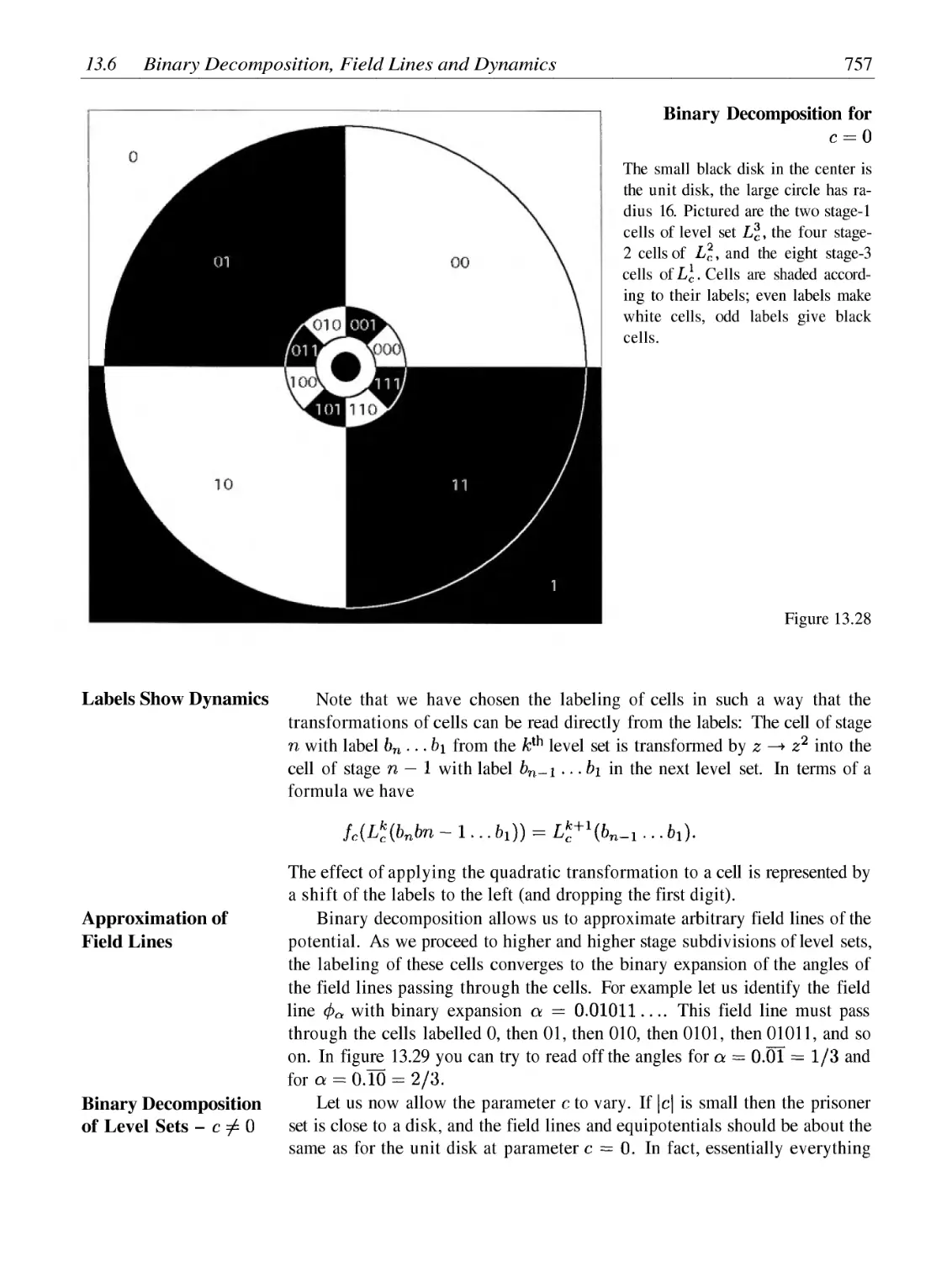
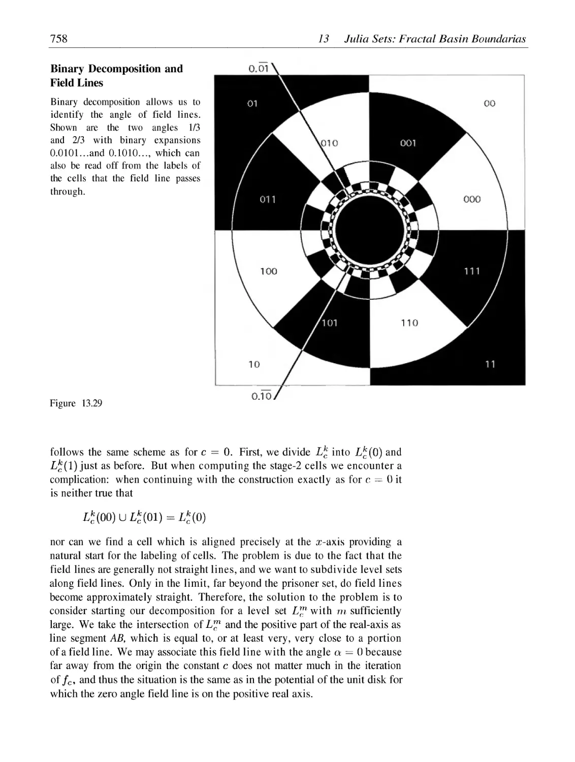
Binary Decomposition, Field Lines and Dynamics
Chaos Game and Self-Similarity for Julia Sets
The Critical Point and Julia Sets as Cantor Sets
Quaternion Julia Sets
715
717
722
729
733
744
756
764
769
780
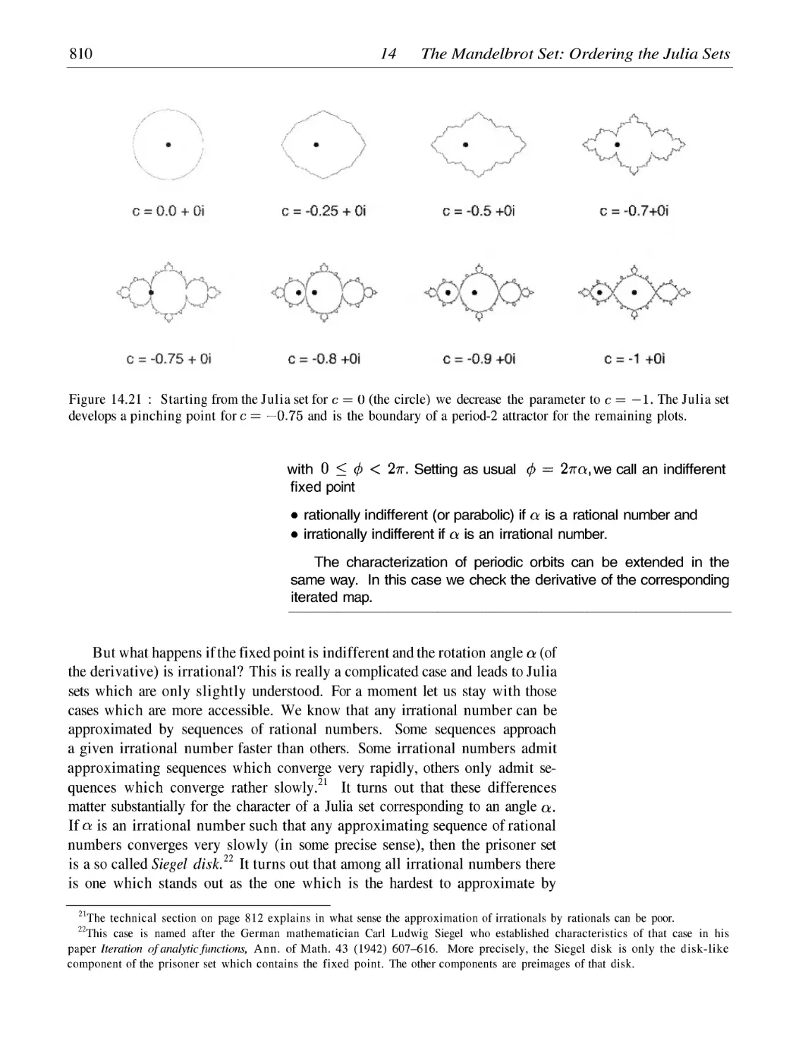
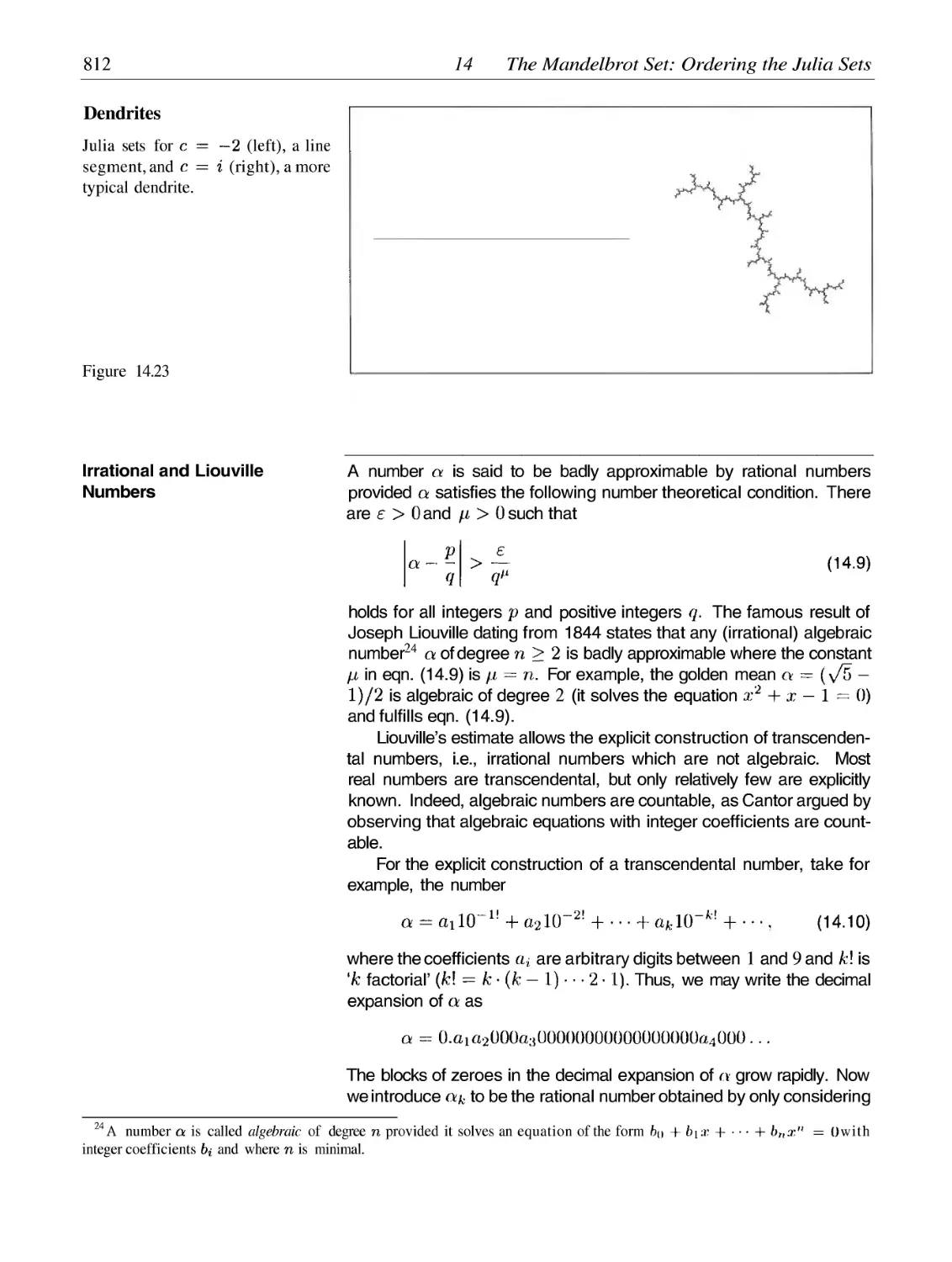
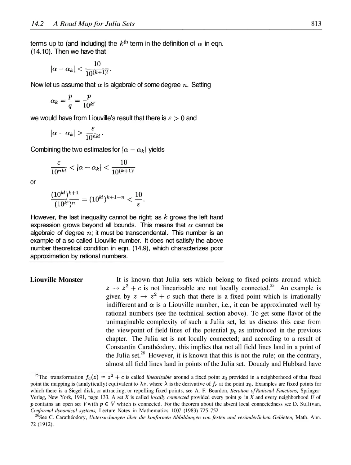
14 The Mandelbrot Set: Ordering the Julia Sets
14.1
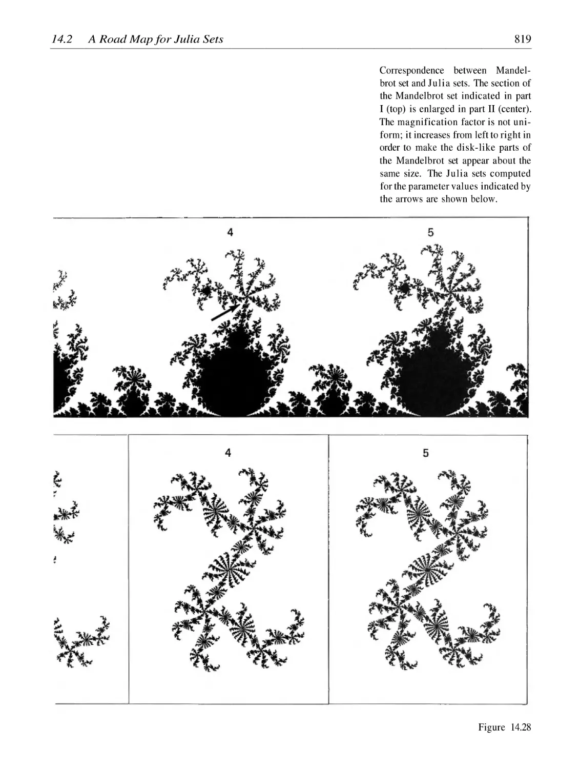
14.2
14.3
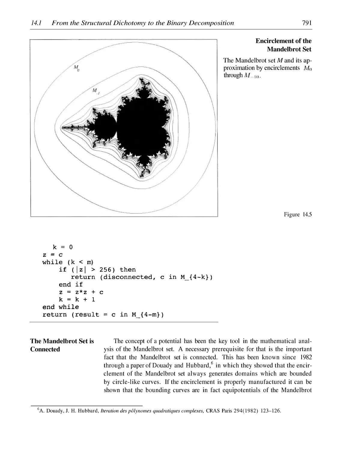
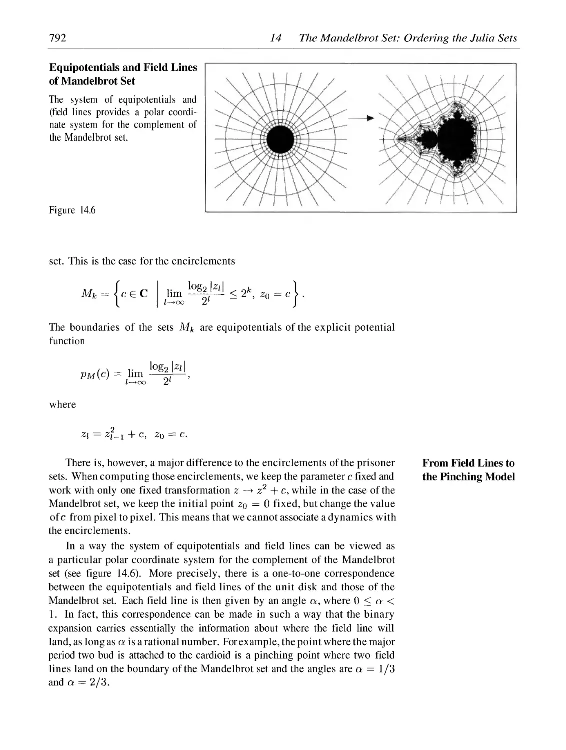
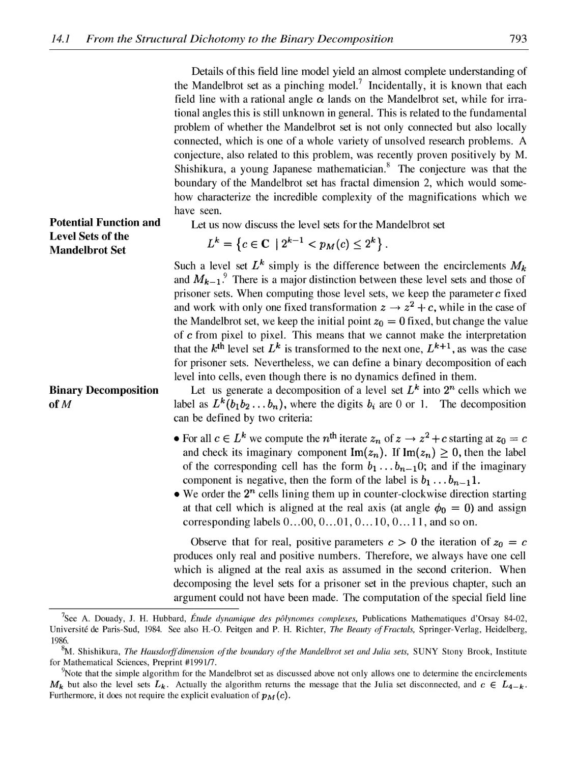
From the Structural Dichotomy to the Binary Decomposition
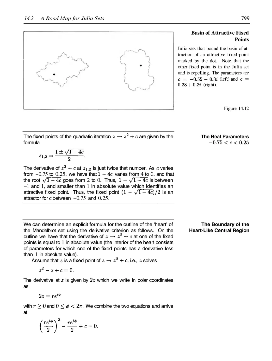
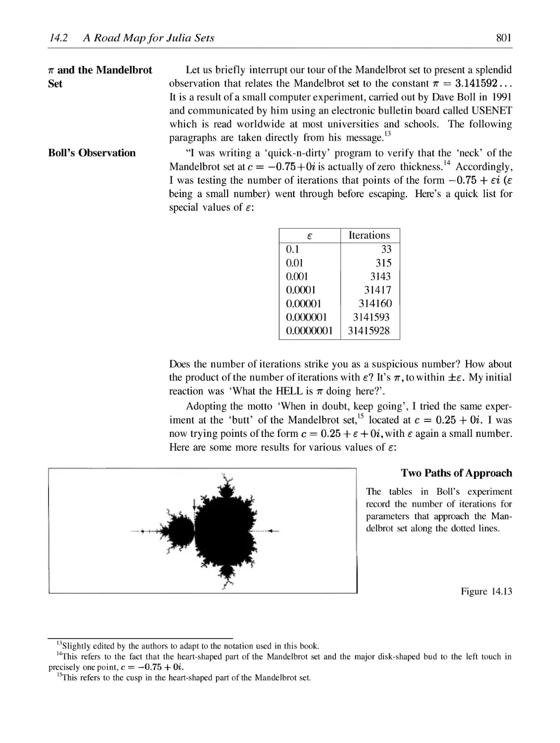
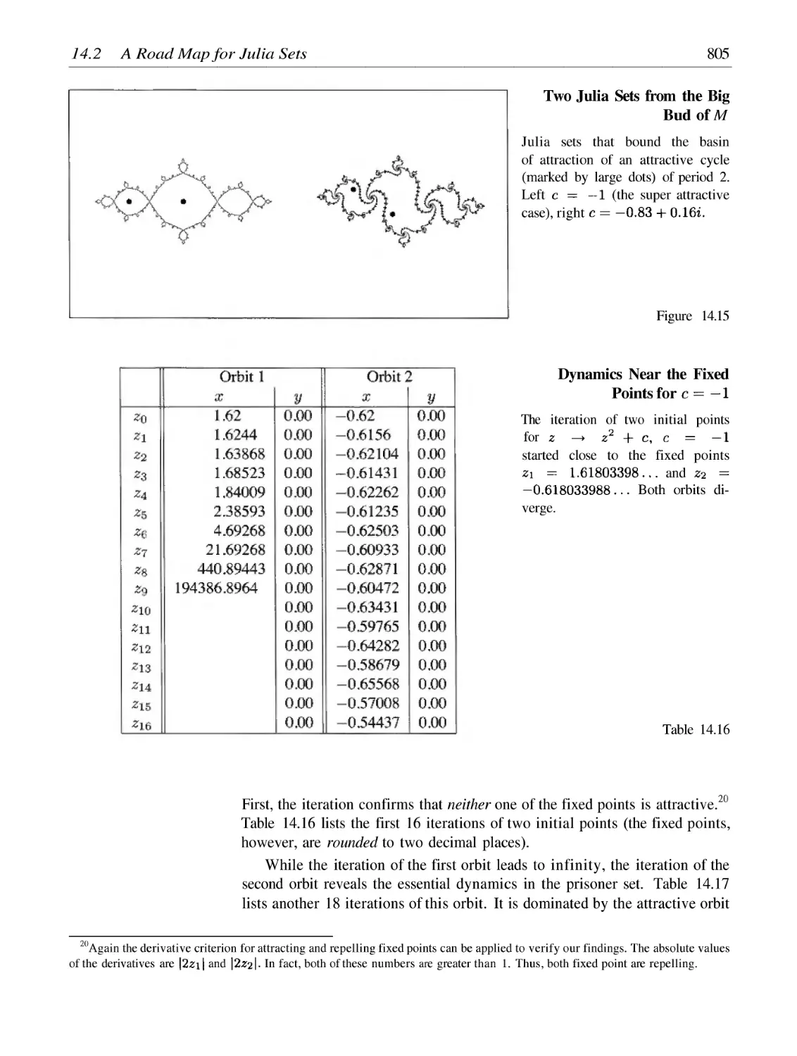
The Mandelbrot Set --- A Road Map for Julia Sets
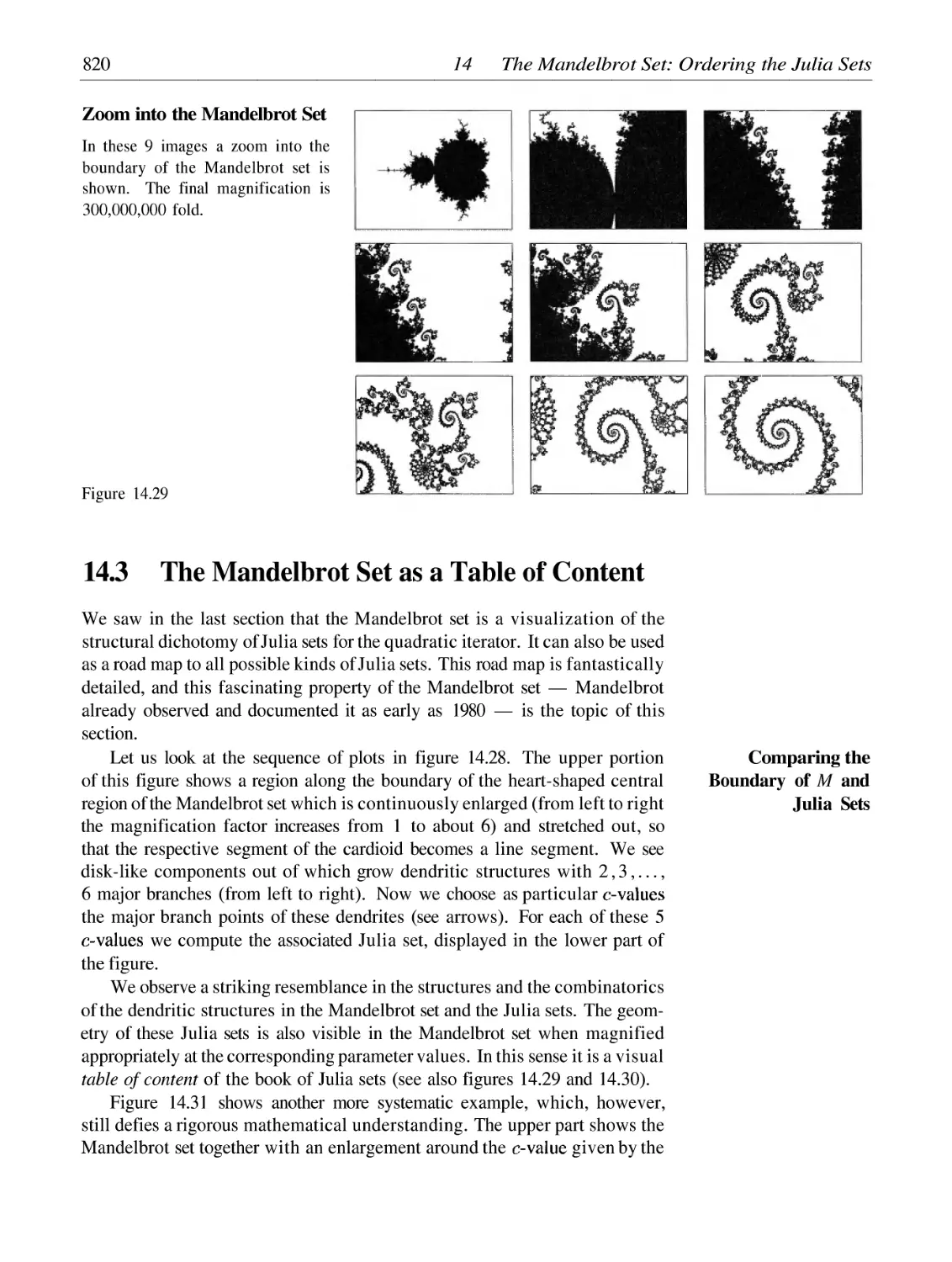
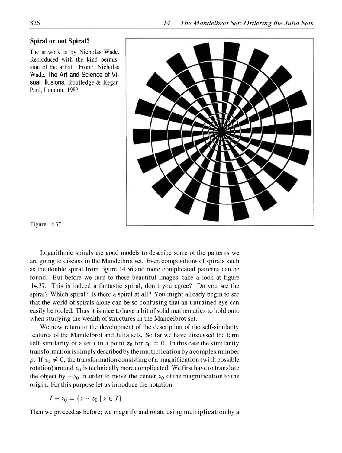
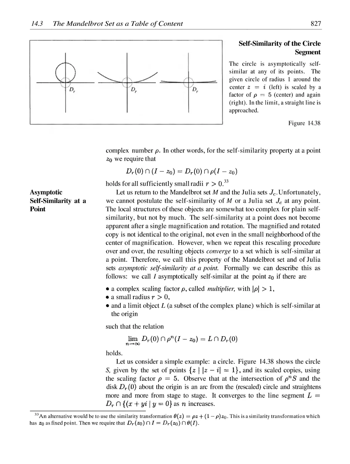
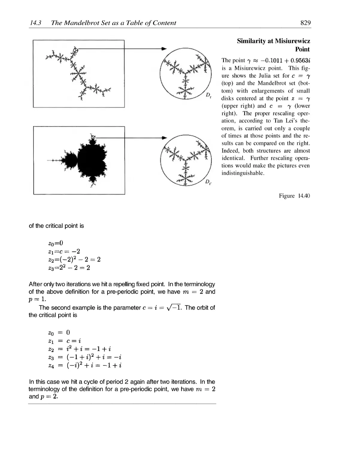
The Mandelbrot Set as a Table of Content
Bibliography
Index
783
785
797
820
839
853
This page intentionally left blank
Foreword
Mitchell J. Feigenbaum1
The study of chaos is a part of a larger
program of study of so-called 'strongly'
nonlinear systems. Within the context of
physics, the exemplar of such a system is
a fluid in turbulent motion. If chaos is not
exactly the study of fluid turbulence, nev-
ertheless, the image of turbulent, erratic
motion serves as a powerful icon to re-
mind a physicist of the sorts of problems
he would ultimately like to comprehend.
As for all good icons, while a vague
impression of what one wants to know
is sensibly clear, a precise delineation
of many of these quests is not so readily
available. In a state of ignorance, the
most poignantly insightful questions are
not yet ripe for formulation. Of course,
this comment remains true despite the fact that for technical exigencies, there
are definite questions that one desperately wants the answers to.
Fluid turbulence indeed presents us with highly erratic and only partially
predictable phenomena. Historically, since Laplace say, physical scientists
have turned to the statistical methods when presented with problems that con-
cern the mutual behaviors of innumerably large numbers of pieces. If for no
other reason, one does so to reduce the number of details that one must mea-
sure, specify, compute, whatever. Thus, it is easier to say that 43% of the
population voted for X than to offer the roster of the behavior of each of mil-
lions of voters. Just so, it is easier to specify how many gas molecules there
are in an easily measurable volume than to write out the list of where and
how fast each one is. This idea is altogether reasonable if not even the most
desirable one. However, if one is to work out a theory of these things, so that
a prediction might be rendered, then as in all matters of statistics, one must
1Mitchell J. Feigenbaum, Toyota Professor, The Rockefeller University, New York.
2
Foreword
determine a so-called distribution function. This means a theoretical predic-
tion of just how often out of uncountably many elections, etc., it is expected
that each value of this average voter response occurs. For the voter question
and the density of a gas question, there is just one number to determine. For
the problem of fluid turbulence, even in this statistical quest, one must ask a
much richer question: For example, how often do we see eddies of each size
rotating at such and such a rate?
For the problem of voters I don't have any serious idea of how to theo-
retically determine this requisite distribution; nor with good frequency do the
polls succeed in measuring it. After all, it might not exist in the sense that
it rapidly and significantly varies from day to day. However, since physicists
have long known quite reliably the laws of fluids --- that is, the rules that al-
low you to deduce what each bit of the fluid will do later if you know what
they all do now, there might be a way of doing so. Indeed, the main idea of
the branch of physics called statistical mechanics is rooted in the belief that
one knows in advance how to do this. The idea is, basically, that each possible
detailed configuration occurs with equal likelihood. Indeed, the word 'chaos'
first entered physics in Maxwell's phrase 'state of molecular chaos' in the
last century to loosely mean this. Statistical mechanics --- especially in its
quantum-mechanical form --- works very well indeed, and provides us with
some of our most wonderful knowledge. However, altogether regrettably, in
the context of fluid turbulence, it has persisted for the last century to roundly
fail. It turns out to be a question of truly deducing from the known laws of
microscopic motion of fluids what this rule of distribution must be, because
the easy guess of 'everything is as random as possibly' simply doesn't work.
And when that guess doesn't work, there exists as of today no methodology
to provide it. Moreover, if in our present state of knowledge we should be
forced to appraise the situation, then we would guess that an extraordinarily
complicated distribution is required to account for the phenomena: Should
it be fractal in nature, then fractal of the most perverse sort. And the worst
part is that we really don't possess the mathematical power to generally say
what class of object it might be sought among. Remember, we're not looking
for a perfectly good quick-fix: If we are serious in seeking understanding of
the analytical description of Nature, then we demand much more. When the
subject of chaos and a part of that larger program called strongly nonlinear
physics shall have been deemed penetrated, we shall know thoroughly how
to respond to such questions, and readily image intuitively what the answers
look like. To date, we can now compellingly do so for much simpler problems
--- and have come to possess that capability only within the last decades.
As I have said earlier, I don't necessarily care about turbulence. Rather, it
serves as an icon representing a genre of problems. I was trained as a theo-
retical high-energy physicist, and grew deeply troubled that no methods save
for that of successive improvements, so-called perturbation methods, existed.
Apart from the brilliant effort of Ken Wilson, in his version of the renor-
malization group, that circumstance is unchanged. Knowing the microscopic
The Laws of Fluids
Foreword
3
laws of how things move --- such schemes are called 'dynamical systems' ---
still leaves us almost altogether in the dark as to their larger consequences.
Are the theories no good, or is it that we just can't determine what they con-
tain? At the moment it's impossible to say. From high-energy physics to fluid
physics and astrophysics our inherited ways of thinking mathematically sim-
ply fail to serve us. In a way, if perhaps modest, the questions tackled in the
effort to comprehend what is now called chaos have faced these questions of
methodology head on.
Let me now backtrack and discuss nonlinearity. This means first linearity.
Linearity means that the rule that determines what a piece of a system is
going to do next is not influenced by what it is doing now. More precisely,
this is intended in a differential or incremental sense: For a linear spring, the
increase of its tension is proportional to the increment whereby it is stretched,
with the ratio of these increments exactly independent of how much it has
already been stretched. Such a spring can be stretched arbitrarily far, and in
particular will never snap or break. Accordingly, no real spring is linear.
The mathematics of linear objects is particularly felicitous. As it happens,
linear objects enjoy an identical, simple geometry. The simplicity of this ge-
ometry always allows a relatively easy mental image to capture the essence of
a problem, with the technicality, growing with the number of parts, basically
a detail, until the parts become infinite in number, although often then too,
precise answers can be readily determined.
The historical prejudice against nonlinear problems is that no so simple
nor universal geometry usually exists. Until recently, the general scientific
perception was that a certain nonlinear equation characterized some particular
problem. If the specific problem was sufficiently interesting or demanding of
resolution, then perhaps particular methods could be created for it. Bu t it
was well understood that the travail would probably be of no avail in other
contexts.
Indeed, only one method was well understood and universally learned,
the perturbation method. If a linear problem was viewed through distorting
lenses, it qualitatively would do the same thing: If it repeated every five sec-
onds it would persist to appear so seen through the lenses. Nevertheless, it
would now no longer appear to exhibit equal tension increments for the equal
elongations. After all, the tension is measurably unchanged by distorting
lenses, whereas all spatial measurements are. That is, the device of distorting
lenses turns a linear problem into a nonlinear one. The method of perturba-
tion basically works only for nonlinear problems that are distorted versions
of linear ones. And so, this uniquely well-learned method is of no avail in
matters that aren't merely distortions of linear ones.
Chaos is absent in distorted linear problems. Chaos and other such phe-
nomena that are qualitatively absent in linear problems are what we call
strongly nonlinear phenomena. It is this failure to subscribe to the spectrum
of configurations allowed by distorting a simple geometry that renders these
problems anywhere from hard in the extreme to impenetrable. How does one
Nonlinearity
Perturbation Method
Geometry of Chaos
4
Foreword
ever start to intelligently describe an awkward new geometry? This question
is for example intended to be loosely akin to the question of how one should
describe the geometry of the surface of the Earth, not through our abstracted
perceptual apparatus that allows us to visualize it immersed within a vastly
larger three-dimensional setting, but rather intrinsically, forbidding this use of
imagination. The solution of this question, first by Gauss and then extended
to arbitrary dimensions by Riemann is, as many of you must know, at the
center of the way of thinking of Einstein's General Theory of Relativity, our
theory of gravity. What is to be the geometry of the object that describes the
turbulent fluid's distribution function? Are there intrinsic geometries that de-
scribe various chaotic motions, that serve as a unifying way of viewing these
disparate nonlinear problems, as kindred? I ask the question because I know
the answer to be affirmative in certain broad circumstances. The moment this
is accepted, then strongly nonlinear problems appear no longer as each one its
own case, but rather coordinated and suitable for theorizing upon as their own
abstract entity. This promotion from the detailed specific to the membership
in a significant general class is one of the triumphs of the study of chaos in
the last decade or two.
An even stronger notion than this generality of shared qualitative geom-
etry is the notion of universality, which means no less than that this shared
geometry is not only one of a qualitative similarity but also one of true quan-
titative identicality. After what has been, if you will, a long preamble, the
fact that strongly nonlinear problems, with surprising frequency, can share a
quantitatively identical geometry is what I shall pursue for the rest of this dis-
cussion, and constitutes what is termed universality in the transition to chaos.
In a qualitative way of thinking, universality can be seen to be not so sur-
prising. There are two arguments to support this. The first part has simply
to do with nonlinearity. Just as a linear object has a constant coefficient of
proportionality between, for example, its tension and its expansion, a similar,
but nonlinear version, has an effective coefficient dependent upon its exten-
sion. So, consider two completely different nonlinear systems. By adjusting
things correctly it is not inconceivable that the effective coefficients of each
part of each of the two systems could be set the same so that then their behav-
iors could, at least initially, be identical. That is, by setting some numerical
constants (properties, so to speak, that specify the environment, mathemati-
cally called 'parameters') and the actual behaviors of these two systems, it
is possible that they can do the identical thing. For a linear problem this is
ostensibly true: For systems with the same number of parts and mutual con-
nections, a freedom to adjust all the parameters allows one to be adjusted to
be identical (truly) to the other. But, for many pieces, this is many adjust-
ments. For a nonlinear system, adjusting a small number of parameters can
be compensated, in this quest for identical behavior, by an adjustment of the
momentary positions of its pieces. But then it must be that not all motions
can be so duplicated between systems.
Thus, the first part of the argument is that nonlinearity confers a certain
Universality
Foreword
5
flexibility upon the adaptability of an object to desirable behavior. Neverthe-
less, should the precise adjustment of too many specific and subtle details be
required in order to achieve a certain universal behavior, then the idea would
be pedantic at best.
The Monadology of
Leibniz
However, there is a second more potent argument, a paraphrasing of Leib-
niz in 'The Monadology' which can render this first argument potent. Let
us contemplate that the motion we intend to determine to be universal over
nonlinear systems has arisen by the successive imposition of more and more
qualitative constraints. Should this growingly large host of impositions prove
to be generally amenable to such systems (this is the hard and a priori neither
obvious nor reasonable part of the discussion), then we shall ultimately dis-
cover these disparate systems to all be identically constrained by an infinite
number of qualitative and, if you will, self-consistent, requirements. Now,
following Leibniz, we ask, 'In how many precise, or quantitative, ways can
this situation be tenable?' And we respond, following Leibniz, by asserting
in precisely one possible uniquely determined way.
This is the best verbalization I know for explaining why such a universal
behavior is possible. Both mathematics and physical experimentation con-
firm its rectitude perfectly. But it is perhaps difficult to have you realize how
extraordinary this result appeared given the backdrop of physical and mathe-
matical thinking in 1976 when it first appeared together with its full concep-
tual analysis. As anecdotal evidence, I had been directed to expound these
results to one of the great mathematicians, who is renowned for his results on
dynamical systems. I spoke with him at the very end of 1976. I kept trying
to tell him that there was a complete quantitative universality to these phe-
nomena, and he equally often understood me to have duplicated some known
qualitative results. Finally, he said 'You mean to tell me these are metrical re-
sults?' (Metrical is a mathematical code word that means quantitative.) And
I said 'Yes.' 'Well, then you're wrong!' he asserted, and turned his back on
me to terminate the conversation.
Anecdote aside, what is remarkable about all this? First of all, an easy
piece of methodological insight. As practitioners of a truly analytical sci-
ence, physicists were trained to know that qualitative explanations are in-
sufficient to base truth upon. Quite to the contrary, it is regarded to be at
the heart of the 'scientific method' that ever more precise measurements will
discriminate between rival quantitative theories to ultimately select out one
as the correct encoding of the qualitative content. (Thus, think of geocen-
tric versus heliocentric planetary theories, both qualitatively explaining the
retrograde motions of the planets.) Here the method is turned on its head:
Qualitatively similar phenomena, independent of any other ideational input,
must ineluctably lead to the measurably identical quantitative result. Whence
the total phenomenological support for this mighty 'scientific method?'
Second, a new principle of 'economy' immediately emerges. Why put out
Herculean efforts to calculate the consequences of some particular and highly
difficult encoding of physical laws, when anything else --- however trivial ---
The Scientific Method
How Universality
Works
6
Foreword
possessing the same qualitative properties will yield exactly the same predic-
tions and results? And this is all the more satisfying because one doesn't even
know the exact equations that describe various of these phenomena, fluid phe-
nomena in particular. And that is because these phenomena have nothing to
do, whatsoever, with the detailed, particular, microscopic laws that happen to
be at play. This aspect, that is, of substituting easy problems for hard ones
with no penalty, has been, as a way of thinking and performing research, the
prominent fruit of the recognition of universality. When can it work? Well, in
complicated interactions of scores of chemical species, in laser phenomena,
in solid state phenomena, in, at least partially, biological rhythmic phenomena
such as apneas and arhythmias, in fluids and, of course, in mathematics.
But now, as I move towards the end of this claim for virtue, let me discuss
'chaos' a bit more per se and revisit my opening 'preamble.' Much of chaos
as a science is connected with the notion of 'sensitive dependence on initial
conditions.' Technically, scientists term as 'chaotic' those nonrandom com-
plicated motions that exhibit a very rapid growth of errors that, despite perfect
determinism, inhibits any pragmatic ability to render accurate long-term pre-
diction. While nomenclaturally speaking this is perforce true, I personally am
not very intrigued or concerned with this facet of my subject. I've never told
you what the 'transition to chaos' means, but you can readily guess from the
verbiage that it's something that starts off not being chaotic, ends up being so,
and hence somehow passes from one to the next. The most important fact is
that there is a discernibly precise 'moment', with a corresponding behavior,
which is neither chaotic nor nonchaotic, at which this transition occurs. Yes,
errors do grow, but only in a marginally predictable, rather than in an unpre-
dictable, fashion. In this state of marginal predictability inheres embryoni-
cally all the seeds of the chaotic behavior to come. That is, this transitional
point, the legitimate child of universality, without full-fledged sensitive de-
pendence upon initial conditions, knows fully how to dictate to its progeny in
turn how this latter phenomenon must unfold. For a certain range of possible
behaviors of strongly nonlinear systems --- specifically, this range surround-
ing the transition to chaos --- the information obtained just at the transition
point fully organizes the spectrum of behaviors that these chaotic systems can
exhibit.
Now what is it that turns out to be universal? The answer, mostly, is
a precise quantitative determination of the intrinsic geometry of the space
upon which this marginal chaotic motion lives together with the full knowl-
edge of how in the course of time this space is explored. Indeed, it was
from the analysis of universality at the transition to chaos that we have come
to recognize the precise mathematical object that fully furnishes the intrinsic
geometry of these sort of spaces. This object, a so-called scaling function,
together with the mathematically precise delineation of universality, consti-
tutes one of the major results of the study of chaos. Granted the broad range
of objects that can be termed fractal, these geometries are fractal. But not
the heuristic sort of 'dragons', 'carpets', 'snowflakes', etc. Rather, these are
The Essence of Chaos
The Geometry of
Chaos
Foreword
7
structures which are elaborated upon at smaller and smaller scales differently
at each point of the object, and so are infinitely more complicated than the
above heuristic objects. There is, in more than just a way of speaking, a ge-
ometry of these dynamically created objects, and that geometry requires a
scaling function to fully elucidate it. Many of you are aware of the existence
of a certain object called the 'Mandelbrot set'. Virtually none of you, though,
even having simulated it on your own computers, are aware that its ubiqui-
tous existence in those sufficiently smooth contexts in which it appears, is the
consequence of universality at the transition of chaos. Every one of its details
is implicit in those embryonic seeds I have mentioned before.
Thus, the most elementary consequence of this deep universal geome-
try is that, in gross organization we notice a set of discs --- the largest the
main cardioid --- one abutting upon the next and of rapidly diminishing radii.
How rapidly do they diminish in size? In fact, each one is times smaller
that its predecessor, with a universal constant, approximately equal to
4.6692016..., the best known of the constants that characterize universal-
ity at the transition of chaos.
I have now come around full circle to my introductory comments. We
have, in the last decade, succeeded in coming to know many of the correct
ideas and their mathematical language in regard to the question, 'What is the
nature of the objects upon which we see our statistical distributions?' 'Di-
mension' is a mathematical word possessing a quite broad range of technical
connotations. Thus, the theory of universality is erected in a very low (that is,
one- or two-) dimensional setting. However the information discussed is of
an infinite-dimensional character. The physical phenomena exhibiting these
behaviors can appear, for example, in the physical three-dimensional space
of human experience, with the number of interacting, cooperating pieces that
comprise the system investigated --- also a statement of its dimension --- ei-
ther merely a few or an infinitude. Nevertheless, our understanding to date
is of what must be admitted to be a relatively simple set of phenomena ---
relatively simple in comparison to the swirling and shattering complexity of
fluid motions at the foot of a waterfall, phenomena that loom large and deeply
impress upon us how much lies undiscovered before us.
This page intentionally left blank
Introduction
Causality Principle, Deterministic Laws
and Chaos
Prediction is difficult, especially of the future.
Niels Bohr
For many, chaos theory already belongs to the greatest achievements in
the natural sciences in this century. Indeed, it can be claimed that very few
developments in natural science have awakened so much public interest. Here
and there, we even hear of changing images of reality or of a revolution in the
natural sciences.
Critics of chaos theory have been asking whether this popularity could
perhaps only have something to do with the clever choice of catchy terms
or the very human need for a theoretical explanation of chaos. Some have
prophesized for it exactly the same quick and pathetic death as that of the
catastrophe theory, which excited so much attention in the sciences at the end
of the 1960's and then suddenly fell from grace even though its mathematical
core is counted as one of the most beautiful constructions and creations. The
causes of this demise were diverse and did not only have scientific roots. It
can certainly be said that catastrophe theory was severely damaged by the
almost messianic claims of some apologists.
Chaos theory, too, is occasionally in danger of being overtaxed by being
associated with everything that can be even superficially related to the concept
of chaos. Unfortunately, a sometimes extravagant popularization through the
media is also contributing to this danger; but at the same time this populariza-
tion is also an important opportunity to free areas of mathematics from their
intellectual ghetto and to show that mathematics is as alive and important as
ever.But what is it that makes chaos theory so fascinating? What do the sup-
posed changes in the image of reality consist of? To these subjects we would
like to pose, and to attempt to answer, some questions regarding the philoso-
phy of nature.
10
Introduction
The main maxim of science is its ability to relate cause and effect. On
the basis of the laws of gravitation, for example, astronomical events such as
eclipses and the appearances of comets can be predicted thousands of years
in advance. Other natural phenomena, however, appear to be much more
difficult to predict. Although the movements of the atmosphere, for example,
obey the laws of physics just as much as the movements of the planets do,
weather prediction is still rather problematic.
Cause and Effect
Tides Versus Weather
Ian Stewart in his article Chaos: Does God Play Dice?, Encyclopæ-
dia Britannica, 1990 Yearbook of Science and the Future, makes the
following striking comparison:
"Scientists can predict the tides, so why do they have so much
trouble predicting the weather? Accurate tables of the time of high or
low tide can be worked out months or even years ahead. Weather
forecasts often go wrong within a few days, sometimes even within
a few hours. People are so accustomed to this difference that they
are not in the least surprised when the promised heat wave turns
out to be a blizzard. In contrast, if the tide table predicted a low
tide but the beach was under water, there would probably be a riot.
Of course the two systems are different. The weather is extremely
complex; it involves dozens of such quantities as temperature, air
pressure, humidity, wind speed, and cloud cover. Tides are much
simpler. Or are they? Tides are perceived to be simpler because
they can be easily predicted. In reality, the system that gives rise to
tides involves just as many variables -- the shape of the coastline,
the temperature of the sea, its salinity, its pressure, the waves on its
surface, the position of the Sun and Moon, and so on -- as that which
gives rise to weather. Somehow, however, those variables interact in
a regular and predictable fashion. The tides are a phenomenon of
order. Weather, on the other hand, is not. There the variables interact
in an irregular and unpredictable way. Weather is, in a word, chaotic."
We speak of the unpredictable aspects of weather just as if we were talking
about rolling dice or letting an air balloon loose to observe its erratic path as
the air is ejected. Since there is no clear relation between cause and effect,
such phenomena are said to have random elements. Yet there was little reason
to doubt that precise predictability could, in principle, be achieved. It was
assumed that it was only necessary to gather and process greater quantities of
more precise information (e.g., through the use of denser networks of weather
stations and more powerful computers dedicated solely to weather analysis).
Some of the first conclusions of chaos theory, however, have recently altered
this viewpoint. Simple deterministic systems with only a few elements can
generate random behavior, and that randomness is fundamental; gathering
more information does not make it disappear. This fundamental randomness
has come to be called chaos.
Causality Principle, Deterministic Laws and Chaos
11
Deterministic Chaos
An apparent paradox is that chaos is deterministic, generated by fixed
rules which do not themselves involve any elements of change. We even
speak of deterministic chaos. In principle, the future is completely determined
by the past; but in practice small uncertainties, much like minute errors of
measurement which enter into calculations, are amplified, with the effect that
even though the behavior is predictable in the short term, it is unpredictable
over the long term.
The discovery of such behavior is one of the important achievements of
chaos theory. Another is the methodologies which have been designed for
a precise scientific evaluation of the presence of chaotic behavior in mathe-
matical models as well as in real phenomena. Using these methodologies,
it is now possible, in principle, to estimate the 'predictability horizon' of a
system. This is the mathematical, physical, or time parameter limit within
which predictability is ideally possible and beyond which we will never be
able to predict with certainty. It has been established, for example, that the
predictability horizon in weather forecasting is not more than about two or
three weeks. This means that no matter how many more weather stations are
included in the observation, no matter how much more accurately weather
data are collected and analyzed, we will never be able to predict the weather
with any degree of numerical accuracy beyond this horizon of time.
But before we go into an introductory discussion of what chaos theory is
trying to accomplish, let us look at some historical aspects of the field. If we
look at the development of the sciences on a time-scale on which the efforts
of our forbears are visible, we will observe indications of an apparent reca-
pitulation in the present day, even if at a different level. To people during
the age of early human history, natural events must have seemed largely to be
pure chaos. At first very slowly, then faster and faster, the natural sciences
developed (i.e., over the course of thousands of years, the area where chaos
reigned seemed to become smaller and smaller). For more and more phe-
nomena, their governing laws were wrung from Nature and their rules were
recognized. Simultaneously, mathematics developed hand in hand with the
natural sciences, and thus an understanding of the nature of a phenomenon
soon came to also include the discovery of an appropriate mathematization of
it. In this way, there was continuous nourishment for the illusion that it was
only a matter of time, along with the necessary effort and means, before chaos
would be completely banned from human experience.
A landmark accomplishment of tremendous, accelerating effect was made
about three hundred years ago with the development of calculus by Sir Isaac
Newton (1643--1727) and Gottfried Wilhelm Freiherr von Leibniz (1646--
1716). Through the universal mathematical ideas of calculus, the basis was
provided with which to apparently successfully model the laws of the move-
ments of planets with as much detail as that in the development of populations,
the spread of sound through gases, the conduction of heat in media, the inter-
action of magnetism and electricity, or even the course of weather events. Also
maturing during that time was the secret belief that the terms determinism and
12
Introduction
predictability were equivalent.
For the era of determinism, which was mathematically grounded in cal-
culus, the 'Laplace demon' became the symbol. "If we can imagine a con-
sciousness great enough to know the exact locations and velocities of all the
objects in the universe at the present instant, as well as all forces, then there
could be no secrets from this consciousness. It could calculate anything about
the past or future from the laws of cause and effect."2
In its core, the deterministic credo means that the universe is comparable
to the ordered running of a tremendously precise clock, in which the present
state of things is, on the one hand, simply the consequence of its prior state,
and, on the other hand, the cause of its future state. Present, past and future
are bound together by causal relationships; and according to the views of the
determinists, the problem of an exact prognosis is only a matter of the difficulty
of recording all the relevant data. The deterministic credo was characteristic
of the Newtonian era, which for the natural sciences came to an end, at the
latest, through the insights of Werner Heisenberg in the 1927 proclamation
of his uncertainty principle,3 but which for other sciences is still considered
valid.
Heisenberg wrote: "In the strict formulation of the causality law --- 'When
we know the present precisely, we can calculate the future' --- it is not the
final clause, but rather the premise, that is false. We cannot know the present
in all its determining details.
"Therefore, all perception is a selection from an abundance of possibilities
and a limitation of future possibilities ...Because all experiments are subject to
the laws of quantum mechanics, and thereby also to the uncertainty principle,
the invalidity of the causality law is definitively established through quantum
mechanics."
Classical determinism in its fearful strictness had to be given up --- a
turning point of enormous importance.
How undiminished the hope in a great victory of determinism still was
at the beginning of this century is impressively illustrated in the 1922 book
by Lewis F. Richardson entitled Weather Prediction by Numerical Process,4
in which was written: "After so much hard reasoning, may one play with
a fantasy? Imagine a large hall like a theater, except that the circles and
galleries go right round through the space usually occupied by the stage. The
walls of this chamber are painted to form a map of the globe. The ceiling
represents the north polar regions, England is the gallery, the tropics in the
upper circle, Australia on the dress circle and the Antarctic in the pit. A
The Laplace Demon
Strict Causality
2Pièrre Simon de Laplace (1749--1829), a Parisian mathematician and astronomer.
3This is also called the indeterminacy principle and states that the position and velocity of an object cannot, even in theory, be
exactly measured simultaneously. In fact, the very concept of a concurrence of exact position and exact velocity have no meaning in
nature. Ordinary experience, however, provides no evidence of the truth of this principle. It would appear to be easy, for example,
to simultaneously measure the position and the velocity of a car; but this is because for objects of ordinary size, the uncertainties
implied by this principle are too small to be observable. But the principle becomes really significant for subatomic particles such
as electrons.
4Dover Publications, New York, 1965. First published by Cambridge University Press, London, 1922. This book is still
considered one of the most important works on numerical weather forecasting.
Causality Principle, Deterministic Laws and Chaos
13
myriad of computers5 are at work upon the weather of the part of the map
where each sits, but each computer attends only to one equation or part of
an equation. The work of each region is coordinated by an official of higher
rank. Numerous little 'night signs' display the instantaneous values so that
neighboring computers can read them.... From the floor of the pit a tall pillar
rises to half the height of the hall. It carries a large pulpit on its top. In this sits
the man in charge of the whole theater; he is surrounded by several assistants
and messengers. In this respect he is like the conductor of an orchestra in
which the instruments are slide-rules and calculating machines. But instead
of waving a baton he turns a beam of rosy light upon any region that is running
ahead of the rest, and a beam of blue light upon those who are behindhand."
In his book, Richardson first laid down the basis for numerical weather
forecasting and then reported on his own initial practical experience with
calculation experiments. According to Richardson, the calculations were so
long and complex that only by using a 'weather forecasting center' such as
the one he fantasized was forecasting conceivable.
Then about the middle of the 1940's, the great John von Neumann actually
began to construct the first electronic computer, ENIAC, in order to further
pursue Richardson's prophetic program, among others. It was soon recog-
nized, however, that Richardson's only mediocre practical success was not
simply attributable to his equipment's lack of calculating capacity, but also to
the fact that the space and time increments used in his work had not met a
computational stability criterion (Courant-Friedrichs-Lewy Criterion), which
was only discovered later. With the appropriate corrections, further attempts
were soon under way with progressively bigger and faster computers to make
Richardson's dream a reality. This development has been uninterrupted since
the 1950's, and it has bestowed truly gigantic 'weather theaters' upon us.
Indeed, the history of numerical weather forecasting illustrates better than
anything else the undiminished belief in a deterministic (viz. predictable)
world; for, in reality, Heisenberg's uncertainty principle did not at all mean
the end of determinism. It only modified it, because scientists had never really
taken Laplace's credo so completely seriously --- as is usual with creeds. The
most carefully conducted experiment is, after all, never completely isolated
from the influences of the surrounding world, and the state of a system is never
precisely known at any point in time. The absolute mathematical precision
that Laplace presupposed is not physically realizable; minute imprecision is,
as a matter of principle, always present. What scientists actually believed was
this: From approximately the same causes follow approximately the same
effects --- in nature as well as in any good experiment. And this is indeed
often the case, especially over short time spans. If this were not so, we would
not be able to ascertain any natural laws, nor could we build any functioning
machines.
But this apparently very plausible assumption is not universally true. And
what is more, it does not do justice to the typical course of natural processes
Weak Causality
The Butterfly Effect
5Richardson uses the word computer here to mean a person who computes.
14
Introduction
over long periods of time. Around 1960, Ed Lorenz discovered this deficiency
in the models used for numerical weather forecasting; and it was he who
coined the term 'butterfly effect'. His description of deterministic chaos goes
like this:6 Chaos occurs when the error propagation, seen as a signal in a time
process, grows to the same size or scale as the original signal.
Thus, Heisenberg's response to deterministic thinking was also incom-
plete. He concluded that the strong causality principle is wrong because its
presumptions are erroneous. Lorenz has now shown that the conclusions are
also wrong. Natural laws, and for that matter determinism, do not exclude the
possibility of chaos. In other words, determinism and predictability are not
equivalent. And what is an even more surprising rinding ofrecent chaos theory
has been the discovery that these effects are observable in many systems which
are much simpler than the weather. In fact, they can be observed in very simple
feedback systems, even as simple as the quadratic iterator
Moreover, chaos and order (i.e., the causality principle) can be observed
in juxtaposition within the same system. There may be a linear progression of
errors characterizing a deterministic system which is governed by the causality
principle, while (in the same system) there can also be an exponential progres-
sion of errors (i.e., the butterfly effect) indicating that the causality principle
breaks down.
In other words, one of the lessons coming out of chaos theory is that the
validity of the causality principle is narrowed by the uncertainty principle
from one end as well as by the intrinsic instability properties of the underlying
natural laws from the other end.
6See Peitgen, H.-O. , Jürgens, H., Saupe, D., and Zahlten, C., Fractals --- An Animated Discussion, Video film, Freeman 1990.
Also appeared in German as Fraktale in Filmen und Gesprächen, Spektrum der Wissenschaften Videothek, Heidelberg, 1990.
Chapter 1
The Backbone of Fractals: Feedback
and the Iterator
The scientist does not study nature because it is useful; he studies it because
he delights in it, and he delights in it because it is beautiful. If nature were
not beautiful, it would not be worth knowing, and if nature were not worth
knowing, life would not be worth living.
Henri Poincaré
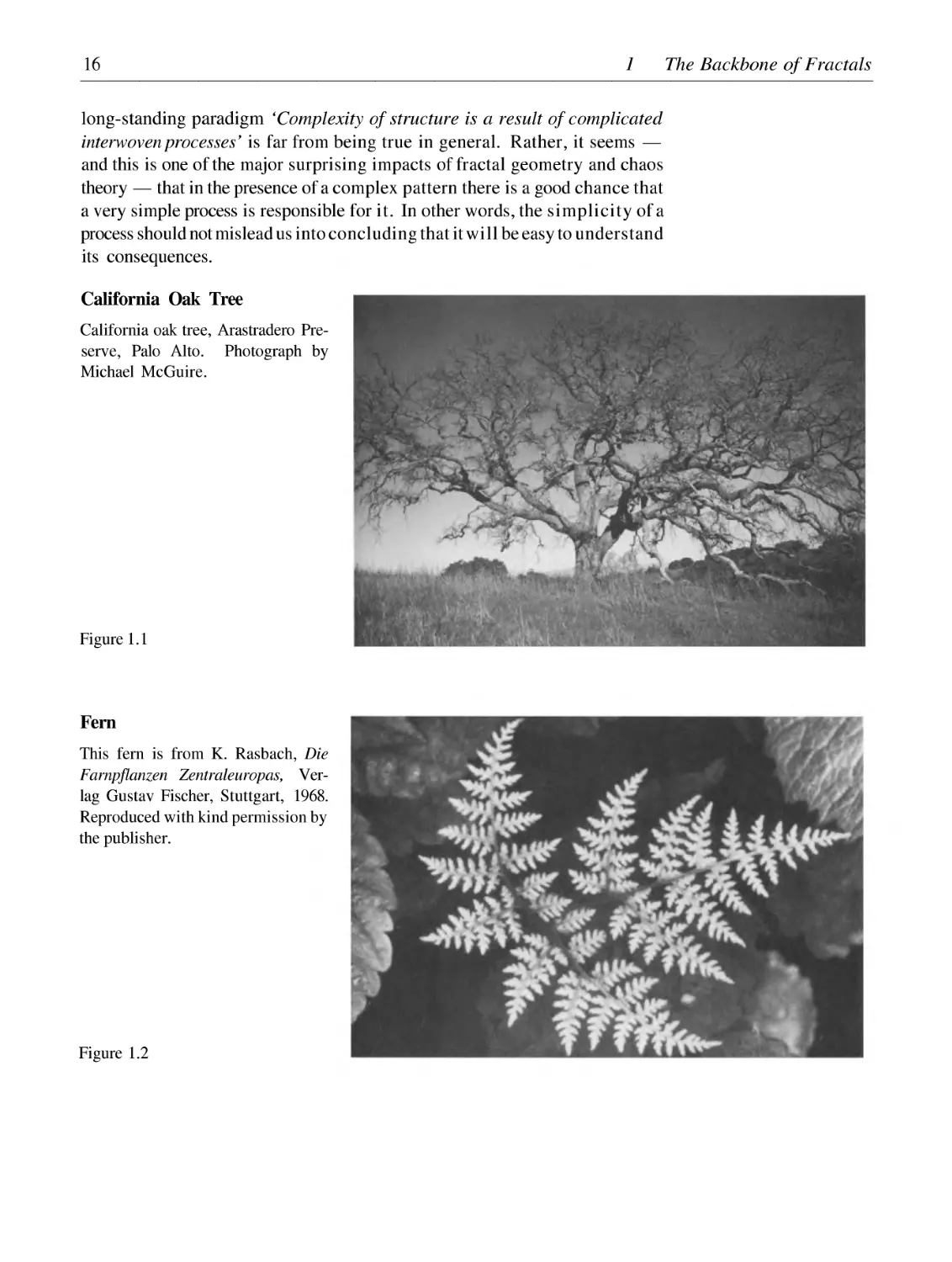
When we think about fractals as images, forms or structures we usually
perceive them as static objects. This is a legitimate initial standpoint in many
cases, as for example if we deal with natural structures like the ones in figures
1.1 and 1.2.
But this point of view tells us little about the evolution or generation of a
given structure. Often, as for example in botany, we like to discuss more than
just the complexity of a ripe plant. In fact, any geometric model of a plant
which does not also incorporate its dynamic growth plan for the plant will not
lead very far.
The same is true for mountains, whose geometry is a result of past tectonic
activity as well as erosion processes which still and will forever shape what
we see as a mountain. We can also say the same for the deposit of zinc in an
electrolytic experiment.
In other words, to talk about fractals while ignoring the dynamic processes
which created them would be inadequate. But in accepting this point of
view we seem to enter very difficult waters. What are these processes and
what is the common mathematical thread in them? Aren't we proposing
that the complexity of forms which we see in nature is a result of equally
complicated processes? This is true in many cases, but at the same time the
Fractals and Dynamic
Processes
16
1 The Backbone of Fractals
long-standing paradigm 'Complexity of structure is a result of complicated
interwoven processes' is far from being true in general. Rather, it seems ---
and this is one of the major surprising impacts of fractal geometry and chaos
theory --- that in the presence of a complex pattern there is a good chance that
a very simple process is responsible for it . In other words, the simplicity of a
process should not mislead us into concluding that it will be easy to understand
its consequences.
California Oak Tree
California oak tree, Arastradero Pre-
serve, Palo Alto. Photograph by
Michael McGuire.
Figure 1.1
Fern
This fern is from K. Rasbach, Die
Farnpflanzen Zentraleuropas, Ver-
lag Gustav Fischer, Stuttgart, 1968.
Reproduced with kind permission by
the publisher.
Figure 1.2
1.1 The Principle of Feedback
17
1.1 The Principle of Feedback
The most important example of a simple process with very complicated be-
havior is the process determined by quadratic expressions such as
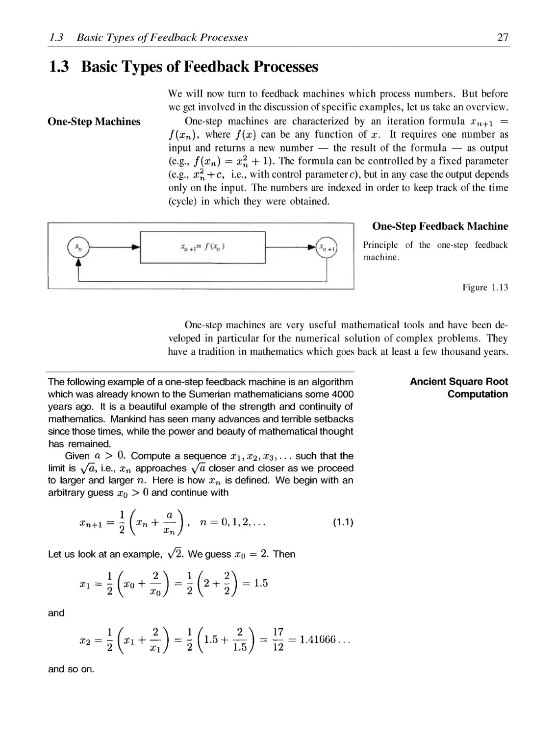
The feedback machine has three storage units (IU = input unit,
OU = output unit, CU = control unit, PU = processing unit), and one
processor, all connected by four transmission lines (see figure 1.3).
The whole unit is run by a clock, which monitors the action in each
component and counts cycles. The control unit acts like a gear shift in
an engine. That is, we can shift the iterator into a particular state and
then run the unit. There are preparatory cycles and running cycles,
each of which can be broken down into elementary steps:
Preparatory cycle:
Step 1 : load information into IU
1 Nature does not make radical jumps.
where is considered to be a fixed constant, or
where is a
constant. Before we enter an initial discussion of this phenomenon --- a more
systematic exploration is offered in chapter 10 --- let us identify and discuss
one of the central icons of our presentation.
Feedback processes are fundamental in all exact sciences. In fact, they
were first introduced by Sir Isaac Newton and Gottfried W. Leibniz some 300
years ago in the form of dynamic laws; and it is now standard procedure to
model natural phenomena using such laws. Such laws determine, for example,
the location and velocity of a particle at one time instant from its values at
the preceding instant. The motion of the particle is then understood as the
unfolding of that law. It is not essential whether the process is discrete (i.e.,
it takes place in steps) or continuous. Physicists like to think in terms of
infinitesimal time steps: natura non facit saltus.1 Biologists, on the other
hand, often prefer to look at the changes from year to year or from generation
to generation.
We will use the terms iterator, feedback and dynamic law synonymously.
Figure 1.3 explains the idea. The same operation is carried out repeatedly, the
output of one iteration being the input for the next one.
Iterator, Feedback and
Dynamic Law
The Feedback Machine
The feedback machine with IU =
input unit, OU = output unit,
CU = control unit.
Figure 1.3
The Iterator: Principle of
Feedback
18
1 The Backbone of Fractals
Step 2: load information into CU
Step 3: transmit the content of CU into PU
Running cycle:
Step 1: transmit content of IU and load into PU
Step 2: process the input from IU
Step 3: transmit the result and load into OU
Step 4: transmit the content from OU and load into IU
To initiate the operation of the machine we run one preparatory cycle.
Then we start the running cycles and execute a certain number of
them, the count of which may depend on observations which we make
by monitoring the actual output. Execution of one running cycle is
sometimes called one iteration.
When we refer to iterations we should imagine aproper feedback machine.
The dynamic behavior of such a machine can be controlled by setting certain
outside parameters, similar to control levers in an engine. We will discuss the
basic principlesguidedbythe simpleexample ofvideofeedback, which infact
permits real experiments. This particular feedback machine can be built using
particular pieces of equipment. It is a real machine in the original sense of the
word. This case is rather the exception in this book. Here the term 'feedback
machine' usually refers to an abstract machine, a'Gedankenexperiment'. Such
an abstract machine may be put into operation by executing an appropriate
computer program, or by using a pocket calculator or merely paper and pencil
to carry out the given feedback mechanism.
What Is a Feedback
Machine?
Video Feedback Setup
Figure 1.4
1.1 The Principle of Feedback
19
Video Feedback
Video feedback is a feedback experiment in the traditional sense of the
word. Its basic configuration is probably as old as television. Nevertheless,
the particular video feedback experiment which we will now present is so
dramatic that its potential can excite even professionals from the television
scene.2 Figure 1.4 shows the basic setup. A video camera looks at a video
monitor, and whatever it sees in its viewing zone is put onto the monitor.
There are quite a few controls which have an impact on what will be seen
by an outside observer, for example, the various control dials on the monitor
(contrast, brightness, etc.) and video camera (focus, iris aperture, etc.), as well
as the position of the camera with respect to the monitor. Below we collect
some important tips which will help you to make a successful video feedback
experiment yourself.
It is quite obvious how we can imbed the experiment into our logo in figure
1.3 (input unit = camera, processing unit = camera and monitor electronics,
output unit = monitor screen, control unit = focus, brightness, etc.). The
feedback clock runs quite fast, i.e., about 30 cycles per second, or whatever
number of frames per second your TV system generates.3
The experiment should be set up in an almost dark room. The distance
between camera and monitor should be such that the mapping ratio is
approximately 1 : 1. Turn up the contrast dial on the monitor all the way
and turn down the brightness dial considerably. The experiment works
better if the monitor or the camera is put upside down. Moreover,
the tripod should be equipped with a head that allows the camera
to be turned about its long axis, while it faces the monitor. Rotate
the camera some 45° (angle out of its vertical position. Connect
the camera with the monitor. Now the basic setup is arranged. The
camera should have a manual iris which is now gradually opened
while the lens is focused on the monitor screen. Depending on the
contrast and brightness setting you may want to light a match in front
of the monitor screen in order to ignite the process.
Hints for the Video Feedback
Experiment
Dramatic Impact of
Controls
Each of the controls has an impact on the process, some a very dramatic
one. In this regard we can think of our setup as an analog computer with
control dials. For some kinds of controls and variables it is relatively easy
to understand their mechanisms; for others it is hard; and for still others it
is hard as hell. In fact, many of the phenomena which can be observed are
still very poorly understood. The physicist James P. Crutchfield has prob-
ably contributed most toward a deeper and systematic understanding of the
process.4
2It was proposed by Ralph Abraham from the University of California at Santa Cruz in the 1970's. See R. Abraham, Simulation
of cascades by video feedback, in: "Structural Stability, the Theory of Catastrophes, and Applications in the Sciences", P. Hilton
(ed.), Lecture Notes in Mathematics vol. 525, 1976, 10--14, Springer-Verlag, Berlin.
3NTSC is typically 30 frames per second at 480 lines per image.
4J. P. Crutchfield, Space-time dynamics in video feedback, Physica 10D (1984) 229--245.
20
1 The Backbone of Fractals
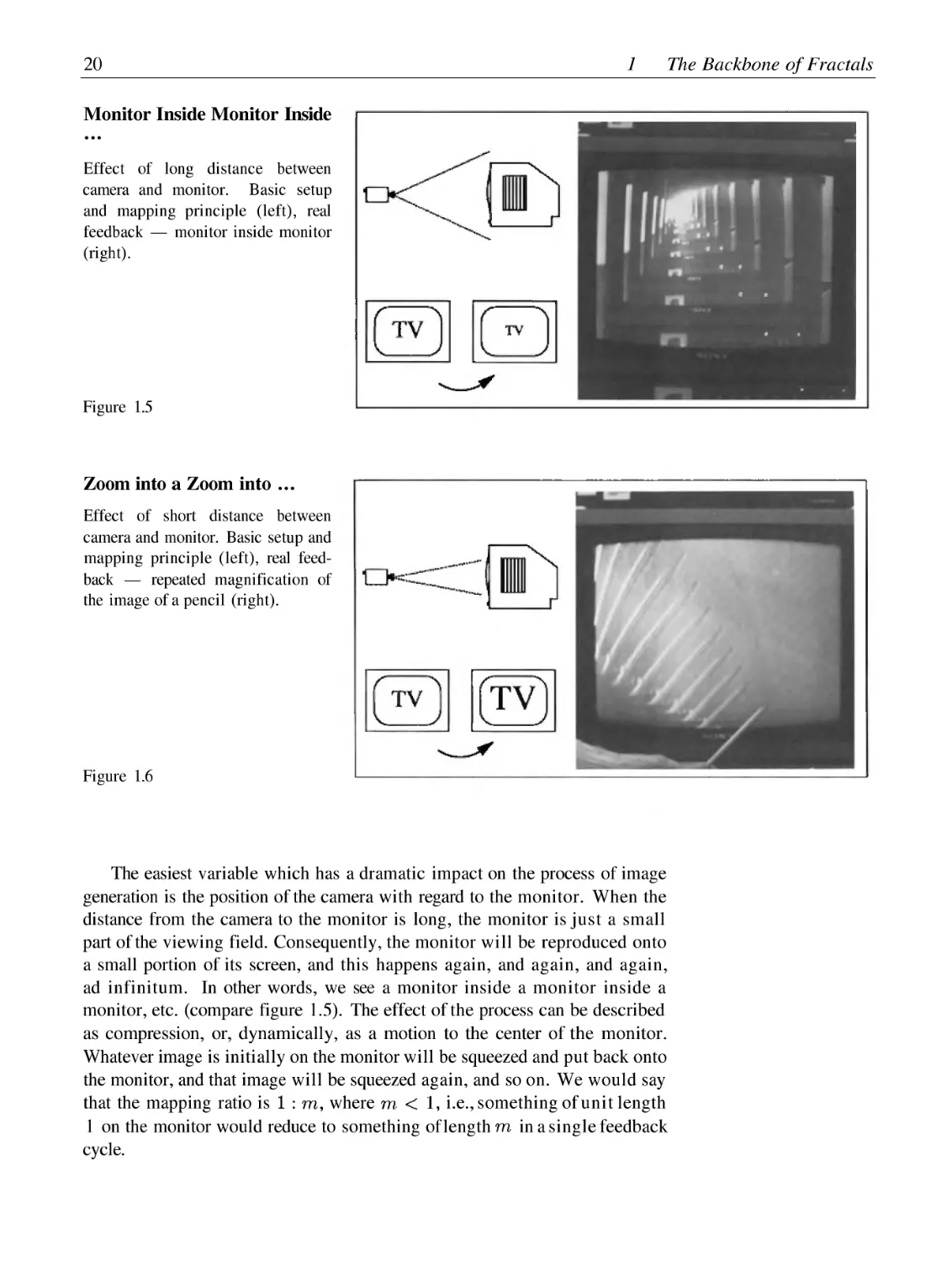
Monitor Inside Monitor Inside
Effect of long distance between
camera and monitor. Basic setup
and mapping principle (left), real
feedback --- monitor inside monitor
(right).
Figure 1.5
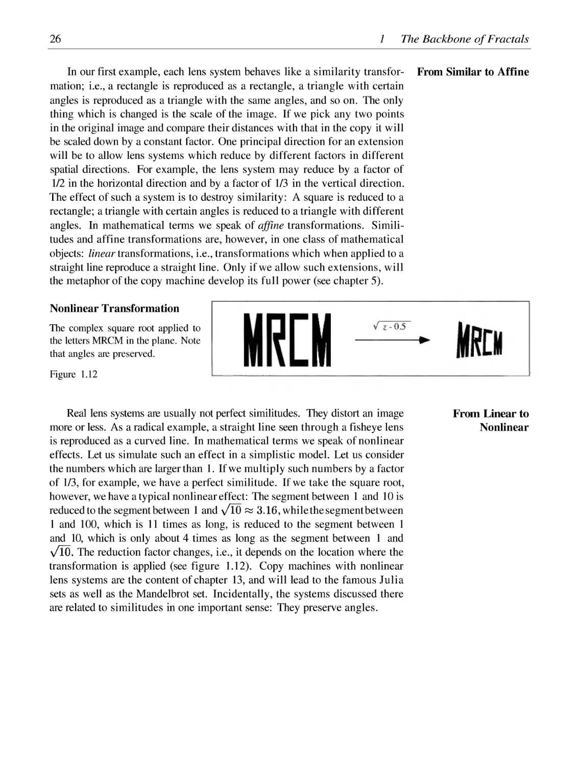
ZoomintoaZoominto...
Effect of short distance between
camera and monitor. Basic setup and
mapping principle (left), real feed-
back --- repeated magnification of
the image of a pencil (right).
Figure 1.6
The easiest variable which has a dramatic impact on the process of image
generation is the position of the camera with regard to the monitor. When the
distance from the camera to the monitor is long, the monitor is just a small
part of the viewing field. Consequently, the monitor will be reproduced onto
a small portion of its screen, and this happens again, and again, and again,
ad infinitum. In other words, we see a monitor inside a monitor inside a
monitor, etc. (compare figure 1.5). The effect of the process can be described
as compression, or, dynamically, as a motion to the center of the monitor.
Whatever image is initially on the monitor will be squeezed and put back onto
the monitor, and that image will be squeezed again, and so on. We would say
that the mapping ratio is
where
i.e., something of unit length
1 on the monitor would reduce to something of length in a single feedback
cycle.
...
1.1 The Principle of Feedback
21
Figure 1.7 : Some examples of real video feedback. There is a more or less pronounced periodicity in these pictures
which depends on the angle of the video camera. From the upper left to the lower right we can see periods 3,5,5,5,
8,8,11,11,>11.
The monitor-inside-a-monitor effect is known by most people as video
feedback. It is almost always easy to reproduce with any kind of equipment.
But there is much more 'life' in this simple system than has been recognized
because it is a little harder to reproduce with some equipment.
Next, let us discuss what will happen at the other extreme end of the
positioning scale --- when the distance between the camera and the monitor
is so short that the viewing field of the camera is just a part of the monitor
screen. That part is put back onto the entire screen, and again, and again, ad
infinitum (compare figure 1.6). We would say that the mapping ratio is
22
1 The Backbone of Fractals
where
i.e., something of unit length 1 on the monitor would expand
to something of length in a single feedback cycle.
Now the action in the process is best described as expansion or, dynam-
ically, as a motion to the border of the monitor. Whatever image is initially
on the monitor, a small part of it will be expanded to the full screen, and of
that a small part will again be expanded, and so on. Since the TV refreshes its
image about 30 times per second, it is impossible to see the individual steps
in this process. The result of the close camera position can be a rather wild
and almost turbulent motion on the screen.
The more interesting effects occur when the position of the camera with
regard to the monitor is carefully chosen to be such that the mapping ratio is
nearly 1:1. The effect is increased dramatically if the camera is turned about
its axis, i.e., an image on the monitor is seen by the camera as if rotationally
changed by some angle. Thus it appears on the monitor (mapping ratio 1 : 1) in
essentially the same size but rotated. From this point on, any simple description
of the mechanisms for the wild and beautiful visual effects that can be observed
breaks down. From what has been said so far, we would expect that in the
rotated position we would eventually observejust a sequence of rotated images.
But this prediction is far too simple. All kinds of peculiar effects occur due
to many different characteristics innate to television image production. For
example, the process of scanning the image on the monitor and in the camera
is one of sequentially putting together a series of lines to compose the image.
There is also the memory effect of the phosphorus on the monitor tube. In
addition, there are electronic time chains and their delays in both the monitor
and camera, as well as other factors.
In any event, this extremely simple feedback system demonstrates very
dramatically how complicated structures can be the result of very simple feed-
back. In a way, this is the theme of the book. Our next set of experiments
tries to bring more of a systematic light into this world of exciting phenomena.
The basic principle is the same as with video feedback: An initial image is
processed and then the resulting image is reprocessed by the same machine
over and over again.
Unchaining the
Feedback
1.2 The Multiple Reduction Copy Machine
23
1.2 The Multiple Reduction Copy Machine
We now turn to a set of experiments which will provide us with a very intuitive
access to the language of fractal geometry. In a sense, it is a continuation of
the video feedback experiment.
First, let us consider a copy machine which is equipped with an image
reduction feature. If we take an image, put it on the machine and push a
button, we obtain a copy of the image. It is, however, reduced uniformly by
say 50%, i.e., by a factor of 1/2. In the language of mathematics we say that
the copy is similar to the original. The process to generate a copy is called a
similarity transformation or similitude. The process just described embedded
into the idea of figure 1.3 constitutes a feedback system5 which would be very
easily predictable in its long-run effect: After some ten or so cycles any initial
image would be reduced to just a point. In other words, running the machine
would be a waste of paper (see figure 1.8).
Single Reduction Copy
Machine
Iteration by a copy machine with re-
duction applied to a portrait of Carl
Friedrich Gauss (1777--1855).
Figure 1.8
We will now modify this principal setup. Remember, the basic action
of our machine is the reduction of images. Such reductions, of course, are
achieved by a lens system. As a simple modification of a stock copier, let us
imagine that our custom copier has 2, or 3, or 7, or 14 532 231, or whatever
number of reduction lenses. Each of them looks at the image on the copier,
reduces it, and puts the result somewhere on the copy paper. One such design
consists of the choice of the number of lenses, the reduction factors and the
placements of the reduced images. It constitutes a particular feedback system
which we can run to see what happens. We call such a machine a Multiple
Reduction Copy Machine, abbreviated by the letters MRCM.
Figure 1.9 shows a first example of an MRCM which incorporates just
three reduction lenses, each of them reducing by 50%, i.e., by a factor of 1/2.
What will we see emerging in the sequence of iterations as we run the
feedback system? Will we see an arrangement of a smaller and smaller com-
posite of images developing toward a point? Figure 1.10 gives the surprising
5Try to identify input, processing and output unit.
24
1 The Backbone of Fractals
Multiple Reduction Copy
Machine (MRCM)
The Multiple Reduction Copy Ma-
chine (MRCM): the processing unit
is equipped with a three-lens system.
Figure 1.9
Rectangle in MRCM
Starting with a rectangle the itera-
tion leads to the Sierpinski gasket.
Shown are the first five steps and
the result after some more iterations
(lower right).
Figure 1.10
answer, the consequences of which could potentially revolutionize almost ev-
erything we have thought about images in a technical sense. Let us start with a
rectangle as an initial test image. We put it onto the multiple copier, obtaining
three reduced copies which we color according to the respective lens system
from which each copy is produced.
Then,indeed,wesee3×3=9smallercopies,andthen3×9=27
even smaller copies, then 81, 243, 729, etc., copies which rapidly decrease
in size, but the resulting compound images do not reduce to a point at all.
Rather, they transform into a perfect Sierpinski gasket, which we will use as a
major example exhibiting important aspects of fractals in general. Using the
imagery of a language paradigm, we have just introduced a first hieroglyph
in our new fractal dialect. From what we have said so far, it is clear that this
basic principle will generate an infinite variety of images. All we have to do
is convert the copier into one consisting of 4, or 5, or any other number of lens
systems, or with different reduction factors. We will be going into this matter
in more detail in chapters 5 and 6, but there are two major surprises which are
A First Hieroglyph:
The Sierpinski Gasket
1.2 The Multiple Reduction Copy Machine
25
MRCM Applied to 'MRCM'
We can start with an arbitrary image
--- this iterator will always lead to
the Sierpinski gasket.
Figure 1.11
not immediately apparent and deserve some preliminary discussion here.
Looking at figure 1.10 again, we may be led to believe that the secret
to the tendency toward the formation of the Sierpinski gasket is our choice
of an appropriately dimensioned rectangle as the initial image in starting the
feedback process. To show that this is not the case, let us assume that instead
of a rectangle as the initial image, we choose a triangle or any arbitrary image,
which may be represented well enough by the letters NCTM. The question is:
What will then evolve in the process? Figure 1.11 gives the answer. The same
final structure is approximated as we run the machine. Each step produces
a composite of images which rapidly decrease in size. It doesn't matter in
the least whether these images are rectangles, triangles, or the letters NCTM;
the same final composite image is approached in each case --- namely, the
Sierpinski gasket. In other words, the machine produces one --- and only
one --- final image in the process, and that final image is totally independent
from the image with which we start! This magnificent behavior seems to be
a miracle. But in mathematical terms it just means that we have a process
which produces a sequence of results tending toward one final object which is
independent from how we start the process. This property is called stability.
The second surprise is that the copy machine paradigm is not just a way
to recover 'mathematical monsters' like the Sierpinski gasket or its relatives
(soon we will see many of them). Let us ask what the images are which we can
obtain this way. What can they look like? The answer is simply incredible.
For many more natural pictures there is a copy machine of the above kind
which generates the desired picture. However, it is a difficult problem to
design the machine for a given picture. But nevertheless, in chapter 5 and the
first appendix we will introduce some of the design principles leading to the
frontiers of current mathematical research.
The point here is to see some of the variety of possible images obtained by
very simple feedback processes, the elements of which are easily manipulated
and under our control, quite unlike the video feedback experiment.
26
1 The Backbone of Fractals
In our first example, each lens system behaves like a similarity transfor-
mation; i.e., a rectangle is reproduced as a rectangle, a triangle with certain
angles is reproduced as a triangle with the same angles, and so on. The only
thing which is changed is the scale of the image. If we pick any two points
in the original image and compare their distances with that in the copy it will
be scaled down by a constant factor. One principal direction for an extension
will be to allow lens systems which reduce by different factors in different
spatial directions. For example, the lens system may reduce by a factor of
1/2 in the horizontal direction and by a factor of 1/3 in the vertical direction.
The effect of such a system is to destroy similarity: A square is reduced to a
rectangle; a triangle with certain angles is reduced to a triangle with different
angles. In mathematical terms we speak of affine transformations. Simili-
tudes and affine transformations are, however, in one class of mathematical
objects: linear transformations, i.e., transformations which when applied to a
straight line reproduce a straight line. Only if we allow such extensions, will
the metaphor of the copy machine develop its full power (see chapter 5).
From Similar to Affine
Nonlinear Transformation
The complex square root applied to
the letters MRCM in the plane. Note
that angles are preserved.
Figure 1.12
Real lens systems are usually not perfect similitudes. They distort an image
more or less. As a radical example, a straight line seen through a fisheye lens
is reproduced as a curved line. In mathematical terms we speak of nonlinear
effects. Let us simulate such an effect in a simplistic model. Let us consider
the numbers which are larger than 1. If we multiply such numbers by a factor
of 1/3, for example, we have a perfect similitude. If we take the square root,
however, we have a typical nonlinear effect: The segment between 1 and 10 is
reduced to the segment between 1 and
while the segmentbetween
1 and 100, which is 11 times as long, is reduced to the segment between 1
and 10, which is only about 4 times as long as the segment between 1 and
The reduction factor changes, i.e., it depends on the location where the
transformation is applied (see figure 1.12). Copy machines with nonlinear
lens systems are the content of chapter 13, and will lead to the famous Julia
sets as well as the Mandelbrot set. Incidentally, the systems discussed there
are related to similitudes in one important sense: They preserve angles.
From Linear to
Nonlinear
1.3 Basic Types of Feedback Processes
One-Step Machines
1.3 Basic Types of Feedback Processes
27
We will now turn to feedback machines which process numbers. But before
we get involved in the discussion of specific examples, let us take an overview.
One-step machines are characterized by an iteration formula
where
can be any function of It requires one number as
input and returns a new number --- the result of the formula --- as output
(e.g.,
The formula can be controlled by a fixed parameter
(e.g.,
i.e., with control parameter but in any case the output depends
only on the input. The numbers are indexed in order to keep track of the time
(cycle) in which they were obtained.
One-Step Feedback Machine
Principle of the one-step feedback
machine.
Figure 1.13
One-step machines are very useful mathematical tools and have been de-
veloped in particular for the numerical solution of complex problems. They
have a tradition in mathematics which goes back at least a few thousand years.
The following example of a one-step feedback machine is an algorithm
which was already known to the Sumerian mathematicians some 4000
years ago. It is a beautiful example of the strength and continuity of
mathematics. Mankind has seen many advances and terrible setbacks
since those times, while the power and beauty of mathematical thought
has remained.
Given
Compute a sequence
such that the
limit is i.e., approaches
closer and closer as we proceed
to larger and larger Here is how is defined. We begin with an
arbitrary guess
and continue with
Let us look at an example, We guess
Then
and
and so on.
Ancient Square Root
Computation
28
1 The Backbone of Fractals
Let us give a brief argument why this method works in order to
understand how well it works. To this end we introduce the relative
error of where is defined by the equation
Replacing by the equivalent
in eqn. (1.1) we arrive at
Thus, using the definition in eqn. (1.2) again, we obtain an expression
for the error
Now
and therefore
and thus
for
But then
for all
Finally, we can obtain
estimates out of eqn. (1.3). If we drop the '2' in the denominator we
obtain
and if we drop we obtain
The first inequality and the definition of by eqn. (1.2) shows that
and that the limit is
The second inequality shows that if
then
i.e., in each step of the sequence
the number of correct digits is nearly doubled. This algorithm for
the computation of the square root is an example of a more general
method for the solution of nonlinear equations, which was discovered
about 4000 years later and is nowadays called Newton's method.
One-step feedback processes represent only a particular class of a whole
family of feedback methods. Another class is known as two-step methods.
Here the output is typically computed by a formula like
Take, for example, the law which generates the Fibonacci numbers
Two-Step Feedback
Methods
1.3 Basic Types of Feedback Processes
29
Leonardo Pisano, also known as Fibonacci6 was one of the outstanding
figures in medieval Western mathematics. He traveled widely in the
Mediterranean world before settling down in his native Pisa. In 1202 he
published his book, Liber Abaci, which changed Europe. It acquainted
Europeans with the Indian Arabic ciphers 0, 1 , 2, . . . His book also
contained the following problem, which has inspired people ever since.
There is one pair of rabbits which is born at time 0. After one month that
pair is mature and a month later gives birth to a new pair of rabbits and
continues to do so (i.e., every month a new pair is born to the original
pair). Moreover, each new pair of rabbits matures after one month and
begins producing pairs of offspring every month after that ad infinitum.
One assumes that the rabbits live forever. What is the number of pairs
after months?
Let us be careful and follow the evolution of rabbits step by step. In
our rabbit population, let us distinguish between adult and young pairs
of rabbits. A just-born pair is young, of course, and turns adult after
one time step. Moreover, an adult pair gives birth to a young pair after
one time step. Now let and be the number of young and adult
pairs after months, respectively. Initially, at time
there is only
one young pair
After one month the young pair
has turned into an adult one
After two months the
adult pair gives birth to one young pair
Then again
after the next month. Moreover, the young pair turns into an adult one
The general rule, of course, is that the number
of newborn pairs
equals the previous adult population The
adult population grows by the number of immature pairs, from the
previous month. Thus, the following two formulas completely describe
the population dynamics
As initial values we take
and
From the first of the
above equations it follows that
Inserting this into the
other equation we obtain
with
and
This is a single equation for the total rabbit
population. Using this equation, the number of pairs in successive
generations is easily computed:
Each number in this sequence is just the sum of its two predecessors.
This sequence is called the Fibonacci sequence.
We have established another feedback system, but this one is a
little different from the previous systems. In all the earlier feedback
loops, the state at time was determined only by the preceding state
6Filius (=son) of Bonacci.
Fibonacci Numbers and the
Rabbit Problem
30
1 The Backbone of Fractals
01
23
4567
8
9
10
11
12
1
1
23
5
8
13
21
34
55
89
144
233
1/1
2/1
3/2
5/3
8/5
13/8
21/13
34/21
55/34
89/55
144/89
233/144
377/233
In Decimals
1.0
2.0
1.5
1 .666666
1.6
1.625
1.615385
1.619048
1.617647
1.618182
1.617978
1.618056
1.618026
at time
Such systems are called one-step loops. For the Fi-
bonacci sequence the state at time
requires information from
states and
Such systems are called two-step loops. The
simple and innocent-looking Fibonacci sequence has a variety of in-
teresting properties. Thousands of papers have been published about
them, and there is even a Fibonacci-Association with its own periodical,
Fibonacci Quarterly, which reports on the never-ending stream of new
results. One property has been known for a long time and has led to
amazing recent research in biology, as well as having had astonishing
applications in architecture and the arts for many centuries.
Apparently the Fibonacci sequence can grow beyond all limits. Our
rabbits exhibit a kind of a population explosion. We can ask, however,
how the population progresses from generation to generation. For that
purpose we look again at the Fibonacci numbers and compute the
ratios of succeeding generations (rounded to six decimals).
Apparently we are approaching steadily, if not exactly rapidly, some
particular number. Have you seen that mysterious number
before? Let us open the curtain.
which is the famous golden mean, or proportio divina,7 as they called
it in the middle ages. This number has inspired mathematicians,
astronomers and philosophers like no other number in the history of
mathematics.
7Divine proportion (Latin).
1.3 Basic Types of Feedback Processes
31
Feedback Machines
with Memory
At first it seems that processes of two-step methods are not covered by
the concept of a feedback machine as we have discussed it so far. Indeed,
the output
depends not only on the last step but also on the step
preceding the last, namely,
Consequently, it may appear natural to
extend the design of our feedback machines so that the concept incorporates
a certain memory which conserves some information from the last cycles.
Machines with memory are typical for our computer age. While a machine
without memory reacts on their inputs always in the same way, a machine
with memory may react differently upon taking its own state or content of
the memory into account. Take, for example, a soft drink machine. You will
not be successful in getting a soda by just pushing a button. First you have
to insert the right amount of money to make sure that the machine is in the
appropriate state to accept your input.
Let us now extend the concept of a feedback machine by equipping the
processing unit with an internal memory unit. Then the iteration of a two-step
method
can be implemented as follows. First note that
to start the feedback machine two initial values and are required.
Preparation: Initialize the memory unit with and the input unit with
Iteration: Evaluate
where is in the input unit and
is in the memory unit. Then update the memory unit with
Somehow it seems that feedback machines with memory should be more
flexible in modeling different phenomena. But this is not at all the case.
Rather, a machine with memory can be seen to be equivalent to a one-step
machine which, however, works on vectors as input and output information.
Input and output are given as pairs, or triples, or quadruples, and so on, of
numbers. In other words, a pair of input variables
generates a pair
of output variables
Formally, we introduce a new variable,
and extend the formula
to the equivalent pair:
One-Step Machines
with Two Variables
Two-Step Loop
Two-step loops are a special case
of one-step feedback machines with
two variables.
Figure 1.14
This simple trick can easily be generalized. For example, let us assume
that the formula which determines the feedback depends on preceding itera-
tions. Then one can rewrite this single formula as a one-step process which is
32
1 The Backbone of Fractals
given by a set of formulas by introducing independent variables. Usually,
the independent variables are combined into a vector of variables. The pair
for example, can be written symbolically as a single new variable
Moreover, we can then rewrite the set of formulas
by a single formula:
In other words, we do
not have to go to the trouble of developing a special machine for two-step
methods. They are perfectly covered by one-step machines.
The Rabbit Problem As
One-Step Machine
Let us give one example, the Fibonacci numbers, defined by the two-
step method
with
and
The equivalent equations for a one-step
method operating on pairs
are
with initial settings
and
This is exactly the same as in
the derivation on page 29 setting
and
Using the compact notation
for a whole set of formulas in the pro-
cessing unit considerably simplifies the description of seemingly complicated
feedback processes. Here is another example, which will become important
in chapters 2 and 10:
Here denotes a parameter, e.g.,
or
Rather than introducing
a feedback machine with two formulas and an additional switch, we will
rewrite the above system of two equations as a one-step process of the form
where is the transformation, whose graph --- known as the
tent transformation --- is given in figure 1.15.
One-Step Machines
Based on Combined
Formulas
The Tent Transformation
The tent transformation is given by
and
if
Here the parameter
has been chosen.
Figure 1.15
1.3 Basic Types of Feedback Processes
33
This is an algorithm which produces sequences of integers in a most
simple way, but yet its unfolding is still not completely understood. Here
is the original formulation due to Lothar Collatz:
Step 1 : Choose an arbitrary positive integer A.
Step2: IfA=1,thenSTOP.
Step 3: If A is even, then replace A by A/2 and go to step 2.
Step4:IfAisodd,thenreplaceAby3A+1andgotostep2.
Let us try a few choices for A:
3,10, 5, 16, 8, 4, 2, 1, STOP
34,17,52,26,13,40,20,10,5,16,8,4,2,1,STOP
75, 226, 113, 340, 170, 85, 256, 128, 64, 32, 16, 8, 4, 2, 1, STOP
The obvious conjecture is the following: the algorithm comes to a stop
no matter what the initial A is. Well, it seems that the larger the initial A
isthemorestepswehavetorununtilwearriveat1.LetustryA=27
to verify that guess.
27, 82, 41, 124, 62, 31, 94, 47, 142, 71, 214, 107, 322, 161, 484,
242, 121, 364, 182, 91, 274, 137, 412, 206, 103, 310, 155, 466, 233,
700, 350, 175, 526, 263, 790, 395, 1186, 593, 1780, 890, 445, 1336,
668, 334, 167, 502, 251, 754, 377, 1132, 566, 283, 850, 425, 1276,
638, 31 9, 958, 479, 1438, 719, 2158, 1079, 3238, 1619, 4858, 2429,
7288, 3644, 1822, 911, 2734, 1367, 4102, 2051, 6154, 3077, 9232,
4616, 2308, 1154, 577, 1732, 866, 433, 1300, 650, 325, 976, 488,
244, 122, 61, 184, 92, 46, 23, 70, 35, 106, 53, 160, 80, 40, 20, 10,
5,16,8,4,2,1,STOP
Apparently our guess was not correct. Moreover, seeing this example
we can really begin to wonder whether all sequences will eventually
stop. As far as we know this problem is still unsolved. However, the
conjecture has been verified with the aid of computers up to at least
Such a test is not as straightforward as we might think, be-
cause in the course of the calculations the sequence may exceed the
largest possible number which the computer is able to accurately rep-
resent. Thus, some variable precision routines must be programmed
in order to enlarge the range of numbers representable by a computer.
The algorithm can easily be extended to negative integers. Here
are a few examples:
--1, --2, --1, --2, ...CYCLEoflength2
--3, --8, --4, --2, --1, ... runs into CYCLE of length 2
--5, --14, --7, --20, --10, --5, --14, . . . CYCLE of length 5
--6, --3, --8, --4, --2, --1, ... runs into CYCLE of length 2
--9, --26, --13, --38, --19, --56, ... runs into CYCLE of length 5
--11, --32, --16, --8, --4, --2, --1, . . . runs into CYCLE of length 2
Are there other cycles? Yes indeed:
--17, --50, --25, --74, --37, --110, --55, --164, --82, --41, --122,
--61, --182, --91, -- 272, --136, --68, --34, --17, ...CYCLE of
length 18
The (3A + 1)-Problem
34
1 The Backbone of Fractals
If we modify our algorithm by removing the STOP in Step 1 we also
obtain a cycle for A = 1:
1,4,2,1, . . .CYCLEoflength3
andifwealsoallowA=0:
0,0, . . .CYCLEoflength1.
Moreover, we may now write the algorithm as a feedback system:
Thus, the general questions are: what are the possible cycles of
the feedback system, and does any initial choice for generate a
sequence which eventually runs into one of these cycles? This seems
to be a moderate question which the enormous body of mathematics
should have already answered --- or at least be prepared to answer
with no great difficulty. Unfortunately, this is not the case, which only
shows that there is still a lot to do in mathematics and, moreover,
simple-looking problems may be awfully hard to solve; a truly important
lesson for life.
A more subtle and surprising case is given by our MRCM machines from
the last section. They also can be interpreted as one-step machines, which are
mathematically described by a single formula of the kind
Incidentally, in this case F is called the Hutchinson operator. We will discuss
the details in chapter 5.
While all previous machines are strictly deterministic our last class of
machines combines determinism with randomness. Similar to the previous
examples, there is a reservoir of different formulas in the processing unit.
In addition, however, there is a wheel of fortune, which is used to select
one of the formulas at random. The input is a single number (or a pair of
numbers), and the output is a new number (or a pair of numbers), which is
the result of a formula with values determined by the input. The formula is
chosen randomly from a pool at each step of the feedback process. In other
words, the output does not just depend on the input, much like in the case of
machines with memory. Unfortunately, however, there is no standard trick
to rewrite the process as a (deterministic) one-step machine. If the number
of formulas is N, then the wheel of fortune has N segments, one for each
formula. The size of the segment can be different for each of them in order to
accommodate for different probabilities in the random selection mechanism.
Random machines like this will furnish extremely efficient decoding schemes
for images, which are encoded by the metaphor of a copy machine. This is
the content of chapter 6.
MRCM As a One-Step
Machine
Wheel-of-Fortune
Machines
1.3 Basic Types of Feedback Processes
35
Wheel-of-Fortune Machine
Feedback machine with fortune
wheel.
Figure 1.16
We want to touch upon a further exciting interpretation of what we
learned in the multiple reduction copy machine, and this is another
incredible relation between chaos and fractals.
The following 'game' has been termed chaos game by Michael F.
Barnsley. At first glance, however, there seems to be no connection
whatsoever with chaos and fractals. Let us describe the rules of the
game. Well, actually, there is not just one game; there is an infinite
number of them. But they all follow the same scheme. We have a die
and some simple rules to choose from. Here is one of the games:
Preparations: Take a sheet of paper and a pencil and mark three points
on the sheet; label them 1, 2, and 3; and call them bases.
Have a die which allows you to pick the numbers 1, 2,
and 3 randomly. It is obvious how to manufacture such
a die. Take an ordinary die and just identify the faces 6
with1,5with2,and4with3.
Rules:
Start the game by picking an arbitrary point on the sheet
of paper and mark it by a small dot. Call it the game point.
Now roll the die. If number 2, for example, comes up,
consider the line between the game point and base 2 and
mark a dot exactly in the middle, i.e., halfway between
the game point and base 2. This dot will be the new
game point, and we have completed the first cycle of the
game. Now repeat (i.e., roll the die again) to randomly
get the number 1, 2, or 3; and depending on the result,
mark a dot halfway between the last game point and the
randomly chosen base.
The first game points shown in figure 1.17 are labeled in the order
of their generation by
The chaos game is a very sim-
ple scheme to produce a random sequence of points; and as such it
appears to be rather boring. But this first impression will immediately
change when we see what is going to evolve in this feedback system.
What do you guess the outcome of the game will be after a
great many cycles, i.e., what is the picture obtained by the dots
Note that once the game point is inside the trian-
The Chaos Game
36
1 The Backbone of Fractals
Figure 1.17: The three base points (vertices of a triangle) and a few iterations
of the game point.
Figure 1.18 : 500, 1000 and 1500 dots of the chaos game.
gle, which is defined by the three base points, the process will remain
inside forever. Moreover, it is obvious that sooner or later the game
point will land inside this triangle even if we start the game outside.
Therefore, intuition seems to tell us that because of the random
generation we should expect a random distribution of dots somehow
arranged between base 1, 2, and 3. Yes, indeed, the distribution will
be random, but not so the picture or image which is generated by the
dots (see figure 1.18). It isn't random at all. We see the Sierpinski
gasket emerge very clearly; and this an extremely ordered structure
--- exactly the opposite of a random structure.
At this point this phenomenon seems to be either a small miracle or
a funny coincidence, but it is not. Any picture which can be obtained by
the MRCM can be obtained by an appropriately adjusted chaos game.
In fact, the picture generation can generally be accelerated this way.
Moreover, the chaos game is the key to extending the image coding
idea which we discussed for the multiple reduction copy machine to
grey scale or even color images. This will be the content of chapter 6,
which will provide an elementary lesson in probability theory --- though
one filled with beautiful surprises.
1.4 The Parable of the Parabola
37
1.4 The Parable of the Parabola --- Or: Don't Trust Your
Computer
Let us now turn to quadratic iterators. First, we implement the expression
in our iterator framework. Here and are just numbers; however,
with different meanings. To iterate this expression for a fixed (control) value
means this: start with any number evaluate the expression, note the result
and use this value as new evaluate the expression, and so on. Let's look at
an example:
Preparation: Choose a number for say
Then choose a number
for example
Iteration: Evaluate the expression for obtaining 0.25 -- 2 = --1.75.
Now repeat, i.e., evaluate the expression using the result of the
first calculation as the new i.e., evaluate for
which
yields 1.0625, and so on.
The Quadratic Iterator
The quadratic iterator interpreted as
a feedback machine. The processing
unit is designed to evaluate
given and
Figure 1.19
The table summarizes the results for the first four iterations:
0.5
--1.75
1.0625
--0.87109375
--1.75
1.0625
--0.87109375
--1.2411956787109375
Already after four cycles we are running into a problem. Because of the
squaring operation the number of decimal places which are needed to represent
the successive output numbers essentially doubles in each cycle. This makes
it impossible to achieve exact results for more than a few iterations because
computers and calculators work with only a finite number of decimal places.8
This is, of course, a common problem in calculator or computer arithmetic,
but we don't usually worry about it. In fact, the omnipotence of computers
leads us to believe that these minor differences don't really matter. For ex-
Do Minor Differences
Matter?
8For example, the Casio 7000G ha s 10, a nd the Hewlet-Packard 28S has 12 decimal digits of accuracy.
38
1 The Backbone of Fractals
ample, if we compute 2 * (1/3) we usually don't worry about the fact that
the number 1/3 is not exactly representable by our calculator. We accept the
answer 0.6666666667, which, of course, is different from the exact represen-
tation of 2/3. Even in a messy calculation, we are usually inclined to take the
same attitude, and some put infinite confidence in the calculator or computer
in the hope that these minute differences do not accumulate to a substantial
error.
Scientists know (or should we say knew) very well that this assumption
can be extremely dangerous. They came up with methods, which go back
to ideas of Carl Friedrich Gauss (1777--1855; see figure 1.8), to estimate the
error propagation in their calculations. With the advent of modern computing
this practice has somehow lost ground. It seems that there are at least two
reasons for this development.
Modern computing allows scientists to perform computations which are of
enormous complexity and are extensive to a degree that was totally unthinkable
even half a century ago. In massive computations, it is often true that a detailed
and honest error propagation analysis is beyond current possibilities, and this
has led to a very dangerous trend. Many scientists exhibit a growing tendency
to develop an almost insane amount of confidence in the power and correctness
of computers.
If we go on like this, however, we will be in great danger of neglecting
some of the great heroes of science and their unbelievable struggle for accuracy
in measurement and computation. Let us remember the amazing story of
Johannes Kepler's model of the solar system. Kepler devised an elaborate
mystical theory in which the six known planets Mercury, Venus, Earth, Mars,
Jupiter, and Saturn9 were related to the five Platonic solids (see figure 1.21).
The Problem of Error
Propagation
Brahe and Kepler
Tycho Brahe, 1546--1601 (left) and
Johannes Kepler, 1571--1630 (right).
Figure 1.20
9These planets were known in ancient times before the invention ofthe telescope. The seventh planet Uranus was not discovered
until 1781 by the amateur astronomer Friedrich Wilhelm Herschel, and Neptune was only discovered in 1846 by Johann Gottfried
Galle at the Observatory in Berlin. The ninth and most distant planet Pluto was discovered in 1930 by Clyde William Tombaugh
at Lowell Observatory in Flagstaff, Arizona.
1.4 The Parable of the Parabola
39
Kepler's Model of the Solar
System
Each planet determines a sphere
around the sun containing its orbit.
Between two successive spheres Ke-
pler inscribed a regular polyhedron
such that its vertices would lie on the
exterior sphere and its faces would
touch the interior sphere. These
are the octahedron between Mercury
and Venus, the icosahedron between
Venus and Earth, the dodecahedron
between Earth and Mars, the tetrahe-
dron between Mars and Jupiter, and
the cube between Jupiter and Saturn.
Figure 1.21
Small Deviations with
Consequences
In attempting to establish his mystical theory of celestial harmony, he had
to use the astronomical data available at that time. He realized that the con-
struction of any theory would require more precise data. That data, he knew,
was in the possession of the Danish astronomer Tycho Brahe (1546--1601)
who had spent 20 years making extremely accurate recordings of the plane-
tary positions. Kepler became Brahe's mathematical assistant in February of
1600 a nd was assigned a specific problem: to calculate an orbit that would
describe the position of Mars. He was given this particular task precisely
because that orbit seemed to be the most difficult to predict. Kepler boasted
that he would have the solution in eight days. Both the Copernican and the
Ptolemaic theories held that the orbit should be circular, perhaps with slight
modification. Thus, Kepler sought the appropriate circular orbits for Earth and
Mars. In fact, the orbit for Earth, from which all observations were made, had
to be determined before one could satisfactorily use the data for the positions
of the planets. After years, Kepler found a solution that seemed to fit Brahe's
observations. Brahe had died in the meanwhile. However, checking his orbits
--- by predicting the position of Mars and comparing it with more of Brahe's
data --- Kepler found that one of his predictions was off by at least 8 minutes
of arc, which is about a quarter of the angle diameter of the moon. It would
have been most natural to attribute this discrepancy to an error in Brahe's ob-
servations, especially because he had spent years in making his calculations.
But having worked with Tycho Brahe, he was deeply convinced that Brahe's
tables were accurate and therefore continued his attempts to find a solution.
40
1 The Backbone of Fractals
This led him in six more years of difficult calculations filling more than 900
pages, to his revolutionary new model, according to which the orbits of the
planets are elliptical rather than circular. In 1609 he published his famous
Astronomica Nova, in which he announced two of his three remarkable laws.
These are the law of elliptical paths, i.e., the orbit of each planet is an ellipse
with the sun at one focus, and the law of areas, i.e., during each time interval,
the line segment joining the sun and planet sweeps out an equal area anywhere
on its elliptical orbit (see figure 1.22). The third law10 was published later and
helped Sir Isaac Newton formulate his law of gravity.
Kepler's First and Second
Law
Figure 1.22
Elis Strömgren Computations
for the Restricted Three-Body
Problem
To demonstrate the enormous leaps which we have made through
computers, we present the following instructive example. Figure 1.23
shows the result of computations, which were carried out by 56 scien-
tists under Elis Strömgren at the Observatory of Copenhagen (Den-
mark) during a period of 15(!) years. The computations show particu-
lar solutions to the so-called restricted three-body problem (orbits of a
moon under the influence of two planets) and were published in 1925.
Computations of this order of magnitude and complication would
keep an ordinary PC busy for just a few days, if that long. This
relation documents very well what some people call a scientific and
technological revolution, namely, the revolution fueled by the means
and power of modern scientific computation.
More and more massive computations are being performed now using
black box software packages developed by sometimes very well known and
distinguishedcenters. These packages, therefore, seem to be verytrustworthy,
and indeed they are. But this doesn't exclude the fact that the finest software
sometimes produces total garbage, and it is an art in itself to understand and
predict when and why this happens. Moreover, users often don't have a
chance to carry out an error analysis simply because they have no access to
the black box algorithms. More and more decisions in the development of
science and technology, but also in economy and politics, are based on large-
The Problem of Black
Box Software
10The law of times: the square of the time of revolution of a planet about the sun is proportional to the cube of its average
distance from the sun.
1.4 The Parable of the Parabola
41
Orbits of the Restricted
Three-Body Problem
Figure 1.23
Weather Paradigm
from James Gleick
scale computations and simulations. Unfortunately, we cannot always take
for granted that an honest error propagation analysis has been carried out to
evaluate the results. Computer manufacturers find themselves in a race to
build faster and faster machines and seem to pay comparatively little attention
to the important issue of scientific calculation quality control.
To amplify the importance of such considerations we would like to quote
from James Gleick's Chaos, Making a New Science.11
"The modern weather models work with a grid of points on the order of
sixty miles apart, and even so, some starting data has to be guessed, since
ground stations and satellites cannot see everywhere. But suppose the earth
could be covered with sensors spaced one foot apart, rising at one-foot intervals
all the way to the top of the atmosphere. Suppose every sensor gives perfectly
accurate readings of temperature, pressure, humidity, and any other quantity a
meteorologist would want. Precisely at noon an infinitely powerful computer
takes all the data and calculates what will happen at each point at 12:01, then
12:02, then 12:03, ... The computer will still be unable to predict whether
Princeton, New Jersey, will have sun or rain on a day one month away. At noon
the spaces between the sensors will hide fluctuations that the computer will
not know about, tiny deviations from the average. By 12:01, those fluctuations
will already have created small errors one foot away. Soon the errors will have
11James Gleick, Chaos, Making a New Science, Viking, New York, 1987.
42
1 The Backbone of Fractals
multiplied to the ten-foot scale, and so on up to the size of the globe."
This phenomenon has become known as the butterfly effect, after the title
of a paper by Edward N. Lorenz 'Predictability: Does the flap of a butterfly's
wings in Brazil set off a tornado in Texas?' Advanced calculation quality
control in weather forecasting means to estimate whether the mechanisms
which are at the heart of weather formation are currently in a stable or unstable
state. Sooner or later the TV weather man will appear and say: 'Good evening;
this is Egon Weatherbring. Because of the butterfly effect, there is no forecast
this evening. The atmosphere is in an unstable state, making it impossible to
take sufficiently accurate measurements for our computer models. However,
we expect it to stabilize in a few days, when we will give you a prediction for
the weekend.'
Logistic Feedback Iterator
Feedback machine for the logistic
equation. The processing unit is de-
signed to evaluate
given and
Figure 1.24
Let us now return to the iteration of quadratic expressions and look at the
expression
First, this expression can be built into an iterator as easily as we did with
The quadratic expression
has a very interesting interpre-
tation and history in biology. It serves as the core of a population dynamics
model which in spirit goes back to the Belgian mathematician Pierre François
Verhulst12 and his work around 1845 and which led May to his famous article
in Nature.13
Back to the Quadratic
Iteration
A Population
Dynamics Model
12Two elaborate studies appeared in the Mémoires de l'Académie Royale de Belgique, 1844 a nd 1847.
13R. M. May, Simple mathematical models with very complicated dynamics, Nature 261 (1976) 459--467.
What is a population dynamics model? It is simply a law which, given
some biological species, allows us to predict the population development of
that species in time. Time is measured in increments
(minutes,
hours, days, years, whatever is appropriate). The size of the population is
measured at time by the actual number in the species Figure 1.25 shows
a typical development.
1.4 The Parable of the Parabola
43
Time Series of a Population
Time series of a population --- a typ-
ical development. Successive mea-
surements are connected by line seg-
ments.
Figure 1.25
Of Mice and Old
Maids
Naturally, the size of a population may depend on many parameters, such
as environmental conditions (e.g., food supply, space, climate), interaction
with other species (e.g., the predator/prey relationship), but also age structure,
fertility, etc. The complexity of influences which determine a given population
in its growth behavior is illustrated in the following medieval parable.
This year there are a lot of mice in the fields. The farmer is very concerned
because he can harvest very little grain. That results in a period of very poor
dowries, which leads to there being many more old maids. They all tend to
love cats, which increases the cat population dramatically. That in turn is bad
for the mice population. It rapidly decreases. This makes for happy farmers
and very rich dowries, very few old maids, very few cats, and therefore, back
come the mice. And so it goes, on and on.
Though we shouldn't take this too seriously as a model for mice and maid
populations, it indicates the potential complexity of population dynamics. It
also shows that populations may display cyclic behavior: up down up
down, and so on.
A natural modeling approach tries to freeze as many of the population
parameters as possible. For example, assume that we have a species of cells
which live in a constant environment, e.g., a petri dish with a constant food
supply and temperature. Under such conditions we expect that there is some
maximal possible population size N which is supported by the environment.
If the actual population P at time which is is smaller than N, we expect
that the population will grow. If, however, is larger than N, the population
must decrease.
Now we want to introduce an actual model. Just as velocity is one of the
relevant characteristics for the motion of a body, so is growth rate the relevant
characteristic for population dynamics. The growth rate is measured by the
quantity
In other words, the growth rate at time measures the increase of the
population in one time step relative to the size of the population at time
The Petri Dish
Scenario
44
1 The Backbone of Fractals
Population Growth and
Interest
If the population model assumes that the growth rate is constant,
then
for some number independent of Solving for
we obtain the
population growth law14
In such a model the population grows by a factor of
each time
step. Indeed, the formula is equivalent to
where is the initial population with which we start our observations
at time 0. In other words, knowing and measuring would suffice
to predict the population size for any point in time without even
running the feedback process. In fact, eqn. (1.7) is familiar from
computing the accumulation of principal and compound interest, when
the rate of interest is
The most simple population model would assume a constant growth rate,
but in that situation we find unlimited growth which is not realistic. In our
model we will assume that the population is restricted by a constant environ-
ment, but this premise requires a modification of the growth law. Now the
growth rate depends on the actual size of the population relative to its maximal
size. Verhulst postulated that the growth rate at time should be proportional
to the difference between the population count and the maximal population
size, which is a convenient measure for the fraction of the environment that
is not yet used up by the population at time This assumption leads to the
Verhulst population model
The Verhulst
Population Model
where measures the relative population count
andNisthe
maximal population size which can be supported by the environment. This is
just a compact notation for our feedback process. We use integer indices to
identify iterates at different time steps
Derivation of the Verhulst
Model
This population model assumes that the growth rate depends on the
current size of the population. First we normalize the population count
by introducing
Thus we interpret
for example,
as the population size being 6% of its saturation value N. Again we
by i.e., we write to refer to the size at time steps
14Note that the concept of growth rate does not depend on N, i.e., if we use a normalized count
then N cancels
out in
the equivalent of eqn. (1.6).
1.4 The Parable of the Parabola
45
Now growth rate is measured by the quantity already given
corresponding to the expression (1.5),
Verhulst postulated that the growth rate at time should be proportional
to
(the fraction of the environment that is not yet used up by
the population at time Assuming that the population is restricted
by a constant environment the growth should change according to the
following table.
Normalized Population
small
about 1
less than 1
greater than 1
Growth Rate
positive, large
small
positive
negative
In other words,15
or, after introducing a suitable constant
Solving this last equation yields the population model eqn. (1.8)
The Logistic Model
Following Verhulst this model given by eqn. (1.8) is called the logistic
model16 in the literature. There are several interesting remarks. First, note
that it is in agreement with the table of growth rates in the technical section
above. Second, it seems as if we again have a law which allows us to compute
(i.e., predict) the size of the population for any point in time just as in the case
of a constant growth rate. But there is a fundamental difference. For most
choices of there is no explicit solution such as eqn. (1.7) for eqn . (1.6). That
is, cannot be written as a formula of and as was previously possible.
In other words, if one wants to compute from one really has to run the
iterator in figure 1.24 times. We will begin our experiments with the setting
17 The table below lists the first three iterates for
i.e., the
initial population is 1% of the maximal population size N.
15The sign means 'proportional to'. The quantity on the left side is a multiple of the expression on the right side.
16From logis (french) = house, lodging, quarter.
17It turns out that
is one of those very special choices for which there is an explicit formula of in terms of and
(see chapter 10).
46
1 The Backbone of Fractals
0.01
0.0397
0.15407173
0.0397
0.15407173
0.545072626044...
For the same reasons as we noted when we iterated
we observe that
continued iteration requires higher and higher computational accuracy if we
insist on exact results. But that appears to be unnecessary in our population
dynamics model. Isn't it enough that we get some idea for how the population
develops? Shouldn't we be satisfied with an answer which is reliable up to
three or four digits? After all, the third decimal place controls only some tenth
of a percent in our model. Thus, it seems, there is no reason not to trust that
a computer or calculator will do the job. But this is definitely not true as a
general rule --- computed predictions in our model can be totally wrong.
This is at the heart of what scientists nowadays call the presence of chaos in
deterministic feedback processes. One of the first ones who became aware of
the significance of these effects was the MIT meteorologist Lorenz in the late
fifties.18 He discovered this effect --- the lack of predictability in deterministic
systems --- in mathematical systems which were designed to test long-range
weather predictions.
As so often is the case with new discoveries, Lorenz stumbled onto the
effect quite by accident. In his own words,19 the essential part of the events
were as follows.
"Well, this all started back around 1956 when some [...] methods of
[weather] forecasting had been proposed as being the best methods available,
and I didn't think they were. I decided to cook up a small system of equations
which would simulate the atmosphere, solve them by computers which were
then becoming available, and to then treat the output of this as if it were real
atmospheric observational data and see whether the proposed method applied
to it would work. The big task here was to get a system of equations which
would produce the type of output that we could test the things on because it
soon became apparent that if the solution of these equations were periodic,
the proposed method would be trivial; it would work perfectly. So we had
to get a system of equations which would have solutions which would not
be periodic, which would not repeat themselves, but would go on irregularly
and indefinitely. I finally found a system of twelve equations that would do
this and found that the proposed method didn't work too well when applied to
it, but in the course of doing this I wanted to examine some of the results in
more detail. I had a small computer in my office then, so I typed in some of
the intermediate conditions which the computer had printed out as new initial
conditions to start another computation and went out for a while. When I
came back I found that the solution was not the same as the one I had before;
The Lorenz
Experiment
18 Lorenz, E. N., Deterministic non-periodic flow, J. Atmos. Sci. 20 (1963) 130--141.
19In: H.-O. Peitgen, H. Jürgens, D. Saupe, C. Zahlten, Fractals --- An Animated Discussion, Video film, Freeman 1990. Also
appeared in German as Fraktale in Filmen und Gesprächen, Spektrum der Wissenschaften Videothek, Heidelberg. 1990.
The Lack of
Predictability
1.4 The Parable of the Parabola
47
The Original Lorenz
Experiment
Numerical integration of the Lorenz
equation (top). It is recomputed
starting at
with an ini-
tial value taken from the first inte-
gration; however, with a small error
introduced (middle). The error in-
creases in the course of the integra-
tion. The difference between the two
computed results (signals) becomes
as large as the signal itself (bottom).
Figure 1.26
the computer was behaving differently. I suspected computer trouble at first,
but I soon found that the reason was that the numbers that I had typed in were
not the same as the original ones, these [former ones] had been rounded off
numbers and the small difference between something retained to six decimal
places and rounded off to three had amplified in the course of two months of
simulated weather until the difference was as big as the signal itself, and to
me this implied that if the real atmosphere behaved as in this method, then
we simply couldn't make forecasts two months ahead, these small errors in
observation would amplify until they became large."
48
1 The Backbone of Fractals
In other words, even if the weather models in use were absolutely correct
--- that is, as models for the physical development of the weather --- one
cannot predict with them for a long time period. This effect is nowadays
called sensitive dependence on initial conditions. It is one of the central
ingredients of what is called deterministic chaos.Our next experiment imitates
Lorenz's historical one in the simplest possible way. He had used much more
delicate feedback systems consisting of twelve ordinary differential equations;
we simply use the logistic equation.20 We iterate the quadratic expression
for the constant
and the initial value
(see table
1.27). In the left column we run the iteration without interruption, while in the
right column we run the iteration until the iterate, stop, truncate the result
0.7229143012 after the third decimal place, which yields 0.722, and continue
the iteration as if that were the last output. The experiment is carried out on a
Casio
pocket calculator.
Sensitive Dependence
on Initial Conditions
The Lorenz Experiment for
the Population Model
In two series of iterations (same
starting point) one of the outputs
of the second series is truncated to
three decimal places and taken as in-
put for the following iteration. Soon
afterwards the two series of numbers
lose all correlation. Underlined are
those first digits which are the same
on both sides.
Table 1.27
Now, of course, the iterates of the two processes agree only in 3
decimal places and it is no surprise that there is a disagreement also in the
iterates. But it is a surprise --- and again that indicates chaos in the
system, or in the words of Lorenz, it "demonstrates lack of predictability" ---
that higher iterates appear totally uncorrelated. The layout of the experiment
suggests that the column on the left is more trustworthy. But that is absolutely
misleading, as we will see in the forthcoming experiments. Eventually the
iterations become as trustworthy as if we had obtained them with a random
number generator or by rolling dice. In fact, the Polish mathematician Stan
Ulam discovered that remarkable property when he constructed numerical
random number generators for the first electronic computer ENIAC in the late
forties in connection with large-scale computations for the Manhattan Project.
Trustworthy as Rolling
Dice
20In fact, later on, Lorenz himself discovered that his system is strongly related to the logistic equation.
1.5 Chaos Wipes Out Every Computer
49
1.5 Chaos Wipes Out Every Computer
Being very skeptical, we might conclude that maybe the error --- truncation
after 3 decimal places --- which we introduced in Lorenz's experiment was
too large. Someone might conjecture that the strange behavior of the iteration
would disappear if we repeated the experiment with much smaller errors in
the starting values. We would not have wasted our time in calculating if that
were the case. The fact is that no matter how small a deviation in the starting
values we choose, the errors will accumulate so rapidly that after relatively
few steps the computer prediction is worthless. To fully grasp the importance
of the phenomenon, we propose a further experiment. This time we do not
change the starting values for the iteration, but we use calculators produced
by two different manufacturers. In other words, we conjecture that sooner or
later their predictions will massively deviate from each other.
What happens if we actually carry out the iteration with two different fixed
accuracy devices? What is the result after 10 iterations, or 20, or even 50?
This seems to be a dull question. Doesn't one just have to evaluate 10, 20 or
50 times? Yes, of course, but the point is that the answer depends very much
on the nature of the computation.
To demonstrate what we mean when we say that things depend on
the computation, let us compare the results obtained by two different
calculators, say a Casio and an HP. Starting with 1 , let's look at 2, 3,
4, 5, 10, 15, 20, ..., 50 repeated feedback evaluations (= iterations);
see table 1.28 and figure 1.29.
The Computer Race into
Chaos
Table 1.28 : Two different calculators at the same job do not produce the same
results.
50
1 The Backbone of Fractals
Figure 1.29 : Plot of the difference between the computed iteration values of
HP and Casio.
While the first and second generation of our populations are pre-
dicted exactly the same by both calculators, they totally disagree at the
generation: the Casio predicts that the population is about 0.4%
of the saturation value, while the HP tells us that it should be about
23%! How is that possible?
We carefully check our programs, and indeed they both are correct
and use exactly the same formula
The only difference
is, of course, that the Casio is restricted to 10 decimals, while the HP
has 12. In other words, neither one is able to exactly represent the
iterations 3 and higher. Indeed, the second iterate needs 8 decimals
and therefore the third iterate would need 16, etc. Thus, there are
unavoidable cut-off errors, which don't seem to matter much. At least
that is suggested if we look at iterations 4 and 5. The results of the
Casio and HP agree in 10 decimal places. However, for the iterate
we observe that the Casio and HP are in disagreement about the
decimal place: the Casio proposes 2 and the HP insists on 7 (see table
1.28). This suggests that we should look at the iterates between 5 and
10 in detail (table 1.30).
Indeed, while for the iterate both calculators agree at the
decimal, they mildly disagree at the decimal for the iterate. The
difference being
which is so minute that one certainly finds
no reason to bother with it. Looking further at the iterate, however,
we see how this tiny disagreement has grown to
which is still
so small that one is inclined to neglect it. But for our records let's note
that the disagreement has grown by an order of magnitude (a factor of
10).When we go back to table 1.28 and now look at 15, 20, 25, 30,
35, . . . iterations we seem to observe how the tiny little infection which
we noticed in the decimal for the iterate has migrated through
all decimal places; i.e., after 40 iterations the initial tiny disagreement
1.5 Chaos Wipes Out Every Computer
51
Table 1.30 : The critical iterations where the two calculators begin to show
signs of differing behavior.
has been amplified by a factor of
But why do we say 'seem to observe'? Well, comparing the Casio
and the HP we are inclined to trust the HP more because it works with
higher accuracy (two extra decimal places). In other words, we tend to
accept the HP answer for the iterate and conclude that the Casio
is totally off. But this is a little premature.
If the Casio is wrong --- and of course at least one of the two must
be totally wrong --- we cannot assume that the error is due to a serious
flaw of its design. Rather, the failure is due to a principal mathematical
problem. And, of course, for that reason the HP is subject to the same
disease, but with a slight delay because of its higher accuracy. In
other words, all we can say for sure is that one of the two calculators
is totally wrong in its predictions despite the fact that the deterministic
process is very simple. But it is also very likely that both calculators
are off. This dramatic effect is the unavoidable consequence of finite
accuracy arithmetic and would produce the same results and dramatic
effects on multimillion-dollar supercomputers.
The minute differences in the two calculators, i.e., their different accura-
cies, accumulate so rapidly that the predictive power of the calculators (com-
puters) evaporates. But, believe it or not, this is still not the end of the story.
Things are even wilder than we have seen so far.
We now run our example of the quadratic dynamic law,
for
and the initial condition
(as before) on one calculator (Casio)
in two comparative runs. So what is the difference? If we keep all data the
same and use an identical calculator, the only thing we can possibly change
is the programming code in the algorithm. And there the only thing we can
possibly change is the way we evaluate the quadratic expression. And even
this almost ridiculously small change matters as demonstrated in table 1.31.
At first one doesn't trust one's eyes. Look at the iterate. It is true.
There it creeps in; the virus of unpredictability strikes again. Hereafter we are
not surprised at all to see our prediction become completely unreliable.
52
1 The Backbone of Fractals
Two different implementations of
the same quadratic law on the same
calculator are not equivalent. We
compare the results: there is to-
tal agreement until the iterate.
Then, in the iterate a minute
disagreement --- check the last three
places --- 734 versus 724.
Table 1.31
If the first experiments didn't convince you that chaos is unbeatable, the last
experiment should have taught you the lesson. With finite accuracy computing
there is no cure for the damaging effects of chaos. Predictability sooner or
later breaks down.
Now you may argue that such phenomena are very rare, or easy to detect or
to foresee. Wrong! Since chaos (= breakdown of predictability) has become
fashionable in the sciences, there has been literally a flood of papers demon-
strating that chaos is more like the rule in nature, while order (= predictability)
is more like the exception. But doesn't this contradict the phenomenal suc-
cess of space missions, for example, the Voyager II mission which left our
planetary system after 12 years of travel when it passed Neptune, only a few
kilometers off the predicted path? No, it does not. There are strong hints that
even the motion of celestial bodies is subject to the same phenomena --- sooner
or later. . .Besides, since chaos has entered upon the scientific stage --- and
despite its amazing historical roots in the work of Henri Poincaré at the turn of
last century, this is essentially an achievement made possible by the new pow-
ers provided to science by computers --- there has been remarkable progress
in the deeper understanding of phenomena such as turbulence, fibrillation of
the heart, laser instabilities, population dynamics, climate irregularities, brain
function anomalies, etc.
Moreover, and this is truly fascinating and gives rise for a lot of hope
that chaos will not resist deeper understanding forever, it has recently become
clear that chaos likes to follow certain very stable patterns. This again was
discovered, strangely enough, by means of computers, which otherwise seem
so vulnerable to chaos. This is the main subject of chapter 11 where we
Sooner or Later
Predictability Breaks
Down
Chaos Will Not Resist
Deeper Understanding
1.5 Chaos Wipes Out Every Computer
53
will discuss the ground-breaking work of Mitchell Feigenbaum, Siegfried
Großmann and Stefan Thomae, and Edward Lorenz, as well as Robert May,
all of whom found order in chaos as well as routes from order into chaos.
The quadratic law
which we have explored so far is just one
of a universe of feedback systems which display very complicated behavior.
The expression
is another example, only in a trivial sense, however.
If we carried out experiments analogous to that in table 1.28 for
we
would observe exactly the same behavior. The reason is simply that the two
quadratic processes can be identified by means of a coordinate transformation,
i.e., they really are the same.
Using indices to identify iterates at different times (index for input,
index
for output), we can write the two quadratic laws as
and
We now verify that with the setting of
the formulas (1.9) and (1.10) are identical. More precisely, we will show
that if
holds, then
holds also for
In other words, the iteration of the
population dynamics model (1.9) and the iteration of quadratic formula
(1.11) using
describe the same dynamical process. The
only difference is that the and
should be interpreted using
different scales (given by eqn. (1.13)). The picture is similar to a physics
experiment in which the temperature is measured by two physicists,
one using degrees centigrade and the other using degrees Fahrenheit.
The numbers they come up with are different yet there is a very simple
relation. A temperature of degrees Fahrenheit corresponds to
degrees centigrade. This relation is analogous to eqn. (1.13).
We have to examine whether
from eqn. (1.9) can be trans-
formed into
as in eqn. (1.10) when we make use of eqn. (1.11).
Equivalence of
and
p+rp(l+p)
54
1 The Backbone of Fractals
Figure 1.32 : Two quadratic iterators running in phase are tightly coupled by
the transformations indicated.
Formally, this is a proof by induction. If we apply eqn. (1.11) to
we get
and using eqn. (1.9) for
On the other hand, eqn. (1.10) with and transformed by eqn. (1.11)
yields
Upon resolving the right-hand sides of both equations we see that they
are in fact the same, namely,
Note that
corresponds to
This explains, indeed,
that we may observe exactly the same behavior in both processes. Let
us verify the equivalence of the two processes with some examples.
If
and
then
and
according
to eqn. (1.11). Computing for
on a Casio yields
After transforming according to eqn. (1.11) we
obtain
which is exactly the value we can read
from table 1.28 for the iterate.
1.5 Chaos Wipes Out Every Computer
55
If, however, we repeat the same for 50 rather than 10 iterations we
obtain
and
(according to
eqn. (1.11)), which is entirely different from the iteration in table
1.28. This does not disprove the validity of the equivalence of the
two processes, but rather reaffirms our earlier finding that even two
different ways of numerical evaluation eventually lead to disagreeing
results, i.e., chaos has hit again.
Why Study Different
Quadratic Iterators?
Why should we look at
when the dynamics for iterators to this
formula are the same (up to some coordinate transformation) as for
There are many different problems to be solved with quadratic iterations,
and indeed, in principle it does not matter which quadratic is taken because all
are equivalent. However, the mathematical formulation of these problems and
their solutions will be more illuminating (and perhaps less complex) depending
on the particular quadratic we pick. Therefore, in each case we may choose
the quadratic transformation which suits best the problem on hand.
Let us return for a moment to the question of whether there is an easy
answer to why we see chaotic behavior. It seems to be obvious that whenever
there is an inaccuracy in the feedback process, this error is amplified, i.e., the
error propagation builds up dramatically, due to the quadratic character of the
expressions. In other words, one might guess that the squaring operation is the
cause of the problem. Yes, that is indeed the case; but in a much more subtle
way than we might think. For the complete story, please refer to chapter 10.
But let us convince ourselves that squaring alone does not explain anything!
Let us look at two more simple experiments to illustrate the difficulties.
In our last experiment with the quadratic iterator
we fixed
and started with
How about
for example? Iteration
now yields: 1, -- 1, -- 1, -- 1, ... And, for another example, iteration for
yields 2,2,2, ... In other words, we have found initial values for with
which the same wild iterator behaves perfectly tamely. We could demonstrate,
however, that this is the exception, i.e., for almost all from [--2, +2] one
observes chaotic behavior. For example if we start with
i.e., with a tiny deviation from
then we will have the familiar messy
behavior back again, provided we just allow sufficiently numerous iterates.
This already shows that the error analysis problem is not a straightforward
one, and this becomes even more apparent in our next experiment.
Let us now shift gears in our iterator by setting the control parameter to
rather than the previous value
If squaring alone were the
secret to understand the lack of predictability, we should make very similar
observations. Let us run an iteration where we start with
(see table
1.33). Here, we observe that after a number of iterations the process settles
down to a repetition of two values: 0 and --1. In fact, repeating the iteration
with other initial values, for example,
or
or
yields the same final answer. The feedback process is now in a perfectly stable
mode.
A Wild Iterator
Becomes Very Tame
56
1 The Backbone of Fractals
Seventeen Iterations of
First seventeen iterates for the start-
ing value
Table 1.33
Stable Cycle in the Logistic
Iterator
The same stability should occur in the iteration of the logistic equation if
we choose the parameter and the initial population appropriately.
Solving eqn. (1.11) for and with the choice
yields
Thus, for this parameter setting there is a stable cycle of two points
corresponding to
and
namely,
and
We have seen this kind ofbehavior already in the discussion ofthe MRCM,
where we always obtained a final image which was independent of the initial
image. This property is called stability, and is very desirable in many cases. In
these cases a process is predictable, and small errors along the way disappear
or decay, i.e., they can be neglected. In other words, these are processes where
a computer with finite precision arithmetic is a perfect tool and cannot fail.
1.5 Chaos Wipes Out Every Computer
57
Principle of Graphical
Iteration
The first steps in the graphical itera-
tion of
Figure 1.34
So far we have been able to detect the stable or unstable state of an iteration
by carefully monitoring the numerical values of competing runs of the feedback
process. For the particular class of quadratic processes, there is another way
to detect the different kinds of behavior, which is much more visual and
immediate.
We will restrict ourselves to the iteration
Graphical Iteration of
Feedback Processes
Note that if we consider the graph corresponding to thefunction
we just obtain a parabola, which passes through the points (0, 0) and (1, 0)
independent of the choice of the parameter The vertex of the parabola,
which is always located at
has height This quadratic iteration
again is equivalent to the logistic equation, or to
We use
it here because it produces iterates which always stay in the range from 0
to 1, provided the initial value is also in this range. There is an efficient
way to construct the sequence
by a ruler based on the graph of
the parabola leading to a nice graphical visualization of the iteration, called
graphical iteration.
To describe the iteration we plot the graph of
and draw the
bisector (diagonal) (see figure 1.34). We start by marking on the
Now we draw a vertical line segment from until we hit the graph. From
that point we draw a horizontal line segment until we hit the bisector. From
there we continue to draw a vertical line segment until we hit the graph, and
so on.
Why does this procedure work? Simply because points on the bisector
have the same distance from both axes. With the aid of this method one can
literally see whether the elementary iterations are in the stable or unstable state.
Figure 1.35 shows the graphical iteration method for three different values of
58
1 The Backbone of Fractals
in the stable range of the process. For
we observe that the iteration
creates a staircase which runs into the point of intersection between the graph
and the bisector. For
the iteration generates a spiral which converges
to the point of intersection between the graph and the bisector. For
we see how the iteration determines cyclic behavior.
Figure 1.36 shows the iteration for
and one starting value
however different numbers of steps of the iteration. From left to right we
show the iteration after 10, 50 and 100 steps. Apparently the process does not
come to rest. Rather, it occupies the entire available space. Thisphenomenon,
called mixing, is an indicator for the unstable state of the system. However, a
rigorous analysis has to use much more subtle means to distinguish genuine
instability from just a cycle of very high order. For example, what is the
difference between the cobwebs in figure 1.35
and figure 1.36
Mixing
The Equivalence of Graphical
Iteration and the Population
Model
We have already shown that the iteration process for the logistic equa-
tion is equivalent to the iteration of
(see page 53). Here we
show the equivalence to the iteration based on
as used in
the graphical method. Recall that
We show that this is the same as
when using the identification
We compute
using eqn. (1.16) and the logistic iteration and then
check if the result agrees with the iteration using eqn. (1.15). We have
and on the other hand
Thus we have that iterating
is really the
same as iterating
In fact, the iteration of any
quadratic polynomial is equivalent to the iteration of the logistic equa-
tion (with a properly chosen parameter). The proof of this assertion is
similar to the above derivation.
1.5 Chaos Wipes Out Every Computer
59
Stable Behavior
Graphical iteration for three parame-
ter values leading to stable behavior.
Figure 1.35
Unstable Behavior
Unstable behavior for
The
same initial value is taken with dif-
fering numbers of iterations.
Figure 1.36
Analysis of Chaos is
Hard
The analysis of the quadratic feedback process is so difficult because the
stable and unstable states are interwoven in an extremely complicated pattern.
The feedback process can behave tamely or wildly depending solely on the
setting of the control parameter.
This is much like the case with the systems used to predict weather. There
are states where prediction is very reliable (like high pressure systems over the
Utah deserts); and then again there are situations where any prediction breaks
down, and where sophisticated multimillion dollar equipment and the brightest
minds are as successful in their prediction as any Tom, Dick or Harry would be
when predicting that the weather tomorrow will be the same as today. In other
words, one and the same system can potentially behave both ways and there
are transitions from one into the other. This is the core of the mathematics
or the science of chaos. The fact that this theme is also intimately connected
with fractals is the content of chapters 10 and 11. The best way to express this
relation is to say that fractal geometry is the geometry of chaos.
This page intentionally left blank
Chapter 2
Classical Fractals and Self-Similarity
The art of asking the right questions in mathematics is more important than
the art of solving them.
Georg Cantor
Mandelbrot is often characterized as the father of fractal geometry. Some
people, however, remark that many of the fractals and their descriptions go
back to classical mathematics and mathematicians of the past like Georg Can-
tor (1872), Giuseppe Peano (1890), David Hilbert (1891), Helge von Koch
(1904), Waclaw Sierpinski (1916), Gaston Julia (1918), or Felix Hausdorff
(1919), to name just a few. Yes, indeed, it is true that the creations of these
mathematicians played a key role in Mandelbrot's concept of a new geome-
try. But at the same time it is true that they did not think of their creations
as conceptual steps towards a new perception or a new geometry of nature.
Rather, what we know so well as the Cantor set, the Koch curve, the Peano
curve, the Hilbert curve and the Sierpinski gasket, were regarded as excep-
tional objects, as counter examples, as 'mathematical monsters'. Maybe this
is a bit overemphasized. Indeed, many of the early fractals arose in the attempt
to fully explore the mathematical content and limits of fundamental notions
(e.g., 'continuous' or 'curve'). The Cantor set, the Sierpinski carpet and the
Menger sponge stand out in particular because of their deep roots and essential
role in the development of early topology.
But even in mathematical circles their profound meaning had been some-
what forgotten, and they were seen as shapes, intended to demonstrate the
deviation from the familiar rather than to typify the normal. Then Mandelbrot
demonstrated that these early mathematical fractals in fact have many features
in common with shapes found in nature. Thus the title The Fractal Geometry
of Nature1 of his book in 1982. In other words, we could say that Mandelbrot
turned the manifested mathematical interpretation and value of these fantastic
Abnormal Monsters or
Typical Nature?
1Freeman, 1982.
62
2 Classical Fractals and Self-Similarity
Cauliflower Self-Similarity
The self-similarity of an ordinary
cauliflower is demonstrated by dis-
section and two successive enlarge-
ments (bottom). The small pieces
look similar to the whole cauliflower
head.
Figure 2.1
inventions upside down. But in fact, he did much more. The best way to
describe his contribution is to say that, indeed, some characters, such as the
Cantor set, were already there. But he went on to develop the language into
which the characters could be embedded. In other words, he noticed that the
seemingly exceptional is more like the rule and then developed a systematic
language with words and sentences and grammar. According to Mandelbrot
himself, he did not follow a certain grand plan when carrying out this pro-
gram; but rather summarized, in a way, his complex --- one is tempted to
say nomadic --- scientific experiences in mathematics, linguistics, economics,
physics, medical sciences and communication networks, to mentionjust some
areas in which he was active.
Before we open our gallery of classical fractals and discuss in some de-
tail several of these early masterpieces, let us introduce the concept of self-
similarity. It will be an underlying theme in all fractals, more pronounced in
some of them and in variations in others. In a way the word self-similarity
needs no explanation, and at this point we merely give an example of a natural
structure with that property, a cauliflower. It is not a classical mathemati-
cal fractal, but here the meaning of self-similarity is readily revealed without
any math. The cauliflower head contains branches or parts, which when re-
moved and compared with the whole are very much the same, only smaller.
Self-Similarity
2 Classical Fractals and Self-Similarity
63
These clusters again can be decomposed into smaller clusters, which again
look very similar to the whole as well as to the first-generation branches. This
self-similarity carries through for about three to four stages. After that the
structures are too small for a further dissection. In a mathematical idealiza-
tion the self-similarity property of a fractal may be continued through infinitely
many stages. This leads to new concepts such as fractal dimension which are
also useful for natural structures that do not have this 'infinite detail'.
Figure 2.2 : The branches of the decimal tree leading to 357 are highlighted.
Self-Similarity in the
Decimal System
Although the notion of self-similarity is only some 20 years old there
are many historical constructions which make substantial use of its core idea.
Probably the oldest and most important construction in that regard is our famil-
iar decimal number system.2 It is impossible to estimate where mathematics
and the natural sciences would be without this ingenious invention. We are so
used to the decimal number system that we are inclined to take it for granted.
However, it evolved after a long scientific and cultural struggle and it is very
closely related to the material from which fractals are made. It is also the pre-
requisite of the metric (measuring) system (for length, area, volume, weight,
etc.). Let us look at a meter3 stick, which carries markers for decimeters
(ten make a meter), centimeters (ten make a decimeter; a hundred make a
meter), and millimeters (ten make a centimeter; a thousand make a meter).
In a sense a decimeter together with its markers looks like a meter with its
markers, however, scaled down by a factor of 10. This is not an accident. It is
2Leonardo of Pisa, also known as Leonardo Fibonacci, helped introduce into mathematics the Indian-Arabic ciphers 0,1,2,3,
4,5,6,7,8, and 9. His best-known work, the Liber Abaci (1202; 'Book of the Abacus') spends the first seven chapters explaining
the place value, by which the position of a figure determines whether it is a unit, ten, hundred, and so forth, and demonstrating the
use of the numerals in arithmetical operations.
3The metric system is now used internationally by scientists and in most nations. It was brought into being by the French
National Assembly between 1791 and 1795. The spread of the system was slow but continuous, and, by the early 1970's only a
few countries, notably the United States, had not adapted the metric system for general use. Since 1960 the definition of a meter
has been: 1 meter = 1,650,763.73 wavelengths of the orange-red line in the spectrum of the krypton-86 atom under specified
conditions. In the 1790's it w a s defined as 1/10,000,000 of the circumference of the quadrant of the Earth's circumference running
fr o m the North Pole through Paris to the equator.
64
2 Classical Fractals and Self-Similarity
in strict correspondence with the decimal system. When we say 357 mm, for
example, we mean 3 decimeters, 5 centimeters, and 7 millimeters. In other
words, the position of the figures determines their place value, exactly as in
the decimal number system. One meter has a thousand millimeters to it and
when we have to locate position 357 only a fool would start counting from
left to right from 1 to 357. Rather, we would go to the 3 decimeter tick mark,
from there to the 5 centimeter tick mark, and from there to the 7 millimeter
tick mark. Most of us take this elegant procedure for granted. But somebody
who has to convert miles, yards and inches can really appreciate the beauty of
this system. Actually finding a position on the meter stick corresponds to a
walk on the branches of a tree, the decimal number tree (see figure 2.2). The
structure of the tree expresses the self-similarity of the decimal system very
strongly. Similar trees reflect the self-similarity of many fractal constructions
considered in this chapter.
2.1 The Cantor Set
65
2.1 The Cantor Set
Cantor (1845--1918) was a German mathematician at the University of Halle
where he carried out his fundamental work in the foundations of mathematics,
which we now call set theory.
Georg Cantor, 1845--1918
Figure 2.3
The Cantor set was first published4 in 1883 and emerged as an example
of certain exceptional sets.5 It is probably fair to say that in the zoo of
mathematical monsters --- or early fractals --- the Cantor set is by far the
most important, though it is less visually appealing and more distant to an
immediate natural interpretation than some of the others. It is now understood
that the Cantor set plays a role in many branches of mathematics, and in fact,
in a very deep sense, in chaotic dynamical systems (we will touch upon this
property at least a bit), and is somehow hidden as the essential skeleton or
model behind many other fractals (for example, Julia sets, as we will see in
chapter 13).
The basic Cantor set is an infinite set of points in the unit interval [0,1].
That is, it can be interpreted as a set of certain numbers, as for example 0,1,
1/3, 2/3, 1/9, 2/9, 7/9, 8/9, 1/27, 2/27, ...Plotting these and all other points
(assuming we could know what they are) would not make much of a picture at
all. Therefore, we use a common little trick. Rather than plotting just points
we plot vertical lines all of the same length whose base points are exactly at all
the different points belonging to the Cantor set. By so doing, we are able to see
the distribution of these points a bit better. Figure 2.4 gives a first impression.
Rather than being able to actually see the Cantor set, it is probably much more
important to remember its classical construction.
4G. Cantor, Über unendliche, lineare Punkimannigfaltigkeiten V, Mathematische Annalen 21 (1883) 545--591.
5The Cantor set is an example of a perfect, nowhere dense subset.
66
2 Classical Fractals and Self-Similarity
The Cantor Set
The Cantor set represented by verti-
cal lines whose base points are ex-
actly at all the different points be-
longing to the set.
Figure 2.4
Start with the interval [0,1]. Now take away the (open) interval (1/3,2/3),
i.e., remove the middle third from [0,1], but not the numbers 1/3 and 2/3.This
leaves two intervals [0,1/3] and [2/3,1] of length 1/3 each and completes a
basic construction step. Now we repeat, we look at the remaining intervals
[0,1/3] and [2/3,1] and remove their middle thirds, which yields four intervals
of length 1/9. Continue on in this way. In other words, there is a feedback
process in which a sequence of (closed) intervals is generated --- one after the
first step, two after the second step, four after the third step, eight after the
fourth step, etc. (i.e., intervals of length after the
step). Figure
2.5 visualizes the construction.
Construction of the
Cantor Set
Initial Steps of the
Construction
Figure 2.5
What is the Cantor set? It is the set of points which remain if we carry
out the removal steps infinitely often. How do we explain infinitely often? Let
us try. A point, say is in the Cantor set if we can guarantee that no matter
how often we carry out the removal process, the point will not be taken out.
Obviously 0,1,1/3, 2/3,1/9,2/9,7/9,8/9,1/27,2/27,... are examples of such
points because they are the end points of the intervals which are created in
the steps; and therefore, they must remain. All these points have one thing in
common. Namely, they are related to powers of 3 --- or rather, to powers of
1/3. One is tempted to believe that any point in the Cantor set is of this kind,
i.e., an end point of one of the small intervals generated in the process. This
conclusion is categorically wrong. We will not give the complete argument
but at least discuss the fact to some extent.
If the Cantor set were just the end points of the intervals of the generating
process, we could easily enumerate them as shown in figure 2.6.
That means, the Cantor set would be a countable set, but it is known to be
uncountable (see further below, page 73). That is, there is no way to enumerate
Interval End Points
Are in the
Cantor Set ...
...But That's Not All
2.1 The Cantor Set
67
End Points of Intervals
Counting end points of intervals
from the Cantor set construction. In
stage
of the construction
process new end points are added
and enumerated as shown.
Figure 2.6
A Modification Using
Decimals
the points in the Cantor set. Thus, there must be many more points which are
not end points. Can we give examples which are not end points? To name
such examples, we will use a simple, but far-reaching characterization of the
Cantor set, namely, by triadic numbers.
But let us first see what can be done with the more familiar decimal num-
bers. Recall our discussion of the meter stick. Let us remove parts of the stick
in several stages (see figure 2.7). Start with the meter and cut out decimeter
number 5 in stage 1. This leaves 9 decimeters from each of which we take
away centimeter number 5 in stage 2. Next, in stage 3, we consider the re-
maining 81 centimeters and remove millimeter number 5 from each one. Then
we continue the process, going to tenth of millimeters in stage 4 and so on.
This clearly is very similar to the basic Cantor set construction. In fact, the set
of points that survive all stages in the construction, i.e., which are never taken
away, are a fractal which is also called a Cantor set.
It is instructive to relate this modified Cantor set construction to the decimal
number tree from figure 2.2. Removing a section of the meter stick corresponds
to pruning a branch of the tree. In stage 1 the main branch with label 5 is cut
off. In the following stages all branches with label 5 are pruned. In other
words, only those decimals are kept which do not include the digit 5. Clearly,
Figure 2.7 : In this meter stick the fifth decimeter (stage 1), the fifth centimeters (stage 2) and fifth millimeters
(stage 3) are removed. This yields the first three stages of a modified Cantor set construction.
68
2 Classical Fractals and Self-Similarity
our choice to remove all fifth decimeters, centimeters, and so on is rather
arbitrary. We could just as well have preferred to take out all numbers with
a 6 in their decimal expansion, or even numbers with digits 3, 4, 5, and 6.
For each choice we get another Cantor set. However, we will never obtain the
classical Cantor set using this approach; this requires triadic numbers.
Triadic numbers are numbers which are represented with respect to base
3. This means one only uses the digits 0,1, and 2. We give a few examples in
the following table.
Characterization of the
Cantor Set
Triadic Conversion
Conversion of four decimal numbers
into the triadic representation.
Table 2.8
Triadic Numbers
Let us recall the essence of our familiar number system, the decimal
system, and its representation. When we write 0.32573 we mean
In other words, any number in [0,1] can be written as
where the
are numbers from {0, 1, 2,
,9}, the deci-
mal digits. This is called the decimal expansion of and may be infinite
(e.g.,
or finite (e.g.,
When we say the expansion
or representation is finite we actually mean that it ends with infinitely
(redundant) consecutive zeros.
You will recall that digital computers depend on binary expansions
of numbers. In computers 10 as base is replaced by 2. For example
0.11001 is
There is a little bit of ambiguity in these representations. For exam-
ple, we can write 2/10 in two ways
or0.2=
0.2000 . . . , or in base 2 the number 1/4 can be represented as
or 0.01 = 0.01000... , where the overlining means that
the respective digit (or digits) will be repeated ad infinitum.
Now we can completely describe the Cantor set by representing
numbers from [0, 1] in their triadic expansion, i.e., we switch to expan-
sions of with respect to base 3, as in eqn. (2.2);
Thus, here the
are numbers from {0, 1, 2}.
2.1 The Cantor Set
69
Figure 2.9 : Visualization of binary expansions by a two-branch tree. In contrast
to real trees, we draw address trees with the root at the top. Any number in the
interval [0,1] at the bottom can be reached from the root of the tree by following
branches. Writing down the labels of these branches (0 for the left and 1 for
the right branch) in a sequence will yield a binary expansion of the chosen real
number. The tree has obvious self-similarity: any two branches at any node are
a reduced copy of the whole tree.
Figure 2.10 : A three-branch tree visualizes the triadic expansion of numbers
from the unit interval. The first main branch covers all numbers between 0 and
1/3. Following down the branches all the way to the interval and keeping note
of the labels 0, 1, and 2 for choosing the left, middle, or right branches will
produce a triadic expansion of the number in the interval which is approached
in this process.
70
2 Classical Fractals and Self-Similarity
Let us write some of the points of the Cantor set as triadic numbers: 1/3
is 0.1 in the triadic system, 2/3 is 0.2, 1/9 is 0.01, and 2/9 is 0.02. In general
we can characterize any point of the Cantor set in the following way.
Fact. The Cantor set C is the set of points in [0,1] for which there is a triadic
expansion that does not contain the digit '1'.
This number theoretic characterization eliminates the problem of the existence
of a limit for the geometric construction of the Cantor set.
The above examples 2/3 and 2/9 are points in the Cantor set according to
this statement, since their triadic expansions 0.2 and 0.02 do not contain any
digits '1'. However, the other two examples 1/3 and 1/9 seem to contradict
the rule, their expansions 0.1 and 0.01 clearly show a digit '1'. Yes, that is
correct; but remember that we have ambiguity in our representations, and 1/3
can also be written as
Therefore, it belongs. But then, you may ask,
what about 1/3 + 1/9? This is a number from the middle third interval which
is discarded in the first construction step of the Cantor set. It has a triadic
expansion 0.11, and can't we also write this in different form and thus get into
trouble? Yes, indeed,
but as you see, there appears
a digit '1' no matter how we choose to represent that number in the triadic
system. Thus, it is out and there is no problem with our description.
Moreover, we can now distinguish points in C which are end points of
some small interval occurring in the process of the feedback construction
from those points which are definitely not. Indeed, end points in this sense
just correspond to numbers which have triadic expansion ending with infinitely
many consecutive 2's or 0's. All other possibilities, as for example
or a number in which we pick digits 0 and 2 at random will belong to the
Cantor set but are not end points, and those are, in fact, more typical for the
Cantor set. In other words, if one picks a number from C at random, then
with probability 1, it will not be an end point. By this characterization of the
Cantor set we can understand that, in fact, any point in C can be approximated
arbitrarily closely by other points from C, and yet C itself is a cloud of points.
In other words, there is nothing like an interval in C (which is obvious if we
recall the geometric construction, namely, the removal of intervals).
Thus, there are infinitely many points in the Cantor set that have a ter-
minating representation in base 3. Let us add a side remark about a curious
result regarding the representation of points of the Cantor set by decimal ex-
pansions. We may ask how many points there are in the Cantor set that have
a terminating decimal expansion. The answer is quite astonishing;6 there are
exactly 14 such numbers, namely,
Distinguishing End
Points from Others
How About Decimal
Expansions?
6See C. R. Wall, Terminating decimals in the Cantor ternary set, Fibonacci Quart. 28, 2 (1990) 98--101.
2.1 The Cantor Set
71
Addresses and the
Cantor Set
Let us return for a moment to the intuitive geometric construction of the
Cantor set by removing middle thirds in each step from the unit interval [0,1].
After the first step, we have two parts; one is left and one is right. After the
second step, each of these in turn splits into two parts, a left one and a right
one, and so on. Now we design an efficient labeling procedure for each part
created in the steps. The two parts after the first step are labeled L and R for
left and right. The four parts after the second step are labeled LL, LR, RL,
RR, i.e., the L part from step one is divided into an L and an R part, which
makes LL and LR, and likewise with the R part. Figure 2.11 summarizes the
first three steps.
Cantor Set Addresses
Figure 2.11
Addresses of Intervals
Versus Addresses of
Points
As a result, we are able to read from a label with 8 letters like LLRLRRRL
exactly which of the parts of length we want to pick. It is important
when reading this address, however, to remember the convention that we
interpret from the left to right, i.e., letters have a place value according to their
position in a word much like the numerals in the decimal system.
Finite string addresses such as LLRLRRRL identify a small interval from
the construction of the Cantor set. The longer the address, the higher the stage
of the construction, and the smaller the interval becomes. To identify points
in the Cantor set, such addresses obviously are not sufficient, as in each such
interval, no matter how small it is, there are still infinitely many points from
the Cantor set. Therefore we need infinitely long address strings to precisely
describe the location of a Cantor set point. Let us give two examples. The first
one is the point 1/3. It is in the left interval of the first stage, which has address
L. Within that it is in the right interval of the second stage. This is [2/9, 1/3]
with address LR. Within that the point is again in the right subinterval with
address LRR, and so on. Thus, to identify the position of the point exactly
we write down the sequence of intervals from consecutive stages to which the
point belongs: LR, LRR, LRRR, LRRRR, and so on. In other words, we
can write the address of the point as the infinite string LRRRR..., or using
a bar to indicate periodic repetition The point 2/3 is in the right interval
of the first stage. Within that and all further stages it is always in the left
subinterval. Thus, the address of 2/3 is RLLL ..., or
Another interesting way to look at the situation which is established by this
systematic labeling is demonstrated in figure 2.12, where we see an infinite
binary tree the branches of which repeatedly split into two branches from top
Binary Tree for the
Cantor Set
72
2 Classical Fractals and Self-Similarity
Address Tree
Addresses for points of the Cantor
set form a binary tree.
Figure 2.12
to bottom. What is the connection between the tree and the Cantor set? Well,
the tree consists of nodes and branches. Each level of the tree corresponds to
a certain step in the Cantor set construction; and in this way, it is actually a
genealogical tree. In other words, we can compare this with a cell division
process, and the tree tells us exactly from where an individual cell of some
future generation is derived. This is quite nice already, but there is much more
to this simple idea. For example, rather than choosing the alphabet {L, R} we
can take another two-letter alphabet and carry out a systematic replacement.
Whynotpick0and2as an alphabet,i.e., replace anyLbya0andanyRbya2.
Then we obtain strings of digits like 022020002 in place of LRRLRLLLR.
You have surely guessed what we are up to. Indeed, that string of digits can
be interpreted as a triadic number by just putting a decimal point in front of
it, i.e., 0.022020002. Thereby, we have demonstrated the connection between
the triadic representation of the Cantor set and the addressing system. In fact,
this provides an argument for the validity of the triadic characterization. In
other words, if we want to know where in the Cantor set a certain number is
located --- up to a certain degree of precision --- we just have to look at its
triadic expansion and then interpret each digit 0 as L and each digit 2 as R.
Then, looking up the resulting address, we can find the part of the binary tree
in which the number must lie.
The relation of L, R addresses with triadic numbers might seem to suggest
going even one step further, namely, to identify L and R with 0 and 1, i .e., with
binary numbers. This is, however, somewhat dangerous. Let us consider again
the example point 1/3. It is represented by the address string This would
correspond to the binary number
which as a binary number, is identical
to 0.1. But translated back
corresponds to
which in the Cantor set is the point 2/3! Clearly, this identification produces
a contradiction. In other words, triadic numbers, but not binary numbers, are
LandRAreNot
0and1
2.1 The Cantor Set
73
natural to the Cantor set. Or to put it another way, two-letter-based infinite
strings are natural for the Cantor set, but these cannot be identified with binary
numbers, despite the fact that they are strings made up of two letters/digits.
We can now see that the cardinality of the Cantor set must be the same
as the cardinality of the unit interval [0,1]. We start with the interval
[0, 1] and show how each point in it corresponds to one point in the
Cantor set.
Each point in the interval has a binary expansion.
Each binary expansion corresponds to a path in the binary tree for
binary numbers.
Each such path has a corresponding path in the triadic tree for the
Cantor set.
Each path in the triadic tree of the Cantor set identifies a unique point
in the Cantor set by an address in triadic expansion.
Therefore, for each number in the interval, there is a corresponding
point in the Cantor set. For different numbers there are different points.
Thus, the cardinality of the Cantor set must be at least as large as
the cardinality of the interval. On the other hand, it cannot exceed
this cardinality, because the Cantor set is a subset of the interval.
Therefore, both cardinalities must be the same.
The Cardinality of
the Cantor Set
Self-Similarity
The Cantor set is truly complex, but is it also self-similar? Yes, indeed, if
one takes the part of C which lies in the interval [0,1/3], for example, we can
regard that part as a scaled down version of the entire set. How do we see that?
Let us take the definition of the Cantor set collecting all points in [0,1] which
admit a triadic representation not containing digit 1. Now for every point, say
(with
in the Cantor set we find a corresponding one in [0,1/3] by
dividing
Indeed, if
and we multiply by 1/3 = 0.1, that means that
we just shift the binary digits one place to the right and obtain 0.0200220...,
which is in C again. Thus, the part of the Cantor set present in [0,1/3] is an
exact copy of the entire Cantor set scaled down by the factor 1/3 (see figure
2.13). For the part of C which lies in the interval [2/3,1], essentially we can do
the same calculation (we only have to include the addition of 2/3 = 0.2). In the
same way, any subinterval in the geometric Cantor set construction contains
the entire Cantor set scaled down by an appropriate factor of
In other
words, the Cantor set can be seen as a collection of arbitrarily small pieces,
each of which is an exact scaled down version ofthe entire Cantor set. This is
74
2 Classical Fractals and Self-Similarity
Self-Similarity of the Cantor
Set
The Cantor set is a collection of two
exact copies of the entire Cantor set
scaled down by the factor 1/3.
Figure 2.13
what we mean when we say the Cantor set is self-similar. Thus, taking self-
similarity as an intuitive property means that self-similarity here is absolutely
perfect and is true for an infinite range. Note that in our discussion of self-
similarity we have carefully avoided the geometrical model of the Cantor set.
Instead, we have exploited the number theoretic representation.
Note that the scaling property of the Cantor set corresponds to the following
invariance property. Take a point from C and multiply it by 1/3. The result
will be in C again. The same is true if we first multiply by 1/3 and then add
2/3. This is apparent from the triadic characterization, and it will be the key
observation for chapter 5.
Before we continue our introduction to classical fractals with some other
examples, let us touch one more property of the Cantor set which reveals an
important dynamic interpretation and an amazing link with chaos.
Let us look at a mathematical feedback system defined in the following
way. If is an input number, then the output number is determined by the
following conditional formula (2.3).
In other words, the output is evaluated to be if
and is
if
Starting with an initial point the feedback process defines a sequence
The interesting question then is: what is the long-term be-
havior of such sequences? For many initial points the answer is very easy to
derive. Take for example a number
Then
and
By
induction it follows that all numbers from this sequence are negative, and,
thus
This sequence then grows negatively without any bound, and
it tends to negativeinfinity, Let us call a sequence with such a long-term
behavior an escaping sequence and the initial point an escaping point.
Let us now take
Then
and again the sequence
escapes to But not all points are escaping points. For example, for
we have that all succeeding numbers in the sequence are also equal to zero.
We conclude, that any initial point which at some stage goes to zero will
remain there forever, and thus is not an escaping point. Such points we call
prisoners. So far we have found that all prisoner points must be in the unit
interval [0, 1]. This leads to the interesting question: which points in the unit
interval will remain and which will escape? Let us look at some examples.
Cantor Set as Prisoner
Set
2.1 The Cantor Set
75
Escaping Points and Intervals
Figure 2.14
0
1/3
1/9
1/2
1/5
01
1/3
3/2
3/5
001
--3/2
6/5
000
--9/2
--3/5
000
--27/2
--9/5
P/E
prisoner
prisoner
prisoner
escapee
escapee
Clearly the entire (open) interval (1/3, 2/3) escapes because when
we have
and
But then every point which eventually
lands in that interval will also escape under iteration. Figure 2.14 illustrates
these points and reveals the Cantor set construction for the points which will
remain.
Fact. The prisoner set P for the feedback system given by eqn. (2.3) is the
Cantor set, while all points in [0, 1] which are outside the Cantor set belong
to the escape set E.
This is a remarkable result and shows that the study of the dynamics of feedback
systems can provide an interpretation for the Cantor set. This close relation
between chaos and fractals will be continued in chapter 13.
76
2 Classical Fractals and Self-Similarity
2.2 The Sierpinski Gasket and Carpet
Our next classical fractal is about 40 years younger than the Cantor set. It
was introduced by the great Polish mathematician Waclaw Sierpinski7 (1882--
1969) in 1916.
Waclaw Sierpinski, 1882--1969
Figure 2.15
Sierpinski was a professor at Lvov8 and Warsaw. He was one of the
most influential mathematicians of his time in Poland and had a worldwide
reputation. In fact, one of the moon's craters is named after him.
The basic geometric construction of the Sierpinski gasket goes as follows.
We begin with a triangle in the plane and then apply a repetitive scheme of
operations to it (when we say triangle here, we mean a blackened, 'filled-in'
triangle). Pick the midpoints of its three sides. Together with the old vertices
of the original triangle, these midpoints define four congruent triangles of
which we drop the center one. This completes the basic construction step.
In other words, after the first step we have three congruent triangles whose
sides have exactly half the size of the original triangle and which touch at
three points which are common vertices of two contiguous triangles. Now
we follow the same procedure with the three remaining triangles and repeat
7W. Sierpinski, Sur une courbe dont tout point est un point de ramification, C. R. Acad. Paris 160 (1915) 302, and W. Sierpinski.
Sur une courbe cantorienne qui contient une image biunivoquet et continue detoute courbe donnée C. R. Acad. Paris 162 (1916)
629--632.
8Lvov, Ukrainian Lviv, Polish Lwów, German Lemberg, city and administrative center in the Ukrainian Republic. Founded in
1256 Lvov has always been the chief center of Galicia. Lvov was Polish between 1340 a nd 1772 u ntil the first partition, when
it was given to Austria. In 1919 it was restored to Poland and became a world-famous university town hosting one of the most
influential mathematics schools during the 1920's and 1930's. In 1939 it was annexed by the Soviets as a result of the Hitler-Stalin
Pact, and the previously flourishing Polish mathematics school collapsed. Later several of its great scientists were victims of Nazi
Germany.
2.2 The Sierpinski Gasket
77
Sierpinski Gasket
The basic construction steps of the
Sierpinski gasket.
Figure 2.16
Sierpinski Pattern
Escher's
studies
of Sier-
pinski gasket-type patterns on the
twelfth-century pulpit of the Rav-
ello cathedral, designed by Nicola
di Bartolomeo of Foggia. Water-
color, ink, 278 by 201 mm. ©1923
M. C. Escher / Cordon Art -- Baarn --
Holland.
Figure 2.17
the basic step as often as desired. That is, we start with one triangle and then
produce 3, 9, 27, 81, 243,... triangles, each of which is an exact scaled down
version of the triangles in the preceding step. Figure 2.16 shows a few steps
of the process.
The Sierpinski gasket9 is the set of points in the plane which remain if one
carries out this process infinitely often. It is easy to list some points which
definitely belong to the Sierpinski gasket, namely, the sides of each of the
triangles in the process.
The characteristic of self-similarity is apparent, though we are not yet
9The Sierpinski gasket is sometimes also called the Sierpinski triangle.
78
2 Classical Fractals and Self-Similarity
LRTT
LRTT denotes a subtriangle in
the Sierpinski gasket which can be
found following the left, right, top,
top subtriangles.
Figure 2.18
Spider-Like Tree
This tree represents not only the
structure of the Sierpinski gasket but
also its geometry.
Figure 2.19
prepared to discuss it in detail. It is built into the construction process, i.e., each
of the three parts in the
step is a scaled down version --- by a factor of
2 --- of the entire structure in the previous step. Self-similarity, however, is
a property of the limit of the geometrical construction process, and that will
be available to us only in chapter 5. In chapter 8 we will explain how the
Sierpinski gasket admits a number theoretic characterization from which the
self-similarity follows as easily as for the Cantor set.
Similar to our above discussion of the Cantor set we can introduce an
addressing system for the subtriangles (or points) of the Sierpinski gasket.
Here we must use three symbols to establish a system of addresses. If we take,
for example, L (left), R (right) and T (top) we obtain sequences like LRTT or
TRLLLTLR and read them from left to right to identify subtriangles in the
respective construction stage of the Sierpinski gasket. For example, LRTT
refers to a triangle in the generation which is obtained in the following way.
Pick the left triangle in the first generation, then the right one therein, then the
top one therein, and finally again the top one therein (see figure 2.18). We
will discuss the importance of addresses for the Sierpinski gasket in chapter 6.
They are the key to unchaining the chaos game introduced in chapter 1. We
should not confuse, however, our symbolic addresses with triadic numbers.
Addresses for the
Sierpinski Gasket
2.2 The Sierpinski Gasket
79
Sierpinski Carpet
The basic construction steps of the
Sierpinski carpet.
Figure 2.20
The Sierpinski Carpet
There are several ways to associate trees with symbolic addresses. A
particular construction is based on the triangles which are taken away in the
construction process. The nodes of the tree are the centers of these triangles.
The branches of the tree grow generation by generation, as shown in figure
2.19. Observe that some of the branches touch when we go to the limit. For
example, the branches corresponding to LTTT . . . and TLLL . . . touch in
point A.
Sierpinski has added another object to the gallery of classical fractals, the
Sierpinski carpet, which at first glance just looks like a variation of the known
theme (see figure 2.20). We begin with a square in the plane. Subdivide into
nine little congruent squares of which we drop the center one, and so on. The
resulting object which remains if one carries out this process infinitely often
can be seen as a generalization of the Cantor set. Indeed, if we look at the
intersection of a line which is parallel to the base of the original square and
which goes through the center we observe precisely the construction of the
Cantor set. We will see in section 2.7 that the complexities of the carpet and
the gasket may at first look essentially the same, but there is in fact a whole
world of a difference between them.
80
2 Classical Fractals and Self-Similarity
2.3 The Pascal Triangle
Blaise Pascal (1623--1662) was a great French mathematician and scientist.
When only twenty years old, he built some ten mechanical machines for the
addition of integers, a precursor of modern computers. What is known as
the arithmetic triangle or Pascal's triangle, was not, however, his discovery.
The first printed form of the arithmetic triangle in Europe dates back to 1527.
A Chinese version of Pascal's triangle had already been published in 1303
(see figure 2.24). Pascal, however, used the arithmetic triangle to solve some
problems related to chances in gambling, which he had discussed with Pierre
de Fermat in 1654. This research later became the foundations of probability
theory.
Blaise Pascal, 1623--1662
Figure 2.21
The Arithmetic Triangle
the coefficients of the expansion of the polynomial
Here
denotes the row starting from
Row has
entries. For
example, for
the polynomial is
Thus, row number 3 reads 1, 3, 3, 1 (see figure 2.22).
There are two ways to compute the coefficients. The first one
inductively computes one row based on the entries of the previous
and the coefficients
of the following row are required:
The arithmetic triangle is a triangular array of numbers composed of
row. Assume that the coefficients
in row are given:
2.3 The Pascal Triangle
81
Pascal's Triangle
The first eight rows of Pascal's trian-
gle in a hexagonal web.
Figure 2.22
Color Coding
Color coding of even (white) and
odd (black) entries in the Pascal tri-
angle with eight rows.
Figure 2.23
These are directly related to the known coefficients
82
2 Classical Fractals and Self-Similarity
Chinese Arithmetic Triangle
Already in 1303 a n arithmetic tri-
angle had appeared in China at the
front of Chu Shih-Chieh's Ssu Yuan
Yii Chien which tabulates the bi-
nominal coefficients up to the eighth
power.
Figure 2.24
Comparing coefficients we obtain the result
The recipe to compute the coefficients of a row is thus very simple.
The first and last numbers are copied from the line above. These will
always be equal to 1. The other coefficients are just the sum of the
two coefficients in the row above. In this scheme it is most convenient
to write Pascal's triangle in the form with the top vertex centered on a
line above it as shown in figure 2.22.
For computing small numbers of rows from Pascal's triangle the
inductive method as outlined above is quite satisfactory. However,
sometimes it is of advantage to have a direct approach available. It is
based on the binomial theorem, which states
where the notation is 'factorial and defined as
2.3 The Pascal Triangle
83
Pascal's Triangle in Japan
Appeared 1781 in
Figure 2.25
for positive integers and 0! = 1. The coefficients in the polynomial
are called binomial coefficients.10
Applying the formula to
we immediately obtain the
coefficient
runs from 0 to of row number of Pascal's triangle
via
For example, the coefficient for
in row
is
see the fourth entry in the last row in figure 2.22.
Another identity is easy to derive: the sum of all coefficients in row
number of Pascal's triangle is equal to which is seen by setting
in the binomial formula.
10The notion of binomial coefficient was introduced in 1544 by Michael Stifel, who also showed how to calculate
from
The notation (factorial for the product
was introduced by Christian Kramp in an algebra book
around 1808. Euler wrote Gauss used the notation
84
2 Classical Fractals and Self-Similarity
Figure 2.26 : Color coding of even and odd entries in the Pascal triangle with 16, 32, and 64 rows.
2.3 The Pascal Triangle
85
Figure 2.27 : Color coding the Pascal triangle. Black cells denote divisibility by 3 (top left), by 5 (top right) and by
9 (bottom).
To keep order we have put the first eight rows of a Pascal triangle into
a hexagonal web (see figure 2.22). Now let us color code properties of the
numbers in the triangle. For example, let us mark each hexagonal cell which
is occupied by an odd number with black ink, i.e., the even ones are left white.
Figure 2.23 shows the result.
It is worthwhile to repeat the experiment with more and more rows (see
figure 2.26). The last image of that series already looks very similar to a
Sierpinski gasket. Is it one? We have to be very careful about this question
and will give a first answer in chapter 3. These number theoretic patterns are
just one of an infinite variety of related ones. You will recall that even/odd just
means divisible by 2 or not. Now, how do the patterns look when we color
code divisibility by 3, 5, 7, 9, etc., by black cells and nondivisibility by white
cells? Figure 2.27 gives a first impression.
Each of these patterns has beautiful regularities and self-similarities which
describe elementary number theoretic properties of the Pascal triangle. Many
of these properties have been observed and studied for several centuries. The
book by B. Bondarenko,11 lists some 406 papers by professional and amateur
mathematicians over the last three hundred years.12
11 B. Bondarenko. Generalized Triangles and Pyramids of Pascal; Their Fractals, Graphs and Applications, Tashkent, Fan,
1990, in Russian.
12In chapter 8 we will demonstrate how the fractal patterns and self-similarity features can be deciphered by the tools which are
the theme of chapter 5.
86
2 Classical Fractals and Self-Similarity
2.4 The Koch Curve
87
2.4 The Koch Curve
Helge von Koch was a Swedish mathematician who, in 1904, introduced what
is now called the Koch curve.13 Fitting together three suitably rotated copies
of the Koch curve produces a figure, which for obvious reasons is called the
snowflake curve or the Koch island (see figures 2.29 and 2.30).
Koch's Original Construction
Excerpt from von Koch's original
1906 article.
Figure 2.28
Little is known about von Koch, whose mathematical contributions were
certainly not in the same category as those of the stars like Cantor, Peano,
Hilbert, Sierpinski or Hausdorff. But in this chapter on classical fractals,
Koch's construction must have its place simply because it leads to many in-
teresting generalizations and must have inspired Mandelbrot immensely. The
Koch curve is as difficult to understand as the Cantor set or the Sierpinski
gasket. However, the problems with it are of a different nature. First of all
--- as the name already expresses --- it is a curve, but this is not immediately
13H. von Koch, Sur une courbe continue sans tangente, obtenue par une construction géometrique élémentaire, Arkiv för
Matematik 1 (1904) 681--704. Another article is H. von Koch, Une méthode géométrique élémentaire pour l'étude de certaines
questions de la théorie des courbes planes, Acta Mathematica 30 (1906) 145-174.
88
2 Classical Fractals and Self-Similarity
The Koch Snowflake
The outline of the Koch snowflake
(also called Koch island) is com-
posed of three congruent parts, each
of which is a Koch curve as shown
in figures 2.31 and 2.33.
Figure 2.29
Some Natural Flakes
The Koch snowflake obviously has
some similarities with real flakes,
some of which are pictured here.
Figure 2.30
clear from the construction. Secondly, this curve contains no straight lines or
segments which are smooth in the sense that we could see them as a carefully
bent line. Rather, this curve has much of the complexity which we would see
in a natural coastline, folds within folds within folds, and so on.
Here is the simple geometric construction of the Koch curve. Begin with
a straight line. This initial object is also called the initiator. Partition it into
three equal parts. Then replace the middle third by an equilateral triangle and
take away its base. This completes the basic construction step. A reduction
of this figure, made of four parts, will be reused in the following stages. It is
called the generator. Thus, we now repeat, taking each of the resulting line
segments, partitioning them into three equal parts, and so on. Figure 2.31
illustrates the first steps. Self-similarity is built into the construction process,
i.e., each of the four parts in the step is again a scaled down version --- by
a factor of 3 --- of the entire curve in the previous
step.
Actually, Koch wanted to provide another example for a discovery first
made by the German mathematician Karl Weierstraß, who in 1872 had pre-
cipitated a minor crisis in mathematics. He had described a curve that could
not be differentiated, i.e., a curve which does not admit a tangent at any of its
points. The ability to differentiate (i.e., to calculate the slope of a curve from
point to point) is a central feature of calculus, which was invented indepen-
Geometric
Construction
2.4 The Koch Curve
89
Koch Curve Construction
The construction of the Koch curve
proceeds in stages. In each stage the
number of line segments increases
by a factor of 4.
Figure 2.31
Generalized Koch
Constructions
dently by Newton and Leibniz some 200 years before Weierstraß. The idea
of slope is a fairly intuitive one and goes hand in hand with the notion of a
tangent (see figure 2.32).
If a curve has a corner, then there is a problem. There is no way to fit a
unique tangent. The Koch curve is an example of a curve which in a sense is
made out of corners everywhere, i.e. there is no way to fit a tangent to any of
its points.
It is almost obvious how one can generalize the construction to obtain a
whole universe of self-similar structures. Such a Koch construction is defined
by an initiator, which may be a collection of line segments, and a generator,
which is a polygonal line, composed of a number of connected line segments.
Beginning with the initiator, one replaces each line segment by a properly
scaled down copy of the generator curve. Here it is necessary to carefully
match end points of the line segment and the generator. This procedure is
Tangents of Curves
At corners the tangent of a curve is
not uniquely defined.
Figure 2.32
90
2 Classical Fractals and Self-Similarity
Comparing Koch Curve
Construction Steps
Construction process of the Koch
curve, step 5 (top) and step 20 (bot-
tom).
Figure 2.33
repeated ad infinitum. In practice, of course, one stops as soon as the length
of the longest line segment in the graph is below the resolution of the graphics
device. Whether or not the Koch construction yields a converging sequence of
images or even curves depends on the choice of initiator and generator. Figure
2.34 shows an example.
Let us return to the original Koch curve and discuss its length. In each
stage we obtain a curve. After the first, we are left with a curve which is made
up of four line segments of the same length, after the second step we have
4×4,andthen4×4×4linesegmentsafterthethirdstep,andsoon.Ifthe
original line had length L, then after the first step a line segment has length
L × 1/3, after the second step we have
then
and so on.
Since each of the steps produces a curve of line segments, there is no problem
in measuring their respective lengths. After the first step it is 4 × L × 1/3,
then
and so on. After the step, it is
We observe
that from step to step the length of the curves grows by a factor of 4/3.
Now there are several problems. First of all, the Koch curve is the object
which one obtains if one repeats the construction steps infinitely often. But
what does that mean? Next, even if we could answer this question, why is it
a curve which comes out? Or, why is it that the curves in each step do not
intersect themselves?
In figure 2.33 we see two curves which we can hardly distinguish. But
they are different. The top one shows the result of the construction after 5
steps, while the other curve shows the result after 20 steps. In other words,
since the length of the individual line segments is
where is the number
of steps, it is clear that any of the changes in the construction are soon below
visibility unless one works under a microscope. Thus, for practical purposes,
one is tempted to be satisfied with a display of something like the
step,
or whatever is appropriate to fool the eye. But such an object is not the Koch
curve. It would have finite length and would still show its straight line con-
The Length of the
Koch Curve
2.4 The Koch Curve
91
Another Koch Construction
A different choice of initiator and
generator produces another fractal
with self-similarities.
Figure 2.34
struction segments under sufficient magnification. It is of crucial importance
to distinguish between the objects which we obtain at any (single) step in
the construction and the final object. We will pick up this difficulty, which
of course is also present in the previous classical fractals, in the following
chapters.
92
2 Classical Fractals and Self-Similarity
2.5 Space-Filling Curves
Talking about dimension in an intuitive way, we perceive lines to be typical
for one-dimensional objects and planes as typical for two-dimensional objects.
In 1890 Giuseppe Peano14 (1858--1932) and immediately after that in 1891,
David Hilbert15 (1862--1943), discussed curves which live in a plane and which
dramatically demonstrate that our naive idea about curves is very limited.16
They discussed curves which 'fill' a plane, i.e., given some patch of the plane,
there is a curve which meets every point in that patch. Figure 2.35 indicates
the first steps of the iterative construction of Peano's original curve.
In Nature the organization of space-filling structures is one of the funda-
mental building blocks of living beings. An organ must be supplied with the
necessary supporting substances such as water and oxygen. In many cases
these substrates will be transported through vessel systems that must reach
every point in the volume of the organ. For example, the kidney houses three
interwoven tree-like vessel systems, the arterial, the venous, and the urinary
systems (see the color plates). Each one of them has access to every part of
the kidney. Fractals solve the problem of how to organize such a complicated
structure in an efficient way. Of course, this was not what Peano and Hilbert
were interested in almost 100 years ago. It is only now, after Mandelbrot's
work, that the omnipresence of fractals becomes apparent.
The Peano curve is obtained by another version of the Koch construction.
We begin with a single line segment, the initiator, and then substitute the
segment by the generator curve as shown in figure 2.35. Apparently the
generator has two points of self-intersection. More precisely, the curve touches
itself at two points. Observe that this generator curve fits nicely into a square,
which is shown in dotted lines. It is this square whose points will be reached
by the Peano curve.
Let us carefully describe the next step. Take each straight line piece of the
curve in the first stage and replace it by the properly scaled down generator.
Obviously, the scaling factor is 3. This constitutes stage 2. There are a
total of 32 self-intersection points in the curve. Now we repeat, i.e., in each
step, line segments are scaled down by a factor of 3. Thus, in the
step,
a line segment has length
which is a very rapidly declining number.
Since each line segment is replaced by nine line segments of one-third the
length of the previous line segments, we can easily calculate the length of
the curves in each step. Assume that the length of the original line segment
constituting the initiator was 1, then we obtain in stage 1: 9 × 1/3 = 3, and
stage
Expressed as a general rule, in each step of the
construction, the resulting curve increases in length by a factor of 3. In stage
the length thus is
Space-Filling
Structures in Nature
Construction with
Initiator and
Generator
14G. Peano, Sur une courbe, qui remplit toute une aire plane, Math. Ann. 36 (1890) 157--160.
15D. Hilbert, Über die stetige Abbildung einer Linie auf ein Flächenstück, Math. Ann. 38 (1891) 459--460.
16Hilbert introduced his example in Bremen, Germany, during the annual meeting of the Deutsche Gesellschaft für Naturforscher
und Ärzte, which was the meeting at which he and Cantor were instrumental in founding the Deutsche Mathematiker Vereinigung,
the German Mathematical Society.
2.5 Space-Filling Curves
93
Peano Curve Construction
Construction of a plane-filling curve
with initiator and generator. In each
step, one line segment is replaced by
nine line segments scaled down by
a factor of 3. For reasons of clarity
the corners in these polygonal lines,
where the curve may intersect itself,
have been slightly rounded.
Figure 2.35
Self-Similarity
The Peano curve construction, though as easy, or as difficult, as the con-
struction of the Koch curve, bears within it several difficulties which did not
occur or were hidden in the latter (construction). For example, take the in-
tuitive concept of self-similarity. For the construction of the Koch curve, it
seemed that we could say that the final curve (i.e., the curve which you see on
a graphics terminal after many steps) has similarity with each of the preced-
ing steps. If you look at the Peano curve in the same intuitive way, each of
the steps has similarity with the preceding steps; but if you look at the final
curve (i.e., the curve which results after many steps on a graphics terminal),
essentially we see a 'filled out' square which doesn't look at all similar to
the early steps of the construction. In other words, either the Peano curve
is not self-similar, or we have to be much more careful in describing what
self-similarity means. In fact, we will see in chapter 7 that the Peano curve
is perfectly self-similar. The problem is to 'see' the final object as a curve
because, in any graphical representation, it 'looks' much more like a piece of
the plane.
Let us explore the space-filling property a bit further. When you look at
the displayed stages of the development of the curve, you notice that
approximately the first of the curve stays within the left subsquare,
and in fact, seems to fill just that area. Corresponding statements hold
for the other subsquares. You will also notice that each subsquare can
also be tiled into nine sub-subsquares, each one reduced by 1/9 when
compared to the whole one. The curve first traces out all tiles of a
Parametrizatlon of a Square by
the Peano Curve
94
2 Classical Fractals and Self-Similarity
Hilbert's Paper --- Page 1
The first page of Hilbert's original
1890, 2-page paper with the first vi-
sualization of a fractal, his space-
filling curve.
Figure 2.36
subsquare before it enters the next subsquare. This process goes on
and on through all stages of the curves.
The implication of this is as follows: if we trace out a stage of the
Peano curve up to a certain percentage, let us say to 10/27 of its total
length, i.e., about 37%, then we end up at a certain point in the square.
Now we go to the next stage and again trace out 37% of the new, longer
curve (see figure 2.38). Again we end up at a point in the square, and
this point is not far from the first one. When repeating this procedure
for the following stages, we obtain a sequence of points. These points
will converge to a unique point in the square. This point may be called
the point with address 10/27. In this manner, we can define for all
percentages --- for all numbers between 0.0 and 1.0 --- a point in the
2.5 Space-Filling Curves
95
Hilbert's Paper --- Page 2
Figure 2.37
square. These points will form a curve that passes through every point
in the square! Using mathematical terms, we say that "the square can
be parametrized by the unit interval". Thus, a curve, which by nature
is something one-dimensional, can fill something two-dimensional. It
seems that the use of the intuitive notion of dimension here is rather
slippery.
To make the argument precise, one would have to introduce an
addressing system, which for the case of the Peano curve would be
based on strings composed of nine symbols, or digits. For each point
in the square there is an address, which is an infinite string. This string
also identifies points from each stage of the Peano curve construction.
96
2 Classical Fractals and Self-Similarity
Figure 2.38 : The Peano curves of four different stages are traced out to
1/3 + 1/27 = 10/27 of the total length. The rest of the curve is not shown
in the bottom figures. The parameter 10/27 identifies a point marked in each
graph. These points converge to a unique point in the square as the number of
steps increases.
That sequence of points (one from each stage) will converge to the
original point in the square.
The space-filling Peano curve, or rather any finite stage of the construction,
certainly is very awkward to draw by hand or even by a plotter under computer
control. The number ofsmall line segments that must be drawn tofillthe square
is just enormous. Moreover, there is a 90 degree turn after every segment.
Therefore it is fair to ask whether there is a much simpler way to fill a square
with a line. Think of how you would approach that problem with a pencil in
your hand. It seems the easiest way would be to just draw a zigzagging line
from one side of the square to the other, making sure that the turns are narrow
enough in order to avoid any white spaces on the paper.
Is There a Better Way
to Fill a Square by a
Curve?
2.5 Space-Filling Curves
97
Filling a Square the Naive
Way
The first four stages in an attempt to
construct another space-filling curve
using zigzag curves.
Figure 2.39
The Naive
Construction . . .
Let us put this procedure into a more mathematical description analogous
to the stages in the Peano curve construction. Stage 0 is a simple line from
the lower left corner to the middle of the top side of the square and back to
the base line ending at the lower right corner. For the next stage let us double
the resolution in the sense that a horizontal line somewhere in the middle of
the square will intersect the next curve at twice as many points. This is easy
to achieve just by doing two zigzags at half the distance (see figure 2.39).
It is obvious how to continue the construction. For each stage we just
double the number of zigzags. For any given resolution
we can certainly
find a stage at which the generated curve passes by every point in the square
with a distance less than and we would say that the job is done. Moreover,
we could even claim to have invented a space-filling curve, which is in some
sense self-similar, because in each stage the curve is composed of two copies
of the curve of the previous stage, properly scaled in the horizontal direction. 17
Any child will accomplish something like this at an early age. Certainly, the
brilliant minds of Peano and Hilbert must have been aware of this. Then, what
was it that drove them to invent such complicated constructions, which then
were even accepted for publication in most renowned mathematical journals?
17For cases like this one, where the scaling factor is different in different directions, the term self-affine is more appropriate.
Affine transformations are discussed further in chapters 5 and 6.
98
2 Classical Fractals and Self-Similarity
The answer seems contra-intuitive, but logical after a little bit of analysis.
What comes out of the Peano curve construction in the limit is a curve, as
pointed out in the technical section starting on page 93. This curve has infinite
length, self-similarities and it reaches every point in the square. By contrast,
the naive construction from above will not lead to a curve, although every stage
of it is a curve! Let us explore this astonishing fact. We label the horizontal
and vertical axes of the square by and which both range from 0 to 1. A
curve from some stage, say the
stage, of the construction then is given
by the graph of a zigzag function, which we call Let us now fix some
coordinate between 0 and 1 and look at the corresponding values
as
the stage increases. If the construction really leads to a well-defined limit
curve, then one must expect that the sequence ofpoints
also
converges, namely, to the
of the limit curve at position Clearly this
is true for all points which allow a finite binary representation such as 1/4 or
139/256 because by construction at such points all curves will have a
of 0, provided the stage is large enough. But then there are other points which
clearly violate the crucial convergence property. For example, at
the
ofthecurvesare2/7,4/7,6/7,2/7,4/7,6/7, . . .andsoonina
periodic fashion. Therefore, there is no limit object, no space-filling curve,
and no new insight. This naive way of filling the square is essentially the same
as just filling a finite array of pixels in an image by assigning 'black' to every
pixel. After a certain number of steps we are done, and continuing for higher
resolutions would not make sense. There is no self-similarity and certainly
not a fractal behind the picture. So this is the real ingenuity of Peano and
Hilbert --- they created a 'monster' with unforeseen properties which were
never thought possible before.
...Does Not Lead
Anywhere
Analysis of the Naive
Approach to Space-Filling
It is not hard to analyze the sequence of curves from the naive space-
filling construction. For this purpose let us introduce the periodically
extended tent transformation
where
denotes the fractional part of i.e.,
With this notation we can write the curves in the construction simply as
2.5 Space-Filling Curves
99
where in all cases ranges from 0 to 1. We see that only the fractional
parts of
determine the
of the curves
at position Considering the example
from the text, we now
see that
Thus, the fractional part of 16/7 again is 2/7 and so on in a pe-
riodic fashion. Applying the tent transformation to these fractional
parts 1/7, 2/7, 4/7, 1/7, . . . finally yields the sequence of values
2/7, 4/7, 6/7, 2/7, 4/7, 6/7, . . . as claimed in the text. Therefore the
limit
does not exist, and the sequence of curves
cannot have a
limit curve.
To conclude we ask whether our choice of
for the con-
vergence test is a rather artificial and rare case. The answer here
is no. In fact, it is true for almost all positions that the sequence
has no limit. Let us briefly elaborate. The fractional
parts of are most easily found, when the position is given in a
binary representation. The example from the text,
has a
binary expansion 0.001001. . .:
Multiplying a binary number by 2 is equivalent to just shifting all
binary digits one position to the left. Taking the fractional part of
the result means deleting any leading digits before the binary point.
For example, the repeated binary shifts of 1/7 are 0.010010 . . .,
0.100100 . . ., and 0.001001 . . ., which is equal to 1/7 again. The
complete operation is also known as the binary shift, and we remark
in passing that it is central to the analysis of chaos in chapter 10.
Applying the binary shift repeatedly to a number is thus the same
as placing that number at the corresponding position on an infinitely
precise ruler, and looking at it through a microscope, increasing the
magnifying power continuously by a factor of two. If we take a random
number between 0 and 1, with random binary digits, then the binary
shift will produce a sequence of random numbers, which certainly will
never settle down to a limiting value. Because 'most' numbers have
random digits, the lack of convergence with regard to our naive curve
construction is typical and not the exception.
100
2 Classical Fractals and Self-Similarity
Two Dithering Methods
Dithering with the Hilbert curve
(right) versus traditional dithering is
shown in the upper row. The squares
are continuously shaded from white
(lower left corner) to black (upper
right corner). The bottom row shows
the test image "Lenna" (left) and
a dithering using the Hilbert curve
(right).
Figure 2.40
It may seem that space-filling curves are mostly an academic curiosity ---
regarded as 'monsters' initially. However, they became important roots in
Mandelbrot's development of fractals as models of nature. Moreover --- and
this may come as a real surprise --- those early monsters are also good for
down-to-earth technical applications 100 years after their discovery. Let us
briefly describe an image processing application published at the prestigious
SIGGRAPH18 convention in 1991. It introduces a novel digital halftoning
technique useful to render a grey-scale image on a bilevel graphic device
such as a laser printer.19 The problem lies in the fact that a printer renders
a bitmap, an array of black and white pixels, while shades of grey cannot be
represented at the pixel level. To cope with this difficulty, several so-called
dithering techniques have been used. They are based on scanning a given
grey-scale image line by line or in small square blocks. A black and white
approximation of the image is produced with the objective to minimize an
overall error. Usually, there are artefacts in the result which make it obvious
that a dithering process was involved. How can space-filling curves help?
Imagine a Hilbert curve that passes through all pixels of the given grey-scale
image. The curve offers an alternative to scanning the image line by line,
An Application of
Space-Filling Curves
18SIGGRAPH is the Special Interest Group Graphics of the Association for Computing Machinery (ACM). Their yearly con-
ventions draw about 30,000 professionals from the field of computer graphics.
19L. Velho, J. de Miranda Gomes, Digital Halftoning with Space-Filling Curves, Computer Graphics 25,4 (1991) 81--90.
2.5 Space-Filling Curves
101
Dithering with the Hilbert
Curve
The principle of the dithering al-
gorithm based on four successive
stages of the Hilbert scan of an im-
age. The same shaded square is used
as in figure 2.40.
namely, to sample the image pixel by pixel along the Hilbert curve. Now a
sequence of consecutive pixels along this convoluted path can be replaced by
a black and white approximation. The advantage of the image scan along
the Hilbert curve is that it is free of any directional features present in the
traditional methods. It produces aperiodic patterns of clustered dots which
are perceptually pleasant with characteristics similar to photographic grain
structures. Figure 2.40 compares the traditional approach, called clustered-dot
ordered dither, with the new method. Besides this dithering algorithm, there
are other earlier applications of space-filling curves in image processing.20
Figure 2.41
Let us describe the details of a simplified version of the dithering algo-
rithm with the Hilbert curve. We consider a square image with contin-
uously varying grey shades which must be approximated by an image
which may contain only black and white pixels. The resolution of the
output image must be a power of 2. For example, we consider images
with 2, 4, 8, and 16 pixels per row and per column in figure 2.41. As
shown for the first few of these cases, we can fit a corresponding Hilbert
curve exactly to such a tiling of the image. This introduces an ordering
Hilbert Curve Dithering
Algorithm
20R. J. Stevens, A. F. Lehar, F. H. Preston, Manipulation and Presentation of Multidimensional Image Data Using the Peano
Scan, IEEE Transactions on Pattern Analysis and Machine Intelligence 5 (1983) 520--526.
102
2 Classical Fractals and Self-Similarity
of the pixels. For the 4 by 4 pixel example, where we label columns by
letters A, B, C, and D, and rows by 1, 2, 3, and 4, the pixels of the
image are ordered as follows
Let us denote by
the intensity values of the corresponding pixels of the shaded input
image (ranging from 0 for black to 1 for white). Here is a power of 2,
the total number of pixels in the image. For the definition of the output
image we have to compute corresponding intensity values
To begin we set
This approximation carries an error
Instead of ignoring this error we can pass it along to the next pixel in
the sequence. More precisely, we set
In other words, the error diffuses along the sequence of pixels. The goal
of this error diffusion is to minimize the overall error in the intensities
averaged over blocks of various sizes of the image. For example, we
have that the errors, summed up over the complete image, are equal
to
which is expected to be relatively small. The crucial point of the algo-
rithm is that the error diffuses along the Hilbert curve which traces out
the image in a way that is conceived as very irregular to our sensory
system. If we replace the Hilbert curve for example by a curve which
scans the image row by row, the regular error diffusion will produce
disturbing artefacts. The algorithm proposed by Velho and de Miranda
Gomes at SIGGRAPH is a generalization of this method. It considers
blocks of consecutive pixels from the Hilbert scan at a time, instead of
individual pixels.21
21The simplified version presented here was first published in I. H. Witten and M. Neal, Using Peano curves for bilevel display
of continuous tone images, IEEE CG&A, May 1982,47--52.
2.5 Space-Filling Curves
103
Conclusion
In conclusion, we have shown that the notion of self-similarity in a strict
sense requires a discussion of the object which finally results from the con-
structions of the underlying feedback systems; and it can be dangerous to use
the notion without care. One must carefully distinguish between a finite con-
struction stage and the fractal itself. But if that is so, then how can we discuss
the forms and patterns which we see in nature, as for example the cauliflower,
from that point of view?
The cauliflower shows the same forms --- clusters are composed of smaller
clusters of essentially the same form --- over a range of several, say five
or six, magnification scales. This suggests that the cauliflower should be
discussed in the framework of fractal geometry very much like our planets are
suitably discussed for many purposes as perfect spheres within the framework
of Euclidean geometry. But a planet is not a perfect sphere and the cauliflower
is not perfectly self-similar. First, there are imperfections in self-similarity: a
little cluster is not an exact scaled down version of a larger cluster. But more
importantly, the range of magnification within which we see similar forms is
finite. Therefore, fractals can only be used as models for natural shapes, and
one must always be aware of the limitations.
104
2 Classical Fractals and Self-Similarity
2.6 Fractals and the Problem of Dimension
The invention of space-filling curves was a major event in the development
of the concept of dimension. They questioned the intuitive perception of
curves as one-dimensional objects, because they filled the plane (i.e., an object
which is intuitively perceived as two-dimensional). This contradiction was
part of a discussion which lasted several decades at the beginning of this
century. Talking about fractals we usually think of the fractal dimension,
Hausdorff dimension or boxcounting dimension (we will discuss this in detail
in chapter 4), but the original concepts reside in the early development of
topology.
Topology is a branch of mathematics which has essentially been developed
in this century. It deals with questions of form and shape from a qualitative
point of view. Two of its basic notions are 'dimension' and' homeomorphism'.
Topology deals with the way shapes can be pulled and distorted in a space that
behaves like rubber.
A World Behaving
Like Rubber
Circle, Square and Koch
Island
A circle can be continuously de-
formed into a triangle. A triangle
can be deformed into a Koch Island.
Topologically they are all equiva-
lent.
Figure 2.42
In topology straight lines can be bent into curves and circles can be pinched
into triangles or pulled out as squares. For example, from the point of view
of topology a straight line and the Koch curve cannot be distinguished. Or
the coast of a Koch island is the same as a circle. Or a plain sheet of paper
is equivalent to one which is infinitely crumpled. However, not everything
is topologically changeable. Intersections of lines, for example remain inter-
sections. In mathematicians' language an intersection is invariant; it cannot
be destroyed nor can new ones be born, no matter how much the lines are
2.6 Fractals and the Problem of Dimension
105
Topological
Equivalence
stretched and twisted. The number of holes in an object is also topologically
invariant, meaning that a sphere may be transformed into the surface of a
horseshoe, but never into a doughnut. The transformations which are allowed
are called homeomorphisms,22 and when applied, they must not change the
invariant properties of the objects. Thus, a sphere and the surface of a cube
are homeomorphic, but the sphere and a doughnut are not.
We have mentioned already that a straight line and the Koch curve are
topologically the same. Moreover, a straight line is the prototype of an object
which is of dimension one. Thus, if the concept of dimension is a topological
notion, we would expect that the Koch curve also has topological dimension
one. This is, however, a rather delicate matter and it troubled mathematicians
around the turn of the century.
The history of the various notions of dimension involves the greatest math-
ematicians of that time: men like H. Poincaré, H. Lebesgue, L. E. J. Brouwer,
G. Cantor, K. Menger, W. Hurewicz, P. Alexandroff, L. Pontrjagin, G. Peano,
P. Urysohn,
and D. Hilbert. That history is very closely related to the
creation of the early fractals. Hausdorff remarked that the problem of creating
the right notion of dimension is very complicated. People had an intuitive idea
about dimension: the dimension of an object, say X, is the number of indepen-
dent parameters (coordinates), which are required for the unique description
of its points.
Poincaré's idea was inductive in nature and started with a point. A point
has dimension 0. Then a line has dimension 1, because it can be split into
two parts by a point (which has dimension 0). And a square has dimension
2, because it can be split into two parts by a line (which has dimension 1). A
cube has dimension 3, because it can be split into two parts by a square (which
has dimension 2).
Topological Dimension
In the development of topology, mathematicians looked for qualitative
features which would not change when the objects were transformed properly
(technically by a homeomorphism). The (topological) dimension of an object
certainly should be preserved. But it turned out that there were severe diffi-
culties in arriving at a proper and detailed notion of dimension which would
behave that way. For example, in 1878 Cantor found a transformation from
the unit interval [0, 1] to the unit square [0, 1] × [0, 1] which was one-to-one and
onto.23 Thus it seemed that we need only one parameter for the description of
the points in a square. But Cantor's transformation is not a homeomorphism.
It is not continuous, i.e., it does not yield a space-filling curve!
But then the plane-filling constructions of Peano and later Hilbert yielded
transformations from the unit interval [0,1] to the unit square [0,1] × [0,1]
which were even continuous. But they were not one-to-one (i.e., there are
points, say and
in the unit interval which are mapped to the
same point of the square
22Two objects X and Y (topological spaces) are homeomorphic if there is a homeomorphism
(i.e., a continuous
one-to-one and onto mapping that has a continuous inverse
23The notion 'onto' means here that for every point of the unit square there is one point in the unit interval that is mapped to
106
2 Classical Fractals and Self-Similarity
Construction of the Menger
Sponge
An object which is closely related to
the Sierpinski carpet is the Menger
sponge, after Karl Menger (1926).
Take a cube, subdivide its faces
into nine congruent squares and drill
holes as shown from each central
square to the opposite central square
(the cross-section of the hole must
be a square). Then subdivide the re-
maining eight little squares on each
face into nine smaller squares and
drill holes again from each of the
central little squares to their opposite
ones, and so on.
Figure 2.43
This raised the question --- which so far seemed to have an obvious answer
--- whether or not there is a one-to-one and onto transformation between I =
[0,1] and
which is continuous in both directions. Or more
generally, is the
homeomorphic to the
one,
If there were such a transformation,
mathematicians felt that they were in trouble: a one-dimensional object would
be homeomorphic to a two-dimensional one. Thus, the idea of topological
invariance would be wrong.
Between 1890 a nd 1910 several 'proofs' appeared showing that and
are not homeomorphic when
but the arguments were not complete.
It was the Dutch mathematician Brouwer who ended that crisis in 1911 by
an elegant proof, which enriched the development of topology enormously.
But the struggle for a suitable notion of dimension and a proof that obvious
objects --- like --- had obvious dimensions went on for two more decades.
The work of the German mathematician Hausdorff (which led eventually to
the fractal dimension) also falls in this time span.
During this century mathematicians came up with many different notions
of dimension (small inductive dimension, large inductive dimension, covering
dimension, homological dimension).24 Several of them are topological in
nature; their value is always a natural number (or 0 for points) and does not
24C. Kuratowski, Topologie II, PWN, 1961. R. Engelking, Dimension Theory, North Holland, 1978.
Line and Square Are
Not Equivalent
2.6 Fractals and the Problem of Dimension
107
Three different coverings of a curve
by circles.
Covering a Curve
Figure 2.44
Covering a Surface
The covering of a surface by balls.
Figure 2.45
change for topologically equivalent objects. As an example of these notions
we will discuss the covering dimension. Other notions of dimension capture
properties which are not at all topologically invariant. The most prominent
one is the Hausdorff dimension. The Hausdorff dimension for the straight
line is 1, while for the Koch curve it is log 4/log 3. In other words, the
Hausdorff dimension has changed, though from a topological point of view
the Koch curve is just a straight line. Moreover, log4/log 3 = 1.2619 ...
is not an integer. Rather it is a fraction, which is typical for fractal objects.
Other examples which are of (covering) dimension 1 are the coast of the
Koch island, the Sierpinski gasket and also the Sierpinski carpet. Even the
Menger sponge, whose basic construction steps are indicated in figure 2.43,
is of (covering) dimension 1. Roughly, the gasket, carpet and sponge have
(covering) dimension 1 because they contain line elements but no area, or
volume elements. The Cantor set is of dimension 0 because it consists of
disconnected points and it does not contain any line segment.
The Covering
Dimension
Let us now discuss the topologically invariant cover dimension. The idea
behind its concept --- which is attributable to Lebesgue --- is the following
observation: let us take a curve in the plane (see figure 2.44), and try to cover
it with disks of a small radius. The arrangement of disks on the left part of the
curve is very different from the one in the middle, which in turn is very different
from the one on the right part of the curve. What is the difference? In the right
part we can only find pairs of disks which have nonempty intersection, while
in the center part we can find triplets and in the left part even a quadruplet of
108
2 Classical Fractals and Self-Similarity
disks which have nonempty intersection.
This is the crucial observation, which leads to a definition. We say that
the curve has covering dimension 1 because we can arrange coverings of the
curve with disks of small radius so that there are no triplets and quadruplets,
but only pairs of disks with nonempty intersection, and moreover, there is no
way to cover the curve with sufficiently small disks so that there are no pairs
with nonempty intersection.
This observation generalizes to objects in space (in fact also to objects
in higher dimensions). For example, a surface in space (see figure 2.45) has
covering dimension 2, because we can arrange coverings of the surface with
balls of small radius so that there are no quadruplets but only triplets of balls
with nonempty intersection, and there is no way to cover the surface with
sufficiently small balls so that there are only pairs with nonempty intersection.
Refinement of Covers and
Covering Dimension
We are accustomed to associating dimension 1 with a curve, or di-
mension 2 with a square, or dimension 3 with a cube. The notion of
covering dimension is one way to make this intuition more precise. It is
one of several notions in the domain of topological dimensions. Let us
first discuss the covering dimension for two examples, a curve in the
plane and a piece of a surface in space, in figure 2.44 and figure 2.45,
respectively.
We see a curve covered with little disks and focus our attention
on the maximal number of disks in the cover which have nonempty
intersection. This number is called the order of the cover. Thus, at the
left end of figure 2.44 the order is 4, while in the center it is 3, and at
the right end it is 2. In figure 2.45 we see a piece of a surface in space
covered with balls and the order of the cover is 3.
We have almost arrived at the definition. For that, we introduce
the notion of a refinement of a cover. For us, covers of a set X in the
plane (or in space) are just collections of finitely many open disks (or
balls) of some radius,25 say
such that their union
covers X. More precisely we assume that we have a compact metric
space X. A finite cover, then, is a finite collection of open sets, such
that X is contained in the union of these open sets. An open cover
is called a refinement of
provided for each there is
such that
The order of
an open cover A is the maximal integer such that there are disjoint
indices
with
If the intersection of all
pairs of sets from a cover is empty, then the order is 1. If a cover has
order then any
sets from the cover have empty intersection.
We will now define the covering dimension of X,26
Let
be an integer. Then we define
provided any finite
open cover of X has a finite open refinement of order
Finally,
provided
but not
In other
words, the latter condition means that there is a finite open cover of X
25'Open' means that we consider a disk (resp. ball) without the bounding circle (resp. sphere) or, more generally, unions of such
disks (resp. balls).
26We assume that X is a compact metric space.
2.6 Fractals and the Problem of Dimension
109
Figure 2.46: The covering at a branching point and a refinement.
such that all finite open refinements have order
Figure 2.46 illustrates that the notion of refinement is really crucial.
The large cover (dotted circles) covers the y-shaped object so that in
one case three disks intersect. But there is a refinement with smaller
disks (solid circles, each smaller open disk is contained in a large open
disk), such that at most two disks intersect.
Now it is intuitively clear that a finite number of points can be cov-
ered so that there is no intersection. Curves can be covered so that
the order of the cover is 2 and there is no cover of sufficiently small
disks or balls with order 1 . Surfaces can be covered so that the order
of the cover is 3 and there is no cover of sufficiently small disks or balls
with order 2. Thus the covering dimension of points is 0, that of curves
is 1 , and that of surfaces is 2.
The same ideas generalize to higher dimensions. Moreover, it
does not matter whether we consider a curve imbedded in the plane
or in space and use disks or balls to cover it.27
27For more details about dimensions we refer to Gerald E. Edgar, Measure, Topology and Fractal Geometry, Springer-Verlag,
New York, 1990.
110
2 Classical Fractals and Self-Similarity
2.7 The Universality of the Sierpinski Carpet
We have tried to obtain a feeling for what the topological notion of dimension
is and we have learned that from this point of view not only a straight line,
but also, for example, the Koch curve is a one-dimensional object. Indeed,
from the topological point of view the collection of one-dimensional objects is
extremely rich and large, going far beyond objects like the one in figure 2.47,
which come to mind at first.
A Tame One-Dimensional
Object
This wild-looking curve is far from a
really complex one-dimensional ob-
ject.
Figure 2.47
The House of
One-Dimensional
Objects
We are now prepared to get an idea of what Sierpinski was trying to
accomplish when he developed the carpet. We want to build a house or hotel
for all one-dimensional objects. This house will be a kind of super-object
which contains all possible one-dimensional objects in a topological sense.
This means that a given object may be hidden in the super-object not exactly
as it appears independently, but rather as one of its topologically equivalent
mutants. Just imagine that the object is made out of rubber and can adjust its
form to fit into the super-object. For example, the spider with five arms in
figure 2.48 may appear in any one of the equivalent forms in the super-object.
In which particular form a spider with five arms will be hidden in the
super-object is irrelevant from a topological point of view. In other words, if
one of the arms were as wild as a Koch curve, that would be acceptable too.
Topologically Equivalent
Spiders
All these spiders with five arms are
topologically equivalent.
Figure 2.48
2.7 The Universality of the Sierpinski Carpet
111
Sierpinski's marvelous result28 in 1916 says that the carpet is such a super-
object. In it we can hide any one-dimensional object whatsoever. In other
words, any degree of (topological) complexity a one-dimensional object may
have must also be present in the Sierpinski carpet. Sierpinski's exact result is:
Fact. The Sierpinski carpet is universal for all compact29 one-dimensional
objects in the plane.
Let us get some initial idea about the meaning of the above statements. Take
a piece of paper and draw a curve (i.e., a typical one-dimensional object) which
fits (this makes it compact) on the paper. Try to draw a really complicated one,
as complicated as you can think, with as many self-intersections as you may
wish. Even draw several curves on top of each other. Whatever complication
you may invent, the Sierpinski carpet is always ahead of you. That is, any
complication which is in your curve is also in some subset (piece) of the
Sierpinski carpet. More precisely, within the Sierpinski carpet we may find
a subset which is topologically the same as the object which you have drawn
on your paper. The Sierpinski carpet is really a super-object. It looks orderly
and tame, but its true nature goes far beyond what can be seen. In other
words, what we can see with our eyes and what we can see with our mind
are as disparate as they can be. We might say the Sierpinski carpet is a hotel
which accommodates all possible (one-dimensional, compact) species living
in flatland. But not everything can live in flatland.
We can draw curves in a plane or in space. But can we draw all curves
that we can draw in space also in a plane? At first glance yes, but
there is a problem. Take the figure "8" (a) in the plane in figure 2.49,
for example.
Is it a real figure "8" (with one self-intersection) or does it just look
like a figure "8" because it is a projection of the twisted circle which
lies in space as in (b)? Without further explanation it could be both.
However, from a qualitative point of view a figure "8" is very different
from a circle because it has a self-intersection and it separates the
plane into three regions rather than only two as for a circle. Thus,
topologically we have to distinguish them from each other. The curve
in (b) is a circle from a topological point of view and can be embedded
easily into a plane without self-intersections once we untwist it.
This raises the question whether any curve in space can be em-
bedded into a plane without changing its topological character. The
answer is no. The WG&E example in figure 2.50 is a simple illustra-
tion. Imagine that we have three houses A, B, and C which have to
be supplied with water, gas and electricity from W, G, and E so that
the supply lines do not cross (if drawn in a plane). There is no way to
Planar and Non-planar Curves
28W. Sierpinski, Sur une courbe cantorienne qui contient une image biunivoquet et continue detoute courbe donnée C. R. Acad.
Paris 162 (1916) 629--632.
29Compactness is a technical requirement which can be assumed to be true for any drawing on a sheet of paper. For instance, a
disk in the plane without its boundary would not be compact, or a line going to infinity would also not be compact. Technically,
compactness for a set X in the plane (or in space) means that it is bounded, i.e., it lies entirely within some sufficiently large disk
in the plane (or ball in space) and that every convergent sequence of points from the set converges to a point from the set.
112
2 Classical Fractals and Self-Similarity
Figure 2.49 : The figure "8" is not equivalent to the circle (a). The twisted circle
is equivalent to a circle (b).
Figure 2.50 : A tough problem: can one get water, gas and electricity to all
three houses without any intersection? The complete graph (with intersections!)
is shown in the upper left corner of the figure.
bring a line from E to A without a crossing. The only way to escape a
crossing is to go into space (i.e., run the supply lines at different levels).
Thus, if we are interested in maintaining the topological character
of one-dimensional objects, we may have to go into space. In fact, ev-
ery one-dimensional object can be embedded into three-dimensional
space. Generalizations of this question are at the heart of topology. It
is this branch which goes beyond the intuitive understanding of why
the skeleton in figure 2.50 cannot be embedded into the plane by
providing very deep methods which generalize to higher dimensions.
2.7 The Universality of the Sierpinski Carpet
113
For instance, any two-dimensional object can be embedded into a
five-dimensional space, and the five dimensions are actually needed
in order to avoid obtaining effects similar to self-intersections, which
would change the topological character.
The Universality of the
Menger Sponge
Note that the graph in figure 2.50 cannot be drawn in the plane without self-
intersections. Thus this graph cannot be represented in the Sierpinski carpet.
This leads to the question, what is the universal object for one-dimensional
objects in general (i.e., both in the plane and in space)?
About ten years after Sierpinski had found his result, the Austrian math-
ematician Karl Menger solved this problem and found a hotel for all one-
dimensional objects. He proved around 1926 the following.30
Fact. The Menger sponge is universal for all compact one-dimensional ob-
jects.
Roughly, this means that for any admissible object (compact, one-dimensional)
there is a part in the Menger sponge which is topologically the same as the
given object.31 That is, imagine that the given object again is made of rubber.
Then some deformed version of it will fit exactly into the Menger sponge.
We cannot demonstrate the proofs of Menger or Sierpinski's amazing
results; they are beyond the scope of this book. But we want to give an idea of
the complexity of the one-dimensional objects we can find here. Let us discuss
just one of many methods to measure this complexity. In particular this will
allow us to distinguish between the Sierpinski gasket and the Sierpinski carpet.
Since their basic construction steps are so similar (see section 2.2), we may
ask whether the gasket is also universal. In other words, how complicated
is the Sierpinski gasket? Is it as complicated as the carpet, or less? And if
less, how much less complicated is it? Would you bet on your guess or visual
intuition?
The answer is really striking: the Sierpinski gasket is absolutely tame
when compared with the carpet, though visually there seems to be not much
of a difference. The Sierpinski gasket is a hotel which can accommodate only
a few (one-dimensional, compact) very simple species from flatland. Thus,
there is, in fact, a whole world of a difference between these two fractals. Let
us look at objects like the ones in figure 2.51.
What we see are line segments with crossings. Or, we could say we see a
central point to which there are different numbers of arms attached. We like
to count the number of arms by a quantity which we call the branching order
of a point. This will be a topological invariant. That is, this number will not
change when we pass from one object to a topologically equivalent one. We
can easily come up with one-dimensional objects of any prescribed branching
order.
30K. Menger, Allgemeine Räume und charakteristische Räume, Zweite Mitteilung: ,,Über umfassendste n-dimensionale Men-
gen", Proc. Acad. Amsterdam 29, (1926) 1125--1128. See also K. Menger, Dimensionstheorie, Leipzig 1928.
31 Formally, for any compact one-dimensional set A there is a compact subset B of the Menger sponge which is homeomorphic
to A.
114
2 Classical Fractals and Self-Similarity
Order of Spiders
Spiders with increasing branching.
Figure 2.51
Branching Order
There is a very instructive way to distinguish one aspect of many differ-
ent (topological) complexity features for one-dimensional objects. This
concerns their branching and is measured by the branching order,32
which we introduce next. Figure 2.52 shows some different types of
branched structures.
Figure 2.52 : Several examples of finite and (countably) infinite branching
order. The numbers indicate the branching order of the corresponding points.
The branching order is a local concept. It measures the number of
branches which meet in a point. Thus, for a point on a line we count
two branches, while for an endpoint we count one branch. In example
(d) of figure 2.52 we have one point --- labelled --- from which there
are infinitely (countably) many line segments. Thus, this point would
have branching order while points on the generating line segments
(disregard the limit line) again would have branching order 2. Let us
call the objects in figure 2.52 spiders. Thus, the spiders shown have
2,3,5, and6arms.
32See A. S. Parchomenko, Was ist eine Kurve, VEB Verlag, 1957.
2.7 The Universality of the Sierpinski Carpet
115
Figure 2.53 : An example of uncountably infinite branching order; the Cantor
brush.
LetXbeaset33andlet
a point. Then we define the
branching order of X at to be34
ord = the number of branches of X at
One way to count these branches would be to take a sufficiently small
disk around the point of interest and count the number of intersection
points of the boundary of the disks with X.
Let us now construct a monster spider whose branching order has
the cardinality of the continuum, i.e., there are as many branches as
there are numbers in the unit interval [0,1].
We begin by taking a single point, say P, in the plane at (1/2, 1)
(see figure 2.53), together with the Cantor set C in [0, 1]. Now from
each point in C we draw a line segment to P. You will recall that
the cardinality of the Cantor set is the same as the cardinality of [0,1].
Therefore the cardinality of the points in the boundary of a small disk
around P will again be the same. We call this set a Cantor brush.
Any pictorial representation of the Cantor brush can be a bit mis-
leading. It might suggest that there is a countable number of bristles,
while in fact they are uncountable. It can be shown that the Cantor
brush is, however, a set of (covering) dimension 1, as is, of course any
spider with a finite number of arms.
Now let us look at the Sierpinski gasket in terms of the branching
order (see figure 2.54). Which spiders can be found in the gasket? It
33Formally, we need that X is a compact metric space.
34 A formal definition goes like this. Let be a cardinal number. Then one defines
provided for any
greater than
Moreover, one defines
provided
and additionally there is
such that for all neighborhoods U of with diameter less than the cardinality of the boundary of U is greater or equal to
there is a neighborhood U of with a diameter
and such that the cardinality of the boundary of U in X is not
116
2 Classical Fractals and Self-Similarity
Figure 2.54 : The Sierpinski gasket allows only the branching orders 2, 3, and
4.
can be shown that if is any point in the Sierpinski gasket S then
If is a corner point, exactly two arms lead to this point. Observe
how the circles drawn around the corner point (they need not to be
centered at intersect the Sierpinski gasket at just two points. If
is a touching point, we can trace four arms to this point. In this case
one can see circles around that intersect the gasket at exactly four
points. Now if is any other point it must be right within an infinite
sequence of subtriangles.35 These subtriangles are connected to the
rest of the Sierpinski gasket at just three points. Thus we can find
smaller and smaller circles around which intersect the Sierpinski
gasket at exactly three points and we can construct three arms which
pass through these points leading to
35 Compare page 291.
2. 7 The Universality of the Sierpinski Carpet
117
Six-Armed Spiders
These two spiders are topologically
equivalent.
Figure 2.55
The Universality of the
Sierpinski Carpet
We can observe that the Sierpinski gasket has points with branching order
2, 3 and 4 (see figure 2.54). These are the only possibilities. In other words,
a spider with five (or more) arms cannot be found in the Sierpinski gasket!36
On the other hand, the Sierpinski carpet is universal. Therefore it must
accommodate spiders with any branching order, and, in particular, it must
even contain a (topological) version of the Sierpinski gasket. Let us try to
construct, as a very instructive example, a spider with five or six arms in the
Sierpinski carpet. This is demonstrated in figure 2.56 and figure 2.57. Figure
2.55 shows the actual spider which we have found in the carpet (right) and a
topologically equivalent spider (left).
Let us summarize. Our discussion of the universality of the Sierpinski
carpet shows that fractals in fact have a very firm and deep root in a beautiful
area of mathematics, and in varying an old Chinese saying37 we may say
fractals are more than pretty images.
36This is rather remarkable and it is therefore very instructive to try to construct a spider with five arms and understand the
obstruction!
37A picture is worth a thousand words.
118
2 Classical Fractals and Self-Similarity
Figure 2.56 : Construction of a spider with six arms using symmetry and a recursive construction.
2.7 The Universality of the Sierpinski Carpet
119
Figure 2.57 : The Sierpinski carpet houses any one-dimensional object: lines, squares, figure "8" like shapes,
five-arm spiders or even deformed versions of the Sierpinski gasket (this is not shown --- can you construct it?).
120
2 Classical Fractals and Self-Similarity
2.8 Julia Sets
Gaston Julia (1893--1978) was only 25 when he published his 199-page
masterpiece38 in 1918, which made him famous in the mathematics centers
of his day. As a French soldier in the First World War, Julia had been severely
wounded, as a result of which he lost his nose. Between several painful
operations, he carried on his mathematical research in a hospital. Later he
became a distinguished professor at the École Polytechnique in Paris.
Gaston Julia
Gaston Julia, 1893--1978, one of
the forefathers of modern dynamical
systems theory.
Figure 2.58
Although Julia was a world-famous mathematician in the 1920's, his work
was essentially forgotten until Mandelbrot brought it back to light at the end
of the seventies through his fundamental experiments. Mandelbrot was intro-
duced to Julia's work through his uncle Szolem Mandelbrojt, who was a math-
ematics professor in Paris and the successor of Jacques Salomon Hadamard
at the prestigious Collège de France.
Mandelbrot was born in Poland in 1924, and after his family had emigrated
to France in 1936, his uncle felt responsible for his education. Around 1945,
his uncle recommended Julia's paper to him as a masterpiece and source of
good problems, but Mandelbrot didn't like it. Somehow he could not relate
to the style and kind of mathematics which he found in Julia's paper and
chose his own very different course, which, however, brought him back to
Julia's work around 1977 after a path through many sciences, which some
characterize as highly individualistic or nomadic. With the aid of computer
graphics, Mandelbrot showed us that Julia's work is a source of some of
38G. Julia, Mémoire sur l'iteration des fonctions rationnelles, Journal de Math. Pure et Appl. 8(1918) 47--245.
Julia's Work Was
Famous in the 1920's
2.8 Julia Sets
121
the most beautiful fractals known today. In this sense, we could say that this
masterpiece is full of classical fractals which had to wait to be kissed awake by
computers. In the first half of this century Julia was indeed world famous. To
learn about his results, Hubert Cremer organized a seminar at the University of
Berlin in 1925 under the auspices of Erhard Schmidt and Ludwig Bieberbach.
The list of participants reads almost like an excerpt of a 'Who's Who' in
mathematics at that time. Among them were Richard D. Brauer, Heinrich
Hopf, and Kurt Reidemeister. Cremer also produced an essay on the topic
which contains the first visualization of a Julia set (see figure 2.59).39
First Visualization
First drawing by Cremer in 1925 vi-
sualizing a Julia set.
The Quadratic
Feedback System
Figure 2.59
Julia sets live in the complex plane. They are crucial for the understanding
simply think of real numbers. Let us look at
as an example. Iterating
means that we fix and choose some value for and obtain
Now
we substitute this value for x and evaluate
again, and so on. In other
words, for an arbitrary but fixed value of we generate a sequence of complex
numbers
This sequence must have one of two following properties:
The Julia Set
Dichotomy
either the sequence becomes unbounded: the elements of the sequence leave
any circle around the origin;
or the sequence remains bounded: there is a circle around the origin which
is never left by the sequence.
The collection of points which lead to the first kind of behavior is called the
escape set for while the collection of points which lead to the second kind
39H. Cremer, Über die Iteration rationaler Funktionen, Jber. d. Dt. Math.Verein. 33 (1925) 185--210.
of iterations of polynomials like
or
etc. A detailed introduction
will be given in chapter 13, but here we assume that you are familiar with
the concept of complex numbers. If you aren't, we propose that for now you
122
2 Classical Fractals and Self-Similarity
Some Samples of Julia Sets
Figure 2.60
2.8 Julia Sets
123
The Julia Set
of behavior is called the prisoner set for This terminology has already been
used in the section on the Cantor set. Both sets are nonempty. For example,
given then for sufficiently large,
is even larger than Thus, the
escape set contains all points x which are very large. On the other hand, if we
choose so that
then iteration remains stationary. Starting with
such an the sequence produced by the iteration will be constant
In other words, neither can the prisoner set be empty.
Both sets cover some part of the complex plane and complement each
other. Thus, the boundary of the prisoner set is simultaneously the boundary
of the escape set, and that is the Julia set for (or rather
Figure 2.60
shows some Julia sets obtained through computer experiments.
Is there self-similarity in the Julia sets? Already from our first crude figure
it seems obvious that there are structures that repeat at different scales. In fact,
any Julia set may be covered by copies of itself, but these copies are obtained
by a nonlinear transformation. Thus, the self-similarity of Julia sets is of a
very different nature as compared to the Sierpinski gasket, which is composed
of reduced but otherwise congruent copies of itself.
124
2 Classical Fractals and Self-Similarity
2.9 Pythagorean Trees
Pythagoras, who died at the beginning of the fifth century B.C., was known to
his contemporaries, and later even to Aristotle, as the founder of a religious
brotherhood in southern Italy, where Pythagoreans played a political role in
the sixth century B.C. The linking of his name to the Pythagorean theorem
is, however, rather recent and spurious. In fact, the theorem was known
long before the life-time of Pythagoras. An important discovery ascribed to
Pythagoras, or in any case to his school, is that of the incommensurability of
side and diagonal of the square; that is, the ratio of diagonal and side of the
square is not equal to the ratio of two integers.
The Pythagorean Theorem
Figure 2.61
The Incommensurability of
Side and Diagonal of the
Square
The discovery that the ratio of diagonal and side of the square is
not equal to the ratio of two integers produced the necessity to
extend the number system to irrational numbers. The length of the
diagonal in the unit square, is irrational. Let us give the argu-
ment. Assume that and are positive integers with
We may also assume that and have no common divisor. Then
must be an even number. But this implies that
itself must be even, because the square of an odd number is odd.
Thus
But then
means that
or
which means that must be even as well. But this contradicts the
assumption that and have no common divisor. Thus, is irra-
tional. This proof is found in the tenth book of Euclid around 300 B.C.
The computation of square roots is a related problem and has inspired
mathematicians todiscover some wonderfulgeometric constructions. One of
them allows us to construct for any integer It could be called the square
root spiral, and it is a geometric feedback loop. Figure 2.62 explains the idea.
The construction which yields the family of Pythagorean trees and their
relatives is very much related to the construction ofthe square root spiral. The
construction proceeds along the following steps and is shown in figure 2.63.
The Construction of
Pythagorean Trees
i.e.,
2.9 Pythagorean Trees
125
The Square Root Spiral
Construction of a square root spi-
ral. We begin with a right-angled tri-
angle so that the sides forming the
right angle are of length 1. Then the
hypotenuse is of length
Now
we continue by constructing another
right triangle so that the sides adja-
cent to the right angle have length 1
and The hypotenuse of that tri-
angle has length and so on.
Figure 2.62
Pythagorean Tree
Construction
Figure 2.63
Step 1: Draw a square.
Step 2: Attach a right triangle to one of its sides along its hypotenuse (here
with two equal sides).
Step 3: Attach two squares along the free sides of the triangle.
Step 4: Attach two right triangles.
Step 5: Attach four squares.
Step 6: Attach four right triangles.
Step 7: Attach eight squares.
Once we have understood this basic construction we can modify it in
various ways. For example, the right triangles which we attach in the process
need not be isosceles triangles. They can be any right triangle. But once we
allow such variations we have, in fact, an additional degree of freedom. The
126
2 Classical Fractals and Self-Similarity
Two Constructions with
Non-Isosceles Triangles
Figure 2.64
right triangles can always be attached in the same orientation, or we may flip
their orientation after each step. Figure 2.64 shows the two possibilities.
Figure 2.65 shows the results of these constructions after some 50 steps. It
is most remarkable that the only thing which we have changed is the orientation
of the triangles, not their size. The results, however, could not look more
different. In the first case we see some kind of spiraling leaf, while the second
reminds us of a fern or pine tree. Note that in the bottom construction in figure
2.65 we see a major stem from which branches radiate off in a right, left, right,
left, ...pattern. This seems to be quite different in the other construction.
There we see a major stem which curls and from which we have only a
branching away to one side. Would you have guessed that both 'plants' derive
from the same feedback principle? Didn't they look at first as if they belonged
to totally different families? They are, however, very close relatives, and this
becomes apparent when analyzing the corresponding construction processes.
This is one way that fractals may help to introduce new tools into botany.
The biologist Aristid Lindenmayer (1925--1989) introduced the concept of
L-systems along these lines, and we will discuss that approach in some detail
in chapter 7.
Let us continue to look into our primitive, but amazing, constructions using
some other modifications. Why not take just any kind of triangle? To keep
some regularity we should take similar ones. This opens the door to a large
variety of fascinating forms which range from plant-like ones to tilings to who
knows what. In figure 2.66 we have attached equilateral triangles, and notice
that the construction becomes periodic.
Passing from equilateral triangles to isosceles triangles with angles greater
than 90° yields another surprise --- a form which is broccoli-like (see figure
2.67). These constructions raise a number of interesting questions. When does
the construction lead to an overlap? By what law do the lengths of the sides of
the triangles or squares decrease in the process? Moreover, we have beautiful
examples of structures which are self-similar, i.e., each structure subdivides
2.9 Pythagorean Trees
127
Figure 2.65 : The two constructions carried out some 50 times. Note that the size of the triangles is the same in
both.
128
2 Classical Fractals and Self-Similarity
Periodic Tiling
Figure 2.66
Broccoli-Like Pythagoras Tree
Construction with isosceles triangles
which have angle greater than 90°.
Figure 2.67
during construction into two major branches, and these again into two major
branches, and so on; and each of these branches is a scaled down version of
the entire structure.
Our gallery of historical fractals ends here, though we have not dis-
cussed the contributions of Henry Poincaré, Karl Weierstraß, Felix Klein,
L. F. Richardson, or A. S. Besicovitch. They all would deserve more space
than we could give them here, but we refer the interested reader to Mandel-
brot's book.40
40B. Mandelbrot, The Fractal Geometry of Nature, Freeman, New York, 1982.
Chapter 3
Lim and Self-Similarity
Now, as Mandelbrot points out [...] nature has played a joke on the math-
ematicians. The 19th-century mathematicians may have been lacking in
imagination, but nature was not. The same pathological structures that the
mathematicians invented to break loose from 19th-century naturalism turn
out to be inherent in familiar objects all around us in nature.Freeman Dyson1
Dyson is referring to mathematicians, like G. Cantor, D. Hilbert, and
W. Sierpinski, who have been justly credited with having helped to lead math-
ematics out of its crisis at the turn of the century by building marvelous abstract
foundations on which modern mathematics can now flourish safely. Without
question, mathematics has changed during this century. What we see is an
ever-increasing dominance of the algebraic approach over the geometric. In
their striving for absolute truth, mathematicians have developed new standards
for determining the validity of mathematical arguments. In the process, many
of the previously accepted methods have been abandoned as inappropriate.
Geometric or visual arguments were increasingly forced out. While Newton's
Principia Mathematica, laying the fundamentals of modern mathematics, still
made use of the strength of visual arguments, the new objectivity seems to
require a dismissal of this approach. From this point of view, it is ironic that
some of the constructions which Cantor, Hilbert, Sierpinski and others cre-
ated to perfect their extremely abstract foundations simultaneously hold the
clues to understanding the patterns of nature in a visual sense. The Cantor
set, Hilbert curve, and Sierpinski gasket all give testimony to the delicacy and
problems of modern set theory and at the same time, as Mandelbrot has taught
us, are perfect models for the complexity of nature.
Finding the right abstract formulation for the old concept of a limit was
part of the struggle to build a safer foundation for modern mathematics. As we
know, the concept of limits is one of the most powerful and fundamental ideas
1Freeman Dyson, Characterizing irregularity, Science 200 (1978) 677--678.
130
3 Limits and Self-Similarity
Romanesco
The new bread romanesco, a cross-
ing between cauliflower and broc-
coli, exhibits striking self-similarity.
Figure 3.1
in mathematics and the sciences. At the same time, it is one which troubles
many nonmathematicians. This is very unfortunate, especially because of the
fact that contemporary mathematics seems to tell us that the concept of limits is
trivial. The truth is, of course, that building the right mathematical framework
for the understanding of limits took the best mathematicians thousands of
years. It is therefore very inappropriate for us to ignore the problems of
nonmathematicians today, for they are sometimes of the same quality and
depth as those which puzzled the great mathematicians in the past.
Self-similarity, by contrast, seems to be a concept which can be understood
without any trouble. The term self-similarity hardly needs an explanation.
One would guess that the term has been around for centuries, but it has not.
It is only some 25 years old. The new bread romanesco, a crossing between
3 Limits and Self-Similarity
131
cauliflower and broccoli, illustrates the concept (see figure 3.1 and the color
plates 3 and 5). Macroscopically we see a form which is best described as
a cluster. That cluster is composed of smaller clusters, which look almost
identical to the entire cluster, however scaled down by some factor. Each of
these smaller clusters again is composed of smaller ones, and those again of
even smaller ones. Without difficulty we can identify three generations of
clusters on clusters. The second, third, and all the following generations are
essentially scaled down versions of the previous ones. In a rough sense, this
is what we call self-similarity,
We will see that a rigorous discussion of the concept of self-similarity is
intimately related to the concept of limit, and therefore it will require some
care. The visual observation in nature, however, is simple and immediate.
Once one has been introduced to this basic phenomenon, it is hard to walk
through the fields and woods without constantly examining plants and other
structures.
Fractals add a new dimension to the problems of dealing with limits; but
also --- and this is our point here --- a refreshingly new perspective from which
to understand the concept of limits. On one hand fractals may visualize the
limit object in a feedback process; on the other hand some fractals demonstrate
self-similarity in its purest form. In fact, many fractals can be completely
characterized and defined by their self-similarity properties.
132
3 Limits and Self-Similarity
3.1 Similarity and Scaling
Self-similarity extends one of the most fruitful notions of elementary ge-
ometry: similarity. Two objects are similar if they have the same shape,
regardless of their size. Corresponding angles, however, must be equal, and
corresponding line segments must all have the same factor of proportionality.
For example, when a photo is enlarged, it is enlarged by the same factor in
both horizontal and vertical directions. Even an oblique, i.e., nonhorizontal,
nonvertical, line segment between two points on the original will be enlarged
by the same factor. We call this enlargement factor the scaling factor. The
transformation between the objects is called similarity transformation.
What Is Similarity?
Similarity Transformations
Similarity transformations are compositions involving a scaling, a ro-
tation and a translation. A reflection may additionally be included, but
we skip the details of that. Let us be more specific for similarity trans-
formations in the plane. Here we denote points P by their coordinate
pairs
Let us apply scaling, rotation and translation to one
point
of a figure. First, a scaling operation, denoted by S,
takes place, yielding a new point
In formulas,
where
is the scale factor. A scale reduction occurs, if
and an enlargement of the object will be produced when
Next,
a rotation R is applied to
yielding
This describes a counterclockwise (mathematically positive) rotation of
about the origin of the coordinate system by an angle of Finally,
a translation T of by a displacement
is given by
which yields the point
Summarizing, we may write
or, using the notation
W(P) = T(R(S(P))),
we have
W is the similarity transformation. In formulas,
Applying W to all points of an object in the plane produces a figure
which is similar to the original.
3.1 Similarity and Scaling
133
Figure 3.2 : A similarity transformation is applied to the triangle ABC. The
scaling factor is
the rotation is by 270° , and the translation is given by
and
The similarity transformations can also be formulated mathemati-
cally for objects in other dimensions, for example, for shapes in three
or only one dimension, In the latter case we have points on the
real line, and the similarity transformation can simply be written as
Scaling
Three-Dimensional
Objects
Consider a photo which is enlarged by a factor of 3. Note that the area
of the resulting image is
times the area of the original. More
generally, if we have an object with area A and scaling factor then the
resulting object will have an area which is
times the area A of
the original. In other words, the area of the scaled up object increases as the
square of the scaling factor.
What about scaling three-dimensional objects? If we take a cube and
enlarge it by a scaling factor of three, it becomes three times as long, three
times as deep, and three times as high as the original. We observe that the area
of each face of the enlarged cube is
times as large as the face of the
original cube. Since this is true for all six faces of the cube, the total surface
area of the enlargement is nine times as much as the original. More generally,
for objects of any shape whatever, the total surface area of a scaled-up object
increases as the square of the scaling factor.
What about volume? The enlarged cube has three layers, each with 3.3 = 9
little cubes. Thus the total volume is
times as much as the
original cube. In general, the volume of a scaled up object increases as the
cube of the scaling factor.
These elementary observations have remarkable consequences, which
were the object of discussion by Galileo (1564--1642) in his 1638 publication
Dialogues Concerning Two New Sciences. In fact Galileo2 suggested 300
2We quote D'Arcy Thompson's account from his famous 1917 On Growth and Form (New Edition, Cambridge University
Press, 1942, page 27): "[Galileo] said that if we tried building ships, palaces or temples of enormous size, yards, beams and
bolts would cease to hold together; nor can Nature grow a tree nor construct an animal beyond a certain size, while retaining the
proportions and employing the material which suffice in the case of a smaller structure. The thing will fall to pieces of its own
weight unless we either change its relative proportions, which will at length cause it to become clumsy, monstrous and inefficient,
134
3 Limits and Self-Similarity
Galileo Galilei's Dialogues
Concerning Two New
Sciences, 1638
Figure 3.3
feet as the limiting height for a tree. Giant sequoias, which live only in the
Western United States and hence were unknown to Galileo, grow as high as
360 feet. However, Galileo's reasoning was correct; the tallest giant sequoias
adapt their form in ways that evade the limits of his model.
What was his reasoning? The weight of a tree is proportional to its volume.
Scaling up a tree by a factor means that its weight will be scaled by At
the same time the cross-section of its stem will only be scaled by Thus
or else we must find new material, harder and stronger than was used before. Both processes are familiar to us in Nature and in art,
and practical applications, undreamed of by Galileo, meet us at every turn in this modern age of cement and steel."
3.1 Similarity and Scaling
135
Magnifying a Logarithmic
Spiral
The magnifying of a logarithmic spi-
ral by a factor shows the same spi-
ral, however, rotated by an angle
(about 210°).
Figure 3.4
Ammonite
The growth pattern of an ammonite
follows a logarithmic spiral.
Figure 3.5
the pressure inside the stem would scale by
That means that if
increases beyond a certain limit, then the strength of wood will not be sufficient
to bear the corresponding pressure.3
This tension between volume and area also explains why mountains do
not exceed a height of 7 miles, or why different creatures respond differently
to falling.4 For example, a mouse may be unharmed by a ten-story fall, but
3Here is a related problem. Suppose a nail in a wall supports some maximum weight how much weight would a nail which
is twice as big support?
4See J. B. S. Haldane, On Being the Right Size, 1928, for a classic essay on the problem of scale.
136
3 Limits and Self-Similarity
a man may well be injured by just falling from his own height. Indeed, the
energy which has to be absorbed is proportional to the weight, i .e., proportional
to the volume of the falling object. This energy can only be absorbed over
the surface area of the object. With scaling up, volume, hence weight, hence
falling energy, goes up much faster than area. As volume increases the hazards
of falling from the same height increase.
In chapter 4 we will continue to discuss scaling properties. In particular
we will look at spirals, as for example the logarithmic spiral. We all have seen
how a spiral drawn on a disk seems to grow continuously as it is turned around
its center. In fact, the logarithmic spiral is special in that magnifying it is the
same as rotating the spiral. Figure 3.4 illustrates this remarkable phenomenon,
which as such is another example of a self-similar structure. Figure 3.5 shows
an ammonite which is a good example of a logarithmic spiral in nature. In
other words, an ammonite grows according to a law of similarity. It grows in
such a way that its shape is preserved.
Most living things, however, grow by a different law. An adult is not
simply a baby scaled up. In other words, when we wonder about the similarity
between a baby and its parents we are not talking about (the mathematical term
of) geometric similarity! In the growth from baby to adult, different parts of
the body scale up, each with a different scale factor. Two examples are:
Relative to the size of the body, a baby's head is much larger than an adult's.
Even the proportions of facial features are different: in a baby, the tip of
the nose is about halfway down the face; in an adult, the nose is about two
thirds above the chin. Figure 3.6 illustrates the deformation of a square grid
necessary to measure the changes in shape of a human head from infancy to
adulthood.
If we measure the arm length or head size for humans of different ages and
compare it with body height, we observe that humans do not grow in a way
that maintains geometric similarity. The arm, which at birth is one-third as
long as the body, is by adulthood closer to two-fifths as long. Figure 3.7
shows the changes in shape when we normalize the height.
In summary, the growth law is far from being a similarity law. A way to
get insight into the growth law of, for example, the head size versus the body
height, is by plotting the ratio of these two quantities versus age. In table
3.8, we list these data for a particular person.5 Entering the ratio and the age
in a diagram we obtain figure 3.9. If the growth were proportional, that is,
according to similarity, the ratio would be constant throughout the lifetime
of the person, and we would have gotten all points on a straight horizontal
line. Graphing therefore provides a way to test for proportional growth. In
our example we do not have an overall proportional growth. We can discern
two different phases: one that fits early development, up to the age of about
three years, and another that fits development after that time. In the first period
5The data in this table is taken from D' Arcy Thompson, On Growth and Form. New Edition, Cambridge University Press,
Cambridge, 1942, page 190.
Similarity and Growth
of Ammonites
Babies Are Not Similar
to Their Parents
Isometric and
Allometric Growth
3.1 Similarity and Scaling
137
Nonlinear Growth
The head of a baby and an adult are
not similar, i.e., they do not trans-
form by a simple scaling. Figure
adapted from For All Practical Pur-
poses, W. H. Freeman, New York,
1988.
Figure 3.6
Changing Proportions
Changes in shape between 0.5 and
25 years. Height is normalized to 1.
Figure adapted from For All Practi-
cal Purposes, W. H. Freeman, New
York, 1988.
Figure 3.7
we have proportional growth, sometimes called isometric growth. After the
age of three years, however, the ratio drops significantly, indicating that body
height is growing relatively faster than head size. This is called allometric
growth. At about the age of 30 the growth process is completed and the
ratio is constant again. A more sophisticated analysis of this data yielding
mathematical growth laws will be presented in the next chapter. In fact, the
well-known phenomenon of nonproportional growth above is at the heart of
fractal geometry, as we will see shortly. Having discussed similarities and
ways of scaling, let us now return to the central theme of this chapter: what is
self-similarity?
138
3 Limits and Self-Similarity
Head Size Versus Body Height
Data
Body height and head size of a per-
son. The last column lists the ra-
tio of head size to body height. The
first few years this ratio is about con-
stant, while later it drops, indicating
a change from isometric to allomet-
ric growth.
Table 3.8
Graphing Growth
Growth of head relative to height for
the data from table 3.8. On the hor-
izontal axis age is marked off, while
the vertical axis specifies the head to
body height ratio.
Figure 3.9
Intuitively, this seems clear; the word self-similar hardly needs a definition
--- it is self-explanatory. However, talking in precise mathematical terms about
self-similarity really is a much more difficult undertaking. For example, in
the romanesco, or for that matter, in any physically existing object, the self-
similarity may hold only for a few orders of magnitude. Below a certain scale,
matter decomposes into a collection of molecules, atoms, and, going a bit
further, elementary particles. Having reached that stage, of course, it becomes
ridiculous to consider miniature scaled-down copies of the complete object.
Also, in a structure like a cauliflower the part can never be exactly equal to
the whole. Some variation must be accounted for. Thus, it is already clear at
this point that there are several variants of mathematical definitions of self-
similarity. In any case, we like to think of mathematical fractals as objects
which possess recognizable details at all microscopic scales --- unlike real
physical objects. When considering cases of fractals where the small copies,
while looking like the whole, have variations, we have so-called statistical
self-similarity, a topic which we will get back to in chapter 9. Moreover,
the miniature copies may be distorted in other ways, for example, somewhat
skewed. For this case there is the notion of self-affinity.
What Is
Self-Similarity?
3.1 Similarity and Scaling
139
Blowup of Koch Curve
One-quarter of the Koch curve (top)
is magnified by a factor of 3. Due to
the self-similarity of the Koch curve
the result is a copy of the whole
curve.
Figure 3.10
Self-Similarity of the
Koch Curve
Different Degrees of
Self-Similarity
To exemplify the concept, we choose the Koch curve which is already
familiar from the second chapter. Can we find similitudes (similarity transfor-
mations) in the Koch curve? The Koch curve looks like it is made up of four
identical parts. Let us look at one of these, say the one at the extreme left. We
take a variable zoom lens and observe that at exactly ×3 magnifying power
the little piece seems to be identical to the entire curve. Each one of the little
pieces breaks into four identical pieces again, and each of them seems to be
identical to the entire Koch curve when we apply a magnifying lens of ×9, and
so on ad infinitum. This is the self-similarity property in its mathematically
purest form.
But even in this case, where copies of the whole appear at all stages and
are exact and not distorted in any way, there are still various degrees of self-
similarity possible. Consider, for example, a cover of a book that contains
on it a picture of a hand holding that very book. Surprisingly, this somewhat
innocent-sounding description leads to a cover with a rather complex design.
As we look deeper and deeper into the design, we see more and more of the
rectangular covers. Contrast that with an idealized structure of a two-branch
tree as shown in figure 3.11. Also pictured is the self-similar Sierpinski gasket.
All three examples are self-similar structures: they contain small replicas of
140
3 Limits and Self-Similarity
Three Different Self-Similar
Structures
The Sierpinski gasket (left) is self-
similar at all of its points, while
the two-branch tree (middle) is self-
similar only at the leaves. The struc-
ture on the right is self-similar only
at the center point.
Figure 3.11
the whole. However, there is a significant difference. Let us try to find points
which have the property that we can identify small replicas of the whole in
their neighborhoods at any degree of magnification.
In the case of the book design, the copies are arranged in one nested
sequence, and clearly the self-similarity property can be found only at one
particular point. This is the limit point at which the size of the copies tends
to zero. The book cover is self-similar at this point.
The situation is much different in the two-branch tree. The complete tree
is made up of the stem and two reduced copies of the whole. Thus, smaller
and smaller copies accumulate near the leaves of the tree. In other words, the
property of self-similarity condenses in the set of leaves. The whole tree is
not strictly self-similar, but self-affine. The stem is not similar to the whole
tree but we can interpret it as an affine copy which is compressed to a line.
Finally, in the Sierpinski gasket, similar to the Koch curve above, we
can find copies of the whole near every point of it, which we have already
discussed. The gasket is composed from small but exact copies of itself.
Considering these differences, we call all three objects self-similar, while only
the Sierpinski gasket and the Koch curve are in addition called strictly self-
similar. Also the set of leaves without the stem and all the branches is strictly
self-similar. Now what would a cauliflower be in these categories? It would be
a physical approximation of a self-similar, but not strictly self-similar, object
akin to the two-branch tree.
Self-Similarity
at a Point
Self-Affinity
Strict Self-Similarity
3.2 Geometric Series and the Koch Curve
141
3.2 Geometric Series and the Koch Curve
Fractals such as the Koch curve, the Sierpinski gasket and many others are
obtained by a construction process. Ideally, however, this process should never
terminate. Any finite stage of it produces an object, which may have a lot of
fine structure, depending on how far the process has been allowed to proceed;
but essentially it still is far from a true fractal. Thus, the fractal only exists as
an idealization. It is what we would get if we let the process run 'indefinitely'.
In other words, fractals really are limit objects, and their existence is not as
natural as it may seem. This is important, and the mathematical foundation of
such limits is one of the goals of this chapter and some others.
Limits often lead to new quantities, objects or qualities; this is true par-
ticularly for fractals (we will come back to that later on). However, given
a sequence of objects, there are cases where it is not immediately obvious
whether a limit exists at all. As for example, the first sum in
is divergent6 (i.e., the sum is infinite) whereas the second one converges to
as shown by Euler.
Let us recall for a moment the discussion of geometric series. For a given
number
the question is, does
have a limit, and what is the limit? To this end one defines
Then on the one hand we have
and on the other hand
Putting these two identities together we obtain
In other words, as becomes larger, becomes smaller, which means that
gets closer and closer to
In short, we have justified
6The sum 1 + 1/2 + 1/3 + 1/4 +... is infinite. An argument for this fact goes as follows. Assume that the sum has a finite value,
say S. Then, clearly 1/2+1/4+1/6+... =S/2. It follows that 1+1/3+1/5+... =S--(1/2+1/4+1/6+...)= S/2.
Butalsosince1>1/2,1/3>1/4,1/5>1/6,...wemusthavethat1+1/3+1/5+...>1/2+1/4+1/6+...
. This is
a contradiction, as both sums should equal S/2. Therefore, our assumption, namely, that the sum 1 + 1/2 + 1/3 + ... = S, must
be wrong. A finite limit of this sum cannot exist.
142
3 Limits and Self-Similarity
Koch Island Construction
The Koch island is the limit ob-
ject of the construction and has area
Figure 3.12
This is one of the elementary limit considerations which is useful,7 even
though the limit 1/(1 -- q) is not at all enlightening. Nevertheless, it will help
us to understand a particular point about fractal constructions. In theory
7Remember, for example, the problem of understanding infinite decimal expansions of the form 0.1543909 ... We know that
it is just 0.1544, but why? Well, first
Then one can apply eqn.
(3.2) with
and obtain
Thus,
which is
Finally,
3.2 Geometric Series and the Koch Curve
143
The Construction
Process of Geometric
Series
will be different from the limit 1 / (1 -- q) , no matter how large we choose
But practically --- for example, in a finite accuracy computer --- both will be
indistinguishable provided is large enough.
The geometric series has an analogy in the construction of basic fractals.
There is an initial object, here the number 1, and a scaling factor, here The
important property of the scaling factor is that it be less than 1 in magnitude.
Then there is a construction process.
The Construction
Process of the Koch
Island
Step 1: Start with 1.
Step 2: Scale down 1 by the scaling factor and add.
Step 3: Scale down 1 by the scaling factor
and add.
Step 4: ...
The point is that this infinite construction leads to a new number, repre-
senting that process --- the limit of the geometric series.
The Koch island, which we see in its basic construction in figure 3.12, is
obtained in an analogous manner, except that rather than adding up numbers,
we 'add up' geometrical objects. 'Addition', of course, is here interpreted as
a union of sets; and the important point is that in each step we add a certain
number of scaled down versions of the initial set.
Step 1:
Step 2:
Step 3:
Step 4: ...
We choose an equilateral triangle T with sides of length
We scale down T by a factor of 1/3 and paste on three copies of the
resulting little triangle as shown. Now the island is bounded by 3 · 4
line segments , each of length
We scaledownTbyafactorof1/3·1/3andpasteon3·4copiesof
the resulting little triangle as shown. The resulting island is bounded
by 3 · 4 · 4 straight line segments, each of length
The point here is that this infinite construction leads to a new geometric
object, the Koch island. In fact, the analogy between the geometric process
and geometric series goes much further. Let us get a first impression. What
is the area of the Koch island, the geometric object which we see as a limit of
the above process?
Well, let us try to figure out how much area we add in each step. At
the beginning we have the area for the initial triangle T, and calculate
In each step we have to add the area of little equilateral
triangles with sides Convince yourself that
Thus,
The sides of the little triangles are obtained by
successively scaling down the side of the original triangle by a factor 1/3.
Therefore,
Combining these results we get
The Area of the Koch
Island
144
3 Limits and Self-Similarity
In other words, if we develop the terms step by step we have the series
The expression in the parentheses is a partial sum of the geometric series
which has the limit
That means that the
Koch island, the geometric object in the limit, has area
and since
we finally obtain
This is quite a convincing argument that there is indeed a new geometric object
resulting from the infinite process. But a rigorous argument would need much
more.
It would need a language which would allow us to talk about the process of
adding new and smaller shapes in the above construction exactly in the same
way as is used to discuss adding smaller and smaller numbers in a series. In
fact, this language already exists. One of the great achievements of what is
called point set topology was to extend the idea of limits as known when dealing
with numbers to far-reaching abstractness. This, together with a notion called
Hausdorff distance, which is a generalization of the usual distance between
points to the distance between two point sets, provides the right framework
in which we can indeed find a perfect analogy between the infinite process of
adding numbers in a geometric series and its limit behavior on the one hand,
and the infinite adding of smaller and smaller triangles in the Koch island
construction and its limit behavior on the other. In some sense, nothing new
and exciting happens or has to be understood. Everything isjust an appropriate
translation of how we are used to thinking about geometric series. In that sense
the Koch island is a visualization of the limit of a geometric scries.
Let us now look at properties of the limit, which are not shared by any of
its finite stage approximations. The most important property is that of self-
similarity. For example, the self-similarity of the Koch curve is reflected by
the fact that the curve is made up of four identical parts. Can we actually
verify the self-similarity with our images on paper? Of course not. There are
two reasons: a technical one and a mathematical one.
The technical reason is obvious. Black ink on white paper comes in little
dots which under a sufficiently high powered microscope look more or less
like random specks and certainly not like a Koch curve. This effect could be
called limited resolution and is very similar to the problem of representing
numbers in a computer. Recall that in a computer representation is never
really but rather some approximation such as 1.414214. Magnifying an
image can be compared with multiplying a number by some factor greater
Limits Lead to New
Qualities
The Technical Problem
with Demonstrating
Self-Similarity
3.2 Geometric Series and the Koch Curve
145
than 1. For example, if we multiply by again and again we will get
2,4,8,
. . . In other words, we will get powers of If we
compute increasing powers of an approximation of then for a while we
obtain results which are close to the true powers of But sooner or later
our numerical results will deviate more and more, and they will eventually
totally disagree with our theoretical expectations.
No Self-Similarity at Finite
Stage
Each single construction stage of the
Koch curve does not generate a self-
similar curve. For example, scaling
a part of the stage 3 approximation
(top) by a factor of 3 (bottom) does
not yield a curve equal to the stage 3
curve .
Figure 3.13
The Mathematical
Problem with
Demonstrating
Self-Similarity
The mathematical reason for the impossibility of running these experi-
ments on paper is similar. Only the limit structure, but none of the interme-
diate construction stages, has the property of perfect self-similarity; and the
limit structure cannot be obtained by any computer whatsoever. This is very
much like the true and precise numerical value of not being representable
by any computer. It would need infinitely many digits. The only pictures of
the Koch curve which are possible are approximating images. For example,
if we draw an image of the stage and compare it with an image of the
stage, we do not see a difference. But there is, of course, a dramatic differ-
ence. The change, however, is below the resolution of the device (printer or
screen). No matter which stage we may choose to represent our Koch curve,
it will be indistinguishable from the true image of the Koch curve if the stage
is sufficiently advanced. But theoretically the two objects (i.e., some stage
in the process here and the Koch curve there) are dramatically different. For
example, for advanced stages, the boundary of the respective object is made
by tiny little straight line segments. Thus under sufficient magnification those
will become macroscopically visible. In other words, if we look at one of
the pieces in, say, the
stage under the microscope, we will see a piece
which is familiar, say, from the
stage, while magnifications (with the cor-
rect magnifying factor) of the boundary in the limit structure will look exactly
like the Koch curve. Also, an approximation of the Koch curve by any of
its finite stage constructions cannot be self-similar, no matter how accurate
146
3 Limits and Self-Similarity
the approximation is (see figure 3.13). The fact is, however, the Koch curve
contains no straight line segment of any length.8
Another property of the Koch curve, which is not shared by any of its
finite stage approximations, is that its length is infinite (see section 2.4). As
the Koch curve is one-third of the boundary of the Koch island, we have that
the boundary of the Koch island is also infinitely long. In contrast to this, the
area of the Koch island is a finite and well-defined number, as seen above.
That, in fact, is the metaphoric message of Mandelbrot's 1967 article in the
magazine Science, entitled How long is the coast of Britain? We will discuss
this in more detail in chapter 4.
A Second New Quality
of the Limit Object
Self-Similarity in Geometric
Series
Looking back at the geometric series one may see a remarkable corre-
spondence to the self-similarity of the Koch curve. If we formally scale
the series
with the factor we obtain
Therefore,
This is the 'self-similarity' of the geometric series. The value of the
sum is 1 plus the scaled down version of the whole series. As in the
case of the Koch curve, the self-similarity only holds for the limit but
not for any finite stage. For example, denote
then
In summary, we have linked the Koch curve and island to the geometric
series, providing strong evidence for the existence of these fractals. Let us
see in the next two sections how we can approach these objects from another
direction, namely, as solutions of appropriate equations.
8Mathematically it is a continuous curve which is nowhere differentiable. It was invented by Helge von Koch just to provide an
example for such a curve; see H. v. Koch, Une méthode géometrique élémentaire par l'étude de certaines questions de la théorie
des courbes planes, Acta. Mat. 30 (1906) 145--174.
3.3 Corner the New from Several Sides
147
3.3 Corner the New from Several Sides: Pi and the Square Root of
Two
Limits have always had something mysterious about them, and it would be
a great loss not to communicate that. Therefore, let us make an excursion
and see how limits can reach out into the unknown. Limits create and char-
acterize new quantities and new objects. The study of these unknowns was
the pacemaker in early mathematics and has led to the creation of some of
the most beautiful mathematical inventions. When Archimedes computed
by his approximation of the circle by a sequence of polygons, or when the
Sumerians approximated by an incredible numerical scheme, which was
much later rediscovered by no one less than Newton, they were well aware of
the fact that and were unusual numbers. The beautiful relation between
the Fibonacci sequence 1, 1, 2, 3, 5, 8, 13, 21, 34, 55, ... and the golden mean
has, over several centuries, inspired scientists and artists alike to
wonderful speculations. It is almost ironic that mathematics and physics at the
most advanced levels have recently taught us that some of these speculations,
which motivated Kepler, among others, to speculate about the harmony of our
cosmos, have an amazing parallel in modern science: it has been understood
that in scenarios, which describe the breakdown of order and the transition to
chaos, the golden mean number characterizes something like the last barrier of
order before chaos sets in. Moreover, the Fibonacci numbers occur in a most
natural way in the geometric patterns which can occur along those routes.
In this section we focus on two numbers,
and
and their approximations from various directions. While the story of is
in some sense a diversion from fractals, the central theme of the book, the
other example will be developed along lines which parallel the definition and
approximation of fractals as worked out in the following sections.
The method used by Archimedes for the calculation of is based on
inscribed and circumscribed regular polygons. In our presentation we
use modern mathematical tools such as the sine and tangent functions
which were not known to Archimedes, of course. We start with an
inscribed hexagon to a circle of radius It has
sides. The
angle covered by one half side is
(see figure 3.14).
The length of the inscribed side is
The length of a side
of the circumscribed hexagon is
Thus, for the length of the
circle
we have
Dividing by we obtain a lower and an upper estimate for
In numbers this is
not a very accurate result. But we
can easily improve the result simply by doubling the number of sides
Archimedes' Method for
148
3 Limits and Self-Similarity
Figure 3.14 : Inscribed and circumscribed regular polygons.
and replacing by which yields
This is
Further doubling, i.e., going from a regular
polygon of 12 sides to one of 24 sides, and then to 48, 96, and so on,
we can obtain an estimate that can be as sharp as we want. After
such doubling steps the formula is
It is not clear, exactly what method Archimedes used to compute the
sines and tangents. Probably he used an iteration method based on
formulas similar to
The computation of the length of a circle, i.e., the computation of is
a problem which challenged ancient mathematicians to a great extent. This
problem has a history which is more than 4000 years old. The Old Testament
uses
(see 1. Kings 7:23). The Babylonians used
and
the Egyptians9 (around 1700 B.C.) proposed
Also in China
philosophers and astronomers were very active in deriving approximations of
One of the best goes back to Zu Chong-Zhi (430--501), who used the value
355/113, which has seven correct digits. At that time Chinese silk was sold as
far as Rome. But it is not clear whether the fundamental work of Archimedes
and the Length of a
Circle
9In fact they proposed an algorithm for the computation of the area of a circle: take away 1/9 of the diameter and square the
remaining 8/9 of the result.
3.3 Corner the New from Several Sides
149
was also known to the Chinese. Archimedes was the first (around 260 B.C.)
to provide a definite solution to the problem. He considered the circle with
radius 1 and approximated half of its circumference by a sequence of regular
polygons. In fact, he considered a sequence of approximating regular polygons
which were inscribed and another sequence of regular polygons which were
circumscribed. He carried out the approximation a few steps and obtained the
numerical value 3.141031951 which has already four leading correct digits.
He could have gone to even higher accuracy because his method was absolutely
correct.
A more elegant method was discovered by the medieval scholar and
philosopher Nicolaus Cusanus around 1450. It is another example for a feed-
back system and a forerunner of the very sophisticated methods used nowadays
to compute on mainframe computers up to millions of digits.
Archimedes considered a fixed circle and approximated its circum-
ference by a sequence of polygons. In a way Cusanus turned this
approach around and employed a sequence of regular polygons with
fixed circumference. More precisely, the regular polygons have
vertices such that the circumference always has length
2! He then computed the length of the corresponding circles which
were inscribed and circumscribed (see figure 3.15).
Cusanus' Method of
Computation of
Figure 3.15 : Initial square and circles in Cusanus' method. For a given
regular polygon with sides which sum up to a circumference of two units, the
inscribed and circumscribed circles are considered.
Let and denote the radius of the circumscribed and inscribed
circle of the polygon. Then we have
or equivalently
For
we have a square with circumference 2 (see figure 3.15),
and thus we compute using the Pythagorean theorem
and
Then Cusanus continued to extract the following useful
150
3 Limits and Self-Similarity
Table 3.16 : The first few steps of Cusanus' method for the iterative calculation
of The approximation in the fourth column is computed by
The error
decreases by about a factor of four in each step.
relations from geometric considerations which were already known to
Archimedes, Pythagoras, and others.
for
It turns out that
for all and that
increases while decreases as grows. Thus, both sequences
have limits, and these limits must be the same.10 But then eqn. (3.4)
implies that the limit must be It turns out that Cusanus' method
yields up to 10 correct decimal places if one computes the feedback
system for up to
Table 3.16 lists the first eleven steps, the
corresponding approximations of and their errors.
Other Approaches to
F. Vieta (1540--1603):
J. Wallis (1616--1703):
J. Gregory (1638--1675) and G. W. Leibniz (1646--1716):
10If they were not the same, say
and
with
then
as it should.
3.3 Corner the New from Several Sides
151
L.Euler (1707--1783):
C. F. Gauss (1777--1855):
S. Ramanujan (1887--1920):
J. M. Borwein and P. M. Borwein (1984):
With these settings converges quadratically to
The following is another interesting characterization.11 An integer
is called square free provided it is not divisible by the square of a prime
number. For example, 15 is square free (15 = 3 · 5), but 50 is not
Now let be the number of, and
be
the fraction of, square free numbers between 1 and Then
World Records in
Like no other irrational number, has fascinated the giants of science as
well as amateurs around the world. For hundreds and even thousands of years
more and more digits of have been worked out using sometimes extremely
tedious methods. This enormous effort stands in absolutely no relation to its
use. It would be hard to find applications in scientific computing, where more
than some 20 digits of are necessary. Nonetheless, people have been pushing
the number of known digits of higher and higher as if it were a sport like the
high jump, where athletes are driven to equal and surpass the standing world
record. When asking mountaineers about their motivation to painfully climb a
particularly high peak, they very well might answer, that they do it 'because it
is there'. In this sense the number is even better than Mount Everest because
the number of digits in is unlimited. Once arrived at a world record, there
11C.R. Wall, Selected Topics in Elementary Number Theory, University of South Carolina Press, Columbia, 1974, page 153.
152
3 Limits and Self-Similarity
is already the challenge to also conquer the next ten, or hundred, or million
digits.
Let us give some examples of the craze that went on in the previous cen-
turies and that is still continuing today with the help of computers. The Dutch
mathematician Ludolph van Ceulen (1540--1610) dedicated a large portion of
his work to the computation of In 1596 he reported 20 digits of andjust
before his death he succeeded in computing 32 and even 35 digits pushing the
method of Archimedes to its extreme: he used inscribed and circumscribed
polygons with
vertices. The last three digits are inscribed on
his tombstone, and henceforth the number was also known as Ludolph's
number.
Ludolph's Number
Approximation of Using
Series and Hand Calculation
Partial list of the world records of the
computation of from 1700 until
computing machines became avail-
able. Only 527 of the 707 digits
computed by Shanks were correct.
Table 3.17
Machin's Formula for
In 1706 John Machin discovered an elegant and computable way to
represent as a limit. Before, in 1671, Gregory had discovered that
the area under the curve
from 0 to was
The
arctangent series
was a direct conclusion of this. Substituting
then gives an easy
formula for
see eqn. (3.5). However, this series is very slowly con-
vergent and, thus, not useful for actual computations. Machin devised a
neat like trick to modify the Gregory series and improve its convergence
dramatically. The derivation is easy using the trigonometric identities
Let be the unique angle less than
such that
3.3 Corner the New from Several Sides
153
Using the above trigonometric formulas, we compute
and
From the last result we see that
and therefore
Now the tangent of the difference between these two angles can again
be computed
In other terms,
or, solved for
we obtain the final result
In contrast to Gregory's formula there are two series to be computed
here, but this drawback is more than compensated for by the fact that
these series converge much more rapidly, especially the second one.
Following Machin's idea many more similar formulas expressing as
a sum of arctangents have been developed, among them one from
Gauss; see eqn. (3.6).
The Number
Cruncher's Pain . . .
After the discovery of differential calculus in the
century, new and
better methods were devised for the computation of These methods used the
series expansions of the arcsine and arctangent. The most convenient one for
calculation with paper and pencil was providedby John Machin (1680--1752).
Table 3.17 lists theprogress made along these lines.12 Computations typically
took several months. Of course, some mistakes in such immense work were
unavoidable. So when Vega computed his 140 digits in 1794, he discovered an
error in the place ofDelaney's result. The 200 digits ofStrassnitzky and
Dase also were not in agreement with Rutherford's. Clausen then showed that
the error was in Rutherford's calculation. Also Shanks' result was wrong from
digit 527 on. Of all these, Strassnitzky deserves special mention. The actual
calculations were carried out by Johann Martin Zacharias Dase (1824--1861),
who was a calculating prodigy. His extraordinary calculating powers were
12Our exposition here is based in part on the book A History ofPi by Petr Beckmann, Second Edition, The Golem Press, Boulder,
1971.
154
3 Limits and Self-Similarity
verified by renowned mathematicians. He multiplied two 8-digit numbers in
54 seconds, two 20-digit numbers in 6 minutes, and two 100-digit numbers
in under 9 hours, all of it in his head! There are at least two abilities that
such prodigies must have: rapid execution of arithmetical operations, and
something like a photographic memory to store the vast amount of information.
On the other hand it seems that extraordinary intelligence is not necessary;
on the contrary, this would be counter-productive. Dase, for example, was no
exception. All who knew him agree, that except for calculating and numbers,
he was quite dull. At the age of 20 Strassnitzky taught him an arctangent
formula for similar to Machin's formula, and in two months time Dase
produced 200 correct digits. But that was not all. In three years he computed
natural logarithms of the first million integers, each to seven decimal places,
and continued to work on a table of hyperbolic functions. He was brought to
the attention of Gauss, and upon Gauss' recommendation, he started to make
a listing of the factors of all numbers from 7,000,000 to 10,000,000, a work
sponsored by the Hamburg Academy of Sciences. However, Dase died in
1861, after finishing about half of them.
In 1885 F. Lindemann succeeded in proving a fundamental theorem on
transcendental numbers which also solved an age-old problem: is a tran-
scendental number,13 which implies that squaring the circle is an impossible
task. Nonetheless, people continued to find 'solutions' to the circle squaring
problem, some more obscure than others. Here is just one example. In 1897,
the house of representatives of Indiana, USA, passed a bill "for an act intro-
ducing a new mathematical truth", which defined two(!) values of namely
3.2 and 4. Fortunately, the senate of Indiana postponed further consideration
of the law indefinitely.
In the
century it became more and more difficult to break the record in
the computation of --- until computers came on the scene. It was a relatively
simple task to program a computer to evaluate, for example, Machin's formula
up to a thousand digits. Of course, as soon as it became possible, it was done.
Table 3.18 lists the records in this second phase.
The computations up until the seventies were all based on arctangent series
that had already been used by the pre-computer age pioneers. A complete
listing of the first 100,000 digits of was published by Shanks and Wrench
in 1962.14 In the last section of the paper the authors speculate about the
possibility of computing a million digits, concluding that "One would really
want a computer 100 times as fast, 100 times as reliable, and with memory
10 times as large. No such machine now exists. [... ] In 5 to 7 years such a
computer [...] will, no doubt become a reality. At that time a computation of
to 1,000,000 digits will not be difficult." The authors were too optimistic; it
took 12 more years until Jean Guilloud and Martine Bouyer checked off that
digit.
...and the Circle
Squarer's Ease
Approaching with
Technology
13A number x is called algebraic provided that it is the root of a polynomial equation with rational coefficients. A transcendental
number is one that is not algebraic.
14D. Shanks and J. W. Wrench, Jr., Calculation of to 100,000 Decimals, Mathematics of Computation 16, 77 (1962) 76--99.
3.3 Corner the New from Several Sides
155
Approximation of by
Computer
World records of the computation of
in the computer age. The comput-
ing times are mostly on the order of
5 to 30 hours, the shortest one be-
ing 13 minutes (1945) and a long one
(400 hours) gave the 2002 record.
Table 3.18
The simplicity of the method using, for example, the Gauss formula (3.6)
in connection with the arctan series (3.7) is a temptation for any ambitious
programmer. It provides an excellent exercise for a programming course.
We have tried it out and succeeded in computing the first 200,000 digits.15
However, the undertaking turned out to be not quite as easy as initially assumed.
In the first run only the first 60,000 digits were correct. The mistake was due
to insufficient treatment of overflow errors.
The question arises, how many digits one can possibly hope to be able to
compute. The algorithms based on arctangent expansions have the property
that doubling the number of digits in the result requires a computation which
is four times as long. The 1973 computation of a million decimals took 23
hours. For example, to get from one million to 128 million digits, one must
double the number of digits seven times
On the same computer,
the time of 23 hours, quadrupled seven times, would have yielded a computing
time requirement of about 43 years . . . Even though computers were becoming
faster and faster, it was clear that there would be an end to that development
sooner or later. Thus, a couple more millions of digits seemed possible, but
certainly not hundreds of millions of digits. So the record of a million decimals
stood for 10 years. But the grounds had already been prepared for yet another
escalation.
A major breakthrough occurred in 1976 when algorithms which yield a
quadratically convergent iteration procedure were discovered independently
by Brent and Salamin.16 This means that in each iteration step of these methods
the number of correct digits is doubled. More recently the Borwein brothers
How Far Can We Go?
Another
Breakthrough: New
Algorithms
15The program ran about 15 hours on a Macintosh IIfx.
16R. P. Brent, Fast multiple-precision evaluation of elementary functions, Journal Assoc. Comput. Mach. 23 (1976) 242--251.
E. Salamin, Computation of using arithmetic-geometric mean, Math. Comp. 30, 135 (1976) 565--570.
156
3 Limits and Self-Similarity
have worked out a family of even more efficient methods.17 All the new
algorithms are more efficient than the good old arctangent series, however, only
because of another breakthrough in a different area --- arithmetic. Addition
of two
numbers costs about operations (add all corresponding pairs
of digits and add up). However, the direct, naive multiplication of two
numbers would essentially have to be carried out in operations (multiply
each digit with all other digits and add up). Thus, when the number of digits
is of the order of a million or more, the difference between addition and
multiplication is dramatic. Thus, the discovery, that the complexity of the
multiplication of numbers, is effectively not significantly larger than that of
the addition of numbers is almost unbelievable: a multiplication can be made
almost as fast as an addition.18 Practical implementations make use of a
form of Fast Fourier Transformation techniques. The combination of the new
feedback methods for and the fast multiplication algorithms for very long
numbers facilitated computations of with millions of digits of precision.19
The record at the end of the 20th century stood at about 206 billion digits. Two
different algorithms (Gauss-Legendre and Borwein's 4-th order convergent
algorithm) running each about 40 to 50 hours provided coinciding results.
Then, in 2002, Yasumasa Kanada reported haviong calculated 1.24 trillion
digits. The prospects are good to get even one more trillion digits in the near
future. Of course, for practical computations almost all of these digits are
completely useless.
However, there are two new reasons for this excessive digit hunting. The
first one is related to a longstanding conjecture which states that the digits in
as well as the pairs of digits, the triplets of digits, and so on are uniformly
distributed. In mathematical terms, is believed to be a normal number. By
extensive computer study, one may be able to find signs about the truth or
falsity of this conjecture. At least up to the digits computed so far, statistical
tests indicate that is, in fact, normal.20 Of course, this is far from a proof.
The other reason why programs for the calculation of should be written is
that they can be used to effectively test the reliability of computer hardware.
It is claimed that some computer manufacturers indeed perform such tests.21
Even the smallest error at any operation in the calculation will invariably
produce wrong digits from some place on, and these errors are very obviously
detectable.
Two Reasons to
Compute
17See the book, J. M. Borwein, P. B. Borwein, Pi and the AGM --- A Study in Analytic Number Theory, Wiley, New York, 1987.
18More precisely, the way the computing requirements grow as the number of digits in the factors of the multiplication is
increased is not much worse than the corresponding (linear) growth of computing time for the addition of long numbers. The
interested reader is referred to the survey in D. Knuth, The Art of Computer Programming, Volume Two, Seminumerical Algorithms,
Addison Wesley, Reading, 1981, pages 278--299.
19For a description of techniques and algorithms see J. M. Borwein, P. B. Borwein, and D. H. Bailey: Ramanujan, modular
equations, and approximations to pi, or how to compute one billion digits of pi, Am. Math. Monthly 96 (1989) 201--219.
20In the first 200 billion digits computed in 1999 by Takahashi and Kanada, the digit zero appeared 20,000,030,841 times, while
the digit one came up 19,999,914,711 times and so on.
21In fact, in the 1962 paper by Shanks and Wrench, one instance of such hardware failure was reported, and an auxiliary run of
the program was made to correct for the error. Thus, at least in the time about 30 years ago, reliability of the arithmetic was an
important practical issue even for the 'end user'.
3.3 Corner the New from Several Sides
157
Is There a Message
in
The advanced and more recent efforts to compute may have inspired Carl
Sagan to a part of his novel Contact22 where he presents speculation about
a hidden pattern or message God may have provided in the digits of In
the story a super computer makes a discovery after countless hours of number
crunching: the sequence of digits of located very far from the beginning,
interpreted bitwise and displayed as a rectangular picture, shows a well-known
figure --- a circle. The novel concludes:
"In whatever galaxy you happen to find yourself, you take the circumfer-
ence of a circle, divide by its diameter, measure closely enough, and uncover a
miracle --- another circle, drawn kilometers downstream of the decimal point.
There would be richer messages further in. It doesn't matter what you look
like, or what you're made of, or where you come from. As long as you live in
this universe, and have a modest talent for mathematics, sooner or later you'll
find it. It's already here. It's inside everything. You don't have to leave your
planet to find it. In the fabric of space and in the nature of matter, as in a
great work of art, there is, written in small, the artist's signature. Standing
over humans, gods, and demons, [... ] there is an intelligence that antedates
the universe."
We now return to more worldly issues of numbers. Although limits are very
useful for numerical computation of irrational numbers such as
or square
roots, it is more satisfying from a theoretical point of view to have a more
direct definition of the numbers. This could be an implicit definition in the
form of a suitable equation that simultaneously prescribes an approximation
by a feedback process, namely, just by iterating the equation. Let us look at
this issue in the remainder of this section.
We recall the problem of the incommensurability of the side and the diag-
onal of a square: the ratio of the diagonal and side of a square is not equal to
the ratio of two integers.23 In other words,
for any integer and
No doubt the diagonal is real, but does that mean that exists as a number
in some sense? This was a great question; and though it sounds naive from
today's point of view, it was not and still is not. Just ask yourself how you
would convince somebody (of the existence of such a number). Certainly you
could not expect much aid from the decimal expansion, which goes on and on
in a seemingly totally disorganized fashion: the first 100 digits in the decimal
expansion are
But there is a different way to expand Namely, to represent it as a special
kind of limit, and then looks almost as 'natural' as an integer does. This
and
Incommensurability
22Carl Sagan, Contact, Pocket Books, Simon & Schuster, New York, 1985.
23 Compare chapter 2, page 124.
158
3 Limits and Self-Similarity
and some of the other most beautiful and mysterious limits are related to
continued fraction expansions.
Let us begin with a seemingly strange way of writing rational numbers.
Here is an example:
Continued Fractions
Let us see how this representation is obtained step by step:
In this way any rational number can be written as a continued fraction ex-
pansion. The point is that a rational number has a finite expansion (i.e., the
process terminates after some definite number of steps). In our example we
write for short
The same algorithm applies to irrational numbers. However, in this case the
algorithm never stops. It produces an infinite continued fraction representa-
tion.Let us look into a slightly more general situation which brings us back to
We begin with the equation:
Continued Fraction
Expansion of
The positive root of this equation is
Note that
can be rewritten as
or
or
Moreover, after replacing x by on the right side,
and then, doing it again,
3.3 Corner the New from Several Sides
159
etc. In other words, there will be an infinite repetition of 2's in the continued
fraction expansion of
Naturally, this implies that has the expansion
This remarkable identity relates
with the sequence of numbers
1 + [2,2,2,2,...], the digits of the continued fraction expansion of
We write
and mean that 1,2,2,2,... are placed into
the fractions as above. In other words, is the limit of the sequence 1,
1+[2]=1.5,1+[2,2]=1.4,1+[2,2,2]=1.416...,andsoon.Thus,
has a perfectly regular and periodic continued fraction expansion, while
in an expansion with respect to some base like 10 the expansion looks like a
big mess. It will never be periodic, because otherwise would be a rational
number.
The process which we discussed in detail for the equation
works the same in a slightly different case,
where is an integer. After dividing by and substituting for twice
we obtain
and so on. Thus, the continued fraction expansion will be
Specifically, if
then the positive root of
is the
golden mean
and we obtain
Therefore the golden mean has the simplest possible continued frac-
tion expansion. All roots of quadratic equations with integer coefficients
have continued fraction expansions, which are eventually periodic, like
2+[2,2,3,2,3,2,3, . . .]or2+[1,1,4,1,1,4,1,1,4, . . .].Rational
numbers are characterized by a finite continued fraction expansion.
Continued Fraction Expansion
of the Golden Mean
160
3 Limits and Self-Similarity
Let us summarize what our main point is about irrational numbers so
far. If we only had a limit representation such as the decimal expansion of
we would feel quite uncomfortable. Comfort comes from some other
characterization:
1. has an elementary continued fraction expansion, 1 + [2,2,2,...].
2.
solves an equation,
But we can do even better. Consider the function
and its fixed points
Compute
Thus, the fixed points of the function
are just the square roots of two,
and we may replace
in our list above by
There is an important reason for favoring this fixed point formulation over
we can use
as the governing of the feedback process,
This iteration process will surely converge to the positive root of two, provided
we start with a positive initial number
We have discussed this already
in chapter 1, page 27, and just give an example here, choosing
sec
table 3.19.
Approximation of the Square
Root of 2
Approximation of square root of 2
using the iteration
The initial guess is
Once the method is about the
same magnitude as the true value
1.4142135623730950 . . . , the iter-
ates converge very rapidly, and the
number of correct digits doubles in
each step.
Table 3.19
Characterization by
Equations
We see that the iteration process converges to very rapidly after some
initial iterations have brought the number into a region close to the root.
3.3 Corner the New from Several Sides
161
The number of correct leading digits roughly doubles in each step. Of course,
this is no coincidence, but, in fact, the predominantly used method for the
calculation of square roots, called Newton's method. Let us summarize our
findings:
1. There is a well-defined approximation procedure for the feedback pro-
cess
with a rapid convergence.
2. There is a corresponding fixed point equation
which characterizes the limit,
The fixed-point equation should be seen in connection with symmetries,
e.g., a regular hexagon is rotationally symmetric by a rotation of 60°, and it
also has a reflectional symmetry. In other words, one has an object, applies
some operation (transformation) to it and obtains the same object. Our goal
will be to corner fractals in the same way as one does irrational numbers,
i.e., by an elementary limit process stemming from a fixed-point equation,
which characterizes the fractal by an invariance property.
162
3 Limits and Self-Similarity
3.4 Fractals as Solutions of Equations
Let us return to fractals and find out how we can carry over the concepts we
have learned from dealing with the square root of 2. Summarizing the main
point about the Koch curve we have that the curve is a limit of a process, a
limit which has special properties, and which we can characterize in a similar
way as is characterized by its beautiful continued fraction expansion. But
does the Koch curve really exist? Well, this question is very much of the
same nature as the question of the existence of irrational numbers. Recall
that in that case we take comfort from the fact that we believe in the validity
of some closely related and characterizing concept. For example, for
we argue that this is the number which solves the equation
or
Or for we argue that this is the number which gives
a length to the unit circle. Observe that here neither number is characterized
as a limit of a sequence, and this really helps us to accept these numbers!
The hypothesis that might still not be known in mathematics if it did not
relate to a circle so beautifully is speculative. Nevertheless, would Euler have
discovered that
is some very special number
worth being investigated even if was not somehow a reality?
In other words, we need some further reasons to accept the existence of
the Koch curve, as well as characterizations which relate it to different ideas
and concepts or principles. This is a major desire in mathematics. If an
object or result suddenly becomes interpretable from a new point of view,
mathematicians usually feel that they have made progress and are satisfied.
We may ask: is there an invariance property for the Koch curve? Can we
find a characterization which is similar to that of One type of invari-
ance transformation is apparent. The Koch curve has an obvious reflectional
symmetry. But this is not characterizing in the sense that it singles out the
Koch curve. Ideally, we would like to find a transformation or a set of trans-
formations which leave the Koch curve invariant. Such a transformation then
could be viewed as some kind of symmetry. Recall the discussion of the self-
similarity of the Koch curve at the end of section 3.2. Let us now be a little bit
more formal and precise. Figure 3.22 illustrates the similarity transformation
of the Koch curve. First, we reduce the Koch curve by a factor of 1/3. We
put it onto a copier with reduction features and produce four copies. Then we
paste the four identical copies as shown in the bottom part of figure 3.22 and
obtain a curve which looks like the original one. The Koch curve is a collage
of the four copies.
Is There an Invariance
Property for the Koch
Curve?
The Similarity Transformations
of the Koch Curve
The following table lists the details of the similarity transformations
to of the Koch curve as shown in figure 3.22. When we take into
account that
3.4 Fractals as Solutions of Equations
163
Table 3.20 : Similarity transformations of the Koch curve collage. The trans-
formations are carried out first by applying the scaling, then the rotation, and
finally the translation (see section 3.1).
Table 3.21 : Explicit formulas for the similarity transformations of the Koch
curve collage.
we obtain explicit formulas for the transformations as given in table
3.21.
Characterization by an
Equation for the
Self-Similarity
This collage-like operation can be described by a single mathematical
transformation. We let
be the four similarity transformations given
by a reduction with factor 1/3 composed with a positioning (rotation and
translation) at piece along the polygon as shown in figure 3.22 (bottom).
Then, if A is any image, let W(A) denote the collection (union) of all four
transformed copies
This is a transformation of images, or more precisely, subsets of the plane.
Figure 3.23 shows the result of this transformation when applied to an arbitrary
image, for example, when A is the word 'KOCH'. When comparing the results
in figure 3.22 and figure 3.23, we make a fundamental observation. In the case
where we apply the transformation W from eqn. (3.9) to the image of the Koch
curve, we obtain the Koch curve back again. That is, if we formally introduce
a symbol K for the Koch curve, we have the important identity
which is the desired invariance (or fixed-point) property. In other words, if we
pose the problem of finding a solution X to the equation W(X) = X, then
164
3 Limits and Self-Similarity
The Koch Collage
The Koch curve is invariant under
the transformations to
Figure 3.22
The KOCH Collage
The word 'KOCH' is not invariant
under W.
Figure 3.23
the Koch curve K solves the problem. Moreover, this equation also shows the
self-similarity of K since
states that K is composed of four similar copies of itself. In other words, we
have characterized K by its self-similarity. If we further substitute for K the
3.4 Fractals as Solutions of Equations
165
Limit Object Koch Curve
Starting with an arbitrary shape, a
rectangle, iteration of the Hutchin-
son operator produces a sequence of
images, which converge to the Koch
curve.
Figure 3.24
Only the Koch Curve
Is Invariant Under W
collection of the four copies on the right-hand side of the equation, then it
becomes clear that K is made of 16 similar copies of itself, and so on. We
will come back to this interpretation of self-similarity later in this section.
When we apply the same transformation W to the name KOCH (i.e., X
is the image 'KOCH'), we do not get back the name KOCH at all. Rather, we
see some strange collage.
We are led to conjecture that maybe the only image which is left invariant
under the collage transformation W is the Koch curve. Indeed, that is a theorem
which has far-reaching consequences which will be discussed in chapter 5. A
collage transformation like W above is called a Hutchinson operator, after J.
Hutchinson, who was the first to discuss its properties.24
Having characterized the Koch curve as a fixed point of the Hutchinson
operator, we now conclude the analogy to the computation of (see eqn.
(3.8)). It remains to show that mere iteration of the operator W applied to a
starting configuration yields a sequence
The Koch Curve
As a Limit Object
which converges to the limit object, the Koch curve. This is indeed the case,
and figure 3.24 visualizes the limit process, providing pictorial evidence that
there is such a self-similar object. Let us summarize.
1. There is a well-defined approximation procedure for the Koch curve, the
feedback process
where can be any initial image and W denotes the Hutchinson operator
24J. Hutchinson, Fractals and self-similarity, Indiana University Math. J. 30 (1981) 713--747.
166
3 Limits and Self-Similarity
for the Koch curve.
2. There is a corresponding fixed-point equation
which uniquely characterizes the limit, the Koch curve.
How can we make sure that what we see --- W applied to the Koch curve
yields the Koch curve again --- is actually true? Can we really trust an image,
or better, a graphic experiment? The answer is that we should take it as some
supporting evidence, but not more than that. After all, it might be that in
some invisibly small detail there is a difference between W(K) and K itself.
In other words, we must go on and convince ourselves that this remarkable
self-similarity property is actually a fact and not just an experimental artefact.
This will be our next goal. However, we will first discuss this property in two
simpler examples, the Cantor set and the Sierpinski gasket.25
The Cantor Set Construction
The geometric feedback construc-
tion of the Cantor set.
Figure 3.25
In chapter 2 the Cantor set was introduced as a limit in a geometric feedback
process (begin with the unit interval, remove the open interval of length 1/3
centered at 1/2, then remove the middle thirds of the remaining intervals, and
so on). Moreover, it has been described as the set of numbers between 0 and 1,
for which there exists a triadic expansion that does not contain the digit 1. This
last characterization allows us to verify that the Cantor set is the fixed point
of the appropriate Hutchinson operator W given by the two transformations
Equation for the
Cantor Set
Thus, for a given set A,
Figure 3.26 shows how
the transformations act when applied to the unit interval.
Our claim is that the Cantor set is a solution to the equation
i.e., the Cantor set C is invariant under W, and W(C) = C.
25The mathematical discussion must be postponed to chapter 5 where we will look at the convergence of images and the char-
acterization of fractals by Hutchinson operators in detail.
3.4 Fractals as Solutions of Equations
167
The Cantor Set
Transformations
The similarity transformations
and for the Cantor set.
Figure 3.26
Cantor himself gave a characterization of the set named after him in
terms of numbers expanded with respect to base 3, triadic numbers.
Recall that any number
can be expanded in
where the digits are from {0, 1, 2}. Then is written in the form
i.e., we take the coefficients
as triadic
digits. Then the Cantor set is determined by
i.e., by all numbers which admit a triadic expansion that misses the
triadic digit 1. Using this characterization we can, in fact, convince our-
selves that the invariance property, which characterizes self-similarity,
is true: first, we have to understand how
and act on triadic
numbers, but that is really easy to explain: if
then
and
Thus, if
then the triadic digits of
and
will also
have that property, i.e.,
is contained in C again.
But can we get all points of C in this way? Indeed, if
i.e.,
and
then there is in C and
exactly one of the two transformations
will have the
property
Simply take
Then if
choose
otherwise choose This establishes that W(C) = C
holds.
The Invariance of C under W
The invariance property explains self-similarity. We start with
i.e., C is a collage of two similar copies of itself --- scaled down by a factor
of 1/3. Then we obtain
The Invariance
Property and
Self-Similarity
168
3 Limits and Self-Similarity
The Sierpinski Gasket
Revisited
Construction of the Sierpinski gas-
ket as a limit. Stages 0 to 3 are
shown.
Figure 3.27
which leads to
i.e., C is a collage of four similar copies of itself --- scaled down by a factor
of 1/9, and so on. That is to say, we can identify smaller and smaller pieces in
C which are just scaled down versions of C.
Let us discuss in a similar fashion the Sierpinski gasket. Again we begin
by a limit characterization which is actually the one given by Sierpinski in
1916.Start with a triangle. It can be any kind, but for reasons which will soon
become apparent, we will let T be a right triangle with two of its sides having
length one. Now pick the midpoints of the sides. These define a center triangle,
which we remove. We are left with three similar triangles, and for each we
pick the midpoints of their sides, take away the center triangles, and are left
with nine smaller triangles, and so on (see figure 3.27).
Also, the Sierpinski gasket is self-similar. To discuss this feature, we think
of it in a plane, so that the vertices are at coordinates (0,0), (1,0), and (0,1).
Then we introduce three similarity transformations
and Each of
these transformations can be interpreted as a scaling by a factor of 1/2, together
The Sierpinski Gasket
as a Limit
3.4 Fractals as Solutions of Equations
169
with a positioning such that
We claim that if S denotes the Sierpinski gasket, then
The Invariance of the
Sierpinski Gasket
In other words, if we introduce the Hutchinson operator
where A is any image in the plane, then
i.e., the Sierpinski gasket is invariant under W, or it solves the equation
W(X) = X.
This means that the Sierpinski gasket can be broken down into 3, or 9, or 27
(abstractly triangles which are scaled down versions of the entire Sierpinski
gasket S by a factor of 1/2, or
or (abstractly
In other
words, once we have given an argument for eqn. (3.10), we have completely
understood the self-similarity of the Sierpinski gasket.
Though it seems to be obvious from the geometric construction that S
should satisfy
we prefer to give a solid
argument. The geometric removal process in figure 3.27 is equivalent
to looking at certain points in the plane and taking away a certain subset
in a systematic fashion. If
is a point in the plane with nonnegative
coordinates and
then
is in the triangle with vertices
(0,0), (1,0), (0,1). Given any point
from this triangle, it can be
tested for membership in the Sierpinski gasket in the following way.
Write down a binary expansion of both coordinates
The point
belongs to the Sierpinski gasket if and only if corre-
sponding digits and are never both equal to 1. In other words,
must imply
and
must imply
and
this holds for all
We will derive this characterization in
chapter 5, section 5.4.
Thus, a point is disregarded if a binary expansion of its coor-
dinates and have a pair of coefficients
re-
spectively. At first there seems to be a problem with some points like
for example. This is clearly a point in the Sierpinski
gasket, although it seems obvious from the equality of and that one
can always find corresponding binary digits and of and which
are both equal to 1. But note that 0.5 has two binary representations:
The Binary Characterization of
the Sierpinski Gasket and the
Invariance of S under W
170
3 Limits and Self-Similarity
Table 3.28 : Explicit formulas in binary expansions for the similarity trans-
formations of the Sierpinski gasket. The point
is defined by
and
one is 0.5 = 0.1000 ... and the other one is 0.5 = 0.0111 ... Choos-
ing the first for and the second for we see that the point belongs to S
also according to the binary characterization of the Sierpinski gasket.
Using the binary characterization of S we can now argue that
Hutchinson's formula
is correct. All
we have to do is understand how acts upon a point
in S. The
details are a bit tedious, but they are of the same nature as with the
ternary characterization of the Cantor set from chapter 2. Table 3.28
lists the three points to which
is transformed under
and
Note that the points of the Sierpinski gasket can be grouped into
three sets depending on the first binary digits of and The first set
collects points with
the second points with
and
and in the third set we find all points with
and
There are just three points which are contained in two of the above
categories simultaneously, namely, (0.5, 0), (0, 0.5), and (0.5, 0.5).
But this does not pose any problem for the following conclusion. Using
the above table it becomes clear that
is equal to the first subset,
is the second and
is the third. Thus, indeed, we have
that
In the discussion of the Koch curve, Cantor set, and Sierpinski gasket we
have learned that each of these basic fractals can be obtained by a limitprocess.
But simultaneously there is a fixed-point characterization by a Hutchinson
operator which is a composition of appropriate similarity transformations.
This is a very far reaching insight. For one thing, it explains the meaning of
self-similarity. But in fact, the Hutchinson operator gives us much more. It
also provides us an alternative way to talk about the existence of the Koch
curve, or Cantor set, or Sierpinski gasket.
It can be shown that each ofthe Hutchinson operators which we introduced
earlier identifies a unique object in a plane (for the Koch curve and Sierpinski
gasket) and on a line (for the Cantor set), which it leaves fixed. Or in other
words, if W is the appropriate Hutchinson operator, then the solution to the
equation W(X) = X will automatically be either the Koch curve, the Cantor
set, or the Sierpinski gasket. Thus we have a characteristic equation for each
ofthese fractals. Naturally, these equations are not unique. Also,for there
A Unique
Identification of
Objects
3.4 Fractals as Solutions of Equations
171
are several possible characterizations by equations, and the same is true here.
This is a topic with very interesting variations, which we will pick up again
in chapter 7. There are also characterizations oftraditional geometric objects
in terms of similarity invariance properties. Take, for example, a square or
simple triangle. The breakdown in figure 3.29 shows how these objects can
be split up in a self-similar way. Thus, we can see fractals like the Sierpinski
gasket in the same family as traditional geometrical objects. In fact, they solve
the same kind of equations. Or in other words, from this point of view, fractals
can be seen as extensions of traditional geometry, very much like irrational
numbers can be seen as extensions of rational numbers by solving appropriate
equations.
Tilings of Square and Triangle
Breakdown of square into four
scaled down squares, and of triangle
into two scaled down and similar tri-
angles.
Figure 3.29
Using the Hutchinson operator W we can complete the analogy to the
geometric series. Let us start out with a triangle T of the coast of the
Koch island, see figure 3.30. We now apply the Hutchinson operator
to T and add the result. Correspondingly, in a geometric series we
would start with the number 1, and the first step would consist of a
multiplication of the number with a factor q with succeeding addition.
Here, after the first application, we have
Self-Similarity in the Series of
Hutchinson Operators
Figure 3.30 : The starting configuration (left) and the first two steps in the
construction of a part of the Koch island in analogy to the geometric series.
172
3 Limits and Self-Similarity
Thus, we have added four triangles. In the next step, we again apply
the Hutchinson operator W to our current configuration
and
add the result:
Here
denotes the repeated application of W, i.e., W(W(T)),
and this is the collection of 16 triangles given by
The next step yields
In analogy to the geometric series we may even write down the limit
object of this construction as
where we imply the convention
Chapter 4
Length, Area and Dimension:
Measuring Complexity and Scaling
Properties
Nature exhibits not simply a higher degree but an altogether different level of
complexity. The number of distinct scales of length of natural patterns is for
Benoit B. Mandelbrot1
all practical purposes infinite.
Geometry has always had two sides, and both together have played very
important roles. There has been the analysis of patterns and forms on the
one hand; and on the other, the measurement of patterns and forms. The
incommensurability of the diagonal of a square was initially a problem of
measuring length but soon moved to the very theoretical level of introducing
irrational numbers. Attempts to compute the length of the circumference of
the circle led to the discovery of the mysterious number Measuring the area
enclosed between curves has, to a great extent, inspired the development of
calculus.
Today measuring length, area and volume appears to be no problem. If at
all, it is a technical one. In principle, we usually think these problems have long
since been solved. We are used to thinking that what we see can be measured
if we really want to do so. Or we look up an appropriate table. Mandelbrot
tells the story that the length of the border between Spain and Portugal has
two very different measurements: an encyclopedia in Spain claims 616 miles,
while a Portuguese encyclopedia quotes 758 miles. Who is right? If you look
up the length of the coast of Britain in various sources, again you will find
1Benoit B. Mandelbrot, The Fractal Geometry of Nature, Freeman, 1982.
174
4 Length, Area and Dimension
that the results vary between 4500 and 5000 miles.2 What is happening here?
There seems to be a problem. That is the theme of Mandelbrot's 1967 article3
How long is the coast of Britain? For a moment we are led to believe that
somebody has done a sloppy job. We have all seen those people surveying in
the field with their high-precision optical gear. Is it possible that they made
a mistake? And who made it; who is right and who is wrong? How do we
find out?4 And today with satellite surveying and laser precision, do we have
more reliable results? The answer is no. And the fact is, we never will.
We will demonstrate that for all practical purposes, typical coastlines do
not have a meaningful length! This statement seems to be ridiculous or at least
counter-intuitive. An object like an island with some definitive area should
also have some definitive length to its boundary.
We know that if we measure the circumference of a circular object, we will
not obtain
the diameter, but rather something close to it . We know we are
inaccurate, but we don't worry because if we need a more accurate result, we
just increase the level of precision in our measurement. Measurement requires
units such as miles, yards, inches, etc.: all idealized straight-line segments. If
we have a curved object such as a circle, then there is no doubt that the object
has a definitive length and that it can be measured as accurately as necessary.
Somehow our experience is that objects which fit on a piece of paper have
finite length. But this is a misleading intuition. We usually measure the length
only of objects, for which the result in fact does make sense and is of some
practical value. But coastlines (and fractals) are not the only exceptions.
2The Encyclopedia Americana, New York, 1958, states "Britain has coasts totaling 4650 miles = 7440 km". Collier's Ency-
clopedia, London, 1986 states "The total mileage of the coastline is slightly under 5000 miles = 8000 km."
3B. B. Mandelbrot, How long is the coast of Britain? Statistical self-similarity and fractional dimension, Science 155 (1967)
636--638.
4Here are several methods of getting an answer: (1) Ask all the people in Britain and take the average of their answers. (2)
Check encyclopedias. (3) Take a very detailed map of Britain and measure the coast using compasses. (4) Take a very detailed
map of Britain and a thin thread, fit it on the coast, and then measure the length of the thread. (5) Walk the coast of Britain.
4.1 Finite and Infinite Length of Spirals
175
4.1 Finite and Infinite Length of Spirals
One possible class of objects which defies length measurement are spirals, it
seems. Spirals fit on a piece of paper, and obviously do have infinite length.
Well, do spirals really have infinite length? This is a very delicate question.
Some have, and others don't.
Spirals have fascinated mathematicians throughout the ages. Archimedes
(287--212 B.C.) wrote a treatise on spirals, and one of them is even named
after him. The Archimedean spiral is a good model for the grooves on a
record, or the windings of a rolled carpet. The characteristic feature of an
Archimedean spiral is that the distance between its windings is constant. The
mathematical model for such a spiral is very easy to obtain once we introduce
polar coordinates: a point P in the plane is described by a pair
where
is the distance to the origin of a coordinate system (the radius) and is the
angle of the radius to the positive
measured in radians, i .e.,
(see figure 4.1).
Polar Coordinates
The polar coordinates of the point P
with Cartesian coordinates
are
where
is the
distance to the origin and is the an-
gle with the positive
Thus,
and
Figure 4.1
In this frame of reference, an Archimedean spiral (seen from its center)
can be modelled by the equation
where we now allow to be any nonnegative number, i.e.,
is one
turn,
corresponds to two turns, and so on. When drawing this spiral
we start in the center. As we make one complete turn, the angle increases
by and increases by the constant distance between two successive
windings.
If we replace by the natural logarithm
we obtain a formula
for the logarithmic spiral:
or,equivalently,
When q > 0 and grows beyond all bounds, the spiral goes to infinity. When
q = 0, we obtain a circle. And when q < 0, we obtain a spiral which winds into
the center of the coordinate system as goes to infinity. This spiral is related
to geometric sequences and has a remarkable property which is related to
176
4 Length, Area and Dimension
Archimedean Spiral
Stepping along the Archimedean
spiral in steps of a constant angle
yields an arithmetic sequence of
radii
Figure 4.2
Logarithmic Spiral
Stepping along the logarithmic spi-
ral in steps of a constant angle
yields a geometric sequence of radii
Figure 4.3
fractals. It is self-similar in a way which has equally inspired mathematicians,
scientists and artists.
The great Swiss mathematician Jacob Bernoulli (1654--1705) devoted a
treatise, entitled Spira Mirabilis (Wonderful Spiral), to the logarithmic spiral.
He was so impressed by its self-similarity that he chose the inscription Eadem
Mutata Resurgo (In spite of changes --- resurrection of the same) for his
tombstone in the Cathedral of Basel.
Spirals and the Arithmetic and
Geometric Means
An Archimedean spiral is related to arithmetic sequences in the fol-
lowing way: we choose an arbitrary angle, say and points on the
spiral, whose radii
have angle to each other (see fig-
ure 4.2). Then the numbers constitute an arithmetic sequence,
i.e., the differences between consecutive numbers are the same. Thus,
and so on. Indeed, if
then
and
In other words,
That means
any radius is the arithmetic mean of its two neighboring radii.
4.1 Finite and Infinite Length of Spirals
177
If we replace the arithmetic mean
by the geometric
mean
we obtain the other classical spiral, the famous logarith-
mic spiral (see figure 4.3). Let us see why. Squaring the equation for
the geometric mean gives
or, equivalently,
Taking logarithms this identity reads
That means, the logarithms of successive radii form an arithmetic se-
quence. Thus, we obtain
the formula for the logarithmic
spiral.
The radii of the logarithmic spiral form a geometric sequence.
We have
Thus, there is a constant, say such that for any index
and
Self-Similarity of the
Logarithmic Spiral
What is the amazing property which Bernoulli admired so much? He
observed that a scaling of the spiral with respect to its center has the same
effect as simply rotating the spiral by some angle. Indeed, if we rotate the
logarithmic spiral
by an angle of clockwise, then the new spiral
will be
Since
The Construction of
Polygonal Spirals
rotating by is the same as scaling by
Now what is the length of the spiral? Let us look at an example of a spiral
where the construction process makes calculation easy. It is, by the way, just
another example of a geometric feedback system.
We generate an infinite polygon. First, choose a decreasing sequence
of positive numbers. Now is the length of our initial piece.
We construct the polygon in the following way: draw verticallyfrombottom
to top. At the end make a right turn and draw again (from left to right). At
the end of that line start to draw (first, continue in the same direction, from
178
4 Length, Area and Dimension
Spiral or Not Spiral?
A 'spiral' by Nicholas Wade. Repro-
duced with kind permission by the
artist. From: Nicholas Wade, The
Art and Science of Visual Illusions,
Routledge & Kegan Paul, London,
1982.
Figure 4.4
left to right). At the end make another right turn and draw again (now from
top to bottom). At the end of that line take Continue on using the same
principles. Figure 4.5 shows the first steps of this construction.
How long is this polygonal spiral? Well, each segment appears twice
in the construction, and thus the length is twice the sum of all i.e.,
Let us now choose particular values of Let be a positive
number. If we take
we obtain as total length
which
is a geometric series. Provided that
the limiting length5 is equal to
Thus, this polygonal spiral has finite length.
If we take, however,
we obtain a series which is
known not to have a limit.6 In other words, the associated spiral is infinitely
long, although it fits onto a finite area! Figure 4.6 shows both cases. Can you
see which of the two spirals is finite and which is infinite?
The above polygonal spiral constructions can easily be used to support a
smooth spiral construction. Observe that the polygons are composed of right
angles with equal sides Each of them encompasses a segment of a circle
--- in fact, exactly a quarter of a circle with radius Putting together these
segments appropriately produces a smooth spiral. Figure 4.7 shows the first
An Infinitely Long
Spiral In a Finite Area
5Recall that the limit of the geometric series
is
when
6The sum 1 + 1/2 + 1/3 + 1/4 + ... is infinite (see the footnote on page 141).
4.1 Finite and Infinite Length of Spirals
179
Polygonal Spiral
The first construction steps of a
polygonal spiral.
Figure 4.5
Infinite and Finite Polygonal
Spirals
The spiral on the left is the one for
(i.e., the length is infi-
nite). The spiral on the right is the
one for
with
a value slightly below 1 (i.e., it has a
finite length).
Figure 4.6
two steps of this construction.
What is the length of these smooth spirals? Observe that the radii of the
circle segments are of length while the circle segments then are of length
In other words, we have the total length
which is finite for
(where ) but infinite for
Figure
4.8 shows both spirals.
Again, it is amazing how little our visual intuition helps us to 'see' finite
or infinite length. In other words, the fact that a curve fits on a piece of paper
does not tell us whether its length is finite or not. Fractals add a new dimension
to that problem.
180
4 Length, Area and Dimension
Smooth Polygonal Spiral
Figure 4.7
Infinite and Finite Smooth
Spirals
The smooth spiral construction from
figure 4.7 is carried out for the
polygonal spirals from figure 4.6:
(left) and
with
(right). Again the left spi-
ral has infinite length while the right
hand one has a finite length.
Figure 4.8
The Golden Spiral
If we take for our polygonal spiral construction
where
is the golden mean, we obtain the
famous golden spiral. For the length of this spiral we compute
Here we have used that satisfies
(i.e.,
The golden spiral can also be obtained in another beautiful con-
struction: start with a rectangle with sides and
where
and
(i.e.,
The rectangle breaks down
into a square with sides and a smaller rectangle with sides and
This smaller rectangle again breaks down into a square with sides
and an even smaller rectangle with sides and and so on (see
figure 4.9). Note that
4.1 Finite and Infinite Length of Spirals
181
Figure 4.9 : The golden spiral.
In the same way we obtain that
With that we compute
The length of the
inscribed smooth spiral is equal to
182
4 Length, Area and Dimension
4.2 Measuring Fractal Curves and Power Laws
The computation of the length of the various spirals --- finite or infinite --- is
based on the corresponding mathematical formulas. The result on the infinite
length of the Koch curve and the coast of the Koch island in chapter 2 is
derived from the precise construction process of these fractals. Both of these
methods for length computation of course fail when we consider fractals in
nature such as real coastlines. There is no formula for the coastline of Great
Britain, and also there is no defined construction process. The shape of the
island is the result of countless years of tectonic activities of the earth on the
one hand and the never-stopping erosion and sedimentation processes on the
other hand. The only way to get a handle on the length of the coastline is to
measure. In practice we measure the coast on a geographical map of Britain
rather than the real coast. We take compasses set at a certain distance. For
example, if the scale of the map is 1:1,000,000 and the compass width is 5 cm,
then the corresponding true distance is 5,000,000 cm or 50 km (approximately
30 miles). Now we carefully walk the compasses along the coast counting
the number of steps. Figure 4.10 shows a polygonal representation of the
coast of Britain. The vertices of the polygons are assumed to be on the coast.
The straight-line segments have constant length and represent the setting of
the compasses. We have carried out this measurement using four different
compass settings.7
This elaborate experiment reveals a surprise. The smaller the setting of
the compasses, the more detailed the polygon and --- the surprising result ---
the longer the resulting measurement will be. In particular, up in Scotland
the coast has a very large number of bays of many different scales. With one
compass setting many of the smaller bays are still not accounted for, while in
the next smaller one they are, while still smaller bays are still ignored at that
setting, and so on.
Let us compare this phenomenon with an experimental measurement of the
perimeter of a circle. We use a circle of diameter 1000 k m , so that the perimeter
is of the same order of magnitude as the measured length of the coast of Britain.
We do not have to go through the process of actually walking compasses around
the circle. Rather, we make use of the classical approach of Archimedes who
had worked out a procedure to calculate what these measurements would
Smaller Scales Give
Longer Results
Measuring a Circle
7 In: H.-O. Peitgen, H. Jürgens, D. Saupe, C. Zahlten, Fractals --- An Animated Discussion, Video film. Freeman, New York,
1990. Also appeared in German as Fraktale in Filmen und Gesprächen, Spektrum der Wissenschaften Videothek, Heidelberg,
1990.
Compass Setting
500 km
100 km
54 km
17 km
Length
2600 km
3800 km
5770 km
8640 km
4.2 Measuring Fractal Curves and Power Laws
183
Approximations of Britain
Polygonal approximation of the
coast of Britain.
Figure 4.10
Measuring the Circle
Length of a circle of diameter
1000 km approximated using in-
scribed regular polygons. The en-
tries are computed from the formula
of Archimedes; see page 147.
Table 4.11
be (see page 147 and table 4.11). In order to compare the results we enter
the measurements in a graph. However, because the size of our compass
setting varies over a broad spectrum from a few kilometers to several hundred,
a length-versus-setting diagram is difficult to draw. In such a situation one
usually passes to a log/log diagram. On the horizontal axis the logarithm of the
inverse compass setting (1/setting) is marked. This quantity can be interpreted
as the precision of the measurement. The smaller the compass setting is, the
more precise is the measurement. The vertical axis is for the logarithms of
the length. We take logarithms with respect to base 10, but that doesn't really
matter. Moreover, we like to interpret as a measure of precision, i.e., when
is small then the precision is large. Our log/log plots will always show
how the total length
changes with an increase in precision
Figure 4.12 shows the results for the coastline of Britain and the circle.
184
4 Length, Area and Dimension
Log/Log Diagram for Coast of
Britain and Circle
Log/log diagram for measurements
of coast of Britain and circle of di-
ameter 1000 km (table 4.11).
=
length in km,
= setting of com-
passes in km . Rather than look-
ing at
we prefer to consider
as a measure of the preci-
sion of the length.
Figure 4.12
We make a remarkable observation. Our points in the diagram roughly fall
on straight lines. It is a topic of mathematical statistics how to define a line that
approximates the points in such a diagram. Obviously, we cannot expect that
the points fall exactly on a line, because of the nature of the measurements.
However, a measure of the deviation of the line from the collection of points
can be minimized. This leads to the widely used method of least squares. In
our case we obtain a horizontal line for the circle and a line with some slope
for the coast of Britain.
Assume that we take these data and use them to make a forecast of the
changes when passing to more precise measurements, i.e., when we use a
smaller compass setting For this purpose we would simply extrapolate the
lines to the right. This would yield about the same result for the circle since
the line is approximately horizontal. In other words, the circle has a finite
length. However, the measured length of the coast would increase at smaller
scales of measurement.
Let us denote by the intercept of the fitting line with the vertical axis.
Thus, corresponds to the logarithm of the measured length at scale
corresponding to 1 km. The relationship between the length and the scale
or size covered by the compasses can be expressed8 by
Fitting a Straight Line
to a Series of Points
Equation 4.1 expresses how the length changes when the setting of the com-
passes is changed, assuming that in a log/log plot the measurements fall on a
straight line. In that case the two constants, and characterize the growth
8Recall that a straight line in a diagram can be written as
where is the
and is the slope of the
line(i.e.,
for any pair of points
and
on the line.
4.2 Measuring Fractal Curves and Power Laws
185
law. The slope of the fitting line is the key to the fractal dimension of the
underlying object. We will discuss this in the next section.
We would not like to take it for granted that the reader is familiar with
log/log diagrams. To explain the main idea, let us take some data from
an experiment in physics. To investigate the laws governing free fall
we may drop an object from different levels of a tall tower or building (of
course with proper precautions taken). With a stopwatch we measure
the time necessary for the object to reach the bottom. With height
differences between levels being 4 meters, we get the following table
of data (table 4.13).
Table 4.13 : Drop time versus height of free fall. The last two columns list
the logarithms (base 10) for the data. The original and the logarithmic data is
plotted in figure 4.14.
Figure 4.14 shows the data graphically. Clearly, the plotted points
are not on a straight line (top curve). Thus, the relation between height
and drop time is not linear. The corresponding plot on double logarith-
mic paper at the bottom, however, reveals that there is a law describing
the relationship between height and drop time. This law is a power law
of the form
Such a law is called a power law because changes as if it were a power
of The problem, then, is to verify the conjecture and determine c and
To begin, let us assume that in fact eqn. (4.2) holds. Now we take
the base 10 logarithm (of course, any base will work) on both sides
and obtain
In other words, if one plots
versus
rather than versus
one should see a straight line with slope and
This is done in figure 4.14 on the bottom.
Thus, when measurements in a log/log plot essentially fall onto a
straight line, then it is reasonable to work with a power law which gov-
erns the relationship between the variables; and moreover, the log/log
plot allows us to read off the exponent in that power law as the slope
Power Laws
186
4 Length, Area and Dimension
Figure 4.14 : The data from table 4.13 shows graphically the dependence
of the drop time on the height of the fall. The data is displayed on the top
using linear scales resulting in a parabola-like c urve. On the bottom a double
logarithmic representation of the same data is given. The data points appear
to lie on a line.
of the straight line. In our example we can draw the fitting line in the
double logarithmic plot and read off the slope and the
Thus,
and the power law determined from the measure-
ments is
By the way, this is in good agreement with the Newtonian law of motion,
which implies that the distance fallen is proportional to the square of
the drop time. Formally,
4.2 Measuring Fractal Curves and Power Laws
187
where
is the gravitational acceleration. Solving this
equation for yields
which is to be compared with our empirical result in eqn. (4.3).
Power Law for Allometric
Growth
When we discussed allometric growth in chapter 3, we saw an inter-
esting example of a power law. Let us remember that we compared
measured head sizes with the body height as a baby developed into
a child and then grew to adulthood. We learned that there were two
phases --- one up until the age of three, and the second after that un-
til the growth process terminates. Using the approach of power laws
with the tools of double logarithmic graphs we now try to model the
allometric phase of growth by an appropriate power law. To this end
we reconsider the original data from table 3.8 and extend it by corre-
sponding logarithms (see table 4.15).
Table 4.15 : Body height and head size of a person with logarithms of the
same data.
The plot in figure 4.16 on log/log scales reconfirms the two-stage
growth of the measured person. We can fit two lines to the data, the
first one reaching until age three and the second one for the rest of
the data. The first line has a slope of about one. This corresponds to
an equal growth rate (see page 43) of head size and body height; the
two quantities are proportional and the growth is called isometric. The
second line has a much lower slope, about 1/3. This yields a power
law stating that the head size should be proportional to the cube root
of the body size. Or --- turned around --- we have that the body height
is proportional to the cube of the head size,
188
4 Length, Area and Dimension
Figure 4.16 : Double logarithmic plot of head size versus body height data.
The body grows much faster than the head; here we speak of allomet-
ric growth. Of course our little analysis should not be mistaken for a
serious research result. The measurements were taken from only one
person and only at large time intervals. Moreover, the test person was
born in the
century. Thus, the cubic growth law above is probably
neither exact nor representative.
Let us summarize. If the and data of an experiment range over
very large numerical scales, then it is possible that there is a power law
which expresses in terms of To test the power law conjecture we
plot the data in a log/log plot. If, then, the measurements fit a straight
line, we can read off the exponent of the law as the slope of that line.
Figure 4.12 supports that there is a power law (i.e., that eqn. (4.1) is true).
Or equivalently, we may then conclude that
For the coast of Britain, we would then find that
The result of this
graphical analysis is, thus, that the measured length of the coast grows in
proportion to theprecision
raised to the power 0.36,
At this point we have to discuss several aspects of relation (4.4). One
immediate consequence is that the length goes to infinity like
as
But can we really let the compass setting go to zero? Of course we can, but
there is some danger. If we let the size of the compass setting go to zero on
some particular map of Britain, then the law (4.4) would be invalid due to the
finite resolution of the map. In fact, in this case the measured length would tend
to a limit. The power law and its consequences are only valid in a measured
Maps with More and
More Detail
4.2 Measuring Fractal Curves and Power Laws
189
range of compass settings based on simultaneously picking maps with more
and more detail. In other words, the power law characterizes the complexity
of the coast of Britain over some range of scales by expressing how quickly
the length increases if we measure with ever finer accuracy. Eventually, such
measurements do not make much sense anymore because we would run out
of maps and would have to begin measuring the coast in reality and face all
the problems of identifying where a coast begins and ends, when to measure
(at low or high tide), how to deal with river deltas and so on. In other words,
the problem becomes somewhat ridiculous. But nevertheless, we can say that
in any practical terms the coast of Britain has no length. The only meaningful
thing we can say about its length is that it behaves like the above power law over
a range of scales to be specified and that this behavior will be characteristic.
What do we mean when we say 'characteristic'? Well, we mean that the
exponents in the power laws are likely to be different when we compare the
coast of Britain with those of Norway or California. The same will be true if
we carry out an analogous experiment for the length of borders, e.g., the border
of Portugal and Spain. Now we understand why the Portuguese encyclopedia
came out with a larger value than the one in Spain. Since Portugal is very
small in comparison with Spain, it is very likely that the map used in Portugal
for the measurement of the common border had much more detail --- was of
much smaller scale --- than the one in Spain. The same reasoning explains the
differences for the measurements of the coast of Britain.9
Let us look at the border of the state of Utah, one of the 50 states in the
U.S.A. Figure 4.17 shows a map and collects a few measurements of the border
of Utah. Obviously (if you did not already know it) the border of Utah is very
straight.10 If we represent the measurements in a log/log diagram, we obtain
insight into the power law behavior. Apparently, the best way to fit a straight
line to the points is by using a practically horizontal line. That is to say, the
border of Utah has a power law with exponent
comparable with that of
a circle, and that means that the border has, for all practical purposes, a finite
length.
Let us now try to understand the importance and meaning of the power
law behavior in a pure mathematical situation. Recall the Koch island from
chapter 3. The Koch island has a coast which is formed by three identical
Koch curves. Now remember that each Koch curve can be divided into four
self-similar parts, which are similar to the entire curve via a similarity trans-
formation which reduces by a factor of 3.
Therefore, it is natural to choose compass settings covering sizes of the
form
Of course there are two ways to work
with these compass settings: an impossible one and the obvious one. It
would be technically impossible to set compasses precisely to say
Characteristic Power
Laws
Measuring Utah
Measuring the Koch
Curve
9The first measurements of this kind go back to the British scientist R. L. Richardson and his paper The problem of contiguity:
an appendix of statistics of deadly quarrels, General Systems Yearbook 6 (1961) 139--187.
10We like Utah for many reasons. One of them is that we were introduced to fractals during a sabbatical in Salt Lake City during
the 1982/83 academic year. And it was there where we did our first computer graphical experiments on fractals in the Mathematics
and Computer Science Departments of the University of Utah.
190
4 Length, Area and Dimension
The Western United States
The table collects a few measure-
ments of the border of Utah based on
maps of various scales.
Setting
500 km
100 km
50 km
20 km
Length
1450 km
1780 km
1860 km
1890 km
Figure 4.17
Log/Log Diagram
Log/log representation of measure-
ments of the border of Utah, where
measured in units of 1
km;
setting measured
in units of 1 km.
Figure 4.18
The thing to do would be to keep the compass setting
constant and look at magnifications by a factor of
Even that
would be a waste of time because, from the construction of the Koch curve,
we know exactly what the measurements would be, namely, 4/3 for compass
setting
for
for
Let us now represent these measurements in a log/log diagram (figure
4.20). Since we are free to choose a logarithm with respect to a convenient
base, we take
so that for compass setting
and length
we obtain
Combining the two equations we obtain for the desired growth law
with
4.2 Measuring Fractal Curves and Power Laws
191
Measuring the Koch Curve
Measuring the length of the Koch
curve with different compass set-
tings (scales).
Figure 4.19
Log/Log Plot for the Koch
Curve
Diagram of
versus
Figure 4.20
This number is smaller than the value
which we found for the
coastline of Britain. In other words, from this point of view, the coastline is
even more convoluted and rugged than the Koch snowflake curve.
192
4 Length, Area and Dimension
4.3 Fractal Dimension
In our attempts to measure the length of the coast of Britain, we learned that
the question of length --- and likewise in other cases, of area or volume ---
can be ill-posed. Curves, surfaces, and volumes can be so complex that these
ordinary measurements become meaningless. However, there is a way to
measure the degree of complexity by evaluating how fast length, or surface,
or volume increases if we measure with respect to smaller and smaller scales.
The fundamental idea is to assume that the two quantities --- length or surface,
or volume and scale --- do not vary arbitrarily but rather are related by a law,
which allows us to compute one quantity from the other. The kind of law
which seems to be relevant, as we explained previously, is a power law of the
formSuch a law also turns out to be very useful for the discussion of dimension.
Dimension is not easy to understand. At the turn of the century it was one of
the major problems in mathematics to determine what dimension means and
which properties it has (see chapter 2). And since then the situation has be-
come somewhat worse because mathematicians have come up with some ten
different notions of dimension: topological dimension, Hausdorff dimension,
fractal dimension, self-similarity dimension, box-counting dimension, capac-
ity dimension, information dimension, Euclidean dimension, and more. They
are all related. Some of them, however, make sense in certain situations, but
not at all in others, where alternative definitions are more helpful. Sometimes
they all make sense and are the same. Sometimes several make sense but do
not agree. The details can be confusing even for a research mathematician.11
Thus, we will restrict ourselves to an elementary discussion of three of these
dimensions:
self-similarity dimension
compass dimension (also called divider dimension)
box-counting dimension
All are special forms of Mandelbrot's fractal dimension12 which in turn was
motivated by Hausdorff's13 fundamental work from 1919. Of these three
notions of dimension the box-counting dimension has the most applications
in science. It is treated in the next section.
We discussed the concept of self-similarity in the last chapter. Let us recall
the essential points. A structure is said to be (strictly) self-similar if it can
be broken down into arbitrarily small pieces, each of which is a small replica
of the entire structure. Here it is important that the small pieces can in fact
be obtained from the entire structure by a similarity transformation. The best
Self-Similar Structures
The Notion of
Dimension
11Two good sources for those who want to pursue the subject are: K. Falconer, Fractal Geometry, Mathematical Foundations
and Applications, Wiley, New York, 1990, and J. D. Farmer, E. Ott, J. A. Yorke, The dimension of chaotic attractors, Physica 7D
(1983) 153--180.
12Fractal is derived from the Latin word frangere, which means 'to break'.
13Felix Hausdorff (1868--1942) was a mathematician at the University of Bonn. He was a Jew, and he and his wife committed
suicide in 1942, after he had learned that his deportation to a concentration camp was only one week away.
4.3 Fractal Dimension
193
Felix Hausdorff, 1868--1942
Figure 4.21
way to think of such a transformation is what we obtain from a photocopier
with a reduction feature. For example, if we take a Koch curve and put it
on a copying machine, set the reduction to 1/3 and produce four copies, then
the four copies can be pasted together to give back the Koch curve. It then
follows that if we copy each of the four reduced copies by a reduction factor
of 1/3 four times (i.e., produce 16 copies which are reduced by a factor of 1/9
compared to the original), then these 16 copies can also be pasted together to
reproduce the original. With an ideal copier, this process could be repeated
infinitely often. Again, it is important that the reductions are similarities.
It would be a mistake to believe that if a structure is self-similar, then it is
also fractal. Take, for example, a line segment, or a square, or a cube. Each can
be broken into small copies which are obtained by similarity transformations
(see figure 4.22). These structures, however, are not fractals.
Scaling Factors Can Be
Characteristic
Here we see that the reduction factor is 1/3, which is, of course, arbitrary.
We could as well have chosen 1/2, or 1/7 or 1/356. But precisely in this fact
lies the difference between these figures and fractal structures. In the latter the
reduction factors --- if they exist --- are characteristic. For example, the Koch
curve only admits 1/3, 1/9, 1/27, etc. The point, however, which is common to
all strictly self-similar structures --- fractal or not --- is that there is a relation
between the reduction factor (scaling factor) and the number of scaled down
pieces into which the structure is divided.
194
4 Length, Area and Dimension
Self-Similarity of Line,
Square, Cube
Figure 4.22
Object
line
line
line
square
square
square
cube
cube
cube
Koch curve
Koch curve
Koch curve
Number of Pieces
36
173
4
16
Reduction Factor
1/3
1/6
1/173
1/3
1/6
1/173
1/3
1/6
1/173
1/3
1/9
Apparently, for the line, square, and cube there is a nice power law relation
between the number of pieces and the reduction factor This is the law
whereD=1fortheline,D=2forthesquare,andD=3forthecube.In
other words, the exponent in the power law agrees exactly with those numbers
which are familiar as (topological) dimensions of the line, square, and cube.
4.3 Fractal Dimension
195
If we look at the Koch curve, however, the relationship of
to
and
to
is not so obvious.
But being guided by the relation for the line, square, and cube, we try a
little bit harder. We postulate that eqn. (4.5) holds anyway. In other words,
Taking logarithms on both sides, we get
or equivalently
But do we get the same if we take smaller pieces, as with a reduction factor of
1/9? To check this out, we would postulate that
orlog16= D·log9,
or D = log 16/ log 9, from which we compute
And as a general rule,
implies that D = log 4/log 3. Hence the power law relation between the
number of pieces and the reduction factor gives the same number D, regardless
of the scale we use for the evaluation. It is this number D, a number between
1 and 2, that we call the self-similarity dimension of the Koch curve.
More generally, given a self-similar structure, there is a relation between
the reduction factor and the number of pieces into which the structure can
be divided; and that is
or equivalently
where D is called the self-similarity dimension. In cases where it is important
to be precise, we use the symbol for the self-similarity dimension in order
to avoid confusion with the other versions of fractal dimension. For the line,
the square and the cube we obtain the expected self-similarity dimensions 1, 2,
and 3, respectively. For the Koch curve we get
a number whose
fractional part is familiar from measuring the length of the Koch curve in the
last section. The fractional part 0.2619...is exactly equal to the exponent of
the power law describing the measured length in terms of the compass setting
used! Before we discuss this in more detail let us try a few more self-similar
objects and compute their self-similarity dimensions. Figure 4.24 shows the
Sierpinski gasket, Sierpinski carpet, and the Cantor set. Table 4.23 compares
the number of self-similar parts with the corresponding scaling factors.
Self-Similarity
Dimension
196
4 Length, Area and Dimension
Dimensions of Some Fractals
Self-similarity dimensions for other
fractal objects.
Table 4.23
What is the relation between the power law of the length measurement
using different compass settings and the self-similarity dimension of a fractal
curve? It turns out that the answer is very simple, namely,
where as before, denotes the slope in the log/log diagram of length versus
precision i.e.,
Let us see why. First, we simplify by choosing
appropriate units of length measurements such that the factor in the power
Self-Similarity
Dimension and Length
Measurement
Three More Fractals
The Sierpinski gasket, Sierpinski
carpet, and Cantor set are shown
with their building blocks, scaled
down copies of the whole.
Figure 4.24
4.3 Fractal Dimension
197
law becomes unity
Taking logarithms, we obtain
where is the length with respect to compass setting On the other hand
we have the power law
where denotes the number of pieces in a
replacement step of the self-similar fractal with scaling factor Inlogarithmic
form, this is
Now we can note the connection between length and number of pieces At
scaling factor
we measure a length
This is true by construction:
above in equation (4.6) we have set up units so that
when
Thus,
when measuring at some other scale where the whole object is composed
of small copies each of size then we measure a total length of times
This is the key to the following conclusion. Taking logarithms again we get
In this equation we can substitute the logarithms
and from equations
(4.7) and (4.8). This yields
Since
we get
and dividing by and sorting terms we finally arrive at
The result is that the self-similarity dimension can be computed in two
equivalent ways:
Based on the self-similarity of geometric forms find the power law describ-
ing the number of pieces versus
where is the scale factor which
characterizes the parts as copies of the whole. The exponent in this law
is the self-similarity dimension.
Using the compass-type length measurement, find the power law relating
the length with where is the compass setting. The exponent in this
law, incremented by 1, is the self-similarity dimension,
198
4 Length, Area and Dimension
Motivated by this result we may now also generalize the dimension found
in the alternative to shapes that are not self-similar curves such as coastlines
and the like. Thus, we define the compass dimension (sometimes also called
divider or ruler dimension) by
where is the slope in the log/log diagram of the measured length versus
precision Thus, since
for the coast of Britain, we can say that the
coast has a fractal (compass) dimension of about 1.36. The fractal dimension
of the state border of Utah of course is equal to 1.0, the fractal dimension of
the straight line.
3/2-Curve: Two Steps
The first two replacement steps in
the construction of the 3/2-curve.
Figure 4.25
We continue with another basic example of a self-similar curve, the 3/2-
curve. The construction process starts from a line segment of length 1. In
the first step we replace the line segment by the generator curve, a polygonal
line of 8 segments, each of length 1/4 (see figure 4.25). That is to say, the
polygonal line has length 8/4, the length has doubled. In the next step, we
scale down the polygonal line by a factor of 1/4 and replace each line segment
of length 1/4 in step 1 by that scaled down polygonal line.
After the second step, we have line segments, each of length
so
that the total length is now
In the next step, we scale down the
generator by a factor of and replace each line segment of length in
step 2 by that scaled down generator, and so on. Apparently, the length of the
resulting curve is doubled in each step (i.e., after the step the length is
The number of line segments grows by a factor of 8 in each step (i.e., after the
step we have line segments of length
Entering these data in a
log/log diagram (preferably working with
we obtain figure 4.26.
Measuring the slope of the fitted line, we obtain
More directly, the
length computed with line segments of length
and this is reflected
in the power law
Measuring the
3/2-curve
4.3 Fractal Dimension
199
Log/Log Plot for the 3/2-Curve
Length versus 1/scale in the 3/2-
curve. The result is a line with slope
1/2.
Figure 4.26
Metabolic Rate As Power Law
The reduction law of metabolism,
demonstrated in logarithmic coordi-
nates, showing basal metabolic rate
as a power function of body mass.
Figure 4.27
The Fractal Nature of
Organisms
with exponent
Thus, the compass dimension and the self-similarity
dimension are equal to
which justifies the name 3/2-curve.
We conclude this section with some fascinating speculations, which go
back to a 1985 paper by M. Sernetz and others,14 concerning the fractal nature
of organs. This paper discusses the metabolic rates of various animals (e.g.,
rats, dogs and horses) and relates them to their respective body masses. The
metabolic rate is measured in Joules per second and the mass in kilogram.
Since body mass is proportional to volume and since volume scales as
when is the scaling factor, a first guess would be that the metabolic rate
should be proportional to the body mass (i.e., proportional to ). Figure 4.27
reveals, however, that the exponent in the power law is significantly different
14From M. Sernetz, B. Gelléri, F. Hofman, The organism as a bioreactor: interpretation of the reduction law of metabolism in
terms of heterogeneous catalysis and fractal structure, Journal Theoretical Biology 117 (1985) 209--230.
200
4 Length, Area and Dimension
Figure 4.28 : Arterial and venous casts of a kidney of a horse as an example of fractal structures in organisms. Both
systems in the natural situation fit entirely into each other and yet represent only the negative of the kidney. The
remaining interspace between the vessels corresponds to the actual tissue of the organ (see also the color plate 2).
Pictures courtesy of Manfred Sernetz.
from this expected value 1.
The slope for the fitted line is approximately 0.75. In other words, if
denotes the metabolic rate and the body mass, then
where
is the
Thus,
Using
this is
equivalent to
where
This means that our guess, according to which the metabolic rate should
be proportional to the mass or volume, is wrong. It merely scales according
to a fractal surface of dimension 2.25. How can that be explained? One of the
speculations is that the above power law for the metabolic rate in organisms is
a reflection of the fact that an organism is, in some sense, more like a highly
convoluted surface than a solid body. In carrying this idea a little further ---
maybe too far --- we could say that animals, including humans, look like three-
dimensional objects, but they are much more like fractal surfaces. Indeed, if
we look beneath the skin, we find all kinds of systems (e.g., the arterial and
venous systems of a kidney) which are good examples of fractal surfaces in
their incredible vascular branching (see color plate 2). From a physiological
point of view, it is almost self-evident that the exchange functions of a kidney
are intimately related to the size of the surfaces of its urinary and blood vessel
systems. It is obvious that the volume of such a system is finite; it fits into the
kidney! At the same time, the surface is in all practical terms infinite! And
4.3 Fractal Dimension
201
the relevant measuring task, quite like the ones for coastlines, would be to
determine how the measured surface area grows as we use higher and higher
accuracy. This leads to the fractal dimension, which characterizes some as-
pects of the complexity of the bifurcation structure in such a system. This
numerical evaluation of characteristic features of vessel systems can poten-
tially become an important new tool in physiology. For example, questions
like the following have been asked: What are the differences between systems
of various animals? Or, is there a significant change in the fractal dimension
when measured for systems with certain malfunctions?
202
4 Length, Area and Dimension
4.4 The Box-Counting Dimension
In this section we discuss our third and final version of Mandelbrot's fractal
dimension: the box-counting dimension. This concept is related to the self-
similarity dimension: it gives the same numbers in many cases, but also
different numbers in some others.
So far, we have seen that we can characterize structures which have some
very special properties such as self-similarity, or structures like coastlines,
where we can work with compasses of various settings. But what can be done
if a structure is not at all self-similar and as wild as figure 4.29, for example?
Non-Self-Similar
Structures
A Wild Fractal
A wild structure with some scaling
properties.
Figure 4.29
In such a case, there is no curve which can be measured with compasses;
and there is no self-similarity, though there are some scaling properties. For
example, the 'cloud' in the lower right corner looks somewhat similar to the
large 'cloud' in the upper portion. The box-counting dimension proposes a
systematic measurement, which applies to any structure in the plane and can
be readily adapted for structures in space. The idea is very much related to
the coastline measurements.
We put the structure onto a grid with mesh size and count the number of
grid boxes which contain some of the structure. This gives a number, say N.
Of course, this number will depend on the size Therefore we write
Now we change to progressively smaller sizes and count the corresponding
numbers
, Next we make a log/log diagram; we plot the logarithms
versus
We then try to fit a straight line to the plotted points of the diagram and
measure its slope This number is the box-counting dimension, another
special form of Mandelbrot's fractal dimension. Figure 4.30 illustrates this
procedure using only two measurements. We find a slope of about
The Box-Counting
Dimension
4.4 The Box-Counting Dimension
203
Box-Count
The wild structure is box-counted
using two grids. The slope of the line
is
Figure 4.30
For practical purposes it is often convenient to consider a sequence of grids
where the mesh size is reduced by a factor of 1/2 from one grid to the next. In
this approach each box from a grid is subdivided into four boxes each of half
the size in the next grid. When box-counting a fractal using such grids we
arrive at a sequence of counts
Here we have adopted
the convention to set
for the coarsest grid. The slope of the line
from one data to the next in the corresponding log/log diagram is
where in the term on the right we have used logarithms with base 2 while the
term on the left holds for any base. The result thus is the base 2 logarithm of
the factor by which the box-count increases from one grid to the next. This
slope is an estimate for the box-counting dimension of the fractal. In other
words, if the number of boxes counted increases by a factor of when the
box size is halved, then the fractal dimension is equal to D.
It is a nice exercise to experimentally verify the fact that the box-counting
dimensions
of the Koch curve and the 3/2-curve are the same as the re-
spective self-similarity and compass dimensions. Note, however, that in the
plane a box-counting dimension will never exceed 2. The self-similarity
dimension however, can easily exceed 2 for a curve in the plane. To
convince ourselves, we need only construct an example where the reduction
Self-Similarity and
Box-Counting
Dimension are
Different
204
4 Length, Area and Dimension
Self-Intersection
First steps of a curve generation with
self-intersections.
Figure 4.31
factor is
and the number of pieces in a replacement step is (see
figure 4.31). Then
The reason for this discrepancy is that the curve generated in figure 4.31 has
overlapping parts, which, by principle, are counted only once in the box-
counting method, but with corresponding multiplicities in the computation of
the self-similarity dimension. For this curve we have
and
and, thus, the self-similarity dimension is
The box-counting dimension is the one most used in measurements in
all the sciences. The reason for its dominance lies in the easy and automatic
computability by machine. It is straightforward to count boxes and to maintain
statistics allowing dimension calculation. The program can be carried out
for shapes with and without self-similarity. Moreover, the objects may be
embedded in higher dimensional spaces. For example, when considering
objects in common three-dimensional space, the boxes are not flat but real
three-dimensional boxes with height, width, and depth. But the concept also
applies to fractals such as the Cantor set which is a subset of the unit interval,
in which case the boxes are small intervals.
Advantages of
Box-Counting
Dimension
4.4 The Box-Counting Dimension
205
Figure 4.32 : Count all boxes that intersect (or even touch) the coastline of Great Britain, including Ireland.
Box-Counting
Dimension of the Coast
of Great Britain
As an example let us reconsider the classic example, the coastline of Great
Britain. Figure 4.32 shows an outline of the coast with two underlying grids.
Having normalized the width of the entire grid to 1 unit, the mesh sizes are 1/24
and 1/32. The box-count yields 194 and 283 boxes that intersect the coastline
in the corresponding grids (check this carefully, if you have the time). From
these data it is now easy to derive the box-counting dimension. When entering
the data into a log/log diagram, the slope of the line that connects the two points
is
This is in nice agreement with our previous result from the compass dimension.
The concept of fractal dimension has inspired scientists to a host of inter-
esting new work and fascinating speculations. Indeed, for a while it seemed as
if the fractal dimensions would allow us to discover a new order in the world of
complex phenomena and structures. This hope, however, has been dampened
by some severe limitations. For one thing, there are several different dimen-
sions which give different answers. We can also imagine that a structure is a
mixture of different fractals, each one with a different value of box-counting
dimension. In such a case, the conglomerate will have a dimension which is
simply the dimension of the component(s) with the largest dimension. That
means the resulting number cannot be characteristic for the mixture. What
we would really like to have is something more like a spectrum of numbers
Fractal Dimensions
and Their Limitations
206
4 Length, Area and Dimension
which gives information about the distribution of fractal dimensions in a struc-
ture. This program has, in fact, been carried out and runs under the theme
multifractals.15
The historical roots of fractal dimensions are in Hausdorff's work from
191816 although his definition of what became later known as Hausdorff di-
mension is not practical in the sense that it is very difficult to compute even
in elementary examples and nearly impossible to estimate in practical appli-
cations. Nevertheless, it is very important in theory and we will see a glimpse
of that in the appendix dealing with multifractal measures. For an account
of the various notions of dimensions related to fractal dimensions as well as
their mutual relation we refer to the excellent books of Gerald A. Edgar17
and Kenneth Falconer.18 We conclude this section with both the definition
of the Hausdorff dimension, which is quite technical, and its relation to the
box-counting dimension.
Definition of Hausdorff
Dimension
We will restrict ourselves to a definition of the Hausdorff dimension for
sets A which are imbedded in Euclidean space
for some natural number We need some mathematical notation to
arrive at a definition. Firstly, there is a distance function
the
Euclidean distance of and in
Secondly, there is the infimum and supremum of a subset X of real
numbers,
This means that
provided
for all
and for any
there is
such that
Similarly,
provided
for all
and for any
there is
such that
Using these notions we can now
define the diameter of a subset
The last notion we need is that of an open cover of a subset A of
A subset
is called open provided for any
there is a
15See B. B. Mandelbrot, An introduction to multifractal distribution functions, in: Fluctuations and Pattern Formation, H. E.
Stanley and N. Ostrowsky (eds.), Kluwer Academic, Dordrecht, 1988; J. Feder, Fractals, Plenum Press, New York, 1988; K.
Falconer, Fractal Geometry, Mathematical Foundations and Applications, John Wiley & Sons, Chichester, 1990.
16F. Hausdorff, Dimension und äußeres Maß, Math. Ann. 79 (1918) 157--179.
17G. A. Edgar, Measure, Topology and Fractal Geometry, Springer-Verlag, New York, 1990.
18K. Falconer, Fractal Geometry, Mathematical Foundations and Applications, John Wiley & Sons, Chichester, 1990.
4.4 The Box-Counting Dimension
207
small ball
of radius
centered
at which is entirely in U. A family of open subsets
is called an open cover (countable) of A provided
Now we are ready to define the Hausdorff dimension of A: Let and
be positive real numbers. Then define
Thus, the infimum is extended over all open covers of A for which the
covering sets have diameter less than For each such cover we
take the diameters of the open sets of the cover, raise them to the
power, and take the sum. This sum may be finite or infinite. As we
decrease the class of permissible covers of A is reduced. Therefore,
the infimum increases and so approaches a limit as
whiuch can
be infinite or a real number. We write
The limit
is called the
Hausdorff measure of A. In
particular, it follows that
Hausdorff measure of the empty
setis0and
if
Moreover , is the length
of a smooth curve A;
is the area of a smooth surface A up to
a factor of
is the volume of a smooth three-dimensional
manifold A up to a factor of
Another important property is this:
If
satisfies a Hölder condition for all pairs
i.e.,
for some constants
then
For example, if is a similarity transformation with contraction factor
then satisfies a Hölder condition with
and
Moreover, Hausdorff proved that for any set A
the following holds true. There is a number
such that
This number
is defined as the Hausdorff dimension
If
then
may be zero, infinite, or some positive
real number. We finally collect some fundamental properties of the
Hausdorff dimension:
208
4 Length Area and Dimension
(1) If
then
(2) If
then
(3) If A is a countable set, then
(4) If
and
then A is totally disconnected.
(5) Let be the Cantor set. Then
Let us give a heuristic argument for property (5), assuming that
Note that splits into two
parts,
and
which are both
similar to but scaled by a factor of
Thus
Now we divide by
and obtain
or
There are several difficulties in evaluating the Hausdorff dimension in a
concrete case. The box-counting dimension in some sense is motivated by
avoiding these difficulties.
Hausdorff Dimension Versus
Box-Counting Dimension
The central difficulty in evaluating the Hausdorff dimension is the one
given by the terms
The box-counting dimension sim-
plifies this problem by replacing the terms diam
by the terms
A formal definition of the box-counting dimension of any bounded
subset A of proceeds as follows. Let
be the smallest num-
ber of sets of diameter at most which cover A. 19 Then
provided that limit exists.
There are several equivalent definitions of
For example,
consider a subdivision of into a lattice of grid size That is a
tessellation of by cubes of side length Now let
be the
number of cubes that intersect A. It is a fact that
provided the limit exists. Roughly speaking the definition says that
for small where
More precisely it says
that
But
19Since A is bounded we can always assume that the cover is finite.
4.4 The Box-Counting Dimension
209
This should be compared with the definition of the Hausdorff dimension
to see that the only difference is in the terms diam
versus the
term
Unfortunately it is not true that the Hausdorff dimension and the box-
counting dimension always are the same.20 For example, it can be shown,
that
for any dense subset of In other words, the box-counting
dimension of the set of rational numbers in [0,1] is 1, the Hausdorff dimension
of the same (countable) set is 0. Another striking example is the set
This set has a fractional box-counting dimension. In
fact
In other words, if
is not an integer we may not
blindly conclude that A has fractal properties. But it is true that the Hausdorff
dimension and the box-counting dimension do agree for a large class of sets
which includes the classical fractals like the Cantor set, the Sierpinski gasket,
Sierpinski carpet and many others, as we will report at the end of chapter 5.
20 For details see K. Falconer, Fractal Geometry, Mathematical Foundations and Applications, John Wiley & Sons, Chichester,
1990.
210
4 Length, Area and Dimension
4.5 Borderline Fractals: Devil's Staircase and Peano Curve
The fractals discussed in this chapter so far have a noninteger fractal dimension,
but not all fractals are of this type. Thus, we want to expand our knowledge
with two examples of fascinating fractals which represent very extreme cases:
the first is the so-called devil's staircase, which implies a fractal curve of
dimension 1.0. The second is a Peano curve of dimension equal to 2.0.
Devil's Staircase:
Construction
Figure 4.33
The Complete Devil's
Staircase
The devil's staircase is the boundary
line between the black and the white
part of the square.
Figure 4.34
The first one of these objects, the devil's staircase, is intimately related
to the Cantor set and its construction. We take a square with sides of length
1. Then we start to construct the Cantor set on the base side (i.e., we take
away successively middle thirds in the usual way). For each middle third
of length which we take away, we paste in a rectangular column with
width and a certain height. Let us see how this is done in figure 4.33.
In the first step, a column is erected over the middle third of the base side
--- the interval [1/3, 2/3] --- of the square with height 1/2. In the second
step, we erect two columns, one of height 1/4 over the interval [1/9, 2/9]
and the other of height 3/4 over the interval [7/9, 8/9]. In the third step,
we erect four columns of heights 1/8, 3/8, 5/8, 7/8, and in the
step, we
erect
columns of heights
In the limit, we
obtain an area, the upper border of which is called the devil's staircase. Figure
Devil's Staircase
The column construction of the
devil's staircase.
4.5 Borderline Fractals: Devil's Staircase and Peano Curve
211
4.34 shows an image obtained in a computer rendering. We see a staircase
ascending from left to right, a staircase with infinitely many steps whose step
heights become infinitely small. As the process continues, the square in figure
4.33 gets an upper white and a lower black part. In the limit, there will be a
perfect symmetry. The white part will be an exact copy of the black part. Put
another way, the white part is obtained from the black by a rotation of 180°. In
this sense the devil's staircase divides the square in two halves fractally. One
immediate consequence of this argument is that in the limit the area beneath
the staircase is exactly half of the initial square.
We will look again at the columns in figure 4.33 and observe that the
two narrow columns of width 1/9 in step 2 make one column of height 1;
likewise, the four columns of width 1/27 in step 3 make two columns of
height 1; and so on. In other words, if we move the columns from the
right side over to the left and vertically cut the center column of width
1/3 into two equal parts, which we put on top of each other, we obtain
a figure which eventually fills half the square (see figure 4.35).
Figure 4.35 : The area under the devil's staircase is 1/2.
With the devil's staircase, we can also check an explicit argument.
If we group the areas of the columns according to figure 4.35 we obtain
the total area A under the staircase using a geometric series as follows:
The sum of the geometric series in the bracket is 3. Thus, the result
is
Area under the Devil's
Staircase
Length of the Devil's
Staircase
Now, to move on to our next question: how long is the devil's staircase?
A polygonal approximation of the staircase makes it obvious that
the staircase is a curve, which has no gaps, and
the length of that curve is exactly 2!
212
4 Length, Area and Dimension
Thus, we have constructed a curve which is fractal, yet it has a finite length.
In other words, the slope in the log/log diagram of length versus 1/scale is
and the fractal dimension would be
This result is
important because it teaches us that there are curves of finite length which we
would like to call fractal nevertheless. Moreover, the devil's staircase looks
self-similar at first glance, but is not. One may ask, of course, why those curves
are called fractal in the first place? An argument in support of spending the
characterization 'fractal' in this case is the fact that the devil's staircase is the
graph of a very strange function, a function, that is constant everywhere except
in those points that are in the Cantor set.
Polygon Construction of
Devil's Staircase
It will be helpful in following the construction if you compare figure 4.33
with the following figure 4.36. We construct a polygonal line for each
step in figure 4.33 by walking in horizontal and vertical directions only.
We always start in the lower left corner and walk horizontally until we
hit a column. At this point, we play fly and walk up the column until
we reach the top. There we again walk horizontally until we hit the
next column which we again surmount. At the top, we again walk on
horizontally and then vertically, continuing on in the same pattern as
often as necessary until we reach the right upper corner. In each step,
the polygonal lines constructed in this way have length 2 because,
when summing up all horizontal lines the result is 1 and the sum of all
vertical lines is also 1.
Polygonal Construction
Figure 4.36
The area under the devil's staircase is not self-similar. Let us explain (see
figure 4.37). The area can be broken down into six identical building blocks.
Block 1 is obtained from the entire area by contracting the image horizontally
by a factor of 1/3 and vertically by a factor of 1/2 (i.e., two different factors).
This is why the object is not self-similar. For a self-similarity transformation,
the two factors would have to be identical. Block 6 is the same as block 1.
Moreover, a rectangle with sides of length 1/3 and 1/2 can house exactly one
copy of block 1 together with a copy obtained by rotation by 180 degrees. This
explains blocks 2 and 3, or 4 and 5. A contraction which reduces an image
Self-Affinity
4.5 Borderline Fractals: Devil's Staircase and Peano Curve
213
Self-Affinity
Figure 4.37
Devil's Staircase by
Curdling
by different factors horizontally and vertically is a special case of a so-called
affine transformation. Objects that are composed of affine copies of the whole
are called self-affine. The area under the devil's staircase is an example.
The devil's staircase may look like an odd mathematical invention. It
is, indeed, a mathematical invention; but it isn't really so odd, for it has great
importance in physics.21 We now discuss a problem --- not really from physics,
though it points in that direction --- where the staircase comes out naturally.
Let us modify the Cantor set (see figure 4.38). Our initial object is no longer
a line segment but rather a bar with density
We suppose that we can
compress and stretch the bar arbitrarily. The initial bar has length
and
therefore mass
Now we cut the bar in the middle, obtaining two
identical pieces of equal mass
Next we hammer them so that the
length of each reduces to
without changing the cross-section. Since
mass is conserved, the density in each piece must increase to
Repeating this process, we find that in the generation we have
bars, each with a length
and a mass
Mandelbrot calls
this process curdling since an originally uniform mass distribution by this
process clumps together into many small regions with a high density. The
density of each of the small pieces is
Figure 4.38 shows the
density as height of the bars in each generation.
Assume now that the curdling process has been applied infinitely often,
and we think of the resulting structure as put on the unit interval. Then we
can ask: what is the mass
of the structure in the segment from 0 to
The mass does not change in the gaps, but it increases by infinitesimal jumps
at the points of the Cantor set. The graph of the function
turns out to
be none other than the devil's staircase.
Having the fractal dimension D = 1, and yet not being an ordinary curve,
the devil's staircase is one extreme case. Let us now look at extreme cases of
The Peano Curve
21P. Bak, The devil's staircase, Phys. Today 39 (1986) 38--45.
22This can be written formally as
214
4 Length, Area and Dimension
Curdling
Density shown as height in the suc-
cessive generations of Cantor bars.
Figure 4.38
the opposite kind, curves which have fractal dimension D = 2. The first curve
of this kind was discovered by G. Peano in 1890. His example created quite
a bit of uncertainty about possible or impossible notions of curves, and for
that reason also for dimension. We have already introduced the Peano curve
in chapter 2 (see figure 2.35). Recall that in its construction, line segments
are replaced by a generator curve consisting of nine segments, each one being
one-third as long.
Based on the scaling factor 1/3 we measure the curve with
as the size of the compass setting. This yields total lengths
of
Assuming the power law
we first note that
because for
we have
Moreover, we conclude from the
equation log
that
In other words,
(i.e., the Peano curve has fractal dimension 2).
This reflects on the area-filling property of the Peano curve. The discussion of
the self-similarity and area-filling properties of the Peano curve is continued
in chapter 7.
Chapter 5
Encoding Images by Simple
Transformations
Fractal geometry will make you see everything differently. There is danger in
reading further. You risk the loss of your childhood vision of clouds, forests,
flowers, galaxies, leaves, feathers, rocks, mountains, torrents of water, car-
pets, bricks, and much else besides. Never again will your interpretation of
these things be quite the same.
Michael F. Barnsley1
So far, we have discussed two extreme ends of fractal geometry. We have
explored fractal monsters, such as the Cantor set, the Koch curve, and the Sier-
pinski gasket; and we have argued that there are many fractals in natural struc-
tures and patterns, such as coastlines, blood vessel systems, and cauliflowers.
We have discussed features, such as self-similarity, scaling properties, and
fractal dimensions shared by those natural structures and the monsters; but
we have not yet seen that they are close relatives in the sense that maybe a
cauliflower is just a 'mutant' of a Sierpinski gasket, and a fern is just a Koch
curve 'let loose'. Or phrased as a question, is there a framework in which a
natural structure, such as a cauliflower, and an artificial structure, such as a
Sierpinski gasket, are just examples of one unifying approach; and if so, what
is it? Believe it or not, there is such a theory, and this chapter is devoted to
it. It goes back to Mandelbrot's book, The Fractal Geometry of Nature, and a
beautiful paper by the Australian mathematician Hutchinson.2 Barnsley and
1Michael F. Barnsley, Fractals Everywhere, Academic Press, 1988.
2J. Hutchinson, Fractals and self-similarity, Indiana Journal of Mathematics 30 (1981) 713--747. Some of the ideas can already
be found in R. F. Williams, Compositions of contractions, Bol. Soc. Brasil. Mat. 2 (1971) 55--59.
216
5 Encoding Images by Simple Transformations
Berger have extended these ideas and advocated the point of view that they
are very promising for the encoding of images.3 In fact, this will be the focus
of the appendix on image compression.
We may regard fractal geometry as a new language in mathematics. As the
English language can be broken down into letters and the Chinese language
into characters, fractal geometry promises to provide a means to break down
the patterns and forms of nature into primitive elements, which then can be
composed into 'words' and 'sentences' describing these forms efficiently.
The word 'fern' has four letters and communicates a meaning in very
compact form. Imagine two people talking over the telephone. One reports
about a walk through a botanical garden admiring beautiful ferns. The person
on the other end understands perfectly. As the word fern passes through the
lines, a very complex amount of information is transmitted in very compact
form. Note that 'fern' stands for an abstract idea of a fern and not exactly
the one which was admired in the garden. To describe the individual plant
adequately enough that the admiration can be shared on the other end, one
word is not sufficient. We should be constantly aware of the problem that
language is extremely abstract. Moreover, there are different hierarchical
levels of abstractness, for example, in the sequence: tree, oak tree, California
oak tree,...
Here we will discuss one of the major dialects of fractal geometry as if it
were a language. Its elements are primitive transformations, and its words are
primitive algorithms. For these transformations together with the algorithms,
in section 1.2 we introduced the metaphor of the Multiple Reduction Copy
Machine (MRCM),4 which will be the center of interest in this chapter.
Fractal Geometry As a
Language
3M. F. Barnsley, V. Ervin, D. Hardin, and J. Lancaster, Solution of an inverse problem for fractals and other sets, Proceedings
of the National Academy of Sciences 83 (1986) 1975--1977; M. Berger, Encoding images through transition probabilities, Math.
Comp. Modelling 11 (1988) 575--577. A survey article is: E. R. Vrscay, Iterated function systems: Theory, applications and
the inverse problem, in: Bélair, J. and Dubuc, S., (eds.), Fractal Geometry and Analysis, Kluwer Academic, Dordrecht, 1991.
A very promising approach seems to be presented in the recent paper A. E. Jacquin, Image coding based on a fractal theory of
iterated contractive image transformations, to appear in: IEEE Transactions on Signal Processing. See also the chapter Fractal
Image Compression by Y. Fisher,R. D. Boss,and E. W. Jacobs, to appear in Data Compression, J.Storer (ed.), Kluwer Academic,
Norwell, MA.
4A similar metaphor has been used by Barnsley in his popularizations of iterated function systems (IFS), which is the mathe-
matical notation for MRCMs.
5.1 The Multiple Reduction Copy Machine Metaphor
217
5.1 The Multiple Reduction Copy Machine Metaphor
MRCM = IFS
Let us briefly review the main idea of the MRCM, the multiple reduction
copy machine. This machine provides a good metaphor for what is known as
deterministic iterated function systems (IFS) in mathematics. From here on
we use both terminologies interchangeably; sometimes it is more convenient
to work with the machine metaphor, while in more mathematical discussions
we tend to prefer the IFS notion. The reader may wish to skip back to the first
chapter to take a look at figures 1.8 and 1.9. The copy machine takes an image
as input. It has several independent lens systems, each of which reduces the
input image and places it somewhere in the output image. The assembly of
all reduced copies in some pattern is finally produced as output. Here are the
dials of the machine
Dial 1: number of lens systems,
Dial 2: setting of reduction factor for each lens system individually,
Dial 3: configuration of lens systems for the assembly of copies.
The crucial idea is that the machine runs in a feedback loop; its own
output is fed back as its new input again and again. While the result of this
process is rather silly when there is only one reduction lens in the machine
(only one point remains as shown in figure 1.8), this banal experiment turns
into something extremely powerful and exciting when several lens systems are
used. Moreover, we allow other transformations besides ordinary reductions
(i.e., transformations more general than similarity transformations).
Imagine that such a machine has been built and someone wants to steal its
secret --- its construction plan. How much time and effort is necessary to get
all the necessary information? Not very much at all. Our spy just has to run
the machine once on an arbitrary image.5 One copy reveals all the geometric
features of the machine which we now start to operate in feedback mode.
Consider an MRCM with three lens systems, each of which is set to reduce
by a factor of 1/2. The resulting copies are assembled in the configuration of
an equilateral triangle. Figure 5.1 shows the effect of the machine run three
times beginning with different initial images. In (a) we take a disk and use
different shadings to keep track of the effect of the individual lens systems.
In (b) we try a truly 'arbitrary' image. In just a few iterations the machine,
or abstractly speaking the process, throws out images which look more and
more like a Sierpinski gasket. In (c) we start with a Sierpinski gasket and
observe that the machine has no effect on the image. The assembled reduced
copies are the same as the initial image. That is, of course, because of the
self-similarity property of the Sierpinski gasket.
An MRCM for
Sierpinski Gaskets
5Almost any image can be used for this purpose. Images with certain symmetries provide some exceptions. We will study these
in detail further below.
218
5 Encoding Images by Simple Transformations
MRCM for the Sierpinski
Gasket
Three iterations of an MRCM with
three different initial images.
Figure 5.1
Let us summarize this first experiment. No matter which initial image we
take and run the MRCM with, we obtain a sequence of images which always
tends towards one and the same final image. We call it the attractor of the
machine or process. Moreover, when we start the machine with the attractor,
then nothing happens, one says the attractor is left invariant or fixed. Perhaps
it will help to explain this result if we compare our experiment with a physical
one in which we have a bowl (figure 5.2, left) and observe how a little iron
ball put into different initial positions and then let loose always comes to rest
at the bottom, the rest point. But if we put the ball right at the bottom to begin
with, nothing happens.
The bowl here corresponds to our machine. Initial positions of the ball here
correspond to initial images in the machine. Observing the path of the ball in
time corresponds to running the machine repeatedly, and the rest point of the
ball corresponds to the final image. The fact that the ball moves continuously
The Attractor of the
MRCM
Bowls
Bowls with one and two dishes (at-
tractors).
Figure 5.2
5.1 The Multiple Reduction Copy Machine Metaphor
219
with time, while our machine operates in discrete steps, is not an essential
difference. The point is that the ball in the bowl provides a metaphor for a
dynamical system with only one attractor. The right-hand image in figure 5.2
shows a situation with two different attractors. There the final development
depends on where we start.
Is the MRCM more like a bowl with one dish or like a bowl with two or
more dishes? And, how does the answer depend on the setting of the control
dials? In other words, can it be that with one setting of the dials, the MRCM has
one attractor, while there are several attractors with another setting? These are
typical questions for modern mathematics, questions typical for a field called
dynamical systems theory, which provides the framework for discussing chaos
as well as the generation of fractals.
There are two ways to answer such a question. If we are lucky, we will
be able to find a general principle in mathematics which is applicable and
gives an answer. If that is not the case, we can either try to find a new theory,
or if that turns out to be too hard at the moment, we can try to gain insight
into the situation by carefully controlled experiments. It is quite clear that
experiments alone will not be satisfactory in many cases. Often we do not
know how the bowl is shaped. Then, if we find, for example, that for all tested
initial positions, we always arrive at the same rest point, what does that tell
us? Not much. We still could be in a situation with several rest points. That
is to say, that quite by accident, the tested initial positions were not taken
sufficiently arbitrarily.
In other words, finding that our MRCM seems to always run towards the
same final image is a wonderful experimental discovery, but it needs theoretical
support. It turns out that using some general mathematical principles and
results developed by Felix Hausdorff and Stefan Banach, we can in fact show
that any MRCM always has a unique final image as an attractor, and that this
final image is invariant under the iteration of the MRCM. This is Hutchinson's
beautiful and fundamental contribution to fractal theory. When we say 'any
MRCM' here, we mean that the number and design of the lens systems may
change in the MRCM. The only property which must be satisfied to have
Hutchinson's result is that each lens system contracts images.
Experiments Need
Theoretical Support
220
5 Encoding Images by Simple Transformations
5.2 Composing Simple Transformations
The Multiple Reduction Copy Machine is based on a collection of contrac-
tions. The term contraction means, roughly speaking, that points are moved
closer together when one contraction is applied. Of course, similarity transfor-
mations (compare section 3.1) describing reduction by lenses are contractions.
But we may also use transformations which reduce by different factors in dif-
ferent directions. For example, a transformation which reduces by one factor,
say 1/3, horizontally and by a different factor, say 1/2, vertically is also allowed
(see, for example, the devil's staircase in section 4.5). Note that a similarity
transformation maintains angles unchanged, while more general contractions
may not.
We may also take transformations of the latter kind combined with a shear-
ing and/or rotation, and/or reflection. Figure 5.3 illustrates some admissible
'lens systems' for our MRCM. Mathematically, these are described as affine
linear transformations of the plane.
Transformations of the
MRCM
Admissible Transformations
Transformations with scaling, shear-
ing, reflection, rotation and transla-
tion (not shown) are admissible in an
MRCM.
Figure 5.3
Affine Linear Transformations The lens systems of our MRCMs can be described by affine linear
transformations of the plane. Talking about a plane means that we fix a
coordinate system, an
and a
Relative to that coordinate
system every point P in the plane can be written as a pair
Sometimes we write
In this way, points can be added
together and can be multiplied by real numbers: if
and
then
5.2 Composing Simple Transformations
221
Sum and Multiplication with
Scalar
(Left) Two points
and
are added:
(Right) A point is multiplied by a
number:
Figure 5.4
and
A linear mapping F is a transformation which associates with every
point P in the plane a point F(P) such that
for all points and and
for any real number and all points P. A linear transformation F can
be represented with respect to the given coordinate frame by a matrix
where, if
and
then
In other words, a linear transformation is determined by four coefficients
and There are special representations which help us to
discuss contractions more conveniently. To this end we write the four
coefficients in our matrix as
Such a representation is always possible. Just set
and
222
5 Encoding Images by Simple Transformations
Figure 5.5 : The affine transformation described by six numbers
is
applied to two points
to obtain and Similar formulas hold for and In this way it is
easier to discuss reductions, rotations and reflections. For example:
and
fixes a mapping which reduces
by a factor of and simultaneously rotates by the angle counter-
clockwise (the mapping is just a reduction, if
and
fixes a mapping which reduces
by a factor of and simultaneously reflects with respect to the
and
and
fixes a
mapping which reduces by a factor of in
and by a factor
of in
Affine linear mappings are simply the composition of a linear map-
ping together with a translation. In other words, if F is linear and Q is
a point, then the new mapping
where P is any
point in the plane, is said to be affine linear. Affine linear mappings
allow us to describe contractions which involve positioning in the plane
(i.e., the translation by Q). Since F is given by a matrix and Q is given
by a pair of coordinates, say
an affine linear mapping is given
by six numbers,
and if
and
then
Another notation for the same equations is also sometimes used in this
text,
In the discussion of iterated function systems, it is crucial to study
the objects which are left invariant under iteration of an IFS. Now, given
5.2 Composing Simple Transformations
223
an affine linear mapping one can ask which points are left invariant
under This is an exercise with a system of linear equations. Indeed,
means
Solving that system of equations yields exactly one solution, as long
as the determinant
This point
is
called the fixed point of Its coordinates are
The First Step:
Blueprint of MRCM
Already the first application of the MRCM to a given image will usually
reveal its internal affine linear contractions. This could be called the blueprint
of the machine. Note, that it is necessary to select an initial image with suf-
ficient structure in order to uniquely identify the transformations. Otherwise
Unfolding the Blueprint
We consider three transformations
(see column headings) and four ini-
tial images (left column). The first
two images obviously are not suit-
able to fully unfold the blueprint of
the machine. They cannot detect the
reflection in the last transformation.
Figure 5.6
224
5 Encoding Images by Simple Transformations
one cannot safely detect some of the possible rotations and reflections. Figure
5.6 illustrates this problem with three transformations. In the following images
in this chapter we typically use a unit square [0,1] x [0,1] with an inscribed
letter 'L' in the top left corner as an initial image to unfold the blueprint.
The lens systems of an MRCM are described by a set of affine transfor-
mations
For a given initial image A, small affine copies
are produced. Finally, the machine overlays all
these copies into one new image, the output W(A) of the machine:
W is called the Hutchinson operator. Running the MRCM in feedback
mode thus corresponds to iterating the operator W. This is the essence of a
deterministic iterated function system (IFS). Starting with some initial image
we obtain
and so on. Figures 5.7 and 5.8
show the MRCM feedback system and its blueprint for the Sierpinski gasket
(3 transformations).
Iterated Function
System
MRCM Feedback System
Figure 5.7
First MRCM Blueprint
Blueprint of an MRCM using a unit
square with an inscribed letter 'L' in
the top left corner as an initial image.
The purpose of the outline of the ini-
tial image on the output on the right
is to allow the identification of the
relative positioning of the images.
Figure 5.8
5.2 Composing Simple Transformations
225
Let
be N contractions of the plane (we will carefully
discuss this term a little bit later). Now we define a new mapping --- the
Hutchinson operator --- as follows: let A be any subset of the plane.
6
Here we think of A as an image. Then the collage obtained by applying
the N contractions to A and assembling the results can be expressed
by the collage mapping:
The Hutchinson operator turns the repeated application of the meta-
phoric MRCM into a dynamical system: an IFS. Let be an initial set
(image). Then we obtain
a sequence of sets (images), by repeatedly applying W. An IFS gen-
erates a sequence which tends towards a final image
which we
call the attractor of the IFS (or MRCM), and which is left invariant by
the IFS. In terms of W this means that
We say that is a fixed point of W. Now how do we express that
tends towards ? How can we make the term contraction precise?
Is
a unique attractor? We will find answers to these questions in
this chapter.
IFS and the Hutchinson
Operator
Sierpinski Gasket Variation
IFS with three similarity transforma-
tions with scaling factor 1/2.
Figure 5.9
What happens if we change the transformations or, in other words, if we
play with the dials of the machine (i.e., if one changes the number of lenses, or
changes their contraction properties, or assembles the individually contracted
images in a different configuration)? In the following figures we show the
6Being more mathematically technical, we allow A to be any compact set in the plane. Compactness means that A is bounded
and that A contains all its limit points, i.e., for any sequence of points from A with a cluster point, we have that the cluster point
also belongs to A. The open unit disk of all points in the plane with a distance less than 1 from the origin is not a compact set, but
the closed unit disk of all points with a distance not exceeding 1 is compact.
226
5 Encoding Images by Simple Transformations
The Twin Christmas Tree
Another IFS with three similarity
transformations with scaling factor
1/2.
Figure 5.10
A Dragon With Threefold
Symmetry
The white lines are inserted only to
show that the figure can be made up
from three parts similar to the whole.
Figure 5.11
results of some IFSs with different settings: the blueprint and the attractor.
The blueprint is represented in a single drawing: the dotted square is for the
initial image, and the solid-line polygons represent the contractions.
Our first example is a small modification of the IFS which generates the
Sierpinski gasket (see figure 5.9). It consists of three transformations, each of
which scales by a factor of 1/2 and translates as shown in the blueprint.
We are tempted to conjecture that all IFSs of three transformations that
scale by 1/2 produce something very similar to the Sierpinski gasket. But this
is far from the truth. In figure 5.10 we try another such IFS which differs from
the original one for the Sierpinski gasket only by the addition of rotations. The
lower right transformation rotates 90 degrees clockwise, while the lower left
rotates by 90 degrees counter-clockwise. The result, called the twin Christmas
tree, is clearly different from the Sierpinski gasket.
Now we start to also change the scaling factors of the transformations.
In figure 5.11 we have chosen the factor of
for all three trans-
formations. Moreover, a clockwise rotation by 90 degrees is also included
in each transformation. The result is a two-dimensional object with a fractal
boundary: a type of dragon with threefold symmetry. It is invariant under a
rotation of 120 degrees. It would be a good exercise at this point to compute
5.2 Composing Simple Transformations
227
the self-similarity dimension of the attractor using the techniques from the last
chapter.
So far we have made use of only similarity transformations. In figure 5.12
there is only one similarity (which scales by 1/3) and two other transformations,
which are rotations followed by a horizontal scaling by 1/3 and a reflection
in one of the two cases. The result is a sort of maze, for which we have
Figure 5.14
Crystal with Four Similarity
Transformations
Figure 5.13
IFS with three affine transformations
(only one similarity).
IFS for a Twig
Figure 5.12
The Cantor Maze
IFS with three transformations, one
of which is a similarity. The attractor
is related to the Cantor set.
228
5 Encoding Images by Simple Transformations
Crystal with Five
Transformations
IFS with five similarity transforma-
tions. Can you see Koch curves in
the attractor?
Figure 5.15
A Tree
The attractor of an MRCM with five
transformations can even resemble
the image of a tree (the attractor is
shown twice as large as the blueprint
indicates).
Figure 5.16
reason to introduce the name Cantor maze. The Cantor set is woven into the
construction in all its details; all points of the cross product of two Cantor sets
are connected in a systematic fashion.
Here is our last example of an MRCM with only three transformations
(see figure 5.13). The transformations involve rotations; some have different
horizontal and vertical scaling factors; and one involves even a shear. What
we get is very familiar: a nice twig.
We continue with two examples with more than three transformations
(figures 5.14 and 5.15). All transformations are similarities with only scaling
and translation. Only one transformation in figure 5.14 includes an additional
rotation. These amazingly simple constructions already reveal quite complex
5.2 Composing Simple Transformations
229
IFS Encodings of Triangle,
Square, and Circle
Figure 5.17
Fractal Geometry
Extends Classical
Geometry
and beautiful structures reminiscent of ice crystals.
Finally, let us close our little gallery by a surprisingly realistic drawing
of a tree. Can you believe that even this image is a simple IFS attractor? In
fact, it is encoded by just five affine transformations (see figure 5.16). This
example convincingly demonstrates the capabilities of IFSs in drawing fractal
images.
Given an arbitrarily designed MRCM, what is the final image (its attractor)
which it will generate? Will it always be a fractal? Certainly not. Many objects
of classical geometry can be obtained as attractors of IFSs as well. But often
this way of representation is neither more enlightening nor simpler than the
classical description. We illustrate in figure 5.17 how the areas of a square and
a triangle can be obtained as IFS attractors. Representations of a plain circle,
however, remain somewhat unsatisfactory using IFSs; only approximations
are possible.
230
5 Encoding Images by Simple Transformations
5.3 Relatives of the Sierpinski Gasket
We have seen already quite impressively how rich and varied the patterns and
structures are that can be obtained by MRCMs. In this section we want to
explore some close relatives of the Sierpinski gasket or rather of the skewed
variation of the gasket shown in figure 5.9. What do we mean by relatives?
The blueprint of the Sierpinski gasket was given by three contractions reducing
an initial square as laid out in figure 5.18.
Blueprint for Relatives
The blueprint determines an MRCM
only up to the eight symmetry trans-
formations of a square.
Figure 5.18
There are several possibilities to transform a square into a square by a
linear transformation which involve rotations and reflections. Our blueprint
is not specific in this respect. In other words, it describes a whole family of
MRCMs. Each choice determines an MRCM of this family. So far we have
only seen the one producing the Sierpinski gasket. Before we introduce the
other members let us define a kind of alphabet which enables us to give names
to the different family members. First we set
These are three contractions which reduce an initial square by a factor of
1/2 and position the resulting square appropriately. Note, that the choice
and
provides the MRCM we already have
seen. Next we specify the eight symmetry transformations of a square, i.e.,
the four rotations
and the four reflections
For example,
is the counterclockwise rotation by 90 degrees,
is the rotation by
180 degrees, is the horizontal reflection, and is the reflection about the
diagonal. Figure 5.19 provides the definitions.
The Symmetries of a Square The eight symmetries of a square
form an elementary exam-
ple of a finite group G. Being a group means that there is a composition
of its elements such
follows for all pairs
which satisfies:
5.3 Relatives of the Sierpinski Gasket
231
Symmetry Transformations of
the Square
The result of the transformations
through applied to a square with
labeled vertices and inscribed 'L'.
Figure 5.19
There is a neutral element
such that
and
for any
For any
there is an inverse element
such that
(1)
(2)
In our example the neutral element is
The composition
is the usual composition of transformations. The composition table
establishes the group structure.
Table 5.20 : The results of the composition
There is another useful way of looking at the transformation which
is revealed when labelling the vertices of the square (counterclockwise)
from 0 to 3. Then a symmetry transformation is given by a permutation
of the four elements. The group G contains a subgroup given by the
four rotations. Since and can be expressed as compositions of
this subgroup is called cyclic. Note that the elements
and
can be expressed by the compositions of and alone (see
figure 5.19).
232
5 Encoding Images by Simple Transformations
Figure 5.21 : The first 80 variations for MRCMs with blueprint 5.18.
5.3 Relatives of the Sierpinski Gasket
233
Figure 5.22 : The next 80 variations for MRCMs with blueprint 5.18.
234
5 Encoding Images by Simple Transformations
Figure 5.23 : The last 64 variations for MRCMs with blueprint 5.18.
Now we can describe the alphabet for our family. A family member is
specified by a triplet
where each is given by
where
and
In other words, there are eight choices
of for each which makes altogether
different triplets
each one describing a specific MRCM.
5.3 Relatives of the Sierpinski Gasket
235
Let us now look at the family picture of all 512 MRCMs. Figures 5.21--
5.23 show 224 of these close relatives of the Sierpinski gasket. Where are the
remaining images? First note that none of the configurations are symmetric
with respect to the diagonal. Therefore, if represents one of the images;
then the image which is obtained by reflection at the diagonal, i.e.,
should be another member of the family of the 512. Indeed, if the triplet
generates
then
(where
is the corresponding triplet of contractions that generates
Figure
5.24 shows an example of such a pair of twins. This makes 2 × 224 = 448
nonsymmetric images.
Symmetric Counterparts
One example chosen from the 224
images of figures 5.21--5.23 and its
symmetric counterpart.
Figure 5.24
Where are the remaining 64 images? It turns out that there are eight more
images which come in multiplicities of eight and which are symmetric with
respect to the diagonal. Figure 5.25 shows these eight images together with
their equivalent MRCMs.
Let us explain why there are exactly eight symmetric images which occur
with multiplicity eight. Our first observation is that each of the images under
consideration has to be symmetric with respect to the diagonal. That is, if
is one of them then
Figure 5.26 shows an image (top) that
has this symmetry. The key of understanding the multiplicity is in monitoring
the black subsquare of the upper right corner.
First note, that for we can only choose
and
Other transformations
would turn the black square off the diagonal and
thus break the symmetry. Finally we need to discuss which choices are ad-
missible for and Clearly, once we choose then we must choose
suitably in order to preserve the symmetry (see figure 5.27). There are four
positions of the black square which are specified by the four pairs of symmetry
transformations:
7Note that
implies
236
5 Encoding Images by Simple Transformations
Figure 5.25 : There are eight different symmetric attractors. Each one can be encoded by eight different sets of
transformations.
Admissible Transformations
A symmetric image (top) is trans-
formed by The two left config-
urations yield two pairs of choices
for
namely,
and
The right two choices
yield configurations which are not
symmetric with respect to the diag-
onal.
Figure 5.26
Thus if we pick
with from one of these pairs, say
then we have to choose
or
Using the composition
table we find the admissible pairs for and which are illustrated in figure
5.27:
In summary, we have 2 × 2 × 2 choices for each configuration in figure 5.27
and that makes 8 × 8 = 64 different MRCMs with multiplicity eight.
5.3 Relatives of the Sierpinski Gasket
237
Transformations for
Symmetric Attractors
These 64 MRCMs (each icon rep-
resents eight MRCMs) generate the
eight symmetric images of our fam-
ily. The order of the icons corre-
sponds to the images in figure 5.25.
Figure 5.27
Analyzing the 224 + 8 = 232 different images we find an amazing variety
of patterns and forms, all of which are close relatives of the Sierpinski gasket.
Some are closer than others. For some of them it is hard to believe that they
actually are the result of such a simple MRCM or an MRCM at all. The
mathematical properties in the family are quite interesting as well. Some
of the images are connected (one piece); others are not. Those which are
not connected are in fact totally disconnected (something like a Cantor set).
Those which are connected again split into two classes. One class is the type
of patterns which are simply connected (no holes) and the other consists of
patterns with infinitely many holes like the Sierpinski gasket itself. Figure
5.28 shows examples of these three cases.
Figure 5.28 : Our fa mily can be divided into three cases: simply connected, connected (but not simply connected),
totally disconnected.
238
5 Encoding Images by Simple Transformations
5.4 Classical Fractals by IFSs
The concept of Iterated Function Systems allows us to make the construction of
classical fractals much more transparent. They can be obtained as attractors of
appropriate IFSs. In other words, the question of their existence as discussed
in chapter 3 (we discussed the problem in detail for the Koch curve) can finally
be settled by showing that for a given IFS there is a unique attractor. This
will be done in the course of this chapter. But IFSs also allow us to better
understand the number theoretical characterizations of some classical fractals
like the Cantor set or the Sierpinski gasket.
You will recall the characterization of the Cantor set by ternaries: it is the
set of points of the unit interval which have a triadic expansion that does not
contain the digit 1 (see chapter 2). Now we look at an IFS with
Cantor Set
Note, that this machine operates only on one variable (i.e., not in the plane).
Figure 5.29 : First iteration stages of the triadic IFS. If is left out, the Cantor set is generated as the attractor.
Figure 5.29 shows the first stages of its iteration (using the unit interval as
initial image). The attractor of this machine is clearly the unit interval (again
and again, the unit interval is simply transformed into the unit interval). But
what would happen if we used only the two transformations and In this
case we obviously would obtain the Cantor set as the attractor (the iteration
would correspond to the classical construction steps of the Cantor set: again
and again middle thirds would be left out).
Now observe that transforms the unit interval to the interval
i.e., points with triadic expansion from 0.1 to
In fact,
whenever is involved in the iteration of the IFS this leads to points with
an expansion that contains the digit 1. In other words, leaving out everything
which comes from just amounts to the ternary description of the Cantor
set. Let us now turn to the Sierpinski gasket (or to its variation as already
shown in figure 5.9). Now we look at the IFS that is given by four simi-
larity transformations transforming the unit square Q into its four congruent
subsquares (see figure 5.30).
Sierpinski Gasket
5.4 Classical Fractals by IFSs
239
Four Contractions
Contractions transforming the unit
square into its four congruent sub-
squares.
Figure 5.30
First Stages
The first two stages of the IFS. Ob-
serve that the generated subsquares
can be identified by a binary coordi-
nate system.
Figure 5.31
It is convenient to label these transformations in binary form (i.e., 00,01,
10 and 11 instead of 0,1,2,3):
Using all the four similarity transformations in an IFS will generate the unit
square as an attractor. Figure 5.31 shows the first stages of the iteration of
this machine. Note that we use a binary coordinate system to identify the
subsquares which are generated in each step. The binary coordinate system
provides a very convenient way to do bookkeeping.
For example, in the first stage, has transformed the unit square Q into
the subsquare
at (0,1), into the subsquare at (1,1), and so on. In
240
5 Encoding Images by Simple Transformations
the second stage we find, for example, the square at (10, 11) is
(i.e., first apply to Q and then to the result). Here is another example:
would produce the square in the third stage at (101,001).
Do you see the labelling system? In the composition
take
the first digits from left to right, i.e., 101. This gives the binary
of the subsquare. Then take the second digits in the composition from left to
right, i.e., 001; this gives the
We know already that the attractor of the IFS given by
and
will be the Sierpinski gasket. In other words, if we leave out everything in
the unit square IFS which comes from
we will also get the Sierpinski
gasket. Now the binary bookkeeping pays off. Given any stage the little
subsquares are identified by pairs of binary coordinates (with digits). How
can we recover whether
was involved in the production of a subsquare
by the IFS? We just take the two binary coordinates which identify the little
square and write them on top of each other, for example, (100111,010000)
and (100111,001100):
Sierpinski Carpet
8This explains the binary characterization of the Sierpinski gasket which we have used in chapter 3, page 169, for the discussion
of self-similarity.
If we find the digit 1 simultaneously in corresponding places, then
was
involved, otherwise not. Thus, omitting all these squares step by step will
generate the Sierpinski gasket from the unit square.8 This is in the same spirit
as in the ternary description of the Cantor set. Moreover, we note that we have
just built the interface to the geometrical patterns in Pascal's triangle, because
our omission criterion here is exactly Kummer's number theoretical criterion
for even binomial coefficients. We will explore this marvellous relation more
in chapter 8.
The Sierpinski carpet (see figure 2.56) has a very similar number theoretical
description. Just start with the unit square and subdivide into nine congruent
squares. For the appropriate IFS we use the transformations which transform
the unit square into these subsquares; see figure 5.32 (again no rotations or
reflections are allowed).
This time we label the transformations using ternary numbers like
Accordingly, each square in the
stage is
identified by a pair of ternary coordinates (with digits). In the limit, each
point in the unit square is described by a pair of infinite ternary digit strings
like (011201..., 210201...). Now the Sierpinski carpet is obtained by
omitting everything which comes from the transformation This means
that we keep only those points in the unit square which admit a description by
a pair of ternary numbers without the digit 1, or if the digit 1 appears in one of
the coordinates, it must not appear at the same place in the other coordinate.
For example, we keep
Also
belongs to the carpet,
5.4 Classical Fractals by IFSs
241
Nine Contractions
The contractions transform the unit
square into nine congruent sub-
squares that can be conveniently
identified by a triadic coordinate
system.
Figure 5.32
because it is equal to
But we omit
and so on. We
remark that in this precise sense the Sierpinski carpet is the logical extension
of the Cantor set into the plane.
In this book we have presented a gallery of classical fractals. This gallery
has had no essential addition until very recently. B. Mandelbrot opened the
doors wide to many new rooms in the gallery and added some potentially
eternal masterpieces --- like the Mandelbrot set --- to it. But there are also two
other creations or discoveries which have given current research significant
momentum. One is the first strange attractor discovered by E. Lorenz at MIT
in 1962, and the second is what we would like to call Barnsley's fern. The
Mandelbrot set, Lorenz attractor, and Barnsley's fern have each opened a new
and separate division in the gallery of mathematical monsters. Of all these,
Barnsley's fern belongs to the subject of this chapter.
Barnsley was able to encode the image in figure 5.34 with only four lens
systems. Figure 5.35 shows the design of his MRCM by means of its applica-
tion to an initial rectangular image. Note that contraction number 3 involves a
reflection. Also, contraction number 4 is obviously not a similarity transfor-
mation; it contracts the rectangle to a mere line segment. The attractor which
is generated by the IFS will not be self-similar in the precise mathematical
Barnsley Fern
Transformations
The angles are given in degrees.
Table 5.33
242
5 Encoding Images by Simple Transformations
Barnsley's Fern
Barnsley's fern generated by an
MRCM with only four lens systems.
Figure 5.34
meaning of the word. The original transformations are given in table 5.33.9
The importance of Barnsley's fern to the development of the subject is that
his image looks like a natural fern, but lies in the same mathematical category
of constructions as the Sierpinski gasket, the Koch curve, and the Cantor
set. In other words, that category not only contains extreme mathematical
monsters which seem very distant from nature, but it also includes structures
which are related to natural formations and which are obtained by only slight
modifications of the monsters. In a sense, the fern is obtained by shaking an
9M. F. Barnsley, Fractal Modelling of Real World Images, in: The Science of Fractal Images, H.-O. Peitgen and D. Saupe
(eds.), Springer-Verlag, New York, 1988, page 241.
5.4 Classical Fractals by IFSs
243
Blueprint of Barnsley's Fern
The small triangle in the initial im-
age and its first copy on the right in-
dicate where the 'stem' of the fern is
attached to the rest of the leaf.
Figure 5.35
MRCM which generates the Koch curve so that the lens systems alter their
positions and contraction factors (see figure 5.36).
Let us now turn to another aspect of our concept of MRCM. The message
which is expressed by the image of the fern is very impressive. Something
as complicated and structured as a fern seems to have a lot of information
content. But as figure 5.35 demonstrates, the information content from the
point of view of IFSs is extremely small. This observation suggests viewing
the IFS as a tool for coding and compressing images. In the following section
we will discuss some basic ideas. A detailed technical discussion can be found
in Fisher's appendix on image compression.
Koch Curve Transformed into
the Fern
Figure 5.36
By changing the parameters of the
transformations for the Koch curve
continuously to those of the fern,
the generated image smoothly trans-
forms from one fractal into the other.
The lower nine images of the fig-
ure show some intermediate stages
of this metamorphosis.
244
5 Encoding Images by Simple Transformations
5.5 Image Encoding by IFSs
Each of the images in our gallery is obtained by a very simple machine, the
blueprint of which is revealed by stage 1 in each experiment. How many
images are there which can be generated this way? The answer is obvious
--- infinitely many. Any number and particular choice of lenses and their
position define a new image. In other words, we can think of the blueprint
of the MRCM (i.e., the set of transformations which describe the IFS) as the
blueprint (or encoding) of an image. In figure 5.37 we have summarized this
interpretation using the twig-like structure. The transformations are:
Let us summarize what we have learned so far. We have introduced a ma-
chine, called an MRCM, which is essentially an arrangement of lens systems
which contract images. The MRCM generates a dynamical system, an IFS.
That is, running the machine in a feedback environment leads to a sequence of
images
where is an arbitrary initial image. The sequence
of images will lead to a final image,
which is independent of the initial
image If we choose
as the initial image, then nothing happens (i.e.,
the IFS leaves invariant). We say that is a fixed point of the IFS, or
that is an attractor for the dynamical system. In this sense we can identify
the resulting attractor with the IFS. The mathematical description of the lens
systems of the machine is given by a set of affine linear transformations, each
one specified by six real numbers. We may interpret these data as a coding of
the final image For the decoding we only need to r u n the machine with
any initial image. Eventually, the coded image
will emerge.
However, in some cases the decoding using the IFS presents a serious prob-
lem. For example, take Barnsley's fern. Figure 5.38 shows the first stages of
the IFS. Obviously, even after 10 iterations we still have a long way to go to
The Problem of
Decoding
Twig Blueprint
Encoding of a twig by three transfor-
mations.
Figure 5.37
5.5 Image Encoding by IFSs
245
The First Iterates
Stage 5 and stage 10 of the fern copy
machine.
Figure 5.38
reach the complete fern. Thus, we are led to the general question: after how
many steps can one assume that the final image has been approximated suffi-
ciently well? To answer this we need to clarify what we mean by sufficiently
well. There are two criteria which seem to be reasonable.
The first would require that two successive iterations change so little that
the change is below graphic resolution. This compares very well to compu-
tational problems. A solution to a square root calculation, for example, is
accepted when the first 10 digits no longer change. The second criterion is
more practical and allows an a priori estimate of the number of necessary iter-
ations. This estimate derives from the following worst-case scenario. Recall
that the initial image may be completely arbitrary. At this point, however, let
us require that it covers the attractor. For example, it could be a sufficiently
large square. Since the final image is independent of the initial image, we
will not accept a given iteration as an approximation for the final image as
long as we still see contracted versions of the initial image in that iteration.
This is the case in figure 5.38. It is apparent that even after 10 iterations the
dynamical system is still far from the final image, the attractor. The reason is
that contraction number 1 (see figure 5.35) reduces by only a factor of 85%.
Therefore, in order to reduce the initial rectangle to a size below pixel size ---
to the point at which the rectangular structure becomes unrecognizable --- we
have to carry out at least N iterations, where N is estimated in the following
way. Assume that the initial rectangle is drawn on a 1000 × 1000 pixel screen
and covers 500 × 200 pixels. Then N approximately solves the equation
Thus,
In a straightforward implementation of the IFS one has to
246
5 Encoding Images by Simple Transformations
calculate and draw
rectangles for N iterations. With N = 39 we compute the incredibly large
number
Even if we assume that our computer calculates
and draws a whopping million rectangles per second, then to see the final
image we would have to wait
seconds, which is about years,
which is a time span of the order of the estimated age of the universe. This
gives some flavor of the decoding problem. In chapter 6, however, we will
learn a very elementary and powerful decoding method which generates a
good approximation of the final image on a computer screen within seconds!
We will also modify the above inefficient algorithm to the point where it
will produce the fern (and other attractors) with the same precision and in a
reasonable time.
Encoding: The Inverse
Problem
In order to make use of IFSs for image coding, one first has to solve another
crucial problem, namely, to construct a suitable MRCM for a given image.
This is the inverse problem; encoding is inverse to decoding. Of course, we
cannot expect to be universally able to build an MRCM which produces exactly
the given image. However, approximations should be possible. We can make
these as close to the original as we desire, as explained next.
Assume we are given a black and white picture, digitized at a resolution
of
pixels. This image can be exactly reproduced by an MRCM simply
by requiring that for every black pixel of the image, there exists a lens which
contracts the whole image to that particular pixel. Running the machine
just once starting out with any image will produce the prescribed black and
white pixel image. Naturally, this is not an efficient way to code an image
because for every black pixel we need to store one affine transformation.
However, the argument demonstrates that in principle it is possible to achieve
approximations of any desired accuracy. Thus, the problem is to find ways to
construct a better MRCM which does not need as many transformations but
still produces a good approximation. Several difficult questions are raised in
this context:
How can the quality of an approximation be assessed? How do we quantify
differences between images?
How can we identify suitable transformations?
How can we minimize the necessary number of affine transformations?
What is the appropriate class of images suitable for this approach?
(1)
(2)
(3)
(4)
Most of these questions have been intensively studied. The first fully
automated fractal image compression algorithm was given in Arnaud Jacquin's
Ph.D. thesis in 1989 and later published in a journal.10 Given an image, the
encoder finds a contractive affine image transformation (fractal transform) T
such that the fixed point of T is close to the given image. The clou is that
10A. E. Jacquin, Image coding based on a fractal theory of iterated contractive image transformations, IEEE Trans. Image
Processing, 1:18-30,1992.
5.5 Image Encoding by IFSs
247
the transform does not operate on the entire image. Instead it copies only
scaled pieces of it to other locations. The decoding is as usual by iteration of
the fractal transform starting from an arbitrary image. Due to the contraction
mapping principle, that is to be discussed in the next section, the sequence of
iterates converges to the fixed point of T. Jacquin's original scheme showed
promising results. Since then, several researchers have improved the original
algorithm. In just 14 years after Jacquin's development over 600 research
papers have appeared, which we have collected in a depository in the world
wide web.11 In spite of the huge effort, fractal image encoding has not reached
the point where it can clearly outperform state-of-the-art algorithms based on
wavelets such as those that are in the recent JPEG2000 still image coding
standard.
11See the links on http://www.inf.uni-konstanz.de/cgip/.
248
5 Encoding Images by Simple Transformations
5.6 Foundation of IFS: The Contraction Mapping Principle
The image coding problem has led us to one of the central questions: how
images can be compared or what the distance between two images is. In fact,
this is crucial for the understanding of iterated function systems. Without an
answer to these questions we will not be able to precisely verify the conditions
under which the machine will produce a limiting image. Felix Hausdorff,
whom we have already mentioned as the man behind the mathematical foun-
dations of the concept of fractal dimension, proposed a method of determining
this distance which is now named after him --- the Hausdorff distance. In-
troducing the Hausdorff distance
has two marvelous consequences.
First, we can now talk about the sequence of images having the limit in
a very precise sense: is the limit of the sequence
provided
that the Hausdorff distance
goes to 0 as goes to But even
more importantly, Hutchinson showed that the operator W, which describes
the collage
is a contraction with respect to the Hausdorff distance. That is, there is a
constant with
such that
for all (compact) sets A and B in the plane. In establishing this fundamental
property, Hutchinson was able to inject into consideration one of the most
powerful and beautiful principles in mathematics --- the contraction mapping
principle, which has a long history and owes its final formulation to the great
Polish mathematician Stefan Banach (1892--1945).
If the works and achievements of mathematicians could be patented, then
the contraction mapping principle would probably be among those with the
highest earnings up to now and for the future. Once he allowed himself a cer-
tain degree of abstraction, Banach understood that many individual and special
cases which floated in the work of earlier mathematicians can be subsumed
under one very brilliant principle. The result is nowadays a theorem in metric-
topology, a branch of mathematics which is basic for a great part of mod-
ern mathematics and is usually a topic reserved for students of an advanced
university-level mathematics courses. We will explain the core of Banach's
ideas in a nonrigorous style.
Measuring Distance: The
Metric Space
The Hausdorff distance determines the distance of images. It is based
on the concept of distance of points to be explained here. Expressed
generally, the distance between points of a space X can be measured
by a function
Here R denotes the real numbers and
the function must have the properties that
(1)
(2)
if and only if
5.6 The Contraction Mapping Principle
249
Figure 5.39 : Three methods of measuring distance in the plane (the lattice
distance, the Euclidean distance, the maximum norm distance) and the corre-
sponding unit sets (the set of points which have the distance 1 to the origin of
the coordinate system).
(3)
(4)
(triangle inequality),
hold for all
We call such a mapping a metric. A space
together with a metric is called a metric space. Some examples are
(see figure 5.39):
(1) For real numbers and we can set
(2) For points
in the plane we can define
This is the Euclidean metric.
(3) Another metric in the plane would be
This is the maximum metric.
(4) A further metric illustrated in figure 5.39, the lattice metric, is given
by
The last metric on the list is sometimes also referred to as the
Manhattan metric, because it is the distance a cab driver in Manhattan
would have to drive to get from P to Q.
250
5 Encoding Images by Simple Transformations
Once we have a metric for a space X we can talk about limits of
sequences. Let
be a sequence of points from X and
an element from X. Then is the limit of the sequence provided
In other words, for any
we can find a point in the sequence
so that any point later in the sequence has distance to less than
In this case we say that the sequence converges to Often it is very
desirable to test the convergence of a sequence without knowledge
of the limit. This, however, works only if the underlying space X has
a special nature (i.e., it is a complete metric space). Then one may
discuss limits by monitoring the distance of consecutive points in the
sequence.
The space X is called a complete metric space if any Cauchy
sequence has a limit which belongs to X. More precisely, this means
the following: Let
be a given sequence of points in X.
It is a Cauchy sequence if for any given number
we can find a
point in the sequence so that any two points later in the sequence
have a distance less than
Then the limit of the sequence exists and is a point of X. Two examples
are:
The set of rational numbers is not complete. There are Cauchy se-
quences of rational numbers whose limits exist but are not rational
numbers. An example of such a sequence is given by
(1)
This sequence of rational numbers converges to the irrational limit
The plane is complete with respect to any of the metrics,
or
(2)
In chapter 1 we learned that a large variety of dynamic processes and
phenomena can be seen from the point of view of a feedback system. A
sequence of events
is generated starting with an initial event
which can be chosen from a pool of admissible choices. As time elapses (as
grows), the sequence can show all kinds of behavior. The central problem
of dynamical systems theory is to forecast the long-term behavior. Often that
behavior will not depend very much on the initial choice That is exactly
the environment for the contraction mapping principle. It provides everything
which we can hope for to make a forecast. But having in mind the variety of
The Environment of
the Contraction
Mapping Principle
both wild and tame behavior which feedback systems can produce, it is clear
that the principle will select some subclass of feedback systems for which it
can be applied. Let us collect the two features which characterize this class:
The Space. The objects --- numbers, images, transformations, etc., which
we call --- must belong to a set in which we can measure the distance
between any two of its elements, for example, the distance between and
is
Furthermore, the set must be saturated in some sense. That
means, if an arbitrary sequence satisfies a special test which examines the
possible existence of a limit, then a limit exists and belongs to the set
(technically, the space is a complete metric space).
The Mapping. The sequence of objects is obtained by a mapping, say
That means that for any initial object a sequence
is
generated by
Furthermore, is a contrac-
tion. That means that for any two elements of the space, say and the
distance between
and is always strictly less than the distance
between and
(1)
(2)
The Result of the
Contraction Mapping
Principle
For this class of feedback systems the contraction mapping principle gives
the following remarkable result:
The Attractor. For any initial object the feedback system
will always have a predictable long-term behavior. There is an
object (the limit of the feedback system) to which the system will go.
That limit object is the same no matter what the initial object is. We
call the unique attractor of the feedback system.
The Invariance. The feedback system leaves invariant. In other
words, if we start with then is returned. is a fixed point of
i.e.,
The Estimate. We can predict how fast the feedback system will arrive
close to when it is started at We only have to test the feedback loop
once on the initial object. That means, if we measure the distance between
and =
, we can already safely predict how often we have to
run the system to arrive near within a prescribed accuracy. Moreover,
we can estimate the distance between and
(1)
(2)
(3)
A mapping is a contraction of the metric space X, provided that there
is a constant
, such that for all in X one has that
The Attractor of a Contractive
Mapping
The constant is called the contraction factor for Let
be a sequence of elements from a complete metric space X defined
by
The following holds true:
(1) There is a unique attractor
12Technically,
with a constant
5.6 The Contraction Mapping Principle
251
(2) is invariant,
(3) There is an a priori estimate for the distance from to the attractor,
Let us explain the estimate in property (3). From the contraction
property of we derive
Applying the triangle inequality, we further obtain
thus,
and likewise
for all
Finally, with
we arrive at the result
This allows us to predict so that is within a prescribed distance
to the limit.
We now examine the operation of an IFS and how it can be described by
means of the contraction mapping principle. To start we need to define the
distance between two images. For simplicity let us consider only black and
white images. Mathematically speaking an image is a compact set13 in the
plane.
Given an image A, we introduce the
of A, written
which is
the set A together with all points in the plane which have a distance from A of
not more than (see figure 5.40). Hausdorff measured the distance between
two (compact) sets A and B in the plane using
Formally, we write
for that distance. To determine its value we try to fit A into an
ofB, andBintoan
of A. If we take large enough, this will
be possible. The Hausdorff distance
is just the smallest such that
the
absorbs B and the
absorbs A.
The Hausdorff
Distance
13 Technically, compactness for a set X in the plane means that it is bounded, i.e., it lies entirely within some sufficiently large
disk in the plane and that every convergent sequence of points from the set converges to a point from the set.
252
5 Encoding Images by Simple Transformations
The
The
ofasetAintheplane.
Note that the
of A includes
A and is not just a set of points close
to A, as the term 'collar' might sug-
gest.
Figure 5.40
In precise mathematical terms the definition of the Hausdorff distance
is as follows. Let X be a complete metric space with metric For any
compact subset A of X and
define the
ofAby
For any compact subsets A and B of X the Hausdorff distance is
According to Hausdorff the space of all compact subsets of X,
equipped with the Hausdorff distance, is another complete metric
space. This implies that the space of all compact subsets of X is a
suitable environment for the contraction mapping principle.
The Hutchinson
Operator
With this definition it follows that
when A is equal to B.
Also, if A is just a point and B is just a point, then
is the distance
between A and B in the ordinary sense. Figure 5.41 illustrates that fact and
gives a few more examples useful for getting acquainted with the notion of
Hausdorff distance.
Let us now return to the state of affairs which Hutchinson obtained when
analyzing the operator W
where the transformations
are contractions with contraction
factors . Hutchinson was able to show that W is also a contraction, how-
ever, with respect to the Hausdorff distance. Thus, the contraction mapping
principle can be applied to the iteration of the Hutchinson operator W. Con-
sequently, whatever initial image is chosen to start the iteration of the IFS, for
example,
, the generated sequence
will tend towards a distinguished image, the attractor
of the IFS. Moreover,
this image is invariant:
Definition of the Hausdorff
Distance
5.6 The Contraction Mapping Principle
253
Four Examples of Hausdorff
Distance
To obtain the Hausdorff distance be-
tween two planar sets A and B we
compute
(left figures) and
(right figures). B barely fits
into the
ofA,andA
barely fits into the
of B.
The Hausdorff distance is the max-
imum of both values,
The setsAandBare
two points (top row), a disk and a
line segment (second row), a disk
and a large square (third row, here
and two intersecting disks
(bottom row).
Figure 5.41
This solves a central problem raised in chapter 3. The Koch curve, the Sier-
pinski gasket, etc., all seem to be objects in the plane, and there are convergent
processes for them, namely, the iteration of the corresponding Hutchinson op-
erators. But we could not prove that these fractals really exist and are not just
some impossible artifact of a self-referential scheme such as the assumption
of a barber who shaves all men who do not shave themselves --- obviously a
falsehood. However, now, with Hutchinson and Hausdorff 's results in hand,
we are sure that the limit object with the self-similarity property truly exists.
The contraction mapping principle even gives us something in addition
for free. Knowing the contraction factor of the Hutchinson operator W, we
can estimate how fast the IFS will produce the final image from just applying
the Hutchinson operator one time to Since the contraction factor of
W is determined by the contraction with the worst contraction factor
i.e.,
the efficiency of the IFS is determined by this individual
contraction. This is the theoretical background of our experiments in figure
5.1 and the encoding of images by IFSs.
254
5 Encoding Images by Simple Transformations
Hutchinson applied the contraction mapping principle to the operator
W. The principle requires that the space in which W operates is com-
plete. The completeness of this space of compact subsets of a space
X, which itself is complete (e.g., the Euclidean plane), was already
known to Hausdorff. So it remained to show that the Hutchinson oper-
ator W is a contraction. Let us briefly illustrate the idea of the argument
with the example of two contractions and with contraction fac-
tors
We take any two compact sets A and B , and show
that the Hausdorff distance
between
and
is strictly less than the distance
between A and B.
Compare figure 5.42 for the following. Let be the Hausdorff dis-
tance between A and B,
ThenBisinthe
of A,
Applying the transformations and yields
From the contraction property of the two transformations it follows that
Setting
we obtain that both
and
are
contained in the
of
The same argument
applied to A and
also yields that both
Figure 5.42 : The Hausdorff distance between the sets A and B, shrinks
at least by the factor
when the Hutchinson operator is
applied.
The Contractivity of the
Hutchinson Operator
5.6 The Contraction Mapping Principle
255
are contained in the
of
With that it is
clear from the definition that the Hausdorff distance
is less than
Thus, the Hutchinson operator W is a contraction
with contraction factor
Therefore the worst contraction of the
transformations in the IFS determines the overall contraction factor of
the machine.
In summary, our experiments are bullion very firm ground and are not just
the results of some lucky or accidental choices. Hutchinson's work lays the
ground for a whole new discussion of images and their encoding. But as we
have seen, there are still some open and very serious problems, for example,
the problem of decoding. We have seen that the fern can be encoded by an
IPS, but we have not yet given away the secret of how the image has been
obtained (i.e., how the fern has been decoded). In a sense this means that we
can lock up images into very tiny little boxes, which makes them invisible;
but we don't yet know the keys needed to get them out again into the visible
world. What we need is some artist who unchains our encodings. But this is
the subject of the next chapter. On the other hand, there is the inverse problem,
the problem to find the encoding of a given image.
Fractal Dimension for IPS
Attractors
We have seen that an attractor generated by a simple IFS whose
contractions are similarities is self-similar. In this case, we can compute
the self-similarity dimension, provided the N contractions
have the property that
for all with
and the
are one-to-one. This type of attractor is said to be
totally disconnected. There is no overlapping of the small copies of the
attractor. If in addition, the contractions are reductions with the same
factor
then the self-similarity dimension
of the
attractor
can be computed from the equation
This is
the same as
Moreover, we can show that the self-similarity dimension is the same
as the box-counting dimension. Note, that the formula can be use-
less when there is substantial overlap of the contractions of the at-
tractor. To see this, consider the example of a square covered by
four reduced copies of it, each one reduced by a contraction factor
of, say, 3/4 (implying substantial overlap). Then the formula gives
If we have N similarities with reduction factors
then
Hutchinson showed that we can still compute the fractal dimension
by solving an equation which includes the special case where
He showed that
Of course, in most cases one cannot solve this equation by hand for
the dimension Rather, a numerical procedure must be employed.
256
5 Encoding Images by Simple Transformations
The condition that the attractor must be totally disconnected for the
formula to hold can be relaxed somewhat.14 It is still true if the attractor
is just touching. An example of such a situation can be constructed in
a straightforward manner as follows. Consider the unit square [0, 1] ×
[0, 1] and its regular square subdivision in
cells (see figure 5.43
for
We select of the subsquares and imagine an MRCM
with contractions each one of which contracts the entire unit square
to one of the subsquares. Thus, such a contraction involves a scaling
by the factor of and a translation by a vector of the form
where
But note, that there may be in addition
a rotation by 0, 90, 180, or 270 degrees and also a reflection involved
(giving rise to eight variations). Thus, we may choose a contraction
from a pool of a total of possibilities. We have already seen some
examples of this form: the Cantor set, the Sierpinski gasket variation
(figure 5.9), the Sierpinski carpet (figure 2.56), and the square (figures
5.30 and 5.32). There will be many more in chapter 7.
Figure 5.43 : Schematic diagram of an IFS of five transformations with con-
traction factor
The fractal dimension of the corresponding attractor
is
For each IFS of this form with contractions which transform
the unit square to one of its
subsquares, the self-similarity or
box-counting dimension is given by
. Indeed, to verify the
formula for the box-counting dimension we just have to choose grids
of mesh size
Then the number
of boxes which contain some portion of the attractor will
be exactly In other words
14See J. Hutchinson, Fractals and self-similarity, Indiana University Journal of Mathematics 30 (1981) 713--747, and G. Edgar,
Measures, Topology and Fractal Geometry, Springer-Verlag, New York, 1990.
5.6 The Contraction Mapping Principle
257
5.7 Choosing the Right Metric
In the last section we mentioned several possible definitions of a distance of
points in the plane. The Hausdorff distance between images is also affected by
the choice of that distance. So it is no surprise, and in fact important, to note
that the contraction mapping principle also depends on the choice ofdistance.
Let us recall the methods of measuring distance in the plane discussed in
the last section. For example, if P and Q are two points we can measure the
Euclidean distance (this is the length of a straight-line segment between P
and Q), the lattice distance (this is the sum of the length of two horizontal
and vertical line segments which connect P and Q), or the maximum norm
distance (see figure 5.39). These are only three of a great many possible
definitions. It is interesting to note the various geometrical shapes that are
given by the sets of points that have a distance less than or equal to 1 from the
origin. Naturallythese shapes depend on the metric. For theEuclidean metric
we obtain the unit disk, and for the maximum metric we get the unit square.
But even more important for our purposes is the fact that it also depends on
the metric whether or not a given transformation is a contraction. It seems
counter-intuitive that a transformation may be a contraction in one case but
not with respect to another metric.
Dependence on the
Distance Notion
The Metric Determines
Contractiveness: An Example
258
5 Encoding Images by Simple Transformations
It is important to note that everything depends on the choice of the
metric. A given transformation may be a contraction with respect to
one metric, but not a contraction with respect to another one. For
example, consider the map which is given by the matrix
which defines a rotation by 45 degrees, a scaling by
and no translation (see figure 5.44). The transformation is a con-
traction for the metric but not with respect to or
To see the argument let us fix the point P = (0, 0) and consider
points Q for each metric. Note that the transformation leaves the
origin P invariant
For the
we choose Q = (1,0). Then Q is transformed
into
and we have
Thus, in terms of the metric the transformation does not shrink
the distance between P and Q; is not a contraction.
For the
welookatQ=(1,1). Itis mappedto
thus
Thus, is not a contraction with respect to
either.
The Euclidean Metric
Is Not Always the
Choice
Let us take as an example a similarity transformation which is a composi-
tion of a rotation of 45° and a scaling by a factor of about 0.778. Figure 5.44
shows how this transformation acts upon the different unit sets.15 In each case
the transformed image is reduced in size, but only the transformed image of
the Euclidean unit disk is contained in the disk. In all other cases there is some
overlap, indicating that the transformation is not a contraction with respect to
the underlying metric.
Based on the above observation one might conjecture that the Euclidean
metric is special in the sense that it captures the contractivity of a transfor-
mation when other metrics do not. However, this is not the case. Take,
for example, a transformation which first rotates by 90° and then scales the
of the result by 0.5, i.e.,
15The unit sets are defined to be the sets of points with a distance not greater than 1 from the origin. Thus, they depend on the
metric used. For example, the unit set for the Euclidean metric is a disk, while it is a square for the maximum metric (see figures
5.44 a nd 5.46).
5.7 Choosing the Right Metric
259
Finally, let us examine the situation for the Euclidean metric. To
show that is a contraction, we need to consider arbitrary points
and
Recall, that
We compute the transformed points
and their distance:
Since the contraction factor is
we have
that is a contraction with regard to the Euclidean metric
Contraction and Metric
Figure 5.44
Square Code
Coding of a square with only two
transformations. The rotation of 90°
is crucial; without it the transforma-
tions would not be contractions.
Figure 5.45
Using two such transformations with appropriate translations added, we have
coded a square (see figure 5.45). It is easy to check that the square is in fact the
fixed point of the corresponding Hutchinson operator. But the transformations
are not contractions with respect to the Euclidean metric (the point (1,0)
is rotated to (0,1), and the subsequent scaling does not have an effect here).
Moreover, they are not contractions with respect to the lattice metric or the
maximum metric either. Therefore it seems an open question, whether the
corresponding IFS in fact does have the square as an attractor.
The question can be settled since there are metrics which make the trans-
formations contractive, see figure 5.46. The trick is to design the metric so
that it measures differently in the and
In this way the unit set
of all points with distance one or less from the origin becomes a rectangle,
which contains its transformed image.
Thus, we see that it may be important to find a suitable metric for an
application of the contraction mapping principle. In particular the third part of
the principle, which predicts how fast the iteration of the IFS will approach the
attractor, is effected by the quality of the metric. The smaller the contraction
ratio the better is the estimate for the speed of convergence of the IFS, and
the contraction ratio of course depends heavily on the choice of the metric.
The power to make a good prediction will be important in the context of the
inverse problem mentioned in section 5.5.
Contraction Mapping
Principle and IFS
260
5 Encoding Images by Simple Transformations
A transformation which rotates by
45°and scales by 0.778 is a contrac-
tion with respect to the Euclidean
metric (center) but not with respect
to the lattice metric (left) or the max-
imum metric (right).
The transformation, which rotates
by 90°and scales in
with
factor 0.5, is neither a contraction
relative to the maximum metric (top)
nor to the Euclidean or lattice met-
ric. But it is a contraction with re-
spect to a metric which measures
using different weights in
and
(bottom). An example
is given by the metric We show
the unit sets (center) and their im-
ages under
(right).
Figure 5.46
5.7 Choosing the Right Metric
261
A Special Metric
Several methods have been proposed for the automatic solution of the inverse
problem, i.e., the encoding of images, and it is still open what will be the
right choice. Therefore, we should discuss a few ideas, some of which go
back to Barnsley in the early 1980's. These ideas, however, do not (yet)
lead to automatic algorithms, they are more suitable for interactive computer
programs requiring an intelligent human operator. Some automatic strategies
will be discussed in Fisher's appendix on image compression.
Assume that we already have approximated a given original image by an
MRCM. Recall that the blueprint of an MRCM is already determined by the
first copy it produces. The copy is a collage of transformed images. Applying
the MRCM to the original image, called target image, one also determines the
quality of the approximation. When the copy is identical to the original, then
the corresponding IFS codes the target image perfectly. When the distance of
the copy to the target is small, then we know from the contraction mapping
principle, that the attractor of the IFS is not far from the initial image, which
is equal to the target image in this case. Figure 5.47 illustrates this principle
for the Sierpinski gasket.
These properties enable us to find the code for a given target image, in
particular for target images which contain apparent self-similarities such as
the fern. With a little practice it is easy to identify portions of the picture which
are affine copies of the whole. For example, in the fern in figure 5.48 the part
is a slightly smaller and rotated copy of the whole fern. This observation
leads to the numerical computation of the first affine transformation . The
same procedure applies to the copies
and in the figure. Even the
bottom part of the stem
is a copy of the whole. However, this copy
is degenerate in the sense that the corresponding transformation contains a
scaling in one direction by a factor of 0.0, i.e., the fern transformed by
is reduced to a line. The resulting four transformations already comprise the
complete system since the portions
to
completely cover the fern.
In general we need a procedure to generate a set of transformations such
that the union ofthe transformed target images cover the target image as closely
as possible. Taking the example of a leaf we illustrate how this can be done
with an interactive computer program. In the beginning the leaf image must be
entered in the computer using an image scanner. Then the leaf boundary can be
extracted from the image using standard tools in image processing. The result
in this case is a closed polygon which can be rapidly displayed on the computer
screen. Moreover, affine transformations of the polygon can also be computed
instantly and displayed. Using interactive input devices such as the mouse,
knobs or even just the keyboard, the user of the program can easily manipulate
the six parameters that determine one affine transformation. Simultaneously
the computer displays the transformed copy of the initial polygon of the leaf.
The goal is to find a transformation such that the copy fits snugly onto a part of
the original leaf. Then the procedure is repeated, and the user next tries to fit
another affine copy onto another part of the leaf that is not yet covered by the
IFS Attractor and
MRCM Blueprint
Encoding Self-Similar
Images
Interactive Encoding:
The Collage Game
262
5 Encoding Images by Simple Transformations
5.8 Composing Self-Similar Images
first. Continuing in this way the complete leaf will be covered by small and
possibly distorted copies of itself. Figure 5.49 shows some of the intermediate
stages that might occur in the design of the leaf transformations.
Testing Collages
Figure 5.47
Contraction Mapping Principle
and Collages
5.8 Composing Self-Similar Images
263
Application of three MRCMs to a
Sierpinski gasket. Top: the correct
MRCM leaves the image invariant;
middle: a reasonable approximation;
bottom: a bad approximation
Let us exploit the contraction mapping principle from page 251 to an-
alyze the results of figure 5.47. The a priori estimate for a sequence
which is generated by a contraction in a metric space
with attractor yields
Here is the contraction factor of and
for
In particular, this means that
Thus, a single iteration starting from the initial gives us an estimate
for how far is from the attractor with respect to the metric Now
let us interpret this result for the Hutchinson operator W with respect to
the Hausdorff distance Let be the contraction factor of W and let
P be an arbitrary image (formally a compact subset of the plane). We
would like to test how good a given Hutchinson operator will encode
This fern is a slight modification of
the original Barnsley fern, allowing
an easier identification of its par-
tition into self-similar components
Figure 5.48
the given image P. This can be obtained from eqn. (5.2). Indeed, in
this setting (5.2) now reads
where is the attractor of the IFS given by W. In other words, the
quality of the encoding, measured by the Hausdorff distance between
P and is controlled by applying the Hutchinson operator just once
to P and quantified by
Barnsley calls eqn. (5.3) the
'collage theorem for iterated function systems'.
264
5 Encoding Images by Simple Transformations
Fern Collage
Design stages for a leaf: scanned
image of a real leaf and a polygon
capturing its outline (top); collage
by seven transformed images of the
polygon and the attractor of the cor-
responding IFS (bottom).
Figure 5.49
Again it is the contraction mapping principle which says that the attractor
of the IFS will be close to the target image, the leaf, when the design of the
collage is also close to the leaf. In the attempt to produce as accurate a collage
as possible, there is a second goal that hinders exactness, namely, the coding
should also be efficient in the sense that as few transformations as possible
are used. The definition of an optimal solution to the problem must thus find
a compromise between quality of the collage and efficiency. The automatic
generation of collages for given target images is a challenging topic of current
research (see Fisher's appendix on image compression).
The collage game is just one example of an entire class of mathematical
problems which goes under the name optimization problems. Such problems
are typically very easily stated but are often very difficult to solve even with
high-powered, supercomputer technology and sophisticated mathematical al-
gorithms.
5.8 Composing Self-Similar Images
265
Leaf Collage
Optimization Problem for
Collages
A well-known example of this class of problems is the traveling salesman
problem, which goes as follows. Choose some number of towns (for example,
all U.S. towns with more than 10,000 inhabitants) and find the shortest route
which a salesman must travel to reach all these towns. We would really think
that a problem as simple as this should be no trouble for computers. But
the truth is that computers become totally useless as soon as the number of
towns chosen is larger than a few hundred. Problems of this kind are said
to be computationally complex and it is understood by now that they are
invariably resistant to quick solutions and always will be. The message from
such examples is that simple problems may not have simple answers, and we
can say that the sea of mathematics is filled with such animals. Unfortunately,
it is not yet clear whether the collage game can be mathematically formulated
in a way which avoids extreme computational complexity.17 In any case, it
is very likely that the computational complexity will be terrible for some
images and very manageable for others. The guess is that images which are
dominated by self-similar structures might be very manageable. That alone
would be reason enough to continue exploring the field simply because we see
such characteristics in so many of nature's formations and patterns.
There are some other problems which lead directly into current research
problems which we want to at least mention.
The Curse of
Computational
Complexity
16The computational problem evaluating the Hausdorff distance for digitized images is addressed in R. Shonkwiller, An image
algorithm for computing the Hausdorff distance efficiently in linear time, Info. Proc. Lett. 30 (1989) 87--89.
17The algorithms discussed in the appendix on image compression try to circumvent this problem.
266
5 Encoding Images by Simple Transformations
The a priori estimate of the contraction mapping principle
gives rise to an optimization problem. Assume we are given a picture
P which we want to encode by an IFS. We decide to limit ourselves to
N contractions in the IFS, which have to be determined. Any N-tuple
defines a Hutchinson operator W. We may further
assume that the contraction factors of the transformations we want to
consider are all less than or equal to some
Following the above
estimate we have to minimize the Hausdorff distance16
among all admissible choices of W.
5.9 Breaking Self-Similarity and Self-Affinity: Networking with
MRCMs
Creating an image with an MRCM quite naturally leads to a structure which
has repetition in smaller and smaller scales. In the cases where each of the
contractions involved in the corresponding IFS is a similarity with the same
reduction factor (for example, the Sierpinski gasket), we call the resulting
attractor strictly self-similar. Also when different reduction factors occur,
the resulting attractor is said to be self-similar. When the contractions are
not similarities, but affine linear transformations (for example, the devil's
staircase), we call the resulting attractor self-affine.
Two ferns different from Barnsley's
fern. Observe that in both cases the
placement of the major leaves on the
stem differ from that of the small
leaves on the major ones. The two
ferns look the same at this scale, but
the blowups in the next figure reveal
important differences.
Figure 5.50
Non-Self-Similar Ferns
In any case, an IFS produces self-similar, or self-affine, images. As we
have pointed out, IFSs can also be used to approximate images that are not
self-similar or self-affine. The approximation can be made as accurate as
desired. However, the very small features of the corresponding attractor will
still reveal the self-similar structure. In this section of this chapter we will
generalize the concept of IFSs so that this restriction is removed.18
Figure 5.50 shows two ferns which almost look like the familiar Barnsley
fern, but they are different. Upon close examination of the two ferns, we
observe that the phyllotaxis has changed. The placement of the major leaves
on the stem is different from that of the small leaves on the major ones. That
18Similar concepts are in M. F. Barnsley, J. H. Elton, and D. P. Hardin, Recurrent iterated function systems, Constructive
Approximation 5 (1989) 3--31. M. Berger, Encoding images through transition probabilities, Math. Comp. Modelling 11 (1988)
575--577. R. D. Mauldin and S. C. Williams, Hausdorff dimension in graph directed constructions, Trans. Amer. Math. Soc. 309
(1988) 811--829. G. Edgar, Measures, Topology and Fractal Geometry, Springer-Verlag, New York, 1990. The first ideas in this
regard seem to be in T. Bedford, Dynamics and dimension for fractal recurrent sets, J.London Math. Soc. 33 (1986) 89--100.
5.9 Networking with MRCMs
267
Two Ferns
Blowups of the Major Lower
Right Leaf
Left: blowups of the left fern of fig-
ure 5.50 reveal the hierarchy (a): all
subleaves are placed opposing each
other. Right: blowups of the right
fern reveal the hierarchy (b): the
subleaves of the major leaf again
show a placement with offset.
Figure 5.51
means that the major leaves are no longer scaled down copies of the entire
fern. In other words, these ferns are neither self-similar nor self-affine in
a strict sense. Nevertheless, we would say that they have some features of
self-similarity. But what are these features and how are these particular ferns
encoded? The answers to these questions will lead us to networked MRCMs,
or, in other words, hierarchical IFSs.
To see some of the hierarchical structure we now look at a blowup of one
of the major leaves from each of the ferns (see figure 5.51). This reveals the
different hierarchies in their encoding. The placement of the sub-subleaves is
different. On the left, the subleaves of all stages are always placed opposing
each other, while on the right, this placement alternates from stage to stage:
in one stage subleaves are placed opposing each other and in the next stage
subleaves are placed with an offset. For ease of reference let us call these
hierarchies type (a) and type (b).
We begin to see that the encoding by IFSs goes much beyond the problem
of image encoding. Understanding the self-similarity hierarchies of plants,
268
5 Encoding Images by Simple Transformations
The feedback system of Barnsley's
fern (without stem).
Figure 5.52
Networking MRCMs
for example, in terms of IFSs opens a new door to a formal mathematical
description of phyllotaxis in botany. We will see that self-similarity structures
can even be mixed.
We expand the concept of the MRCM to include several MRCMs operating
in a network. We will illustrate, how a non-self-similar fern can be obtained by
two networked MRCMs. To keep things as simple as possible, we disregard
the stems. Figure 5.52 displays the basic machine for a fern without stem.
Let us first consider the fern with hierarchy of type (a) from figure 5.51.
We can identify two basic structures: the entire fern
, and one of its major
leaves, say the one at the lower right, (see figure 5.53).
The leaf in this case is a self-similar, or more precisely, a self-affine struc-
ture. All subleaves are copies of the whole leaf and vice versa. The complete
Division of a fern of hierarchy type
(a) into its basic structures: the
whole fern and one of its major
leaves.
Figure 5.53
5.9 Networking with MRCMs
269
Basic Machine for Fern
Basic Structure
Figure 5.54 : This network of two MRCMs generates the fern with the leaf placement given by the hierarchy of
type (a). The graph of the corresponding IFS is shown on the right.
fern is made up of copies of this leaf, but it is not simply a copy of the leaf.
This is due to the different placement of the leaves and subleaves. This is the
crucial difference between Barnsley's self-affine fern and this one, where the
self-affinity is broken. Due to this breaking of self-similarity the fern cannot
be generated with an ordinary MRCM. However, we may join two different
machines to form a networked MRCM as shown in figure 5.54 which will
accomplish the task.
One of the machines (bottom) is used to produce the main leaf alone. This
machine works like the one for Barnsley's fern (disregarding the stem for
simplicity). Thus, it has three transformations: one transformation maps the
entire leaf to its lower left subleaf, the second maps to the corresponding upper
left subleaf, and finally, the third transformation maps the leaf to all subleaves
except for the bottom subleaves, which are already covered by the other two
transformations.
The other machine (top) produces the whole fern. It has two inputs and
one output. One input is served by its own output. The other input is served
by the bottom MRCM. There are also three transformations in this machine.
However, each transformation is applied to only one particular input image.
Two transformations
and in the figure 5.54) operate on the results
produced by the bottom MRCM. These produce the left and right bottom leaves
at the proper places on the fern. The other transformation in the figure)
270
5 Encoding Images by Simple Transformations
Figure 5.55 : This network of two MRCMs generates the other fern with the leaf placement given by hierarchy of
type (b).
Rearranging Input
Connections
operates on the results from the top MRCM. The results of all transformations
are merged when they are transferred to the output of the top machine. This is
indicated by the
sign. Transformation maps the entire fern to its upper
part (i.e., the part without the two bottom leaves). This was also the case in
the plain MRCM for Barnsley's fern. In this way the fern with the prescribed
pattern for the leaf placement from hierarchy of type (a) will be generated.
In order to produce the fern as in hierarchy of type (b), we need to go just
a small step further interconnecting the two MRCMs both ways. This fern is
characterized by the fact that the entire fern reappears in the main leaves as
subleaves, while the main leaves themselves are not copies of the entire fern.
This is easy to do as shown in figure 5.55. The only change relative to the
network for the hierarchy (a) fern is given by the extra input in the bottom
MRCM. This input image (in the limit it is the entire fern) will be transformed
to make the two lowest subleaves of the leaf.
But how do we run these networks? Well, we just take any initial image,
like a rectangle, and put it on the two copy machines. The machines take these
input images following to the connections of the input lines and produce two
outputs, one for the main leaf and one for the fern. These outputs are now
used as new inputs as indicated by the feedback connections. When we iterate
this process we can observe how the leaf-MRCM creates the major lower right
hand leaf and how the fern-MRCM generates the complete fern.
5.9 Networking with MRCMs
271
The Contraction
Mapping Principle
Does It Again
Is the successful operation of this machinery just a pure accident? Not
at all! Above, we discussed the contraction mapping principle. It turns out
that we can also subsume the network idea under that principle, which shows
the value of that rather abstract but very powerful mathematical tool. In
conclusion, the networking machine has exactly one limit image, its attractor,
and this attractor is independent of the initial images. To put it another way,
the networking machines are encodings of non-self-similar ferns, and their
hierarchies decipher the self-similarity features of these ferns. In fact, the
hierarchy of the network deciphers the self-similarity of an entire class of
attractors. Imagine that we change the contraction properties and positioning
of the individual lens systems. As a result, we will obtain an entire cosmos
of structures. However, each of them has exactly the same self-similarity
features. We have thus reached the beginning of a new and very auspicious
theory which promises to systematically decipher all possible self-similarity
properties. The mathematical description of networked MCRMs is the topic
of the remainder of this section.
Formalism of Hierarchical IFSs
be an
with elements and let
be an
Then Ab is the
c = Ab with components
, where
In analogy to this concept of ordinary matrices, a hierarchical IFS
(corresponding to a network of M MRCMs) is given by an (M × M)-
matrix
where each is a Hutchinson operator (i.e., is given by a finite
number of contractions). This is the matrix Hutchinson operator W,
272
5 Encoding Images by Simple Transformations
There is an extension of the concept of a Hutchinson operator for a
network of MRCMs. It requires working with matrices. Let
which acts on an M-vector B of images
where each is a compact subset of the plane The result of
W(B) is an M-vector C with components where
It is convenient to allow that some of the Hutchinson operators are
'empty',
Here the symbol plays a similar role as 0 in
ordinary arithmetic: the operator transforms any set into the empty
set (i.e., for any set B we have
Next we make a natural identification. The network of MRCMs cor-
responds to a graph with nodes and directed edges. For the output of
each MRCM there is exactly one node, and for each output-input con-
nection in the network there is a corresponding directed edge. These
graphs, displayed next to our MRCM networks, are a compact repre-
sentation of the hierarchy of the IFSs (see, for example, the non-self-
similar ferns and the Sierpinski fern).
Note that a directed edge from node to node means that the
output of is transformed according to a specific Hutchinson operator
(i.e., the one that operates on the corresponding input of the MRCM)
and then fed into node The output of this node is the union of all
the transformed images which are fed in. Now we define
If
there is a directed edge from node to node then denotes the
corresponding Hutchinson operator. In the other case we set
For our examples we thus obtain
for the fern of type (a),
for the fern of type (b), and
for the Sierpinski fern. Observe that here we have used a short form
for writing Hutchinson operators. For example, when transforming any
setBby
we write
5.9 Networking with MRCMs
273
Figure 5.56 : A network of three MRCMs to generate a fern which is made up of Sierpinski gaskets.
With these definitions we can now describe the iteration of a hier-
archical IFS formally. Let be an initial M-vector of images. The
iteration defines the sequence of M-vectors
It turns out that this sequence again has a limit
which we call the
attractor of the hierarchical IFS.
The proof is again by the contraction mapping principle. We start
with the plane equipped with a metric such that the plane is a complete
metric space. Then the space of all compact subsets of the plane with
the Hausdorff distance as a metric is also a complete metric space.
Now we take the M-fold Cartesian product of this space and call it H.
On H there is a natural metric
which comes from the Hausdorff
274
5 Encoding Images by Simple Transformations
The Sierpinski Fern and One
of Its Main Leaves
Figure 5.57
distance: Let A and B be in H, then
where and denote the components of A and B and
denotes their Hausdorff distance. It follows almost from the definitions
that
H is again a complete metric space, and
is a contraction.
For completeness we must add the requirement that the iterates
of the matrix Hutchinson operator do not consist entirely of
Thus, the contraction mapping principle applies with the
same consequences as for the ordinary Hutchinson operator.
The Sierpinski Fern
To finish this section we will use the networked MRCMs for a rather strange
looking fern, which we may call the Sierpinski fern (see figure 5.57). It is the
fern of hierarchy (a) with subleaves replaced by small Sierpinski gaskets. The
network incorporates three MRCMs as shown in figure 5.56. The first two
are responsible for the overall structure of the fern as before, while the third
is busy with producing a Sierpinski gasket which is fed to one of the other
machines.
The experiment generating a Sierpinski fern demonstrates that networked
MRCMs are suitable discussing and encoding hierarchies of self-similarity
features, and, moreover, is the appropriate concept mixing several fractals
together.
5.9 Networking with MRCMs
275
Figure 5.58 : The lower MRCM generates a line which is fed into the upper MRCM to build the stem of the fern.
When we introduced Barnsley's fern by an MRCM we observed that it
was not strictly self-similar, the problem being first of all in the stem. There
we obtained the stem from a degenerate affine linear copy of the whole fern
(i.e., collapsed to a line). From the point of view of networked MRCMs this
aspect becomes much clearer. The design in figure 5.58 is a network with two
MRCMs. The top machine produces the leaves and the bottom machine the
stems. From that point of view Barnsley's fern is essentially a mix of two
(strictly) self-similar structures.19
The variety of structures which can be obtained by networked MRCMs is
unimaginable. As an application of networked MRCMs we present in chapter 8
an elegant solution to some long-standing open problems: the deciphering of
the global geometric patterns in Pascal's triangle, which are obtained from
divisibility properties of binomial coefficients.
Networked MRCMs also bring us a step closer to a solution of the problem
of automatic image encoding. The encoding by iterated function systems only
leads to self-similar approximations of the target image. With networked
MRCMs we break the target image into pieces which can be encoded more or
less independently. This results in an approximation with mixed self-similarity
structures. This concept can be formalized by the so-called partitioned IFS
(see the appendix on image compression).
The Stem in Barnsley's
Fern
19More precisely, the fern without the stem is self-affine, not self-similar, because the transformations which produce the leaves
are only approximate similitudes.
276
5 Encoding Images by Simple Transformations
Chapter 6
The Chaos Game: How Randomness
Creates Deterministic Shapes
Nothing in Nature is random...A thing appears random only through the
incompleteness of our knowledge.
Spinoza
Our idea of randomness, especially with regard to images, is that structures
or patterns which are created randomly look more or less arbitrary. Maybe
there is some characteristic structure, but if so, it is probably not very inter-
esting --- like a box of nails poured out onto a table.
Or look at the following example. Small particles of solid matter suspended
in a liquid can be seen under a microscope moving about in an irregular and
erratic way. This is the so called Brownian motion,1 which is due to the random
molecular impacts of the surrounding particles. It is a good example of what
we expect from a randomly steered motion. Let us describe such a particle
motion step by step. Begin at a point in the plane. Choose a random direction,
walk some distance and stop. Choose another random direction, walk some
distance and stop, and so on. Do we have to carry out the experiment to be
able to get a sense of what the evolving pattern will be? How would the pattern
look after 100, or 1000, or even more steps? There seems to be no problem
forecasting the essential features: we would say that more or less the same
patterns will evolve, however, just a bit more dense.
In any event, there doesn't seem to be much to expect from randomness
in conjunction with image generation. But let us try a variant which, at first
glance, could well belong to that category. Actually, following Barnsley2 we
Brownian Motion
1The discovery was made by the botanist Robert Brown around 1827.
2M. F. Barnsley, Fractal modelling ofreal world images, in : The Science of Fractal Images, H.-O. Peitgen and D. Saupe (eds.),
Springer-Verlag, New York, 1988.
278
6 The Chaos Game
The Chaos Game Board and
the First Steps . . .
The first six steps of the game.
Game points are connected by line
segments.
Figure 6.1
are going to introduce a family of games which can potentially change our
intuitive idea of randomness quite dramatically.
Here is the first game of this sort. We need a die whose six faces are labeled
with the numbers 1, 2, and 3. An ordinary die, of course, uses numbers from 1
to 6; but that does not matter. All we have to do is, for example, identify 6 with
1, 5 with 2, 4 with 3 on an ordinary die. Such a die will be our generator of
random numbers from the reservoir 1, 2, and 3. The random numbers which
appear as we play the game, for example, 2, 3, 2, 2, 1, 2, 3, 2, 3, 1, ...,
will drive a process. The process is characterized by three simple rules. To
describe the rules we have to prepare the game board. Figure 6.1 shows the
setup: three markers, labeled 1, 2, and 3, which form a triangle.
Now we are ready to play. Let us introduce the rules as we play. Initially
we pick an arbitrary point on the board and mark it by a tiny dot. This is our
current game point. For future reference we denote it by Now we throw the
die. Assume the result is 2. Now we generate the new game point which
is located at the midpoint between the current game point and the marker
with label 2. This is the first step of the game. Now you can probably guess
what the other two rules are. Assume we have played the game for steps.
We have thus generated
Roll the die. When the result is generate
a new game point
, which is placed exactly at the midpoint between
and the marker labeled Figure 6.1 illustrates the game. To help identify
the succession of points, we connect the game points by line segments as they
evolve. A pattern seems to emerge which is just as boring and arbitrary as the
structure of a random walk. But that observation is a far cry from the reality.
In figure 6.2 we have dropped the connecting line segments and have only
shown the collected game points. In (a) we have run the game up to
in(b)upto
in(c)upto
andin(d)upto
The impression which figure 6.2 leaves behind is such that we are inclined,
at first, not to believe our eyes. We have just seen the generation of the Sier-
pinski gasket by a random process, which is amazing because the Sierpinski
gasket has become a paragon of structure and order for us. In other words, we
The Chaos Game
Randomness Creates
Deterministic Shapes
6 The Chaos Game
279
...and the Next Game Points
The chaos game after 100 steps (a),
500 steps (b), 1000 steps (c), and
10,000 steps (d). Only the game
points are drawn without connecting
lines. (Note that there are a few spu-
rious dots that are clearly not in the
Sierpinski gasket.)
Figure 6.2
have seen how randomness can create a perfectly deterministic shape. To put it
still another way, if we follow the time process step by step, we cannot predict
where the next game point will land because it is determined by throwing a
die. But nevertheless, the pattern which all the game points together leave
behind is absolutely predictable. This demonstrates an interesting interplay
between randomness and deterministic fractals.
But there are a few --- if not many --- questions about this interaction. For
example, how can we explain the small specks which we observe upon close
examination of the images in figure 6.2 and which definitely do not belong
to the Sierpinski gasket? Or what happens if we use another die, maybe one
which is slightly or severely biased? In other words, does the random process
itself leave some imprint or not? Or is this creation the result of a special
property of the Sierpinski gasket? In other words, are there chaos games
which produce some other, or even any other, fractal as well as the Sierpinski
gasket?
280
6 The Chaos Game
6.1 The Fortune Wheel Reduction Copy Machine
As you may have guessed, there are many variations of the chaos game, which
produce many different fractals. In particular, all images that can be generated
by means of a Multiple Reduction Copy Machine of the last chapter are also
accessible using the chaos game played with appropriate rules. This is the
topic of this section.
The basic rule of the above chaos game is: generate a new game point
by picking the midpoint between the last game point and the randomly
chosen marker, which is represented by a number from the set {1,2,3}. The
three possible new game points can be described by three transformations, say
and applied to the last game point. What kind of transformations
are these? It is crucial to observe that they are the (affine linear) transformations
which we discussed for the Sierpinski gasket in chapter 5. There we interpreted
them as mathematical descriptions of lens systems in an MRCM. In fact, here
each is just a similarity transformation which reduces by a factor of 1/2
and is centered at the marker point That implies, that leaves the marker
point with label invariant. In the language of the above rules: if a game
point is at a marker point with label and one draws number by rolling the
die, then the succeeding game point will stay at the marker point. As we will
see, it is a good idea to start the chaos game with one of these fixed points.
Random Affine
Transformations
Chaos Game and IFS
Transformations for the
Sierpinski Gasket
Our first chaos game generates a Sierpinski gasket. Let us try to derive
a formal description of the transformations which are used in this game.
To that end we introduce a coordinate system with and
Now
suppose that the marker points have coordinates
The current game point is
and the random event is the
number (1, 2, or 3). Then the next game point is
where
In terms of a matrix (as introduced in the last chapter) the affine linear
transformation is given by
Note that with
the marker points are fixed. Now we can
play the chaos game following this algorithm:
Preparation: Pick arbitrarily in the plane.
6.1 The Fortune Wheel Reduction Copy Machine
281
Iteration: For 0, 1, 2, ... set
where is
chosen randomly (with equal probability) from the set
{1, 2, 3} and plot
In other words, in step
keeps track of the random choice,
i.e., the result of throwing the die. The sequence
together with the initial point is a complete description of a round
of the chaos game. We abbreviate the sequence with
More
formally, we would say that is a random sequence with elements
from the 'alphabet' {1, 2, 3}.
The Fortune Wheel
Feedback machine with fortune
wheel (FRCM).
Figure 6.3
MRCM and FRCM
Note that our concept of an MRCM (or IFS) is strictly deterministic. We
describe now a modification of our machine which corresponds to the chaos
game: rather than applying the copy machine to entire images, we apply it
to single points. Moreover, we do not apply all lens systems simultaneously.
Rather, in each step we pick one at random (with a certain probability) and
apply it to the previous result. And finally the machine does not draw just a
single point; it accumulates the generated points. All these accumulated points
form the final image of the machine. This would be a random MRCM. Cor-
respondingly, we call it a Fortune Wheel Reduction Copy Machine (FRCM).
Running this machine is the same as playing a particular chaos game.
What is the relation of an MRCM and its random counterpart? For the
Sierpinski gasket we have just seen the answer. The corresponding FRCM
also generates a Sierpinski gasket. And indeed this is a case of a general
rule: the final image of an MRCM (its IFS attractor) can be generated by a
corresponding FRCM, which is the same as playing the chaos game according
to a specific set of rules.
282
6 The Chaos Game
Random Iterated Function
Systems: Formal Description
of FRCM
We have shown that an MRCM is determined by N affine-linear con-
tractions
One copying step in the operation of the machine is described by the
Hutchinson operator
Starting with any initial image the sequence of generated images
converges to a unique attractor
the final image of the machine. A corresponding FRCM is given by the
same contractions
and some (positive) probabilities
where
This setup is called a random iterated function system, while the cor-
responding MRCM is called a deterministic iterated function system.
Let
. . . be a sequence of random numbers which are chosen
from the set {1 , 2, . . . , N} independently and with probability for the
event
Assume is a fixed point of one of the transformations
(e.g.,
then
(1) all points of the sequence
...lie
in the attractor
(2) the sequence
. . . almost surely fills out the attractor
densely.
The first fact is immediate from the invariance property of the attractor.
The second one will be investigated in the next section. In summary,
an MRCM and a corresponding FRCM encode the same image
we can produce the attractor by playing the chaos game with this
machine. The restriction 'almost surely' in the second property is
only a fine technical point. Theoretically, it may happen for example,
that even though the sequence
... is random, all events are
identical. This is like having a die that forever rolls the number '1', even
though it is a perfect and fair die. In this case the chaos game would
certainly fail to fill out the attractor. However, the chance of such an
abnormal outcome is zero.
Figure 6.4
The Fern
100,000 ga m e points of the chaos
game. Left: FRCM with equal prob-
ability for all contractions. Right:
Tuned FRCM. Here the probabilities
for choosing the different transfor-
mations are not the same.
6.1 The Fortune Wheel Reduction Copy Machine
283
A New Approach to the
Decoding Problem
In other words, the chaos game provides a new approach to the problem of
decoding images from a set of transformations. Let us recall the problem of
computational complexity which occurred when we tried to obtain Barnsley's
fern by straightforward IFS iteration. We estimated in chapter 5 that we would
need about 1010 years of computer time for a computer which calculates and
draws about a million rectangles per second. If we switch to a chaos game
interpretation of the fern, the situation becomes rather different. Now we only
have to keep track of one single point. This can be done easily by a computer
even if we perform millions of iterations. So let us play the chaos game with
the FRCM which is determined by the four transformations
which
generate the fern. We assume equal probability for all transformations (as we
did in our first chaos game). We start with a point choose at random a
transformation --- say --- and apply it to Then we continue with our
new game point
and choose another transformation at random,
etc. The left part of figure 6.4 shows the disappointing result after more than
100,000 iterations. Indeed, the incompleteness of this image corresponds to
the difficulty in obtaining the fern image by running the MRCM. Playing this
284
6 The Chaos Game
chaos game for even millions of iterations, we would not obtain a satisfying
result.
Now you certainly will wonder how we obtained the right-hand image of
figure 6.4. It is also produced by playing the chaos game, and it shows only
about 100,000 iterations. What is the difference? Well, with respect to this
image we could say we used a 'tuned' fortune wheel where we did not use
equal probabilities for all transformations but made an appropriate choice for
the probability to use a certain transformation.3 The satisfactory quality of
the right image is a very convincing proof of the potential power of the chaos
game as a decoding scheme for IFS encoded images. But how does one select
the probabilities, and why does a careful choice of the probabilities reduce the
required time of the decoding process from 1010 years to a few seconds? And
why does the chaos game work at all?
Chaos Game for Networked
IFSs
3We will present details of tuned fortune wheels in section 6.3.
4See the technical section on page 272.
We can play the chaos game also for networked MRCMs, i.e., hierarchical
IFSs. From a formal point of view a hierarchical IFS is given by a
matrix Hutchinson operator
which operates on M planes, where each is a Hutchinson oper-
ator mapping subsets from the to the plane.4 It is important to
allow that some of the
are the
i.e., the operator which
maps any set into the empty set Let us recall, how the chaos game
works for an ordinary Hutchinson operator given by N contractions
We need probabilities
and an initial point,
say Then we generate a sequence
. . . by computing
where
is chosen randomly with probability
The chaos game for a matrix Hutchinson operator generates a
sequence of vectors
the components of which are
subsets of the plane. Here
is obtained from by applying
randomly selected contractions from W to the components of
To avoid writing many indices we describe one single generation step
using the notation
and
The components of these
two vectors are denoted by
and
The random
selection of contractions from W is best described in two steps. For
each row in W we make two random choices:
Step 1: Choose a Hutchinson operator in the row of W randomly,
(it must not be the
Assume that this operator
is given by N contractions
6.1 The Fortune Wheel Reduction Copy Machine
285
Step 2: Choose a contraction from these
at random, say
Then to determine the component of Y we apply the random
choice to the component of X is part of the Hutchinson
components of
the contractions are applied to the components
of according to the column index of their Hutchinson operator in
W. The random choices are governed by probabilities. The way we
have set up the random iteration it is natural to associate probabilities
for both of the above steps. For step 1 we pick probabilities for
each Hutchinson operator in W so that the sum of each row is 1,
where
This ensures that the
are never chosen. Now assume that
is given by the contractions
We pick probabilities
for each such that
and
Now the probability of choosing is provided the Hutchinson
operator has already been selected in step 1 .
Why Does the Chaos
Game Work?
But before looking at the issue of efficiency, we need to discuss why the
chaos game fills out the attractor of an IFS in the first place. From chapter 5
it is clear that starting the IFS iteration with any initial image we obtain
a sequence
. . . of images that converge to the attractor image
Without any loss we may pick just a single point as the initial image, say
Assume that the IFS is given by N affine transformations. Then
the result after the first iteration is an image consisting of N points, namely
After the second iteration we get points, and so on. Of course, these points
will get arbitrarily close to the attractor and eventually provide an accurate
approximation of the whole attractor.
Playing the chaos game with the same initial point is very similar to
this procedure. It produces a sequence of points
. . . where the point
belongs to the image obtained from the IFS. Thus, the points get
closer and closer to the attractor in the process. If the initial point is already
a point of the final image, then so are all the generated points as shown in
figure 6.5. It is very easy to name some points which must be in the attractor,
namely the fixed points of the affine transformations involved. Note that is
such a fixed point if
for some
This explains the
spurious dots in the Sierpinski gasket back in figure 6.2. There the initial point
5Compare the section on affine transformations on page 220.
operator
That is, we compute
Again, to obtain the
286
6 The Chaos Game
FRCM Versus MRCM
The first five iterations of the
MRCM for the Sierpinski gasket
starting out from a single point (the
top vertex of the triangle). The
points generated by the chaos game
starting out from the same initial
point are shown in solid black.
Figure 6.5
was not chosen to be already a point in the gasket. Thus, the first iterations of
the chaos game produce points which come closer to the gasket but still are
visibly different. The visible difference vanishes after only a few iterations,
of course.
To fully understand the success of the chaos game, it remains to be shown
in the next section that the sequence of generated points comes arbitrarily close
to any point in the attractor.
6.2 Addresses: Analysis of the Chaos Game
287
6.2 Addresses: Analysis of the Chaos Game
To analyze the chaos game we need a suitable formal framework which allows
us to precisely specify the points of the attractor of an IFS and also the positions
of the moving game point. This framework consists of a particular addressing
scheme which we will develop using the example of the Sierpinski gasket.
The basic idea of such an addressing system is in fact some thousand years
old. The decimal number system with the concept of place values explains
well the way we look at addresses and the idea behind the chaos game. Let
us look at the decimal system in a more materialistic form: a meter stick
subdivided into decimeters, centimeters, and millimeters. When specifying a
three-digit number like 357 we refer to the 357th o u t of 1,000 m m . Reading
the digits from left to right amounts to following a decimal tree (see figure
6.6) and arriving at location 357 in three steps.
The Metric System As
an IFS
Figure 6.6 : Locating 357 by the decimal tree on a meter stick.
It is crucial for our discussion of the chaos game that there is another way
to arrive at location 357 reading the digits from right to left. This makes us
familiar with the decimal MRCM. The decimal MRCM is an IFS consisting of
ten contractions (similarity transformations)
given explicitly
by
In other words
reduces the meter stick to the decimeter. Running the
decimal MRCM establishes the familiar metric system on the meter stick.6
Start with the 1 meter unit. The first step of the decimal MRCM generates
all the decimeter units of the meter stick. The second step generates all the
centimeters, and so on. In this sense the decimal --- together with its ancient
relatives like the hexagesimal --- system is probably the oldest MRCM.
Let us now read 357 from right to left by interpreting digits as contractions.
Thus, starting with a 1 meter unit, we first apply the transformation which
6 Here is an exercise: can one also construct an MRCM for the British/American system relating miles to feet and inches?
288
6 The Chaos Game
Figure 6.7 : Locating 357 by applying contractions of the decimal MRCM.
leads to the decimeter unit starting at 7 (see figure 6.7). Next we apply
and arrive at the 57th centimeter. Finally brings us to the 357th millimeter
location again. Thus, reading from left to right and interpreting in terms of
place values, or reading from right to left and interpreting in terms of decimal
contractions is the same.
We now play the chaos game on the meter stick. We generate a random
sequence of digits from {0,..., 9}, start with an arbitrary game point (= a
millimeter location) and move to a new location according to the random
sequence. We would consider the chaos game to be successful if it eventually
visits all millimeter locations. Let us look at a random sequence like
The Chaos Game on
the Meter Stick
. . . 765016357,
where we write from right to left for convenience. After the third step in the
game we arrive at the millimeter location 357. The next random number is 6.
Which millimeter location is visited next? Clearly 635! The initial number
7 has therefore lost its relevance; no matter what this number is we visit the
millimeter site 635 in the fourth step. For the same reason we continue to visit
163, then 016, and so on. In other words, running the chaos game amounts
to moving a slider with a window three digits wide from right to left over the
random sequence (see figure 6.8).
When will we have visited all millimeter locations? This will obviously
be the case, when the slider window will have shown us all possible three-digit
combinations. Is that likely to happen, if we produce the digits by a random
number generator? The answer is 'yes', because that is one of the fundamental
features which are designed into random number generators on computers. It
is just a lazy way to generate all possible three-digit addresses. Even a random
number generator which is miserable with respect to the usual statistical tests
6.2 Addresses: Analysis of the Chaos Game
289
A three-digit window sliding over
the sequence . . . 0119765016357 al-
lows to address millimeter locations.
Figure 6.8
would do the job provided it generates all three-digit combinations.7
Let us now see how the same idea works for the Sierpinski gasket, the
fern, and in general. We know that there is a very definite hierarchy in the
Sierpinski gasket. At the highest level (level 0) there is one triangle. At the
next level (level 1) there are three. At the level 2 there are nine. Then there
are 27, 81, 243, and so on. Altogether, there are triangles at the level.
Each of them is a scaled down version of the entire Sierpinski gasket, where
the scaling factor is (refer to figure 2.16).
We need a labeling or addressing scheme for all these small triangles in
all generations. The concept for this is similar to the construction of names
in some Germanic languages as, for example, Helga and Helgason, John and
Johnson, or Nils and Nilsen. We will use numbers as labels instead of names:
Triangle Addresses
Level 1
1
2
3
Level 2
11
12
13
21
22
23
31
32
33
Level 3
111 112 113
121 122 123
131 132 133
211 212 213
221 222 223
231 232 233
311 312 313
321 322 323
331 332 333
Unfortunately, we run out of space very rapidly when we try to list the
labels at more than a very few levels. The system, however, should be apparent.
It is a labeling system using lexicographic order much like that in a telephone
book, or like the place value in a number system. The labels 1,2, and 3 can be
interpreted in terms of the hierarchy of triangles or in terms of the hierarchy
of a tree (see figure 6.9). For triangles:
1 means lower left triangle;
2 means lower right triangle;
3 means upper triangle.
7Barnsley explains the success of the chaos game by referring to results in ergodic theory (M. F. Barnsley, Fractals Everywhere,
Academic Press, San Diego, 1988). This is mathematically correct but practically useless. There are two questions: One is, why
does the properly tuned chaos game produce an image on a computer screen so efficiently? The other is, why does the chaos game
generate sequences which fill out the IFS attractor densely? These are not the same questions! The ergodic theory explains only
the latter, while it cannot rule out that it may take some 1010 years for the image to appear. In fact, this could actually happen, if
computers lasted that long.
290
6 The Chaos Game
Address Trees
Sierpinski tree (left), symbolic tree
(right).
Figure 6.9
Locating Addresses
Locating the subtriangle with ad-
dress 132 in the Sierpinski gasket by
a sequence of nested subtriangles.
Figure 6.10
Thus, the address 13213 means that the triangle we are looking for is in
the 5th level. The address 13213 tells us exactly where to find it. Let us now
read the address. We read it from left to right much like a decimal number.
That is, the places in a decimal number correspond here to the levels of the
construction process. Start at the lower left triangle of the first level. Within
that find the upper triangle from the second level. Therein locate the lower
right triangle from the third level. We are now in the subtriangle with address
132 (see figure 6.10). Within that take the lower left triangle from the fourth
level, and finally therein come to rest at the upper triangle. In other words, we
just follow the branches of the Sierpinski tree in figure 6.9 five levels down.
The Triangle With
Address 13213
Let us summarize and formalize. An address of a subtriangle is a string of
can be as large as we like. It identifies the level in the construction of the
Sierpinski gasket. The size of a triangle decreases by 1/2 from level to level,
at the level it is
Let us now pick a point in the Sierpinski gasket. How can we specify an
address in this case? The answer is that we have to carry on the addressing
scheme for subtriangles ad infinitum specifying smaller and smaller subtrian-
gles all of which contain the given point. Thus, we can identify any given point
by a sequence of triangles,
There is one triangle from each
level such that
is a subtriangle of and is in for all
That sequence of triangles determines a sequence of integers
...such
Address of a Point
digits
where each is an integer from the set {1, 2, 3}. The index
6.2 Addresses: Analysis of the Chaos Game
291
Address of a Point
The point address 13222... Note that
this point could also be identified by
address 12333...
Figure6.11
that
and so on. Selecting more and more terms in that sequence means locating
in smaller and smaller triangles (i.e., with more and more precision). This
is just like fixing a location on a meter stick in higher and higher precision.
Therefore, taking infinitely many terms identifies exactly:
Reading Left to Right
Touching Points in the
Sierpinski Gasket
It is important to remember how to read the address. The address is read
from left to right and is thus interpreted as a sequence of nested triangles. The
position of the digit in the sequence determines the level in the construction.
We must point out, though, that our addressing system for the points of
the Sierpinski gasket does not always yield unique addresses. This means that
there are points with two different possible addresses much like
and 0.5 in
the decimal system. Let us explore this fact. When constructing a Sierpinski
gasket, we observe that in the first stage there are three triangles, and any two
of these meet at a point. In the next stage there are nine triangles, and any
adjacent pair of these nine triangles meet at a point. What are the addresses
of the points were subtriangles meet? Let us check one example (see figure
6.11). The point where the triangles with label 1 and 3 meet has the addresses:
1333...and also 3111...Likewise, the point where the triangles with labels 13
and 12 meet has two different addresses: namely, 13222...and 12333...As a
general rule all points where two triangles meet must have addresses of the
form
and
where
are from the set {1,2,3} and and are different. Points
which have that nature are called touching points. They are characterized by
twin addresses (compare figure 6.12).
292
6 The Chaos Game
Touching Points
The touching point with twin ad-
dresses 1333...and 3111...
Figure 6.12
From the construction process of the Sierpinski gasket one might be misled
to conjecture that, except for the three outside corner points, all its points are
touching points. This conjecture is wrong; and here, using the language of
addresses, is a nice argument which makes the issue clear. If all points of the
Sierpinski gasket were touching points they could be characterized by twin
addresses of the above form. But obviously most addresses we can imagine
are not of this particular form (e.g., address
where each is
randomly chosen). In other words most points are not touching points.
Let us now develop the formalism of addresses a little more. To this end
we introduce a new object,
the space of addresses. An element from
that space is an infinite sequence
where each is from the set
{1, 2, 3}. Each element from that space identifies a point in the Sierpinski
gasket. However, different elements in
may correspond to the same point.
This is the case for all touching points.
At this point let us see how the concept of addresses works in another
example of fractals, the Cantor set C. Here we would address with only two
labels, 1 and 2. All infinite strings of 1's and 2's together are the address space
There is a significant difference when we compare the Cantor set with
the Sierpinski gasket. Points on the Cantor set have only one address. We
say that addresses for the Cantor set are unique. Thus, for each address there
Space of Addresses
Addresses for the
Cantor Set
6.2 Addresses: Analysis of the Chaos Game
293
Cantor Set Addresses
Point A has address 11222... and the
address of point B is 212111...
Figure 6.13
is exactly one point, and vice versa. In other words, is in a one-to-one
correspondence with C: we can identify and C. In the case of and
the Sierpinski gasket, this is not possible because there exist points with two
different addresses.
Any fractal which is the attractor of an IFS has a space of addresses attached
to it. More precisely, if the IFS is given by N contractions
then
any point from the attractor has an address in
the space of all infinite
sequences
where each number is from the set {1, 2,..., N}.
To be specific, let us take any point in the attractor
of the IFS, which
is given by the set of N contractions
These contractions applied
to yield a covering of the attractor as explained in chapter 5,
Our given point surely resides in at least one of these sets, say in
This determines the first part of the address of namely
The set
is further subdivided into N (not necessarily disjoint) subsets
Again our given point surely is in at least one of these subsets, say
and this determines the second part of the address of
namely
Note that there may be several choices for in which case
we would have several different addresses for one point. This procedure can
be carried on indefinitely. Computing more and more components of the
address specifies the point more and more precisely because the subsets
considered get smaller and smaller due to the contraction property of the
affine transformations of the IFS.
As in the case of the Sierpinski gasket, we get a sequence of nested subsets
of increasing level of the attractor, all of which contain the given point
. . . denotes an address of these subsets are
For brevity of notation we often omit the brackets. So
Addresses for IFS
Attractors
294
6 The Chaos Game
Address Interpretation
Reading
the
ad-
dress backwards when applying the
contractions.
Figure 6.14
and
It is important to note here that in a sense we have now read the sequence
from right to left because we first apply to Then to the
result of that, we apply
and so on, until we finally apply Let us
look at an example. In figure 6.14 we show how the subtriangle with address
213 is obtained by
In words, this is 'the top (3) of the left
(1) of the right (2) subtriangle' (note the correspondence in the order). This
simple observation that addresses may be interpreted from left to right or from
right to left in different operational ways leading however to the same location
is very crucial for understanding why the chaos game works.
Assume there is a one-to-one correspondence between points in
and
In other words, there is a unique address for each point in the attractor
Then we call the attractor totally disconnected. Figure 6.15 shows the
attractors of three IFSs, one totally disconnected, one just touching, and the
third with overlap. In the overlapping case it is hard to see an address for a
given point by visual inspection. However, it is always easy to compute the
corresponding point for a given address.
So far we have developed a labelling scheme for points of the IFS attractor.
Using this technique we now discuss why the chaos game works and how it
can generate the attractor. We will once again discuss the basic ideas for the
Sierpinski gasket and then see how we can extend to the general case.
Let us begin with some straightforward observations. In the ideal case our
die will be perfect. Any of the numbers 1, 2, or 3 will appear with the same
statistical frequency. If denotes the probability of the event of our throwing
number
then
Let us now play the chaos game with such a perfect die. We assume
that the actual game point is in the Sierpinski gasket, but we do not know
where. The Sierpinski gasket can be broken down into three sets in the first
level, nine in the second, and in the level. Let us pick one of these sets,
for example, one from the first level. What is the probability that we will see
Reading Right to Left
One-to-One or
Many-to-One
Chaos Game with
Equal Probabilities
6.2 Addresses: Analysis of the Chaos Game
295
Three Cases
Three IFS attractors, totally discon-
nected, just touching, and overlap-
ping (MRCM blueprints appear re-
duced).
Figure 6.15
the next game point in this subtriangle? Obviously, the probability will
be 1/3, no matter where
and for that same reason
. . . are(see
figure 6.16).
Now let us pick a set from the second level. Again, we assume no infor-
mation about the location of other than its being in the Sierpinski gasket.
Therefore, if we want to see a succeeding game point on a selected set D of
the second level, we should generate two new game points
and
What is the probability that we will see in D? Obviously it is 1/9. Thus,
if we pick a set D from the level, then the probability that the chaos game
296
6 The Chaos Game
Probabilities
The probability that a game point
lands in a selected set of the first
level after one iteration is 1/3. For
a set of the second level after two it-
erations the probability is 1/9.
Figure 6.16
will produce a game point
which lands in D after iterations is
Let us repeat in terms of the contractions
and Each of the
contractions
and is drawn with probability 1/3. Consequently, each
pair
is drawn with probability 1/9, and in general each ofthe possible
compositions
with from the set {1, 2, 3}, is selected with
probability
We can now explain why the chaos game produces a sequence of game
points which will eventually fill out the entire Sierpinski gasket at any resolu-
tion. Mathematically, the chaos game produces a sequence
where the sequence of events
is randomly generated.
The last point is in a generation subtriangle D which has the address
Pick a test point P on the Sierpinski gasket. We need an argument which
establishes that if we play the chaos game sufficiently long, we will produce
points which come as close to P as we wish. To this end we want to see a game
point which has, at most, a small distance from P. Let us assume that the
diameter of the Sierpinski gasket is We know that the triangles in the
level of the Sierpinski gasket have the diameter
In other words, if we
choose so large that
and pick a triangle D in the generation
which contains P, then every point in D has, at most, distance from P. This
set D has an address
The Game Points Get
Close to Any Point of
the Gasket
Now let us look at a run of the chaos game with many events. We like to
write the sequence in reverse order,
As soon as we
detect a block of length within the sequence
which
is identical to
we are finished. For example, let us take
6.2 Addresses: Analysis of the Chaos Game
297
Then is some point in the Sierpinski gasket, and therefore
will be in D. Thus, everything is settled if we can trust to eventually seeing
block
as we play. But the probability that any sequence of length
matches up with
is equal to
Therefore, playing the chaos
game with a perfect die will sooner or later produce such a sequence, and thus
a point which is in the subtriangle D and therefore as close to the test point P
as we required.
The chaos game will produce points which densely cover the Sierpin-
ski gasket. We can generalize this fact for the attractor of an arbi-
trary IFS. Let us briefly sketch the arguments for this general situation.
Let the IFS be given by N contractions
and let be
its attractor. The attractor is invariant under the Hutchinson operator
A corresponding random IFS is given
by these contractions and associated probabilities (with
and
We need to show that we can get arbitrarily
close to any point P of the attractor by playing the chaos game
with this setup. Now let us try to generate a point which lies within a
distance from P . Let the address of P be given by
where
Then the point P is contained in all sets
We have
and the diameter8 of decreases to zero as increases. Knowing
the contraction ratios
of the transformations
these diameters can be estimated. By definition of the contraction
ratios we have for any set B with diameter diam(B) that after transfor-
mation by the diameter is reduced by the contraction ratio
Therefore, the diameter of can be bounded:
Since the contraction ratios are all less than 1, we can make this
diameter as small as just by considering a sufficiently large number
of transformations in this sequence. Thus, all points with addresses
starting with
have a distance of at most from the given
point P. In other words, we need to see this sequence
sometime during the chaos game. The chance that any given block of
8Recall from chapter 4 that the diameter of a bounded set B is diam(B)
where
denotes
the distance between and
Chaos Game Generates IFS
Attractor
298
6 The Chaos Game
length exhibits this sequence is equal to the product of probabilities
a positive number. In other words, we can get from
any point of arbitrarily close to P when playing the chaos game
sufficiently long.
Addresses for Rectangular
Array
Figure 6.17
So far we have discussed the chaos game from a mathematical point of
view. Let us try to materialize the setup a bit (i.e., discuss the chaos game
in a form that is closer to the situation encountered on a computer screen).
The pixels of a computer screen form a rectangular array. Usually they are
identified by coordinates (e.g., pixel number 5 in row number 12). But we can
also use an address system as discussed in this chapter.
First we divide the screen into four equal squares and assign the addresses
0 to 3 as shown in figure 6.17. Next we divide each square into four equal
parts, each of which is then identified by two-digit addresses. In this way we
can describe the pixels of an 8 × 8 pixel screen by three-digit addresses and a
16 × 16 pixel screen by four-digit addresses (in general
pixel screen
by
addresses).
Assume we work with an 8 × 8 pixel screen. How do we find the pixel
with address 301? We read the address from left to right and follow a sequence
of nested squares which finally identifies the pixel at screen coordinates (4,5)
--- see figure 6.18. Now we set up four contractions
and as in
section 5.4 (i.e., the transformation transforms the whole screen into the
square in correspondence to our address system.
For example, if the square Q represents the whole screen, the sequence
is just the sequence of nested rectangles enclosing our pixel P in figure 6.18.
In section 5.4 we have demonstrated what happens if we drop the con-
traction which transforms the whole screen into the upper right square.
As a result we obtain only those pixels that have an address which does not
contain the digit 3. We have shown that the IFS associated with
and
generates a Sierpinski gasket as in figure 5.9 (or in this case its 8 × 8
pixel approximation). Let us now see how the chaos game played with the
contractions
and also generates exactly these pixels.
Chaos Game on a
Computer Screen
6.2 Addresses: Analysis of the Chaos Game
299
Screen Coordinates and
Addresses
Addressing pixels: pixel at screen
coordinates (4,5) has the address
301.
Figure 6.18
Route to Pixel 212
First steps of the chaos game leading
to pixel 212.
Figure 6.19
Again let us look at a concrete example of random numbers, say,
...01211210010212.
Starting with a game point anywhere on the screen, the first move brings us to
square 2, the second one into the square with address 12 and the third to pixel
212 (see figure 6.19). The next step would lead to address 0212 (a subsquare
of pixel 021) provided we had four-digit addresses. But since we work with an
8 × 8 resolution and corresponding three-digit addresses we can forget about
the fourth digit in the address, the trailing 2. Next we would visit pixel 102,
then 010, and so on. In other words, we slide a three-digit window over our
random sequence and switch on all pixels whose addresses appear.
In this setup the chaos game will be successful if the sequence of numbers
which drives the game contains all possible three-digit combinations of the
numerals 0, 1 and 2. In fact, the drawing would not even have to be random.
The only property which we need is that all possible addresses would appear.
Moreover, the efficiency of the chaos game would be governed by how fast
all possible combinations would be exhausted. That is the true secret of the
chaos game. It has nothing to do with deep mathematical results like ergodic
theory, as is sometimes argued in some research literature.9
9This was first observed by Gerald S. Goodman; see G. S. Goodman, A probabilist looks at the chaos game, in: Fractals in the
Fundamental and Applied Sciences, H.-O. Peitgen, J. M. Henriques, L. F. Peneda (eds.), North-Holland, Amsterdam, 1991.
300
6 The Chaos Game
6.3 Tuning the Fortune Wheel
Our discussion of the Fortune Wheel Reduction Copy Machine has been based
on the assumption that the die used for the chaos game is perfect. The proba-
bilities for the transformations are the same. But what effect would a change
of these probabilities have on the outcome of the chaos game?
Let us discuss this in a little more formal way for the triangles D in the
level of the Sierpinski gasket. If we play times and to are the game
points, the question is, how many points among
fall into D? Let us
denote this count by
When the die is perfect we correctly
expect that in the long run, each of the small triangles in the level will be
hit the same number of times. More precisely, the statement is that the fraction
of points from
which are in D tends to
as we consider more
and more points, i.e., as the total number of points increases. Note, that
there are subtriangles of the generation, all of which should be equally
probable. Expressed in a formula,
In other words, counting the events falling in D generates a measure
which is nothing but the probability which we have attached to D in our earlier
discussion.
The following table lists the counts of points falling in each subtriangle
of the second generation when 1000 points are generated as in figure 6.20. In
the long run each subtriangle should collect 11.1% of all points.
Address
11
12
13
21
22
23
31
32
33
Count
103
122
105
107
112
117
108
108
118
In%
10.3
12.2
10.5
10.7
11.2
11.7
10.8
10.8
11.8
Now let us change the situation slightly. Let us assume that our die is
biased. This means that the probabilities for number 1 to come up, or
for number 2 to appear, or for number 3 to be shown are no longer the same.
In other words, we have that
and for example,
and
Before we discuss what will happen to the chaos
game under these circumstances, we want to explain how we can produce a
die with exactly this bias.
Naturally we will simulate the rolling of a die with a computer by call-
ing random numbers from a random number generator. Usually, whatever Simulating Loaded
Dice
How Many Hits Are in
a Subtriangle?
Game Points with Perfect Die
One-thousand game points, when
all transformations are chosen with
equal probability.
Figure 6.20
the actual algorithm may be, random numbers which are supplied in a pro-
gramming environment are normalized (i.e., take values between 0 and 1) and
are uniformly distributed. Uniform distribution means that the probability of
producing a random number in a small interval
with
is equal to
Thus, if the interval [0,1] is broken down into say 100
subintervals [0.00, 0.01], [0.01,0.02], etc. we can expect in the long run that in
each subinterval we will collect about 1% of all generated random numbers.
6.3 Tuning the Fortune Wheel
301
Tuning of Random Number
Generators
The random number generator returns a sequence of numbers
from the interval [0, 1] which we divide into N subintervals
where
Let us denote by the
such interval. After calls for random
numbers, we have obtained
and count the number of re-
sults falling in the subinterval Let us call the result of this count
For a good random number generator, we expect
that
will only depend on the length of and is in fact
equal to this length. In terms of a formula, we expect
It is interesting to note that we can turn this relation around to compute
the length of the interval by counting random numbers! Let us remark
in passing that a whole class of methods for the numerical computation
for many different types of problems have been based on a similar use
of random numbers. For apparent reasons these methods are called
Monte Carlo methods.
For example, in the year 1777 Georges L. L. Comte de Buffon
(1707--1788) suggested computing the probability that a needle,
302
6 The Chaos Game
dropped on a page of ruled paper, will intersect one of the lines. He
solved the problem, and the answer turned out to reveal a relation to
the number
Assuming that the distance of the
parallel lines is greater than the length of the needle, it is not hard to
show that the probability the needle will hit one of the lines is equal
to
Later Pierre Simon de Laplace (1749--1827) interpreted
this relation as an entirely new way of computing Just throw the
needle many times and count the intersections. This count divided by
the total number of throws approximates this probability and thus,
facilitates the computation of
10
But let us return to the tuning of the chaos game. We obtain an
arbitrarily tuned random number generator (a die with N faces and N
prescribed corresponding probabilities) in the following way: if we want
probabilities
we define
and choose event provided the random number is in the inter-
val
With such a random number generator on hand it is easy to simulate a
biased die. Given probabilities
and one defines three intervals
Note that the length of is equal to Therefore, if we choose number
whenever the random number falls into then event will be drawn with
probability For example, when
and
then
Let us now see how the chosen probabilities effect the generation of game
points. Figure 6.21 shows the result of plotting 1000 and 10,000 points.
In the long run we again obtain a Sierpinski gasket. But we observe an
obvious additional pattern in the distribution of game points. The density of
points varies in different subtriangles, however, in a very systematic way. For
example, look at the pattern in the lower left subtriangle. Here the distribution
of points looks the same as the distribution in the whole triangle, although this
subtriangle contains only about 50% of the points. Indeed, it turns out that
also the distribution of points is self-similar.
Rerunning the Chaos
Game with a Biased
Die
10Of course, this approach to the computation of is rather inefficient. It can be shown that, for example, the probability of
obtaining correct to five decimal places in 3400 throws is less than 1.5%.
6.3 Tuning the Fortune Wheel
303
Game Points with Loaded Die
Here are 1000 (left) and 10,000
(right) game points, when is cho-
sen with 50%, with 30%, and
with 20% probability.
Figure 6.21
Let us try to estimate the probabilities by which we will see events falling
within the triangles of the different levels of the Sierpinski gasket. The an-
swer is simple for the three triangles which make the first level. Figure 6.22
illustrates the result.
But already for the nine triangles of the second level, it is crucial that
we recall how each of these triangles is obtained from the entire triangle by
compositions of transformations of the form
with
from the set
{1,2,3}. This is exactly what the addresses tell us. Thus, if D is one of these
triangles with address
then the probability that we will see an event in
D after two iterations is (see figure 6.23).
The probabilities vary between 0.04 and 0.25. The lower left triangle is
hit about six times as often as the topmost triangle. We verify these estimates
in the left image which we obtained in figure 6.21 by counting points in the
subtriangles as before. The last column in the following table lists the expected
outcomes in percent.
Address
11
12
13
21
22
23
31
32
33
Count
238
139
108
146
91
64
101
72
41
In%
23.8%
13.9%
10.8%
14.6%
9.1%
6.4%
10.1%
7.2%
4.1%
Expected
25%
15%
10%
15%
9%
6%
10%
6%
4%
Expressed as a general rule, we can say that when we pick a triangle D in the
level which has
then the probability that this triangle will be hit after iterations is the product
This implies that this construction also yields self-similarity of
the probability distribution of the game points in the Sierpinski gasket. The
304
6 The Chaos Game
Probabilities Level 1
Probabilities attached to triangles in
first level.
Figure 6.22
Probabilities Level 2
Addresses and corresponding proba-
bilities attached to triangles of sec-
ond level.
Figure 6.23
geometric self-similarity means that subtriangles of level
are reduced
copies of the subtriangles of level (e.g., copies subtriangle
to
subtriangle
Likewise we obtain the probabilities for subtriangles
of level from the probabilities of the corresponding subtriangles of level
(e.g., the probability to hit triangle
is times the probability
to hit triangle
We can test the probability to hit a triangle D of the generation by
sampling the relative counts, and expect to get for all such subtriangles
As before,
denotes the number of hits among thefirst game
points
in D. In fact, this number is visualized in our chaos game
images in the form of the density of the displayed points. This result leads to
two major consequences:
(1) A strategy to design efficient decoding schemes for IFS codes.
(2) An extension of the concept of IFSs from an encoding of black-and-white
images to an encoding of color images. This point will be discussed further
below (see page 308).
6.3 Tuning the Fortune Wheel
305
Unbiased Dice Are
Best for the Sierpinski
Gasket ...
We have seen that even with a biased die, we will eventually generate the
Sierpinski gasket. Depending on the chosen probabilities it may, however,
take a very, very long time to see its final shape. According to eqn. (6.3), the
relative number of hits in some parts of the Sierpinski gasket can be extremely
small, though always greater than zero, while it will be very large in other parts.
In other words, for reasons of efficiency, we should keep all probabilities the
same for the generation of the Sierpinski gasket. But is that a general rule of
thumb for all IFS attractors?
Let us recall the problems we had when we tried to generate the Barnsley
fern by the chaos game. Namely, we were not able to see the final image when
playing the game with equal probabilities for all transformations. To analyze
the situation, we pick one of the tiny primary leaves T at the top of the fern
(see figure 6.24). We can describe this leaf in terms of the contractions to
where F denotes the entire fern, and the total number of transformations is
Therefore, leaf T represents one of the sets of level with address
where 1 occurs
times. In other words, the probability of seeing a game
point in T after iterations is just
Now let us take in the order of 15. Thus, T is the leaf on the right
side of the fern. Breaking down the fern F to the level means that we have
sets, and T is just one of them. If we take uniform probabilities,
then the probability to see a game point up there is
Thus, for all practical purposes the probability
is zero; and therefore the fern on the left of figure 6.4 is as incomplete as it
is. In other words, this way of generating one or two hundred thousand game
points to picture
sets is doomed to failure.
If we take, however, a relatively large probability for and small proba-
bilities for
and then we can arrange
as more appropriate.
For example, with
and
we estimate
In
only, say, 100,000 iterations we expect about 500 points in the tiny leaf T.
Thus, by modifying the probabilities we can push the likelihood of seeing a
game point in T after iterations from practically zero to a very reasonable
likelihood. In other words, the strongly biased die here creates a distribution
of the game points over the
sets, which is sufficiently efficient for the
decoding of the fern image as shown on the right of figure 6.4.
... But Not for the Fern
Changing the
Probabilities
Recipe for Choosing the
Probabilities
It is a difficult and still unsolved mathematical problem to determine
the best choice for the probabilities The problem can be stated in
the following way. Let be a prescribed precision of approximation
in the sense that for every point of the attractor there is at least one
point generated by the chaos game close by, namely at a distance of
306
6 The Chaos Game
A Tiny Leaf on the Fern
Description of one of the tiny leaves
of the fern.
Figure 6.24
not greater than In other words, the Hausdorff distance between the
attractor and its approximation is at most Now the optimization prob-
lem consists in finding the probabilities to so that the expected
number of iterations in the chaos game needed to reach this required
approximation is minimal.
Although the problem is unsolved, there are some heuristic meth-
ods for choosing 'good' probabilities. Below we present one of them
which has been popularized by Barnsley.11 In the last section of this
chapter we will discuss improved methods.
We consider an IFS with N transformations
and as-
sume that its attractor is totally disconnected. So, if A denotes the
attractor,12 then the transformed images
form a
disjoint covering of the attractor. These small affine copies of the at-
tractor are called attractorlets. If in the course of running the corre-
11M. F. Barnsley, Fractals Everywhere, Academic Press, San Diego, 1988.
12 For ease of notation we drop the
in the symbol for the attractor.
6.3 Tuning the Fortune Wheel
307
sponding chaos game we generate a total of points, then we may
ask how these points are distributed among the N attractorlets. Allot-
ting the same number of points in each attractorlet, i.e.,
points,
will yield a point set which is uniformly distributed over the attractor in
the case of the Sierpinski gasket, but not in the case of the Barnsley
fern. Let us now consider an
of the attractor,13 the set of
all points which have a distance not greater than from the attractor.
Then
For small values
the sets
are close approximations of
the attractorlets. We now assign the number of points to fall into the
attractorlet according to the percentage that the area of the corre-
sponding set
contributes to the area of 14 Thus, in order
to achieve a uniform distribution of points the number of points in each
attractorlet should be proportional to the corresponding area, where
we assume that there is no significant overlap of the attractorlets. It is
a well-known fact from linear algebra that the factor by which an area
changes after undergoing an affine transformation is the absolute
value of the determinant of the corresponding matrix of coefficients
Thus, the area of the
of the attractorlet is roughly times
the area of the
of the entire attractor, where
Therefore, we aim at collecting points of the chaos game in the
attractorlet. This is easily achieved just by choosing the probabilities
according to the above formula.
This recipe for choosing the probabilities also usually works fine in
cases when there are some small overlapping parts of the attractor.
However, special consideration is necessary in cases when there is
large overlap or one of the transformations has a zero determinant. In
the latter case the recipe from above would just prescribe a zero prob-
ability; and consequently the transformation would never be used. The
transformation which yields the stem of Barnsley's fern is an example.
Here we arbitrarily assign a small probability, say
The whole
procedure may be summarized by the formula
where
is a small constant.
13See section 5.6 for a definition of an
14We need the above construction using the
of the attractor because the area of the attractor itself may not be meaningful.
For example, the area of the Sierpinski gasket is zero.
308
6 The Chaos Game
So far we have discussed only black-and-white images and their encoding
through IFSs together with their decoding through the chaos game. We have
seen that the probabilities give us very explicit control over the distribution
of the game points falling within the sets into which an attractor can be broken
down. In other words, counting the relative frequency of points falling into
subsets of the attractor establishes a measure on the attractor. This so-called
invariant measure can be interpreted as a half-tone image.
Assume we were looking at a raster of screen pixels, say rows and
columns. Each of the pixels,
carries a unit of
half-tone information, a value which we interpret as a number
somewhere
between 0 and 1. The value 1 corresponds to black and 0 to white. Now, let us
pick an IFS with contractions
and probabilities
Then
we can look at the statistics of the chaos game in pixel
That means we run the chaos game with our probabilities and count the relative
number of hits in pixel Now, we can interpret the relative pixel count
in terms of half-tone information. We simply select the intensity of a pixel
proportional to the count (with some factor of proportionality
In other words, we encoded an image up to an overall brightness setting, which
can be adjusted afterwards.15 The code for the image simply consists of the
necessary transformations and the corresponding probabilities
Running the chaos game and evaluating pixel hits turns this information into a
half-tone image. Now the question arises, can we use this approach to encode
a given image with pixel intensity by an IFS? This leads to the following
inverse problem: find a code
so that
where
means proportional? This means that the half-tone images would
be encoded into 7N real numbers. From a solution to that problem to an
understanding of color images is only a small step. Any color image can be
regarded as an image which is composed of three components: a red, a green
and a blue image. This is just the RGB technique of producing a color image
on a TV screen. Each of the components can, of course, be interpreted as a
half-tone image combined with the respective color information red, green, or
blue.As we have seen it is possible to use the chaos game and pixel hit statistic
to visualize the invariant measure. However, there are even more promising
methods for half-tone image encoding and decoding by IFS. They will be
discussed in Fisher's appendix on image compression.
Half-Tone and Color
15Thus, a picture, which is uniformly white has the same encoding as a picture which is uniformly grey or black.
6.3 Tuning the Fortune Wheel
309
The contractions
and the probabilities
determine how frequently a certain pixel will be hit by the chaos
game. The average fraction of hits
is the result of a particular measure which has the attractor
of
the IFS as its support (i.e.,
16 In other words,
This measure is a Borel measure and is invariant under the Markov
operator
which is defined in the following way. Let X be a large
square in the plane which contains the attractor of the IFS, and
a (Borel) measure on X. Then this operator is defined by
In other words,
defines a new normalized Borel measure on X.
We evaluate this measure for a given subset B in the following way:
first we take the preimages
with respect to X, then evaluate
on that, and finally we multiply with the probabilities and add up
the results.
Here is an example. Let
This is an IFS which has the unit interval as its attractor
Now assume that we start with a measure given by the density
i.e., the initial measure is
For a subset
of the left half of the unit interval we have
and
Thus,
A corresponding
argument holds for the right half interval [1/2, 1]. Intuitively speaking,
draws the measure multiplied by into the left half-interval
[0, 1/2] while does the same with the right half-interval, multiplying
the result by Thus, after the first step we obtain the density
and
We construct the measure
along the same lines and obtain the density function as shown in
The Invariant Measure
16This is of a more mathematical nature requiring notions from measure theory. Readers without corresponding mathematical
background may wish to skip this section.
310
6 The Chaos Game
Figure 6.25 : The probabilities and generate a binomial measure on the
unit interval. The figure shows the corresponding densities developing under
iteration of the Markov operator M.
figure 6.25. In the limit this process generates a binomial measure,
that is a self-similar multifractal measure. Details will be discussed in
the appendix by Evertsz and Mandelbrot.
The Markov operator M turns out to be a contraction in the space
of normalized Borel measures of X, equipped with the Hutchinson
distance17
where the supremum is taken over all functions
with the
property that
denotes the distance
in the plane. The contraction mapping principle can be applied
because the space of normalized (Borel) measures is complete with
this distance. Thus, there
operator
exists a unique fixed point of the Markov
This is exactly the measure which we are
looking for when we try to find a solution to the inverse problem for
half-tone images.
17J. Hutchinson, fractals and self-similarity, Indiana University Journal of Mathematics 30 (1981) 713--747.
6.4 Random Number Generator Pitfall
311
6.4 Random Number Generator Pitfall
Anyone who considers arithmetical methods of producing random digits is,
of course, in a state of sin.
John von Neumann (1951)
The chaos game played on a computer inherently needs a random number
generator. So far we have not examined this topic other than noting how
to obtain random numbers with a prescribed distribution provided that the
generator on the computer supplies numbers with a uniform distribution. On
a computer, random numbers are not really random; they are obtained using
deterministic rules actually stemming from a feedback system. Thus, the
produced numbers only appear to be random, while, in fact, they are even
completely reproducible in another run of the same program. For this reason
the random numbers produced by computers are also called pseudo-random.
There are quite a lot of methods in use for random number generation, which
often are not apparent to the programmer. Thus, the statistical properties of the
numbers coming out of the machine are typically unknown except for a claim
of uniform distribution. In this section we demonstrate that when playing the
chaos game a lot more than the simple uniform distribution of the random
numbers is required. These requirements are naturally fulfilled by using a
perfect die.
In the first chapter we studied the chaos presented by iteration of the
simple quadratic functions. It would seem possible to make use of the logistic
equation
as a method for generating random numbers. In fact, this approach was sug-
gested by Stanislaw M. Ulam and John von Neumann, who had been interested
in the design of algorithms for random numbers to be implemented on the first
electronic computer ENIAC. The iteration of eqn. (6.6) produces numbers in
the range from 0 to 1. Let us divide this range into three equal intervals [0,1/3),
[ 1 /3,2/3) and [2/3,1]. Each number generated will be in one of the three inter-
vals. Now we drive the chaos game for the Sierpinski gasket by this 'random
number generator'. Figure 6.26 shows the result after 1000 iterations.
The result is rather strange looking because only some very limited details
of the Sierpinski gasket show through.18 All of the points are exactly in the
triangle. However, most parts of the Sierpinski gasket seem to be missing,
even when iterating for a much longer time. Recalling the last section, one
is tempted to believe that the probabilities are perhaps not adjusted correctly.
To perform a test we compute a histogram19 of a total of 10,000 computed
random numbers.
Random Numbers
from the Logistic
Equation
Failure to Produce the
Sierpinski Gasket
18This procedure was suggested among other pseudo-random number generators by Ian Stewart, Order within the chaos game?
Dynamics Newsletter 3, Nos. 2 & 3, May 1989, 4--9. Stewart ends his article: 'I have no idea why these results are occurring [...]
Can these phenomena be explained? [...]' Our arguments will give some first insight. They were worked out by our students
E. Lange and B. Sucker in a semester project of an introductory course on fractal geometry.
19It is important to do the histogram computation using double precision calculations. Otherwise it is very likely, that the
312
6 The Chaos Game
Sierpinski Gasket via Logistic
Equation I
The first attempt to generate the
Sierpinski gasket using a random
number generator based on the logis-
tic equation.
Figure 6.26
Sierpinski Gasket via Logistic
Equation II
Another attempt to generate the Sier-
pinski gasket. The 'improved' ran-
dom number generator based on the
logistic equation is used.
Figure 6.27
Interval
[0,1/3)
[1/3,2/3)
[2/3,1)
Count
3910
2229
3861
Frequency
39%
22%
39%
The result demonstrates a substantial deviation from the optimal frequencies
of 1/3 per interval (33.3%). In order to revise the way our choices of the
affine transformations are derived from the random numbers we must perform
a more detailed empirical analysis. Let us subdivide the unit interval into 20
small intervals of length 0.05 each, and count the corresponding numbers for
100,000 iterates (see table 6.28).20
iteration for the logistic equation will run into a periodic cycle of a low period (perhaps even less than 1000), and, as a consequence
a histogram based on such an orbit would be a numerical artifact. This effect and the topic of histograms will be continued in
chapter 10.
20This experiment approximates the so-called natural measure of the quadratic iterator. See chapter 10 for more details.
6.4 Random Number Generator Pitfall
313
Statistics for the Quadratic
Iterator
100,000 iterations of the quadratic
iterator are produced and for each
interval in the table we count the
corresponding number of iterations.
Clearly, the intervals near the end-
points of [0,1] receive the highest
counts.
Table 6.28
Adjusting the
Probabilities Correctly Based on the results in the table, we divide the unit interval into the three
subintervals [0,1/4), [1/4,3/4) and [3/4,1]. Now iteration of the logistic equa-
tion seems to produce about the same number of iterates in each subinterval.
Thus, this setting will produce a random number generator for the three out-
comes 1,2 and 3 with about equal probability of 1/3 each. Using this scheme
we again play the chaos game hopeful that now we will produce the complete
Sierpinski gasket fairly rapidly. But figure 6.27 reveals a great disappointment;
the result is even worse than before.
The conjecture that the problem is due to badly chosen probabilities has
obviously proven false. To get to the core of the matter we need to take a
look at other properties we need to have guaranteed by the random number
generator to make the chaos game work. Recall that the addressing system
was the key to understanding the operation of the game. For each point of the
attractor there was an address consisting of an infinite string of digits from
{1,2,3}. The chaos game will produce a point close by any point of the
attractor provided it is set up to generate all possible finite addresses with
some appropriate probability. Looking back at the poor results of the last
two experiments, we realize that we were not able to produce most of the
314
6 The Chaos Game
Rerun with Addresses
Rerun of the last experiment with
addresses inscribed and fat points.
Figure 6.29
addresses. In our adjustment of the iteration (6.6) to the intervals [0, 1/4),
[1/4, 3/4), and [3/4, 1] we made sure that addresses starting with 1, 2 and 3
would occur with the same frequency. But how about the addresses starting
with 11, 12, 13 and so on? Let us try to find out which addresses do not occur
by rerunning the last experiment and plotting the points on a grid inscribed
with 3-digit addresses.
We discover that certain combinations of three digits in the addresses never
show up, namely,
In other words, only the following eight 3-digit addresses actually appear:
Having reached this far we should also be able to deduce these artifacts
directly from the construction of the random numbers by means of iteration of
the logistic equation. Figure 6.30 shows the graphical iteration for
The three intervals [0,1/4), [1/4,3/4) and [3/4,1] are also marked on both
axes. Looking at the diagram it becomes clear that in the iteration certain
combinations of random number outcomes are simply impossible. If we start
with a point in the first interval [0,1/4), then the next point must necessarily
be either again in the first interval [0,1/4) or in the second interval [1/4,3/4).
Therefore, the combination 13 can never appear in the scheme. Continuing,
we realize, that a number in the second interval [1/4,3/4) will be transformed
into a number of the third interval [3/4,1], and all numbers of the third will
be in the first or second interval after one iteration.21 Does this mean that the
combinations 13, 21, 22, and 33 are not possible? Careful! Yes, our digital
computer die, after rolling a 1, cannot roll a 3 next. But in terms of addresses,
Where Are the
No-Shows?
21There is only one exception to this rule, namely the point 3/4. This point stays fixed, i.e., 4 · 3/4 · (1 -- 3/4) = 3/4. This is
irrelevant for our discussion.
6.4 Random Number Generator Pitfall
315
The Logistic Parabola
Graphical iteration for
with indicated regions used by the
random number generator for the
chaos game.
Figure 6.30
this translates into the reverse sequence 31! Recall, that addresses are read
from left to right, and rolls in the chaos game right to left. Thus, we have
verified that the chaos game played with our random number generator will
not be able to produce points which have one of the following 2-digit strings
in their address: 31, 12, 22, and 33. This is exactly, what we observed above
in the experiment.
Of course, we can now extend our analysis to the case of our first attempt
with the logistic equation (with intervals [0,1/3), [1/3,2/3), and [2/3,1]). The
possible addresses are somewhat different, but in principle the failure to render
the Sierpinski gasket stems from the same source: not every finite length
sequence of interval indices can be produced. In other words, the events (the
individual indices 1, 2, and 3) are not independent.
Modeling the Attractor of a
Hierarchical IFS Driven by the
Quadratic Iterator
There is an astonishing relation between driving the chaos game with
the quadratic iterator
eqn. (6.6), and hierarchi-
cal IFSs. This stresses once again the significance of the concept of
hierarchical IFSs as a new mathematical tool.
Driving the chaos game with the quadratic iterator and appropri-
ately adjusted probabilities as used in figure 6.27 means that trans-
formation cannot be followed by
not by
not by
and not by Or, turned the other way around, we can see the
316
6 The Chaos Game
Figure 6.31 : Graph of hierarchical IFS corresponding to the chaos game
based on the 'random numbers' produced by the logistic equation.
following admissible sequences of transformations
followed by
then
then
then
then
Building an IFS as indicated by the graph in figure 6.31 leads to exactly
the same result. First, consider the nodes 1, 2, and 3 and their connec-
tion by directed edges. Informally speaking, these nodes prescribe the
'next admissible transformation'. You can check that the transformation
can only be applied in the order we just discussed. Now consider
node 4. It collects all admissible compositions. The corresponding
matrix Hutchinson operator would be
The relevant attractor would appear
figure 6.31).
in the component (shown in
Independent Rolls
This leads us to an important requirement for random number generators,
which we have implicitly assumed in the chaos game but have not yet formu-
lated explicitly. The rolls of the die, or the outcomes of the digital computer
die, must be independent from each other. Without that, it is possible that
even though the three outcomes 1, 2, and 3 appear with the same frequency,
we can have a sequence of events which is rather restricted. The chance of
6.4 Random Number Generator Pitfall
317
rolling a '3' may be 100% when the previous result had been '2', and it may
be 0% when the last roll was a '1' or a '3'. The right way to play the chaos
game, however, requires a die that produces a '3' with a fixed probability no
matter what the previous roll (or any of the previous rolls for that matter) has
been. A real unbiased die with six faces naturally has this property. To roll a
'1', and then a '2' occurs with probability 1/36 independent of all the previous
results.
The Linear Congruential
Generator
The most widely used random number generators on current comput-
ers use variants of the linear congruential method. With a modulus
and a starting value
the numbers are computed
with the formula
where the multiplier and the increment are nonnegative integers
less than the modulus The modulus usually is conveniently chosen
to be a power of 2 matching the word length of the particular machine.
This method produces integers in the range from 0 to
Each
number is completely determined by its predecessor according to the
above formula. In conclusion, all sequences of pseudo random num-
bers generated in this way must be periodic. The multiplier and the
increment can be chosen so that the period has the maximal value
Because of the periodicity, which is inherent in the construction,
the sequences of random numbers thus generated cannot be truly
random. The randomness comes in various flavors, and there exist a
large number of statistical tests, e.g., frequency test, run test, collision
test and spectral test.22
We conclude that it is important for the chaos game played on a computer
to rely on a random number generator which guarantees the independence
of all numbers produced. Only in this way is it possible to generate points
for all necessary addresses. Most random number generators supplied with
computers nowadays seem to fulfill this property sufficiently well. But it is by
no means true for all generators in use. We illustrate this with two examples
which were considered in the 1950's: the middle-square generator and the
Fibonaccigenerator.
Before computers existed people who needed random numbers used to
roll dice, draw cards from a deck or, later, use mechanical devices. Tables
of random digits had also been published. For example, in 1927 L. H. C.
Tippet produced a table of over 40,000 digits 'taken at random from census
reports'. In 1946 John von Neumann was the first to suggest that random
numbers could be computed on a machine using a deterministic algorithm, the
middle-square generator. In this method a decimal number with digits
is given as a seed. This seed value is squared and the middle digits of the
22For an introduction into the topic of random number generation see D. E. Knuth, The Art of Computer Programming, Volume
2, Seminumerical Algorithms, Second Edition, Addison-Wesley, Reading, Massachusetts, 1981.
The First Random
Number Generator
318
6 The Chaos Game
The Middle-Square Generator
The middle-square method for ran-
dom number generation fails to pro-
duce the Sierpinski gasket (points
fattened).
Figure 6.32
The Fibonacci Generator
The Fibonacci generator for random
number generation also fails to pro-
duce the Sierpinski gasket.
Figure 6.33
result are extracted, yielding the next number Then square extract the
middle digits to obtain
and so on. The range of numbers produced in
this way extends from 0 to
and by dividing the results by we get
numbers distributed over the unit interval [0,1] as required for the normalized
random numbers. The middle-square generator, however, has been shown to
be a rather poor source of random numbers, although when set up with certain
numbers of digits and initial seeds, it may produce a long sequence of numbers
that passes all practical tests for randomness. Figure 6.32 shows our attempt
for the Sierpinski gasket.
The Fibonacci generator is probably the simplest method of second order
for production of random numbers. Each number is computed not only from
its predecessor, but also from the second predecessor. The formula is
In Figure 6.33 we have chosen
The result is a rather surprising
fractal --- but it is far from the complete Sierpinski gasket it should be.
A Second-Order
Formula
6.5 Adaptive Cut Methods
319
6.5 Adaptive Cut Methods
As shown in this chapter and the last one, a wide range of fractals can be
encoded as attractors of an IFS. We have discussed two alternatives for the
rendering of this attractor: a deterministic algorithm (i.e., the iteration of
the MRCM), and a probabilistic method, the chaos game. However, both
approaches have limitations. The deterministic algorithm performs poorly
when the contraction ratios of the affine transformations vary significantly, as
in the case of Barnsley's fern. On the other hand, the performance of the chaos
game depends strongly on the choice of probabilities; and so far we have only
seen a rule of thumb for the determination of probabilities (see page 307). But
now we will discuss a method of computing improved probabilities from a
deterministic approximation of the attractor.
In fact, the algorithm we are going to discuss can be used to implement a
deterministic rendering of the attractor which avoids the drawbacks of simply
iterating an MRCM.23 In many cases this algorithm is a better choice than
the probabilistic rendering. It can especially render the attractor up to a pre-
scribed precision, whereas with the probabilistic method there is no criterion
that ensures that the chaos game has been played sufficiently long to achieve
the desired approximation. On the other hand, a well-tuned chaos game is
extremely efficient in rapidly rendering a first impression of the global ap-
pearance of the attractor.
First, let us discuss the problem of approximating the attractor
of an
IFS given by the contractions
to a prescribed precision
In
other words, we are looking for a covering of the attractor by sets measuring
less than in diameter. The iteration of the Hutchinson operator can provide
such a covering. Starting with any set A which includes the attractor
the first iteration gives a covering by N sets,
the second a covering by sets,
and so on. All transformations
are contractions. Thus,
after a certain number of iterations, say all covering sets of the form
A Good Idea
have a diameter less than However, from the example of the fern we know
that the number
of these sets can be astronomically high, ruling out any
practical computation by machine.
We note that most of the final covering sets are much smaller than
necessary. Thus, it would be a great improvement if we could adaptively
Covering Sets for the
Attractor
23Details have appeared in the paper Rendering methods for iterated function systems by D. Hepting, P. Prusinkiewicz and D.
Saupe, in: Fractals in the Fundamental and Applied Sciences, H.-O. Peitgen, J. M. Henriques, L. F. Peneda (eds.), North-Holland,
Amsterdam, 1991.
320
6 The Chaos Game
Adaptive MRCM Iteration
Restricting the iteration of the
Hutchinson operator to those sets
which are larger than a prescribed
tolerance finally provides only sets
of the desired size. However, in gen-
eral they do not cover the whole at-
tractor.
Figure 6.34
stop the iteration depending on the size of the sets
at the
intermediate steps
Let us discuss a simple example to make the issue clear. Consider the
following system of only two transformations
which operate on the set of real numbers. Note that the contraction factor for
is 1/3 but for it is 2/3. There is a strong connection between these
transformations and those corresponding to the Cantor set.24 However, the
attractor of this set of transformations is not a Cantor set; it is not even a fractal
but simply the unit interval I = [0, 1]. This can be seen by noting that the
interval is invariant under the associated Hutchinson operator:
Setting Up a Simple
Test Example
thus
From the characterization of the attractor of an IFS by its invariance property
we conclude that the unit interval is indeed the attractor of our simple system
above.
Let us try to cover the attractor by sets not exceeding the size
If we
start with I = [0,1] the first iteration step provides the sets
and
which --- both together --- should be used as input for
the next step of the iteration. But since the first one of these,
is already
of the desired size we continue the iteration only with the other one,
(see figure 6.34). This yields
24Recall that those are
and
(see page 166).
First Try of an
Adaptive Method
6.5 Adaptive Cut Methods
321
Adaptive Cut Hierarchy
The hierarchical subdivision intro-
duced in the discussion of addresses
provides the appropriate framework
for the adaptive cut algorithm.
Figure 6.35
The first of these sets is less than in size, but the other one is not yet of that
size. Thus, we repeat the procedure one more time for [5/9,1] obtaining
The sizes of these intervals are 4/27 and 8/27, respectively, both less than
We are finished and expect that the collection of small intervals
obtained in this procedure covers the attractor. But our check
reveals that some portions of the unit interval are still missing (see also figure
6.34). In other words, simply cutting off some parts of the IFS iteration does
not work.
We need a different kind ofhierarchical refinement. Figure 6.35 shows the
ideal strategy of subdivision for our example. It ends up with the sets
and
each of which has the desired size
and all together cover the unit interval I. But how can we obtain this kind of
subdivision? Upon closer examination of figure 6.35 we see that it shows the
hierarchical subdivision used for the addressing mechanism for the attractor.
Figure 6.36 shows a corresponding address tree. The branches in the tree have
different lengths; the nodes of one level are not at the same height. Rather,
the height coordinate represents the size to which the unit interval is reduced
when the corresponding composed contraction is applied to it. Thus, the idea
of the method consists in pruning precisely those branches of the address tree
which pass the height 1/3.
Expressed more formally, we subdivide in the first step
The Correct Adaptive
Method
In the next step we subdivide each of the sets
according to
322
6 The Chaos Game
Adaptive Address Tree
The left address tree corresponding
to figure 6.35 is pruned at branches
where the corresponding composed
contractions reach the contractivity
1/3. The right tree has branches
pruned at contraction factor 1/6
yielding a covering of the unit in-
terval at a higher resolution. (The
widths of the columns in the figure
have no meaning; they do not match
the size of the corresponding attrac-
torlets.)
Figure 6.36
In the third step we subdivide each of the sets
following
In other words, in stage each subset of the attractor with address
is subdivided into those with addresses
These subsets of are the attractorlets already described on page 306.
Whenever we have reached an attractorlet which is smaller than in diameter
we keep it. All other attractorlets must be subdivided further. In our example
this process generated the attractorlets with the addresses 1, 21, 221 and 222.
On the basis of these ideas we can efficiently compute approximations
of the attractor
We simply select one point from each of the final at-
tractorlets. In this way we obtain a representative point set. Accordingly, in
this construction we have that for each point in the attractor there will be an
approximation in our point set that is not further away than
Let us demonstrate this for our example. We know that
is a point
in (0 is the fixed point of This allows us to compute points of the
attractorlets:
Since the size of the corresponding attractorlets is not larger than we have
the approximation
6.5 Adaptive Cut Methods
323
IFS Iteration Versus Adaptive
Cut Method
A comparison of two methods for
the rendering of the attractor of an
IFS. (a) Iteration of the Hutchinson
operator (starting with a point) for
a total of
iterations, result-
ing in
points.
(b) The adaptive cut algorithm using
points.
Figure 6.37
and surely no point in has a distance greater than
from all points
in Let us compare this with the simple IFS iteration starting with the fixed
point 0. Achieving the desired precision would require three complete steps.
Thus we would generate eight points in contrast to the four points of
doubling the necessary workload. We note that actually a much worse factor
of inefficiency is typical.
In summary, the adaptive algorithm subdivides an attractorlet recursively
until the diameter is guaranteed to be less than or equal to the tolerance
For the final collection of attractorlets we pick one point of each set as a
representative. These points cover the attractor with precision Figure 6.37
compares the different methods when applied to rendering Barnsley's fern.
Since the contraction ratios of the transformations involved in constructing
the fern are significantly different from each other, running the MRCM some
number of cycles yields a highly uneven distribution of points in the attractor.
The adaptive cut algorithm removes this drawback as can be seen impressively
in the figure.
Comparing
Algorithms: The Fern
Example
The adaptive cut method allows us to compute approximations
of to a prescribed precision so that the Hausdorff distance25
is less than or equal to Thus, all points of lie within
the distance to points of and vice versa. Now we look at
and compute the contraction ratios of these transformations.
Let us introduce the symbol
for these ratios. All transformations
which satisfy
can be eliminated from further
25See chapter 5 for the definition of Hausdorff distance.
The Adaptive Cut Method
324
6 The Chaos Game
subdivision because the corresponding attractorlets
are less
than in diameter. For all other transformations we continue with
the second level and compute the contraction factors of the composite
transformations
The procedure is repeated, i.e., we eliminate those compositions
whose contraction ratio is less than or equal to
and
continue with the others, considering composite transformations with
three elements, and so on.
Thus, the general procedure is the following. Having reached a
composition with sufficiently small contraction factor,
we have found an attractorlet with address
and size
which is what we are looking for. When a composition
has a contraction factor which is still too large, i.e., greater than
then we continue to consider the N compositions of the
next level,
In this way we construct all compositions which satisfy
Let S be the set of the corresponding attractorlet addresses
For any point
(e.g., take the fixed point of the Hausdorff
distance between the attractor and the set
is bounded by i.e.,
This completes the basic de-
scription of the adaptive cut method.
For practical purposes the method can be even more accelerated
using the fact that the attractor can be displayed only with a finite screen
resolution. The idea is to eliminate from further consideration images
of more than one point falling in the same pixel.26 This is of particu-
lar importance in cases of overlapping attractors, since the adaptive
algorithm ignores such overlapping.
26See S. Dubuc and A. Elqortobi, Approximations of fractal sets, Journal of Computational and Applied Mathematics 29 (1990)
79--89.
6.5 Adaptive Cut Methods
325
The remaining problem is to compute or estimate the contraction
factors
Here we propose three methods which vary
in ease of computation and in the quality of the estimates. In all cases
distances are measured using the Euclidean metric.
The first and simplest method relies on the property
and estimates the contraction factor of a composite affine
transformation
as the product of the individual contraction
factors. Thus,
Unfortunately this formula may grossly overestimate the actual value
of the contraction ratio of the composite transformation. For example,
consider the following two affine mappings:
Since
we obtain
On the other hand,
and
Thus, the use of the product
overestimates the actual value of
by a factor of 99.
We can use an alternative method for estimating the contraction
ratio using the following property.27 The contraction ratio
of an
affine transformation
satisfies the inequality
In the above example this result provides a bound 0.0198 which is
much improved over
but still off by a factor of 2.
The third method is computationally more expensive than the previ-
ous two, but provides exact values. It uses the fact that the contraction
ratio
of the affine transformation
(where A de-
notes a matrix and B a column vector) can be expressed as the square
root of the maximal eigenvalue of
denotes the transpose of
the matrix A)
This formula is valid for the affine transformations in spaces of arbitrary
dimension In the two-dimensional case
with
27See G. H. Golub and C. F. van Loan, Matrix Computations, Second Edition, Johns Hopkins, Baltimore, 1989, page 57.
326
6 The Chaos Game
the evaluation of
involves the computation of two square roots.
Explicitly, the result is
where
As we are not interested in the exact contraction ratio but only in a tight
bound of it, we may replace the square root computation by a properly
organized table look-up procedure, which will speed up the method
considerably.
As we stated at the start, the distances in this discussion are mea-
sured using the Euclidean metric. Alternatively we could switch to a
different metric. For example, for the maximum metric (see page
249) the contraction ratio can be computed efficiently by the formula
where the coefficients
are the elements of the matrix A as
above.
Covering Sets for the Fern
The adaptive cut algorithm may pro-
duce renderings of different reso-
lution depending on the choice of
the tolerance for the Hausdorff
distance. Three different values
are used in the above plots
Each point was
drawn as a small disk with appropri-
ate radius such that the attractor is
guaranteed to be covered by the im-
age.
Figure 6.38
The adaptive cut method provides a list of points approximating the at-
tractor
with prescribed accuracy. When these points are taken as centers
of small disks, then they provide a covering of Let
6.5 Adaptive Cut Methods
327
Chaos Game --- Two Sets of
Probabilities
The chaos game using 198, 541
points. (a) The probabilities used
are 0.85, 0.07, 0.07 and 0.01. (b)
The improved probabilities are 0.73,
0.13, 0.11, and 0.03.
Figure 6.39
the set of points in the plane which lie within the distance from the point
Then for our simple one-dimensional example the set
would cover the attractor (i.e,
and all points of would have a
distance to
which is at most
Figure 6.38 shows such covering
sets for the fern.
The chaos game requires a set of probabilities
that deter-
mine which of the transformations
should be taken in each step
of the algorithm. As demonstrated, the choice of these probabilities is not
obvious. The adaptive cut method may provide another way to assign values
for the probabilities. We subdivide the points plotted by the adaptive method
into N subsets, each one collecting points drawn in the corresponding attrac-
torlet
28 The relative number of points in each subset determines the
corresponding probability. For example, for the fern we obtain the numbers
0.73, 0.13, 0.11, 0.03.29 When used as probabilities in the chaos game, these
values result in an image with more evenly distributed points as compared to
images based on the chaos game using probabilities suggested by the above
formula from page 307 (see figure 6.39).
28This specification is not precise because the attractorlets
of the first stage may be overlapping. The algorithm counts
a point representing the attractorlet
as a point belonging to
29These probabilities should not be taken as absolute because their values depend to some extent on the resolution of the image.
Other weight factors may be better for other resolutions.
Estimating
Probabilities for the
Chaos Game
This page intentionally left blank
Chapter 7
Recursive Structures: Growing
Fractals and Plants
The development of an organism may [...] be considered as the execution
of a 'developmental program' present in the fertilized egg. The cellularity of
higher organisms and their common DNA components force us to consider
developing organisms as dynamic collections of appropriately programmed
finite automata. A central task of developmental biology is to discover the
underlying algorithm from the course of development.
Aristid Lindenmayer and Grzegorz Rozenberg1
The historical constructions of fractals by Cantor, Sierpinski, von Koch,
Peano, etc., have been labeled as 'mathematical monsters'. Their purpose
has been mainly to provide certain counterexamples, for example, showing
that there are curves that go through all points in a square. Today a differ-
ent point of view has emerged due to the ground-breaking achievements of
Mandelbrot. Those strange creations from the turn of the century are anything
but exceptional counterexamples; their features are in fact typical of nature.
Consequently, fractals are becoming essential components in the modeling
and simulation of nature. Certainly, there is a great difference between the
basic fractals shown in this book and their counterparts in nature: mountains,
rivers, trees, etc. Surely, the artificial fractal mountains produced today in
computer graphics already look stunningly real. But on the other hand they
still lack something we would certainly feel while actually camping in the real
mountains. Maybe it is the (intentional) disregarding of all developmental
processes in the fractal models which is one of the factors responsible for this
shortcoming.
1In: Automata, Languages, Development, A. Lindenmayer, G. Rozenberg (eds.), North-Holland, Amsterdam, 1975.
330
7 Recursive Structures: Growing Fractals and Plants
Figure 7.1: An attempt to simulate growth by an MRCM. The two top rows show the first steps of the iteration of a
single MRCM with two different initial images. In the top row a small 'stem', and in the middle row a tall 'stem' is
taken as the initial image. Both cases reveal deficiencies. The small stem seems to grow, but unnatural gaps develop
between the parts of the structure. The iteration of the tall stem does not produce gaps; however, the branches seem
to split and do not grow. In contrast, the bottom row shows the development we would like to simulate. Small new
twigs are growing from the stem and the other branches. Note that the bottom figures are not just scaled down copies
from the middle row.
Fractals in nature are always a result of some growth process. In contrast,
we have regarded fractals as static. Indeed, it was a goal to characterize fractals
as solutions to equations. And nothing can be more eternal than the solution
of an equation. You may argue on the other hand that these fractals have
usually been obtained from dynamical processes such as the one in the Multiple
Reduction Copy Machine introduced in chapter 1. However, our attention has
always been focused on the end result, the attractor of the machine. The process
leading to this end product was important merely when it revealed properties
of the attractor. In this chapter we pay more attention to the intermediate
stages in the production of a fractal. We begin the discussion with another
dialect of the language of fractals which has been created specifically for the
description of natural growth processes. This dialect is called L-systems.
In figure 7.1 we illustrate the contrast between the way an MRCM may
generate a twig from a bush or tree and how one would actually expect a real
twig to grow with time.
7 Recursive Structures: Growing Fractals and Plants
331
Aristid Lindenmayer,
1925--1989
Figure 7.2
Development in Time
If we want to include the development in time in our fractal models we
have to consider, for example, erosion models for the generation of fractal
mountains or growth and evolution models for plants. While erosion models
in the context of computer graphics2 have just started to play a role in current
research and will not be discussed in this presentation, growth models for
plants have been around for a while; and some of them are also applicable
to imaging. The view that growth and form are interrelated actually has a
long tradition in biology. In his monumental work On Growth and Form
D'Arcy Thompson traces its origins back to the late seventeenth century and
comments:3
The rate of growth deserves to be studied as a neces-
sary preliminary to the theoretical study of form, and
organic form itself is found, mathematically speaking,
to be a function of time. [...] We might call the form
ofan organism an event in space-time, and not merely
a configuration in space.
In 1968 the biologist Aristid Lindenmayer invented a formalization of
the description of plant growth that is also very suitable in computer imple-
mentations. These formal descriptions are now known as parallel rewriting
systems or L-systems.4 A recent account of the state of the art of L-systems in
the context of pattern formation in botany is presented in the beautiful book
2K. Musgrave, C. Kolb and R. Mace, The synthesis and the rendering of eroded fractal terrain, SIGGRAPH '89, Computer
Graphics 24 (1988).
3D'Arcy Thompson, On Growth and Form, New Edition, Cambridge University Press, Cambridge, 1942.
4A. Lindenmayer, Mathematical models for cellular interaction in development, Parts I and II, Journal of Theoretical Biology
18 (1968) 280--315.
332
7 Recursive Structures: Growing Fractals and Plants
The Algorithmic Beauty of Plants by Przemyslaw Prusinkiewicz and Aristid
Lindenmayer.5
But the modeling of growth for plants by L-systems is only one theme of
this chapter. We also reexamine many of the fractals we have seen in the pre-
ceding chapters and demonstrate how we can describe 'natural' developmental
processes which finally create these fractals. We will use two approaches to-
wards this issue: our familiar concept of MRCMs (carefully set up for this
problem) and the language of L-systems. In other words, we will see the
growth of fractals.
5P. Prusinkiewicz and A. Lindenmayer, The Algorithmic Beauty of Plants, Springer-Verlag, New York, 1990.
7.1 L-Systems: A Language for Modeling Growth
333
7.1 L-Systems: A Language for Modeling Growth
To begin, let us consider a plant, namely, a blue-green alga, a species called
anabaena catenula. The alga grows in filaments of strings of cells. There
are two types of cells: specialized cells, which do not divide and which are
called heterocysts, and unspecialized cells, which divide and are responsible
for the entire growth of the alga. In a laboratory experiment6 cells divided
about every 14 hours. The cell division was asymmetric in the sense that one
of the offspring was generally smaller than the other at the time of division.
Moreover, division was governed by a simple rule: if a given cell arose as the
left offspring of a division, then its left progeny would be the smaller one in
the next generation. Correspondingly, for a right offspring, the right progeny
would be the smaller one in the next generation. In a figure illustrating the
procedure (figure 7.3) we indicate the reproductive history of a cell by an arrow.
The arrow points to the left, when the cell has emerged as a left daughter cell,
and it points to the right for a right daughter cell. The smaller cells need about
20% more time to mature. This difference, however, is ignored in our first
model as pictured in the figure. Therefore, in each following stage there is no
difference between the children of large and small cells. A second model that
takes these differences into account will be derived further on.
First Model of Cell Division
In (a) one large cell is shown with an
arrow to the left, indicating that the
cell is a left daughter cell. In (b) the
cell has subdivided into two cells, a
small one on the left and a big one on
the right. The arrows again indicate
whether a cell has been created on
the left or on the right. In the next
division, (c), there are a total of four
cells.
Figure 7.3
Reproduction Rules
Let us now write down the reproduction rules in a more formal manner.
For that purpose we denote a string of cells by a string of symbols, each symbol
denoting an individual cell. Let stand for a small cell which was created as
a left daughter cell (i.e., in the diagram it would appear with an arrow pointing
to the left). Likewise, denotes a small right daughter cell, and and
are the large left and right cells, respectively. Now the observed rule for
states that this cell produces a small cell on the left and a large cell on the
right. Thus, we can signify the reproduction rule for a small left cell with
6G. J. Mitchison and M. Wilcox, Rule governing cell division in anabaena, Nature 239 (1972) 110--111.
334
7 Recursive Structures: Growing Fractals and Plants
Development of Anabaena
Catenula
Sequence of photographs of a grow-
ing
blue-
green alga (anabaena catenula) fila-
ment, demonstrating the asymmetric
division rule and the appearance of
a new heterocyst (specialized) cell at
arrow. Photographs (a) to (e) were
taken at 0, 6, 10, 15 and 21 hours,
respectively. The division of the cell
bracketed in (a) can be followed by
referring to the bracketed cells in (b),
(c) and (d). The picture is from G.
J. Mitchison and M. Wilcox, Rule
governing cell division in anabaena,
Nature 239 (1972) 110--111.
Figure 7.4
Using the same principles of notation, we write the reproduction rules for the
other cells as
With this notation it is now very easy to predict the sequence of cells as
they appear. For example, if we start with we look up its reproduction in
the above table, and we find
Now we apply the same procedure to
and simultaneouslyto obtain four cells
7.1 L-Systems: A Language for Modeling Growth
335
In the next cell division we have 8 cells, namely,
then 16 cells
and so forth. Obviously, there is a repeating behavior in this sequence. The
cell sequence
is a periodic cycle. This is the case because
its
first half, produces the same sequence as the second half
As a first step to improve the model for cell division for anabaena
catenula, we may consider the different time spans needed by small
and large cells to mature and to divide. The laboratory observation
has been that small cells take about 20% more time on the average
between successive divisions. Thus, whereas an initially large cell
takes five time steps to divide, an initially small cell takes a total of six
to grow and divide. A large cell B might develop in four stages into
states denoted by C, D, E and F. Then, a division takes place pro-
ducing either two cells AB or BA as before, depending on whether
the initial cell B was a left daughter or a right one. A small cell A, on
the other hand, needs one additional time step for the whole process.
This can be simply modeled by introducing a transition from cell type
A to type B. Thus, for small cells A the development is in six stages
either
or
again depending on whether the initial cell was a left or right daughter.
As before, let us use arrows to denote left and right daughter cells and
summarize the production rules of the model:
and
Starting with the following transitions will take place:
Obviously, the behavior of the cells is more complicated than in the
first crude model. Cells in different cytological states, of different sizes,
Modeling Anabaena Catenula
with Ages
336
7 Recursive Structures: Growing Fractals and Plants
Figure 7.5 : Action of the modified L-system for cell division of blue-green alga
anabaena catenula as given in the long transition formula for Note that cells
in different cytological states and of different sizes coexist.
and even from different generations, coexist (see figure 7.5). The
photograph from the original laboratory experiment confirms that this
model captures the actual process more accurately (see figure 7.4).
What we have described here in (7.1) and (7.2) is a first very simple
L-system for the vegetative part of the filament. It consists of the four
(re)production rules and the definition of an initial state, which we have cho-
sen to be This initial state in L-systems is called the axiom. The concept
is just another concrete form of an iterator as pictured in figure 7.6. It is a
feedback machine which operates on strings. The production (or rewriting)
rules determine how a given input string is transformed into an output string.
In fact, string rewriting feedback machines lie at the heart of what is
known as formal languages and formal grammars in computer science. On
these topics an enormous amount of work has been done. The concept has
been explored in many directions and several classes (or types) of feedback
machines have been identified. L-systems are string rewriting machines which
are characterized by the fact that the production rules are applied simultane-
ously to all symbols of the input string7 This property reflects the biological
origin of L-systems. Lindenmayer intended to capture, for example, cell divi-
L-Systems: Another
Example of an Iterator
7This is in contrast to sequential application, as is typical for Chomsky grammars.
7.1 L-Systems: A Language for Modeling Growth
337
The L-System Machine
The internal operation of the ma-
chine is given by the production
rules, Input and output consist of
strings of symbols. The initial input
string is called the axiom.
Figure 7.6
sions in multicellular organisms, where many divisions may occur at the same
time.
In the following we will use so called deterministic context-free L-systems.
This means that the rewriting rules depend only on single, isolated symbols
(i.e., the substitution of a particular symbol of an input string depends only on
this symbol and not on its neighbors). Moreover, for each symbol the machine
can work on, there is exactly one rewriting rule.8
In this chapter we only use context-free L-systems. Such systems are
formally defined by an alphabet
the production map
where V* is the set of all strings formed by symbols from V , and an
axiom
the initial string.
Note that for all symbols of the alphabet
there is exactly one
production (or rewriting) rule
Starting with the axiom
the
L-system generates a sequence of strings:
where
the string
is obtained from the preceding string by applying
the production rules to all (e.g., symbols
of the string
simultaneously:
Deterministic L-Systems
8In this special case it does not matter whether the symbols in a string are sequentially rewritten one by one or simultaneously
all at once.
338
7 Recursive Structures: Growing Fractals and Plants
Formally, we write an L-system using the following notation (exemplified
by the basic anabaena model):
L-system:
Axiom:
Production rules:
Anabaena (basic model)
It seems apparent that the approach of L-systems can be very useful in
describing growth phenomena in a short and precise manner. The axiom and
the production rules constitute the system. These rules are typically derived
from research, in our example from controlled laboratory experiments with a
strain of the alga organism. Once the rules have been set, they can easily be
implemented on a computer in order to check in a simulation if they really
capture the essential phases of the development of the plant. This verification
would hardly be possible without the tool of a modern computer, at least for
L-systems of such complexity as can be expected for real living plants that are
somewhat more complicated than the simple string of alga cells.
There is, however, one point we have not yet discussed. Namely, it would
be hopeless to carry out the verification process if we had to look at long,
confusing strings of symbols. Each symbol might have a precise and un-
derstandable interpretation, but the whole string would be too long and too
complicated to be understood. This is already very obvious from looking at
the results of our above calculations in our very simple model.
Again, the computer can help. A visual translation of the generated strings
is required, and here it is literally true that a picture is worth a thousand words.
On the other hand, the graphical interpretation should reflect the meaning of
symbols. In this sense it should be closely coupled to the underlying problem.
In the above case of alga, we may picture the cells and (and also
and as cylinders or rectangles of varying lengths enclosing an arrow to
the left or to the right as in figure 7.5. In this way a long string is interpreted
graphically, and a visual inspection of the result will readily reveal important
qualities of the underlying L-system model.
The graphical interpretation of strings of symbols is not predetermined in
any way. This is one important strong point of the L-system approach to de-
velopmental models. The quality of the pictorial representation is completely
independent of the generation process of the symbol string and can be adjusted
to the available graphics environment and to the intentions of the experiment.
For example, the interpretation may be as simple as a straightforward line
drawing, or it may be the outcome of an elaborate ray-tracing computation
yielding highly realistic three-dimensional images.
Let us summarize. To develop an L-system for a particular biological
species we can proceed in the following steps:
analyze the object in nature (observation) and/or in a laboratory;
Visualization of
L-Systems
7.1 L-Systems: A Language for Modeling Growth
339
set up the rules in an informal way;
formulate rules and the initial state as an L-system;
run a simulation on a computer generating a long string of symbols;
translate the result into a graphical output;
compare the picture (or several pictures for different developmental stages)
with the behavior of the real object.
Finally, corrections can be made in the model, if necessary, and the steps may
be repeated.
In 1968, Lindenmayer was interested in the development of filamentous
plants on the cellular level. He considered two classes of filaments, simple
(consisting of sequences of cells) and branching. The L-system symbols that
he used corresponded to individual cells, thus only organisms consisting of
relatively small numbers of cells (of the order of hundreds) could be handled
in practice. He chose two species of algae, which are multicellular organisms
with a small enough number of cells, to illustrate his concepts. Later on
(in the seventies) Lindenmayer extended the interpretation of L-systems, so
that L-system symbols were applied to represent entire plant modules, such
as an internode, a leaf, or a bud. Using this interpretation, he analyzed the
structure of compound inflorescences. This work provided a basis for the
realistic visualization of the models of herbaceous (non-woody) plants. This
was the first realistic visualization of plant models generated using L-systems.9
Towards the end of this chapter we will sketch a few of the more elementary
of these recent results. But before we turn to these applications of L-systems,
let us start the second theme of this chapter: the growth of fractal patterns.
9 See P. Prusinkiewicz, A. Lindenmayer, J. Hanan, Developmental models of herbaceous plants for computer imagery purposes,
Computer Graphics 22, 4 (1988) 141--150. Previous application of L-systems to image synthesis, pioneered by Alvy Ray Smith in
1978, used L-systems to generate abstract branching structures that did not correspond to the existing species. See A. R. Smith,
Plants, fractals, and formal languages, Computer Graphics 18, 3 (1984) 1--10.
340
7 Recursive Structures: Growing Fractals and Plants
7.2 Growing Classical Fractals with MRCMs
Classical fractals like the Cantor set, the Koch curve, the Sierpinski gasket, the
Peano curve, etc., were very strange objects at the time they were introduced.
Their creators were extremely careful in their definitions and exactly described
the construction processes. We will demonstrate that L-systems provide a new
language to efficiently and precisely define such constructions. On the other
hand, this approach is in some respects rather formalistic and it is a good idea
to start in a more visual and more familiar manner. Thus, before we let fractals
grow using L-systems, let us find out what we can do with Multiple Reduction
Copy Machines and iterated function systems.10
We introduced the concept of the MRCM as a tool to encode images.
We described several ways of decoding; the basic method is the iteration
of the feedback machine, the MRCM. Starting with an arbitrary image one
application of the machine produces a new image, a collage of contracted
copies of the first image. Applying the machine to this new image and iteration
of the process leads to a final image, the attractor of the machine, which is the
decoded image.
The fact that the outcome of the process, the attractor of the machine, is
completely independent of the starting image has been stressed in the preceding
chapters on MRCMs. However, the intermediate stages in the iteration very
much depend on the initial image. In this sense, the iteration of an MRCM is an
example of recursive pattern generation. In this section we take a closer look
at these patterns and observe that by choosing an appropriate initial pattern,
we may very well reproduce the historical construction process given for many
classical fractals.
As a first example, we compare the MRCM encoding of the Cantor set
with the original construction process (divide a line segment into three equal
parts, remove the middle part, repeat this process ad infinitum). Figure 7.7
shows the blueprint of the MRCM. We use the word 'Cantor' as initial image.
Figure 7.8 shows the iteration (left) leading to the Cantor set as final image and
compares this with the classical construction (right). Observe that the classical
construction seems to somehow capture the Cantor set C more accurately in
every stage: the Cantor set is a subset of all the intermediate stages
... This is not true for the MRCM representation when started with an
arbitrary pattern as shown in the left part of the figure.
In some sense the MRCM for the Cantor set seems to grasp only the
structure of the final image, namely, its self-similarity. But we can do more.
In the case of the Cantor set this is not a difficult observation. We simply have
to do two things:
Encoding Images ...
... Versus Pattern
Generation
The Cantor Set
10The relation between L-systems and IFSs was first studied in T. Bedford, Dynamics and dimension for fractal recurrent
sets, J. London Math. Soc. 33 (1986) 89--100. Another discussion more oriented towards formal languages is presented in P.
Prusinkiewicz and M. Hammel, Automata, languages, and iterated function systems, in: Fractals Modeling in 3-D Computer
Graphics and Imaging, ACM SIGGRAPH '91 Course Notes C14 (J. C. Hart, K. Musgrave, eds.), 1991.
7.2 Growing Classical Fractals with MRCMs
341
MRCM Blueprint of Cantor
Set
MRCM encoding of the Cantor set
by two affine transformations, which
reduce by a factor of 1/3 and position
as indicated by the squares.
Figure 7.7
Cantor Set
MRCM iteration (left) is compared
with the original construction pro-
cess (right). In the course of the
iteration of the MRCM, the initial
pattern vanishes and the shape of
the Cantor set becomes visible. The
classical construction of the Cantor
set proceeds by repeatedly remov-
ing the middle thirds of all line seg-
ments.
Figure 7.8
use the line segment as initial image;
set up the two transformations
of the MRCM such that is mapped
onto the two line segments of i.e., the left and right thirds of the initial
segment
The Koch Curve
Then the iteration of the machine exactly generates the sets of the classical
construction as shown on the right in figure 7.8.
Next let us examine some further examples. A close relative of the Cantor
set is the Koch curve. Figure 7.9 shows the classical construction of the Koch
curve, which is just a variation of the Cantor set construction. Here in each
line segment the middle third is not omitted but replaced by two segments
forming a tentlike angle. In chapter 2 we noted that self-similarity is built into
the construction process: the curve
is composed from four contracted
similar copies of This observation leads directly to the correct setup of an
MRCM:
use
a line segment, as initial image;
set up four contractions
such that the transformed copies
are exactly mapped onto the line segments of
342
7 Recursive Structures: Growing Fractals and Plants
The Koch Curve
The first stages of Koch's classical
construction. All end points of the
generated line segments are part of
the final curve.
Figure 7.9
The Sierpinski Gasket
The first stages of the classical
construction of the Sierpinski gas-
ket. Starting with a shaded triangle
we repeatedly remove the mid-
dle parts of the remaining triangles.
Note that in this construction the fi-
nal set is a subset of all the preceding
stages.
Figure 7.10
The iteration of this machine exactly generates the sequence
... of the classical construction.
Let us now turn to our favorite example, the Sierpinski gasket, and illumi-
nate some further aspects. Figure 7.10 shows its classical construction. The
setup of an appropriate MRCM is straightforward:
The Sierpinski Gasket
use
a shaded equilateral triangle, as the initial image;
choose three transformations
and such that the copies
are aligned with the three triangles in
7.2 Growing Classical Fractals with MRCMs
343
Nonunique
Transformations ...
You may have noted that the selection of the transformations is not
completely determined by Indeed, even if we assume that
is the
left,
is the top and
is the right triangle of there are still
possible choices because each of the transformations may include
reflection and rotations of 120 degrees, 240 degrees or 0 degrees (which may
be the only case you may have thought of). But for all possible choices the
iteration of the machine generates the desired sequence
of the
classical construction.
The same kind of ambiguity is true for the selection of transformations for
the MRCMs which generate the Cantor set and the Koch curve. But in these
cases they do not matter either. So why is it interesting to discuss this at all?
Let us demonstrate this point for the MRCMs which generate the Sierpinski
construction.
Sierpinski's Rose Garden
Rose gardens obtained by the iter-
ation of another MRCM which en-
codes the Sierpinski gasket.
Figure 7.11
...Uncovered by
Choice of Initial
Pattern
Figure 7.11 shows the iteration of a particular MRCM which encodes the
Sierpinski gasket. Taking the triangle as the initial image would plainly
generate the usual classical sequence
as shown in figure 7.10.
However, choosing a somewhat different initial pattern in figure 7.11, a 'rose',
we uncover the details of the MRCM. From the top two images (the blueprint
of the machine) we can conclude that the lower left transformation involves
a 120 degree rotation and a horizontal reflection, the top transformation is
just a reduction and the lower right transformation is a horizontal reflection
followed by a 120 degree rotation. Because of the unusual initial image it
is nearly impossible to see from the blueprint or the first iteration that this
344
7 Recursive Structures: Growing Fractals and Plants
Figure 7.12 : The blueprint for three choices of transformations, the first one of which is the standard configuration
for the Sierpinski gasket. Note, that the overlap is required to obtain an equilateral Sierpinski gasket.
Figure 7.13 : The same choices of transformations as in 7.12, however, using an equilateral triangle as initial image.
machine encodes a Sierpinski gasket. Rather, it may remind you of some
computer artistic attempt. But there is much more hidden, something which
makes this a very special rose garden.
Figure 7.15 shows the iteration of precisely the same MRCM yielding
some kind of interesting maze. In contrast to the rose garden, each generated
pattern is a subset of the Sierpinski gasket. However, is it possible to find an
initial image such that in each stage all line segments join up to form a single
path that visits all subtriangles of that stage? The answer is yes. The path
always starts at the left corner and ends at the right corner. In the limit it visits
all points of the Sierpinski gasket. Figure 7.16 reveals this very surprising
construction called the Sierpinski arrowhead.
In the figure we choose an arrow pointing from left to right as the initial
image. It is positioned at the bottom of For reference we show in a
dotted pattern to provide a better orientation. You will observe that in the first
step the MRCM generates a curve which visits all subtriangles of from this
initial image. In the next step we obtain a curve which visits all subtriangles
of and so on. In the limit this defines a curve which visits all points of the
Sierpinski gasket.
MRCM Blueprint Pitfalls
There are 216 possible choices of transformations to encode the equi-
lateral Sierpinski gasket with the left vertex at (0, 0), the right vertex
at (1, 0), and the top vertex at (1/2,
Our standard method for
7.2 Growing Classical Fractals with MRCMs
345
Figure 7.14 : Running the MRCM with the transformations specified in figure 7.12 reveals that only one of the
modifications of the standard design produces the Sierpinski gasket.
visualizing the MRCM blueprint uses the unit square with the inscribed
letter 'L' as an indication of the orientation as the initial image. The 216
different possible choices of transformations are not at all obvious. In
fact, one can easily be mislead.
Figure 7.12 shows three different design choices. Guess which of
these three settings will generate the Sierpinski gasket! Without much
experience we would be inclined to bet on the designs 1 and 2, but
certainly not on design 3. Figure 7.14 reveals the surprising answers.
Designs 3 yields the Sierpinski gasket while design 2 is as far from
the gasket as it can be. What's going on here? Observe that in design
2 the upper transformation involves a 90 degree (clockwise) rotation
which does not appear to be dramatically different from design 1 when
we just look at the first iteration. In contrast, design 3 involves a 120
degree (clockwise) rotation and the first iteration certainly does not
immediately suggest that a Sierpinski gasket will result. But as figure
7.14 shows, it does, and the reason is obvious after the experiment.
The Sierpinski gasket decomposes into three pieces, each of which is
346
7 Recursive Structures: Growing Fractals and Plants
The Sierpinski Maze
The iteration of the same MRCM as
in figure 7.11 started with a different
initial image.
Figure 7.15
The Sierpinski Arrowhead
The iteration of the same MRCM as
in the previous two figures (started
with an arrow as initial image) gen-
erates a sequence of curves which
visit all subtriangles of the classi-
cal construction. The limit curve
touches all points of the Sierpinski
gasket. The resulting structure is
called the Sierpinski arrowhead by
Mandelbrot.
Figure 7.16
a reduced copy of the whole. Moreover, each piece is invariant under
multiples of 120 degree rotations and reflections, as we remarked
above. Thus, in other words, symmetries which may or may not be
suggested by the first iteration and the arbitrary choice of an initial
image --- like the square in design 2 --- of an MRCM are irrelevant.
In fact, as we have seen they can be quite misleading. The only
symmetries which provide us with choices for the transformations of
an MRCM are those which are valid for the limit image. For the design
of the Sierpinski gasket an equilateral triangle is appropriate since it
has suitable symmetries (see figure 7.13). Note, that such a triangle
is used to obtain an MRCM which generates the classical construction
as shown in figure 7.10.
7.2 Growing Classical Fractals with MRCMs
347
The Sierpinski gasket can be interpreted as a parametrized curve, i.e.,
there exists a continuous transformation of an interval to the gasket
which covers all of its points. This fact can be understood using an ad-
dressing scheme which is induced by the transformations
and
of the MRCM which generates the path sequence of the Sierpinski
arrowhead from figure 7.16 (to make things more obvious we use the
indices 0, 1 and 2 instead of 1, 2 and 3). Figure 7.17 shows the first
two stages of the hierarchy of addresses, which we obtain in this way.
Sierpinski Gasket As a Curve
Figure 7.17 : A modified address hierarchy for the Sierpinski gasket.
In the first stage we label the subtriangles of according to
(label 0),
(label 1),
(label 2). In the next stage
we label according to
The corresponding labels are 00, 01, 02, 10, ... , 22.
This labeling method is then continued to all further stages. Observe
that the arrangement of the transformations implies that in all stages
the arrows form a directed curve. The starting and end points of
curves obtained from a preceding stage are matched to build up a
new curve. This has an important consequence for our addressing
scheme, namely, that the neighborhood relations in the address space
carry over to geometric neighborhood relations of corresponding sub-
triangles. For example, in the sequence (0, 1, 2) of subtriangles of the
first stage each subtriangle shares a vertex with the subtriangle whose
address follows in the list. This is not different from the traditional
addressing scheme. But the same property also holds for the next
stage and all following ones. For example, neighbors in the sorted lists
(00, 01, 02, 10, 11, 12, 20, 21, 22) and (000, 001, 002, 100, ... , 222)
are also neighbors geometrically, and this is new. Recall from chapters
2 and 6 that the points of the Sierpinski gasket can be identified by
infinitely long addresses of three symbols. These addresses were not
to be confused with triadic numbers. But it is a good idea to use this
type of identification in the case we are discussing here. Identifying
the triadic numbers of the unit interval with point addresses as derived
in this section defines a continuous transformation of the unit interval
onto the Sierpinski gasket. For example the triadic number 0.101 is
identified with the address 101000 ... which represents the marked
point in figure 7.17 (the circle within triangle 10). Also, note that
348
7 Recursive Structures: Growing Fractals and Plants
0.101 is equal to 0.100222 ... in the triadic system, and that the
corresponding address 100222 ... identifies the same point in the
Sierpinski gasket.
Peano Curve Construction
The first stages of the original space-
filling curve construction of Peano.
The grey background indicates the
square which is finally filled by the
curve. Furthermore it shows the
resulting tiling associated with the
first construction step (including ro-
tations) which is used for the design
of the MRCM.
Figure 7.18
Our next example is another classical and important curve construction:
the original Peano curve. It was proposed by Giuseppe Peano in 1890 as a
curve which fills a square and therefore had a strong impact on the discussion
of the concept of dimension. Although Peano did not provide any illustrations
of his construction, let us describe the approach in terms of collections of lines.
He started with a straightline the diagonal of the square which the curve is
going to fill (see figure 7.18). For the next step he reduced by the factor 1/3
and fitted 9 copies into the square in the order shown. The second and eighth
copies are rotated by 90 degrees counter-clockwise, the fourth and sixth copies
are rotated clockwise and the fifth copy is rotated 180 degrees. All segments
together form the new curve In the following steps this process is repeated:
the curve
is scaled down by the factor 1/3 and 9 copies are fitted as in
the first step to form the new curve You will observe that already the
curve has two points of self-intersection (or touching points). has 32
such points and in the limit the number increases by the factor 9 from step to
step. In this respect Peano's construction is a bit unsatisfying. It seems that
the great mathematician David Hilbert shared this feeling: one year later he
The Peano Curve
7.2 Growing Classical Fractals with MRCMs
349
Self-Avoiding Space-Filling
Curve
Blueprint (top) of an MRCM which
generates a self-avoiding and space-
filling curve. Looking at stage three
(bottom right) it is hard to believe
that this construction is really self-
avoiding.
Figure 7.19
presented a space-filling curve construction which is self-avoiding. We will
discuss his ideas a bit later. First let us return to the original Peano curve and
set up an appropriate MRCM. This is a simple task:
use the curve as the initial image;
choose transformations
such that the square is mapped onto the
subsquares as indicated in figure 7.18. Thereby we map onto the line
segments of
Iterating this machine produces exactly the sequence of curves
which lead to the Peano curve in the limit. This limit object actually is a
curve as already discussed in chapter 2 (see page 93). The fact that the limit
curve fills a complete square follows from the MRCM interpretation. Indeed,
just observe that the shaded square in figure 7.18 remains invariant under the
9 contractions of the MRCM. Thus, it is the attractor.
In passing, let us add that there even exist curves that cover a full cube of
three dimensions. The discovery that such seemingly impossible objects really
exist shocked the world of mathematics around the turn of the century. Such
excitement can be experienced today not only by first-rate mathematicians but
by anybody with access to a computer. It takes only a matter of seconds to
produce recursive geometric patterns and, with a suitable program on hand,
Curves That Fill a
Cube
350
7 Recursive Structures: Growing Fractals and Plants
The Dragon Curve
The dragon curve is another example
of a space-filling curve. Its bound-
ary is a fractal. In the bottom right-
hand corner the limit curve of this
construction is shown. The starting
curve, shown on a grey square, and
the first stage (top) are used as the
blueprint of an appropriate MRCM.
Figure 7.20
one may join the early pioneers in their hunt for new curve constructions. An
implementation of our MRCM should be a first step in that direction. However,
with a plain MRCM it is not possible to create a self-avoiding and space-filling
curve that is aesthetically pleasing. Figure 7.19 shows one attempt. There is a
'chaotic' ensemble of lines which makes it hard to believe that the construction
is in fact space-filling and self-avoiding.11
Let us conclude this section with another more recent example, the Harter-
Heighway dragon.12 This is a construction of a space-filling curve which
finally fills an area with a fractal boundary. We start with a right angle as
shown in figure 7.20. The first stage of the construction is obtained by fitting
two copies of this curve (each one reduced by the factor
and rotated
clockwise by 45 or 135 degrees respectively) to form a new curve. Again this
procedure is repeated stage by stage ad infinitum and can be described by a
simple MRCM,13 for which we use the right angle curve as initial image and
choose transformations
as indicated by the blueprint in figure 7.20.
Several relatives of this curve are known. This one (and you will see this in
the next section) is especially well suitable for an L-system approach.
The Dragon Curve
11It is an interesting and open question whether one can construct such a curve with fewer transformations than five as used in
figure 7.19. Note that the space-filling property again follows from the invariance of the initial square under the MRCM.
12See C. Davis and D. E. Knuth, Number Representations and Dragon Curves, Journal of Recreational Mathematics 3 (1970)
66--81 and 133--149. Also page 66 in B. B. Mandelbrot, The Fractal Geometry of Nature, Freeman, New York, 1982.
13Note that the curves in the first two stages are self-avoiding while those of all subsequent stages are not. The self-similarity
dimension is
7.3 Turtle Graphics: Graphical Interpretation of L-Systems
351
7.3 Turtle Graphics: Graphical Interpretation of L-Systems
In order to grow the classical fractals from the previous section by using
L-systems the resulting symbol strings must be interpreted graphically. This
interpretation is independent of the string generation. We have already pointed
out that this feature is of special value. Data generation and data visualization
can be separated into independent modules.
In this section we present a very simple graphical interface for symbol
strings.14 It is based on Seymour Papert's concept of turtle graphics15 and is
especially suited for curves in the plane. With such an interpretation we can
formulate the original constructions of the classical fractals in a very concise
and compact form, namely, as L-systems with just a few production rules. Of
course, these production rules must be very carefully set up in order to correctly
interface with the graphical interpretation. In other words, all aspects of the
graphical interpretation have to be firmly defined.
Let us imagine a turtle sitting on a sheet of paper facing in a certain
direction. The tail of the turtle is a bit dirty. Thus, it leaves a trace on the
paper as soon as the turtle starts to move. The turtle is thoroughly trained.
It understands several commands, which we transmit by remote control. The
commands are given in the form of symbols (from the list of symbols used in
the L-system). These symbols will be just ordinary letters from the alphabet
and some special symbols such as + or --. Here is a first set of instructions to
the turtle:
F move forward by a certain fixed step length and draw a line from the
old to the new position
move forward as for F but do not draw the line (raise the tail)
+ turn left (counterclockwise) by a fixed angle
-- turn right (clockwise) by the angle
Figure 7.21 shows a short string of symbols and the corresponding graphi-
cal interpretation. In this case the angle for left and right turns is 90 degrees.
Thus the turtle starts to move one step to the right (thereby drawing a line of
length Then it turns left and continues to draw a line upward. At this point
it raises its tail and makes another step upward (without drawing). Then it
turns right and draws a line, and so on. With such few and simple directives
we can already let the turtle draw amazingly complex images.
Instead of drawing a line the turtle could draw an arrow (as shown in 7.21),
a dashed line or even a thin cylinder. This is some of the freedom we have in
the graphical interpretation. On the other hand, after each command the turtle
may have a new position and direction. This change must be defined firmly.
Especially the size of the step length and the angle must be specified
before the interpretation can be started. In fact, the size of the angle has an
State Changes Must Be
Defined Firmly
14It was introduced in P. Prusinkiewicz, Graphical applications of L-systems, Proceedings of Graphics Interface '86, Kaufmann,
1986, 247--253. See also P. Prusinkiewicz and J. Hanan, Lindenmayer Systems, Fractals and Plants, Vol. 79 of Lecture Notes on
Biomathematics, Springer-Verlag, New York, 1989.
15S. Papert, Mindstorms: Children, Computers, and Powerful Ideas, Basic Books, New York, 1980.
352
7 Recursive Structures: Growing Fractals and Plants
Turtle Interpretation
Initially the turtle is headed left to
right. When the interpretation of all
12 symbols is completed the turtle
will be headed up.
Figure 7.21
Two Strings --- Three Angles
Graphical
interpretation
oftwostrings,F+F+F--F--F
(upper images) and FF+FF+F+
F--F--F+F+FF+F(lower
images), and for three different an-
gles 60 degrees (left), 90 degrees
(middle) and 120 degrees (right).
Figure 7.22
important impact on the shape of the resulting graphics, while the step length
only influences the overall size of the image. Let us demonstrate this fact.
Figure 7.22 shows the graphical interpretation of two strings:
Top: F+F+F--F--F
Bottom:FF+FF+F+F--F--F+F+FF+F.
We show the interpretation for three different angles (60, 90 and 120 degrees).
The results are quite different. Some are even surprising. In particular this is
true for the bottom right-hand curve which shows only 9 lines although there
are 12 symbols F in the string. But if you follow the path of the turtle you
will observe that some of the lines are drawn twice.
7.3 Turtle Graphics: Graphical Interpretation of L-Systems
353
In mathematical terms (and more useful for programming) we say that
the turtle has a state consisting of a current position, given by two
coordinates and and a current heading, specified by an angle
This is written as a triplet
The state of the turtle is changed
every time a command is interpreted. Using elementary trigonometry
the following table can be deduced:
Here denotes the step length (by which the turtle moves forward)
and the angle (by which the turtle turns left or right). We always start
with the state (0, 0, 0), i.e., the turtle is headed to the right.
State of the Turtle
More Symbols
The symbols L, R, S and Z rep-
resent curves which are composed
from the commands F, + and --.
The bottom curve is the result of the
string FLRF -- S.
Figure 7.23
Symbols with Complex
Interpretation
It is very convenient to assume that our turtle can also accept commands
which represent composite movements. In other words, it should be able to
interpret a single symbol as a certain defined sequence of commands like F,
+ and --. In the following we will use the symbols L, R, S and Z. They all
represent small curves and you will find the choice of these symbols and their
graphical interpretation quite obvious. The turtle will interpret these symbols
in the following way:
354
7 Recursive Structures: Growing Fractals and Plants
symbol
L
R
Sz
interpretation
+F--F--F+
--F+F+F--
FF+F+FF
FF--F--FF--F--
+F+FF
FF
Figure 7.23 shows the graphical interpretation of these symbols for the angle
degrees. In all cases the start and end positions of the turtle are marked
by an arrow which indicates the direction the turtle is headed to. The symbol
L represents a kind of small detour from a direct step forward (it starts with
a left turn). The symbol R represents a small detour in the other direction (it
starts with a right turn). The S-shaped curve is represented (you would have
guessed this) by the symbol S and the reflected S-shaped curve is represented
by the symbol Z.
7.4 Growing Classical Fractals with L-Systems
355
Let us now explore how we can use L-systems for constructing fractals. As
a first example we will use the Koch curve. Its description by an L-system
is pleasingly simple. In the classical construction we repeatedly replace a
straight line segment by a sequence of four lines, as shown in figure 7.24
(right). This sequence can be described by the string F + F --
--F +F (where
we choose the angle
degrees). This is a straight line segment forward
(F), a left turn by 60 degrees (+), another line forward (F), then two turns
to the right by 60 degrees each (--
--) (i.e., a total turn of 120 degrees), a line
forward (F), a left turn (+) and another line forward (F).
The elements of the classical Koch
construction for the curve can be
represented by the symbol F (left)
and the string F+F --
--F+F
(right). But note that F represents
different step lengths in the two
stages shown (see page 356).
Figure 7.24
Thus, the process of the Koch construction can easily be described by the
following L-system:
The second and third production rules simply state that the symbols +
and -- should be replaced by the same symbols, respectively (i.e., they should
not change in the substitution process). For now we can assume that the step
length is reduced to one-third of the previous step length in each stage of the
derivation (we will return to this issue in a moment). Elaborating the L-system,
we obtain the following strings of symbols for the first two stages:
Axiom: F
Stage1:F+F--
--F+F
Stage2:F+F--
--F+F+F+F--
--F+F--
--F+F--
--F+F+
F+F--
--F+F
The L-system prescribes replacing an F (a straight line segment) by a sequence
oflinesF+F--
-- F + F. If we interpret this geometrically, it is exactly
the classical replacement. Thus, it is not surprising that the L-system works
in exactly the same fashion as the original Koch construction. The advantage
7.4 Growing Classical Fractals with L-Systems
L-system:
Koch curve
Axiom:
F
Production rules: F F + F --
--F+F
++
----
Parameter:
degrees
356
7 Recursive Structures: Growing Fractals and Plants
Cantor Set by L-System ---
First Try
The first stages of L-system
tor the Cantor set.
Figure 7.25
of the L-system is that it is directly applicable as a method for (graphical)
computer generation of the curve. The graphical interpretation according to
the defined rules is the same as in figure 7.9.
In the case of the Koch snowflake curve, it is quite obvious how to choose
the step lengths for the turtle for any given stage. For each stage we have
to reduce the length by a factor of three. Then the size of the total curve is
always the same since a line segment will be replaced by four segments, the
first and last of which come to lie on the two ends of the original segment. The
situation maybe much more complex in many other cases. There is no general
theory that permits us to compute the scale of the generated curves.16 Thus,
the only practical way to proceed is to first assume an arbitrary step length,
for example, equal to 1.0, to compute the whole graphical interpretation of
the turtle command string, and then to rescale the result so that it will fit
conveniently on the monitor for viewing or on the page for printing.
Our next example is the generation of the Cantor set. Again we start
with a straight line. The line is divided into three equal parts and the middle
segment is removed. This process is repeated ad infinitum. For an L-system
we can formalize this by the production rule
(i.e., we replace a
line segment by three line segments, of which the middle one is not drawn).
This suggests the following L-system:
L-system:
Cantor set (first try)
Axiom:
F
Production rules:
Figure 7.25 shows the first three stages of this system and its graphical inter-
pretation. Obviously this is not the desired result. But what is wrong? Where
is the mistake in our L-system? Let us look at the second stage. We observe
that the size of the middle gap is too small. It should be three times as large
as it is. The gap is represented by a single symbol This particular symbol
derived from the which was already generated in stage one. Obviously it
should have been replaced by a sequence of three symbols (which rep-
resents a gap three times as long as a single Thus the L-system for the
16For a solution to this problem for a restricted class of L-systems see F. M. Dekking, Recurrent sets, Advances in Mathematics
44, 1 (1982) 78--104.
Determining the Step
Length
7.4 Growing Classical Fractals with L-Systems
357
Cantor Set by L-System ---
Second Try
The first stages of the correct L-
system for the Cantor set.
Figure 7.26
Cantor set should be:
L-system:
Cantor set (second try)
Axiom:
F
Production rules:
Indeed, figure 7.26 shows the desired result. This simple example already
demonstrates that there are many hidden pitfalls in the derivation of an appro-
priate L-system for a concrete example. But the graphical interpretation of
the generated strings will uncover most mistakes immediately.
Let us now return to the Sierpinski arrowhead and try to find out how we
can describe the curve construction (which we introduced using an MRCM)
in terms of an L-system. Figure 7.27 shows the first two stages. First, we
obviously have to choose the angle
degrees. Then we could describe
the curve on the left by +F -- F -- F+. The first and the last symbol +
are needed to have the turtle facing in the appropriate direction for its first or
next movement. But wait, let us recall the symbol L. By definition the turtle
interprets this symbol just as the string +F -- F -- F+. Thus, the left curve is
simply described by the symbol L. Likewise the right curve is +R -- L -- R+
whereRis interpretedas --F +F+F-- .
Now imagine flipping the curves of figure 7.27 upside down. Then the
left curve would be represented by the symbol R and the right curve would
The Sierpinski Arrowhead
Generator
The first two stages of an L-system
Sierpinski curve.
Figure 7.27
Graphics Uncover
Hidden Pitfalls
358
7 Recursive Structures: Growing Fractals and Plants
The Peano Curve
A space-filling construction --- the
Peano curve: (top) axiom and pro-
duction; (bottom) the second and
third stages.
Figure 7.28
be described by -- L + R + L--. Combining both observations suggests the
following L-system:
L-system:
Sierpinski arrowhead
Axiom:
L
Production rules: L +R -- L -- R+
R --L+R+L--
++
Parameter:
degrees
For the first three stages this L-system gives:
Axiom: L
Stage1:+R--L--R+
Stage2:+--L+R+L--
--+R--L--R+--
--L+R+L--+
Stage3:+--+R--L--R++--L+R+L--++R--L--R+--
--+--L+R+L--
--+R--L--R+--
--L+R+L--+
--
--+R--L--R++--L+R+L--++R--L--R+--+.
These strings exactly describe the curves which we have already seen in figure
7.16.
--
--
7.4 Growing Classical Fractals with L-Systems
359
Multiple Choices for
Correct Production
Rules
Our next example demonstrates a minor complication, which is rather
typical for L-systems. Figure 7.28 once again shows the original space-filling
Peano curve. Its construction starts with just one line segment. We certainly
will not hesitate to encode this by a simple F command. But the curve in
the upper right part might cause some doubt. This curve (which we are going
to substitute for plain line segments) can be encoded in several ways. After
a forward step, the turtle can be told to make a left or a right turn, or to go
straight ahead. For example, after a right turn there must be two left turns with
line segments in between all three turns. Then, the turtle has again arrived
at a point where the curve meets itself, and there is a choice, namely, to go
straight ahead or to make a left turn. In either case the turtle will trace the
top loop of the generator counterclockwise or clockwise, and then it just has
to finish up the last line segment to the end of the curve. In terms of turtle
commands, these two alternatives can be described as follows (in any case we
choose
degrees):
F--F+F+F+F--F--F--F+Fand
F--F+F+FF+F+F+FF.
The options for an initial left turn at the first bifurcation of the curve are:
F+F--F--F--F+F+F+F--Fand
F+F--F--FF--F--F--FF.
If the turtle goes straight at the first decision point, we have
FF--F--F--FF--F--F+For
FF+F+F+FF+F+F--F.
The complete L-system may work with any of the above choices, for example,
we can set:
L-system:
Peano curve
Axiom:
F
Productionrules:F FF+F+F+FF+F+F--F
++
Parameter:
degrees
Our last example, which we already discussed from the viewpoint of MR-
CMs, is the dragon curve. The construction starts with an L-shaped curve.
Let us call this The next stage is obtained by fitting two copies of
rotated clockwise --- one rotated by 45 degrees, the second rotated by 135
degrees (see figure 7.29).
First we note that we obviously should use an angle
degrees. Then
can be encoded by --
-- F + +F. It is convenient to define for this curve a
new symbol: D(i.e., the turtle will interpret D as --
--F++F).Letusnow
analyze The first part of the curve can be encoded directly (i.e., by the
symbol D), but we have to be careful with the second part. Loosely speaking
----
360
7 Recursive Structures: Growing Fractals and Plants
The Dragon Construction
L-system construction of the Dragon
curve. The new symbols D and E
(top) are the main building blocks.
Figure 7.29
the end points of the two copies of are fitted together to make up the new
curve. Therefore, we have to trace the second copy of in reversed order:
F--
-- F + +. For this we introduce the new symbol E. We arrive at the
encoding -- D + +E for the curve (the minus sign rotates everything by
45 degrees) which also gives us the first rewriting rule: D -- D + +E. The
rewriting rule for E is symmetric and reflects the reversed order we found in
the second part of the curve. Thus we obtain the L-system:
L-system:
Dragon curve
Axiom:
D
Production rules: D -- D + +E
ED--
--E+
++
Parameter:
degrees
We check the first three stages:
Axiom: D
Stage1:--D++E
----
7.4 Growing Classical Fractals with L-Systems
361
The Koch Island
The quadratic Koch island: (top) ax-
iom and production of the L-system;
(bottom) first and second stages.
Figure 7.30
Not Suitable for
MRCMs
Stage 2: --
--D++E++D--
--E+
Stage 3: --
--
--D++E++D--
--E+
++--D++E--
--D--
--E++.
The graphical interpretation of these strings indeed generates the curves
and (see figure 7.29).
Let us now turn to fractal curves which we have not seen in this chapter
so far because we cannot obtain them using an MRCM.
Our first example is the quadratic Koch island shown in figure 7.30. The
construction starts with a closed polygon of four sides (a square). If we
choose an angle
degrees this square can be described by the string
F + F + F + F. In the following stages all line segments are replaced by the
zig-zag curve which is shown in the upper right-hand corner of figure 7.30.
WecanencodethiscurvebyF+F--F--FF+F+F--F.Weget:
L-system: Quadratic Koch island
Axiom:
F+F+F+F
Production rules: FF
+
F
--F--FF+F+F--F
++
Parameter:
degrees
----
362
7 Recursive Structures: Growing Fractals and Plants
At the bottom of figure 7.30 we show the first stages of this curve con-
struction. Now, why is it not possible to describe this construction by an
MRCM?
The answer is simple. This construction does not produce a self-similar
image in the sense of an MRCM. On the other hand, an MRCM always gen-
erates a self-similar final image, and this property is tightly built into the
feedback operation of the machine. In other words, the curve produced in
a certain stage is made up of complete (although transformed) copies of the
curve which was produced at the preceding stage. The construction process of
the quadratic Koch island violates this principle. Thus, it cannot be described
by an MRCM.
But restricting the construction to just one side of the Koch island (e.g.,
the bottom segment, which stems from the first F of the axiom) changes the
situation completely. Each of the four sides is made of a curve construction
which is self-similar (in the limit) and which can be described by an MRCM.
In other words, the only reason why the property of self-similarity is violated
istheaxiomF+F+F+F. Becauseofthisaxiomthelimitcurveisnot
simply self-similar but a composition of four self-similar curves.
Let us now discuss two curve constructions which are really not feasible
for a simple MRCM. Both examples are space-filling curves like the original
Peano curve. But whereas the Peano construction creates curves which have
self-intersections the following constructions are self-avoiding. This means
that each curve (at all stages) has neither self-intersections nor touching points.
The first of the two examples is attributed to David Hilbert (1862--1943) and
was published in 1891 just one year later than Peano's.17
Hilbert's construction is extraordinarily elegant, especially when we take
into consideration that it was created decades before tools like L-systems,
MRCMs or recursive computer programming were invented. Let us try a
description which follows Hilbert's ideas.18 In figure 7.31 the dotted square
shows the area which we are going to fill by the curve. We divide this square
into four quarters. The construction starts with a curve
which connects
the centers of the quadrants by three line segments. Assume the size of the
segments to be 1. In the next step we produce four copies (reduced by 1/2)
of this initial stage and place the copies into the quarters as shown. Thereby
we rotate the first copy clockwise and the last one counterclockwise by 90
degrees. Then we connect the start and end points of these four curves using
three line segments (of size 1/2) as shown and call the resulting curve In
the second step we scale by 1/2 and place four copies into the quadrants of
the square as in step one. Again we connect using three line segments (now of
size 1/4) and obtain This curve contains 16 copies of each of size 1/4.
As a general rule, in step we obtain from four copies of
which
are connected by three line segments of length and this curve contains
copies of (scaled down by
Hilbert's Construction
17D. Hilbert, Über die stetige Abbildung einer Linie auf ein Flächenstück, Mathematische Annalen 38 (1891) 459--460.
18The original paper of Hilbert is reproduced in the figures 2.36 and 2.37 on pages 94--95 in chapter 2.
7.4 Growing Classical Fractals with L-Systems
363
Four Stages of the Hilbert
Curve
The first stages of the construction of
a Hilbert curve.
Figure 7.31
Inner Versus Outer
Replacements
What we have just demonstrated is a geometric construction which is
similar to the curve generation using an MRCM. We generate the curve at
a certain stage from copies of the curve in the previous stage. This could
be called a macroscopic (or outer) replacement. In this respect the L-system
construction is different. It is restricted to the replacements of the smallest
elements (symbols), and we could call this a microscopic (or inner) replace-
ment. Macroscopic replacements are easy to visualize and therefore easy
to understand whereas microscopic replacements seem to be much harder to
comprehend. Let us explore this point of view. How should we define the
second stage of the Hilbert curve suitable for the L-system approach? Let
us look at again. There are four copies of in Loosely speaking
each of these copies has to be replaced by a copy of to obtain However,
this is not quite what we want because the connecting line segments must also
be modified. L-systems provide a solution to this problem. With L-systems
we only use formal substitutions, and the appropriate size of the line segments
is adjusted automatically. Let us demonstrate this in detail.
First we have to choose the angle
degrees. Then can be encoded
by the symbol L (which is interpreted by the turtle as +F -- F -- F+) and
can be encoded by +RF -- LFL -- FR+ (see figure 7.32). Please note that
in both cases the turtle is headed right at the start and end positions. Since we
obtain from this determines the first production rule of the L-system.
For the next step, the generation of we also need a rewriting rule for
364
7 Recursive Structures: Growing Fractals and Plants
L-System for Hilbert Curve
Geometric interpretation of the en-
coding of the curves
and
using the symbols L and R (left).
When starting with axiom R in place
of L, we obtain mirror images of the
corresponding stages of the Hilbert
curve (right).
Figure 7.32
R. But the only difference between the mirrored symbols L and R is their
orientation. The turtle traces the L-curve in clockwise direction --- starting
with a left turn --- whereas the R-curve is traced counterclockwise, starting
with a right turn. Therefore, the rewriting rule for R is a mirror of the rule for
L. Instead of right turns, make left turns and vice versa. Moreover, we must
exchange the symbols R and L. Thus we arrive at:
L-system:
Hilbert curve
Axiom:
L
Production rules: L +RF -- LFL -- FR+
R --LF+RFR+FL--
FF
++
Parameter:
degrees
For the first three stages this L-system gives:
Axiom: L
Stage1: +RF--LFL--FR+
Stage2:+--LF+RFR+FL--F--+RF--LFL--FR+F+RF--
LFL--FR+--F--LF+RFR+FL--+
Stage3:+--+RF--LFL--FR+F+--LF+RFR+FL--F--LF+
RFR+FL --+F+RF --LFL --FR+ --F--+--LF+RFR+
FL--F--+RF--LFL--FR+F+RF--LFL--FR+--F--
LF+RFR+FL--+F+--LF+RFR+FL--F--+RF--
LFL--FR+F+RF--LFL--FR+--F--LF+RFR+FL--
+--F--+RF--LFL--FR+F+--LF+RFR+FL--F--
----
7.4 Growing Classical Fractals with L-Systems
365
Another Space-Filling Peano
Curve
The first stages of the space-filling
S-curve. It is a collage of S- and Z-
shaped curves.
Figure 7.33
LF+RFR+FL--+F+RF--LFL--FR+ --+.
which is a valid description of
and (see figure 7.31).
Let us complete this section with a close relative of the Peano curve. The
first stages of this space-filling and self-avoiding construction are shown in
figure 7.33. It starts with an S-shaped curve and continues by joining small
S- and Z-shaped curves. Setting the angle
degrees we can use our
symbols S and Z to encode these curves. The initial curve is simply encoded
by the symbol S. The curve of the second stage is given by SFZFS + F +
ZFSFZ -- F -- SFZFS (see figure 7.34). You should observe that the turtle
traces the middle part (ZFSFZ) of the curve from right to left; thus, this part
is a vertical reflection of the first part (we have tried to indicate this by the
placement of the letters S and Z in the graphics). The complete L-system is
given by:
L-system:
S-shaped Peano curve
Axiom:
S
Production rules: S SFZFS + F + ZFSFZ -- F -- SFZFS
The SZ-Curve
366
7 Recursive Structures: Growing Fractals and Plants
L-System for SZ-Curve
The axiom of the L-system 'S-
shaped Peano curve' is given by the
symbol S. The production rules
can be interpreted graphically as
the arrangement of S- and Z-shaped
curves shown.
Figure 7.34
Parameter:
Z FSFZ--F--SFZFS+F+ZFSFZ
FF
++
degrees
--
--
7.5 Growing Fractals with Networked MRCMs
367
7.5 Growing Fractals with Networked MRCMs
From the discussion in the last section it is clear that it requires some (maybe
even a bit more) experience to derive appropriate L-systems for fractals that
are not strictly self-similar. Therefore it would be a pity if the more geometric
approach using MRCMs really could not be extended to such constructions.
But you already know the solution to this problem from chapter 5: networked
MRCMs or hierarchical iterated function systems. Let us find out how we can
use this concept in the present context.
You will recall that all machines of a network of MRCMs work in parallel
and all machines produce (in each step) their own image. The transformations
of a particular machine may operate not only on its own image, but also on
all images of the other machines in the network. In other words, each of the
machines may compose its image by transforming the images of all the other
machines. We will see immediately that this is exactly what we need.
Composing Images by
Networked MRCMs
First Stages of Hilbert Curve
--- Review
The first stages of a Hilbert curve
construction: from stage to stage the
size of the line segments is reduced
by the factor 1/2.
Figure 7.35
Let us start with the Hilbert curve construction. Figure 7.35 shows the first
stages. However, note that the curves are extended slightly. In contrast to the
original construction the curve reaches from the right to the left boundary of the
grey square. The purpose of this extension is to simplify the discussion. Now
consider the curve of the first stage, which is subdivided into four parts --- one
in each quadrant (see the center curve in figure 7.35). These curve segments
are obviously not small copies of the initial image (the stage 0 curve). Rather,
they look a bit like four copies of a P-shaped curve. Some of these are rotated
or reflected.
In figure 7.36 we show a close-up of this P-shaped curve segment (from
the upper left quadrant) and compare it with the corresponding close-up of the
second stage. We have also divided the close-up of the second stage curve into
four parts as indicated. This time we find three copies of the P-shaped curve
and one copy of the stage 0 curve rotated 90 degrees in the lower left-hand
quadrant. Based on these observations we are able to describe two networked
MRCMs. Let us call them the H- and the P-machines. The H-machine will
produce the images which show the curves of the Hilbert construction (as in
figure 7.35). The P-machine will start with the P-shaped curve and continue as
indicated in figure 7.36. It will operate on its own images and on the product
368
7 Recursive Structures: Growing Fractals and Plants
Close-Up of One Quadrant
Close-up of the upper left quadrant
of the first and second stage curves
as indicated in figure 7.35. The
close-up of the second stage curve
(right) is divided into four parts
again.
Figure 7.36
Blueprint of Networked
Hilbert MRCMs
Blueprint of the two MRCMs which
are required to generate the Hilbert
construction. The H-machine is
shown above, the P-machine is at the
bottom.
Figure 7.37
of the H-machine. The H-machine will only operate on the images of the
P-machine. Figure 7.37 shows the blueprint of the two MRCMs. Note that
both machines use the same transformations.
In symbolic notation we can describe the operation of the machines by the
equations:
Operation of the
Hilbert MRCMs
The transformations
are completely determined by the blueprint.
They all reduce by the factor 1/2. The design is set up such that
is
the sequence of Hilbert curves provided that is chosen to be equal to the
first curve of figure 7.35.
is the sequence of supplementary
curves which starts with the P-shaped curve
as indicated on the left of
figure 7.36. In the definition of
all transformations are applied to
This reflects that all inputs for the H-machine are connected to the output of
the P-machine. On the other hand, in the definition of observe that only
is applied to So only one input line of the P-machine is connected to
7.5 Growing Fractals with Networked MRCMs
369
Blueprint of Networked Peano
MRCMs
Blueprint of the MRCMs which are
required to generate the Peano curve
from figure 7.33.
Figure 7.38
the output of the H-machine. All other input is feedback from the output of
the P-machine.
Obviously there is a minor difference between the classical construction
and the one just presented, namely, those small line segments which extend to
the boundary. In fact, those line segments indicate the neighborhood relation
of quadrants in the construction (i.e., how the curve leaves and enters the
adjacent quadrants). In the original construction this is hidden by the process
of adding the three short line segments in each stage. Finally, let us remark that
the MRCM construction can be extended to precisely generate the classical
construction but this would require two more MRCMs. These again use the
same transformations but start with different initial images. We omit these
technical details.
Let us briefly discuss the other example of a self-avoiding Peano curve
that we have generated using an L-system. The same kind of analysis that we
have demonstrated for the Hilbert curve leads in this case to the blueprint of
two networked MRCMs as shown in figure 7.38.
Let us call the first of these two machines the S-machine. Because of
the short vertical line at the top of the S-shaped curve in the blueprint of the
other machine, we call that one the $-machine. The S-machine has four input
lines which are connected to the $-machine (the transformation
and are applied to the product of this machine). The $-machine also has
four input lines which are connected to the other machine (this involves the
transformation
and Thus, the operation of this network of
A Small Difference
Operation of the
Network for Peano's
Curve
370
7 Recursive Structures: Growing Fractals and Plants
Blueprint of a Network for a
Twig
The two networked MRCMs geo-
metrically simulate the growing of a
twig (bottom).
Figure 7.39
MRCMs can be described by the equations:
The transformations
are chosen according to the blueprint. They
7.5 Growing Fractals with Networked MRCMs
371
all reduce by the factor 1/3. The initial images and have to be selected
exactly as indicated by the left side images for the S- and $-curves in figure
7.38.Let us conclude this discussion with a network of MRCMs which can grow
a twig. Figure 7.39 shows the blueprint of two networked MRCMs which can
be used as an example. The attractor of the first machine (L) is a straight line.
Here we use two transformations which reduce by a factor of 1/2. Since in this
set-up we take just this line as the initial image the machine simply provides
this image as a constant output which we use for the stem of the twig. The
other MRCM (T) is set up to let the twig grow. Its initial image represents the
stem of the twig. The transformation is applied to the output of the first
MRCM. It superimposes the line exactly onto the stem of the twig, thereby
fixing the stem once and for all. The other two transformations and are
chosen in such a way that they fit small copies of the initial image to the end
of the stem.
The iteration of the two MRCMs can be described by the equations
Growing of a Twig
L-Systems Are More
Appropriate
Using the attractor L as the initial image we obtain
If we define
(which we also use as initial image we obtain a single equation
for the production of the twig machine:
Figure 7.39 (bottom) shows the result of the iteration of this network
But it is obvious from the construction that this machinery does
not really simulate growth. It rather creates a geometric illusion of this process.
In this sense L-systems are much more appropriate. They are designed to
capture realistic growth processes. This is an important aspect which we have
already mentioned in the introduction to this chapter. So let us now extend this
concept and see how we can describe the growing of more complex structures
than just strings of algae.
372
7 Recursive Structures: Growing Fractals and Plants
7.6 L-System Trees and Bushes
The representation of a string of cells by a string of symbols is straightforward.
But how can we represent a branching structure (as is typical for trees) by a
string of symbols which is just a linear sequential list of characters? For
a moment this seems to be a problem. But there is a simple solution: we
introduce a new symbol which indicates a branch point (we will denote this by
a left square bracket '['). This left bracket will be matched by a corresponding
closing bracket ']' indicating that at that point the definition of the branch is
completed. Take as an example the string
ABA[BBAA][CCBB]ABA[AABB]ABA.
Removing the bracketed portions of the string we obtain
ABAABAABA
which represents the segments of the stem of a plant from which three branches
spring off (at one point of the stem the branches BBAA and CCBB and a
bit further up one branch AABB).
Now what should our turtle do when it encounters these new symbols?
First, upon receipt of the [-command it should remember its current position
and direction. Technically speaking the turtle state has to be stored and saved.
Then the branch can be drawn by the usual interpretation of the subsequent
commands. Termination of the branch is triggered by the ]-command. The
turtle must then return to the location of the branch point, which it remembers.
Turtle Interpretation
of Branch Commands
Stacking of Turtle States
A computer implementation is most conveniently carried out by stack-
ing the turtle states. This allows us to keep track of even complex
branching hierarchies. When encountering a [-command, the current
state of the turtle is saved at the top of the stack. The ]-command, on
the other hand, pops the top state from the stack and puts the turtle
into this state. Technically the state S of the turtle is described by
three numbers, its position
and its direction, given by the angle
Thus,
Initially the stack is empty. Whenever the
turtle encounters a [-command we save the current state
and increment by 1 the counter for the number of states on the
stack. On the other hand when it receives a ]-command we restore its
state
and decrease the stack counter by 1.
Now let us examine some simple examples. The first one looks like some
weed-like plant. There is a stem with three segments and two main branches.
Each segment and branch looks the same (i.e., it also has three smaller segments
and two branches). Here is the L-system, again using the symbols which we
introduced for turtle graphics. For compactness we omit those production
rules from the list which do not change any symbols such as
We do
this also in all the remaining L-systems.
A Weedlike Plant
7.6 L-System Trees and Bushes
373
A Regular Weed
The first stages of a weedlike plant.
Figure 7.40
L-system:
Weedlike plant I
Axiom:
F
Production rules: F F[+F]F[--F]F
Parameter:
degrees
Figure 7.40 shows the first five stages. The first two of them are:
Axiom: F
Stage 1: F[+F]F[--F]F
Stage 2: F[+F]F[--F]F[+F[+F]F[--F]F]F
[+F]F[--F]F[--F[+F]F[--F]F]F[+F]F[--F]F
Figure 7.41 shows one more example, a two-dimensional bush. The com-
plexity of this figure increases dramatically from step to step. Indeed the
image of stage 4 is represented by 160,000 symbols.
A Simple Bush
This simple bush is produced by an
L-system with axiom F, production
F FF+[+F--F--F]--[--F+
F+F]andangle
degrees.
Figure 7.41
374
7 Recursive Structures: Growing Fractals and Plants
A Different Weed
Note the two different types of
branching.
Figure 7.42
The next example involves two important production rules, one for F and
another one for B, where B is an auxiliary symbol which we introduce to
model this kind of branching. The turtle simply ignores this symbol. Here is
the L-system:
L-system:
Weedlike plant II
Axiom:
B
Production rules: F FF
B F[+B]F[--B] + B
Parameter:
degrees
Figure 7.42 shows the first stages. You should be able to easily identify
two kinds of branching in this plant. They correspond to the strings [+B] and
[--B] + B in the production rule for B.
So far we only have presented L-systems for the generation of images of
single plants. But when making pictures of fields of plants, we need to include
variations for the same plant so that we are not merely copying one plant image
many times. This might lead us from deterministic rewriting systems, which
we have considered so far, to non-deterministic L-systems. These systems are
characterized by multiple production rules for the same symbol (e.g., there may
be several production rules for the symbol F). The decision as to which one of
the rules to apply in a particular instance is determined by a random process.
Most conveniently, we can attach certain probabilities to the individual rules
and then choose the rule according to these probabilities. For example, if there
are six production rules for one symbol, each one with the same probability
(1/6), then the choice could be made rolling a die. Such L-systems are said to
be stochastic. Figure 7.43 shows an example for the first weedlike structure
from above.
L-system:
Stochastic weedlike plant III
Axiom:
F
Grass
Adding Randomness to
L-Systems
7.6 L-System Trees and Bushes
375
Random Weeds
Figure 7.43
Production rules: F F[+F]F[--F]F (probability 1/3)
F F[+F]F (probability 1/3)
F F [--F ] F (probability 1/3)
Parameter:
degrees
The random Koch island from chapter 9 also may be described by a stochas-
tic L-system.
L-system:
Random Koch curve
Axiom:
F
Production rules: F F -- F ++F -- F with probability 0.5
with probability 0.5
Parameters:
degrees
For the random Koch island, just replace the axiom by F --
--F--
--F.
Random Koch Curve
Figure 7.44
376
7 Recursive Structures: Growing Fractals and Plants
The method of stochastic L-systems has in fact been used to produce
stunningly realistic images of plants.19 Of course, the full developmental
models for such structures are much more complicated than the simple weeds
presented here.
There are many possible ways to extend the concept of L-systems. For
example, the strategy for the expansion of characters can be modified so that
one or another rule may apply according to preceding and succeeding symbols.
In addition, the turtle which interprets the expanded strings may be allowed
to learn a wider vocabulary of commands. For example, parentheses can be
used to group drawing commands which define the boundary of a polygon to
be filled. Naturally, line-style and color are also parameters of interest, and
the turtle may be instructed to move and draw in three dimensions. Curved
surfaces may be considered in addition to polygons. Another restriction is
the fixed step length associated for example with the symbol F. One can
create parameters attached to symbols that specify their interpretation also
with precise numerical values such as step length or angle increment. This
feature, present in so-called parametric L-systems, is very powerful and helps
enormously to create more realistic biological models. These extensions are
beyond the scope of this chapter, but they can be found along with further
references and applications in the book by Prusinkiewicz and Lindenmayer,
from which we drew many of the examples given in our presentation.
Further Extensions
19See P. Prusinkiewicz and A. Lindenmayer, The Algorithmic Beauty of Plants, Springer-Verlag, New York, 1990. The figure
7.43 is also from this book.
Chapter 8
Pascal's Triangle: Cellular Automata
Mathematics is often defined as the science of space and number [. . .] It was
not until the recent resonance of computers and mathematics that a more apt
definition became fully evident: mathematics is the science of patterns.
Lynn Arthur Steen, 1988
and Attractors
Being introduced to the Pascal triangle for the first time, one might think
that this mathematical object was a rather innocent one. Surprisingly it has
attracted the attention of innumerable scientists and amateur scientists over
many centuries. One of the earliest mentions (long before Pascal's name be-
came associated with it) is in a Chinese document from around 1303.1 Boris
A. Bondarenko,2 in his beautiful recently published book, counts several hun-
dred publications which have been devoted to the Pascal triangle and related
problems just over the last two hundred years. Prominent mathematicians as
well as popular science writers such as Ian Stewart,3 Evgeni B. Dynkin and
Wladimir A. Uspenski,4 and Stephen Wolfram5 have devoted articles to the
marvelous relationship between elementary number theory and the geomet-
rical patterns found in the Pascal triangle. In chapter 2 we introduced one
example: the relation between the Pascal triangle and the Sierpinski gasket.
This relationship is indeed a wonderful marvel, and we want to take this
opportunity to demonstrate how approaching one mathematical question from
totally different angles can beautifully lead to a thorough understanding of
One Theme ---
Many Faces
1See figure 2.24 in chapter 2.
2B. Bondarenko, Generalized Pascal Triangles and Pyramids: Their Fractals, Graphs and Applications, Tashkent, Fan, 1990,
in Russian.
3I. Stewart, Game, Set, and Math, Basil Blackwell, Oxford, 1989.
4E. B. Dynkin and W. Uspenski: Mathematische Unterhaltungen II, VEB Deutscher Verlag der Wissenschaften, Berlin, 1968.
5S. Wolfram, Geometry of binomial coefficients, Amer. Math. Month. 91 (1984) 566--571.
378
8 Pascal's Triangle: Cellular Automata and Attractors
Capturing Pascal's Triangle
Three approaches to the patterns in
Pascal's triangle.
Figure 8.1
that matter. Let us restate the problem.6 Look at the Pascal's triangle in figure
8.1. It has long been observed that by coloring
all odd entries black, and
all even entries white,
we obtain a geometrical pattern which is very closely related to the Sierpinski
gasket. Figure 8.1 shows the first 5 rows and the beginning of this pattern
formation (first, the black cells only outline a triangle) and figure 8.2 shows
the first 128 rows.7 In fact, the more rows we take into account (e.g., 256, 512,
etc.), the more details of the Sierpinski gasket become visible in the geometric
pattern.
But we can also use different coloring rules. This leads to all kinds of
amazing fractal structures in the triangle. Thus, it is a very interesting question
whether there is a way to describe these global pattern formations and how we
can find their mathematical foundations for them.
The most important mathematical interpretation of Pascal's triangle is
through binomial coefficients, i.e., the coefficients of the polynomials:
6For a more complete discussion see also M. Sved, Divisibility --- With Visibility, Mathematical Intelligencer 10, 2 (1988)
56--64.
7See also figure 2.26 in chapter 2.
8 Pascal's Triangle: Cellular Automata and Attractors
379
Modulo 2 Pattern
The first 128 rows in Pascal's trian-
gle (each cell carries one entry) col-
ored according to divisibility by 2.
Figure 8.2
These coefficients8 are explicitly given by
where, as usual, factorial is defined as
for
and 0! = 1.9 Here are some particular cases, which directly follow
from these definitions.
Moreover,
In other words, introducing a coordinate system for the cells in the tri-
angular array as in in figure 8.1, where
is the row index and
is the column index, then the entry in cell with coordinates
is
8The notation
was introduced by Andreas von Ettingshausen in his book Die kombinatorische Analysis, Vienna, 1826.
9For later consideration in the context of cellular automata, we also adopt the convention
for
and
380
8 Pascal'sTriangle: Cellular Automata and Attractors
Thus, one approach to the patterns in Pascal's triangle would be to under-
stand the divisibility properties of binomial coefficients. However, computing
the entries according to eqn. (8.1) for figures like 8.2 does not lead very
far. The reason is that factorials grow extremely rapidly.
Divisibility of Binomial
Coefficients
123
45
126
24
120
6
7
89
10
720
5,040
40,320
363,880
3,628,800
The number 100! has 158 digits,
100! = 9332621544
5968264381
6089414639
5118521091
3944152681
6214685929
7615651828
6864000000
6992388562
6389521759
6253697920
0000000000
6670049071
9993229915
8272237582
00000000,
and 1000! about 2568 digits, which surely is beyond the range of common
computer arithmetic.10
As a first step to overcome these difficulties we use the recursive definition
of Pascal's triangle (as indicated in figure 8.1) which is obtained from the
addition rule11
This fundamental relation avoids the computation of large factorials. However,
the binomial coefficients themselves also grow rapidly as the row index
increases. Already in row
we find an entry
which cannot be represented exactly in normal computer arithmetic. Fortu-
nately, we do not need the actual numerical values of the binomial coefficients
when testing for divisibility. For example, the decision whether a binomial
coefficient is odd or even follows directly from the addition rule. Observe that
is odd provided
is odd and is even, or vice versa. Systemat-
ically we have:
10The estimate of 2568 digits is obtained by a famous formula developed by James Stirling in 1730 which approximates
where
denotes Euler's number.
11 See section 2.3.
8 Pascal 's Triangle: Cellular Automata and Attractors
381
Cellular Automata . . .
...and IFS
This elementary observation is not only of computational importance; it
also provides the link to cellular automata. This is another approach to Pascal's
triangle which will be explored in the following. We will see that there is a
whole class of cellular automata which are closely related to the evolution of
divisibility patterns in Pascal's triangle.
However, running a cellular automaton and testing divisibility properties
of binominal coefficients have a common property, namely, that they are local
(or microscopic) procedures. They allow the generation of a geometric pattern
but do not at all explain the global (or macroscopic) appearance of the pattern.
For example, why do we begin to see the Sierpinski gasket when coloring the
odd entries in Pascal's triangle?
To address this problem we once again will bring iterated function sys-
tems (IPS) into play. If you recall section 5.4, this does not come as a total
surprise and you might have a initial vague idea how this approach to Pascal's
triangle could look. We will guide you to this point and explore its relation to
divisibility properties and cellular automata, and you will watch the pieces of
the puzzles falling into place.
382
8 Pascal 's Triangle: Cellular Automata and Attractors
8.1 Cellular Automata
Cellular automata have starting points far back in the sciences. In some sense
we might say that Pascal's triangle is the first cellular automaton. Their recent
development is rooted in the work of Konrad Zuse, Stanislaw Ulam and John
von Neumann and is closely related to the first computing machines. During
the 1970's and 1980's cellular automata had a strong revival through the work
of Stephen Wolfram, who published an interesting survey.12 Today cellular
automata have become a very important modeling and simulation tool in sci-
ence and technology, from physics, chemistry, and biology, to computational
fluid dynamics in airplane and ship design, and to philosophy and sociology.
One-Dimensional Two-State
Automaton
The first steps of a one-dimensional
cellular automaton with two states
(black and white cells).
Figure 8.3
Cellular automata are perfect feedback machines. More precisely, they are
mathematical finite state machines which change the state of their cells step
by step. Each cell has one out of possible states represented by the numbers
0,1,...,
Sometimes we speak of a
cellular automaton. The au-
tomaton can be one-dimensional where its cells are simply lined up like a chain
or two-dimensional where cells are arranged in an array covering the plane.13
Figure 8.3 shows the first steps of a one-dimensional two-state automaton.
Sometimes we like to draw the succeeding steps of a one-dimensional cellular
automaton one below the other and call the steps layers. When running the
machine it grows layer by layer as shown in figure 8.4.
To run a cellular automaton we need two entities of information: an initial
state of its cells (i.e., an initial layer) and a set of rules or laws. These rules
describe how the state of a cell in a new layer (in the next step) is determined
from the states of a group of cells from the preceding layer. The rules should not
depend on the position of the group within the layer. Thus, it can be specified
by a look-up table or if possible by a formula. Figure 8.6 shows look-up tables
for two-state cellular automata which are given by configurations as in (a) and
(b) of figure 8.5. These are just two examples of rules for one-dimensional
cellular automata. The look-up table (a) was used in figures 8.3 and 8.4.
Feedback Machines
12 S. Wolfram (ed.), Theory and Application of Cellular Automata, World Scientific, Singapore, 1986.
13In fact, the automaton can have anydimension where is a natural number.
8.1 Cellular Automata
383
Game of Life
Growing of Layers of a
One-Dimensional Automaton
The iterations of the one-dimen-
sional cellular automaton from fig-
ure 8.3 are continued. The first 10
steps of are drawn from top to bot-
tom.
Figure 8.4
Automata Rules
There are several ways a rule may
determine the state of a cell in the
succeeding layers. In (a) the state of
a new cell is determined by the states
of two cells, in (b) by the state of
three cells. In (c) and (d) the states
of five cells determine the state of a
new cell, but note that the position
of the new cell with respect to the
group is different in (c) and (d).
Figure 8.5
Particular two-dimensional cellular automata became very popular as the
Game of Life through the work of John Horton Conway in the 1970's. In the
Game of Life each cell is either dead (0) or alive (1) and changes its state
according to the states in its immediate neighborhood, including its own state.
More precisely, a cell that is alive (symbolized as a black cell) at one time
step will stay alive in the next step when precisely two or three cells among
its eight neighbors (see figure 8.7) in a square lattice are alive. If more than
three neighbors are alive, the cell will die from overcrowdedness. If fewer
than two neighbors are alive, the cell will die from loneliness. A dead cell
will come to life when surrounded by exactly three live neighbors. Figure 8.8
shows the evolution of the Game of Life in some steps. One of the challenges
of the game is to design cell clusters which exhibit a particularly interesting
behavior. For example, there are clusters, called blinkers, which reproduce
384
8 Pascal 's Triangle: Cellular Automata and Attractors
Automata Look-Up Tables
Two examples of look-up tables. (a)
four rules for a configuration based
on two cells and two states. (b) eight
rules for a configuration based on
three cells and two states.
Figure 8.6
Neighborhood in
Two-Dimensional Automata
In the Game of Life the neighbor-
hood of a cell decides over life or
death. Cell (a) and (b) will stay alive
but cell (c) and (d) will die. At (f) a
cell will come into life but not at (e).
Figure 8.7
themselves after some steps, gliders move in a certain direction, star ships
leave a trace of blinkers, and guns periodically eject gliders.
The rules of the Game of Life are only one choice out of many imaginable
sets of rules. For the two possible states and a neighborhood of eight cells
generating a new center cell there are
different possible sets.
Let us briefly touch some variants of the Game of Life. The one-out-
of-eight rule is given by the following set of rules: a cell becomes alive if
exactly one of its neighbors is alive; otherwise it remains unchanged. Figure
8.9 shows the resulting pattern which evolves after 29 steps starting with just
one living cell. Apparently some self-similarity is built into the formation of
this pattern.
Another example, the majority rule, is obtained by these conventions: if
five or more of the neighborhood of nine cells (including the cell itself) are
The Number of Games
8.1 Cellular Automata
385
The Game of Life
Six successive steps of the Game of
Life. Dots indicate the position of
living cells of the previous step. Ob-
serve that some of the cell clusters
shown exhibit a periodic behavior.
The center right one is a so-called
glider which slowly moves to the left
as long as it does not hi t another cell
cluster. It takes 4 steps to move one
cell to the left.
Figure 8.8
alive, then this cell will also become or remain alive. Otherwise it will die
or remain dead. In other words, the center cell adjusts to the majority in the
neighborhood. The resulting patterns resemble some phenomena in statistical
physics such as percolation14 or Ising spin systems. Figure 8.11 shows some
14See section 9.2 in chapter 9.
386
8 Pascal 's Triangle: Cellular Automata and Attractors
One-Out-of-Eight Rule
Starting with just one cell this
self-similar pattern evolves after 29
steps.
Figure 8.9
experiments which evolve as stable pattern after some 30 steps starting in each
case with a random initial distribution of living cells.
NWSE Neighbors
The north, west, south, and east
neighbors.
Figure 8.10
Finally, we consider rules which only take four neighbors (again in a two-
dimensional square lattice) into account (see figure 8.10). Following Tommaso
Toffoli and Norman Margolus15 we label the center cell by C = center, and the
four neighbors are labelled E = east, W = west, S = south, and N = north. If
we allow two states for each cell of this configuration of five cells (CSWNE)
then the state of CSWNE will be given by five binary digits. For example.
15T. Toffoli and N. Margolus, Cellular Automata Machines: A New Environment For Modelling, MIT Press, Cambridge, Mass.,
1987.
8.1 Cellular Automata
387
Figure 8.11: Two examples for a game with the majority rule. Starting from a random distribution of black cells
the game settles down (i.e., further iterations do not change the state of cells) to the patterns shown. For the two
images, two different initial distributions were used.
CSWNE = 11010 indicates that cells C, S, and N are alive, while the other
two are dead. A complete set of rules can be given by a table of the 32 possible
states of CSWNE and the subsequent values of the center cell C. Note that
for such a configuration there are
i.e., 4 billion possible different
tables.
CSWNE
00000
00001
00010
00011
00100
00101
00110
00111
C
00001111
CSWNE
01000
01001
01010
01011
01100
01101
01110
01111
C11110000
CSWNE
10000
10001
10010
10011
10100
10101
10110
10111
C11111111
CSWNE
11000
11001
11010
11011
11100
11101
11110
11111
C11111111
Applying the rules from the above table we obtain a familiar pattern.
Figure 8.12 shows the
and step starting with just one live cell near
the lower left corner. Studying the table you can find a rather simple rule for
producing the entries. Note that if the center cell C is dead (0) then the new
value depends only on cells W and S. On the other hand, if the cell is alive (1)
then it will remain alive in the next step. In fact, we have just seen an example
of how we can construct a two-dimensional automaton with the behavior of
Figure 8.12 : Starting with just one cell this two-dimensional automaton behaves like a one-dimensional one, but
the layers grow diagonally from the bottom left corner.
Figure 8.13 : Starting with an 8 × 8 cell cluster these patterns evolve after 13 (left) and 27 (right) steps using the
parity rule (8.3).
a one-dimensional one.16 In other words, cells grow layer by layer like the
layers of a one-dimensional cellular automaton (although in this example the
layers are diagonals and the pattern grows from bottom left to top right).
16In fact, the same basic idea works for any given one-dimensional automaton.
388
8 Pascal 's Triangle: Cellular Automata and Attractors
8.1 Cellular Automata
389
Sierpinski Automaton
The first 16 layers of a cellular
automaton with look-up table dis-
played in the upper right.
Figure 8.14
Many interesting rules can be expressed by a simple formula. For example,
the parity rule is given simply by
which means that is 0 or 1 if the sum on the right-hand side is even or
odd, respectively. Here E, W, S, N and C represent the old and new cell states
as indicated by the indices 'old' and 'new'. Thus for CSWNE = 11010 we
obtain
forCSWNE= 11011
and so on. Figure 8.13
shows the evolution of this cellular automaton after 13 and 27 steps starting
with a square block of 8 × 8 black cells.
Let us return to one-dimensional automata. The look-up table used in
figure 8.14 reflects the addition of even and odd binomial coefficients. An
odd entry is colored black. That is, the evolution of the corresponding cellular
automaton will produce the pattern which is obtained from the Pascal triangle
when we color cells with odd entries black and cells with even entries white
and start with an appropriate initial layer. This is seen in the figure, where we
follow the evolution of the first 16 layers starting with the initial layer, which
has one black cell.
Let us explore the connection between cellular automata and coefficients
of polynomials a bit further. First we look at an example involving the powers
Pascal's Triangle...
...and Polynomials
390
8 Pascal's Triangle: Cellular Automata and Attractors
of the polynomial
Now let
for all integers and
denote the state of cell number
of the layer of a one-dimensional automaton.17 Starting with
and
for
the rule
generates the coefficients of
Equation (8.4) is nothing else but the
addition rule in eqn. (8.2) for binomial coefficients.
Now we want to look at the divisibility properties of
with respect
to an integer We write
provided
is a multiple of 18 Using this language, our test for odd and
even binominal coefficients
or cells
is simply to check whether
Moreover, our addition rules (8.2) and (8.4) imply in mod 2 arithmetic
0101
0011
0110
This is just the look-up table of the 2-state automaton shown in figure 8.14
where black corresponds to 1 and white to 0. Thus, this figure shows the
coefficients of the powers of
modulo 2.
17Strictly speaking, this is not a finite state automaton because the numbers
grow beyond all bounds. However, we will
arrive at a finite state machine when restricting our attention to the divisibility properties.
18In other words,
provided and differ by a multiple of For
this means that is even. Furthermore,
(mod 2) means that is even and
(mod 2) means that is odd. The notation was introduced by Carl Friedrich
Gauss.
8.1 Cellular Automata
391
Figure 8.15
Mod 3 Automaton
Cellular automaton generated by the
polynomial
and
There are two types
of indices, a row index which
runs
and a col-
umn index which runs in the in-
tegers ..., --2, --1, 0, 1, 2,... The
initial layer,
consists of cells
of state 0 except for the cell at
which is a cell with state 1. The
rule for the cells of the new layer
is:
mod 3
Generalizations
Now we can generalize in two ways: we can look at coefficients modulo
integers other than 2 and we can look at arbitrary polynomials. Let us take the
example:
Do you see an extension of the addition rule for binomial coefficients, eqn.
(8.4)? You can check in the first few lines that the law
holds. A proof of this relation would proceed by induction. When looking at
the divisibility properties with respect to
we obtain the coefficients
Linear Cellular
Automata
and so on. Figure 8.15 shows the evolution of the corresponding 3-state
automaton.
In a similar way we could start with any polynomial
of degree and integer coefficients and then look at the coefficients
of
modulo some positive integer for
and the result
would be that the
coefficient of
is obtained by an addition
392
8 Pascal's Triangle: Cellular Automata and Attractors
formula involving
coefficients from
In other words, given
a polynomial with integer coefficients and a positive integer there is an
associated cellular automaton which generates the coefficients modulo of
the powers
1, 2,... Since the look-up table is generated by an
addition formula these automata are called linear cellular automata (LCA).
The choice of the positive integer determines the number of states of the
automaton. If
i.e., we are considering arithmetic modulo 2, then we
have an automaton which can be graphically represented in black and white.
For
we would need colors to adequately represent the evolution of an
automaton. We can often simplify a
to a 2-state automaton by the
following modification:
Cells representing a nonzero coefficient are colored black.
Cells representing a zero coefficient are colored white.
With this background of linear cellular automata, we can state a number
of very interesting problems:
Pattern Formation. Given a polynomial with integer coefficients and a pos-
itive integer discuss the global pattern formation which evolves when the
automaton has produced for a long time.
Colors. What is the relationship between the global patterns which are
obtained for different choices of and a fixed, given polynomial?
Fractal Dimension. What is the fractal dimension of the global pattern?
Higher Dimensions. Polynomials in one variable generate one-dimensional
linear cellular automata. A polynomial in variables determines a linear
cellular automaton in dimensions. How can we generalize the results to
automata?
Factorization. If a polynomial is the product of two polynomials
and
how is the pattern determined by
related to the patterns
determined by and and how are the dimensions related?
Actually, the last problem critically depends on the choice of thenumber
of states, because what actually counts is whether
For example, the polynomial
is irreducible with respect to the
integers, i.e., if
then the factorization must be trivial, i.e.,
and
If we use arithmetic modulo and is not a
prime number, however, then
admits nontrivial factorizations
like, for example,
Several of these problems are still wide open while others have been under-
stood only recently through new tools provided by fractal geometry (namely,
hierarchical iterated function systems) which stresses again that fractals are
more than pretty images.
States and Colors
8.2 Binomial Coefficients and Divisibility
393
8.2 Binomial Coefficients and Divisibility
In the remaining part of this chapter we will discuss some of the problems
listed at the end of the last section for the particular choice
and
positive integers Thus, in the following we will only look at the divisibility
properties of binomial coefficients,19 although a similar discussion can be
done for general polynomials.20
In our discussion we will primarily address the question of whether a
binominal coefficient is divisible by or not. In other words, we consider
the black and white coloring of the Pascal triangle interpreted modulo (see
figure 8.16). The question of divisibility can be approached with the aid of
prime number factorization. Below we will see that in order to understand the
patterns in Pascal's triangle formed by the coefficients divisible by an integer
we should build on the patterns generated by the prime factors of
Pattern in Pascal's Triangle
Mod 3
Coefficients in the Pascal triangle
which are divisible by 3 are shown
in black.
Figure 8.16
We have seen that we can answer the question of divisibility by recursively
computing binominal coefficients using an addition rule like eqn. (8.2) modulo
with a subsequent test as to whether the result is 0 or not. On the other
hand, we know very well how to describe the coefficients without a recursion,
namely, by
19F. v. Haeseler, H.-O. Peitgen, G. Skordev, Pascal's triangle, dynamical systems and attractors, Ergod. Th. & Dynam. Sys. 12
(1992) 479--486.
20F. v. Haeseler, H.-O. Peitgen, G. Skordev, Linear cellular automata, substitutions, hierarchical iterated function systems and
attractors, in: Fractal Geometry and Computer Graphics, J. L. Encarnacao, H.-O. Peitgen, G. Sakas, G. Englert (eds.), Springer-
Verlag, Heidelberg, 1992.
394
8 Pascal 's Triangle: Cellular Automata and Attractors
Coordinate Systems
Two coordinate systems for the pre-
sentation of binomial coefficients.
The new modified system is on the
right.
Figure 8.17
The major question for now will be to understand whether or not these coeffi-
cients are divisible by also by means of a direct, nonrecursive computation.
It turns out that this problem was solved in a most elegant manner some 150
years ago by the German mathematician Ernst Eduard Kummer.21 The care-
ful development of Kummer's criterion, which is local in nature, will build
a solid foundation for the next step towards understanding the global pattern
formation in Pascal's triangle.
It turns out that for the following it will be more convenient to work in a
new
system (see figure 8.17). The connection between the
old and new representation is easy. In the old system we find at position
the coefficient
while in the new system we have at position
the
binomial coefficient
Figure 8.18 shows the array in the new system, however, rotated and right
angled, together with the usual coloration corresponding to even and odd
entries.
We will now describe our problem more formally. We define the following
set:
where is some integer. Thus, figure 8.18 is a graphical representation of a
part of P(2).
Observe that if and are two different prime numbers and a given integer
is not divisible by then it is also not divisible by or alone. Thus,
For example,
(see figure 8.19). This observation can
be generalized to the factorization in prime powers. If we consider the prime
factorization of an integer
Divisibility Sets P(r)
if
prime.
21E. E. Kummer, Über Ergänzungssätze zu den allgemeinen Reziprozitätsgesetzen,Journal für die reine und angewandte Math-
ematik 44 (1852) 93--146. For the result relevant to our discussion see pages 115--116.
8.2 Binomial Coefficients and Divisibility
395
Divisibility by 2
Presentation of Pascal's triangle in
the new
system.
Position
shows
Odd
numbers are colored black.
Figure 8.18
where the prime numbers are different and the exponents are natural
numbers, then
Thus, to understand the pattern formation for it suffices to understand
for a prime number and some positive integer
Now let us discuss some gems from elementary number theory attributable
to Adrien Marie Legendre (1808), Ernst Eduard Kummer (1852), and Edouard
Lucas (1877). These results, together with hierarchical iterated function sys-
tems, will completely decipher the patterns in
for any prime number
and positive integer
We would like to have a direct method to check whether
is divis-
ible by Kummer observed that this information is encoded in the
representation of and You are familiar with decimal expansions like
where the numbers
are the decimal digits. Thus can be
represented as the decimal number
The p-adic Approach
396
8 Pascal's Triangle: Cellular Automata and Attractors
Figure 8.19 : The first 66 rows of Pascal's triangle and its mod-6 pattern generated by a cellular automaton using
the rule:
mod 6.
Now the
expansion of an integer is given analogously by
where the digits are now
and may be different from
the used above in the decimal number. Corresponding to decimal numbers,
we introduce the
representation
8.2 Binomial Coefficients and Divisibility
397
For example,
and
have the expansions
Kummer's observation concerns the number of carries which occur when we
add and in the
representation when is a prime. For example, let
us add the triadic representations:
Observe that when adding the rightmost digits we obtain a carry to the next
digit. The same is true when adding the second digits of the two numbers.
Thus, we obtain two carries. On the other hand, if we add the corresponding
binary representations:
we obtain no carry at all. In other words, if we define
we have demonstrated that
and
Now we can
state Kummer's result.
Let
is divisible by the prime power but not by
In other words, the prime factorization of
contains exactly
factors of Applied to our example,
and
we should have that
has no factors of 2, because
and exactly two factors of
3, because
Thus, it is an odd number and divisible by 9, but
not by 27. In fact, we compute that
which confirms our conclusions.
Interpreting Kummer's result the other way around, we conclude from the
factorization in eqn. (8.6), that
Kummer's Result
398
8 Pascal's Triangle: Cellular Automata and Attractors
In fact, we check, for example,
by adding 17 and 8 in modulo
11 arithmetic, obtaining one carry --- as expected,
Lucas' Criterion
To determine whether is odd or even we can use Lucas' criterion
as follows.22 We compute the binary form of and say,
and
Then we write them one over the
other.
Now is odd, if and only if every digit of the bottom number is less
than or equal to the digit of above. This is the case for our example,
and
In fact,
is odd.
Let us see how Lucas' criterion follows directly from Kummer's re-
sult. Let the binary expansions of and be
with binary digits
Since
some of the leading
binary digits of may be 0. First observe that we know from Kummer's
result that
is not divisible by 2 if and only if we have
for the 2-adic expansion
the property
In other words, in the
addition of
and there will be no
carry.
To complete the argument, we have to show two implications.
First, if is odd, then Lucas' criterion follows, i.e.,
for all
Second, if Lucas' criterion is satisfied, then it follows that is odd.
Let denote an arbitrary index
Now we start with the
first part, assuming that is odd. Kummer's result above states that
And this implies that
and, in conclusion,
also
which is what was to be shown. Now we do the second
part. We assume
Then
which implies that
Thus, according to Kummer's result is odd. This
finishes the second part and completes the proof of Lucas' criterion.
22 It is related to several published criteria, like the one in I. Stewart, Game, Set, and Math, Basil Blackwell, Oxford, 1989, which
Stewart attributes to Edouard Lucas following Gregory J. Chaitin's book Algorithmic Information Theory, Cambridge University
Press, 1987.
8.2 Binomial Coefficients and Divisibility
399
Mod-p Condition
As a particular case we obtain from Kummer's criterion that
is not
divisible by the prime number provided
In other words, we
have
Moreover, the number of carries
is0ifandonlyif
where and denote the
digits of and i.e.,
This we will call the
condition.
For prime powers, Kummer's result implies that
The proof of Kummer's observation can be based on a formula by Legendre
dating from 1808 which determines the largest exponent of the prime power
which divides
Kummer's Result and
Legendre's Identity
We recall Kummer's theorem of 1852.
Let
be the number of carries in the
addition of and
and
Then
is divisible by the prime power
but not by
In order to derive this beautiful result we will use a formula by Legendre
from 1808 which deals with the divisibility of by a prime power. The
formula is as follows.
Let
be the largest integer exponent of the prime power
which divides
Thus, is divisible by
but not
by
Then
where is the sum of the
coefficients
of
To show Legendre's formula we first establish the useful identity
400
8 Pascal's Triangle: Cellular Automata and Attractors
where the brackets denote the greatest integer less than or equal
to the enclosed quantity. Thus, e.g.,
Note that
for large Thus, the sum in eqn. (8.9) is
a finite sum. Let us first prove this identity (8.9). We observe that
the term
is the number of elements from
which
are divisible by For example, if
and
then
In other words, there are two integers less than or equal
to 17 which are divisible by namely, 8 and 16. Next we observe
that the sum in eqn. (8.9) counts any factor in the product
which is divisible by but not by exactly times, namely, once in
once in
and once in
This accounts for all
occurrences of as a factor of i.e., identity (8.9) is established.
Here is an example:
and
Thus, we consider factors
of2intheproduct10!=2·3·4·5·6·7·8·9·10.Indeed,2isdivisible
by 4by 6by 8by and10by Thus,10!isdivisibleby
This is shown in the following representation,
showing the 8 occurrences of the factor
Thus,
Observe that the sum
is just the number of these occurrences.Here is another example:
and
1000! is divisible by but not by since
Let us now establish Legendre's identity. By means of eqn. (8.9)
Legendre's formula (8.7) is equivalent to
We proceed by showing this relation. Using the
representation
of in (8.8) and the definition of the brackets we get
8.2 Binomial Coefficients and Divisibility
401
With that we compute the two sums
The difference between the two sums is to be computed,
This establishes Legendre's identity (8.7).
Now we derive Kummer's criterion from Legendre's identity. Thus,
let the
expansions of and be
where
Now, if is the largest prime power
of which divides
then
since
In other words, we have to show that
402
8 Pascal's Triangle: Cellular Automata and Attractors
where
is the number of carries in the
addition of
and
Carrying out the addition of these two numbers in the
represen-
tation produces carries
which are either 0 or 1. Formally,
they are obtained from
The sum of carries in Kummer's theorem is
Now we consider the sum
in
representation, i.e.,
where
If we define for convenience of notation
then we can express the
digits
in terms of
those of and and the carries as follows:
Finally, we use Legendre's identity to show (8.11):
finishing with
With this computation, Kummer's result is established.
8.2 Binomial Coefficients and Divisibility
403
Coloring Pascal's
Triangle
So far we have only discussed whether a binomial coefficient is divisible
by a prime number or not, which we used for black and white coloring.
However, if a coefficient is not divisible by we could color the respective entry
in Pascal's triangle with one of colors (depending on the modulus). Let
us close this section with a short remark on the computation of the color. The
crucial result which determines the color without having to run the associated
linear cellular automaton is attributable to Lucas (1877). Let
where
are the
digits. Then
Let us look at an example. According to the above criterion
because
and
In fact,
and also
Again, the criterion follows from Legendre's identity, as did Kummer's
result.23 We will, however, skip these details and turn now to the description
of the global pattern formation in Pascal's triangle.
In summary, we use the
condition to test a binomial coefficient for
the divisibility by a prime number, and we resort to Lucas' factorization eqn.
(8.12), when we want to know in addition what the value of the coefficient is
in the modulo sense.
23For a proof not using Legendre's identity, see also N. J. Fine: Binomial coefficients modulo a prime number, Amer. Math.
Monthly 54 (1947) 589. Lucas' identity can also be used to analyze the global structure of the colored Pascal triangle, i.e., the color
patterns which are obtained if one uses colors, one for each modulus
In fact Sved derived Lucas' result from the geometrical patterns of Pascal's triangle mod In other words, the fractal patterns in
Pascal's triangle are equivalent to number theoretical properties of binomial coefficients, and understanding more about the fractal
properties will lead to a wider understanding of these number theoretical properties.
404
8 Pascal's Triangle: Cellular Automata and Attractors
8.3 IFS: From Local Divisibility to Global Geometry
You will recall the surprisingly short program 'Skewed Sierpinski gasket' from
chapter 2. Its secret was hidden in just one BASIC statement:
The logical expression of this statement determined whether a point was drawn
or not. The expression 'x AND y' in the if-clause stands for the bitwise
logical AND operation. For example, 101 AND 010 is 0 while 101 AND
110 is 1. In other words, the expression is equal to 0 (false) only if no two
matching binary digits of x and y are both 1. Thus, this expression allows us
to test for the occurrence of a carry in the binary addition of the coordinates x
and y. In other words this program uses the Kummer criterion for
and
setting
and
Figure 8.20 gives an impression of the
resulting pattern showing more and more details of the Sierpinski gasket. Let
us now try to explain why this criterion really is able to generate the Sierpinski
gasket.
Mod-2 Pattern and Binary
Addresses
Addresstestingona2×2,4×4
and 8 × 8 grid. More and more de-
tails of the familiar Sierpinski gasket
are revealed.
Figure 8.20
Let us consider the unit square in the plane,
Now we expand and in base 2, i.e.,
With this notation we can provide a number theoretical description of the
Sierpinski gasket:
Sierpinski Gasket and
Base 2
8.3 From Local Divisibility to Global Geometry
405
Let us look at some examples:
The first three points, (0,0), (1,0), and (1/2,1/2) are in S. In the last example we
also see why we have to say 'there is an expansion...' in the characterization
of S. Otherwise we would not have that (1/2, 1/2) is in S. On the other hand
(3/4, 3/4) is not in S, no matter how we expand, because and must both
be 1, i.e.,
Note that there is a direct relation to Kummer's carry-condition above.
Indeed, saying that there is a base 2 expansion for and with
is
the same as saying that in adding and in the binary number system there
is no carry.
In section 5.4 we used iterated function systems (IFS) to convince ourselves
that (8.13) indeed characterizes the Sierpinski gasket. We introduced four
contractions
and which contract the unit square Q as in
figure 8.21 by a factor of 2:
Four Similarity
Transformations
Transformations of the square Q.
Figure 8.21
406
8 Pascal's Triangle: Cellular Automata and Attractors
Three of these transformations
provide a Hutchinson equa-
tion for the Sierpinski gasket S:
The Number Theoretical
Description
We base the proof of the number theoretical description in eqn. (8.13)
on the definition that the Sierpinski gasket is given by the contractions
and the corresponding Hutchinson equation (8.14). Any
object (compact, nonempty set) which satisfies this equation must be
the Sierpinski gasket because there is only one solution. Thus, to verify
that S from (8.13) is the Sierpinski gasket, we must prove that S as in
(8.13) satisfies (8.14). We proceed by showing the two relations
and
For the first, take any point
and its binary expansion
Following eqn. (8.13),
holds for all indices
Now we apply the three transformations,
and
Clearly, all three resulting points are also in S, because the first digits of
the and
of the results are never both equal to 1, and
for the remaining pairs of digits the same holds because
for To show the second relation, we again take any point
with binary expansion as above and have to provide another point in
such that one of the images
or
is equal to the given point
We may choose
Note that and cannot both be equal to 1. Therefore, we immedi-
ately obtain
and there are no other cases. This concludes our proof, and, thus,
(8.13) characterizes the Sierpinski gasket.
8.3 From Local Divisibility to Global Geometry
407
The binary representation also allows us to see how the iteration of the
Hutchinson operator, applied to an arbitrary point in the square Q, yields a
sequence of points that get closer and closer to the Sierpinski gasket. Observe
that if
with arbitrary and then applying
the maps
and again and again as in an IFS, yields points with
coordinates for which more and more of the leading binary decimals satisfy
In other words, starting with
and then running the IFS, generates the sequence
where the coordinates of the points of satisfy
in the leading
binary decimals. Furthermore, the sequence will lead towards the Sierpinski
gasket as an attractor, i.e.,
The first steps are shown in figure 8.22. Now observe that this would be
exactly the result of figure 8.20 if the coordinates used in that figure had been
preceded by a decimal point. In this case the patterns found on the 2 × 2, 4
system. But introducing a decimal point in figure 8.20 simply means that
we look at rescaled versions of Pascal's triangle (i.e., scaled by 1/2, 1/4 or
in general). In other words, the mod-2 pattern which we see in Pascal's
triangle is exactly the pattern which we obtain when iterating the IFS which
encodes the Sierpinski gasket.
Now we are prepared to look at the patterns obtained from the divisibility
of binominal coefficients primes. Or more formally, we want to describe the
global pattern formations in
First we construct an appropriate iterated function system. We consider the
unit square Q and subdivide it into congruent squares
with
Then we introduce corresponding contraction mappings
where
This is the generalization of what we have already done for the case
in
figure 8.21. Now we define a set of admissible transformations by imposing
the restriction
Divisibility by Primes
× 4 or 8 × 8 grid would exactly match the steps
of our iterated function
408
8 Pascal's Triangle: Cellular Automata and Attractors
Patterns of
The first three steps of the iterated
function system coding the Sierpin-
ski gasket.
Figure 8.22
This yields a total number of
contractions, each with contrac-
tion factor We now introduce the Hutchinson operator
corresponding
to these N contractions,
where A is any subset of the plane. With the initial set
we can start
the iteration
and figure 8.23 shows the first two steps for the choice
In order to keep track of the iteration, we subsequently subdivide each of
the subsquares of Q into even smaller ones, and so on repeatedly. Having
indexed the first subdivision of Q by we continue to label the subsquares
of the second subdivision by
and so on. For the example
shown
in figure 8.23, the square
are identified in the following way: the pair
(1,1), made from the leading digits in the index of
determines the
center square in the first subdivision, and the pair (0,2) determines the upper
left corner square therein. In other words, the square
is a square of the generation. We find it by reading the double
addresses given by the pair
This natural address-
8.3 From Local Divisibility to Global Geometry
409
Mod-3 Machine
First two steps of the iteration of the
function system for
Figure 8.23
ing system helps us to keep track of all the iterations of the Hutchinson
operator. For example, we obtain
where
In other words, we now can say that is the collection of all those
squares of the
subdivision of Q into little squares, whose addresses
satisfy the condition
i.e.,
Rescaling the Pascal
Triangle
Let us now relate the subsquares
to the entries of the
Pascal triangle. First we generate a geometric model of the divisibility pattern
in the Pascal triangle. To this end we equip the first quadrant of the plane with
a square lattice so that each square has side length 1. Thus, each square is
indexed by an integer pair
and we call it
The geometrical model of will now be obtained by selecting all squares
for which does not divide
We will now relate this infinite pattern to the evolution of the Hutchinson
operator, i.e., to the sequence of patterns
Note that all are within
Q and that is a union of a finite number of squares of side length
To see the relation between
and
we will look at
through a
sequence of square 'windows'
of side length Now for
410
8 Pascal's Triangle: Cellular Automata and Attractors
The
Subsquares
The squares
(the six black
squares with grey underlay in the
lower left-hand group) and
(all black squares). Compare with
figure 8.23.
Figure 8.24
we pick that part from the geometrical model which falls
in the corresponding window:
Figure 8.24 displays
and
for
Comparing
and
with the pattern of and in figure 8.23 we observe that they are
identical, though and are in the unit square and (resp.
fit into a square of side length (resp. In other words, if we rescale the
patterns
by a factor of
we obtain an object which we want to
show is identical with To this end we introduce
or more explicitly
Indeed, each subsquare in
is indexed by an integer pair
such that
does not divide
In other words each such subsquare is identical with
a
where
and
according to Kummer's
condition. Summarizing we have that
8.3 From Local Divisibility to Global Geometry
411
The First Primes
The limit sets of the rescaled geo-
metric models of P(2), P(3), P(5),
and their associated IFSs (i.e., a
graphical representation of the trans-
formations
Figure 8.25
As we let go to infinity, we know that will converge towards the
attractor of the IFS, and consequently the rescaled geometric models
will also converge to the attractor of the IFS.24 We denote the limit set by
In this manner we have just seen that the rescaled geometric models
have a limit set. It represents a rescaled geometric model of the (infinite)
Pascal triangle modulo which we denoted by
25
Figure 8.25 shows the resulting geometric models
when running the
IFSs corresponding to for
The approach by iterated function
systems allows us to compute the fractal dimensions of these sets:
Fractal Dimension
If is prime then the formula for the self-similarity dimension of is
Can you explain why? Just note, that these sets are strictly self-similar and
recall the definition of the self-similarity dimension from chapter 4.
24Convergence is with respect to the Hausdorff metric.
25In this regard we also refer to S. J. Willson, Cellular automata can generate fractals, Discrete Applied Math. 8 (1984) 91--99
who studied limit sets of linear cellular automata via rescaling techniques.
412
8 Pascal's Triangle: Cellular Automata and Attractors
8.4 HIFS and Divisibility by Prime Powers
We have seen that iterated function systems are in some sense the natural
framework in which to decipher the global pattern formation obtained by the
divisibility properties in Pascal's triangle (or of pattern formations in linear
cellular automata). We have, however, only taken the first step, namely, with
respect to the divisibility by a prime Our next step, considering divisibility
by prime powers is rather long compared with the first one. We will
describe how in this case the global patterns arising in Pascal's triangle26 can
be completely understood through hierarchical IFSs.27 The fractal patterns in
can be deciphered by a hierarchical IFS whose design and properties are in
very close correspondence with Kummer's criterion for finding the largest
prime power which divides
Figure 8.26 shows two examples where
we observe that the straightforward self-similarity properties of the sets
have been replaced by hierarchies of self-similarity features.
First Prime Powers
Rescaled geometric models of P(4)
and P(8).
Figure 8.26
Let us start with some observations concerning the example P(4). In this
case Kummer's criterion implies:
If
then
is not divisible by 2. If
then
is divisible by 2, but not by 4. Thus, if either one of the conditions is satisfied,
then
is not divisible by 4. Therefore, we also have to take into account
those coordinates
whose
addition have exactly one carry (i.e.,
where
is divisible by 2 but not by 4). How can we reflect this property
in an iterated function system?
26Sketching some recent work from F. v. Haeseler, H.-O. Peitgen, G. Skordev, Pascal's triangle, dynamical systems and attrac-
tors, Ergod. Th. & Dynam. Sys. 12 (1992) 479--486.
27See section 5.9.
8.4 HIFS and Divisibility by Prime Powers
413
HIFS for Mod-4
The graph of a hierarchical iterated
function system for the mod-4 exam-
ple. Iterating this system generates
three images, one for each node (the
nodes representing three networked
MRCMs). The final image of node 1
is a Sierpinski gasket. The final im-
age of node 3 is the desired mod-4
pattern.
Figure 8.27
Again we look at the unit square Q and the contractions
of
figure 8.21.
We have seen that iterations of these transformations, first applying
then
etc. lead to the subsquare
So far we have only considered the case where the binary addition of
and
had no carry (i.e.,
Now,
how can we achieve exactly one carry? At first glance it appears that all we
have to use is the transformation
For example, applying the sequence
would lead to
And indeed in this example the addition would provide a carry in the third
binary decimal. But wait; there is also a carry in the fourth binary decimal
counted from the right! What is wrong? Obviously we have to be a bit more
careful. The transformation provides a carry --- so far okay --- but the
transformation which follows has to be
Otherwise we would obtain
another carry. Therefore, having followed by as in our example, is
not allowed.
Figure 8.27 shows the graph of a hierarchical iterated function system
which reflects our observations. The nodes 1, 2 and 3 represent three net-
worked MRCMs. The first one operates in a feedback loop applying the
Hutchinson operator
The second one transforms the output
of the first one using
The third machine again operates in a feedback
414
8 Pascal's Triangle: Cellular Automata and Attractors
loop with
but additionally it merges the output of the second
machine, transformed by
How do we iterate this network? We start the iteration with three copies
of the unit square Q, one for each node,
and
The first step provides for these nodes:
and for the second step we obtain
These steps and the next are visualized in figure 8.28. In step we obtain
in node 1 all subsquares
whose indices produce no carry,
which yields the rescaled geometric model
For node 2 we obtain
subsquares with the carry produced by the leading binary decimal of its indices,
and for node 3 we obtain subsquares whose indices provide no carry or just
one. In other words,
provides the desired geometric model of P(4)
after rescaling by (see also figure 8.30).
Let us now build a hierarchical iterated function system for general prime
powers As before, we consider contractions with contraction factor
Construction of a
Hierarchical IFS
and
for
Again the
unit square Q is subdivided into congruent squares
which are indexed
by the
pair
Our hierarchical IFS will have
nodes (i.e., there will be
individual IFSs which are networked with each other). Each IFS will use
mappings from definition 8.15, which operate on a unit square Q. In order to
distinguish them, we designate them
8.4 HIFS and Divisibility by Prime Powers
415
Figure 8.28 : The first three steps of the networked MRCM for P(4) shown in figure 8.27.
In principle, a hierarchical IFS can have mappings from any to any
other However, our particular hierarchical IFS will only have particular
connections. They are the systematical extension of what we already have
seen for P(4). Figure 8.29 shows the resulting network. The black squares
are numerated from 1 to
and represent the individual nodes of our HIFS.
The arrows between squares specify Hutchinson mappings. More precisely,
we have four types of such mappings. They are distinguished by an index to the
letter W, which determines a selection of the contraction mappings
More
precisely, let B be any (compact) subset of the plane and
Then:
In our hierarchical IFS we have
Now we run this IFS. Starting with a unit square for each node, we see an
evolution of patterns in each node. In fact, as we run the machine sufficiently
long, the evolution of these patterns will begin to stagnate, i.e., run into a
416
8 Pascal's Triangle: Cellular Automata and Attractors
Tower Machine
Tower of IFSs and their network
channels.
Figure 8.29
limit. Imagine that what we have termed the tower machine in figure 8.29 has
viewing windows through which we can watch this evolution. Our particular
interest would be to monitor the evolution in the nodes shown on the right-
hand side (i.e., the nodes corresponding to
The result
is that we see exactly the patterns which are given by
the pattern in
node
corresponds to the pattern in
In particular the global pattern of
can be found in
But also
note that the network in figure 8.29 shows how we have to' mix together' all the
to obtain
In other words, the hierarchical IFS
not only allows the generation of the pattern of
Even more importantly,
it exactly deciphers the hierarchy of the self-similarity features in
Our result once again shows very strongly that hierarchical IFSs are not
just there to make pretty pictures. They are deeply rooted in pure mathemat-
ics. They appear here as entirely natural for the explanation of the discussed
geometrical patterns in the Pascal triangle.
Deciphering the
Hierarchy of
Self-Similarity
Features
8.4 HIFS and Divisibility by Prime Powers
417
Let us spend a little more effort to explain how the tower machine in
figure 8.29 actually runs. We construct a
matrix
The entries in this matrix are two kinds of symbols, the empty
symbol or one of the Hutchinson mappings from 8.16. Let us denote
the general element of by i.e., we think of this element as a
mapping from to Thus, if according to figure 8.29 there is no
mapping, we put the empty symbol:
Then
Let us look at the example of
Herewehavea5×5matrix:
Now we let this matrix
operate on a stack of subsets of the plane,
say
and let
i.e., if
then
where
provided
Now let
and
We can analyze the content of component
in the stack of objects for each and compare it with
a rescaled geometrical model of a colored part of the Pascal triangle,
which we call
as in the analysis of divisibility by More
precisely we introduce unit squares at a lattice point
in
representing a black cell in the colored version of
i.e., an
entry
in
for which
is not divisible by If we
rescale by
we obtain a square (in the unit square Q) which
has width
i.e., a square which can be identified with one of
the squares
where
and
Running the Tower IFS
418
8 Pascal's Triangle: Cellular Automata and Attractors
Figure 8.30 : The top node of this IFS network generates the Sierpinski gasket
The upper three nodes form the part for (compare with figures 8.27 and
8.28). The whole network generates
We will write alternatively
Then we introduce
the rescaled geometrical model for the colored version of
The collection of little squares in
will be identical with the
component of Figure 8.30 shows the results in the hierarchical
IFS for
and
The layout is adopted from that in figure
8.29.
To complete the argument we use Kummer's criterion, according
to which
is not divisible by if
where
is
8.4 HIFS and Divisibility by Prime Powers
419
the number of carries in the
addition of and Observe that
each arrow in figure 8.29 is marked by a 0 or 1 which represents the
carry.
Now we can complete the comparison of the
component
of in the iteration of the hierarchical IFS and the rescaled part of
the Pascal triangle
Any of the little squares in is of the
form
where the pair
satisfies
by the construction of
the hierarchical IFS (see figure 8.29). Indeed, the mappings of type
and
will produce no carry, while a mapping of type
will obviously produce a carry. But also a mapping of type
in figure 8.29 will produce a carry because it will always be preceded
by a mapping of type
Finally, we note that
This shows that the two patterns in the
component of
and the rescaled model of
agree. As a consequence of the
above observations, we also obtain that the rescaled geometric models
have a limit set
as
Let us finally remark that there is an illuminating formula for the
fractal dimension of these objects appearing in the components of a
limit set of a hierarchical IFS.28 Applying this formula to our example we
obtain that the Hausdorff dimension of
is equal to the Hausdorff
dimension of
i.e., it is independent of This result has been
obtained in a different way by John M. Holte by exploiting Kummer's
result.29 Intuitively the independence of the Hausdorff dimension of
from is suggested from the images of
where we can
observe that the patterns in
are in some hierarchical fashion
just mixtures of the patterns for
28R. Mauldin and S. C. Williams, Hausdorff dimension in graph directed constructions, Trans. Amer. Math. Soc. 309 (1988)
811--829.
29See J. Holte, A recurrence-relation approach to fractal dimension in Pascal's triangle, International Congress of Mathemati-
cians, Kyoto, Aug. 1990.
420
8 Pascal's Triangle: Cellular Automata and Attractors
8.5 Catalytic Converters, or How Many Cells Are Black?
Pascal's triangle has been in existence for many centuries and has inspired
beautiful investigations. We have seen the first step of how it has laid the
foundation for the understanding of pattern formation for linear cellular au-
tomata in one dimension.30 But it has also recently sparked the investigation
of a problem which at first glance seems to have no relation to the triangle at
all. Assume we were to play darts with a large Pascal triangle as a target.
What are the probabilities that we would hit a black cell or a white one, or
more precisely, an odd or an even number, or a number which is divisible
by 3 or one which is not, or a number which is divisible by or one which
is not? Our discussion of the global patterns in the Pascal triangle makes it
possible to answer such questions. Wejust have to evaluate the corresponding
areas in the structures corresponding to the rescaled geometric models of
Depending on the parameters, this may turn out to be a rather technical
computation.
Let us look at a related question which allows a more immediate answer.
We again use the original coordinate system for the Pascal triangle (see the
left option of figure 8.17). How many black cells are there in the row? In
other words, how many of the numbers which appear in the row are not
divisible by 2, or 3, or 5, or any other prime number There is a remarkably
direct procedure to arrive at the result. First, take and expand it with respect
to base
Now let
be defined by
Then
is the number of entries in the row of the Pascal triangle which
are not divisible by
Determining the Count
Let us give an argument using again the modified coordinate system
as in figure 8.17 (right). Here the row is characterized by
Thus, we are asking for the cardinality of
Consider the
representations of and
30For a discussion of higher dimensions see F. v. Haeseler, H.-O. Peitgen, G. Skordev, On the hierarchical and global structure
of cellular automata and attractors of dynamical systems, to appear.
Number of Black Cells
inaRow
8.5 Catalytic Converters, or How Many Cells Are Black?
421
Pascal Dart
What is the probability of hitting a
point of the mod-2 pattern in the Pas-
cal triangle?
Figure 8.31
According to Kummer's
criterion,
is not divisible by if
and only if
for all
In this case there is
no carry in the
addition of and Thus, the coefficients of the
sum
must satisfy
How many choices of are there such that this condition is satisfied?
For the
digit there are
such choices, namely,
Thus, the total number of possible choices is the product
Exactly that many entries
in row have the property that
is not divisible by
Connection to the
Invariant Measure
Figure 8.32 shows
for
as a function of You might recog-
nize this graph. It seems that we already obtained the same function in our
discussion of the invariant measure for the chaos game (see figure 6.25). Let
us give a short argument for this coincidence. Observe that for
the
count of black cells in row
(with
is
(compare equation 8.18, where
Thus, it is twice as large as the
count in row In other words, if we look at the first
rows of Pascal's
triangle with mod-2 coloring, 1/3 of the black cells fall into the first rows
and 2/3 fall into the second rows, and this is true for all
...This
observation links the count
to the construction of the invariant measure
in figure 6.25: the density plot corresponds exactly to the count
for
A detailed discussion of this measure (and the various connec-
tions to the chaos game and Pascal's triangle) are carried out in the appendix
on multifractal measures.
422
8 Pascal's Triangle: Cellular Automata and Attractors
Number of Entries
The number of entries in the row
of the Pascal triangle.
Figure 8.32
Reaction Rate Measurement
Chemical reaction rate in a catalytic
oxidation process.
Figure 8.33
Now imagine the graph of figure 8.32 flipped over and compare with figure
8.33, which shows the measurement of the chemical reaction rate as a function
of time in a catalytic oxidation process. The remarkable resemblance of the
flipped-over graph and this kind of measurements provided the motivation to
model a catalytic converter by one-dimensional cellular automata.31 Thus,
we are back to the relation of cellular automata and polynomials which we
discussed at the beginning of this chapter. This relation allows us to interpret
as a count of 'oxidized' cells in an appropriate cellular automaton. In this
sense our discussion has provided a first glimpse of an idea of why modeling
a catalytic converter by cellular automata could be a successful approach and
exhibits the qualitative behavior found in real chemical experiments.
Towards Catalytic
Converters
31 A. W. M. Dress, M. Gerhardt, N. I. Jaeger, P. J. Plath, H. Schuster, Some proposals concerning the mathematical modelling of
oscillating heterogeneous catalytic reactions on metal surfaces. In L. Rensing and N. I. Jaeger (eds.), Temporal Order, Springer-
Verlag, Berlin, 1984.
Chapter 9
Irregular Shapes: Randomness in
Fractal Constructions
Why is geometry often described as 'cold' and 'dry'? One reason lies in its
inability to describe the shape of a cloud, a mountain, a coastline, or a tree.
Clouds are not spheres, coastlines are not circles, and bark is not smooth,
nor does lightning travel in a straight line. [...] The existence of these
patterns challenges us to study those forms that Euclid leaves aside as being
'formless', to investigate the morphology of the 'amorphous'.
Benoit B. Mandelbrot1
Self-similarity seems to be one of the fundamental geometrical construc-
tion principles in nature. For millions of years evolution has shaped organisms
based on the survival of the fittest. In many plants and also organs of animals,
this has led to fractal branching structures. For example, in a tree the branching
structure allows the capture of a maximum amount of sun light by the leaves;
the blood vessel system in a lung is similarly branched so that a maximum
amount of oxygen can be assimilated. Although the self-similarity in these
objects is not strict, we can identify the building blocks of the structure --- the
branches at different levels.
In many cases the 'dead' world also carries some fractal characteristics.
An individual mountain, for example, may look like the whole mountain range
in which it is located. The distribution of craters on the moon obeys some
scaling power laws, like a fractal. Rivers, coastlines, and clouds are other
examples. However, it is generally impossible to find hierarchical building
blocks for these objects as in the case of organic living matter. There is no
apparent self-similarity, but still the objects look the same in a statistical sense
--- which will be specified --- when magnified.
1Benoit B. Mandelbrot, The Fractal Geometry of Nature, Freeman, New York, 1982, p. 1.
424
9 Irregular Shapes: Randomness in Fractal Constructions
In summary, many natural shapes possess the property that they are ir-
regular but still obey some scaling power law. One of the consequences ---
as discussed in chapter 4 --- is that it is impossible to assign quantities such
as length or surface area to these natural shapes. There cannot be a simple
numerical answer to the question 'How long is the coastline of Great Britain?'.
If 5000 miles would be measured by someone as the length of the coastline,
someone else with a better (finer) measuring technique would come up with
a result longer than 5000 miles. The more appropriate question to ask would
be: how irregular, how convoluted is a coastline, or what is its fractal dimen-
sion? In this chapter this question is turned around. Methods for generating
models of coastlines (and other shapes) with prescribed fractal dimension are
given. Well, you may propose that the Koch snowflake curve, for example,
may already serve as a good model for the coastline of an island. However,
even though such exact self-similar curves have the desired scaling invariance
and fractal dimension, they still are not perceived as realistic models of a
coastline. The reason lies in their lack of randomness. To model coastlines,
we need curves that look different when magnified but still invoke the same
characteristic impression. In other words, looking at the magnified version of
the coastline one should not be able to tell that it is indeed a magnification of
the original. Rather, it ought to be regarded just as well as a different part of
the coastline drawn at the same scale.
We begin our discussion at just that point --- introducing some element of
randomness into the otherwise rigorously organized classical fractals.2 This
leads to physical, so-called percolation models with applications ranging from
the fragmentation of atomic nuclei to the formation of clusters of galaxies. An
experiment which yields random fractal dendritic (tree-like) structures at an
intermediate scale --- useful for practical demonstration in a classroom --- is an
electrochemical aggregation process discussed in section 9.3. A mathematical
model of this aggregation process is based on Brownian motion of particles.
This can be implemented on a computer without much trouble. The underlying
scaling laws of Brownian motion and one important generalization (fractional
Brownian motion) are the topic of the fourth section. With these tools in hand,
fractal landscapes and coastlines can be simulated on a computer, as shown in
the last section and on the color pages.
2The randomization of branching structures obtained from MRCMs is more conveniently discussed in the context of chapter 7.
9.1 Randomizing Deterministic Fractals
425
9.1 Randomizing Deterministic Fractals
Introducing
Randomness in the
Koch Snowflake Curve
Randomizing a deterministic classical fractal is the first and simplest approach
generating a realistic 'natural' shape. We consider the Koch curve, the Koch
snowflake, and the Sierpinski gasket.
The method for including randomness in the Koch snowflake construction
requires only a very small modification of the classical construction. A straight
line segment will be replaced as before by a broken line of four segments, each
one one-third as long as the original segment. Also the shape of the generator
is the same. However, there are two possible orientations in the replacement
step: the small angle may go either to the left or to the right (see figure 9.1).
Two Possible Replacement
Steps in the Koch
Construction
Figure 9.1
Let us now choose one of these orientations at random in each replacement
step. Let us call the result the random Koch curve. Composing three different
versions of the random Koch curve, placed so that the end points meet, yields
the random Koch snowflake. In this process some characteristics of the Koch
snowflake will be retained. For example, the fractal dimension of the curve
will be the same (about 1.26). But the visual appearance is drastically different;
it looks much more like the outline of an island than the original snowflake
curve (see figures 9.2 and 9.3). A different island can be constructed using
the same ideas applied to the 3/2-curve introduced in chapter 4 (see figures
9.4 and 9.5). Here the dimension of the curve is higher, exactly 1.5.
In these first two above examples of random fractals, random decisions had
to be made in the construction process. Each decision was based on a random
choice of one out of two possibilities. Let us now give an example where
a random number from an entire interval is used, the randomized Sierpinski
gasket. The construction process is identical to the original one. Thus, in each
step a triangle is subdivided into four subtriangles, the central one of which
is removed. However, in the subdivision we can now allow for subtriangles
which are not equilateral. On each side of a triangle to be subdivided we
pick a point at random, then we connect the three points and obtain the four
subtriangles. The center subtriangle is removed and the procedure repeats (see
figure 9.6).
Let us next discuss a modification of the Sierpinski gasket. This will
lead us directly to the topic of the next section, a physical phenomenon with
many applications: percolation. We again use the standard subdivision into
equilateral triangles. One easy modification is then to simply choose one of
the four subtriangles in a replacement step at random and remove it. Thus, the
Two Ways to
Randomize the
Sierpinski Gasket
426
9 Irregular Shapes: Randomness in Fractal Constructions
Random Koch Curve
One realization of the random Koch
curve. The replacement steps are the
same as in the original Koch curve,
with the exception that the orienta-
tion of the generator is chosen ran-
domly in each step.
Figure 9.2
Random Koch Island
The random Koch island is com-
posed of three different versions of
the random Koch curve, placed such
that the end points meet.
Figure 9.3
9.1 Randomizing Deterministic Fractals
427
Initiator and Generator for
the Randomized 3/2-Curve
Figure 9.4
Random 3/2 Island
Composing four different versions
of the random 3/2-curve produces an
island with a coastline of dimension
1.5.
Figure 9.5
Modified Sierpinski Gasket 1
The points subdividing the sides are
picked at random. Stage 4 of the
construction process is shown.
Figure 9.6
center subtriangle may be removed, but a different one might just as well be
selected and removed (see figure 9.7).
In the figure we can see small and large clusters of connected triangles. A
cluster is defined as a collection of black triangles, which are connected across
their sides and which are completely surrounded by white triangles.3 Is there
3Two triangles touching each other only at a vertex are not considered a cluster.
428
9 Irregular Shapes: Randomness in Fractal Constructions
Modified Sierpinski Gasket 2
In each replacement step the subtri-
angle to be deleted is picked at ran-
dom. The black triangles are those
from stage 5 of the construction pro-
cess.
Figure 9.7
a cluster that connects all three sides of the underlying large triangle? What
is the probability for that? What is the expected size of the largest cluster?
Questions of this type are relevant in the percolation theory, which is discussed
in the following section.
9.2 Percolation: Fractals and Fires in Random Forests
429
9.2 Percolation: Fractals and Fires in Random Forests
Let us carry the idea one step further. We consider a triangular lattice of some
resolution and deal with each subtriangle independently. Such a subtriangle
is colored black or not according to a random event which occurs with a
prescribed probability
The overall shape of the result depends
dramatically on the probability chosen. Obviously, for
we get nothing,
while for
we obtain a solid triangle of full size. For intermediate values
of the object has a density that increases with (see figure 9.8).4 Initially,
for small values of we get only a few specs here and there. For higher values
of the probability the specs grow larger, until at some critical value of
the shape seems to become glued together into one big irregular lump. Further
increases in the probability, of course, thicken the cluster even more.
Triangular Lattice with
Randomly Occupied Sites
Subtriangles of stage 5 are chosen
with probability The four values
of used in this figure are (from top
left to bottom right): 0.3, 0.4, 0.6,
0.7. In the first two graphs many
small clusters coexist
In the graph for
one ma-
jor big cluster exists and allows only
very few further small clusters.
Figure 9.8
Percolation --- When
Things Start to Flow
When a structure changes from a collection of many disconnected parts
into basically one big conglomerate, we say that percolation5 occurs. The
name stems from an interpretation of the solid parts of the structure as open
pores. Assume that the whole two-dimensional plane is partitioned into a
regular array of such pores which are either open (with probability or
closed (with probability
Let us pick one of the open pores at random
and try to inject a fluid at that point. What happens? If the formation is
'below the percolation threshold', i.e., if the probability is less than we
4Formally, the average density is equal to
5'Percolation' originates from the Latin words 'per' (through) and 'colare' (to flow).
430
9 Irregular Shapes: Randomness in Fractal Constructions
expect that the pore is a part of a relatively small cluster of open pores. By
a cluster we mean a collection of connected open pores, which is completely
surrounded by closed ones. In other words, below the threshold we will be
able to inject only some finite amount of fluid until the cluster is filled, but no
more. If the probability is above the threshold value, then chances are good
that the corresponding cluster is infinitely large. We can inject as much of
the fluid as we like. In a practical example, the water percolates through the
coffee grains and drips into the pot as coffee. The most interesting phenomena
happen while increasing the probability from below the percolation threshold
to a value above For example, the probability that a pore picked at random
indeed belongs to the cluster of maximal size changes at
from zero to
a positive value. Moreover, right at the percolation threshold this maximal
cluster is a fractal! It has a dimension that can be determined experimentally
and, in some cases, also analytically.6
A paradigm often used for percolation is given by forest fires. Points in
the clusters correspond to trees in the forest, and the fire cannot spread across
gaps between trees. So the question whether the forest is below or above the
percolation threshold is a vital one. In the first case trees are relatively sparse
and only a small portion of all trees will burn down, while the other case is
devastating: almost the complete forest will be destroyed. Let us elaborate the
model a bit further. For simplicity we assume that the forest is not a natural
one. Rather, the trees are planted in rows and columns in a square lattice.
When all sites from this array are occupied by trees, the situation is clear ---
a fire ignited anywhere will spread over the whole forest (unless disturbed by
strong winds or fire fighters not accounted for in this model). Thus, let us
assume the more interesting case where each site in the lattice is occupied by
a tree with a fixed probability
A burning tree may ignite its immediate
neighboring trees. In the square lattice these are the trees at the four locations
beside, above and below the burning one. In physicists' jargon these sites are
called 'nearest neighbors'. Given a square with sites we distribute trees
according to the chosen probability and start a fire. Let us set all those trees
on fire which are located along the left side of the square. In this simple model
we can now simulate how the fire spreads. We proceed in discrete time steps.
In each step a burning tree ignites all those neighbor trees that are not already
on fire. After the tree has burned out, it leaves a stump, which from then on is
no longer relevant. See figure 9.9 for a small simulation of this kind. It goes
without saying that this type of percolation model will be of little or no help
in fighting or analyzing actual forest fires. The point is that this paradigm is
very suitable for an explanation and introduction of the topic.
How long will such a fire last? If trees are very sparse --- due to a low
probability --- then the fire has not much material to burn, and it dies out
very quickly, leaving most of the forest unharmed. On the other hand, if the
trees are very dense is large), the forest does not have much of a chance
Dangerous Forest Fires
Beyond Percolation
Forest Fires at
Percolation Burn
Longest
6A very nice and enjoyable introduction to the topic for nonspecialists is given in Dietrich Stauffer, Introduction to Percolation
Theory, Taylor & Francis, London, 1985. There is a new expanded edition by D. Stauffer and A. Aharony, 1992.
9.2 Percolation: Fractals and Fires in Random Forests
431
Figure 9.9 : The sequence of pictures displays 17 steps of the spreading of a forest fire simulated on a square
10 × 10 lattice. Initially, trees are placed at the lattice sites with probability 0.6 and ignited along one side of the
lattice (step 0). After 17 steps the fire is dead; only a single tree survives.
for survival. Virtually the whole forest will be destroyed. Moreover, this will
happen rather quickly; in not many more than L time steps the fire will have
swept across the whole square leaving almost nothing but blackened stumps.
There must be an intermediate probability which leads to a maximal duration
of the forest fire (see figure 9.10).
In the diagram there is a sharp peak near the probability 0.6: this is the
percolation threshold. The peak is indeed very sharp, if we increase the size
of the forest, i.e., the number L of columns and rows, then the amplitude of
432
9 Irregular Shapes: Randomness in Fractal Constructions
Forest Fire Duration
Average duration of forest fires
versus probability simulated on
square lattices with 20 rows (bot-
tom), 100 rows (middle), and 500
rows (top). For each point in the plot
1000 r u n s were performed and aver-
aged. The larger the lattice chosen,
the more pronounced the peak of the
forest fire duration near the percola-
tion threshold at about
Figure 9.10
the peak grows without bound.7 In mathematical terms, there is a singularity
at the percolation. The probability corresponding to the percolation has been
measured experimentally very carefully; the accepted value is
A logical activity to pursue at this point would be to analyze the scaling
laws of the forest fire duration. How long does the fire burn as the size of the
underlying lattice grows without bound? There are three very different cases
corresponding to
and
where the special case right at
the percolation reveals a power law with a noninteger exponent --- evidence
for a fractal structure.
A quantity that has been more thoroughly studied is the maximal cluster
size, which is closely related to the fire duration. Let us denote the number
of trees in the largest cluster in a lattice of size L by M( L ) . As indicated, the
cluster size will vary with L. A normalized measure of the maximal cluster
size may be more convenient. It is given by the probability that a lattice site,
picked at random, is a member of the maximal cluster. The notation is
It depends on the probability and (to a lesser degree) on the lattice size L.
In order to estimate
we can average the relative cluster size
over many samples of the random forest. With larger and larger lattices, the
dependence on L diminishes. In other words, we arrive at a limit
7The amplitude will increase faster than the width L of the forest, but not as fast as the area
The Maximal Tree
Cluster Size
9.2 Percolation: Fractals and Fires in Random Forests
433
Phase Transition at
Percolation
The graph shows the probability that
a site with a tree picked at random
will be reached by the forest fire in
the simulation. It corresponds to the
data shown in figure 9.10. The lat-
tice sizes (numbers of rows) are 20,
100, a nd 500. The probability that a
given tree will be burned decreases
to zero below the percolation thresh-
old when the lattice size is increased.
Above the percolation the portion
of trees burned grows asymptotically
according to a power law.
Figure 9.11
The Phase Transition
at the Percolation
Threshold
For low values of the probabilities
are negligible, and in the limit
they tend to zero. But there is a critical value --- namely the percolation
threshold --- beyond which
grows rapidly. In other words, if is
above percolation, the maximal cluster is infinitely large and comes close to
all lattice sites, while for
the probability that a site picked at random
belongs to the maximal cluster is negligible.
At the percolation probability this likelihood increases abruptly. In fact,
for
and close to the probability
is given by a power law8
with an exponent
In terms of our forest fire simulation, we may
equivalently consider the fraction of trees burned down after termination of
the fire (see figure 9.11). There is a sharp increase near the critical value
which becomes more drastic for lattices with more rows. This effect is
also called a phase transition like similar phenomena in physics. For example,
when heating water there is a phase transition from liquid to gas at 100 degrees
Celsius.9
8The symbol means 'proportional'.
9Under standard pressure.
434
9 Irregular Shapes: Randomness in Fractal Constructions
From this observation we can make some conclusions about the size of the
maximal cluster: if
then the probability
implies that the
cluster size scales as On the other hand, for
we may conjecture
that a power law holds so that the size is proportional to
withD<2.
This would indicate a fractal structure of the maximal cluster. This is true,
however, only for one special value of namely exactly at the percolation
The fractal percolation cluster at the threshold is often called the
incipient percolation cluster. Its dimension has been measured; it is
For values below the maximal cluster size scales only as log(L).
This analysis, of course, is not the whole truth about percolation. For
example, there are other lattices. We can consider three-dimensional or even
higher-dimensional lattices. We can also include other neighborhood relations.
There are many other quantities besides D, and
of interest. For
example, the correlation length is an important characteristic number. It is
defined as an average distance between two sites belonging to the same cluster.
As approaches from below, the correlation length grows beyond all
bounds. This growth is again described by a power law
A Fractal Called the
Incipient Percolation
Cluster
Other Aspects of
Percolation
with an exponent which is equal to 4/3 for two-dimensional lattices. The
correlation length is of relevance for numerical simulations. When the lattice
size L is smaller than the correlation length all clusters look fractal with the
same dimension. Only when the resolution of the lattice is sufficiently high
is it possible to determine that clusters are in fact finite and have
dimension 0 for
It is important to note that the percolation threshold depends on the
choices in the various models, e.g., on the type of lattice and the neighborhood
relations of a site. However, the way quantities such as the correlation length
scale near the percolation do not depend on these choices. Thus, numbers
characterizing this behavior, such as the exponents and and the fractal
dimension of the percolation cluster, are called universal. The values of
many constants, for example,
and
are, however,
only approximations obtained by elaborate computer studies. It is a current
challenge to derive methods for the exact computation of these constants, but
we cannot go into any more details here --- a lot of problems are still open and
are areas of active research.
To conclude this section let us return to the triangular lattice with which
we started and which was motivated by the Sierpinski gasket. The quantities
M(L),
and
can also be analogously defined for this case. The
first numerical estimates in 1960 indicated that the percolation threshold is
about 0.5. Then it took about 20 years from the first nonrigorous arguments
to a full mathematical proof to show that
exactly. Moreover, it was
shown that the fractal dimension of the incipient percolation cluster is
Some Constants Are
Universal
From Square Back to
Triangular Lattices
9.2 Percolation: Fractals and Fires in Random Forests
435
Fractal Dimension of the
Incipient Percolation Cluster
The fractal dimension D of the in-
cipient percolation cluster in a trian-
gular lattice is determined here in a
log-log diagram of the cluster size
M (L) versus the grid size L. The
percolation threshold is
The slope of the approximating line
confirms the theoretical value D =
91/48. (Figure adapted from D.
Stauffer, Introduction to Percolation
Theory, Taylor & Francis, London,
1985.)
Figure 9.12
The Renormalization
Technique
(compare figure 9.12). This is about the same value as the one determined nu-
merically for the square lattice. Therefore it has been conjectured that it is the
correct dimension of the incipient percolation cluster in all two-dimensional
lattices.
Instead of looking at the proof for the result
we may provide
a different interesting argument, which opens the door to another method for
the analysis of fractals which we have not discussed so far: renormalization.
One of the keys to understanding fractals is their self-similarity, which reveals
itself when applying an appropriate scaling of the object in question. Is there a
similar way to understand the incipient fractal percolation cluster? The answer
is yes; and it is not hard to investigate, at least for the triangular lattice. The
claim is that a reduced copy of the cluster looks the same as the original from a
statistical point of view. But how can we compare the two? For this purpose we
systematically replace collections of lattice sites by corresponding so-called
super-sites. In a triangular lattice it is natural to join three sites to form one
super-site. This super-site inherits information from its three predecessors
which determines whether it is occupied or not. The most natural rule for
this process is the majority rule; if two or more of the three original sites are
occupied, then --- and only in this case --- the super-site is also occupied.
Figure 9.13 shows the procedure and also the geometrical placement of
the sites.10 The super-sites themselves form a new triangular lattice which can
now be reduced in size to match the original lattice, allowing a comparison.
The concentration of occupied sites --- let us call it --- in the renormalized
10 Note that this is not the same as the triangular lattice obtained in figure 9.8.
436
9 Irregular Shapes: Randomness in Fractal Constructions
Renormalization of Sites in
Triangular Lattice
Three neighboring sites are joined to
form a super-site. The super-site is
occupied if two or all three of the
sites are occupied. The super-sites
form another triangular grid, how-
ever, rotated by 30 or 90 degrees.
Scaling down the size of this grid
of super-sites completes one cycle of
the renormalization scheme. See fig-
ure 9.15 for examples.
Figure 9.13
lattice will not generally be the same as in the old lattice. For example, if
is low, then there are only a few isolated occupied sites, most of which will
have vanished in the process of renormalization, thus
At the other end
of the scale, when is large, many more super-sites will be formed, which
close up the gaps left in the original lattice, resulting in
Only at
the percolation threshold can we expect similarity. There the renormalized
super-cluster should be the same as before, in other words,11
In this case we are lucky; we can compute at which probability the above
equation holds! A super-site will be occupied if all three of the original sites
are occupied, or if exactly one site is not occupied. The probability for an
occupied site is Thus, the first case occurs with probability In the other
case, we have a probability of
that any particular site is not occupied
while the other two are. There are three such possibilities. Thus, summing up
we arrive at
as the probability for the super-site being occupied. Now we are almost there.
What is such that
For the answer we have to solve the equation
or, equivalently,
It is easy to check that
11Here we see a remarkable interpretation of self-similarity in terms of a fixed point of the renormalization procedure. This
relation of ideas from renormalization theory has turned out to be extremely fruitful in the theory of critical phenomena in statistical
physics.
9.2 Percolation: Fractals and Fires in Random Forests
437
The Renormalization
Transformation
Graphical iteration for the renormal-
ization transformation
of the triangular lattice.
Figure 9.14
Thus, there are three solutions,
and
Of these three so-
lutions, two are not of interest, namely
and
A forest without trees
renormalizes to another forest without trees, which is not surprising.
Likewise, a saturated forest
also does not change when renormalized.
But the third solution,
is the one we are after. It corresponds to
a nontrivial configuration, i.e., the forest does have a structure, which after
renormalization is still statistically the same. The super-sites have the same
probability 0.5 of being occupied as the sites in the original lattice. This is
the statistical self-similarity expected at the percolation threshold. Thus, an
elementary renormalization argument tells us that
in accordance to
the actual result.
At the percolation threshold, renormalization does not change anything
--- even when applied many times over. This is not the case for all other
probabilities
To study the effect of repeated renormalization
we need to consider something very familiar, a feedback system, which relates
the probabilities of a site being occupied before and after a renormalization.
Thus, we have to consider the iteration of the cubic polynomial
This study is best presented in the corresponding diagram of the graphical
iteration (see figure 9.14). The situation is very clear. Starting with an initial
probability
the iterations converge to 0, while an initial
leads to the limit 1. Only right at the percolation threshold
do we
obtain a dynamical behavior different from the above, namely a fixed point.
As an application of this renormalization transformation we could check
whether a given lattice is above or below percolation. We would carry out the
renormalization procedure a number of times. If the picture converges to an
Using Renormalization
as an Investigative Tool
438
9 Irregular Shapes: Randomness in Fractal Constructions
Figure 9.15 : Three renormalization stages for three given configurations (top) corresponding to the cases
and
(from left to right).
9.2 Percolation: Fractals and Fires in Random Forests
439
empty configuration (no sites occupied), then the parameter belonging to the
lattice in question is below percolation; and if in the long run all sites tend to be
occupied, the original configuration is above the percolation threshold. This
program is carried out in figure 9.15. From the three original configurations
in the top row it is not quite clear by visual inspection whether they are above
or below percolation, but the renormalization reveals this information after
already three steps.
The triangular lattice is a rather special case. When applying the technique
to other lattices, only approximations of can be expected. But it is remark-
able how this new idea has created a method to approach the very difficult
problem of determining percolation parameters. The basic idea of renormal-
ization came from the physicist Leo P. Kadanoff in 1966, in connection with
critical phenomena in a different area of theoretical physics. The idea eventu-
ally led to quantitative results and explained the physics of phase transitions
in a satisfactory way. After all, the way from the idea of renormalization to
its concrete, final form was so elusive that Kadanoff did not find it. Rather,
Ken G. Wilson at Cornell in 1970 surmounted the difficulties and developed
the method of renormalization into a technical instrument that has proven its
worth in innumerable applications. About a decade later he was honored with
the Nobel prize for his work.
The situation at the percolation threshold, or more generally at the renor-
malization fixed point, has an analogy in fractal constructions. Recall, for
example, the Koch curve construction where the object must be scaled by a
factor of
in each step of the construction. If we scale by a factor
then in the limit we arrive at just a point. On the other hand, scaling
by
in each step lets the construction grow beyond any bounds. Only
if we scale exactly by 1/3 from step to step will we get an interesting limit
with self-similarity. In most other cases besides the Koch construction it is
not at all obvious how to choose the 'right' scaling.12
Percolation is a widely used model and applies to many phenomena ob-
served in nature and the engineering sciences. An example is the formation
of thin gold films on an amorphous substrate, where the parameter in question
corresponds to the amount of gold provided.13 At the percolation threshold
the metal provides electrical conductivity. On the other hand, percolation is
also relevant at scales as large as in the formation of galaxies and clusters of
galaxies.14
12See F. M. Dekking, Recurrent Sets, Advances in Mathematics 44, 1 (1982) 78--104.
13See R. Voss, Fractals in Nature, in: The Science of Fractal Images, H.-O. Peitgen and D. Saupe (eds.), Springer-Verlag, New
York, 1988, pages 36--37.
14For a survey of the state-of-the-art of percolation theory see A. Bunde and S. Havlin (eds.), Fractals and Disordered Systems,
Springer-Verlag, Heidelberg, 1991.
440
9 Irregular Shapes: Randomness in Fractal Constructions
9.3 Random Fractals in a Laboratory Experiment
Cluster by Aggregation
of Small Particles
There exists a wealth of fractal structures observed in nature and laboratory
experiments.15 In this section we concentrate on one particularly interesting
example: aggregation.
The research on the aggregation of small particles to form large clusters
in polymer science, material science and immunology, among other fields,
has been going on for a long time. However, their study has recently been
revitalized tremendously by concepts from fractal geometry.16 In this section
we describe only one particular experiment from this volume, reported on
by Mitsugu Matsushita, dealing with electrochemical deposition leading to
dendritic structures. It has the advantage that its setup is small and easy
to build, and the necessary chemical substances are easily obtained and not
dangerous.17 The complete experiment takes only about 20 minutes. Thus,
it may be conveniently conducted right in the classroom. The setup may be
filmed and projected by video equipment or even put directly on an overhead
projector18 for viewing by a larger audience.
Dendritic Electrochemical
Deposition
Let us quote the description of the experiment directly from Mat-
sushita's article:19
"Electrochemical deposition has for a long time been one of the
most familiar aggregation phenomena in chemistry. Only very recently
has it received attention from the entirely new viewpoint of fractal ge-
ometry. In practice, electrodeposition processes may be complex, and
the resulting deposits may exhibit a variety of complex structures. How-
ever, if the metal deposition is controlled mainly by a single process,
e.g., diffusion, then the deposits usually exhibit statistically simple, self-
similar, i.e., fractal, structures.
"In this experiment metallic zinc in the form known as zinc metal-
leaves was grown two-dimensionally. The experimental procedures
used to grow zinc metal-leaves are as follows. A Petri-dish of diame-
ter approx. 20 cm and depth approx. 10 cm is filled with
aqueous solution (depth approx. 4 mm), and a layer of n-butyl acetate
is added to make an interface (Fig. 9.16). A
tip of a carbon cathode (pencil core of diameter approx. 0.5 mm) is
polished carefully so as to make it flat perpendicularly to the axis. The
cathode is then set at the center of the Petri-dish so that the flat tip
is placed just on the interface (Fig. 9.16). The electrodeposition is
15E. Guyon and H. E. Stanley (eds.), Fractal Forms, Elsevier/North-Holland and Palais de la Découverte, 1991.
16See The Fractal Approach to Heterogeneous Chemistry: Surfaces, Colloids, Polymers, D. Avnir(ed.), Wiley, Chichester, 1989,
and Aggregation and Gelation, F. Family and D. P. Landau (eds.), North-Holland, Amsterdam, 1984.
17Of course, after the experiment, the used liquids must be disposed of properly (not in the sink). Moreover, a good ventilation
of the room is recommended.
18However, the heat of the lamp in the projector disturbs the experiment, which runs best at constant temperature (large solid zinc
leaves form). It is therefore advisable to leave the overhead projector off most of the time. It is best to video film the experiment
for immediate viewing on monitors of a projection unit.
19M. Matsushita, Experimental observation of aggregations, in: The Fractal Approach to Heterogeneous Chemistry: Surfaces,
Colloids, Polymers, D. Avnir(ed.), Wiley, Chichester 1989.
9.3 Random Fractals in a Laboratory Experiment
441
Figure 9.16 : In the Petri-dish a solution of zinc sulfate is covered by a thin
layer of n-butyl-acetate.
initiated by applying a d.c. voltage between the carbon cathode and a
zinc ring-plate anode of diameter approx. 17 cm, width approx. 2.5 cm
and thickness approx. 3 mm placed in the Petri-dish. A zinc metal-leaf
grows two-dimensionally at the interface between the two liquids from
the edge of the flat tip of the cathode towards the outside anode with
an intricately branched random pattern (Fig. 9.17). If the cathode tip
is rounded or is immersed in the
solution the deposit grows
three-dimensionally into the solution. Usually, the zinc metal-leaves
grow to a size of about 10 cm in about 10 min by applying a constant
d.c. voltage of about 5 V. The temperature of the system was kept fixed,
e.g., at about room temperature.
"The investigation of fractal structures of electrodeposits and their
morphological changes is also of practical importance. The electrode-
position experiments presented here are clearly relevant to processes
such as metal migration on ceramic or glass substrati and to zinc
deposits on cathodes in various batteries. In both cases the growth of
deposits is the main factor limiting the lifetime of many electronic parts
and batteries."
The mathematical modeling of the electrochemical deposition of zinc
metal-leaves is based on the fundamental concept of Brownian motion. Brow-
nian motion refers to the erratic movements of small particles of solid matter
suspended in a liquid. These movements can only be seen under a microscope.
After the discovery of such movement of pollen it was believed that the cause
of the motion was biological in nature. However, about 1828 the botanist
Robert Brown realized that a physical explanation, rather than the biological
one, was correct. The effect is due to the influence of very light collisions
442
9 Irregular Shapes: Randomness in Fractal Constructions
Sample Result
This dendritic growth pattern was
produced in only about 15 minutes
by Peter Plath, University of Bre-
men. The reproduction here is in
about the original size. The real zinc
dendrite looks very attractive due to
its metallic shiny character.
Figure 9.17
with the surrounding molecules. In the electrochemical experiment zinc ions
randomly wander around in the solution until they are caught by the attractive
pull of the carbon cathode. The aggregation of a zinc ion is most likely where
the density of field lines is greatest. This is the case at the interface between
the solution and the acetate, in particular at the tips of the dendrite. We derive
a simple method for the computer simulation of such Brownian motion, which
will enable us to also simulate the results of the electrochemical experiment.
To simulate diffusion limited aggregation (= DLA) based on the Brownian
motion of particles is not hard.20 We fix a single 'sticky' particle somewhere,
say at the origin of a two-dimensional coordinate system. This particle is not
allowed to move. Next we select a region of interest centered around the initial
sticky particle, say a circular area of some radius, which could be chosen as
100 or perhaps 500 particle diameters. We inject a free particle at the boundary
of the region and let it move about randomly. Two things may happen in the
course of this motion. Either the particle leaves the region of interest, in which
case we forget about it and start a new free particle at a random position at
the boundary of the region, or it stays in this region until it gets close to the
Simulation of Diffusion
Limited Aggregation
(DLA)
20The model presented here originates from T. A. Witten and L. M. Sander, Phys. Rev. Lett. 47 (1981) 1400--1403 and Phys.
Rev. B27 (1983) 5686--5697.
9.3 Random Fractals in a Laboratory Experiment
443
Simulation of the
Electrochemical Aggregation
Experiment
Simulation of Brownian motion in
two dimensions is used for the paths
of the zinc ions in the liquid. Par-
ticles move from pixel to pixel until
they 'attach' to the existing dendrite.
Figure 9.18
sticky particle. In that latter case it attaches and also becomes a sticky particle
(with some probability). Now the procedure is repeated, in effect growing a
cluster of connected sticky particles which very much resembles the dendrites
resulting from DLA in electrochemical deposition (see figure 9.19).
The practical computation is usually based on a square lattice of pixels
(see figure 9.18) and the free particle may move to one of its four neighboring
pixels in one time step. For a large cluster the process may take very long, and
several tricks should be used to accelerate the process. For example, at each
step the particle may be allowed to move a larger distance than just one pixel.
This is possible when the current particle is relatively far from the cluster.
More precisely, the distance it may jump in one step is limited by the distance
of the particle to the cluster.
Based on time records of both the real electrochemical experiment and the
computer simulation, several questions are of interest.
1. What is the fractal dimension of the aggregate?
2. Clearly, the density of the particles decreases the greater the distance to
the center of the dendrite is. Is there a mathematical (power law) relation
between density and distance?
3. Does the voltage between the ring anode and the carbon cathode in the
experiment have an effect on the value of the fractal dimension of the
aggregate? If so, how can we modify the simulation to take account of
that?
4. How is the electrical current related to the size of the aggregate?
Answers to some of these questions have been found, but the research on
aggregation is far from complete.21 The fractal dimension, for example, has
21See the review article by H. Eugene Stanley and Paul Meakin, Multifractal phenomena in physics and chemistry. Nature 335
Problems
444
9 Irregular Shapes: Randomness in Fractal Constructions
Simulation Results
Result of the numerical simulation
of DLA based on Brownian motion
of single particles.
Figure 9.19
been measured extensively in experiments and simulations, both yielding the
same value 1.7. When the dendrites grow in three dimensions instead of two,
the dimension is about 2.4 to 2.5. The dependence of the dimension on the
voltage has been studied also (see figure 9.20).
The mathematical model for diffusion limited aggregation can be extended
and improved. For example, the sticking probability mentioned further above,
which determines whether an ion close to the dendrite attaches to the structure
or continues to wander around, is a parameter of interest. It allows variations
of the small-scale structures. The smaller the sticking probability, the farther
particles may reach in the fjords of the dendrite, thickening the dendrite to
form a moss-like structure.22
Some interesting extensions of the simple model for DLA have been stud-
ied. Instead of tracing a single particle, many particles can be considered
simultaneously.23 Moreover, alternatively, the dendritic cluster may be al-
lowed to move about, picking up particles that are close by. There is another
seemingly unrelated very different model for DLA. Instead of tracing particles,
an equation is solved which reflects that in reality there are infinitely many
particles moving about simultaneously. Thus, in place of individual particles
(1988) 405--409 and the survey by A. Aharony, Fractal growth, in: Fractals and Disordered Systems, A. Bunde and S. Havlin
(eds.), Springer-Verlag, Heidelberg, 1991.
22At large scales, however, the dendritic structure obtained using a small sticking probability does not look 'thick'. The fractal
dimension, measured at large scales, is independent of the sticking probability.
23Se e R. F. Voss a nd M. Tomkiewicz, Computer simulation of dendritic electrodeposition, Journal of Electrochemical Society
132, 2 (1985) 371--375.
Extensions of the DLA
Model
9.3 Random Fractals in a Laboratory Experiment
445
Fractal Dimension Versus
Voltage
This graph shows the experimental
results relating the fractal dimension
of the DLA aggregate to the applied
voltage. For low voltages the di-
mension seems to be about constant.
Then there is a critical voltage after
which the dimension grows abruptly.
Figure 9.20
some continuous density function is considered. The equation governing the
electrostatic potential is a partial differential equation, known as the Laplace
equation. Aggregation occurs along the boundary of the dendrite where the
gradient of the potential is greatest. Sometimes fractals such as DLA clusters
are therefore also called Laplacian fractals. It is easy to introduce a parameter
in the Laplacian model which controls the dimension.24 For visualizations of
simulated DLA clusters and their electrostatic potential see color plates 33--37
and 39.
Phenomena similar to the aggregation discussed here occur at all scales of
measurement, in distribution of galaxies as well as in the microcosm. In addi-
tion to diffusion limited aggregation and percolation, which we have already
mentioned, a partial list of phenomena would range from molecular fractal
surfaces to viscous fingering in porous media and clouds and rainfall areas.25
24For details see L. Pietronero, C. Evertz, A. P. Siebesma, Fractal and multifractal structures in kinetic critical phenomena, in:
Stochastic Processes in Physics and Engineering, S. Albeverio, P. Blanchard, M. Hazewinkel, L. Streit (eds.), D. Reidel Publishing
Company (1988) 253--278.
25For a discussion of these and other phenomena from a physical point of view see the book Fractals by J. Feder, Plenum Press,
NewYork,1988.
446
9 Irregular Shapes: Randomness in Fractal Constructions
9.4 Simulation of Brownian Motion
Brownian motion is not only important part of the model for diffusion limited
aggregation, but it also serves as the basis of many other models for natural
fractal shapes such as landscapes. In order to study these models it is necessary
to better understand Brownian motion and its generalizations. In this and the
following section we take a closer look at Brownian motion and methods for
its simulation.
Before stating the results and the extensions, we simplify and consider
Brownian motion in only one space variable. Thus, the motion of particles is
restricted to a line. The tiny molecular impacts affect the particle only from the
left or the right causing a displacement of a certain length in either direction.
Can we make any prediction about the total displacement after a number of
such time steps, say steps? If so, we could also simulate Brownian motion
for larger time intervals, thus reducing the cost for the simulation.
Let us solve this problem; it is not hard. First of all, we realize that it is not
very sensible to ask for the total expected displacement, i.e., the displacement
of a particle averaged over many samples. This would be zero because all in-
dividual displacements are or both with equal probability 0.5. Instead
of the average overall displacement, let us consider the square of the dis-
placement, a nonnegative number. The average of the square displacements,
called the mean square displacement, tells us how much the particles spread
in a given number of time steps on the average. The result of its computation
is the number of steps times the square of the step length Thus, the
more steps we allow, the farther the particles spread out. Moreover, we have
quantified this relation: on the average the square of the displacement is equal
to the number of steps multiplied by
The Mean Square
Displacement
Computing the Mean Square
Displacement
To compute the mean square
the displacements of length displacement denote by
We consider the value of the square
The individual terms in the sum on the right-hand side are easy to
analyze. Each factor is either or with the same probability 0.5,
and, moreover, the factors are independent from each other in the case
From this it follows that there are four cases for the product,
which are all equally likely, as given in the table.
Thus, the product is equal to
0.5, and the expected value of such a product for
or
with the same probability
is zero. Of
9.4 Simulation of Brownian Motion
447
course, the value of the terms
are always equal to for all
Therefore, the result is clear: the expected value of
the squared total displacement is equal to the number of steps,
multiplied by the square
The number of steps corresponds to the number of impacts on a particle
and cannot be directly measured in an experiment. To arrive at more useful
representation of Brownian motion we consider the time duration Assuming
an average number of impulses during a time span the particle travels a
total length of Denoting by the average speed of the particle we get
the relation
Using this formula, we obtain for the mean square
displacement the expression
In other words, the mean square
displacement is proportional to the time span The factor of proportionality
depends on the average speed of the particle and the step length This
is the fundamental property of Brownian motion, verified in 1908 in a series
of seminal experiments by the French physicist Jean Perrin. It is also true in
spaces having two or more dimensions.
Up to this point we know that the total displacement after some time is zero
on the average, and that the expected square of the displacement is proportional
to What more can we say about the distribution of the displacement after
time In other words, if we sample Brownian motion (or Brownian motion
simulated on a computer) at regular time intervals of length what is the
distribution of the resulting measured displacements? In table 9.22 we list
the outcome of such an experiment, which is graphed in figure 9.21. For the
sake of simplicity unit length displacements have been introduced here, i.e.,
the step length was set equal to 1. In each time interval of length 100 unit
length displacements have been carried out and added up. The sum is listed
as the total displacement during a time period of length corresponding to
the
steps.26 The mean square displacement is 99.82, very close to
the theoretically expected number 100.27
The shape of the curve in the graph is very familiar to most of us. It is a
graph belonging to a distribution which is commonly known as the Gaussian
or bell-shaped distribution. For example, consider the deviation in the body
heights of a large group of people, or the variation of several measurements
of the length of some (nonfractal) object. Sometimes the Gauss distribution
is taken as a model for a statistically healthy sample --- which may not always
have desirable practical consequences. For example, grades in a class are
often given so that the fluctuations of the grades around the average match the
prescribed bell-shaped form. Taken to the extreme, this implies that in any
class --- no matter how brilliant the students may be --- there must be a couple
of students who flunk the course because Gauss' distribution demands it.
26Note that these sums must be even numbers, because
where
and and denote the number of times
a positive or negative unit length displacement occurred. Thus,
and
an even number.
27 With
and arbitrarily choosing
we obtain an average speed of
The expected mean square displacement
thus is
448
9 Irregular Shapes: Randomness in Fractal Constructions
Statistics for Simulated
One-Dimensional Brownian
Motion
Graph corresponding to the data
from table 9.22.
Figure 9.21
Brownian Motion in One
Dimension
Displacements
of Brownian mo-
tion sampled 10,000 times at regu-
lar time intervals. In each time in-
terval 100 unit length displacements
have been carried out and added up.
For example, the displacement
occurred 335 times out of the to-
tal of 10,000 trials.
Table 9.22
Returning to the results of the above experiment on Brownian motion
in one dimension, we note that in this case they are not an accident, nor
are they due to an arbitrary decision of some statistically minded individual
that the outcome should match the Gaussian distribution so well. In fact,
the Gaussian distribution arises in all cases where independent and similar
(i.e., identically distributed) random events are summed up or averaged. This
is the content of an important mathematical theorem called the central limit
theorem.28 Thus, the characterization of Brownian motion in one variable is
now complete. The displacement after time is a so-called random variable
28See any textbook on probability theory or statistics.
9.4 Simulation of Brownian Motion
449
Throwing Six Dice 100,000
Times
Six dice are thrown 100,000 times.
The points of all six dice are totalled
up and a statistic of these sums is
shown in the table.
Table 9.23
Gaussian Random
Numbers
with a Gaussian distribution, which is specified by its mean zero and the mean
square displacement proportional to the time difference Samples from such
a Gaussian distribution, where the mean square is normalized to 1, are called
(normalized) Gaussian random numbers.
From these observations it is clear that a simulation of Brownian motion
can be based on such Gaussian random numbers. They are equivalent to the
displacements corresponding to some time interval. If a displacement for a
different time interval is desired, for example, a time twice as long, then simply
multiply the Gaussian random number by the appropriate factor --- here
There are efficient and accurate methods available for producing Gaussian
random numbers.29 For our purposes it is sufficient, however, to consider only
a simple method based on the above-mentioned central limit theorem. We can
even construct a Gaussian random number using the rolls of a die. This would
initially produce random numbers from the list 1, 2, 3, 4, 5, 6, where each
number in this set carries the same probability, 1/6, of being chosen. This is
called a uniform distribution of a random variable. On most computers such
random numbers are available with a much wider range of outcomes, usually
0, 1, 2,..., A with
or even
If we divide the result
by A then we obtain a number in the interval from 0 to 1; and the probability
that the result of such an evaluation is, for example, between 0.25 and 0.75 is
50% or 0.50.30 More generally, the probability, that the random number lies
between and is
when and are chosen with
To
simulate Gaussian random numbers, simply take any number of dice, e.g., 6,
and roll them. Here the result will be defined as the sum of all dice values,
which is a number from 6 to 36. Let us repeat the throw many times and keep
a record of how many times we come up with each number between 6 and 36
(see table 9.23 and figure 9.24).
The distribution has the characteristic bell shape. In fact, the central limit
theorem again ensures that the Gaussian distribution is approximated by the
29For example, the Box-Muller method, see W. H. Press, B. P. Flannery, S. A. Teukolski, W. T. Vetterling, Numerical Recipes,
Cambridge University Press, Cambridge, 1986, p. 202.
30In many programming environments this division is internally carried out, and those random numbers are already uniformly
distributed in the unit interval.
450
9 Irregular Shapes: Randomness in Fractal Constructions
Approximate Gaussian
Distribution by Throwing Dice
The data from table 9.23 of throw-
ing six dice many times is drawn as
a graph. The distribution is approxi-
mately Gaussian.
Figure 9.24
above experiment, and, moreover, the quality of the approximation is improved
by raising the number of throws and the number of dice.
For practical purposes it is advisable to normalize the results before actu-
ally making use of them in a fractal construction. One reason is that the results
do not belong to a Gaussian distribution centered around 0. For example, they
are always positive, and the expected value, which is the average of all num-
bers depends on the number of dice used. The recipe for the normalization
can easily be derived using elementary probability theory, but here we only
state the final formulae. Let us define the notation
A
the upper limit of our random number generator, which returns
numbers0,1, . . . ,A(as above)
number of 'dice' used
results of one throw of all 'dice'.
Then an approximate Gaussian random variable is given by
when A and are large. It is normalized so that the expected value is zero
and the variance31 is one. This formula is easily implemented on a computer.
For our purposes it suffices to use a small number for e.g.,
Then the
formula simplifies to
31The variance is the mean square deviation from the expectation. In our case a variance equal to 1 implies that about 68.27%
of all outcomes D are less than 1, 95.45% are less than 2, and 99.73% are less than 3 in magnitude.
9.4 Simulation of Brownian Motion
451
In the special case above with six real dice, we have to take into account that
the dice values range from 1 (and not 0) to a rather small maximum, 6. Using
the exact variance we obtain
The following table 9.25 is based on this formula.
Normalizing the Throw of Six
Dice
The table lists the conversion of the
dice su m to an approximate normal-
ized Gaussian random number.
Table 9.25
The Next Step:
Summing Up
Independent Gaussian
Random Numbers
The Gaussian random numbers above can be used in a simulation of Brow-
nian motion in one dimension. Let us proceed in the time direction in equal
steps Within each time slot of length we accumulate the impacts of all
molecules that bump into our particle resulting in a total displacement which
is correctly modelled as a Gaussian random number. We set the position of
the particle at the starting time to 0, written in shorthand as X(0) = 0. After a
time step of length we evaluate our (normalized) Gaussian random number,
call the output and the position thus is changed to
After
two time steps we get another displacement, a number returned from our
second call to the random number generator. The position is now the sum
Continuing in this way we sum up our Gaussian random numbers, in formula,
The outcome is displayed in figure 9.26.
If an approximation is desired only at every other time, we can shorten the
computation because we know that the mean square displacement for twice the
time differences is also twice as large. Thus, a multiplication of the Gaussian
random numbers by suffices. In other words,
452
9 Irregular Shapes: Randomness in Fractal Constructions
Brownian Motion by
Summing Up Gaussian
Random Variables
Independent Gaussian random num-
bers (upper curve) ares summed up
yielding a crude model of Brown-
ian motion in one variable (bottom
curve). The particle's position
is plotted in the vertical direction,
horizontally time is varied. The
particle moves up and down with-
out any correlation, i.e., if the par-
ticle gains height in one time step,
the chance for a continuation and the
chance for a change of this trend are
exactly the same (50 : 50).
Figure 9.26
Another straightforward and the most popular way to produce Brownian
motion is called random midpoint displacement.32 It has several advantages
over the method of summing up white noise, the most important one being that
it can be generalized to several dimensions useful, for example, for modelling
height fields of landscapes.33
If the process is to be computed for times between 0 and 1, then we
start out by setting X (0) = 0 and by selecting X (1) as a sample of a Gaussian
random number. Next
is constructed as the average of X(0) and X(1),
i.e.,
plus an offset Compare the visualization of this step
and the next one in figure 9.27. The offset is a Gaussian random number,
which should be multiplied by a scaling factor Then we reduce the scaling
factor by i.e., it is now
and the two intervals from 0 to and from
to 1 are divided again.
is set as the average
plus
an offset
which is a Gaussian random number multiplied by the current
An Alternative: The
Random Midpoint
Displacement Method
32The method was introduced in the paper by A. Fournier, D. Fussell and L. Carpenter, Computer rendering of stochastic models,
Comm. of the ACM 25 (1982) 371--384.
33 Another advantage is that we can prescribe the values of for various times and have the random midpoint displacement
compute intermediate values. In this sense, the method could be interpreted as fractal interpolation.
9.4 Simulation of Brownian Motion
453
Displacing Midpoints
The first two stages of the midpoint
displacement technique as explained
in the text.
Figure 9.27
scaling factor
The corresponding formula holds for
i.e.,
where is a random offset computed as before.
The third stage proceeds in the same manner: reduce the scaling factor by
i.e.,it is
Then set
In each formula, is computed as a (different) Gaussian random number
multiplied by the current scaling factor
The following step computes
at
using a scaling factor again reduced by
and continues as indicated above and illustrated in figure 9.28.
and thus
has mean value 0 and the same holds for
Further, for (9.1) to be true we must require that
Analysis of the Random
Midpoint Displacement
Method
If the Brownian motion is to be computed for times between 0 and 1,
then one starts by setting X(0) = 0 and selecting X(1) as a sample of
a Gaussian random variable with mean 0 and variance (mean square)
Then
also, and we expect
for
We set
to be the average of X(0) and
X(1) plus some Gaussian random offset with mean 0 and variance
Then
454
9 Irregular Shapes: Randomness in Fractal Constructions
Eight Stages of Midpoint
Displacement
Brownian motion via midpoint dis-
placement. Eight stages are shown
depicting approximations of Brow-
nian motion using 3, 5, 9,..., 257
points.
Figure 9.28
Therefore
In the next step we proceed in the same fashion setting
and observe that again the increments in X, here
and
are Gaussian and have mean 0. So we must choose
the variance of such that
holds, i.e.,
We apply the same idea to
and continue to finer resolutions
yielding
as the variance of the displacement
Thus, corresponding to
time differences
we add a random element of variance
which is proportional to as expected.
9.4 Simulation of Brownian Motion
455
Trace of Brownian Motion in
the Plane
Shown is the trace of the Brownian
motion of a particle. The boxed de-
tail of the trace (magnified in the up-
per left portion of the figure) sug-
gests an invariance of scale or self-
similarity: the detail looks like the
whole.
Figure 9.29
Moving Up to the Next
Degree of Freedom
Having produced Brownian motion in one dimension it is now an easy task
to generalize to the two-dimensional case. The small impacts on a particle
are no longer restricted to only two possible directions, a bump from the left
or a bump from the right. Rather the direction may be chosen arbitrarily
from a range of angles between zero and 180 degrees, in radians from 0 to
34 All angles are equally likely; thus, in a simulation, a random variable
with a uniform distribution will suffice. In summary, the displacement of the
particle is computed by choosing the direction in this specified manner and
the amount of the displacement as before by means of a normalized Gaussian
random variable.35
A graphical record of the Brownian motion of a particle looks as expected,
a very erratic trace (see figure 9.29). The particle wanders around without
any pattern. Some regions of the plane are filled densely by the trace. In fact,
the fractal dimension of such a trace is equal to two. The enlargement of a
section of the path reveals the self-similarity of the motion, it looks very much
the same as the whole curve. This resemblance is true, of course, only in a
statistical sense and not exactly.
34It is not necessary to consider larger angles because the displacement may be positive or negative.
35Note that this is not the generalization of Brownian motion which yields height field models of landscapes mentioned earlier
on page 452 (see also section 9.6).
456
9 Irregular Shapes: Randomness in Fractal Constructions
9.5 Scaling Laws and Fractional Brownian Motion
Let us now return to the one-dimensional Brownian motion and discuss its
self-similarities that define it as a fractal. By construction and also just by
looking at the graph in figure 9.26 it is clear that we cannot expect a similarity
of the usual type in which we can take the graph of the Brownian motion and
scale it up or down in the time direction and in the amplitude (with possibly
different scaling factors) to obtain the original graph. Such an exact affine self-
similarity is obviously not possible due to the randomness in the generation
mechanism. However, in figure 9.30 we have tried the construction of the
scaled copies of the original anyway. Here we have used the enlargement
factor of two for the horizontal direction, while the amplitudes were kept
unchanged. We note that the curves do not look very similar; there is much
less variation in the bottom curves where we have stretched time with factors
2, 4, 8,..., and 64.
In the next figure we repeat the experiment with the same factor of two
in the horizontal as well as in the vertical direction. As we scale by two
horizontally we also multiply amplitudes by two. This changes the curves
dramatically as displayed in figure 9.31. Now the bottom curves have greatly
increased variation in amplitude; the graphs look much more erratic.
From these observations we can conclude that between the two scaling
factors 1 (figure 9.30) and 2 (figure 9.31), there should be a scaling factor
that yields curves that are visually the same, i.e., when scaling Brownian
motion in time by a factor of 2 and in amplitude by a factor of we see no
striking general differences, even when we repeat the scaling procedure many
times. To find this number we may continue by trial and error. However,
What Is the Scaling
Invariance in the
Graph of
One-Dimensional
Brownian Motion?
Brownian Motion Rescaled
Wrongly
In this experiment we scale up a
sample of Brownian motion in one
variable by factors of two in the hor-
izontal direction, while maintaining
amplitudes. The result over six such
steps is given here with the original
curve. Note how the peaks of the
'mountains' are shifted to the right
when going down to the next curves.
In each plot half of the data from
the previous curve disappears due to
clipping at the right boundary of the
plot.
Figure 9.30
9.5 Scaling Laws and Fractional Brownian Motion
457
Brownian Motion Rescaled
Wrongly Again
The same experiment as in figure
9.30, but with the same horizontal
and vertical scaling factors 2.
Figure 9.31
the result is known to be
This follows directly from our analysis
of the mean squared displacements
of the Brownian motion
which
showed proportionality to the time differences
Consider the rescaled random function
i.e., the graph of X is stretched in the time direction by a factor of and in
the amplitude by The displacements in Y for time differences are the
same as those in X multiplied by for corresponding time differences
Thus, the squared displacements are proportional to
In order to ensure
the same constant of proportionality as in the original Brownian motion, we
simply have to require
or, equivalently,
When replacing
by i.e., stretching the graph by a factor of 2 as in the figures 9.30 and
9.31, we have
and thus,
as stated.
The last figure in this sequence, figure 9.32, demonstrates the result. In-
deed, the curves look about the same. In fact, they are the same, statistically
458
9 Irregular Shapes: Randomness in Fractal Constructions
Properly Rescaled Brownian
Motion
The same experiment as in figure
9.30, but with horizontal scaling fac-
tor 2 and the proper vertical scal-
ing factor
The curves
are statistically equivalent, revealing
the scaling law for Brownian mo-
tion. The shaded regions shows the
same shape properly rescaled for the
different stages.
Figure 9.32
speaking. An analysis of mean values, variances, moments and so forth would
give the same statistical properties of the rescaled curves. This is the scaling
invariance of the graph of Brownian motion.
In the discussion of scaling invariance we have shown that for ordinary
Brownian motion, we need to scale amplitudes by when time (the horizon-
tal direction) is scaled by a factor of 2. Scaling amplitudes by other factors,
such as 1 or 2, changes the statistical properties of the graphs as the figures
9.30 and 9.31 show. Now we may ask the next logical question: for an ar-
bitrary vertical scaling factor between 1 and 2 what would a curve look like
if it did exhibit scaling invariance? Such curves in fact do exist and what
they describe is called fractional Brownian motion. The figures 9.33 and 9.34
show examples for scaling factors
and
In
general, fractional Brownian motion is characterized by the exponent that oc-
curs in the scaling factor (0.2 or 0.8 in the figures above mentioned, 0.5 for
ordinary Brownian motion). This exponent is usually written as H and some-
times called the Hurst exponent, after Harold Edwin Hurst, a hydrologist who
did some early work, together with Mandelbrot, on scaling properties of river
fluctuations. The proper range for the exponent is from 0, corresponding to
very rough random fractal curves, to 1 corresponding to rather smooth looking
random fractals. In fact, there is a direct relation between H and the fractal
dimension of the graph of a random fractal. This relation is explained in a
paragraph further below.
Are Other Scaling
Factors Possible?
9.5 Scaling Laws and Fractional Brownian Motion
459
Fractional Brownian Motion 1
Properly reseated fractional Brown-
ian motion with vertical scaling fac-
tor
The curves are
much rougher as compared to usual
Brownian motion (see figure 9.32).
Figure 9.33
Although possible, it is hard to obtain curves of different fractal dimensions
by modifying the method of summing up white noise, the method described
first on page 451 and in figure 9.26. But a small change in the random midpoint
displacement method yields approximations of fractional Brownian motion.
Ordinary Brownian motion is a random process
with Gaussian
increments and
where
The generalization to parameters 0 < H < 1 is
called fractional Brownian motion. We say that the increments of X
are statistically self-similar with parameter H, in other words
are statistically indistinguishable, i.e., they have the same finite dimen-
sional joint distribution functions for any and
For convenience
let us set
and
Then the two random functions
can be clearly seen as statistically indistinguishable. Thus 'acceler-
ated' fractional Brownian motion
is properly rescaled by dividing
amplitudes by
For a random fractal with a prescribed Hurst exponent
we only
Fractional Brownian Motion
and Statistical Self-Similarity
460
9 Irregular Shapes: Randomness in Fractal Constructions
Fractional Brownian Motion 2
Properly rescaled fractional Brown-
ian motion with vertical scaling fac-
tor
The curves
are much smoother as compared to
usual Brownian motion (see figure
9.32).
Figure 9.34
have to set the initial scaling factor for the random offsets to
and in further steps the factor must undergo reductions by
In this section we give a simple formula for the fractal dimension of the
graph of a random fractal. The graph is a line drawn in two dimensions. Thus
its dimension should be at least 1 but must not exceed 2. In fact, the exact
formula for the fractal dimension of the graph of a random fractal with Hurst
exponent H is
Thus, we obtain the whole possible range of fractal dimensions when we let
the exponent H vary from 0 to 1. This yields dimensions D decreasing from
2to1.
The Relation Between
H and Dimension D
Box-Counting Graphs of
Fractional Brownian Motion Let us employ the box-counting method for the estimation of fractal
dimension of the graph of a random fractal
Recall, that all statis-
tical properties of the graph remain unchanged when we replace
by
Suppose we have covered the graph of for be-
tween 0 and 1 by N small boxes of size Now consider boxes of half
the size
From the scaling invariance of the fractal we see that
the range of in the first half interval from 0 to 1/2. is expected to
be
times the range of over the whole interval. Of course
9.5 Scaling Laws and Fractional Brownian Motion
461
the same holds for the second half interval from 1/2 to 1. For each
half interval we would expect to need
boxes of the smaller
size
For both half intervals combined we therefore would need
smaller boxes. When we carry out the same idea again for
each quarter interval, we will find again that the number of boxes must
be multiplied by
i.e., we need
boxes of size
Thus, in general, we get
Using the limit formula for the box-counting dimension and a little bit of
calculus we compute
Fractional Brownian motion can be divided into three quite distinct cat-
egories:
and
The case
is the ordinary
Brownian motion, which has independent increments, i.e.,
and
with
being independent in the sense of prob-
ability theory; their correlation is 0. For
there is a positive correlation
between these increments, i.e., if the graph of X increases for some then
it tends to continue to increase for
For
the opposite is true.
There is a negative correlation between the increments, and the curves seem
to oscillate more erratically.
36For details we refer to R. Voss, Fractals in nature, in: The Science of Fractal Images, H.-O. Peitgen, D. Saupe (eds.), Springer-
Verlag, New York, 1988, pages 63--64 and B. B. Mandelbrot, Self-affine fractals and fractal dimension, Physica Scripta 32 (1985)
257--260.
This result is in accordance with chapter 4, page 203, where it is shown
that the fractal dimension is equal to D if the number of boxes increases
by a factor of when the box size is halved.
At this point, however, a word of caution must be given. It is
important to realize that the above derivation implicitly fixes a scaling
between the amplitudes and the time variable, which really have no
natural relation. Therefore the result of the computation, the fractal
dimension, may depend on the choice of this association of scales.
This is particularly visible when one tries to estimate the dimension
based on measurements of length.36
462
9 Irregular Shapes: Randomness in Fractal Constructions
9.6 Fractal Landscapes
The next big step is to leave the one-dimensional setting and to generate graphs
that are not lines but surfaces. One of the first ways to accomplish this uses a
triangular construction. In the end the surface is given by heights above node
points in a triangular mesh such as shown in figure 9.35.
Triangular Mesh
The fractal surface is built over the
mesh with surface heights specified
at each of the node points.
Figure 9.35
The algorithm proceeds very much in the spirit of the midpoint displace-
ment method in one dimension. We start out with a big base triangle and
heights chosen at random at the three vertices. The triangle is subdivided into
four subtriangles. Doing this introduces three new node points, at which the
height of the surface is first interpolated from the heights of its two neighbor
points (two vertices of the original big triangle) and then displaced in the usual
fashion. In the next stage we obtain a total of 16 smaller triangles, and heights
for nine new points must be determined by interpolation and offsetting. The
random displacements necessary in each stage must be performed using the
same recipe as used in the usual midpoint displacement algorithm, i.e., in each
stage we have to reduce the scaling factor for the Gaussian random number
by
Figure 9.36 shows the procedure and a perspective view of the first
few approximations of the resulting surface.
The actual programming of the fractal surface construction is made a little
easier when triangles are replaced by squares. Going from one square grid
to the next with half the grid size proceeds in two steps (see figure 9.37).
First the surface heights over the midpoints of all squares are computed by
interpolation from the heights of their four neighbor points and an appropriate
random offset. In the second step the elevation of the remaining intermediate
points are computed. Note that these points also have four neighbor points
(except at the border of the square) whose heights are already known, provided
the first step has been carried out. Again interpolation from the heights of these
four neighbors is used and the result offset by a random displacement. Care
has to be taken at the boundary of the base square, where the interpolation can
only incorporate three neighbor points. The reduction of the scaling factors
must also be modified slightly when using squares. Since there are two steps
necessary to reduce the grid size by a factor of two, we should reduce the
scaling factor in each step not by
but rather by the square root
A sample of a result of the algorithm is presented in figure 9.38.
Let us note that the fractal dimension of the graphs of our functions are
determined, just as in the case of curves, by the parameter H. The graphs are
Extension to Two
Dimensions Using
Triangles
The Method Using
Squares
9.6 Fractal Landscapes
463
Fractal Surface on Triangle
Base
Fractal construction of a surface us-
ing the tessellation of a triangle.
Figure 9.36
Square Mesh
The two refinement steps for the
first two stages of the algorithm
for generating fractal surfaces on a
square by midpoint displacement are
shown.
Figure 9.37
Refinements and
Extensions
surfaces residing in a three-dimensional space, thus, the fractal dimension is
atleast2butnotlargerthan3:itisD=3--H.
Many refinements of the algorithm exist. The approximation of a true,
so-called Brownian surface may be improved by adding additional 'noise',
not only at the new nodes created in each step but to all nodes of the current
mesh. This has been termed random successive additions. Another algorithm
is based on the spectral characterization of the fractal. Here one breaks down
464
9 Irregular Shapes: Randomness in Fractal Constructions
Figure 9.38 : A fractal landscape with corresponding topographical map. The midpoint displacement technique is
applied for a mesh of 64 × 64 squares. Height values less than zero are ignored so that the resulting landscape looks
like a rugged island with mountains.
9.6 Fractal Landscapes
465
the function into many sine and cosine waves of increasing frequencies and
decreasing amplitudes.37 Current research has focussed on local control of the
fractal. For example, it is desirable to let the fractal dimension of the surface
depend on the location. The 'valleys' of a fractal landscape, for example,
should be smoother than the high mountain peaks. Of course the computer
graphical representation of the resulting landscapes including the removal of
hidden surfaces can be very elaborate; and proper lighting and shading models
may provide topics for another whole book.38
Simple Generation of a
Fractal Coast
Generating a fractal coastline by
means of successive random mid-
point displacements.
Figure 9.39
Extracting Fractal
Coastlines from
Fractal Landscapes
In this final section we return to one of the leading questions, namely
how to create imitations of coastlines. There are several ways. One cheap
version is given first. It is a direct generalization of the midpoint displacement
technique in one dimension (compare figure 9.39). We start out with a coarse
approximation of the coastline of an island. The approximation could, for
example, be done by hand, just plotting a polygon with a few vertices. Each
side of the polygon is then subdivided simply by displacing the center point
of the side along the direction perpendicular to the side. The amount of
the displacement is determined by the Gaussian random number generator
multiplied by a scaling factor as in the usual midpoint displacement algorithm.
Thus, in this step the number of edges of the polygon is doubled. We may then
repeat the step with the new sides of the refined polygon using a scaling factor
for the random numbers which should be reduced by
The parameter
H between 0 and 1 again determines the roughness, i.e., the fractal dimension
D, of the resulting fractal curve; the larger H the smoother is the curve. There
are three shortcomings in this procedure.
1.
2.
3.
The limit curve may have self-intersections.
There are no islands possible.
The statistical properties of the algorithm do not specify mathematically
'pure' random fractals, i.e., statistically the curves are not the same every-
where.
37Several more algorithms, including pseudo code, are discussed in the first two chapters of The Science of Fractal Images,
H.-O. Peitgen and D. Saupe (eds.), Springer-Verlag, New York, 1988.
38See, for example, Illumination and Color in Computer Generated Imagery, R. Hall, Springer-Verlag, New York, 1988.
466
9 Irregular Shapes: Randomness in Fractal Constructions
At least the first two problems of the above method are overcome by a more
elaborate approach. The basis of it is a complete fractal landscape that may be
computed by any method, e.g., by the method using squares, described in detail
further above. One chooses an intermediate height value as a 'sea level' as in
figure 9.38. The task is then to extract the corresponding coastline of the given
fractal. The easiest way of accomplishing this is to push the subdivision of the
underlying triangle or square so far that there are as many points computed
as one wishes to plot in a picture, e.g., 513 × 513 for display on a computer
graphics screen. Note that 513 is a good number, because
and, thus, it occurs naturally in the subdivision process of the square. All
height values, about a quarter-million in this case, are scanned and a black
dot is produced at the appropriate pixel, provided the corresponding height
value exceeds the selected sea level. The fractal dimension of the coastline is
controlled by the parameter H that is used in the generation of the landscape.
It is D = 2 -- H, the same formula as for the fractal dimension of the graphs
of fractional Brownian motion.
With a color computer display, convincing clouds can be generated very
fast using the fractal landscapes. Consider such a landscape generated at some
resolution of the order of about 513 × 513 mesh points as above. For each pixel
there is an associated height value, which we now interpret rather as a color.
The very high peaks of the mountains in the landscape correspond to white,
intermediate height values to some bluish white, and the lowlands to plain
blue. This is very easy to adjust using a so-called color map, which in most
computer graphics hardware is a built-in resource. The display of a top view
of this data with a one-to-one correspondence between the mesh points in the
fractal and the pixels of the screen will show a very nice cloud. The parameter
H in the fractal, which controls the fractal dimension, can be adjusted to the
preferences of the viewer. The only drawback of such a rendering is that the
model of the cloud is a two-dimensional one. There is no thickness to the
cloud; a side view of the same object is impossible.
But the concept of fractals can be extended. We can produce random
fractal functions based not only on a line or a square, but based on a cube.
The function then specifies a numerical value for all points inside a cube. This
value may be interpreted as a physical quantity such as temperature, pressure
or water vapor density. The volume that contains all points of the cube with
water vapor density exceeding a given threshold may be seen as a cloud. One
can go even a step further. Clouds are fractal not only in their geometry but also
in time. That is, we may introduce a fourth dimension and interpret random
fractals in four variables as clouds that change in time, allowing animation of
clouds and similar shapes.39
Two-Dimensional Fake
Clouds
Animation of True
Three-Dimensional
Clouds
39This method has been used in the opening scene of the video Fractals: An Animated Discussion, H.-O. Peitgen, H. Jürgens,
D. Saupe, C. Zahlten, Freeman, 1990.
Chapter 10
Deterministic Chaos: Sensitivity,
Mixing, and Periodic Points
A dictionary definition of chaos is a 'disordered state of collection; a con-
fused mixture'. This is an accurate description of dynamical systems theory
today --- or of any other lively field of research.
Morris W. Hirsch1
Mathematical research in chaos can be traced back at least to 1890, when
Henri Poincaré studied the stability of the solar system. He asked if the planets
would continue on indefinitely in roughly their present orbits, or might one
of them wander off into eternal darkness or crash into the sun. He did not
find an answer to his question, but he did create a new analytical method, the
geometry of dynamics. Today his ideas have grown into the subject called
topology, which is the geometry of continuous deformation. Poincaré made
the first discovery of chaos in the orbital motion of three bodies which mutually
exert gravitational forces on each other.
Others followed Poincaré's pioneering trail. In the former Soviet Union,
for example, the mathematician Andrey Kolmogorow made basic advances in
the irregular features of dynamics. By the 1960's, the American mathemati-
cian Stephen Smale had formulated a plan to classify all the typical kinds of
dynamic behavior. Within Smale's world view, chaos found a place as a nat-
ural phenomenon completely on a par with such regular behavior as periodic
cycles.
Practical applications of the concept of chaos as a natural phenomenon
followed. For example, sometimes a fluid flows smoothly, but sometimes
it becomes turbulent and irregular for no apparent reason. In attempting to
explain why, two European mathematicians, David Ruelle and Floris Tak-
1In: Chaos, Fractals, and Dynamics, P. Fischer, W. R. Smith (eds.), Marcel Dekker, Inc., New York, 1985.
468
10 Deterministic Chaos
ens, suggested in 1970 that turbulent flow might be an example of dynamic
chaos. At about the same time, chaos began to get attention in the sciences.
Experimental scientists, notably the American physicists Harry Swinney and
Jerry Golub and the French physicist Albert Libchaber, showed that Ruelle
and Takens were partly right. Chaos docs occur in turbulent flow but not in
precisely the way they suggested.
This work raised important questions. How can chaotic models be tested
experimentally, and how can different types of chaos be distinguished? The
usual technique for testing a theory is to make a long series of observations and
compare the results with the theoretical predictions. With chaos, however, the
butterfly effect invalidates the results; they will vary widely because of even
the slightest errors in the observations.
Following up on these questions, here are some which we would like to
settle in this chapter. How can we make the notion of chaos more precise?
How can we be sure that what looks like chaos is really chaotic and not just
very complicated but perfectly predictable? For example, when we see a
seemingly chaotic time series, how can we be sure that it is not periodic, just
with an extremely long period? In other words, what are the signs of chaos?
How can they be measured? What is the value of numerical calculations in
the presence of chaos? How can we build examples of chaos which can be
intuitively understood?
There are many dynamical systems that can produce chaos. However,
in this chapter and the next the focus of our presentation is the iteration of
only one particular transformation. It is the quadratic transformation which
comes in different forms, for example,
This may seem
like a rather artificial choice which may not bear much significance for the
many other chaotic systems studied in mathematics and observed in physical
experiments. However, on the contrary, it has turned out that the qualitative
phenomena of the quadratic transformation are in fact the paradigm of chaos in
dynamical systems. Moreover, for the quadratic transformation the properties
of chaos can be observed and completely analyzed mathematically. Thus, their
study is time well spent and later, in chapter 12, we will see how the quadratic
transformation reappears as the basic chaos generator in other systems.
10.1 The Signs of Chaos: Sensitivity
469
10.1 The Signs of Chaos: Sensitivity
Sensitivity Versus
Stability --- The Main
Issue
In Chapter 1 we experienced a big surprise. The computer, paradigm of
reliability and precision was knocked out by a simple feedback process, the
quadratic iterator. The greatest problem that computers are confronted with
when dealing with chaos is the extreme sensitivity of an iterator. It is reflected
in a host of unexpected numerical phenomena which lead us to the conclusion
that we must be very careful with the interpretation of the computer output.
We will now reveal some of the difficulties that the machine cannot cope with
in the presence of chaos.
First Time Series
Time series for the quadratic iterator
starting with
and pa-
rameter
Figure 10.1
We have seen three different versions of the quadratic iterator:
(for
(for
and
(for
In this chapter we will base our discussion mainly on the quadratic iterator of
the form
We start our tour with a couple of very simple time
series experiments. Figure 10.1 shows the computed time series of
starting at
with the parameter set at
This is called the orbit
cannot escape the bounds 0 and 1. This is clear from the formula
when is between 0 and 1, then so is
when
Now let us look at the second time series in figure 10.2, which is based
on the same formula and the same initial value. The only difference lies in
the choice of the parameter At first glance the graph looks just as chaotic
as the previous one. But this is categorically wrong; the two could not be
any more different from a qualitative point of view. If you consider the last
quarter of the second graph you will notice a periodicity. In fact, the graphics
suggest that the orbit settles in on a cycle with an apparent period 5 or 10.
of On the horizontal axis the number of iterations ('time') is marked, while
on the vertical axis the amplitudes (ranging from 0 to 1) are given for each
iteration. The points are connected by line segments. The picture shows an
irregular pattern much like stock market indices, which are difficult to predict.
The only thing that one can be sure of seems to be the fact that the graph
470
10 Deterministic Chaos
Second Time Series
Time series for the quadratic iterator
starting with
and pa-
rameter
Figure 10.2
Stability
Nonsensitive, stable behavior: all
initial values between 0 and 1 lead
to the same final state.
Figure 10.3
Every fifth or tenth iteration seems to give the same amplitude, and the cycle
repeats.2 Although this sort of behavior is not totally trivial, computers will
not be seriously troubled by such phenomena. We will discuss the scenario of
periodic cycles much more in chapter 1 1 , but at this point let us already make
the difference clear.
Figure 10.3 shows a very similar, but simpler, case. Here the two orbits
shown converge to a single value
rather than some periodic orbit. It does
not matter where we start the iteration, we will always end up at this same final
state. The underlying mechanism is well observable by means of graphical
iteration, which was introduced in chapter 1.3 We briefly summarize: the left
part of figure 10.4 shows the graphical iteration starting at the initial point
The parabola is the graph of the iteration function
and
is the locus of points
because by definition of the iteration one
2Looking more closely at the numerical values of the iterates we see that the period is really 20.
3See page 57.
10.1 The Signs of Chaos: Sensitivity
471
Attraction to a Point
Graphical iteration of an initial point
leads to an attracting final state, the
intersection of the parabola and the
diagonal (left). On the right the it-
eration of an entire interval of initial
values is contracted into the final sta-
ble state.
Figure 10.4
must have
Thus, above the parabola has height On the diagonal at the same
height we find the point with coordinates
Above that point we find
the parabola with height and so on. Continuing the graphical iteration
leads us to the intersection of the parabola and the diagonal, this is the point
In the right half of figure 10.4 we repeat the experiment with a variation.
Not only do we iterate the same initial point
but also all values
between
and
in effect iterating an entire interval. We
observe that all values in the interval are attracted by the same final state, and
this is an example of stability, which definitely cannot survive in the presence
of chaos.
The phenomenon of sensitivity, however, magnifies even the smallest error.
This is demonstrated dramatically by setting the parameter to the value 4.
Repeating the experiment from figure 10.4 we obtain the plot shown in figure
10.5. The initial small interval has already grown considerably afterjust a few
iterations. Allowing some more iterations would show us that every number
from the whole interval [0,1] will be covered. To convince ourselves that this
is not an artifact resulting from the width of the initial interval being too large,
we repeat the same experiment with an even smaller initial interval. In figure
10.5 (right) the width is only 0.0005, less than in our imitation of the Lorenz
experiment; see page 48 in chapter 1. What was shown there in a table as plain
numbers can be seen here in graphical iteration: even the smallest deviation
will escalate in the course of the iteration.
Let us summarize. Sensitivity implies that any arbitrarily small interval
of initial values will be enlarged significantly by iteration. More precisely,
this behavior is called sensitive dependence on initial conditions. For the
quadratic iterator discussed here it is even true that any interval will expand
under iteration to the full interval from 0 to 1.
Sensitivity Amplifies
Even the Smallest
Error
472
10 Deterministic Chaos
Sensitivity
Sensitivity demonstrated by graph-
ical iteration: in the course of the
iteration even a small deviation in-
creases substantially (left). The ex-
periment is repeated with an even
smaller interval of initial points
(right).
Figure 10.5
The property of sensitivity is central to chaos. Sensitivity, however, does
not automatically lead to chaos. Indeed, there are sensitive systems which
certainly do not behave chaotically. This is demonstrated with the simple
example
where the parameter is greater than 1. This is a linear
transformation, and it exhibits sensitive dependence on initial conditions: any
deviation is magnified during the course of the iteration (see figure 10.6).
Given an initial point then after iterations we have
The
deviations or errors of an orbit started nearby behave in the same fashion.
Given an initial error
i.e., we start with
then after
iterations we have
and the error has developed to
Example of a Linear
Transformation
Therefore, any deviation is magnified by the factor
in each iteration.
The system is sensitive, but it is certainly not chaotic.
The meteorologist Lorenz described the sensitivity of chaotic systems in
a way that differentiates between the quadratic iterator and the tame linear
transformation. Given an initial deviation, then in a chaotic system, it will
become as large as the true 'signal' itself. In other words, after some itera-
tions the error will be in the same order of magnitude as the correct values.
Consider the quadratic iterator
and the initialvalue
again.
Introducing a very small deviation of
we have another nearby ini-
tial value
Figure 10.7 shows the corresponding time series
(top),
(center), and the development of
the absolute value of deviation, i.e., the error
(bottom). In other
words, in the top the original signal is shown along with the approximating
signal, while in the bottom the difference or error signal is displayed.
In the beginning the error remains very small. For about the first 15
iterations it is not distinguishable from zero in our figure. Although the error
is growing during these iterations, it is still too small to be seen. But after it
has attained some critical magnitude it seems to explode. For the following
The Characterization
by Lorenz
10. 1 The Signs of Chaos: Sensitivity
473
Sensitivity in Linear Systems
Iteration of the linear transformation
Left: single initial value;
right: interval of initial values.
Figure 10.6
iterations the error signal looks just as erratic as the original time series.
Moreover, the amplitudes of the error are of the same order as the amplitudes
of the time series on the left, namely, 1. This behavior is typical for chaotic
systems.
We can contrast this to the error development in the linear system
Here the error and the true values grow in harmony. The relation between the
signal, the values of the iteration, and the error remain the same at all times.
The relative error computes as
Thus, the iteration is quite harmless and may be safely carried out on a com-
puter until the limit of the allowable range of numbers of the machine has been
reached.
The phenomenon of sensitive dependence on initial conditions as described
above is a quality that all chaotic systems definitely have. Other systems may
or may not exhibit sensitivity. This is already a big step forward in the direction
of understanding chaos. However, one of the major driving forces of science
has always been to also quantify the qualities it has discovered. How would
that be possible in the case of error propagation as discussed here?
Let us begin with the error propagation in the simple linear system
Per iteration the error grows by a factor of Therefore
Analysis of Error
Propagation
The experiment in figure 10.7 clearly shows that such a simple law cannot be
expected for the error propagation of the quadratic iterator
On the other hand, during the first 15 iterations or so, the error must have
grown more or less uniformly. This motivates another experiment. We count
the number of iterations necessary for the error to exceed a certain threshold
for the first time, say 0.1. We can do this for various initial values and also
for different initial errors. We choose three initial values, 0.202, 0.347, and
474
10 Deterministic Chaos
Error Development
The quadratic iterator
applied to two initial values dif-
fering by (top and center) and
the (absolute) difference of the two
signals (bottom).
Figure 10.7
0.869, and four possible initial errors, to arrive at a total of 12 cases. Table
10.8 documents the results.
For example, when starting the iteration with the correct initial value 0.202
and comparing the iteration with that of a perturbed initial value 0.203, then the
error of 0.001 at the beginning builds up in
steps to
To
derive a measure of how fast the error grows per iteration we take another look
at eqn. (10.1). It relates the ratio
to the factor c which characterizes the
error growth. In our experiment above, we have and conveniently at our
disposal and can now pretend that these data come from a linear system. This
allows us to derive the corresponding factor which numerically characterizes
10.1 The Signs of Chaos: Sensitivity
475
Error Propagation
For three initial values orbits are
started nearby using the quadratic it-
erator
Four dif-
ferent initial errors are tried. After
steps the error has accumulated to
a magnitude exceeding the threshold
0.1 for the first time; see the columns
'Steps and 'Error
The last
column lists a measure of how much
the error increases per iteration; see
the text for an explanation of the ex-
ponent.
Table 10.8
the growth process of the error. To find the appropriate formula we take natural
logarithms on both sides of eqn. (10.1)
Dividing by yields
The quantity on the right side thus gives us the logarithm of the error growth
constant This number is listed in the last column of table 10.8, headed by
'exponent'. It is interesting to note that the results are all about 0.7. Thus, the
factor is
The result of the experiment is thus the following:
In the quadratic iterator
small errors will roughly double
in each iteration.
The Ljapunov
Exponent
Of course, the errors can double only if they are sufficiently small. Moreover,
the error doubling occurs only on the average. There are points in the unit
interval where small errors do not magnify. For example, this is the case
near
where the graph of the parabola is rather flat, and errors are
compressed. On the other hand, near the end points of the unit interval, errors
are enlarged by factors up to 4.
The reasoning above directly leads to the concept of Ljapunov exponents
It quantifies the average growth of infinitesimally small errors in the
initial point Indeed, in eqn. (10.2) and table 10.8 we have derived a method
to approximate the exponent. It is interesting that it seems to be independent
476
10 Deterministic Chaos
Alexander Michailowitsch
Ljapunov, 1857--1918
Figure 10.9
of the initial value How can we make the computation more precise? In
order to compute the average growth of an error it would be of advantage
to consider many more iterations than just a dozen or so as in table 10.8. It
seems that this necessarily implies that we start with a very small initial error
because it will be roughly doubled in each iteration until it exceeds the
threshold 0.1 for the first time. It is clear that this approach does not reach
very far. Even if we reduce the initial error to the smallest possible given by
the machine precision (which is of the order of
or so) we can expect to
be able to perform only a few more iterations, but not hundreds and thousands
of them. Thus, a different procedure is asked for. Let us assume that we
can work with arbitrarily small initial errors We rewrite the total error
amplification factor
as
and attempt to estimate each factor separately! Assume for now that there is
a workable method for this task. Now, however, when computing the total
error amplification
we must multiply allthe individual factors which
surely will result in a number much too large to be represented by an ordinary
computer number (causing an overflow error). Fortunately we can avoid this
because what we really are interested in is the geometric mean of the factors
or rather the logarithm of the mean (see eqn. (10.2)). In formula,
10.1 The Signs of Chaos: Sensitivity
477
Summing up the logarithms of the amplification factors surely avoids the
overflow problems.
Now how can we estimate the error amplification factors in each iteration?
Let us consider
This describes by how much a small error in the iterate, is enlarged
(or reduced) in the following iteration. This error amplification factor is in
essence independent of the size of the (small) error For example, if we
consider an error in being only half as large, i.e.,
then we can also
expect the error in
to be half as large, i.e.,
Thus, it does not
really matter whether we use the precise number
or just some arbitrary
small error say
This provides a solution to the problem;
we fix an arbitrary small error and estimate the error amplification factors
for very small initial errors by
where
and
is the quadratic iterator. We do not have to worry
about errors growing too large and are in the position to compute as many
error amplification factors as we desire.
In summary, we have arrived at an improved and feasible method to com-
pute the Ljapunov exponent more reliably by averaging over many iterations.
The formula for this procedure is
The results for the initial values used in table 10.8 are given in table 10.10.
An error of 0.001 has been used in each iteration. As the number of iterations
grows the exponent converges to
Measuring these exponents in this more careful analysis results in the
number
With that we have succeeded in quantifying the
sensitive dependence on initial conditions for the quadratic iterator. Now we
are in a position to compare the sensitivity found here with that in other chaotic
systems.
The Ljapunov exponent
is a powerful experimental device to sepa-
rate unstable, chaotic behavior from that which is stable and predictable and
to measure these properties. Especially where
is large, sensitivity
4To justify this argument consider an error
Then the error
in
is
Dividing the error by yields
a quantity dominated by
The term is
comparatively small. Thus, we see that the error amplification factor
is independent of the error
as long as is
small. It is given by
478
10 Deterministic Chaos
For three initial values (compare
table 10.8) Ljapunov exponents are
calculated from averaging error am-
plification factors over varying num-
bers of iterations.
Table 10.10
with respect to small changes in initial conditions is large. It is important to
note that the concept of Ljapunov exponents has been generalized so that it
applies to many interesting dynamical systems in mathematics and the sci-
ences. It has become one of the keys to measuring, evaluating and detecting
chaotic behavior.5
The Ljapunov Exponent for
Smooth Transformations
The characterization of the Ljapunov exponent needs a bit of calculus.
To this end we assume that we consider the iteration of a smooth
transformation which certainly is the case when is a polynomial
such as the quadratic
In this iteration we have
for
The equation (10.2) will guide us
to an appropriate definition. First we rewrite the relative growth of the
error after steps as a product
and taking absolute values and natural logarithms we see that
By definition of the error terms we have
and from calculus we obtain
Thus,
Now letting
we obtain the Ljapunov exponent
5See for example H. G. Schuster, Deterministic Chaos, Physik-Verlag, Weinheim and VCH Publishers, New York, 1984.
10.1 The Signs of Chaos: Sensitivity
479
Let us present an explicit formula for the Ljapunov exponent
for
the special case that the orbit of is periodic with a period
Thus,
Because of this periodicity we have
In other words, the average of the logarithmic amplification factors,
taken over one periodic cycle, is the same as the average taken over
two, three, or more periods, and, thus, equal to the limit in eqn. (10.3).
Thus, if is a fixed point, i.e.,
we get
For a 2-cycle the Ljapunov exponent is
In the case of the quadratic iterator, where
we get
Note that since
is a fixed point of the quadratic iterator, we have
(and also
For
this is approximately
1.39, which indicates the instability of this fixed point. For most other
points6 between 0 and 1 we compute
6To be technical and more precise, we note in passing that for
the result
holds for all points whose orbits
eventually end in the fixed point 0. This is a dense subset of the interval [0, 1]. On the other hand, almost all points in the interval
will have a Ljapunov exponent equal to
This means that if an initial point is picked at random, then the orbit (almost
surely) fills the interval densely and the exponent is ln 2.
480
10 Deterministic Chaos
10.2 The Signs of Chaos: Mixing and Periodic Points
Let us now turn to what is called the mixing behavior of the quadratic iterator.
In figure 10.5 we saw how a small error is amplified in the course of the
iteration. But we can also interpret this figure from a slightly different point of
view. The points of the small interval of initial values finally become spread
over the whole unit interval (the numbers from 0 to 1). In fact, we can start
with an arbitrary interval of initial values. When iterated they become spread
over the whole interval.
An intuitive way to interpret mixing is to subdivide the unit interval into
subintervals and require that by iteration we can get from any starting subin-
terval to any other target subinterval. If this requirement is fulfilled for all
finite subdivisions, we say that the system exhibits mixing.
Let us check an example for
using the subdivision of
I = [0, 1] into 10 subintervals of length 1/10,
Mixing
Consider the starting subinterval
It is transformed by iteration
of the quadratic function giving the sequence of intervals listed in table 10.11.
Intervals Reached by
Subinterval
The subinterval
is it-
erated four times. The subintervals
which are reached at each iteration
are marked with a bullet.
Table 10.11
After one iteration subintervals to are reached. The next iterate
produces only points from However, the third and fourth iteration yield
points from the remaining intervals
and We would have obtained
a similar result if we had taken a starting subinterval different from
or
if we had subdivided the unit interval into 100, 1000, or even one million
subintervals. This is the essence of mixing. Expressed informally, 'mixing is
if we can get everywhere from anywhere'.
A bit more formally we describe this mixing property in the following
way:
The Definition
For any two open intervals I and J (which can be arbitrarily small, but
must have a nonzero length) one can find initial values in I which, when
iterated, will eventually lead to points in J.
Figure 10.12 demonstrates mixing for the quadratic iterator for the value
We show two very small intervals I and J and you can follow the iteration of
one initial value taken from I which leads (after 11 steps) to a point in J. You
10.2 The Signs of Chaos: Mixing and Periodic Points
481
might compare this with stirring a drop of milk into your coffee or mixing a
small pocket of spice into dough by kneading it thoroughly. Indeed, this will
be discussed in more detail in section 10.4.
FromItoJ
Mixing: the iteration of an initial
value from the interval I is spread
all over the unit interval. For any in-
terval J there is an initial point in I
with an orbit that reaches J. In this
example 11 iterations suffice. The
parameter is
Figure 10.12
Given a small interval I for initial points and a small target interval J we
may choose points in I, compute their orbits and check whether they
ever enter the target interval. Some orbits will accomplish this sooner
than others. Some initial points may have orbits that never reach the
target interval. Let us do a straightforward numerical experiment that
collects some statistics about the behavior of these orbits and which
leads to an interesting exponential law.7 We select a family of 10,000
initial points equally spaced in the interval I and follow their orbits until
they have hit the target interval and are discarded. We call the orbits
which remain after some number of iterations the survivors. How many
survivors will there be after, say 100 iterations? After 1000 iterations?
Is there some power law by which the number of survivors decays?
The answers, of course, depend on the choice of the intervals. For
example, we could arrange them so that all orbits fall into the target
already in the first iteration. That would be rather uninteresting. Thus,
let us make the interval I very small and choose J in such a way so that
at least for a few dozen iterations no orbits land in the target interval J.
For example, we may choose
During the first 36 iterations none of the initial 10,000 orbits reach the
target. In the following iterations some of the orbits finally succeed; in
Measuring the Mixing Property
7Such an experiment has been carried out by James Yorke and also Robert Shaw. See R. Shaw, Strange attractors, chaotic
behavior, and information flow, Z. Naturforsch. 36a (1981) 80--112.
482
10 Deterministic Chaos
Figure 10.13: Survivors
are plotted versus number of iterations. Below
the same data are shown logarithmically.
the iteration 63 of them end up in the target set, then again 63,
then 62, 63, and so on. When the number of survivors has decreased
to about half the initial number of 10,000, we expect that the decay
has dropped to about one-half of 63 per iteration. In fact, we obtain
a decrease of 31 orbits from 5037 survivors down to 5006 after 133
iterations. This leads us to the hypothesis that the number
of sur-
vivors decays exponentially with the number of iterations according
to
The number can be interpreted as an estimate for the number of
iterations necessary to reduce the survivors by a factor of
and is also called the average lifetime of the orbits. In order to check
this formula we use a semi-logarithmic plot of
versus (see
figure 10.13).
After an initial transient period of 36 iterations the logarithm
decreases linearly which confirms the conjecture of expo-
nential decay. Based on the results S(100) = 6346 and S(600) = 171
we estimate that
These facts can be summarized as follows. The information con-
tained in the small interval persists for a certain number of iterations
10.2 The Signs of Chaos: Mixing and Periodic Points
483
depending on the size and location of the interval I. After that it is no
longer possible to see that the orbits initially had started very close
to each other. Moreover, once this state is achieved the number of
the survivors decays exponentially, in this case with the rate of
per 138 iterations. This number depends on the choice of the target
interval J. Below we derive histograms and invariant distributions
which will reconfirm the numerical result presented here.
Small Intervals
Iterated Expand to
[0, 1]
The quadratic iterator exhibits not only mixing as specified in the above
definition, but an even stronger type of spreading. Take an arbitrary small
subinterval and consider its iteration. In each step the result will be an interval
again, however, of different size and location. Small intervals will grow in size
on average and after a certain finite number of iterations the whole unit interval
is covered. For example, carrying out one more iteration of
in
table 10.11 would yield the entire unit interval,
In other words, any given point of the unit interval has preimages in the
small initial subinterval. Or, any subinterval will expand to the full unit
interval in the course of the iteration. The following question now comes
naturally. On the average, how many iterations are necessary for this to happen
when considering the collection of subintervals of a given width? Table 10.14
provides the answer. We start with the two subintervals of width 1/2. Already
the first iteration produces the unit interval. Then we double the number of
subintervals over and over again and compute the desired average number of
iterations: 2.5, 4.0, 5.12, ...
N is the number of subintervals of
[0, 1], is the average number of it-
erations of
necessary to
expand subintervals to [0, 1].
Table 10.14
Periodic Points Are
Central to Chaos ...
The result is surprisingly clear. When doubling the number of subintervals,
i.e., reducing their size by a factor of 1/2, the average number of iterations
seems to grow by exactly 1. This is not a coincidence. We recall that the
numerical computation of the Ljapunov exponent for this iterator yielded
which states that small errors are amplified by a factor of 2, which is
another way expressing the observation above.
You already know that there are also points which are of an entirely differ-
ent nature: periodic points. If we start our iteration with a periodic point, this
leads only to some few intervals which are visited again and again. Theoreti-
cally we can find infinitely many points of this type in each interval. Besides
sensitivity and mixing, the existence of periodic points in any given subinterval
484
10 Deterministic Chaos
is regarded as one of the necessary conditions for chaos and will be discussed
next. At the end of this chapter we will even learn how the periodic points can
be found by a simple formula. This formula applied for
yields that, for
example,
is a cycle of period three for the quadratic iterator. One of the three points,
namely, the first, is in the interval I from figure 10.12. Thus, even though the
interval I is very small it contains a point from a 3-cycle besides initial points
whose orbits reach everywhere. So what kind of behavior will we see if we
choose an initial value at random?
An Unstable 3-Cycle
Sensitivity strikes again: the ma-
chine computed iteration of a peri-
odic point with period 3. Due to
roundoff errors in the computer and
the sensitivity the orbit eventually
moves away from the exact periodic
cycle (at about the middle of the time
series on the left). On the right the
development of the error is plotted.
Figure 10.15
Well, assume we have chosen
as an initial
point. This is certainly a number which cannot be represented precisely in
the computer. The error in representing this number by a single-precision
floating point number is approximately 0.00000005.8 Based on the sensitive
dependence on initial conditions, we can predict what will happen. In each
step of the iteration the error will become about twice as large. After 20
steps it will have multiplied by a factor of a million: about 1/20. In other
words, for at most 20 iterations we will be close to the 3-cycle, and then
sensitivity strikes again. This is demonstrated convincingly in figure 10.15.
The same problem arises for all the other unstable periodic points which we
can compute. And even when a periodic point can be represented exactly in
computer arithmetic, after one iteration a minute round-off error will throw
the orbit off the periodic one and open the door to letting sensitivity play
its destructive part again.9 Summarizing, we conclude that in a system with
sensitivity there is no possibility of detecting a periodic orbit by running time
series on a computer.
...But Cannot Be
Detected
8The number depends on the particular machine.
9There are some exceptions to this, namely, when the complete periodic orbit is computed exactly by the machine. For the
quadratic iterator, this will be the case when starting with
all the following points are also zero, and the machine has no
problems with that because there is no round-off error when multiplying by zero.
10.3 Ergodic Orbits and Histograms
485
10.3 Ergodic Orbits and Histograms
Ergodic Orbits
For the discussion of mixing we use small intervals and their iteration, but why
don't we simply take single initial points? This question seems to be justified
by figure 10.16. Here we have continued the iteration of the initial value which
took us from the starting interval I to the target interval J in figure 10.12. It
seems that the iteration eventually fills out the whole unit interval similar to
the iteration of a small subinterval. Indeed, we will see that in each interval
there are infinitely many points of this type.10 When iterated they are mixed
throughout the whole unit interval. The iteration of such a point
gets arbitrarily close to any other point of the unit interval. Such orbits are
called ergodic. But we must be careful: not all initial points of an interval like
I produce ergodic orbits. For example, periodic points and their preimages
yield orbits of only finitely many different points which, thus, cannot reach all
subintervals of arbitrary small size.
An Ergodic Orbit
The orbit from figure 10.12 is con-
tinued here for a few hundred itera-
tions. It densely covers the unit in-
terval.
Figure 10.16
Computing a
Histogram
So let us look for numerical detection of ergodicity. Here is a simple
experiment. We pick an initial point and iterate our quadratic iterator, say
times. Now we would like to see which parts of the unit interval are
visited by the orbit
and how often. To this end we divide the unit
10This is only a theoretical result. On a computer there is only a finite collection of numbers representable. Thus, it is impossible
to get arbitrarily close to all of the numbers in the unit interval.
486
10 Deterministic Chaos
Distribution of an Orbit
Distribution of the orbit
Hits are counted in 600 different
subintervals of [0, 1]. The number
of hits in an interval is proportional
to the area of the columns drawn on
this interval. The total area is 1.
Figure 10.17
interval again into a large number N of small subintervals given by
Then we note the number of events in we count how many of the iterates
fall into each interval Let this number be Naturally,
however, we want to produce a count which is somewhat independent from
the length of the orbit Thus, noting that the orbit has
elements, we
define
These numbers vary between 0 and N by definition, and sum up to N,
In other words,
can be interpreted as a probability: it is the probability
that we guess correctly (without calculations) the interval into which a point
falls, randomly chosen from the first
points of the orbit of Now
we can plot columns of height and width 1/N into a histogram as in figure
10.17, where we have chosen
and N = 600. The columns cover an
area which is equal to 1.
We see a distribution for the which is symmetric with respect to 1/2, and
which is rather flat in the center while having steep boundary layers at 0 and
1. This means that during the course of the quadratic iteration
the probability that we see a point of the orbit near 0 or 1 is comparatively
much higher than that of seeing it in the center of the unit interval. Running
the same experiment again for different initial values results in histograms
which are indistinguishable from the one above. As we would increase the
A Histogram for
Mixing
10.3 Ergodic Orbits and Histograms
487
number N of subintervals and the length of the underlying orbit, the effect
would be a smoothing of the shape seen in figure 10.17. In the limit we would
approximate a well-known curve:
If X is a random variable with the density
it is easy to check that
has the same
distribution.
The key for this property is that the probability density must satisfy
a functional equation which we derive from conservation of probability.
Consider the probability contained in some small interval J of length
centered around some point
in the unit interval.
This is
For an orbit to land in that small interval about it must first be in some
small interval near or another small interval around
Just
how small these intervals must be, depends on how small was
chosen and on the slope of the generic parabola
at and
(see figure 10.18). The larger the slope, the closer the orbit.
More precisely, if and denote the sizes of the two intervals
we have
Derivation of the Invariant
Distribution
Figure 10.18: The point has two preimages,
and
To
hit the interval J of width an orbit must first pass through either or
488
10 Deterministic Chaos
In other words, the probability to see a point in the interval J near
must be equal to the sum of the probabilities to have points in the
intervals and near and
Thus,
Let us put the three equations together. Substitute
for
in eqn. (10.7), solve eqn. (10.6) for
and
and substitute
the results in eqn. (10.7). Finally, divide by to obtain the functional
equation
This is called a Frobenius-Perron equation. Now we check that this
equation holds true when the density function
is inserted. Using the identity
we compute the left side of eqn. (10.8).
Observe that
and
implying
With that we compute the right side of eqn.
(10.8).
This establishes the equality of both sides for the given distribution
Moreover, it can be shown that
is the only
possible density function that can satisfy the functional equation.11
Furthermore, we can produce the invariant distribution by iteration
of the corresponding Frobenius-Perron operator.12 Namely, the right-
11See P. Collet, J.-P. Eckmann, Iterated Maps on the Interval as Dynamical Systems, Birkhäuser, Boston, 1980.
12See, for example, R. Shaw, Strange attractors, chaotic behavior, and information flow, Z. Naturforsch. 36a (1981) 80--112.
10.3 Ergodic Orbits and Histograms
489
hand side of the functional equation can be interpreted as an operator
which assigns a new probability density to a given one,
Starting with an arbitrary initial probability density we can iterate this
Frobenius-Perron operator
to arrive at a sequence of probability distributions that rapidly con-
verges to the invariant one,
Let us apply the invariant density function
to estimate the persis-
tence parameter in the exponential law in eqn. (10.4) for the decay
of the survivors. Consider the collection of initial points and their orbits
disregarding the target interval for the moment. After some small num-
ber of iterations (here about 36) the points of the orbits are scattered
over the entire interval with a distribution which is approximately given
by eqn. (10.5). Now we ask the question how many of these points fall
into the target interval J = [0.68, 0.69]. This can be estimated by the
value of the invariant distribution at the center of the interval, multiplied
by the width, i.e.,
times the total number of points.13
Thus, based on a total of 10,000 points, approximately 68.525
points are removed per iteration which roughly agrees with our numeri-
cal findings of 63 points. To estimate we need to compute the number
of iterations necessary to reduce the number of remaining points to a
fraction of based on the removal rate of a fraction of 0.0068525 of
all points per iteration. Thus, we solve
for The result is
iterations which again is in accordance
with our numerical findings.
The Exponential Decay Rate
13Precisely the expectation of this number is
times the total number of points.
490
10 Deterministic Chaos
Histogram Detail
Histogram for the interval [0.4, 0.5]
and the interval [0.45, 0.46], corre-
sponding to an increase in resolution
of 10 times and 100 times respec-
tively.
Figure 10.19
If we want to be sure, at least from an experimental point of view, that
a given orbit is in fact ergodic, then we have to look at a whole sequence of
experiments refining that of figure 10.17. One way to do this would be to
take an arbitrary subinterval, say [0.4, 0.5], and subdivide this interval into
N, say again N = 600, subintervals and repeat the counting experiment. In
other words, we increase the resolution by a factor of 10. Of course, the
length of the orbit must be increased correspondingly to provide enough data
to support the statistical evaluation we have in mind. If we still see that this
Testing for Ergodicity
10.3 Ergodic Orbits and Histograms
491
Single-Precision Histogram
Histogram of 5000 iterations for
with intial point
using single-precision arithmetic.
Figure 10.20
Another Single-Precision
Histogram
Histogram of 5000 iterations for
with intial point
using single-precision arithmetic.
Figure 10.21
A Bad Histogram
subinterval [0.4, 0.5] has positive values everywhere, then we have gone
one step further in supporting the ergodicity hypothesis. Figure 10.19 shows
the result.
Let us summarize what we have seen in our experiments so far. Starting the
iteration numerically with any number different from 0, 1, and 1/2 the behavior
will always be ergodic. In particular, we do not see the periodic points which
are theoretically present. But now with the following experiments let us turn
everything upside down. And this really should show you how delicate it is
to reason about chaos based on computer simulations.
When we did the first quick tests to compute histograms, as in figure
10.17, we were not careful enough and stumbled into a big surprise. Our
492
10 Deterministic Chaos
Periodicity After All
(a) Implementation of
Pe-
riods 1, 436, 836, 4344;
(b) Implementation of
Pe-
riods 1, 1135.
Figure 10.22
computations were done in single-precision arithmetic BASIC, and we picked
an initial value which should reflect some arbitrariness, namely,
When we looked at the resulting histogram reproduced in figure 10.20 it did
not at all show the distribution which we expected.
Very distinct gaps in the histogram are visible. They correspond to small
subintervals which have not been visited by the orbit. We repeated the exper-
iment with another initial value, this time
and obtained something
more satisfactory (see figure 10.21). But shouldn't the histogram be indepen-
dent from the initial value?
Maybe we did not iterate enough times? We increased from
to
and obtained exactly the same images. Now it was clear that
something was really wrong. But what? The bad histogram and its stability
versus an increase in the number of iterations suggested that for
the iteration had run into a periodic cycle. But didn't that contradict what we
have discussed so far? Shouldn't small unavoidable errors in the computation
guarantee that we never run into a periodic cycle? Unfortunately, not at all!
10.3 Ergodic Orbits and Histograms
493
Our next experiment confirmed that. We simply asked the following
questions: Given initial sampling values spread over the entire unit interval,
is there a periodic cycle into which the iteration
will run if started with And if so, what is the corresponding period? The
setup for the experiment was very simple. Starting at 5000 iterations were
carried out, and we assumed that the last point
was already a periodic
point. To compute the corresponding period, we performed another 10,000
iterations and checked at each iteration whether was equal to
The
first time that such an was found, the period was determined as
Indeed, it turned out that any of these sampling initial values eventually led
to a periodic cycle of period 1, 436, 836, or 4344. Figure 10.22 (top) shows
which periodic cycle was eventually reached for the different initial values.
The majority of initial values led to the cycle of length 4344. By the way,
led to a cycle of length 436, which was short enough to remain
visible in the histogram reproduced in figure 10.20. Once this became clear
we changed the implementation of the quadratic function in the code. Instead
of
we then used
which is the same mathematically, of
course, but makes a big difference in the experiment, as can be seen in the
bottom part of the figure. Then almost all initial values led to a periodic cycle
of period 1135, and a few to the fixed point 0, which corresponds to the number
1 in the figure.
So what is the conclusion? Once again we have experienced extreme
sensitivity in the iteration which renders the computer results worthless and
even misleading. These periodic orbits are artifacts of the computation, the
result of systematic rounding-off or truncation errors. They seem to vanish as
soon as the precision of the arithmetic is increased, as for example in figure
10.17, where double-precision arithmetic is used.
Let us investigate the mechanism, which produces the periodic orbits, a
bit further. To make things clearer we decrease the precision dramatically.
In figure 10.23 we show a situation where we distinguish only 25 different
values
in the range from
to
Our purpose is
to demonstrate the effect of truncation.14 In this example all real numbers
between and are truncated to the value Since the corresponding
truncation is carried out for the evaluation of
we obtain a staircase
function as an approximation of the parabola as shown in our figure 10.23.
The table 10.24 captures the essence of the staircase function approximating
the parabola in figure 10.23. For the 25 points
the indices of the
transformed points are listed. Thus,
and so on.
14Truncating a number is the process of keeping the first significant digits, discarding or chopping off all others. Most computers
nowadays use rounding instead which may modify the last possible significant digit depending on the following digits. For example,
in a machine working with a precision of five decimal digits, the number 3.14159265 would be stored as 3.1415 when truncation
is used, while the result would be 3.1416 with rounding.
Periodic Cycles
Very Low Precision
Arithmetic
494
10 Deterministic Chaos
Grid Arithmetic
Graphical iteration on a coarse grid.
The parabola
becomes a
staircase function. This table below
captures the essence of this func-
tion approximating the parabola. For
the 25 points
the indices
of the transformed points are listed.
For example,
Figure 10.23
Staircase Function
Only the indices of points are listed.
Read
and so on.
Table 10.24
Let us examine the iteration of which represents all real numbers
from
to 6/24 = 0.25 (not including the last number).15
The quadratic iterator transforms this range of numbers to the interval from
to 3/4 = 0.75. Thus, the size of the interval is expanded by
the factor
which agrees with our expectation from the analysis
of the sensitivity to initial conditions. But what we observe using our low
precision arithmetic is drastically different: is simply mapped onto
We can interpret this as the introduction of an additional contraction in the
iteration process: the range of real numbers represented by is contracted to
The next step of the iteration leads us to then to
and again
to Thus we have run into a periodic 4-cycle. We can also find a 3-cycle
and two fixed points
and There are no other periodic
15In general, represents all numbers
where
10.3 Ergodic Orbits and Histograms
495
The Complete Picture
The very low precision arithmetic al-
lows only four different long-term
behaviors of the quadratic iteration,
two fixed points and two periodic cy-
cles of period three and four. The
figure shows the complete list of
all transformations as listed in table
10.24 so that orbits can be seen by
following the arrows. For the cycles
and the initial values only the corre-
sponding indices are given. For ex-
ample, 15 corresponds to
Figure 10.25
cycles, especially no periodic 2-cycles. All initial values of the iteration lead
to one of these periodic orbits or fixed points. These facts are summarized in
figure 10.25.
If we increase the precision of our arithmetic (perhaps to 100 or 1000
different values) everything changes: the periodic orbits vanish and new ones
arise. In other words, the periodic orbits are artifacts of the computation with
limited precision. Indeed, essentially the same mechanisms can be found if
we use floating point arithmetic. When iterating
more and more
orbits fall onto each other and only a few periodic cycles survive. This result
explains figure 10.22.
Do you recall how we obtained the 'good' histogram in figure 10.17?
We used double-precision arithmetic rather than single precision. Indeed,
we still have that any iteration will eventually run into a periodic cycle ---
there is no way out simply because there are only finitely many, though very
many, machine numbers --- but these cycles are different from those found
for single-precision arithmetic; and the length of the cycles will be so large
that it doesn't destroy the experiment immediately. In fact, we have tested for
periodic cycles for some samples of initial values and have not found that they
become periodic for the first billion iterations.
Periodic Orbits Are
Artifacts
496
10 Deterministic Chaos
10.4 Metaphor of Chaos: The Kneading of Dough
Generally speaking, the analysis of chaos is extremely difficult. However,
in the specific model case of the quadratic iterator there is a beautiful and
illuminating way to really understand chaotic behavior through and through.
First we prepare the ground for one of the most important metaphors in chaos
theory: the kneading of dough. The kneading process guarantees that a pocket
of spices inserted into the dough will be mixed thoroughly throughout the mass.
While a general definition for chaos applicable to most cases of interest
is still lacking, mathematicians agree that for the special case of iteration of
transformations there are three common characteristics of chaos:16
sensitive dependence on initial conditions,
mixing, and
dense periodic points.
1.
2.
3.
The kneading of dough provides an intuitive access to all of these mathe-
matical properties of chaos. Moreover, we will see that the kneading process
is closely related to the quadratic iterator! In this way the scenario of chaos
that we have been discussing so far can be completely understood without
having to resort to some higher mathematics.
Kneading with a Rolling Pin
Kneading as a feedback process:
stretch, fold, stretch, and so on.
Figure 10.26
There is nothing random about the kneading process itself. Rather, a
baker applies a certain action over and over again. We imagine kneading as
the process of stretching the dough and folding it over, repeated many times.
But in spite of this deterministic definition, the results have many features in
common with randomness. Let us see why.
We look at an idealized situation, which certainly only a highly trained
baker can achieve. The dough is homogeneously stretched to twice the length.
Then it is bent at the center and folded over. Figure 10.27 shows a side view
of this operation. Let us see how this kneading works on different parts of
the dough by dividing the dough into 12 blocks which then are put through
two stretch-and-fold operations (see figure 10.28). The resulting layers of
transformed blocks of dough already look a bit mixed.
We idealize the situation even one step further. Imagine we work with
infinitely thin layers of dough. Folding these layers does not change the thick-
A Definition of Chaos
Kneading, a
Deterministic Process
Stretch-and-Fold
Kneading
16See R. L. Devaney, An Introduction to Chaotic Dynamical Systems, Addison-Wesley, Redwood City, Second Edition, 1989.
Devaney uses the notion of transitivity for mixing.
10.4 Metaphor of Chaos: The Kneading of Dough
497
Stretch-and-Fold
Uniform kneading by stretch-and-
fold.
Figure 10.27
ness and we can represent the dough by a line segment. Figure 10.29 shows
some stages of the corresponding representation of the kneading process. We
mark two grains of spice and follow their paths. The two grains are rather
close together initially. But where will they be after a dozen kneadings? It
is very likely that we will find them in very different places in the dough.
In fact, that would be a consequence of the mixing properties of kneading.
In other words, kneading destroys neighborhood relations. Grains which are
very close initially will likely not be close neighbors after a while. This is
Figure 10.28 : Two operations of stretch-and-fold kneading applied to 12 textured blocks of dough.
498
10 Deterministic Chaos
Kneading
Two grains, symbolized by a dot and
a square, are subjected to four stages
of the stretch-and-fold. They are
mixed throughout the dough.
Figure 10.29
Stretch-Cut-and-Paste
Uniform kneading by stretch-cut-
and-paste.
Figure 10.30
the effect of sensitive dependence on initial conditions. Small deviations in
initial positions lead to large deviations in the course of the process.
Let us discuss a second kneading operation. Here we again stretch the
dough uniformly to twice its length. But then we cut the dough at the center
into two parts and paste them on top of each other (see figure 10.30).
When comparing the stretch-and-fold operation with the stretch-cut-and-
paste operation, our intuition would be that both kneading operations appar-
ently mix particles around, but in a very different manner, generating quite
distinct iteration behaviors. The surprise is, however, that both kneadings are
essentially the same! A first idea of this fact can be obtained from figure
10.31. Again we divide the dough into 12 blocks. Then we apply the stretch-
Stretch-Cut-and-Paste
Kneading
10.4 Metaphor of Chaos: The Kneading of Dough
499
Figure 10.31 : Stretch-cut-and-paste followed by stretch-and-fold applied to 12 textured blocks of dough. The
resulting horizontal order of the blocks is identical to the one obtained from the application of the two succeeding
stretch-and-fold operations in figure 10.28.
cut-and-fold operation followed by one stretch-and-fold operation. The result
is compared with the one obtained for two succeeding stretch-and-fold opera-
tions in the bottom part of the figure. We observe that they are identical when
ignoring the vertical order of the pieces!
This again suggests to neglect any thickness of the dough. Thus, from
now on we think of the dough being represented by a line segment. And
after a kneading operation --- for example stretch-cut-and-paste --- the result
will be represented again by an immaterial straight line. This is the first step
towards a mathematical model of the kneading operations. Taking the interval
[0,1] as the original line segment modeling the dough, we can now check how
the two different kneading operations act. Let us use the symbol T for the
stretch-and-fold operation and the symbol S for stretch-cut-and-paste.
As an example, let us follow a particle through several kneading steps once
applying the stretch-and-fold operation T three times (see figure 10.32, left)
and another time using two stretch-cut-and-paste transformations S followed
by one stretch-and-fold operation T (see figure 10.32, right). We observe in
500
10 Deterministic Chaos
Tracing a Particle
The interval [0, 1] at the top is the
model for the dough. We follow
the path of a particle at
when the following kneading opera-
tions are applied: left T, T, T; right
S,S,T.
Figure 10.32
both experiments that the particle arrives exactly at the same position, though
the route in between is different. Thus, if the particle is initially at position
we have seen that
This experience along with the result in figure 10.31 motivates us to conjecture
an substitution property of the two kneading operations. In fact, we will prove
this conjecture below starting on page 502.
Fact. N kneading steps using the stretch-and-fold operation T, i.e.,17
yield the same material in each vertical column as N -- 1 kneading steps by
the stretch-cut-and-paste operation S followed by one kneading step of T,
i.e.,
The mathematical model for kneading of the one-dimensional ideal of
dough is a function. The stretch-and-fold kneading operation is represented
by the following transformation, for which we use the symbol T again:
Figure 10.33 shows the graph of this transformation, which is called the tent
transformation because of its shape. This graph looks like a simplification of
the parabola.
17It is common mathematical notation to interpret a composition of operators such as T S S S from right to left. In this case S is
applied three times followed by one application of T.
Substitution Property
Formula for
Stretch-and-Fold
Kneading
10.4 Metaphor of Chaos: The Kneading of Dough
501
Tent Transformation
Graph of piecewise-linear tent trans-
formation eqn. (10.9) corresponding
to stretch-and-fold transformation.
Figure 10.33
Saw-Tooth Transformation
Graph of saw-tooth transforma-
tion eqn. (10.10) corresponding to
the stretch-cut-and-paste transfor-
mation.
Figure 10.34
The justification of this model is almost self-evident. The dough is modeled
by the unit interval [0, 1]. The stretching operation is taken care of by the factor
2 in front of The first half interval of [0, 1] is only stretched and not folded.
Thus, the first part of the definition of T is in order,
for
The second half interval becomes [1,2] after the stretching, and must be folded
over its left end point. This is equivalent to folding
i.e., multiplying
by --1 and shifting to the right by two units. Thus,
for
The model for the second procedure, the stretch-cut-and-paste kneading
operation, is another elementary mathematical transformation, the saw-tooth
transformation S, defined for numbers from the unit interval [0,1]:
Formula for
Stretch-Cut-and-Paste
Kneading
Its graph (see figure 10.34) justifies the name. Again the verification of the
model is evident, and we omit the details.18
18Only for the point
is it not self-evident what the corresponding value, S(1/2), of the saw-tooth function should be.
We cut the dough precisely at
Now the right end point of the left portion of the dough, which is 1/2, moves to the point
1. However, the left end point of the right dough segment also corresponds to 1/2, but it is moved to 0. Thus, we may choose either
S(1/2) = 0 or S(1/2) = 1 in the definition of S. However, all of the following arguments can be carried through with either
definition using only very minor modifications. For the presentation in this book we have chosen the first option which leads to a
502
10 Deterministic Chaos
Substitution Property of the
Kneading Operations
As announced we can now show the substitution property of the knead-
ing operations using their appropriate mathematical descriptions. Let
T denote the piecewise-linear tent transformation (10.9) and S the
saw-tooth transformation (10.10). Then we can verify by straightfor-
ward calculation that for any in [0, 1]
This is visualized in figure 10.35. Let us look at an example:
Then
On the other hand,
Now let us check eqn. (10.11) formally. On the left side we compute
the result in four cases as follows.
and the corresponding right-hand sides yield
which completes the proof. (Note that
The identity eqn. (10.11) is the key to obtaining identities for higher
iterations very elegantly: for example
or
and so on. Indeed, when we apply T to both sides of
we obtain
slightly simpler discussion.
10.4 Metaphor of Chaos: TheKneading of Dough
503
Figure 10.35 : The composition of two tent functions (left) and the saw-tooth function followed by the tent function
(right). Both approaches lead to the same result, a double tent. The lower left graph in each part provides for a given
the value (left) or (right) which then is fed to the upper right graph leading to the value
(left) and
(right). The upper left graph is the graph of the composition TT (left part) and TS (right part). Both are the
same demonstrating the substitution property.
Now we can substitute TS for TT on the right side and obtain
and so on. This actually means that N iterations of T -- stretch-
and-fold -- lead to the same result as N -- 1 iterations of S --
stretch-cut-and-paste -- followed by one application of T. This is the
substitution property.
Kneading and the
Quadratic Iterator
Let us introduce an argument which makes a connection between the
feedback system
and the kneading of dough. When we graph
the transformation
in an
system, we obtain the
generic parabola shown in figure 10.36.
Here we are interested only in
ranging from 0 to 1. Note that
corresponding
also range from 0 to 1. We have that monotonically
increases for
and monotonically decreases for
We observe
that the interval [0,1/2] on the
is stretched out to the interval [0, 1] on
the
and the same is true for the interval [1/2, 1]. In other words, the
transformation
stretches both intervals to twice their length.
The stretching, however, is nonuniform. In fact, small intervals which are
close to 0 or 1 are stretched a great deal, while intervals, which are close to the
midpoint 1/2 are compressed. To show this we have put markers on the
which are equally spaced and observe how their corresponding
are
not uniformly spaced in figure 10.36.
Nonuniform Stretching
504
10 Deterministic Chaos
The Generic Parabola
Graph of the generic parabola
Figure 10.36
Now we can get to the point of making a connection with kneading. What
happens if we apply the transformation
to the interval [0, 1]? We
already know that each half of the interval is stretched to twice its length.
Moreover, checking the end points of the intervals, we find:
This means that the result of one application of the transformation
to the interval [0, 1] can be interpreted as a combination ofa stretching
and folding operation (see figure 10.37). In other words, the iteration of
is a relative of the uniform stretch-and-fold kneading operation.
Actually we will see that it is a very close relative.
To understand the properties of chaos for the quadratic iterator we will
study those of the iteration of the tent function and show that both are equiv-
alent. The goal of this section is to derive the central tool for this purpose, a
formula that allows the direct computation of any iterate for the tent transfor-
mation without having to carry out the iteration process over and over again.
In other words, we will obtain an explicit expression for the result
for
all initial points and all iteration stages The first piece of the solution of
this problem is the substitution property of the tent and the saw-tooth transfor-
mations explained above. This yields
The remaining
piece is an explicit formula for the iteration of the saw-tooth function needed
for the evaluation of
There is an elegant formula for the saw-tooth function which is different
from the original definition in eqn. (10.10). It uses a function which computes A New Notation for the
Saw-Tooth Function
10.4 Metaphor of Chaos: The Kneading of Dough
505
Nonuniform Stretching With
Parabola
Interpretation of the quadratic trans-
formation as a stretch-and-fold oper-
ation using elastic bars.
Figure 10.37
the fractional part19
of a number
Some examples for the evaluation of this function are
With this notation the saw-tooth transformation can be written as
This is straightforward to check. If
then
and
yielding the same result. On the other hand, if
1, then
thus,
and
giving the same result again. Only for the point
the formula in eqn.
(10.13) does not work. But this is not significant, because
is a fixed
point of the operator S and, moreover, there are no other points in the unit
interval which are transformed to this fixed point. In other words, the dynamics
of the iteration of the saw-tooth transformation S in the unit interval can be
split into two independent parts, the interval [0, 1), which does not include the
point
and the singleton {1}. Of course, all of the interesting dynamics
happens in [0, 1). Thus, it is no loss to neglect the fixed point
in the
following discussion, where we will use mostly the representation of eqn.
(10.13) for the saw-tooth function.
19In the mathematical literature the fractional part
of a number is usually expressed using the modulo function,
written as mod 1.
506
10 Deterministic Chaos
The first advantage of the Frac-version of the saw-tooth transformation is
the fact that iterating this transformation is possible in a closed form. What
does that mean? Assume we start with
andcompute
and then
and so on. In other words
Assume we want to know what will be for some very large value of Do
we have to carry out the iteration process times? Not at all. We can express
explicitly in terms of alone. The result of the following straightforward
derivation is the simple closed form
Let us look at an example. We iterate
ten times using the
saw-tooth function and check the closed form.
Derivation of the Closed Form
Iterate
The closed form eqn. (10.14) of the iteration of the saw-tooth function
eqn. (10.13) follows from two basic properties of the operator Frac. Let
be any integer. Then
The first formula follows directly from the definition in eqn. (10.12). To
verify the other we let be an integer such that
Thus,
Then
10.4 Metaphorof Chaos: TheKneading of Dough
507
where the last equality follows from the first property. With these results
we show the validity of the closed form iterate eqn. (10.14) by induction.
The first iterate
is already in the closed form as claimed. For the induction step from
to
let us assume the hypothesis
Then we compute
using the second property of the Frac-operator in the last equality.
This concludes the proof by induction.
We do not recommend the closed form of the saw-tooth transformation for
the numerical computation of the iterations because the required powers of 2
rapidly grow large and become untractable. However, the closed form is of
great value for the theoretical discussion of chaos in the iteration as we will
see in the next section.
We now have collected the two necessary tools for the final result of this
section, namely, the substitution property of the kneading operations and the
closed form of the iteration of the saw-tooth transformation. Assume we have
and would like to know the result after stretch-and-fold operations T.
Without the substitution property there would be no other way to do this than to
compute iteration after iteration. But with the aid of the substitution property,
we would first compute iterations of the stretch-cut-and-paste operation
S, based on the shortcut according to the explicit formula eqn. (10.14), which
gives
Direct Computation of
Iterates of the Tent
Transformation
and then apply the stretch-and-fold operation T once,
In other words, rather then iterating times, we just have to compute a power
of 2, and carry out two multiplications and one addition! Extracting the
fractional part, i.e., evaluation the function Frac costs almost nothing because
it just means neglecting the integer part of the result.
Let us present an example. The initial point
is a periodic point
of the tent transformation with period 10. We can now check this fact without
iterating ten times! Instead we compute directly, using the above method
for
We obtain
508
10 Deterministic Chaos
The result
is greater than 1/2. Thus,
Voilà!
Let us summarize the mathematical results of this section. They will be
used in the following. The saw-tooth function
Summary of Results
is the mathematical model for the stretch-cut-and-paste kneading. Using the
notation of the fractional part
we can put the saw-tooth function into the simplified form
There is an explicit formula for the iterate,
The tent transformation
is the mathematical model for the stretch-and-fold kneading. The substitution
property relates the two kneading transformations in the sense that
applications of S followed by one transformation T yield the same result as
the tent transformation T, applied times,
This relation allows the direct computation of iterates also for the tent trans-
formation. Let
and compute
10.5 Analysis of Chaos: Sensitivity, Mixing, and Periodic Points
509
10.5 Analysis of Chaos: Sensitivity, Mixing, and Periodic Points
We are now prepared to carry out the next step in the plan of attack for
unraveling the chaos for the quadratic iterator. We start with the iteration of
the saw-tooth transformation using its closed form description to derive the
central properties of chaos: sensitivity, mixing, and dense periodic points. The
substitution property allows us to carry over these features to the iteration of the
tent transformation. In the following section we conclude the analysis of chaos
by exploiting another equivalence, namely, between the tent transformation
and the quadratic iterator.
We begin with the saw-tooth transformation
and reveal a new interpretation by passing to binary representations of the
real number between 0 and 1. Recall that any real number from the unit
interval can be written as
where the are binary digits,
i.e., each is either 0 or 1 and
For example 1/2 = 0.100..., 3/4 = 0.1100...,
(overlining
means periodic repetition),
One useful observation related to
binary expansions is the following. Let and be numbers in the unit interval
having binary expansions
and
Then
The Shift Operator
provided that and agree in the first binary digits, i.e.,
for
Now what does the iteration of the saw-tooth function mean in terms of
binary expansions? Very simply, multiplication by 2 means passing from
to
Therefore one application of the transformation is
accomplished by first shifting all binary digits one place to the left and then
erasing the digit that is moved in front of the point,
Because of the type of this almost mechanical procedure the transformation
is also called the shift operator when interpreted in the context of binary
representations. For the examples above, we list the results in the following
table 10.38.
There is a technicality which we must address here, namely, the ambiguity
of the binary representations. For example, the decimal number 0.5 has two
possible binary versions, 0.1 and
The application of the
Resolving the
Ambiguity
20To derive this property, we assume
and compute
20
510
10 Deterministic Chaos
Shift Operator
Four examples for the transforma-
tion of the shift operator.
Table 10.38
shift operator will have different results for the two numbers, 0 and
To arrive at the correct result, we require that binary numbers must not end
with repeating digits '1'. Thus, we represent 1/2 = 0.1 and 1/4 = 0.01, but
not as
or
21
Binary Encoding of a Number How can one obtain the binary representation of a decimal or rational
number? There are several small algorithms for this purpose. It may
come as a surprise that the shift operator provides a direct method to
do the transformation. Interpreted this way it is a binary encoder. Here
are the details.
Assume the binary representation of a number with
is
desired. Set
and start the iteration of the shift operator. Thus,
we compute
Then the binary representation of is given by
where the binary digits are related to the iterate
Let us take two examples, 3/4 and 1/7. In the first case the it-
eration gives 3/4, 1/2, 0, 0, 0, ...Thus, the binary encoding of
3/4 is 0.11000 ... For 1/7 we obtain a periodic cycle 1/7, 2/7,
4/7, 1/7, ... Thus, the binary encoding is also periodic, namely,
The motion of a spice particle in the dough (when kneading by the stretch-
cut-and-paste operation) can now be studied by investigating eqn. (10.16),
which is also called the shift on two symbols. As simple as it may look, the
dynamics which it generates are extremely complicated. We now turn to the
three characteristics of chaos in iterated transformations: sensitivity, mixing,
21 Two remarks are in order here. Firstly, our convention to outlaw all binaries ending with repeating digits '1' implies that
we cannot represent the number 1.0 in the form 0.111... But we have already argued that the point
is uninteresting and
irrelevant for the dynamics of the iteration of the saw-tooth transformation. Secondly, referring to the footnote on page 501, note
that in order to comply with the alternative definition of the saw-tooth function, where S(l/2) = 1, we would have to forbid all
finite binaries, i.e., numbers
that end with repeating digits '0'.
10.5 Analysis of Chaos: Sensitivity, Mixing, and Periodic Points
511
Sensitivity to Initial
Conditions
and periodic points merged in everywhere. All three of them can be verified
for the stretch-cut-and-paste kneading.
Imagine that we pick an initial number
but only specify
it up to N digits, say N = 100. Then the true number will differ from the
specified one by at most
a difference so small that we would say it
should not matter at all. In any event, we can consider this difference to
be something like an error of measurement. Since we don't know the digits
we can assume that in each step of our calculation somebody
flips a coin and thereby determines those digits
and so on (head = 0, tail
= 1). Thus, we could say that our initial number is known to us only up to
some degree of uncertainty --- sometimes called noise --- in the data which
only affects the digits at position 101 and higher. Now let us run the iteration
in eqn.(10.16).
At the beginning everything is tame. But as we continue iterating the noise
creeps closer and closer to the decimal point, and after precisely 100 iterations,
the results will become perfectly random. That is the phenomenon of sensitive
dependence on initial conditions, but it is simultaneously an accurate and solid
argument for the properties of the corresponding kneading operation on the
dough.
Moreover, we can now provide an argument for the uniform distribution of
spices in the dough after kneading. If the spice originally comes in a clump, the
coordinates of its particles should be given as
where
the first digits are the same for all particles, because they are clustered.
The remaining digits are uniformly distributed, modeling the random mixing
of the spice in the cluster. After applications of the shift, the common
coordinates are gone, and only the random digits are left, which yields a
uniform distribution of spice in the entire dough.
A more precise definition of sensitivity is the following: given any point
between 0 and 1, there exists a point a
rbitrarily close to such
that the outcome of the iteration started at points and will even-
tually differ by a certain threshold. This threshold must be the same for
all points in the interval and is called the sensitivity constant. Note
that it is not required that all orbits started close to will develop this
deviation exceeding the threshold.
Let us argue that this definition of sensitivity holds for the iteration
of the shift operator. We claim that the threshold in this case can be as
large as 1/2. Let us pick an arbitrary sample starting point in binary
representation by rolling a die, writing 0 for an even roll and 1 for an
odd one. The result might be
Now we try to find a starting point close by which should develop a
difference to the orbit of which reaches the threshold 1/2 at some
point. For we may pick the same number as except for one of
the binary digits, which we change. For example, if we require that
Sensitivity --- A Closer Look
512
10 Deterministic Chaos
has a distance to of at most then it suffices to flip the sixth digit
of
After five iterations we have
and
Thus,
as required. Clearly, we can find starting points arbitrarily close to
with the same property. All we need to do is to just flip one of the
binary digits which must be of sufficiently high order. At one point in
the iteration this digit will be the most significant one and the difference
with the orbit of will be 1/2 again. Note that all further iterates in
both orbits are identical. A difference also in those iterations is not
required by the definition. Of course one may devise other strategies
for the choice of that produce an orbit which is different from that of
in all iterations.
A Cycle of Period 4
The point
is a periodic point.
The binary expansion allows to im-
mediately read off the iterative be-
havior (here visualized as graphical
iteration).
Figure 10.39
10.5 Analysis of Chaos: Sensitivity, Mixing, and Periodic Points
513
Periodic Points . . .
Let us proceed to an understanding of another phenomenon which goes
with chaos. What happens if we specify
In other words, we have an infinite string of binary digits which repeats after
digits. Now running the iteration means that after steps we will see again,
and then after another steps again, and again, and so forth. In other words,
we see a cycle of length We call periodic with respect to the binary shift.
Clearly, we can produce cycles of any length. But more importantly, for any
given number we can find a number arbitrarily close to
which is
periodic. Let us see how this works.
...Are Dense
Well, if
then choose
for some Then and differ only by (at most) and is periodic.
This means that periodic points are dense. An illustrative example for a
periodic point is given in figure 10.39. Let us discuss another example in
more detail. We want to approximate the irrational number
better and better by periodic points. In binary representation is
Allowing longer and longer periods we can approach the initial point as closely
as we like. In the table below we use the first 5, 10, 15, 20, and 25 binary
digits and repeat them periodically to generate the approximations, which we
list also as decimal fractions.
514
10 Deterministic Chaos
The final property is mixing; see page 480. Choose any two arbitrarily
small intervals I and J. For mixing, one requires that one can find a starting
point in I, whose orbit will enter the other interval at some iteration (see
figure 10.40). It is straightforward to check this property for the shift operator.
Mixing
Derivation of Mixing
Choose any two intervals I and J and let
such that interval I
has a length greater than
Further, let
be the binary representation of the midpoint of the first interval I. More-
over, let
be the binary representation of a point of the second interval J. Now
we construct an initial point in I which, after exactly iterations of
the shift operator, will be equal to thus, providing the required point
in the target interval J. To define we copy the first digits of the
center of I and then append all digits of the target point
Now we check: differs from the center of I by at most which is
at most half the width of interval I. Thus, it must be contained in the
interval I. Secondly, after iterations we have
So we have even over-fulfilled the requirement. In the case of the shift
operator (saw-tooth transformation) we can hit any target point in the
interval J.
So far we have verified the three properties of chaos for the saw-tooth trans-
formation: sensitivity, dense periodic points, and mixing. Closely related to
mixing is ergodic behavior. Ergodicity means that if we pick a number
in the unit interval at random, then almost surely22 the results of the shift
operation will produce numbers which will get arbitrarily close to any number
in the unit interval. Numbers with a periodic pattern in their binary expan-
sion do not show such behavior and in some way they are extremely scarcely
populated in the unit interval.
Ergodic Behavior
22The technical term 'almost surely' means that the probability for the following assertion is equal to one. For example, a
number picked at random from the unit interval almost surely is irrational.
10.5 Analysis of Chaos: Sensitivity, Mixing,andPeriodicPoints
515
Typical numbers are more like this number:
Can you identify the pattern? Here is the rule: first write all numbers
which need one binary digit, i.e., 0 and 1, then all strings of two binary
digits, i.e., 00, 01, 10, and 11. Continue in this fashion with strings
of three digits (000, 001, 010, 011, 100, 101, 110, 111) and so forth.
Clearly by construction the resulting number will get close, and in fact
arbitrarily close, to any given number under iteration of the shift oper-
ator. Indeed, let us take any number in the interval and expand it in
binary form
Cutting off the expansion after digits results in a number
which is very close to
Now we observe that the string of digits
must appear in
by construction at some place, and, therefore, sufficiently many shifts
will bring this string to the leading digits. This provides a number that
agrees with and in the first leading digits; thus, it is as close to
as It may seem that our example of the initial point is rather artificial.
However, selecting the binary digits for at random has the same
effect. The resulting orbit almost surely is ergodic. To see this just
note that any block of binary digits must appear at some point in the bi-
nary representation of and the same reasoning as above applies.
The Next Step: Chaos
for the Tent
Transformation
We have seen that the iteration of the saw-tooth transformation S (or
the shift operator, or the stretch-cut-and-paste kneading) exhibits the three
properties of chaos. Now we proceed to the next stage and unfold the chaos
for the tent transformation T (or the stretch-and-fold kneading). We recall
that by means of the substitution property the iteration of T can be reduced
to the iteration given by the saw-tooth transformation S. The iterate is
obtained by binary shifts followed by a single stretch-and-fold operation
T. Since the first part is just a shift by
binary digits, we now can
easily carry all the complicated dynamic behavior --- sensitive dependence,
denseness of periodic points, and mixing --- of the shift transformation over
to the stretch-and-fold transformation. As a first example, let us see how a
periodic point for the shift transformation generates a periodic point for the
stretch-and-fold transformation. Or to phrase this differently, let us see how a
seemingly impossible question turns into a very simple one.
Assume that we ask: what are periodic points for the iteration of the
tent transformation T? Or, more precisely, find so that
for a
Periodic Points for
Stretch-and-Fold
Example for Ergodicity
516
10 Deterministic Chaos
given integer where
for
We claim that all we
have to do is to take a point which is periodic for the shift transformation
with period and to apply the tent transformation to obtain a periodic point
of T. Indeed, let
be a periodic point of S. Then
we check whether
using our definition of and the substitution
property of the two kneading transformations.
Hence, it is true: if is a periodic point for the binary shift, then
is a periodic point for the stretch-and-fold transformation T with the same
period.23
Using this result it is not hard to reason that periodic points of T are dense
in the unit interval. Likewise it is a bit technical but not difficult to derive
sensitivity and mixing for the tent transformation. The details are given in the
following technical section.
Chaos for the Tent
Transformation
Binary Representation of the
Tent Transformation
The goal of this technical section is to derive the three central properties
of chaos for the iteration of the tent transformation T: dense periodic
points, sensitivity, and mixing.
As for the analysis of chaos for the saw-tooth function, the represen-
tation of the transformation in terms of binary expansions is essential
for the discussion of the three properties of chaos. We recall that the
tent transformation is given by
Let
be a binary expansion of
Clearly, if
the tent
transformation is identical to the saw-tooth transformation, thus
If
then
and
Introducing the dual binary digit
23To ensure that is also the minimal period, i.e.,
for
certain restrictions on the choice of the
binary digits in
must be applied.
10.5 Analysis of Chaos: Sensitivity, Mixing, and Periodic Points
517
we have in that case,
because
The binary representation of the tent transformation therefore is
To deal with the ambiguous binary representations of rational numbers
we only have to require to use 0.1 for 1/2. The above binary version
of T works also for
when representing 1 as 0.111...
Let us start the discussion of chaos with periodic points. We
have already shown that a periodic point
of the saw-tooth
function S with
induces a periodic point
of T with
To show the denseness of these periodic
points of T we demonstrate that we can find periodic points whose bi-
nary expansions start with an arbitrary sequence
The point
is periodic under S with period
Thus,
recalling that T is the shift transformation when the first digit of the
argument is 0, we obtain
and is periodic
under T with period
For an example we take the interval I = [27/32, 28/32] consisting
of all binary numbers whose expansion starts with 0.11011 and look for
a periodic point in I. The midpoint of the interval is 55/64 = 0.110111.
Then, according to the above we may choose
Dense Periodic Points
Indeed, is in I and periodic under T with period 7.
We continue with the sensitive dependence on initial conditions.
Thus, let
be an arbitrary initial point from the unit
interval and its binary expansion. For
given we search for a
point near such that
and such that the orbits
of and differ at some iterate by
We choose
Sensitive Dependence on
Initial Conditions
i.e., we flip bit number
Using the estimate (10.15), we obtain
and claim that
For the proof we
consider the two cases
and
separately.
Case
Then
and the claim follows.
Case
Then
518
10 Deterministic Chaos
Figure 10.40 : Mixing requires that any given interval J can be reached from
any other interval. Here two examples are shown how we can reach a small
interval at 0.0110.
and again, the claim follows also for this case.
For an example let us reconsider the interval I = [27/32, 28/32]
and its midpoint
We choose
so that we are
looking for an initial point in I which will drift away from the orbit of
during the course of iteration of the tent transformation. We flip the
seventh bit of yielding
and compute
Thus,
as required.
We conclude with the derivation of the mixing property. Given are
two arbitrary open intervals I and J in the unit interval. It is always
possible to choose large enough and bits
and
so
that all binary numbers in [0,1] whose binary expansion begins with
are in the interval I and all binaries starting with
are
in J. Now we specify an initial point
such that the iterate
isinJ,
Again we treat the two cases
and
separately.
Mixing
10.5 Analysis of Chaos: Sensitivity, Mixing, and Periodic Points
519
Case
Then we choose
and verify
Case
Then we choose
and verify
For an example we use I = [27/32,28/32], as before, and J =
[14/32,15/32]. Here
and all binaries of the form 0.11011...
are in I and all binaries 0.01110.. .are in J. Since
we choose
Then
Thus, the knowledge of the shift operator and its relation to the
tent transformation indeed provides us with the key to derive the three
properties of chaos for the tent transformation.
This concludes the theoretical discussion of chaos for the iteration of the
kneading operations and the binary shift operator.
520
10 Deterministic Chaos
10.6 Chaos for the Quadratic Iterator
What we have learned in the previous sections may seem to be a rather special
case, but in fact the contrary is true. This section is devoted to the equivalence
of the iteration of the uniform kneading operator given by the tent transforma-
tion and the quadratic iteration
(the non-uniform kneading).
In other words, all the complex behavior which we were able to show first for
the shift operator and then for the tent transformation can also be found in the
quadratic iterator. And in some respects this gives a theoretical background
for what we have learned in our experiments in the first part of this chapter:
there is sensitivity on initial conditions; there is mixing; we can determine
ergodic and also periodic points. Thus, we have made a full circle in our story
about chaos and kneading.
Coordinate Transformation
The function
is a coordinate transformation. For
each there is a corresponding value
and vice versa. As indi-
cated along the axes, intervals do not
retain their lengths when subjected
to the transformation.
Figure 10.41
The equivalence of the iteration of the tent transformation
and the
quadratic parabola
is established by a nonlinear change of coordi-
nates given by
Tent Function Versus
Parabola
Before we show why this is true let us first explain what it means. The S-shaped
graph of the function is shown in figure 10.41. Note that transforms the
unit interval [0,1] to itself in a one-to-one fashion, i.e., for all
there
is exactly one
with
How does this function translate the
dynamics of the tent transformation to that of the quadratic iterator? Assume
we are looking at an initial point and its orbit
under the tent
transformation. Thus,
The transformed initial point is
The Last Step
10.6 Chaos for the Quadratic Iterator
521
Coordinate Transformation of
Graphical Iteration
Changing the coordinates accord-
ing to the function
transforms
the graph of the tent transforma-
tion to that of the quadratic func-
tion
Further-
more, graphical iteration for T (left)
is transformed into graphical itera-
tion for (right) also using The
two orbits are equivalent.
Figure 10.42
This is --- so to speak --- the initial point in new coordinates, namely, those
belonging to the iteration of the parabola. Now we compute the iteration of
using the quadratic transformation
obtaining
The claim is that this is really the same orbit as the above in eqn. (10.17),
however, given in the modified coordinates (see figure 10.42). In other words,
not only is
but also
Thus, iterating under T produces an orbit which is --- after change of
coordinates --- the same as that of
under the quadratic In
terms of the functions and T this equivalence can be put in the form of the
functional equation
for all
Let us present an example, the iteration of
The data for the
first nine iterations is collected in table 10.43 and the equivalence is visualized
in figure 10.44. Indeed we find that the transformed coordinates of the orbit
for the tent transformation perfectly matches the orbit of the quadratic iterator
started at
However, this result must be interpreted with caution! Although the math-
ematics seem to provide the definite and assuring claim that the two rightmost
columns in table 10.43 are identical for as many iterations as we wish, we must
not conclude that this equivalence holds in practice when computing more and
more entries with a calculator or computer program. The reason, of course,
lies in the sensitive dependence on initial conditions. Although
is
exact, cannot be exactly represented in the machine, and, moreover, there
Example
Sensitivity May
Destroy the
Equivalence
522
10 Deterministic Chaos
Checking the Equivalence
The table lists the first nine iterates
of
under T, the corre-
sponding iterates of
un-
der and makes the check, comput-
ing the transformed numbers
Table 10.43
will be additional small errors introduced at every step of the iteration. Thus,
after a finite number of iterations, depending on the precision of the arithmetic,
we end up producing a numerical orbit that has no resemblance to the true orbit
belonging to
and, thus, the numerical observation of the equivalence is in
fact destroyed by chaos.
The Equivalence of the Tent
Transformation and the
Quadratic Iterator
In this section we present the mathematics behind the equivalence of
the iteration of the tent transformation and the quadratic iterator. To
see that they are really the same, all the tools we need are two familiar
trigonometric identities,
and
Iterating an initial point under the tent function and iterating the trans-
formed point
under the parabola
produces iterations that correspond to each other by means of the
transformation
To establish this algebraically, we start with for the tent function
and use
for the parabola. Thus,
is the iteration
under the tent function and
is the corresponding iteration
under the parabola. We can show by induction that, in fact,
for all numbers
proving the equivalence.
We start with the transformation
where
We substitute for in the formula for the quadratic iteration.
We substitute using the trigonometric identity
Simplify using the double-angle identity
10.6 Chaos for the Quadratic Iterator
523
Figure 10.44 : The first few iterations of the tent transformation in table 10.43 and their counterparts for the parabola
are visualized here together with the coordinate transformation establishing the equivalence.
524
10 Deterministic Chaos
The first iterate of under the tent function is
We now
show that above is in fact identical to after change of coordinates,
i.e.,
We begin with the case
Thus,
and
Now we do the other case,
First we substitute
Then we simplify, first using
and then
The result shows
and the conclusion
for all now fol-
lows by induction. Thus, since
and
we have shown the functional equation (10.18).
By the way it is also possible to define a transformation that
relates the iteration of the saw-tooth transformation S to that of the
quadratic iterator. For this purpose use
The cor-
responding functional equation again is
Note,
however, that does not induce an equivalence relation, because
is not one-to-one. This means that we only can conclude from prop-
erties of S to properties of but not vice versa. We omit the details.
As an application of the above formulas for the change of coordinates
we can easily name periodic points for the quadratic iterator. All we need
is a periodic point for the tent transformation, say Then we apply the
equivalence transformation to obtain
which is guaranteed to be
periodic in the quadratic iterator. For example,
is periodic with
period three for the tent transformation,
Exploiting the
Equivalence: Explicit
Periodic Points
Therefore, the initial value
is also a point from
a periodic orbit of period three in the quadratic iterator. This is what we have
used in the first section of this chapter on page 484.
Thus, the iteration of the tent transformation and the parabola are totally
equivalent. All the signs of chaos are found when iterating the quadratic
function
From Chaos for T to
Chaos for
Points that are periodic for the tent transformation correspond to points that
are periodic for the parabola.
10.6 Chaos for the Quadratic Iterator
525
Points that show mixing by leading from one given interval to another for
the tent transformation correspond to points that have the same behavior for
the parabola.
Points that exhibit sensitivity for the tent transformation correspond to points
that show sensitivity for the parabola.
However, we remark that these conclusions are not self-evident. In the
following technical section we present the proof for the first two properties.
Let T be the tent transformation,
the quadratic
transformation, and
the transformation for the
change of coordinates. The functional equation
for
and
has been shown above. Furthermore,
we know that periodic points of T are dense in [0, 1] and T is mixing.
(a) We claim that periodic points of are dense in [0,1]. Let
We will show that there is a sequence of periodic points of with limit
We may choose as a preimage of under i.e.,
because is onto. Since periodic points of T are dense in [0, 1] we
find a sequence of points
with limit and such that each
point is a periodic point of T of some period, say 24 Thus,
for
We claim that the sequence
with
has limit and is a sequence of periodic points of
The first claim is true because is continuous.25 The second claim
follows from the functional equation
Indeed,
(b) We claim that the transformation is mixing. Let U and V be two
open intervals in [0, 1]. We have to find a point
and a natural
number so that
We start with taking the preimages
and
Note
that A and B are open, because is continuous. Thus there exists
a natural number and
such that
since T is
mixing. Set
Now, using the functional equation we obtain
And since
we conclude
that
Thus, is mixing.
Dense Periodic Points and
Mixing
These proofs are rather straightforward and require only to properly use
the appropriate definitions together with the functional equation
Dense periodic points for the tent transformation and the equivalence
of T and yield that also has dense periodic points. Mixing for T and the
equivalence yield that also is mixing. Now, this approach does not work
24Note that --- in contrast to our standard use of notation --- the sequence
is not an orbit of T.
25One way of defining what continuity for a function
(where X is, for example, a subset of the real line) means is
the following. The function is said to be continuous provided that for any
and any sequence
with limit we
have that the sequence
has also a limit which is
An alternative and equivalent definition is the following.
The transformation is continuous provided for any open set U in X the preimage
is open
in X. A subset U of the real line R is said to be open provided for any
there is an open interval I containing which is
entirely in U.
526
10 Deterministic Chaos
for the third property of chaos, sensitivity. This can be demonstrated by the
following rather simple counterexample.
The iterations of the functions
Sensitivity:
Counterexample
and
are equivalent by means of the coordinate transformation
Indeed,
is a continuous, one-to-one and onto transfor-
mation and the inverse of
is continuous as well. Moreover,
since
From this we get the functional equation
for
Note that has sensitive dependence on initial conditions but has
not, because is just a translation. Initial errors are magnified as powers
of 2 in the course of the iteration of while initial errors remain constant
using As a consequence of this observation, sensitive dependence on initial
conditions is not generally inherited from one dynamical system to another
which has iterations that are equivalent by change of coordinates. In contrast,
the properties of mixing and dense periodic points are passed over to the
equivalentsystem.
Therefore, the derivation of sensitivity for the quadratic transformation
requires more thanjust the sensitivity of T and the equivalence of and T. In
this case we must exploit the fact that the underlying space is just a (compact)
interval. This is the crucial difference to the counter example presented above.
Derivation of Sensitivity
We claim that has sensitive dependence on initial conditions. Let
be an arbitrary point in [0, 1]. We will show that there is a sequence of
initial points
with limit such that the corresponding orbits will
drift away from that of by at least a distance of some certain
We may choose as the preimage of under i.e.,
Now
T is sensitive, and, thus, there is a constant
and a sequence of
initial points
for T with limit such that the corresponding
orbits under T will drift away from that of by at least a distance of
Precisely, this means that for each initial point there is an iteration
count such that the iterate of differs from the iterate of
by at least
10.6 Chaos for the Quadratic Iterator
527
We define
Since
is a strictly monotonically increasing func-
tion we conclude that is the minimum of the continuous function
defined for
In our case this minimum
is
.
26
Now we consider the sequence
with
i.e.,
we apply the change of coordinates to the sequence of initial points for
T. Firstly, since the transformation is continuous, we have that this
sequence has a limit, namely,
Secondly, we apply the functional equation
to obtain
Because of the inequality (10.19) and the definition of we get
Thus, the orbit with initial point achieves a distance greater than
or equal to after iterations. Since
we have found
initial points arbitrarily close to that have this property. Thus, has
sensitivity at the point
Mixing and Dense
Periodic Points Imply
Sensitivity
There is an alternative and elegant solution of the problem of deducing
sensitivity which works not only for the quadratic transformation but for all
similar cases. The result has recently been worked out by a group of five
Australian mathematicians.27 They showed in a theorem that the properties
of mixing and dense periodic points already suffice to show the third property
of chaos, sensitivity. In other words, if is chaotic and and are equivalent
via a change of coordinates i.e.,
then also is chaotic.
Thus, we do not need to undertake the task of deriving sensitivity of from
that of T. The proof of this theorem is technical but not difficult and will be
discussed in the following section.
We close this section with an example of a chaotic transformation which
is similar to the quadratic transformation in the sense that it allows a complete
analysis of its qualitative and quantitative properties of chaos. The transfor-
mation is
Chaos for the Gauss
Map
26Note that this definition of does not work in the counterexample presented further above where the change of coordinates is
given by
In that case inf
which is the point where the proof would
collapse if applied to the counterexample.
27J. Banks, J. Brooks, G. Cairns, G. Davis, P. Stacey, On Devaney's definition of chaos, American Math. Monthly 99.4 (1992)
332--334.
528
10 Deterministic Chaos
which is called the Gauss map. The iteration of G is related to the continued
fraction expansion of numbers (see chapter 3). Consider
and define
Then there is a corresponding sequence of integers
with
In other words,
is the fractional part of
while
is
the corresponding integer part of
It is an easy exercise to verify that the
continued fraction expansion of is simply given by
For this purpose make use of the relation
We note that the iteration of the Gauss map terminates, i.e., lands in the fixed
point 0, provided that the initial point is a rational number. For an irrational
number the sequence
never reaches the fixed point zero,
and
In terms of continued fraction expansions the Gauss map can be written as
and this provides an analogy to the shift transformation corresponding to the
quadratic iterator. In fact, the three properties of chaos --- dense periodic
points, mixing, and sensitivity --- can be derived in a similar way as for the
shift transformation.28 Furthermore, one knows that the Ljapunov exponent
for the Gauss map is equal to
for almost all initial
points in the unit interval. The invariant distribution of G was already known
to Gauss. Starting with a uniform distribution of initial points Gauss
considered the resulting distributions
of
of and so on. The
invariant distribution, is obtained in the limit of as
The problem that troubled Gauss --- and that he was not able to solve to his
satisfaction -- was the analysis of the speed of convergence with which the
limit is attained. Only many years later, this question could be settled.29
28See R. M. Corless, Continued fractions and chaos, American Math. Monthly 99, 3 (1992) 203--215.
29For an account of this story see D. E. Knuth, The Art of Computer Programming, Volume 2, Seminumerical Algorithms,
Addison-Wesley, Reading, Massachusetts, 1981, pages 345--349.
10.7 Mixing and Dense Periodic Points Imply Sensitivity
529
10.7 Mixing and Dense Periodic Points Imply Sensitivity
How Is Chaos
Inherited?
We have followed Devaney's book30 for a definition of chaos by the three
fundamental properties: mixing,31 dense periodic points, and sensitive depen-
dence on initial conditions. We have seen above that we were able to analyze
the chaos properties of the saw-tooth transformation quite easily. Then we
used the functional relation TS = TT to establish chaos also for the tent
transformation T. It is quite natural to ask whether the three chaos properties
are in fact independent. That is, whether one or two of these conditions could
imply the other(s) or not. Another natural question is that of inheritance.
Given that a mapping is chaotic and that is related to can we conclude
that is chaotic as well? We will answer these basic questions following
an elementary discussion in a short note published recently.32 We have seen
several examples of mappings in the previous sections which are chaotic and
which are related to each other. Let us first sharpen the notion of being related.
The proper notions are those of topological conjugacy and topological semi-
conjugacy. The discussion could be carried out in a very general situation but
we prefer to stay with transformations of the real line.
Let X and Y be two subsets of the real line and let and be transforma-
tions,
and
Then and are said to be topologically
conjugate provided and are continuous and there is a homeomorphism
such that the functional equation
holds for all
The transformation
is said to be continuous provided for
any
and any sequence
with limit we have that
the sequence
has also a limit which is
An
alternative and equivalent definition is the following. The transforma-
tion is continuous provided for any open set U in Y the preimage
isopeninX.AsubsetVofthe
real line R is said to be open provided for any
there is an open
interval I containing which is entirely in V. If X is any subset of the
real line we can also introduce open subsets of X, as we have used
it in the above definition of continuity. A subset U of X is said to be
open (in X) provided there is an open subset of the real line R, say V,
such that
A mapping
is said to be a homeomorphism provided
is continuous, one-to-one and onto, and the inverse mapping is
also continuous.
Note that topological conjugacy is an equivalence relation. In other
words the following three properties are true:
30R. Devaney, An Introduction to Chaotic Dynamical Systems, Second Edition, Addison-Wesley, Redwood City, CA, 1989.
31Devaney uses the notion of transitivity for mixing.
32J. Banks, J. Brooks, G. Cairns, G. Davis, P. Stacey, On Devaney's definition of chaos, American Math. Monthly 99.4 (1992)
332--334.
Definitions
530
10 Deterministic Chaos
a) is topologically conjugate to
b) If is topologically conjugate to then is topologically conjugate
to
c) If is topologically conjugate to and is topologically conjugate
to then is topologically conjugate to
Indeed, in order to show property a) choose as a homeomorphism
the identity transformation. For b) choose as a homeomorphism
Then
implies
For c) let be the homeo-
morphism satisfying
and let be the homeomorphism
satisfying
Then
satisfies the functional equation
Let us look at a class of examples. In several sections above we have
related the dynamics of
to that of
We now show
that for any polynomial of second degree like
there is
a homeomorphism such that
where
In fact, can be chosen as an affine linear mapping
It is easy to verify that
Equivalence of Quadratic
Polynomials
Let us derive the coefficients for from the assumption that
and that solves the functional equation
where
and
Using the explicit
forms of and this yields
Comparing coefficients this gives
For example, taking the logistic population model
we have
and
This yields the topologically
conjugate function
with
which reconfirms our result from page 53 of chapter 1 .
10.7 Mixing and Dense Periodic Points Imply Sensitivity
531
The consequences of having a topological conjugacy between and are
strong. For example, when is mixing then is mixing, and likewise when
is mixing then is mixing. Similarly, when has dense periodic points then
so has and when has dense periodic points then so has The reason
for this equivalence is that mixing and dense periodic points are topological
properties. Recall, however, that the property of sensitive dependence on
initial conditions is not in general inherited under topological conjugacy.
In our discussion of the saw-tooth and tent transformation we established
the crucial relation TT = TS. In other words, if we let
we have a
functional relation of the form
But there is a problem in using this
for a topological conjugacy between T and S. There are in fact two problems.
The transformation T is continuous and S is not. If were a homeomorphism
then also S would have to be continuous because of the functional equation
(which would be equivalent to
but it is not. The
reason is that is not a homeomorphism. It is continuous and onto, but
not one-to-one (each
in [0,1] has two preimages .
such that
and therefore there is no inverse transformation for
This situation leads to a very useful modification of the notion of topological
conjugacy.
Let X and Y be two subsets of the real line and let and be transfor-
mations,
and
. Then is said to be topologically
semi-conjugate to provided there is a continuous and onto transformation
such that the functional equation
Saw-Tooth and Tent
Transformation
Revisited
Topological
Semi-Conjugacy
holds for all
Note that this is not an equivalence relation, because when is semi-
conjugate to we may still have that is not semi-conjugate to Moreover,
note that we did not require that or is continuous.
This is exactly the situation which we found for T and S in the previous
sections. In other words T is semi-conjugate to S. Let us now draw two
important consequences.
Fact. The functional equation
implies
for any natural
number
Indeed,
implies
and using
this implies
Likewise, we obtain the general case by induction.
The next fact shows that our work in section 10.5, where we established
the chaos property for T from that of S has to be seen on a very general back-
ground.
Fact. Assume that is semi-conjugate to via a continuous and onto trans-
formation Moreover, assume that has dense periodic points and is mix-
ing. Then also has dense periodic points and is mixing.
532
10 Deterministic Chaos
Dense Periodic Points and
Mixing Are Inherited
Let us prove the above fact. Let
and
(a) Periodic points of are dense in Y. Let
We will show
that there is a sequence of periodic points of with limit We may
choose as a preimage of under i.e.,
because is
onto. Since periodic points of are dense in X we find a sequence
with limit and such that
In other words,
is a periodic point of period We claim that the sequence
with
has limit and is a sequence of periodic points of
The first claim is true because is continuous. The second claim
follows from the functional equation
Indeed,
(b) The transformation is mixing. Let U and V be two open
sets in Y. We have to find
and a natural number so that
We start with taking the preimages
and
Note that A and B are open, because is continuous.
Thus there exists a natural number and
such that
since is mixing. Set
Now, using the functional equation
we obtain
And since
we
conclude that
Let us finally come to a discussion of whether the three properties of chaos
are independent from each other. Here we follow the exposition of a recent
paper.33
Fact. Let X be an arbitrary subset of the real line and
bea
continuous transformation which has the properties of mixing and has dense
periodic points. Then has also sensitive dependence on initial conditions.
In other words, if is chaotic and is topologically semi-conjugate to then
also is chaotic.34
Are Properties of
Chaos Independent?
Dense Periodic Points and
Mixing Imply Sensitivity
Let us sketch the proof of this fact. We have to find
so that for
any
and any open subset J in X containing we have to find a
point in J and and a natural number so that
The argument has two steps.
Firstly, there is a
such that for any
there is a
periodic point
with the property that
for all
We prove this assertion by contradiction. We choose
two arbitrary periodic points and with disjoint orbits, i.e., such that
for all We define to be the distance between
these orbits, i.e.;
Now let
We show that has a distance of at least
to at
least one of the two periodic orbits. Let us assume the contrary, i.e.,
33J. Banks, J. Brooks, G. Cairns, G. Davis, P. Stacey, On Devaney's definition of chaos, American Math. Monthly 99,4 (1992)
332--334.
34This fact can be generalized to arbitrary metric spaces (see the paper by Banks et al).
10.7 Mixing and Dense Periodic Points Imply Sensitivity
533
that has a distance less than
to the orbit of and also to the
orbit of In other words,
and
for some and Then by the triangle inequality
But this is a contradiction to our defintion of which proves our first
claim.
Secondly, we will show that has sensitive dependence on initial
conditions with sensitivity constant
To this end let be any
point in X and let J be any open subset of X containing Since
periodic points are dense in X we find a periodic point in
Let denote the period of Now there exists
a periodic point
whose orbit is of distance at least
from Set
where
denotes the preimage of
the set A under Note that
so that V is not empty. Moreover,
V is an open set, because is continuous.35 Since is also mixing
we find a natural number and
such that
Now
choose to be the integer part of
Thus,
By construction we have that the point
is contained in the open set
On the other hand
so that by the triangle inequality,36
Therefore, since
and
we obtain
Thus, we have that either
or that
Indeed, if both distances would be strictly less than
then by the triangle inequality
35That means that for any in V there is an open interval I containing such that
is entirely in V. To see that V is
open we first note that is open in X. Then
is open as a preimage of an open set under a continuous transformation.
Finally, the finite intersection of open sets is open.
36
534
10 Deterministic Chaos
which is a contradiction. Since
we have that the
iterate of at or is more than a distance from the iterate of
at
The reader may have wondered why we have presented the inheritance of
chaos under topological semi-conjugation in the setting of an arbitrary subset
X on the real line and not just for intervals of the real line. Here is the reason.
Let us conclude this section with a brief discussion of the transformation
This transformation is familiar from chapter 2 (page 74) where we showed that
T leaves the Cantor set invariant. In other words, if
then
Recall that the Cantor set C consists of all number
that admit a
ternary representation
Let us argue that T is chaotic on the Cantor set C. To this end we introduce a
saw-tooth function
with three teeth by setting
Observe that in terms of ternary representations of numbers the transformation
S is just the shift operator, i.e.,
Moreover, S leaves the Cantor set C invariant, S(C) = C, and S is chaotic
on C by exactly the same arguments as the old saw-tooth function was seen
to be chaotic on [0,1] in section 10.5. Finally, we observe that there is a
semi-conjugation
between T and S. More, precisely, with
we have
Thus, we can argue that also the tent transformation T is
chaotic on the Cantor set.
10.8 Numerics of Chaos: Worth the Trouble or Not?
535
10.8 Numerics of Chaos: Worth the Trouble or Not?
In chapter 1 (and also here) we demonstrated that the theoretical and compu-
tational behavior of the iteration of chaotic systems will almost always differ
significantly. This is a consequence of two central aspects of these systems.
The first one is the extreme sensitivity which is inherent to chaotic systems.
The other reason is due to the limited precision when doing floating point
arithmetic on a computer. It is only natural to question whether it is worth-
while at all to compute any orbits for chaotic systems. Strictly speaking, all
computed values clearly will be wrong. The first numbers will have only small
errors, but soon the errors become as large in magnitude as the points in the
true orbit. So what is the use of the computed orbit? The answer is stunning
and unbelievable at first sight. Although the computed orbit is fundamentally
wrong, it is also equally correct in that it approximates a true orbit of the same
chaotic system very well. Moreover, this approximation holds not only for
the first few iterations but for all of them! This means that the computed orbit
always stays close to a true one, like the hiker's shadow on the ground stays
close to the hiker wherever he chooses to go. How can that be true in the
presence of sensitivity? There seems to be some contradiction. But if the
statement of the shadowing of an orbit is really true --- and we will in fact
show that further below --- then the question raised in the title of this section
can be answered affirmatively.
Before we go into details of this shadowing lemma, as it is called in the
initiated circles of chaos researchers, we would like to raise your attention
to another problem illustrating again the fact that computed orbits must be
carefully interpreted. In the last section we clearly made the point that the shift
operator is the central chaos generating mechanism. Perhaps some readers
have already felt inspired to try a quick and straightforward implementation
of the shift operator on a computer or calculator. But to their dismay, the orbits
will certainly have been anything but chaotic. What is your guess as to what
we will see if we iterate the shift operator on a computer?
Most people who know a little bit (or more) about the internal works of
computers regard this as a rather boring question. They reckon that indepen-
dent of the initial value, after only a few iterations we end in the fixed point
0. The reasoning is simple. Computers encode real numbers in the binary
system, but of course they can only use a finite number of digits. Therefore
they can only represent binary numbers like:
where the digits are 0 or 1 and is a constant which depends on the chosen
precision and the type of the computer. Thus, after iterations of the shift
operator we reach
In other words, on the computer we do not expect
to see ergodic or periodic behavior. But let us be safe and try to confirm our
argument by an experiment on the computer.
Most people take it for granted that a calculator is a computer,just smaller.
We enter (for example) 0.6 into a pocket calculator. With this initial value
Shift Operator on the
Calculator
536
10 Deterministic Chaos
we start some iterations of the shift operator. First, we multiply by 2, subtract
1 and obtain
For the next step we obtain
then
and again
etc. Yes, we see a perfect periodic behavior.
If you want to check this, go ahead. We tried several pocket calculators and
always found the same result. If you should not have a pocket calculator at
hand but rather a personal computer on your desk, you might want to check it
on that machine. Perhaps you can write a small BASIC program which can be
done in a couple of minutes. The outcome of the experiment will depend on
the BASIC interpreter on the machine. Some interpreters really compute in
binary arithmetic and after 22 iterations you have reached 0 but some others
work more like a pocket calculator and show the periodic behavior. So, what
is the trick?
Most pocket calculators use binary coded decimal arithmetic. This means
that the individual digits of decimal numbers are binary coded in four bits per
digit. In that way up to a certain number of digits it is possible to encode
decimals exactly. For example the number 0.6 is encoded by
The Trick of Pocket
Calculators ...
Note that 110 is simply the binary encoding of 6. Let us compare this with
the ordinary binary encoding of 0.6 which is the periodic extension
The exact binary encoding on a computer would require infinitely many binary
digits which of course are not available. Therefore 0.6 cannot be encoded
exactly in binary form whereas it can be encoded exactly as a binary coded
decimal. And this carries over to the iteration of the shift operator. Using
(plain) binary encoding we can represent only those decimals exactly which
have a finite encoding (e.g., 0.375 is binary encoded 0.011), thus the iteration
will always lead to 0. Using binary coded decimal arithmetic we can also
represent decimals exactly which have an infinite binary encoding (like 0.6),
and therefore we can see some periodic behavior.
But be warned. This trick does not really change the problems. Sensitivity
is present, and its problems cannot be circumvented by any machine with
finite precision. Just recall the experiments from chapter 1. Somehow pocket
calculators only fake precision; they do not really provide it. And even a
simple choice like 1/3 taken as initial value will knock out the tricky pocket
calculator.
Let us now discuss why any computed orbit of a chaotic system, although
exposed to sensitivity, manages to be a close approximation of a truthful orbit
of the same system. Since the quadratic iterator is equivalent to the shift
transformation, we concentrate on the latter.
Given an initial point and the corresponding exact orbit under the shift
operator
The Shadowing
Lemma
...KnockedOutby
Chaos
10.8 Numerics of Chaos: Worth the Trouble or Not?
537
we allow errors to be made in each step of the computation. First of all, the
initial point may not be represented exactly. A machine can only use a
number close to Let us call the error made in this approximation
Based on this value an orbit is calculated, for which we use the notation
However, this is not the exact orbit for because in each itera-
tion step there will be an error. Let us call the error in the step More
precisely, we define
From our discussion of sensitivity it is clear that any error introduced any-
where doubles in each iteration. After only a few steps, there is absolutely
no correlation between what is computed and either of the true orbits started
at or Still we can show that there is some exact orbit started at some
initial point near and say which is approximated closely for all of
the computed iterations! The situation is sketched in figure 10.45. The only
assumption we must require to prove that fact and to derive the initial point
is that the errors are bounded by some constant
The conclusion is that for any iteration the exact orbit generated out of will
fallwithin
of the computed orbit. In the iteration we have
The proof for the shadowing lemma as stated in the text requires a fair
amount of formula writing. This should not distract the reader, because
everything is elementary, and the underlying idea is simple. To begin
with the derivation let us consider a finite sequence of computed
points for the shift operator as already stated above. For a given initial
point we get the computed orbit which is listed explicitly here for
completeness:
The errors are bounded by
Derivation of the Shadowing
Lemma
538
10 Deterministic Chaos
The Shadow of the Computed
Orbit
Starting at the exact orbit would
be
The computed
orbit starts within
at
and soon will deviate from the ex-
act orbit. However, in the
of the computed orbit
there will be an exact orbit which
starts at
Figure 10.45
We can express the points in terms of and errors alone using the
properties of Frac on page 506:
For each iteration we must multiply the previous result by two and add
the corresponding error term. Thus, in the step we obtain
More conveniently this is expressed in mathematical shorthand as
In particular, in the last iteration
we obtain
10.8 Numerics of Chaos: Worth the Trouble or Not?
539
Now we can specify the initial point of the exact orbit whose shadow
we have computed as the orbit
The idea is simply to define
as that point, which when multiplied with will yield exactly the
argument of the Frac-function in the last formula. This is
With that choice we have made sure that
Thus, the error
between the computed and the exact orbit
is zero in the
last iterate. To analyze the deviation between the orbit of and the
computed orbit
in the other iterates we first derive an explicit
formula for the exact iterate
To discuss the difference in the iterate between the exact orbit of
and the computed one of we consider first the difference in
the arguments of the Frac-function in eqn. (10.21) and eqn. (10.23),
To obtain an error bound for this expression we use the bound on the
errors and compute
Here we must include a word of caution because from these inequalities
we cannot conclude that
holds for
although
in most cases this will be true. The reason lies in the discontinuities of
the Frac-function at integer points. Thus, for example, in the case that
the argument in eqn. (10.21) is slightly below an integer, and that in
eqn. (10.23) is slightly above an integer we arrive at
Formally, in order to resolve this problem correctly, we would have to
define a new metric for the unit interval which identifies the points 0
and 1. In other words, we think of the unit interval as a circle with
circumference equal to 1. Then the closeness of the arguments in
540
10 Deterministic Chaos
equations (10.21) and (10.23) carries over to that of and as
claimed. Speaking rigorously, the statement in eqn. (10.20) must be
modified in this sense to be true.
Moreover, a straightforward modification is in order to show that the
claim holds for all integers
We just have to consider the
limit as
in equations (10.22). Then
and the rest follows as above.
Let us summarize and interpret this result. We have learned that when
we compare computed orbits with exact orbits then the deviation due to ac-
cumulated error propagation will soon amplify so rapidly in the course of the
computation that typically any correlation between exact orbits and computed
orbits will vaporize. Nevertheless, the iteration behavior of our system is so
enormously rich that within the shadow of the computed orbit there will be
some exact orbit traveling along. This is a truly amazing fact, in particular
if we remind ourselves that the errors in the computed orbit may be chosen
randomly, as long as they remain bounded overall, i.e., the individual errors
in each step of the computation could be thought of as being even chosen by
a random number generator, as long as
for some appropriate choice
of 37
On the other hand, the shadowing lemma should not mislead us to think
that it provides us with a way to escape the consequences of sensitivity to
initial condition and some value for the long-term prediction of orbits in our
chaotic system. However, the shadowing lemma does ensure us that statistical
properties measured by computer experiments are in fact significant.
The assertions of the shadowing lemma hold true in many chaotic systems.
They can be interpreted in a rather dramatic way: Under the circumstances of
shadowing a deterministic model supports almost any prediction.
37A complete discussion of the shadowing property for tent transformations has been presented by E. Coven, I. Kan, J. A. Yorke
in Pseudo-orbit shadowing in the family of tent maps, Trans. Amer. Math. Soc. 308,1 (1988) 227--241.
Chapter 11
Order and Chaos: Period-Doubling
and Its Chaotic Mirror
... there is a God precisely because Nature itself, even in chaos, cannot
proceed except in an orderly and regular manner.
Immanuel Kant
Routes to Chaos
Chaos theory began at the end of the last century with some great initial
ideas, concepts and results of the monumental French mathematician Henri
Poincaré. Also the more recent path of the theory has many fascinating success
stories. Probably the most beautiful and important one is the theme of this
chapter. It is known as the route from order into chaos, or Feigenbaum's
universality.
Chaos and order have long been viewed as antagonistic in the sciences.
Special methods of investigation and theory have been designed for both.
Natural laws like Newton's law or Kepler's law represent the domain of order.
Chaos was understood to belong to a different face of nature where simple
--- or even complicated --- laws would not be valid. In other words, chaos
was seen not just as a higher degree of complexity or as a more complex form
of order, but as a condition in which nature fails to obey laws. Even more
challenging was the observation that natural systems seem to have no difficulty
switching from one state into the other, from laminar flow into turbulent flow,
from a regular heart beat into a fibrillating heart beat, from predictability into
unpredictability.
One of the great surprises revealed through the studies of the quadratic
iterator
is that both antagonistic states can be ruled by a single law. An even bigger
surprise was the discovery that there is a very well defined 'route' which leads
542
11 Order and Chaos: Period-Doubling and Its Chaotic Mirror
Time Series and Final State
The long-term behavior of the
quadratic iterator for
plot of time series (left) and final
state marked in a final-state diagram
(right).
Figure 11.1
from one state --- order --- into the other state --- chaos. Furthermore, it was
recognized that this route is universal. 'Route' means that there are abrupt
qualitative changes --- called bifurcations --- which mark the transition from
order into chaos like a schedule, and 'universal' means that these bifurcations
can be found in many natural systems both qualitatively and quantitatively.
The following computer experiment turns out to be loaded with marvellous
scientific discoveries. We will soon see that it raises more questions than we
can answer. Some of them are still open today and present tough research
problems. Here is the experiment. We want to explore the behavior of the
quadratic iterator (11.1) for all values of the parameter between 1 and 4.
To be more precise, we are only interested in the long-term behavior, i.e., we
would like to know what happens to the iterates when the dependence on
the initial choice is diluted to almost zero.
Clearly, the iteration produces values which remain in the interval [0, 1]
as long as the initial value is from that interval. For example, what do we
obtain for
Figure 11.1 (left) shows the time series for this parameter
and a randomly chosen initial value After a transient phase of a few
iterations the orbit settles down to a fixed point, which we call the final state.
If we repeat this experiment for different initial values between 0 and 1 we
always reach the same final state, the value 0.5. Let us enter this point into
a final-state diagram: we draw the final state versus the value of the chosen
parameter This is done in figure 11.1 (right) where we have marked the
point
final state = 0.5).
Now let's complete the diagram. But how can we compute the final state
of the iteration for a particular parameter Here is a procedure which works
fine to obtain a first draft:
1. We choose an initial value at random from the interval [0, 1] and carry
out, say 200, iterations computing
2. We drop the first 100 iterations
3. We plot the remaining iterations
in the diagram.
Long-Term Behavior
The Feigenbaum
Diagram
11 Order and Chaos: Period-Doubling and Its Chaotic Mirror
543
Final-State Diagram
Final-state diagram for the quadratic
iterator (11.1) and parameter be-
tween 1 and 4.
Figure 11.2
Applying this procedure only for the parameter
we obtain the
diagram shown in figure 11.1 (right). Thus, all plotted points
to
fall onto just one dot. Figure 11.2 shows the result for all parameters between
1 and 4. We note that for parameters
the final state is not a mere
point but a collection of 2,4, or more points. For
of course we have
the chaos discussed in the previous chapter, and the points of the final state
densely fill up the complete interval. Sometimes this image is also called
the Feigenbaum diagram because it is intimately connected with the ground-
breaking work of the physicist Mitchell Feigenbaum. Indeed this diagram is
a remarkable fractal, and later we will even see that it is closely related to the
famous Mandelbrot set.
The Feigenbaum diagram has become the most important icon of chaos
theory. It will most likely be an image which will remain as a landmark of the
scientific progress of this century. The image is a computer-generated image
and is necessarily so. That is to say that the details of it could have never
been obtained without the aid of a computer. Consequently, the beautiful
mathematical properties attached to the structure would definitely be still in
the dark and would probably have remained there if the computer had not
been developed. The success of modern chaos theory would be unimaginable
without the computer.
One essential structure seen in the Feigenbaum diagram 11.2 is that of a
branching tree which portrays the qualitative changes in the dynamical behav-
ior of the iterator
Out of a major stem we see two branches
bifurcating, and out of these branches we see two branches bifurcating again,
and then two branches bifurcating out of each of these again, and so on. This
is the period-doubling regime of the scenario.
544
11 Order and Chaos: Period-Doubling and Its Chaotic Mirror
Let us explain very crudely what period-doubling means. Where we see
just one branch the long-term behavior of the system tends towards a fixed
final state, which, however, depends on the parameter This final state will
be reached no matter where --- at which initial state --- we start. When we
see two branches this just means that the long-term behavior of the system is
now alternating between two different states, a lower one and an upper one.
This is called periodic behavior. Since there are two states now, we say that the
period is two. Now, when we see four branches all that has happened is that
the period of the final-state behavior has increased from two to four. That is
period-doubling:
Beyond this period-doubling
cascade at the right end of the figure we see a structure with a lot of detailed
and remarkable designs. Chaos has set in, and eventually, at
chaos
governs the whole interval from 0 to 1.
The Feigenbaum diagram has features that are both of a qualitative nature
and a quantitative one. The qualitative features are best analyzed through
the methodology of fractal geometry. The structure in figure 11.2 has self-
similarity properties, which, we will now show, means that the route from
order to chaos is one with infinite detail and complexity.
Figure 11.3 shows a sequence of close-ups. We start this sequence with
a reproduction of figure 11.2 and magnify the rectangular window indicated
in the initial diagram, but showing it upside-down. This is our first close-up
image, which indeed looks like the whole diagram. Again we make a magni-
fication of the rectangle indicated and show the result upside-down obtaining
the second close-up. The third close-up is the last one in our demonstration.
Theoretically, we could go on infinitely often, which we have symbolized by
drawing the next two succeeding close-up windows into the bottom image. In
other words, the final-state diagram is a self-similar structure.
To get the flavor of some quantitative features let us note that the branches
in the period-doubling regime become shorter and shorter as we look from left
to right. It is therefore a tempting thought to imagine that the lengths of the
branches (in the direction of the
relative to each other might decrease
according to some law, perhaps a geometric law. This idea leads to several
consequences.
First of all, if true, it would constitute a threshold, i.e., a parameter
beyond which the branches of the tree could never grow. This would mark the
end of the period-doubling regime. Indeed, there is such a threshold, which
has become known as the Feigenbaum point
It is
precisely the
at which the sequence of rectangles shown in figure 11.3
converges. The Feigenbaum point splits the final-state diagram into two very
distinct parts, the period-doubling tree on the left and the area governed by
chaos on the right. However, the right part is not simply a region of utter
chaos; it hides a variety of beautiful structures which we will reveal in this
chapter.
The Period-Doubling
The Feigenbaum Point
11 Order and Chaos: Period-Doubling and Its Chaotic Mirror
545
Self-Similarity in the
Feigenbaum Diagram
A close-up sequence of the final-
state diagram of the quadratic iter-
ator reveals its self-similarity. Note
that the vertical values in the first
and third magnifications have been
reversed to reflect the fact that the
previous diagram has been inverted.
The second magnification is, of
course, also a vertical inversion of
the first; the values, however, are in
their 'normal' relationship.
Figure 11.3
546
11 Order and Chaos: Period-Doubling and Its Chaotic Mirror
Feigenbaum's
Figure 11.4
Secondly, if there is a rule that quantifies the way the period-doubling tree
approaches the Feigenbaum point, one could try to compare it with the laws
which one might observe in related iterators. In fact, experiments regarding
these fascinating ideas were carried out by Feigenbaum around 1975; and to
the great surprise of the scientific community, he found that the law could be
isolated from the branching behavior and that this law, in fact, was exactly
the same for many different iterators. Naturally, his discoveries stimulated a
whole new mathematical research direction. Actually, in a very precise sense
the law can be captured in just one number which Feigenbaum measured at
first by numerical experiments to be
and then found that this
number was the same for related iterators. This number became known as
the Feigenbaum constant and its appearance in many different systems was
called universality.
Roughly the meaning of the constant is this: if we measure the length
of two succeeding branches (in the
direction) then their ratio turns out
to be approximately (see figure 11.4). In fact, this number is also reflected
in the sequence of magnifications in figure 11.3; is the magnification factor
from one enlargement to the next.
The number
is a constant of chaos comparable only to
the fundamental importance of numbers like Feigenbaum's discovery was
the first of many footprints by which the tracks of chaos are now recognized.
The number has been observed in systems as varied as dripping faucets, the
oscillation of liquid helium, and the fluctuation of gypsy moth populations. It
is a predictable constant in the world of chaos.
One possible and very useful interpretation of the universality of would
be by using it for predictions. For example, by just measuring two successive
bifurcations we would be able to predict the bifurcations thereafter and also
predict where the threshold would be. This interpretation became, in fact,
an achievement of incredible consequences some years after Feigenbaum's
work, when experimental physicists discovered that the scenario of period-
doubling and the value of manifest themselves in real physical experiments
like the dynamic behavior in certain fluid flows. In other words, the meaning
of universality was suddenly covering not just very primitive mathematical
The Feigenbaum
Constant and
Universality
11 Order and Chaos: Period-Doubling and Its Chaotic Mirror
547
Figure 11.5 : Final-state diagram for the quadratic iterator (11.1) and parameter between 2.8 and 4.
models but also real physical phenomena. Soon a gold rush in the experimental
sciences set in and the region of validity for the universality became larger
and larger. Simultaneously, it was understood that there was not just one
universal aspect in the structure of figure 11.2 but many other quantitative
and qualitative ones. In essence that means whenever a system (even a very
complex real system) behaves in a period-doubling fashion then it is very
likely that one will see the full structure of the Feigenbaum diagram in it. In
other words, although the quadratic iterator in some sense is certainly much
too simple to carry any information about real systems, in a very striking
and general sense it, in fact, does carry the essential information about how
systems may develop chaotic behavior.
This discovery is one of first-rate importance and gives testimony to the
beauty and adventure of mathematical thinking.
548
11 Order and Chaos: Period-Doubling and Its Chaotic Mirror
11.1 The First Step from Order to Chaos: Stable Fixed Points
The portion of the final-state diagram to the left of the Feigenbaum point
is a self-similar fractal tree (see figure 11.6). It describes the period-doubling
scenario of the quadratic iterator, which leads from a very simple and orderly
behavior of the dynamics right to the beginning of the chaotic region. Let us
try to understand the mechanism lying at the base of its generation and leading
to the self-similarity of the tree.
The Period-Doubling Tree
The first portion of the final-state di-
agram --- the period-doubling tree.
Figure 11.6
We start our discussion at the 'stem' of the tree, the part which lies between
and
This part represents rather simple dynamics, a stable
situation where the iteration is always led to a rest point. In figure 11.7 we
show two typical examples. The left plot shows the time series of the initial
point 0.1 for the parameter
The iteration settles down on a final state
which we denote by A(1.75). In this case the final state is simply the value
3/7. Indeed, starting with any initial value between 0 and 1, we approach
this limiting value. The right graph shows the situation for
In this
case the final state A(2.75) is 7/11, but the course of the iteration does not
approach this value directly. Rather, it oscillates around the final state while
settling down.
In both cases we have a situation which, from the point of view of making
predictions, could not be better. No matter where we choose an initial value
we can predict that in the long run we will be near or at the attractor
It seems as if that point is equipped with a magic force which attracts iterations
independent of
For ease of notation in this chapter let us introduce the symbol for the
quadratic function
AttheStem...
11.1 The First Step from Order to Chaos
549
Stability of Final State
Stable behavior of time series for
initial value 0.1 and
(left)
and
(right).
Figure 11.7
...a Stable Fixed Point What would we observe when starting the iteration of the quadratic iterator
exactly with the value of the attractor, i.e.,
Then we would
have for all iterates
In other words, would be a fixed
point of (sometimes also called a rest point) .Thus would solve the fixed
point equation
There are two solutions, which we call and
Moreover, we note that if
then
and
We
say that 1 is a preimage of the fixed point
But
and
are the only initial values which lead to 0; all other values are attracted by
Indeed, if we take any between 0 and
then
for all parameters
1 In other words, the iteration is pushed
away from the rest point
We say that is a repeller or an unstable
fixed point. On the other hand
is a stable fixed point (or
attractive fixed point) for all parameters between 1 and 3.2 Let us verify
these facts using graphical iteration as shown in figure 11.8. You will recall
that here the iteration is represented by a path with horizontal and vertical
steps, which for convenience, we will now call a poly-line (see chapter 1, page
57). The left image shows the situation for
The parabola
intersects the bisector at the fixed points
and
Between
these values the parabola lies above the bisector, but its vertex lies beyond the
intersection. Thus the iteration must be repelled away from 0. On the other
hand the poly-line representing the iteration is trapped between the parabola
and the bisector and thus is led directly to the second intersection point at
1Assume
We compute
From the assumption
it follows that
thus,
and
In other words,
2However for
this point also looses its stability, and this will be discussed later.
550
11 Order and Chaos: Period-Doubling and Its Chaotic Mirror
Graphical iteration for
(left) and
(right). In both
cases we start with
The
iteration settles down at
which is 3/7 (left) and 7/11
(right).
Figure 11.8
The right graph in figure 11.8 shows the situation for
In this
case the bisector intersects the parabola beyond its vertex. Thus the poly-line,
which represents the iteration, begins to spiral around the point of intersection.
This spiraling is directed inwards; the process again settles down at
In other words, the fixed point is still attractive although the local behavior
(i.e., the way orbits are attracted) has changed. The spiraling of the poly-line
explains the oscillations which we observed in figure 11.7.
Four Types of Local Dynamics There are four basic types of iteration behavior near a fixed point. As
an example we consider the linear feedback process
i.e., the iteration function is and its graph is a straight line intersect-
ing the bisector at the origin, which is the only fixed point if
The
slope of the straight line determines the way it intersects the bisector
(see figure 11.9). The slope is given by the parameter Accordingly
we classify the different iteration behavior into four cases:
S1:
iteration as staircase inwards to stable fixed point 0
S2:
iteration as spiral inwards to stable fixed point 0
U1:
iteration as staircase outwards from unstable fixed
point 0
U2:
iteration as spiral outwards from unstable fixed
point 0.
The cases
are special. If
every point is a fixed point,
while for
all orbits have the form
We proceed by considering nonlinear systems. The type of the
fixed point of a nonlinear feedback process
can be
characterized by the derivative
which can be interpreted as the
slope of the graph of at In the case of a linear transformation
the type of dynamics near the fixed point are characterized by the
parameter For a nonlinear transformation the same characterization
Graphical Iteration Near a
Stable Fixed Point
11.1 The First Step from Order to Chaos
551
Figure 11.9 : The fixed point at the origin is stable (top) or unstable (bottom)
depending on the slope of the function at the fixed point.
is possible by the derivative
In particular, the fixed point is
attractive if
and repelling if
Let us apply this fact to the two fixed points
and
of the quadratic iterator
The derivative of
the transformation is given by
Consider the first fixed point
The derivative is
Thus,
552
11 Order and Chaos: Period-Doubling and Its Chaotic Mirror
Thus, as soon as the parameter passes from
to
the fixed
point loses its stability and becomes a repelling fixed point (type U1,
staircase out).
To discuss the other fixed point
we compute the
derivative
Thus, for this fixed point we obtain:
Iteration to Super Attractive
Fixed Point
For
we observe a super at-
tractive situation. The graphical it-
eration demonstrates how the orbit
rushes into the fixed point.
Figure 11.10
Now we can ask: is there a parameter for which the behavior at the
rest point changes to spiraling (or oscillation)? Yes, the spiraling sets in as
soon as the vertex of the parabola surpasses the right intersection point of
the parabola and the bisector. In other words, we are looking for the case
where the intersection point and the vertex of the parabola fall together. Since
the parabola has its maximum at
we must solve the equation
The solution is
Figure 11.10 shows this situation. The left graph
is the plot of the time series for the initial value 0.1. Comparing it with the
time series for
and
(figure 11.7), we find that for a =
2 the attractive fixed point is approached much faster. This impression is
also supported by the graphical iteration; when the poly-line representing the
iteration approaches the vertex of the parabola it rushes to the fixed point very
quickly. Indeed, this point is called super attractive. This case is very special;
in the interval of parameters from 1 to 3 it occurs only at one point,
The Super Attractive
Case
11.1 The First Step from Order to Chaos
553
A Direct Approach to the
Fixed Point
Examples of initial values which di-
rectly lead to the fixed points:
and
(left),
and
(right).
Figure 11.11
It seems reasonable to conjecture that for a given starting point the
iteration reaches the attractive fixed point fastest when the parameter is of
the super attractive type. In fact, this is true for most initial values but not
for all; there are a number of exceptions. Figure 11.11 shows just two of them
(compare figure 11.7). On the left (for
we startwith
This
leads within one step directly to the fixed point.3 On the right
we
set
which leads within two steps exactly to the fixed point.
Somehow it seems to be a paradox, but in the super attractive case
this
behavior is not possible; there are no starting points which end up right in
the fixed point after a finite number of iterations.
We have characterized a fixed point of a nonlinear feedback process
by its derivative
It is stable provided
It is said to be super attractive if
Let us see what
happens if the iteration approaches such a rest point for the example
of the quadratic iterator
The fixed point in question
is
Let us start the iteration close to
we set
Super Attractive Fixed Points
equal to the fixed point plus a small perturbation Then we obtain
and calculate
Now the fixed point is attractive provided
Then will be closer to than
and --- using the same line of
arguments --- will be even closer, and so on. This is always the
3We check that for
the fixed point is
With the starting point
we get
554
11 Order and Chaos: Period-Doubling and Its Chaotic Mirror
Time Profile for Super
Attractive Case
Time profile for the super attractive
case
and the graphi-
cal iteration of a typical orbit
case when
and is sufficiently small. In the special case
when
the term on the left becomes
which means that the
initial perturbation is reduced quadratically. This implies that the
number of digits which agree when we compare with will double
in each step. However, for
the linear term
remains and
therefore the reduction is less powerful. Thus, it becomes apparent
why we call the fixed point in the case
super attractive.
Figure 11.12
Time Profiles
These observations raise the question how long it will take the iteration
of an arbitrary initial value to settle down at the fixed point. Let us set up
an experiment to investigate this question. From the unit interval, we choose
equally spaced initial values
For each of these starting values we begin the iteration and count how many
steps it takes to get to the fixed point
within a short distance, say
1/6000. The result of each sequence of iterations is a count
which
depends on the initial value and the parameter We present the result of
the experiment in a diagram which we call the time profile. On the horizontal
axis the initial values are marked. For each starting value we plot a column
whose height represents the computed iteration count
Figure 11.12
shows the time profile for the super attractive case
The diagram shows a valley shape which agrees with a first intuitive guess.
The attractor A(2) = 0.5 lies in the center of the interval and exactly where
the valley has its deepest point. In other words, the number
increases
as moves from the center towards either one of the endpoints of the unit
interval. Note that the parabola of the quadratic iterator and its time profile
exhibit the same symmetry. We can verify this property if we compare the
iteration of an initial value from the left part L of the unit interval
and
its symmetric counterpart
from the right side R. In both cases the
11.1 The First Step from Order to Chaos
555
Time Profile
Time profile for
and
graphical iteration of a typical orbit
Figure 11.13
first step of the iteration gives
(which lies on the left side).
Thus
and
are the same; the valley must be symmetric.
Let us now examine the time profile for a parameter below the super
attractive case, say
(see figure 11.13). Surprisingly, we observe
two small sub-valleys within the large valley and one intermediate flat-topped
mountain. Further experiments for other values of between 1 and 2 provide
the same result: two sharp sub-valleys within one large valley. Again the
reason for this behavior can be studied with graphical iteration, also shown in
figure 11.13.
Every chosen in the left interval L generates a poly-line which creeps up
towards the fixed point. In other words, the iteration monotonically approaches
the fixed point
The number of steps of the staircase
which it takes to get close to the attractor increases as we move closer to
0. This explains the steep angle of the slope on the extreme left of the time
profile. What, however, about initial points in the remaining part of the
unit interval? The graphical iteration makes it clear that there is exactly one
new choice
such that the first step of the iteration
hits the fixed point
In other words, is a preimage of the fixed
point. Solving the quadratic equation
we obtain the two solutions,
which is the fixed point itself, and
In terms of graphical iteration, this means that the parabola has the
same height at both points. The two sub-valleys of the time profile are located
precisely at these two points.
556
11 Order and Chaos: Period-Doubling and Its Chaotic Mirror
More generally, let us ask, when does the first iterate coincide with the
fixed point
The answer is obtained from the equation
The Center Peak in the
Time Profile
or
which is solved by
Based on these results let us rearrange the left and right intervals L and R and
introduce a third interval C:
The graphical iteration for initial values in the center interval C produces
poly-lines that creep down to the intersection point of parabola and bisector,
which represents the attractor. The number of iterations needed to get close
to will go up as is chosen closer to 1/2, and it will decrease as gets
closer to the endpoints of the interval C. This explains the central mountain
around
in the time profile. Finally, we note that initial points
chosen from the interval R will be carried in one step of the iteration into the
interval L and then follow the pattern which we have discussed already. This
explains the extreme right slope in the time profile.
In the super attractive case
the two end points
and
of the center interval are identical. Thus the interval C vanishes and the
two sub-valleys form one big valley. Let us now see what happens when we
increase the parameter further. Figure 11.14 shows the result for
Here we see many sub-valleys (theoretically there are infinitely many) and
intermediate mountain tops. Further experiments would show that for all
parameters between 2 and 3 there are similar results. Again let us see what
the graphical iteration can teach us in this situation.
While for parameters below 2 the fixed point
is always
to the left of 1/2 (i.e., on the left side of the vertex of the parabola in the
graphical iteration), it is now to the right of 1/2 (i.e., beyond the apex of the
parabola); and that has remarkable consequences. Also the preimage of the
fixed point has reversed sides. Now is left of 1/2, and this implies that
the bisector lies below the parabola at this point. This suggests that now there
are preimages of (i.e., solutions to the equation
If
is such a solution, then
and
In other words,
starting the iteration with would lead exactly to the fixed point in just two
Beyond the Super
Attractive Case
11.1 The First Step from Order to Chaos
557
Time Profile
Time profile for
and
graphical iteration of a typical orbit
Figure 11.14
steps. Indeed, for
the quadratic equation
yields the
solutions
both symmetrically located around 1/2 for
Note that these solutions are
defined only for parameters
This establishes three interesting intervals:
which belong to the three central mountains of the time profile. Now we can
look for the preimages of
and then for the preimages of and
so on. The valleys of the time profile are precisely at these values and
Given an initial point
or
the first
iterations are
Thus, after
iterations, the fixed point is reached.
For between 2 and 3 the iteration behavior is as follows: if we are in
C then the following step will be in and the next step back in C, and
so on. This explains the spiral part of the poly-line in figure 11.14. If
we start in then the next step will also be in C. We can extend this
observation using the iterated preimages of to obtain a complete
decomposition of the unit interval. With and as above, we define
sequences
and
implicitly by
Preimages of and Iteration
Patterns
558
11 Order and Chaos: Period-Doubling and Its Chaotic Mirror
These equations can also be solved explicitly,
for
There is an ordering
These preimages are the locations of the small valleys in the time
profile. These values define intervals
and
The intervals cover the left part of the unit interval from
time profile. Each one corresponds to one of the intervals
or C. Let us contrast this behavior to the dynamics of the quadratic
iterator for parameters below 2. For
we have:
For the super attractive case
we have only
The iteration behavior switches to much more complicated patterns
when the parameter crosses the super attractive case
0to
while the intervals cover the right part from
to
1. Together with these intervals the iteration behavior is easily de-
scribed:
This yields an interpretation of the infinite number of mountains in our
11.2 The Period-Doubling Scenario
559
11.2 The Next Step from Order to Chaos: The Period-Doubling
Scenario
Stable Oscillation
Having studied the dynamics of the quadratic iterator in detail for parameters
between 1 and 3, we continue to increase beyond 3. For such large parameters
the fixed point
is not stable anymore; it is a repeller. Is there
a different attractor that takes over the role of
Let us see what happens, for example, if
(see figure 11.15).
We obtain a time series which exhibits an entirely new behavior. There is
oscillation as in the case of between 2 and 3, but it does not finally settle
down to one single point. Rather, it stabilizes in oscillating between two
values, a low number
and a high value
Thus, in the final-state
diagram we obtain just these two points at parameter
Time Series
Time series for
and ini-
tial value 0.1. The iteration leads
to a final state which consists of two
points
and
Figure 11.15
Again we turn to graphical iteration to obtain some further insight. In
figure 11.16 we consider initial values
(left) and
(right). Indeed, we observe a new phenomenon. In the left graph we first
notice a familiar staircase. But then the poly-line turns into an inward spiral
which slowly runs into a repeating loop. In the right plot the initial value is
close to the unstable fixed point Its orbit spirals outward towards the same
loop as seen on the left. In other words, while for
the fixed point
attracts all iterations, it turns into a repeller when grows larger than 3. Close
to iterations will be pushed away. The fixed point loses its stability
as crosses the border
This particular parameter value is called a
bifurcation point.
Let us summarize our findings for the final-state diagram (see figure 11.17);
is an attractor for all iterations starting in the interval (0,1)
for parameters
Formally, the attractor is a single point,
For
still exists. Thus, an iteration started precisely at this point
560
11 Order and Chaos: Period-Doubling and Its Chaotic Mirror
Graphical Iteration
The periodic cycle
is the
attractor for the quadratic iterator at
parameter
On the left the
initial point for the iteration is
while on the right
Figure 11.16
remains there forever,4
However, is a repeller, and
therefore is not part of the final state
The attractiveness has been taken
over by the loop which oscillates between the two values
and
Thus, the final state is the attractor made of two points,
We call the pair
a 2-cycle or an orbit of period two. It is
characterized by the fact that is transformed into and vice versa. This
can be used for an explicit calculation of these numbers, see below. This
periodic orbit exists for all parameters
However, as the fixed
point loses stability at
also the 2-cycle loses stability at a certain
parameter value
and this will be discussed below.
Explicit Calculation of
Bifurcations
We have already calculated the fixed points of the quadratic iterator.
Also for the 2-cycle we can carry out a direct calculation. Writing again
we need to find the solutions of the equation
This is a fourth order equation:
This looks complicated. But luckily we already know two solutions,
namely, the fixed points of the iteration which solve
(i.e., 0
and
The solution
allows us to simplify the equation
to a third-order equation
Knowing the second solution,
we now divide this equation
by
which gives the second-order equation
4The same holds for the other fixed point of the iterator,
which is unstable for parameters
11.2 The Period-Doubling Scenario
561
Figure 11.17: In this bifurcation diagram the fixed points and the 2-cycles
are shown.
or, dividing by
The roots of this quadratic equation are
and
Considering only parameters between 0 and 4, we note that these
solutions are defined only for
Moreover, at
we get
i.e., the two solutions bifurcate from
the fixed point Figure 11.17 shows a bifurcation diagram of the
explicitly calculated solutions.
Note that in the final-state diagram you do not see the solution
for
This corresponds to the fact that although
the fixed point continues to exist, it has become unstable (i.e., the
iteration is pushed away from this point).
562
11 Order and Chaos: Period-Doubling and Its Chaotic Mirror
Figure 11.18 shows an experiment which is related to the time profiles we
have computed so far. Here we take again sample starting points from the unit
interval and run the iteration, counting the number of iterations until the orbit
comes close to the 2-cycle. In practice, the iteration can be stopped as soon
as and have become very close,
More Time Profiles
where is some small number, for example
In the figure we
choose three parameters,
The results are much more complex than the time profiles for parameters
between 1 and 3. In particular, there are two striking phenomena.
The sub-valleys found for parameters just below (see figure 11.14)
have turned into spikes.
The central areas between the two inner spikes at and
look
like compressed versions of the complete diagrams found in figures 11.12,
11.13, and 11.14, corresponding to the present cases
and
There must be a reason for this striking similarity. First, we recall that 0
is a repeller for the iteration if
and 1 is its preimage. For
we
now find that
is also a repeller, and is its preimage. This
already explains to some degree that the 'spikes' at 0 and 1 in figures 11.12 to
11.14, can now be found at and
The other 'spikes' in the new
diagrams are at the points and which we already have introduced as
iterated preimages of the fixed point Spikes correspond to high iteration
counts, which, however, seem to raise a contradiction. Starting the iteration
exactly at one of the points
or
we arrive exactly at the fixed
point after only
iterations,
Then the next two iterations
are
and, thus, the test
is satisfied. This yields an iteration count
a rather low number compared to the spikes observed in the numerical studies.
But since the fixed point is unstable, this behavior is not observable. To be
visible, infinitely precise computation would be required, but also the specifi-
cation of the starting points with infinite precision. This is not possible, and
therefore it is not visible. On the contrary, starting the iteration close to one of
thepoints or produces a
iterate close to the fixed point The
closer it gets, the more further iterations it takes to move the orbit away from
the repulsive fixed point and to come close to the attractive periodic cycle.
This results in the spikes as seen in the figures.
The Spikes at
and
11.2 The Period-Doubling Scenario
563
Time Profile
Time profiles for
(top),
(middle) and
(bottom). Note the similarities of the
portion between
and
to the preceding time profiles 11.12,
11.13, and 11.14 which implies the
reversal of the labels L and R.
Figure 11.18
The Iterate of
But there is more to our observation of similarity, and that is revealed in
the graphical iterations to the right of the time profiles. They show a typical
orbit, not for the quadratic iterator
but for its second-order
composition
(i.e., we look at the iterator
For
564
11 Order and Chaos: Period-Doubling and Its Chaotic Mirror
and
Comparing
(left) and
(right) for
and
Figure 11.19
You should not, however, confuse this with the square of the values of
The graph of
is given by the fourth-degree polynomial
shown in the figures. The second iterate of has four fixed points:
These are the fixed points of and the two elements
of the 2-cycle. They can be seen in the figures as intersections of the graph
with the bisector. Between
and
we have outlined a square to
draw your attention to this section of the graph (see figure 11.18). Doesn't
it look like the familiar parabola of
upside-down? In fact, we also
observe that the poly-line representing the iteration behaves in this region
similar to what we have seen for the iteration of
Let us compare the graphs of
and
more systematically (see
figures 11.19 and 11.20). We start at
which is the parameter where
short we call this composition the second iterate of and write this as
11.2 The Period-Doubling Scenario
565
and
Comparing
(left) and
(right) for
to
Figure 11.20
the fixed point
of
becomes unstable and a new fixed point
begins to exist (for ). Here the graph of
looks
a bit lower and the fixed points are identical to those of
Then at
we reach the super attractive case for
The new fixed point
and the critical point
coincide. The graph of
has now
reached the same height, but its top is almost flat.
566
11 Order and Chaos: Period-Doubling and Its Chaotic Mirror
At
the fixed point for
loses its stability.5 Also for
the fixed point loses its stability; but here two new, additional fixed
points begin to exist (for ):
and
Note that the portion of the
graph which is enclosed by the dashed square looks like the graph of
for
The bifurcation at
is called a period-doubling bifurcation;
a fixed point becomes unstable and gives birth to a 2-cycle.
Then at
we obtain the super attractive case for
the
fixed point
and the critical point
are identical. For
this
means that iterating for two steps brings us back to
If we increase
the parameter further to
the fixed point
of
also
becomes unstable. In other words, all the changes which we observe for
while varying the parameter between 1 and 3 can also be found for
in the parameter range
to
This is recapitulated in the
following table:
Now you can guess what happens if we increase beyond Yes, we
find fixed points of
which bifurcate off from (and also from
This composition of (applied to a point ) is nothing else but the
fourth iterate of i.e.,
and will be written for short
The new stable fixed points of are equivalent to the birth of a stable cycle of
period four for If we increase the parameter even further, stability is lost
again, which marks the birth of a period 8 cycle for and so on . . . Again,
the bifurcations are called period-doubling bifurcations. The periods of the
attractive cycles are 1, 2, 4, 8, 16, 32, ...
This process establishes two sequences of important parameters.
the parameters
for which we obtain a super attractive case
for
For these the critical point
is a fixed point of
etc.
the sequence
of parameter values for which we have a period-
doubling bifurcation.
Period-Doubling
Bifurcation Series
We have seen
and
and
we already know where these sequences lead to: the Feigenbaum point
(recall our observation of self-similarity in the final-state diagram). Let us
discuss the sequence of period-doubling bifurcations a bit further. It appears
5The derivative is
11.2 The Period-Doubling Scenario
567
Period-Doubling Tree
Two close-ups of the period-
doubling tree. Note the relative po-
sition of the points
and
which indicates that
Figure 11.21
that the distance between two successive bifurcation points
decreases rather rapidly. This is also visible in figure 11.21 where we have
enlarged the period-doubling tree to show some more of its bifurcation points.
A first guess would be that the decrease is geometric, i.e., that
568
11 Order and Chaos: Period-Doubling and Its Chaotic Mirror
In that case the bifurcation values would form a converging sequence
with limit
Unfortunately things are not that easy. For example,
Based on these values we compute
but only approximately geometric (i.e., the ratio
converges with
increasing ) and Feigenbaum computes6
At first, it seems that this is just another number which somehow documents
the behavior of our particular example, the quadratic iteration. It certainly has
to be expected that the number depends on this specific model, just as the
value of the Feigenbaum point
does. Indeed, if we just
changed the scale of then naturally the value of would turn out different.
However, the nature of Feigenbaum's number
discovered
in October 1975, is quite different. It is universal, i.e., it is the same for a wide
range of different iterators. Due to his achievement, this number is now called
the Feigenbaum constant.
A Universal Constant
Computation of the
Feigenbaum Constant
At first glance it may seem very difficult to compute the bifurcation pa-
rameter sequence
from which can be estimated. How-
ever, Feigenbaum did his first experiments merely using a pocket cal-
culator, and it is not black magic at all. In this technical part we present
an algorithm to compute from the sequence
of super
6See M. J. Feigenbaum, Quantitative universality for a class of nonlinear transformations, J. Stat. Phys. 19 (1978) 25--52.
Thus, the decrease in from bifurcation to bifurcation is not exactly geometric
11.2 The Period-Doubling Scenario
569
attractive parameters, which are more accessible than the bifurcation
parameters.7 The computation is based on the formula
where
are the super attractive parameters corresponding
to periodic cycles of length 1, 2, 4, 8, ... In other words, we may replace
the bifurcation parameters in the usual approach described in the main
text above by the super attractive parameters and arrive at the same
constant, We already know the first two parameters
The following parameters
can be computed numerically us-
ing Newton's method for solving the appropriate nonlinear equations.
We recall that the super attractive parameter is characterized by a
corresponding periodic orbit of minimal period
with the property
that the critical point
is a member of the cycle. Thus, is a
solution of the equation
where the unknown variable is the parameter However, note that
also
solves the same equation, because at these
parameter values the point
is also periodic --- however, with
a minimal period smaller than
Thus, a numerical method for
solving eqn. (11.3) for
must be carefully tuned in order not to
produce one of the irrelevant solutions.
By Newton's method we can approximate zeroes of differentiable
functions, and in the case at hand the function can be taken as
The method consists of iterating the transformation
variable In other words, for a given initial guess
we compute
the sequence
where
If this sequence converges to some number, then the limit is a solution
to the equation
Under suitable conditions, convergence
can be guaranteed provided that the initial guess is sufficiently close
7We assume here that the reader is familiar with basic calculus (in particular the product rule) and Newton's method in one
dimension.
where denotes the derivative of the function with respect to the
570
11 Order and Chaos: Period-Doubling and Its Chaotic Mirror
to the solution. At this point we need to address the following three
questions:
Given some parameter how do we compute
and
What is a good starting point near the (unknown) solution
How do we decide to stop the iteration in Newton's method? In
other words, under what conditions do we accept as a sufficient
approximation of
Let us discuss these questions one by one. We begin by introduc-
ing the notation
for the critical orbit, i.e.,
for
Note that these numbers depend on the parameter
More precisely, we may think of them as functions of
Setting
we can now write
and, thus,
may be computed using the iteration in eqn. (11.4).
To compute the derivative of we need to differentiate
We use the prime notation to indicate derivatives with respect to the
parameter
Again we have to use some iteration. First we note that is the
constant and does not depend on Thus,
Then we
consider
use the product rule applied to the
three factors
and
and obtain
for
In summary, we have to simultaneously carry out
the iterations
for Good starting points for the method are easy to obtain. If the se-
quence of super attractive parameters has already been computed up
to
then we can estimate the Feigenbaum constant by
11.2 The Period-Doubling Scenario
571
Using this result, we can produce an estimate
for the next pa-
rameter
to be computed,
This is very close to the true value of and only a couple of Newton
iterations suffice to bring the estimate to the highest possible precision.
Initially, before any computations are done, we have only two numbers
available, and which are not sufficient to compute the estimate
of Here we simply set
The last point is related to error estimation in Newton's method.
The usual approach is to make use of the relation
Thus, we may stop the iteration as soon as the estimate
for the relative error is of the same order as that of the
machine unit.8 Further iterations would not improve the quality of the
result anymore. Thus, we set
The following table records the results using double-precision cal-
culations. The column labeled # lists the number of Newton iterations
that were necessary to compute the super attractive parameters.
Convergence is very rapid; only a few Newton iterations suffice.
The major computational burden lies in the number of iterations for
obtaining and Already at
we obtain an approximation
of correct in the leading 8 digits. The computer used in this exper-
iment has a machine unit of
i.e., 19 significant
8The machine unit is the smallest number such that the expression
can still be distinguished from the number 1 using
machine arithmetic.
1
2
3
45
67
8
9
10
11
12
13
14
15
2.000000000000000000
3.236067977499789696
3.498561699327701520
3.554643880189573995
3.566667594798299166
3.569243531637110338
3.569795293749944621
3.569913465422348515
3.569938774233305491
3.569944194608064931
3.569945355486468581
3.569945604111078447
3.569945657358856505
3.569945668762899979
3.569945671205296863
#
61
1
4
4
3
3
3
3
3
3
3
2
4.0000000000
4.7089430135
4.6805191559
4.6642974062
4.6677055227
4.6685641853
4.6691571813
4.6691910025
4.6691994706
4.6692011346
4.6692015094
4.6692015880
4.6692016018
4.6692016148
572
11 Order and Chaos: Period-Doubling and Its Chaotic Mirror
decimal digits. At this precision it is not sensible to continue the table
for larger indices because the change in consecutive values of
i.e.,
will have less than half as many significant digits, which
signals large errors in the computation of the approximations due
to cancellation of digits.
Universality of
The Feigenbaum constant
is universal, i.e., it is exactly
the same for a whole class of iterations generated by functions similar to
a quadratic function, such as
or
to take an example which is not symmetric (figure 11.22 shows this
function for
). This class is better described by the following
properties:
is a smooth function from [0, 1] into the real numbers.
has a maximum at which is quadratic, i.e.,
is monotone in
and in
has a negative Schwarzian derivative, i.e.,
for all in
[0, 1], where
Figure 11.22 : Graph of
for
11.2 The Period-Doubling Scenario
573
Figure 11.23 : The final-state diagram of
for between
1.5 and 2.3265. Again we observe the scenario familiar from the quadratic
iterator (see figure 11.2). There is a break point at about
where
the period-doubling tree begins. For parameters less than that the final state is
the attractive fixed point 0.
If one computes the bifurcation points of the period-doubling tree for
a function from this class the difference of its bifurcation parameters
will form a sequence which is asymptotically geometric. Again the
ratios
converge to
Figure 11.23 shows the final-state diagram for the iteration of
from figure 11.22.
For a while this universality appeared as a mathematical mystery, but it
turned out that this number was much more important than that. It was conjec-
tured that this number should also be verifiable in real physical experiments.
This seemed to be really a little too far-fetched because there is no reason
whatsoever that a real physical experiment should have anything in common
with the simple-minded iteration process
However,
the idea was right. In the early 1980's physicists carried out a whole va-
riety of extremely sophisticated experiments in hydrodynamics, electronics,
laser physics, and acoustics and found period-doubling bifurcations, with the
surprising result that the associated numbers
did in fact numeri-
574
11 Order and Chaos: Period-Doubling and Its Chaotic Mirror
Universality of the
Feigenbaum Constant
Results from experiments wherein
period-doubling plays a role. The
numbers in the third column are
to be compared with the Feigen-
baum constant
Table
adapted from
Univer-
sality in Chaos, Adam Hilger, Bris-
tol, 1984.
Table 11.24
cally show a remarkable degree of agreement with Feigenbaum's constant
see table 11.24.
11.3 The Feigenbaum Point: Entrance to Chaos
575
11.3 The Feigenbaum Point: Entrance to Chaos
We started the discussion of this chapter with the self-similarity features in
the final-state diagram of the quadratic iterator (see figure 11.3). This kind
of self-similarity is already contained in the first part of the diagram, the
period-doubling tree, ranging from
to
the Feigenbaum point.
However, the self-similarity in either case is not strict: although the branches
of the tree look like small copies of the whole tree there are parts, like the
stem of the tree, which clearly do not. Moreover, even the branches of the
tree are not exact copies of the entire tree. Here we have to use the term
'self-similarity' in a more intuitive sense without being precise. By contrast,
the self-similarity of the address tree of the Sierpinski gasket or the Cantor set
was described very precisely in chapters 2, 3 and 5. In those cases the 'small
copies' really are exact copies of the whole.
Period-Doubling Tree
Schematic representation of the
period-doubling tree with scaling
factors
The ver-
tical range of the complete tree is
and the range of the upper main
branch The ratio is
Note that the leaves of this tree form
a strictly self-similar Cantor set.
Self-Similarity of the
Period-Doubling Tree
Figure 11.25
For the period-doubling tree everything is more complicated. First, we
have noted that the sequence of differences between the parameters of the
bifurcation points is not precisely geometric. In other words, when we make
close-ups as in figure 11.3, the scaling factor slightly changes from close-up
to close-up approaching the factor
But this is only true for the
576
11 Order and Chaos: Period-Doubling and Its Chaotic Mirror
scaling in the horizontal direction of the parameter With respect to the
vertical direction we have to scale (in the limit) with approximately 2.3.
In figure 11.25 we have used these scaling factors 4.669... and 2.3 to obtain
a schematic representation of the period-doubling tree which exhibits these
limiting scaling properties in all stages. Note that the leaves of this tree form
a strictly self-similar Cantor set.9
When comparing this tree with the original bifurcation tree, the non-linear
distortion becomes apparent. Here branches of the same stage are exactly
the same. In the original period-doubling tree, branches have different sizes.
Nevertheless, we can identify corresponding branches. Also, the leaves of the
original tree form a Cantor set. This happens right at the Feigenbaum point
where the final-state diagram reaches a new stage which is much more
delicate than the situation for parameter values less than
For all parameters between 3 and we observe stable periodic orbits
as final states. Now the natural question arises: what kind of dynamics do we
have for
This is a difficult problem. Considering a starting point
from the final state, the Cantor set, the complete orbit of is also in the Cantor
set. This reminds us of the chaos game for the Sierpinski gasket. In chapter 6
we used infinite symbolic addresses to identify points of the Sierpinski gasket
and to describe the iteration process. It turns out that the same technique can
be used to analyze the dynamics on the Cantor set at the Feigenbaum point.
We introduce addresses for the branches and the leaves of the period-
doubling tree as we did previously for other binary trees. First, we label the
lower main branch of the tree with L (for low) and the top branch with H
(for high). When the two branches split into four we label the upper two parts
with HH and HL and the lower two parts with LH and LL. This is the
second stage of our addressing hierarchy. In figure 11.25 we have already
indicated these labels for the schematic tree. The branches of the third stage
would obtain the labels HHH, HHL, HLH, HLL, LHH, LHL, LLH,
and L L L. In general we would obtain sub-branches labeled with
addresses for stage The leaves would have infinite address strings. The
first letters of these addresses indicate the sub-branch of stage to which a
particular leaf belongs.
Now we can start to discuss the dynamics of orbits on the Cantor set in
terms of addresses. For all parameters between
and
we
have a stable periodic oscillation of period two. This is the range of parameters
were one-letter addresses are sufficient: we oscillate between the H-branch
and the L-branch.
In the right half of figure 11.26 we show the super attractive case as an
example of this oscillation. The diagram on the left shows the corresponding
mapping of addresses: Lis mapped to H (this relation is indicated by the
upper left-hand grey box) and H is mapped to L (which is marked by the
lower right-hand grey box).
Dynamics at the
Feigenbaum Point
Addresses for the
Branches
Dynamics in Terms of
Addresses
9The fractal dimension D of of this special Cantor set has been estimated as 0.5376 < D < 0.5386 by Peter Grassberger. See
P. Grassberger and I. Procaccia, Measuring the strangeness of strange attractors, Physica 9D (1983) 189--208.
11.3 The Feigenbaum Point: Entrance to Chaos
577
Period 2 Dynamics --- Stage 1
Period 2 oscillation: L is mapped to
HandHis mappedtoL.
Figure 11.26
Period 4 Dynamics --- Stage 2
Period 4 oscillation: HH LL
HL LH HH.
Figure 11.27
Now we turn to the next stage
which represents the
oscillation between four different values. Here we need two-letter addresses.
The right half of figure 11.27 shows the super attractive case. If we trace
the poly-line, which represents the iteration, we can read off the mapping of
addresses
This transformation is shown in the left diagram.
Now you might wonder whether there is a reason why we see precisely
this sequence of addresses, and not, for example, HH HL LH
LL HHorHH LH HL LL HH.Indeed,wecanruleout
these other cases as follows.
First, we observe that the iteration always has to oscillate up and down
between addresses which start with H and addresses which start with L. This
carries over from the oscillation between H and L from which the 4-cycle
bifurcated off. Next we note that the topmost address HH must be followed
by the lowest, i.e., LL. These two observations already determine the complete
578
11 Order and Chaos: Period-Doubling and Its Chaotic Mirror
From Period 8 to the
Feigenbaum Point
Diagrams for period 8 (upper left),
16 (upper right), and 32 (lower left).
The lower right-hand diagram shows
the transformation of infinite ad-
dresses, i.e., describes the symbolic
dynamics at the Feigenbaum point.
Figure 11.28
sequence. Note that these facts are clearly visible in the diagram. The grey
boxes of the preceding diagram 11.26 now are refined, corresponding to the
fact that the orbit oscillates between the main high to the main low branch as
before. Furthermore, the box in the lower right-hand corner indicates that the
highest address is mapped to the lowest.
The same kind of argument allows us to determine the address sequence
which describes the orbit of period 8, which bifurcates from the 4-cycle. In
figure 11.28 we show the related diagram (upper left) and the diagrams for the
following two stages. The last diagram shows the transformation of infinite
addresses, a transformation from points in a Cantor set to other points in the
Cantor set. It describes the symbolic dynamics of our quadratic iterator at the
Feigenbaum point.
Diagrams and Symbolic
Dynamics
Let be the set of all
addresses (formed by H and L) and
the set of all infinite addresses. The dynamics of a periodic orbit
with respect to point addresses is described by a transformation
For example, the 4-cycle can be described by
This transformation is visualized in the stage-2 transformation diagram
11.3 The Feigenbaum Point: Entrance to Chaos
579
of figure 11.27. For each stage, we divide the axis of the transformation
diagrams as in a typical Cantor set construction. Thus in the limit we
obtain a diagram which visualizes the transformation
as a transformation of points of a Cantor set. Already when comparing
the transformation diagrams of the first stages, it becomes apparent
that there is a clear structure in these diagrams. First, let us discuss
the refinement of the lower right grey box of the stage-1 diagram. In
stage 3 it becomes apparent that here a diagonal of boxes begins to
form. Thus, for the corresponding addresses starting with H we have
the transformation rule:
Table 11.29 : Example transformation of an address.
where denotes the complement of X (i.e., is H if X is L and
is L if X is H). Next, let us examine the refinement of the two
upper boxes from the stage-2 diagram 11.27. The refinement of the
leftmost grey box again leads to a diagonal of boxes (see figure 11.28).
Again we can write down a transformation rule, now for all addresses
which start with LL:
The refinement of the topmost grey box is not as simple, but even more
striking since here self-similarity is built in. In fact, the refinement of
this box shown in stage 3 is just a scaled down copy of the stage-1
diagram, and in general, at stage this is a scaled down copy of the
complete diagram for stage
In the limit this leads to the self-
similarity of the transformation diagram for the graph of for the
580
11 Order and Chaos: Period-Doubling and Its Chaotic Mirror
addresses which start with LH is a scaled down copy of the complete
graph. To compute the transformation of an address beginning with
we first write down HH, then we drop the first two
letters of the original address and apply to the remaining letters,
thus we compute
Finally we append the result of
this evaluation to the initial letters HH. Thus,
Let us demonstrate the transformation of an address keeping track
only of the first five digits. The recursive rule (11.7) is applied twice
in steps 14 and 30. Moreover, in step 30 (LHLHL) the rule may
possibly be applied even more times depending on the letters following
the first five. Note that after 32 iterations the initial 5-letter address
repeats. However, this is only true for the first five digits; the others
have changed. In fact, it is true, that any number of leading digits
in the address of an orbit must go through a cycle of all possible
combinations. Therefore, the orbit is not periodic. Moreover, the orbit
gets arbitrarily close to any point in address space.
At the Feigenbaum point the final state of the iterator is given by an in-
finitely long, nonperiodic orbit in a Cantor set which gets arbitrarily close to
every point of the Cantor set. We may say that this is a first sign of chaos; we
are at the entrance to chaos.
Let us now turn to the self-similarity features related to the change of the
dynamics as the parameter increases. You will recall that for intheinterval
(1, 3) we have just one attractive fixed point at
and all orbits
belonging to initial values between 0 and 1 converge to that attractor. The
way initial values are attracted changes at
which marks the super
attractive case. For parameters below initial values are attracted directly
(monotonically) while for parameters above the orbit spirals around the
fixed point. At
the fixed point becomes unstable, and an
attractive 2-cycle is born. The old fixed point continues to exist, but it now
repels. Now the 2-cycle undergoes all the changes which we have seen for
the fixed point. Especially to be noted is the fact that there is again the super
attractive case at
The 2-cycle finally becomes unstable at
Then the story repeats for a 4-cycle, and so on.
At each period-doubling bifurcation the dynamics of the iteration becomes
dramatically more complex, though the mechanism is always the same. This
is related to the 'similarity' of the graph of
(parabola) to
sections of the graphs of the iterated transformations
and
so on at higher parameters Figure 11.30 illustrates this similarity between
the graphs of (for
(for
and (for
We can make the similarity of the graphs even more apparent if we make
a close-up of the squares outlined in figure 11.30. We enlarge the squares
such that they match the unit square which encloses the whole graph. This
Similarity Mechanisms
in the Change of
Dynamics
A New Universal
Function
11.3 The Feigenbaum Point: Entrance to Chaos
581
Similarity of the Parabola
and parts of the graph of
and
at the super at-
tractive parameters
and
Figure 11.30
Enlargements
Similarity between the graph of
and 'close-ups' of (inverted) and
(See the dotted squares in fig-
u re 11.30). Only the left graph, how-
ever, is a parabola, the other two rep-
resent fourth-order or eighth-order
polynomials.
Figure 11.31
is demonstrated in figure 11.31, which shows, from left to right, the graph of
and magnifications of
and
Note that when magnifying
we also flipped the graph horizontally and vertically. If we did this for
all values and the corresponding compositions of we would obtain a
sequence of close-ups settling down on the graph of a new function When
comparing the graphs shown in 11.31, it is already hard to see differences. The
fact is that this new function is as universal as the constant
Let us describe the magnification process a bit more carefully and from
a slightly different point of view: how do we get from to the 'close-
up-graph' of
This is shown in figure 11.32.
We can formalize this process using an operation on functions like
This operator would turn the graph of into the graph of
In this respect it is like the Hutchinson operator (see chapter 5), which
also is not a plain function of numbers but operated on images. But
there is another similarity between these operators. When iterated, a
particular Hutchinson operator H leads to a final image I which does
not depend on the starting image. Rather, it is determined by the
operator H alone, namely, as its fixed point I = H(I). For there
also exists such an invariance property and this is:
Furthermore, we could start with graphs of other functions (like
the iteration of would lead to the universal function
A Rescaling Operator
582
11 Order and Chaos: Period-Doubling and Its Chaotic Mirror
Figure 11.32 : We start with the graph of (left). In the next step (cen-
ter) we go to
and consider the composite of the function (i.e., we form
The square outlined is enlarged on the right using the mag-
nification factor
and additionally reflected both horizontally and
vertically.
again. And is also related to the operator. It is a so called eigenvalue
and controls the way the iteration approaches the fixed point.
In other words, the secret behind the universality of and (and
therefore also behind the self-similarity of the final-state diagram at
the Feigenbaum point) is this operator It captures the essentials of
this process. But we have to skip the mathematical details since the
required techniques are definitely beyond the scope of this book.10
Again this means that if we had investigated for example the iteration
instead of the quadratic iteration, then all our obser-
vations made so far would have had exact analogies, except that the crucial
parameters of and would have different values. But the constant
and the function
would be the same. To show this kind of universality
would require some very deep methods from current mathematics and would
need the ingenuity of several of the best living mathematicians and physicists
aided by extensive computer studies.
Let us return to our initial observation of self-similarity in the final-state
diagram. We have seen that the scaling which is necessary to make the close-
ups (as shown in figure 11.3) for the direction of the parameter isessentially
the universal constant
Now we can also point out what lies
behind the scaling in the vertical direction. In fact, these are exactly the same
scaling factors which we used to make the close-ups of or to be able
to compare
and
and etc.
10See P. Collet and J.-P. Eckmann, Iterated Maps on the Interval as Dynamical Systems, Birkhäuser, Boston, 1980, and M.
Feigenbaum, Universal behavior in nonlinear systems, Physica 7D (1983) 16--39, also in: D. Campbell and H. Rose (eds.), Order
in Chaos North-Holland, Amsterdam, 1983.
11.4 From Chaos to Order: A Mirror Image
583
11.4 From Chaos to Order: A Mirror Image
Let us now turn to the second part of the final-state diagram, the parameter
range between the Feigenbaum point and the value
(see figure
11.33). We call this part the chaotic mirror image of the period-doubling
tree. Indeed, there are features of the period-doubling, though in reversed
order, but that is not all. Where chaos reigns, everything becomes infinitely
more complicated. While for the first part of the final-state diagram we can
predict for each parameter exactly what the dynamics are, here we have great
difficulty even distinguishing stable periodic from chaotic behavior.
Final-State Diagram, Part
Two
The second part of the final-state di-
agram of the quadratic iterator.
Figure 11.33
Band Splitting
Merging Points
We have already investigated the situation for the parameter value
in great detail in chapter 10. This is the parameter where the graph of
spans the unit square and we can observe chaos in the whole
unit interval. In the final-state diagram this is represented by the random-
looking distribution of dots which vertically span the range between 0 and
1. This kind of chaotic dynamics is not present for all parameters in the
second part of the diagram. The chaos seems to be interrupted by windows of
order where the final state again collapses to only a few points, corresponding
to attractive periodic orbits. Furthermore, there seems to be an underlying
structure of bands resulting from points not being uniformly distributed in each
vertical line. Points seem to condense at certain lines which border bands that
encapsulate the chaotic dynamics. For
there is only one band spanning
the whole unit interval. As decreases this band slowly narrows. Then at the
parameter labeled with it splits into two parts; and at
the two
split into four parts (see figure 11.34).
Now we magnify the diagram between the parameters
and at the
window shown in figure 11.34. There are more band splitting points. In fact,
there is an infinite, decreasing sequence of parameter values
584
11 Order and Chaos: Period-Doubling and Its Chaotic Mirror
Band Splitting
Magnifying the diagram at the win-
dow framed in black next to the
Feigenbaum point reveals further
band splitting parameters.
Figure 11.34
at which one observes the splitting into 2, 4, 8, . . . (in general ) bands. This
can be interpreted as another consequence of the self-similarity of the final-
state diagram at the Feigenbaum point. Thus, this sequence leads exactly to
the limit
(i.e., to the Feigenbaum point). Moreover, we can guess
what the result of the following experiment by Großmann and Thomae should
be.11 They tried to find out whether the distances of the band merging points
obey a particular growth law. They guessed that this would
be similar to what had been found for the sequences (the parameters of super
attractiveness) and (the parameters of the period-doubling bifurcations).
11See S. Großmann and S. Thomae, Invariant distributions and stationary correlation functions of one-dimensional discrete
processes Zeitschrift für Naturforschung 32 (1977) 1353--1363.
11.4 From Chaos to Order: A Mirror Image
585
Time Series for
Time series for
(just be-
low ). The orbit oscillates from
step to step between the two marked
bands (top). Within each band the
dynamics look chaotic. In the lower
two images is shown.
Figure 11.35
And indeed, they were able to confirm that the ratio
converges to the
universal constant
as the number increases.
Let us explore these bands a little bit further. What kind of change lies
behind the splitting (or merging) of bands? Figure 11.35 (top) shows a typical
time series of for the parameter
which is slightly below
It becomes immediately apparent what the two bands mean. Although the
dynamics behave chaotically, it oscillates from step to step back and forth
between two distinct bands. In other words, when we look at the dynamics of
we see points only moving chaotically either in the upper or in the lower
band. This is shown in the lower two images of figure 11.35. In summary, the
first band splitting is also a kind of period-doubling bifurcation.
You will recall our histogram experiment from chapter 10. We visualized
the mixing property of the chaos parabola by measuring how frequently the
iteration of an orbit visits the different points of the unit interval (we had broken
the unit interval into equally spaced sub-intervals, then we counted how often
586
11 Order and Chaos: Period-Doubling and Its Chaotic Mirror
Mixing Histograms
The histogram for
(bottom) looks like two
scaled down copies of the histogram
for (top) fitted together.
Figure 11.36
a given orbit had hit each of these intervals). Figure 11.36 shows the same
experiment for
and compares it with the histogram for
The
range of the two bands at
is clearly visible. Indeed, this looks a bit
like two differently scaled copies of the diagram for
fitted together.
Let us again compare and using graphical iteration. Figure 11.38
shows the result for (top) and for
(bottom). Let us call the
parabola in the upper left graph
a generic parabola. Generic
parabolas are characterized by the fact that their graph precisely fits into a
square which has one of its diagonals on the bisector of the
system. Note that for
we can also find a generic parabola in the
graph of (lower right of figure 11.38). However, this is not quite correct,
because is not really a parabola, but rather a fourth-degree polynomial
having a graph that only looks parabolic in the outlined region enclosed by
a dashed square. Once the iteration of
has led into this region it is
Comparing
11.4 From Chaos to Order: A Mirror Image
587
Another Histogram
Mixing histograms for a = 3.7
(above) which is a bit above
and
for
(below) which is
smaller than
Figure 11.37
trapped, and we should expect to see chaotic behavior which spans the interval
This corresponds to the lower band visible in the final-state
diagram right at
The upper band corresponds to the part of the graph
of enclosed by the small dotted square. Also in this region the iteration is
trapped and spans the interval
Now you guess what the situation for all other parameters
will
be. In all these cases we find a generic parabola (i.e., in the graph of
in the graph of
etc.). Of course this explains only what we see at the
special parameter values
On the other hand it seems possible to trace
these bands also in between. Somehow they shine through the whole second
588
11 Order and Chaos: Period-Doubling and Its Chaotic Mirror
and
Comparing and at
and at
forms two
small versions of graphs similar to
the parabola for (enclosed by
the dashed square).
Figure 11.38
part of the final-state diagram; there is a mechanism behind this observation.
In figure 11.39 we show the graphical iteration of a few initial values
which we have chosen to be equally spaced near 0.5. For each initial value
we have performed three iterations and drawn the corresponding outcome on
the right side of the graph. First we note, that the iteration never leaves the
outlined square (i.e., the points of the final-state diagram have to lie within the
interval between the critical value
and
Furthermore,
we observe that the values of the iteration condense a bit at these points. This
happens because the parabola has its vertex at 0.5 which squeezes nearby
orbits together.
In the histogram, we thus expect a spike at
Moreover, there
should be another spike at the next iterate,
and also at the
following one,
and so on. For
however,
and all further
iterates are 0. Thus, it is reasonable to expect only the two spikes at 0 and
1. For
on the other hand, we have
the
fixed point of and all further iterates are the same. Therefore, there should
be three spikes, at
and
This, in fact, is just what
figure 11.36 shows. In summary, this leads to the conjecture that what we see
Critical Value Lines
11.4 From Chaos to Order: A Mirror Image
589
Initial Values Near 0.5
Graphical iteration of some equally
spaced initial values near 0.5. The
first three iterates condense at
and
Figure 11.39
shining through as lines of condensation in figures 11.33 and 11.34 could be
the trace of the iterates of the critical value
Figure 11.40 shows the experiment which confirms this conjecture. We
compute the first eight iterates of 0.5 for the parameter range from to 4.
The upper plot shows the first four iterates (i.e., to
These lines
apparently correspond to the main bands (or stripes) which shine through the
final-state diagram in figures 11.33 and 11.34. The lower plot shows all eight
iterates exhibiting more of the relation to finer band structures.
Although these critical lines (i.e., the iteration
of the critical value
explain our perception of a band structure in the final-state diagrams, this
does not mean that the complete lines as shown are part of the final state.
Already for this is not true, as demonstrated in figure 11.41, which shows
a close-up of the final-state diagram next to the line of critical values
The final states are bound by this line, but we undoubtedly can see that from
a certain parameter value12 (about
the final states consist of
a stable attracting periodic cycle, of which only one point is shown in the
blow-up.
In fact, this close-up shows a small part of one of the white windows which
interrupt the chaotic region of the final-state diagram.13 There are an infinite
number of such windows, which all correspond to stable periodic cycles. This
one between
and
is the most prominent one; it is the so
Periodic Windows
12More precisely, the parameter is
(compare section 11.5).
13The name 'window' was used first in R. M. May's remarkable paper, Simple mathematical models with very complicated
dynamics, Nature 261 (1976) 459--467.
590
11 Order and Chaos: Period-Doubling and Its Chaotic Mirror
Critical Lines
Iterates of the critical value for
the second part of the final-state dia-
gram: (top)
and
(bottom) to
Figure 11.40
called period-three window. In figure 11.42 we have indicated not only this
window but also the windows of period 5, period 7 and the window of period
6. But let us first examine the period-3 window a bit closer. The bottom part
of the figure shows two successive close-ups of the part which is marked by
the black frame.
11.4 From Chaos to Order: A Mirror Image
591
Start of the Period-3 Window
Close-up of the final-state diagram
between
and
next to the line of critical values
which is shown in dashed patterns.
Figure 11.41
Self-Similarity Again
Again we discover self-similarity. We see smaller and smaller copies of
the whole final-state diagram. And indeed we can find the complete scenario of
period-doubling, chaos and band splitting again, however, on a much smaller
scale. And again the mechanisms behind this are the same as before. There is
only one important difference; instead of
here everything is based on
The period-doubling begins when the three fixed points of
lose
their stability and six new fixed points of
are born (i.e., for we have
a 6-cycle). As increases further, each of the stable fixed points of will
undergo a period-doubling bifurcation (i.e., for we will obtain attracting
cycles of length
and so on. The relative length of the intervals for which
these stable cycles exist will be governed once more by the universal number
At the end ofthis period-doubling scenario, near
there will again be a transition to chaotic behavior very much like that at the
Feigenbaum point
Let us take a look at some graphs of In figure 11.43 (left) we have
drawn the super attractive case. At the center again we observe a segment
which looks like a small parabola. Indeed, the changes of this small part
are responsible for the complete scenario of period-doubling which ends at
in fully developed chaos as it is shown in the center part of figure
11.42. The corresponding graph of is shown on the right-hand side of
figure 11.43. And indeed, at the center a generic parabola is visible.
If we magnified any of the other periodic windows, we would indeed make
exactly the same finding; but everything would be on an even smaller scale.
In fact, between the period-3 window and the band merging point there
are an infinite number of windows for all odd integers, i.e., for 3, 5, 7, 9, 11,
..., which can be found in reversed order (i.e., 3 is right of 5, etc.). But as the
period increases the size of these windows rapidly decreases and the period-9
window is already hard to find.
592
11 Order and Chaos: Period-Doubling and Its Chaotic Mirror
Windows of Periodicity
Two successive close-ups of the
period-3 window. It starts at
and extends up
to
Figure 11.42
11.4 From Chaos to Order: A Mirror Image
593
The Third Iterate
The graphs of the third iterate of
Left: super attractive case; right:
fully developed chaos.
Figure 11.43
The Charkovsky
Sequence
Are these all the periodic windows? Certainly not! You have heard of self-
similarity --- haven't you? Look at the left part of the diagram in figure 11.42
(top) which we have enclosed by a dashed rectangle. Here we find everything
once again, but now with a doubled period. In other words, it starts with a
period-6 window, then we find a period-10 window, etc. Expressed generally,
in this step we find windows of period
for all odd integers
In
summary, self-similarity reveals a sequence of windows with period
exactly in this order from right to left in the final-state diagram. Actually the
last row of this sequence is special. It represents the period-doubling at the
beginning of the diagram (we could say that this is the last periodic window).
This strange sequence of numbers is named after the Russian mathematician
Alexander N. Charkovsky and is the heart of some remarkable results on
periodic points of feedback systems. But let us return to the question: are
these all the periodic windows? You probably already suspect that this is not
everything. Indeed, it is known that theoretically in any parameter interval we
can find a periodic window (i.e., a stable periodic cycle).
In 1964 Charkovsky introduced his famous sequence
It is ordered by the symbol (i.e., comes before is written as
Charkovsky Sequence and
Periodic Points
594
11 Order and Chaos: Period-Doubling and Its Chaotic Mirror
He was able to prove some very remarkable results such as
the following.
Assume that transforms an interval I onto itself and has a point
of period (i.e., there is in I such that
Then has
points of period for every such that
The consequences of this amazing result are manifold: if has a
point of period 3, then has periodic points of any period. If has a
point of period
then has infinitely many periodic points.
11.5 Intermittency and Crises: The Backdoors to Chaos
595
11.5 Intermittency and Crises: The Backdoors to Chaos
Periodic windows interrupt the chaotic region in an extreme way. At the
beginning of such a window there is a sudden and dramatic change in the
long-term behavior of the quadratic iterator. For example, let us look at the
neighborhood of the parameter
The Vexatious Path to
Chaos
at the start of the period-3 window. For parameters slightly above
a
perfectly stable cycle of period 3 exists. On the other hand, as soon as we
decrease the parameter bit below the value
we immediately stumble
into chaos spanning the whole interval
14 This is quite a different
route to chaos compared to the orderly path of period-doubling bifurcations.
But the situation is even more troublesome. The chaos for parameters
below reveals itself only in the long term. The short-term behavior wrongly
suggests stable periodic orbits. This is demonstrated in figure 11.44, which
shows the time series of
for
For more than 50
iterations the orbit looks perfectly stable and predictable, but then it rapidly
falls into chaotic oscillation.
Intermittent Time Series
Time series of
for
(left) iteration of
(right) iteration of In the right-
hand graph the time axis is scaled up
by 3 to allow a better comparison.
Figure 11.44
This experiment gives us a first impression of what is called intermittency
--- a new type of iterative behavior. What are the ingredients of intermittency?
The first one is a so-called tangent bifurcation of fixed points. Let us explain
by means of an example which is already familiar from section 11.2. It is the
iterator
which we used to illustrate the universality of Now please take another look
at figure 11.23, the final-state diagram for Note that the period-doubling
14 Recall that is the critical value
596
11 Order and Chaos: Period-Doubling and Its Chaotic Mirror
Graphical Iteration for
This series of graphs shows the
tangent bifurcation for
near
For
parameters below this value (top
left and right) all orbits converge
to the origin. Right at the bifur-
cation (lower left) the bisector be-
comes tangential to the graph of
There is a new fixed point which at-
tracts orbits from the right and re-
pels them on the left. For parameters
beyond there are two new fixed
points, one is stable and the other is
unstable.
Figure 11.45
bifurcation tree seems to start out of nothing at about
But what
is going on for parameters less than 1.7264? Well, let us take a look at the
corresponding graphical iteration.
First, figure 11.45 shows the situation for
(top left). In this case,
the iteration of all initial values will eventually lead to the attractive fixed point
0. Now we increase the parameter and observe the graph of getting closer
and closer to the bisector (top right). Finally, at
(bottom left) the bisector touches the graph tangentially at
If we increase the parameter even further (bottom right), we see that the bisector
intersects the graph near There are two new fixed points, a stable and an
unstable one.
The new stable fixed point corresponds to the stem of the period-doubling
scenario which we have found in the final-state diagram of When the
parameter increases further, this stable fixed point will become unstable at
Tangent Bifurcation
11.5 Intermittency and Crises: The Backdoors to Chaos
597
Evaluating Time Series
The number of iterates required to
bring into a
of0
when
for
The inserts show the corresponding
time series for
and
illustrating how
the iteration is trapped for many it-
erations near the point where
the graph of touches the bisector
when
Figure 11.46
a certain parameter, giving birth to a stable cycle of period 2. Later stable
cycles of period 4 will appear, and so on in the familiar fashion. The square
outlined in figure 11.45 (bottom right) encloses a part of the graph which again
looks similar to a parabola. Indeed, this part is responsible for the familiar
appearance of the final-state diagram. But let us return to the two fixed points.
If we reduce the parameter to these two fixed points join into a single point
at called a saddle point. If we decrease even further this fixed point also
vanishes. This mechanism is called tangent bifurcation.15
Note that the point is neither attracting nor repelling. Rather, it attracts
values which lie above and repels for points below In particular if we
start the iteration with the initial value
(i.e., the
belonging
to the maximum of the orbit converges to the fixed point and not to
0 (see figure 11.45, bottom left). But as soon as we decrease the parameter
only a little bit, the fixed point disappears. At first only an extremely narrow
channel opens (top right). If we again trace the iteration of we observe
that the orbit is trapped for quite a while between the graph of and the
bisector; it is tacking like a sailboat in a narrow channel. But eventually the
orbit leaves this channel and reaches the fixed point 0.
If we decrease the parameter further, the width of the channel becomes
larger; and the orbit may pass through the channel with fewer tacks, thus
approaching 0 much faster. This behavior is measured in the experiment
shown in figure 11.46. We vary the parameter from 1.6 to
and run
iterations always starting with
We count the number
of iterations
required for the orbit to reach a small neighborhood of the
Counting Tacks
15In some texts the term saddle-node bifurcation is used instead.
598
11 Order and Chaos: Period-Doubling and Its Chaotic Mirror
Counting Intermittent
Iterations
For a sequence of parameters
approaching the
saddle-node bifurcation at from
below we compute the number of it-
erations
of the orbit starting
at the critical point
until it enters a small neighborhood
of 0. The last column records the
product
revealing
the square root power law governing
the exploding numbers of iterations.
Table 11.47
attractive fixed point 0. As gets close to the number of iterations increases
rapidly. Just how rapidly the number of iterations explode is explored in
the experiment which is reported in table 11.47. The last column lists the
product
and reveals that it converges to approximately 2.36 as
the parameter approaches From this we conclude that there is a square
root power law which describes the increase of the iteration count,
In other words, as we reduce the distance of from by a factor of 1/100,
the number of iterations goes up by the factor of 10.
What do we learn from this experiment? If an iterator is close to a tangent
bifurcation, it is nearly impossible in a numerical study to distinguish between
transient and long term behavior. The final state becomes apparent only after
many iterations, perhaps many more than the time frame of the experiment
and the computer allow.
Let us now return to our quadratic iterator. Figure 11.48 shows the graph
of for
and for the slightly smaller parameter value
Indeed, we observe
a tangent bifurcation at
with a saddle point at Note that this
point lies slightly to the right of 1/2. Note also that the graph touches the
bisector at two more points, namely,
and
which makes up
the corresponding 3-cycle for In figure 11.43 we have already seen what
happens if we increase the parameter even further: the saddle splits into a
stable and an unstable fixed point, and finally we could identify a small copy
of the generic parabola. In other words, the tangent bifurcation at
11.5 Intermittency and Crises: The Backdoors to Chaos
599
Tangent Bifurcation
Tangent bifurcation in
Figure 11.48
Intermittency
Homoclinic Points
gives birth to the period-doubling scenario, chaos, and band-merging, which
we observe in the period-3 window.
To investigate the behavior of the quadratic iterator for parameters slightly
below the tangent bifurcation, we compute a long time series (see figure 11.49).
The experiment shows recurrent long phases of almost resting behavior for
corresponding to almost perfect cyclic behavior of period 3 for These
phases of 'stability' --- also called laminar phases --- alternate with erratic
and chaotic behavior. This dramatic interplay between bursts of chaos and
almost periodic behavior is called intermittency.
The orderly parts of the time series correspond to phases of the iteration
close to where the orbit is cruising against the wind in a narrow channel.
But what happens after the orbit has escaped from these narrows? And what
is the mechanism which always forces the iteration back to the orderly phase?
This brings us to the second ingredient of intermittency: homoclinic points.
Homoclinic points were discovered by the great French mathematician
Henry Poincaré in his famous studies of the stability of the solar system at the
end of last century. Poincaré already understood very well that homoclinic
points generate chaos. However, it was not until the 1960's that Stephen
Smale created the appropriate mathematical framework. Homoclinic points
can occur in connection with saddle points. We have seen that saddles have
unstable and stable parts. Vaguely speaking a homoclinic point is a point
which belongs to both parts.
Let us return to our concrete example, the saddle at of for
In this case a homoclinic point is defined to be any point on the repelling
side of the saddle, which, when iterated, is eventually transformed onto or
which gets back to the stable side of the saddle. Formally, either there is a
number such that
or
as
Figure 11.50 shows
an example for each case. It is a fact that there exist an infinite number of
homoclinic points, and that they densely fill a small interval on the unstable
side of the saddle point.
at
600
11 Order and Chaos: Period-Doubling and Its Chaotic Mirror
Intermittency in Time Series
Time series of
for
(top) some 300 iterations
of (bottom) the corresponding
100 iterations of (note: time axis
is scaled up by 3 to allow a better
comparison).
Figure 11.49
Now consider a homoclinic point as a starting value for the iteration at a
slightly reduced parameter
The saddle point is gone, but the orbit
of the formerly homoclinic point does not change very much (at least not for
an initial finite number of iterations). This orbit will lead from the formerly
unstable side of to the stable side. Now imagine the iteration of an initial
value which has just traveled through the narrow channel. Unavoidably it
will get close to a homoclinic point on the unstable side, which then guides
it back to the stable side. In other words, we will see intermittent behavior.
There is only one possibility for the iteration to escape from this behavior,
namely, when the orbit hits one of the unstable fixed or periodic points (for
example
But the chance that this will happen is zero.
11.5 Intermittency and Crises: The Backdoors to Chaos
601
Homoclinic Points
Two homoclinic points for
Figure 11.50
The Scaling Law of
Intermittency
As the parameter approaches from below the laminar phases be-
come longer and longer. Eventually the intermittent chaotic bursts disappear
altogether and only the asymptotic periodic behavior remains. The average
number of iterations that an orbit spends in the laminar phase thus tends to
infinity. Moreover it obeys a power law which is of the same quality as the
one which we found for the tangent bifurcation for in eqn. (11.8); it is
proportional to
This relation can be derived analytically.16
Of course the vicinity of is only one example of the intermittency route
to chaos. The same findings can be made at all other periodic windows.
The period-doubling scenario is the primary route to chaos. As a first
alternative we have presented intermittency a backdoor to chaos. There is
one more important route which can be regarded as a close relative of inter-
mittency: crisis. At the onset of a crisis --- when a parameter of the system
is varied appropriately --- a chaotic region can be turned into a chaotic re-
peller. The typical phenomenon is that orbits started in the previously chaotic
region behave chaotically only for a finite number of iterations. Eventually
the chaoticity must break down and the long-term fate of the orbit is very
definite and predictable. A crisis can be studied for the quadratic system
at the borderline parameter
All our previous work on
the quadratic iterator was limited right at this point of crisis. But what happens
for
A quick look at the corresponding graphical iteration (see figure
11.51) reveals that the unit square which housed the model of pure chaos at
breaks together. The parabola is no longer confined to the unit interval
Breakdown of
Chaoticity via Crisis
l6See Y. Pomeau and P. Manneville Intermittent transition to turbulence in dissipative dynamical systems Commun. Math.
Phys. 74 (1980) 189--197. See also R. W. Leven B.-P. Koch and B. Pompe Chaos in Dissipativen Systemen Vieweg Braun-
schweig 1989.
602
11 Order and Chaos: Period-Doubling and Its Chaotic Mirror
Escaping Orbits
For
in the quadratic itera-
tor
most orbits es-
cape from the unit interval through
the gap at the vertex of the parabola.
Figure 11.51
Example Orbit
Time series of an orbit started at
for
Figure 11.52
which causes points in a small interval around the critical point
to be
transformed outside of the unit interval from where orbits rapidly escape to
negative infinity. But also all preimages of that interval escape leaving almost
no orbits which remain in the unit interval for all times.17
Figure 11.52 displays a typical orbit for the parameter
slightly
above 4. We observe that for a large number of iterations the orbit looks
chaotic until eventually it escapes the unit interval and diverges. Orbits of
this type are called chaotic transients. In other words the chaos --- which
has ceased to exist for this parameter value --- still casts a spooky shadow
on the orbits. Only in the long term the phantom disappears. But how many
iterations are necessary for this to happen? Or what is the lifetime of a chaotic
transient? This number clearly depends on the choice of the initial point as
well as on how close the parameter is to the value 4. For example the initial
point
escapes the unit interval in just one step while the orbits of
the fixed points 0 and 1 as well as their preimages of course cannot escape.
Chaotic Transients
17In fact only a Cantor set remains. We will pick up this scenario in more detail again in section 13.8.
11.5 Intermittency and Crises: The Backdoors to Chaos
603
Moreover if
is large then large portions of the unit interval escape in
only a few iterations since only a small portion of the parabola remains in the
unit square. The first deficiency can be removed by considering an average
escape time of orbits with initial points uniformly distributed over the entire
unit interval. The dependence of this average escape time on the parameter
is established in the form of another interesting power law.
Let us make a numerical experiment to uncover this power law for param-
eters beyond the crisis. We take 10 000 initial points equally spaced in the
unit interval and compute their orbits until they have escaped the unit interval.
Table 11.53 lists the average escape times obtained for a decreasing sequence
of parameters.
Lifetime of a Chaotic
Transient
Table 11.53
Average Escape Times Near
Crisis
Escape times
averaged over
10 000 orbits for a decreasing se-
quence of parameters
Plotted on a doubly logarithmic scale the data reveals the power law (see
figure 11.54) represented by a straight line fit. The resulting slope is about
1/2. Thus the power law is
and we say that is the critical exponent of the chaotic transient. The last
column of table 11.53 reveals that the product
tends to about 3.1
as the parameter a approaches a = 4. Thus this is the factor of proportionality
in the power law
We can give an argument which supports these numerics.18 It is based on the
expectation that the relative number of orbits which escape the unit interval is
approximately proportional to the length of the small interval around
in which the parabola
surpasses the value 1 i.e. to the fraction of
the unit interval which escapes in one iteration. In conclusion the average
escape time should be inversely proportional to the length of the interval. To
compute that interval we need to solve the equation
which
yields
18Compare with the similar reasoning on page 489 for the lifetime of an orbit in the mixing experiment.
604
11 Order and Chaos: Period-Doubling and Its Chaotic Mirror
Escape Time Versus
Parameter
Plot of the escape times from ta-
ble 11.53 versus
using a
logarithmic scale (base 10) on both
axes. The slope of the line fit is
about 1/2.
Figure 11.54
The sought interval thus is
Letting
we find that its length
is
The second factor converges to 1 as tends to 0. Thus the length of the
interval is (asymptotically) proportional to
This yields the same
critical exponent as our numerical test above.
Let us present another view of the crisis as the parameter passes through
the critical value
Below the critical parameter orbits are confined to
the interval which is bounded by the critical value
and its image
Orbits started between 0 and 1 outside of this interval rapidly iterate to
the final states which are inside the interval. There is one exception namely
the repelling fixed point at 0. It is right on the boundary between initial points
whose orbits tend to the invariant set in the unit interval and those which lead
to diverging sequences.19 Precisely at
the final states collide with the
repeller at 0 and the chaotic region suddenly disappears. This type of crisis is
therefore also called a boundary crisis.20
To conclude let us remark that the phenomena of intermittency and crisis
are presented here only for the simplest possible model the quadratic iterator.
Of course they also occur in many other mathematical systems which are far
from this simple case. Moreover intermittency and crises have been observed
in physical experiments for example in pipe flows a compass forced by
a magnetic field electronic oscillators lasers thermal convection in liquid
crystals and more.21
19These are negative initial values.
20There are other types of crises for example the interior crisis in which a sudden widening of chaotic bands occurs. Such
a crisis happens at the parameter which limits the period-3 window. For a review of crises see Grebogi C. E. Ott J. A. Yorke
Crises sudden changes in chaotic attractors and transient chaos Physica 7D (1983) 181--200.
21For references and a review of the theory of chaotic transients see T. Tél Transient chaos to be published in: Directions in
Chaos III Hao B.-L. (ed.) World Scientific Publishing Company Singapore.
Boundary Crisis
Chapter 12
Strange Attractors: The Locus of
Chaos
Never in the annals of science and engineering has there been a phenomenon
so ubiquitous a paradigm so universal or a discipline so multidisciplinary
as that of chaos. Yet chaos represents only the tip of an awesome iceberg
for beneath it lies a much finer structure of immense complexity a geometric-
labyrinth of endless convolutions and a surreal landscape of enchanting
beauty. The bedrock which anchors these local and global bifurcation
terrains is the omnipresent nonlinearity that was once wantonly linearized
by the engineers and applied scientists of yore thereby forfeiting their only
chance to grapple with reality.
Leon O. Chua1
Having discussed the phenomena of chaos and the routes leading to it in
'simple' one-dimensional settings we continue with the exposition of chaos
in dynamical systems of two or more dimensions. This is the relevant case for
models in the natural sciences since very rarely can processes be described by
only one single state variable. One of the main players in this context is the
notion of strange at tractors.
To talk about strange attractors we have to consider a particular kind of
dynamical systems: dissipative dynamical systems i.e. systems with some
sort of friction. The chief feature of dissipative systems is loss of energy. For
example a real pendulum swinging in air will have dissipation. Energy is
lost continuously through the various kinds of friction which the pendulum
experiences. In contrast we speak of conservative dynamical systems when
energy is maintained. This is the case in systems without friction. For example
the friction which heavenly bodies sustain is so little that we think of their
motion as conservative; no energy is lost.
1In: International Journal of Bifurcation and Chaos Vol. 1 No. 1 (1991) 1--2.
606
12 Strange Attractors: The Locus of Chaos
Guided by mathematical development physicists and mathematicians were
led to believe that the long-term behavior of dissipative systems would always
run into simple patterns of motion such as a rest point or a limit cycle. In
contrast strange attractors are those patterns which characterize the final state
of dissipative systems that are highly complex and show all the signs of chaos.
They very strongly defy the power of an intuitive understanding and yet they
now are proven to be all around us. It seems as if all of a sudden a whole new
world of previously invisible beings is flying around us. Moreover strange
attractors are the point where chaos and fractals meet in an unavoidable and
most natural fashion: as geometrical patterns strange attractors are fractals;
as dynamical objects strange attractors are chaotic. There is now a whole
new experimental and theoretical science dealing with strange attractors their
classification the measurements of their quantitative properties their recon-
struction from physical data and so on. But undoubtedly the mathematical
understanding of strange attractors is just in its infancy and they will be one
of the great challenges of future mathematical generations. It is by no means
easy to understand even the notion of a strange attractor. In fact strange at-
tractors still have not received a final mathematical definition. Mathematics
is sometimes described as the science which generates eternal notions and
concepts for the scientific method: derivatives continuity powers logarithms
are examples. The notions of chaos fractals and strange attractors are not yet
mathematical notions in that sense because their final definitions are not yet
agreed upon.
Strange attractors have however become a very popular topic which has
drawn interest not only from physics and mathematics but also from all other
natural sciences and even the social sciences. The reason for the overwhelm-
ing popularity of chaos and strange attractors lies in the great expectations
with which people come to the topic. Scientists hope to be able to crack
the mysteries of our planet's climate or human brain activity as well as the
secrets of turbulence through the metaphor of strange attractors. Fluid turbu-
lence --- one of the great unsolved problems in theoretical physics --- occurs
even in common daily routines for example when we open the water tap at
the kitchen sink. First a smooth and regular flow of water appears. But as
the water flow is increased the fluid starts to forcefully splash out without any
regularity: turbulence. More important and with relevant technical applica-
tions is the turbulence occurring in the turbo-prop engines of an airplane or at
the propeller of a ship or in large water pumps where turbulence can actually
eat away the metal impeller blades. There are also some chemical reactions
which are periodic in time. In 1971 David Ruelle one of the scientific nota-
bles in chaos theory asked a specialist in these periodic reactions if he thought
that one would find chemical reactions with chaotic time dependence. Ruelle
recalls that he answered that if an experimentalist obtained a chaotic record in
the study of a chemical reaction he would throw away the record saying that
the experiment was unsuccessful.2 This attitude of course was characteristic
2From D. Ruelle Strange Attractors Math. Intelligencer 2 (1980) 126--137.
12 Strange Attractors: The Locus of Chaos
607
Figure 12.1 : The abstract of Lorenz's paper which pioneered chaotic strange attractors.
not only of experimental chemistry but also of all other natural sciences. But
soon after the news of strange attractors had spread around the scientific labo-
ratories of the world in the 1970's things changed fundamentally. Researchers
became aware of the subject and concentrated on the irregular patterns of pro-
cesses which they previously had dismissed as misfits. Now we know several
examples of chaotic behavior even in simple reaction systems. There have
also been numerous strange attractors discovered in physics which are similar
to the Lorenz attractor (discussed later in this chapter) and the concept of
strange attractors is used in the sciences ranging from astronomy almost all
the way to zoology.
A part of the drawing power in the concepts of chaos and strange attractors
is probably due to the choice of the catchy names for these phenomena. The
word 'chaos' was introduced in an article by Tien-Yien Li and James A. Yorke
entitled Period 3 implies chaos 3 while the term 'strange attractor' even goes
back to 1971. Let us again quote from Ruelle's exposition in the Mathematical
Intelligencer. "It seems that the phrase 'strange attractor' first appeared in
print in a paper by Floris Takens (of Groningen) and myself.4 I asked Floris
Takens if he had created this remarkably successful expression. Here is his
answer. 'Did you ever ask God whether he created this damned universe?
...I don't remember anything...I often create without remembering it ...'
The creation of strange attractors thus seems to be surrounded by clouds and
thunder. Anyway the name is beautiful and well suited to these astonishing
objects of which we understand so little."
3Li T. Y. and Yorke J. A. Period 3 implies chaos American Mathematical Monthly 82 (1975) 985--992.
4 D. Ruelle and F. Takens On the nature of turbulence Comm. Math. Phys. 20 (1971) 167--192 and 23 (1971) 343--344.
608
12 Strange Attractors: The Locus of Chaos
The first strange attractor ever recognized as such in the natural sciences is
the Lorenz attractor discovered in 1962. However the work was published in
the Journal of the Atmospheric Sciences which is not usually read by physicists
and mathematicians. So the research on chaos was unnecessarily delayed by
a decade or so until the real implications of Lorenz's achievement became
clear. Although the Lorenz attractor is one of the 'oldest' known strange
attractors answers to some very basic questions about it are still outstanding.
Recently on the occasion of his sixtieth birthday the great mathematician
Stephen Smale who has been one of the leading pioneers in dynamical systems
and chaos theory for several decades posed ten major open research problems.
One of them asks for a proof that the geometric model of the Lorenz attractor
proposed by John Guckenheimer and Philip Holmes5 is true.
Given a dynamical system such as the Lorenz system we can see the
attractors on our computer graphics screens. This is fine. However when
physicists for example make measurements in some real-world experiment
they only obtain long and messy sequences of numbers not equations. Then
they must answer the question of what kind of dynamical system is behind
the scene or perhaps even whether there is a strange attractor lurking behind
their irregular and noisy data. One of the most fascinating achievements of
chaos theory is that it has made available a tractable numerical method to
attack this problem the reconstruction of strange attractors. It even leads to
algorithms which can compute numerical quantities such as dimensions and
Ljapunov exponents that specify the degree of strangeness and 'chaoticity' of
the attractor.
Strange attractors offer some new understanding of nonlinear effects.
Moreover they can be aesthetically pleasing. Thus it is no wonder that
the subject attracts researchers from all disciplines. It has been and continues
to be a hot topic. The amount of literature that has been written on the topic
of chaos surely surmounts any individual's reading capacity. Computers are
needed to study dynamics on strange attractors and computers are equally
needed to maintain data bases of that vast literature. An (incomplete) list
published by Hao Bai-Lin contains 117 books conference proceedings and
collections of papers and an unbelievable number of 2244 technical papers. It
is therefore an outstanding achievement for Hao to have compiled the most in-
fluential papers along with some of an introductory type and the bibliography
in one large volume of reprints entitled Chaos II.6 It contains for example
the original papers by Feigenbaum Hénon Lorenz and May to name just a
few.
5J. Guckenheimer and P. Holmes Nonlinear Oscillations Dynamical Systems and Bifurcations of Vector Fields Springer-
Verlag New York 1983. See section 5.7 therein.
6Hao B. L. Chaos II World Scientific Singapore 1990. For a n even larger bibliography on chaos containing over 7000
references see Zhang Shu-yu Bibliography on Chaos --- Directions in Chaos Vol.5 World Scientific Singapore 1991.
12.1 A Discrete Dynamical System in Two Dimensions
609
12.1 A Discrete Dynamical System in Two Dimensions: Hénon's
Attractor
In chapter 10 we built our analysis of chaos for the iteration of the quadratic
map starting from the paradigm of the kneading of dough (see section 10.4).
The dynamics could be modeled by a stretch-and-fold operation. Of course
real dough has some thickness which must be ignored in this approach. Here
we learn about a particularly simple transformation which does not neglect this
extra dimension. It was suggested by the French astronomer Michel Hénon7 in
1976 as a simplified model for the dynamics of the Lorenz system which is the
topic section 12.4 below. Because of its simplicity it lends itself to computer
studies and numerous investigations followed. Moreover the gently swirling
boomerang-like shape of the attractor that arises through the dynamics is very
appealing aesthetically. This object is now known as the Hénon attractor. In
fact it has become another icon of chaos theory next to the Mandelbrot set
the Feigenbaum diagram and the Lorenz attractor.
The Hénon Attractor
The figure shows 100 000 computed
points of the orbit of the initial point
(0 0) of Hénon's system (the first
100 points are omitted). The region
shown is
and
Figure 12.2
7See M. Hénon A two-dimensional mapping with a strange attractor Comm. Math. Phys. 50 (1976) 69--77.
610
12 Strange Attractors: The Locus of Chaos
Decomposition of Hénon's
Transformation
The gridded square in the upper left
is transformed in three steps: a non-
linear bending (upper right) in the
the contraction towards
the (lower left) and a reflec-
tion at the diagonal (lower right).
The region shown is
and
Figure 12.3
In a way which we will specify the Hénon system leads from the one-
dimensional dynamics of the quadratic transformation to higher-dimensional
strange attractors. It is simple enough to allow an analysis similar to the anal-
ysis of chaos in the logistic transformation yet it possesses features inherent
in more complicated attractors such as the Lorenz attractor about which we
do not know nearly as much.
The stretch-and-fold action of the Hénon system happens in two dimen-
sions with coordinates denoted by and The transformation thus is a trans-
formation in the plane which operates just like one of the affine transformations
from our paradigm the Multiple Reduction Copying Machine (MRCM) from
the first chapter. Explicitly Hénon suggested a transformation
where and are adjustable parameters. An orbit of the system consists of a
starting point
and its iterated images i.e.
Similar to the logistic equation these dynamics depend dramatically on the
choice of the constants and besides that of the starting point. For some
The Model
12.1 A Discrete Dynamical System in Two Dimensions
611
The 'MRCM' for Hénon
The Hénon transformation is applied
to a square (digitized by an array of
100 × 100 regularly spaced points
and shown in the upper left). The re-
sults of 0 1 2 3 5 10 iterations are
shown from upper left row by row.
Note that the initial square in the up-
per left portion of the figure is dif-
ferent from that in figure 12.3 which
implies that the folding becomes vis-
ible only after several applications
of the transformation. The region
shown in each part is
and
Figure 12.4
parameters almost all orbits tend to a unique periodic cycle while chaos seems
to reign for other choices. Hénon used the values
and
Let us study the transformation to see the correspondence to the stretch-
and-fold action. We can partition the application of the transformation H into
three steps visualized in figure 12.3.
612
12 Strange Attractors: The Locus of Chaos
Invariance of the Hénon
Attractor
Slow motion action of the Hénon
transformation applied to the attrac-
tor itself. The upper two rows
of figures show how the attractor
(top left) is stretched according to
The
bottom row continues with the fold-
ing part of the Hénon transforma-
tion
When
the bottom right figure is reflected
at the diagonal (or turned 90 de-
grees clockwise and flipped horizon-
tally) the attractor from the top left
is exactly reproduced. Figure 12.6
shows how the transformation acts
on some e xample points. The region
is
Figure 12.5
1. Bend up. The first step consists of a nonlinear bending in the
given by
Three Phases of
Stretch-and-Fold
For example a horizontal line
becomes a parabola with
vertex at
and opening up at the bottom. In contrast the remaining
two steps are linear transformations.
2. Contract in Next a contraction in the
is applied
The contraction factor is given by the parameter which is 0.3 for Hénon's
attractor.
3. Reflect. Finally a reflection at the diagonal
is in order.
The result of the concatenation is the same as applying the original transfor-
mation once i.e..
12.1 A Discrete Dynamical System in Two Dimensions
613
Invariance of the Hénon
Attractor
Six points on the Hénon attractor
are labeled by numbers 1 to 6. Af-
ter the stretching folding and re-
flection of the Hénon transformation
point 1 arrives at point 2 2 arrives
at 3 and so on. In other words the
initial points are chosen as consecu-
tive points from an orbit. Try to fol-
low these dynamics in figure 12.5.
The region is
Figure 12.6
The Attractor Appears
Speaking in terms of the kneading paradigm we may say that the first step
is the stretching of the dough. One person holds up the dough at the center
while another person pulls down at the two ends of the dough. Step 2 folds
the dough together i.e. the second person moves both ends toward each other.
Then at the end the dough is put back on the table and turned over.
Let us see the effect of repeated application of these transformations. We
take an arbitrary shape for example a square and apply the transformation H
iteratively (see figure 12.4). Of course the square is severely deformed and
not even recognizable after only a couple of steps. After a few dozen more
steps a curious shape emerges --- the Hénon attractor. This attractor must be
a subset of the plane which is invariant with respect to the kneading. The
sequence in figure 12.5 demonstrates how the various parts of the attractor are
transformed into each other.
Just as the logistic iterator may have periodic attractors which attract orbits
of nearby starting points the Hénon attractor pulls in nearby orbits. Moreover
these orbits typically fill up the attractor densely.
But how can we be sure that this phenomenon is not due to our particular
choice of the initial point? After all the transformation given by Hénon
is quadratic and if is large then will be much larger and repeated
applications of H drive the orbit beyond all bounds. For example starting
Not All Points Are
Attracted
614
12 Strange Attractors: The Locus of Chaos
The Trapping Region
The trapping region is
the quadrilateral with vertices
and
Its image is also
shown; it lies entirely inside the trap-
ping region. An orbit of an initial
point within the trapping region can-
not escape the region.
Figure 12.7
with
and
produces
and clearly the orbit escapes to 'infinity'. By the way the initial value of
does not even have to be very large for this effect to take place. The orbit of
(1.292 0.0) also escapes although the starting point is already quite close to
the attractor.
Even though many orbits do escape to infinity we may still speak of an
attractor because there is a so-called trapping region R from which no orbit
can escape thus orbits started within the region must converge to some limit
set. The region is a quadrilateral carefully designed by Hénon and shown in
figure 12.7. It can be verified using elementary algebra that the image of the
region R obtained from one application of Hénon's transformation H does
in fact lie entirely within the trapping region
Thus repeated
application of H must always produce subsets of the region; no orbits can
escape. Of course the Hénon attractor lies in this trapping region. We may
The Trapping Region
12.1 A Discrete Dynamical System in Two Dimensions
615
Basin of Attraction
The boundary of the basin of attrac-
tion for Hénon's attractor (shaded)
which is shown in the center. The re-
gion shown is the square
and
Figure 12.8
now define it as
The Basin of
Attraction
where
means the
composition of H as usual.
Now that we know that on the one hand there are escaping points and
on the other there is a trapping region for the Hénon attractor the question
arises which points in the plane have orbits that are eventually caught by the
trapping region? The set of all such points is called the basin of attraction
of A. Of course the trapping region itself must be contained in the basin of
attraction. Figure 12.8 provides a plot.8 Basins of attraction will be in the
center of interest in the two remaining chapters.
Looking again at figure 12.7 we notice how the area of the quadrilateral
shrinks when we apply the transformation. The same holds true for the square
in figure 12.4. This observation can be mathematically verified (see the fol-
lowing technical section). The result is that any area considered shrinks by
the factor of
when iterated once. Thus taking a region of area 1
we obtain after two iterations an area of only 0.09. After iterations the area
The Area Shrinks
8Pictures of this sort were first published in S. D. Feit Characteristic exponents and strange attractors Comm. Math. Phys. 61
(1978) 249--260.
616
12 Strange Attractors: The Locus of Chaos
has reduced to
When we apply this to the trapping region we arrive at
the conclusion that the attractor A which must reside in all the iterates of the
region can only cover a subset of the plane with an area equal to 0.
The Area Reduction
Consider a matrix
and the parallelogram spanned by its two column vectors. It is a result
from basic linear algebra that the corresponding area is
the absolute value of the determinant of the matrix T. This is also the
factor by which an area grows or shrinks when the linear transforma-
tion given by the matrix is applied. The Hénon transformation is not
linear, but a similar result holds locally, based on the linearization of the
transformation. A small area near a point
is reduced by the
factor given by the absolute value of the determinant of the derivative
(the Jacobian matrix) of the transformation at that point. For the Hénon
transformation this is
Since is a constant which does not depend on the location of P the
area changes uniformly by that factor.
Let us now come to the chaoticity and the strangeness of the Hénon attrac-
tor. We will highlight two corresponding aspects: the sensitive dependence
on initial conditions and the fractal structure. Thereafter we present an initial
mathematical definition of the concept of a strange attractor.
To obtain a picture of the attractor it is sufficient to compute just a single
orbit of an initial point picked at random somewhere within the trapping region.
Picking a different random initial point does not change the visual result in
any way if we ignore the first hundred points or so which are needed to bring
the orbit sufficiently close to the attractor. However although two different
orbits generate the same limit set typically there is no correlation between
them even if the initial points are chosen very close to each other (see figures
12.9 and 12.10). Strictly speaking this is not entirely true. For example if the
second initial point is a point from the first orbit (which may be as close to the
first initial value as we want to) then both orbits of course are correlated as
demonstrated in figure 12.11. What we mean is that almost all random points
chosen arbitrarily close to the first initial value produce orbits which do not
correlate with the first one.
The Strangeness of the
Attractor
Sensitive Dependence
on Initial Conditions
12.1 A Discrete Dynamical System in Two Dimensions
617
Sensitivity
To demonstrate the sensitivity to ini-
tial conditions, we compute two or-
bits
and
with initial
points
and
We plot three time
series: the values
(cen-
ter) and the difference
(bot-
tom). In the beginning the time se-
ries are undistinguishable, but after
a number of iterations, the difference
between them builds up rapidly and
this 'error' becomes as large as the
'signal' itself --- a consequence of
sensitivity.
Figure 12.9
Zoom into the Fractal
Structure
The first look at the Hénon attractor gives the appearance of a collection
of a few curves which look like sections of parabolas. But this impression
could not be further from the truth as the enlargements in figure 12.12 shows.
The more we magnify a portion of the attractor the more 'curves' become
visible. Thus the Hénon attractor consists of an infinite number of parabola-
618
12 Strange Attractors: The Locus of Chaos
No Correlation Between
Orbits
To show another effect of sensitiv-
ity to initial conditions we com-
pare again the two orbits
and
with initial points as in figure
12.9. We plot points
for
the first 50 200 1 000 and 100 000
iterations (from upper left to lower
right). These points densely fill a
square. Similar results would be
obtained by plotting the second co-
ordinates of the orbits against each
other. The region shown is the
square
and
Figure 12.10
like layers. When we think about the kneading action of the transformation
this infinitely detailed puff pastry structure becomes in fact quite reasonable.
Assume that there is at least one parabola-like curve in the attractor. The
stretching and folding of this curve produces a curve composed of a parabola
with two layers which must consequently also be part of the attractor.9 The
next iteration generates a structure with four layers then we get eight and so
on. Thus after considering all the images of the initial parabola we obtain an
infinity of layers all of which belong to the attractor. This is what we can see
in the graphics when we zoom in on a point of the attractor. Due to the folding
in the transformation a cross-section of the attractor looks much like a Cantor
set. We may say that sections of the Hénon attractor as in figure 12.12 are
cross products of an interval with a Cantor set.10
In contrast to its one-dimensional cousin the quadratic iterator the Hénon
transformation has an inverse. This expresses the fact that for any initial
point there is not only a unique forward orbit but also a unique sequence of
Backward Orbits
9These two layers are separate they must not intersect or overlay each other. The reason for this lies in the fact that no two
points are transformed to the same image point. Hénon's transformation is one-to-one (see below).
10 This means that we replace each point in the Cantor set by a small vertical line segment.
12.1 A Discrete Dynamical System in Two Dimensions
619
Correlation Is Possible
This plot demonstrates that the result
from figure 12.10 depends on the
choice of initial conditions. Here we
chose the initial condition
of the second orbit to be equal to
the iterate of the original or-
bit i.e.
In effect we
are plotting points
The number is 1 (up-
per left) 2 (upper right) 3 (lower
left) and 4 (lower right). Note that
we can choose the initial points of
all orbits considered as close to each
other as we wish by placing them
in a neighborhood of a (repelling)
fixed point. In all graphs there is
a clear structure of the collection of
points. In fact they represent just
modified versions of the Hénon at-
tractor (compare the account of the
reconstruction of strange attractors
from time series in section 12.7).
Figure 12.11
predecessors. The forward iteration of a point is given by
which we now solve for and
Using these last two equations we can compute the backward orbit for any
initial point
i.e.
for
It is not a proven
fact but from numerical studies it seems apparent that all backward orbits
must escape to infinity except those started in the attractor or in an unstable
invariant set. Since these exceptional points cover a region of area 0 this case
should almost never be observed numerically when iterating backwards. Even
the smallest roundoff error in the course of the computation will throw such an
orbit off the true one outside of the attractor and ultimately to infinity. More
precisely orbits diverge such that
as
620
12 Strange Attractors: The Locus of Chaos
Enlargements of the Hénon
Attractor
Two successive enlargements of the
Hénon attractor. The same 100 000
points as in Figure 12.2 are used.
The regions shown are
and
on the left and
and
on the right.
Figure 12.12
Again the result of the magnifications in figure 12.12 shows a Cantor-
like structure of parallel lines. The attractor definitely is a fractal. We can
compute the box-counting dimension as usual overlaying the attractor with
grids of varying lattice sizes and counting cells which cover part of the attractor
(see chapter 4). The result is a dimension of about 1.28 a value well above 1.
We will return to the topic of dimension in section 12.6. It may be a surprise
that this number is not the same as the dimension of the Cantor set raised by
1 i.e.
The Fractal Dimension
However log2/ log3 is only the dimension of one particular Cantor set
namely the standard one obtained by recursively deleting the middle thirds of
intervals. We can change the construction by subdividing each interval into
equal parts of which we keep the first and last one while deleting all the
others. This produces a Cantor set with dimension
For example
for
we get that the dimension raised by 1 is
which is much closer to the numerically computed dimension of the Hénon
attractor.
Up to this point we have discussed a number of properties of the Hénon
transformation. Let us summarize: there is a trapping region within which all
initial points have orbits leading to the attractor. These orbits show sensitive
dependence on initial conditions and a single orbit seems to get close to all
points of the attractor. Moreover the attractor exhibits a fractal structure.
These are the four chief properties of strange attractors which we note in the
list below. Although strange attractors typically exist in spaces of more than
two dimensions we will restrict our presentation for simplicity to the two-
dimensional case applicable to the Hénon attractor. Thus let
bea
given transformation in the plane with coordinates and A bounded subset
Characterization of
Strange Attractors
12.1 A Discrete Dynamical System in Two Dimensions
621
Four Properties
A of the plane is a chaotic and strange attractor for the transformation T if
there exists a set R with the following properties.11
Attractor. R is a neighborhood of A i.e. for each point
in A there
is a small disk centered at
which is contained in R. This implies in
particular that A is in R. R is a trapping region i.e. each orbit started in
R remains in R for all iterations. Moreover the orbit becomes close to A
and stays as close to it as we desire. Thus A is an attractor.
Sensitivity. Orbits started in R exhibit sensitive dependence on initial
conditions. This makes A a chaotic attractor.
Fractal. The attractor has a fractal structure and is therefore called a strange
attractor.
Mixing. A cannot be split into two different attractors.12 There are initial
points in R with orbits that get arbitrarily close to any point of the attractor
A.
1.
2.
3.
4.
We need to point out that the above attempt at a definition is indeed only a
first try. The discussion about what should be the most appropriate definition
mathematically is still going on and it seems that we will have to wait for the
final clarification until some kind of breakthrough in understanding strange
attractors has been achieved.13
In fact the situation is even worse. Up to now no one knows whether
the attractor in Hénon's transformation for
and
really is a
strange attractor according to the above or a similar definition even though very
extensive numerical checks have been performed which all indicate a positive
answer. This underlines the incomplete state of affairs. For example we could
speculate that the experimental observations are due to an attractive periodic
orbit with a very long period. If that is really the case then we will never be
able to compute that period because rounding errors in the computation will
disturb the orbit too much.
However the situation is perhaps not as bleak as it may now appear. One
first step towards a solution of the problem has been carried out by Michal
Misiurewicz.14 He proved an earlier conjecture by René Lozi 15 who hypoth-
esized that a simplified version of Hénon's transformation in fact admits a
strange attractor. The transformation is given by
Lozi's Piecewise
Linear Model
and Lozi suggested the parameter values
and
(see figure
12.13). The only difference between Lozi's and Hénon's transformations is
11Except for part 3 which we added here this definition has been given in D. Ruelle Strange attractors Math. Intelligencer 2
(1980) 126--137.
l2Caution; this does not imply that the attractor must be a connected set.
13See the discussion on pages 255--259 in J. Guckenheimer and P. Holmes Nonlinear Oscillations Dynamical Systems and
Bifurcations of Vector Fields Springer-Verlag New York 1983.
14M. Misiurewicz Strange attractors for the Lozi mappings in Nonlinear Dynamics R. H. G. Helleman (ed.) Annals of the
New York Academy of Sciences 357 (1980) 348--358.
15R. Lozi Un attracteur étrange (?) du type attracteur de Hénon J. Phys. (Paris) 39 (Coll. C5) (1978) 9--10.
622
12 Strange Attractors: The Locus of Chaos
The Lozi Strange Attractor
The attractor for Lozi's transforma-
tion eqn. (12.2) with
and
The region shown is
and
100,000 points are plotted.
Figure 12.13
The Dynamics
that the term is replaced by The fact that this modification makes the
transformation linear for
and
allowed Misiurewicz to complete
the analysis and the confirmation of a strange attractor.
One of the purposes of the Hénon transformation is to provide a gener-
alization of the quadratic iterator to two dimensions. In fact for the special
choice
the Hénon transformation reduces to
The two coordinates are decoupled and only the
is relevant for
the dynamics for
This iterator
is quadratic and equivalent to the logistic iterator
where we have chosen the symbol for the parameter to avoid confusion with
the parameter from Hénon's transformation. Therefore in the case
the Hénon transformation presents just another version of the Feigenbaum
scenario (see chapter 11) of the quadratic iterator as the parameter varies.
In chapter 1 we identified the equivalence of the quadratic iteration
with the logistic iterators
and
(see pages 63 and 68). Here we proceed along the same
lines of argument to show that also the family
which is
nothing but Hénon's transformation eqn. (12.1) for the special choice
is equivalent to the other quadratic iterators. We show that
is identical to
when using the setting
To verify this statement we compute
in terms of using equa-
tions (12.3) and (12.5) and then compare the result with what we get
from equations (12.4) and (12.5). This yields
and on the other hand
It remains to be shown that
which readily follows from
Thus the case
does not provide anything new. But what happens
when
Several interesting questions come up. For example what effect
does this choice have on the dynamics? Is there still the Feigenbaum scenario
present? If so what about the universal Feigenbaum constant? How does the
Hénon attractor fit into this picture? And are there perhaps other attractors
possiblebesidesthoseindicatedbytheFeigenbaumscenario? SincetheHénon
transformation is so simple to implement on a computer these questions can
befollowed up experimentally to some degree.
Equivalence of
and
12.1 A Discrete Dynamical System in Two Dimensions
623
624
12 Strange Attractors: The Locus of Chaos
The Period-Doubling Cascade
Parameters
for the period-doubling cascade
in Hénon's transformation (12.1) for
This sequence of parame-
ters is approximately geometric. The
last column specifies the estimates
for the corresponding number In
the row this estimate is computed
by
Table 12.14
We begin by studying the fixed points of the Hénon transformation given
by the solutions to the systems of equations
The Tangent
Bifurcation
There are two solutions
and
namely
From now on we will consider only the choice
which is the parameter
in the attractor suggested by Hénon. The discriminant
is negative
if
No fixed points exist in this case. Only when grows above
do both fixed points
and
exist and the first one of them is
attracting. This is exactly the scenario of the tangent bifurcation (or saddle-
node bifurcation) discussed in chapter 11 page 596.
12.1 A Discrete Dynamical System in Two Dimensions
625
Figure 12.15 : We fix the parameter
in Hénon's transformation (12.1). The graph has as horizontal axis the
range of parameters
For each parameter value of several initial points were taken and iterated. Note
the spurious small specs at parameter value about 1.08. The bottom one is in the the boxed detail. This is enlarged
in figure 12.16 revealing that the small spec corresponds to another complete Feigenbaum scenario.
The Feigenbaum
Scenario
When the parameter further increases the attractive fixed point eventu-
ally becomes unstable and gives rise to an attractive cycle of period 2. This
transition happens at the value
16 As expected the whole se-
quence of period-doubling bifurcations which is so familiar from the quadratic
iterator also appears here in the Hénon transformation for
as in-
creases (see figure 12.15 and table 12.14).17 The sequence of parameters for
the period-doubling is almost geometric as for the quadratic iteration. And
the table confirms that the 'universal' Feigenbaum constant 4.6692...is also
encountered in this two-dimensional system.
16This value can be derived explicitly using the linearization (i.e., the derivative) of Hénon's transformation at the attractive fixed
point
Its eigenvalues are given by
and precisely at
the
second eigenvalue passes through
which signals a period-doubling bifurcation.
17The table is adapted from B. Derrida, A. Gervois, Y. Pomeau, Universal metric properties of bifurcations of endomorphisms,
J. Phys. A: Math. Gen. 12, 3 (1979) 269--296.
626
12 Strange Attractors: The Locus of Chaos
Figure 12.16 : The small boxed region in figure 12.15 is enlarged indicating that there are two coexisting attractors
which are shown in the following figure.
Two Attractors
We are tempted to conjecture that everything is the same as in the one-
dimensional case. But this is wrong. One important feature which can only
arise here is included in the final-state diagram. This is the small version of the
Feigenbaum tree in the lower part of the diagram in figure 12.16. It corresponds
to a separate attractor. Thus for the parameters about 1.08 there are two
attractors with two corresponding basins of attraction (see figure 12.17). This
cannot happen in the one-dimensional quadratic transformation.18
A spectacular success towards proving what the computer experiments
seem to reveal were reported by Michael Benedicks and Lennart Carleson in
1991.19 They were able to show that the chaotic dynamics which are present
in the case
carry over to small values
For each sufficiently
small
there are many parameters such that the dynamics are beyond
any doubt chaotic. In fact when choosing parameter at random there is a
The Next Step
18 A very extensive analysis of the scenario of appearing and disappearing strange attractors and periodic orbits has been carried
out in C. Simó On the Hénon-Pomeau attractor Journal of Statistical Physics 21 4 (1979) 465--494. See also F. R. Marotto
Chaotic behavior in the Hénon mapping Comm. Math. Phys. 68 (1979) 187--194.
19M. Benedicks and L. Carleson The dynamics of the Hénon map, Annals of Mathematics 133 1 (1991) 73--169.
12.1 A Discrete Dynamical System in Two Dimensions
627
Coexistence of Two Attractors
For
two at-
tractors coexist. The left attractor
belongs to the lower piece of fig-
ure 12.16 (initial point (0.5, 0.0))
while the right attractor corre-
sponds to the main branch in
the final-state diagram (initial point
(--0.1111, --0.105555)).
Figure 12.17
positive probability that we get chaotic dynamics. The proof, however, does
not reveal what these parameter values precisely are. And perhaps we will
never know.
628
12 Strange Attractors: The Locus of Chaos
12.2 Continuous Dynamical Systems: Differential Equations
Differential equations have become the language in which modern science en-
codes the laws of nature. The victories of this approach are numerous. They
reach from the laws governing the motion of the planets, to the laws of elec-
tromagnetism describing the orbit of an elementary particle in an accelerator,
to the air flow carrying an airplane, to the models for the generation of blood
cells in the bone marrow, to the mathematical model for numerical weather
prediction. The mathematics of differential equations is not elementary. It is
one of the great achievements made possible by calculus. Lorenz's discovery
of a strange attractor was made in the numerical study of a set of differential
equations which he had refined from mathematical models used for testing
weather prediction. Although the topic of differential equations is some 300
years old and the results have filled libraries, nobody would have thought
it possible that differential equations could behave as chaotically as Lorenz
found in his experiments. Moreover, the computer was more than an aid in
Lorenz's discovery; it was absolutely crucial, as crucial as for the discovery of
Feigenbaum's universality. Up to today a rigorous mathematical understand-
ing of Lorenz's discovery is still open. Lorenz is a meteorologist with a strong
mathematical background. In fact one of his teachers at Harvard was George
D. Birkhoff who was one of the historical fathers of modern chaos theory.
It is not our aim to introduce a theory of differential equations in this book.
After all, we have tried to carefully avoid using methods of calculus wherever
we thought it was possible. This is not because we do not appreciate calculus.
How could we not? In fact, much of our own research work has been and is
in differential equations. But we felt that we should try to explain the major
thoughts of fractals and chaos without reference to that more advanced branch
of mathematics as far as we could. Here we cannot avoid the subject any more,
and we will try to provide a glimpse at what differential equations are about,
though without history and any breadth.
Since Lorenz's discovery was made in numerical simulations of differential
equations, we think it is a good idea to approach differential equations from
the numerical side. We will do that with an old friend: the logistic equation
with initialvalue We rewrite this equation in the form
Here the left-hand side of the equation is the growth of the population from
one generation to the next, and denotes the population size at time
where time is measured in generations. Let us now use a slightly different
way to indicate the same dependence substituting for When time is
measured in discrete steps like
we prefer the old notation. We
now interpret time as a continuous entity and choose the alternative notation.
Let us assume we are given the population sizes
and
where
Time Steps for the
Logistic Equation
12.2 Continuous Dynamical Systems: Differential Equations
629
denotes a small increment. Based on these numbers we can estimate the
total population change per unit time, i.e., per generation, as
When substituting for in this expression for the left side in eqn. (12.7) we
obtain a modified logistic equation
Note that in eqn. (12.7)
Now we can compute the population size
from that at time by
solving the above equation,
Given an initial value a parameter and the time step size this formula
generates the complete list of population sizes
Figure
12.18 provides graphs for
The plots show population sizes versus
time for four different step sizes and three initial points each. As becomes
smaller and smaller, the resulting iteration will converge towards 1 in smaller
and smaller steps. In fact, the time series which we will observe will look
more and more like a smooth curve and there is a deep reason for that. As
the iteration in eqn. (12.9) makes a transition into the world of
differential equations and in turn can be seen as a numerical approximation of
that differential equation. In fact, what we are looking at is the famous Euler's
method, which is only one of a whole variety of numerical schemes.
Let us assume that the population is developing along a smooth curve
Then the estimate (12.8) for the population change per unit time can
be interpreted graphically as the slope of the secant going through the points
and
(see figure 12.19). As we let
the
resulting secants appear to approximate the tangent to the curve in the
point
The slope of that tangent would be obtained as we let
in eqn. (12.8). In fact, we say that has a tangent in
with slope
provided the limit
exists. This limit is denoted by and is called the derivative of at
Replacing the expression
by the derivative
we
arrive at the limit equation, which is a differential equation for
In other words, eqn. (12.10) means that we are looking for a function
such that
and such that for each the graph
of has
Computing Time
Series for Different
Step Sizes
Transition to the
Differential Equation
630
12 Strange Attractors: The Locus of Chaos
Verhulst Dynamics
In each diagram, several initial con-
ditions are taken and iterated. The
step
sizes are
(from top to bottom).
Figure 12.18
a tangent with slope
Such a function is called a solution
of the differential equation (12.10) with initial value
A problem
like eqn. (12.10) is called an initial value problem. This particular equation
12.2 Continuous Dynamical Systems: Differential Equations
631
Secant and Tangent
Slope of secant and tangent as limit
of secants as
Figure 12.19
can be solved analytically. The result is the same regardless of the parameter
the solution for any given initial value
monotonically20 tends to the
fully saturated population size
This is illustrated in the bottom part of
figure 12.18, which shows close approximations to the true solutions.
Since the right-hand side of eqn. (12. 10) is nonlinear, this is an example
of a nonlinear differential equation. Usually it is hard or impossible to
provide an explicit solution for nonlinear differential equations, while
there is a complete theory to solve linear differential equations. In our
case we are lucky to be able to relate eqn. (12.10) to a linear differential
equation by introducing the variable
Then formal calculation using eqn. (12.10) gives
When setting
we obtain the initial value problem
This linear differential equation has the explicit solution
From this formula we read off that if
then
for all times
and
Moreover, the solution approaches the
constant 1,
as
Likewise, if
then
for
all
and again
as
This translates directly to the
populations
the solutions of the differential equation
(12.10). We have
decreasing. In both cases
Solving the Differential
Equation
20If
then the solution is a monotonically increasing function. For initial values
it is monotonically
632
12 Strange Attractors: The Locus of Chaos
Graphical Iteration
Iteration of
for different val-
ues of which correspond to the
values used in the upper three plots
in figure 12.18.
Figure 12.20
and in either case the population will go into saturation,
The various choices of
will only affect how fast saturation is
reached.
This is dramatically different from the discrete model eqn. (12.9), where
we see that the numerical solution substantially depends on the choice of the
step size If the step size is large, as in the upper plot of figure 12.18, the
solution is not monotonic and does not even approach the saturation
Let us explain why this is the case. Compare the numerical solution
with the original logistic equation
Note that these formulas coincide for
Or interpreted differently, that
means that the growth law for arbitrary time steps reduces to the original
Verhulst model by replacing the expression by the parameter We
know quite well from chapters 10 and 11 that changing the parameter may
dramatically effect the behavior of the corresponding orbits. In other words,
if we let
for example,21 then we have chaotic orbits for
while
we have orbits converging to 1 for
Look at figure 12.20 to
understand this change in behavior in terms of graphical iteration.
In terms of the numerical approximation for the differential equation this
means that for a given parameter we have to restrict the step size so that
in order to achieve at least the convergence to the saturation
A condi-
tion like this is called a stability condition for the numerical approximation.
Conditions of this sort were first observed by Richard Courant, Hans Lewy,
21Recall that the logistic equation is equivalent to the quadratic iterator
using
and
(see chapter 1, page 58).
True Solution Versus
Approximation
Stability Condition
12.2 Continuous Dynamical Systems: Differential Equations
633
and Kurt Otto Friedrichs and were the initial impulse in the development of
the field of numerical stability analysis.
The relation of the differential equation (12.10) to its numerical approxi-
mation in eqn. (12.6) is very delicate. The stability condition eqn. (12.11) is a
reflection of that. Another one lies in the fact that the continuous model eqn.
(12.10), though formally nonlinear, is actually related to a linear problem,
much unlike the discrete approximation eqn. (12.6) which is really nonlin-
ear. This shows dramatically that passing to limits --- or passing to discrete
approximations --- may change the nature of a problem significantly, a fact
which has only entered the conscience of numerical analysts quite recently.
This is another merit of chaos theory.
Differential equations such as
are one of the most
important tools for modeling processes in the natural sciences, partic-
ularly in physics. Thus, there is a continuously growing body of mathe-
matical research on the various different types of differential equations.
However, for most equations considered, there is no known solution
that we could write down in terms of a common formula. Only the nu-
merical approximation with the help of the computer is possible; and,
in fact, widely used. There are plenty of numerical methods available
for this task. The first one, given by
which we have already introduced above. It is called Euler's method,
and the step from one point to the following,
is called an
Euler step. The smaller the step size the more accurate is the
solution. Euler's method is of first order, meaning that the error of
the numerical solution relative to the true solution of the differential
equation is proportional to the step size In a second-order method,
the error is proportional to the square
Such methods are much
superior to Euler's method because here the error decreases by a factor
of 1/4 each time the step size is halved. In other words, in order to
achieve the same precision we may choose a much larger step size
and thus may save a lot of computational effort in comparison to Euler's
method. As an example for a second-order method we mention
which is called the trapezoidal or Heun's method. Both methods may
also be used when the variable is a vector of several components,
which is the case considered in the following. Almost all textbooks on
numerical methods present an analysis of such methods and some
others. There exist many computer codes for higher-order methods
which even adjust the step size to the local properties of the solution.22
Numerical Methods
22For most figures and computations presented in this book, we have used the code in Numerical Recipes in C by W. H. Press,
B. P. Flannery, S. A. Teukolsky, W. T. Vetterling, Cambridge University Press, Cambridge, 1988.
634
12 Strange Attractors: The Locus of Chaos
One of the crucial differences between the discrete system eqn. (12.6) and
the continuous counterpart eqn. (12.10) is the fact that it is plainly impossible
for the dynamics of the differential equation to be chaotic. The reason is that
no two trajectories (as shown in the lower part of figure 12.18 when
can cross each other. This is important.
Life in the real world, however, is not so simple. In almost any physical
system the state cannot be described by a single variable such as a population
in the Verhulst model. Usually there are two, three and more (sometimes many
more) variables necessary. For example, with a pendulum which is allowed to
swing in a plane, we need to know angle and angular momentum (besides the
configuration of the pendulum) in order to be able to forecast the motion. Or to
compute the orbit of an asteroid, we need to know position and velocity, each
one of which has three components for each of the spatial directions, giving a
total of six variables. It turns out that in order to find chaos in such continuous
dynamical systems we need to consider at least three-dimensional systems.
As in the one-dimensional case, trajectories must not cross; and this implies
that trajectories in a plane cannot act chaotically. They typically converge to a
point, or escape to infinity, or perhaps spiral around closing in on some loop.23
But in three dimensions chaos may reign; and it is the general consensus that
in dynamical systems in nature, chaos is typical rather than the exception.
Let us therefore now briefly introduce a more general viewpoint, which is
necessary to comprehend Lorenz's work. Consider the differential equation
where is some function. How would we think about this equation? Just
like we did in the above special case. We would use the numerical Euler
approximation
for small and pass to the limit
With this in mind we can easily
go one step further and look at systems of differential equations. Let us take
real-valued functions
and
and consider the
system
As for one equation, we would just set up a system of numerical approxima-
23The basic tool for understanding planar dynamical systems is the Poincaré-Bendixson theory (see chapter 11 in M. W. Hirsch
and S. Smale, Differential Equations, Dynamical Systems, and Linear Algebra, Academic Press, New York, 1974).
No Chaos in
Dimensions 1 and 2
Approximation
Method in 3
Dimensions
12.2 Continuous Dynamical Systems: Differential Equations
635
tions
and construct solutions by letting
636
12 Strange Attractors: The Locus of Chaos
12.3 The Rössler Attractor
In 1976 Otto E. Rössler found a particularly simple system, which is probably
the most elementary geometric construction of chaos in continuous systems.
Thus, before we start to discuss the Lorenz attractor in detail, let us follow
Rössler's ideas.24 His system of differential equations is
where the three coefficients
are adjustable constants. In this section, we
will fix the parameters and and change only
Otto E. Rössler
Figure 12.21
This system is the same type as that of the continuous Verhulst system in
eqn. (12.10), with the difference that here we are given three variables
and
instead of the one for the population, Thus, we can interpret the system in
eqn. (12.12) as a collection of laws of motion for a point at coordinates
in three-dimensional space. For any given initial coordinates
the
system defines a unique trajectory which is parametrized by time and satisfies
the equations at all times. Denoting the coordinates of this trajectory by
for time
this means
24Rössler, O. E., An equation for continuous chaos, Phys. Lett. 57A (1976) 397--398.
The Rössler Model
12.3 The Rössler Attractor
637
A Trajectory
The initial condition (--1, 0, 0) for
Rössler's system eqn. (12.12) pro-
duces these plots of
and
versus time The parameter is
Figure 12.22
Figure 12.22 shows a plot of the three components
ver-
sus time However, it is more instructive to plot this trajectory in three-
dimensional space with coordinates
and consecutive points connected
by short line segments; we obtain a first picture of the Rössler attractor (see
figure 12.23). Orbits on the attractor spend most of their time near the
spiraling out from the origin. When an orbit has attained some critical
distance from the origin it is first lifted away from the
Then, after
reaching some maximal
it is reinserted into the spiraling piece of the
attractor close to the plane. The larger the
of this excursion has
been, the closer to the origin the orbit will land, and the spiraling process
followed by ejection and reinsertion repeats (see figure 12.25).
Let us first take a look at the phenomenology of the attractor by means
of some simple numerical experiments before we try to understand how the
equations provide the foundations for these effects. First of all we note that
we are indeed dealing with an attractor. When we start the solution of the
differential equation at some other initial point somewhere in the vicinity of
the structure shown in figure 12.23, we get essentially the same result. Only the
first part of the trajectory is noticeably different stemming from the transitional
period necessary for the solution to get close to the attractor.
The Attractive
Property
638
12 Strange Attractors: The Locus of Chaos
The Rössler Attractor
The trajectory from figure 12.22 is
plotted in three-dimensional space
revealing a first picture of the
Rössler attractor. Two projections
are given in figure 12.24.
Figure 12.23
Figure 12.24 : The Rössler attractor, top view (left) and side view (right).
In order to understand the chaotic behavior of the dynamics in Rössler's
attractor, we begin by showing how the nonlinear stretch-and-fold operation
is hidden in the system. From the pictures, it appears that the attractor has the
structure of a folded band. Starting from a section across the band near the
negative
we can observe two effects (see figure 12.26).
The Kneading
Transformation
12.3 The Rössler Attractor
639
Dynamics on the Attractor
Schematic graph of the dynamics
on the Rössler attractor. Reprinted
with permission from R. H. Abra-
ham, C. D. Shaw, Dynamics, The
Geometry of Behavior, Part Two:
Chaotic Behavior, 1983, Aerial
Press, Santa Cruz, second edition
Addison-Wesley, 1992.
Figure 12.25
Figure 12.26 : Three iterations of the stretch-and-fold action are illustrated here for an initial line segment.
Reprinted with permission from R. H. Abraham, C. D. Shaw, Dynamics, The Geometry of Behavior, Part Two:
Chaotic Behavior, 1983, Aerial Press, Santa Cruz, second edition Addison-Wesley, 1992.
As the band winds around the center for about half of a turn its width
increases. This corresponds to the stretching in the dough analogy.
Near the positive
the band is more than twice as wide and the outer
part begins to fold over and eventually covers the inner part and also part of
the 'hole' at the center. This folding action is completed after about another
half of a turn and the process then repeats.
1.
2.
The One-Dimensional
Return Map
In other words, what we see here in three dimensions is essentially the
same as the iteration of stretch-and-fold operations. Therefore, there must
640
12 Strange Attractors: The Locus of Chaos
Paper Model of Rössler
Attractor
To attain a three-dimensional paper
model of the Rössler attractor follow
these steps: 1. Make a photo copy of
the figure enlarging it by a factor of
two. 2. Using scissors c ut the fig-
ure along the outline. 3. Cut a small
slit at the position indicated between
points A and B. 4. Fold at point
B so that point C comes to lie on
point A. 5. Insert the little flap be-
tween points B and C through the
slit and fix it to the underside of the
figure with some glue. Now we can
follow around the trajectories of the
system. The one already drawn is
a periodic one which circles around
the center 3 times before repeating.
Hint: the lines are appearing only on
one side of the paper, it may be more
instructive to also draw them on the
reverse side before starting the paper
construction.
Figure 12.27
also be a direct relation to the quadratic iteration25
because its dynamics are also nothing but stretch-and-fold operations. Let us
uncover this relation and make it explicit. Recall that the relation between
the quadratic transformation and the kneading is very elementary: the value
specifies a particle in the dough and
is its position after one stretch-
and-fold operation. Here we can proceed in the same manner. We define a
cross-section of the Rössler band as a reference frame --- for example, the
part of the attractor which lies along the negative
where the
of trajectories are at their minimum.26 The band is quite flat, and therefore
we can identify points in the intersection of the attractor and the half-plane
simply by the absolute values of their
We regard such points
as initial points and follow their trajectories around the band for one complete
turn until they reenter the half plane. We arrive at a new position with a new
In order to record the stretch-and-fold operation we can mark in a
25Here we have called the parameter in order to avoid confusion with the parameter of the Rössler system.
26We consider the plane given by the equation
This implies that at the points where a trajectory pierces through the
plane the value of is zero. Thus, the plane cuts the trajectories precisely at their minima and maxima of the
12.3 The Rössler Attractor
641
The Lorenz Map for Rössler's
Attractor
A trajectory has local minima of
near the negative
After one turn around the attractor
the next minimum is attained. The
graph above the attractor, the Lorenz
map of this system, displays this new
as a 'function' of the old
one.
Figure 12.28
diagram the absolute value of this new
compared to the old one. When
performing this procedure for a long trajectory on the Rössler band, we should
obtain a good representation of the stretch-and-fold dynamics, which is in the
same spirit as the parabola in the graphical iteration method (see figure 12.28).
And moreover, the figure indeed reveals a shape which closely resembles a
parabola! A function modeling the plot is called a Lorenz map. It provides a
link between the dynamics of a continuous system and the discrete dynamics
of transformations of an interval.27 Once this link is known, it provides
a shortcut for computing the dynamics of the underlying system. Instead of
following a trajectory of the differential equation with possibly many steps and
a large computational effort, we may simply evaluate the Lorenz map once (or
27The discovery of this quasi-one-dimensional character of the dynamics of a system of differential equations was made by
Lorenz (see the following section 12.4).
642
12 Strange Attractors: The Locus of Chaos
A Periodic Solution
An attracting periodic solution for
the Rössler system.
Figure 12.29
perform one step of graphical iteration) and arrive at the same result. What is
more, it is usually much easier to analyze the properties of a Lorenz map than
the dynamics for a differential equation. Thus, the results of chapters 10 and
11 regarding the chaos for transformations of intervals and the routes leading
to it help to understand the dynamics of the more complicated continuous
system.
We may conclude that the chaos present in the iteration of the quadratic
iterator carries over to the Rössler band by means of the Lorenz, map. Of course,
when we change the parameters
or in Rössler's system the parabola-like
graph of the Lorenz map must change accordingly. In particular, we expect
that the band can be replaced by periodicity, implying a periodic attractor in
the Lorenz map corresponding to a periodic loop in phase space
for
the differential equation (see figure 12.29).
Let us continue these experiments with the next logical step: drawing a
Feigenbaum-type diagram. Does the analogy between the quadratic iterator
and the Rössler system go as far as to reproduce the period-doubling cascade or
even the Feigenbaum constant 4.6692...? We do not claim to have performed
this experiment with utmost numerical care, but the result shown in Figure
12.30 seems to suggest that it is true. We retrieve the fundamentals of the
spectrum of dynamics from the quadratic iterator.
The Feigenbaum
Experiment
12.3 The Rössler Attractor
643
Figure 12.30 : Feigenbaum diagram for Rössler's system. The plot shows the parameter range
Vertically the absolute values of the minimal
of the corresponding trajectories from the attractor are shown.
This corresponds to a projection of a Lorenz map diagram such as given in figure 12.28 on the vertical axis. Initially,
for small values of the attractor consists of a periodic orbit which has only one local minimum of
i.e.,
it is a single loop. As the parameter increases, this periodic orbit undergoes a period-doubling bifurcation. Check
that for
there are 5 points in the diagram corresponding to the periodic solution shown in figure 12.29 which
has 5 loops.
This may seem like the end of the story of the chaotic attractor, but we
have omitted one crucial limitation of its one-dimensional model, the Lorenz
map; it is false. If it were exact, then this would imply that initial points
in the cut through the band come in pairs which would land at precisely the
The Strangeness of the
Attractor
644
12 Strange Attractors: The Locus of Chaos
same point when iterated once with the Lorenz map. (A parabola transforms
two points into one.28) This would violate the fundamental property of the
continuous systems discussed here, namely, that trajectories must not cross.
If they share a single point then they must be identical for all times from
that point on. And this applies in both directions of a trajectory forward and
backward in time. So what is really happening? Our experiments are certainly
not completely wrong. Similar studies which yield the same qualitative results
have, however, been carried out by numerous researchers with more precision
and effort. Thus, we are forced to conclude that since the folded part of the
Rössler band cannot exactly merge with the other part, it can at least come
close to it . Indeed, the two parts of the band can come very close to each other,
as close as we want them to. Thus, what we see in the pictures after one turn
around the attractor is not one band but two tightly packed layers of the band.
After another rotation, both of these layers (which still must be separate) fold
over and form four layers. Then we get eight, then sixteen and so on. Thus, in
effect we should see an infinite number of layered bands stacked up somewhat
like a pile of strangely intertwined extra thin pancakes which, moreover, have
been subjected to a compactor. Expressed more academically, it is a Cantor
set of sheets. And because these sheets are so close to each other, we cannot
see them in the phase plots or in the figure 12.28, from which we assumed
the Lorenz map. Only if we work with extraordinary precision, do we have a
chance to see a glimpse of these layers. In other words, the fractal dimension
of a chaotic attractor from the Rössler family must be
where is a very
small number.29 It is this fractal character that qualifies Rössler's attractor as
a strange one.
The one-dimensional Lorenz map is a simplification of the real dynam-
ics happening in the Rössler system. The dots which accumulate in the
diagram of a section of the Rössler band in figure 12.28 do not exactly
lie on a curve. They are very close, almost indistinguishably close, to a
curve which looks like a parabola. To create a discrete transformation
which reflects the true dynamics let us consider a rectangle containing
the Rössler band in the section given by the
and the negative
part of the
This rectangle is transversal to the flow of the sys-
tem which means that trajectories pierce right through it and do not
approach it tangentially. A surface with this property is also called a
Poincaré section.30
The dynamics of the system can be described with a transforma-
tion T defined on such a section. Given an initial point on the section
we follow the corresponding trajectory until the section is entered
again. That point is taken as
and by the same procedure an
image point
is defined for all initial points of the section. The
transformation T is called a Poincaré map (see figure 12.31). In place
of a 'complete' trajectory, we may consider the corresponding iterates
Poincaré Sections
28When using
these points are
and
where can he any number.
29The dimension can he estimated between 2.01 and 2.02.
30After Jules-Henri Poincaré (1854--1912) who laid the mathematical foundations of modern dynamical systems theory.
12.3 The Rössler Attractor
645
Figure 12.31 : The Poincaré map transforms the point into defined by
the first reentry point of the trajectory starting at in the shown cross-section.
of the Poincaré map. For example, a periodic trajectory matches up
with a fixed point of the Poincaré map or one of its iterates.
To explain how the differential equations of the Rössler system
can generate trajectories of the type discussed, we reproduce here the
explanation of J. M. T. Thompson and H. B. Stewart from their book
Nonlinear Dynamics and Chaos, Wiley, Chichester, 1986, pp. 235--236.
This simple, autonomous system has only a single nonlinear term, the
product of and in the third equation. Each term in these equa-
tions serves its function in generating the desired global structure of
trajectories. Considering the first two equations, let us for the moment
suppose that is negligibly small. Then the subsystem
can be transformed to the second-order linear oscillator
With positive this oscillator has negative damping, and the origin is
an unstable focus for
Thus in the full system of three
first-order equations, trajectories near the
plane spiral outwards
from the origin. This produces a spreading of adjacent trajectories,
which is the first ingredient in the mixing action of chaos.
This spreading is achieved with only linear terms. But if the full
system of three equations were linear, the spreading would merely
How the Differential Equation
Operates
646
12 Strange Attractors: The Locus of Chaos
continue as all trajectories diverge to an infinite distance from the ori-
gin. To confine the spreading action within a bounded attractor, the
nonlinear term is required. The constant in the third equation acts
as a threshold for switching on the nonlinear folding action. Consid-
ering the third equation alone, whenever the value of is less than
the constant the coefficient of is negative, and the subsystem is
stable, tending to restore to a value near
However, if
should exceed then will appear in the third equation multiplied by a
positive factor, and the previously self-restoring subsystem diverges.
Choosing
ensures that this divergence will be towards positive
The effect of this is shown in figure 12.23. A trajectory spirals
outwards while appearing to remain in a plane near to and parallel to
the
plane. When becomes large enough, the subsystem
switches on and the trajectory leaps upwards. Once becomes large,
the term in the first equation comes into play, and becomes large
and negative, throwing the trajectory back towards smaller Eventu-
ally decreases below the variable becomes self-restoring, and
the trajectory lands near the
plane again. Through the feedback
of to the equation, trajectories are folded back and reinserted
closer to the origin, where they begin an outward spiral once more.
12.4 The Lorenz Attractor
647
12.4 The Lorenz Attractor
The Rössler system is an artificial system designed solely with the purpose of
creating a model for a strange attractor which uses only the simplest chaos-
generating mechanism, stretch-and-fold. Of course, Rössler knew about the
Lorenz system, which had been published 13 years before. In fact, we may
say the Rössler attractor is a model of the Lorenz model.
Edward N. Lorenz
Figure 12.32
The Lorenz System
The system of equations that Lorenz proposed does not look a ny more
complicated than that of Rössler. Here it is:
The numbers B, and R are the system's physical parameters, which Lorenz
fixed at
Figure 12.33 shows the corresponding attractor, which is now called the Lorenz
attractor. Clearly the geometry is more involved than for the Rössler band.
There are two sheets in which trajectories spiral outwards. When the distance
from the center of such a spiral becomes larger than some particular threshold,
the solution is ejected from the spiral and attracted by the other spiral, where
it again begins to spiral out and the game is repeated. The number of turns
that a trajectory spends in one spiral and then in the other is not specified. It
may wind around one spiral two times, then three times around the other, then
648
12 Strange Attractors: The Locus of Chaos
The Lorenz Attractor
Some trajectories from the Lorenz
attractor.
Figure 12.33
ten times around the first and so on. In fact, we believe that for any sequence
of positive numbers which are not too large, for example 3, 11, 7, ... there
exists a trajectory on the Lorenz attractor with precisely these numbers as turns
around the spirals. Thus, there is a solution that turns 3 times around the right
spiral, then 11 times around the left, then 7 times around the right again and
so on.
What is the connection between these wildly spinning solutions and
weather forecasting which is what Lorenz was interested in? Certainly, the
trajectories should not be mistaken for the paths of air currents! If this
were the case then the Lorenz attractor would act similar to a black hole in
astrophysics, sucking in all the atmosphere --- leaving nothing but emptiness
around it and laying waste to the whole planet Earth. But we are not far from
the truth. The Lorenz system is in fact a model of thermal convection which,
however, includes not only a description of the motion of some viscous fluid
or atmosphere but also the information about distribution of heat, the driving
force of thermal convection.
When air is warmed near the Earth's surface it rises. This is an important
factor in the atmospheric weather factory. Convection air currents may ac-
cumulate and give rise to convection cells of several types and, when forced
more vigorously, may produce very turbulent motion in the atmosphere. Ex-
amples of convection cells are cylindrical rolls and structures, which are called
Bénard cells, resembling a honeycomb from above. In these hexagonal cells
the warmed portions of the fluid rise in the center, get colder near the top and
sink back down to the surface around the boundary of the cell. The Lorenz sys-
tem is related more to the cylindrical roll type of fluid motion in which one of
Lorenz's Physical
Model
12.4 The Lorenz Attractor
649
the dimensions can be disregarded pretending that these rolls extend to infinity.
The mathematical model of the fluid motion had originally been developed
by Lord Rayleigh31 in 1916. It assumes that all convection happens in a rect-
angular region whose bottom is heated such that the temperature difference
between bottom and top remains constant. With certain parameter configura-
tions in this model it turns out that the solutions to the model equations have
a rather special form which was already known to Rayleigh. Lorenz took
these special solutions, regarded their amplitudes as time-dependent, inserted
them in the Rayleigh model, disregarded all terms that are not in this special
form,32 and arrived at a system of differential equations for the time-dependent
amplitudes, eqn. (12.13).33
It is almost impossible to find out what the variables
and in
the Lorenz system precisely stand for without consulting Lorenz's orig-
inal paper. Let us give some technical details and visualizations of
the convection process which was investigated by Lorenz. As already
stated we deal with convection currents and temperature distribution
in a rectangular region where the temperature difference between
the bottom and the top is kept constant. The dynamics are assumed
to be identical in all slices parallel to the rectangular region. The gov-
erning equations for the more general three-dimensional problem were
worked out by Lord Rayleigh. The simplification to the two-dimensional
case considered here is by B. Saltzman.34
Figure 12.34 : The coordinate system in the cross-section of a bar where the
Lorenz equations present a model for fluid flow and temperature.
31Lord Rayleigh, On convective currents in a horizontal layer of fluid when the higher temperature is on the under side, Phil.
Mag. 32 (1916) 529--546.
32Except for one particular term related to the temperature distribution.
33Another interpretation is that the solutions of the Rayleigh equations can be written as Fourier series with time-dependent
coefficients. Using these series in place of the original variables produces a system containing infinitely many equations. When
keeping only the three most significant of these we again obtain the Lorenz system given in eqn. (12.13).
34B. Saltzman, Finite amplitude free convection as an initial value problem, J. Atmos. Sci. 19 (1962) 329--341.
The Meaning of and
650
12 Strange Attractors: The Locus of Chaos
We do not include these formulas but instead, present the type of
approximation of a solution used by Lorenz. It involves a so-called
stream function and a temperature function. The variables in these
functions are the spatial coordinates and and time In place
of the actual temperature, the difference with a temperature profile
belonging to the state of no convection is used, i.e., where the temper-
ature decreases linearly from some value at the bottom to
at the top (see figure 12.34).
Let us give these complicated-looking equations and then explain.
The symbols used have the following interpretation.
H
stream function
local temperature difference
horizontal spatial coordinate
vertical spatial coordinate
time-dependent coefficients (amplitudes)
time
depth of fluid layer (maximum of
parameter of geometry (fixed at
thermal conductivity
Rayleigh number
critical value of
total temperature difference
The rectangular region has coordinates ranging from 0 to
and ranging from 0 to H. The stream function is interpreted
in the following sense. is a scalar field and the fluid motion at a time
occurs along the isolines
Thus, to obtain a
picture of the fluid motion we can simply plot these isolines (see figure
12.35). More precisely, the velocity V of the fluid at a given point
in space and in time is
The corresponding temperature profile is given by
and can
be read directly from the formula (12.14).
12.4 The Lorenz Attractor
651
Figure 12.35 : Streamlines of convection currents (left) and corresponding
temperature profile (right) at steady state.
Figure 12.36 : The corresponding state variables
are (2.403, 4.892,
4.673) (left) and (16.610, 7.428, 45.428) (right).
Using this form of solution, Saltzman's equations reduce to the
system of Lorenz which contains only the unknown time-dependent
coefficients. Recall
which includes three parameters: the Prandtl number,
and
35 Lorenz explains: 'In these equations
is proportional to the intensity of the convective motion, while is
proportional to the temperature difference between the ascending and
the descending currents, similar signs of and denoting that warm
fluid is rising and cold fluid is descending.'
Lorenz chose the parameters
and R = 28. For this setting
there are two steady states of the differential equation, i.e., values of
which remain constant (besides the origin (0, 0, 0)). These are
and correspond to the centers of the two 'holes' in the attractor shown
in figure 12.33. Associated with these solutions are steady states
of convection. We illustrate the first of these in figure 12.35. Other
35The derivatives
are with respect to reparametrized time namely,
652
12 Strange Attractors: The Locus of Chaos
of convection. We illustrate the first of these in figure 12.35. Other
points in phase space correspond to other convection currents and
temperature profiles. Two more examples for points on the Lorenz
attractor are given in figure 12.36. Thus, when we follow a point along
its trajectory on the Lorenz attractor, we must interpret its coordinates
in this sense as given by the formulas in eqn. (12.14) and the figures.
With these remarks we conclude the discussion of the modeling aspect
of the Lorenz system.36
Model of the Dynamics with
Lorenz Map
A schematic diagram of the stretch-
split-and-merge process in the dy-
namics on the Lorenz attractor is
shown at the top. The Lorenz map
of the system shown below models
the stretch-split-and-merge process
as observed at the interval I. Each
(graphical) iteration corresponds to
a turn around one of the lobes of the
attractor.
Figure 12.37
As outlined, there are several severe simplification steps before we get to
the final set of equations, and we may rightfully say that the solutions of the
system may not bear any significance for the real convection process. But it
was not Lorenz's intention to be as precise as possible in the modeling. On
the contrary, after having discovered a strange attractor (in a more complex
system) he strived for the most elementary system that can be derived from the
36For more details and references see the original paper of E. N. Lorenz, Deterministic nonperiodic flow, J. Atmos. Sci. 20
(1963) 130--141. The book by J. M. T. Thompson and H. B. Stewart, Nonlinear Dynamics and Chaos, Wiley, Chichester, 1986,
contains a broad introduction and much more material about the geometry underlying the attractor and its route to chaos.
12.4 The Lorenz Attractor
653
Lorenz Map
This Lorenz map for the Lorenz sys-
tem models the dynamics of the at-
tractor as observed at the dotted ver-
tical lines pictured in figure 12.37.
From this point of view it can be
described by a stretch-and-fold pro-
cess.
convection equations and that would still demonstrate the extreme sensitivity
to initial conditions, which since has become the trademark of chaos.
Figure 12.38
A Model for the
Lorenz Dynamics
The chaos-generating mechanism in the Lorenz system is a bit more in -
volved than the one in the Rössler system. Rather than featuring a stretch-
and-fold action, we have a stretch-split-and-merge operation as shown in the
model in figure 12.37. Around the two spirals a stretching takes place. Both
stretched bands split near the horizontal line in the center, one half of them
returning to the left spiral, the other to the right. During the subsequent turn,
the two bands on each part of the attractor merge, and the cycle is completed.
Similar to the Lorenz map for the folded band, a Lorenz map for points on the
central line segment can now be defined. The result is shown in the lower part
of the figure.
The graphical iteration using this graph corresponds to the dynamics
of points
on the attractor. The left half of it belongs to the left
spiral of the attractor, the other to the right. There is a connection be-
tween this one-dimensional model and the shift transformation in chapter 10,
from which we deduced the essential properties
of chaos: sensitive dependence on initial conditions, dense periodic points,
and mixing.
654
12 Strange Attractors: The Locus of Chaos
A Periodic Solution
A
stable,
periodic solution to Lorenz's system
at parameter R = 100.5, projected
onto the
Figure 12.39
Originally Lorenz had proposed a different one-dimensional model. He
observed that a trajectory "leaves one spiral only after exceeding some critical
distance from its center. Moreover, the extent to which this distance is ex-
ceeded appears to determine the point at which the next spiral is entered; this in
turn seems to determine the number of circuits to be executed before changing
spirals again." He then concluded that the maximum
alone suffices to
predict the maximum for the following circuit. To check this idea, he plotted
many points with coordinates being two consecutive maximum
of
a trajectory as in figure 12.38; thus was born the first Lorenz map.37 The
points appear to lie on a curve and graphical iteration can be used to predict
the maximum
of the following spiral turns if the current one is given.
The similarity of the graph to the tent function is quite apparent and Lorenz's
paper continues with a short study of the chaotic dynamics associated with
the tent function and concludes that there must be an infinity of trajectories
corresponding to what he called nonperiodic deterministic flow, i.e., that one
now calls chaos.
Again, it is true that the Lorenz maps from figures 12.37 and 12.38 are only
models for a truly two-dimensional Poincaré map. If such one-dimensional
models were exact, this would imply a perfect merging of the two 'spiral
surfaces' which contradicts the uniqueness of solutions of Lorenz's system
of differential equations. Similar to the bands in the Rössler attractor, these
surfaces come very, very close to each other, indistinguishable to the eye, but
they cannot completely merge. Again, there is a Cantor set structure of these
Cantor Set Structure
and Fractal Dimension
37There is a surface which contains all points
with a maximum
of a corresponding trajectory. At such a
maximum the derivative must necessarily vanish. Thus, from eqn. (12.13),
or
This equation
describes a surface, the graph of the function
A portion of this surface may be interpreted as a proper Poincaré section of
the Lorenz system.
Another Lorenz Map
12.4 The Lorenz Attractor
655
Figure 12.40 : Bifurcation diagram showing a few of the shorter periodic trajectories. Reproduced with permission
of the publisher from C. Sparrow, The Lorenz Equations: Bifurcations, Chaos, and Strange Attractors, Springer-
Verlag, New York, 1982, page 99.
Changing the
Parameter R
surfaces leading to a fractal dimension only slightly above 2.38
Let us conclude this section by looking at phenomena brought to light by
changing the parameter R in the Lorenz system. There are a large number
of periodic solutions, some of which are stable and attracting, while others
are unstable and repelling. For some parameters, chaos and stable equilibria
coexist. The whole palette of features worth discussing cannot be included
here; it would take up too much space. Here we can only highlight a couple
of aspects; for further details we can only point to the literature.39
We begin by looking at the range of parameters 99.524 < R < 100.795.
Here we can observe a period-doubling scenario similar to the one in the
Rössler attractor. This cascade of bifurcations occurs as we decrease the
parameter R. Figure 12.39 shows an attractive periodic orbit obtained for
R = 100.5. It spirals around twice in the 'positive' half-space
then
one time in the negative half-space
before it repeats. This solution
would be called an
following the naming conventions in some of
the literature.40 When we lower the parameter below
this solution
Period Doubling
Window and
Feigenbaum Number
38The dimension has been e stimated as 2.073. See E. N. Lorenz, The local structure of a chaotic attractor in four dimensions,
Physica 13D (1984) 90--104.
39For example, see the book by C. Sparrow, The Lorenz Equations: Bifurcations, Chaos, and Strange Attractors, Springer-
Verlag, New York, 1982.
40 In the code
a n stands tor a turn around the fixed point in the hall-space
while the symbol denotes a turn in
the other half-space. Thus, in this example there are turns of type followed by turns of type The notation can be extended
656
12 Strange Attractors: The Locus of Chaos
Intermittency
Intermittency in the Lorenz system.
For the parameter R = 166 there is
a periodic solution (top), while for
R = 166.2 solutions appear simi-
lar, however, interrupted by sudden
chaotic bursts (bottom).
Figure 12.41
doubles up to a periodic solution of twice the period and type
This happens in the same spirit as in the bifurcation of periodic
solutions in Rössler's system. Further bifurcations of period-doubling can be
observed when we continue to lower the parameter, as listed in the following
table.
Parameter R
100.795
99.98
99.629
99.547
99.529
99.5255
Type of Solution
to longer symbol strings such as
and so on.
12.4 The Lorenz Attractor
657
A Crisis of the Lorenz
Attractor
ForR = 25(top)thereisa
strange attractor for the Lorenz sys-
tem. When the parameter is lowered
to R = 22.4 (bottom) the attractor
undergoes a crises. Trajectories ap-
pear chaotic only in an initial tran-
sient phase. After that one of the at-
tractive rest points is approached.
Figure 12.42
Based on more precise calculations the Feigenbaum number belonging
to this sequence has been estimated.41 The result is
a number
which at this precision is indistinguishable from Feigenbaum's famous ratio
4.6692...There are other windows in the parameters R with period-doubling
bifurcations. To give an impression of the complicated scenarios, we repro-
41V. Franceschini, A Feigenbaum sequence of bifurcations in the Lorenz model, Jour. Stat. Phys. 22 (1980) 397--406.
658
12 Strange Attractors: The Locus of Chaos
duce a chart (figure 12.40) compiled by Colin Sparrow.
Knowing that the dynamics of Lorenz's and Rössler's systems have a strong
connection to the one-dimensional iteration of quadratic transformations, it is
no longer a surprise to again find the back doors to chaos that we discussed
in chapter 11: intermittency and crises. Recall that intermittency means that
a solution spends most of its time near a periodic solution but is interrupted
by sudden and erratic chaotic bursts. For an only slightly perturbed parameter
value, these bursts disappear and only the periodic behavior remains. Exactly
the same can be observed, for example, in the Lorenz system for the parameters
R = 166.2 and R = 166.0 (see figure 12.41).
When a periodic solution 'disturbs' the chaos, an intermittent trajectory
is produced. In this case, the chaos prevails. However, the chaotic attractor
deteriorates, when a periodic trajectory steals the attractivity from the attractor.
What remains of the chaos, is the long transient chaotic behavior of solutions,
all of which approach the periodic one asymptotically. The chaotic attractor
is said to be in a crisis. And again this can also be discovered in the Lorenz
system (see figure 12.42). These phenomena are by no means restricted to the
quadratic iterator and the Lorenz system; they have been identified in many
other mathematical and physical dynamical systems.42
Intermittency
Crises
42See T. Tél, Transient chaos, in Directions in Chaos III, Hao B.-L. (ed.), World Scientific Publishing Company, Singapore.
12.5 Ljapunov Exponents of Chaotic Attractors
659
12.5 Quantitative Characterization of Strange Chaotic
Attractors: Ljapunov Exponents
We have come to live in a world where almost everything can and must be
measured or estimated in terms of dollars or billions of dollars, seconds or
centuries, inches or light-years, milliliters or gallons,... It is only logical and
in fact necessary to also define quantitative properties of attractors in dynamical
systems. Physicists, especially, have developed that approach to the subject
matter to a rather specialized form of an art difficult for the uninitiated to keep
up with.
A Gallon of
Attraction?
What are the questions we can ask about attractors which lead to some
hopefully meaningful quantitative description? Dealing with chaotic attrac-
tors, immediately two aspects come to mind. Firstly, an attractor pulls in
neighboring points, and secondly, in a truly chaotic attractor, orbits of nearby
points must diverge from each other due to the sensitive dependence on initial
condition. This leads to the measurement of some averaged attraction and
repulsion by the so-called Ljapunov numbers and exponents, which we have
already encountered in chapter 10. Attractors in two or more dimensions al-
ways have several Ljapunov exponents. We will see how a negative Ljapunov
exponent is necessary for any attractor, while an additional, positive exponent
qualifies the attractor as a chaotic one.
The next question to be answered is, how strange is a strange attractor?
The fractal character of the attractor should somehow come in at this point.
Therefore, the quantity of the corresponding fractal dimension is crucial when
attempting to quantify strangeness. These dimensions are the topic of the
following section.
To begin with, we will aim at quantifying the sensitivity on initial con-
ditions for a discrete transformation such as the Hénon transformation from
the first section of this chapter. We will use the same technique that we have
already applied for the quadratic transformation
in section 10.1.43
Let us briefly recall the main idea. By comparing an orbit belonging to some
initial condition with an orbit for an initial condition which carries an error
we can record how the error amplifies during the course of the iteration to
The error amplification factor
is written as a 'telescope
product'
The Ljapunov exponent characterizes the average logarithmic growth of the
relative error per iteration. To arrive at a well-defined exponent we must let
the size of the initial error go to zero,
43Perhaps it would be a good idea at this point to reread the last pages of that section.
The First Ljapunov
Exponent for the
Hénon Attractor
An Ounce of
Strangeness?
660
12 Strange Attractors: The Locus of Chaos
In practice we can renormalize the size of the error in each iteration to some
convenient number This should lead to a Ljapunov exponent which
characterizes for a given orbit how fast nearby orbits get closer or move away.
In other words, a small error in an initial point will be scaled by the factor of
(on the average) in each iteration. Thus, a positive exponent means that
nearby orbits move away, while a negative exponent means that nearby orbits
are attracted, which we would not expect for a chaotic attractor.
However, for the Hénon transformation the situation is more complex than
in the one-dimensional case given by the quadratic iteration. In one dimension
an error may be either positive or negative, and we can expect in either case
that the error amplification factors are the same. But here --- for the Hénon
system --- a point is given by two numbers
and an error of still leaves
the choices
where is an arbitrary angle. A priori it is not clear that errors in different
directions cause the same effect. Thus, let us numerically test different choices
of using the following procedure. For a set of given parameters
and
number N of iterations, we perform the following steps:
The Algorithm
1.
2.
3.
4.
5.
6.
7.
Initialization. Choose the initial point (0,0) and iterate the Hénon trans-
formation 100 times. The point arrived at,
is precisely on the Hénon
attractor (at least as far as the precision of the machine allows for). Initialize
an accumulator to the value zero (for storage of the sum of the logarithms
of the error amplification factors).
Initial error. Compute the perturbed point
according to eqn.(12.15).
Transformation. Iterate both points one time, i.e., obtain the points
and
and compute the distance between these two points.
Error amplification. The error of has increased (or decreased) by the
factor of We accumulate the logarithm of this factor.
Renormalization. Move the point
on the line to
so that
the distance of both points becomes equal to (see figure 12.43). Replace
the old (exact) point
by its successor
and replace
by
the above constructed point which will serve as the displaced point for the
next iteration.
Loop. Go back to step 3 until N iterations have been performed.
Result. The average of the logarithms of the amplification factor is the
exponent. Thus, divide the contents of the accumulator by N.
It it important to stress that in the renormalization step 5, we need to
maintain the direction of the error while reducing the actual error to a size
of Otherwise the error amplification factor
would not come
out correctly. Errors in different directions produce different amplification
factors. Let us demonstrate this with just one example. For simplicity, take
the initial point (0,0) and consider perturbed initial points
and
Directions of Errors
Must Be Maintained
12.5 Ljapunov Exponents of Chaotic Attractors
661
Renormalization
The renormalization step in the cal-
culation of a single Ljapunov expo-
nent.
Figure 12.43
The calculation of a Ljapunov ex-
ponent using different initial errors
of magnitude
and in-
creasing numbers of iterations.
Table 12.44
which both carry an error of size The transformed points are
The size of the error in the iterate of is the distance between H(0,0) and
which is approximately On the other hand the size of the error in
is equal to Thus, these error sizes are clearly different and would
produce different amplification factors. Therefore, when we replace an actual
error by a smaller one, we are not allowed to change the direction of the error.
Table 12.44 lists the results when using the four angles 0,
and
Thus, initial points are displaced in step 2 in the east, north, west and
south directions by an amount of
The result is surprising but clear. As the number of iterations increases
the computed exponents converge to the same number no matter what initial
error direction, i .e., angle is used. Moreover, a slightly modified experiment
indicates that it does not matter the least at which point on the attractor we start
Ljapunov Number
Computation
662
12 Strange Attractors: The Locus of Chaos
The Unstable Directions
Two points of an orbit on the Hénon
attractor are shown along with line
segments indicating the directions in
which deviations are amplified most.
These directional vectors arise natu-
rally during the computation of the
Ljapunov exponent (compare (figure
12.43).
Figure 12.45
the computation of the exponent; the convergence is to the same number.44
This Ljapunov exponent is
which we can interpret in the sense that
small deviations are amplified by the factor of
on the average,
where the average is taken over a long orbit which 'covers' the whole Hénon
attractor. We have remarked above that deviations are amplified differently in
different directions. What this Ljapunov exponent measures is the maximal
average amplification. In figure 12.45 we visualize these directions as line
segments at two points of an orbit on the attractor. Apparently, we have that
these most unstable directions are 'tangential' to the attractor.
The Exact Method for
Calculating the Exponent
The calculation of the Ljapunov exponent according to the algorithm
presented above is unsatisfactory in one respect. Namely, the choice of
the size of the error to which we renormalize after each iteration may
effect the result. What we are really interested in is the amplification
factor for infinitesimally small errors, which we obtain when we let
To overcome this ambiguity, we need the concept of the derivative
44For example, we can choose a different initial point in place of (0,0) in step 1, or we allow more than 100 preparatory
iterations. Of course, if we start exactly at a fixed point or a periodic point of the attractor, and if the machine is not thrown off
this periodic orbit by round-off errors, then we expect to arrive at a different exponent. But the likelihood of this happening is
practically zero.
12.5 Ljapunov Exponents of Chaotic Attractors
663
of the Hénon transformation. In matrix notation it is
Using the derivative, we can compute how an infinitesimally small error
in a point
of the attractor is transformed by one iteration. If the
error is in the direction given by the vector
then we multiply
this vector by the derivative matrix
The amplification factor is determined by the quotient of the lengths
of the two vectors
and
Using this
approach, the algorithm for the computation is modified as follows.
Table 12.46 : The calculation of a Ljapunov exponent using differently sized
errors is compared with the method using the derivative of the transformation
(last column). Using errors
the exponent is slightly underestimated.
1. Initialization. Iterate the initial point (0, 0) 100 times to arrive at
Initialize an accumulator to zero.
2. Initial error. For an arbitrary angle consider
the
direction of the error.
3. Transformation. Compute the transformed error according to eqn.
(12.16) and iterate
i.e., obtain the point
and the
transformed error
4. Error amplification. The error has increased (or decreased) by the
factor
Accumulate
the logarithm of this factor.
5. Renormalization. Replace the old point
by its successor
and replace the error direction
by the new
directional vector
6. Loop. Go back to step 3 until N iterations have been performed.
7. Result. Divide the contents of the accumulator by N.
664
12 Strange Attractors: The Locus of Chaos
Transformation of a Disk
A small disk centered at a point of
the Hénon attractor and its image un-
der the transformation.
Figure 12.47
Thus, the chaoticity of the attractor can be measured the same way as for
the quadratic transformation and expressed as a positive Ljapunov exponent.
Now we can come to the second question regarding the speed at which points
are pulled in by the attractor.
The Second Ljapunov
Exponent
This can be expressed in the form of a second Ljapunov exponent. Imagine
a small disk of diameter centered at a point on the attractor and consider
its transformed image (see figure 12.47), which looks similar to a slightly
deformed ellipse. The center
of the disk is transformed to the next point
on the attractor, the center of the ellipse. The diameter of the disk
which is in the direction of the strongest error amplification is transformed
to the long axis of the ellipse. The short axis gives a measurement of how
much points near
are attracted in one iteration. In fact, we have all the
information to compute the average attraction already in our hands! There are
two pieces of information:
1.
2.
On the average, the long axis of the ellipse results from a stretching of a
diameter of the disk and the magnification factor is the Ljapunov number
The area of the ellipse must be exactly 0.3 times the area of the disk (see
page 615).
12.5 Ljapunov Exponents of Chaotic Attractors
665
Since the area of an ellipse is proportional to the product of both axis
lengths, the length of the small axis of the ellipse must be equal to about
Now the result can be stated. On the average, small disks
centered at points on the Hénon attractor are elongated in one direction by the
factor of
and compressed in another direction by the factor of
0.197. This motivates us to relabel the Ljapunov exponent 0.42 as and to
introduce a second Ljapunov exponent
such that the corresponding
Ljapunov number is
In other words, we arrange the new exponent
so that the product
equals the factor 0.3 by which the area changes per
iteration. These definitions are summarized in the following table.
Ljapunov Exponent
Ljapunov Number
Interpretation
error amplification
contraction factor
area reduction factor
There are two Ljapunov exponents for attractors of systems in two dimen-
sions. If a transformation is defined in three dimensions then there are three
Ljapunov exponents
Intuitively, we can define them by requiring
that
1. is the maximal average factor by which an error is amplified.
2.
is the maximal average factor by which an area changes.
3.
is the maximal average factor by which a volume changes.
The exponents are ordered,
Positive exponents mean expansion along a certain direction, while negative
exponents characterize contractions. Algorithms for their computation can be
based on the above definitions.45
Instead of going into the technical details of an implementation of nu-
merically computing several exponents let us continue to discuss Ljapunov
exponents for attractors for differential equations in three dimensions such as
the Lorenz and the Rössler systems. We proceed along the same lines as in
the case of discrete systems. Given a trajectory on the attractor we can perturb
its initial condition and observe how the trajectory starts to diverge from the
reference trajectory. After some time interval, say has elapsed we can stop,
The First Ljapunov
Exponent for
Continuous Systems
45 See for example:
1. Benettin, G. L. and L. Galgani, A. Giorgilli, J.-M. Strelcyn, Lyapunov characteristic exponents for smooth dynamical systems
and for Hamiltonian systems; a method for computing all of them. Part 1: Theory, Part 2: Numerical application, Meccanica 15,
9 (1980) 21.
2. Eckmann, J.-P. and D. Ruelle, Ergodic theory of chaos and strange attractors, Reviews of Modern Physics 57, 3 (1985) 617--
656.
3. Leven, R. W., B.-P. Koch a nd B. Pompe, Chaos in Dissipativen Systemen, Vieweg, Braunschweig, 1989.
4. Parker, T. S. and L. O. Chua, Practical Numerical Algorithms for Chaotic Systems, Springer-Verlag, New York, 1989. This last
reference also contains pseudo code for an implementation.
666
12 Strange Attractors: The Locus of Chaos
Renormalization
Renormalization of errors along a
trajectory.
Figure 12.48
Ljapunov Exponent for
Lorenz System
Table 12.49
evaluate the accumulated difference, renormalize that error and continue (see
figure 12.48).
This amounts to considering the transformation that moves an initial point
along its trajectory a distance corresponding to the time interval This oper-
ator can be treated just like an ordinary discrete transformation. Its iteration
produces points on the attractor which eventually should fill up the whole
attractor. Moreover, it has three Ljapunov exponents, the largest of which we
can compute using the same algorithm as above (with the only difference being
that we are dealing here with three in place of two dimensions). Table 12.49
lists the results of such a computation for
There are two parameters
of the numerical method, the size to which an error is renormalized in each
step (see column headings), and the Euler step size in the integration of the
differential equation (see first column). Choosing
means that in
order to follow a trajectory for a time interval of
a total of N Euler steps
are necessary. Depending on these choices, we get differing results computed
from a total of 10,000 time units for the first Ljapunov exponent. In another
test run, we experimented with increasing lengths of the trajectory on which
the calculation is based.46 In particular we see that the numerical results de-
pend most strongly on the choice of the Euler step length. At this point we can
46Using
and N = 400 Euler steps per time unit the results are
after 100 units, 0.93456 after 200
units, 0.93470 after 10,000 units, and 0.93572 after 100,000 units of time.
12.5 Ljapunov Exponents of Chaotic Attractors
667
only say that the largest Ljapunov exponent seems to be about
The
numerical shortcomings can be removed from the method almost completely
by the use of more sophisticated techniques.
The numerical problems can be solved with two techniques. The first
one implements the limiting case
As in the case of Ljapunov
exponents for discrete transformations, we have to resort to a deriva-
tive. If denotes the transformation that shifts an initial point time
units down its trajectory (this is called the flow), we need its derivative
to compute by how much an infinitesimal error in the initial condition
is amplified. Just as is not given explicitly but only numerically as
the outcome of some integration procedure, so is the development of
infinitesimal errors. In other words, we must solve another initial value
problem to compute the error amplification factors. This extra system
is called the variational equation. It involves derivatives of the terms
occurring in the original equation. We cannot explain the derivation of
this system here;47 instead we will exemplify the variational equation
for the Lorenz system to give you a flavor of the procedure. Recall the
Lorenz system
Removing the Discrepancy
Let
denote a particular solution, a
trajectory of the attractor, for example. The development of an error
along this trajectory is governed by the variational equa-
tion which we represent here in matrix notation
This is a linear system of differential equations where the coefficients
in the matrix depend on time (the symbols
must be replaced by
the coordinates of the trajectory to evaluate the variational equation
correctly). In a computer implementation both the trajectory and the
error development can be computed simultaneously using an initial
value solver. This brings us to the second topic. In place of the
primitive Euler method for the initial value problem, we should use a
better initial value solver. For example, the adaptive step size Runge-
Kutta method is an option. Such an improved method increases the
precision significantly without requiring more computer time.
47The theory of differential equations is needed here. See for example M. W. Hirsch, S. Smale, Differential Equations, Dynam-
ical Systems, and Linear Algebra, Academic Press, New York, 1974.
668
12 Strange Attractors: The Locus of Chaos
We conclude the part about the Ljapunov exponents with some arguments
for the second and third exponent of the Lorenz system. As we have seen in the
numerical experiments leading to the table 12.49 an arbitrary deviation of an
initial value on the attractor magnifies exponentially. On the average, an error
is amplified by the factor of
during one time unit. However, this is
only the 'generic' result which we expect to see in simulations with randomly
chosen initial errors. Bu t there are also special directions of errors so that
perturbed trajectories in the ideal mathematical system (without any systematic
error from a numerical procedure) do not actually diverge from the reference
trajectory. The first such direction is the one given by the velocity vector of the
trajectory. To clarify the point, consider a trajectory
on the
attractor and the 'perturbed' trajectory
with initial condition
with
In other words, we choose the error in the initial condition
precisely such that the new trajectory starts on the reference trajectory, only
at a little time away. Now do the two trajectories diverge from each other?
The answer is a clear 'no'. Both trajectories must be identical except for a
small time shift, i.e.,
Thus, the two points
and
move around the
spiraling attractor in great harmony, sometimes getting closer to each other
only to eventually spread out again. However, on the average the trajectories
can neither spread away from each other nor can they get closer together. Thus,
a Ljapunov exponent calculation with such data would result in an average
amplification factor equal to exactly 1, the logarithm of which is 0. This is
the second Ljapunov exponent,
of the Lorenz system. This says that
there is a direction in which errors are preserved. This direction is the one
along the tangent of the trajectory.
Another interpretation of the second Ljapunov exponent is in terms of
how an area is transformed along the flow of the system. We consider a small
quadrilateral with one side along the tangent of the trajectory and the other side
in the direction corresponding to the maximal Ljapunov exponent. Moving
along the flow of the system, one side elongates by a factor of
while
the other remains constant (on the average). Thus,
can be considered
as the exponent by which an area changes on the average.48 By the way, these
arguments are always applicable when the attractor arises from a dynamical
system given by a differential equation. Thus, for example, also for the Rössler
attractor, there is one Ljapunov exponent equal to zero.
48We have already mentioned this above. In fact, when following a randomly chosen element of area along a trajectory (with a
properly adjusted renormalization technique), it converges to the one described here.
The Second Ljapunov
Exponent for
Continuous Systems
12.5 Ljapunov Exponents of Chaotic Attractors
669
The Third Ljapunov
Exponent for
Continuous Systems
All that remains to be measured now is the rate by which nearby points
are attracted by the Lorenz attractor. Similar to the method used for the
Hénon attractor, we can discuss this rate using the factor by which volumes
are contracted. Extending the concept from above, we reconsider the small
quadrilateral and place another vector perpendicular to the other two, thus
creating a small volume element. In this third direction, distances must shrink
by the factor of where the product
yields the volume contraction factor. From this formula, it is easy to extract
the third Ljapunov exponent
In the case of the Lorenz attractor, we do not even have to numerically
compute the volume contraction factor, because there is a basic result from
vector calculus49 which when applied to our system states that this rate is
constant and independent of the particular choice of the volume. Furthermore,
this rate is
In other words, the sum of the three Ljapunov exponents must be equal to the
exponent in the above formula,
Thus, with
we obtain the result
In other words, a trajectory in the vicinity of the Lorenz attractor approaches
this strange attractor incredibly fast; the distance to the attractor reduces by a
factor of
per unit of time!
One last remark should be made regarding different coordinate systems.
For example, we may stretch the Lorenz attractor by a factor of 2 in the
direction. Certainly, we would not say that this creates an entirely new object.
Therefore, we expect that the dynamical features represented by the set of
Ljapunov exponents also do not change. Indeed this important invariance
property is guaranteed, even when the change of coordinates is not simply
linear.
Let us summarize the main aspects of Ljapunov exponents relevant to
strange attractors
1. It is recognized that an attractor is chaotic if it has one positive Ljapunov
exponent.
2. In discrete systems, as well as in continuous systems, there are as many
Ljapunov exponents as there are dimensions of the underlying space.
49The rate of change of a volume element in a vector field is given by the divergence. If
is a system in three dimensions, then the divergence is
See V. I. Arnold,
Ordinary Differential Equations, MIT Press, Cambridge, 1973.
Invariance of the
Exponents
Summary
670
12 Strange Attractors: The Locus of Chaos
3.
4.
5.
6.
For a chaotic attractor belonging to a system of three differential equations,
the second Ljapunov exponent is equal to zero.
The sum of all Ljapunov exponents characterizes how fast area (in two-
dimensional systems) or volume (in three-dimensional systems) shrinks.
The sum is negative.
We have presented straightforward numerical methods for the computation
of the first, largest Ljapunov exponent.
The Ljapunov exponents are independent of the choice of coordinates.
In some cases such as those presented here all Ljapunov exponents can be
deduced from the knowledge of the largest one, which is easily estimated from
numerical experiments. There exist more complicated algorithms for their
computation when such information is not available (see the cited literature).50
50A recent study and comparison of various algorithm is given in K. Geist, U. Parlitz, W. Lauterborn, Comparison of Different
Methods for Computing Lyapunov Exponents, Progress of Theoretical Physics 83,5 (1990) 875--893.
12.6 Dimensions of Strange Attractors
671
12.6 Quantitative Characterization of Strange Chaotic
Attractors: Dimensions
While the main purpose of the Ljapunov exponents is to characterize the dy-
namical properties of orbits and trajectories on attractors the fractal dimension
focuses on the geometry of the attractor. However, it turns out that the usual
box-counting dimension is extremely difficult to compute for strange attrac-
tors. Thus, researchers have devised other forms of fractal dimension more
suitable in this context. Two new dimensions, called information and correla-
tion dimensions, have joined the box-counting dimension. They are designed
to reflect not only the fractal geometry of the underlying objects, but also the
dynamics which take place in them.
Once there were several definitions of dimension in competition, it became
a hot topic of research to bring order to these numbers. Relations between the
different dimensions and the Ljapunov exponents were stated. Some of them
were obvious, some needed a proof, while another one has remained as the
famous Kaplan-Yorke conjecture, which has allowed only a partial proof up
to this date. Moreover, the various dimensions are linked to each other by a
whole continuous spectrum of dimensions.
Let us start the discussion by recalling the box-counting dimension of
chapter 4 (in our first volume) and applying it to the Hénon attractor. The
figures presented in section 12.1 indicate that the attractor has the shape of a
Cantor set of lines, from which we conjecture that its fractal dimension should
lie somewhere between 1 and 2.
To compute this dimension we first find a rectangular region that contains
the whole attractor.51 This region is subdivided into square tiles of linear size
Then we count those tiles which contain a part of the Hénon attractor and
call that number
When repeating the same procedure using smaller
sizes we expect to find that the count
scales like a power of
where is the box-counting dimension.52 The attractor is usually computed
using a great many iterations of Hénon's transformation. After each such
iteration (except for the first few dozen or so which are needed to get sufficiently
close to the attractor) we check if the current point is in a tile that we have not
yet visited, in which case we increase our count by 1. After we have visited all
tiles that cover the attractor we stop the iteration, repeat the whole procedure
for a different size and finally compute from the power law as the slope
of the graph of
versus
This sounds quite straightforward
and innocent, doesn't it? So let's do it!
Well, there is a problem. Assume we decide to carry out the iteration for
a fixed number of times, say 1,000,000. When counting boxes for decreasing
51 An example is the rectangle given by
and
52In this section we use the symbol for the box-counting dimension, which is the version that most commonly used for the
fractal dimension.
Box-Counting the
Hénon Attractor
672
12 Strange Attractors: The Locus of Chaos
Log/Log Plot
The plot shows the box count
versus
for the
Hénon attractor. Note how the curve
flattens off for small values of i .e.,
just where the dimension (slope of
the curve) could be calculated rela-
tively precisely. Thus, data such as
this cannot be used in the straight-
forward manner for dimension cal-
culations. To demonstrate this effect
more dramatically we have based the
figure on data obtained from an orbit
of only 1000 points.
Figure 12.50
box sizes we initially get an increasing count. However, there is a definite
small size such that any box count
with
will yield the same
number, namely, 1,000,000. This is so because eventually each iterate is in a
box by itself.53 We have carried out the computation for only 1,000 points and
have summarized the result in figure 12.50. The diagram shows points that
seem to be on a curve rather than a straight line. How can we fit a line to that
data? We have three options, all of which, however, are unsatisfactory:
If we ignore the flat part of the curve stemming from the high-resolution
grids, we will get a systematic error because we are using only the very
coarse grids.
Fitting the line only to the data for the high-resolution grids yields a slope
of about zero. Thus, the measured fractal dimension is also
However, this is the correct box-counting dimension only for the collection
of 1,000,000 points and not the dimension for the infinite number of points
that form the Hénon attractor.
We can leave the decision to some automatic program which treats all data
points equally. However, the result will be some interpolation between the
two wrong values from the above methods.
Thus, in any case we get a result, some number for a dimension, but we
do not know whether we are really measuring the dimension of the attractor
or just seeing an artifact of the limitations of the method.
Thus, there is a serious problem, which even caused researchers to give up
computing box-counting dimensions for many attractors they were studying.
So where exactly is the impediment in this can of worms? It seems that we
have to adapt the number of iterations to the resolution The smaller the size
The Problem with
Box-Counting
Dimensions
53To see this, just set to the minimum distance between any two points of the computed orbit.
1.
2.
3.
12.6 Dimensions of Strange Attractors
673
the more iterations we should perform to measure
the total number
of boxes. But how many iterations are enough? Well, let us assume that after,
say, 14,365,811 iterations we have found a box not previously visited. But is
it the last one we will find if we continue to iterate? There is no way to tell.
But still we must make a decision. For example, we can propose to perform
another 100,000 iterations; and if we do not find any more new tiles, we are
content and stop the iteration. But probing only the next iteration beyond
the 100,000 may prove that we are wrong in this assumption. The lesson
to learn is that we are not able to count
directly; all we can expect is
a count
which depends on the number of iterations performed.54
Table 12.51 examines this dependence.
is the count of tiles of linear
size that contain one or more iterates from an orbit on the Hénon attractor
computed for a length 55
Counting Boxes and Iterations
Table 12.51
Now what can we say about the results in the table? The numbers confirm
our reservations about the method. At resolution
we get 27 boxes after
100 iterations, only one more box in the next 900 iterations, and no more in
almost another million iterations. Thus, we would assume that N(1/8) = 28.
The picture becomes worse when we improve the resolution. At
(which is not yet a small enough value for a serious study) we find 391 boxes
in the first 100,000 iterations and another four boxes in the next 900,000.
How many more iterations should we perform? In the case of the Hénon
attractor iterations are very cheap, the numbers cited in the research literature
are typically in the order of tens of millions.56 But for many other systems one
million iterations may be well above any reasonable computational time frame.
And for the Hénon transformation, even 100 million iterations are probably
insufficient when we require results for even smaller resolutions. Thus, the
problem outlined above really exists in practice, and a solution should be
sought.
New phenomena raise new questions, and this also is true in the case
Analysis of the
Problem
54To a lesser degree the box count also depends on the choice of the initial point of the orbit used and the positioning of the
lattice which defines the boxes.
55To be more precise, the numbers in this table have been computed using rectangular boxes. The value
for example,
means that we have subdivided the region shown in figure 12.2 into 16 × 16 rectangles, which would be represented as squares in
the figure.
56In the case presented here even 10 million iterations produce the same result as the first million listed in the table.
674
12 Strange Attractors: The Locus of Chaos
Box-Count Versus Number of
Iteration
Figure adapted from P. Grassberger,
On the fractal dimension of the
Hénon attractor, Physics Letters
97 A (1983) 224--226. Changes
averaged over five
runs and for five different box sizes.
Clearly a line fit is appropriate for
large verifying the power law con-
jecture in eqn. (12.17).
Figure 12.52
considered here. Specifically we may now ask what the dependence of
on the number of iterations is. If we know this dependence up to some
precision, then perhaps we can extrapolate from our counts
to arrive
at an estimate for
which is needed for the dimension calculation. These issues were addressed
in 1983 in a paper by Peter Grassberger.57 His tabulated data suggested a
behavior
for large numbers of iterations.58 In order to test this conjecture, consider
the growth rates of
as increases. If eqn. (12.17) is true, then these
rates should scale according to
57P. Grassberger, On the fractal dimension of the Hénon attractor, Physics Letters 97A (1983) 224--226.
58A heuristic derivation of such scaling behavior has been provided by W. E. Caswell and J. A. Yorke in the paper Invisible errors
in dimension calculations: geometric and systematic effects, in: Dimensions and Entropies in Chaotic Systems, G. Mayer-Kress
(ed.), Springer-Verlag, Berlin, 1989 (second editio n), pp. 123--136.
12.6 Dimensions of Strange Attractors
675
where the constant is different from that in eqn. (12.17). Given a table of values
of
for different box sizes and iteration counts we can extract the
growth rates using a not too small increment
This data can be plotted
in log/log diagrams of
versus and If these plots reveal
straight lines, then the conjecture is supported, and the exponents and can
be obtained from the corresponding slopes (see figure 12.52). Grassberger
performed such an analysis with five runs of 7.5 million iterations each and
using five different box sizes His findings are positive, and his estimate for
the exponents is
Having calculated and we can now compute an estimate for
based on two measurements, for example,
and
as follows. Let us denote the constant in eqn. (12.17) by Then we
assume
We estimate the constant by solving these equations for
and obtain the result (with variable and
where the parameters
and on the right-hand side are known.
For example, Grassberger computed
513 ± 200 for
The calculation of the box-counting dimension can then
proceed along the same line. With another constant of proportionality
we assume
Thus,
and it follows
Several such evaluations can be made and compared to estimate
what the dimension should be when tends to 0.
How to Get the Dimension
from and
676
12 Strange Attractors: The Locus of Chaos
These estimates for and along with the measurements for
are sufficient to first extrapolate
and then to calculate the box-counting
dimension for these extrapolated values. Grassberger reported the number
The Result
Why We Need an
Alternative to
Box-Counting
for the dimension of the Hénon attractor.59
It is clear that the procedure outlined above is very elaborate even in
the relatively simple two-dimensional case considered here. More typical
attractors arise from more complex systems where even the mere computation
of trajectories requires some numerical approximation techniques. Moreover,
in other cases the dimension may be much larger than 1.28, perhaps on the
order of 4, 5 or even more, which implies that a very much larger effort is
necessary. All in all, the box-counting dimension is nice to have, but there
are too many problems with its computation for the numerical results to be
dependable.
There is another reason why a different dimension might be preferable.
When looking at an orbit which densely fills up the attractor we notice that
it visits some areas of the attractor much more frequently than others. For
example, at an intermediate box size Grassberger counted about 40,000
visited boxes in a ru n of 7,500,000 points. That gives rise to an average of
about 190 points per box. But clearly figure 12.52 (center curve) shows that
during the last million iterations or so, we can expect to hit one empty box
in about every 10,000 iterations. At the end of the computation these boxes
have a much lower than average count. The box-counting dimension ignores
such differences; if a box is visited it is counted only once no matter how
many million more times the orbit passes through that box. In other words,
the box-counting dimension does not reflect the distribution of points from an
orbit on the attractor (compare figure 12.53).
To overcome this shortcoming of fractal dimension, boxes should be
weighted according to how many times an orbit visits them. Let us go one
step further, introducing a more general concept called measure.60 Consider
an open subset B of a space X in which an attractor lies, for example, a subset
B of the plane or of the Euclidean three-dimensional space. Orbits that are
typically observed in computer studies seem to eventually fill up the attractor
densely. If almost all exact orbits which start in or near the attractor fill up
the attractor densely, then the system is called ergodic. We can count the
number of times an orbit
enters the subset B, and it is
natural to assume that the percentage of all points which are in B stabilizes as
we perform more and more iterations. This percentage is called the natural
The Natural Measure
59Previous computations using the straightforward box-counting procedure resulted in the underestimate
See D.
A. Russell, J. D. Hanson, E. Ott, Dimension of strange attractors, Phys. Rev. Lett. 45 (1980) 1175--1178.
60For a mathematical treatise on ergodic theory including measures (and Ljapunov exponents) see the book R. Mañé, Ergodic
Theory and Differentiable Dynamics, Springer-Verlag, Heidelberg, 1987.
12.6 Dimensions of Strange Attractors
677
Density Distribution
An orbit on the Hénon attractor con-
sisting of 44 million points is com-
puted, and frequencies for boxes of
linear size 0.000125 are counted.
Such a density distribution may
serve as the basis for dimension cal-
culations. The figure is adapted from
W. E. Caswell and J. A. Yorke, In-
visible errors in dimension calcula-
tions: geometric and systematic ef-
fects, in: Dimensions and Entropies
in Chaotic Systems, G. Mayer-Kress
(ed.), Springer-Verlag, Berlin, 1986
and 1989, p. 123--136.
Figure 12.53
and
is the number of points from the (finite) orbit
which fall in the set B.
The natural measure can be understood as a means of quantifying the
mass of a portion of the attractor. Consider an orbit on the Hénon attractor
and imagine that we drop a grain of sand at every point of the orbit. In some
places the sand will accumulate faster than in other places. The weight of the
sand collected in the subset B is approximated by times the total weight
of the distributed sand. While following the orbit and distributing more and
more grains of sand this approximation becomes more and more exact.
The natural measure is an invariant measure. For the system
this means that if
denotes the set of points which after one
iteration land in B (the preimage of B) then its measure must be the
same as that of B itself,
More on the Natural Measure
measure
for the system. Formally,
where
is afunction which is 1 or0when is in Bor not. In other
words,
678
12 Strange Attractors: The Locus of Chaos
This is clear when we think of the natural measure being generated
from the statistics of a long orbit: for each point of the orbit which falls
in
there is also a point in B, namely, its successor. Note that
only when the transformation is one-to-one, i.e., for every point
there is one and only one point such that
we have that
the above condition is equivalent to
Given a continuous transformation there is at least one invariant
measure. In general, however, there are many invariant measures.
For example, if has a fixed point
and
for
all
then the Dirac measure defined by
if
is in Band
otherwise, is invariant. However, if this fixed
point is a repeller, which is the typical case when is in a chaotic
attractor, then the Dirac measure is of no practical importance, because
almost no orbits generate this measure in the sense of eqn. (12.18).
A dynamical system given by a transformation and an associated
invariant measure is called ergodic if almost all orbits generate 61
In this case is called the natural measure.
The natural measure can also be defined for continuous dynamical
systems. In that case the measure
is the relative time that a
The natural measure captures the long-term statistics of the iteration pro-
cess, and we would like to see it entered in a new kind of fractal dimension.
The logical approach would be to replace the simple box-count by a counting
procedure in which each box is weighted according to its natural measure.
Thus, places which the orbit passes through very frequently have a stronger
impact on the calculation than boxes which the orbit rarely visits. In terms of
a formula, we replace
by
measure on A. Further let be an arbitrary function on A taking real values (for example, the function from above). Then the
system given by A
, and is ergodic if for almost all orbits (i.e., for all initial points in some set
with
the average value of is the same as the value of averaged with respect to the measure In terms of a formula, this is
trajectory spends in the region B. Formally,
61More precisely, let be a transformation defined on a subset A of the Euclidean
space and an invariant
12.6 Dimensions of Strange Attractors
679
How Much Is 4.3 Bits
of Information?
Here the sum ranges over all
boxes
of linear size that cover the
attractor.62 This quantity specifies the amount of information necessary
an amount
Before presenting the results of a computation let us give an interpretation
of this information using a little game. One point in the attractor is chosen
at random on the basis of the natural measure. For example, we may run
the iteration of the corresponding dynamical system on a computer. At some
point we decide to push a button which halts the program and outputs the
current point of the orbit. This point is in a certain box Assume there
is an 'investigator' outside who attempts to determine this box
This
person knows all the boxes and their corresponding probabilities. He may
ask questions about the outcome of the experiment, which we are allowed
to answer only with 'yes' or 'no'. For example, he may ask, 'is the box in
question among the boxes to
After some finite number of questions
the investigator knows the box in which the random point lies, and the game
can be repeated. There is an optimal strategy for the investigator to formulate
the questions, and the information is a measure of how successful this
strategy is. Namely, the information is the average number of questions asked
until the right box is discovered. Here is a simple example. There are eight
boxes, numbered to
which contain an equal amount of the measure
i.e.,
for
What is the optimal strategy to
discover the box containing a randomly chosen point? The investigator would
intuitively try to pose the questions such that after each answer the number of
possibilities is reduced by a factor of one-half. Thus, we ask if the number
of the box is 0, 1, 2, or 3. Let us assume that answer is 'yes'. Then the next
question would ask whether the number is 0 or 1. If the answer to the second
question is 'no', we finish up with the question, is it the box number 2? Three
questions have sufficed to find the correct box. Moreover, it does not matter
the least in which box the unknown point lies; in any case three questions
suffice to identify the box. There is no better strategy. Thus, the information
content is I = 3.
To complicate the matter let us remove one of the boxes and adjust the
probabilities to
for all boxes. Using the same strategy as before,
we find again that three questions will always suffice. Moreover, in one case
we are finished with only two questions.63 Thus, on the average some number
between two and three questions will be used (about 2.857). We can further
reduce the average number of questions when considering several unknown
boxes at once (see below). The optimal result is
which is
precisely what formula (12.19) prescribes.
62The logarithm is taken with base 2. Often the definition is made with natural logarithms. This merely introduces a factor of
proportionality. The advantage of the base-2 logarithm is that the result is given in units of bits (see below).
63The first question determines in which of the sets {0, 1, 2, 3} and {4, 5, 6} the unknown number is. The second question
differentiates between the sets {0, 1}, {2, 3}, {4, 5}, and {6}. I n t h e l a s t case (6), we are already done. If the number is less than
6, we need one more question. The average number of questions needed thus is
to specify a point of the attractor to within an accuracy of or in other words,
it is the information obtained in making a measurement that is uncertain by
680
12 Strange Attractors: The Locus of Chaos
The Information Theory of
Shannon
Why do we call the quantity in eqn. (12.19) a measurement of
information? And what are the physical units of such information?
The theoretical foundation of information had been given by Claude
Shannon64 in 1948. Let us give some heuristic arguments starting
again with the eight boxes from above. We can rewrite the list of indices
of the boxes, the numbers 0,. . . , 7, in binary notation using three bits
per number as follows:
With this notation the investigator's questions are: Is the first bit in the
code of the unknown box set, i.e., equal to 1? The second? The third?
After these three questions the box is known. In other words, we need
three binary digits to code the eight different outcomes. Therefore, the
information is
and it is measured in units of bits. In
other words, the information I specifies the average word length when
we encode the possible events in binary numbers. In the above case
the result is rather obvious because the number of possible events is
a power of 2 and, moreover, all events are equally likely.
Let us take the first step to generalize to other numbers of events
with equal probabilities. For example, consider a setup with three out-
comes, A, B, and C, each one with probability 1/3. Using not more
than two questions, we can find out which of the three events hap-
pened. The first one differentiates between {A, B} and {C}, and the
second determines whether A or B was chosen in the first case. We
summarize the procedure in the following table where the two ques-
tions are 'Is the set C?' and 'Is the set B?' 0 stands for the answer
'no', and 1 for 'yes'.
To compute the average number of questions asked we sum up the
products of the probabilities and number of questions from each line,
The formula in eqn. (12.19) tells us, however, that an optimal strategy
will require only
64Claude Elwood Shannon, an engineer and mathematician, became one of the pioneers of computer science introducing a
mathematical theory of the capacity of communication channels. He worked at the Bell Laboratories and since 1956 as a professor
at the Massachusetts Institute of Technology.
Event
A
B
C
Prob.
1/3
1/3
1/3
Questions
1
0
01
2
01
Number of
Questions
2
21
12.6 Dimensions of Strange Attractors
681
questions on the average. How can we improve the strategy? Since
we are dealing with averages, we may assume that the experiment
is carried out many times and we may group pairs of events and ask
questions to determine both events. In our case these pairs are AA,
AB, AC, BA, ... , CB, CC. Then we can use the strategy outlined
in the following table.
There are nine different cases. In seven of them three questions suffice,
while for the remaining two we need four questions. Thus, the average
is
Since we always determine two events simultaneously, we divide by
two to get an average of
questions per event. This is an improvement over 1.667 from the sim-
ple strategy but still not optimal. We may now continue to consider
triple events in place of pairs, then quadruple and so on, improving our
average. The way to pose a question is to always group all possible
events into two groups such that the total probability in each one of
them is as close to 0.5 as possible. Shannon's results indicate that at
the end we get
as the optimal average.
Moreover, it does not matter whether or not the events are equally
likely. Let us reconsider the setup of N = 8 boxes and ask how much
information there is in a message which says that the event was a
'2 or 3'. This information should carry the same number of bits as
outcomes '0 or 1', '4 or 5', and '6 or 7'. There are four such cases, and
therefore the number of bits in this information is
Note that
is the probability of the event, and another way to
express our result is to say that the information contains
Event
AA
AB
AC
BA
BB
BC
CA
CB
CC
Prob.
1/9
1/9
1/9
1/9
1/9
1/9
1/9
1/9
1/9
Questions
1
0
0
0
01
1
1
1
1
2
0
01
1
0
01
1
1
3
01
01
01
0
01
4
01
Number of
Questions
3
3
3
33
3
4
4
3
682
12 Strange Attractors: The Locus of Chaos
In fact, this can be applied to more general situations. For example,
consider the information that the outcome of a measurement is one
of M specified events out of a total of N equally likely events. The
probability of such a result is
and the information content is
again
To illustrate, take M = 3 and N = 24. Then the
message has
Or, setting N = 22, we
would obtain
We can now make the step towards a collection of mutually exclu-
sive events or measurements which occur with different probabilities.
Let us use the symbols
for the events and
for
the probabilities, where we assume that they sum up to 1. According
to our reasoning above, we may say that the information contained in
the measurement is
Now we can do the last step
and ask what the average information content would be in this case.
This average is not simply the arithmetic mean,
be-
cause the events are not equally likely. Thus, the expectation of the
information we get is the weighted sum
and its units of measurements are bits.65
Let us take, for example, the independent events A with probability
1/8 and B with 7/8. The information, according to Shannon, is
Grouping three consecutive events the following strategy can be ap-
plied.
The result is an average of one-third of
which is
and quite close to the theoretical optimal
value.
65 When working with the natural logarithm the information is given in units of
Event
AAA
AAB
ABA
BAA
ABB
BAB
BBA
BBB
Prob.
1/512
7/512
7/512
7/512
49/512
49/512
49/512
343/512
Questions
1
0
0
0
0
0
0
0
1
2
0
0
0
0
01
1
3
0
0
0
01
0
1
4
0
01
1
5
01
01
Number of
Questions
5
55
5
3
3
31
12.6 Dimensions of Strange Attractors
683
Figure 12.54 : Partitioning of the Hénon attractor into 16 boxes. The numbers
indicate the natural measure of the boxes.
Let us finally give an example of the formula as applied to the natural
measure of a strange attractor. Figure 12.54 shows the subdivision of
the Hénon attractor into 16 boxes. We have computed a long orbit
and collected its statistics resulting in the probabilities attached to the
boxes as shown. In this configuration the information that a point is
in the upper left box has a value of
The
average amount of information per measurement is
This result is the same as the number
in table 12.55.
Clearly, as the box size decreases the information
must increase.
Table 12.55 present a first rough numerical draft for the evaluation of this
information for the case of the Hénon attractor. In figure 12.56 we plot the
684
12 Strange Attractors: The Locus of Chaos
Using 10,000,000 iterations and
grids of up to 1024 × 1024 boxes
covering the region
and
we com-
pute the number of nonempty boxes
and the information
using eqn. (12.19). The last column
contains estimates for the informa-
tion dimension. The entry in row
of the last column is computed
by
Table 12.55
Information Versus Scale
The information
is plotted
versus the index in table 12.55.
The slope of the line is about 1.2.
Figure 12.56
information
versus the logarithmic inverse scale
These data reveal another power law, namely, that increases logarithmi-
cally with as
In other words,
where is a constant and the slope of the line in the plot of versus
the number
characterizes this information growth. It is the
additional amount of information obtained when doubling the resolution of
66To be precise, note that the boxes used are not squares, but rectangles chosen so that by of them cover the indicated
region with the attractor. Thus, is not equal to the horizontal or vertical size of a box but a certain multiple of that. This is
done only for convenience of notation and does not have an effect on the dimension calculation.
12.6 Dimensions of Strange Attractors
685
the subdivision of the attractor. is called the information dimension. In our
case it ranges from 1.21 to 1.24. Just like the fractal (box-counting) dimension
it is not an integer, which provides another reason to call the Hénon attractor
a fractal and a strange attractor.67 In fact, the information dimension is a
lower bound for the fractal (box-counting) dimension
This is confirmed by our crude estimate,
and Grassberger's
result,
Information and Box-Counting
Dimension
The relation
for the information and box-counting dimen-
sion can be shown directly. This follows from basic inequalities for the
arithmetic and geometric means. Let
be positive numbers.
Then their geometric mean is less than or equal to the arithmetic mean,
We need a generalization of this fact. If denote positive numbers
(probabilities) with
then
Furthermore, equality holds if and only if all numbers are the same.
In our application we set
and obtain
Taking the logarithm on both sides we arrive at
Using this result and the definition of the box-counting and the infor-
67The box dimension of a nonfractal such as an interval or a square is an integer. The corresponding statement holds true for the
information dimension. Consider for example the unit interval with the uniform measure Let us choose
and compute
the information
For any interval (box) B of length we have
Thus,
and therefore the information dimension is equal to 1.
686
12 Strange Attractors: The Locus of Chaos
mation dimension in the form of
we are done with the argument for
There is another interesting version of dimension which has a strong re-
lation to the information dimension. It is the pointwise or mass dimension.
Consider a point
in the attractor and disks
of radius centered
at
The probability or mass contained in this disk is
The
pointwise dimension at the point
is the exponent in the power law
which specifies how fast this mass decreases as the radius decreases to 0,
The Mass Dimension
In other words,
This exponent is also called the Hölder exponent at the point
If
this scaling law holds for all points on the attractor with the same then the
attractor is a homogeneous fractal. However, it actually happens very often
that the Hölder is not the same for all points, and in this case the attractor
is called an inhomogeneous fractal or a multifractal (see the appendix on
multifractals).68
A Spectrum of Dimensions The box-counting and information dimensions can be embedded in a
collection of dimensions called Rényi dimensions, which have attracted
much attention from physicists in the last 10 years.69 The idea is to
modify the formula for the information in eqn. (12.19) obtaining
the Rényi information of the
for
where we have abbreviated
Only boxes
with positive measure
need to be considered in this sum. The
Rényi dimension for the parameter is defined as
Let us start the discussion with two special cases,
and
It follows directly from the above definitions that
68Compare D. Ruelle, Chaotic Evolution and Strange Attractors, Cambridge University Press, Cambridge, 1989.
69This part of our exposition is written along the lines presented in R.W. Leven, B.-P. Koch and B. Pompe, Chaos in Dissipativen
Systemen, Vieweg, Braunschweig, 1989.
12.6 Dimensions of Strange Attractors
687
the logarithm of the number of nonempty boxes of linear size in
other words, the Rényi dimension is nothing but the usual fractal
(box-counting) dimension,
Let us now consider
Here eqn. (12.20) is not directly applicable
because the denominator
vanishes. This problem can be solved
by using the limit of as
According to the rule of I'Hospital70
we have
This is just the information discussed in detail above! Thus, it
follows
We have already shown that
The fact is that the Rényi
dimension is a decreasing function, i.e.,
If decreases strictly for increasing parameter
then the mea-
sure on the attractor is called inhomogeneous or multi-fractal (compare
appendix A.2). This may be the case even though the pointwise dimen-
sion may be the same almost everywhere.
When computing for integers
there is an alternative to
the direct approach using equations (12.20) and (12.21). The term
is the probability that points drawn randomly from the attractor
according to its natural measure fall in the same box Furthermore,
the sum
can be interpreted as the probability that the random
points mentioned above together fall into any one of the boxes
of size How can we create such samples? A representation of
the natural measure of the attractor can be obtained from almost all
orbits on it, and we may simply draw samples of points from such an
orbit. The probability that points fall in the same box is proportional
to the relative number
of
where all pairwise distances
are bounded by the size But let us be more precise. We consider
a finite portion of an orbit
(where each is a point
in a Euclidean space) and define the number
of
of different points from the orbit satisfying
where
denotes the Euclidean distance between points and
Then we let
70The rule of l'Hospital is useful when evaluating indeterminate forms. If
and
approaches a limit as tends to then
approaches the same limit.
688
12 Strange Attractors: The Locus of Chaos
In the special case
we deal with pairs of points and
is
a kind of correlation in pairs of points. Therefore, is called the
correlation dimension.
Now we have
and it follows that
Based on numerical experiments made around 1978 James L. Kaplan and
James A. Yorke came to the conclusion that in most cases it is possible to predict
the dimension of a strange attractor from the knowledge of the Ljapunov
exponents of the corresponding transformation.71 Although their formula
for the dimension has not been rigorously proven (except for some special
cases) it opens up the door to the experimental study of dimensions for many
dynamical systems. This so called Kaplan-Yorke conjecture has been tested
and discussed in many research papers.72 It is such an important topic because
in many dynamical systems the various dimensions of the attractors are hard
to compute, while the Ljapunov exponents are relatively accessible.
Now what is the Kaplan-Yorke conjecture? Let us consider a dynamical
system
The Ljapunov
Dimension
where is a transformation in
Euclidean space. Let us assume
that has Ljapunov exponents, ordered by magnitude,
We define a function
for integers
Moreover we set
and extend to all real
numbers
such that its graph is linear between two adjacent integers
(see figure 12.57). Because of the ordering of the exponents the graph of
is concave, and there is exactly one point
at which
This
value is called the Ljapunov dimension
71J. L. Kaplan and J. A. Yorke, Chaotic behavior ofmultidimensional difference equations, in: Functional Differential Equations
and Approximation of Fixed Points, H.-O. Peitgen and H. O. Walther (eds.), Springer-Verlag, Heidelberg, 1979.
72See for example D. A. Russell, J. D. Hanson, E. Ott, Dimension of strange attractors, Phys. Rev. Lett. 45 (1980) 1175--1178.
12.6 Dimensions of Strange Attractors
689
Expressed more explicitly, the Ljapunov dimension is
where is the maximum integer with
(In the
case
we simply set
Defining the Ljapunov
Dimension
Determination of the Ljapunov di-
mension
The function
is an interpolation of the sum of
Ljapunov exponents.
Figure 12.57
The Kaplan-Yorke
Conjecture
The conjecture proposed by Kaplan and Yorke claims that generally the
Ljapunov dimension is equal to the information dimension 73 Instead of
going into the heuristic motivation for the conjecture given in the literature
cited, we concentrate on a special case, namely, continuous dynamical systems
in three dimensions, such as the Lorenz system. This is not a loss, because
this case already contains the main ingredients of the flavor of the original
derivation. We may assume without doing any harm that the three Ljapunov
exponents satisfy
and
This is the typical situation in, for example, the Lorenz or the Rössler systems.
We consider a small cube with side length and how this cube evolves under
the flow of the system (see figure 12.58). For simplicity we assume that such
cubes behave according to the Ljapunov exponents as follows. One side of
the cube is expanded to
where is the largest positive exponent in the
system and
denotes time. The next side does not change because we
assume that the second exponent is
The remaining side contracts to
length
We now fill such a distorted cube by smaller cubes. To provide a
73In their first paper in 1979 they believed that
the fractal (box-counting) dimension. However, later they dropped
this idea and conjectured that
Such historical information and a heuristic argument (too technical to be included here)
for the conjecture can be found in P. Frederickson, J. L. Kaplan, S. D. Yorke, J. A. Yorke, The Liapunov dimension of strange
attractors, Journal of Differential Equations 49 (1983) 185--207.
690
12 Strange Attractors: The Locus of Chaos
The Flow of a Box
A cube is positioned on a trajec-
tory of a strange attractor such as the
Lorenz attractor. After time it is a
deformed box with approximate av-
erage side lengths as indicated.
Figure 12.58
nice fit we choose the side length of the small cubes to be equal to the shortest
side of the deformed cube,
How many of these small cubes do
we need? The volume of the original cube is reduced by a factor of
thus the volume is
The small cubes have volume
To get an estimate the number
of small cubes necessary to cover the
transformed original cube after time we have to divide these two numbers
and obtain
As we let the time grow, two things happen:
The image of the original cube of size covers and approximates the whole
attractor. The longer we wait the better the approximation becomes.
The size of the small cubes used to fill the image of the first one rapidly
decreases to zero,
as
because
Thus, we can estimate the box-counting dimension by comparing
with
for
on a double logarithmic scale. In other words, we
expect
The right-hand side is exactly the Ljapunov dimension as given in eqn. (12.23).
This supports the original conjecture that
However, it seems that
the cubes used in this approach tend to cover the regions of space with large
natural measure better than those with extremely low measure. Thus, the
conjecture was changed to
12.6 Dimensions of Strange Attractors
691
For a further support and insight we discuss an example of a two-
dimensional transformation for which the Ljapunov dimension is exactly
equal to the box-counting dimension and the information dimension.74
A system is created with
An Exact Confirmation of the
Kaplan-Yorke Conjecture
so that the Ljapunov dimension becomes
For the notation of the transformation we use the operator Frac which
denotes the fractional part of its argument75 and its counterpart Int
which stands for the corresponding integer part. Thus,
With these definitions the transformation is
We choose an integer
and a number with
More instructive than the formulas is the figure 12.59, which illustrates
the operation of this transformation in two steps for the example
and
The unit square is transformed into itself yielding
vertical strips, each one of width Further applications produce more
and thinner strips always within those from the previous stages; after
transformations we have such strips of width The attractor thus
consists of an infinite number of vertical lines. A horizontal cut through
the attractor is obviously a Cantor set. To compute the box-counting
dimension, cover the attractor by squares of linear size
A
number of
squares stacked up on top of each other will cover a
complete vertical strip of the stage approximation of the attractor.
Thus, the total number of squares required to cover the whole attractor
is
Letting
we obtain for the dimension
74This example has been furnished in D. A. Russell, J. D. Hanson, E. Ott, Dimension of strange attractors, Phys. Rev. Lett. 45
(1980) 1175-1178.
75This was introduced on page 504 in chapter 10.
692
12 Strange Attractors: The Locus of Chaos
Figure 12.59 : An example for a transformation with explicitly calculable
Ljapunov exponents. In the intermediate stage pictured in the middle, the unit
square undergoes an affine transformation. The width is reduced by the factor
and the height is enlarged by a factor
In the final step
the long strip is cut in pieces which are placed back into the unit square as
shown on the right.
To determine the Ljapunov exponents of the transformation, we note
that deviations in the
are damped by the factor
while errors in the
are amplified by the factor
In
other words, the derivative matrix is diagonal with entries and
Thus, the Ljapunov exponents are
and
We
note that our result for the box-counting dimension coincides with the
Ljapunov dimension. In this case it is also equal to the information
dimension because the natural invariant measure on the Cantor set of
lines is 'uniform'.
The main uses of Ljapunov dimension arise in systems where the attrac-
tor has a very high dimension, say 10 and above. In these cases it is nearly
hopeless to estimate the box-counting or information dimension in the usual
way. However, Ljapunov exponents may still be calculated in sufficient num-
bers and precision.76 Let us discuss the basic problem with high dimensions.
Consider the box-counting procedure in its crudest form. We compute an orbit
of, say a total of M points, using a given discrete transformation and look at
the numbers
and
of boxes of size and needed to cover the
computed orbit. From these two numbers the dimension D can be estimated
using the usual procedure. In order to achieve a result in which we can trust
The Problem of High
Dimensionality
76See D. Farmer, Chaotic attractors of an infinite-dimensional system, Physica 4D (1982) 366--393.
12.6 Dimensions of Strange Attractors
693
to some extent, we should require that
is not too small. For example,
should be of the order (about 1000). Then we must expect that
where D is the fractal dimension. To obtain that many boxes we obviously
need at least the same number of iterations in the orbit. Thus,
Now let us assume that the attractor in question has a very high dimension, say
D = 20. This implies that the length of the orbit must be at least which is
about one billion, a number that is almost impossible to reach in such complex
systems using today's technology. And even if we could compute such long
orbits it would be very questionable to conclude a dimension of D = 20 from
a single scaling ratio of 1,000 to 1,000,000,000 boxes. Thus, we indeed find
that high dimensions are a problem, and only the Ljapunov dimension seems
to be a candidate for a feasible means of measurement.
Another problem with dimension calculation, even for small dimensions,
is the accuracy of the results. In many publications we can read statements like
'the dimension of such and such an attractor is D = 1.234 ± 0.005'. We may
rightfully ask what this statement really means. The typical procedure when
computing dimensions is to fit a line to measured data in a double logarithmic
scale. Estimating the slope of this line (and thus the dimension) is normally
done by solving a so-called least-squares problem. The underlying assumption
is that the measured data points are distributed about a line with errors due to
fluctuations which are normally distributed. The error bounds such as ±0.005
then indicate some standard deviation from the estimated slope. However,
none of the assumptions of this model are verified for the application at hand.
Only in its pure mathematical idealization do we have that the data comes
from a straight line with imperfections only due to inaccurate measurement
techniques. In practice there are upper and lower cutoffs at large scales and
small scales Even between these limits different slopes may be appropriate
in different ranges. This is especially true when evaluating measurements
coming from a concrete physical experiment. Moreover, there is no theory yet
for analyzing the statistical fluctuations of these measurements about the fitted
line. All in all, it is true that dimension measurements should be interpreted
with a healthy amount of scepticism.77
How Precise Is a
Dimension?
77Regarding this topic see for example W. E. Caswell and J. A. Yorke, Invisible errors in dimension calculations: geometric
and systematic effects, in: Dimensions and Entropies in Chaotic Systems, G. Mayer-Kress (ed.), Springer-Verlag, Berlin, 1986 and
1989, p. 123--136, and K. Judd and A. I. Mees, Estimating dimensions with confidence, International Journal of Bifurcation and
Chaos 1,2 (1991) 467--470.
694
12 Strange Attractors: The Locus of Chaos
12.7 The Reconstruction of Strange Attractors
Understanding natural processes does not start with a set of equations for a dy-
namical system. On the contrary such models are usually obtained at the end
of a long course of action consisting of the identification of the phenomena to
be studied, conducting series of often difficult and elaborate experiments, run-
ning trial and error computer simulations, and finally making a mathematical
analysis. Somewhere in this process the question about order or chaos arises.
How can we determine from measured data whether there is some underlying
deterministic governing equation for the phenomena observed, or whether the
data is merely noise without any structure? In other words, we want to know
from a given sequence of numbers whether they come from an attractor, and
if so, we also need to quantify this attractor in terms of Ljapunov exponents
and dimension so that we may speak of a chaotic and strange attractor.
Let us imagine a somewhat simpler situation; we have a black box in which
some continuous dynamical system is running. We may only probe the system
at discrete time intervals and obtain the value of one of the state variables of
the system. For example, choose one of the variables, calling it
and a
time interval Our examination of the black box would yield the sequence
of numbers
Given such data, can we reconstruct some meaningful picture of some under-
lying attractor? Can we say something about its dimension and the Ljapunov
exponents? At first thought this seems a rather hopeless undertaking.
The prospects, however, are not as bleak as they seem. Here is an example.
Figure 12.60 shows three time series all of which look more or less random.
However, if one of them really is deterministic, then the numbers must follow
some rule. In other words, may be determined from the past of the sequence,
andwemayhopetobeabletoputitintheformof
Distinguishing
Random from
Deterministic Behavior
where denotes some (so far) unknown transformation. Let us be even more
optimistic and assume that strongly depends on its predecessor,
and
only mildly (or not at all) on all earlier predecessors. To check this assumption
we produce plots of versus
as shown in figure 12.61. The result is
quite clear. There is no evident structure in the first set of data. The points
obtained from the second series clearly lie on a section of what appears to be
a parabola. This tells us that this set of data can be generated by means of
graphical iteration of a function whose graph is the parabola pictured in the
figure. In fact, we used the formula
of the generic parabola to produce
the data. Thus, this simple procedure already enables us to completely unravel
the random-looking data and to uncover its deterministic quadratic generation
process. But will such a cheap trick work in real applications where other
variables are hidden in the 'black box' or the dependence of the presence on
12.7 The Reconstruction of Strange Attractors
695
Random or Not Random
Data?
Three series obtained from a 'black
box'. Which one is random, which
is deterministic? Or are they all ran-
dom?
Figure 12.60
the past is more complicated? The third data set presents such a case. The
corresponding plot of versus
shows a collection of points which are
not distributed throughout the entire square in contrast to the points of the
first random data set. They form a clear structure which, however, cannot be
obtained as the graph of a function. But this structure can be interpreted as
an attractor of some underlying system which is a crucial insight opening the
door to further numerical investigations.78
78 The structure seen in the bottom plot of figure 12.61 seems to be related to the Hénon attractor. In fact, the underlying
696
12 Strange Attractors: The Locus of Chaos
Reconstruction Attempts
The plots show the points
ver-
sus
from the three time se-
ries in figure 12.60. This test shows
that the first series is apparently ran-
dom, while the second comes from a
simple one-dimensional determinis-
tic system. In the third, there is some
structure indicating a strange attrac-
tor.
Figure 12.61
The Phase Space
Reconstruction
Thus, this method of analysis of time series may lead to useful results. The
fact is that a straightforward extension of this very simple procedure allows us
to retrieve the geometric structure of any underlying attractor.79 Let us hide
sequence
has been generated using the Hénon system
(see section 12.1) and setting
79This procedure was suggested by David Ruelle, see N. H. Packard, J. P. Crutchfield, J. D. Farmer, R. S. Shaw, Geometry from
a time series, Phys. Rev. Lett. 45 (1980) 712--716.
12.7 The Reconstruction of Strange Attractors
697
Reconstruction of the Rössler
Attractor
UsingatimedelayofT=0.5we
obtain a picture of phase space with
a reconstruction of the Rössler at-
tractor.
Figure 12.62
the Rössler system in the 'black box', run the system, and again assume that
the sequence in eqn. (12.24) is extracted from the machine. We now choose a
time delay T (a multiple of and look at the following sequence of vectors
Plotting these points in three-dimensional space with connecting line seg-
ments, we obtain figure 12.62. Clearly, the essential features of the Rössler
attractor are apparent.
This is not an accident! Strange attractors theoretically can always be
faithfully reconstructed using the above procedure. However, working in three
dimensions, we cannot expect the procedure to perform when the dimension of
the attractor surpasses 3. In such a case a dense subset of the three-dimensional
space would be filled. We may, however, simply work in higher-dimensional
spaces using vectors
with 2N + 1 components. If N is chosen large enough the attractor will
'fit' in the chosen space. Following some theorems derived by Ricardo Mañé
and Floris Takens, this can be guaranteed if the dimension of the attractor is
not larger than N
.80 Here the choice of the time lag T is almost arbitrary.
However, in practice there are limitations. If T is quite small, then the vectors
to be plotted will have components which are almost identical, resulting in a
reconstructed attractor which will be very close to the 'diagonal' of the space.
On the other hand if T is very large, then there is only very little correlation
The Reconstruction
Principle
80Mañé, R. , On the dimension of the compact invariant set of certain nonlinear maps, in: Dynamical Systems and Turbulence,
Warwick 1980, Lecture Notes in Mathematics 898, Springer-Verlag (1981) 230--242. Takens, F., Detecting strange attractors in
turbulence, in: Dynamical Systems and Turbulence, Warwick 1980, Lecture Notes in Mathematics 898, Springer-Verlag (1981)
366--381.
698
12 Strange Attractors: The Locus of Chaos
Different Time Lags
The time lag in the reconstruction
process should not be too small or
too large. Here T = 10 (top) and
T = 0.1 (bottom) for the Rössler at-
tractor.
Figure 12.63
between the components of the vectors, and trajectories on the attractor appear
to wander all around phase space such that the structure is hard to detect. In
figure 12.63 we have chosen two different values of the time lag T to illustrate
these points.
The reconstruction of strange attractors can be interpreted as a change of
coordinates. Often the attractor is defined in some infinite-dimensional space
(e.g., a space of functions).81 In this case the reconstruction amounts to a
81Doyne Farmer presents an in-depth study of reconstructions of attractors in an infinite-dimensional space with calculations
12.7 The Reconstruction of Strange Attractors
699
Reconstruction of the Lorenz
Attractor
A reconstruction of the Lorenz at-
tractor based on time series of the
coordinate. We have used T = 0.05.
Figure 12.64
Reconstruction of the Lorenz
Attractor
Another
reconstruc-
tion of the Lorenz attractor based on
time series of the
We
have used T = 0.2. This image re-
veals that the folded band structure
of the Rössler attractor is hidden in
the Lorenz attractor.
Figure 12.65
projection of the original to a finite-dimensional Euclidean space. Choosing
the dimension 2N + 1 of the embedding space large enough guarantees that
the projection is injective. This means that each point in the projected attractor
corresponds to one and only one point in the original attractor. In other words,
we see a truthful representation and not some image where parts of the attractor
are collapsed onto each other. Thus, the reconstructed attractor is not identical
to the original but a more or less distorted copy (see figures 12.64 and 12.65 for
of dimensions and Ljapunov exponents. See D. Farmer, Chaotic attractors of an infinite-dimensional system, Physica 4D (1982)
366--393. This study is continued in P. Grassberger and I. Procaccia, Measuring the strangeness of strange attractors, Physica 9D
(1983) 189--208.
700
12 Strange Attractors: The Locus of Chaos
reconstructions of the Lorenz attractor). Changing coordinates moderately82
does not effect the dimension or the Ljapunov exponents. Thus, we should be
able to extract that information from a time series of a single variable.
In the following we sketch the computation of the Ljapunov exponents
from time series. The dimension calculation based on the reconstruction does
not yield any additional difficulties. Thus, the methods presented in section
12.6 may be used.
This problem was addressed and solved in the mid 1980's. The first
algorithm was proposed by A. Wolf et al. 83 and is visualized in figure 12.66. It
is a direct generalization of the method for explicitly given dynamical systems
as described in our section 12.5. The method can be extended to compute the
other Ljapunov exponents. This involves following more than one trajectory
besides the reference orbit. An alternative and advanced method, proposed
by Jean-Pierre Eckmann and David Ruelle uses least-squares approximations
of derivative matrices.84 It offers some advantages and is considered current
state of the art.
Ljapunov Exponents
from Time Series
Computing the Largest
Exponent
For a given sequence from eqn. (12.24) we first construct an embed-
ding according to eqn. (12.25) obtaining a finite sequence
of vectors with 2N + 1 components. This is the basic data upon which
the method builds; we call it the reference orbit. If we had an explicit
governing equation that would generate this orbit, then we could start
with prescribe a small error, add it to
obtaining
Fur-
thermore, using the governing equation we could compute
and
compare that with
compute the error amplification factor, and
proceed in the same manner with the next time step. The main prob-
lem lies in the fact that we do not have a formula to compute but
only a finite sequence of points from the reference orbit. However, from
this sequence we may choose a point
which approximates the
desired initial point
i.e.,
for some a priori chosen tolerance
Let us rename this point
For this point we know the successors, namely,
82Formally speaking, this means that the coordinate transformation and its inverse must both be Lipschitz continuous (see
chapter 4).
83A. Wolf, J. B. Swift, H. L. Swinney, J. A. Vastano, Determining Lyapunov exponents from a time series, Physica 16D (1985)
285--317.
84See J.-P. Eckmann, S. O. Kamphorst, D. Ruelle, S. Ciliberto, Liapunov exponents from time series, Phys. Rev. 34A (1986)
4971--4979. The method was independently proposed by M. Sano and Y. Sawada, Measurement of the Lyapunov spectrum from a
chaotic time series, Phys. Rev. Lett. 55 (1985) 1082.
12.7 The Reconstruction of Strange Attractors
701
Figure 12.66 : For a discrete time series the renormalization procedure is
modified.
Now we have two orbits to compare. The logarithmic error amplification
factor for the first time interval is
where the norm indicates the Euclidean length of a vector. Then
we repeat the procedure for the next point
of the reference orbit.
At that point we need to find another point
from the orbit which
represents an error with a direction close to the one obtained from
relative to
In the event that our previous orbit is still close
to the reference orbit, we may simply continue with it, thus setting
This yields an error amplification factor Continuing
we obtain factors
until the data is exhausted. Next we
average the logarithmic error amplification factor
over the whole reference orbit. This gives an approximation of the
largest Ljapunov exponent.
There are a couple of important technical remarks to make about
this method. First of all, since the data usually stems from physical
measurements there is some amount of noise present in the numbers
obtained. Therefore, we must not choose our perturbed points
too close to the reference point
because then the noise would
dominate the stretching effect on the chaotic attractor. On the other
hand we should not allow the error to become too large in order to
avoid nonlinear effects. Thus, in practice we prescribe some minimal
error and a maximal error and require
as shown in figure 12.66. When choosing
the direction of
the error should match that of the previous point,
This is
accomplished by minimizing the angle in figure 12.67. However, it
702
12 Strange Attractors: The Locus of Chaos
Figure 12.67 : Selecting a point from the reference orbit in a cone.
may be the case that there are no points at all in the reference orbit
which lie in the annulus. Then one has to start anew with just any point
close to
If this occurs only seldom, then it should not have a
dramatic negative effect on the result. Moreover, the result depends
on the choice of the time step When we replace by a multiple of
itself, we get a different Ljapunov exponent approximation. All in all
the method has many parameters that need to be tuned properly.85
Michael Faraday's
Pioneering Experiment
We conclude this section with an impressive application of the time delay
reconstruction method to a physical system termed acoustic turbulence. This
example is very interesting from several perspectives. On the one hand, it
provides a convincing reconstruction along with a successful calculation of
dimensions and exponents.
On the other, there is a link to the first historical observation of the period-
doubling route to chaos. This is an experiment by Michael Faraday86 with
a periodically driven nonlinear system and dates back to the year 1831.87
Faraday constructed a large, 18-foot-long vibrating plate which held a shallow
layer of water. He observed how 'heaps' of liquid were oscillating in a sloshing
motion. In particular he reported that "each heap recurs or is re-formed in two
complete vibrations of the sustaining surface." In other words, he observed
the first step in a period-doubling cascade. Later, in 1883, Lord Rayleigh
confirmed these results, and today the sophisticated methods of chaos theory
and modern computer-controlled experiments are performed to study these
transitions from order to chaos in similar systems.88
85The time delay may be chosen optimally in the reconstruction process. See A. M. Fraser and H. L. Swinney, Independent
coordinates for strange attractors from mutual information, Phys. Rev. A 33 (1986) 1034--1040.
86Michael Faraday (1791--1867), British physicist, pioneered electromagnetism and invented the dynamo.
87M. Faraday, On a peculiar class of acoustical figures, and on certain forms assumed by groups of particles upon vibrating
elastic surfaces, Phil. Trans. Roy. Soc. London 121 (1831) 299--340.
88For references see the historical notes in W. Lauterborn and J. Holzfuss, Acoustic chaos, International Journal of Bifurcation
and Chaos 1 ,1 (1991) 13--26.
12.7 The Reconstruction of Strange Attractors
703
Setup for Acoustic Chaos
Experimental arrangement for a-
coustic measurement of driven liq-
uids.
Figure 12.68
Acoustic Chaos in
Ultrasonic Cavitation
For display in this section we have chosen one of these experiments re-
ported by Werner Lauterborn and Joachim Holzfuss. Its purpose is to study
acoustic chaos in ultrasonic cavitation, which appears as a hissing noise when
a liquid is bombarded with sound of high intensity. This noise stems from
the rupture of the liquid structure which results in an organized cloud of small
bubbles undergoing complicated dynamics. The driving signal is of a con-
stant frequency and the intensity increases from zero to a high value within
a fraction of a second. A spectral analysis of the emitted noise shows strong
subharmonic spectral lines at 1/2, 1/4, and also 1/3 of the driving frequency
before the broadband hissing noise occurs at high-intensity values of the driv-
ing sound near the end of the experiment.89 These spectral lines are a sign of
a period-doubling cascade and the Feigenbaum scenario.
The experimental setup is shown in figure 12.68.90 The water in the con-
tainer must be specially prepared with certain additions. The high-intensity
sound which drives the experiment is produced in a cylindrical transducer of
about 3 inches in length and diameter. The voltage applied to the transducer
is computer controlled. Finally, the sound produced is picked up by the hy-
drophone, appropriately 'cleaned' by the filter bank and stored in the computer
memory for later processing. The duration of such an experiment typically is
about the order of a quarter of a second.
For the phase space reconstruction of the pressure data it is suffi-
89The first observations of this sort go back to R. Esche in 1952.
90Our exposition is based on the above mentioned paper by W. Lauterborn and J. Holzfuss. The figures 12.68,12.69, and 12.70
are reproduced with their kind permission.
704
12 Strange Attractors: The Locus of Chaos
Reconstruction
Phase space reconstruction of peri-
odic trajectories and a chaotic attrac-
tor.
Figure 12.69
cient to consider only a three-dimensional setting, i.e., vectors
where the time delay T is about one-tenth of the period of
the driving signal. Figure 12.69 shows six such reconstructions for increasing
driving intensities. Following the interpretation of Lauterborn and Holzfuss,
the periodic trajectory in part (a) splits into two bands in (b) and four bands
in (c). This structure breaks up when the voltage is further increased in parts
(d) to (f), where a strange attractor appears. Thus, the hissing sound in the ex-
periment clearly is not some stochastic noise but linked to pronounced effects
in nonlinear dynamics. This has been further supported by the computation
of dimensions (see figure 12.70) and Ljapunov exponents for the reconstruc-
tions. For instance, the first three exponents for the strange attractor from
figure 12.69(f) are
and
These values yield a
Ljapunov dimension of
in agreement with figure 12.70.
12. 7 The Reconstruction of Strange Attractors
705
Dimension
Fractal dimension versus driving
voltage. At high voltages the dimen-
sion is between 2 and 3. The dimen-
sion has been calculated as an aver-
age of the pointwise dimension (see
page 686) evaluated at several points
in the attractor.
Figure 12.70
Acoustic chaos is only one of the many examples which convincingly
demonstrate that the methods and notions of chaos theory can be successfully
applied to problems which only a couple of decades ago would have been
discarded as intractable.91 Chaos theory has opened our eyes and shown us
where to look to find those rich structures which indicate once hidden laws of
nature.
91To give one example, reconstructions of chaotic attractors in hydrodynamics have been reported by Tom Mullin, in: Chaos in
physical systems, in: Fractals and Chaos, A. J. Crilly, R. A. Earnshaw, H. Jones (eds.), Springer-Verlag, New York, 1991. Several
examples for chaos in mechanical systems is described in the introductory text F. C. Moon, Chaotic Vibrations, John Wiley &
Sons, New York, 1987.
706
12 Strange Attractors: The Locus of Chaos
12.8 Fractal Basin Boundaries
Sensitive dependence on initial conditions is one of the central properties
in chaos. In this last section of this chapter we present a different kind of
sensitivity, namely, the so-called final-state sensitivity. This phenomenon may
occur whenever there are several coexisting attractors. We have seen such
a case already for the Hénon transformation in certain parameter ranges.92
These may be strange attractors or perhaps simply attractive fixed points of a
transformation. With such a transformation on hand, the orbit (or trajectory)
for a given initial point will typically converge to either one of the attractors.
Therefore, there must be a boundary ofthe corresponding basins of attractions.
Such boundaries often are fractals. Physically, and also numerically, an initial
point can only be specified up to some precision If all orbits started within
the distance of from the initial point converge to the same attractor, then there
is no problem regarding the prediction of the final state. However, if some of
these orbits converge to one attractor and the rest of them to the other attractor,
we have a problem. No longer can we safely predict the final state belonging
to the given initial point. Clearly, the severity of this problem becomes worse
when the fractal dimension of the basin boundaries gets larger. Thus, we
have that fractal basin boundaries with a large fractal dimension present an
increased obstruction to the predictability in nonlinear systems with several
attractors. In other words, in this situation the fractal dimension obtains an
immediate dynamical interpretation.
How Large Is the Unsafe
Region?
Given an uncertainty we call an initial point unsafe, if there is another
initial point at a distance less than which converges to a different
attractor. We may now ask how large the area (or the volume)
formed by unsafe initial points is. In the simple situation pictured in
figure 12.71, this area is given by a strip of width around the (smooth)
basin boundary and is thus proportional to This means that when
we improve our precision of initial points by a factor of 2, the region of
unsafe initial points reduces by the factor 1/2.
However, if the basin boundary is fractal, then the scaling law
should be more complicated. To see this, recall the box-counting di-
mension (see chapter 4). The size of the region of unsafe initial points
is about the same as the area (or volume) of the
boxes of
width needed to cover the basin boundary. If denotes the fractal
dimension and the Euclidean dimension of the embedding space, we
get that the number
is proportional to
and
The exponent
is called the uncertainty exponent, and because
we get
that
92See figure 12.15.
12.8 Fractal Basin Boundaries
707
Figure 12.71 : Safe and unsafe initial points. Two attractors (A and B) with
basins bounded by a smooth curve. The initial point which has an uncer-
tainty of amount is safe, while the point is unsafe. The region of unsafe
initial points is the strip of width around the basin boundary.
Let us present another interpretation of this exponent. Assume
that we intend to reduce the size of the region of unsafe initial points
by a factor of 1/10 by improving the precision with which we measure
and approximate the initial points. How many more significant digits
do we need? If is the necessary precision then
Taking
logarithms (with base 10) we get
Thus, we need additional digits of precision to achieve our goal.
If the uncertainty exponent is small then this increase in precision
can become very expensive.
The Pendulum
Experiment
In the remainder of this section we present a study of such fractal basin
boundaries arising in a physical experiment. Imagine a metal ball tied to
a string which is attached to the ceiling. This pendulum may swing in all
directions, and we adjust the length of the string so that the ball is close to
the ground, where we place three strong magnets near the resting position of
the pendulum (see figure 12.72). Holding the ball close to each of the three
magnets, we can feel the attracting forces; when we let go of the ball close to
one of the magnets, it will stay there. When we release the ball somewhere
else, we can observe how the pendulum swings back and forth; and when the
course of the ball comes close to one of the magnets, the direction of movement
may drastically change due to the attracting force. In general, the pendulum's
swings seem erratic and quite unpredictable. But eventually, the ball comes
to rest due to the friction involved (air resistance and internal friction in the
string, the attachment, and so on). You can play a little game to forecast which
of the magnets the ball will finally be attracted to. For some initial positions it
is easy to make a reliable prediction; for others it is nearly impossible. In fact,
the experiment is one exhibiting the final-state sensitivity described above.
708
12 Strange Attractors: The Locus of Chaos
The Pendulum Setup
The metal ball of the pendulum
swings over three magnets.
Figure 12.72
In spite of this inherent difficulty, we may try to make many experiments
with the pendulum in order to draw a map depicting the final rest point of the
ball for all the chosen initial positions. Of course, it would be a very long and
tedious physical experiment to do this for an array of, say, 100 × 100 initial
conditions. Therefore, we prefer to employ a computer simulation for the
experiment. This involves setting up a mathematical model for the pendulum
motion and the implementation of routines for the solution of the underlying
equations. Our central assumptions are the following:
The pendulum length is long compared to the spacing of the magnets. Thus,
we may assume for simplicity that the ball moves about on a plane rather
than on a sphere with a large radius.
The magnets are point attractors positioned a short distance below the pen-
dulum plane at the vertices of an equilateral triangle.
The force applied to the ball by a particular magnet is proportional to the
inverse of its squared distance from the magnet.
A Computer Model Is
Necessary
The conclusion of the premises is given by a differential equation of sec-
ond order in two variables. There are several parameters in the model. For
example, the amount of friction in the pendulum is a parameter that can eas-
ily be changed in a computer program even while it is running, whereas it
would be very hard, if not impossible, to change the friction in a physical
experiment (we might have to consider building a pendulum suspended in a
liquid). Another parameter is the strength of the force pulling the pendulum to
its mid-point position. The figures 12.73 and 12.74 list the outcomes of some
trajectories of solutions for different parameter settings.
We now come to the central experiment with the pendulum, plotting the
basins of attraction. Here we can produce three diagrams (one for each of
the three magnets) collecting all the initial points which lead the pendulum to
one of the three resting positions. These sets of points are called the basins of
attraction. The three magnets are in competition over all points in the plane,
System Parameters
Basins of Attraction
12.8 Fractal Basin Boundaries
709
Trajectories and Friction
Top view of the paths of the pen-
dulum. Same initial point in the
lower left, but different friction pa-
rameters (low friction on the left and
high friction on the right). Note that
the final rest point of the pendulum
is not the same in the three experi-
ments.
Figure 12.73
Trajectories and Gravitational
Force
Top view of the paths of the pendu-
lum. Same initial point and differ-
ent force parameters with low force
pulling the pendulum to its mid-
point position (left), and strong force
(right).
Figure 12.74
and it is not at all clear how the plane is divided up between them. Figure
12.75 shows the outcome of the experiment. Note, that the union of the three
shaded regions essentially fills up the whole square.93 The boundaries of the
basins are shown in the fourth plot of the figure. Although it looks as if the
boundaries are made up of just a few line segments, it is demonstrated in a
close-up that they really have a very complicated structure (see figure 12.80)
which has similarity to a Cantor set. In other words, wherever two basins seem
to meet, we discover upon closer examination that the third basin is there in
between them, and so ad infinitum.
We can also observe that the fractal structure of the basin boundaries
becomes more apparent when we reduce the friction parameter in the computer
simulation (see figure 12.77).
93Theoretically it is also possible that the pendulum comes to rest at another fourth position. For example, if we choose very
weak magnets and place them at a certain distance from the natural resting position of the pendulum, then the ball may come to a
full stop close to this resting position as if the magnets did not exist. In the experiments discussed here, the magnets are assumed
to be so strong that this fourth resting position is not stable. Any arbitrarily small deviation will be magnified, and the ball will
be driven to one of the other three resting positions above the magnets. Therefore, this unstable fourth resting position is not
numerically observable. It is located exactly in the centers of the plots in figure 12.75.
710
12 Strange Attractors: The Locus of Chaos
Basins of Attraction
Basins of attraction for the pendu-
lum over three magnets. For each of
the three magnets, one of the above
figures shows the basin shaded in
black. The fourth picture displays
the borders between the three basins.
This border is not a simple line;
but within itself it has a Cantor-like
structure, as the enlargement in fig-
u r e s 12.79 and 12.80 show (see also
the color plates 27 and 28).
Figure 12.75
The Equation of Motion for the
Pendulum Over Three
Magnets
The pendulum point mass moves about in the
and the
magnets are positioned below the
say at a distance of
from the plane. Thus, assume the pendulum at position
and
a magnet at
According to the second law of Coulomb,
we assume that the force that the magnet applies to the pendulum is
inversely proportional to the square of the distance between the two
Figure 12.76 : The force of a magnet applied to the pendulum.
12.8 Fractal Basin Boundaries
711
Basin Boundaries with Low
Friction
A sequence depicting the fractal
basin boundaries for increasing fric-
tion parameters (0.2, 0.3, 0.4, 0.5,
from upper left to lower right).
Increasing the friction results in
smaller areas of uncertain initial
points. Systems with high friction
are more predictable than those with
little friction
Figure 12.77
given points, i.e., proportional to
However, the pendulum motion is restricted to the
and there-
fore we should multiply the force by the cosine of the angle which is
indicated in the figure 12.76.
After some transformations using the elementary expressions for
the cosine, we arrive at a force in the
proportional to
This is a vector in the
There are two other forces that must
be considered, namely, the gravitational force that pulls the pendulum
ball back to the center of the
and the friction force. The
gravitational force can be modeled simply as a force proportional to
712
12 Strange Attractors: The Locus of Chaos
Basin Boundaries with Low
Spring Constant
The fractal basin boundaries change
with the choice of the spring con-
stant C. Here we have used the val-
ues 0.3,0.2,0.1,0.0 (from upper left
to lower right.) The pendulum intro-
duces complexity in the system. The
more pronounced the self-restoring
force of the pendulum the larger the
region of unsafe initial points be-
comes.
Figure 12.78
whereas the friction force acts in opposition to the direction of move-
ment and is proportional to the speed. Thus, the force vector is taken
to be proportional to
The above forces can be summed up in a differential equation using
Newton's law, which relates the total force to the acceleration of the
mass. With a setup of three magnets at positions
the force from the magnets becomes a sum over three terms.
After moving all terms onto the left side of the equation we get
which is a system of two ordinary differential equations of second order.
The solution of the corresponding initial value problem requires spec-
ification of the position
and velocity
In our experiment
12.8 Fractal Basin Boundaries
713
Figure 12.79 : Same as the lower right picture in figure 12.75, however at the fourfold resolution of 2048 × 2048
pixels.
the position varies over a square region around the magnet positions
and the initial velocity is always chosen to be zero.
The numerical procedure used to solve such an initial value
problem can take many different forms. Any standard textbook on
numerical analysis will have a number of methods to choose from,
starting from the simple Euler scheme, which is not recommended
here because of a serious lack of stability, up to more complex algo-
714
12 Strange Attractors: The Locus of Chaos
Blowup of Basin Boundaries
This enlargement of a portion of fig-
ure 12.75 reveals the Cantor-set like
structure of the boundaries of the
basins of attraction in the pendulum
experiment.
Figure 12.80
rithms such as adaptive Runge-Kutta methods.94
94A good source of reference and algorithms, including codes in three programming languages, is given in Numerical Recipes,
W. H. Press, B. P. Flannery, S. A. Teukolsky, W. T. Vetterling, Cambridge University Press, Cambridge, 1986.
Chapter 13
Julia Sets: Fractal Basin Boundaries
I must say that in 1980, whenever I told my friends that I was just starting
with J. H. Hubbard a study of polynomials of degree 2 in one complex
variable (and more specifically those of the form
they would all
stare at me and ask: Do you expect to find anything new? It is, however, this
simple family of polynomials which is responsible for producing these objects
which are so complicated --- not chaotic, but on the contrary, rigorously
organized according to sophisticated combinatorial laws.1
The goal of this chapter is to demonstrate how genuine mathematical re-
search experiments open a door to a seemingly inexhaustible new reservoir
of fantastic shapes and images. Their aesthetic appeal stems from structures
which are beyond imagination and yet, at the same time, look strangely famil-
iar. The ideas we present here are part of a world wide interest in so called
complex dynamical systems. They deal with chaos and order, both in com-
petition and coexistence. They show the transition from one condition to the
other and how magnificently complex the transitional region generally is. One
of the things many dynamical systems have in common is the competition of
several centers for the domination of the plane. A single boundary between
territories is seldom the result of this contest. Usually, an unending filigree
entanglement and unceasing bargaining for even the smallest areas results. We
studied the quadratic iterator in chapters 1,10 and 11 and learned that it is the
most prominent and important paradigm for chaos in deterministic dynamical
systems. Now we will see that it is also a source of fantastic fractals. In fact
the most exciting discovery in recent experimental mathematics, i.e., the Man-
delbrot set, is an offspring of these studies. Now, about 10 years after Adrien
Douady and John Hamal Hubbard started their research on the Mandelbrot
1Adrien Douady, Julia sets and the Mandelbrot set, in: The Beauty of Fractals, H.-O. Peitgen, P. H. Richter, Springer-Verlag,
Heidelberg, 1986.
Adrien Douady
716
13 Julia Sets: Fractal Basin Boundaries
set, many beautiful truths have been gained about this 'most complex object
mathematics has ever seen'. Almost all of this progress stems from their work.
This chapter begins with an informal discussion of basin boundaries (sec-
tion 13.1) and a short introduction to complex numbers (section 13.2) and
methods for complex quadratic equations (section 13.3). Thus, readers who
are already familiar with these notions and tools may want to only briefly scan
through these sections and then start reading section 13.4 where Julia sets
finally come in.
13.1 Julia Sets as Basin Boundaries
717
13.1 Julia Sets as Basin Boundaries
Pixel Game Rules
Pixel Game Scenarios
In section 12.8 we have presented the pendulum over three magnets as a phys-
ical example of competition between centers of attraction. The corresponding
dynamical system is given by means of certain physical laws, which manifest
themselves in the form of a differential equation. We now consider a sort of
game where the dynamical laws are much simpler. They are given as a table
of rules. Imagine a large square board where the fields are assigned labels as
in the game of chess. For example A1 denotes the lower left square, and C8
is the eighth square of the third row. In each square we write the coordinates
of a follow-up square as shown in figure 13.1. The game simply consists in
following the instructions: we place a peg on an initial square at pleasure, read
the coordinates from that square and move the peg to the indicated destination.
Then the procedure is repeated.
Having understood the simple rules of the game, we now may ask what
the possible dynamical patterns in this game are. The answer is quite easy.
Assuming that the player is never required to leave the domain given by the
board, i.e., all destinations are coordinates on the board, the journey of the peg
has the following alternatives:
The path comes to a halt, i.e., at some point the peg arrives on a square
whose destination is itself. Such a square may be called a fixed point.
The above is not true. In that case the sequence of visited squares must be
periodic from some point on. This is true because there are only finitely
many squares on the board; and thus, after a finite number of moves, the
peg will arrive on a square that was already visited before. From then on
the sequence becomes periodic.
Let us carry out this procedure for all squares on the board. The result is
shown in figure 13.2. In summary, the figure shows:
There are three fixed squares, namely, B3, F10 and K3.
All trajectories, i.e., all sequences starting anywhere on the board, terminate
at one of the three above fixed squares. There are no cycles.
For each fixed square (for example, B3), there is a basin of attraction which
consists of all initial squares which eventually lead to the fixed square. The
basins of attraction can have several components.
We may add one additional piece of information on the entries of the
board, namely, the number of moves necessary to advance the peg from an
initial square to the final fixed square. This is also shown in figure 13.2; see
the numerical entries in the squares. It seems to be suggested here that from
squares near the boundary of a basin it takes more moves.
This simple game already shows the basic procedure used in the compu-
tation of Julia sets. The squares correspond to the finite, though possibly very
large, number of points in the plane that can be represented in the computer.
The rules that prescribe the transition from one square to the next are given
in terms of a formula, and not as a table. In fact, as the reader probably has
Julia Sets and the Pixel
Game
718
13 Julia Sets: Fractal Basin Boundaries
Pixel Game Transitions
Each square contains the coordinates
of a next square. Pick an initial
square at pleasure and follow the se-
quence of squares. Does this jour-
ney ever end; and if so, where does
it end?
Figure 13.1
already guessed, the transition rules of our pixel game have been derived from
a formula corresponding to a Julia set with three basins of attraction.
The mathematical analysis of the dynamical properties analogous to our
simple pixel game is carried out in dynamical systems theory. There are
many different classes of dynamical systems. In section 12.8, for example,
we looked at a mathematical model of a pendulum --- in mathematical terms,
a so called ordinary differential equation. Population models in biology have
led to another example, namely, discrete dynamical systems based on the
iteration of a real function (a function with one real variable and real values,
e.g.,
such as those discussed in chapter 1). When the
transition function from one state of the system to the next is given as a complex
polynomial or complex rational function, then the corresponding background
is provided by the theory of Julia sets.
The name Julia set stems from the French mathematician Gaston Julia
(1893--1978), who developed much of the theory while he was recovering
from his war wounds in an army hospital. During World War I he served as
an officer. On 25 January 1915 the German headquarters decided to celebrate
the Kaiser's birthday by organizing an attack on the French front with the
intention of taking 1000 prisoners. The attack took place and was extremely
violent, but the goal was not achieved. Many on both sides were killed or
Complex Polynomial
Transition Functions
Gaston Julia and
Pierre Fatou
13.1 Julia Sets as Basin Boundaries
719
Results of the Pixel Game
This figure summarizes the results
for the Pixel Game of the previ-
ous figure. There are three fixed
squares (marked by a large dot) with
three corresponding basins of attrac-
tion (black, white and grey) around
them. The numbers in the squares
indicate the number of moves nec-
essary to advance to the final fixed
square.
Figure 13.2
wounded. Julia was one of those who were badly wounded. He lost his
nose during the aforementioned attack, and thereafter wore a black leather
strap across his face. Simultaneously Julia's competitor Pierre Fatou (1878--
1929) created another huge volume of results in the area of complex iteration.2
These early results were almost forgotten for many years and became popular
again only in the 1980s through Mandelbrot's work. The immense progress
that Julia and Fatou were able to make must be valued all the more because
in those days there were no computers to aid in the understanding of the
complicated matter; instead they had to rely completely on their imagination.
Much of Julia's work was motivated by a one page article by the famous
British mathematician Sir Arthur Cayley, who published a problem in 1879,
the 'Newton-Fourier Imaginary Problem' (see figure 13.3).3 When computing
the roots of
using Newton's method one is led to a competition
situation which is very similar to our pendulum experiment.
Cayley's Problem
Cayley's problem is related to the pendulum over three magnets from
the last chapter in a very nice way. We considered the question of which
2 In addition to his work in astronomy at the Paris observatory Pierre J. L. Fatou was very productive in mathematics, delivering
numerous results, in particular in complex analysis.
3Arthur Cayley, The Newton-Fourier imaginary problem, American Journal of Mathematics 2, 1879.
720
13 Julia Sets: Fractal Basin Boundaries
Cayley's Paper
The original paper entitled The
Newton-Fourier Imaginary Problem
of Sir Arthur Cayley, 1879.
Figure 13.3
magnet the pendulum would come to rest over. Cayley considered
Newton's method and asked, which solution of the equation
in the complex plane4 would the method converge towards if one starts
with an arbitrary initial guess. The equation
has three
solutions,
. Newton's method for this equation is
given by the feedback iteration
Its basic properties are designed so that the three solutions of the cubic
equation behave like magnets for the iteration. Julia understood that
the three corresponding basins of attraction have a common boundary.
Any boundary point is like a three-corner point between three countries,
i.e., arbitrarily close to any boundary point we can find points in each
4Complex numbers will be introduced in the next section.
13.1 Julia Sets as Basin Boundaries
721
Figure 13.4 : The figure shows the basins of attraction for Newton's method applied to the equation
Left,
the basin for the solution
is shown in black, while at right only the basin boundaries are pictured. It is an example
of a Julia set.
of the three basins of attraction.5
Actually, our pixel game of figures 13.1 and 13.2 is based on a
variant of Newton's method. The pixels correspond to squares in
the complex plane, their centers being taken as points
and the
coordinates of the target square being derived from the complex
number
according to equation 13.1.
Before being able to understand and compute Julia sets you must feel
comfortable with complex numbers. On the following few pages we provide
the reader with a short introduction that contains the most important facts.
Readers already basically familiar with complex numbers may skip to the
following section dealing with complex square roots.
5A recent collection of papers discussing Newton's method as dynamical systems is in Newton's Method and Dynamical
Systems, H.-O. Peitgen (ed.), Kluver Academic Publishers, Dordrecht, 1989. See also H.-O. Peitgen P. H. Richter. The Beauty of
Fractals, Springer-Verlag, Heidelberg, 1986, chapters 6 and 7.
722
13 Julia Sets: Fractal Basin Boundaries
13.2 Complex Numbers --- A Short Introduction
Complex numbers are an extension of real numbers. The historical motivation
for their invention stems from the desire to be able to solve algebraic equations
that normally, i.e., by using traditional real numbers, have no solution. For
example,
has no real solution and, thus, a symbolic solution was
created and called the imaginary unit with the postulated property
A complex number has two components which are called the real and the
imaginary part. We write
where
denotes the real,
the imaginary part, and the
imaginary unit.
The arithmetic of complex numbers is a straightforward extension of the
arithmetic of real numbers. We add two numbers
and
by
i.e., by adding the real and imaginary parts separately. We multiply the two
numbers by
Note that the term
contributes to the real part of the product, since
Let us look at a special case, namely, choosing and with imaginary
component being zero, i.e.,
Embedding of the Real
Numbers
For these numbers the addition and multiplication rules say that
This indicates that the real numbers can be regarded also as complex numbers,
namely, as those having imaginary components being zero. All the arithmetic
laws for real numbers also apply for the real numbers interpreted as complex
numbers. However, there is an important distinction between real and complex
numbers. There are positive real numbers, and this idea induces an ordering
of all real numbers. In other words, given two distinct real numbers, and
we have either
or
Such an ordering does not exist in the
complex numbers.
13.2 Complex Numbers --- A Short Introduction
723
Complex Number
The complex number corresponds
to a point in the plane with coordi-
nates and The length of the
vector from the origin to the point
is
and is
called the absolute value or modulus
of The counterclockwise angle
that the vector makes with the real
positive axis is called the argument
Figure 13.5
Complex Addition
The addition of two complex num-
bers is identical to the addition of
two point vectors from the origin to
thenumbers.
Figure 13.6
Complex Numbers as
Points in the Plane
While real numbers can be geometrically interpreted as points on a line, it
is common to identify complex numbers as points in a plane. The coordinates
of a complex point are its real and imaginary parts (see figure 13.5). Thus, we
may write a complex number
as a vector
Polar Coordinates
and and are also called the Cartesian coordinates of
The length of the point vector corresponding to a complex number is
called its absolute value or modulus
For
it is given by
The counterclockwise angle that the vector makes with the real positive axis
is called the argument
Thus, there are two ways to specify a complex number either by the Carte-
sian coordinates
and
or using its so called polar
724
13 Julia Sets: Fractal Basin Boundaries
coordinates, i.e., its modulus
and argument
Using the sine
and cosine trigonometric functions we may write
Thus, the conversion from polar to Cartesian coordinates is given by
The conversion of Cartesian to polar coordinates, however, is more compli-
cated.
Converting to Polar
Coordinates
A point in the
can be specified as usual by its and
An alternative way is given by the polar coordinates which
characterize a point (respectively a complex number
by the absolute value
and the angle between the vector from
the origin to the point
and the
This angle is also called
the argument of Thus,
Care must be taken since the argument is not uniquely defined: if the
point is zero, all angles can be used, if is not zero, then the argument
is defined only up to integer multiples of Thus, and
describe the same. As a formula, the polar coordinate transformation
point is given by
The second formula is not explicit, it defines the argument in terms of
and
In practice we would use the arctan function applied
to to obtain an angle between
and (assuming
Then it is left to decide whether the argument is this angle or the angle
plus Explicitly, the algorithm is:
13.2 Complex Numbers --- A Short Introduction
725
Complex Multiplication
Multiplication of two complex num-
bers. The product is given by a point
whose argument is the sum of the
arguments of the factors and whose
absolute value, i.e., its distance to
the origin of the plane, is given by
the product of the absolute values of
the factors.
Figure 13.7
Geometry of
Multiplication
Using polar coordinates we can present an elegant geometrical interpreta-
tion of multiplication of complex numbers. Consider two complex numbers
and their product Then the polar coordinates of the product are easy to
obtain. The modulus of the product is equal to the product of the moduli and
and its argument is simply the sum of the arguments of the factors,
Thus,
In other words, multiplying two complex numbers means adding the corre-
sponding angles and multiplying the lengths of the associated vectors (see
figure 13.7).
It remains to be shown that the geometric interpretation agrees with
the initial definition of the product of two numbers. We let
and make use of the double angle identities
We show eqn. (13.2) by computing
Derivation
726
13 Julia Sets: Fractal Basin Boundaries
Complex Conjugate
For a complex number
the complex conjugate is
and their product is
the squared modulus of
Figure 13.8
Closely related to the polar representation is the Euler notation of complex
numbers. In this notation a complex number with modulus 1 and argument
can be written as
The polar representation of a number with modulus and argument is con-
veniently expressed as
With this definition the laws for the exponential
function with real exponents carry over to complex exponents. For example,
The remarkable fact about complex numbers is that we can compute with
them in almost the same fashion as with ordinary real numbers. For example,
the common laws such as the commutative and the distributative laws apply.
Let us finally state the arithmetic rules for subtraction and division of
complex numbers. Subtraction is straightforward just like addition
while division is somewhat more complicated. Division, of course, is the
inverse of multiplication. Thus, geometrically, dividing by a complex number
with modulus
and argument should correspond to a scaling by the
inverse factor
and a clockwise rotation by the angle Thus, in polar
coordinates,
To derive the formula for division in terms of Cartesian coordinates, it is
helpful to introduce the so-called complex conjugate number If
Euler Notation
Subtraction and
Division
13.2 Complex Numbers --- A Short Introduction
727
then
Thus, in the complex plane is the point mirrored at the
real axis (see figure 13.8). To be specific, we have that
if and only if
is a real number. Also,
Now, we compute for
Thus, a division is computationally more expensive than a multiplication.
In the complex division scheme presented above, a total of 8 multipli-
cation and division steps are used. It is possible to reduce this number
to 6 as follows. First compute
and then multiply nominator and denominator by
i.e., we have
This procedure is numerically stable for
In the other case,
for
multiplication of nominator and denominator by
will do the job. It has been proven that we cannot further reduce the
number of multiplications and divisions in a complex division operation.
Whether this improvement is of practical value or not depends very
much on the computer hardware used and on the precision desired
in the calculation. Note that we have not counted additions, which on
some computers are about as costly as a multiplication.
The Point at Infinity
Mathematicians like to think about the complex plane as a sphere, called
the Riemannian sphere. This is justified if we carry out an identification of a
punctured sphere with a plane, much like when we create a map of our planet
(see figure 13.9). In this identification every point in the plane corresponds to
a unique point on the sphere, and every point on the sphere, except the north
pole, corresponds to a point in the plane. Observe that points in the plane
which are further and further away from the origin correspond to points on the
sphere located closer and closer to the north pole. In this way mathematicians
regard the north pole on the sphere as the point at infinity.
There is a transformation that defines the complex number
corresponding to a point
on the sphere as shown. To be
specific, we choose the radius of the sphere equal to 1 and fix the south
pole of the sphere at the origin of the complex plane. The
points
upwards through the poles of the sphere. Then the transformation is
The Mathematics of
Stereographic Projection
On the Cost of a Division
728
13 Julia Sets: Fractal Basin Boundaries
Stereographic Projection
Stereographic projection is a method
to create a planar map of a sphere.
Here we use a sphere of radius 1 and
the complex plane which touches the
south pole of the sphere at the ori-
gin. For each point
on the
sphere there is a corresponding pro-
jected point
in the plane.
To construct this projection consider
the ray from the north pole through
The intersection of the ray
with the complex plane defines the
Stereographic projection
of
Figure 13.9
Hence,
The inverse of this transformation is required for the computation of the
point
on the sphere when
is given. The formula is
Let us take as an example the complex number
The last formula for the inverse specifies the corresponding point on
the sphere
It is located on the equator. The transformation P applied to this point
produces the original complex number
of course.
The
of the inverse transformation is
When
tends to infinity, i.e.,
grows without bounds, then
the
tends to 2,
Thus, the point on the sphere slides up to the north pole, which
therefore is called the point at infinity.
13.3 Complex Square Roots and Quadratic Equations
729
13.3 Complex Square Roots and Quadratic Equations
Complex Square Roots With the above explanation of complex multiplication, it is also geometrically
clear how to compute a square root of a complex number
We must divide the argument by 2 and take the square root of the absolute
value:
Except for
there are always two square roots,
as in the formula, and
However, in most applications relevant to Julia sets we will work with the
Cartesian coordinates
rather than the polar coordinates
It is
possible to first make a change of coordinates to obtain the polar coordinates,
then carry out the square root as described and finally make another change
of coordinates to get back the usual Cartesian coordinates. This is rather
cumbersome. Therefore, let us derive a more efficient algorithm for complex
square root computation. Let
be the complex number for which the square root
is desired. We have that
and to satisfy
the two equations
must hold. We now solve this system of equations for and The second
equation solved for yields
and, substituting this into the first one we obtain
730
13 Julia Sets: Fractal Basin Boundaries
Sorting terms in this equation then gives rise to a biquadratic equation for
We now solve this for using the standard formula for quadratic equations.
There is a special case, namely, when
which we postpone until later,
so let us assume for now that is not zero. Then we have
Notice that the right hand side is strictly positive since the square root of
is always greater than Here we use only the plus sign before the
square root because a minus sign would give us a negative right side, which
does not lead to a real solution Taking the square root again and inserting
the result into the equation for yields the final result
Note that this denotes two symmetric solutions, a pair
for each sign in
the first expression.
The special case
is very simple, of course. It corresponds to the
root of a real (not necessarily positive) number In this case, when
we have
while
when
The derived formulas, although being mathematically correct, may exhibit
a severe limitation once implemented on a computer. Suppose that is very
small in magnitude as compared to a negative value of say, for example
and
Then
and although
and are computed exactly on the machine, their sum cannot be represented
correctly as a 32 bit single-precision or even as a 64 bit double-precision
floating point number. This is so because
would require 24
significant decimal digits in the machine representation of numbers. Thus, the
machine rounds off to obtain the result
As a conclusion
evaluates to zero. This is the wrong answer, since
Errors in the
Computation
Plate 29: Two different renderings of a detail of the Mandelbrot set. The 3D-
rendering shows the height corresponding to the distance to the set (top). The
2D-rendering uses colors to represent the distance (bottom).
Plate 30: 3D-rendering of the distance to the Mandelbrot set (height corresponds to dis-
tance). The insert shows an enlargement near the boundary of the Mandelbrot set.
Plate 31: 3D-zoom sequence of
details of the Mandelbrot set.
Height corresponds to distance.
The black-and-white images indi-
cate the location of the closeups.
Plate 32: Continuation of the 3D-
zoom sequence of plate 31. The
size of the area shown in the last
closeup is approximately 0.000015.
Plate 33: A 50,000 particle DLA cluster initi-
alized at a point on a square lattice. © B.B.
Mandelbrot, C.J.G. Evertsz, C. Kolb.
Plate 34: DLA cluster starting from a line
with fuzzy regions of low growth probability.
© B.B. Mandelbrot, C.J.G. Evertsz, C. Kolb.
Plate 35: Combination of two DLA clusters at
different potentials with field lines. © C.J.G.
Evertsz, B.B. Mandelbrot, F. Normant.
Plate 36: The boundary lines between the
grey and black bands are equipotential lines.
© B.B. Mandelbrot, C.J.G. Evertsz, C. Kolb.
Plate 37: The configuration of plate 35 with rendering showing equipotentials. © C.J.G.
Evertsz, B.B. Mandelbrot, F. Normant.
Plate 38: Exactly self-similar Koch tree with
equipotential lines and field lines. © C.J.G.
Evertsz, B.B. Mandelbrot, F. Normant.
Plate 39: Off-off-lattice DLA cluster with
particle color indicating time of addition. ©
L. Woog, C.J.G. Evertsz, B.B. Mandelbrot.
Plate 40: Ray Tracing images of the construction of a 3D-Sierpinski gasket at stage 5 (left) and
stage 7 (right). © R. Lichtenberger.
13.3 Complex Square Roots and Quadratic Equations
731
and, thus,
The relative error in the computed value of is therefore 100 percent. This
may not sound so bad, since the absolute error is indeed very small. But the
worst is yet to come. The evaluation of
yields a division by
zero --- an error which usually terminates the program rather unexpectedly.
The problem encountered here is a consequence of what has been termed by
numerical analysts loss of significance or cancellation of significant digits.
Fortunately, in our case there is a remedy for the problem. The solution to
the square root problem
can also be written as
This is derived in much the same way as our first solution, and we skip these
details. Let us again assume that is small in comparison to The second
solution also exhibits loss of significance, namely, when
while in the
previous solution cancellation occurs for
Thus, we may effectively
eliminate loss of significance by choosing one or the other method depending
on the sign of You can check that for our specific example
we indeed get
and
Summarizing, a complete algorithm which takes into account the special
cases
and
is given below. Here only one root is computed,
namely, the one with a positive real component (if the real component is not
zero). The other root is identical except for the signs of and This algorithm
is very fast. It essentially involves just substituting two real square roots for
one complex square root while avoiding loss of significant digits.
The Complete
Algorithm
This algorithm computes the complex square root with nonnegative
real part.
Algorithm for the Complex
Square Root of
732
13 Julia Sets: Fractal Basin Boundaries
The functions sqrt, sign, abs are the real positive square root, the
sign, and the absolute value of real numbers. The sign of is +1 if
and --1 otherwise. The factor sign(v) ensures that the root
computed has a nonnegative real component.
With this tool for calculating the complex square root we can solve any
quadratic equation in complex numbers using the same formula as for real
ones. If
Solving Complex
Quadratic Equations
where all numbers are complex, must be solved, then we can write the solutions
as
Similar to the case of a complex square root, cancellation may occur when
is small compared to
As demonstrated, polynomial equations of degree two have two complex
roots. In general, any polynomial of degree has exactly complex zeros,
where the zeros must be counted with proper multiplicities. For example, if
in the quadratic equation, the root
is counted as a double
root.Let us present an example that will come up again in a section further
below. Up to three decimal places, solve the quadratic equation
where
The recipe formula prescribes the computation
(set
and
Now the algorithm for the computation of the square root of
can be
applied (here we have
and
Thus,
and thus
Substituting this result in the expression for and we obtain
i.e.,
and
13.4 Prisoners versus Escapees
733
13.4 Prisoners versus Escapees
We are now well prepared to come to the real stuff of this chapter: Julia
sets. The simplest example of a nonlinear iteration procedure in the complex
numbers is given by the transformation
Geometrically the squaring of a complex number means that the corresponding
length of is squared in the ordinary sense and that the corresponding angle
arg of is doubled (mod The following table lists three examples. We
take an initial point inside the unit circle, i.e., a complex number with absolute
value less than 1, another initial point on the unit circle, and finally one outside
the unit circle.6 Squaring gives
squaring it again gives and so on as
listed.
Dynamics of
The iteration of three initial points
using the simple squaring operation
Table 13.10
Table 13.10 shows the dynamical behavior of the generated points. In all
cases we observe that the sequences of points circle around the origin. How-
ever the initial point inside the unit circle leads to a sequence which converges
to the origin, the point exactly on the unit circle leads to a sequence which re-
mains there forever, and the point outside leads to a sequence which escapes to
infinity, i.e., the absolute value of the iterates become larger and larger (see also
figure 13.11). In fact, if the initial point has absolute value of 10, say, then the
absolute values of the iterates are
for the first,
for the
second,
for the third,
for the fourth,
for the fifth, and so on. In other words, the absolute values of the iterations
literally explode within a few steps.
This leads us to an important dynamic dichotomy: the complex plane of
initial values is subdivided into two subsets. The first one collects points for
which the iteration escapes. It is called the escape set E. The iteration for all
other initial values remains in a bounded region forever, and we collect these
points in the so-called prisoner set P. Note that P is the disk around zero with
radius 1 and that E is the outside of that disk.7 The boundary between E and
P is the unit circle. In this context it is called the Julia set of the iteration.
Prisoner and Escape
Set
6The unit circle is the set of points in the complex plane having distance 1 to the origin, i.e.,
7Compare the section about the Cantor set as a prisoner set in chapter 2.
Iterating
The three initial points from table
13.10 are iterated.
Figure 13.11
For initial values in the Julia set, i.e.,
the iteration generates
only points which again lie on the unit circle. In other words, the Julia set is
invariant under iteration.
Note that the interior of P can be interpreted as a basin of attraction, the
attractor being the point 0. If we just restrict attention to real initial points
then the behavior can be visualized by graphical iteration (see figure 13.12).
Note that the iteration has two fixed points; 0 and 1. However, 0 is attracting
and 1 is repelling, i.e., if we start near 1 as, for example with
then
is about twice as far from 1 than
If we consider
the iteration of on the sphere as explained in the previous section, the north
pole is an attractor for the dynamics of
Likewise the escape set E can
be interpreted as a basin of attraction, the basin of the point at infinity. Thus
the dynamic dichotomy is that we have orbits
which escape to
infinity, and orbits which do not.
We have two attractors, the origin 0 and the point at infinity, whose basins
of attraction are the open unit disk and everything outside the unit disk re-
spectively, while the boundary points, which are all located on the unit circle,
wander around on the circle forever. It is the boundary, which is shared be-
tween the basins of attraction, that is called the Julia set. Here in this simple
Two Basins of
Attraction
Fixed Points and
Basins of Attraction
734
13 Julia Sets: Fractal Basin Boundaries
13.4 Prisoners versus Escapees
735
Graphical Iteration for
Initial points
with
rapidly converge to the origin, while
points with
escape to infin-
ity.
Figure 13.12
example, the Julia set is a circle and, thus, a geometrical object from classical
Euclidean geometry. However, it is very special because it is not a fractal, and
most Julia sets are. Besides that property, however, it shares the important
typical properties of many Julia sets: it is the boundary of basins of attraction;
and the dynamics on it are chaotic.
The special case
is the entrance door into an amazing zoo of
beautiful fractal Julia sets. One department of that zoo of Julia sets is built
on the iteration of
where c is some complex parameter. The
Julia set of
is right in the center of this class; set
As the
unit circle is the boundary of the escape set for
the other Julia
sets are the boundaries of the escape set of
This we can view
as their definition. To see these other Julia sets we need a special viewing
device. Let us therefore learn how to build this apparatus. In reality it is
only a visualization of the escape set E for an arbitrary choice of because
whatever remains will then be the prisoner set P, and the common boundary
between E and P is the Julia set.
Julia Sets for the
Quadratic Family
Let us first make some more precise definitions. The escape set for the
parameter is
The Definition
In this definition the orbit
of the initial point of course is given
by
The prisoner set for parameter is
736
13 Julia Sets: Fractal Basin Boundaries
Three Escaping Points
The iteration of three initial points
for
All three orbits escape to infinity.
Table 13.13
Three Prisoner Points
The iteration of three initial points
for
All three orbits do not escape to in-
finity. Rather they seem to converge
to a point
Table 13.14
it is the complement of The Julia set for parameter c is the boundary of
the escape set A point is a boundary point if arbitrarily close to it we can
find initial points with escaping orbits as well as points from the prisoner set.
For a first example let us choose
and a few initial points
(see tables 13.13 and 13.14). We can observe two basic behaviors. In the first
table, the iterated points escape to infinity. In the second table, the iterated
points do not escape but eventually settle down to a certain point, namely,
This indicates that we again have two basins of
attraction, but zero is no longer one of the attracting points. Further below, in
section 13.7, we will compute this fixed point of the iteration as a solution of
an equation.
Figure 13.15 shows the result of an extended experiment which tests all
points in the complex plane. The prisoner set is pictured in black, while
everything white belongs to the escape set. Consequently, the boundary of
the black region is the Julia set. This bordering curve is obviously a typical
A First Fractal Julia
Set
13.4 Prisoners versus Escapees
737
Prisoner Set for
The prisoner set for
is shown in black.
Points outside escape to infinity. The
framed region is enlarged in figure
13.16.
Figure 13.15
Blowups of Prisoner Set for
The prisoner set for
from figure 13.15 is
successively enlarged near a bound-
ary point. Each picture (from left to
right) is a computation of the small
framed region in the previous one.
Figure 13.16
The Point of No Return
fractal. No matter how much we magnify a region near the Julia set, there is
always detail which looks similar (see the next figure 13.16).
The key to the computation of the escape set is the observation that
points from an orbit will escape to infinity with certainty once their absolute
value is large enough. This seems clear because the square of a large number
is much larger and adding the constant will be rather insignificant. Then in
the next step of the iteration of
this effect is even more pronounced.
As a result we can see that in the iteration for large the constant can be
neglected, and we are left with
which we understand very well. But
how large must an iterate be so that we can decide that the orbit will definitely
escape to infinity? Fortunately, there is an optimal answer to this question.
It is given by a computable number
which depends on the parameter
We can show that one may choose the number
as the maximum of the
absolute value and 2:
Thus, if exceeds in absolute value, we can be confident that the
iteration escapes to infinity. The algorithm which classifies an initial point as
a member of the escape set or the prisoner set may therefore proceed as follows.
738
13 Julia Sets: Fractal Basin Boundaries
If the absolute value exceeds
at some iteration, the algorithm terminates
and returns the result that the initial point is in the escape set. Clearly, the
iterates of a point that escapes to infinity must exceed in magnitude at
some iteration. Otherwise, the points from the orbit would never be able to
move far away, and the initial point would have to be a prisoner. Therefore,
the criterion really catches all escaping points. However, in practice it may
take a very long time until the orbit escapes a disk of radius
Thus, we
prescribe a maximal number of iterations; and if the iterated point does not
exceed in absolute value during these iterations, then we must assume ---
up to the precision of the algorithm --- that the initial point does not belong to
the basin of infinity, but to the prisoner set.
The Threshold Radius
Here we demonstrate the following proposition:
Let be a complex number not less than and greater than 2 in
absolute value. Then is an escaping point for the iteration
Let a parameter be given and set
For the starting
point of the iteration we assume that
holds. Then there exists a (possibly) small but positive number
with
The triangle inequality for complex numbers implies
Thus, if we iterate once, the absolute value will increase by at least a
factor
The iterate of will thus be at least
times as
large as in magnitude. Therefore, the absolute values clearly tend to
infinity and is in the basin of attraction of infinity.
From this proposition it immediately follows that the orbit must
escape to infinity if any one point in an orbit for
is larger
than
in magnitude; the initial point of that orbit is
in the escape set.
Solving this inequality for
and continuing, we derive
Let us demonstrate how an algorithm makes use of this important fact in
order to encircle the prison closer and closer. To begin with we choose a
parameter and compute the threshold radius
We also
define a region of interest in the complex plane and place it on a grid of pixels
for viewing on a computer graphics screen. The pixels correspond to initial
points for the orbits which we will test next. First we check if there are some
Encirclement of the
Prisoner Set
13.4 Prisoners versus Escapees
739
Encirclement for
Encirclement for
The initial approximation
is
shown in the upper left (a disk of ra-
dius 2). The other approximations
are
for
(upper right),
(lower left), and
(lower right).
Figure 13.17
initial points which are greater in magnitude than the threshold radius
All these can be discarded; they have already been identified as points of the
escape set Thus, our initial approximation of the prisoner set is simply
the disk ofradius
centered at 0. For this approximation, we introduce the
notation
We now allow one iteration for each of the remaining points or pixels, obtain-
ing a complex number for each pixel. Again we can apply the criterion for
escaping orbits. If the absolute value is larger than
then the corre-
sponding point is identified as an escapee and can be removed from further
consideration. In effect we obtain an improved approximation containing the
prisoner set. It consists of all points which after one iteration of are still in
We say that they form the preimage of and use notation
Next we repeat the procedure for all remaining points, which yields the next
approximation, and so on. In each iteration we remove points and thus move
in on the prisoner set more and more closely. Formally, we write
740
13 Julia Sets: Fractal Basin Boundaries
Encirclement in Alternating
Colors
In the upper figure an overlay of
encirclements for
is drawn in alternating colors. In
black:
with
in white:
with
The lower figure shows a
detail of the encirclement. In black:
with
in white:
with
Figure 13.18
and
For the case
we can write down explicitly what these approximating
sets are. We have
and the initial approximation is the disk with
radius 2. The following approximations are also disks. For example,
is the collection of all points that satisfy
This is the set of points
with
Thus,
is a disk of radius The radius of the next
approximation,
is
A general formula is
The Case
This sequence of radii rapidly approaches 1, the radius of the prisoner set
The first few radii are: 2, 1.414, 1.189, 1.090, 1.044, 1.022, 1.011, 1.005,...
13.4 Prisoners versus Escapees
741
Encirclements
Encirclements for
and (from upper left to lower
right).
Figure 13.19
The Case
For the case
from figures 13.15 and 13.16, we cannot
give explicit formulas for the approximations of the prisoner set, but we show
a sequence of figures illustrating how the prisoner set is encircled more and
more closely (see figure 13.17).
It is possible to stack encirclements on top of each other, allowing a better
comparison and insight into how the prisoner set is approximated. For this
purpose it is necessary to shade the encirclements differently, for example,
using alternating black and white sets. In our next figure 13.18 we show
encirclements drawn on top of each other in this way.
and
are black while
and
are white.
In figure 13.19 this is done for some further choices of the parameter
Indeed, we can observe a variety of rather different results. For
we
have a connected (one piece) Julia set which is the common boundary of two
basins of attraction (the basin of the infinite attractor and the basin of a finite
attractor, which in this case is the period-2 cycle: --1, 0, --1, 0, ...). In the
other cases there is no finite attractor, the prisoner set has no interior points and
is equal to the Julia set. For
the prisoner set has dissolved into a dust
of points, while for
and we observe boundary cases: the Julia set
is a single connected set. We are about to discover an important dichotomy:
prisoner sets are either connected or a dust of points. This is explained further
in section 13.8.
Stacking
Encirclements
742
13 Julia Sets: Fractal Basin Boundaries
Implementation Details for the
Pixel Game
Pixel game algorithms to compute Julia sets (and the Mandelbrot
set) have become very popular through an article in the mathematics
column in the Scientific American.8 Here we want to visualize the
prisoner set approximation
by coloring an array of pixels like
the one shown in figure 13.2. A pixel with coordinates and is
colored black if
is an initial point belonging to
At
the beginning we present an overview of the algorithm using complex
notation for the variables c and z. In a computer implementation the
complex addition and multiplication rules must be properly used.
The algorithm requires the iteration of z*z + c. Here some care
must be taken. Let x and y be the real and imaginary part of z, and
cr and ci those of c. People have often erroneously written
The mistake is that when the new value of y is computed, the old
value of x has already been lost (overwritten by its new value); and
thus 2*x*y is not what one expects. The correct version, of course,
uses a temporary variable to hold the new value of x as in
One hint for an efficient implementation is in order here. It is far more
efficient to check whether
than to check if
because
and the absolute value of requires a costly square
root for the computation. Moreover, the numbers and can be
reused for the next iteration, resulting in an additional speed-up. Here
are the details:
8 A. K. Dewdney, Computer Recreations: A computer microscope zooms in for a look at the most complex object in mathematics,
Scientific American (August 1985) 16--25.
13.4 Prisoners versus Escapees
743
744
13 Julia Sets: Fractal Basin Boundaries
13.5 Equipotentials and Field Lines for Julia Sets
Capturing the prisoner set by the encirclements
has turned out to be
a very fruitful idea. We will now see how we can refine it to an even more
powerful tool. This leads us to the work of Douady and Hubbard. More
than 60 years had passed since the outstanding work of Julia and Fatou at the
beginning of the century before Douady and Hubbard developed new methods
to continue the unveiling of the secrets of Julia sets. They found a beautiful
way to do this using an analogy from electrostatics.
Think of the prisoner set as a piece of metal charged with electrons. This
charge produces an electrostatic field in the surrounding space, resulting in an
attracting force on any small test charge of the opposite polarity. The field is
given by vectors indicating the direction and the strength of the force per unit
test charge (see figure 13.20). The lines which follow the vectors from any
given point to the charged prisoner set are those that infinitesimally small test
particles would travel when exposed to the field. These lines are called field
lines.
The Electrostatic Field
Field of a Wire
The electrostatic field of a wire
shown in a cross-section which con-
tains the charged wire.
Figure 13.20
Now the theory of electrostatics applies to objects and charges in three-
dimensional space, while prisoner and Julia sets are embedded in the two-
dimensional space of complex numbers. However, a flat prisoner set placed in
three-dimensional space has an electrostatic field which varies in all three di-
rections ofspace. To get back to a theory which is completely two-dimensional
in nature, we extend the prisoner set in the third dimension; we consider an
infinitely long cylinder-like set whose cross-section is the prisoner set. On it
we imagine an infinite amount ofcharge uniformlydistributed along its entire
length. The electrostatic field of this extended prisoner set is identical in all
cross-sectional slices, any one of which completely describes the whole field.
13.5 Equipotentials and Field Lines for Julia Sets
745
The Field of an Infinite
Cylinder
In principle we can compute the electrostatic field from Coulomb's law,
which states that the force between two charged particles is proportional to
the product of the two charges and inversely proportional to the square of
their distance. Thus, the field of a single point charge is spherical: all field
vectors point to the center, and the field strength is the same for all points
on a sphere centered at the point charge (inversely proportional to the square
of the radius). From this basic principle it follows that the electrostatic field
of an infinite straight is cylindrical and the strength is inversely proportional
to the distance to the wire (and not the square of the distance). Moreover,
the electrostatic field is the same when we consider a wire which has some
thickness, for example with a unit disk as the cross-section, and when the
distance is measured to the center of the wire.
For a given force field such as an electrostatic field it is possible and useful
to discuss the potential energy of an object in terms of the external work
necessary to move it from place to place against the forces of the field. The
idea is familiar from Newtonian mechanics and the gravitational force field.
In this case the potential is proportional to height; the work necessary to lift
an object from height to height is proportional to the height difference
In an electrostatic field there is also a potential function which
allows us to compute the work required to move a test charge from one point
to another as the difference of the potentials at the two points. This implies, of
course, that this work is independent of the particular path chosen to move the
test charge. Moreover, we can retrieve the energy by allowing the particle to
return to its initial position. We say that the electrostatic field is conservative.
Of special importance are the equipotential surfaces. These are defined
as surfaces on which the potential is constant.9 For example, the equipoten-
tials of a point charge are spheres, those of the infinite wire are cylinders.
Equipotential surfaces are perpendicular everywhere to the direction of the
electrostatic field. In many cases, a system of equipotentials and field lines
can be regarded as a very special system of polar coordinates. By the definition
of equipotentials it is clear that there is no external work required to move a
test charge to any other place as long as the destination point is on the same
equipotential surface as the initial point. But more than this, the equipotential
surfaces give an idea of the intensity of force: the intensity of the field is in-
versely proportional to the distance between equipotential surfaces when they
are drawn for equally spaced values of the potential. Crowded equipotentials
mean relatively high force, and sparse equipotentials, relatively low force.
The computation of the electrostatic potential requires advanced tech-
niques from calculus. The work to move a particle in a field is proportional
to the distance traveled and the active field force. However, because the field
force is not a constant, this calculation must be done in practice as a summation
over many steps, each one representing the work performed to move a particle
a small distance in which the field is approximately constant. The background
for this computation is the theory of line integrals; and we have chosen not to
The Potential
Function . . .
...and its
Equipotential Surfaces
9In the following we often call these surfaces just 'equipotentials'.
746
13 Julia Sets: Fractal Basin Boundaries
present these details here.10 In general the complexity of the computation is
too great to allow for explicit formulas for the electrostatic potential. But there
are some special cases, namely, the potential of a point charge is proportional
to the inverse of the distance, and the potential of the infinitely long wire is
proportional to the logarithm of the distance.11
Let us now return to prisoner sets and how their potential functions can aid
in the understanding of the dynamics of the quadratic iteration. This ground-
breaking connection between dynamics and potentials was made in Douady
and Hubbard's theory. It applies to cases where the prisoner and Julia sets are
connected. This implies that typically field lines converge to the Julia set. We
begin by discussing the important example of the unit disk, the prisoner set of
corresponding to an infinite wire with a unit disk cross-
section. The electrostatic field and the potential are not affected by the third
(vertical) dimension. Thus, in the following we will ignore this thirddimension
of the physical setting and concentrate on the two-dimensional complex plane.
Of course, the field lines in this plane cannot leave the plane. Moreover, the
equipotential surfaces intersect the complex plane in curves, which we call
equipotential curves or simply equipotentials. As already explained above the
potential function is logarithmic, we may write
Potential of the Unit
Disk
for the potential, where the base of the logarithm does not matter.12 The
equipotential curves are concentric circles (given by
where is the
radius with
and the field lines are straight lines (given by arg
where is an angle between 0 and In other words, we choose angle zero
for the radial line attached to the disk at
and going counterclockwise
we identify each field line by an angle between 0 and In figure 13.21 we
also show some equipotential lines. These are circles with
Stepping from circle to circle outward the potential becomes twice as
large. Note that if we use logarithms to the base 2, the equation for the
circles becomes
In the following we will therefore use base-2
logarithms.
10Any college level physics text book on electricity and magnetism should have a section on the electrostatic potential and some
examples for its computation.
11The reader familiar with calculus will see a connection with the corresponding force fields. If denotes the distance to the
point charge or the center of the infinite wire, then the electric fields are proportional to
and respectively. Integrating
these functions gives factors
and
12In any case the formula ignores the factor of proportionality which depends on the density of charge considered for the infinite
wire, among other things. Changing the base of the logarithm is the same as introducing a different factor which affects neither the
equipotentials nor the field lines.
13.5 Equipotentials and Field Lines for Julia Sets
747
Potential of Unit Disk
Field lines and equipotential lines
for the unit disk. The angles of the
field lines are given in multiples of
(i.e.,
Figure 13.21
A set is called connected provided it cannot be decomposed into two
disjoint, non-empty subsets (which are both open and closed in the
topology of the set). There are several other mathematical notions
of connectedness. For example, a set is called pathwise connected
provided any two of its points can be connected by a continuous path
which is entirely within the set. The property of being connected is not
the same as pathwise connected. For example, take as a set A the
graph of the function
together with the line segment
see figure 13.22.
Figure 13.22: The graph of the function sin together with a piece of the
form a set that is connected, but not pathwise connected.
A is connected but not pathwise connected, because a point on
the graph and a point on the line segment cannot be connected by a
Connected versus
Disconnected
748
13 Julia Sets: Fractal Basin Boundaries
continuous path which is entirely in A! On the other hand, a set which
is not connected can be decomposed into disjoint parts. In particular,
a set is called totally disconnected provided its connected components
(i.e., the maximal connected subsets) are single points. Any finite set
of points is totally disconnected. Infinite point sets can also be totally
disconnected, for example, the set
or the set of
rational numbers within all real numbers. These are examples where
the sets are still countable. The Cantor set is an example of a set
which is both totally disconnected and uncountable (see chapter 2).
The field lines of the unit disk are closely related to the dynamics of
From our introduction to complex numbers, we know that
squaring a number means doubling its argument In other words, the
iteration of all initial points from a field line with argument produces results
which are all on the field lines with twice that argument. Thus, field lines are
transformed into field lines. This transformation is given by
When defining
with
this is nothing else but our familiar
shift transformation
which we studied extensively in chapter 10. There it turned out that it was
fruitful to use the binary expansion of numbers to reveal properties of the
iteration. Let us apply this to our situation. For example, we have the binary
expansion
Applying the shift transformation means that we
have to shift digits:
After two iterations an initial point is back on the same field line. This corre-
sponds to a 2-cycle in the transformation of field lines
and this periodicity is apparent in the binary expansion of the angle. From
the expansion
we read off that
iterates in one step to
the cycle just discussed. Indeed, all kinds of iterative behavior of the shift
transformation can also be found in the transformation of field lines: periodic
angles (like 1/3), pre-periodic ones (like 1/6), but also sensitive dependence
on initial conditions, and so on. These dynamics also apply for points on the
unit circle (the Julia set), where the field lines terminate.
Iteration of Field Lines
13.5 Equipotentials and Field Lines for Julia Sets
749
Rational numbers
in the unit interval
can be
written as infinite periodic decimal or binary fractions. In other words,
we can write as a decimal of the form
where the are decimal or binary digits and the overlining denotes
periodic repetition. Here we consider only binary digits.
What happens if we iterate
mod 1? This can be read off
directly from the binary expansion. In the case
we obtain an orbit
of period
If
then is pre-periodic; iterations will lead to the periodic
cycle. We can also write in the form
where is an integer less than
Let us briefly verify this nota-
tion. First, we again consider the case
thus
We let
and obtain
Solving this equation for yields
The case
can be verified in just the same way
(let be the integer
From the Potential of
to that of
The electrostatic potential has turned out to be the crucial tool for the
mathematical analysis of prisoner sets. This is the fundamental work of Adrien
Douady and John H. Hubbard. If the prisoner set is connected, then the
escape set carries a system of field lines and equipotentials (see figure 13.24
for
Recall that the potential of the prisoner set the unit disk,
can be interpreted as an ordinary polar coordinate system equipped with a
dynamics given by
The beauty of Douady and Hubbard's work13 lies
in the fact that the potential of any connected prisoner set can be interpreted
as a particular polar coordinate system for the escape set equipped with
dynamics given by
Underlying this work is a famous result of the
German mathematician Bernhard Riemann, the Riemann mapping theorem,
13A. Douady, J. H. Hubbard, Étude dynamique des pôlynomes complexes, Publications Mathematiques d'Orsay 84-02, Univer-
sité de Paris-Sud, 1984.
Periodic and Pre-Periodic
Angles
750
13 Julia Sets: Fractal Basin Boundaries
Riemann Mapping Theorem
A one-to-one correspondence be-
tween the potential of the unit disk
and the potential of any connected
prisoner set.
Figure 13.23
which allows to relate the potential of the unit disk to that of any connected
prisoner set: equipotentials and field lines of and can be brought into a
one-to-one correspondence. Moreover, the dynamics of field lines of can
be played back to the dynamics of the field lines of the unit disk which is
governed by the binary arithmetic for the transformation
Let us begin to work out the procedure for labeling the field lines for
the prisoner set corresponding to
There are many possible
choices but there is only one which relates the dynamics of
in to
the dynamics of
in The goal is a labeling of field lines by
angles
such that a field line with angle is transformed to another
with angle Frac
under
The crucial field line is the one
corresponding to the line
of the unit disk that lands at the point
on the boundary of the disk. The property of that point in this context is that
it is a fixed point of
Thus, the entire field line landing at
is
transformed onto itself under the dynamics of
Moreover, note that
is a repelling fixed point. Now we turn to
using the example
(see figure 13.24). There are two fixed points,
and
They are located at the left far end of and at the pinching point marked in
figure 13.24. The derivatives of
at and are
Thus, both fixed points are repelling and consequently points of the Julia set,
which is the boundary of
Therefore, we expect that each will identify
a field line. It would be natural to define angles for the field lines of so
that angle
corresponds to either or But which one? Well, if we
want to be consistent with the dynamics of
we have to be careful.
There is one field line landing at That is the set
We verify that if is from that line then
is from that line as well.14 In
other words, we label that field line with
because it remains invariant
14Let
Then
Field Lines for
13.5 Equipotentials and Field Lines for Julia Sets
751
Potential and Field Lines
Equipotentials and field lines for
The angles of the field lines are
given in multiples of
Figure 13.24
under
exactly as the corresponding field line of
under
But now there seems to be a problem. What happens with the field
line(s) landing at ? First of all, if there was only one line landing at
then it would also remain invariant under
following the dynamics
associated with field lines. But that would trouble our choice of labeling the
field line for because there is only one angle such that
namely,
which we have already used for the field line which lands
at However, there is a way out of the dilemma allowing two field lines
landing at which is just what we see in figure 13.24. This means that
must be pinched at Now
sends field lines to field lines by
simply doubling the angle. Thus, the two field lines at must be transformed
to each other. There are only two angles and having the property that
and
namely,
and
Thus, we label the two lines landing at the fixed point by 1/3 and 2/3.
Continuing in this way one can understand all the pinching points which give
rise to an interpretation of the prisoner set itself. The same procedure
applies to other parameter values as long as the associated prisoner set is
connected.
Let us summarize. The comprehension of connected Julia sets requires
a study of the potential and an appropriate analysis of the dynamics of field
752
13 Julia Sets: Fractal Basin Boundaries
Encirclement
Overlay of encirclements for
drawn in alternating col-
Figure 13.25
lines under
That dynamics is just given by an angle-doubling. To
work out the details it is necessary to understand where on the Julia sets field
lines land. A priori it is not even clear that field lines land at all. It turns out
that for a special class of Julia sets15 all field lines land. For all other cases it
is only known that field lines corresponding to rational angles land on the
boundary of the prisoner set.
The computation of a potential function for connected prisoner sets is
strongly related to encirclements of the prisoner sets. Recall that the encir-
clements of Julia sets from the previous section are approximations of the
prisoner sets given by
which also can be written as
In other words, the
are the iterated preimages of
which can be called a reference or target set. Now we can also look at the
Towards the Potential
of Prisoner Sets
15The class of locally connected Julia sets, see section 14.2.
ors:
for
and --3. Observe that only
circle.
isa
13.5 Equipotentials and Field Lines for Julia Sets
753
Figure 13.26 : Approximation of by
(left) and
(right).
images of
denoted by
The same construction can be carried out using an arbitrary target set T, setting
for all integers When is negative, denotes a preimage of i.e.,
iterations started at produce If we look at the special case
and the
target set
then the images and preimages
are just the disks
which are bound by the equipotential lines shown in figure 13.21, denoted by
If, however, we choose
then things become a bit more complicated
and interesting. We can observe that in this case only the target set
is a disk (see figure 13.25). Indeed most published images of Julia sets show
the sets
in black and white (or with an appropriate color coding).
In other words, they use the disk with radius
as the target set. Such
images may look nice, but they have a major deficiency. We cannot interpret
the boundaries of as approximations of equipotential lines when
This is clear because we cannot expect that the circle with radius 2 is an
equipotential curve for all prisoner sets. There is only a single case where
this holds, namely, for
For all other cases the equipotentials are not
circles. Only when we consider equipotentials distant from the prisoner set, it
acts approximately like the unit disk and the equipotentials are very close to
circles. The defect is visually apparent. For example, observe that in figure
Choosing the Right
Target Set
754
13 Julia Sets: Fractal Basin Boundaries
Encirclements
Encirclements by for
0.4, --2, (from upper left to lower
right). Compare these images with
figure 13.19. Note that for
the Julia set is not connected. Thus
the image has to be interpreted with
care. In this case field lines are not
even defined.
Figure 13.27
13.18 the boundaries of the
come closer in some places and diverge in
other places in a rather artificial way which is not related to the approximated
prisoner set. Equipotential lines should not exhibit such a behavior. The
problem arises from the choice of the target set T. Let us again look at the
case
For this parameter the target set
is not very
special. We could also take
or
and
obtain essentially the same result. In fact one has the equality
for the special case
In other words, we can say that the boundary of
is a potential curve independent of the value of
For
this is certainly not true. But what we might consider to be next
best in fact holds true. The limit, denoted by
does converge to a set with an equipotential as its boundary.16 Figure 13.26
shows the approximations of a prisoner set by
for
and
16A. Douady, J. H. Hubbard, Étude dynamique des pôlynomes complexes, Publications Mathematiques d'Orsay 84-02, Univer-
sité de Paris-Sud, 1984.
13.5 Equipotentials and Field Lines for Julia Sets
755
Decomposition into
Level Sets
In fact, even for
it is hard to see any differences as compared
to
Note that the radius of the disk is Thus the radius of
is already 256. In practice we can use
as a rather good
approximation of
More explicitly, we can write
In fact, the boundary of is an equipotential curve, and the potential
function is given by
Using this function has another advantage; it allows us to drop the special
considerations with respect to the threshold (which is 2 if is small,
but is if
It is no longer required in the definition of the sets
which also provide an encirclement of the prisoner set with the additional
effect of simultaneously approximating the equipotentials.
The potential function and the sets induce a natural decomposition
of the escape set into level sets
For any integer this is what remains of
when we take away
In other words,
transforms into
Note that these level
sets have indices that range throughout all integers. The level sets with large
positive indices are very large rings, while those close to the prisoner set have
negative indices with large absolute value.
The level sets capture one important aspect of the dynamics, namely, the
magnitude of the iterates. The other aspect, corresponding to field lines, can
be visualized using a suitable decomposition of the level sets, presented in the
following section.
756
13 Julia Sets: Fractal Basin Boundaries
13.6 Binary Decomposition, Field Lines and Dynamics
In the last section we subdivided the escape set into an infinite collection of
level sets. Now we can turn to the binary decomposition of these level sets
which provide a means of identifying field lines and dynamics.17
Again, let us first look at the case
and then generalize. We start by
decomposing a level set into two sets
which are the upper and lower halves of 18 We call these subsets the stage-
1 cells of the level set with associated labels 0 and 1. We can do this for
all level sets, i.e., for all integers Now let us find out how we can obtain
the next stage of binary decomposition. We refine
and
into four
cells with two-digit labels written as
These four sets are defined as the preimages of the stage-1 cells of the next level
set
More precisely, we let
and
be the two preimages
of
and we let
and
be the two preimages of
With
as usual and we have
Furthermore, we order these cells counterclockwise starting at angle
so that the labels appear in the order 00, 01, 10 and 11. Thus, we have indeed
defined a refinement of the stage-1 cells into stage-2 cells with
There are
cells in a level set. They have
labels
When these
cells are known, the
cells can be defined.
A stage-n cell
of the next level has two preimages which are
the
cells
Of these two cells, the first one,
comes first in counterclock-
wise orientation starting at
The other one
is just
reflected at the origin. Binary decomposition is clearly a re-
cursive process. Thus, if we start with a stage-1 decomposition of say this
defines the stage-2 cells of which in turn define the stage-3 cells of
etc. This is shown in figure 13.28.
17The idea of binary decomposition was introduced in H.-O. Peitgen, F. v. Haeseler, D. Saupe, Cayley's problem and Julia sets,
Mathematical Intelligencer 6.2 (1984) 11--20 and H.-O. Peitgen and P. Richter, The Beauty of Fractals, Springer-Verlag, 1986.
18These sets are not disjoint; they intersect along the real line. But that is not relevant for our discussion.
Binary Decomposition
of Level Sets --
13.6 Binary Decomposition, Field Lines and Dynamics
757
Binary Decomposition for
The small black disk in the center is
the unit disk, the large circle has ra-
dius 16. Pictured are the two stage-1
cells of level set the four stage-
2 cells of and the eight stage-3
cells of Cells are shaded accord-
ing to their labels; even labels make
white cells, odd labels give black
cells.
Figure 13.28
Labels Show Dynamics
Approximation of
Field Lines
Binary Decomposition
of Level Sets --
Note that we have chosen the labeling of cells in such a way that the
transformations of cells can be read directly from the labels: The cell of stage
with label
from the level set is transformed by
into the
cell of stage
with label
in the next level set. In terms of a
formula we have
The effect of applying the quadratic transformation to a cell is represented by
a shift of the labels to the left (and dropping the first digit).
Binary decomposition allows us to approximate arbitrary field lines of the
potential. As we proceed to higher and higher stage subdivisions of level sets,
the labeling of these cells converges to the binary expansion of the angles of
the field lines passing through the cells. For example let us identify the field
line with binary expansion
This field line must pass
through the cells labelled 0, then 01, then 010, then 0101, then 01011, and so
on. In figure 13.29 you can try to read off the angles for
and
for Let us now allow the parameter to vary. If is small then the prisoner
set is close to a disk, and the field lines and equipotentials should be about the
same as for the unit disk at parameter
In fact, essentially everything
758
13 Julia Sets: Fractal Basin Boundarias
Binary Decomposition and
Field Lines
Binary decomposition allows us to
identify the angle of field lines.
Shown are the two angles 1/3
and 2/3 with binary expansions
0.0101...and 0.1010..., which can
also be read off from the labels of
the cells that the field line passes
through.
Figure 13.29
follows the same scheme as for
First, we divide into
and
just as before. But when computing the stage-2 cells we encounter a
complication: when continuing with the construction exactly as for
it
is neither true that
nor can we find a cell which is aligned precisely at the
providing a
natural start for the labeling of cells. The problem is due to the fact that the
field lines are generally not straight lines, and we want to subdivide level sets
along field lines. Only in the limit, far beyond the prisoner set, do field lines
become approximately straight. Therefore, the solution to the problem is to
consider starting our decomposition for a level set with sufficiently
large. We take the intersection of and the positive part of the real-axis as
line segment AB, which is equal to, or at least very, very close to a portion
of a field line. We may associate this field line with the angle
because
far away from the origin the constant does not matter much in the iteration
of and thus the situation is the same as in the potential of the unit disk for
which the zero angle field line is on the positive real axis.
13.6 Binary Decomposition, Field Lines and Dynamics
759
Angle 0
is constructed as a chain of curve
segments which are fitted from the
(iterated) preimages of the line seg-
ment AB.
Figure 13.30
By construction we have that
where the approximation can be made as precise as desired by considering
an initial level set with sufficiently large. The line segment AB has
two preimages, which are curves that lie in the level set
One of the
preimages of B is A, and thus, one of the two preimage curves links up with
the segment AB. Next we can consider the preimages of that curve; one of
them links up with the curve (see figure 13.30). Continuing this process of
fitting curve segments together we form a chain of curves which approaches
the prisoner set This is the field line with angle
Having produced
this crucial field line we can start to subdivide the level sets and label the cells
starting with the cell which is attached to the field line with angle 0.
But there is yet another complication. Generally (for
it is not true
that a cell has two disjoint preimages, cells of the next level closer to the pris-
oner set. But this is required for the construction of the binary decomposition
of level sets. It turns out that this requirement is true for all parameter values
corresponding to connected Julia sets. We discuss disconnected Julia sets at
the end of this chapter.
We are now prepared to apply the above method to decompose the levels in
the electrostatic potential of non-trivial (i.e., for
connected prisoner sets.
Our first choice is
Figure 13.31 shows how the binary decomposition
of escape set works in this case. First of all, one of the complications
mentioned above is not yet present in this example. The field line with angle 0
is a part of the positive real axis, as is the case for the unit disk and
This
is true because
is a real parameter, and preimages of real numbers
under
are real.
The cells in the level sets are coded by the same rules as for the special
case
and in figure 13.31 we have assigned binary labels going coun-
Decoding the Structure
of Julia Sets
760
13 Julia Sets: Fractal Basin Boundaries
Binary Decomposition for
The two (field lines with angles
1/3 = 0.0101... and 2/3 =
0.1010 ... are shown.
Figure 13.31
terclockwise starting at the crucial field line with angle
Based on the
construction we can approximate field lines, read off the binary expansion of
their angles and determine how a field line is transformed under
For example, we may read off the binary expansion
for the field line from the binary decomposition. Now the question is, to
which (field line will it be transformed? Well, obviously we have chosen the
labeling of the cells of our binary decomposition appropriate to the dynamics
of
Thus, the line will be exactly the field line for the angle
In other words, we have just confirmed one of the crucial observations of
Douady and Hubbard: from the point of view of (field line dynamics in the
dynamics of
acts like angle doubling, just as for
Using the Riemann mapping theorem Douady and Hubbard showed in a
mathematically rigorous way that as long as the prisoner set is connected,
the dynamics of
in the escape set is equivalent to the dynamics
Equivalence to
13.6 Binary Decomposition, Field Lines and Dynamics
761
of
outside the unit disk. The binary decomposition of level sets
provides a visual approach to this work and allows us to follow Douady and
Hubbard for a while on their way of understanding Julia sets (and even the
Mandelbrot set).
Let us continue our discussion of pinching disks by field lines started
in section 13.5. First we look at the Julia set for
We already
discussed the field line which ends in the repelling fixed point
Now we consider the field line with angle
According to field line dynamics, this field line must be transformed
into the field line with angle 0. Therefore, it must land at a preimage of
The two preimages of are itself (it is a fixed point) and
Thus, the field line lands at
We also discussed the field lines for
and for
ending in the second fixed point
which
is also repelling. Thus, the prisoner set had to be pinched at
The two field lines
and are transformed into each other by
We can continue to understand the pinching process by just looking
for field lines which are transformed into
and
or by looking
for the iterated preimages of Exploiting field line dynamics we find
more places to pinch the unit disk, as listed in table 13.32.
Table 13.32 : Field lines with angle are transformed to field lines with angle
using
with
Corresponding field lines with pinching are
shown in figure 13.33.
They explain the pinching in figure 13.33. If we start with a disk
and pinch first following field lines
and
then following field
lines
and
and so on, we obtain a model of with
Let us finally turn to figure 13.34 to carry out the procedure for
a different example,
Note that in this case the field line with
angle 0 is not a straight line. From the figure we may guess the binary
expansion for the field line landing in the point
and obtain
Now note that in terms of angles the transformation
Pinching Model for
Pinching Model for
762
13 Julia Sets: Fractal Basin Boundaries
Figure 13.33 : Pinching of a disk by field lines which meet in a repelling fixed
point and their iterated preimages.
of this field line under
gives
If we follow the dynamics of
under
we obtain
which is exactly the same dynamics --- in both cases a pre-periodic
point of period two! This was expected, of course, and confirms our
guess of the angle 1/6.
Moreover, just as in the case of
there are two repelling
fixed points
One of these fixed points corresponds to the fixed point
for
and therefore has angle
The other one is a point
at which three field lines meet and consequently these three field
lines
must be permuted among themselves, thus we
compute that
and
13.6 Binary Decomposition, Field Lines and Dynamics
763
Figure 13.34 : Binary decomposition for
and field lines with angle 1/6
(landing in point
and 1/7, 2/7, and 4/7.
764
13 Julia Sets: Fractal Basin Boundaries
13.7 Chaos Game and Self-Similarity for Julia Sets
The method for the computation of the prisoner sets and the Julia sets as
their boundaries using the pixel game is quite slow. Even on modern PCs
and workstations, the resulting image will not appear in a matter of seconds.
To obtain a faster, but usually sufficiently detailed, picture of the Julia set
we can use the chaos game as introduced in chapter 6. For this purpose we
need a set of transformations that when applied iteratively to a point will
generate an approximation of the Julia set. In contrast to chapter 6, however,
these transformations cannot be affine transformations because one look at our
figures reveals that Julia sets do not possess the affine self-similarity properties
characteristic of iterated function systems.
The idea of the chaos game for Julia sets is not as far fetched as we might
think. When points from the escape set close to the Julia set are iterated using
the rule
they move away from the Julia set and approach infinity.
Thus, we may call the Julia set a repeller with regard to the transformation
Now, we can think about the inverted transformations, i.e., the
transformations that take a point to the point where
thus
effectively iterating backwards. With respect to such inverse transformations
the character of the Julia set must be different, it cannot be a repeller anymore
but now plays the role of a new kind of attractor. The situation is completely
analogous to the Multiple Reduction Copy Machine (MRCM), where the at-
tractor in the chaos game is also a more or less complicated geometric point
set in the plane. Now the remaining question is: what are the correct inverse
transformations, that must be applied for this kind of chaos game?
The problem to be solved is the following: given a complex number
what are its preimages such that
This is an exercise in equation
solving for
Julia Sets as Attractors
Two Nonlinear
Transformations
We need not go back to the general formula for quadratic equations from
section 13.3 since the above equation does not contain a linear
We
simply rewrite it as
and apply the complex square root to obtain
Taking the plus-minus sign into account we have two solutions to the equation.
This means there are generally two preimages for each point (except for
Thus, there are two transformations in the MRCM:19
The chaos game for these two transformations then works as usual. First, we
pick an arbitrary initial point Then one of the two preimages according to
the above formulas is selected at random and is replaced by this preimage
and shown on the monitor. The process is repeated until enough points have
19Heuristically, the situation is quite clear. Taking square roots, for example,
means to reduce, at least for large numbers.
13.7 Chaos Game and Self-Similarity for Julia Sets
765
MRCM for Julia Set
The MRCM with the two nonlinear
lenses
with
is ap-
plied to an initial image consisting of
the sequence of letters 'FRACTAL'.
In each step two deformed copies of
the input image are composed which
rapidly converge to the correspond-
ing Julia set.
Figure 13.35
been collected. The first few computed points should not be displayed as they
come from the transitional period necessary for the random initial point to
be attracted close enough to the Julia set. We can skip this phase if we start
directly on the Julia set. Fortunately there is one point of the Julia set which
can be easily determined: a repelling fixed point.20
A fixed point can be computed directly from the equation
without iterating, so
must be solved. Let us do this for
This is exactly the exercise
from section 13.3. The result was two solutions
The second solution is an attracting fixed point and certainly not a point of
the Julia set. However, the other fixed point is a repeller (i.e., points nearby
are pushed away by the iteration); and is in the Julia set.
20It is already known from the work of Julia and Fatou that any repelling periodic point belongs to the Julia set. In fact, the
repelling periodic points are dense in the Julia set.
766
13 Julia Sets: Fractal Basin Boundaries
A Derivative Criterion for
Repelling and Attracting Fixed
Points
The distinction between attractive and repelling fixed points can be
made mathematical so that one does not have to test numerically for
the attractive or repelling property. However, this test involves a tool
from calculus because the essence of the method lies in the derivative
of the transformation
at the fixed point This derivative
is computed the same way as for real functions; it is Given this
number the fixed point can be classified: the fixed point is attractive
if the absolute value of the derivative at that fixed point is less than
1; it is repelling if the derivative is greater than 1 in absolute value.
The remaining case, in which the absolute value of the derivative is
exactly 1 is undecided; such fixed points are called indifferent and have
been the source of rather deep mathematical research. The criterion
is also applicable for all other underlying transformations besides the
quadratic
The proof of this criterion is not difficult, and we
omit it.
In our example of the quadratic transformation with
and its two fixed points
and
we compute the absolute values of the derivatives up to three decimals
of precision
and
The result is clear; the first fixed point is repelling, and the other
one is attracting.
Depending on the choice of the parameter the performance of the chaos
game algorithm may be more or less satisfactory. In some cases there are
regions in the Julia set that are hard to get to. Then the Julia set may look
as if it is composed of several parts, while it really is connected. There are
modifications possible to improve the method, called the Modified Inverse
Iteration Method.21 The next figure illustrates the progress of the algorithm
as more and more points are computed.
Julia sets can be seen as attractors in the chaos game, and this reveals
an important fact about the self-similarity of Julia sets. Recall that for the
attractor of an MRCM the whole attractor is covered by small copies of itself.
These small copies are nothing but the images of the whole attractor under
the transformations in the iterated function system.22 The same property
should be true here. This says specifically that as we apply one of the two
transformations of our iterated function system for the Julia set
The Invariance of
Julia Sets
21See page 178 in The Science of Fractal Images, H.-O. Peitgen, D. Saupe (eds.). Springer-Verlag, New York, 1988.
22Recall from chapter 5 that if
are the contractions and A is the attractor, then
13.7 Chaos Game and Self-Similarity for Julia Sets
767
Progress of the Chaos Game
Computation of the Julia Set for
(termed the rabbit
by Douady and Hubbard). Although
the performance of the Chaos Game
is in this case not too satisfactory,
a first overview of the Julia set ap-
pears rather rapidly. The top left
image shows 1,000 points, the top
right one shows 10,000. In the bot-
tom left one even 100,000 points of
the Chaos Game are plotted. For the
bottom right image the Modified In-
verse Iteration Method was used. It
requires only 4,750 points.
Figure 13.36
to any point of the Julia set, then we obtain yet another point of the Julia set.
Therefore, the Julia set is called an invariant set with respect to the inverse
transformations of
Moreover, if again is a point from the Julia set, we may ask the question:
What kind of point is the image of i.e.,
It cannot be in the basin of
attraction of infinity because then the initial point would also have to be an
escaping point, but was chosen in the Julia set. On the other hand,
cannot be in the interior of the prisoner set; it must be on the boundary. The
reason for this lies in the continuity of the quadratic transformation: arbitrarily
close to there are escaping initial points, and continuity of
implies
that this neighborhood relation must also hold for the set of transformed points.
Summarizing, this observation is expressed in the statement that the Julia set is
invariant not only with respect to the inverse transformations
and
but also with respect to the transformation
itself.
Thus, the Julia set remains invariant under forward iteration (using
as well as under backwards iteration (using either of the two inverse
transformations). This property is called complete invariance and describes
one of the key properties of Julia sets. Therefore, the global structure of the
Julia sets must also appear in the images and preimages of the Julia set, which
explains the apparent self-similarity. This self-similarity is not to be confused
with the strict or affine self-similarity that is discussed in earlier chapters of
this book. The similarity here is based on a nonlinear transformation, and
thus, the smaller copies of the Julia set contained in itself are not exact copies
but strongly distorted ones, which are even folded back on themselves.
The Self-Similarity of
Julia Sets
768
13 Julia Sets: Fractal Basin Boundaries
Self-Similarity of a Julia Set
The self-similarity of the Julia sets.
These two pictures show how a very
small section of the Julia set, de-
noted by
is transformed sev-
eral times. In each transformation
the covered portion of the Julia set
indicated by the bold black parts la-
beled to increases. After
six iterations the result
is al-
ready one half of the Julia set; one
more application of
yields the whole set
Figure 13.37
Nevertheless, the following amazing property has been shown to be true
(see figure 13.37). Take any small section of the Julia set, e.g., intersect a
small disk with the Julia set and assume that this intersection is not empty.
Then we apply the iteration
to every point in this set. We obtain
a new, typically larger, subset of the Julia set. Iterating this procedure a finite
number of times will result in the complete Julia set! This says that the
immensely complicated global structure of the Julia set is already contained
in any arbitrarily small section of it.
13.8 The Critical Point and Julia Sets as Cantor Sets
769
13.8 The Critical Point and Julia Sets as Cantor Sets
We have visualized Julia sets using encirclements
and leading to the
powerful tools of potential functions and field lines. These, however, apply
only to connected Julia and prisoner sets. Let us now develop an understanding
of the reasons for this limitation.
For this purpose we return for a moment to the discussion of the iterative
behavior of
for real numbers and You will recall that the
dynamics of this iteration is equivalent to that of
again for real
numbers and If
we can translate one into the other by
We will use this equivalence later to interpret the discussion that follows. What
are the prisoner sets for
and how do they change with the
parameter Let us adapt our encirclement experiments to the case of interest.
We start with some large interval guaranteed to enclose the prisoner set
Then we look at the iterated preimages
which in the limit tend
to the prisoner set This would not be difficult by explicit calculation, but
we prefer to carry out the evaluation graphically to make the issue visually
apparent. For this task we introduce backward graphical iteration. We are
given a value, say and we want to find so that
This
amounts to solving a quadratic equation which we do graphically as follows.
Backward Iteration --- One
Stage
Three cases for the backward iter-
ation: two solutions, one solution,
and no solution.
Figure 13.38
Backward Graphical
Iteration
We pick on the
and draw the horizontal line through this point.
It may intersect the graph of
in two points, one point, or
no point at all. Then we draw vertical lines from these intersection points
to the
There we can read off the solutions to the equation. These
are the preimages of The procedure really is nothing but carrying out the
usual graphical iteration backwards. If we want to repeat this procedure, we
draw the vertical lines only up to the diagonal and then draw horizontal lines
again to meet the graph (see figure 13.39). In this way we generate backward
orbits, which can be described by a tree: given we may find two, one, or no
preimages. For each of those we may again find two, one, or no preimages, and
770
13 Julia Sets: Fractal Basin Boundaries
Backward Iteration --- Two
Stages
Backward iteration for two stages.
There are two preimages of and
there are four points which, when it-
erated twice, land in
Figure 13.39
so on. When there is no preimage, then the tree is pruned at the corresponding
branch.23
Now we use this method to find when
is given as an initial
large interval.24 Figure 13.40 shows the result for
We observe that
the
are a nested sequence of intervals which shrink towards the unit
interval; and in fact, if we restrict attention to real numbers only, then we may
conclude that the prisoner set is
Indeed, for this example
we could have obtained the result much
more cheaply. Observe first, that any
leads to an orbit escaping to
infinity. Then also orbits starting at
escape because the first iterate
is
and thus the following iterates grow negatively without bound as
in the first case. Moreover, an orbit for
cannot escape the unit
interval because
However, if we take
for example, we cannot argue that way,
although it is true that orbits starting outside the interval [0,1] do escape to
infinity as before. Let us look at the backward graphical iteration of a large
interval. Its preimage consists of two disjoint parts (refer to figure 13.41).
Thus, we are led to conjecture that the prisoner set is not connected.
To investigate further let us iterate backwards a few times (see figure 13.42).
We position several graphs of
for
in such a way
23Using complex numbers in place of real ones, branches are never pruned since we always have two preimages (except for
where only one preimage
exists). Thus, when computing the backward iteration in the (complex) chaos game it is
always possible to choose randomly between two options.
24In fact, one can take any interval which encloses the unit interval [0, 1].
13.8 The Critical Point and Julia Sets as Cantor Sets
771
Backward Iteration of an
Interval
Encirclement by backward iteration.
Here an entire interval indicated by
the thick line on the
labeled
is iterated backwards once
(left) and again(right).
Figure 13.40
Encirclement by Backward
Iteration
Two cycles of backward iteration of
the interval yield two intervals.
Figure 13.41
that the result of the first step feeds into the second step and so on. We make
a very important observation: the resulting encirclements
correspond
to a Cantor set construction. In other words, will be a Cantor set. Why do
we call a 'Cantor set'? Usually one refers to the Cantor set as an interval
from which the (open) middle thirds are recursively removed. Thus, in the
usual Cantor set all pieces in a given construction stage have the same length;
and the resulting limit object is strictly self-similar. In our construction of
encirclements we obtain something very similar, but the pieces of a given step
have different sizes and the limiting object is not self-similar in the strict sense.
It is a Cantor set --- but slightly distorted.
772
13 Julia Sets: Fractal Basin Boundaries
Backward Iteration
Generating Cantor Set
Encirclement of Cantor set through
backward iteration of the unit inter-
val.
Figure 13.42
Let us summarize. We have just seen that for
the prisoner set on
the real line is an interval, while for
the prisoner set is a Cantor set.
In other words, as we increase from 3.5 to 4.5 something comparable to a
phase transition occurs. Exactly at which parameter is the transition? To
answer this question we observe that the disintegration of the preimage of the
unit interval into two parts is caused by the fact that the vertex of the parabola
of the graph of
is above the unit square [0,1] × [0,1]. The
coordinates of the vertex are
The
is usually
called the critical point, while the
is referred to as the critical
value of thefunction
Both are characterized by the fact that
the critical value has only one preimage, namely, the critical point (compare
figure 13.38). The fate of the critical point, i.e., the long-term behavior of the
The Fate of the Critical
Point Is Decisive
13.8 The Critical Point and Julia Sets as Cantor Sets
773
Essential Squares
Graphical iteration of
(left) and
(right).
Figure 13.43
orbit of
called the critical orbit
determines whether is an interval (one connected piece) or a Cantor set.
When
then the critical value does not exceed 1,
and thus the
critical orbit remains in the unit interval for all iterations; is an interval.
However, if
then
the critical orbit goes to
and isa
Cantor set.
So far we have verified only the real case and the iteration
Let us now begin to translate this into the iteration
for real
Is there a square which corresponds to the unit square for the
Indeed, this is easy to locate, using either the explicit transformation rules in
eqn. (13.4) or by an analysis of the graphical iteration (see figure 13.43).
The square here is determined by the far right intersection of the graph of
with the diagonal, which is at the positive solution of
i.e.,
as long as
This number is equal to
according to eqn. (13.4).
Thus, the square extends from
and we call it the essential square.
What is the critical orbit here? Again we can use the transformation rules in
eqn. (13.4) and compute the corresponding initialpoint:
for
which is
Alternatively, we can observe that the prisoner
set is the interval
as long as the minimum of the graph of
does not exceed the essential square in figure 13.43. In other
words, the critical orbit is now given by the orbit generated by the critical point
Translation to
774
13 Julia Sets: Fractal Basin Boundaries
At
When is large, all orbits escape to
infinity (right). Precisely at
the parabola touches the bisector and
some orbits do not escape (left).
Figure 13.44
And again we have to check whether the critical orbit goes to infinity or not.
Also note that if the critical value leaves the essential square we will have a
Cantor set for as before.
This observation allows us to make a conjecture about all real
corresponding to connected prisoner sets. First, we observe that the minimum
of the graph of touches the base of the essential square when
Using the transformation rules, this equation is the same as
and also
Squaring the last equation yields
and
or,equivalently,
Clearly, there are two solutions to this last equation,
and
But only the latter one solves the original eqn. (13.5).25 Thus, the vertex of
the parabola exceeds the essential square when
On the other hand,
if is very large then the parabola is completely above the bisector as in
figure 13.44 (left), and then the critical orbit definitely goes to infinity. The
transition between this case and the case where the critical orbit will remain
25The other solution
is an artefact of the squaring of the equation.
13.8 The Critical Point and Julia Sets as Cantor Sets
775
Figure-Eight Level Set
If not all preimages of the cells
of
are disjoint the level set
forms a figure-eight shape.
Figure 13.45
in the prisoner set occurs at a certain parameter Precisely at this parameter
the parabola just touches the bisector (see the right hand graph in figure
13.44). This configuration occurs when the two points of intersection of the
graph of with the diagonal coincide, i.e., when
This is the case when
thus
In summary, we expect that the
prisoner set is connected provided is in the interval [--2,1/4],
Let us now take the last step and allow the parameter to be complex and
see how the critical orbit determines which Julia sets are Cantor sets. When
we looked at the binary decomposition of level sets we made the assumption
that each cell of, say, level set would have two disjoint preimages. This
provided the decomposition of
which then again formed a ring of cells
encircling the prisoner set. But what happens when the preimages of a cell
are not disjoint? This is shown in figure 13.45. The cell labeled 0110 has
only one cell as a preimage. Because of the symmetry with respect to 0, this
preimage includes the critical point 0. Thus, the original cell with label 0110
must contain the critical value
is glued together at one cell, this
level set forms a kind of figure-eight shape. This figure-eight encircles two
Complex Parameters
776
13 Julia Sets: Fractal Basin Boundaries
A Cantor Set in the Complex
Plane
For
the prisoner set is a
Cantor set.
Figure 13.46
disjoint parts of
Thus the prisoner set decomposes into at least
two parts.
Now we look at the level set
It obviously also decomposes into
two disjoint parts, and we find that each of them again encloses two parts of
making four parts all together, each of which encloses a part of the
prisoner set, and so on. We again observe, as in the case of real numbers, a
typical Cantor set construction. In other words, in this construction we end
up with a prisoner set which is a Cantor set in the complex plane (see figure
13.46).
Now what happens to the critical point 0 in this case? We have found that
the critical point is contained in
Therefore, its first iterate is in
its second in
and so on. In other words, its absolute value iterates
towards infinity. We see that in the complex case, the fate of the critical point
is decisive. In fact, these observations have been crucial for the understanding
of what is now called the structural dichotomy of Julia sets in the complex
plane and were explored in the early work of Julia and Fatou. Julia sets for
are either connected or Cantor sets. This dichotomy will be a
major theme in the last chapter.
Cantor Set
Construction in the
Complex Plane
Encircling Prisoner Sets and
the Critical Point
Let us briefly demonstrate how the fate of the critical point becomes
decisive for the structure of Julia sets. We have seen some initial
arguments for the following facts:
13.8 The Critical Point and Julia Sets as Cantor Sets
777
Figure 13.47 : The three possible preimages of a disk-like set.
The Julia set is a Cantor set if, and only if, the iteration of the critical
point 0 leads to infinity (in absolute value).
The Julia set is one piece (connected) if, and only if, the iteration of
the critical point 0 is bounded.
The prisoner set is a subset of
whose boundary curve, for
sufficiently large is a circle (or at least as close to a circle as we would
like). The encirclement
is a connected set, and it is symmetric
with respect to 0. Now, what is the shape of for
Well, for
close to it is certainly still very similar to a disk, but is this true for
all values of
The crucial observation is that if is disk-like (i.e., a deformed
disk), then there are exactly three possible cases for the next approxi-
mation
of the prisoner set:
is either
disk-like (and contains the critical point 0),
made up of two disjoint disk-like subsets (and does not contain the
critical point),
made up of two disk-like subsets which touch exactly at one point
(the critical point 0), i.e., its boundary forms a figure-eight.
Assume we were to move a point B around the boundary of
With respect to
the point B has two symmetric preimages,
namely, the two square roots
and
of
Imagine the point B starting at makes a full turn, then the points
and
completely trace out the boundary of
which
must be symmetric with respect to the origin 0. Let us take a closer
look at the trace of, say,
There are two cases. Either the root
returns to the initial position
(case 1) or it ends at the symmetric
point
(case 2).
Case 1. In the first case the root has circumscribed a disk-like set
Since the other root is symmetric it encircles a set symmetric
778
13 Julia Sets: Fractal Basin Boundaries
Figure 13.48 : This figure demonstrates the Cantor set property of a Julia set.
The Julia set is located in the lobes of corresponding figure-eight shapes.
to If and are disjoint, then
is made up of two disk-
like sets; and the critical point 0 is not in
If and are
not disjoint, they can meet at just one point, namely, the critical point 0
(which then is on the boundary of
Case 2. One of the roots traces a path from
to
while the other root traces the symmetric path from
to
These paths cannot intersect, and, thus, together they form the bound-
ary of another disk-like and symmetric set,
In this case the
critical point 0 is in the interior of
Figure 13.47 summarizes these three possible configurations.
Now let us assume that all are connected, disk-like sets. Then
the critical point is included in all these sets. Since the prisoner set
is approximated by the sets
we can conclude in this case that
is also connected and that the critical point is in the prisoner set
(otherwise it cannot not be in all sets
On the other hand, if the
orbit of the critical point does not leave the prisoner set, then the critical
point 0 is an element of all sets
thus, they all must be disk-like.
13.8 The Critical Point and Julia Sets as Cantor Sets
779
Let us finally look at the alternative. Assume that while for
is disk-like,
is not, i.e., it is made up of two disjoint
disk-like sets or a figure-eight shape. In this case, the critical point is
either not in
or it is on the boundary of
In both cases, it
is in the escape set. On the other hand, if the iteration of the critical
point leads to infinity (in absolute value), then it cannot be an element
of all
which implies that not all these sets are disk-like. Now if
is made up of two disjoint disk-like sets,
must be made
of four disjoint sets (one pair in the
component and one pair in
Then
is made up of 8 components, and so on. This is a
typical Cantor set construction. Figure 13.48 shows the construction
for the case where
is a figure-eight.
780
13 Julia Sets: Fractal Basin Boundaries
13.9 Quaternion Julia Sets
Complex numbers are a two-dimensional extension of real numbers. It is
possible to extend the space of complex numbers further. However, the attempt
by the Irish physicist and mathematician William R. Hamilton to create a space
of numbers with three components failed. Instead he had to resort directly
to a space of numbers with four components. This space, invented in the
year 1843, is called the space of quaternions H. A quaternion
can be
represented by the symbol
where and denote two additional imaginary units and to denote
the four components of the quaternion. Thus, is the real part of and
is the complex part of the quaternion Almost all the rules for
real and complex number hold also in the space of quaternions. The only
exception is the multiplication, which is not commutative, i.e., if and are
two quaternions, then generally
Rules for Quaternions
With these definitions we can interpret the iteration
for quater-
nions. Moreover, we can extend the notion of prisoner and escape sets from
the complex to the quaternion space. A quaternion Julia set consequently is
defined as the boundary of a quaternion prisoner set. However, the visualiza-
tion of quaternion Julia sets is significantly more demanding compared to the
complex case, because we have to deal with fractal objects in four dimensions.
Rendering techniques have been pioneered by V. Alan Norton in 1982, who
Let and be two quaternions
Then the sum is
The product is computed by formally multiplying and by use of
the distributive law and the conventions
The division of quaternion numbers is also defined but not relevant to
this section.
13.9 Quaternion Julia Sets
781
produced a collection of amazing images.26 In the color section of this book
we have included two images of this type.27
Let us explain some more details which are needed to understand what
these images are displaying. First we note that a simplification can be achieved
by choosing the quaternion parameter in the iteration of
asa
complex number, i.e.,
If the initial point
is complex
(i.e., with third and fourth component being 0) then the orbit remains in the
complex plane and we have the same outcome as if we had worked in the
complex space from the beginning. In other words, the quaternion Julia set,
restricted to the subset which corresponds to the complex plane, is identical
to the traditional Julia set. Moreover, the set
which contains all quaternions with the last component
is invariant
under the iteration. In other words, if
then
also. Thus,
in a first attempt, we may ignore the fourth component of quaternions and
work only with the first three. The result is a Julia set in three dimensions. An
example is shown in color plate 16 for the case
The object
is cut open at the complex plane revealing a familiar looking rabbit-type Julia
set (compare figure 13.36). In the third dimension the Julia set seems to have
a very complicated structure, which, however, also reveals some elements of
regularity.28 This picture shows only a three-dimensional section of the entire
Julia set which is a subset of the four-dimensional quaternion. To get a feeling
for the whole structure of the Julia set we may display a different section (see
color plate 15). Note that again the rabbit-type complex Julia set is contained
as a cross-section of the object displayed.
26See B. B. Mandelbrot, The Fractal Geometry of Nature, W. H. Freeman and Co., New York, 1982, and V. A. Norton, Genera-
tion and display of geometric fractals in 3-D, Computer Graphics 16, 3 (1982) 61--67. A more recent reference with an advanced
rendering technique is J. C. Hart, D. J. Sandin, L. H. Kauffman, Ray tracing deterministic 3-D fractals, Computer Graphics 23, 3
(1989)91--100.
27The pictures stem from the computer science diploma thesis (1991) of our student Ralph Lichtenberger, which is based on the
ray tracing technique introduced by Hart, Sandin, and Kauffman mentioned in the above footnote.
28The Julia set contains circles. For a discussion of this effect see V. A. Norton, Julia sets in the quaternions. Computers and
Graphics 13,2 (1989) 267--278.
This page intentionally left blank
Chapter 14
The Mandelbrot Set: Ordering the
Julia Sets
In the Mandelbrot set, nature (or is it mathematics?) provides us with a
powerful visual counterpart of the musical idea of 'theme and variation':
the same shapes are repeated everywhere, yet each repetition is somewhat
different. It would have been impossible to discover this property of iteration
if we had been reduced to hand calculation, and I think that no one would
have been sufficiently bright or ingenious to 'invent' this rich and compli-
cated theme and variations. It leaves us no way to become bored, because
new things appear all the time, and no way to become lost, because familiar
things come back time and time again. Because this constant novelty, this set
is not truly fractal by most definitions; we may call it a borderline fractal,
a limit fractal that contains many fractals. Compared to actual fractals, its
structures are more numerous, its harmonies are richer, and its unexpected-
ness is more unexpected.
Benoit Mandelbrot1
The Mandelbrot set is certainly the most popular fractal, probably the
most popular object of contemporary mathematics of all. Some people claim
that it is not only the most beautiful but also the most complex object which
has been seen, i.e., made visible. Since Mandelbrot made his extraordinary
experiment in 1979, it has been duplicated by tens of thousands of amateur
scientists around the world.2 They all like to delve into the unlimited variety
1Edited from an interview in the video film: Fractals, An Animated Discussion, by H.-O. Peitgen, H. Jürgens, D. Saupe, C.
Zahlten, W. H. Freeman and Company, New York, 1990.
2See B. B. Mandelbrot, Fractal aspects of the iteration of
for complex and Annals New York Academy
of Sciences 357 (1980) 249--259. For an historical account of the discovery read Mandelbrot's contributions in Fractals for the
Classroom, Part One, H.-O. Peitgen, H. Jürgens, D. Saupe, Springer-Verlag, New York, 1991, p. 1--16, and Fractals and the Rebirth
of Iteration Theory in The Beauty of Fractals, H.-O. Peitgen, P. H. Richter, Springer-Verlag, Heidelberg, 1986.
784
14 The Mandelbrot Set: Ordering the Julia Sets
Benoit B. Mandelbrot
Figure 14.1
of pictures which can develop on a computer screen. Sometimes many hours
are required for their generation; but this is the price you have to pay for the
adventure of finding something new and fantastic where nobody has looked
before.
Is this wealth just a generous gift from mathematics to those who like to
marvel at beautiful pictures, or does this apparent beauty and complexity have
a deeper meaning? Do the apparent pictorial features of the Mandelbrot set
have an equal counterpart in its mathematical beauty? In other words, does
the Mandelbrot set present a glimpse of what mathematicians sometimes call
the aesthetics of mathematics? The answer is a vigorous 'yes' indeed.
14.1 From the Structural Dichotomy to the Binary Decomposition
785
14.1 From the Structural Dichotomy to the Binary Decomposition
We learned in chapter 13 that for each parameter value of in the iteration
of
there is a unique prisoner set and a corresponding escape
set Moreover, we also learned how to draw images of and The
equipotentials and field lines reveal the natural structure of leading to a
deeper understanding of the dynamics of
in the escape set and
its boundary, the Julia set But so far we have only seen a glimpse of the
infinite variety of Julia sets that can be explored.
Speaking in terms of a metaphor, we are confronted with an infinite picture
book, each page of which holds the image of one particular Julia set and
where the page numbers are the complex parameters belonging to the Julia
sets. How many chapters does this infinite book have? And is there a principle
of order? The answer to the latter query is 'yes' and follows from results
already contained in the mathematical masterpieces of Julia and Fatou. The
key is the structural dichotomy, which states that for any choice of the
associated Julia set and the prisoner set are both
either one piece (mathematically: connected)
or a dust (mathematically: totally disconnected).
We already discussed this dichotomy in the previous chapter. In fact, in
the case of totally disconnected prisoner sets the study of their encirclements
explained that the corresponding Julia sets can be understood as generalized
Cantor sets. In other words, the infinite book of Julia sets can be organized in
two chapters: the first for all connected Julia sets and the other for those that
are totally disconnected. Around 1979 Mandelbrot had the idea of picturing
this dichotomy within the set of all parameters varying in the complex plane
C . This led directly to the Mandelbrot set
The Mandelbrot Set ---
Dichotomy of Julia Sets
Any point in the
interpreted
as a parameter for the iteration of
corresponds to a Julia
set. The point is colored black if the
corresponding Julia set is connected,
and white if the set is disconnected.
This is the essence of Mandelbrot's
experiment from 1979.
Figure 14.2
786
14 The Mandelbrot Set: Ordering the Julia, Sets
The Mandelbrot Set --- Old
and New Rendering
The insert shows an original printout
from Mandelbrot's experiment. We
have produced the large Mandelbrot
set using a modern laser printer and
a more accurate mathematical algo-
rithm.
Figure 14.3
He colored each point (pixel of a computer screen) in the plane of
black or white depending on whether the associated Julia set turned out to be
one piece or a dust (see figure 14.2). The result was a black and white image
(see insert in figure 14.3) which, given the graphics technology of that time,
did not look very impressive or promising. But Mandelbrot realized that he
had discovered one of the gems of mathematics and pushed further. Thus, he
initiated a revitalization of a mathematical field which had been dormant for
nearly 60 years.
But how did he actually let the computer make the decision whether a
parameter belongs to the Mandelbrot set or not? He was one of the few
people at that time who knew the works of Julia and Fatou very well. In
particular, he was aware of the fact that there is a tight interrelation between
the dichotomy of Julia sets and the fate of the critical point. Let us recall this
fact from section 13.8:
Fact. The prisoner set is connected if and only if the the critical orbit
is bounded.
This fact provides an alternative definition for the Mandelbrot set. In other
words, Mandelbrot used
as the definition for M in his 1979 experiments.
Characterization by
the Orbit of the
Critical Point
14.1 From the Structural Dichotomy to the Binary Decomposition
787
Figure 14.4 : A connected and a disconnected Julia set.
Note that this definition is very similar to that of the prisoner set (see
page 735), written as
However, while the Julia set is part of the plane of initial values whose
orbits reside in the same complex plane, the Mandelbrot set is in the plane of
parameter values and it is not appropriate to plot any orbits from the iteration
of
in this plane.
From our studies we already have a few clues about the Mandelbrot set.
First of all, everything outside of a disk of radius 2 is not part of the Mandelbrot
set, because, if
then the critical point escapes to infinity,3 and the Julia
set is a Cantor set. Further, in chapter 13 we saw that for real parameters
with
the iteration of the critical point is bounded and the Julia
set is connected. Thus, the interval [--2, 0.25] on the real axis belongs to M,
which is contained in a disk of radius 2 centered at the origin.4
Given a parameter how can we computationally decide whether the orbit
of is bounded or not, i.e., whether
Theoretically, this might require
knowledge of the complete critical orbit, i.e., an infinite number of iterations.
The problem is the same as computing whether an initial point is in the
prisoner set or not. Therefore, we again look at encirclements
of M,
Encirclement of M
The First Clues
About M
3See the technical section on page 738.
4In fact, the point
is the only point of the Mandelbrot set that has an absolute value equal to 2.
788
14 The Mandelbrot Set: Ordering the Julia Sets
which we may define analogous to the encirclements of prisoner sets, namely,
as
where
In this technical section we derive the formula (14.2). Since M is
contained in a disk of radius 2 around the origin we may use a disk of
radius greater than or equal to 2 as a target set T. We set
where
denotes the critical orbit, i.e.,
Let us first point out in this paragraph that
implies that
all the previous iterates
are also in T. Let
be
the radius of the disk T and consider the case
with initial point
Let be any point of the orbit of with
For the
next point
of the orbit it follows that
Since already fulfills the assumption for
we conclude
In other words, the sequence
is monotonically in-
creasing. Thus, if is in the disk T , then also to
must be in
T. Let us now consider the remaining case
and assume that
i.e.,
. Then
By induction it follows that also all the following points in the orbit are
not in T, i.e.,
Thus, if
then also all iterates to
must be in T, which
was to be shown.
In other words, the encirclement
is given by precisely
those parameter values for which all of the first iterations of
hit the target set T. Recall from the characterization in equation
Encirclements of M
14.1 From the Structural Dichotomy to the Binary Decomposition
789
(14.1) that belongs to the Mandelbrot set if the entire critical orbit
is in the target set. In other words, the encirclement
is an
approximation of M which improves as the number increases. Let
us elaborate this important point.
We already pointed out above that M is contained in a disk of
radius 2. This implies that M is also contained in the target set T
(which must contain the disk). Expressed in a formula,
Now
is the set of all parameters for which the critical value
is in T and the first iterate
is also in T.
Thus,
is a subset of
Moreover, M is contained in
Now
is the set of all parameters for which
isinT,
is in T, and the second iterate
is also in T.
Thus,
is a subset of
and contains M :
This reasoning can go on producing better and better encirclements
for
and so on. In the limit we obtain the Mandel-
brot set itself,
There is an important difference between the encirclements of pris-
oner sets and those of the Mandelbrot set, which must be kept in mind
when interpreting pictures of the Mandelbrot set. This is the fact that
the encirclements
of M are not iterated preimages of T with
respect to some fixed transformation (i.e.,
is not an image
of The encirclements
of the Mandelbrot set depend on the
choice of the target set T. Besides disks of radius greater than or equal
to 2 we could as well have chosen ellipses, squares, or any other shape
as long as the property in eqn. (14.3) is guaranteed. In order to remove
this ambiguity, we proceed along the same line as carried out for the
prisoner sets. We use the disks
as target sets T and define the encirclement of M as
for any integer Let us put this rather abstract formula into a more
accessible form. The parameter is in
if
790
14 The Mandelbrot Set: Ordering the Julia Sets
or, after dividing by
In this case taking the limit
is the same as letting
Thus,
where
This is now in the form suitable for computer implementation. More-
over, we clearly see the analogy to the encirclements
of the
prisoner set (compare eqn. (13.3)).
For positive indices the encirclements
are almost identical to large
disks. This is due to the fact that
acts like
when
is large. For example, is approximately a disk with radius
In other words, we can accept a parameter as an element of if
iterations, started at
do not escape the disk of radius 256. The result
is given in figure 14.5, which shows the boundaries of the encirclements
through
A Simple Algorithm for the
Mandelbrot Set
For a given parameter the fate of the critical point
must be
determined by the algorithm. If
we already know that the orbit
must escape, thus an algorithm can terminate immediately and return
the result that the Julia set is disconnected. So let us assume that
In the most simple algorithm we would iterate
starting with
and check the points on the orbit. If a point from
the orbit is outside a disk of radius
we are sure that the orbit must escape to infinity,5 and again the algo-
rithm may terminate with the same result (i.e., is not in M). Of course,
some maximum number of iterations must be prescribed to avoid
infinite loops. But computing the parameters for which the iteration
does not leave
within steps is nothing other
than computing
which is an approximation of M. Instead
of using 2 as the threshold radius of the target set, we propose using
256, which ensures that the resulting boundaries of encirclements can
be interpreted as equipotentials of the Mandelbrot set.
5See the derivation on page 737.
14.1 From the Structural Dichotomy to the Binary Decomposition
791
Encirclement of the
Mandelbrot Set
The Mandelbrot set M and its ap-
proximation by encirclements
through
Figure 14.5
The concept of a potential has been the key tool in the mathematical anal-
ysis of the Mandelbrot set. A necessary prerequisite for that is the important
fact that the Mandelbrot set is connected. This has been known since 1982
through a paper of Douady and Hubbard,6 in which they showed that the encir-
clement of the Mandelbrot set always generates domains which are bounded
by circle-like curves. If the encirclement is properly manufactured it can be
shown that the bounding curves are in fact equipotentials of the Mandelbrot
6A. Douady, J. H. Hubbard, Iteration des pôlynomes quadratiques complexes, CRAS Paris 294(1982) 123--126.
The Mandelbrot Set is
Connected
792
14 The Mandelbrot Set: Ordering the Julia Sets
Equipotentials and Field Lines
of Mandelbrot Set
The system of equipotentials and
(field lines provides a polar coordi-
nate system for the complement of
the Mandelbrot set.
Figure 14.6
set. This is the case for the encirclements
The boundaries of the sets
are equipotentials of the explicit potential
function
where
There is, however, a major difference to the encirclements of the prisoner
sets. When computing those encirclements, we keep the parameter fixed and
work with only one fixed transformation
while in the case of the
Mandelbrot set, we keep the initial point
fixed, but change the value
of from pixel to pixel. This means that we cannot associate a dynamics with
the encirclements.
In a way the system of equipotentials and field lines can be viewed as
a particular polar coordinate system for the complement of the Mandelbrot
set (see figure 14.6). More precisely, there is a one-to-one correspondence
between the equipotentials and field lines of the unit disk and those of the
Mandelbrot set. Each field line is then given by an angle where
In fact, this correspondence can be made in such a way that the binary
expansion carries essentially the information about where the field line will
land, as long as is a rational number. For example, the point where the major
period two bud is attached to the cardioid is a pinching point where two field
lines land on the boundary of the Mandelbrot set and the angles are
and
From Field Lines to
the Pinching Model
14.1 From the Structural Dichotomy to the Binary Decomposition
793
Details of this field line model yield an almost complete understanding of
the Mandelbrot set as a pinching model.7 Incidentally, it is known that each
field line with a rational angle lands on the Mandelbrot set, while for irra-
tional angles this is still unknown in general. This is related to the fundamental
problem of whether the Mandelbrot set is not only connected but also locally
connected, which is one of a whole variety of unsolved research problems. A
conjecture, also related to this problem, was recently proven positively by M.
Shishikura, a young Japanese mathematician.8 The conjecture was that the
boundary of the Mandelbrot set has fractal dimension 2, which would some-
how characterize the incredible complexity of the magnifications which we
have seen.
Let us now discuss the level sets for the Mandelbrot set
Such a level set simply is the difference between the encirclements
and
9
There is a major distinction between these level sets and those of
prisoner sets. When computing those level sets, we keep the parameter fixed
and work with only one fixed transformation
while in the case of
the Mandelbrot set, we keep the initial point
fixed, but change the value
of from pixel to pixel. This means that we cannot make the interpretation
that the level set is transformed to the next one,
as was the case
for prisoner sets. Nevertheless, we can define a binary decomposition of each
level into cells, even though there is no dynamics defined in them.
Let us generate a decomposition of a level set into cells which we
label as
where the digits are 0 or 1. The decomposition
can be defined by two criteria:
For all
we compute the iterate of
starting at
and check its imaginary component
If
then the label
of the corresponding cell has the form
and if the imaginary
component is negative, then the form of the label is
We order the cells lining them up in counter-clockwise direction starting
at that cell which is aligned at the real axis (at angle
and assign
corresponding labels 0...00, 0...01, 0...10, 0...11, and so on.
Observe that for real, positive parameters
the iteration of
produces only real and positive numbers. Therefore, we always have one cell
which is aligned at the real axis as assumed in the second criterion. When
decomposing the level sets for a prisoner set in the previous chapter, such an
argument could not have been made. The computation of the special field line
7See A. Douady, J. H. Hubbard, Étude dynamique des pôlynomes complexes, Publications Mathematiques d'Orsay 84-02,
Université de Paris-Sud, 1984. See also H.-O. Peitgen and P. H. Richter, The Beauty of Fractals, Springer-Verlag, Heidelberg,
1986.
8M. Shishikura, The Hausdorff dimension of the boundary of the Mandelbrot set and Julia sets, SUNY Stony Brook, Institute
for Mathematical Sciences, Preprint #1991/7.
9Note that the simple algorithm for the Mandelbrot set as discussed above not only allows one to determine the encirclements
but also the level sets
Actually the algorithm returns the message that the Julia set disconnected, and
Furthermore, it does not require the explicit evaluation of
Potential Function and
Level Sets of the
Mandelbrot Set
Binary Decomposition
ofM
794
14 The Mandelbrot Set: Ordering the Julia Sets
Figure 14.7 : All level sets are decomposed into 64 cells. Field lines become apparent. In the right image an
alternating coloring scheme is applied making also the level sets visible.
was necessary. In the case of the Mandelbrot set, we get the field line
for free!10 While we have a loss in same ways --- no dynamic interpretation
of binary cells --- we have a gain in another.
Figure 14.7 displays the decomposition of the level sets to into 64
cells which gives a good idea of the field lines in the larger neighborhood of
the Mandelbrot set M. However, if we want a closer look at the boundary of
M, we need more and more field lines. A nice solution to this visualization
problem is obtained if we decompose, say, level set into 2 cells, into
4 cells,
into 8 cells, and in general level set into
cells (see
figure 14.8). In this way we automatically obtain more and more detail when
looking closer at the boundary of M (see figure 14.9). As for the prisoner sets
an appropriate pinching model has been worked out also for the Mandelbrot
set. Here, however, since there is no dynamical interpretation for the cells a
full understanding would require a deeper analysis of the work of Douady and
Hubbard.11
Pinching for the Mandelbrot
Set
In section 14.2 we will see that the buds that are attached to the main
body of the Mandelbrot set correspond to prisoner sets that are the do-
mains of attraction of stable periodic points. In those points where the
buds are are pinching points, where two field lines meet. Their angles
are always given by
For example, the major bud
10This comes from the fact that the coefficients of the polynomials which must be iterated for the computation of are real.
The same applies in the case of Julia sets for real parameters their field lines for angle 0 are also on the positive real axis.
11See A. Douady, Systèmes dynamiques holomorphes, Expose no. 599 Séminaire Bourbaki 1982/83, Astérisque 105/106 (1983)
39--63.
14.1 From the Structural Dichotomy to the Binary Decomposition
795
Binary Decomposition for
Mandelbrot Set
The binary decomposition is shown
for a few level sets with the corre-
sponding labels of the cells. Some
field lines are shown with their angle
with angle
and
As Douady's and
Hubbard's work shows, there is a deeper reason for the coincidence
that the period 2 bud has
In fact this goes on as a firm rule:
the period three buds have
i.e., for example, the upper period
3 bud has angles
and
In general
a period bud is characterized by two angles with
Understanding these field lines is a first step to a pinching model of
the Mandelbrot set. However, this approach would not give a complete
understanding of the Mandelbrot set because it is not known whether
all field lines land on the Mandelbrot set. If this were the case, then
the boundary of the Mandelbrot set would be locally connected, and
that is still an open conjecture. But the work of Douady and Hubbard
has shown that all field lines with rational angles do, in fact, land in the
Mandelbrot set, and that gives a very extended description. We have
indicated the role of rational angles with odd denominator. Let us look
at angles with even denominators, like
for example.
given in binary form.
Figure 14.8
which describes the stable period 2 cycles is pinched by the field lines
796
14 The Mandelbrot Set: Ordering the Julia Sets
Figure 14.9 : More details of the binary decomposition for the Mandelbrot set.
With respect to multiplication by 2 in mod 1 arithmetic we obtain
i.e., a preperiodic cycle of length 2. Exactly the same behavior is
obtained when we study the critical orbit
for
and
and
Indeed
The general rules is this: if the critical orbit
for
and
becomes periodic after iterations and the period
is equal to or divides then the angle of the field line attached at
the point is
14.2 A Road Map for Julia Sets
797
14.2 The Mandelbrot Set --- A Road Map for Julia Sets
The complexity of the Mandelbrot set is in an altogether different class com-
pared to that of Julia sets. On the one hand, the Mandelbrot set has a solid
interior without any structure, and on the other hand it is bordered by a very
complex boundary with an infinity of different shapes. For a first impression
of this variety, we provide a selection of images around the boundary (figure
14.10) and a zoom sequence (figure 14.11).
Journey Around the
Mandelbrot Set
Journey around the Mandelbrot set
with locations of the individual im-
ages being marked on the initial one.
Figure 14.10
The Buds in the
Mandelbrot Set
The first striking feature of the Mandelbrot set are its small buds which
are lined up along the big, heart-shaped, central region. These buds have a
meaning for the associated Julia sets. Let us first take a look at the main
body of the set in the center. This heart-like set intersects the real axis in the
interval from --0.75 to 0.25. We recall that the Julia set for
is a circle
with an attractive fixed point at the origin. This fixed point is super attractive;
the critical point is equal to the fixed point (see chapter 11). It is a fact that
the parameters on the line between --0.75 and 0.25 are precisely those real
parameters for which one of the fixed points of
is an attractor.12
Therefore, it is no surprise that the big heart-shaped region is the set of all
(complex) parameters for which one of the two fixed points of
is attractive. Figure 14.12 shows two examples of Julia sets of this type (see
also figure 13.15). Observe the position of the fixed points.
12 This
(--0.75, 0.25) corresponds to the
(1, 3) for
(see chapter 1).
798
14 The Mandelbrot Set: Ordering the Julia Sets
Figure 14.11 : Zoom into the Mandelbrot set.
14.2 A Road Map for Julia Sets
799
Basin of Attractive Fixed
Points
Julia sets that bound the basin of at-
traction of an attractive fixed point
marked by the dot. Note that the
other fixed point is in the Julia set
and is repelling. The parameters are
(left) and
Figure 14.12
The fixed points of the quadratic iteration
are given by the
formula
The derivative of
at is just twice that number. As varies
from --0.75 to 0.25, we have that
varies from 4 to 0, and that
the root
goes from 2 to 0. Thus,
is between
--1 and 1, and smaller than 1 in absolute value which identifies an
attractive fixed point. Thus, the fixed point
is an
attractor for between --0.75 and 0.25.
The Real Parameters
The Boundary of the
Heart-Like Central Region
We can determine an explicit formula for the outline of the 'heart' of
the Mandelbrot set using the derivative criterion as follows. On the
outline we have that the derivative of
at one of the fixed
points is equal to 1 in absolute value (the interior of the heart consists
of parameters for which one of the fixed points has a derivative less
than 1 in absolute value).
Assume that is a fixed point of
i.e., solves
The derivative at is given by which we write in polar coordinates
as
with
and
We combine the two equations and arrive
at
(right).
800
14 The Mandelbrot Set: Ordering the Julia Sets
This last equation is now solved for
Given an arbitrary number this result specifies a parameter such
that the derivative of
at one of the corresponding fixed
points matches the given number. For example, in order to obtain a
representation of the interior of the heart-like center of the Mandelbrot
set we consider
while
yields its boundary curve. Writing
we can split the real and the imaginary components of the
above equation (for
These final equations readily produce a complex point for any given ar-
gument Such a representation of a curve is called a parametrization
( being the parameter of the curve in this case). Here are examples
of points on the curve for 5 values of
0 0.25
0.35676
0.25
--0.12500
--0.75
0.0
0.32858
0.5
0.64952
0.0
It turns out that at the parameter values
one of the main buds of the Mandelbrot set is attached to the heart-
shaped center. Moreover, the period of the attractive cycles that belong
to these buds is given by the number in
Let us make a final remark. The fixed points of
are
and the derivatives at these fixed points are twice that, namely,
From this representation it follows that if one derivative
is inside the unit circle, then the other must be outside. Thus, if one
fixed point is attracting, then the other must be repelling. Also, if one
fixed point is indifferent, then the other must be repelling (except in the
case where the fixed points are identical, i.e., for the case
14.2 A Road Map for Julia Sets
801
and the Mandelbrot
Set
Boll's Observation
Let us briefly interrupt our tour of the Mandelbrot set to present a splendid
observation that relates the Mandelbrot set to the constant
It is a result of a small computer experiment, carried out by Dave Boll in 1991
and communicated by him using an electronic bulletin board called USENET
which is read worldwide at most universities and schools. The following
paragraphs are taken directly from his message.13
"I was writing a 'quick-n-dirty' program to verify that the 'neck' of the
Mandelbrot set at
is actually of zero thickness.14 Accordingly,
I was testing the number of iterations that points of the form
being a small number) went through before escaping. Here's a quick list for
special values of
0.1
0.01
0.001
0.0001
0.00001
0.000001
0.0000001
Iterations
33
315
3143
31417
314160
3141593
31415928
Does the number of iterations strike you as a suspicious number? How about
the product of the number of iterations with It's to within My initial
reaction was 'What the HELL is doing here?'.
Adopting the motto 'When in doubt, keep going', I tried the same exper-
iment at the 'butt' of the Mandelbrot set,15 located at
I was
now trying points of the form
with again a small number.
Here are some more results for various values of
Two Paths of Approach
The tables in Boll's experiment
record the number of iterations for
parameters that approach the Man-
delbrot set along the dotted lines.
Figure 14.13
13Slightly edited by the authors to adapt to the notation used in this book.
14This refers to the fact that the heart-shaped part of the Mandelbrot set and the major disk-shaped bud to the left touch in
precisely one point,
15This refers to the cusp in the heart-shaped part of the Mandelbrot set.
802
14 The Mandelbrot Set: Ordering the Julia Sets
0.1
0.01
0.001
0.0001
0.00001
0.000001
0.0000001
0.00000001
0.000000001
0.0000000001
0.00000000001
0.000000000001
Iterations8
30
97
312
991
3140
9933
31414
99344
314157
993457
3141625
Again, we get the same type of relationship, this time it is
where
is the number of iterations. [...] Has anyone seen this? What's
going on?"
So far Boll's experiment. Initially, he did not get any responses, except for
a couple saying in effect 'that's pretty strange'. A year later he re-posted his
findings on the bulletin board,16 and this time, there were some reactions with
attempts for an explanation. In fact, it turned out that the second occurrence
of near
had already been noticed even long before 1991 in the
context of intermittency. This can be illustrated by graphical iteration since
the computations in the experiment near
involve only real numbers
(see figure 14.14). Clearly there is a connection to the tangent bifurcation
we considered in the study of intermittency in section 11.5. For that case
we already demonstrated that
tends to a constant for the iteration of
as approaches the bifurcation point
However, the constant is about 2.36 while it is a surprise that for the system
belonging to the Mandelbrot set we get In the following section we provide
a heuristic explanation for this astonishing fact.17
Why is it
We consider the iteration
16D. Boll, Pi and the Mandelbrot set (again), USENET article < 1992Feb26.222630.36612@yuma.acns.colostate. edu>.
17It stems from J. Guckenheimer, P. Holmes, Nonlinear Oscillations, Dynamical Systems, and Bifurcations of Vector Fields,
Springer-Verlag, New York, 1983 (see page 344) and is in the spirit of the paper by Y. Pomeau and P. Manneville, Intermittent
transition to turbulence in dissipative dynamical systems, Commun. Math. Phys. 74 (1980) 189--197, which initiated the discussion
of intermittency.
14.2 A Road Map for Julia Sets
803
Tangent Bifurcation at
In the second experiment reported
by Boll the number
of itera-
tions of
starting
at
is measured in relation to
obtaining
Figure 14.14
and interpret this as a sequence of Euler steps for a corresponding
differential equation
Thus, we claim that the iteration can be written in the form
for some function with parameter and step size 18 In fact, using
the step size
we can solve this equation for the function
obtaining
We arrive at the differential equation
Starting a solution at the initial condition
we now compute the
time that the solution of the differential equation spends until it arrives
at
Translated into the context of the discrete iteration in eqn.
(14.5), the time is the number of Euler steps until
which
corresponds to the number of iterations in the computer experiment.
As we let
we will see that
We divide eqn. (14.6) by
the right hand side and integrate from time 0 to time
18 Then
approximates the solution
for
804
14 The Mandelbrot Set: Ordering the Julia Sets
Using the substitution rule we replace
byandby on
the left.
An antiderivative is given by
Using this to evaluate the definite integral in eqn. (14.7) and multiplying
by we obtain
We are interested in the time when
And we get
Letting
the left hand side tends to and we see the result
Although this is not a rigorous proof for the observed phenomenon, it
provides a supporting argument for it. To be rigorous, it must still be
shown that passing from the differential equation to the corresponding
discrete iteration using the Euler method in fact does not destroy
the asymptotics that we have derived above. Concerning the other
experiment for the point
a similar but more complicated
approach can be taken.19
We now return to the discussion of the Mandelbrot set itself. At the left
end of the heart-shaped region (at
where the number can be seen
in the iteration counts) there is a bud. It is a perfect disk of radius 0.25 centered
at
Figure 14.15 shows two Julia sets for parameters from this disk.
For such parameters neither one of the two fixed points of
can be
attractive because c is outside of the heart-shaped center of M. Now what are
the dynamics of the iteration within the prisoner set in this case? Let us check
this with an experiment. For
we pick two initial points close to the
fixed points
The Period-Two Disk
which are
19See G. Edgar, Pi and the Mandelbrot set, USENET article < 1992Mar27.135743.28423@zaphod.mps.ohio-state. edu>.
14.2 A Road Map for Julia Sets
805
Two Julia Sets from the Big
BudofM
Julia sets that bound the basin
of attraction of an attractive cycle
(marked by large dots) of period 2.
Left
(the super attractive
case), right
Figure 14.15
Dynamics Near the Fixed
Points for
The iteration of two initial points
for
started close to the fixed points
and
Both orbits di-
verge.
Table 14.16
First, the iteration confirms that neither one of the fixed points is attractive.20
Table 14.16 lists the first 16 iterations of two initial points (the fixed points,
however, are rounded to two decimal places).
While the iteration of the first orbit leads to infinity, the iteration of the
second orbit reveals the essential dynamics in the prisoner set. Table 14.17
lists another 18 iterations of this orbit. It is dominated by the attractive orbit
20Again the derivative criterion for attracting and repelling fixed points can be applied to verify our findings. The absolute values
of the derivatives are
and
In fact, both of these numbers are greater than 1. Thus, both fixed point are repelling.
806
14 The Mandelbrot Set: Ordering the Julia Sets
Dynamics Near the Fixed
Points (Continued)
Continuation of the computation of
the second orbit of the last table
14.16. It converges to the periodic
orbit which oscillates between 0 and
--1.
Table 14.17
of period 2:
All initial values of the interior of the prisoner set are attracted by this orbit,
and the Julia set is the boundary of this basin of attraction.
In fact, for all parameters from the interior of the 'period-two disk' of
the Mandelbrot set we obtain an attractive orbit of period two, and the Julia set
is the boundary of its basin of attraction. Note that in this disk of parameters,
the value
is special. Here the critical point coincides with one of the
periodic points. Therefore, this point is called super attractive.
The Derivative Criterion for the
Periodic Cycle
The derivative criterion for repelling and attracting fixed points (see
page 766) can be generalized to periodic cycles. Let us take for exam-
ple
Here the points
are periodic points for
Thus, they are fixed points of the
transformation iterated twice, i.e., of
Now the same criterion applies as in the case of fixed points for the
quadratic transformation. If the absolute value of the derivative of this
transformation at the fixed point exceeds 1, then the fixed point is a
repeller. If the absolute value is less than 1, then the fixed point is an
attractor. In our case the derivative is
The evaluation of the
derivative at the two fixed points gives
and
14.2 A Road Map for Julia Sets
807
Thus, the fixed points are attractive for
This translates
to the original situation as claimed. Namely, that the periodic sequence
of points 0, --1, 0, --1, ... is also attractive with respect to the original
transformation
The derivative criterion allows us also to compute the period-2 disk,
i.e., the locus of all parameters c such that an orbit of period 2 is attrac-
tive. First we derive a quadratic equation for the periodic points with
(minimal) period 2. By definition a point of period 2 must satisfy
We note that also the two fixed points, given by
solve
this equation. Therefore, the polynomial
must be a factor
of the polynomial
of degree 4. In fact,
From this it follows that the solutions and of
are precisely the points of period 2. In other words, we have
which, of course, can also be checked directly, which is, however, more
cumbersome. We now compute the derivative of the twice iterated
transformation
at the periodic point (using the
chain rule),
(The derivative at is identical.) It follows from Vieta's law applied to
the solutions
of eqn. (14.8) that
Thus, the above computed derivative is equal to
a quantity
that is less than 1 in magnitude provided that
This inequality describes a disk of radius 1/4 centered at
and gives us the result that precisely for parameters in this disk the
periodic points and are attractive.
808
14 The Mandelbrot Set: Ordering the Julia Sets
Two Julia Sets from the Next
Buds of M
Julia sets that bound the basin of at-
traction of an attractive cycle of pe-
riod 3 and 4. Left
right
Figure 14.18
The next big buds attached at the edge of the heart-shaped center of M
correspond to period-three behavior; then there are buds which house param-
eters belonging to attractive cycles of period 4, and so on. Figure 14.18 shows
Julia sets which bound basins of attraction for period-3 and period-4 cycles.
Figure 14.19 presents an overview of the periodic behavior associated with
the buds, or atoms as Mandelbrot calls them. Clearly they are strictly orga-
nized. Each bud carries on its boundary another complete set of smaller buds
with corresponding sequences of periodic attractive cycles. Note that there is
an amazing rule for the periods corresponding to the buds. Two given buds
of periods and at the cardioid determine the period of the largest bud in
between them as
Similar rules are true for the buds on buds.
Now let us take a look at the points of the cardioid again. The fixed
point which has been attractive for parameters within the heart-shaped region
loses this property right on the cardioid. Here the corresponding fixed point
is said to be indifferent. In other words, the iteration
is at the
fixed point neither attractive nor repelling; it is related to a rotation (see eqn.
(14.4)). Depending on whether that rotation is given by a rational or irrational
number, the associated prisoner set is dramatically different. Moreover, when
the rotation is irrational, several striking cases can be distinguished. In the
following we will not make an attempt to discuss the classification to the
extent it is known. Rather we will pick some particular cases to demonstrate
the intricacies which evolve in understanding the prisoner sets. For the points
where the buds are attached this rotation is given by an angle
which
is a rational multiple of (i.e., is a rational number). For example, we
have
at the point where the 'period-two disk' is attached and we have
where the 'period-three bud' above the cardioid is attached. Figure
14.20 shows the Julia sets for these two examples.
The Touching Points of
Buds
14.2 A Road Map for Julia Sets
809
The Mandelbrot Set and Its
Atoms
The buds of the Mandelbrot set cor-
respond to Julia sets that bound
basins of attraction of periodic or-
bits. The numbers in the figure in-
dicate the periods of these orbits.
Figure 14.19
Parabolic Fixed Points
Julia sets corresponding to parabolic
fixed points.
(left) and
(right), the
point where the 'period-three bud' is
attached to the heart-shaped center
of M.
Figure 14.20
The Derivative Criterion for
Indifferent Fixed Points
We have characterized a fixed point of
by its derivative
It is
attractive if
and repelling if
Now we turn to the intermediate case. We call the fixed point
indifferent if the derivative is equal to 1 in absolute value. In this
case the derivative is determined by the argument
810
14 The Mandelbrot Set: Ordering the Julia Sets
Figure 14.21 : Starting from the Julia set for (the circle) we decrease the parameter to
The Julia set
develops a pinching point for
and is the boundary of a period-2 attractor for the remaining plots.
with
Setting as usual
we call an indifferent
fixed point
rationally indifferent (or parabolic) if is a rational number and
irrationally indifferent if is an irrational number.
The characterization of periodic orbits can be extended in the
same way. In this case we check the derivative of the corresponding
iterated map.
But what happens if the fixed point is indifferent and the rotation angle (of
the derivative) is irrational? This is really a complicated case and leads to Julia
sets which are only slightly understood. For a moment let us stay with those
cases which are more accessible. We know that any irrational number can be
approximated by sequences of rational numbers. Some sequences approach
a given irrational number faster than others. Some irrational numbers admit
approximating sequences which converge very rapidly, others only admit se-
quences which converge rather slowly.21 It turns out that these differences
matter substantially for the character of a Julia set corresponding to an angle
If is an irrational number such that any approximating sequence of rational
numbers converges very slowly (in some precise sense), then the prisoner set
is a so called Siegel disk.22 It turns out that among all irrational numbers there
is one which stands out as the one which is the hardest to approximate by
21The technical section on page 812 explains in what sense the approximation of irrationals by rationals can be poor.
22This case is named after the German mathematician Carl Ludwig Siegel who established characteristics of that case in his
paper Iteration of analytic functions, Ann. of Math. 43 (1942) 607--616. More precisely, the Siegel disk is only the disk-like
component of the prisoner set which contains the fixed point. The other components are preimages of that disk.
14.2 A Road Map for Julia Sets
811
A Siegel Disk
The Julia sets that belongs to
is a Siegel disk. With being the
golden mean, use
in eqn. (14.4) on page
800 to obtain the real and imaginary
components of The dynamics near
the fixed point is characterized by in-
variant curves on which the iteration
acts like a rotation by the angle
Figure 14.22
rational numbers. This number is the golden mean
Figure
14.22 shows the corresponding, most prominent Siegel disk. Note that in this
case the indifferent fixed point lies in the interior of the prisoner set, while
it is known that for the rationally indifferent case it is on the boundary (i.e.,
part of the Julia set). Thus, if
is a sequence of rational
numbers which approaches the golden mean, the associated Julia sets are
fundamentally different from the one corresponding to the limit
What we have looked at so far are the Julia sets that correspond to the
attractive and the super attractive case, the rationally indifferent case and the
Siegel disk case.23 All these cases are characterized by the fact that the
prisoner set has non-empty interior. Besides those prisoner sets which are
totally disconnected (with parameter values that are not in M) and those
which have a non-empty interior, there are also boundary cases: prisoner sets
with no interior point, but which, however, are still connected. These typically
have many branches at all levels of details and are called dendrites. The most
popular, certainly, is the dendrite for
But also the prisoner set for
which is simply the real interval [--2, 2] (which has no branches),
is in this class. See figures 14.23 and 14.28 for more examples. While these
Julia sets are quite easy to compute and draw, this class of dendritic Julia sets
also contains an infinity of monsters for which it probably is impossible to
provide a valid computer graphic representation.
23For more general than quadratic iterations, given by rational functions
with and being polynomials,
there is even a fifth different type of prisoner set with non-empty interior. The other four cases are: attractive case, super-attractive
case, rationally indifferent case, and Siegel disk case. This is a result which partially goes back to Julia and Fatou and was
completed by Dennis Sullivan (see Quasiconformal homeomorphisms and dynamics I, Annals of Math. 122 (1985) 401--418). This
fifth type is a so-called Herman ring, named after M. R. Herman who constructed the first example (see M. Herman, Exemples de
fractions rationelles ayant une orbite dense sur la sph/'ere de Riemann, Bull. Soc. Math. France 112 (1984) 93--142). See also A.
F. Beardon, Iteration of Rational Functions, Springer-Verlag, New York, 1991.
812
14 The Mandelbrot Set: Ordering the Julia Sets
Dendrites
Julia sets for
(left), a line
segment, and (right), a more
typical dendrite.
Figure 14.23
Irrational and Liouville
Numbers
A number is said to be badly approximable by rational numbers
provided satisfies the following number theoretical condition. There
are
and
such that
holds for all integers and positive integers The famous result of
Joseph Liouville dating from 1844 states that any (irrational) algebraic
number24 of degree
is badly approximable where the constant
in eqn. (14.9) is
For example, the golden mean
is algebraic of degree 2 (it solves the equation
and fulfills eqn. (14.9).
Liouville's estimate allows the explicit construction of transcenden-
tal numbers, i.e., irrational numbers which are not algebraic. Most
real numbers are transcendental, but only relatively few are explicitly
known. Indeed, algebraic numbers are countable, as Cantor argued by
observing that algebraic equations with integer coefficients are count-
able.For the explicit construction of a transcendental number, take for
example, the number
where the coefficients are arbitrary digits between 1 and 9 and is
factorial'
Thus, we may write the decimal
expansion of as
The blocks of zeroes in the decimal expansion of grow rapidly. Now
we introduce to be the rational number obtained by only considering
24 A number is called algebraic of degree provided it solves an equation of the form
with
integer coefficients and where is minimal.
14.2 A Road Map for Julia Sets
813
terms up to (and including) the term in the definition of in eqn.
(14.10). Then we have that
Now let us assume that is algebraic of some degree Setting
we would have from Liouville's result that there is
and
Combining the two estimates for
yields
or
However, the last inequality cannot be right; as grows the left hand
expression grows beyond all bounds. This means that cannot be
algebraic of degree it must be transcendental. This number is an
example of a so called Liouville number. It does not satisfy the above
number theoretical condition in eqn. (14.9), which characterizes poor
approximation by rational numbers.
Liouville Monster
It is known that Julia sets which belong to fixed points around which
is not linearizable are not locally connected.25 An example is
given by
such that there is a fixed point which is irrationally
indifferent and is a Liouville number, i.e., it can be approximated well by
rational numbers (see the technical section above). To get some flavor of the
unimaginable complexity of such a Julia set, let us discuss this case from
the viewpoint of field lines of the potential as introduced in the previous
chapter. The Julia set is not locally connected; and according to a result of
Constantin Carathéodory, this implies that not all field lines land in a point of
the Julia set.26 However, it is known that this is not the rule; on the contrary,
almost all field lines land in points of the Julia set. Douady and Hubbard have
25The transformation
is called linearizable around a fixed point provided in a neighborhood of that fixed
point the mapping is (analytically) equivalent to
where is the derivative of at the point Examples are fixed points for
which there is a Siegel disk, or attracting, or repelling fixed points, see A. F. Beardon, Iteration of Rational Functions, Springer-
Verlag, New York, 1991, page 133. A set X is called locally connected provided every point in X and every neighborhood U of
contains an open set V with
which is connected. For the theorem about the absent local connectedness see D. Sullivan,
Conformal dynamical systems, Lecture Notes in Mathematics 1007 (1983) 725--752.
26See C. Carathéodory, Untersuchungen über die konformen Abbildungen von festen und veränderlichen Gebieten, Math. Ann.
72 (1912).
814
14 The Mandelbrot Set: Ordering the Julia Sets
succeeded in showing that in particular all field lines corresponding to angles
which are rational multiples of must land in a point of the Julia set. It is
beyond imagination to picture the complexity which such a strange condition
must enforce: all rational field lines land but at least some irrational field
lines do not! Note, that it is also not known whether Julia sets associated to
Siegel disks (i.e., their boundaries) are locally connected in general. In other
words, we begin to see how important the idea of the potential of prisoner
sets is for understanding the structure of Julia sets. Moreover, concepts such
as local connectedness are not just a phantasy of too theoretically minded
mathematicians. They are decisive in understandingvery physicalproperties
of real objects if we accept Julia sets as real objects!
Do Field Lines Land?
It is not easy to imagine a structure of a Julia set so that it has field
lines that do not land on the Julia set. In figure 14.24 we present a
model (it is certainly not a Julia set) where the nature of this problem
becomes apparent and understandable.
Figure 14.24 : For this model of a double-comb, there is a field line which
oscillates infinitely often and which does not converge to a point at the left end
of the comb. The double comb is not locally connected: in any small disk
centered around the midpoint of the far left tooth, there is an infinite set of
separate line segments piling up towards the left end.
We show a double comb-like structure which is essentially given by
two combs with infinitely many intertwined teeth positioned as shown
in the figure. The combs are connected by an additional, longer tooth
at the left end. A field line which is trying to get to this far left tooth
must wiggle more and more to get around the infinitely many teeth
and therefore will never arrive at the goal. But there must be a field
line which oscillates infinitely often and which separates lines that land
on the upper comb from those that land on the lower one. Pathologies
like this were studied around 1912 by Carathéodory, who found that a
14.2 A Road Map for Julia Sets
815
compact, connected subset K of the plane has a potential with field
lines that land everywhere on the boundary of K provided that the
boundary is locally connected.27 This explains the problems in figure
14.24. Although the infinite double comb is connected, it is not locally
connected.
Miniature M-Set I
Enlargement of a secondary Man-
delbrot set in the upper region of the
Mandelbrot set. The Julia set is for
Figure 14.25
Miniature M-Set II
Enlargement of a secondary Man-
delbrot set in the left region of the
Mandelbrot set (the tip). The Julia
set is for
Figure 14.26
Secondary Mandelbrot
Sets
Let us now briefly look at those prisoner sets which appear to be hybrids of
Julia sets which are dendrites and those which bound prisoner sets with interior
points. We find such cases for parameter values c from so called secondary
Mandelbrot sets. These are small copies of M which, however, are subsets
of M. In fact, one can find such small copies of M in the neighborhood
of any point of the boundary of the Mandelbrot set. In other words, this is
27Another condition that must be satisfied is that the exterior of K is simply connected, i.e., must not contain any 'holes'. See
C. Carathéodory, Über die Begrenzung einfach zusammenhängender Gebiete, Math. Ann. 73 (1913).
816
14 The Mandelbrot Set: Ordering the Julia Sets
Final-State Diagram and
Mandelbrot Set
The final-state diagram of
in comparison to the Mandelbrot
set.
Figure 14.27
a self-similarity feature of M.28 Figure 14.25 shows an enlargement of the
upper region of M and a corresponding Julia set. The interior of the prisoner
set is attracted by a period-3 cycle. The same is true for our other example of
a secondary Mandelbrot set, which is located on the real axis and shown in
figure 14.26.
This brings us back to the discussion of
for real numbers and
In chapter 11 we used the final-state diagram as an ordering principle for the
28The exact relation of a copy with M is discussed in A. Douady, J. H. Hubbard, On the dynamics of polynomial-like mappings,
Ann. Sci. Ecole Norm. Sup. 18 (1985) 287--344.
14.2 A Road Map for Julia Sets
817
long term behavior of the quadratic iterator. Figure 14.27 shows the final-state
diagram of
in comparison to the Mandelbrot set. At real parameters
from the heart-shaped region of M we seejust one branch in the diagram, which
identifies the attractive fixed point for the varying parameters Reading from
right to left this branch splits, representing the two points forming period-2
cycles. This corresponds to the real parameters of the 'period-2 bud' in M.
We observe that the complete period-doubling tree corresponds to a stack of
smaller and smaller buds aligned at the real axis starting at the heart-shaped
region of M. Now look at the periodic windows in the final-state diagram.
They correspond to the secondary Mandelbrot sets at the tip of M.
14.2 A Road Map for Julia Sets
819
Correspondence between Mandel-
brot set and Julia sets. The section of
the Mandelbrot set indicated in part
I (top) is enlarged in part II (center).
The magnification factor is not uni-
form; it increases from left to right in
order to make the disk-like parts of
the Mandelbrot set appear about the
same size. The Julia sets computed
for the parameter values indicated by
the arrows are shown below.
Figure 14.28
820
14 The Mandelbrot Set: Ordering the Julia Sets
Zoom into the Mandelbrot Set
In these 9 images a zoom into the
boundary of the Mandelbrot set is
shown. The final magnification is
300,000,000 fold.
Figure 14.29
14.3 The Mandelbrot Set as a Table of Content
We saw in the last section that the Mandelbrot set is a visualization of the
structural dichotomy of Julia sets for the quadratic iterator. It can also be used
as a road map to all possible kinds of Julia sets. This road map is fantastically
detailed, and this fascinating property of the Mandelbrot set --- Mandelbrot
already observed and documented it as early as 1980 --- is the topic of this
section.
Let us look at the sequence of plots in figure 14.28. The upper portion
of this figure shows a region along the boundary of the heart-shaped central
region of the Mandelbrot set which is continuously enlarged (from left to right
the magnification factor increases from 1 to about 6) and stretched out, so
that the respective segment of the cardioid becomes a line segment. We see
disk-like components out of which grow dendritic structures with 2,3,...,
6 major branches (from left to right). Now we choose as particular
the major branch points of these dendrites (see arrows). For each of these 5
we compute the associated Julia set, displayed in the lower part of
the figure.
We observe a striking resemblance in the structures and the combinatorics
of the dendritic structures in the Mandelbrot set and the Julia sets. The geom-
etry of these Julia sets is also visible in the Mandelbrot set when magnified
appropriately at the corresponding parameter values. In this sense it is a visual
table of content of the book of Julia sets (see also figures 14.29 and 14.30).
Figure 14.31 shows another more systematic example, which, however,
still defies a rigorous mathematical understanding. The upper part shows the
Mandelbrot set together with an enlargement around the
given by the
Comparing the
Boundary of M and
Julia Sets
14.3 The Mandelbrot Set as a Table of Content
821
Zoom into a Julia Set
A parameter is chosen from the
center of the last image in the previ-
ous figure 14.29. We compute suc-
cessive enlargements centered about
this parameter as for the Mandel-
brot set in figure 14.29. Note how
similar these Julia set sections are to
the Mandelbrot set closeups. In the
final images the objects are practi-
cally indistinguishable except for the
scale and a rotation.
Figure 14.30
cross hair cursor. Incidentally, the magnification factor is about and the
result is identical with part (f) in figure 14.11. The bottom part of figure 14.31
shows the Julia set for the
which is determined by the cross hair cursor
and a blow up of a tiny portion of that Julia set around the point of the cursor
in the Julia set. The magnification factor is about here, and the resulting
image is rotated by approximately 55° clockwise. The resulting similarity
is striking and cannot be an accident. But if there is a systematic relation
between the enlargements seen in the Mandelbrot set and enlargements of
corresponding Julia sets, it cannot be easy to grasp in this case.
Note that the center of the upper magnification in figure 14.31 is a tiny
copy of the Mandelbrot set, as figure 14.32 reveals, while the center of the
lower left enlargement in figure 14.31 is definitely not a Mandelbrot set, as
figure 14.33 shows. Thus, the similarity between the Mandelbrot set and the
particular Julia set seen in figure 14.31 is a transitional one, i.e., it depends on
the magnification factor.
For a large variety of Julia sets, however, the similarity is now understood
quite clearly and with all mathematical rigor. This is a result of the beautiful
work of the Chinese mathematician Tan Lei.29 To discuss her results we need
a few new tools. In particular, we have to extend our concept of self-similarity.
29Tan, Lei, Similarity between Mandelbrot set and Julia sets, Commun. Math. Phys. 134 (1990) 587--617.
822
14 The Mandelbrot Set: Ordering the Julia Sets
Figure 14.31 : Similarity of an enlargement of M and the closeup of the Julia set at
14.3 The Mandelbrot Set as a Table of Content
823
Figure 14.32
Enlargement of Julia Set
An enlargement for the Julia set for
The figure is centered at and has
width 0.000045.
Figure 14.33
Magnification at a
Particular Point
In order to discuss the similarity between Julia sets and the Mandelbrot
set we have to magnify in a very particular fashion: we scale up around a
given point, rotate by a certain angle, and repeat this procedure infinitely
often. Recall that an image I (i.e., a subset of the plane) is self-similar if it is
composed of parts which are small copies of the whole. Thus,
where the transformations are similarity transformations. Turned the other
Enlargement of Mandelbrot
Set
An enlargement centered at The
width of the figure is 0.000006.
824
14 The Mandelbrot Set: Ordering the Julia Sets
Self-Similarity of Stars
The rays extend beyond all bounds.
The stars are self-similar at the cen-
ter.
Figure 14.34
way around, a suitable magnification (i.e., scaling and rotation) of the parts
produces the complete set I. We center the magnification at one point, for
example at
This can be described as a scaling operation using a factor
Then denotes all points of I scaled up by
Now assume that we have an object I which is invariant with respect to scaling
by
An object which satisfies this condition obviously must extend to infinity. The
infinite stars shown in figure 14.34 are examples. But let us focus our attention
on the neighborhood of the point We choose a disk
centered at
withradius as our area of interest. If there is a number
such that
holds for all radii
we say that the set I is self-similar in 0. The infinite
and finite stars (see figure 14.34) are examples.30 More generally, we may
even allow that the scaling factor is a complex number. In chapter 13 we
showed that the multiplication by a complex number can be understood as
scaling by and rotating by the angle
31 In other words, the
multiplication of an object (in the complex plane) by the complex number
with
can be interpreted as magnification in our sense. Look for
example again at figure 14.34. The multiplication could involve a rotation by
a multiple of 120 degrees (right) or 60 degrees (left). But let us go for more
interesting examples.
Can you imagine an object which is self-similar in 0 under scaling with the
golden mean
and rotation by 90 degrees (i .e.,
and
which is not a star like the objects in figure 14.34? You have already seen such
an object! It is the golden spiral familiar from chapter 4. Figure 14.35 shows a
small collection of logarithmic spirals. You will recall that logarithmic spirals
are best described in polar coordinates
The equation for the logarithmic
30 A cover of a book that shows a picture of a hand holding that very book provides another example (see figure 3.11).
31Recall that
14.3 The Mandelbrot Set as a Table of Content
825
Different Scaling Values
The
logarithmic spiralwith
--0.061, --0.258 and --8.795 (from
upper left to lower right) is invariant
under rotating by 90 degrees (clock-
wise) and scaling by
1.1,
1.5, a nd 1,000,000.
Figure 14.35
Interwoven Spirals
One of the two spirals shown is a
simple spiral, while the other is a
double spiral, i.e., it is a composition
of two interwoven logarithmic spi-
rals. Can you decide at a first glance
which is which? If not, just follow
the spirals for one turn.
Figure 14.36
spiral is
where denotes the radius of the spiral at angle From this notation we see
that if we rotate by, for example, 90 degrees, we have to scale by to obtain
the same spiral. In other words, it is self-similar in 0 under the multiplication
by
Observe how the appearance of the spirals changes
from almost circular to almost straight. In the latter case it is hard to see any
rotation at all. The stretching is so large that it overrides the rotational effect
in the visualization.
32This result can be extended; the spiral is self-similar under multiplication with
for all angles
826
14 The Mandelbrot Set: Ordering the Julia Sets
Spiral or not Spiral?
The artwork is by Nicholas Wade.
Reproduced with the kind permis-
sion of the artist. From: Nicholas
Wade, The Art and Science of Vi-
sual Illusions, Routledge & Kegan
Paul, London, 1982.
Figure 14.37
Logarithmic spirals are good models to describe some of the patterns we
are going to discuss in the Mandelbrot set. Even compositions of spirals such
as the double spiral from figure 14.36 and more complicated patterns can be
found. But before we turn to those beautiful images, take a look at figure
14.37. This is indeed a fantastic spiral, don't you agree? Do you see the
spiral? Which spiral? Is there a spiral at all? You might already begin to see
that the world of spirals alone can be so confusing that an untrained eye can
easily be fooled. Thus it is nice to have a bit of solid mathematics to hold onto
when studying the wealth of structures in the Mandelbrot set.
We now return to the development of the description of the self-similarity
features of the Mandelbrot and Julia sets. So far we have discussed the term
self-similarity of a set I in a point for
In this case the similarity
transformation is simply described by the multiplication by a complex number
If
the transformation consisting of a magnification (with possible
rotation) around is technically more complicated. We first have to translate
the object by in order to move the center of the magnification to the
origin. For this purpose let us introduce the notation
Then we proceed as before; we magnify and rotate using multiplication by a
14.3 The Mandelbrot Set as a Table of Content
827
The circle is asymptotically self-
similar at any of its points. The
given circle of radius 1 around the
center
(left) is scaled by a
factor of
(center) and again
(right). In the limit, a straight line is
approached.
Figure 14.38
complex number In other words, for the self-similarity property at a point
we require that
Asymptotic
Self-Similarity at a
Point
holds for all sufficiently small radii
33
Let us return to the Mandelbrot set M and the Julia sets Unfortunately,
we cannot postulate the self-similarity of M or a Julia set at any point.
The local structures of these objects are somewhat too complex for plain self-
similarity, but not by much. The self-similarity at a point does not become
apparent after a single magnification and rotation. The magnified and rotated
copy is not identical to the original, not even in the small neighborhood of the
center of magnification. However, when we repeat this rescaling procedure
over and over, the resulting objects converge to a set which is self-similar at
a point. Therefore, we call this property of the Mandelbrot set and of Julia
sets asymptotic self-similarity at a point. Formally we can describe this as
follows: we call I asymptotically self-similar at the point if there are
a complex scaling factor called multiplier, with
a small radius
and a limit object L (a subset of the complex plane) which is self-similar at
the origin
such that the relation
holds.
Let us consider a simple example: a circle. Figure 14.38 shows the circle
S, given by the set of points
and its scaled copies, using
the scaling factor
Observe that at the intersection of and the
disk
about the origin is an arc from the (rescaled) circle and straightens
more and more from stage to stage. It converges to the line segment
as increases.
33An alternative would be to use the similarity transformation
This is a similarity transformation which
has as fixed point. Then we require that
Self-Similarity of the Circle
Segment
828
14 The Mandelbrot Set: Ordering the Julia Sets
Misiurewicz Points
The similarity between Julia sets and the Mandelbrot set is rigorously
understood in the neighborhood of certain points along the boundary
of the Mandelbrot set, the so called Misiurewicz points. Let us explain
what these points are.
We consider the iteration
and call an initial point
pre-periodic provided there exist
and
such that
In other words, after iterations the orbit becomes
periodic with period It is important that must not be 0, i.e., the initial
point must not be part of the periodic orbit itself! In the case
the
initial point is a point of the periodic cycle and would be periodic but
not pre-periodic. Now we come to the definition of Misiurewicz points.
A parameter value is called a Misiurewicz point, if the critical point
is pre-periodic when iterating
Figure 14.39 :
and are pre-periodic points with period 7.
If is a Misiurewicz point, then the critical orbit does not escape.
Thus, all Misiurewicz points are in the Mandelbrot set. But there are
many more facts about Misiurewicz points which have been proven.34
For example,
If is a Misiurewicz point, then the corresponding periodic cycle
is repelling.
If is a Misiurewicz point, then the associated prisoner set is equal
to the Julia set:
(i.e., has no interior),
Misiurewicz points are dense at the boundary of the Mandelbrot set
M. This means that if we take any point on the boundary of M
and an arbitrarily small disk around that point, then there exists a
Misiurewicz point in that disk.
Let us give two examples of Misiurewicz points. The first such point is
the point at the leftmost tip of the Mandelbrot set. The orbit
34See A. Douady, J. H. Hubbard, Etudes dynamiques des polynômes complexes I, II, Publ. Math. d'Orsay 84-02 (1984), 85-02
(1985).
14.3 The Mandelbrot Set as a Table of Content
829
Similarity at Misiurewicz
Point
The point
is a Misiurewicz point. This fig-
ure shows the Julia set for
(top) and the Mandelbrot set (bot-
tom) with enlargements of small
disks centered at the point
(upper right) and
(lower
right). The proper rescaling oper-
ation, according to Tan Lei's the-
orem, is carried out only a couple
of times at those points and the re-
sults can be compared on the right.
Indeed, both structures are almost
identical. Further rescaling opera-
tions would make the pictures even
indistinguishable.
Figure 14.40
of the critical point is
After only two iterations we hit a repelling fixed point. In the terminology
of the above definition for a pre-periodic point, we have
and
The second example is the parameter
The orbit of
the critical point is
In this case we hit a cycle of period 2 again after two iterations. In the
terminology of the definition for a pre-periodic point, we have
and
830
14 The Mandelbrot Set: Ordering the Julia Sets
Misiurewicz Point
The Mandelbrot set near the Misi-
urewicz point
Figure 14.41
Now we can state Tan Lei's result:35 Loosely speaking, if the parameter
is a particular type of point, called a Misiurewicz point36 then the
following is true.
The Julia set and the Mandelbrot set are both asymptotically self-similar
in the point
using the same multiplier
The associated limit objects and are essentially the same; they differ
only by some scaling and a rotation
where is a suitable
complex number).
The second fact is illustrated in figure 14.40 for the Misiurewicz point
Since Misiurewicz points are dense at the boundary of the Mandelbrot
set,37 Tan Lei's theorem is quite powerful. In a way, near all these points in
the Mandelbrot set we can see the shape of the corresponding Julia sets. Or
we could say the boundary of M is a visual table of contents for infinitely
many Julia sets.
35Tan Lei, Similarity between the Mandelbrot set and Julia sets, Report Nr 211, Institut für Dynamische Systeme, Universität
Bremen, June 1989, and, Commun. Math. Phys. 134 (1990) 587--617.
36 A parameter is a Misiurewicz point, if the critical point
of
is pre-pcriodic -- but not periodic
itself, i.e., the iteration starting at leads to a periodic cycle, which does not contain itself (sec the technical section above).
Michal Misiurewicz is a Polish mathematician who became well known in the study of dynamics of one-dimensional maps like
Also he showed that the Lozi model of the Hénon system bears a strange attractor (see section 12.1).
37This means that in the neighborhood of any point of the boundary, there exists a Misiurewicz. point. See A. Douady, J. H.
Hubbard, Étude dynamique des pôlynomes complexes, Publications Mathematiques d'Orsay 84-02, Université de Paris-Sud, 1984.
14.3 The Mandelbrot Set as a Table of Content
831
Tan Lei's Theorem
The details of Tan Lei's theorem cannot be presented without using
derivatives from calculus. Let be a Misiurewicz point. Then by def-
inition the critical point 0 is pre-periodic. Let us consider the orbit of
the critical value (i.e., we drop the initial point of the orbit of the
critical point). Denote by
the minimal number of iterations such
that is periodic, and
for some minimal period
Let
and define the multiplier of by
where denotes the
composition of Note that is a fixed
point of corresponding to a cycle of period for the iteration of
Recall that the derivative criterion states that the fixed point (and the
cycle) is attractive if the derivative is less than 1 in absolute value
and repelling if it is greater than 1. Since the periodic orbit started at
is a repelling one (because is a Misiurewicz point) we must have
thatTo compute the multiplier of we use the chain rule from calculus.
Applied once, it yields
Repeatedly applying the chain rule to
a total of
times, we obtain
In other words, we have to compute the periodic orbit that is associated
with a Misiurewicz point and then multiply the derivatives of
at the points of the cycle. Since
this yields a simple
formula, namely,
Let us compute the multipliers for the examples
and
In the first case, we have
and
Hence
For
we obtain
and
Hence
Thus,
and
The result is that for
the multiplier corresponds to a scaling by about 5.66 and a rotation
by an angle of
degrees.
Tan Lei's Theorem can now be stated as follows. Let be a
Misiurewicz point with multiplier
There exist closed subsets and of the complex plane such
that
832
14 The Mandelbrot Set: Ordering the Julia Sets
The Julia set is asymptotically self-similar at the point and
there exists
such that
Furthermore, the Mandelbrot set is asymptotically self-similar in the
point and there exists
such that
and
Finally, there is a complex number
such that
Thus, the limit objects are the same except for some scaling and a
rotation.
Moreover, there is an explicit formula for
where is the 'first point of the periodic orbit' of (minimal) period
More precisely, is the analytic function which satisfies
Implicit differentiation of this (left) formula can be used to compute the
derivative of required in eqn. (14.11).
Let us close this section with two amazing observations which can be
explained by means of Tan Lei's result. First, let us reconsider the Misiurewicz
point at (see figure 14.41). In the technical section above we calculated
the multiplier of The result was
which means that the
similarity transformation that yields the self-similarity of the Mandelbrot set
and the Julia set at
is given by scaling factor of
and a
rotation by 45 degrees.
Is the Dendrite at
a Spiral?
Fast Spiral
The figure shows a spiral which is
invariant under scaling by
and simultaneous rotation by
degrees.
Figure 14.42
14.3 The Mandelbrot Set as a Table of Content
833
Closeup at
Successive magnification by a scal-
ing factor
reveals a rotation by
45 degrees from one image to the
next.
Figure 14.43
Inspecting the dendrite near
in figure 14.41 we seem to encounter
a contradiction. On the one hand there appears to be an ordinary dendrite
with branches. On the other Tan Lei's result tells us that we really should
see a spiral because the limit model L is invariant under multiplication with
with
But what does that mean graphically? Let us look in figure
14.42 at a logarithmic spiral which is self-similar at 0 under multiplication
with the same complex factor Now we understand: it is very hard to see
that this is really a spiral, the rotational effect is dominated by the stretching
too much. Looking back at the number this should really be no surprise,
a 45 degree turn stretches the spiral by a factor of
and thus,
a full turn means stretching by the same factor raised to the eighth power,
i.e., about a million times!
Now let us try to reveal the same spiraling structure that must be present
at the tip of the dendrite at the parameter value
In figure 14.43 we take
successive magnifications centered at
each one enlarged by a factor of
However, we do not rotate! According to Tan Lei's result we should
see that the resulting dendrite appears as if it were rotated by 45 degrees from
step to step. Thus, after eight magnifications we should see a repetition; and
indeed we do!
Finally we consider another amazing consequence from Tan Lei's result.
As we have seen, close-ups of the Mandelbrot set near its boundary typically
result in images which apparently contain small copies of the Mandelbrot set.
In fact, it is known that there are infinitely many small copies ofthe Mandelbrot
834
14 The Mandelbrot Set: Ordering the Julia Sets
Pollution With Small M-Sets
This
sequence of enlargements zooms in
on a small copy of the Mandelbrot
set. Its diameter is about
At
the center of the spiral in the upper
left, there is a Misiurewicz point.
Figure 14.44
set populating the boundary region.38 Figure 14.44 confirms that for a typical
The existence of small copies of the Mandelbrot set everywhere along its
boundary seems to contradict Tan Lei's theorem, which postulates that near
Misiurewicz points the Mandelbrot set and corresponding Julia sets look sim-
ilar. Moreover, the similarity should become increasingly stronger when we
magnify at a Misiurewicz point. On the other hand Julia sets cannot contain
small copies of the Mandelbrot set; these would contradict the self-similarity
of the Julia sets. Thus, continuous magnification of the Mandelbrot set at
a Misiurewicz point will reveal copies of M without end, while magnifica-
tion of the corresponding Julia set cannot produce these copies (see figure
14.45). Yet, according to Tan Lei's theorem, both structures should become
indistinguishable as the magnification factor increases. How can we resolve
this contradiction? The answer is surprising and is related to the meaning of
asymptotic self-similarity at some point
Figure 14.46 shows a rather artificial but instructive example which ex-
hibits the same 'contradiction'. We consider a straight line segment of length
1 placed with one end at the origin. At the other end we attach a square with
side length
Then we bisect the line segment. The left half interval is
bisected again, and we repeat the procedure again and again. In other words,
we construct the bisection points at
38See A. Douady, J. H. Hubbard, Etudes dynamiques des polynômes complexes I, II, Publ. Math. d'Orsay 84-02 (1984), 85-02
(1985).
14.3 The Mandelbrot Set as a Table of Content
835
Two Spirals
An enlargement of the Julia set
with a Misiurewicz point,
is shown on the left. The image is
centered at and has width 0.00036.
Pictured on the right is an enlarge-
ment of the Mandelbrot set at the
same Misiurewicz point (the width
is 0.00048). The double spirals are
almost identical, although the right
one must contain infinitely many
small copies of the Mandelbrot set,
while the left one must not have any
such copies in it (see figure 14.44.
Figure 14.45
At these bisection points we place squares of side lengths
This is the set B. Now we successively magnify around 0, each time by a
factor of
and watch what we see in the disk of radius 1. After each
magnification the side length of the squares is doubled, but on the other hand
they seem to move outward. Now look at a bisection point, say,
After the first magnification, we have the square
at this point, scaled by
the factor
This square
has side length
After the second magnification we have the square
at the point
which has side length
In general, after such iterations we see the square
at the point
which has side length
Thus in the limit for
these side lengths diminish and, moreover, this
is true at all the bisection points. In other words, we have shown that our set
B is asymptotically self-similar at 0 and the limit model L is just the straight
line segment of length 1, which is quite a surprise when comparing B with L
visually.
836
14 The Mandelbrot Set:Ordering the Julia Sets
Asymptotic Self-Similarity
This object is asymptotically self-
similar at the origin 0, and the limit
object is a straight line. The lower
part is obtained from the upper part
by a scaling by a factor of 2.
Figure 14.46
The reason for this effect lies obviously in the fact that the sizes of the
squares in B decrease much more rapidly than the magnification can compen-
sate for in successive magnifications. In other words, if the sizes of the squares
were rather to go like 1/2, 1/4, 1/8,..., for example, then each magnification
would yield the same object in the disk of radius 1, i.e., in this case B would
be even self-similar in 0.
Thus, we have learned by means of this construction that if we take a limit
model which is self-similar at a point and pollute it with 'garbage' near
making sure that the size of the 'garbage' decreases sufficiently rapidly close
to then we obtain a structure which is still asymptotically self-similar in
Since the 'garbage' can be arbitrary as long as it decreases in size sufficiently,
that means that one limit model L stands for a whole class of such structures.
We may replace some squares in our set B by triangles, others by hexagons,
or whatever shape we like. As long as their sizes are chosen appropriately, the
set is still asymptotically self-similar.
This explains why the upper left double spiral in figure 14.44 does not
show any copies of the Mandelbrot set, and we will never see any such copies
if we continue to magnify around the Misiurewicz point
(the center of the double spiral). Yet there are infinitely many
copies of the Mandelbrot set in the image. But we cannot see them because
their sizes decrease so rapidly towards Or, to put it in another way, the two
14.3 The Mandelbrot Set as a Table of Content
837
images in figure 14.45 are the same from any practical point of view, i.e., as
an assembly of pixels. But for the underlying mathematical objects which are
visualized here, there is a world of a difference.
It is interesting to turn the argument around: If a set B is asymptotically
self-similar at a point with a limit object L, then whatever the pollution in B
is, it must decrease in size sufficiently rapidly near that point. In other words,
Tan Lei's result gives us an estimate for how small copies of the Mandelbrot
set must be near the center of the double spiral. The sizes of the small
Mandelbrot set copies are beautifully balanced; they are just at the threshold
between becoming submerged into invisibility and explosion upon successive
magnification. These small copies can be seen when magnifying properly
chosen regions. However, they cannot be seen when iteratively magnifying a
region centered at the point
This page intentionally left blank
Bibliography
1. Books
Abraham R. H. Shaw C. D. Dynamics The Geometry ofBehavior Part One:Periodic Behavior
(1982) Part Two: Chaotic Behavior (1983) Part Three: Global Behavior (1984) Aerial Press
Santa Cruz. Second edition Addison-Wesley 1992.
Aharony A. and Feder J. (eds.) Fractals in Physics Physica D 38 (1989); also published by
North Holland (1989).
Allgower E. Georg K. Numerical Continuation Methods --- An Introduction Springer-Verlag
New York 1990.
Arnold V. I. Ordinary Differential Equations MIT Press Cambridge 1973.
Avnir D. (ed.) The Fractal Approach to Heterogeneous Chemistry: Surfaces Colloids Polymers
Wiley Chichester 1989.
Banchoff T. F. Beyond the Third Dimension Scientific American Library 1990.
Barnsley M. Fractals Everywhere Academic Press San Diego 1988.
Beardon A. F. Iteration of Rational Functions Springer-Verlag New York 1991.
Becker K.-H. Dörfler M. Computergraphische Experimente mit Pascal Vieweg Braunschweig
1986.
Beckmann P. A History of Pi Second Edition The Golem Press Boulder 1971.
Bélair J. Dubuc S. (eds.) Fractal Geometry and Analysis Kluwer Academic Publishers Dor-
drecht Holland 1991.
Bondarenko B. Generalized Pascal Triangles and Pyramids Their Fractals Graphs and Appli-
cations Tashkent Fan 1990 in Russian.
Borwein J. M. Borwein P. B. Pi and the AGM --- A Study in Analytic Number Theory Wiley
New York 1987.
Briggs J. Peat F. D. Turbulent Mirror Harper & Row New York 1989.
Bunde A. Havlin S. (eds.), Fractals and Disordered Systems Springer-Verlag Heidelberg 1991.
Campbell D. Rose H. (eds.) Order in Chaos North-Holland Amsterdam 1983.
Chaitin G. J. Algorithmic Information Theory Cambridge University Press 1987.
Cherbit G. (ed.) Fractals Non-integral Dimensions and Applications John Wiley & Sons Chich-
ester 1991.
Collet P. Eckmann J.-P. Iterated Maps on the Interval as Dynamical Systems Birkhäuser
Boston 1980.
[1]
[2]
[3]
[4]
[5]
[6]
[7]
[8]
[9]
[10]
[11]
[12]
[13]
[14]
[15]
[16]
[17]
[18]
[19]
839
840
Bibliography
Crilly, A. J., Earnshaw, R. A., Jones, H. (eds.), Fractals and Chaos, Springer-Verlag, New York,
1991.
P. (ed.), Universality in Chaos, Second Edition, Adam Hilger, New York, 1989.
Devaney, R. L., An Introduction to Chaotic Dynamical Systems, Second Edition, Addison-Wesley,
Redwood City, CA, 1989.
Devaney, R. L., Chaos, Fractals, and Dynamics, Addison-Wesley, Menlo Park, 1990.
Durham, T., Computing Horizons, Addison-Wesley, Wokingham, 1988.
Dynkin, E. B., Uspenski, W., Mathematische Unterhaltungen II, VEB Deutscher Verlag der Wis-
senschaften, Berlin, 1968.
Edgar, G., Measures, Topology and Fractal Geometry, Springer-Verlag, New York, 1990.
Engelking, R., Dimension Theory, North Holland, 1978.
Escher, M. C., The World of M. C. Escher, H. N. Abrams, New York, 1971.
Falconer, K., The Geometry of Fractal Sets, Cambridge University Press, Cambridge, 1985.
Falconer, K.,Fractal Geometry, Mathematical Foundations and Applications, Wiley, New York,
1990.
Family, F., Landau, D. P. (eds.), Aggregation and Gelation, North-Holland, Amsterdam, 1984.
Family, F., Vicsek, T. (eds.), Dynamics ofFractal Surfaces, World Scientific, Singapore, 1991.
Feder, J. , Fractals, Plenum Press, New York 1988.
Fleischmann, M., Tildesley, D. J., Ball, R. C., Fractals in the Natural Sciences, Princeton Univer-
sity Press, Princeton, 1989.
Garfunkel, S., (Project Director), Steen, L. A. (Coordinating Editor) For All Practical Purposes,
Second Edition, W. H. Freeman and Co., New York, 1988.
GEO Wissen --- Chaos und Kreativität, Gruner + Jahr, Hamburg, 1990.
Gleick, J., Chaos, Making a New Science, Viking, New York, 1987.
Golub, G. H., Loan, C. F. van, Matrix Computations, Second Edition, Johns Hopkins, Baltimore,
1989.
Guckenheimer, J., Holmes, P., Nonlinear Oscillations, Dynamical Systems, and Bifurcations of
Vector Fields, Springer-Verlag, New York, 1983.
Guyon, E., Stanley, H. E., (eds.), Fractal Forms, Elsevier/North-Holland and Palais de la
Découverte, 1991.
Haken, H., Advanced Synergetics, Springer-Verlag, Heidelberg, 1983.
Haldane, J. B. S., On Being the Right Size, 1928.
Hall, R., Illumination and Color in Computer Generated Imagery, Springer-Verlag, New York,
1988.
Hao, B. L., Chaos II, World Scientific, Singapore, 1990.
Hausdorff, F., Grundzüge der Mengenlehre, Verlag von Veit & Comp., 1914.
Hausdorff, F.,Dimension und äußeres Maß, Math. Ann. 79 (1918) 157--179.
Hirsch, M. W., Smale, S., Differential Equations, Dynamical Systems, and Linear Algebra, Aca-
demic Press, New York, 1974.
Hommes, C. H., Chaotic Dynamics in Economic Models, Wolters-Noordhoff, Groningen, 1991.
[20]
[21]
[22]
[23]
[24]
[25]
[26]
[27]
[28]
[29]
[30]
[31]
[32]
[33]
[34]
[35]
[36]
[37]
[38]
[39]
[40]
[41]
[42]
[43]
[44]
[45]
[46]
[47]
[48]
Bibliography
841
Jackson E. A. Perspectives of Nonlinear Dynamics Volume 1 and 2 Cambridge University Press
Cambridge 1991.
Knuth D. E. The Art of Computer Programming Volume 2 Seminumerical Algorithms Addison-
Wesley Reading Massachusetts.
Kuratowski C. Topologie II PWN Warsaw 1961.
Lauwerier H. Fractals Aramith Uitgevers Amsterdam 1987.
Lehmer D. H. Proc. 2nd Symposium on Large Scale Digital Calculating Machinery Harvard
University Press Cambridge 1951.
Leven R. W. Koch B.-P. Pompe B. Chaos in Dissipativen Systemen Vieweg Braunschweig
1989.
Lindenmayer A. Rozenberg G. (eds.) Automata Languages Development North-Holland
Amsterdam 1975.
Mandelbrot B. B. Fractals: Form Chance and Dimension W. H. Freeman and Co. San Fran-
cisco 1977.
Mandelbrot B. B. The Fractal Geometry of Nature W. H. Freeman and Co. New York 1982.
Mañé R. Ergodic Theory and Differentiate Dynamics Springer-Verlag Heidelberg 1987.
McGuire M. An Eye for Fractals Addison-Wesley Redwood City 1991.
Menger K. Dimensionstheorie Leipzig 1928.
Mey J. de Bomen van Pythagoras Aramith Uitgevers Amsterdam 1985.
Moon F. C. Chaotic Vibrations John Wiley & Sons New York 1987.
Parchomenko A. S. Was ist eine Kurve VEB Verlag 1957.
Parker T. S. Chua L. O. Practical Numerical Algorithms for Chaotic Systems Springer-Verlag
New York 1989.
Peitgen H.-O. Richter P. H. The Beauty of Fractals Springer-Verlag Heidelberg 1986.
Peitgen H.-O. Saupe D. (eds.) The Science ofFractal Images Springer-Verlag 1988.
Peitgen H.-O. (ed.) Newton's Method and Dynamical Systems Kluver Academic Publishers
Dordrecht 1989.
Peitgen H.-O. Jürgens H. Fraktale: Gezähmtes Chaos Carl Friedrich von Siemens Stiftung
München 1990.
Peitgen H.-O. Jürgens H. Saupe D. Fractals for the Classroom Part One Springer-Verlag
New York 1991.
Peitgen H.-O. Jürgens H. Saupe D. Maletsky E. Perciante T. Yunker L. Fractals for the
Classroom Strategic Activities Volume One and Volume Two Springer-Verlag New York 1991
and 1992.
Peters E. Chaos and Order in the Capital Market John Wiley & Sons New York 1991.
Press W. H. Flannery B. P. Teukolsky S. A. Vetterling W. T. Numerical Recipes Cambridge
University Press Cambridge 1986.
Preston K. Jr. Duff M. J. B. Modern Cellular Automata Plenum Press New York 1984.
Prigogine I. Stenger I. Order out of Chaos Bantam Books New York 1984.
Prusinkiewicz P. Lindenmayer A. The Algorithmic Beauty of Plants Springer-Verlag New York
1990.
[49]
[50]
[51]
[52]
[53]
[54]
[55]
[56]
[57]
[58]
[59]
[60]
[61]
[62]
[63]
[64]
[65]
[66]
[67]
[68]
[69]
[70]
[71]
[72]
[73]
[74]
[75]
842
Bibliography
Rasband S. N. Chaotic Dynamics of Nonlinear Systems John Wiley & Sons New York 1990.
Richardson L. F. Weather Prediction by Numerical Process Dover New York 1965.
Ruelle D. Chaotic Evolution and Strange Attractors Cambridge University Press Cambridge
1989.
Sagan C. Contact Pocket Books Simon & Schuster New York 1985.
Schröder M. Fractals Chaos Power Laws W. H. Freeman and Co. New York 1991.
Schuster H. G. Deterministic Chaos VCH Publishers Weinheim New York 1988.
Sparrow C. The Lorenz Equations: Bifurcations Chaos and Strange Attractors Springer-Verlag
New York 1982.
Stauffer D. Introduction to Percolation Theory Taylor & Francis London 1985.
Stauffer D. Stanley H. E. From Newton to Mandelbrot Springer-Verlag New York 1989.
Stewart I. Does God Play Dice Penguin Books 1989.
Stewart I. Game Set and Math Basil Blackwell Oxford 1989.
Thompson D'Arcy On Growth an Form New Edition Cambridge University Press 1942.
Thompson J. M. T. Stewart H. B. Nonlinear Dynamics and Chaos Wiley Chichester 1986.
Toffoli T. Margolus N. Cellular Automata Machines A New Environment For Modelling MIT
Press Cambridge Mass. 1987.
Vicsek T. Fractal Growth Phenomena World Scientific London 1989.
Wade N. The Art and Science of Visual Illusions Routledge & Kegan Paul London 1982.
Wall C. R. Selected Topics in Elementary Number Theory University of South Caroline Press
Columbia 1974.
Wegner T. Peterson M. Fractal Creations Waite Group Press Mill Valley 1991.
Weizenbaum J. Computer Power and Human Reason Penguin 1984.
West B. Fractal Physiology and Chaos in Medicine World Scientific Singapore 1990.
Wolfram S. Farmer J. D. Toffoli T. (eds.) Cellular Automata: Proceedings of an Interdisci-
plinary Workshop in: Physica 10D 1 and 2 (1984).
Wolfram S. (ed.) Theory and Application of Cellular Automata World Scientific Singapore
1986.
Zhang Shu-yu Bibliography on Chaos World Scientific Singapore 1991.
[76]
[77]
[78]
[79]
[80]
[81]
[82]
[83]
[84]
[85]
[86]
[87]
[88]
[89]
[90]
[91]
[92]
[93]
[94]
[95]
[96]
[97]
[98]
2. General Articles
Barnsley M. F. Fractal Modelling of Real World Images in: The Science of Fractal Images H.-O.
Peitgen D. Saupe (eds.) Springer-Verlag New York 1988.
Cipra B. A. Computer-drawn pictures stalk the wild trajectory Science 241 (1988) 1162--1163.
Davis C. Knuth D. E. Number Representations and Dragon Curves Journal of Recreational
Mathematics 3 (1970) 66--81 and 133--149.
Dewdney A. K. Computer Recreations: A computer microscope zooms in for a look at the most
complex object in mathematics Scientific American (August 1985) 16--25.
Dewdney A. K. Computer Recreations: Beauty and profundity: the Mandelbrot set and a flock
of its cousins called Julia sets Scientific American (November 1987) 140--144.
[99]
[100]
[101]
[102]
[103]
Bibliography
843
Douady A. Julia sets and the Mandelbrot set in: The Beauty of Fractals H.-O. Peitgen P. H.
Richter Springer-Verlag 1986.
Dyson F. Characterizing Irregularity Science 200 (1978) 677--678.
Gilbert W. J. Fractal geometry derived from complex bases Math. Intelligencer 4 (1982) 78--86.
Hofstadter D. R. Strange attractors : Mathematical patterns delicately poised between order and
chaos Scientific American 245 (May 1982) 16--29.
Mandelbrot B. B. How long is the coast of Britain? Statistical self-similarity and fractional
dimension Science 155 (1967) 636--638.
Peitgen H.-O. Richter P. H. Die unendliche Reise Geo 6 (Juni 1984) 100--124.
Peitgen H.-O. Haeseler F. v. Saupe D. Cayley's problem and Julia sets Mathematical Intelli-
gencer 6.2 (1984) 11--20.
Peitgen H.-O. Jürgens H. Saupe D. The language of fractals Scientific American (August
1990)40--47.
Peitgen H.-O. Jürgens H. Fraktale: Computerexperimente (ent)zaubern komplexe Strukturen
in: Ordnung und Chaos in der unbelebten und belebten Natur Verhandlungen der Gesellschaft
Deutscher Naturforscher und Ärzte 115. Versammlung Wissenschaftliche Verlagsgesellschaft
Stuttgart 1989.
Peitgen H.-O. Jürgens H. Saupe D. Zahlten C. Fractals --- An Animated Discussion Video
film W. H. Freeman and Co. 1990. Also appeared in German as Fraktale in Filmen und
Gesprächen Spektrum Videothek Heidelberg 1990. Also appeared in Italian as I Frattali Spek-
trum Videothek edizione italiana 1991.
Ruelle D. Strange Attractors Math. Intelligencer 2 (1980) 126--137.
Stewart I. Order within the chaos game? Dynamics Newsletter 3 no. 2 3 May 1989 4--9.
Sved M. Divisibility -- With Visibility Mathematical Intelligencer 10 2 (1988) 56--64.
Voss R. Fractals in Nature in: The Science of Fractal Images H.-O. Peitgen D. Saupe (eds.)
Springer-Verlag New York 1988.
Wolfram S. Geometry of binomial coefficients Amer. Math. Month. 91 (1984) 566--571.
[104]
[105]
[106]
[107]
[108]
[109]
[110]
[111]
[112]
[113]
[114]
[115]
[116]
[117]
[118]
3. Research Articles
Abraham R. Simulation of cascades by video feedback in: "Structural Stability the Theory of
Catastrophes and Applications in the Sciences" P. Hilton (ed.) Lecture Notes in Mathematics
vol. 525 1976 10--14 Springer-Verlag Berlin.
Aharony A. Fractal growth in: Fractals and Disordered Systems A. Bunde S. Havlin (eds.)
Springer-Verlag Heidelberg 1991.
Bak P. The devil's staircase Phys. Today 39 (1986) 38--45.
Bandt C. Self-similar sets I. Topological Markov chains and mixed self-similar sets Math. Nachr.
142 (1989) 107--123.
Bandt C. Self-similar sets III. Construction with sofic systems Monatsh. Math. 108 (1989) 89--
102.
Banks J. Brooks J. Cairns G. Davis G. Stacey P. On Devaney's definition of chaos American
Math. Monthly 99 4 (1992) 332--334.
[119]
[120]
[121]
[122]
[123]
[124]
844
Bibliography
Barnsley M. F. Demko S. Iterated function systems and the global construction of fractals The
Proceedings of the Royal Society of London A399 (1985) 243--275
Barnsley M. F. Ervin V. Hardin D. Lancaster J. Solution of an inverse problem for fractals
and other sets Proceedings of the National Academy of Sciences 83 (1986) 1975--1977.
Barnsley M. F. Elton J. H. Hardin D. P. Recurrent iterated function systems Constructive
Approximation 5 (1989) 3--31.
Bedford T. Dynamics and dimension for fractal recurrent sets J. London Math. Soc. 33 (1986)
89--100.
Benedicks M. Carleson L. The dynamics of the Hénon map Annals of Mathematics 133 1 (1991)
73--169.
Benettin G. L. Galgani L. Giorgilli A. Strelcyn J.-M. Lyapunov characteristic exponents for
smooth dynamical systems and for Hamiltonian systems; a method for computing all of them. Part
1: Theory Part 2: Numerical application Meccanica 15 9 (1980) 21.
Berger M. Encoding images through transition probabilities Math. Comp. Modelling 11 (1988)
575--577.
Berger M. Images generated by orbits of 2D-Markoc chains Chance 2 (1989) 18--28.
Berry M. V. Regular and irregular motion in: Jorna S. (ed.) Topics in Nonlinear Dynamics
Amer. Inst. of Phys. Conf. Proceed. 46 (1978) 16--120.
Blanchard P. Complex analytic dynamics on the Riemann sphere Bull. Amer. Math. Soc. 11
(1984) 85--141.
Borwein J. M. Borwein P. B. Bailey D. H. Ramanujan modular equations and approximations
to or how to compute one billion digits of American Mathematical Monthly 96 (1989) 201--
219.
Brent R. P. Fast multiple-precision evaluation of elementary functions Journal Assoc. Comput.
Mach. 23 (1976) 242--251.
Brolin H. Invariant sets under iteration of rational functions Arkiv f. Mat. 6 (1965) 103--144.
Cantor G. Über unendliche lineare Punktmannigfaltigkeiten V Mathematische Annalen 21
(1883) 545--591.
Carpenter L. Computer rendering of fractal curves and surfaces Computer Graphics (1980)
109ff.
Caswell W. E. Yorke J. A. Invisible errors in dimension calculations: geometric and systematic
effects in: Dimensions and Entropies in Chaotic Systems G. Mayer-Kress (ed.) Springer-Verlag
Berlin 1986 and 1989 p. 123--136.
Cayley A. The Newton-Fourier Imaginary Problem American Journal of Mathematics 2 (1879)
p. 97.
Charkovsky A. N. Coexistence of cycles of continuous maps on the line Ukr. Mat. J. 16 (1964)
61--71 (in Russian).
Corless R. M. Continued fractions and chaos, The American Math. Monthly 99 3 (1992) 203--
215.
Corless R. M. Frank G. W. Monroe J. G. Chaos and continued fractions Physica D46 (1990)
241--253.
Coven E. Kan I. Yorke J. A. Pseudo-orbit shadowing in the family of tent maps Trans. Amer.
Math. Soc. 308 1 (1988) 227--241.
[125]
[126]
[127]
[128]
[129]
[130]
[131]
[132]
[133]
[134]
[135]
[136]
[137]
[138]
[139]
[140]
[141]
[142]
[143]
[144]
[145]
Bibliography
845
Cremer H. Über die Iteration rationaler Funktionen Jahresberichte der Deutschen Mathematiker
Vereinigung 33 (1925) 185--210.
Crutchfield J. Space-time dynamics in videofeedback Physica 10D (1984) 229--245.
Dekking F. M. Recurrent Sets Advances in Mathematics 44 1 (1982) 78--104.
Derrida B. Gervois A. Pomeau Y. Universal metric properties of bifurcations of endomor-
phisms J. Phys. A: Math. Gen. 12 3 (1979) 269--296.
Devaney R. Nitecki Z. Shift Automorphism in the Hénon Mapping Comm. Math. Phys. 67
(1979) 137--146.
Douady A. Hubbard J. H. Iteration des pôlynomes quadratiques complexes CRAS Paris 294
(1982) 123--126.
Douady A. Hubbard J. H. Étude dynamique des pôlynomes complexes Publications Mathema-
tiques d'Orsay 84-02 Université de Paris-Sud 1984.
Douady A. Hubbard J. H. On the dynamics of polynomial-like mappings Ann. Sci. Ecole Norm.
Sup. 18 (1985) 287--344.
Dress A. W. M. Gerhardt M. Jaeger N. I. Plath P. J Schuster H. Some proposals concerning
the mathematical modelling of oscillating heterogeneous catalytic reactions on metal surfaces in:
L. Rensing N. I. Jaeger (eds.) Temporal Order Springer-Verlag Berlin 1984.
Dubuc S. Elqortobi A. Approximations of fractal sets Journal of Computational and Applied
Mathematics 29 (1990) 79--89.
Eckmann J.-P. Ruelle D. Ergodic theory of chaos and strange attractors Reviews of Modern
Physics 57 3 (1985) 617--656.
Eckmann J.-P. Kamphorst S. O. Ruelle D. Ciliberto S. Liapunov exponents from time series
Phys. Rev. 34A (1986) 4971--4979.
Elton J. An ergodic theorem for iterated maps Journal of Ergodic Theory and Dynamical Systems
7 (1987)481--488.
Faraday M. On a peculiar class of acoustical figures and on certain forms assumed by groups of
particles upon vibrating elastic surfaces Phil. Trans. Roy. Soc. London 121 (1831) 299--340.
Farmer D. Chaotic attractors of an infinite-dimensional system Physica 4D (1982) 366--393.
Farmer J. D. Ott E. Yorke J. A. The dimension of chaotic attractors Physica 7D (1983) 153--
180.
Fatou P. Sur les équations fonctionelles Bull. Soc. Math. Fr. 47 (1919) 161 --271 48 (1920) 33--94
208--314.
Feigenbaum M. J. Universality in complex discrete dynamical systems in: Los Alamos Theoret-
ical Division Annual Report (1977) 98--102.
Feigenbaum M. J. Quantitative universality for a class of nonlinear transformations J. Stat.
Phys. 19(1978)25--52.
Feigenbaum M. J. Universal behavior in nonlinear systems Physica 7D (1983) 16--39. Also in:
Campbell D. Rose H. (eds.) Order in Chaos North-Holland Amsterdam 1983.
Feigenbaum M. J. Some characterizations of strange sets J. Stat. Phys. 46 (1987) 919--924.
Feit S. D. Characteristic exponents and strange attractors Comm. Math. Phys. 61 (1978) 249--
260.
Fine N. J. Binomial coefficients modulo a prime number Amer. Math. Monthly 54 (1947) 589.
[146]
[147]
[148]
[149]
[150]
[151]
[152]
[153]
[154]
[155]
[156]
[157]
[158]
[159]
[160]
[161]
[162]
[163]
[164]
[165]
[166]
[167]
[168]
846
Bibliography
Fisher Y. Boss R. D. Jacobs E. W. Fractal Image Compression: Image and Text Compression
J. Storer (ed.) Kluwer Academic Publishers Norwell MA 1992.
Fournier A. Fussell D. Carpenter L. Computer rendering of stochastic models Comm. of the
ACM 25 (1982) 371--384.
Franceschini V. A Feigenbaum sequence of bifurcations in the Lorenz model Jour. Stat. Phys. 22
(1980) 397--406.
Fraser A.M. Swinney H. L. Independent coordinates for strange attractors from mutual infor-
mation Phys. Rev. A 33 (1986) 1034--1040.
Frederickson P. Kaplan J. L. Yorke S. D. Yorke J. A. The Liapunov dimension of strange
attractors Journal of Differential Equations 49 (1983) 185--207.
Geist K. Parlitz U. Lauterborn W. Comparison of Different Methods for Computing Lyapunov
Exponents Progress of Theoretical Physics 83 5 (1990) 875--893.
Goodman G. S. A probabilist looks at the chaos game in: Fractals in the Fundamental and
Applied Sciences H.-O. Peitgen J. M. Henriques L. F. Peneda (eds.) North-Holland Amsterdam
1991.
Grassberger P. On the fractal dimension of the Hénon attractor Physics Letters 97A (1983)
224--226.
Grassberger P. Procaccia I. Measuring the strangeness of strange attractors Physica 9D (1983)
189--208.
Grassberger P. Procaccia I. Characterization of Strange Attractors Phys. Rev. Lett. 50 (1983)
346.
Grebogi C. Ott E. Yorke J. A. Crises sudden changes in chaotic attractors and transient
chaos Physica 7D (1983) 181--200.
Grebogi C. Ott E. Yorke J. A. Attractors of an N-torus: quasiperiodicity versus chaos Physica
15D (1985) 354.
Grebogi C. Ott E. Yorke J. A. Critical exponents of chaotic transients in nonlinear dynamical
systems Physical Review Letters 37 11 (1986) 1284--1287.
Grebogi C. Ott E. Yorke J. A. Chaos strange attractors and fractal basin boundaries in
nonlinear dynamics Science 238 (1987) 632--638.
Großmann S. Thomae S. Invariant distributions and stationary correlation functions of one-
dimensional discrete processes Z. Naturforsch. 32 (1977) 1353--1363.
Haeseler F. v. Peitgen H.-O. Skordev G. Pascal's triangle dynamical systems and attractors
Ergod. Th. & Dynam. Sys. 12 (1992) 479--486.
Haeseler F. v. Peitgen H.-O. Skordev G. Linear cellular automata substitutions hierarchical
iterated function systems and attractors in: Fractal Geometry and Computer Graphics J. L.
Encarnacao H.-O. Peitgen G. Sakas G. Englert (eds.) Springer-Verlag Heidelberg 1992.
Hammel S. M. Yorke J. A. Grebogi C. Numerical orbits of chaotic processes represent true
orbits Bull. Amer. Math. Soc. 19 2 (1988) 465--469.
Hart J. C. DeFanti T. Efficient anti-aliased rendering of 3D-linear fractals Computer Graphics
25 4 (1991) 289--296.
Hart J. C. Sandin D. J. Kauffman L. H. Ray tracing deterministic 3-D fractals Computer
Graphics 23 3 (1989) 91--100.
[169]
[170]
[171]
[172]
[173]
[174]
[175]
[176]
[177]
[178]
[179]
[180]
[181]
[182]
[183]
[184]
[185]
[186]
[187]
[188]
Bibliography
847
Hénon M. A two-dimensional mapping with a strange attractor Comm. Math. Phys. 50 (1976)
69--77.
Hentschel H. G. E. Procaccia I. The infinite number of generalized dimensions of fractals and
strange attractors Physica 8D (1983) 435--444.
Hepting D. Prusinkiewicz P. Saupe D. Rendering methods for iterated function systems in:
Fractals in the Fundamental and Applied Sciences H.-O. Peitgen J. M. Henriques L. F. Peneda
(eds.) North-Holland Amsterdam 1991.
Hilbert D. Über die stetige Abbildung einer Linie aufein Flächenstück Mathematische Annalen
38 (1891) 459--460.
Holte J. A recurrence-relation approach to fractal dimension in Pascal's triangle International
Congress of Mathematicians Kyoto Aug. 1990.
Hutchinson J. Fractals and self-similarity Indiana University Journal of Mathematics 30 (1981)
713--747.
Jacquin A. E. Image coding based on a fractal theory of iterated contractive image transforma-
tions to IEEE Transactions on Image Processing (1992) 18--30.
Judd K. Mees A.I. Estimating dimensions with confidence International Journal of Bifurcation
and Chaos 1 2 (1991) 467--470.
Julia G. Mémoire sur l'iteration des fonctions rationnelles Journal de Math. Pure et Appl. 8
(1918) 47--245.
Jürgens H. 3D-rendering of fractal landscapes in: Fractal Geometry and Computer Graphics
J. L. Encarnacao H.-O. Peitgen G. Sakas G. Englert (eds.) Springer-Verlag Heidelberg 1992.
Kaplan J. L. Yorke J. A. Chaotic behavior of multidimensional difference equations in: Func-
tional Differential Equations and Approximation of Fixed Points H.-O. Peitgen H. O. Walther
(eds.) Springer-Verlag Heidelberg 1979.
Kawaguchi Y. A morphological study of the form of nature Computer Graphics 16 3 (1982).
Koch H. von Sur une courbe continue sans tangente obtenue par une construction géometrique
élémentaire Arkiv för Matematik 1 (1904) 681--704.
Koch H. von Une méthode géométrique élémentaire pour l'étude de certaines questions de la
théorie des courbes planes Acta Mathematica 30 (1906) 145--174.
Kummer E. E. Über Ergänzungssätze zu den allgemeinen Reziprozitätsgesetzen Journal für die
reine und angewandte Mathematik 44 (1852) 93--146.
Lauterborn W. Acoustic turbulence in: Frontiers in Physical Acoustics D. Sette (ed.) North-
Holland Amsterdam 1986 pp. 123--144.
Lauterborn W. Holzfuss J. Acoustic chaos International Journal of Bifurcation and Chaos 1 1
(1991) 13--26.
Li T.-Y. Yorke J. A. Period three implies chaos American Mathematical Monthly 82 (1975)
985--992.
Lindenmayer A. Mathematical models for cellular interaction in development Parts I and II
Journal of Theoretical Biology 18 (1968) 280--315.
Lorenz E. N. Deterministic non-periodic flow J. Atmos. Sci. 20 (1963) 130--141.
Lorenz E. N. The local structure of a chaotic attractor in four dimensions Physica 13D (1984)
90--104.
[189]
[190]
[191]
[192]
[193]
[194]
[195]
[196]
[197]
[198]
[199]
[200]
[201]
[202]
[203]
[204]
[205]
[206]
[207]
[208]
[209]
848
Bibliography
Lovejoy S. Mandelbrot B. B. Fractal properties of rain and a fractal model Tellus 37A (1985)
209--232.
Lozi R. Un attracteur étrange (?) du type attracteur de Hénon J. Phys. (Paris) 39 (Coll. C5)
(1978) 9--10.
Mandelbrot B. B. Ness J. W. van Fractional Brownian motion fractional noises and applica-
tions SIAM Review 10 4 (1968) 422--437.
Mandelbrot B. B. Fractal aspects of the iteration of
for complex and Annals
NY Acad. Sciences 357 (1980) 249--259.
Mandelbrot B. B. Comment on computer rendering of fractal stochastic models Comm. of the
ACM 25 8 (1982) 581--583.
Mandelbrot B. B. Self-affine fractals and fractal dimension Physica Scripta 32 (1985) 257--260.
Mandelbrot B. B. On the dynamics of iterated maps V: conjecture that the boundary of the M-set
has fractal dimension equal to 2 in: Chaos Fractals and Dynamics Fischer and Smith (eds.)
Marcel Dekker 1985.
Mandelbrot B. B. An introduction to multifractal distribution functions in: Fluctuations and
Pattern Formation H. E. Stanley and N. Ostrowsky (eds.) Kluwer Academic Dordrecht 1988.
Mañé R. On the dimension of the compact invariant set of certain nonlinear maps in: Dynami-
cal Systems and Turbulence Warwick 1980 Lecture Notes in Mathematics 898 Springer-Verlag
(1981) 230--242.
Marotto F. R. Chaotic behavior in the Hénon mapping Comm. Math. Phys. 68 (1979) 187--194.
Matsushita M. Experimental Observation of Aggregations in: The Fractal Approach to Hetero-
geneous Chemistry: Surfaces Colloids Polymers D. Avnir (ed.) Wiley Chichester 1989.
Mauldin R. D. Williams S. C. Hausdorff dimension in graph directed constructions Trans.
Amer.Math. Soc. 309 (1988) 811--829.
May R. M. Simple mathematical models with very complicated dynamics Nature 261 (1976)
459--467.
Menger K. Allgemeine Räume und charakteristische Räume Zweite Mitteilung: Über umfassen-
ste n-dimensionale Mengen Proc. Acad. Amsterdam 29 (1926) 1125--1128.
Misiurewicz M. Strange Attractors for the Lozi Mappings in Nonlinear Dynamics R. H. G.
Helleman (ed.) Annals of the New York Academy of Sciences 357 (1980) 348--358.
Mitchison G. J Wilcox M. Rule governing cell division in Anabaena Nature 239 (1972) 110--
111.
Mullin T. Chaos in physical systems in: Fractals and Chaos Crilly A. J. Earnshaw R. A.
Jones H. (eds.) Springer-Verlag New York 1991.
Musgrave K. Kolb C. Mace R. The synthesis and the rendering of eroded fractal terrain
Computer Graphics 24 (1988).
Norton V. A. Generation and display of geometric fractals in 3-D Computer Graphics 16 3
(1982) 61--67.
Norton V. A. Julia sets in the quaternions Computers and Graphics 13 2 (1989) 267--278.
Olsen L. F. Degn H. Chaos in biological systems Quarterly Review of Biophysics 18 (1985)
165--225.
Packard N. H. Crutchfield J. P. Farmer J. D. Shaw R. S. Geometry from a time series Phys.
Rev. Lett. 45 (1980) 712--716.
[210]
[211]
[212]
[213]
[214]
[215]
[216]
[217]
[218]
[219]
[220]
[221]
[222]
[223]
[224]
[225]
[226]
[227]
[228]
[229]
[230]
[231]
Bibliography
849
Peano G. Sur une courbe qui remplit toute une aire plane Mathematische Annalen 36 (1890)
157--160.
Peitgen H. O. Prüfer M. The Leray--Schauder continuation method is a constructive element in
the numerical study of nonlinear eigenvalue and bifurcation problems in: Functional Differen-
tial Equations and Approximation of Fixed Points H.-O. Peitgen H.-O. Walther (eds.) Springer
Lecture Notes Berlin 1979.
Pietronero L. Evertsz C. Siebesma A. P. Fractal and multifractal structures in kinetic critical
phenomena in: Stochastic Processes in Physics and Engineering S. Albeverio P. Blanchard M.
Hazewinkel L. Streit (eds.) D. Reidel Publishing Company (1988) 253--278. (1988) 405--409.
Pomeau Y. Manneville P. Intermittent transition to turbulence in dissipative dynamical systems
Commun. Math. Phys. 74 (1980) 189--197.
Prusinkiewicz P. Graphical applications of L-systems Proc. of Graphics Interface 1986 -- Vision
Interface (1986) 247--253.
Prusinkiewicz P. Hanan J. Applications of L-systems to computer imagery in: "Graph Grammars
and their Application to Computer Science; Third International Workshop" H. Ehrig M. Nagl A.
Rosenfeld and G. Rozenberg (eds.) (Springer-Verlag New York 1988).
Prusinkiewicz P. Lindenmayer A. Hanan J. Developmental models of herbaceous plants for
computer imagery purposes Computer Graphics 22 4 (1988) 141--150.
Prusinkiewicz P. Hammel M. Automata languages and iterated function systems in: Fractals
Modeling in 3-D Computer Graphics and Imaging ACM SIGGRAPH '91 Course Notes C14 (J.
C. Hart K. Musgrave eds.) 1991.
Rayleigh Lord On convective currents in a horizontal layer of fluid when the higher temperature
is on the under side Phil. Mag. 32 (1916) 529--546.
Reuter L. Hodges Rendering and magnification of fractals using iterated function systems Ph.
D. thesis School of Mathematics Georgia Institute of Technology (1987).
Richardson R. L. The problem of contiguity: an appendix of statistics of deadly quarrels General
Systems Yearbook 6 (1961) 139--187.
Rössler O. E. An equation for continuous chaos Phys. Lett. 57A (1976) 397--398.
Ruelle F. Takens F. On the nature of turbulence Comm. Math. Phys. 20 (1971) 167--192 23
(1971) 343--344.
Russell D. A. Hanson J. D. Ott E. Dimension of strange attractors Phys. Rev. Lett. 45 (1980)
1175--1178.
Salamin E. Computation of Using Arithmetic-Geometric Mean Mathematics of Computation
30 135 (1976) 565--570.
Saltzman B. Finite amplitude free convection as an initial value problem -- I J. Atmos. Sci. 19
(1962) 329--341.
Sano M. Sawada Y. Measurement of the Lyapunov spectrum from a chaotic time series Phys.
Rev. Lett. 55 (1985) 1082.
Saupe D. Efficient computation of Julia sets and their fractal dimension Physica D28 (1987)
358--370.
Saupe D. Discrete versus continuous Newtons method: A case study Acta Appl. Math. 13 (1988)
59--80.
[232]
[233]
[234]
[235]
[236]
[237]
[238]
[239]
[240]
[241]
[242]
[243]
[244]
[245]
[246]
[247]
[248]
[249]
[250]
850
Bibliography
Saupe, D., Point evolutions of multi-variable random fractals, in: Visualisierung in Mathematik
und Naturwissenschaften - Bremer Computergraphiktage 1988, H. Jürgens, D. Saupe (eds.),
Springer-Verlag, Heidelberg, 1989.
Sernetz, M., Gelléri, B., Hofman, F., The Organism as a Bioreactor, Interpretation of the Reduction
Law of Metabolism in terms of Heterogeneous Catalysis and Fractal Structure, Journal Theoretical
Biology 117 (1985) 209--230.
Siegel, C. L., Iteration of analytic functions, Ann. of Math. 43 (1942) 607--616.
Sierpinski, W., Sur une courbe cantorienne dont tout point est un point de ramification, C. R.
Acad. Paris 160 (1915) 302.
Sierpinski, W., Sur une courbe cantorienne qui contient une image biunivoquet et continue detoute
courbe donnée, C. R. Acad. Paris 162 (1916) 629--632.
Simó, C., On the Hénon-Pomeau attractor, Journal of Statistical Physics 21,4 (1979) 465--494.
Shanks, D., Wrench, J. W. Jr., Calculation of to 100,000 Decimals, Mathematics of Computation
16, 77 (1962) 76--99.
Shaw, R., Strange attractors, chaotic behavior, and information flow, Z. Naturforsch. 36a (1981)
80--112.
Shishikura, M., The Hausdorff dimension of the boundary of the Mandelbrot set and Julia sets,
SUNY Stony Brook, Institute for Mathematical Sciences, Preprint #1991/7.
Shonkwiller, R., An image algorithm for computing the Hausdorff distance efficiently in linear
time, Info. Proc. Lett. 30 (1989) 87--89.
Smith, A. R., Plants, fractals, and formal languages, Computer Graphics 18, 3 (1984) 1--10.
Stanley, H. E., Meakin, P., Multifractal phenomena in physics and chemistry, Nature 335 (1988)
405--409.
P., A theorem of arkovski on the existence of periodic orbits of continuous endomorphisms
of the real line, Comm. Math. Phys. 54 (1977) 237--248.
Stevens, R. J. , Lehar, A. F., Preston, F. H., Manipulation and presentation of multidimensional
image data using the Peano scan, IEEE Transactions on Pattern Analysis and Machine Intelligence
5 (1983) 520--526.
Sullivan, D., Quasiconformal homeomorphisms and dynamics I, Ann. Math. 122 (1985) 401--418.
Sved, M., Pitman, J., Divisibility of binomial coefficients by prime powers, a geometrical ap-
proach, Ars Combinatoria 26A (1988) 197--222.
Takens, F., Detecting strange attractors in turbulence, in: Dynamical Systems and Turbulence,
Warwick 1980, Lecture Notes in Mathematics 898, Springer-Verlag (1981) 366--381.
Tan Lei, Similarity between the Mandelbrot set and Julia sets, Report Nr 211, Institut für Dynamis-
che Systeme, Universität Bremen, June 1989, and, Commun. Math. Phys. 134 (1990) 587--617.
Tél, T., Transient chaos, to be published in: Directions in Chaos III, Hao B.-L. (ed.), World
Scientific Publishing Company, Singapore.
Velho, L., de Miranda Gomes, J., Digital halftoning with space-filling curves, Computer Graphics
25,4 (1991) 81--90.
Voss, R. F., Random fractal forgeries, in : Fundamental Algorithms for Computer Graphics, R. A.
Earnshaw (ed.), (Springer-Verlag, Berlin, 1985) 805--835.
Voss, R. F., Tomkiewicz, M., Computer Simulation of Dendritic Electrodeposition, Journal Elec-
trochemical Society 132, 2 (1985) 371--375.
[251]
[252]
[253]
[254]
[255]
[256]
[257]
[258]
[259]
[260]
[261]
[262]
[263]
[264]
[265]
[266]
[267]
[268]
[269]
[270]
[271]
[272]
Bibliography
851
Vrscay E. R. Iterated function systems: Theory applications and the inverse problem in: Pro-
ceedings of the NATO Advanced Study Institute on Fractal Geometry July 1989. Kluwer Academic
Publishers 1991.
Wall C. R. Terminating decimals in the Cantor ternary set Fibonacci Quart. 28 2(1990) 98--101.
Williams R. F. Compositions of contractions Bol. Soc. Brasil. Mat. 2 (1971) 55--59.
Willson S. Cellular automata can generate fractals Discrete Appl. Math. 8 (1984) 91--99.
Witten I. H. Neal M. Using Peano curves for bilevel display of continuous tone images IEEE
Computer Graphics and Applications May 1982 47--52.
Wolf A. Swift J. B. Swinney H. L. Vastano J. A. Determining Lyapunov exponents from a time
series Physica 16D (1985) 285--317.
Yorke J. A. Yorke E. D. Metastable chaos: the transition to sustained chaotic behavior in the
Lorenz model J. Stat. Phys. 21 (1979) 263--277.
Young L.-S. Dimension entropy and Lyapunov exponents Ergod. Th. & Dynam. Sys. 2 (1982)
109.
Zahlten C. Piecewise linear approximation of isovalued surfaces in: Advances in Scientific
Visualization Eurographics Seminar Series F. H. Post A. J. S. Hin (eds.) Springer-Verlag Berlin
1992.
[273]
[274]
[275]
[276]
[277]
[278]
[279]
[280]
[281]
This page intentionally left blank
Index
Abraham, Ralph, 19
absolute value, 723
adaptive cut algorithm, 321
addresses, 288
addressing scheme, 289
dynamics, 576
for IFS Attractors, 293
for Sierpinski gasket, 78, 289, 347
for the Cantor set, 71, 292
language of, 292
of period-doubling branches, 576
space of, 292
three-digit, 288
aggregation, 440
of a zinc ion, 442
Alexandroff, Pawel Sergejewitsch, 105
alga, 333
algorithm, 33, 51
automatic, 262
allometric growth, 137
ammonite, 136
anabaena catenula, 333, 334
anglebinary expansion, 760
periodic, 749
pre-periodic, 749
approximations, 144
finite stage, 144
quality of the, 262
Archimedes, 147, 175
arctangent series, 154
area reduction, 616
Aristotle, 124
arithmetic mean, 685
arithmetic triangle, 80
Astronomica Nova, 40
attractive, 549, 766
attractor, 218, 319, 734, 764
coexisting, 706
covering of the, 319
derivative criterion, 766
for the dynamical system, 244
problem of approximating, 319
totally disconnected, 294
attractorlets, 306, 322
Avnir, D., 440
axiom, 336, 337, 362
Banach, Stefan, 219, 248
band merging, 583
band splitting, 583, 591
Barnsley's fern, 241, 242
transformations, 242
Barnsley, Michael F., 306
basin boundary, 707
basin of attraction, 706, 708, 721, 734, 799
basin of infinity, 738
Beckmann, Petr, 153
Bénard cells, 648
Benedicks, Michael, 626
Berger, Marc A., 216
Bernoulli, Jacob, 176
bifurcation, 542, 559, 573, 596
bifurcation diagram, 561
calculation, 560
period-doubling, 566
binary decomposition, 756, 793
binary representations, 169
binomial coefficients, 378, 390
divisibility properties, 403, 407
binomial measure, 310
Birkhoff, George David, 628
bisection, 834
blinkers, 383
blueprint, 223
body, 136
height, 136
mass, 199
Bohr, Niels, 9
Boll, Dave, 801
853
Bondarenko, Boris A. , 377
Borel measure, 309
Borwein, Jonathon M., 151, 156
Borwein, Peter B. , 151, 156
boundary crisis, 604
Bouyer, Marline, 154
box-count power law, 674
box-counting dimension, 202, 208, 706
limitations, 672, 676
Brahe, Tycho, 39
brain function anomalies, 52
branch point, 820
branching, 372
branching order, 113, 114
Brent, R. P., 155
broccoli, 131
Brouwer, Luitzen Egbertus Jan, 105, 106
Brown, Robert, 277
Brownian motion, 441, 446
fractional, 458, 459
one-dimensional, 456
Buffon, L. Comte de, 301
bush, 373
butterfly effect, 42
calculator, 49, 535
camera, 20
cancellation of significant digits, 731
Cantor brush, 115
Cantor maze, 228
Cantor set, 209, 238, 320, 340, 356, 534, 579, 618,
654,691,771
Cantor set of sheets, 644
addresses for the, 71
construction, 66
dynamics on, 576
in complex plane, 776
Cantor, Georg, 105, 167, 812
capacity dimension, 192
Caratheodory, Constantin, 813, 814
Carleson, Lennart, 626
carry, 404, 405, 413, 421
Cartesian coordinates, 723
Casio fx-7000G, 48
catalytic oxidation, 422
Cauchy sequence, 250
cauliflower, 103, 131, 138, 215
Cayley, Sir Arthur, 719, 720
cell division, 333
cellular automata, 381, 382
linear, 392
central limit theorem, 448
Ceulen, Ludolph van, 152
chain rule, 831
Chaitin, Gregory J., 398
chaos, 46, 52, 55, 59, 74, 496, 527, 528, 529, 541,
580, 591
chaos game, 307, 319, 764, 766
analysis of the, 287
density of points, 302
game point, 278
statistics of the, 308
with equal probabilities, 294
acoustic, 703
icons of, 609
inheritance of, 534
routes to, 541, 595
chaotic transients, 602
characteristic equation, 170
Charkovsky sequence, 593
Charkovsky, Alexander N., 593
chemical reaction, 606
circle, encoding of, 229
classical fractals, 121
climate irregularities, 52
cloud, 202, 466
cluster, 427
correlation length, 434
dendritic, 444
incipient percolation, 434
maximal size, 432
of galaxies, 424
percolation, 434
coast of Britain, 188
box-counting dimension, 205
complexity of the, 189
length of the, 189
code, 51
collage, 262
collage theorem, 264
design of the, 265
fern, 262
leaf, 263
mapping, 225
optimization, 266
quality of the, 265
Collatz, Lothar, 33
color image, 308
comb, 814
compass dimension, 192, 198, 199
854
Index
compass settings, 182, 189
complete metric space, 250, 253
complex argument, 724
complex conjugate, 726
complex division, 727
complex number, 722
complex plane, 121
complex square root, 729, 764
complexity, 16, 38
degree of, 192
complexity of nature, 129
composition, 564
computer arithmetic, 493
computer hardware, 156
concept of limits, 129
connected, 237, 747
continued fraction expansions, 158, 528
continuity, 525
continuous, 529
contraction, 220
factor, 251
mapping principle, 248, 251, 272
ratio, 297
contraction factor, 665
control parameter, 59
control unit, 17, 19
convection, 648, 649, 652
convergence, 250
test, 99
Conway, John Horton, 383
correlation, 461
correlation dimension, 688
correlation length, 434
Coulomb's law, 745
cover
open, 206
order of, 108
Courant, Richard, 632
Cremer, Hubert, 121
crisis, 601, 658
critical exponent, 603
critical line, 589, 590
critical orbit, 773, 828, 831
critical point, 772, 776, 828
critical value, 588, 772, 789
critical value lines, 588
Crutchfield, James P., 19
curdling, 213
curves, 111, 198
non planar, 111
parametrized, 347
planar,111
self-similar, 198
space-filling, 348
Cusanus, Nicolaus, 149
cycle, 34, 35, 58, 513
periodic, 492
Dase, Johann Martin Zacharias, 153
decay rate, 489
decimal, 287
decimal MRCM, 287
numbers,63
system, 287
decoding, 246, 283
images, 283
method, 246
dendrite, 815, 833
dendritic structures, 440
dense, 513
derivative, 629, 667
derivative criterion, 800, 806, 809, 831
deterministic, 34, 46, 51
feedback process, 46
fractals, 279
iterated function system, 282
rendering of the attractor, 319
shape, 279
strictly, 281
Devaney, Robert L., 496, 529
devil's staircase, 210, 213
area of the, 211
dialects of fractal geometry, 216
diameter, 206
die, 35, 278
biased, 300, 305
ordinary, 278
perfect, 294
differential equation, 708, 712
numerical methods, 633
system, 634
diffusion limited aggregation, 442
mathematical model, 444
digits, 28
dimension, 104, 105, 106, 192
box-counting, 208
correlation, 688
covering, 107
fractal, 185, 411
Hausdorff, 107, 206, 207
Index
855
information, 685
Ljapunov, 688
mass, 686
pointwise, 686
precision, 693
problem of, 692
Renyi, 686
self-similarity, 411
disconnected, 237
displacement, 446
mean square, 446
proportional, 447
distance, 248, 252, 258
between two images, 252
between two sets, 252
Euclidean, 206
Hausdorff, 248, 253
in the plane, 258
of points, 258
distribution, 65
distribution function, 2
bell-shaped, 447
Gaussian, 447
invariant, 487, 489, 528
divisibility properties, 380, 391, 393
divisibility set, 394
DLA, 443
DNA, 329
Douady, Adrien, 715, 744, 760, 795, 813
dough, 511
dragon, 226, 350, 359
dynamic law, 17
dynamic process, 250
dynamical system, 608
attractor for the, 244
conservative, 605
dissipative, 605
linear, 550
dynamical systems theory, 219, 250
Dynkin, Evgeni B., 377
Eadem Mutata Resurgo, 176
Eckmann, Jean-Pierre, 700
Edgar, Gerald, 206, 804
eigenvalue, 582, 625
Einstein, Albert, 4
electrochemical deposition, 440
mathematical modeling, 441
electrostatic field, 744
encirclement, 738, 752, 769
algorithm,742
energy, 605
ENIAC, 48, 311
252
equipotential, 745, 753
ergodic, 514, 676
ergodicity, 485, 678
erosion model, 331
error amplification, 700, 730
error propagation, 41, 55, 472, 475
escape set, 75, 121, 733, 735
escape time, 603
escaping sequence, 74
Escher, Mauritz C., 77
Ettingshausen, Andreas von, 379
Euclidean dimension, 192
Euler step, 633, 666
Euler, Leonhard, 83, 151, 162
expansion, 68, 158
binary, 509, 515, 517, 536
binary coded decimal, 536
continued fraction, 158
decimal, 68, 395
p-adic, 396
triadic, 68, 70
factorial, 379
factorization, 392, 394, 397
Falconer, Kenneth, 206
Faraday, Michael, 702
Fatou, Pierre, 719
feedback, 17, 57
clock, 19
cycle, 20
experiment, 19
loop, 217, 251
machine, 17, 31
feedback system, 29, 34, 35, 74, 251
geometric, 177
quadratic,121
Feigenbaum constant, 546, 568, 574, 625, 657
Feigenbaum diagram, 543, 643
Feigenbaum point, 544, 566, 575, 578, 584
Feigenbaum scenario, 703
Feigenbaum, Mitchell, 53, 543, 546, 568
Fermat, Pierre de, 80
fern, 215, 269
non-self-similar, 272
Fibonacci, 29
generator, 317
856
Index
generator formula, 318
numbers, 30
sequence, 29, 147
Fibonacci, Leonardo, 63
fibrillation of the heart, 52
field line, 744, 746, 757, 760, 793, 795, 813, 814
angle, 748, 758, 796
dynamics, 760
figure-eight, 775, 777
final curve, 93
final state, 708
final-state diagram, 542
final-state sensitivity, 706
fixed point, 804
fixed point equation, 223
(un)stable, 549
attractive, 806
indifferent, 809
of the IFS, 244
parabolic, 810
repelling, 806
stability, 550
super attractive, 552, 797
unstable, 559
fixed-point equation, 161
floating point arithmetic, 495
flow, 667, 690
folded band, 638
forest fires, 430
simulation, 431
Fortune Wheel Reduction Copy Machine, 300
Fourier transformation technique, 156
fractal branching structures, 423
fractal dimension, 185, 192, 392
prescribed, 424
universal, 434
fractal geometry, 23, 59
fractal surface construction, 462
fractal surfaces, 200
fractals, 35, 74
classical, 61
construction of basic, 143
gallery of historical, 128
FRCM, 281
friction, 605
Friedrichs, Kurt Otto, 633
Frobenius-Perron equation, 488
Frobenius-Perron operator, 488, 489
Galilei, Galileo, 133
Galle, Johann G., 38
Game of Life, 383
majority rule, 384
one-out-of-eight rule, 384
parity rule, 389
game point, 35, 278
Gauss map, 528
Gauss, Carl Friedrich, 38, 83, 151, 390, 528
Gaussian distribution, 447
Gaussian random numbers, 449
generator, 88, 198
generic parabola, 504, 586
geometric feedback system, 177
geometric mean, 685
geometric series, 141, 211, 568
construction process, 143
Giant sequoias, 134
Gleick, James, 41
glider, 384, 385
golden mean, 30, 147, 159, 811, 812, 824
continued fraction expansion, 159
Golub, Jerry, 468
graphical iteration, 315, 437, 470, 549
backward, 769
grass, 374
Grassberger, Peter, 674
Great Britain, 182
Gregory series, 152
Gregory, James, 150, 152
Großmann, Siegfried, 53, 584
group, 230
growth, 184
allometric, 187
cubic, 188
proportional, 136
growth law, 136, 185
growth rate, 43
Guckenheimer, John, 608
Guilloud, Jean, 154
guns, 384
Hénon, Michel, 609
Hadamard, Jacques Salomon, 120
half-tone image, 308
Hamilton, William R., 780
Hanan, James, 339
Hao, Bai-Lin, 608
Hausdorff dimension, 206, 207
Hausdorff distance, 144, 248, 253
Hausdorff measure,
207
Index
857
Hausdorff, Felix, 105, 106, 206, 219, 248
head size, 136
Henon attractor, 609, 613, 617
box-counting dimension, 671
dimension, 620, 676
information, 683
information dimension, 685
invariance, 612, 613
Ljapunov exponent, 662
natural measure, 683
unstable direction, 662
Henon transformation, 610, 660
decomposition, 611
derivative, 663
Feigenbaum diagram, 625
fixed points, 624
inverse, 618
Herman, M.R., 811
Herschel, Friedrich W., 38
hexagonal web, 86
Hilbert curve, 61, 363, 367
Hilbert, David, 105, 348, 362
Hirsch, Morris W., 467
histogram, 486, 585
spike, 562, 588
Holmes, Philip, 608
Holte, John M., 419
Holzfuss, Joachim, 703
homeomorphism, 104, 530
homoclinic point, 599
HP 28S, 49
Hubbard, John H., 715, 744, 760, 795, 813
Hurewicz, Witold, 105
Hurst exponent, 458
Hurst, Harold Edwin, 458
Hutchinson distance, 310
Hutchinson equation, 406
Hutchinson operator, 34, 408
contractivity, 255
Hutchinson, J., 165, 215, 219, 248
hydrodynamics, 705
ice crystals, 229
IFS, 306, 405, 407
fractal dimension for the attractors, 256
hierarchical, 268, 274, 315, 367, 412, 414
image, 217
attractor image, 285
code for the, 308
color, 308
final, 218
half-tone, 308
initial, 224
leaf, 262
target, 262
imitations of coastlines, 465
incommensurability, 124, 157
indifferent, 766
infimum, 206
information, 679
definition, 679
power law, 684
information dimension, 192, 685
relation to box-counting dimension, 685
information theory, 680
initial value, 630
initial value problem, 630
initiator, 88
injective, 699
input, 17, 27, 31, 34
input unit, 17, 19
interest rate, 44
intermittency, 604, 658
scaling law, 601
intersection, 104
invariance, 74
invariance property, 167
invariant measure, 308, 677
invariant set, 767
inverse problem, 246, 262
irreducible, 392
isometric growth, 137
iterated function system, 216
iteration, 18, 42, 49, 504, 507, 511
graphical, 57
iterator, 17, 37, 55
Julia set, 121, 717, 721, 733, 734, 764, 766, 820
(dis)connected, 776
by chaos game, 764
invariance, 766
iterated function system, 766
pinching model, 761
quaternion, 780
self-similarity, 766, 832
structural dichotomy, 776, 785
Julia, Gaston, 61, 120, 718, 720
Kadanoff, Leo P., 439
Kaplan, James L., 688
858
Index
Kaplan-Yorke conjecture, 688, 689, 691
Kepler's model of the solar system, 38
Kepler, Johannes, 38, 39
kidney, 200
kneading, 496, 511
cut-and-paste, 503
stretch-and-fold, 503, 504, 610, 638
substitution property, 502
Koch curve, 61, 87, 110, 189, 341, 355
construction, 89
Koch's Original Construction, 87
length of, 90
random, 375, 425
self-similarity dimension, 195
Koch island, 87, 143, 189, 361
area of the, 143
random, 375
Koch, Helge von, 61, 87, 139, 146
Kolmogorow, Andrej N. , 467
Kramp, Christian, 83
Kummer criterion, 404, 405
Kummer, Ernst Eduard, 240, 394, 395
L-system, 330, 337, 351, 355
extensions, 376
parametric, 376
stochastic, 374
labeling, 71
Lange, Ehler, 311
language, 144, 216
Laplace equation, 445
Laplace, Pierre Simon, 1, 302
Laplacian fractals, 445
laser instabilities, 52
Lauterborn, Werner, 703
law of gravity, 40
leaf, 126,262
spiraling, 126
least-squares method, 693
Lebesgue, Henri L., 105, 107
Legendre's identity, 399
Legendre, Adrien Marie, 395, 399
Leibniz, Gottfried Wilhelm, 17, 89, 150
lens system, 23, 26
level set, 756, 793
cell, 756, 760, 775, 793
level sets, 755
Lewy, Hans, 632
Li, Tien-Yien, 607
Libchaber, Albert, 468
Liber Abaci, 29
Lichtenberger, Ralph, 781
limit, 129
limit object, 141
limit structure, 145
boundary of the, 145
Lindemann, F., 154
Lindenmayer, Aristid, 126, 329, 331, 339, 376
linear congruential method, 317
linear mapping, 221
Liouville monster, 813
Liouville number, 812
Liouville, Joseph, 812
Ljapunov dimension, 688, 690
acoustic chaos, 704
Ljapunov exponent, 475, 478, 483, 528, 659, 662,
664, 688, 689
acoustic chaos, 704
algorithm, 660, 662
algorithm for time series, 700
continuous system, 665
from time series, 700
invariance, 669
zero, 668
Ljapunov, Alexander Michailowitsch, 475
locally connected, 795, 813, 815
log/log diagram, 183
for the coast of Britain, 184
of the Koch curve, 190
logistic equation, 42, 45, 48, 311, 628
look-up table, 382, 390
Lorenz attractor, 608, 647, 648, 652
dimension, 655
model, 652
reconstruction, 699
Lorenz experiment, 48
Lorenz map, 641, 643, 653
Lorenz system, 647, 649, 667
crisis, 657
intermittency, 656
Ljapunov exponent, 666
Lorenz map, 652, 653
periodic solution, 655
physical model, 648
streamlines, 651
temperature profile, 651
Lorenz, Edward N. , 42, 46, 53, 472, 628, 647, 650
1963 paper, 607
Lozi attractor, 622
Lozi, Rene, 621
Index
859
Lucas' criterion, 398
Lucas, Edouard, 403
Machin, John, 152, 154
Mandelbrojt, Szolem, 120
Mandelbrot set, 783, 785
algorithm, 790
atom, 808
binary decomposition, 793
buds, 808
central piece, 799
dimension, 793
encirclement, 787, 790
equipotentials, 793
field lines, 793
level set, 793
pinching model, 794
potential function, 793
secondary, 815, 834
self-similarity, 816, 832
Mandelbrot, Benoit B., 61, 87, 120, 173, 458, 783,
785
Mañé, Ricardo, 697
Manhattan Project, 48
mapping ratio, 20
mappings, 221
affine linear, 222
linear, 221
Margolus, Norman, 386
Markov operator, 309
Mars, 39
mass, 213, 677
mass dimension, 686
Matsushita, Mitsugu, 440
Maxwell, James Clerk, 2
May, Robert M. , 42, 53
mean square displacement, 446
measure
binomial, 310
multifractal, 310
memory, 31, 34
memory effect, 22
Menger sponge, 107
construction of, 107
Menger, Karl, 105, 106, 113
metabolic rate, 199
meter, 63
meter stick, 288
method of least squares, 184
metric, 258
choice of the, 258
Euclidean, 249
Manhattan,249
maximum, 249
suitable, 260
topology, 248
metric space, 108, 248, 249
compact, 108
complete, 250
middle-square generator, 317
Misiurewicz point, 828, 830
Misiurewicz, Michal, 621, 830
Mitchison, G. J. , 334
mixing, 58, 480, 514, 518
condition, 403, 410
criterion, 421
modulo, 390, 392, 393
modulus, 723
Monadology, 5
monitor, 20
monitor-inside-a-monitor, 21
monster, 98
fractal, 215
of mathematics, 61
monster spider, 115
Monte Carlo methods, 301
moon, 40, 76
mountains, 15
MRCM, 23, 34, 36, 216, 219, 330, 340, 362, 764
adaptive iteration, 320
blueprint of, 244, 262
decimal, 287
lens systems, 272
limit image, 272
mathematical description, 272
networked, 268, 315, 367
Mullin, Tom, 705
multi-fractal, 687
multifractal, 310, 686
multifractals, 206
Multiple Reduction Copy Machine, see MRCM
multiplier, 827, 831
natural flakes, 88
natural measure, 677
NCTM, 25
Neumann, John von, 311, 317, 382
Newton's method, 28, 161, 719
Newton, Sir Isaac, 17, 40, 89
noise, 511
860
Index
nonlinear effects, 26
nonlinear physics, 2
nonlinearity, 3
Norton, V. Alan, 780
object, 133
one-dimensional, 110
scaled up, 133
one-step machines, 27
open, 529
open set, 525
orbit, 469
backward, 619, 769
ergodic, 485
periodic, 469, 492, 495, 560
organs, 92, 199
oscillator, 645
output, 17, 27, 31, 34
output unit, 17, 19
overlap, 259
overlapping attractors, 324
parabola, 57, 564, 641, 774
parameter, 18, 27
parametrization, 800
Pascal triangle, 80, 377, 389, 417
a color coding, 403
coordinate systems, 394
Pascal, Blaise, 80, 86, 240
pattern formation, 392
Peano curve, 61, 92, 210, 348, 359, 369
construction, 93
S-shaped, 365
space-filling,96
Peano, Giuseppe, 105, 214, 348
pendulum over magnets, 707, 710, 719
percolation, 424, 425
cluster, 435
models, 424
threshold, 430, 436
period, 544
period-doubling, 702, 817
periodic orbit, 806, 831
derivative criterion, 806
periodic point, 483, 513, 515, 517, 524, 535, 593
periodic trajectory, 655
periodic window, 589, 590, 658, 817
Perrin, Jean, 447
perturbation method, 3
phase transition, 433
phyllotaxis, 267, 269
pi, 302approximations of, 152, 155
Cusanus' method, 149
Ludolph's number, 152
Machin's formula, 154
Rutherford's calculation, 153
pinching, 794
Pisa, 29
Pisano, Leonardo, 29
pixel, 308
pixel game, 717, 721
planets, 38, 40
plant, 15
Plath, Peter, 442
Platonic solids, 38
Poincaré, Henri, 105, 467, 541, 599, 644
point at infinity, 727, 734
point charge, 745
point of no return, 737
point set topology, 144
point sets, 144
pointwise dimension, 686
polar coordinate, 724, 745
poly-line, 549
polynomial, 389, 391
equivalent,530
Pontrjagin, Lew Semjenowitsch, 105
population dynamics, 29, 42, 52
Portugal, 173, 189
potential energy, 745
potential function, 745, 755
power law, 185
behavior, 189
pre-periodic point, 828
preimage, 549, 557, 562, 677, 739, 759, 764
Principia Mathematica, 129
prisoner set, 123, 733, 735, 738, 744, 746, 769, 777,
786
(dis)connected, 785
connected, 775
probabilities, 284
badly defined, 313
choice of, 284
for the chaos game, 327
heuristic methods for choosing, 306
probability theory, 80
problem, 265
optimization,265
traveling salesman, 266
Index
861
processing unit, 19, 31, 34, 42
production rules, 336
proportio divina, 30
Prusinkiewicz, Przemyslaw, 332, 339, 376
pseudo-random, 311
Pythagoras of Samos, 124
Pythagorean tree, 124
quadratic, 42, 51, 59
quadratic equation, 557,732
quadratic iterator, 37, 480, 496, 541, 622, 640, 660,
769
equivalence to tent transformation, 522
generalization to two dimensions, 610
in low precision, 494
quaternions, 780
rabbit, 767, 781
rabbit problem, 32
rabbits, 29
Ramanujan, Srinivasa, 151
random, 425
random function, 457
rescaled, 457
fractals, 425
midpoint displacement, 452
number generator, 300
process, 279
successive additions, 463
randomness, 34, 277, 425
Rayleigh, Lord, 702
reaction rate, 422
real number, 722
reconstruction, 608, 694, 697
acoustic chaos, 703
reduction, 222
reduction factor, 23, 26, 193, 222
reflection, 222, 230
renormalization, 435, 660
renormalization group, 2
Renyi dimension, 686
repeller, 549, 559, 764
derivative criterion, 766
repelling, 766
rescaling, 581
rest point, 549
return map, 639
Riemann, Bernhard, 4
Riemannian sphere, 727
Rössler, Otto. E., 636
romanesco, 130, 138
rose garden, 344
rotation, 222, 230, 824
Rozenberg, Grzegorz, 329
Ruelle, David, 606, 700
Runge-Kutta method, 667
Rutherford,William,153
saddle point, 597, 599
saddle-node bifurcation, 597
Sagan, Carl, 157
Salamin, Eugene, 155
Saltzman, B., 651
saw-tooth transformation, 501, 515, 531
scaling factor, 132, 193, 289
Schwarzian derivative, 572
scientific method, 5
self-affine, 138, 140, 213, 267
self-intersection,204
self-similar, 74, 267
perfect, 74
statistically, 459
strictly, 140,267
self-similarity, 93, 131, 192, 575, 591, 766, 816
asymptotic, 827, 832, 836
at a point, 824
at Feigenbaum point, 579
of probability distribution, 303
of the Feigenbaum diagram, 544
statistical, 138
self-similarity dimension, 192, 195
of the Koch curve, 195
sensitive dependence on initial conditions, 48, 471,
498,511,517,521,616,653,748
sensitivity, 471, 484, 493
sensitivity constant, 51 1
series, 141
geometric, 141
Sernetz, Manfred, 200
set, 66
set theory, 65
countable, 66
shadowing lemma, 536
Shanks, Daniel, 154
Shannon, C., 680
Shaw, Robert, 481
shift, 73
binary, 99
shift on two symbols, 510
shift operator, 509
862
Index
shift transformation, 514, 528, 535, 748
Shishikura, M., 793
Siegel disk, 810, 814
Siegel, Carl Ludwig, 810
Sierpinski arrowhead, 344, 346, 357
Sierpinski carpet, 209, 240
Sierpinski fern, 275
Sierpinski gasket, 209, 404
binary characterization, 404
perfect, 24
relatives, 230
variation, 225
Sierpinski, Waclaw, 61, 76, 168
similar, 23
similarity, 132
similarity transformation, 23, 132, 192
similitude, 23, 26
simply connected, 237
singularity, 432
Smale, Stephen, 608
Smith, Alvy Ray, 339
snowflake curve, 87
software, 40
space-filling, 92, 349
Spain, 173, 189
Sparrow, Colin, 655, 658
spectral characterization, 463
spiders, 110
monster, 115
order of, 113
Spira Mirabilis, 176
spirals, 83, 175, 833
Archimedean, 175
golden, 180,824
length of, 175, 179
logarithmic, 136, 175
polygonal, 178
smooth, 179
square root, 124
square, 230
square root, 26, 27, 160
approximation of, 160
of two, 160
square, encoding of, 229
stability, 25, 467, 471, 566, 599
stability condition, 632
stable, 55, 57, 59
staircase, 211
star ships, 384
statistical mechanics, 2
statistical tests, 317
statistics of the chaos game, 308
Steen, Lynn Arthur, 377
stereographic projection, 727
Stewart, H.B., 311, 377, 645
Stifel, Michael, 83
Stirling, James, 380
strange attractor, 606, 643
characterization, 620
coexistence, 626
dimension, 671
reconstruction, 694
Strassnitzky, L. K. Schulz von, 153
stream function, 650
Stroemgren, Elis, 40
structures, 193
basic, 269
branching, 423
complexity of, 16
dendritic, 440
in space, 202
in the plane, 202
mass of the, 213
natural, 63
random fractal dendritic, 424
self-similar, 193
space-filling,92
tree-like, 424
Sucker, Britta, 311
Sullivan, Dennis, 811
Sumerian, 27
super attractive, 805, 806
super-cluster, 436
super-object, 110, 111
super-site, 435
supremum, 206
survivors, 481
Swinney, Harry, 468
symmetry transformation, 230
Takens, Floris, 607, 697
Tan Lei, 821, 831
tangent bifurcation, 595, 597, 624
target set, 752, 788
temperature, 650
tent transformation, 32, 500, 501, 516, 531, 654
binary representation, 516
equivalence to quadratic iterator, 522
Thomae, Stefan, 53, 584
Thompson, J.M.T., 331, 645
Index
863
three-body problem, 40
threshold radius, 738
time delay, 697
time profile, 554, 558, 563
time series, 469, 542
Toffoli, Tommaso, 386
Tombaugh, Clyde W., 38
topological conjugacy, 529
topological dimension, 192
topological invariance, 106
topological semi-conjugacy, 529, 531
topology, 104
totally disconnected, 748
touching point, 808
touching points, 292
periodic, 642
transcendental, 812
transformation, 105, 500
affine, 26, 213, 280
affine linear, 220
Cantor's, 105
for the Barnsley fern, 242
invariance, 162
linear, 26
nonlinear, 123, 764
renormalization, 437
shift, 509, 515
similarity, 132, 162, 192, 220, 280
symmetry, 230
transition to chaos, 6
transitivity, 496
trapezoidal method, 633
trapping region, 614
tree, 64, 228
decimal number, 64
Pythagorean, 124
triadic numbers, 67, 72
triangle, encoding of, 229
triangular construction, 462
triangular lattice, 429
truncation, 493
turbulence, 1, 52
acoustic, 702
turtle graphics, 351
step length, 356
turtle state, 353
stacking of, 372
twig, 228, 371
twin Christmas tree, 226
two-step method, 28, 31
Ulam, Stanislaw Marcin, 48, 311, 382
uncertainty exponent, 706
uniform distribution, 301, 449
unit disk, 746
universal object, 113
universality, 4, 110, 542, 546, 572, 574, 580
of the Menger sponge, 113
of the Sierpinski carpet, 110
unstable, 57, 59, 549
Urysohn, Pawel Samuilowitsch, 105
Uspenski, Wladimir A., 377
Utah, 189
variational equation, 667
vascular branching, 200
vectors, 31
Verhulst, Pierre F., 42, 44, 45
vessel systems, 92
vibrating plate, 702
video feedback, 19
setup, 19
Vieta's law, 807
viscous fingering, 445
visualization, 338, 351
volume, 690
Voyager II, 52
Wallis, John, 150
weather model, 41
weather prediction, 46, 59
Weierstrass, Karl, 88
wheel of fortune, 34
Wilcox, Michael, 334
Wilson, Ken G., 2, 439
wire, 745
Wolf, A. , 700
Wolfram, Stephen, 377, 382
worst-case scenario, 245
Wrench, John W., Jr., 154
Yorke, James A., 607, 688
Zu Chong-Zhi, 148
Zuse, Konrad, 382
864
Index