/


Текст
Black Hole
Uniqueness
Theorems
CAMBRIDGE
LECTURE
NOTES I N
PHYSICS
MARKUS HEUSLER
This timely review provides a self-contained introduction to the
mathematical theory of stationary black holes and a self consistent
exposition of the corresponding uniqueness theorems.
The opening chapters examine the general properties of space-
times admitting Killing fields and contain a detailed derivation of the
Kerr Newman metric. Strong emphasis is given to the geometrical
concepts.The general features of stationary black holes and the laws
of black hole mechanics are then reviewed. Subsequently critical steps
towards the proof of the'no hair'theorem are discussed, including the
methods used by Israel, the divergence formulae derived by Carter,
Robinson and others, and finally the sigma model identities and the
positive mass theorem.The book is rounded off with an extension of the
electrovacuum uniqueness theorem to self-gravitating scalar fields and
harmonic mappings.
This volume provides a rigorous textbook for graduate students in
physics and mathematics. It also offers an invaluable, up-to-date
reference for researchers in mathematical physics, general relativity and
astrophysics.
I
CAMBRIDGE LECTURE NOTES IN PHYSICS 6
General Editors: P Goddard, J.Yeomans
Black Hole Uniqueness Theorems
c;ambridge lecture notes in physics
1. Clarke: The Analysis of Space-Time Singularities
2. Dorey: Exact S-Matrices in Two Dimensional Quantum
Field Theory
Sciama: Modern Cosmology and the Dark Matter Problem
4. Veltman: Diagrammatica-The Path to Feynman Rules
. Cardy: Scaling and Renormalization in Statistical Physics
6. Heusler: Black Hole Uniqueness Theorems
Black Hole Uniqueness
Theorems
MARKUS HEUSLER
University of Zurich, Switzerland
CAMBRIDGE
UNIVERSITY PRESS
Published by the Press Syndicate of the University of Cambridge
The Pitt Building,Trumpington Street, Cambridge CB2 IRP
40 West 20th Street, New York, NY 10011-4211, USA
10 Stamford Road, Oakleigh, Melbourne 3166,Australia
© Cambridge University Press 1996
First published 1996
Printed in Great Britain at the University Press, Cambridge
catalogue record for this book is available from the British Library
Library of Congress cataloguing in publication data
Heusler, Markus.
Black hole uniqueness theorems/Markus Heusler.
p. cm.- (Cambridge lecture notes in physics ;6)
Includes bibliographical references and index.
ISBN 0 521 56735 1 (pbk.)
1. Black holes (Astronomy) - Mathematics. I.Title. II. Series.
QB843.B55H48 1996
523.8'875'0151 - dc20 96-11787 CIP
ISBN 0 521 56735 1 paperback
Contents
Preface page xi
1
1.1
1.2
2
2.1
2.2
2.3
2.4
2.5
2.6
2.7
3
3.1
3.2
3.3
3.4
4
4.1
4.2
4.3
5
5.1
5.2
5.3
5.4
5.5
5.6
Preliminaries
Conventions
Differential forms
Spacetimes admitting Killing fields
Killing fields
Basic identities
The vacuum variational principle
Asymptotic flatness and stationarity
Static spacetimes
Foliations of static spacetimes
Stationary and axisymmetric spacetimes
Circular spacetimes
The metric
The orbit manifold
Hh.4 orthogonal manifold
Weyl coordinates and the Papapetrou metric
The Kerr metric
The vacuum Ernst equations
Conjugate solutions
The Kerr solution
Electrovac spacetimes with Killing fields
The stress-energy tensor
Maxwell's equations with symmetries
The electrovac variational principle
The electrovac circularity theorem
The circular Einstein-Maxwell equations
The Kerr-Newman solution
1
1
2
6
7
9
12
14
17
21
24
31
32
33
36
39
42
43
45
48
56
57
61
65
69
72
75
VH
viii Contents
6
6.1
6.2
6.3
6.4
6.5
7
7.1
7.2
7.3
7.4
8
8.1
8.2
8.3
8.4
9
9.1
9.2
9.3
9.4
9.5
10
10.1
10.2
10.3
10.4
10.5
11
11.1
11.2
11.3
11.4
11.5
Stationary black holes
Basic definitions
The strong rigidity theorem
The weak rigidity theorem
Properties of Killing horizons
The topology of the horizon
The four laws of black hole physics
The zeroth law
The first law
The second law
The generalized entropy
Integrability and divergence identities
The circularity theorem
The staticity theorem
Divergence identities
Static identities and further applications
Uniqueness theorems for nonrotating holes
The Israel theorem
Uniqueness of the Schwarzschild metric
Uniqueness of the Reissner-Nordstrom metric
Uniqueness of the magnetically charged Reissner-
Nordstrom metric
Multi black hole solutions
Uniqueness theorems for rotating holes
Outline of the reasoning
The Ernst system and the Kinnersley group
The uniqueness proof
The Robinson identity
Appendix: The sigma model Lagrangian
Scalar mappings
Mappings between manifolds
Harmonic mappings
Skyrme mappings
The SU(2) Skyrme model
Conformal scalar fields
84
86
88
92
94
97
102
103
109
117
119
122
123
124
128
135
140
141
146
151
157
161
166
167
169
172
175
178
180
182
185
188
193
199
Contents ix
12 Self-gravitating harmonic mappings 205
12.1 Staticity and circularity 206
12.2 Nonexistence of soliton solutions 209
12.3 Uniqueness of spherically symmetric black holes 211
12.4 Divergence identities 215
12.5 The uniqueness theorem for nonrotating black holes 220
12.6 The uniqueness theorem for rotating black holes 222
References 230
Index 246
Preface
In a manuscript communicated to the Royal Society by Henry
Cavendish in 1783, an English scientist. Reverend John Michell,
presented the idea of celestial bodies whose gravitational
attraction was strong enough to prevent even light from escaping their
surfaces. Both Michell and Laplace, who came up with the same
concept in 1796, based their arguments on Newton's universal law
of gravity and his corpuscular theory of light.
During the nineteenth century, a time when the notion of "dark
stars" had fallen into oblivion, geometry experienced its
fundamental revolution: Gauss and Lobachevsky had already found
examples of non-Euclidean geometry, when Riemann became
aware of the full consequences which arise from releasing the
parallel axiom. In a famous lecture given at Gottingen University
in 1854, the former student of Gauss introduced both the notion
of spatial curvature and the extension of geometry to more than
three dimensions.
It is these features of Riemannian geometry which, more than
fifty years later, enabled Einstein to reveal the connection between
the gravitational field and the metric structure of spacetime. In
February 1916 - only three months after having achieved the final
breakthrough in general relativity - Einstein presented, on behalf
of Schwarzschild, the first exact solution of the new equations to
the Prussian Academy of Sciences.
It took, however, almost half a century until the geometry of the
Schwarzschild spacetime was correctly interpreted and its physical
significance was fully appreciated. The neutron had yet to be
discovered and the theory of stellar evolution to be developed such
that neutron stars could be understood; only then would it
become clear that there existed no physical laws to prevent certain
stars from undergoing total gravitational collapse. This ultimate
XI
xii Preface
fate of sufficiently massive stars had already been predicted in
the early 1930s by Chandrasekhar, who also elaborated the
critical limit for the masses of white dwarf stars. At the present time
there is hardly any doubt concerning the existence of black holes
in the Universe. In fact, the picture given by Oppenheimer and
Snyder in 1939 has turned out to be in full agreement with current
knowledge:
When all the thermonuclear sources of energy are exhausted a
sufficiently heavy star will collapse. Unless fission due to rotation, the
radiation of mass, or the blowing off of mass by radiation, reduce
the star's mass to the order of that of the sun, this contraction will
continue indefinitely... Oppenheimer and Snyder (1939)
The mathematical theory of black holes has been steadily
developing during the last thirty years. One of its most intriguing
outcomes is the so-called "no-hair" theorem, which states that
a black hole in a stationary electrovacuum spacetime is uniquely
characterized by its mass, angular momentum and electric charge.
This result bears a striking resemblance to the fact that a
statistical system in thermal equilibrium is also described by a small
set of state variables, whereas considerably more information is
required to understand its dynamical behavior. This similarity is
reinforced by the black hole mass variation formula and the area
increase theorem, which are analogous to the corresponding laws
of ordinary thermodynamics. These mathematical relationships
are given physical significance from the observation that the
temperature of the black-body spectrum of the Hawking radiation is
equal to the surface gravity of the black hole.
The purpose of this text is to provide an introduction to
stationary black holes and to present a self-consistent exposition of
the corresponding uniqueness theorems. Although the emphasis
is given to the new approach to these theorems, based on the
positive energy theorem and sigma model identities, I have tried
to take the traditional line of reasoning into account as well. In
view of the recent developments in the field - notably the new
black hole solutions which reflect the limited realm of the classical
uniqueness theorems - some stress is laid upon the distinction
between purely geometric results and conclusions which involve the
matter fields. The book starts out with some general properties
Preface xiii
of spacetimes with Killing fields and with a systematic derivation
of the Kerr-Newman metric. The body of the work is devoted to
the properties of stationary black holes and their uniqueness
theorems. The last chapters deal with self-gravitating mappings and
include, in part, some recent results. I have also tried to provide a
link with research in the field, by referring to problems which are
currently under investigation.
This text is intended to be intelligible to the reader familiar
with the basic notions of general relativity. Differential forms are
used throughout, mainly for the sake of the improved efficiency of
numerous derivations. It is therefore desirable that the reader is
comfortable with both the calculus of tensor fields and differential
forms. Most derivations are worked out in detail; however, I have
given priority to a clear presentation of the geometrical concepts
rather than to mathematical rigor.
I would like to acknowledge discussions with many colleagues.
In particular, I wish to thank Robert Wald, Jiirgen Ehlers and the
Relativity Groups at the Enrico Fermi Institute in Chicago, the
Max-Planck-Institute in Munich and the University of Zurich. I
am very grateful to Piotr Chrusciel for pointing out weak parts
in the draft and providing me with the appropriate amendments.
I owe especial thanks to Vivek Iyer for having read critically the
manuscript and helping me to improve the style of this book with
numerous valuable suggestions. Finally, I am particularly indebted
to Norbert Straumann for many instructive discussions, his
continuous support during the years and for drawing my attention to
the uniqueness problem.
I gratefully acknowledge financial support from the Swiss
National Science Foundation, the Max-Planck-Gesellschaft and the
Tomalla Stiftung. It is a pleasure to thank Adam Black of the
Cambridge University Press for his courtesy and cooperation.
I dedicate this book to my wife Regina, whose patience and
understanding enabled me to write it.
1
Preliminaries
We assume that the reader is familiar with the fundamental
notions of differential geometry. Prom a large number of
mathematical texts we suggest the books of Helgason (1962), Bishop and
Crittendon (1964), Kobayashi and Nomizu (1969), Matsushima
(1972), Westenholz (1978), Spivak (1979), Choquet-Bruhat et al
(1982) and Willmore (1993) for comprehensive introductions into
the subject. Concise accounts, designed to meet the needs of a
relativist, can beiound in Hawking and Ellis (1973), Kramer et
al (1980), Chandrasekhar (1983), Straumann (1984) and Wald
(1984). The reader is referred to these books for introductions
into the concepts of manifolds, tensor fields, connections and
curvature. Since we intend to use an efficient formalism, we shall start
this text with a brief review of the basic properties of differential
forms. Before doing so, we fix some notations and conventions.
1.1 Conventions
Throughout this text, spacetime is denoted by (M,g), where M is
a 4-dimensional differentiable manifold endowed with a pseudo-
Riemannian metric g = g^i, 6^ ® 0^ with signature (—,+,+,+).
(In order to avoid confusion, we occasionally write (^)g instead
of g.) Greek indices label spacetime components of tensor fields,
whereas Latin indices usually refer to components of
lower-dimensional quantities.
The tangent space at a point p e M is denoted by Tp{M) and
the set of C°° vector fields X by X{M). We use the symbol V for
the unique metric, torsion-free affine connection on M, assigning
the vector field VxY ^ X{M) to every pair of C^ vector fields
X,YeX{M).
The curvature tensor maps the triple of fields X^Y^Z e X{M)
2 Preliminaries
to the vector field R{X^Y)Z G X{M). In terms of the connection
V, the latter is defined by
R{X,Y)Z = Vx(Vy^) - Vy{VxZ) - V[x,y]^. (1.1)
The components of the Ricci tensor are obtained by the
contraction
where the components of the Riemann tensor are found from eq.
(1.1). In terms of Christoffel symbols one has
The commutation relations for the second covariant derivatives of
a vector field X G X{M) are
[V.V;,-V;,V,]X^ = R^JX^. (1.4)
Let T = T^jjO^ ® O"" and R = R^vQ^"" denote the stress-energy
tensor of the matter fields and the Ricci scalar, respectively. The
metric fields g^j^ are subject to Einstein's field equations
G^,^ = R^^ - -Rg^,^ = SirGT^^, (1.5)
which form a system of ten nonlinear, second order partial
differential equations. The speed of light is set equal to 1 throughout
this text. . ■'"
1.2 Differential forms
Differential forms arise naturally in Riemannian geometry.
Numerous formulae in general relativity are most efficiently obtained
by deriving them within the framework of the exterior calculus.
For instance, it is often easier to solve Cartan's structure
equations than to compute the Riemann tensor from the Christoffel
symbols. It is not our intention to provide an introduction into
the exterior calculus in this section. Instead, we give only a brief
account of the basic concepts and fix the conventions which we will
need later. The reader who is not familiar with the subject should,
for instance, consult Willmore (1993) for a concise introduction.
Consider an n-dimensional, orientable (pseudo-)Riemannian
manifold (M,g). Let A(M) == ©^Ap(M) denote the exterior
algebra of differential forms on M. In a positively oriented local
1.2 Differential forms 3
coordinate system {x^} {i = l...n) one has the representation
a = jj a^,,„^^ dxf"^ A ... A dx^p , (1.6)
V = ^Vfii...pn dx^'^ A ... A dx^'- = ^\ dx^ A ... A dx"", (1.7)
for an arbitrary p-form a G Ap(M) and for the volume-form rj G
A^(M), respectively. In terms of the determinant g = det(^^iy) of
the metric, the components of the volume-form are
%l.../in = yl9\^Hl...fin^ (1-8)
where S/j,^,,,^^ — 1 (—1) if (/xi, ..., /i^i) is an even (odd) permutation
of (1, ..., n), and e^^,„^^ = 0 otherwise.
Let us denote the interior multiplication of ap-form a G Ap(M)
by a vector field X G X{M) by ixoi^-, and let da be the exterior
derivative of a. The endomorphisms ix and d are anti-derivatives
A(M) —> A(M) of degree -1 and 1, respectively:
(ixa)(Xi,.;.Xp_i)-a(X,Xi,...Xp_i) GAp_i(M), (1.9)
da - ,d (a;,i...;,J Kdx^^ A ... A da;'^^ G Ap+i(M). (1.10)
Note that the definition of da is independent of the coordinate
system. Also recall that da = 0 for a G A^(M) and ixa = Q for
a G Ao(M). In addition, both ix and d give zero when repeatedly
applied to any p-form:
ixoixOL = Q^ doda = 0 for any a G Ap(M). (1.11)
A p-form a is called closed if da — 0, and errac^ if there exists
a (p — l)-form P such that a = dp. Clearly every exact form
is closed whereas, in general, the converse statement holds only
locally. More precisely, Poincare's lemma states that in a star-
shaped domain every closed form is exact.
To every p-form a one can assign its Hodge dual, the (n — p)-
form *a, defined such that
aA/3 = (-l)^(*a 1^)77, (1.12)
for all /3 G An-p(M), where s denotes the number of negative
eigenvalues of the metric. (Here we have used the natural extension
of the inner product to each Ap{M).) The components of *a are
(*^Wl.../.n = ^^m.../.n a^^•••'^^. (1.13J
4 Preliminaries
where a^^"'^p = g^^^^ -...-g^p^p aui...up- The inverse and the square
of the Hodge dual of a p-form are given by
Hence, for arbitrary p-forms a, ^ G Ap(M), one has the identity
{a\(3) ri = aA^(3 = (3A^a = {-!)' (*a | * ^) ry, (1.15)
since
*1 zz: ry, *77 - (-l)^ (1.16)
To every p-form a one can also assign the {p — l)-form d^a E
Ap_i(M). In terms of the exterior derivative and the Hodge dual,
the latter is defined by
d^a = ^(-1)^(^+1)+^ * d * a. (1.17)
The component expression for d^a becomes
vm ^
The operator d^ : Ap{M) —> Ap_i(M) is called the co-derivative.
The sign convention in the above definition is chosen such that d
and d^ are formal adjoints of each other with respect to the inner
product
(•,•)=/ (-l-)^, (1-19)
Jm
that is, such that {da^ /3) = {a^ d^P) for an orientable manifold
M and a E Ap_i(M), (3 G Ap{M).
A p-form a is said to be harmonic if both d^a and da vanish
and hence Aa = 0, where, for arbitrary p-forms, the Laplacian is
defined by
A - -[dU + dd^]. (1.20)
The sign convention in this definition is such that we obtain the
usual coordinate expression
Af = -^^d,{^\g'^^d^f) (1.21)
for the Laplacian of a function /. (In the case of a pseudo-Rie-
mannian metric the operator defined in eq. (1.20) is also called
the d'Alembertian and is denoted by "D". Throughout this text
we shall use the symbol A and, for any signature of the metric,
refer to it as the Laplacian.)
1.2 Differential forms 5
Let us now restrict ourselves to the 3 + 1-dimensional case. For
n = 4: and sig(5') = (-, +, +, +) we find
*-^ = -(-IF*, *^ = -(-1)^, d^ zz: *d* . (1.22)
In particular, the co-derivative of the product of a function / G
Ao(M) with a 1-form a G Ai(M) becomes
d\fa) = fd^a- {df\a). (1.23)
In the following we shall often take advantage of the fact that
the interior multiplication can be expressed in terms of the Hodge
dual and the exterior product as
ixoi = - * (X A *a), ix "^ Oi = ^ {a A X), (1-24)
where a G Ap{M). Here we have used the symbol X for both the
vector field X G X{M) and the 1-form X G Ai(M) associated
with it. As an application, we obtain the identity
{X\Y) {a\a) = {X A a\Y A a) - {X A ^a\Y A *a)
== {ixOi\iYOi) — {ix * Oi\iY * Oi), (1.25)
which holds for arbitrary 1-forms X, y G Ai(M) and arbitrary
p-forms a G Ap(M), since
{X A a\Y A a)ri = -iy * a A (X A a) = (-1)^ * a A iy (X A a)
= {-iy[{X\Y){^aAa)-^aAX Aiya]
= [ {X\Y) {a\a) + (X A ^a\Y A *a) ] ry.
This establishes the first line in eq. (1.25). Applying eqs. (1.15)
and (1.24), we also obtain the second part of the identity since
(XAa|yAa) = —(ix*ci^|iy*ci^) and (XA*a|yA*a) = —{ixOiliya).
For a G Ai(M), eq. (1.25) yields the familiar formula
(XAa|yAa) - (X|y) (a|a) - {X\a){Y\a). (1.26)
2
Spacetimes admitting Killing fields
Einstein's field equations form a set of nonlinear, coupled partial
differential equations. In spite of this, it is still sometimes possible
to find exact solutions in a systematic way by considering space-
times with symmetries. Since the laws of general relativity are
covariant with respect to diffeomorphisms, the corresponding
reduction of the field equations must be performed in a coordinate-
independent way. This is achieved by using the concept of Killing
vector fields. The existence of Killing fields reflects the symmetries
of a spacetime in a coordinate-invariant manner.
A spacetime (M,g) admitting a Killing field gives rise to an
invar iantly defined 3-manifold S. However, S is only a hypersurface
of (M, gf) if it is orthogonal to the Killing trajectories. In general,
E must be considered to be a quotient space M/G rather than
a subspace of M. (Here G is the 1-dimensional group generated
by the Killing field.) The projection formalism for M/G was
developed by Geroch (1971, 1972a), based on earlier work by Ehlers
(see also Kramer et al 1980). The invariant quantities which play
a leading role are the twist and the norm of the Killing field.
In the first section of this chapter we compile some basic
properties of Killing fields. The twist, the norm and the Ricci 1-form
assigned to a Killing field are introduced in the second section.
Using these quantities, we then give the complete set of reduction
formulae for the Ricci tensor.
In the third section we apply these formulae to vacuum space-
times. In particular, we introduce the vacuum Ernst potential and
derive the entire set of field equations from a variational
principle. As we shall see later, these equations reduce to the ordinary
Ernst equations if spacetime admits two Killing fields satisfying
the FrobeniuB integrability conditions.
The fourth and fifth sections are devoted to stationary and
2.1 Killing fields 7
static spacetimes, respectively. We recall the notions of Ricci-
staticity and metric staticity and discuss the relationship between
the two concepts. In the sixth section we derive some formulae
for static spacetimes admitting a foliation by regular 2-surfaces.
These will be relevant to later applications - especially to the
original proof of the Israel theorem.
Spacetimes admitting two Killing fields are discussed in the last
section of this chapter. In an asymptotically flat spacetime, the
Killing fields generating the stationary and axisymmetric isome-
tries form an Abelian group. This leads to the notion of stationary
and axisymmetric spacetimes. We shall introduce the concepts of
Ricci-circularity and metric circularity and discuss the integrabil-
ity conditions for the Killing fields within these terms. In
particular, we give a simple proof of the general circularity theorem,
establishing the integrability conditions for Ricci-circular space-
times. Some implications of the Probenius conditions for the
Killing 2-form assigned to a stationary and axisymmetric spacetime
are discussed at the end of this chapter.
2.1 Killing fields
Consider the 1-parameter group of difFeomorphisms (f) : M —^ M
generated by a vector field X G X{M). A tensor field is invariant
under (/> if its Lie derivative with respect to X vanishes.
Definition 2.1 A vector field X G X{M) satisfying
Lx9 = 0 (2.1)
is called a Killing field.
We recall that the 1-parameter group of point transformations
corresponding to a Killing field is an isometry.
In order to avoid an unnecessarily complicated notation, we
shall use the same symbol for vector fields and their associated 1-
forms. The following relations, which hold for arbitrary p-forms
a G Ap(M) and Killing fields (1-forms) K, turn out to be useful:
d^K = 0, (2.2)
Lk ^a = ^LxOi, (2.3)
dt(iC A a) + K A d^a = -Lxa. (2.4)
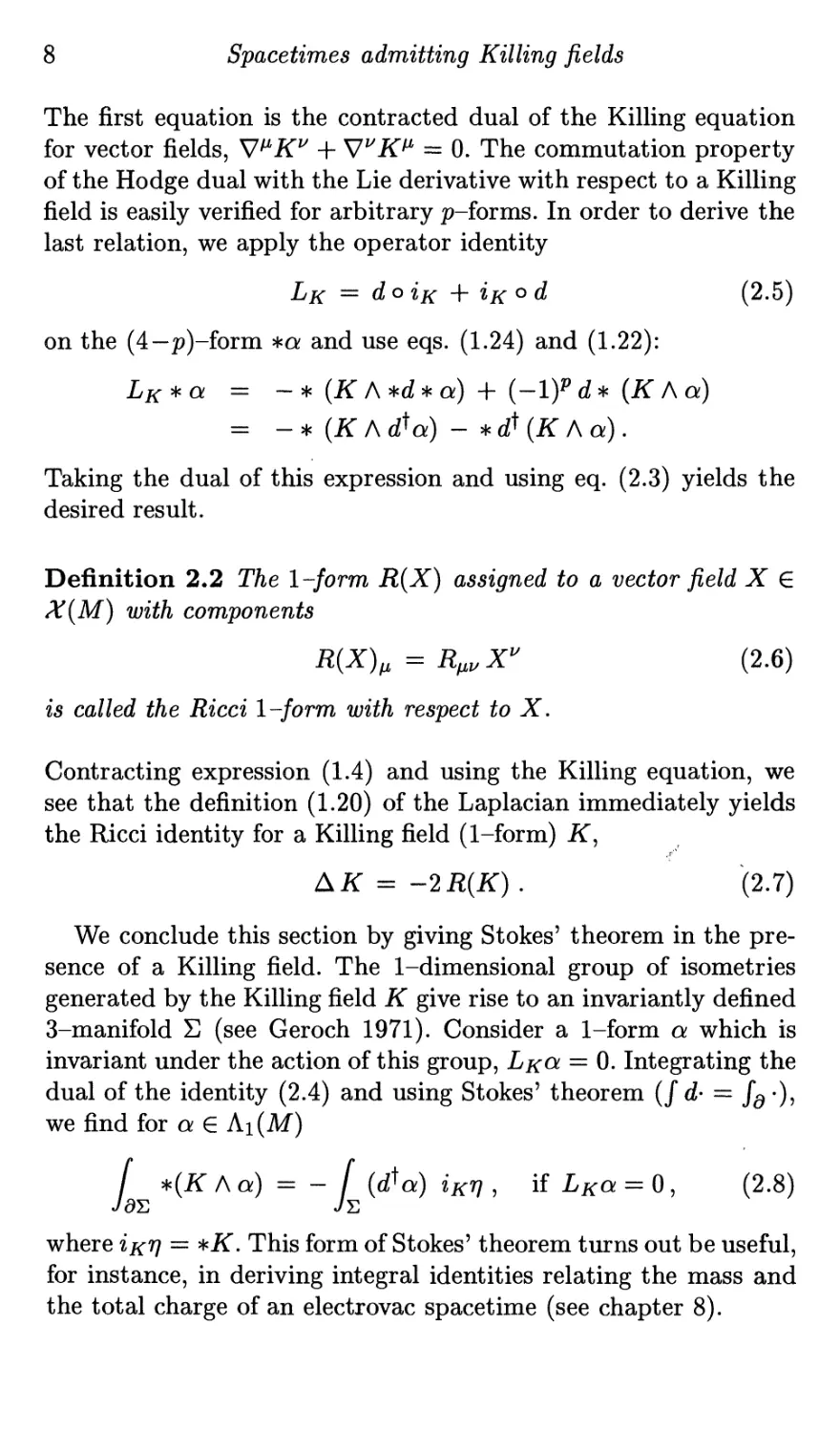
8 Spacetimes admitting Killing fields
The first equation is the contracted dual of the Killing equation
for vector fields, V^K^ + V^K^ = 0. The commutation property
of the Hodge dual with the Lie derivative with respect to a Killing
field is easily verified for arbitrary p-forms. In order to derive the
last relation, we apply the operator identity
Lk = doij^ + iK ^ d (2.5)
on the (4—p)-form *a and use eqs. (1.24) and (1.22):
Lx^a = - * (ii: A *d * a) + (-1)^ d * {K ^a)
= -^ {K ^ d+a) - * d^ {K f\a).
Taking the dual of this expression and using eq. (2.3) yields the
desired result.
Definition 2.2 The 1-form R{X) assigned to a vector field X G
X{M) with components
R{X)^ = R^^X^ (2.6)
is called the Ricci 1-form with respect to X.
Contracting expression (1.4) and using the Killing equation, we
see that the definition (1.20) of the Laplacian immediately yields
the Ricci identity for a Killing field (1-form) K,
AK = -^2R{K) . (2.7)
We conclude this section by giving Stokes' theorem in the
presence of a Killing field. The 1-dimensional group of isometries
generated by the Killing field K give rise to an invariantly defined
3-manifold S (see Geroch 1971). Consider a 1-form a which is
invariant under the action of this group, Lkol = 0. Integrating the
dual of the identity (2.4) and using Stokes' theorem (/d- = /^ •),
we find for a G Ai(M)
/ ^{K Aa) = - f (d^a) ixV , if Lxa = 0, (2.8)
JdT. Jt,
where ixf] = *-K'. This form of Stokes' theorem turns out be useful,
for instance, in deriving integral identities relating the mass and
the total charge of an electrovac spacetime (see chapter 8).
2.2 Basic identities 9
2.2 Basic identities
In this section we establish a set of differential identities between
the Ricci l-form, the twist and the norm of a Killing field. As we
shall see later, these relations reduce to the Ernst equations for
vacuum and electrovac spacetimes. In addition, they turn out to
be the key identities for the proof of the staticity and circularity
theorems.
Definition 2.3 Let K be a Killing field (l-form). The fuitction
N e Ao(M) and the l-form u e Ai(M),
N = {K\K), u =^\^{K^dK) (2.9)
are called the norm and the twist (rotation-form) associated with
K. In the domain of (M^g) where N is positive (negative^ zero)
the field K is said to be spacelike (timelike, null).
By virtue of eq. (1.24) and the above definition for a;, we have
— 2^{K/\u) = 2iK ^(jo = iK{K ^ dK). Now using the fact that
ixdK = —dixK = —dN (since LkK = 0), we obtain the
expression
-dK = ^[2^{K Au) + K AdN] (2.10)
for the derivative of the Killing form in terms of its twist and norm.
Taking advantage of this formula, it is also not hard to verify the
identity
N{dK\dK) = {dN\dN) - 4:{uj\uj). (2.11)
(First, the cross-terms do not contribute, since they are
proportional to KAK. Secondly, eq. (1.15) yields {^[KAuj] \ ^[KAu]) =
~{K A u)\K Au)) = -iV(a;|a;), since {K\u)) = 0. Finally, eq. (1.26)
hnplies {K A dN\K A dN) = N{dN\dN), since {K\dN) = LkN =
0.)
It is worthwhile pointing out that the Killing property of K has
not been used so far. Hence, the above identities between the norm
and twist hold for arbitrary vector fields (1-forms). However, in
the remainder of this chapter, K is assumed to be a Killing field.
We now derive the formulae for the derivative and the co-
derivative of the twist uj. We first note that both N and u have
vanishing Lie derivatives with respect to K^ LkN = Lk^j^ = 0.
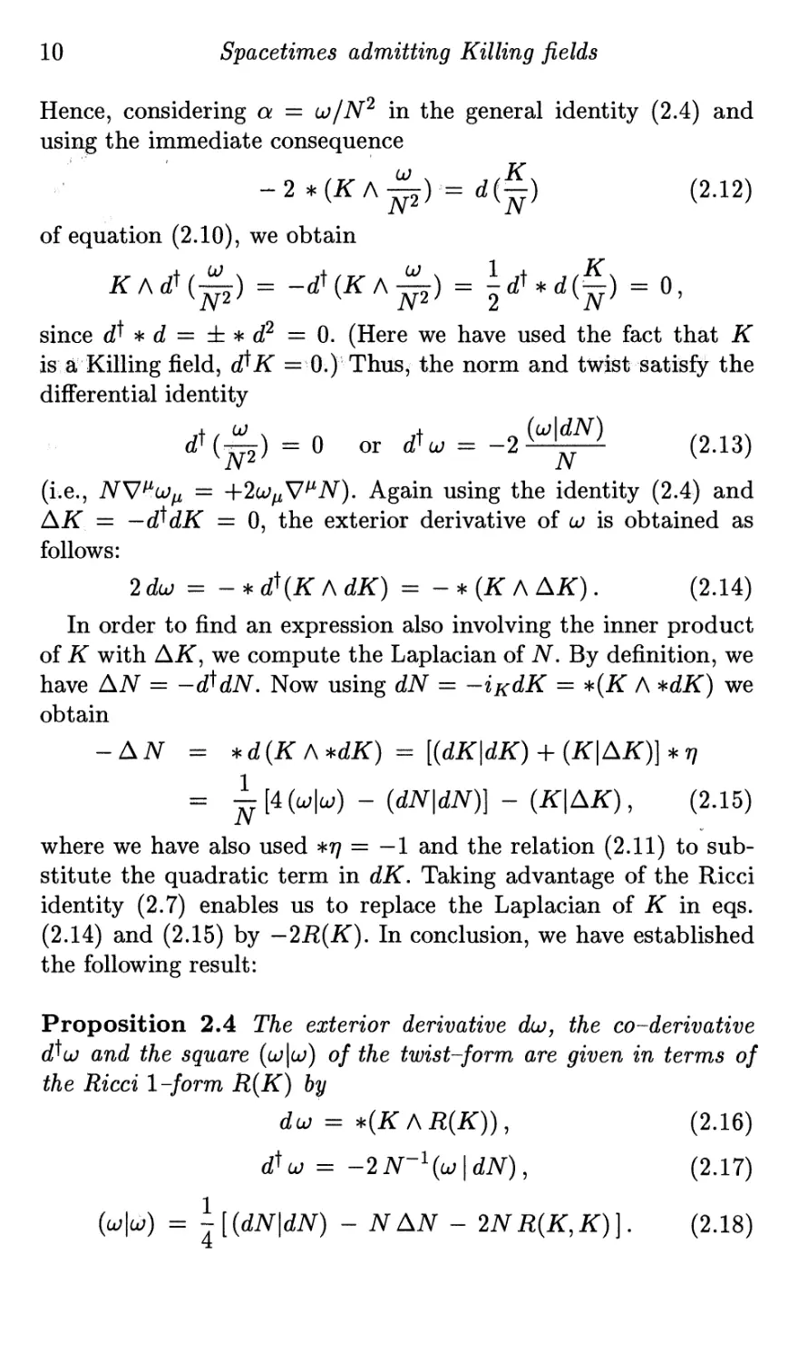
10 Spacetimes admitting Killing fields
Hence, considering a = u/N'^ in the general identity (2.4) and
using the immediate consequence
-2*(ifA^) = d(|) (2.12)
of equation (2.10), we obtain
since d^ ^ d = ± ^ d'^ = 0. (Here we have used the fact that K
is a Killing field, d^K = 0.) Thus, the norm and twist satisfy the
differential identity
rft(^) = 0 or dt„_2fe!^ (2.13)
(i.e., NV^cjj^ = +2uJ^V^N). Again using the identity (2.4) and
AK = —d^dK = 0, the exterior derivative of a; is obtained as
follows:
2duj = -^d^KAdK) = -^{K AAK). (2.14)
In order to find an expression also involving the inner product
of K with Aif, we compute the Laplacian of N. By definition, we
have AN = -d^dN. Now using dN = -ixdK = ^{K A ^dK) we
obtain
-AN = ^d{K A^dK) = [{dK\dK) + {K\AK)\^r]
= ^[4(a;|a;) - {dN\dN)] - {K\AK), (2.15)
where we have also used *r/ = -1 and the relation (2.11) to
substitute the quadratic term in dK. Taking advantage of the Ricci
identity (2.7) enables us to replace the Laplacian of K in eqs.
(2.14) and (2.15) by '-2R{K). In conclusion, we have established
the following result:
Proposition 2.4 The exterior derivative dij, the co-derivative
d^o; and the square {<jj\oj) of the twist-form are given in terms of
the Ricci 1-form R{K) by
du = ^{KAR{K)), (2.16)
d^u = -2N-\uj\dN), (2.17)
{uj\u;) = ^[{dN\dN) - NAN - 2NR{K,K)]. (2.18)
2.2 Basic identities 11
It is worth noting that the integrability conditions for eq. (2.16)
are fulfilled as a consequence of Bianchi's identity for the Einstein
tensor and the Killing equation for K: By virtue of eq. (2.4) we
have d'^u = - ^ {K A d:^G{K)) = 0, since the co-derivative of
the Einstein 1-form G{K) vanishes: d^G{K) = -K^V^G^^ -
^G^^{Vf'K^ + V^K^) = 0.
The above proposition yields the expressions for the R{K^ • )-
components of the Ricci tensor. It remains to compute the
expression for i?(X, y), where X and Y are orthogonal to K. We do so
by introducing the projection tensor P, defined in terms of the
spacetime metric ^^^g and the Killing field K by
Note that P is positive definite if K is timelike, \N\ = —iV,
whereas the signature of P is (—,+,+) if if is a spacelike
Killing field. The conformal factor in front of P turns out to be very
convenient and is responsible for the relatively simple form of the
Ricci tensor R^^^ of M/G. The latter can be derived in an
invariant manner or, of course, by writing the metric with respect to a
coordinate basis adapted to K — dt (see, e.g., Israel and Wilson
1972 or Kramer et al. 1980). Since we shall present the reduction
in some detail for the stationary and axisymmetric case, we give
here only the result and invite the reader to verify it as an
exercise. In terms of the Killing field if, its norm N and twist a;, one
finds
RiP) = R + ^R{K,K)^^^g + -^{dN®dN + A:Uj®uj}
- j^{K0R{K) + R{K)®K}, (2.20)
where (^)g and R denote the metric and the Ricci tensor of space-
time. As a test, we observe that LkN = 0 and i^o; = 0 imply
R^^\K^ .) — 0. Hence, as required, R^^^ vanishes unless it is
evaluated on two vector fields orthogonal to K. Using Einstein's
equations to express the Ricci tensor in terms of the stress-energy
tensor, eqs. (2.16)-(2.20) yield the complete set of field equations
for spacetimes admitting a Killing field.
12 Spacetimes admitting Killing fields
2.3 The vacuum variational principle
In the previous section we demonstrated that both the component
R{K^ K) of the Ricci tensor and the 2-form K A R{K) can be
expressed in terms of the twist and the norm of the Killing field K.
When R{K, K) and K A R{K) are replaced by the corresponding
stress-energy expressions, the identities (2.16)-(2.18) reduce to a
set of differential equations - the Ernst equations - for N and u on
a 2-dimensional flat background manifold. This is, however, only
the case if the spacetime admits two Killing fields which fulfil the
integrability conditions. Nevertheless, the existence of one Killing
field is sufficient to introduce the Ernst potential and to
understand the basic structure of the Ernst equations. In addition, the
entire set of vacuum (and electrovac) field equations for a space-
time with one Killing field can be obtained from a variational
principle for the Ernst potential(s) and the projection metric P.
We start by considering the complex 1-form <5, defined in terms
of N and a; by
£ = -dN + 2iu). (2.21)
The equation for the derivative of £ is immediately obtained from
the corresponding expression for du. In order to find the co-
derivative of <5, we add the expression (2.17) for d^u to eq. (2.18)
for AiV = -dtdiV. This yields
d£ = 2i ^{KA R{K)), (2.22)
Ss -^ N-^{£\£) ^ -2{K\ R{K)). (2.23)
If Einstein's equations (together with the invariance properties of
the matter fields) imply that ^{K A R{K)) vanishes, then the first
of the above equations implies the (local) existence of a potential E
with dE = £. This is, of course, the case for vacuum models and,
as we shall argue below, is also true for self-gravitating scalar
fields.
For the remainder of this section we restrict ourselves to vacuum
spacetimes. In this case, by virtue of eq. (2.22), we can introduce
the vacuum Ernst potential E G Ao(M), defined (up to an exact
differential) by
dE = £. (2.24)
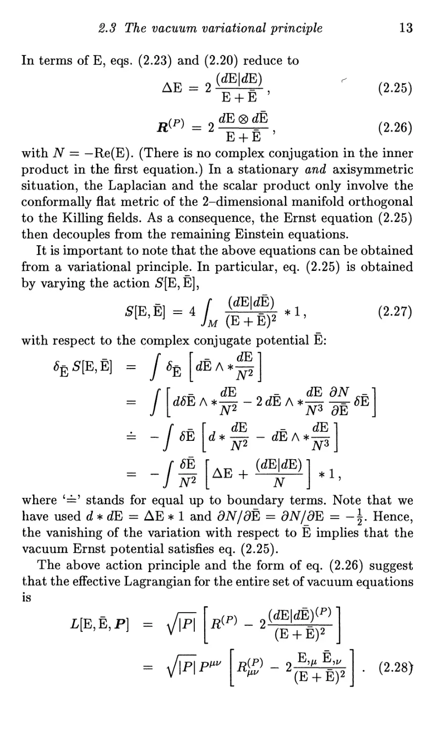
2.3 The vacuum variational principle
13
In terms of E, eqs. (2.23) and (2.20) reduce to
, (dE|dE)
AE
fl(^)
E + E '
dE®dE
(2.25)
^ r. , (2-26)
E+E ' ^ '
with N = —Re(E). (There is no complex conjugation in the inner
product in the first equation.) In a stationary and axisymmetric
situation, the Laplacian and the scalar product only involve the
conformally flat metric of the 2-dimensional manifold orthogonal
to the Killing fields. As a consequence, the Ernst equation (2.25)
then decouples from the remaining Einstein equations.
It is important to note that the above equations can be obtained
from a variational principle. In particular, eq. (2.25) is obtained
by varying the action S[E, E],
(dE|dE)
S[E,E] = 4 /
Jm
*1,
Im (E + E)2
with respect to the complex conjugate potential E:
dE
(2.27)
6^S[E,E] = JS^
dEA*
JV2
-I
dSEA*
6E \d*
dE _
iV2 ~
dE
„ ,- dE dN -
_ f ^
J m
iV2
AE +
dEA*
(dEjdE)
N
dE
*i
where '=' stands for equal up to boundary terms. Note that we
have used d * dE = AE * 1 and dN/dE = dN/pE = -\. Hence,
the vanishing of the variation with respect to E implies that the
vacuum Ernst potential satisfies eq. (2.25).
The above action principle and the form of eq. (2.26) suggest
that the effective Lagrangian for the entire set of vacuum equations
is
L[E,E,P] =
^(P) _ ,(dE|dE_)(P)
= ^J\P\P"'
(E + E)2
d(p) _ o E,^ E,^
^'^ (E + E)2
(2.28)
14 Spacetimes admitting Killing fields
In fact, variations with respect to the projection metric P yield
eq. (2.26) since, as usual, y/lP^P^^SRltu gives rise to a boundary
term.
This concludes our brief introduction to the structure of the
Ernst equations and the corresponding variational principle for
vacuum spacetimes with one Killing field. As we shall see later, a
completely analogous formulation exists for the Einstein-Maxwell
system with a Killing field.
2.4 Asymptotic flatness and stationarity
The study of isolated systems iii general relativity involves a
detailed investigation of the properties of asymptotically flat space-
times (Geroch 1970b, 1972b, 1976). The first major step towards
an understanding of this concept was achieved by Bondi (1960),
by examining the null hypersurfaces of spacetime (see also Bondi
et al 1962, Sachs 1962, 1964). Later on, Penrose (1963, 1964,
1965a) realized that the notion of infinity can be made precise by
adding the future and past endpoints of null geodesies to space-
time. Considering a conformal transformation (with
asymptotically vanishing conformal factor) then enables one to understand
the asymptotic properties of the metric by studying the boundary
of the conformal spacetime. Roughly speaking, a spacetime is said
to be asymptotically flat if there exists a conformal
transformation such that conformal infinity (spacelike and null) has similar
properties to Minkowski spacetime.
For a detailed introduction into the asymptotic properties of
the gravitational field we refer the reader to the literature. In
particular, precise definitions of asymptotic flatness can be found
in the review article of Newman and Tod (1980), the book of
Wald (1984) and the work of Ashtekar and Hansen (1978) (see
also Ashtekar 1980, Chrusciel 1989a, 1989b). For our purposes it
will, however, not be necessary to enter into the subtleties of the
subject, since we restrict ourselves to stationary spacetimes. In
this case, we avoid the whole issue of radiation, which allows us
to adopt an intuitive notion of asymptotic flatness.
It is well known that the concept of local energy density in
general relativity is vacuous. In an asymptotically flat spacetime
it is, however, possible to obtain meaningful expressions for both
2.4 Asymptotic flatness and stationarity 15
the total 4-momentum and the total angular momentum tensor of
an isolated system. Bartnik (1986) has given a rigorous treatment
of the asymptotic decay conditions which guarantee that the ADM
mass (Arnowitt et al. 1962),
Madm = Az I, i^iOij - di9jj)dS\ (2.29)
is well defined (see also Ashtekar 1984). Here di = d/dx\ where
{x'^} are asymptotically Euclidean coordinates on a spacelike hy-
persurface, and dS^ denotes the unit surface element of the 2-
sphere at infinity, S^.
As already mentioned, we shall assume that spacetime is also
stationary: For physical reasons, one expects that "sufficiently
long" after the gravitational collapse of a star to a black hole,
the latter settles down into a stationary configuration. A space-
time is said to be stationary if it admits a 1-parameter group of
isometrics with tin^ielike orbits, that is, if it admits a timelike
Killing field k. In order to distinguish situations with and without
orgoregions, it is convenient to adopt the following definitions:
Definition 2.5 An asymptotically flat spacetime is called
stationary if it admits an asymptotically timelike Killing field k.
Definition 2.6 A domain of spacetime admitting a nowhere
vanishing, timelike Killing field is called strictly stationary (or
stationary in the strict sense).
(Note that these notions are not used consistently in the literature:
One also encounters the terms pseudo-stationary or stationary
near infinity for stationary, and stationary for strictly stationary.)
Note also that throughout this text an arbitrary Killing field is
(kuioted by K^ whereas the lower case letter k is reserved for the
Killing field generating the stationary symmetry.
Beig and Simon (1980a, 1980b, 1981) have shown that an
asymptotically fiat and stationary metric is analytic at spacelike
infinity. Their result was based on the assumption that - in an
lulapted asymptotically Cartesian coordinate system with k =
O/dxP - the metric becomes fiat like r~^ (or faster). Only re-
ccrntly were Kennefick and O Murchadha (1995) able to show
tliat all asymptotically fiat solutions which fall off slower than
16 Spacetimes admitting Killing fields
r~^ involve gravitational radiation near spacelike infinity (see, e.g.,
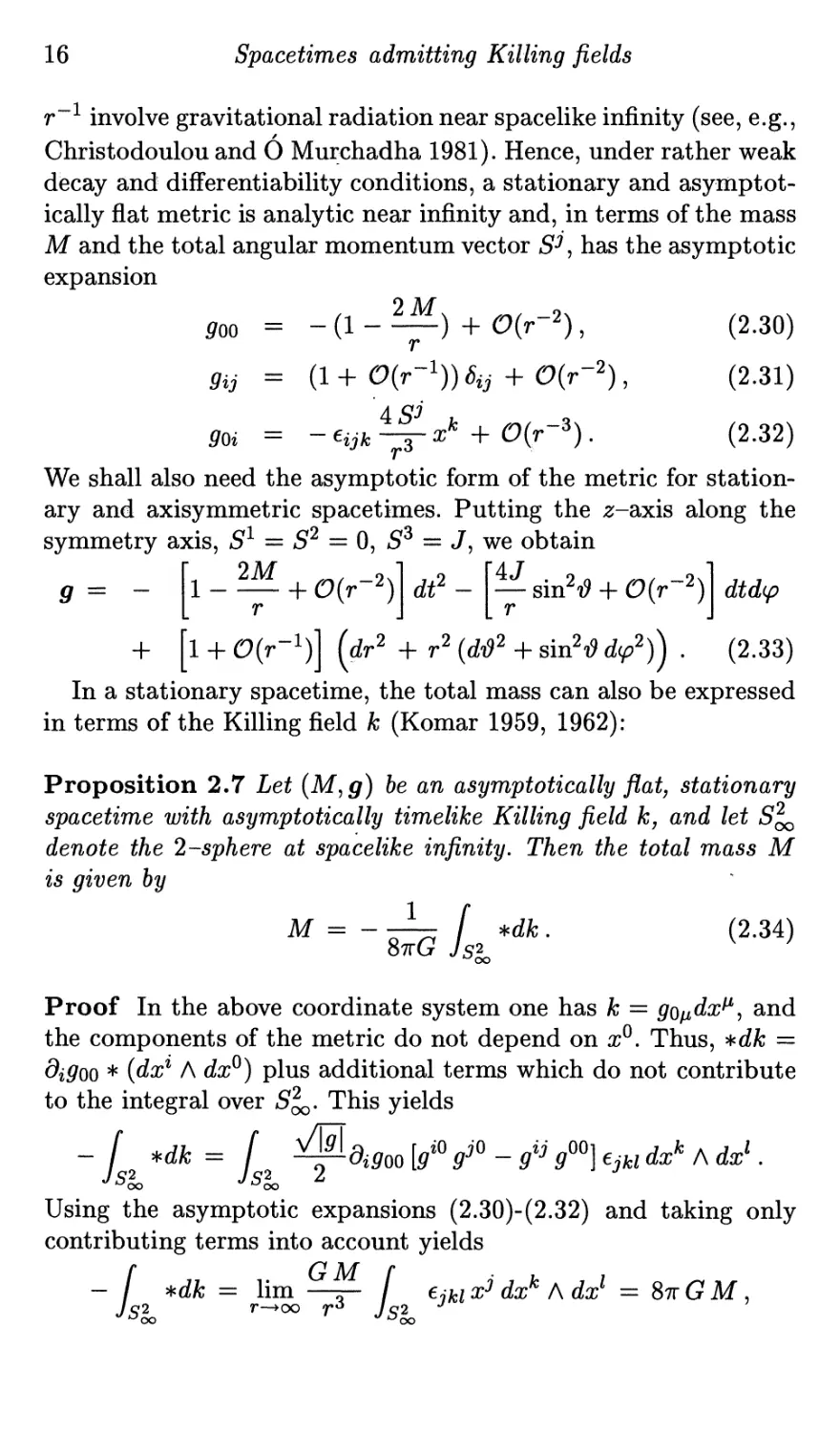
Christodoulou and O Murchadha 1981). Hence, under rather weak
decay and differentiability conditions, a stationary and
asymptotically flat metric is analytic near infinity and, in terms of the mass
M and the total angular momentum vector 5-^, has the asymptotic
expansion
goo = -(l-^) + 0(r-2), (2.30)
9ij = (l+0(r-i))% + O(r-2), (2.31)
goi = -eijk^^x'' + 0{r-^). (2.32)
We shall also need the asymptotic form of the metric for
stationary and axisymmetric spacetimes. Putting the 2-axis along the
symmetry axis, S^ — S^ = 0, S^ = J, we obtain
g = _ [l - ^ + 0(r-2)] dt' - [y sin^^ + 0(r-2)l dtdcp
+ [l + 0(r-^)] (dr^ + r^ {d'd^ + sin^^ V)) • (2.33)
In a stationary spacetime, the total mass can also be expressed
in terms of the Killing field k (Komar 1959, 1962):
Proposition 2.7 Let (M,g) be an asymptotically flat, stationary
spacetime with asymptotically timelike Killing field k, and let S^
denote the 2~sphere at spacelike infinity. Then the total mass M
is given by
M = - -^ / *dfc . (2.34)
Proof In the above coordinate system one has k = gofidx^^ and
the components of the metric do not depend on x^. Thus, ^dk =
digoo * {dx^ A dx^) plus additional terms which do not contribute
to the integral over 5^. This yields
- / ^dk= [ ^digoo [g'' g^' - g'^ g''] ejki dx' A dx'.
Using the asymptotic expansions (2.30)-(2.32) and taking only
contributing terms into account yields
- / *dfc = lim —5- / €^u x^ dx^ A da;^ =: Stt G M ,
J52 r->oo r^ Js2
2.5 Static spacetimes 17
where we have used d[€jkix^dx^ A dx^] = €jkidx^ A dx^ A dx^ =
6 dx^ A dx'^ A dx^ and Stokes' theorem in the last step. D
It will also turn out to be useful to convert the asymptotic Ko-
mar integral (2.34) into a volume integral. Let S denote a spacelike
hypersurface extending from spacelike infinity to a bounding 2-
surface Ti. Using the Ricci identity for Killing fields (see eqs. (1.20)
and (2.7)),
d*dfc=-*Afc=:2* R{k),
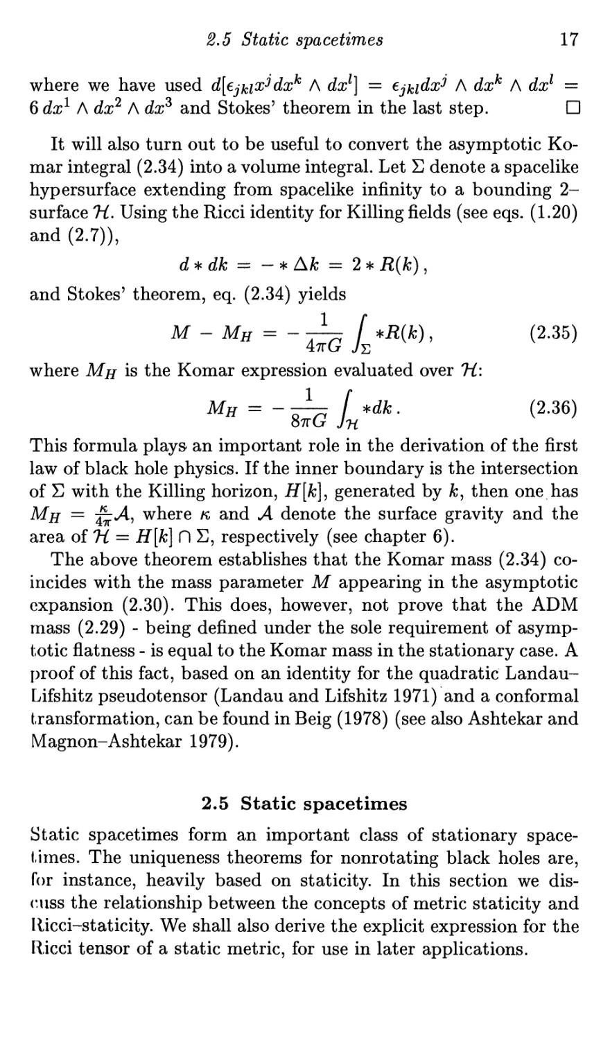
and Stokes' theorem, eq. (2.34) yields
M - Mh = -^ l^*R{k), (2.35)
where Mh is the Komar expression evaluated over Ti:
This formula plays' an important role in the derivation of the first
law of black hole physics. If the inner boundary is the intersection
of E with the Killing horizon, -fiTffc], generated by fc, then one has
Mh — -^A^ where k and A denote the surface gravity and the
area oiTi = H[k] O S, respectively (see chapter 6).
The above theorem establishes that the Komar mass (2.34)
coincides with the mass parameter M appearing in the asymptotic
expansion (2.30). This does, however, not prove that the ADM
mass (2.29) - being defined under the sole requirement of
asymptotic flatness - is equal to the Komar mass in the stationary case. A
proof of this fact, based on an identity for the quadratic Landau-
Lifshitz pseudotensor (Landau and Lifshitz 1971) and a conformal
transformation, can be found in Beig (1978) (see also Ashtekar and
Magnon-Ashtekar 1979).
2.5 Static spacetimes
Static spacetimes form an important class of stationary space-
times. The uniqueness theorems for nonrotating black holes are,
(or instance, heavily based on staticity. In this section we dis-
(!uss the relationship between the concepts of metric staticity and
Ilicci-staticity. We shall also derive the explicit expression for the
Ricci tensor of a static metric, for use in later applications.
18 Spacetimes admitting Killing fields
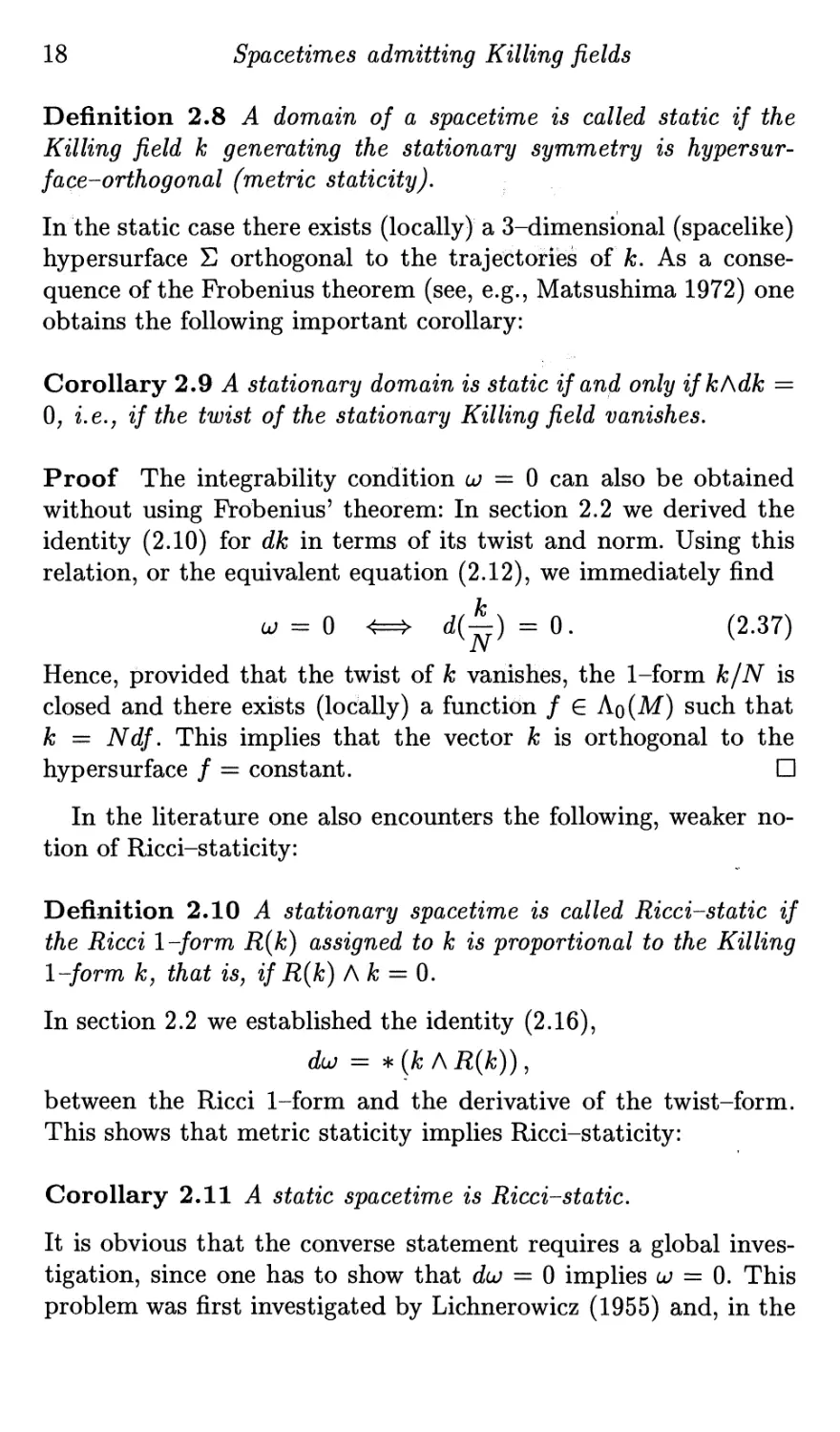
Definition 2.8 A domain of a spacetime is called static if the
Killing field k generating the stationary symmetry is hypersur-
face-orthogonal (metric staticity).
In the static case there exists (locally) a 3-dimensional (spacelike)
hypersurface E orthogonal to the trajeetoriies of fc. As a
consequence of the Frobenius theorem (see, e.g., Matsushima 1972) one
obtains the following important corollary:
Corollary 2.9 A stationary domain is static if and only ifkAdk =
0; i.e.J if the twist of the stationary Killing field vanishes.
Proof The integrability condition a; == 0 can also be obtained
without using Frobenius' theorem: In section 2.2 we derived the
identity (2.10) for dk in terms of its twist and norm. Using this
relation, or the equivalent equation (2.12), we immediately find
a; =:. 0 ^=^ d{^) = 0. (2.37)
Hence, provided that the twist of k vanishes, the 1-form k/N is
closed and there exists (locally) a function / G Ao(M) such that
k = Ndf. This implies that the vector k is orthogonal to the
hypersurface / = constant. D
In the literature one also encounters the following, weaker
notion of Ricci-staticity:
Definition 2.10 A stationary spacetime is called Ricci-static if
the Ricci 1-form R{k) assigned to k is proportional to the Killing
1-form k, that is, if R{k) Ak = 0.
In section 2.2 we established the identity (2.16),
dij = ^{kAR{k)),
between the Ricci 1-form and the derivative of the twist-form.
This shows that metric staticity implies Ricci-staticity:
Corollary 2.11 ^4 static spacetime is Ricci-static.
It is obvious that the converse statement requires a global
investigation, since one has to show that du = 0 implies a; = 0. This
problem was first investigated by Lichnerowicz (1955) and, in the
2.5 Static spacetimes 19
context of black holes, was solved by Hawking and Ellis (1973)
for vacuum spacetimes. We shall return to this question in section
8.2, where we present a simple proof of the fact that Ricci-staticity
implies metric staticity. The argument is based on strict station-
arity and also applies to spacetimes with nonconnected Killing
horizons.
The remainder of this section is devoted to the derivation of
the Ricci tensor of a static spacetime. In the domain where the
hypersurface orthogonal Killing field fc is timelike, the metric of a
static spacetime assumes the form
Wg = -SUt^ +g, (2.38)
where now g denotes the Riemannian metric on the 3-dinaensional
hypersurface E orthogonal to k. The Laplacian of an arbitrary
function / E Ao(S) with respect to g is given by
A(^)/ = a/ - S-^{dS\df). (2.39)
Using equation (2.18) with N = -5^ and a; = 0, we therefore
have
5A(^)5 = SAS - {dS\dS)
= -^ [{dN\dN) - NAN] = R{k, k). (2.40)
The remairiing components of the Ricci tensor are most easily
obtained by solving Cartan's structure equations,
de^' + a;'^^Ar = 0, (2.41)
fi/^^ zz. duj^^ + LJ^"^ A uj% , (2.42)
in an orthonormal tetrad basis {0^} of {M^^ g) {9^ = Sdt).
Denoting the connection-forms of the 3-dimensional Riemannian
manifold (S,g) with respect to 0^ by ^^^u'^p we find from the first
structure equation (2.41)
u\ = {S-^V^f^S)e\ a;^, = (^V,, (2.43)
where V^^^ denotes the covariant derivative with respect to g.
Using this in equation (2.42) yields the curvature-forms
oo. = (5-1 vJ^Vl^)^) e^ A e"^, n\ - ^^^n\. (2.44)
Using the relation Vt^j, = \R^j,^p6'^ A ^^, the nonvanishing
components of the Ricci tensor and the curvature scalar with respect to
20 Spacetimes admitting Killing fields
the static metric (2.38) become
Ru = 5A(^)5, (2.45)
it;-. .. R(f - S-'vf^v\'^S, (2.46)
R - R^9) ^ 2S-^A^9)s, (2.47)
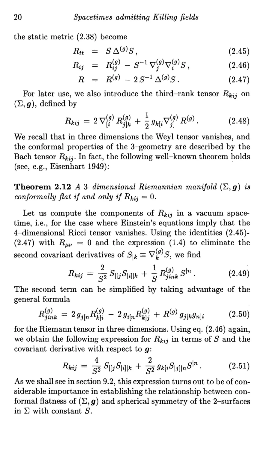
For later use, we also introduce the third-rank tensor Rkij on
(S,g), defined by
Rkij = ^vfR^f, + \9,[iyfR^'^. (2.48)
We recall that in three dimensions the Weyl tensor vanishes, and
the conformal properties of the 3-geometry are described by the
Bach tensor Rkij- In fact, the following well-known theorem holds
(see, e.g., Eisenhart 1949):
Theorem 2.12 A 3-dimensional Riemannian manifold (S,flr) is
conformally flat if and only if Rkij = 0.
Let us compute the components of Rkij in a vacuum space-
time, i.e., for the case where Einstein's equations imply that the
4-dimensional Ricci tensor vanishes. Using the identities (2.45)-
(2.47) with R^jy = 0 and the expression (1.4) to eliminate the
second covariant derivatives of 5|fc = V^^^S, we find
«fci. = ^%^NP + |^Sfc'5l". (-2.49)
The second term can be simplified by taking advantage of the
general formula
R^k = ^9j[nR% - 29i[nR'ii + R^'^Hk9n]i (2-50)
for the Riemann tensor in three dimensions. Using eq. (2.46) again,
we obtain the following expression for Rkij in terms of S and the
covariant derivative with respect to g:
Rkij = '^^\[j^\i]\k + '^ 9k[iS\j]\nS^^ . (2.51)
As we shall see in section 9.2, this expression turns out to be of
considerable importance in establishing the relationship between con-
formal flatness of (E,gf) and spherical symmetry of the 2-surfaces
in E with constant S.
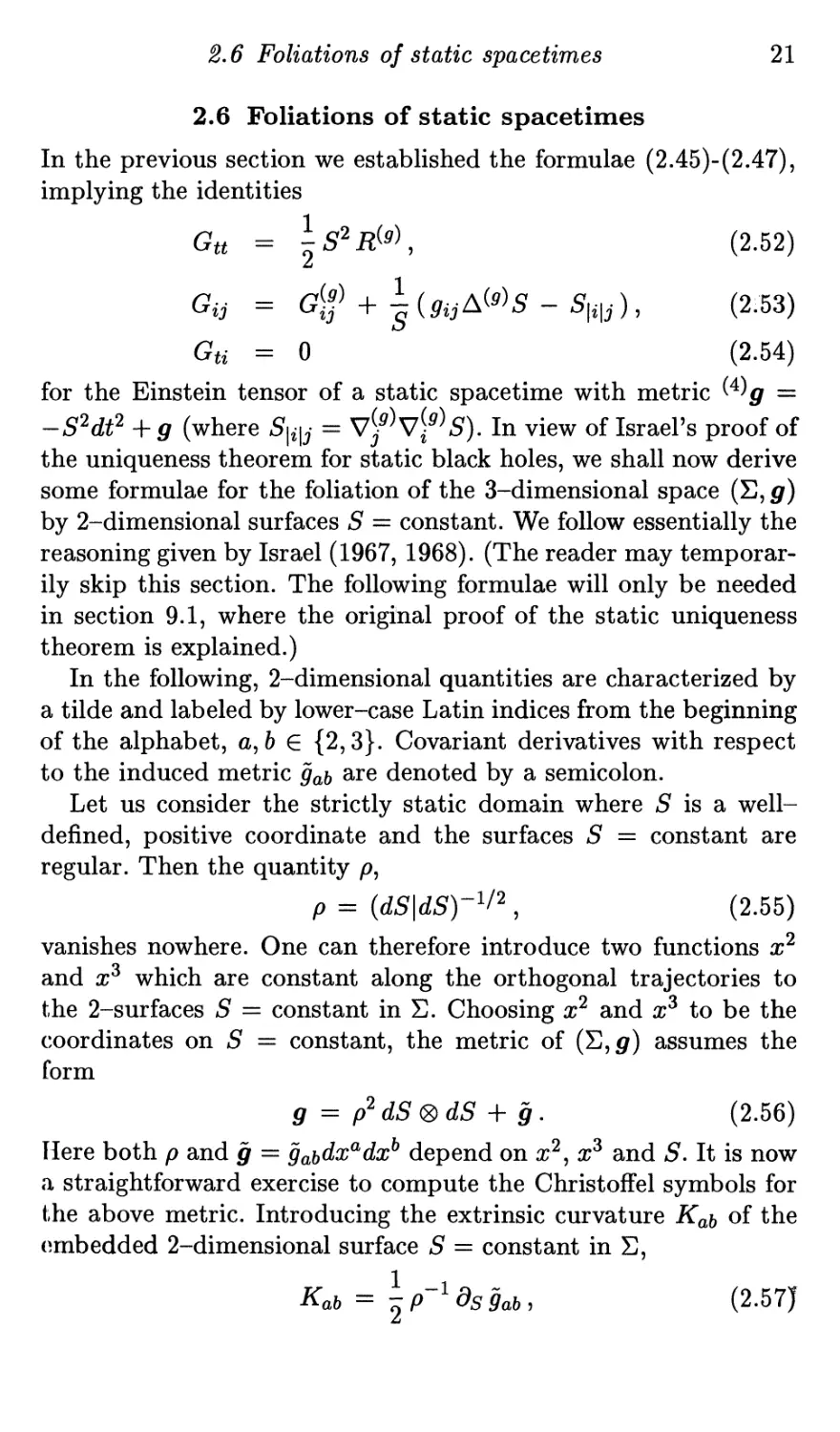
2.6 Foliations of static spacetimes 21
2.6 Foliations of static spacetimes
In the previous section we established the formulae (2.45)-(2.47),
implying the identities
Gtt = ^S^R^'K (2.52)
Gij = G^f + |(5,,A(^)5-5|,|,-), (2.53)
Gti = 0 (2.54)
for the Einstein tensor of a static spacetime with metric ^^^g =
-S^dt^+g (where 5|,|^- - vf^v\^^S). In view of Israel's proof of
the uniqueness theorem for static black holes, we shall now derive
some formulae for the foliation of the 3-dimensional space (S, g)
by 2-dimensional surfaces S = constant. We follow essentially the
reasoning given by Israel (1967, 1968). (The reader may
temporarily skip this section. The following formulae will only be needed
in section 9.1, where the original proof of the static uniqueness
theorem is explained.)
In the following, 2-dimensional quantities are characterized by
a tilde and labeled by lower-case Latin indices from the beginning
of the alphabet, a^b e {2,3}. Covariant derivatives with respect
to the induced metric gab cire denoted by a semicolon.
Let us consider the strictly static domain where 5 is a well-
defined, positive coordinate and the surfaces S = constant are
regular. Then the quantity p,
p = {dS\dS)-^/^ , (2.55)
vanishes nowhere. One can therefore introduce two functions x^
and x^ which are constant along the orthogonal trajectories to
the 2-surfaces S = constant in E. Choosing x'^ and x^ to be the
coordinates on 5 = constant, the metric of (S,g) assumes the
form
g = p^dS^dS + g. (2.56)
Here both p and g = Qahdx^dx^ depend on x^, x^ and S. It is now
a straightforward exercise to compute the Christoffel symbols for
the above metric. Introducing the extrinsic curvature Kah of the
(imbedded 2-dimensional surface S = constant in E,
Kah = \p'^ds9ah. (2.57J
22 Spacetimes admitting Killing fields
we obtain
The Ricci tensor of (S,g) is now obtained from the general
expressions (1.2) and (1.3),
4^] = -p{Ap + K,s+pKabK''''), (2.58)
b!£ = Rab-p~^P;ab-KKab- p-^gacKU, (2-59)
4s = p{K\.b-K,a), (2.60)
where K = iC'Jj. In addition, eq. (2.53) also requires us to compute
A^^^S and the second covariant derivatives of S with respect to g.
Using eqs. (2.56) and the F-symbols given above, one finds
PiS
iA—O = p \,J\ -
and
A'^s^S = p-^{K - f^) (2.61)
p^
5ssA(^)5-5|5|s = PK,
gab^^^^S - 5|a|6 = -{Kgab - Kab - 9ab P~^ P,S ),
gsa^^'^S - S^sia = p-'p,a. (2.62)
In order to compute the right hand sides of the basic equations
(2.52)-(2.53), it remains to calculate the Einstein tensor and the
Ricci scalar of (S,g). Taking advantage of the above expressions,
we have
Gfs = ^{-R + K' -KabK'''), (2.63)
G'f^ = Gab-KKab + \gab{K^ +KabK'''')
+ - {gab^p - p-ab) + - {9abK,s -gacK%,s ) , (2.64)
and
G?i = p{K\.b-K,a) (2.65)
i?(») = R- {K^+ KabK''^) - -(Ap + K,s ). (2.66)
P
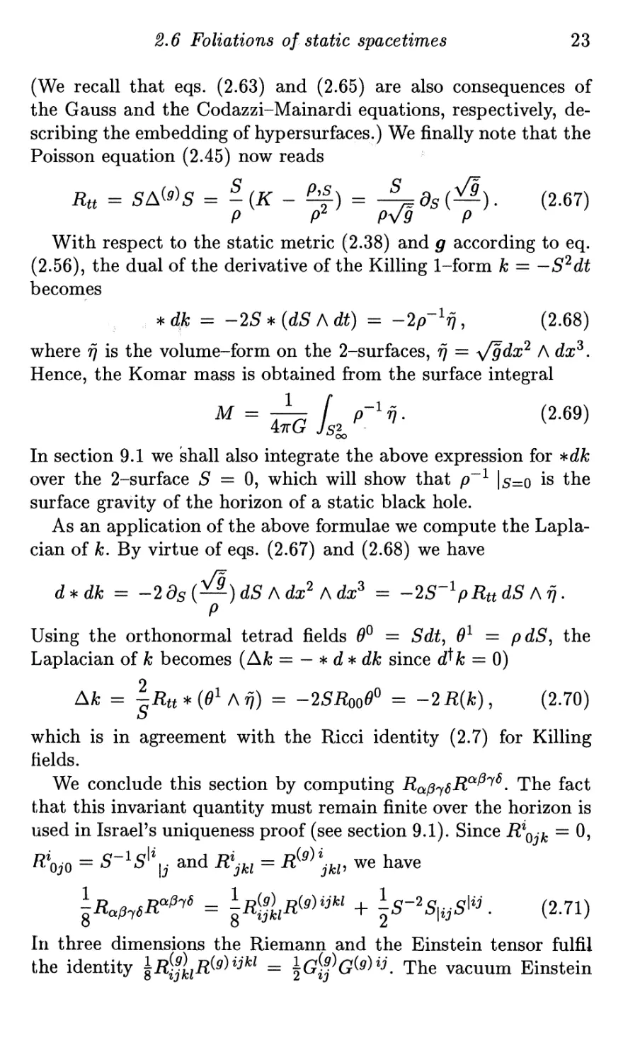
2.6 Foliations of static spacetimes 23
(We recall that eqs. (2.63) and (2.65) are also consequences of
the Gauss and the Codazzi-Mainardi equations, respectively,
describing the embedding of hypersurfaces.) We finally note that the
Poisson equation (2.45) now reads
it;,, ^ SA(9)s = ^(k - ^) = -^ds{^). (2.67)
P P^ PV9 P
With respect to the static metric (2.38) and g according to eq.
(2.56), the dual of the derivative of the Killing 1-form k = -S'^dt
becomes
^dk = -2S^{dSAdt) = -2p"^7?, (2.68)
where rj is the volume-form on the 2-surfaces, fj = ^/gdx^ A dx^.
Hence, the Komar mass is obtained from the surface integral
JgI""'*- (^■«^'
47rG
In section 9.1 we shall also integrate the above expression for -^dk
over the 2-surface 5 = 0, which will show that p"^ |5=o is the
surface gravity of the horizon of a static black hole.
As an application of the above formulae we compute the Lapla-
cian of k. By virtue of eqs. (2.67) and (2.68) we have
d*dfc - -lLds{—)dSNdx^Ndx^ - -iLS-^pRttdSNf).
P
Using the orthonormal tetrad fields Q^ — Sdt, 6^ = pdS, the
Laplacian of k becomes (Afc = — * d * dfc since d^k = 0)
Ak = ^Rtt^iO^ /\fj) = -2SRooO^ = -2R{k), (2.70)
which is in agreement with the Ricci identity (2.7) for Killing
fields.
We conclude this section by computing R^/s^sR^^^^ • The fact
that this invariant quantity must remain finite over the horizon is
used in Israel's uniqueness proof (see section 9.1). Since R^qaj^ = 0,
R^o,o = ^"''^I'l. and R),i = R^^^, we have
\Rc.^,6R-^'^' = \r%R^'^'^^' + \s-^S\i^S\'^. (2.71)
In three dimensions the Riemann and the Einstein tensor fulfil
the identity \R^^)^^R'^9)^J^^ = iG^f G^^)^^'. The vacuum Einstein
24 Spacetimes admitting Killing fields
equations A^^)^ = 0 and G\j = S~^S\ij now imply the relation
Using eqs. (2.62) with A(»)5 = 0 finally yields the result
(2.72)
1 1
X2+if„,X«^ + 2^^^l^^)
P'
2.7 Stationary and axisymmetric spacetimes
The problem of finding stationary and axisymmetric solutions to
Einstein's equations arises if one is interested in equilibrium
configurations of rotating sources. The first asymptotically flat
solution exhibiting these symmetries was given by Kerr (1963).
Later on, Tomimatsu and Sato (1972, 1973) presented a further
class of stationary and axisymmetric exact solutions. Although
the Tomimatsu-Sato solutions are asymptotically flat, they do
not approach spherically symmetric configurations in the limit of
vanishing angular momentum, since their static counterparts are
the Weyl solutions (Weyl 1917, 1919). More seriously, all solutions
of the Tomimatsu-Sato class (with nonvanishing quadrupole
moment, 6^1) exhibit naked singularities.
In addition to the solutions mentioned above, there exists a
variety of other stationary and axisymmetric solutions to Einstein's
vacuum equations (see Kramer et ah 1980). However, they are
all flawed in being either not asymptotically flat or having naked
singularities or, in the best case, degenerate horizons.
We start this section by introducing the notions of axial
symmetry, Ricci-circularity and (metric) circularity. We then give a
simple proof of the circularity theorem. The theorem guarantees
that Ricci-circularity implies integrability of the 2-dimensional
subspaces orthogonal to the Killing fields generating the
stationary and axisymmetric isometries. The metric of a circular space-
time can be written in a standard form, involving no off'-diagonal
terms between the 2-dimensional subspaces (Papapetrou 1953).
The remainder of this section is devoted to the derivation of some
identities for the Killing 2-form.
2.1 Stationary and axisymmetric spacetimes 25
According to definition 2.5, a spacetime is stationary if it admits
an asymptotically timelike Killing field k. Let us now consider
spacetimes which exhibit the following additional symmetry:
Definition 2.13 A spacetime is called cyclic symmetric if it is
invariant under the action tt of the 1-parameter group 50(2). A
cyclic symmetric spacetime is called axisymmetric if the fixed point
set of TT (i.e.J the rotation axis) is nonempty.
Definition 2.14 A spacetime is called stationary and
axisymmetric if it is both stationary and axisymmetric, and if the Killing
fields generating the symmetries commute with each other.
Throughout this text, the Killing field (1-form) generating the
cyclic symmetry will be denoted by m. A theorem due to Carter
(1970) guarantees that the group generated by k and m is Abelian
if spacetime is asymptotically flat and admits a symmetry axis:
Theorem 2.15 An asymptotically flat, stationary, axisymmetric
spacetime with Killing fields k and m is stationary and
axisymmetric, that is, [k^m] = 0.
Since we are dealing exclusively with asymptotically flat space-
times in this text, it is understood that k and m commute when
using the term stationary and axisymmetric in the following. (We
also refer to Schmidt 1978, Xanthopoulos 1978 and Chrusciel 1993
in this context.)
The total mass (2.34) of a stationary spacetime can be expressed
in terms of a flux integral involving the stationary Killing field.
Similarly, one obtains the total angular momentum, J, of an
axisymmetric spacetime,
where m denotes the Killing 1-form generating the axial
symmetry. Note that the Komar expressions for M and J differ by a
factor of 2 (and a sign). It is worth pointing out that this is not
an accident, but has a deep significance: Wald (1993b) and Iyer
and Wald (1994) have shown that the ADM mass of a diffeomor-
phism invariant theory is not equal to the Noether charge associ-
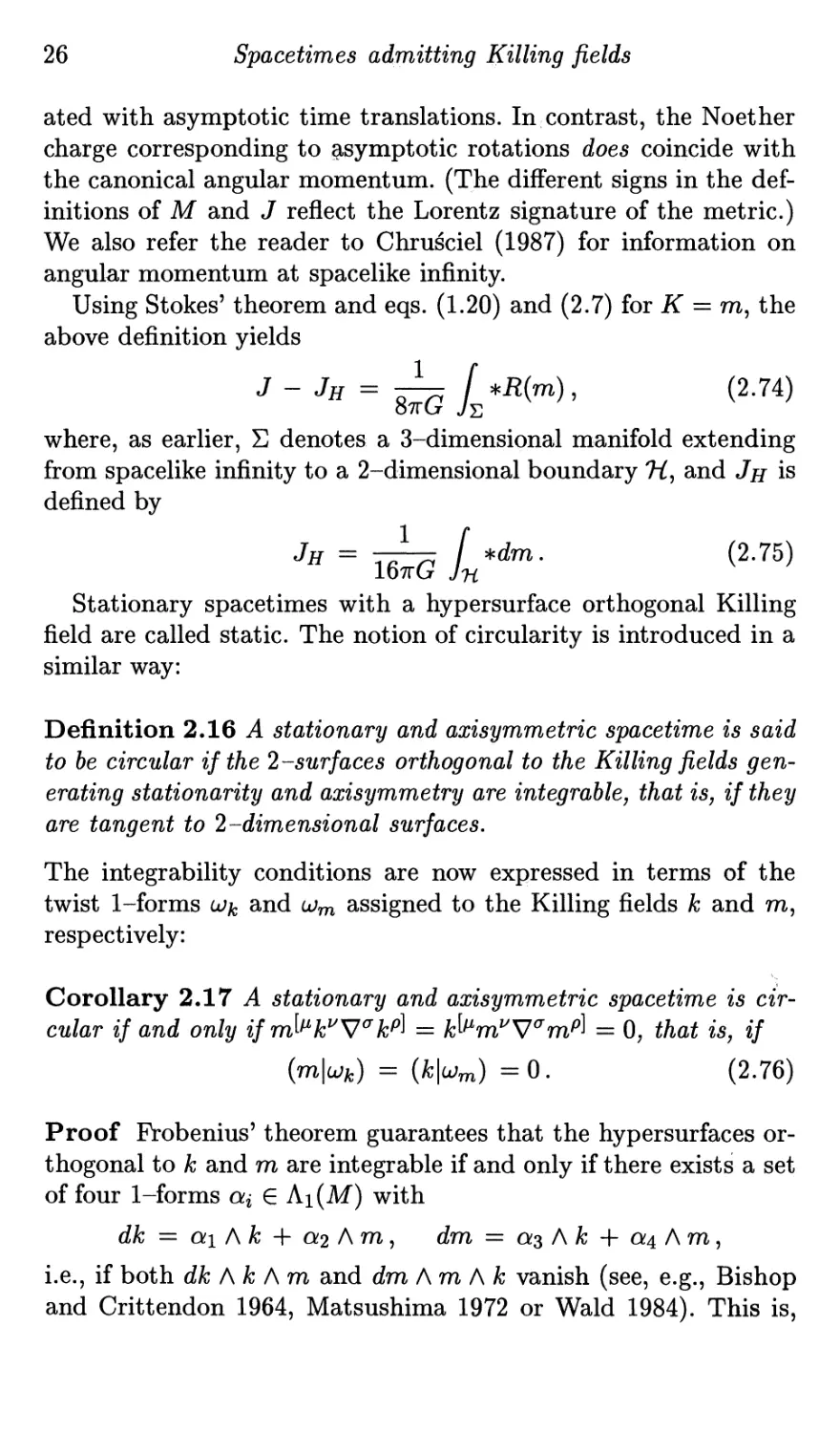
26 Spacetimes admitting Killing fields
ated with asymptotic time translations. In contrast, the Noether
charge corresponding to asymptotic rotations does coincide with
the canonical angular momentum. (The different signs in the
definitions of M and J reflect the Lorentz signature of the metric.)
We also refer the reader to Chrusciel (1987) for information on
angular momentum at spacelike infinity.
Using Stokes' theorem and eqs. (1.20) and (2.7) for K — m^ the
above definition yields
where, as earlier, S denotes a 3-dimensional manifold extending
from spacelike infinity to a 2-dimensional boundary Ti^ and Jh is
defined by
'" = 1^ !„"""■ ("='
Stationary spacetimes with a hypersurface orthogonal Killing
field are called static. The notion of circularity is introduced in a
similar way:
Definition 2.16 A stationary and axisymmetric spacetime is said
to be circular if the 2-surfaces orthogonal to the Killing fields
generating stationarity and axisymmetry are integrahle, that is, if they
are tangent to 2-dimensional surfaces.
The integrability conditions are now expressed in terms of the
twist 1-forms u^ and ujm assigned to the Killing fields k and m,
respectively:
Corollary 2.17 A stationary and axisymmetric spacetime is
circular if and only if m^^k^'V^kP^ = k^^m^'V^m^'^ = 0, that is, if
{m\ujk) = {k\ujm) =0. (2.76)
Proof Probenius' theorem guarantees that the hypersurfaces
orthogonal to k and m are integrable if and only if there exists a set
of four 1-forms ai G Ai(M) with
dk = ai Ak -\- a2 Am, dm = as Ak + a4 Am,
i.e., if both dk Ak Am and dm Am A k vanish (see, e.g.. Bishop
and Crittendon 1964, Matsushima 1972 or Wald 1984). This is,
2.1 Stationary and axisymmetric spacetimes 27
however, equivalent to the condition (2.76), since {mlujk)^ = m A
^LJk = \'m Ak Adk. D
As in the static case, it turns out to be convenient to introduce
the weaker notion of Ricci-circularity:
Definition 2.18 A stationary and axisymmetric spacetime is said
to be Ricci-circular if m Ak A R{k) = k Am A R{m) = 0 or, equi-
valently, if
im^{kA R{k)) = ij,^{mA R(m)) = 0 . (2.77)
It may be helpful to compare the concepts of staticity {uk = 0)
and Ricci-staticity {^{k A R{k)) = 0) on the one hand, and
circularity and Ricci-circularity on the other hand: The circularity
conditions (2.76) and (2.77) are obtained from the correspoiiding
staticity conditions by a contraction with the second Killing field.
In analogy with the static case (see corollary 2.11) we have the
following corollary:
Corollary 2.19 A circular spacetime is Ricci-circular.
Proof The simplicity of the proof of this (and the converse)
statement is an example of the efficiency of the calculus with
forms: Clearly [k^m] = 0 implies Lm^k = LfkCVm = 0. Using Lm =
imd + dim and the fundamental identity (2.16), dujk = ^{kAR{k)),
we immediately obtain
d{m\ujk) = dim^k =" -imduJk = -im ^ {k A R{k)), (2.78)
which demonstrates that {m\ujk) = 0 implies Ricci-circularity. D
As mentioned above, a similar corollary for static spacetimes was
established in section 2.5. However, there we had to postpone the
proof of the converse statement, since it involves global arguments
to show that the vanishing of the 2-form duk implies the
vanishing of the 1-form a;^. Here the situation is much simpler since
Ricci-circularity (2.77) is equivalent to the vanishing of a 1-form.
In order to conclude from this that the integrability conditions
(2.76) are satisfied, one has to establish the vanishing of a
function (rather than a 1-form as in the static case). This is the reason
why the following circularity theorem (Kundt and Triimper 1966,
28 Spacetimes admitting Killing fields
Carter 1969; see also Carter 1987) is considerably simpler to prove
than the corresponding staticity theorem (see section 8.2):
Theorem 2.20 Let (M,g) be an asymptotically flat, stationary
and axisymmetric spacetime. Then Ricci-circularity implies that
the Killing fields fulfil the Frobenius integrability conditions
(circularity) and vice versa.
Proof Prom equation (2.78) we conclude that Ricci-circularity
implies d{m\ujk) = 0. Hence, the function {m\ujk) G Ao(M) is
constant. Since spacetime is asymptotically flat and
axisymmetric, there exists a 2-dimensional set of points (the rotation axis)
where m vanishes. Hence, {m\ujk) vanishes identically (in every
domain of (M^g) containing a part of the axis). Since the same
argument applies also to the function {k\ujrn)^ we conclude that
the 2-surfaces orthogonal to k and m are integrable, i.e., that
spacetime is circular. D
Finally, let us derive some identities for the Killing 2-form Jl
and its norm J\f, defined by
n = kAm, ^f=-{n\n). (2.79)
The reader who is not interested in these derivations may skip the
remainder of this section. In what follows, the only formula which
will be used is eq. (2.85), which holds if the Killing fields fulfil the
integrability conditions.
To start, we write the integrability conditions (2.76) in terms
of the Killing 2-form O:
Proposition 2.21 The integrability conditions {k\uJm) = {m\uJk)
= 0 are equivalent to
* O A *dO =: 0. (2.80)
In addition, they imply the relation
{dM\dM) + M{d^\d^) - 0. (2.81)
Proof The first part of the proposition is obtained as follows:
Using i^*O = i^*O = 0 and the identity (1.24), we have
2.1 Stationary and axisymmetric spacetimes 29
*(iO A *0 = *[m Adk - k A dm] A *0 = imi'^dk A *0)
—iA;(*dm A *0) = -im(<^^ A O) + iA;(dm A O)
= 2im{m A *a;A;) + 2iA;(A; A *a;^)
=: 2 [(m|a;A;) * m + (A;|a;^) *.A;],
which demonstrates that eqs. (2.76) and (2.80) are equivalent. In
order to prove the second assertion, we first note that
dAf = -^ (*dO A O). (2.82)
This is obtained from dM" = ^d^{k Am A *0) after repeated
application of eq. (2.4) with L^O = Lm^ = 0. Using the general
identity (1.25) for the 1-form ^dfl and the 2-form Q now yields
(with {dM\dM) - -{UM\ * dM)),
{dJ\f\dM) - -(*dOAO|*dOAO) = -(*dO| * dO) (0|0)
-(*dnA*n|*dOA*0) = -A/'(dO|dO),
where we have used the first part of the proposition in the last
step. D
Let us finally derive the expressions for (0|A0) and A(0|0),
generalizing the corresponding identities {K\l^K) = —2R{K,K)
and A{K\K) = {K\AK) + {dK\dK) for the Killing 1-form K (see
eqs. (2.7) and (2.15)). Note that these identities hold
independently of the integrability conditions.
Proposition 2.22 Let k and m denote two commuting Killing
fields, [k^m] = 0. Let ft = k Am, and X = (m|m), W = {i^\k)y
V = -{k\k). Then
(0|A0) - 2[2WR{m,k) + VR{m,m) - XR{k,k)l (2.83)
A(0|0) - {dn\dn) + (0|A0). (2.84)
Proof As a trivial consequence of the general identity (2.4) and
Lkdm, = dLkm, = d[k,m] = 0, we have AO = k A Am — m A Ak.
Hence, we obtain the first identity from
{k Am\k A Am - m A Ak) =
{k\k){m\Am) + {m\m){k\Ak) - {k\m) [{m\Ak) + {k\Am)],
30 Spacetimes admitting Killing fields
using {m\Ak) = -2{m\R{k)) = -2R{k,m). The second identity
follows from eq. (2.82) for commuting Killing fields:
A(f2|fi) = dUM" = -*d{nA*dn)
= - * (dfi A *dQ) - *( f2 A *Af2)
= [{dQ\dn) + (fi|Afi)] (-* r?).
D
If the integrability conditions are fulfilled, we can use the
expression (2.81) for {dn\dn) ineq. (2.84). Substituting (J^|Af2) with
the help of equation (2.83) finally yields the following result:
Corollary 2.23 Let k and m he two commuting Killing fields
satisfying the integrability conditions kAmAdm = mAkAdk — Q,
and let M =—{k Am\k Am). Then
{k\k)R{m,m) - 2{m\k)R{m,k) + {m\m)R{k,k)
2
^^ _mm
u
(2.85)
3
Circular spacetimes
Einstein's equations simplify considerably in the presence of a
second Killing field. Spacetimes with two Killing fields provide the
framework for both the theory of colliding gravitational waves and
the theory of rotating black holes (Chandrasekhar 1991). Although
they deal with different physical objects, the theories are, in fact,
closely related from a mathematical point of view. Whereas in
the first case both Killing fields are spacelike, there exists an
(asymptotically) timelike Killing field in the second situation, since
the equilibrium configuration of an isolated system is assumed to
be stationary- It should be noted that many stationary and axi-
symmetric solutions which have no physical relevance give rise to
interesting counterparts in the theory of colliding waves. We
refer the reader to Chandrasekhar (1989) for a comparison between
corresponding solutions of the Ernst equations. In this chapter we
discuss the properties of circular manifolds, that is, asymptotically
flat spacetimes which admit a foliation by integrable 2-surfaces
orthogonal to the asymptotically timelike Killing field k and the
axial Killing field m.
In the first section we argue that the integrability conditions
imply that locally M = S x T and (^)g = a + g. Here (S,cr)
and (r,g) denote 2-dirQensional manifolds where, in an adapted
coordinate system, the metrics a and g do not depend on the
coordinates of S.
In the second section we discuss the properties of (S,cr), the
pseudo-Riemannian manifold spanned by the orbits of the 2-
dimensional Abelian group generated by the Killing fields. We
derive an expression for the 2-dimensional Laplacian of \/—a
and give a differential identity for the 1-form E = —dX + 2iu.
Iliroughout this chapter, X and u denote the norm and the twist
of the axial Killing field m.
31
32 Circular spacetimes
The third section deals with the properties of the manifold
(r,gf) orthogonal to the Killing fields. Introducing the Rieman-
nian metric 7 which is conformally related to g by the norm of
the axial Killing field, 7 = Xg, the Ricci tensor of (r,7) can be
expressed in terms of ^/—a and the Ernst 1-form E. We conclude
this section with a summary of the basic identities.
The differential identities for the Ricci tensor in terms of p =
\/—cr, £ and the metric 7 are further simplified if p is harmonic
with respect to the 2-dimensional Riemannian metric 7 (or g).
We shall see in the last section that this enables one to introduce
Weyl coordinates and to write the metric in the Papapetrou form
(Papapetrou 1953, 1966). As an application we consider vacuum
spacetimes. We argue that Einstein's equations essentially reduce
to a boundary value problem for one complex function (the Ernst
potential E, dE == <5) in a flat 2-dimensional background
metric. Having solved this equation, the remaining components of the
metric are obtained by quadrature. In view of later applications we
conclude this chapter by writing these equations in terms of
prolate spheroidal coordinates, which turn out to be very convenient
when deriving the Kerr and the Kerr-Newman metric.
3.1 The metric
We consider an asymptotically flat, stationary and axisymmetric
spacetime {M^^ g) which admits a foliation by 2-dimensioiial in-
tegrable surfaces orthogonal to the Killing fields k and m. The
integrability conditions then imply that M is locally a product
manifold,
M - E X r , (3.1)
where (r,g) and (S,cr) are 2-dimensional manifolds with
Riemannian metric g and pseudo-Riemannian metric cr, respectively.
Parametrizing E = JR x S0(2) with coordinates t and (/?, the
Killing vector fields become k = d/dt and m = djd^). Introducing
the coordinates {x^^^
X
t, o;^ = ¥? EE; x^,x^ eV, (3.2)
and choosing an adapted local basis of 1-forms,
r = dx"", a = 0,1; e' = dx\ i = 2,3, (3.3)
3.2 The orbit manifold 33
the spacetime metric becomes
^^^9 = (TahO^'^e^ + gije'®eK (3.4)
It is crucial that both 2-dimensional metrics, a and g, depend
only on the coordinates {x'^] of F,
(^ah = (^ab{x'), 9jk "= 9jk{x')- (3.5)
Note also that the co-derivative of an arbitrary stationary and
axisymmetric 1-form, a = a{x^), and the Laplacianof a stationary
and axisymmetric function, f = f(x^)^ become, respectively
d^a = d^^^^a - p-\dp\a) = p-U^^9\pa), (3.6)
A/ - A(^^f + p-'{dp\df). (3.7)
Here p = i/—a, and d^^^^ and A^^) denote the co-derivative and
the Laplacian with respect to g. (The difference in the signs occurs
because d^a ~ -p~^{pa^)^i whereas A/ = +p~^{pf'^)^i; see eqs.
(1.18), (1.21).) The determinant, —/?^, of the pseudo-Riemannian
metric a coincides with the norm, —J\f^ of the Killing 2-form O,
introduced in eq. (2.79),
p2 ^ -det((j) =: -{kAm\kA7n) = Af. (3.8)
3.2 The orbit manifold
In this section we discuss some properties of the 2-dimensional
pseudo-Riemannian orbit manifold (S, cr) with metric
a = -Vdt^ + 2Wdtdip + X dtp'^, (3.9)
where
-V = {k\k), W = {k\m), X = (m|m). (3.10)
First note the following: Both pairs {—V^Uk) and (X, o;^)
satisfy the general identities (2.16)-(2.18) for the norm N and the
twist u of an arbitrary Killing field K. Hence, one has to select
the Killing field with respect to which the Ernst equations will
be formulated. As we shall see below, the appropriate choice -
although not the traditional one - is to consider the Killing field
rn which generates the axial symmetry. There are two reasons for
this: First, the norm, -F, of k has no fixed sign if spacetime is
not strictly stationary. Thus, the system of differential equations
formulated on the basis of the Killing field k turns out to be
singular at the boundaries of "ergoregions" (which exist for rotating
34 Circular spacetimes
solutions). Secondly, if electromagnetic fields are also taken into
account, the electrovac Ernst equations can still be derived from
an action principle. However, only the Ernst equations based on
the axial Killing field can be obtained from a positive definite La-
grangian. Definiteness of the effective Lagrangian is, in turn, a
necessary condition in order to apply the uniqueness proof for
rotating electrovac black holes (Mazur 1982, Bunting 1983). If we
choose m as the fundamental Killing field, the metric (3.9) can be
written iii the form
a = -^dt'^ + X{dip + Adtf , (3.11)
where we have eliminated V and W in favor of the quantities
p z=z yJVX + W^ and A = WjX, Instead of the function A, we
can also consider the twist uj = o;^. The differential identities for
u) and X were derived in section 2.2, whereas the basic identity
for the Laplacian of p was given at the very end of the previous
chapter (recall that (? — J\f). It remains to write these identities
in terms of the differential operators associated with the metric
g and to establish the connection between the twist cv and the
function A.
Let us start with the second problem and find the expression for
the twist 1-form in terms of the functions A, p and X. Using the
Killing 1-form m = Xdip + Wdt = X{d(f + Adt) and the definition
u) = (1/2) * (m A dm), we obtain
u = -X^ * {dA AdtA dip). (3.12)
This can be further simplified, since
^{dAAdtr\dip) = -^*(dAA77(^)) - -- *(^)dA,
V-cr p
where if^^ and *(^) denote the volume 2-form on (S,or) and the
Hodge dual with respect to the 2-dimensional metric g,
respectively. (Note that forn =: 2 and 5 = 0, eqs. (1.14) and (1.17) yield
(*(P))-1 zz: (-1)P*(P), (*(P))2 zz: (-l)P aud dt(p) zz: -*(P)d*(P).) The
twist assigned to m is thus related to the derivative of A by
u = -—- *(^)dA. (3.13)
2p
3.2 The orbit manifold 35
The metric function A can therefore be obtained from a; by
integrating the equation
dA = 2p*(^H^). (3.14)
The integrability condition for this equation is verified by using
the identity d'^{uj/X'^) = 0 (see eq. (2.13)) and the expression (3.6)
for the co-derivative d^^^^ with respect to g:
d^A = 2d *(^) [p-^] = -2 *(») dt(s)[p^] = -2 *(») pdt(^) = 0.
Below we shall also need the consequence
dA®dA = (^)2 [(a;|a;)(^)ff - a;® a;] (3.15)
of eq. (3.14). This is established by using where
(•!•)(») and r/(ff) denote the inner product and the volume form
with respect to g..
In order to obtain the differential identities for the remaining
metric coefficients X and p of cr, we rewrite eq. (2.23) for the
1-form £ = —dX + 2iu) and eq. (2.85) for M in terms of the 2-
dimensional operators A^^) and d'^^^\ Using J\f = p^ and eq. (3.7)
gives
AAr-(^^ = 2pA(^V, (3.16)
tr^R = \ [2WR{m, k) - XR{k, k) + VR{m, m)], (3.17)
p^
where tr^-JR = a^^Rah- Again taking advantage of eq. (3.6) for
the co-derivative with respect to g, the basic identities (2.23) and
(2.85) now become, respectively
-dt(^)(p^) - ^^ - 2it!(m,m), (3.18)
p X
-A^9)p ^ -ir^R, (3.19)
P
Note that the above equations are purely geometric identities
for two Killing fields which are subject to the integrability
conditions. They may, of course, also be derived by computing the
components of the Ricci tensor for the metric (3.4), (3.11). As a
36 Circular spacetimes
simple exercise, we suggest the reader verifies the trace equation
(3.19), using the Christoffel symbols
^ be ^ ij ^ aj ^5
r"6i = |cr-5i(7ftc, r{, = -y:idjaab. (3.20)
3.3 The orthogonal manifold
In the previous section we expressed the components of the Ricci
tensor of (E, cr) in terms of the Ernst 1-form £ = —dX + 2iuj^
the quantity p = ^J—g and the metric g. It remains to compute
the components of the Ricci tensor of the 2-dimensional Rieman-
nian manifold (r,g) orthogonal to the Killing fields. This can be
achieved by a further reduction of the general formula (2.20) with
respect to the second Killing field. Alternatively, we can use the
ChristofFel symbols (3.20) to derive the relation between Iv^^ and
the Ricci tensor of spacetime. Since we did not give the derivation
of the general formula (2.20), we present here the second method
and verify the result by using eq. (2.20) at the end of the
derivation.
In terms of the ChristofFel symbols (3.20) derived from the
metric (3.11), one finds (with fi = ^i f — dif for a stationary and
axisymmetric function, Lkf = Lmf = 0):
In order to simplify this expression, it is convenient to
introduce the metric 7 on F, which is obtained from ff by a conformal
transformation with the norm of the axial Killing field,
Jij = Xgij. (3.22)
(Clearly 7 is a positive Riemannian metric in the region of space-
time where m is spacelike.) The Ricci tensor R^j and the
second covariant derivative V^^^V^ v i^ terms of the corresponding
3.S The orthogonal manifold 37
quantities B^f^ and vJ^VJ-^V are (see, e.g., Wald 1984)
^Sf =^&^ + ^7i,AWlnX, (3.23)
VJ^VJ^V = V,Wv$^)/+2^[/iX,+/,X,-7i,(d/|dX)W], (3.24)
A(s)/ = XAW/, (3.25)
where (• | • )(t) = X'-^{ ■ \ ■ )(«> denotes the inner product with
respect to 7. Using these expressions in eq. (3.21) one finds after
some simple algebra
Rij = ^Qij [A(^)lnX + (dlnp|dlnX)(^)] + f^AAj
+ i?S?-^vS^M'V--^XiXi. (3.26)
The term in brackets is equal to the 4-dimensional Laplacian of
InX, for which we use the general expression (2.18). Substituting
for the quadratic term in the derivatives of A by using eq. (3.15),
the first line in the above equation becomes
-9ij
(w|a;)(9)
"I ^
X X2
+ ^ X2
Using this in eq. (3.26) we obtain the desired result
4)_1VS-'V<-V = Jt^+T^g^ + '^'^^r'. (3-")
where the last term can also be written as {2X)~'^{£i£j + £j£i).
We can also derive this identity by evaluating the projection
formula (2.20) for the axial Killing field m, also using the second
symmetry in the projection metric P: First, eq. (2.19) with K =
m = Xdcp + Wdt and iV = X > 0 yields the expression
P zz: -p'^dt^ + 7 (3.28)
for the projection metric in terms of the 2-dimensional metric 7.
(Here we have used ^^^g = cr + ^^7 and eq. (3.9) for the metric of
the orbit space.) Hence, the (i, j)-components of the Ricci tensor
for the metric P become
^Sf = ^S^-^VWV5^V. (3.29)
38 Circular spacetimes
On the other hand, these components can be read off from eq.
(2.20): Using K — m^ ^^^9ii = 9ij — ^~^7ij ^^^ ^i — 0? this gives
^ij - ^ij + lij -jp + 2X2 • ^^'^^)
Comparing the above two equations confirms the formula (3.27).
We conclude this section with a summary of the identities
derived so far in this chapter:
Corollary 3.1 Consider an asymptotically flat, stationary and
axisymmetria spacetime (M/^) g) admitting a foliation by
integrate 2-surfaces orthogonal to the Killing fields. Then locally
M — E X r and ^^^g = a + g, and there exist coordinates t,
(^ such that k = d/dt, m = d/d(p and
(4)g = ^^dt^ + X{dcp + Adtf + ^7, (3.31)
where {Ti, a) and (r,7) are 2-dimensional manifolds with pseu-
do-Riemannian metric a and Riemannian metric 7, respectively.
The functions p, A and X are subject to the identities
-dtW(p5) = ^mS)^"^ - 2R{m,m)], (3.32)
P X
-AWp = -4tr^H, (3.33)
p X
ld^ = 2*W(^), (3.34)
,W^,,_ivWv(-)p = i^,+7..^^ + ^^^^, (3.35)
where d'^^^\ A^'^\ *(^) and n^^^ denote the co-derivative, the La-
placian, the Hodge dual and the Gauss curvature with respect to
the 2-dimensional metric 7. The complex 1-form £ is defined by
£ = -dX + 2iuj, (3.36)
and the twist u associated to m fulfils the identity
du) = *(m A R{m)). (3.37)
3.4 Weyl coordinates and the Papapetrou metric 39
3.4 Weyl coordinates and the Papapetrou metric
Let us assume that the stationarity and axial symmetry of the
matter fields imply that tr^rJ? vanishes. Then, by virtue of eq.
(3.33), p = -sZ—a is a harmonic function on (r,7). In this case, the
system given at the end of the previous section achieves a further,
considerable simplification, which we discuss in this section. (We
shall see later that tr^^jR vanishes for circular electromagnetic fields
and for self-gravitating harmonic mappings. It does, however, not
vanish for Yang-Mills fields with arbitrary gauge groups and for
scalar fields with nonvanishing potentials.)
Our first goal is to show that /? is a well-defined coordinate on
(r,7). Using the Morse theory for harmonic functions (see, e.g.,
Milnor 1963), Carter (1973a, 1987) has argued that p has no
critical points in the region where it is positive (i.e., in the domain
of outer communications; see chapter 6). The following proof for
this assertion was given by Weinstein (1990): For an
asymptotically flat, simply connected domain of outer communications, the
boundary of the region {0 < p < po} C (r,7) (with arbitrary
positive po) consists of the two simple, nonclosed curves {p = 0}
and {p = Po}' By virtue of the Riemann mapping theorem, there
exists a conformal mapping, 0, from the above region into the
strip {0 < Re(C) < po} i^ the complex ("-plain. As a consequence
of Caratheodory's extension of the mapping theorem (see, e.g.,
Behnke and Sommer 1976), we can also achieve that the
boundaries are mapped into each other. Since in two dimensions A/ = 0
is invariant under conformal transformations, the pull-back of the
harmonic function f = p — Re(C) to the C-plain by (/> is again
harmonic. Using the maximum principle and asymptotic flatness, one
therefore finds p = Re(C)5 implying that p has no critical points in
{p > 0}. As was recently shown by Chrusciel and Wald (1994b),
the domain of outer communications of a stationary black hole is
indeed simply connected, provided that the null energy condition
holds.
Hence, if A^^^p = 0, it is possible to choose p as one of the
coordinates on (r,7). Now considering the conjugate harmonic
function z, one has A(t)z = 0, (d/9|dz)W = 0 and {dz\dz)'^'f^ ^
(dp\dp)^'^'. Hence, there exists a conformal factor exp{2h{p,z)),
40 Circular spacetimes
such that the metric 7 assumes the diagonal form
7 = e2^(V + dz^). (3.38)
The spacetime metric (3.31) is now parametrized by the three
functions X, A and h of the two variables p and z (Papapetrou
1953, 1966),
^^g = -^dt^ + X {dip + Adtf + ^ e^^ (V + dz'^). (3.39)
X X
It remains to rewrite eq. (3.35) in terms of the coordinates p
and z. The second covariant derivatives of p transform into first
partial derivatives of the conformal factor e^^ with respect to p and
z. Using rp, = T% = -rp, = dph, v\, = v% = -r^,, = d,K
one immediately finds
vWvi'^V = -VWvWp = ap/i, (3.40)
V^vWp = vWv(7)p=-a,/i, (3.41)
and
kW = -A^/i = -~e-2^A/i. (3.42)
Here iJ-J^ = /^^^^Tij, and A. denotes the flat Laplacian with respect
to p and z. Hence, in terms of the metric (3.38), eq. (3.35) assumes
the final form
^-dph = '^{Rpp-R,,)+^{£pSp-£,S,), (3.43)
^d,h = ^{Rp, + R,p) + ^ {£p£, + £,£p), (3.44)
P
g2h
-A/i = -(i?pp+i?^,) + ^i?(m,m) + ^^(£p£p+£^£,). (3.45)
The consistency and integrability conditions of this system are
guaranteed by Bianchi's identities for the Ricci tensor and by the
Ernst equation (3.32), which now reads
dp£p + d,£, + -£p + ^^^f} = 2 4 e^'' R{m, m). (3.46)
p X X
As an example, we verify the integrability conditions for the
vacuum case. Differentiating eq. (3.43) with respect to z and eq. (3.44)
with respect to p yields {Rpp = Rzz = Rpz = 0)
3-4 Weyl coordinates and the Papapetrou metric 41
9[zdp]h = -p^^iSpSp - S^Sz) ^^3^ [SpSz + £z£p)
+ 4^ [dziSpSp - £,£,) - dp{£p£, + £,Ip)\
— o 1 £^ + £'^
= -£z ^ [dp£p + d,£, + -£p + -^^] + c.c. = 0 ,
where c.c. denotes complex conjugation. In the last step we have
used diX = —^{£i + £%) (i = P-,z) and the Ernst equation (3.46)
with R{m,m) = 0. The consistency condition for eqs. (3.43)-
(3.45), dpdph + dzdzh = A/i, is established in a similar way.
This concludes our derivation of the basic identities for
circular spacetimes. In the next chapter we shall impose the vacuum
Einstein equations and derive the Kerr solution from the resulting
system (3.32)-(3.37).
4
The Kerr metric
In the previous chapter we compiled the basic geometric identities
for stationary and axisymmetric spacetimes. We shall now use
these relations to derive the Kerr metric. Although we have to
postpone the general definitions of black holes and event horizons
to a later chapter, we feel that this is the right time to present
the Kerr solution. As we shall argue when going into the details of
the uniqueness theorems, the Kerr metric occupies a distinguished
position amongst all stationary solutions of the vacuum Einstein
equations.
The nonrotating counterpart of the Kerr solution was found
by Schwarzschild (1916a, 1916b) immediately after Einstein's
discovery of general relativity (Einstein 1915a, 1915b). In contrast to
this, it took almost half a century until Kerr (1963) was eventually
able to derive the first asymptotically fiat exterior solution of a
rotating source in general relativity. As is well known, both the
Schwarzschild and the Kerr metric have charged generalizations,
which were found by Reissner (1916) and Nordstrom (1918) in the
static case, and by Newman et ah (1965) in the circular case.
The fact that it was not until 1963 that the Kerr metric was
discovered refiects the difiiculties of its derivation. As was pointed
out by Chandrasekhar (1983), this does, however, not imply that
"there is no constructive analytic derivation of the Kerr metric
that is adequate in its physical ideas..." (Landau and Lifshitz
1971). In fact, the derivation of the Kerr solution appears fairly
transparent when based on a discussion of the general properties
of stationary and axisymmetric spacetimes.
We begin this chapter by stating the vacuum field equations for
stationary and axisymmetric spacetimes. We then show that the
Ernst equations can be obtained from a variational principle for
the Gauss curvature of the orthogonal manifold (r,7).
42
4.1 The vacuum Ernst equations 43
In the second section we introduce the notion of the conjugate
solution (X^A.h) and give the algebraic relations between the
latter and a solution (X, A, h) of the vacuum equations.
Prolate spheroidal coordinates, x = x{p^z) and y = y{p,z),
are introduced in the last section. In terms of x and y, the Ernst
equations admit the simple, linear solution e = px + iqy^ where
6 = (1+ E)/(I-E), and p and g'are real parameters with p^ + g'^ =
1. We show that the solution conjugate to e = px + iqy yields the
Kerr metric and conclude this chapter with a brief discussion of
its asymptotic properties. This will also establish the relationship
between the parameters p and q and the total mass M and angular
momentum J.
4.1 The vacuum Ernst equations
In the previous chapter we derived the expressions for the Ricci
tensor in terms of the Ernst 1-form E = —dX + 2ia;, the function
p = y/—a and the 2-dimensional metric 7 (see eqs. (3.32)-(3.37)).
As a first application, we shall now solve these equations for R^i, =
0, that is, we consider the vacuum Einstein equations
-R/ii/ = SttG
T - i(4)o T
0. (4.1)
Using Rij = 0, R{m^m) = 0 and tr^^J? = 0 in corollary 3.1, we
obtain the following proposition:
Proposition 4.1 Let (M,(^)g) he an asymptotically flat,
stationary and axisymmetric vacuum spacetime. Then (M,(^) g) is
circular and the metric, ^^^g = a + X~^j, can be parametrized in
terms of three functions X, A and h,
i^)g = -^dt'' +X{dip + Adtf + ^e''^{dp'' + dz^). (4.2)
X X
These functions are obtained from the complex Ernst potential E,
E{p,z) = -X{p,z) + iY{p,z), (4.3)
by quadrature:
44 The Kerr metric
-dph = ^[dpEdpE-d,Ed,E],
-d,h ^ -^[dpEd,E + d,EdpE]. (4.5)
The potential E is subject to the Ernst equation^
la,VB) H- <?«1 = 0, (4.6)
p X
which decouples from the remaining equations and is the Euler-
Lagrange equation for the effective action
Svac = 4 y" AcWpr/W = 4 | k^-^^ ^ p dpdz,
where k^^^ is the Gauss curvature of (r,7); 6 = dp'^ + dz'^j and
Proof The Ricci-circularity conditions (2.77) are identically
fulfilled in a vacuum spacetime. Hence, by virtue of the
circularity theorem 2.20, the integrability conditions for the two Killing
fields are satisfied as well, implying that M is circular with metric
(^)g == cr + X~^j. Since tr^J? = 0 implies that p is a harmonic
function with respect to 7, one can introduce Weyl coordinates
and write the metric in the Papapetrou form (3.39). The identity
(3.37) immediately gives that the twist, a;, is closed. Hence, the
Ernst 1-form, E = ~dX + 2ia;, is closed as well, implying the
local existence of a potential E = —X + iY with dE = £ and
dY = 2a; (Ernst 1968a, 1968b). Eqs. (4.4) and (4.5) for A and h
are now obtained from the corresponding identities (3.34), (3.43)
and (3.44) with R^jj = 0. Finally, the vacuum Ernst equation (4.6)
is obtained from eq. (3.46) or (3.32) with £ =^ dE and
--dtW(pdE) - AWE + (dlnp|dE)W - -e'^'^ V(/>VE).
p p
Since we have already established the integrability conditions
for the metric functions A and /i, it only remains to prove that the
Ernst equation can be derived from the variational principle for
4-2 Conjugate solutions 45
the action (4.7). Using (• | • )^^^-y/j = (• | • )^^\ the action becomes
f (VE|VE)(^)
S'vac == / CyB,cdpdz, £vac == P rp /^^Tg—• (4-8)
It is not hard to verify that the Euler-Lagrange equation for £vac ?
« -V '
81 -c»(YE)'^'- = °' <">
coincides with the Ernst equation (4.6). D
The last part of the above proof can also be obtained from the
variational principle established in section 2.3 for the case of one
Killing field: For E = E(p, z), the action (2.27) with respect to the
metric (4.2) reduces to
S|E,E] = Ijf&^^l^i.'i^Upd.
= /r ^^^ """'^ L ^° ^' = ™"=' '^ ■
In agreement with this, the general variational equation (2.25)
for 5[E,E] reduces to the above vacuum Ernst equation when
evaluated in the metric (4.2):
E + E E + E
- Xe-'^^ [AE + -^pE + 4(SE|VE)(^)] - 0.
4.2 Conjugate solutions
In a moment we shall see that the Ernst equation (4.6) has a very
simple solution, for which e = (1+E)/(1 — E) is a linear function in
terms of prolate spheroidal coordinates. The real part, —X, of the
Ernst potential assigned to this solution does, however, not vanish
on the rotation axis. Moreover, X is not positive semi-definite and
has the wrong asymptotic behavior. It is, nevertheless, possible to
obtain the Kerr metric from this solution by considering the so-
called conjugate metric (see Chandrasekhar 1983). This additional
step in the derivation of the Kerr solution becomes necessary if th©
Ernst equations are formulated with respect to the axial Killing
46 The Kerr metric
field m. (As already mentioned, the Ernst system obtained on the
basis of the stationary Killing field k exhibits other, more serious
shortcomings.)
Proposition 4.2 Consider a solution (X, A, h) of the vacuum
field equations (4-4)'(4-^)' Then the conjugate metric functions
(X, A, h) solve the same equations, where
X = X[A'-^], A = -J^-l^\ e2^ = e2'*|. (4.10)
Proof The basic observation consists of the fact that the metric
(J of the orbit manifold is invariant under the (t, (/?)-rotation
t -^ i = (p, (p -^ (p = -t, ' (4.11)
provided that X and A are transformed according to (4.10):
a zz. -L^dP + X {dtp + Adif
p^X , , p2_j^2^2 ^j^2
V - ^ ;^ ^^ {dt - —^i^^--dcpr
p2_x2^2 ^ X ' p2_X2A2
2
= -^ d*^ + X (dv? + Adt)2 = a.
X
It is clear that the transformation (4.11) does not affect the metric
of the orthogonal manifold (r,g). Hence, g — g — X~^e^^{dp^ +
dz'^) and thus X-^e^^^ - X'^e^^^. D
It is instructive to consider the following derivation of the
transformation law for e'^^: Let us assume that we are given a solution
E of the vacuum Ernst equation (4.6), i.e., a pair (X, A) (see eqs.
(4.3) and (4.4)). Transforming (X, A) according to the above
formulae, we obtain a new solution (X,^), from which we compute
dY (= 2a;) by using eq. (4.4). This provides us with the
conjugate Ernst 1-form £ = -dX + 2iCj. Now writing eq. (4.5) in
terms of the conjugate quantities yields h by integration. In order
to illustrate this procedure, we first derive the expression for the
conjugate Ernst 1-form in terms of the unconjugated quantities.
Differentiating the transformation laws for X and A, we have
^ - -dX - ~X2 *Wdi,
4.2 Conjugate solutions
47
and thus
Hence
+ 2iA *'^'*^ dp - 2ip —
x.
dX + -X^ *(t) dA
P
*(7)rfX - -X'^dA
P
S^{j^ + A^)S + 2ip- *(t) £ + 2J^dp + 2i Adz . (4.12)
Using *^'^>£ = £pdz — £zdp, we find, after some short algebraic
manipulations,
£z£z 2p
^p^ p
^z^z i'pt'p
X2
and
x^
X2
^O^ Z I ^Z^
^P^z
z^P
XX
2p
^£±^ + iA^
-£z 2
P P
X^
XX
^z "^ ^z
X
-iA-
-2^dzA, eq.
Since £p + £p = —2dpX and i{£p — £p) = ^ujp
(4.5) yields the following decoupled expressions for the partial
derivatives of h in terms of h, X and A:
-dph =
P
-dzh =
P
We thus obtain
dph
dzh
{X^lp)AAp + {plX)Xp
pi _ ^2^2
{X''Ip)AAz^{pIX)Xz
p2 - X2^2
dh = dh^ -zd\\u{J>?
X2
)],
which gives the desired result: e^^ — e^\J^ - j^\ = e^^X^^X.
In the domain where X is negative, e^^ must become negative
as well, since the signature of g = X~^e'^^{dp'^ + dz'^) is (+,+).
It is therefore convenient to use exp{2h)/X = exp(2^)/X, and to
write the metric of the orthogonal manifold in terms of conjugate
(juantities as well. The spacetime metric then assumes the form
(^)g = ^ILdP +X {dip + Adif + ^ (V + dz^) . (4.13)
X X
48 The Kerr metric
4.3 The Kerr solution
In this section we perform the last step in the derivation of the
Kerr metric. We start by rewriting the vacuum Einstein equations
(4.4)-(4.6) in terms of prolate spheroidal coordinates. As we shall
see later, the region "outside" an axisymmetric black hole (the
domain of outer communications) is characterized by the local
requirement that the Killing 2-form, ft = k Am^ (see section 2.7)
is timelike, i.e., that p^ = —{Q\Q,) is positive; the exception being
the rotation axis, where the Killing field m vanishes and hence
p = 0. Since p also vanishes on the horizon, it is convenient to
introduce prolate spheroidal coordinates x and y (see, e.g.. Carter
1973a), defined in terms of p and z by
p^ = ^l''{x'' -1){1 -y^), z = tixy, (4.14)
where /x is an arbitrary positive constant. Note that (p, z) \-> (a:, y)
maps the upper half plane to the semi-strip {{x^y)\x > 1, |y| <
1}. The boundary p = 0 consists of the horizon {x = 0) and the
northern {y = 1) and southern {y = —1) segments of the rotation
axis. The Riemannian metric 7 now becomes
7 = e^^idp^ + dz'^)
dx^ dy^
e^V'(^'-2/')(-F-r + r^). (4.15)
It is a straightforward task to rewrite the vacuum Ernst
equation (4.6) (or (3.32)), as well as eq. (4.4) for A and eq. (4.5) for h,
in terms of the new coordinates. One finds:
[ (pVrf ^') E,j U + J {Py/ll'') E,i E„- = 0, (4.16)
Ax = m(1-2/')||, Ay=-/^(^'-l)|f, (4.17)
^'^^ " 4X2(x2 - y2) [ -y (^' - 1) (^'^ E'V +E>y E>x)
+ a; (x2 - 1) E,^ E,^ - a; (1 - 2/2) E,j, E,j, ],
x^ -I — —
+ y{x''- 1) E,^ E,^ - 2/ (1 - 2/^) E,,, %y ], (4.18)
where X = -Re(E), Y — Im(E). It is an important fact that
4.3 The Kerr solution 49
eq. (4.16) is an equation for the Ernst potential alone. In
particular, as a consequence of the conformal invar iance of 1/77*-^ in two
dimensions, it does not involve the function h.
In order to solve the above equations, it is convenient to
introduce the potential e, which maps the semi-plane X = —Re(E) > 0
into the unit disc |e| < 1,
With respect to prolate spheroidal coordinates, the vacuum
Einstein equations for e, A and h finally assume the following form:
Corollary 4.3 With respect to the metric
(^)ff - -~pdt'^ + X {dip + Adtf
+ '^.n.^-/)(^ + j^) (4.20)
0/ a circular spacetime, the vacuum field equations reduce to the
vacuum Ernst equation,
[{x^ - 1)€,^],^ +[il-y^)e,y],y
= _2e(l - 66)-i [{x' - l)e,^ +(i-y2)e,y2^, (4.21)
and the equations
Ax = /x(l-y')||, A,y=-f,{x'-l)^, (4.22)
(1 - ee)^(a;^ - 2/^) , r/ 2 ,\ - ,-, 2v - 1
_ h,^ = x[{x - 1)€,^ €,^-{1 - y )e,y €,y]
y(x 1) [e,j; e,j/+e,j/e,x J,
(l^i^lV-/), _ „r.„2
+ x{l-y'^)[e,xe,y+e,ye,x] (4.23)
for A and h, where the potentials X and Y are given in terms of
r by
X = ^—^ Y = '^'~'^ (4 24)
50 The Kerr metric
Eq. (4-^i) can also be obtained from the variational principle for
the effective action
>vac
MX -l)e e,.+( -^)6„e„^ (4.25)
Jt (1 - eeV
(1 - 66)2
^vac
Proof The corollary is a direct consequence of proposition 4.1
and the preceding equations: The differential equations (4.23) for
h are immediately obtained from eqs. (4.18) and
^n ^^j __ ^n ^?j
4 X2 "^ (1 - ee)2 •
The Ernst equation (4.21) is derived from eq. (4.16). It can also
be obtained from the variational principle for the effective action
(4.7), which, in terms of e and prolate spheroidal coordinates,
becomes
~ Vr 4X2 PV -4y^ ^^ _^_^2 dxdy
Jv (1 - €€y
n
The Kerr solution is now derived as follows: First, the Ernst
equation (4.21) admits the linear solution
e = px -\- iqy, (4.26)
where the real constants p and q are subject to the condition
/ + g2 = 1. (4.27)
(Note that ±{px + iqy)~^ and ±{px — iqy)~^ are solutions of the
vacuum equation (4.21) as well, which is most easily seen from the
invariance of the effective action (4.25) with respect to inversion
and complex conjugation of e; see also section 5.3.) Substituting
the solution (4.26) into the expressions (4.24) for X and Y gives
^ 1 - (px)^ - [qy? y ^ 2qy
(1 + pxy + {qyy ' ^ (1 + px)^ + {qyy ' ^^'"''^
which yields
d^A = 2qii{l-y')
2n {'^ + Pxf - {(ly)
2 _ („„,\2
[1 - [pxf - (qy)
2 _ (no,\2]2 '
^'^ = '^"'-'-^'ii-wf-toff- (^■^^)
4-3 The Kerr solution
51
drh
dyh =
The solutions are
and
[x^-
[x^-
- Oil (n/i
a;(l
- y') [1 -
y{x'
-y')[i-
.^ (1 - y
-y')
(pxf
^-1)
(pa;) 2
')(! +
- {qy?]'
- (qy)']'
px)
-I'^'^l^'l-ipxY-iqyf
2ft _ 1
- ijpxf ■
- (qy?
(4.30)
(4.31)
(4.32)
p2 (a;2 — 2/2)
As is seen from eq. (4.28), the norm, X, of the Killing field m
does not vanish on the rotation axis. In addition, it is not positive
definite on the whole semi-strip {\y\ < 1, x > 1}. (Note, however,
that X'^e^^ is non-negative.) In order to obtain a physically
acceptable solution, one must consider the conjugate quantities X,
A and h. Performing the transformations (4.10) and using the
algebraic identity
4g2(l - y2)(i +p-^)2 _ ^2(^2 _ 1) [(1 ^p^)2 ^ (gy)2]2
1 - {pxf - {qyf
= [(1 +px)' + q'f - qV{x' - 1)(1 - y'), (4.33)
we obtain the conjugate solution after some straightforward
algebraic manipulations:
y M%. oAil+pxf + q']'-pV{x'-l){l-y')
A =-2
qp
(l+px)
fl [(1 + px)^ + g2]2 _ p2^2(a.2 _ 1)(1 _ y2) '
il+px)^ + {qyf
e^^ = X
p^ {x^ — 2/2)
(4.35)
(4.36)
The rotation potential Y {dY = 1CS) is computed by integrating
Yx = -[/x(a;2 - \)Y^X''Ay and fj, = [/x(l - y')Y^X''h:
^ = 22^.
[l+pxf + iqyy
(4.37)
52 The Kerr metric
Finally, the metric functions W and F, which are given by W' =
Ax = -AX and V = -X, become
p {l+pxy + iqyY
and
^ ^ _ 1 - {pxf - (qy)'
{1+pxy + iqyy ^^■''''^
In terms of the conjugate quantities F, W^ X and h^ the Kerr
metric in prolate spheroidal coordinates reads
, ^ 2/2 2\
+ ^M (^ -2/ )
dx^ dy^
+
x^ — 1 1—2/^
(4.40)
For many purposes it is convenient to write the Kerr metric in
terms of Boyer-Lindquist coordinates (t, r,'??, (p) (Boyer and Lind-
quist 1967), where r and 'd are defined in terms of x and y by
r = m{l+px)^ COS'?? == y. (4-41)
The parameters /x, p and q are replaced by the two new parameters
m and a,
m = 11 v'^ ^ cb = lJiqp~^- (4.42)
(Note that p^ + g^ = 1 implies m?' — a? = y?.) Introducing A and
H, defined by
A =: r^ - 2mr + a^ S =: r^ + a^ cos^'i?, (4.43)
and using the relations
x^-l - -^, ^—- = j-dr^, 4.44
/x^ o;^ -1 A
l-y'' = sin^^, -^ - d^2^ (4.45)
l-y^
and the identities
(l+pa;)2+(g2/)2 - m-^S, (l+pa;)^ V - m-'^{r'^W), (4.46)
(P^)^ + {qyf - 1 == m~2(A - a^sin^^), (4.47)
l+p.= i = fc!±4^, (4.48)
4.3 The Kerr solution 53
finally yields the result
X = S-^ sin^^ [(r^ + a'^f - Aa^ sin^^], (4.49)
W = E-^a sin^^ [A - (r^ + a^)], (4.50)
V = S-^[A - a^sin^^], (4.51)
e^^ - XS [A + (m^ - a^) sin^^]"^, (4.52)
Y = 2am cos 'i? [(3 - cos^^) + E'^ a^ sin^'i?]. (4.53)
In terms of Boyer-Lindquist coordinates, the Kerr metric assumes
the form
(^)g = 1 [-(A - a^ sin^i?) dt'^ + 2a sin^^ (A - (r^ + a^)) dtdip
+ sin^^ ((r^ + ay ~ Aa^ sin^i?) V] + S [^ dr^ + d^2] ^ (4 54)
The Kerr metric represents a 2-parameter family of stationary
and axisymmetric black hole solutions of Einstein's vacuum
equations. For a = 0 it reduces to the Schwarzschild metric with mass
parameter m.
Corollary 4.4 The quantities m and a parametrizing the Kerr
metric (4-54) CLf^ identical to the total mass M and the ratio J/M,
respectively J where J is the total angular momentum of the
asymptotically flat, stationary and axisymmetric Kerr spacetime.
Proof For large values of r one finds
(*(dr A dt))^^ = - Vlsj^ V - r-2 sin^ + 0{r), (4.55)
(*(dr A dip)h^ = - Vl^5 V - 2am— + 0{^). (4.56)
sin'??
Using this in the expressions k = —Vdt + Wd(p and m = Wdt +
Xd(p for the two Killing 1-forms, we obtain (/' ^ df/dr)
i^dk)^^ = -V' (*(dr A dt))^^ + W' (*(dr A dtp))^^
(*dm)^^ = W' (*(dr A dt))^^ + X' (*(dr A d(p))i^^
sin^'i? 2 . n . . 9nSini? ,^, 1, -
= 2am—TT-rsiii'd + 4amrsm'^'i? h 0(r M.
r^ r
54 The Kerr metric
The Komar expressions (2.34) and (2.73) for the total mass M
and the total angular momentum J now yield
M = -—-/ :^dk = -^ siii'dcMdip = m, (4.57)
Sir J SI, Sir J SI, ^ • ^
J = / *dm = ——- / sin^'ddi^dip — am. (4.58)
167r J SI, 167r J si, ^ ^ ^
D
The asymptotic flatness of the Kerr metric is established from
its expansion as r ^ oo:
r r
+ [! + — + C(r-2)] dr2 + [1 + ©(r-i)] r^ (d,?^ ^ gin^i^V) _
r
This coincides with the expansion (2.33) of an asymptotically flat,
stationary and axisymmetric metric in spherical coordinates and
again eonfirms that M = m and J = ma. For a rigorous proof of
asymptotic flatness one has to verify the appropriate conditions for
the conformally transformed metric (1/r) -^^^ g (see, e.g., Penrose
1963 or Ashtekar 1980). It is worth noting that the interpretation
of r as a radial coordinate is not unproblematic since, in order
to construct a complete spacetime, one has to allow for negative
values of r as well. (In fact, the extended Kerr spacetime turns out
to be also asymptotically flat as r ^ -oo.) This indicates that the
Kerr spacetime exhibits some interesting, nontrivial features, for
a detailed discussion of which we refer the reader to the literature
(see, e.g.. Hawking and Ellis 1973, Chandrasekhar 1983 or Wald
1984). Here we recall only the following facts:
(i) The singularity ai E = 0 {r = 0^ 'd = 7r/2) is the only
real curvature singularity of the Kerr metric (Boyer and Lindquist
1967, Carter 1968). Its nature is different from the corresponding
singularity at the origin of the Schwarzschild or Reissner-Nord-
strom spacetime, since it has the topology of a ring with coordinate
radius a, as can be seen in Kerr-Schild coordinates (Kerr and
Schild 1965). By analytic continuation of r to negative values, the
Kerr spacetime can be extended to cover the region inside the ring
as well (see Hawking and Ellis 1973).
(ii) The singularity at S = 0 is "shielded" by a horizon if M >
|a|, that is, if the equation A = 0 has positive, real solutions. The
4-3 The Kerr solution 55
latter occur ior r = r± = M ± (M^ - a^)^/^ and are coordinate
singularities: r = r-^ being an event horizon and r = r- a. Cauchy
horizon.
(iii) In contrast to the Schwarzschild metric, where the horizon
coincides with the surface {k\k) = 0, the latter is now located at
A - a2 sin^^, that is, at r - ro(^) = M + {M^-a'^ sin^^)^2. The
only common points of the event horizon, r = rj^^ and the ergo-
region, r == ro{'d), are the north pole, 'd = 0, and the south pole,
i^ = 7r/2. Since the asymptotically timelike Killing field becomes
spacelike for r-^ < r < ro ('??), there exist no static observers in the
ergoregion.
We conclude this chapter by recalling that a solution of the
circular vacuum equations is determined by the Ernst potential. The
uniqueness theorem for the Kerr metric will therefore be based on
the uniqueness of regular, asymptotically flat exterior solutions to
the Ernst equation, subject to the following boundary and
regularity conditions (see Mazur 1984a, Carter 1985, Weinstein 1990):
(i) In prolate spheroidal coordinates, the asymptotic expansion
(2.33) of a stationary and axisymmetric, asymptotically flat metric
implies
X = {l-y')[ii'x' + 0{x)], (4.59)
Y = 2Jy{3-y^) + 0{x-^). (4.60)
Here we have used eq. (4.17) to obtain the asymptotic behavior of
Y from the expansion of A. (Also note that {ii/p){fxq/p) = ma =
J.) These formulae are in accordance with the expansions of the
Kerr potentials (4.34) and (4.37) for a; ^ oo.
(ii) In the vicinity of the rotation axis, y -^ ±1, we require
X = 0(1-y'), {l-y^)^^^2 + 0{l-y\{4M)
Y = ±4 J +0(1-2/2), a,r - 0((1-2/2)2), (4g2)
which is also fulfilled by the Kerr solution (4.34), (4.37). In
particular, dyX /X remains finite, despite the fact that X vanishes
on the axis.
(iii) Finally, the solution (4.34), (4.37) shows that the potentials
X and Y behave regularly on the horizon, x = 1.
5
Electrovac spacetimes with Killing fields
In this chapter we consider self-gravitating electromagnetic fields
which are invariant under the action of one or more Killing fields.
As an application, we present the derivation of the Kerr-Newman
metric in the last section.
In the first section we introduce the electric and magnetic 1-
forms, E = —ixF and B = i^ * F, which can be defined in
terms of the electromagnetic field tensor (2-form) F and a Killing
field K. We also express the stress-energy tensor in terms of X,
E and B. We then focus on the case where spacetime admits two
Killing fields, k and m, say, and establish some algebraic identities
between their associated electric and magnetic 1-forms.
The invariance conditions for electromagnetic fields are
introduced in the second section. The homogeneous Maxwell equations
imply the existence of a complex potential. A, which can be
associated with E and B if the Killing field K acts as a symmetry
transformation on F. In terms of A, the remaining Maxwell
equations reduce to one complex equation for A A, involving the twist,
a;, and the norm, iV, of the Killing field. In the Abelian case, to
which we restrict our attention in this chapter, the presence of
gauge freedom does not require a modified invariance concept for
F. In contrast, the symmetry conditions must be reexamined if one
deals with arbitrary gauge groups (see, e.g., Forgacs and Manton
1980, Harnad et al. 1980, Jackiw and Manton 1980, Brodbeck and
Straumann 1993, 1994, Heusler and Straumann 1993b).
Taking advantage of the general relations derived in section 2.2,
we introduce the electrovac Ernst potential E in the third section.
The real part of E is composed of the norm of the Killing field
and |Ap, whereas the imaginary part combines the twist and the
1-form (AdA — KdK) into a common potential. In terms of E and
A, the i?(iir)-Einstein equations and Maxwell's equations reduce
56
5.1 The stress-energy tensor 57
to two complex equations for AE and AA. As in the vacuum
case (see section 2.3), these relations can also be obtained from a
variational principle.
In the presence of a second Killing field, the symmetry
conditions imply that the components F{k,m) and (*F)(A;,m) of the
field tensor vanish. As we shall argue in the fourth section, this
enables one to conclude that spacetime is Ricci-circular. The
circularity theorem 2.20 then implies that the Killing fields are inte-
grable.
In the fifth section we use the general properties derived in
chapter 3 for circular spacetimes. By virtue of these, the Einstein-
Maxwell equations reduce to a decoupled system of Ernst
equations for E and A, and two additional equations for the remaining
metric functions in terms of these potentials.
The last section is devoted to a detailed derivation of the Kerr-
Newman metric (Newman et al. 1965). Introducing the potentials
e ^ (1 + E)/(l - E) and A ^ 2A/(1 - E), we show that the
Kerr-Newman solution is obtained from the linear ansatz A = Aq,
€ = px + iqy^ where the constant Aq is related to the electric
charge (and x, y are prolate spheroidal coordinates). As in the
vacuum case, the remaining metric functions can be computed from
the Ernst potentials by quadrature. The Kerr-Newman metric is
finally obtained by considering the conjugate solution.
5.1 The stress-energy tensor
In this section we introduce the electric and magnetic 1-forms,
E and J5, which can be associated with the electromagnetic field
tensor F and a Killing field K. In particular, we give the expression
for the stress-energy tensor in terms of these quantities and derive
some algebraic identities between the 1-forms associated with two
different Killing fields.
Consider the electromagnetic action
S[A] = f C[A]ri = ^ f FA*F (5.1)
Jm ott Jm
(with C[A] = {87r)-^{F\F) = (167r)-iF^^F'^^), where F = dA
denotes the field strength 2-form. The stress-energy tensor is ob-
58 Electrovac spacetimes with Killing fields
tained from the variation
SgS[A] = ~ f T^^6^')g^,ri, (5.2)
^ JM
which yields
^/''' = 2^|^-(^)^,.£, (5.3)
since the variation with respect to the metric involves no
integrations by parts, that is, C[A\ does not depend on connection
coefficients. {Sg denotes variations with respect to the metric.)
The electromagnetic stress-energy tensor becomes
T^. = l;^[F^'rK - Y'^9^.AF\F)], (5.4)
(with trT =(4) gi^T^ = (47r)-i[i5;'^F^^ - 2{F\F)] = 0).
For an arbitrary Killing field K, we define the 1-forms E G
Ai(M) and B € Ai(M) by
E = -ixF = *{K ^*F), (5.5)
B = iK *F ^ *{K AF). (5.6)
We shall refer to E and B as the electric and the magnetic
components of F with respect to K. The electromagnetic 2-form, F,
is recovered from E, B and K by the relation
F = -^[KAE + *{KAB)], (5.7)
where, as usual, N = {K\K) denotes the norm of the Killing field.
(To verify the above equation one applies i^ and i^* to it and uses
the consequences ixE = 0 and ikB = 0 of the definitions (5.5)
and (5.6): ir ^ F = -N~Hk *^ {K A B) = N-Hk{K A B) = B.)
Using the general identity (1.25), we also obtain {K\K){F\F) =
{iKF\iKF) — {iK * F\iK * F)^ and thus
{F\F) = ^[{E\E) - {B\B)]. (5.8)
The following expression for the stress-energy tensor in terms
of E^ B and K turns out to be very useful:
47rT = ^ [{E\E) + {B\B)] {K®K-^ (^)ff}
+ ^{E®E + B®B] + -^{K®S + S®K}, (5.9)
5.1 The stress-energy tensor 59
where S is proportional to the Poynting vector (1-form) as seen
by an observer moving along the Killing trajectories (Racz 1993),
S = ^{K AEAB). (5.10)
The derivation of the above formula is left to the reader as an
exercise. Hint: Consider two arbitrary vector fields, X and y,
say, and write 47rT(X,y) - (ixFliyF) - {1/2){X\Y){F\F), Use
eq. (5.8) in the second term and compute the first term by
taking advantage of eq. (5.7) and the identities given at the eiid of
chapter 1. This results in the expressions: —NixF — {K\X)E—
{E\X)K + *(X A if A 5); N'^{ixF\iYF) - {K\X){K\Y)[{E\E)^
{B\B)] - N{X\Y){B\B) + N[{X\B){Y\B) + {X\E){Y\E)\+
{K\X){K A yI * [E A B]) + {K\Y){K A X| * [£; A B]),
As an application of eq. (5.9) one easily derives the following
expression for the electromagnetic 1-form T{K) (with components
T{K)^=T^^K-):
S-KTiK) = [{E\E) + {B\B)]^ + 2*{^AEAB). (5.11)
By considering the interior and the exterior product with K, this
also yields the identities
T{K,K) = ^[{E\E) + {B\B)], (5.12)
* (K A T{K)) = -^{E AB), (5.13)
47r
where T{K,K) = iKT{K) = Tf,i,KfK''. The above formulae
imply the identity
T + 1 T{K, K) (4)g -1^{K® T{K) + T{K) 0 K}
= ^{E®E + B®B}, (5.14)
which bears a striking resemblance to the formula (2.20) for the
projection of the Ricci tensor in the presence of a Killing field.
Using the two formulae (i.e., eqs. (5.14) and (2.20)) in Einstein's
equations with electromagnetic fields, jR == Stt T, we immediately
find
1 2
fl^^) = ^^{dN®dN + 4.u}®u}} + —{E®E + B®B}, (5.15)
60 Electrovac spacetimes with Killing fields
where jR^^^ is the Ricci tensor with respect to the projection
metric P = |iV|((^)flf - N-^K ® K) (see eq. (2.19)). The similarity
of eqs. (5.14) and (2.20) is also responsible for the fact that the
vacuum variational principle (section 2.3) generalizes to electrovac
spacetimes (see below).
Later we shall be interested in stationary and axisymmetric
spacetimes. We therefore also derive some identities involving two
Killing fields. The following notations are used throughout: The
electric and magnetic 1-forms obtained from the asymptotically
timelike Killing field k are denoted by Ek and S^, respectively,
whereas Em and Bm are used for the corresponding quantities
associated with the axial Killing field m:
Ek = -ikF, Bk = ik^F, (5.16)
Em = -imF, Em - im ^F. (5.17)
The following algebraic relations between Ej^, S^, Em and Bm
turn out to be useful:
W ^F = mABk - ^{kAEm) = kABm - ^{mAEk), (5.18)
XBk-WBm = {^F){k,m)m - ^{ilAEm), (5.19)
XEk-WEm = -F{k,m)m -{- ^{QABm), (5.20)
where Q = k Am denotes the Killing 2-form defined in eq. (2.79),
and X = (m|m), W = {m\k) and V = —{k\k) were introduced
in equation (3.10). The relation (5.18) is a consequence of the
definitions (5.16) and (5.17) since, for instance,
* (A; A Em) = -ik ^Em = -ik (^ A *F) == -W ^F + mABk-
In order to derive the expression (5.19) for XBk-, one applies im
to the first part of eq. (5.18). This yields
W Bm = imW^F = imimABk) - im * (fc A Em)
= XBk - {m\Bk) m - * (m A A; A Em),
where {m\Bk) = imh * i^ — (*F)(A;,m). In a similar way one
obtains eq. (5.20) for XEk^ applying im to the dual of the second
part of the identity (5.18). Using these identities and eq. (5.11)
one also finds the expression
W 2
= {Ek\Em) + {Bk\Bm)- (5.21)
5.2 MaxwelVs equations with symmetries 61
for the mixed components of the stress-energy tensor. Having
established the electrovac circularity theorem, eqs. (5.19) and (5.20)
will also provide us with the compact expression (5.58), which
turns out to be crucial in order to discuss the relationship
between conjugate solutions.
The following proposition is important for the derivation of
the Kerr-Newman solution. Together with the circularity
theorem for electrovac spacetimes (see the fourth section), it implies
that iVfjR = 0 (see eq. (3.33)). As in the vacuum case, this will be
used to establish that \/—a is a harmonic function.
Proposition 5.1 Let k and m be two Killing fields and let T^jy be
the electrom,agnetic stress-energy tensor. Then
87r[(A;|A;)T(m,m) + (m\m)T(k,k) - 2(k\m)T{k,m)]
- 2 [F{k, m)f + 2 [(*F)(A;, m)f . (5.22)
Proof Taking advantage of eq. (5.12) and the identity (1.26), we
obtain for the terms on the l.h.s. of eq. (5.22),
{k\k) [{Em\Em) + {Bm\Bm)\ + {m\m) [{Ek\Ek) + {Bk\Bk)]
-2{k\m)[{Ek\Em) + {Bk\Bm)\ = 2{ikimFf + 2{ij,im^Ff
+ \k^Em-m^Ek\'^ + \k^Bm-m^Bk\'^,
where \a\^ = (q:|q:). Here we have again used the consequences
{k\Ek) = {k\Bk) = 0 and {m\Em) = {m\Bm) = 0 of the definitions
(5.16) and (5.17). The entire last line vanishes since kAEm—mAEk
is the dual of A; A Bm — mABk (see eq. (5.18)) and since (q:|q:) +
(*q:| * a) = 0 for any p-form a. D
5.2 Maxwell's equations with symmetries
So far, we have established a set of algebraic identities between
the quantities which can be formed from F and two Killing fields,
k and m^ say. In order to proceed, we now consider the invari-
ance conditions for the electromagnetic field F with respect to
the action of a Killing field. We will then discuss the implications
of these conditions in combination with Maxwell's and Einstein's
equations. This will lead us to the staticity and circularity issues
62 Electrovac spacetimes with Killing fields
for electrovac spacetimes, which we shall address in the fourth
section of this chapter. ,,
Let K denote an arbitrary Killing field. The electromagnetic
field is invariant under the action generated by K if the Lie
derivative of F with respect to K vanishes. Since the Lie derivative with
respect to a Killing vector field commutes with the Hodge dual
(see eq. (2.3)), this implies that the dual 2-form *F is invariant
as well,
Lj^F = 0, Lk *F - 0. (5.23)
Definition 5.2 An electromagnetic field is called stationary if
it is invariant under the 1-parameter group of transformations
generated by the (asymptotically) timelike Killing field kj L^F = 0.
// F is invariant under the 1-parameter group generated by an
axial Killing field m, LmF = 0, then the electromagnetic field is
called axisymmetric.
It is worthwhile pointing out that the above definition needs
to be modified for Yang-Mills fields. As a matter of fact, even
in the Abelian case, the invariance condition LkA = 0 for the
gauge potential is not gauge invariant. It must be replaced by
LkA = dV, where V is the generator of an infinitesimal gauge
transformation (see, e.g., Forgacs and Manton 1980, Heusler and
Straumann 1993b). However, in the Abelian case, the above
invariance condition for A yields LkF = 0, since LxdA = dLxA
= d^V = 0. In contrast to this, the corresponding non-Abelian
condition, LkA — DV, implies the modified symmetry condition
LkF =: [F, V] since
LkF = LkDA =^ LK{dA-^A^A)
= dLKA + [A, LkA] = DLkA = D^V = [F, V].
Although it is possible to choose a gauge where V = 0, it is
appropriate to describe the invariance properties for Yang-Mills fields in
a gauge-invariant manner. In particular, adopting a gauge where
V vanishes restricts the freedom to impose boundary conditions
for the electric potential. In fact, this problem already occurs in
the Abelian case, if Higgs fields are also taken into account (see
Gibbons 1991). For the pure Einstein-Maxwell system, to which
5:2 MaxwelVs equations with symmetries
63
we restrict our attention in this chapter, it is, however, sufficient
to adopt the notion of symmetry given in the above definition.
The following proposition gives the Maxwell equations in terms
of the electric and magnetic 1-forms:
Proposition 5.3 Consider an electromagnetic field F E A2(M)
and a current j G Ai(M)^ subject to the Maxwell equations
dF = 0, d *F = 47r *x. (5.24)
Let F be invariant under the action of the Killing field K. Then the
1-forms E == —irF CLi^d B = ix "^F fulfil the following equations:
dE
dB
E^
iV
(I)
0,
47r * (K A j),
7V2
^ 7V2
N
(5.25)
(5.26)
where N and u denote the norm and the twist of K, respectively,
N - {K\K) and u = (1/2) * (K A dK).
Proof Using Lk — ixd + dix^ the invariance condition (5.23)
and Maxwell's equations (5.24), we have
dE = -dixF = -LkF + iRdF = 0,
dB = dix ^ F = Lk ^F - ixd ^ F = An ^ {K Aj).
As an immediate consequence of these equations and {K\E) =
{K\B) = 0, we also obtain the invariance of E and B under the
action of K,
LkE = 0, LkB = 0, (5.27)
since, e.g., LkB = ixdB + d{K\B) = An ^ {k A k A j) = 0. The
co-derivative equations (5.26) are obtained as follows: We first use
rjt zz: *(i* and E = —ixF = *(i^ A *F) to write
s
(f)
*d
N
A*F
' AT
A*F
K_
Ad*F
The second term has already the desired form since
— *
N
Ad*F\
-A-K *
N
A*j\
= 47r
{K\j)
N
64 Electrovac spacetimes with Killing fields
where we have used *r; = — 1. In the first term we use the general
identity (2.12) for d{K/N) and the expression (5.7) for F in terms
of E and B. Now taking advantage of {a\f3) = —(*a| * (3) and the
fact that the electric part of *F does not contribute, we find
*[rf (^j A*F] ^ (*d (-j |*F) = 2(-^^|-^) ^ —,HB),
which completes the proof of the first relation in eq. (5.26). In a
similar manner one establishes the formula for the co-derivative
of (B/N). n
The following corollary shows that the equations (5.25) and
(5.26) for E and B are equivalent to the Poisson equation for one
complex potential:
Corollary 5.4 Let F be invariant under the action of a Killing
field K and let K A j = 0. Then there exists (locally) a potential
Aj such that
dA = -E + iB ^ iK{F + i^F) (5.28)
and
AA = -i^^^^^^±^ + 4.(ifU). (5.29)
In terms of A, T{K, K) and K A T{K) become
T{K,K) - -^(dA|dA), (5.30)
OTT
* (if A T{K)) = T^d {AdA ~ AdA). (5.31)
167r
Proof Clearly dE = dB = 0 implies the local existence of a
complex potential A with dA according to eq. (5.28). Using A A =
—d^dA^ the Maxwell equations (5.26) imply eq. (5.29), since
The expressions (5.30) for T{K,K) and (5.31) for ^{K A T{K))
can be read off from the corresponding equations (5.12) and (5.13)
and the definition (5.28). D
5.3 The electrovac variational principle 65
5.3 The electrovac variational principle
In section 2.2 we derived the basic relations between the twist 1-
form, a;, the norm, iV, and the Ricci 1-form, R{K)^ assigned to
an arbitrary Killing field K (see eqs. (2.16)-(2.18)). In the vacuum
case, these identities imply the existence of the complex Ernst
potential E, which satisfies the differential equation (2.25). (In the
presence of a second Killing field this equation decouples and
becomes the Ernst equation (4.6) on a 2-dimensional manifold.) The
purpose of this section is to show that the system (2.16)-(2.18),
together with Maxwell's equation (5.29) and Einstein's equations
for R{K^K) and K A R{K), implies the existence of a modified
Ernst potential E. In addition, we shall see that the entire set of
Einstein-Maxwell equations with a Killing field can be obtained
from a variational principle for E, A and the projection metric P
defined in eq. (2.19).
We start by using Einstein's equations
R{K,K) = 87r[T{K,K) - ^iVtrT],
* (KA R{K)) = 8n * {KA T{K)), (5.32)
(with trT = 0) and eqs. (5.30), (5.31) to write the identities
(2.16)-(2.18) and the Maxwell equation (5.29) in the form
d{2ia} + AlK-MA) = 0, (5.33)
,i»(2i.) = -(^li^, (5.34)
AA = -mri^±^+4.™. (6.36)
Despite the fact that duj does not vanish, eq. (5.33) still implies
the existence of a potential Y with
dY = 2uj - i {AdK - AdA), (5.37)
which reduces to the vacuum twist potential when A = 0. Now
defining the Ernst potential E by
E = -{N + AA) + iY, (5.38)
we obtain from eq. (5.37):
dE =^ -dN+ 2iu - 2AdA. (5.39)
66 Electrovac spacetimes with Killing fields
Together with eqs. (5.34)-(5.36), this yields the following
expression for the Laplacian of E:
AE - -AN - 2{dA\dK) - 2AAA - d\2iuj)
A{uj\uj) - {dN\dN) {2KdA\-dN + 2iuj) {4iuj\dN)
N ~2 "^ ^ '^ N
{dE\dE + 2AdA)
Here we have restricted ourselves to the source-free case, j — 0.
To summarize, we have the following corollary:
Corollary 5.5 Let F be invariant with respect to the action of
a Killing field K with norm N and twist u. Then the electrovac
Einstein-Maxwell equations imply the (local) existence of the two
potentials A and E, such that
dA = iK{F + i^F), dE = -dN+ 2iuj - 2AdA. (5.40)
The potentials are subject to the equations
idA\dE + 2AdA) {dE\dE + 2MA)
^^-—n(e;a) ' ^^- TmA) ' ^^-^^^
which are also the Euler-Lagrange equations for the action
S'[E,E,A,A]= /
Ja
*
/M
(dE + 2AdA\dE + 2AdA) {dA\dA)
iV2(E,A) Ar(E,A)
(5.42)
where
N = N{E,A) = -Re{E) - AA. (5.43)
Proof It remains to prove the last assertion: Making use of
diV = - ^ (dE + 2AdA) - \ (dE + 2AdA)
and SyN = — |^E, we obtain
fe5[E,E,A,A] = / d6E A
^ Jm
*{dE + 2AdA)
iv2
/
M ^
^ *{dE + 2AdA\dE + 2AdA) *(dA|dA)
2 JV3 +^ m
5.3 The electrovac variational principle
67
d*{dE + 2AdA)
- J
JK
+ / ^2 * (dA|dA) = - /
/,
SE
M
2t79 ^ *
M N^
SE
*(rfE + 2ArfA|rfE + 2ArfA)"
N
(dE|dE+2AdA)
AE +
AA +
{dA\dE + 2AdA)
N
N
where '=' stands for equal up to boundary terms which arise from
integrations by parts. A similar equatioil, involving a different
combination of the two last integrals, is obtained from variations
with respect to A. Requiring that both S^S and Sj^S vanish yields
the Euler-Lagrange equations (5.41). D
It is important to note that the Lagrangian assigned to the
action (5.42) is manifestly positive definite if N is positive. It is
mainly for this reason that we shall formulate the stationary and
axisymmetric Ernst system on the basis of the spacelike Killing
field m. If, instead, we were to choose the asymptotically timelike
field k as the fundamental Killing field, the two integrands in the
action (5.42) would not assume the same sign in the whole domain
of outer communications.
We conclude this section by noting that - as in the vacuum
case - the remaining Einstein equations are also obtained from
a variational principle: First, the electrovac projection formula
(5.15) can be written in terms of the complex potentials as
r(^)
1 (dE + 2AdA) 0 ((JE + 2AdA) dA^dA
2 iV2 '•' AT
(5.44)
Since the variation of R^^^ does not depend on the Ernst
potentials, and since 6{^/\P\P^'''RiP) = R^P 8{./\F\P''''), the effective
Lagrangian becomes
R^^)
L[E,E,A,A,P] = yJ\P\P'"'X
'(E,^+2AA,^)(E,^+2AA,^) ^ ^A^^K
^^ \ 2iV2(E,A) ' "iV(E,A
(5.45)
which generalizes the corresponding vacuum expression given in
<!q. (2.28).
68 Electrovac spacetimes with Killing fields
Table 5.1. Symmetry Transformations
(E,A) h^ E = (E,A) ^ A =
lapE aA
E + iu A
E{l+_ivE)-^ A{l + ivE)-^
E - 2M - I^P A + ^
E (1 - 27A - |7pE)-i (A H- 7EXI - 27A - |7pE)-i
The above discussion shows that the Einstein-Maxwell
equations in the presence of one Killing field are the Euler-Lagrange
equations for the two potentials E, A and the 3-metric P. This
enables one to generate new solutions from given ones, by finding
the invariance transformations of the Lagrangian (5.45).
Kinnersley (1973) has shown that this can be achieved by parametrizing
the Ernst potentials E and A by the complex 3-vector Vy
ivo,vi,V2) = —^(E-1,E+1,2A). (5.46)
In terms of the Kinnersley vector v, the action (5.42) exhibits
a manifest S'C/(2,1) invariance (Kinnersley 1977, Kinnersley and
Chitre 1977, 1978a, 1978b, Hoenselars et al 1979; see also section
10.2). In the vacuum case, the symmetry group is S'C/(1,1), as
had been pointed out earlier by Geroch (1971). The associated
invariance transformations for E and A are parametrized by eight
real parameters, a, ^,7 £W] u^v E IR^ and are given in table 5.1.
They provide a nonlinear representation of the Kinnersley group,
and were found by Neugebauer and Kramer (1969) by analyzing
the Killing vectors of the potential space (i.e., the 4-dimensional
target manifold with coordinates Re(E), Im(E), Re(A), Im(A) and
metric given by the integrand in eq. (5.42)). Here we shall not
go into the details of the generation techniques; a comprehensive
account and references to the literature can be found in Kramer
et al. (1980).
5-4 The electrovac circularity theorem 69
5.4 The electrovac circularity theorem
In this section we consider electromagnetic fields which are
invariant under the action of both the Killing field k generating the
stationary isometry and the Killing field m generating the axial
isometry. In section 2.7 we quoted a theorem stating that k and
m commute with each other if spacetime is asymptotically flat.
By virtue of theorem 2.20, the integrability conditions for k and
m are fulfilled if spacetime is Ricci-circular. It therefore remains
to establish the Ricci-circularity conditions. This is achieved by
taking advantage of the field equations and the symmetry
conditions for the electromagnetic 2-form F. We start by proving the
following proposition:
Proposition 5.6 Consider an asymptotically flat, stationary and
axisymmetric spacetime with Killing fields k and m. Let F and j
denote the stationary and axisymmetric electromagnetic field and
current, respectively;
LkF = LmF = 0, k Am A j = 0. (5.47)
Then, in every domain of spacetime which intersects the rotation
axis, MaxwelVs equations imply
F{k,m) = 0 , (*F)(A;,m) - 0 . (5.48)
Proof Commuting Killing fields fulfil the identity
dimik = imikd + iuLm - imLk, (5.49)
since dimik = {Lm-imd)ik = Lmik-im{Lk-ikd)- Using Maxwell's
equations (5.24) and the commutation property of the Hodge dual
with the Lie-derivative with respect to a Killing field (see eq.
(2.3)), we obtain
dimikF = {ikLm - imLk)F, (5.50)
dimik ^F = {ik ^Lm-im"^ Lk)F + 47r * (A; A m A j). (5.51)
Hence, by virtue of the symmetry conditions (5.47), both 1-forms
d[F{k^m)\ and d[{^F){k^m)\ vanish, implying that the functions
F(k^ m) and (*F)(A;, m) assume constant values and vanish on the
rotation axis (where m = 0). D
Using the Einstein equations, k A R{k) = Sirk A T{k) and m A,
R{m) = 87rm AT(m), and the algebraic identity (5.13), it is now
70 Electrovac spacetimes with Killing fields
easy to verify that F{k^ m) — 0 and (*F)(A;, m) = 0 together imply
Ricci-circularity (2.77):
im * {k A R{k)) ^ -2im{Ek A Bk)
= 2[F{k,m)Bk + {^F){k,m)Ek], (5.52)
ik^{mAR{m)) = -2ik{Em A Bm)
= -2 [F{k, m) Bm + {^F)(k, m) Em], (5.53)
where we have used {m\Ek) = —imikP = —F{k^m) = ikimF =
-{k\Em) and {m\Bk) = (*F)(A;,m) = —{k\Bm)' The above
proposition now demonstrates that an asymptotically flat, stationary
and axisymmetric electrovac spacetime is Ricci-circular. As a
corollary to theorem 2.20 one obtains the electromagnetic
generalization (Carter 1969) of the vacuum Kundt and Triimper (1966)
theorem:
Theorem 5.7 Consider an asymptotically flat, stationary and
axisymmetric spacetime containing a stationary and
axisymmetric electromagnetic field (and current j, with k A m A j = 0).
Then every domain of spacetime intersecting the rotation axis is
circular,
{m\ujk) = 0, {k\ujm) - 0. (5.54)
Note that the proof of this theorem makes use of the fact that m
vanishes on the rotation axis. This is used twice in order to argue
that the vanishing of the derivative of a function implies that the
latter vanishes itself: First, the argument is applied to conclude
that d[F{k^ m)] = 0 and d[(*F)(A;, m)] = 0 imply Ricci-circularity.
Since the Ricci-circularity conditions are the derivatives of the
Probenius conditions (see eq. (2.78)), the argument is used again
to conclude that the latter hold as well. As we already emphasized,
the corresponding problem requires a more involved investigation
if only one Killing field is present. In fact, the staticity theorem
(Lichnerowicz 1955, Hawking and Ellis 1973, Carter 1973a, 1987)
was proven only recently for the electrovac case by Sudarsky and
Wald (1992). We shall turn our attention to this problem in section
8.2.
We conclude this section by evaluating the algebraic identities
(5.19) and (5.20) for the case where k and m fulfil the integrability
conditions. The metric of a circular spacetime assumes the form
5,4 The electrovac circularity theorem 71
(4)gr zzi <T + X~^7 (see chapter 3), implying that the 4-dimensional
Hodge dual of (Q A Em) becomes (using k Am= —p^{dt A d(p))
* (Jl A Em) - -P^ * (dt A dip A Em) ^ P *^^^ £^m . (5.55)
Using the fact that F{k,m) and (*F)(A;,m) vanish, the identities
(5.19) and (5.20) for Bk and Ek in terms of Bm and J5^ now
become
Bk = ABm - |: ^^^^Em, (5.56)
Efc = A^^m + |: *(^)5m, (5.57)
where, as in chapter 3, A = W/X and p = \/—a. In terms of the
complex potentials A^ and A^, defined by dAk = ik{F + i "^ F) =
-Ek + iBk and dAm = im{P + i^F) = -Em + iBm, respectively
(see eq. (5.28)), we now have
dAk - (A+i|:*W)dA^. (5.58)
This relation provides a helpful tool in establishing the connection
between conjugate solutions of the Ernst equations (see section
5.6).
It is worth noticing that circularity also implies that the
vector fields Ek^, Bk-, Em and Bm (associated with the corresponding
1-forms) are perpendicular to the orbit manifold (S,^). (For
instance, {k\Ek) = 0 by definition and {m\Ek) = 0 since F{k^m)
vanishes in the circular case.) This also implies that the Poynting
vectors (1-forms) assigned to k and m^
Sk = *(A; AEkA Bk), Sm = *(m A Em A Bm), (5.59)
are tangent to (S,cr). Hence, in a circular, electrovac spacetime
one has
{EkT = {BkT = {EmT = {Bn.T = 0, o = 0,1, (5.60)
{Skr = {Smy = 0, i = 2,3. (5.61)
(Since the metric is circular, the vanishing of contravariant and
covariant components is equivalent.)
72 Electrovac spacetimes with Killing fields
5.5 The circular Einstein-Maxwell equations
Now that the circularity theorem for the Einstein-Maxwell
system is established, we can apply corollary 3.1: The metric can be
written in the Papapetrou form (3.31) and the terms in eqs. (3.32)-
(3.37) containing components of the Ricci tensor can be evaluated
as follows: First, we have
tr^jR =: 0, (5.62)
which is due to the algebraic identity (5.22) and the consequence
F{k^m) = {^F){k^m) = 0 of the symmetry conditions and the
Maxwell equations:
tr^R = ,,J'',,,^ [-XT{k, k) + VT{m, m) + 2 WT{k, m)]=0.
Secondly, eq. (5.9) for the stress-energy tensor (with K =^ m^
N = X) together with {SmY = 0 (see eq. (5.61)) yields
2
Rij = 'j?[{^m)i{Em)j + {Bm)i{Bm)j]
- ^9ij[{Em\Em)^'^ + {Bm\Bm)^'^], (5.63)
for the nonvanishing components of the Ricci tensor. Using eq.
(5.12) ioY K = m and the 2-dimensional conformal Riemannian
metric 7 = Xg (see eq. (3.22)), we thus have
Rij + -zz^jijR{m,m) = —[diAdjA + djAdiTi]. (5.64)
In the remainder of this chapter we use A to denote the
complex potential which is obtained from the electric and magnetic
components of F with respect to the axial Killing field m^
dA = dAm = -Em + iBm- (5.65)
Finally, eq. (3.32) is replaced by the two Ernst equations (5.41)
for E and A, where the 4-dimensional Laplacian reduces to
AE - a(^)e + -(d/9|dE)(^) - ~ —dt(7)(prfE), (5.66)
P P
where E denotes the electrovac Ernst potential, defined in eq.
(5.38).
In combination with the above results, corollary 3.1 implies the
following corollary:
5.5 The circular Einstein-Maxwell equations 73
Corollary 5.8 Let (M/^) g) denote an asymptotically flat,
stationary and axisymmetric electrovac spacetime with Killing fields
k, m and stationary and axisymmetric electromagnetic field F-.
Then (M/^^ g) is circular with metric ^^^g = cr + gr,
(^)ff - -^dt^ + X{dcp + Adtf + ^7- (5.67)
The Einstein-Maxwell equations reduce to the following set of
equations on the 2-dimensional Riemannian manifold (r,7);
A^p = 0, (5.68)
id^ = *W(^), (5.69)
-dtW(prfA) = 4 {dK\dE + 2AdA)(^), (-5.70)
idt(7.)(prfE) = 4 (^1^ + 2AdA)(^), (5.71)
P X
J.1)^.. _ \^ii)yii)o- gjAOjA + c.c.
^ {djE + 2KdiK) (^jE + 2KdjK) + c.c. .. „,
where d^^'^\ A^'^\ *(''') and k^'^^ denote the co-derivative, the La-
placian, the Hodge dual and the Gauss curvature with respect to
the metric 7.
The complex Ernst potential E is defined by
E = -{X + AA) + iY, (5.73)
where the complex electromagnetic potential A is given by
dA ^ im{F + i*F). (5.74)
The real potential Y is related to the twist a; (assigned to m) and
A by
dY = 2u - i (AdA - AdA). (5.75)
As in the vacuum case, the function p is harmonic with respect
to the 2-dimensional Laplacian of the orthogonal manifold (r,7).
Again, this enables one to introduce Weyl coordinates p and z,
which yields the following generalization of proposition 4.1:
74 Eleetrovac spacefimes with Killing fields
Proposition 5.9 Let (M/^) g) and F be as in corollary 5.8. Then
the metric can be parametrized in terms of three functions X, A
and h,
(^^3 =^ -^dt^ + X{dip + Adtf + -e^^ {dp^ + dz'^), (5.76)
X X
which are obtained from, two com,plex potentials, A and E, by
quadrature:
-dpA = ^\d^ + i(AdJi-Ad,A)],
-d,A - -l^PpY+ i {Adp A-AdpA)], (5.77)
r
1
dph = —^[idpE + 2AdpA){dpE + 2AdpA)]
+ -[dpAdpA] - (p^z),
-d,h = ^ [{dpE + 2AdpA) (5.E + 2Aa,A) ]
+ l^[dpAd,A] + {p^z), (5.78)
where —X = Re{E) + AA and Y = Im{E). The potentials E and
A are subject to the Ernst equations,
P X
iv(,VA)+«^^H±?^^=0, (5.80)
P X
which are also the Euler-Lagrange equations for the effective
action
Sem = ^ f K^^^pr?^ = 4 /" n^^)^pdpdz, (5.81)
where n^'^^ denotes the Gauss curvature of the 2-dimensional
metric 7 and V = {dp^dz).
Proof It remains to show that S'em is the effective action for the
Ernst equations (5.79), (5.80). Taking the trace of equation (5.72)
5.6 The Kerr-Newman solution 75
with respect to 7 and using 7*-^ V^^^ V^-^V = 0 yields
(^) (dE + 2AdA|dE + 2AdA)W (rfA|dA)W
where X = X(E,E, A, A) = (-1/2)(E + E + 2AA), and where we
have also used ^/7( • | • )^^^ = (• I • )^*^•
We already established the variational principle for the general
action (5.42). Evaluating this expression by using the metric (5.76)
and taking into account that both E and A depend only on p and
z, we find
^/J\/\a\dx dx dpdz
- 4 / K^^^y/jpdpdz I dx^dx^ - vol(S) 5em,
where |dAp = {dK\dh)^'^\ Hence, the effective Lagrangian with
Euler-Lagrange equations (5.79) and (5.80) is given by S'em ==
/r ^exndpdz^ where
-em
|VE + 2AVA|2 |VAp
(5.83)
X2 X
and |VA|2 - (VA|VA)(^). D
Note that the Ernst equations (5.79) and (5.80) are the inte-
grability conditions for the differential equations (5.78). This
generalizes the corresponding result established in section 3.4 for the
vacuum case.
5.6 The Kerr-Newman solution
The last section of this chapter is devoted to the derivation of the
Kerr-Newman solution, describing the gravitational and
electromagnetic fields of a rotating charged black hole (Newman et al
1965). Introducing the new potentials e = (1 + E)/(l — E) and
A = 2A/(1 - E), one finds that the Ernst equations (5.79), (5.80)
admit the simple solution e = px + iqy^ A == Aq, where p^ q ^ M
and Aq G (T are constants. The equations for the metric functions
A and h in terms of the prolate spheroidal coordinates x^ y are
76 Electrovac spacetimes with Killing fields
almost the same as in the vacuum case and can be integrated
without further difficulties. Again, the final step in the derivation of
the solution is the construction of the conjugate metric. We shall
see that the conjugate electric and magnetic fields Ek and Bk are
identical to the fields Em and Bm of the direct solution.
With respect to prolate spheroidal coordinates x and y (see eqs.
(4.14), (4.15)), the Ernst equations (5.79) and (5.80) for the new
potentials
1 + E X 2A .^.^
become (see eq. (4.21))
A(7)e + ^ = (Ve|eVe + AVA)^^) - 0, (5.85)
1 — ee — AA
A(^)A + ^ = (VA|eVe + AVA)(^) - 0, (5.86)
1 — ee — AA
where the metric 7 is conformally related to 7 by
7 = [e^'^t^Hx^-y^r^j = (^ + ^). (5.87)
In terms of e and A, the effective action (5.83) assumes the
symmetric form
r (1 - AA)(Ve|Ve)ffl + eA(Ve|VA)ffl + (e ^ A)
5em - 4^ I (l-ee-AA)2 ^"^^'
(5.88)
which reduces to the vacuum action (4.25) if A vanishes.
Clearly A = constant fulfils the second Ernst equation (5.86).
In addition, the first Ernst equation (5.85) (and the above action)
reduce for constant values of A to the corresponding vacuum
expressions, up to an extra constant in the denominators. Hence,
the ansatz
€ = px + iqy, A = Ao, (5.89)
solves both Ernst equations, provided that the real constants p
and q are subject to the condition
P^ + g^ - 1 - AoA^. (5.90)
Note that in terms of the original potentials, E and A, the ansatz
A = constant corresponds to the linear relation
A = y(l-E). (5.91)
5,6 The Kerr-Newman solution 77
In terms of e and Aq, the functions X and Y and the twist 1-form
a; become, respectively
1 - €6- AqAq e -e
^ = 11 ■ .12 ' ^ =^ * h -^ .12 ' (5.92)
|l + e|2 ' "11 +
e
X^ .(6 + l)(e + l-AoAo)rfe - c.c.
"^ " 1"' {1-e-e-XoToy ' ^^-^^^
since w = {l/2){dY + i{AdA — AdA)). The following equations
for the partial derivatives of the metric functions A and h with
respect to x and y are obtained in a similar manner to the vacuum
case (see eqs. (4.22) and (4.23)):
d,A = f^{l-yy-^, dyA^-t^ix'-l)'-^, (5.94)
dxh _ 1-y^ {x^ - l)da;ed3;e - (1 - y^)dyedye
(1-AoAo) a;2^y2 I (i_ee_AoAo)2
1-
a;2 -
x^
x^ -
-y' 1
-y
-1 f
-y''[
dyh _ x'^ — 1 I (a;^ — l)dxedxe — (1 — y'^)dyedye
(1 -AoA^) ~ x^-y^^ [ (1 - ee - AoA^)^ '
(5.95)
with 2a;/X2 according to equation (5.93). The dots in the above
equations stand for terms proportional to {dxedyl+dyedxt), which
do not contribute for e = px + iqy. Inserting the solution (5.89)
finally gives the slightly modified equations (see eqs. (4.29), (4.30))
f) A On.,(^ „.2^ {^+Px) {l+px- AqA^) - {qyf
'^^ '''^'-'^ [l-ipxr-iqyr-XoX^? '
dyA = 2p,(.^-l) (\+^--W2)2,y
[1 - (pxy - {qyY - AoAo]2
dxh
(1-AoAo) a;(l-y2)
(a;2-y2)[i_(p^)2_(^y)2_AoAo]
p,u ^ (1 - AqAq) y {x'^ - 1)
Integration of these equations yields the solutions
1 - (pa;)2 - {qyY - AqAq
78 Electrovac spacetimes with Killing fields
For the same reasons as in the vacuum case, the above solution is
physically not acceptable. In order to obtain the correct solution,
one must again consider the conjugate metric functions. These
are obtained from the transformation (4.10), using the algebraic
identity
V(l - y^){l +px- AoV2)2 - pHx^ - 1)_[(1 +px)^ + {qy)^f
1 - ipx)^ - {qyf - AoAo
= [(1 +pxf + q^ - qV{x^ - 1) (1 - y2), (5.IOO)
which generalizes the corresponding vacuum formula (4.33). Using
V = —X and W = AX = —AX eventually yields the desired
result:
A ^ _r,QP {l+px-\oX^/2)
% [(1 +px)^ + q^Y - p^qH^^ - i)(i - y^)'
T> 1 - {pxf - {qyf - AqA^
"^ = —ii+pxr + i,yr ^ ^'-'"'^
w - oM (l-y^)(l+pa;-AoAo/2)
^ - -'7 (i+p^)2 + (,y)2 . (5-104)
X> o^^^ r^Q 2x , /i 2N9^(l-y^)-AoMl+P^)l /r-mfiN
Y = 2 ^y[(3-y )+(l-y )-_^^__^^-^-^^]. (5.106)
The electromagnetic potential A = A^ corresponding to the
unconjugated solution, becomes
A - ^0- - Aq {1 +px - iqy)
^-- 1 + e - {l+pxY+{qyY ■ ^^;^"^^
As we shall see in a moment, it is not necessary to compute the
conjugate potential to obtain the correct electric and magnetic
fields. (The reason for this lies in the fact that A^ is the
unconjugated potential for the electric and magnetic components of F with
respect to the axial Killing field. We are, however, interested in
5.6 The Kerr-Newman solution 79
the conjugate electric and magnetic components of F with respect
to the stationary Killing field, that is, in Ek and Bk-)
Let us again rewrite the above expressions in terms of Boyer-
Lindquist coordinates,
r = m{l+px)^ cos-?? = y. (5.108)
In addition to the parameters m arid a (see eq. (4.42)), we
introduce the real parameter Q. Restricting ourselves to real values of
Ao, we define
m = iJip~^ ^ a = iJiqp~^ ^ Q = fiXop'^, (5.109)
where p"^ + q^ = 1 — XqXq implies
^2 ^ m^ - a^ - Q^ (5.110)
(A nonvanishing imaginary part of Aq corresponds to a magnetic
charge.) Defining A and H by (see eq. (4.43))
A = r^ - 2mr + a^ + Q^ E = r^ + c? o.os^'Q, (5.111)
we see that the relations (4.44)-(4.46) remain unchanged. Instead
of the identities (4.47) and (4.48) we now have
{pxf + {qyf + AoA^- 1 = m'^ (A - a^sin^i?), (5.112)
l+^,_AoAj=^_^=(!:id^^!4^. (5.113)
m 2m^ 2m^
By virtue of these formulae, the metric functions X, W^, V and h
can be expressed in terms of A and 5 with the same relations as in
the vacuum case (see eqs. (4.49)-(4.52)). Hence, the Kerr-Newman
metric becomes
(4)g = 1 [_(A - a^ sin^i?) dt^ + 2a sin^i? (A - (r^ + a^))dtdip
+ sin^i? ((r^ + a'^f - Aa^ sin^i?) V] + ^ tx ^^^ + ^^^]' (5.114)
with A and 3 according to eq. (5.111). In addition, the imaginary
part Y of the conjugate Ernst potential and the unconjugated
complex potential A^ become, respectively
Y = 2am cos i?[(3 - cos^i?) + sin^i?""' ^'""^"^ -Jr/m)Q^^ ^ ^^^^^^
7—-Jocosi? fK^■^a\
Am = Q ^^ . (5.116)
The Kerr-Newman metric describes a 3-parameter family of
asymptotically flat, stationary and axisymmetric solutions to the
80 Electrovac spacetimes with Killing fields
Einstein-Maxwell equations. For a = 0, it reduces to the static,
spherically symmetric Reissner-Nordstrom solution, whereas it
coincides with the vacuum Kerr solution if Q vanishes.
In order to complete the derivation of the Kerr-Newman
solution, it remains to compute the conjugate electric and magnetic
fields, Ek and S^. At first glance this might seem to be laborious,
since our derivation was based on the fields Em and Bm- However,
as we shall prove at the end of this section, the unconjugated
electric and magnetic components oi F with respect to m are identical
to the conjugate components with respect to k:
Ek = Em. Bk = Bm. (5.117)
Hence, using dA = dKm = —Em + iBm. the conjugate electric and
magnetic fields become
Ek = % [(^^ - ^^ cos^^) dr - 2ra2 cost? sini? di?], (5.118)
Bk = ^ [(r^ - a^ cos^t?) sini? di? + 2r cos i? dr]. (5.119)
Taking advantage of eq. (5.7) (with K = k and N = —F), this
eventually yields the electromagnetic 2-form F,
F = ^ (r^ - a^cos^i?) [dr A {dt - a sink's dcp}]
+ §^2ra cost?sint?[di? A {(r^ + a^) dcp -adt}], (5.120)
and the associated vector potential A^
A = ^r{dt - a sink'sd(p}. (5.121)
The asymptotic behavior of the electric field suggests that Q is the
total charge of the system. In fact, we have the following corollary:
Corollary 5.10 The quantities m, a and Q parametrizing the
Kerr-Newman metric (5.114) ^^^ identical to the total mass, M,
the angular momentum per unit mass, J/M, and the total electric
charge, respectively.
Proof The asymptotic behavior oi^dk and *dm remains the same
as for the vacuum solution (4.54), which implies that m and ma
5.6 The Kerr-Newman solution 81
are equal to the total mass M and the total angular momentum
J, respectively. Using the expressions (4.55) and (4.56), we obtain
- a sin^i? (*(dr A dcp))^^ ]
= -^[r^sini? + 0(r)], (5.122)
which yields
-L /" ^p = ^ I smdddd^ = Q. (5.123)
47r Js^ 47r 7500
This establishes that the parameter Q is the charge as seen by an
asymptotic observer. D
This completes our derivation of the Kerr-Newman metric. We
refer the reader to the literature for a discussion of the highly
nontrivial properties of the Kerr-Newman geometry. We conclude
this chapter by giving the boundary conditions for an
asymptotically flat, stationary and axisymmetric electrovac spacetime. We
must also state the proof of the following proposition, which was
applied in order to find the conjugate electric and magnetic fields:
Proposition 5.11 Let (X^A^h^Km) be a solution of the circular
electrovac equations. Then the conjugate quantities (X^A^h^Krn)
solve the same equations, provided that X, A and h are related to
X, A and h according to eq. (4.10) and
- dAm = {A + i-^ *W) dAm . (5.124)
This also implies
Ek = Em, Bk = Bm ■ (5.125)
Proof Following Chandrasekhar (1983), we first demonstrate
that A fulfils the equation
d
(^ + i^*(^)) dK
= 0. (5.126)
Substituting dE + 2KmdKm by -dX + 2ia; in eq. (5.70) and using
-dt(7)
(f^A.)
p X "*" X2
82
Electrovac spacetimes with Killing fields
and eq. (3.13), relating the dual of the twist-form to the derivative
of A, we find
d*W {~dAm^ = -{dAm\^2iu;) *Wl,
-dAm A *(^^ \y2*^^^) ^ ~id^m ^ dA ^ id{AdAm),
which proves eq. (5.126). (Here we have used (*(t))2 = (-l)P and
Sit) =-*(7)(i*(7);
see eqs. (1.14) and (1.17).)
We now show that dAm and dAm are indeed conjugate
quantities. Inverting the assertion (5.124) we find
-Adkm + ij^ *^^^ dkm = {A^ - Y2) d^rn ,
or, equivalently, using the transformations X = X{A'^ — p^/X'^)
andA = -A{A^-p^/X'^)-\
dAm = {A + i4*(^))dA„
(5.127)
The integrability condition ddAm = 0 for this expression yields
the same equation for dAm in terms of X and A as eq. (5.126) for
dAm in terms of X and A. Hence, dAm and dAm are conjugate
quantities. We can now apply the conjugate version of the identity
(5.58) and eq. (5.127) to write
-Ek + iBk = dAk = {A + i ^*(^)) dAm = dAm = -Em + iBm-
n
For the saJce of completeness, we also give the explicit
expression for Krn- This is obtained from integrating equation (5.124)
and using the expressions for X, ^ and p. A straightforward but
tedious computation yields
Kn ^ Q
= Q
-9(1 - y')
1 +px
+ iy-
{l+px)'^ + q'^
{l+pxy + {qy)^ ^{l+px)^ + {qy)^
ar
r'^ + a^
— sin 1? -^ + i cos 1? ;::;-
(5.128)
5.6 The Kerr-Newman solution 83
We finally note that the behavior of the Kerr-Newman
potentials at infinity, the rotation axis, and the horizon is in accordance
with the following, general conditions (see, e.g., Mazur 1984a,
Carter 1985, Weinstein 1990):
(i) The asymptotic form (2.33) of a stationary and axisy^nmet-
ric, asymptotically flat metric, together with the asymptotic
conditions ^k = -{Q/r)[l + 0{l/r)l ^k = -(Q/r2)acosi?[l + 0(l/r)],
yields
X = {l-y')[i,'x' + 0{x)] ,
Y = 2Jy(3-y2) + o(a;-i),
Am = -ii-y')^[M-' + Oix-')]
+ iQ[y + 0{x-^)]. (5.129)
(ii) In the vicinity of the rotation axis, i.e., for y —)■ ±1, we need
X = Oil-y'), il-y')^ = T2+Oil-y'),
Ji.
Y - =b4J+0(l-2/'), a,y - 0((1-2/^)2),
km ^ ±iQ + 0{l - y^), da:Am = 0{l - y^). (5.130)
This also shows that both components of the twist are of 0(1—?/^),
u = ^[dY + i {kmdim - Imdkm)] = 0{1 - y^), (5.131)
since the terms which are not oi 0{1 — y^) cancel each other in
the expressions for dY and i{kmdkm — kmdkm)-
(iii) On the horizon, i.e., for a; = 1, the potentials must behave
regularly,
X = 0(1), l-i = 0(l),
d^Y = 0{l), dyY = 0{l),
d^m^Oil), dykm = 0{l). (5.132)
6
Stationary black holes
In 1931 Chandrasekhar established an upper bound for the mass of
a cold self-gravitating star in thermal equilibrium (Chandrasekhar
1931a, 1931b). This leads one to consider the ultimate fate of a
star which, having radiated all its thermo-nuclear energy, still has
a mass beyond the critical limit (a few solar masses). Once the
nickel and iron core has been formed, there exists no possibility
for any further nuclear reactions; the core must therefore undergo
gravitational collapse. The collapse may cease by the time the
core has reached nuclear densities, which leads to the formation
of a neutron star, provided that the mass of the collapsing part
lies below the critical value. If this is not the case, then
nothing can prevent total gravitational collapse (Chandrasekhar 1939,
Oppenheimer and Snyder 1939, Oppenheimer and Volkoff 1939),
resulting in the formation of a black hole (Wheeler 1968; see Israel
1987 for a historical review).
Birkhoff's theorem (Birkhoff 1923), which states that a
spherically symmetric spacetime is locally isometric to a part of the
Schwarzschild-Kruskal metric (Kruskal 1960), yields a significant
simplification in the discussion of the spherically symmetric
collapse scenario (Harrison et al. 1965). However, in order to treat
more general situations, one has to find the generic features of
gravitational collapse in general relativity. This was achieved by
Geroch, Hawking, Penrose and others in the late sixties and early
seventies (Hawking and Penrose 1970; see also Hawking and Ellis
1973, Clarke 1975, 1993): The singularity theorems show that - in
contrast to Newtonian gravity - deviations from spherical
symmetry, internal pressure or rotation do not prevent the formation of
a singularity. More precisely, the development of a singularity is
inevitable once a marginally trapped surface has formed.
Eventually, the apparent horizon (the boundary of the region where there
84
Stationary black holes 85
are trapped surfaces) becomes the event horizon, representing the
boundary of the black hole region of spacetime.
Numerous authors have contributed to the investigation of the
global and local properties of black hole spacetimes. One of the
most interesting predictions of the theory is the area increase
theorem, which suggests a relationship between black hole physics and
the second law of thermodynamics (see chapter 7). A further
outcome of the general theory is the so-called strong rigidity theorem
(Hawking 1972). Based mainly on the assumptions of asymptotic
flatness and stationarity, it establishes the existence of a Killing
field tangent to the event horizon. In particular, this implies that
either the null-generators of the horizon coincide with the
asymptotically timelike Killing field, or spacetime is stationary and
axisymmetric. This subdivision of stationary black hole
configurations into rotating and nonrotating ones must be considered the
basis of the uniqueness theorems. In addition, the rigidity
theorem can be applied to show that the surface gravity of a stationary
black hole is uniform over the horizon, a fact which is known as
the zeroth law of black hole physics (Bardeen et al. 1973, Carter
1973a).
This chapter is organized as follows: In the first section we recall
the notions of black holes and event horizons. In the second section
we discuss the strong rigidity theorem, which will underly the
subsequent discussion. We shall, however, not go into the details
of its proof, which lies beyond the scope of this text and is not
required in order to understand the remainder of this chapter.
The weak rigidity theorem (Carter 1969, 1973b) is discussed
in the third section. In contrast to the strong theorem, the weak
version already assumes the existence of a second, axial Killing
field (in addition to the stationary one). Applying a theorem due to
Vishveshwara (1968), the Killing property of the horizon and the
rigidity of its rotation are then established from the integrability
conditions for the two Killing fields.
The fourth section is devoted to the general properties of
Killing horizons. We introduce the surface gravity, k, and give an
efficient derivation of the fundamental fact that R{K^ K) vanishes
on the horizon, where K is the horizon Killing field, i.e., the
Killing field tangent to the null-generators of the horizon. Together
with Einstein's equations and the dominant energy condition, this
86 Stationary black holes
property will be used in the next chapter to show that the surface
gravity is constant over the horizon.
The last section deals with the topology of the horizon. The
derivation of the uniqueness result for nonrotating black holes
is based on the assumption that each connected component T-L
of the horizon "at time E" is a topological 2-sphere. Moreover,
the uniqueness proof for rotating black holes requires a connected
horizon with spherical topology. Here we present a brief outline
of the arguments given in Hawking and Ellis (1973). Although
strongly suggesting that each connected component of H has
spherical topology, the proof does not seem to exclude the toroidal
case in a conclusive way if the metric is not assumed to be analytic
(see Galloway 1993, 1994). In fact, this problem was solved only
recently by Chrusciel and Wald (1994b) who - under fairly mild
conditions - were able to show that the domain of outer
communications (Geroch 1970a) is simply connected.
6.1 Basic definitions
In this section we briefly recall the basic concepts and definitions
applying to black hole spacetimes. The notions are mainly adopted
from Wald (1984, chap. 12). We refer the reader to this book and
to the original literature (see, e.g.. Hawking 1972, Hawking and
Ellis 1973, Carter 1979 and refs. therein) for a detailed and more
comprehensive presentation of the subject. Here we restrict
ourselves to a descriptive introduction. We assume that the reader is
familiar with the basic concepts of asymptotic flatness and con-
formal infinity and refer to Ashtekar (1980), Newman and Tod
(1980) and Wald (1984, chaps. 7 and 11) for further reading.
A considerable body of work dealing with the theory of black
holes - such as the classical uniqueness theorems - is restricted
to stationary and asymptotically flat situations. The first
requirement is based on the expectation that a black hole, representing
the ultimate fate of a (sufficiently massive) collapsing star, settles
down to a stationary configuration, once the excitations of the
external fields are damped away by gravitational radiation.
Unfortunately, the assumption of asymptotic flatness is, for instance, not
appropriate when describing black holes in certain cosmological
situations, such as in a recoUapsing universe. However, it provides
6.1 Basic definitions 87
a convenient definition of a black hole in terms of its event
horizon (Hawking 1973). This is a global concept, which requires the
existence of conformal infinity:
Definition 6.1 An asymptotically flat spacetime (M, gr) is called
strongly asymptotically predictable if there exists an open region V
in the conformal spacetime (M, g), with V D M f) J~{J'^), such
that (F, g) is globally hyperbolic.
We recall that a spacetime is called globally hyperbolic if it admits
a Cauchy surface, that is, a subset E G M which is intersected
exactly once by every inextensible timelike trajectory of M.
The assumption that gravitational collapse results in a strongly
asymptotically predictable spacetime (Hawking 1972) excludes the
existence of naked singularities, that is, singularities which lie in
the causal past of future null infinity J~{J'^). This is, roughly
speaking, the contents of the famous cosmic censor conjecture
(Penrose 1969, 1979; see also Geroch and Horowitz 1979). More
precisely, the conjecture states that the maximal Cauchy evolution
of an asymptotically flat initial data set is an asymptotically flat,
strongly asymptotically predictable spacetime, provided that the
coupled Einstein and matter equations assume the form of a
second order, quasi-linear, diagonal hyperbolic system and that the
stress-energy tensor satisfies the dominant energy condition. (See
Wald 1984 for a detailed discussion and alternative formulations.)
A spacetime contains a black hole if the past of all timelike
curves in M having endpoints on future null infinity J'^ is not the
entire spacetime. More precisely, we have the following definition:
Definition 6.2 The black hole region B of a strongly
asymptotically predictable spacetime (M, g) is the part of M which is not
contained in the causal past J~ of future null infinity J^, i.e.,
B = M-J-{J-^).
Definition 6.3 The (future) event horizon H^ is the boundary
of the black hole region in M, H^ — M r\ dJ~{J'^), i.e., the
boundary of the region from which there is lo^o escape to infinity-
for photons or particles.
88 Stationary black holes
It also turns out to be convenient to introduce the concept of a
black hole at a given "time S":
Definition 6.4 Let H be a Cauchy surface for the globally
hyperbolic region V and let B be the black hole region. Then S fl B is
called the black hole region at time S, and each connected
component o/ E n B is called a black hole at time E. The event horizon
at time S is the 2-surface H~^ = S fl H^.
As already mentioned, the event horizon is a global concept
since it is specified in terms of events at future infinity. Local
criteria characterizing the presence of black holes include
apparent horizons (Hawking 1972, Hawking and Ellis 1973; see also
Hay ward 1993) and trapped surfaces (Penrose 1965b). The future
event horizon H^ is an achronal 3-dimensional submanifold, each
point of which lies in a future inextensible null geodesic segment
which is entirely contained in iJ"^. We refer the reader to the
literature mentioned above for more information on the evolution
of achronal boundaries and the kinematics of null congruences.
The theory is highlighted by Hawking's strong rigidity theorem,
establishing the Killing property of the event horizon. Since this
theorem represents the point of departure for a multitude of
applications, we devote the next section to some comments concerning
its content and domain of validity.
6.2 The strong rigidity theorem
The power of the strong rigidity theorem lies in the fact that it
relates the concept of event horizons to the independently defined,
and logically distinct, local notion of Killing horizons. In all that
follows, the latter will be of fundamental importance. Here we
adopt the definitions given by Chrusciel (1994):
Definition 6.5 Consider a Killing field K and the set of points
on which K is null and not identically vanishing. Let Hi[K] be a
connected component of this set which is a null hypersurface. Any
union H[K] = UHi[K] is called a Killing horizon.
Roughly speaking, a Killing horizon is a null hypersurface to which
a Killing field is normal. (Recall that the normal vector field to
6.2 The strong rigidity theorem 89
a null hypersurface is also tangent to it.) The connected
components of the Killing horizon generated by the asymptotically
limelike Killing field in Schwarzschild-Kruskal-Szekeres spacetime
intersect in a 2-dimensional subset. This motivates the following
definition:
Definition 6.6 A bifurcate Killing horizon consists of a pair of
Killing horizons (associated with the same Killing field) which
intersect in a submanifold T, The smooth, compact, embedded 2-
surface T on which the Killing field must vanish is called the
bifurcation surface.
The existence of a nondegenerate Killing horizon does not
automatically imply the existence of a bifurcation surface, although
the converse statement is true. However, Racz and Wald (1992)
showed that one can find a local extension of a neighborhood of a
regular Killing horizon such that the latter comprises a part of a
bifurcate horizon. Moreover, the extension can be made global
under certain weak conditions, which are automatically fulfilled in a
static or circular spacetime (Racz and Wald 1995). This strongly
suggests that the only Killing horizons in spacetimes with
matter satisfying the dominant energy condition are either of
bifurcate type or degenerate (i.e., their surface gravity vanishes). Here
we shall not go into further details of this problem and refer the
reader to Kay and Wald (1991), Racz and Wald (1992, 1995) and
Chrusciel (1994) for more information. It is, however, important
to be aware of the fact that many derivations require the existence
of a bifurcate Killing horizon.
As already mentioned, the logical basis of the black hole
uniqueness theorems is the rigidity theorem. It guarantees that the iso-
metry group of an asymptotically flat, stationary (but not static)
analytic spacetime with complete Killing field is at least
2-dimensional. The proof proceeds in two steps:
Theorem 6.7 (first part): The event horizon of a stationary black
hole spacetime is a Killing horizon, provided that spacetime is
analytic, the fundamental matter fields obey well behaved hyperbolic
equations and the stress-energy tensor fulfils the weak energy
condition.
90 Stationary black holes
For the proof of this theorem we refer the reader to Hawking (1972)
and Hawking and Ellis (1973). The reasoning given in
Hawking (1972) requires the existence of both future and past event
horizons, intersecting in the compact 2~surface T = dJ~{J'^) fl
dJ^{J~): The first observation consists of the fact that the
solution lying to the future of the bifurcation surface is determined
by Cauchy data on the horizons dJ~{J'^) and dJ'^{J~). One
then shows that the data are invariant under a continuous
transformation which leaves T invariant and moves points on the one
horizon toward !F and points on the other horizon away from !F.
Finally, one takes advantage of the uniqueness of the Cauchy
development, in order to argue that the solution admits a Killing
field which coincides with the null generator of the event horizon.
As a consequence of this, one of the following alternatives must
hold:
Theorem 6.8 (second part): The horizon Killing field K either
coincides with the stationary Killing field k, or the spacetime
admits at least one axial Killing field.
Definition 6.9 A Killing field m which is tangent to the
generators of an S0{2) symmetry group with nonempty fixed point set
is called an axial Killing field.
Before we proceed, we would like to stress that the proof of the
rigidity theorem is based on analyticity. This presents no
restriction if the Killing field K is timelike, since the stationary field
equations are elliptic in this case (Carter 1987). However, in
regions where K becomes null or spacelike, the metric need not be
analytic. In fact, even in situations without ergoregions, there is
no justification for analyticity of the metric on the event horizon.
As was pointed out by Chrusciel (1994), the analyticity problem
in the proof of the rigidity theorem is probably the most serious
gap in the uniqueness theory of black holes (see also Chrusciel
1991).
Regarding theorem 6.8, it should be mentioned that the
classification of stationary, asymptotically flat spacetimes with at least
two Killing fields is now understood quite well: This is due to the
fact that, under some mild conditions, the Killing Lie algebra of
6.2 The strong rigidity theorem 91
spacetime is the Poincare group if the additional Killing field is
not axial (see CoUinson 1970 and Chen 1981). We can therefore
restrict ourselves to the two situations described in theorem 6.8:
In the first case the black hole is said to be nonrotating.
Provided that there exists no third Killing field - which would imply
spherical symmetry - one has in the rotating situation
K = £ = k + VtHm. (6.1)
Here and henceforth we use K to denote the generator of an
arbitrary Killing horizon and i for the generator of the Killing horizon
of an axisymmetric black hole. (As usual, k and m denote the
stationary and the axial Killing field, respectively.) The angular
velocity of the horizon is denoted by O/y and the Killing field
m is normalized such that its closed orbits have the period 27r.
Note that, as a further consequence of asymptotic flatness, one
has [k^m] = 0 (Carter 1970; see also theorem 2.15). Since the
horizon is invariant under the symmetry groups generated by k
and m, these Killing fields are tangent to H[(]. Using the fact
that a tangential null vector is also orthogonal to H[(]^ we obtain
{i\k) = 0, (£|m) - 0 on H[(]. (6.2)
By virtue of eq. (6.1), this also implies
-n„ = a!!i = MI o^fiM, (6.3)
(m|m) {k\m)
M = {k\k){m\m) - {k\mf - 0 on H[i], (6.4)
where M ~ —{k A m\k A m) (see eq. (2.79)). Equation (6.1)
implies that both m and flnm are Killing fields. Using the Killing
equations we therefore have rUjjV^Q.h + m^Vj^Qn = 0.
Contracting this with m^my gives Lm^H = 0. Using this and contracting
the above equation with m^ yields dfln = 0 {ii m is not null).
The angular velocity assumes therefore a constant value over the
horizon,
Q.H = constant on H[i]. (6.5)
The simplicity of the above argument for the uniformity of O/y
reflects the power of the strong rigidity theorem. If, on the other
hand, spacetime is assumed to be stationary and axisymmetric^
then the Killing property of the horizon and Qh =" constant can
92 Stationary black holes
be established by different means. We shall now present this so-
called weak rigidity theorem, which is due to Carter (1969) and
holds for two Killing fields which are subject to the integrability
conditions.
6.3 The weak rigidity theorem
The strong rigidity theorem establishes the Killing property of
a stationary event horizon, provided that the metric is analytic
and the matter fields satisfy suitable hyperbolic equations and
energy conditions. In this section we present a weaker version of
this theorem. It establishes the Killing property of the horizon and
the rigidity of its rotation for circular spacetimes (Carter 1969; see
also DeFelice and Clarke 1990). We shall encounter a very similar
situation when establishing the uniformity of the surface gravity
(zeroth law) in the next chapter: Imposing integrability conditions
considerably simplifies the proof of both the zeroth law and the
rigidity theorem.
Before proving the weak rigidity theorem, we recall a theorem
due to Vishveshwara (1968):
Theorem 6.10 Let K be a Killing field and let S[K] denote the
surface {N = {K\K) = 0}. Then S[K] is a null surface (i.e., a
Killing horizon, S[K] = H[K]) if and only if
u) = 0, ixdK^Q on S[K]. (6.6)
Proof Let S[K] be a null surface, S[K] - H[K]. Then the 1-
form dN is null on H[K]. In order to see that the twist vanishes
on H[K]^ we note that dN is orthogonal to K^ since the action of
K leaves S[K] invariant,
{K\dN) = LkN = {LKg){K,K)+2{K\[K,K]) = 0.
Since two orthogonal null vectors are proportional, we also have
K AdN = 0. Together with the basic identity (2.10),
2^{KAu) = - {NdK + K AdN), (6.7)
and N = 0, this yields a; =: 0 on H[K]. Clearly dN j^ 0 implies
ixdK ^ 0, since ixdK = LkK - dixK = —dN.
6.3 The weak rigidity theorem 93
Let a; = 0, ixdK 7^ 0 on S[K]. Then we can apply the general
identity (2.11) to deduce that
{dN\dN) - N{dK\dK) - 0 on S[K]. (6.8)
Since, by assumption, dN ^^ 0 on S[K]^ we conclude that dN is
null on S[K]^ which shows that S[K] is a Killing horizon, that is,
S[K] - H[K]. D
We also establish the following proposition in preparation for the
weak rigidity theorem:
Proposition 6.11 Consider two commuting Killing fields k and
m with twist Uk andumj respectively. Let X = (t^It^), V = —(A;|A;)
and W — {k\m)j and let ^ and O be defined as
W
^ = k + Om, n = - — . (6.9)
Then the twist of the vector field (1-form) ^ fulfils the identity
m
u^ = [{m\uk)-nik\u^m)] J. (6.10)
Proof By virtue of definition (6.9) we have
^ Ad^ = k Adk + Q.'^{mA dm) + Q.{k A dm + m A dk) —kAmAdQ.
Since Lkm = [k^m] = 0, we obtain dW = dimk = —imdk and
dX = —imdm, and thus
1 W 1 W
dQ = -- {dw - Y "^^^ " X '^ ^"^^ - Y "^"^^ • ^^--^^^
Using this expression in the last term of the formula for ^ A d^
now yields
^Ad( = — [X {k A dk) - W {m A dk) - k Am A imdk]
X
w
+ -^ [W (m A dm) — X {k A dm) + k Am A imdm]
X
w
(m Ak A dk) + — {k Am A dm)
X
Using m Ak Adk = 2{m\u)k) * 1, k Am A dm = 2{k\u)m) * 1 and
irn * 1 = *m then establishes the identity (6.10). D
94 Stationary black holes
Corollary 6.12 Consider a circular spacetime with Killing fields
k and m. Then the vector field ^;
^ = k - m,
{m\m)
is hypersurface orthogonal^ i.e., ^ /\d^ = Q.
Let us now prove the weak rigidity theorem:
Theorem 6.13 (weak rigidity) Consider a circular spacetime. Let
^ z=z k + Qm with ft = —W/X and let S[^] denote the surface
{(^10 — 0}. Then ft is constant on S[^], ^ is a Killing field on
S[^]j and S[l^] is a stationary null surface, S[^] = H[^].
Proof We first show that the integrability conditions for k and
m yield O = constant on S[l^]: Using Lkm = [k^m] = 0, we obtain
dW = di^m = —ikdm = ^{k A ^dm) and dX = ^(m A dm). Hence
^dO, = — — (^ A *dm).
X
By definition of ^ and Q we have (^|m) =- 0 and {(\k) = {(\(). The
above expression therefore yields
ikim ^dn = ^ [{m^m - {k\ujm)^] = 0 on S[^], (6.12)
since (^|^) = 0 on S[^] and {k\ujrn) = 0. This shows that dO. is
a linear combination of k and m on S[^], dfl = ak + bm. For an
arbitrary vector field v orthogonal to the Killing fields we now
have LyQ = iydQ = a{v\k) + b{v\m) = 0 on S[^]. In addition,
the definition of Q, also implies that L^fi = Lm^ = 0; hence fl is
constant on S[^].
Since k and m are required to fulfil the integrability conditions
we can apply the previous corollary to conclude that the twist of
^ vanishes. Since Q, is constant on S[(], ^ is a Killing field on S[^].
Theorem 6.10 then implies that S[^] is a null surface. D
6.4 Properties of Killing horizons
In this section we introduce the surface gravity, /^, and discuss
some important properties of Killing horizons. As before, we use
the quantities K^ N and cv to denote the horizon Killing field and
6.4 Properties of Killing horizons 95
its norm and twist, as defined in eq. (2.9). In theorem 6.10 we
argued that the twist of K vanishes on the horizon,
N = 0, u = 0 on H[K]. (6.13)
The fact that both K and dN are null on H[K] implies that they
are proportional. This suggests the following definition:
Definition 6.14 Let H[K] be the Killing horizon generated by the
Killing field K with norm N = {K\K). Then the surface gravity
n of H[K] is defined by the relation
dN = -2nK on H[K]. (6.14)
We first note that the above definition implies that k is constant
along each null geodesic generator of the horizon,
L^/^ = 0. (6.15)
An explicit expression for n is obtained as follows: Using the
definitions of N and a;, we have the identity
{dK\dK) ^K = ixidK A ^dK) - -dN A ^dK + 2dK Au,
which we evaluate on the horizon: Since a; = 0 on H[K]^ we obtain
after repeated application of eq. (6.14),
{dK\dK)^K = -2K^iKdK = 2K^dN = -Ak^^K on H[K],
which gives the following expression for the surface gravity in
terms of K:
k2 = -
\ {dK\dK)
(6.16)
\H[K]
This yields the following interpretation of k: Together with the
general identity (2.11) and the fact that N~^{(jj\u}) vanishes on
H[K], eq. (6.16) implies that k^ = -(4iV)-i(diV|dAr) \jj^j^y Now
using LkN = 0 and the Killing equation, we also have dN =
-2VkK (where {VkKY = K^V^Ri'). Thus
K^ = -
^{VkK\VkK)
(6.17)
H[K]
On the other hand, considering the 4-velocity u = K/y/—N and
again using L^N = 0, the acceleration a = V^u of an orbit of
K becomes a = N~^VkK. Hence, for a static black hole, k =
lim.{y/—N\a\) is the limiting value of the force applied at infinity
96 Stationary black holes
to keep a unit mass at H[K] in place (see, e.g., Wald 1984). Our
next aim is to prove the following fundamental proposition:
Proposition 6.15 Let K he the null generator of a Killing horizon
H[K]. Then
R{K,K) = 0 on H[K]. (6.18)
Proof We first note that the derivative operator Vj^jy = K^Vy —
KjyV^ is tangent to the horizon. It may therefore be applied to
equations which are restricted to H[K]. For an arbitrary vector
field (1-form) a and Killing field K, the contraction V^jjO^ can
be written as
{K^V^ - K^V^) a^ - -( [kS + diK] a + iadK)^. (6.19)
We now apply this operator to the definition (6.14) for the surface
gravity. Since the last term is algebraic in a, it gives the same
contribution when applied on the l.h.s. and the r.h.s. of eq. (6.14).
We thus obtain
-{Kd^ + diK)dN = 2{Kd^ + dix) (i^K)
=> K/^N ^ -2\K\dn)K + 2d{nN)
=> KAN = -2KLKi^ + 2Ndi^ + 2KdN on H[K],
where we have used dixdN — dLj^N = 0 and d^K = 0. Since the
Lie derivative of n with respect to K vanishes and since N = 0
and dN = —2nK on the horizon, we obtain the second explicit
expression for the surface gravity,
.2 _
n
4
(6.20)
H[K]
In order to complete the proof, we observe that the general
identities (2.18) and (2.11) yield
2R{K,K) - {dK\dK) - AN.
Taking advantage of the two expressions (6.16) and (6.20) for the
surface gravity gives the desired result. D
It is worth pointing out that the fundamental property (6.18)
is also obtained from more general arguments: In order to prove
the strong rigidity theorem, one has to show that the vector
tangent to the generator of the future event horizon has vanishing
shear and expansion. The above result is then obtained from the
6.5 The topology of the horizon 97
Penrose-Raychaudhuri equation for this null tangent vector,
without needing to establish the Killing property of the horizon.
Let us eventually note that the surface gravity, n^ measures the
extent to which the parametrization of the geodesic congruence
C{s) generated by iiT = dC/ds is not affine. In order to see this,
we use the Killing equation to write {ixdRY = 2K^Wj^K^, that
is, ixdK = 2VkK. Since dN = dixK = —ixdR^ the
definition (6.14) describes nonafl&nely parametrized geodesies (see, e.g.,
Choquet-Bruhat ei al 1982)
VkK = kK. (6.21)
Under a reparametrization, s ^ A(5), C{s) = C{X) = C o X{s),
k - dCld\ one has (V - dX/ds)
V^k = [kX'- X"]{X')-^k.
Since k is constant, we see that X{s) = e'^^ is the ajfine parameter
for the geodesies C{X) with tangent field k:
V^K-0, k = {nX)-^K. (6.22)
This enables one also to conclude that K^ vanishes along each geo-
desically complete null-generator of H[K]^ provided that k, ^ 0.
Thus, K^ = 0 on a spacelike cross section ^, implying that the
horizon is of bifurcate type (Kay and Wald 1991):
Corollary 6.16 A regular (i.e., hz "^ 0) Killing horizon with geo-
desically complete null-generators is a bifurcate Killing horizon.
6.5 The topology of the horizon
This section is devoted to an outline of the proof of the topology
theorem as given in Hawking and Ellis (1973). The theorem is of
fundamental interest for the black hole uniqueness results since
the latter only apply to configurations for which the connected
components of the event horizon have spherical topology.
The basic idea is to establish a connection between the Euler
characteristic, x? of ^^e 2-surface H and the expansion of the
outgoing null geodesic congruence. Assuming that the
stress-energy tensor obeys the dominant energy condition, it is then argued
that for x('W) < 0 it is possible to deform H outwards into J~ {J'^}
such that the outgoing null geodesies have nonpositive expansion.
98 Stationary black holes
In order to avoid a contradiction to the fact that no outer trapped
surface can intersect J~{Jt) (see the next chapter), one concludes
that the Euler characteristic is non-negative, that is x(^) ^^ 0 or
x(?^) = 2. Hence, % has either toroidal or spherical topology.
The exclusion of the toroidal case requires more involved
arguments. In fact, the problem was settled only recently by different
means. Here we present the original reasoning given by Hawking,
which excludes the cases with strictly negative Euler
characteristic. The reader is referred to the end of this section for some
comments on recent progress toward the final proof of the
theorem.
Theorem 6.17 Consider a stationary, regular predictable space-
time. Then, provided that the stress-energy tensor satisfies the
dominant energy condition, each connected component % of the
intersection of the horizon H with a Cauchy surface E is homeo-
morphic to a 2-sphere.
Proof Let us denote the null-generator of the horizon by K and
the second future directed null vector orthogonal to the horizon
by n; normalized such that {K\n) = —1. The induced metric on
the 2-surface H is
(3 = g + K0n + n®K. (6.23)
According to the Gauss-Bonnet theorem (see, e.g., Kobayashi and
Nomizu 1969, Vol. 2) the Euler characteristic of a compact
orientable 2-dimensional Riemannian manifold H is given by the
integral
xiU) = 1- f Kcfj, (6.24)
27r Jn
where Kq and fj denote the Gauss curvature and the volume form
of ?^, respectively. Recall that x(^) ^ 0 foi" stU compact orientable
2-surfaces which are not homeomorphic to S''^, and xi'^'^) — 2. The
equations of Gauss and Codazzi imply that the Gauss curvature of
the 2-surface H can be expressed in terms of the Riemann tensor
as (see, e.g., Spivak 1979)
Kg = In^^uap^^T. (6.25)
6.5 The topology of the horizon 99
provided that % has vanishing shear and expansion. Since this
is the case for the horizon, one can use the above expressions to
write the Gauss curvature in terms of K and n. Taking advantage
of the symmetry properties of the Riemann tensor, one finds
Kg =^ R + 4:R{K,n) - 2R{K,n,K,n), (6.26)
where R{K^ n, K^ n) = R^yfjpK^inyK^nP and R is the Ricci scalar.
Together with the normalization {K\n) = —1, the (iiT, n)-compo-
nent of Einstein's equations becomes 167r T{K^ n) = 2R{K^ n) + R.
This yields the following formula for the Euler characteristic (6.24)
X{n) = 4 / T{K, n)fj + ^ f [R{K, n) - R{K, n, K, n)] fj.
(6.27)
In order to evaluate the second integral, we consider the null
geodesic congruence tangent to n, parametrized by 5, say. This
defines a family H{s) of 2-surfaces, with H being the surface 5 = 0.
The variation of the expansion rate 6 = /3^^VuK^ with respect to
s is
ds
Introducing the field p'^ = —n^/3^^VuKa, a lengthy but
straightforward derivation yields the following expression for the second
integrand in eq. (6.27) (use the general relation (1.4) in order to
commute second covariant derivatives):
R{K,n) - R{K,n,K,n)
dG
= -^ - P^^'p "^X "^uK- - d}p + {p\p), (6.29)
where d'^p = —(i^^Vpli^. In order to proceed, one observes that
both the normalization condition [K\n) = —1 and the induced
metric (5 are invariant with respect to a scaling transformation of
the form
K -^ K' = e^ K, n -^ n' = e-fn. (6.30)
Making again use of the fact that the horizon has vanishing shear
and expansion, we see that the second term on the r.h.s. of eq.
(6.29) vanishes on H. Hence
R{K,n) - R{K,n,K,n) + JV + dUf
dG' ^
= {p'\p') -^, onH, (6.3iy
n''V,(/3';V^ii:'^). (6.28)
X(«) = ijjiK.n)^ + ^ [W) - ^
100 Stationary black holes
where p^ = p^ + (i^^V^f^ 0' is the expansion rate with respect
to iiT' and 5' parametrizes the null congruence tangent to n'.
Integrating this equation over % and using the fact that the third and
fourth integrand on the l.h.s. are exact 2-forms [d)p' fj — iSp' =
d*p'), eq. (6.27) finally becomes
X(«) = 4 /^ TiK, „)« + i- /J (p'IpO - ^ ] «. (6.32)
According to a theorem of Hodge (1959), there exists a function /
such that the l.h.s. of eq. (6.31) assumes a constant value. Hence,
denoting the area of % by A^ the Euler characteristic finally
becomes
^f *1 , (6.33)
5=0
since the term in brackets is constant on the horizon.
Since K and n are future directed and null, the dominant energy
condition implies that T{K^ n) is not negative. Hence, a negative
Euler number can be obtained only if
^ > (p'IpO >0, fors = 0, (6.34)
that is, if dO'Ids' is positive over the entire horizon. Suppose that
/ can be chosen such that this is the case. Then, for small
negative values of 5, one obtains a 2-surface in J~[J^) with
converging outgoing null geodesies, contradicting the fact that no outer
trapped surfaces can intersect J~{J^). This proves that the Euler
number is either positive (i.e., x(^) — 2) or zero. D
It remains to exclude the toroidal case, x(^) — 0- As already
mentioned, this was achieved only recently by Chrusciel and Wald
(1994b). Their proof takes advantage of the topological
censorship theorem (Friedman et al. 1993), in order to establish that
the domain of outer communications is simply connected if the
null energy condition holds. (This excludes, of course, all non-
spherical topologies.) In addition, the reasoning does not require
the same amount of diffierentiability (on the horizon) as the
traditional proof.
A similar result was recently obtained by Jacobson and Ven-
kataramani (1995). Also making use of the topological censorship
theorem, they were able to establish that the horizon cross
section consists of a disjoint union of 2-spheres. Their arguments,
6.5 The topology of the horizon 101
which do not require stationarity, are based on the averaged null
energy condition and global hyperbolicity of the domain of outer
communications. The reader who is interested in the modern
approach to the topology theorem should also consult Masood-ul-
Alam (1987), Galloway (1993, 1994) and Lindblom and Masood-
ul-Alam (1994).
^ 7
The four laws of black hole physics
The area theorem is probably one of the most important results
in classical black hole physics. It asserts that (under certain
conditions which we specify below) the area of the event horizon of
a predictable black hole spacetime cannot decrease. This result
bears a resemblance to the second law of thermodynamics. The
analogy is reinforced by the similarity of the mass variation
formula to the first law of ordinary thermodynamics. Within the
classical framework the analogy is basically of a formal,
mathematical nature. There exists, for instance, no physical relationship
between the surface gravity, k, and the classical temperature of
a black hole, which must be assigned the value of absolute zero.
Nevertheless, on account of the Hawking effect, the relationship
between the laws of black hole physics and thermodynamics gains
a deep physical significance: The temperature of the black-body
spectrum of particles created by a black hole is hi/27r. This also
sheds light on the analogy between the entropy and the area of a
black hole.
The Killing property of a stationary event horizon implies that
its surface gravity is constant. If the Killing fields are integrable
(that is, in static or circular spacetimes), the zeroth law of black
hole physics is a purely geometrical property of Killing horizons.
Otherwise, it is a consequence of Einstein's equations and the
dominant energy condition.
The Komar expression for the mass of a stationary spacetime
provides a formula giving the mass in terms of the total angular
momentum, the angular velocity, the surface gravity and the area
of the horizon. Variation of this expression between neighboring
stationary states yields the so-called first law of black hole physics.
It was originally derived by Bardeen et al. (1973) for the vacuum
case and was subsequently generalized by Carter (1973a, 1979)
102
1.1 The zeroth law 103
to electrovac black hole spacetimes. More recently, the first law
has also been established for new black hole solutions with non-
Abelian gauge or Skyrme fields (Sudarsky and Wald 1992, 1993,
Heusler and Straumann 1993a, 1993b). Moreover, Iyer, Sudarsky
and Wald were able to show that the first law is valid for a
considerably larger class of perturbations than the ones admitted in
the original derivation (Sudarsky and Wald 1992, Wald 1993a,
Iyer and Wald 1994). In addition, Wald (1993b) gave a derivation
of the first law which is based on symmetry considerations and
applies to arbitrary theories of gravity which arise from diffeo-
morphism-invariant Lagrangians.
This chapter is organized as follows: The first section is devoted
to the zeroth law. The traditional reasoning establishes the
uniformity of K for arbitrary Killing horizons if the matter is subject
to the dominant energy condition. We also present two newer
arguments for K — constant. They are, however, restricted to the
cases where either the horizon is of bifurcate type (Kay and Wald
1991) or spacetime is static or circular.
The second section deals with the first law of black hole physics.
Following the traditional approach of Bardeen et al. (1973), the
mass variation formula for two neighboring stationary black hole
configurations is derived from the generalized Smarr formula. In
view of later applications, the matter model is not specified. We
shall find that - besides the usual vacuum terms - the total mass
and its variation can be expressed in terms of the matter La-
grangian, provided that the latter does not involve derivatives of
the metric (Heusler and Straumann 1993a). As an application, we
give the mass variation formula for electrovac spacetimes.
A brief discussion of the area increase theorem is given in the
third section. We conclude this chapter with some comments on
the third law and on the relationship between the laws of black
hole physics and the laws of ordinary thermodynamics.
7.1 The zeroth law
It is an interesting fact that the surface gravity plays a similar role
in the classical theory of black holes as the temperature does in
ordinary thermodynamics. Since the latter is constant for a body in
thermal equilibrium, the result that k is uniform over the horizon
104 The four laws of black hole physics
is usually called the zeroth law of black hole mechanics. As already
mentioned, this formal analogy gains a deeper significance by the
fact that K is (up to a factor of fi/27r) equal to the temperature of
the black-body spectrum of the Hawking radiation.
In this section we derive the well-known result that k assumes a
constant value on a Killing horizon (Bardeen et al. 1973). We first
present the traditional approach, which is valid for arbitrary
Killing horizons, provided that Einstein's equations hold with matter
satisfying the dominant energy condition (see, e.g., Wald 1984).
As was pointed out by Kay and Wald (1991), there exists a much
simpler proof which does not involve Einstein's equations if the
Killing horizon is of bifurcate type. In fact, this is probably not a
strong restriction since, as was recently pointed out by Racz and
Wald (1992, 1995) all "physically relevant" Killing horizons are
either bifurcate horizons or degenerate (i.e., have vanishing
surface gravity). There exists yet another method of establishing the
zeroth law: The proof is of purely geometric nature and
considerably simpler than the traditional argument. It has, however, the
drawback of being restricted to static or circular configurations,
since it is based on integrability conditions.
Let us now derive the first law under the assumption that
Einstein's equations, with matter satisfying the dominant energy
condition, are satisfied. To start, we note that the former, together
with the fundamental identity (6.18) implies that the component
T[K^ K) of the stress-energy tensor vanishes on the horizon. Thus,
the 1-form T{K) is perpendicular to K and therefore spacelike or
null on H[K]. On the other hand, the dominant energy
condition requires that T{K) is timelike or null. Hence, T{K) is null on
the horizon and therefore also proportional to K. Using Einstein's
equations again yields
R{K) ^ K = Q on H[K]. (7.1)
The main task in establishing the zeroth law is to derive the
identity
K ^dn = -K ^ R{K) on H[K]. (7.2)
In combination with the consequence (7.1) of the field equations,
this formula proves that k is constant, since the l.h.s. is equal to
the tangential derivative Vfj,jy of k.
7.1 The zeroth law 105
V^^ K = {K^V^ - K^V^) K = {KA dK)f,^ on H[K]. (7.3)
In order to prove the identity (7.2), which is valid for arbitrary
Killing horizons, one first notes that the Killing horizon property
K A dK = 0 (6.13) and the definition (6.14) can be written in the
form
V^^K^ = K^V^K^, nK^ = K^VpK^ on H[K], (7.4)
respectively. As an immediate consequence of these expressions
one has
from which one finds that two terms in the tangential derivative
of eq. (6.14) cancel:
By virtue of the explicit expression for V^jj and the general
consequence VjyVpKcj = —Rp^j^^Kp of eq. (1.4) for Killing fields, we
obtain the following equation for the tangential derivative of k:
K,V^,K = 2K'>K[^V,]VpKa = 2K[^R^]p^pKl^Kr (7.5)
In order to complete the derivation, one has to verify the identity
(vaUd on H[K])
K[^Ru]0apK^KP = - Ky^R,\Kp K, , (7.6)
which is obtained by applying the tangential operator Pq,^ to the
first equation (7.4) and contracting over a and /3 (see Wald 1984).
Substituting this expression in eq. (7.5) eventually gives the
desired result (7.2).
This completes the derivation of the zeroth law of black hole
dynamics in its original form (Bardeen et al. 1973):
Theorem 7.1 (zeroth law) Let H[K] be a Killing horizon. Then
the surface gravity is constant on H[K]j provided that Einstein^s
equations hold with matter satisfying the dominant energy
condition.
As already mentioned, a stronger form of the zeroth law is
obtained if the generators of the horizon are assumed to be geodesi-
cally complete (Kay and Wald 1991, Wald 1992). In this case,
Einstein's equations and the dominant energy condition are not
106 The four laws of black hole physics
required. As mentioned at the end of section 6.4, geodesic
completeness implies the existence of a bifurcation 2-surface ^ in a
neighborhood of a generator along which k does not vanish.
(Recall that K is constant along the generators.) In order to show
that K cannot vary between generators either, one considers the
derivative of the explicit expression (6.16) for k in a direction
tangent to T, Z^, say. Using again the general property V^Vj^Ka- =
-R^^^PKp, this yields
1
2
since Rf^ vanishes on the bifurcation 2-surface T. Hence, Lki^ = 0
and Lzt^ = 0, implying the desired result (Kay and Wald 1991):
Rf^Z^R^^^pV^'K^ - 0, (7.7)
Theorem 7.2 (zeroth law; for bifurcate horizons) Let H[R] be a
bifurcate Killing horizon. Then the surface gravity is constant on
H[K].
In this connection we also refer to the work of Racz and Wald
(1992), which shows that for any connected Killiilg horizon with
nonconstant surface gravity, some incomplete null-generators
terminate in a curvature singularity. In addition they prove that -
if K is assumed to be constant and nonvanishing over a Killing
horizon H[R] - the spacetime can be extended such that H[R] is
a subset of a bifurcate Killing horizon. As the authors emphasize,
these results suggest that all physically relevant Killing horizons
are either of bifurcate type or degenerate.
The following observation implies an alternative formulation of
the zeroth law: The traditional proof of the zeroth law is based
on the identity (7.2) and the observation that Einstein's equations
for matter satisfying the dominant energy condition imply R{R)A
R = 0 on H[K]. However, this is equivalent to the condition
duK — 0 on H[R]. We thus have the following theorem (see also
Racz and Wald 1995):
Theorem 7.3 (zeroth law; for closed twist) Let H[R] be a Killing
horizon generated by R. Let dux = 0 on H[R]. Then the surface
gravity is constant on H[R].
7.1 The zeroth law 107
One way to achieve do; = 0 on the horizon is, of course, to
require that u vanishes identically (i.e., not only on the horizon).
Thus, in a static spacetime, the surface gravity is automatically
constant. In fact, the same is true in the circular case. Hence, we
obtain the fourth form of the zeroth law:
Theorem 7.4 (zeroth law; for static or circular spacetimes) Let
H[K] be an arbitrary Killing horizon and let the domain of outer
communications be static or circular. Then the surface gravity is
constant on H[K].
As already mentioned, this theorem is, at least in the static case,
an immediate consequence of the identity (7.2). However, since the
derivation of this identity is not especially illuminating, we shall
now present a direct proof of the above theorem. The reasoning
basically consists in the evaluation of the following identity on the
horizon:
Proposition 7.5 Let K be a Killing field (with twist uj and norm
N) and let Z be an arbitrary vector field (1-form). Then
2diziK'^cjj = -iz{dNAdK) + d{Z\K)AdN + KAdizdN. (7.8)
Proof Using the definition (2.9) for a; and the fact that ixdK =
—dixK = —dN^ we obtain the identity 2ix *a; = NdK + K AdN.
The inner product of this with respect to Z becomes
2iziK ^(^ = NizdK + {Z\K)dN -K A izdN .
Applying the exterior derivative on this formula and writing dN A
izdK — dK AizdN as —iz{dN AdK) then establishes the desired
result. D
Using the above proposition, it is now not difficult to give the
following direct proof of theorem 7.4:
Proof (of theorem 7.4) Let us start with the static case and
evaluate the identity (7.8) on the horizon. Since the null-generator
Killing field K coincides with the stationary Killing field A;, a;
vanishes identically. Hence, the derivative of iziK * ^ is zero as
well, implying that the l.h.s. of eq. (7.8) vanishes. Using dN =i
—2kK^ the first term on the r.h.s. vanishes as well since it becomes
108 The four laws of black hole physics
proportional to KAdK (which is always zero on a Killing horizon).
Again taking advantage of the definition of k, we thus obtain from
eq. (7.8)
0 - d{Z\K) A{kK) + K Adiz{^^K)
= {Z\K)K AdK on H, (7.9)
which establishes KAdn = 0 on the horizon. (For instance, let Z =
n be the second null vector orthogonal to the horizon, normalized
such that {n\K) = —1.) As we have argued above, K Adn = 0 is
sufficient to conclude that k is constant.
The proof of the circular case {K = i) requires an additional
step, since u = uj£ does not vanish identically. However, as a
consequence of the integrability conditions, the quantity mA^u =
{m\uj)rj does vanish identically, since
(m\uj) = (rn\^k) - ^H {k\ujm) =0.
We therefore consider the vanishing quantity dizieimA^u))^ which
we write in the form
diziiirn A^u) = d[(/|m)i^ * a;] — d[(Z\m)ii^u)]
— dm A izii * a; + m A dizii * c*;.
Let us evaluate the r.h.s. on the horizon. The first term vanishes,
since both (£|m) and *a; = ^£ A di vanish on the Killing horizon
generated by £. The only contribution which does not manifestly
vanish in the second term comes from applying the derivative
operator on ii * u). However, dii^u) = ^d[Ndi + iA dN] = dN A di,
which also vanishes on the horizon, since dN is proportional to i
and £ A d£ = 0 on H[i]. The third term is manifestly zero since
a; = 0 on H[jt]. Since the l.h.s. vanishes identically^ we obtain for
the last term
m A dizii * a; = 0 on H[i].
Now we can apply the proposition and proceed exactly in the same
way as in the static case. This yields the conclusion mA£Ad^ = 0,
or equivalently
mAkAdK = 0 on H[e].
This is, however, sufficient to conclude that k is constant on the
horizon. D
1.2 The first law 109
7.2 The first law
As we have seen in section 2.4, the total gravitating mass of a
stationary asymptotically flat spacetime can be expressed in terms
of the Killing field k by the Komar integral.
M
=-^/..**• ("»'
Applying Stokes' theorem and using k = i — Jl/ym (see eq. (6.1)),
the above expression yields a formula for the mass of a stationary
(and axisymmetric, if Hh ¥" 0) black hole spacetime in terms of
the area A^ the surface gravity k, the angular velocity ftn and
the angular momentum Jjj of the event horizon. This generalizes
an expression first derived by Smarr (1973) for the Kerr metric.
On the basis of this formula, Bardeen et al. (1973) computed the
infinitesimal difference between two neighboring stationary black
hole solutions (see also Carter 1979). In the vacuum case, this
yields
SM = ^kSA + ^hSJe, (7.11)
OTT
which stands in an obvious analogy to the first law of
thermodynamics, 6E = TSS+pSV. We have already seen that the zeroth law
of black hole physics indicates a relationship between the surface
gravity k and the temperature T. Hence, the variation formula
(7.11) suggests an analogy between the area A of the event
horizon and the entropy S. In fact, the analogy is reinforced by the
second law of black hole physics (see below), asserting that the
area cannot decrease in a classical process.
In this section we present an outline of the traditional approach
to the first law. By now, there also exists a more general
derivation of the mass variation formula (Sudarsky and Wald 1992, Wald
1993a, Iyer and Wald 1994). The reasoning is based on the Hamil-
tonian formalism of general relativity (Arnowitt et al. 1962; see
also Fischer and Marsden 1972, 1976, 1979) and does not require
stationary perturbations. Moreover, the arguments can be
generalized to arbitrary diffeomorphism-invariant theories of gravity
which are obtained from a Lagrangian (Iyer and Wald 1994). The
reader is also referred to Wald (1994) for an introduction into
these new methods.
110 The four laws of black hole physics
We start by deriving the mass formula. Using Stokes' theorem
and the Ricci identity (2.7) for the Killing field A;, the Komar
expression (7.10) becoraes
M = Mh - ^ [ ^R{k). (7.12)
47r Js
As usual, E denotes a spacelike hypersurface extending from the
inner boundary H (the intersection of E with the horizon H) to
spacelike infinity S'^. In order to evaluate the expression for Mh
we use k == I— Jl/ym (flfj = 0 in the nonrotating case):
Mh = -— / *dk = -^ [ ^M +2^hJh' (7.13)
Here we have also used the fact that Q.h is constant and the
definition
Jh
= ±. f ^dm (7.14)
for the angular momentum of the horizon. The surface
contribution from the horizon can be evaluated by using the fact that for
an arbitrary 2~form A we have
/ *A = / in.hA dA, (7.15)
where ni denotes the second future-directed null vector orthogonal
to the horizon, normalized such that (n^|^) = —1. Hence, the
boundary integral in eq. (7.13) becomes
:^M = / imiidi dA= - {ni\dN) dA
- -2n [ dA= -2kA, (7.16)
Jn
where N = {i\t) and where we have used jL^£ == 0, the definition
(6.14) of the surface gravity and the fact that n is constant.
Substituting the boundary term in eq. (7.13) by this expression^and
using the result in eq. (7.12) gives the mass formulae
- ^nA + 2ftHJH - ^ [ ^R{k), (7.17)
47r 47r Js
= ^nA + 2Q,HJ - ^ I ^R{f), (7.18)
47r 47r Jy,
where we have replaced Jh ^Y J - -^ J^, *^(^) (see eq. (2.74)) in
order to obtain the second expression.
M
M
1,2 The first law 111
Following Bardeen et al. (1973), we can now compute the mass
variation between two neighboring stationary (and axisymmet-
ric) configurations. In contrast to this "equilibrium state version",
there also exists a "physical process version" of the derivation. The
latter can, for instance, be found in Wald (1994).
To start, we note that the gauge may be chosen such that the
Killing fields k^ and m^ are the same for both solutions,
Sk^" - 0, 5k^ = V^^ (7-19)
Sm^ = 0, 5m^ = h^^fny, (7.20)
and thus
8i^ = m^S^H, Si^ = m^Sftn + Kvt. (7.21)
Here we have introduced the variation of the metric, h^^,^ defined
by
Ku = %. , n = 9"" Kv . (7.22)
Requiring, in addition, that for both solutions the event horizon
is located at the same position, we also see that the l~form 5i
satisfies
£ A (5£ = 0, LiSi - 0. (7.23)
As a consequence of these properties, the following useful relations
hold on the horizon if [£]:
n^Si^ + (Jn''^ - 0, (7.24)
ixiydiSi) = 0, (7.25)
where X and Y denote two arbitrary vector fields tangent to the
horizon with {X\i) = {y\^) = 0. As before, n ^ n^ is the second
null vector orthogonal to the horizon, normalized such that (£|n) =
— 1. Equation (7.24) is an immediate consequence of Si = f i^
Sn = f n and the normalization condition, which implies that the
functions / and —/ are equal. In order to derive eq. (7.25), one
first notes that the orthogonality of £ to X and y, together with
iAM = 0 on F[£], implies ixiydi = 0 (since 0 = ix«V(^ A M) =
iixiydi). Thus, one obtains on the horizon
ixiyd(Si) = ixiy {df Ai + f di)
= m)LYf-{e\Y)Lxf + fixiydi = 0,
which establishes eq. (7.25). We are now in a position to prove the
following proposition:
112 The four laws of black hole physics
Proposition 7.6 Consider the vector field h^, defined in terms
of the covariant derivative of the variation of the metric by
h^^V^^h^l, (7.26)
Then the variation of the surface gravity between two neighboring
stationary (and axisymmetric) black hole solutions is
Si^ = -{e\h) + ^6^H iiindm, (7.27)
Proof Let us derive this result in component notation. We first
note that
n^'V^iUn - [i^n^ - i^n^]V ^5t, .(7.29)
Here we have added the vanishing term n^ {LgStj^^ i.e.,
n^" (t VJi^ + (54 V^r) = 0, (7.30)
on the r.h.s. of eq. (7.28), and subtracted the same term on the
r.h.s. of eq. (7.29). Contracting the definition (6.14) for n with n
gives the expression
2n = indN = n''V;,(r4)
for the surface gravity. Together with eqs. (7.28) and (7.29) this
yields the variation formula
2Sk =^ n^ V^ (tSe^) + n^ V^ {ijt) + 8n^ V^ (^4)
= [tn^" + i^n''\ ^^biy + 2 {n^biy + bn^li^\ V^t
+ %n^-nJ^]V^6t, (7.31)
where eq. (7.24) implies that the second term on the r.h.s.
vanishes. In addition, eq. (7.25) shows that the first term on the r.h.s.
is equal to minus the covariant divergence of 5i^^
V;, ((54) [n'^r + nn^"] = -V^ {Si^), (7.32)
which can be further evaluated by using eq. (7.21):
V^{6e^) = V^(h\i^ + b^nm^) - li^V^h\ = 2 (£|/i). (7.33)
Here we have used the Killing equations for i and m and the fact
that Q,H is constant and jL^tr(h) = 0. Finally, taking advantage
of eq. (7.21) in order to evaluate the last term in eq. (7.31), we
obtain
Sk = - {i\h) + SftH i^^'n^'^ V^m^ ,
which completes the proof. D
1.2 The first law 113
Corollary 7.7 Let n, A, Jh o^i^d ^H be the surface gravity, the
surface area, the angular momentum and the angular velocity of
the horizon, respectively. Let h denote the 1-form assigned to the
vector field h^ defined in eq. (7.26). Then
- A6n = ^TiSM + SttJhSQh + ( d^h^k, (7.34)
where S denotes a spacelike hypersurface extending from % to S^,
and M is the total mass.
Proof The corollary is the integral version of the formula (7.27)
for the variation of hz. Using the expression (7.15) for the
evaluation of a 2-form on the horizon yields
/ *GJm = — {iiin dm) dA, (7.35)
Jn Jn
[ ^(kAh) ^ f inii{kAh)dA = [ {h\i)dA, (7.36)
Jn Jn Jn
since {k\i) = 0 and {k\n) = -1 on H[i]. Integrating eq. (7.27)
over H and using the fact that n and ftfj are constant, the above
expressions yield
-Shi f dA= / *(A;A/i) + 1-6Qh [ "^dm, (7.37)
Jn Jn 2 Ju
where the last term is equal to SttJhSQ^h- In order to evaluate
the first term on the r.h.s. we apply Stokes' theorem and use the
Killing field identity (2.4) and Lkh = 0 to write d ^ {k A h) =
^dUj^ Ah) = —d^h * k. This gives
/ *(A;A/i) =: / *(A;A/i)- / d^{kAh) =:47r^M+ / d'^h *fc.
Jn Jsi, Jt. Jt.
Here we have also used the formula
SM = ^1 ^k^ V^^h% dS^^ , (7.38)
which is obtained from the asymptotic expansion of the variation
of the stationary metric, hij = 26MR~^ Sij + 0(r~^). Using the
above expressions in eq. (7.37) yields the desired result (7.34). D
In order to conclude the derivation of the first law, we note that
the integral in the variation formula (7.34) can be evaluated with
114 The four laws of black hole physics
the help of the Einstein-Hilbert action principle,
-L S{R y/^) = -G^^ h^u + 2 vM^h% , (7.39)
where -VuV^^h% = -V^/i^ = d^h. Using Skt" = 0 and *A; - ikf]
we have ^(-7= ^ k) = 0 and thus S{R ^ k) = -^^{Ryf-g) * k-
Equation (7.39) now assumes the form
Sh^k = -]- [G^'' h^^ ^k + S{R * k)]. (7.40)
The desired mass variation formula is finally obtained from
varying the mass formula (7.17) and using eqs. (7.34) and (7.40) to
substitute ASk, + Sir Jr^^h-
AttSM - hzSA + 87rQHSJH+A6K + 87rJHSQH-S [ ^R{k)
= nSA + 8t:9.h SJh - 47r SM
+ 11 G^^'K^ ^k + ]-6 I R^k - 6 I ^R{k).
2 7i; 2 J^ Jy,
In terms of the l~form G{k) (with components G{k)^ = G^i,k^)
we also have ^R{k) — \R^k = ^G{k). This yields the final result:
Theorem 7.8 (first law) The variation of the total mass
between two infinitesimally neighboring stationary (and axisymmet-
ric) black hole solutions can be expressed in terms of the horizon
quantities k, 8A, Q^h ^^^ ^Jhj the Einstein tensor and the
asymptotically timelike Killing field k by
SM = ^KSA + nHSJH + z^ [ G^"^ Sg^^ ^ k - ^S [ *G(A;).
(7.41)
For a large class of field theories it is possible to express the
integrals in eq. (7.41) in terms of the matter Lagrangian £: If £
does not depend on derivatives of the metric then the variation of
the matter action with respect to gj^jy does not lead to integrations
by parts. In this case the stress-energy tensor is obtained from
^9i^v) = -^T'^'Sg^uV, T^u = 2^ - £5^., (7.42)
where Sg denotes variations with respect to the metric and where
the first equation remains valid if t; is replaced by *A; = ikf].
Introducing the tensor {Cg)^y = dC/dg^^ and the 1-form {Cg{k))^ =
1.2 The first law 115
{^g)iivk^ 1 Einstein's equations imply
5g{C*k) = -z^Gi"'5g^u*k, 2Cg(k) - Ck = ^G{k).
IDTT OTT
Using these relations in the mass formula (7.17) and in the
variation expression (7.41), and denoting the variation with respect to
the matter fields with 6^ finally yields
M - ^kA- 2^hJh = -4/i -2/2 +2/3, (7.43)
47r
6M - —nSA - ^hSJh = -26h + 6^12, (7.44)
where the integrals /i, I^ and I3 are given in terms of the matter
Lagrangian C and the asymptotically timelike Killing field k:
h = f *Cg{k), I2 = f C*k, h = f tv{Cg) *k. (7.45)
For any Lagrangian field theory where the dynamical fields are
stationary for stationary physical solutions, the integrals in the
variation formula (7.44) can be converted into surface terms (see
Wald 1993b). In general this is, however, not true for the
integrals appearing in the mass formula (7.43) itself (see Heusler and
Straumann 1993a, 1993b).
As is shown in Brodbeck et al. (1996), the mass variation
formula can be obtained from a v^ry simple and short calculation
in the spherically symmetric case. In particular, the spherically
symmetric version applies to a variety of recently found black
hole configurations "with hair", such as self-gravitating Yang-
Mills solutions (Volkov and Gal'tsov 1989, Bizon 1990, Kiinzle
and Masood~ul-Alam 1990), Skyrme fields (Droz et al. 1991), di-
laton fields (Lavrelashvili and Maison 1993), or Yang~Mills~Higgs
configurations (Breitenlohner et al. 1992, Greene et al. 1993).
As an example, we evaluate the expressions (7.43) and (7.44) for
nonrotating, electrovac black holes. Using the Maxwell Lagrangian
C = {167r)~^FapF^s9^^9^^ and the electric and magnetic fields
E ^ Ek = —ikF^ B = Bk = ik"^ F (see section 5.1) we find
tv{Cg) *k = 2£*k = -^{BAF-EA*F).
116 The four laws of black hole physics
By virtue of Maxwell's equations, dF = d ^ F = 0, E = d(j) and
B = d'lj)^ the integrand on the r.h.s. of the mass formula (7.43)
becomes an exact differential form:
-4/i - 2/2 + 2/3 = ^ [ {BAF + EA^F)
47r Js
In the next chapter we shall see that both the electric and the
magnetic potential assume constant values on the horizon. Adopting
a gauge where <^ and x/j vanish asymptotically, one obtains (using
Q = -(47r)-i/52^*F = -(47r)-i/^*F and P = -{4n)-^ J^F)
the mass formula
M = ^kA + (f>HQ + ^hP- (7.46)
47r
In order to evaluate the mass variation formula, we must
compute —2SIi -\- SaI2- First, we have
SAh = SA~l^{F\F)^k = ^l^ikiSFA^F)
= -T- f (SEA^F - SF AB)
47r Js
- -^ [ Scp^F + ^f SAAB,
47r JsT. 47r Jst.
where we have again used E = dcj) and dF = d^F = dB = 0. The
variation of /i becomes
-2SIi = ^ [ 6(j)^F ^ ^ I (j)6^F.
47r JsT. 47r Jst,
Hence, the terms involving variations of the electric potentials
cancel each other. Again using the formula for the total charge
yields
-28Ii + SAh = (PhSQ + ^ [ SAAB.
47r JsE
It remains to compute the last boundary integral. Taking
advantage of the fact that SA A B = SA A d^l; = -d{ipSA) - ipSF, we
obtain (47r)~^ J^^ SA A B = t/^SP. This finally yields the desired
variation formula
SM = ^kSA + (I)hSQ + iPhSP. (7.47)
OTT
7.5 The second law 117
It is an easy exercise to verify these formulae for the Reissner-
Nordstrom solution, for which {w = \/M'^ — Q^)
{M + wY, (l)H =
{M + w)^' 47r ^ ^ ' ^"^ M + w'
To conclude this section, we note that the vacuum variation
formula for the Kerr solution is immediately obtained by
differentiating the explicit expression
^ = M^ + yjM^ - Jl (7.48)
for the area of the Kerr black hole in terms of M and Jh- Using
also the formulae
K = ~ ^ ~ ^"^ , S^H = K , •^^ (7.49)
^^M^ + ^M^-Jl yjM^ - Jl
one finds
'^8A=-8M--^hSJh^ (7.50)
in agreement with the general vacuum expression (7.41). This is,
in fact, the way Bekenstein (1973) originally derived the mass
variation formula for the Kerr metric.
7.3 The second law
In the previous sections we derived the zeroth and first laws of
black hole physics. These are based on the fact that the event
horizon of a stationary black hole is a Killing horizon. As already
mentioned, the proof of this theorem makes use of local
techniques which do not require the knowledge of the global evolution
of spacetime. These concepts - notably the notion of trapped
surfaces (Penrose 1965b) and the kinematics of geodesic congruences
- which also lead to the famous singularity theorems, are also used
to derive the area increase theorem. This theorem, known as the
second law of black hole physics, applies to the event horizon of a
strongly asymptotically predictable spacetime. Here we give only
a brief outline of its proof and refer the reader to the literature
for more detailed presentations (see, e.g., Wald 1984, chap. 12).
Our starting point is the generalized Raychaudhuri (1955)
equation for a null geodesic congruence generated by ^'^, say. It is
118 The four laws of black hole physics
most easely derived in the complex null tetrad of the null vectors
^ and 7?, {^Irf) = — 1, and the pair of complex conjugate vectors
v± = {vi ± iv2)/V^^ where vi and V2 are real spacelike vectors
orthonormal to ^ and r] (Newman and Penrose 1962; see Wald
1984 or DeFelice and Clarke 1990 for derivations). Consider the
expansion 6 = ^fi^^ of the geodesic null congruence with
tangent vector ^^ with respect to an affine parameter A. The rate of
change of 6 is then given by
de_ _ _i
dX ~ 2^
where a^i, and uj/^jy are the shear and the twist of the congruence,
respectively. (Recall that the factor in front of 6'^ is | in the case
of a timelike congruence.)
The event horizon, -H^~^[^], is a null hypersurface with vanishing
twist. Since 6 corresponds to the relative change of an area element
when Lie transported along a generator of this null surface, we
have
;e^ - a^^a^^ + u^^LJ^' - R{^,0 , (7.51)
dO .K2
dA + 2^
1 rl A
^a^ + i?(e,0 , where 6 = A'^-j^ . (7.52)
2 dX
The r.h.s. of this equation is manifestly non-negative, provided
that i?(^,0 ^ 0- By virtue of Einstein's equations and the fact
that ^ is null, this is equivalent to the null energy condition
T'(^,^) > 0. Assuming that the stress-energy tensor is subject
to this condition, we can integrate the resulting inequality, which
yields
This shows that the expansion rate diverges at a finite affine length
A^ if the congruence is initially converging, i.e., if ^(Aq) < 0. One
thus has the following theorem (see Wald 1984):
/
Theorem 7.9 Let 6 be the expansion of a hypersurface orthogonal
null geodesic congruence and let Einstein^s equations hold with
matter satisfying the weak or the strong energy condition. If6{Xo)
is negative at any point on any geodesic in the congruence, then
6{Xi,) = —oc on that geodesic for a finite affine length A^ with
X^<Xo + 2\e{Xo)-^\.
l.J^ The generalized entropy 119
This theorem is now used to conclude that the expansion cannot
be negative on the event horizon of a predictable black hole. As in
the proof of the zeroth law, the reasoning is less difficult if the null-
generators of the horizon are required to be geodesically complete:
For, if ^ were negative at a point on -H^~^[^], then the corresponding
null-generator would reach a point of infinite convergence after a
finite affine distance, beyond which the generators intersect and
must leave -iff~^[^]. This is, however, in contradiction to the fact
that the null-generators of the horizon have no future endpoints.
Using global hyperbolicity, a more involved argument can be
applied to conclude that 6 cannot become negative on the horizon,
even without assuming completeness of the null^generators (see
Hawking and Ellis 1973, Carter 1979 and Wald 1984 for
comprehensive discussions). Once ^ > 0 on H~^[(] is established, the
second law of black hole dynamics follows immediately:
Theorem 7.10 (second law) Let {M,g) be a strongly
asymptotically predictable spacetime with spacelike Cauchy surfaces Ei and
S2 for the globally hyperbolic region V. Let Hi = H^ fl Ei and
H2 = H^ n E2 be the event horizons at time Ei and Y,2,
respectively, and let Ai = A(l-Li) denote the area of Hi. //E2 is contained
in the chronological future o/Ei, E2 C /"^(Ei), then A2 > Ai.
Proof Since each point pi G Hi lies on a future inextensible
null geodesic of H which must intersect the Cauchy surface E2 at
P2 G H2, say, one obtains a map /: Hi —)- H2 (with H2 2 f{Hi)).
Since the expansion is non-negative, this implies that A{H2) >
AU(Hi)) > A{Hi). U
7.4 The generaUzed entropy
The analogy between the surface gravity and the thermodynamic
temperature suggests that it is impossible to achieve a black hole
state with vanishing surface gravity. In the Kerr geometry, this
would correspond to an extreme solution with M^ = J^. The
impossibility of reaching this limit by a finite sequence of operations
(Wald 1974, Israel 1986), resembles the third law of ordinary
thermodynamics. However, the third law of black hole physics stands
on a less solid foundation than the other three laws, which are
120 The four laws of black hole physics
rigorous theorems in differential geometry.
The formal relationship between the laws of thermodynamics
and those of black hole physics suggests the identifications E = M,
T ^ an and S = Q^~^ g^? (^ being an arbitrary constant within the
classical framework. Although the energy E and the total mass
M actually do represent the same physical quantity, the analogy
remains on a formal level, since the thermodynamic temperature
of a black holfe (being a perfect absorber and emitting nothing) is
absolute zero in classical relativity.
The situation changes if the prediction due to Hawking (1975)
is taken into account (see also Wald 1975): This states that a black
hole emits particles with a black-body spectrum corresponding to
a temperature of T = K/27r (= ^^)- This immediately suggests
that ^/4 (= ^^) is the entropy of a black hole. As a matter
of fact. Gibbons and Hawking (1977) gave strong evidence for the
validity of this formula, using the Euclidean approach to quantum
gravity. More recently. Brown and York (1993a, 1993b) have also
given a derivation which is based on the microcanonical
ensemble, rather than the (modified) canonical one as used in earlier
attempts.
More support for the conjecture that ^/4 must be considered
as the entropy of a black hole is provided by the following
consideration: Both the area theorem and the second law of ordinary
thermodynamics can be violated by taking quantum processes into
account. For instance, the area of a black hole evaporating due
to Hawking radiation decreases to zero. On the other hand, the
thermodynamic entropy outside the horizon may be decreased by
dropping matter into the black hole. However, both problems may
be solved simultaneously by introducing the generalized entropy
5gen = 5 + ^, (7.54)
and conjecturing that
^Sgen > 0 ^ (7.55)
in any process (Bekenstein 1974a). The generalized version of the
second law therefore states that in any process of the above kind a
decrease in S is accompanied by an increase in the area A (and vice
versa), such that ^5gen ^ 0 remains valid. If this turns out to be
correct, the laws of black hole thermodynamics may be considered
H- The generalized entropy 121
to be the ordinary laws of thermodynamics for a self-gravitating
quantum system containing a black hole.
In conclusion, we would like to emphasize that the laws of black
hole mechanics are still subject to numerous investigations. On the
one hand, one would like to extend their validity to the largest
possible class of matter models. Of particular interest are, for
instance, Yang-Mills(-Higgs) theories or models with Skyrme fields,
both of which are not covered by the uniqueness theorems. On the
other hand, recent investigations have shown that the first law
applies to arbitrary theories of gravity which can be derived from a
diffeomorphism-covariant Lagrangian. Moreover, the new
derivations of the first law have also led to a deeper understanding of
the entropy of a black hole. In fact, the latter turns out to be
the Noether charge which is associated with the symmetry
generated by the horizon Killing field (Wald 1993b, Iyer and Wald
1994). The reader is referred to Wald (1994) for an up-to-date
presentation of the status of black hole thermodynamics and to
Davies (1978), Jacobson and Kang (1993), Hay ward (1994c) and
Jacobson et al. (1994) for more information.
8
Integrability and divergence identities
The strong rigidity theorem implies that stationary black hole
spacetimes are either axisymmetric or have a nonrotating
horizon. The uniqueness theorems are, however, based on stronger
assumptions: In the nonrotating case, staticity is required whereas
the uniqueness of the Kerr-Newman family is established for
circular spacetimes. The first purpose of this chapter is therefore to
discuss the circumstances under which the integrability conditions
can be established.
Our second aim is to present a systematic approach to
divergence identities for spacetimes with one Killing field. In particular,
we consider the stationary Einstein-Maxwell equations and derive
a mass formula for nonrotating - not necessarily static - electrovac
black hole spacetimes.
The chapter is organized as follows: In the first section we
recall that the two Killing fields in a stationary and axisymmetric
domain fulfil the integrability conditions if the Ricci-circularity
conditions hold. As an application, we establish the circularity
theorem for electrovac spacetimes.
The second section is devoted to the staticity theorem. As
mentioned earlier, the staticity issue is considerably more involved
than the circularity problem. The original proof of the staticity
theorem for black hole spacetimes applied to the vacuum case
(Hawking and Ellis 1973). Here we present a different proof which
establishes the equivalence of staticity and Ricci-slaticity for a
strictly stationary domain. Since our reasoning involves no
potentials, it is valid under less restrictive topological conditions. We
conclude this section with some comments on the electrovac
staticity theorem, which is still subject to investigations. Sudarsky
and Wald (1993) were recently able to settle the problem for space-
times admitting a foliation by maximal slices. The existence of the
122
8.1 The circularity theorem 123
latter was meanwhile established by Chrusciel and Wald (1994a)
(see also Bartnik 1984).
Maxwell's equations and the Einstein equations for the Ricci
1-form (with respect to the stationary Killing field) yield four
expressions for the Laplacians of the electric, the magnetic, the
gravitational and the combined twist potentials. Using Stokes'
theorem, we shall gain four divergence identities from these
relations in the third section. These identities are then used to
derive the formula M^ = (il^)^ + Q^ + i?^ for a nonrotating -
not necessarily static - stationary black hole spacetime (with
total mass M, electric charge Q^ magnetic charge P, surface gravity
n and horizon area A). In particular, this yields an elementary
proof of the Bogomol'nyi inequality M > |Q| (see Gibbons and
Hull 1982, Gibbons et al. 1983) for a stationary electrovac black
hole spacetime with nonrotating horizon.
Further applications of the divergence formulae are discussed in
the last section. Restricting ourselves to the static case, we recover
the fact that the electric and the magnetic potentials depend only
on the norm of the Killing field. This crucial result was the key
to the extension of the vacuum uniqueness theorem (Israel 1967)
to electrovac configurations (Israel 1968, Miiller zum Hagen et
al. 1974). We also re-derive the identity used in Carter's (1987)
attempt to prove the electrovac staticity theorem. Eventually, we
discuss the relation between the new potentials introduced in this
chapter and the Ernst potentials E and A.
Some derivations and results discussed in this chapter are, to
the best of our knowledge, not available elsewhere. In particular,
the version of the staticity theorem presented in the second section
and the derivation of the mass formula given in the third section
seem to be new.
8.1 The circularity theorem
The strong rigidity theorem implies that the null-generator of the
horizon of a stationary black hole either coincides with the
asymptotically timelike Killing field A;, or the spacetime admits a further,
axisymmetric Killing field m. In view of numerous applications,
in particular of the uniqueness theorems, one would like to write
the metric in the second case in the Papapetrou form discussed
124 Integrability and divergence identities
in chapter 3. This can be achieved by establishing the Probenius
integrability conditions, (a;^!?^) = {(jJm\k) = 0. As we showed in
theorem 2.20, these conditions are fulfilled if the Ricci-circularity
conditions, mAkAR{k) = kAmAR{m) = 0, hold. The key point
was the observation that the latter relations are actually the
exterior derivatives of the former, ^(a;^!?^) ==: — * (t^ A A; A R{k)). In
addition, we used the fact that ^(a;^!?^) = 0 implies (a;fc|m) = 0
in every domain of spacetime intersecting the rotation axis.
In combination with Einstein's equations, the above connection
provides the link between the integrability conditions on the one
hand and the symmetry properties of the matter fields on the
other:
Corollary 8.1 Consider an asymptotically flat, stationary and
axisymmetric domain of outer communications. Then the latter is
circular if and only if it is Ricci-circular or, equivalently, if and
only if the stress-energy tensor fulfils the conditions
mAkA T{k) = 0 , kAmA T(rn) =- 0. (8.1)
The above condition is trivially satisfied for vacuum spacetimes.
In the case of a stationary and axisymmetric electromagnetic field
{LkF — LmF = 0), Maxwell's equations imply F{k^m) = 0 and
(*F)(/u,7n) = 0 (see proposition 5.6), which establishes Ricci-
circularity (see eqs. (5.52), (5.53)). Hence, for rotating electrovac
black hole solutions the domain of outer communications is
circular. A similar argument establishes circularity in the presence
of other matter models, such as scalar fields or, more generally,
mappings from spacetime into Riemannian target manifolds (see
section 12.1). The theorem does, however, not generalize to non-
Abelian gauge fields in a straightforward way.
8.2 The staticity theorem
Let us now consider the situation where spacetime admits only
the asymptotically timelike Killing field k. Then the rigidity
theorem states that k coincides with the null-generator of the Killing
horizon. In this case, one would wish to establish staticity which,
as before, involves establishing the appropriate integrability
conditions.
8.2 The staticity theorem 125
The situation is, however, more complicated than in the case
of two Killing fields. First, one has to establish strict stationarity,
that is, one would like to exclude ergoregions in the nonrotat-
ing case. This problem, first discussed by Hajicek (1973, 1975)
and Hawking and Ellis (1973), was solved only recently by Su-
darsky and Wald (1992, 1993), assuming a foliation by maximal
slices (Chrusciel 1994a). Once ergoregions are excluded, it still
remains to establish staticity (see, e.g.. Carter 1987 for a detailed
discussion). This was originally done by Lichnerowicz (1955) and
Choquet-Bruhat for spacetimes which are topologically iR^. Later,
Hawking (1972) was able to extend the theorem to the vacuum
black hole case. An early success of Carter's (1973a) for electrovac
spacetimes was, unfortunately, due to a sign error. The latter was
cured by requiring a rather "unphysical" inequality between the
norm of the Killing field and the electric potential (Carter 1987).
As already mentioned, Sudarsky and Wald (1992, 1993) were
eventually able to derive staticity for electrovac black holes by using
the generalized version of the first law of black hole physics.
Here we present a version of the staticity theorem which
establishes the equivalence of Ricci-staticity and metric staticity in the
strictly stationary case. The theorem is stronger than the vacuum
version given in Hawking and Ellis (1973), since it applies to
arbitrary matter fields satisfying the Ricci condition k A T{k) = 0.
In addition, it does not involve the twist potential. However, the
theorem does not solve the electrovac staticity problem (unless
the Poynting vector vanishes) since the symmetry conditions and
Maxwell's equations do not imply Ricci-staticity. (This is, in fact,
the reason why the electrovac staticity theorem is much harder to
establish than the corresponding circularity problem.) In all that
follows we use the general identities of chapter 2 for the stationary
Killing field, i.e., for K = k, N = —V and u =u)]^.
Theorem 8.2 Consider an asymptotically flat spacetime with a
nondegenerate, nonrotating (not necessarily connected) Killing
horizon and strictly stationary domain of outer communications.
Then the latter is static if and only if it is Ricci-static or, equiv-
alently, if and only if the stress-energy tensor fulfils the condition
k A T{k) = 0. (8.2)
d{u;A^)
126 Integrability and divergence identities
Proof Let us first prove the trivial direction, establishing that
staticity implies k A T{k) = 0. This is an immediate consequence
of the identity (2.16) and Einstein's equations:
da; - SttG * {kAT{k)). (8.3)
Let us now consider the converse problem. This obviously requires
global arguments, since we have to show that dcv = 0 implies
uj = 0. The proof makes essential use of the Killing property of
the horizon. The latter, however, is not required to be connected.
The starting point is the identity
<hjA- -2^*fc, (8.4)
which is obtained from eq. (2.12) and the fact that i^o; = 0 implies
a; A* (A; A a;) == —a; A 2^*0; = 2^(0; A *a;). If spacetime is Ricci-static,
that is, if do; = 0, then Stokes' theorem yields
f k ^ f (uj\uj) .
where S denotes the 3-dimensional spacelike hypersurface
extending from its inner boundary, H = TiH i7[fe], to spacelike infinity,
and ikT] = ^k is the volume 3-form on S. In order to conclude
that cjj vanishes, we have to argue that the boundary terms on the
l.h.s. of eq. (8.5) vanish. This is clearly the case for the
contribution from S'^, since V -^ 1 and u -^ 0. However, since V
vanishes on each component Hi of the horizon, it is not obvious
that J^.(jiJ /\ y vanishes as well. In order to see this, we note that
,k Au.k Au. 1 ,,.,., . . (^1^) ^ 9
(-^1-^) =^ y^{k\k){uj\uj) = -^ = 2k^
remains finite on the horizon. (Here we have used eqs. (2.11),
(6.14) and (6.16) in the last step.) Using also eq. (7.15) to evaluate
*A = (A; A uj)/V on the horizon yields the desired result,
(8.6)
where n is the second future-directed null vector orthogonal to
the horizon, normalized such that {k\n) = —1. Hence, the
volume integral on the r.h.s. of eq. (8.5) must vanish. Since k is
orthogonal to cv and k is nowhere spacelike in the domain of outer
8.2 The staticity theorem 127
communications, u is nowhere timelike. The integrand is therefore
semi-definite and the integral can vanish only if a; = 0. D
As already mentioned, no restrictions concerning the topology
of H enter into the above reasoning. A closely related, but less
powerful, proof is obtained by using da; = 0 to introduce the
potential U with uj — dU. Taking advantage of Stokes' theorem (2.8)
for the 1-form a = Uuj/V'^ and using the identity d^u)/V'^) = 0,
as well as the fact that U assumes a constant value on the horizon,
also yields the conclusion a; = 0. However, the existence of the
potential U depends, of course, on stronger topological assumptions.
As an immediate consequence of the above theorem, we are also
able to draw the conclusion that there must exist an ergoregion if
the domain of outer communications is not static, but kAT{k) = 0.
In fact, it is easy to see that the converse statement holds as well
(Hawking and Ellis 1973). Hence, strict stationarity and staticity
imply each other if the stress-energy tensor fulfils k AT{k) = 0.
Let us conclude this section by applying the above theorem to
the electrovac case. In section 5.1 we derived the identity du =
SttG * (A; a T{k)) = 2GBk A Ek (see eq. (5.13) with K = k),
where B^ and Ej^ are the magnetic and the electric components
of the field tensor F with respect to the Killing field k: Bk =
ik ^ F^ Ek = —ikE' Prom this and definition (5.10) we conclude
that Ricci-staticity is equivalent to the vanishing of the Poynting
vector, since
Sk = -^ ^{kAdu). (8.7)
(Note that dcv = 0 ^^=> k A duj = 0 ii V ^^ 0.) This yields the
following corollary to the above staticity theorem:
Corollary 8.3 Consider an asymptotically flat electrovac space-
time with nondegenerate, nonrotating (not necessarily connected)
Killing horizon and strictly stationary domain of outer
communications. Then the latter is static if and only if the Poynting vector
associated with the Killing trajectories vanishes or, equivalently, if
and only if the electric and the magnetic field are parallel, or one
of them vanishes.
In view of applications to other matter models, we would like
to emphasize again that the strong rigidity theorem does not im-
128 Integrability and divergence identities
ply that the domain of outer communications is either static or
circular, as is sometimes claimed. In order to establish these
properties one has to perform a number of intermediate steps. In
the nonrotating case, these steps are not even trivial for vacuum
configurations and, if matter fields are involved, make essential
use of their symmetry properties. We shall return to this problem
when discussing the extension of the uniqueness theorems to other
nonlinear classical field theories, such as self-gravitating harmonic
mappings.
8.3 Divergence identities
Divergence identities play a central role in the original proof of
the uniqueness theorem for nonrotating black holes. Although we
shall mainly be concerned with the modern approach to the
theorem (Bunting and Masood-ul-Alam 1987), based on the positive
energy theorem (Schoen and Yau 1979, 1981, Witten 1981), we
devote this section to a systematic investigation of divergence
formulae for the stationary Einstein-Maxwell system. This
generalizes the methods invented by Israel (1968) and Miiller zum Hagen
et al. (1974) for the corresponding static equations. (We also
refer to Lindblom (1980) for a systematic derivation of divergeence
formulae.)
As a first application, we establish the relation M^ = {'^^'^ +
q2 _j_ p2 £qj. ^ nonrotating, not necessarily static, electrovac black
hole spacetime. This also proves the inequality M > |Q|, where
(for vanishing magnetic monopole moment P) equality holds if
and only if the horizon is degenerate.
The methods presented in this section might also turn out to
be of some relevance for the uniqueness proof of the Papapetrou-
Majumdar multi-black hole solution (Papapetrou 1945, Majum-
dar 1947) and the Israel-Wilson (1972) metric. We shall, however,
not treat these issues here and refer the reader to Chrusciel and
Nadirashvili (1995) and Heusler (1995c) for recent results.
Throughout the remainder of this chapter we assume that the
domain of outer communications is simply connected. We use the
equations derived in sections 5.1 and 5.2 for the asymptotically
timelike Killing field, that is, ior K = k, N = —F, u = ujk^
E = Ek and B = Bj^. The source-free Maxwell equations (5.25),
8.3 Divergence identities 129
(5.26) for a stationary electromagnetic field now imply
,.(|)=_,M|), ^(f)=3M|). (S.S,
where E — d(j)^ B = dij). In addition, we have the general Killing
field identities (2.16)-(2.18), where Einstein's equations imply that
R{k,k) = {E\E) + {B\B) and *(A; A R{k)) = -2E AB (see eqs.
(5.12), (5.13)). Hence, the four potentials (/>, ip, V and U fulfil the
following (Poisson) equations:
^^ = -2*^. ..(^)=2(^, (8.9,
^(i|) = ,W_,WW) + WI#)_ ,3.10)
rft f^\ = 0, where u) ^ dU + il)d(j) - (j)dil). (8.11)
Before we apply Stokes' theorem to these equations, we first prove
the following proposition:
Proposition 8.4 Let (f) and ij) he the electric and the magnetic
potentials, defined with respect to the stationary Killing field k,
i.e., d(j) = —ikPj dtp = ik "^ F. Let V = —(^1^) (^'n^d let U be the
combined twist potential, dU — u — ipd(l) + (l)dip. Then (j), xp, V and
U are invariant under the action of k and assume constant values
on the horizon.
Proof The Lie derivative of a function is Lk = ikd- Hence
Lkip = ikd't/j = ikB = ikik "^ F = 0,
and similarly for the other potentials, which proves the first
assertion.
By definition, V vanishes on the Killing horizon H[k]. In order
to show that the other potentials assume constant values as well,
we first recall proposition 6.15, according to which R{k^k) = 0
on H[k]. The Einstein equation R{k,k) = {E\E) + {B\B) now
implies that both E and B are null on H[k]. This is due to the
fact that they are orthogonal to k (by definition) and k is null on
the horizon. Hence, E and B are also proportional to k on H[k]^
E = ask, B = ask on H[k]. (8.12)
M,Mh =
Q,Qh =
P,Ph =
-- f
--/
47r J Si,,
--I
47r J St.,
130 Integrability and divergence identities
For an arbitrary vector field Z tangent to the horizon we now have
Lz(l> = izdct) = izE = crE{Z\k) = 0 onH[k],
and similarly for x/j. Using the definition of the potential U and
the general property a; = 0 of a Killing horizon, we finally obtain
LzU = iz{uj ~ ipE + (j)B) - {Z\uj) = 0 on H\k\,
which completes the proof. D
We now set up the Komar formulae for the total mass M and
the charges Q and P. In terms of the 2~forms *dA;, *F and F,
these quantities are defined by the flux integrals
^dk, (8.13)
n
*F, (8.14)
n
F. (8.15)
n
Here we have also introduced the quantities Mh-, Qh and P/f,
which are defined by the corresponding Komar integrals over H
instead of 5^. (Note also that Mh = (47r)~^/^^, as is seen from
eq. (7.16) in the nonrotating case.) The following proposition gives
an alternative set of formulae for the above quantities:
Proposition 8.5 Consider a stationary electrovac black hole
spacetime with asymptotically timelike Killing field k and non-
rotating horizon H[k]. Then the total ^^charges" M, Q and P and
the corresponding horizon quantities Mjj, Qh o^'^d Ph defined in
eqs. (8.13)-(8.15) are given by
Proof Using the identities (2.10) and (5.7) for dk and F,
ji 2 ,. , / ^ dV\ ^ kAE kAB
*dk = --{k A w) - * (^fc A — j , F = -^ + *-^ ,
8.3 Divergence identities
131
the above equations are immediately verified for the asymptotic
integrals. In order to establish the horizon integrals, we have to
convince ourselves that the additional terms do not contribute,
i.e., that
*Aa,^„_ /^=0, /^ = 0. (8.19)
L
V ' Jn V ' Jn V
We have already argued that the first integral vanishes (see eq.
(8.6)). In order to verify the remaining formulae, we note that E
is orthogonal to k amd hence
kAEkAE
j^{k\k){E\E)
4
on H[k]
V ' V
where we have used eq. (8.12) in the last step. (A similar
expression holds for B.) Hence, V~'^{k A E\k A E) remains finite on
the horizon. Applying the same argument as used in the proof of
theorem 8.2 yields the desired result. D
We are now in a position to apply Stokes' theorem (2.8) with
9E = S^ — %. Using eq. (1.23), Stokes' theorem for arbitrary
stationary 1-forms a and functions ^, LkOt = LkJ^ = 0, implies
/ T ^{kAa) = [ [{a\dT) ~ Td^a]ikV- (8.20)
Choosing for a the 1-forms d(j)IV^ dip/V^ dV/V and ou/V'^ and
taking advantage of the basic equations (8.9)-(8.11) for the co-
derivatives, and the expressions (8.16)-(8.18) for the boundary
terms, we obtain the following four integral identities
47r(aooQ - anQn)
\{E\da)_
L V
+ 2a
i[^-
K2
(8.21)
(8.22)
(8.23)
,^ yi -'• (8.24)
These formulae hold for arbitrary functions a, 6, / and g which
are algebraic expressions in the potentials (/), t/^, V and V. Since
/.
87r(/ooM-/^Mff) =
^ /■ (dplw)
is
l-kf):
l-kf],
«fc^,
0
•^kf]-
132 Integrability and divergence identities
the latter have vanishing Lie derivatives with respect to k and
assume constant values on H, the same also holds for the former:
Tff = J^{(I)h,'^h^Vh = OjC/h)? where !F = a, bf or g. Note that
eq. (8.24) is obtained from the fact that the integral is equal to
IdT.S * (^ /^ ^) which vanishes since g is constant on both parts
of the boundary and *(A; A y^) is an exact 2~form (see eq. (2.12)).
Let us now find the most general algebraic expressions a, 6, /
and g for which the equation
2/ooM - 2fHMH = aooQ - anQn + h^P - bnPH (8.25)
is satisfied. Considering the r.h.s. of the formulae (8.21)-(8.24) and
using dT - T,ci> E+T,^ B+T,v dV+T,u dU = {T,^ -il^T.u )E+
i^^ip +(l>^^u )B + T^y dV + J^^u (jo iov T — a^ b f and g, we obtain
the following set of differential equations:
-2a = g,^ +(j)g,u +V b,u , 2b = g,ct>-ipg,u+V a,u ,
2/ = ipa,u -a,(t> , 2/ =^(f)_b,u -b.tp ,
a,^ +b,(j,= il)b,u - (l>o.,u , 9u = ^f '
Solving these equations yields the following result:
Proposition 8.6 Let a, b, f and g be the expressions
a = +{a^P ~(3i)V - {act) + P2) 2U + a((/), ^P), (8.26)
b = -(a(l) + (32)V - {a^ - (3i) 2U + b{(t), ^), (8.27)
f ^ aU + 13^ + ^i(j> + (32^, (8.28)
g = 2aU^ + [P^ + M + MW~^V''+g{(j>,^){^.2^)
in terms of the potentials <p, V', V and U, where a, b and g are the
following polynomials in (f) and ip:
a = -axj;{4>'^ + V-^) + /3i(3V'^ - 4>'^) - 4.^2^ - Wo(f> + tV' + <5i,
h = +a(j){(t)'^ + tj?) + Ihi'ict? - ■0^) - 4/3i.^ - 2M -j(f>-62,
~g = {<j?+ V'')[(a/2)(<^2 ^ ^2) ^ 2^2<^ - 2^ - 7] - 2(<Si^ + (52#".
Then the identity (8.25) holds for arbitrary constants a, /3oj ^i,
^2; ^1; ^2 and^.
8.3 Divergence identities 133
Proof The verification of this proposition is straightforward:
Since the system of differential equations is linear, we can set six of
the above constants equal to zero and the remaining one equal to
one. For oj = 1 this yields, for instance, a = ij^iV — cfP' —ifp') —2U(f>j
b ^ ^^(y-^2_^2y_2C/t/;, f = U,g = 2C/2_\/2/2 + (^2^^2)2/2,
which is easily seen to solve all differential equations. D
Let us now evaluate the relation (8.25) for different choices of
the above constants. In the following we adopt the gauge
(l>oo=0, t/;oo = 0, C/oo = 0. (8.30)
Setting six of the constants qj, ^So? A? ^^2, ^i, ^2? 7 equal to zero
and the remaining one equal to one, eq. (8.25) yields the following
relations:
(i) Si=^loY 62 = 1==^ a = l,b = 0, f = 0,g = -2^) or a = 0,
b = —1^ f = 0^ g = —2(1). Inserting this in eq. (8.25) gives
Q = Qh. P = Ph- (8.31)
(Note that Q = Qh is a trivial consequence of Maxwell's equations
in the static case. However, if neither u nor B are assumed to
vanish one has to take eq. (8.24) and B = dip into account in
order to draw this conclusion.)
(ii) 7 = 1 => a = ij^^b — —(/), f = 0. This implies the relation
Q^H = P(I>H (8.32)
between the values of the potentials on the horizon.
(iii) Pq = 1 =-^ a = -2(/), b = -2ip, f =^ I. Together with the
gauge condition (8.30), eq. (8.25) now yields
M = Mh + (I>hQ+^hP. (8.33)
which is the generalized Smarr formula for nonrotating electrovac
black holes {Mh = {^ti)~^kA). (Recall that we already established
this relation by different means in section 7.2; see eq. (7.46).)
(iv) a==l=^ a = ii){V -(j)^ - V^2) _ 2C/(/), b = -(f){V - (j)'^ -
ilp-) — 2Uij)^ f = U. Using the values of these functions on the
horizon and S'^, eq. (8.25) becomes {Mh + Q(j)H + P'^h)Uh = 0,
that is, MUh = 0 and hence
C/i/ - 0. (8.34)
As we shall see in the next section, the fact that Uh == f^oo == 0
is of fundamental importance in order to show that, in a static
134 Integrability and divergence identities
domain of outer communications, the electric and magnetic
potentials depend only on V.
(v) Pi = 1oj: P2=l=^ a = -V + 3ip^ - (/)^ b = 2U-4(pi},
f = (l)^OYa = -2U - Acpip, b= -V + 3(l>^- iP-, f = ip. These
solutions, together with Uh = 0, provide the following two relations
Q(l + S^pjj - (j)]j) - P4.(j>H^H - 2Mh^h.
P{l + 'i(t>]i -^]j) - Q^H^H = "^Mh^h- (8.35)
Using Qil)H — P(I>H enables one to compute the values of the
electric and the magnetic potentials on the horizon:
^H = Q^ Q^TW^ ' ^^ = '^^Q- (8.36)
Finally, taking advantage of these expressions in the Smarr
formula (8.33), yields the expression
M^ - M^ + Q2 + p2 (8.37)
for the total mass in terms of the charges and the horizon quantity
Mh = (47r)~^/^A
In summary, we have established the following result:
Corollary 8.7 Consider a stationary electrovac black hole space-
time with asymptotically timelike Killing field k and nonrotating,
connected horizon H[k]. Then the total mass and charges are
subject to the relation
M^ - {^Af = Q^ + P\ (8.38)
47r
where k and A are the surface gravity and the area of H[k]j
respectively. On H[k]j the combined twist potential U (defined by
dU = u + (l)dij) — ij)d(l)) and the electric and magnetic potentials
assume the values
"•> = "' '>'•'-uTm-„' 1'« = MTJh' <'■'*"
where Mh == {4:7r)~^KA, and the gauge is chosen such that (j), i/j
and U vanish asymptotically.
The reasoning presented above can easily be generalized to the
case where the horizon is not connected. In fact, one only has to
replace eq. (8.25) by
2/ooM - Yl ^fi^i = «ooQ - E ""iQi + booP-Yl biPi, (8.40)
Static identities 135
where the sum runs over the connected components of the horizon
and Q = Y, Qi^ P — J2 Pi' Taking again advantage of the solutions
(i)-(iv), one obtains the relations between the horizon values of the
potentials and the charges. However, unless the horizon consists
of exactly one component, or the values of the potentials are
required to be equal on each component, it is no longer possible to
solve for the potentials and derive a relation similar to eq. (8.38).
Nevertheless, the method is likely to provide a useful tool for the
uniqueness proof of the Papapetrou-Majumdar multi-black hole
solution (Heusler 1995c).
8.4 Static identities and further applications
In this section we introduce two new potentials $ and ^. In terms
of (/), t/^, $ and ^, the Einstein-Maxwell equations (8.9)-(8.11)
assume a particularly symmetric form. Moreover, the new potentials
vanish on both parts of the boundary, S^ and H. In the static
case, this enables one to conclude that the electric (and the
magnetic) potential depends only on the gravitational potential V.
As already mentioned, this result, first derived by Israel (1968)
for the purely electric case, is of fundamental importance for the
uniqueness proof of the Reissner-Nordstrom metric. We conclude
this section with some comments on the staticity theorem for non-
rotating electrovac black holes. As we argued in the second section,
the latter is easy to prove if one imposes the condition E AB = 0.
However, dropping this requirement, all attempts to generalize the
staticity theorem along the lines indicated by Carter (1987) and
further developed in the present chapter have failed until now. We
conclude this chapter by recalling Carter's argument, which works
only if the inequality (2(/))^ < F is imposed.
Let us now introduce the new potentials $ and ^ and establish
the following proposition:
Proposition 8.8 Let Q = j^zt^, P = ^fj^s and let $ and
^ be defined as
$ zz: U +P(I) - Q^P, (8.41)
* = ^ (F - 1 - (/)2 - ,/;2) + Q^ + P^. (8.42)
136 Integrability and divergence identities
Then the Einstein-Maxwell equations (8,9)-(8.11) become
<'*(f)=-2^. .'•(f)=2(^. (8.44)
In addition, $ and ^ vanish at infinity and at the horizon,
^oo = <&if = 0, *oo = *H = 0. (8.45)
Proof Using the derivatives
d$ = uj - (Q - <I))B + (P - iP)E, (8.46)
d^ = ^ + {Q-^)E + {P-rP)B, (8.47)
and the basic equations (8.9)-(8.11), it is a simple task to verify
eqs. (8.44): For instance, the co-derivative oi d^/V becomes
^ (f) ='' (^^) - ^
i<l>-Q)^
-S
{^ - P)^
^{a;\[dV/2 + {Q-<l>)E + {P-xP)B]) _ _„ Md*)
- "^ . yi - ^ yi ■
In a similar way one establishes the second relation in eq. (8.44).
As a consequence of the gauge conditions C/qo = <^oo = V'oo = 0
and the fact that T4o = !> both $ and $ vanish at S"^. In addition,
$ vanishes on the horizon since Uu = 0 and P(f>H = Q'^h (see
eqs. (8.32) and (8.34)). It remains to be verified that ^h = 0 as
well. This is, however, immediately seen from Vff = 0 and eqs.
(8.37), (8.39). D
As a consequence of the above relations we now obtain the well-
known result that the electric and magnetic potentials depend only
on V, provided that the domain is static.
Corollary 8.9 Consider a strictly static domain of outer
communications and let (j) and tp denote the electric and the magnetic
Static identities 137
potential, respectively. Then
± _ ± _ ±_
Q~ P ~ M
'-S(-^)
(8.48)
where V = -{k\k), M = ^'^^^ = ^^ and Mr = {A'k)-'^kA.
Proof For a; = 0 eqs. (8.44) reduce to d+(d$/F) = 0 and
S{d^/V) - 0. Hence, using Stokes' theorem (8.20) with / = ^
and a = d^/V^ we find
y^^*.(*A-) = y^L^.„. (8.49)
It is easy to verify that V~^{k A d^) remains finite at S^ and
H. Using now the result that ^ vanishes on the horizon and at
infinity, and the fact that the same arguments apply to $, we have
|^»i„ = /^m.,, = o. (8.50)
Since d^ and d^ are orthogonal to k (recall that 0 = Lk^ =^
{k\d^))^ and since k is nowhere spacelike, we are able to conclude
that d^ and d^ vanish. Hence, both ^ and ^ are constant, i.e.,
^ =0, * - 0. (8.51)
The assertion is now established by solving eqs. (8.41) and (8.42)
(with ^ = "$ = uj = 0) {or (j) and t/^, making also use of Q'^ + P'^ =
MM. a
The demonstration that the electric potential is constant on the
surfaces of constant V represents one of the fundamental steps in
the original uniqueness proof for the Reissner-Nordstrom metric
(Israel 1968, Miiller zum Hagen et al. 1974). Having established
this fact, it remains to prove that the surfaces of constant V have
spherical symmetry. Instead of using divergence identities, the idea
behind the new attempts to the static uniqueness theorem is to
establish conformal flatness of the 3-geometry. Prom this, the
desired results are then obtained as a consequence of the positive
energy theorem (see below).
Let us eventually try to generalize the above corollary to the
nonstatic case. First of all, we note that the r.h.s. of eqs. (8.44)
can be written as co-derivatives as well, since d\u)/V'^) = 0.
138 Integrability and divergence identities
This yields the relations d){d^/V) = 2d^-^uj/V^), d'^id^/V) =
-2d^{^uj/V'^), and thus
dt
^d$ ^d* ,^^ LJ
(d*|d^) {d^\d^)
L
\/2 y2
Using Stokes' theorem and the fact that the boundary integrals
vanish, we obtain
r {d^d^) . f {d^\d^) .
j^ -jTF- ^'^^ - y, -^72- *^^ = 0 • (8-52)
In a similar way one also finds J^. V~'^{d^\d^) = 0 and hence
{dZ\dZ) .^^ ^ ^^ ^^^^^ 2 = ^^ + 1^. (8.53)
If the relative signs in front of the quadratic terms in eq. (8.52)
were different, we would immediately be able to conclude that
^ = 0 and $ = 0, as in the static case. This would also imply
a; = 0, i.e., it would prove the electrovac staticity theorem.
It might be instructive to mention that the Ernst potentials E
and A defined in section 5.3 (based on the Killing field A;, i.e.,
N = —V) also obey the same co-derivative equation as the
complex potential Z introduced above:
-2i ^^^V^ . for Z, E and A. (8.54)
This is seen from eq. (5.41) with dE—dV+2AdA = 2iu) (see also eq.
(5.39)). However, the potential Z is more suited to establish the
functional relationship (8.48) between (f) and V since, in contrast
to the Ernst potential E, it vanishes at infinity and on the horizon.
Clearly Z can be expressed in terms of the potentials E and A,
since dZ = M^^ d [E/2 - A(Q + iP)].
We conclude this section by briefly reviewing Carter's (1987)
staticity argument: Consider the choice g = U + 'i(j)ij) in eq. (8.24)
and b = ip in eq. (8.22). Adding the resulting expressions gives
([B + 2(l)uj/V] I [B + 2(t)Uj/V])
<^)
-AttiPhP = /
Ji.
s V
f'kV
which shows that both a; and B must vanish if the magnetic charge
is zero and if (f) and V are subject to the inequality V > (2(^)^.
Static identities 139
However, this additional assumption has no physical justification,
as is already obvious from the fact that it is violated for the static
Reissner-Nordstrom solution with 4:M/5 < Q < M. Moreover,
even for nonvanishing magnetic charge P, it should be possible to
establish that in a strictly stationary domain of outer
communications E and B are parallel, implying a; = 0.
As mentioned earlier, the staticity theorem for nonrotating elec-
trovac black holes has been established by means of the ADM
formalism for a foliation by maximal slices. We feel, however, that it
should be possible to prove the theorem also within the reasoning
presented in this chapter, at least under the assumption of strict
stationarity.
9
Uniqueness theorems for nonrotating holes
In this chapter we present the arguments which establish that
the Schwarzschild metric describes the only static, asymptotically
flat vacuum spacetime with regular (not necessarily connected)
event horizon (Israel 1967, Miiller zum Hagen et ah 1973,
Robinson 1977, Bunting and Masood-ul-Alam 1987). We then discuss
the generalization of this result to the situation with electric fields;
that is, we demonstrate the uniqueness of the 2-parameter Reis-
sner-Nordstrom solution amongst all asymptotically flat, static
electrovac black hole configurations with nondegenerate horizon
(Israel 1968, Miiller zum Hagen et al 1974, Simon 1985, Ruback
1988, Masood-ul-Alam 1992). Taking magnetic fields into account
as well, we finally establish the uniqueness of the 3-parameter
Reissner-Nordstrom metric. We conclude this chapter with a brief
discussion of the Papapetrou-Majumdar metric, representing a
static configuration with M = \Q\ and an arbitrary number of
extreme black holes (Papapetrou 1945, Majumdar 1947). This metric
is not covered by the static uniqueness theorems, since the latter
apply exclusively to electrovac solutions which are subject to the
inequality M > |Q|.
Throughout this chapter the domain of outer communications is
assumed to be static. In the vacuum or the electrovac case staticity
is, as we have argued in the previous chapter, a consequence of
the symmetry conditions for the matter fields.
Our main objective in this chapter concerns the ''modern"
approach to the static uniqueness theorem, which is based on
conformal transformations and the positive energy theorem. We
shall, however, start this chapter with some comments on the
traditional line of reasoning, which is due to Israel, Miiller zum
Hagen, Robinson and others.
140
9.1 The Israel theorem 141
9.1 The Israel theorem
In 1967, Israel presented the first proof for the uniqueness of the
Schwarzschild metric amongst all static vacuum black hole
configurations (Israel 1967). His strategy consisted in constructing two
integral identities, which he used to investigate the geometric
properties of the 2-surfaces V = —{k\k) = constant. Assuming that
the latter are regular and homeomorphic to 2-spheres, Israel was
able to conclude that the solution is spherically symmetric and
therefore had to be the Schwarzschild metric.
In a technically involved paper, Miiller zum Hagen et ah (1973)
succeeded in removing the regularity condition for the surfaces of
constant V. In addition, they were able to justify certain
topological assumptions used in Israel's paper.
A further simplification of the uniqueness proof was achieved
by Robinson in 1977. Deriving a manifestly regular divergence
formula for the square of the tensor Rahc (see eq. (2.48)),
Robinson was able to conclude that Rahc vanishes. Since Rahc is the
3-dimensional analogue of the Weyl tensor, this implies that the
hypersurfaces orthogonal to k are conformally flat (see theorem
2.12). In the vacuum case, an identity for RahcR^^^ then
establishes spherical symmetry.
Turning to the uniqueness proof with electromagnetic fields,
the first step was again performed by Israel (1968), who
generalized the results previously obtained for the vacuum case. Applying
Stokes' theorem, he first derived a relation between the electric
potential (j) and the norm V of the Killing field (see corollary 8.9).
Subsequently, he established spherical symmetry by similar means
as in the vacuum case.
Later, Miiller zum Hagen et al. (1974) were again able to weaken
Israel's assumptions concerning the topology and the regularity
of the 2-surfaces with constant V. As in the vacuum case, they
used a suitably constructed divergence formula to show that Rahc
vanishes. Again, Einstein's equations, together with an identity
for RahcR^^^i imply spherical symmetry.
Simon (1985) achieved a further simplification by using the
S'0(2,1) symmetry of the static Einstein-Maxwell equations.
Performing an S'0(1,1) transformation and using the expression for
(j) in terms of V reduces the problem to the vacuum case. The
142 Uniqueness of nonrotating holes
uniqueness result for the Reissner-Nordstrom solution is then
obtained as a consequence of the corresponding vacuum theorem
after restoring the SO{l/i) symmetry (see also Simon 1992).
The main idea of the new approach to the static uniqueness
theorems is to establish conformal flatness of the spacelike hyper-
surface (S,g). However, in contrast to the ''traditional" method,
the strategy is not to conclude this from ingeniously constructed
divergence formulae. Instead, one looks for conformal
transformations on (S,ff), such that the transformed 3-dimensional Rie-
mannian manifold has non-negative scalar curvature and
vanishing mass (Bunting and Masood-ul-Alara 1987, Masood-ul-Alam
1993). Taking advantage of the positive mass theorem (Schoen
and Yau 1979, 1981, Witten 1981; see also Horowitz and Perry
1982, Taubes and Parker 1982, Tod 1983), enables one then to
conclude that (S,gr) is conformally flat. A further advantage of
this strategy is that no assumptions concerning the connectedness
of the horizon enter the proof. This enables one to exclude multi
black hole solutions with nondegenerate event horizon.
Before we present this reasoning, we give an outline of Israel's
arguments (Israel 1967), which are based on the general
formulae derived in section 2.6. The key idea is to integrate two
suitably chosen combinations of Einstein's vacuum equations over the
spacelike hypersurface S and to compare the result with the Ko-
mar formula (that is, with the integrated Poisson equation). Using
the results and notations of section 2.6, the relevant combinations
of Einstein's equations turn out to be Gqq + Gjj and Ggg + 3Gjj.
(In order to avoid ambiguities, we equip tensor indices referring to
the orthonormal tetrad fields 9^ — Sdt and 9^ = pdS with a hat.
Throughout this chapter we use the notation S'^ ^ V = —{k\k)
and assume that the surfaces of constant S are regular.) Using
eqs. (2.52), (2.53) and (2.62)-(2.63), we obtain
P
^-dsK^^-K^] -4=AV^
S " 2
(VplVp) o oah
+ KahK
2/92
(9.1)
9.1 The Israel theorem
143
where Kah denotes the trace-free part of the extrinsic curvature
of the 2-surfaces S = constant in S, Kab = I^ab — ^9abK. (We
recall that g denotes the 3-dimensional metric on S and that g is
the induced metric on the 2-surfaces S = constant.) In a similar
way one finds
1
Gqq + 3 Gil
i§-m
R - Alnp
(^^+2^.,r'
(9.2)
In order to complete the list of relevant equations, we recall the
Poisson equation (2.67),
dsp = pHK- ^Rtt),
(9.3)
and the equation for ds^/g^ which is a consequence of the definition
(2.57) of the extrinsic curvature:
dsy/§=V§Kp. (9.4)
Israel's theorem is now obtained from the vacuum equations
Ggg = 0, Gil = 0 and Ru = 0 as follows: Using the consequence
9s{\^/y/p) = V^V^^/2 of eqs. (9.3) and (9.4), one finds for the
first term in brackets in eq. (9.1)
f-SsK-lK^
which yields the inequality
<-2^AVp,
(9.5)
where equality holds if and only if both Kab and Vp vanish. In a
completely analogous manner one extracts the inequality
ds(^[KS+-]\ < -S^iAlnp + R)
(9.6)
from the second combination (9.2) where, as before, equality holds
iff Kab= V/9 = 0.
Before we are able to integrate the above inequalities over S,
we must investigate the asymptotic properties and the behavior of
the various quantities near the horizon. In order to do so, we first
144 Uniqueness of nonrotating holes
note that on the horizon p"^ coincides with the surface gravity.
One way to see this is to evaluate the expression (6.16) for k in the
metric given by eqs. (2.38) and (2.56). With k = —S'^dt we have
{dk\dk) = AS'^{dS\dS){dt\dt) \H[k]= -Uph, which establishes the
desired result, k = l/pH- In particular, this implies that pH is
constant with 0 < p/y < oo, provided that we deal with a regular
Killing horizon. In addition, eq. (2.72) implies that Kah and K
vanish on the horizon if Rap^sR^^^^ is required to remain finite.
Now using the Gjj equation (see eqs. (2.53), (2.62) and (2.63)) we
have
ifafe = 0, ^ ^\pR onH{k]. (9.7)
Turning to the asymptotic behavior, one assumes the existence of
an asymptotic coordinate system {x^} in which the metric has
the usual asymptotically flat form,
r
Qij = (1 + 0{r-^))Sij + 0(r-2), (9.8)
where r^ = S^i,x^x^. Using the fact that p"^ = {dS\dS)^ we find
in leading order
-A M ^^2 ,^ ^,
p->-^, K -^ -, asr-^00. (9.9)
r^ r
We are now ready to integrate the above inequalities over S,
which extends from its inner boundary H [S = Q) to spacelike
infinity S'^ [S = 1). In order to compute the right hand sides,
we note that the Gauss-Bonnet theorem yields for the topological
2-surfaces given by S' = constant,
/ SRdSAfj = [ SdS [ Rfj = Istt. (9.10)
Je Jo Js 2
In addition, Stokes' theorem implies
/ A^fj = [ dUJ^ - 0 (9.11)
Js Js
and, in a similar way, /^ Alnpr/ — 0. Thus, the inequalities (9.5)
and (9.6) yield the following estimates:
Js \/pS I ' \ Js
KS-^Ap-^ ^
-V
Is p
<-47r. (9.12)
9.1 The Israel theorem 145
Now using the properties (9.7) and (9.9), and again the Gauss-
Bonnet theorem, one obtains %T^yfM — ^T^^fpu for the first
integrand, and —^Ap~j^ for the second one. (As usual, A denotes the
area of ?^ = S fl J^[fc].) This eventually gives the estimates
M<JpH, ^Ap-jl>\pH. (9.13)
O
where we recall that equality holds if and only if Kah— 0 si^d
V/9 = 0. In order to complete the argument, we use the Komar
expression for the total mass. Since, in a vacuum spacetime, the
Komar integrals over % and S'^ have the same value (M = Mu =
^^), we conclude from the above estimates and k~^ = pu that
\pH>M=P^A>\pH, (9.14)
which yields a contradiction unless equality holds everywhere.
Hence, the inequalities (9.5) and (9.6) become equalities as well,
implying that
Kai,-\gabK = Q, Vp = 0. (9.15)
Prom this, one finally concludes that the 2-surfaces S =
constant are spherically symmetric (see also Kiinzle 1971): Using eq.
(9.15) in eqs. (9.1) and (9.3) with Gqq = Gjj =: Rtt = 0, shows
that p and K depend only on S. Equation (9.2) then implies that
R is constant on the surfaces of constant S. Explicitly one finds
— ^" K = ^{l-S')^ R=K^^ (9-16)
where c is a constant of integration. (It is easy to prove that this
is the only solution of eqs. (9.1) and (9.3) with R ^ 0.) Hence,
defining r[S) by the relation R = 2/r^, yields (with c — M)
52 = i_?^, p-^dS^ ^ {l-—r'dr\ g = r'dQ\ {9.17)
r r
which is the familiar form of the Schwarzschild metric.
The main flaw of the above reasoning lies in the regularity
requirement for the embedded 2-surfaces. As already mentioned,
Miiller zum Hagen et al. (1973) succeeded in removing the
condition [dS\dS) ^ 0. Later on, Robinson (1977) found a diflFerent
proof which was based on an ingeniously constructed divergence
146 Uniqueness of nonrotating holes
identity for the square of Rkij- In 1987, Bunting and Masood-ul-
Alam presented yet another proof of the static uniqueness
theorem, making essential use of the positive energy theorem, which
had been established in the intervening time. The following
sections, discussing the uniqueness of the Schwarzschild and the Reis-
sner-Nordstrom metrics, are devoted to this method.
9.2 Uniqueness af the Schwarzschild metric
We now present the proof of Bunting and Masood-ul-Alam (1987)
establishing the uniqueness of the Schwarzschild metric amongst
all asymptotically flat, static vacuum solutions with regular event
horizon. First, we recall that the metric of a static spacetime can
be written in the form (see section 2.5)
(4)g ^ -s^dt^ + ff, (9.18)
where S'^ = —{k\k) and k denotes the stationary Killing field. The
general identities (2.45)-(2.47) for the Ricci tensor in terms of S
and the covariant derivative V^^^ of the 3-dimensional manifold
(S,gr), together with the vacuum Einstein equations Rj^jy = 0,
yield the equations
R(f = S-'vfv\'^S, (9.19)
jlig) ^ 0, A^9)s = 0. (9.20)
The following notion of asymptotic flatness is adopted: Let /C G
S be a compact set, such that S — /C is diffeomorphic to M^ — D
{D being the closed unit ball centered at the origin in iR^), and
such that g = S + 0{\y\-^) and 5 = 1 - M\y\-^ + 0{\y\-^) in
S — /C (with respect to standard coordinates {y^} of JR^). Then
there exists an adapted coordinate system {x^} such that
g = {l + ^)S + 0(r-2), 5=1- — + 0(r-2), (9.21)
r r
where the first derivatives of the terms of 0(r~^) are of 0{r~^)
and M denotes the total mass (see Simon and Beig 1983, Simon
1984, Bunting and Masood-ul-Alam 1987, Kennefick and 6 Mur-
chadha 1995).
We next consider conformal transformations of the
3-dimensional Riemannian manifold (S,gr): Let
9 = n'^g- (9.22)
9.2 Uniqueness of the Schwarzschild metric 147
Then the Ricci scalar R assigned to the conformally transformed
metric g becomes (see, e.g., Wald 1984)
-^R= ^tB^^^ - 2fi A(^)fi + (df]|df])(^). (9.23)
In addition, the second fundamental form i of a 2--dimensional
hyp ersurface ^^^E transforms according to
L = QL + ^ ^^^^ (2)g. (9.24)
Here ^^^gr and n denote the induced metric from g on ^^^E and the
outward unit normal of ^^^S, respectively. We are now ready to
prove the following proposition:
Proposition 9.1 Consider the vacuum equations (9A9), (9.20)
with asymptotic behavior (9.21). Let S4- and S_ denote two copies
ofT> with boundaries H+ andTi- and metrics gj^ and g_,
respectively,
ff± = Q^\g, where ^± - hl±Sf. (9.25)
Let S = S-i- U S_ U {P}, where S-|- and S_ are pasted together
along %j^ and H-, and {P} denotes the point at infinity. Then
(i) Qs± vanishes nowhere in E;
(a) g and L match continuously on H±;
(Hi) ff_ is extensible to S_ U {P};
(iv) the Ricci curvature R vanishes identically on S;
(v) Ttj^Js asymptotically flat with vanishing mass.
Proof
(i) Clearly Q^ > ^ since the domain of outer communications
is assumed to be strictly stationary, i.e., S' > 0 in E. As for fi_, we
first note that the general equation (6.14) (with N = —S'^) yields
{dS\dS) = — K^ on the horizon. Hence, the outward unit normal of
the horizon becomes n = —n~^dS. The regularity of the horizon
{n ^ 0) then implies that ^^"^^ < 0 on ?/. On the other hand,
as r -> cx), we have (S' - 1) = -Mjr + 0{r~'^). Since [S - 1)
is harmonic with respect to g (see eq. (9.20)), we conclude that
[S — 1) attains its maximal value of zero only at infinity, implying
that fi_ 7^ 0 in S.
L± =
148 Uniqueness of nonrotating holes
(ii) Since S' = 0 on the horizon, the metric of E is continuous
on H±. Since, in addition, the horizon has vanishing shear and
expansion, the first term in eq. (9.24) vanishes on the 2-surface
n±. Using dn± = i(5 ± l)dS and n - -n'^dS, eq. (9.24) yields
^{n\dS)(^^ X (2)ff ^ T8K(^)ff (9.26)
for the second fundamental form with respect to the conformal
metric g^. Hence, the metric and the second fundamental form
match continuously on 7i±. (As a matter of fact, the metric of E
is C^'^ in the vicinity of H± since the second derivatives of S and
g are bounded with respect to Gaussian normal coordinates.)
(iii) Using the asymptotic expansion (9.21) and the coordinates
z'^ zz: a^YkPj one can show that the metric
-e _ j 9-{^) for 0 < |z| < e
^- ~\ (M/2)4 Sijdz'dz^ at P
compactifies S_ in a C^'^ manner on adding {P} (see Bunting
and Masood-ul-Alam 1987 for details).
(iv) Substituting the expression (9.25) for the conformal factor
into the equation for the transformed Ricci scalar (9.23), we obtain
^R=^r(9) - n^{S± 1)A^^^S = 0, (9.27)
where we have used the vacuum equations (9.20) in the last step.
Hence, S has vanishing scalar curvature.
(v) Using the expansion of S', we find f]+ = 1 — M/r + 0{r~'^)
as r -> cx). Together with eq. (9.21) for gr, this yields
g^ = n^g = I -\- 0(r~^), as r -> oo , (9.28)
where the term of 0(r~^) vanishes. Hence, S+ is asymptotically
flat and has vanishing mass. D
Following Bunting and Masood-ul-Alam, we now apply the
following corollary of the positive mass theorem (Schoen and Yau
1979, Witten 1981):
Theorem 9.2 Let (TV, h) be an asymptotically flat (in the sense
discussed above), complete, orientable 3-dimensional Riemannian
manifold with non-negative scalar curvature and vanishing mass.
Then (N^h) is isometric to (iR^,5).
9.2 Uniqueness of the Schwarzschild metric 149
It is worth pointing out that this theorem cannot be applied to
the 3-dimensional manifold (E+,gr_,.). However, the requirements
of the above theorem are fulfilled for the Riemannian manifold
(E,gr) which is composed of the two copies E± of E. As a
consequence of the positive mass theorem and the preceding
proposition, one now obtains the following result:
Corollary 9,3 The spatial geometry (E,gr) of the domain of outer
communications of an asymptotically flat^ static vacuum spacetime
with regular event horizon is conformally flat. The flat metric is
^(1 + S)^Qj where S^ = —{k\k) and k denotes the hypersurface
orthogonal Killing field.
The last step in the proof of the uniqueness theorem for the
Schwarzschild metric consists in the task to establish spherical
symmetry from the vacuum field equations and the fact that (E, g)
is conformally flat.'We already recalled theorem 2.12, according
to which the third-rank tensor Rkij vanishes if and only if (E,gr)
is conformally flat. Using the vacuum field equations (9.19) and
(9.20), we derived the expression
4 2
Rkij = 'g2 ^\\j^\i]\k + 'g2 ^Hi^\J]\n^ (9.29)
for Rkij in terms of S and the covariant derivative with respect
to g. In order to proceed, we now investigate the consequences
of Rkij = 0 for the 2-surfaces ^^^E with constant S. This may
be done by introducing the following quantities characterizing the
geometry ^(^)E. The unit normal to ^^^E is
n = w-^/^dS, where w = {dS\dS)^^\ (9.30)
and the induced metric from g becomes
f^ij = 9ij - rhiUj. (9.31)
o
The extrinsic curvature Hij and its trace-free part Hij are given
by
Hij = ^r /5/ rik\m, Hij = Hij - ^-H /3ij , (9.32)
where H = HijP^K A straightforward, but lengthy computation
yields the useful identities (not involving Einstein's equations)
150
Uniqueness of nonrotating holes
o oij 1
HijH -^-^^'wiWj
1^
\{^i9)s)A + l^S^SJSij^S - ^S^S^S^Su
2
4 „ „ 2
_i_(A(5)5)2, (9.33)
, S'ij = S'lJij and (tjjfc)^ = Uj^f^''. Now using the
8w^
where Wi
vacuum expression (9.29) for i?jfcjj and the fact that A(^)5 = 0,
we obtain the relation
^RkijR"'' = HijH' + g^ 13"^ wiwj , (9.34)
which is valid if the vacuum equations hold. The conformal flatness
of (Sjff) enables us now to conclude that
^ij - 2^f^ij — Oj
/3'^w.j - 0,
(9.35)
which implies spherical symmetry. Thus, E is diffeomorphic to
S^ xM and the metric on S can be written as g = f'^dS'^-\-r'^dCt'^^
with / and r depending on the radia.1 coordinate S only. With
respect to this metric, the Poisson equation (9.20) for S and the
i?55-equation (9.19) become, respectively (/' = df/dS)
/ 2/•-1\/ n /'^ V ^ ^ _L /'^ ^2 _ ^ ^
Together with the asymptotic expansion for 5, we obtain the so-
', r{S) - ^ and thus, with fdS'^ = S-^dr^,
lution f = jf
i^)g = -S^dt" + S-^dr^ + r^dn^ , S^ = l
2M
(9.36)
This concludes the uniqueness proof for the Schwarzschild metric
(Schwarzschild 1916a, 1916b). We point out that no assumptions
concerning the connectedness of the horizon enter the above
reasoning. Note, however, that the arguments apply only to regular
Killing horizons, k 7^ 0. To summarize, we have established the
following theorem (Bunting and Masood-ul-Alam 1987):
Theorem 9.4 The Schwarzschild metric represents the only
vacuum black hole solution with regular event horizon and static,
asymptotically flat domain of outer communications.
9.3 Uniqueness of the Reissner-Nordstrdm metric 151
9.3 Uniqueness of the Reissner-Nordstrom metric
We shall now generalize the results obtained in the previous
section to electrically charged black holes; that is, we shall prove
the uniqueness of the Reissner-Nordstrom metric amongst all
asymptotically flat, static electrovac spacetimes with regular event
horizon. We do so by again applying the positive mass theorem
in order to establish conformal flatness of (S,gf) (Ruback 1988,
Masood-ul-Alam 1992). A similar argument as was given before
is then used to derive spherical symmetry from Rkij — 0 (Miiller
zum Hagen et al. 1974).
In this i^ection we restrict ourselves to black holes with vanishing
magnetic charge, P = 0. In the static case this implies that the
configuration is purely electric. This is immediately seen from eq.
(8.22), which for u = 0, b = ip dnid V = S'^ = -{k\k) yields (with
Ph = -P, see eq. (8.31))
Att^PhP = j^'^^'kV- (9.37)
Since B is orthogonal to the (nowhere spacelike) field A;, this
implies that
B = 0, ifP-0, a;-0 (9.38)
and if the domain is strictly static. As in the vacuum case, we
assume that there exists a compact set /C G E such that E — /C
is diffeomorphic to JR^ — D, and such that g and S have the
same asymptotic behavior as before. With respect to standard
coordinates induced by this diffeomorphism on E — /C, one can
establish the asymptotic expansion (9.21) for the metric, and the
asymptotic expansion
(/) = ^ + 0{r-^) (9.39)
r
for the electric potential. As usual, M and Q denote the total mass
and the total electric charge, respectively, and the first derivatives
of the terms of 0(r~^) are required to be of 0(r~^). Recall that
tlie electric potential, (/), is defined by dcj) = E = —i^P, where
(.he gauge is chosen such that (/) vanishes at spacelike infinity. In
terms of (/>, the stress-energy tensor becomes (with (pi = Vf (f>
152 Uniqueness of nonrotating holes
and(-|-) = (-|-)^^^)
Ttt = ^ (#|#), Tij = ^ [9ij{d(f>\d<l>) -2Mj], (9.40)
implying, of course, R^^ = 0. Together with Einstein's equations,
the basic relations (2.45)-(2.47) now become
A^9)s = S'^ {d(j)\d(j)), (9.41)
R^^^ = S-^vfv^^^S+S-\gij^^^^ (9.42)
Rio) ^ 2 5-1a(^)5. (9.43)
In addition, we have Maxwell's equation (8.9) for (/), which (with
V = S'^) in the static case becomes 2S-^{d(l)\dS) = Acp = A(^)0 +
S-^{d(l)\dS); that is,
A(^)(/) = S'^ [d(j)\dS). (9.44)
Again, the key to the uniqueness proof lies in the fact that there
exists a conformal transformation of (S,gr) such that the
transformed 3-dimensional Riemannian manifold becomes flat. More
precisely, we have the following proposition, generalizing the
corresponding proposition of the previous section:
Proposition 9.5 Consider the electrovac equations (9.41)-(9.44)
with asymptotic behavior (9.21), (9.39). Let E+; E_; S and g^
be defined as in proposition 9.1, where now
n± = \[{l±Sf -(f>^]. (9.45)
Then, provided that \Q\ < M, the assertions (i)-(iii) and (v) of
proposition 9.1 remain true. In addition, (iv): the Ricci-curvature
R is non-negative.
Proof
(i) Since S is not negative in S, it is sufficient to show that
{l-Sf-(j)^ = {S + (t)-l){S-(t)-l) is positive. The following
argument establishes that both factors are negative in the interior
of E: First, the Poisson equations (9.41) and (9.44) for S and (j)
imply
A(^)(5 ± (/) - 1) t *5"^ (# \d[S±(j)-l]) = Q. (9.46)
9.3 Uniqueness of the Reissner-Nordstrom metric 153
Secondly, k ^0 implies ^ ^^~ ^ < 0 with respect to the outward
unit normal n = —K~^dS. This is a consequence of the relation
(6.14) and d(j) = ask on H[k] (see eq. (8.12)). In addition, the
asymptotic expansions of the two factors are
S±(j)-l - -^"^^ + 0(r-2), asr-^oo.
r
Applying the maximum principle and using |Q| < M, enables one
to conclude that both factors are nonpositive in E and vanish only
at infinity. (Note that the argument does not work if |Q| = M,
reflecting the fact that the Papapetrou-Majumdar metric is not
covered by these considerations.)
(ii) Again 17+ = 0_ for S' = 0, which shows that the metric is
continuous on H±. Since the horizon is totally geodesic, the first
term in eq. (9.24) vanishes. In order to evaluate the second term,
we use dcf) — aEk^ n = —i<~^dS and the fundamental relation
SdS = nk on H±.{see eq. (6.14)). This yields
L± =
2^1
{n\dS)
x(2)g = T8/.(2)ff, (9.47)
5=0
which is the same result as in the vacuum case (see eq. (9.26)).
(iii) As before, an asymptotic expansion shows that the
metric gri defined in the previous section compactifies S_ in a C^'^
manner.
(iv) In order to prove that the conformally transformed metric
has non-negative Ricci curvature, we use
dO± = \[{S±l)dS - (j)d(j)],
A(^)0± - ]-[{dS\dS) - {d(l>\d(t)) + (5± 1) A(^)^ - (/) A<^)(/)],
and the field equations (9.41), (9.43) and (9.44) to substitute for
the Laplacians of S and </>. After some straightforward algebra,
the relation (9.23) for the conformally transformed Ricci scalar
becomes [0. = Qs±)
4
|#|2 + i</,2 \dS\'
+ ^{l~S'-<t>'){d(f>\dS). (9.48f
154 Uniqueness of nonrotating holes
Since the term in the first bracket is equal to [(1 — S'^ — (/)^)/4]^,
it is easy to see that the r.h.s. of eq. (9.48) is a perfect square,
establishing that S has non-negative scalar curvature:
Y^= (4^ [(l-52-</.2)d^ + 2<^S'd5]'. (9.49)
(v) As in the vacuum case, fi+ = 1 — M/r + 0(r~^) as r -> oo,
which, together with the asymptotic expansion for the 3-metric,
gr, again yields
g^ = n^g = 1 + 0(r-2), as r -^ oo , (9.50)
establishing that I]_j_ is asymptotically flat and has vanishing mass.
D
The corollary (theorem 9.2) to the positive mass theorem may
now be applied to the 3-dimensional Riemannian manifold (S,gr)
constructed above. This yields the result:
Corollary 9.6 The spatial geometry (S,gr) of the domain of outer
communications of an asymptotically flat, static, electrovac space-
time with regular event horizon and vanishing magnetic charge is
conformally flat. The flat metric is ^((1 + S)'^ — 4>^)'^ g, where
5^ zz: —{k\k) and k denotes the hypersurface orthogonal Killing
field. In addition, the electric and gravitational potentials are
subject to the relation
S^ -<!>'' + 2^<t>^l. (9.51)
The last statement in the above corollary is obtained from ^ = 0
and eq. (9.49) after integrating (1 - S'^ - (/)^)V(/) == -2(I)SVS and
using the asymptotic relation S'^ = 1 — 2^(j) + 0{(tP'). (In section
8.4 we also derived eq. (9.51) for connected horizons by the means
of divergence identities; see eq. (8.48) with M = Q^ jM {P = 0)
and V = S^.)
In order to conclude the uniqueness proof, it remains to be
demonstrated that spherical symmetry is obtained from the
electrovac field equations (9.41)-(9.44) and the conformal flatness of
(Il,gr), i.e., from the relation (9.51). This is achieved by the same
technique as in the vacuum case. The proof requires, however,
some more algebra. We start by eliminating (/) from the electrovac
9.3 Uniqueness of the Reissner-Nordstrom metric 155
field equations, using the consequence dcj) — SdSI{(j) — m) of eq.
(9.51) (m = M/Q). This yields
^^'^S= s^_l^^2idS\dS), (9.52)
Rf = I SiJ + s^^l + m^ [9ij{dS\dS) -2SiSj], (9.53)
R(^^ = g,_l^^, {dS\dS), (9.54)
where, as before, Sij = S\i\j = vf^V^^S.
It is now a straightforward task to compute the tensor Rkij
defined in eq. (2.48). Instead of the vacuum expression (2.49) we
obtain, using the above equations and the 3-dimensional Riemann
tensor to eliminate the second covariant derivatives of Sk,
2 ^ ^ '1 (g) _ 2
Rkij - -^ SijSi]k + ^ Rjink ^"^ + ^2 _ 1 4. ^2 ><
—2"—T— 2^^^'^3K^^3] ■*" ^^9k\jSi]n + 2S'[^Sj]fc
(9.55)
We now take advantage of the general expression (2.50) for the
3-dimensional Riemann tensor and obtain, again using the field
equations (9.53) and (9.54),
Rjink ^"^ = gSliSi]k+-S''gk[iSj]n+ ^2 _ ^ _^^2 9k[jSi] . (9.56)
Inserting this in the above expression for Rkij yields the result
52
'"^/cij —
52 - 1 + m2
X
^S[jSqk + ^9k[iSj]nS'^ + ^2 _ 1 + ^2 5 9k[jSi]
, (9.57)
which replaces the corresponding vacuum expression (9.29). Now
we consider RkijR^^^ and use the general identity (9.33) to express
the square of the first two terms in the above equation in terms of
the quantities characterizing the geometry of the 2-surfaces with
constant S. Performing the necessary manipulations gives
156
Uniqueness of nonrotating holes
2
1-
52 - 1 + m2
+
1-
52
52 - 1 + m2
2(52-1+7712)
8zi;2
wS
52-1 +
2w J
m^
m2-l
52 - 1 + m2
■°2 l3'JwiWj 1 A(s)S
52 - 1 + m2
f
o 2 o oij
where H =HijH . Since the term in the parenthesis vanishes as
a consequence of the field equation (9.52), we finally obtain the
desired result
|2 r
8w^
RkijR ^"^
M2 - Q2
M2 + Q2(52_i)
o o ij R^^WiWi
TT . TT ' '^ '' J
Hj
8w^
(9.58)
This is, up to the prefactor, exactly the same expression as we
obtained in the vacuum case (see eq. (9.34)). Since this factor
does not vanish in the nondegenerate case, |Q| < M, we again
conclude that conformal flatness of (S,g) (i.e., Rkij = 0) implies
Hij - -^HPij
0, 0'^w.j = 0.
(9.59)
The 3-geometry is thus spherically symmetric, which enables
one to write the metric on S in the form g = f'^dS'^ + r^dfi^,
where the functions / and r depend only on the radial coordinate
S. The Poisson equation (9.52) for S now becomes (/' = df/dS)
(r2/-i)
which has the solution
f{S) =
Q2(S^_1)+M2'
rHS)
In addition, we consider the i?55-component of eq. (9.53), which
now reads
^r' fr ^ \' 25
/'
+
Q^S
f ' Q^{S^-1)+M^
It is fulfilled for r'{S) = Sf{S), with f{S) given by the
solution (9.60). Using the asymptotic condition r~^{S = 1) = 0,
9.4 The magnetic Reissner-Nordstrom metric 157
we have r{S) - Q'^[M - ^Q'^{S'^-I) + M'^]-^, Together with
pdS'^ = S~'^dr^^ we finally obtain the Reissner-Nordstrom
metric (Reissner 1916, Nordstrom 1918):
2
(4)ff = -S'^dt' + S-^dr'' + r^dn\ 52 = 1 - ^ + ^ . (9.61)
The electromagnetic potential is computed from the relation (9.51)
between S and (/>,
(/)2 - 2^(/) + 1 - 52 ^ 0 =^ cl>=^. (9.62)
Q r
This concludes the uniqueness proof for the
Reissner-Nordstrom solution. We recall that, as in the vacuum case, the proof
holds only for regular horizons; that is, if the total electric charge
and the mass are subject to the inequality |Q| < M. Again, the
reasoning does not a priori require a connected horizon. To
summarize, we have established the following theorem (Simon 1985,
Ruback 1988, Masood-ul-Alam 1992):
Theorem 9.7 The 2-parameter Reissner-Nordstrom metric is
the unique electrovac black hole solution with vanishing
magnetic charge, regular event horizon and static, asym,ptotically flat
domain of outer com,m,unications.
9.4 Uniqueness of the magnetically charged
Reissner-Nordstrom metric
In this section we consider a further, straightforward application of
the methods presented above. Taking magnetic fields into account
as well, we establish the nonexistence of multi black hole solutions
and the uniqueness of the Reissner-Nordstrom metric amongst all
static, asymptotically flat black hole solutions with electric and
magnetic charge, subject to the inequality M^ > Q'^+P'^. We do so
by generalizing the conformal factor introduced in eq. (9.45) in the
most obvious way, that is, by replacing the square of the electric
potential by the sum of the squares of the electric and the magnetic
potentials (Heusler 1994). As a consequence, the expression for the
conformally transformed 3-dimensional Ricci curvature becomes
a difference of two positive terms, rather than a sum, as would be
required in order to apply the positive mass theorem. However,
158 Uniqueness of nonrotating holes
using the static Maxwell equations, the additional term with the
undesired sign is easily seen to vanish.
We start be recalling Maxwell's equations (5.25), (5.26) for
invariant electromagnetic fields. In the stationary case, the
expressions reduce to the two co-differential equations (8.8) for
the potentials (/> and ^ (d(/) =z E = —ikF^ d^ip = B = i^ ^ F).
In the static case, i.e., for a; = 0, we have (with V = S^ and
-dtd/ = A/ - A(^)/ + S-\df\dS))
A(ff)(/) = 5-^ {d(f>\dS), A^3)^ = 5-1 (drgdS). (9.63)
Instead of eq. (9.41) for A^^^S and eq. (9.43) for ft(*) we obtain
^(9)5 ^ 5-1 [(d(^\d(j)) + (dAp\d^)], (9.64)
Ri9) = 2S-^A^3^S. (9.65)
In order to apply the positive mass theorem, we again consider a
conformal transformation of the 3-dimensional Riemannian
metric g. The most obvious generalization of the transformation (9.45)
of the purely electric case is
Q± = ^[{1±S)^ - AJ], where A = -</) +iV-. (9.66)
Using this expression for Q,± and the field equations (9.63)-(9.65),
we find instead of eq. (9.48),
ill T ^±S + ^S-^AA
(dA|dA) + ^AA |c/5p +
C2_AA __ 1__ __
(AdA + AdA\dS) + —[{AdA\AdA) + {AdA\AdA)]
8S ^ ' ' W
Since the term in the first bracket is equal to [|(1 — S"^ — AA]-^,
we can write the above expression as a difference of two squares.
Hence, the Ricci curvature of the conformal 3-manifold (S, g)
becomes
,n
4
4^^K
{l-S^-AA)^ + 2AdS
2
AdA - AdA
(9.67)
which reduces to the expression (9.49) in the purely electric case.
At first glance, this expression does not look very promising, since
R is not manifestly non-negative. However, if it is possible to
show that the second term vanishes, then the positive mass
theorem can be applied again in order to conclude that the first term
9.4 The magnetic Reissner-Nordstrom metric 159
also vanishes. In fact, the following proposition yields the desired
result:
Proposition ^.8 Consider a static electrovac spacetime with
Killing field k. Then the Einstein-Maxwell equations im,ply that either
the electric field, E = —ikF, or the magnetic field, B = ik "^ F,
vanishes or that they are parallel with a constant factor of
proportionality,
B = cE^ where c = constant. (9.68)
Proof We start by recalling the identity (2.16) which, together
with Einstein's equations and eq. (5.13), becomes
du = -2E AB. (9.69)
Hence, in a static spacetime, a; = 0 implies the existence of a
function c such that the 1-forms E and B are proportional, B =
cE (provided that neither field vanishes). It remains to show that c
is constant. The first set of Maxwell's equations, dE = 0, dB = 0,
implies that the 1-forms E and dc are parallel, since
0 = dB = dcAE + cdE = dcAE.
On the other hand, the co-derivative equations (8.9) become in
the static case d^{E/S'^) = 0 and d^B/S'^) = 0, which yields
implying that dc is perpendicular to E. Since, by definition, E
is spacelike {k is timelike), there exists no nonvanishing 1-form
which is both parallel and orthogonal to E. Hence c is a constant,
also implying (together with the asymptotic conditions (/) -^ 0,
x/j -> 0) that ip = 0(1). D
The fact that in a static domain of outer communications E and
B are proportional with a constant factor was established already
l)y Miiller zum Hagen et al. (1974) by different means. This shows
that the second term in the expression (9.67) for R vanishes:
AdA - AdA = 2i{il;E - (l)B) = 0. (9.70)
160 Uniqueness of nonrotating holes
The Ricci curvature of the conformal manifold (S,gr) therefore
becomes
f^i A 1 + c^
R
{Asy
{l-S^-(t)i)d(t)c + 2(t)cSdS\ , (9.71)
2
where (/)c = yl + ^4^. This is, up to a constant factor, exactly
the same expression as in the purely electric case (9.49), provided
that (j) is replaced by 4>c- The asymptotic decay conditions
(/) zz: ^ + 0(r-2), ^ = L + o{r-'^) asr-^oo, (9.72)
r r
yield c — PjQ^ where Q and P denote the electric and the
magnetic charge, respectively, as measured by an observer at spacelike
infinity (see eqs. (8.14), (8.15)). Asymptotic flatness requires that
5 - 1 - Mr-^ + 0(r-2) and
(/)c = ^^^ ^ ^^ + 0{r-^) as r -^ oo, (9.73)
r
c
also implying that g = (1 + 2Mr^^) S + 0(r~^). In addition, (/),
fulfils the same Maxwell equations as (/> in the purely electric case.
Hence, the entire line of reasoning presented for vanishing
magnetic fields can now be directly adopted, provided that the
quantities (j) and Q in the previous section are replaced by (/)c and
\/Q2 + p2 Assuming
^Jq^^kM, (9.74)
enables one to conclude that the results derived in the previous
section remain true if the above replacements are made. This
establishes the following generalization of theorem 9.7:
Theorem 9.9 The 3~parameter Reissner-Nordstrdm metric,
(4)ff = - 52 dt" + 5-2 dr2 + r2 df22 , (9.75)
describes the unique electrovac black hole solution with r^ular
event horizon and static, asymptotically flat domain of outer
communications. The gravitational potential S and the electromagnetic
potentials (j) and ip are, respectively
9.5 Multi black hole solutions 161
It is worth pointing out that there exists no additional difficulty
in proving the above uniqueness theorem, once the key observation
(9.68) is established: Performing a duality rotation, the uniqueness
of the 3-parameter Reissner-Nordstrom family is a direct
consequence of this observation and the uniqueness theorem for the
purely electric case.
This concludes our discussion of the uniqueness theorems for
static electrovac black holes. A further application of the above
methods will be discussed in chapter 12. It concerns the
generalization of the static uniqueness theorem to black hole configurations
with scalar fields or, more generally, nonlinear sigma models. It is
also interesting to reconsider the above reasoning for non-Abelian
gauge fields. As is well-known, there do exist black hole
solutions of such theories with vanishing global Yang-Mills charges
(see page 115 for references). The fact that these configurations
are not identical with the Schwarzschild solution excludes a
generalization of the Abelian uniqueness result to non-Abelian gauge
fields. Considering purely electric configurations, it is nevertheless
possible to gain non-Abelian uniqueness results along the lines
presented above.
9.5 Multi black hole solutions
The uniqueness theorem for the Reissner-Nordstrom metric is
restricted to configurations which are subject to the inequality
IQI < M (or v'Q2 + p2 ^ MY Hence, the case |Q| = M must be
considered separately. We have already established the relation
S'^ -I = (j>^ -2^(j> (9.77)
between the gravitational potential S and the electric potential (j)
in two ways (see sections 8.3 and 8.4). For |Q| = M this reduces
to the linear expression
S = I - (j), (9.78)
which is valid for the extreme Reissner-Nordstrom solution.
However, the fact that the latter is not covered by the
uniqueness theorem raises the question of whether there exist further
solutions for which the electric and the gravitational potential are
subject to this simple relation. This is indeed the case:
162 Uniqueness of nonrotating holes
In Newtonian gravity, a system of n arbitrarily located, charged
mass points with \qi\ = \/Gmi will remain in static equilibrium.
This suggests that in general relativity the gravitational
attraction of n black holes can be balanced by their electrbstatic
repulsion, provided that for each of them \qi\ — sfOvfii^ where all
qi have the same sign. (Here m^ and qi denote the
asymptotically measured mass and charge of spacetime in the absence of all
but the «th black hole.) In fact, Papapetrou (1945) and Majum-
dar (1947) independently found a solution of the
Einstein-Maxwell equations of this kind, representing n arbitrarily arranged
extreme Reissner-Nordstrom black holes. In order to derive the
Papapetrou-Majumdar metric, we use ^ — 1 — S' in the static
Einstein-Maxwell equations (9.41)-(9.44). Both the Maxwell
equation (9.44) and the Poisson equation (9.41) for the gravitational
potential then become,
A(^)5 - S-^ {dS\dS)^^^. (9.79)
In addition, one has to consider the Einstein equations on S.
This is most easily done in the projection metric P introduced in
eq. (2.19). In the static case (where K = k = —S^dt) the latter is
given by (iV =: -S'^)
(^)g = -S^dt^dt + ^P. (9.80)
The remaining Einstein equations are now obtained from the
projection formula (2.20). In the electromagnetic case, this yields the
expression (5.15), which for a; = 0 and B = 0 becomes
r(p) = l.dS®dS - ^d(j)®d(j). (9.81)
Now inserting the relation (9.78) between ^ and S immediately
yields jR^^^ == 0, which shows that (S, P) is a flat 3-manifold.
Hence, the remaining Einstein equations are fulfilled for P = 5
and the entire set of static electrovac equations reduces to^
(4)g =. -S'^dt®dt^ S-'^S, (9.82)
(Note that g = S-^S yields A(9)S = S^A^^^S - S{dS\dS)(^^ and
thus A(^)5-i - 0.)
9,5 Multi black hole solutions 163
The simplest nontrivial solution of the flat Poisson equation
corresponds to a linear combination of n monopole sources rui
located at arbitrary points x^,
5-n^) = l + Eu^> (9-84)
(with S -^ 1 3.S \x\ -^ oo). If the sources are widely separated,
m^ can be interpreted as the mass enclosed by a distant sphere
centered at ^^. The total mass and charge are equal, since
which holds for every solution with S = 1 — (/>. (Here we have
used the general relations (8.16) and (8.17) with V = S'^ and
E = dcj) — —dS.) For n = 1, the Papapetrou-Majumdar solution
reduces to the extreme Reissner-Nordstrom solution.
Hartle and Hawking (1972) have given arguments which
indicate that the Papapetrou-Majumdar geometries obtained from
other solutions than (9.84) of the Poisson equation A^^^S'"^ = 0
exhibit naked singularities. The above solution describes a regular
black hole spacetime with n disconnected components of the event
horizon, represented by the surfaces \x_i\ = 0. All real
singularities are "hidden" behind these null surfaces (Hartle and Hawking
1972). This is most easily seen by analyzing the geometry of two
sources,
5-^ = 1 + ^+ ,, ,"^^ (9.86)
^ V r^ -\- a/- — 2ar cos 9
(Here the first source is placed at the origin of a polar coordinate
system with the second source lying on the >^-axis at the distance
a.) As is seen from the metric
(^)g = - 5-2 dt'' + 5-2 [dr^ + r^ dil^ ], (9.87)
the area of a small sphere centered at the origin of the above
coordinate system remains finite as r -> 0, since 47rS'~^r^ -> 47rmf.
This indicates that r = 0 is a surface, rather than a point. Iia
fact, r = 0 is a regular null surface. In order to make this evident.
164 Uniqueness of nonrotating holes
one considers the coordinate transformation (see Chandrasekhar
1983)
r = t-f{r), wheref = (1 + ^ + !^)^
dr a r
Using the asymptotic behavior of S'~^ and df/dr^ one has {S~^ —
y/df/dr) = a~'^m2 cos Or + O(r^) as r -> 0, from which one finds
/ ^^ , 9 ^ , , X . mim2COs9 , ^ 9 ,^9
~iz72^r + ^drdr) + 4 ^^ dr^ + m{ d^^
(^)n-.-(l-dr'
'I
as r -> 0. Hence, the metric remains regular as r -> 0 and it is
easy to see that r = 0 is indeed a null surface with area 47rm^.
In order to extend the manifold to negative values of r, one
considers the transformation r -^ r' and the solution (S")"^, defined
by
(9.88)
J
^ ^ r' V(r')2 + a2 + 2ar'cos^" ^ " ^
The metric ^^^g' = -{S'fdf + {S')-'^{d{r'f + {r'fdO^^) becomes
singular at the surface {S')~^ — 0. As is seen from the diverging
curvature invariants, this is now a real singularity. Again
computing the area, one finds that {S')~^ = 0 is not a surface, but a
point singularity, which is ''hidden" behind the null-surface r = 0.
We refer the reader to Hartle and Hawking (1972) for a detailed
description of this spacetime.
The uniqueness theorem for the Papapetrou-Majumdar
metric has not yet been established conclusively. Recent progress has
been achieved by Chrusciel and Nadirashvili (1995), who were able
to settle the uniqueness of the standard Papapetrou-Majumdar
spacetime amongst the nonsingular (in an appropriate sense) elec-
trovac black hole spacetimes of the Papapetrou-Majumdar form
(see Perjes 1971, Israel and Wilson 1972, Hartle and Hawking
1972). A further step towards a complete classification bf the
static, asymptotically flat electrovac spacetimes could be achieved
by proving the equality M = |Q|, which is presumed to hold if
the horizon has degenerate components. It is possible that the
methods presented in section 8.3 will provide a useful tool in
settling this problem. Partial answers are known for the case where
9.5 Multi black hole solutions 165
all components of the Killing horizon are assumed to be
degenerate and all "horizon charges" are required to have the same sign
(Heusler 1995c).
In the next chapter we shall discuss the uniqueness of the
stationary Kerr-Newman family with parameters M, J and Q,
subject to the inequality M^ > (J/M)'^ + Q^. If this restriction is
dropped, one may again look for axisymmetric spacetimes
containing more than a single black hole. In fact, Israel and
Wilson (1972) found stationary generalizations of the Papapetrou-
Majumdar metric. However, these solutions share certain
unpleasant properties with NUT spacetime (Newman et al. 1963; see also
Brill 1964, Misner 1965): The work of Hartle and Hawking (1972)
and Chrusciel and Nadirashvili (1995) strongly suggests that the
solutions obtained by the Israel-Wilson technique are either not
asymptotically Euclidean or exhibit naked singularities. Hence, it
is most likely that the static Papapetrou-Majumdar spacetime is
the only asymptotically flat, regular multi black hole solution of
the Einstein-Maxwell equations. The reader is referred to Wein-
stein (1992, 1994a, 1994b) for a detailed treatment of
axisymmetric multi black hole configurations.
10
Uniqueness theorems for rotating holes
In this chapter we present the uniqueness theorem for the Kerr-
Newman metric. The latter describes the only asymptotically flat,
stationary and axisymmetric electrovac black hole solution with
regular event horizon. The proof of this fact involves the
following steps: First, one has to establish cirGularity of the domain of
outer communications as a consequence of the symmetry
properties of the electromagnetic field. The Einstein-Maxwell equations
are then reduced to a 2-dimensional elliptic boundary-value
problem for the complex Ernst potentials E and A. One then takes
advantage of the symmetries of the Ernst equations to derive a
divergence identity for the difference of two solutions. Since the
boundary and regularity conditions are completely parametrized
in terms of the total mass, angular momentum and charge, Stokes'
theorem finally yields the desired result.
The chapter is organized as follows: The first section gives a
short outline of the reasoning. In the second section we
parametrize the Ernst potentials in terms of the hermitian matrix $,
describing the nonlinear sigma model on the symmetric space
G/H = SU{l,2)IS{U{l) xU{2)) (or G/H = SU{1,1)/U{1) in
the vacuum case). We then establish the variational equation for
$ and derive an identity for the difference of two solutions to this
equation. Evaluating the expressions in a circular spacetime, we
obtain the Mazur identity (Mazur 1982) in the third section. This
identity - or a related identity found by Buntiiig in 1983 - must be
considered the key to the uniqueness theorems for rotating black
holes. In the vacuum case, it reduces to the famous identity
obtained by Robinson in 1975, which will be discussed in the fourth
section. In order to understand the existence of the positive and
hermitian matrix <&, we conclude this chapter with some comments
on the relationship between harmonic maps and sigma models.
166
10.1 Outline of the reasoning 167
10.1 Outline of the reasoning
We start by briefly describing the main issues involved in the proof
of the liniqueness theorem.
Concerning the circularity problem, we refer to theorem 5.7,
which establishes the integrability conditions from the symmetry
properties of the electromagnetic field with respect to the
stationary and the axial Killing field.
Once circularity is established, the field equations can be
reduced to a 2--^dimensional bounda,r3r-value problem (Carter 1971,
1973e). This is achieved in Weyl coordinates, using the fact that
p = \/—a is a harmonic function (with respect to the 2-dimen-
siona,l metric of the Riemannian manifold orthogonal to the Killing
orbits) for both the vacuum and the electrovac case (see Carter
1973a, Weinstein 1990 and section 3.4). The Einstein-Maxwell
equations in terms of the two complex Ernst potentials E and A
were derived in section 5.5. A very important feature of the 2-di-
mensional boundary-value problem lies in the Lagrangian
structure of the Ernst equations (Carter 1973a). As we have emphasized
several times, the effective Lagrangian turns out to be positive
definite only if the Ernst system is based on the axial Killing field.
The last - and most diflEicult - part of the uniqueness proof is
to show that two solutions of the boundary-value problem are
equal if they are subject to the same set of boundary and
regularity conditions. In the case of infinitesimally different solutions.
Carter (1971) solved this problem for the vacuum case by means
of a divergence identity. Subsequently, Robinson (1974) found a
complicated identity which enabled him to extend Carter's result
to electrovac spacetimes.
Considering two arbitrary, not necessarily infinitesimally
neighboring solutions of the Ernst equations, Robinson (1975) also
succeeded in proving the uniqueness of the vacuum Kerr metric. The
fact that the linearized electrovac identity was very complicated
compared with the linearized vacuum identity, and the already
complicated nature of the full vacuum identity, dashed the hope
to find the full electrovac identity by using trial and error methods:
If such a generalization exists it will certainly be extremely
complicated .... I feel strongly that there must be a deep but essentially ^
simple mathematical reason why the identities found so far should
168 Uniqueness theorems for rotating holes
exist, and I would conjecture that the generalization required to tie
up the problem completely .will not be constructed after the
discovery of such an underlying explanation, which would presumably
show one how to construct the required identities directly (without
recourse to the algebraic trial and error method to which Robinson
and I were obliged to resort). Carter (1979)
In fact, Carter's prediction was shown to be true when Mazur
(1982, 1984b) and Bunting (1983) independently succeeded in
deriving the desired divergence identities in a systematic way:
Their different methods, which prove the uniqueness of the Kerr-
Newman metric, are based on the circumstance that the
effective Lagrangian is a quadratic expression in terms of the exterior
derivatives of the Ernst potentials. Bunting's approach,
applying to a general class of harmonic mappings between Riemannian
manifolds, yields an identity which enables one to establish the
uniqueness of a harmonic map if the target manifold has
negative curvature. Since we shall not go into the details of this
construction, we refer the reader to Carter (1985) for a
discussion of Bunting's method.
The Mazur identity, which we discuss in this chapter, is based
on the observation that the Ernst equations describe a
nonlinear sigma model on the symmetric space G/if, where G is a
connected Lie group and H is a maximal compact subgroup of
G. In the vacuum case, G/H = S'C/(1,1)/C/(1), whereas G/H =
SU{1,2)/S{U{1) X C/(2)) if electromagnetic fields are also taken
into account. In both situations it is possible to establish the
identity
-Jt [pd{Tr^)] + Tr{$(2)Jt(pAJ)$^,5}
= pTr($^,5Ajt|$(2)AJ)^ (10.1)
where <&(^) {A = 1,2) are two G-valued fields, J(^) = $7^xd$(^),
A J = J(2) - J(i) and * = ^(2)^n) - 1- (Throughout this chapter,
quantities with a tilde refer to the metric (5.87) of the
^dimensional Riemannian manifold (r,7); e.g., {a\/3y = aif3jj^^.) Since
the second term vanishes for two solutions of the Ernst equations,
Stokes' theorem yields a relation between the boundary integral of
/9d(Tr ^) and the integral of the r.h.s. of the above identity. Using
the fact that $ is a positive and hermitian matrix whenever G/H
10.2 The Ernst system and the Kinnersley group 169
is of the form SU{p^ q)/S{U{p) x U{q)), as well as the circumstance
that 7 is a Riemannian metric, one finds that the integrand on
the r.h.s. is non-negative. The Mazur identity implies then that
two solutions, $(i) and ^(2)? for which /9d(Tr^) vanishes at the
boundary, are in fact equal.
10.2 The Ernst system and the Kinnersley group
The purpose of this section is to rewrite the action (5.42) in terms
of a hermitian S'C/(l,2)-valued matrix $. We then formulate the
Ernst equations for the potentials E and A associated with a
Killing field K in terms of $. An identity for the Laplacian of the
relative differenee of two configurations, $(i) and ^(2)5 is
established at the end of this section.
We point out that the results derived in this section do not
depend on the spacetime metric. The only property of spacetime
which is used is the existence of one Killing field, K^ say. If K is
spacelike, then the electrovac action describes a harmonic
mapping into the symmetric space SU{1,2)/S{U{1) x U{2)). (If no
electromagnetic fields are taken into account one obtains, instead,
a mapping with target manifold S'C/(1,1)/C/(1).) If the Ernst
equations are formulated on the basis of a timelike Killing field, then
the target manifold becomes SU{1,2)/S{U{1) x C/(l,l)).
In the next section we shall evaluate the results for a circular
spacetime with K = m. In this case $ is positive and describes a
mapping from the 2-dimensional Riemannian manifold (r,7) into
SU{1,2)/S{U{1) xU{2)).
The following three propositions are the key to the Mazur
identity. They are valid for an arbitrary spacetime metric ^^^g
admitting a Killing field K. (We use the notation |ap =^^^g^^a^au for
the norm of a complex 1-form a with respect to ^^^g.)
Proposition 10.1 LetE and A be the Ernst potentials associated
with a Killing field K with norm N = {K\K) = —Re{E) — AA.
Then the Lagrangian
170 Uniqueness theorems for rotating holes
can be written in the form
£[$] = lTr(J|7), with J = $-^df, (10.3)
where the hermiUan SU{1^2/) matrix # is defined by
^ab = rjab + 2sign{N)VaVb. (10.4)
Here rj = diag(-l,+1,+1), sign(7V) = iV"/|iV| and v is the Kin-
nersley vector,
(vo , vu V2) = —p^ (E - 1, E + 1, 2A). (10.5)
Proof The reasons for the existence of the matrix $ and the
sigma model structure of the Ernst system are explained in the
last section of this chapter. For the moment, we content ourselves
with a verification of the above assertions: We first note that the
definition (10.5) implies the normalization
vav"" ^ rfvaV^ - -sign(7V). (10.6)
A straightforward calculation shows that the Lagrangian (10.2)
now assumes the form
C - 4 [sign(7V) {dva I dv^) + (vad^^ \ v^dui^ ]. (10.7)
Differentiating the definition (10.4) and using the inverse matrix,
^ab ^ ^a6 _^ 2 sign(7V) v^'v^, we find
J% = 2sign{N){vbdv^ - Ifdvt) + ^v^bV^'dAJc, (10.8)
which we use to compute Tr(J|J) = {J% \ J^J. Also using the
consequence v^dva+Vadv^ = 0 of the normalization (10.6), establishes
that the Lagrangians (10.2), (10.3) and (10.7) are equal. D
Proposition 10.2 The variational equation for /i^[^] * 1 with
Lagrangian (10.3) is
d * J - 0. (10.9)
Proof Since ^$~^ = —^~^S^^~^ andd$~^ = -J$~^, we,obtain
5J ^ J ^-^6^ - ^-^S^J + d{^-^S^).
Performing the variation of the action with respect to $ and
integrating by parts now yields
^(5Tr(JA*J) = -TV{$-^(5$([*J, J] + d* J)},
10.2 The Ernst system and the Kinnersley group 171
where '=^' stands for equal up to an exact differential, and where
we have used Tr{ [J, $-^^$]A*J} =- Tr{ [*J, J] c^-^c^}. Since this
term vanishes, we obtain the desired result. □
We are now ready to derive the basic divergence identity. It
relates the Laplacian of the difference of two configurations, $(i)
and ^(2) J say, to a quadratic expression in J(2) — J(i). As we shall
argue in the next section, this expression becomes positive in a
stationary and axisymmetric spacetime, provided that the ^(a)
are formed with respect to the Ernst potentials associated with
the axial Killing field.
Proposition 10.3 Let $(^) = $Lx be hermitian matrices and let
JiA) = ^^A)d^{A) (^ = hV- Then
- dU'h: * = -Tr { $(2) d\/SJ) $^^j } + Tr ($(-j AJ^ | $(2) A J),
(10.10)
where
* = $(2)$^i; -1, Aj = j(2) - j(i). (10.11)
If, in addition, the $m) are solutions to the variational equations
(10.9) for f*Cm, then
- dt(f Tr * = Tr ($^^j A J^ | $(2) A J) = TV (A J^ | d*). (10.12)
Proof As an immediate consequence of the definitions we obtain
d* = $(2) AJ$(~i). Since d'^(/a) = -{df\a) + fd^a for arbitrary
1-forms a and functions /, we find
-dU^ = - $(2)d^(AJ)$^lj
+ ( d$(2) I A J ) $^^5 + $(2) ( A J I d^l^] ) .
In order to simplify this expression, we note that $ = $t implies
d^ = ($-idc&)t$ zz: Jt$ and thus d^~^ = -^'^J^. Hence, the
trace of the second line becomes
Tr {($^^; 4 $(2) IA J) - (A JI $^^; 4 $(2))}
= Tr ($(-j A J^ I $(2) A J) = Tr (A jt | d*),
which completes the proof of the identity (10.10). If the $(^) are
subject to the equations d* J(^) = 0, then d^(AJ) vanishes,
implying eq. (10.12). D
172 Uniqueness theorems for rotating holes
10.3 The uniqueness proof
We are now in a position to prove the uniqueness theorem for the
Kerr-Newman metric. According to proposition 5.9, the metric
of an asymptotically flat, stationary and axisymmetric electrovac
spacetime is parametrized in terms of the three functions X, A
and /i,
(4)g = _^di2 ^ X {d^ + Adi}^ + le2 V'(a;'-y')7, (10.13)
with 7 according to eq. (5.87) (see eq. (10.15)). Once the complex
potentials E and A have been computed, the functions A and h
are obtained by quadrature (see eqs. (5.77) and (5.78)).
Let us now evaluate the expressions obtained in the previous
section for the circular metric (10,13). We consider the Ernst
potentials and the corresponding matrices ^ which are constructed
on the basis of the axial Killing field, i.e., we set K = m^ N = X^
sign(iV) = +1. We recall that for stationary and axisymmetric
1-forms a one has
d^a = -d^ipa), (10.14)
P
where quantities furnished with a tilde refer to the metric
dx'^ dy^
We now obtain the following corollary to the above propositions:
^ = (;f^ + 7^)- (1«-15)
Corollary 10.4 Consider a circular spacetime with metric as
given in eq. (10.13). Then the Lagrangian (10.2) describes a
nonlinear sigma model on the symmetric space SU{1^2)/S{U{1) x
U{2)) with Riemannian base manifold (r,7). The matrix ^ -
defined in terms of the Ernst potentials associated with the
axial Killing field by eqs. (10.4)j (10.5) - is positive and hermitian
and subject to the Ernst equations
di{pj) = 0, i.e., Vi{pf) ^ 0. (10.16)
The identity (10.10) becomes the Mazur identity (10.1) which,
after integration over S CT, yields
f p^d{Tr^)= //9Tr(c&-JAjt|$(2)AJ)~r7 > 0, (10.17)
J oS J S
for two solutions c&(i) and <&(2) of eq. (10.16).
10.3 The uniqueness proof 173
The only points in the above corollary which need further
explanations are the assertions that ^ is positive and that the integrand
on the r.h.s. of eq. (10.17) is non-negative: The matrix ^ is
positive since the embedding of the symmetric space G/H in G can be
represented in the form gg^ if G/H = SU{p,q)/S{U{p) x U{q)).
We refer the reader to the last section of this chapter for a brief
discussion of this point. In order to obtain eq. (10.17), we have
used d^ = —idi and *^ = (~1)^ foi" the co-derivative and the
Hodge dual with respect to 7. The semi-definiteness of the
integrand on the r.h.s. is a consequence of p > 0, the fact that 7 is a
Riemannian metric, A J is spacelike and ^(A) — 9{A) 9(a)''
TV (<&^i) A Jt I c&(2) A J y=Tr{M\ M^Y > 0,
where M. = g7-} AJ^ ^(2) • We now obtain the following uniqueness
result:
Corollary 10.5 Let <&(i) and <&(2) denote two solutions of the
sigmd model equations (10.16) on SU{p,q)/S{U{p) x U{q)) with
2-dimensional Riemannian base manifold (r,7). Let p > 0
and pd{Tr "$) = 0 on the boundary dS of S C T, where
^ = c&(2)^QN — 1. Then c&(i) = c&(2) *^ ^'^ ^/ ^j provided that
^{i){p) — ^(2)(p) /^^ (^i least one point p £ S.
In order to apply this result to stationary and axisymmetric
black hole solutions, we must convince ourselves that the
boundary and regularity conditions (5.129), (5.130) and (5.132) imply
that pd{Tr ^) vanishes on dS: Since p = 0 on the horizon and on
the rotation axis, it remains to be verified that d{Tr ^) is bounded
for a; = 1 and for \y\ = 1. In addition, we have to establish that
/9d(Tr^) -> 0 as a: -> 00. Using the parametrization (10.4) for ^
in terms of v and the definition (10.5) for v, we find
Tr* = TV($(2)$^i;) -(I + 9) = 4(|U(2)at;fi)|'-l)
1
(I E(i) + E(2) + 2 A(i)A(2) I - 4X(i)X(2)).
^(1) ^(2)
Since E = —X — AA + iY, it is now easy to express Tr ^ in
terms of the potentials X, Y and A. Performing the necessary
174 Uniqueness theorems for rotating holes
manipulations gives
(AX)2 + |AA|2(| AA|2 + 2EX) + [AY + Im(AAEA)]^
Tt*
UX
(10.18)
where Uf = /(2) • /(i), S/ = /(2) + /(i) and A/ = /(2) - /(i).
We are now able to verify that pd{Tr $) vanishes on all parts of
the boundary dS; that is, (i) for a; = oo, (ii) on the horizon {x = 1),
and (iii) on the northern and southern part of the rotation axis
(y = ±l).
(i) The asymptotic behavior of X, Y and A is given in terms
of the total mass M, the angular momentum J and the electric
charge Q by eqs. (5,129). Hence, as a: -> oo, the leading
contribution in the numerator of eq. (10.18) is (AX)^ = 0{x'^)^ whereas
the leading term in the denominator is (1 — y^)^ji^^^sji^sX^. (Note
that /i(i) = jU(2) = M^ - (J/M)'^ - Q^ since $(i) and $(2) ^.re
solutions with the same set of asymptotic "charges".) Now using
p =: 0{x) we find pd{Tr *) -> 0 as x -> 00.
(ii) On the horizon, X, Y and A are well-behaved functions
with X = 0(1) and X-^ = 0{1) (see eqs. (5.132)). This implies
that d{Tr ^) remains finite for x = 1 which, together with p = 0,
enables one to conclude that p d{Tr ^) vanishes on the horizon.
(iii) The most difficult part of the boundary to deal with is y =
±1, i.e., the rotation axis, where X = {m\m) vanishes. Requiring
that the derivatives of the potentials in the vicinity of the axis are
subject to the regularity conditions (5.130) enables one to show
that X, Y and A are completely determined by the asymptotic
conditions (5.129) on the entire axis; X = 0^ Y = ±47 and A =
±iQ. The differences AX, AY and AA are therefore of 0(1 -y^)
as y -> ±1, as is X. This shows that d{Tr ^) remains finite on the
axis, implying that pd{Tr ^) vanishes for y = ±1.
By virtue of eq. (10.17), /9d(Tr*) = 0 implies that A J
vanishes in the semi-strip S = {(x^y) | x > 1, \y\ < 1}. Since d^ =
$(2) ^J ^7i)^ ^^^^ shows that ^ is a constant matrix. Considering
two solutions with the same set of asymptotic charges, one has
^ -> 0 as X -> 00. This eventually yields the conclusion ^ = 0,
i.e., c&(i) zz. $(2).
Since the remaining metric functions A and h are uniquely
determined by the Ernst potentials E and A (i.e., by ^) and the
10.4 ^^^ Robinson identity 175
requirement of asymptotic flatness (see eqs. (5.77), (5.78)), they
must also be identical. This concludes the proof of the following
uniqueness theorem, due to Robinson (1975) in the vacuum case
and to Mazur (1982) and Bunting (1983) if electromagnetic fields
are taken into account as well:
Theorem 10.6 The Kerr-Newman metric (5.114) with
parameters m = Mj a = J/M, Q and electromagnetic field (5.120) is the
only electrovac black hole solution with M^ > a^ + Q^, vanishing
magnetic charge, regular event horizon and stationary and axi-
symmetric, asymptotically flat domain of outer communications.
The extension of the theorem to configurations with nonvan-
ishing magnetic charge poses no additional difiiculties. The 4-
parameter Kerr-Newman metric is obtained from the
construction presented in section 5.6 if the parameter Aq in eq. (5.109) is
not restricted to real values.
10.4 The Robinson identity
In 1975 Robinson was able to establish the uniqueness of the
vacuum Kerr family (with M^ > a^) amongst all stationary and axi-
symmetric black hole solutions with nondegenerate event horizon.
The key to his proof is an identity which relates the covariant
divergence of a suitably constructed quantity to a sum of manifestly
non-negative terms - plus a number of additional contributions
which vanish if the Ernst equations are fulfilled. In terms of the
real potentials X and y (E ^^ —X + iY)^ the Ernst equations
assume the form (see eq. (4.16))
e{X,Y)+if{X,Y) = Q, (10.19)
where
e{X,Y) = V.(pX-2vX) + ^(|VX|2 + |vy|2)
/(x,y) = v-(px-2vy), (10.20)
and V denotes the covariant derivative with respect to the 2-
dimensional Riemannian metric 7 (10.15). In terms of these
functions, Robinson succeeded in "deriving" the following identity:
176
Uniqueness theorems for rotating holes
AY
^^^ UX - )
+ 2
UX
[^fl)/(l)-^f2)/(2)]
+ ^ [{AYf + AX ex] + ^ [(Ay)2 - AX SX]
(2)
+
UX
UX
(1)
^^vy(i) + |^VX(2) - vx(i)
X,
(1)
X,
(2)
AY~
X,
(2)
vy(2) -
X,
(2)
X,
(1)
VX(i) + VX,
(2)
+
2nx
VY(
(2)
X,
(2)
—^)EX - (—-^ + —-^)Ay
X,
(1)
X,
(2)
X,
(1)
+
2nx
vy
(2)
X,
(2)
+ Z^,A;f - (^^®
X,
(1)
X,
(2)
+ ^)Ay
X,
(1)
(10.21)
where we have again used the notation IIX = X(2) • ^{i)^ 5]X =
X(2) + X(i) and AX = X(2) - X(i).
For two solutions (X(^),Y(^)) of the field equations one has
e(A) = e(X(A),y(A)) == 0 and /(^) - /(X(A),y(A)) ==0. Stokes'
theorem then implies that the boundary integral over pV{[(AX)^
+ (Ay)^]/nX} is equal to the sum of the integrals of the
manifestly non-negative terms on the r.h.s. of eq. (10.21). Since the
former vanishes as a consequence of the boundary conditions, the
integrands on the r.h.s. must vanish as well.
A look at Robinson's identity (10.21) shows that it is certainly
an extremely difficult, if not impossible, task to find its
generalization to the electromagnetic case. Hence, it is not surprising that
the earlier attempts which were based on ingenious trial and error
methods failed, until eventually Bunting and Mazur came up with
a systematic approach. In fact, Robinson's identity is recovered
from Mazur's identity (10.1) for the vacuum case, A == 0: Using
the parametrization (10.4) for the positive hermitian 5C/(1,1)-
valued matrix ^ in terms of the Kinnersley vector -y, as well as
the expression (10.5) for v in terms of the Ernst potential E (and
A = 0), one finds
10-4 The Robinson identity 177
|E|2 + ]^ |E|2 + (E-E)-1 \
|E|2 + (E-E)-1 |E|2 + 1 ) ■
Prom this one also obtains the matrix ^ = $(2)^m ~ ^' which
parametrizes the difference of two solutions,
(2nx) * =
/ (AX)2 + (Ay)2+i/_ AXSX + AYTiY - i 1+ \
\ Axsx + Aysy + i i+ (ax)^ + (AYf -ii_ ; '
where I± = 1^(2)1^(1)1 ~^(i)|E(2)P=t^^- As is seen from the trace
of this matrix, the divergence terms in Mazur's identity (10.1) and
Robinson's identity (10.21) are indeed identical.
dHpdlr^) = V
- (AX)^ + (Ay)^
^^( ux )
(10.22)
Computing the second term on the l.h.s. and the term on the r.h.s.
of the Mazur identity (10.1) yields, after some simple but
unpleasant algebra, the corresponding terms on the r.h.s. of Robinson's
identity (10.21).
For the sake of completeness, we also give the explicit
expressions for the SU{2,1) matrix $, playing the relevant role in the
electrovac case. A short computation yields
(2X) $ =
/ |E|2 + 2|A|^+1 |E|2 + (E-E)-1 2A(E-1)
|E|2+_(E - E) - 1 |E|2^2|A|2 + 1 2A(E + 1)_
\ 2A(E-1) 2A(E + 1) 2|A|2-(E + E)
where X = -Re(E) - AA. In terms of e = (1 + E)/(l - E) and
A = 2A/(1 — E) introduced in eq. (5.84), one has
(l_|e|2_|A|2)$ =
l + |e|2 + |A|2 -2e -2A
-21 i + |e|2_|A|2 2eA
-2A 2eA l-|e|2 + |A|2
This enables one - in principle - to make Mazur's identity explicit,
t,hat is, to write down the electrovac generalization of the Robinson
identity. However, this is superfluous and is not expected to yield
more insight. Comparing the divergence term (see eq. (10.18)),
178 Uniqueness theorems for rotating holes
' ^ (AX)^ + |AAp(|AAp + 2SX) + (Ay + Im(AASA))
with the corresponding vacuum expression (10.22), already
indicates the impossibility of obtaining the resulting identity in a
nonsystematic way. In conclusion, we note that the sigma model
approach to the uniqueness theorem is an excellent example of
how insight into the structure and the symmetries of a physical
problem may greatly simplify its treatment.
10.5 Appendix: The sigma model Lagrangian
The objective of this appendix is to give the reasons for the
existence of the matrix ^ providing a description of the nonlinear
sigma model on the symmetric space GjH. We shall argue that
$ is hermitian and positive if G/H = SU{p,q)/S{U{p) x U{q)).
Our discussion is necessarily brief and we refer the reader to the
second volume of Kobayashi and Nomizu (1969) and to Boothby
(1975) for an introduction to symmetric spaces and to Eichenherr
and Forger (1980x) for the subject treated in this section.
We have already mentioned that SU{1,2)/S{U{1) x U{2)) is a
symmetric space. More generally, let G be a connected Lie group,
H a closed subgroup of G and a an involutive automorphism of
G. Then the triple (G, H, a) is called a symmetric space if Go C
H C Gai where G^ denotes the closed subgroup of G containing
the fixed points of a, and Go is the identity component of G^-
Consider the canonical embedding a of G/H in G,
a: gH ^ ga-\g). (10.23)
By virtue of a one can assign a map ^ with target manifold G to
the map (j) with target manifold G/H,
(^: r->G, ^ = a o (/). ^10.24)
Let 6 denote the left-invariant Cartan form of G, L^O = 6,
6: TgG -^ TeG , e{X) = dLg-i X . (10.25)
Using ^, it is possible to assign a bi-invariant Riemannian metric,
r, to the Ad(G)-invariant scalar product ( • , • ) of the Lie algebra
10.5 Appendix: The sigma model Lagrangian 179
GoiG,
r{X,Y) = {eiX),eiY)). (10.26)
Taking advantage of this metric, the harmonic Lagrangian ||rf(^|p
for the map ^ can be written as follows:
||#||2 = Trid^\d4)) = f^r{d^-ei,d4>-ej)
= r{0{d^-ei),9{d4>-ej))
= fi {4>*0{ei), 4>*e{ej) ) = {^*9\4>>'e). (10.27)
The pull-back of 9 with respect to the mapping 4* defines a Q-
valued 1-form J on the base manifold F,
J = ^-"9, (10.28)
in terms of which eq. (10.27) becomes \\d^\\^ = {J\ J). Since we
are interested in the harmonic map (j) with target manifold G/H^
we look for an expression for ||d(/)|p instead of ||<i(^|p. Making use
of the embedding (10.23), the definition (10.24) for ^ and the Q-
valued 1-form 9 = a'^9 of G/H^ it is a straightforward task to show
that ||<i(/)||^ = IM<^lP- Hence, the Lagrangian for the harmonic map
(/): r -> G/H becomes
||#|p = {J,J), where J = ^""9 = (!>''{&''9) = (/)*^. (10.29)
Consider now the group G = SU{p^ q) = {ol 9^9^ = v} ^^d the
involutive automorphism a : G -^ G^
ct{9)=V9V~\ with 77 ^diag(-l,---,-1,1, •••,!). (10.30)
P Q
The elements a E G which are invariant under a are subject to
a = riari"^^ that is, a G H = S{U{p) x U{q)). The embedding a of
SU{p, q)/S{U{p) X U{q)) in SU{p, q) is given by eq. (10.23), which
now yields
H9) = 9{'n9V~Y^ = 9V9~^V~^ = 99^' (10.31)
For the example under consideration, a{g) can therefore be
represented by a positive hermitian matrix, which was denoted by ^
in this chapter. In terms of $, the ^-valued 1-form J — (^^{g^9)
becomes (see eq. (10.29))
J = $-^dc&, (10.32)
which supplies the link to the previous sections.
11
Scalar mappings
A natural generalization of the notion of ordinary scalar fields is
provided by mappings between (pseudo-)Riemannian manifolds.
Among these, the harmonic mappings (Fuller 1954), to which a
large amount of mathematical literature has been devoted
during the last thirty years, are especially prominent. (See Eells and
Lemaire 1978, 1988 for comprehensive reviews and reference lists.)
The developments in this field - initiated by the work of Eells and
Samson (1964) on harmonic maps into manifolds with nonpositive
curvature - have also led to considerable insight into the
differential geometry of manifolds (see, e.g.. Sacks and Uhlenbeck 1981,
Schoen and Uhlenbeck 1982, 1983, Uhlenbeck 1989 and Li and
Tian 1992).
Besides being interesting in their own right, it has also
become obvious that harmonic maps have numerous applications
in physics. In the simplest case, that is, for linear target spaces,
harmonic maps reduce to harmonic functions, describing ordinary
free scalar fields. However, if the target manifold has a nontrivial
geometrical structure, the harmonic map equation becomes
nonlinear. Important examples are the sigma models. In its original
form, the nonlinear sigma model consists of a map into S'^, and
was introduced in order to describe the meson fields tti, 7r2, tts
and a^ subject to 7rf + tt^ + tt^ + cr^ = 1 (Gell-Mann and Levy
1960; see also Duff and Isham 1977). More generally, one considers
mappings into coset (symmetric) spaces G/H^ whei*e G denotes a
Lie group and if is a closed subgroup of G. This class of ^nodels
provides, for instance, an important tool for proving uniqueness
theorems by means of integral identities (see chapter 10).
As Misner (1978) pointed out when introducing the subject
to physicists in a well-known paper, part of the attractiveness
of harmonic mappings also stems from their aesthetic features
180
Scalar mappings 181
- a property they share with gauge theories. Our treatment of
harmonic mappings in this chapter will be rather modest: Our
main goal is to introduce the basic notions in so far as they are
relevant to the uniqueness theorems for self-gravitating harmonic
fields (see chapter 12).
We start by introducing the connection V o.long a mapping (/)
between two (pseudo-)Riemannian manifolds. We also give the
expressions for the curvature and the torsion associated with V-
In the second section we introduce an action for (j). As a,lready
indicated, we choose the most natural possibility, that is, the
harmonic action. As an illustration, we consider the special cases for
which the variational equations describe either harmonic functions
or geodesies on the target manifold.
The third section is devoted to mappings with a Skyrme action.
Prom a mathematical point of view, the Skyrme Lagrangian
represents the most natural extension of the harmonic Lagrangian.
It was originally introduced for physical reasons, in order to
provide nontrivial soliton solutions for the sigma model from M^ into
S^ (Skyrme 1961). Our presentation of the Skyrme model in this
section is probably less familiar to physicists than the usual one,
which is based on the Maurer-Cartan form of SU{2), and which
will be presented in the fourth section. However, in contrast to
the latter, the mathematical approach (Manton 1987) is more
general, since it covers arbitrary target manifolds. The motivation for
dealing with the Skyrme model in this text is given by the fact
that there do exist black holes with Skyrme "hair" (Luckock and
Moss 1986, Droz et al. 1991), whereas the situation is completely
different in the harmonic case (Heusler 1992, 1993, 1995b). The
uniqueness theorem for black holes with self-gravitating harmonic
scalar fields will be discussed in the next chapter.
The original formulation of the Skyrme model is given in the
fourth section, where we also present an efficient derivation of
the self-gravitating Skyrme equations for spherically symmetric
configurations. As already mentioned, the latter admit black hole
solutions with scalar ''hair".
The last section is devoted to conformally coupled scalar fields.
Using two generating techniques due to Janis et al. (1969) and
Bekenstein (1974b), we conclude this chapter with a derivation of
the Bekenstein solution for conformally coupled scalar fields.
182 Scalar mappings
11.1 Mappings between manifolds
In this section we introduce some concepts for mappings between
manifolds, (/): (M,gf) —> (TV, G). In the following, these mappings
will also be called general scalar fields. In particular, we define
the connection along (/>, y? ^^d introduce the Laplacian, A,
associated with V- The reader may also skip temporarily this
section and read it later for a better understanding of the harmonic
mapping equation (11.21). The outline follows the reasoning given
by Straumann (1992). Unless otherwise specified, M and N are
arbitrary (pseudo-)Riemannian manifolds with metrics g and G
and dimensions dim(M) and dim(7V), respectively. Their tangent
spaces are TM and TiV, and tt denotes the projection map from
TN into the target manifold, n : TN -> N.
Definition 11.1 The mapping
X : M -^ TN with tt o X - </) (11.1)
is called a vector field along (/>; the set of all C^ vector fields along
(j) is denoted by X{(f)).
Of particular importance are the tangential vector fields in X{(j)).
They are defined in terms of tangential mappings Tcj) : TM —>
TN and ordinary vector fields A' G X{M) as follows:
Definition 11.2 The mappings A which can be represented in the
form
A = T(l) o A' with A' e X{M) (11.2)
are called tangential vector fields along (f), A^ ^{4^)^ C ^(</>).
The computation of covariant derivatives requires the concept of
a connection associated with (/). This connection is induced by the
connection V of the target manifold as follows:
Definition 11.3 Let V be a linear connection on N^ X_a vector
field along (j), f ^ T{M) and A^= T(j)o A', where A G X{(f)f,
A' G X{M). Then the mapping \/,
V : X{(t>f X X{(j)) -> X{(t)) with {A,X) ^-> Va^ , (11-3)
is called the (induced) connection along (f) if it has the following
properties:
11.1 Mappings between manifolds 183
Va+bX = VaX + Vb^ , (11-4)
VfAX = f^AX, _ (11.5)
V^AiX + Y) = y_aX + VaY, (11.6)
Va(/^) = f-S7AX + {A'f)X, (11.7)
S/a{YocI>) = {VAY)o<f,, (11.8)
where Y 6 X{N) is defined by X = Y o^, and ((V^i^) o<l>)(p) =
Va(p)Y E T^{j,)N.
Corollary 11.4 The connection V odong (f) is uniquely given
in terms of V. Its representation in local coordinates {y^} of
4>{U) C N is
Va^ = i^'X'') {dj o(f>)+X'^- (VAdj) o4>, (11.9)
where U C M, dj = d/dy^, X 6 X{<p), A G X{<pf and A' G
X{M).
Proof In terms of local coordinates on (f){U), the vector field
X G X{(f)) has the representation
X ^ X'^ (dj o (f>) with X-^ G HU). (11.10)
Let A = T4>o A' with A' G X{M). Since the components X-^ are
functions on U C M, we can use the property (11.7) to compute
S7aX,
Va^ = X'^Aidj o <t>) + (A'X'^) {dj o cf>).
This establishes the expression (11.9): Since the dj are vector fields
on TV, the property (11.8) yields S7a{^J^4^) — {^Adj)o(j). In order
to prove the existence of the induced connection, one defines y
for [/ c M with </>([/) C N according to eq. (11.9). Verifying the
properties (11.4)-(11.8), the uniqueness of the local definition of
Va-^ then implies the existence of the corresponding vector field
in X{(/)). D
It is now straightforward to define the torsion T and the
curvature R along (j) by using the corresponding quantities associated
with the connection V of N. One can then show that T and jR are
given in terms of v sts follows:
184 Scalar mappings
Corollary 11.5 Let A,B e X{(j)f and X G X{(j)). Then the
torsion and the curvature along (j) are given in terms of the connection
V along (f) by the formulae
TiAB) = VajS ^Vb^ ^[AB],_ (11.11)
R{A,B)X = [VaS7b,S7bVa]X-S7[a,b]X. (11.12)
We leave the proof of this corollary as an exercise to the reader.
As a hint, we note that for tangential fields A and B {A — T(l)oA',
B — Tcj) o S'), [A^B] is again a tangential field along (/), that is,
[A,B] - T</)o[A',B']. (11.13)
In order to establish the above expressions, it is also convenient to
use local coordinates, in terms of which a tangential vector field
has the representation
A^T(j)oA' =^ A'{y^ o(l))djo(j). (11.14)
Let us now compute the coordinate expression for the
connection along (j). Using local coordinates {x^} oiU C M and {y^} of
(/)([/) C N with y^ = 4>^ i^)-) stnd choosing for A' a basis field on
TM, A' = d^, eq. (11.14) becomes
A - T(t>od^ - (t>\t,dj.
Together with X — X^ {dx o </>) and eq. (11.9) we thus have
Va^ = d,X'{djo<j>) + X'(y^K,^e^dj)o<}>.
In order to compute the second term, we recall that V^k^ Sk^J
= 4>^^^ Vdj^dj^ and use the Christoffel symbols F^^j of the target
manifold, T^^J^i ~ ^Qr^J^ ^^ write
X'V^K^^sJjocf> = cf>'',^xJv'Kjo4>{dioct>).
This gives the result
VT4>od,x = (d^x' + .^^,^ r^;,^ o cj>x-') M = ^^x\di o ct>),
from which we finally obtain the following coordinate
representation for the connection along (/):
^^X' = d^X' + T'^jX\
where T^^j - </>^,;.r^i^j o (/>. (11.15)
We finally consider the differential dcj) of the map (/): M -^ N.
For every point a; G M, d(l){x) maps the tangent space TxM
linearly to Tfj,(^x^N. Using local coordinates on M and iV, one has the
11.2 Harmonic mappings 185
representation
d(l) = (j)-^,^ [x) {dj o (/)) dx^ , (11.16)
which shows that the components (j)'^ ^jy of dcj) are elements of the
tensor bundle ^''{TN) ^T^'M (see, e.g., Misner 1978). The co-
variant derivative along (j) of the (j)'^^jy is now obtained from eq.
(11.15),
= <j>\^ ,^ - V"^, (l>\, + r^,^ </.^^ <f>^,^ , (11.17)
where we have written F'j^ for F'j^ o (j). The above formula also
suggests the following definition of the Laplacian along (j):
^^J = 9'"'Vt.<l>',u = ^<t>' + T'^iK {d(l>'\d(f>''), (11.18)
where A and (• | •) denote the Laplacian and the inner product
with respect to g. As will be discussed in the next section, A is the
relevant operator iassociated to variations of the harmonic density
Gij{d(l)^\d(t)'^), It is also known as the tension field and is denoted
by r: A(/)'^ = t'^{(J)) (see, e.g., Eells and Lemaire 1978).
11.2 Harmonic mappings
As already mentioned, harmonic mappings play a distinguished
role amongst the mappings between (pseudo-)Riemannian
manifolds. In fact, they provide the natural extension of harmonic
functions to nonlinear target spaces. The harmonic action is the
pull-back of the line element of the target manifold. More
precisely, we have the following definition:
Definition 11.6 Let (•, •) denote the inner product with respect
to both the metric g of the base manifold M and the metric G
of the target manifold N, and let rj = ^1 be the volum,e-form, on
(M, gr). The quantities e2[</>] and S'2[</>],
e2[cl>] ^ \{dcj>,dcj>), S2[cj>] = I e2[(/>]r/, (11.19)
are called the harmonic energy density and the harmonic action
of (pf respectively.
186 Scalar mappings
Note that in local coordinates on M and TV, the harmonic
energy density has the representation
(11.20)
We now compute the first variation of S'2 [</>]• (As usual, we
assume that the quantities involved in the calculation, such as the
vector field generating the variation, are sufficiently differentiable
(see, e.g., Hungerbiihler 1994). More precisely, we consider the
class F of mappings M -^ N defined by certain boundary
conditions on dM (if there is a boundary) and assume that the
solution of the variational problem is an element of F. For small
values of |t|, the variations (l)t{x) : M -^ N around (/) = (/)o
are required to coincide with (/)o outside a compact set in M
and to be C^ in x and t. Assuming further that the vector field
v{x) = [■^(l>t{x)]t=o ^ T(j^{x)^ is also C^, one knows that e2[</>t] is
finite, which enables one to bring the differentiation with respect
to t under the integral. Provided that (f) is at least C^, one may
finally integrate by parts.) The variation of the harmonic density
becomes
6e2r] = dS(l)^ A Gab * #^ + ^ SGab dcj)^ A ^dcp^
= -6(f A d [Gcb * #^] + \ ^<f Gab^c d(t>^ A *#^
= H'^ [(^X^ - ^CB,A ) d4>'^ A *d(t>^ + GcBd* d4>^
where, as usual, '=' stands for equal up to a total derivative, here
d{GAB^^ *d(t>^). Prom this, one concludes that the variation
of the harmonic action (11.19) vanishes if the nonlinear Euler-
Lagrange equations,
A(/)^ = A(/)^ + V%c{d(l>^\d(t>'^) = 0, ^-^ (11.21)
are satisfied, that is, if (/) is a harmonic mapping with respect to
the Laplacian along (j) (see eq. (11.18)). To illustrate this equation,
we consider the following simple examples:
(i) Let N be the 1-dimensional target manifold JR. Then the
mapping (/>: M -^ JR is a real function and the harmonic density
11.2 Harmonic mappings 187
becomes e2[</>] = ^{d(l)\d(j)). The Laplacian along (j) reduces to the
ordinary Laplacian A with respect to the metric g of M. Hence,
the Euler-Lagrange equation (11.21) then becomes the usual
linear equation Ac/) = 0, characterizing harmonic functions on M.
(ii) Let TV be a vector space. Then the connection on the target
manifold is trivial, F^^ = 0. The situation is therefore the same
as above, where now are n = dim(7V) linear, decoupled
equations.
(iii) Let the base manifold be 1-dim^nsional, for instance M f I
G M. Then (j): I -^ N^ t E [to^h] h^ (/)(t) describes a curve on the
target space {N,G) with e2[i] = \GAB[(l>)dt(t>^dt(l>^. The
Laplacian on the base manifold reduces to the ordinary second
derivative with respect to t, and the Euler-Lagrange equation (11.21)
becomes the geodesic equation on the target manifold:
(iv) The nonlinear sigma model: Consider n + 1 real functions
(^^, subject to Yj^^^ if^ip^ = 0-0=1. Since the cp^ parametrize
the n-sphere in M^^^^ one can equivalently consider the map (j) :
M -^ S'^^ where now the n = dim(7V) fields (j)"^ are independent.
The variation of the sigma model action with constraint,
SxM = ][i^{d0\d0) - \{0'0-l)]r],
with respect to ip^ and A yields the equation
A(^ + {d0\d0)0 = 0. (11.23)
(Use 2A = —0A0 = d\0d0) + {d0\d0) and 0d0 = 0 to derive
this.) This is, in fact, equivalent to the general equation (11.21)
for the (j)^^ where F"^^ are the Christoffel symbols of S'^. As
an exercise, we suggest the reader considers the parametrization
0 = (sin 4>^ cos (jP", sin (j)^ sin cfp", cos (f)^) of the 2-sphere in JR^ with
metric G(</>) = of((/)^)^ + sin^ (l^d{(tP')'^ and verifies the equivalence
of eqs. (11.21) and (11.23) explicitly.
(v) In view of later applications, we also consider harmonic
maps from a spherically symmetric spacetime M into the 3-sphere
S^ with metric G = d[(j)^f + sin^ (t)^{d{(t)^f + sin^ (j)'^ d{(j>^)'^).
Denoting the coordinates on M by r, t, i? and (^, the spacetime
metric is (^)gf = g(r, t) + r^dJl^, where g denotes a 2-dimensional
188 Scalar mappings
pseudo-Riemannian metric. Restricting our attention to
spherically symmetric mappings,
(l>'=x{r,t), (f>^ = ^, <t^=V, (11.24)
the harmonic action becomes
S2[<j>] =Anj e2[x] r^fl, e^ix] = \{dx\dx) + ^ , (11-25)
where fj and (• | •) refer to the metric g.
We conclude this section by giving a Bochner (1940) identity,
first derived by Eells and Samson (1964) for the harmonic
density 62 [</>]. The identity will be used in section 12.4 to establish
uniqueness theorems for a class of harmonic mappings. (As we
shall demonstrate in section 12.5, there exist, however, different
methods which are more powerful, since they cover a larger class
of harmonic maps.) The Bochner identity is obtained as follows:
Using the property
(see eq. (11.17)) and the Ricci identity (1.4), one finds after some
algebraic manipulations
[GabR'"' - RABCD9>"'9''^<P'^,a<p'',fi] , (11-26)
where the colon and A denote the covariant derivative and the
Laplacian along (/>, respectively (see eqs. (11.17), (11.18)). Note
that in the trivial case, AT = JR, the above formula reduces to the
identity
Ai(#|d.^) = r(A<^);;. + </.^;..^='' + R'"'<P,^<P,U , (11.27)
which is immediately verified from the ordinary Ricci identity,
11,3 Skyrme mappings
As we shall argue in the next chapter, there exist a number of
uniqueness theorems for harmonic mappings - with and without
taking gravitational interactions into account. This motivates the
consideration of mappings with more general Lagrangians.
11,3 Skyrme mappings 189
The original physical reason for extending the harmonic
action was based on the expectation that in the low-energy limit
of QCD, bosons might emerge as soliton solutions of an effective
nonlinear sigma model Lagrangian (see Witten 1983). However,
as is seen from a scaling argument, such (flat space) solitons can
not exist for the ordinary sigma model (see the previous section,
example (iv)). In order to overcome this problem one can, for
instance, take higher order terms into account. The most natural
realization of this idea is to consider an SU{2) x SU{2) invariant
Lagrangian, first introduced by Skyrme (1961). A brief description
of the Skyrme model in its usual form is given in the next section.
Prom the point of view which was assumed in the preceding
sections, the Skyrme term arises in a very canonical way: The
fact that the harmonic density e2[</>] is the pull-back of the line
element of the target manifold (iV, G), suggests the introduction
of an additional term 64 [(/>], having the geometrical interpretation
of the area element of (TV, G) (see Esteban 1986, Manton and
Ruback 1986, Manton 1987). (A third contribution, corresponding
to the volume element, can be considered as well. In fact, there
exists a physical motivation for doing so: The Skyrme Lagrangian
describes the tt and a fields, whereas the volume term might be
responsible for effects which are related to the cv mesons (Jackson
et al. 1985). Here we restrict ourselves to the Skyrme term.)
Definition 11.7 Let (j) : {M,g) -> {N,G). The quantities es[(l)]
and Ss[(l>],
es[cl>;\ = 62^ + eM. Ss[cl>] = f es[cl>]v (11.28)
JM
are the Skyrme energy density and the Skyrme action assigned to
(j), respectively. As before, e2[4>] is the harmonic density (11.19),
and
^4[</>] = --{dcj) Adc/)^ dc/) Ad(j))
= ^GAcGBD{d(t)^ Ad(t)^\d(tf Ad(j)^). (11.29)
As an example, we evaluate this expression for the case where
the base manifold is a spherically symmetric spacetime, the
target manifold is the 3-sphere and (j) is spherically symmetric in
190 Scalar mappings
the sense that it maps 2-spheres into 2-spheres (see section 11.2,
example (v)). Writing e4[4] in the form
\GAcGBD[{dcl>^\d(f>'^){d(f>^\d(l>^) - (#'^|#^)(#^|#^)] ,
a short computation gives
sin^ X
6410] =
r2
, , , , , sin^ X
(dxldx) + -^
(11.30)
Denoting the volume-form of the 2-dimensional metric g hy fj,
and recalling that ^^^gr — g -\- r'^dil'^^ the spherically symmetric
Skyrme action (11.28) becomes
Ss[(l>] = 47r / r'^fj
({dx\dx) sin^'
V 2 -" r^ ^
sin^ y /,,,,, sin^ y
+-;t^ [idx\dx) +-^
(11.31)
Topological bounds for the energy of static solutions exist in
various classical field theories (Bogomol'nyi 1976, Coleman et al.
1977). In its usual formulation, the static (and flat) Skyrme model
describes mappings U from the compactified IR^ into SU{2). The
Bogomol'nyi bound, which involves the degree 113(5'^) = Z of f7,
is then derived directly from the action integral (see the next
section). For the moment we keep the framework somewhat more
general and, following Manton (1987), prove the following
theorem:
Theorem 11.8 Let (j) : M -^ N be a solution of the variational
equations for the Skyrme action (11.28). Let M and N he ori-
entahle, connected Riemannian manifolds^ where dim(M) = 3 and
N has finite volume. Then the total energy Ss[(l>] rnay be estimated
in terms of the degree of (j) by
Ss[(l>] > 3deg((/))vol(iV). ~^ (11.32)
Note that this estimate holds without further restrictions on the
geometry of either of the two manifolds. In addition, it does not
depend on the dimension of the target space. The topological
requirements are, of course, essential.
11.3 Skyrme mappings 191
Proof Consider the orthonormal frames {e'^} and {E\} on M
and N, respectively, e^^e^^g^j, = Sap, E\E^^G^^ = 6^K Define
the 3 X dim(7V) matrices A according to
^ai — -^ A Sk ifi ^ ol'
In terms of A, the energy densities e2[4>] and e^[(j)] (see eqs. (11.20)
and (11.29)) become
62 = \ix{A-A^), (11.33)
2
64
= ^ [tr2(A.A^) -tr(A.A^)2] . (11.34)
Since A • A-^ is a positive definite 3x3 matrix, its
eigenvalues Af, \\ and A3 are positive and the invariants 62 and 64 aipe
equal to ^I]A? and ^I]x<jA?A^, respectively. Hence, we find
62 + 64 = ^(Ai - A2A3)^ + A1A2A3 + cycl. > 3A1A2A3. This yields
the inequality
62 + 64 > 3det^/2(A-A^) = 3det(A).
Noting that (j)^^^ is the Jacobian of the map (f) and that det(A) =
\/Gdet((^)y^~^, yields the desired result
Ss[(t>] = I (62+ 64)7? > 3deg((/))vol(7V),
Jm
where we have also used the fact that the manifolds are orient able.
D
As an illustration, we consider spherically symmetric Skyrme
mappings into S^ (see above and section 11.2, example (v)). In
order to have a 3-dimensional Riemannian base manifold, we
require that the spacetime is static with metric (^)gr = g -\- r'^dVt^^
where g = —dt^ -\- f~^{r)dr'^. After a formal time integration, the
action (11.31) becomes
^, (11.35)
where 5 = sinx- In order for (j) to have finite energy, we must
impose the boundary conditions x(0) = 0 (without loss of generality)
and x(^) =" '^'^' Here n must be an integer and the value of R
depends on the geometry of the static 3-surface. (If the latter is a
geometric 3-sphere then R = l and N{r) = 1 — r^. If, in contrast.
rM - ^nf \^{r' + 2s') + ^{2r' + s')
+ 47r /
^0
192 Scalar mappings
spacetime is asymptotically flat, then the boundary condition at
Rz=z oo still enables one to.(Compactify the spacelike hypersurface.)
However, since the derivation of the bound (11.32) depends only
on the topology of the manifolds, both the numerical value of R
and the explicit form of the metric function f{r) are irrelevant in
this context. In fact, the above action can be written as
fR flip
Sf[cl>] ^iTT J^ 3x'N/7sin2x^
/o 2(r2 + 2s2) ^-
Observing that the second integrand is non-negative, and
changing the integration variable from r to x, gives the desired result,
rnn
Sf[(l)] > 3 • 47r / sin^x^X = 3nvol(5^),
where n is identified with the degree of the map. (If the timelike
Killing field does not have unit norm, then the bound is slightly
modified. Here we have chosen —V = 1 in the static metric in
order to obtain a mapping with 3-dimensional base manifold, as
is required in the previous theorem.) The same bound is obtained
in the next section for the Skyrme model in the "usual" setting.
It is also interesting to search for solutions which saturate the
topological bound. Clearly, such configurations are stable due to
topological reasons. In the spherically symmetric example above,
the bound is attained if and only if
r = smx and -— = f ^/^.
dr
Hence, f~^{dr\dr) = {dx\dx)^ and the metric of the spacelike
hypersurface coincides with the metric G of the target manifold S^.
We therefore conclude that the Bogomol'nyi bound for spherically
symmetric Skyrme maps into S^ is attained if and only^f the base
manifold is also a geometrical 3-sphere, and the mapping is the
identity. In fact, this result remains true even without imposing
spherical symmetry on the base space: In the next section we
shall see that the only Skyrme mapping from a 3-dimensional
Riemannian manifold into SU{2) attaining the bound (11.32) is
the identity from S^ into SU{2) -- S^ (Manton 1987).
11.4 The SU(2) Skyrme model 193
11.4 The SU(2) Skyrme model
As already mentioned, Skyrme (1961) introduced the additional
term to the quadratic Lagrangian in order to describe solitons in
the low-energy limit of QCD (see also Skyrme 1962, 1971, Pak
and Tze 1979, Adkins et al 1983, Witten 1983 and Zahed and
Brown 1986). The SU{2) x SU{2) invariant Skyrme Lagrangian
density is
Cs = ^TriV^C/V^f/t}- ^TV{ [V^UU\ V^C/f/t]^ }, (11.36)
where V denotes the covariant derivative with respect to the
spacetime metric ^^^gr, e is the dimensionless (rho meson / pionic
current) coupling constant, / {c:=^ 190 MeV) is the pion decay
constant and U{x) is the S'f7(2)-valued function describing the meson
fields. It is very convenient to rewrite the Skyrme Lagrangian in
terms of the antihermitian S'f7(2)-valued 1-form A, defined as
the pull-back of the Maurer-Cartan form of SU{2), A = C4©. By
virtue of the Maurer-Cartan equation, A satisfies the identity
dA + AAA = 0. (11.37)
Using
A = UUU, F = AAA, (11.38)
the Skyrme Lagrangian assumes the simple form
Cs = -^Tr{A\A) - ^Tr{F\F). (11.39)
The variation with respect to the fundamental field U yields
^6Tr{AA*A) = -Ti{uUud*A),
i(STr(FA*F) = +Tr([/U[/[A,c/*F]),
where '=' stands for equal up to a total derivative. In order to
derive the above formulae, one uses f>A = UU{6U) - U^6U)A
and [a,(3]=aAl3- {-l)Pif3 A a (for arbitrary 5t7(2)-valued p-
and g-forms a, /3). The general SU{2) Skyrme equations for an
arbitrary spacetime metric ^^^g now become
d*A ^[A,d*F] = 0, (11.40)
194 Scalar mappings
where fi — 2/e. Since the Skyrme Lagrangian (11.39) does not
depend on derivatives of the metric, the stress-energy tensor is
T = 2dCld^^^g~^ — ^^^g C Hence, Einstein's equations become
G„u = -kTt
A^A, - -^{A\A)
+ 7^ {i^.pi^/-%(W
(11.41)
(2/5)^
where n — ^7r{f/mpi)'^.
Let us now consider static, finite energy solutions on a fixed,
asymptotically flat, static spacetime M = jR x S with metric
(4)gr = _^^2_|_g^ gy requiring that asymptotically f7 -> 1, the
spacelike hypersurface S can be compactified such that U
describes a mapping from a topological 3-sphere into SU{2) ~ S^.
Hence, the static Skyrme solutions fall into homotopy classes,
n3(S'f7(2)) = Z. In agreement with the general theorem 11.8, one
finds that the energy of such soliton solutions is bounded from
below by their topological charge:
Theorem 11.9 Consider a static spacetime (M,(^) gr) with
metric (^)gr = —dt^ + g and connected, asymptotically flat spacelike
hypersurface (S,g). Let f7 : E -> SU{2) be a static, finite energy
solution with Skyrme Lagrangian (11.39). Then the Skyrme energy
is hounded from below by
E[U] > 3 deg(C/) (//e) 27r2 . (11.42)
g g
Proof Using *A = —dt/\ * A and *F — dtA * F, we obtain the
following expression from the Lagrangian (11.39) for the energy
of a static configuration:
E[U] = --^ [ Trifx^AAlA + FaIf}. (11.43)
loe^ Jt.
Denoting the scalar product with respect to the 3-metric g with
(• I •), this yields
^f^] = ~ li^ /s ^^ ^ ^^^'^ * ^] I ^^^^ * ^]) ~ ^'"^^i * ^) ^^
> j^ f TtIAaUf} = ^ f Tr{AAAAA}, (11.44)
11.4 The SU(2) Skyrme model 195
where we have used the fact that {a\a) = aiajg^^ < 0 for an
antihermitian 1-form a and a Riemannian metric g. In order to
conclude the proof, we recall that the normalized volume-form on
SU{2) is (see below)
risui2) = ^^ Tr { UUU A UUU A UUU } . (11.45)
Hence, the last integrand in eq. (11.44) is the pull-back of r]su{2)
times the volume of S'f7(2), implying that E[U] > £ 2^'^ deg(f7).
D
(Note that a factor of W appears in the integrals in eq. (11.44) if
the Killing field is not unit normalized, i.e., if (^^g = —Vdt^ +9-)
Let us eventually derive the full set of field equations for the
self-gravitating, spherically symmetric case. The most efficient
way to do this is by expressing the Maurer-Cartan form of SU(2)
in terms of a conveniently chosen basis of hermitian matrices and
1-forms on S'^:
Proposition 11.10 Let {6'^} be the orthonormal standard basis
of 1-forms on S^ with respect to spherical coordinates Xy '^ <^^^
ip. Then there exist matrices {d^i}, with [a"i,a"j] = 2ieijkak and
af = Ij such that the Maurer-Cartan form of SU{2) is given by
e = i [aiO^ + (J2^^ + asO^]. (11.46)
In addition^ © fulfils the identity
OAO + 2*0 - 0, (11.47)
where * denotes the Hodge dual on S^, ^6^ = 6^ A6^ (and cyclic).
Proof Let {y^} be standard coordinates on JR^ and consider the
embedding {y^)'^ + |^p = 1 of S'^ in JR^. Then
U — y^\ -\- iy^- a =^ 1 cosx + iaRsinx- (11.48)
Here a denote the ordinary Pauli matrices and the third angle
on S^ is defined by cosx = 2/^, sinx — |^|. In addition, we have
introduced the matrix cxr^ R-a^ where R is the radial unit vector
in JR^, R = y_/\y\- Also introducing the orthonormal basis vectors
196 Scalar mappings
1? and (f^ we have dR — ddd + (p sin'dd(p, and thus daR — a>^d'd +
a^pSmddip. Now using the orthonormal tetrad on S'^, 6^ = dx-,
9'^ = smxd^, 0^ — sinxsini?d(^, we find
dU = {-smx^i(yRCOsx)0^ + i{a^e'^ ^ a^O^). (11.49)
Eventually taking advantage of the fact that cr^ = 1, [cr.^,cr^] =
2iaR (and cyclic), we obtain the desired result (11.46) for WdU^
where
ai = GR, (J2,3 = cosxcr^,(^±sinxor<^,7?- (11.50)
Equation (11.47) is a consequence of the fact that the Hodge dual
and the commutator have a similar effect for SU{2):
OAO = -J2[ai,aj]e^Ae^ = -2i ^^ akekijO^ AO^
i<j i<j,k
= -2iJ2ak^e^ = -2^&.
k
D
Before we proceed, we consider the following two applications
of the above proposition:
(i) The exphcit expression (11.46) for the Maurer-Cartan form
enables a verification of the normalization factor of the volume-
form (11.45) oiSU{2): Using eq. (11.47) one has
TrlOAOAO} = -2Tr {O A iO} = -2Tr (OIO)??
= -2Y.Tr{iaj}He^\e^)fj=^ 12fj,
3
where f] denotes the volume form on S'^, 77 = sin^x^X ^ dO,. We
thus obtain the desired result,
(ii) As we have demonstrated in the previous section, the
topological bound (11.42) is saturated only if the base manifold is a
geometric 3-sphere. In the present context, this result is recovered
as follows: First, eq. (11.44) implies that iiA-{- * F must vanish.
Taking advantage of eq. (11.47), this yields
iiA^If = iue + * (oag) - iue-2*ie = 0,
(where we have not written out the pull-backs). Recall that *
and * denote the Hodge duals with respect to the 3-dimensional
11.4 The SU(2) Skyrme model 197
metrics of the base manifold S and the target manifold 5^,
respectively. Hence, up to a constant factor, the metrics must be
identical, that is * *0 = (fe) ©.
We are now prepared to derive the full set of spherically
symmetric equations. The "hedgehog" Lagrangian is obtained as
follows: Using the metric ^^^g = S(^5^) + r'^dQ'^ and the ansatz
^ = x(^5^)5 the expression (11.46) for the Maurer-Cartan form
yields
]Tr{A\A) = h(dx\dx) + ie'\e^) + ie'\e')]
4V,/ 2
1
1 sin^x
idx\dx) + -:2^ = e2[x], (11-51)
-^TriF\F) = l[{dx\dx)iie'\e') + ie'\e')) + ie^\9')i9'\e')]
{dx\dx) + -j^
= e4[x]. (11.52)
Here we have used the fact that 6'^ and 6^ are normalized with
respect to the metric on S'^, whereas (• | •) is the scalar product with
respect to the spacetime metric. Thus, {6'^\6'^) = sin^x(^'^M'^) =
r^^sin^X "= (^^|^^). (The above expressions coincide, of course,
with the corresponding results (11.25) and (11.30), derived in the
previous section for spherically symmetric Skyrme maps with
target manifold S^.) The Lagrangian now becomes Cs = /^e2[x] +
e~^e4[x]. In order to get rid of the coupling constants, we
consider the conformal transformation gij -> {fe)~'^gij and replace
r by {fe)~^r and Cs by [fef'Cs- Integrating the action over
the angular variables, this yields the effective Lagrangian, Ls =
Anr'^y/gCs-
Ls = 27r/2 v^ [{dx\dx) u{x) + ^(x)], (11.53)
where
. 2
^(X) = r2 + 2sin2x, ^(x) = ^^(2r2 + sin^x). (11.54)
The spherically symmetric Skyrme equations are obtained by
varying Ls with respect to x- In order to perform variations with
respect to the 2-metric g, we must take the effective gravitational
198 Scalar mappings
Lagrangian into account as well. The latter is obtained from the
Einstein-Hilbert action after subtracting the appropriate
boundary term. A coordinate independent derivation shows that the
effective gravitational Lagrangian assumes the form (Brodbeck et
al 1996)
i„ = -il^V?. (11.65)
(jr 77-
Note that r has an intrinsic meaning defined by the warped
structure of a spherically symmetric spacetime (The metric is ^^^g =
7r^(g) + (r o7r)V^(df]2), where tt : M-^ M = M/S0{3), a : M -^
S^ and r is a function on M, r : M -^ M.) In terms of r, the
quantities n and m are defined by
2777
n = {dr\dr) = 1 . (11.56)
r
Again using the dimensionless coupling constant k = 47r(//mp/)^,
the total effective Lagrangian becomes
L = V^
^^^^^^ + '^{{dx\dxHx) + v{x)}
(11.57)
Parametrizing the 2-dimensional metric g in terms of the three
functions n, s and ^,
n = {dr\dr), s = ^/§, (3 ^ -n-^{dr\dt), (11.58)
the entire set of field equations is now derived by considering
variations of L with respect to n, 5, ^ and x- Since it is always
possible to diagonalize g, we can set ^ = 0 after having performed
the variations. (Note that /3 must be introduced in order to obtain
the (t, r)-component of Einstein's equations from the effective
Lagrangian L. If one is only interested in static configurations, one
may start by setting (3 = 0.) Using {dm\dr) = n{m'-Pm)^ we
eventually obtain all field equations by applying the Euler-Lagrange
operator 1)9, "^
Dj
Of ^df' ^df'>
1/3=0
to L. Considering f = s, m, /3 and x, yields the following set of
equations:
11.5 Conformal scalar fields
199
m = —
S' =
("^'^ ~ r72^^) ^ + ^
ns^
.•,2\
(-X +^^X )« + «^
9 9 '
m == K [nuxx'] 5
{nsuxy-{^J)-= (^^X'^-^X^)
(11.59)
(11.60)
(11.61)
It is clear that these equations are also obtained from
evaluating the general Einstein-Skyrme equations (11.40), (11.41) in
the spherically symmetric metric ^^^g = —nsdt^-\-n~^dr'^ + r'^dQ'^.
The above method provides, however, a considerably more efficient
derivation, since it does not involve the computation of the stress-
energy tensor. For a detailed discussion of the effective action
formalism for self-gravitating spherically symmetric fields, we refer
to Brodbeck et al (1996).
It is known that the above equations admit static black hole
solutions which do not coincide with the Schwarzschild metric
(see Luckock and Moss 1986, Droz et al. 1991, Heusler et al. 1991,
1992, 1993). Since these solutions have a regular event horizon
and vanishing asymptotic scalar charge, they provide
counterexamples to the "no-hair" conjecture for scalar fields. In fact, the
scalar uniqueness theorem, which we shall establish in the next
chapter, is restricted to mappings with harmonic action. Before
we discuss this issue, we will make some comments on another class
of scalar fields which also admits nontrivial black hole solutions.
11.5 Conformal scalar fields
The uniqueness theorem mentioned earlier will be established for
minimally coupled harmonic mappings, that is, the total action
will be assumed to have the form {n = SttG)
S = J{-^R + e2[(f>])v. (11.63)
We have already pointed out that there do exist static black hole
solutions with scalar hair if more general densities, such as th^
Skyrme Lagrangian, es = 62 + 64, are considered. Another way
200 Scalar mappings
of generalizing the above action is to consider the additional non-
minimal coupling term R-ap^. (Throughout this section if) denotes
a conformally coupled scalar field and the target manifold is
assumed to be trivial, N = JR.) The conformal action is (Callen et
al 1970, Parker 1973)
Variation with respect to tj} yields the equation
1
rj. (11.64)
d*
^ = 0. (11.65)
Under a conformal transformation of the spacetime metric, ^^^g ->
g^ =(4) g f]2^ ^YiQ Ricci scalar and the Laplacian transform
according to
Rq - Qr'^R - 6f]-^Af], (11.66)
Ant/; = f]-^[At/; + 20,-^ {dil)\dn)]. (11.67)
Although neither of these quantities is conformal invariant, the
transformation laws imply that (An — \Rq)% = J1~^(A — ^)V'-
Hence, the field equation (11.65) is invariant with respect to
transformations
^'^ff -^ 5n = ^'^9 fi' , V' -^ V'n = ^"V • (11.68)
(Note that the numerical value ^ of the conformal coupling factor
appearing in the action is crucial. In n + 1 dimensions the value
is ^0
We are considering conformally coupled fields mainly because
the theory exhibits a static black hole solution with a nontrivial
scalar field. This solution, discovered by Bekenstein (1974b, 1975),
was the first "counter-example" to Wheeler's famous "no-hair"
conjecture. It is, however, important to note that the Bekenstein
black hole has the following two flaws: First, the scalar field
becomes unbounded on the horizon. Secondly, the horizon is
degenerate, that is, the surface gravity vanishes. As was firstjpointed out
by DeWitt (see Bekenstein 1975), the former fact is not actually a
severe problem as far as physical implications are concerned (see
below). Regarding the horizon, the situation is similar to the elec-
trovac case: Both the Papapetrou-Majumdar (see section 9.5) and
the Bekenstein solutions are not covered by the respective
uniqueness theorems since they have degenerate horizons. However, in
11.5 Conformal scalar fields 201
both cases there exist arguments which suggest that these are the
only solutions with vanishing surface gravity. (See Xanthopoulos
and Zannias 1991 for the uniqueness of the Bekenstein black hole
in the spherically symmetric case.)
In the following we adopt the reasoning and notation given by
Xanthopoulos and Zannias (1991) and Gal'tsov and Xanthopoulos
(1992). In order to complete the set of field equations, one also has
to vary the conformal action (11.64) with respect to the metric.
This yields Einstein's equations, G^jj — kT^i/, where
+ ^ [(4)3^,At/;2 - V^V,t/;2] + \^''G^,. (11.69)
As a consequence of the field equations (11.65) and (11.69), the
stress-energy tensor is traceless,
trT = ' -(#|#) + ^At/;2 + 7t/;^trG?
2 6
= ^Axjj-l^'^R = iI;{A-Ir)^ = 0. (11.70)
6 6
Hence, provided that Einstein's equations are satisfied, the
conformal equation (11.65) reduces to the ordinary equation for a free
scalar field. The complete set of field equations for i/; and ^^^g then
becomes
A^ = 0, R^^ = nT%, (11.71)
where the conformal stress-energy tensor, T^^^, is obtained from
eq. (11.70), using G^j^ = nT^jj and At/^ = 0 on the r.h.s.:
T^. = ^3^ [#,.^. - 9Ad^\d^) - 2t/^V;,V,t/;] . (11.72)
Thus, in the presence of Einstein's equations, the distinction
between the minimally and the conformally coupled scalar fields
lies only in their different energy momentum tensors. (Recall that
T = d(j)®d(l)—^^^ g^{d(j)\d(l)) for the minimally coupled, harmonic
scalar field.) By virtue of the matter equation, Aip = 0, the energy
momentum tensor is covariantly conserved, V^T^^ = 0, which is
also required by the Bianchi identity for G^i, and Einstein's
equations. (This can also be verified by using eq. (1.4).)
A very useful tool for generating solutions of the field equations^
(11.71) was given by Bekenstein (1974b):
202 Scalar mappings
Theorem 11.11 Let {(p^^ g) be a solution of the minimally
coupled harmonic scalar field^equations^ A(j) = 0, G^jy = tiTjj^i,' Then
{ipS^^ g) is a solution of the conformally coupled equations (11.71 )j
if
^% = (l - 1^"' ^% = cosh^ (^<^) (%. (11.74)
The proof of this theorem is obtained from the transformation
law for the Einstein tensor under conformal transformations (see,
e.g., Wald 1984). Bekenstein's original theorem is even more
general, in the sense that electromagnetic fields are also included.
We now derive the Bekenstein black hole solution (Bekenstein
1974b). We do so by first constructing a family of solutions to the
minimally coupled free scalar field equations, using a generating
technique due to Janis et al. (1969). Despite the fact that the
solutions obtained in this way are physically not acceptable, one can
use them to obtain a family of solutior*s to the conformal
equations by applying the above theorem. In order to find a solution
of the minimal scalar field equations, one writes the static metric
(2.38) in the form
(4)g = -s^dt'^ + g = -S^dt'^ + S-^h. (11.75)
Under the 3-dimensional conformal transformation h = S^g^ the
Laplacian and the Ricci tensor on S become, respectively,
A(^)5 = S^A^^hnS, (11.76)
- R\f + hijA^^^ InS- 2Vf ^ InSwf^ \nS. (11.77)
Using Einstein's equations for a static, minimally coupled scalar
field, Rtt = 0, Rij = n(t>i(j>j^ the general expressioni^(2.45), (2.46)
now yield
A^ln^ = 0, (11.78)
R^l^^ = n{(j)i(j)j + 2Vi\nSVj\TiS), (11.79)
AW(/) = 0. (11.80)
11.5 Conformal scalar fields 203
The last equation arises from the fact that the 4-dimensional
Laplacian of a static field coincides with the 3-dimensional Laplacian
with respect to the metric h.
The observation of Janis et al. (1969) comprises the fact that
the pair (S', (/>),
S = {SoT , </> = y^Vl - a2 In^o , (11.81)
solves the above equations if (S'o,</>o = 0) is a vacuum solution
and a is a real constant, a G [0,1].
The Bekenstein black hole is now obtained by applying both
generating techniques to the Schwarzschild vacuum solution. In
terms of So and h, the latter reads
S^=. ^l-^^ h = dr^ + (So)^ r^ d^^ . (11.82)
By virtue of the above formulae, this yields the following 1-para-
meter family of minimally coupled scalar field solutions:
(j) = J- Vl - a2 In^o , (11.83)
V K
(4)g = -{Sof^dt" + [SoY'^^'dr'^ + {Sof^^-^'^r'^d^^. (11.84)
Before we use this solution to generate the Bekenstein black hole,
we note the following: For a G [0,1], the above solutions are
asymptotically flat and have non-negative total mass, M = am.
(This is immediately seen from the Komar formula, using ^dk =
-[{Sof''Y{Sof^^-''h^dn'^.) Using Roo = 0 and Rij = n(t)i(t)j, one
finds that (for all admissible values of the parameter a) the
curvature invariant R^i,R^^ becomes unbounded for r = 2?n, unless
a = 1. In fact, for all a G [0,1[, r = 2m is a naked singularity. The
exception a = 1 is, of course, the Schwarzschild vacuum solution,
S=^So,(l> = 0.
In order to obtain solutions to the conformal scalar field
equations, we finally apply the transformation (11.73), (11.74). The
above family then yields the following solutions:
"'9 = j[(Sor + (Sonl'''"9, (11.85)
^ = \/ItT^' -"'. = 71(1-<.^), (11.86)
204 Scalar mappings
where (^^g is the metric (11.84). Computing the invariant R^j^R^^
for this solution shows that the surface r = 2m corresponds again
to a naked curvature singularity (see Bekenstein 1974b for a
discussion). However, in addition to the exception a = 1,
corresponding to the Schwarzschild solution, there now exists a second value
for which the solution remains regular: For a = ^ {j = ^) the
surface r = 2m is nonsingular and has the finite area nm?.
Introducing the new radial coordinate p{r) = m[l — S'o(r)]~^, the
metric (11.85) assumes the form (a = 7 = ^)
which is completely regular for r = 2m (i.e. p = m). However,
there exists a horizon for p = y. Since the norm of the timelike
Killing field isiV=-(l-^)^, we find that dN vanishes on the
horizon, implying that k = 0 (see eq. (6.14)). In fact, the above
metric describes exactly the Reissner-Nordstrom geometry with
an extreme horizon, i.e., with |Q| = M.
In terms of the new coordinate p, the conformal scalar field
becomes ij) = yf(^ — 1)"^, which is unbounded on the horizon.
Nevertheless, the above metric describes a smooth, asymptotically
flat geometry with finite mass ^. Any test objects interacting only
gravitationally do not feel the unbounded horizon magnitude of
the conformal field. In addition, for test particles which do interact
with the conformal field, the horizon occurs at an infinite proper
time (Bekenstein 1975).
In the spherically symmetric case, the uniqueness of the
Bekenstein solution was settled by Xanthopoulos and Zannias (1991). In
view of the uniqueness theorem for harmonic maps we also draw
the following conclusion from the above example: Any finiteness
assumptions for scalar fields which cannot be derived from
geometrical requirements - such as asymptotic flatness, boundedness
of curvature invariants or regularity properties of the event
horizon - must be handled very carefully. We shall eiicounter this
problem in section 12.4, where a discussion of boundary terms
will be necessary to exclude nontrivial harmonic fields.
12
Self-gravitating harmonic mappings
In this chapter we establish the uniqueness of the Kerr metric
amongst the stationary black hole solutions of self-gravitating
harmonic mappings (scalar fields) with arbitrary Riemannian
target manifolds. As in the vacuum and the electrovac cases, the
uniqueness proof consists of three main parts: First, taking
advantage of the strong rigidity theorem (see section 6.2), one es-
tabhshes staticity for the nonrotating case, and circularity for the
rotating case. One then separately proves the uniqueness of the
Schwarzschild metric amongst all static configurations, and the
uniqueness of the Kerr metric amongst all circular black hole
solutions.
The three problems mentioned above are treated in the first
section and the last two sections, respectively: The staticity and
circularity theorems are derived from the symmetry properties of
the scalar fields and the general theorems given in sections 8.1
and 8.2. The static uniqueness theorem is then proven along the
same lines as in the vacuum case, that is, by means of conformal
techniques and the positive energy theorem. The uniqueness
theorem for rotating configurations turns out to be a consequence of
the corresponding vacuum theorem (see chapter 10) and an
additional integral identity for stationary and axisymmetric harmonic
mappings.
Besides dealing with general harmonic mappings, we shall also
pay some attention to ordinary scalar (Higgs) fields. By this, we
mean harmonic mappings into linear target spaces with an
additional potential term in the Lagrangian. By 1972, Bekenstein
had already established the static no-hair theorem for ordinary
massive scalar fields, by means of a divergence identity. Using a
Bochner (1940) identity, it is not hard to extend the argument
to models with a convex potential (see the fourth section). How-
205
206 Self-gravitating harmonic mappings
ever, without the convexity requirement, the problem is still open
- unless additional symmetries are imposed: In fact, in the
spherically symmetric case, there exist at least three different arguments
which exclude black hole solutions with arbitrary non-negative
potentials (see Heusler 1992, 1995a, Heusler and Straumann 1992
and Sudarsky 1995).
We address the above issues in the remaining parts of this
chapter: In the second section we take advantage of the Komar formula
to construct a contradiction to the positive energy theorem for
self-gravitating soliton solutions of field theories with R{k^ k) <0
(where k denotes the timelike Killing field). This immediately
yields an efficient proof of the uniqueness theorem for harmonic
soliton mappings with arbitrary non-negative potentials and
arbitrary Riemannian target manifolds. The third section deals with
a modification of this reasoning, which provides the corresponding
uniqueness theorem for spherically symmetric hlack hole solutions
(Heusler 1995a).
The "traditional" approach to the static uniqueness theorem,
based on integral identities (Bekehsteirl 1972), is presented in the
fourth section. It yields positive results for harmonic mappings
with convex potentials and target manifolds with nonpositive
sectional curvature.
As already mentioned, the difficulties concerning the curvature
of the target manifold are eliminated in the uniqueness proof for
self-gravitating harmonic mappings which will be presented in the
last two sections (Heusler 1993). If the potential is not assumed to
be convex, the problem remains open, unless spherical symmetry
is imposed. (We note that solutions with nonconvex potentials
have been found numerically (Bechmann and Lechtenfeld 1995).)
However, their existence is probably less due to the fact that the
potential has local maxima, than to the circumstance that the
model violates the dominant energy condition in those parts of
the domain where the potential is negative.
12.1 Staticity and circularity
Throughout this chapter, the terms general and ordinary scalar
field will be used in order to distinguish between mappings into
arbitrary Riemannian manifolds, iV, and mappings into ]R^,
12.1 Staticity and circularity 207
By virtue of the strong rigidity theorem, the asymptotically
timelike Killing field either coincides with the generator of the
horizon or the spacetime is stationary and axisymmetric. In both
cases one must establish the appropriate integrability conditions
in order to write the metric in the static or circular form. We
do so by introducing the notions of stationary and axisymmetric
mappings and applying the general integrability theorems given
in sections 8.1 and 8.2.
Definition 12.1 A mapping (general scalar field) (j) : (M, g) ->
(TV, G) is called stationary, if it is invariant under the 1-parameter
group of transformations generated by the asymptotically timelike
Killing field k, Lj^cj) = 0. Ifcj) is invariant under the 1-parameter
group generated by the axial Killing field m, Lm(f> = 0, then the
mapping is called axisymmetric.
In order to apply the staticity and circularity theorems, we have
to compute the energy-momentum l-forms T{k) and T{m)
associated with (j). If the matter Lagrangian, £ = £(gf, 6?, (/>, dcj))^ does
not depend on derivatives of the spacetime metric, then the stress-
energy tensor becomes
T = 2-^- C-g^ fABdcj>'^®dcj>^ - C-g, (12.1)
where the fAB = fAB{g^G^(f),d(f))) depend on the explicit form
of the Lagrangian. (In the harmonic case, where £ = 62, we have
fAB = Gab^ whereas for the Skyrme density, C = 62 + 64, we
obtain fAB = Gab + {GabGcd - GADGBc){d(tf\d(t>^)-) If </> is
invariant with respect to the action of the Killing field K (where
K = k ox K — m)^ then we have ixdcj) = Lk(I> = 0. The stress-
energy 1-form with respect to K becomes proportional to K itself,
T{K) = -C-K. (12.2)
This implies, of course, that stationary mappings satisfy the
condition
k A T{k) = 0, (12.3)
whereas stationary and axisymmetric mappings fulfil
m A k A T{k) =0, k Am A T{m) = 0. (12.4)
208 Self-gravitating harmonic mappings
Since these are the Ricci conditions (8.1) and (8.2), respectively,
we can apply the theorems 8.1 and 8.2 to draw the following
conclusions:
Corollary 12.2 Consider an asymptotically flat spacetime with
nondegenerate, nonrotating (not necessarily connected) horizon
and strictly stationary domain of outer communications <^ S ^.
Let (j) he a self-gravitating stationary mapping from <^ S ^ into
a Riemannian manifold. Then <^ S ^ is static.
Corollary 12.3 Consider an asymptotically flat spacetime with
nondegeneratCj rotating horizon and stationary and axisymmetric
<^ S ^. Let (j) be a self-gravitating stationary and axisymmetric
mapping from <^ S ^ into a Riemannian manifold. Then <^ S ^
is circular.
In view of the uniqueness proof for static black holes, it is crucial
to note that for an invariant mapping, LK(t> = 0, with a harmonic
density, the Ricci 1-form R{K) vanishes identically:
C = e2[(t>] =^ T{K) - iKtrT = 0. (12.5)
This observation - together with the positive energy theorem on
the one hand, and the Komar mass expression on the other -
enables one to prove a nonexistence theorem for asymptotically
flat, self-gravitating harmonic soliton solutions. In fact, there are
good reasons to conjecture that the violation of the strong energy
condition, R{k^k) < 0, also prohibits the existence of static black
holes other than the Schwarzschild solution in any field theory
satisfying the dominant energy condition. Under the additional
assumption of spherical symmetry, this can indeed be proven, as
we shall see in the next section.
We finally point out that the vanishing of the Ricci 1-form is
a feature particular to the harmonic density. As an example, we
obtain for the Skyrme Lagrangian, e^ = 62 + 64, \
C = es[(t>] =^ T{K) - ^KivT = -e4[(t>]K. (12.6)
This also shows that, in contrast to the harmonic case, the strong
energy condition does hold for all Skyrme mappings with strictly
stationary domain, R{k^k) = -Ke4[(/)] {k\k) > 0.
12.2 Nonexistence of soliton solutions 209
12.2 Nonexistence of soliton solutions
As we have argued above, all stationary harmonic mappings have
vanishing Ricci 1-form with respect to the Killing field A;, also
implying R{k^ k) = 0. If, in addition to the harmonic density, 62 [</>],
the Lagrangian also contains a non-negative potential term, P[</>],
the situation becomes even more constrained, in the sense that
the strong energy condition is strictly violated whenever k is not
null and P does not vanish:
C = e^m + P[<t>] =»
T{k,k) - \{k\k)ixT = P[(j)]{k\k) < 0. (12.7)
The first aim of this section is to derive an expression for the
Komar mass involving the twist of k and R{k^ k). We then apply
this formula to strictly stationary spacetimes without horizons.
The positive energy theorem then enables us to establish a
general uniqueness result for soliton solutions of matter models which
violate the strong energy condition, such as harmonic mappings
with non-negative potentials. (Self-gravitating soliton solutions
can exist in theories which fulfil the strong energy condition, such
as Einstein-Yang-Mills models; see Bartnik and McKinnon 1988.)
Consider the Komar mass (2.35) of an asymptotically flat
stationary spacetime with nonrotating horizon,
M = ^kA- ^ [ ^R{k). (12.8)
47r An J^
Taking advantage of the general identity (2.16) for the derivative
of the twist a; = a;^, we have (with V = —N = —{k\k))
kAdu = V^ R{k) + R{k, fc) * fc , (12.9)
by means of which we can express the integrand in eq. (12.8) in
terms of R{k^k):
In order to proceed, we integrate the general identity 8.4 over
S. As we argued in the proof of the staticity theorem 8.2, the
boundary term does not contribute. We therefore have
f kAdu) ^ f (u\u) ,
210 Self-gravitating harmonic mappings
Hence, we obtain the following useful expression for the Komar
mass of a stationary spacetime with nonrotating Killing horizon:
47r 47r
If the domain of outer communications is strictly stationary, then
k is nowhere spacelike and cv is nowhere timelike. In this case, the
violation of the strong energy condition implies an upper bound
for the total mass in terms of the horizon quantities k and A:
M < -^kA, if m,fc) + IvtrT < 0. (12.13)
Restricting ourselves to spacetimes without horizons, the above
inequality reduces to M < 0. On the other hand, the positive mass
theorem yields M > 0 as a consequence of the dominant energy
condition. We thus obtain the following uniqueness theorem for
soliton solutions of a class of self-gravitating field theories (Heusler
1995a):
Theorem 12.4 Let (M,gf) be a strictly stationary, asymptotically
flat spacetim,e coupled to a matter model satisfying the dominant
energy condition and violating the strong energy condition for the
Killing field k at every point, R{k,k) < 0. Then {M^g) is flat.
In order to apply this result to scalar fields, we consider Higgs
fields on the one hand and harmonic mappings on the other. (We
use the term Higgs field for a mapping into a vector space with
Lagrangian 62[0] + P[(l>]') If the potential, jP[</>], is non-negative,
then the conclusion M = 0 immediately yields P[(/)] = 0, implying
that 0 is a constant map. For a harmonic mapping into an
arbitrary Riemannian manifold, the fa^ts that the base manifold must
be flat and the target manifold is Riemannian also show that (/)
is constant. We thus obtain the following two corollaries to the
above theorem:
\__
Corollary 12.5 Let (M^g) be a strictly stationary, asymptotically
flat spacetime coupled to a stationary Higgs field (j) with arbitrary
non-negative potential. Then (M, g) is flat and (f) is a zero of the
potential.
12.3 Uniqueness of spherically symmetric black holes 211
Corollary 12.6 Let (M,g) be a strictly stationary, asymptotically
flat spacetime coupled to a harmonic mapping (/) with arbitrary
Riemannian target manifold (JV, G). Then (M, g) is flat and (f) is
a constant map.
It is, of course, tempting to try to extend the above reasoning
to black hole spacetimes. This is indeed possible if the inequality
M > T^^A can be obtained as a consequence of the dominant
energy condition. This estimate has, however, not been established
yet. In fact, the Penrose (1973) conjecture, M^ > ^/(IGtt), which
is closely related to the above inequality, has been proven only
under additional geometrical assumptions (Ludvigson and Vickers
1983) or in the spherically symmetric case (see also Geroch 1973,
Jang and Wald 1977, Jang 1978 and Heusler 1995a). In the general
case, the strongest result consists in the generalization of Witten's
proof of the positive mass theorem (Witten 1981; see also Parker
and Taubes 1982) .by Gibbons et al. (1983), establishing M > 0
also for black hole spacetimes.
As we shall see in the next section it is, however, not hard to
derive the desired bound in the spherically symmetric case. This
yields the conclusion that all static, spherically symmetric black
hole solutions with matter satisfying the dominant energy
condition, but violating the strong energy condition (for A;), coincide
with the Schwarzschild metric.
12.3 Uniqueness of spherically symmetric black holes
In the strictly stationary case all black hole solutions of matter
models with R{k^k) < 0 are subject to the inequality (12.13).
The purpose of this section is to establish the converse inequality
on the basis of the dominant energy condition. However, for the
time being, this seems to be possible only under the additional
assumption of spherical symmetry.
A static and spherically symmetric metric is parametrized in
terms of two functions of the radial coordinate r. Using the
quantities m{r) and s{r) (see section 11.4), we have
g = -ns^dt^ + n'^dr'^ + r^dfi^ (12.14)
n(.).l-^!^. (12.15)
212 Self-gravitating harmonic mappings
(In terms of the familiar Schwarzschild parametrization one has
s =1 e^^-^^ and n = e~^^.) Tensor components refer to the or-
thonormal frame of 1-forms 6^ = y/ns dt^ 6^ = n~^/'^dr^ 6'^ = r d^,
0^ — rsiii'ddcp^ where 5 and n are positive, except on the horizon,
^(^F) = 0. In terms of these quantities, the Killing 1-form
becomes k = -ns^dt = -y/nsO^. Since *((9^ A 6^) -= -0^ A 6>^ this
yields ^dk - s'^ins^y * {0^ A Q^) - -r^s'^ins^yd9.. Defining the
"local mass" M{r) by the Komar integral over the 2-sphere S^
with coordinate radius r, we find
1 /* r^
M{r) =: / *(ifc =: —p^ins^y == ms + nsW^ - m!sr . (12.16)
Stt 752 26
As we have argued before, M(r) is a decreasing function if R{k^ k)
is negative, that is, if the strong energy condition is violated. In
contrast to this, we shall now establish that limoo M{r) > Mh =
M{rH) if the dominant energy condition holds.
With respect to the orthonormal frame {6^} we have
2 2r? <?'
Goo = -^rn', Goo + di - — - • (12.17)
r^ r s
Requiring that —T{X) is future directed timelike or null for all
future directed timelike vectors X, Einstein's equations imply that
the quantities Goo and Goo + Gu are non-negative. Hence,
provided that matter is subject to the dominant energy condition,
both functions, m{r) and 5(r), are increasing,
m\r) > 0, s\r) > 0 for r > rn • (12.18)
In order to derive estimates for M{r) at infinity and at the
horizon, it remains to note that the last term in eq. (12.16) does not
contribute for r -> oo, whereas the second term vanishes on the
horizon. We thus obtain an upper bound for Mh and a lower bound
for M = limoo M(r). More precisely, asymptotic flatness implies
the existence and finiteness of moo = linioo ^(^)5 ^oo^ linioo s{r)
and limoo(^^5'). Since, in addition, limoo(^^') vanishes and the
second term in eq. (12.16) is non-negative, we have M > moo^oo-
The facts that n{rH) = 0 and m'sr is non-negative yields the
estimate Mh < trhSh for the Komar integral at the horizon. Hence,
again using m' > 0 and 5' > 0, we eventually find
12.3 Uniqueness of spherically symmetric black holes 213
Mh < ruHSH < rriooSoo < M. (12.19)
This shows that the entire Komar integral is non-negative if the
matter fields are subject to the dominant energy condition,
- — / ^dk = M - Mh = M - -^kA > 0, (12.20)
87rJdE 47r - ' ^ ^
where dE = Si,- U.
We are now able to conclude that both m{r) and s{r) assume
constant values if the dominant energy condition holds but the
strong energy condition is violated for the timelike Killing field.
In this case, the metric (12.14) coincides with the Schwarzschild
metric and both Too and Too + Tn must vanish. We thus have
the following uniqueness result for harmonic mappings and Higgs
fields (Heusler 1995a):
Corollary 12.7 Let (M^g) be a spherically symmetric,
asymptotically flat static black hole spacetime, and let (j) be a self-gravitating
stationary harmonic mapping with Riemannian target manifold,
either with or without an arbitrary non-negative potential. Then
g is the Schwarzschild metric and (j) is a trivial map with zero
energy density.
The uniqueness of the Schwarzschild metric amongst the
spherically symmetric black hole solutions with scalar fields with
arbitrary non-negative potentials was also proven by using a
generalized version of scaling arguments (Heusler 1992, Heusler and
Straumann 1992). A different proof, based on the construction of
a monotonic function, was presented by Sudarsky (1995) for Higgs
fields. The argument presented above does not use any details of
the matter model. It simply plays the strong and the dominant
energy conditions against each other.
It is important to be aware of the fact that R{k^ A;) < 0 is
special to minimally coupled harmonic mappings (with arbitrary
Riemannian target space and arbitrary non-negative potentials).
Hence, neither the Skyrme model nor the conformally coupled
scalar field are covered by the above reasoning. In fact, both of
these theories do admit spherically symmetric black hole solutions
"with hair" (see the previous chapter).
214 Self-gravitating harmonic mappings
To conclude, we observe the following consequences of the above
discussion: The dominant energy condition together with the
expression (12.16) provides a simple estimate for the surface gravity
of a spherically symmetric black hole: Evaluating the formula for
M{r) at the horizon and using Mh = ^^^^ = ^^^ immediately
yields
K = ^ (1 - 2m'^). (12.21)
Since m'(r) > 0 and sh ^ ^o© = 1, we recover the fact (Visser
1992) that the Hawking temperature Th = nfi/{27rk) of a non-
degenerate, spherically symmetric black hole with matter
satisfying the dominant energy condition is bounded from above by the
Hawking temperature T^^^^ of the Schwarzschild black hole with
the same area.
We also point out that the inequality (12.20) (positivity of the
Komar boundary integral) is weaker than the well-known Penrbse
(1973) conjecture
m2 > A . (12.23)
However, in the static and spherically symmetric case under
consideration, the latter is also established from eq. (12.19) since
(using m' > 0 and the gauge 5oo = 1) one has M > mn = ^/f/2 =
y/A/{lQ7r). We finally emphasize that eq. (12.21), together with
5/f < 5oo = 1 and m' > 0, yields the inequality k < y/iTfA. Using
this and the Penrose inequality, we find
The inequaUty between the surface gravity and thV area of the
horizon is also obtained in the nonstatic case, applying the
generalized version of the zeroth law (Hayward 1994a). In addition,
Hayward (1994b, 1994d) also established the Penrose conjecture
(12.23) for the nonstatic, spherically symmetric case, using the
Misner-Sharp (1964) local energy.
12.4 Divergence identities 215
12.4 Divergence identities
In 1972 Bekenstein showed that there are no black holes with
nontrivial massive scalar fields. Basically, his strategy consisted of
multiplying the matter equation (A — m^)(/) = 0 by (/>, integrating
by parts and using Stokes' theorem for the resulting identity
-^{V9cl>n.f. = ^^cl>V^cl> + m^ct>^ . (12.25)
By arguing that the boundary integral vanishes on both parts of
5E, 5^ and H = H DT,, Bekenstein was able to conclude that a
static massive scalar field cj) must vanish in the domain of outer
communications.
. The aim of this section is to discuss this reasoning in some detail
and to extend it to the largest possible class of potentials P[(/)] on
the one hand, and to the largest possible class of target manifolds
on the other. In view of Bekenstein's black hole solution presented
in section 11.5, we shall give some emphasis to the discussion of
the boundary terms.
Using divergence identities, it turns out that uniqueness results
for static black hole solutions can only be derived for mappings
with convex potentials, into target manifolds with negative
sectional curvature. Regarding the convexity of the potential, there
exists no better result until now. The restriction on the curvature
of the target manifold can, however, be removed by using different
methods (see the next section). We also recall that both problems
are absent in the spherically symmetric case (see the previous
section) .
In the first part of this section we consider minimally coupled
ordinary scalar fields, (/) : M -> JR, with non-negative potentials
P[cf>] (Higgs fields),
S = I (-^i? + l{d<P\d<P) + P[<t>]^ n- (12.26)
Variation with respect to (j) and g yields the matter and Einstein
equations, respectively,
^(l> = Pct>. (12.27)
Rfiu = /^ (</>,/. </>,^ +9i.i^P[4>]) , (12.28)
where A denotes the ordinary spacetime Laplacian, Ac/) = —Sdcj)
216 Self-gravitating harmonic mappings
Integral identities are obtained from Stokes' theorem which, for
arbitrary stationary l-forirjs a {Lj^a = 0), reads
/ * (A; A a) = —
ikV- (12.29)
Jdi: JT,
As usual, E is the spacelike hypersurface extending from the inner
boundary ?/ — EfliJ to S'^. In the following we shall assume that
the domain of outer communications is strictly static. Let /[(/>] be
an arbitrary expression in (f) and let
a = /[0]#, (12.30)
where stationarity of (j) implies L^a = 0. Using Sa = -~{df\d(t)) +
fd^dcf) = —f(j){d(j)\d(j)) — Ac/) and the matter equation (12.27), we
obtain from Stokes' theorem
/ m * (fe A#) = / [U{d4>\d4>) + fP^]ikri- (12.31)
(For f — I and P — \Tr?(^ we recover the identity (12.25).) The
aim is now to choose /[(/>] such that the boundary integral vanishes
and, in addition, the integrand on the r.h.s. has a fixed sign. We
start by focusing on the horizon contribution to the boundary
term: Using the general formula (7.15) to compute the integral of
a 2-form on the horizon, we find
/ *(fcAd(/)) == / inik {k A d(t)) dA = / {k\k) Ln(t> = 0.
Jn Jn Jn
Here we have used Lkcf) = 0 and the fact that k is null on the
horizon. Hence, the boundary term from the horizon does not
contribute, provided that /[(/>] remains finite on H. Turning to
the integral over 5^, asymptotic flatness requires that the scalar
charge density, *(fc A d^), does not become infinite and vanishes
only if (f) decays faster than r~^. Thus, in order to avoid overly
restrictive assumptions on the asymptotic behavior of the scalar
field, we must consider asymptotically vanishing Ihnctions /[(/>].
To summarize, we have to find /[(/>] such that
I /[(/)] I < oo on F , /[(/)] = 0 on 5^ . (12.32)
We are now in the position to prove the following uniqueness
theorem:
12.4 Divergence identities 217
Theorem 12.8 Let (f) be a stationary^ minimally coupled self-
gravitating scalar fields (f) : M -^ JR, with harmonic density and
non-negative convex potential P[(/)] (withP[(f)] < oo for |(/)| < oo/
Then the only black hole solution of the field equations (12.27) and
(12.28) with regular and nonrotating event horizon and strictly
stationary, asymptotically flat domain of outer communications is
the Schwarzschild metric with a constant field (po with P[0o] == 0.
Proof First, the staticity theorem for stationary scalar fields
implies that the domain of outer communications is static if the
horizon is nonrotating. We now show that the choice
m = PM (12.33)
(i.e., a = dP\ see eq. (12.30)) satisfies the requirements (12.32):
Since the curvature invariant
R^.R^'^ ^ n^{[ {d(t>\d(t>) + Pf + 3P2 }
must remain finite, we conclude that the potential, and hence (f)
and also P<^, remain finite on the horizon. (Note that this part of
the argument does not work for free or conformally coupled scalar
fields. In fact, the scalar field of the Bekenstein black hole solution
presented in section 11.5 becomes infinite on the horizon, even
though the above invariant remains bounded.) Since the Komar
formula can be written as an integral of the potential over E (see
eq. (12.8)), asymptotic flatness requires that P[(/)] vanishes on S'^.
The assumption P[(j)] > 0 then implies that, asymptotically, 0 ->
00 with P<^[0o] — 0 (where 00 is not required to be finite). Hence,
f = P^ fulfils the conditions (12.32) from which, together with eq.
(12.31), we conclude that
/.
[P^^{d(t>\d(t>) + P$]ikV = 0.
s
Since the domain is strictly static, (fc|d(/)) = L^^ — 0 implies
that d(j) is nowhere timelike. Together with the convexity of P,
this yields the conclusion that both integrands vanish separately.
Hence, 0 = 00? st^^d the field equations reduce to the vacuum
equations. Applying the vacuum uniqueness theorem for the
Schwarzschild solution then concludes the proof. D
As mentioned above, this proof applies to free scalar fields only
if (j) is assumed to remain finite on the horizon. (The finiteness
218 Self-gravitating harmonic mappings
of the curvature invariant does not imply the finiteness of <jf> in
the absence of the potential.) However, the case without potential
is covered by the following theorem, which also applies to
harmonic mappings into nonpositively curved target manifolds (see
also Gibbons 1991):
Theorem 12.9 Let (f) be a stationary^ minimally coupled, self-
gravitating harmonic mapping from spacetime into a Riemannian
manifold {N^G) with nonpositive sectional curvature. Then the
only black hole solution with regular and nonrotating event
horizon and strictly stationary, asymptotically flat domain of outer
communications is the Schwarzschild metric with a constant
mapping 00.
Proof We use again the static Stokes formula (12.29): Instead
of considering a = d-P[</>], we now choose a = d 62[</>]. Stokes'
theorem now yields
/ *(fcAde2M) = / Ae2[(l>] ikV ^ (12.34)
The idea is again to establish that (i) the l.h.s. vanishes and (ii)
the integrand on the r.h.s. is a sum of non-negative terms. The
computations are more involved than before since, unlike P[</>],
e2[</>] = ^GAB[4]{d(l>'^\d(l)^) is not an algebraic expression in (/).
The vanishing of the boundary term is, however, immediately
established: Einstein's equations,
R,.u = i^Gab[(I>](I>^.^.(I>^.u. (12.35)
imply that R = 2/^62 [</^] 5 from which we conclude that 62 remains
finite on the horizon. Since stationarity of (/) implies L^e2 = 0, we
conclude as before that the horizon integral vanishes. Asymptotic
flatness requires that dR = 0{r~^) and thus *(fc Ade2) = 0{r~^).
Hence, the l.h.s. of eq. (12.34) vanishes. As for (ii), we use
Einstein's equations (12.35) and the matter equation A^"^ = 0 (11.21)
in the Bochner identity (11.26) for Ae2[</>]. This yields
[i^GabGcd - Rabcd] {d(j>^\d(tf){d(j>^\d(j>^). (12.36)
(Recall that the colon and A denote the covariant derivative
and the Laplacian with respect to the connection V along (/).)
12.4 Divergence identities 219
Requiring that the sectional curvature of the target manifold is
nonpositive, the integrand on the r.h.s. of Stoke's identity (12.34)
consists of a sum of non-negative terms. Since the l.h.s. vanishes,
this implies that dc/)^ = 0. Einstein's equations then reduce to the
vacuum equations, which concludes the proof. D
In the simplest case, where (j) is an ordinary scalar field, (j) :
(M, gf) -> iR, the above reasoning closes the gap for free fields,
which were not covered by theorem 12.8. In fact, the Bochner
identity (11.27) may also be used to obtain a second proof of
theorem 12.8: Using the field equations (12.27) and (12.28), the
identity (11.27) yields
Ae2 = </>;m^</>'^^ + {d(l>\d(l)) [P^^ + n{P + {d(l>\d(l>))], (12.37)
which provides one with the uniqueness result for both free Higgs
fields and Higgs fields with convex potentials.
The methods presented in this section have the following
shortcomings: First, they cannot deal with nonconvex potentials, such
as the physically relevant symmetry breaking potential P[(/)] =
((/)^ — rf')'^. Secondly, they yield no uniqueness results for Rieman-
nian target manifolds with arbitrary curvature. However, as we
have seen in the previous sections, neither of the problems
occur for soliton or spherically symmetric black hole configurations.
This clearly indicates the existence of a static no-hair theorem for
self-gravitating harmonic mappings with arbitrary non-negative
potentials and arbitrary Riemannian target manifolds. The
problem concerning the target manifold is indeed completely removed
by applying conformal techniques and the positive mass theorem
(see the next section).
Regarding the potential, one might hope to get rid of the
convexity restriction by taking divergence identities for Einstein's
equations into account as well. The motivation for doing so is
giyen by the Einstein-Maxwell system: Only a combination of
divergence identities for both Maxwell's and Einstein's equations
shows that the electric potential depends only on the gravitational
potential - an observation which may be considered the key to the
uniqueness theorem for the Reissner-Nordstrom metric. Following
the reasoning given in section 8.3, we obtain an additional
integral identity by using the general relation (2.18) (with a; = 0 and
220 Self-gravitating harmonic mappings
N = —V) and the Rqq Einstein equation, together implying
d^ (^) =-^Rik,k) = 2kP[<^]. (12.38)
Choosing a = g{4>^V)^ and taking advantage of the above
relation, or choosing a = f{(t)^ V)d(l) and using the matter equation
(12.27), Stokes' identity (12.29) yields, respectively
SnigooM-gnMH)
f r {dv\dV) {d(i)\dV) 1 . ,^^^^,
= J^ [gv^ y + 9<t> y - l^9P^^kV. (12.39)
- 47r/ooQ^ = / [fv{dV\dcl>) + U{dcl>\dcl>) + f P^] i^r/. (12.40)
Here we have also used the mass formula (8.16), the definition
Q^ = -j- [ ^{kAd(l>) (12.41)
47r J SI,
of the scalar charge, and the fact that the corresponding integral
over the horizon does not contribute for finite functions /.
(Considering, for instance, / = ln(F), the horizon integral must be taken
into account as well.) Note that for gf[(/), F] = 1 and /[(/>, F] = P<^,
the above identities reduce to the Komar mass expression and to
the identity (12.31), respectively. The hope that the above
relations can be combined to yield a uniqueness result for nonconvex
potentials has, to date, not been fulfilled.
12.5 The uniqueness theorem for nonrotating black
holes
Using integral identities, we have seen that there exist no static
black hole solutions with nontrivial harmonic mappings, provided
that the target manifold has nonpositive sectional curvature. In
this section we apply the conformal methods already used in the
vacuum and the electrovac case, to extend this result to arbitrary
Riemannian target manifolds. Since the reasoning is closely related
to the vacuum case, we restrict ourselves to a brief outline of the
proof, and refer to section 9.2 for details.
As in the vacuum and the electrovac cases, the horizon is
assumed to be nondegenerate and is not required to be connected.
12.5 The uniqueness theorem for nonrotating black holes 221
Using Rfj,i, = k>Gab[4^]4^^^ii4^^^u^ the static Einstein and
matter equations for self-gravitating harmonic mappings are (see eqs.
(2.45)-(2.47) and (11.21)):
A^^^S = 0, (12.42)
R^'^ = nGAB9''cj>'',iCJ>^,^, (12.43)
iiSf - S-'vfv^^^S = nGABcl>^.ict>^.j , (12.44)
A(^V^ + S-^{dS\d(j)^) + r^e((/))(d(/)^|#^) = 0, (12.45)
where, as earlier, (^)gf = —S'^dt^ + g.
Concerning asymptotic flatness, we require again the existence
of a compact set /C G S, such that E—/C is difieomorphic to IR^—D^
and such that S and the 3-dimensional metric g have the usual
asymptotic expansions with respect to standard coordinates of JR^
(see section 9.2). As mentioned earlier, this implies the existence
of an adapted coordinate system, such that asymptotically g =
(1 + 2Mr-^)S + 0(r-2) and 5 = 1 - Mr-^ + 0{r-^), where M
denotes the total mass, and the derivatives of the terms oiO{r~'^)
are required to be of 0(r~^).
The strategy is again to show that there exists a conformal
transformation of (S,gf), such that the transformed Riemannian
manifold is flat. In fact, the conformal factor which yields the
desired result is the same as in the vacuum case. More precisely,
we have the following proposition:
Proposition 12.10 Consider an asymptotically flat solution of
eqs. (12.42)-(12.45). Let S+, S_, S and g^ be defined as in
proposition 9.1. Then the assertions (i)-(iii) and (v) of
proposition 9.1 remain true. In addition: (iv), the Ricci curvature R is
non-negative.
Proof Since S is subject to the Poisson equation A^^^S' = 0, the
maximum principle implies (i) as in the vacuum case. By the same
reason, (ii), (iii) and (v) remain valid for the coupling to harmonic
fields. Concerning the Ricci tensor R^ we use the transformation
law (9.23), which for the conformal factor Jl± = ^(1 ± S')^ yields
^ ^ = ^ Ri9) -n±{S± 1) A(^)5 . (12.46)
222 Self-gravitating harmonic mappings
Einstein's equations (12.43) now yield the desired result
^R= '^GABg''<l>^,i<t>^.j = «e2[<A] > 0 (12.47)
since, for a Riemannian target metric, e2[</>] is manifestly non-
negative, n
The conformal 3-manifold S constructed in this way satisfies
the conditions which are required to apply the positive mass
theorem. As in section 9.2 we therefore conclude that R = 0 and
that the spatial geometry of the domain of outer communications
is conformally flat. Equation (12.47) then implies that the scalar
fields assume constant values and Einstein's equations reduce to
the vacuum equations. The vacuum uniqueness theorem for the
Schwarzschild metric then completes the proof of the following
theorem:
Theorem 12.11 Let (f) : (M,gf) —)► (iV, G) be a minimally
coupled, finite, stationary harmonic mapping with Riemannian target
manifold (TV, G). Then the only black hole solution with regular
and nonrotating event horizon and strictly stationary,
asymptotically flat domain of outer communications is the Schwarzschild
metric with a constant mapping 4>{i-
12.6 The uniqueness theorem for rotating black holes
To conclude, we extend the above uniqueness theorem to the
rotating case. The circularity theorem was already established in
section 12.1. The spacetime metric can therefore be written in the
Papapetrou form (3.31), subject to the general identities (3.32)-
(3.37).
We shall first argue that the field equations split into two
decoupled sets, provided that (f) describes a self-gravitatingTiarmonic
mapping. As in the vacuum case, both sets of equations can be
derived from a variational principle. Since the first set is identical
to the vacuum case, it uniquely determines the Ernst potential
(and the associated metric functions) as the solution of a regular,
2-dimensional boundary-value problem. The second set of
equations involves the matter fields and an additional metric function
which is not determined by the Ernst potential. Using asymptotic
12.6 The uniqueness theorem for rotating black holes 223
flatness and Stokes' theorem for a suitably constructed 2-dimen-
sional vector field, we show that these equations admit only trivial
scalar field configurations. This implies that the Kerr metric is the
only asymptotically flat, stationary and ajcisymmetric black hole
solution with regular event horizon and self-gravitating harmonic
mappings.
We start by recalling Einstein's equations for a harmonic
mapping (/),
Rf,u - /^GAB[#^>i. (12.48)
Stationarity and axisymmetry of (/) imply
R{m,m) = R{k,k) = R{m,k) = tr^R = 0, (12.49)
where the trace is with respect to the metric a of the 2-dimen-
sional manifold generated by the orbits of the Killing fields k and
m (see chapter 3 for the notations used in this section).
Since R{m) vanishes for harmonic fields (see eq. (12.5)), we
conclude (as in the vacuum case) that the twist u) = u)m is closed,
du) = *(m A R{m)) = 0. We can therefore introduce the same
Ernst potential as in the vacuum case:
E = -X + iY, where dY = u. (12.50)
Together with Einstein's equations (12.48) and the symmetry
properties (12.49), the basic identities (3.32)-(3.35) for the metric
functions p, X, A and the metric 7 become
AWe + -(dp|dE)W + 4(^E|dE)W = 0, (12.51)
P X
A^p = 0, (12.52)
idA = 2*w(^), (12.53)
.(7)^,,-1 V(^)V(^V = ^^^^^-^f^^- ^G^scP^i^^,, (12.54)
where X = -Re(E) and Y = Im(E). In addition to these
equations one has the matter equations, Ac/)"^ + r'^^((/))(d(/)^|d<^^) =
0. Since the (j)"^ do not depend on t or (^, one has (dcp'^ldc/)^)
- X(#^|d(/)^)W and A(/)^ = X[AW(/)^ + {d ln/9|#^)W], and
hence
AW^^ + -(dp|#^)W + r^c W'^l^^)^^^ = 0. (12.55)^
r
224 Self-gravitating harmonic mappings
The formulae (12.51)-(12.55) represent the complete set of field
equations for the functions E^ p^ (j)^ and the 2-dimensional Rie-
mannian metric 7. All quantities depend only on the two
coordinates of the orthogonal manifold.
The crucial observation consists of the fact that no matter fields
appear in the Einstein equations (12.51)-(12.53), which determine
the metric of the orbit manifold. As in the vacuum case (and the
Einstein-Majcwell system), p is a harmonic function on (r,7). It
is therefore again possible to choose p as one of the coordinates on
(r, 7). The metric 7 can then be written in the diagonal form 7 =
e^^{dp^ + dz^) and the spacetime metric is finally parametrized
by the three functions X, A and h of the two variables p and z^
(^^3 = --^dt^ + X (d(^ + Adtf + ^e^h (^^2 ^ ^^2) ^ (12.56)
The differential equations for h{p^ z) are obtained from eq. (12.54)
as in the vacuum case,
11 1 _ _
- Kp = 2^Rpp - Rzz) + ^^2 (^'P^•>P ~-^'^^'^ )' (12.57)
- h,z = -^{Rpz + Rzp) + T^ (E,p E^z + E,;2 E,p), (12.58)
- Ah = ^{R^^ + R,,) +_j(E,^E,p+E„E„), (12.59)
where Rij is given by eq. (12.48), i,j E {p^z} and, as earlier,
underlined operators refer to the flat metric S = dp^ + dz'^. The
linearity of the above equations in the metric function h suggests
the partition
h = /i(^^^) + n /iW , (12.60)
where /i(^^^) is required to fulfil eqs. (12.57)-(12.59) with Rij = 0.
The entire set of field equations is now solved as foUowa:^
(i) Vacuum equations: As in the vacuum case, one first solves the
2-dimensional boundary-value problem in the (p, z) plane (with
fixed, flat background metric S) for the potential E, subject to the
Ernst equation
ly(,yE) + ^?^=0. (12.61)
p X
12.6 The uniqueness theorem for rotating black holes 225
The metric functions A and /i(^^^) are then obtained from the
Ernst potential E = -X + iY by quadrature,
^ A^p — -^ Y^z 5 A^z — -rro 'P ' (12.62)
-^^'"^- = ^ [E„E,.+E„E,p] . (12.63)
(ii) Matter equations: Like the Ernst equation, the field
equations for the matter fields (Z)"^,
-mp^<t>^) + r^BC (V</.^lW) = 0, (12.64)
involve no unknown metric functions. Having solved the
boundary-value problem for (l)'^{z,p)^ the remaining metric function h^^^
is also obtained by quadrature:
-h!''^\p - ^ [(/)^,p(/)^,p -^^,z(t>^,z\ ,
i/.w„ = %i^[^^p^^.+^^.^^p]. (12.65)
Before we proceed, we recall that the Ernst equation (12.61)
coincides with the integrability condition for the system (12.63)
and, in addition, guarantees the consistency of these first order
equations with the Poisson equation
for the function /i(^^^) (see eq. (12.59)). In exactly the same
manner, the matter equations (12.64) are identical to the integrability
conditions for the system (12.65) and guarantee the consistency
of these equations with the second order equation
- A/.W = ^ [^^,<^^, +<^^.</.^.] . (12.66)
As an example, we demonstrate the consistency of eqs. (12.65) and
the above expression for Ah^^\ Differentiating h^^\p with respect
to p and h^^\z with respect to z yields
226 Self-gravitating harmonic mappings
+ {Gab,C - \GbC,a) 4>^,z f^z + \GABfi <f>^,p <f,p }
where we have used VBC\A^^,p(t>^,z(t>^,z = {Gab.c -^Gbc.a)
(l>^,p(l>^,z(t>^.z\ ^BC\A(t>^.p<t>^.p(f\p= ^ABfi (t>^.p (t>^.p (t>^,p
and the matter equation (12.64).
As in the vacuum and the electrovac cases, the second order
equations for both E(p, >^) and (j)^[p^z) are the Euler-Lagrange
equations for the effective Lagrangian t^ ~ PV^^^^\ where k^'^)
is the Gauss curvature of the orthogonal manifold, n^^^ = —A^^^h:
^eS = P
(VE|VE) ^ GAB{V,(j>^m^)
(12.67)
(E + E)2 2
As usual, we introduce prolate spheroidal coordinates x and y,
p2 = ^2 (^2 _ 1) (1 _ ^2) ^ z = iJixy, (12.68)
where /i is an arbitrary positive constant. Recall that the
transformation (p, z) H-> (a;, y) maps the upper half-plane to the semi-strip
5 = {{x^y)\x > 1,|2/| < 1}, where the boundary p = 0 consists
of the horizon, a; = 0, and the northern and southern segments of
the rotation axis, y = 1 and ?/ = — 1, respectively. In terms of x
and 2/, the 2-dimensional metric 7 assumes the form (4.20) and
the effective Lagrangian for the potential e{x^ y) = (H-E)/(l — E)
becomes
.(vac) __ (a:^ - l)e,x €,x + (1 - y'^)€,y €
"eff -^ (1 - 66)2 -
Cff^ = II^—^^v;" ' ]:, '' 'y 'y. (12.69)
Before presenting the uniqueness proof, we consider, as an
example, mappings from spacetime into the pseudo-sphefe^JPS'^,
</> = (X,^), Gab[(I>] = diag(l,sinh2x).
Parametrizing PS^ by complex coordinates w in the unit disc X>,
w = tanh(|)e*'^, V = {w\ww < 1}, we find
(1 — ww)"^
12.6 The uniqueness theorem for rotating black holes 227
for the harmonic density 62 [</>]. The effective matter Lagrangian
now becomes
^eff - '^^ (1 - ww)^ • ^^^-^"^
Hence, if (/> is a stationary and axisymmetric mapping from space-
time into the pseudo-sphere, then both e and w satisfy exactly
the same Ernst equation. Let us now prove the following theorem
(Heusler 1995b):
Theorem 12.12 Let (f): {M^g) -> (TV, G) be a minimally coupled,
finite^ stationary harmonic m,apping with Riemannian target
manifold (iV, 6?) and asymptotic behavior (12.71). Then the only black
hole solution with regular event horizon and stationary,
asymptotically flat domain of outer communications is the Kerr metric
with a constant mapping (/)o-
Proof First, the vacuum uniqueness theorem presented in
chapter 10 guarantees that the quantities X, F, A and h^'^^^\ which
are obtained from the Ernst potential E, are uniquely determined
by the vacuum equations (12.61)-(12.63) and the boundary and
regularity conditions (4.59)-(4.62). Hence, the metric of the
orbit manifold is exactly the same as in the vacuum case. The only
possible change in the metric must therefore be due to the
function h^^\ It remains to prove that h^^^ vanishes identically. Once
the circularity theorem is established and the basic equations are
derived, this is in fact the only additional step which has to be
performed in order to extend the vacuum uniqueness theorem to
self-gravitating harmonic mappings.
Let us now show that the matter equations (12.64) and (12.65)
admit only the trivial solution cj)^ = cj)^^ h^^^ = 0. We shall find
that this is a consequence of asymptotic flatness, the (weak) fall-
off conditions
'<t>^ = <t>i+0{r-'), <t>^,r=0{r-^), (f>^,^=Oir-') (12.71)
and the requirement that Gab [(!>] and the derivatives of the scalar
fields with respect to r and i? remain finite at the boundary of
the domain of outer communications. As usual, r and i? denote
Boyer-Lindquist coordinates,
r = m{l+px), cost? = y, (12.72)
228 Self-gravitating harmonic mappings
in terms of which S = {(r, i?) | r > r/f, i? G [0, tt]}. We start by
noting that eq. (12.65) for h^^"^ in prolate spheroidal coordinates
becomes
2 x"^ — y^ ^
- x{l - y^)<t>^,y (t>^,y - 2y{x'' - 1)<^^,^ </.^,^ },
, - 2/(1 - y^)(f>^,y (f>^,y + 2a;(l - y^)(f>^,^ cf>^,y},
from which we also obtain the asymptotic behavior of the
derivative of h^^^ with respect to r,
+ sin(2t9)[l + 0{r-'')](t>^,r(l)^,^ }.
The fall-off conditions (12.71) imply that all terms on the r.h.s.
are maximally of 0{r~^). Hence, the metric function h^'^^ (r, t?) has
the asymptotic properties
lim r^ /iW,^ = 0, lim r /iW,^ - 0, (12.73)
r—>oo r—>oo
where the second equation is established in a similar way.
We now apply Stokes' theorem for a suitably chosen vector field,
in order to prove that eq. (12.65) has no nontrivial solutions with
asymptotic behavior (12.73). Consider the vector field
w = pVe-^^^^ (12.74)
in the (p^z) plane, where V = (dp^dz). Stokes's theorem for w
and the domain 5 with counter-clockwise oriented boundary dS
yields ^__/
i
Is
pe-''^'^[|V/iW|2-(i/iW„+MW)'
L P "
dpdz. (12.75)
The key observation consists of the fact that the r.h.s. of this
identity is a sum of two non-negative terms, provided that the metric
12.6 The uniqueness theorem for rotating black holes 229
Gab of the target manifold is Riemannian. This is immediately
seen from eqs. (12.65) and (12.66), which together yield
- (/iW,pH-pA/iW) = pGAB[<l>]<f>^,z<f>^,z > 0. (12.76)
Our final task is to show that the boundary integral on the
l.h.s. of eq. (12.75) vanishes, implying that h^^^ is constant. In
terms of prolate spheroidal coordinates, we must establish that
nmij_^oo Ir = 0, where
/i^ = /i£^ e-^'''[{l-y^)h(^\ydx-ix'-l)h,,dy], (12.77)
and where the oriented boundary OSr is the rectangle j}i = {y =
l,x = E...1}, j^ = {x = 1,2/ = l...-~l}, 7l = {y = -hx = l...i?}
and jj^ ~ {x = R^y = -1...1}. The finiteness of the Ricci scalar
and the regularity of the derivatives of h^^^ with respect to Boyer-
Lindquist coordinates imply that h^^\x^ h^^\y ^tnd exp(—/i^*^))
remain finite along 7^, 7^ and 7^. Hence, both integrals in eq.
(12.77) vanish on these parts of the boundary. It remains to
compute the contribution from the integration along 7^ as i? -^ 00,
that is
lim Ir = — ji lim / e~^ {x'^ — 1) h^x dy
R-^00 R-^00 7^4
= - r lim (e-^^^\^h,r) sini?di?. (12.78)
Jo ^-^°°
The asymptotic behavior (12.73) oir^h^r and the fact that h^^^ is
bounded imply that this integral vanishes as well. The l.h.s. of eq.
(12.75) is therefore zero, which enables us to conclude that both
integrands on the r.h.s., |V/i^p and -[/i^,^ +pA/iW], must
vanish. Hence, h^^"^ is constant in all of the domain of outer
communications. Since lim^_^oo h^^^ = 0, we finally have
/i^*^) = 0. (12.79)
This proves that (j) is constant and establishes the uniqueness of
the Kerr metric amongst the black hole solutions with circular
domain of outer communications.
Together with the strong rigidity theorem, the staticity and
circularity theorems and the static uniqueness theorem 12.11, we
finally obtain the uniqueness of the Kerr metric amongst all
stationary black hole solutions of self-gravitating harmonic mappings
with Riemannian target manifolds. D
References
Adkins G.S., Nappi C.R. & Witten E. (1983), Static Properties of
Nucleons in the Skyrme Model. Nucl Phys, B 228: 552-556.
Arnowitt R., Deser S. & Misner C.W. (1962), The Dynamics of
General Relativity. In: Gravitation: An Introduction to Current
Research^ ed. L. Witten. New York, Plenum.
Ashtekar A. (1980), Asymptotic Structure of the Gravitational Field at
Spatial Infinity. In: General Relativity and Gravitation 2, ed. A.
Held. New York, Plenum.
Ashtekar A. (1984), On the Boundary Conditions for Gravitational and
Gauge Fields at Spatial Infinity. In: Asymptotic Behavior of Mass
and Spacetime Geometry. Lecture Notes in Physics 202, ed. F.J.
Flaherty. New York, Springer.
Ashtekar A. & Hansen R.O. (1978), A Unified Treatment of Null and
Spatial Infinity in General Relativity. J. Math. Phys. 19: 1542-1566.
Ashtekar A. & Magnon-Ashtekar A. (1979), On Conserved Quantities
in General Relativity. J. Math. Phys. 20: 793-800.
Bardeen J.M., Carter B. & Hawking S.W. (1973), The Four Laws of
Black Hole Mechanics. Commun. Math. Phys. 31: 161-170.
Bartnik R. (1984), The Existence of Maximal Surfaces in
Asymptotically Flat Spacetimes. Commun. Math. Phys. 94:
155-175.
Bartnik R. (1986), The Mass of an Asymptotically Flat Manifold.
Commun. Pure Appl. Math. 39: 661-693.
Bartnik R. & McKinnon J. (1988), Particle-Like Solutions of the
Einstein-Yang-Mills Equations. Phys. Rev. Lett. 61: 141-144.^
Bechmann 0. & Lechtenfeld 0. (1995), Exact Black-Hole Solutidh with
Self-Interacting Scalar Field. Class. Quantum Grav. 12: 1473-1481.
Behnke H. & Sommer F. (1976), Theorie der Analytischen Funktionen
einer Komplexen Verdnderlichen. Berlin, Springer.
Beig R. (1978), Arnowitt-Deser-Misner Energy and poo- Phys. Lett.
A 69: 153-155.
Beig R. & Simon W. (1980a), Proof of a Multipole Conjecture Due to
Geroch. Commun. Math. Phys. 78: 75-82.
230
References 231
Beig R. & Simon W. (1980b), The Stationary Gravitational Field near
Spacelike Infinity. Gen. Rel Grav. 12: 439-451.
Beig R. & Simon W. (1981), On the Multipole Expansion for
Stationary Space-Times. Proc. R. Soc. London Ser. A 376: 333-341.
Bekenstein J.D. (1972), Nonexistence of Baryon Number for Static
Black Holes. Phys. Rev. D 5: 1239-1246.
Bekenstein J.D. (1973), Extraction of Energy and Charge from a Black
Hole. Phys. Rev. D 7: 949-953.
Bekenstein J.D. (1974a), Generalized Second Law of Thermodynamics
in Black Hole Physics. Phys. Rev. D 9: 3292-3300.
Bekenstein J.D. (1974b), Exact Solutions of Einstein-Conformal Scalar
Equations. Ann. Phys. (NY) 82: 535-547.
Bekenstein J.D. (1975), Black Holes with Scalar Charge. Ann. Phys.
(NY) 91: 75-82.
Birkhoff G.D. (1923), Relativity and Modern Physics. Cambridge MA,
Harvard Univ. Press.
Bishop R.L. & Crittendon R.J. (1964), Geometry of Manifolds. New
York, Academic Press.
Bizon P. (1990), Colored Black Holes. Phys. Rev. Lett. 64: 2844-2847.
Bochner Sv (1940)^ Harmonic Surfaces in Riemannian Metric. Trans.
Am. Math. Soc. 47: 146-149.
Bogomol'nyi E.B. (1976), The Stability of Classical Solutions. Sov. J.
Nucl. Phys. 24: 449-454.
Bondi H. (1960), Gravitational Waves in General Relativity. Nature
186: 535.
Bondi H., van de Burg M.G.J. & Metzner A.W.K. (1962),
Gravitational Waves in General Relativity. VII. Waves for
Axisymmetric Isolated Systems. Proc. R. Soc. London Ser. A 269:
21-52.
Boothby W.M. (1975), An Introduction to Differentiable Manifolds and
Riemannian Geometry. New York, Academic Press.
Boyer R.H. k Lindquist R.W. (1967), Maximal Analytic Extension of
the Kerr Metric. J. Math. Phys. 8: 265-281.
Breitenlohner P., Maison D. k Gibbons G.W. (1988), 4-Dimensional
Black Holes from Kaluza-Klein Theories. Commun. Math. Phys.
120: 295-334.
Breitenlohner P., Forgacs P. k Maison D. (1992), Gravitating
Monopole Solutions. Nucl. Phys. B 383: 357-376.
Brill D.R. (1964), Electromagnetic Fields in Homogeneous, Nonstatic
Universe. Phys. Rev. 133: B845-B848.
Brodbeck 0. k Straumann N. (1993), A Generalized Birkhoff Theorem
for the Einstein-Yang-Mills System. J. Math. Phys. 34: 2412-2423.
232 References
Brodbeck 0. & Straumann N. (1994), Self-Gravitating Yang-Mills
Solutions and their Chern-Simons Numbers. J. Math. Phys. 35:
899-919.
Brodbeck 0., Heusler M. & Straumann N. (1996), Pulsation of
Spherically Symmetric Systems in General Relativity. Phys. Rev.
D 53: 754-765.
Brown J.D. & York J.W. (1993a), Quasilocal Energy and Conserved
Charges Derived from the Gravitational Action. Phys. Rev. D 47:
1407-1419.
Brown J.D. & York J.W. (1993b), Microcanonical Functional Integral
for the Gravitational Field. Phys. Rev. D 47: 1420-1431.
Bunting G.L. (1983), Proof of the Uniqueness Conjecture for Black
Holes. PhD Thesis, Univ. of New England, Armidale, N.S.W.
Bunting G.L. & Masood-ul-Alam A.K.M. (1987), Nonexistence of
Multiple Black Holes in Asymptotically Euclidean Static Vacuum
Space-Times. Gen. Rel. Grav. 19: 147-154.
Callen C.G., Coleman S. & Jackiw R. (1970), A New Improved
Energy-Momentum Tensor. Ann. Phys. (NY) 59: 42-73.
Carter B. (1968), Global Structure of the Kerr Family of Gravitational
Fields. Phys. Rev. 174: 1559-1571.
Carter B. (1969), Killing Horizons and Orthogonally Transitive Groups
in Space-Time. J. Math. Phys. 10: 70-81.
Carter B. (1970), The Commutation Property of a Stationary,
Axisymmetric System. Commun. Math. Phys. 17: 233-238.
Carter B. (1971), Axisymmetric Black Hole has only Two Degrees of
Freedom. Phys. Rev. Lett. 26: 331-332.
Carter B. (1973a), Black Hole Equilibrium States. In: Black Holes, eds.
C. DeWitt & B.S. DeWitt. New York, Gordon & Breach.
Carter B. (1973b), Rigidity of a Black Hole. Nature (Phys. Sci.) 238:
71-72.
Carter B. (1973c), Elastic Perturbation Theory in General Relativity
and a Variational Principle for a Rotating Solid Star. Commun.
Math. Phys. 30: 261-268.
Carter B. (1979), The General Theory of the Mechanical,
Electromagnetic and Thermodynamic Properties of Black Holes. In:
General Relativityj an Einstein Centenary Survey, eds. S.W.
Hawking & W. Israel. Cambridge Univ. Press.
Carter B. (1985), Bunting Identity and Mazur Identity for Non-Linear
EUiptic Systems Including the Black Hole EquiHbrium Problem.
Commun. Math. Phys. 99: 563-591.
References 233
Carter B. (1987), Mathematical Foundations of the Theory of
Relativistic Stellar and Black Hole Configurations. In: Gravitation
in Astrophysics, eds. B. Carter & J.B. Hartle. New York, Plenum.
Chandrasekhar S. (1931a), The Maximum Mass of Ideal White Dwarfs.
Astrophys. J. 74: 81-82.
Chandrasekhar S. (1931b), Highly Collapsed Configurations of Stellar
Mass. Mon. Not. R. Astron. Soc. 91: 456-466.
Chandrasekhar S. (1939), An Introduction to the Study of Stellar
Structure. Univ. of Chicago Press.
Chandrasekhar S. (1983), The Mathematical Theory of Black Holes.
Oxford, Clarendon Press.
Chandrasekhar S. (1989), How One May Explore the Physical Content
of the General Theory of Relativity. In: Proceedings of the Gibbs
Symposium. Yale University, The American Math. Soc.
Chandrasekhar S. (1991), The Mathematical Theory of Black Holes
and of Colliding Plane Waves. Selected Papers, Vol 6. Univ. of
Chicago Press.
Chen B. (1981), Geometry of Submanifolds and its Applications.
Science Univ. of Tokyo.
Choquet-Bruhat Y., DeWitt-Morette C. & Dillard-Bleick M. (1982),
Analysis, Manifolds and Physics. New York, North-Holland
Publishing.
Christodoulou D. & 6 Murchadha N. (1981), The Boost Problem in
General Relativity. Commun. Math. Phys. 80: 271-300.
Chrusciel P.T. (1987), On Angular Momentum at Spatial Infinity.
Class. Quantum Grav. 4: L205-L210.
Chrusciel P.T. (1989a), On the Structure of Spatial Infinity. I. The
Geroch Structure. J. Math. Phys, 30: 2090-2093.
Chrusciel P.T. (1989b), On the Structure of Spatial Infinity. II.
Geodesically Regular Ashtekar-Hansen Structures. J. Math. Phys.
30: 2094-2100.
Chrusciel P.T. (1991), On Uniqueness in the Large of Solutions of
Einstein Equations ("Strong Cosmic Censorship"). Canberra,
Australian Univ. Press.
Chrusciel P.T. (1993), On Completeness of Orbits of Killing Vector
Fields. Class. Quantum Grav. 10: 2091-2101.
Chrusciel P.T. (1994), "No-Hair" Theorems: Folklore, Conjectures,
Results. In: Differential Geometry and Mathematical Physics,
eds. J. Beem & K.L. Duggal. Am. Math. Soc, Providence.
Chrusciel P.T. & Nadirashvili N.S. (1995), All Electrovac
Majumdar-Papapetrou Spacetimes with Non-Singular Black Holes.
Class. Quantum Grav. 12: L17-L23.
234 References
Chrusciel P.T. & Wald R.M. (1994a), Maximal Hypersurfaces in
Stationary Asymptotically Flat Space-Times. Commun. Math.
Phys. 163: 561-604.
Chrusciel P.T. & Wald R.M. (1994b), On the Topology of Stationary
Black Holes. Class. Quantum Grav. 11: L147-L152.
Clarke C.J.S. (1975), Singularities in Globally Hyperbolic Space-Time.
Commun. Math. Phys. 41: 65-78.
Clarke C.J.S. (1993), The Analysis of Space-Time Singularities.
Cambridge Lecture Notes in Physics, Cambridge Univ. Press.
Coleman S., Park S., Neveu A. & Sommerfeld CM. (1977), Can One
Dent a Dyon? Phys. Rev. D 15: 544-545.
CoUinson CD. (1970), Curvature Collineations in Empty Spacetime.
J. Math. Phys. 11: 818-819.
Davies P.C.W. (1978), Thermodynamics of Black Holes. Rep. Prog.
Phys. 41: 1313-1355.
DeFelice F. & Clarke C.J.S. (1990), Relativity on Curved Manifolds.
Cambridge Univ. Press.
Detweiler S. (1982), Black Holes: Selected Reprints. Stony Brook, NY,
Am. Assoc, of Phys. Teachers.
Droz S., Heusler M. & Straumann N. (1991), New Black Hole Solutions
with Hair. Phys. Lett. B 268: 371-376.
Duff M.J. & Isham C.J. (1977), Form-Factor Interpretation of Kink
Solutions to the Non-Linear a-Model. Phys. Rev. D 16: 3047-3059.
Eells J. & Lemaire L. (1978), A Report on Harmonic Mappings.
Bull London Math. Soc. 10: 1-68.
Eells J. & Lemaire L. (1988), Another Report on Harmonic Mappings.
Bull London Math. Soc. 20: 385-524.
Eells J. & Samson H.J. (1964), Harmonic Mappings of Riemannian
Manifolds. Am. J. Math. 86: 109-160.
Eichenherr H. & Forger M. (1980), More about Non-Linear
Sigma-Models on Symmetric Spaces. Nucl Phys. B 164: 528-535.
Einstein A. (1915a), Zur AUgemeinen Relativitatstheorie.
Preuss. Akad. Wiss. Berlin, Sitz.her. H: 778-786, 799-801.
Einstein A. (1915b), Die Feldgleichungen der Gravitation.
Preuss. Akad. Wiss. Berlin, Sitz.her. H: 844-847.
Eisenhart L.P. (1949), Riemannian Geometry. Princeton Univ. Press.
Ernst F.J. (1968a), New Formulation of the Axially Symmid;ric
Gravitational Field Problem. Phys. Rev. 167: 1175-1178.
Ernst F.J. (1968b), New Formulation of the Axially Symmetric
Gravitational Field Problem. IL Phys. Rev. 168: 1415-1417.
Esteban M.J. (1986), A Direct Variational Approach to Skyrme's
Model. Commun. Math. Phys. 105: 571-591.
References 235
Fischer A.E. k Marsden J.E. (1972), The Einstein Evolution
Equations as a First-Order Symmetric Hyperbolic Quasilinear
System. Commun. Math. Rhys. 28: 1-38.
Fischer A.E. k Marsden J.E. (1976), A New Hamiltonian Structure for
the Dynamics of General Relativity. Gen. Rel. Grav. 12: 915-920.
Fischer A.E. k Marsden J.E. (1979), The Initial Value Problem and
the Dynamical Formulation of General Relativity. In: General
Relativity, an Einstein Centenary Survey, eds. S.W. Hawking k
W. Israel. Cambridge Univ. Press.
Forgacs P. k Manton N.S. (1980), Specie-Time Symmetries in Gauge
Theories. Commi^n. Math, Rhys. 72: 15-35.
Friedman J.L., Schleich K. k Witt D.M. (1993), Topological
Censorship. Rhys. Rev. Lett. 71: 1486-1489.
Fuller F.B. (1954), Harmonic Mappings. Rroc. Natl. Acad. Sci. 40:
987-991.
Galloway G. (1993), On the Topology of Black Holes. Commun. Math.
Rhys. 151: 53-60.
Galloway G. (1994), Least Area Tori, Black Holes and Topological
Censorship. In: Differential Geometry and Mathematical Rhysics,
eds. J. Beem k K.L. Duggal. Providence, Am. Math. Soc.
Gal'tsov D.V. k Xanthopoulos B.C. (1992), A Generating Technique
for Einstein Gravity Conformally Coupled to a Scalar Field with
Higgs Potential. J. Math. Rhys. 33: 273-277.
Gell-Mann M. k Levy M. (1960), The Axial Vector Current in Beta
Decay. Nuovo Cimento 16: 705-726.
Geroch R.P. (1970a), The Domain of Dependence. J. Math. Rhys. 11:
343-348.
Geroch R.P. (1970b), Multipole Moments. II. Curved Space. J. Math.
Rhys. 11: 2580-2588.
Geroch R.P. (1971), A Method for Generating Solutions of Einstein's
Equations. J. Math. Rhys. 12: 918-924.
Geroch R.P. (1972a), A Method for Generating New Solutions of
Einstein's Equations. J. Math. Rhys. 13: 394-404.
Geroch R.P. (1972b), Structure of the Gravitational Field at Spatial
Infinity. J. Math. Rhys. 13: 956-968.
Geroch R.P. (1973), Energy Extraction. In: Sixth Texas Symposium on
Relativistic Astrophysics. Ann. N.Y. Acad. Sci. 224: 108-117.
Geroch R.P. (1976), Asymptotic Structure of Space-Time. In:
Asymptotic Structure of Space-Time, eds. P. Esposito k L. Witten.
New York, Plenum.
236 References
Geroch R.P. k Horowitz. (1979), Global Structure of Spacetimes. In:
General Relativity, an Einstein Centenary Survey,
eds. S.W. Hawking k W. Israel. Cambridge Univ. Press.
Gibbons G.W. (1991), Self-Gravitating Magnetic Monopoles^ Global
Monopoles and Black Holes. In: The Physical Universe: The
Interface Between Cosmology, Astrophysics and Particle Physics.
Lecture Notes in Physics 383, ed. J.D. Barrow. New York, Springer.
Gibbons G.W. k Hawking S.W. (1977), Action Integrals and Partition
Functions in Quantum Gravity. Phys. Rev. D 15: 2752-2756.
Gibbons G.W. k Hull CM. (1982), A Bogomol'nyi Bound for General
Relativity and SoUtons in N = 2 Supergravity. Phys. Lett. 109:
190-194.
Gibbons G.W., Hawking S.W., Horowitz G.T. k Perry M.J. (1983),
Positive Mass Theorems for Black Holes. Commun. Math. Phys. 88:
295-308.
Greene B.R., Mathur S.D. k O'Neill CM. (1993), Eluding the
No-Hair Conjecture: Black Holes in Spontaneously Broken Gauge
Theories. Phys. Rev. D 47: 2242-2259.
Hajicek P. (1973), General Theory of Vacuum Ergospheres. P/i^5. Rev.
i^ 7: 2311-2316.
Hajicek P. (1975), Stationary Electrovac Spacetimes with Bifurcate
Horizon. J. Math. Phys. 16: 518-527.
Harnad J., Shnider S. k Vinet L. (1980), Group Actions on Principal
Bundles and Invariance Conditions for Gauge Fields. J. Math. Phys.
21: 2719-2724.
Harrison B.K., Thorne K.S., Wakano M. k Wheeler J.A. (1965),
Gravitation Theory and Gravitational Collapse. Univ. of Chicago
Press.
Hartle J.B. k Hawking S.W. (1972), Solutions of the Einstein-Maxwell
Equations with Many Black Holes. Comm. Math. Phys. 26: 87-101.
Hawking S.W. (1972), Black Holes in General Relativity. Commun.
Math. Phys. 25: 152-166.
Hawking S.W. (1973), The Event Horizon. In: Black Holes,
eds. C DeWitt k B.S. DeWitt. New York, Gordon and Breach.
Hawking S.W. (1975), Particle Creation by Black Holes. Commun.
Math. Phys. 43: 199-220. \
Hawking S.W. k Ellis G.F.R. (1973), The Large Scale Structure of
Space Time. Cambridge Univ. Press.
Hawking S.W. k Penrose R. (1970), The Singularities of Gravitational
Collapse and Cosmology. Proc. R. Soc. London Ser. A 314:
529-548.
References 237
Hayward S.A. (1993), Dual-Null Dynamics of the Einstein Field.
Class. Quantum Grav. 10: 779-790.
Hayward S.A. (1994a), General Laws of Black Hole Dynamics.
Phys. Rev. D 49: 6467-6474.
Hayward S.A. (1994b), Quasilocal Gravitational Energy. Phys. Rev.
D 49: 831-839.
Hayward S.A. (1994c), Spin CoefRcient Form of the New Laws of Black
Hole Dynamics. Class. Quantum Grav. 11: 3025-3035.
Hayward S.A. (1994d), Gravitational Energy in Spherical
Space-Times. Kyoto Univ. Preprint, gr-qc/9408002.
Helgason S. (1962), Differential Geometry and Symmetric Spaces.
New York, Academic Press.
Heusler M. (1992), A No-Hair Theorem for Self-Gravitating Nonlinear
Sigma Models. J. Math. Phys. 33: 3497-3502.
Heusler M. (1993), Staticity and Uniqueness of Multiple Black Hole
Solutions of Sigma Models. Class. Quantum Grav. 10: 791-799.
Heusler M. (1994), On the Uniqueness of the Reissner-Nordstrom
Solution with Electric and Magnetic Charge. Class. Quantum Grav.
11: L49-L53.
Heusler M. (1995a), A Mass Bound for Spherically Symmetric Black
Hole Spacetimes. Class. Quantum Grav. 12: 779-789.
Heusler M. (1995b), The Uniqueness Theorem for Rotating Black Hole
Solutions of Self-gravitating Harmonic Mappings. Class. Quantum
Grav. 12: 2021-2035.
Heusler M. (1995c), On the Uniqueness of the Papapetrou-Majumdar
Metric. Enrico Fermi Inst. Preprint, Univ. of Chicago; to appear in
Class. Quantum Grav.
Heusler M. & Straumann N. (1992), ScaUng Arguments for the
Existence of Static, Spherically Symmetric Solutions of
Self-Gravitating Systems. Class. Quantum Grav. 9: 2177-2189.
Heusler M. k Straumann N. (1993a), The First Law of Black Hole
Physics for a Class of Non-Linear Matter Models. Class. Quantum
Grav. 10: 1299-1321.
Heusler M. & Straumann N. (1993b), Mass Variation Formulae for
Einstein-Yang-Mills-Higgs and Einstein-Dilaton Black Holes.
Phys. Lett. B 315: 55-66.
Heusler M., Droz S. & Straumann N. (1991), Stability Analysis of
Self-Gravitating Skyrmions. Phys. Lett. B 271: 61-67.
Heusler M., Droz S. k Straumann N. (1992), Linear Stability of
Einstein-Skyrme Black Holes. Phys. Lett. B 285: 21-26.
238 References
Heusler M., Straumann N. & Zhou Z-H. (1993), Self-Gravitating
Solutions of the Skyrme Model and their Stability. Helv. Phys. Acta
66: 614-632.
Hodge W.V.D. (1959), The Theory and Applications of Harmonic
Integrals. Cambridge Univ. Press.
Hoenselars C, Kinnersley W. & Xanthopoulos B.C. (1979),
Symmetries of the Stationary Einstein-Maxwell Equations. VI.
Transformations which Generate Asymptotically Flat Spacetimes
with Arbitrary Multipole Moments. J. Math. Phys. 20: 2530-2536,
Horowitz G. T. k Perry M.J. (1982), Gravitational Energy Cannot
Become Negative. Phys. Rev. Lett. 48: 371-374.
Hungerbiihler N. (1994), P-Harmonic Flow. PhD Thesis 10740,
ETH Zurich.
Israel W. (1967), Event Horizons in Static Vacuum Space-Times.
Phys. Rev. 164: 1776-1779.
Israel W. (1968), Event Horizons in Static Electrovac Space-Times.
Commun. Math. Phys. 8: 245-260.
Israel W. (1986), Third Law of Black Hole Dynamics: A Formulation
and Proof. Phys. Rev. Lett. 57: 397-399.
Israel W. (1987), Dark Stars: The Evolution of an Idea. In: 300 Years
of Gravitation, eds. S.W. Hawking k W. Israel. Cambridge Univ.
Press.
Israel W. k Wilson G.A. (1972), A Class of Stationary
Electromagnetic Vacuum Fields. J. Math. Phys. 13: 865-867.
Iyer V. k Wald R.M. (1994), Some Properties of Noether Charge and a
Proposal for Dynamical Black Hole Entropy. Phys. Rev. D 50:
846-864.
Jackiw R. k Manton N.S. (1980), Symmetries and Conservation Laws
in Gauge Theories. Ann. Phys. 127: 257-273.
Jackson A., Jackson A.D., Goldhaber A.S., Brown G.E. k Castillejo
L.C. (1985), A Modified Skyrmion. Phys. Lett. B 154: 101-106.
Jacobson J.A. k Kang G. (1993), Conformal Invariance of Black Hole
Temperature. Class. Quantum Grav. 10: L201-L206.
Jacobson J.A., Kang G. k Myers R.C. (1994), On Black Hole Entropy.
Phys. Rev. D 49: 6587-6598.
Jacobson T. k Venkataramani S. (1995), Topology of Ev^t Horizon
and Topological Censorship. Class. Quantum Grav. 12:1^055-1061.
Jang P.S. (1978), On the Positivity of Energy in General Relativity.
J. Math. Phys. 19: 1152-1155.
Jang P.S. k Wald R.M. (1977), The Positive Energy Conjecture and
the Cosmic Censor Hypothesis. J. Math. Phys. 18: 41-44.
References 239
Janis A.I., Robinson D.C. & Winicour J. (1969), Comments on
Einstein Scalar Solutions. Phys. Rev. 186: 1729-1731.
Kay B.S. & Wald R.M. (1991), Theorems on the Uniqueness and
Thermal Properties of Stationary, Nonsingular, Quasifree States on
Spacetimes with a Bifurcate Horizon. Phys, Rep. 207: 49-136.
Kennefick D. & 6 Murchadha N. (1995), Weakly Decaying
Asymptotically Flat Static and Stationary Solutions to the Einstein
Equations. Class. Quantum Grav. 12: 149-158.
Kerr R.P. (1963), Gravitational Field of a Spinning Mass as an
Example of Algebraically Special Metrics. Phys. Rev. Lett. 11:
237-238.
Kerr R.P. & Schild A. (1965), A New Class of Vacuum Solutions of the
Einstein Field Equations. In: Proceedings of the Galileo Galilei
Centenary Meeting on General Relativity, Problems of Energy and
Gravitational Waves, ed. G. Barber a. Comitato Nazionale per le
Manifestazione Celebrative, Florence, Italy.
Kinnersley W. (1973), Generation of Stationary Einstein-Maxwell
Fields. J. Math.'Phys. 14: 651-653,
Kinnersley W. (1977), Symmetries of the Stationary Einstein-Maxwell
Field Equations. I. J. Math. Phys. 18: 1529-1537.
Kinnersley W. & Chitre D.M. (1977), Symmetries of the Stationary
Einstein-Maxwell Field Equations. II. J. Math. Phys. 18:
1538-1542.
Kinnersley W. & Chitre D.M. (1978a), Symmetries of the Stationary
Einstein-Maxwell Field Equations. III. J. Math. Phys. 19:
1926-1931.
Kinnersley W. & Chitre D.M. (1978b), Symmetries of the Stationary
Einstein-Maxwell Field Equations. IV. Transformations which
Preserve Asymptotic Flatness. J. Math. Phys. 19: 2037-2042.
Kobayashi S. & Nomizu K. (1969), Foundations of Differential
Geometry. New York, Interscience Publishers.
Komar A. (1959), Covariant Conservation Laws in General Relativity.
Phys. Rev. 113: 934-936.
Komar A. (1962), Asymptotic Covariant Conservation Laws for
Gravitational Radiation Phys. Rev. 127: 1411-1418.
Kramer D., Stephani H., MacCallum M. & Herlt E. (1980), Exact
Solutions of Einstein's Equations. Cambridge Univ. Press.
Kruskal M.D. (1960), Maximal Extension of Schwarzschild Metric.
Phys. Rev. 119: 1743-1745.
Kiinzle H.P. (1971), On the Spherical Symmetry of a Static Perfect
Fluid. Commun. Math. Phys. 20: 85-100.
240 References
Kiinzle H.P. & Masood-ul-Alam A.K.M. (1990), Spherically
Symmetric Static SU(2) Einstein-Yang-Mills Fields. J. Math. Phys.
31: 928-935.
Kundt W. & Triimper M. (1966), Ann. Physik. 192: 414-418.
Landau L. k Lifshitz E. (1971), The Classical Theory of Fields.
London, Addison Wesley.
Laplace P.S. (1796), Exposition du Systeme du Monde. Paris,
J.B.M. Duprat.
Lavrelashvili G. & Maison D. (1993), Regular and Black Hole Solutions
of Einstein-Yang-Mills-Dilaton Theory. Nucl. Phys. B 410:
407-422.
Li Y. & Tian G. (1992), Regularity of Harmonic Maps with Prescribed
Singularities. Commun. Math. Phys. 149: 1-30.
Lichnerowicz A. (1955), Theories Relativistes de la Gravitation et de
VElectromagnetisme. Paris, Masson.
Lindblom L. (1980), The Properties of Static General Relativistic
Stellar Models. J. Math. Phys. 21: 1455-1459.
Lindblom L. k Masood-ul-Alam A.K.M. (1994), On the Spherical
Symmetry of Static Stellar Models. Commun. Math. Phys. 162:
123-145.
Luckock H. & Moss L (1986), Black Holes have Skyrme Hair.
Phys. Lett. B 176: 341-345.
Ludvigson M. k Vickers J.A.G. (1983), An Inequality Relating Total
Mass and the Area of a Trapped Surface in General Relativity.
J. Phys. A: Math. Gen. 16: 3349-3353.
Majumdar S.D. (1947), A Class of Exact Solutions of Einstein's Field
Equations. Phys. Rev. 72: 390-398.
Manton N.S. (1987), Geometry of Skyrmions. Commun. Math. Phys.
Ill: 469-478.
Manton N.S. k Ruback P.J. (1986), Skyrmions in Flat Space and
Curved Space. Phys. Lett. B 181: 137-140.
Masood-ul-Alam A.K.M. (1987), The Topology of Asymptotically
Euclidean Static Perfect Fluid Space-Time. Commun. Math. Phys.
108:193-211.
Masood-ul-Alam A.K.M. (1992), Uniqueness Proof of Static Black
Holes Revisited. Class. Quantum Grav. 9: L53-L55. v
Masood-ul-Alam A.K.M. (1993), Uniqueness of a Static Chairged
Dilaton Black Hole. Class. Quantum Grav. 10: 2649-2656.
Matsushima Y. (1972), Differentiable Manifolds. New York,
Marcel Dekker.
Mazur P.O. (1982), Proof of Uniqueness of the Kerr-Newman Black
Hole Solution. J. Phys. A: Math. Gen. 15: 3173-3180.
References 241
Mazur P.O. (1984a), Black Hole Uniqueness from a Hidden Symmetry
of Einstein's Gravity. Gen. Rel Grav. 16: 211-215.
Mazur P.O. (1984b), A Global Identity for Nonlinear Sigma-Models.
Phys. Lett A 100: 341-344.
Michell J. (1784), On the Means of Discovering the Distance...
Phil Trans, R. Soc. (London) 74: 35-57; see Detweiler (1982).
Milnor J. (1963), Morse Theory. Princeton Univ. Press.
Misner C.W. (1965), The Flatter Regions of Newman, Unti, and
Tamburino's Generalized Schwarzschild Space. J. Math. Phys. 4:
924-937.
Misner C.W. (1978), Harmonic Maps as Models for Physical Theories.
Phys. Rev. i^ 18: 4510-4524.
Misner C.W. & Sharp D.H. (1964), Relativistic Equations for
Adiabatic, Spherically Symmetric Gravitational Collapse. Phys.
Rev. (Sect. B) 136: 571-576.
Miiller zum Hagen H, Robinson D.C. k Seifert H.J. (1973), Black Hole
in Static Vacuum Space-Times. Gen. Rel. Grav. 4: 53-78.
Miiller zum Hagen H, Robinson D.C. & Seifert H.J. (1974), Black
Holes in Static Electrovac Space-Times. Gen. Rel. Grav. 5: 61-72.
Neugebauer G. & Kramer D. (1969), Eine Method© zur Konstruktion
stationarer Einstein-Maxwell-Felder. Ann. Physik. 24: 62-71.
Newman E.T. & Penrose R. (1962), An Approach to Gravitational
Radiation by a Tetrad of Spin Coefficients. J. Math. Phys. 3:
566-578. (erratum 4: 998.)
Newman E.T. k Tod K.P. (1980), Asymptotically Flat Space-Times.
In: General Relativity and Gravitation 2, ed. A. Held.
New York, Plenum.
Newman E.T., Tamburino L. & Unti T. (1963), Empty-Space
Generalization of the Schwarzschild Metric. J. Math. Phys. 4:
915-923.
Newman E.T., Couch E., Chinnapared E., Exton K., Prakash A. &
Torrence R. (1965), Metric of Rotating, Charged Mass. J. Math.
Phys. 6: 918-919.
Nordstrom G. (1918), On the Energy of the Gravitational Field in
Einstein's Theory. Proc. Ron. Ned. Akad. Wet. 20: 1238-1245.
Oppenheimer J.R. & Snyder H. (1939), On Continued Gravitational
Contraction. Phys. Rev. 56: 455-459.
Oppenheimer J.R. & VolkofF G. (1939), On Massive Neutron Cores.
Phys. Rev. 55: 374-381.
Pak N. & Tze H.C. (1979), Chiral Solutions and Current Algebra.
Ann. Phys. 117: 164-194.
242 References
Papapetrou A. (1945), A Static Solution of the Gravitational Field for
an Arbitrary Charge-Distribution. Proc. Roy. Irish Acad. 51:
191-204.
Papapetrou A. (1953), Eine Rotationssymmetrische Losung in der
AUgemeinen Relativitatstheorie. Ann. Physik. 12: 309-315.
Papapetrou A. (1966), Champs Gravitationels Stationaires a
Symmetrie Axiale. Ann. Inst H. Poincare A 4: 83-105.
Parker L. (1973), Conformal Energy-Momentum Tensor in
Riertiannian Space-Time. Phys. Rev. D 7: 976-983.
Parker T. k Taubes C.H. (1982), On Witten's Proof of the Positive
Energy Theorem. Cornmun. Math. Phys. 84: 223-238.
Penrose R. (1963), Asymptotic Properties of Fields and Space-Times.
Phys. Rev. Lett. 10: 66-70.
Penrose R. (1964), Conformal Treatment of Infinity. In: Relativity,
Groups and Topology; The 1963 Les Houches Lectures,
eds. B. DeWitt & C. DeWitt. New York, Gordon and Breach.
Penrose R. (1965a), Zero Rest Mass Fields Including Gravitation:
Asymptotic Behavior. Proc. R. Soc. London Ser. A 284: 159-203.
Penrose R. (1965b), Gravitational Collap)se and Space-Time
Singularities. Phys. Rev. Left. 14: 57-59.
Penrose R. (1969), Gravitational Collapsei: The Role of General
Relativity. Riv. Nuovo Cimento 1: 252-276.
Penrose R. (1973), Naked Singularities. Ann. N.Y. Acad. Sci. 224:
125-134.
Penrose R. (1979), Singularities and Time Asymmetry. In: General
Relativity, an Einstein Centenary Survey, eds. S.W. Hawking &
W. Israel. Cambridge Univ. Press.
Perjes Z. (1971), Solutions of the Coupled Einstein-Maxwell Equations
Representing the Fields of Spinning Sources. Phys. Rev. Lett. 27:
1668-1670.
Racz I. (1993), Maxwell Fields in Spacetimes Admitting Non-Null
Killing Vectors. Class. Quantum Grav. 10: L164-L172.
Racz I. k Wald R. M. (1992), Extension of Spacetimes with Killing
Horizons. Class. Quantum Grav. 9: 2643-2656.
Racz L k Wald R. M. (1995), Global Extensions of Spacetimes
Describing Asymptotic Finite States of Black Holes, gr-qc/9507055;
to appear in Class. Quantum Grav.
Raychaudhuri A. (1955) Relativistic Cosmology. I. Phys. Rev. 98:
1123-1126.
Reissner H. (1916), Ueber die Eigengravitation des Elektrischen Feldes
nach der Einsteinschen Theorie. Ann. Physik. 50: 106-120.
References 243
Robinson D.C. (1974), Classification of Black Holes with
Electromagnetic Fields. Phys. Rev. 10: 458-460.
Robinson D.C. (1975), Uniqueness of the Kerr Black Hole. Phys. Rev.
Lett. 34: 905-906.
Robinson D.C. (1977), A Simple Proof of the Generalization of Israel's
Theorem. Gen. Rel. Grav. 8: 695-698.
Ruback P. (1988), A New Uniqueness Theorem for Charged Black
Holes. Class. Quantum Grav. 5: L155-L159.
Sachs R.K. (1962), Asymptotic Symmetries in Gravitational Theory.
Phys. Rev. 128: 2851-2846.
Sachs R.K. (1964), Gravitational Radiation. In: Relativity, Groups and
Topology; The 1963 Les Houches Lectures, eds. B. DeWitt &
C. DeWitt. New York, Gordon and Breach.
Sacks G. & Uhlenbeck K. (1981), The Existence of Minimal
Immersions of Two-Spheres. Ann. Math. 113: 1-24.
Schmidt B. (1978), Null Infinity and Killing Fields. J. Math. Phys. 21:
862-867.
Schoen R. & Uhlenbeck K. (1982), A Regularity Theory for Harmonic
Maps. J. Diff. Geom. 17: 307-335.
Schoen R. & Uhlenbeck K. (1983), Boundary Regularity and the
Diriehlet Problem for Harmonic Maps. J. Diff. Geom. 18: 253-268.
Schoen R. & Yau S.-T. (1979), On the Proof of the Positive Mass
Conjecture in General Relativity. Commun. Math. Phys. 65: 45-76.
Schoen R. k Yau S.-T. (1981), Proof of the Positive Mass Theorem.
Commun. Math. Phys. 79: 231-260.
Schwarzschild K. (1916a), Ueber das Gravitationsfeld eines
Massenpunktes nach der Einsteinschen Theorie. Sitz.ber. Deut.
Akad. Wiss. Berlin, Kl. Math.-Phys. Tech. 189-196.
Schwarzschild K. (1916b), Ueber das Gravitationsfeld einer Kugel aus
inkompressibler Fliissigkeit nach der Einsteinschen Theorie.
Sitz.ber. Deut. Akad. Wiss. Berlin, Kl. Math.-Phys. Tech. 424-434.
Simon W. (1984), The Multipole Expansion of Stationary
Einstein-Maxwell Fields. J. Math. Phys. 25: 1035-1038.
Simon W. (1985), A Simple Proof of the Generalized Israel Theorem.
Gen. Rel. Grav. 17: 761-768.
Simon W. (1992), Radiative Einstein-Maxwell Spacetimes and
"No-Hair" Theorems. Class. Quantum Grav. 9: 241-256.
Simon W. & Beig R. (1983), The Multipole Structure of Stationary
Space-Times. J. Math. Phys. 24: 1163-1171.
Skyrme T.H.R. (1961), A Non-Linear Field Theory. Proc. R. Soc.
London Ser. A 260: 127-138.
244 References
Skyrme T.H.R. (1962), A Unified Theory of Mesons and Baryons.
Nucl Phys. 31: 556-559.
Skyrme T.H.R. (1971), Kinks and the Dirac Equation. J. Math. Phys.
12: 1735-1743.
Smarr L. (1973), Mass Formula for Kerr Black Holes. Phys. Rev. Lett.
30: 71-73. (erratum 30: 521.)
Spivak M. (1979), A Comprehensive Introduction to Differential
Geometry. Berkley, Publish or Perish Inc.
Straumann N. (1984), General Relativity and Relativistic Astrophysics.
Berlin, Springer.
Straumann N. (1992), Fields along Mappings between Manifolds.
Lecture Notes, unpublished.
Sudarsky D. (1995), A Simple Proof of a No Hair Theorem in Einstein
Higgs Theory. Class. Quantum Grav. 12: 579-584.
Sudarsky D. k Wald R.M. (1992), Extrema of Mass, Stationarity and
Staticity, and Solutions to the Einstein-Yang-Mills Equations.
Phys. Rev. D 46: 1453-1474.
Sudarsky D. k Wald R.M. (1993), Mass Formulas for Stationary
Einstein-Yang-Mills Black Holes and a Simple Proof of Two
Staticity Theorems. Phys. Rev. D 47: R5209-R5213.
Taubes C.H. k Parker T. (1982), On Witten's Proof of the Positive
Energy Theorem. Commun. Math. Phys. 84: 223-238.
Tod K.P. (1983), All Metrics Admitting Supercovariantly Constant
Spinors. Phys. Lett. B 121: 241-244.
Tomimatsu A. k Sato H. (1972), New Exact Solution for the
Gravitational Field of a Spinning Mass. Phys. Rev. Lett. 29:
1344-1345.
Tomimatsu A. k Sato H. (1973), New Series of Exact Solutions for
Gravitational Fields of Spinning Masses. Progr. Theor. Phys.
(Kyoto) 50: 95-110.
Uhlenbeck K. (1989), Harmonic Maps into Lie Groups (Classical
Solutions of the Chiral Model). J. Diff. Geom. 30: 1-50.
Vishveshwara C.V. (1968), Generalization of the "Schwarzschild
Surface" to Arbitrary Static and Stationary Metrics. J. Math.
Phys. 9: 1319-1322.
Visser M. (1992), Dirty Black Holes: Thermodynamics and Horizon
Structure. Phys. Rev. D 46: 2445-2451.
Volkov M.S. k Gal'tsov D.V. (1989), Non-Abelian
Einstein-Yang-Mills Black Holes. JETP Lett 50: 346-350.
Wald R.M. (1974), Gedankenexperiments to Destroy a Black Hole.
Ann. Phys. 82: 548-556.
References 245
Wald R.M. (1975), On Particle Creation by Black Holes. Commun.
Math, Phys. 45: 9-34.
Wald R.M. (1984), General Relativity. Univ. of Chicago Press.
Wald R.M. (1992), Black Holes and Thermodynamics. In: Black Hole
Physics^ eds. V. de Sabbata & Z. Zhang. Series C: Math, and Phys.
Sciences, Vol 364, The Netherlands, Kluwer Academic Publishers.
Wald R.M. (1993a), The First Law of Black Hole Mechanics. In:
Directions in General Relativity, Vol i, eds, B.L. Hu, M.P. Ryan &
C.V. Vishveshwara. Cambridge Univ. Press.
Wald R.M. (1993b), Black Hole Entropy is the Noether Charge.
Phys. Rev. D 48: R3427-R3431.
Wald R.M. (1994), Quantum Field Theory in Curved Spacetime and
Black Hole Thermodynamics. Univ. of Chicago Press.
Weinstein G. (1990), On Rotating Black Holes in Equilibrium in
General Relativity. Commun. Pure Appl. Math. 43: 903-948.
Weinstein G. (1992), The Stationary Axisymmetric Two-Body Problem
in General Relativity. Commun. Pure Appl. Math. 45: 1183-1203.
Weinstein G. (1994a), On the Force between Rotating Co-Axial Black
Holes. Trans. Am. Math. Soc. 343 No. 2: 899-906.
Weinstein G. (1994b), N-Black Hole Stationary and Axially Symmetric
solutions of the Einstein-Maxwell Equations gr-qc/9412036.
Westenholz G., von (1978), Differential Forms in Mathematical
Physics. New York, North-Holland Publishing.
Weyl H. (1917), Zur Gravitationstheorie. Ann. Physik. (Leipzig, 44-)
54: 117-145.
Weyl H. (1919), Bemerkung iiber die axisymmetrischen Losungen der
Einsteinschen Gravitationsgleichungen. Ann. Physik. (Leipzig, 4-f-)
59: 185-188.
Wheeler J.A. (1968), Our Universe: The Known and the Unknown.
American Scientist 56: 1-20.
Willmore T.Y. (1993), Riemannian Geometry. Oxford, Clarendon
Press.
Witten E. (1981), A New Proof of the Positive Energy Theorem.
Commun. Math. Phys. 80: 381-402.
Witten E. (1983), Global Aspects of Current Algebra. Nucl. Phys.
B 223: 422-444.
Xanthopoulos B.C. (1978), Isometries Compatible with Asymptotic
Flatness at Null Infinity. J. Math. Phys. 19: 2216-2222.
Xanthopoulos B.C. & Zannias T. (1991), The Uniqueness of the
Bekenstein Black Hole. J. Math. Phys. 32: 1875-1880.
Zahed I. & Brown G. E. (1986), The Skyrme Model. Phys. Rep.
142: 1-102.
Index
action, see Lagrangian
ADM mass 15
angular momentum 25
horizon 110
Kerr metric 53
Kerr-Newman metric 80
angular velocity
Killing horizon 91
uniformity 91
weak rigidity 94
anti-derivative 3
apparent horizon 88
area theorem 119
asymptotic expansion 16
electric potential 151
Kerr-Newman metric 83
stationary metric 11, 16
asymptotic flatness 14
Kerr metric 54
static spacetime 146
asymptotic predictability 87
axial Killing field 90
axisymmetry 25
electromagnetic field 62, 69
scalar mapping 207
Bach tensor 20
electrovac spacetime 155
vacuum spacetime 149
Bekenstein black hole solution 203
Bianchi identity 11
bifurcate Killing horizon 89, 97, 106
bifurcation surface 89
black hole 87
at time E 88
rotating, nonrotating 91
Bochner identity 188
Boyer-Lindquist coordinates 52
Kerr-Newman metric 52, 79
Cart an, structure equations 19
Cauchy horizon 55
Cauchy surface 87
causal past 87
Christ off el symbols
circular spacetime 36
static spacetime 21
circularity 26
Ricci-circularity 27
zeroth law 107
circularity theorem 28
electrovac 70, 124
general 124
scalar mappings 208
closed form 3
Codazzi-Mainardi equations 22
co-derivative 4
product 5
stationary 1-form 33
conformal flatness 20, 149, 154
conformal scalar field 200
field equations 200
stress-energy tensor 201
conformal transformation 147
conjugate electromagnetic
potential 80
conjugate Ernst 1-form 46
conjugate solution 46, 51
connection 1
along a mapping 182, 183, 184
coordinate representation 183
connection-forms 19 \
cosmic censor conjecture~^7
covariant derivative,
commutation rule 2
curvature 2
along a mapping 184
singularity in Kerr spacetime 54
curvature-forms 19
246
Index
247
degree, of Skyrme mapping 188
differential, of mapping
between manifolds 185
differential form 2
closed, exact 3
harmonic 4
dominant energy condition
cosmic censor conjecture 87
topology 98
zeroth law 105
Einstein equations 2
Einstein-Hilbert principle 114
Einstein-Maxwell equations
circular spacetime 73
static 152, 158
stationary 136
Einstein tensor 2
static metric 21
submanifold 22
electric charge 80, 130
electromagnetic action 57
electromagnetic field 57, 58, 60
algebraic relations 60
invariance conditions 62
Kerr-Newman spacetime 80
Ricci-circularity 70
stationarity and axisymmetry 69
stationary 62
electromagnetic potential
asymptotic expansion 151
complex circular 73
and gravitational potential 137
Kerr-Newman solution 80
Reissner-Nordstrom solution 157
uniformity on Killing horizon 129
energy density
harmonic 185
Skyrme 188
entropy 120
ergoregion 15
Kerr spacetime 55
staticity 127
Ernst equations
electrovac 65, 74, 76
vacuum 44, 49
variational principle 13, 45, 50, 76
Ernst potential, vacuum 12, 43
conjugate 46
electrovac 66, 73, 74
Euler characteristic 98
Euler-Lagrange equations
electrovac Ernst potential 66, 73
harmonic mappings 186
sigma models 172
event horizon 87
future and past 90
Kerr spacetime 55
Killing horizon 89
at time E 88
exact differential form 3
expansion, of null congruence 99, 118
exterior algebra 2
exterior derivative 3
exterior product 5
extrinsic curvature 21, 142, 145, 150
first law, see mass, variation formula
flux integrals 130
gauge potential, symmetry
condition 62
Gauss-Bonnet theorem 98, 144
Gauss curvature of horizon 98
Gauss equation 22
generalized entropy 120
generating technique 202
geodesic congruence 97
geodesic equation 187
global hyperbolicity 87
gravitational collapse 87
harmonic energy density 185
harmonic form 4
harmonic function 187
harmonic mapping 185
solitons 211
symmetric space 172, 178
uniqueness theorem 218, 222, 227
variational equation 186
Hawking radiation 104, 120
Hawking temperature 214
Higgs field 210, 217
Hodge dual 3
horizon
bifurcate 89, 97
event horizon 87
Kerr-Newman 83
Killing horizon 88, 90, 92 ?
Papapetrou-Majumdar 163
248
Index
induced connection, along a
mapping 182, 183
integrability conditions
circularity 26
Killing 2-form 28
staticity 18
interior multiplication 3, 5
invarian::e conditions 8
electromagnetic field 62, 63
gauge potential 62
isometry 7
Kerr metric 52
in Boyer-Lindquist
coordinates 53
Kerr-Newman metric 79, 175
Killing equation 8
Killing field 7
axial 90
horizon 90
Killing horizon 88, 89, 90
bifurcate 89, 97
twist 92, 95
Killing parameter 97
Killing 2-form 28
Kinnersley vector 68, 170
Komar integral 130
Kerr spacetime 54
positivity 213
Komar mass 16, 23, 54, 110, 130,
210, 212
Lagrangian
confo^mal scalar field 200
electromagnetic 57
electrovac Ernst equations 75, 169
harmonic 179, 185
sigma model 170, 179
Skyrme 188, 190, 193, 198
spherically symmetric gravity 198
Ernst equations 13, 45, 50
vacuum equations with
Killing field 13
Laplacian 4
along mapping 185
stationary and axisymmetric 33
Lie derivative 7
mass, ADM 15
electrovac spacetime 116, 134
Kerr spacetime 53
Kerr-Newman spacetime 80
Komar 16, 23, 54, 110, 130, 210,
212
variation formula 109, 114, 116
Maurer-Cartan form 193, 195
Maxwell equations 63, 129, 136
Mazur identity 168, 171, 172
metric
circular 33, 38, 43
circular electrovac 73
induced on null surface 98
orbit manifold 33
Papapetrou 39
in prolate spheroidal
coordinates 48
multi black hole solutions 163
naked singularity 87
null congruence 99, 118
energy condition 118
generator 91, 95
infinity 87
surface, see Killing horizon
tetrad 118
Papapetrou metric 40
Papapetrou-Majumdar solution 163
Penrose conjecture 211, 214
Poincare lemma 3
positive mass theorem 148
potential space 68
Poynting vector 58, 71, 127
prolate spheroidal coordinates 48
Raychaudhuri equation 118
Reissner-Nordstrom solution 157
extreme 161
uniqueness 157, 160
Ricci-circularity 27
circularity theorem 28, 124
electrovac 70
Ricci identity 8, 188 \
Ricci 1-form 8, 10, 208 ^ -
Ricci scalar 2
conformal transformation 147
Ricci-staticity 18, 125
Ricci tensor 2
circular spacetime 27
static spacetime 20, 146
Index
249
Riemann tensor 2
3-dimensional 20
rigidity theorem 89, 90, 94
Robinson identity 176
rotating black hole 91
rotation-form, see twist
scalar field, uniqueness theorem 213
Schwaxzschild metric 150
second fundamental form 147
second law 119
generalized version 120
Sigma model 178, 187
singularity
Kerr metric 54
naked 87
Papapetrou-Majumdar metric 164
Skyrme
energy bound 190, 194
energy density 188
Lagrangian, SU(2) J.93
spherically symmetric action 190
Smarr formula 133
staticity 18, 107
staticity theorem 125
electrovac 127, 138
scalar mappings 208
stationarity
and staticity 125
strict 15
stationary and axisymmetric
spacetime 25
stationary electromagnetic
field 62, 69
stationary mapping 207
stationary spacetime 15
Stokes' theorem
in presence of Killing field 8
staticity proof 126
stress-energy tensor 2
circularity condition 124
conformal scalar field 201
electromagnetic 58
staticity condition 125
strong energy condition 210
strong rigidity theorem 89, 90
structure equations, Cartan 19
surface gravity 95, 96
geodesic congruence 97
Kerr solution 117
Reissner-Nordstrom metric 117
spherical symmetry 214
uniformity, see zeroth law
variation 112
symmetric space 178
symmetry conditions, see
invariance conditions
tangent space 1
tangential field, along mapping 182
third law 119
topological censorship 100
topological bound 190, 194
topology of horizon 98
torsion, along mapping 184
trapped surface 88
twist 9
circular spacetime 34
co-derivative 10
exterior derivative 10
Killing horizon 92, 95
staticity 18
uniformity of surface gravity,
566 zeroth law
uniqueness theorem
harmonic mappings 218, 222, 227
Kerr-Newman 175
Reissner-Nordstrom 157, 160
Schwarzschild 142, 150
sigma models 173
static Higgs fields 217
variation formula for mass,
566 mass, variation formula
variational principle,
566 Lagrangian
vector field 1
along mapping 182
volume-form 3
of SU(2) 196
weak rigidity theorem 94
zeroth law 104
bifurcate horizon 106
dominant energy condition 105
Ricci-staticity 106
static, circular spacetime 107