PURE AND APPLIED MATHEMATICS
A SERIES OF MONOGRAPHS AND TEXTBOOKS
Topological Vector Spaces
Second Edition
Lawrence Narici
Edward Beckenstein
@CRC Press
Taylor & Francis Group
A CHAPMAN & HALL BOOK

Topological Vector Spaces
Second Edition

PURE AND APPLIED MATHEMATICS
A Program of Monographs, Textbooks, and Lecture Notes
EXECUTIVE EDITORS
Earl J. Taft
Rutgers University
Piscataway, New Jersey
Zuhair Nashed
University of Central Florida
Orlando, Florida
EDITORIAL BOARD
M. S. Baouendi
University of California,
San Diego
Jane Cronin
Rutgers University
Jack K. Hale
Georgia Institute of Technology
S. Kobayashi
University of California,
Berkeley
Marvin Marcus
University of California,
Santa Barbara
W. S. Massey
Yale University
Anil Nerode
Cornell University
Freddy van Oystaeyen
University of Antwerp,
Belgium
Donald Passman
University of Wisconsin,
Madison
Fred S. Roberts
Rutgers University
David L. Russell
Virginia Polytechnic Institute
and State University
Walter Schempp
Universitdt Siegen

MONOGRAPHS AND TEXTBOOKS IN
PURE AND APPLIED MATHEMATICS
Recent Titles
M. M. Rao, Conditional Measures and Applications, Second Edition (2005)
A. B. Kharazishvili, Strange Functions in Real Analysis, Second Edition (2006)
Vincenzo Ancona and Bernard Gaveau, Differential Forms on Singular Varieties:
De Rham and Hodge Theory Simplified (2005)
Santiago Alves Tavares, Generation of Multivariate Hermite Interpolating Polynomials
(2005)
Sergio Macfas, Topics on Continua (2005)
Mircea Sofonea, Weimin Han, and Meir Shillor, Analysis and Approximation of Contact
Problems with Adhesion or Damage (2006)
Marwan Moubachir and Jean-Paul Zolesio, Moving Shape Analysis and Control:
Applications to Fluid Structure Interactions (2006)
Alfred Geroldinger and Franz Halter-Koch, Non-Unique Factorizations: Algebraic,
Combinatorial and Analytic Theory (2006)
Kevin J. Hastings, Introduction to the Mathematics of Operations Research
with Mathematica®, Second Edition (2006)
Robert Carlson, A Concrete Introduction to Real Analysis (2006)
John Dauns and Yiqiang Zhou, Classes of Modules (2006)
N. K. Govil, H. N. Mhaskar, Ram N. Mohapatra, Zuhair Nashed, and J. Szabados,
Frontiers in Interpolation and Approximation (2006)
Luca Lorenzi and Marcello Bertoldi, Analytical Methods for Markov Semigroups (2006)
M. A. Al-Gwaiz and S. A. Elsanousi, Elements of Real Analysis (2006)
Theodore G. Faticoni, Direct Sum Decompositions of Torsion-Free Finite
Rank Groups (2007)
R. Sivaramakrishnan, Certain Number-Theoretic Episodes in Algebra (2006)
Aderemi Kuku, Representation Theory and Higher Algebraic K-Theory (2006)
Robert Piziakand P L Odell, Matrix Theory: From Generalized Inverses to
Jordan Form (2007)
Norman L Johnson, Vikram Jha, and Mauro Biliotti, Handbook of Finite
Translation Planes (2007)
Lieven Le Bruyn, Noncommutative Geometry and Cayley-smooth Orders (2008)
Fritz Schwarz, Algorithmic Lie Theory for Solving Ordinary Differential Equations (2008)
Jane Cronin, Ordinary Differential Equations: Introduction and Qualitative Theory,
Third Edition (2008)
Su Gao, Invariant Descriptive Set Theory (2009)
Christopher Apelian and Steve Surace, Real and Complex Analysis (2010)
Norman L Johnson, Combinatorics of Spreads and Parallelisms (2010)
Lawrence Narici and Edward Beckenstein, Topological Vector Spaces, Second Edition
(2010)

Topological Vector Spaces
Second Edition
Lawrence Narici
St. John's University
New York
Edward Beckenstein
St. John's University
New York
cf»
<A CRC Press
Taylor & Francis Group
Boca Raton London New York
CRC Press is an imprint of the
Taylor & Francis Group, an informa business
A CHAPMAN & HALL BOOK

Cover image by Jos Leys — www.josleys.com
Chapman & Hall/CRC
Taylor & Francis Group
6000 Broken Sound Parkway NW, Suite 300
Boca Raton, FL 33487-2742
© 2011 by Taylor and Francis Group, LLC
Chapman & Hall/CRC is an imprint of Taylor & Francis Group, an Informa business
No claim to original U.S. Government works
Printed in the United States of America on acid-free paper
10 987654321
International Standard Book Number: 978-1-58488-866-6 (Hardback)
This book contains information obtained from authentic and highly regarded sources. Reasonable efforts
have been made to publish reliable data and information, but the author and publisher cannot assume
responsibility for the validity of all materials or the consequences of their use. The authors and publishers
have attempted to trace the copyright holders of all material reproduced in this publication and apologize to
copyright holders if permission to publish in this form has not been obtained. If any copyright material has
not been acknowledged please write and let us know so we may rectify in any future reprint.
Except as permitted under U.S. Copyright Law, no part of this book may be reprinted, reproduced,
transmitted, or utilized in any form by any electronic, mechanical, or other means, now known or hereafter invented,
including photocopying, microfilming, and recording, or in any information storage or retrieval system,
without written permission from the publishers.
For permission to photocopy or use material electronically from this work, please access www.copyright.
com (http://www.copyright.com/) or contact the Copyright Clearance Center, Inc. (CCC), 222 Rosewood
Drive, Danvers, MA 01923, 978-750-8400. CCC is a not-for-profit organization that provides licenses and
registration for a variety of users. For organizations that have been granted a photocopy license by the CCC,
a separate system of payment has been arranged.
Trademark Notice: Product or corporate names may be trademarks or registered trademarks, and are used
only for identification and explanation without intent to infringe.
Library of Congress Cataloging in Publication Data
Narici, Lawrence.
Topological vector spaces / Lawrence Narici and Edward Beckenstein. — 2nd ed.
p. cm.
Includes bibliographical references and index.
ISBN 978-1-58488-866-6
1. Linear topological spaces. I. Beckenstein, Edward, 1940- II. Title.
QA322.N375 2011
515'.73-dc22 2010007966
Visit the Taylor & Francis Web site at
http://www.taylorandfrancis.com
and the CRC Press Web site at
http://www.crcpress.com

Contents
Contents vii
Preface to This Edition xiii
Preface to First Edition xv
1 Background 1
1.1 TOPOLOGY 1
1.1.1 Closure and Interior 2
1.1.2 Filterbases and Nets 2
1.1.3 Compactness 5
1.2 VALUATION THEORY 7
1.3 ALGEBRA 8
1.4 LINEAR FUNCTIONALS 9
1.5 HYPERPLANES 11
1.6 MEASURE THEORY 13
1.7 NORMED SPACES 14
1.7.1 Inner Product Spaces 17
2 Commutative Topological Groups 19
2.1 ELEMENTARY CONSIDERATIONS 20
2.2 SEPARATION AND COMPACTNESS 23
2.3 BASES AT 0 FOR GROUP TOPOLOGIES 26
2.4 SUBGROUPS AND PRODUCTS 28
2.5 QUOTIENTS 30
2.6 5-T0P0L0GIES 33
2.7 METRIZABILITY 37
2.8 EXERCISES 41
3 Completeness 47
3.1 COMPLETENESS 48
3.2 FUNCTION GROUPS 51
3.3 TOTAL BOUNDEDNESS 53
3.3.1 Total Boundedness and Subbases 54
vn

viii CONTENTS
3.3.2 Cauchy Boundedness 54
3.4 COMPACTNESS 55
3.5 UNIFORM CONTINUITY 56
3.6 UNIFORMLY CONTINUOUS MAPS 58
3.7 COMPLETION 60
3.8 EXERCISES 62
4 Topological Vector Spaces 67
4.1 ABSORBENT AND BALANCED SETS 68
4.2 CONVEXITY—ALGEBRAIC 71
4.3 BASIC PROPERTIES 77
4.4 CONVEXITY—TOPOLOGICAL 80
4.5 GENERATING VECTOR TOPOLOGIES 83
4.6 A NON-LOCALLY CONVEX SPACE 86
4.7 PRODUCTS AND QUOTIENTS 88
4.8 METRIZABILITY AND COMPLETION 91
4.9 TOPOLOGICAL COMPLEMENTS 95
4.10 FINITE-DIMENSIONAL AND LOCALLY COMPACT SPACES 101
4.11 EXAMPLES 105
4.12 EXERCISES 107
5 Locally Convex Spaces and Seminorms 115
5.1 SEMINORMS 116
5.2 CONTINUITY OF SEMINORMS 117
5.3 GAUGES 119
5.4 SUBLINEAR FUNCTIONALS 120
5.5 SEMINORM TOPOLOGIES 121
5.6 METRIZABILITY OF LCS 123
5.7 CONTINUITY OF LINEAR MAPS 126
5.8 THE COMPACT-OPEN TOPOLOGY 128
5.9 THE POINT-OPEN TOPOLOGY 132
5.10 ASCOLFS THEOREM 133
5.11 PRODUCTS AND QUOTIENTS 136
5.12 ORDERED VECTOR SPACES 139
5.13 EXERCISES 149
6 Bounded Sets 155
6.1 BOUNDED SETS 156
6.2 METRIZABILITY 160
6.3 STABILITY OF BOUNDED SETS 161
6.4 CONTINUITY 163
6.5 WHEN LOCALLY BOUNDED IMPLIES CONTINUOUS ... 165
6.6 LIOUVILLE'S THEOREM 166
6.7 BORNOLOGIES 167
6.8 EXERCISES 171

CONTENTS
7 Hahn-Banach Theorems 177
7.1 WHAT IS IT? 178
7.2 THE OBVIOUS SOLUTION 179
7.3 DOMINATED EXTENSIONS 179
7.4 CONSEQUENCES 184
7.4.1 The Dual of C [0,1] 186
7.5 THE MAZUR-ORLICZ THEOREM 187
7.6 MINIMAL SUBLINEAR FUNCTIONALS 189
7.7 GEOMETRIC FORM 191
7.8 SEPARATION OF CONVEX SETS 196
7.8.1 Smoothness 201
7.9 ORIGIN OF THE THEOREM 202
7.10 FUNCTIONAL PROBLEM SOLVED 206
7.11 THE AXIOM OF CHOICE 209
7.11.1 Avoiding the Axiom of Choice 210
7.12 NOTES ON THE HAHN BANACH THEOREM 211
7.13 HELLY 214
7.14 EXERCISES 216
8 Duality 225
8.1 PAIRED SPACES 227
8.2 WEAK TOPOLOGIES 228
8.3 POLARS 232
8.4 ALAOGLU 235
8.5 POLAR TOPOLOGIES 241
8.6 EQUICONTINUITY 244
8.7 TOPOLOGIES OF PAIRS 247
8.8 PERMANENCE IN DUALITY 250
8.9 ORTHOGONALS 254
8.10 ADJOINTS 256
8.11 ADJOINTS AND CONTINUITY 258
8.12 SUBSPACES AND QUOTIENTS 260
8.13 OPENNESS OF LINEAR MAPS 264
8.14 LOCAL CONVEXITY AND HBEP 268
8.15 EXERCISES 269
9 Krein—Milman and Banach—Stone 275
9.1 MIDPOINTS AND SEGMENTS 276
9.2 EXTREME POINTS 278
9.3 FACES 283
9.4 KREIN-MILMAN THEOREMS 285
9.5 THE CHOQUET BOUNDARY 291
9.6 THE BANACH-STONE THEOREM 298
9.6.1 The Realcompactification 302
9.7 SEPARATING MAPS 303

x CONTENTS
9.7.1 Definitions and Examples 303
9.7.2 Support Map 305
9.7.3 Continuity of Weakly Separating Maps 309
9.7.4 Biseparating Maps 312
9.8 NON-ARCHIMEDEAN THEOREMS 320
9.9 BANACH-STONE VARIATIONS 326
9.9.1 Subspaces 326
9.9.2 Into Isometries 328
9.9.3 Vector-Valued Functions 329
9.9.4 Ordered Versions 333
9.10 EXERCISES 334
10 Vector-Valued Hahn—Banach Theorems 341
10.1 INJECTIVE SPACES 342
10.2 METRIC EXTENSION PROPERTY 345
10.3 INTERSECTION PROPERTIES 347
10.4 THE CENTER-RADIUS PROPERTY 350
10.5 METRIC EXTENSION = CRP 354
10.6 WEAK INTERSECTION PROPERTY 357
10.7 REPRESENTATION THEOREM 359
10.8 SUMMARY 365
10.8.1 Radial Descriptions 367
10.9 NOTES 368
10.10 EXERCISES 368
11 Barreled Spaces 371
11.1 THE SCOTTISH CAFE 372
11.2 <S-TOPOLOGIES FOR L(X,Y) 379
11.3 BARRELED SPACES 383
11.4 LOWER SEMICONTINUITY 385
11.5 RARE SETS 387
11.6 MEAGER, NONMEAGER AND BAIRE 389
11.7 THE BAIRE CATEGORY THEOREM 392
11.8 BAIRE TVS 394
11.8.1 Baire Variations 398
11.9 BANACH-STEINHAUS THEOREM 399
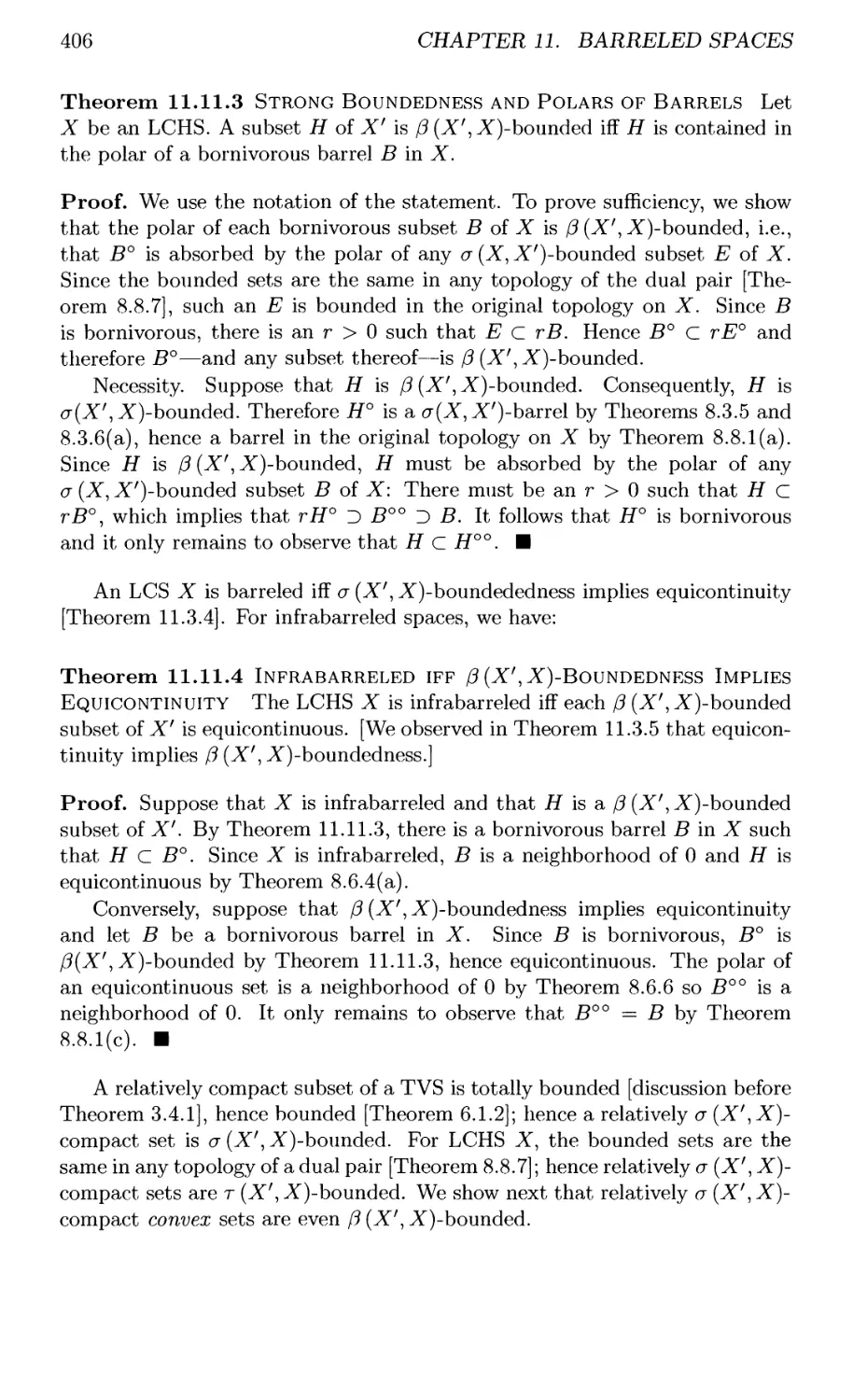
11.10 A DIVERGENT FOURIER SERIES 403
11.11 INFRABARRELED SPACES 405
11.12 PERMANENCE PROPERTIES 408
11.13 INCREASING SEQUENCES OF DISKS 413
11.14 EXERCISES 416

CONTENTS xi
12 Inductive Limits 425
12.1 STRICT INDUCTIVE LIMITS 426
12.2 INDUCTIVE LIMITS OF LCS 434
12.3 EXERCISES 435
13 Bornological Spaces 441
13.1 BANACH DISKS 441
13.2 BORNOLOGICAL SPACES 443
13.3 EXERCISES 451
14 Closed Graph Theorems 459
14.1 MAPS WITH CLOSED GRAPHS 460
14.2 CLOSED LINEAR MAPS 461
14.3 CLOSED GRAPH THEOREMS 464
14.4 OPEN MAPPING THEOREMS 466
14.5 APPLICATIONS 469
14.6 WEBBED SPACES 470
14.7 CLOSED GRAPH THEOREMS 473
14.8 LIMITS ON THE DOMAIN SPACE 476
14.9 OTHER CLOSED GRAPH THEOREMS 477
14.9.1 Webs without Convexity Conditions 479
14.10 EXERCISES 479
15 Reflexivity 485
15.1 REFLEXIVITY BASICS 487
15.2 REFLEXIVE SPACES 487
15.3 WEAK-STAR CLOSED SETS 491
15.4 EBERLEIN-SMULIAN THEOREM 496
15.5 REFLEXIVITY OF BANACH SPACES 501
15.6 NORM-ATTAINING FUNCTIONALS 503
15.7 PARTICULAR DUALS 505
15.8 SCHAUDER BASES 508
15.9 APPROXIMATION PROPERTIES 515
15.10 EXERCISES 516
16 Norm Convexities and Approximation 519
16.1 STRICT CONVEXITY 520
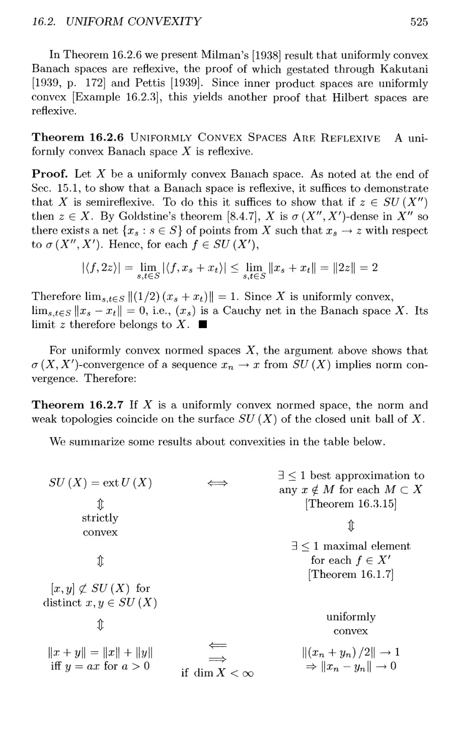
16.2 UNIFORM CONVEXITY 523
16.3 BEST APPROXIMATION 526
16.3.1 Best Approximation in C(T,F, IHI^) 534
16.4 UNIQUENESS OF HB EXTENSIONS 536
16.4.1 Dominated Extensions 536
16.4.2 Norm-Preserving Extensions 538
16.4.3 HB-Subspaces 541
16.5 STONE-WEIERSTRASS THEOREM 544

xii CONTENTS
16.6 EXERCISES 549
Bibliography 555
Index 591

Preface to This Edition
How is this edition different from the first? Aside from a great deal of
rewriting and rearrangement, we have included much more on the Hahn-Banach
theorem, e.g., its connection with the axiom of choice, uniqueness of Hahn-
Banach extensions, things like that. There is a whole new chapter on vector-
valued Hahn-Banach theorems and an enlarged presentation of the Banach -
Stone theorem. We discuss different approaches to Banach-Stone as well as
such variants as vector-valued versions. Since mathematics is done by
mathematicians, we have included a couple of stories, some heart-throbbing, about
them—Eduard Helly, for example. Helly proved the first Hahn-Banach
theorem and he did it in a more flexible manner than Hahn or Banach. (And
each of thein relied on what Helly had done.) Instead of reducing the complex
case to the real one, Helly's geometric approach treats the real and complex
cases simultaneously. The technique was resuscitated in the 1970s and proved
very effective in the investigation of vector-valued Hahn-Banach theorems. In
Section 11.1 we discuss the Scottish Cafe, the cafe in Lwow (Poland, then,
Ukraine now) where Banach and many others regularly gathered in the
twilight interval between the conflagrations. When these young mathematicians
first gathered there, there were no normed spaces, only collections of functions,
sequences, etc., with various specific metrics that we call "norms"today. They
(and others) recognized the features that united them and forged functional
analysis. In so doing, they eliminated a lot of context-specific clutter. The
perspicacity of that hardy group was commensurate with their curiosity but
they were in the wrong place at a terrible time. Amidst the slaughter of many
of his closest friends, including his thesis advisor, Banach survived the war,
but barely. The university was closed, as were all universities in Poland,
during the Nazi occupation. Officially reclassified as "subhuman," he spent the
lean years feeding lice with his own blood at a bacteriological institute while
living with the constant terror, including a stint in jail. The privations took
their lethal toll and Banach died in August 1945.
We must thank Albrecht Pietsch [2007] for his sparkling history of
Banach spaces. We have generously helped ourselves to this trove of remarkable
scholarship.
We assume that you, the reader, will not read this book from page 1, that
you will dip into it from time to time. Therefore we do not assume familiarity
xin

XIV
PREFACE TO THIS EDITION
with our (pretty standard) notation and often repeat it to minimize visits
to the index. The index is quite detailed—see the entry for continuity, for
example—and should simplify the searching process.
We dedicate the volume to you, our fellow mathematicians, with a little
extra for the many, many good friends we've made at conferences over the
years. We raise our glasses (not H2O) to you.
Lawrence Narici
Edward Beckenstein

Preface to First Edition
Functional analysis started as a fusion of algebra and metric topology. With
the accretion of general topology in the 1930s, it evolved from being the
theory of Banach spaces to the theory of topological vector spaces (TVS)—not
arbitrary TVS really, but a special kind introduced by von Neumann called
locally convex spaces (LCS). (von Neumann, incidentally, called them convex
spaces.) They are mostly what this book is about. The feature that makes
them relatively more attractive is their good supply of continuous linear func-
tionals. It becomes possible to study a LCS X with the aid of its "dual space"
X' of continuous linear functional. Some things—the class of closed convex
sets, for example—can be freed from the topology on X and viewed strictly as
attributes of the "dual pair" (X, X'). These and others of the pioneering
discoveries of Mackey are the subject matter of Chapter 8. Interestingly enough,
some things whose discovery was strongly tied to duality theory, hence to
LCS, are proving to be true in general TVS (compare Exercise 11.201 with
the results of Chapter 11, for example), although they must be argued
differently. In any case, we hardly touch on that delightful turn of events; a source
that does is Adasch et al [1978].
This book is addressed to a mythical creature, known as The Beginner:
he knows and likes general topology rather well, likes to see it used to prove
things, and is delighted by the ingenuity of its quirky counterexamples; he
knows and likes linear algebra after deducting those hideous calculations with
matrices, but does not know anything about TVS; he likes concrete examples
and do-able exercises. The detail presented should make for easy digestibility
though, of course, some chewing will be required.
The exercises are divided into 100- and 200-level categories. The 100-level
ones are meant to be fun. The 200-level ones possess some combination of
the following attributes; harder, longer, tangential. Some of them are mini-
subjects. Hints for selected exercises are given on the page right after the
200-level ones. What is a hint? Sometimes a word, sometimes "Use theorem
so-and-so," sometimes not a hint at all, but the whole argument, occasionally
reference to another source. We separated them from the exercises proper to
discourage premature peeking, but of course we mean them to be used. We
are undoubtedly guilty at times of (a) saying too much, (b) saying too little,
and (rarely, we hope) (c) pointing you in the wrong direction. In no case (well,
xv

XVI
PREFACE
maybe one) does a subsequent result depend on an exercise. Most theorems
and exercises have a "headline" to facilitate scanning.
A TVS is a topologized vector space in which the vector operations of
addition and scalar multiplication are continuous. Before looking at them per
se, we consider commutative topological groups. In other words, we postpone
investigation of the effect of scalar multiplication. We can dispatch metriz-
ability and completeness in this context since neither of them depends on
scalar multiplication. (No knowledge of uniform spaces is assumed or used,
incidentally.)
Topological groups are very localized things. If you know the topological
contours around 0, you know them everywhere: there is a homeomorphism
mapping any point of a topological group into any other point. For this reason
we spend considerable time developing the properties of the neighborhoods of
0.
We get to TVS proper in Chapter 4. A significant difference between
topological groups and TVS (over R or C) is that TVS must always be connected
topological spaces. Thus the discrete topology is a group topology but is never
(except for the vector space consisting only of 0) a vector topology. While
touching on the subject of separation, let us mention that we do not routinely
require Hausdorff separation. We have tried to assume it only when needed,
although it can definitely be removed in some spots.
By Chapter 5 we have arrived in the locally convex space, the territory in
which we remain for the rest of the book. A locally convex space is a TVS
in which each neighborhood of 0 contains a convex subneighborhood of 0.
Even though that is correct, and the way a topologist might define it, locally
convex spaces do not usually arise by specifying their neighborhoods; rather,
they come equipped with a collection of seminorms. They are then endowed
with the weakest topology that makes all the seminorms continuous.
A seminormed space is a TVS whose topology is defined by one seminorm.
A subset of a seminormed space is bounded if it is contained in all sufficiently
large multiples of the unit ball U. We say that a subset of a TVS is bounded
if it is contained in all sufficiently large multiples of any neighborhood U of
0. (As we show in Chapter 6, this is a stronger notion than that of metric
boundedness.) If one has some acquaintance with normed spaces, there may
be an expectation that neighborhoods of 0 in a general TVS are bounded.
Not so. If there is so much as one bounded neighborhood of 0, the space is
pseudometrizable; if there is a bounded convex neighborhood of 0, the space
is seminormable.
As the four basic principles of functional analysis, we take the Hahn-
Banach, Banach-Steinhaus, Krein-Milman, and closed graph theorems. In
presenting the Hahn-Banach theorem we proceed by way of sublinear func-
tionals. The basic idea is that a sublinear functional squashes down to a linear
one. More precisely, a sublinear functional is linear if and only if it is a
minimal element in the class of sublinear functional [with respect to the ordering
/ < g iff f(x) ^ g(x) for all x] The problem of continuously extending a con-

PREFACE
xvn
tinuous linear map on a normed space into another normed space, rather than
the underlying field, is probed in Chapter 10 where we present the solution
obtained by Nachbin and Goodner. Kelley's finishing touch appears in Sec.
10.7, after extreme points have been introduced.
The Banach-Steinhaus theorem or principle of uniform boundedness
asserts that, under certain conditions, a family of continuous linear maps which
is bounded at each point of the (common) domain is uniformly bounded. The
class of domain LCS for which the principle obtains is the class of barreled
spaces, the subject of Chapter 11. For the sake not of The Beginner, but
the Journeyman, we mention that Webb's recent proof of the barreledness of
subspaces of countable codimension of barreled spaces appears in Sec. 11.12.
(The result was discovered independently by Saxon and Levin and Valdivia
earlier; a word of thanks to Steve Saxon here for apprising us of Webb's proof.)
The Krein-Milman theorem appears in Chapter 9. The theorem extends
an old result of Minkowski's. An "extreme point" is a generalization of the
notion of vertex of a convex polygon. Minkowski proved that a convex polygon
in euclidean n-space can always be recovered as the convex hull of its vertices.
The Krein-Milman theorem is an infinite-dimensional version. It says that
a convex compact subset of a locally convex HausdorfF space may always be
reconstituted as the closure of the convex hull of its extreme points. Thus the
points of the original set may be approximated by the points of the convex hull
of the extreme points in this case. An area opened up by the Krein-Milman
theorem is Choquet theory. We give a brief introduction to it in Sec. 9.5.
Conditions under which a linear map with a closed graph is continuous
are the focus of Chapter 14. We introduce webbed spaces (a slightly simpler
version of them than de Wilde used) for the sake of proving that a closed linear
map of an inductive limit of Banach spaces into a webbed space is continuous.
Aside from its uses in solving some very practical problems, webbed spaces
are already as permanent a fixture in functional analysis as barreled and
bornological spaces are.
We started this book in 1969 and it would have been done much sooner if
the chapter on topological algebras had not become so bloated that it became
a separate book. There have been many people who have been helpful along
this long road. Charles SufFel, although he has left this lovely land for the far
shores of graph theory (something about connecting dots by lines, we believe),
was a willing listener to many a late-night paradox. Donald McCarthy, despite
the trauma induced by computer miasma, helped a lot in the daytime. Jean
Schmets read chunks of the book, as did Marc de Wilde (another casualty in
our ranks). Seth Warner gave us the benefit of his mighty erudition and so did
Aaron Todd. Thanks are also due to Milos Dostal. More generally, thanks are
due to Bourbaki, Kothe, Kelley and Namioka, and many, many others whose
great works created and communicated this magnificent subject.
Lawrence Narici
Edward Beckenstein

Chapter 1
Background
1.1 TOPOLOGY
1.1.1 Closure and Interior
1.1.2 Filterbases and Nets
1.1.3 Compactness
1.2 VALUATION THEORY
1.3 ALGEBRA
1.4 LINEAR FUNCTIONALS
1.5 HYPERPLANES
1.6 MEASURE THEORY
1.7 NORMED SPACES
1.7.1 Inner Product Spaces
With the exception of Sees. 1.4 and 1.5 on linear functional, we list some
terms and notations here for the sake of definiteness.
R and C denote the real and complex numbers with their usual topologies.
F stands for either, without specifying which. R+ denotes the positive real
numbers. Q, N, and Z denote the rationals, positive integers, and integers,
respectively. "Iff' stands for if and only if. "Almost all" means "for all but a
finite number." The end of proofs, examples, etc. is marked with a ■.
1.1 TOPOLOGY
Let T be a set. A map d : T xT ^ [0,oo) such that d(s,t) = d(t,s) and
d (,s, u) < d (s, t) + d (t, u) (the triangle inequality) for all s, £, u G T is a
pseudometric. (T, d) is a pseudometric space. A topological space whose topology
is determined by a pseudometric is called pseudometrizable. If d (s, i) = 0
1

2
CHAPTER!. BACKGROUND
implies that s = t then d is a metric. If (T, d) is a pseudometric space then
the relation 5 ~ t iff d(sit) = 0 is an equivalence relation on T and the set
of equivalence classes T/d is a metric space with respect to d~ where, for
s~,t~ G T/d, d~ (.s~,*~) = d(s,£) for any s G s~,and t e r. If the
pseudometric d satisfies d(s,u) < max [d(s, £) ,d(£, u)] (the strong or ultrametric
triangle inequality) for all ,s,£,?i G T, d is an ultrapseudometric and (T, d)
an ultrapseudometric space; similar meanings attach to ultrametric and ultra-
metric space. If d is a pseudometric on a set T, the closed and open balls of
radius r > 0 about £ G T are denoted, respectively, as
C{t, r) = {seT : d(s, *) < r} and B(J, r) = {5GT: d(s, *) < r}
Most of the topologies encountered in the theory of topological vector
spaces are defined by specifying neighborhoods of 0 rather than open sets.
We do not require that a neighborhood of a point be an open set: we say that
V is a neighborhood of t if V contains an open set to which t belongs.
The discrete topology on T is the one in which all subsets are open; the
trivial topology is {0,T}.
1.1.1 Closure and Interior
An adherence point t of a subset A of a topological space T is a point whose
every neighborhood meets (i.e., has nonempty intersection with) A. The set
cl A of adherence points of A is the closure of A. If S is a topological subspace
of T and A is a subset of 5, then cls A denotes the closure of A computed in
S. We say that t is an interior point of A if A contains a neighborhood of t.
The set int A of interior points of A is called the interior of A; for a subspace
S of T, ints A denotes interior points of A computed in S.
1.1.2 Filterbases and Nets
We deal with convergence through the use of nets and filterbases (rather than
filters). We discuss some facts and properties of nets and filterbases in this
section; for more information, Dugundji [1966] is an excellent source.
A collection B of nonempty sets such that the intersection of any two of
them contains another from B is called a filterbase.
Definition 1.1.1 Cluster Points and Limits Let B be a filterbase of
sets from a topological space T. (a) Limits We say that t is a limit of B (B
converges to t), B —> t, if for any neighborhood V of t there is some B e B
such that B C V. The set of limits of B is denoted lim B.
(b) Cluster Points We say that t is a cluster point of B if each
neighborhood of t meets each B in B. We denote the (closed) set of cluster
points by cl B. ■
Evidently:

1.1. TOPOLOGY
3
Theorem 1.1.2 Given a filterbase B (a) clB = n {c\B : B G B} ;
(b) limits are cluster points;
(c) if T is Hausdorff, then limits of filterbases are unique.
Example 1.1.3 Filterbases (a) Given a sequence (£n), the "tails" Bn =
{tj : j > v,}, n G N, of the sequence (tn) form a filterbase called the Frechet
or elementary filterbase associated with (tn). Clearly, (Bn) —» t iff tn —» £.
(b) For any filterbase # and any map /, / (#) is a filterbase; f~l (B) is a
filterbase iff 0 i f~l [B)
(c) The collection V (t) of all neighborhoods of an element t of a
topological space forms a filterbase called the neighborhood filter of t. Generally, a
filterbase B with the property that any superset of a member of B is also in
B is called a filter—hence neighborhood filter rather than filterbase. The
collection T (B) of supersets of the sets of a filterbase B is a filter called the filter
generated by B. The neighborhood filter V (t) of a point t obviously converges
tot.
(d) Trace If B is a filterbase and A is a set such that A D B ^ 0 for each
B e B then {B D A : B G B} is a filterbase called the trace of B on A.
(e) If A and B are filterbases such that A D B ^ 0 for each A e A and
J5 G B, then .4nB={j4n£:,4e.4,£eS}isa filterbase.
(f) In the complex plane, the collection of disks C (0, n) — {z £ C : \z\ < n} ,
n G N, is a filterbase which has no limit. ■
If <S is a collection of sets that satisfies the finite intersection condition
(i.e., the intersection of any finite number of them is nonempty), then the
collection forms a filter subbase; the collection of finite intersections of sets
from a filter subbase is the filterbase generated by S.
Subordinate filterbases are the analog of subsequences. Given filterbases A
and B, we say that B is subordinate to A, B < A, if each A in A contains some
B in B. Given a subsequence (tnk) of a sequence (in), the Frechet filterbase
B of (tnk) is subordinate to the Frechet filterbase A of (tn).
Convergence and continuity may be described by subordination as follows:
Theorem 1.1.4 Convergence and Continuity Let S and T be
topological spaces and let V (p) denote the neighborhood filter of a point p. Let
/ :S -► T. Then: (a) B -► s iff B < V (s);
(b) / is continuous at s G S iff / (V (*)) < V (/ (s));
(c) / is continuous at s G 5 iff for any filterbase B, B —> s => / (#) —►
We note that subordination is not antisymmetric: A < B and B < A does
not imply that A = B. If B is such that for any filterbase A, A < B implies
that B < A, then B is called a maximal filterbase. A straightforward Zorn's
lemma argument shows that given any filterbase, there is a maximal filterbase
subordinate to it. A useful characterization of maximal filterbases is the
complement condition of Theorem 1.1.5.

4
CHAPTER 1. BACKGROUND
Theorem 1.1.5 Complement Condition A filterbase B in a set T is
maximal iff for any subset A of T either A contains an element of B or the
complement CA of A contains an element of B.
Proof. Let B be a maximal filterbase. Given a set A, either B C A for
some B G B or B D CA ^ 0 for all B G B. In the latter case, the trace
A — \B D ZA : B G B} of B on CA is a filterbase which is clearly subordinate
to B. By the maximality of B, B < A. Hence for any B G B, there must be a
D G B such that D C BdCAcCA.
Conversely, suppose that the condition holds on B and that A < B. Let
A G A. By the condition there exists B G B such that B C A or B C CA If
£? C Ct4 then, since A < B, there must be some A! G A such that Ar C £?,
hence the contradictory result that two elements of A do not meet. Therefore
there must exist B <G B such that B C A, i.e., B < A. ■
Theorem 1.1.6 CONVERGENCE IN PRODUCTS Let {Ts : s G S} be a family
of topological spaces and let T = YlseS Ts denote their Cartesian product
endowed with the product topology. Let prs denote the projection of T onto
Ts. For any filterbase B in T, B —> t iff prs (B) —> prs (t) for every s £ S.
Proof. Let t = (t8) eT.UB-+t then prs (B) -► pr5 (*) for every s e S by the
continuity of projections and Theorem 1.1.4(c). Conversely, suppose that for
all ,s <G 5, pr5 (#) —► pr5 (^) = ^5. We show that B -± t. A basic neighborhood
of t is of the form U — H^L^r"1 (V^7) where VSi is a neighborhood of tSi in T5.,
i = 1,2,..., n. Since each prs (B) —> ts, each filterbase prs (B) is subordinate
to the neighborhood filter V (ts) in T5. Therefore each V^z contains some
prSi (B7), Si g B. It follows that B* C pr"1 (F5J for i = 1,2,..., n. Since B
is a filterbase, there is some B e B such that B C C\^=1Bi C fl^^r"1 (V^J .
■
Definition 1.1.7 Directed Sets and Nets A set M together with a
reflexive, transitive ordering relation < such that finite subsets of M have
upper bounds in M is called a directed set. A net in a topological space T is
a mapping rn i—> tm from the directed set M into T; we usually write (tm) or
{£m : m G M} . We say that tm converges to i, tm —> ^, (^ is a /imzi of (im)) if
for any neighborhood V of t there is an mo € M such that tn G V for n > mo-
This is also expressed by saying that tm is eventually in any neighborhood of
t. The set of limits of (tm) is denoted limim. We say that t is a cluster point
of {tm) if £ is frequently in any neighborhood V off, i.e., for any m G M there
exists n > m such that fn G V. The set of cluster points of (tm) is denoted
cl(*m). ■
In a first countable space, i is a cluster point of a sequence (tn) iff a
subsequence of (tn) converges to t.
As the proofs are widely available, we omit the details of showing that
nets are topologically equivalent to filterbases in the sense that, given any net

1.1. TOPOLOGY
5
(tm), there is a filterbase B with the same cluster points and limits as (tm)
and vice-versa.
Theorem 1.1.8 Equivalence of Nets and Filterbases Let T be a
topological space, (a) net to filterbase Let {tm : m G M} be a net in T. For
each rn G M, let Bm = {tn : n > m}. The collection B = {Bm : m G M] is a
filterbase for which c\B = cl (£m) and lim# = lim£m.
(b) filterbase to net Let B be a filterbase in T. The set M of ordered
pairs (6, S) with B e B and 6 G S ordered by taking (a, .A) < (6, S) if S C A
(a e A e B) is a directed set and the map M —> T, (6, jB) i—>• 6, is net with the
same cluster points and limits as B.
We will frequently use the net characterization of continuity of Theorem
1.1.9.
Theorem 1.1.9 Nets and Continuity Let S and T be topological spaces.
A map / : S —> T is continuous at s G S iff for any net sm —» «s, / (,sm) —> f (s).
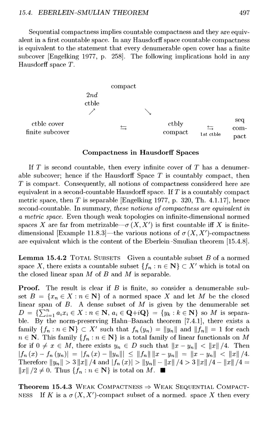
1.1.3 Compactness
A topological space T is compact if every open cover has a finite subcover. T
is:
(a) locally compact if each point in T has a neighborhood whose closure is
compact;
(b) sequentially compact if each sequence has a convergent subsequence;
(c) countably compact if every sequence has a cluster point (meaning that
the sequence frequently enters any neighborhood of the point); this is
equivalent to requiring that every countable open cover has a finite
subcover or that every infinite subset S C T has a limit point t G T
(neighborhoods of t contain infinitely many points of S). Note also
that although sequential compactness implies countable compactness,
the converse is false. Indeed, the Stone-Cech compactification /3N of
N is compact but not sequentially compact: there are no nontrivial
convergent sequences in /3N [Engelking 1977, p. 229].
(d) a-compact if it can be written as a countable union of compact sets;
(e) Lindelof if every open cover contains a countable subcover;
(f) pseudocompact if every real-valued continuous function on T is bounded;
(g) hemicompact if there is a countable family (Kn) of compact subsets of
T such that each compact subset of T is contained in one of them;
(h) a subset of T is relatively compact if its closure is compact.

6
CHAPTER!. BACKGROUND
If a set is both open and closed, we call it clopen. If T has a base consisting
of clopen sets, we call it 0-dimensional. If there is a countable base for the
topology, T is second countable; if there is a countable neighborhood base at
each point, then T (or its topology) is first countable. If T has a countable
dense subset, T is separable.
Our conventions about separation are:
(a) Hausdorff if distinct points are separated by open sets, i.e., for
distinct s,t £ T, there exist disjoint neighborhoods U and V of s and
i, respectively.
(b) regular if it is Hausdorff and points and closed sets are separated by
open sets, i.e., for a point s e T and a closed subset F C T to which s
does not belong, there exist disjoint open subsets U, V of T with s G U
and F C V. T is ultraregular if points and closed sets are separated by
clopen sets.
(c) completely regular if it is Hausdorff and for any point t eT and closed
subset F C T to which t does not belong, there exists a continuous map
/ : T -+ [0,1] such that / (t) = 0 and / (F) = {1}.
(d) normal if it is Hausdorff and disjoint closed sets are separated by open
sets. T is ultranormal if disjoint closed sets are separated by clopen sets.
Theorem 1.1.10 Compactness Let T be a topological space.
(a) A cluster point of a maximal filterbase M. is a limit.
T is compact iff either of the following conditions holds:
(b) every filterbase has a cluster point (equivalently, each net has a
convergent subnet);
(c) every maximal filterbase converges.
Proof, (a) Let t be a cluster point of the maximal filterbase M and let V
be a neighborhood of t. Since M. is maximal, there is some M £ Ai such
that M C V or M C CV. Since t is a cluster point of M, M must meet V so
MC V.
(b) Let T be compact and let B be a filterbase on T. The collection
{c\B : B G B} is a collection of closed sets that satisfies the finite
intersection condition. Hence, by the compactness of T and Theorem 1.1.2(a),
D {c\B : B e B} = c\B ^ 0. Conversely, let B be a collection of closed sets
that satisfies the finite intersection condition so that they form a filter sub-
base. The filterbase T generated by B has a cluster point by hypothesis so
0 7^ Dj7 C C\B and T is compact. For the assertion about nets, we refer to
Kelley 1976, p. 136.
(c) Suppose that T is compact and M is a maximal filterbase. M has a
cluster point by (b) which is a limit by (a). Conversely, suppose that B is a
filterbase. Using a Zorn's lemma argument, there exists a maximal filterbase

1.2. VALUATION THEORY
7
A subordinate to B [Dugundji 1966, p. 219]. By hypothesis, A has a limit t
so any neighborhood V of t must contain some A € A. For B e B there exists
Ar e A such that A'cBso0^AnA'cVr)B and t is a cluster point of
B. The compactness of T now follows from (b). ■
1.2 VALUATION THEORY
In the body of the text all vector spaces are real or complex but we sometimes
indicate what happens if the underlying field is not R or C but a field K with
an absolute value defined on it.
A map |-| of afield if into [0, oo) such that \ab\ = \a\ \b\ and \a + b\ < |a| + |6|
for all a,b e K and which is 0 only at 0 is called an absolute value or valuation
on K. If, in addition, \a + b\ < max(|a|,|b|) for all a,b G K (the strong or
ultrametric triangle inequality), then the valuation is called non-Archimedean
or an ultravalue. (The reason for the term non-Archimedean is that a valuation
is non-Archimedean iff there is some real number M such that \n\ < M for
all "integers" n in K; compare that to the "Archimedean" ordering of the
real numbers.) The pair (K, |-|) is called a valued field or ultravalued field if
|-| is an ultravalue. A valued field is always assumed to carry the topology
induced by the metric d(a,b) = \a — 6|, with respect to which, incidentally,
addition and multiplication are continuous operations. If the valuation is
non-Archimedean, then K is 0-dimensional, as we now show.
Theorem 1.2.1 Non-Archimedean Properties Let (K, | • |) be an ultra-
valued field. Then:
(a) If \a\ > |6|, then \a + 6| = \a\.
(b) Any point b in a closed ball C(a, r) = {c € K : \a — c\ < r}, r > 0, is
a center, i.e., C(a,r) = C(b,r); the same is true for open balls.
(c) If two balls, open or closed, meet, then the one of smaller radius is
contained in the one of larger radius.
(d) K is 0-dimensional.
Proof, (a) If \a\ > \b\, then \a 4- 6| < \a\. If the latter inequality is strict then
\a\ = \a + b — b\ < max (\a + b\ , |6|) < \a\; this contradiction yields the result.
(b) Suppose b e C (a, r). If c e C(b, r) then \c-a\ = \c-b-\-b - a\ <
max(|c — /;|, \b — a\) < r, so c G C(a,r); hence C{b,r) C C(a,r). The same
argument establishes the reverse inclusion.
The result for open balls is proved in the same way.
(c) We prove only the statement for open balls. Suppose that 0 < r < t
and that c e B(a, r) n B(b, t). By (b), then B(c, r) C B(c, t) = B(b, t).
(d) We show that each open ball B(a,r), r > 0, is closed. We effect
this by showing that if b £ B(a,r) and 0 < t < r, then B(b,t) n B{a,r) =
0. Indeed, by (c), if B(b,t) n B(a,r) ^ 0, then B(b,t) C B(a,r) which
contradicts b £ B(a,r). To see that closed balls C(a,r) are clopen, note that
C(a,r) = U {B(6,r) : b e C(a,r)} by (b). ■

8
CHAPTER!. BACKGROUND
Example 1.2.2 VALUATIONS (a) [Bachman, 1964, p. 127] The usual
absolute value |-| on R or C is a valuation which is Archimedean, i.e., not non-
Archimedean. Any field K with an Archimedean valuation is field-isomorphic
to a subfield of C and the valuation on K, viewed as a subfield of C, is a
power |-|r , r > 0, of the usual absolute value |-| on C.
(b) Trivial Valuation On any field K the map sending each nonzero
element into 1 and 0 into 0 is a non-Archimedean valuation called the trivial
valuation. It induces the discrete topology. Its exclusion is marked by an
expression such as "let Kbea nontrivially valued field."
(c) p-ADic Valuation Let p be a positive prime. Any rational number x
can be written in the form pk (a/b) (a, 6, k £ Z) where p is not a factor of a or
b. The p-adic valuation \x\ of x is p~k and is non-Archimedean. The metric
completion Qp. of the rationals ( Q, |-| J is called the p-adic numbers. ■
For more on valuation theory, see Bachman [1964] and Mahler [1973].
1.3 ALGEBRA
Except for a few exercises, when we say vector space (or linear space) we
mean real or complex vector space. When we say subspace of a vector space,
we mean linear subspace, i.e., one which is closed under addition and scalar
multiplication. A linear map A : X —> Y of a vector space X into a vector
space Y is such that for all a, b € F = R or C and .x, y £ X, A (ax + by) =
aAx 4- bAy; if Y = F, we call A a linear functional. A linear or vector
isomorphism is a 1-1 linear map—it does not have to be onto; if A is onto,
then X and Y are (linearly) isomorphic.
We deal with vector spaces of F-valued functions x, y,... on some set T
with respect to the pointwise operations, i.e., for each t e T, (x + y)(t) =
x(t) + y(t) and (ax)(t) = ax(t) for any scalar a.
The (linear) span of a set E of vectors is denoted [E]. To say that E spans
the vector space X means that [E] = X. A Hamel base for a vector space X is
a maximal (with respect to set inclusion) linearly independent set B of vectors
(or a minimal spanning set). A Hamel base (or basis) must exist in any vector
space X (Zorn's lemma) and necessarily spans the space. The dimension of
a vector space is the cardinality of any Hamel base. The algebraic dual X*
of X is the linear space (pointwise operations) of all linear functional on X.
Concerning the size of X*:
Theorem 1.3.1 Dimension of X* [Jacobson, 1953, p. 247]. If the
vector space X is finite-dimensional, then dimX = dimX*. If X is infinite-
dimensional, dimX = b say, then dimX* = c6, where c denotes the
cardinality of F = R or C, i.e., the power of the continuum. Hence, for infinite-
dimensional spaces X, dimX* > dimX.

1.4. LINEAR FUNCTIONALS
9
The space described in Example 1.3.2 is of denumerable dimension and is
useful in some counterexamples in the text.
Example 1.3.2 Space (p of Finite Sequences The linear (pointwise
operations) space of sequences (an), an G F, which are 0 eventually is denoted
{p. We often call it the space oi finite sequences. It is isomorphic to the space
F[.x] of polynomials in one indeterminate x with coefficients from F. That it
is of denumerable dimension can be seen by considering the Hamel base of
standard basis vectors {en : n G N} where en is the sequence with 1 at the
nth position and O's everywhere else. ■
Definition 1.3.3 Algebra Let X be a vector space over F. If there is
a multiplication (indicated by juxtaposition) defined between elements of X
which is associative and distributive (x(y + z) = xy + xz) then X is a an
algebra] if xy = yx for all x,y G X, then X is commutative. An element
e G X such that ex = xe = x for all x G X is an identity for X. If X and Y
are algebras over F and A : X —> Y is a linear map for which, for all x,y G X,
A (xy) = Ax Ay then A is an algebra homomorphism or just a homomorphism
or a multiplicative linear map; if A is 1-1, then it is an algebra isomorphism-,
if A is bijective then X and Y are algebra isomorphic. ■
An important algebra is the commutative algebra C (T, F) of continuous
maps of the completely regular space T into F; the function e : C (T, F) —►
F, t i—> 1, is an identity. There is no algebraic reason to consider apparently
more general topological spaces because of Theorem 1.3.4; the proof can be
found in Gillman and Jerison 1960 [3.9].
Theorem 1.3.4 For every topological space S there exists a completely
regular space T and a continuous mapping h : S —> T such that for every
.x G C (5, F) the composition map x i—> x o h is an algebra isomorphism
ontoC(T,F).
1.4 LINEAR FUNCTIONALS
We collect some basic facts about linear functionals here. The subspace
N{f) = /_1 (0) of vectors on which a linear functional / vanishes is called
the null space or kernel of /. Theorem 1.4.1(b) shows that null spaces are
generally very large, dimensionally speaking.
Theorem 1.4.1 The Null Space Let X be a vector space over F = R or
C and let / be a nontrivial linear functional on X with null space N. Then:
(a) / is surjective;
(b) X/N is linearly isomorphic to F; hence the codimension dimX/N of
iV is 1;
(c) for any x £ N, X = TV 0 Fx = {n + ax G X : n G TV, a G F};

10
CHAPTER!. BACKGROUND
(d) for any scalar a and any x e H = /_1(a), TV = H—x — {y—x : y G H};
(e) for any nontrivial linear functional g on X, N(f) C A/(#) iff there is
some scalar a such that g = af and iV(/) = N(g)\
(f) Let / be a linear functional on X. If gi,... ,gn are nontrivial linear
functionals on X, then C\f=1N(gi) C A/ (/) iff there are scalars ai,..., an such
that / = EiLi^t- Hence if n?=lN(gi) = {0} then, since {0} C iV (/) for
any linear functional /, {pi,... , gn} spans the algebraic dual X*.
Proof, (a) Choose a vector x such that f(x) = 1. Then, for any scalar
a, f(ax) = a.
(b) The map x + A/ i—> /(#) is an isomorphism of X/A" onto F.
(c) For any a; ^ A/ and y e X, y - (f(y)/f(x))x G N.
(d) Suppose x G H = /-1(1). Then H - x C N. Conversely, ifweN,
then w + x e H and w = w + x — x.
(e) Suppose A/(/) c A/(g). If N(f) is a proper subset of N(g), there is some
x G N(g) such that x £ N(f). By (c), therefore, X = N(f)+Fx C N(g) and p
would be 0. Hence N(f) = N(g) = N. For x £ N and p G X = N + Fx, there
exist a G F and n e N such that y = n + ax; hence p(p) = a#(:r) and
/($/) = af(x). Therefore g{y) = (f(y)/f(x))g(x) and it follows that g =
(g(x)/f(x))f. The sufficiency of the condition is obvious.
(f) If / = YJl=i ai9i then clearly n?=1N(gi) C N (/). We prove the
converse by induction on n. The result for n = 1 is (e) so we now assume that the
result holds for n — 1 and suppose that nf=lN(gi) C N(f). There is no loss
of generality in assuming that pi,... ,pn are linearly independent so we
assume that no gk can be written as a linear combination of the remaining ones;
hence, by the induction hypothesis, for each 1 < k < n, n^AT^) 't- ^(dk)
and there exist Xk G X (1 < k < n) such that gj(xk) — £7fc, 1 < j < n
(Kronecker delta). For any x G X, each gj vanishes on x — Y^k=i 9k(x)%ki i-e.,
x - ELi 9k{x)xk € nUN{gi) C N(f). Therefore / = £?=1 f(Xj)gj. ■
On any complex vector space X, there is an intimate connection between
the real and imaginary parts of a linear functional / on X, namely that
Ref{x)=Imf(ix) {x G X)
Although usually credited to F. Murray [1936], H. Lowig discovered this in
1934. Any complex vector space X can, of course, be viewed as a real one. A
linear map of X into R is then called a real linear functional or H-linear
functional on X. For emphasis we often refer to linear functionals / on X as
complex linear functionals. For each x G X, f(x) = Ref(x) + ilmf(x) and Re/
and Im / are each R-linear functionals as is trivial to verify. A surprising fact
about Re / and Im / is that Ref(ix) = — Im f(x) and Re / (x) = Im / (ix) for
every a; G X since f(ix) = Re f(ix)+i Im f(ix) = if(x) = i Ref(x) — Imf(x).
In summary:

1.5. HYPERPLANES
11
Theorem 1.4.2 Real Versus Complex Let X be a complex vector space,
let X* denote the collection of all linear functionals on X and let XR denote
the class of real linear functionals on X. Then for any / £ X* and any x £ X,
lmf(x) = — Ref(ix) = and the map / »—> Re/ establishes the following 1-1
correspondence between X* and XR:
X* *-> X*R
f (x) = Re / (x) -iRef (ix) *-> Re / (x)
Proof. For /,g e X*, if Re/ = Reg then clearly / = g. To see that the
correspondence is surjective, we show that if r £ X*R, then (its preimage)
f[x) — r(x) — ir(ix) (x £ X) is a complex linear functional. Since / is
obviously a real linear functional, it only remains to show that f{ix) = if{x).
To that end, note that f(ix) = r(ix) — ir(—x) = r(ix) + ir(x) = i(r(x) —
ir(ix)) = if (x). ■
1.5 HYPERPLANES
A maximal subspace M of a vector space X is a proper subspace not properly
contained in any proper subspace of X. Planes through the origin in R3,
for example, are maximal subspaces of R3. As shown in Theorem 1.5.1,
maxiinality of M is equivalent to M missing the dimension of X by just 1
in the sense that dim X/M = 1. A linear variety (affine subspace, linear
manifold) is a translate x + M of a subspace M. A hyperplane is a translate
of a maximal subspace.
In Sec. 1.4 we saw the close connection between real and complex linear
functionals. The development of analogous "geometric" statements about
subspaces is the subject of this section.
Theorem 1.5.1 Maximal Subspaces and Hyperplanes Let M be a
subspace of a vector space X over F = R or C. Then:
(a) M is maximal iff dim X/M = 1;
(b) M is maximal iff M = N(f), the null space of some nontrivial linear
functional / on X;
(c) a linear variety H is a hyperplane iff H = {x € X : f(x) = a} for some
nontrivial linear functional f on X and scalar a. For a/Owe may replace /
by a~lf and say that H = {x e X \ f(x) = 1}.
Proof, (a) If dim X/M > 2, there are x,y G X such that x + M and y + M
are linearly independent in X/M. Moreover, letting [ ] denote linear span,
we have the proper inclusions M £ [M, x] £ [M, x, y] and M is not maximal.
Conversely, if M is not maximal, there is a proper subspace N of X which
contains M properly; hence dim X/M > dim N/M > 1.
(b) Let / be a linear functional and let M = N (f). By Theorem 1.4.1(b),
dim X/M = 1; hence M is maximal by (a). Conversely, if M is maximal and

12
CHAPTER!. BACKGROUND
x £ M, then [M, x] = M + Fx = X. Since Mn Fx = {0}, if 2/ = m + ax (m G
M, a e F), then ra and a are unique. Defining /(?/) = / (m + ax) = a for
each |/Gl, / is a linear functional with null space M.
(c) If H is a hyperplane, then H = x + M for some ,tgI and maximal
subspace M C X. Since M is maximal, there is a nontrivial linear functional
/ on X such that M = N(f) by (b). Let f(x) = a. Clearly H C f~l (a).
As to the reverse inclusion, if / (y) = a then y — x £ M and y e H, i.e.,
Conversely, suppose if = {a; £ X : f(x) = a} for some nontrivial linear
functional / and scalar a. By Theorem 1.4.1(d), for any x G H, H — x is the
null space of / by Theorem 1.4.1(d); H — x is maximal by (b). ■
If X is a complex vector space, we say that M C X is an R- subspace if
it is closed under addition and multiplication by real scalars. An R-variety
is a translate of an R-subspace; an H-hyperplane, a translate of a maximal
R-subspace. As observed in Sec. 1.4, for any complex linear functional / on
X, f(x) — r{x) — ir{ix) (x G X) where r = Re f is a real linear functional on
X. By Theorem 1.5.1(b), the null space N(r) of 7- is a maximal subspace of
the real linear space X—in other words, a maximal R-subspace. As follows
from Theorem 1.5.2(a) below, N(f) = N(r)niN(r).
Theorem 1.5.2 Real and Complex Hyperplanes Let X be a complex
vector space. Then
(a) a subspace M of X is maximal iff there is a maximal R-subspace TV
such that M = NniN;
(b) a linear variety H is a hyperplane iff there is a maximal R-subspace
M and x, y G X such that H = (x + M) D (y + iM).
Proof, (a) If M is a maximal subspace of X, then there is a nontrivial
linear functional / on X such that M = N(f) [Theorem 1.5.1(b)]. Moreover,
with r = Re/, f(x) = r(x) — ir(ix) for every x £ X [Theorem 1.4.2]. Hence
x e M <^> f(x) = 0 <^> r{x) = 0 and r{ix) = 0
^ xG N(r) n (-ziV(r)) = N(r) n iN(r)
Conversely, if TV is a maximal R-subspace, there is a real linear functional r
whose null space is N. With f(x) = r(x) - ir(ix) (x G X), N DiN = N(f).
(b) If H is a hyperplane, then H = x + M for some xGl and maximal
subspace M. There exists a maximal R-subspace N such that M = N DiN
by (a). Thus H = x + N DiN = (x + N) D (x + iN).
Conversely, if TV is a maximal R-subspace and x, y G X, we want to show
that (x + iV) fl (2/ + 2AT) = i/ is a hyperplane. To do this, it suffices to
show that there is a complex linear functional / on X and a G C such that
H = {w G X : /(iu) = a}. Since TV is a maximal R-subspace, there is
a real linear functional r on X such that N = N(r) by Theorem 1.5.1(b).

1.6. MEASURE THEORY 13
Let / be the associated complex linear functional of Theorem 1.4.2, namely,
f(w) = r(w) — ir(iw) (w G X). With a = r(x) — ir(iy), then
f(w) = a 4=> r(w) = r(x) and r(iw) = r(iy)
<=> xv — x e N and w — y G —iN = iN
<=> w G (x + N) D (y + iN) ■
In summary, we have the 1-1 correspondences of the following diagram where
N denotes null space.
Ref(x)-iR,ef(ix) = f(x) N (f) = N (Re f) n iN (Re f)
complex linear functional <-» maximal subspace
I I
real linear functional *-> maximal R-subspace
Ref(x) N(Ref)
1.6 MEASURE THEORY
A nonempty collection S of subsets of a set S is an algebra (of sets) if S is
closed with respect to the formation of finite unions and contains the
complement of each of its members. If, in addition, it is closed with respect to
the formation of countable unions, then S is a a-algebra . A measure m is a
nonnegative function defined on a a-algebra which is count ably additive and
vanishes on the null set. We call (5, <S, m) a measure space. A property which
holds at each point of S except a set of a measure 0 is said to hold almost
everywhere (a.e.). If there is some .s G S such that m(E) = 1 if s G E and
rn(E) = 0 if ,s ^ E, then m is called a point mass.
If 5 is a locally compact Hausdorff space, the smallest a-algebra containing
the compact G^-sets (countable intersections of open sets) is called the Baire
sets. A measure m on the Baire sets which is finite on compact G^-sets is
called a Baire measure. A Baire measure is regular in the sense that if B is
a Baire set,
m(B) = sup{m(A) : B D A, A compact Gs}
= inf{m(U) : B C U, U open Baire set}
[Halmos, 1974a, p. 228]. The Borel sets are the a-algebra generated by the
compact (or open) subsets of 5. A Borel measure rn is a measure defined on
the Borel sets which is finite on compact sets. A Borel measure is regular if,
given any Borel set E,
m(E) = sup{m(K) : E D K, K compact} = inf{m(U) : E C U, U open}
Unlike Baire measures, Borel measures do not have to be regular. A regular
Borel measure m on S such that m(S) = 1 is called a probability measure.
For more on measure theory, see Halmos [1974a] and Dunford and Schwartz
[1958].

14
CHAPTER 1. BACKGROUND
1.7 NORMED SPACES
Let X be a vector space over a valued field (K, |-|). A seminorm p on X is a
nonnegative map of X such that p(ax) = |a|p(x) and p(.x + y) < p(x) + p(y)
for all x,y G if and all a G if. (-X",p) is called a seminormed space. If
p(x) = 0 only when x = 0, then p is a norm and (X,p) is a normed space.
The symbol || • || is reserved for norms. If K is ultravalued and the norm
satisfies ||x + it/|| < max[||x||, \\y\\] for all x,y G X, then ||-|| is called a non-
Archimedean norm or an ultranorm and (X, ||-||) is called a non-Archimedean
normed space or ultranormed space. If we say simply normed space we always
mean that K = R or C. Seminormed spaces (X,p) are always assumed to
carry the topology determined by the pseudometric d(x,y) — p(x — y). It is
trivial to verify that N = p~] (0) is a linear subspace. If a normed space is
complete in the sense that every Cauchy sequence converges, then X is called
a Banach space. A linear map A : X —► Y between normed spaces X and
Y such that ||Ax|| = ||x|| for each x G X is called a linear isometry or norm
isomorphism-, If A is bijective, then X and Y are linearly isometric or norm
isomorphic and X and Y are norm isomorphs of each other. Although we
do not do it, the reader should be aware that in Banach space theory it is
commonly said that two Banach spaces X and Y are "isomorphic" when they
are linearly homeomorphic and that isometry usually means linear isometry.
Except in a few exercises, "vector space" means real or complex vector
space from this point on.
Two norms || • || and || • ||* on a vector space X are equivalent if they
determine the same topology.
Theorem 1.7.1 EQUIVALENT NORMS The norms || • || and || • ||* on the
vector space X are equivalent iff there exist positive numbers a and b such
that a \\x\\ < \\x\\* < 6||x|| for every x in X.
Proof. Let U and U* denote the closed solid unit balls {x G X : ||x|| < 1} ,
etc., determined by ||-|| and ||-||*, respectively. If the condition is satisfied and
x eU, then x/b G U*, i.e., (l/b)U C C/*, so U* is a ||-||-neighborhood of 0.
Similarly, U is a ||-^-neighborhood of 0. Conversely, suppose that ||-|| and
||-||* determine the same topology. Then U* is a ||-||-neighborhood of 0, i.e.,
for some a > 0, all C U*. Hence, for any nonzero x, \\ax/ ||x||||* < 1 or
||#||* < (Va) llxll • The other inequality is obtained similarly. ■
A result subsumed by Theorem 4.10.3(b) is the following:
Theorem 1.7.2 All norms are equivalent on a finite-dimensional space.
If X is a normed space, its continuous or topological dual (or conjugate) is
the linear space X' (pointwise operations) of all continuous linear functionals
on X. X' is a Banach space with respect to the canonical norm
H/ll =sup{|/(x)|: |N| <1}

1.7. NORMED SPACES
15
Whenever we speak of X' as a normed space, it is always with respect to
this norm. Likewise, when we consider X" — {Xf)', we assume it carries its
norm topology and call it the bidual of X. Every element x e X determines
a continuous linear functional on Xf, namely Jx : X' —► F, / i—> f(x). The
map J : X —> Xn', x j-» Jx, is called the canonical embedding and is a linear
isometry of X into X" [Theorem 8.4.5(b)]. If J(X) = X"', then X is said to
be reflexive, a topic we take up at length in Chapter 15.
Notation. For any normed space X, U (X) denotes the (closed, solid) unit
ball {x e X : ||z|| < 1} of X; SU (X) denotes {x e X : ||z|| = 1} , the surface
of the unit ball. ■
Some Banach spaces (see Dunford and Schwartz 1958 for the verifications)
are listed below.
Example 1.7.3 £p (n), l<p<oo,neN, denotes the Banach space Fn of
?vtuples (x(i)) normed by the p-norm
(x(i)
X>wr
i=\
1/P
We call || • ||2 the Euclidean norm. To restrict consideration to real n-tuples
(x (i)), we write (^ (??,). ■
Example 1.7.4 £p, 1 < p < oo, is the Banach space of all pth power
summable sequences x = (x (n)) (i.e. J2neN \x (n)\P < °°) of elements of
F, normed by ||.t|| = (]CneN \^{^)\V)l^v < oo. We denote real pth power
summable sequences by £^. ■
Example 1.7.5 Bounded Functions and Sequences 4o (T) denotes the
Banach space of all bounded F-valued function x on a set T with sup norm:
IMIoo = snPteT \x Ml '■> ^S) (D or ^oo (T, R) denotes bounded real-valued
functions. With T = {1,... ,n} or N we write f,^ (n) or £oo, respectively, the
spaces of ?vtuples or bounded scalar sequences. ■
Example 1.7.6 Convergent and Null Sequences Thesymbol (c, IHI^)
= c represents the Banach subspace of ^oo [Example 1.7.5] of all convergent
sequences (x (?i)) from F; Co = {(x (??,)) e c : x (n) —> 0} is the Banach subspace
of all null sequences. ■
Example 1.7.7 Continuous Functions C([a,6],F, IHI^) or just C[a,b]
stands for the linear space of all continuous F-valued maps of the closed
interval [a, b] . It becomes a Banach space when endowed with the sup norm:
IMIoo = sup \x[a, b}\ for x e C[a, b}. C (T, F) denotes the linear space of
continuous functions on the topological space T. If T is a compact Hausdorff space

16
CHAPTER 1. BACKGROUND
and C (T, F) is normed by H^H^ = sup \x (T)|, it is a Banach space; we denote
it by C (T, F, IHI^). For an arbitrary topological space T, if x G C (T, F) is
such that for any r > 0 there is a compact subset K of T such that \x (t)\ <r
for all t G ZK, we say that x vanishes at infinity. We denote the linear
subspace of C (T, F) of such functions by C^ (T, F). With IHI^ as above,
Coo (T,F, IHI^) is a Banach space. For arbitrary T, C6 (T,F, IHI^) denotes
the Banach space of bounded continuous functions on T.
Example 1.7.8 Lp(E,m), 1 < p < oo, and LOQ(E,m) Let <S be a <r-
algebra of subsets of a set T, m, a measure on <S, E1 a fixed member of <S,
and 1 < p < oo; Lp(E,m)" denotes the collection of F-valued measurable
functions x on E such that fE\x\p dm < oo seminormed by
qp (x) = ( / |.t|p dm J < oo
The collection N = {x G Lv(E,m)~ : </p (x) = 0} is a closed linear subspace
of Lp(E,m)" and Lp(E,m)~/N = Lp(E,m) is a Banach space when normed
by taking ||(x + N)\\ = ini{qp (x + n) : n G A/"} . In other words, we identify
functions in Lp(E, m) that are equal almost everywhere. As in Examples 1.7.3
and 1.7.4, that qp satisfies the triangle inequality follows from the Minkowski
inequality, namely, for x,y G Lp(E,m)"
( f \x + y\p dm\ <(j \x\v dm) + ( f \y\p dm
and, for p > 1, equality holds iff y is a scalar multiple of x [Kothe 1983, pp.
135 140].
L00(E,m)^ denotes the Banach space of essentially bounded measurable
F-valued functions—those functions x for which there exists M such that
\x(t)\ < M almost everywhere on E, normed by the essential sup:
qoo (x) = inf {M : \x(t)\ < M a.e. on E}
For N = {x € L00(E,m)^ : q^ (x) = 0} , we take L00(E, in) = LOQ(E,m)^/N,
normed by ||(x + N)!^ = inf {q^ (x + n) : n G N} , i.e., we identify
functions that are equal almost everywhere. Some important special cases are
Lp(T,m), 1 < p < oo, where T is a subset of R such as R itself or a closed
interval [a, b] and m is Lebesgue measure. In these cases we write simply
Lp (R) or Lp [a, b), respectively.
Example 1.7.9 BV[a, b] The variation v(x) of a function x mapping [a, b]
into F is sup{]T^=0 \x(ti) — x(ti_i)\ : n G N, a = £o < U < ••• < in = b} with
the possibility that v(x) = oo. BV[a,b] denotes the functions of bounded
variation, those x for which v(x) < oo. As norm on BV[a,b] we take
||.x|| = v(x) + \x(a)\ [without the \x(a)\ term, it would only be a seminorm, as
*■/ y

1.7. NORMED SPACES
17
nonzero constant functions would then have "norm" 0]. The vector subspace
NBV[a,b) of normalized functions of bounded variation consists of those x
for which x(a) = 0 and are continuous from the right everywhere on [a, b]. ■
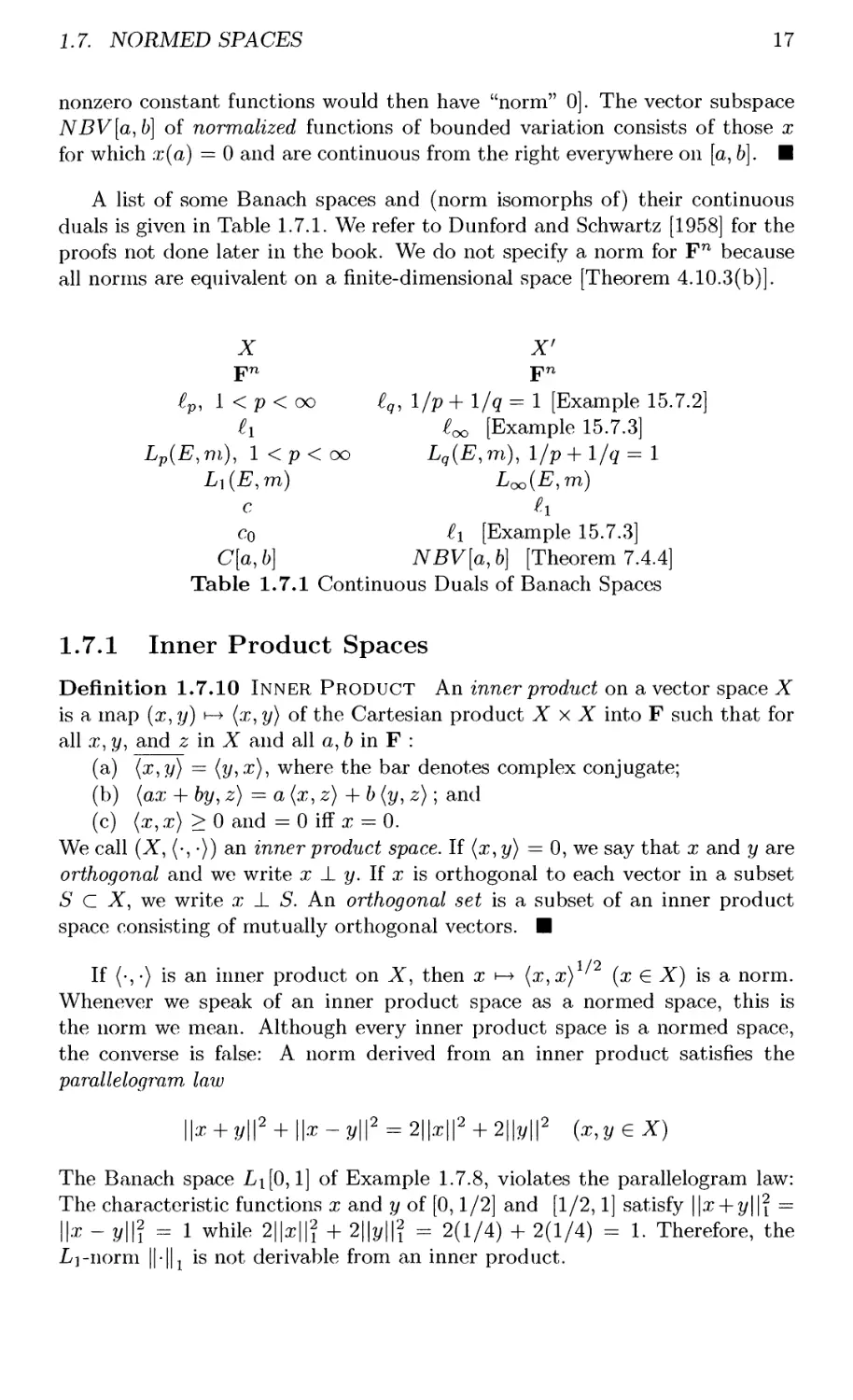
A list of some Banach spaces and (norm isomorphs of) their continuous
duals is given in Table 1.7.1. We refer to Dunford and Schwartz [1958] for the
proofs not done later in the book. We do not specify a norm for Fn because
all norms are equivalent on a finite-dimensional space [Theorem 4.10.3(b)].
X X'
ep, 1 < p < oo eq, l/p +l/q = l [Example 15.7.2]
h too [Example 15.7.3]
LP(E, m), 1 < p < oo Lq(E, m), l/p + 1/q = 1
LA{E,m) Loo(E,m)
c h
c0 h [Example 15.7.3]
C[a,b] NBV[a,b] [Theorem 7.4.4]
Table 1.7.1 Continuous Duals of Banach Spaces
1.7.1 Inner Product Spaces
Definition 1.7.10 Inner Product An inner product on a vector space X
is a map (x, y) y-> (x, y) of the Cartesian product X x X into F such that for
all x, y, and z in X and all a, b in F :
(a) (x,y) = (y, x), where the bar denotes complex conjugate;
(b) (ax + by,z) = a(x,z) + b (y, z); and
(c) (x, x) > 0 and = 0 iff x = 0.
We call (X, (•,•)) an inner product space. If (x, y) = 0, we say that x and y are
orthogonal and we write x J_ y. If x is orthogonal to each vector in a subset
S C X, we write x _L S. An orthogonal set is a subset of an inner product
space consisting of mutually orthogonal vectors. ■
If (•, •) is an inner product on X, then x i—»• (x,x) ' (x G X) is a norm.
Whenever we speak of an inner product space as a normed space, this is
the norm we mean. Although every inner product space is a normed space,
the converse is false: A norm derived from an inner product satisfies the
parallelogram, law
\\x + V\\2 + \\x - y\\2 = 2\\x\\2 + 2\\y\\2 (x,ye X)
The Banach space L\[0,1] of Example 1.7.8, violates the parallelogram law:
The characteristic functions x and y of [0,1/2] and [1/2,1] satisfy ||x + t/||i =
\\x - y\\l = 1 while 2||x||'f + 2||y||? = 2(1/4) + 2(1/4) = 1. Therefore, the
L]-norm HIL is not derivable from an inner product.

18
CHAPTER!. BACKGROUND
Definition 1.7.11 HlLBERT SPACE An inner product space which is
complete with respect to the inner product-derived norm is called a Hilbert space.
■
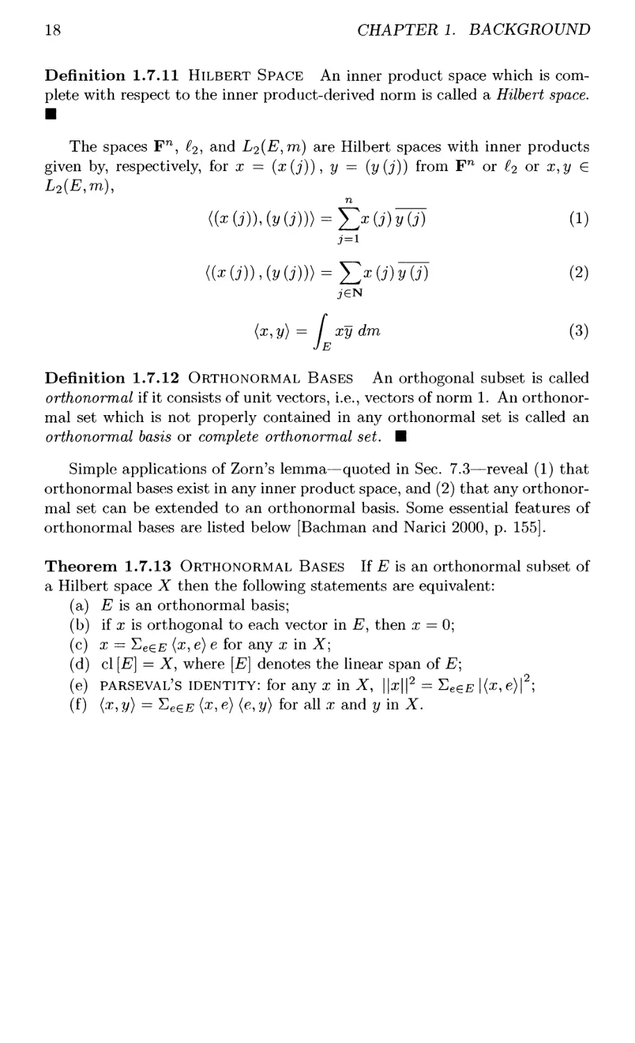
The spaces Fn, £2, and L2{E,m) are Hilbert spaces with inner products
given by, respectively, for x = (x(j)), y = (y (j)) from Fn or £2 or x,y G
L2(£,m),
((xtiMvti))) = Jtxti)y(fi U)
3 = 1
((xti)),(y(m = Y,x^y^ (2)
(x,y) = I xy dm (3)
Je
Definition 1.7.12 Orthonormal Bases An orthogonal subset is called
orthonormal if it consists of unit vectors, i.e., vectors of norm 1. An
orthonormal set which is not properly contained in any orthonormal set is called an
orthonormal basis or complete orthonormal set. ■
Simple applications of Zorn's lemma—quoted in Sec. 7.3—reveal (1) that
orthonormal bases exist in any inner product space, and (2) that any
orthonormal set can be extended to an orthonormal basis. Some essential features of
orthonormal bases are listed below [Bachman and Narici 2000, p. 155].
Theorem 1.7.13 Orthonormal Bases If E is an orthonormal subset of
a Hilbert space X then the following statements are equivalent:
(a) E is an orthonormal basis;
(b) if x is orthogonal to each vector in E, then x = 0;
(c) x = T,e£E (x, e) e for any x in X\
(d) cl [E] = X, where [E] denotes the linear span of E\
(e) parseval's identity: for any x in X, \\x\\2 = EeGE |(x,e)|2;
(f) (.x, y) = £eG# (x, e) (e, y) for all x and y in X.

Chapter 2
Commutative Topological
Groups
2.1 ELEMENTARY CONSIDERATIONS
2.2 SEPARATION AND COMPACTNESS
2.3 BASES AT 0 FOR GROUP TOPOLOGIES
2.4 SUBGROUPS AND PRODUCTS
2.5 QUOTIENTS
2.6 5-T0P0L0GIES
2.7 METRIZABILITY
One of the principal reasons for superimposing a topological structure on
an algebraic object is to permit the tools and insights of analysis (i.e.,
limits) to bear. Generally, in "topological algebra," a topology is introduced to
an algebraic structure which makes the basic algebraic operations
continuous. The idea of the topologic-algebraic fusion is fairly venerable and has
numerous applications. It enabled Krull [1928], for example, to develop an
infinite-dimensional Galois theory in which there exists a 1-1 correspondence
between the intermediate fields and closed subgroups of the Galois group of
a separable normal extension, after suitably topologizing the Galois group.
In this connection—topologizing the Galois group of a separable normal field
extension—it seems that a rudimentary grasp of the notion of topological
group had already occurred to Dedekind in the nineteenth century, judging
from his remark: "The set of these permutations forms a continuous
multiplication in a certain sense, a question which we shall not address ourselves to
any further here" [Dedekind 1932]. And certainly, Sophus Lie's "continuous
groups," presently called "Lie groups," were topological groups whose theory
was well developed in the second half of the nineteenth century. The notion of
19

20 CHAPTER 2. COMMUTATIVE TOPOLOGICAL GROUPS
topological group to be introduced in this chapter was enunciated by Schreier
[1925].
In this chapter we develop the most elementary properties of
commutative topological groups. We are actually obtaining the basic properties of
topological vector spaces, those that do not depend on scalar multiplication.
We will see that topological groups are quite uniform in structure
("homogeneous"): the filter V(0) of neighborhoods of 0 completely determines the
topology in the sense that the filter V (x) of neighborhoods of any point x is
x + V(0) = {x + V :V eV(0)}.
After determining several properties of the neighborhoods of 0 in a
topological group, we turn the question around in Sec. 2.3. We obtain conditions
under which a collection of sets in a group X will be a base at 0 for a
topology which makes X a topological group. These results enable us to efficiently
topologize quotients and products of topological groups and groups of
functions [Sec.2.6].
2.1 ELEMENTARY CONSIDERATIONS
Notation. The filter of neighborhoods of a point x is denoted V(x). ■
We define a topological group X in this section and show that they would
be a census taker's delight: if you know what is happening near 0, you know
what is happening everywhere. They are homogeneous in that given any two
points x and y, there is a homeomorphism of X onto itself mapping x onto y.
Thus, 0 serves as an "everypoint."
Let X be an additive group. For any nGN and x e X, nx denotes the
sum obtained by adding x to itself n times and — nx denotes — x added to
itself n times. If W is a subset of X, —W = {—iv : w G W} and W + W =
{x + y : x,y G W}. If X is also a topological space in which the algebraic
operations are linked to the topology by
(Gi) Continuity of Inversion: the map x i-> -x of X into X is
continuous;
(G2) Continuity of Addition: the map (x,y) i-> x 4- y of X x X
(product topology) into X is continuous,
then X is called a topological group. Equivalently, one says that the
topology on X is a group topology or is compatible with the group structure. As
an alternate phrasing of (G\) and (G2), we have:
(Gi) Continuity of Inversion: For any x e X and neighborhood V
of —x, there is a neighborhood W of x such that —WcV.
(G2) Continuity of Addition: For any x,y G X and any
neighborhood V of x + y there exist neighborhoods U of x and W of y such that
U + W CV

2.1. ELEMENTARY CONSIDERATIONS
21
(Gi) implies by induction that for any positive integer n and any W G
1/(0), there is a U G V(0) such that U + U + --- + U (n terms) C W\ We can
combine (Gi) and (G2) into:
(Gj2) The map (x, y) \-> x — y of X x X into X is continuous.
Equivalently, for any x,y € X and any neighborhood V of x — y,
there exist neighborhoods [/ of x and VF of ?/ such that U — W C V.
Clearly, (G12) is a consequence of (Gi) and (G2). Conversely, (G12) implies
the continuity of the map y 1—»• 0 — y, so (Gi) is implied by it. (G12) and (G\)
together imply (G2) for they imply the continuity of the map (x, y) 1—» x—(—y).
Any group with the discrete topology is a topological group, the
continuity conditions being trivially satisfied; such discrete groups provide many
counterexamples. (Although the discrete topology is a group topology for
any group, it is never a vector topology because topological vector spaces are
connected [Theorem 4.3.4].) More interesting examples of topological groups
are given here, at the end of Sec. 2.3, and in Sec. 2.6.
Example 2.1.1 (R, +), (C, +) AND (X, \\-\\, +) The additive groups R and
C of real and complex numbers with their usual topologies are topological
groups. More generally, so is any normed (or seminormed) space (X, ||-||)
viewed as an additive group. As we verify next, the triangle inequality yields
continuity of addition and the fact that ||x|| = ||— x|| makes for continuity of
inversion. For x G X, let B(x, r) = {z G X : \\z — x\\ < r}, r > 0. Given x, y G
X, consider a basic neighborhood B{x — y, r), r > 0, of x — y. For v G B(x, r/2)
and w G £?(?/,r/2), then \\{v - w) — (x - y)\ < \\v - x\\ + \\y - w\\ < r. Thus
B(x,r/2) - B(y,r/2) C B(x - y,r) and (G]2) is satisfied. ■
We say more about metric topological groups in Sec. 2.7.
Example 2.1.2 (R*,-) AND (C*,-) The multiplicative groups R* and C*
of nonzero real and complex numbers in their usual topologies are topological
groups. To see this, consider nonzero (real or complex) numbers a$ and bo.
For any nonzero numbers a and b,
\ab - a0b0\ = \(a - a0)(b - b0) + a0(b - b0) + (a - a0)M
< \a- a0\ \b - 601 + l^ol \b - b0\ + \a - a0\\bo\
It follows that if a is sufficiently close to ao and b is sufficiently close to bo,
then ab is close to aobo, i.e., multiplication is continuous. The continuity of
the map a ^ a"1 is verified by observing that the convergence of an to a
implies the convergence of l/an to 1/a. ■
Another immediate consequence of the axioms is that translation and
inversion are homeomorphisms:

22
CHAPTER 2. COMMUTATIVE TOPOLOGICAL GROUPS
Theorem 2.1.3 Translation and Inversion Homeomorphisms For any
topological group X and any z G X, the maps x i—»• —x and x h j 4- z are
homeomorphisms of X onto X.
Proof. The inversion map x 1—> — x is clearly bijective. Continuity of inversion
follows from (G\); its inverse is x 1—»• — j; (same map) so it is a homeomorphism.
To see that translation x 1—»• x + z is a homeomorphism, first observe that it is
bijective. Its inverse, the map x »-> x — z, is also a translation, so it suffices to
prove that translation is continuous to prove that it is a homeomorphism. If
W is a neighborhood of z + x, there must be neighborhoods [/ and V of z and
x, respectively, such that C/+V C W by (G2). Hence V *-> z+V c C/+V C W
and translation is continuous. ■
We show next that translates x -f V of neighborhoods V of 0 constitute
the neighborhoods of x.
Theorem 2.1.4 NEIGHBORHOOD BASES If B is a neighborhood base at 0
in a topological group X then, for any x G X, x + B = {x + B : B G B} is a
neighborhood base for V(x).
Proof. We use the notation of the statement. The map y 1—»• y + x is a
homeomorphism [Theorem 2.1.3] taking 0 into x. Its inverse is the map y 1—>
y — x. Thus if F e ^(^) then — x + V is a neighborhood of 0. Since B is a
base, there exists B G B such that £? C — x + V\ Hence x + B C V and x + ^
is a neighborhood base at x. ■
Definition 2.1.5 Homogeneous Spaces A topological space X is
homogeneous if, given any two points x,y G X, there is a homeomorphism of X
onto X mapping x into y. ■
If X is a topological group and x, y G X, the translation map 2 1—»• 2 — x +1/
is a homeomorphism [Theorem 2.1.3] which takes x into y\ hence:
Theorem 2.1.6 Any topological group is homogeneous.
It follows that for many important purposes, it suffices to examine the
contours around 0 in a topological group. For example, if there is a compact
neighborhood of 0, X is locally compact; if {0} is an open set, any one-point
set is open—in other words, X is discrete; X is a T\-space iff {0} is closed.
Definition 2.1.7 HOMOMORPHISM A (group) homomorphism is a map /
from a group X into a group Y such that f(x + y) = f(x) + f(y) for all
x and y in X. If, in addition, / is 1-1, then / is a (group) isomorphism.
Continuous homomorphisms mapping one topological group into another are
called morphisms. Group isomorphisms of one topological group into another
which are homeomorphisms are called group homeomorphisms or topological
group isomorphisms.

2.2. SEPARATION AND COMPACTNESS
23
Theorem 2.1.8 Continuity at One Point A homomorphism mapping
one topological group into another continuous at one point is continuous.
Proof. Suppose that X and Y are topological groups and that / : X —> Y is
a homomorphism. Suppose that / is continuous at y G X. To see that / is
continuous everywhere, let x G X and suppose that the net xm —> x. Then
y + xm — x —» y. Since / is continuous at ?/,
/(y + im-i) = /(y) + /W-/(i)^/(»)
which implies that / (xm) —» / (x) and proves the continuity of / at x. ■
The use of "symmetric" (defined below) neighborhoods of 0 simplifies
many arguments.
Definition 2.1.9 Symmetric Sets A subset E of a group X is called
symmetric if E = — E. ■
If E is any subset of a topological group, then EU—E, EC)-E, and E — E
are symmetric; moreover, if E1 is symmetric, so is cl E.
Theorem 2.1.10 Base of Symmetric Neighborhoods of 0 In any
topological group: (a) every neighborhood of 0 contains a symmetric
neighborhood of 0; (b) given any neighborhood V of 0, there is a symmetric
neighborhood W of 0 such that W - W C V.
Proof, (a) Since the map x i—> — x is a homeomorphism, given any
neighborhood V of 0 — V is a neighborhood of 0; U = V D — V is a symmetric
neighborhood of 0 contained in V.
(b) By (G12) and (a), given V G V (0), there are symmetric neighborhoods
U,U' G V (0) such that U -U' C.V. Now let W = U n Uf. ■
As a simple but useful application, we have:
Corollary 2.1.11 Let X be topological group X, let U (0) denote the
symmetric neighborhoods of 0. Then cl {0} = C)U (0) = nV (0).
Proof. Since U (0) is a base for V (0), it suffices to prove that cl {0} = C)U (0).
If x G cl {0} then, for each U G U (0), x + C/ meets {0} , i.e., 0 G x + £/. Since
U is symmetric, this means that x G C/ for all U G C/ (0). Conversely, if
x G n£/(0) then -x G n£/(0). Hence 0 G x + C/ for all [/ G 1/(0) which
implies that x G cl {0}. ■
2.2 SEPARATION AND COMPACTNESS
Notation. X denotes a commutative topological group with neighborhood
filter V (0) at 0. ■

24
CHAPTER 2. COMMUTATIVE TOPOLOGICAL GROUPS
We show in Theorem 2.2.1 that every topological group is a regular
topological space, i.e., given any neighborhood V of a point x, there is a
neighborhood U of x such that cl U C V. Consequently, a nonregular topology such
as the cofinite topology (U is open iff CU is finite) on any infinite group X is
not a group topology—in the case of the cofinite topology, the closure of any
neighborhood is X.
Theorem 2.2.1 Regularity Every topological group is regular. (Although
this does not imply that every topological group is Hausdorff, it does if the
group is T0.)*
Proof. Let V G V(0). Since 0 - 0 = 0, it follows by (G12) of Sec. 2.1 that
there is some U G 1^(0) such that U - U C V. We show that clU C V. If
x G cl U then every neighborhood x + U of x must meet U so there must be
u, y G U such that x + u = y G U. Therefore, x = y — ueU — UcV. ■
Concerning the separation properties of a topological group, we have:
Theorem 2.2.2 SEPARATION In any topological group X the following
statements are equivalent:
(a) X is a To-space.
(b) X is a T2-space.
(c) nv(0) = {0}.
(d) For any nonzero element x G X, there exists V G V (0) such that
x i V.
Proof. That (a) => (b) is clear from the regularity of X [Theorem 2.2.1]. To
see that (b) => (c), note that if y ^ 0 and y G nV(0), then X is not Hausdorff
for y cannot be separated from 0. To prove that (c) => (a), we need only prove
that {0} is closed by Theorem 2.1.6 (homogeneity). To show this, we note
that cl{0} = nV(0) = {0} [Corollary 2.1.11]. Clearly (b) => (d). Conversely,
we show that (d) => (c). If x ^ 0 and x (£ V G V (0) then x £ DV (0); hence
ny(0) = {0}. ■
By Theorem 2.1.3, translates of open sets or closed sets are open or closed,
respectively. Moreover:
Theorem 2.2.3 Sums of Open Sets In any topological group X, if G is
a nonempty open set and B is any subset, then G + B is open since we can
write G + B = UX£b{G + x). In particular, sums of open sets are open.
Sums of closed sets need not be closed, however, as the following example
shows.
*Every topological group is completely regular [Bushaw 1963, p. 123, Th. 52] but
generally not normal [Husain 1966, p. 51].

2.2. SEPARATION AND COMPACTNESS
25
Example 2.2.4 Sums of Closed Sets Let X = (R, +), the additive
topological group of real numbers with the usual topology. The sets A =
{n G N : n > 2} and D = {—n — \/n : n > 2} are closed but A + B contains
{ — l/n : n > 2} which has 0 as an adherence point so A + D is not closed. ■
The sum of a compact set and a closed set is generally closed, however.
We prove this in Theorem 2.2.6 after establishing the following result.
Theorem 2.2.5 Neighborhoods OF Compact Sets In any topological
group, if the compact set K is contained in the open set U then there is a
neighborhood V of 0 such that K + V C U. (A neighborhood of K is contained
in U.)
Proof. Let K and U be as above. For each x G if, there exists Vx G V(0)
such that x + Vx C U. By continuity of addition, there exists a neighborhood
Wx of 0 such that Wx + Wx C Vx. Since K is compact, a finite number
x\ + WXi,..., xn + WXii, of these sets covers K. Let V — n^=] WX/. To show
that K + V C [/, consider any x G K. There must be some integer i such
that x G Xi + WXi. Hence
x + F C Zi + WXi + y C Xi + WXi + H^T? Cx, + ^?C[/
Therefore K + V cU. ■
Theorem 2.2.6 Compact + Closed Is Closed In any topological group
X, if if is compact and F is closed, then K + F is closed.
Proof. Suppose K is compact, F is closed and let x G cl (A" + F). Then for
all neighborhoods V G V(0),
(x + F) n (if + F) ^ 0 <£> (-if + x + V) n F ^ 0 (•)
To show that x G if + F, first observe that if(-if + x)nF = 0, then the
compact set — if + x is contained in the open set CF. By Theorem 2.2.5 it
follows that there is some V G V(0) such that (-if + x + V) C CF which
contradicts (•). ■
As a final word on closure and addition, we prove:
Theorem 2.2.7 cl A + cl B C cl (A + £) If A and £ are subsets of a
topological group X, then cl A + cl B C cl (A + B).
Proof. Let x e c\A, y € c\B, and U G V(0). By the continuity of addition,
there are neighborhoods V, W G V(0) such that (x + V) + (y + VF) C x + y + U.
Since x G cl A and y e dB, there exist a G A Pi (x + V) and b € B n (y + W).
Hence a + bex + y-{- U and therefore x + y G c\(A -{- B). ■

26
CHAPTER 2. COMMUTATIVE TOPOLOGICAL GROUPS
As mentioned earlier, for a topological group to be locally compact it
suffices for 0 to possess a compact neighborhood. A little more is true, however,
namely:
Theorem 2.2.8 Locally Compact Groups For each neighborhood V of 0
in a locally compact topological group, there is a relatively compact symmetric
neighborhood U of 0 such that cl U C V (cl U is symmetric as well).
Proof. Since any topological group is regular [Theorem 2.2.1], given V G V(0)
there exists W G V(0) such that cl W C V. Since X is locally compact, there
exists W G V(0) such that clW' is compact. Since cl(WnW) C c\W,
cl(Wn W) is compact. Since W fl W is a neighborhood of 0, there is a
symmetric neighborhood U of 0 such that U C cl (W n W) [Theorem 2.1.10].
As cl U C cl (W fl W) C V, cl U is compact. Thus, U is the desired
neighborhood. Since the map x i—> —x is a homeomorphism, —c\U = cl ( — U) = cl U
so cl U is symmetric. ■
Definition 2.2.9 Topological Rings A ring X endowed with a group
topology and such that the map (x, y) i—> xy of X x X into X is continuous is
called a topological ring. In this case the topology is said to be a ring topology
or compatible with the ring structure. Fields K topologized in such a way
as to be topological rings and in which the map xhx-1 from the nonzero
elements K* of K into K* is continuous are called topological fields. ■
To guarantee that a topologized field K be a topological field, it is not
enough to demand that K be an additive topological group and K* a
multiplicative topological group, for this would not require multiplications involving
0 be continuous. R and C with their usual topologies are topological fields,
and more generally any valued field [Sec. 1.2] is a topological field.
2.3 BASES AT 0 FOR GROUP TOPOLOGIES
Notation. X denotes a commutative typological group with neighborhood
filter V (0) at 0. ■
In the last section we noted some properties of bases for V (0) in a
topological group. In this section, we reverse direction and develop conditions for
a fllterbase B of subsets of a group X to determine a group topology for which
B is a basis at 0. The analogous discussion for topological vector spaces is in
Sec. 4.5.
We have already seen [Theorem 2.1.10(b)] that:
(F) For any V G V (0) there is a symmetric W G V (0) such that W-W CV
This condition on a filter T of sets from a group X suffices to determine
a compatible topology for X in which T is the filter of neighborhoods of 0

2.3. BASES AT 0 FOR GROUP TOPOLOGIES
27
as we prove next. (F) immediately implies that for any W G T, there are
£/, V G T such that (U nV) - (U C)V) C U - V C W; therefore 0 belongs to
each W ef.
Theorem 2.3.1 Base at 0 for Group Topology Let B be a filterbase
in a group X. B is a neighborhood base at 0 for a group topology for X if B
satisfies:
{FB) For each B e B there is a symmetric V e B such that V - V C B.
(OB) If for each B G B and any x G B there exists V G B such that
x + V C jB then # is an open base at 0.
Proof. Let B be a filterbase in a group X and let T denote the filter of
all supersets of sets in B. For any x G X we show that x + T satisfies the
neighborhood axioms at x.
Since, as noted above, 0 belongs to every F G T, it is clear that x belongs
to every x + FGx-ff. We illustrate the argument for finite intersections by
considering two sets. Given F,G G T, there exist A,B e B such that AcF,
B C G. Since B is a filterbase, there exists C G B such that Cc^lnR
Therefore x + Cc(x + A)n(x + B)=x + AnBCx + FnGex + Jr.
Now consider F G T and £ G S such that B C F. By (FB) there exists a
symmetric W G B such that W - W C £. For any y € x + W, y + W C
x + W — Wcx + Bcx + F which implies that x + F is a neighborhood of
y. It follows that x + J7 is a system of neighborhoods of x.
To see that this is a group topology, we show that (FB) implies that the
neighborhoods x + T (x G X) satisfy (G12) of Sec. 2.1. For x,y G X and
F € J7, consider the neighborhood x — y + F of ,t — y. Choose B € B such
that I? C F and (by (FB)) F G B such that IZ-VcR Then
(x-\-V)-(y + V)Cx-y+(V-V)Cx-y + BCx-y-\-F
Condition (OB) clearly makes each B in B a neighborhood of each of its
points, hence an open set. ■
As an immediate corollary we have:
Theorem 2.3.2 Subbases If S is a family of subsets of a group X that
satisfies the finite intersection condition (finite intersections of sets from S
are not empty) and (FB) then S is a neighborhood subbase at 0 for a group
topology on X. US also satisfies (OB), then it is an open subbase.
Example 2.3.3 Finite Topology Let X and Y be linear spaces over the
same field and let C (X, Y) denote the commutative additive group of all linear
maps of X into Y with respect to (A + B)x = Ax + Bx for any x G X and
A,B G C(X,Y). For any x G X let 5(0,x) = {A e C(X,Y) : Ax = 0}. It
is a simple matter to verify that the sets {5(0, x) : x G X} satisfy the finite
intersection condition (they all contain the trivial linear map x »—> 0) and

28 CHAPTER 2. COMMUTATIVE TOPOLOGICAL GROUPS
(FB) of Theorem 2.3.1. Consequently, by Theorem 2.3.2, {5(0, x) : x e X}
is a neighborhood subbase at 0 for a compatible topology on C(X,Y). This
topology is called the finite topology.
If A ^ 0, then there is some x e X such that Ax ^ 0, so A £ 5(0, x);
the finite topology is therefore Hausdorff. Actually, its separation properties
are even stronger, as we now show. The sets 5(0, x) also satisfy (OB) of
Theorem 2.3.1 for, for any A e 5(0, x), A + 5(0, x) C 5(0, x). Hence the
sets 5(0, x) are an open subbase at 0. But the sets 5(0, x) are subgroups of
C(X,y); hence they must also be closed [Theorem 2.4.4(b)]. Consequently,
the finite topology has a basis of clopen sets. This, together with the fact that
it is Hausdorff, means that the finite topology is totally disconnected: The
only connected subsets are points. As we shall see later [Theorem 4.3.4], this
property prevents C (X, Y) with the finite topology from being a topological
vector space. We further remark that the finite topology is discrete iff X is
finite-dimensional and that, by defining (AB)x to be A(Bx) for each x G X,
C(X, X) becomes a topological ring [Definition 2.2.9] with respect to the finite
topology.
If E is a Galois extension (= separable + normal) field of the field L and
X denotes the set of all field automorphisms of E which leave L fixed, then
X is a group with respect to composition. X is called the Galois group of E
over L. Viewing X as a subset of C(E,E) endowed with the finite topology,
then X in its relative topology is also a topological group. In this context, it
is often denominated the Krull topology after W. Krull, who proved [Krull
1928] that there is a 1-1 correspondence between the intermediate fields of E
over L and the closed subgroups of X, thus developing a "Galois theory" in
the infinite-dimensional case. For further discussion of this aspect of Galois
theory, see Artin [1967, pp. 103-108] and Jacobson [1964, pp. 147-151]; for a
more general discussion of the finite topology, see Jacobson [1953]. ■
2.4 SUBGROUPS AND PRODUCTS
Notation. X denotes a commutative typological group with neighborhood
filter V (0) at 0. ■
Consider a map / : 5 —> T (or family of maps) where only one of 5, T
is a topological space. We topologize the other in such a way as to make
/ continuous. We topologize the domain 5 in this section to get an inverse
image (weak, initial) topology; in Sec. 2.5 we topologize the codomain T to
obtain a direct image (final, identification) topology. Inverse and direct image
topologies determined by homomorphisms are group topologies.
Definition 2.4.1 Inverse Image Topology Let {(YS,TS) : s e 5} be a
family of topological spaces and let X be a set. Let fs : X —> Ys (s G 5)
be a family of maps. The coarsest topology for X with respect to which each

2.4. SUBGROUPS AND PRODUCTS
29
fs is continuous has {/s 1(TS) : s G £} as a subbase. It is called the inverse
image (weak, initial) topology induced by {fs : s G 5} on X. (Cf. Example
4.7.1). ■
Our principal interest is when X is a group, the fs are homomorphisms
and the Ys are topological groups in which case we get a group topology on
X as we show next.
Example 2.4.2 Inverse Image Topology and Groups Let X be a
group and let {Xs : s G 5} be a family of topological groups such that for
each s e S there is a homomorphism hs : X —> Xs. For each s G 5 let
Vg (0) denote the filter (or a base for the filter) of neighborhoods of 0 in Xs.
A base Vt(0) at 0 for the inverse image topology T for X determined by
the family {hs : s G 5} is given by intersections of the form rifee^/i^ ^V^),
where K is a finite subset of S and Vk G Vk (0) for each k € K. It is a
group topology: To illustrate how to verify (FB) of the basis theorem [2.3.1],
consider ,s, k G S and suppose Vs G Vs (0), and Vk G Vk (0). Choose
symmetric neighborhoods Bs G Vs (0) and i?fc G 14 (0) such that Bs -\- Bs C Vs
and Bk + BkC Vk, so that /ij1 (Ba) + h~l (Bs) C /7"1 (Ba + Bs) C /ij1 (Vs)
and ftj^1 (Bk) + /i^1 (Bk) C ftj^1 (14)- Then h~l (Bs) n Z^1 (Bfc) + /ij1 (Ba) n
^](^)c/^(v;)n^]^). ■
If M is a subgroup of a topological group X then the injection I : M —>
X, x \-* rr, is a homomorphism. The inverse image topology determined by
/—i.e., M in its relative topology—is therefore a group topology.
A subgroup of a topological group is said to be closed, open, etc., if it is
a closed set, and so on. For example, the additive group of real numbers is a
closed subgroup of the additive topological group of complex numbers.
Theorem 2.4.3 CLOSURES OF SUBGROUPS If M is a subgroup of a
topological group X, then so is the closure cl M of M.
Proof. The continuous map f : XxX -+ X, (x,y) \-± x — y, maps MxM onto
M. Since / is continuous,/(cl (M x M)) = f(c\M x clM) = clM - clM C
cl/((M x M)) = clM and it follows that clM is a subgroup. ■
As a result of Theorem 2.4.3, it is clear that cl {0} is a subgroup in any
topological group.
Theorem 2.4.4 Open and Closed Subgroups A subgroup M of a
topological group X is:
(a) open iff its interior intM ^ 0;
(b) open only if M is closed;
(c) discrete iff M has an isolated point.

30
CHAPTER 2. COMMUTATIVE TOPOLOGICAL GROUPS
Proof. Let M be as above, (a) If M is open then 0 G intM. Conversely,
suppose that M has an interior point x. For any y in M, the map z »—>
z + (y — x) maps M homeomorphically onto M and maps x into y. Thus y is
also an interior point of M.
(b) Suppose that M is open. Then if x G clM, (x + M) n M ^ 0, so
there exist y,z € M such that x + ?/ = z; hence x = 2-t/G M.
(c) If x is an isolated point of M then by translation as in (a), each point
y of M is also isolated and therefore M is discrete. The converse is clear. ■
We discuss products of topological groups next.
Example 2.4.5 Products Let {Xs : s e S} be a family of topological groups
For elements x = (xs) and y = (ys) from the product X = IIsesXs, define
x + y to be (xs + ys). It is easy to verify that X is a group with respect to
this pointwise operation and that each projection prfc : IIsGisXs —> Xk is a
homomorphism. The product topology T, the coarsest topology with respect
to which each projection is continuous, is the inverse image topology
determined by {prs : s G 5}. Since projections are homomorphisms, it is a group
topology [Example 2.4.2]. Let Vs(0) denote the filter of neighborhoods of 0 in
Xs (s G 5). A base at 0 for T is given by
RsesVs, where each V8 G V8(0)
and Vs = Xs for almost all indices s
Whenever we speak of a product of topological groups it is always with respect
to the product topology. ■
2.5 QUOTIENTS
Suppose X is a topological space, Y a set and / : X —» Y a map. We
want to topologize Y in such a way that / is continuous. The direct image
(final, identification) topology 7} for Y induced by f has as its open sets
those U C Y such that f~l(U) is open in X; that this is a topology (as
opposed to generates a topology) is clear since f~l preserves set operations.
We further note that Tf reduces to the discrete topology on Cf(X) since, for
any A C C/(X), f~l(A) = 0, which is open and closed in X. If / is not
surjective, since / (X) is 7}-open (X = f~lf (X)) then Y = f(X)\j£f (X)
is 7}-disconnected. In terms of neighborhoods, V is a neighborhood of y =
f (x) G F iff f~l (V) is a neighborhood of x.
The direct image topology on Y clearly makes / continuous. Moreover,
it is the finest topology for Y with respect to which / is continuous—if T is
any other such topology, then U G T implies that f~1(U) is open in X, i.e.,
U G 7}, so that T c Tf.
Direct Image Topologies and Groups Suppose X is a topological group,
Y a group, and h : X —» Y a homomorphism. The direct image topology

2.5. QUOTIENTS
31
induced by h on Y has as a base at 0 the collection 8 of all subsets B C Y
such that h~l(B) is a neighborhood of 0 in X. To see that it is a group
topology, first note that 8 is clearly a filterbase. For any B G 8 there exists
a symmetric neighborhood V of 0 in X such that V — V dh~l (B) [Theorem
2.1.10(b)]. Hence
h(V-V) = h{V)-h(V) C.B
Since V C h~x {h(V)), it follows that h(V) G B; therefore 8 satisfies
condition (FB) of Theorem 2.3.1 and is a base a 0 for a group topology T for X.
In summary:
Theorem 2.5.1 Direct Image Topology on a Group Suppose X is a
topological group, Y a group, and h : X —> Y a homomorphism. Then:
(a) the direct image topology for Y is a group topology;
(b) the filterbase 8 of all subsets B C.Y such that h~1(B) is a
neighborhood of 0 in X is a base at 0 for the direct image topology.
Definition 2.5.2 Quotient topology Suppose M is a subgroup of a
topological group X and let k : X —» X/M, x \-* x = x + M denote the
canonical homomorphism. The direct image topology on X/M determined
by k is called the quotient topology for X/M. Since it is determined by a
homomorphism, it is a group topology on X/M. Whenever we discuss a
quotient group, we assume that it carries its quotient topology. ■
We mention that k~1(x) = x + M (x G X). By our general comments
above on direct image topologies, k is continuous.
Theorem 2.5.3 Quotient Topology; k Is Open But Not Closed Let
M be a subgroup of a topological group X. The canonical map k : X —» X/M
is:
(a) open—indeed, every open subset of X/M is of the form G + M where
G is open in X; in particular, k(V(0)) is the neighborhood filter at 0 for the
quotient topology;
(b) k generally does not map closed sets into closed sets.
Proof. We use the notation of the statement, (a) Let G C X be open.
Then k~l (k (G)) = G + M = UmGM (G + m) is open; therefore k (G) is open.
(b) Let Z denote the subgroup of integers of the additive group R of real
numbers in its usual topology and consider the canonical map k : R —» R/Z.
For x G R, let [x] denote the greatest integer < x. Every coset x + Z contains
x — [x] and no other number in [0,1). Hence we may map R/Z in a bijective
fashion onto [0,1) and reflect the quotient topology of R/Z onto [0,1). A
basis for [0,1) in this topology is then given by the sets (a, b) and [0, a) U (6,1),
0 < a < b < 1. The set A = {3/2,9/4,..., n 4- 2~n,...} is closed in R but
k(A), under the identification, is {1/2,1/4,..., 2_n,...} which has 0 as an
adherence point; thus k(A) is not closed. ■

32
CHAPTER 2. COMMUTATIVE TOPOLOGICAL GROUPS
Theorem 2.5.4 Hausdorff Quotient Groups Let M be a subgroup of
the topological group X. Then X/M is Hausdorff iff M is closed.
Proof. We use the notation of the statement. Let k : X —> X/M denote the
canonical map. If X/M is Hausdorff, then {6} is closed; hence /c_1({6}) = M
is closed. Conversely, suppose that M is closed. By Theorems 2.2.2 and 2.1.6,
to show that X/M is Hausdorff, it suffices to show that {0} is closed. To this
end suppose that x G cl{6}. Then for every neighborhood V of 0, 6 G k(x+V);
equivalently, (x + V) n M ^ 0 for each V G V(0). Thus x G clM = M and
x = 6. ■
It is often convenient to split a homomorphism / : X —» Y as in the
accompanying diagram.
X/7V X /(X)
Here fc denotes the canonical homomorphism x i—► x + A/" = x where A/" =
/_1 (0) denotes the kernel (subgroup) of /; / represents the bijective
homomorphism x i—> f(x) and 7 represents the canonical injection map f(x) \—>
/(x). We observe that / is an isomorphism of X/N onto /(X) called the
canonical isomorphism associated with f'.
Theorem 2.5.5 Let X and y be topological groups, / : X —> Y a
homomorphism and everything else as in the diagram above. Then
(a) The canonical injection I is a group homeomorphism of f(X) into Y\
(b) /is continuous iff / is continuous;
(c) / is open iff / is relatively open [i.e., / maps open subsets of X onto
open subsets of f{X)].
Proof. We use the notation of the statement, (a) Clear.
(b) If / is continuous, then / is the composite of three continuous maps and
is therefore continuous. Conversely, suppose that / is continuous and let U
be an open subset of Y. Since k is an open map and (7/)_1([/) = k(f~1(U)),
If is continuous, from which the continuity of I~lIf = / follows.
(c) For each open subset U of X, f(U) = If(k(U)). Since k is open and
7 is a homeomorphism, the result follows. ■
By Theorem 2.5.5, it is easy to see that:
Theorem 2.5.6 / is a relatively open continuous map iff / is a group
homeomorphism.

2.6. S-TOPOLOGIES
33
2.6 <S-TOPOLOGIES
Notation. Throughout the section T is a set and X a commutative
topological group with neighborhood filter V(0) at 0. F(T, X) denotes the set Xr of all
functions mapping T into X. For x, t/ G F(T, X) and £ G T, define (x + y)(t) =
x(t)+y(t). With respect to these pointwise operations, (F(T, X), +) is a
commutative topological group. ■
We topologize F(T, X) in various ways that make it a topological group.
Various different notions of convergence of functions—uniform, pointwise,
etc.—all fit under this umbrella. This was very important, historically, for
it shows that general topology is a broad enough tool to encompass these
diverse types of convergence. Our general remarks below apply just as well to
any subgroup of F (T, X). When T is a topological space, we can consider the
subgroup C{T, X) of continuous maps of T into X, as we do in Sees. 5.8-5.10.
The building blocks for the topologies for F (T, X) to come are the sets
W(S, V) = {x G F(T, X) : x(S) C V}, S C T, V G V (0) (*)
Their vital properties follow. The proofs of all parts are immediate.
Theorem 2.6.1 PROPERTIES OF W(S, V) Let T be a set and X a
commutative topological group with neighborhood filter V(0) at 0. For any 5, S' C T
and U,VeV(0) :'
(a) UcV =>W{S, U) c W{S,V)\
(b) W{S, -V) = -W(S, V); thus if V is symmetric, so is W(S, V);
(c) W(S,U)-W{S,U) c W(S, U-U)\
(d) Sc Sf ^ W(S, V) DW(S',V);
(e) for any family {St : i e 1} of subsets of T, W(UieISi, V) = nieIW{Si, V)',
(f) for any family {V^ : i e 1} of neighborhoods of 0 in X, W(S, C\ieiVi) =
nteIW(S,Vz).
Example 2.6.2 5-Topologies Let S be a collection of subsets of T, and
consider
Bs(0) = {W(S, V) : (5, V) G S x V(0)}
Since the 0 function, t i—> 0, of T into X, belongs to each W(S, V), finite
intersections of sets from Bs{0) are nonempty. Let S G S and V G V(0).
Choose a symmetric neighborhood U G V(0) such that U — U C V. By
Theorem 2.6.1(a,c), it follows that
W(S, U) - W(S, U) c W(S, U - U) C W(S, V) (**)
thus showing that ^(0) satisfies condition (FB) of Theorem 2.3.1. Thus:

34
CHAPTER 2. COMMUTATIVE TOPOLOGICAL GROUPS
Bs (0) forms a neighborhood subbase at 0 for a group topology
Ts for F(T, X) called the topology of uniform convergence on S,
or the S-topology. We denote the neighborhood filter it determines
at 0 by Vs (0) and F(T, X) equipped with Ts by Fs (T, X). ■
Suppose the topological group (X, d) is metrizable and and that B consists
of the sets B(0,r) — {x G X : d(.x,0) < r}, r > 0. Then, for any collection S
of subsets of T, the sets W(S, B(0, r)), r > 0, 5 G 5, is a base at 0 for Ts.
Since W(UieISi,V) = nieIW(Si,V) [Theorem 2.6.1(e)], if S is closed
under the formation of finite unions, then the W(S, V) form a base at 0
rather than just a subbase. Actually, we can always assume that S is closed
with respect to the formation of finite unions in view of the following result.
Theorem 2.6.3 Subsets of Finite Unions Let S be a collection of subsets
of the set T. The 5-topology Ts is unaffected by replacing S by the collection
<S* of all subsets of finite unions of sets of S.
Proof. We use the notation of the statement. Since S C <S*, clearly Ts C Ts*
so it only remains to show that Vs*(0) C ^(0). To this end, suppose that
Si,..., Sn G S (n G N) and that S C Uf=is]. By Theorem 2.6.1(d), for any
neighborhood V of 0 in the topological group X,
W(U?=1Si, V) C W(S, V) [V G V(0)}
Since W(U?=1Si,V) = n?=lW(St,V) [Theorem 2.6.1(e)], W(U?=lSi,V) G
Vs (0) and the result follows. ■
Theorem 2.6.4 Hausdorff 5-Topologies Let S be a collection of
subsets of the set T. If the topological group X is Hausdorff and S covers T then
FS(T,X) is Hausdorff.
Proof. We use the notation of the statement. By Theorem 2.2.2(c), it
suffices to show that flV^(O) = {0}. To this end let x G flV^(O) and choose
any t G T. Now select S G S such that t G 5. Since x G nV^(0), x G
Hvg\/(o)^/(^^) = W(S,nV(0)) = ^(£,{0}) by Theorem 2.6.1(f) and the
fact that X is Hausdorff. It follows that x(t) — 0. Since t is arbitrary, x — 0.
■
Theorem 2.6.4 is one instance of a somewhat more general phenomenon:
namely, that the behavior of a function x G F(T, X) on US determines the
position x will occupy in the 5-topology. For example, if x vanishes on U«S,
then x is an adherence point of the filter V^s(0).
We consider some particular S-topologies next.
Example 2.6.5 Topology of Uniform Convergence Let S = {T}. The
sets {W (T, V) : V G V (0)} = VT (0) form a filterbase in F (T, X) by Theorem
2.6.1(f). The topology Tu obtained this way is called the topology of uniform
convergence. We denote F(T, X) endowed with Tu by F(T, X, u). ■

2.6. S-TOPOLOGIES
35
The following remark explains why the preceding topology is called the
topology of uniform convergence.
Remark 2.6.6 "Uniform" Convergence Suppose a net (xm) from F(T, X,
u) converges to x G F(T,X,u). Then for any V G V(0), xm{t) - x (t) G V
eventually for all t eT. ■
Example 2.6.7 Uniform Convergence on a Subset Rather than T as
in Example 2.6.5, consider any subset S of T. As in the preceding example,
the sets Vs (0) = { W(S, V) : V G V(0)} are a base at 0 for a group topology
on F(T, X) called the topology of uniform convergence on S. In this case
if a net from F(T,X) converges, the convergence is "uniform" on the set S.
If X is metrizable, since the open balls {B(0,1/n) : n G N} are a base at
0 in X, the sets {W(S,B{0,1/n))) : n G N} are a base at 0 for VS (0) and
Ts is first countable. Hence, sequences are adequate to describe closures and
continuity. ■
Example 2.6.8 Pointwise CONVERGENCE Let S denote the class of all
singletons of T. In view of Theorem 2.6.3 we get the same 5-topology by
taking S to be the set of all finite subsets of T. This 5-topology is called
the topology of pointwise convergence; we denote 7^, Ks(0), and F$(T, X),
respectively, by Tp, V^(0), and F(T, X,p). It is clear that a net (xm) from
F(T, X,p) converges to x G F(T, X,p) iff the nets (xm(t)) in X converge to
x(t) for each t G T. Another name for Tp is the point-open topology. If we
replace T by a subset S of T, we call the resulting topology the topology of
pointwise convergence on S.
Since the collection of all finite subsets of T is generally a rather small
collection, the topology of pointwise convergence is a fairly weak topology. A
subbasic 7^-neighborhood of 0 is a set of the form {x G F(T,X) : x (t) G V}
for some t G T and neighborhood V of 0 in X which is V x UseT,s^tXs
where Xs = X for all ,s ^ t, i.e., a subbasic neighborhood of 0 for the product
topology on II^tX^, where Xt = X for each t G T; in other words the product
and point-open topologies coincide on F (T, X). By Theorem 2.6.3, given any
collection S of subsets of T, the point-open topology on US is coarser than
the 5-topology. ■
Example 2.6.9 Compact-Open Topology Let S be the collection of all
compact subsets of a topological space T. We denote this 5-topology by Tc. It
is called variously the compact-open topology, topology of uniform convergence
on compact sets and the topology of compact convergence. Fs (T, X) is denoted
by F(T, X, c) in this case. An open base at 0 for Tc is given by the sets
W{K, [/), where K is a compact subset of T and U an open neighborhood
of 0 in X. Since there are generally more compact sets than finite sets, Tc is
generally finer than the topology of pointwise convergence. ■

36
CHAPTER 2. COMMUTATIVE TOPOLOGICAL GROUPS
We consider next a topology which generalizes the topology of pointwise
convergence on a one-point set. Let B be a filter base in the set T and V a
neighborhood of 0 in X. Let
Q{B,V) = {fe F(T,X): for some 5 G B, f{B) C V)
The sets Q{B, V) are a base at 0 for a compatible topology for F(T, X) called
the topology of convergence on B [Example 2.6.11]. First, we note some
properties of the Q (B, V).
Theorem 2.6.10 Properties of Q(B,V) For any U,V e V(0),
(a) UcV=>Q(B,U)cQ(B,V)
(b) Q(B,-V) = -Q(B,V)-
(c) Q(B,U)-Q(B,U)CQ(B,U-U)',
(d) If B\ is subordinate to B2 (i.e., for each B2 G B2 there is a B\ G B\
such that J5i C 52), then Q(B2, V) C Q(Si, V"); and
(e) for any family {Vm : m G M} of neighborhoods of 0 in X,
<9(B, nmGMKn) = nmGMQ(B, Fm).
Proof. In the notation of the statement, we prove only (c). For f,g G
Q{B,U), choose Bf and Bg from B such that f(Bf) C C/ and g(Bg) C [/.
Choose 5E^ such that B C 5/ n Bg. Clearly, /(£) - g(B) CU -U. ■
Example 2.6.11 Topology of Convergence on a Filterbase Clearly,
0 G Q(B, V) for each V G V(0). This, in conjunction with Theorem 2.6.10(e),
shows that {Q{B,V) : V G V (0)} is a filterbase. Parts (a)-(c) of Theorem
2.6.10 show that the condition (FB) of the basis Theorem 2.3.1 is satisfied so
the sets Q(B, V) form a base at 0 for a group topology T& for F(T, X)\ T& is
called the topology of convergence on the filterbase B.
To get an intuitive grasp of what convergence in this topology is like,
suppose that T is a topological space and that B —» t in T. Then a filterbase
T from F(T,X) "converges to x on B" (i.e., in the topology of convergence
on B) iff for each V G V(0) there is an F G T such that F - x C Q(B, V),
i.e., iff T is "close" to x in the vicinity of t.
If B is a filterbase consisting of just one nonempty set B, then Q(B, V) =
VK(i3, V) and T& is just the topology of uniform convergence on J5, i.e.,
convergence on a filterbase subsumes uniform convergence on a subset.
As another illustration of a topology of convergence on a filterbase, suppose
that T = X = R. Let the filterbase in T be the collection B of open balls
5(0, r), r > 0, and consider a sequence (xn) from F(R,R) converging to x
on B. This means that, for any r > 0, there is some N e N such that for
each n > N, there is a dn > 0 such that (xn — x) (5(0, dn)) C 5(0, r). Hence,
if xn —» .x uniformly on some 5(0, d), d > 0, in the usual function-theoretic
sense, xn —» x in the topology of convergence on B; hence uniform convergence
is stronger than convergence on B. Since convergence on B obviously does
not imply uniform convergence on some neighborhood 5(0, d) of 0, uniform

2.7. METRIZABILITY
37
convergence on a neighborhood of zero is is strictly stronger than convergence
on B.
In virtue of Theorem 2.6.10(e), it follows that if X is Hausdorff, then the
topology of convergence on the filterbase B is Hausdorff iff the only function
that vanishes on each B G B is the zero function [Theorem 2.6.4]. ■
Example 2.6.12 <£-Topologies We use the same notation as Example
2.6.11. Extending the notion of topology of convergence on a filterbase to
the topology of convergence on a family <£ of filterbases involves only an
application of the subbase theorem [Theorem 2.3.2]: B&(0) — {Q(B, V) :
B G $, V e V(0)} satisfies the finite intersection condition because the zero
function is in each Q(B, V). The resulting topology 7$ is called the topology of
convergence on the family of filterbases <£ or the Q-topology; the neighborhood
filter at 0 is denoted by V$(0) and the topological group by F$(T, X).
The ^-topology yields convergence of a filterbase T from F<j»(T, X) to
x G F<&{T, X) if T is close to x at several sites in T—namely, iff T —» x on
each B G $ [see Example 2.6.11].
For the class $ of all maximal filterbases in T the resulting ^-topology is
called the topology of almost uniform convergence. The topology of almost
uniform convergence is quite similar to the topology of pointwise convergence
[Example 2.6.8] and actually coincides with it in certain cases (for example,
when T is compact). ■
2.7 METRIZABILITY
As usual, X denotes a commutative group. If X is pseudometrizable and d
generates its topology, B (0, r) = {x G X : d (0,rr) < r}, r > 0.
We show in Theorem 2.7.3 that a topological group is pseudometrizable
iff it has a countable base at 0, in which case the topology is generated by
an invariant pseudometric. After showing that quotients of pseudometrizable
groups are pseudometrizable, we show that the topology of any topological
group is generated by a family of invariant pseudometrics.
First, we exhibit a pseudometric that does not yield a group topology.
Example 2.7.1 Incompatible Pseudometric Topolocy We define a
pseudometric d on the integers Z as follows: For j, k G Z, d(j, k) = d(k,j) =
0 if j = k or j < k < 0; take d(j,k) = 1 = d(kj) if j > k > 0 and
d(j, k) = d (k,j) = d(0, k) = 1 if j < 0 < k. It is trivial to verify that:
(a) d is a pseudometric;
(b) any neighborhood of 0 must contain the negative integers; and
(c) the open ball £?(1, ^) of radius \ about 1 is {1}.
Writing 1 as a 1 + 0, there can be no neighborhoods U of 0 and V of 1 such
that U + V C B{1, 7j). This, then, is an incompatible pseudometric topology.
(Is there an incompatible metric topology?) ■

38
CHAPTER 2. COMMUTATIVE TOPOLOGICAL GROUPS
A sufficient condition for a pseudometric d to induce a group topology
is that it be invariant (or translation-invariant), namely, that d(x + z, y +
z) — d{x,y) for all x,y and z in the group. Associated with an invariant
pseudometric is a value.
Definition 2.7.2 VALUES A value is a map |-| of a group X into the non-
negative reals such that
(a) |0| = 0,
(b) \x\ — |-x|, and
(c) |x +2/| < |a:| + |2/|. ■
The usual absolute value function on the additive groups of integers or
real or complex numbers is a value. If d is an invariant pseudometric, then
j.j = d(-,0) is a value, called the value associated with d. Conversely, given a
value |-|, \x — y\ is an invariant pseudometric so there is a 1 — 1 correspondence
between invariant pseudometrics and values.
For any value |-|, the open balls B(0,r) = {x G X : \x\ < r}, r >
0, are a filterbase of symmetric sets by (b). Moreover, by (c), J5(0,r/2) +
S(0,r/2) C J3(0,r) for any r > 0. Thus the sets £(0,r), r > 0, are a base at
0 for a group topology by the basis theorem [2.3.1]. In summary: invariant
pseudometrics determine group topologies. Nevertheless it is not necessary
for a pseudometric to be invariant for it to generate a group topology, as the
metric of Example 3.1.3 shows. Nevertheless, if a group topology is obtainable
from a pseudometric then there is an invariant pseudometric that generates
the topology [Theorem 2.7.3].
Metrizability of a topology depends on its separation and countability
properties. Since group topologies have a certain amount of inherent
separation (namely, regularity [Theorem 2.2.1]) metrizability reduces to just a count-
ability condition. Theorem 2.7.3 was discovered independently by Birkhoff
[1936] and Kakutani [1936].
Theorem 2.7.3 Pseudometrizable <^> Countable Base at 0 A
topological group X is pseudometrizable iff it has a countable base at 0. If X is
pseudometrizable then there exists an invariant pseudometric d that generates
its topology. (X, d) is metrizable iff (X, d) is Hausdorff.
Proof. We use the notation of the statement. The countability condition is
obviously necessary. Conversely, suppose that (V^) is a denumerable base of
neighborhoods of 0. By Theorem 2.1.10(b), we can define a sequence (Un) of
symmetric neighborhoods of 0 such that U\ = V\ and Un+\ + Un+\ + Un+\ C
Un n Vn for each n G N. Since (V^) is a base at 0 so is (Un). As a first
step toward getting an invariant pseudometric that generates the topology,
consider the function / defined as follows: f{x,y) = l\fx — y$LU\\ f{x,y) =
0 if x — y G Un for every n; otherwise, f(x,y) = 2~k if x — y G Uk but
x — y fi C/fc+i. For future reference we note that, for any n,
/(.x,t/)<2"n iff x-yeUn
(1)

2.7. METRIZABILITY
39
Obviously, / is nonnegative, symmetric, and f(x + z,y + z) = f{x,y) for all
x,y and z in X. It is almost a pseudometric. The function d, defined next,
is: d{x,y) — infXX=o /(^>2*+i) where the infimum is taken over all finite
sequences zo,..., zp for which zo = x and zp = y. In effect, we are seeking
a path of shortest distance from x to y. We show that d is an invariant
pseudometric such that
(1/2)/<d</ (2)
Assuming that this has already been demonstrated, it follows that
Un C 5(0, 2~n) = {.x G X : d(x, 0) < 2"n} C t/n_i (3)
which shows that the metric topology coincides with the original. Therefore,
let us verify that d is an invariant pseudometric which satisfies (2).
Clearly, d is nonnegative and d(x,x) = 0 for all x G X. It is symmetric
and invariant because / is. That d satisfies the triangle inequality is a routine
verification and obviously d < f. The central part of the proof is to show that
(1/2)/ < d, the inequality which yields the right-hand inclusion in (3). We
prove (1/2)/ < d by showing that
v-\
^/(z,,^+1)>(l/2)/(x,?y) (4)
i=0
for any finite sequence zq = x, z\,..., zp = y. We establish this by induction
on p. Clearly, this holds for p = 1, so suppose that p > 1 and that (4) holds for
all integers q < p and x, y in X. Let a denote the sum on the left side of (4).
Consider two possibilities for a : a > 1/2 and a < 1/2. If a > 1/2, obviously
(4) holds because f(x,y) < 1. If a < 1/2, let h be the largest integer such
that.£i<fc/(2i,Zi+i) < a/2; hence £i<M-i/(*i>*i+i) > a/2. This implies
that Z^fc/ta^i+i) < «/2. By the induction hypothesis, {l/2)f{x,zh) <
Y,i<hfiz^z*+i)i so f(x->zh) < a- Similarly, f{zh+i,y) < a, while, obviously,
f{zh>,zh+Y) < a. For a > 0, let A: be the least positive integer such that
(l/2fc) < a. Since a < 1/2, k must be at least 2. Thus, by the choice of k,
if follows that f(x,zh) < 2~\ f{zh,zh+l) < 2~\ and f(zh+uy) < 2~k. By
(1), then x — Z}x, z^ — Zh+i and Zh+i — y must each belong to Uk- Therefore,
x - y G E/fc + Uk + % C C/fc-i> so f{x,y) < 2~^h~1^ < 2a, which is what we
wanted to show.
If a = 0, then /(^,z?+]) = 0 for i = 0,... ,p — 1, which implies that
Zi — Zi+ [ G Un for every n. Thus x — y£ Un-\-Un-\ \-Un (p summands) for
every n. It follows that x — y G nnG]\ft/n so f{x,y) = 0. Thus (4) holds when
a = 0 as well and the proof of the pseudometrizability of X is complete. ■
From now on when we say a group is pseudometrizable, we
assume that the pseudometric is translation invariant.
Corollary 2.7.4 QUOTIENTS If the topological group X is pseudometrizable
then, for any subspace M of X, so is the quotient group X/M.

40
CHAPTER 2. COMMUTATIVE TOPOLOGICAL GROUPS
Proof. We use the notation of the statement. It suffices to note that if X has
a countable base (V^) at 0, the canonical images (Vn) are a countable base at
6 in X/M [Theorem 2.5.3(a)]. ■
Example 2.7.5 Quotients of Metrizable Groups By Corollary 2.7.4
we know that if the topological group (X, d) is pseudometrizable then so
is any quotient group X/M. The following procedure produces a specific
pseudometric for X/M. Let |-| = d(-,0) be the value associated with d. For
± — x + M G X/M we define the quotient value to be \x\ = inf{|.x + m\ :
m G M}; the map dq(x,y) = \x — y\ is called the (associated) quotient
pseudometric. We show now that:
(a) |-| is a value on X/M;
(b) the quotient topology Tq and the topology T\.\ induced by |-| on X/M
coincide; and
(c) if d is a metric and M is closed, then X/M is metrizable. ■
Proof. We use the notation of the statement, (a) It is evident that |-|
satisfies |0| = 0, part (a) of Definition 2.7.2. In regard to (b), for any x e X
and m <E M, \—x\q < \—x — m\ = \x + m\. Hence \—x\ < \x\ . Replacing
x by —x, it follows that \—x\ = \x\ . As for (c), the triangle inequality,
note that for any x,y G X and mi, 1712 G M, |x + y\ < \x + m\ + y + 7712I <
|x + m\\ + \y + 777,21- The desired result now follows from the arbitrariness of
mi and m2.
(b) Let k : X —» X/M denote the canonical map. We show that
fc(B(0,r)) = B(0,r) = {x G X/M : \x\q < r} for each r > 0. If x €
.8(0, r), r > 0, then |i| < |x| < r; hence fc(J3(0,r)) C S(6,r). Conversely, if
|x| < r then there exists m e M such that |x + m\ < r; hence x + m G ^ (0, r)
and k (x + m) = k (x) = x.
(c) In view of (a) and (b), it suffices to show that |x| = 0 implies x = 0.
If 0 = |x| = inf{|x + m| : m G M}, there is a sequence (mn) of elements
of M such that |x + mn\ —»• 0, i.e., such that mn —> —x which implies that
x G M and x = 0. ■
Suppose that 73 is a family of invariant pseudometrics on a group X. For
each d G D, consider the associated value |-|d = d(-,0). The symmetric sets
{x G X : \x\d < r] where d G D and r > 0 form a filter subbase satisfying
the conditions of Theorem 2.3.2, including (OB), and therefore are a filter
subbase of open sets for a group topology T^ on I. We call To the topology
determined by the family of pseudometrics D. It is trivial to verify that To is.
the weakest topology with respect to which each |-|d is continuous. We show
next that the topology of any topological group is generated by a family of
invariant pseudometrics.
Theorem 2.7.6 Group Topologies Are Generated by
Pseudometrics The topology of any topological group (X, T) is determined by a family
of invariant pseudometrics.

2.8. EXERCISES
41
Proof. Let U(0) denote the collection of symmetric neighborhoods of 0 in
the topological group (X, T). For each U G U(0) we may inductively define
a sequence (Un) of symmetric neighborhoods of 0 such that U\ = U and
C/n+i + f/n+i + f^n+i C C/n for n > 1 as in the proof of Theorem 2.7.3.
Also as in the proof of Theorem 2.7.3, there is an invariant pseudometric djj
associated with each U G U (0) such that x G U iff \x\v < 1 where |-|f/ =
d(/(-, 0). In other words, the closed unit ball determined by \'\v is just U so the
topology generated by {du : f/ G f/(0)} is finer than T. By (3) of the proof of
Theorem 2.7.3, |-|(/ is continuous; therefore each {.tgX : \x\fj < r} , r > 0,
is a neighborhood of 0 in X and the topology generated by {du : U G U (0)}
is coarser than T. ■
2.8 EXERCISES
Notation. X is a commutative topological group with neighborhood filter
V(0) at 0.
2.101 Give an example of two topological groups which are algebraically
isomorphic but not topologically isomorphic.
2.102 If x is a nonzero element of a Hausdorff topological group, then there is
a neighborhood U of 0 such that U Pi (x + U) — 0.
2.103 For any element x of a topological group, cl{.x} = x + cl{0}.
2.104 Identify the open subgroups of a connected topological group.
2.105 Homogeneous Topologies Let X be an untopologized commutative
group. A topology T for X which makes all translations x >-^ x + w (w £
X) homeomorphisms is called a homogeneous topology. A homogeneous
topology is a group topology iff for each neighborhood U of 0 (a) there
exists a neighborhood V of 0 such that V C — U and (b) there exist
neighborhoods V and W of 0 such that V + W C U.
2.10G Closed Subgroups If M is a subgroup of a topological group and U
a neighborhood of 0 such that (cl U) n M is closed then M is closed.
2.107 Show that a discrete subgroup of a To topological group is closed.
2.108 Connectedness For any subset S of X, let [S] denote the subgroup
generated by S.
(a) Show that if X is connected, then X — [V] for any neighborhood
V of 0—i.e., a connected group is generated by any neighborhood
of 0.

42
CHAPTER 2. COMMUTATIVE TOPOLOGICAL GROUPS
(b) Components The component K (x) of a point x in any topological
space is the union of all connected sets containing {#}; it is the
largest connected set containing {x}. In any topological group X,
show that K(0) is a closed subgroup and that, for any x G X,
K(x) = x + K(0).
(c) A subgroup / in a ring E such that al C I (la C I) for all a G E is
a left (right) ideal. Show that the component K (0) in a topological
ring X is a closed 2-sided (i.e., left and right) ideal.
2.109 If M is a dense subgroup of X which is generated by every neighborhood
of 0 in M in the sense used in Exercise 2.108(a), then X is generated
by every neighborhood of 0 in X.
2.110 Homomorphisms Let Y be a commutative topological group and let
/ : X —» Y be a homomorphism. Show that:
(a) The direct and inverse images under / of a symmetric set are
symmetric.
(b) For any subsets A and B of X, c\f(A) + cl/(J5) C c\f(A + B).
The analogous statement holds for f~l.
(c) ALMOST CONTINUOUS We say / is almost (nearly) continuous if for
any neighborhood V of 0 in Y, cl/_1(y) is a neighborhood of 0 in
X. We say that / is almost (nearly) open if for any neighborhood
U of 0 in X, cl/(V) is a neighborhood of 0 in Y. Let K = /_1(0),
let k : X —» X/K denote the canonical map x *—> x + K and let
g : X/K ->7 be the map x-\- K \-^ g{x), i.e., f = gok. Show that
g is almost continuous if / is and that g is almost relatively open iff
/ is, i.e., if U is any neighborhood in X, c\f(U) is a neighborhood
in /(X).
2.111 Quotients Let M be a subgroup of X, equip X/M with the quotient
topology [Sec. 2.4], and let k denote the canonical map x i—► x + M.
Show that:
(a) If X is compact or locally compact then X/M is compact or locally
compact, respectively.
(b) X/M is discrete iff M is open; X/M carries the trivial topology iff
clM = X.
(c) If M and X/M are compact or locally compact then so is X.
(d) Suppose that M is closed and contains the subgroup N. Let g :
X -» X/7V be the map x ■-> x + N. Show that #(M) is a closed
subgroup of X/N.
(e) If M is closed and X is locally compact and 0-dimensional, then
X/M is 0-dimensional.

2.8. EXERCISES
43
2.112 Finite Topologies Let Z and Y be vector spaces over the same field
and let C(Z,Y) denote the additive topological group of linear maps
from Z into Y with finite topology [Example 2.3.3]. Show that:
(a) C(Z,Y) is discrete iff Z is finite-dimensional.
(b) Any finite-dimensional subspace of C (Z, Y) is closed.
2.113 Function Groups Let S be any collection of subsets of a set T and
let F(T, X) be the topological group of all functions mapping T into
X with pointwise operations endowed with the 5-topology of Example
2.6.2.
(a) Show that F(T, X) may fail to be Hausdorff even though X is.
(b) Let W(S, V) = {x e F(T, X) : x(S) C V} be as in (*) of Sec. 2.6.
Show that if V is a clopen neighborhood of 0 in X then W(S, V) is
clopen for any S e S. Thus, conclude that if X is zero-dimensional,
then so is F(T,X).
(c) Let T be a topological space. If X is Hausdorff and U*S is dense in
T, show that the subspace C(T, X) of continuous maps of T into
X is a Hausdorff space.
2.114 Matrix Groups Let Fn denote the additive topological group of n-
tuples from F = R or C with euclidean topology; Mn(F) denotes the
additive topological group of n x n matrices with entries from F. Map
(atj) e Mn(F) into (an,..., ain, a2i,..., ann) in Fn and endow Mn(F)
with the inverse image topology (Sec. 2.4) determined by this map.
(a) Mn(F) is a Hausdorff topological group which is locally compact,
not compact and second countable.
(b) General (Full) Linear Group GLn(F) Let GLn(F) denote
the nonsingular matrices of Mn(F). GLn(F) is a noncommuta-
tive Hausdorff multiplicative topological group called the general
or full linear group of degree n. It is an open subset of Mn(F).
Closed subgroups of GLn(F) are called matrix groups and are an
important class of Lie groups.
(c) Each of the maps (i)-(iv) are homeomorphisms of GLn(F) onto
itself, (i) and (iii) are antiautomorphsims while (ii) and (iv) are
automorphisms.
i. A^A~l;
ii. A i—> A = (atj), the bar denoting complex conjugate;
iii. ^4 i—> A! where A! denotes the transpose of A\ and
iv. A^{A')-\

44 CHAPTER 2. COMMUTATIVE TOPOLOGICAL GROUPS
(d) A matrix A G GLn(F) is called orthogonal it A = ~A = (A)-1.
The subgroup of orthogonal matrices is designated On (R). yl G
GLn(C) is called complex orthogonal if A = (A')'1. The subgroup
of complex orthogonal matrices is designated On(C). A matrix
A G GLn(C) is unitary ii A = (Af)~l. The subgroup of unitary
matrices is designated Un. Show that On(R), On(C), and C/n are
closed subgroups of GLn(C).
Hints
2.102 Choose a neighborhood V of 0 to which x does not belong and a
neighborhood C7 of 0 such that U - U C V.
2.103 If F is any closed set to which x belongs, then F — x is a closed set
containing 0.
2.104 See Theorem 2.4.4.
2.106 Let x G cl Af and let (rns) be a net of elements from M that converges
to x. Choose a symmetric neighborhood V of 0 such that V + V C U.
Since cl Af is a subgroup, — x G cl M so there exists 2/ G (— x + V) n M.
Thus, eventually, ras + y G (x + V) + (-x + F) = V + F C U. Therefore
ms+y eUnM eventually. This and the fact that (cl U) n M is closed
imply that x + y G cl [/ n M.
2.107 Choose a neighborhood [/ of 0 such that U n M = {0} and a
neighborhood V of 0 such that cl V C [/; cl V n M = {0} which is closed in X.
Now use Exercise 2.106.
2.108 (a) Show that [V] is open and use Theorem 2.4.4.
(b) K(0) must be closed because the closure of a connected set is
connected. To see that K(0) is a subgroup, let y G K(0) and show
that K(0) — y is connected and contains 0. Hence K(0) — K(0) C
K(0). For the second statement, for any x in X, consider the map
w i—► x + u>.
2.109 If V is a symmetric neighborhood of 0 in X, then VnMisa symmetric
neighborhood of 0 in M. [V] is open, therefore closed by Theorem 2.4.4.
Since [V] CM, [V] C clAf.
2.112 (a) For xi,...,Xk G Z and y\,..., y^ G Y, show that sets of the form
{A G C{Z,Y) : An^ = it/?;, ?' = l,...,/c} = 0(x^,^) are open. Now if
{xi,... ,Xk} is a basis for Z, then for any yl in C(Z, Y), 0(x^, ylx^) =
{A} is open, i.e., singletons are open.
Conversely, if dim Z = oo, given any linearly independent subset {xi,...,
Xk} C Z, it can be extended to a basis for Z. As linear maps exist
mapping basis elements of Z into arbitrary elements of Y, the open subsets

2.8. EXERCISES
45
of the finite topology must be infinite (nondenumerable, actually), so
the topology cannot be discrete.

Chapter 3
Completeness
3.1 COMPLETENESS
3.2 FUNCTION GROUPS
3.3 TOTAL BOUNDEDNESS
3.3.1 Total Boundedness and Subbases
3.3.2 Cauchy Boundedness
3.4 COMPACTNESS
3.5 UNIFORM CONTINUITY
3.6 UNIFORMLY CONTINUOUS MAPS
3.7 COMPLETION
Some of the seminal results of early (i.e., metric) functional analysis, such
as the closed graph and Banach-Steinhaus theorems [cf. Theorems 14.3.4
and 11.9.2], require completeness because completeness in a metric setting
permits invocation of the Baire category theorem, namely, that a complete
metric space is nonmeager [Theorem 11.7.2].
In order to investigate the validity of the above-mentioned results in the
broader context of topological vector spaces, an analog of completeness is
needed. For that, we use an analog of Cauchy sequence, namely, the Cauchy
net, a net (xs) in a topological group such that, given any neighborhood V
of 0, xs — Xi G V eventually. Certainly, Cauchy sequences in normed spaces
are Cauchy nets, so it is accurate to say that Cauchy nets generalize Cauchy
sequences. But do other more or less vital properties of Cauchy sequences
transfer to Cauchy nets? For example, must a convergent net be Cauchy?
Must a cluster point of a Cauchy net be a limit? We show here, easily, that
both of these properties survive. Heartened by the knowledge that Cauchy
nets share these properties of Cauchy sequences, we define a topological group
to be complete if each Cauchy net converges. If topological vector spaces which
are complete in this sense must also be nonmeager, then many classical proofs
47

48
CHAPTER 3. COMPLETENESS
could painlessly be adapted to the more general setting. This is not the case,
however. There are plenty of complete-but-meager topological vector spaces.
The LF-spaces of Chap. 11, for example, are meager but complete.
Although completeness is of some importance in the theory of topological
vector spaces, it has nothing like its former clout. We must turn to other
settings to validate analogs of some of the classical theorems, in particular to
"barreled spaces" for the Banach-Steinhaus theorem [Chap. 9] and to webbed
spaces for the closed graph theorem [Chap. 13].
Throughout the chapter "group" means "commutative group."
3.1 COMPLETENESS
Notation. X denotes a commutative topological group with neighborhood
filter V(0) of 0. ■
As motivation for the notion of £/-small defined below, consider a subset S
of a normed space. We could say that S is small "of order r" if the diameter of
S is less than r: For all x,y G S, \\x — y\\ < r or, equivalently, x — ye B(0, r).
We use neighborhoods of 0 to characterize closeness in topological groups as
well:
Definition 3.1.1 £/-Small Sets Let U be a neighborhood of 0 in the
topological group X. A subset E is said to be small of order U (U-small) if
x — y G U for all x,y G E. ■
A Cauchy net (xs) in a topological group X is a net whose elements are
arbitrarily "close" for sufficiently "large" indices: Given a neighborhood U
of 0, there exists an index r such that xs — xt G U for .s, t > r. Clearly a
Cauchy sequence is a Cauchy net. It is also straightforward to verify that the
continuous homomorphic image of a Cauchy net is a Cauchy net.
Definition 3.1.2 Completeness A topological group X is complete if every
Cauchy net converges; if only each Cauchy sequence converges, then X is said
to be sequentially complete. A subset E of X is complete or sequentially
complete if each Cauchy net or sequence in E converges to a point of £*,
respectively. ■
The notion of completeness in a topological group is different from the
notion of completeness in a pseudometrizable space (X, d). In the latter case
a net (xs) is Cauchy if d(xs,xt) eventually becomes arbitrarily small. A
situation in which the two notions differ is the subject of the next example.
Example 3.1.3 Metric versus Group Completeness Consider the
additive group R of real numbers. A metric for R is given by d(x, y) = | tan-1 x—
tan-1 y\. As a metric space (R,d) is not complete for (n) is a nonconvergent

3.1. COMPLETENESS
49
Cauchy sequence. Since, for r > 0, B (0, r) = {b £ R : |tan_1 &| < r} =
(—tan-1 6,tan-1 6), d induces the usual Euclidean topology on R, (R,d) is a
complete topological group. Note that (n) is a Cauchy sequence in (R, d) but
not in the topological group R with its usual topology. ■
The metric of Example 3.1.3 is not invariant [Sec. 2.7], yet it induces a
group topology on R. Invariance, or rather the lack of it, is really the key to
the situation of the example. If d is an invariant pseudometric, then d(xs,xt)
goes to 0 iff d(xs —xt,0) goes to 0, so what occurred in Example 3.1.3 cannot
happen. In summary:
Theorem 3.1.4 Invariant Metrics and Completeness If d is an
invariant pseudometric on the group X then (X, d) is complete as a
pseudometric space iff it is complete as a topological group.
We can also describe completeness by means of filterbases. In a metric
space (X, d) the diameter d(B) of a subset B is sup{d(.x, y) : x,y £ B}. Hence,
a sequence (xn) in (X,d) is Cauchy iff the diameter of Bn = {xn,.xn+i,...}
goes to 0 with n. The sets Bn constitute the Frechet filterbase associated with
{xn)\ evidently d(Bn — Bn) —> 0. This suggests the following way to define a
Cauchy filterbase.
Definition 3.1.5 Cauchy Filterbase A filterbase B in a topological group
X is Cauchy if, given any neighborhood V of 0, there exists an element B of
B such that B - B C V. ■
Theorem 3.1.6 Cauchy Nets and Filterbases Under the
correspondence between nets (xs) and filterbases B noted in Theorem 1.1.8, (xs) is
Cauchy iff B is Cauchy.
Proof. If (xs)ses is a Cauchy.net, the corresponding filterbase B is given by
the sets Bs = {xt : t > .s}, .s G S. If (xs) is Cauchy, then given a neighborhood
V of 0, there exists an index r such that Bs — Bt C V for 5, t > r.
Conversely, suppose B is a Cauchy filterbase. The set S = {(a, ^4) : a £
,4 and ,4 £ #} ordered by (a, ;4) < (6, B) iff B C A is a directed set. The net
corresponding to B is the map (6, 5) i—> x^b) = &• Since # is Cauchy then,
given a neighborhood V of 0, there exists C £ B such that C — C C V. Let
r £ C and suppose (a, A), (6,1?) > (c, C), i.e., that A, B C C. Then X(a>i4) -
x(b,B) = a — b £ A — B c C — C C V and the net (x^b)) is seen to be Cauchy.
■
Another way to characterize Cauchy filterbases B which shows that B
contains arbitrarily small sets B (rather than B — B) is given in the following
result.

50
CHAPTER 3. COMPLETENESS
Theorem 3.1.7 Cauchy Filterbases Contain Small Sets In a
topological group X, a filter base B is a Cauchy filter base iff for each neighborhood
V of 0, there exists B G B and an element xs G X such that B C xb + V.
Proof. It is clear that Cauchy filterbases satisfy the condition. Conversely,
suppose that the condition holds and let V be a neighborhood of 0. Choose
a neighborhood U of 0 such that U — U C V. By the condition, there exists
B G B and an element xB e X such that B C xB + U. Thus B - B c
(ib + [/)-(xB + C/) = [/-C/cK ■
By Theorem 3.1.7, it is clear that convergent filterbases are Cauchy. It is
also easy to see that a filter base subordinate to a Cauchy filter base is Cauchy.
Theorem 3.1.8 Cluster Points of Cauchy Nets In a topological group
X, if x is a cluster point of a Cauchy net (xs) or a Cauchy filterbase B, then
xs —> x or B —> x, respectively.
Proof. Let V be a neighborhood of 0 and let U be a neighborhood of 0 such
that U + U C V. Suppose (xs) is a Cauchy net with cluster point x and
choose an index t such that xr — xs G [/ for r,s > t. Choose p > £ such that
xp G x + U. For any r > t, xr-xpeU,soxrexp + Ucx + U + Ucx + V
and (xs) is seen to converge to x.
Now suppose that x is a cluster point of the Cauchy filterbase B and
C/eF(0). Since x is a cluster point of B, x + U meets each B G B. Since # is
Cauchy, there exists B such that B—B C [/. For any b in (x+[/)nfi, 6-x G U.
Hence, for any b' in B,
b' -x = (bf -b) + (b-x)e(B-B) + U cU + U cV
Thus £ C x + F and B -» x. ■
Theorem 3.1.9 Closedness and Completeness Let E be a complete
subset of a topological group X. Then:
(a) a closed subset B of £* is complete;
(b) if X is Hausdorff then E is closed.
Proof. Let E be a complete subset of a topological group X. (a) Let (,xs)
be a Cauchy net in 5. Since (xs) must also be a Cauchy net in E, it must
converge to a point x of E1. Hence x £ c\B = B.
(b) Suppose that x G clE1 so that there exists a net (xs) in £* which
converges to x. Since E is complete, the Cauchy net (xs) converges to a point
of E. As limits are unique in a Hausdorff space, x e E. ■
We show next that the existence of a complete neighborhood of 0 implies
that the group is complete.
Theorem 3.1.10 Complete Neighborhood of 0 If the topological group
X has a complete neighborhood V of 0 then X is complete.

3.2. FUNCTION GROUPS
51
Proof. Let V be a complete neighborhood of 0. If (xs) is a Cauchy net, there
is some index t such that xs G xt + V for s > t. As a translate of a complete
set, xt + V is complete. Since {xs : .s > t} is also a Cauchy net, it converges
to some x G xt + V; clearly, x is also a limit of (xs). ■
Theorem 3.1.11 Compact Implies Complete A compact subset E of
a topological group X is complete. Hence any locally compact topological
group X is complete.
Proof. We use the notation of the statement. Let V be a complete
neighborhood of 0. If (xs) is a Cauchy net in E, then (xs) must have a cluster point x
in E by Theorems 1.1.10(b) and 1.1.8. Since (xs) is Cauchy, it must converge
to x by Theorem 3.1.8.
As for the second statement, it suffices to note that a locally compact
topological group has a compact neighborhood of 0, hence a complete
neighborhood of 0. X is therefore complete by Theorem 3.1.10. ■
Since discrete groups are locally compact, it follows that discrete groups
are complete. The following result is also a consequence of Theorem 3.1.10.
Theorem 3.1.12 A Criterion for Completeness Let Ts and Tw be
Hausdorff group topologies for a group X. Let Vs(0) denote the filter of Ts-
neighborhoods of 0. If Ts is stronger than Tw and there exists a base Bw of
^-complete sets for Vs(0), then X is 7^-complete.
Proof. We use the notation of the statement. To prove than X is 7^-complete,
we show that it has a Ts-complete neighborhood of 0 and use Theorem 3.1.10.
Specifically, we show that any B G Bw is Tg-complete.
Let (xs) be a net from D G Bw which is 7^-Cauchy. Note that (xs) is
also a Cauchy net with respect to the weaker topology Tw. Since B is Tw-
complete, there exists x G B such that (xs) is 7^-convergent to x. Let V be
a Zj-neighborhood of 0 and choose U G Bw such that U C V. Since U is Tw-
complete and Tw is Hausdorff, it follows that U is 7^-closed [Theorem 3.1.9].
Since (xs) is 7^-Cauchy, there exists an index t such that xs G xt + U for
s > t. Thus x G clr(ll (x3 + U) =x3 + U for any s > t. Therefore, x G xs + V
eventually and (xs) is Ts-convergent to x. ■
3.2 FUNCTION GROUPS
Notation. X denotes a commutative topological group and T a set
throughout. ■
If T is any set, the set F(T,X) of all maps of T into X forms a group with
respect to pointwise addition of functions as discussed in Sec. 2.6. In Sec. 2.6
we also discussed a class of group topologies for F(T, X) called 5-topologies:

52
CHAPTER 3. COMPLETENESS
S is any family of subsets of T and the basic neighborhoods of 0 for the S-
topology are the sets W(S, V) = {x e F(T, X) : x(S) C V} where S G S and
F is a neighborhood of 0 in X. By Theorem 2.6.3, we may suppose that S
is closed with respect to the formation of subsets of finite unions. We denote
F(T,X) endowed with the 5-topology Ts by FS(T,X).
The result below provides a necessary and sufficient condition for <S-conver-
gence and also relates 5-convergence and pointwise convergence [Example
2.6.8].
Theorem 3.2.1 S-Convergence and Pointwise Convergence With
notation as above, a net (xm) from F$(T, X) is 7s-convergent to x G F$(T, X)
iff (xm) is a Ts-Cauchy net and xm (s) —> x (s) for each s G U*S; this latter
property is called pointwise convergence on US and is the same as convergence
with respect to the topology of pointwise convergence on S = U<S discussed
in Example 2.6.8.
Proof. We use the notation of the statement. Suppose that xm —> x with
respect to 7$. Then (xm) is a 7s-Cauchy net. Since S may be supposed
to contain all subsets of finite unions of sets of S [Theorem 2.6.3], given any
neighborhood V of 0 in X and any s G 5, xm (s) — x (.s) G V eventually and
the conditions are seen to be necessary.
Conversely, suppose that the Xs-Cauchy net xm —> x pointwise on S G S.
Since (xm) is 75-Cauchy, given any neighborhood V of 0, there exists an index
r such that xm — xn G W(S, V) for m,n > r. Since xm —> x pointwise on
5, for any 5 G 5, there is an index o(.s) > r such that xa(3)(s) — x(s) G V.
Hence, for any s G S and u > r,
xtt(5) - x(s) = xtt(s) - £a(s)(s) + xa(s)(.s) - x(s) eV + V
Since V is arbitrary, the desired result follows. ■
The next result provides a sufficient condition for the completeness of a
function group FS(T,X).
Theorem 3.2.2 X Complete => Fs(T,X) Complete If the topological
group X is complete, then so is F$(T, X) for any collection S of subsets of T.
Proof. We use the notation of the statement. Let (xm) be a Cauchy net in
Fs(T, X) and let H = U*S. Since S may be assumed to contain singletons
[Theorem 2.6.3], given any t G H = US and neighborhood V of 0 in X, xm —
xn G ^({^},^) eventually, i.e., xm(t) — xn(t) G V eventually. For each
t e H, then (xm(t)) is a Cauchy net in X. Since X is complete, each (xm(t))
converges; we call the limit x(t). For t £ H, take x(t) = 0. Thus xm —> x
pointwise on H so, by Theorem 3.2.1, xm —> x in the 5-topology. ■

3.3. TOTAL BOUNDEDNESS
53
Corollary 3.2.3 Any Power of a Complete Group Is Complete If X
is a complete topological group and T any set then X1 = HteTXt (product
topology) is complete.
Proof. We use the notation of the statement. Let *S be the collection of
finite subsets of T and consider F$ (T, X). As noted in Example 2.6.8, XT =
F (T,X,p) = literXt and the result follows from the theorem. ■
3.3 TOTAL BOUNDEDNESS
Notation. X denotes a commutative topological group with neighborhood
filter V(0) of 0. ■
For r > 0, a finite r-net for a subset S of a metric space (T, d) is a
finite collection xi,... , xn of elements from T such that S is covered by r-
neighborhoocls B(xi,r) — {y : d(xi,y) < r}: S C U^=1B(xi,r). In a normed
space B(x, r) = x + £(0, r) for each x and each r > 0 so the covering condition
becomes S C U™=1(xi + f?(0,r)). In an arbitrary metric space (T,d), if a
finite r-net exists for S for every r > 0 then S is said to be totally bounded.
Moreover, by the triangle inequality, the r-net may actually be assumed to be
a subset of S for each r. The notion of total boundedness of Definition 3.3.1
is due to von Neumann [1935, pp. 7-8].
Definition 3.3.1 Totally Bounded A subset B of a topological group X
is said to be totally bounded or precompact if for all neighborhoods V of 0
there exists a finite number of elements Xi,..., xn from X such that the sets
£cu?=1(x, + n ■
Clearly any subset of a totally bounded set is totally bounded. Total
boundedness in a topological group X is closely related to compactness. In
Sec. 3.3.1, we show that relative compactness implies total boundedness; in a
complete topological group, a closed and totally bounded subset is compact
[Theorem 3.4.1].
Theorem 3.3.2 Coverings by Small Sets A subset B of a topological
group X is totally bounded iff it can be covered by a finite number of small
sets no matter what order of smallness is specified.
Proof. Suppose that B is totally bounded and let U G V(0). Choose V G
V(0) such that V — V C U. Since B is totally bounded, there are elements
Xi,...,xn in X such that B is covered by the sets {x^ + V}. For any x and
y from x% + V,
x — y = x — X{ 4- Xi — y G V — V C U
so each x% + V is small of order U.

54
CHAPTERS. COMPLETENESS
Conversely, suppose that for each U G V(0), B can be covered by a finite
number of sets {Bi}, each of which is small of order U. Choose Xi G Bi
for i = 1,2,... , n. Then for all y G Bi, y - xH G U or r/ G x^ + [/; hence
f?? CXi-f[/ and the total boundedness of B follows. ■
3.3.1 Total Boundedness and Subbases
The next result shows that Theorem 3.3.2 can be refined to the extent that
orders of smallness need only be investigated for subbases of the neighborhood
filter V(0) of 0.
Theorem 3.3.3 Finite Subbasic Covers Let B be a subbase for the filter
V(0) in the topological group X and suppose that K C X. If, for each B G B,
there is a finite cover for K by sets small of order B, then K is totally bounded.
Proof. We use the notation of the statement. To show K C X to be totally
bounded, it suffices to show that K has a finite cover by sets small of order U,
where U is an arbitrary member of a filterbase for V(0)—in particular where
U is a finite intersection of sets from B. To simplify the notation, we suppose
that U = B\ fl f?2 where B\, B^ G B. By hypothesis there exist finite covers
{Ei} and {Fj} of K where each Ei is small of order B\ and each Fj is small
of order B2. Clearly, {Ei n Fj} covers K and it only remains to note that
each Ei D Fj is small of order U. ■
3.3.2 Cauchy Boundedness
The notion introduced next, Cauchy boundedness, is equivalent to total
boundedness.
Definition 3.3.4 Cauchy Bounded Let B be a subset of a topological
group X. If for any U E V(0) and each denumerable subset / of B there are
distinct points x,y e I such that x — y G U, then B is said to be Cauchy
bounded. ■
Theorem 3.3.5 Cauchy Bounded = Totally Bounded In any
topological group X, Cauchy boundedness is equivalent to total boundedness.
Proof. Let / be an infinite subset of the totally bounded set B and let U be
a neighborhood of 0. Choose a neighborhood V of 0 such that V — V C U.
Since B is totally bounded, there are elements x \,..., xn G X such that
I C B C U^=1(xi + V). Since / is infinite, for some i there exist distinct
x,y e I such that x,y G (xi + V). Thusx-y G (xi + V)-{xi-\-V) = V-V C U
and B is Cauchy bounded.
Conversely, suppose that B is not totally bounded so that there must be
some symmetric neighborhood U of 0 such that no finite number of translates
of U covers B. Thus there must be some e\ G B such that e\ £ U. By

3.4. COMPACTNESS
55
induction we select a sequence (en) of distinct points from B such that for
every n G N, en £ Ur-~^(ej + U). We contend that no two points of / =
{^i,...} can be [/-close. To see this, suppose that i < j. Since U = — U, if
e,j — Ci G ±[/, this contradicts the way in which the e's were chosen. Hence
B is not Cauchy bounded and the proof is complete. ■
Theorem 3.3.6 Closures of Totally Bounded Sets If B is a totally
bounded subset of a topological group X, then so is its closure.
Proof. Given a neighborhood V of 0, choose a closed neighborhood U of 0
such that U C V. For a totally bounded set B C X, there exist Xi,..., xn G B
such that B C U?=1(xi + U). Hence clB C dU^fo 4- C/) = U^=l{xz + C/) C
3.4 COMPACTNESS
Notation. X denotes a commutative topological group with neighborhood
filter V(0) of 0. ■
Suppose that B is a relatively compact subset of X. If V is any
neighborhood of 0, the collection {x + V : x e B} certainly covers c\B. Since elf?
is compact, a finite subcollection x\ + V,... ,xn + V covers B. Hence, if
B is relatively compact, B is totally bounded. For T0-topological groups—
hence HausdorfF by Theorem 2.2.2--compact subsets are closed. In complete
topological groups we have a converse statement, which explains why upre-
compact" is a synonym for "totally bounded."
Theorem 3.4.1 A complete totally bounded subset of a topological group
X is compact; in particular [Theorem 3.1.9(a)], a closed and totally bounded
subset of a complete group is compact.
Proof. We show that the complete totally bounded set B is compact by
showing that every maximal filterbase B on B converges to a point of B
[Theorem 1.1.10]. Since B is complete, it suffices to show that B is a Cauchy
filterbase. To that end, let V be a neighborhood of 0. Since B is totally
bounded, there exist {xi,... ,xn} C X such that B C U"=1 (x{ + V). We
want to show that, for some z, there exists E G B such that E C Xi + V. Since
B is maximal, if (x? +V)C\B does not contain any element of B, then its
complement C (xi 4- V) must contain some Ei G B [Theorem 1.1.5(a)]. Hence,
if none of the Xi + V contain an element of B, there exist E^ i = 1, 2,..., n,
such that Ei C C (xi + V). Since B is a filterbase, there exists E G B such
that E C (X=1Ei C n^=1C[(xi + V)} C CB, a contradiction. ■
If K is a compact subset of a topological group X then K is totally
bounded by the discussion preceding Theorem 3.4.1. By Theorem 3.1.11,

56
CHAPTER 3. COMPLETENESS
K is complete. Conversely, by Theorem 3.4.1, a complete, totally bounded
subset is compact. In summary:
Theorem 3.4.2 Compact = Complete + Totally Bounded A subset
of a topological group is compact iff it is complete and totally bounded.
3.5 UNIFORM CONTINUITY
Notation. X denotes a commutative topological group with neighborhood
filter V(0) of 0. As usual, all groups are commutative. ■
Let / map a subset D of the topological group X into the topological
group Y. We say that / is uniformly continuous if to each neighborhood V of
0 in Y there exists a neighborhood U of 0 in X such that when x,y G D and
x — y E U, then f(x) — f(y) G V. In other words, closeness anywhere in the
domain—x and y can be anywhere—yields closeness in the range. Clearly,
uniform continuity implies continuity. In Theorem 2.1.8 we proved that a
homomorphism is continuous iff it is continuous at a single point. We can say
more:
Theorem 3.5.1 Continuous Homomorphisms are Uniformly
Continuous A continuous homomorphism / mapping a topological group X into
the topological group Y is uniformly continuous.
Proof. With notation as above, for any neighborhood V of 0 in Y, there
exists a neighborhood U of 0 in X such that f(U) C V by the continuity of
/. Therefore, if x, y G X and x -y e U, then f(x — y)= f(x) - f(y) G V. ■
In any topological group the inversion map x i-» — x is a continuous
homomorphism, hence is uniformly continuous. Translation, although not a
homomorphism, is seen to be uniformly continuous by a direct argument.
Theorem 3.5.2 Uniform Continuous Image of a Cauchy Net Let /
be a uniformly continuous map of a subset D of a topological group X into a
topological group Y. If (xs) is a Cauchy net in D, then (f(xs)) is a Cauchy
net.
Proof. We use the notation above. Given the neighborhood V of 0 in Y,
choose a neighborhood U of 0 in X such that for x,y G D and x — y G
^ f(x) ~ f(y) £ V- Since (xs) is Cauchy, xs — xt G U for sufficiently large s
and t\ hence f(xs) - f(yt) G V. ■
Theorem 3.5.3 Uniform Continuous Image of a Totally Bounded
Set Let X and Y be topological groups and let / : X —* Y be uniformly
continuous. Then if B is a totally bounded subset of X, f(B) is totally
bounded.

3.5. UNIFORM CONTINUITY
57
Proof. We use the notation above. Let V by any neighborhood of 0 in Y.
Choose a neighborhood U of 0 in X such that x — y G U implies f(x) —
f(y) G V. Since B is totally bounded, there exist xi,... ,xn G B such that
B C UjLi (x?: + C/). To complete the proof we show that /(.x; + U) C / (:r;) + V
(i = 1,2,..., n). To do that, suppose that y G x?; + [/. Then y — Xi G U and
/(!/) - /(*,-) € V. Thus / (5) C UJU/fc + C/) C U?=1(/(iO + F). ■
As an immediate application of Theorem 3.5.2 we show the product of
complete sets to be complete.
Theorem 3.5.4 Products of Complete Sets Let (Xm)meM be a
collection of topological groups and, for each m G M, let Em be a complete subset
of Xm. Then their product UmeMEm is a complete subset of the topological
group X = HmeM^m m its product topology.
Proof. We use the notation above. Let (xs) be a Cauchy net in IImeAf£,m.
Each projection prm of X onto Xm is a continuous homomorphism, hence is
uniformly continuous by Theorem 3.5.1. Thus each (prm(xs)) is a Cauchy net
in Era by Theorem 3.5.2. As each Em is complete, there exists xm G Em such
that limiSprm(xs) = xm. It follows that xs -^ x = (xm) by the net version of
Theorem 1.1.6. ■
As in Sec. 2.6, let F(T, X) denote the group of all maps of the set T into
the topological group X. For each t in T the evaluation m,ap (Dime measure)
t/ determined by t is the map
t': F(T,X) -> X
x h-» x (t)
Evidently, t! is a homomorphism. Suppose S is a collection of subsets of T
and we endow F{T,X) with the *S-topology of Example 2.6.2. For t G S G *S
and V a neighborhood of 0 in X, then ^(W^S, V))) C V by the definition
of W(S,V). Therefore t' is continuous at 0, hence uniformly continuous by
Theorem 3.5.1.
Definition 3.5.5 Unimorphism An injective map / of a subset D of a
topological group X into a topological group Y is called a unimorphism if /
and f~l arc uniformly continuous. If / : X —> Y is a bijective unimorphism,
we say that X and Y are unimorphic. ■
Unimorphisms preserve properties of a topological group related to its
uniform structure, such as completeness, as we now show.
Theorem 3.5.6 Unimorphic Image of a Complete Group The
unimorphic image Y = f(X) of a complete topological group X is complete.

58
CHAPTER 3. COMPLETENESS
Proof. We use the notation of the statement. If (ys) is a Cauchy net in Y,
then (f~1(ys)) is a Cauchy net in X by Theorem 3.5.2. Since X is complete,
f~l{ys) converges to some x in X. By the continuity of/, f(f~l(ys)) = Us —►
fa)- ■
3.6 UNIFORMLY CONTINUOUS MAPS
Notation. X denotes a commutative topological group with neighborhood
filter V(0) of 0. All groups are commutative. ■
Addition of nets in a topological group is a little more complicated than
addition of sequences because the directed sets on which they are defined may
differ. Even so, it does not present a serious problem.
Example 3.6.1 Addition of Nets If S and T are directed sets, it is easy
to verify that S x T is directed by the pointwise ordering: (a, b) < (c,d) iff
a < c and b < d. If {xs : s e S} and {yt : t e T} are nets in a topological
group X, then we define their sum (xs) + (yt) to be the net (xs 4- yt) defined
by (s,t) —* xs + yt. It is straightforward to verify that xs —► x and yt —► y
implies that xs + yt —> x + y\ we also write lim(xs + yt) = limxs + lim^. ■
Theorem 3.6.2 Extending Uniformly Continuous Maps If / is a
uniformly continuous map of a dense subset D of a topological group X into
a complete Hausdorff topological group Y, then there is a unique uniformly
continuous extension / of / to all of X.
Proof. We use the notation of the statement. Let Vx (0) and Vy (0) denote
the neighborhoods of 0 in X and Y, respectively. Given x G X, choose a
net (xs) in D which converges to x. Since / is uniformly continuous (f(xs))
is a Cauchy net in Y by Theorem 3.5.2. Since Y is complete and Hausdorff,
(f(xs)) has a unique limit which we define to be f(x). Extending a function in
this way is called extension by continuity; f is called the continuous extension
of /. We verify next that / is well defined.
Let (xs) and (yt) be nets in D which converge to x. Let a = lim/(xs)
and b — lim/(^)- To show that a = 6, we show that b G cl{a} = n(a +
Vy(0)) = {a} [since X is Hausdorff]. Let V G Vy(0) and choose a symmetric
neighborhood U G Vy(0) such that U + U + U C V. Since / is uniformly
continuous, we can choose a neighborhood W G Vx (0) such that f(W) C U.
Since (xs) and (yt) converge to x, xs — yt G W eventually; hence f(yt) —
f(xs) G U eventually (addition of nets as in Example 3.6.1). Since f(xs) —> a
and f(yt) —» b, f(xs) G a + U and f(yt) G b + U eventually; hence, for
sufficiently large s and t,
b G f(yt) + UC (f(xs) + f/) + [/Ca + [/ + f/ + [/Ca + y
Therefore b G cl{a} = {a} and / is well defined.

3.6. UNIFORMLY CONTINUOUS MAPS
59
To see that / is uniformly continuous, let W G Vy(0) and let V G Vy(0)
be symmetric and such that V + V + V C W. Let U G Vx{0) be such that if
u,v e D and u - v G U, then f(u) - f(v) e V. Suppose x,y e X, x - y G U
and (xs) and (yt) are nets in D which converge to x and y, respectively. For
sufficiently large s and £, xs —yt G U; consequently, f(xs) — f(yt) G V. Since
1/ is symmetric and f(xs) —» /(x), for sufficiently large .s and t,
f(x) e f(xs) + VC (f(yt) + V) + VC ((/(y) + V) + V)+VC J(y) + W
As for uniqueness of /, suppose that g is also a continuous extension of /,
x G X, and (xs) is a net from D converging to x. By continuity, g{x) =
limg(x8) = limf(xs) = J(x). ■
The uniform continuity of / in the previous result cannot be replaced by
continuity as shown by Example 3.6.3.
Example 3.6.3 Nonextendibility Let R be the reals and Q the rationals
and consider the continuous map / : Q -> R, q >- l/(v/2 - q). As q -+
y/2, 1/ \y/2 — q\ —> oo so there can be no continuous extension of / to R. ■
Theorem 3.6.4 Extending Homomorphisms If / is a uniformly
continuous homomorphism of a dense subset D of a topological group X into a
complete Hausdorff topological group Y then its continuous extension / to X
is a homomorphism.
Proof. We use the notation of the statement. If xs —> x and yt —> y then
%s+yi —► x + y [Example 3.6.1]. Hence f{x + y) — lim f(xs-\-yt) = lim(/(xs) +
f(yt))=]hnhxs) + limf(yt)=J(x)+7(y). ■
Theorem 3.6.5 Dense Isomorphic Subgroups If A and B are dense
topologically isomorphic subgroups of the Hausdorff topological groups X
and y, respectively, then X and Y are topologically isomorphic.
Proof. We use the notation of the statement. Let / be the continuous
extension of the topological isomorphism / : A —► B to X; f is a continuous
homomorphism by Theorem 3.6.4. Let f~[ be the continuous extension of
f~l to Y. We now argue that h = f~l o / is the identity map x h-> x of X
onto X. The restriction of h to A is clearly the identity map %a of A. As zx
is a continuous extension of %a to X, it follows that h = ix by the uniqueness
statement of Theorem 3.6.2. Similarly, the identity map y i—> y of V onto
itself is / o /_1. These two equalities imply that / and /_1 are inverses of
each other, from which we conclude that / is bijective. That / is an open
map follows from the continuity of /_1 = {f)~l. ■

60
CHAPTER 3. COMPLETENESS
3.7 COMPLETION
Notation. X denotes a commutative topological group with neighborhood
filter V(0) of 0. All groups are commutative. ■
A completion of a topological group X is a complete topological group
which contains a dense topologically isomorphic copy of X. We show in
Theorem 3.7.1 that a pseudometrizable group (X,d) has a completion. Since the
topology of any topological group X is generated by a family {ds : s G S} of
invariant pseudometrics [Theorem 2.7.6], we can complete each (Xs,ds). The
product I1sg5^s °f these complete groups Xs is complete by Theorem 3.5.4
and we can embed X in the product by mapping x G X into the "tuple" (x)
consisting solely of x's. The closure X of this image is the desired
completion of X [Theorem 3.7.2]. Even though any commutative topological group
possesses a completion, noncommutative groups generally do not. A noncom-
mutative group X possesses a completion X as a uniform space but it may
not be possible to extend the group operations from X to X [Bourbaki 1966a,
p. 248; 1966b, p. 331].
Theorem 3.7.1 Completion of a Pseudometrizable Group Any
pseudometrizable topological group (X,d), where d is an invariant pseudometric,
possesses a completion (X,d) as a pseudometrizable topological group where
d is an invariant pseudometric that extends d.
Proof. We use the notation of the statement. Let X denote the collection of
all Cauchy sequences (xn) from X. The class X of these Cauchy sequences is
a commutative group when we add sequences pointwise as (xn) + (yn) = (xn 4-
yn). Furthermore, d((xn), (yn)) = lhnn<i(xn,?/n) is an invariant pseudometric
on X so (X, d I is a topological group. For x G X, let (x) denote the sequence
whose every entry is x and consider the map / : X —> X, x h-» (x) . Clearly
d extends d on / (X) so the isometric isomorphism / embeds X in X. Given
% = (xn) £ X, f (xk) is d-close to x for sufficiently large k because (xn)
is Cauchy; hence f(X) is dense in X. If (f(xn)) is a Cauchy sequence in
f(X), it is straightforward to verify that (xn) is a Cauchy sequence in X
and that (f(xn)) converges to (xn) in X. In other words, Cauchy sequences
from / (X) have limits in X. For an arbitrary Cauchy sequence (wn) from X,
choose elements (yn) from / (X) such that d(wn,yn) < 1/n for every n G N.
Since (wn) is Cauchy, so is (yn). Since each (yn) is a Cauchy sequence in
f (X), it must converge to a point y G X\ since d(wn,yn) < 1/n for every
n G N, it follows that wn —► y as well and establishes jbhe completeness of X.
Finally, for any x, y G X, it is evident that d (x, y) = d ((x), (y)).

3.7. COMPLETION
61
For a more detailed approach to the proof of Theorem 3.7.1, see Bachman
and Narici 2000, pp. 48-53. ■
Theorem 3.7.2 Completion OF A Topological Group Any
commutative topological group X possesses a completion.
Proof. Let f/(0) denote the symmetric neighborhoods of 0 in the
topological group X. As shown in the proof of Theorem 2.7.6, therejs an
invariant pseudometric du associated with each U G U(0). Let X\j denote the
completion of (Xu,du) and let fu : X —> Xy, x »-* (x), be the
isometric isomorphism embedding Xy in Xy mentioned in the proof of Theorem
3.7.1. X = HUeU(Q)Xu is complete by Theorem 3.5.4. Consider the map
/ : X —> X, x h-» (fu(x))ueu(o)- It 1S routine to verify that / is a
topological isomorphism. Since the closure X of f(X) in X is complete [Theorem
3.1.9(a)], this is the desired completion of X. ■
Are completions unique? No, not even to within topological isomorphism
as shown in Example 3.7.3 which also demonstrates that completions of
Hausdorff groups need not be Hausdorff.
Example 3.7.3 Nonuniqueness OF Completion Let Kt denote R
endowed with the trivial topology. The nonempty basic open sets in R x Ht are
of the form (a, b) x R where (a, b) is an open interval in R. Each (a, b) x R
intersects R x {0} in (a, b) x {0} so R x {0} is dense in RxR(. Since Rt is
obviously complete, so is R x Ht by Theorem 3.5.4. Thus, even though R x {0}
is complete, RxR( is a completion of R x {0} which is not topologically
isomorphic to the Hausdorff space R x {0} since R x Ht is not Hausdorff. ■
Obviously, if a topological group X has a Hausdorff completion X then
X must be Hausdorff. As the proof is widely available, we do not prove here
that a Hausdorff topological group has a Hausdorff completion. Theorem
3.6.5 implies that Hausdorff completions are unique. If (X,d) is a metric
topological group it lias a completion lasa pseudometrizable group. With
N = cl{0} = C\V(0), X/N is a completion of X as a metric topological group.
Completeness of a topological group X does not generally imply
completeness of X/M even when M is closed subgroup of X. If X is metrizable, it
does, however, as we show next.
Theorem 3.7.4 Complete Quotient If M is a closed subgroup of a
complete pseudometrizable topological group (X, d) then X/M is complete.
Proof. We use the notation of the statement. Let |-| = d(-,0) be the value
associated with d and \x\ — inf{|x + m\ : m G M} be the associated quotient
value of Example 2.7.5 for X/M. By Corollary 2.7.4 we know that X/M is
pseudometrizable so to demonstrate the completeness of X/M, it suffices to

62
CHAPTER 3. COMPLETENESS
show that Cauchy sequences converge. To this end, let (xn) be a Cauchy
sequence from X/M. By choosing a subsequence if necessary, we may assume
that I %n+i — xn\ < l/2n for each n G N. For n — 1, choose m,i G Af and
let w\ — x\ + m\. Now choose W2 G ±2 — x\, u>2 = (#2 ~ -Ti) + m2 for
some 777,2 £ M, such that \w2\ < 1/2. Similarly, choose mn G M such that
wn = xn — xn-\ 4- rnn G xn — xn-i with \wn\ < l/2n-1. Now form the sums
yn = wi + — - + wn and note that these sums telescope: yn = (xi + rai) 4- (#2 —
x\ +777,2) H h(xn —xn_i 4-7nn) = xn + (mi H hmn) so that the canonical
image k(yn) = xn. Since, for each n G N, |yn+1 - yn| = |tyn+i| < l/2n, it
follows that, for each p G N, |yn+p - 7/n| < l/2n+P + • • • + l/2n < l/2n-1;
hence (yn) is a Cauchy sequence in X and therefore has a limit y. By the
continuity of k, k (yn) = xn —>• fc (r/) and X/M is complete. ■
Two remarks are in order: (1) There is a converse to Theorem 3.7.4 which
says that if M and X/M are complete, then so is the metrizable group X
[Exercise 3.201]. (2) For a counterexample to Theorem 3.7.4 in the absence
of metrizabihty, a case of a complete topological group with an incomplete
quotient, see Kothe [1983, p. 434] or Bourbaki [1955, Chap. IV, Sec. 4, Ex.
10b].
3.8 EXERCISES
Notation. X denotes a commutative topological group with neighborhood
filter V(0) of 0. If (X,d) is a pseudometrizable group, the pseudometric d is
invariant.
3.101 Completeness
(a) Let B be a filterbase in X. Show that B -+ x iff x e clB and B is
a Cauchy filterbase.
(b) Prove that a discrete topological group is complete.
(c) Suppose that X is not Hausdorff and that Xq ^ 0 belongs to cl {0} .
Show that E = cl {0} \ {xq} is compact (hence complete) but not
closed.
3.102 Completeness of (RV)
(a) If (X,d) is pseudometrizable, then D(x,y) = d(x,y) 4- d(—x,—y)
is a pseudometric which generates the same topology.
(b) Let (R*, •) denote the topological group of nonzero real numbers.
For x,y G R*, let d(x,y) = \x - y\ , and D(x,y) = \x - y\ +
\l/x — l/y\. Show that (R*, •) is complete with respect to d and
D. [Cf. Exercise 3.204.] The point is that the incomplete subset
R* C R is complete as a multiplicative topological group.

3.8. EXERCISES
63
3.103 If |-| is a value on a group X [Def. 2.7.2], then |-| is uniformly continuous.
3.104 Absolute Convergence in Complete Groups Suppose that the
pseudometrizable group (X,d) is complete. Let |-| = d(-,0) be the value
associated with d. Show that Y^neis \xn\ < °° implies that Y^ne*Nxn <
oo. In other words, absolute convergence implies convergence in a
complete pseudometrizable group.
3.105 Base for the Completion If B is a neighborhood base at 0 in the
Hausdorff group X, then {cljf B : B G B} is a base at 0 in the completion
X.
3.106 A locally compact subgroup of a Hausdorff group is closed.
3.107 Af-ADIC Topology Let M be an ideal in the commutative ring A
with identity. For each positive integer n, Mn denotes the collection of
finite sums of products of elements from M. Mn is an ideal. Show that
the collection {Mn : n G N} forms a base at 0 for a topology which is
compatible with the ring structure of A; it is called the M-adic topology.
When A carries the M-adic topology, we write (A, M). By the radical
y/M of M is meant the ideal of all elements x in A such that xn G M for
some nGN, Show that if A is Noetherian (i.e., every ascending chain
/1C/2C- of ideals In must terminate), then (A, M) = (A, y/M).
3.108 Let F(T,X) be the function group of all maps of the set T into X
[Example 2.6.2]. Let S\_ and S2 be families of subsets of T such that
S\ C S-2. In reference to the <S-topologies of Example 2.G.2, show that
if Fs^T,X) is complete, then Fs2(T, X) is complete.
3.201 M, X/M Complidte Implies X Complete If M is a complete
subgroup of the metrizable group (X, d) and X/M is complete then so is
X.
3.202 Summability Let {xi : i e 1} be a collection of elements of the
Hausdorff group X. For each finite subset J C /, let sj = T,jejXj. The set
T of all finite subsets of / is a directed set with respect to A < B iff
B c A where A,B G T. Consider the net
s: T -+ X
J \-> sj
The collection {x^} is said to be summable if the net s has a limit x in
X; x is called the sum of the family {x^} and we write x = T,iejXi.
(a) Prove that £?;<=/£.; = x if, for each neighborhood U of 0, there is
a finite subset L of / such that sj G x + U for each finite subset
J <Z I which contains L.

64
CHAPTER 3. COMPLETENESS
(b) Cauchy Criterion If {xj is summable to x then, for each
neighborhood U of 0, there is a finite subset L of / such that S?:€ jx\ G U
for all finite subsets J of I which do not meet L. Prove that the
condition is sufficient if X is complete.
(c) Nth Term Goes to 0 If T,ieIXi = x then any neighborhood U
of 0 contains all but finitely many of the X{.
(d) Let X be first countable and let E^/x^ = x. Prove that the set
{i G I : Xi ^ 0} is countable.
(e) Prove that if X is not first countable then the conclusion of (d) no
longer holds.
(f) If X is complete, show that every subcollection of a convergent
collection {xi} is summable.
(g) If / is continuous homomorphism of X into the Hausdorff group
y, show that if {x^ is summable in X then {f(xi)} is summable
in Y and YiieIf{xi) = f(EieIXi).
3.203 Completion of a Topological Ring To complete a Hausdorff
topological ring A [Definition 2.2.9] to A, it is necessary to extend
multiplication by continuity to A x A. The following result is helpful in doing
that.
(a) Let E, F and X be complete Hausdorff topological groups. Let
A be a dense subgroup of E and B a dense subgroup of F. A
function / : E x F —► X is Z-bilinear if it is additive in each
argument when the other is held fixed. If / is a continuous Z-
bilinear map of A x B into X, then show that / can be extended
by continuity to a continuous Z-bilinear map of E x F into X.
(b) Show that a Hausdorff topological ring A is topologically ring
isomorphic to a dense subring of a complete Hausdorff ring A.
3.204 Property of a Complete Field Let E be a Hausdorff topological
field [Definition 2.2.9] and suppose that E, viewed additively, is a
complete topological group. Show that the multiplicative group (£*,♦) of
nonzero elements of E is also a complete topological group.
3.205 Spherical Completeness If T is a metric space, then T is complete
iff every decreasing sequence (Cn) of closed balls whose diameters shrink
to 0 has nonempty intersection. A stronger version of this condition is
obtained when we drop the requirement that the diameters go to 0: A
metric space is called spherically complete if every decreasing sequence
of closed balls has nonempty intersection. The notion arises in Hahn-
Banach theorems for continuous linear maps of an ultranormed space
into another [Exercise 10.201]. Recall that an ultrametric is a metric d
such that d(x,y) < max[d(x, z),d(z,y)] for all x,y and z.

3.8. EXERCISES
65
(a) In an ultrametric space (T,d) show that any collection T of closed
balls is totally ordered by set inclusion (i.e., for all U, V G T, U C V
or V C U) iff they satisfy the binary intersection condition (any
two of them meet).
(b) Show that an arbitrary ultrametric space is spherically complete
iff any totally ordered collection of closed balls has nonempty
intersection.
(c) Give an example of a complete ultrametric space which is not
spherically complete.
(d) If (T,d) is a complete ultrametric space, show that D(x>y) =
inf{2~n : d(x,y) < 2_n, n G Z} is an ultrametric with the
properties that d < D < 2d and (T, D) is spherically complete. Conclude
that spherical completeness is not a topological property in the
sense that it is not preserved by homeomorphism.
Hints
3.101 (c) Show that E is a subset of any neighborhood of 0.
3.102 (1)) Show that D-Cauchy sequences (xn) are d-Cauchy and bounded
away from 0 in the sense that for some r > 0, \xn\ > r for every n; cf.
hint to Exercise 204.
3.103 Show that ||.x| - \y\\ < \x - y\.
3.106 Use Theorems 3.1.11, 3.1.9 and Exercise 3.105.
3.201 Consider the canonical image (x5) in X/M of a Cauchy net (x5) in X.
3.202 (e) Consider the additive topological group F(R, R,p) of real-valued
functions on R with the topology of pointwise convergence defined in
Example 2.6.8. For each a G R, let ka denote the characteristic function
of {a} and show that {ka : a G R} is summable to the function that is
identically 1.
(g) Use the net analog of Theorem 1.1.4(c).
3.203 (a) Let (x,y) G E x F and let (xs) and (yt) be Cauchy nets in A
and B which converge to x and y, respectively. Show that f(xs,yt) is a
Cauchy net by verifying the identity f(x\,y\) — /(.x, y) = f(x\ — x, 2/2) +
/(x2, y\-y) + f(xi - x, 2/1 - 2/2).
3.204 Show that if (xs) is a Cauchy net in E* (i.e., given a neighborhood W
of 1, xsx^1 G W eventually) then (x5) is a Cauchy net with respect to
the additive structure which does not converge to 0. To do this, let U
be a neighborhood of 0 in E and let V be a closed neighborhood of 0
such that V C U, VF C (7, and -1 ^ V.

66 CHAPTER 3. COMPLETENESS
3.205 (c) On N define d(ra,n) = 0 if ra = n and max(l + 1/n, 1 + l/rn)
otherwise.

Chapter 4
Topological Vector Spaces
4.1 ABSORBENT AND BALANCED SETS
4.2 CONVEXITY-ALGEBRAIC
4.3 BASIC PROPERTIES
4.4 CONVEXITY- -TOPOLOGICAL
4.5 GENERATING VECTOR TOPOLOGIES
4.6 A NON-LOCALLY CONVEX SPACE
4.7 PRODUCTS AND QUOTIENTS
4.8 METRIZABILITY AND COMPLETION
4.9 TOPOLOGICAL COMPLEMENTS
4.10 FINITE-DIMENSIONAL AND LOCALLY COMPACT SPACES
4.11 EXAMPLES
Definition Topological Vector Space A topological vector space
(TVS) is a vector space X over F = R or C endowed with a group topology
that makes scalar multiplication a continuous map of F x X into X. ■
In one sense we have arrived; in another, we have already been here since
Chap. 2. We investigate topological vector spaces per se in this chapter, by
which we mean that we examine the implications of the continuous scalar
multiplication superimposed on the topological group structure.
Topological vector spaces are, naturally, as localized as topological groups—
knowledge of the neighborhoods of 0 constitutes knowledge of the
neighborhoods of any point. In this case, however, the neighborhoods of 0 have more
texture, more character, so to speak. For example, in a topological group,
there is a base at 0 of symmetric neighborhoods V of 0, i.e., V = — V. In a
topological vector space there is a base of balanced neighborhoods V of 0: If
x e V then so does ax for any scalar a of magnitude less than or equal to 1.
67

68
CHAPTER, 4. TOPOLOGICAL VECTOR SPACES
There are other things too. Of special importance is a property that does not
arise automatically but is usually hypothesized. That property is that there
be a base of convex neighborhoods of 0. Everywhere but in this chapter we
deal almost exclusively with spaces of this type.
The properties of bases at 0 are the subject of Sees. 4.1 to 4.5. We
then discuss products, quotients, metrizability, and completion. These are
little more than grafts onto what has already been established for topological
groups.
In Sec. 4.9 we examine the idea of a topological direct sum. The idea is
to split a TVS X into two linear subspaces M and N in such a way that X
can be recovered by adding M and TV back together again. The hard part is
reconstituting X topologically. It is not always possible. In Example 4.9.7 we
show that the subspace Co (null sequences) of i^ (bounded sequences with
sup norm) has no "complement"—there is no subspace of f^ which can be
"added" to Co that will yield ^qq.
Finite-dimensional topological vector spaces are characterized in two ways
in Sec. 4.10: A Hausdorff topological vector space X is n-dimensional over F
iff X is linearly homeomorphic to ioo (??,); moreover, X is finite-dimensional iff
it is locally compact. It is worth mentioning that linearly homeomorphic
topological vector spaces can differ in significant ways; one such way is discussed
before Theorem 4.10.4.
4.1 ABSORBENT AND BALANCED SETS
A topological vector space (TVS) is a vector space X over F = R or C
equipped with a topology that makes vector addition and scalar
multiplication continuous, i.e., the maps
X xX -+ X and FxI-^I
(.x, y) \-> x + y (a, x) »—► ax '
continuous. (If E is any topological field, the same definition defines a TVS
over E.) The topology is said to be a linear or vector topology. We sometimes
abbreviate Hausdorff TVS as HTVS.
Definition 4.1.1 Linear Homeomorphism A linear map A of the TVS
X into the TVS Y which is also a homeomorphism is called a linear
homeomorphism or a topological isomorphism. If there is a linear homeomorphism,
mapping X onto Y, X is said to be linearly homeomorphic or topologically
isomorphic to Y. If A is a linear homeomorphism mapping X into Y, we
sometimes say X is embedded in Y. ■
If X is a TVS, it is a topological group. Hence, with V(0) denoting the
filter of neighborhoods of 0:
(a) The neighborhoods of any point x G X are x 4- V(0) [Theorem 2.1.4].

4.1. ABSORBENT AND BALANCED SETS
69
(b) Any neighborhood V of 0 contains a closed neighborhood of 0 [Theorem
2.2.1].
(c) For any neighborhood V of 0 there exists a neighborhood U of 0 such
that U + U CV [Theorem 2.1.10].
(d) There is a base of symmetric neighborhoods of 0 [Theorem 2.1.10].
Definition 4.1.2 Absorbent and Balanced Let C(0,1) = {a e F :
\a\ < 1}. A subset E of a vector space X is:
(a) balanced {circled, equilibree) if ax belongs to E for any scalar \a\ < 1
and x G E, i.e., C (0,1) E = {ax :aeC (0,1), x G E) C E;
(b) absorbent (absorbing, radial at 0) if for any x G X, there is a positive
number r such that ax belongs to E for all \a\ < r. Thus, an absorbent set is
one such that any vector can be shrunk into it. Equivalent ly, E is absorbent
if it can be inflated to cover any vector: Given x G X there exists r > 0 such
that x G a,E for \a\ > r; consequently X = \Jr>orE. ■
Clearly, 0 must belong to any balanced or absorbent set. The underlying
field can make a substantial difference. The closed interval [—1,1] is balanced
in the real space R2, for example, but it is not a balanced subset of the
complex space C because il = i £ [—1,1]. Similarly, the union of two unit
circles centered at (1,0) and ( — 1,0) together with {0} x [—1,1] is balanced in
the real space R2 but not in the complex space C.
Example 4.1.3 Absorbent and Balanced Sets (a) In R3 the closed
unit ball C(0,1) centered at the origin is absorbent and balanced. The disk
C(0,1) n R2 is balanced but not absorbent in R3.
(b) The unit circle C (1/2,1), centered at (1/2,0) in the real space R2, is
absorbent but not balanced. (Having 0 as an interior point suffices to make
a set absorbent [Theorem 4.3.6(b)]. Can you think of an absorbent set in the
real space R2 which does not have 0 as an interior point?)
(c) The collection P of polynomials is not an absorbent subset of the
linear space C ([0,1], F) of continuous maps of [0,1] into F, but P is clearly
balanced.
(d) Obviously, any subspace M of a vector space X is balanced. If E C X
is absorbent then its linear span [E] must be all of X. Thus, proper subspaces
are never absorbent.
(e) Arbitrary unions and intersections of balanced sets are balanced.
(f) Arbitrary unions of absorbent sets are absorbent; infinite intersections
of absorbent sets need not be absorbent: Consider a decreasing sequence
of circles about the origin in R2 whose diameters shrink to 0. Absorbency
survives finite intersections, however [Theorem 4.1.7].
(g) In the more general situation of a TVS defined over a topological field
K, neither absorbent nor balanced make sense. They do if ICs topology is
defined by an absolute value. ■

70
CHAPTER 4. TOPOLOGICAL VECTOR SPACES
Definition 4.1.4 Balanced Hull The balanced hull (balanced envelope)
Efj of a subset E of a linear space X is the intersection of all balanced sets
containing it, X itself being one such set. ■
Theorem 4.1.5 Balanced Hull Let C(0,1) denote the closed unit disk
in F = R or C and let E be a subset of the vector space X over F. Then
Eb = C (0,1) E = U{aE: \a\ < 1}.
Proof. We use the notation of the statement. Since C (0,1) [C (0,1) E] c
C(0,1)£, C(0,1)£ is balanced. Therefore C(0,1)£ D Eb. If S is any
balanced set containing E then S D C (0,1) E. Consequently, Eb D C (0,1) E.
■
The balanced core B (E) of a subset E of a vector space X is the largest
balanced subset of E. It is the union of all balanced subsets of E. As E
may not have any balanced subsets, it may be empty. The balanced core of
E may also be characterized as n {aE : \a\ > 1} since, for A C X, x G aA
for all \a\ > 1 iff ax G A for all |a| < 1. From the latter characterization of
balanced core as an intersection, it is clear that if E is closed then so is its
balanced core. Furthermore, as is straightforward to verify, if E is absorbent,
so is B(E).
Example 4.1.6 Balanced Core
(a) The balanced core of [1,2] c R is empty.
(b) The balanced core of [-1,2] C R is [-1,1].
(c) The balanced core of [-1,2] c C is {0}. ■
As intersections of absorbent sets may fail to be absorbent [Example
4.1.3(f)], a notion of absorbent hull, analogous to balanced hull, cannot be
defined.
Theorem 4.1.7 Finite Intersections of Absorbent Sets Finite
intersections of absorbent sets are absorbent.
Proof. If E\,... ,En are absorbent and x is any vector, there exist positive
numbers rx,..., rn such that x G aEi for scalars a such that \a\ < r^ for i =
1,... ,n. For r = min^r^, then, x G a [C]^=lEi} for \a\ < r. ■
Theorem 4.1.8 Linear Images of Absorbent and Balanced Sets Let
X and Y be linear spaces over F and let A : X —> Y be linear.
(a) If E c X is balanced then A (E) is balanced.
(b) If E c X is absorbent and A is surjective then A (E) is absorbent.
(c) Inverse images under A of absorbent or balanced subsets of Y are
absorbent or balanced, respectively.

4.2. CONVEXITY- ALGEBRAIC
71
Proof. We use the notation of the statement, (a) If E is balanced then
C (0,1) E C E, so C (0,1) A (E) =
A(C (0,1) E)cA(E).
(b) Suppose that E is absorbent. If A is surjective then for any y € Y
there is an x G X such that y = Ax. Since £* is absorbent, there is an r > 0
such that C (0, r) x C £\ which implies that C (0,r)y C A (E).
(c) Let E be a balanced subset of Y. Then C (0,1) E C E and therefore
A"1 (C (0,1)E) = C (0,1) A"1 (E) c A"1 (£).
Let E be an absorbent subset of Y and let x G X. Since E is absorbent,
there is an r > 0 such that C (0, r) Ax C E. Hence C (0, r) icA"1 (£) and
A~l (E) is absorbent. ■
It follows immediately from Theorem 4.1.8 that if E is balanced or
absorbent then nonzero scalar multiples of E are also balanced or absorbent,
respectively. It is straightforward to verify that if S and T are balanced then
so is their sum S 4- T. Hence linear combinations aS 4- bT of balanced sets
are balanced for any scalars a and b. As long as a and 6 are not both 0, linear
combinations aS 4- bT of absorbent sets S and T are absorbent.
Two useful observations about balanced sets are:
Theorem 4.1.9 If E is balanced then:
(a) aE = \a\E for any scalar a;
(b) if \a\ < \b\ then aE c bE.
The notion of absorbency may be generalized as follows. If A and B are
subsets of the linear space X, we say that A absorbs B if A can be sufficiently
inflated to contain B. More precisely, A absorbs B if there is an r > 0 such
that for all scalars a such that \a\ > r, a A D B\ equivalently, A absorbs B iff
for some positive r, C (0,r) B <Z A.
4.2 CONVEXITY—ALGEBRAIC
A subset E of the plane R2 is convex if the line segment [x, y] connecting
any two of its points, x and y, lies wholly within E. Thus, the interiors of
figures which are "bowed outward," such as circles and triangles, are convex,
whereas those with dents (the interior of the letter "B," for example) or holes,
such as an annulus, are not. After introducing a suitable generalization of line
segment connecting two points in an arbitrary vector space, we define convex
set in general. A reason for doing this is that the most widely studied kind of
TVS is the "locally convex" TVS, a kind for which there is a base of convex
sets at 0. We take them up in Chap. 5 and then really do not consider
anything else from then on.
Definition 4.2.1 Convexity Let x and y be points in a linear space X. The
set L (x.y) = {ax + (1 — a) y : a G R} is called the line through x and y. The

72
CHAPTER 4. TOPOLOGICAL VECTOR SPACES
set [x, y] = {ax + (1 - a) y : 0 < a < 1} = {ax + 6i/ : a + 6 = 1, a > 0, 6 > 0}
is called the line segment joining x and y\ sets such as \x,y) = [x,y] \ {y} ,
etc. are also called intervals. A subset S of X is called convex if it contains
the line segment joining any two points in S. Equivalently, S is convex if
aS + (1 - a) S C S for all a G [0,1]. Note that for any a G [0,1], 5 C
aS 4- (1 — a) 5, so the inclusion of the preceding statement is actually an
equality. ■
In R, R2, and R3, "line" and "line segment" have their usual geometric
sense so sets such as the interior of a hexagon are convex while the interior
of a crescent is not. (What are the only convex subsets of R?) Translates
of linear subspaces are clearly convex. If / is a linear functional on a vector
space X and a is a scalar then f~l (a) = {x G X : / (x) = a} is convex; if a
is positive, {x G X : \f (x)\ < a} and {x G X : \f (x)\ < a} are each convex.
If (X,p) is a seminormed linear space, the triangle inequality shows that
any closed or open sphere is convex. As convexity is invariant under
translation [Theorem 4.2.4], we show that a sphere centered at 0 is convex to prove
this last contention. If x,y G C(0,r) = {xGl: p(x) < r} and a G [0,1]
then
p (ax + (1 — a) y) < ap (x) 4- (1 — a) p (y) < ar + (1 — a)r = r
The defining requirement of convexity of a set S is that aS + bS C S for all
positive numbers, a and 6, which add up to 1.
Linear combinations Y^i=\ aixi m which the a's are nonnegative and
Yl7=i ai = 1 are ca^e<^ convex combinations of the x's. In this terminology, a
convex set is one that contains all its convex combinations.
Unions of convex sets are not convex generally (consider two disjoint
convex sets in the plane) but intersections obviously are. The latter fact enables
us to consider a smallest convex set containing a given set.
Definition 4.2.2 Convex Hull The convex hull (convex envelope) Ec of a
subset E of a linear space is the intersection of all convex sets which contain
E. M
We characterize the convex hull of a set E as the collection of all convex
combinations of elements from E in Theorem 4.2.3; we also get a form for the
convex hull of a family of convex sets.
Theorem 4.2.3 Convex Hull (a) The convex hull Ec of a set E is the
collection S of all convex combinations ^^^_j aiXi, n G N, where the x's are
from E.
(b) families OF convex SETS Let {Ki : i G /} be a family of convex sets.
The convex hull of Ui^jKi is the set S of all convex combinations X^=i aixi->
n G N where each xi G Ki. Thus, for a finite family {Ki : i = 1, 2,..., k} of
convex sets, the convex hull of U%=lKi is the set S of all convex combinations
12i=] °"i>Xi wnere eacn xi € Ki-

4.2. CONVEXITY-ALGEBRAIC
73
Proof. We use the notation of the statement, (a) To see that S is convex,
suppose that Y^i=\ aixi an<^ Y^i=i bixi belong to S (we may assume that each
sum involves the same x's by using some zero coefficients). If a and b are
nonnegative scalars such that a + b = 1 then
n n
a Z-, aiXi + b Z_^ biXi G S
2=1 ?;=i
because 5^=1 aa«: + Z^=i ^ = a + ^ = *• Therefore, 5 D i£c. Clearly Ec D S.
(b) Let 5 be as in the statement of (b). Since S is clearly a subset
of Kc, we need only prove that S is convex. To this end, let n G N and
let x — Y^i=\aixi anc^ V = Ym=\ biyi be points of S. By using some zero
coefficients if necessary, we may use the same n for x and y. Let a and b be
positive numbers such that a + b = 1. Consider
?=i
z = a 2_^ &iXi + b 2_. b%
i=
but rewrite it as
n
z = ^2 (tt*a + bib)
z=l
—m;x*+ —rrr^
a2a + bib ciid + o^o
The ICs are convex, so for each ?',
a,a+676X* ^ a1a+b,by'1
e Ki. It only
remains to note that the terms a^a + bib are nonnegative and add up to 1 to
prove that z G S. ■
It follows from our next result that scalar multiples and translates of
convex sets are convex. The proofs of both parts follow directly from the definition
of convexity and are omitted.
Theorem 4.2.4 Linear Combinations and Images of Convex Sets
(a) If K\ and if2 are convex then so is aK\ + bl<2 for any scalars a and b.
(b) Let X and Y be vector spaces and let A : X —» Y be a linear map.
If K is a convex subset of X, so is A (K). If K is a convex subset of V, so is
Our next result is a sort of distributive law for convex sets and positive
scalars.
Theorem 4.2.5 If a and b are positive scalars and K is convex then (a + b) K -
aK + bK.
Proof. We use the notation of the statement. For a, b > 0 and any set
K, (a + b) K C aK + bK. For y G aK + bK, then y = ax + bw for some

74
CHAPTER 4. TOPOLOGICAL VECTOR SPACES
x,w e K. For convex K, ax/ (a + b) + bw/ (a + b) = y/ (a + b) e K and
2/ G (o + 6) if. ■
Hence, if if is convex and ai,..., an are positive numbers whose sum is 1
then Yli^i aiS = S-
The convex hull K = {xo, Xi,..., xn}c of a finite set of points is called a
polytope. If x\ — xo,... ,xn — xo are linearly independent then K is called an
n-simplex with vertices xo,..., xn. A 0-simplex is a point, a l-simplex, a line
segment, a 2-simplex, a triangle, and so on. A point x in an n-simplex can
be written in a unique way as a convex combination x = YH=i aixi °f the
vertices, the numbers ao,...,an being called the barycentric coordinates of
x. We return to this theme in Chap. 9 when we consider the Krein-Milman
theorem and its progeny.
Example 4.2.6 Convex Hulls in Finite-Dimensional Spaces Let K
be a subset of Fn. If F = C, the convex hull Kc of K consists of convex
combinations of 2n + 1 elements of K, i.e.,
{2n+l 2n+l "|
^ diXi : 0 < Oi < 1, ^(li = 1, Xi e K >
i=l i=l J
If F = R, Kc consists of convex combinations of n + 1 elements of K. We
prove it for the complex case by treating Cn as a real vector space. To prove
it for Rn merely replace the 2n + 1 in the argument below by n + 1. View
Cn as a real vector space and let K be a subset of Cn. For each m e N, let
Lm = {Y^iLl aiXi : Xi E K-> ° ^ ai ^ *> Y^iLl ai = !}' The COI1VCX hull Kc of
if is given by UmGN^?n- We show now that Kc = Z^n+i- Clearly, Lm C Lm+i
for every m. We show that Lm C Lm_i for m > 2n + 1, so that the Lm are
equal from m = 2n + 1 on. For m > 2n + 1, let x = XlHi a*x* ^ Lm. We may
assume that none of the a^ is 0 or x would already belong to Lm-i. Since the
dimension of Cn is 2n and ra — 1 > 2n, them —1 vectors x^—xm, 1 < i < m— 1,
are linearly dependent. Therefore there are real numbers &i,...,6m_i, not
all 0, such that YTJi'^%ix% ~ xm) = 0. Letting 6m = - fe^1^) tnen
JXi 6,x, = 0 and YZi &* = °-
Let |6fc| /a/fe = max{|6^| /a^ : 1 < ?' < m, a^ 0} and note that \bk\ j&k
must be positive. Let a = ai — biak/bk for 1 < i < in. Each q is non-
negative by the following argument: If, for some i, a^ — biak/bk < 0 then
0 < ai < biak/bk < \bi\ a^j \b^\, i.e., |6^| /a^ > |6fc| lak which contradicts the
maximality of \bk\ /dk- Note also that Ck = 0. Since YaLi b% — 0, it follows
that
m m m mm
YlCi = Yl°7 = ]C(a* ~biak/bk) = Ylai ~ (ak/bk)^bi = ]>^ai = 1
?.= ! i^k i=l i=\ i=l i=\

4.2. CONVEXITY—ALGEBRAIC
75
Since YT=i b&i = °>
i=\ i^k i=l
m
diXi - (ak/bk) ^2 bixi = X] aiXi = x
Since Yi^k c* = * anc' x = 5^#fc c%xi^ lt follows that x G Z/m-i- ■
Definition 4.2.7 Disk A subset D of a linear space X is said to be a disk
or to be absolutely convex or disked if it is convex and balanced. ■
Open or closed spheres in any seminormed space are disks and so is any
linear subspace. If / is a linear functional and a is a positive number, {x G
X : |/ (x)\ < a} is a disk, too.
Theorem 4.2.8 Disk CONDITION A subset D of a linear space is a disk iff
for all scalars a and b such that \a\ + |6| < 1, aD + bD C D; equivalently if
|c| > \a\ + |6| then aD + bD c cD.
Proof. We use the notation of the statement. If the condition holds, D is
obviously balanced (just choose 6 = 0). As for D's convexity, if a and b are
nonnegative scalars which add up to 1 then aD + bD C D so D is convex.
Conversely, suppose that D is convex and balanced, that x,y G D and
that \a\ + |6| < 1. If a = 0 or b = 0, the condition is satisfied because D
is balanced, so suppose that neither is 0. Since D is balanced, (a/ \a\)x and
(6/ |6|) y each belong to D. Since D is convex,
lal a 161 b ^ . .
|a| + |6||a| |a| + |6||6|<
Since D is balanced and \a\ + |6| < 1, we conclude that (\a\ + \b\) z = ax + by
ED. M
By a simple modification of the argument surrounding (*) [like the
induction used in Example 4.2.6], we obtain:
Theorem 4.2.9 If D is absolutely convex then for any n G N and scalars
ai,a,2,... ,an such that Yn=i la*l — ^ ^ follows that X^=i a^ c ^' c(luiva-
lently, if \c\ > Y%=i \a>i\ then YJl=\ aiD C cD.
A stronger sort of factorization theorem than that of Theorem 4.2.5
prevails for disks D: namely, for any scalars ai, ..., an, YJk=\ akD =
(XX=i la/e|) £*• Intersections of disks are clearly disks, so we may consider a
disked or absolute convex hull of a set, namely:

76
CHAPTER 4. TOPOLOGICAL VECTOR SPACES
Definition 4.2.10 Disked Hull The disked (absolute convex, balanced
convex) hull Ebc of a subset E of a linear space is the intersection of all disks
containing E. ■
Some motivation for the notation Ebc is provided by the following result.
Theorem 4.2.11 Disked Hull For any subset E of a linear space, Ebc =
{Eb)c , the convex hull of the balanced hull of E. [(Eb)c may not be the same
as (Ec)b because (Ec)b may not be convex; see Example 4.2.12.] Moreover,
E\yC consists of the set S of all linear combinations ^ ak%k of elements Xk
from E and scalars a^ for which ^ \<ik\ < 1-
Proof. We use the notation of the statement. It is straightforward to verify
that (Et>)c is balanced. Hence (i£&)c is absolutely convex and therefore Ebc C
(Eb)c. Using Theorem 4.1.5 on balanced hulls and then Theorem 4.2.3(a) on
convex hulls, it is easy to see that typical members of (i£&)c are of the form
Y^ Cbk%k described in the statement. Since E^ is absolutely convex, all such
elements are in Ebc [Theorem 4.2.9]; hence (Eb)c C E^. ■
Example 4.2.12 (Ec)b Need not be Convex In R2 let E be the convex
hull of (0,0), (0,1), and (1,1). Its balanced hull Ef, is not convex since the
line connecting ( — 1,-1) and (0,1) falls outside E^. ■
Remark 4.2.13 There is an extensive literature about convexity. Its
systematic investigation was begun by H. Minkowski and H. Brunn and helped
integrate geometric ideas into analysis. It is especially well developed in Rn
and there are many variations—projective convexity, spherical convexity, hy-
perconvexity, and quasi-convexity—to name just four. We discuss uniform
and strict convexity in normed spaces in Chapter 16. You consider convexity
in any partially ordered set (X, <) by defining a subset A to be convex if
whenever x,y G A and x < w < y then w G A. In a metric space (X, d),
a subset S is said to be metrically convex if for each pair of distinct points
x,y E S, there is a point w G S such that d (x, y) — d (x, w) + d (w, y).
Various notions of convexity have also been considered in topological groups, and
there is a "complex" convexity, called pseudo-convexity, which plays an
important role in the theory of functions of several complex variables. A survey
of these and other notions of convexity, with an extensive bibliography, can
be found in Klee [1963]. Another excellent survey is Bonnesen and Fenchel
[1934]. Some introductory books on convexity are Valentine [1964], Yaglom
and Boltyanski [1961], van Tiel [1984] and Varberg and Roberts [1973].
Following somewhat Grunbaum and Klee [1967], we list a number of
convex-type notions in Table 4.2.1; everything takes place in a linear space
(over R or C, as usual).

4.3. BASIC PROPERTIES
77
Type of set
Subspace
Affine set
Cone
Midpoint convex
Convex
Absolutely convex
p-convex (0 < p < 1)
Absolutely p-convex
(0 < V < 1)
Together with x and y
the set also contains
ax + by
ax + by
ax + by
(1/2) (x + y)
ax + by
ax + by
ax + by
ax + by
Whenever
a, b G F and:
no other condition
a + 6 = 1, a, 6 G R
a >0,6 > 0
no other condition
a + 6 = l,o,6 > 0
M + i&i < i
a, b > 0, ap + bp = 1
HP + |6|P<1
Table 4.2.1 Variations on Convexity
In order to investigate topological vector spaces over ultravalued fields
(K, |-|), a notion of convexity is desirable. One such notion is called K-
convexity: If X is a linear space over the ultravalued field K and D C X
then D is said to be absolutely K-convex if whenever a,b E C(0,1) C K
then aD + bD C D. Translates x + Dof absolutely If-convex sets are called
K-convex. Some further discussion of X-convexity may be found in Exercises
4.202-4.204 as well as Narici et al. [1971], Springer [1965], van Tiel [1965],
Prolla [1982], and von Rooij [1978].
4.3 BASIC PROPERTIES
In this section we point out some of the most elementary properties of
topological vector spaces. Some of them only depend on the additive topological
group structure, so we need only quote our earlier results. As was the case
for topological groups, topological vector spaces are very localized structures:
Overall behavior is determined by what happens at 0 and we devote attention
to the properties of the neighborhoods of 0 in Theorem 4.3.6. Conversely,
in Sec. 4.5, we investigate conditions under which a collection of sets will
be a neighborhood base at 0 for a vector topology. Ways of manufacturing
new topological vector spaces from given ones—products and quotients—are
discussed in Sec. 4.7.
We denote the filter of neighborhoods of x by V (x). Some properties of
topological vector spaces that have already been proved are:
Theorem 4.3.1 Basic Properties Let X be a TVS over any topological
field E. Then:
(a) Let xo G X. Translation maps, x i—► xo + x, inversion maps x i—> —x,
and multiplier maps x »—► ax (a G F, a / 0) are linear homeomorphisms of X
onto X. For any x, a i—> ax is a continuous map of F into X.
(b) X is a homogeneous topological space [Definition 2.1.5].
(c) If B is a neighborhood base at 0 in X then x + B is a neighborhood
base at x for any x G X.

78
CHAPTER 4. TOPOLOGICAL VECTOR SPACES
(d) Every TVS is a regular topological space—for any neighborhood V of
0, there is a neighborhood U of 0 such that cl U C V. X is a Tq topological
space iff X is Hausdorff, and X is Hausdorff iff CW (0) = {0}.
Proof. We use the notation of the statement, (a) The statement for
translations and inverses follows from Theorem 2.1.3. That x i—> ax is bijective
follows directly from the fact that a / 0. The continuity of the maps x^ax
and a »—► ax follows from the continuity of scalar multiplication. For
example, to see that a i—► ax (x ^ 0) is continuous, suppose U is a neighborhood
of ax. By the continuity of scalar multiplication, there is some r > 0 and
neighborhood V of x such that C (a, r) x C C (a, r) V C U.
(b) Theorem 2.1.6.
(c) Theorem 2.1.6.
(d) Theorem 2.2.1 and Theorem 2.2.2. ■
An interesting consequence of Theorem 4.3.1(a) is that
Theorem 4.3.2 CLOSURE For any subset A of a TVS X and any x e X,
cl (x + A) = x + cl A; for any scalar a, cl {aA) = aclA.
By Theorem 2.2.3, the corresponding result for topological groups, it
follows that:
Theorem 4.3.3 In a TVS over any topological field, if A is a nonempty open
set and B is any subset then A + B is open.
We observed in Sec. 2.1 that the discrete topology is a group topology.
It is not a vector topology because every topological vector space (over R or
C) is connected [Theorem 4.3.4]. TVS over other topological fields may be
disconnected, however [Example 4.3.5(c)].
Theorem 4.3.4 CONNECTEDNESS OF TVS Every X is connected.
Proof. Let X be a TVS. Recall that a collection of connected sets with a
point in common has a connected union. Note that X = UxGxFx, where
F denotes R or C. Next observe that each Fx is connected, since it is the
continuous image of a connected set and 0 belongs to every Fx. ■
It is now easy to give examples of topologized linear spaces X that are not
topological vector spaces.
Example 4.3.5 Let X be a nontrivial vector space.
(a) The discrete topology is not a vector topology. On the other hand,
any linear space over any topological field with the trivial topology {X, 0} is
a topological linear space.
(b) Since X ^ {0}, X has an infinite number of elements. The cofinite
topology (a set is open iff its complement is finite) is not a vector topology

4.3. BASIC PROPERTIES
79
for X because it is not regular as it must be by Theorem 4.3.1(d): the cofinite
topology is not regular because open sets are infinite and the closure of any
infinite subset is X.
(c) The connectedness of any TVS establishes a profound difference
between real and complex TVS and TVS over arbitrary valued fields. In the
proof of Theorem 4.3.4, it is the connectivity of R and C that yields the
connectedness of TVS. Ultravalued fields (K, |-|) are totally disconnected (the
biggest connected set to which any point x belongs is just {x}). In particular,
if X is a vector space over a trivially valued field then the discrete topology
is a vector topology for X. If X is an ultranormed space, it is Hausdorff and
topologically zero-dimensional—hence totally disconnected.
(d) If X and Y are complex linear spaces and C(X, Y) denotes the
vector space of all linear maps of X into Y then C(X, Y) with finite topology
[Example 2.3.3] is not a TVS since the finite topology is totally disconnected
[Example 2.3.3]. ■
Theorem 4.3.6 Neighborhoods OF 0 In a TVS X with filter V (0) of
neighborhoods of 0:
(a) any V G V (0) contains a U G V (0) such that U + U CV;
(b) all neighborhoods of 0 are absorbent;
(c) if a ^ 0 and V G V (0) then aV G V (0);
(d) each neighborhood of 0 contains a balanced neighborhood of 0; and
(e) there is a neighborhood base at 0 consisting of closed, balanced
neighborhoods.
Proof. We use the notation of the statement, (a) Use Theorem 2.1.10, the
corresponding statement for topological groups.
(b) Let U be a neighborhood of 0, and let x G X. Since 0.x = 0 then, by
the continuity of scalar multiplication, there exist neighborhoods C (0, r) C
F (r > 0) of 0 and V of x such that C (0, r) V C U. Thus C(0,r)xCU and
the absorbency of U follows.
(c) Use Theorem 4.3.1(a).
(d) Consider the continuous map / : F x X —> X, (a,rr) i—» ax. Given
a neighborhood U of 0 in X, then f~l ([/) is a neighborhood of (0,0) in
F x X. Consequently, f~l (U) must contain a set of the form C(0,r) x V
for some positive r and V e V(0), i.e., /(C(0,r) x V) = C(0,r)V C U.
As C(0,r)V = UaGC(0,r)aF, C(0,r)V is a neighborhood of 0 in X. For
b G C (0, r) and a scalar \a\ < 1, ab G C (0, r) which implies that C (0, r) V is
balanced.
(e) First, note that the closure of a balanced set is balanced. To prove
(e), let W be a neighborhood of 0 in X. By the regularity of TVS [Theorem
4.3.1(d)], W contains a closed neighborhood V of 0. By (d) of this theorem, V
contains a balanced neighborhood U of 0. Now cl U is a closed and balanced
neighborhood of 0 which is contained in^. ■

80
CHAPTER 4. TOPOLOGICAL VECTOR SPACES
4.4 CONVEXITY—TOPOLOGICAL
In this section we consider questions like: If K is a convex subset of a TVS,
what about its closure? Generally, we begin to probe the interactions between
the algebraic and topological structures in a topological vector space. We also
define here the most important type of topological vector space, the locally
convex topological vector space.
Theorem 4.4.1 Closure and Interior In a topological vector space X
over F = R or C (or any topological field):
(a) the sum of a compact set and a closed set is closed (sums of closed
sets are not always closed as Example 2.2.4 shows);
(b) for any subsets A and B of X, cl A + cl B C cl (A + B)\
(c) the closure of a subspace is a subspace;
(d) if B is a base for the filter of neighborhoods of 0 and E is any subset
of X then cl E = DBeB (E + B)\
(e) for any subsets A and B of X, if int B ^ 0 then int A + int B C
A + 'mtB c mt{A + B).
Proof. We use the notation of the statement, (a) and (b) follow from the
corresponding statements for topological groups, namely Theorems 2.2.6 and
2.2.7.
(c) By Theorem 2.4.3, if M is a subspace of X, its closure cl M is an
additive topological group. To show that clM is closed under scalar
multiplication, consider the continuous map / : F x X —> X, (a, x) i—» ax. By
continuity, / (cl(F x M)) Ccl/(FxM) so
/ (cl (F xM)) = f (clF x clM) = / (F x clM)
= FclMccl/(FxM) = clM
(d) Suppose x G A = n#G# (E + B). Let B be a balanced neighborhood
of 0 and choose B' G B such that B' C B. Since x G E + £?', there exists
e G E such that x G e + B'. Hence e e x - B' C x - B = x + B. Thus every
neighborhood of x contains a point of E, and it follows that x G clE, i.e.,
A C c\E. Conversely, suppose that x G c\E; choose B G B and a balanced
subneighborhood Bf of 0 of B. Then (x + Bl) D E ^ 0, which implies that
xeE-Bf = E + BfcE + B. Hence clEc A (For more on closure, see
Exercise 4.107.)
(e) It suffices to prove that A + int B C int (A + Z?). By Theorem 4.3.3
A + inti? is open and it is clearly contained in A + B. Since int (A + B) is a
maximal open subset of A + B, it follows that A + int B C int (A + 5). ■
Next, we consider the durability of convexity and balancedness with
respect to closures, etc.

4.4. CONVEXITY-TOPOLOGICAL
81
Theorem 4.4.2 Convexity, etc. If E is a subset a of a TVS X then:
(a) if E is balanced and 0 G intE [i.e., if E G V (0)] then the interior of
E is balanced;
(b) if E is an open neighborhood of 0 then the balanced hull of E is open;
(c) if E is balanced, so is clE;
(d) the interior of an absorbent set is not generally absorbent; any superset
of an absorbent set is absorbent; hence if E is absorbent then so is clE;
(e) if E is open then so is the convex hull of E\
(f) if E is convex then int E is convex;
(g) if E is convex, so is cl E.
Proof. We use the notation of the statement, (a) Since E is balanced
and 0 G int E, it suffices to show that a (int E) C int E for scalars a such that
0 < \a\ < 1. In this case, a (intE1) C aE C E since E is balanced. Since
a ^ 0, a (int E) is an open subset of E and is therefore contained in int E.
(b) For any o/O, aE is open; hence E\> = Uo<|a|<i&^ 1S open.
(c) Suppose E is balanced and consider a scalar a such that 0 < \a\ < 1.
For such a, by Theorem 4.3.1(a), ac\E = cl (aE) C clE, so clE" is balanced.
(d) The interior {(a, b) G R2 : |6| > a2} of the absorbent set E = {(a, b) G
R2 : |6| > a2}U [—1,1] cannot absorb any point of R.
(e) For any finite set of nonzero scalars at,..., an, the set S = X^Li a^
is open. If the a's are positive and add up to 1, then S C Ec. Since any x G Ec
must belong to some such 5, each x is an interior point of Ec. It follows that
Er is open.
(f) Suppose that E is convex and that a and 6 are positive and add up to
1. By Theorem 4.4.1(e) and £"s convexity
aintE + bintE = intaE + intbE C int (aE + bE) = intE
(g) For 0 < a < 1, using Theorem 4.4.1(b),
acl£ + (l-a)cl£ = cl(a£)+cl(l - a) E C cl(aE + (I - a) E) =c\E ■
As the intersection of closed convex sets is closed and convex, we can define
the closed convex hull K (E) of a subset E of a TVS X to be the intersection
of the closed convex supersets of E, X itself being one such set.
Theorem 4.4.3 Closed Convp:x Hull For any subset E of a TVS X, the
closed convex hull K (E) of E is given by cl (Ec) = (clE)c. We denote it by
cl£c.
Proof. We use the notation of the statement. Let K (E) denote closed
convex hull of E. By Theorem 4.4.2(g), cl(Ec) is a closed convex superset
of E\ therefore K (E) C d(Ec). Since E c K (E) and K (E) is convex,
Ec c K(E)\ since K (E) is closed, c\(Ec) c K (E). As to the equality
cl (Ec) = cl (E)c, (cl E)c is a closed convex set that contains E, hence cl (Ec) C

82
CHAPTER 4. TOPOLOGICAL VECTOR SPACES
(clE)c. Conversely, since E C Ec, c\E c c\(Ec). Since cl(Ec) is convex,
(clE)cCcl(Ec). ■
The convex hull of a compact set is generally not compact as shown in
Example 4.8.8. On the positive side, we have the following two results.
Theorem 4.4.4 Convex Hulls of Convex Compact Sets In any TVS
X the convex hull of a finite union of convex compact sets is compact.
Proof. Let K\,..., Kn be convex compact subsets of the TVS X.. Since each
Ki is convex, the convex hull of U™=1Ki is the collection of all points of the form
Xir=i aixii wnere eacn ai is nonnegative, X^Li a* ~ 1> an<^ xi ^ Ki [Theorem
4.2.3(b)]. Now consider the set
S = I (au ... ,on) e i* (n) : a?: > 0, ^a, = 1 I
5 is obviously bounded in f^ (n) and since convergence of a sequence in f^ (??,)
is equivalent to componentwise convergence, 5 is closed as well. Hence S is
compact. Since each Ki is compact, it follows that Uf=1Ki is compact. The
map
n
S x Il?=lKi -» X, ((ai), (x^) i-> ^diXi
i=]
is continuous since it is the composite of continuous maps. The range of this
map, however, is the convex hull of Uf=1Ki; in other words, the convex hull
of Uf=1Ki is the continuous image of a compact set. ■
Definition 4.4.5 Local Convexity A topological vector space X is said
to be locally convex if there is a neighborhood base at 0 of convex sets. We
say simply that "X is locally convex" or that "X is a locally convex space
(LCS)." The topology for such a space is called a locally convex topology. If
X is Hausdorff and locally convex, we abbreviate this as "X is an LCHS."
■
The first to consider LCS was von Neumann [1935, p. 4] who called them
convex spaces; the term "locally convex space" was first used by Tihonov
[1935, p. 768] which was adopted by Dieudonne [1942, p. 110, 1981b, p. 238]
who required them to be Hausdorff as well.
Since balls, closed or open, determined by seminorms are convex [Theorem
5.2.1(d)], any normed linear space is locally convex. There is an intimate
connection between locally convex spaces and seminorms: A linear topology
is locally convex iff it is generated by a family of seminorms [Theorem 5.5.2].
It is routine to verify that any subspace of a locally convex space is locally
convex in its relative topology. The same is true of appropriately topologized
quotient spaces of locally convex spaces as we discuss in Sec. 4.7. We exhibit
a nonlocally convex space in Example 4.6.2.

4.5. GENERATING VECTOR TOPOLOGIES
83
Theorem 4.4.6 Base at 0 IN LCS If X is locally convex then there are
neighborhood bases at 0 consisting of:
(a) disks as well as
(b) closed disks and open disks.
Proof, (a) If V is any neighborhood of 0, V contains a convex neighborhood
B of 0. By Theorem 4.3.6(d), B must contain a balanced neighborhood U
of 0. Since B is convex, B contains the convex hull Uc of U. Since U is
balanced, so is its convex hull, as is easy to verify. Thus V contains the
disked neighborhood Uc.
(b) Let B denote a base of disked neighborhoods of 0. Each B G B contains
a closed neighborhood U of 0 by Theorem 4.3.1(d) and U must contain some
B' G B. The closure of B' is a disk [Theorem 4.4.2(c,g)j and yields the result
about closed disked neighborhoods of 0. The collection {intf? : B G B} is a
base of open disked neighborhoods at 0 [Theorem 4.4.2(a,f)]. ■
4.5 GENERATING VECTOR TOPOLOGIES
In Sec. 3.2 we examined some conditions which, if satisfied by a filter B of
subsets of a group X, generate a group topology for X in which B is the filter
of neighborhoods of 0. We consider similar results in this section for TVS.
Theorem 4.5.1 Base at 0 for Vector Topology Let X be a linear
space over F = R or C. Consider a filterbase B of subsets of X for which:
(FBi) Each B G B is balanced and absorbent.
{FB2) For each B eB there is a U G B such that U + U C B.
Then B is a neighborhood base at 0 for a vector topology for X.
Proof. We use the notation of the statement. Since each B G B is balanced,
each B is symmetric (B = —B). Thus, the basis condition (FB) of Theorem
2.3.1 is satisfied, and B is a neighborhood base at 0 for a group topology for X.
Let V (0) denote the filter generated by B so that the family of neighborhoods
of any x is given by x + V (0). To prove continuity of scalar multiplication,
we show first that
Given any B G B and a ^ 0, there exists V G B such that aV C B (1)
Proof of (1): Give any B G B, there exists V G B such that 2V = {2v : v G V}
C V + V C B by (FB2). Hence, for any positive integer n, there is a V G B
such that 2nV C B. For a ^ 0, choose n G N such that \a\ < 2n. Since
V G B, V is balanced and it follows that aV C 2nV C B and (1) is verified.
For a0 G F, xq G X, and B e B, consider the basic neighborhood aoXo + B
of doXo- To prove continuity of scalar multiplication, we must exhibit r > 0
and V e B such that C (ao, r) (x0 + V) C a0x0 + 5.
By (FB2), there exists W G B such that W + W + W + OcB. Suppose
that ao = 0. Since W is absorbent, there is a positive number r such that

84 CHAPTER 4. TOPOLOGICAL VECTOR SPACES
C (0, r) xq C W c B. Since W is balanced, there is some positive r < 1 such
that
C (0, r) (x0 + W) = C (0, r) x0 + C (0, r) W C VF + W C B = 0x0 + B
Now suppose that ao ^ 0 and let VF be as above. By (1), there is a W G B
such that aoVF' C W. Since # is a filterbase, there is V G S such that
F C VF n W; since F is absorbent, there is a positive r < 1 such that
C (0, r) xo C V\ Now if a G C (ao, r) and x G xo + V then the following three
conditions hold: Since C (0, r) .xo C V
(a-ao)xo eV dW (2)
Since V is balanced,
(a - a0) (x - x0) G C (0, r) V C V C W (3)
and
a0 (.x - x0) G ao^ C a0W C W (4)
Combining (2)-(4), we have
(a - a0) x0 + (a - a0) (x - x0) + a0 (x - x0) = ax - aoXo CVF + VF + VFCB
so that ax G aoXo + B\ in other words, C (ao, r) (xo + V) C aoXo + B. ■
Next we look at basis conditions for a locally convex topology. Another
way, using seminorms, is discussed in Chap. 5.
Theorem 4.5.2 Base for Locally Convex Topology Let B be a
filterbase of subsets of the linear space X. In order for B to be a neighborhood
base at 0 for a locally convex topology, it suffices that B satisfy the following
two conditions:
{LCi) Each B G B is an absorbent disk.
\lC2) For each B G B there is an a G (0,1/2] such that aB G B.
Proof. We use the notation of the statement. Clearly if B is a base for a
vector topology, that topology is locally convex. Comparing the hypothesis
of this theorem with that of Theorem 4.5.1, we see that we only have to
show that (FB2) is satisfied. To that end, let B G B. By (LC2) there is an
a G (0,1/2] such that aB G B. Since aB is convex, aB -\-aB — 2aB [Theorem
4.2.5]; since B is balanced and 2a < 1, 2aB C B. ■
If the absorbent disks in B of the preceding theorem do not satisfy (LC2)
then the collection {aB : a > 0, B € B} is a base at 0 for a locally convex
topology for which the sets {aB : a G (0,1/2], B G B} are a base at 0.
If the filterbase B of Theorem 4.5.1 or 4.5.2 also satisfies:

4.5. GENERATING VECTOR TOPOLOGIES
85
{OB) For any B G B and any xe5 there is a V G B such that x + V C B
then # is an open base at 0.
In Theorem 4.5.3(a) we focus attention on conditions on a collection S of
subsets that ensure that S is a subbase at 0 for a vector topology. In Theorem
4.5.3(b) we return to locally convex topologies; we do not quite get a subbase
(hence the quotation marks: "subbase"), because we have to consider positive
multiples of finite intersections.
Theorem 4.5.3 Subbases; Locally Convex "Subbases" Let S be a
nonempty collection of subsets of a linear space X.
(a) If S satisfies {FB\) and (FB2) of Theorem 4.5.1, it is a neighborhood
subbase at 0 for a vector topology for X.
(b) If S consists of absorbent disks then a neighborhood base at 0 for a
locally convex topology for X is given by the collection B of positive multiples
of finite intersections of sets from S.
Proof. We use the notation of the statement, (a) If S satisfies {FB\) and
(FB2) then so does the collection B of finite intersections of sets from S and
the result follows from Theorem 4.5.1.
(b) If S consists of absorbent disks then so does the collection B of positive
multiples of finite intersections of sets from S. Moreover, B is a filterbase for,
given 0 < a < 6, and elements a n™=1 Si and 6fljL15^ of B then [Theorem
4.1.9]
i,j \ j = l J \ t=l /
Clearly, for each a G [0,1/2) and B G B, aB G B. The result now follows from
Theorem 4.5.2. ■
The topologies obtained in Theorem 4.5.3 are the weakest vector topologies
for which each S G S is a neighborhood of 0.
Example 4.5.4 Seminorm Topologies Let X be a linear space.
(a) ONE SEMINORM Let p be a seminorm on X. Then Vp = {x G X :
P {x) < 1} is an absorbent disk and so is each rVp : r > 0, as is easy to verify.
Thus, condition (LC\) of the basis theorem [4.5.2] for locally convex
topologies. Clearly Bv = {rVp : r > 0} also satisfies condition (LC2) of Theorem
4.5.2. Hence, seminormed—in particular normed—spaces are LCS.
(b) FAMILY OF SEMINORMS Let P be a family of seminorms on X. Since
S = {Vp : p G P} consists of absorbent disks, the collection of positive
multiples of finite intersections of sets from S is a base at 0 for a locally convex
topology Tp for X [Theorem 4.5.3(b)]. It is called the topology determined
or generated by P; it is clearly the weakest topology with respect to which
each p G P is continuous.

86
CHAPTER 4. TOPOLOGICAL VECTOR SPACES
(c) finest locally convex topology If P is the family of all semi-
norms on X, the topology 7/c determined by P is called the finest locally
convex topology. ■
4.6 A NON-LOCALLY CONVEX SPACE
We need some preliminary results to exhibit a space that is not locally convex
in Example 4.6.2. For p > 0, by a "pth-power summable" F-valued function x
on (—oo, oo), we mean that the Lebesgue integral JR \x (t)\p dt is finite. Let
Lp (—oo, oo) denote the set of complex-valued, pth-power summable functions
x defined on R made into a vector space with pointwise operations. For
0 < p < 1, we topologize Lp (—oo, oo) by means of the map
oo
11*11* = f \x{t)\p dt {xeLp (-00,00))
which fails to be a seminonn only in that \\ax\\* ^ \a\ \\x\\* (a G F,x G
X). The topology it generates is not locally convex because no ||-||*-sphere is
convex; indeed, as we show in Example 4.6.2, the only convex neighborhood
of 0 is Lp(—00,00). We show next that ||-||* is &p-seminorm, i.e., that ||-||* is
a seminorm in all respects save for absolute homogeneity: instead of ||a.x||* =
\a\ \x\\* for a G F we have ||a,x||* = \a\p \x\\*. (The terminology p-seminorm is
only used for 0 < p < 1.) In regard to ||-||* being ap-seminorm, the only thing
not obviously satisfied is the triangle inequality which follows from Theorem
4.6.1(b) below.
Theorem 4.6.1 (a) If 0 < r < s and ai,..., an are nonnegative reals then
(£r=i«?)1/s <(£?=1 o1/r-
(b) If 0 < t < 1, and a\,...,an are nonnegative reals then (5^=1 a*) —
Proof. We use the notation of the statement, (a) Let d = X^=i ai an(^
note that the result is clear when d = 0. Suppose d ^ 0. Since a\/d < 1 for
i = 1, 2,..., n and s/r > 1,
QXiO
d»/r
n ns \1/S T ™ /nr\s/r~\1/S ( n nr
i=l / \_i=l J \?' = 1
1/s
Since
It, rp - II
it follows that (Er=,«?)1/s < d]/r = (Er=i o1/r-

4.6. A NON-LOCALLY CONVEX SPACE
87
(b) In the inequality of (a), let s = 1 and r = t. This yields Yl7=i ai —
Since, for p > 0, / (t) = tp is an increasing function of t > 0 and, for
all a, 6 G F, |a + 6| < |a| + |6|, it follows that for 0 < p < 1, |a + b\p <
(\a\ + \b\)p < \a\p + \b\p [Theorem 4.6.1(b)]. This implies that ||-||*
satisfies the triangle inequality. To see that the filterbase B of balls C (0, r) =
{x G Lp ( — oo, oo) : ||x||* < r} , r > 0, is a base at 0 for a vector topology, we
show that the conditions (FB\) and (FB2) of Theorem 4.5.1 are satisfied.
As to (FB\), each C (0, r) is clearly absorbent and balanced. The induced
pseudometric d(x,y) = ||.x — y||* is clearly translation invariant so it
generates a group topology by the discussion after Definition 2.7.2; the continuity
of addition means that B satisfies (FB2). (Lp (—00,00), ||-||*) is therefore a
TVS.
Example 4.6.2 (Lp(-oo,oo), |H|*), 0 < p < 1, Is Not Locally Convex
We specialize to the case p = 1/2, although the result is valid for any p e
(0,1). We contend that the only convex neighborhood of 0 in Lx/2 (—00, 00)
is L1/2 (—00, 00), in other words, that no proper neighborhood of 0 is convex.
Specifically, we show that the convex hull of any C (0, r) is L1/2 ( — 00, 00). For
the sake of this argument, we denote C (0, r) by just Cr. We show that
°r C (Cr/V^j for any r > 0 (*)
To show this, let r > 0 be given, consider x G L1/2 ( — 00,00) such that
||x||* = r, and consider the function
w(t)= / \x{t)\pdt
J \x(t)\*
Using some obvious abbreviations for limits, we observe that w (—00) = 0
and w (00) = r. Since id must be continuous because of the way it is defined,
there must be some t'GR such that w (t/) = r/2. Now consider the pth-power
summable functions y and z defined as
m - / x W for t-t' d\ - / ° for t < l'
y[) ~ \ 0 for t > t' Z[) " \ x (t) for t > t'
Clearly, x = y + z and \\y\\* = \\z\\* = r/2; hence
x = (1/2) (2y + 2z) and ||2y|r = 21/2 ||y||* = ||2«||* = r/V2
This last line shows that 2y and 2z belong to Cr,^ hence x G (C/^j
which proves (*) for x such that ||x||* = r. If x G Cr and ||x||* = ^ < r then,
by the argument just given, x G (C^/y^j c (^r/v^) wmcn establishes (*).

88
CHAPTER 4. TOPOLOGICAL VECTOR SPACES
By replacing r by y/2r in (*), it is evident that Crx/2 C (Cr)c. Doing this
again, we see that C2r C {C^r) C (Cr)c, and so on, so that for any n G N,
C2"r C (Cr)c. Hence L1/2 (-00,00) = UnGNC2-r C (Cr)c.
To complete the proof, suppose that U is a convex neighborhood of 0
in Lx/2 ( — 00,00). Since {Cr : r > 0} is a base at 0, U must contain some
Cr. Since U is convex, it must also contain the convex hull (Cr)c , which
implies that L1/2 ( — 00,00) C t/; in other words, there are no proper convex
neighborhoods of 0. ■
4.7 PRODUCTS AND QUOTIENTS
As we did with topological groups in Example 2.4.2, we approach products of
TVS through the portal of inverse image topologies.
Example 4.7.1 Inverse Image Topology Let X be a TVS and let {Xs :
s G S} be a family of TVS such that for each s G S there is a linear map
As : X —> Xs. The inverse image topology T for X determined by the family
{As : ,s G S} is the coarsest topology with respect to which each As is
continuous [Def. 2.4.1]. For each s G 5, let Vs (0) denote the filterbase of balanced
neighborhoods of 0 in Xs. A base Vr(0) at 0 for the inverse image topology
T for X determined by the family {As : ,s G S} is given by intersections of
the form H^kA^ (Vk) where K is a finite subset of S and Vk G V^ (0) for
each k G K. As noted in Example 2.4.5, it is a group topology. Therefore
(FB2) of Theorem 4.5.1 (i.e., U + U C V) is satisfied. As to (FBi) of Theorem
4.5.1, the sets C\keKA^l(Vk), where K is a finite subset of 5, are clearly
balanced and absorbent by Theorem 4.1.7(c). Thus T is a vector topology. We
also say that T is the projective limit topology of {Xs : ,s G S} with respect
to {As : s G S). If each Xs is a LCS, each possesses a neighborhood base of
disks; it follows that the inverse image topology is locally convex by Theorem
4.2.4(b).
Suppose that X is a vector space and Y is a TVS with filter Vy (0) of
neighborhoods of 0. Let A : X —* Y be a surjective linear map and let
Ta be the inverse image topology induced by A on X with neighborhood
filterj^"1 (V) : V G Vy (0)} at 0. Then A : {X,TA) -> Y is an open map
by the following argument. Suppose A is any map, linear or not, and let U
be an open subset of X. As such, there is an open subset V in Y such that
U = A~l (V); since A is onto, A (U) = A (A~l {V)) = V. ■
Let X = Tls(zsXs denote the Cartesian product of a family {Xs : s G S}
of TVS endowed with the product topology. For elements x = (xs) and
V = (Vs) of X and any scalar a, define x + y = (,xs + y5) and ax = (axs).
These operations clearly make X into a vector space. Since projections are
linear maps and the product topology is clearly the inverse image topology
determined by them, the product topology is a vector topology. The basic
neighborhoods of 0 are of the form:

4.7. PRODUCTS AND QUOTIENTS
89
TlsesVs where each Vs is a balanced neighborhood of 0 in Xs
and Vs = Xs for all but a finite number of indices s
Whenever we speak of a product of TVS, it is always with respect to the point-
wise operations and the product topology. As is generally true for products,
IlsesXj is Hausdorff iff each Xs is.
Suppose that M is a subspace of the TVS X. The relative topology on M
is the inverse image topology determined by the injection x >-> x from M into
X so it is a vector topology forM.
Another way to look at the inverse image topology for X determined by
the family {As : X —* Xs : s G S} of linear maps is as the the inverse image
topology T induced on X by the single linear map
A:X -+ l\Xs
ses
x h-> (Asx)seS
Example 4.7.2 Direct Image and Quotient Topology As first
discussed in Sec. 2.5, if X is a topological space, Y any set, and / : X —» Y any
map, the finest topology 7} for Y with respect to which / is continuous is
the direct im,aqc (final, identification) topology for T determined or induced
by f. A set U C Y is 7}-open iff f~l (U) is open in X. If X is a topological
group, Y a group, and / a homomorphism then the direct image topology is
a group topology for Y [Theorem 2.5.1]. A neighborhood base for 7} at 0 is
given by the collection B of all symmetric subsets B of Y such that f~[ (B)
is a neighborhood of 0 in X.
Similar considerations obtain for TVS. As noted in Sec. 2.5, the direct
image topology induced by a non-surjective map is disconnected. Hence, for
direct image topologies, we restrict consideration to surjective linear maps
A of a TVS X onto a vector space Y. We show next that the direct image
topology Ta determined by A on Y is a vector topology by showing that
conditions (FB\) and (FB2) of the basis theorem [4.5.1] are satisfied. A
neighborhood base at 0 for Ta is given by the filterbase B of all balanced
subsets B of Y such that A~l (B) is a neighborhood of 0 in X. For any
B G B, A(B) is absorbent [Theorem 4.1.8(b)] because A is surjective so B
satisfies (FBi). Since A-1 (B) is a neighborhood of 0, there is a balanced
neighborhood U of 0 in X such that U + U C A'1 (B). A(U) is balanced by
Theorem 4.1.8(a). Since U C A~v (A ([/)), A~l (A ([/)) is a neighborhood of
0 in X. Since A (U) + A (U) =A(U + U)cB,B satisfies (FB2).
Quotient topology. If M is a subspace of TVS X then the quotient
topology on X/M is the direct image topology determined by the
canonical (linear) map k : X —* X/M, x h-> x = x 4- M. Note that for any
x G X, k~l (x) = x 4- M and that the open subsets of X/M are of the
form k(U) where U is an open subset of X. If B is the filterbase of balanced
neighborhoods of 0 in X then k (B) is a neighborhood base at 0 for the
quotient topology. Whenever we speak of a quotient space of a TVS, it carries

90
CHAPTER 4. TOPOLOGICAL VECTOR SPACES
the quotient topology. Some other facts about quotient topologies follow in
Theorem 4.7.3. ■
Similar to what we did for quotients of pseudometrizable groups in
Example 2.7.5, if M is a subspace of a seminormed space {X,p), the canonical semi-
norm p on X/M is defined by taking p (x + M) = inf {p (x + m) : m G M}.
This seminorm induces the quotient topology by an argument similar to the
one for groups in Example 2.7.5.
Theorem 4.7.3 Quotient Topology Let M be a subspace of the
topological vector space X and let k : X —* X/M denote the canonical map
x i—► x + M = x. Then:
(a) A; is a continuous, open linear map;
(b) X/M is Hausdorff iff M is closed;
(c) A: is not generally a closed map;
(d) if X is locally convex, so is X/M.
Proof. We use the notation of the statement, (a) Clear from the discussion
in Sec. 2.5 and Example 4.7.2.
(b) Use the corresponding statement for topological groups, Theorem
2.5.4.
(c) View the complex numbers C in its usual topology as a real TVS and
consider the subset 5 = {1 + z, 2 + (1/2) i,..., n 4- (1/n) z,... }. Clearly S is
closed. Consider the subspace R and associate with each coset a 4- bi'. + R
the unique real number b. Let B(a + bi,r) denote the open disk of radius
r > 0 about a + bi. Letting k stand for the canonical map from C onto C/R
then k (B (a + bi, r)) = (b — r, b + r) z + R, so a base for the quotient topology,
reflected onto R, consists of the open intervals (b — r, b + r) , r > 0, b G R.
The canonical image of S under this identification is {1,1/2,..., 1/n,... }
which is not a closed subset of R. [See Theorem 2.5.3(b) for the analogous
statement on topological groups.]
(d) If U is a neighborhood of 0 in X/M then k~l(U) is a neighborhood
of 0. Since X is locally convex, k~](U) contains some convex neighborhood
V of 0. Hence k(V) is a convex neighborhood of 0 contained in U. ■
In any TVS X, N = cl {0} is a closed linear subspace and X/N is a
HTVS by Theorem 4.7.3(b). If X and Y are topological vector spaces over
any topological field, a linear map A : X —* Y may be dissected in a way
similar to the way in which homomorphisms between topological groups were
deconstructed in Sec. 2.5. The main facts are contained in Theorem 4.7.4.
Theorem 4.7.4 Decomposition of A Linear Map X and Y are
topological vector spaces over a topological field and A : X —» Y is linear. N = A~l (0)
and k denotes the canonical map x h-> x = x + N; A : X/N —> A (X), x i—► Ax,
is called the canonical isomorphism associated with A; I : A(X) —> V,
Ax >-» Ax, is called the canonical injection of A (X) into Y.

4.8. METRIZABILITY AND COMPLETION
91
(a) / is a linear homeomorphism of A (X) into Y and A is a vector space
isomorphism of X/N onto A (X);
(b) A is continuous iff A is continuous; and
(c) A is relatively open iff A is open. [Note that if we had dispensed
with / and viewed A as mapping X/N into Y, this would be phrased as: A
maps open subsets of X onto relatively open subsets of A (X) iff A maps open
subsets of X/N onto relatively open subsets of A (X).]
Proof. We use the notation of the statement, (a) Clear.
(b,c) Use Theorem 2.5.5(b,c), respectively, the analogous statements for
topological groups. ■
Combining (b) and (c), it follows that A is a linear homeomorphism iff A
is open and continuous.
4.8 METRIZABILITY AND COMPLETION
We discuss pseudomctrizabiHty and completion of a TVS here. Since we
have already discussed these topics for topological groups in Sees. 2.7 and
3.7, not much remains to be clone. There is a little surprise in regard to
pseudometrizability of TVS in that the topology of a pseudometrizable TVS
may always be obtained from an F-seminorm [Definition 4.8.1 and Theorem
4.8.3]. With completion available, we return to a question mentioned in Sec.
4.4: When is the convex hull of a compact set compact? Example 4.8.8
shows that the convex hull of a compact set need not be compact. Conditions
under which it is are given in Theorem 4.8.9. We return to the topics of
pseudometrizability and completion in the context of locally convex spaces in
Sees. 5.6 and 5.11.
Let us recall some things. A pseudometric d on an additive topological
group X is called (translation-)invariant if d(x,z) = d (x + t/, z 4- y) for all
x,y, and z in X. The value |-| = d(-,0) associated with d has properties like
ordinary absolute value: It is nonnegative, satisfies the triangle inequality and
satisfies |— x\ = \x\ for every x G X [Dei. 2.7.2]. There is a 1-1 correspondence
between invariant pseudometrics and values (see after Definition 2.7.2); the
balls C (0, r) = {.x G X : \x\ < r} , r > 0, form a base at 0 for a group topology
for a group X.
Does an invariant pseudometric on a TVS X induce a linear topology?
As the trivial metric d is decidedly invariant, inducing the discrete topology,
and TVS are connected [Theorem 4.3.4], the answer is no. For the associated
trivial value |-| = d(-,0), if x ^ 0 then \x/n\ = 1 for every n G N, so x/n -» 0
and scalar multiplication is discontinuous. The triangle inequality makes for
continuity of addition, but additional conditions must be imposed to guarantee
continuity of scalar multiplication.

92
CHAPTER 4. TOPOLOGICAL VECTOR SPACES
Definition 4.8.1 F-SEMINORMS An F-seminorm is a map p of a vector
space X into the nonnegative reals such that for each a G F and x and y in
X:
(a) p(ax) < p(x) for \a\ < 1;
(b) p(x/n) —> 0; and
(c) p(x + y) <p(x)+p(y).
If p (x) is 0 only when x = 0 then p is an F-norm. ■
Although invariant pseudometrics do not necessarily determine vector
topologies, F-seminorms do.
Theorem 4.8.2 F-seminorms determine pseudometrizable vector topologies.
Proof. Let p be an F-seminorm on a vector space X. We show that p is a
value on X. By Def. 4.8.1(a), p(—x) < p{x) for every x e X. Consequently
p(x) < p{-x) as well and p(x) = p(—x). Clearly p(0) > 0 and for n G N,
P(0) <p{x/n) +p(-x/n) = 2p(x/n) so (1/2) p(0) <p{x/n) -► 0; it follows
that p (0) = 0. As the triangle inequality follows from Def. 4.8.1(c), this shows
that p is a value on X. As such, the invariant pseudometric d (x, y) = p(x — y)
determines a group topology T on X (see before Theorem 2.7.3) and therefore
satisfies (FB2) of the basis theorem [4.5.1]. Since p(x/n) —► 0, each closed
ball C (0,r) = {x € X : p (x) < r}, r > 0, is absorbent; since p (ax) < p (x) for
M < 1, C (Q,r) is balanced. Therefore T satisfies (FB\) of the basis theorem
[4.5.1] and {C(0,1/n) : n G N} is a base at 0 for a vector topology. Since T
has a denumerable base at 0, it is pseudometrizable by Theorem 2.7.3. ■
We show next that a TVS X is pseudometrizable iff its topology is
generated by an F-seminorm.
Theorem 4.8.3 Pseudometrizability and F-seminorms A TVS X is
pseudometrizable iff it has a countable base at 0; in this case its topology is
generated by an F-seminorm. The pseudometrizable group X is metrizable
iff the topology is Hausdorff, in which case its topology is generated by an
F-norm.
Proof. The pseudometrizability assertion follows immediately from
Theorem 2.7.3. Now suppose that a TVS X is pseudometrizable so that it has a
countable base (Un) of balanced neighborhoods of 0. By Theorem 2.7.3 we
also know that there is an invariant pseudometric d whose associated value
p(-) = d(-,0) determines the topology on X. We now show that, by a slight
modification of the proof of Theorem 2.7.3, there exists an F-seminorm which
generates the topology on X. Since the Un are balanced, the function / of
Theorem 2.7.3 is such that /(to,0) < /(x,0) for \t\ < 1. This means that
the invariant pseudometric d of Theorem 2.7.3 satisfies d(tx,0) < d(x,0) for
\t\ < 1, and therefore that p(-) = d(-,0) satisfies (a) of Definition 4.8.1. Since

4.8. METRIZABILITY AND COMPLETION
93
the Un are absorbent, p satisfies (b) of the definition; p satisfies the triangle
inequality because d does. The remaining parts are clear. ■
The results of Theorem 2.7.4 and Example 2.7.5 can now be adapted to
yield:
Theorem 4.8.4 Quotients Let M be a subspace of the TVS X. If X is
pseudometrizable then so is X/M. If p is any F-seminorm on X then the
quotient F-seminorm p(x) = inf{p(;r + ra) : ra £ M} determines the quotient
topology; if p is an F-norm and M is closed then X/M is metrizable.
A TVS is complete if it is complete as a topological group [Definition 3.1.2].
A complete metrizable locally convex space is called a Frechet space. Frechet
was the first to use the term "Banach space." Banach repaid this favor by
coining the term "Frechet space" for complete metrizable TVS; Banach did
not require local convexity, which was later appended by Bourbaki. Whenever
you encounter "Frechet space," check to see if local convexity is included as
both meanings are in use.
Definition 4.8.5 Completion A complete TVS X which contains a
linearly homeomorphic image of a TVS X as a dense subspace is called a
completion of X. ■
Given a pseudometrizable TVS (X,d) (d invariant), let X denote the
collection of Cauchy sequences from X. Given (xn),(yn) G X and a scalar a,
define a(xn) = (axn) and (xn) + (yn) = (xn + yn)- With respect to these
definitions, X is a vector space; moreover, d[(xn), (yn)] = limnd(xn,yn) defines
an invariant pseudometric on X with respect to which X is complete. The
map / : X —> X, x i—> (x), where (x) denotes the sequence consisting solely
of x's, is an isometric linear isomorphism and / (X) is dense in X, i.e., (X,d)
is a completion of (X,d). (See Theorem 3.7.1, the corresponding result for
a pseudometrizable topological group.) Let V(0) denote the neighborhoods
of 0 in X and let TV denote the subspace cl{0} = n1/(0). Then X/N is a
completion of X as a metric TVS.
With minor modifications to Theorem 3.7.2 on completion of a topological
group to cover scalar multiplication we have:
Theorem 4.8.6 Completion Any TVS X possesses a completion.
It follows from Theorem 3.7.4, on completeness of quotients of a topological
group, that:
Theorem 4.8.7 Completeness of Quotient If X is a complete
pseudometrizable TVS and M is a closed subspace then X/M is complete.

94
CHAPTER 4. TOPOLOGICAL VECTOR SPACES
With completion available, we can now return to a point raised in Sec. 4.4
about compactness of the convex hull of a compact set.
Example 4.8.8 Compact Set with Noncompact Convex Hull As
noted in Theorem 3.4.2, a compact subset of a topological group is complete.
To show that there is a compact set with noncompact convex hull, it therefore
suffices to exhibit a compact set K whose convex hull Kc is not complete. If
Kc were complete then Kc = c\Kc, so it suffices to exhibit a compact set K
whose closed convex hull cl Kc is not complete.
View the vector space ip of "finite sequences" (sequences which are almost
always 0) as a subspace of the Hilbert space £2- For each n e N, let xn be
the sequence which has 1/n as its nth entry and 0's everywhere else. Clearly,
xn —> 0 in £2 so the terms of the sequence together with 0 form a compact
subset K of ip. With ,sn = Y^j=\ ^~^xj^ a direct computation shows that sn
converges to the sequence (1/J2-7) in £2- With an = ]C?=i ^ "^ then, for every
n, sn/an = (J27j=i^~Jxj)/(^/Yl7j=i^~j) belongs to the convex hull Kc of
K. Since sn/an —> (limnsn)/l = (1/J2-?) has no 0 entries, it is certainly not
a vector of (/?, hence not of cl^ Kc either. It follows that Kc is not compact.
■
As ip is incomplete (the sequence Xk = (1,1/2,..., l//c, 0,0,,...) is Cauchy
but has no limit in (/?), maybe some sort of completeness condition provides
a framework in which the convex hull of a compact set is compact. Indeed,
Mazur [1930] proved that the closed convex hull of a compact subset of a
Banach space is compact. Lindenstrauss and Tzafriri [1977, p. 30] show
that a closed subset of a Banach space is compact iff it is contained in the
closed convex hull of a null sequence (the "if" part being straightforward). In
Theorem 4.8.9 we show that the convex hull of a totally bounded subset of a
locally convex space is totally bounded; hence, if X is a complete LCS then
the closed convex hull of a compact set is compact.
Theorem 4.8.9 Hulls of Compact Sets (a) balanced hull In any
TVS X the balanced hull K^ of a totally bounded or compact set K is totally
bounded or compact, respectively.
(b) convex hull IN LCS If K is totally bounded subset of an LCS X
then so is its convex hull Kc and therefore (by (a)) its disked hull K\,c.
(c) completeness If K is a compact subset of an LCS then its
convex hull Kc and disked hull K^ are compact iff Kc and Kt>c are complete,
respectively. Thus, if X is complete, cl Kc and cl K^ are compact.
Proof, (a) Let X be a completion of the TVS X. If K C X is totally
bounded, so is its closure cl^ K in X by Theorem 3.3.6; clj^ K is therefore
compact by Theorem 3.4.1.
The closed unit disk D of F is compact; hence D x clg K is compact in
the product topology on FxX. By the continuity of scalar multiplication,

4.9. TOPOLOGICAL COMPLEMENTS
95
the algebraic product Dcl^ K is therefore compact. Since the balanced hull
Kb = DK C D{c\% K), Kb is totally bounded.
Clearly, if K is compact, so is DK = Kb.
(b) Suppose that K is a totally bounded subset of the LCS X. Given a
neighborhood U of 0, choose a disked neighborhood V of 0 such that V + V C
U. Since K is totally bounded, there exist xi,..., xn in K such that K C
UjLji^i + y) C {xi,...,a:n}c+V\ As this last set is convex [Theorem 4.2.4(a)],
ifc C {xi,... , xn}c + F. Since {xi,... , xn}c is compact [Theorem 4.4.4], there
exist 2/i,..., 2/jfe e {:ri,...,xn}c such that {xi,...,xn}c C ujL^ + F). Thus
tfc C [ujiifo + V)] + V = uJUfo + V + V) C u{L,(yi + U)
(c) By Theorem 3.4.2, completeness is equivalent to compactness for totally
bounded sets. Since compactness implies total boundedness, it follows from
(b) that if K is compact then Kb and Kbc are totally bounded. ■
4.9 TOPOLOGICAL COMPLEMENTS
Two subspaces M and TV of a vector space X are algebraic complements if
M n N — {0} and X = M + N. Under these circumstances each vector x in
X has a representation of the form m + n for a unique in in TV and a unique n
in TV; we write X — M(BN and say X is the algebraic direct sum of M and TV
and that M and TV are an algebraic direct sum decomposition of X and that
M and TV are algebraic complements of each other. The space X has been
split into two parts and recovered by "adding" them back together again. In
this section we investigate analogous considerations for TVS X—reconstitute
X topologically as well as algebraically when M and TV carry their subspace
topologies and AfxN the product topology. We have to consider the question:
If X — M 0 N, under what circumstances is the product topology on M x N
equal to the original on X? In other words, when is the map S ("5" for
"sum")
S:MxN-*M + N , .
[ ^)
(ra, n) i—► ra + n
a homeomorphism? S is always linear, bijective, and continuous (by continuity
of addition), so the question reduces to: When is S an open map?, i.e., when
does in + n —► 0 imply that m —> 0 and n —► 0?
When S is a homeomorphism, we say that M and TV are topological
complements (or supplements) and M is (topologically) complemented, that X is
the topological direct sum of M and N, and write X = M 0 TV (top). The
common usage is to say that M is complemented, rather than topologically
complemented. Note that "is a topological complement of is a symmetric
relation.
Any subspace M of a vector space X has an algebraic complement iV:
Extend a Hamel basis B for M to a basis Bx for X; then the linear span TV

96
CHAPTER 4. TOPOLOGICAL VECTOR SPACES
of Bx \ B is an algebraic complement of M. As we show in Example 4.9.7,
not every subspace has a topological complement. For one thing, to have
a topological complement a subspace of an HTVS must be closed [Theorem
4.9.3] but even a closed subspace of a Banach space can be "uncomplemented."
We show in Theorem 7.3.5 that any finite-dimensional (or codimensional)
subspace of an LCHS has a topological complement.
Definition 4.9.1 Projection Let X be a vector space. A linear map
P : X —> X such that P2 = P o P = P (i.e., such that P is idempotent) is
called a projection. ■
The range P (X) = {x £ X : Px = x} of a projection P and its null space
are algebraically complementary: Any x £ X can be uniquely represented as
x = Px + (x — Px). Conversely, if M and TV are algebraic complements in
X, the map sending x = m + n e M + N into m is a projection called the
projection on M along (or parallel to) N.
Theorem 4.9.2 Topological Complement Let M be a linear subspace
of a TVS X. An algebraic complement TV of M is a topological complement
of M iff either of the following conditions holds:
(a) Projections The projection Pm on M along TV is continuous. Hence
M is complemented in X iff there is a continuous projection of X onto M.
(b) Quotients The canonical isomorphism n »—» n + M of TV onto
X/M is bicontinuous. Hence any topological complement of M is linearly
homeomorphic to X/M.
Proof. We use the notation of the statement, (a) Let M have a topological
complement TV and let P be the projection on M along TV. Suppose that
the net ms + ns —> 0, ms e M, ns e N\ then, since the map S of (*) is
a homeomorphism, ms —> 0 and ns —> 0. Hence ms + ns —> 0 implies that
?ns = P(rns -\- ns) —► 0 and Pm is continuous.
Conversely, suppose that P is a continuous projection with range M. It is
elementary to show that the null space TV of P is an algebraic complement of
M. To prove that TV is a topological complement, suppose that ms + ns —> 0,
where (ms) and (ns) are nets from M and TV, respectively. By the continuity
of P, ms = P(ms + n,s) —► 0 and ns = (ras + ns) — P(ms + ns) —> 0 and it
follows that TV is a topological complement of M.
(b) If TV is an algebraic complement of M then we may decompose the
projection P on TV along M as follows:
P: X = M0JV -^ X/M A TV
(m, n) y-> n + M >-» n
(X/M carries its quotient topology, and TV its subspace topology.) TV is a
topological complement of M iff P is continuous by (a). P = h o k is continuous,
however, iff h is continuous. Since h is open (ns —> 0 => ns +M —> 0 + M), the

4.9. TOPOLOGICAL COMPLEMENTS
97
continuity of h is equivalent to the bicontinuity of the canonical isomorphism
ft-1. ■'
As an immediate consequence of Theorem 4.9.2(a), we show next that a
complemented subspace of an HTVS is closed.
Theorem 4.9.3 Complemented Implies Closed A topologically
complemented subspace M of a Hausdorff TVS is closed.
Proof. Let TV be a topological complement of M of a Hausdorff TVS and let
PN be the (continuous) projection on N along M so that M = P^x(0). ■
An infinite-dimensional Banach space X for which there exist infinite-
dimensional subspaces M and TV such that X = M 0 TV (top) is called
decomposable. Gowers and Maurey [1993, pp. 862-863] invented a Banach space Xq
to negatively settle the unconditional basic sequence problem, namely: Does
every infinite-dimensional Banach space contain an infinite-dimensional closed
subspace with an unconditional Schauder basis [Definition 15.8.1]? Gowers
and Maurey quote W. Johnson [ibid. p. 852] as having observed that not
only is Xq not decomposable, it does not even have a decomposable sub-
space; in other words, it is hereditarily indecomposable. Two other properties
of this exotic specimen Xq are (1) every complemented subspace of Xq is of
finite dimension or codimension and (2) it is reflexive.
A subspace M of a vector space X is maxim,al if there exists no proper
subspace TV of X (i.e., N ^ X) which contains M properly. If X is a TVS
then cl M is a subspace, so a maximal subspace of a TVS must be closed or
dense in X. It follows immediately from Theorem 1.5.1(b,c) that:
Theorem 4.9.4 Closed Maximal Subspaces and Continuous Linear
Functionals Let X be a TVS over F = R or C.
(a) M is a closed maximal subspace of X iff M is the null space of a
nontrivial continuous linear functional on X.
(b) H is a closed hyperplane in X iff H = {x £ X : f(x) = a} for some
nontrivial continuous linear functional f on X and a G F.
We now show that a closed maximal subspace of a TVS always has a
topological complement.
Theorem 4.9.5 Closed Maximal Subspaces Are Complemented If
M is a closed maximal subspace of a TVS X then any algebraic complement
N of M is a topological complement.
Proof. Let M be a closed maximal subspace of a TVS X. Since M is
maximal, codimM = 1 [Theorem 1.5.1(a)]; hence if TV is an algebraic complement
of M, dim AT = 1. Therefore there must be some x ^ 0 such that TV = F.t.
Consequently X = M 0 F,t and each vector y has a unique representation

98
CHAPTER 4. TOPOLOGICAL VECTOR SPACES
in the form y = m + tx, m G M, t € F. To show that Fx is a topological
complement of M, we use the criterion of Theorem 4.9.2(a): We show that
the projection P on Fx along M, ix + m^ tx, is continuous.
To this end note that P_1(0) = M. As M is closed and x ^ M, there
exists a balanced neighborhood U of 0 in X such that (x + U) D M = 0. We
claim that if ra + tx G C/ then |£| < 1. If \t\ > 1 then, as U as balanced,
(l/t)(m + tx) = m/t + x G [/. Hence x - (m/t + x) = -m/t G (x + C/) n M,
which contradicts (x + U) n M = 0. Hence if 0 < r < 1 and m + tx e rU
then |t| < r.
To establish the continuity of P at 0, suppose that the net ras + tsx —» 0.
As such, for any 0 < r < 1, ras + £sx G rC/ eventually. Therefore \ts\ < r
eventually. In other words, ts —> 0, which implies that tsx = P(ms -\-tsx) —> 0
and proves the continuity of P. ■
Example 4.9.6 Complements
(a) hilbert space Any closed subspace M of a Hilbert space (X, (•,•)) is
complemented by its orthogonal complement M1 = {n £ X : (m,n) =0for
all m G M} [Bachman and Narici 2000, p. 172]. Do any other Banach spaces
have the property that every closed subspace is complemented? The question:
If every closed subspace M of a Banach space X is complemented,
is X linearly homeomorphic to a Hilbert space?
is known as the complemented subspaces problem. Lindenstrauss and Tzafriri
[1971] answered it affirmatively. To put it another way, any Banach space X
has uncomplemented closed subspaces unless X is linearly homeomorphic to
a Hilbert space.
(b) null SPACE OF A linear functional Let X be a TVS and let
/ : X —> F be a nontrivial continuous linear functional. Since its null space
is maximal [Theorem 1.5.1(b)], it has a topological complement by Theorem
4.9.5.
(c) For any subset A C [0,1] of positive Lebesgue measure with
characteristic function Ua, the map P : L\ [0,1] —► L\ [0, 1],xh x/c^, is a continuous
linear projection. For x G L\ [0,1], let cozx = {t G [0,1] : x (t) ^ 0}. Then
P(X) = {xGLi [0,1] :cozx C A} has TV = P"1 (0) = {x G Lx [0,1] :cozx C
CA as a topological complement.
(d) C [0,1], Lp [0,1] and £p, 1 < p < oo, p ^ 2, have closed
uncomplemented subspaces [Kothe 1983, pp. 430-431].
(e) finite-dimensional subspaces of lchs Any finite-dimensional or
codimensional subspace M of a locally convex Hausdorff space is
complemented [Theorem 7.3.5]. But see (f) below.
(f) No finite-dimensional subspace of the non-locally convex space Lp [0,1],
0 < p < 1, [Example 4.6.2] has a topological complement [Kothe 1983, p. 158].

4.9. TOPOLOGICAL COMPLEMENTS
99
The first closed uncomplemented subspace was invented by Banach and
Mazur [1933, footnote, p. 111]. Murray [1937] showed that £p, 1 < p / 2, has
uncomplemented subspaces. Bennett et al. 1977 showed that for 1 < p < 2,
Lp [0,1] has an uncomplemented subspace that is linearly homeomorphic to a
Hilbert space. Phillips [1940] discovered that c0 is uncomplemented in ^, a
fact also discovered by Sobczyk [1940]. We present Whitley's [1966] simplified
version of Phillips's proof in Example 4.9.7.
Example 4.9.7 c0 Uncomplemented in ^ Let (^, IHI^) be the Banach
space of bounded sequences of real numbers and cq the closed subspace of
null sequences. To show that Cq is uncomplemented, we show the criterion of
Theorem 4.9.2(a) to be violated, that there is no continuous projection of i^
onto Co- What moves the proof is the following ingenious observation:
(a) Any denumerable set / has an uncountable family {Us : 5 £ S} of
infinite subsets, each of whose pairwise intersections is finite.
Proof (a): We may suppose that / is the set of rationals in (0,1). Let
S denote the irrationals in (0,1) and for each 5 in S let Us consist of the
elements of a sequence of rationals in (0,1) which converges to s.
(b) i^/co in its quotient topology is a normed space. The canonical norm
of the coset x + Co is given by ||.x + co|| = inf{||x + yW^ : y £ cq} [Theorem
5.11.2].
(c) If h is a continuous linear functional on a normed linear space (X, ||-||)
then h is bounded on the unit ball U = {x £ X : \\x\\ < 1} for otherwise
there exists a sequence (xn) from U such that |/i(.xn)| > n for each n £ N.
As h(xn/n) -» 0, h is discontinuous.
A collection T of linear functional on a vector space X is called total if
the only vector on which each member of T vanishes is 0. The coefficient
functional fj'.i^ —> F, (an) \—> a^, (j G N) for example, are a total set of
continuous linear functional on i^. Moreover, if X is linearly isomorphic
to y, under an isomorphism A : X —> Y say, and T is a total set of linear
functional on X then {/ o A~l : / G T} is a total set of linear functionals
for y. If E is a continuous projection of £^> onto cq then the closed subspace
M = E~x({)) is a topological complement of Cq. Since the continuous dual of
^ - all continuous linear functionals on £^—has {fj : j £ N} as a countable
total subset, so does M and therefore so does i^/co since ^/co is linearly
homeomorphic to M [Theorem 4.9.2(b)]. We now seek to contradict this fact
about f^/co.
Let {Us : s £ S} be an uncountable family of infinite subsets of N with
finite pairwise intersections as in (a). For each s £ S let ks be the
characteristic function of Us\ note that each ks £ i^. Let ks denote the coset
ks + Co. For a nontrivial continuous linear functional / on £^>/cq and n £ N,
let B(n) = {ks : 1/ (ks) I > 1/n, s £ S}. We show that
{k8:f(k8)?0,seS}= [j B(n)

100
CHAPTER 4. TOPOLOGICAL VECTOR SPACES
is countable by showing that each B(n) is finite. To this end, suppose that
gi,..',9m € B(n) and let b{ = sgn/(&) = /(&)/|/(&|, 1 < i < m. We
claim that y = Y^T=\ bi9i nas norm 1 by the following argument. If g\ and
g-2 are the characteristic functions of USl and US2 (si,«2 £ £)> respectively,
then the only values that g\ + #2 can assume are 0,1, and 2, and it may be 2
only finitely many times since USl D US2 is finite. Let v = —kus nus • Clearly
v e cq and
\\gi+92 + v\\00 = i>\\gi+g2\\
For any w E Co, there is a positive integer pw such that sup^>Pi \w(j)\ <
1; hence, since C/Sl and C/Sl are infinite, supJ>P/ |#i(j) +^(j) + w(j)\ > 1.
Hence ||gi + #2 + Hloo > 1 which implies that \\g\ + g2\\ > 1. It follows that
II#1 + 92W = 1; a similar argument shows that y = X^i ^iPi a^so nas norm 1-
Since / is continuous, it is bounded by some positive K on the unit ball
U ote^/co by (c); hence \f(y)\ < K. Thus, since g\,..., gm
^>l/(y)l =
Etsgn/^)]/(9i)
i=l
J^\f(9i)\>m/n
1=1
Therefore m < Kn and the finiteness of B(n) is established.
Now let {fi : i € N} be a countable collection of continuous linear
functional on f^/cQ. By the previous argument, any particular fi can be nonzero
on only countably many ks. Therefore, since S is uncountable, there exists
some s £ S such that fi(ks) = 0 for each i. Thus {fi : i G N} is not a total set
of continuous linear functionals on i^/co and there can be no countable total
set of continuous linear functionals on t^/co. The proof is now complete. ■
If we restrict consideration to separable Banach superspaces X of cq then
there is a continuous projection P of norm less than or equal to 2 of X onto
Co- The proof is widely available: some sources are Kothe 1979, p. 21, Diestel
1984, p. 71, or Lindenstrauss and Tzafriri 1977, p. 105.
If X and Y are sets and each is in 1-1 correspondence with a subset of
the other then X is in 1-1 correspondence with Y. This result is known by
some combination of the names of Cantor, Schroeder and Bernstein. For TVS
X and y, if X is linearly homeomorphic to a subspace of Y and vice-versa,
must X and Y be linearly homeomorphic? By considering X — C [0,1] and
y = C[0,1] 0^i, Banach and Mazur [1933, p. 106] showed that this was
false. In proving that ^00 and L^ [a, b] are linearly homeomorphic, Pelczynski
[1958], displaying a little sample of his genius, developed his decomposition
method of Theorem 4.9.8. This led to consideration of the Schroeder-Bernstein
Problem for Banach spaces that we discuss after the theorem. We denote
linear homeomorphism by =.
Theorem 4.9.8 The Decomposition Method Let X and Y be TVS such
that X = X 0 X and Y = Y 0 Y\ in addition, suppose that Y contains a
complemented copy of X and X contains a complemented copy of Y. Then

4.10. FINITE-DIMENSIONAL AND LOCALLY COMPACT SPACES 101
Proof. We use the notation of the statement. The proof is quite simple.
Since X and Y contain a complemented copy of Y and X, respectively, there
exist subspaces Xi and Yx such that X ^ Y 0 X\ and Y = X 0 Yx. Hence
X 9* {Y 0 Y) 0 Xx ^ Y 0 (Y 0 Xi) = Y 0 X
Likewise
y ^ x 0 Fi ^ (x 0 x) 0 Fi ^ x 0 (x 0 yx) ^ x 0 y ■
Among its varied uses, the decomposition method can be used to show
that every infinite dimensional complemented subspace of X = Cq or £p, 1 <
/; < oo, is linearly homeomorphic to X [Lindenstrauss and Tzafriri 1977, p.
54]. The proof relies on the fact that each space is linearly homeomorphic to
a complemented subspace of the other. That fact and other arguments using
it, ultimately led to refraining Banach's problem as:
The Schroeder-Bernstein Problem. If X and Y are Banach
spaces and each is linearly homeomorphic to a complemented sub-
space of the other, is X = Y?
Gowers [1996] solved the Schroeder-Bernstein negatively by exhibiting a
Banach space X such that 1^101©! but X ¥ X 0 X. Hence X
is complemented in Y = X 0 X and Y is complemented in X 0 X 0 X =
x, but x ^ y.
4.10 FINITE-DIMENSIONAL AND LOCALLY
COMPACT SPACES
There are two points to this section. One is that there is only one n-dimensional
HausdorffTVS for each n in N up to linear homeomorphism [Theorem 4.10.2].
The other [Theorem 4.10.4] is that local compactness is an overwhelming
hypothesis on a TVS: it is equivalent to finite-dimensionality. We begin with
two lemmas.
Theorem 4.10.1 One-Dimensional Spaces If X is a one-dimensional
Hausdorff TVS over F then for any nonzero vector x, the map g : F —> X,
a k-» ax, is a linear homeomorphism of F onto X.
Proof. We use the notation of the statement. Clearly g (a) = ax (a £ F)
establishes a surjective linear isomorphism between X and Fx; continuity of
g follows from the continuity of scalar multiplication. It remains to show that
g is open. To this end let r be positive and C(0,r) = {a £ F : \a\ < r}. We
show that g is open by showing that there is a neighborhood V of 0 in X such
that if y = bx £ V then |6| < r; in other words, that that the relatively open

102
CHAPTER 4. TOPOLOGICAL VECTOR SPACES
neighborhood FxilV C C(0, r)x = g (C(0, r)). Let a e C (0, r), a ^ 0. Since
X is Hausdorff and ax ^ 0, there is a balanced neighborhood V of 0 in X such
that ax £ V. Now choose y = bx £ Fx n V for some scalar 6. If |6| > r > \a\
then |a/6| < 1. Since V is balanced and y € V, (a/b)y = a(bx)/b = ax G V
which contradicts ax ^ V. We conclude that \b\ < r and therefore that
FxflV cC(0,r)x. M
Theorem 4.10.2 Finite-Dimensional Spaces For any n e N, if X is an
n-dimensional Hausdorff TVS over F then every surjective linear isomorphism
A : ^oo (n) —> X is bicontinuous.
Proof. Let X be an ?i-dimensional Hausdorff TVS over F and let A :
^oo (ft) —> X be a surjective linear isomorphism. We proceed by induction on
the dimension n. The case n = 1 has already been covered in Theorem 4.10.1.
Suppose that dimX = n and that the theorem holds for dimensions < n — 1.
Let (ei) denote the standard basis for Fn, i.e., e^ is the n-tuple whose entries
are all 0 but the ith which is 1. Since A is a linear isomorphism, X{ = Ae^
1 < % < n, is a basis for X. Let M be the linear span of xi,..., xn_i in X.
Endowed with its relative topology, M is a Hausdorff TVS. By the induction
hypothesis, the linear isomorphism (ai, ... ,an_i) >—► X^fc=i afcxfc is
bicontinuous. Since ^oo (^ — 1) is complete [Theorem 3.5.4], M = A (^ (n — 1)) is
complete by Theorems 3.5.6 and 3.5.1. Since X is Hausdorff, M is closed
by Theorem 3.1.9. Since dimX/M = 1, M is a maximal subspace of X.
N = Fxn is clearly an algebraic complement of M and is therefore also a
topological complement of M by Theorem 4.9.5; hence the linear isomorphism
of M x TV onto X
M x N -» X
n—l n
k=i k=l
is bicontinuous. By the induction hypothesis, the maps a *-* axn and
(ai,..., an_i) i—> E^-JafeXfc are bicontinuous, so the linear isomorphism
4o(n-l) x4o(l) -» MxTV
((ai,...,an_i),an) i-> f ]C (ajfe£jfe,anZn) J
is also bicontinuous. Combined with the previous observations, it follows that
the map ((a^ ... ,an_i) ,an) i—» S^=1a/Cx/C is a bicontinuous linear
isomorphism. To complete the proof it only remains to observe that the map
4o(n) -> 4o(n-l)xF
(ai,...,an) h-> ((ai,... ,an_i) ,an)
is a bicontinuous linear isomorphism of ^oo (w) onto ^(n-ljxF. ■
As a consequence of Theorem 4.10.2, finite-dimensional spaces have the
following properties.

4.10. FINITE-DIMENSIONAL AND LOCALLY COMPACT SPACES 103
Theorem 4.10.3 Finite-Dimensional Properties Let X and Y be TVS
over F; let X be ?i-dimensional with basis {xi,#2, • • • i%n
}. Then:
(a) If X and Y are Hausdorff and dim X = dim Y = n then every linear
isomorphism of X onto Y is bicontinuous.
(b) uniqueness OF topology If 71 and 72 are Hausdorff vector
topologies for X then 71 = 72. In particular, all norms are equivalent on a finite-
dimensional HTVS. [See also the discussion after Theorem 14.5.1.]
(c) completeness If X is Hausdorff then the topology for X is generated
by a norm which makes X a Banach space and X is linearly homeomorphic
to <oo(n).
(d) finite-dimensional implies CLOSED If X is a subspace of a
Hausdorff TVS Y then X is closed.
(e) If M C Y is a closed subspace and N C Y a finite-dimensional
subspace then M + iV is closed.
(f) finite-dimensional domain If A : X -> y is a linear map and X
and y are Hausdorff then A is continuous. In particular, any linear functional
defined on X is continuous. (We show in Corollary 5.6.3 that a normed linear
space X is finite-dimensional iff every linear functional on X is continuous.)
(g) finite-dimensional range If A : Y -> X is a continuous surjective
linear map and X is Hausdorff then A is an open map. Furthermore, X is
linearly homeomorphic to Y/A~l (0). In other words, any linear surjection with
finite-dimensional Hausdorff range must be open. In particular, nontrivial
linear functional must be open.
Proof. We use the notation of the statement, (a) Let A be a linear
isomorphism of X onto Y. Consider the surjective linear isomorphisms B : X —>
4o(rc), YJi=vaixi •-* (ai,a2,...,an) and C : 4o (*0 -► ^ (ai,a2,... ,an) »->
Sr=i aiAxi. B and C are bicontinuous by Theorem 4.10.2; so therefore is
A = CoB.
(b) This was already proved in Theorem 1.7.2 but, by (a), the identity
map of (X, 71) onto (X, 7^) is a linear homeomorphism.
(c) Norm X by taking HEa^H^ = max^|a^|, (a$ G F). Since X is
Hausdorff, the norm topology must coincide with the original topology by (b).
The surjective linear homeomorphism B : X —> i^ (n) of (a) is a unimorphism
by Theorem 3.5.1. Since ^oo (n) is complete [Theorem 3.5.4], X is complete
by Theorem 3.5.6.
(d) By (c), X is a complete Hausdorff TVS in its relative topology; it is
therefore closed by Theorem 3.1.9(b).
(e) Since Y is not necessarily Hausdorff, N need not be closed. Since M
is closed, Y/M is Hausdorff by Theorem 4.7.3(b). Let k : Y -> Y/M be the
canonical map y •—> y + M. Since fc is linear, fc(iV) is a finite-dimensional
subspace of the Hausdorff space Y/M, hence closed in Y/M by (d). Since k
is continuous, k~1(k(N)) = N + M is closed in Y.
(f) Since A is linear, j4(X) is finite-dimensional, in fact, a finite-dimensional
Hausdorff TVS in its relative topology. Let N = A~l (0) and decompose A

104
CHAPTER 4. TOPOLOGICAL VECTOR SPACES
into A o k as in Theorem 4.7.4:
A: X ^ X/N A A(X)
x i—> x + iV i—► ylx
Since iV is finite-dimensional, N is closed by (d), so X/N is Hausdorff and
therefore the isomorphism A is bicontinuous by (a). Since k is continuous,
the continuity of A follows.
(g) Since X is Hausdorff, {0} is closed, so N — A~x($) is closed in Y and
Y/N is Hausdorff. X is linearly isomorphic to Y/N under the map A sending
x + N into Ax. By (a), A is bicontinuous and the openness of A follows from
Theorem 4.7.4(c). ■
Just as homeomorphic topological spaces may differ in significant ways—
completeness, for example, is not generally preserved by homeomorphism, nor
are other properties related to the uniform structure—linearly homeomorphic
TVS may differ in consequential ways. Since a linear homeomorphism must be
a unimorphism [Definition 3.5.5 and Theorem 3.5.1], properties related to the
uniform structure are preserved by linear homeomorphisms, but the property
of "1-injectivity" of real normed linear spaces is not. In particular £^ (n) is
1-injective but its linear homeomorph £%- (n) is not (see Example 10.5.4(a,b)).
Theorem 4.10.4 Locally Compact <t=> Finite-Dimensional A
Hausdorff TVS X is locally compact iff X is finite-dimensional.
Proof. Let X be a Hausdorff TVS of dimension n e N. Since a base at 0
for ^oo (n) is given by finite products of closed, bounded intervals sets, l^ (n)
is locally compact. Since X is linearly homeomorphic to ^ (n) by Theorem
4.10.3(c), X is locally compact. To prove the converse we use the fact that
if a subspace M contains a neighborhood V of 0 then, since V is absorbent,
M = X.
Assume that the Hausdorff TVS X is locally compact and let V be a
balanced compact neighborhood of 0. We show that the sets 2_nV, n e N,
form a neighborhood base at 0. Let B be any neighborhood of 0 and choose
a balanced neighborhood U of 0 such that U + U C B. Since V is compact,
it is totally bounded by Theorem 3.4.2; hence there exists a finite subset S
of X such that V C S + U. Since U is absorbent, there exists a > 1 such
that S C tU for \t\ > a. Since U is balanced, for any \t\ > 1, U C tU so, for
\t\ > a,
VcS + UctU + UctU + tUctB
and it follows that the sets 2~nV, n e N, form a base at 0.
Since V is totally bounded, there is a finite subset D = {#i, #2,..., xn} C
X such that V C D + (1/2) V\ We show that dimX < n. The linear span M
of D is closed by Theorem 4.10.3(d). Since V C M + (1/2)V and tM = M
for all nonzero scalars £, (1/2)V C M + (1/4)V. Hence, multiplying by 2,
V C M + (1/2)V C M + (Af + (1/4V) = M + (1/4)F

4.11. EXAMPLES
105
By induction, V C nnGN(Af + 2~nV). This last set is the closure of M by
Theorem 4.4.1(d) which is just M. Thus, M contains a neighborhood of 0
and therefore M = X. ■
Theorem 4.10.5 Convex Hulls Let X be an n-dimensional space TVS.
If K C X is compact, then its convex hull Kc is compact.
Proof. We use the notation of the statement. By Theorem 4.10.3(c), we may
assume that X = i^ (n). As shown in Example 4.2.6, for F = R or C, Kc
consists of all convex combinations of the form Yl7=i aiXi or Si=i a%xu
0 < di < 1, Ylai = *> xi ^ ^ respectively. By the argument used to show
that (Uf=iKi)c is compact in Theorem 4.4.4, Kc is seen to be compact. ■
4.11 EXAMPLES
Example 4.11.1 Topology of Uniform Convergence Incompatible
Let F(Ty C, u) be the linear space of complex-valued functions on the
topological space T with pointwise operations and the topology of uniform convergence
[Example 2.6.5]. As shown there, the topology Tu of uniform convergence is
a group topology for F(T, C). It is not generally a linear topology, however.
In particular, if T = R and x = t2 (or any other unbounded function) then
(1/n) t2 does not converge to 0 with respect to Tu\ i.e., does not converge to
0 uniformly in the usual function-theoretic sense. Thus, scalar multiplication,
(a, x) i—> ax, is not continuous. ■
We consider a particular inverse image topology [Example 4.7.1] next.
Example 4.11.2 Supremum Topology Let X be a linear space and let
{Tj : j e J} be a family of vector topologies for X. By the supremum
topology T for X, we mean the topology generated by the sets Uj^jTj (as a sub-
base) and we write T = sup{7J : j e J}. Let Xj be X topologized by Tj and
let Ij : X —> Xj, x i—> x, denote the canonical injection of X into Xj. T is
readily identified as the weakest topology for X with respect to which each Ij is
continuous, i.e., the inverse image topology for X determined by {Ij : j G J}.
As such, T is a vector topology [4.7.1] with neighborhood base at 0 for T
given by sets of the form H^k Vk where K is a finite subset of J and each 14
is a ^-neighborhood of 0. If each Tj is locally convex then so is T. ■
Example 4.11.3 Dirp:ct Image Topologies for Families of Maps (a)
Let X be a vector space and let {Xj : j G J} be a family of TVS such that for
each j € J there is a surjective linear map A; : Xj —> X. The trivial topology
for X is a vector topology with respect to which each Aj is continuous so
the set Q of such topologies is not empty. By the result of Example 4.11.2,
T = supQ is a vector topology for X. A neighborhood base at 0 for T is
given by finite intersections nJLtVi, n G N, where each Vj is a neighborhood

106
CHAPTER 4. TOPOLOGICAL VECTOR SPACES
of 0 in a topology for X with respect to which each A\ is continuous. Since,
for each j G J,
is a neighborhood of 0 in Xj, each Aj is T-continuous. Therefore T G Q and
it follows that T is the finest topology for X with respect to which each Aj
is continuous. T is called the direct image (final) topology for X determined
by the family {Aj : j G J}.
(b) direct image locally convex topology (cf. Examples 5.6.4
and 5.11.7) Let X, {Xj : j G J} and {Aj : j G J} be as in (a). Consider the
collection Qc of all locally convex topologies for X with respect to which each
Aj is continuous. The statements above retain their validity. The significant
difference is that T = sup Qc is a locally convex topology for X by the result of
Example 4.11.2. It is the finest locally convex topology for X with respect to
which each Aj is continuous and T is called the direct image (or final) locally
convex topology or inductive limit topology determined by the family (Aj),
a topic we return to in Chapter 12. An important special kind of inductive
limit topology is discussed in Sec. 12.1. If M is a subspace of the LCS X then
the quotient topology is locally convex [Theorem 4.7.3(d)]; hence the quotient
topology coincides with the direct image locally convex topology determined
by the canonical map k.
BASE AT 0 for T A neighborhood base at 0 for T is given by the filterbase
V of all absorbent disks D of X such that A~l(D) is a neighborhood of 0 in
Xj for each j £ J. To see that this is so, note first that V is a neighborhood
base at 0 in X for a locally convex topology T' since V satisfies the conditions
of the basis theorem for locally convex topologies [Theorem 4.5.2]. Every Aj
is certainly T'-continuous, so T7 G Qc and it follows that T'cT.
Conversely, as noted in (a), a neighborhood base at 0 for T is given by
sets of the form V = n™=1V^, n G N, where each VJ is a disked neighborhood
of 0 in a topology % for X with respect to which A~l(Vi) is a neighborhood
of 0 in Xj for each j G J. Since each such V belongs to P, T c T'. The
gauges po of the sets D G V are seminorms. The weakest topology for X
with respect to which each pry is continuous is T.
(c) finest locally convex topology Let P denote the collection of
all seminorms on a vector space X and for each p G P let Xp denote the
seminormed space (X,p). For each p G P consider the injection Ap : Xp —>
X, x \—> x. The direct image topology for X determined by {Ap : p G P} is
the finest locally convex topology T\c of Example 4.5.4(c). ■
Example 4.11.4 DIRECT Sums TVS If {Xs : s G 5} is a family of vector
spaces, the (external) direct sum 0sGsXs is that topological vector subspace
of the product IIsGsXs consisting of elements (xs) which are almost always 0.
If S is finite, the direct sum and the product coincide. l0l,X0l©I, etc.
are called the (Cartesian) square, cube, etc. of X. The canonical injections

4.12. EXERCISES
107
are the maps.
Xs -► ®a€SXa , (0, f/s
Where^ = ( x, t =
x h-> (2/t) ' ' yt \ x, £ = 5
If each Xs is locally convex then the direct sum endowed with the direct
image locally convex topology Td determined by the canonical injections Is
[Example 4.11.3(b)] is called the locally convex direct sum of the Xs. If we
identify each Xs with its canonical image Is (Xs) in ®sGsXs then a base at 0
for Td is given by the set of all absorbent disks V in 0sGsXs such that VCiXs
is a neighborhood of 0 in Xs for each s in S. ■
4.12 EXERCISES
4.101 Products of Convex Sets Let {Xs : s e S} be a family of vector
spaces. If, for each s G 5, Ks C Xs is convex, show that HsesKs is
convex.
4.102 Continuity Let Y be a TVS, let {Xs : s G S} be a family of TVS,
and let X be a vector space.
(a) products Let prs denote the projection ofUseSXs onto Xs. Show
that a function / : Y —> TlsesXs is continuous iff each composite
map prs o / is continuous for each index 5.
(b) inverse image topology For each s in 5, let j45 : X -> Xs be a
linear map. Topologize X with the inverse image topology induced
by {As : s G S} , the weakest topology on X that makes each As
continuous [Example 4.7.1]. If A : Y —> X is linear, show that ^4 is
continuous iff A5 o A is continuous for each s in 5.
(c) direct IMAGE topology Let {As : s g 5} be a family of linear
maps of Xs into X. Topologize X with the direct image locally
convex topology induced by the {As : s G S} , the strongest locally
convex topology with respect to which each As is continuous
[Example 4.11.3(b)]. Show that a linear map A : X —> Y is continuous
iff A o As is continuous for each s in 5.
(d) quotient Let M be a subspace of the LCS X, let k be the
canonical map x*-*x + M = xoiX onto X/M and let Y" be any TVS.
If A : X/M —> y is linear then A is continuous iff the composite
map A o k : X —► Y is continuous. A is open iff A o fc is open.
4.103 Balanced, Convex, and Absorbent Sets E is a subset of a vector
space X.
(a) If E is balanced then E is absorbent iff for each x in X, there is a
positive number r such that x G rE.

108
CHAPTER 4. TOPOLOGICAL VECTOR SPACES
(b) If E is a disk and the linear span of E is X then E is absorbent.
(c) If E is convex then for any a, b > 0 for which a + b > 0, aE1 + bE =
(a + 6) £.
(d) A convex set £ is balanced iff aE C £ for all scalars a of magnitude
1.
(e) Give an example of a set which is balanced but not convex.
(f) Give an example of a convex set whose balanced hull is not convex.
(g) Show that a convex subset E of a TVS must be connected.
(h) Let X be a normed space and let x,y e X. Show that for all
ze [x,y], H*-2/H = \\x - z\\ + \\z - y\\.
4.104 Linear Function als and Convex Sets Let / be a linear functional
on the real vector space X.
(a) If f(x) < 1 for each x in a subset E of X then / is also < Ion the
convex hull Ec of E.
(b) If E is a convex subset of X and a € ~R\f(E) then either f(x)>a
for each x in E or f(x) < a for each x in E.
4.105 Convex Hull Let E and G be subsets of a vector space X. Then:
(a) (aE)c = (iEc for any scalar a.
(b) (E + G)c = EC + Gc.
(c) Give an example of a closed set whose convex hull is not closed.
4.106 Interiors Let X be a TVS.
(a) If E C X has nonempty interior, show that E—E is a neighborhood
ofO.
(b) The only linear subspace of X which has an interior point is X.
(c) In reference to Theorem 4.4.1(e), give a specific TVS X and subsets
A and B for which the inclusions mtA + intf? C A + intf? C
mt{A + B) are proper.
(d) If B is a disk with nonempty interior, show that 0 G int B.
(e) Give an example of a closed balanced set with nonempty interior
for which 0 is not an interior point.
4.107 Closure Let X be a TVS.
(a) In reference to Theorem 4.4.1(d), give an example of a TVS X and
a subset E such that c\E ^ Pi {U : E C t/, U open}.
(b) If A and B are subsets of X then cl [cl A + clB]= cl(A + B).

4.12.
EXERCISES
109
(c) For any subset A of X and any neighborhood V of 0, cl A C A + V.
4.108 Closed Convex Hull Let E be a subset of a TVS X. Recall
[Theorem 4.4.3] that the closed convex hull c\Ec of E is the intersection of
the closed convex sets which contain E. Show that:
(a) If c\Ec is compact then cl(E + G)c = c\Ec + clGc for any subset
GolX.
(b) If c\Ec and clGc are compact then c\(E U G)c = {c\Ec U clGc)c.
4.109 Closed Disked Hull The closed disked hull of a subset E of a TVS
X is the intersection of all closed disks that contain E. Show that the
closed disked hull of E is given by cl (E^).
4.110 Case When the Canonical Map Is Closed Generally [Theorem
4.7.3] the canonical map fc, x i—> x + M — x, of a TVS X into a quotient
space X/M is not closed. Show that if M — cl{0} then k is closed.
4.111 Algebraic Closure and Interior Let A be a subset of a vector
space X. The algebraic interior aint A of A consists of those x e A such
that for every line L through x, L n A contains a line segment (y,z) to
which x belongs. A point xGlis linearly accessible from A if there
exists y € A such that [y,x) C A. The algebraic closure a,c\A of j4
consists of the union of A and those x G X that are linearly accessible
from A. If if C X is convex, show that:
(a) aint K and acl K are convex.
(b) If x G aint if and y G acl if then [x, ?/) C aint A".
(c) GAUGE If 0 E aint K, we define the gauge or Minkowski functional
Pk (x) = inf {a > 0 : x G aK} of K for each x G X. Show that
Pk is a positive sublinear functional, i.e., is nonnegative, positive
homogeneous [pk {ax) > 0 for any x G X and any a > 0] and
subadditive [p# (x 4- ?/) < Pk {%) + Pk (2/) for any x, yGl].
(d) Let pk be as in (c). Show that
aint (aint K) = aint K = aint (acl if) = {x e X : pk (x) < 1}
(e) gauge of absorbent convex set Let D be an absorbent
convex set. Define its gauge to be the function po (x) = inf {a > 0 : x G aZ>}
for each x G X. Show that po is a positive sublinear functional.
4.112 Tietze Topology Let {Xt : t G T} be an infinite family of nontrivial
HTVS over the topological field E and let X be the linear space UteTXt.
The Tietze or box topology T for X is that topology which has as a base
at 0 sets of the form UteTVt where each Vt is a neighborhood of 0 in Xt.

110
CHAPTER 4. TOPOLOGICAL VECTOR SPACES
(a) Show that T is compatible with the additive group structure of X.
(b) Unless E carries the discrete topology, show that T is not a vector
topology.
(c) Let M be the the subspace consisting of those elements (xt) E
UterXt for which xt = 0 for almost all indices t. Show that T
induces a vector topology T' on M. If each Xt is locally convex
then so is M.
(d) With T7 as in (c), show that if each Xt is complete then {M,T')
is complete.
4.113 Linear Compactness Call a translate x + M (x e X) of a subspace
M of a vector space X a linear variety. A TVS X is linearly compact
if every collection {Hs : s G 5} of closed linear varieties has the finite
intersection property (Sec. 10.3). The most elementary properties of
linear compactness follow.
(a) CLOSED subspace A closed subspace of a linearly compact space
is linearly compact.
(b) CONTINUOUS LINEAR IMAGE The continuous linear image of a
linearly compact space is linearly compact.
(c) QUOTIENT SPACE The quotient of a linearly compact space by any
subspace is linearly compact.
(d) "tihonov theorem" The Cartesian product of linearly compact
spaces is linearly compact.
4.114 Balanced Subsets of F Let U and D denote the open and closed
unit disks, respectively, in F (= R or C). Show that the only balanced
subsets of F are the trivial ones {0} and F and positive multiples of U
or D.
4.115 Direct sums If {Xs : s e S} is a family of TVS, their topological
direct sum (BsesXs is the subspace of the product HsesXs consisting
of elements (xs) which are almost always 0.
(a) Show that ®sGsXs is dense in IlsGsX;.
(b) DIRECT VERSUS TOPOLOGICAL DIRECT If Mi,...,Mn are Sllb-
spaces of a TVS X and X = ®^=1M^ then the canonical bijection
U^=1Mi —> X, (xi) i—> Ya=ixj> 1S continuous but not
necessarily a homeomorphism (counterexample?), so X is not necessarily
the topological direct sum of the M^. X is the topological direct
sum of the M?: iff for each i, the map X —> M$, Yl7=i xj l—> x*' *s
continuous.

4.12. EXERCISES 111
4.116 Locally Compact Spaces Let X be a TVS over a nontrivially ultra-
valued field (if, |-|). If (if, |-|) is complete then X is locally compact iff K
is locally compact and, for some positive integer n, X is linearly home-
omorphic to (ifn, IHI^) where ||(ai,... ,6^)11^ = max; \ai\ [cf. Exercise
5.206].
4.117 Finest Vector Topology Let X be a vector space.
(a) Show that there is a finest vector topology 7} on X.
(b) For any TVS Y and any linear map A : (X,Tf) —> y, show that A
is continuous.
(c) If the dimension of X is uncountable, show that Tf is not locally
convex.
4.201 One-Dimensional Subspaces Let X be a Hausdorff TVS over a
nontrivially valued field if.
(a) Show that if X is one-dimensional over K then X is linearly home-
omorphic to the one-dimensional TVS if.
(b) Show that the result of (a) fails if K carries the trivial valuation.
4.202 ^-Convexity Let X be a TVS over an ultravalued field (if, |-|); let
U = {a G K : \a\ < 1}. A subset E of X is absolutely K-convex or
a K-disk if VE + VE C E. Translates x + E (x G X) of absolutely
K-convex sets E are called K-convex.
(a) If 0 G £" and E1 is if-convex, show that E is absolutely if-convex.
(b) E is if -convex iff ax + by + cz e E for all x, ?/, and z in E and all
a, 6, c e U such that a + b + c = 1.
(c) If the characteristic of K is not 2 then E is if-convex iff for each
a in [/, ax + (1 — a)y G £ for all x and 2/ in E.
(d) The K-convex hull of a subset £ of X is defined in formally the
same way as for real or complex vector spaces [Definition 4.2.2].
It comprises all linear combinations of the form x + Ea^, where
each Xi G E, x is a fixed vector in E, and the a^ are from U.
(e) The absolute K-convex hull E^c of a subset E of X is also defined
in formally the same way as for real and complex spaces [Definition
4.2.10]. Ebc consists of all linear combinations of vectors in E with
scalars from U. If E is open, so is Ebc>
(f) If E is absolutely if-convex then int E = E or int E = 0.
4.203 Locally K-convex Spaces A TVS X over an ultravalued field (if, |-|)
is locally K-convex if it has a base of if-convex neighborhoods of 0.
X is said to be a non-Archimedean TVS if it has a base of balanced
neighborhoods D of 0 such that B + B C D.

112
CHAPTER 4. TOPOLOGICAL VECTOR SPACES
(a) If X is non-Archimedean then X is zero-dimensional in the sense
that there is a base of clopen sets for the topology.
(b) X is locally if-convex iff X is non-Archimedean.
4.204 c-Compactness Let X be a TVS over a nontrivially ultravalued field
(if, |-|). A filterbase B of X of if-convex sets is called a K-convex fil-
terbase. X is said to be c-compact if every K-convex filterbase has an
adherence point. The notion of spherical completeness [Exercise 3.205]
is pivotal in discussing the Hahn-Banach theorem for non-Archimedean
normed spaces X over K [Exercise 10.201] and is equivalent to c-compact-
ness.
(a) Any compact set is c-compact and any closed subset of a c-compact
set is c-compact.
(b) A maximal convex filterbase B on a if-convex subset E of X
converges to x e E iff x is an adherence point of B.
(c) If E is if-convex and c-compact then E is closed.
(d) If X is c-compact then X is linearly compact [see Exercise 4.113].
(e) The Cartesian product of c-compact spaces is c-compact.
(f) if is spherically complete iff K is c-compact.
(g) If X is locally if-convex then the absolute if-convex hull of a finite
union of c-compact if-disks is c-compact.
Hints
4.103 (g) Consider any two distinct points x,y G E and consider the map
t*->tx+(l- t)y of [0,1] into A.
(h) For y ^ x, let u = (1/ \\y - x\\) (y - x) and z (t) — x + tu for
0 < t < \\y - x\\. Show that \\z -x\\=t and \\y - z\\ = \\y - x\\ - t.
4.105 (c) Let E = {(s,t) e R2 : t = ±(l/s), s > 0}.
4.106 (c) Let X = R, let A be the rationals, and let B be the irrationals
together with 0.
4.107 (a) Let X = R and let E = {1,1/2,1/3,...}.
4.108 (a) Use the fact that the sum of a compact and a closed set is closed
[Theorem 4.4.1(a)]. (b) Consider the map F : c\Ec x clGc x [0,1] ->
(clE'c U clGc)c which sends (x,y,t) into tx + (1 — t)y. Show that the
range of F is compact and convex.
4.110 If E is a closed subset of X and k(x) £ k(E), choose a neighborhood U
of 0 such that (x + U + U) n E = 0 and use the fact that U D M.
4.111 (b) Consider two cases: y e C and y e aclC \ C.

4.12. EXERCISES 113
4.114 Use Theorem 4.1.9 to show that if B is a balanced proper subset of F
then B must be bounded. Let sup {\a\ : a G B} = b > 0 and show that
bU C B C bD. libU ^ B then there is some a in B such that |a| = 6;
this implies that B = bD.
4.115 (b) See Example 4.9.7.
4.117 (a) Consider the collection of all vector topologies for X and use the
result of Example 4.11.2. (b) Consider the inverse image topology
induced by A on X. (c) Let {xs : s G S} , S uncountable, be a Hamel basis
for X. Show that D = I x G X : ,x = X]se5 asxs> E5es lasl < 1 [is a
neighborhood of 0 in the finest vector topology that does not contain
an absorbent disk.

Chapter 5
Locally Convex Spaces and
Seminorms
5.1 SEMINORMS
5.2 CONTINUITY OF SEMINORMS
5.3 GAUGES
5.4 SUBLINEAR FUNCTIONALS
5.5 SEMINORM TOPOLOGIES
5.6 METRIZABILITY OF LCS
5.7 CONTINUITY OF LINEAR MAPS
5.8 THE COMPACT-OPEN TOPOLOGY
5.9 THE POINT-OPEN TOPOLOGY
5.10 ASCOLFS THEOREM
5.11 PRODUCTS, QUOTIENTS AND COMPLETION
5.12 ORDERED VECTOR SPACES
We call the weakest topology that makes each member of a family P of
seminorms on a vector space continuous a "seminorm topology," a topic we
first discussed in Example 4.5.4. The local convexity of a seminorm topology
stems from the fact that the open ball Vp = {x e X : p(x) < 1} determined by
a seminorm p is convex, a consequence of the fact that p satisfies the triangle
inequality. Indeed, a topology is locally convex iff it is generated by a family
of seminorms. Two prominent seminorms are:
Let C(R, R) be the linear space of all continuous maps of R into
R. For each n e N, let pn(x) = sup|x([-n,n])|, x G C(R,R).
Each pn is a seminorm and the topology determined by P —
{pn : n G N} on C(R,R) is called the compact-open topology.
115

116 CHAPTER 5. LOCALLY CONVEX SPACES AND SEMINORMS
Let X* denote the algebraic dual—the linear space of all linear
functionals on the vector space X. For any / G X*, the map
defined by p/(x) = \f(x)\ (x G X) is a seminorm.
Every locally convex topology is a seminorm topology because each convex
neighborhood of 0 produces a seminorm by way of the following mechanism:
If E an absorbent set in a vector space X then each vector x will belong to
aE for scalars a of sufficiently large magnitude. By choosing the "smallest"
a > 0 for which this happens, we define a function ps on X called the gauge
or Minkowski functional of E. If E is a disk as well, pe is a seminorm.
Aside from looking at seminorm topologies in general, we examine a few
concrete cases in some detail such as C (T, F, c), the space of F-valued
continuous functions on the topological space T with the compact-open topology in
Sec. 5.8. We determine conditions on T that make C (T, F, c) metrizable and
complete and also prove Ascoli's venerable theorem [Theorem 5.10.4]
characterizing the compact subsets of C (T, F,c) as essentially the equicontinuous
ones.
An ordering < on a real vector space X such that, for x,y,z G X and
a G F, x < y implies x -f z < y -f z, and a > 0 and x > 0 imply that ax > 0 is
called a linear ordering and X an ordered vector space. We dip briefly into the
large subject of ordered vector spaces in Sec. 5.12. An ordered vector space
is Dedekind or order complete if every majorized subset has a least upper
bound. For completely regular spaces T, we prove that the pointwise ordered
space C{T, R) of continuous real-valued functions is order complete iff T is
"extremally disconnected" in the sense that disjoint open subsets of T have
disjoint closures. Extremal disconnectedness makes a prominent appearance
in Theorem 10.7.5 where a question related to the vector-valued Hahn-Banach
theorem is resolved.
5.1 SEMINORMS
A seminorm is a map p : X —-> R+ U {0} of a real or complex vector space
X over F which is absolutely homogeneous, p(ax) = |a|p(.x) for all a G F and
x G X, and subadditive, p(x -f y) < p(x) -f p(y) for all x,y G X. If p(x) can
be 0 only when x = 0 then p is a norm. An immediate consequence of the
subadditivity of a seminorm is the second triangle inequality:
\p(x) -p(y)\ <p{x-y)
If p is a seminorm then p(x — y) is an invariant pseudometric.
Another evident property of seminorms is:
Theorem 5.1.1 SUMS AND MAXIMA If a\,... ,an are nonnegative scalars
and pi,... ,pn are seminorms then max^ aipi and J] JLi^?Pz are seminorms.

5.2. CONTINUITY OF SEMINORMS
117
Seminorms arise naturally in many ways in analysis, through integrals,
evaluation at a point, and suprema of functions on sets. Also any norm is
a seminorm, so each of the norms of Chap. 1 is an example of a seminorm.
Here are some others.
Example 5.1.2 Seminorms (a) If A is a linear map of a vector space X
over F into a seminormed space (Y,p) then p o A is a seminorm on X. In
particular, if / is a linear functional on X then x i—» \f(x)\ is a seminorm on
X. (When is it a norm?)
(b) If X is a linear space of integrable F-valued functions on some set T
then p(x) = \JTx\ is a seminorm on X,
(c) If X is a vector space of F-valued functions on a set T then, for any
to G T, the map x —» |x(£o)| *s a seminorm on X.
(d) Let C(T, F) be the linear space of all continuous maps of the
topological space T into F and let K be a compact subset of T. Then pk{x) =
sup |x(i^)| (x G C(T, F)) is a seminorm. ■
5.2 CONTINUITY OF SEMINORMS
Notation. If p is a seminorm on a vector space X then the open unit ball or
sphere determined by p is the set Vp = {x G X : p(x) < 1}; the closed unit
ball is Vp = {x G X : p(x) < 1}. ■
Some properties of the balls Vp and Vp follow.
Theorem 5.2.1 PROPERTIES OF Vp Let p be a seminorm on a vector space
X. Then:
(a) if q is a seminorm on X then p < q [i.e., p(x) < q(x) for every x] iff
Vq C Vp;
(b) for any positive r, rVp = {:r G X : p(x) < r} = V(1/r)p;
(c) for any xGl, x + VP = {y e X : p(x — y) < 1};
(d) Vp is an absorbent disk;
(e) if X is a TVS and p is continuous then cl Vp — Vp.
Proof. Note that the analogs of (a)-(d) hold for Vp. As (a)-(d) require
only routine verification, we prove only (e). To that end, suppose p / 0 is
a continuous seminorm. For x G c\Vp, consider a net of points xs G Vp that
converges to x. Then p(xs) —> p(x) and p(xs) < 1 for each s imply that
p(x) < 1. Hence p(c\Vp) C c\p(yp) = cl[0,l) = [0,1]. Hence, cl VP C Vp.
Conversely, suppose that x G Vp. If p (x) < 1 then x G Fp so suppose
p(x) = 1. Let tn = 1 — 1/n so that £nx G V^ for every n. Since tnx —> x, it
follows that x G cl Vp. ■
An immediate consequence of (a) is that p = q iff Vq = Vp. In regard to
(e), note that if (T, d) is a metric space and x a point of T then the closure

118 CHAPTER 5. LOCALLY CONVEX SPACES AND SEMINORMS
of the open ball B(x,r) = {y G T : d(x,y) < r}, r > 0, is not necessarily
equal to the closed ball {y G T : d(x,y) < r}. If d is the trivial metric, for
example (the distance between distinct points is 1, otherwise 0) then c\B(x, 1)
is{x}^{yeT:d(x,y)<l}=T.
Theorem 5.2.2 Continuity of Seminorms If p is a seminorm on the TVS
X with filter V(0) of neighborhoods of 0 then the following are equivalent:
(a) p is uniformly continuous.
(b) Vp is an open set.
(c) Vp is a neighborhood of 0.
(d) p is continuous at 0.
(e) There is a continuous seminorm q such that p < q.
Proof. In the notation of the statement, the chain of implications from (a)
to (c) is clear. To see that (c) implies (d), suppose that Vv G V(0). Since, for
any nonzero a, the map x i—> ax is a homeomorphism of X onto X, it follows
that rVp is a neighborhood of 0 for any positive r. Consequently, if the net
xs —> 0 in X, xs G rVp eventually or, equivalently, p(xs) < r eventually. In
other words, p{xs) —> 0.
(d) => (a): Continuity of p at 0 means that for any r > 0 there is a
neighborhood V of 0 such that p(V) C [0,r). By Theorem 4.3.6(a,d) there
is a balanced neighborhood U of 0 such that U - U C V. For x,y G U then
x — y e V so p(x — y) < r. The second triangle inequality yields the uniform
continuity of p.
To capture the equivalence of (d) and (e), note that if p is continuous at 0
then (e) holds trivially: p < p. Conversely, note that for any two seminorms
p and q, p < q iff Vq C Vp [Theorem 5.2.1(a)] Thus, if q is continuous, Vq
is a neighborhood of 0 and therefore so is Vp. The desired result now follows
from (c). ■
If (X, p) is a seminormed space then certainly a positive multiple rp, r > 0,
of p is a continuous seminorm. These are essentially the only ones by the
following argument: If q is a continuous seminorm on (X, p) then for some
r > 0, q (rVp) < 1, i.e., {x G X : p(x) < r} = rVp = V{1/r)p C Vq which
is equivalent to q(x) < (l/r)p(x) for every x G X [Theorem 5.2.1(a,b)]. In
other words:
Theorem 5.2.3 Continuous Seminorms on a Seminormed Space For
a seminorm q to be continuous on a seminormed space (X, p) it is necessary
and sufficient for q to be dominated by a positive multiple of p.
As an immediate application, we have the following two simple but useful
results.
Example 5.2.4 (a) continuity OF coefficient functionals ON £p For
1 < p < oo the coefficient functionals qk : ^oo —> F, (an) i—> a/e, (k G N) are

5.3. GAUGES
119
continuous linear functionals. They are clearly linear and (therefore) pk = \qk\
is a seminorm. Moreover pk is continuous iff qk is. To prove continuity of p^,
suppose that x = (an) G £p. For any k G N, |afc|p < Ejgn laj|P = (lMIP) •
Hence \ak\ = pk (x) < ||x||p, i.e., pk (•) < ||.||p and the continuity of pfc
follows from Theorem 5.2.3. Finally, note that pk = |a/c| is continuous iff qk
is continuous.
(b) continuity OF evaluation maps ON (^<x> CO JHloo) For any set
T and any t G T, the map £' (x) = x (t) (x G ^ CO) is called the evaluation
ma,p determined by t. Clearly the seminorm Pt(-) = \t' (-)| is continuous iff £'
is. Since p^. < IHI^ , the continuity of pt follows from Theorem 5.2.3. ■
5.3 GAUGES
We noted in Sec. 5.2 that if p is a seminorm then Vp = {x : p(x) < 1}
and Vp = {x : p(x) < 1} are absorbent disks. There is a closer connection
between absorbent disks and seminorms. If D is an absorbent disk, there is a
seminorm /; such that Vp C D C Vp, as we show in the next two results.
Theorem 5.3.1 Gauges If D is an absorbent disk in the linear space X
then the gauge (or Minkowski functional) of D, defined at each x in X by
Pd(x) = inf{r > 0 : x G rD}
is a seminorm on X. The French term for "gauge" is jauge; in German it
is Strahldistanz or Distanzfunktion. An alternative way to compute pp(x) is
obviously given by
supjc > 0 : ex G £>}
Proof. Let L> be an absorbent disk. Since D is absorbent, {r > 0 : x G rD}
is nonempty. Since D is convex then aD + 6D = (a -\-b)D for any positive a
and 6 [Theorem 4.2.5]. Thus, if x G aD and y e bD then i + j/e (a + 6)D.
Consequently, a -f b > pn(% + y)- Since a and fr are arbitrary, it follows that
Pd(x + y) < Pd{x) + Pd(2/)-
As to the absolute homogeneity of po, consider a nonzero scalar b. For
a > 0, bx G aD if and only if x G (a/6) D. Since |a/6| = a/ |6| and D is
balanced then, by Theorem 4.1.9, (a/b)D = (a/\b\)D. Hence
pD(fcr) = inf ja > 0 : x G ^D J = |6| inf j^ > 0 : x G ^d|
= \b\ inf {a > 0 : x G aD} = |6|pD(x) ■
Theorem 5.3.2 Unit Ball of a Gauge If D is an absorbent disk in the
TVS X then intD C VPn C D C VPn c clD.

120 CHAPTER 5. LOCALLY CONVEX SPACES AND SEMINORMS
Proof. Let D be an absorbent disk in the TVS X. If x G int D then D is a
neighborhood of x. Since (1 -f l/n)x —> x, (1 -f \/n)x G int D eventually; since
1/ (1 -f 1/n) < 1, this implies that po(x) < 1 and int D C Vpn. For x G V^„,
there exists a G [0,1) such that x G aD. Since L> is balanced, aD C £> and
therefore VPn C L>. Clearly, x e D implies that po (x) < 1 so D C V^^.
To prove that \Zp/) C c\D, first consider x G X such that po (x) < 1.
There must exist a G [0,1) such that x G aD cDCclD. If po{x) = 1 then
for any 0 < a < 1, ax G V^ C £>. By the continuity of scalar multiplication,
for any neighborhood V of x, there is some open ball B(l,r)cF, 0 < r < 1,
such that B(l,r)x C V. It follows that V contains points of D. Hence
xGclD. ■
The criteria for continuity of seminorms of Theorem 5.2.2 apply, of course,
to gauges. For gauges, we have:
Theorem 5.3.3 Continuity of Gauges Let pD denote the gauge of an
absorbent disk D of the TVS X. Then:
(a) if D is open then D = VPJ);
(b) po is continuous iff D is a neighborhood of 0; and
(c) if po is continuous then Vpn = intD and VPn = c\D.
Proof. Let D be an absorbent disk in the TVS X. (a) If D is open then
D = intD and the fact that D = VPI) follows immediately from Theorem
5.3.2.
(b) If po is continuous, it is clear that VPl) is an open neighborhood
of 0. Conversely, suppose that D is a neighborhood of 0. Since D C VPn
[Theorem 5.3.2], Vpn is a neighborhood of 0 and the continuity of p follows
from Theorem 5.2.2(c).
(c) If po is continuous then VPn is open. Since VPn C D [Theorem
5.3.2], VPD C intD and equality follows from Theorem 5.3.2. Likewise, if po
is continuous then VPn is closed. By Theorem 5.3.2, D C VPn C c\D so
c\DcVPl). M
5.4 SUBLINEAR FUNCTIONALS
Banach invented the notion of sublinear functional when he proved his version
of the Hahn-Banach theorem.
Definition 5.4.1 Sublinear Functional A map p : X -* R+ U {0}
defined on a vector space X over F such that, for all x, y G X,
(a) (subadditive) p(x + y) < p(x) -f p(y) and
(b) (positive homogeneous) for r > 0, p(rx) = rp{x)
is called a sublinear functional. If p (x) > 0 for all x G X then p is called a
positive sublinear functional.

5.5. SEMINORM TOPOLOGIES
121
Any linear map is sublinear so the map t i—> — t on R is sublinear. Hence
sublinear functionals can be negative. For any sublinear functional p, the
positive homogeneity implies that p (0) = 0 and therefore also that 0 < p (x) -f
p(-x).
Seminorms are clearly sublinear and the next result indicates a way to
generate a seminorm from a sublinear functional on a real vector space.
Theorem 5.4.2 Sublinear to Seminorm Let p be a sublinear functional
on a real vector space X. For x G X, define q (x) = max[p (x) ,p (—x)]. Then
q is a seminorm called the associated seminorm.
Proof. We use the notation of the statement. Since one of p(x) and p(—x)
must be nonnegative, it follows that q (x) > 0 for every x G X. By definition,
q(0) = p(0) = 0. If a > 0 then p(ax) = ap(x) and p(—ax) = ap(—x)\
hence q (ax) — max[p (ax) ,p(—ax)} = amax[p (x),p (—x)] = aq (x). Clearly
q (-x) = q (x) so for a < 0, q (ax) = q (-ax) = (-a) q (x); therefore q (ax) =
|a|g(x). For x,y G X, q (x -f y) = p (x -f y) or p(—x — y)\ as each is <
max[p (x) ,p (—x)] -f max[p (xj) ,p(—y)) = # (x) -f q (y), the subadditivity of q
follows. ■
5.5 SEMINORM TOPOLOGIES
As noted in Example 4.5.4(b), a seminorm topology determined by a family
P of seminorms is locally convex. As a further note on them we have:
Theorem 5.5.1 Seminorm Topologies Let P be a family of seminorms
on the vector space X. Let Vp(0) denote the filter of neighborhoods of 0 for
the seminorm topology Tp. Then:
(a) Tp is Hausdorff iff for each nonzero x in X there is a p G P such that
p(x) / 0; and
(b) an open base for Vp(0) is given by positive multiples of finite
intersections of open balls Vp = {x G X : p(x) < 1}, p G P. Since each Vp is convex,
it follows that Tp is a locally convex topology.
Proof. We use the notation of the statement, (a) If Tp is Hausdorff then for
any vector x / 0, there is a basic neighborhood r H^=1 VP) of 0 to which x
does not belong. Therefore, p7(x) / 0 for some j, 1 < j < n. Conversely,
if p(x) / 0 for some p in P then x ^ p(x)Vp. Therefore Tp is Hausdorff by
Theorem 2.2.2(d).
(b) Suppose that pi,... ,pn € P and x G r[n^=1VJ>.], r > 0. For a > 0
such that a + max^p^x) < r then x -f a[n^=1V^J C ^[n^=1V^.]. Hence the
open base condition (OB) mentioned after Theorem 4.5.2 is satisfied. ■
Having seen that families of seminorms generate locally convex topologies,
we show next that this is the only way—that any locally convex topology is
determined by a family of seminorms.

122 CHAPTER 5. LOCALLY CONVEX SPACES AND SEMINORMS
To this end let X be a locally convex space, let V(0) denote the
neighborhood filter at 0 in X, and let P denote the collection of all continuous
seminorms on X. Certainly, P is not empty, for there must be disked
neighborhoods of 0 and the gauges of such sets populate P. Let Vp(0) denote the
neighborhood filter at 0 in the seminorm topology determined by P. Since
each p G Pis continuous, Vp(0) C V(0) . Conversely, if V G V(0), there
must be some open disk U such that U C V. With pu denoting the gauge
of [/, Vpu C U C V [Theorem 5.3.2]; since VPv G Vp(0), V G VP(0) and
Vp(0) = V(0). We summarize this now for future reference.
Theorem 5.5.2 Seminorms and Locally Convex Spaces A TVS X is
locally convex iff its topology is generated by a family of (perforce continuous)
seminorms. In particular, the topology is determined by the gauges pu of all
open disks U in X.
Since Cartesian products of convex sets are convex, the product of LCS is
a LCS. It is easy to verify the following assertion about a family of seminorms
that generates the product topology.
Theorem 5.5.3 Seminorms AND Products OF LCS Let X = UseSXs
where each X8 is a LCS. For each s G 5, let Ps denote a family of seminorms
that determines the topology on Xs and let prs : UtesXt —> Xs, (xt) i—> xs,
denote the projection of II^sXj onto Xs. Then the seminorms {ps o prs :
ps € Ps, s e S} determine the product topology.
Definition 5.5.4 BASE OF CONTINUOUS SEMINORMS Let P be the class of
all continuous seminorms on the TVS X. A subset Q of P is said to be a base
of continuous seminorms if, for any p G P, there is a q G Q and a constant
r > 0 such that p < rq. ■
If Q is a base of continuous seminorms then sets of the form aVq where a >
0 and q G Q are a neighborhood base at 0 as is easy to show. It follows from
Theorem 5.2.3 that the singleton {p} is a base for the continuous seminorms
on a seminormed space (X,p). If X carries a topology Tp generated by a
family P of seminorms and Q is a base of continuous seminorms then the
topology generated by Q is a base for Tp, as follows from the fact that p < rq
(r > 0) iff (l/r)Vq = Vrq C Vp.
By Theorem 5.1.1, it follows that if pi,... ,pn are seminorms then so is
p = maxj pj and Vp = n^=1V^;. This motivates us to consider the following
notion.
Definition 5.5.5 Saturated Families A family P of seminorms is
saturated if maxj pj G P for any p\,..., pn G P. ■
For saturated families P of seminorms, a typical basic neighborhood of
0 is of the form rVp where r > 0 and p G P—no intersections needed.

5.6. METRIZABILITY OF LCS
123
Example 5.5.6 Compact-Op en Topology Let C(R, R) denote the linear
space of all continuous maps of R into R. For any compact subset K of R,
let Pk{x) = sup |x(AT)|, x G C(R, R). Each pk is a seminorm on C(R, R)
and the seminorm topology determined by {px ' K compact C T} is called
the compact-open topology, a topic first mentioned in Example 2.6.9 and one
we return to in Sec. 5.8. C(R, R, c) denotes C(R, R) equipped with the
compact-open topology. Since R is hemicompact in the sense that it has a
countable family of compact subsets, namely, Kn = [—n, n], n G N, such that
any compact subset of R is contained in one of them, it is easy to see that
the gauges pxn, n G N, are a base of continuous seminorms in C (R, R, c);
they are obviously saturated as well. ■
We discuss weak and weak-* topologies at length in Chap. 8.
Example 5.5.7 Weak Topologies a (X, Xf) and a (X', X) Let Xf denote
the continuous dual of X, the linear space of all continuous linear functionals
on the TVS X.
(a) Weak Topology <j(X, X') Consider the family P of seminorms
pf(.) = |/(.)|, / g Xf. The topology a{X,X') generated by P on X is
called the weak or weakened (affaiblie) topology. This locally convex topology
is clearly weaker than the original topology on X.
(b) Weak-* Topology a (X', X) The topology a (Xf, X) generated by
{px : x G X} on X' where px (/) = \f (x)\, / G X'', is called the weak-* (read:
weak-star) topology. ■
5.6 METRIZABILITY OF LCS
Suppose that X is a LCS whose topology is determined by a countable family
{pn} of seminorms. There is no loss of generality in assuming that the pn are
increasing (i.e., p\ < p2 < • • •) for we may replace each pn by qn = max{pj :
1 < j < n} and still get the same the topology. Since (pn) is increasing, the
balls VPn = {x G X : pn(x) < 1} are decreasing [Theorem 5.2.1(a)]. Moreover,
as {{l/j)VPn : (j, n) G N x N} is a countable base at 0, X is pseudometrizable
by Theorem 4.8.3. In Theorem 5.6.1 we exhibit an F-seminorm [Definition
4.8.1] that generates the topology.
Theorem 5.6.1 PSEUDOMETRIZABLE LCS An LCS X is pseudometrizable
iff its topology is generated by an increasing sequence (pn) of continuous
seminorms. In this case the topology is generated by the F-seminorm p defined
by p{x) = J2ne^~n[Pn{x)/{l +Pn{x))} {x G X). We mention that if X is
metrizable, p is an F-norm.
Proof. The assertion about pseudometrizability of an LCS X being implied
by the presence of an increasing sequence (pn) of seminorms follows from the
discussion above. Conversely, if X is pseudometrizable, it has a countable base

124 CHAPTER 5. LOCALLY CONVEX SPACES AND SEMINORMS
{Vn : n G N} of neighborhoods of 0 [Theorem 4.8.3] which we may assume to
be decreasing. By the local convexity, each Vn contains a disked neighborhood
Un of 0 and we can assume that the Un are decreasing as well. Consequently
the gauges pn of the Un are an increasing family of seminorms which generate
the topology. We show now that the p of the statement is an F-seminorm. The
series by which p is defined is seen to converge by comparison with £nGN2_n
and obviously p > 0. The function h(t) — t/(l + t) is increasing for t > 0
and, for \t\ < 1 and x G X, pn(tx) = \t\pn(x) < pn(x). Therefore, for each
n G N, pn(tx)/[l +pn{tx)] < pn{x)/[l + pn{x)]\ it follows that, p(tx) < p(x)
for |£| < 1. To show that p satisfies the triangle inequality, we show that, for
every n G N and x, y G X,
Pn{x + y) < Pn(x)+pn(y) < Pn(x) Pnfa) ,^
l+pn(x + y) 1 + pn(x) + pn(y) l+pn(x) l+pn(y)
To accomplish this, we prove the following lemma: For a,b,c > 0 such that
c < a + b,
-£-<-^- + -*- (2)
1+c " l+o 1 + 6 V ;
If c = 0 or a + 6 = 0, (2) is clearly satisfied so we assume that each of a, 6, c
is nonzero, in which case 1/c > 1/ (a -\-b). Therefore 1 + \ > 1 + zjt\% which
implies that
or
n a + 6 a 6 a 6
< z r = ^ r + ^ r < +
l+c~l+a+6 l + a + 6 l+a+6~l+a 1+6
Since each pn satisfies the triangle inequality, it only remains to take c =
Pn {x + y), a = pn (x) and b = pn (y) to establish (1) from which the triangle
inequality for p follows.
To see that p(x/n) —> 0, let x G X and r > 0 be given. Choose k G N
such that En>/c2_n < r/2. By the continuity of each pn and h at 0, there
exists a > 0 such that
Pn{x/a) r
< —- for n = 1,... ,/c
2"[1+pn(x/a)] 2k
It follows that p(x/a) < r and that p is an F-seminorm.
To see that the topologies determined by p and {pn : n G N} coincide, let
r > 0 be given and choose k such that J2n>k+i ^~n < r/^" Since ,s/(l + s) —> 0
as s —»• 0, we may choose t > 0 such that £r/(l + £r) < r/2. For any x G X
such that p/c(x) < rt, since the pn are increasing,
y 2-> Pj(x) < y2-*-^- < - (*)
fr{ 1+Pi(x) f^ l+rt<2 [)

5.6. METRIZABILITY OF LCS
125
Since En>/C2~T? < r/2 and pn (x) / [1 + pn (x)] < 1 for all n, it follows from
(*) that p{x) < r; therefore rtVPk C rVp and the topology determined by
p is seen to be weaker than that determined by pk, hence weaker than that
determined by {pn : n G N}.
Conversely, consider the basic neighborhood rVPi) of 0, r > 0, n G N, in
the original topology. Consider t > 0 such that t < r/ [2n (1 + r)]. For xGl
such that p(x) < t then, by the way p is defined,
; < o (t) < £ <
2«(l+pn(x)) -^'^ ^ 2»(l+r)
Since .$/ (1 + s) is increasing, this implies that pn (x) < r and therefore that
^Vp C rVPn. Hence the topology determined by {pn : n G N} is coarser than
that determined by p and the two are seen to be equal. ■
We use the following result to show that a certain space is not metrizable
in Example 5.6.4.
Theorem 5.6.2 Discontinuous Linear Functionals Discontinuous
linear functional exist on any infinite-dimensional pseudometrizable TVS X.
Therefore the continuous dual Xf is a proper subset of the algebraic dual
X*. If all linear functionals are continuous—if X' — X* -then X is finite-
dimensional.
Proof. Let {xn} be a denumerable linearly independent subset of the infinite-
dimensional pseudometrizable TVS X and let (Un) be a decreasing sequence
of neighborhoods of 0 which are a base at 0. Choose positive numbers tn for
each n G N such that tnxn G Un. Clearly, tnxn —► 0. Extend {xn} to a
Hamel base B. A discontinuous linear functional / is defined on X by taking
f(xn) = \/tn for each n G N and 0 on the elements of the set difference
B\{xn}. m
Corollary 5.6.3 A normed linear space X is finite-dimensional iff every
linear functional on X is continuous.
Proof. If the normed space X is finite-dimensional, the continuity follows
from Theorem 4.10.3(f). By Theorem 5.6.2 , if all linear functionals are
continuous on X then X is finite-dimensional. ■
Example 5.6.4 Finest Locally Convex Topology Let X be any linear
space endowed with the finest locally convex topology T\c of Examples 4.5.4(c)
and 4.11.3(c). Because of the correspondence between gauges of absorbent
disks and seminorms, T\c may also be described as the topology having the
family of all absorbent disks as a base at 0. If D is the unit disk in the scalar
field F and / is any linear functional on X then f~i(D) is an absorbent disk
in X, hence a 7/c-neighborhood of 0. Therefore every linear functional on X is

126 CHAPTER 5. LOCALLY CONVEX SPACES AND SEMINORMS
continuous. Since there are no discontinuous linear functional on (X, 7jc), T\c
is not pseudometrizable on any infinite-dimensional space by Theorem 5.6.2.
5.7 CONTINUITY OF LINEAR MAPS
From Theorems 2.1.8 and 3.5.1 on topological groups, it is clear that:
Theorem 5.7.1 Continuity of Linear Maps If X and Y are topological
vector spaces over the same topological field and A : X —» Y is a linear map
then:
(a) A is continuous iff it is continuous at one point of X.
(b) If A is continuous then it is uniformly continuous.
We use the following convergence result for nets in LCS to characterize
continuity of certain linear maps,
Theorem 5.7.2 Convergence in LCS Let P be a base of continuous
seminorms [Definition 5.5.4] in the LCS X. For each net (xs) of points of X:
(a) xs —» x iff p(xs — x) —» 0 for each p in P;
(b) if (xs) is a Cauchy net then so is (p(xs)) for each p G P.
Proof. We use the notation of the statement, (a) Clearly, if xs —► x then
xs — x —> 0 and p(xs — x) —► p (0) = 0 for any continuous p £ P. Conversely,
suppose that p(xs — x) —► 0 for each p in P. Since X is locally convex, it
suffices to show that xs — x eventually belongs to any open disk D. The gauge
po of D is a continuous seminorm [Theorem 5.3.3(b)]. Since P is a base, for
some r > 0 and p G P, po < rp. By hypothesis, rp(xs — x) < 1 eventually, so
xs — x G Vp0 eventually. Since D is open, VpD = D by Theorem 5.3.3(a).
(b) Any continuous seminorm is uniformly continuous by Theorem 5.2.2(a)
and the uniformly continuous image of a Cauchy net is Cauchy by Theorem
3.5.2. ■
Theorem 5.7.3 Continuity of Linear Maps The linear map A mapping
the TVS X into the LCS Y is continuous iff for each continuous seminorm
q on Y there is a continuous seminorm p on X such that q o A < p. In
particular, for a TVS X, a linear functional / : X —» F is continuous iff there
is a continuous seminorm p on X such that |/| < p. Note that if X is real,
/ : X —> R a linear functional and p a seminorm, then / < p iff |/| < p.
Proof. We use the notation of the statement. If A is continuous and q is a
continuous seminorm then qoA is a continuous seminorm on X which satisfies
q o A < q o A.
If q is a seminorm on Y, q o A is a seminorm on X. If the condition holds
then, for each continuous seminorm q onY, there is a continuous seminorm

5.7. CONTINUITY OF LINEAR MAPS
127
p on X which dominates q o A. Therefore, q o A is continuous by Theorem
5.2.2(e). To prove that A is continuous suppose that x3 —► 0 in X. If so, then
p{xs) —> 0 which implies that g(i4x5) —> 0. Since q is arbitrary, Ar5 —» 0 by
Theorem 5.7.2(a). ■
We generalize these connections between continuity of linear maps and
domination by seminorms in Theorem 5.7.4. We say that a subset B of a
seminormed space (X, p) is bounded if p (B) is a bounded set of scalars. If
(X, p) and (Y, g) are seminormed spaces and g : X —> Y maps bounded sets
into bounded sets, we say that g is locally bounded. We deviate from this
convention for linear maps on seminormed spaces for historical reasons and
often say "bounded" linear map instead of locally bounded linear map.
Theorem 5.7.4 Continuity Between Seminormed Spaces If (X,p)
and (Y, q) are seminormed spaces and A : X —> Y is linear then the following
statements are equivalent:
(a) A is continuous.
(b) A is bounded on Vp.
(c) ,4 is locally bounded.
Proof. We use the notation of the statement, (a) <=> (b) Since q is a seminorm
on y, q o A is a seminorm on X. Since g is continuous, qo A is continuous iff
A is. By Theorem 5.2.3, qo A is continuous iff there is some positive constant
7* such that q o A < rp, i.e., continuity of A is equivalent to the statement
that for any x G Vp, (g o A) (x) < r.
(c) <=> (b) Since Fp is bounded, (c) implies (b). To show that (b) implies
(c), let r > 0 be such that (qoA)(Vp) C [0,r] and let B be a bounded
subset of X. As such, there is some positive s such that B C sVp. Hence
A(B) C sA(Vp) and (q o A) (B) C [0, ,sr]. ■
We show in Theorem 6.5.1 that if there is a neighborhood V of 0 in a TVS
X such that f(V) is a bounded subset of F then / is continuous.
Example 5.7.5 The Bidual Let X be a normed space with closed unit
ball U = {x G X : ||x|| < 1} and X' its dual, normed by the
canonical norm: For / G X;, ||/|| = sup {|/ {U)\}. The dual X" of X' is called
the bidual of X and is normed in the same way: For F G X", ||F|| =
sup{|F(/)| : / G X;, ll/H < 1}. Each x G X determines a linear functional
Jx on X; by taking Jx(f) — f (x) (f G X'). To show that Jx is continuous,
we show it to be bounded on the unit ball of X' : If / G X;, ||/|| < 1, then
\Jx(f)\ = |/ (x)| < ||.x||. The map J : X —> X" is generally a linear isometry
[Theorem 8.4.5]. If J is surjective, we say that X is reflexive. ■
We show in Theorem 5.7.7 that a linear functional is continuous iff its null
space is closed. First, we need a lemma.

128 CHAPTER 5. LOCALLY CONVEX SPACES AND SEMINORMS
Lemma 5.7.6 Let / be a nontrivial linear functional on a vector space X
over F = R or C with null space N (/) = f~l (0). If /(x) = 1 and U C X is
balanced then (x + U) n N(f) = 0 iff |/(u)| < 1 for all u in [/.
Proof. We use the notation of the statement. Suppose /(x) = 1. Clearly, if
\f{u)\ < 1 for each u in U then for any u e U, f (x + u) = / (x) 4- / (u) =
1 + / (u) ^ 0; hence (x + U) n JV(/) = 0. Conversely, if |/(u)| > 1 for some
ueU then -u/f{u) G U and x - u/f(u) e {x + U) n N{f). ■
Theorem 5.7.7 Continuous iff Closed Null Space Let / be a linear
functional on a TVS X over F = R or C. Then / is continuous iff (a) or (b)
holds:
(a) N{f) is closed;
(b) Re / is continuous;
(c) If / is continuous and nontrivial then / is an open map;
(d) If X is a normed space and / is continuous then ||/|| = ||Re/||.
Proof. We use the notation of the statement, (a) If / is continuous then
clearly N(f) is closed. Suppose conversely that N(f) is closed and f(z) = 1.
Since N(f) is closed, there is a balanced neighborhood U of 0 such that
(z + U)n N{f) = 0. By Lemma 5.7.6, therefore, U C {x G X : |/(x)| < 1}
and {x G X : |/(x)| < 1} is a neighborhood of 0. Since / is linear, for each
r > 0, {x G X : |/(x)| < r} = r{x G X : |/(x)| < 1} and it follows that / is
continuous at 0.
(b) We may write f(x) = Re/(x) - iRef{ix) by Theorem 1.4.2. The
equivalence of the continuity of / and Re/ is now apparent.
(c) This follows from Theorem 4.10.3(g).
(d) Suppose / is continuous. Clearly |Re/(x)| < |/(x)| for every x G X
which implies that ||Re/|| < ||/||. For any unit vector x G X, there exists
a unit scalar a G C such that af (x) = / (ax) = |/(#)|. Since ||ax|| = 1,
|/(x)| = /(ax) = Re/(ax) = |Re/(ax)| < ||Re/|| which implies that ||/|| <
||Re/||. ■
5.8 THE COMPACT-OPEN TOPOLOGY
Notation. Throughout the section T denotes a topological space and C (T, F)
the linear space of continuous maps of T into F = R or C. ■
We consider C (T, F) endowed with the (locally convex) compact- and
point-open topologies. We characterize when C (T, F) with the compact-open
topology is metrizable (T hemicompact) and complete (T a /c^-space).
Let /C denote the class of compact subsets of T. For K G /C, Pk{%) —
sup|x(if)|, x G C (T, F), is a seminorm. (For singletons K = {t}, we write
pt instead of P{t}.) The topology Tc generated by {pk ' K G JC} is called the
compact-open topology, topology of uniform convergence on compact sets, or

5.8. THE COMPACT-OPEN TOPOLOGY
129
topology of compact convergence. Since {pk} is evidently a saturated family
of seminorms, a base at 0 for Tc is given by positive multiples of open balls
VPK = {x G C (T, F) : pk (x) < 1} , K G /C. We have already encountered the
compact-open topology in Examples 2.6.9 and 5.5.6.
Since Tc is generated by a family of seminorms, it is a locally convex
topology. For a nonzero x G C (T, F), there exists t E T such that x (t) ^ 0.
Hence, the continuous seminorm pt (x) = \x (t)\ ^ 0 and it follows that Tc
is Hausdorff [Theorem 5.5.1(a)]. We denote C (T, F) equipped with Tc by
C(T,F,c).
If T is compact, the compact-open topology simplifies considerably: {pr} is
a base of continuous seminorms and C (T, F, c) is a normed space. When T is
compact, we refer to pr as the uniform norm or sup norm and denote it by
ll-lloo-
We can also view the compact-open topology as an inverse image topology.
For each K G /C, the restriction of pk to C (K, F) is a norm and we suppose
C (K, F) to carry this norm topology. Now consider the family of linear maps
AK:C(T,F)-+C(K,F), x - x\K (*)
where x\k denotes the restriction of x to K. Certainly, a base at 0 for the
norm topology on C (K, F) is given by the collection of sets of the form Bkt =
{y G C(K,F) : sup\y(K)\ < r}, r > 0, so [Example 4.7.1] a subbase at
0 for the weakest topology on C (T, F) with respect to which each Ak is
continuous is given by sets of the form A^Kl(BKr) = r^p/< (K ^ /C, ||♦ ||00
r > 0). Consequently, this inverse image topology and the compact-open
topology coincide.
As follows from Theorem 5.7.2(a), convergence in the compact-open
topology is the usual function-theoretic notion of uniform convergence on compact
sets:
Example 5.8.1 Uniform Convergence on Compact Sets A net {xs)ses
in C (T, F, c) converges to x iff for each compact subset K of T and r > 0, there
exists an index ,sq G S such that s > so implies \xs(t) — x(t)\ < r for all t in
K.
The following criterion for convergence of sequences obtains.
Theorem 5.8.2 CONTINUOUS CONVERGENCE When T is first countable, a
sequence (xn) in C (T, F,c) converges to x G C(T, F,c) iff xn(tn) —> x(t) for
each t G T and sequence tn —> t. This latter type of convergence is called
continuous convergence so on first countable spaces T, continuous convergence
(of continuous functions) is equivalent to uniform convergence on all compact
subsets. ■
Proof. We use the notation above. Suppose that xn —► x in the compact-
open topology and tn —» t. Since {£n}U{£} = K is compact, xn —> x uniformly

130 CHAPTER 5. LOCALLY CONVEX SPACES AND SEMINORMS
on K. The continuity of x and the inequality
\xn{tn) ~ X{t)\ < \xn(tn) ~ X(tn)\ + \x(tn) - x(t)\ {fl G N)
imply that xn(tn) —» x(t). Note that no use was made here of the first
countability of T, so we can say that uniform convergence on compact sets
always implies continuous convergence. Conversely, suppose that xn —» x
continuously but for some compact set K, PK(xn — x) -& 0. Then for some
r > 0 there exist integers m < ri2 < • • ■ and points tk e K such that
\xnk(tk) ~ x(tk)\ > t for every k. Since K is compact and first countable, we
may assume that tk converges to some t G K (otherwise, use a convergent
subsequence). Since xn —» x continuously, it follows that xnk(tk) —»• x(t).
Since x is continuous, we have
\xnk{tk) ~ *(**)! < \xnk(tk) ~ X{t)\ + \X(t) ~ X(tk)\ - 0
which is a contradiction. ■
We noted in Example 5.2.4(b) that for t G T, the evaluation map t/ (x) »—►
x(t) associated with t on f.^ (T), is continuous; since \t/ (-)| is a seminorm, it
follows from Theorem 5.2.1 that t' is uniformly continuous. Essentially the
same argument proves that:
Theorem 5.8.3 Evaluation maps uniformly continuous on C (T, F, c).
The notion of hemicompactness completely characterizes metrizability of
C(T,F,c).
Definition 5.8.4 HEMICOMPACT A topological space T is hemicompact if it
has a countable family (ifn) of compact subsets such that each compact set
in T is contained in some Kn. ■
Compact spaces are hemicompact as are locally compact cr-compact spaces.
The space Q of rationals in its Euclidean topology is not hemicompact. For
a little more about hemicompactness in general, see Exercise 5.201.
Theorem 5.8.5 Metrizability of C (T, F, c) For completely regular Haus-
dorff spaces T, C (T, F, c) is metrizable iff T is hemicompact.
Proof. We use the notation of the statement. As observed earlier, the
compact-open topology is generally Hausdorff. Suppose that T is
hemicompact and let (Kn) be a countable family of compact sets such that each
compact set in T is contained in some Kn. If the compact set K is contained in
Kn then pk < Pk„ and the seminorms {pk„ : n G N} are therefore a base
of continuous seminorms. Since the compact-open topology is generated by a
countable family of seminorms, it is metrizable by Theorem 5.6.1.

5.8. THE COMPACT-OPEN TOPOLOGY
131
Conversely, if C (T, F, c) is metrizable, the compact-open topology Tc must
have a countable base at 0. Hence there must be positive numbers an and
compact sets Kn such that {anVPK) : n G N} is a base at 0. Consequently, for
any compact set K, there is some n G N such that anVPKit C VPK ,\iK(jL Kn,
there is some point t in K \ Kn. Since T is a completely regular Hausdorff
space, there exists x G C (T, F) such that x(t) = \an\ and x(Kn) — {0}. Hence
x G cbnVPK but x ^ V^K which is contradictory. Thus /<" C jRT^ and the proof
is complete. ■
Definition 5.8.6 K/?-Spaces A completely regular Hausdorff space T is a
kf?-space if a scalar-valued function x whose restriction to each compact subset
of T is continuous must be continuous on T. ■
First countable completely regular Hausdorff spaces are /c^-spaces
(Exercise 5.202).
Theorem 5.8.7 Completeness OF C(T,F,c) For a completely regular
Hausdorff space T, C (T, F, c) is complete iff T is a fc^-space.
Proof. Let T be a completely regular Hausdorff space and suppose that T is
a fcft-space. Note that if T is compact then C (T, F, c) is complete since (1) a
Cauchy net from C (T, F, c) is a "uniform" Cauchy net in the usual function-
theoretic sense whose pointwise limit is therefore a uniform limit, and (2)
a uniform limit of continuous functions is continuous. For noncompact T,
suppose that (xs)s^s is a Cauchy net in C(T, F,c). By Theorem 5.7.2, it
follows that {pk{xs)) is a Cauchy net for each compact subset K of T. Hence
the net (xs\k) of restrictions of xs to K is a Cauchy net in the complete space
C(K, F,c). Let xk G C(K,F,c) be its limit. Since each t in T belongs to
some compact set, we can define the function x(t) = xx(t), where K is some
compact set in T to which t belongs. To see that x is well defined, suppose
that t belongs to the compact set H as well as K. Since, for any .s G 5,
\xK{t) - xH(t)\ < \xK(t) - xs{t)\ + \xs{t) - xH{t)\
it follows that x is well defined. Since x is continuous on compact subsets
of the fc/f-space T, x is continuous on T. Since, for any compact set K,
Pk {x — xs) —► 0, x = lim.xs [Theorem 5.7.2(a)].
Now assume that C (T, F,c) is complete and let x be a bounded map of
T into F which is continuous on compact subsets of T. We have to show
that x is continuous on T. Let f3T be the Stone-Cech compact ification of
T [Example 8.3.3]. Since /3T is a normal topological space, for any compact
subset K of T, x\k can be extended to a continuous function y^ defined on (3T
in a sup-preserving way—sup \y^(pT)\ = sup |.t(K)|—by the Tietze-Urysohn
extension theorem. Let xk denote the restriction of yx to T. The class /C
of compact subsets of T is a directed set with respect to the ordering: for
K,H eK,,K <H iff K CH. To show that the net {xK)Ke}C in C (T, F, c) is

132 CHAPTER 5. LOCALLY CONVEX SPACES AND SEMINORMS
Cauchy, let H be a compact subset of T, a > 0, and consider the neighborhood
aVPH of 0. For any compact subsets L and K of T which contain H (i.e.,
L,K>H) then
Ph{xl ~ xK) = Vh{xl\h - xK\H) = ph(xh - xH) = 0
Hence xl — %k £ °^v\\ anc^ (xk) is seen to be a Cauchy net in C (T, F,c).
Moreover, since xk{1) = x(t) for any compact set K D {t}, xx{t) —► x(£) at
each £ in T (x^ is "pointwise convergent" to x). As C(T, F,c) is complete,
the Cauchy net (xk) has a limit y in C (T, F, c). We conclude that x = y and
therefore that x £ C (T, F, c).
Now suppose that x is an unbounded real-valued function on T with
continuous restriction to each compact subset K of T and consider the following
truncations of x: For each positive integer n
{x{t) if |x {t)\<n
n if x(t) > n
—n if x(t) < —n
As the maximum or minimum of continuous maps, each xn is continuous and
so is the restriction of xn to any compact set K. Hence, by the previous
argument for bounded functions, each xn £ C (T, F) and (xn) obviously
converges pointwise to x on T. For any compact set K, the continuous function
x\k is bounded and therefore equal to xn\x for sufficiently large n. Thus
xn —► x uniformly on each compact set. It follows that (xn) is a Cauchy
sequence on C (T, F,c). By the completeness of C (T, F,c), it follows that
xn —> y £ C(T, F,c). As (xn) must also converge to ?/ pointwise, it follows
that x — y and proves that x is continuous. If x is an unbounded complex-
valued function with continuous restriction to each compact set, the argument
just used applies to the real and imaginary parts of x. ■
5.9 THE POINT-OPEN TOPOLOGY
Notation. Throughout the section T denotes a topological space and C (T, F)
the linear space of continuous maps of T into F = R or C. ■
We first discussed the point-open topology in Example 2.6.8.
Example 5.9.1 Point-Open Topology Let C(T,F) denote the linear
space of continuous maps of the topological space T into F = R or C. For
each t in T, pt(x) = |x(£)|, x £ C(T,F), is a seminorm on C(T,F). The
topology Tp generated by {pt : t £ T} is called the point-open topology
or topology of pointwise convergence. We denote C(T, F) endowed with the
point-open topology by C(T, F,p). ■

5.10. ASCOLFS THEOREM
133
Since singletons are compact, the point-open topology is clearly weaker
than the compact-open topology; it is a locally convex topology since it is
generated by seminorms, it is HausdorfT because x/0 implies pt (x) ^ 0 for
some t G T. Since VPt n VPs — Vp(s/) (s,t G T), it is clear that finite subsets
of T also "generate" the point-open topology. For this reason it is also called
the topology of uniform convergence on finite sets.
Evidently:
Theorem 5.9.2 Pointwise Convergence A net (xs) in C (T, F,p)
converges to x in C (T, F,p) iff for each t in T, xs(t) —> x(£).
The point-open topology can also be described as an inverse image
topology.
Theorem 5.9.3 Point-Open Topology as Inverse Image Topology
The point-open topology Tp is is the inverse image topology [Example 4.7.1;
cf. Example 2.4.2] induced by the linear map
/: C(T,F,p) - n^ = FT
ter
x i-> (x(t))t€T
Indeed, / is a linear homeomorphism.
Proof. We use the notation above and compare subbasic neighborhoods in
the two topologies. A 7^-subbasic neighborhood of 0 in C (T, F,p) is given by
rVPt = {x G C(T,F) : \x (t)\ < r} {t G T, r > 0)
A typical product subbase neighborhood of 0 [Example 2.4.5] is of the form
V = TIseTVs, where Vs = F for all s except s = t and Vt = {6 G F : |6| <
r}, r > 0. Thus, a subbasic inverse image neighborhood of 0 induced by / is
of the form
r1 (Vt) = {x e C(T,F) : |x(«)| <r}= rVp,
I is clearly 1-1 and open. ■
5.10 ASCOLFS THEOREM
Notation. Throughout the section T denotes a topological space and C (T, F)
the linear space of continuous maps of T into F = R or C. ■
After introducing the notion of equicontinuous sets of continuous functions,
we prove Ascoli's (pronounced AS-coli) theorem [Theorem 5.10.4] about
compactness of sets H of continuous functions in the compact-open topology; it
says essentially that H C C (T, F, c) is compact iff it is equicontinuous. The
connection between some condition like compactness and equicontinuity of
a family of linear maps is one we return to in Sees. 8.6 and 11.9 (on the
Banach-Steinhaus theorem).

134 CHAPTER 5. LOCALLY CONVEX SPACES AND SEMINORMS
Definition 5.10.1 Equicontinuity Suppose that T is a topological space,
X a topological group, and F(T,X) the set of all functions mapping T into
X. To say that H C F(T,X) is equicontinuous at t G T means that given
any neighborhood V of 0 in X, there is some neighborhood U of t such that
x(U) C x(t) + V for each x e H. To say that # is equicontinuous means that
H is equicontinuous at each t G T. ■
It immediately follows that: (1) # equicontinuous at t implies that each x
in H is continuous at t\ and (2) any finite subset of C (T, F) is equicontinuous.
If T = R and H = {x G C (T, F) : x is differentiable on the open interval (a, b)
and there exists M > 0 such that \x'(t)\ < M for all x G # and £ G (a, 6)
then H is equicontinuous on (a, b) because for each x G H, by the mean value
theorem,
|x(t) - x(Ol <M\t- t'\ (t,t G (a,b))
Thus, given any r > 0, we may take U to be (t - r/2M, t + r/2M) n (a, 6) for
any £ G (a, 6) to make \x(t) — x(t')\ < r for any t G (a, 6).
We obtain the close relationship between equicontinuity and compactness
in C(T, F,c) in Theorem 5.10.4. First, we need the preliminary results
Lemmas 5.10.2 and 5.10.3.
Lemma 5.10.2 Induced Topologies on Equicontinuous Subsets Let
T be a topological space. The same topology is induced on equicontinuous
subsets H of C (T, F) by the point-open topology Tv and the compact-open
topology Tc: with HnT = {H n G : G G T}, we show that HnTc = HnTp.
Proof. Let H C C(T, F) be equicontinuous. Generally, Tp C Tc, so we need
only show that TcnH cTpC)H. To this end, let x0 e H. ATCD #-subbasic
neighborhood of xq is of the form
Uc = {x G H : pxO - so) < rl
where r > 0 and K is a compact subset of T. We now find r' > 0 and
£i,..., tn G T such that the 7^ D ^-neighborhood of xo
Up= {xeH : p{^,...A,}(x - x0) < r'} C Uc
To this end, let K and r > 0 be given. Since H is equicontinuous, there exist
neighborhoods Vt of £ for each t G T such that |x(s) — x(£)| < r/4 for each
s G 14 an(i each x £ H. A finite number V^,..., Vi7j of the Vt cover the
compact set K. Now consider x e H such that P{flv..,tTI}(a: — #o) < r/2}- For
t E K, there is an i, 1 < i < n, such that t eVti. Thus
|*(*) - x0(t)\ < \x(t) - x(U)\ + \x(U) - x0(U)\ + \x0(U) - x0(0l
< r/4 + r/2 + r/4 = r
Since t G if is arbitrary, it follows that x G t/c. ■

5.10. ASCOLFS THEOREM
135
Lemma 5.10.3 Pointwise Closures of Equicontinuous Sets Let H
be an equicontinuous subset of the linear space F(T, F) of all functions
mapping the topological space T into F. Then the pointwise closure (i.e., the
7^-closure) clp H of H in F(T, F,p) is an equicontinuous subset of C (T, F).
Proof. We use the notation of the statement. Let H C F(T, F) be
equicontinuous. Given r > 0 and t G T, there is a neighborhood F of t such that
|x(s) - x(t)\ < r (**)
for each x G iZ and s € V\ We show that (**) holds for each y G c\pH as
well. To this end let y G c\pH and let s G V. Since y e c\pH then, given
r' > 0, there is an x G H such that P{s,t}(.x — y) < rr. Hence
\y(s) - y(t)\ < \y(s) - x(s)\ + \x(s) - x(t)\ + \x(t) - y(t)\ < r'+ r + r'
It follows that clp H is equicontinuous. ■
As an immediate consequence of Lemmas 5.10.2 and 5.10.3, the 7^-closure
of an equicontinuous subset of F(T, F) is equicontinuous in C(T, F,c). In
our next result we obtain some results connecting pointwise boundedness of
equicontinuous sets and compactness.
Theorem 5.10.4 Equicontinuity and Compactness (Ascoli) Let T be
a topological space. If H is an equicontinuous subset of C (T, F, c) such that
t'(H) = {x(t) : x G H] is a bounded subset of F for each t G T then H is
relatively compact. Conversely, if T is locally compact and H is a relatively
compact subset of C (T, F, c) then H is equicontinuous and t'(H) is a bounded
subset of F for each t eT.
Proof. We use the notation of the statement. Suppose first that H is
equicontinuous and that t'{H) is bounded for each t eT. As such, each tf (H) is
relatively compact by the Heine-Borel theorem. Let clp H and clc H denote the
Tp- and ^-closures of H in C (T, F), respectively [ Lemmas 5.10.2 and 5.10.3].
By Lemma 5.10.3, the pointwise closure clp H of H computed in F(T, F,p) is
an equicontinuous subset of C (T, F). For each t G T, let Ft = F and consider
the homeomorphism of Theorem 5.9.3:
/: C(T,F,p) - UteTFt = F(T^p)
x ^ (x(t))teT
To see that c\pI(H) is compact in F(T, F), consider
clp/(H) = /(clpff) = {(ar(t))t€T : x € clpF} = FJ t'(clpH) C JJ clFt'(clpff)
teT teT
where clp denotes closure computed in F. It follows from Tihonov theorem's
on products of compact sets that clp 1(H) is compact and therefore clp H is

136 CHAPTER, 5. LOCALLY CONVEX SPACES AND SEMINORMS
7^-compact. Since H is equicontinuous, c\pH = c\cH by Lemma 5.10.2 and
clc H is ^-compact.
Conversely, suppose that T is locally compact and that H C C (T, F, c)
is relatively compact. For any t G T, the evaluation map t' is continuous on
C(T, F, c) by Theorem 5.8.3; hence each t'(c\cH) is compact. It follows that
t'(H) is relatively compact—hence bounded—for any t £ T.
To show equicontinuity of H, consider t e T and r > 0. Since T is
locally compact, we may choose a compact neighborhood K of £. Let VVK —
{x G C (T, F) : px (x) < 1}. Since H is relatively ^-compact, there exists n £
N and Xi £ clc #, z = 1,..., n, such that {x^ + (r/3)VPK : z = 1,..., n) cover
H. Thus for each s e K and x £ H, there is some x^, 1 < i < n, such that
|x(s) — .Ti(.s)| < r/3. Since each x^ is continuous, there exist neighborhoods
Vi 1 < i < n, of t such that
\xi(s) — x^(^)| < r/3 for each .s £ Vi
Now for any x £ H, any s £ £/ = K D Vi D • • • D Fn, we have, for some i whose
choice depends on x,
\x(s)-x(t)\< \x(s)-xi(s)\ + \xi(s)-xi(t)\ + \xi(t)-x(t)\ < r/3 + r/3 + r/3
Hence x (L7") C x (t) + B (0, r) and the equicontinuity of H is established. ■
5.11 PRODUCTS AND QUOTIENTS
This section has two principal purposes: (1) To describe the families of semi-
norms that generate the topologies of products and quotients of LCS and (2)
to discuss completions of LCS.
If X is locally convex then its topology is determined by the gauges pu
(seminorms) of open disks U of X [Theorem 5.5.2]. A subspace M of X is
locally convex and its topology is generated by {p\m : P £ P}- X/M in its
quotient topology is locally convex as well [Theorem 4.7.3(d)]. We identify
the seminorms that generate the quotient topology next.
Theorem 5.11.1 Quotient Topology Let V denote the family of open
disks in the locally convex space X. Let M be a subspace of X and let
k : X —► X/M denote the canonical map x i—► x = x + M. The open
disks of X/M are {k (D) : D e V}. For D e X>, let D = k(D) with gauge
Pf)(x) — inf < r > 0 : x G rD ,xGl. The quotient topology is generated by
{p^ : D G V) and for any x G X and DgP,
p^(ir) = infpD(x + M) (1)
where Pd(x) = inf {r > 0 : x G rD} , the gauge of D.

5.11. PRODUCTS AND QUOTIENTS
137
Proof. We use the notation of the statement. By Theorem 4.7.3(a), for any
open disk D of X, k{D) = D is an open disk in X/M. Conversely, if W is
an open disk in X/M, k~l (W) = D is an open disk in X and W = k (D) =
D. Consequently the gauges {p^ : D G V) generate the quotient topology of
X/M. For any xGl and any open disk D of X,
Pp(x) = inf I r > 0 : x G rD >
For r > 0 and xGl, x G rD iff there is some ra G M such that x + ra G rD.
Hence, r > pp(x + m) > mipp(x + M). Since r is arbitrary, it follows that
Pp(x) > inf Pd(x + M). To reverse the inequality, let ra G M and suppose
that r > 0 is such that x + ra G rD. It follows that r > Pp(x) and, since
r is arbitrary, that pp{x + m) > p^{x). Formula (1) now follows from the
arbitrariness of ra. ■
More generally, the following, easily verified result obtains.
Theorem 5.11.2 Seminorms in Quotient Topologies If P is a base of
continuous seminorms for the locally convex space X and M is a subspace of
X then a base P of continuous seminorms for X/M is given by seminorms of
the form p (p G P) where p{±) — inf p(x + M) (x G X).
It follows that if M is a subspace of a seminormed space (X,p) then
the quotient topology on X/M is determined by p. In particular, if M is
a closed subspace of a normed space X, we always norm X/M by taking
\\x + M|| = inf{||x + M|| : ra G M}.
To illustrate how the seminorms p mentioned in Theorem 5.11.2 behave,
consider ^(2). For the sake of this discussion, we denote ||-||2 by p. Let
M = {0} x R. We may identify X/M with Rx {0}. Having done so, p(a, 0) =
inf{p(a,ft) :beK} = mf{(a2 + 62)1/2 :kR} = |a|.
If p is a seminorm on a vector space X then clearly the null space (or
kernel) Np = p_J (0) of p is a subspace of X. Moreover, for any y G Np, p(x) <
p(x + y) < p(x), so p(x + Np) = p(.x) for any x G X. This implies that p is
actually a norm on X/Np : p(x + Np) =0 <(=> p(x) = 0 <(=> x G Np. We
call p the factor norm on X/Np.
Theorem 5.11.3 Completion^of Seminormed Space A seminormed
space (X,p) has a completion (X,p) as a seminormed space. If p is a norm
then (X,p) has a completion as a Banach space.
Proof. A seminorm p on a vector space X determines an invariant pseu-
dometric d when we take d{x,y) = p(x — y) (x,y G X). Consequently, by
Theorem 3.7.1, a seminormed space (X,p) possesses a completion (X,d) as
a complete pseudometrizable group where d extends d. X consists of Cauchy
sequences (xn) from X and is a topological group with respect to pointwise

138 CHAPTER 5. LOCALLY CONVEX SPACES AND SEMINORMS
addition. With respect to scalar multiplication defined as a(xn) = (axn)
(a G F), X becomes a TVS. We can extend p to X by taking p((xn)) to be
the limit of the Cauchy sequence p(xn) [Theorem 5.7.2(b)] and p is a semi-
norm on X. For details on the completion of a normed space, see Bachman
and Narici 2000, pp. 118-121. ■
We make use of some of these notions now in obtaining the characterization
of locally convex HausdorfT spaces of Theorem 5.11.4. We identify them as a
subspace of a space of continuous functions in Theorem 8.4.8(b).
Theorem 5.11.4 Locally Convex Spaces Let X be a locally convex
space whose topology is generated by a family P of seminorms.
(a) X is linearly homeomorphic to a subspace of a product of seminormed
spaces.
(b) If X is HausdorfT then X is is linearly homeomorphic to a subspace of
a product of Banach spaces.
Proof. We use the notation of the statement, (a) For each p G P, let Xp
denote the seminormed space (X, p) and Av the continuous linear map x^x
from X onto Xp. Now consider the injective map
A:x -^ ripGPxp /2)
x i-> (Apx)peP
By considering subbasic neighborhoods rVq x Y\p^q Xp of 0 in the product,
we see that the the inverse image topology induced by A [Example 4.7.1] is
just X's original topology. Consequently, A is a continuous open rnap of X
onto A(X) [Example 4.7.1]. That A is a linear isomorphism is clear.
(b) Suppose that X is HausdorfT. For p G P, let Np denote the closed
subspace p~l(0) and, for any x G X, p{±) = infp(x + Np). Let Xp denote
the normed space (X/Np,p). For each p G P, let Yp denote a completion of
Xp as a Banach space [Theorem 5.11.3]. Let kp denote the canonical map
xhx from X onto Xp and let Vp — {x G X : p (x) < 1} denote the open unit
ball determined by p and note that Vp = hpl{Vp). Since a base B at 0 for
the topology for X is given by finite intersections of the unit balls Vp, B is
a base at 0 for the inverse image topology for X determined by the maps kp
(p G P) or, equivalently [Example 4.7.1] as the inverse image topology for X
determined by the map
A:X - A(X)cl\PePYP ,ox
x ^ (fcp(x)) W
That A is 1-1 follows immediately from the fact that X is HausdorfT (x ^ 0 =>
there exists p e P such that p (,t) ^ 0 =^> x ^ 7Vp). The openness of yl follows
from the fact that A is onto i4(X) [Example 4.7.1]. ■

5.12. ORDERED VECTOR SPACES
139
The converse of each part of Theorem 5.11.4 is apparent. It is worth noting
that an infinite product of normed spaces is never normable [Theorem 6.4.5].
Theorem 5.11.5 Completion of LCS Every LCS X possesses a
completion which is a LCS.
Proof. Let X be a LCS and let P be the collection of continuous seminorms
on X. Each seminormed space (X,p), p G P, has a completion Yp which is
also a seminormed space by Theorem 5.11.3. By Theorem 3.5.4, the product
UpepYp is complete. It is locally convex by Theorem 5.5.3. As in Theorem
5.11.4(a), the map A : X —► Yp, x i—> (xp), where xp = x for each p G P
is a linear homeomorphism. The closure of A{X) in TipepYp is therefore the
desired completion of X. ■
Let (Xs)ses be a family of LCS. For each s G 5, let Ps be the
family of continuous seminorms on Xs. As we have already observed
[Theorem 5.5.3], the product Yis<zsXs is locally convex. With prs denoting the
projection of UsesXs onto Xs, the topology is generated by the seminorms
{p ° Prs : s ^ ^ P € Ps}- This result is generalized in Example 5.11.6.
Example 5.11.6 Locally Convex Inverse Image Topology and Semi-
norms Consider a linear space X, a family {Xs : s G S} of locally convex
spaces and a family of linear maps As : X —► Xs. Let T denote the
inverse image topology determined by {As : s G S}, the weakest (necessarily
locally convex) topology with respect to which each As is continuous
[Example 4.7.1]. Letting Ps be the family of continuous seminorms on Xs then
for each index ,s, we may take Bs to be the filterbase {Vp : p G Ps} as a base
at 0 in Xs. The subbasic neighborhoods of the inverse image topology are
Us = Ajl(Vp) = (po As)-\[0,1)). It follows that T is determined by the
seminorms p o As where ,s G S and p G Ps. ■
Example 5.11.7 Locally Convex Direct Image Topology and Semi-
norms Let {(XS,TS) : s G S} be a family of locally convex subspaces of the
vector space X and let Is : Xs —> X demote the canonical injection x h-> x for
each index s. Let P denote the collection of seminorms p on X with respect
to which the restriction of p to each Xs is ^-continuous. As pointed out in
Example 4.11.3(b), the direct image locally convex topology Tc for X
determined by the family {Is : s e S} has a neighborhood base at 0 given by the
filterbase V of all absorbent disks D C X such that I~X(D) = D D Xs is a
neighborhood of 0 in Xs for each s G S. It follows that Tc is generated by P.
5.12 ORDERED VECTOR SPACES
All vector spaces in this section are real.

140 CHAPTER 5. LOCALLY CONVEX SPACES AND SEMINORMS
The most important spaces of functional analysis are spaces of functions.
When they consist only of real-valued functions, a natural ordering is
available: namely, x < y iff x(t) < y(t) for each t in the domain. It would be
profligate not to avail ourselves of the information that the ordering has to
offer, just as we help ourselves to complex function theory when dealing with
complex spaces. We begin a brief introduction to the large subject of ordered
vector spaces by promulgating the criteria that link the order to the linear
structure.
An ordered vector space X is order complete if every majorized subset
has a least upper bound. The deepest result of the section characterizes
those topological spaces T for which the pointwise ordered space C (T, R) of
continuous functions is order complete. Roughly, it says that C (T, R) is order
complete iff T is "extremally disconnected."
A preorder < on a set T is a reflexive (t < t for every teT), transitive
(r < s and s < t => r < t for all r, ,s, t G T) binary relation, while an order
is an antisymmetric (r < s and s<r=>r = sr,seT) preorder. If (T, <)
is preordered, S C T is bounded above by t G T if s < t for each s G S; we
also say that t is an upper bound for S. Analogous conventions apply to lower
bounded and bounded below. S C T is bounded if it is bounded above and
below. An upper bound t for S is the least upper bound or supremum for S if,
for any upper bound u for S,t < u; we write t = sup S. Analogous conventions
apply to greatest lower bound or infimum t of 5, denoted t = inf S. For two-
point sets {x, y} , we write and x V y — sup (x, y) and x A y = inf (x, r/). A
preorder or order on a real vector space X is said to be a vector preorder or
order, respectively, or to be compatible with the linear structure if the order is
preserved by translation and multiplication by positive numbers: For all x, y,
and z in X:
(a) x < y implies x + z < y + z\ and
(b) x < y implies ax < ay for any a > 0.
A vector space X with a compatible preorder < is called a preordered vector
space. Sets such as [x, y] = {w G X : x < w < y} and (x, y) = {w G X : x <
w < y}, etc., are called order intervals. A subset £ which is contained in an
order interval is called order bounded. It is easy to verify that order intervals
are convex and that, for x > 0, [—x, x] is balanced.
In Example 5.12.1, we discuss some examples which involve the so-called
pointwise order.
Example 5.12.1 Pointwise Ordering
(a) Let T be any set and X any linear space of real-valued functions on
T. For x, y G X, define x < y iff x{t) < y(t) for each t in T. This is called the
pointwise order for X.
(b) Particular spaces that are usually ordered in this manner include the
spaces ^oo (T, R) of bounded real-valued maps on the set T and C (T, R) of

5.12. ORDERED VECTOR, SPACES
141
continuous maps of the topological space T into R. For the discrete space
T = {l,2,...,n}, Rn is a special case of or C (T, R). As other special cases
we have £^ and the subspace Co of null real sequences.
(c) Let Loo(R, R) denote the space of almost-everywhere-bounded real-
valued Lebesgue measurable functions mapping R into R. A vector preorder-
ing is defined by taking, for x,y G Loo(R, R), x < y iff x(t) < y(t) almost
everywhere; this is easily generalized to more general spaces of measurable
real-valued functions with respect to a positive measure. We refer to this
preorder as the almost everywhere pointwise preorder. If we identify functions
that are equal a.e., < is an order. ■
Theorem 5.12.2 Basic Properties In a preordered vector space (X, <),
for each x,y in X:
(a) x > 0 and y > 0 imply x + y > 0;
(b) x < y iff —y < —x;
(c) x < y and a < 0 imply that ax > ay.
Proof. We use the notation of the statement, (a) x + y>0 + y>0 + 0.
(b) x<y=>0<y-x=>-y< —x.
(c) For x < y and a < 0, {-a)(y - x) > 0. ■
The set P = {x:x>0}of positive elements has the following three
properties:
(1) P + PcP;
(2) aP C P for a > 0; and
(3) P H -P = {0} (where -P = {-x : x G P}) iff < is an order.
[To prove (3), note that if P n —P = {0}, x < y and y < x then y - x G
P H —P. Conversely, if < is an order and x G P D — P then x > 0 and x < 0;
thus x = ().]
Generally, when a subset C of a vector space has properties (1) and (2),
it is called a cone (with vertex 0). (Many authors call such a thing a convex
cone or a wedge.) In accordance with this terminology, we refer to the set P
of positive elements of an ordered vector space as the positive cone. If a cone
P has been specified in a real vector space, a compatible preordering that has
P as its set of positive elements is produced by taking y > x to mean that
y — x G P, as is trivial to verify. Put another way, on any real vector space X,
there is a 1-1 correspondence between vector preorders and cones. Because of
this, one commonly sees expressions such as "let X be ordered by the positive
cone P." A case in which this is the most natural way to do things appears
in the following example.
Example 5.12.3 Dual Cone and Dual Ordering If (X, <) is an ordered
vector space, we say that a linear functional / on X is positive if x > 0 implies

142 CHAPTER 5. LOCALLY CONVEX SPACES AND SEMINORMS
that f(x) > 0 for each x G X. (Integrals with respect to positive measures
are positive linear functional if the space of measurable functions carries the
pointwise or pointwise almost everywhere ordering.) By the linearity of /,
this is equivalent to / being order preserving, i.e., x < y implies f(x) < f{y).
If X* denotes the linear space of all linear functionals on X then the set P*
of all positive linear functionals on X is a cone in X* called the dual cone.
The preorder induced by it is called the dual preorder for X*. ■
The real numbers are "Archimedean ordered" in the sense that for any
positive number a, na —► oo or, equivalently, 1/n —► 0. The generalization of
this is contained in the following definition.
Definition 5.12.4 Archimedean Orders; Order Unit A preordered
vector space (X, <) is Archimedean preordered if the only elements x G X
for which {nx : n G N} is bounded above are x < 0. If, as happens with
R, there is a positive element u in the preordered space X such that each
vector x G [—ru,nu] = r[—u,u] for some r > 0—in other words, [—u, u] is
absorbent—then u is called an order unit ■
Example 5.12.5 Archimedean Orders
(a) Each of the pointwise ordered spaces of Example 5.12.1 are Archimedean
ordered.
(b) LEXICOGRAPHIC ORDER The lexicographic order for R2 is that
induced by the positive cone P = {(a, b) : a > 0 or a = 0 and b > 0}. It is not
Archimedean since r(0,1) < (1,1) for each positive r. ■
Example 5.12.6 Order Units (a) order units for ^ (T,R) The
function u which is identically 1 is an order unit for the pointwise ordered space
£oo(T,R) [Example 5.12.1(b)]; indeed, any positive constant function is an
order unit. Likewise, if T is compact then C (T, R) has positive constants as
order units.
(b) ORDER units FOR RT Consider the pointwise ordered set RT of all
functions from the set T into R. If T is finite, consisting of n elements say
then the n-tuple u = (1,1,..., 1) is an order unit. If T = N then consider a
positive element x = (an) of RN such that an —► oo. As ea?'/an —► oo, there
cannot be a positive integer k such that ea" < kan for sufficiently large n and
x cannot be an order unit. Generally, RT has an order unit iff T is finite.
(c) NO ORDER unit for C (R, R) OR Lp [0,1] for 1 < p < oo By
arguments similar to that of (b), C (R, R) has no order unit and neither do
the spaces Lp [0,1] for 1 < p < oo. ■
Theorem 5.12.7 Archimedean Order A preordered vector space (X, <)
with an order unit u is Archimedean preordered iff nx < u for each n G N
implies that x < 0.

5.12. ORDERED VECTOR SPACES
143
Proof. We use the notation of the statement. The condition is clearly
necessary. Conversely, suppose that the condition holds and that for some
x,y G X, nx < y for each n in N. Since u is an order unit, there is some
positive integer k such that y < ku\ thus (n/k)x < u for all n G N. By letting
n = ink, m G N, it follows that m/x < u for all m G N. The condition implies
that x < 0. ■
As shown in our next two results, order units generate sublinear functionals
and, in the case of Archimedean ordered spaces, norms.
Theorem 5.12.8 A Sublinear Functional On any prcordered (real)
vector space X with order unit u, the map p(x) = inf {t G R : x < tu} (x G X)
is a sublinear functional.
Proof. We use the notation of the statement. As to the positive homogeneity
of p, consider p (0.x) = p (0) = inf {t G R : 0 < tu} = 0. For x G X, let
P(x) = {t G R : x < tu} so that p(x) = infP(:r). It is easy to see that,
for a > 0, P (ax) = aP (x) which implies that p(ax) — ap(x). Likewise, it is
easy to verify that, for any x,y G X, P (x) + P (y) C P (x + y) which yields
the subadditivity by standard properties of infima. ■
Theorem 5.12.9 Order Unit Norm On any Archimedean ordered (real)
vector space X with order unit u, let U denote the absorbent disk [—u, u).
Then the gauge pu of U \pu(%) = hif{r > 0 : x G r[—u,u]}, x G X] is a norm
called the order unit norm; furthermore pu(u) — 1 and the closed ball Vpu
determined by pu is the order interval [—u, u].
Proof. We use the notation of the statement. As a gauge, pu is a seminorm
[Theorem 5.3.1]. We now use the Archimedean nature of the ordering of X to
show that —pa(x)u < x < pu(x)u for any x G X, from which it follows that
p{] (x) = 0 implies that x = 0, i.e., that pu is a norm. For any n G N and
x G X, x < \pu(x) + l/n]u so nx < npu(x)u + u or n(x — pu(x)u) < u. Since
the ordering is Archimedean, x — pu(x)u < 0 or x < pu (x) u. Replacing x by
—x and using the fact that pu is a seminorm, this implies that — x < pu (x) u
from which the result follows. Clearly pu (u) < 1. If pu (u) = r < 1 then
u < ru which implies that u < 0, a contradiction. The assertion VPu = [—u, u]
is straightforward to verify. ■
Example 5.12.10 Order Unit Norm for 4o(T,R) Let T be any set
and X = ioo (T, R) be the pointwise Archimedean ordered linear space of all
bounded real-valued functions on T (or any linear subspace thereof)
containing the order unit u, u(t) = 1, normed by
llxH^ =sup|x(T)| =max(supx(T),-infx(T)), xeX
Let pu be the gauge of U — [—u, u]. Since H-tH^ < 1 iff — 1 < x(t) < 1 for each
t G T and this is equivalent to —u < x < u, ||x|| < 1 iff pu {x) < 1. Hence

144 CHAPTER, 5. LOCALLY CONVEX SPACES AND SEMINORMS
pu and ||-1|00 determine the same unit balls which means that H-H^ = pu
[Theorem 5.2.1(a)]. We can also recover IM!^ from the order by means of
the sublinear functional p(x) = inf{£ G R : x < tu) of Theorem 5.12.8:
Moo = max(p(x),p(-x)). ■
Thus, the closed balls of C(T, R, IHIJ (T compact), (c0, |HU, ^ (n), £*,
and Loo(R, R) are order intervals. Note, however, that while every closed ball
is an interval in an Archimedean ordered space with order unit, not every order
interval is a closed ball. In ^ (2) with pointwise ordering, for example, with
w = (0,1) and order unit u = (1,1), the order interval [w,u] = [0,1] x {1},
is not a closed H-H^-ball. [Generally, an order interval [x,y] is a closed ball
with respect to H'll^ iff y — x = ru, for some r > 0.]
Many of the ordered pointwise spaces X have the additional property that
sup(x, y) G X for each x, y G X. In particular, if X — t^ (T, R) or Cb(T, R),
bounded and bounded continuous functions, respectively, on the set T or
the topological space T then X has this property. We define supremum and
infimum in ordered vector spaces in formally the same way as for subsets of
R. As we show in Theorem 5.12.12, if sup(x,y) G X exists for x, y G X, so
does inf(x,y).
Definition 5.12.11 Vector Lattice A preordered linear space X which
contains the supremum of each pair of its elements is called a (vector) lattice
or Riesz space. ■
Other synonyms for vector lattices are k-lineal spaces in the Russian
literature and semiordered linear spaces in the terminology of Nakano and his
school.
C (T, R) is a vector lattice (pointwise suprema) but, as the sup of
differentiable functions need not be differentiable, the subspace D ([0,1] ,R) of
differentiable functions on [0,1] is not; t^ (T,R) is a vector lattice as well.
Theorem 5.12.12 SUPS AND Infs Let (X, <) be a preordered vector space.
For any x, y G X:
(a) x > y iff x = sup(x, y) and iff y = inf(x, y)\
(b) if sup(x,y) exists then inf(—x, — y) exists; moreover inf(—x, — y) =
-sup(x,2/);
(c) sup(x, y) G X iff inf (x, y) G X and if either of them exists then, for all
w G X, sup(x + w,y-\-w) — sup(x, y)-\-iv and inf(x+ w,y-\-w) = inf(x,y)+u>;
moreover x -h y = inf(x, y) + sup(x, y). If sup(x, 0) exists for each x in X then
X is a vector lattice.
Proof. We use the notation of the statement, (a) Obvious.
(b) If z = sup(x, y) then —z = inf(—x, —y) as is straightforward to verify.
(c) If sup(x,y) = z then z-\-w is an upper bound for {x-hiu, y-\-w} for any
w in X. liv majorizes {x -h w, y -h w} then v — w majorizes {x, y} so v — w > z
or v > z + w. Thus z + w = sup(x, y) + w = sup(x -h w, y -\-w). An identical

5.12. ORDERED VECTOR SPACES
145
sort of argument proves the dual statement about infima. Now suppose that
sup(x,t/) exists and let w = — x — y in the previous equality. This yields
sup(—x, — y) = sup(.x,y) — x — y. Since sup(—x, — y) — — inf(x,y) by (b) we
get that inf(x,y) = x + y — sup(x, y), the desired result. Finally, if sup(.x,0)
exists for each x G X then sup(x-y, 0) exists and sup(x — y, 0) -\-y = sup(x, y).
Definition 5.12.13 Lattice Isomorphism A linear map A : X —> Y
between vector lattices X and Y is called a lattice homomorphism or Riesz
homomorphism if A preserves suprema and infima of two-point sets. An in-
jective lattice homomorphism is a lattice isomorphism. ■
We omit the simple proof of the following result.
Theorem 5.12.14 Lattice Homomorphism A linear map A : X —► Y
between vector lattices X and Y is a lattice homomorphism iff any of the
following conditions hold:
(a) A is order preserving;
(b) A is positive in the sense that x > 0 => Ax > 0;
(c) A preserves suprema of two-point sets;
(d) A preserves infima of two-point sets.
As is well known, Dedekind's way to complete the rationals was to supply
suprema for all bounded sets. With that in mind, we now make the following
definition.
Definition 5.12.15 Order Completeness An ordered (real) vector space
X is order complete or Dedekind complete (or to be a complete vector lattice
or complete Riesz space) if every nonempty majorized set has a supremum.
■
As observed in Theorem 5.12.12(b), if B is a two-point subset of an ordered
vector space which possesses a supremum then sup(-.B) = — inf£? which
implies that inf (—D) = —sup B. Hence each nonempty minorized subset of
an ordered space has an infimum iff each majorized subset has a supremum.
Example 5.12.16 Order Completeness (a) The vector lattice C([0,2], R)
of real-valued continuous functions on [0, 2] with pointwise ordering is not
order complete: The set xn(t) = tn, for 0 < t < 1 and xn(t) = 1 for
1<£<2, n G N, for example, is decreasing, so its pointwise limit is its
infimum; yet the infimum is discontinuous.
(b) The pointwise ordered vector space RN of all real sequences is order
complete—the supremum of any upper-bounded set being just the pointwise
supremum. The pointwise ordered linear space RT of all real functions on the
set T is order complete by essentially the same argument as for RN.

146 CHAPTER 5. LOCALLY CONVEX SPACES AND SEMINORMS
(c) ^oo (T, R) is order complete. The subspace cp of RN of sequences
(tn) such that almost all tn = 0, is not order complete: The bounded sequence
of sequences xn G <p where xn has l's in the first n places and O's thereafter
has no supremum in <p. ■
Our next goal is to characterize order-complete spaces of continuous
functions C(T, R). To do so, we need the notion of an extremally disconnected
space, a topological space in which each open set has open closure, as, for
example, any discrete space. For an alternative characterization of extremal
disconnectedness:
Theorem 5.12.17 Extremal Disconnectedness A topological space T
is extremally disconnected iff for all pairs of disjoint open subsets A and
B, cUnclfl = 0.
Proof. We use the notation of the statement. Suppose that T is extremally
disconnected and that A and B are disjoint open subsets. Then B is contained
in the closed set CA; hence cl.Bc CA, soCclB D A. Since cl.B is open, this
implies that the closed set CclB D clA and therefore that clinclB = 0.
Conversely, suppose that the condition holds and let G be open. G and
C cl G are then disjoint open sets; therefore cl GDcl (C cl G) = 0 as well. Hence
cl (CclG) C CclG, which implies that C(clG) is closed. ■
Since a normal Hausdorff space T is extremally disconnected iff its Stone-
Cech compactification (3T is extremally disconnected [Engelking 1977, p. 453],
it follows that /3N, N discrete, is extremally disconnected. Cartesian
products of extremally disconnected spaces need not be extremally disconnected
[Engelking 1977, p. 465] and /3N\N is not extremally disconnected [Engelking
1977, p. 453], so the property is not hereditary either. Stone [1937a] implicitly
introduced the notion of extremal disconnectedness and proved [1973b; 1940;
1941; 1949, Th. 17; cf. Kakutani 1941, Th. 12, and Semadeni 1971, p. 457ff.]
that every complete boolean algebra is isomorphic as a Boolean algebra to the
Boolean algebra of all clopen (= closed and open) subsets of an extremally
disconnected compact Hausdorff space.
Theorem 5.12.18 Order Completeness of C(T,R) If T is extremally
disconnected then the space C(T, R) of continuous functions mapping T into
R with pointwise order is order complete. If T is completely regular and
C(T, R) is order complete then T is extremally disconnected.
Proof. We use the notation of the statement. First we assume that T is
extremally disconnected and show that C(T, R) is order complete. If E C
C(T, R) is bounded below by y then E — y = {x — y : x G E} is bounded
below by 0. If E — y has w as an infimum then inf E = y + w [cf. Theorem
5.12.12(c)]. Hence it suffices to assume that for each x G E, x(t) > 0 for all t
in T and show that E has an infimum.

5.12. ORDERED VECTOR SPACES
147
For each x G E and positive r, let Gxr = {t G T : x(t) < r}. Clearly, Gxr
is open and therefore Gr = UxG£GtTr is open. Note too that {Gr : r > 0} is
increasing in the sense that p < q implies that Gp C Gq and that T = Ur>oGr.
Since T is extremally disconnected, each clGr is open. Since T = Ur>oclGr,
we may define y(t) = inf{r > 0 : t G clGr} for each £ in T. We now show
that y is continuous and next that y = inf E.
To show that y is continuous, we show, for 0 < a < 6, that y-1((a,6))
is open. Since y~[((a,b)) = y_1([0,6)) \ y_1([0,a]), it suffices to show that
y_1([0,6)) is open and that y_1([0,a]) is closed. Thus, since
y"1([0,&))= UclG- and y-1[(0,a])= |JclGr = clGa
y is seen to be continuous. To see that y is a lower bound for E, consider any
t in T. Either y(t) = 0 or there is some r such that 0 < r < y(t). The latter
condition implies that t £ clGr, i.e., that x(t) > r for each x in E. It follows
that x(t) > y(t) for every x G £ or that y minorizes E.
Finally, let w be any lower bound for E and let t G T. For any r > 0, if
.s G Gr, there exists x in £" such that x(s) < r; hence w(s) < x (s) < r. Since
V) is continuous, it follows w(t) < r for any t G clGr. In other words, w(t) is
a lower bound for the set {r > 0 : t G clGr}. As y(t) = inf{r >0:tG clGr},
w(t) < y(t). Since t is arbitrary, iv < y.
Now suppose that T is completely regular and that C(T, R) is order
complete. Let G be any proper nonempty open subset of T and let E = {x G
C(T,R) : x(T) C [0,1] and x(CG) = {0}}. The function u, ?i(£) = 1, is an
upper bound for E, so E has a supremum, y say. By the complete regularity
of T, for each t G G there is some x G E such that a?(£) = 1. Hence y is
identically equal to 1 on G. Since y is continuous, y is identically 1 on clG as
well For s £ clG, there exists z G G(T, [0,1]) such that z(s) = 0 and z = 1
on clG. Hence 2 is an upper bound for E and therefore z > y > 0. This,
however, implies that y(s) = 0, from which we conclude that y is identically
0 on CclG. Thus, the continuous function y is the characteristic function of
clG; hence y"1 (1/2,3/2) = clG is open. ■
We note that the result above implies that Rn is order complete with
respect to the pointwise ordering since Rn = G({1, 2,..., ?*,}, R) with {1,,..., n)
endowed with the discrete topology.
In any vector lattice, \x\ = sup(x, —x) is called the absolute value of x;
note that the range of |-| is in X, not R, however. For all ,x,y G R:
(a) \x\ > 0 and = 0 iff x = 0;
(b) \ax\ = \a\ \x\ for all a G R;
(c) \x + y\ < |x| + |y|;and
(d) ||x|-|y||<|x-y|.

148 CHAPTER 5. LOCALLY CONVEX SPACES AND SEMINORMS
If X has a norm as well and |x| < \y\ implies that ||x|| < \\y\\ [as happens
with C(T, R, IHloo), T compact, for example] then the norm is called a lattice
norm and X a normed lattice. If, in addition, X is a Banach space then X is
called a Banach lattice. The linear space L^R, R) of all essentially bounded
Lebesgue-measurable real-valued functions on R with ess sup as norm is also
a Banach lattice when it carries the almost everywhere pointwise ordering
[Example 5.12.1(c)]. C(T,R, IHloo), ^ compact Hausdorff, and Loo(R, R) are
each Banach lattices with the additional property
||sup(.T, y)|| = sup(||x|| , \\y\\) for x, y > 0 (M)
Generally, a Banach lattice which satisfies (M) is called an M-space or abstract
M-space (AM-space), C(T, R) and L^R, R), being concrete M-spaces.
If the Banach lattice X is additive on the (positive) cone,
lk + 2/ll = Wl + I|y|| forx,y>0 (L)
then X is called an (abstract) L-space. Li(R, R), for example, the linear
space of all Lebesgue-measurable maps x of R into R such that JR \x(t)\ dt =
11a:|| j < oo, with almost everywhere pointwise order, is an example of such a
space.
A unit ?/ of an abstract M-space X is a positive element such that ||w|| = 1
and ||.t|| < 1 implies x < u; equivalently, a unit is the largest element of the
closed unit ball. Kakutani [1941, p. 998, Th. 2] showed that if X is an abstract
M-space with a unit then there is a compact Hausdorff space T and a surjective
linear isometry A : X —* C(T, R, IHloo) sucn ^nat A(sup(x,y)) = sup(Ar, Ay)
for all x,y e X. Kakutani [1941, p. 1021, Th. 15] also showed that the
continuous dual of an abstract M space in the dual order [Example 5.12.3] is
an abstract L-space, and vice versa (cf. Kelley and Namioka 1963, p. 239).
For further discussion of Kakutani's results, see Schaefer [1971, p. 246ff.]; cf.
also Peressini [1967, p. 113ff.], Semadeni [1971, p. 457ff], and Asimow and
Ellis [1980, p. 67].
Finally, we consider a link between a vector ordering and a topology.
Suppose that X is a vector lattice. A subset E of X is order convex if for all x, y
in E, the order interval [x,y] C E.
Definition 5.12.19 Topological Vector Lattice A vector lattice X
which is also a TVS (real, of course) is called a topological vector lattice if
(a) the cone of positive elements is closed; and
(b) there exists a base of order convex neighborhoods of 0. ■
The Banach lattices mentioned above are topological vector lattices
[Peressini 1967, p. 6Iff.]; other references to ordered vector spaces and topological
vector lattices include Schaefer [1971, p. 235ff], Cristescu [1977, p. 125ff.],
Nachbin [1965, p. 83ff.], and Jameson [1970, p. 78ff.]. An excellent general
reference on Riesz spaces is Luxemburg and Zaanen 1971.

5.13. EXERCISES
149
5.13 EXERCISES
5.101 For x = {*i,..., *n) G Cn, let pj(x) = \tj\, j = l,2,...,n. Show that
the topology determined by the family (pj) of seminorms is the usual
Euclidean topology [cf. Exercise 5.203(e)].
5.102 Seminorms
(a) Let p and q be seminorms on X. Show that if p(x) < 1 implies
q(x) < 1 for every x £ X then q < p.
(b) If pi,... ,pn are seminorms and a and 6 are positive numbers such
that m&x.jPj(x) < a implies q(x) < b for everv x £ X then (/ <
(Va)E"=iPi-
(c) Separation and Domination Let / be a nontrivial linear
functional on a real vector space X, let H = /_1 (1) and let p be a
seminorm on X. With Vp = {x £ X : p(x) < 1}, show that f < p
irr/-1(i)nyp = 0.
5.103 Let X be a vector space. If D is an absorbent disk in X then there is
an absorbent disk G such that G + G C D.
5.104 Seminorms and Closure Let X be an LCS whose topology is
generated by a family P of seminorms.
(a) For any subset E of X, show that x £ cl E iff for any positive r and
Pi> • • • >Pn £ P there exists y £ E such that X^?=i Pj(x ~ y) < r-
(b) ci{0} = npGPp-1(0).
5.105 Gauges Let A and 5 be absorbent disks in the TVS X with gauges
Pa and p#, respectively. Then:
(a) If^O, ptA = (l/\t\)pA.
(b) It AcB then pA >pB.
(c) If p is a seminorm then p is the gauge of every absorbent disk D
for which {x £ X : p(x) < 1} C D C {x G X : p(x) < 1}. Give an
example of an absorbent disk D for which strict inclusions prevail
on both sides.
(d) The gauge of the absorbent disk D is a norm iff D contains no
subspace of positive dimension.
5.106 Finest Locally Convex Topology Let the vector space X carry
the finest locally convex topology 7/c [Example 5.6.4], the topology
generated by the collection of all seminorms on X. Show that:
(a) Tic is Hausdorff.

150 CHAPTER 5. LOCALLY CONVEX SPACES AND SEMINORMS
(b) If M is a subspace of (X, 7/c) then M is closed.
(c) Any linear map of (X, 7/c) into any LCS is continuous.
5.107 Continuity of Multilinear Maps [cf. Theorem 5.7.3] Let A be
a multilinear map (i.e., linear in each argument when the others are
held fixed) mapping a product Uf=1Xi of TVS Xi,... , Xn into a LCS
Y whose topology is determined by a family Q of seminorms.
(a) A is continuous iff for each seminorm q in Q there are seminorms
pi,... , pn on X\,..., Xn, respectively, and r > 0 such that for all
(xi,...,xn) G IIJLiXi, q(A(x1,...,xn)) < rpl{xx)'"pn(xn).
(b) A is continuous iff for each seminorm q in Q there is some
neighborhood of 0 in Uf=lXi on which q o A is bounded.
5.108 Cones Let E be a, subset of a real vector space X.
(a) If E is a nonempty cone (i.e., E + E C E and r£ C E for r > 0
as in Sec. 5.12) then the linear span [E] of E is the set E — E =
{x-y :x,y £ E}.
(b) If E is a cone then En(—E) is a subspace of X and is the largest
subspace contained in E.
(c) If A is a linear map of X into the real vector space Y and E is a
cone in X then so is A(E); if £ is a cone in Y then so is A~1(E).
(d) The cone K(E) generated by £ is defined to be the intersection of
all cones which contain E (such as X, for example, or the linear
span of E). K(E) consists of all finite sums of the form Yliaixi
where each Xi G E and each a* is a positive number.
(e) If {Es : s G S} is a family of cones then the cone generated by
their union consists of all finite sums of the form ^asxs, where
xs G Es and each as is positive.
5.109 Extending Seminorms Let p be a seminorm on a subspace M of a
TVS X. If q is a seminorm on X such that q\M > P then there is a
seminorm r on X which reduces to p on M and is such that r < q.
5.110 Completeness
(a) Let S be a covering of the topological space T and let F$(T, F)
denote the linear space of all functions mapping T into the scalar
field F with S-topology Ts [Example 2.6.2 and Sec. 3.2]. Show that
Ts is locally convex, Hausdorff, and that F$(T, F) is complete.
(b) If X is a vector space and X* its algebraic dual, the linear space of
all linear functionals on X then X* is a linear subspace of F(X, F).
Let F(X, F,p) denote F(X, F) equipped with the point-open
topology of Example 5.9.1. Show that X* is a complete subspace of
F(X,F,p).

5.13. EXERCISES 151
5.111 C(R, R, c) Metrizable Let C(R, R, c) be the LCS of continuous maps
of R into R with the compact-open topology introduced in Example
5.5.6 and Sec. 5.8. Show that C(R, R, c) is metrizable and complete.
5.112 Metrizability of C(T,F,p) Let C(T,F,p) be the linear space of
continuous maps of the completely regular Hausdorff space T into F
with the point-open topology as in Example 5.9.1. Show that C(T, F,p)
is metrizable iff T is countable.
5.201 Hemicompactness A topological space T is hemicompact if it has a
countable family (Kn) of compact subsets such that any compact subset
of T is contained in one of them. R, for example, is hemicompact since
any compact subset is contained in Kn = [—n, n] for some n G N.
(a) Hemi- versus ^-Compactness A topological space T is a-compact
if there is a countable family (Kn) of compact subsets which cover
T. R in its usual topology, for example, is <7-compact since R =
UnGz[^,^ + !]• Show that any hemicompact space is cr-compact
and that the converse holds if T is locally compact.
(b) Any locally compact second countable space is hemicompact.
(c) If T is first countable and hemicompact then T is locally compact.
(d) Give an example of a cr-compact space which is not hemicompact.
5.202 &/?-Spaces A Ur-space is a completely regular Hausdorff space T in
which the continuity of an F-valued function is implied by its continuity
on compact subsets of T [Definition 5.8.6].
(a) On any first countable completely regular Hausdorff space, show
that sequential continuity implies continuity.
(b) If sequential continuity implies continuity on the completely regular
Hausdorff space T then T is a fc#-space.
(c) fc-SPACES A completely regular Hausdorff space T is a k-space if a
subset G of T is open iff its intersection G Pi K with each compact
subset K of T is open in K. If T is a fc-space then T is a fc#-space.
(d) Any locally compact or first countable completely regular Hausdorff
space is a fc-space.

152 CHAPTER 5. LOCALLY CONVEX SPACES AND SEMINORMS
5.203 Families of Seminorms
(a) Let 5 be a set and for each s G S let Ps be a family of seminorms
on a vector space X. Let Ts denote the topology generated by Ps
on X. Let T be the the topology generated by P = UsGsPs. Show
that T = supsG5Ts [cf. Example 4.11.2].
(b) Let P and Q be families of seminorms on the vector space X
generating the topologies Tp and 7q, respectively. If P C Q then
TpCTq.
(c) If P and Q, as in (b), determine the same topology then P is said
to be equivalent to Q. Show that P is equivalent to Q iff for each
p G P there are #i,..., qn (n G N) in Q and r > 0 such that
p <r maxj ^, and vice-versa for each q in Q.
(d) If P is a countable family of seminorms, show that there is an
equivalent family (qn) of seminorms such that q\ < q2 < • • •.
(e) The topology generated by a finite collection p\,..., pn of semi-
norms is the same as that generated by Y^j=\Vj an<^ max? Pj [cf-
Exercise 5.101].
(f) DIRECTED FAMILY A family P of seminorms is directed if for each
p,q G P, there is an r G P such that max(p, q) < r. (This is
sometimes called "filtrant.") Thus, "directed" is somewhat weaker than
"saturated" [Definition 5.5.5]. Show that "base of continuous semi-
norms" in Theorem 5.11.2 may be replaced by "directed system of
continuous seminorms."
5.204 Ultraseminorms Let X be a vector space over an ultravalued field
(K, |-|). A seminorm p on X is defined in formally the same way as
for real or complex spaces. If p also satisfies p(x + y) < max[p(x),p(2/)]
for all x and y in X then p is said to be an ultraseminorm or a non-
Archimedean seminorm.
(a) If p is an ultraseminorm on X then p(x) ^ p(y) => p(x -\- y) —
max[p(x),p(i(/)] for any x,y G X.
(b) If p is an ultraseminorm then Vp = {x G X : p(x) < 1} is an
absorbent K-disk [Exercise 4.202].
(c) If X is a TVS over K and D is an absorbent K-disk in X then the
gauge of D, Pd(%) = inf{|a| : x G aD}, x G X, is an
ultraseminorm. Moreover [cf. Theorem 5.3.2]:
(d) {x G X : pD(x) < 1} C £> C {x G X : pD(x) < 1}; and
(e) if D has nonempty interior then pp is continuous (note the result
of Exercise 4.202(f)).
5.205 Locally K-Convex Spaces Let X be a vector space over a nontriv-
ially ultravalued field (K, |-|).

5.13. EXERCISES
153
(a) ULTRASEMINORMS If P is a family of ultraseminorms [Exercise
5.204] on X then the (inverse image) topology generated by P on
X is locally K-convex [Exercise 4.203]. Conversely, if X is locally
K-convex, the gauges (same formal definition) of any collection of
disked neighborhoods of 0 which are a base at 0 are a collection of
continuous ultraseminorms which generate the topology on X.
(b) continuity Let X and Y be locally if-convex spaces over K.
The linear map A : X —> Y is continuous iff for each continuous
ultraseminorm q onY there is a continuous ultraseminorm p on X
and positive number c such that q o A < cp.
(c) PSEUDOMETRIZABILITY If X is locally if-convex then the following
conditions are equivalent.
i. There is an ultrapseudometric d [i.e., d(x,y) < max((d(x,z),
d(z, y)) for all x, y,z G X] which generates the topology on X.
ii. There is a countable base for the topology at 0.
iii. There exists an increasing sequence (pn) of ultraseminorms
which generates the topology on X.
If the locally if-convex space X satisfies any of these conditions
and is complete then X is called a non-Archimedean Frechet space.
5.206 Locally c-Compact Spaces Let X be a TVS over a nontrivially
ultravalued field (K,\-\).
(a) [Cf. Exercise 4.116.] If X is an ultranormed space [Exercise 5.204]
and is locally c-compact in the sense that there exists a c-compact
[Exercise 4.204] if-disked [Exercise 4.202] neighborhood of 0 then
the underlying field K is c-compact and X is finite-dimensional.
(b) If X is locally if-convex [Exercise 4.203] and locally c-compact then
X is c-compact.
Hints to Exercises
5.109 Consider the sets Bp = {x G M : p(x) < 1} and Vq = {x G X : q(x) <
1}. Let B = {ax 4- (1 — a)y : x G Bp, y G Vq} and let r be the gauge of
B.
5.111 (a) Use Theorems 2.6.4 and 3.2.2.
5.201 (a) If T is locally compact and cr-compact then there are compact sets
{Kn : n G N} such that T = UnGN^n- Show that there exists a
relatively compact open set U\ which contains K\. Then show that
there is a relatively compact open set U^ which contains cl JJ\ U K2.
Produce a cover (Un) of T of relatively compact open sets such that
cl Un-i C Un for all n > 2. Show that any compact set K is covered
by a finite number of the cl Un.

154 CHAPTER 5. LOCALLY CONVEX SPACES AND SEMINORMS
(c) Let {Kn : n G N} be an increasing cover of compact subsets of T
such that each compact subset of T is contained in one of them.
Choose a point t G T and let (Vn) be a decreasing base of open
neighborhoods of t. If no cl Vn is compact then Vn is not a subset
of Kn for any n. For tn G Vn\Kn, tn —> t, so {tn}U{t} is compact.
Therefore there is some m such that {tn} U {t} C ifm.
(d) The first countable space Q of rationals is not locally compact.
Now use (c).
5.202 (b) If tn -> t then {tn} U {t} is compact.
(c) If x : T —> F is continuous on the compact subsets K of T then for
each open subset G of F,x-X(G) n if = x|^(G) is open in if.
For further facts about k- and /c^-spaces, see Beckenstein et al.
[1977, pp. 63-73, 116 124].

Chapter 6
Bounded Sets
6.1 BOUNDED SETS
6.2 METRIZABILITY
6.3 STABILITY OF BOUNDED SETS
6.4 CONTINUITY
6.5 WHEN LOCALLY BOUNDED IMPLIES CONTINUOUS
6.6 LIOUVILLE'S THEOREM
6.7 BORNOLOGIES
The idea of bounded set in a TVS is a natural extension of what it is in a
normed space:
A subset B of a normed space is bounded if it is contained in all
sufficiently large multiples kU of the unit ball U.
A subset D of a TVS is bounded if it is contained in all sufficiently
large multiples kV of any neighborhood V of 0.
Boundedness has interesting connections with metrizability and continuity.
For example: A TVS is seminormable iff it has a bounded convex
neighborhood of 0 [Theorem 6.2.1]. Although normed spaces have "small"
neighborhoods of 0, more general TVS do not: If a TVS has a bounded neighborhood
of 0, it must be pseudometrizable. Unlike the situation for normed spaces,
there are many metric TVS which do not have any bounded neighborhood of
0 [Examples 6.1.7 and 6.2.2],
A continuous map is often described as one which transforms small changes
into small changes, despite the fact that the continuous map t i—> \/t
transforms the interval (0,1) into (l,oo). A continuous linear map, however, of
one TVS into another is "bounded" in the sense that it transforms bounded
sets into bounded sets.
155

156
CHAPTER 6. BOUNDED SETS
Must a bounded linear map be continuous? Generally, "no" [Example
13.2.8(c)], but it must be in a wide variety of special cases. For linear maps
between normed spaces, for example, local boundedness implies continuity.
More generally, if the domain is pseudometrizable and the range any TVS,
local boundedness implies continuity [Theorem 6.5.2]. If the range is an LCS
then the class of domains for which local boundedness implies continuity is
the "bornological" spaces, a topic we take up in detail in Chap. 13.
6.1 BOUNDED SETS
A subset B of a normed space X is bounded if it is contained in a sufficiently
large ball C(0,r) = {xGl: ||x|| < r} of radius r > 0 about 0. In other
words, B is bounded if it is contained in a sufficiently large multiple of the
unit ball. If A and B are subsets of a TVS, we say that A absorbs B if B C a A
for all scalars a of sufficiently large magnitude. Thus, a subset B of a normed
space X is bounded if it is absorbed by the unit ball.
Definition 6.1.1 Bounded Sets A subset B of a TVS is said to be bounded
(beschrankt, borne) if B is contained in all sufficiently large multiples of any
neighborhood V of 0; thus, given V, there must be some k > 0 such that
whenever \a\ > k, B C aV. Equivalently, for all scalars b of sufficiently small
magnitude, bB C V. ■
For B to be bounded, it suffices that it be absorbed by each neighborhood
of a basic system of neighborhoods of 0. As there is a basis of balanced
neighborhoods of 0 in any TVS, we can say that B is bounded if for every
balanced neighborhood V of 0, there exists a G F such that B C aV. In a
LCS whose topology is generated by a family P of seminorms, B is bounded
iff p(B) is bounded for each p in P [Theorem 6.1.5]. The finer the topology,
the fewer bounded sets there will be; if a set is bounded in one topology, it
remains so in all coarser topologies. Finite sets are obviously bounded.
Is there a base of bounded neighborhoods at 0 in the general TVS? More
basically: When is a neighborhood of 0 bounded? As it turns out (see Sec.
6.2), the existence of so much as one bounded neighborhood of 0 implies
that the space is pseudometrizable. There can only be a bounded convex
neighborhood of 0 in a seminormed space [Sec. 6.2].
A type of set frequently classified as "small" is the compact set. Our next
result shows that compact sets are bounded. Recall that a subset E of a
topological group X is totally bounded if, for all neighborhoods V of 0, there
exists a finite number of elements x\,...,xn from X such that the sets X\ +
V,... ,xn + V cover E [Definition 3.3.1]. As observed before Theorem 3.4.1,
relatively compact sets are totally bounded and complete totally bounded sets
are relatively compact [Theorem 3.4.1].

6.1. BOUNDED SETS
157
Theorem 6.1.2 Totally Bounded Implies Bounded In any TVS X
totally bounded sets are bounded.
Proof. Let B be totally bounded and let V be a neighborhood of 0. Choose
a balanced neighborhood U of 0 such that U + U C V. Since B is totally
bounded, there is a finite subset S of X such that B C S + U; since U is
absorbent and balanced there is an a > 1 such that S C all. Thus, by
Theorem 4.1.9, for \b\ > a, B C bU + U C bU + bU C bV, and it follows that
B is bounded. ■
In the very important case of weak topologies, the converse holds: weakly
bounded implies weakly totally bounded [Theorem 8.2.8].
If (xn) is a Cauchy sequence in a TVS then {xn : n G N} is Cauchy
bounded [Definition 3.3.4], hence totally bounded by Theorem 3.3.5.
Therefore any Cauchy sequence (strictly speaking, the set of points which comprise
the sequence) is bounded.
We mentioned above that boundedness and norm boundedness are
identical notions in a normed space. In metrizable TVS this coincidence does not
take place.
Example 6.1.3 Boundedness Stronger Than Metric Boundedness
In a pseudometric space (5, <i), a set B C S is metncally bounded or d-bounded
if sup{d(x, y) : (x, y) G B x B} = d < oo. In this case B is said to be of finite
diameter and d is called the diameter (or d-diameter) of B.
(a) metrically bounded =fr bounded In his thesis, Frechet [1906,
pp. 39- 40] invented the following remarkable invariant metric for the linear
space (s) of all real (it works for complex as well) sequences with pointwise
operations. For x = (an), y — (bn) G (s),
It follows as in the proof of Theorem 5.6.1 that, with each pn = p, d(x,0) =
7>(x) is an F-norm and so induces a vector topology on (s). Obviously (s)
is d-bounded by 1. It is not bounded, however. The proper neighborhoods
of 0 are of the form C (0,r), 0 < r < 1, and we can choose a > 0 such that
a J (1 + a) is arbitrarily close to 1; by so doing, the sequence (a) is such that
^neN2_n \a\ / (1 + \a\) > r so (s) is not contained in C (0, r).
(b) bounded implies metrically bounded If (X,d) is a pseudometriz-
able TVS, there is an F-serninorm p which generates the topology on X by
Theorem 4.8.3. By the triangle inequality, p{kx) < kp(x) for any positive
integer k. Hence for any ball about the origin, C(0,r) = {x G X : p(x) < r},
r > 0, it follows that fcC(0,r) C C(0,Ax). If B C X is bounded then, for
some k G N, B C fcC(0,1) C C(0, fc). Hence, for any x,y G B, p(x - y) <
p{x)+p{y) < 2k. Since we may assume that p(x — y) = d(.x, ?/), i5 is metrically
bounded. ■

158
CHAPTER 6. BOUNDED SETS
In metrizable LCS, the notions of bounded and metrically bounded
coincide [Theorem 8.8.7].
Komolgorov [1934, pp. 29-30] defined a subset B of a TVS X to be
bounded (beschrankt) if, for any sequence (an) of real numbers, an —> 0, and
any sequence (xn) of vectors, anxn —> 0, the same definition that had been
introduced by Mazur and Orlicz [1933, p. 152] for metrizable TVS.
Komolgorov immediately put the notion to use in proving that a TVS is seminormable
iff it has a bounded convex neighborhood of 0 [Theorem 6.2.1(b)]. The
version of boundedness we use, introduced by von Neumann [1935], is equivalent
to Komolgorov's as we show in Theorem 6.1.4. For a detailed history of the
"bounded set," see Przeworska-Rolewicz and Rolewicz [2005].
Theorem 6.1.4 Boundedness and Sequences If B is a subset of a TVS
X then:
(a) B is bounded iff for any sequence (xn) from B and any sequence (an)
of scalars which tends to 0, anxn —> 0;
(b) for B to be bounded, it suffices that all denumerable subsets be
bounded.
Proof. Let X be a TVS, suppose that B is bounded and let Vbea
neighborhood of 0. Since B is bounded, there is some k > 0 such that aB C V
for all scalars a such that \a\ < k. Hence, if an —> 0, anB C V eventually; it
follows that, for any sequence (xn) from £, anxn G V eventually.
Conversely, if B is not bounded, there must be some balanced
neighborhood U of 0 such that, for each n G N, there is some xn G B such that
xn £ nil. Thus (l/n)xn -» 0. and (a) follows. As the set {xn : n G N} is an
unbounded denumerable subset of B, (b) follows. ■
If p is a seminorm on X and Vp = {x G X : p(x) < 1} then B C aVp
iff p(B) C [0, \a\). As a result of this observation, it is clear that we may
characterize bounded subsets of locally convex spaces as follows.
Theorem 6.1.5 Boundedness in Locally Convex Spaces In a locally
convex space X whose topology is generated by a family of seminorms P, a
subset B is bounded iff p(B) is bounded for each p in P. By Theorem 6.1.4
then B is bounded iff for any denumerable subset D of £, p(D) is bounded
for each p in P.
As an immediate application of Theorem 6.1.5, let C (T, F,c) denote the
TVS of continuous scalar-valued functions on the topological space T with
compact-open topology Tc (Sec. 5.8), i.e., with topology defined by the semi-
norms pk(%) — SUP lx(^)l> where K is a compact subset of T. For a subset
of B C C (T, F,c) to be ^-bounded, we must have px{B) < oo for each
compact set K. Stated another way, for B C C (T, F,c) to be bounded, B
must be uniformly bounded on each compact subset of T.

6.1. BOUNDED SETS
159
As mentioned in Example 5.5.7, the weakened topology cr(X, X') on a TVS
X is that generated by the seminorms x —> \f(x)\ , / G X'. Hence B C X
is <t(X, X')-bounded [i.e., weakly bounded] iff |/(£?)|, is bounded for each
/ e X'.
Generally subspaces of a TVS are not bounded because they contain lines
R,t. Our next result characterizes bounded subspaces. Note that among its
consequences is the fact that no nontrivial subspace of a Hausdorff TVS can
be bounded.
Theorem 6.1.6 Bounded Subspaces A subspace M of a TVS X is bounded
iflFAf Ccl{0} = nVr(0).
Proof. If B C cl{0} = flV(O) then B is a subset of any neighborhood V of
0; therefore any subset of cl{0} is bounded.
Conversely, suppose that M is a bounded subspace and that x is an element
of M which is not in cl{0}. Since nx G M for any positive integer n and M
is bounded and 1/n —> 0, Theorem 6.1.4 implies that lim(l/n)(nx) = 0. It
follows that x G cl{0} which is contradictory. (Since X is not necessarily
Hausdorff, sequences may have more than one limit.) ■
In Example 6.1.7 we exhibit three TVS which have unbounded basic
neighborhoods of 0. The first two are metrizable spaces. In each case we
demonstrate unboundedness of a set V by showing that V contains a nontrivial linear
subspace.
Example 6.1.7 Unbounded Neighborhoods of 0 (a) Let C(R, R,c) be
the LCHS of continuous maps of R into R with compact-open topology
[Example 5.5.6]. A saturated family of seminorms [Definition 5.5.5] for C (R, R, c)
is given by pn(x) = sup \x[—n,?i]| (x G C(R, R, c), n G N). For any
positive integer n, VPri = {x G C (R, R, c) : pn (x) < 1} contains the nontrivial
subspace Mn = {x G C(R, R, c) : x ([—n, n]) = ()}. It follows from Theorem
6.1.6 that no VPii is bounded and therefore that no neighborhood of 0 in
C(R, R, c) is bounded.
(b) Let (s) be the metric TVS of all sequences of complex numbers with
the metric of Example 6.1.3(a). Given a basic neighborhood of 0, J3(0,r) =
{x G (s) : d(x,0) < r}, 0, < r < 1, choose n G N such that 2"n < r. Let en
be the sequence with zeros everywhere but the nth position where there is a
1. For any complex number c, d(cen,0) = 2~n[|c| /(l + |c|)] < 2"n < r. It
follows that the subspace Cen C i5(0,r); therefore B (0, r) is unbounded.
(c) weak neighborhoods of 0 unbounded Let X be a TVS whose
continuous dual X', the linear space of all continuous linear forms on X, is
infinite-dimensional. The weak topology cr(X, Xr) for X [Example 5.5.7(a)]
has basic neighborhoods of 0 of the form V(0,/i,... ,/n,r) = {x G X :
\fi(x)\ < r, i = l,...,n}, for /i,...,/n G X'\ n G N and r > 0. Let
N = n™=1/-1 (0). Since Xr is infinite-dimensional there exists g G Xr linearly

160
CHAPTER 6. BOUNDED SETS
independent of /i,..., /n; consequently, there exists x G N such that g(x) = 1
[Theorem 1.4.1(f)] sox^O. Therefore Rx C V(0, .A,..., /n, 1). Could Rx be
bounded? If so then Rx C nV(0) [Theorem 6.1.6]. Since g (2x) = 2, however,
Rx gL V (0,(7,1). The weak topology is Hausdorff—cl {0} = {0}—iff X' is
total in the sense that for every nonzero x G X, there exists / G X' such that
f (x) 7^ 0 [Theorem 5.5.1(a)], a condition satisfied by every LCHS [Theorem
7.7.7(b)]. ■
6.2 METRIZABILITY
This section has to do with the consequences of there being a bounded
neighborhood of 0 in a TVS X. If there is a bounded neighborhood of 0 then
X is pseudometrizable; X is semiriormable iff it possesses a bounded convex
neighborhood of 0. We have already established a result like this [Theorem
4.10.4]: A Hausdorff TVS X has a compact neighborhood of 0 iff it is finite-
dimensional and therefore normable by Theorem 4.10.3(c).
Theorem 6.2.1 Metrizability and Normability Let X be a TVS.
Then:
(a) If X has a bounded neighborhood of 0 then X is pseudometrizable;
the converse is false [Example 6.2.2].
(b) If X has a bounded convex neighborhood of 0 then X is seminormable.
If X is a Hausdorff space then the "pseudo" and the "semi" may be omitted
in (a) and (b), respectively.
Proof. Let X be a TVS. (a) If B C X is a bounded neighborhood of 0 and V
any neighborhood of 0 then B C kV for some k in N. Hence {(l/n)B : n G N}
is a base at 0 in X and X is pseudometrizable by Theorem 4.8.3.
(b) Suppose now that B is a bounded convex neighborhood of 0. Since B
must contain a balanced neighborhood of 0 [Theorem 4.3.6(d)] and since the
convex hull of a balanced set is balanced, we may suppose that B is a disk.
We now show that the gauge pb of B determines the topology on X.
Since B is bounded, if V is any neighborhood of 0, there is some positive
r such that rB C V. Hence, letting VPn denote the open unit ball determined
by Pb, rVvn c rB c V [Theorem 5.3.2]. The positive multiples of Vpn are
therefore a base at 0 for the topology on X.
The last statement follows directly from Theorem 4.8.3. ■
If (X, p) is a seminormed space then positive multiples rVp of the open unit
ball Vp determined by p are a base at 0. In particular, since any neighborhood
V of 0 must contain some rVp, i.e., Vp C (l/r)V, Vp is a bounded convex
neighborhood of 0. In other words, the existence of a bounded neighborhood
of 0 of Theorem 6.2.1(b) is necessary as well as sufficient for seminormability.
Unlike the situation for normability, a TVS can be pseudometrizable
without having a bounded neighborhood of 0, as Examples 6.2.2(a)--(d) show.

6.3. STABILITY OF BOUNDED SETS
161
Example 6.2.2 Metrizable =£> Bounded Neighborhood of 0
We consider four metrizable TVS below that are not normable:
(a) C(R, R, c) The LCHS C(R, R, c) of continuous maps with compact-
open topology has no bounded neighborhood of 0 [Example 6.1.7(a)], hence
no bounded convex neighborhood of 0 and is therefore not normable. Since R
is hemicompact [Example 5.5.6], C(R, R, c) is metrizable by Theorem 5.8.5.
(b) The metric TVS (s) of all sequences of complex numbers with the
metric of Example 6.1.3 does not have a bounded neighborhood of 0 either,
as shown in Example 6.1.7(b). Therefore, (s) is not normable.
(c) The space Lp( —oo, oo), 0 < p < 1, of Example 4.6.2 is a pseudo-
metric TVS whose only convex neighborhood of 0 is the whole space. Since
Lp( — oo,oo) is not bounded [Theorem 6.1.6], it is not seminormable.
(d) Let D[0,27r] be the LCHS of infinitely differentiable real-valued
functions on [0, 2tt] with topology generated by the increasing sequence of semi-
norms pn, n = 0,1,..., where pn(x) = sup{|x^([0,27r])| : 0 < j < n},
x G D[0, 2tt}. D[0, 2tt] is metrizable since its topology is defined by a countable
family of seminorms [Theorem 5.6.1]. As (pn) is a saturated family of semi-
norms, to see that D[0,27r] has no bounded neighborhood of 0, it suffices to
show that none of the unit balls VPn is bounded. As pi({smnt : n G N}) = N,
{sinr?i : n G N} is unbounded by Theorem 6.1.5. As {sinnt : n G N} C VP(),
it follows that VPu is unbounded. Similar considerations show that none of
the VPn , n = 0,1,..., are bounded. ■
6.3 STABILITY OF BOUNDED SETS
In this section we examine the stability of boundedness and total boundedness
in regard to the formation of Cartesian products and balanced and convex
hulls. In regard to convex hulls we see that in LCS, bounded sets have bounded
convex hulls. The analogous result for totally bounded sets has already been
proved in Theorem 4.8.9.
Theorem 6.3.1 Stability of Bounded Sets In any TVS X with
neighborhood filter V(0) of 0:
(a) subsets of bounded sets (hence intersections) are bounded;
(b) finite unions of bounded sets are bounded (arbitrary unions obviously
can be unbounded);
(c) finite sums and scalar multiples of bounded sets are bounded;
(d) the "quotient'' of a bounded set is bounded in a quotient topology;
(e) PRODUCTS if {Xs : s G 5} are TVS and Bs is a bounded subset of Xs
for each ,s G S then HsesBs is a bounded subset of HsesXs.
Proof. Parts (a) and (b) are clear, as is the boundedness of scalar multiples
of bounded sets.
(c) To prove that Bi H \- Bn is bounded if each B{ is, let U G V(0) and
choose V G V(0) such that V + V H \-V (n terms) C U. Since each Bi is

162
CHAPTER 6. BOUNDED SETS
bounded, there is an r > 0 such that
Bi + • • • + Bn C rV + • • • + rV = r(V + • • • + V) C rU
(d,e) As noted in Example 4.7.2, with k denoting the canonical map of X into
the quotient, if B is the filterbase of balanced neighborhoods of 0 in X then
k(B) is a neighborhood base at 0 for the quotient topology. Hence, if B C rV
then k (B) C rk (V). To prove (e), it suffices to show that UsesBs is absorbed
by each basic neighborhood HsesVs of 0 in IlsGsXs where the neighborhoods
Vs = Xs for each s G S except s = si,..., ,sn. As there is some r > 0 such
that BSi C rVSi (i = 1,... ,n), it follows that UsesBs C rnsGlsVs. ■
Theorem 6.3.2 Closure and Balanced Hull In any TVS X over F
with neighborhood filter V(0) of 0:
(a) the closure (and interior) of a bounded set is bounded;
(b) the balanced hull of a bounded set is bounded;
(c) the closure of a totally bounded set is totally bounded;
(d) the balanced hull of a totally bounded set is totally bounded.
Proof. Let B be a bounded subset of the TVS X. By Theorem 4.3.6, there
is a base of closed neighborhoods V of 0 so that B C rV => cl B C rV (r > 0)
and (a) follows. The proof of (b) is quite similar, only here we use the fact that
there is a base of balanced neighborhoods of 0. We have already shown (c) to
hold in any topological group in Theorem 3.3.6. As for (d), let E be totally
bounded, let V be a neighborhood of 0, and choose a balanced neighborhood
U of 0 such that U + U C V. Let D denote the closed unit disk in F. Since
E is totally bounded, there is a finite subset S C X such that Ed S + U.
Hence the balanced hull Eh = DE C D(S + U) C DS + U. Since S is finite,
DS is compact and can therefore be covered by S' + U for some finite subset
S' of X. It follows that Eh C S' + U + U C Sf + V. ■
The following results are for locally convex spaces.
Theorem 6.3.3 Convex Hulls in LCS In a locally convex space, the
convex hull Bc of a bounded set B is bounded and this is not true in general.
Proof. Let B be bounded and suppose that U is a convex neighborhood of
0. Let r > 0 be such that B C rU. The desired result now follows from the
fact that Bc C (rU)c = rU.
As for the ill-fated general statement, consider the p-seminormed TVS
Lp(—oo,oo), 0 < p < 1, of Example 4.6.2. Since ||-||* is a /^seminorm and
boundedness is equivalent to pseudometric boundedness in any p-seminormed
space, it follows that that the closed ||||*-balls
C(0,r) = {xe Lp(-oo,oo) : ||x||* < r}, r > 0,
are bounded. As shown in Example 4.6.2, the convex hull of any C(0,r) is
Lp(—oo,oo) which is unbounded. ■

6.4. CONTINUITY
163
A base B for a neighborhood filter V(x) is a collection of neighborhoods
of x such that each V G V(x) contains some B G B as a subset. A notion of
"base" for the system of bounded sets in a TVS is defined next.
Definition 6.3.4 Base of Bounded Sets In a TVS X a collection B
of bounded sets is a base (fundamental system) of bounded sets if for any
bounded subset E of X there is a B G B such that E C B. ■
The closed intervals [—n, n] (n G N) are a base of bounded sets in R, as
are the closed balls C(0, n) about 0 of radius n G N in any seminormed space.
Theorem 6.3.5 In any LCS the closed bounded disks are a base of bounded
sets.
Proof. Let X be an LCS, suppose that B C X is bounded and let C be
the closure of the disked hull B^ of B. Since B is bounded, B^ is bounded
by Theorem 6.3.2(b). Since X is locally convex, B\yC is bounded by Theorem
6.3.3; therefore, so is c\Bbc = C, by Theorem 6.3.2(a). ■
6.4 CONTINUITY
For TVS X and Y, we say that / : X —> Y is locally bounded if / maps bounded
sets into bounded sets. Having seen that local boundedness and continuity
of a linear map between seminormed spaces are equivalent [Theorem 5.7.4],
we investigate this connection in more general situations here and in the next
section. (We take up the subject in detail again in Chap. 13.) What emerges
is that continuity of a linear map always implies local boundedness [Theorem
6.4.1] while the converse holds in a wide variety of special cases. An example
of a locally bounded discontinuous linear map is given in Example 13.2.8(c).
Theorem 6.4.1 Continuous "Homogeneous" Image of Bounded Set
Let X and Y be TVS, and suppose that / : X —* Y is continuous and such
that f(ax) = arf(x) for some r > 0 for all a > 0 and any x G X. If B C X
is bounded then / (B) is bounded. It follows that continuous linear maps are
locally bounded.
Proof. With notation as above, let Vx(0) and Vy(0) denote the neighborhood
filters of 0 in X and Y, respectively. Since f(ax) = arf(x) for some r > 0,
for all a > 0 and any x G X, it follows that /(0) = 0. Since / is continuous,
for any U G Vy(0), V = f~l(U) G VX(0). Since B is bounded in X, there is
some positive number a such that B C aV. Hence f(B) C arf(V) C arU. ■
It follows from Theorem 6.4.1 that if a subset B of an arbitrary product
UseSXs of TVS {Xs : s G 5} is bounded then so are all its projections
(continuous linear maps). Conversely, if all projections prs (B) of B C TlsesXs

164
CHAPTER 6. BOUNDED SETS
are bounded, so is B since B C Uses pr5 {B) and IIs€s prs (B) is bounded by
Theorem 6.3.1(e). We summarize this now for future reference.
Theorem 6.4.2 BOUNDEDNESS AND PRODUCTS A subset of a product of
TVS is bounded iff all its projections are.
Definition 6.4.3 Multilinear Map Given finitely many vector spaces Xi,
X2,..., Xn and Y, a map A : U7^=1Xi —* Y is multilinear if it is linear in each
argument while the others are held fixed. ■
The following statement is an immediate consequence of Theorems 6.4.1
and 6.4.2.
Theorem 6.4.4 Continuous Multilinear Maps Locally Bounded An
image of a finite product of bounded sets under a continuous multilinear map
is bounded. Equivalently, we could say: A continuous multilinear image of a
bounded set is bounded.
It is interesting to compare our next result with the embedding results of
locally convex spaces in products of seminormed spaces of Theorem 5.11.4.
Theorem 6.4.5 Product of Normed Spaces Not Normable Let {Xs :
s G S} be an infinite family of nontrivial seminormed spaces. The product
n5(EsX is not seminormable.
Proof. With notation as above, if IIS£sX were seminormable, it would have
a bounded convex neighborhood of 0. Hence it would have a bounded basic
neighborhood of 0 in the product topology. We now show that no basic
neighborhood of 0 is bounded.
To this end, let n^^Vs be a basic neighborhood of 0 : Vs = Xs for all s
except s = si,...,sn. For any s £ {si,...,sn}» Prs(nsGsVs) = X8, which is
not bounded. Consequently, n^s^s is not bounded by Theorem 6.4.2. ■
The next result characterizes boundedness in a weak topology generated
by a family of linear maps.
Theorem 6.4.6 Bounded Sets in an Inverse Image Topology Let
{Xs : 5 G 5} be a family of TVS. For each s G 5, let As : X -* Xs be a
linear map from the vector space X into Xs and let X carry the inverse image
topology generated by the family {As : s G 5} [Example 4.7.1]. Then B C X
is bounded iff As (B) is bounded for each ,s G 5.
Proof. With notation as above, since the inverse image topology for X is
determined by the map
A-X -» n.eSX> = Y
x >-► (Asx)s€S

6.5. WHEN LOCALLY BOUNDED IMPLIES CONTINUOUS 165
A is continuous. Therefore, by Theorem 6.4.1, if B C X is bounded then A(B)
is bounded. Hence the projection prs A(B) — AS(B) is bounded for each ,s in
S [Theorem 6.4.2]. Conversely, if each AS(B) is bounded, so is US€sAs(B)
by Theorem 6.4.2 and A(B) C UseSAs(B). Since A(B) is bounded, B is
bounded by the way the inverse image topology is defined. ■
Using Theorem 6.4.6, we have another [see after Theorem 6.1.5] way of
showing that a subset B of C (T, F, c) is bounded iff, for each x G B, x (K) is
uniformly bounded on each compact subset K of T. By Theorem 6.4.6, each
Ak{B) = {x\k : b G B} is a bounded subset of C(if, F,c) [see (*) in Sec.
5.8]. For Ak(B) to be bounded in C(K,F,c) it is necessary and sufficient
that for each t G K there exist kj< > 0 such that for all x G B, \x(t)\ < kx.
6.5 WHEN LOCALLY BOUNDED IMPLIES
CONTINUOUS
We have seen that continuous linear maps are locally bounded [Theorem 6.4.1].
The converse is false [Example 8.8.8] but there are many important special
cases in which local boundedness implies continuity—normed spaces, for
example, or more generally bornological spaces [Chap. 13]. We develop a
criterion for continuity in Theorem 6.5.1 and then show that locally bounded
maps with pseudometrizable domains must be continuous.
Theorem 6.5.1 BOUNDED ON NEIGHBORHOOD OF 0 If a linear map A :
X —» Y takes a neighborhood V of 0 in the TVS X into a bounded subset of
the TVS Y then A is continuous.
Proof. With notation as above, since A(V) is bounded, then for any
neighborhood U of 0 in Y, there is some positive number r such that rA(V) =
A(rV) C U. The continuity of A follows from the fact that rV is a
neighborhood of o in x. m
Recall that a TVS is pseudometrizable iff it has a countable base of
neighborhoods of 0 [Theorem 4.8.3].
Theorem 6.5.2 Bounded on A Pseudometrizable Domain Suppose
that A is a linear map taking a pseudometrizable TVS X into a TVS Y.
Then if A is locally bounded, it is continuous.
Proof. With notation as above, let (Un) be a countable neighborhood base
at 0 in X. By taking some intersections, it is easy to see that we may assume
that U\ D U2 D - • •. If A is not continuous, there is a balanced neighborhood
V of 0 in Y such that A~l(V) is not a neighborhood of 0. Thus, for every
n, (l/n)Un (jL A~](V), so there is a sequence of elements un G (l/n)Un such
that for each n, Aun £ V. Since (Un) is decreasing, it follows that nun —» 0.

166
CHAPTER 6. BOUNDED SETS
Hence {nun : n € N} is relatively compact and therefore bounded. Since A
is a locally bounded map, {nAun : n G N} is bounded; consequently, there is
some a > 0 such that {nAun : n G N} C aV. Since F is balanced, for n > a,
Aun G (a/n)V C V which contradicts the way in which the un were chosen.
Example 6.5.3 Uniform Norm for L(X,Y) Let X and F be normed
spaces and L(X, Y) be the linear space of all continuous linear maps A : X —*
Y. (a) Each A G L(X,Y) is bounded on the unit ball {x e X : \\x\\ < 1}
[Example 5.7.4(a)] and it is straightforward to verify that ||A|| = sup{||Ar|| :
\\x\\ < 1} is a norm for L(X,Y) called the uniform norm, the topology it
induces, the uniform operator topology. Some other ways of computing \\A\\
are ||A|| = sup{||Ax|| : ||x|| = 1} = inf{fc : \\Ax\\ < k\\x\\ for every x}.
Since the uniform limit of continuous linear maps is linear and continuous,
the normed space L(X, Y) is complete iff Y is. For another approach to the
uniform norm topology, see Example 11.2.4(a). In the normed space context,
we assume L (X, Y) to carry the uniform norm unless we indicate otherwise.
(b) In the special case when Y = F we write X' instead of L (X, F) with
the uniform norm. We refer to the uniform norm in this case as the canonical
norm for X'\ we assume X' to carry the canonical norm unless we specifically
indicate otherwise. Since F is complete, X' is a Banach space even if X is
not. We refer to X" in its norm topology as the bidual of X.
6.6 LIOUVILLE'S THEOREM
The classical Liouville theorem states that a bounded entire function must
be constant. After introducing suitable analogs of "entire" and "bounded"
we prove a version of Liouville's theorem for entire vector-valued functions
/ : C —* X where X is a TVS with sufficiently many continuous linear
functional. A striking application of this version of Liouville's theorem is
given in Example 7.7.9 where we prove a Cauchy integral theorem for vector-
valued functions. The Gelfand-Mazur theorem is another, namely, that a
complex Banach division algebra is linearly isometric to C [Bachman and
Narici 2000, p. 321; Beckenstein et al., 1977, p. 212].
Definition 6.6.1 Bounded Maps Let X be a TVS and / a map from a
subset G C C into X; / is called bounded if f(G) is a bounded subset of X.
Definition 6.6.2 Analyticity Let G be an open subset of the complex
plane and let X be a TVS. The map x : G —» X is analytic (or holomorphic)
in G if the limit
,. x(s) — x(t) ., x
lim-^ ^ =x(t)
s-*t s-t w

6.7. BORNOLOGIES
167
exists for each t G G. If x is analytic throughout C then x is called entire.
■
Theorem 6.6.3 If / is a continuous linear functional on the TVS X and
x : G —> X is analytic in G then the composite map / o x : G —* C is analytic
in G.
Proof. We use the notation of the statement. Since / is continuous and
linear,
s^t S-t J \s->t S-t J J V W;
exists at each to € G. ■
In the paragraph preceding Definition 6.6.1, the expression "sufficiently
many" continuous linear functionals was used. We specify what "sufficiently
many" is in the following definition.
Definition 6.6.4 Total Subset A subset S of linear functionals on a vector
space X is called total if f(x) = 0 for each / G S implies that x — 0. ■
In Theorem 6.6.5 we hypothesize that the space X' of all continuous linear
functionals on a TVS X is total. For any LCHS X, X' is total [Theorem
7.7.7(b)].
Theorem 6.6.5 Liouville's THEOREM Let X be a TVS with a total dual.
If x : C —> X is entire and bounded then x is constant.
Proof. We use the notation of the statement. Since the continuous
homogeneous image of a bounded set is bounded [Theorem 6.4.1], if x is bounded
then / o x is bounded and entire for any / G X' [Theorem 6.6.3]. Thus the
standard Liouville theorem applies to each of the entire functions fox and
we conclude that / o x is constant for each / G X'. Hence for any a,b € C,
f(x(a)) = f(x(b)), i.e., f(x(a) — x(b)) = 0 for every / in a total set of linear
functionals. We conclude that x(a) = x(b). Since a and b are arbitrary, the
constancy of x is proved. ■
6.7 BORNOLOGIES
A general notion of boundedness for subsets of a set T is introduced briefly
here. The basic idea is to abstract the properties of bounded sets of Theorem
6.3.1(a,b).
Definition 6.7.1 BORNOLOGY A bornology (or boundedness) on a set T is
a collection B of subsets of T which covers T and which is closed with respect
to the formation of subsets and finite unions. The elements B G B are called
bounded sets. (T, B) is called a bounded structure. ■

168
CHAPTER 6. BOUNDED SETS
If X is a TVS, its collection of bounded sets constitutes a homology called
the usual bornology or natural boundedness. A similar convention about
"natural" and "usual" prevails in any metric space. On any set T, the collection
V of all subsets as well as T = {0} are homologies. V is called the discrete
bornology for T and T the trivial.
Example 6.7.2 Compact Bornology If T is a topological space, the
family of relatively compact sets is a bornology on T called the compact bornology.
Example 6.7.3 Boundedness in Topological Rings If 5 is a subset of
a commutative topological ring X, we say that S is bounded if for each
neighborhood V of 0 there exists a neighborhood W of 0 such that SW C V. If,
for example, K is a valued field, this notion of boundedness coincides with the
metric boundedness induced by the valuation. Kaplansky [1947] (cf. Narici et
al. 1971, pp. 10-18) used this notion of boundedness to obtain necessary and
sufficient conditions for a topological field K to admit a valuation. Calling
a G K nilpotent if neither (an) nor (a~n) approaches 0, K admits a valuation
preserving the topology iff the set of nilpotent elements is open and B C K
being bounded away from 0 (i.e., disjoint from a neighborhood of 0) implies
that {6_1 : b G B) is bounded. ■
In a bounded structure (T,B), if T is not bounded, the collection CB =
{CB : B G B} of complements of bounded sets forms a filter, called the filter
at infinity, with empty intersection.
Definition 6.7.4 BASES AND SUBBASES A base B for a bornology B' is a
collection of bounded sets such that each B' G B' is a subset of some B G B.
A subbase S for B' is a collection of bounded sets such that the collection of
finite unions of sets of S is base for B' [Definition 6.3.4]. ■
Thus, the collection of disks {C (0, n) : n G N} about the origin in C is a
base for the usual bornology of C. If (5, B) and (5, B') are bounded structures
then B x B' = {B x B' : B G B,} is a base for a bornology for S x T. As
intersections of homologies are clearly homologies, given any collection S of
subsets of a set T, there is a smallest bornology [S] containing S called the
bornology generated (determined) by S. US covers T, [S] consists of subsets
of finite unions of sets from S.
Definition 6.7.5 Weaker and Stronger A bornology A is weaker (coarser)
than a boundedness B—or B is stronger (finer) than A—on a set T if A C
B.* M
*Many authors (e.g., Hogbe-Nlend 1971 and Waelbroeck 1971) use the reverse convention
and say that A is weaker than B if A D B. Our usage is consistent with that of Hu [1949].

6.7. BORNOLOGIES
169
Clearly, the trivial homology on a set is the weakest possible, the discrete,
the strongest.
If (S,A) and (T,B) are bounded structures and / a map from S into T
which takes bounded sets into bounded sets, / is called locally bounded. If /
is a bijection and / and f~l are locally bounded, / is a bornomorphism.
Example 6.7.6 Inverse and Direct Image Bornologies Consider / :
S —» T. If (T, B) is a bounded structure, the inverse image (initial) homology
Bi induced by / on S is that which has f~l (B) as a base. Bi is the strongest
homology for S with respect to which / is locally bounded. If (S,B) is a
bounded structure, T any set, and / is surjective then the direct image (final)
homology Bf determined by f on T is the bornology [/ (B)] generated by
f (B). Bf is the weakest bornology for T with respect to which / is locally
bounded. ■
Evidently, intersections and unions of bornologies are bornologies.
Theorem 6.7.7 Sup AND Inf Let (Bi)ieI be a family of bornologies on a set
T. The supremum V^jBi and infimum A^jBj of (Bi)ieI are the bornologies
[Uje/i%] and [n^/#7;] determined by U^/Z^ and niejBz, respectively.
(a) AitjBi = C\i€iBi; A^jBi consists of all sets of the form n^/i^, where
Bi G Bi for each i G /.
(b) Vi(zjBl consists of all subsets of T of the form U^/^, where Bi G Bi
and Bi = 0 in all but finitely many cases.
Proof. Clear. ■
The next result is similar in appearance to the corresponding results for
topologies [Examples 4.7.1 and 4.11.3].
Theorem 6.7.8 Inverse and Direct Image Bornology (a) consider a
set 5, a family of bounded structures (Ti,Bi)iei and maps fa:S—>Ti(i€ I).
The Inverse image {initial) bornology B for S determined by the maps (fa) is
the strongest bornology for S with respect to which each fa is locally bounded
and is given by nieI[f~l(Bi)}.
(b) Consider a set T, a family (Si,Bi)iej of bounded structures and
surjective maps fa : Si —> T. The direct image (final) bornology B for T determined
by the maps (fa) is the weakest bornology for T with respect to which each
fa is locally bounded. If A% denotes the bornology generated by fa(Bi) then
B = \zieIAl.
Proof. We use the notation of the statement and prove only part (a). By
Example 6.7.6, [f~l (B)} is the strongest homology for S with respect to which
fa is locally bounded. Since, for each i, (^jei[f71(Bj)] C \f^l(Bi)}, it follows
that nieJ[f~l(Bi)} C B. Since B makes each fa locally bounded, however, B
is weaker than each [/"* (#*)]• B

170
CHAPTER 6. BOUNDED SETS
With these results, we can consider some natural homologies for subsets
and products of bounded structures (T,B). For S C T, we "bornologize"
S with the initial homology induced by the injection t i-> t of S into T,
the finest homology for S such that t \-^ t is locally bounded. We call this
homology S D B for S the subspace homology. For products YliejTi = T
of bounded structures (T^,Z^)^/, the product homology for T is the initial
homology induced by the projections (pr^G/. This, the strongest homology
for T with respect to which each projection is locally bounded, has the sets
YlieiBi, Bi G Bi, as a base.
We can now introduce homologies to vector spaces.
Definition 6.7.9 VECTOR BORNOLOGY A homology on a vector space X
is a vector homology (is compatible with the linear structure of X) if the maps
FxI-)I and X xX -> X
(a, x) i—► ax (x,y) \-^> x + y
are each locally bounded when F carries its natural homology and F x X
and X x X carry their product homologies. A convex homology is a vector
homology which has a base of convex sets. ■
If X is a TVS and B consists of the bounded (in the sense of Definition
6.1.1) subsets of X then B is a vector homology, for vector addition and scalar
multiplication are each easily seen to be locally bounded. Moreover, in LCS
the closed absolutely convex bounded sets form a base for B [Theorem 6.3.5].
An equivalent description of vector homology follows.
Theorem 6.7.10 VECTOR BORNOLOGY The homology B is a vector
homology on the linear space X iff finite sums and balanced hulls of bounded sets
are bounded.
Proof. Let C(0,1) = {a G F : \a\ < 1}. If B is a vector homology the linear
space X and B G B, its balanced hull B^ = C(0,1)B is bounded because
the map (a,x) i—► ax (a G F,x G X) is locally bounded. The finite sum
condition follows by induction. Conversely, suppose that the condition holds.
We need only prove that (a,x) i—► ax is locally bounded. It suffices to show
that C(0,r)i?, r > 0, is bounded when B is bounded and balanced. Since B
is balanced then for n > r > 0, (n G N)
C(0, r)B dnBaB + B+'+B (n summands)
As a finite sum of bounded sets, B + B + • • • + B is bounded. ■
We conclude the section with two more examples.
Example 6.7.11 BORNOLOGY of Equicontinuity Let C(T,F) denote the
linear space of continuous scalar-valued functions on the topological space T.

6.8. EXERCISES
171
The collection B of equicontinuous subsets of C(T, F) forms a vector homology
for C(T, F). If C(T, F) is endowed with the compact-open topology then, by
Ascoli's theorem [5.10.4], B is the compact boundedness of C (T, F,c) first
mentioned in Example 6.7.2 ■
Example 6.7.12 LCS of Locally Bounded Functions Let (T,S) be
a bounded structure and let LB(T,F) be the linear space of locally bounded
maps of T into the scalar field F. The topology J\> for LB(T,F) determined
by the seminomas p#, B G B, where p#(.x) = sup\x(B)\ for x G LB(T,F)
is called the topology of uniform convergence on bounded sets. We remark
that the LCS LB(T,F) is complete. If a subset E of LB(T,F) is bounded
then each ps must be bounded on E. In other words, for each B G B, the set
UX£p:x(B) is a bounded subset of F. In this case we say that E is equibounded.
An important special case occurs when T is a TVS X, and the homology B
consists of the a(X, X')-bounded subsets of X or some subcollection thereof,
such as the finite subsets of X or the cr(X, X;)-compact disks and we restrict
consideration to the subspace X' of LB(X,F) (see Sees. 8.5 and 11.2). ■
6.8 EXERCISES
6.101 Finer Topologies If T is a finer vector topology than the vector
topology T on the vector space X then each T'-bounded set is T-
bounded. In particular, if (X, T) is a TVS, every T-bounded set is
cr(X, X;)-bounded where a{X,X') is as in Example 5.5.7(a). Theorem
8.8.7 shows that the converse is true too in LCHS.
6.102 Subspaces A subset B of a subspace M of a TVS X is bounded in M
iff it is bounded in X.
6.103 Let (X,d) be a metrizable TVS and let \x\ = <i(x,0). Show that:
(a) for each n G N, ^ |x| < |^|;
(b) if B is a bounded subset of X then sup \B\ < oo.
6.104 Boundedness versus Metric Boundedness For each real number
t, define p(t) = \t\/(l + \t\). Show that p induces a compatible metric
topology on R by showing that p is an F-seminorm [Definition 4.8.1].
For the metric d(s,t) = p(s — t) (s,t G R), show that (R, d) is bounded
but the TVS (R,p) is not.
6.105 Consider the sequence space £p, 0 < p < 1, of sequences of scalars
x = (an) such that q(x) = J] \cin\p < oo. Show that q induces a vector
topology on X.
(a) Show that boundedness and metric boundedness coincide in £p.

172 CHAPTER 6. BOUNDED SETS
(b) Show that the closed unit ball determined by q is bounded but that
its convex hull is not.
6.106 Show that a LCS X is seminormable iff it has a nonempty bounded open
set.
6.107 Let (X,T) be a TVS with a bounded neighborhood of 0. Show that
the supremum of the locally convex topologies weaker than T [Example
4.11.2] can be defined by a single seminorm.
6.108 Let B be a subset of an LCS X. If (an) is a sequence of nonzero scalars
such that, for every sequence (xn) from B, (anxn) is bounded then B is
bounded.
6.109 Quasi-Completeness If each closed bounded subset of a TVS X is
complete then X is said to be quasi-complete.
(a) Show that complete implies quasi-complete and that quasi-complete
implies sequentially complete.
(b) The result of Theorem 5.8.7 says that for a completely regular
Hausdorff space T, the space C (T, F, c) of continuous scalar-valued
maps on T with compact-open topology is complete iff T is a k,R-
space. Show that C(T, F,c) is quasi-complete iff T is a /c#-space.
(c) Products of quasi-complete spaces are quasi-complete.
The converses of the implications in (a) are generally false; in this
connection see Jarchow [1981, p. 227, Prop. 1; p. 71, 3.6G].
6.110 Continuity of Linear Functionals Let / be a nontrivial linear
form on a TVS X and let N = f~l (0) be its null space. The following
statements are then equivalent.
(a) / is continuous;
(b) N is closed;
(c) N is not dense in X;
(d) for some neighborhood U of 0 in X, f(U) is bounded.
6.111 If U is a subset of the pseudometrizable TVS X and U absorbs each null
sequence [i.e., each (xn) such that xn —> 0] then U is a neighborhood of
Oin X.
6.112 BORNIVOROUS SETS A subset of a TVS which absorbs each bounded
set is said to be bornivorous or to be a bornivore. Neighborhoods of 0
are bornivorous but there can be other bornivorous sets as well.
(a) If X is a pseudometrizable TVS, show that each bornivore is a
neighborhood of 0.

6.8. EXERCISES
173
(b) Let A be linear map of a TVS X into a TVS Y. Show that A
is locally bounded iff A~l takes bornivorous sets into bornivorous
sets.
6.113 Sequential Description A linear map A of a seminormed space
(X, p) into a LCS Y is locally bounded iff A maps null sequences into
bounded sequences [cf. Exercise 13.201(d)].
6.114 Sequential Continuity Implies Local Boundedness A
sequentially continuous linear map of one TVS into another is locally bounded.
6.115 Totally Bounded Sets
(a) Show that the continuous linear image of a totally bounded set is
totally bounded.
(b) In a LCS, show that a linear combination of totally bounded sets
is totally bounded.
6.116 Bounded Sets in Function Spaces Let X be a linear subspace of
the linear space F(T, Y) of all functions mapping the set T into the TVS
Y. As in Sec. 2.6, for a subset S of T and a neighborhood V of 0 in Y,
let W(S, V) = {xeX : x(S) C V}.
(a) Show that W(S, V) is absorbent iff x(S) is bounded for each x in
X [see Theorem 11.2.1].
(b) If S is a collection of subsets of T then the sets W(S, V), where
S G S and V is a neighborhood of 0 in Y, form a subbase at 0 for
a vector topology iff x(S) is bounded for each x in X and S in S
[cf. Theorem 11.2.2].
6.117 Direct Sums
(a) Let {Xs : s G S} be a family of Hausdorff TVS over a nondiscrete
topological field K and let X be the direct sum ®XS as in Example
4.11.4; endow X with the relative box topology of Exercise 4.112.
Show that a subset B of X is bounded iff B is contained in a
product U{XS : s G H} = {(xs) : s £ H => xs = 0} where
H C S is finite and the projection prs B onto Xs is bounded for
each s G H.
(b) Let (Xs) be a family of LCS and let X be their locally convex
direct sum [Example 4.11.4]. Show that a subset of X is bounded
iff the conditions of (a) are met.
6.118 Seminorms from Disks Let Dbea disk in a vector space X and let
Xd denote the linear span [D] of D in X. View X& as a seminormed
space where the seminorm is the gauge po of D in Xfj. (Verify that D
is absorbent in Xq-)

174
CHAPTER 6. BOUNDED SETS
(a) If X is a TVS and D is a bounded disk, show that the topology Xq
receives from po is finer than that which it inherits as a subspace
of X.
(b) With everything as in (a), show that if the topology on X is Haus-
dorff then po is a norm.
6.119 Bounded Sets in TVS over Valued Fields Let X be a TVS over
a nontrivially valued field K. As in the real or complex case, a subset
B of X is called bounded if it is absorbed by each neighborhood V of 0
in X: Be aV for sufficiently large \a\.
(a) Show that if X has a bounded neighborhood of 0 then X is pseudo-
metrizable.
(b) Suppose that the valuation on K is non-Archimedean. Then the
topology on X is generated by a non-Archimedean seminorm
[Exercise 5.204] iff X has an absolutely K-convex [Exercise 4.202]
bounded neighborhood of 0.
6.120 C-Compact Does Not Imply Bounded A ocompact [Exercise 4.204]
subset of a locally K-convex space [Exercise 4.203] is not necessarily
bounded.
6.201 Mackey's Countability Condition Let {Bn) be a sequence of
bounded subsets of the metrizable LCS X. Show that there exists
a bounded set B and a sequence (an) of positive scalars such that
Bn C anB for each n G N.
6.202 p-Norms A subset E of a vector space X is called p-convex if ax + by G
E for all x and y in E and all scalars a, b > 0 such that av + bv — 1
for some 1 > p > 0; E is called absolutely p-convex or a p-disk if
ax 4- by G E whenever \a\p + \b\p < 1. A p-seminorm, 1 > p > 0, q
on a vector space X is a map that only fails to be a seminorm because
it satisfies q(ax) = \a\pq(x) (a G F,x G X) instead of being absolutely
homogeneous. An example of a p-seminorm that is not a norm is given
in Example 4.6.2. Show that a TVS X is p-seminormable, 0 < p < 1,
iff it has a bounded p-convex neighborhood of 0.
6.203 Bounded Structures Let T be a topological space and let B be a
bornology for T. The bornology c\B generated by the sets cl jB, B G B,
is called the closure of B\ similarly, int B = {int B : B G B} determines
a bornology called the interior of B.
(a) Show that int B C B C cl B.
(b) If A and B are bornologies and A D B then cl A D cl B and int A D
int B. B is called closed if B — cl B, open if B — int B, proper if it
is both open and closed.

6.8. EXERCISES
175
(c) Show that (1) B is closed iff (2) the closed subsets of B generate
B which is equivalent to (3) the closure of each bounded set is
bounded. T is called locally bounded if each point of T possesses a
bounded neighborhood.
(d) Every compact subset of a locally bounded space is bounded.
(e) The compact homology [Example 6.7.2] of a topological space S
mates S locally bounded iff S is locally compact.
(f) Show that the natural boundedness of any pseudometrizable space
is proper and has a countable base. (T, B) is called boundedly
pseudometrizable if there is a pseudometric d for T which determines
the topology on T and for which the d-bounded sets are B.
(g) Metrization Theorem (T,B) is boundedly pseudometrizable iff
the following three conditions are satisfied:
i. The topological space T is pseudometrizable;
ii. T is locally bounded; and
iii. B is proper and has a countable base.
Hints to Exercises
6.104 To see that R is not a bounded subset of the TVS (R,p), let xn = n,
and tn = 1/n, n G N, and use Theorem 6.1.4.
6.108 If B is not bounded and (an) is a sequence of nonzero scalars, there
exists a continuous seminorm p and a sequence (xn) from B such that
p{xn) > n/\an\.
6.109 (b) See proof of Theorem 5.8.7.
6.111 Let (V^) be a decreasing neighborhood base at 0. If U is not a
neighborhood of 0 then for every n, there exists xn in
but nxn £ nU, so U does not absorb {nxn : n G N}.
6.112 (a) Use Exercise 6.111.
6.113 Use Theorem 6.1.4.
6.114 Use Exercise 6.113.
6.119 (b) Use the fact that cl{0} is the intersection of the neighborhoods of 0.
6.201 Let (pn) be a countable family of seminomas which determines the
topology on X. For each n G N, there exists a sequence (an ) of positive
numbers such that Pj(x) < an> for each x G Bn and j G N. Define
an = max(ai7), a27),..., aUii) and let B = {x G X : pn(x) < an for every
nGN}.

176
CHAPTER 6. BOUNDED SETS
6.202 If {X,q) is a p-seminormed space then U = {x G X : q(x) < 1} is a
bounded p-convex set. Conversely, if V is a bounded p-convex
neighborhood of 0 in a TVS X then V contains a balanced neighborhood W of
0. Let U be the absolute p-convex hull of W, the set of all linear
combinations of the form Y^ &iXi, where the Xi G W and J^ \ai\P ^ 1- Show
that U C V and that r(x) = inf {ap : a > 0, x G at/} is a p-seminorm
that generates the topology.

Chapter 7
Hahn—Banach Theorems
7.1 WHAT IS IT?
7.2 THE OBVIOUS SOLUTION
7.3 DOMINATED EXTENSIONS
7.4 CONSEQUENCES
7.4.1 The Dual of C [0,1]
7.5 THE MAZUR- ORLICZ THEOREM
7.6 MINIMAL SUBLINEAR FUNCTIONALS
7.7 GEOMETRIC FORM
7.8 SEPARATION OF CONVEX SETS
7.8.1 Smoothness
7.9 ORIGIN OF THE THEOREM
7.10 FUNCTIONAL PROBLEM SOLVED
7.11 THE AXIOM OF CHOICE
7.11.1 Avoiding the Axiom of Choice
7.12 NOTES ON THE HAHN BANACH THEOREM
7.13 HELLY
The Hahn Banach theorem has the power that only existence theorems
can have. It has rightly been called the crown jewel of functional analysis. Its
deep and diverse applications include proof of the existence of Green's and
Neumann's functions, a Cauchy integral theorem for Banach algebras, proof
of the existence of finitely additive measures defined on all subsets of R, the
basis for the duality theory of LCHS and many other things. We prove various
versions of the theorem and provide some of its history. We trace the evolution
of the theorem and also discuss the role of Eduard Helly in its development.
We argue that the theorem should be called the i/e/ty-Hahn-Banach theorem.
177

178
CHAPTER 7. HAHN-BANACH THEOREMS
7.1 WHAT IS IT?
Two principal versions of the Hahn-Banach theorem are as a continuous
extension theorem (analytic form) and as a separation theorem (geometric form)
about inserting a hyperplane between open convex sets.
Analytic Forms
Dominated extension. Let / be a linear functional defined on a subspace
M of a real vector space (no norm) X,pa sublinear functional defined on X
and / < p on M ("dominated" by p), / can be extended to a linear functional
F defined on X with F < p:
F: X F<p
I \
/: M -^ R f<p
For complex spaces, we mainly need some absolute values: If X is complex,
and p a seminorm such that |/| < p on M then \F\ < p [Theorem 7.3.2].
Continuous extension. If X is normed space over F = R or C and / :
M —► F is a continuous linear functional then there exists a continuous linear
functional F extending / defined on all of X [Corollary 7.3.3]; in particular,
there is a continuous extension F such that ||F|| = ||/|| [Theorem 7.4.1].
Geometric Form
If a ball B lies to one side of a line L in R3 then there is a plane containing
L that lies to one side of B. The plane is not unique unless the line is tangent
to B. The geometric form [Theorem 7.7.3] of the Hahn-Banach theorem
generalizes this idea: Let M be a linear subspace of a real or complex topological
vector space X. If the linear variety x + M (xG X) does not meet the open
convex set G then there exists a closed hyperplane H containing x 4- M that
does not meet G. Mazur [1933] deduced the geometric form from the analytic
form but he made no mention of the converse possibility. In a 1941 article,
Dieudonne [1981b] refers to the geometric form as the Hahn-Banach theorem,
so he was apparently aware of the equivalence of the two. It is first called the
geometric form by Bourbaki.
The analytic form is a cousin of Tietze's theorem that a bounded
continuous / : K —> [a, b] defined on a closed subset K of a normal space T
possesses a continuous extension F : T —> [a, 6]. The geometric form
resembles Urysohn's lemma about separating disjoint closed subsets of a normal
space by a continuous function that assumes different values on the sets.
There are many other versions of the theorem—for vector lattices,
modules, boolean algebras, bilinear functionals, groups, semigroups and more. It
has many applications not only outside functional analysis but outside
mathematics. Feinberg and Lavine [1983], for example, develop thermodynamics

7.2. THE OBVIOUS SOLUTION
179
using the Hahn-Banach theorem, Neumann and Velasco [1994] apply Hahn-
Banach type theorems to develop feasibility results on the existence of flows
and potentials and Delbaen and Schachermayer [1994] use it to develop a
fundamental theorem of asset pricing.
7.2 THE OBVIOUS SOLUTION
Suppose that X is a vector space—no norm—over F = R or C and the linear
functional / maps a subspace M C X into F. An easy way to linearly extend
/ to X is to take an algebraic complement N of M, consider the projection
Pm on M along N and take F = / o PM. In effect, take F to be 0 outside
M. (A nice application of this result is the proof of the existence of additive
maps of R into R which are not of the form x i-» tx for some £ G R [Exercise
7.102]). Will this technique work for continuous linear functional / defined
on a closed subspace M (extend / by continuity to cl M if M is not closed)
of a TVS X? If Pm is continuous then F = f o PM is a continuous linear
extension of /. Generally, however, we cannot rely on this method because
Pm is continuous if and only if M has a topological complement [Theorem
4.9.2(a)] and uncomplemented subspaces are common—cq, for example, is an
uncomplemented subspace of ^ [Example 4.9.7] so there is no continuous
projection of l^ onto cq. C [0,1], Lp [0,1] and £p, 1 < p < oo, p ^ 2, have
closed uncomplemented subspaces [Kothe 1983, pp. 430 431] and no finite-
dimensional subspace of Lp [0,1], 0 < p < 1, [Example 4.6.2] has a topological
complement [Kothe 1983, p. 158]. In fact, any Banach space X has
uncomplemented closed subspaces unless X is linearly homeomorphic to a Hilbert space
[Lindenstrauss and Tzafriri 1971]. Some instances in which a subspace M of
a locally convex Hausdorff space is complemented are M finite-dimensional or
-codimensional, or M a closed subspace of a Hilbert space (X, (•,•)), in which
case its orthogonal complement M± = {x e X : (m,.x) = 0 for all m G M}
is a topological complement. We say a little more about the Hilbert space
situation in Example 10.4.5, this being a case in which / o PM is the only
continuous linear extension of / with the same norm.
7.3 DOMINATED EXTENSIONS
Recall that a sublinear functional is a map p of a vector space X into R
which is subadditive (p(x 4- y) < p(x) + p(y) for all x,y G X) and positive
homogeneous (p(ax) = ap(x) for all x e X and a > 0).
The first Hahn-Banach theorem [Helly 1921] showed that a continuous
linear functional defined on a subspace of a certain type of normed space has
an extension of the same norm. Helly proved the theorem for certain normed
subspaces of CN, the general normed space not having been defined yet. Hahn
[1927, p. 217] defined a general Banach space and used Helly's technique—the
one-dimensional extension —to prove the norm-preserving version for general

180
CHAPTER 7. HAHN-BANACH THEOREMS
Banach spaces. Banach [1929, Part I, p. 213], unaware of Hahn's result,
generalized the result from the norm-preserving version to the dominated
extension one that we prove in Theorem 7.3.2(a). The key inductive step is the
extension of / from MtoM© Rx for x £ M [Theorem 7.3.1]. We prove the
dominated version in quite a different way in Sec. 7.6 after identifying
minimal sublinear functionals as linear. Banach's and Hahn's versions were more
general than Helly's in three ways: (1) They were valid in a general Banach
space; (2) Banach circumvented the norm and proved a dominated version for
sublinear functionals; and (3) each eliminated a separability requirement on
a type of dual space that Helly used. They paid a stiff price, however: While
Helly treated real and complex spaces, Hahn and Banach only dealt with the
real case.
Helly's proof used mathematical induction. Hahn and Banach's
generalization used transfinite induction. We use transfinite induction in the form of
Zorn's lemma after establishing the existence of one-dimensional extensions
in Theorem 7.3.1. The decisive inequality (7.1) of the proof was established
for C [a, b] by Helly [1912, pp. 273-274].
Theorem 7.3.1 Dominated One-Dimensional Extensions Let M be a
subspace of a real vector space X, x £ M, p a sublinear functional defined
on X and let / be a linear functional defined on M with / < p on M. Then
there exists a linear functional F defined on M 0 Rx such that F < p.
Proof. With notation as in the statement, since / < p on M, then for
arbitrary ra, n G M,
f (m — n) = f (ra) — f (n) < p(m + x — x — n)
< p(m 4- x) +p(—x — n)
It follows that
—p (—x — n) — f (n) < p (ra 4- x) — f (ra)
which implies that
a = sup [—p(—x - n) - f (n)] < inf [p (x + m) - f (ra)] = b
Hence, for any c G [a, b] and m e M,
—p(-x - ra) - / (ra) < c<p(x + ra) - / (ra) (7.1)
For d G R, define F on ra + dx G M 0 Rx as / (ra) + dc. Clearly F is a linear
extension of /. It remains to show that F < p. If d = 0, this follows from the
hypothesis. For d > 0, in the right half of Ineq. (7.1), replace ra by m/d to
get
c < p {m/d 4- x) - f (m/d)

7.3. DOMINATED EXTENSIONS
181
Since p is sublinear, we can multiply both sides by d to get
F (m 4- dx) = / (ra) + cd < p (m + dx)
that is, that F < p. Now suppose that d < 0 and replace m by m/d in the
left side of Ineq. (7.1) to get
—p(—x — m/d) — f (m/d) < c
Multiplying by —d, we see that F (m 4- dx) = / (m) 4- cd < p(m + dx). ■
The extension F of the theorem will be unique iff wc have equalities in
(7.1), a theme (uniqueness) we return to in Theorem 16.4.2.
To establish the general form of the Hahn-Banach theorem, we first recall:
Zorn's Lemma Let (T, <) be an ordered set (Sec. 5.12). A
subset S of T is totally (linearly) ordered if for all s,t e 5, s < t
or t < s. An upper bound sf G T for S is such that s < s' for
all s G S. A maximal element s' of S is an element of 5 such
that, for all s G 5, s' < s implies 5 = sf. (T, <) is inductively
ordered if any totally ordered subset of T has an upper bound in
T. Zorn's lemma says that every nonempty inductively ordered
set has a maximal clement.
Note that upper bounds for S C T need not belong to S but maximal
elements do.
The dominated extension theorem below enables us to prove continuous
extension theorems [Corollary 7.3.3] because a linear functional / on a TVS
X is continuous iff there is a continuous seminorm p on X such that |/| <
p [Theorem 5.7.3]. The key to obtaining the complex version from the real
one- Theorem 7.3.2(b) -is the 1-1 correspondence between real and complex
linear functionals of Theorem 1.4.2, namely,
complex linear functional real linear functional
/ (x) = Re/ (x) -iRef (ix) <- Re/ (x)
Theorem 7.3.2 Dominated Extensions Let M be a subspace of a vector
space X over F = R or C, let p be a sublinear functional defined on X and
let / be a linear functional on M.
(a) Real If F = R and / < p on M then there exists a linear functional
F defined on X which extends / such that F < p. If p is a seminorm then
1*1 < p-
(b) Complex If F = C, p is a seminorm and |/| <p on M then there is
a linear functional F on X which extends / and such that \F\ <p.
Proof. We use the notation of the statement, (a) Let / be a linear functional
defined on M majorized by a sublinear functional p on M. Consider the set

182
CHAPTER 7. HAHN-BANACH THEOREMS
M of pairs (N,gw) of linear functionals g^ defined on a subspace N D M
which extend / with gjq < p. M is not empty by Theorem 7.3.1. Order M.
by taking (NugNl) < (N2,gN2) if Ni C N2 and gN2\Nx = 9nx- We show that
A/f is inductively ordered by showing that if A/" is a totally ordered subset of
M, an upper bound for A/" is given by (AT,#~) where N~ = U(N,gN)eAfN and
9~ (x) = 9n (x) if x G A/". As to the definition of g~, note that if x G N and
x G N' then, since <7;y extends g^ or vice-versa, #~ is well-defined. It is easy
to verify that AT is a subspace and that g~ is linear and extends /. Next, we
show that (N~,g~) is an upper bound for N. For any vector x G AT, A/" such
that (N,gN) G A/" and x e N, g~ (x) = gN (x) < p(x) so #~ < p. Hence
(AT,#~) G A/f and (N,giv) < (N\g~), i.e., (N\g~) is an upper bound for
A/f. A/f is therefore totally ordered and so has a maximal element (A/", F). If
N ^ X, choose z fi N. By Theorem 7.3.1, we may extend F to a linear map
F~ : N + Fz —> R with F~ < p and thereby contradict the maximality of
F. We conclude that N = X. If p is a seminorm then F < p implies that
F (-x) < p (—x) = p (x) (x G X) and therefore that |F| < p.
(b) Now suppose that p is a seminorm on X and |/| < p on M. View X as a
real vector space. Since, by Theorem 1.4.2, |/(m)| = |Re/(m) — zRe/(zm)| <
p(m) (m G M). Since Re/ (m) < |/ (m)|, it follows that Re/ < p on M. By
(a) there is a real linear functional G which extends Re / and such that G < p.
Let F(x) = G(x) — iG(ix), x G X, a complex linear functional by Theorem
1.4.2. Therefore F = / on M. To see that \F\ < p, suppose x G X and
F(x) = re2* 7^ 0, r > 0, so that F(e~ltx) = r, a purely real quantity. Thus
F(e-Ux) = G(e-Ux), so \F(x)\ = F(e"zix) = G(e-Hx) < p{e-ux) = p(x).
Corollary 7.3.3 Continuous Extensions ON LCS Let M be a subspace
of a LCS X over F = R or C and let / : M —> F be a continuous linear
functional. Then / has a continuous linear extension F G X'.
Proof. We use the notation of the statement. As a subspace of a LCS,
M is locally convex in its relative topology. Moreover, if P is the family of
continuous seminorms on X then P\m = {p\m '• P £ P} generates the relative
topology on M. Thus, if / is a continuous linear form on M, there exists
p G P such that |/| < p on M [Theorem 5.7.3]. By Theorem 7.3.2 there exists
a linear extension F of / such that \F\ < p. Continuity of F follows from
Theorem 5.7.3. ■
Thus, local convexity is sufficient for the Hahn-Banach extension property
(HBEP), the ability to extend a continuous linear functional from any sub-
space to the whole space. Although local convexity is not necessary for HBEP,
it helps [Theorem 7.7.8]. We discuss the linkage between local convexity and
HBEP in Sec. 8.14.
What about uniqueness of the extension? In the proof of Theorem 7.3.1
we chose c G [a, b] in Inequality (7.1); a different choice would produce a

7.3. DOMINATED EXTENSIONS
183
different extension. The extension is unique more often than you might think,
however—on subspaces of any Hilbert space or ^p, 1 < p < oo, for example,
to mention two. We explore the subject of uniqueness in Sec. 16.4.
As an immediate consequence of the dominated version [7.3.2], we have
Theorem 7.3.4. In it, p could be a norm in which case if w ^ 0 then p (w) ^ 0;
hence, if every continuous linear functional vanishes on w then w = 0.
Theorem 7.3.4 Let p be a sublinear functional on a real vector space X.
For any w G X, there exists a linear functional F on X such that:
(a) F (w) = p(w)\
(b) -p(-x) <F(x) <p(x) for all xGl;
(c) Up is a seminorm then \F\ < p.
In either case, if p is continuous then F is continuous.
Proof. We use the notation of the statement. (a,b) Let M = Rw and
consider / : M —> R, aw i-» ap(w) (a G R). Clearly / is a linear functional;
we show that / < p on M by showing that / (aw) = p (aw) for a > 0
and f (aw) < p(aw) for a < 0. For a > 0, f (aw) = ap(w) — p(axv).
Note that 0 = p(w — w) < p(w) + p(—w)] hence p(u>) > —p(—w) and for
a < 0, ap(w) < -ap(-w) = p(aw). Thus, f (aw) = ap(w) < p(aw). By
Theorem 7.3.2(a), there exists a linear functional FonI extending / such
that F < p everywhere. Since —F(x) = F (—x) < p(—x), it follows that
—F(—x) = F (x) > —p(—x). As to (c), if p is a seminorm, p(—x) = p(x)
and the result follows from (b). The assertion about continuity follows by
proving continuity at 0. ■
In Sec. 4.9 we discussed topological complements and showed, in
particular, that the subspace Co (null sequences) of (^oo> IMIoo) (bounded sequences)
did not have a topological complement. We can now prove an affirmative
result about complements.
Theorem 7.3.5 Finite-Dimensional Implies Complemented Let X be
a LCHS over R over C and let M be a finite-dimensional (or codimensional)
subspace. Then M has a topological complement.
Proof. We use the notation of the statement. By Theorem 4.9.2(a), it
suffices to show that there is a continuous projection P from X onto M. Let
{xi,...,xn} be a basis for M. For any scalars {ai,a2,... ,an} and each
1 < i < n, let fi(Y2ajxj) = ai- Since M is finite-dimensional, the fi
are continuous [Theorem 4.10.3(f)] and therefore may be extended to
continuous linear functional Fi (1 < i < n) on I by Corollary 7.3.3. For
each 1 < i < n, the map x h-> Fi(x)xi is continuous; hence so is the map
P : X —> M, x h-> J2i^i(x)xi- Since, for each i, P (xj) = fi (xijXi = x?;, it
follows that P o P = P. M

184
CHAPTER 7. HAHN-BANACH THEOREMS
7.4 CONSEQUENCES
We deduce the norm-preserving version of the Hahn-Banach here and a
number of important consequences of it. We prove in Theorem 7.4.3 that there
are always continuous extensions of greater norm. In Theorem 10.1.2 we
show that linear maps, rather than functionals, can be extended for certain
codomains. We assume as always that the dual X' of a normed space X
carries the canonical norm of Example 5.7.5.
Theorem 7.4.1 Norm-Preserving Hahn-Banach Theorem Let X be a
normed space over R or C. Then if / is a continuous linear functional defined
on a linear subspace Mof X, there exists a continuous linear extension F of
/ such that ||F|| = ||/||.
Proof. We use the notation of the statement. Let the linear functional /
be continuous on M. As such, |/(-)| < ||/|| ||-|| on M by the comment after
Theorem 5.7.4. Theorem 7.3.2 yields a continuous linear extension F of /
such that |F(-)| < ||/|| ||-|| on X. This immediately implies that ||F|| < ||/||,
whereas the fact that the unit ball of M is a subset of the unit ball of X
implies that
H/ll = sup{||/(m)| : |M| = 1, meM}
= sup{|F(m)| : ||m|| = 1, meM}
< sup{\F(x)\:\\x\\ = l, xeX} = \\F\\ ■
Some immediate implications of Theorem 7.4.1 are collected in Theorem
7.4.2.
Theorem 7.4.2 CONSEQUENCES Let (X, ||-||) be a normed space over F = R
or C with normed dual space X'\ let SU' = {/ G X1 : ||/|| = 1}.
(a) For any x G X, there is a continuous linear functional / G SU' such
that f(x) = \\x\\ Therefore x = 0 iff every / G X' vanishes on x.
(b) For any x G X, ||x|| = sup{|/(x)| : / G SU'}.
(c) Suppose M is a subspace of X and w £ clM. Then d(w,M) =
inf{||u? — m\\ : m G M] = d > 0 and there exists / G SU' that vanishes on
M and / (w) = d. Hence w G clM iff every continuous linear functional that
vanishes on M vanishes on w.
(d) Suppose M is a subspace of X and w £ cl M. Then there exists g G X'
that vanishes on M, g (w) = 1 and \\g\\ = 1/d.
(e) Given a finite set {xi, x<2,..., xn} of linearly independent vectors, there
exists {/i, /2,..., fn} C X' such that fc (xj) = Sij for all ij G {1,2,..., n}.
Proof. We use the notation of the statement, (a) The result is clear if x — 0
so assume x ^ 0. Let M — Fx and define g (ax) = a \\x\\ for each a G F. As
the unit vectors of M are {ax : \a\ = 1/ ||x||} , it follows that \\g\\ = 1. Now
use Theorem 7.4.1 to linearly extend g to / G X' with ||p|| = ||/||.

7.4. CONSEQUENCES
185
(b) For any x G X, sup{|/(x)| : / G SU'} < \\x\\. The result now follows
from (a).
(c) With notation as in the statement, for m + aw G N = M ® Fu>, define
/ (m + aw) = ad. Clearly / is linear, vanishes on M, and f (w) = d. For any
a G F and any m G M, \a\ d < \\aw — ara||; indeed,
\a\d < \\aw + m\\ (a G F, ra G M) (*)
To see that / is continuous, suppose (rnn) and (an) are sequences from M
and F, respectively, such that mn + anw —> 0. By (*), for every n, |an| d <
\\anw + ?nn||; hence an —» 0. Therefore / (?nn + anw) = and —> 0 and / is
continuous. To see that ||/|| = 1, consider x = in + aw G A/", a ^ 0. Since
/ (w - m) = d,
??i + at/;
«(™ - (-7))|>M<* = !/(*)! (**)
Hence ||/|| < 1. Conversely, given r > 0, choose m e M such that ||u> — m\\ <
d + r and let y = ^E^ G AT. Then
l/(y)l = ]4^4i> "
d + r
Since ||?/|| = 1, it follows that ||/|| > 1 and therefore that ||/|| = 1. Now use
Theorem 7.4.1 to extend / to X.
(d)For/asin(c),let(7 = (l/d)/.
(e) Let M denote the linear span of {xi, #2, • • •, #n}- For each i = 1, 2,..., n,
there exist linear functional fi defined on M such that fa (xj) = Sij. As M is
finite-dimensional, each /^ is continuous [Theorem 4.10.3(f)]. It only remains
to extend each fa to X by Theorem 7.4.1. ■
We show next that there are extensions of continuous linear functionals of
strictly greater norm on any subspace of any normed space.
Theorem 7.4.3 Extensions of Greater Norm Always Exist If / is a
continuous linear functional defined on the closed proper subspace M of the
normed space X over F = R or C then there are continuous linear extensions
F of/ with ||F||> H/ll.
Proof. Let /, M and X be as above. Choose a unit vector u £ M, let d
be the positive distance from u to M and choose a scalar b > \\f\\. Define
g on M 0 Fu by taking g (rn 4- au) = f (m) + a6 for a G F and 777, G M.
Clearly g is linear. As to its continuity, suppose (mn) and (an) are sequences
from M and F, respectively, such that mn + anu —> 0. By (*) in the proof of
Theorem 7.4.2(c), \an\ d < \\mn + anu\\ for every n and therefore an —> 0; this
implies that mn —> 0. Therefore g (mn + anu) = / (mn) + anb —> 0 and g is
continuous. Since g (u) = b > ||/||, it follows that ||#|| > ||/||. Finally, extend
9 to FeT with II.9H = ||F|| by Theorem 7.4.1. ■

186
CHAPTER 7. HAHN-BANACH THEOREMS
7.4.1 The Dual of C [0,1]
C([0,1], C, IHIqq) or just C [0,1] denotes the Banach space of continuous
complex-valued functions on the closed interval [0,1]. We show that its
continuous dual C[0, 1]' "is" the space BV[Q, 1] of complex-valued functions of
bounded variation on [0,1] with seminorm v (x), the variation of the function
x [Example 1.7.9]. By ^ [0,1], we mean the Banach space of all bounded
complex-valued functions on [0,1] of Example 1.7.5. In Theorem 7.4.4 we
show that any / G C[0,1]' can be represented as the Riemann-Stieltjes
integral /(•) = f0 (-)dg(t) for some g G BV[0,1]. The g is not unique, however: If
g serves to "represent" / in this manner, so does g + c for any scalar c. And
this is not the only way in which "representative" g's may differ. There is a
linear isometry between C [0,1] and a certain subspace of BV[0,1], however;
the details may be found in Bachman and Narici [2000, p. 221ff.].
Theorem 7.4.4 C[0,1]' "=" BV[0,1] Let BV[0,1] be as above. For any
/ G C[0, 1]', there is a function g G W[0,1] such that /(•) = f*(-)dg(t)
(Riemann-Stieltjes integral) and ||/|| = v(g), the variation of g, where ||/|| =
sup{\f(x)\:\\x\\oo<l,x€C[0,l}}.
Proof. Let / G C[0,1]' and let kt denote the characteristic function of [0, t].
View C [0,1] as a subspace of £oq [0,1] and extend / to a linear functional F
defined on ^ [0,1] with ||F|| = ||/|| [Theorem 7.4.1]. If g "represents" / as in
the statement of the theorem then for each 0 < t < 1, F(kt) = fQ kt(s)dg(s) =
g(t) — g(0). Moreover, since adding a constant to g does not change the value
of the integral, we may assume that g(0) = 0; thus, a necessary condition for g
to satisfy is that F(kt) = g(t) for 0 < t < 1. We now prove that g(t) = F(kt)
is the desired function.
Let 0 = to < t\ < • • • < tn = 1 be a partition of [0,1]. For k = 1,..., n,
let sk and r^ > 0 be such that
g(tk) - g(tk-i) = rkelSk and ak
{»
X g(tk) ± 9{tk-i)
if g(tk) = g(tk-i)
Consider the step function x(t) = a\ for t G [0,t\] and x(t) = (ij for t G
(tj-itj], j = 2,... ,n. Clearly, x — YTj=\ aj(kt, — ^,_i) and it follows that
F(x)= £?=i ajlFikt,) - F(ktl_x)\ = E;=1 aMtj) - g^.x)] = E"=1 r, =
E"=i Wi) ~ 9(tj-i)\. As llxll^ < 1, it follows that \F(x)\ = E"=i WW ~
g(tj-i)\ < \\F\\ = ||/||. Hence, g is of bounded variation and v (g) < ||/||.
Now let x G C [0,1] and let z = Y^Jj=\ x(tj-i)[ktj ~ ^,-J- By the linearity
of F, F(z) = Y^j=\ x(tj-i)[g(tj) - g{tj-i)\- By the uniform continuity of x,
given r > 0, for partitions 0 = to < t\ < - • • < tn = 1 of sufficiently small
gauge, ||£ — #||oo < t—in other words, as the gauge goes to 0, z —> x while
F(z) —> f0 x(t)dg(t). Thus, since F is continuous and x G C [0,1], F(x) =
f(x) = JoX(t)dg(t). Finally, since |/(x)| = \tf x(t)dg(t)\ < IMI^wfo) for

7.5. THE MAZUR ORLICZ THEOREM
187
any x G C [0,1], it follows that ||/|| < v(g). Combining this with the
observation that v (g) < \\f\\ at the end of the preceding paragraph, it follows that
11/11 =v(g). m
7.5 THE MAZUR-ORLICZ THEOREM
The Mazur-Orlicz [1953] theorem is equivalent to the Hahn-Banach theorem.
We present Ptak's [1956] simplified proof in Theorem 7.5.1. A word on
notation: We use v to denote the vector-valued function in the theorem and r for
the real-valued function. We state it for real vector spaces X but X could be
complex; in that case the linear functional F would be a real linear functional.
Theorem 7.5.1 Mazur-Orlicz Theorem Let X be a real vector space,
/; a sublinear functional and T any set. For any two maps v : T —> X and
r : T -+ R :
(a) there exists a linear functional F such that F < p and r < F o v iff
(b) for any finite subset {ai,a2,... ,an} of nonnegative scalars and any
{*1,*2, . . . ,*n} C T, J27=i a*r (U) < P(E?=1 W (*»))•
x XXi air (u) < p (EILi o.iV (u))
F
T ^ \ F < p on X
T -^ R r < Fov onT
Remark 7.5.2 Before proving the theorem, we note that it yields the Hahn-
Banach theorem. To see that, let T be a subspace M of X, let v be the
injection / : M —> X, m i-» in, and let r be a linear functional / defined on
M. For n = 1, ai = 1 and t\ = in G M, / (m) < p(m) by (b), in other words,
f < p on M. By (a), there exists a linear functional FonI that satisfies
r<Fovon M, i.e., f < F on M.
X F <ponX
U \ F\M=f
M -^ R / < p on M
Since / and F are linear, f < F on M implies that / (—in) < F (—m) for all
rn G M and therefore that F = / on M.
Proof of Theorem 7.5.1. We use the notation of the statement, (a) =>
(b). With notation as in the statement, suppose that F < p and r < F o v.
Let {at, a2,.. •, an} be nonnegative scalars and let {t\, ti, ■ ♦ • ,tn} be points in
T. Since r < F o v, a^r (ti) < a^F (v (tt)) for each i; since F < p is linear,
n n / n \ / n \
?=i i=i \«=i / \t=i /

188
CHAPTER 7. HAHN-BANACH THEOREMS
(b) => (a). Given p,v and r as in the statement of the theorem, we
construct a linear functional F such that F < p and r < F o v. Given
n G N and xGl, consider the set
Qn= lp[x + ^2aiv (*i) - ^ ^ (**) f
i=\
?,= 1
as {ai,a2,. •. , an} ranges through all n-tuples of nonnegative scalars and
{^1,^2, • • • ,t>n} C T. We show next that q(x) — infnGN Qn is a sublinear
functional. First, we show that q is well-defined by showing that — p (—x) is a
lower bound for Qn for any n. By hypothesis, for any choice of nonnegative
scalars (ij and points tj of T,
ElL^rfe) < piZtiWiU))
< p{x + YZ=i aw (ti)) + p (-x)
which implies that
(n \ n
x+YlaiV (**)) ~ YlaiT (**)
i=l / i=l
Subadditive: Supposes,?/ G X, n G N, {a'^a^,... ,a'n} and {ai,a2,... , an}
are nonnegative scalars and {t[, t2,..., t'n} , {£i, t<i,.. •, £n} C T. Then
g (x + ?/) = infnGN {p (.x + ?/ + ELi a^ (**)) ~ ElLi a*r (**)}
< P [x + 2/ + £IU a,* (*,) + ELi <v (*i)l " EIU a*r &) - £?=1 ajr (t{)
<P[x + Z?=iW(U)]-Zti*ir(ti)+ph
which implies that q (x + y) < q(x) + q (y).
Positive homogeneous: For a > 0 and x G X,
g(ax) = inf
n
= inf
n
= ainf
n
/ n \
p [ax + ^divfa) J
P I ax + ^aa-i?;(^)
\p Ix + ^diviti) 1
L \ i=i /
n
- y^ajr{ti)
n
-^aa^r(^)
n
i=l
ag(x)
F < p : Clearly g < p and by Theorem 7.3.4 there exists a linear functional
F < q.
r < F o v : By the definition of g, for any t G T,
qr (-v (*)) < p (-v (t) + v (£)) - r (t) = -r (t)
Since F < q, F (-v (t)) < q (-v (t)) < -r (t) and therefore F (v (t)) > r (t). ■

7.6. MINIMAL SUBLINEAR FUNCTIONALS
189
7.6 MINIMAL SUBLINEAR FUNCTIONALS
# #
We denote the class of sublinear functionals on a vector space X by X . X
is not a linear space but it is closed under the pointwise operations of addition
and multiplication by numbers a > 0. We order X by taking, for p,gG X#,
p < q to mean that p(x) < q(x) for every a; in J.
The goal of the section is a different proof of the dominated extension
theorem, Theorem 7.3.2(a). We prove it by establishing two things: (1) The
linear functionals on a real vector space X are the minimal sublinear
functionals, i.e., the minimal elements of X [Theorem 7.6.3]; and (2) "beneath" each
sublinear functional, there is a linear one [Theorem 7.6.4]. Theorem 7.6.1 is
an elementary criterion for linearity of a sublinear functional.
Theorem 7.6.1 Linear iff p(x) + p(-x) < 0 If p is a sublinear functional
on a real vector space X then the following are equivalent:
(a) p is a linear functional;
(b) for every x G X, p(x) + p(—x) = 0;
(c) for every x G X, p(x) 4- p(—x) < 0.
Proof. We use the notation of the statement, (a) => (b) If p is linear then
0 = p(0) = p(x - x) = p(x) + p(-x). Clearly, (b) => (c). (c) =4> (a): If (c)
holds then 0 = p(0) = p(x - x) < p(x) + p(—x) < 0, so p(x) + p(—x) = 0;
hence p(—x) = —p(x) and it follows that, for any scalar a, p(ax) = ap(x). For
all x,yeX, p(x) =p(x + y-y) < p(x + y) + p(-y) = p(x + y) -p(y) which
implies that p (x) + p(y) = p(x + y). ■
The following result has many important applications; in particular, it
creates a sublinear functional beneath a given sublinear functional.
Theorem 7.6.2 Auxiliary Functionals Up is a sublinear functional on a
real vector space X then the auxiliary functional q(x) = inf{p(x+tiv) — tp(w) :
t > 0,u? G X} (x G X) is a sublinear functional such that q < p.
Proof. Given p in X , x,w G X and t > 0, p(tw) < p(x + tw) +p(—x).
Thus — p(—x) < p(x + tw) — p(tw) and we can define the auxiliary functional
(associated with p)
q(x) = inf {p(x + tw) - tp(w) : t > 0, w G X} (*)
By letting t = 0, it is clear that q < p. We now show that q is sublinear. If
a = 0 then p(ax + tw) — tp(w) = p (tw) — tp (w) = 0 for alH > 0 and w G X
so q(0x) = q(0) = 0. For a > 0,
q(ax) = inf{p(ax + tw) — tp(w) : t > 0, w G X}
= inf{ap(x + (t/a)w) - a(t/a)p(w) :t>0,xvG X}
= aini{p(x + (t/a)w) - (t/a)p(w) :t>0,weX} = aq(x)

190
CHAPTER 7. HAHN-BANACH THEOREMS
Subadditivity: For .x, y G X and 5, t > 0 but not both 0, let w =
(1/ (.s + t)) (sx + ty) so that sx + ty = (s + t) w. Then
q(x + y) < p(x + y + (s + t)w) - (s + t)p(w)
< p(x + sw + t/ + £u>) — sp(?tf) — tp (w)
< p (x + siu) — sp(iy) + p (y + £w) — tp (w)
which implies that q (x + y) < q (x) + q (y). ■
Theorem 7.6.3 Sublinear Linear iff Minimal A sublinear functional p
on a real vector space X is a minimal element of X# iff /; is linear.
Proof. Suppose that p,gG X#, q < p, p is linear and x e X. Since g is
sublinear, 0 = q (x - x) < q (x) + q (—x) so —q (—x) < q (x). Since q(—x) <
p(—x) = — p(x), it follows that p(x) < —q(—x) < q (x), i.e., p < q.
Therefore q = p and p is a minimal element of X#.
Conversely, suppose that p is a minimal element of X# and let q be the
auxiliary sublinear functional of Theorem 7.6.2. Since q < p, the minimality of
p implies that q — p- If we let t = 1 and x = — w then, by the definition of q in
(*), p(—w)=q(—w)<p(—w + w)—p(w) = —p(w). Hence p(—tv) +p(w) < 0
for any w e X and the linearity of p follows from Theorem 7.6.1(a,c). ■
Theorem 7.6.4 Linear below Sublinear For any sublinear functional p
on a real vector space X there is a linear functional / on X such that / < p.
Proof. Let p G X#. Clearly, the class L — {q G X* : q < p} is nonempty.
We now show that L is inductively ordered so that it will have a minimal
element / by Zorn's lemma; / must be linear by Theorem 7.6.3.
Let P be a totally ordered subset of L. We claim that for any x G X,
{q(x) : q G P} is bounded below. If not, then for each n G N there exists pn G
P such that pn(x) < —n. Since P is totally ordered, gn = min(pi,... ,pn) G P
for each n G N. Thus (gn) is a decreasing sequence of sublinear functionals
with the property that qn(x) < —n for every n. Hence
0 = qn(x - x) < qn(x) + qn(-x) < -n + qn(~x)
Hence n < qn(—x) < q\{~x) f°r every n. As this contradicts the fact that q\
is real-valued, p*(x) — h\£{q{x) : q G P} is a real number for every x G X.
For any q G P, p* < q < p, i.e., p* < p. Hence it only remains to show that
p* is sublinear to prove that p* is a lower bound for P.
By standard properties of infima, p*(0) = 0 and p*(tx) = tp*(x) for all
t > 0. Let r,q G P. Since P is totally ordered, we may assume that r < q;
hence, for any x,y G X, p*(x + y) < r(x + y) < r(x) + g(t/) and, similarly,
p*(x + y) < q(x)+r(y). Therefore p*(x + y) < infqeP [q(x) +r(y)] = p* (x) +
r{y)<p*(x)+p*(y). ■

7.7. GEOMETRIC FORM
191
We can now reprove the dominated version of the Hahn-Banach theorem.
It suffices to establish the real case, the complex version following exactly as
in Theorem 7.3.2(b).
Theorem 7.6.5 Dominated Extension Theorem Let X be a real vector
space, p a sublinear functional on X, Ma subspace of X and / : M —> R a
linear functional on M such that / < p. Then there is a linear functional F
on X which extends / and such that F < p.
Proof. With notation as above, for any in G M, /(—m) < p(—m). For
x G X, therefore — p(—x) + f(—rn) < —p(—x) + p(—m). Thus,
-p(-x) < -p(-x) + p(-rn) - /(-ra) (1)
Since p(—m) < p(x — m)+p(—x), —p(—x)+p(—m) < p(x — m) and (1) yields
—p(—x) < p(x — m) 4- /(ra). The map
q(x) = inf{p(x - ra) + /(ra) : ?n G M} (x G X)
is therefore real-valued. Two things are immediate: q < / on M (let m = x)
and q < p on X (let m = 0). We now show that q is sublinear.
For each ra in M, /(—ra) < p(—m); hence /(?n) +p(—m) > 0 for every
m in M so q (0) > 0. By letting m = 0 in p(0 — m) + /(m), it follows that
0 G {/(m) + p{-m) : m G M}, so q(0) < 0 and therefore that q (0) = 0.
For a > 0, g(ax) = inf{p(a.T — m) + /(m) : m G M} = inf{ap(x — m/a) +
af{m/a) : m G M} = aq{x). Given x, y G X and r > 0, there exist m, n G M
such that
p(x - m) + f(m) < q(x) + r/2 and p(i/ — n) + /(n) < q(y) + r/2
Therefore,
q(x) + g(j/) > p(x - m) + p(j/ - n) + /(m + n) - r
> p(x + y — (m + n)) + f(m + n) — r
> q(x + y) —r
and the subadditivity of q follows. By Theorem 7.6.4 there exists a linear
functional F < q < p on X. Since F < q < f on M, it follows that F = f on
M since / is a minimal element of M# [Theorem 7.6.3]. ■
7.7 GEOMETRIC FORM
The geometric form of the Hahn-Banach theorem [Theorem 7.7.3] generalizes
the notion that if a line L does not pierce a sphere B in R3 then L is contained
in a plane disjoint from B. In the geometric form, we replace "line" by "linear
variety," "ball" by "open convex set," and "plane" by "hyperplane." This
version is equivalent to the Hahn-Banach extension theorem [Theorem 7.3.2].

192
CHAPTER 7. HAHN-BANACH THEOREMS
Before proving the geometric version, we establish a connection between
domination by a sublinear functional and separation [Theorem 7.7.1] and that
any open convex set Gin a TVS is expressible in the form {x : p(x — w) < 1}
for some sublinear functional p [Theorem 7.7.2].
Let p be a sublinear functional on the real or complex vector space X and
let Vp = {x G X : p(x) < 1}. It is easy to verify [cf. Theorem 5.2.1] that:
(1) Vp is convex;
(2) rVp = {x G X : p(x) < r} for any r > 0;
(3) for w G X, w + Vp = {x G X : p(x - w) < 1}.
If a sublinear functional p is such that p(x) > 0 for every x G X then p is
called positive. In regard to Theorem 7.7.1(b), note that a linear functional /
on a TVS is continuous iff there is a continuous seminorm p such that |/| < p
[Theorem 5.7.3].
Theorem 7.7.1 Let / be a nontrivial linear functional on a real vector space
X, let p be a positive sublinear functional and let Vp = {x G X : p(x) < 1}.
Then
(a) SEPARATION AND DOMINATION / < p iff f~l (1) D Vp = 0.
(b) CONTINUITY AND DOMINATION If X is a TVS, p is continuous and
f < p then / is continuous.
Proof. We use the notation of the statement, (a) Suppose that f < p and
let H = {x G X : f(x) = 1} = /_1 (1). Then if x G Vp, /(x) < 1, so
x £ H, i.e., f~l (1) (iVp = 0. Conversely, suppose there exists x / 0 such
that f(x) > p(x) > 0 and let a = l//(x). Then p(ax) < /(ax) = 1 and
axG/-1!!)^.
(b) Suppose p is continuous and f < p. Since V^ is an open convex
neighborhood of 0, it contains a disked subneighborhood D of 0; let q be
the gauge of D. Since D C Vp, p < q. Since f < p, for every x G X,
f (—%) ^ p(—x) ^ <z(—x) = tfO^)? i-e-> 1/1 ^ <?♦ Since D is a neighborhood
of 0, q is continuous [Theorem 5.3.3(b)]; hence, / is continuous by Theorem
5.7.3. ■
In Sees. 5.1-5.3 we noted some connections between seminorms and
absorbent disks. If p is seminorm then Vp = {x : p(x) < 1} and Vv — {x :
p(x) < 1} are absorbent disks. If D is an absorbent disk in a TVS then its
gauge
pD{x) = inf{a > 0 : x G a£>) (x G X) (*)
is a seminorm and VPn C D C VP/). Also, a seminorm p on a TVS is
continuous iff Vv is open [Theorem 5.2.2].
If we take an absorbent convex set D instead of an absorbent disk—i.e.,
if we drop "balanced"—and consider the gauge function po of (*), the only

7.7. GEOMETRIC FORM
193
difference is that po is positive homogeneous instead of absolutely
homogeneous; in other words, the gauge po of an absorbent convex set is a positive
sublinear functional.
One difference between positive sublinear functionals and seminorms is the
loss of the second triangle inequality \p(x) — p(y)\ < p(x — y). It is replaced
by the weaker condition of Theorem 7.7.2(a) below.
Theorem 7.7.2 Continuity of Sublinear Functionals If X is a vector
space over R or C and p is a sublinear functional on X then:
(a) p{x) — p(y) < p(x — y) for any ,x, y G X.
If X is a TVS then
(b) p is uniformly continuous iff p is continuous at 0;
(c) if p is positive then p is continuous iff Vp — {x G X : p(x) < 1} is open;
(d) if D is an open convex neighborhood of 0 and po is its gauge (as in
Eq. (*) above) then D = VPl) and pi) is continuous;
(e) the open convex subsets of X are those of the form w + Vp = {x G X :
p(x — w) < 1} for some w G X and continuous positive sublinear functional
V-
Proof. Let p be a sublinear functional on X. (a) For any x, y G X, p(x) <
p(x-y)+p(y).
(b) We prove only the sufficiency. Suppose p is continuous at 0 and xs —* x.
Then xs — x —> 0 and x — xs —> 0. Thus, given r > 0, for sufficiently large
,s, p(x — xs) < r and p(xs — x) < r. By (a) it follows that \p(x) — p(xs)\ < r.
(c) Again we prove only sufficiency. Suppose Vp is open and xs —> 0. For
any r > 0, rVp = {x G X : p{x) < r} is open so xs G rVp eventually, i.e.,
p (xs) < r eventually. Thus p (xs) —> 0 and p is continuous at 0; p is therefore
continuous by (b).
(d) Suppose D is an open convex neighborhood of 0 and po is its gauge.
Let x G D. Since (1 + l/n)x —* x, x G (1 4- l/n)~1D eventually. Therefore
Pd(x) < 1 and D C VPn. Conversely, if pd(x) < 1, there exists b > 1
such that bx G D. Since D is convex and OgD, the line segment [0,6.x] =
{(1 - t)0 + tbx : 0 < t < 1} C D, which implies that x G D. The continuity
of po follows from (c).
(e) If G is an open convex set and w G G then D = G — w is an open
convex neighborhood of 0. Let po be the gauge of D as in Eq. (*). By (d),
G-w = D = VPI). M
The result below was essentially first proved by Mazur [1933] for normed
spaces. Bourbaki subsequently called it the geometric form of the Hahn-
Banach theorem.
Theorem 7.7.3 Geometric Form Let G be an open convex subset of a
TVS X over F = R or C and let M be a linear variety of X. If M n G = 0
then there is a closed hyperplane H D M such that H DC = 0.

194
CHAPTER 7. HAHN-BANACH THEOREMS
Proof. With notation as above, first note that we may translate things so
that M is a subspace and prove the existence of a maximal subspace H D M
which does not meet G. Second, it suffices to prove the theorem in the case
F = R. If that has been done and F = C, view X as a real vector space and
M as an R-subspace. The result for the real case then yields a maximal R-
subspace H D M which does not meet G. Then iH D iM = M and H DiH
is a maximal complex subspace by Theorem 1.5.2(a) which does not meet G.
Suppose that F = R and that M is a subspace of X. Since G is an an
open convex set, there exists a continuous positive sublinear functional p such
that G — w + Vp = {x G X : p(x — w) < 1} for some w G X [Theorem
7.7.2(e)]. Since G n M = 0, p(m - w) > 1 for each m G M. Define / on
M 4- Hw by taking f(m + aw) = -a (m G M, a G R). We show next that
/ < p on M 0 Rw. For a > 0, /(m + aw) = -a < 0 < p(m + aw). For
a < 0, /(m + aw) = —a < —ap(—m/a — w) [since p(y — w) > 1 for y G M] =
p(m-{-aw). Thus / < p on M0Rtu. By the Hahn-Banach extension theorem
[7.3.2(a)], / has a linear extension F such that F < p everywhere on X. By
Theorem 7.7.1(b), F is continuous. Since / vanishes on M, the null space
N(F) of F is a closed maximal subspace of X which contains M [Theorem
4.9.4(a)]. To see that N(F)nG = 0, we show that if x G N(F) then x $ G. If
F(x) = 0 then, since F < p, F(x-w) = F(x)-F(w) = -f(w) = 1 < p(x-w),
so x$G. ■
It is common to describe separation of sets in topological spaces by means
of real-valued continuous functions—as in completely regular spaces, for
example. Theorems 7.7.4 and 7.7.5 effect separations of this type as do all the
results of Sec. 7.8.
Theorem 7.7.4 Separating Open Convex Set and Subspace Let M
be a subspace of a TVS X over F = R or C and G a nonempty open convex
subset which does not meet M. Then there is a continuous linear functional
/ on X such that / = 0 on M and
(a) / > 0 on G if F = R, or
(b) Re/>0onGifF = C.
Proof. We adhere to the notation of the statement, (a) F = R: We know that
there is a closed maximal subspace H D M which does not meet G by Theorem
7.7.3. We may assume that H is the null space N(f) of some continuous linear
functional / by Theorem 4.9.4(a). Can / change sign on G? If there are
vectors x and y in G such that f(x) = a > 0 and f(y) = b < 0, let c = —a/b
or —b/a, whichever makes c > 1. Now, with c = —a/6, x/(l+c)-\-cy/(l-\-c) =
w G G and f(w) = 0 which contradicts the fact that H D G = 0. It only
remains to choose / or —/.
(b) F = C: View X as a real vector space. By (a) there is a real linear
functional g such that g > 0 on G and g = 0 on M. Let / be the continuous
linear functional defined by taking f(x) = g(x) -ig(ix) at each x G X and let

7.7. GEOMETRIC FORM
195
H = g~{ (0). By Theorem 1.5.2(a), N(f) = H niH D M (since %M = M).
■
Theorem 7.7.5 Point and Closed Subspace Let X be a LCS over R or
C, M a closed subspace of X and x £ M. Then there is a continuous linear
functional / on X which vanishes on M but not on x.
Proof. We use the notation of the statement. Since X is locally convex and
x is not in the closed set M, there is an open convex neighborhood G of x
which does not meet M. By the previous result, there is a continuous linear
functional / which vanishes on M but not on G, hence not on x. ■
Theorem 7.7.6 Abundance of Continuous Linear Functionals Let
X be a LCS over R or C and x ^ cl{0}. Then there is a continuous linear
functional / such that /(.?;) / 0.
Proof. Since cl{0} is a closed subspace we need only apply the preceding
result. ■
As a consequence of Theorem 7.7.6, if X is a LCHS and x ^ {0} = cl{0},
there exists a continuous linear functional / which does not vanish on x—the
dual X' of a LCHS X is total, in other words. This and a few other corollaries
like it are listed in Theorem 7.7.7 below.
Theorem 7.7.7 Continuous Functionals on LCHS Let X be an LCHS
and X' its continuous dual. Then:
(a) X' separates the points of X in the sense that if x / y (x,y G X),
there is / G X' such that f(x) / f(y)\ if x and y are linearly independent,
there exists /el' such that f(x) = 0 and f(y) = 1.
(b) If f(x) = 0 for all / G X' then x = 0.
(c) If M is a subspace of X and w a vector such that, for any / G X',
f(M) = 0 implies f(w) = 0 then w G clM.
Theorem 7.7.8 Nontrivial Dual and Convex Neighborhood of 0 A
TVS X has a nontrivial dual iff there is a proper convex neighborhood of 0.
Proof. Let V be a proper convex neighborhood of 0 in then TVS X and let
Pv be its gauge [Eq. (*) above]. For all r > 0 and x G rV, pv (x) < r so py
is continuous at 0 and therefore continuous by Theorem 7.7.2(b). Since V is
proper, there exists w £ V so that py (w) > 0. By Theorem 7.3.4(a) there is a
continuous linear functional / on X such that / (w) = py (w). Conversely, if /
is a nontrivial continuous linear functional / on X, V = {x G X : |/ (x)\ < 1}
is a proper convex neighborhood of 0. ■
Since the space (Lp (—oo,oo),||-||*) of Example 4.6.2 has no proper convex
neighborhood of 0, It follows that (Lp (—oo, oo), ||-||*) has a trivial dual.

196
CHAPTER 7. HAHN-BANACH THEOREMS
Example 7.7.9 Cauchy Integral Theorem If x maps a region D of C
into a TVS X, we have a notion of analyticity for x [Definition 6.6.2] and
proved a Liouville-type theorem [Theorem 6.6.5] for TVS X with total duals.
By Theorem 7.7.7(b), LCHS possess total duals, thus validating the Liouville
theorem for them. We can now prove: If x maps a region D of C bounded by
a rectiflable Jordan arc C into a Banach space (X, ||-||) and x is analytic in D
and continuous on C then Jcx(s)ds = 0 (line integral limit in the norm ||-||).
Proof. Let / be a continuous linear functional on the TVS X. With y =
fcx(s) ds, since / is linear and continuous, f(y) = Jc f(x(s)) ds. Since x is
analytic in D and continuous on C, so is the complex-valued function /(#(•)).
Therefore f(y) = 0 by the ordinary Cauchy integral theorem. Since / is an
arbitrary continuous linear functional, y = 0 by Theorem 7.7.7(b). ■
7.8 SEPARATION OF CONVEX SETS
In Theorem 7.7.4 we showed that an open convex set G and a subspace M
could be separated by a continuous linear functional / in the sense that / = 0
on M but is positive on G. Thus
sup/(M)<inf/(G) (s)
Separating convex sets in this manner is the theme of this section. We consider
three kinds:
Definition 7.8.1 Separated by a Hyperplane Let A and B be disjoint
convex subsets of a vector space X and let / be a real nontrivial linear
functional on X. For c G R and H = f~l(c) we say that A and B are:
(a) separated by the hyperplane H if for all a G A and b G B, f(a) <
c < f(b), i.e., sup/ (A) < inf / (£?); equivalently, A and B are separated by a
hyperplane iff {0} is separated from the algebraic difference B — A, a convex
set, by a hyperplane;
(b) strictly separated by the hyperplane H if for all a G A and b G B, f(a) <
c < /(&); equivalently, {0} is strictly separated from B — A by a hyperplane;
(c) strongly separated by the hyperplane H if there is some r > 0 such that
for all a G A and b G B, f(a) < c — r < c + r < f(b); equivalently, {0} is
strongly separated from B — A by a hyperplane, or sup f(A) < inf f(B)].
Let us interpret these things geometrically now. With notation as in
Definition 7.8.1, the hyperplane H = f~l{c) splits X into a lower, a middle and
an upper convex part:
L={xeX : /(*) < c}, H, and U = {x G X : f(x) > c}
L and U are called the half spaces determined by H. When defined by strict
inequalities, L and U are called the strict half spaces determined by H. If a

7.8. SEPARATION OF CONVEX SETS
197
set E is wholly in L or £/, we say that E lies to one side of H. With respect
to these conventions, A and B are
(a) separated if they lie in the distinct half spaces determined by H\ and
(1)) strictly separated if they lie in the strict half spaces determined by H.
The geometric interpretation of strong separation is that A and B are on
opposite sides of hyperplanes [namely, f~l(c — r) and f~l(c + r)] "parallel"
to H, lying a positive distance to either side of it. In the first case, A and B
separated, A and B can actually meet, while if they are strictly separated, they
cannot—although possibly sup f(A) = inf f(B). They are strongly separated
iff
sup/(^)<inf/(£) (ss)
As we show next, a convex set does not meet a hyperplane iff it lies strictly
to one side of it.
Theorem 7.8.2 Convex Sets and Half Spaces Let X be a real vector
space. A convex subset G of X is strictly to one side of a hyperplane H iff
G D H = 0. If H = {x G X : f(x) = c} for some linear functional / on X
and real number c, this means that G D H = 0 implies that f(G) C (—co,c)
or/(G) C (c,oo).
Proof. We use the notation of the statement. The necessity of the condition
is obvious. Conversely, suppose that H — f~l(c) for some linear functional /
on the real vector space X and real number c. If the convex set Gclis not
strictly on one side of H, there exist x,y G G such that / ' (x) = a < c < b =
/ (y). Since c G [a, b], there exist a, 0 > 0, a + 0 = 1, such that aa + 0b = c.
Since c = f (ax + /3y) and G is convex, ax + 0y e G C~) H. ■
So far everything has been purely algebraic. Our main interest, of course,
centers on what happens in topological vector spaces, in situations where /
is a continuous linear functional (H is a closed hyperplane) and the disjoint
convex sets A and B have additional topological properties such as openness
[Theorem 7.8.4] or one compact and the other closed [Theorem 7.8.6]. As our
first entrance into these waters, we note the following fact.
Theorem 7.8.3 Half Spaces Let X be a real TVS and let H = {x G X :
f(x) = c} for some nontrivial continuous linear functional / on X and real
number c. If G has nonempty interior and lies to one side of H then cl G is
also on one side of H and int G is strictly to one side of H.
Proof. Suppose / is a nontrivial continuous linear functional on the real
TVS X, that G C X has nonempty interior and f(G) C (—co,c] for some
c G R. Then f(c\G) C cl/(G) C (—oo,c]. Since / is nontrivial, / is an open

198
CHAPTER 7. HAHN-BANACH THEOREMS
map [Theorem 5.7.7(c)]. Thus, since f(G) C (-co,c], hit/(G) = /(intG) C
(-00, c). ■
Having established some preliminary results, we can now prove our first
separation theorems for convex sets. In Theorems 7.8.4 and 7.8.5, the complex
variant follows trivially from the real version.
Theorem 7.8.4 Separating Open Convex Sets Let A and B nonempty
disjoint convex subsets of a TVS X over F = R or C.
(a) If F = R and A is open then A and B are separated by a closed
hyperplane; if B is open as well then A and B are strictly separated by a
closed hyperplane.
(b) If F = C and A is open, there is a continuous linear functional g on X
and real number c such that Reg > c on A and Reg < c on B\ if B is open
too then Reg < c on B.
Proof. We use the notation of the statement, (a) The algebraic difference
A — B — \JX£b(A — x) is open, convex, and does not meet {0}. Therefore,
by Theorem 7.7.4(a), there is a continuous linear functional / on X which is
positive on A - B. Hence f(x) > f(y) for any x G A and y e B and f(A) is
bounded below. Let a = inf f{A). Then for any x G A and y G B, f(x) >
o> > f{y)- Since / is nontrivial, / is an open map [Theorem 5.7.7(c)]. Since
A is open and f(A) C [a, oo) [Theorem 7.8.3], 'mtf(A) = f(intA) = f(A) C
(a, oo). If B is open as well then f(B) C (—oo, a), by the same argument.
(b) View X as a real TVS, let / be as in (a), and let g be the complex
linear functional, g (x) = / (x) — if (ix) [Theorem 1.4.2] whose real part is /.
Theorem 7.8.5 Strong Separation Let A and B be disjoint nonempty
convex subsets of a real or complex TVS X.
(a) A and B are strongly separated by a closed hyperplane iff there is an
open convex neighborhood V of 0 such that (A-{-V)nB = 0 [or, equivalently,
Vn(B-A) = 0].
(b) If X is a LCS then A and B are strongly separated by a closed
hyperplane iff 0 <£cl(B-A).
Proof. We use the notation of the statement, (a) Let V be an open convex
neighborhood of 0 such that (A-{-V)nB = 0. Since A-{-V is open and convex
[Theorems 2.2.3 and 4.2.4] and disjoint from B, there is a closed hyperplane
/_1(c) for some continuous real linear functional / and c G R which separates
(A + V) and B by Theorem 7.8.4(a). Since / is nontrivial, it is an open map
by Theorem 5.7.7(c). Hence there is some positive number r such that the
open interval (—r,r) C f(V) and we may choose v G V such that f(v) < 0.
Since f~l(c) separates (A + V) and B, it follows that, for all a G A and b G
B, f(a) + f(v) > f(b) (using -/, if necessary). Hence inf f(A) > sup/(£?).

7.8. SEPARATION OF CONVEX SETS
199
Conversely, suppose that A and B are strongly separated by a closed
hyperplane f~{(c) as above so that there is some r > 0 such that for all a G A
and be B
f(b) <c-r <c + r < f(a) (*)
Let V — /_1(—r, r). Clearly, V is an open convex neighborhood of 0 and
if (A + 7)nB/0, there are elements a e A, b e B, and v £ V such
that f(b) = f(a) + /(t;). This implies that \f(b) - f(a)\ = \f(v)\ < r, which
contradicts (*). We conclude that (A + V) 0 B = 0.
(b) If A and 5 are strongly separated then, by (a), there is a convex
neighborhood V of 0 such that Vn(B-A) = 0, so 0 £ cl(B-A). Conversely, if
0 ^ cl(B-A), there is a convex neighborhood V of 0 such that VD(B-A) = 0,
i.e., (A + V) D 5 = 0 and the strong separation follows from (a). ■
Theorem 7.8.6 Closed and Compact Convex Sets Let A and B be
nonempty disjoint convex subsets of the LCS X over F = R or C.
If F = R then:
(a) If A is closed and B is compact then they are strongly separated by
a closed hyperplane, i.e., there exists a continuous linear functional / on X
such that sup f(A) < inf/(B).
(b) If A is closed and w £ A, there is a continuous linear functional / on
X such that f(w) > sup f(A). [With g = -/, note that g(w) < 'mfg(A).]
If F = C then:
(c) If A is closed and B is compact then there is continuous linear
functional g on X and real number c such that Reg < c on A and Reg > c on
B.
(d) If A is closed and w £ A then there is a continuous linear functional g
on X such that Reg(iv) > sup(Reg)(A).
Proof. We use the notation of the statement. Once (a) is established, (b)
follows by taking B — {w}; (c) and (d) follow from (a) and (b) by viewing X
as a real space, taking / as in (a) and (b), respectively, and letting g be the
complex linear functional whose real part is /. Therefore we prove only (a).
Suppose that A is closed and B is compact. The compact set B is contained
in the open set CA so, by Theorem 2.2.5 and the local convexity of X, there
is a convex neighborhood V of 0 such that B + V C CA The desired result
now follows from Theorem 7.8.5(a). ■
In R2 a square is the intersection of four closed half planes, closed half
spaces actually; triangles are the intersection of three closed half planes. A
circle is the intersection of the closed half planes determined by its tangents.
The generalization of these notions to general convex subsets of locally convex
spaces is contained in Theorem 7.8.7(b) below. As we point out in the proof,
Theorem 7.8.7(a,b) provides geometric reformulations of Theorems 7.7.5 and
Theorem 7.8.6(b), respectively. These descriptions are internal in that they
do not rely on functions on the space.

200
CHAPTER 7. HAHN-BANACH THEOREMS
Theorem 7.8.7 Structure of Convex Sets and Hyperplanes Let X
be a LCS over F = R or C. Then:
(a) any closed linear variety M C X is the intersection of all closed
hyperplanes which contain it [cf. Theorem 7.7.5];
(b) viewing X as a real space, any nonempty closed convex set K is the
intersection of all closed half spaces that contain it [cf. Theorem 7.8.6(b)].
Proof. We use the notation of the statement, (a) Since we can translate
things, there is no loss of generality in assuming that M is a subspace. Let
L denote the intersection of all closed maximal subspaces H that contain M.
Clearly M C L. To reverse the inclusion, suppose that x £ M. By Theorem
7.7.5 there is a continuous linear functional / on X which is 1 on a: and 0
on M. Thus M C f~l (0) and x $ f~l (0); therefore, x £ L. It follows that
LcM.
We remark that the result of (a) implies Theorem 7.7.5 about separating
a point x from a closed subspace M by a continuous linear functional: If (a)
holds and x £ M, a closed subspace, then there is a closed maximal subspace
H — f~l (0) D M such that x ^ Hfor some continuous linear functional /
[Theorem 4.9.4(a)]. Consequently / vanishes on M but f(x) / 0.
(b) Let L be the intersection of the closed half spaces that contain K.
Clearly K C L. If x £ K, by Theorem 7.8.6(b), there is a continuous linear
functional / on X such that a = / (x) > sup / (K) = b. Thus K is a subset
of the half space /-1(-oo,6] but x £ /_1(-co,6]. Therefore x £ L.
Conversely, if Theorem 7.8.7(b) holds then Theorem 7.8.6(b) (on
separating a point x from a closed convex set K by a continuous linear functional)
follows for if x £ K, x is not in some half space S D K. If S = {x <E X : f(x) < c]
then supf(K) <c< f(x). ■
There are many other, stronger, results like Theorem 7.8.7. For example
Mazur [1933] proved that in a Banach space, every closed bounded convex set
can be expressed as the intersection of a family of closed balls iff its norm is
Frechet differentiable. For more results like this, see Giles [1982, Chap. 4]
and Granero et al. 2004.
The result below is a cousin of Theorem 7.8.6 (separating closed and
compact convex sets) which we put to use in proving a theorem of Helly's [7.10.2]
on solving systems of linear equations with a constraint.
Theorem 7.8.8 Points and Disked Neighborhoods Let X be a LCS
over F = R or C, V & balanced, convex neighborhood of 0. For any x £ V,
there is a continuous linear functional / on X such that sup |/(V)| < |/(x)|.
Proof. We use the notation of the statement. Let V be a disk such that
x £ V and let p be the gauge of V so that p(x) > 1 and p < 1 on V. On
the linear space Fx define g(cx) = cp(x) for c G F. Since \g\ = p on Fx, g
may be extended to a continuous linear functional / on X such that |/| < p

7.8. SEPARATION OF CONVEX SETS
201
everywhere by Theorem 7.3.2(b). Hence sup |/(V)| < supp(V) = 1 < p(x) =
/(*)• ■
7.8.1 Smoothness
The notion of supporting hyperplane generalizes the notion of tangent line or
plane.
Definition 7.8.9 Support Points and Smoothness (a) Let K be a
convex subset of a real linear space X, f a linear functional on X and H = f~l(c)
(c G R). We say that H supports (is a supporting hyperplane [hyperplan
d'appui] for) K if H meets K and K lies to one side of H. If H supports
K and u G K Pi H, u is called a support point of K. If there is a unique
supporting hyperplane H at u G K we say that u is a smooth point of K; we
call H the tangent hyperplane.
(b) SMOOTH NORMED SPACE If at each point x of the unit ball U (X) of a
normed space X there is a unique closed supporting hyperplane to U (X) at
x, we say that X is smooth. Smoothness at a point x is equivalent to Gateaux
differentiability of the norm at x [Kothe 1983, p. 350]. ■
Example 7.8.10 Smooth Points (a) Let u = (1,1) e U(£*(2)) = {/,
consider the two orthogonal projections prx and pr2 onto Rx {0} and {0} x R,
respectively, and the two supporting hyperplanes prj-1 (1) = {1} x R and
prj1 (1) = R x {1} to U at u. As these are distinct hyperplanes, u is not a
smooth point of U.
(b) Let u = (0,1) G U(£f(2)) = U. Let pr2 denote the orthogonal
projection onto {0} x R. Then pnj3 (1) = R x {1} supports U at u. Since
hyperplanes in R2 may be identified with lines in R2 and any other line
through u would pierce the circle, pr^1 (1) is the unique supporting hyperplane
to U at u and u is a smooth point of U.
(c) Consider X = C([0,3] ,F, IHI^), let U = U (X), and consider the
constant function u it) = 1 on [0, 3]. Let / and g denote the evaluation maps I'
and 2'. Clearly u G U C {x G X : / (x) < 1} and u G U C {x G X : g (x) < 1}.
Consequently f~l (1) and g~x (1) support U at u. As there exist x,y G
CaO^l.PJHU such that x(l) = 1, x(2) = 0 and j/(l) = 0, y (2) = 1,
f ^ g, and these are distinct hyperplanes. Therefore u is not a smooth point
off/. ■
In Sec. 10.2 we discuss the possibility of replacing the field F by a normed
space Y and consider extending continuous linear maps A : M —> Y from a
subspace M of a normed space X to X. Normed spaces Y for which norm-
preserving extensions exist for all A, M and X are called 1-injective. As we
discuss after Theorem 10.8.2, a real smooth finite-dimensional space Y is not
1-injective.
Given a unit vector u G X, there exists / G SU (Xf) = {/ G X' : ||/|| = 1}
such that f(u) = \\u\\ = 1 by Theorem 7.4.2(a). Since f (U) C [-1,1],

202
CHAPTER 7. HAHN-BANACH THEOREMS
U C {x G X : / (x) < 1} so / l (1) = H supports U at u. Smoothness at u
is characterized by there being a unique / of this type.
Theorem 7.8.11 Smoothness Criterion If a real normed space X is
smooth at a unit vector u then there exists a unique / G SU (X') = {/ G X' :
ll/H = 1} such that H = f~l (1) supports the unit ball U at u.
Proof. Suppose the real normed space X is smooth at a unit vector u.
As noted above, there exists / G SU (Xf) such that / (u) = 1 and f~l (1)
supports U at u. If g G ST/ (X') is such that g(u) = 1 and #_1 (1) supports
U at u then, by the smoothness, #~[ (1) = f~l (1) which implies that / = g.
7.9 ORIGIN OF THE THEOREM
The Hahn-Banach theorem arose from attempts to solve infinite systems of
linear equations such as the moment and Fourier series problems below. The
key to the solvability is determining "compatibility" of the system of
equations. For example, the system x + y = 2 and x + y — 4 cannot be solved
because it requires contradictory things and so are "incompatible." The first
attempts to determine compatibility for infinite systems of linear equations
extended known determinant and row-reduction techniques. It was classical
analysis—almost solve the problem in a finite situation, then take a limit. A
fatal defect of these approaches was the need for the (very rare) convergence
of infinite products.
• The moment problem. If all moments fn{x) = f0 tnx(t) dt = cn (n G
N) of a function x are known, find x.
• The Fourier series problem. If all Fourier cosine coefficients
i r
Cn = ~ (cosnt)x(t)dt = (n G N)
K J-n
of a function x are known, find x.
Riesz and Helly obtained solutions to problems like these in important
special cases such as Lp [0,1] and C[a,b]. In effect, they discovered that
solvability was equivalent to the continuity of a certain linear functional.
Consider more general versions of the problems above: Let X be a normed
space with dual X'', let S be a set, and let {cs : s G 5} be a collection of scalars.
(V) The vector problem. Let {fs : s G S} be a collection of locally bounded
linear functionals on X. Find x G X such that fs (x) = cs for every 5.
and its dual:

7.9. ORIGIN OF THE THEOREM
203
(F) The functional problem. Let {xs : s <G S} be a collection of vectors
from X. Find /el' such that / (xs) = cs for every s.
As we discuss after Theorem 7.10.1, if X is "reflexive" then solving (F)
also solves (V).
Motivated by Hilbert's work on L2[0,1], Riesz [1910] invented the spaces
Lp[0,1], 1 < p < oo (he didn't consider the £p spaces until 1913). Instead of
the moment and Fourier series problems per se [1910, 1911], he considered the
vector problem (LP) below. In doing so, he inadvertently proved a special
case of the Hahn -Banach theorem.
(LP) Let S be a set. For p > 1 and l/p + l/q = 1, given ys <G Lq[a, b]
[equivalent^, consider the functionals /,, of Eq. (7.2)] and scalars {cs : s G S} ,
find x <G Lp[a,b] such that
f8(x) = I x(t)y8(t)dt = cs for each se S (7.2)
J a
For there to be a solution x, he showed that the following necessary and
sufficient connection between the y's and the c's had to prevail: There exists
K > 0 such that for any finite subset J of S and scalars {as : s <G J} ,
s€J
< K
(i:
seJ
Vs
i/q
= K
Vs
(*)
Condition (*) implies that if 2_\asys = 0 for a finite set of scalars {as : ,s <G J}
s£J
then \Jascs = 0. Thus, if we consider the linear functional g on the lin-
s€J
ear span M = [ys :sGS] of the y's in Lq[a, b] defined by taking g(ys) =
cs (5 G 5), g is well-defined. Not only that, for any y e M, \g (y)\ < K \\y\\
so g is continuous on M. If there is an x <G Lp[a, 6] which solves (LP) then g
has a continuous extension G to Lq[a, 6], namely, for any ?/ G Lq[a, 6],
G(y) = Jx(t)y(t) dt
Thus, Riesz showed that:
• (LP) is solvable if and only if a certain linear functional g defined on a
subspace of Lq[a,b] is continuous.
• If the system is solvable then g can be extended to a continuous linear
functional defined on all of L9[a, b}.

204
CHAPTER 7. HAHN-BANACH THEOREMS
Helly [1912] also solved a functional problem for C [a, 6] and developed an
early Hahn-Banach theorem. He continued to work on such problems for his
Habilitationsschrift. He published the results in 1921 in an article Dieudonne
[1981, p. 130] subsequently called "a landmark in the history of functional
analysis." As Helly says at the beginning of the article, the conditions for
solving infinite systems of linear equations had been given by Schmidt [1908]
and Riesz [1913] "in the case that the coefficients and solutions satisfy certain
inequalities." His aim, he said, was to show that the conditions could be
interpreted geometrically. Some high points of Helly's 1921 article are:
General normed sequence space. He abandoned special cases and
considered a general subset X C CN equipped with a norm D as we define it
today; he did not require that X be a vector space, nor did he use the word
norm or the notation ||-||.
Dual space. Helly took as the "dual space" of X the set Xd of all
complex sequences u = (un) such that X^neNx™w™ < °° f°r a^ sequences
(xn) € X. He did not give Xd a name. He did call a certain seminorm A
(see below) on Xd a polare Ab stands funktion, so he may have been thinking
of polare Raum, the name Hahn later used for the dual in a more general
setting. Xd is a vector space regardless of what X is. If X = c or Co then
Xd = tx\ if X = £i then Xd = l^ but if X = ^ the Xd you get is a proper
subset of what we call the dual of X today. Nowadays, such pairs (X, Xd),
subject to absolute convergence of Y^xnUn> are called Kothe sequence spaces
and a-duals, respectively.
Seminorm for the dual. For x = (xn) <G X and u = (un) <G Xd, Helly
defines an analog of an inner product (•, •) on X x Xd: for x e X and u e Xd,
(x,u) = EnGNXnWw- (If X is a vector space, (•,•) is a bilinear form and
(X, Xd) a dual pair.) Using an idea of Minkowski's, he defines the polare
Ab stands funktion A for Xd as
A(u) =sup{|(.T,w)| : D(x) = 1}
He observes that A is generally a seminorm, not a norm. He notes that D
and A satisfy a Cauchy-Schwarz-type inequality, namely,
\{x,u)\ < D(x)A(u)
The problem. Helly sought to solve the following vector problem:
• Given sequences fn = (fnj) from Xd C CN and a sequence (cn) e CN,
find x = (xj) <G X such that
fa fn) = ^2 Xjfnj = cn for each n G N
His method of attack is quite original: He doesn't seek the x right away.
Apparently with a belief in reflexivity (when he began his investigation) he
seeks:

7.9. ORIGIN OF THE THEOREM
205
(1) a continuous linear functional h G Xdd = (Xd) such that h(fn) = cn
for each ??, then
(2) x G X such that h (fn) = /n (x) for every n.
He discovered that the x G X corresponding to h did not always exist,
thus showing that some spaces are not reflexive.
The first Hahn-Banach theorem. In order to establish (1), Helly
extended a locally bounded linear functional / from a subspace M to the
whole space. Assuming that Xd is separable so he could use induction, the key
step was the one-dimensional extension: For x £ M, find a linear functional
F such that, for F = R or C,
F: M0F.x \F\<k\\-\\
I \
/: M —> F |/| <k ||-|| (for some ib)
Hahn [1927] and Banach [1929] also employed the technique of the one-
dimensional extension to prove what we call the Hahn-Banach theorem today.
As they used transfinite induction rather than ordinary induction, they
generalized Helly's result not only to the general normed space but also eliminated
the separability requirement on the dual. Each acknowledged Helly's work.
Their gain in generality was offset by the fact that their proof required the
choice of a number between two others and so only applied to real spaces
whereas Helly used his intersection theorem [10.3.5(a)], a result that applied
to the real and complex cases simultaneously.
Riesz [1910b] solved the functional problem in some special cases. Helly
[1912] did so in more general situations. In one of the first important
applications of the Hahn-Banach theorem, Banach [1932, pp. 55-57, Theorems
4 and 5] solved the general functional problem. In the proof of sufficiency
in Theorem 7.9.1 below, he used condition (**) to create a continuous linear
functional on a subspace which he then continuously extended to the whole
space. Theorem 7.9.1 is often referred to as Helly's theorem. We prove a
slightly more general version in Theorem 7.10.1.
Theorem 7.9.1 Let X be a real normed space, let {xs} and {cs}, s G 5,
be sets of vectors and scalars, respectively. Then there is a continuous linear
functional / on X such that / (xs) = cs for each s G S if and only if there
exists K > 0 such that for all finite subsets J of S and scalars {a,j : j G J}
(**)

206
CHAPTER 7. HAHN-BANACH THEOREMS
7.10 FUNCTIONAL PROBLEM SOLVED
Given a vector x ^ 0 from a LCHS X over F = R or C and a scalar c,
there exists a continuous linear functional / such that f(x) = c [Theorem
7.4.2(a)]. If we consider the analogous question for two vectors x and y and
two scalars c and d, we meet the situations {x, y} linearly dependent and {x, y}
linearly independent separately. If {x, y} is linearly dependent, if y = 2x say,
then we must also have d = 2c. If x and y are linearly independent, the
problem is easy to solve: Let g be defined on Fx by taking g(ax) = ad
for a G F; let /i(6y) = be on Fy for each b G F; for any z = ax + by e
[x,y] = Fx + F?/, let k(z) = g(ax) + h(by) = ad + be. Since its domain
is finite-dimensional, k is continuous [Corollary 5.6.3]. Now let / be the
continuous linear extension of k to X. These ideas easily extend to any
finite collection of vectors x\,...,xn and scalars ci,...,cn: If the vectors
are linearly independent, there is always a continuous linear functional on X
which maps Xj into c3for j = 1,..., n; if the vectors are linearly dependent
then the problem is solvable iff the scalars are "compatible": For normed
spaces, the condition of the next theorem guarantees compatibility. Before
proceeding, recall that a linear functional / on a normed space X is continuous
[Theorem 5.7.4(a,b)] iff / is bounded on the unit ball U = {x G X : \\x\\ <
1}; sup{|/(x)| : \\x\\ < 1} = ll/H is a norm on the dual space X' of all
continuous linear functionals on X.
Theorem 7.10.1 shows that to solve a certain system of linear equations,
it is necessary and sufficient that a continuity-type condition be satisfied.
Theorem 7.10.1 The Functional Problem Let X be a normed space
over F = R or C, let {xs : s G S} and {es : s G S} be sets of vectors and
scalars, respectively. Then there is a continuous linear functional / on X such
that f(xs) = cs for each s G S iff there exists K > 0 such that
^ ascs
ses
<k\
\s€S \
for any choice of scalars {as : s G S} for which as = 0 for all but finitely many
s G S ("almost all" the as = 0).
Proof. We use the notation of the statement. Necessity. Let / be a
continuous linear functional on X such that f(xs) = cs for each 5 G S and let
{as : s G S} be a collection of scalars, almost all of which are 0. Then ||/||
functions as the K of condition (1):
y^ascs
ses
=
^2a<sf(xs)
s£S
< 11/11
\ses \
Sufficiency. Suppose that (1) holds and let M be the subspace spanned
by {xs}. For x G M, there exists a finite subset J of S and scalars {as : s G J}

7.10. FUNCTIONAL PROBLEM SOLVED
207
such that x = Y^sgj as'xs\ define g on M by taking g(x) = Y^seJasCs' ^s 9
well-defined? If {xs : s G S} is linearly independent, the representation x =
J2s£J asxs ls unique and there is no problem but suppose that Y^seJ(lsXs ~
x = ^2S£jbsxs. (By using some zero coefficients, we may assume that J is
a finite subset of S to which the indices of the scalars as and bs belong.) By
the condition,
^2ascs -^2b8cs
s€J s£J
^2(a8 - bs)cs
<K
^2(a8 - b8)x8
seJ
and g is seen to be well-defined. Clearly, g is linear on M and for any x =
Y.seJasxs e M,
\g(*)\ =
^ a8c8
seJ
<K
/ v asxs
s£J
K\\x\\
so g is continuous M. As such, by Theorem 7.4.1, g may be extended from
M to a continuous linear functional / on X. ■
In reflexive spaces [Example 5.7.5], solving the functional problem solves
the vector problem. Suppose {fs : s G S} C X' and {cs : s G S} C F. If
X is reflexive, the preceding result applied to X' implies that there is an
/ G X"—hence a corresponding x G X by reflexivity—such that f (fs) =
(Jx) (fs) = fs(x) = cs for each 5 G S if there is some K > 0 such that
l^ses ascs\ ^ ^ ||Ssgs asfs\\ for all families (as) of scalars which are almost
all 0/
Banach used the Hahn-Banach theorem to prove Theorem 7.10.1 but
Theorem 7.10.1 implies the Hahn-Banach theorem: Assuming that Theorem
7.10.1 holds, let {xs} be the vectors of a subspace M, let / be a continuous
linear functional on M; for each s G 5, let cs = f (xs). Since / is continuous,
(1) is satisfied and / possesses a continuous extension to X.
For normed spaces which are not necessarily reflexive, we have the
following result on consistency of a finite set of linear equations subject to the
constraint ||.x|| < K + r.
Theorem 7.10.2 Finite Systems with a Constraint Let X be a normed
space over F = R or C, K > 0, fr,..., fn G X', and cu ..., cn G F (n G N).
Then for r > 0, there exists x = x(r) G X, ||x|| < K + r, such that
/^(.x) = c?- (1 < i < ?i) iff for all n-tuples (a?) G Fn,
n
i=\
<K\
1 n 1
h-1
(2)
Proof. We use the notation of the statement. Necessity. Let r > 0 be
given, suppose ||;r|| < K + r, /? G Xr such that fi(x)=Ci(l<i< n) and let

208
CHAPTER 7. HAHN BANACH THEOREMS
a],
,a„GF. With/ = Er=i°i/<.
\f(x)\ =
E^w
< ll/ll \\x\\ =
=
1 n
U=i
n
2=1
^i/t
2-iQ
Ik
II <
1 n 1
(K + r)
Since r is arbitrary, (2) follows.
Sufficiency. Suppose that the condition holds and that the fa (1 < i <
n) are linearly independent. Consider the linear map A : X —> £2 (n), x »-»
(/i(.t), ... ,/n(x)). Since the /^ are linearly independent, ^4 is surjective by
the following argument: For fa to be a linear combination of fa, 1 < i <
n, i ^ k, it is necessary and sufficient that Di^^ifa) C N(fj£) [Theorem
1.4.1(f)]. Consequently, there exist .Ti G 1, 1 < i < n, such that fa{xh) = Sue,
1 < i,k < n; thus ^4x/c = e^, (1 < fc < n), the kth standard basis for £2 (n)
with kth entry 1 and the rest 0. That A is onto is now evident. Let pr^ denote
the ?'th projection of £2 (n) onto F. Note that pr^ oA = fa for each 1 < i < n.
As each fa and pr^ are continuous, A is continuous. Since £2 (n) is a Hausdorff
space, the openness of A follows from Theorem 4.10.3(g).
Let D = {x e X : \\x\\ < K + r}. Since A is an open map, A(D) is
a disked neighborhood of 0 in £2 (n). We want to find x G D such that
fa(x) — Ci, 1 < i < n, i.e., x e D such that Ax = (ci,...,cn). If no
such x exists then (ci,...,cn) ^ A(D). Since -A(i}) is a disked
neighborhood of 0, there exists a continuous linear functional g on £2 (n) such that
sup \g(A(D))\ <5f(ci,...,Cn) [Theorem 7.8.8]. Letting g(ek) = 6fc, 1 < fc < n,
for any (a^) G ^2 (ft), 9((ai)) = SlLi a*^- Let h = Y^7=i ^ifa and n°te that
sup{|/i(x)| :x€C(0,if + r) = (AT + r) C (0,1)} = (K + r)\\h\\, a fact that
we use on the second line below:
|0(ci,..
•,Cn)| =
=
n 1
i=l \
{K + r)
>supxg£) \g(Ax)\ =siif
1 n 1
E6^
> #
1 n 1
eH
^€D
n
As ElLi c*^l > ^ IE?=i ^i/ill this proves the contrapositive of the desired
result when {fa} is linearly independent.
Now suppose that {fa} is linearly dependent and, renumbering if necessary,
let {/i,...,/a;} be a maximal linearly independent subset. By the result
above, there is an x G X, ||x|| < K + r, such that fa(x) = c?; for 1 < i < k.
We show next that (2) guarantees that fm(x) = cm for in > k as well. For
m > k choose a? such that fm = Yli=i aifa- Letting am = — 1 and o,i — 0, for

7.11. THE AXIOM OF CHOICE
209
i > A:, we have by (2),
k
Y2aiCi '
7 = 1
Cm
<k\
1 k 1
1 / JLjJi ~ Jm
\i = l 1
Therefore fm (x) = £*"=1 a*/* (x) = ^,=i a%Ci = Om,. ■
7.11 THE AXIOM OF CHOICE
As the axiom of choice, we take the ability to form a set consisting of one
element from each of a family of nonempty sets. By teasing out a maximal
element F from the dominating extensions of a linear functional /, the
standard proof of the Hahn-Banach theorem (HB), Theorem 7.3.2, uses the axiom
of choice (AC) in its Zorn's lemma formulation, so AC => HB.
Does HB imply AC? as Tihonov's theorem on products of compact sets
does? Can we call it "the analyst's form of AC?" In a word: "No." The details
are as follows.
It follows from Zorn's lemma that every filter of sets is contained in a filter
that is not properly contained in any other filter, an ultrafilter. This property
is known as the ultrafilter theorem (UT); so
AC => (UT)
Halpern [1964] proved that UT ^> AC. Los and Ryll-Nardzewski [1951] and
Luxemburg [1962, 1967a,b] proved that UT =^> HB. Pincus [1972, 1974] proved
that HB =£> UT. We therefore have the following irreversible hierarchy:
AC => UT => HB
The "prime ideal theorem for Boolean algebras" asserts that there is a
function F defined on the class of all Boolean algebras B such that F (B) is a prime
ideal of B for each B. Using techniques from non-standard analysis,
Luxemburg [1962] showed that the prime ideal theorem implies the Hahn-Banach
theorem and conjectured that the prime ideal and Hahn-Banach theorems
might be equivalent. Halpern [1964], however, proved that the prime ideal
theorem is strictly weaker than AC. Luxemburg [1967b] showed that a
modified form of the Hahn-Banach theorem is valid if and only if every Boolean
algebra admits a nontrivial measure. The modification consists of allowing
the extended linear functional on the real Banach space X to take values
in a "reduced power of the reals" (as used in nonstandard analysis) rather
than R; the modified version is also equivalent to the unit ball of the dual of
the normed space X being convex-compact in the weak-* topology [Example
5.5.7(b)], i.e., that every family of weak-*-closed convex sets that satisfies the
finite intersection condition has nonempty intersection. Luxemburg and Vath
[2001] proved that the assertion that any Banach space has at least one non-
trivial locally bounded linear functional implies the Hahn-Banach theorem.

210
CHAPTER 7. HAHN-BANACH THEOREMS
7.11.1 Avoiding the Axiom of Choice
Various people have proved weaker versions of the Hahn-Banach theorem that
do not rely on the axiom of choice.
►Axiom of Dependent Choices (ADC): Let R be a relation on a set T such
that Rt = {s e T : tRs} ^ 0 for each t <G T. Then given t0 e T, there exists
a sequence (tn) of elements of T such that toRtitiRt2,
ADC is stronger than the countable axiom of choice (the ability to form a
set consisting of one element from each of a denumerable family of nonempty
sets) but weaker than AC. Garnir, de Wilde and Schmets use only ADC to
prove the following version of the Hahn-Banach theorem for separable spaces.
Theorem 7.11.1 [Garnir et al. 1968, p. 183] Let X be an LCHS over R
or C whose topology is generated by a family P of seminorms for which the
seminormed space (X,p) is separable for each p G P. If / is a linear functional
defined on a subspace M of X and |/| < kp for some k > 0 and p G P (i.e., /
is continuous on M) then there is a linear extension F of / such that |F| < kp
onl.
►Ishihara [1989] proved another "constructive" version.
►Mulvey and Pelletier [1991]. Locales generalize the lattice of open sets of a
space without reference to the points of the space. Mulvey and Pelletier avoid
dependence on AC and use locales to prove a version of the Hahn-Banach
theorem in any Grothendieck topos. Coquand and Cederquist [2000] give a
direct constructive proof of the Hahn-Banach theorem for normed spaces in
a topos.
► Cederquist, Coquand and Negri [1998] present a constructive proof of the
theorem in the setting of formal topology; they have a good bibliography
about other such "pointfree" arguments.
►Coquand [2006] has a constructive proof of the geometric form.
►Dodu and Morillon [1999] add a little and take a little. They suppose
that the Banach space X satisfies the stronger completeness requirement that
Cauchy nets converge. They then prove the Hahn-Banach theorem for
uniformly convex Banach spaces whose norm is Gateaux differentiable without
AC. Still assuming that the Banach space X satisfies the stronger
completeness requirement, Albius and Morillon [2001] show that to have the Hahn-
Banach theorem, it suffices to have a strengthened differentiability condition,
uniform smoothness, namely, the uniform convergence of (\\x + h\\ + \\x — h\\ —
2 H^H / H^ll) as /i —> 0 for all x on the surface of the unit ball of X.
Pietsch [2007, pp. 579-588] has a thorough discussion of the axiom of
choice in functional analysis.

7.12. NOTES ON THE HAHN-BANACH THEOREM
211
7.12 NOTES ON THE HAHN-BANACH
THEOREM
For the moment let us take as the Hahn-Banach theorem the version of
Theorem 7.3.2(a), that a linear functional / defined on a subspace M of a real linear
space X and majorized on M by a sublinear functional p can be extended to
a linear functional F on X which is majorized by p.
Some consequences of the Hahn-Banach theorem that we have not proved
are:
1. The existence of Green's and Neumann's functions [Garabedian and
Schiffman 1954].
2. Generalized limits [Banach 1932, pp. 33-34; Berberian 1974, pp. 117—
122]. On the Banach space ^ of all bounded sequences of real numbers,
there is a linear functional L which essentially makes nonconvergent
sequences have limits. The properties of L are, for x = (dk) G ^oo>
(a) if Xj — (0,0,..., 0, aj+i,(ij+2,...) then L(xj) = L(x) for each j G
N;
(b) mfkak < L(x) < supfeafe;
(c) lim inf fc afc < L(x) < lim sup^a^;
(d) L(x) = lirrifc afe whenever x = (a^) is convergent.
For another interesting approach to "Banach limits," see Larsen [1973,
p. 264f].
3. The solution of the "easy" problem of measure (Banach 1932, pp. 33-
34; Bachman and Narici 2000, pp. 188-194). There is a finitely
additive (hence the "easy") translation-invariant set function m such that
ra([0,1]) = 1 defined on all subsets of R.
In addition to these, there are applications (to name just a random few) to
control theory [Leigh 1980, p. 88ff], convex programming [Balakrishnan 1981],
game theory [Konig 1982], and a development of thermodynamics based on it
[Feinberg and Lavine 1983].
The complex version Theorem 7.3.2(b) was obtained by F. J. Murray for
Lp spaces but in a perfectly general way which enabled Bohnenblust and
Sobczyk [1938] to obtain it for general normed spaces; they were the first
to denominate it the Hahn Banach theorem. The complex version was also
obtained independently by Soukhomlinov [1938]. Banach, who only treated
real spaces in his 1932 book might have treated complex spaces if he had had
the complex Hahn-Banach theorem. Mazur [1933] proved the geometric form
Theorem 7.7.3 in normed spaces. It is first called the "geometric form" by
Bourbaki. In a 1941 article, Dieudonne [1981b, pp. 231-234] refers to the

212
CHAPTER 7. HAHN BANACH THEOREMS
geometric form as the Hahn-Banach theorem so he was apparently aware of
the equivalence of the two. Apropos of what geometric separation can mean,
we mention James's result (see Holmes 1975, p. 161) that a real Banach
space is reflexive iff each pair of disjoint closed convex subsets, one of which
is bounded, can be strictly separated by a hyperplane.
The approach to the Hahn-Banach theorem by way of minimal sublinear
functionals in Sec. 7.6 was developed in a series of papers by Konig [1968,
1970, 1972a, 1978, 1982], Fuchsteiner and Konig [1978], and Simons [1970a,
b; 1975]. The principal result of this approach is the Hahn-Banach sandwich
theorem [Exercise 7.105(c)]. A more general version of the sandwich theorem
[Exercise 7.202] is the following:
Theorem 7.12.1 [Fuchsteiner and Konig 1978; Konig 1982] Let S be any
subset of the real linear space I, pa sublinear functional on X, and / any
map of S into R with f <p\s. If there exist a, b > 0 such that
infsGi9[p(s - ax - by) - f(s) + af(x) + bf(y)] < 0 for all x,y G S (*)
then there is a linear functional F on X such that F < p and / < F\S.
A number of applications of this version to general minimax theorems such
as the following appear in Konig [1982].
Theorem 7.12.2 Let T be a compact Hausdorff space and let USC(T)
denote the class of upper semicontinuous maps x [i.e., x such that x~l[c, oo)
is closed for each real c] of T into R U {—oo}. USC(T) is closed under
pointwise addition and multiplication by nonnegative scalars. Let S be a
nonempty subset of USC( T) and suppose that a, 6, c, d > 0, a + b = 1 = c + d,
are such that: (L) for any x,y G S and r > 0, there exists z G S such
that z < ax + by + r and (R) for any s,t G T and r > 0 there exists
u e T such that cx(s) + dx(t) < x(u) + r. Then, with maxx = supx(T)
and infT£s x denoting the pointwise infimum, there exists t G T such that
inf^smaxx = infT(Es #(£); in other words (which is where the name "mini-
rnax" comes from), inf^^^maxx = max inf^^^x.
Konig gets many consequences from this and theorems like it. He shows,
for example, that the Silov boundary is the closure of the Choquet boundary
[Sec. 9.5], proves the existence of Jensen measures, and deduces the Farkas
lemma, namely: If X is a real vector space and f\,..., fn and / are linear
functionals on X such that for any x G X, fi(x),..., fn(x) < 0 implies
f(x) < 0 then there are numbers t\,...,tn > 0 such that / = Y^t-ifi- (The
converse is obvious.) An even more general theorem of this type is that of
Rode 1978; see also Konig's [1980] simplified version of Rode's proof.
Blatter and Seever [1975] consider the general question of when one class
of functions can be sandwiched between two others. If T is any set and A,

7.12. NOTES ON THE HAHN-BANACH THEOREM
213
B, and C are families of maps of T into R, they say that C interposes A
and B, A < C < B, if for any a G A and b e B there is a c G C such that
a < c < b (pointwise). If, for instance, T is a commutative semigroup then
the class C of additive functions on T interposes A and B, where A denotes
the superadditive functions [x(s + t) > x(s) + x(t)] and B the subadditive
functions [Kaufman 1966a].
Andenaes [1970] proved the following variant of the Hahn-Banach
theorem, which has a number of interesting consequences.
Theorem 7.12.3 Let M be a subspace of a real vector space J,pa sublinear
functional on X, f a linear functional on M, / < p[M, and let S be any subset
of X. Then there exists a linear functional F on X which extends / and which
is majorized by p which is (pointwise) maximal on S in the class of such linear
functionate, i.e., if G is a linear extension of / which is majorized by p and
G > F on S then G\S = F\S (see Exercise 7.201).
Using this theorem, Andenaes gets an efficient proof of a version of the
Choquet-Bishop-de Leeuw theorem, the existence of extreme measures, and
part of the Choquet-Meyer characterization of simplexes.
For information on other ordered Hahn-Banach theorems as well as on
the Hahn -Banach theorem generally, some expository articles with good
bibliographies are Buskes 1993, Narici and Beckenstein 1997, Narici 2007, Herrero
2003, Rodriguez-Salinas 1971 and Horvath 1973.
A normed algebra X is an algebra over F = R or C equipped with a
submultiplicative norm [||xy|| < [|x|| ||y||]. A homomorphism h : X —> F
is a linear multiplicative map. If M is a subalgebra of X, h : M —» F a
homomorphism which is majorized by a sublinear functional p, is there a
homomorphic extension H of h which is also majorized by pi As we now
show, even if p is multiplicative, there may not be such an extension. For
example, view R as a subalgebra of C with the usual absolute value and
consider the identity homomorphism / : R —► R, x •—» x. Let p be absolute
value. If I* were a homomorphic extension of I to C then I*(i)2 = I*(i2) =
/*( —1) = /( — 1) = —1 which is not satisfiable since I*(i) is a real number.
Some positive results about Hahn- Banach-type theorems for homomorphisms
on normed algebras may be found in Grilliot [1967] (cf. Sec. 9.5).
Theorem 7.12.4 Let T be any topological space and let Cb(T, R, IHI^)
be the Banach algebra of all bounded continuous functions of T into R.
Let M be any subalgebra of Cb(T, R, IH^). Then any continuous
homomorphism h : M —► R can be extended to a continuous homomorphism
H : C6(T,R, ||-H^) -> R of the same norm.
There is, of course, the following standard sufficient condition about ex-
tendibility of homomorphisms (see Naimark 1959, p. 212f. or Zelazko 1973,
p. 61 ff.) for which we need to define the Silov boundary of a commutative
Banach algebra with identity X. A closed subset F of the space M of maximal

214
CHAPTER 7. HAHN-BANACH THEOREMS
ideals of X with the Gelfand topology is called a determining or maximizing
set if each of the functions x : M —► C, M i—> x(M), achieves its maximum
absolute value there. A minimal (with respect to set inclusion) maximizing set
is called the (the uniqueness is justified by the theorem below) Silov boundary
and:
Theorem 7.12.5 Every commutative complex Banach algebra X with
identity has a unique minimal maximizing set. If Y is a commutative Banach
subalgebra of X with identity then each continuous complex homomorphism
of Y whose kernel is in the Silov boundary of Y may be extended to a
continuous homomorphism on X.
There may, however, be other continuous homomorphisms on subalgebras
than those with kernel in the Silov boundary which permit continuous
extension to the whole space.
7.13 HELLY
Eduard Helly was born in Vienna in 1884 and got his PhD from the University
of Vienna in 1907. (A reproduction of the first page of his handwritten
dissertation appears on p. 130 of Butzer et al. 1980; that article and another by
Butzer et al. [1984] are excellent sources for information about Helly and his
work.) By means different from and simpler than Riesz [1911], Helly [1912]
also solved a moment problem, proved special cases of the Hahn-Banach
theorem and the Banach-Steinhaus theorem [1912, p. 268] for linear functionals
on C[a, b] as well as [1912, p. 267] an early version of the Alaoglu theorem
[8.4.1] for C[a,b\, for Helly's version, see Theorem 8.4.2.
Helly volunteered for the Austrian Army in 1914 and went to the Russian
front in 1915. He was wounded by a bullet through the lungs in September
1915, a wound that ultimately caused his death. He spent almost the next
five years as a prisoner of war in a camp near Tobolsk, Siberia. He endured
eastern Siberia's frigidity along with a Hungarian university student named
Tibor Rado (1895-1965). Helly tutored Rado in the camp and imbued him
with a taste for mathematical research. The Great War ended but peace
did not come to Russia. The White Russian forces contended with the Red
armies. Other players on the scene were a Czech army of some 50,000 escaped
prisoners who joined the White Russians. Japan saw an opportunity to pick
up some Russian territory and sent troops; so did the Americans, the British
and others. In the midst of this chaos, there was no repatriation of POWs.
Rado escaped from the camp in 1919 and went north! With the help of
some Eskimos, he traversed thousands of kilometers on his way west and
reached Hungary in 1920. He abandoned civil engineering and switched to
mathematics at the University of Szeged. His teachers included Frigyes Riesz
and Alfred Haar. His most famous work is his solution to the Plateau problem

7.13. HELLY
215
[1930a-c; see also Gray and Micallef 2008] concerning bounding contours for
minimal surfaces.
As of the summer of 1920, Helly was still a POW in Tobolsk but by going
east to Japan, then to the Middle East and Egypt, Helly got back to
Vienna in November 1920. In order to be a professor in the Austrian system,
it was necessary to write a post-doctoral thesis called a Habituationsschrift.
As with a doctoral dissertation, it is reviewed by and defended before an
academic committee. It is necessary to attain the Habilitation (the qualification)
to be a Privatdozent, one who may supervise doctoral students. Helly had
presented talks about what became his 1921 paper to the Wiener Mathematis-
chen Gesellschaft before the war. He successfully presented his Habilitation
thesis to the faculty of the University of Vienna in 1921 and then applied
for a professorship there. Largely as a result of Hahn's opposition, he did
not get one. Helly's wife, Dr. Elise Bloch, also a mathematician, attributed
Hahn's opposition to two sources: Helly was (1) Jewish and (2) too old, Helly
being 37 at the time. Helly did become a Privatdozent in August 1921, a
position that paid nothing. To support himself, he went to work for a bank.
As a Privatdozent, he supervised three doctoral students and taught
practically every semester from 1921 until 1938. The bank failed in 1929 and
he got a job in 1930 in the actuarial department of the insurance company
Lebensversicherungs-Gesellschaft Phonix where his co-workers included the
mathematicians Eugene Lukacs (who had taken courses with Helly and Hahn
at the University of Vienna) and Z. W. Birnbaum. In a 1979 letter [Butzer
et al. 1980, p. 139], Birnbaum said:
Helly was a delightful man, cheerful in the face of adversities, with
a gentle sense of humor. There were three mathematicians in the
Phonix office who were my immediate superiors. One of them had
the title "Prokurist" while Helly, to my knowledge, did not get that
high. Whenever a non-routine question came up, the difference
between Helly and the other two became apparent: Helly gave
the problem a mathematical formulation and obtained a solution
which could be used over and over again in similar cases; the
other two worked the problem numerically in each case, by trial
and error, grinding it out on their hand-operated Odhner desk
calculators. Incidentally, even the manner in which he handled his
desk calculator was ingenious, devising shortcuts and step-saving
routines.
On March 13, 1938, the day after the Anschluss Osterreichs, the political
union of Germany and Austria, Jews were ordered to appear in evening dress
and scrub the streets. Their stores and apartments were pillaged. In May
1938 the Nazis promulgated the Nuremberg racial laws. These excluded Jews
from most professions, barred them from attending universities and forced
them to wear a yellow badge. All Jewish women had to take the name Sarah
as part of their name, all Jewish men the name Israel. All Jewish bank

216
CHAPTER 7. HAHN-BANACH THEOREMS
accounts were frozen and all licenses held by Jews—even driver's licenses—
were revoked. As a result, Helly was fired by the Phonix and could no longer
teach at the university. It was still possible, indeed encouraged, for Jews to
emigrate after paying an emigration tax, the Reichsfluchtsteuer and 130,000
did. Among the 30,000 who came to the United States were Helly, his wife, and
their eight-year old son Walter Sigmund; they emigrated to Brooklyn in 1938.
(Birnbaum and Lukacs also emigrated to the United States.) There were so
many qualified emigres that Helly was unable to secure a university position,
even though he had letters of recommendation from Einstein, Oswald Veblen
and Hermann Weyl. He survived by tutoring high school students. Eventually,
he found employment at some junior colleges in New Jersey. In 1943, upon the
recommendation of Karl Menger, among others, he was offered the position
of visiting lecturer at Illinois Institute of Technology in Chicago. This turn of
good fortune did him no good, however. His second heart attack, a remnant
of his WWI wound, killed him on November 28, 1943. Godel, a thesis student
of Hahn's, summed it up in a note to Walter in the funeral book: "Now all is
well but . . . Papa dies." Walter got a PhD in physics from the Massachusetts
Institute of Technology and later became Professor of Operations Research
at the Polytechnic Institute of Brooklyn, our alma mater, now called NYU-
Polytechnic Institute. He is noted for "(p, c/)-Helly cliques" and also his 1975
book Urban Systems Models. We were at "Poly" as students and teachers but
never met him. A friend of ours, Maurice Figueres, took a course with him
there in 1987 and was frequently driven back to Manhattan by him after class.
He said to Maurice, "My dad was a real mathematician."
The Hahn Banach theorem should be called the #e/ft/-Hahn-Banach
theorem but, as with so many other misnamed results, this will never happen, a
final piece of bad luck for Eduard Helly.
7.14 EXERCISES
Notation. X and Y stand for vector spaces over R or C unless otherwise
noted. X' denotes the linear space of all continuous linear functionals on
a TVS X. X* denotes the linear space of all linear functionals on X, the
algebraic dual of X.
7.101 Consider the subspace M = Rx {0} C if- (2) and the linear functional
/(a,0) = a defined on M. Let y G if" (2) be a unit vector of angle
P ^ 0,7r with the x-axis. Show that the subspace TV = Ryx {0} is a
topological complement of M. Show that, for any such TV, the projection
Pm on M along TV is a continuous extension of / and / o PM is a
continuous extension of / of norm |csc/?|.
7.102 Let X and Y be vector spaces over the same field K.
(a) Let M be a subspace of X and let A : M —► Y be a linear map.
Show that there is a linear map A : X —» Y which extends A.

7.14. EXERCISES
217
(b) Prove that there exist additive maps / : R —» R (i.e., f(x 4- y) =
f(x) + f(y)) other than those of the form /(#) = £x for some fGR.
(These latter ones are the only continuous ones, however.)
7.103 Sublinear Function ALS Let X be a real vector space and let X*
denote the class of sublinear functionals on X.
(a) max and sup If pi,... ,pn e X# then p(x) = maxjPj(x), x e X,
is a sublinear functional. If P is any subset of X# such that for
each x e X, q(x) = suppGP P(x) < oo then q G X#.
(b) SPECIAL CASE Show that the algebraic dual (Rn)* ofRn is linearly
isomorphic to Rn. In particular, if for x = (ai,..., an) G Rn and
/ e (Rn)*, f(x) = YJl^Udt, consider the map / i-> (tu...,tn).
Show that /((*i,...,*n)) < ||(*l,...,*n)ll2 iff [[ (*1, • • • , tn) ||2 < 1.
With ||(ai,... ,ari)||00 = max(ai,... ,an), show that / ((tu..., tn))
< \\(tu • • •, *n)||oo iff *i,, • • -,*n > 0 and 5^ *i = 1.
7.104 Convex and Concave Functions Let / be an extended real-valued
map / defined on a real vector space X or a convex subset thereof; /
is called convex if / (ax + by) < af (x) + bf (y) for all a, b > 0 such
that a + 6 = 1 and all x and y in the domain of /. If x ^ y implies
that / (ax 4- by) < af (x) + 6/ (y), we say that / is strictly convex.
Geometrically, this means that the line connecting any two points of the
graph of / is above the curve. (Unfortunately, such functions are usually
called "concave upward" in calculus courses.) Real linear functionals
and norms are convex functions. With a and b as above, if / (ax 4- by) >
af (x) 4- bf (y) then / is called concave. If / is convex and concave— i.e.,
if equality holds—then / is called affine.
(a) Let / be a real function defined on the open interval (c, d). Show
that if / is twice differentiate then / is convex iff fn > 0 on (c, d)
and strictly convex if fn > 0.
(b) A normed space X is called strictly convex if for all distinct unit
vectors x and y, ||.x + y\\ < \\x\\ + ||y|| or, equivalently, if ||^p|| <
1. Show that f (x) = (1/2) ||x|| is convex and that X is strictly
convex iff / is strictly convex.
(c) If g is a linear functional on Rn then show that x i—> g (x) + c is an
affine map for any real number c.
A certain duality exists between convex and concave functions
which stems from (d).
(d) / is convex iff — / is concave.
(e) epigraph The epigraph of f : K —> R is the set epi/ = {(#, r) e
K x R : / (x) < r}. Show that / is convex iff epi / is a convex set.
If X is a TVS and K is closed, show that / is lower semicontinuous
[i.e.{x e K : f (x) < r} is closed for each r G R] iff epi/ is closed.

218
CHAPTER 7. HAHN-BANACH THEOREMS
(f) If {fs : s G S} is a family of convex functions defined on K then
/ (x) = inf5G>g fs (x) (x G K) is a convex function.
7.105 Hahn-Banach Sandwich Theorem Part (c) generalizes Theorem
7.3.2; it is further generalized in Exercise 7.202.
Let S be any subset of the real vector space X, let p be a sublinear
functional on X, and let / : S —► R be any map with / < p on S.
(a) Show that the auxiliary functional g (x) = inf {p (x + is) — tf (s) :
s G 5, * > 0} = inf {p (a + is) - */ (s) :sGS,t> 0}, x G X, is
real-valued and < p.
(b) Let g and 5 be as in (a). If h is a linear functional on X then
h < g iff / < h\S and h < p. Moreover, if S is convex and /
concave then g is sublinear.
(c) SANDWICH THEOREM If S is convex and / concave then there is a
linear functional F on X such that F < p and / < F on S.
Let X# and X* denote the sublinear and linear functionals,
respectively, on X. The result of (d) is sometimes called the convex
version of the Hahn-Banach theorem.
(d) If S is a nonempty convex subset of X and p G X#, there exists
FgT such that F < p and inf F(5) = infp(S).
(e) For peX# and any x G X, {/ (x) : f e X*, f < p} = [-p (-x),
p(x)].
7.106 Separation Theorems Things take place in a vector space X.
(a) Let D be an absorbent convex set in X and let pu be its gauge as
defined in Eq. (*) of Sec. 7.7. For a real linear functional f on X,
show that f < po iS f < 1 on D. If D is an absorbent disk then
l/l < PD iff |/| < 1 on D.
(b) Let D be an absorbent disk and let / be a real linear functional
defined on a subspace M of X such that |/| < 1 on D n M. Then
there is a linear extension F defined on X of / such that |F| < 1
on D.
(c) For any subset A of X, let K (A) = {x e A : A - x is absorbent}.
Let A and B be nonempty convex sets such that K (A) ^ 0. Then
A and 5 are separated by a hyperplane iff B D K {A) = 0.
(d) Two convex sets A and 5 are strongly separated by a hyperplane
iff there is an absorbent convex set U such that (A + U) n B = 0.
7.201 Maximal Extensions Let / be a linear functional on a subspace M
of a real linear space X which is dominated by a sublinear functional
p and let S be any subset of X. A linear extension F of /, F < p, is
(S,p)-maximal if whenever G is another linear extension of /, G < p,
such that G \s > F\s then G \s = F\s.

7.14. EXERCISES
219
(a) There exist (S',p)-maximal extensions.
(b) Let p' (x) = inf {/ (x) +p(x-m):me M}. If S = {w} (w G X)
then for any (S,p)-maximal extension F of /, F (w) = j/ (w).
(c) uniqueness Let p' be as in (b). If S is a cone [Sec. 5.12] containing
M then the (5, p)-maximal extensions of / coincide on the subspace
M (S) spanned by M and S iff p' is additive on 5.
7.202 Generalized Hahn-Banach Sandwich Theorem [Fuchsteiner and
Konig 1978; Konig 1982]: Part (a) below is a lemma to the main theorem
in (b) and its corollary (c). The decisive greater generality of (c) over
the sandwich theorem of Exercise 7.105(c) stems from the weakening
of the statement "for all a, b > 0, a + b = 1" to merely "there exist
a, b > 0." X denotes a real linear space.
(a) Let R~ = R U { — oo}, let K be a nonempty cone in X, and let
g : K —► R~ be such that for each x G K the map t h-> g (tx) is
upper semicontinuous on (0, oo) [i.e., g~1[c, oo) is closed for each
c G (0, oo)]. Suppose there exist a, b > 0 such that
g (ax 4- by) < ag (x) + bg (y) for all x,y G K (*)
Define h : K —> R~ to be ft (x) = inf^>0 t"1^ (£x) for each x e K.
Then ft is sublinear. Moreover, if a 4- 6 ^ 1 then
ft (a:) = limn 9^ + b)^ for all x G if
(a 4- 6) '
where the limit exists since g ((a + b) x) < (a + b) g (x) for each
x e K by (*).
(b) generalized sandwich theorem Let p be a sublinear functional
on the real vector space X, let W be a nonempty subset of X, and
let / : W —► R be any map which is < p\w-
If there exist a, b > 0 such that, for all u, v G W,
infwGty [p (-u; — aw — bv) — f (w) + a/ (w) + 6/ (v)] < 0 (**)
then there is a linear functional F on X such that F < p and
/<*v.
(c) Let p, W, and / be as in (b). If there exist a, b > 0 such that
u,v e W => au 4- fa; G VK and / (aw + fa;) > a/ (it) + bf (v) then
there is a linear functional F on X such that F < p and / < F\w
(d) generalized convex version Let p be a sublinear functional
on X and let W be a nonempty subset of X. If there exist a, 6 > 0
such that a + b = 1 and infwew(pw — au — bv) < 0 for all u, v G W
then there is a linear functional F on X such that F < p and
infF(W) = infp(W).

220
CHAPTER 7. HAHN-BANACH THEOREMS
(e) Let p be a sublinear functional on X and let W be a nonempty
subset of X. Suppose that there are a, b > 0 such that
inf p(w - au - bv) < 0 for all u,v eW
wEW
If p\w > 0 then there is a linear functional F on X such that F < p
and F\w > 0.
Hints to Exercises
7.102 (b) View R as a vector space over the rationals Q. Use (a) to extend
the identity map / : Q —» R, x i—> x. If x and y are linearly independent
over Q and J* is an extension of / for which I*x = 0 and J*y = 1, can
r (.) =*(.) for any * G R?
7.105 (d) In the case when p (S) is bounded below, let k = inf p (5) and define
/ : 5 —► R to be the constant k. Now use (c).
(e) For any / G X*, f < p implies that -p(-x) < /(x) < p(x) for
every x € X. To get the reverse inclusion, use (a) with S = {x} and
{— x} , respectively. This yields /, g G X* such that / (x) = p(x)
and g(—x) = p(—x).
7.107 (a) Let P= {x e X :x > 0}. Show that M + P = M-P = M + P-P.
Deduce that even though P is not generally a subspace, TV = M 4- P is,
and also, for any n G A^, there exist m,m' e M such that m < n < m'.
The strategy is to extend / positively to TV and then take any extension
(as in Exercise 7.102(b), for example) to X. For any n G N, let p (n) =
inf {/ (u) : n < u G M}. Show that p is sublinear and that p = / on M.
Now use the dominated extension theorem [Theorem 7.3.2(a)], to get an
extension F of / to TV with F < p. Clearly, x < 0 implies p (x) < 0 and
therefore that F (x) < 0, so that F is positive.
(b) Show that any subspace containing an order unit is cofinal.
(c) If F is a positive extension of /, let U = {x G X : F (x) < 1}.
Conversely, let p be the gauge of U — P (as defined in Sec. 7.7),
and use Exercise 7.106(d) and the Hahn-Banach extension theorem
[7.3.2(a)].
7.201 (a) You can assume without loss of generality that S is a cone since a
linear functional F is (S',p)-maximal iff F is (K (S), p)-maximal where
K (S) denotes the cone generated by S [Exercises 5.108(d)]. If S C
M, the result follows from the dominated extension theorem [7.3.2(a)].
Therefore, suppose that S \ M ^ 0 and let M (S) be the subspace
spanned by M and 5. Extend / to M (S). Consider the collection
of pairs (/', Mf) where /' is a linear functional on a subspace M' of
M (5). Order the pairs by extension: (f, M') ■< (/", M") iff M' C M"
and f"\M' = /' an^ let -4 consist of pairs (/', Mf) such that

7.14. EXERCISES
221
(a) (l)(/,MH(f,M'),
(2)/'<p|m',
(3) /' is maximal on Mf n 5 (i.e., /' is (Mf n 5, p|Af/)-maximal,
and
(4) M' is the linear span of M and M' n 5.
Show that (/, M) satisfies these conditions (which is routine) and that
any totally ordered subset {(ft,Mt) : t G T} of .4 has an upper bound
in A, namely, (/t,Mt), where Mr = UterMt and fr(x) = /* (#)
where £ is such that x G Mt. Conclude that A has a maximal element
(/o, M0) with respect to ^. Suppose now that M (S) \ M0 ^ 0 and let
X) G M (5) \ Mo- Let Mi be the subspace spanned by M and x\. Since
Mo satisfies (4), Mi must also. Define a linear functional f\ on Mi by
taking f\ (x + tx\) = /o (x) + tf\ (xx) for x G M0 and £ G R where
/i(xi) = inf{fo(x)+p(xi-x):xeMo}. Now (/0,M0) r< (/i,Afi)
and /i < p|a/i- Let #i be a linear functional on Mi such that gwt =
/, <7i < p|mi, and ^U^ns > ZiU^ns- Since /0 is maximal on M0nS, it
follows that #i |Af„n5 — /oIa/ ns- Hence g\ and /o coincide on the linear
span of M and Mon^S; by (4), <7i|m(, = /o- We havegi (xi) > /i (xi) but
if 9i (xi) > f\ (xx) then, for some x G M0, #i (xx) > f0 (x)+Pi (xx - x),
i.e., gi (xi — x) > p(x,{ — x), contradicting g\ < p\m • Thus g\ (x,\) =
/i (xi), so pi = fi. In particular, /i is maximal on M\ C\S, so (/i, M]) G
^4, and (/i,Mo) -<: (/i,Mi) which contradicts the choice of (/o,Mo).
Therefore, M0 = M(S'). If Af (5) ^ X, use the dominated extension
theorem [7.3.2(a)] to extend /o to a linear functional F on X such that
F < p. F is then the desired (S',p)-maximal extension.
(b) For any linear extension F of /, F < p, it is also true that F < pf.
Using a construction like the one used to define f\ in part (a),
there is a linear functional Fq extending /, Fq < p, such that
Fo(w) = p' (w). The conclusion now follows from the definition of
(5, p)-maximality.
(c) Assume that all (5,p)-maximal extensions of / coincide on M (S).
By (b) there exists, for each x G 5, an (5, p)-maximal
extension Fx such that Fx (x) = p' (x). This implies that p' (x + y) =
Fx+y (x + y) = Fx+y (x) + Fx+2/ (y) = Fx (x) + Fy (y) = p' (x) +
p' (y). Conversely, suppose that pr is additive on S. From the
definition of p', p'\m = f, p' < P, and p' is a sublinear functional.
Since S is a cone and M C 5, M (S) = S - 5. Define /' onM(5)
by /' (x — y) = p' (x) — p' (y) for x,y e S; f is well-defined and
f'\M = /. Also, /' (x - y) = p' (x) - p' (y) < p' (x - y) < p (x - y)
for all x,y e 5. Thus /' < p\m(S)- An extension F of /', F < p,
is (S',p)-maximal since F\s = p'\s- For any linear extension G of
/, G < p, we have G\s < p's s° if G is (S',p)-maximal, G\s = F\s.

222
CHAPTER 7. HAHN-BANACH THEOREMS
7.202 (a) (i) Define H : K -> R" to be H (x) = infnGZ 9 ((a 4- b)n x) / (a 4- b)n
= limn g((a + b)nx)/ (a 4- 6)n for each x G if. It follows that H (ax 4- by)
< aH (x) 4- bH (y) for all x, y G if and H ((a + b)x) = (a + b)H (x) for
each x e K. Hence for each x G K, the map t \-^ H (tx) is upper
semicontinuous on (0, oo).
(ii) Show that H is convex on K as follows. Let M C [0,1] consist of
those t G [0,1] such that H ((1 - t) x 4- ty) < (1 - t) H (x) 4- tH (y)
for all x,y e K [with the convention 0 x (—oo) = 0]. Then
1. 0,1 GM,
2. s,t e M => (as 4- bt) J (a + b) G M; from now on let d =
(as + bt) /(a + 6).
In fact for x, y G if we have
^((l-d)x + ^) = ^(^±^)x+^t/]
= [^H [a((l - s)x + sy) + 6 [(1 - t)x + ty])]
< [^]ff ((1 - s) x + «y) 4- [^]ff ((1 - t) x + ty)
< [^] [(1 - s) ff (x) + sH (y)] + [^] [(1 -t)ff (x) + tH (y)]
= (l-d)ff(x)4-dif(y)
From (1) and (2) it follows that
3. clM = [0,1], and
4. since M is closed, M = [0,1]. To see that M is closed, note that
the set difference [0,1] \M consists of t G (0,1) such that there
exist x,yeK with H((l-t)x + ty) > (1 - t) H (x) 4- tH (y)
or H (x 4- y) > (1 - t) H (x/ (1 - t)) + tH (y/t) which must be
open by the upper semicontinuity of H mentioned in (i).
(iii) For x G K we have
infi>0 r xff (tx) = infi>0 infnGZ £ ((a 4- 6)n te) / (a 4- 6)n *
= mit>{)t~lg(tx) = h(x)
Next, show that h is subadditive and therefore sublinear on K. In
particular, for x,y G K and «s,£ > 0, we have, by (ii),
i. h{x + y)<(s + t)H ((,s + t)"1 (x 4-y))
= (s +t)ff (^! + ^?) < sH(x/s) + tH(y/t).
Hence h (x 4- y) < h (x) 4- /i (y).
(iv) Assume now that a-f 6^ 1. We claim that H (tx) = tH (x) for
each x e K and £ > 0 so that H = h by the following argument.
For p G Z with 0 < t < (a 4- b)p and n G Z we have

7.14. EXERCISES
223
H([((a + b)p-t)(a + b)n + t}x)
^{a + brH[(l-I^w)(a + b)nx
<(a + bf{[(l
+
(a+b)
(a + b)n H (x) +
rX)
(a+by
H
(*)}
(a+bY\
= [(a + 6)p - *] (a + 6)n H (x) + «J (x)
The map t \—> H (tx) is convex on (0, oo) and therefore is always
— oo or always finite-valued and hence continuous. We can assume
the latter case. Show that H (tx) < tH (x) for all x G K and £ > 0
to establish the equality.
(b) Consider the auxiliary functional h (x) = inf{p(x + tw) — tf (w) :
w e W, t > 0} discussed in Exercise 7.105(a). By Theorem 7.6.4
it suffices to prove that h is sublinear.
To do this, introduce the functional g defined at each x G X by
g (x) = miwew [p {x + w) — f (w)]; g is real-valued and g (ax + by) <
ag (x) + bg (y) for all x,y G X. Moreover, for x G X, s,t > 0,
and it; G VK we have [p (tx + w) — / (iu)] — [p (sx + t/;) — / (w)} <
p((t — .$) x) < n ((t — s) x) = \t — s\ n (x), where n (x) = max[p (x),
p(—x)] is a seminorm [Theorem 5.4.2]. Hence \g (tx) — g (sx)\ <
\t - s\n(x) for all x G X and s,t > 0. Thus, for fixed x G X,
the function t »-» # (tx) is continuous on (0, oo). Finally, show that
//, (x) = inft>o (1 A) <? (^) and apply the result of (a).
(c) Let w = au + bv in (**) of (b).
(d) See the hint to Exercise 7.105(d).
(e) Let / = 0.

Chapter 8
Duality
8.1 PAIRED SPACES
8.2 WEAK TOPOLOGIES
8.3 POLARS
8.4 ALAOGLU
8.5 POLAR TOPOLOGIES
8.G EQUICONTINUITY
8.7 TOPOLOGIES OF PAIRS
8.8 PERMANENCE IN DUALITY
8.9 ORTHOGONALS
8.10 ADJOINTS
8.11 ADJOINTS AND CONTINUITY
8.12 SUBSPACES AND QUOTIENTS
8.13 OPENNESS OF LINEAR MAPS
8.14 LOCAL CONVEXITY AND HBEP
The linear space X' of continuous linear functionals on a TVS X is called
the dual space of X. "Duality theory" comprises mainly two things:
1. Special Duality Theory: identifying the duals of particular spaces—the
dual of ^2 "is" ^2 for example, or that £'p = £q.
2. General Duality Theory: using things about X' to discover things about
X.
This chapter is mostly about general duality theory.
Suppose X and X' are just vector spaces, untopologized, and that (•, •) is
a bilinear functional onlxl', in which case we say that X and X' are paired
225

226
CHAPTER 8. DUALITY
spaces. Any x' G X' determines a linear functional on X, namely x i—> (x,xf).
We say that a vector topology J on J is a topology of the pair (X, Xf) if X' is
the continuous dual (X, J)' of (X, J) [Definition 8.7.1]. It happens that some
things depend only on the pair. The bounded subsets of a locally convex space
X, for example, are the same for any topology of the pair (X, Xf) [Theorem
8.8.7]. Thus, the specific topology on X can be bypassed to some extent when
investigating the bounded sets of X. Sometimes the topology on X can be
replaced by another more manageable topology of the pair (X, Xf).
If the topology on X is weak enough, then X' can be very small—too small
to be "sensitive" to events in X. If X carries the trivial topology, for example,
then X' = {0}. If X is an LCHS, then a consequence of the Hahn-Banach
theorem [7.7.7] guarantees that X' distinguishes the points of X [i.e., if x ^ y,
then there exists / G X' such that / (x) ^ f (y)]. Some of the strongest results
require this hypothesis; the invariance of bounded sets mentioned above does,
for example.
One of the major results of duality theory, the Mackey-Arens theorem
[8.7.4], establishes the extent to which a topology of a pair (X, X') can vary:
A locally convex topology J of the pair must fall between the weak topology
o{X,X') [Example 8.5.3] and the "Mackey topology r(X,X')" [Example
8.5.4].
There is a symmetry to many of the results of the chapter that stems from
the fact that each vector in X may be viewed as a linear functional on X' by
way of the map / »-> / (x) on X'. There are times when we say things like "by
the dual form of a certain result. Still, there is an asymmetry that should
be mentioned. If X is a normed space, then there is a "natural" topology for
its dual X', its canonical norm topology [Example 6.5.3(b)]. As the dual of a
normed space is always complete, here is an instance in which X and X' cannot
be treated equally. If X is a TVS, then there is no "natural" topology for X'.
Instead, there are various, reasonable, possibilities. Which to choose? One
choice is not consistently made. Rather, different topologies are employed in
different circumstances. For reflexivity, for example, it is customary to endow
X' with the "strong topology" /3(X',X) [Example 8.5.5].
The origins of duality theory date from the time when duals of certain
spaces were considered and identified for the first time. Some confusion
undoubtedly was caused initially by the fact that the duals of £2 and L2 [0, 2tt]
were £2 and L2 [0, 2-7r], respectively. Riesz's investigation of the spaces £f, p >
1, made it clear that this was generally untrue but suggested a different false
trail. The dual £'p of £p for p > 1 (1/p+l/q = 1) "is" £q. Hence £'p' = £fq = £p,
thus suggesting that all spaces were "reflexive," i.e., that X" = X generally.
Subsequently, of course, it was realized that this was not the case either.

8.1. PAIRED SPACES
Til
8.1 PAIRED SPACES
A bilinear functional (■,•): X x Y —» F, (x,y) »-» (x,y), is a map which is
linear in either argument when the other is fixed. We usually omit explicit
reference to the bilinear functional (•, •) and just refer to (X, Y) as a pairing
or pair or say that X and Y are paired spaces. The order is unimportant: We
also refer to (Y,X) as a pair with respect to (y,x)' = (x,y), i.e., the same
bilinear functional. If for each nonzero x G X there exists y € Y such that
(,x,y) ^ 0 then Y is said to distinguish points of X; the analogous meaning
is attached to X distinguishes points of Y. If each vector space distinguishes
the points of the other, then we call (X, Y) a dual pair.
If X is a linear space and X* its algebraic dual—the vector space of all
linear functionate on X—then the natural pairing of X and X* is that
arising from the natural or canonical bilinear functional on X x X*: (x,x*) ^
(.x,.x*) = x* (x). The expression "natural map" is also used to indicate this
bilinear functional acting on the product of X and any subspace of X*. If X is
a TVS, then its topological (continuous) dual X1', the space of all continuous
linear functionate on X, is a conspicuous subspace of X* to consider natural
pairings of X with. If X and Y are paired spaces and t/GF, then the map y*
y* : X —> F, x i-> (x,y)
is obviously a linear functional on X; that is, y* G X*. The map
D:Y^X\ y^y* (*)
is generally not 1-1: It is possible that y* = w* even though y ^ w. For it to
be injective, it is clearly necessary and sufficient that
(x, y) = 0 for each .x G X => y = 0
or, equivalently,
y/0=> there is some x G X such that (x, y) 7^ 0
i.e., when X distinguishes points of Y; in this case, we will usually not
distinguish between y and the linear functional y* and refer to y itself as a member
ofX*.
Example 8.1.1 Pairs Let X be a vector space.
(a) Under the natural pairing (X, X*) is a dual pair.
(b) If M is a subspace of X*, then (X, M) is a dual pair with respect to
the natural pairing iff M is a total subspace [Definition 6.6.4].
(c) If X is a TVS and //0(/gT) then there exists x G X such that
/ («x) 7^ 0, i.e., X distinguishes points of X'.

228
CHAPTERS. DUALITY
(d) If X is an LCHS, then X' distinguishes points of X by the Hahn-
Banach theorem [7.7.7(b)] so (X, X') is a dual pair.
(e) For X = Rn, for x = (a,) G Rn and y = (&,-) G Rn, (x, y) = EHi a^
establishes a pairing for (X, X).
(f) If (X, (-,♦)) is an inner product space, then (X, X) does not form a
paired system with respect to (♦, ♦) since the inner product is sesquilinear, not
bilinear: (x, ay) — a (x, y) instead of a (x, y) (a G C). ■
In many of the results to follow, having a dual pair is not necessary: In
some, validity remains intact for any pairing; in others, only something like
"Y distinguishes points of X" is needed. We have not made a consistent
attempt in the sequel to always provide minimal hypotheses, however.
Early terms for dual include polare Raum [Hahn 1927, p. 219], espace
conjugue and transponierte Raum [both due to Schauder 1930, p. 184], the
former also used by Banach [1932, p. 188], adjoint space [Alaoglu 1940, p.
252]; dual is due to Bourbaki [1938, p. 1702].
8.2 WEAK TOPOLOGIES
In an inner product space (X, (•,•)) to say that xn —► x "weakly" means that
(xn,y) —► (x,y) for all y G X. Riesz and Hilbert made extensive and effective
use of weak convergence from the early 1900s on. As a result of the invention of
the Lebesgue integral there came many new types of convergence. There was
nothing sacrosanct about norm convergence for the pioneers; if anything, weak
convergence was the preferred form. Banach [1929 Part II, p. 231] introduced
weak convergence of vectors in normed spaces—namely xn —* x weakly if
/ (xn) —► / (x) for all / G X'—and the analogous notion for convergence of
a sequence (fn) from X', what we call weak-* convergence today. We first
considered weak topologies on a TVS X in Example 5.5.7.
Definition 8.2.1 Weak TOPOLOGIES If X and Y are paired vector spaces,
each over the real or complex field F, then the map py (•) = |(-, y)\ determines
a seminorm on X for each y G Y. The weakest topology a (X, Y) for X for
which the seminorms {py : y G Y} are continuous is called the weak topology
(topologie faible, schwache Topologie) on X for the pair (X, Y); the space
of the second argument determines the topology on the first. An analogous
meaning is attached to a (Y, X). ■
The following simple result is useful.
Theorem 8.2.2 Pairs For a pair (X, Y), the following are equivalent:
(a) X distinguishes points of Y;
(b) the map D : Y —► X*,y »-» t/*, of (*) of the preceding section is
injective;
(c) a (Y, X) is Hausdorff.

8.2. WEAK TOPOLOGIES
229
Proof. We prove only (a) => (c). If X distinguishes the points of Y, then
for each nonzero y G Y, there is some x e X such that 0 ^ \(x,y)\ = Px (y)-
Hence a (Y,X) is Hausdorff by Theorem 5.5.1(a). ■
Remark 8.2.3 For any TVS X, X distinguishes the points of X' [Example
8.1.1(c)] so a(X',X) is always Hausdorff.
A neighborhood base at 0 for a (X, Y) is given by finite intersections of
sets {x G X : \(x,y)\ < r}, r > 0, y G Y, i.e., by sets such as
V(0,yu...,yn,r) = {xeX: \(x,yj)\ < r, 1 < j < n) (*)
where n G N and y\,... ,yn G Y. A typical neighborhood of z G X, namely
z + V{0,yi,...,yn,r) is F (z,?/i,... ,yn,r) = {z G X : |(z-x,^)| < r, 1 <
.7 < ™}-
Definition 8.2.4 Weakened Topologies If (X, J) is a TVS and X' its
dual, view X and X' as paired by the natural pairing. The weak topology
(j(X,X') induced on X by X' is sometimes called the weakened topology
(topologie affaiblie). X' endowed with a(X',X) is called the weak dual of
X. ■
For a TVS X, a base for a (X, X') at 0 is given by the collection of J^-open
neighborhoods V(0Ju ... ,/n,r) of (*) (/X,... Jn G X', r > 0), a (X,X') is
seen to be coarser than the original topology on X. Hence convergence
implies weakened convergence. Although we tend to think of neighborhoods
as "small," weak neighborhoods of 0 are generally of considerable girth. As
to their topological obesity, weak neighborhoods of 0 in infinite-dimensional
LCHS are unbounded [Example 6.1.7(c)]. As to their algebraic breadth, for
infinite-dimensional X, for any / G Xr, V(0,/, 1) contains f~l (0), a sub-
space of codimension 1! The weak topology a(X',X) is called the weak-*
(read: weak star) topology for X'.
In many cases the dual X' of a TVS X can be completely characterized
such as those listed in Table 1.7.1. If X is a finite-dimensional HTVS, then
the dual of X is essentially just X. If (X, (•,•)) is a Hilbert space and / is
a continuous linear functional on X, then there is a unique y G X such that
/ = (-,$/) [Example 15.7.1]. The map / i—> y is an additive bijection of X'
onto X but it is not an isomorphism since af —> ay, a denoting the complex
conjugate of a.
Example 8.2.5 Weakened Convergence If X is a TVS, it is easy to
characterize "weakened" convergence of a net (xs): xs —► x in a (X, X') iff
for each x' G X', x' (xs) —> x' (x). This follows from the facts that (1) the
seminorms {|(-,x')| : x' G X'} generate a(X,X') and (2) [Theorem 5.7.2(a)]
a net (ivs) in an LCS converges to w iff p (ws — w) —► 0 for each seminoma p
from a family of seminorms which generates the topology on X.

230
CHAPTER 8. DUALITY
The weak topology with its comparatively huge neighborhoods is so coarse
that it makes convergence much easier. If (X, (•,•)) is a Hilbert space, for
example, then all continuous linear functional on X are of the form x i—» (x, y)
(y G X) [Example 15.7.1]. If (xn) is a sequence of orthonormal vectors, then
(xn) converges weakly to 0 but does not converge to 0 in the norm topology:
By BessePs inequality—J2neN \(xn,y)\ < \\y\\ for any y G X—it follows that
|(xn,y)| —* 0 for any y G X; since ||xn|| = 1 for every n, xn -» 0 in the norm
topology. Thus, in infinite-dimensional Hilbert spaces, the weakened topology
is strictly coarser than the original topology. ■
As follows from the definitions, if (X, Y) is a pair a net (xs) in X, is
as Cauchy net with respect to a(X,Y)—a weak or a (X,Y)-Cauchy net—if
(xs,y) is a Cauchy net for each y eY. X is weakly or a (X, Y)-complete if
every weak Cauchy sequence converges.
Example 8.2.6 Complete ^Weakly Complete As we show in Example
15.7.3(a), the dual of the Banach space (co, IHloo) of null sequences is i\ in
that any / G c'0 is of the form / (x) = XlneN arJ>n (% = (&n) £ c0) for some
(bn) G £\. Consider the sequence xn = (1,1,1,0,0,...) which is 0 after the
nth entry. For / G X', for some (bn) G £i, f (xn) = YTj=\ fy; hence (xn) is a
weak Cauchy sequence without a weak limit. ■
Nomenclature. If X and Y are paired spaces and K C X is compact with
respect to a(X,Y), we say UK is a (X, Y)-compact" or the less precise "K
is weakly compact." Similarly, if / is a scalar-valued function on X which is
continuous when X carries a (X, Y), we say that "/ is weakly continuous,"
or the safer "/ is a(X, F)-continuous." We denote the a (X, F)-closure of a
set S by «clCT(x,Y) 5." ■
Example 8.2.7 Weak Topology as Inverse Image Topology Let
(X, Y) be a pair and consider the canonical map y »-> y* of Y into the
algebraic dual X* of X : for y G F, y* (x) = (x,y) (x G X). Then a(X,Y)
is the inverse image topology [Example 4.7.1] determined by the linear maps
{y* : y G Y}. It is straightforward to verify that this is the same as the inverse
image topology determined by the linear map
A : X -► YlyeY F^ where F^ = F for each y G Y (*)
x^ ((x,y))yeY
Note that A is 1-1 iff Y distinguishes points of X; in this case A is a
relatively open map [Example 4.7.1] and (X, a (X, Y)) is linearly homeomorphic
toA(X). M
Certain properties of a (X, Y) are immediate because it is a seminorm
topology. For example: a subset B C X is weakly bounded iff (B,y) is a
bounded set of scalars for each y G Y [Theorem 6.1.5]. We can say more

8.2. WEAK TOPOLOGIES
231
about weak boundedness, however, namely: Weak boundedness and weak
total boundedness are the same thing as we show in Theorem 8.2.8.
Theorem 8.2.8 Weakly Bounded = Weakly Totally Bounded If
(X,Y) is a pair and Y distinguishes points of X, then B C X is a(X,Y)-
bounded iff B is o~(X, Y)-totally bounded.
Proof. Since totally bounded sets are generally bounded [Theorem 6.1.2], we
need only prove that weakly bounded implies weakly totally bounded. To this
end, suppose that B is a (X,Y)-bounded. According to Theorem 6.1.5, B is
a (X, Y")-bounded iff (B, y) is a bounded set of scalars for each t/GF. By the
Heine-Borel theorem, however, a set of scalars is bounded iff it is relatively
compact. Thus, by the Tihonov product theorem, Uyey c\(B,y) is compact.
With A as in (*) above, this implies that A (B) C II (B,y) is relatively
compact, hence totally bounded. Since Y distinguishes points of X, A is 1-1
and it follows that B = A~l (A (B)). Since A is a linear homeomorphism of
(X,a(X,Y)) onto A(X) [Example 8.2.7], the linear map A'1 is uniformly
continuous [Theorem 3.5.1]. Since the uniformly continuous image of a
totally bounded set is totally bounded [Theorem 3.5.3], B is a (X, Y)-totally
bounded. ■
Our next result shows that the pointwise limit of linear functionals is a
linear functional.
Theorem 8.2.9 X* IS a (X*,X)-COMPLETE If X is any vector space and
X* its algebraic dual, then (X*,cr (X*, X)) is complete.
Proof. We use the notation of the statement. If (fs) is a Cauchy net in
(X*,cr (X*,X)) then, for any x G X, (fs (#)) is a Cauchy net of scalars by
Theorem 5.7.2(b). Define the function / at each x G X to be Y\mfs(x).
The linearity of / follows immediately from the linearity of each fs and the
continuity of scalar operations. ■
We rioted in Theorem 3.4.1 that a closed, totally bounded subset of a
complete topological group is compact. Hence, Theorems 8.2.8 and 8.2.9 show
that weak algebraic duals (X*,cr (X*,X)) resemble finite-dimensional spaces
in that their closed and bounded subsets are compact. Generally, LCHS with
this property are called semi-Montel spaces [Exercise 12.203].
What are the a (X, Y)-continuous linear functionals on X? Certainly, each
y G Y is such a functional, but are there others? As we show next, there are
not.
Theorem 8.2.10 Weak Representation Theorem For any pair (X, Y),
the set Y comprises all a (X, Y)-continuous linear functionals on X:
(a) If g is a weakly continuous linear functional on X, then there exists
y G Y such that for each x G X, g (x) = (,x, y)\ y is unique iff X distinguishes
points of Y.

232
CHAPTER 8. DUALITY
(b) Letting X1- = {y eY : (X,y) — {0}} then, whether X distinguishes
points of Y or not, (X, a (X, Y))' may be identified with Y/X±.
Proof. We use the notation of the statement. For a seminorm q on X, Vq =
{x G X : q (x) < 1}. As noted after Def. 5.5.5, if pi,... ,pn are seminorms,
then maXjPj = p is a seminorm, Vp = n™=1V^. and p_1 (0) = n^=1pjx (0).
Continuity of a linear functional / on a TVS X is equivalent to |/| < p for
some continuous seminorm p on X [Theorem 5.7.3]. This means that for a
a (X, Y)-continuous linear functional g, there exist t/i,..., yn G Y such that
for each x G X, |#(.x)| < max,- |(x,%)|. For 1 < j < n, let p^ (•) = |(-,%)|,
let p = maxjp^. and identify yj G y with the linear functional (•,%). Since
p-i (0) = n^p"1 (0) = n^r/71 (0) c 0"1 (0), it follows that flf may be
expressed [Theorem 1.4.1(f)] as a linear combination g — Y^aiVi = y (a* G F).
The uniqueness assertion and (b) are clear. ■
The smaller a family of functions, the coarser the initial topology it
generates. The following consequence of Theorem 8.2.10 is in this spirit.
Theorem 8.2.11 Proper Subspaces, Coarser Topologies If (X,y) is
a pair and M is a proper subspace of Y such that (X, M) is a dual pair with
respect to the restriction of (•, •) to X x M, then a (X, M) is strictly coarser
than a(X,y).
Proof. With notation as above, if y G Y but y £ M, then the map x i—> (x, y)
is a (X, y)-continuous but not a (X, M)-continuous by Theorem 8.2.10. ■
8.3 POLARS
In Sec. 2.6 we topologized groups of functions. We considered the additive
group F (T, X) of all functions mapping the set T into the commutative
topological group X. For any collection S of subsets of T, there is a group topology
Xs for F (T, X) called the <S-topology formed by taking as a subbase at 0 sets
of the form
W (5, V) = {/ G F (T, X) : / (5) C V} , S G 5, Fa neighborhood of 0 in X
functions which are "small" on the sets of S. If the range X is F = R or C,
the subbasic neighborhoods of 0 are denoted
W(S,r) = {/ € F(T,F) : sup|/(S)| < r}, r > 0
If (X, y) is a pair, we can view X as a subspace of F (Y, F). The 5-topology
for X determined by the collection S of one-point subsets of Y is a (X, Y).
We begin our approach to polar topologies by singling out sets of functions
in y which are small on certain subsets of X and developing some of their
properties. For each statement about y, there is, of course, a corresponding
dual statement about X.

8.3. POLARS
233
Definition 8.3.1 POLARS Let (X,Y) be a pair. U E C X then the polar
E° of E is {y G Y : sup \(E, y)\ < 1}. If E c Y, then the polar of E is given
by£° = {xe X:sup\(x,E)\ < 1}. ■
Remark 8.3.2 Real vs. Absolute Polar Some authors use the term
absolute polar for what we call polar and use "polar" of E C X for {y e Y :
sup Re (E,y) < 1}. Clearly, E° C Er but if E is balanced, then Er = E° by
the following argument: If Re (x,y) < 1 for all x in the balanced set E then
Re (ax, y) < 1 for all |a| < 1—in particular for a = ez<9 for all 0—which implies
that \(x,y)\ < 1. For more information on real polars, see Exercise 8.104. ■
Example 8.3.3 Polars of Unit Balls U(X)° = U (X') and U (X')° =
U (X) Let X be a normed space with solid unit ball U (X); let SU (X) =
{x G X : \\x\\ = 1}. X' denotes the continuous dual of X equipped with its
canonical norm topology—1|/|| = sup \f (U (X))\ = sup |/ (SU (X))\ for / G
X'. U (X') and SU (X') denote the unit ball and surface of the unit ball
of X\ respectively. Then U (X) ° = {/ G X' : sup |(*7 (X), /)| < 1} =
{/Gl': ll/H < 1} = U(X'). As in the proof of Theorem 7.4.2(b), \\x\\ =
sup|(:r,t/(X')>|so
U(X')° = {xeX:sup\(x,U(X'))\ < 1} = {x G X : ||x|| < 1}-/7(X). ■
Example 8.3.4 POLAR OF A SlJBSPACE If (X, Y) is a pair and M is a
subspace of X, then M° = {?/ G y : (M,t/) = 0} for if |(m,t/)| < 1 for each
m G Af, then for any r > 0, |(m/r,?/)| < 1, i.e., \(m,y)\ < r. ■
In dealing with <S-topologies, we considered functions that are arbitrarily
small on certain sets; in singling out polars, we only consider functions that
are "< 1" on certain sets—not very small. Should we consider "r-polars"
Er = {y eY :sup|(£?,t/)| < r} r >0
instead? Since we are going to consider positive multiples of polars and
|(a:,y)| <r<*\(x,y/r)\< 1
y G Er iff y/r G E°. Thus, rE° = Er so it is unnecessary to deal with the
sets Er.
We use the subbase Theorem 4.5.3(b) to define polar topologies in Sec.
8.5. Therefore, we want absorbent sets. The following result characterizes
sets with absorbent polars.
Theorem 8.3.5 Weakly Bounded iff Absorbent Polar If (X,Y) is a
pair, then B C X is a (X, y)-bounded iff B° is an absorbent subset of Y.

234
CHAPTER 8. DUALITY
Proof. We use the notation of the statement. By Theorem 6.1.5 , B C X
is a (X, Y)-bounded iff (B, y) is a bounded set of scalars for each y G Y. For
any y G Y, (B,y) is bounded iff \(B,ay)\ < 1 for sufficiently small values of
\a\. In other words, (B,y) is bounded iff ay G B° for sufficient small values
of \a\—i.e., iff B° absorbs y. ■
The elementary properties of polars are summarized in Theorem 8.3.6.
Theorem 8.3.6 POLAR FACTS Let (X, Y) be a pair and let A and B be
subsets of X. Then:
(a) A° is a a (Y, X)-closed disk;
(b) if Ac S, then ,4° d B°;
(c) for a ^ 0, (aA) ° = aTlA° = |a|_1 A°;
(d) Aci°° = (A0) °, and A° = A000; A°° is called the bipolar of A.
Proof. We use the notation of the statement, (a) To prove that A° is
absolutely convex, let a and b be scalars such that \a\ + \b\ < 1, and let
y,z e A°. For any x e A
\(x,ay + 6*)| < \a\ \(x,y)\ + |b| |(x,z)| < \a\ + \b\<l
To see that A° is a (K, X)-closed, note that for any x in A the set {y E Y :
K#>2/)| ^ 1} is cr(F, X)-closed since a (V, X) is the inverse image topology
determined by the maps {(x, •) : x G X}. It only remains to observe that
A°= r|{j/€y:Kx,y)|<l}
xEA
(b) and (c) follow directly from the definition of polar.
(d) The inclusion A C A°° follows directly from the definition. Thus
A° C (j4°) °° = A000. By (b), however, A C A°° implies that A° D A000. ■
The results of Theorem 8.3.7 show that a set can be swollen in certain
ways without affecting its polar. This simplifies certain things about polar
topologies [Theorem 8.5.2].
Theorem 8.3.7 Polars of Hulls and Closures Let (X,Y) be a pair
and let S be a subset of X. Then:
(a)5° = (5fc)°;
(b)S° = (Sc)°;
(c)S° = (da{x<Y)S)°;
(d)5° = (cla(x,y)(5f)C))0.
Proof. We use the notation of the statement. All parts follow from Theorem
8.3.6 and their proofs are virtually identical, so we prove only (d) here. To
see this, note that S C c\a{x y) Sbc C S'00 [Theorem 8.3.6(a)]. Hence S° D
(cUx,Y)SbcyDS°°° = s°. ■

8.4. ALAOGLU
235
The preceding results about polars follow directly from definitions. The
following central characterization of bipolars relies on the Hahn-Banach
theorem.
Theorem 8.3.8 The Bipolar Theorem Let (X,Y) be a pair and let S
be a subset of X. Then S°° = c\a{x,Y) ^fee-
Proof. We use the notation of the statement. Theorem 8.3.6(a,b) imply
that S C c\a{x,Y)Sbc C S°°. By Theorem 7.8.6(b), if w (£ cla{Xx) sbc
there exists a a (X,Y)-continuous real linear functional / on X such that
sup/ (cl(7(X,y) Sbc) =a< f (w). Since c\a(x,Y) Sbc is balanced, 0 G cl(j(x,y) Sbc
and therefore 0 = / (0) < a. Hence, we may replace / by g = f/a to get
supg (clcr(x,y) Sbc) = 1 < d(w). Now consider the complex linear functional
h{x) = g (x) — ig(ix) (x G X). By Theorem 8.2.10(a), there is some y E Y
such that h(x) = (x,y) for all x G X. Since cla(x,y) Sbc is balanced and
Re(x,y) = g (x) < 1 for all x G clcr(x.y) Sbc, it follows that \(x,y)\ < 1 for all
x G cla(x,y) Sbc [Remark 8.3.2]; hence y G S°. Since \(w,y}\ > \g {w)\ > 1, it
follows that w i (5°) °, whence S°° C cl(7(x,y) 56c. ■
We characterize polars of unions and intersections next. Theorem 8.3.9(a),
on unions, has actually been proved already in a more general setting in
Theorem 2.6.1(e).
Theorem 8.3.9 Unions and Intersections Let (X,Y) be a pair, let
{Sj : i e 1} be a collection of subsets of X. Then:
(a) {\JieISi)° = ni€ISi°;
(b) If each S* is a a (X,y)-closed disk, then {nieISi) ° = cla(X,Y) (^ieiSi°)bc
Proof. Part (a) follows from the observation that
ye(ui€ISi)° <^ supKUie/Si.j/)! < l
<^ for each i G /, sup|(5i,r/)| < 1
As for (b), note that the bipolar theorem [8.3.8] implies that Si = Si°° =
cla(x.v) (Si)bc for each i G /. By (a), ni€ISi = nieISt°° = {UieISi°) °, which
implies that (nieISi) ° = (Ui€TSi°) °° = da{x,Y) (^eiSi°)bc ■
8.4 ALAOGLU
In this section we prove Alaoglu's theorem, that neighborhoods of 0 in a TVS
have weak-* compact polars. This very important result—maybe the most
important fact about the weak-* topology—echoes throughout functional
analysis. To illustrate its potency, we put it to immediate use in showing: (1) that
an LCHS is embedded in a space of continuous functions [Theorem 8.4.8] and
(2) to prove the existence of the Stone-Cech compactification (3T of a
completely regular Hausdorff space T [Example 8.4.10]. We call it the Alaoglu

236
CHAPTER 8. DUALITY
theorem because it is commonly done; Banach-Alaoglu [Banach proved a
version [1932, p. 123] for separable normed spaces] and Bourbaki-Alaoglu are
also in common use. Noting that weak-*-compactness theorem would be more
appropriate, Pietsch [2007, p. 77] lists 12 mathematicians who can lay claim
to it or an important predecessor.
Theorem 8.4.1 Alaoglu Theorem If U is a neighborhood of 0 in the
TVS X over F then its polar U° is a (Xf, X)-compact.
Proof. Let U be a neighborhood of 0 in the TVS X and let X* denote the
algebraic dual of X. Since U is absorbent and U C Z7°°, it follows that U°°
is absorbent. This implies that U°°° = U° is a (X', X)-bounded by Theorem
8.3.5. Since X distinguishes points of X', boundedness and total boundedness
coalesce in a(X',X) [Theorem 8.2.8] and U° is therefore a (X', X)-totally
bounded. Since a (X*,X) n X' = a (Xf, X), it follows that U° is a (X*,X)-
totally bounded as well. Since X* is a (X*,X)-complete [Theorem 8.2.9], if
U° can be shown to be a (X*, X)-closed, its a (Xf, X)-compactness will follow
from Theorem 3.4.1. To see that U° is a (X*,X)-closed, consider the polar
computed in the algebraic dual
Ud = {y€X*:sup\(U,y)\<l}
If y G Ud, then y is bounded on a neighborhood 0 in X. Therefore it is
continuous [Theorem 6.5.1] and Ud = U°. Ud is a (X*, X)-closed by Theorem
8.3.6(a). ■
Let U be the unit ball in an infinite-dimensional normed space X. By
Example 8.3.3, U° = U'', the unit ball of X\ which is a (X', X)-compact by the
Alaoglu theorem [8.4.1]; U° is certainly not compact in the norm topology for
X', however, because that would mean that X' is finite-dimensional [Theorem
4.10.4]. Note too that the Alaoglu theorem provides something of a Heine-
Borel property for the weak-* topology, namely that closed norm-bounded
subsets of X' are weak-* compact.
Helly [1912, p. 267] proved the following early version of the Alaoglu
theorem for C[a,b).
Theorem 8.4.2 Given a norm-bounded infinite subset B C {/ G C[a,b]f :
ll/ll < r}, r > 0, of C[a, b] , there exists a sequence (/n) from B and / G
C [a, b)', ll/ll < r, such that fn —> / pointwise on C [a, b].
In other words, the unit ball of C [a, b]f is relatively countably a (Xr, X)-
compact. In the same paper [p. 283; cf. Natanson 1961, p. 222] he got
something similar, what is now called the Helly selection [or choice) theorem.
Note that BV [a,b] is essentially C [a,b]' [Theorem 7.4.4].
Theorem 8.4.3 Helly Selection Theorem Let BV [a, b] denote the set
of functions of bounded variation on [a, b]. Given an infinite bounded subset

8.4. ALAOGLU
237
B C BV [a,b] , supTGB |x| [a, b) < a, a > 0, say, such that the total variation
v {x) < b, b > 0, for each x G B, then there exists x G BV [a, 6] and a sequence
(:cn) from B such that xn —* x pointwise on [a, b].
Banach [1932, p. 123, Th. 3] showed that, for any separable Banach
space X, the unit ball of X' is sequentially a (Xf, X)-compact. (Sequential
compactness is the only kind that Banach considers in his book.)
Halin [1927, p. 219] introduced the canonical embedding of X in X** of
the next definition.
Definition 8.4.4 Canonical Embedding in X** Let X be a vector space.
Given any x G X, (x, •) G X**. We call the map J : X -> X**, x »-> (x, •) ,
the canonical embedding of X in X**. ■
J is clearly linear. Since X* distinguishes the points of X, Jx = 0 implies
that Jx(x*) = (x,x*) = 0 for all x* G X* and therefore that x = 0; hence
,7 is 1-1. When J is 1-1, we usually identify X and J {X). If X is a normed
space, it follows immediately from Theorem 7.4.2(a,b) that:
Theorem 8.4.5 J IS AN Isometry If X is a normed linear space, the
canonical embedding J is a linear isometry.
This enables us to show that finite-dimensional normed spaces are
reflexive:
Theorem 8.4.6 Finite-Dimensional SPACES For a normed space X the
following are equivalent: For n G N
(a) dim X = n\
(b) dimX' = n;
(c) dimX" = 7i.
Since dim X" = n = dim X, it follows from the proof of (c) => (a) that J
is onto, i.e., that X is reflexive.
Proof. We use the notation of the statement, (a) => (b) Let {.xi,... ,xn}
be a basis for the normed space X. For i,j = l,2,...,n, define the linear
functional /?; (xj) = 8ij. The fi are continuous because X is finite-dimensional
[Theorem 4.10.3(f)]. To see that the fi are a basis for X'—the dual basis—
consider / G X' and let a? = / (x?) so that / = Y^=i aifi- The fi are linearly
independent because if X^ILi hfi = 0 then, for all j, 0 = Y^i=\ bifi (xj) = bj.
The same argument shows that (b) => (c). As to (c) => (a), suppose dimX" =
n. Since J is a linear isometry, dimX = dim J (X) < dimX" = n. Hence, X
is finite-dimensional, and therefore, by (a)=> (c), dimX = dimX" = n. ■
How big is the normed space X in its bidual X"? As Goldstine's [1938]
theorem below shows, it is a (X", X;)-dense in X".

238
CHAPTERS. DUALITY
Theorem 8.4.7 Density of X in X" If X is a normed space then X is
a(X//,X/)-denseinX,/.
Proof. Let /7, Uf and U" denote the unit balls of the normed space X, X'
and Xh', respectively. It suffices to show that U is a (X", X')-dense in U".
By Theorem 8.4.5, we may view X as a subset of X". For the dual pair
{X", X'), it follows from the bipolar theorem [8.3.8] that c\a{X",x>) U = C/°°.
By Example 8.3.3, U° = U' and U°° = (U')° = U". ■
The Alaoglu theorem points to a necessary condition for a normed space
to be reflexive in the sense that J (X) = X"\ If X is to be the (normed) dual
of a normed space Xf, then its unit ball U (X) must be a (X, X')-compact.
Banach [1932, p. 189, Th. 13] took the first step in proving that this condition
was also sufficient—he showed that if the unit ball of a separable Banach space
is sequentially a (X, X^-compact, then X is reflexive. We prove in Theorem
15.5.1 that a Banach space X is reflexive iff U (X) is a (X, X')-compact. (We
show in Theorem 15.4.8 that, for a a(X, X')-closed subset K of a normed space
X, the notions of a (X, X^-compactness, a (X, X')-sequential compactness
and a (X, X')-countable compactness coincide.)
The direct ancestor of the representation theorem, Theorem 8.4.8(a), is a
theorem of Banach and Mazur [Banach 1932, p. 185] identifying a separable
real Banach space as a closed subspace of C ([0,1], R, IM!^)- Their argument
is quite different from the one given here, however, using the fact that
every compact metric space is the continuous image of Cantor's ternary set.
The space C(T, F, c) of continuous functions on a topological space T with
compact-open topology is discussed in Sec. 5.8.
Theorem 8.4.8 Representation as Subspace of C(T,F, IHI^)
(a) NORMED SPACE Each normed space X is linearly isometric to a sub-
space of C(T, F, IHIqq) for some compact set T. Since every normed space
is contained in some C(T, F, ||-lloo)» tne ^a^er spaces are called universal for
normed spaces. (Every separable Banach space is linearly isometric to a sub-
space of C([0,1],F,|HU.)
(b) LCHS If X is an LCHS then there is a locally compact topological
space T such that X is linearly homeomorphic to a subspace of C(T, F,c).
Proof, (a) Let X be a normed space and consider the solid unit ball U' of
X'. Since U' = J7°, the polar of the unit ball U of X [Example 8.3.3], U' is
a (X', X)-compact by the Alaoglu theorem [8.4.1]. With respect to (X, X')
in the natural pairing, consider a slightly modified canonical embedding, the
linear isomorphism
K:X->C(U\F,\\-\U, x~(x,-)
By Theorem 7.4.2(b),
||.T||=sup{|(a;,x')|:x'e{/'} = ||KT||00 (*)

8.4. ALAOGLU
239
Hence K is a linear isometry. Since K maps Cauchy sequences into Cauchy
sequences, if X is a Banach space, then it is linearly isometric to a closed
subspace of C (U\ F, c).
(b) Since any LCHS X is linearly homeomorphic to a subspace of a product
HS€sXs of Banach spaces (Xs, \\-\\s) [Theorem 5.11.4(b)], it suffices to
demonstrate the theorem for such products. By identifying the Banach space Xs with
its canonical image in II^sX., we may assume that the spaces {Xs : s G S}
are disjoint. For each s G 5, let U's be the solid unit ball in the normed
space X's. Each Ufs is compact in its relative a (X's, Xs)-topology Ts. The sets
U {Ts : s G S} form a base of open sets for a topology on T = \JS£sU's. Since
each U's is compact, it follows that T is locally compact. If E is a subset of T
which intersects infinitely many of the disjoint sets U's then E cannot be
compact. Consequently, any compact subset K of T must be contained in finitely
many of the Ufs and therefore the compact-open topology on C (T, F, c) is
determined by the seminorms pk — sup |(-) (K)\ where K is a finite union of
the U's. (The collection of such px forms a base of seminorms in the sense of
Definition 5.5.4.)
Next, consider the map A : Tls<zsXs —► C(T, F,c) defined as follows: Let
x — (xs) G nS£sXs and t G UsesU's. Since the sets U's are disjoint, there is
a unique s G S such that t = us G Us and we define Ax (t) = (xs,us). Since
each xs is 7^-continuous on U's and a convergent net in T must eventually
belong to some Ufs, Ax is continuous, i.e., Ax G C(T,F). A is clearly a
linear isomorphism. For a finite subset {si, ,S2,..., sn }oiS,K = yjy=lU's. and
areC(T,F,c),
Pi,(x) = sup|x|([/;u..-U^J=sup(sup|x|(C/;),...,sup|x|(^J)
= sup(||xSl||Si ,..-,||xsJ|5J
Hence, for any r > 0, Pk (x) < r iff sup(||:r<Sl ||s ,..., ||xSri || ) < r so
A ({x G UseSXs : sup(||o;5l ||5i ,..., ||x5r, ||Sr>) < r}) = rVPK
and A is a linear homeomorphism. ■
Definition 8.4.9 COMPACTIFICATION A compactification S of a topological
space T is a compact space which contains a dense homeomorphic copy of T.
■
We now prove that a completely regular Hausdorff space T possesses a
compactification (3T with the property that each bounded continuous map
of T into R has a continuous extension to (3T. The construction depends on
Tihonov's theorem on compactness of products by way of the Alaoglu theorem
[8.4.1].
Example 8.4.10 Stone-Cech Compactification A completely regular
Hausdorff space T possesses a compactification (3T with the property that

240
CHAPTER 8. DUALITY
each bounded continuous map x of T into F has a continuous extension f3x
to /?T. Since T is dense in /?T, the bounds on /?.x are the same as for x. It is
customary to call (3T the Stone-Cech compactification of T.
Consider the Banach space X = C^(T, F, IHI^) of all bounded F-valued
continuous functions on T. Let U' denote the solid unit ball of of the normed
dual X' of X and SU (Xf) = {f e X' : \\f\\ = 1}.
(a) V C SU (Xf) For each t G T, the evaluation map *' on C6 (T, F, IHI^)
is a continuous linear functional [Theorem 5.8.3] on X. Since T is completely
regular, for any t G T, ||*'|| = sup{|fr (x)| : Hx^ = 1} = 1.
rc5[/(C6(T,F,|H|oo))/
I
I
T
(b) The map / : T —► (U\a(X\X)), t i—► £', is a homeomorphism.
Clearly, / is 1-1 and if a net f5 —* tin T, then, for any x G C& (T, F, ||-|loo)'
x (ts) —► x (£); hence ^ (x) —* £' (x) for every x in X, which means that t/s —> t'
in a(X',X)\ /, therefore, is continuous. To see that / is a homeomorphism,
we show that / maps closed subsets K of T into closed sets. To that end,
let f (K) = K' = {tf : t G K}. Since T is a completely regular Hausdorff
space, if t £ K, then there exists x G C& (T, R) such that x (t) = 0 and
x(K) = {2}. Hence {x}° is a neighborhood of t' which is disjoint from Kf;
therefore t' £ cla(X',x) ^ and it follows that K' = f (K) is a closed subset
of r.
(c) We now identify T and T". Since U' is a (X',X)-compact by the
Alaoglu theorem [Example 8.3.3 and Theorem 8.4.1], the closure (3T of V in
U' is a compactification of T.
(d) To see that each x e C^ (T, F, IHI^) has a continuous extension (3x to
/?T, consider the canonical embedding J : X —> X", xh (x, •). Clearly, Jx is
a (X',X)-continuous on X'; so, therefore, is its restriction (3x to (3T and this
is the desired extension of x to pT. ■
For T = N with the discrete topology, C6(T,F, IHI^) is just l^ and N
is homeomorphic to the evaluation maps {nr : n G N} so /?N =clcr(^/ ^oo) N.
That is about as concrete as we can get about /?N.
To avoid the pathological situation of Hausdorff spaces whose only
continuous functions were constant, Tihonov [1930, p. 545] introduced "complete
regularity" and constructed a Hausdorff compactification for a completely
regular space. (This is the same article in which he proved the "Tihonov
theorem.") His technique was elaborated by Cech [1937, p. 831] who introduced
the notation f3T for it. Stone [1937b, pp. 461-463, 476], using very different
methods, also constructed /?T. Nowadays Tihonov's name is never associated
with f3T even though his was the first work on the subject and was cited by
both Stone and Cech.

8.5. POLAR TOPOLOGIES
241
8.5 POLAR TOPOLOGIES
Suppose T is a set, X a topological group and S a collection of subsets of T.
The (group) <S-topology Ts on the group F (T,X) of maps of T into X has
as subbasic neighborhoods of 0 the sets [Sec. 2.6]
W (5, V) = {x G F (T, X) : x (5) C V) , 5 C T, V a neighborhood of 0 in X.
We consider some special <S-topologies in this section. Given a pair (X, Y),
we view X as a collection of functions (namely, x* = (x, •), x G X) on Y, more
exactly we view X as a subgroup of F (Y, F). We then consider a collection
S of subsets 5 of Y and topologize X by means of the sets W (5,1) = 5° =
{xGX:sup|(x,S)| < 1}.
Notation. (X, Y) denotes a pair for the remainder of the section.
Polar topologies. If S is a collection of a(Y, X)-bounded subsets of Y,
S° = {S° : S G S} determines a topology Ts for X. By considering a (Y,X)-
bounded sets S of Y, we guarantee that each S° is absorbent in X [Theorem
8.3.5]. By Theorem 8.3.6(a), each S° is a disk. Hence, by the subbase theorem
[4.5.3(b)], the collection of positive multiples of finite intersections of sets from
S° is a base at 0 for a locally convex topology Ts for Y that we call the
polar topology determined by S. The complication of having to consider finite
intersections is frequently unnecessary in practice. In many cases (Examples
8.5.3 to 8.5.5, for example), S is "directed" in the sense that for any A, B G «S,
there exists C eS such that Al)B cC; therefore (A U B)° = A° n B° D C°;
hence positive multiples of the sets S° themselves form a base at 0 for 7^.
We show in Theorem 8.6.6 that every locally convex topology is a polar
topology. Since polar topologies Ts are locally convex, we know that they
are generated by seminorms. What seminorms? We show next that Ts is
generated by the gauges ps° of the sets 5° (S G S).
Polar topologies as seminorm topologies. Consider a collection S of
a (Y, X)-bounded subsets of Y. Then (x, S) is a bounded set of scalars for
each S G S and x G X [Theorem 6.1.5]. Thus, we can consider the function
ps:X -+R{S eS) defined by
p5(x) = sup | (x,S)| (xeX)
It is routine to verify that each such ps is a seminorm on X. lips (x) = r > 0,
then x/r G S° or x G rS°. If t < r, then x/t <£ S°. In other words,
r — P.s° (x) = mf {a > 0 : x G aS°}. The polar topology determined by S has
as a subbase at 0 positive multiples of the sets
S° = {x G X : ps (x) = sup |(x, S)\ < 1} = VPsQ ■
Since polar topologies are S-topologies, several things follow immediately. For
example, by Theorem 2.6.4, an <S-topology is Hausdorff if S covers Y. For
polar topologies in dual pairs:

242
CHAPTER 8. DUALITY
Theorem 8.5.1 HAUSDORFF Polar TOPOLOGIES Let {X,Y) be a dual
pair. A collection S of a (X, Y)-bounded subsets of X determines a Hausdorff
polar topology T$ on Y iff the linear span M of US is a (X, Y)-dense in X.
Proof. We use the notation of the statement. To demonstrate sufficiency,
we consider an element y G Y and suppose that ps (y) = sup \(S,y)\ = 0 for
every S in S. Since y vanishes on each S G «S, then y vanishes on the linear
span M of U<S as well. Since y is a (X, Y)-continuous, it must also vanish on
clcr(x,y) M = X. Since (X,Y) is a dual pair, this means that y must be 0.
By Theorem 5.5.1(a), it follows that Xs is Hausdorff.
Conversely, suppose that c\a(x,y) M ^ X. By the Hahn-Banach theorem
[7.7.5] there is a nonzero a (X,Y)-continuous linear functional y on X such
that y (cla(x,y) M) = {0}. By the weak representation theorem [8.2.10] we
may assume that y G Y. Thus y^O and ps {y) — 0 for each S G «S; hence T$
is not Hausdorff [Theorem 5.5.1(a)]. ■
Generally, if S is replaced by the collection «S' of all subsets of finite unions
of sets in <S, the <S-topology is unaffected [Theorem 2.6.3]. For polar topologies
we have the following stronger result.
Theorem 8.5.2 Modifications of S If (X, Y) is a pair and S a collection
of a (X, Y)-bounded subsets of X then the polar topology determined by S
on Y is not altered if S is replaced by any of the following collections of
[a (X, Y)-bounded] subsets of X:
(a) subsets of finite unions of sets in <S;
(b) the sets aS, where a is a scalar and S G <S;
(c) balanced hulls S& or convex hulls Sc of sets S G «S;
(d) a (X, y)-closures of sets in <S;
(e) a (X, Y)-closures of the balanced convex hulls of sets in S.
Proof. X, Y and S are as above and Vs (0) denotes the filter of neighborhoods
of 0 in the polar topology on Y determined by S.
(a) If S\ is the collection of subsets of finite unions of sets of <S, then the
polar topology Ts1 is finer than T$. Conversely, suppose that S is a subset of
U£=1Sj, where Sj G 5, for j = 1,... ,n. Then (u£=1Sj) ° = n^S/ C 5° by
Theorem 8.3.9(a), from which it follows that S° is a T^-neighborhood of 0.
In (b)-(e) S represent an element of S.
(b) If a ^ 0, then (aS) ° = |a|-1 S° and |a|-1 ^° G Vfe (0). If a = 0, then
(aS) ° = y. In either case (aS) ° G Vs (0).
(c) By Theorem 8.3.7(a,b), S° = (Sb) ° = (5C) ° G V5 (0).
(d) By Theorem 8.3.7(c), S° = (c\a{x,Y) S) ° G Vs (0).
(e) By Theorem 8.3.7(d), S° = (cl^x^) Shc) ° G Ks (0). ■
The following polar topologies are discussed in Examples 8.5.3-8.5.5. For
a pair (X, Y), S denotes a collection of of a (Y, X)-bounded subsets of Y.

8.5. POLAR TOPOLOGIES 243
s
finite subsets
a (Y, X) -compact disks
a (Y,X) -bounded sets
equicontinuous subsets of Y
Topology
°(X,Y)
t(X,Y)
P(X,Y)
e(X,Y)
Name
weak
Mackey
strong
see Theorem 8.6.6
Polar Topologies
Example 8.5.3 Weak Topology a(X,Y) If S denotes the collection
of one-point subsets of Y, then T$ = a(X, Y). Thus a (X, Y) is a
topology of pointwise convergence [Example 2.6.8]. In view of Theorem 8.5.2,
S may be expanded to the collection of a (Y, X)-closed absolutely convex
hulls of finite subsets of Y—all sets of the form {^2iaiyi : ^- |a^| < 1} for
finite collections {a^} of scalars and vectors {yi} C Y—without affecting 7^.
The basic a (X, Y)-neighborhoods of 0 are of the form V (0, yi,..., t/n, r) =
{x G X : |(x, yi)\ < r for i = 1, 2,..., n} where r > 0 and it/i,..., yn G Y; the
basic a (X, Y)-neighborhoods of :ro € X are of the form
V (.to, r/i, • • •, 2/n, r) = x0 + V (0, i/j,..., yn, r)
= x0 + r{yu...,yn}°
= {:r G X : |(x-z0,2/t)| < r for i = 1,2,... ,n} ■
Example 8.5.4 Mackey Topology r(X, Y) As the class of a(Y,X)-
bounded sets, consider the collection S of all a (Y, X)-compact disks of Y.
The polar topology r (X, Y) determined by S on X is called the Mackey
topology. Note that Theorem 8.5.2 notwithstanding, r (X,Y) is not generated
by the class of a (Y, X)-compact subsets of Y since the balanced convex hull
of a a (Y, X)-compact set need not be a (Y, X)-compact [Example 4.8.8], ■
As we already know, each y G Y determines a continuous linear functional
on (X, a (X, Y)) and there are no others by the representation theorem,
Theorem 8.2.10. In other words, the dual of (X, a (X, Y)) is Y. It turns out that
(X,r(X,Y))/ = Y, too, even though r (X, Y) is generally a finer topology
than cr(X, Y). We prove in Theorem 8.7.4 that t{X,Y) is the finest locally
convex topology for X which leaves Y as the continuous dual of X. Many
prominent LCS X carry r (X, X')\ For example, every pseudometrizable LCS
X carries r (X, Xr) [Example 8.8.10]; so does every infrabarreled space X
[Theorem 11.11.6] and every bornological space [Theorem 13.2.10(d)].
Example 8.5.5 STRONG TOPOLOGY fi(X,Y) The strongest possible
polar topology for X is that determined by the class of all a (Y, X)-bounded
subsets of Y. This topology, 0(X,Y) — UI3" as in "bounded-the
topology of uniform convergence on weakly bounded subsets of Y, is called the
strong (strongest polar) topology. Generally, since positive multiples and finite

244
CHAPTERS. DUALITY
unions of bounded sets are bounded, the sets {B° : B is a (Y, X) -bounded}
form a base (not just a subbase) at 0 for /3(X, Y). Since a weakly compact
set must be weakly bounded, the Mackey topology r (X, Y) of Example 8.5.4
is coarser than 0(X,Y). Given a TVS X, (X',0(X',X)) is referred to as
the strong dual of X and (5 (X', X)-bounded subsets of X' are called strongly
bounded.
If (X, T) is a normed or barreled space then T = (3{X, Xf) [Example
8.8.9 and Theorem 11.3.6]. When we consider reflexivity for TVS X, we
suppose X' and X" to be equipped with /?(X',X) and 0(X'\X'), respectively
[Sec. 15.1]. Finally, note that f3{X,Y) may be viewed in the context of the
topologies discussed in Example 6.7.12 as a topology of uniform convergence
on weakly bounded sets. ■
Example 8.5.6 Real and Complex Weak Topologies If X is a
complex TVS, it can also be viewed as a real one. The point of this
example is to show that the weakened topology on X is the same, regardless of
which perspective is adopted. Let the "real" and "complex" duals of X
be denoted X' (R) and X1 (C), respectively. For / e X' (C), it follows
from Theorem 1.4.2 that f (x) = r (x) — ir (ix), where r denotes the real
linear functional Re/. Since / is continuous, so is r by Theorem 5.7.7(b).
Thus r (•) and r(i(-)) are continuous, i.e., they belong to X'(R). The
equality of a (X, X' (C)) and a (X, X' (R)) follows from the observation that
(1/V2) {r,r(i-)}° C {f}° C {r,r(i(-))}°- ■
8.6 EQUICONTINUITY
Ascoli's theorem [5.10.4] shows a close connection between equicontinuity of a
set of continuous functions and compactness in the compact-open topology. A
similar sort of consanguinity exists between equicontinuous [Definition 5.10.1]
subsets of X' and a (X', X)-compactness [Theorem 8.6.5]. The principal result
of the section is Theorem 8.6.6: Every locally convex topology for a vector
space X is a polar topology generated by the equicontinuous subsets of X'.
Notation If H is a collection of maps and U some subset of their common
domain, then H (U) denotes the set U^/fft (U). Up and q are seminorms on
X and p(x) < q (x) for each x G X, then we write p < q. L (X, Y) denotes
the linear space of all continuous linear maps of the TVS X into the TVS Y.
■
We considered equicontinuity for maps on a topological space taking values
in a topological group in Definition 5.10.1. When we consider collections of
linear maps, it simplifies as follows. A collection H of linear maps from the
TVS X into the TVS Y is equicontinuous if for each neighborhood V of 0 in
y, there is a neighborhood U of 0 in X such that H (U) C V. In other words,

8.6. EQUICONTINUITY
245
H is equicontinuous if it is equicontinuous at 0—h (x + U) = h (x) + h (U) C
h (x) + V for any x G X and h G H. Hence H is equicontinuous at every
point of X. Moreover, since U depends only on V and not on x, an expression
such as "uniformly equicontinuous" might be more appropriate to describe
equicontinuity of linear maps. Linear or not, equicontinuity of a family implies
that each member of the family is continuous.
Let X be a TVS and F (X, F) and C (X, F) the spaces of functions and
continuous functions, respectively, mapping X into F. By Lemma 5.10.2,
the same topology is induced on equicontinuous subsets of X' C C (X, F) by
the topology a (X', X) of pointwise convergence on X' and the topology of
uniform convergence on compact subsets of X. By Lemma 5.10.3 it follows
that the pointwise closure of an equicontinuous subset H of X' in F (X, F) is
an equicontinuous subset of C (X, F). By an argument similar to that used to
prove Theorem 8.2.9, the pointwise closure of H in C (X, F) actually consists
of linear maps, i.e., is an equicontinuous subset of X''. We single this out for
future reference.
Theorem 8.6.1 Closures of Equicontinuous Sets If X is a TVS and
H is an equicontinuous subset of its dual X', then the a (X', X)-closure of H
is also an equicontinuous subset of X'.
Theorem 8.6.2 Disked Hull of Equicontinuous Set Let L(X,Y)
denote the linear space of all continuous linear maps of the TVS X into the
LCS Y. Then the balanced convex hull H^ of an equicontinuous subset H of
L (X, Y) is equicontinuous. Since subsets of equicontinuous sets are
equicontinuous, it follows that if H is equicontinuous, then so are Hb and Hc.
Proof. Let i/, X and 7 be as above. Let V be a balanced convex
neighborhood of 0 in Y and choose a neighborhood U of 0 in X such that H (U) C V.
Then
Hbc (U) = {Efinite flihf M :u^[/, hi e H, ^finite N < 1, ^ G F}
C H {U\c = {^finite «&i ("i) : Ui e U, hi G ff, ^finite H < 1}
c vbc = v
and it follows that H^c is equicontinuous. ■
In Theorem 5.7.3 we showed that for a linear map A taking a TVS X
into an LCS Y to be continuous, it is necessary and sufficient that for each
continuous seminoma q on Y, there be a continuous seminorm p on X such
that q o A < p. The following result yields a similar equicontinuity criterion
for a family of linear maps.
Theorem 8.6.3 Seminorm Criterion for Equicontinuity Let H be
a family of linear maps mapping the LCS X into the LCS Y. Then H is
equicontinuous iff for each continuous seminorm q on Y, there is a continuous
seminorm p on X such that q o h < p for each h G H.

246
CHAPTERS. DUALITY
Proof. In the notation above, suppose that the condition holds. To prove
equicontinuity, it suffices to consider neighborhoods of 0 in Y of the form
Vq = {y G Y : q (y) < 1} where q is a continuous seminorm on Y. By the
condition, there exists a continuous seminorm p on X such that for each
ft G H, q o ft < p—p(x) < 1 => h(x) G Vq. Hence H (Vp) C Vq where
Vp = {xeX :p(x) < 1}.
Conversely, suppose that H is an equicontinuous subset of L(X,Y). If
q is a continuous seminorm on Y, then the equicontinuity of H implies that
there must be some continuous seminorm p on X such that H (Vp) C Vq.
If x G Vp and p (x) = 0, then for all a > 0, p (ax) = 0, so (a o ft) (ax) < 1
for each ft G i/; the latter condition implies that (go ft) (x) = 0 = p(x). If
p(x) 7^ 0, then p(x/p(x)) = 1, so
q(h(x/p(x))) = (l/p(x))(qoh)(x)<l
or (go ft) (x) < p(x). ■
Theorem 8.6.4 demonstrates that the equicontinuous subsets of X' are
essentially just the polars of neighborhoods of 0 in X.
Theorem 8.6.4 EQUICONTINUITY IN X' Let X be a TVS and let X1 be its
dual. A subset H of X' is equicontinuous iff (a) or (b) hold.
(a) H is contained in the polar of some neighborhood of 0 in X.
(b) H° is a neighborhood of 0 in X.
Proof. Let X be a TVS. (a) If H C X' is equicontinuous, then there is
some neighborhood V of 0 in X such that H (V) C D, the closed unit disk
of F which implies that H C V°. Conversely, suppose H C V° for some
neighborhood V of 0 in X. For r > 0, then \h(rv)\ < r for all ft G H and
veV, i.e., #(rV) CrD.
(b) <£> (a) Let V be a neighborhood of 0 in X.IfH C V° then #° D V°° D
V and i/° is a neighborhood of 0 in X. Conversely, if H° is a neighborhood
of Oin X, theni/C H°°. ■
Ascoli's theorem [5.10.4] shows a close connection between compactness
in the compact-open topology and equicontinuity. The following result bears
some resemblance; see also Theorem 11.2.6.
Theorem 8.6.5 Equicontinuity => Relative a (X/,X)-Compactness
If X is a TVS and H is an equicontinuous subset of X\ then H is relatively
a (Xf, X)-compact.
Proof. Let X and H be as above. Since H is equicontinuous, H is contained
in the polar of some neighborhood V of 0 in X by Theorem 8.6.4(a). By the
Alaoglu theorem [8.4.1], V° is a (Xf, X)-compact. Since a (X', X) is Hausdorff
[Remark 8.2.3], c\a{X',x) H is a (X', X)-compact. ■

8.7. TOPOLOGIES OF PAIRS
247
As a consequence of Theorem 8.6.5, an equicontinuous set of linear func-
tionals is weak-* bounded; we denote by e (X, X') the polar topology
determined by the equicontinuous subsets of X'. We put this to immediate use in
Theorem 8.6.6, a central result in the theory of LCS.
Theorem 8.6.6 Every Locally Convex Topology Is Polar If T is a
locally convex topology for the linear space X then T — e (X, X'), the polar
topology determined by the equicontinuous subsets of X'.
Proof. Let (X, T) be an LCS. Consider the neighborhood base B at 0 for
(X, T) of closed disks. By the weak representation theorem [8.2.10], it
follows that the dual of (X, a (X, X')) is X'. Hence the closed half spaces of
(X, a (X, X')) are the same as those of (X, T). Since any B G B is the
intersection of all closed half spaces that contain it [Theorem 7.8.7(a)], B is
cr(X,X')-closed. By the bipolar theorem [8.3.8], B = B°° for each B e B.
If H C X' is equicontinuous, then H° is a T-neighborhood of 0 by Theorem
8.6.4(b); consequently £ (X, X') C T. On the other hand, B° is
equicontinuous for any B e B [Theorem 8.6.4(a)]; therefore B = B°° e e(X,X') and
Tce(X,X'). ■
8.7 TOPOLOGIES OF PAIRS
By weakening a topology on a given space, its space of continuous functions
generally diminishes. Yet if (X, T) is an LCS and T is weakened to a (X, X'),
the class X' of continuous linear functional on X remains the same [Theorem
8.2.10]. Similarly, the stronger the topology on a given set, the more
continuous functions there are. And just as T may be weakened somewhat without
altering X', T may also be strengthened without changing X'\ indeed, T
may be strengthened up to r (X, X'), the Mackey topology, or topology of
uniform convergence on the a (X', X)-compact disks of X' without affecting
X' [Theorem 8.7.4]. This profound result concerning the allowable variability
in T without affecting X' is called the Mackey-Arens theorem (after Mackey
[1946] and Arens [1947]) and is the main result of this section. It is central in
duality theory and its consequences reverberate throughout the sequel.
For paired spaces X and Y, we usually we identify the element y G Y
with the linear functional (-,t/) = y*. Since X distinguishes points of Y, the
correspondence y \-+ y* is injective [Theorem 8.2.2(b)]. In this sense we can
make the following definition.
Definition 8.7.1 Topology OF the Pair Let (X, Y) be a pair in which
X distinguishes points of Y. A locally convex topology T for X is a topology
of the pair (is compatible with the pairing) if Y — (X, T)'. ■
The weak topology a (X, Y) for a pair (X, Y) in which X distinguishes
points of Y is a topology of the pair as shown by the weak representation the-

248
CHAPTER 8. DUALITY
orem [8.2.10]. If the normed space X is not reflexive then the norm topology
on X' is not a topology of the pair (X', X).
The following result says that the continuous linear functionals on a TVS
are precisely the linear functionals that are bounded on neighborhoods of 0.
Theorem 8.7.2 Dual of a TVS Let X be a TVS, let X* be its algebraic
dual and consider the pair (X, X*). If B is a base at 0 in the TVS X, then
the dual X' = UbgbB° (polars computed in X*).
Proof. Let B be a base at 0 in the TVS X. Any / e UBgbB° is bounded
on a neighborhood of 0, hence continuous by Theorem 6.5.1. Conversely, if
/gI', then |/| must be < 1 on some B e B by continuity. ■
Theorem 8.7.3 Topologies OF THE Pair (Mackey-Arens I) Let (X, Y)
be a pair in which X distinguishes points of Y. A locally convex topology
T on X is a topology of the pair iff T is a polar topology determined by a
collection S of a (Y, X)-compact disks of Y which cover Y.
Proof. If T is a topology of the pair (X, Y) on X then Y = (X,T)'.
Consequently T = e (X, Y), the polar topology determined by the class £ of
equicontinuous subsets of Y [Theorem 8.6.6]. Since singletons are equicontin-
uous, £ covers Y. As follows from Theorem 8.5.2, e (X, Y) is unchanged if £
is replaced by the collection S of a (Y, X)-closures of disked hulls of sets in £.
Such sets are disks by Theorem 4.4.2(c,g). The disked hull of an
equicontinuous set is equicontinuous [Theorem 8.6.2] and the closure of an equicontinuous
set is equicontinuous [Theorem 8.6.1], so the sets of S are a (Y, X)-compact
by Theorem 8.6.5.
Conversely, suppose that S' is a cover of Y consisting of a (Y, X)-compact
disks. If S' is replaced by the collection S of positive multiples of disked
hulls of finite unions of sets in <S', the polar topology T induced by it is
unchanged. Since the disked hull of a finite union of convex compact sets
is compact [Theorem 4.4.4], the sets in S are a (Y, X)-compact disks. Thus,
S° = {S° : S e S} is a base at 0 for T. Let 5°* denote the polar of S°
computed in X*. By Theorem 8.7.2, the dual of (X,T)' = U«S°*. Since
each S e S may be viewed as a subset of X*, it follows from the bipolar
theorem [8.3.8] that 5°* = cla{x*tx) S for each S e S. Since each S e S is
a (Y, X)-compact and a (Y, X) is the topology induced by a (X*, X) on Y, S is
a (X*,X)-compact, therefore a (X*,X)-closed. Hence 5°* = cl(j(x%x) S = S
and therefore (X,T)' = U<S°* = US. Since S covers Y, (X,T)r = US =Y. ■
Theorem 8.7.4 is a direct consequence of Theorem 8.7.3 and is also called
the Mackey-Arens theorem.
Theorem 8.7.4 Bounds ON Topologies OF THE Pair (Mackey-Arens II)
Let (X, Y) be a pair in which X distinguishes points of Y. A locally convex
topology T is a topology of the pair (X, Y) iff a (X, Y) C T C r (X, Y).

8.7. TOPOLOGIES OF PAIRS
249
Proof. With notation as above, if T is a topology of the pair (X, Y) then
T is a polar topology determined by some collection of a (Y, X)-compact
disks of Y by Theorem 8.7.3. Hence T is coarser than the Mackey topology
r (X, Y)—the polar topology determined by all a (Y, X)-compact disks of Y.
On the other hand, we know that a (X, Y) is a topology of the dual pair by
Theorem 8.2.10(a) and that it is the coarsest topology on X with respect to
which each member of Y is continuous. Hence a {X, Y) C T. Conversely, if
(j(I,y)cTc t(X,Y) , it follows from Theorems 8.2.10(a) and 8.7.3 that
Y = (X, a (X, Y)Y C (X, T)' C (X, r (X, Y))' = Y. ■
As another application of Theorem 8.7.3, we obtain a characterization
of the dual of the space C(T, F,c) of continuous F-valued functions on the
topological space T with compact-open topology [Example 5.5.6]. For t G
T consider the associated evaluation map (continuous linear functional) first
mentioned in Sec. 5.8
*':C(T,F,c) ->F, XHx(t)
We characterize C (T, F,c) in terms of evaluation maps in Theorem 8.7.5
from which it follows that when T is compact, {T')hc is a (X*, X)-dense in
C(T,F,c)'.
Theorem 8.7.5 C(T,F,c)' and Evaluation Maps Let T be a topological
space, X = C (T, F, c), /C the compact subsets K of T, ZT = {£' : £ G K) and
X* the algebraic dual of X. Then C (T, F, r)r is the linear span
U—CT(*CV^
# of UK€K cl (A"')*
<t(X*,X)
If T is compact, then this simplifies to
C(T,F,c)/=[cl<T(x.iX)(T')6c]
Proof. We use the notation of the statement. Since t/ e H for each
t G T, (A", if) is a dual pair. To show that H = C(T,F,c);, we show
that the compact-open topology is the polar topology generated by a
collection of a (H, X)-compact disks of H [Theorem 8.7.3], namely the sets
{d*(x;x) {K')hc :KeJC}. To see that each K* = c\a{x*,x) {K')hc"is a
(incompact, recall three things:
(1) (X*,(j(X*,X)) is complete [Theorem 8.2.9].
(2) A closed and totally bounded subset of a complete topological group
is compact [Theorem 3.4.1].
(3) A set is a (X*, X)-totally bounded iff it is a (X*, X)-bounded [Theorem
8.2.8].
As a (X*,X)-compactness implies a (H, X)-compactness, it suffices to show
that each K* (K G /C) is a (X*,X)-bounded. To do this, we use the criterion
of Theorem 6.1.5 and show that sup |(:r, K*)\ < oc for each x in X. To this

250
CHAPTER 8. DUALITY
end, let t\,... ,tn G K and ai,... ,an G F be such that Yn=i la*l — 1- Then
YJU aA e (K')bcand for any xeX>
c, ^ a^
i=l
Ea^(*)
^a^x(^)
- ^2 la^l Pk (x) - PK (x"> = sup \x Wl
By Theorem 6.3.2(a), it follows that K* is a (X*,X)-bounded. Finally, we
show that
(K*)° = VPK={xeX:pK(x)<l}
By the argument above, |/(#)| < Pk (x) for each x G X and each / G K*;
hence VrP/< C (i^*) °. To obtain the reverse inclusion, consider any x G (K*) °
and any t e K. Then |.x (^)| < 1 and it follows that px (x) = sup \x (K)\ < 1.
8.8 PERMANENCE IN DUALITY
The result of Theorem 7.8.7(b) states that any closed convex set in a real
LCS X—and any LCS can be viewed as real—is the intersection of all the
closed half spaces that contain it, a half space being a set of the form L =
{x : f(x) < c)} where / is a linear functional and c a real number. A half
space L is closed iff / is continuous. Thus, if TJ and 7-2 are topologies of the
pair (X, X;), since (X, 71) = (X, 7^) , the class of closed convex sets is the
same in either topology—we emphasize the convex here since because it is
not generally true that closed implies weakly closed. We record this for future
reference.
Theorem 8.8.1 Permanence of Closed Convex Sets Let (X, Y) be a
pair. Then
(a) the class of closed convex subsets of X is the same with respect to any
topology of the pair; and
(b) the closure of a convex subset of X is the same in any topology of the
pair.
(c) For any topology T of the pair and any T-closed disk B of X, B = B°°
by the bipolar theorem [8.3.8].
The very definition of topology of a pair is one which ensures a certain kind
of permanence, namely, of the space of continuous linear functionals. Theorem
8.8.1 is an example of another kind of immutability. Our main result in this
section [Theorem 8.8.7] asserts that, for any LCHS X, the bounded sets of X
are the same in any topology of the dual pair (X, X').

8.8. PERMANENCE IN DUALITY
251
Definition 8.8.2 Barrels A barrel (tonneau) is a closed absorbent disk.
■
Certainly, there is no dearth of barrels in a TVS since the closure of the
absolute convex hull of any absorbent set is a barrel; in particular, the closed
absolute convex hull of any neighborhood of 0 is a barrel. In LCS there is a
base of barrels at 0 [Theorem 4.4.6]. In many cases -any Banach space, for
example—every barrel is a neighborhood of 0, such LCS being called barreled
spaces; their special properties are examined in Chap. 11. Last, we note
that if X is an LCS, it is not necessary to distinguish between "barrel" and
"weak barrel" by virtue of Theorem 8.8.1. Since dealing with polars forces
consideration of weak closures, this observation simplifies (as well as makes
possible) many results, such as Theorems 8.8.3 and 8.8.4.
In Theorem 8.6.4(a) we showed that a subset H of the dual X' of a TVS
X is equicontinuous iff H is contained in the polar of a neighborhood of 0
in X. Since equicontinuous sets are weakly totally bounded [Theorem 8.6.5],
they are weakly bounded.
Theorem 8.8.3 Weak-* Boundedness and Polars of Barrels Let X
be an LCS. A subset H of X' is cr(X', X)-bounded iff H C B° for some barrel
B'mX.
Proof. Let B be a barrel in the LCS X. By Theorem 8.3.5 to show that B°
is <j(X\ X)-bounded, we have to show that B°° is absorbent. By the bipolar
theorem [8.3.8], B°° = B, an absorbent set; therefore B° is a(X', X)-bounded
and so is any subset H of B°. Conversely, suppose that H is <j(X',X)-
bounded. Then H° is a a(X, X')-closed disk by Theorem 8.3.6(a); it is
absorbent by Theorem 8.3.5 and therefore a barrel in X. Since H° is closed
and convex, it is a barrel in the original topology on X as well by Theorem
8.8.1(a). H C H°° by Theorem 8.3.6(d). ■
Having established a connection between weak boundedness and polars
of barrels, we consider next the connection between barrels and polars of
cr(F, X)-bounded sets.
Theorem 8.8.4 Barrel = Polar of a(Y, X)-Bounded Set Let T be a
topology of the pair (X, Y). Then B is a barrel in the LCS (X, T) iff B is the
polar of a a(Y, X)-bounded subset of Y.
Proof. Let T be a topology of the pair (X, Y). If B is a barrel in the LCS
(X, T) then, since B is absorbent, B° is a(Y, X)-bounded [Theorem 8.3.5].
By the bipolar theorem [8.3.8], B = B°°. Conversely, if H C X is a(Y,X)-
bounded then H° is absorbent by Theorem 8.3.5, a <j(X, Y)-closed disk by
Theorem 8.3.6(a). ■
Our next two results have to do with the absorbent properties of
barrels. The more significant one is Theorem 8.8.5, Theorem 8.8.6 being a direct

252
CHAPTER 8. DUALITY
consequence of it. Even though Theorem 8.8.4 is stated for barrels B, the
convexity of B is not necessary: The result remains true for closed balanced
absorbent sets. This is not the case in Theorem 8.8.6, however.
Theorem 8.8.5 Barrels Absorb Convex Compact Sets If B is a barrel
in the TVS X, then B absorbs each convex compact subset K of X.
Proof. With notation as in the statement, suppose that there is some x G K
such that
K fl (x + V) C nB for some neighborhood V of 0 and n G N (*)
In other words, suppose that K contains a relative neighborhood of x which is
absorbed by B. Translated to the origin, the condition becomes {K — x)C\V c
nB — x. We contend that the existence of such an x,V, and n suffices to
prove the theorem. To see this, we argue as follows: K is compact, so K — x
is bounded and there must be some a > 1 such that (K — x) C aV. Since K
is convex and 0 G K — x, it follows that for any y e K — x,
(l/a)y = (l/a)y + (1 - l/a)0 G K - x
i.e., K-x C a(K-x). Since (K-x) C aV, K-x C a(K-x)naV C a(nB-x)
which implies that
K C a(nB — x) + x = anB + (1 — a)x
As B is absorbent, there exists r > 0 such that (1 — a) x G vB. Since B is
convex, K C anB + rB = (an + r) 5 by Theorem 4.2.5 and B absorbs K.
We now show that if (*) is not satisfied, then B is not absorbent. If
K fl (x + V) ^ n£? for any n and V, then for n = 1, any open neighborhood
V0 of 0 and any x0 G K, there exists rci G K fl (xo + Vb) fl Ci3. Since
(xq + Vb) H Ci3 is open, there is an open neighborhood V\ of 0 such that
x\ + cl Vi C (xo + Vb) fl C#. Similarly, there exists x2 G K fl (zi + Vi) fl C(2£)
and an open neighborhood V2 of 0 such that
x2 + clF2C (xi+Vi)nC(2B)
and so on, to yield a decreasing sequence (K fl (xn 4- cl Vn) of closed nonempty
subsets of K. Since K is compact, the sequence must have a nonempty
intersection. If y is a member of this intersection, however, then y £ nB for any
positive integer n—in other words, B is not absorbent, which is contradictory.
Hence the condition must be satisfied and the proof is complete. ■
Theorem 8.8.6 Barrels Absorb Convex Bounded Complete Sets in
LCHS If B is a barrel in the LCHS X, then B absorbs each convex bounded
complete subset E of X.

8.8. PERMANENCE IN DUALITY
253
Proof. With notation as above, if B does not absorb E, then there is some
sequence (xn) of points of E such that, for each n, xn £ n2B. Since E
is bounded, (l/n)xn —* 0 by Theorem 6.1.4(a). Since X is HausdorfT, the
completeness of E implies that it is closed [Theorem 3.1.9(b)]. Therefore
0 G £. Since 0 G E and E is convex (l/n)xn G E for every n. Thus,
H = {0,xi, (l/2)x2, (1/3) £3,...} is a compact subset of E. Since X is locally
convex, the convex hull Hc of H is totally bounded by Theorem 4.8.9(b).
Since E is closed, c\Hc C E. As a closed subset of a complete set, c\Hc is
complete by Theorem 3.1.9(a). As a complete and totally bounded set, it is
compact by Theorem 3.4.2. Since cAHc is convex and compact, B absorbs
clHc by Theorem 8.8.5. Since the points (l/n)xn of H do not belong to nB
for any n, B does not absorb c\Hc, a contradiction. ■
Next, we prove Mackey's theorem that the bounded sets of an LCHS X
are the same in any topology of the dual pair (X, X'). Consequently, we need
not distinguish between bounded and weakly bounded subsets of an LCHS.
Theorem 8.8.7 Permanence of Bounded Sets in Dual Pairs For
any LCHS (X, T) the bounded sets are the same in any topology of the pair
(X,X').
Proof. Let (X, T) LCHS. If a set is T-bounded, then it is bounded in any
topology which is coarser than T. Since a(X, X') C T C r(X, X') by the
Mackey - Arens theorem [8.7.4], it suffices to show that any a(X,X')-bounded
subset B of X is r(X, X')-bounded. To this end, let V be a closed balanced
convex r(X, X')-neighborhood of 0. Since V is a neighborhood of 0, V°
is a(X',X)-compact by the Alaoglu theorem [8.4.1]. Since B is a(X, X')-
bounded, B° is <j(X', X)-barrel in X1 by the dual form of Theorem 8.8.4. As
such, B° must absorb V° by Theorem 8.8.5. Consequently, V = V°° absorbs
B°° D B and the proof is complete. ■
We showed that discontinuous linear functionals exist on any infinite-
dimensional pseudometrizable linear space [Theorem 5.6.2]. The next result
provides instances in which a linear map that takes bounded sets into bounded
sets is discontinuous.
Example 8.8.8 Locally Bounded Discontinuous Linear Map We
observed in Example 8.2.5 that the weak topology a(X, X') on an infinite-
dimensional Hilbert space X is strictly weaker than the norm topology: Any
orthonormal sequence (xn) of vectors converges weakly to 0 but does not
converge to 0 in the norm topology. In particular, for the orthonormal
sequence (cosnt/y/n) in the Hilbert space L2 [—7r,7r] , for any x G L2 [—7r, it] ,
J_=7r x(t) cos nt/y/ndt —> 0, a fact often called the Riemann-Lebesgue lemma
[Baciiman et al. 2000, p. 104]. Thus, the identity map / : (X,a(X,X7)) ->
(X, 11 • 11), .x f-> ;r, is discontinuous, something that remains true for any TVS

254
CHAPTER 8. DUALITY
X where a(X, X') is strictly weaker than the original topology. The identity
map takes bounded sets into bounded sets by Theorem 8.8.7. ■
Example 8.8.9 For Normed X, X' Carries 0(X', X) Let X be a normed
space and let X' carry its norm topology Tn [Example 6.5.3(b)]. Let U(X) and
U(X') denote the closed unit balls of X and X', respectively. By Example
8.3.3, U(X') = U(X)°. The norm topology is a topology of the dual pair
(X, Xr) so the norm-bounded set U(X) is a(X, X')-bounded by Theorem
8.8.7. As such, U(X)° G P(X',X) and Tn C 0(X\X).
Conversely, if B is a <j(X, X')-bounded subset of X, it is norm bounded
by Theorem 8.8.7. Therefore, there exists r > 0 such that B C rU(X). Hence
B° D (l/r)U(X)° = {l/r)U(X') and B° is seen to be a norm neighborhood of
0; thus 0(Xf,X) C Tn. A normed space X need not carry 0(X,X'), however
[Exercise 11.103]. ■
Another consequence of Theorem 8.8.7 is that if (X, T) is a metrizable
LCS, then T = t(X,X') as we demonstrate in Example 8.8.10.
Example 8.8.10 Metrizable LCS X Carry t(X,X') Let (X,T) be
a metrizable LCS. By the Mackey-Arens theorem [8.7.4], we know that T c
r(X, X'). To see that each r(X, X')-neighborhood U of 0 is a T-neighborhood
of 0, let (V^) be a decreasing base of balanced T-neighborhoods of 0 in X.
If U is not a T-neighborhood of 0, then for each n G N, there exists xn G
(l/n)Vn \ U. Since nxn —> 0, {nxn} is T-bounded. By Theorem 8.8.7, {nxn}
is t(X, X')-bounded as well and therefore should be absorbed by U. Hence
there should be k G N such that {nxn : n G N} C kU which implies that
kx,k G kU or that Xk G U which contradicts the way the xn were chosen.
8.9 ORTHOGONALS
The notion of "orthogonal" of this section provides a sort of generalization
of the geometric notion of orthogonality. Orthogonals facilitate conversion of
certain statements in X to assertions in X' and generally play a role in duality
theory. For example [Theorem 8.12.1] for a subspace M of an LCS X, (X/M)'
is linearly isomorphic to M1- and M' is linearly isomorphic to X''/M1-.
Notation. If X and Y are paired spaces and S is a subset of X, the linear
span of S in X is denoted (as usual) by [S]. The a(X, Y)-closure of S in X
is denoted by clCT(x,y) S the first time it appears in a proof and by c\a S in
subsequent appearances. ■
Definition 8.9.1 Orthogonals Let X and Y be paired spaces. For S C X
the set S1- = {y G Y : (s,y) = 0 for each 5 G S} is the orthogonal (or
annihilator) of S. Analogous conventions hold for subsets of Y. ■

8.9. ORTHOGONALS
255
It is immediate that S1- is a subspace no matter what S is. If S is a
subspace, however, then S° = S1- [Example 8.3.4].
Theorem 8.9.2 CALCULUS OF ORTHOGONALS Let X and Y be paired linear
spaces and let H and S be subsets of X. Then:
(a) if S C H, then H1 C 5,-L;
(b)5-L = [S]± = (cl<r(xiy)[S])-L;
(c) ScS±J- = (S^)1 and S1- = S±±JL;
(d) 5-1 is a(Y, X)-closed;
(e) 5-1-1 = clCT(X y)[^]; thus, if M is a a(X, F)-closed subspace of X, M =
(f) if (Si)i£i is a collection of subsets of X then (U^/5^)1- = niejS^-\
(g) if (Mi)iei is a family of a(X, F)-closed subspaces of X, then
(ni€/Mi)x = c\ pi€,Mt\
(J{Y,X)
Proof. We use the notation of the statement, (a) Clear.
(b) Since S C [S] C da{x,Y)[S], it follows that S1- D [S]1- D (cl^S])-1.
Using the bilinearity of (•,•), it is straightforward to verify that S1- = [S]1-,
so it only remains to show that [S]1- C (cl^fS])-1-. To this end suppose that
y G [5]-1- and rr G cla[5]; we have to show that (x,y) = 0. Choose a net (xs)
from [S] which converges weakly to x. Since (xs,y) = 0 for every s and (•,?/)
is a(X, F)-continuous, it follows that (x,y) = lims (xs,y) = 0.
(c) For any x G 5 and y G 5X, (x,y> = 0. Hence S C S±J-. By (a) this
implies that S111 C S"1; equality follows from the fact that S1 C (S1)11.
(d) S-1 = [S]1- = [S}° which is a(F,X)-closed by Theorem 8.3.6(a).
(e) By (b) and (c), S-11 = (clCT(X)y)[5])-L-L d clff[5]. If this inclusion
is proper, there is an x G S±J~ \ c\a[S]. By a consequence of the Hahn-
Banach theorem [7.7.5], there exists a a(X, Y)-continuous linear functional /
on X such that f(x) = 1 that vanishes on clefs']. By the weak representation
theorem [8.2.10], there exists y G Y such that / = (•, y). Thus y G (cl^S])1- =
S1 but y £ (S-1-1)1- which contradicts (c).
(f) Clear.
(g) By (e) Mi = M^x for each i G /, so nteIMt = n^M^ = (Ui€/M^)1-
= (c\a^x)[UieIM^. Hence, by (e), (n^Af^ = (cia(y,x)[U,G/M^])^ =
cla(y,x)[nt€/A^L]. ■
If X is a normed space and S C X then (a) S1- = [Sp is a(X';,X)-closed
by (d) above, hence norm-closed in X' by Mackey's theorem on the closure of a
convex set in paired spaces [Theorem 8.8.1(b)]. Similarly, S^-1- is norm-closed
inX.

256
CHAPTERS. DUALITY
8.10 ADJOINTS
Notation. (X,Xf) and (Y,Y') denote dual pairs throughout the section,
A : X -> Y is a linear map and N(A) = i4"l(0). We regard (X\X) and
(Yf, Y) as paired spaces as well: if (x, x') is the bilinear functional on (X, X')
we take (x',x) = (x,x;) as the bilinear functional on (X\X). ■
In solving finite systems of linear equations, it is possible to achieve a
certain symmetry in phrasing through the use of adjoints; i.e., through the
use of the conjugate transpose of the matrix of coefficients. Generalizations
include the Fredholm alternative theorem for compact (= completely
continuous) maps A mapping a normed space into itself.
Occasionally some fact about the adjoint is easier to obtain than a
corresponding fact about the map itself. Particular instances of this appear in Sec.
8.11 concerning continuity of a map versus continuity of its adjoint; in Sec.
8.13, we use the adjoint to obtain some relations between openness of a linear
map and weak openness. In addition, the notion of adjoint facilitates the
introduction of certain operations to spaces of distributions (duals of certain
spaces of functions).
Let X* and Y* denote the algebraic duals of X and Y, and let A : X —> Y
be a linear map. We define the algebraic adjoint A* : Y* —> X* as follows:
For y* G y*, consider the map A*y* : X —> F, x »-> (Ax,y*). Evidently
A*y* G X*. Thus, the defining equation for A* is
(Ax,y*) = (x,A*y*) (xeX, y* eY*)
Example 8.10.1 Matrices Let B = {ei,... ,en} be a basis for Rn. The
dual basis {e\,... ,e'n} for (Rn)* = Rn, is e^-(e^) = <5^-, i,j = l,...,n.
Associate with each linear map A : Rn —> Rn the matrix (a^) where Aej =
Yl^-i aijei f°r eacn 3- The matrix associated with A* with respect to the
dual basis is the matrix transpose (a^).
As noted in Sec. 8.1, the continuous duals X' and Y' of TVS X and Y
are embedded in X* and y*, respectively. Moreover, by the weak
representation theorem [8.2.10], X' and Y' are the respective duals of (X,a(X,Xf))
and {Y,a(Y,Y')). Although we are certainly at liberty to restrict A* to Y\
A*\y> = A! need not map Y' into X'. A complete answer to the question
"When does A' map Y' into X'T is given in Theorem 8.10.3 below.
Definition 8.10.2 Weak Continuity Let (X,X') and (Y,Y') denote dual
pairs. In saying that linear map A : X —> Y is weakly continuous, we mean
that A : (X,a(X,X')) —> (Y,a(Y,Yf)) is continuous. The analogous meaning
is attached to "a linear map B : Y' —> Xf is weakly continuous." This latter
situation is sometimes also described "B is weak-* continuous" ■

8.10. ADJOINTS
257
Theorem 8.10.3 A'{Y') c X' <=> A Weakly Continuous Let (X,Xf)
and (y, Y') denote dual pairs and let A : X -> y be linear. Then A' (y') C X7
iff A is weakly continuous.
Proof. Let (X, X') and (y, Y') denote dual pairs and let A : X -> y be
linear. Suppose ^'(y7) C X7 and that (xs) is a net from X that is a (X, X')-
convergent to 0. This means that for any x' G Xf, (xs,x') —> 0. In particular,
for any y' G Y'', (xs, A'y') —> 0 which is equivalent to (Axs,y') —> 0; this
implies that (Axs) is a (y, Y^-convergent to 0, i.e., that A is weakly continuous.
Conversely, suppose that A is weakly continuous. To show that A! (Yf) C
X'', suppose that the net (xs) from X is a (X, X^-convergent to 0. Since
A is weakly continuous, (Axs) is a (Y,Y ^-convergent to 0. Hence, for any
yr G y', {A'y') (xs) = (Axs,y') —» 0. In other words, A'y' is continuous on
(X,a(X,Xf)). By the weak representation theorem [8.2.10], A'y' G X''. ■
Because of Theorem 8.10.3, we always assume that the linear map is
weakly continuous whenever we speak of adjoints. It is worth noting
here that a continuous linear map A of the LCHS X into the LCHS Y is
weakly continuous [Theorem 8.11.3(c)].
Definition 8.10.4 Adjoint Let (X,Xf) and (Y,Yf) be dual pairs and let
A : X —> y be a weakly continuous linear map. The restriction A! : Y' —> X'
of the algebraic adjoint A* to Y' is called the adjoint (or transpose) of A. ■
Assuming that the appropriate conditions hold, it is easy to verify that
{ABY = B'A' and (A"1)' = (A')'1 (*)
For example, to see that (A-1)' = (Af)~ , consider x' G X' and y E Y and
choose 2/ G y' and x e X such that A'y' = x' and Ax = y. Then
<y,(i4-l)V) = (A"Vx') = (x,x') = (x,AV)
= (Ax,?/) = (y,y') = (y,(A')-1.x')
Theorem 8.10.5 A" = A Let (X,X') and (y,y;) be dual pairs and let the
linear map A : X —> y be weakly continuous. Then A' : (y',<7 (y',y)) —>
(X', a (X', X)) is continuous—i.e., A' is weak-* continuous—and A" = (A')' =
A.
Proof. Let (X,Xf) and (y, y') be dual pairs and let the linear map A :
X —>• y be weakly continuous. To see that A' is weak-* continuous, suppose
that (y's) is a (Yf, y)-convergent to 0. This implies that (Ax,y's) —> 0 for
each x G X. Since (x, A'^) —> 0 for each x G X, A!y's —> 0 with respect to
cr(X',X). We define A" by
(x, A'y') = (A'y', x) = (y', A"x) (x gIj'g y')

258
CHAPTER 8. DUALITY
As (Ax,yf) = (x,A'yf), the action of Ax on y' is the same as that of A"x.
Since (Y, Y') is a dual pair, it follows that A"x = Ax and therefore that
A" = A. ■
Theorem 8.10.6 Polars and Adjoints Let (X,Xf) and (Y,Yf) be dual
pairs and let the linear map A : X —■> Y be weakly continuous. For any
subsets E C X, G C Y,
(a) A(E)° = (^,)~1(^°);
(b) 4(E) C(?^i'(G°) c£°;
(c) if £7 and G are weakly closed disks then A{E) C G iff A'(G°) C E°-
(d) 4/~1(o) = iV(4/) = ^(^)±;
(e) Injectivity of Adjoint c\g{y,x) M%) =Y ifi N (A') = 0; in other
words, A! is 1-1 iff A(X) is weakly dense in Y.
Proof. We use the notation of the statement, (a) Let D = {a G F : \a\ < 1}.
Then
yeA(E)° ^ \(A(E),y)\cD
& A'y G E°
& ye(A')-l(E°)
(b) By Theorem 8.3.6(b), A(E) C G => j4(E)° D G°. By (a), A(£)° =
(Af)-1(^°) so i'(G°) c£°.
(c) Part (b) yields the necessity half of (c). If E° D A'(G°), then E°° c
A'(G°)° = (A")-1^00) by (a). Since A" = A, and E°° = E, and G°° = G
by the bipolar theorem [8.3.8], the desired result, E C A_1(G), follows.
(d) Clearly, Ay' = 0 iff y' G A(X)-1.
(e) By Theorem 8.9.2(b), A(X)1- = (cla{YiX) A(X))^. Thus, by (d), if
A(X) is weakly dense in Y, then TV (A') = 0. Conversely, if N(A') = 0, then
N(A')1- = Y = ^(X)-1-1 [by (d)]= clCT(y)X) A(X) by Theorem 8.9.2(e). ■
8-11 ADJOINTS AND CONTINUITY
In this section A denotes a linear map of an LCHS X into an LCHS Y. We
obtain various relations about and between continuity of A and continuity of
A'.
Recall from Examples 8.5.4 and 8.5.5 that the Mackey and strong
topologies, t(X, X') and P(X, X'), are the polar topologies generated by the a (Xf, X)-
compact disks and a (X', X)-bounded subsets of X', respectively.
Definition 8.11.1 Strong and Mackey Continuity Let (X,Xf) and
{Y,Yf) be dual pairs. The linear map A : X —> Y is strongly continuous if
A : (X,0(X,X')) -> (Y,0(Y,Y')) is continuous, Mackey continuous if A :
(X, t(X, X')) -► (Y, r(Y, Y')) is continuous. ■
In our first result, we characterize continuity of A by means of its adjoint
A'.

8.11. AD JOINTS AND CONTINUITY
259
Theorem 8.11.2 Continuity Let A be a weakly continuous linear map of
the LCHS X into the LCHS Y. Then A : X -> Y is continuous iff A! maps
equicontinuous subsets of Y' into equicontinuous subsets of X'.
Proof. Let A, X and Y be as above. Suppose that A is continuous and that
E is an equicontinuous subset of Yf. To prove that A'{E) is an equicontinuous
subset of X', we use the criterion of Theorem 8.6.4(a) and show that A'{E) C
V° for some neighborhood V of 0 in X. Since E is equicontinuous, E° is
a neighborhood of 0 in Y by Theorem 8.6.6. Since A is continuous, V =
A~l(E°) is a neighborhood of 0 in X. By the dual form of Theorem 8.10.6(a),
A'{E)° = A-l(E°) = V. Thus V° = Af(E)00 D A'(E).
Conversely, suppose that A' preserves equicontinuity. By Theorem 8.6.6,
polars of equicontinuous subsets V dY' form a base at 0 in Y. By Theorem
8.10.6(a), A-\V°) = A'{V)°. Hence A~l(V°) is a neighborhood of 0 in X
by Theorem 8.6.6. ■
The results of Theorem 8.11.3 are of two types: an external type in which
some kind of continuity about A implies some kind of continuity about A' and
an internal kind, some sort of continuity of A implying another kind about A.
Results of this type concerning openness of A appear in Sec. 8.13. The result
of Theorem 8.11.3(c), that continuity of a linear map implies weak continuity,
had been rioted by Baiiach for normed spaces in his book, the false converse
by Dunford.
Theorem 8.11.3 Continuities Let A be a linear map of the LCHS X into
the LCHS Y. Then:
(a) if A is weakly continuous, then A is Mackey continuous;
(b) if A is weakly continuous, then A is strongly continuous;
(c) if A is continuous, then A is weakly continuous but not conversely;
(d) if A is continuous, then A' is strongly continuous and Mackey
continuous.
Proof. Let A be a linear map of the LCHS X into the LCHS Y. (a) Suppose
that A is weakly continuous and that V is a a (Yr, Y)-compact disk in Y'\ as
such, V° is a basic r (V, Y')-neighborhood of 0 in Y. By the weak-* continuity
[Theorem 8.10.5] and linearity of A\ A' {V) is a a{X', X)-compact disk of X'.
Hence, by Theorems 8.10.5 (A = A") and 8.10.6(a), A'{V)° = {A")~Y (V°) =
A-\V°) is a basic r (X, ^-neighborhood of 0 in X.
(b) Suppose that A is weakly continuous and that V is a a (Y', Y)-bounded
subset of Y'; as such, V° is a basic ft (Y, Y')-neighborhood of 0 in Y. Since A!
is weak-* continuous [Theorem 8.10.5] and continuity implies local bounded-
ness [Theorem 6.4.1], A'(V) is a a (X', X)-bounded subset of X'. By Theorem
8.10.6(a), A'(V)° = A-\V°) and A-\V°) is a basic ft (X, ^-neighborhood
ofOinX.
(c) The weak topology a(Y,Y') is generated by the seminorms {qy> (•) =
\{'->y')\ '■ yf € Y'}. If A is continuous, then for each yf eYf, the map py> (•) =

260
CHAPTER 8. DUALITY
\(A (•), y')\ is a continuous seminorm on X. It follows from Theorem 5.7.3 that
A is weakly continuous. In Example 8.8.8 we mentioned that any sequence
(xn) of orthonormal vectors in an infinite-dimensional Hilbert space X is
weakly convergent to 0, but not norm-convergent to 0. Consequently the
identity map / : (X,a(X,Xf)) —> (X, ||-||),x ^ x, is weakly continuous but
not continuous.
(d) If A is continuous, then A is weakly continuous by (c). Therefore, Af
is weak-* continuous by Theorem 8.10.5. Hence, by the dual forms of (a) and
(b), A! is strongly and Mackey continuous. ■
Even though weak continuity does not generally imply continuity, it does
for linear maps between normed spaces: Normed spaces X carry the strong
topology 0 (X, X') [Example 8.8.9] and weak continuity implies strong
continuity by Theorem 8.11.3(b). We summarize this below for future reference
(see also the corresponding result for barreled spaces, Cor. 11.3.7).
Corollary 8.11.4 Weak Continuity = Continuity in Normed Spaces.
If X and Y are normed spaces, the linear map A : X —> Y is continuous iff it
is weakly continuous.
For normed spaces we also have the following result.
Theorem 8.11.5 ||j4|| = ||j4'|| in Normed Spaces For a continuous linear
map A : X —> Y between normed spaces X and Y, ||^4|| = ||-A'||.
Proof. We use the notation of the statement. Continuous linear maps and
functionals are normed as in Example 6.5.3. For A e L (X, Y), y' G Y' and
\(A'y') (x)\ = \yf (Ax)\ < \\y'\\ \\Ax\\ < \\y'\\ \\A\\ \\x\\ (♦)
which implies that \\A'y'\\ < \\A\\ \\y'\\ and therefore that ||A'|| < \\A\\. Since
A" = A [Theorem 8.10.5], \\A\\ = \\A"\\ < \\A'\\. ■
8,12 SUBSPACES AND QUOTIENTS
If M is a subspace of a linear space X, then, after making some identifications,
X/M is seen to be complementary to M in the sense that X = M 0 X/M.
This lies at the base of the duality exhibited in Theorem 8.12.1 below.
All pairings of TVS X are the natural pairings with their continuous duals
Xf. If M is a subspace of a TVS X, X/M carries the quotient topology, the
direct image topology induced by the canonical map k : X —> X/M, x i—>
x + M. The results of Theorem 8.12.1 are purely algebraic.
Theorem 8.12.1 Duals of Quotients and Subspaces Let M be a sub-
space of the TVS X. Then:
(a) Quotients (X/M)' is linearly isomorphic to Mx.

8.12. SUBSPACES AND QUOTIENTS
261
(b) Subspaces If X is an LCS, then M' is linearly isomorphic to X1 jML.
Proof. Let M be a subspace of the TVS X. (a) Given / e M1- = {/ G X' :
f(M) = {0}}, we define / : X/M -> F by taking / (x + M) = f {x). The
map / is well-defined because / G M1-; its linearity is clear. The open sets
U C X/M of the quotient topology are those such that k~l(U) is open in X.
Since A: is continuous and / = / o k, the continuity of / implies the continuity
of /. The map
B : M1- -> (X/M)', / »-> /
is linear and injective. It is surjective since, for any / G (X/M)', f ok e M1-.
It follows that that M1- and (X/M)' are linearly isomorphic,
(b) Consider the linear map
A:X'-+M\ f*-*f\M
where J\m denotes the restriction of / to M. If X is an LCS, then any linear
functional which is continuous on M may be extended to a continuous linear
functional on X by the Hahn-Banach theorem [Corollary 7.3.3]. That is, if
X is an LCS, A is surjective and it follows that M' is linearly isomorphic to
X'/A~\0). It is clear, however, that j4_1(0) = M^. ■
Theorem 8.12.2 Weak Topologies on Subspaces (a) If Mis a subspace
of an LCS X, then a(M, M') is the relative topology induced by a(X, X') on
M. Also a(M, AT) = a(M,X'\M), where X'\M = {x'\M : x! G X'}.
(b) If X and Y are paired spaces and M is a subspace of X, then M and
Y/M1- are paired spaces and a(M,Y/M±) is the relative topology induced
by ct(X,Y) on M. If (X,Y) is a dual pair, then so is (M,Y/M±).
Proof. We use the notation of the statement, (a) A base at 0 for a(M,Mf)
is given by polars H° of finite subsets H of M' [Example 8.5.3], polars
being computed in M. Since X is locally convex, any / G M' may be
extended to an /' G X' [Corollary 7.3.3]. Hence M' = X'\M and a(M,Mf) =
o(M,X') = a(M,X'\M)- To see that a(M,M') is the relative topology
induced by <j(X, X') on M, note that a relative a(X, X')-basic neighborhood
of 0 is, for a finite subset H of X',
Mn{meX : \(mj)\ < 1, / G H} = {m G M : |(ra,/)| < 1, / G H}
= {meM:|(m,/)|<l, / G H\M)
which is a basic <j(M, M')-neighborhood of 0.
(b) Let X' = (X,a(X,Y))'. Since (X,a(X,Y)) is an LCS, X'/M1- is
linearly isomorphic to M' by Theorem 8.12.1(b) where M1- is computed in
X'. By the weak representation theorem [8.2.10(b)], X' may be identified with
Y/X^, X-1 being computed in Y. Computing Mx in Y/XL yields M^/X1.
Thus X'/M1- is linearly isomorphic to (Y/X±)/(M-L/X^), which is linearly
isomorphic to Y/M1-, M1 being computed in Y. In summary, M' is linearly

262
CHAPTER 8. DUALITY
isomorphic to Y/M1- and M and Y/M1- are paired spaces with respect to the
bilinear functional:
M x Y/ML -> F
(m,y + M-L) h-» (m,y)
which is well-defined because we are identifying functions y eY which vanish
on M. It is a dual pairing if the original pairing is.
By (a), it follows that cr(Af,M') = <t(M,Y/Ml) = a(M,X') =
a(M,y/X±) and that a(M,Y/X^) is the relative topology induced by a(X,
Y/X^) on M. By the nature of the pairing of X and Y/X^, namely that
induced by
X x Y/X1- -► F
fay + X-*-) ^ (x,y>
a(X, Y/X-1) is seen to coincide with a(X, Y). Finally, note that the proof of
(b) is trivial if X distinguishes points of Y. In this case (X,a(X, F))' = Y
and everything fits into the framework of (a). ■
Given a subspace M of a TVS X, here are potentially three topologies for
X/M: the quotient topology Tq induced by the original topology on X, the
weakened topology a (X/M, (X/M)') [when X/M carries Tq], and the quotient
topology induced on X/M by a(X, X'). Theorem 8.12.3 shows that the latter
two topologies are the same.
Theorem 8.12.3 Weak Topologies on Quotients (a) If M is a sub-
space of a TVS X, then the weakened topology a (X/M, (X/M)') for X/M is
the quotient topology on X/M induced by <j(X,X').
(b) If X and Y are paired spaces and M is a subspace of X, then X/M
and M± are paired spaces and a (X/M, M1) is the quotient topology on X/M
induced by a(X1Y).
Proof. We use the notation of the statement, (a) A neighborhood base at 0
for a(X/M, {X/M)') consists of polars in X/M of finite subsets H of (X/M)'.
Thus a typical weakened basic neighborhood of 0 in X/M is of the form
U
{x = .t + MgX/M: I (*,/)| <1, /Gi/}
Associated with each / G X' is an / G (X/M)' via / = / o fc, as in the proof
of Theorem 8.12.1(a): f(x + Af) = f(x). Let
U = krl{U)
= {xeX:\(xJ)\<lJ = fok, feH)
= H°ea(X,Xf)
Since sets such as U—polars of finite subsets of X'—form a base of balanced
neighborhoods of 0 for a(X, X'), the family of all such k(U) is a base at 0
for the quotient topology on (X,a(X, X'))/M. (See the general discussion

8.12. SUBSPACES AND QUOTIENTS
263
of quotient topologies in Example 4.7.2.) It follows that cr(X/Af, (X/M)')
coincides with the quotient topology induced on X/M by cr(X,Xf).
(b) The proof is quite similar to that of Theorem 8.12.2(a). Let X carry
a(X,Y). Then, by Theorem 8.12.1(a), identify {X/M)' with M±. By (a)
it follows that a(X/M,M±) is the quotient topology induced by cr(X, X') =
a(X,Y/X±) = cr(X,Y) on X/M. The bilinear functional pairing X/M and
M1- is the map (x + M, y) \—» (x, y); it is a dual pairing if the original pairing
is. ■
Equicontinuous subsets of the dual M' of a closed subspace M of an LCHS
X and of {X/M)' are completely determined by the equicontinuous subsets
of X', as we show next.
Theorem 8.12.4 Equicontinuity in Subspaces and Quotients Let M
be a subspace of an LCHS X.
(a) Subspaces A subset E of the dual M' of M is equicontinuous on M
iff there is an equicontinuous subset E' of X' such that E'\m = {x'\m ' xf G
E'} = E. Using the identification of M' and X'/M-1 of Theorem 8.12.1(b),
we may say that E C M' is equicontinuous iff it is the image k (E') under the
canonical map k : X' —> X'/M1- of an equicontinuous subset E' of X'.
(b) Quotients If M is closed [so that X/M is Hausdorff and (X/M, (X/M')
form a dual pair], then the equicontinuous subsets of (X/M)' are in 1-1
correspondence with the equicontinuous subsets of of X' which lie in M-1.
Proof. We use the notation of the statement, (a) Consider the injection map
/ : M —> X, in i—> ra. Since / is continuous, it is weakly continuous [Theorem
8.11.3(c)] so we can consider its adjoint V : X' —> M'. For m G M and
???/ G Af, (Im,m/) = (ra,???/) = (m, I'm')] in other words i7 is the map
ra' i-» m'\M- Since / is continuous, V maps the equicontinuous subset E' of
X' into the equicontinuous set E'\m C M' [Theorem 8.11.2].
Conversely, if E1 is an equicontinuous subset of M', then by Theorem
8.6.4(a), there is a closed balanced convex neighborhood V of 0 in X such that
E C (M n V)°, the polar being computed in M'. Let py denote the gauge of
V in X. For any m G M and r > 0 [ra/ (py (ra) + r)] G FnM. Hence for any
f € E, \f (in/ (py (ra) + r))| < 1. Since r is arbitrary, |/ (?n)| < py (ra) and
1/1 < Pv on M. Therefore / can be extended to F G X' with |F| < pv on X by
the Hahn-Banach theorem [7.3.2(b)]. Hence for x G V, |F(x)| < py (x) < 1.
It follows that the set E' = {F : / G £} of such extensions is a subset of F°
and therefore that E' is equicontinuous.
(b) Let k : X —>• X/M denote the canonical map and identify Af-1- and
(X/M)' by Theorem 8.12.1(a). For x G X and n' G AT1, (/cx,^) = n'(x) =
(x, k'nf) so the adjoint k' is seen to be the canonical injection n' \-+ n' of M1-

264
CHAPTER 8. DUALITY
into X .
X' £- M1- * (X/M)f
I I
X -^ x/M
Since k is continuous, k' maps equicontinuous subsets of M1- into equicon-
tinuous subsets of X' [Theorem 8.11.2] which lie in X'. Conversely, if E is
an equicontinuous subset of X' lying in M-1, there is a neighborhood V of 0
in X such that E C V° D M1- [Theorem 8.6.4(a)]. Hence {k')-l(E) = E c
(A:')-1^0) = V° D M-1. It follows that E is an equicontinuous subset of M1-
[Theorem 8.6.4(a)]. ■
8.13 OPENNESS OF LINEAR MAPS
If A is a linear map of the TVS X into the TVS Y and N = .4-1(0), A
can be decomposed as in Diagram 8.13.1. By Theorem 4.7.4, A is a linear
isomorphism and is continuous iff A is continuous; A maps open subsets of X
onto open subsets of A{X) (i.e., A is relatively open) iff A is relatively open.
X -±+ A(X) Ax
k
\ M T
X/N x + N
Diagram 8.13.1
In this section we obtain some criteria concerning when A is relatively open
and some connections between weak openness and openness. The main tools
are the results of the preceding two sections about adjoints and continuity
and duals of subspaces and quotients.
Notation. (X, X') and (Y, Y') are dual pairs, A : X —> Y is a weakly
continuous linear map, A' its adjoint and N (A) — A~l(0); k denotes the canonical
map x >-> x + N (A) and A is as in Diagram 8.13.1. To say that A is relatively
open means that A : (X, cr(X, X')) —> (Y,a(Y,Y')) is relatively open. ■
As we show next, if a linear map A satisfies an openness condition, its
adjoint has a certain closedness property.
Theorem 8.13.1 Weak Openness Let (X,X') be (Y,Yf) be dual pairs.
If A : (X, cr(X, X')) —> (y, cr(Y, Y')) is a continuous linear map, then the
following conditions are equivalent:
(a) A is relatively open;
(b) A'(Y') is d(X,,X)-closed in X';
(c) A'(Y') = N(A)±.

8.13. OPENNESS OF LINEAR MAPS
265
Proof. We use the notation of the statement, (a) <^> (b) We prove the
equivalence of (a) and (b) for 1-1 maps and then reduce the general case to
the 1-1 case through use of the isomorphism A. Observe that, by the dual form
of Theorem 8.10.6(d), N (A) = A^Y')1-- As A'iY')-1-1 = cl^x'.x) A'(Y'), A
is 1-1 iff A'(Y') is (i(X',X)-dense in X'. Hence, when A is 1-1, (a) & (b)
becomes:
A is relatively open iff A' is surjective (*)
Suppose A is injective. If A is relatively open, then A~l is a weakly continuous
linear map of A(X) onto X. So, for any x' e X', the map Ax »-» (A~1(Ax), xf)
is a cr(y/,y)-continuous linear functional on A{X). As such, by the Hahn-
Banach extension theorem [Corollary 7.3.3] and the representation theorem
[8.2.10(a)], there must be some linear functional y' e (Y,a(Y',Y)) = Y' such
that for each (x,x') € X x X', (Ax,yf) = {A~l(Ax),x') = (x,xf). It follows
that x1 = A!yf and A' is seen to be surjective.
Conversely, suppose that A! is surjective and consider the basic a (X, X')-
neighborhood of 0 in X :
V={xeX:\(x,x'j)\ <1, j = l,...,n} (xJeX', n G N)
Since A' is onto, there exist y[,..., y'n e y such that A'^ = Xj for each j,
\(x,x'j)\<im\(x,A'y'j)\ = \(Ax,y'j)\<l
WithV" = {t/eF : |(y,y})| < 1, j = 1, ■•■ ,n} , it follows that A(V) = V n
A (X) and that A is relatively open. We have now shown the equivalence of
(a) and (b) for injective maps A.
(a) => (c) By Theorem 8.9.2(e), c\a{X',x) A'(Y') = A'(Y')X±. By the dual
form of Theorem 8.10.6(d), N = N (A) = A' (Y')-1. Hence c1<t(x->x) A'(Y') =
A'(Y')LL = Nx. Let (X/N)' denote the dual of (X,a(X,X')) /N.
(X/N)' 41 Y'
I . I
X/N -^ Y
By Theorem 4.7.4(c), A is relatively open iff A is relatively open. It follows
from the preceding argument that if A is relatively open, then A' is onto. Now
consider the surjective isomorphism B considered in the proof of Theorem
8.12.1(a):
B : N1- - (X/N)', f~f
where f(x + N) = f(x) for each x e X. Since A' = B~x o A', then
yl'(y') = B~1(A(Y')) = B~l ((X/N)') = ATX
As AT-1 is a (X.X')-closed in X', clff( Y, X) A'(Y') = A' (Y') = ATX. Hence (a)
=* (c).

266
CHAPTER 8. DUALITY
(c) => (a) Conversely, if A'(Y') = N-1, then A'(Y') is (i(X',X)-closed in
X'. Consequently A'{Y') = A'(Y')±A- = NL by Theorem 8.10.6(d). Since
A' = B~] o A', B-1(Af(Yf)) = AM-. Therefore A'(Y') = B(NL) = (X/N)';
that is, A! is onto, whence A is relatively open by (*) which implies that A is
relatively open. ■
There is the following duality between a linear map and its adjoint.
Theorem 8.13.2 Surjective AND Injective Let (X,X') and (Y,Yf) be
dual pairs. The weakly continuous linear map A : X —> Y is surjective iff
A' : (Y',a (Yf,Y)) —► (X/,cr(X/,X)) is injective and relatively open.
Consequently A is injective iff A is surjective and A is bijective iff A' is bijective.
Proof. In the notation of the statement, by the dual form of Theorem
8.13.1(a,c), A' is weakly relatively open iff A(X) = N(Af)L. Thus if A' is
injective, A is surjective. Conversely, suppose A is onto. Then, by Theorem
8.10.6(d), N{Af) = A(X)-1 = {0} so A' is injective. Taking orthogonals,
N{A')A- =Y = A{X). Therefore A is weakly relatively open by the dual form
of Theorem 8.13.1(c). ■
We have already seen that continuity of A : X —► Y implies weak
continuity when X and Y are LCHS [Theorem 8.11.3(c)]. The following result shows
that openness implies weak openness.
Theorem 8.13.3 Relative Openness => Weak Relative Openness
If X and Y are LCHS and the linear map A : X —> Y is relatively open, then
A is weakly relatively open.
Proof. Let X, Y and A be as above and TV, /c, and A be as in Diagram
8.13.1. As shown by Theorem 8.12.3, the weakened topology cr(X/N, (X/N)')
[when X/N carries its quotient topology] and the quotient topology induced
on X/N by a(X,X') are the same; consequently, {k(V) : V a cr(X, X')-
basic neighborhood of 0 in X} is a base at 0 for a (X/N, (X/N)'). Since A
is relatively open, A~l is continuous on A(X)—hence weakly continuous by
Theorem 8.11.3(c). In other words, A is weakly relatively open and the weak
relative openness of A follows from Theorem 4.7.4(c). ■
As we show next, in the context of Theorem 8.13.3, if A is continuous,
then A is open iff A is weakly open.
Theorem 8.13.4 Relatively Open Continuous Maps If X and Y are
LCHS and the linear map A : X —> Y is continuous then A is relatively open
iff A is weakly relatively open and each equicontinuous subset of A'(Yf) is the
image of some equicontinuous subset of Yf.
Proof. Let X, Y and A be as above. (1) A bijective. Suppose that A
relatively open. Since A is bijective, A is open. Consequently A is weakly open

8.13. OPENNESS OF LINEAR MAPS
267
by Theorem 8.13.3 which also implies that Af is bijective. By (*) before
Theorem 8.10.5, (A~ly = (A')~ . Now suppose that E C X' is equicontinuous.
Since A is open, A~l is continuous; therefore (A~])'(E) is an equicontinuous
subset of y [Theorem 8.11.2]. It follows that {A')~l (E) = {A-l)'{E) or that
E = A'[{A-')'{E)].
Conversely, suppose that A is weakly relatively open and each
equicontinuous subset of A'(Yf) is the image of some equicontinuous subset of Y'.
We show that A~l is continuous by showing that (A~1)' maps equicontinuous
subsets of X' into equicontinuous subsets of Y' and use Theorem 8.11.2. If
E is an equicontinuous subset of X'', let U be an equicontinuous subset of Y'
such that A'(U) = E. Since (A"1)' = (A')'1,
(A-lY(E) = (Ar\E) = (A')-l(A'(U)) = U
and the continuity of A~l follows.
(2) General case. Let N = A-1(0), let k be the canonical map of X
onto X/N, and let / be the injection y \—» y of A(X) into Y; for any x G
X, i(/cx) = Ax.
X' X- N-1 ^ (X/N)f £- Y'/A (X)1 2* A(X)f S- Yf
I I . I I
X -^ X/N -±+ A(X) -U Y
In the diagram above we have identified (X/N)' with N^ and A(X)f with
yVA(X)-1- by Theorem 8.12.1. As in the proof of Theorem 8.12.4(a,b), V is
the canonical map of Y' onto Y'/A(X)-1 and k' is the injection n' •—> nf of A/"-1-
into X'. By Theorem 4.7.4(c), A is (weakly) relatively open iff A is (weakly)
open.
Suppose that A is relatively open. Then A is open, hence weakly open by
Theorem 8.13.3, and therefore A is weakly relatively open. If E is an
equicontinuous subset of N1-, then there exists E' C Y'/A(X)±, equicontinuous on
A(X), such that A'(E') = E by (1) above. E'', however, is the image under
k' of an equicontinuous subset U' of Y' by Theorem 8.12.4(b). Thus
E = A' (k'(U')) = A' (U')) = A'(U')
and the condition on equicontinuous sets is seen to be satisfied.
Conversely, suppose that A is weakly relatively open and each
equicontinuous subset of A'(Y') is the image of some equicontinuous subset of Y'.
To show that A is relatively open, we show that A is open. To do this it
suffices by (1) to show that A is weakly open and that equicontinuous subsets
of N-1 = A'(Y'/A(X)-1) are images of equicontinuous subsets of Y'/A(X)L.
The weak openness of A follows from the weak relative openness of A while
the equicontinuity condition on A yields the equicontinuity condition on A.
It follows that A is open. ■

268
CHAPTER 8. DUALITY
In Theorem 8.11.2 we proved that a weakly continuous linear map A is
continuous iff its adjoint Af maps equicontinuous sets into equicontinuous sets.
The following consequence of Theorem 8.13.4 gives a similar characterization
of linear homeomorphisms.
Theorem 8.13.5 Linear Homeomorphisms Let X and Y be LCHS and
let A : X —> Y be an injective continuous linear map. A is a linear horneo-
morphism of X into Y iff each equicontinuous subset of X' is the image of an
equicontinuous subset of Y' under A'.
Proof. Let X, Y and A be as above. If A is a linear homeomorphism, it is
relatively open, hence weakly relatively open by Theorem 8.13.3. By the dual
form of Theorem 8.13.2, A is onto. By Theorem 8.13.4, the equicontinuous
subsets of X' must be the A'-images of equicontinuous subsets of Y'.
Conversely, suppose that each equicontinuous subset of Xf is the image of
an equicontinuous subset of Y' under A. Since one-point sets are
equicontinuous, it follows that A is onto. By Theorem 8.13.2, it follows that A is
1-1 and weakly relatively open. Since the conditions of Theorem 8.13.4 are
satisfied, A is relatively open. ■
8.14 LOCAL CONVEXITY AND HBEP
By saying that a topological vector space X has the Hahn-Banach extension
property (HBEP) we mean that any continuous linear functional / : M —► F
on any linear subspace M possesses a continuous extension to X. Every locally
convex Hausdorff space has HBEP. What about the converse?
In the absence of local convexity, a topological vector space X need not
have any nontrivial continuous linear functionals. By Theorem 7.7.8, a TVS
X has a nontrivial dual iff there is a proper convex neighborhood of 0. Hence
the space [Lp (-co, oo), ||-||*) of Example 4.6.2 has a trivial dual.
A. Shields had observed that given a dual pair (X, X'), any topology
between the weak (a (X, X')) and the Mackey topologies (r (X, X')) has HBEP;
he asked if such topologies had to be locally convex. Gregory and Shapiro 1970
showed that if a (X, X') ^ r (X, X'), there are non-locally convex topologies
in between, thereby providing a plethora of non-locally convex topologies with
HBEP.
Topological vector spaces can have rich duals and still not have HBEP.
For 0 < p < 1, the non-locally convex spaces lv and the Hardy spaces Hv do
not have HBEP but have an abundance of continuous linear functionals such
as the evaluation functionals at n G N for £p or points t in the open unit disk
for Hp. Indeed, t!p = 4o for any 0 < p < 1 [Kalton et al. 1984].
Kakol 1992 gives an elementary construction for a profusion of vector
topologies T on a fixed infinite-dimensional vector space X such that (X, T)
does not have the HBEP even though X' is rich enough to separate the points
ofX.

8.15. EXERCISES
269
Let us say that a subspace M of a TVS X has the separation property
if any x £ M can be separated from M by a continuous linear functional
/ in the sense that f (M) = {0} and f (x) = 1. If it is possible to extend
any / G Mf to an element of X'', we say that M has the extension property.
For individual subspaces there is no connection between the separation and
extension properties. Duren et al. 1969 showed that there are closed subspaces
M of Hp, 0 < p < 1, with the separation property which do not have the
extension property and vice-versa. Nevertheless (ibid.), for an arbitrary TVS
X, every subspace has the separation property if and only if every subspace
has the extension property.
Shapiro 1970 showed that a complete metrizable TVS X with a Schauder
basis has the HBEP if and only if it is locally convex. Kalton removed the
"with a basis" hypothesis. Using the fact that a complete metrizable TVS has
HBEP if and only if every closed subspace is weakly closed and developing
some basic sequence techniques for complete metrizable TVS, Kalton [1974;
Kalton et al. 1984, p. 71] showed that a complete metrizable TVS with
HBEP must be locally convex. This is false without metrizability, however—
Any vector space X of uncountable dimension with the finest vector topology
T has the Hahn-Banach extension property [Shuchat 1972], but is not:
(1) metrizable [Example 5.6.4] or
(2) locally convex [Exercise 4.117(c)].
8.15 EXERCISES
8.101 For paired spaces (X, y), when is a(X,Y) Hausdorff?
8.102 For any TVS X, show that (X',<t(X', X))' = X.
8.103 How does the Alaoglu theorem [8.4.1] depend on Tihonov's theorem on
compactness of products of compact spaces?
8.104 Real Polars Let X and Y be paired spaces. We defined the polar E°
of a subset E of X to be those y in Y such that sup \(E, y}\ < 1. Many
authors call this the absolute polar of E and use the following notion
instead: The real polar Er = {y G Y : Re (x, y) < 1}.
(a) Generally, E° C Er but if E is balanced, Er = E°.
(b) E° = (Eb)r where Et, denotes the balanced hull of E.
(c) Er is a(y, X)-closed and convex.
(d) If (X, Y) is a dual pair and E C X, then Err = cl(j(x,y) (E U {0})c,
where (E U {0})c denotes the convex hull of E U {0}.
8.105 For any normed space X, show that cr(X', X)-compactness is equivalent
to being cr(X', X)-closed and norm-bounded.

270
CHAPTER 8. DUALITY
8.106 If X is an infinite-dimensional normed space then the closed unit ball
of X' cannot contain any a[X', X)-neighborhood of 0.
8.107 Metrizability of /?(X',X) Show that, for any LCHS X, the strong
topology /?(X', X) is metrizable iff X has a denumerable base of bounded
sets [Definition 6.3.4]. Note that this means that although the strong
dual of a normed space is a normed space [Example 8.8.9], the strong
dual of a metrizable space need not be metrizable since they generally
have unbounded neighborhoods of 0. Indeed, if a Frechet space has a
bounded neighborhood of 0, it is normable. Strong duals of Frechet
spaces, (DF)-spaces, first investigated by Grothendieck [1954a], are of
considerable interest in their own right. Bierstedt and Bonet [2003] have
an excellent survey of them.
8.108 Total Sets For any dual pair (X, Y), we say that ^c^is total with
respect to X if EL = {0}.
(a) Show that E is total iff the linear span of E is dense in (Y, a(Y, X)).
(b) [Converse to Theorem 8.2.9] The LCS X is cr(X,X')-complete iff
X = (X')* where (X')* denotes the algebraic dual of X'.
(c) For any vector space X, each cr(X,X*)-bounded subset of X is
finite-dimensional.
(d) For any vector space X, show that any linear subspace of X is
d(X,X*)-closed.
8.109 For a normed space X, let T denote the norm topology on X' [Example
6.5.3(b)] and let X" denote the continuous dual of (X',T). Show that
(j(x,,x)C(j(x,,x,,)cr.
8.110 Dual of the Completion Let (X,T) be a Hausdorff TVS and let
(X,T) be a completion. Show that:
(a) X' = (X)'.
(b) If X is an LCHS then the same topology is induced on any equicon-
tinuous subset of X' = (X)' by cr(X',X) as by a(X',X).
(c) If the LCHS X carries r(X,X')—as any metrizable LCHS does,
for example—then T = r(X,X/).
8.111 Bounded versus Strongly Bounded Let <p denote the linear space
of all "finite" sequences (an) of scalars such that an — 0 eventually,
and consider (ip,(p) as a dual pair with the bilinear form ((an), (bn)) =
J2anbn-
(a) Show that a subset E of (p is a((p, (^)-bounded iff there exists a
sequence (ran) of positive numbers such that for all (an) G E, \an\ <
rnn for every n.

.15. EXERCISES 271
(b) A subset E of ip is /?((/?, (^)-bounded iff E satisfies the condition
of (a) and inn = 0 eventually. Thus, show that there are a((p,(p)-
bounded sets that are not /?(<£, (^)-bounded, weakly bounded sets
that are not strongly bounded, in other words.
(c) Show that a((p, ip) = r((/?, (p).
112 View the space ip of all finite sequences as a subspace of l^. Identify the
continuous dual ip' of (p.
113 Dual of a Direct Sum For TVS X and Y over F, show that the
continuous dual of X 0 Y, i.e., X x Y with the product topology as
in Example 4.11.4, is X' ® Y'. (For infinitely many summands, see
Exercises 12.201 and 12.202.)
201 Separable Spaces Let X be a locally convex space. Roughly, there
is a certain duality between separability and metrizability.
(a) Let E be a subset of X whose linear span [E] is dense in X. Show
that a(X',E) induces the cr(X',X) topology on any cr(X',X)-
compact subset K of X'.
(b) Show that the conclusion of (a) holds if K is equicontinuous.
(c) metrizability OF equicontinuous SETS If X is separable (i.e.,
has a countable dense subset) and K is an equicontinuous subset
of X', then K is metrizable in the relative a(X',X) topology.
(d) separability OF X' If X is a separable metrizable space, then
(X',<t(X',X)) is separable.
(e) separable normed SPACES A normed space X is separable iff the
closed unit ball U{X') of X' is metrizable in its relative cr(X',X)
topology.
(f) separable dual If the normed space X has a separable dual X'
(in its norm topology), then X is separable.
202 Duality in Non-Archimedean Spaces [van Tiel 1965] Let X and
Y be locally if-convex spaces [Exercise 4.203] over a nontrivially ultra-
valued field (K, |-|). So that a Hahn-Banach theorem [Exercise 10.201]
holds, we assume that K is spherically complete [Exercise 3.205]. X' and
Y' denote the dual spaces of continuous linear functionals (i.e., linear
maps into K) on X and Y, respectively.
(a) polars For E C X, define E° = {/ e X' : sup \f(E)\ < 1}. Some
properties that these polars have include:
(1) If E is bounded [Exercise 6.119], then E° is absorbent in X';
in fact, E° is a cr(X', X)-barrel.

272
CHAPTER 8. DUALITY
(2) ["Alaoglu"; cf. Theorem 8.4.1] If U is a neighborhood of 0
in X, then U° is a(X', X)-c-compact, where c-compact is as
defined in Exercise 4.204.
(3) If K is locally compact and U is a neighborhood of 0 in X,
then U° is cr(X/,X)-compact.
(b) bipolars We compute the bipolar E°° of E C X as E°° = {y e
X : sup \(y,E°)\ < 1}. The properties of bipolars include:
(1) If the valuation on K is discrete [Exercise 10.201(e)], then the
closure of the absolute-if-convex hull clE^ = E°°.
(2) If the valuation on K is dense [Exercise 10.201(e)] and E is a
closed if-disk in X, then for all \a\ > 1, E°° C aE.
(c) TOPOLOGIES OF THE DUAL PAIR Dual pairs and polar topologies
are defined as in the real or complex case.
(1) The polar topology generated by a (X', X)-bounded, c-compact
[Exercise 4.204] if-disks of X' is a compatible topology.
(2) If if is locally compact, then a compatible topology is a polar
topology generated by a (X', X)-compact if-disks of X'. By
r (X, X') and rc (X, X') we mean the polar topologies
generated by the polars of a (X', X)-compact if-disks and a (X', X)-
c-compact and a (X', X)-bounded (see Exercise 6.120) if-disks
of X', respectively.
(3) rc (X, X') is the finest topology of the dual pair (X, X').
(4) If if is locally compact, then r (X, X') is the finest topology
of the dual pair (X, X').
(5) The bounded sets of X are the same with respect to any
topology of the dual pair (X, X').
(6) The if-convex c-compact sets are the same in all topologies of
the dual pair.
Hints to Exercises
8.105 Shrink the set into the closed unit ball U {X') and use Theorem 8.4.1.
8.106 If it did, (X', ||-||) would be locally compact.
8.110 (a) A continuous linear functional on X is uniformly continuous
[Theorem 3.5.1]. Therefore, it can be extended to X [Theorem 3.6.2].
(b) Let U be a closed disked neighborhood of 0 in X. Show that its
closure cl^ U in X has the same polar as [/, each being computed
in X''. By Theorem 8.6.4, X and X determine the same class
of equicontinuous sets in X''. The polar U° of any neighborhood
U of 0 in X is a (X/,X)-compact, consequently also cr(X',X)-
compact. Since o{X', X) is finer than a (X', X), the identity map

8.15. EXERCISES
273
of the compact space (C/°, a(X\ X)nU°) into the Hausdorff space
(J7°, a (Xf, X) n U°) is a homeomorphism.
(c) Apply the result of (b) to the class of a (Xf, X)-compact disks and
a (Xr,X)-compact disks.
8.113 For / G X' and g G Y', define (/ © g) (x ®y) = f(x)+g (y).
8.201 (a) Note that a continuous injection of a compact space into a
Hausdorff space is a homeomorphism as it maps closed sets into closed sets.
Consider the identity map of (A", a (Xf, X)) into (K, a (X', E)).
(b) If K is equicontinuous, there is some neighborhood V of 0 in X
such that K C V° by Theorem 8.6.4. V° is a (X',X)-compact by
Theorem 8.4.1.
(c) If E is a countable dense subset of X then a (X\ X) is metrizable
by Theorem 5.6.1. Now use (b).
(d) If (Un) is a countable base of neighborhoods of 0 in X then X' —
UneNU° for if / G X' then, for some n G N, Un C {/} °. Each U°n
is a (X\ X)-compact [Theorem 8.4.1], therefore metrizable by (c).
Any compact metric space T is separable since:
(1) for each n G N, the open balls {D (t, \/n) : t e T} have a finite
sub cover, and
(2) the set of centers of the finite subcovers forms a countable
dense set.
(e) If X is separable, use (c). If U (X') is metrizable, there exists
a countable base (££) of a (X', ^-neighborhoods of 0 in U (Xf)
where each En is a finite subset of X. Now use Theorem 7.7.7(c).
(f) X is a subspace of the separable space (X'\ a {Xh', X')).

Chapter 9
Krein—Milman and
Banach—Stone
9.1 MIDPOINTS AND SEGMENTS
9.2 EXTREME POINTS
9.3 FACES
9.4 KREIN MILMAN THEOREMS
9.5 THE CHOQUET BOUNDARY
9.6 THE BANACH -STONE THEOREM
9.6.1 The Realcompactification
9.7 SEPARATING MAPS
9.7.1 Definitions and Examples
9.7.2 Support Map
9.7.3 Continuity of Weakly Separating Maps
9.7.4 Biseparating Maps
9.8 NON-ARCHIMEDEAN THEOREMS
9.9 BANACH-STONE VARIATIONS
9.9.1 Subspaces
9.9.2 Into Isometries
9.9.3 Vector-Valued Functions
9.9.4 Ordered Versions
If the compact Hausdorff spaces S and T are homeomorphic, the Banach
spaces C (T, F, IHI^) and C(5,F, IHloo) are linearly isometric. This is easy.
The deeper result is the converse, the Banach Stone theorem, that linear
275

276 CHAPTER 9. KREIN-MILMAN AND BANACH-STONE
isometry implies homeomorphism [Theorem 9.6.2]. We prove it using a
technique invented by Arens and Kelley. To do that we need a generalization of
the notion of vertex of a polygon, something called an extreme point. After
developing the elementary properties of extreme points, we prove the Krein-
Milman theorem which generalizes the notion that if you connect the vertices
of a square and fill in the resulting figure, you recover the square. We discuss
several variants of the Banach-Stone theorem in Sees. 9.7-9.9.
9.1 MIDPOINTS AND SEGMENTS
We recall our conventions about lines and line segments in vector spaces
[Definition 4.2.1].
Definition 9.1.1 Line Segments Let x and y be two points in a vector
space X over F. Then:
(a) The closed line segment (or interval) [x,y] with end/points x and y
or line joining x and y is the set {tx + (1 — t) y : t G [0,1]} of convex
combinations of x and y. It is a proper line segment if x ^ y. If x = y, then
[x,y] = {x}.
(b) The open line segment (interval) with endpoints x and y is (x,y) =
{tx + {l-t)y : t G (0,1)}. If x = y, {x,y) =0. If x ± y and z G (x, y),
then we say that z is between x and y. The point (1/2) (x + y) is called the
midpoint of [x,y] and (x,y) and is between x and y for x ^ y.
(c) The line through x and y is L (x, y) — {tx + (1 — t) y : t G R} = y 4-
R(x-y). M
We prove the Banach-Stone theorem in Sec. 9.6 but not the way Banach
or Stone proved their versions. Theorem 9.1.2 below, due to Mazur and
Ulam [Banach 1932, p. 166], was the key to Banach's proof. Banach called
isometries with a fixed point—such as the A in Theorem 9.1.2—rotations.
Theorem 9.1.2 Isometries and Midpoints Let X and Y be normed
spaces over F and let A : X —» Y be a surjective isometry such that ^10 = 0.
Then A maps midpoints into midpoints and is R-linear.
Proof. With notation as above, for any x,y G X, it is routine to verify
that m = (1/2) (x + y) is equidistant from x and y, namely that \\m — x\\ =
IIm — V\\ = (V^) II# — 2/||- There can be other points w equidistant from x and
y, however. [In £^ (2), for example, with x = (-1,0) and y = (1,0) , each
point w G {0} x [—1,1] is equidistant from x and y] We denote the set of such
equidistant points by E\ (x, y) = {w G X : \\w - x\\ = ||w — y|| = (1/2) \\x - y\\}
and let d(Ei (x,y)) denote the diameter of E\{x,y). Now compress E\{x,y):
Consider E2(x,y) = {w G E\ : \\w - z\\ < (1/2) d(E1(x,y)) for each z G
E\(x,y)}. [In the example just considered, E2(x,y) = {0} x [-1/2,1/2].] For
n > 2, let

9.1. MIDPOINTS AND SEGMENTS
277
En(x,y) = {we En-i{x,y) : \\iv - z\\ < (1/2) d(En-i(x,y)) Vz G En-i{x,y)}
Uw,zeE2{x,y), \\w-z\\ < (1/2) d(E1(x,y)). Thus d(E2(x, y)) <
{l/2)d{E1{x,y)). Indeed, for each n > 2,
d{En{x,y))<l/2n-1d{E1{x,y))
Since EA (x,y) D E2 (x, y) D • • • and d(En(x,y)) -> 0, if nn€N£n (x, y) is
not empty, it is a singleton. We now show that nneNEn(x,y) — {m} —
{(1/2) (x + y)}. First, we need the following result:
For each n G N, z G En {x, y) implies that ~z = x + y — z G En{x,y). We
argue by induction. For n = 1 and z G E\(x,y),
\\z - x\\ = \\y - z\\ and \\z - y\\ = \\x - z\\
Therefore \\z - x\\ = \\z - y\\ = \\y - z\\ = \\x - z\\ = \\x - y\\ /2 and z G
E\{x,y). Suppose that n > 2 and u G En-\(x,y) =>u = x + y-ue
En-i{x,y). Hence, forty G £n_i(x,y), x+y-w G £n_i and for z G En{x,y),
\\z-w\\ = ||x + y-z-™|| = ||x + y-w-z|| < (1/2) d(En-i(x,y))
Therefore ~z G En(x, y).
We now show that m G En(x,y) for all n. Clearly m G E\(x,y). Now
suppose that n > 2 and z G En-i(x,y). Then
2 ||m - z|| = \\x + y- 2z\\ = \\x + y - z - z\\ = ||* - z|| < d(£n_i(x,y))
Thus ||ra — z|| < (1/2) d(En-i(x,y)) for all z G En-\(x,y)\ therefore m =
(1/2) (x + y) G En(x,y). Since d(£n (x,y)) -> 0, {m} - nnGN£n (x,y). By
the same argument, Dn€N^n (Ax, Ay) = {(1/2) (Ax + Ay)}-
We now show that A(£n(x,y)) = .En(Ar,j4y) for all n. Note that w G
2?i (x, y) iff \\w — x\\ — \w — y\\ = (1/2) ||x — y||; since A is an isometry, this
is is equivalent to
\\Aw - Ax\\ = \\Aw - Ay\\ = (1/2) \\Ax - Ay\\
i.e., Aw G Ei (Ax, Ay) and therefore A(Ev(x,y)) = Ei(Ax,Ay). Now
suppose n > 2. Since A is a an isometry, d(En-\ (Ax, Ay)) = d(En-\ (x,y))\
hence, since A is surjective,
v e A (En (x, y)) <=>3w € En (x, y) such that v = Aw G A (En (x, y))
^ Vz G £n (x, y) || A™ - Az\\ < (1/2) d (£n_i (Ax, Ay))
^VzEEn (x,y) \\w - z\\ < (l/2)d(En-i (x,y))
^we En(x,y)<=> A (En(x, y)) = En(Ax, Ay)

278 CHAPTER 9. KREIN-MILMAN AND BANACH-STONE
Hence
A (nn€N£n (x, y)) = A ({m}) = nneNEn (Ax, Ay) = {(1/2) (Ax + Ay)}
Thus Am = (1/2) (Ax + 4y). This yields the additivity of A by the following
argument:
/2x + 0\ A(2x) + A0 A(2x) . , . nA
Ax = A (^^—J = -~ = ~~ =» 4(2x) = 2Ar
Therefore
. /2x + 2t/\ 4 (2x) + A (22/) . , .
4(x + j/) = j4(——- J 2—^= Ax + >h/
It follows easily now that A (gx) = gAx for all q G Q and R-linearity follows
by continuity. ■
Theorem 9.1.3 Linear Functionals Monotone on Lines Any real
linear functional is monotone (hence 1-1) or constant on lines and line segments.
Proof. Let / be a real linear functional on a vector space and let x and
y be distinct vectors. Since x ^ y, the map t —» y + t(x — y) establishes a
1-1 correspondence between R and the line L (x, y) through x and y and we
order L (x, y) accordingly: y + s (x — y) < y + t (x — y) iff s < t. Now the
restriction f\L(XyV) sends y+t (x - y) into / (y)+tf (x - y). Identifying R and
L (x, y), the derivative of / with respect to t is / (x — y), so / is increasing if
f (x — y) > 0, constant if / (x) = / (y), and decreasing if / (x — y) < 0. ■
Definition 9.1.4 Affine Map A map A of a vector space X into a vector
space Y is said to be affine if A (tx + 1 (1 — t) y) = tAx + (1 — t) Ay for all
x,y e X and £ G [0,1], in other words, if A ([x, y\) = [Ax, Ay) for all x,y e X.
m
A translate x i—> Bx + v of an R-linear map 5 : X —> Y", ?; G Y", is affine and
many authors take this to be the definition of "affine." As this latter notion
is equivalent to A (tx + (1 — t) y) — tAx + (1 — t) Ay for alH G R rather than
just t G [0,1], it is a stronger notion. The same proof shows that Theorem
9.1.3 can be strengthened to state that affine functionals are monotone on line
segments.
9.2 EXTREME POINTS
The corners of a square "characterize" it in a sense: If you connect the dots
and fill in the resulting figure, the square is recovered. In other words, the
convex hull of the vertices of a square is the square. The same thing happens
for any convex polygon: The convex hull of the vertices yields the original
figure. This raises some questions:

9.2. EXTREME POINTS
279
1. What properties of the vertices permit this? What makes a vertex a
vertex?
2. Assuming that some generalization of vertex has been chosen, for what
sets K is K the convex hull of its "vertices?"
In answer to Question 1 we take as the intrinsic verticial property that of
not being in the interior of any line segment in the set. The term that we
ultimately use is "extreme point" [Definition 9.2.1]. Minkowski proved that
a compact convex subset of Rn can always be reconstituted as the convex
hull of its extreme points. The Krein-Milman theorem [Theorem 9.4.6] is an
infinite-dimensional version of this result: It is the closure of the convex hull
of the extreme points that reconstitutes the set in this case. Thus, the points
of the original set are approximated by the points of the convex hull of the
extreme points. Extreme points were first considered by Minkowski in R3
around 1909 [see his 1911 collected works]. Caratheodory [1911, p. 200] and
Steinitz [1913/16, Part III, p. 16] generalized it to Rn. Roy [1987] has a nice
survey of the development of extreme point.
Definition 9.2.1 Extreme Points A point x of a convex set K is an
extreme point of K if x is not between any two distinct points of K. The set
of extreme points of K is denoted ext K. ■
We omit the easy proof of the following result.
Theorem 9.2.2 Characterizing Extreme Points Let K be convex and
x G K. Then x G ext K iff any of the following conditions hold.
(a) K\ {x} is convex;
(b) x is not the midpoint of any proper line segment of K\
(c) if y, z G K are such that x G [y, z] then x — y = z\
(d) if x + y, x — y G K, then y = 0.
Clearly, a and b are extreme points of [a, b] in R and the vertices of a square
are extreme points of the square; the open interval (a, b) has no extreme points.
If x G ext if (K convex), then x can only be written as a trivial convex
combination of any two points in K. A similar statement holds for convex
combinations of more than two points in K : If x = t\X\ + • • • 4- tnxn for
Xi G K, ti G [0,1] , 1 < i < n, and Yli^i ~ 1> tnen a^ tne ^'s must be 0
but one, for suppose ^1,^2 € (0,1). Then Y^i=2l^/ (^ ~ ^01 = 1 an<^ w =
x =tlX,+(i-t1)^Jh_x\
= t1xi + (l-ti)w
which implies that x £ ext if.

280 CHAPTER .9. KREIN-MILMAN AND BANACH-STONE
The linear image of an extreme point of a convex set need not be an
extreme point of the image. Consider, for example, an equilateral triangle
whose base is on the x-axis. The projection onto the x-axis maps the apex of
the triangle into an interior point of the image. As shown in Theorem 9.2.3,
however, 1-1 linear maps—hence linear isometries—carry extreme points into
extreme points. An important application of this fact propels a relatively
simple proof of the Banach-Stone theorem [Theorem 9.6.2].
Theorem 9.2.3 Injective Affine Maps and Extreme Points Let X
and Y be linear spaces, K a convex subset of X, and A an affine map of X
into Y. If A is 1-1, then extA(K) = A(extK). Hence injective linear maps
take extreme points into extreme points.
Proof. With notation as above, if A is 1-1, then Ax G (Ay, Az) implies that
x G (y, z). Thus if x G ext K, then Ax must be an extreme point of A (K). ■
We give some examples about extreme points in Example 9.2.5 but first
we investigate the connection between the purely algebraic notion of extreme
point of a convex subset K of a TVS and the topological boundary of K.
For a subset A of a topological space, the (topological) boundary bdry A =
(c\A) D (cl(L4) is the set of points that adhere to A and to CA It is easy to
verify that, for any set A, A = int A U bdry A Comparing boundary points
and extreme points, we first note that an extreme point must be in the set—a
boundary point need not. Extreme points, however, are necessarily boundary
points as we show in Theorem 9.2.4; hence open sets have no extreme points.
Theorem 9.2.4 Ext K c Bdry K Let K be a convex subset of a TVS
X. If x G int K, then x is not an extreme point of K.
Proof. Let K be a convex subset of a TVS X and suppose x G int if. Since
the map g : R —* X, t \-> tx, is continuous, there must be some r > 0 such
that the segment g (1 - r, 1 4- r) = ((1 - r) x, (1 + r) x) C int K C K. Since
x G ((1 - r) x, (1 + r) x), x <£ ext K. ■
Notation. For a normed space X, U (X) = {x G X : ||.t|| < 1} and SU (X) =
{*GX: ||a;|| = l}. ■
By Theorem 9.2.4, for any normed space X, it follows that ext U (X) C
SU(X) and that bdryt/ = SU (X). In Examples 9.2.5(a,b) we deal with
normed spaces X in which extU (X) = SU (X). Spaces like this are called
strictly convex and have some interesting properties. We study them at some
length in Sec. 16.1. One interesting consequence of strict convexity, for
example, is the Taylor-Foguel theorem [16.4.8]: It says that norm-preserving
extensions of continuous linear functional defined on any subspace of a normed
space X are unique iff X' is strictly convex. Warning: In the context of

9.2. EXTREME POINTS
281
Banach spaces X, you will see the expression "extreme point of X." What is
meant is extreme point ofU(X).
Example 9.2.5 Extreme Points of Unit Balls
(a) EUCLIDEAN N-SPACE ext U (if (n)) = 517 (if (n)) Vertices of convex
polygonal figures E in if (2) are their only extreme points as are the points
on the circumference of any circle. For circles C, ext C = bdry C. Analogous
statements hold in if (n). In particular, every point on the surface of the unit
ball U (if (n)) is an extreme point. More generally, in any inner product
space X, ext U (X) = SU (X) [Theorem 16.1.5].
Proof. We prove the assertion about balls for n = 2. Let y = (6i, 62) and
z = (ci, c2) be unit vectors, let t G (0,1) and let x = ty + (1 — t) z. Then
||x||* = t2 (b'i + b\) + 2t (1 - t) (he, + b2c2) + (1 - t)2 (c2 + c2)
= £2 + 2t (1 - t) {b^ + &2c2) + (1 - 02
This can only be 1 = (t 4- (1 — t)) if 61 Ci+62^2 = 1, in which case (61 — Ci) 4-
(62 — C2) =0 which implies that y = z = x.
(b) PTH POWER SUMMABLE SEQUENCES ext U (Lp) = 517 (Lp) , 1 < p <
00 We show in Theorem 1G.1.4 that in any normed space X, SU (X) =
ext (7 (X) iff for any nonzero x and y, \\x + y\\ = \\x\\ + \\y\\ implies that there
exists a > 0 such that y = ax. For p > 1, equality holds in the Minkowski
inequality [see Example 1.7.8] iff one vector is a scalar multiple of the other;
hence the Lp spaces are such that ext U (Lp) = SU (Lp) for p > 1.
(c) NULL SEQUENCES ext U (c0) = 0 Let (coJHIoo) denote the
Banach space of all complex null sequences. By Theorem 9.2.4, ext U (co) C
bdryU (co) = SU(co). We show next that no point x = (tn) G SU (co) is an
extreme point. Choose ??, G N such that |£n| < ||x|| = 1. For sufficiently small
positive r, replace tn by tn — r and ^n 4- r to create vectors y and z in S'f/ (co)
such that x = (1/2) (y + z).
(d) ORDERED SPACES Let X be a real Archimedean ordered vector space
with an order unit u [Definition 5.12.4] as, for example, are the pointwise
ordered spaces Rn, i^ (T, R), C (T, R), and L^ (R). An order unit for each
of these is the function u that is identically 1. By Theorem 5.12.9, n(x) =
inf{r > 0 : — ru < x < ru} (x G X) is a norm—indeed, n = IHI^ for Rn,
^oo (T, R), C (T, R), and L^ (R). The ?^-closed balls are the order intervals
[x, y] = {w G X : x < w < y} and the unit ball is the order interval [—u, u}; u
and —u are extreme points of [—u, u] since u £ (x,y) for any x, y G (—u,u).
These are not usually the only extreme points, however (see (g) below).
(e) CONTINUOUS FUNCTIONS ON COMPACT SETS ext C7 (C (T, F, IHI^)) =
{xe C(T,F) : \x(t)\ = 1} C(T,F, ||-H^) denotes the Banach space of all
continuous maps of the compact Hausdorff space T into F = R or C. By (d), for
F = R, we know that u (t) = 1 is an extreme point of U (C (T, R, IHI^)) and
so is —u. For F = C, as we prove next, the extreme points of U (C (T, F, IHI^))
are those x such that \x(t)\ = 1; for connected T and C(T, R, IHI^), they are

282 CHAPTER 9. KREIN-MILMAN AND BANACH-STONE
just x (t) = 1 and —x. Arens and Kelley [1947, p. 503] used this
observation to give the simple proof of the Banach-Stone theorem that we use here
[Theorem 9.6.2].
By Theorem 9.2.4 we know that if x G ext U (C (T, F, H^)), then {{x]]^ =
1. Moreover, as in (c), if \x (s)\ < 1 for some s in T, by the complete regularity
of T, there must be some y G C (T, R), which vanishes outside a neighborhood
of 5, of sufficiently small norm that x—y and x+y belong to U (C (T, F, IHI^)).
Hence x = (1/2) (x + y) + (1/2) (x — y) and x is not an extreme point of
U (C (T, F), IHI^). On the other hand, if \x (t)| = 1 then for each teT, x (t)
is on the circumference of the closed unit disk D of F. In other words, x (t)
is an extreme point of D for each t in T. Thus, if x = (1/2) (y + z) for
y,z G t/(C(T,F, IMI^)), then for each t e T, y(t) ,z (t) £ D and x(t) =
(1/2) [x(£) +y(*)] imPly that x (£) = y (t) = z(t) [(a) above and Theorem
9.2.2(c)]; therefore x = y = z.
Something else is clear now: The extreme points of U (C (T, R, IHI^))
are in one-to-one correspondence with the clopen subsets of T. On the one
hand, if K is a clopen subset of T then the function that is 1 on K and —1
on its complement is an extreme point of U (C (T, R, IHI^)) by the result
above. On the other hand, if x G ext U (C (T, R)) then, since \x(t)\ = 1,
xrl({l}) = xrl ((1/2,3/2)) is clopen.
(f) BOUNDED CONTINUOUS FUNCTIONS ext U (Cb (T, R, IHI^)) =
{x G Cb (T, R) : \x(t)\ = 1} Cb (T, R, IHI^) denotes the Banach space of all
bounded continuous maps of the completely regular HausdorfT space T into
R. Let (3T be the Stone-Cech compactification of T [Example 8.4.10]. Then
Cb (T, R, IHIqq) is linearly isometric to C(/3jT, R, H'H^) under the mapping
A : C6(T,F, ||-H^) -* C(/?T,R, IHI^), x ^ f3x, the continuous extension of
xtoPTd,ndA(U(Cb(T,KA\'\U)) = U(C(PT^H00)). By (e),
extC/tC^RJHIJ) = {u G C(/JT,R) : |u(t)| = 1 V t G /3T}
Since A is an isometry [Theorem 9.2.3],
extU(Cb (T,R, IHI^)) = A'1 ({u G C(/3T,R) : \u(t)\ = lVtG /3T})
= {u G C6(T,R) : |u(t)| = l\/teT}
an observation first made by Krein and Milman [1940, pp. 136-137].
(g) BOUNDED SEQUENCES ext U (£*) = {(tn) G RN : |tn| = 1 V 71 G N}
Endow N with the discrete topology so that Cb (N, R, IHI^) = ^x>- The result
now follows from (f). It is also easy to see that for each n G N, U (i^ (n))
has 2n extreme points.
(h) SUMMABLE SEQUENCES extU (£i) = {aen : \a\ = 1, n G N} Let £i
be the Banach space of all absolutely summable complex sequences x = (an)
with ||^271|x = J^n \an\. The extreme points of U (£\) are unit multiples of the
standard basis vectors en, vectors of the form aen where \a\ = 1 and en is

9.3. FACES
283
the sequence whose nth entry is 1 and whose other entries are 0. Similar
reasoning shows that, for each n G N, U (£f- (n)) has 2n extreme points.
Proof. Suppose that \a\ = 1 and aej = (1/2) (x + y) for x = (sn) and
y = (tn) in U(£[). This immediately implies that a = (1/2) (sj +tj) and
that sn = tn = 0 for n / j. Since a is an extreme point of the solid
unit disk D C C (by (a)) and a = (1/2) (sj + tj), (sj,tj G D), it
follows that a — Sj = tj; hence x = y = aej. On the other hand, suppose
that x = (an) G SU (i\) has two nonzero entries a^ and dk with fc < j.
Then for some t G (0,1), J2n<k\an\ = t and Z)n>fc \an\ = 1 - t. With
2/ - (l/t)(oj,...,ofc,0,0,...) and z = (1 - t)'1 (0,0,..., 0, ak+u ...), it
follows that y ^ z, \\y\\x = \\z\\x = 1 and x = ty + (1 —t)z. It follows that
x^ext?7(«i).
(i) summable functions ext U (L\ (R)) = 0 Let Lx (R) be the Banach
space of (absolutely) Lebesgue-integrable real- or complex-valued functions
x on R normed by \\x\\{ = fn\x(t)\ ^£. By Theorem 9.2.4, to show that
ext U (Li (R)) = 0, it suffices to consider vectors x of norm 1. Choose r G
R such that J^ \x(t)\dt = 1/2 and let p and q denote the characteristic
functions of (—00, r), and [r, 00), respectively. With y — 2xp and 2 = 2xq, it
follows that y^z, Wy^ = \\z\\x = 1, and x = (1/2) (y + 2). ■
In any normed space X, the unit ball U (X) is convex. Could £^ (2) be
linearly isometric to if (2) for some 1 < p < 00 under an isometry A say? If
so, then A (ext U (if (2)) = ext U (i^ (2)) [Theorem 9.2.3]. As the latter set
contains only four points and the former is infinite, i^ (2) cannot be linearly
isometric to if (2).
Example 9.2.6 For What n Is ef- (n) Linearly Isometric to i^ (n)?
For 7?, = 1 and 2, (^ (n) is linearly isometric to if- (n): For n — 2, consider
the linear map determined by e\ h-> (1/2) (ex + e^) and e<2 h-> (1/2) (ei — 62).
For n > 2 they are not linearly isometric: By Examples 9.2.5(g,h), U (if- (n))
has 2n extreme points while U (i^ (n)) has 2n. It follows from Theorem 9.2.3
that they are not linearly isometric. ■
9.3 FACES
Now consider a weaker kind of extremality condition, a generalization of face
of a cube rather than vertex.
Definition 9.3.1 Face of a Convex Set Let K be a nonempty convex
set. A nonempty subset F of K is a face (extremal subset) of K if for any
x in F, x being between two points of K implies that those points are in
F : x G (y,z) for y, z in K implies y,z G F. ■

284 CHAPTER 9. KREIN-MILMAN AND BANACH-STONE
Example 9.3.2 Faces (a) The perimeter of any convex polygon in R2 is a
face of the polygon.
(b) Any convex subset of a vector space is a face of itself.
(c) A singleton {x} is a face of a convex set K iff x G ext if.
(d) "Is a face of" is a transitive relation: For convex sets F and if, if A is
a face of F and F a face of if, then A is a face of if. As to this statement,
suppose x G A and x G (y, z) for y,z G if. Since F is a face of K and x G F,
this implies that y,z e F. Since A is a face of F, y,z e A and it follows that
A is a face of if.
(e) If F is a convex face of the convex set /sT then ext F C ext if. For
if x" G ext F and y,z e K are such that x G [y, z) then y, 2 G F. Since
x G ext F, x — y — z. ■
The notion of face of a convex set K enunciated above is not a good
generalization of "edge" of a convex polygon or face of a cube because these
are convex and faces need not be (although many authors require a face to
be convex). The perimeter of a triangle, for example, is not convex. Two
possible ways to improve on the analogy with "edge," for a convex subset K
of an LCS X, are (1) for any boundary point x of if, consider a maximal
convex subset of the boundary to which x belongs; or (2) as any point x of K
is in some face of K (if itself, for one), consider the intersection F (x) of all
faces of K to which x belongs.
Theorem 9.3.3 Boundaries and Faces in LCS Let K be a convex subset
of the LCS X with boundary bdry if. If K n bdryif = F / 0 then F is a
face of if. Conversely, if x belongs to a proper face F of K (i.e., F is a proper
subset of if), then x belongs to the boundary of if.
Proof. Let if be a convex subset of the LCS X. Suppose F = if nbdry K / 0
and v G F. If v G ext K then v is not between distinct points of if, so suppose
v £ ext if. If F is not a face of K then v can be between two points of if,
at least one of which is not in the boundary of K. In other words, v may be
between an interior point y of K and some other point x of K. (If int K — 0,
then K = bdry if and theorem is trivial.) Choose t G (0,1) such that v =
tx + (l — t)y. Since y G int K and X is locally convex, there must be a disked
neighborhood V of 0 such that y + V C int if. Therefore, there is a continuous
seminorm p (namely, the gauge of V) such that y + {w G X : p(w) < 1} =
{w G X : p(w — y) < 1} C int if. Since v is a boundary point of if, for any
positive d there must be some z £ K such that p (z — v) < d. Choose d such
that dj (1 - t) < 1 and let w = (1 — t)~l (z - tx), so z = ta + (l - £) w. Since
(z - v) = (1 - £) (w - y), p(z - v) = (1 - t)p(w - y) < d. Then p(t<; - y) <
d/ (1 — t) < 1 which implies that w G int if. Since if is convex, this implies
that z = tx + (I — t)w E K which is contradictory.
Conversely, suppose that x int if is in a proper subset F of if. We show
that F cannot be a face of if. Since F is proper, there is some w G if \

9.4. KREIN-MILMAN THEOREMS
285
F. Since x G hit if, there is a continuous seminorm p on X such that
{y e X : p(x — y) < 1} C K. For any r > 0, p(x - [(1 + r)x — rvj}) =
rp(.x — w); hence, for sufficiently small r, (1 4- r) x — rw G if. Hence
1 r
x = f(l + r) x — rw] -\ w
1 +r LV y J 1 + r
is between (1 + r) x — rtu and w and if; ^ F. Therefore F is not a face of K.
■
Theorem 9.3.4 Extremal Values and Faces Let K be a convex subset
of a vector space X and let / be a real linear functional on X which is bounded
below on K. If F = {x G K : / (x) = inf / (K)} / 0 then F is a convex face
of K. The analogous statement holds for suprema.
Proof. We use the notation of the statement. Since the hyperplane f~l (t) is
convex for any t G R, it follows that F is convex. With a = inf / (K), since
the linear image of a convex set is convex, / (K) = [a, b] or [a, b) for some
b G R, or / (if) = [a, oo). Suppose x = ty + (1 — £) z for some y,z € K and
£ G [0,1] and assume that f (y) < / (2). Since a is an extreme point of [a, 6]
or [a, 00), /(x) = a = £/ (y) + (1 - t) f (z) implies / (y) = a = f (z), i.e.,
that?/, 2 GF. ■
In Theorem 9.3.4, if / is only concave [Exercise 7.104] the assertion about
infima still holds; if / is convex, then /~] (max/|x) D K is a face of K.
Theorem 9.3.5 Adjoints and Extreme Points Let X and Y be normed
spaces and let their continuous duals X' and Y' carry their norm topologies
[Example 6.5.3(b)]. Suppose A : X —» Y is a continuous linear map with
adjoint A!. If ||A|| < 1, / G extU (Xf) and A!~l (f) n U (Yf) ^ 0 then
A'"1 (/) n U (Yf) is a convex face of the unit ball U (Yf) of Y'.
Proof. With notation as above, suppose that / G ext U (Xf), g G Af~x (/) Pi
U (Yf), and # G [h,^] where /i, j G J7 (>"); thus # = th + (1 - t) j for some
* G [0,1]. Applying A1, A'g = f = tA'h + (1 - t) A'j. By Theorem 8.11.5,
\\Af\\ = p||, so P^H < P||||A:|| < ||A|| < 1 for any k G U (Yf); hence
A'(U(Y')) C U{X'). In particular, A!h and A'j must belong to U(X').
Since / G extf/(X/), however, it follows that / = Afh = A'j—in other
words, that h,j G A''1 (/). The convexity of A'~l (/) n U (Yf) is obvious. ■
9.4 KREIN-MILMAN THEOREMS
Notation cl Ec stands for the closed convex hull of E, i.e., the closure of Ec.
■
Any closed half plane of £^ (n) is a closed convex set with no extreme
points. We have already seen [Example 9.2.5(c,i)] that there are bounded

286 CHAPTER 9. KREIN-MILMAN AND BANACH-STONE
closed convex sets that are devoid of extreme points as well, namely, the
closed unit balls of Co and L\ (R). If one thinks of a compact convex set as
the generalization of an interval in R, then here is a genus of set that should
have extreme points. Our first result shows that they do. The idea of the
argument in Theorem 9.4.1 below is to go from K to a face F of K, then to
a face of F, and so on, until terminating in an extreme point.
By the Krein-Milman theorem,, Theorem 9.4.6(b) is most likely what is
meant; however, Theorems 9.4.1 and 9.4.3 are also possible. Theorem 9.4.1 is
one of those curious hybrids—a topological hypothesis, an algebraic
conclusion.
Theorem 9.4.1 Krein-Milman I: Compact Convex Sets Have
Extreme Points If K is a nonempty compact convex subset of an LCHS X
then ext K / 0.
Proof. Let K be as above. Using Zorn's Lemma we get a minimal face F of
K and then show that F is a singleton.
Let / be a real continuous linear functional on X. Since K is compact,
the closed set F — {x G K : / (x) = mmf (K)} is nonempty. Hence F is a
convex face of K by Theorem 9.3.4. It follows that the class T of nonempty
closed convex faces of K is nonempty. Order T by inclusion: F < G iff F C G
for F, G in T. If {Fs : s G S} is a totally ordered subset of T, it must satisfy
the finite intersection condition; hence, the compactness of K implies that
E — nsesFs is nonempty and closed; E is a convex face of K because each Fs
is. Thus, E is a lower bound for {Fs : ,s G S} and Zorn's lemma implies the
existence of a minimal element FGf, i.e., a closed convex face of K which is
minimal with respect to set inclusion. If F is a singleton {x} , then the theorem
is proved because, as observed in Example 9.3.2(c), a singleton {x} is a face
of K iff x is an extreme point of K. Suppose that x and y are distinct points
of F. Since X is an LCHS, there is a real continuous linear functional g on X
such that g(x) ^ g (y) by Theorem 7.7.7(a). Since F is compact, g is bounded
below on F so, by Theorem 9.3.4, the set E = {w G F : g (w) = mmg (F)} is
a closed convex face of F, hence also of K [Example 9.3.2(d)]. Since g (x) /
g (y), only one of x, y can belong to E which means that E is a proper subset of
F. As this contradicts the minimality of F, we conclude that F is a singleton.
■
How important is local convexity for the Krein-Milman theorem? In an
arbitrary TVS, a compact convex set need not have any extreme points. Roberts
[1976, 1977] (cf. Kalton and Peck 1980) gives an example of a compact
convex subset of Lp [0,1], 0 < p < 1, with no extreme points. If, however, the
compact convex subset K of a real HTVS is "strongly" locally convex—for
each x in K and each relative neighborhood U of x contained in K, there is
a relatively open convex neighborhood V of x contained in U—then K must
have extreme points [Jamison et al., 1976].

9.4. KREIN-MILMAN THEOREMS
287
Kelley [1950] proved that Tihonov's theorem on the compactness of
products of compact spaces implies the axiom of choice. Bell and Fremlin [1972, pp.
168-169] showed that the original Banach space version of Theorem 9.4.1—
namely, that the closed unit ball of the dual Xf of a normed space X has an
extreme point—implies the axiom of choice as well.
Some applications of Theorem 9.4.1 follow in Example 9.4.2. Note the
similarity of the results in (c) and (d) to the classical maximum modulus
theorem of complex analysis, a theme we return to in Sec. 9.5.
Example 9.4.2 (a) Reflexivity Let X be a normed space and let X'
be its continuous dual. Let U (X') denote the solid unit ball in X'. By
the Alaoglu theorem [8.4.1], U (Xf) (= U (X)°) is a (^X)-compact, Since
U (Xf) is convex, it must have extreme points by Theorem 9.4.1. In other
words, the unit ball of the dual of any normed space must have extreme
points. As the unit balls of Co and L[ (R) have no extreme points [Example
9.2.5(c,i)], neither of them can be the dual of a normed space—in particular,
they cannot be reflexive.
(b) If F is a closed convex face of a compact convex subset K of an LCHS,
then F has an extreme point x by Theorem 9.4.1; x is an extreme point of K
by Example 9.3.2(e).
(c) extrema AT extreme points If K is a compact convex subset of
an LCHS X and / a real continuous linear functional on X, then / assumes
its extremal values max/(if) and m'mf(K) at extreme points of K. Thus,
if / = 0 on ext if, then / = 0 on if.
Proof. We prove only the statement about minima. Since K is compact,
F = {x G K : / (x) = min / (if)} is nonempty and is therefore a closed convex
face of K by Theorem 9.3.4. Consequently, an extreme point of K is in F by
(b).
A similar argument establishes the following result which has important
consequences in optimization theory.
(d) extrema at extreme points If if is a compact convex subset of
an LCHS X, then (1) a lower semicontinuous concave function assumes its
minimum on K at an extreme point of if, and (2) an upper semicontinuous
convex function assumes its maximum value at an extreme point of if.
(e) LINEAR PROGRAMMING For (au ... ,an), (£i,.. .,tn) e Rn, a problem
such as "minimize / (t[,..., tn) = a\t^ + • ■ • + antn subject to the condition
that (t\,..., tn) satisfy a finite set of linear inequalities (constraints)" is called
a "linear programming problem" or an "abstract mathematical program"; /
is called "the objective function." The set of (£i,...,£i) satisfying all the
constraints is called the "set of feasible solutions." As a finite intersection of
half spaces, the set of feasible solutions is a convex set. When the set of feasible
solutions is closed and bounded, the result of (c) or (d) shows that solutions
exist at extreme points of the set of feasible solutions, the "corners" of the set.
Moreover, one need only solve the problem on the extreme points to solve the
problem. More details about optimization within the framework of functional

288 CHAPTER 9. KREIN-MILMAN AND BANACH-STONE
analysis can be found in Holmes [1972], Krabs [1979], and Balakrishnan [1981].
■
One version of the Krein-Milman theorem [9.4.6(b)] says that a compact
convex set K may be reconstituted as the closed convex hull of its extreme
points: K = cl(extK)c. Theorem 9.4.3 provides an equivalent description of
those subsets B of a convex compact set K for which cl Bc = K.
Theorem 9.4.3 Krein-Milman II: When K = c\Bc Let B be a subset
of a compact convex set K in an LCHS X. Then:
(a) inf / (B) = inf / (c\Bc) for any real continuous linear functional / on
X and
(b) cl Bc = K iff for all real continuous linear functional / on X, inf / (B) —
mm f(K).
Proof. Let B be a subset of a compact convex set K in an LCHS X. (a)
Let / be a real continuous linear functional on X. Since K is compact,
/ (K) is bounded below; hence, since B C cl£?c, b = inf / (B) > inf/ (c\Bc).
To reverse the inequality, let x G Bc : x — Y^l=\ ^ixi f°r xi € &•> U >
0 (1 < i < n), and £"=1 U = L Then / (x) > b = EHi Ub, so inf / (Bc) > b.
Since / is continuous, / (cl Bc) C cl / (Bc), so inf / (cl Bc) > inf (cl / (Bc)) —
inf/(JBc) >6.
(b) If K = clBc, then mm f(K) = inf/(clBc) = inf f (B) by (a).
Conversely, suppose that for all real continuous linear functionals / on X,
inf f (B) = min/(if). Clearly, cl£?c C K. To reverse the inclusion, suppose
that x G K. If x ^ cl£?c, there is, by Theorem 7.8.6(b), some real-valued
f e X' such that f (x) < inf/(clBc) = inf f (B) [by (a)] = mm f(K) which
is contradictory. ■
The structure of the set of extreme points of a set is unpredictable. They
form a G^-set in a metrizable LCHS [Exercise 9.107]. If K is a compact convex
set, then extif is a Baire space [Definition 11.6.5] in its relative topology
[Dixmier 1964, p. 355]. As Example 9.4.4 shows, the set of extreme points of
a compact convex set need not even be closed.
Example 9.4.4 Ext K Need Not Be Closed Consider the line segment
\v,iv] connecting v = (0,0,1), w = (0,0, —1) in if- (3). Let D be the closed
disk in the xy-p\&ne of radius 1 centered at (1, 0,0). Let K be the convex hull
of L U D. The extreme points of the compact set K are v, w and all points on
the circumference of D except (0,0,0). ■
Lemma 9.4.5 Case When extcl£c c c\B If B is a subset of an LCHS X
whose closed convex hull cl£?c is compact, then extcl£?c C c\B.
Proof. Let B be a subset of the LCHS X such that cl Bc is compact and
let x G extcl£?c. Let V be a closed disked neighborhood of 0. We show that

9.4. KREIN-MILMAN THEOREMS
289
(x + V) n B / 0. Since c\Bc is compact, jB is totally bounded [Definition
3.3.1] so there exist Xj G B (1 < i < n) such that B C U?- (xj + V). Each set
cl [(x1 + V)n B]c = Kj (1 < i < n) is convex and compact [Theorem 4.8.9(b)],
so (UiKj)c is a compact convex set by Theorem 4.4.4(a). Since B C U?;^,
it follows that c\Bc C (UiKi)c. The reverse inclusion holds as well: For
each i, Kj C c\Bc, so (U^^)c C c\Bc—hence cl£?c = (\JiKi)c. Thus any
x G extcl£?c must be a convex combination Y^iUVit where yi G if* [Theorem
4.2.3(b)], tj > 0, 1 < i < n, and J^t = 1. As x is an extreme point of
cl£?c, this convex combination must be trivial (see discussion after Theorem
9.2.2): for some j we must have x = yj G Kj = cl[(xj + V)C\B] . Since
(xj + V) n B C Xj + V and V is convex and closed, cl \{xj + V) n B]c C
Xj + VCB + V\ Therefore x e B + V which implies that (x + V)C\B ^Q
and proves that x G cl£?. ■
If X is a complete LCHS, it follows from Theorem 4.8.9(c) that if K C X
is compact then cl Kc is compact; hence, by Lemma 9.4.5, extclKc C K. The
result below subsumes the fact that for compact convex K, K = cl (extK)c.
It says that any subset of K whose closure contains the extreme points of K
can be used to reconstitute K.
Theorem 9.4.6 Krein-Milman III Let B be a subset of the compact
convex set K in the LCHS X. Then:
(a) K = clJ5c iffexttf C clB;
(b) thus, ir = cl(extlOc.
Proof. We prove only (a). Let X be an LCHS and let B be a subset of the
compact convex set K C X. If K = cl£?c, then, by Lemma 9.4.5, ext/\T =
extclBc C clB.
Conversely, suppose that extif C c\B. To show that K = cl£?c, we show
that the condition of Theorem 9.4.3(b) is satisfied, namely that inf f (B) =
mm f(K) for all real continuous linear functionals / on X. By continuity,
inf f(B) = inf/(clB). Since B C K, inf f {B) > mm f{K). Since K is
compact and convex, it follows from Example 9.4.2(c) that / achieves its
minimum at an extreme point x of K. By hypothesis then x G c\B. Hence
mm f(K) = f(x) >inf/(clB) = inf f (B). ■
Observe that compact cannot generally by replaced by closed and bounded
in Theorem 9.4.6 since there are spaces X (e.g. cq and L\ (R), Example
9.2.5(c,i)) in which the unit ball U (X) has no extreme points. Nevertheless,
there are spaces—1\ for example—in which each closed bounded convex subset
is the closed convex hull of its extreme points. (See Lindenstrauss [1966] for
the statement about £\.)
The analytic consequences of the Krein-Milman theorem [9.4.6] are
extensive, reaching far into abstract harmonic analysis [Berberian, 1974, p. 293],
approximation theory [Singer, 1970, p. 58ff], operator theory [Berberian,

290
CHAPTER 9. KREIN-MILMAN AND BANACH-STONE
1974, p. 316], ergodic theory [Choquet, 1969c, Chap. 7], and various
representation theorems [Choquet, 1969c, Chap. 7; Edwards, 1965, Chap. 10]. It
ranks second only to the Hahn-Banach theorem in importance in functional
analysis.
How important is local convexity in Krein-Milman theorems? As Kelley
[1951] noted, Theorem 9.4.6(b) remains valid in any TVS in which, for any
compact convex set K and any point x not in K, there is a continuous linear
functional whose value at x is smaller than its value at any point of K. Kalton
[1980] gives an example of a complete metrizable space with trivial dual in
which the Krein-Milman theorem holds.
Given any distinct points x and y in an LCHS X, there is an / G Xf such
that / (x) ^ / (y) [Theorem 7.7.7(a)]. In particular, this is so for any normed
space (X, ||-||). We can sharpen this to the assertion that the unit ball U (Xf)
distinguishes the points of X (just divide / by ||/||). The Krein-Milman
theorem permits the following refinement.
Theorem 9.4.7 Ext U (Xf) Separates Points For any normed space X
and any two distinct points x and y of X there is an extreme point / of the
unit ball U {Xf) of X' such that / (x) ^ f (y).
Proof. With notation as above, by the Alaoglu theorem [8.4.1], U (Xf) is
cr(X/,X)-compact, so U (Xf) = cla(X',x)[ext U {Xf)]c. It suffices to show
that there exists / G ext U (Xf) that separates x ^ 0 from 0, i.e., that / (x) ^
0. Given x ^ 0, there exists g G U {Xf) such that g (x) ^ 0. Since U (Xf) =
cl<j(X',x)[ext U (Xf)]c, we may approximate g by a convex combination of
extreme points f\,..., fn of U (Xf) to any degree of closeness in the a (Xf, X)
topology. Hence for 0 < r < \g(x)\ there must be a convex combination
£?=! aifi of elements /,- G ext U (X') such that \g (x) - £?=1 aji (x)\ < r;
therefore not all the fa can vanish on x. It follows that there must be an
fi G ext U (Xf) such that /,- (x) / 0. ■
Theorem 9.4.7 shows that the dual ball of a normed space has lots of
extreme points. The abundance of extreme points of the unit ball is also the
theme of Example 9.4.8.
Example 9.4.8 (a) C ([0,1], R, IHI^) Is Not a Dual If the Banach space
X = C ([0,1], R, IHIqo) of continuous real-valued functions on [0,1] were the
dual of a normed space Y, then the unit ball U of (C ([0,1], R, IHI^)) would
be a (X, Y)-compact [Alaoglu, Theorem 8.4.1]. Hence U = clcr(x,y)(ext U)c
by a form of the Krein-Milman theorem [9.4.6(b)]. Since [0,1] is connected,
the extreme points of U are just x (t) = 1 and y (t) = — 1 by Example 9.2.5(e).
The convex hull of {#, y}, the line segment [x, y] , is closed [Theorem 4.4.4(a)],
so this would say that any continuous function on [0,1] of norm one could be
written as a convex combination of the constants x and y which is ridiculous.
It also follows that C([0,1] ,R, IHI^) is not reflexive. We show in Example

9.5. THE CHOQUET BOUNDARY
291
15.5.2 that, for any compact Hausdorff space T, C(T, F, IHI^) is reflexive iff
T is finite.
(b) Infinite-Dimensional Banach Spaces More generally, no infinite-
dimensional normed space X whose unit ball U has only a finite number of
extreme points can be the continuous dual of any normed space Y. If X = Y'
and ext U = {x\,... ,xn} then U is a (X, y)-compact [Alaoglu] and by
Theorem 9.4.6(b), U = cla(x,y) (extC/)c = (extU)c C [xi,...,xn] which
implies that X is finite-dimensional. Consequently, the unit ball of any infinite-
dimensional reflexive normed space must have infinitely many extreme points.
9.5 THE CHOQUET BOUNDARY
Notation. T : a compact Hausdorff space, F = R or C.
C(T, F, IHloo) : the Banach space of continuous F-valued functions on T.
e : the map T —» F, t >—> 1.
X : a subspace of C (T, F) that is self-adjoint [x G X => x G X where x
denotes the complex conjugate of x], contains e and separates points of T in
the sense that, given distinct points s,t G T, there exists x G C(T, F) such
that x(.s) ^x(f).
X' : the continuous dual of X. When we speak of closure in Xf it will
always be a (Xf, X)-closure, which we denote by c\a in this section.
U (X), U (Xf) : the norm-unit balls in X and Xf, respectively.
517 (X), 517 (Xf) : the surfaces (norm one elements) of U (X) and U (Xf)
of X and Xf, respectively.
T" : the collection of evaluation maps t! determined by the points t of T,
where for each x G X, t! (x) = x(t).
cl Bc : the closed convex hull of B, i.e., the closure cll?c of the convex hull
BcofB M
We investigate a closed a (Xf, X)-compact subset S (X) of the dual Xf
called the state space of X in this section. In particular, we show that
[Theorem 9.5.5]
S(X) = cla{x,tX) (T')c and extS(X) C T'.
Among other things, each x in X achieves its norm on chX [Theorem 9.5.9],
so that it serves in somewhat the same way as the topological boundary
B = {a G C : \a\ = 1} for continuous maps on the closed unit disk which
are analytic in its interior. In a finite dimensional space any element x in a
convex polygon K decomposes into a convex combination of extreme points.
The body of information concerning how elements of a compact convex set
K C X decompose into extreme points of K—how a state can be written as
an integral of pure states— is called Choquet theory. We briefly introduce it for
compact T in this section; the theory for locally compact T is well-developed

292 CHAPTER 9. KREIN-MILMAN AND BANACH-STONE
but harder. Some sources for further exploration are Phelps [1966], Choquet
[1969c], Alfsen [1971], and Asimow and Ellis [1980] (cf. Fuchsteiner 1981).
We say that / G X' is positive if / (x) > 0 whenever x > 0 in the pointwise
ordering on X, namely, x > y iff for each t e T, x (t) > y (t); it is easy to see
that positive is equivalent to order preserving. We abbreviate "/ is positive"
to / > 0.
Since the subspace X is self-adjoint, Rex and Imx belong to X if x does.
If X consists only of real-valued functions then, of course, X is self-adjoint.
As we argue below, for any /el',
f>0^Ref(x)=f (Rex) (x G X) (9.1)
To see this, suppose y G X is R-valued and let w — e + y. Since w2 > 0,
/ (u>2) = / (e) + 2/ (j/) + / (y2) > 0. Since / (e) and / (y2) are nonnegative,
this implies that / (y) is real. Since X is self-adjoint, any x G X can be
written x = y + ?'z, where y, z G X are R-valued. Since / (x) = / (y) 4- i/ (2)
and / (y) and / (z) are real, it follows that Re/ (x) = / (y) = / (Rex).
We use the following characterization of closed convex hull in Hilbert
spaces to prove Theorem 9.5.2.
Theorem 9.5.1 CONVEX HULL IN Hilbert SPACE If B is a bounded subset
of a Hilbert space X then its closed convex hull H is the intersection of all
closed balls which contain it.
Proof. Let B be a bounded subset of the Hilbert space X. Since B is
bounded, its convex hull Bc is bounded [Theorem 6.3.3] and so is c\Bc = H
[Theorem 6.3.2(a)]. We show that if x ^ iJ, then there is a closed ball which
contains H but excludes x. By Theorem 7.8.6(b), for x ^ H, there is a
continuous R-linear functional / on X such that f(x) < inf f(H). Choose
an orthonormal basis {xs : 5 G S} for the null space N(f) of / so that
X = cl[{xs : s G 5}] 0 [w] for some unit vector w orthogonal to each xs. By
replacing w by — w if necessary and since / must be nontrivial, we may suppose
that f(w) > 0. We may further assume that f(w) = 1 by replacing / by
f/f(w), if necessary. For each z € X there exist scalars as?2 (5 G 5) and aWyZ
such that z = X^es as,z^s + aw,zW- Since H is bounded, the translate H — x is
bounded, so for some positive K, Y,ses \as,z ~ as,x\ < Y^ses \as,z ~ as,x\ +
\0"w,z - Q"w,x\2 < K2 for each z G H. Since f(x) < inf f(H), f(x) < f (z), and
we can choose scalars c and d such that f(x) = aWyX < c < d < aw,z = / (z)
for each z G H. Let C(y, r) denote the closed solid ball of radius r > 0 and
center y in X. By the argument below, we may choose p G N sufficiently large
that H C C(Yl8€s as,xxs + PW,P ~ c) an(l x £ C(Yses as,x%s + pw,p - c).

9.5. THE CHOQUET BOUNDARY
293
For p > au
^ txs + pw
= ||(<Va: -P)^l|2
1/2
= |p-aw,a;|2 > (P-C)
Therefore x £ C (J2 as,x%s + pw,p — c). If z G H, then
\\Hses(as,zX8 +aWiZw) -T,ses(as,xXs+pw)\
= (llEsGS (as>z ~a8,x) Xs~ (p- aWiZ) w\\ J
/ 2 2\l/2
< (E5G5 K* - as,x\ +(P~d) )
< [K2 + (p-d)2}]/'2
which is less than p—c if p is sufficiently large because (p—c)2 — (K2-\-(p—d)2) —
p2 - 2pc + c2 - K2 - p2 + 2pd - d2 = 2p(d - c) - d2 - K2, which is positive
for sufficiently large p. ■
Theorem 9.5.2 For / G Xr, if /(e) = 1 = ||/|| , then f (x) G clx (T)c for
any x G X.
Proof. For a G F and r > 0, let C (a,r) = {b G F : \b - a\ < r}. Since
for any x G X, x (T) is compact and F is complete, clx(T)c is compact
[Theorem 4.8.9(c)]. Since F is a Hilbert space and clx(T)c is bounded, it
follows from Theorem 9.5.1 that clx (T)c = n {C (a, r) :C(ayr)Dx (T)}. For
r > 0 and x (T) C C (a, r) then |x (t) - a\ < r for each t G T so ||x - ae|| oo =
sup {|x (t) — a\ : t G T} < r. Hence, with / as in the hypothesis,
|/ (x) - a\ = |/ (x) - af (e)| = |/ (x - ae)\ < \\f\\ \\x - ae^ < r
If follows that / (x) G clx (T)c. ■
Theorem 9.5.3 ||/|| = /(e) IFF / POSITIVE For any / G X'', /(e) = ||/||
iff / is positive. Thus, any two of the following conditions imply the third:
(a) / is positive;
(b)/(e) = l;
(c) 11/11 = I-
Proof. For / e X', suppose that /(e) = ||/|| ^ 0 and x > 0. Then
IK// 11/11)11 = 1 = /(e)/11/11- By Theorem 9.5.2, then /(.x)/||/|| € clx(T)c.
Since x > 0, however, clx(T)c C [0,oo) and it follows that / (x) > 0. Now
suppose that / is positive so that by Eq. (9.1), /(Rex) = Re/(x) for any
x G X. Choose llxll^ < 1 and a G F, \a\ = 1, such that |/(x)| = a/(x).
Since Re ax < e,
|/(x)| = /(ax) = Re/(ax) = /(Re ax) < /(e)

294 CHAPTER 9. KREIN-MILMAN AND BANACH -STONE
which implies that ||/|| < / (e). Since / (e) < \f (e)| < ||/||, the desired result
follows. ■
Definition 9.5.4 State Space The state space of X is
S(X) = {/eX':/>Oand/(e) = l}
The elements of S (X) are called states of X. The extreme points of S (X)
are called the pure states of X. By Theorem 9.5.3, it follows that ||/|| = 1 for
every fe S (X). ■
Evaluation maps tf (t G T) are clearly states. Some elementary properties
of the state space are:
Theorem 9.5.5 State Space Properties
(a) COMPACT S(X) is a (X',X)-compact and convex.
(b) EVALUATIONS S (X) = cla(X',X) (T')c.
(c) PURE STATES ext S (X) C T\
Proof, (a) Since (/ + g) (e) = 2 for any f,g G S (X), S (X) is not a
subspace but it is easy to verify that it is convex. Clearly, any evaluation map
tf is a state, so T' C S(X). Moreover, since (e, •) is a a (X/,X)-continuous
linear functional on X'', H = {/ G X' : (e, /) = 1} is a a (Xf, X)-closed hyper-
plane in X''. Since the conditions ||/|| < 1 and / (e) = 1 imply that ||/|| = 1
[Theorem 9.5.3],
S(X) = Hn{feX': ll/H = 1} = h n {/ g X': ll/H < 1} = H n U {Xf)
As U (Xf) is convex and a (Xf, X)-compact [Alaoglu, 8.4.1], S (X) is a (Xf, X)-
compact.
(b) Since V C 5(X), c\a{X',x) (T')c C S(X). To reverse the inclusion,
first note that for any x G X, x (T) = (x,T;) C {x,c\a{X',x) (T/)c)- Since
(x, clcr(x',x) (TOc) ^s a convex and closed (since it is compact) subset of F, it
follows that clx(T)c C <x,clff(X',x) (^')c)- For any / e 5(X), /(e) = 1 so,
by Theorem 9.5.2, / (x) G clx(T)c. Therefore
Re/(.x) < max{Re/i(x) : h G clff(X/>X) (^Od
If / does not belong to the a (X\ X)-compact convex set cl^x'.x) (T')c , then
by a consequence of the Hahn-Banach theorem [7.8.6(d)] and the weak
representation theorem [8.2.10], there is some x G X such that max{Re/i(x) :
h £ cl<x(X',x) 0Oc} < ^e/(-x)' which is contradictory. Therefore / G
da(X',X) (T')c-
(c) Tr is a subset of the a (X/,X)-compact, convex set S (X). Since the
map t i—> t' of T into (X',a (X',X)) is a homeomorphism (as in Example
8.4.10(b)), r is a(X',X)-compact, hence a (X\X)-closed. Since 5(X) =

9.5. THE CHOQUET BOUNDARY
295
c\a(X',X)(T')c by (b), it follows from the Krein-Milman theorem [9.4.6(a)]
that ext S (X) c c\a{x^x) V = V. ■
Not every point t' of Tf need be an extreme point of S (X), i.e., need be
a pure state of X. We single out those that are for further study.
Definition 9.5.6 Choquet Boundary Those* G T such that*' G extS(X)
constitute the Choquet boundary chX of X. ■
As we show in Theorem 9.5.12, the points of the Choquet boundary are of
sufficient quality and quantity to reconstitute the unit ball of X'\ U (X') =
ciaiX,,x)[(chxy}bc.
With respect to pointwise multiplication \{xy) (t) = x(t)y(t)}, C(T,F)
is an algebra. When speaking of Xas an algebra, we mean as a subalgebra
of C(T, F). A multiplicative linear functional or (algebra) homomorphism of
X into Fis a linear map / : X —> F such that / (xy) = f (x) f (y) (x, y G X).
Evaluations f'are continuous algebra homomorphisms of any subalgebra X of
C(T, F) although they may be trivial since X, for example, could consist of
functions that vanish at certain points of T.
Theorem 9.5.7 Homomorphisms = Pure States If X is an algebra, then
/G5 (X) is a nontrivial homomorphism of X iff / G ext S (X).
Proof. Suppose that X is an algebra and / G extS(X). We show that
f(xy) = f (x) f (y) (,x, y G X) in three stages. Let x G X.
(1) Suppose 0 < y < e. Let g (x) = / (xy) - / (x) f (y) (x G X). Since
/ (e) = 1 and g (e) = 0, (/ + g) (e) = (f - g) (e) = 1. We show next that
g = 0. To see that f ±g is positive, consider z > 0. Since / > 0 and /(e) = 1,
(f + g)(z) = f(z) + f(zy)-f(z)f(y) = f (z) (1 - / (y)) + / (zy) > 0;
similarly, (/ - g) (z) > 0. In other words, / ±g G S (X). Since / G ext 5 (X)
is the midpoint of [/ — #,/ + <?], it follows that # = 0.
(2) Real-valued y. Since y is bounded, there exist a, 6 > 0 such that
0 < ay + be < e. Hence, by (1),
f(x(ay + be))=f(x)f(ay + be)
or af (xy) + bf (x) = a/ (x) f (y) + 6/ (x) or a/ (xy) = af (x) f (y)
(3) Suppose y is arbitrary. We split y into its real and imaginary parts:
y = z + iw. Since X is self-adjoint, z,u> G X. By (2), for any x G
X, f (xy) = f (x (z + iw)) = f (xz) + if (xw) = f (x) f (z) + if (x) f (w) =
f(x)f(z + iu,) = f(x)f(y).
To prove the converse, we first demonstrate that for any / G S (X) ,
/ (x)2 < / («^2) for real-valued x. Since X is self-adjoint then, by Eq. (9.1),
/ > 0 and x real-valued imply that Re f (x) = / (Rex) = /(#), i.e., / (x) is
real. Therefore, for any t G R, (tx + ef > 0. Hence 0 < / ((tx + e)2) =

296 CHAPTER 9. KREIN-MILMAN AND BANACH-STONE
t2f (x2) + 2tf (x) + / (e), so the discriminant of this quadratic form must be
< 0, i.e., 4/ (xf < Af (x2) f (e) = 4/ (x2).
Now suppose that f £ S (X) is a homomorphism and that / = (1/2) (g + ft)
for g,h G S (X). If x G X is real-valued, since g, ft > 0, it follows from the
observation above that
(1/2) g (xf + (1/2) h (xf < (1/2) [g (x2) + h (z2)] = / (*2)
= / (x)2 = (1/4) g (xf + (1/2) g (x) h (x) + (1/4) h (xf
Since (1/2) g (xf + (1/2) h (xf < (1/4) g (xf + (1/2) g (x) ft (x) + (1/4) h (xf,
subtracting the right-hand expression from each side yields
(1/4) g (xf - (1/2) g (x) h (x) + (1/4) h (xf = [(1/2) (g (x) - h (x))]2 < 0
By Eq. (9.1), g (x) and h(x) are real, so g = ft on real-valued x G X.
Generally, for z = x + itu G X, where x and tu are real-valued, g (z) =
# (x) + ig (tu) = ft (x) + ift (t/;) = ft (2), where, as above, we use the fact that
X is self-adjoint to infer that x and w belong to X. This proves that g = ft
and consequently that / G extS(X). ■
Example 9.5.8 Choquet Boundary chC(T,F, IHI^) = T Each
evaluation map tf (t G T) of C(T, F, IHI^) is a nontrivial homomorphism of X,
hence is an extreme point of S (X) [Theorem 9.5.7]. Since extS(X) C T"
[Theorem 9.5.5(c)], it follows that chC(T,F, IHI^) = T. If X is the subal-
gebra (maximal ideal, actually) of all functions which vanish at t G T, then
chX = T\{t}. M
The structure of the Choquet boundary is quite variable. If T is metrizable,
then chX is a G^-set. Otherwise, it need not even be a Borel set (see, e.g.,
Stout 1971, pp. 54-55, 138-139). The following characterization of Choquet
boundary is often used to define it. (See Sec. 1.6 for definitions of the measure-
theoretic terms.) A point t G T is in the Choquet boundary of X iff t' (♦) =
JT(-) d\x for some probability measure // on T implies that // = fit where (it
denotes the "point mass" concentrated at t [Phelps 1966, p. 38; Larsen 1973b,
p. 257]. More generally, / G S (X) iff there is a probability measure \x on T
such that /(•) = JT(-)d(i. In this case we say that // represents f (or is a
representing measure for f) [Asimow and Ellis, 1980, p. 16].
A subset of T on which each x G X achieves its norm is called a boundary
of X. We prove now that the Choquet boundary is a boundary in this sense.
Theorem 9.5.9 chX is A Boundary Each x G X achieves its norm on the
Choquet boundary of X.
Proof. Let x G X. Since T is compact, there is some to £ T such that
|x(£o)| = IMIoo- Now consider the a (X',X)-continuous seminorm |(x,-)|
on X'. Since V C 5(X), x(t) = (x,tf) G (x,S(X)) for all* G T so

9.5. THE CHOQUET BOUNDARY
297
Moo < max |(.x, S (X))\ ("max" because S (X) is a (X', X)-compact by
Theorem 9.5.5(a)). On the other hand, for any h G S (X) C U {X'), \h{x)\ <
\\x\\00,sonmx\(x,S(X))\ = \\x\\00.
Thus K = {he S(X) : \(x,h)\ = max|(:r,S(X))| = IMI^} is nonempty,
convex and a (X'', X)-compact; hence, by Theorem 9.3.4, it is a convex face of
S (X). As a closed convex subset of the a (X'', X)-compact set S (X), K has
extreme points h by the Krein-Milman Theorem [9.4.1]. Since h G extK and
K is a face of S (X), it follows from Example 9.3.2(e) that h G extS(X).
By Theorem 9.5.5(c), extS(X) C V, so h = t' for some t e chX =
{teTit'e extS(X)} and \h(x)\ = U*^ = |x(*)|. ■
Example 9.5.10 Choquet Boundary If T = [0,1] and
X = {.x G C(T,R, IHU : x(l/2) = (1/2) [* (0) +x(l)]}
then (1/2)' = (1/2) (()' + 1'). Therefore 1/2 £ chX. All points t G [0,1] \
{1/2} are in chX as can be seen by choosing an x G X that peaks at t
because, by Theorem 9.5.9, each x G X must achieve its maximum absolute
value at a point of chX. Thus, no point other than 1/2 can be missing from
diX and chX = [0,1] \ {1/2}. ■
For the sake of perspective, we consider two other boundaries.
Definition 9.5.11 (a) SiLOV BOUNDARY If there exists a (necessarily unique)
minimal closed boundary Si X for X, it is called the Silov boundary of X (see
Larsen 1973, p. 222ff). ■
(b) Bishop Boundary A point t e T is a peak point for X if there exists
an x G X such that \x (t)\ = Wx]]^ = 1 and, for all s ^ t, \x (s)\ < \x (t)\. The
set B (X) of peak points is called the Bishop boundary of X. Other names
for peak points are strong boundary points and unique maximum points. ■
If X is a Banach algebra then SiX ^ 0 and for any closed subalgebra
M which separates points and contains the identity, we have a sort of Hahn-
Banach theorem for homomorphisms in that if a continuous homomorphism
h G SiM then we can continuously extend h from M to X [Gelfand et al.
1964, pp. 73-80; Naimark 1960, pp. 212-215]. For algebras X such as we
have been considering (separating, self-adjoint), SiX = T [Larsen 1973b, p.
226]. Also, SiX = cl(T(AwX) chX [Larsen 1973b, pp. 236-241]. If X is the
Banach algebra of functions continuous on the unit disk DcC, analytic in
the interior of D, SiX = {a G C : \a\ = 1} , the topological boundary of D, by
the maximum modulus theorem. The Bishop boundary can be empty [Larsen
1973b, pp. 230-232] and generally B (X) Cchlc SiX. If T is metrizable
and X is a Banach algebra, then B (X) = chX [Phelps 1966, p. 53].
Theorem 9.5.12 Unit Ball of X' U {X') = c\a(x,,X) [(chX)']^.

298 CHAPTER 9. KREIN-MILMAN AND BANACH-STONE
Proof. Since chX is a boundary for X, for any xel, there exists to £ chX
such that \x (t)\ = ||x||TO by Theorem 9.5.9. Thus, for any / G U (Xf), |/(x)| <
Moo = k(*o)| = \t'0(x)\ = \(x,t'0)\. Hence, if x G [(chX)']°, then |(x,/>| < 1
for any / G U (X'); in other words, [(chX)'] ° C U (Xf) °. By Example 8.3.3,
U(X') = U(X')°°. Hence, taking polars, U (Xf) C c\a{x^X) [(chX)']6c.
Since (chX)' C U (X') and U {X') is a a (X',X)-closed disk in X',
c1<t(x',x) [(chX)']6c C C/ (X') and the theorem follows. ■
We show next that the extreme points of the unit ball of C (T, F, IHI^)'
are unit multiples of evaluation maps, a fact that plays a crucial role in the
proof of the Banach-Stone theorem [9.6.2].
Example 9.5.13 Ext U (C (T,F, |H|oc)/) = {a? : \a\ = l.teT} Let X =
C(T,F, IHI^). First we show that extS(X) C extU(X'). We accomplish
this by showing that S (X) is a convex face of U (Xf) and using the
result of Example 9.3.2(e). To this end let h G S (X) and suppose that
h = (1/2) (/ + g) for f,g G U {Xf). Since 1 is an extreme point of the unit
disk in F, ft (ej = 1 = (1/2) [/ (e) 4- g (e)] implies that /(e) = g (e) = 1.
Hence ||/|| = \\g\\ = 1 and it follows that f,g G 5(X) by Theorem 9.5.3 and
S (X) is a convex face of U (Xf).
By Example 9.5.8, chX = T, i.e., V = ext5(X). By Theorem 9.5.12,
replacing chX by T, we have U {X') = c\a(X\x) (Tf)bc- For this to
happen, by the Krein-Milman theorem [9.4.6(a)], we must have extU (X1) C
c\a(x',x) (^Ofe- Since {T')h is the continuous image under scalar
multiplication of the compact set a G F : \a\ < 1 x T}, it is a (X',X)-compact;
hence cl^x'.x) C06 = (Tr)6. Therefore, if / G extt/(Xr), there exist
a G F, |a| < 1, and * G T such that / = at'. Since / G extf/(X/),
however, 11/11 = 1 [Theorem 9.2.4]. Thus 1 = ||/|| = \a\ \\t% since \\t'\\ = 1,
\a\ = 1. With B = {at : \a\ = \,t e T} , we now have extU {X') C B.
For |a| = 1, the map A : X' —-»■ Xr, / i—> a/, is a linear isometry of Xr
onto itself; hence, by Theorem 9.2.3, each at' G B is an extreme point of
A ([/ {X')) = at/ (Xr) = U (Xf). In other words, BcextU (X'). ■
9.6 THE BANACH-STONE THEOREM
Notation. C (T,F, IHI^) and C (5,F, IHI^) denote the Banach spaces of
continuous maps of the compact Hausdorff spaces S and T, respectively, into
F (= R or C). (By the well-known Gelfand-Naimark theorem, any complex
commutative B*-algebra with identity is of this type.) We denote by e the
map e : T -> F, t >-> 1. ■
Clearly there is a correlation between the topological properties of T and
Banach space properties of C (T, F, IHI^). If T carries the trivial topology
then the only continuous functions are constants, essentially C (T, F) = F;

9.6. THE BANACH-STONE THEOREM
299
if T is discrete then C (T, F) = FT. The classical Banach-Stone theorem
characterizes the connection between linear isometries of C (T, F, IHI^) and
C (S, F, ||-11^) and S and T when S and T are compact. We discuss some
variations on that theme in Section 9.9.
If S and T are homeomorphic, then the Banach spaces C (T, F, ||• lloo) and
C(5, F, IHIqq) are linearly isometric: if /i : T —■»■ 5 is a surjective homeomor-
phism, then the composition map H : C(S,F, IHI^) -> C(T,F, IHloo) >x ^
xo/?,, is a surjective linear isometry. Thus, homeornorphism of S and T implies
linear isometry of C (T, F, IHI^) and C (5, F, IHloo)- The interesting question
is the converse: If C(T, F, IHI^) is linearly isometric to C(S,F, IHI^), must
5 be homeomorphic to T? Using the Mazur-Ulam result, Theorem 9.1.2 and
the Gateaux differentiability of IHI^, Banach [1932, p. 170] proved this to
be so for real-valued functions and metrizable S and T. Stone [1937b, p.
469] proved it without metrizability by very different methods-—essentially
using flat faces of the unit ball of C (5,R, IHloo); Behrends [1979, p. 139]
uses a similar approach. Semadeni [1971, p. 129] also uses Theorem 9.1.2
(for real-valued functions) but -unlike Banach—completes the argument
using Kaplansky's theorem [ibid., p.131] that order isomorphism of C (T, R)
and C (5, R) implies homeornorphism of S and T. Subsequently, Arens and
Kelley [1947] proved it using facts about extreme points of the unit ball of
C (T, F, ||• ||00) and adjoints. We use their technique to prove what is now
known as the Banach-Stone theorem in Theorem 9.6.2.
Can linear isometry be weakened to linear homeornorphism? Absolutely
not [Example 9.6.3] but the norm-preservation requirement can be
weakened a little. Amir [1965] and Cambern [1966, 1967] showed that S and
T are homeomorphic if there is only a surjective linear homeornorphism A :
C(S,R, IHloo) -> ^(T.R, ll-H^) such that ||j4|| H^H < 2 but even if
PIlH^H = 2
the result can fail [Cambern 1967; see also the discussion after Theorem 9.9.2].
Linear isometries between spaces of continuous functions on compact sets
must have the canonical form of Definition 9.6.1(b).
Definition 9.6.1 Weighted Composition and Banach-Stone Map Let
S and T be topological spaces, let h : S —■> T be continuous and let w G
C(5,F). A map A : C(T,F) ->C(S,F), Ax (s) = w(s)x(h(s)) (s e 5), is
called a (a) weighted composition map, w being the weight or weight function.
We write Ax = w • (x o h). (b) If w is nonvanishing and h is a surjective
homeornorphism, then A is called a Banach-Stone map. A scalar-valued function
w on S is called unimodular if \w (s)\ = 1. ■
The Banach-Stone theorem shows that linear isometry of C (S, F, IHI^)
and C (T, F, IHI^) not only implies homeornorphism of S and T but also that
the linear isometry is a Banach Stone map with a unimodular weight.

300 CHAPTER 9. KREIN-MILMAN AND BANACH-STONE
Theorem 9.6.2 Banach-Stone Theorem Let C(S,F, IHI^) = C(S,F)
and C(T, F, INI^) = C(T, F) be the Banach spaces of continuous maps of
the compact Hausdorff spaces S and T into F, respectively. If A : C (T, F) —►
C (5, F) is a surjective linear isometry then:
(a) HOMEOMORPHISM There is a surjective homeomorphism ft : 5 —► T
and
(b) canonical FORM A is a Banach-Stone map, Ax = w-(xo h) for each
x G C (T, F) where the weight w = Ae e C (S, F) is such that \w(s)\ = 1.
Proof. With notation as above, let A : C (T, F) —» C(5, F) be a surjective
linear isometry and let A' : C (S, F)' —► C(T,F)' be its adjoint. As follows
directly from the definitions, the fact that A is a surjective linear isometry
implies that Af is a surjective linear isometry when C (S, F)' and C (T, F)'
carry their norm topologies. Therefore A' is weak-* continuous by the dual
form of Theorem 8.11.3(c), i.e., is continuous when C (S,F)' and C (T, F)'
carry their weak-* topologies which we assume that they do for the rest of
the proof. S' and V denote the spaces of evaluation maps determined by
the points of S and T; as follows from Example 8.4.10(b), S' and V are
a (Xf, X)-compact subsets of C (T, F)' and C (T, F)'.
As shown in Example 9.5.13, ext U (C (5, F)') = U|a|=1aS'. Since A' is
a linear isometry, it follows from Theorem 9.2.3 that A'(extU (C (S, F)') =
A'(U\a\=1aS') = extA,(£/(C(S',F)/)) = ext t/(C(T,F)/ = U\a\=1aT'. Since
^4; (U|a| = 1aS,/) = U\a\ = iaTf, for each s e S there exists ft, (s) G T and and a
unit scalar w (s) G F such that AV = t/; (5) ft (s)''. In other words, there exist
maps h : S —> T and w : 5 —■>■ F, |ty (s)| = 1, such that for each s G 5, and
x G C (T, F), (Ax) (.s) = s' (Ax) = A's' (x) = ri; (5) ft (s)' (x) = r/; (s) x (ft (s)).
It remains to show that ft is a homeomorphism and that w is continuous.
The continuity of w is easy: Let e G C (T, F) be the map that is identically
1. Then for each 5 in 5, (Ae) (s) = s'(Ae) = A's'(e) = w(s)h(s)'(e) =
w (s) e(h(s)) =w (s). Therefore w = Ae and w is continuous.
(1) ft IS INJECTIVE If h(si) = ft (52), then ft (51)' = ft(s2)/. Since, for any
x G C (T, F), A'si (x) = w(si)h (si)' (x) and A's'2 (x) = w (s2) ft (s2); (x),
^(si)"1^; =w(s2)~1A,s,2
Applying (A')~ to each side, this implies that w (s\)~ s[ = w (s2)~ s2.
Thus, for each x G C (5, F), |(x, s^)! = |x (si)| = |x (s2)\. Since 5 is a normal
Hausdorff space, this implies that s\ = s2.
(2) ft is surjective Since A' (U\a\=1aSf) = U\b\=1bT\ for each £ G T
and |6| = 1, there exists \a\ = 1 and s e S such that 6^ = A! (as1) —
aA's' = aw(s)h(s)'. Hence, for each x G C(T,F), |x(ft(s))| = \x(t)\. By
the normality of T, ft (5) = t.
(3) ft IS bicontinuous Since [Example 8.4.10(b)] S and T are homeo-
morphic to S' and Tr, respectively, it suffices to show that ft/ : S' -+T', sf h->
ft(.s)r = A/,s//^'(5) is a surjective homeomorphism. (1) and (2) show that ft'

9.6. THE BANACH-STONE THEOREM
301
is a bijection. Generally, a continuous 1-1 map between compact Hausdorff
spaces is a homeomorphism since it sends closed sets into closed sets. Thus,
since S' and Tf are compact Hausdorff spaces, it only remains to show that h!
is continuous. Since w is never 0, \/w is continuous; since A' is continuous,
A' is weak-* continuous by Theorem 8.11.3(c). Identifying S and S' and T
and T'', the (weak-*) continuity of h' = ((1/w) A')\sf follows. ■
We can use the Banach-Stone theorem to show that certain normed spaces
are not linearly isometric. For example, £* (2) = C ({0,1} , R, IHI^) ({0,1}
discrete) is not linearly isometric to R = C ({0} , R, IHI^) because {0,1} is
not homeomorphic to {0}.
As shown in Example 9.6.3, if the geometric bond between C(T, F, ||• lloo)
and C (S, F, ||-1|oo) is weakened to linear homeomorphism, the
homeomorphism between S and T withers:
C[0,1] is linearly homeomorphic to C([0, l]2) but [0,1] is not
homeomorphic to [0,1]2.
Example 9.6.3 Linear Isometry vs. Linear Homeomorphism
(a) C[0,1] is linearly homeomorphic to C([0,1]2) Banach [1932, p.
185] remarked that It is not known if C[0,1] is linearly homeomorphic to
C([0, l]2). Apparently unaware that Banach had raised the question, Miljutin
proved a more general result in 1952 [although not published until 1966;
see Semadeni 1971, p. 380, for the story], namely that for any
uncountable compact metric spaces S and T, C (5, F, IHI^) is linearly homeomorphic
to C (T, F, ||-|loo)' m particular, for any uncountable compact metric space
T, C(T, F, IHIqq) is linearly homeomorphic to C[0,1], thereby affirmatively
settling Banach's question. While we are on the subject, we mention that
Cengiz 1978 showed that for locally compact S and T, linear homeomorphism
of C(S,F, || - lloo) and C{T,¥, IHI^) implies that S and T have the same
cardinality.
(b) C[0,1] is not linearly isometric to C([0,1]2) If C([0,1] ,F, IHI^)
is linearly isometric to C([0,1] , F, || - lloo) then, by the Banach-Stone theorem,
there is a surjective homeomorphism h : [0,1] —> [0,1] . This implies the
contradictory result that the disconnected space [0, l]\{l/2} is homeomorphic
to the connected space [0,1] \ {h (1/2)}. ■
What if we weaken the compactness hypothesis on S and T in the Banach-
Stone theorem and consider only bounded continuous functions C& (5, F, IHI^)
and C& (T, F, H'H^) on the completely regular Hausdorff spaces S and T? For
x G Cfc(T,F), let fix denote the continuous extension of x to the Stone-
Cech compactification f3T of T. The map x i—> fix establishes a linear isom-
etry between Ch (T,F, |H|J and C (/3T,F, IHIJ. Hence if C6(T,F, IHU
and Cb(5,F, H'H^) are linearly isometric, then so are C (fiT, F, ||• lloo) an(^
C(fiS\F, ||.|| ). We conclude that:

302 CHAPTER 9. KREIN-MILMAN AND BANACH-STONE
Theorem 9.6.4 NONCOMPACT S AND T For completely regular Hausdorff
spaces S and T, Cb (T,F, IHI^) is linearly isometric to Cb (5,F, IHI^) iff (3T
is homeomorphic to PS.
Banach [1932, p. 178] (almost) got a result very similar in appearance
to the Banach-Stone Theorem for linear isometries H : Lp [0,1] —-»■ Lp [0,1].
Lamperti [1958, pp. 461-462] completed Banach's argument and extended
the result to the a-finite case. Royden [1968, p. 333] has the following result
for Lp [0,1]'
Theorem 9.6.5 Linear Isometries of Lp [0,1] For pe [1, oo) \ {2} and a
linear isometry H : Lp [0,1] —> Lp [0,1] there is a Borel measurable map h of
[0,1] onto almost all of [0,1] and w G Lp [0,1] such that for any x G Lp [0,1],
Hx = w • (x o /i); furthermore w and h are uniquely determined to within a.e.
equivalence on the cozero set of h.
A topological space is N- compact if it is homeomorphic to a closed sub-
space of a power of N. The Banach-Stone theorem is about preservation of
suprema. Preservation of infima is equivalent to preservation of suprema in
a certain situation as shown in Theorem 9.6.6. Although T is assumed to be
N-compact, note that there is no continuity assumption on A.
Theorem 9.6.6 Preservation of Infima Araujo [2002b, Theorem 4.1]
Let S be an N-compact Hausdorff space and let T be completely regular
Hausdorff space. Let C (5, F) and C (T, F) denote the spaces of continuous
maps of S and T into F, respectively, and let A : C (T, F) —► C (5, F) be a
surjective linear map. Then the following are equivalent:
(a) preservation of inf For every xgC(T,F), inf \x (T)\ = inf \Ax (5)|.
(b) canonical FORM A is a Banach -Stone map, Ax = w-(x oh) for each
x GC(T, F) where the weight w G C (5,F) is such that \w(s)\ = 1.
9.6.1 The Realcompactification
For any completely regular (Hausdorff ) space T, any x G Cb (T, R) has a
unique continuous extension /3.x to (3T. There is a subspace vT of (5T such
that each x G C(T, F) has a unique continuous extension vx to vT\ vT is
called by the jawbreaking term realcompactification or repletion of T. There
are many ways to describe it. In Sec. 2.4 we discussed the inverse image
topology induced on a set S by a function f : S —> T where T is a topological space.
It is the weakest topology for S that makes / continuous. The
realcompactification can be obtained similarly: There is a weakest uniform structure C
for C (T, R) with respect to which each x G C (T, R) is uniformly continuous.
The completion of the uniform space (T,C) is vT [Beckenstein et al. 1977, p.
22, Gillman and Jerison 1960, p. 225]. Indeed, (3T can be obtained similarly
as the completion of (T,Cb) where C\> is the weakest uniform structure for
C (T, R) with respect to which each x G Cb (T, R) is uniformly continuous

9.7. SEPARATING MAPS
303
[Beckenstein et al. 1977, p. 9, Gillman and Jerison 1960, p. 226]. If T = vT,
we say that T is realcompact. The points of 0T are in 1-1 correspondence with
the maximal ideals of C (T, R) [Beckenstein et al. 1977, p. 18; Gillman and
Jerison 1960, p. 102] whereas the points of vT are in 1-1 correspondence with
the nonzero ring homomorphisms of C (T, R) into R [Beckenstein et al. 1977,
p. 29; Gillman and Jerison 1960, p. 142]. By extending the real and complex
parts separately, complex-valued continuous functions can also be extended
to vT.
A fact concerning realcompactifications that we need later is listed in
Theorem 9.6.7. Its proof can be found in Beckenstein et al. 1977, p. 22, Theorem
1.5-l(b).
Theorem 9.6.7 Realcompactification For a completely regular Haus-
dorff space T, vT consists of those p G f3T such that for all sequences (V^) of
neighborhoods of p in 0T, (nnGNFn) nT/0. Thus p ^ vT iff there is some
Gs-set in ftT to which p belongs that does not meet T.
9.7 SEPARATING MAPS
The Banach- Stone theorem [9.6.2] asserts that a surjective linear isometry H :
C (T, F, IHIqq) —> C(5, F, H'll^) between spaces of continuous functions on
compact Hausdorff spaces S and T into F must be a weighted composition—
Hx = w • (x o h) for each x e C (T, F) where the weight w = He G C (5, F) is
such that |w(.s)| = 1, i.e., a Banach-Stone map [Def. 9.6.1(b)]. It is easy to see
that such maps satisfy xy = 0 implies HxHy = 0 (x, y € C (T, F, IHI^)). We
call additive maps with this latter property separating and investigate them in
this and subsequent sections. We show in Theorem 9.7.15 that, for completely
regular Hausdorff S and T, if H : C (T, F) -* C (5, F) is biseparating (H and
H~[ separating), then vT is homeomorphic to vS; hence, if S and T are
realcompact, they are homeomorphic.
9.7.1 Definitions and Examples
Let X and Y be linear spaces in which multiplication is possible—spaces of
scalar-valued functions, for example—and suppose H : X —> Y is an additive
map. If, for x, y € X, xy = 0 implies HxHy = 0, we say that H is separating.
For a scalar-valued function x with domain T, the cozero set of x is coz x =
{t G T : x (t) t^ 0} of x. Using this notation, H is separating iff
coz x n coz y — 0 => coz Hx D coz Hy = 0
In the vector lattice environment this is: inf (|.t| , |y|) = 0 => inf (\Hx\ , \Hy\) =
0. Since elements x, y of a vector lattice such that inf (|x|, |y|) = 0 are called
disjoint or orthogonal, separating maps are also called disjointness-preserving,
orthogonality-preserving or d-homomorphism,s.

304 CHAPTER 9. KREIN-MILMAN AND BANACH-STONE
Linear isometries between spaces of continuous functions on compact sets
must be Banach-Stone maps, hence separating [Example 9.7.1(d)]. With the
usual identification of almost everywhere equal functions, Banach [1932, p.
175] proved that linear isometries of Lp [0,1] onto itself had to be separating
almost everywhere for all 1 < p < oo, p ^ 2. More generally, if /i is a measure
on any measure space, then linear isometries H : Lp[ji] —> Lp[fj], 1 < p < oo,
p 7^ 2, onto itself must satisfy
xy = 0 (/i-a.e.) implies HxHy — 0 (/i-a.e.) (**)
As noted before and in Theorem 9.6.5, Lamperti [1958, pp. 461-462; cf. Roy-
den 1968, p. 333] completed Banach's [1932, p. 178] argument characterizing
the linear isometries of Lp [0,1] into itself (essentially as weighted
compositions) and extended the result to the cr-finite case. Arendt [1983, p. 200]
subsequently called order bounded linear maps between Banach lattices that
satisfy inf (\x\, \y\) = 0 => inf (\Hx\, \Hy\) = 0 Lamperti operators. Other
cognomens in the Lp[fj] context are separation-preserving operators [Asmar
et al. 1991] and disjoint operators [Peller 1976].
Example 9.7.1 Separating Maps
(a) HOMOMORPHISM IS If X and Y are rings and H : X —> Y is a ring
homomorphism then H is separating.
(b) DIFFERENTIATION IS Let C1 [0,1] denote the continuously
differentiate functions on [0,1]. Then the map x >—» x! (the derivative of x) of
C1 [0,1] into C [0,1] is separating.
(c) INTEGRATION IS NOT The map H : C ([0,1], R) -> C ([0,1] , R), x >->
J0 x (s) ds is not separating since it maps "triangles" into functions that are
eventually constant.
(d) WEIGHTED COMPOSITION IS Let S and T be topological spaces,
suppose w e C(5,F) and h : S -> T is continuous. Then H : C(T,F) ->
C (5, F), x >-» w ■ (xo h), is separating. If 5 and T are compact and w is
unimodular (|tu(s)| = 1) then H : C (T,F, IHI^) -> C(S,F, H^) is a linear
isometry. ■
Definition 9.7.2 Separating and Separated Let C(S,F) and C(T,F)
be the spaces of continuous functions on the completely regular Hausdorff
spaces S and T.
(a) SEPARATED SETS Subsets of S or T with disjoint closures are called
separated.
(b) SEPARATED FUNCTIONS Scalar-valued functions on S or T are
separated if their cozero sets are separated.
(c) WEAKLY SEPARATING The additive map H : C (T, F) -> C (5, F) is
weakly separating if for x,y G C(T, F), c1coz.t Pi clcoz?/ = 0 => cozHx C\
coz Hy = 0.

9.7. SEPARATING MAPS
305
(d) WEAKLY BISEPARATING If H : C (T, F) —> C (5, F) is bijective and if
and if_1 are weakly separating, then H is weakly biseparating; if H and if-1
are separating then H is biseparating. ■
9.7.2 Support Map
For the rest of this section through Sec. 9.7.4 we adhere to the following
conventions.
Notation. S,T : completely regular Hausdorff spaces.
ew : the map w i—» 1 of a set W into F.
C(S,F), C(T,F) : continuous functions on S and T. C(S,F,c) and
C (T, F, c) denote, respectively, C (5, F), C (T, F) endowed with their compact-
open topologies.
H : C (T, F) —> C (5, F) : at least a weakly separating map.
sr,t' : evaluation maps associated with .s G 5, £ G T, respectively.
For ,s G 5, s' o if denotes the composite map sending x G C (T, F) into
Hx (s); if C (5, F) and C (T, F) are TVS and H is linear and weakly
continuous, ,s' o H = HV where if7 denotes the adjoint of if.
L> = U{cozif.T : x € C{T,F)}. For a surjective map H : C(T,F,c) ->
C(5,F,c), note that
D = (J {coz Hx :xeC (T, P)} = U {cozy : y G C (5, P)} = 5
cT : a Hausdorff compactification of T.
h : D —> cT, s i—> supp .sr o if, the support map of if [Definition 9.7.5,
Theorem 9.7.6]. ■
Associated with each weakly separating map if : C (T, F) —> C (5, F) is
a continuous map h : S —> cT called the support map associated with if.
We develop some of its properties in this subsection. To do that we need
Dieudonne's result on continuous partitions of the identity. It generalizes the
fact that in a normal space if F (closed) C G (open), there is an open set U
such that F CU Cc\U CG.
Theorem 9.7.3 Continuous Partition of the Identity Let {Gi,...,
Gn} be a finite open cover of the normal space T. Then
(a) there exists a closed cover {Fi,...,Fn} of T such that Fi C Gi for
i = l,2,...,n;
(b) there exist {x],...,xn} C C (T, [0,1]) such that Yl7=i Xi = fT anc*
cozxi C Gj; for i = 1, 2,..., n. The functions {xi,..., xn} are called a
continuous partition of the identity.
Proof. Let {Gi,..., Gn} be a finite open cover of the normal space T.
(a) We proceed by induction. For n = 1 we have T — G which means G is
clopen and the result is clear. For n = 2 and T = G\ U G^ it suffices to take

306 CHAPTER 9. KREIN-MILMAN AND BANACH-STONE
F\ — CG?2 and F^ — CGi. Now suppose the theorem holds for open covers
consisting of n-1 sets for n > 2. We have T = U™=1G* = (U^G^UG^. By what
we just showed for n = 2, there exist closed sets F C U^~^Gi and Fn C Gn
such that FU Fn = T. Consider the open cover {Gi n F : i = 1, 2, ...,n — 1}
of F in its relative topology. By the induction hypothesis, there exist closed
subsets Ft,... ,Fn_i of F which cover FwithF* C G^nFfor i = 1,2,... , n-1;
hence (u^F*) U Fn = T.
(b) Let {G\,..., Gn} be a finite open cover of T. By (a), there is a closed
cover {Fi,..., Fn} of T with F^ C G{ for i = 1, 2,..., n. By Urysohn's lemma,
for i = 1, 2,..., n, there exist yi G C (T, [0,1]) such that |/j = 1 on F^ and
vanishes on CGj, i.e., coz^ C Gi. Since z (£) = Ya=i V* W > ^ ^or eacn * G T,
we may consider a^ (t) — yi (t) jz (t) for i = 1,2,..., n. Clearly X^Li x* = eT
and coz o^ C Gi for i = 1, 2,..., n. ■
Corollary 9.7.4 Partition of Identity on Closed Subspace Given
a finite open cover {G\,... ,Gn} of a closed subset F of the normal space
T, there exist {xi,...,xn} C C (T, [0,1]) such that Y^i=ixi\F = 6IF anc^
coz a?i C G^ for i = 1,2,..., n.
Proof. We use the notation of the statement. Since {G\,..., Gn, CF} is an
open cover of T, by the theorem there are {xi,..., xn+i} C C (T, [0,1]) such
that coz .7^ C Gi for i = 1,2, ...,n, cozxn+i C CF and Ya=i Xi = e'T' ^
follows that Y^7=i Xi\F = e\F' "
Definition 9.7.5 Vanishing and Support Sets Let if : C (T, F) ->
C (5, F) be weakly separating and let cT be a Hausdorff compactification
of T. Let 5 G S.
(a) vanishing SET An open subset U of cT is a vanishing set for s' o H
if, for any x G C (T, F), coz x C U implies that Hx (s) = 0.
(b) NONVANISHING SET An open subset U of cT is a nonvanishing set for
s' oH (s G 5) if there exists x G C (T, F) such that cozx C C/ and ifx (5) 7^ 0.
(c) SUPPORT SET The set supp sf o H = cT\ U{U C cT :U is a vanishing
set for s' o H} is the support (set) of sf o H. ■
Let D = D(H) = U{coz/fx : x G C(T,F)}. As we show in Theorem
9.7.6, given any weakly separating map H : C(T, F) —> C (5, F) there is a
"support" map h : D —> cT associated with H.
Theorem 9.7.6 SUPPORT Map Let H : C(T,F) -> C(S,F) be a weakly
separating map and cT be a Hausdorff compactification of T. Consider D —
(J {coz ifx : x G C (T, F)} , those points s G S at which ifx (5) 7^ 0 for some
x G C (T, F) (in effect, we disregard those points s at which Hx (s) — 0 for
every x G C (T, F)). For F> 7^ 0 and any 5 G F>,
(a) the support set supp sf o H = cT\ \J{U C cT : U is a vanishing set for
s' o if} is a singleton {h (s)} in cT\ we call /i (s) the H-support point of 5. We

9.7. SEPARATING MAPS
307
call the map
ft : D —> cT, s i—> supp s' o H
the support map of iif.
(b) An open set U is a nonvanishing set for sf o if iff ft (,s) G £/. To put it
another way, [/ is a vanishing set for s' o H iff ft (5) ^ [/.
Proof. We use the notation of the statement, (a) Let s G D. If supp s'off =
0 then cT = U{[/ C cT : U is a vanishing set for sr o H}; therefore cT is
covered by a finite number of vanishing sets U\,..., Un for supp s'off. By
Theorem 9.7.3, there exists a continuous partition of the identity {xi,... ,xn} C
C (cT, F) such that Y?i=i Xi ~ e°r ailc* coz Xi C [/$ for ?! = 1, 2,..., n. Hence,
for any x G C (T, F), x = (5^=1 ^^It* ^or eacn ^> cozxx^ = cozx D cozx* C
cozXi C Ui and U{ is a vanishing set for s'oH. It follows that H (xx^ (s) = 0
for each x G C(T,F) and therefore that if x (5) = YZ=i H (xxi) (s) = °-
This contradicts .s G D = U {coz if x : x G C (T, F)}. Having shown that
supp.s' o H 7^ 0, suppose that £ and it are distinct elements of supps' o H.
Since cT is normal, there exist separated open neighborhoods U and V of £
and it, respectively (i.e., c1ct C/nclCT V = 0). As £ G supp s'off, [/ cannot be a
vanishing set for s'oH so there must be some x G C (T, F) such that cozx C £/
with (V o H) (x) = Hx 0) 7^ 0. Similarly, there exists yeC (T,F) such that
coz y C U with ffy (5) /- 0. Now cIt coz xDcIt coz y C c1ct coz xDc1ct coz y =
0 but HxHy 7^ 0 which contradicts the weakly separating property of H and
shows that supp «s' o H is a singleton, (b) follows directly from the definitions.
■
We show in Theorem 9.7.8 that the support map is continuous, but first
we consider an important example.
Example 9.7.7 Support Map of a Weighted Composition Let w e
C(S,F) and g : S -> T be continuous. Let H : C(T,F) -> C(S,F) be the
weighted composition defined for each x e C (T, F) and s G S as (if x) (5) =
w (s) x (g (s)). With D = U {coz ffx : x G C (T, F)} , we show next that the
support map ft of H is g\p. First, we show that D C cozu>. For s £ coz?/;,
tu(,s) = 0 and Hx{s) = w(s)x(g(s)) = 0 for all x G C(T,F); therefore
.s ^ D. For s G coz w, we show that supp.s' o H — {g («s)} by showing that an
open set V is a vanishing set for s' o H iff g (s) £ F To that end, consider
an open set V such that g (s) £ V. If cozx C V then x (g (s)) = 0; hence
Hx(s) = w (s) x (g (s)) = 0, i.e., any such V is a vanishing set for sf o if.
Therefore supp,s' o H = {^(.s)} and the support map ft of if is g\o. Since
£> C coz?/;, for any x G C (T, F), coz Hx n £) = {sGD: 51(5) G cozx} =
#_1 (cozx) n D. Since ft = #|d, this implies that ft (coz ifx) C cozx with
equality holding if ft is surjective. A more general result along these lines is
Theorem 9.7.8(c). ■

308 CHAPTER 9. KREIN-MILMAN AND BANACH-STONE
Theorem 9.7.8 Properties of Support Map Let H : C (T, F) -> C (S, F)
be weakly separating and let cT be a Hausdorff compactification of T.
Consider the support map
h : D = |J {coz Hx :xgC(T,F)}-» cT, 5 •-> supp s' o if
of H. Then:
(a) ft is continuous.
(b) For any x G C (T, F) and any open subset {/ of cT, if x = 0 on U D T
then ifx = 0 on ft"1 (£/).
(c) For any x G C (T, F), ft (coz ifx) C clcT cozx (cf. Theorem 9.7.10(b)).
(d) ALTERNATE COMPUTATION OF ft (s) For all S G £>,
ft (.s) = f| {clcT coz x : x G C (T, F) such that if x (5) 7^ 0}
(e) DENSITY c1ct ft (£>) = cT iff, for all nonempty open subsets U of T,
there exists x G C(T,F) such that cozx C U and Hx 7^ 0. As proved below,
it follows immediately that if if is 1-1 then c1ct ft (D) = cT.
(f) SYMMETRIC DESCRIPTION OF WEAKLY SEPARATING If D = S then
if is weakly separating iff separated functions x,y G C(T, F) have separated
images Hx and if 2/.
Proof. We use the notation of the statement, (a) Let Sd be a net in D
converging to s G D. Since cT is compact, ft (sd) has a convergent subnet—
that we continue to denote by ft (sd)—convergent to t G cT. If t 7^ ft (s)
then there exist separated open neighborhoods U and V in cT of ft (,s) and
t, respectively. As an open neighborhood of ft (,s), U cannot be a vanishing
set for s' o if so there must be some x G C (T, F) with coz x C U such that
fix (5) 7^ 0. Consequently, there must be an index d such that Hx (sd) ^ 0
and ft (sd) G V. Since ft ($<*) G V, there exists y G C (T, F) such that coz y CV
and if ?/ (s^) 7^ 0. Thus x and y are separated but HxHy 7^ 0 which is
contradictory.
(b) Suppose that U is an open subset of cT such that x = 0 on U D T and
that 5 G ft-1 ([/). Choose an open neighborhood V of ft (5) whose closure is
contained in U. Since ft (s) G V, V is a nonvanishing set for sf o H so there
exists y G C (T, F) such that coz yCV and if ?/ (5) 7^ 0. Since x and y are
separated, and if is weakly separating, it follows that Hx (s) = 0.
(c) Suppose that s G coz fix and h(s) £ c\ctcozx. Choose an open
neighborhood V in cT of ft (5) such that c\ct VP\c\ct cozx = 0. Since ft (5) G
V, V is a nonvanishing set for sf o H so there exists y G C (T, F) such that
cozy C V and Hy (s) 7^ 0. Since x and y are separated and H is weakly
separating, it follows that Hx (s) = 0, a contradiction. Therefore ft (s) G
c1ct cozx.
(d) For any x G C(T,F), if if x (.s) 7^ 0 then ft (s) G clcTcozx by
(c). Hence ft (,s) G n {clcT coz x : x G C (T, F) such that Hx (s) ^ 0}.
Suppose that t ^ ft (.s) and let [/ and V be disjoint neighborhoods in cT of

9.7. SEPARATING MAPS
309
h(s) and t, respectively. Since h(s) G [/, there exists x G C (T, F) such
that cozx C [/ and Hx(s) ^ 0. Since [/ D V = 0, £ ^ c1ctcozx and
t <£ n{clcT cozx : x G C (T, F) such that Hx (s) ^ 0}.
(e) If clCT '& (£*) = cT then, for each nonempty open set V of cT, there is
some s G £) such that h (s) G V. Since V is a nonvanishing set for s'oif, there
exists x e C (T, F) such that coz x C V n T = U and if x (s) ^ 0. Conversely,
let V be a nonempty open subset of cT. Let VK be a nonempty open subset
of cT such that c1ct W C V. By hypothesis, there exists x e C (T, F) and
5 G 5 such that cozx C W C\T = U such that Hx(s) ^ 0. Hence 5 G D
and, by (c), /i (.s) G clcTcozx C clcT VK C V. Therefore V n h(£>) 7^ 0 and
clcrft(/?) = cT.
Suppose H is injective and U is a nonempty open subset of T. Let V be
an open subset of cT such that U = V D T. Let tG E/ and let VF be an open
neighborhood of t in cT such that clcT W C V. There exists x G C (cT, F)
such that x (t) — 1 and x = 0 on CVK. For x = x|t, we have x/0 and
cozzCWrnTcVrnT={7. Since H is 1-1 and x ^ 0, #x ^ 0 and the
density of h (D) in cT follows.
(f) Sufficiency is clear. Conversely, if H is weakly separating and x,y G
C(T,F) are separated, it follows from (c) that c\cTh(cozHx) C c1ctcozx
and clcT h (coz if y) C c1ct coz y. ■
We identify the support map in another important special case below.
Example 9.7.9 Support Map Let T be completely regular, let S = vT, the
realcompactification of T, and let cT — (3T, the Stone-Cech compactification
of T. For any x G C (T, F), let vx denote the continuous extension of x to vT.
Then the linear map H : C (T, F) —> C (t/T, F), ih t;x, is a surjective ring
isomorphism. Since if is multiplicative, it is biseparating. We show below
that the support map h : vT —> (5T of if is the canonical injection s 1—» s.
Suppose x G C (T, F) and s G uT is such that .s G coz Hx = coz ^;x. Since
T is dense in ?;T there exists a net (t^) of points in T such that td —> 5.
By the continuity of ux it follows that vx (td) — x (td) 7^ 0 eventually, i.e.,
that td G cozx eventually. It follows that s G c^cozx C cl/^cozx. Hence
sen {clpT cozx :xeC (T, F) such that Hx (s) ^ 0} = {h (s)} by Theorem
9.7.8(d). ■
9.7.3 Continuity of Weakly Separating Maps
We use the same notation as in Sec. 9.7.2. In order to discuss continuity of
weakly separating maps, we endow C (T, F) and C (5, F) with their compact-
open topologies which we denote by C (T, F, c) and C (5, F, c), respectively
[Sec. 5.8].
Let Cl ([0,1] ,F, ||• lloo) denote the subalgebra of continuously differen-
tiable functions of C ([0,1] ,F, ||• ||00). As is well known, the differentiation

310 CHAPTER 9. KREIN-MILMAN AND BANACH-STONE
operator D : C1 ([0,1] ,P, IHIJ - C ([0,1] ,F, IHIJ , x -> x', is
discontinuous [Example 14.1.2(c)]. It is an example of of a discontinuous separating
linear map. This is not an exotic phenomenon. Jarosz [1990] showed that if
T is an infinite compact set and S any compact set, there is a discontinuous
separating linear map H : C(T,F,c) —> C(5, F,c). We show in Theorem
9.7.11 that the only continuous separating maps are weighted compositions.
In Theorem 9.7.10 we characterize continuity of s' o H at one point s G S. It
follows from Theorem 9.7.10 that continuity of sf o H a linear weakly
separating map H is equivalent to ft (s) G T and x (ft (s)) = 0 => Hx (s) = 0 for
any xGC(T,F,c).
Theorem 9.7.10 CONTINUITY OF s' o if Let
h: D = (J{cozHx:xe C(T,F,c)} -> cT, .s^supps'o if
be the support map of the weakly separating map H : C (T, F, c) —► C (5, F, c).
For any s G 5, if sf o H is continuous on C (T, F, c) then (a) and (b) hold:
(a) ft(.s)GT;
(b) for any x G C (T, F, c), x (ft (5)) = 0 => ifx (s) = 0;
(c) Conversely, if H is linear and (a) and (b) hold at s G S then, for any
x G C (T, F, c), if.x (s) = if er (s) x (h (.s)) and sf o H is continuous.
Proof. With notation as above, suppose that s' o if is continuous.
(a) Let {Ka : a G A} denote the compact subsets of T and suppose that
h(s) $. T. For a compact set Ka and t G Ka, choose separated [disjoint
closures] open neighborhoods in cT, Ut of t and Vt of h (5). Since ft (s) £ Ut,
Ut is a vanishing set for s' o H by Theorem 9.7.6(b). Hence Ka is covered by
vanishing sets {Ut : t G Ka} for s'oH such that ft (s) ^ c1ct ^; therefore there
are finitely many vanishing sets {Utl : i = 1,2,..., n} for s'oif that cover ifa.
With K = nJLjVJ,, clcT (UjLit/t.) H clcT K = 0 so each Fa is disjoint from
Ka. Since each Vti is a nonvanishing set for s'oH, so is Va. Therefore, for each
a G A, there exists xa G C(T, F,c) such that cozxa C Va and |if.Ta (s)| > 1.
Order A by taking, for a, 6 G A, a > b if Ka C fQ> and consider the net
{xa : a e A}. Since cozxa C V^j for each o> G -A, xa — 0 on Ka. Hence, for
any a > 6, the seminorm pxh (xa) = sup \xa (K{,)\ = 0. Therefore xa —> 0.
Since |Jfxa (s)| = |(s' o H) (xa)| > 1 for each a e A, it follows that s' o if is
discontinuous. Thus, the continuity of .s; o H implies that ft (5) G T.
(b) Now suppose that x (ft (5)) = 0 and let V (ft (s)) denote the set of open
neighborhoods of ft (5). Order V(h(s)) by taking U > V ({/, V G T^(ft(s)))
to mean [/ C V. For each F G F(ft(s)), choose yv G C(T, F,c) such that
yv = 1 on a closed subneighborhood W of V and yy = 0 on CF. Let iiT
be a compact subset of T. If h(s) £ K then, since K is closed, there exists
V G F(ft(s)) such that V D K = 0 which implies that xyy = 0 on K. If
ft (5) G K, given r > 0, there exists V G V (ft (5)) such that
Pk (zyv) = sup \xyv (K)\ < sup \x (V)\ < r

9.7. SEPARATING MAPS
311
and it follows that the net xyy —> 0. Since sfoH is continuous, (Y o H) (xyv) =
H {xyv) (s) -> 0. By Theorem 9.7.8(b), since x = xyv on V (V G V (ft (s))),
H (xyy) (s) = Hx (s) —> 0; tnerefore ifx (s) = 0.
(c) Suppose H is linear and (a) and (b) hold at s G 5. Then, for any
x G C(T,F,c), [(x-x(ft(.s)))eT](ft(s)) = 0. Since H linear, fix (s) =
/feT(.s)a:(/i(.s))by (b). ■
Theorem 9.7.11 Continuity of Weakly Separating Linear Maps
Let h: D = \J {coz Hx :xeC (T, F, c)} -> cT, 5 i-> supp s' o if, be the
support map of the weakly separating linear map H : C(T, F,c) —► C(5, F,c).
Then the following are equivalent:
(a) H is continuous.
(b) For all .s G 5, ,s' o H is continuous.
(c) For all s G 5, h(s) G T and ifx(s) = HeT(s)x(h(s)) for each
.x G C(T, F,c), i.e., if is a weighted composition. Clearly Her(s) ^ 0 for
any s G D.
(d) ft (S) CT and coz a; C coz y => coz if x C coz Hy.
Proof. We use the notation of the statement, (a) => (b) The continuity of H
implies the weak continuity of H by Theorem 8.11.3(c). With H' denoting the
adjoint of if, the weak continuity of H implies the continuity of sf o H = HV
for each s G S [Theorem 8.10.3].
(b) => (c) Follows from Theorem 9.7.10(c).
(c) => (a) Suppose (xd) is a net from C (T, F, c) such that Xd —> 0 and let
K be a compact subset of S. Since h is continuous [Theorem 9.7.8(a)], h (K)
is compact and therefore sup \xd{h{K))\ —> 0. Since Her (K) is bounded,
it follows that sup \HeT (K) xd (h (K))\ -> 0, i.e., that Hxd -> 0. Since H is
linear, this proves that H is continuous.
(c) => (d) By (b), it follows from Theorem 9.7.10(a) that h(S) C T.
That cozx C cozy => coz Hx C coz Hy, follows from the fact that, for any
z G C (T, F), coz Hz = coz if eT n h~v (coz z).
(d) =£• (a) We prove the contrapositive. Suppose that H is discontinuous.
Then there is some s G S for which sr o H is discontinuous by (b). By
Theorem 9.7.10, this means that h (s) ^ T or there is some x G C (T, F) such
that x(h(s)) = 0 but Hx(s) ^ 0. If h(s) £ T, this negates (d), so suppose
x eC{T, F) is such that x (h (s)) = 0 but Hx {s) ^ 0. Suppose HeT (s) = 0.
Then cozx C cozer = T but coz Hx (jL coz Her because s G coz ifx while
.s ^ coz ffer, i.e., (d) does not hold. Now suppose Her (s) ^ 0. Since
x (h (s)) = 0, there exist open neighborhoods W and V of ft (5) in cT such that
clW C V such that sup|x(F)| < \Hx (s)/HeT (s)\. Choose j/ G C(cT,R),
0 < r/ < 1, such that y (c\cT W) = {1} and y (CV) = {0}. Since xy = x
on W fir, ffxy = ffx on ft"1 (VK) [Theorem 9.7.8(b)], so if xy (s) = ifx(.s).
Restrict y to T but continue to denote the restriction by y. Consider
HeT (s) HeT (s)
z = 6t ~ TFT—\T^xy= Ct ~ u (\ xy
H (xy) (s) Hx (s)

312
CHAPTER 9. KREIN-MILMAN AND BANACH-STONE
We claim that z never vanishes. For t ^ V n T, y (t) = 0 and therefore
z(t) = 1. ForteVnT, since sup\x(V)\ < \Hx(s) /HeT (s)\,
HeT (s)
Hx{s)
(xy) (*)
<
HeT (s)
x(t)
<1
Consequently, \z(t)\ > 1
/),-' (W), Hxy (s) = tfz (s) ^ 0 and
^g? (*W) (*)
> 0 and cozz = T. Since s G
Hz (s) = HeT (s) -
HeT (s)
_H(xy)(s)\
Hence coz er — coz z = T but coz Her <jL coz Hz.
H(xy)(s) = 0
9.7A Biseparating Maps
We use the same notation as in Sec. 9.7.2. We briefly discussed realcompact-
ifications in Sec. 9.6.1.
We show here [Theorem 9.7.15] that if H : C(T,F) -+ C(S,F) is
biseparating then the realcompactifications vS and vT of S and T are homeomor-
phic. Since ring homomorphisms are separating, this generalizes the well-
known result that ring isomorphism of C (T, F) and C (5, F) implies homeo-
morphism of vS and vT. If H is linear and biseparating and T is realcom-
pact, then H : C(T,F,c) -> C(S,F,c) is continuous [Theorem 9.7.16(b)];
consequently, we obtain the automatic continuity result that if S and T are
realcompact, then H is bicontinuous.
For a surjective map H : C (T, F) —> C (5, F), we note that
D = {}{cozHx : x G C(T,F)} = U{cozy : y G C(5,F)} - 5
Theorem 9.7.12 Inverses of Support Maps Let H : C (T, F) -> C (5, F)
be weakly biseparating, let cT and cS denote Haiisdorff compact ificat ions of
T and 5, respectively, and let ft : S —> cT and g : T -^ cS be the support
maps of /f and if-1, respectively. Then:
(a) ft is injective on ft-1 (T) and # is injective on g~l (5);
(b) #U(S)nT = h~l and /llp(T)n.s = g~X*
Proof. We use the notation of the statement, (a) We prove only the assertion
about ft. To prove that ft is injective on ft-1 (T), let S\ and 52 be distinct points
of ft-1 (T). Since cS is completely regular, there exist w,z G C (cS, F) such
that clClscoz?x> n cicscozz = 0 and w (si) z ($2) 7^ 0- Since /f is surjective,
there exist x, y G C(T, F) such that /fa: = tu|s and Hy = z|s and we still
have clc,s coz Hx n clc,s coz Hy = 0. Since .Si G coz Hx, ft (s\) G ft (coz /fx) C
c1ctcozx and, similarly, ft ($2) G h (coz Hy) C clCTCOzy [Theorem 9.7.8(c)].
As x = H~lHx and y = H~lHy, it also follows from Theorem 9.7.8(c) that
# (coz x) = g (coz H~1Hx) C clcs coz /fx and # (coz y) C clcs coz Hy. Since #

9.7. SEPARATING MAPS
313
is continuous, g (clr coz x) C c\cs coz Hx and g (cIt coz y) C clCjs- coz Hy which
implies that cl^cozx Pi cl^coz?/ = 0 and h(s\) £ c1ctcozx Pi T = cl^cozx
and ft (52) € c1ct coz y Pi T = cl^ coz y, we conclude that ft {s\) / ft (<s2).
(b) We show that gU^nT — h~l. Suppose s £ 5 is such that ft (5) G T.
By Theorem 9.7.8(d) applied to H~l and the surjectivity of H,
9(h(s)) = f){c\cScozy :yGC(S,P), ft (s) G coz if "^J
= fl {clcS cozHx-.xeC (T, F), ft (s) £ coz x}
If g(h (.<$)) = si ^ s then 5 ^ n{cicScozHx : x £ C(T,F), ft (s) £ cozx},
i.e., there exists x G C(T, F) such that ft (5) € cozx but 5 ^ c\cscozHx. By
the complete regularity of 5, there exists y £ C (S, F) such that y (s) / 0
and y = 0 on els coz Hx. Choose 2; G C (T, F) such that if 2: = y. Then,
since Hz = y = 0 on els coz if x, cl^cozifx Pi els coz Hz = 0. By Theorem
9.7.8(c), ft (coz if 2;) C c1ct coz 2; therefore, since s £ coz Hz, ft (s) £ c\ct coz 2.
Since ft (s) also belongs to the open set coz x, coz x must meet coz z. As
if- L is weakly separating and Hx and Hz are separated functions, this is a
contradiction. ■
Now we need a technical lemma.
Lemma 9.7.13 Let H : C(T,F) -> C(S,F) be weakly biseparating, let cT
and CiS denote Hausdorff compactifications of T and 5, respectively. Then:
(a) If coz x C coz y (x, y € C (T, F)) then coz Hx C clcs coz ify.
(b) Let W be a neighborhood of so £ S and let U be an open neighborhood
in cT of ft (.So). Then there exists x £ C (T, F) and a neighborhood F of .So
contained in W such that:
ft (.So) £ clcT COZX C [/,
coz if x C W,
0 < if x < 1 and if x = 1 on V\
Proof. We use the notation of the statement, (a) We argue by
contradiction. Suppose that cozx C cozy, ,so £ coz ifx but So £ c\cs coz Hy. Since
els coz if y C clCi9 coz if y, it follows that ,s0 ^ cl^ coz if ?/. Since S is completely
regular and if is surjective, there exists w £ C(T, F) such that Hw (,So) / 0
but Hw = 0 on c\s coz Hy so that cl^ coz Hy Dels coz Hw = 0. Since Hy
and ifw are separated functions on S and H~l is weakly separating and
surjective, it follows from Theorem 9.7.8(f) that y and w are separated. Since
cozx C cozy, x and w are separated as well. Therefore HxHxu = 0. As
Hx (so) ifw (50) / 0, this is a contradiction.
(b) Let W be a neighborhood of sq £ S and let U be an open neighborhood
in cT of ft (.So). Since if is surjective and S is completely regular, there exists
w £ C (T, F) such that Hw = 1 on a subneighborhood F (of so) of W while
ifw = 0 on S \ W (so that coz Hw C W). Since U is a neighborhood of
ft (so), it is a nonvanishing set for s0 ° if [Theorem 9.7.6(b)] so there exists
z £ C(T,F) such that clcrcozz C U and if z (s0) / 0. Since HwHz £

314 CHAPTER 9. KREIN-MILMAN AND BANACH-STONE
C (5, F) and H is surjective, there exists v € C (T, F), such that HwHz =
Hv\ hence cozHv = coz Hw Pi coz Hz C W. Since cozHv C cozHz, by (a)
applied to if-1, cozv C cIctcozz c U. By the continuity of Hv, cozHv is
a neighborhood of .s0. Now let x e C (T, F) be such that 0 < Hx < 1 and
.#x = 1 on a neighborhood V of So contained in cozHv while #£ = 0 on
S \ cozHv. Since cozHx C cozHv it follows from (a) that cozH_1Hx =
coz a: C c1ct coz H~1Hv = c1ctcozv c U and therefore that c1ctcoz:t c
c1ct coz H~lHv C U. Since [9.7.8(c)] h(cozHx) C c1ct (coz.t) and #:r (s0) =
1, it follows that ft (so) € clC7-coz:r. ■
We strengthen the hypothesis from weakly biseparating to biseparating
in Theorems 9.7.14 and 9.7.15 and to linear biseparating in Theorem 9.7.16.
Theorem 9.7.14 plays a key role in the proof of one of our main results, that
the existence of a biseparating map between C (T, F)and C (5, F) means that
the realcompactifications of S and T are homeomorphic [Theorem 9.7.15].
Theorem 9.7.14 Biseparating Map => ft (S) C vT Let H : C(T,F) ->
C (5, F) be biseparating, let cT = /3T, the Stone-Cech compactification of T,
and let ft : S -> 0T be the support map of H. Then ft (5) C ttf1.
Proof. We use the notation of the statement. Suppose that so £ S and
ft (,s0) e 0T\ vT. Since ft (s0) € /3T \ vT, by Theorem 9.6.7, there exist open
neighborhoods {Un : n G N} of ft(so) in 0T such that cI^t C/n+i C Un for
every n and (nn€N dpr Un) DT — 0. Given the neighborhoods U\ of ft (50)
and W1 = ft-1 (t/i) of s0, by Lemma 9.7.13(b), there exists x^C (T, F) and
a neighborhood Vi C Wj of ,s0 such that
(ai) ft (so) € cl/3TCOz:ri C C/i,
(bi) cozi^xi C Wi,
(ci) 0 < i/zi < 1, and HxA = 1 on Vi C Wi.
Now consider the neighborhoods U2 n cozxi of ft (50) and W2 = ft-1 (C/2) n
cozHxx n Vi of 50. By Lemma 9.7.13(b), there exist x2 G C(T,F) and a
neighborhood V2 C W2 of ,s0 such that
(a2) ft (.s0) e cI^tcoz^ C t/2,
(b2) cozHx2 C W2 C Vi,
(c2) 0 < Hx2 < 1, and #0:2 = 1 on V2 C W2.
For each n, let Wn = ft-1 (C/n)DcozHxn-iDVn-i and continue inductively to
generate a sequence (xn) of elements of C (T, F) and neighborhoods Vn C Wn
of .so such that, for n > 2,
(an) ft (.s0) e clprcozxn C t/n,
(bn) cozHxn cWnC Vn_i,
(cn) 0 < #:rn < 1 and #xn = 1 on Vn C Wn.
We now claim that
intfln€N^ = 0 (*)
If intp|n€NVn / 0 then, since # is surjective and S is completely regular,
there exists z £ C (T, F) such that coz Hz / 0 and COZ HZ C nn^N^n* For

9.7. SEPARATING MAPS
315
every n then, by the way the xn were chosen, coz Hz CV^C cozHxn-\. By
Lemma 9.7.13(a) applied to #_1, this means that coz z C c\pTcozxn-] C
c\pr coz :rn C c\$t Un for every n; since (nnGN cl#r Un)C)T — 0 and coz z / 0,
this is a contradiction.
By (an) above, for every n, coz:rn c C/n, so nnGN coz:rn = 0. Let t £ T.
Since (nn€N cI^t £Ai) H T = 0 , there must exist no such that t £ c\pr Uno.
Let B be a neighborhood in T of t disjoint from c\@t Uno. Since the sets Un
are descending, B is disjoint from cI^t ^n for ™ > ™o- Since cl/3TCOz:rn C Un
for every n, it follows that xn = 0 on B for ?i > no- Consequently, for any
scalars {an : n G N} , Eugn a^n (w) = J2n<nn anxn (w) for any mGR This
implies that X^nGN anx™ £ C (T, F); in particular, x = £n€N n (x„ - zn+i) G
C(T,F). For any .s G Vn+i C 1^, #:rn (5) = 1 = Hxn+i (s); hence Hxn+\ -
Hxn = 0 on Fn+i- This and the facts that cozHxn^.i C Vn and cozHxn C
V^-i imply that coz H (xn — xn+\) C V^_i \ V^+i. Given r > 0, choose an
open neighborhood G of so such that |/fa; (s) — Hx (so)\ < r for each s e G.
By (*), int Pin€NT4i = 0 so, for each fc G N, it follows that Vfc nG ^ nn€NFn-
Because (Vn) is descending, there exist infinitely many fc for which there exists
Sk ^ vk H G but .Sfc ^ V"n for 71 > fc + 1. For n G N and m > n + 2,
coz (Hxn - Hxn+i) C Vn_i \ Vn+i and coz (#:rm - Hxm+l) C V"m_i \ Fm+1
Since K1-1 \ ^n+i anc* Vm,-\ \ Kn+i are disjoint and H~l is separating, it
follows that coz (xn - xn+i) n coz (,xm - xm+i) = 0. Therefore
fc+i / \
Hx(sk) = ^2n(Hxn-Hxn+x)(sk) + H I ^ n (x
) K)
n=l \n>fc+2 /
If H (k(xk - Xfc+i) (sfc)) / 0 then sfc G cozH (xk - xk+i) and
# ^ n (xn - xn+i) J (sfe) = 0
\n>/c+2 /
Since s^ G T4 \ ^/c+i> it follows that Hxk (sk) = 1 and
Hx (sk) = k (Hxk - Hxk+i) (sk) + (fc + 1) (Hxk+\ - Hxk+2) {sk)
= fc + i/x/c+i (.Sfc)
Since, for each fc, 0 < Hxk < 1, i7x is unbounded on G which contradicts
\Hx(s) — Hx(s0)\ < r for each ,s G G. This contradiction establishes that
h («s0) G vT and completes the proof. ■
For compact Hausdorff spaces S and T, Gelfand and Kolmogorov [1939]
showed that if the algebraic connection between C (5, R) and C (T, R) is
strengthened to ring isomorphism, then the isometry hypothesis can be
eliminated: if C (S, R) is ring isomorphic to C (T, R), then S and T are homeo-
morphic and the isomorphism must be a composition map x »—>• x o /?, where

316 CHAPTER 9. KREIN-MILMAN AND BANACH-STONE
ft is a surjective homeomorphism. The same result holds for complex-valued
functions if the ring isomorphism H preserves conjugates (Hx = Hx) [Dun-
ford and Schwartz 1958, p. 278]. In the absence of compactness, the
result fails. What remains for completely regular Hausdorff spaces S and T is
that their realcompactifications vS and vT must be homeomorphic as follows
from Theorem 9.7.15 since surjective ring isomorphisms are biseparating. The
Gelfand-Komolgorov theorem can also be deduced from the Banach-Stone
theorem since an algebra isomorphism between C& (5, R) and C^ (T, R) must
be an isometry [Gillman and Jerison 1960, p. 23, Exercises 11.2 and 1J.6].
Theorem 9.7.15 BISEPARATING => HOMEOMORPHIC
REALCOMPACTIFICATIONS If H : C (T, F) —> C (5, F) is biseparating then vT is homeomorphic
to vS.
Proof. We use the notation of the statement. Consider the surjective ring
isomorphisms A : C (vT, F) -> C (T, F),,xh x\t and B : C (5, F) -> C (vS, F),
y i-> vy where vy represents the extension of y G C (5, F) to vy £ C (vS, F).
As is easy to verify, the composition H* = BE A : C (vT, F) —> C (vS, F) is
biseparating. Let cT = 0T, cS = 0S and let ft* : v5 -^ /3T and g* : vT -^ 0S
denote the support maps of H* and H*~[, respectively. By Theorem 9.7.14,
ft* (vS) C vT and #* (vT) C t;5. By Theorem 9.7.12, g* and ft* are injective
and are inverses of each other. Since g*h* and ft*#* are identity maps, each is
surjective as well. As ft* is a continuous bijection with a continuous inverse,
it is a homeomorphism. ■
Theorem 9.7.16 shows that for realcompact S and T, linear
biseparating maps are homeomorphisms. The "biseparating" hypothesis of Theorem
9.7.16 can often be weakened to "separating" because it is automatic in some
cases. If, for example, (1) 5 is connected or (2) T is 0-dimensional and S is
pseudocompact, then a linear separating bijection H : C (T, F) —> C(5,F)
is biseparating [Araujo et al. 1996, Theorems 16 and 17]. For vector
lattices X and Y, Abramovich and Kitover 2000 extensively discuss when linear
separating bijections H : X —> Y are biseparating. For Banach lattices X
and y, linear separating bijections are biseparating [Huijsmans and de Pagter
1994, Theorems 2.1, 2.3 and Corollary 2.2; Koldunov 1995, Theorem 3.6]. For
an instance in which a linear separating bijection H : X —> X, X a normed
lattice, is not biseparating, see Abramovich and Kitover 2000, Theorem 13.1.
Theorem 9.7.16 Case When Linear + Biseparating Implies Bicon-
TINUOUS If H : C (T, F,c) —> C(5,F,c) is linear and biseparating with
support map ft : S —> /?T then:
(a) For 5 G ft-1 (T), s' o H is continuous.
(b) If T is realcompact then H is continuous. If 5 and T are each real-
compact, then the support map ft : S —> /3T of i7 is a homeomorphism and
there exists a nonvanishing w e C (5, F) such that for all :r e C (T, F) and

9.7. SEPARATING MAPS
317
,s G 5, if:r (s) = it; (s) x (h (,s)); in other words, if is a Banach-Stone map. As
a bijective Banach Stone map is clearly open, H is bicontinuous.
Proof. We use the notation of the statement, (a) Suppose that s G h~l (T).
By Theorem 9.7.10(c), if we can show that x(h(s)) = 0 => Hx(s) = 0
(x G C(T, F)) then s' o H is continuous so suppose that £ (/i(s)) = 0. By
Theorem 9.7.8(b), if x G C (T, F) vanishes on a neighborhood U of h (s) then
Hx = 0 on h~l (U), hence on .s, so the result is proved in this case. Now
assume that x does not vanish identically on any neighborhood of h(s). By
continuity, there exists a neighborhood U of h(s) on which |x| < 1. Let
x = inf(|x|,l) and note that \x\ — \x\ on U. Consider the nonempty
disjoint closed sets A = {t G T : \x (t)\ < 3/4} and B = {t G T : \x (t)\ > 1}. By
considering the continuous extension 0x of x to /3T, it is clear that A and B
have disjoint closures in 0T. Consequently, by Urysohn's lemma, there exists
y G C (/?T, F), 0 < y < 1, such that y (cl^r A) = {0} and y (cl^r B) = {1}.
With .X] = ?/|t G C (T, F), we have a function that is 0 on A and 1 on B. Let
dn
1
1
n6 (n + l)d
(n G N)
For n > 2, consider the disjoint closed sets
teT : |x(*)| <
1
1
2dn^u{*eT: \x(t)\ >
^+dn~1}
and Mn = it G T : — - dn < \x (t)\ <
7l3J
Similar to what we did above to create the function x\, for each n > 2, there
exists xn G C (T, F), 0 < xn < 1, such that
xn(Ln) = {0} andxn(Mn) = {l}
With Dn = (1/n3 - 2dn, l^3 + dn_i) , CLn = Ixf1 (Dn). For all ?i > 2,
(n + l)d
dn <
■2cL
n°
so the sets Dn (n > 2) are pairwise disjoint. Therefore the sets CLn =
\x\~ (Dn) (n > 2) are pairwise disjoint as well. Since coz:r:rn = cozx Pi
coz.xn C cozxn C CLn, the cozero sets coz,x:rn are pairwise disjoint open
sets and we can define z\ = Yln€NXXn' ^or an^ n — ^> x:rn (£) = 0 if
t e Ln and |xxn(£)| < l/?i3 + dn_i < 2/n3 otherwise. Consequently \z{\ <
EneN lx:rn (01 < En€N (2/n'3) and zi € C (T>F) bY Weierstrass's M-test. Let
22 = x — Z{. As x (/«- (.s)) = 0, it follows that
zi(h(s))= ^x(ft(s))xn(ft(.s)) = 0
nGN

318 CHAPTER 9. KREIN-MILMAN AND BANACH-STONE
and therefore that 2:2 (h (s)) — x (h (s)) — z\ (h (s)) = 0.
We show next that z<i — x — X^nGN xxn can ^e written as a sum of
continuous functions with disjoint cozero sets. Pick n G N and choose t G Mn.
Then (x - xxn) (t) = x (t) - x (t) = 0; for k / n, xxk (t) = 0. Thus, on Mn,
2:2 = x — xxn = 0 for all n > 2. Consider the pairwise disjoint open sets
f Ixf1 (l/8,oo), n=l
n 1 Ixr^l/Cn + l)3,!/^-^), n>2
It is straightforward to verify that Une^Gn = C(\Jn^^Mn). Since 2:2 = 0
on each Mn, coz 2:2 C U^N^n- With wn = 22&Gr, (n G N), it follows that
z2 = x - ]Cn€N x:rn = Eugn wn- Since coz:rm n Gn = 0 for m > n + 1 and
all n,
^n|Gr, = X - X.Xn - XXn+i
We now show that each wn is continuous. Let n G N. Since u>n coincides
with the continuous function z2 on Gn, u;n is continuous on Gn. Since wn = 0
on CGn, wn is continuous on the exterior of Gn. It only remains to show that
wn is continuous on the boundary of Gn. Fix n G N and choose t G bdry Gn;
let {id} be a net of points from T such that td —> £. Since bdryGi C M2
and bdryGn C Mn U Mn+i for n > 2 and wn = z2 = 0 on Mn, it follows
that wn (t) = 0 = Z2 (0- Either ^ G CGn eventually or £d G Gn frequently.
In the former case, wn (td) = 0 eventually and wn (td) —> wn (t) = 0. In the
latter case, wn (td) — z2 (td) frequently and it follows that wn (td) = z2 (td) —>
z2 (t) = 0 and establishes the continuity of wn.
We show next that Hz\ (h (s)) = 0 and Hz2 (h (s)) = 0; since x = z\ + z2,
this yields the desired result that Hx (s) = 0.
We claim that z = X^n€N Hxxn is continuous, consider a point s G
UneNCOz/fa:a:n. Since H is separating, the sets {coz Hxxn : n G N} are
pairwise disjoint so there exists a unique k such that 5 G cozHxxk', hence
2: (5) = J]n€N (Hxxn) (s) = Hxxk (s) and 2; is continuous at .s. If s ^
clUn€N coz Hxxn then 2; (5) = 0 and any net .s^ —> 5 would eventually have to
be in C (cl Un€N coz Hxxn); therefore z (,Sd) = 0 eventually and z (sd) —> 2 (s).
Finally, suppose that s G bdry UnGN coz Hxxn. Since each cozHxxn is
open, s £ coz Hxxn for any n G N. Hence Hxxn (s) = 0 for each n and
2; (,s) = X^n€N Hxxn (s) = 0. If z is discontinuous at s then, for some r > 0
and any neighborhood U of s, there exists so G [/ such that |jz (,so)| > r. Since
{cozi^rrxn : n G N} are pairwise disjoint, there exists a unique n(so) £ N
such that so G cozHxxn(So) and |^ («So) I = \Hxxn(so)\ > r- Since the
functions xxn (n G N) have disjoint cozero sets, u — YlneNnxxn converges.
Furthermore, X^neN nxxn is continuous because for any n G N and any
t G coza:xn C CLn, |:r (t) xn (t)\ < 2/n3. Hence ]^n€N |na:xn (t)| < 2/n2
and continuity follows by the Weierstrass M-test. Since the cozero sets of

9.7. SEPARATING MAPS
319
•^n(sn) ari(^ Yln^niso) xx"> are (USJom^ and the linear map H is separating,
H I ^ 7lXXn I (50)
VnGN /
(*)
= H I ?i (s0) xxn(S()) + ^ n (s0) (x.xn(so)) (50)
y n^n(so) y
= n (50) Hxxn(8l)) (s0) + i? I ^ ?i (50) (xzn(S())) J (50)
\n#n(s„) y
= n (50) Hxxn{S{)) (so) = n (s0) z (s0)
Since s G bdry Un€N cozHxxn, any neighborhood of s must meet
UngN coz Hxxn
If some neighborhood of s meets coz Hxxn for finitely many values of n, then
it is straightforward to show that z is continuous at s so we can eliminate that
possibility. Finally, suppose that each neighborhood of s meets coz Hxxn for
infinitely many n. Since there must be infinitely many points so G W such
that
H I ^2 nxxn I 0so) = n (s0) |z (s0)| > n (s0) r
VnGN /
for arbitrarily large n (so), we have a contradiction. Therefore X]n€N Hxxn is
continuous. We show next that z = XlnGN Hxxn = Hz\ = H (J2neN xxn) •
Note that
7/ = Hz{ - z = H I ^2 xxn I - ( JZ ^^ 1
VnGN / VnGN /
= H I ^ xxn I — I 22 Hxxn I for any & € N
\n>fc / \n>k J
It follows that coz y is disjoint from coz Hxxn for any n; this being the case,
coz y is disjoint from coz z = UnGN coz Hxxn and 7/2; = 0. Since (Hxxn) y — 0,
xxnH ^7/ = 0 for every 71 and therefore (iif ^7/) ^LmGN 3^n ~
(H-1y)zl=0.
Hence
0 = yHzi =y{z + y) = yz + y2 = t/2
which implies that 7/ = 0; therefore z = Hz\.
Now suppose that Hz\ (s) / 0. Since H is separating and
ff ( Y, XXn) (*) = Z (*) = E ^^ (*)
VnGN y nGN

320 CHAPTER 9. KREIN-MILMAN AND BANACH-STONE
there exists a unique k such that Hz\ (s) = Hxxk {s) / 0. By
Theorem 9.7.8(c), h(s) G cl/5T cozxxk C cl^cozx/c. Since cozx^ C Cl^ and
\x\ > 1/k2 — 2dn > 0 on Cl^, this implies that x(h(s)) / 0 and contradicts
x (ft (s)) = 0. Hence Hzx (s) = 0. Similarly, Hz2 (s) = 0.
(b) Suppose that T is realcompact. By Theorem 9.7.14, for each s G
S, h(s) G t/T = T. By (a) and Theorem 9.7.11(a,b), it follows that H
is continuous. By Theorem 9.7.15, ft is a surjective homeomorphism. The
form of Hx = He • (x o ft) follows from Theorem 9.7.11(c). Since H is onto,
D = U {coz Hx:x eC (T, F)} = U {coz y : y G C (S, F)} = 5, so w = H e is
nonvanishing. ■
Example 9.7.17 BlSEPARATING ^> CONTINUOUS If T and S are not real-
compact, a biseparating linear map need not be continuous.
To illustrate the point, let T be pseudocompact but not realcompact. As
such, its realcompactification vT is compact [Beckenstein et al. 1977, p. 27];
hence vT = (3T. As noted in Example 9.7.9, the extension map H, x i—» ux,
is a linear biseparating map of C (T, F, c) onto C (vT, F,c) = C (/?T, F, IHI^).
if is discontinuous, however. Suppose d, r > 0. Given any proper compact
subset K of T and t ^ jRT, there exists x G C(T,F) such that x (K) = {0}
while x (t) = vx(t) = d 4- 1. Hence there is no compact subset K of T such
that, for all x G C(T,F,c), sup|:r (K)| < r => sup|ux(T)| = IMI^ < d. ■
9.8 NON-ARCHIMEDEAN THEOREMS
The Banach-Stone theorem [Theorem 9.6.2] tells us that, for compact Haus-
dorff spaces S and T, C(S,F, IHI^) is linearly isometric to C(T,F, W^^) iff
5 is homeomorphic to T and that the linear isometry A : C (T, F, IHI^) —>
C (S, F, ||-11^) is a Banach-Stone map [Definition 9.6.1]: There is a
surjective homeomorphism ft : 5 —> T such that for all x G C(T, F) and s £ S,
(Ax)(s) = w(s)x(h(s)) where w = Ae e C(S,F)and \w(s)\ = 1. What
happens if we replace F by an ultravalued field (K, |-|)? In brief, the result
fails: Linear isometries need not be Banach-Stone maps [Example 9.8.6]. We
consider necessary and sufficient conditions for a weakly continuous linear
bisection to be a Banach-Stone map in Theorem 9.8.3.
Notation (jFsT, |-|) denotes a complete nontrivially ultravalued field.
Recall that a topological space is 0-dimensional if it has a base of clopen sets.
C (iS, jFsT, ||-|loo) anc* C (^ ^ 11*11 oo) ^enote the normed spaces of continuous K-
valued functions on the compact 0-dimensional Hausdorff spaces S and T,
respectively. For a subset U of T (or 5), ku denotes the characteristic function of
U: ku {t) = 1 for t G [/, fc[/ (£) = 0 otherwise. For t eT, t' denotes evaluation
at* and, as in Example 8.4.10(a), (T',a (C(T,K, IHI^)' ,C(T,K, IHU)) is
homeomorphic to T. Terms such as weak topology, adjoint, etc., have formally
the same meaning as for real and complex spaces. ■

9.8. NON-ARCHIMEDEAN THEOREMS
321
If U is clopen, ku is continuous. Not only that, but as we show in
Lemma 9.8.1, the linear span of {ku : U clopen C T}—i.e., step functions
J2™=i aihj7 > ai £ K—is dense in C(T, K).
Lemma 9.8.1 Density OF Step Functions IN C (T,K, IHI^) Let T be a
compact O-dimensional Hausdorff space and (K, |-|) a nontrivially ultravalued
field. Then the linear span of the if-valued characteristic functions of clopen
subsets of T is dense in C (T, K, H^).
Proof. We use the notation of the statement. Given x G C (T, if, IHI^)
and r > 0, for each t G T, there exists a clopen neighborhood V (t,r) of t
such that \x(t) — x (s)\ < r for all 5 G V (t,r). As T is compact, a finite
number of these, 1^(^,7*), i = l,2,...,n, cover T. Let C/i = ^(t^r) and
C/2 = y (^2,^) \ U\. Note that C/2 is clopen and disjoint from U\. By letting
C/3 = V (£3, r) \ {U\ U C/2), etc., we can rewrite U™=1 F (ti,r) as a disjoint union
Wi=iUj of clopen sets. For y = Yh=\ x (**) fcc/,> ll«x ~ 2/lloo < r- ■
For linear spaces X and Y over if, we define separating map H : X —> y
in formally the same way as in Sec. 9.7.1: namely that if be additive and
coz x n coz y = 0 =$■ coz if x n coz if y = 0 for all a: and y in the domain.
Multiplicative maps (if (xy) = HxHy), in particular, evaluation maps
and weighted compositions are obviously separating; for other examples, see
Example 9.7.1.
Lemma 9.8.2 Evaluation Maps Let T be a compact O-dimensional
Hausdorff space and (if, |-|) a nontrivially ultravalued field. A nontrivial continuous
linear functional f on C (T, if, IHI^) is a nonzero scalar multiple of an
evaluation map iff / is separating on the linear span M of characteristic functions
of clopen subsets of T, i.e., kuky = 0 implies / (ku) f (ky) = 0 for all clopen
subsets U and V of T.
Proof. We use the notation of the statement. Scalar multiples of evaluation
maps are clearly separating on M. To prove sufficiency, suppose that / is a
nontrivial continuous linear functional on C (T, if, IHI^) that is separating on
M and let B denote the clopen subsets U of T such that / (ku) ^ 0. Since
/ is continuous and nontrivial and M is dense in C (T, if, H-H^) [Lemma
9.8.1], it follows that B / 0. To see that B is a filterbase, consider C/, V G
B. U n V is clopen and U \ (U n V) and V \ (U D V) are disjoint clopen
sets. By the separating condition, / (ku\(unv)) f (kv\(unv)) = 0- Since
ku = ku\unv + kunv and ky = kV\Unv + kunv, if f (kunv) = 0, then
0 / f (ku) = f {ku\(unv))'i similarly / (Av\([/nv)) / 0 which contradicts
/ (*c/\(t/nv)) / {ky\(unv)) = 0- Therefore / (kunv) ± 0 and C/ n V G B.
Since T is compact, # has a cluster point £0 £ ^)B = (~){B : B G B}
[Theorem 1.1.10(b)]. We show next that £0 is the unique limit of B. Choose U G B
and consider the map e : T —> K, t *—> 1. Since e = ku + k^v and / is
nontrivial, it follows that /(e) = / (ku) / 0— indeed, by the same argument

322 CHAPTER 9. KREIN-MILMAN AND BANACH-STONE
it follows that for any clopen set [/, exactly one of [/, CU is an element of
B. We claim that if t0 G £/ then f (kv) / 0—if not, if f (kv) = 0, then
f (kfiu) / 0 which implies that CU G B and, since to is a cluster point of B,
that to € C£/, a contradiction. Since any clopen neighborhood of to belongs
to B, B —> to; to is unique because T is Hausdorff [Theorem 1.1.2(c)]. With
a = /(e), we show next that / = at0 on M. For any clopen set [/, if to € C/,
then U e B and / (e) = / (fct/) = a = afct/ (t0) = a*o (fct/). If t0 G Cf7 then
f (ku) = 0 = akjj (to) = atg (ky). Since / is linear, it follows that / = at0 on
M. ■
If S and T are topological spaces and E is a topological field, we say that
A : C (T, £) —> C (S, i£) is a Banach-Stone map [Definition 9.6.1] if there is a
surjective homeomorphism h : S —> T and a nonvanishing w G 0(5, F), such
that for all a: G C (T, £) and sg5, (Ax) (s) = w (s) x (h (s)).
Theorem 9.8.3 Banach-Stone Maps [Beckenstein and Narici 1987] Let
S and T be compact O-dimensional Hausdorff spaces and (K, |-|) a nontrivially
ultravalued field. For a weakly continuous linear bijection A : C (T, K', || • IIoo) "^
C(5, K, IHIqo), the following conditions are equivalent:
(a) A is separating on the linear span M of the characteristic functions of
clopen subsets of T.
(b) Let A' denote the adjoint of A. For each s G S there exists a nonzero
w (s) G jRT and point h (s) G T such that A's' = ti; (s) h (s)'.
(c) The map h : S —> T of (b) is a surjective homeomorphism, w = ie G
C(S,K) and for all ,s G 5 and x G C(T,K), Ax(s) = w(s)z(h(»), i.e., A
is a Banach-Stone map.
(d) A is biseparating.
Proof. We use the notation of the statement, (a) => (b) Let s G S and
let [/ and V be disjoint clopen subsets of T. Since A is separating on M,
coz j4fc[/ n coz Aky = 0. Since A's' (ku) = Akjj (s) and A's' (kv) = A/cy (5),
s belongs to at most one of coz Aky and coz Aky. Since A is surjective, the
continuous linear functional A's' is nontrivial; it is separating on M because
A is. It follows from Lemma 9.8.2 that there exist a nonzero w (s) G K and
h (s) G T such that A's' = w (s) h (s)'.
(b) => (c) By hypothesis, for each s G 5, there exists a nonzero scalar
u> (5) and point h (s) G T such that A's' = w (s) h (s)'. It follows that for each
xeC(T,K),
(Ax) (s) = s; (Ax) = (A's') x = w (s) h (s)' x = w (s) x (h (s)) (*)
It remains to show that w is continuous and that h is a surjective
homeomorphism. Since S is compact and T is Hausdorff, we need only prove that h is
a continuous bijection to prove the latter assertion.
Let e G C (T, F) be the function with constant value 1. By (*), w (s) e (h (s))
= Ae (s) = w (s) for each ,s G 5; therefore w = Ae is continuous. To see

9.8. NON-ARCHIMEDEAN THEOREMS
323
that ft is injective, suppose that u and v are distinct points of S for which
h(u) — h(v). Choose a clopen neighborhood V of v such that u £ V. Then
ky (v) = 1 and ky (u) = 0. Choose x G C (T,F) such that Ax = ky. Since
,4 V = w (u) ft (u)' and A'v' = u> (f) ft (v)' and h(u) = h (v),
(x, (1/iy (u)) ;4V) = (x, (1/iy (v)) ,4V)
or (1/w (u)) (Ax, u') = (1/w (?;)) (Ar, ?/)
Thus, (1/w (u)) (kv,u') = (1/w (v)) (kv,vf) so (1/w (u)) kv (u) = 0 =
(1/w (v)) ky (v) = 1/w (v) 7^ 0. We conclude from this contradiction that ft
is 1-1.
Next, we show that ft is continuous. Note that the weak continuity of A
implies the weak-* continuity of A' by Theorem 8.10.5. It is easy to verify that
the map a -> A's' from S to (C (T, K, \\-\\J , a (C (T, K, \\-\\J, C (T, K, \\-\\J))
is continuous. Since w is nonvanishing, s \—> (1/w (s)) A's' is continuous as
well. As ft is the composite of the continuous maps (viewing T' as a topological
sub^ce of {C (T,K,\\-\W,a (C (T,K,\\-\W ,C (T,K,\\-\U))
S -» C(T,K,\\-\U' -> r ^ T
.s i—► A's' = w(s) h(s)f i—>• ft(<s)' i—► ft(s)
ft is continuous. As such, ft is a homeomorphism of S onto ft(T). Since S
is compact, ft (5) is compact and therefore closed in T. If h(S) / T, choose
£ ^ ft (S) and a clopen neighborhood U of £ disjoint from ft (5). Then for any
s G 5,
0 = fct/ (ft (s)) = (kt/, ft (*)') = (ku,w (s) ft (*)') = (ku,A's') = Akv (s)
Thus Aku = 0 even though ku / 0 which contradicts the 1-1-ness of A. It
follows that ft is surjective. The implications (c) => (d) => (a) are clear. ■
Although we do not prove it here, in the context of Theorem 9.8.3, a
separating linear bijection is bicontinuous [Narici et al. 1994, Corollary 2].
Hence we have another sort of Banach-Stone theorem, namely:
Theorem 9.8.4 Banach -Stone without Isometry Let S and T be
compact 0-dimensional Hausdorff spaces and (K, |-|) a nontrivially ultravalued
field. If A : C (T,K, \\-WJ) -> C (S, K, IHI^) is a weakly separating linear
bijection then S and T are homeomorphic and A is a Banach-Stone map.
As the next example shows, separating linear maps can be discontinuous.
Example 9.8.5 Discontinuous Linear Separating Map The subspace
T = {0} U (1/n : n G N) of R is a compact ultraregular Hausdorff space. Let
U be an ultrafilter containing the cofinite subsets of T. Since U contains the
filter of neighborhoods of 0 in T, U —> 0. Choose a nonzero d G K such that

324
CHAPTER 9. KREIN-MILMAN AND BANACH-STONE
\d\ < 1 and define the continuous map u : T —> K by 1/n »—► cP (n > 1),
1 ^ 1 and 0 m 0. Let M = {x G C (T, if) : there exists [/ G W and c G K
such that x/c(/ = cuku). Scalar multiples of elements in M are also clearly in
M. If x, y G M then there are a, 6 G if and U,V eU such that x/cr/ = au/cj/
and y/c(/ = buku. Therefore x + y = (a + b) ku^v and M is a subspace. Let
e e C (T, if) be the map that is identically 1; note that u G M, e ^ M, arid let
TV be an algebraic complement of M in C (T, if) such that e — u e N. Define
/ : C (T, if) —> if as follows: for x = m + n G M + AT, there exists c G if
and [/ G U such that m/c^/ = cuku; define / (x) = c. Since e = u + e-«
and e — u G iV, / (e) = / (u) = 1. To see that / is well-defined, suppose that
a,b e K and U,V e U are such that mku = cmfcf/ and ra/cy = buky. We
show that a — b. Clearly any member of U must be infinite so there exists
t G U n (V \ {0,1}). Then au (t) kv (t) = ad1'1 = bu (t) kv (t) = bd1'1 which
implies that a — b. The linearity of / is clear. To see that it is separating,
let U and V be the disjoint cozero sets of x, y G C (T, if), respectively. If
U i U then W G U so x/cCt/ = 0 = 0u/cCr/; hence / (x) = 0 = f(x)f(y).
H U eU then CU £U which implies that V ^ hi and, as in the previous case,
f(y) = o = f(x)f(y). m
In the next example we deal with compact 0-dimensional HausdorfT spaces
that have disjoint nonempty homeomorphic clopen subsets. Any discrete dou-
bleton D has this property; so does D x T where T is a nonempty compact
0-dimensional HausdorfT space with disjoint nonempty homeomorphic clopen
subsets.
Example 9.8.6 A Non-Banach-Stone Linear Isometry Let T be any
nonempty compact 0-dimensional HausdorfT space with disjoint
homeomorphic nonempty clopen subsets U and V and let (if, |-|) be a nontrivially ul-
travalued field. Let h map U homeomorphically onto V. Choose a nonzero
a G K with \a\ < 1. Endow UUV with its relative topology and define the map
A : C (U U V, if, ||• H^) -> C (U U V, if, ||• H^) as follows: For xsC(U\JV, if)
and t eUUV
A<rm-f «*(t)+*(M*)), *et/
We show that A is a surjective linear isometry but not a Banach-Stone map.
The linearity of A is clear. As h is a homeomorphism, Ax G C (U U V, if).
Since |-| is non-Archimedean, for any c,d G if, |c| < |d| implies that |c + d| =
max(|c|, |d|) [Theorem 1.2.1(a)]. Since \a\ < 1, it therefore follows that A is
an isometry. To see that A is surjective, consider the map D : C (U U V, if) —»
C (E/ U V, if) defined as follows: For x G C (E/ U V, if),

9.8. NON-ARCHIMEDEAN THEOREMS
325
Since \a2 - l| = 1, D is an isometry. Since AD = ZM = 7, the identity map
x i—> .x on C (E/ U V, jFQ, A is snrjective. To see that A is not a Banach-Stone
map, note that ku and ky have disjoint cozero sets but, for any t e U,
Aku (t) = akv (t) + kv (h (t)) = a / 0 and Aky (t) = 1
Hence A is not separating and is therefore not a Banach-Stone map
[Theorem 9.8.3]. We can linearly extend A to a non-Banach-Stone map D of
C(T,/<:, Hoc) onto C(r,/tT, ||.|loo) ^ defining, for x e C(T,K,\\.\\oo) and
teT,
Bx(t) = I *<'>' t^UUV
*x [T) \ Ax (t), t e U u V
Araujo and Martinez [1990, Theorem 2] show that if the compact space
T has at least two points then there are surjective linear isometries A :
C(T,K, ||-11^) —> C (T, K, IHIqq) that are not even weighted compositions,
let alone Banach-Stone maps; indeed, they show that the collection of linear
isometries that are not Banach-Stone maps is dense in the space of linear
isometries of C (T, K, IHI^) onto itself. Van Rooij [1978, p. 190] shows that
if T is an infinite compact ultrametrizable space then C (T, K, IHI^) is
linearly isometric to the "non-Archimedean Banach" space (co (K), H'Hoo) of
K-valued null sequences. For more on the Banach-Stone theorem in the non-
Archimedean setting, see Araujo's impressive investigations 1999a, 2001 and
2002b. Araujo [2002b, Theorem 4.1] proves that preservation of infima is
equivalent to preservation of suprerna by way of the following result. Note
that there is no continuity assumption on A.
Theorem 9.8.7 Preservation of Infima Let K be a complete nontriv-
ially ultravalued field which is not locally compact. Let S be an N-compact
Hausdorff space and let T be a 0-dimensional Hausdorff space. C^ (S,K) and
Ct (T, K) denote the spaces of bounded continuous maps of S and T into K,
respectively, and let A : Cb(T,K) —> Ct>{S,K) be a surjective linear map.
Then the following are equivalent:
(a) preservation OF INF For every x G Cb (T, K), inf |,x| (T) = inf \Ax\ (5).
(b) canonical form A is a Banach-Stone map, Ax = tu-(x o h) for each
x e Cb (T, K) where the weight w e Cb (5, F) is such that \w(s)\ = 1.
In Narici et al. [1977, p. 156] it is shown for algebra isometries that:
Theorem 9.8.8 If K is a complete nontrivially ultravalued field and S and
T are compact 0-dimensional Hausdorff spaces then C (5, K, IHI^) is
algebraically isometric to C (T, K, IMIoo) (i.e., there exists a surjective norm-
preserving algebra isomorphism) iff S is homeomorphic to T.

326 CHAPTER 9. KREIN-MILMAN AND BANACH-STONE
9.9 BANACH-STONE VARIATIONS
We discuss some variations on the Banach-Stone theorem [Theorem 9.6.2] in
this section.
Notation. S and T denote at least completely regular Hausdorff spaces
and C (T, F) and C (5, F) denote the spaces of continuous maps on S and T,
respectively, into F = R or C. C^ (5, F) and C^ (T, F) denote the subspaces
of functions that vanish at oo. We denote by e the map e : T —> F, 11—> 1. A
scalar-valued function w on T is called unimodular if \w (t)\ = 1. ■
Some of the questions we consider are:
• For compact S and T, if the isometry of C (T, F, IHI^) and C(S, F, IHI^)
is strictly into, what connections between S and T can be deduced?
• For compact S and T, to guarantee homeomorphism of S and T, is
linear isometry of a certain subspace of C(T, F, IHI^) and a subspace
of C(S,F, IHI^) sufficient?
• If S and T are locally compact and C^ (T, F, ||• lloo) 1S unearrv isometric
to Coo (S, F, IHIoq), is T homeomorphic to 5? What forms can the linear
isometry have?
• For various S and T, what if F is replaced by a Banach space? a Banach
lattice?
9.9.1 Subspaces
S and T are locally compact Hausdorff—hence, completely regular—
spaces in this subsection.
As the results quoted here indicate, if sufficiently selective subspaces of
C (T, F, ||'Hqo) and C (5, F, IHI^) are closely enough related as normed spaces,
we can still deduce homeomorphism of the base spaces S and T. Our first
selectivity condition is extreme regularity [Definition 9.9.1]. As Theorem 9.9.2
shows, if we have something close to isometry between extremely regular sub-
spaces of C (T, F, ||-H^) into C (5, F, IHI^), S and T must be homeomorphic.
Definition 9.9.1 Extremely Regular Subspace A closed subspace X c
Coo (T,F, ||-Hoo) is extremely regular if for each to e T, each neighborhood U
of to and each r G (0,1) there exists x e X such that H^H^ = \x (to) | = 1 and
\x(t)\ < r for all* G CU. ■
Theorem 9.9.2 differs from the Banach-Stone theorem in three ways: (1)
S and T are locally compact; (2) We deal with functions that vanish at oo,
rather than with all continuous functions and (3) A is not an isometry but is
a linear homeomorphism "of small bound."

9.9. BANACH-STONE VARIATIONS
327
Theorem 9.9.2 Homeomorphic Extremely Regular Subspaces [Cen-
giz 1973b] Let S and T be locally compact HausdorfF spaces. If X C
Coo(T,F, Il-H^) and Y C C^ (S, F, IHI^) are extremely regular subspaces
and A : X —> Y is a surjective linear homeomorphism such that ||j4|| ||^4_1|| <
2 then S and T are homeomorphic.
This extends earlier results of Amir 1965 (for R-valued functions) and
Cambern 1967 concerning surjective isometries
^:C00(T,F,|H|00)->C00(5,F,|H|00)
(Cengiz was Cambern \s doctoral student.) The number 2 is the largest number
for which Theorem 9.9.2 holds: it can fail even if ||A|| ||^_1|| = 2 [Cambern
1970; see Exercise 9.109]. The result also shows that Banach's [1932, p. 242]
notions of isometric and almost isometric are equivalent in the context of
spaces Coo (T,F, IHI^). As to the possibilities for the size of ||A|| ||^_1|| ,
Cambern [1968] showed that if A is a linear homeomorphism of (c, IHI^) onto
(coJ|-|loo) then ||j4|| ||^4-J || > 3 and there exists a linear homeomorphism
A:c-+ c{) such that ||A|| ||^_l|| = 3.
Now consider a weaker notion than extreme regularity.
Definition 9.9.3 Completely Regular Subspace A closed subspace
X C Coo (T,F, IHIqq) is completely regular if for each to G T and any
neighborhood U of to there exists x G X such that H^H^ = |#(£o)| = 1 and
I* (01 < IkIL for alU G Cf/. ■
Extreme regularity clearly implies complete regularity but the converse is
false [Cengiz 1973a]. It is also clear that C^ (T, F, IHI^) is completely regular.
For a full description of isometries between completely regular subspaces, see
Cengiz 1990.
If we weaken the extreme regularity condition of Theorem 9.9.2 but
strengthen A to an isometry, we recover the canonical form of the isometry as a
weighted composition with a unimodular weight: In particular, Myers 1948
(for compact S and T) and Araujo and Font [1997, Cor. 4.4] showed that:
Theorem 9.9.4 Isometric Completely Regular Subspaces If X c
Coo (T,F, H-IIqJ and Y C C^ (5,F, IHI^) are completely regular subspaces
and A : X —> Y is a surjective linear isometry then there is a surjective
homeomorphism h : S —> T and a unimodular w G C (5, F) such that Ax =
w - (x o h) for each x € X.
Although it can be deduced much more easily using essentially the same
proof as the Banach-Stone theorem [Behrends 1979, p. 138], Theorem 9.9.4
yields Corollary 9.9.5.
Corollary 9.9.5 Banach-Stone FOR C^ (T,F, IH^) If A : C^ (T, F, IH^)
—» Coo (£, F, IHIqq) is a surjective linear isometry then there is a surjective

328 CHAPTER 9. KREIN-MILMAN AND BANACH STONE
homeomorphism ft : S —> T and a unimodular w G C (5, F) such that
Ax = w - (x o ft) for each x e X.
Now consider an even weaker separation condition.
Definition 9.9.6 Strongly Separating Subspace A subspace X c C^T,
F, IHIqq) is strongly separating if for any £ E T there exists x e X such that
x (£) t^ 0 and for any distinct points u, v G T, there exists x G X such that
\x(u)\?\x(v)\. ■
Complete regularity clearly implies strongly separating. If strongly
separating subspaces X and Y are linearly isometric, then the isometry is a
weighted composition but, instead of S and T, we can only conclude that the
Silov and Choquet boundaries of X and Y are homeomorphic:
Theorem 9.9.7 Isometric Subspaces [Araujo and Font 1997] If
X C Coo (T,F, \\-\U and Y C C^ (5,F, \\-\U
are strongly separating subspaces and A : X —> y is a surjective linear
isometry then there is a surjective homeomorphism ft : Si Y —> Si X (Silov
boundaries) and a unimodular w G C(Siy, F) such that, for every x G X and
s G Siy, Ar(s) = w(s) • (io/i)(s), In addition, h(ChY) = ChX, where
ChX denotes the Choquet boundary of X.
Araujo and Font show by examples that the result fails if X is not strongly
separating and that even though the Silov boundaries of X and Y are
homeomorphic, it does not follow that S and T are homeomorphic.
9.9.2 Into Isometries
For compact S and T, the Banach-Stone theorem asserts that an onto linear
isometry A : C^ (T, F, IH^) -> C^ (5, F, IHI^) is a weighted composition
with a surjective homeomorphism h : S —> T. For an m£o isometry, we
have a representation of A as a weighted composition utilizing a continuous
surjection h defined on a closed subset of S.
Theorem 9.9.8 Into Isometries [Holsztynski 1966, p. 134] Let S and T
be compact. If A is a linear isometry of C(T,F, IMI^) into C(5,F, IH^)
then there exists a closed subset So of 5, a continuous surjection h : So -^ T
and u> G C(So,F), |w(s)| = 1, such that Ax = u> • (x o ft) on 5o for each
£GC(T,F).
Semadeni [1971, p. 391fF.] has a proof of Theorem 9.9.8 in his discussion
of linear isometries of C (5, F) into Coo (T, F, IHI^) when T is compact and S
locally compact. Holsztynski's result figures prominently in the classification
of isometric shift operators on C (T, F) [Farid et al. 1994 and Gutek et al.

9.9. BANACH-STONE VARIATIONS
329
1991]. Araujo et al. [1996] extend Holsztynski's result to functions that vanish
at infinity as follows:
Theorem 9.9.9 Into Isometries Let S and T be locally compact Haus-
dorff spaces. If A is a linear isometry of a completely regular subspace of
Coo (T,F, IHI^) into Coo (5,F, IHI^) then there exists a closed subset S0 of
5, a continuous surjection h : So —> T and w G C(5o,F), \w(s)\ = 1, such
that Ax = w • (x o h) on S0 for each xgC(T,F).
9.9.3 Vector-Valued Functions
Notation. 5, T completely regular Hausdorff spaces
X, y: Banach spaces
L(X,Y): continuous linear maps of X into Y with the strong operator
topology [Sec. 11.2].
Cfc (5, y, IHIqo) , Ob (T, X, IHIqq): bounded continuous maps of S into Y
and T into X, respectively, normed by
||x||00 = siip{||x(t)||:t€T} (x€Cb(T,X))
with a similar convention for Ct (S, Y, H'll^).
Coo(5,y, IHloo), Coo(T,X, H-ll^): continuous maps of 5 into Y and T
into X, respectively, that vanish at infinity. ■
Questions. Suppose A : C^ (T,X, || -11 oo) "^ ^ (5,^ IHI^) is a surjective
linear isometry.
(a) Must S be homeomorphic to T?
(b) Must X be linearly isometric to Y?
(c) What forms may A take?
As the following example illustrates, neither (a) nor (b) has an affirmative
answer.
Example 9.9.10 Non-Banach-Stone Isometry Consider the compact
discrete spaces {0} and {0,1} , let X = ^ (2), Y = R and let (a, b) G R2.
For x e C ({0} , ^ (2)) ,0 »—► (a, 6), consider the surjective linear isome-
try tf : C ({0} ,** (2), \\-\\J -+ C ({(), 1} ,R, \\-\U where tfs(0) = a and
Ha;(l) = ft. Since
\\HxWn = mBx(\Hx(0)\,\Hx(l)\) = max(|o| ,|ft|) = 11*1^
# is a linear isometry, but {0} is not homeomorphic to {0,1} and £^ (2) is
not linearly isometric to R (see before Example 9.6.3). ■

330 CHAPTER 9. KREIN-MILMAN AND BANACH-STONE
Sundaresan [1973, p. 22] shows that for n / 2, there exist nonhomeo-
morphic compact Hausdorff spaces S and T such that C (T, £^ (n), IHI^) is
linearly isometric to C (S,£^ (n), ll'lloo)•
Recall:
Definition 9.6.1 Banach-Stone Maps Let S and T be topological
spaces, let h : 5 —> T be continuous and let w G C(5, F). (a) A map
A : C(T,F) -> C(S,F), Ax (s) = iu (s)a;(h(s)) (x G C(T,F),s G 5), is
called a weighted composition map, w being the weight or weight function.
We write Ar = tu • (x o h).
(b) If w is nonvanishing and h a surjective homeomorphism, then A is
called a Banach-Stone map. ■
Suppose w G C(5, F). At any s G 5 we define /w(s) G C (S, F)' on
?/ G C (S, F) as the multiplier map /w;(s) (?/) = tu (s) y (s); note that if w is
unimodular, then \fw(s) (y)\ = |y(s)|. We are considering the functional-
valued map W : S —> C (S, F) , s h-> /w(s). This motivates the following
definition.
Definition 9.9.11 Vector Banach-Stone Maps If W : S -> L(X,Y)
and /?, : 5 —> T are continuous then the map
H: CooCT.XJMU -> CooCS.y.H-IU
x .-> (Ws)[a;(h(s))] (s G 5)
is called:
(a) a vector Banach-Stone map.
(b) If h is a surjective homeomorphism and Ws is an isometry for each
s G 5, then H is a strong vector Banach-Stone map. ■
Consider two negative examples.
Example 9.9.12 Non-Vector Banach-Stone Maps
(a) Non-Vector [Araujo 2004, p. 249] Suppose T is not realcompact,
e.g., T = [0,S1) = {ordinal a : a < Q}, the space of ordinals less than the
first uncountable ordinal Q [Gillman and Jerison 1960, 5.12, Beckenstein et
al. 1977, p. 27] and let X = t^. Since £2 is separable, it is realcompact
[Gillman and Jerison 1960, 8.2]. We can therefore continuously extend each
bounded continuous map x : T —> £2 to a bounded continuous map vx :
vT —> £2 and thereby define a surjective linear isometry H : C& (T, £2, IHIoq) —>
C\y (vT,#2, ll'lloo) ,x ^ vx, that is clearly not a vector Banach-Stone map.
(b) Vector but Not Strong The map H of Example 9.9.10 is not a
strong vector Banach-Stone map since there is only one map h : {0,1} —* {0}
and h is not 1-1. It is a vector Banach-Stone map, however: Let prj and
pr2 denote the projections on the first and second components of £^ (2),
respectively, and define W : {0,1} -> L(^(2),R) by taking W0 = pr2

9.9. DANACH-STONE VARIATIONS
331
and W\ = pr2. Then at each s G {0,1}, (Ws) [x (h (s))] = (Ws)[x(0)} =
(Ws) [(a, b)} = Hx (s) for each xeC ({0} , £* (2)). ■
Definition 9.9.13 SEPARATING AND Biseparating If if : C(T,X) ->
C (S, Y) is additive and, for all x, y G C (T, F),
coz x n coz y = 0 => coz iifx fl coz Hy = 0
or equivalently, for all x, y G C (T, F),
foralUGT, ||x (t)|| ||y (t)|| = 0 =* for alls G 5, ||#.t (s)|| ||ffy (s)|| = 0
we say that H is separating; if H is bijective and i7_] is separating as well,
we say that H is biseparating. ■
Biseparating characterizes strong vector Banach-Stone maps in the class
of surjective linear isometries for compact S and T:
Theorem 9.9.14 Banach-Stone and Biseparating
(a) COMPACT SPACES [Hernandez et al. 1995, Theorem 4.1] For compact
S and T, a surjective linear isometry H : C (T,X) —> C (5, Y) is a strong
vector Banach- Stone map iff H is biseparating.
(b) realcompact spaces [Araujo 2004, Theorem 2.4] Let X and Y be
normed spaces (i.e., not necessarily Banach spaces), let B(X,Y) denote the
space of all (not necessarily continuous) bijective linear maps of X onto Y
and suppose S and T are realcompact. If H : C {S,Y, H^) -> C(T,X, IHI^)
is a linear biseparating map or X and y are infinite-dimensional and H :
Ch (5, y, IHIqo) —> Cb (T, X, IHIqq) is a linear biseparating map then there
exists a surjective homeomorphism h : S —* T and a map W : S —> B (X, y)
such that for every ,s G 5 and x in the domain of H, Hx (s) = (Ws) (x (h (s))).
In regard to dealing with all linear biseparating maps in Theorem 9.9.14(b),
we note that such maps are usually continuous [Araujo and Jarosz 2003b], but
not always as Examples 9.9.15 and 9.7.17 show.
Example 9.9.15 Linear Biseparating =£> Continuous Let X = (c0, IMIoo)
and let S = T = {t}. Consider a Hamel base B of unit vectors for cq. Let
£* = {xn} be a denumerable subset of 3 and define Ax = x if x G B \V
and Axn = nxn for xn G V. Extend the bijective linear map A by
linearity to A : C ({t} , Co) —* C({t} ,co). ^4 is clearly biseparating but since it is
unbounded on the unit ball of Cq, it is discontinuous. ■
To state Corollary 9.9.18, we need the notion of strict convexity, something
we discuss at length in Sec. 16.1.
Definition 9.9.16 Strict Convexity A norrned space X is strictly convex
if the surface SU (X) = {x G X : ||,x|| = 1} of the solid unit ball U of X
consists entirely of extreme points of U.

332 CHAPTER 9. KREIN-MILMAN AND BANACH-STONE
Two easy examples: the spaces £p, 1 < p < oo, are strictly convex; £\ and
ioo are not.
Jeang and Wong [2003, Theorem 6] show that:
Theorem 9.9.17 t^ (2) <jL Y =* Banach-Stone Map Let S and T be
locally compact Hausdorff spaces. If Y does not contain a copy of (,<& (2) then
every surjective linear isometry A : C^ (T,X, IHI^) -* C^ (S,Y, || -11 oo) is a
vector Banach-Stone map.
It follows from this that:
Corollary 9.9.18 Vector-Valued Banach-Stone Theorem Suppose
S and T are compact and A : C(T,X, IHI^) -> C(5,y, IHI^) is a surjective
linear isometry. If Y or its dual Y1 is strictly convex then A is a vector
Banach-Stone map; if X or X' is also strictly convex then A is a strong
vector Banach-Stone map and (therefore) S and T are homeomorphic.
The result of Corollary 9.9.18 for strictly convex X and Y is due to Jerison
[1950] (from an article based on his dissertation), that for strictly convex duals
to Lau [1975]. It is proved by separating map techniques in Hernandez et al.
1995. Cambern [1975] has a stronger version. Cambern [1985] proves a "small
bound" version for compact Hausdorff spaces S and T and a uniformly convex
[Definition 16.2.1] Banach space X which asserts that S and T are
homeomorphic if the linear homeomorphism A : C(T, X, IHI^) —> C(S,X, IHI^) is
such that ||A|| ||^4-1|| is smaller than a fixed number which depends on the
modulus of rotundity of X.
Corollary 9.9.18 also follows from the following extension of Holsztynski's
theorem for into isometries [Theorem 9.9.8] to vector-valued functions:
Theorem 9.9.19 Vector-Valued Holsztynski Theorem [Jeang and
Wong 1997, Theorem 1] For locally compact Hausdorff spaces S and T,
suppose that Y is strictly convex. Then, for any linear isometry
ArCooCT.X.H-IU-Coo^y.ll-IU
there exists a closed subset S$ of 5, a continuous map W : S —> L (X, Y) and
a continuous surjection h : Sq —* T such that Ax (s) = (Ws) x (h (s)) for each
seSoandxeCoo^Xj-IIJ.
We need a little terminology to conclude our discussion of vector-valued
Banach-Stone theorems.
Definition 9.9.20 Multipliers and the Centralizer Let X be a
Banach space and A G L (X, X).
(a) A is called a multiplier if each extreme point / of the unit ball U (Xf) of
X' is an eigenvector of the adjoint A'. This means that there is a nonvanishing

9.9. BANACH-STONE VARIATIONS
333
scalar-valued function wa on X' such that, for each / G extU(X'), A'f =
wA(f)f-
(b) A multiplier A is an adjoint for a multiplier 5 if wa = ^b, the
pointwise complex conjugate of wb- (Adjoints don't always exist; they do if
X is real.)
(c) The set Z (X) of all multipliers which have an adjoint is called the
centralizer of X. (If X is real, Z (X) is the set of all multipliers.) ■
In many cases the centralizer is trivial (Z (X) = {0}), e.g., any strictly
convex or smooth space [Behrends 1979]. A number of things related to
Banach Stone maps follow if the Banach space(s) have a small centralizer.
Theorem 9.9.21 One-Dimensional Centralizers [Araujo 2004, Prop.
3.5 and Theorem 3.6] Suppose S and T are realcompact, the Banach spaces
X and Y are infinite-dimensional and A : C\>{S,Y, IHI^) —► Cb(T,X, IH^ is
surjective linear isometry. Then:
(a) A is biseparating.
(b) If dim Z (X) = dim Z (Y) = 1 then A is a strong vector Banach-Stone
map.
We say that a normed space X has the Banach-Stone property if for any
locally compact Hausdorff spaces S and T, linear isometry of C^ (5, X, IHI^)
and Coo (T, X, IHI^) implies homeomorphism of S and T. Neither £^\ (2) nor
C ([0,1], F, IHI^) has the Banach-Stone property [Behrends 1979, p. 143] but
every 3-dimensional space does except ^oo (3) [Behrends 1979, pp. 142-147;
Cambern 1977]. Moreover, [Behrends 1979]:
Theorem 9.9.22 Trivial Centralizer => Banach-Stone Property
A Banach space with trivial centralizer has the Banach-Stone property.
Araujo [2006] weakened the compactness conditions and showed:
Theorem 9.9.23 Noncompact Banach -Stone Theorem Let X and Y
be infinite-dimensional Banach spaces with trivial centralizers and let S and
T be realcompact. Then any surjective linear isometry A : Q, (T, X, IHI^) —►
C\y (5, y, IHIqq) is a strong vector Banach-Stone map.
9.9.4 Ordered Versions
Notation. 5, T completely regular Hausdorff spaces.
X, Y: Banach lattices, hence real vector spaces.
L(X,Y): continuous linear maps of X into Y with the strong operator
topology.
C (S,Y), C (T,X): pointwise ordered vector lattices of continuous maps
of S into Y and T into X, respectively [Example 5.12.1].

334
CHAPTER 9. KREIN-MILMAN AND BANACHSTONE
Cb (5, Y), C\y (T, X): bounded continuous maps of S into Y and T into X,
respectively.
Cqo (S^) ^ Coo CF>^0: continuous maps of 5 into Y and T into X,
respectively, that vanish at infinity.
For x G C (T, X), z (x) = {t G T : x (t) = 0} denotes the zero set of x. ■
Questions. If A : C (T, X) —> C (5, Y) is a surjective lattice isomorphism,
(a) Must 5 be homeomorphic to T?
(b) Must X be lattice isomorphic to Y?
(c) What forms may A take?
As £^ (2) and R are Banach lattices and the map H of Example 9.9.10 is
a lattice isomorphism, neither (a) nor (b) need hold.
If S and T are compact Hausdorff spaces and C(S, R) and C (T, R) are
lattice isomorphic then S and T are homeomorphic [Kaplansky 1947; cf. Se-
madeni 1971, p. 129]. Shirota 1952 and Henriksen 1956 extended Kaplansky's
result to noncompact spaces.
Moving to continuous functions C (T,X) taking values in a vector lattice
X, Cao et al. [2003, Theorem 3.3, Corollary 3.4] proved the following Banach-
Stone type theorems in the presence of a nonvanishing condition:
Theorem 9.9.24 For compact Hausdorff spaces S and T and a real Banach
lattice X:
(a) If A : C(T,X) —> C(S, R) is a surjective lattice isomorphism such
that z (x) = 0 => z (Ax) = 0 then S and T are homeomorphic and X and R
are lattice isomorphic.
(b) If C (T, R) and C (5, R) are lattice isomorphic then S and T are
homeomorphic (since, in this case, the nonvanishing condition of (a) is automatically
satisfied).
Chen et al. [2008, Theorems 3 and 4] proved that:
Theorem 9.9.25 For compact Hausdorff spaces S and T, real Banach
lattices X and Y and a surjective lattice isomorphism A : C(T, X) —> £?(£, Y)
such that z (x) = 0 iff z (Ax) = 0 :
(a) S is homeomorphic to T.
(b) REPRESENTATION There exists a continuous map VK : S —► L (X, Y)
and a surjective homeomorphism h : 5 —> T such that for each x G C (T,X)
and s G 5, ^4x (s) = (W,s) [x (h (s))], VKs is a lattice isomorphism of X onto
Y for each s G 5 and ||4|| = sup{||Ws|| : s G 5}.
9-10 EXERCISES
Notation. When X is a normed space, U(X) = {x e X : \\x\\ < 1}, the solid
unit ball of X. ■

9.10. EXERCISES 335
9.101 Convexity Criterion Let / map the vector space X into R. If for
all x,y G X, / ((l/2)(x 4- y)) < (l/2)[/(.x) + /(y)], show that / is convex
(defined in Exercise 7.104).
9.102 Extreme Points of Symmetric Sets If E is asymmetric (E = -E)
convex subset of a TVS, show that ext E and clext E are symmetric as
well.
9.103 In £^ let {en} be the the standard basis vectors and let K be the closed
convex hull of {0} U {en/n : n G N}. Show that K is compact but not
equal to the convex hull of its extreme points.
9.104 Identify the extreme points of the unit ball of an inner product space.
9.105 Let X be a Banach space. Show that every boundary point of U (X)
is an extreme point of U (X) iff, for all x,y G X, ||x + y\\ ^ ||x|| + \\y\\
unless x and y are linearly dependent.
9.106 For unit vectors .x, y G X, a normed space, show that if a point w G (x, y)
has norm one then so does every point in [x,y\.
9.107 Extreme Points Are Gs Show that if E is a metrizable compact
convex subset of a TVS, then the extreme points of E are a G$ set.
9.108 Choquet Simplex Let K be a compact convex subset of a real LCHS
X. Let (A(K), IHIqq) denote the Banach space of all continuous affine
[Def. 9.1.4] maps of K into R.
(a) EVERY COMPACT CONVEX SET IS A STATE SPACE State spaces
are generally compact and convex [Theorem 9.5.5(a)]. Show that
the map E sending x G K into the evaluation map x' on A(K)
is an affine homeomorphism of K into the state space S(A(K)).
Let A(K) be ordered pointwise and let its continuous dual A(K)f
carry the dual order [Example 5.12.3]. We say that K is a Choquet
simplex if A{K)' is a vector lattice [Definition 5.12.11].
(b) If T is a compact HausdorfT space and X is a closed subspace of
C(T, R, IHloo) which contains constants and separates points, then
X is linearly isometric to A(S(X)) where S (X) denotes the state
space of X.
9.109 We consider an example here to show that 2 is the greatest bound for
Theorem 9.9.2 [Cambern 1970; Garrido and Jaramillo 2002, pp. 361-
362]. Let S = {±l/n : n G N} U {0} and T = {-1/n : n G N} U {0} U
N each in their relative R-topologies. Define A : C^ (T, R, IHI^) —>
Coo (S, R, H-lloo) at x G Coo (T, R, |HU by
( x(0), 5 = 0
Ax (s) = < x (-1/n) + x (n), s = 1/n
[ x ( — 1/n) — x (n), s = —1/n

336 CHAPTER 9. KREIN-MILMAN AND BANACHSTONE
Show that A is a linear isometry, that \\A\\ ||^4_1|| = 2 and that S is not
homeomorphic to T.
9.201 Supporting Hyperplanes The notion of "supporting hyperplane"
[Definition 7.8.9] generalizes the notion of tangent plane to a convex
figure in R3. In the discussion and exercises below, K denotes a convex
subset of a real linear space X, / is a linear functional on X and H =
{x G X : f(x) = t} is a hyperplane in X. Recall that if is a supporting
hyperplane for K if K meets H and K lies to one side of H. A point of
K which is in some such hyperplane is called a support point of K.
(a) Show that H = {x G X : f(x) = a} supports K iff a is the
greatest or least element of f(K). A linear functional g such that
sup g(K) = g(u) for some u G K is called a support functional for
(b) If K + 0 then if n if is a face of K.
(c) If X is a TVS and the interior of K is nonempty then any
supporting hyperplane H of K is closed and every boundary point u G K
which is in K is a support point of K.
(d) The result of this part shows that when K is compact, there are
supporting hyperplanes "in any direction." If X is a TVS and K
is nonempty and compact, then for any closed hyperplane H in X,
there is some x G X such that x + H supports K\ in other words,
given H and K, there is a supporting hyperplane for K which is
"parallel to H."
(e) If X is an LCHS and K a nonempty compact subset, then any
closed supporting hyperplane H of K contains an extreme point of
K.
(f) A convex set containing only support points [Rolewicz 1978]. Let
^2(R) denote the real Hilbert space of all real-valued functions
x on R which vanish outside a countable subset of R and such
that J2ten.\x(t)\ < °°- ^ne mner product of x,y G ^(R) is
(x,y) = EteRx(fM0- Let K = {x G £2(R) : z(t) > 0 for all
tGR and \\x\\ < 1}, the intersection of the positive cone and the
unit ball. Show that each point of K is a support point of K.
Notes. The result of (c) shows that closed convex "bodies" —
convex sets with nonempty interior—have support points. If we
drop the assumption that K has nonempty interior, then the result
fails. As shown in Holmes [1975, p. 166], there exist bounded closed
convex subsets of Prechet spaces which have no support points.
[This is shown by showing that f(K) is open for each continuous
linear functional f on X; hence there can be no u G K such that
sup/(if) = f(u) as would have to occur at a support point by
(a).] In a Banach space, however, not only must closed convex sets

9.10. EXERCISES
337
have support points, the set of support points must be dense in
the boundary of the set [Holmes 1975, p. 166]. Moreover, if K
is a closed bounded convex subset of a Banach space X, then the
support functional of K are dense in X' (in its norm topology)
[Holmes 1975, p. 1G9; Diestel 1975, p. 30]. This last result is
the "Bishop-Phelps subreflexivity theorem" [Bishop and Phelps
1963]. One reason for interest in it is its application to questions
of rcflexivity stemming from James's profound theorem that a real
Banach space X is reflexive iff every / G X' attains its norm on
the unit ball U(X) of X. For that result and many applications,
see James 1957, p. 167, for the separable case and 1964, p. 215 for
the general case; cf. also James 1972 and Diestel 1975, p. 12.
9.202 Non-Archimedean Krein-Milman Theorem [Ajupov 1974]. Let
(if, |-|) be a complete discrete ultravalued field and let X be a locally
if-convex TVS over K [Exercise 4.203]. A subset E of X is called c-
compact if each filterbase of if-convex subsets of E has an adherence
point [Exercise 4.204]. A supporting variety of a if-convex set A is a
linear variety V such that
(1) V meets A and
(2) V is the intersection of some family of supporting hyperplanes
(usual definition) for A.
If A is a if-convex subset of X and {Ms : s e S} is the family of
all minimal (with respect to set inclusion) supporting varieties of
S then TV = UseS(A n Ms) is called the extremal set of A. The
following results hold for if-convex c-compact subsets A of X.
(a) Every closed supporting hyperplane of A contains at least one
point of the extremal set of A.
(b) If A is locally bounded, then A is the closed if-convex hull of
its extremal set.
(c) If A is compact (not c-compact), then A is the closed if-convex
hull of its extremal set.
9.203 WhenC/(C6(T,RJH|to)) =cl[extC/(C6(T,RJ|.||00))]c [Goodner 1964].
Let C&(T, R, || -1|00) =C&(T, R) denote the Banach space of all bounded
continuous maps of the Hausdorff space T into R. The point of this
exercise is to obtain a necessary and sufficient condition on T for U(Cb(T, R))
to be the closed convex hull of its extreme points. If T = [0,1], the
extreme points of U(Cb(T, R)) are just e(t) = 1 and -e [Example 9.2.5(e)],
so C/(C&(T,R)) is certainly not the closed convex hull of its extreme
points. Note too that if T is completely regular, there is no loss of
generality in supposing that T is compact since C&(T,R, IHI^)) is linearly
isometric to C(/3T,R, IHI^)) where (3T denotes the Stone-Cech com-
pactification of T [Example 8.4.10]. As usual, "clopen" means closed

338 CHAPTER 9. KREIN-MILMAN AND BANACH-STONE
and open. A zero set is a subset of T of the form x_1(0) for some x in
C6(T,R). Prove that C/(C6(T,R)) = cl[extt/(C6(T,R))]c iff zero sets
may be separated by clopen sets, i.e., for each pair of disjoint zero sets
E and F of T there exists a clopen set K D E such that K n F = 0.
Hints to Exercises
9.103 Show that ext if = {0} U {en/n : n G N} and that if must contain
any point of the form x = X^nGN (Wn) en f°r anv sequence (tn) of
nonnegative numbers such that X^nGN£n = 1- After identifying the
general form of points in the convex hull of ext if, show that if t n > 0
for each n G N, X)nGNtn = 1, then X)n€N£nen/n cannot be in that
convex hull.
9.104 Let (X, (•, •)) be an inner product space. Suppose that ||x|| = 1 and that
y,z G U(X) are such that x = (l/2)(?/ 4- z). Calculate the inner
product (x,y) and use the Cauchy-Schwarz inequality (|(x,?/)| < ||.x|| \\y\\).
Conclude that the boundary points of U(X) are the extreme points.
9.106 Let (X, (•, •)) be a normed space. Suppose that 0 < a < 1,
||ax + (l-a) 2/|| = l
and b G (a, 1). With z = bx + (l-b)y, ax + (1 - a)y = dz + (1 - d)y
where d = a/b < 1.
9.107 Let d be a metric generating the topology and let Fn = {(l/2)(y + z) :
y,z e E, d(y,z) > l/n} for each n G N. Show that each Fn is closed
and that a point x of E is not an extreme point of E iff x G Fn for some
n G N.
9.108 (b) Use Theorem 9.5.12.
9.201 (c) The open convex set intif is disjoint from the linear variety {u} =
u + [0]. Use the geometric form of the Hahn-Banach theorem [7.7.3].
(d) Look at f{K).
(e) Let T be the family of closed faces F of K which are contained in
H, ordered by reverse inclusion: F < G iff F D G. Conclude that
T has a minimal element.
(f) Let w G K and choose s G R such that w(s) = 0. Now consider
the evaluation map s' determined by s.
9.203 Suppose that zero sets of T may be separated by clopen sets, that r is
positive, that x G U{Cb{T, R)), and let TV be the smallest integer > 2/r.
For each integer n such that 0 < n < N - 1, let Un = {t G T : x(t) >
1 - nr} and Ln = {t G T : .t(£) < 1 - nr}; let UN = {* G T : x(t) > -1}

9.10. EXERCISES
339
and LN = {t G T : x(t) < -1}. Show that for 0 < n < JV, Un
and Ln are zero sets and that Un D Ln+i = 0 for 0 < n < TV 4- 1.
By hypothesis, there exist disjoint clopen sets Pn and Qn+1 such that
^n 3 C/n, Qn+i D Ln+i and Pn U Qn+1 = T. Let Q0 = PN = T. Show
that U^=0(Pn H Qn) = T and if t G Pn n Qn, then \x(t) - (1 - nr)| < r.
The characteristic function kn of Pn D Qn is continuous since Pn Pi Qn is
clopen and for cn = ±1, En=0 c^^n is an extreme point of U(Ct>(T, R)).
Let an = nr/2 for 1 < n < N and let a^ = 1. Form the functions
1 TV
yi = (1 - ai)t/0 + M*/o - 2fci) = ^(1 - ir)fci + ^^
z=0 j=2
n N
yn = (1 - an)t/n-i + an(z/n_i - 2fcn) = ^(1 - ir)^ + ^ fc,
and
N-l
yN = ^(1 -?t)^ - kN
i=0
The function y^ belongs to [ext U(Cb(T, R))]c and ||x — 2/iv || < v. Thus
x G cl[extt/(C6(T,R))]c; therefore t/(C6(T,R)) - cl[ext t/(C6(T,R))]c.
Conversely, let 5 = cl[extt/(C6(T, R))]c and let x"1^) and ^(O) be
disjoint zero sets in T. The function z defined as z(t) = \x(t)\ /(|x(£)| +
12/(01) at eacn ^ m ^ nas the properties 0 < z < 1, z(t) = 0 for t G
x_1(0) and z(£) = 1 for /: G ?/_1(0). Since z e S there exists u> G
[ext U{Cb{T, R))]c such that ||z — w|loo < V^« Since tu can only assume
the values ±1 on T [Example 9.2.5(e)], the sets H = ^([-l, 1/2])
and K = ur1 ((1/2,1]) are disjoint clopen sets containing x-1(0) and
?/-1(0), respectively. Since H U K = T, T is seen to separate zero sets
by clopen sets.

Chapter 10
Vector-Valued
Hahn—Banach Theorems
10.1 INJECTIVE SPACES
10.2 METRIC EXTENSION PROPERTY
10.3 INTERSECTION PROPERTIES
10.4 THE CENTER-RADIUS PROPERTY
10.5 METRIC EXTENSION = CRP
10.6 WEAK INTERSECTION PROPERTY
10.7 REPRESENTATION THEOREM
10.8 SUMMARY
10.8.1 Radial Descriptions
10.9 NOTES
For TVS X and Y, L (X, Y) denotes space of continuous linear maps from
x into y.
We consider a continuous extension problem and a norm-preserving
extension problem:
• The Extension Problem for LCS For what LCS Y can any A G L (M, Y)
defined on any subspace M of any LCS X be extended to A G L (X, Y)l
We say that such Y have the extension property.
• The Metric, Extension Problem for Banach Spaces For what Banach
spaces Y can any A G L(M,Y) defined on any subspace M of any
Banach space X be extended to A G L(X,Y) of the same norm? We
say that such Y have the metric extension property.
341

342 CHAPTER 10. VECTOR-VALUED HAHN-BANACH THEOREMS
X
I \ p|| = Pll
M -^ Y
In the Banach space context, Grothendieck [1953a, p. 169] proved that a
Banach space with the extension property is either finite-dimensional or non-
separable. We characterize Banach spaces with the metric extension
property internally in various ways in terms of intersection properties of balls in
Sees. 10.2-10.6. We show [Theorem 10.7.5] that a real Banach space X has
the metric extension property iff there is a compact extremally disconnected
Hausdorff space T such that X is linearly isometric to the space C(T, R, IHI^)
of all continuous maps on T. As we note in Theorem 10.8.1(f), the analogous
characterization obtains for complex Banach spaces as well.
10.1 INJECTIVE SPACES
For a subspace M of a TVS X, a continuous linear functional / : M —> F
can be continuously extended to a linear functional F : X —> F [Corollary
7.3.3]. What if F is replaced by a TVS Y and / is replaced by A G L (M, Y)?
Banach and Mazur [1933], Fichtenholz and Kantorovich [1934], Murray [1937]
and others, showed that there are situations in which extensions A G L (X, Y)
do not exist. We discuss such a case next.
Recall that a subspace M is complemented in the TVS X iff there is a
continuous projection of X onto M [Theorem 4.9.2(a)]. Therefore, since the
closed subspace Co of real null sequences is uncomplemented in the Banach
space £^ of bounded real sequences [Example 4.9.7], there is no continuous
projection of £^ onto Co- Consider the identity map / : Co —► Co, y i—> y. If
^ : ^oo ~* co ls a continuous linear extension of / to £^ then, for any xG^,
Ix G Co; therefore I (Ix) = I (ix) = /x, i.e., IoI=I and / would be a
continuous projection of t^ onto Co- Therefore there can be no continuous
extension of / to £^ and c0 does not have the extension property. Although cq
does not have the extension property, if we restrict consideration to separable
Banach superspaces X of Co, then it does; indeed, for any separable Banach
superspace X of Co there is a continuous projection P, ||P|| < 2, of X onto Cq
(see Theorem 10.1.3(b) for why this suffices). As to the existence of projections
of norm less than or equal to 2 of X onto Co, see Kothe 1979, p. 21, Diestel
1984, p. 71, or Lindenstrauss and Tzafriri 1977, p. 105.
If there is a continuous projection of X onto M then any A G L(M,Y)
has a continuous linear extension, namely, A = A o PM G L(X,Y). Since
[Theorem 4.9.2(a)] there is a continuous projection of X onto M iff M is
complemented in X and there are plenty of uncomplemented subspaces [Sec.
7.2], there are many instances in which no continuous projection Pm exists.

10.1. INJECTIVE SPACES
343
Closed subspace M, complete codomain. Let Y be a TVS. Since
it is always possible to continuously extend a linear map A G L(M,Y) by
continuity from M to clM, we assume that M is closed in our discussion
of the extension problem. We also restrict consideration to complete range
spaces Y because if Y has the extension property, then Y must be complete—
it must be possible to extend the identity map I :Y —» Y, y ^ y, to I: Y —> F
on a completion Y of Y. If (ys) is a (Cauchy) net from Y that converges to
y in y, then Iys = ys —> y\ since 7ys —> Iy G y, it follows that 7y = r/. Thus,
Y = Y.
Definition 10.1.1 Injective AND Pi-Spaces
(a) Injective An LCS Y is injective if, for every LCS X containing Y,
there is a continuous projection of X onto Y.
(b) 1-injective A Banach space Y is 1-injective or a Pi-space if, for
every Banach space X containing Y, there is a continuous projection of norm
1 of X onto y.
(c) 1-COMPLEMENTED In view of Theorem 4.9.2(a), an injective Banach
space y has a topological complement in any space in which it is norm
embedded; in the special case of a 1-injective space, we say that Y is 1-complemented
in any space in which it is norm embedded. ■
We consider some examples of injective spaces in Theorem 10.1.2; i^ (T)
is as in Example 1.7.5.
Theorem 10.1.2 Injective Spaces Let X be a LCS over F = R or C and
let M be a subspace of X. Then:
(a) F7' HAS EXTENSION PROPERTY Let T be a set and consider the
LCS F7 of all maps of T into F with the product topology. Then any
Ae L (M, FT) has an extension ~A e L(X, FT).
(b) ^oo (T) HAS METRIC EXTENSION PROPERTY For any set T and any
A G L (Af, ^oo (T)), A has an extension ~A e L(X, i^ (T)). If X is a normed
space, then \\~A\\ = \\A\\.
Proof. Let X and M be as above, (a) Suppose A G L(M,FT). For
each t G T, let prt denote the projection of FT onto F. The maps ft = prt oA
are therefore continuous linear functional on M; by Corollary 7.3.3, each ft
may be continuously extended to a continuous linear functional Ft on X. The
desired continuous extension A of A is given by the map Ax = (Ft(x)), the
continuity of A following because pr^ oA = Ft is continuous for each t G T.
(b) Suppose A G L(M,£00 (T)). Since A is continuous, there is a
continuous seminorm ponl such that ||A(-)||00 < p(-) on M by Theorem 5.7.3.
Therefore, for each t G T and m G M, |Ara(£)| < p(m) and the linear
functional ft (m) = Am (t) are continuous on M for each t eT. For each t G T,
by Theorem 7.3.2(b), there is a linear extension Ft of ft on X such that
|Ft| < P- For x G X and * G T define Ax (£) = Ft (x). Since for all x e X

344 CHAPTER 10. VECTOR-VALUED HAHN-BANACH THEOREMS
and t G T, |Ar(£)| = \Ft(x)\ < p(x), it follows that ll-Ax^ < p(x) and
establishes the continuity of A. If X is a normed space, we may choose Ft to
be of the same norm as //, by the Hahn-Banach theorem [7.4.1] and define A
as above. Then
I|i4|| = sup \\Ax\\ = sup I sup |Ar(t)| ) = sup I sup |Ft(x)|]
||a:||=i °° ||or||=i Wr ) ter \\\x\\=i J
= sup ||Ft|| = sup \\ft\\ = sup sup \ft (x)\ )
ter ter ter \\\x\\=i,xeM I
— sup sup |Ar(£)| = sup lsup|Ar(£)|
ter \\\x\\=i,xeM J \\x\\=i„xeM \ter
= sup 11^11^ = 11^11 ■
\\x\\=i,xeM
We show in Theorem 10.1.3 that the extension property is equivalent to in-
jectivity and that the metric extension property implies 1-injectivity; we show
in Theorem 10.5.2 that 1-injectivity implies the metric extension property.
Theorem 10.1.3 Injective = Extension Property
(a) extension property IMPLIES injective If the LCS Y has the
extension property then Y is injective. If the Banach space Y has the metric
extension property then it is 1-injective.
(b) injective IMPLIES extension property Let X and Y be Banach
spaces. If Y is injective then, for any subspace M C X and A G L(M,Y),
there exists an extension A G L (X, Y) of A.
Proof, (a) Suppose the LCS Y has the extension property. Let M be a
subspace of the LCS X and let I : M —> M, m i—» m, be the identity map on
M. Let / be its continuous linear extension to X. As 7o/=/, 7 is a continuous
projection of X onto M. If Y is a Banach space with the metric extension
property then there exists an extension 7 of I to X such that ||7|| = ||/|| = 1.
(b) Suppose the Banach space Y is injective, that M is a subspace of X
and A G L(M,Y). Let T = {y' eY' : \\y'\\ = 1}. Now we locate a copy (a
linearly isometric image) of Y in i^ (T). Since \y' (y)\ < \\y\\ for all y' G T, we
can consider the linear map B : Y —> i^ (T), y i—► (yf (y))y,eT. Since ||y|| =
supfly' (y)\ :yf eT} = WByW^ [Theorem 7.4.2(b)], B is an isometry. Let A' :
Y' —> M' denote the adjoint of A. By the Hahn-Banach theorem [7.4.1], there
exists a norm-preserving extension A'y' G X' of A'y' : M—> F for each y' G T.
For x G X and y' G T, \A^(x)\ < ||^Y|| ||x|| = ||i4VII \\x\\ < \\A'\\ \\x\\ =
\\A\\ \\x\\. Therefore (3y(x))y/€T G ^ (T). The map U : X -> t^ (T),
x ^ (3V(x)) T is clearly linear and ||C/|| < ||A||, i.e., U G L(X,^oo (T)).
Identifying Y and -B(^), there exists by hypothesis a continuous projection
P of 4o (T) onto 5 (F). It only remains to take ~A = B~lPU G L (X, y). ■

10.2. METRIC EXTENSION PROPERTY
345
We characterize Banach spaces with the metric extension property in Sees.
10.2 10.6.
10-2 METRIC EXTENSION PROPERTY
Notation X and Y denote Banach spaces over F. X1 is the normed dual of
X [Example 6.5.3(b)]. L(XiY) denotes the linear space of continuous linear
maps from X into Y. ■
The Problem. Identify the spaces with the metric extension property,
those Banach spaces Y such that any A G L(M,Y) defined on any closed
subspace M of any Banach space X can be extended to A G L (X, Y) with
PII = mii-
X _ \\A\\ = \\A\\
A
I \
M -±+ Y Y fixed, A, X, M arbitrary
The fields F = R or C are such that linear functional / G L (M, F) that
satisfy |/ (-)l < fc 1/ (')l f°r some & > 0 always possess one-dimensional extensions
/ G L(M 0 Fx, F), (x G X) [Theorem 7.3.1]. This is the key inductive step
in proving the metric extension property of F [Theorem 7.4.1]. We show in
Theorem 10.2.2 that Banach spaces with the one-dimensional metric extension
property have the metric extension property.
Definition 10.2.1 Immediate 1-Extension Property Let Y be a
Banach space and let M be a subspace of a Banach space X. Suppose that for
any x ^ M, any continuous linear map A : M —> Y has a continuous linear
extension A : M® Fx —> Y such that \\A\\ = || A\\. If this is so for any Banach
space X, any M and x ^ M then we say that Y has the immediate 1-extension
property. ■
Theorem 10.2.2 Metric Extension = Immediate 1-Extension The
Banach space Y has the metric extension property iff it has the immediate
1-extension property.
Proof. We need only show that the immediate 1-extension property of Y
implies the metric extension property. To that end, let M be a proper sub-
space of the normed space X and let A : M —> Y be continuous. We must
show that there exists a continuous extension A~ : X —> Y of A of the same
norm. To that end let M be the collection (N,An) of subspaces N of X
containing M and linear maps AN : N —> Y such that \\AN\\ = \\A\\. Since
Y has the immediate 1-extension property, Ai is not empty. We order Ai by
taking (N, AN) < (N',AN>) if N C N' and AN> extends AN. If M is a
totally ordered subset of M, an upper bound for J\f is given by (N\ A~) where

346 CHAPTER 10. VECTOR-VALUED HAHN-BANACH THEOREMS
N~ = ]J(n,a)gN'^ and A x — Anx if x G N. A~ is well-defined because if
x e N and x € N' then, since Aw extends A^ or vice-versa, Ajvx = A^x.
It is easy to verify that A~ is linear and extends A. Next, we show that
(N~,A~) is an upper bound for A/". For any unit vector x G N", N such
that (JV,;4) GAfandxeiY, ||yTx|| = ||j4nx|| < ||;4N|| ||x|| = \\A\\ \\x\\ so
\\A"\\ < \\A\\. Since M C AT, it follows that p|| < ||>T|| and therefore that
||A|| = ||AA||. Hence (A~,N~) is an upper bound for M. M is therefore
totally ordered and has a maximal element (A, AT). If AT ^ X, there exists
z ^ N. Since V has the immediate extension property, we may extend A to
a linear map A~ : N ® Fz —> Y of norm ||>T || = ||A|| and thereby contradict
the maximality of A. We conclude that N = X. ■
We show in Theorem 10.2.3 that the metric extension property of a Banach
space Y is characterized by an intersection property (IP) of closed balls. An
undesirable feature of this characterization is the presence of a subspace M of
a space which has nothing to do with Y. We obtain a purely internal
characterization of the metric extension property by means of another intersection
property of closed balls in Theorem 10.5.2.
Theorem 10.2.3 Metric Extension Property and Intersections of
Closed Balls Let Y be a Banach space and C (yo»r) = {y € y : \\y — 2/o||
< r}, r > 0. Y has the metric extension property iff for any subspace M of
any normed space X, any x £ M and any A G L (M, Y),
D C(Am,||A||||a;-m||)^0 (IP)
meM
Proof. With notation as above, suppose the condition holds. By
Theorem 10.2.2, it suffices to show that this implies that Y has the
immediate 1-extension property. Suppose x € X \ M, A e L (M, Y) and y G
flmeM C (Am, \\A\\ \\x - m||). We show that
~A: M0Fx -> Y
m + ax i—> Am + ay
is a continuous linear extension of A of the same norm. For any nonzero
a G F, and all m G M
\\~A(m + ax)\\ = \-a\ \\A(-m/a - x)\\ = \-a\ \\A(-m/a) - y\\
<|-a|||A||||(-m/a)-x|| = P||||m + ax||
Therefore A is continuous and ||;4|| < \\A\\. Clearly \\A\\ < \\A\\ and the
condition is sufficient. Conversely, suppose A G L{M,Y), x G X \ M,
A : M ® F.x —> Y is a continuous linear extension of A, \\A\\ = \\A\\ and
~Ax = y. Then, for any meM, \\A(x - m)\\ = ||y - Am\\ < \\A\\ ||x - m\\
which establishes the necessity of the condition. ■

10.3. INTERSECTION PROPERTIES
347
With the goal of a purely internal characterization of the metric extension
property, we consider some other intersection properties next.
10.3 INTERSECTION PROPERTIES
Notation X and Y denote Banach spaces over F. C(x,r) — {y G X :
\\y — x\ < r}, r > 0, and X' denotes the normed dual of X. ■
If any finite subcollection of a collection C of sets has nonempty
intersection, we say that C satisfies the finite intersection condition. If T is a compact
topological space, for example, and C is a collection of closed subsets then:
If C satisfies the finite intersection condition then DC ^ 0.
We describe this latter implication by saying that C has the finite intersection
property. Compactness of T may be described by saying that every
collection of closed subsets of T has the finite intersection property. We use this
condition-property scheme in the definition below.
Definition 10.3.1 c-ary Intersection Condition and Property Let
C be a collection of closed balls of a normed space Y.
(a) c-ARY For any cardinal number c we say that C satisfies the c-ary
intersection condition if any subcollection of cardinality c of them has nonempty
intersection; if the c-ary intersection condition implies that DC ^ 0, we say
that C has the c-ary intersection property.
(b) If every collection C of closed balls of Y has the c-ary intersection
property, we say that Y has the c-ary intersection property.
(c) binary, ternary If c = 2 or 3, we speak of of the binary or ternary
intersection conditions and properties, respectively. ■
It follows from Theorem 10.3.2 below that R has the binary intersection
property.
Theorem 10.3.2 Binary Intersection Property Any order complete
Arch-imedean ordered space Y with an order unit u and the order unit norm
[Theorem 5.12.9] has the binary intersection property.
Proof. Let Y be as above. As observed in Example 5.12.10, a closed ball
C (x,r), r > 0, in Y is an order interval
[x — ru, x + ru] = {y G Y : x — ru < y < x + ru}
Consider a mutually intersecting family C = {[xs,ys] : s G S} of closed
intervals in Y. Since C satisfies the binary intersection condition, each ys
must be > each xt (s,t G S). Consequently, {xs : s G 5} is majorized by any

348 CHAPTER 10. VECTOR-VALUED HAHN-BANACH THEOREMS
yt and {ys : s G S} is minorized by any xs. By the completeness of Y, there
exist x = sups xs and y = infs ys. Clearly, x < t/, so 0 / [x, y] C n5(Es[x<s, ys].
■
Theorem 10.3.2 enables us to provide many more examples.
Example 10.3.3 Binary Intersection Property
(a) ORDERED SPACES As observed in Example 5.12.10, the pointwise
ordered space £oo(T, R) of bounded R-valued functions on the set T is an
order complete Archimedean ordered space with order unit u(t) = 1. By
Theorem 10.3.2, ^(T, R) has the binary intersection property. In particular,
^(n), 1 < n < oo, has the binary intersection property.
(b) C(T,R, ||-H^) The space C(T,R, IHI^) of continuous functions of the
compact extremally disconnected Hausdorff space T into R is order complete
by Theorem 5.12.18. Since it has an order unit u (t) = 1 and IH^ is the order
unit norm, C(T, R, IHI^) has the binary intersection property by Theorem
10.3.2. We prove in Sec. 10.7 that this is the most general type of real Banach
space with the binary intersection property.
(c) if (n), 1 < p < oo, n G N DOES NOT Although each ^(n), 1 < n <
oo has the binary intersection property, (% (2) does not—it is easy to construct
three mutually intersecting circles whose overall intersection is empty. [Draw
one large circle and two pairwise intersecting smaller ones above it in such a
way as to leave a gap between their intersection and the larger circle.] For
essentially the same reason, none of £f(n), 1 < p < oo, have the binary
intersection property for n > 1.
(d) ISOMORPHISM AND HOMEOMORPHISM The c-ary intersection property
is a metric property, preserved by linear isometry. It is not preserved by linear
homeomorphism, however, as £^ (2) is linearly homeomorphic to (% (2); the
former has the binary intersection property, the latter does not. Indeed, all
of the spaces if (n), n £ N, l<p<oo, are pairwise linearly homeomorphic
but only £^ (n) and tf- (n) have the binary intersection property. The latter
two are the only ones whose unit balls have "sharp corners." ■
When Helly [1912] proved the first version of the fundamental lemma—
the one-dimensional extension—to a version of the Hahn- Banach theorem for
C [a, 6], he observed that a family of closed intervals {[as, 6i9] : s G S} of R with
the binary intersection property has nonempty intersection. Helly generalized
the result to showing that finite collections {Ci,..., C/J , k > n, of convex
subsets of Rn had the (n 4- l)-ary intersection property and presented it to
the Wiener Mathematischen Gesellschaft in 1913. He subsequently used it to
prove a version of the Hahn-Banach theorem for certain normed spaces [Helly
1921]. While Helly was a POW in Siberia (see Sec. 7.13), Radon [1921] and
Konig [1922] independently discovered Theorem 10.3.5(a) and published it;
Helly's proof was not published until 1923. The result of (b) is also Helly's
[1930].

10.3. INTERSECTION PROPERTIES
349
First, we prove the following simple lemma.
Lemma 10.3.4 Given vectors x\,... ,xn, if there exists 1 < i < n such that
{xi — Xj : j ^ i} is linearly dependent then there exist a^, 1 < i < n, not all
0, such that Y%=i a%xi = ° an(i Z)?=i a* = °-
Proof. Suppose {x\ — x3- : j > 2} is linearly dependent. Then there are Oj,
2 < J < ra, not all 0 such that Y^j=2aj (xi ~~ xj) = ^* ^ only remains to let
tt! = -Ej=2flJ- B
The finiteness hypothesis of Theorem 10.3.5(a) cannot be dispensed with
since, for example, the collection of half-rays {[n, oo) : n G N} does not have
the binary intersection property in R. Arbitrary collections of compact convex
subsets of Rn, however, have the (n + l)-ary intersection property [Theorem
10.3.5(b)].
Theorem 10.3.5 Helly Intersection Theorem A collection C of nonempty
convex subsets of Rn, n G N, has the (n + l)-ary intersection property if:
(a) finitely many C = {Cu C2,..., Ck), fc > n, is finite or
(b) arbitrarily many if the sets in C are compact.
Proof, (a) We prove this by induction on the number k of sets. For k — n + 1,
the conclusion holds by hypothesis so suppose it holds for some positive integer
k > n + 1 and consider a collection C = {C\, C2, • • •, Cfc+i} of k + 1 convex
subsets of Rn that satisfy the (n + l)-ary intersection condition. By the
induction hypothesis, for each 1 < i < k + 1, there exists Xi G Rn such that
k+l
Xie p| C3
3 = 1 J&
Since k > n, by Lemma 10.3.4, there exist a\, a2,..., afc+i G R, not all 0, such
that J2i=i aixi ~ 0 an(l Xli=i a* = ^- We group ai, a2,..., (ik+\ into positive
and negative subsets and reindex them so that a\ > 0, a2 > 0,..., am > 0
and am + i < 0, am+2 < 0,..., afc+i < 0. Since not all of the a^ are 0, it follows
that ^jttj ^ 0. Let y = YlT=v aixi/ (J2T=i a*)» a convex combination.
For i < m, each ,x?; G PL^m+i^' a convex set; therefore ?/ G f]j=m-\-i^3'
Similarly, since £™ 2 a^ = E^m+i (-a*)** and £™ x a* = E^m+i (~a*) »
y ~ y^ (_a.) G I I 6j
and it follows that y G 0^1 Cj.
(b) Suppose that C is a collection of nonempty compact subsets of Rn that
satisfies the (n + l)-ary intersection condition. By (a), C satisfies the finite

350 CHAPTER 10. VECTOR-VALUED HAHN-BANACH THEOREMS
intersection condition. Let D G C. The collection {C n D : C e C} is then a
collection of closed subsets of D that satisfies the finite intersection condition.
Since D is compact, 0 ^ n {C n D : C e C} C DC. ■
10.4 THE CENTER-RADIUS PROPERTY
We investigate another intersection property—the center-radius property—in
this section that characterizes the metric extension property. Our first result
elaborates on the theme that two circles meet iff their centers are close enough
and their radii are big enough.
Theorem 10.4.1 Intersections of Balls in Normed Spaces Let x and
y be elements of the normed space X. The closed balls C (x, n) and C (y, r2)
(n>?~2 > 0) meet iff the distance \\x — y|| between their centers is less than or
equal to the sum r\ +r2 of their radii: ||x - y|| < r\ +r2. If they intersect, they
must meet at a point on the line segment [x,y] = {ax + (1 — a)y : 0 < a < 1}
joining the centers.
Proof. If C (,x, ri)C\C (y, r2) ^ 0 then, by the triangle inequality, ||x — y\\ <
n 4- r2. Conversely, if C {x,r{) D C (y,r2) = 0 then for any z such that
||2 - x\\ = ri, \\z - y\\ > r2. This implies that ||x - y|| > r\ + r2.
Now suppose that x ^ y and C {x,r{) D C (y,r2) ^ 0 so that ||y — x|| <
n 4-7*2. We may write any z G [x, y] in the form z = x+t (y — x) ,t G [0,1]. For
||y-x|| < n, then [x,y] C C(x,t*i) and z G C (y,r2) for £ sufficiently close
to 1. For ri < ||y - ,x||, let t = n/ ||y - ,x||. Then \\z - x\\ = ri and \\z - y\\ =
\\(l-t)(y-x)\\ = \\y-x\\ -n <r2. Therefore 2; GC(x,n)nC(y,r2). ■
Thus, for the closed balls C (,x, r\) and C (y, r2) (ri, r2 > 0) and the scalars
{ai,a2} = {1,-1}, we have a\ + a2 = 0 and ||aix + a2y|| = ||x - y|| <
l^iln + |«2|^2 = T\ 4- r2 as a condition for C(x,ri) and C (y,r2) to meet.
The following notion generalizes this idea.
Definition 10.4.2 Center-Radius Condition and Property Let X
be a normed space over F = R or C and let C = {C (xs,rs) : s G 5} be a
collection of closed balls in X.
(a) If for any finite subset a\, a2,..., an G F (n G N),
n n n
^ afc = 0 implies that || ^ akxSk \\ < ^ \ak\rSk
fc=i fc=i it=i
for any {5 1, «s2,..., 5n} C S, then C satisfies the center-radius condition
(CRC).
(b) If any collection of closed balls that satisfies the center-radius condition
has nonempty intersection, we say X has the center-radius property (CRP).

10.4. THE CENTER-RADIUS PROPERTY
351
We show in Theorems 10.4.3 and 10.4.5 that R, C and ^ (2) have the
center-radius property, but ^ (2) and the real space (co, IHIqo) of null
sequences do not. The center-radius condition is equivalent to the binary
intersection condition in real spaces as we show in Theorem 10.4.3.
Theorem 10.4.3 CRC = BIC in Real Spaces A collection C = {C(x5,rs)
: s G S} of closed balls in a real normed space X satisfies the binary
intersection condition iff it satisfies the center-radius condition.
Proof. CRC => BIC. Suppose that C satisfies the center-radius condition
and consider two balls C (x,ri) and C(y, r2) from C. With a\ — 1 and
(i2 = —1, the center-radius condition implies that \\x — y\\ < r\ + r2. By
Theorem 10.4.1, it follows that the balls meet.
BIC => CRC. Suppose that C satisfies the binary intersection condition.
By Theorem 10.4.1, it follows for C (x, n), C (y, r2) G C that \\x - y\\ < ri+r2.
For scalars a and b such that a 4- b = 0, then a = —b and
a.x + i
\a(x-y)\\ < \a\ \\x - y\\ < \a\(ri + r2) = |a| n + |6|r2
which is the center-radius condition for two balls. Now we argue by induction
on the number n of elements of the finite subset J C S. Assume that the
center-radius condition is satisfied for sets of n — 1 balls and consider balls
C (xi,ri) (i = 1, 2,..., n) from C and scalars ai, a2,..., an G F, such that
Y^=\ ai ~ 0- We- may assume that none of the the scalars are 0 and we
separate them into positive and negative groups with oi, a2,..., am > 0, and
am+i,... ,an < 0. Since XX=i a& = 0 we may assume that there exist i,j
with a7; < 0 and a7 > 0 such that |a?;| < cij. We reindex the scalars so that
Wm+i I ^ «m; as we will use it below, note that this means that — am+i < am
or om + am+i > 0. By the induction hypothesis,
^ fli^
/ v Q>i%i i Q>m+l%m Q>m+l%m '
i=l
djXi
m—1
^2 aixi + (am + am+l) ^m + ^ a*X* + ttm+1 (
i=l
i=m+2
<
m— 1
^ aia:* + (am + am+i) :rm + ^ a?:.x*
i=m+2
+ ||Om+l (-#m + #m+l)
As there are n — 1 x's in the expression on the left and their coefficients
YTJ]1 ai + (flm + «m+i) + Er=m+2a^ = Z)?=i ai = °> it; follows from the

352 CHAPTER, 10. VECTOR-VALUED HAHN-BANACH THEOREMS
i=m+2
induction hypothesis that
\m— 1 n
^ diXi + (am + am+])
i=l i=m+2
m—\ n
< ^2 din + (am + am+]) rm + ^ (-a^n)
and therefore that
I n
I 2 = 1
m—1
< J^ a?:r; + (am + am+i)rm + J^ (-a^) - am+i (rm + rm+i)
i=l
n
= I>
=m+2
In Theorem 10.4.5 we show the equivalence of the ternary intersection
condition and the center-radius condition for sets of three balls in C. First,
we need the following technical result.
Lemma 10.4.4 Given a complex number c = \c\ e11 "between" a = \a\ eia
and b = \b\el(3 in the sense that a<j<p<7r + a then there exist complex
numbers 5 and t that satisfy ,s 4-1 = 1 and \sa + tb + c\ = \s\ \a\ + \t\ \b\ + \c\.
Proof. As to the second equation, with s = (je^7_a^ and t = re^7-^,
a, r > 0, we have
\sa + tb + c\ =
oe
i{"y—a)
a eta + re
ih-0)
\b\elf3 + \c\e
iy
= \(a\a\+T\b\ + \c\)e^\
= (7|a|+r|6| + M = H|o| + |t||6| + |c|
The equation s+t = 1 = cre^7_a)+Te^7~^ is a system of two linear equations
in the unknowns a and r. Since a<7</3<7r-ba, the ratios below are
nonnegative and the solution of the equations is given by
sin (7-/3) sin (a-7)
a = ——; — and r = ™
sin (a — p)
sin (a — 0)
We show next that C has the center-radius property and that the center-
radius property is equivalent to the ternary intersection property for C.
Theorem 10.4.5 CRC = Ternary Intersection Condition in C Three
balls C (xi.Ti) ,i = 1, 2, 3, in C have nonempty intersection iff they satisfy the

10A. THE CENTER-RADIUS PROPERTY
353
center-radius condition. Hence, by Helly's intersection theorem [10.3.5(b)], an
arbitrary collection of closed balls in C has nonempty intersection iff any three
of them satisfy the center-radius condition. In other words, the center-radius
and ternary intersection properties are equivalent in C.
Proof. View C as a real normed space. If three balls in C meet then
any two of them meet. Hence, they satisfy the center-radius condition by
Theorem 10.4.3. Conversely, still viewing C as a real normed space, suppose
that {C (xi, Ti) : i = 1, 2, 3} satisfies the center-radius condition. By Theorem
10.4.3, the center-radius condition is equivalent to the binary intersection
condition in real normed spaces; hence B = C (x],rj) H C (x2,r2) ^ 0. It
follows that if one ball is contained in another, then all three meet, so assume
that no ball is a subset of another. Let Si and S2 denote the circumferences
of the balls C {xurx) = Cv and C (x2,r2) = C2 and let {x,xf} = Sx D
S2; assume that \x\ < \x'\. We may further assume without loss of generality
that :r3 = (0,0), and X\ = (c, 0) with c > 0 in Cartesian coordinates. By
the symmetry of the problem, we may also assume that C2 is centered in the
upper half-plane, at x2 = (a, b), b > 0, say. Since the balls meet pairwise,
there exist points w e [0,x2] n S2 n C3 and iv' e [0,xi] n Si D C3. Let
d(0,B) = inf {\x\ : x e B) and note that \w\ < \x\. We show that B meets
C3 by showing that d((),B) < r3. There are two possibilities:
(1) argx < 0 or argx = 7 > arg#2 = 0- In either case we must have (a)
d(0,B) < |ti;| = |x2|-r2or (b) d(0,S) < \w'\ = \Xi\-r}.
(a) Since w e C2 D C3 = B c C2, \w\ = d(0,C2) < d(0,S). Hence,
d(Q,B) = |k;| = \x3 - x2\ - r2 < r3 + r2 - r2 = r3 by the center-radius
condition.
(b) d(Q,B) < \iv'\ = |x3 - .xlI - ri < r\ + r3 - r\ = r3.
Figure 10.1: Case 1

354 CHAPTER 10. VECTOR-VALUED HAHN-BANACH THEOREMS
(2) 0 = argxi < argx = 7 < argX2 = /?. In this case, d (xs,B) = \xs - x\
or \xs — xf\. Since x,x' G B, d(x^,B) < d(x%,x) and d(xs,B) < d(xs,xf).
Figure 10.2: Case 2
In this case x is "between" (in the sense of Lemma 10.4.4) x\ and #2- This
implies that —x is between x—X\ and x —#2. Hence, by Lemma 10.4.4, there exist
complex numbers ,s and t, s + t = 1, such that \s (x — x\) +1 (x — X2) — x\ =
|s| |x — x\\ + |fc| |x — #21 + |#|. Since s (x — xi) + £(x — X2) — x = —sxi — £x2 =
— sx\ — tx2 + x3, it follows from the center-radius condition that
|.s(x - xi) + t(x - x2) - x| = \s\ \x - xi| + |t| |x - x2| + |x|
= \-sxi - tx2 +x3|
< j.s|ri + \t\r2 +r3
Since |x — x\\ = n and |x — X2I = r2, it follows that |x| < r,3. ■
10.5 METRIC EXTENSION = CRP
We show that the metric extension property is equivalent to the center-radius
property in this section.
To show that spaces with the metric extension property have the center-
radius property, we need the following lemma which yields a weakened form
of the center-radius property. It says that if we start with a collection C =
{C (ys,rs) : s G S} of closed balls that satisfy the center-radius condition, we
do not get that DC / 0 but OsesC (ys, \\P\\rs) ^ 0 for certain continuous
projections P, in short, a nonempty intersection of balls in which the radii
are enlarged.

10.5. METRIC EXTENSION = CRP
355
Lemma 10.5.1 Weaker CRP Let C — {C(ys,rs) : s G S} be a
collection of closed balls that satisfy the center-radius condition in the Banach
space (y, ||-||). Then there exists a normed space (W, ||-||) in which Y is norm-
embedded and, for every continuous projection P : W —> Y, f^sesC (ys, ||P|| rs)
Proof. Let Y and C be as above, let W = Y 0 F and let r = infsGs rs.
Case 1: r = 0. For y + a G Y 0 F, define ||y + a\\' = ||y|| + \a\. Observe
that (1) || - H is clearly a norm and (2) its restriction to Y is ||-||. Since r =
infsGl9 rs = 0 there exists a countable collection {rn} C {rs : ,s G S} such that
rn —> 0. For £ > 0, choose A; such that n > k implies rk < s/4. By the
center-radius condition, for m,n > k,
||ym - 2/n|| < \\Vm ~ Vk\\ + 112/ife ~ 2/n|| < ^m + rk + rk + Tn < 6
This means that (j/n) is Cauchy and therefore has a limit y. For any s G 5,
||ys — T/n|| < ^s +rn- Taking the limit as n —> oo, this yields ||y5 — y|| < rs for
each ,s G 5; in other words y G nsGsC (y3,rs). For any continuous projection
P of y 0 F onto y, ||P|| > 1. Hence na€SC (j/a, rs) C DseSC (y8, ||P|| rs).
Case 2: r > 0. Let y + a G y 0 F. Let J be a finite subset of S
and consider scalars {a3; G F : j G J} such that a = ~YljeJaJ' By taking
yf = y-EjgjaJ%'we have y + a = y' + EjGj% (yj ~ *)• Define lly + all' =
inf |||?/|| + E-Gj l%kj • y + a = y' + Y,jej aj (Vj ~ !)} > the infimum being
taken over all such representations (i.e., a = — YljeJ ai ^or some finite subset
J C 5) of y + a. To see that ||-|| is a norm, note first that, for any scalar c,
||c(?y + a)||' = |c| \\y + a||'. As to the triangle inequality, let y+a,z + b G y0F.
For any e > 0, there exist finite subsets J and K of £ and sets {aj : j G J}
and {6fc : fc G /(} of scalars such that a — — V G j a^ and b = — E/eG^ fr/c with
2/ + a = y' + XVej a, (%■ - 1) and z + b = z' + E/cgk ^ fa* _ x) that satisfy
lly'll + Y. \aMi < \\y + flll' + \ and ll*'ll + Z N r* < Ik + all' +1
We now have
||y + a + * + &|f < ||(!/ + «)'||+Eje./|ojki + Efc€if|6fckfc
< lly,ll + ll^ll + Ei6l/hki + Efe€/fNrfe
< ||j, + a||'+||« + 6||' + e
which establishes the triangle inequality.
To see that ||-||' extends II-|| , consider y + a G Y 0F with a = 0. Then y =
V' + HjeJ aJ (Vj - 1) ^ y and ^jGj % = -a = 0; hence j/ = j/' + EjGJ a;y^
Since we can take all the aj = 0 for j from a finite subset J of 5, ||y|| is
one of the values of which ||?y|| is the infimum. Hence \\y\\' < \\y\\. Since
y = y' + E,-6
jdjyj and Y satisfies the center-radius condition,
llyll < 11^11 +EK-I^-

356 CHAPTER 10. VECTOR-VALUED HAHN-BANACH THEOREMS
which implies that ||y|| < ||y|| and shows that ||-||' extends ||-||.
Now suppose that ||y + a\\ = 0. If so, given e > 0, there is a representation
y + a = y' + Y^jeJ aJ (Vj ~ 1) sucn that
\\y'\\+J2\"j\rj <£
Thus, Yljej\aj\rj < £ an<^ therefore \a\ = — J2jejaj\ ^ Yljej\aj\rj < e
which implies that a = 0. Since ||*|| extends ||-|| , it follows that ||y|| =0 and
that y = 0.
Now suppose that P : y©F —> Y is a continuous projection of (Y ® F, H-H')
onto Y. To complete the proof, we show that
P(Q + l) = P(l)e(~]seSC(ys,\\P\\rs)
For any s G S, note that
||Py8 - Pl|| = ||y8-Pl|| <||P||||y8-1||' (*)
For ys — l = y's + (ys — 1) we must have y's = 0 which implies that ||ys — 1||; <
rs from the way 11-11r is defined. It follows from (*) that ||ys - Pl|| < ||P||rs.
■
We can now characterize spaces with the metric extension property.
Theorem 10.5.2 Metric Extension Property iff CRP For a Banach
space y, the following are equivalent:
(a) Y is 1-injective;
(b) Y has the center-radius property;
(c) Y has the metric extension property.
Proof, (a) => (b) Suppose Y is 1-injective and let C = {C(ys,rs) : s G S}
be a family of closed balls that the satisfy the center-radius condition. By
Lemma 10.5.1, Y is norm embedded in a certain normed space W. Since
Y is 1-injective, there is a continuous projection P, ||P|| = 1, of W onto Y.
By Lemma 10.5.1, D {C (ys,rs) : s G S} ^ 0 and Y has the center-radius
property.
(b) => (c) By Theorem 10.2.3, the metric extension property is equivalent
to showing that for any subspace M of any normed space X, any x £ M and
any ,4 GL(M,y),
r\C(Am,\\A\\\\x-m\\)t0 (IP)
meM
Since Y has the center-radius property, it suffices to show that
{C{Am, || A|| ||x-ra||) : m G M}

10.6. WEAK INTERSECTION PROPERTY
357
satisfies the center-radius condition. Consider scalars {at : i = 1, 2,..., n}
such that Yl7=i a* ~ ® anc* {miim'2-> • • •»w&n} C M. Then
||E?=iMmt|| = ||i4(E?=iai^i)ll
< MIIIIEILi^ll
= PIIIIELi^K-.t:)||
< E?=i|ailPIII|mi-x||
(c) => (a) Follows from Theorem 10.1.3(a). ■
Since the center-radius and binary intersection conditions are equivalent
in real spaces [Theorem 10.4.3] we conclude that:
Corollary 10.5.3 Real Banach spaces have the metric extension property iff
they have the binary intersection property
Example 10.5.4 The Metric Extension Property
(a) ^(n), 1 < p < CO, n > 1 DO NOT HAVE THE METRIC EXTENSION
PROPERTY Since the real spaces £^ (n), 1 < p < oo, n > 1, do not have the
binary intersection property [Example 10.3.3(c)], they do not have the metric
extension property.
(b) f^ has the binary intersection property by Example 10.3.3(a);
therefore it has the metric extension property by Corollary 10.5.3, a fact already
established in Theorem 10.1.2(b).
(c) C(T, R, II'Hqq) has metric extension property The space C(T,R,
IHIoq) of R-valued continuous functions of the compact extremally
disconnected Hausdorff space T has the binary intersection property [10.3.3(b)],
hence has the metric extension property by Corollary 10.5.3. As noted after
Theorem 10.8.1, C([0,1] ,F, IHI^) does not have the metric extension
property.
(d) Heredity Real c$ is a non-1-injective subspace of the 1-injective space
£^ [Theorem 10.1.2(b)] so the metric extension property is not hereditary.
Indeed, as we show next, any real normed space is linearly isometric to
a subspace of a Banach space with the metric extension property.
Let Uf denote the solid unit ball of the dual X' of a real normed space X.
Let £oo(Uf, R) be the 1-injective space [Theorem 10.1.2(b)] of locally bounded
linear maps on U'. For each x G X, define J : X —> ^(C/^R), x i—> (x, /) ,
(/ G [/'). Then J is a linear isometry: || J^H^ = supjGf7/ \f{x)\ = ||x|| by
Theorem 7.4.2(b). Furthermore, every infinite-dimensional injective Banach
space has a subspace that is linearly homeomorphic to £oo [Lindenstrauss and
Tzafriri 1977, p. 105]. ■
10.6 WEAK INTERSECTION PROPERTY
By Theorem 10.5.2 we know that a Banach space has the metric extension
property iff it has the center-radius property. We show in Theorem 10.6.2 that

358 CHAPTER 10. VECTOR-VALUED HAHN-BANACH THEOREMS
the center-radius property is equivalent to an intersection property called the
weak intersection property.
Definition 10.6.1 Weak Intersection Property (WIP) Let Fbea
normed space over F = R or C. For each ,s G 5, let ys G Y and let rs be
positive. A collection C = {C (ys,rs) : s G S} of closed balls in Y satisfies the
weak intersection condition (WIC) if, for any / in the solid unit ball Uf of Y'',
f]{C(f (ys) ,rs) : s e S} ^ 0 (in F).
If the weak intersection condition implies that DC ^ 0, we say that C has the
weak intersection property (WIP). If every collection of closed balls in Y has
the weak intersection property, then we say that Y has the weak intersection
property (WIP). ■
The equivalence of the weak intersection property and the metric extension
property follows from Theorems 10.5.2 and 10.6.2.
Theorem 10.6.2 CRP = WIP A normed space Y over F has the center-
radius property iff it has the weak intersection property.
Proof. Let C = {C (ys, rs) : s G S} be a collection of closed balls in Y.
WIP => CRP Suppose that Y has the weak intersection property and let
C = {C(ys,rs) : s G S} satisfy the center-radius condition. First, suppose Y
is complex and let J C S consist of three elements; consider {yj : j G J} and
consider scalars {a,j : j G J] such that Yljejaj — 0- For any / G Y' such
that H/ll < 1, by the center-radius condition,
^2ajf(Vj)
jeJ
<
J2aM
jeJ
<
^2\aj\rj
jeJ
Since the ternary intersection and center-radius conditions are equivalent in
C, [Theorem 10.4.5], it follows that DjeJC (/ {y3) ,r^) ^ 0. By Helly's
intersection theorem [10.3.5], this implies that HsesC (f (ys), rs) ^ 0. Since Y has
the weak intersection property, it follows that nsGsC(t/s,rs) ^ 0 and shows
that Y has the center-radius property. If Y is real, consider a two-element
subset J of S and use the equivalence of the binary intersection condition and
the center-radius condition of Theorem 10.4.3.
CRP => WIP Suppose that Y has the center-radius property and that
C = {C (ys,rs) : s G S} satisfies the weak intersection condition. Since the
proofs for the real and complex cases are so similar, we prove it only for
the complex case. By the weak intersection condition, for any / G Yr with
ll/H < 1, r\{C{f{ys),r8) :seS} ^ 0. Hence, by Theorem 10.4.5, for any
3-element subset J C S and scalars {ctj : j G J} such that Yl
jeJuJ
0, it

10.7. REPRESENTATION THEOREM
359
follows that EjGJai/fe) - ^jeJ \aj\rj- Hence
Since [Theorem 7.4.2(b)]
X^^ll =sup
we conclude that
<
Y.\aj
jeJ
'feY\
< l
YljeJaJyj\\ — SjGj \aj\ rj-> i-e-> that C satisfies the center-
radius condition. Since Y has the center-radius property, it follows that
nC / 0. ■
10.7 REPRESENTATION THEOREM
Notation. All the spaces of this section are real normed spaces. The
dual X' of such a space X carries its weak-* (= cr(X/,X))-topology and the
cr(X\ X)-closure of a subset A of X' is denoted clCT A. The closed unit ball
of X or X' is denoted U(X) or U (Xf), respectively. C (T, R) denotes the
Banach space C(T, R, IHI^) of continuous maps of the compact space T into
R. ■
In this section we characterize real Banach spaces Y with the metric
extension property, those such that for any A G L (M, Y) of any subspace M of
any real normed space X there exists an extension A G L(X,Y) of A with
the same norm. We observed in Example 10.5.4(c) that spaces C(T, R, IHI^)
of continuous maps of an extremally disconnected compact Hausdorff space T
into R have the metric extension property. We essentially prove the converse
in this section. Nachbin [1950] and Goodner [1950] had each proved (in Vols.
G8 and 69 of the Transactions of the AMS) that if Y is a real Banach space
with the metric extension property whose unit ball had an extreme point, then
there is a compact extremally disconnected (closures of open sets are open,
Sec. 5.12) Hausdorff space T such that Y is linearly isometric to C(T, R).
Nachbin [1950, p. 42] conjectured that the unit ball of a space with the metric
extension property had to have extreme points, so that to hypothesize their
existence was redundant. Kelley [1952] (and also Aronszajn and Panitchpakdi
1956) showed that the assumption was indeed superfluous (cf. Kaufman 1966b
and Goodner 1976). Kelley [1952] proved that real Banach spaces with the
metric extension property were linearly isometric to some C(T, R, IHI^) of
the type just mentioned without the extreme point hypothesis. Since the unit
ball of such a space does have extreme points, e(t) = 1, for example [Example

360 CHAPTER 10. VECTOR-VALUED HAHN-BANACH THEOREMS
9.2.5(e)], this validated Nachbin's conjecture. Goodner [1976] gave a direct
proof that the unit ball of a Banach space with the metric extension property
has extreme points. We present Kelley's [1952] solution to the problem.
Remark 10.7.1 Suppose that A is a linear isometry of a Banach space X
with the metric extension property into the Banach space Y. A-1 is then a
linear isometry of A(X) onto X. Since X has the metric extension property,
there is a continuous linear extension A-1 of A'1 to Y such that -A-1 =
\\A-l\\ = l.
If X is any normed space, the unit ball U(Xf) of Xf is cr(X',X)-compact
by the Alaoglu theorem [8.4.1] and Example 8.3.3 and therefore has extreme
points by the Krein-Milman theorem [9.4.1]. Let S = cla[extU(X')]. Since
U{X') is symmetric—i.e., U (X') = -U (X')-extU(X') and cla[extU(X')]
are symmetric as well [see Exercise 9.102].
Definition 10.7.2 Tearing Let X be a real normed space. If U and V
are relatively a(X',X)-open disjoint subsets of S — clCT[ext U(X')} such that
-(UUV) and (U U V) are disjoint and
S = cla[-(U U V) U (U U V)] = -(c\a U U c\a V) U (cla U U c\a V)
then we say that U and V form a tearing of S. ■
Example 10.7.3 Tearing Let X = if- (2) so that Xf = ef (2) as well;
since X is finite-dimensional, the norm topology coincides with the weak-*
topology on X''. U {Xf) is the solid unit disk in ^(2). Its circumference
comprises its extreme points: S = cl^ ext U(X') = SU {Xf). Consider the
open arc of the unit circle in the first quadrant, namely
U = {(a,b) GR2 :a2 + b2 = l,0<o< 1,0 <6< 1}
Let V be the open arc of the circle in the fourth quadrant. It is straightforward
to verify that U and V are a tearing of S. ■
If U and V form a tearing of 5, let T = ({0} x da U) U ({1} x da V),
so that T consists of disjoint copies of c\a U and clCT V. We topologize T by
taking as an open base sets of the form {0} x G, where G is open in c\a U,
and {1} x W with W open in c\a V. Note that {0} x cla U and {1} x c\a V
are clopen disjoint subsets of T. Since c\a U and cla V are closed subsets of
the cr(X',X)-compact set S C U{X') and {0} x claU and {1} x c\a V are
homeomorphic to cl^ U and cla V, respectively, it follows that
T = ({0} x clo- U) U ({1} x clo- V) is a compact Hausdorff space (*)
We construct a linear map H : X —> C(T, R) by taking at each x in X,
(Hx) (0, u) = u(x) for u e c\aU and (Hx) (l,v) = ?;(#) for v e c\a V (**)

10.7. REPRESENTATION THEOREM
361
Essentially, H is the canonical embedding x i—► (x, •) of X into X" and will
ultimately yield the linear isometry between X and C(T, R, IHI^) for T as
in (*). H is clearly linear. That Hx G C(T, R) for each x in X follows from
the following equivalences: For a net (us) in c\a U,
(0, u8) —> (0, u) <^> us -> u in a(Xf, X)
«=> us(x) —> ^(#) for each x in X
^ (Hx) (0, us) -> (#x) (0, u) for each x in X
A similar argument for nets (vs) in c\a V shows that (l,vs) —> (1, v).
T' denotes the set of evaluation maps of C(T, R, IHI^) = C (T, R)
determined by the points t GT, i.e., £'(x) = x(£) for x G C(T, R). T is homeomor-
phic to V endowed with cr(C(T,R)',C(T,R)) [Example 8.4.10(a)]. We show
next that if X has the metric extension property and U and V form a
tearing of cla[extU(X')}, then X is linearly isometric to C(T, R) under the map
H. In Theorem 10.7.5 we show that tearings exist and that T is extremally
disconnected.
Theorem 10.7.4 X is Linearly Isometric to C(T,R) Let the real Ba-
nach space X have the metric extension property, let U and V be a tearing
of S = c\a ext U(X'), and let T and # be as in (*) and (**) above. Then:
(a) H : X —> C(T, R, IHI^) = C(T, R) is a surjective linear isometry;
(b) the adjoint Hf of iJ maps T' homeomorphically onto c\a U U clCT V;
(c) do- {/ n ck F = - (da u u clCT K) n (da u u cla v) = 0.
Proof. We use the notation of the statement and split the proof into several
parts.
(1) If u G U and v G V are extreme points of U(X'), then Hf~l({u}) D
U(C(T, R) ) = {(0,u)'}, where (0,u)' denotes the evaluation map determined
by (0,u) and H'-X({v}) n U(C(T,R)') = {(l,v)'}.
PROOF (1) By the Alaoglu theorem [8.4.1], U(X') is a(X', X)-compact.
For x in X and z' in X' we define x"{z') = z'(x)- By Theorem 7.4.2(a),
given x G X, there exists 2/ G X' of norm 1, such that z'(x) = ||x||; it follows
that x"(U(X')) = [-||x||,||x||]. By Theorem 9.3.4, K = {*' G C/(X') :
x"(zf) = ||x||} is a convex face of U(X'). As a cr(X/, X)-closed (convex)
subset of U{Xr), K is a(X', X)-compact and therefore has extreme points
by the Krein-Milman theorem [9.4.1]. As observed in Example 9.3.2(e), any
extreme point z' of K is an extreme point of U(X') as well. Hence z' G S =
- (c\a U U clCT F)U(clCT {/UcU V), so z' G clCT UUcla V or zf e -(c\a UUcla V).
Thus
\\Hx\\ oo = max[supnGcU(/ \u(x)\,supv€c]trV \v(x)\] > \z'(x)\ = \\x\\ (x G X)
Since c\aU Uc\aV C C/(X')> however, ||tfx|| ^ < ||x||. Thus ||ffx|| *> = ||x||
and H is an isometry which proves part (a).

362 CHAPTER 10. VECTOR-VALUED HAHN-BANACH THEOREMS
Let H' denote the adjoint of H. By Theorem 8.11.5, \\H'\\ = ||if|| = 1. For
u G U, v G V, and x G X, if'(0,u)'(x) = {Q,u)'Hx = u{x) and H'{l,v)'{x) =
v(x). Thus
H'(0,u)' = u and H'(l,v)' = v
When cla U D c\a V is shown to be empty, it will follow that H' is 1-1 on T'.
We can note now that H' is 1-1 on the sets ({0} x [/)' and ({1} x V)'.
Next, we show that if u G C/, then /r-1^})^(C(T,R)'nT' = {(0,u)'};
that is, the only evaluation map in if'"1^}) n t/(C(T,R)') is (0,u)'. If
(0,tu)' G ff'-^u}) H C/(C(T,R)' flf, then tf'(0,w)' = iu = u G c\aU;
since (0,w) = (0,u), (0,w)' = (0,u)'. Let v G clff V\ If (l,v)' G /f'-^MJO
C/(C(T,R)') flf, then if'(M)' = v G clCT K. But Hf(Q,u)f = u G U, so
tt^^Gt/Dcl^K. Since [/ and V are disjoint and open in 5, however, it
follows that t/nclay = 0. Hence H'-l({u})nU(C(T,TL)')nT' = {(0,u)'}. A
similar argument shows that F-^^nt/fC^R/jnf = {(M)'}. Next,
we show that we can omit the T'.
Suppose that u G U is an extreme point of U(Xf). The set H'~l({u}) D
U(C(T, R)') is a convex face of U(C(T, R)') by Theorem 9.3.5. It now follows
from the Krein-Milman theorem [9.4.6] that it is the <7(C(T,R)', C(T, R))-
closed convex hull of its extreme points and the extreme points of this face
of {/(C(T,R)') are extreme points of t/(C(T,R)'). By Example 9.5.13, the
extreme points of U(C(T, R) ) are evaluation maps t' multiplied by ±1. By
our previous observations, however, the only evaluation map in Hr~l{{u}) D
U(C(T,R)f) is (0,?i)/. If -(M)' or -(0,w)' belong to this set, application of
Hf leads to
#'[-(0, w)r] = -iv = ueU<~) -c\aU and JJ'[-(1, v)'] = -v = u G U n -cl„ V
Since [/ and V form a tearing of 5, however, neither of these relationships can
hold. Thus, the only extreme point of U(C(T, R)' in Hf-\{u})C\U(C{T, R)')
is (0, u)'\ by the observation that this set is the closed convex hull of its
extreme points, H'-l{{u}) n U(C(T,K)f) = {(0,u)'}. Similarly, if v G V is
an extreme point of E/(X'),then iT"1^;}) n C/(C(T,R)') = {(l,v)'} and (1)
has been established.
As observed in Remark 10.7.1, since X has the metric extension property
and H is an isometry, H~l : H(X) —► X has a continuous extension G to
C(T, R) of the same norm.
X' S- C(T,R)' S- X'
I I I
X -^ C(T,R) -^ X
(2) G' and i/' are linear homeomorphisms and inverses of each other,
G' maps S = cla[ext U(X')} onto V U -T' = ext U(C(T, R)') and if' maps
T" U —T" homeomorphically onto S.

10.7. REPRESENTATION THEOREM
363
PROOF (2) Let I : X —> X, x \—» x, denote the identity map and note that
V — {GH)r = HfG' is the identity map on Xf. Since H~l is an isometry,
||G|| = \\H~l || = 1; therefore ||G'|| = ||G|| = 1 by Theorem 8.11.5. We
consider next the effect of G' on certain extreme points. If u G U is an extreme
point of U{Xf), then V{u) = H'G'{u) = u so G'(u) G if'"1^}); since
||G'|| = 1, Gf(u) G {/(CC^R)')^'"1^}) = {(0,0; hence G'{u) = (0,u)'.
Similarly, if v G extU(X') n V then G» = (l,v)'.
Since [/ and V form a tearing of 5, the extreme points of U(Xf) that
lie in U and V together with their images in — U and —V are dense in S.
Let {ua : a e A} C U and {^ : 6 G jB} C V be the extreme points of
U{Xf) that lie in U and V, respectively. As noted in Example 8.4.10(a), T is
homeomorphic to T' under the map t \—> t/ which is the way G' behaves on
ext U (Xf) n (U U V). Therefore G' {{ua : a G A} U {vh : b G B}) = {(0, ufl)' :
a G j4} U {(l,^)' : 6 G £} is dense in T'. By the continuity of G' and the
compactness of cl^ £/, cl, V and T', G'(da (U U V)) = G'{c\a J7 U cl, V) = V
and G'(-(clff £7 U clff V)) = -T'. Thus G'(S) = T' U -T'. The facts that
G'iJ'(0,ua)' = Gf{ua) = (0,ua)' and G'iJ'(l,r;6)' = G'{vh) = (l,vb)' for each
a e A and b £ B lead to the conclusion that G'/T = /ona dense subset of
Tf. The continuity of G'H' and compactness of Tr mean that G'if7 = I on
T', therefore on T' U -T'. But the a(C(T, R)', C(T, R))-closed convex hull
of V U -V is t/(C(T,R)'), so G'H' = V on C(T,R)'. Since H'G' = V (see
above), G' and /T are homeomorphisms and inverses of each other. Since we
have already observed that G'(S) = Tf U —T", the proof of (2) is complete.
(3) H'(T) = clff £/ U clff V.
PROOF (3) This follows from the facts that #'({(0, ua)' : a G .A}U{(1, v&)' :
/; G 5}) = {ua : a G A} U {v^ : 6 G 5}, these last two sets are dense in
clfj U U clfj V, Tf is compact, and Hf is continuous. This also proves (b).
(4) ff(X)=G(T,R).
PROOF (4) If #(X) ^ C(T, R), since # is an isometry and X is complete,
H(X) is a closed proper subspace of C(T, R). Consequently, by Theorem
7.7.5, there exists / G C(T, R) such that / ^ 0, which vanishes on H(X).
Thus, for each x in X, /(#x) = H'f(x) = 0. Since, by (2), #' is a homeo-
morphism, this is contradictory.
(5) clff 17 n cl, V = - (clff £/ U cl,, V) n (clff 17 U clff V) = 0.
PROOF (5) If w G clo- U D clo- V, then there are nets (t/,a) from U and (v&)
from V converging to w, with each net consisting of extreme points of U(Xf).
Thus G'(ua) = (0,ua)' -> G'(w) and G'(v6) = (l,^)' -♦ G'M- Since T' =
({0} x clff 17)'U ({1} x clff V)', then G» G clff(c(WiC(TiR))({0} x clff £/)' n
c1<t(C(t,r)',c(t,r))({1} x cl<r ^0' an(i therefore this intersection is not empty.
But since {0} x claU and {1} x clCT V are a clopen disjoint decomposition
of T, this is contradictory. The fact that Tr and — Tf are disjoint compact
subsets of U (C(T, R) ) and an argument similar to the preceding one proves
that (clo- U U clo- y) H -(clo- J7 U clCT V) = 0 and completes the proof. ■
In view of Theorem 10.7.4(a), to show that any real Banach space X

364 CHAPTER 10. VECTOR-VALUED HAHN-BAN ACH THEOREMS
with the metric extension property is linearly isometric to C(T, R, IHI^) for
some extremally disconnected compact Hausdorff space T, it only remains to
show that tearings of S = clCT ext U(Xf) exist and that the space T of (**) is
extremally disconnected.
Theorem 10.7.5 Real X with metric extension property If the real
Banach space X has the metric extension property, then there exists a tearing
of S = clCT ext U(X') and a compact extremally disconnected Hausdorff space
T such that X is linearly isometric to C(T,R, IHI^). By the Banach-Stone
theorem [9.6.2], T is unique up to homeomorphism.
Proof. Let W = {Wa : a G A} be the open subsets of S = clCT ext U(X') with
the property that Wa D — Wa = 0. To see that W is nonempty, let # G S
be such that ||#|| = 1 and w G X such that |<7(w)| = 1. Then g e W =
{f e X' : \f(w) - g(w)\ <1}C)S soW is nonempty. If / G IV (V-IV, then
1/ (w) - 9 {w)\ < 1 and |—/ (w) - g (w)\ < 1. This implies the contradictory
result
2 = |-2(7 H| < \g(w) -f(w)\ + |-/(t/;) - <?(w)| < 2
Therefore W is nonempty. We order W by inclusion: Wa < Wb iff Wa C W5.
A totally ordered family of these sets will have an upper bound, so, by Zorn's
lemma, W has a maximal element W.
We contend that W U -W is a(X',X)-dense in S. If not, let # G 5 D
C(clCT (IV U -W)) = U. Since U is a relatively a(X/,X)-open subset of S =
clCT ext U(Xf), U must contain a point of extU(X') which we continue to
denote by g\ since g G extU(Xf), \\g\\ = 1. The relative cr(Xf, X)-openness
of U in S implies that there exist Xj G I, 1 < i < n, and r > 0 such that
V = {/ G 5 : \f(xi) — g(xi)\ < r, 1 < i < n) C U. Since # is nontrivial, we
may choose xo G X such that #(xo) = 1- Now G = {/ G 5 : |/(xi) - ^(x^)| <
r, 0<z<n}cVct/ and we may choose r sufficiently small, r < 1/2 say,
to guarantee that G D -G = 0. Since Get/, G D (IV U -IV) = 0, which
implies that
(G U IV) n (-(G U W)) = 0 (*)
Consequently GUJV G W. Since GnlV = 0, GUTV must contain IV properly,
so (A) violates the maximality of W in W. Therefore claW U - c\a W = S.
It is now clear that W and 0 form a tearing of S and, with notation as
in Theorem 10.7.4, the map H is a linear isometry of X onto C(T, R) by
Theorem 10.7.4(a).
It remains to show that T is extremally disconnected, which we effect by
the following scheme. By Example 8.4.10(a), T is homeomorphic to
(T',a(C(T,R)\C(T,R)))
which is homeomorphic to clCT W U clCT 0 = clCT IV by Theorem 10.7.4(b). In
the remainder of the argument we show that clCT W is extremally disconnected.

10.8. SUMMARY
365
Let D be any relatively a{X', X)-open subset of clCT W and let E = da WD
C(cla D) so that D and E are disjoint, relatively a(X',X)-open subsets of W.
Since (£>U£)n-(L>U£) C da WD- da W = 0 and clCT[(DUE)U-(DUJE;)] =
do- W U - clo- VK = 5, D and E form a tearing of 5. Hence, by Theorem
10.7.4(c), clo- D fl clo- £" = 0 and, by the way D and £" are defined, the union
of the relative <r(X\ X)-closures of D and E in da W is da W. It follows that
the relative a(X', X)-closure of D in clCT VK is open which proves that da W
is extremally disconnected and completes the proof. ■
10.8 SUMMARY
We summarize some results about spaces with the metric extension property
in this section.
Theorem 10.8.1 General Case A Banach space Y over F = R or C has
the metric extension property iff:
(a) Y is 1-injective; [Theorem 10.5.2].
(b) Y is 1-complemented in each Banach space X in which it is norm-
embedded [Theorems 4.9.2(a) and 10.5.2].
(c) The identity map I : Y —> Y, y i—> y, can be extended to a linear map
of the same norm, 1, to any Banach space X containing Y.
(d) Y has the center-radius property [Theorem 10.5.2].
(e) Y has the weak intersection property [Theorem 10.6.2].
(f) [Hasumi 1958] There exists an extremally disconnected [open sets have
open closures] compact Hausdorff space T such that Y is linearly isometric
to C(T,F, IHIoJ. By the Banach-Stone theorem [9.6.2], T is unique up to
homeomorphism.
Theorem 10.8.1(f) in conjunction with the Banach-Stone theorem implies
that C (T, F, || - Moo) d°es n°t have the metric extension property for any
connected compact Hausdorff space T since this would imply that T is homeo-
morphic to a disconnected space. In particular, C([0,1] ,R, IHI^) does not
have the metric extension property.
Theorem 10.8.2 Real Spaces A real Banach space Y has the metric
extension property iff any of conditions of Theorem 10.8.1 hold as well as iff any
of the following conditions hold:
(a) Y has the binary intersection property [Corollary 10.5.3].
(b) Y is linearly isometric to a complete Archimedean ordered vector
lattice with order unit with order unit norm. That it suffices for F to be a
complete Archimedean ordered vector lattice with order unit was established
in Theorem 10.3.2. The converse follows from Theorems 5.12.18 and 10.7.5
which we state here as (c).
(c) Y is linearly isometric to some C(T, R, IHI^) where T is an extremally
disconnected compact Hausdorff space.

366 CHAPTER 10. VECTOR-VALUED HAHN-BANACH THEOREMS
Some additional equivalents of the metric extension property for real Ba-
nach spaces are listed next. Each is an intersection property of a family of
closed balls involving nonempty intersection of the balls with enlarged radii.
(d) [Lindenstrauss 1964] Any family C = {C (ys,rs) : ys G Y, s G S} of
closed balls with the binary intersection property is such that for every r > 0,
nae5C(2/a,(l+r)ra)^0.
(e) [Davis 1977] Any family C = {C (ys, 1) : ys G Y, .s G S} of closed balls
with the binary intersection property is such that for every r > 0,
ftseSC{ys,\+r)^0.
Goodner [1960] showed that imposing the requirement of separability on a
space with the metric extension property has drastic consequences—it forces
the space to be finite-dimensional; moreover, any real separable space with the
metric extension property must be linearly isometric to some C(T, R, IHI^ ),
where T is a finite set with discrete topology.
A point u of the surface S of the unit ball of a normed space Y is a smooth
point if there is a unique supporting hyperplane at u [Def. 7.8.9]. Y is called
smooth if it is smooth at each u G S. Akilov [1948] (cf. Goodner 1950, Cor.
4.8) showed that if a real finite-dimensional normed space Y is smooth, then
it does not have the metric extension property.
Lindenstrauss [1962; 1963a,b; 1964a,b,c] considered a notion called e-
extendibility. A linear map A of one TVS into another is compact if there
is a neighborhood U of 0 such that A(U) is relatively compact. A real Ba-
nach space Y is e- extendible if for any subspace M of any Banach space X,
any compact map A of M into Y has a compact extension A to X such that
Ax11 < (1 + e) || A||. Y has the metric approximation property if for each
compact subset K of Y and e > 0, there is a compact map A : Y —> Y with
||j4|| = 1 such that \\Ay - y\\ < e for all y G K.
Theorem 10.8.3 ^-Extendible Spaces For a real Banach space Y the
following conditions are equivalent:
(a) Y is e-extendible.
(b) Y has the metric approximation property and for any Banach spaces Z
and Y where Y D Y, each compact map A : Y —> Z has a compact extension
A: Y-> Z where \\A\\ = \\A\\.
When the unit ball of Y has at least one extreme point, then the following
conditions are equivalent:
(c) Y is e-extendible;
(d) for all Banach spaces X and any subspaces M C N with dim M = 2
and dim N = 3 and any e > 0, each continuous linear map A : M —> Y has a
linear extension ^4 to N with ||v4|| < (1 + e) ||.A||;
(e) If C\,..., C4 are pairwise intersecting closed balls in Y whose centers
are in a two-dimensional subspace of Y, then C\ D • • • D C4 ^ 0.
In addition to the sources cited, see also Herrero 2003, pp. 149f.

10.8. SUMMARY
367
Theorem 10.8.4 Reflexivity [Goodner 1950, Theorem 6.8; Nachbin 1950,
Theorem 5] A real Banach space with the metric extension property is
reflexive iff it is finite-dimensional.
For real separable spaces, we therefore have:
Theorem 10.8.5 Separable spaces Let Y be a real Banach space with
the metric extension property. Then Y is separable if and only if
(a) [Goodner 1960] Y is reflexive.
(b) [Goodner 1950] Y is finite-dimensional.
(c) [Goodner 1960] There exists a finite discrete space T such that Y is
linearly isometric to C (T,R, IHI^).
10.8.1 Radial Descriptions
We need to define a few terms to state the next characterizations of the metric
extension property of real spaces of Theorem 10.8.7.
Definition 10.8.6 Diameter and Radius Let D be a bounded subset of a
normed space X and for x G X and r > 0, let B (x, r) = {y e X : ||.x — y\\ < r}.
(a) The diameter d (B) of B is sup {||x — y\\ : x, y G B}.
(b) The radius r (B) of B is inf{r > 0 : B C B (x,r), x G X}.
In addition to boundedness, suppose that B is closed and convex for (c)
and (d).
(c) B is diametrically maximal if for every x ^ B, d({x} U B) > d{B).
(d) B has constant width d > 0 if for each /Gl' with ||/|| = 1,
sup / (B-B)=d. M
Sets of constant width must be diametrically maximal; the two notions
coincide in any two-dimensional space as well as in £2 (n) (n G N) [Eggle-
ston 1965]. They are distinct in certain three-dimensional spaces. It
follows from Franchetti 1977, Moreno 2005 and Moreno et. al. 2005 that if
Y = C(T, R, ||*lloo)» wnere T is a compact Hausdorff space, they coincide if
and only if T is extremally disconnected; this yields Theorem 10.8.7(b).
Theorem 10.8.7 RADIAL DESCRIPTIONS A real Banach space Y has the
metric extension property iff any of the conditions of Theorem 10.8.2 are
satisfied as well as iff:
(a) [Davis 1977] For every bounded subset B of Y, the diameter d(B) =
2r(B).
(b) For every closed bounded convex subset B of Y, B has constant width
iff B is diametrically maximal.

368 CHAPTER 10. VECTOR-VALUED HAHN-BANACH THEOREMS
10.9 NOTES
Helly's [1921] original argument used his intersection theorem [10.3.5(a)].
Nachbin [1950] returned intersection properties to a position of prominence
when he characterized real Banach spaces with the metric extension property
by means of the binary intersection property. Some articles from the 1970s
in which intersection properties play a major role in subsequent versions of
Hahn-Banach type theorems are Davis 1977, Holbrook 1975, Hustad 1973,
1974, and Mira 1982. Ingleton [1952] (cf. Narici et al. [1971, p. 78]) adapted
Nachbin's argument to ultranormed spaces over an ultravalued field: If Y is
an ultranormed space over an ultravalued field (i.e., the norm and absolute
value satisfy ||x + y\\ < max(||x|| , \\y\\), etc.), then Y has the metric extension
property iff it has the binary intersection property (see Exercise 10.201).
What normed spaces X have the property that continuous linear maps A of
any subspace M of X into any normed space Y always have norm-preserving
linear extensions? Kakutani [1941] and Bohnenblust [1942] solved the problem
in real and complex spaces, respectively: The real or complex Banach space
X has this property iff dim X < 2 or X is a Hilbert space!
There are many versions of the Hahn-Banach theorem in which the domain
X and codomain Y are preordered linear spaces. The key in Theorem 10.9.1 to
the ability to extend dominated linear maps A : X —> Y is order completeness
of y.
Theorem 10.9.1 [Bonnice and Silverman 1966, 1967; To 1971; Ioffe 1981] A
real preordered linear space Y (Sec. 5.12) is p-injective if for any linear map
A of any subspace M of any real linear space X, A : M —> F, any sublinear
map p : X —► Y, A < p\M, may be extended to a linear map A on X which
is also dominated by p. The ability to extend continuous linear maps in this
sense is equivalent to order completeness of V, namely that each majorized
subset of Y have a least upper bound [cf. Theorem 9.9.4 and Exercise 10.101].
In the context of linear maps between Banach lattices there is an extensive
literature—too much to go into—but we mention Danet and Wong [2002a,b].
10.10 EXERCISES
10.101 Monotone Extension Theorems Let X be a preordered real linear
space (Sec. 5.12). We consider positive extensions of a positive linear
functional (see below) in various circumstances in this exercise. A map
/ : X —► R is called monotone if x < y => f (x) < f (y) for all x, y G X.
For linear maps / this is equivalent to x > 0 => / (x) > 0 for all x G X
which is why monotone linear maps are also called positive.
(a) cofinal SUBSPACE A subspace M of X is called cofinal if for any
x > 0 in X there exists m G M such that m > x. Z, for example, is

10.10. EXERCISES
369
a cofinal subset of R. If / is a positive linear functional defined on
a cofinal subspace M of X, then / has a positive linear extension
toX.
(b) ORDER UNIT An element u G X is an order unit if for any x e X
there exists n G N such that — nu < x < nu [Definition 5.12.4]. If
X has an order unit u and M is a subspace to which u belongs,
show that a positive linear functional defined on M has a positive
linear extension to X.
(c) Let P = {x G X : x > 0}. If / is a positive linear functional on a
subspace M of X, then / has a positive linear extension to X iff
there is a convex absorbent set U such that f < 1 on M C\ (U — P)
where U — P = {u — p : u G U, p G P}.
10.201 Haiin-Banach Theorems for Ultranormed Spaces [van Tiel
1965] Let X be a vector space over a nontrivially ultravalued field
(K, |-|). "Linear functional on X" means a linear map of X into if.
Suppose that K is spherically complete in the sense that every
descending sequence of closed balls has nonempty intersection [Exercise 3.205].
(a) An ultranormed space (Y, ||-||) over K has the metric extension
property if for any continuous linear map A of a subspace M of
a ultranormed space X into Y, there exists a continuous linear
extension A of A defined on all of X such that sup{||Ara|| / ||?u|| :
m G M, m ^ 0} = sup {||Ar|| / ||.x|| : x G X, x ^ 0}. Show that
Y has the metric extension property iff Y is spherically complete.
(Note that two balls in an ultranormed space intersect iff one is
contained in the other.)
(b) If M is a subspace of a locally if-convex space X [Exercise 4.203],
p an ultraseminorm [Exercise 5.204] on X and / a linear functional
on M satisfying, for some c > 0, |/(m)| < cp(m) for all m G M—
so that / is continuous by Exercise 5.205(b)—then there exists a
continuous) linear extension F of / to X such that |F| < cp on X.
(c) Any continuous linear functional on a linear subspace M of a locally
if-convex space X has a continuous linear extension to X.
(d) If x is a nonzero vector in the locally if-convex Hausdorff space X,
then there exists a continuous linear functional f on X such that
fix) = 1-
(e) Let D be a closed if-disk [Exercise 4.202] in the locally if-convex
Hausdorff space X and let x be a vector not in D. Then:
i. If the valuation on if is dense, i.e., {\a\ : a G if} is dense in the
positive reals, then there exists a continuous linear functional
/ on X such that sup \f (D)\ < 1 and / (x) = 1.

370 CHAPTER 10. VECTOR-VALUED HAHN-BANACH THEOREMS
ii. If the valuation on K is discrete, i.e., for some positive r, {\a\ :
a G K} = {rn : n G Z} U {0} , then there exists a continuous
linear functional f onX such that sup \f (D)\ < 1 and \f (x)\ >
1.
(f) If M is a closed linear subspace of the locally if-convex Hausdorff
space X and x ^ M, then there exists a continuous linear functional
/ on X which vanishes on M and / (x) = 1.

Chapter 11
Barreled Spaces
11.1 THE SCOTTISH CAFE
11.2 5-TOPOLOGIES FOR L(X, Y)
11.3 BARRELED SPACES
11.4 LOWER SEMICONTINUITY
11.5 RARE SETS
11.6 MEAGER, NONMEAGER AND BAIRE
11.7 THE BAIRE CATEGORY THEOREM
11.8 BAIRE TVS
11.8.1 Baire Variations
11.9 BANACH STEINHAUS THEOREM
11.10 A DIVERGENT FOURIER SERIES
11.11 INFRABARRELED SPACES
11.12 PERMANENCE PROPERTIES
11.13 INCREASING SEQUENCES OF DISKS
A Principle of Uniform Boundedness for Linear Functionate: If (/n) is
a sequence of continuous linear functional on a Banach space X and for
each x G X there exists Mx such that \fn (x)\ < Mx for every n then the
sequence (||/n||) of norms is bounded. As the latter bound does not depend
on any particular point, it is a "uniform" bound. Alternatively, if {/n} is
a(X',X)-bounded, then it is norm bounded or: the concepts of norm and
weak-* boundedness coincide.
Helly [1912, p. 268] established a principle of uniform boundedness for
linear functionals on C [a, &]; his argument is easily adapted to Banach spaces.
Banach space versions were proved by Banach [1922, p. 157], Hahn [1922, p.
G] and Hildebrandt [1923, p. 311].
371

372
CHAPTER 11. BARRELED SPACES
Banach and Steinhaus [1927] generalized the result to pointwise bounded
sequences (An) of continuous linear maps between Banach spaces X and Y.
They used a technique that had been exploited by Lebesgue many times called
the "gliding hump" method. Prior to submitting the manuscript for
publication, they showed it to S. Saks (1897-1942) who suggested a "category
argument" instead of the gliding hump. They followed his advice and changed
their argument accordingly. Category arguments have been a powerful tool
in Banach space theory ever since.
How can we phrase a principle of uniform boundedness for families {As e
L(X,Y) : s G S} of continuous linear maps between locally convex spaces X
and y? To do so, we need analogs of pointwise and uniform boundedness.
Pointwise boundedness is easy: Require each {Asx : s G S} to be bounded as
in Definition 6.1.1 for each x G X. But what about supsG5 \\AS\\ < oo? It
happens that the latter condition is equivalent to equicontinuity of {As : s G S}
so we may rephrase the question as: When is a pointwise bounded family of
continuous linear maps equicontinuous? Bourbaki [1953] identified the class
of locally convex spaces X for which such an implication holds in L (X, Y)
for any LCS Y—namely, that every barrel in X (a closed absorbent disk as
in Definition 8.8.2) is a neighborhood of 0. We use the catchy term coined
by Bourbaki [1950] and call such spaces barreled. If X is barreled and Y is
any LCS, pointwise boundedness implies equicontinuity in L (X, Y) [Theorem
11.9.1]. Conversely, if X is such that pointwise boundedness in L(X,Y)
implies equicontinuity for any LCS y, then X is barreled [Theorem 11.9.3]. A
similar characterization obtains in the absence of local convexity as well (see
Exercise 11.201).
We study barreled spaces in this chapter. We also define and investigate
Baire spaces, the most important class of barreled spaces—Banach spaces are
Baire spaces, for example. As to the stability of barreledness [Sec. 11.12],
quotients, locally convex direct sums and products of barreled spaces are
barreled. Subspaces generally need not be, an exception being when the
subspace is of countable codimension [Theorems 11.12.8 and 11.12.9].
11.1 THE SCOTTISH CAFE
Mathematics is the most beautiful and most powerful creation of the human
spirit. Mathematics is as old as Man.
Stefan Banach
"The book, please." That was all Banach had to say to the waiter at Cafe
Szkocka, The Scottish Cafe, in Lwow, Poland when he entered. "The book"
in which Banach and others wrote problems and solutions and notes is what
later became known as The Scottish Book (Ksie^ga Szkocka). The regulars who
gathered at The Scottish Cafe with Banach in the period between the wars,
especially on Saturday evenings after the mathematical seminar, included:

11.1. THE SCOTTISH CAFE
373
O. Nikodym (1887 1974), H. Steinhaus (1887-1972), W. Orlicz
(1903-1990), S. Mazur (1905-1981), M. Kac (1909-1985), S. Ulam
(1909-1984),
and, sadly,
J. Schreier (1909-1942), M. Eidelheit (1911-1943), L. Sternbach
(1905-1943), S. Kaczmarz (1895-1939), J. Schauder (1899-1943),
H. Auerbach (1901-1942), and A. Lomnicki (1881-1941) [Banach's
thesis advisor], and S. Saks (1897-1942).
"Sadly" in regard to the latter because they were all murdered by the
Nazis. Ulam in his preface to The Scottish Book described the kinetic
intellectual energy in the Scottish Cafe as follows:
The mathematical life was very intense in Lwow. Some of us met
practically every day, informally in small groups, at all times of
the day to discuss problems of common interest, communicating
to each other the latest work and results.
As Paul Halmos once said, mathematics is not a team science but it is a
social science.
Andrzej Turowicz worked at the Krakow branch of the Polish Institute
of Mathematical Sciences. Although he continued working there, he became
a monk after the war and lived in a nearby cloister. Before the war, he
spent three years in Lwow working mainly with Mazur and Eidelheit. Of that
period, he described Banach's style of working as:
[Banach] would spend most of his days in cafes, not only in the
company of others but also by himself. He liked the noise and the
music. They did not prevent him from concentrating and thinking.
There were cases when, after the cafes closed for the night, he
would walk over to the railway station where the cafeteria was
open around the clock. There, over a glass of beer, he would think
about his problems.
Before Cafe Szkocka, he and some colleagues frequented Cafe Roma.
Annoyed because they wouldn't extend credit to him, Banach suggested that they
relocate to Cafe Szkocka, essentially right in front of the Roma. Steinhaus
preferred the more genteel atmosphere and excellent pastry at Ludwik Za-
lewski's Confectionery at 22 Akademicka Street, but Banach (being Banach)
prevailed and Cafe Szkocka is where they went. Ulam recalled:
It was difficult to outlast or outdrink Banach during these sessions.
We discussed problems proposed right there, often with no solution
evident even after several hours of thinking. The next day Banach
was likely to appear with several small sheets of paper containing
outlines of proofs he had completed.

374
CHAPTER 11. BARRELED SPACES
The group ate and drank and talked and argued and scribbled on the
marble tables, to the considerable displeasure of the ownership of the Cafe who
had to scrub them. After a marathon session—one lasted 17 hours—in which
they felt they had solved an important problem, they returned the next day to
find the precious residue expunged from the table. In part because of this loss,
Banach suggested in 1935 that they record the open problems they discussed.
His wife Lucja bought a sturdy notebook for them which became The Scottish
Book [see Mauldin 1981 and other entries listed with it]. When asked for "the
book," the waiter retrieved it from its hiding place and brought it to the table
along with coffees and a "few" glasses of vodka, one more instance of the
dependence of mathematics on the proper mixture of stimulating caffeine and
lubricating alcohol. After having decided on a proper formulation, they wrote
the problem at the top right of the right hand page, leaving space below and
on the following page for subsequent remarks. In a few cases the author(s)
offered a prize for the solution. Wavre (Problem 151, 1936) for example,
offered a fondue in Geneva to the solver but the best story is about Problem
153 for which Mazur (1936) offered a live goose to the solver. Grothendieck
[1955] showed that Problem 153 was equivalent to a problem first formulated
by Hildebrandt [1931, pp. 196-197] called the approximation problem, namely,
given Banach spaces X and F, is every compact linear operator A : X —» Y
a limit of operators of finite rank? If Y has a Schauder basis, the answer is
affirmative [Theorem 15.9.2]. P. Enflo [1973] showed that there are subspaces
of Co and £p, 2 < p < oo, that do not have the approximation property. [For
a simplified version of Enflo's construction due to Davie, see Lindenstrauss
and Tzafriri 1977, p. 87ff.] By Theorem 15.9.2, these (perforce separable)
subspaces cannot have Schauder bases, thereby negatively settling the basis
problem: Does every separable Banach space have a Schauder basis? [The
first published reference to the problem is Banach's [1932, p. Ill]: On ne sait
pas si tout espace du type (B) separable admet une base.} Enflo subsequently
went to Warsaw and received the goose from Mazur on live Polish television.
His solution to these two problems altered the course of Banach space research
forevermore.
By 1939 Banach was a professor at Jan Kazimierz University and President
of the Polish Mathematical Society. As a result of the Nazi-Soviet Pact of
August 1939, Lwow was occupied by the Soviets from September 1939 until
June 1941. On 8 January 1940, they renamed it Ivan Franko Lviv State
University, the name it bears today. Banach was allowed to retain his post
in 1939 and ultimately became Dean of the Faculty of Science. In the same
year Banach's father fled from the German armies advancing towards Krakow
and came to Lwow while Banach continued his research, textbook writing,
lecturing and sessions in the cafes. In 1940 Soviet mathematicians such as
Alexandrov, Liusternik and Sobolev sampled the nutrient-rich environment
of The Scottish Cafe and made notes in "the book" and Banach attended
conferences in the Soviet Union.

ILL THE SCOTTISH CAFE
375
Ulam had emigrated to the United States in 1935 but continued to visit
Lwow in the summer. His recollection of the summer of 1939 was:
It seems that in general people were expecting another crisis like
that of Munich in the preceding year, but were not prepared for
the imminent world war. Mazur, in a discussion concerning such
possibilities, suddenly said to me "A world war may break out.
What shall we do with The Scottish Book and our joint
unpublished papers? You are leaving for the United States shortly and
presumably will be safe. In case of a bombardment of the city, I
shall put all the manuscripts and The Scottish Book into a case
which I shall bury in the ground." We even decided upon a
location of this secret hiding place; it was to be near the goal post of
a football field outside the city. It is not known to me whether
anything of the sort really happened. Apparently the manuscript
of The Scottish Book survived in good enough shape to have a
typewritten copy made, which Professor Steinhaus sent to me ...
The last of the 193 entries—some numerical results dealing with the
distribution of the number of matches in a box—was made by Hugo Steinhaus on
31 May 1941, right before the Nazi occupation; he, being not only an
intellectual but a Jew (both capital offenses), evaded the Gestapo throughout the
occupation in desperate circumstances.
Banach was in Kiev when Germany invaded the Soviet Union on 22 June
1941 and he returned immediately to his family in Lwow. The jackboots
arrived in Lwow about a week later, on 30 June 1941. As a continuation of
the Ausserordentliche Befriedungsaktion started in 1940, the killing in Lwow
began immediately. Of the 120,000 Jews of Lwow at the beginning of 1941,
only 200-800 were left by 1944. In addition to the Jews and Gypsies, the
master plan was to eliminate all Poles who might have the capacity to lead—
politicians, artists, sportsmen, intellectuals, priests. Those chosen, some from
lists prepared by their Ukrainian students, were transported to killing sites
such as the Gestapo prison on Pelczyriska Street, the Brygidki Prison, the
former military prison at Zamarstynow and to killing fields surrounding the
city. During the night of 3 July-4 July 1941- -just three days after the arrival
of the Nazis to Lwow—Banach's thesis advisor Antoni Lomnicki and several
dozen professors and their families, a total of about 45 people, were arrested
by Einsatzgruppen for murder by bullet, by bayonet, and by battery (some
with a hammer); at least two of them were probably buried alive. The bodies
were buried where they fell but several days later the Wehrmacht exhumed and
transported them to an unknown location. SS-Hauptsturmfuhrer Hans Kriiger
commanded the unit supervising the slaughter. Several weeks after the killing
in Lwow, his unit was transferred to Stanislawow for more mass murder. He
was sentenced to life imprisonment in Germany for the Stanislawow crimes but
neither he nor anyone else was ever prosecuted for the Lwow murders. After
the war, by Soviet decree, crimes committed east of the Curzon line could not

376
CHAPTER 11. BARRELED SPACES
be prosecuted by Polish courts and information on the Lwow atrocities was
restricted.
Somehow The Scottish Book and Steinhaus survived the war and Banach's
son Stefan brought it to Steinhaus in Wroclaw. Steinhaus subsequently sent
a copy to Ulam who translated it into English in 1957; he distributed copies
to attendees of the International Congress of Mathematicians in Edinburgh
in 1958. The original remained with Banach's wife Lucja until her death in
1954, then went to their son Stefan.
Banach was born on 30 March 1892 in Krakow, Galicia, in what was then
part of the Austro-Hungarian Empire. Banach's father Stefan Greczek had
been drafted into the Austro-Hungarian army. Banach's mother's name is
given on his baptismal certificate as Katarzyna Banach but some people
believe that his mother was actually some lady of the aristocracy. There is at
least one person who claimed he knew who the mother was but was sworn to
secrecy. Banach's niece, Monika Waksmundzka-Hajnos [2006] believed that
Katarzyna worked for the same officer to whom Greczek was an orderly and
that Katarzyna was, in fact, his mother. As Greczek could not marry without
permission from the military authorities, the couple separated. The niece also
says that Greczek promised Katarzyna that he would take care of the child and
never reveal who the mother was. In any case, Greczek took Banach to Os-
trowsko, his birth village, and placed him in the care of his mother Antonina.
She lived in a small cottage of a type referred to by the locals as a "chicken
hut." As Antonina's health began to fail, she went to live with Greczek in
Krakow. Because of Antonina's health and with Katarzyna's acquiescence,
Banach went to live with Franziska Plowa, a moderately well-to-do laundry
owner in Krakow. Greczek paid her for caring for his son. He married two
more times and was the father of five more children. One of them, a daughter
named Antonina, knew of Banach as a friend of the family. She discovered
that he was her half-brother in 1939 at the outbreak of the war when she met
him for the first time and he explained what had happened.
Banach had been friendly with Witold Wilkosz since their days at the
Henryk Sienkiewicz Gymnasium Number 4 in Krakow. Banach graduated in
1910; Wilkosz had transferred to a different gymnasium and graduated in the
same year. Each had an abiding love for mathematics but decided that there
was nothing left to do in it. Banach went to Lwow, Galicia (Poland), to study
engineering at the Lwow Polytechnic Institute. (Lwow is the Polish spelling;
the Soviets annexed it after the war and it is now part of Ukraine and spelled
Lviv; in German, it is Lemberg.) Wilkosz studied oriental languages at the
Jagiellonian University in Krakow. Banach supported himself by tutoring and
other odd jobs. Because of the outbreak of the First World War, he did not
graduate and returned to Krakow. He was not conscripted because of his left
handedness and poor eyesight. Hugo Steinhaus had no such excuses.
After his military service in the Polish Legion at the beginning of World
War I, Steinhaus was living in Krakow in the spring of 1916, waiting to take
up a post at the Jan Kazimierz University in Lwow. He liked to walk in the

ILL THE SCOTTISH CAFE
377
evening. As he related in his memoirs:
During one such walk [in the Planty Gardens] I overheard the
words "Lebesgue measure." I approached the park bench and
introduced myself to the two young apprentices of mathematics.
They told me they had another companion by the name of Witold
Wilkosz, whom they extravagantly praised. The youngsters were
Stefan Banach and Otto Nikodym. From then on we would meet
on a regular basis, and ... we decided to establish a mathematical
society.
Steinhaus told Banach about a problem he had been working on without
success. After a few clays Banach had the main idea for a counterexample and
Steinhaus and Banach wrote a joint paper which they presented to Stanislaw
Zaremba for publication. The paper, Banach's first, appeared in the Bulletin
of the Krakow Academy in 1918. It was also through Steinhaus that Banach
met his wife Lucja Braus. They were married in the mountain resort of
Zakopane in 1920. Even though Steinhaus amassed 170 journal publications,
he said that Banach was his greatest mathematical discovery.
On Steinhaus's initiative, the Mathematical Society of Krakow was founded
in 1919. The first meetings took place in Steinhaus's apartment, much to the
annoyance of his landlord. Zaremba chaired the inaugural meeting and was
elected its first president. Banach lectured to the Society twice during 1919
and continued to produce high quality research papers. The Mathematical
Society of Krakow became the Polish Mathematical Society in 1920.
Through Steinhaus, Banach got an assistantship to Antoni Lomnicki at
Polytechnika Lwowska in Lwow in 1920. Banach repeatedly postponed
submitting a dissertation on the grounds that he could do better. Ciesielski [2007,
p. 2] says that ultimately somebody wrote down Banach's remarks on some
problems and this was accepted as his PhD dissertation. Then one day while
walking in the hall, Banach was asked to go to a Dean's room to answer some
questions and this constituted his examination. As Banach had no university
mathematics degree, it was highly unusual to grant him a PhD, but he got it
in 1920 from the Jan Kazimierz University in Lwow. The article based on his
thesis, Sur les operations dans les ensembles abstraits et leur application aux
equations integrates, was the first display of Banach's incandescent
perspicacity. Published in Fundamenta Mathematicae in 1922, it is a landmark in
the history of functional analysis—among other things, this is where Banach
spaces are first defined. In the same year Banach received his habituation, the
qualification that would permit him to mentor doctoral students. He became
a full professor in 1924 and remained at the university, which he listed as the
University of Lwow, for the rest of his life.
He and Steinhaus founded Studia Mathematica in 1929 and were its first
editors. The stated aim of the journal was ". . . to focus on research in
functional analysis and related topics."

378
CHAPTER 11. BARRELED SPACES
They started another important publishing venture in 1931, the series
called Monografie Matematczyne. The original editors were Banach and Stein-
haus from Lwow and Knaster, Kuratowski, Mazurkiewicz, and Sierpinski from
Warsaw. Volume 1 was the French translation of Banach's Operacje Liniowe
of 1931, renamed Theorie des Operations Lineaires and became the analyst's
vade mecum for the next 30 years. (When it was first published, it was
displayed in some Lwow bookshops under "Medical Books.") Volume 7 was
Saks's Theory of the Integral, Number 15, Banach's Mechanics.
In a plenary address at the International Congress of Mathematicians in
Oslo in 1936 Banach described the work of the Lwow school and spoke of their
plans for further development. Kuratowski spent the years 1927-1934 at the
Polytechnika Lwowska and was another important influence on Banach.
During the Nazi occupation of June 1941-July 1944 all universities were
closed as Poles were destined to become serfs, doing only agricultural and
other menial work in Die Neuordnung. Banach and his son survived because
they worked at the Rudolf Weigl Bacteriological Institute. There, Banach fed
lice with his own blood by placing a box of them over his hand as part of
a program about infectious diseases. At one point, Banach was accused of
trafficking in German currency and jailed for a few weeks. In the summer of
1944 the Red Army and the Polish Home Army ejected the Wehrmacht from
Lwow and the university reopened. Because of the impending annexation of
Lwow to Ukraine, the Soviets began to "evacuate" Poles. Banach prepared
to leave for Krakow to take up a chair at Jagiellonian University. He was also
considered as a possible Minister of Education in Poland. None of this was to
be.
The privations of the Nazi occupation had taken a severe toll on Banach's
health. He used to tutor the son of the lawyer/businessman Tadeusz Riedl
and went to live with the family in their home on Dwernickiego Street in July
1944 for what turned out to be the last 13 months of his life. He met Sobolev
outside Moscow during this time but was clearly seriously ill. At a memorial
conference for Banach, Sobolev said of this meeting:
Despite heavy traces of the war years under German occupation,
and despite the grave illness that was undercutting his strength,
Banach's eyes were still lively. He remained the same sociable,
cheerful, and extraordinarily well-meaning and charming Stefan
Banach whom I had seen in Lwow before the war. That is how he
remains in my memory: with a great sense of humour, an energetic
human being, a beautiful soul, and a great talent.
He was diagnosed with lung cancer in January 1945 and died in August of
that year. He is buried in Lichakiv cemetery (= Lyczakowski's Necropolis) in
Lwow. His tombstone is inscribed (sic) "D.R. Stefan Banach." Brailey Sims
[2001] describes seeing Banach's yellowed university file at the university in
June 2001. On the first page in blue pencil is "File Closed, Died 8 August

11.2. S-TOPOLOGIES FOR L(X,Y)
379
1945." It contained Banach's one-page, handwritten CV in Ukrainian from
1945 along with the records of his teaching assignments, promotions, etc., as
well as letters of recommendation from Sergei Sobolev and Pavel Aleksandrov.
(Imagine submitting a one-page CV today?) In a (very) modest tribute, a
classroom at the university is dedicated to Banach. It contains a bronze bust
and a small oil painting of him atop the blackboard.
A butterfly flapped his wings in the Planty Gardens one evening in 1916;
its consequences have been with us ever since.
11.2 5-TOPOLOGIES FOR L(X, Y)
Notation. L (X, Y) denotes the linear space of continuous linear maps of the
TVS X into the TVS Y. ■
If X and Y are normed spaces, L (X, Y) is a normed space by taking, for
Ae L (X, Y) [Example 6.5.3],
P||=sup{||Ar||: ||*|| = 1}
We investigate some other ways to topologize L (X, Y) in this section.
Let T be a set and Y a commutative topological group with neighborhood
filter V (0) at 0. Let F (T, Y) denote the commutative group of all functions
(with pointwise addition) mapping T into Y. In Sec. 2.6 we considered S-
topologies on F (T, Y). If S is any collection of subsets of T then the sets
W (5, V) = {/ e F (T, Y):f(S)cV} SeS,VeVY (0)
form a subbase at 0 for a group topology Ts, the <S-topology, on F (T, Y) [Sec.
2.6, especially Example 2.6.2]. The principal properties of the W (S, V) are
listed in Theorem 2.6.1. By Theorem 2.6.3, we know that Ts is unaffected if
S is enlarged to subsets of finite unions of sets in S in which case the W (5, V)
are a base at 0, rather than just a subbase.
Now replace T and Y by TVS X and Y, respectively, and let Vy (0) denote
the filter of neighborhoods of 0 in Y. Restrict consideration to the continuous
linear maps L(X,Y) of X into Y and let
W (5, V) = {AeL (X, Y) : A (S) C V} S eS, V e VY (0)
Clearly, for any nonzero scalar a, aW (5, V) = W {aTlS,V) = W (S,aV).
Since UcV implies that W (5, U) C W (5, V) [Theorem 2.6.1(a)], it follows
that if V is balanced, so is W (5, V).
When will the W (5, V) be a base at 0 for a vector topology on L (X, Y)l If
S is a collection of subsets of X which is closed with respect to the formation of
subsets of finite unions and the V's are the balanced neighborhoods of 0 in F,
then the W (5, V) form a filter base of balanced sets for a group topology Ts on
L (X, Y). By Theorem 4.5.1, it is evident that if the W (S, V) are absorbent,

380
CHAPTER 11. BARRELED SPACES
then Ts is a vector topology. We show next that S'cXis bounded iff W (5, V)
is absorbent in L (X, Y). Theorem 11.2.1(a) is the analog of Theorem 8.3.5 in
which we showed that, for paired spaces (X, y), B C X is a (X, Y )-bounded
iff B° is an absorbent subset of Y.
Theorem 11.2.1 S Bounded => W(S,V) Absorbent Let X and Y
be TVS. For S C X and V a neighborhood of 0 in Y. Then:
(a) W (5, F) = {ieL (X, y) : A (5) C F} is absorbent in L (X, y) iff V
absorbs A (5) for each AeL(X,Y).
(b) Hence, if S is bounded, then VK (5, V) is absorbent in L (X, y) for
every neighborhood V of 0.
Proof. We use the notation of the statement, (a) W (5, V) is absorbent in
L(X,y) iff, given any A G L(X,Y), there exists r > 0 such that \a\ > r =>
A G aW(S,V) = W{S,aV) or, equivalently, A{S) C aV, i.e., V absorbs
A (5). (b) If S is bounded then so is A(S) for any A G L (X, Y) [Theorem
6.4.1]. ■
Theorem 11.2.2 5-Topologies FOR L(X,Y) Let X and y be TVS,
let By (0) denote a base of balanced neighborhoods of 0 in Y and let S be
a collection of bounded subsets of X which is closed with respect to the
formation of subsets of finite unions. The sets W (5, V), 5 G <S, Kg By (0),
form a base at 0 for a vector topology Ts called the S-topology on L (X, y). 7^
is:
(a) Hausdorff if the linear span of U<S is dense in X and Y is Hausdorff;
(b) locally convex if Y is. Moreover, if P is a family of continuous semi-
norms which generates the topology on Y then the seminorms ps (A) =
supp(A(5)),
iGL(I,F), S eS,pe P, generate 7^.
Proof. With notation as above, it follows from the remarks above that Ts is
a vector topology for L (X, Y). (a) Suppose that Y is Hausdorff and that the
linear span of US is dense in X. If A is a nonzero element of L (X, Y) then,
because of the density of U<S, there must be some x G U<S such that Ax ^ 0.
Since Y is Hausdorff, there must be some neighborhood V of 0 in Y such that
Ax i V. Thus, if x e S e S, A£W{S,V). It follows that Ts is Hausdorff
by Theorem 2.2.2(d).
(b) The local convexity statement follows from two easily verified
observations: (1) If B (0) is a base of neighborhoods of 0 in Y then {W (5, B): S eS,
B G B (0)} is a neighborhood base at 0 for Ts; and (2) if B is convex, so is
W(S,B).
As for the seminorm assertion, if P is a base of continuous seminorms
[Definition 5.5.4] for y, then the sets V~v = {y G Y : p(j/) < 1} (p€ P) are
a base at 0 for Y. Hence the sets W (5, V^,), S e S, p e P, are a base of
neighborhoods of 0 for Ts. Since, for any p G P, S e S, and A e L (X, y),
p5(^) <l<^supp(A(5')) < 1<^ ;4(S)C V£

11.2. S-TOPOLOGIES FOR L(X,Y)
381
it follows that Vps = {AeL (X, Y) : p3 (A) < 1} = W (S, Vp). ■
As mentioned above, an S-topology is unchanged if S is replaced by subsets
of finite unions of sets in S. Some other modifications which do not alter Xs
are listed in Theorem 11.2.3.
Theorem 11.2.3 Enlargements of S Let X and Y be TVS, S a
collection of bounded subsets of X and L (X, Y) the space of continuous linear
maps of X into Y. Let T$ be as in Theorem 11.2.2. Then S may be replaced
by any of the following collections S' without affecting T$:
(a) subsets of finite unions of sets of S;
(b) scalar multiples aS of sets 5 in S;
(c) finite sums S\ -f • • • + Sn of sets Si,..., Sn in S;
(d) balanced hulls or closures of sets in S; and
(e) if X and Y are LCS, closed balanced convex hulls of sets in S.
Proof. We use the notation of the statement. Part (a) follows from Theorem
2.6.3.
(b) Clearly T$ C Ts*. Conversely, by Theorem 6.3.1(c), a scalar multiple
of a bounded set is bounded and, for a ^ 0 and V a neighborhood of 0 in Y,
W (aS, V) = W (S, a~1V), a ^-neighborhood of 0.
(c) Sums of bounded sets are bounded by Theorem 6.3.1(c). Given a
neighborhood V of 0 in Y, choose a neighborhood U of 0 in Y such that
U+U C V. For Si, S2 G S, note that W (Si, U)nW (S2, U) C W (S1 + S2, V).
(d) The balanced hull and the closure of a bounded set S are bounded by
Theorem 6.3.2(a,b). Moreover, the balanced hull St of S is given by U{aS : \a\
< 1} by Theorem 4.1.5. If V is balanced and A (S) C V, then for any
\a\ < 1, i4(o5) = Oi4(5) C aF c V. Thus W(S,F) c W(S6,F). If V
is closed and A e W (S, 1/), then A(clS) c cM(S) C V by continuity, so
W(S,V) C ^(clS,^).
(e) Suppose X and F are LCS. The closed balanced convex hull of a
bounded subset of an LCS is bounded by Theorems 6.3.2 and 6.3.3. Since, for
any subset E of any TVS, cl (Ebc) = (c\E)bc, in view of (d), we only have to
show that if the sets of S are replaced by their convex hulls, the S-topology
does not change. To this end, let V be a convex neighborhood of 0 in Y and
note that if A e W (S, V) then A (Sc) cVorAeW (Sc, V). ■
If S is the class of all finite subsets of X, the resulting S-topology for
L(X,Y) is called the strong operator topology or the topology of pointwise
convergence. Unfortunately, if Y = F—-so that L(X,F) = X'—this is the
weak-* topology a (X',X). If S is the class of compact subsets or bounded
subsets of X, the resulting S-topologies for L(X,Y) are called, respectively,
the topologies of uniform convergence on compact sets (or the topology of
compact convergence) and the topology of uniform convergence on bounded
sets ("topology of bound or bounded convergence1' and "bound topology")
[cf. Example 6.7.12].

382
CHAPTER 11. BARRELED SPACES
Example 11.2.4 5-Topologies on Normed Spaces
(a) uniform TOPOLOGY = bound topology ON L (X, Y) Suppose that
X and Y are normed spaces and that L (X, Y) is topologized by the uniform
norm [Example 6.5.3]: \\A\\ = sup{||Ar|| : ||x|| < 1} for A G L(X,Y). Then
the topology Tu induced by the uniform norm is the topology % of uniform
convergence on bounded sets.
Proof. Let Ux and Uy denote the closed solid unit balls in X and
Y, respectively and let r be positive. Since {A G L(X,Y) : \\A\\ < r} =
W (UxirUy), %l C %. Let B be a bounded subset of X and consider
W (B,rUy), r > 0. Since B is bounded, B c dUx for some d > 0.
Thus W(B,rUY) D W{dUx,rUY) = W (Ux,d-lrUY) [Theorem 2.6.1(d)]
and every ^-neighborhood of 0 is a uniform neighborhood of 0.
(b) STRONG TOPOLOGY = NORM TOPOLOGY If X is a normed space, there
is no distinction between norm bounded and a (X, X')-bounded by Mackey's
Theorem [8.8.7] on bounded sets. Recall that the strong topology
[Example 8.5.5] (5{X,X') for X is that determined by the polars of all a(X',X)-
bounded subsets of X'. Consequently, /?(X',X) = Tb on X' = L(X,F). By
(a), (3{X\X) is the norm topology of Example 6.5.3(b), something already
noted in Example 8.8.9. ■
Example 11.2.5 Polar versus <S-Topologies Let X be a TVS.
(a) Polar topologies (Sec. 8.5) are similar to <S-topologies, but generally not
the same. For polar topologies for Xr, S consists of a (X, X')-bounded subsets
of X, not the stronger notion of bounded subsets of X. Polar topologies are
locally convex; <S-topologies need not be.
(b) In TVS X where a (X, X^-boundedness and boundedness coincide, as
in LCHS, for example [Theorem 8.8.7], every polar topology is an <S-topology.
Theorem 11.2.6 Equicontinuous Implies 7^-Bounded Let X and Y
be TVS and let S be a collection of bounded subsets of X. A subset H of
L (X, Y) is bounded in the <S-topology T$ iff for each neighborhood V of 0 in
y, DAeHA-1 (V) absorbs each S G S or, equivalently, H (S) = UAeHA(S)
is a bounded subset of Y for each S G S. Thus, equicontinuous subsets of
L (X, Y) are bounded in any S-topology.
Proof. In the notation of the statement, H C L (X, Y) is 7^-bounded iff for
any S G S and any neighborhood V of 0 in Y, there exists r > 0 such that
\a\ > r implies that H C aW (S,V) = W(S,aV) or H (S) C aV, i.e., that
H (S) is bounded. This is equivalent to S C rDAeHA~1 (V).
If H is equicontinuous then, for any neighborhood V of 0 in Y, there is a
neighborhood U of 0 in X such that H (U) C V or U C r\AeHA~l (V).
Consequently, for each neighborhood V of 0 in Y, \^a^hA~1(V) is a neighborhood
of 0 in X and so absorbs any bounded subset of X, hence each S G S. It
follows from the discussion above that H is 7^-bounded. ■

11.3. BARRELED SPACES
383
11.3 BARRELED SPACES
A barrel, recall from Definition 8.8.2, is a closed absorbent disk.
Definition 11.3.1 Barreled A locally convex space X is barreled (ton-
nele) if each barrel in X is a neighborhood of 0. ■
In Theorem 11.2.6 we observed that, for any TVS X and Y, an equicon-
tinuous subset H C L(X,Y) is bounded in any <S-topology for L(X,Y), in
particular, H is bounded in the strong operator topology (S = {{x} : x G X}),
which means that H (x) = {Ax : A G H} is bounded for each x G X. Thus,
equicontinuity implies pointwise boundedness. A result in the converse
direction is the Banach- Steinhaus theorem or principle of uniform boundedness
[Theorem 11.9.1]: If X is barreled and Y an LCS, then pointwise boundedness
in L (X, Y) implies equicontinuity. A point of this chapter is to show that the
widest class of LCS X for which pointwise boundedness implies equicontinuity
in L(X,Y), for any TVS Y, is the class of barreled spaces [Theorem 11.9.3].
Any complete pseudometrizable space is barreled [Theorem 11.7.2] but
there are plenty of barreled incomplete normed spaces as well as normed
spaces that are not barreled (see Examples 11.3.2 and 11.3.3 for two of them).
The finest locally convex topology 7/c [Example 5.6.4] for a linear space X
has the filterbase B of all absorbent disks as a base at 0. Thus, if B is a 7/c-
barrel, B e B, so any linear space with the finest locally convex topology is
barreled. This suggests that stronger topologies are more likely to be barreled
than weaker ones [cf. Theorem 11.3.6].
Example 11.3.2 (C[0,1], ||-|li) Not Barreled Consider the linear space
X = (C[0,1], F, II * II i) °f continuous F-valued functions on the closed interval
[0,1] normed by H'l^ = JQ \-\dt. We exhibit a barrel B in X which is not a
neighborhood of 0. Let B = {x G X : sup \x [0,1]| < 1}. That B is absorbent,
balanced, and convex is clear. To see that B is closed, let y G cl5 and
(yn) be a sequence of points from B that is || -1| ^-convergent to y. Since
Jo \Un — y\ dt —> 0, (yn) must possess a subsequence (ynk) that converges
to y pointwise almost everywhere. Since each continuous function ynk G B,
sup \y [0,1]| < 1, i.e., y G B and B is a barrel.
Is B a neighborhood of 0 in X? If so, then B would have to contain a ball
C(0,r) = [x G X : f* \x(t)\dt <r}, r > 0, of functions of small integral. Yet
no matter how small a function's integral is, its peak can still be arbitrarily
large. Since membership in B involves only a peak restriction, it cannot
contain any such C(0,r) and therefore cannot be a neighborhood of 0 in X.
■
Example 11.3.3 if Not Barreled Let ip denote the space of all sequences
whose entries are almost always 0; for x = (an) G <£, take 11.x11oo = supn \an\
and define fn (x) = an for each positive integer n. Let B = {x G ip : \fn (x)\ <

384
CHAPTER 11. BARRELED SPACES
\/n for each n). It is easy to verify that B is a barrel. Can B contain
a neighborhood V — {x G P : H^H^ < r} of 0 (r > 0)? For n such that
r/2 > 1/n the sequence whose nth entry is r/2, 0 elsewhere, belongs to V but
not B. Hence B cannot contain any such neighborhood V and is therefore
not a neighborhood of 0. ■
Given a TVS X, for H C X' to be a (X',X)-bounded, each seminorm
Px (/) = 1/ (x)\ (/ € i/) must be bounded on H for each x e X [Theorem
6.1.5]; in other words, for each x in X, (x,H) = {(x, /) : / G i/} is bounded
or H is pointwise bounded. Thus, Theorem 11.3.4 says that pointwise bound-
edness (= a (X',X)-boundedness) of a set of linear functional on a barreled
space implies equicontinuity and characterizes barreled spaces in the class of
LCS.
Theorem 11.3.4 Banach-Steinhaus Theorem for Functionals An
LCS X is barreled iff a (X', X)-bounded subsets of X' are equicontinuous.
Since equicontinuity generally implies a (X', X)-boundedness [Theorem 11.2.6],
the equicontinuous and a (X', X)-bounded subsets of X' are the same for a
barreled space X.
Proof. Suppose that (X, T) is barreled and that H is a o (X',X)-bounded
subset of X'. Since H is a (X', X)-bounded, it is contained in the polar B° of
some barrel B in X [Theorem 8.8.3]. Since X is barreled, B is a neighborhood
of 0; since H C B°, equicontinuity of H follows from Theorem 8.6.4(a).
Conversely, suppose that o (Xr,X)-boundedness implies equicontinuity
and let B be a barrel in the LCS X. Since B is a barrel, B° is a(X',X)-
bounded by Theorem 8.8.3, hence equicontinuous by hypothesis. Since the
polar of an equicontinuous set is a neighborhood of 0 [Theorem 8.6.4(b)], it
follows that B°° is a neighborhood of 0 in X. B°° = B by Theorem 8.8.1(c).
■
Equicontinuity implies more than boundedness.
Theorem 11.3.5 Equicontinuity Implies Strong Boundedness Let
X be an LCHS. If H is an equicontinuous subset of X'', then H is j3 (Xf, X)-
bounded.
Proof. With notation as above, it follows from Theorem 11.2.6 that an
equicontinuous subset of X' is bounded in the topology % of uniform
convergence on bounded subsets of X. By Mackey's theorem [8.8.7] on bounded sets,
the bounded subsets of X are the a (X, X')-bounded sets so % = (3 (X',X).
■
This yields our first characterization of barreled topologies.
Theorem 11.3.6 Barreled Topology = p{X,X') The LCS (X,T) is
barreled iff T = 0(X,X').

11.4. LOWER SEMICONTINUITY
385
Proof. Suppose that (X, T) is barreled. Since X is locally convex, T is the
topology of uniform convergence on equicontinuous subsets of X' [Theorem
8.6.6]. Since X is barreled, those are the a (X',X)-bounded subsets of X'
[Theorem 11.3.4]. Thus, T coincides with the topology 0(X, X') of uniform
convergence on cr(Xf, X)-bounded subsets of X'.
Conversely, suppose that T = p(X,X'). By Theorem 11.3.4, it follows
that X is barreled if a {X', X)-boundedness implies equicontinuity If E C X'
is a (X\ X)-bounded, E° is a 0 (X, ^-neighborhood of 0. Since E C (E°) °,
i.e., E is a subset of the polar of a neighborhood of 0, E is equicontinuous by
Theorem 8.6.4. ■
It follows from Theorem 11.3.4 that, for a barreled space X, the
equicontinuous subsets, the a (Xr, X)-bounded subsets, and the f3 (X/,X)-bounded
subsets of X' are the same.
Continuity implies weak continuity but the converse is generally false
[Theorem 8.11.3(c)]. As barreled spaces X carry the strong topology (3 (X, X') and
weak continuity implies strong continuity [Theorem 8.11.3(b)] we have:
Corollary 11.3.7 Weak Continuity = Continuity in Barreled Spaces
A linear map A : X —» Y between barreled spaces X and Y is continuous iff
it is weakly continuous.
11.4 LOWER SEMICONTINUITY
The principal result of this section is the automatic continuity characterization
of barreled spaces of Theorem 11.4.3.
Definition 11.4.1 Lower Semicontinuity A real-valued function x on
a topological space T is lower semicontinuous if x~l (—oo, a] is closed for each
a e R. ■
Continuous functions are lower semicontinuous. So are characteristic
functions of open sets; in fact, a set is open iff* its characteristic function is lower
semicontinuous. If a function is continuous except for a jump
discontinuity and it assumes the lower limit at the jump, it is lower semicontinuous.
The following lower semicontinuous function is continuous at each irrational:
x : [0,1] —» R is 0 at each irrational and —1/q at each rational p/q (p and q
relatively prime).
Theorem 11.4.2 Lower Semicontinuous Properties
(a) EXTREMA ON COMPACT SETS A lower semicontinuous function x :
T -* R attains a minimum on a compact space T.
(b) SUPREMA If {xs : s G S} is a family of lower semicontinuous functions
with a common domain T such that for each t e T, x (t) = supsGs xs (t) < oo,
then x = supsGs xs is lower semicontinuous.

386
CHAPTER 11. BARRELED SPACES
Proof. We use the notation of the statement, (a) Each of the sets x~l (—oo, a],
a G R, is closed and the set B of nonempty ones among them is clearly a fil-
terbase. Since T is compact, B has a cluster point, t say, which belongs to
each B G B [Theorem 1.1.10(b)]; x (t) is the desired minimum.
(b) The result follows from the observation that
x-1(-oo,a] = nsG5.T71(-oo,a]
Note that Theorem 11.4.2 implies that the supremum of a family of
continuous functions is lower semicontinuous.
Theorem 11.4.3 Lower Semicontinuous Seminorms and Barreled-
NESS The locally convex space X is barreled iff each lower semicontinuous
seminorm on X is continuous.
Proof. The essence of the proof lies in showing that the barrels in any
TVS Y are the sets of the form Vp — {y G Y : p (y) < 1} where p is a lower
semicontinuous seminorm. To see this, suppose that B is a barrel in Y and
let p be its gauge. Since B is closed, B = Vp by Theorem 5.3.2. The lower
semicontinuity of p follows from the fact that for each a > 0, p~l(—oo,a] =
p~l [0,a] = aVp = aB. On the other hand, if p is a lower semicontinuous
seminorm on Y, it is clear that Vv — p~l [0,1] is a barrel.
To return to the original argument, if X is a barreled space and p is a lower
semicontinuous seminorm on X, then Vp is a barrel, therefore a neighborhood
of 0, whence [Theorem 5.2.2] the continuity of p. Conversely, if each lower
semicontinuous seminorm on X is continuous and B is a barrel in X, we may
write B as Vp for some lower semicontinuous—hence continuous—seminorm
p. The continuity of p implies [Theorem 5.2.2 again] that B is a neighborhood
ofO. ■
Theorem 11.4.4 Barreled Equivalents an LCS (X, T) is barreled iff:
(a) [Theorem 11.3.4] a (X',X)-bounded (= pointwise bounded) subsets of
X' are equicontinuous.
(b) [Theorem 11.3.6] T = (3(X,X').
(c) [Theorem 11.4.3] Each lower semicontinuous seminorm on X is
continuous.
(d) [Theorem 14.3.1] Each linear map A of X into any locally convex space
Y is almost continuous, namely that cl A~l (V), rather than A'1 (V), is a
neighborhood of 0 for each neighborhood V of 0 in Y.
(e) [Theorem 14.4.3] Each linear map A of any LCS Y onto X is almost
open, i.e., for any neighborhood U of 0 in Y, c\A(U) is a neighborhood of 0
inX.

11.5. RARE SETS
387
11.5 RARE SETS
We develop the elementary properties of rare sets here. They enter the
development because of the role they play in defining classes of spaces (the
nonmeager spaces) on which principles of uniform boundedness hold
[Theorems 11.6.4, 11.9.1; cf. also Theorem 11.6.8]. Throughout the section (T,T)
denotes a topological space.
Early in the development of Lebesgue measure theory, several
mathematicians (Baire, Vitali, Lebesgue) attempted to discover the structure of sets of
measure 0. It was not merely a case of cardinality for the Cantor perfect set
K (all numbers expressible in the form J2ieN n*/3*> where n^ is 0 or 2) was of
measure 0, yet had the power of the continuum. The points of this closed set
were rather thinly distributed, however: K had no interior. A neighborhood
of any of its points had to contain numbers which required l's in their triadic
expansions. Might this low population density provide the denouement to the
question of which are the sets of measure 0? The property was abstracted for
further investigation.
Definition 11.5.1 Rare Sets A subset A of a topological space T is called
rare [nowhere dense) if its closure has empty interior: intclA = 0. ■
The more descriptive "rare" (due to Bourbaki) is replacing the older term
"nowhere dense." Although correct, its translation from the French "rare"
might better have been "rarefied" since the desired meaning is "sparsely
populated," not "uncommon." As follows from Theorem 11.5.2(b), rare sets A are
so thinly distributed that their complements are dense. Before giving some
examples, we consider some elementary properties of rare sets.
Theorem 11.5.2 Rare Basics In a topological space T:
(a) A C T has empty interior iff CA is dense.
(b) A CT is rare iff C (cAA) is dense.
(c) A C T is rare iff every nonempty open subset G of T contains a
nonempty open subset U that is disjoint from A.
Proof. We use the notation of the statement, (a) mtA = 0 iff every
nonempty open subset G of T meets CA.
(b) Follows immediately from (a).
(c) If A = 0, the result is clear so suppose that the rare set A ^ 0. Then
any nonempty open subset G of T meets the dense subset C (cl A) and the
nonempty open set GnC (cl A) C CA. Conversely, the condition says that any
nonempty open set meets C (cl A) which means that C (cl A) is dense and the
result follows from (b). ■
We point out that when we speak of a set A C T as being rare, we mean
with respect to T's topology, not the topology it induces on A—a nonempty
set A is never a rare subset of itself, because intA cIa A = A.

388
CHAPTER 11. BARRELED SPACES
Example 11.5.3 Rare Sets
(a) Any subset of a rare set is rare. The null set is rare; so are singletons
in any Hausdorff space as long as the point is not isolated. The only rare
subset of a discrete space is 0. R is a rare subset of R2.
(b) The rationals Q are not rare in R, but the integers Z are.
(c) K = {{x,y) : xy = 1} is a rare subset of R2, but its balanced hull is
not.
(d) The set {1/n : n G N} U {0} is rare in R.
(e) boundaries of open or closed sets The boundary, bdryA, of
a set A is the set (clA) n (cl£A). If A is open, then bdryA C CA while
a neighborhood of any point in bdryA must meet A and CA. Thus bdryA
has no interior. By the same reasoning, if A is closed, bdryA C A and
int bdry A = 0. Two things follow: (1) a closed set is rare iff it coincides with
its boundary; (2) boundaries of open or closed sets are rare.
(f) linear subspaces rare OR dense A linear subspace M of a TVS
X is rare or dense. Note that the closure of a subspace is again a subspace.
If M is not rare, intclM / 0. By translation, it follows immediately that 0
is an interior point of cl M. Thus cl M is a neighborhood of 0 and is therefore
absorbent. Since clM is a subspace, it follows that clM = X.
(g) finite-dimensional subspaces rare In a Hausdorff TVS, finite
dimensional subspaces are closed by Theorem 4.10.3(d). Thus, by (f), proper
finite-dimensional subspaces of a HTVS are rare. ■
Theorem 11.5.4 Elementary Properties of Rare Sets Let T be a
topological space.
(a) finite unions Finite unions of rare sets are rare.
(b) SUBSETS Suppose that A c S C T. If A is rare in 5, then A is rare in
T. Conversely, if S is open in T and A is rare in T, then A is rare in S.
Proof, (a) The key fact is that finite intersections of dense open sets are
dense. To prove this, suppose that A and B are dense open sets. Thus, if
G is a nonempty open set, G Pi A / 0. As G D A is a nonempty open set,
(GO A) f~)B = Gn(A C)B) ^ 0 amd A C)B is seen to be dense.
Now suppose that F and H are rare. Since we have to consider closures
anyway, we may assume that F and H are closed. To show that FUH is rare
we note that that C (F U H) = CF n ZH. The result follows from Theorem
11.5.2(a).
(b) Suppose that A C S C T and that A is not rare in T. Then there is a
nonempty open set G in T that does not meet C cIt A, i.e., such that G C cIt A
and G n S C clT A D S = els A. Since GoAcGnS and GP\A^0 because
G C c\t A, this shows that els A has nonempty interior, i.e., that A is not
rare in S.
For the converse, suppose that A is rare in T, S is open and G is a nonempty
open subset of S. Since S is open in T, so is G. Since A is rare in T, G must

11.6. MEAGER, NONMEAGER AND BAIRE
389
contain a nonempty open subset U of T — hence also of S—that does not meet
A. The rareness of A now follows from Theorem 11.5.2(c). ■
11.6 MEAGER, NONMEAGER AND BAIRE
As mentioned at the beginning of Sec. 11.5, the motivation to study rare
sets was to discover the structure of sets of Lebesgue measure 0. Although it
might provide a clue to the structure of such sets, it was obviously only going
to be a fragment: The set Q rationals is of measure 0 but is not a rare subset
of R. Still, Q is a countable union of rare sets. Perhaps this would be the
key to sets of measure 0—unbounded sets of measure 0, anyway.
Definition 11.6.1 Meager Sets A meager (first category) subset E of
a topological space T is one which can be written as a countable union of
rare sets or, equivalently, is a subset of such a union. Otherwise, E is called
nonmeager {of the second category). ■
The classical terminology for "meager" and "nonmeager" is "of the first
category" and "of the second category," respectively. Aside from "meager"
being more descriptive, "category" has, as S. Berberian has remarked, "been
conscripted for higher service." The empty set is manifestly meager, so to
prove a set to be nonmeager automatically shows it to be nonempty. There
are some interesting proofs of existence based on this principle—for example,
proof of the existence of continuous nowhere differentiable functions (see, e.g.,
Bachman and Narici 2000, p. 80) by showing that the set of such functions is
nonmeager in the Banach space C ([0,1], R, IHI^) of continuous functions on
[0,1].
Example 11.6.2 Meager and Nonmeager Sets (a) As we can write
the rationals Q as a countable union of singletons, Q is a meager subset of
R. Indeed, any countable Hausdorff space without isolated points is meager.
(b) Any topological space which contains an isolated point t is nonmeager,
as no set to which t belongs can be rare. Thus discrete spaces are never
meager.
(c) Singletons are always nonmeager sub spaces. A singleton is a nonmeager
subset of a topological space iff the point is isolated.
(d) NONMEAGER SUBSPACES View Q x Q together with the x-axis as a
subspace of R2. As the x-axis is a rare subset of R2 and we can enumerate
Q x Q, (Q x Q) UR is a meager subset of R2. As Theorem 11.7.2 will show,
however, R is a nonmeager subspace. The point is that the presence of a
nonmeager subspace does not imply that the space itself is nonmeager. If,
however, a topological space T has an open subset G which is a nonmeager
subspace, then T is nonmeager—if T is meager and G is open in T then
there are rare subsets {Rn : n G N} of T such that T = UnRn; hence G =

390
CHAPTER 11. BARRELED SPACES
Un (Rn H G); as G is open in T, each Rn n G is rare in G and therefore G is
meager. ■
To return to the question of meagerness and measure 0 for a moment,
Oxtoby and Ulam [1938] proved that for each meager subset E of [0, l]n,
n G N, there is a homeomorphism of [0, l]n onto itself carrying E into a set
of measure 0. On the other hand there are rare—not just meager—sets such
as the Cantor-style set of the example below which have positive measure.
Example 11.6.3 Rare Set of Positive Measure We construct a rare
subset of [0,1], similar in style of construction to the classical Cantor set,
whose Lebesgue measure is 9/10. The 9/10, as the construction will show, is
arbitrary—we can construct a rare subset of [0,1] whose Lebesgue measure
is any number less than 1. From the unit interval / — [0,1], delete the
open interval Gn = (1/2 - 1/40,1/2 + 1/40) of length 2/40 = (1/2) (1/10)
centered at 1/2. Let Kx = I \ Gn = [0, .475] U [.525,1] = Fn U F12. Let G2\
and G22 the open intervals of length (1/8) (1/10) centered at the midpoints of
F\\ and Fi2. Let K2 = Ki\(G2i U G22)' We can now write K2 as the union of
four closed intervals: K2 == F21UF22UF23UF24. In these four closed intervals,
delete the open intervals G31, G32, G33, and G34, each of length (1/32) (1/10),
centered at the midpoints of F21, F22, ^23,^24, respectively. Continue in this
way and take K = Dne^Kn. Thus we have deleted an open set from [0,1]
of Lebesgue measure equal to (1/10) (1/2 + 1/4 + 1/8 H ) = 1/10, so the
remaining closed set K is of measure 9/10. K must be rare because if K were
to contain an interval (a, b), then (a, b) must be a subset of K\, hence of either
Fn or F\2- Assuming it to be a subset Fn, (a, b) would have to be a subset of
F21 or F22. Continuing in this way, we see that (a, b) must be a subset of each
set in a nested sequence of closed intervals whose diameters 2~(2n+1) (1/10)
go to 0 which cannot happen. Even though K is rare in [0,1] or R, K is
nonmeager in itself by virtue of being compact (closed and bounded) and
Hausdorff [Theorem 11.7.3]. ■
Theorem 11.6.4 Nonmeager LCS Barreled A nonmeager LCS is
barreled.
Proof. Let B be a barrel in the nonmeager LCS X. Since B is absorbent,
X = UneN^- Since X is nonmeager, there exists n G N such that nB has
nonempty interior; hence so does B. As B is a disk, however, so is int-B
[Theorem 4.4.2]; therefore 0 € int£? and B is a neighborhood of 0. ■
The Baire spaces, a subcollection of the nonmeager spaces, have very full
open sets.
Definition 11.6.5 Baire Space A topological space is a Baire space if
each nonempty open set is nonmeager. ■

11.6. MEAGER, NONMEAGER AND BAIRE
391
Complete metric spaces and locally compact Hausdorff spaces are Baire
spaces [Theorems 11.7.2 and 11.7.3]; hence Banach spaces are Baire spaces.
Since Baire spaces are nonmeager, Baire LCS are barreled.
In the proof of Theorem 11.5.4(b) we showed that the intersection of a
finite number of dense open sets is dense. The assertion does not remain
valid if we pass to infinitely many sets, however, for the sets R\{.x} (x G R)
are each open and dense but their intersection is empty. In Baire spaces a
countable intersection of dense open sets is dense as we show next.
Theorem 11.6.6 Equivalents of the Baire Condition The following
conditions on a topological space T are equivalent:
(a) Countable unions of closed rare sets have no interior.
(b) The intersection of countably many dense open sets is dense.
(c) T is a Baire space.
(d) Complements of meager sets are dense.
Proof. The key observation for this proof is that for any set A, int A = 0 iff
EA is dense.
(a) => (b) Suppose that countable unions of closed rare sets have no
interior and let (Gn) be a sequence of dense open sets. Then (EGn) is a
sequence of closed rare sets. By hypothesis, int (UnCGn) = 0, so C (UnEGn) =
DnGn is dense.
(b) => (c) Suppose that the intersection of countably many dense open
sets is dense. Let G C T be a meager open set so that there are rare sets
{Rn : n G N} such that G = UnRn C Uncli?n. Then EG D nnC(cli?.n) and
since each C(cl Rn) is dense and open, DnC (cl Rn) must be dense by hypothesis.
Since EG is a closed dense set, it follows that EG — T or G = 0.
(c) => (d) Suppose that T is a Baire space. Suppose that A C T is meager,
so int A must be meager, too. Since T is Baire, int A = 0 and therefore EA is
dense.
(d) => (a) Suppose that complements of meager sets are dense. Let (Rn)
be a sequence of closed rare sets and let E = UnRn. Since E is meager, EE is
dense by hypothesis. Therefore mtE = 0. ■
Theorem 11.6.7 Locally Baire Implies Baire If each point in a
topological space T has a neighborhood which is a Baire space, then T is a Baire
space.
Proof. Let G C T be a nonempty open subset and let t G G. By hypothesis,
t has an open neighborhood V which is a Baire space. If G were meager in
T, V C\G would be meager in V and open in V, contradicting the Baireness
ofV\ ■
By Theorem 11.6.7 it follows that in a TVS X, the existence of a Baire
neighborhood of 0 implies that X is Baire. In Theorem 11.4.2(a), we observed
that a lower semicontinuous function on a compact space is bounded from

392
CHAPTER 11. BARRELED SPACES
above. It follows from Theorem 11.6.8 that a lower semicontinuous function
on a Baire space T is bounded above on a nonempty open subset U C T.
Theorem 11.6.8 PUB for LSC Functions Let T be a Baire space
and {fs : 5 G S} a family of lower semicontinuous real-valued functions on T
such that, at each t in T, supsG5 fs (t) < cxd—i.e., {fs : s G S} is pointwise
bounded from above on T. Then each nonempty open subset G of T contains
a nonempty open subset U on which {fs : s G S} is bounded from above.
Proof. In the notation of the statement, it suffices to prove the theorem
for G = T. The map / = supsG5 fs is lower semicontinuous by Theorem
11.4.2(b). Decompose T into the union of the closed sets Fn = {t e T : f (t) <
n}, n G N. Since T is nonmeager, some Fn has a nonempty interior. The
theorem now follows. ■
Not only does Theorem 11.6.8 remain valid for complex-valued functions,
but even for functions {fs : s G S} with values in a normed space: Consider
the functions ||/s||- The theorem can certainly fail if T is not a Baire space,
however. Consider the map / : Q —» R, p/q i—► q (p and q relatively prime,
q > 0). For any k G N, /_1(—cxd, k] = U^=l{p/q : p e Z, p,q relatively prime}
is a collection of isolated points, hence a closed set. It follows that / is lower
semicontinuous. It is unbounded on any nonempty open subset of Q since
any nonempty open subset of Q must contain rationals with arbitrarily large
denominators.
11.7 THE BAIRE CATEGORY THEOREM
Osgood showed in 1897 that the intersection of a sequence of dense open
sets in R was dense, that R was a Baire space. Baire generalized the result
to Rn in 1899. It remains true when Rn is replaced by a complete metric
space, a result known as Baire's "category theorem." The usual proof relies
on Cantor's nested sequence characterization of completeness, namely, that
a metric space (X,d) is complete iff each decreasing sequence (Fn) of closed
sets whose diameters shrink to 0 has nonempty intersection (see, e.g., Bach-
man and Narici [2000, p. 77ff]). The proof we give of this important result
here [Theorem 11.7.2] is due to Choquet [1958, 1969a]. Similar in form to
the nested sequence characterization of completeness, it hinges on a space's
capacity for admitting a relation among the nonempty open sets which has
one open set "strongly" included in another, while "decreasing" sequences
still have nonempty intersection. The relation is defined abstractly in
Theorem 11.7.1; specific instances are given in Theorems 11.7.2 and 11.7.3. We
mention another approach to these results in Exercise 11.105.

11.7. THE BAIRE CATEGORY THEOREM
393
Theorem 11.7.1 Criterion for Baireness A topological space {T,T) is
a Baire space if there exists a relation < among the collection T* of nonempty
open subsets of T such that for A, B, C, D e T*,
(a) if A < B, then A C B;
(b) for every B e T*, there is an A e T* such that A < B\
(c) if Ad B <C c £>, then A < D; and
(d) if (An) is a sequence of nonempty open sets such that An > An+i for
each n e N, then nnAn ^ 0.
Proof. Suppose that the relation < satisfies (a)-(d) is defined on the nonempty
open sets T* of the topological space (T,T). If T is not a Baire space,
it must contain a nonempty meager open set G. Consequently, there must
be a sequence (Rn) of closed rare sets whose union contains G. We now
construct a sequence (Un) of open subsets of G such that Un > t/n+i and
Un n (Rx U • • • U Rn) = 0 for each n e N.
Since mtRi = 0, certainly G <jL R\. Hence G Pi CR\ is a nonempty open
subset of G which does not meet R\. By (b), there is a nonempty open set
U\ such that U\ < G n ZR\. By (c), U\ < G. Since U\ is a nonempty open
set, U\ <£_ (R\ U R'i) and there must be a nonempty open set U^ such that
U'2 < Ui and U2^{R\ U i?2) = 0- By induction, the sequence (Un) mentioned
above is now seen to exist.
Clearly, (nnUn) n (Uni?n) = 0, so 0 - (nnUn) n (UnRn) D (nnUn) nG =
Hn£/n while flnC/n 7^ 0 by (d) which is a contradiction. ■
We show next that a complete pseudometric space is a Baire space by
showing that a relation such as the one of Theorem 11.7.1 may be defined on
the nonempty open sets.
Theorem 11.7.2 Baire Category Theorem A complete pseudometric
space (T, d) is a Baire space, hence is nonmeager.
Proof. For any subset A of the complete pseudometric space (T, d), let
d(A) = sup{d(,M) : s,t e A}, the diameter of A; defined* (A) = min(l,d(A))
and note that A C B => d* (A) < d* (B). Let T* denote the nonempty open
sets of T and suppose A,B,C,D e T*. Define A < B if clA C B and
d(A) < (1/2) d* (B). To complete the proof, we show that < satisfies
conditions (a)-(d) of Theorem 11.7.1. That A < B => A C B is clear, so
(a) is satisfied. As for (b), let s € G € T* and choose r e (0,1) such that
B (s, r) = {teT :d (s, t) < r} C G. With r' = d(B (5, r)) < r < 1 and
[/ = B(s,r74), we have U < G. As for (c), if A C B < C C £>, then
clA C C C D; since d(A) < (1/2) d*(C) < (l/2)d*(D), it follows that
A< D.
We use the completeness of T to show that (d) is satisfied. For this
purpose, let (Gn) be a sequence of nonempty open sets, decreasing with respect
to <. Since, d* (d) < 1, d{Gn) < 2~n+1 for each n e N. Hence, choosing
t<n ^ Cn for each n G N yields a d-Cauchy sequence. Since T is complete,

394
CHAPTER 11. BARRELED SPACES
(tn) has a limit t. For k > n, tk G Gn, so t G clGn for each n G N. Thus
£ G nnclGn C HnGn and (d) is satisfied. ■
Since Baire spaces are nonmeager, Theorem 11.7.2 is stronger than the
classical Baire category theorem. We note too that a product of complete
metric spaces is Baire [Bourbaki 1966b, p. 254, Ex. 17].
In a locally compact Hausdorff space T, if t belongs to an open set U',
there is an open neighborhood V of £ such that cl V C U. (View T as a
subspace of its one-point compactification T*. T* is normal, hence completely
regular. Since complete regularity is hereditary, the complete regularity of T
follows.) We mention this for the sake of the result below, another application
of Theorem 11.7.1.
Theorem 11.7.3 Locally Compact Hausdorff Implies Baire Every
locally compact Hausdorff space T is a Baire space.
Proof. For nonempty open sets A and B of the locally compact Hausdorff
space T, define A < B if A is relatively compact (i.e., has compact closure)
and c\A C B. Keeping the comment about complete regularity preceding
this theorem in mind, properties (a)-(c) of Theorem 11.7.1 are easy to verify.
As for (d), suppose that (Gn) is a sequence of nonempty open sets such that
G\ > G<2 > • • • • The sets {Gn : n > 2} form a filterbase in the compact
space CIG2. Therefore, by Theorem 1.1.10(b), it has a cluster point t G
As an easy corollary, we see that a compact Hausdorff space is a Baire
space. Thus if tn —► t in a Hausdorff space, then {tn : n G N} U {t} is a
Baire subspace. By Theorem 11.7.3, the locally compact Hausdorff space
{tn : n G N} is a Baire subspace. Coupled with the remark of Example
11.6.2(a) that countable Hausdorff spaces without isolated points are
meager, we have an indirect proof of the fact that the points of a convergent
sequence in a Hausdorff space must have an isolated point. We may also infer
from Theorem 11.7.3 that Q is not locally compact, since it is meager.
11.8 BAIRE TVS
Since Baire LCS are barreled [Theorem 11.6.4], we see that Frechet spaces—
hence Banach and Hilbert spaces—are barreled by Theorem 11.7.2. Not all
barreled spaces are Baire spaces, however, and one of a different kind is given
in Example 11.8.1.
Example 11.8.1 Meager Barreled Space Let X be an
infinite-dimensional vector space over F endowed with the finest locally convex topology
T[c [Example 5.6.4], the inverse image topology determined by the class of all
seminorms on X or, equivalently, the topology that has the filterbase of all

11.8. BAIRETVS
395
absorbent disks as a base at 0. As noted after Definition 11.3.1, (X,7/c) is
barreled. A few more observations about 7/c are now in order.
(a) Tic IS HAUSDORFF If x ^ 0, the map ax h-> a defines a nontrivial linear
functional g on Fx. By extending {x} to a Hamel base for X and defining
g arbitrarily on the rest of the basis vectors, we get a linear functional g is
defined on all of X. The seminorm \g\ then does not vanish on x and therefore
Tic is a Hausdorff topology by Theorem 5.5.1(a).
(b) ALL LINEAR FORMS ON X ARE CONTINUOUS Given any linear
functional / on X, |/| is a seminorm.
(c) ALL SUBSPACES OF X ARE CLOSED By an argument like the one in
(a), if x is not in the subspace M, there exists a linear form f on X which
vanishes on M but not on x; f is continuous by (b). By Theorem 7.7.7(c),
a consequence of the Hahn-Banach theorem, x G clAf iff every continuous
linear form which vanishes on M vanishes on x.
To see that (X, 7/c) is meager, let A = {xn} be a denumerable subset of a
Hamel base B for X. For each n e N, let Mn be the linear span of BnCA and
{x\,... ,.xn}. As each Mn is a closed proper subspace, each is a rare subset
of X [Example 11.5.3(f)]. Since X = Un^Ni\<fn, X is meager. I
Example 11.8.2 Countable Dimension => Meager Let X be a
Hausdorff TVS and suppose that {xn : n € N} is a Hamel base for X. For each n
the linear span Mn of {x\,..., xn} is closed by Theorem 4.10.3(d). Since each
Mn is rare [Example 11.5.3(g)] and X = \Jne^Mn, this means that X is
meager. Hence any infinite-dimensional Baire space has uncountable dimension.
In particular, by the Baire category theorem [Theorem 11.7.2] any infinite-
dimensional complete pseudometrizable TVS is of uncountable dimension. ■
Suppose X is an infinite-dimensional normed space. As such, X' is infinite-
dimensional as well [Theorem 8.4.6] and therefore the o (X, X^-neighborhoods
of 0 are unbounded [Example 6.1.7(c)]; hence a(X,Xr) is not normable [see
the discussion following Theorem 6.2.1]. But when is a (X, Xr) metrizable?
The non-metrizability of the weak topology for infinite-dimensional normed
spaces of Example 11.8.3 was discovered by Wehausen [1938].
Example 11.8.3 a (X, X') Metrizable iff X Finite-Dimensional If
X is a finite-dimensional HTVS then (X, a (X, X')) is linearly homeomorphic
to ^oo (?0 [Theorem 4.10.3(c)] so a (X, X') is metrizable. If X is an infinite-
dimensional normed space, then X' is a Banach space, hence a Baire space,
and therefore the dimension of X' is uncountable [Example 11.8.2]. We show
next that a (X, X') is not first countable, hence not metrizable [Theorem
4.8.3]. To see that a (X, X') is not first countable, suppose that (V^) is a
denumerable base of a (X, Xr)-neighborhoods of 0. Each Vn is the polar of
a finite subset Fn of X'. Since F — UnGN^n is denumerable and X' is of
nondenumerable dimension, the linear span of F is a proper subset of X'.
Hence, there is some g € X' which is linearly independent of F. Thus, no

396
CHAPTER 11. BARRELED SPACES
matter what n G N you choose, n/GFri/_1 (0) <£_ g"1 (0) [Theorem 1.4.1(f)].
This means that there must be some x G DfeF7if~1 (0) and g G X' such that
2(.t) > 1. Thus x G Fn° = Vn but x i {g}°"so Fn £ {</}° G a(X,X') for
any n and (Vn) cannot be a base at 0 for a (X, X'). ■
Example 11.8.4 Barreled ^> Baire Let <p be the space of all "finite"
sequences (tn) of complex numbers, i.e., (tn) such that tn = 0 for almost all n,
with the finest locally convex topology. Since cp is of denumerable dimension,
it cannot be a Baire space by Example 11.8.2. It is barreled by the result of
Example 11.8.1. ■
Nonmeager topological spaces need not be Baire [Example 11.8.5] but a
nonmeager TVS must be [Theorem 11.8.6].
Example 11.8.5 Nonmeager ^> Baire Obviously, Baire spaces are
nonmeager. To see that nonmeager spaces need not be Baire, consider the metric
space Q U (0,1). Since it contains the open nonmeager subspace (0,1), it
is nonmeager [Example 11.6.2(d)]. Since it has meager open sets such as
{t G Q : t > 1} , it is not a Baire space. Note also that this is an incomplete
metric space which is nonmeager. ■
Theorem 11.8.6 Nonmeager TVS is Baire A TVS X is a Baire space
iff it is nonmeager. Thus, by Theorem 11.6.4, a Baire LCS is barreled.
Proof. Since a Baire space is nonmeager, we need only show that a nonmeager
TVS is Baire. To this end, let X be a TVS which is not a Baire space. As
such, it must have a meager neighborhood V of 0. Hence X = UnnV and X
is meager. ■
The result of Theorem 11.8.8 is even stronger, but first we need the
following lemma.
Lemma 11.8.7 Let A and B be subsets of a topological space. If B is closed
and int A = 0, then int (A U B) = int B.
Proof. Suppose that B is closed, int A = 0 and t G int A U B. Let G be an
open neighborhood of t such that G C AuB. Since G C AuB, GnEB C A.
Since int A = 0, G n CB = 0, i.e., GcB. I
Theorem 11.8.8 Baire iff No Rare B Such That X = UnGN™£ A
TVS X is Baire iff there is no rare set B for which X = UnGN™-£?-
Proof. If the TVS X is Baire, it is nonmeager so there cannot be a rare set
B for which X = UnnB. Conversely, suppose that X is not a Baire space.
As such, it must be meager by Theorem 11.8.6, so let (Bn) be a sequence
of rare sets which covers X. Since not all the Bn can be empty, i.e., since

11.8. BAIRETVS
397
there are nonempty rare sets, the topology on X cannot be the indiscrete
topology {X, 0}. Let U be a proper balanced neighborhood of 0 and choose
a closed balanced neighborhood V of 0 such that V + V C U. Note that
V = Vn (UneNBn) = UnGN (V n Bn). We show that
* = U Q(ynB»>)
nGN V 7
is a rare set such that X — Une^nB.
To see that X = UnGNn£, note that for any nGN, V D Bn C nB. Thus,
for any k G N, kV = k [UnGN (V D Bn)] C fc [UnGNn£] C UnGNnB. Since V
is absorbent, U^n^ = X and the statement follows. To see that B is rare,
suppose that y G int (cl B) and let W be an open neighborhood of y such that
W C c\B. Since £ = U„€N (n"1 (V fl Bn)) , for any fc G N,
cl B = cl ^fefi"1 (V n Bn)) U cl (Un>kn-1 (V n Bn))
Since each V Pi J5n is rare, Un</c?i_J (Fn5n) is rare; therefore, by Lemma
11.8.7, W C cl [Un^n-1 (V n Bnj\. Since V is balanced, Un>fcn_1 (V n Bn) C
/c~ly and VK C k~lV. Choose x £ U and r > 0 so that dbrx G W — y, so
that 2rx = (y + rx) - (y - rx) G W - W C A:-1!/ + /c-lF C k~1U. Since
2/crx G U and [/ is balanced, for k such that 2At > 1, x = (1/2/cr) (2krx) G L7"
which contradicts x £ U. ■
Theorem 11.8.8 is strengthened a little further in Theorem 11.8.9. In the
course of that argument we construct a balanced set by taking the balanced
core of a certain set, the balanced core of a set A being the largest balanced
subset B of A (see Sec. 4.1).
Theorem 11.8.9 Baire iff no Rare Balanced Absorbent Set A
TVS X that does not have the indiscrete topology is a Baire space iff there
are no rare balanced absorbent sets in X.
Proof. By Theorem 11.8.6, if the TVS X is a Baire space there cannot be a
rare subset B such that X = UnGN?iJ3, hence no rare balanced absorbent set.
We argue the converse for complex vector spaces only and just mention what
happens in the real case which is much easier to prove. We suppose that X
is not a Baire space and construct a rare balanced absorbent subset.
If X is not a Baire space, it is meager by Theorem 11.8.6, so let (Rn) be
a sequence of closed rare sets which covers X. Let U be a closed balanced
proper neighborhood of 0. Choose a closed balanced neighborhood V of 0
such that V + V C U. For each positive integer n, let An = V n Rn so that
{An) is a sequence of closed rare sets which covers V. We combine and rotate
the An as follows: For each nGN, let

398
CHAPTER 11. BARRELED SPACES
[In the real case, take Bn = (AXU • • • UAn) U (-1) (AXU • • • UAn).} Using 1/n
as an astringent, as in the proof of Theorem 11.8.8, we use contractions of Bn
to form the rare absorbent set B = U {l/n)Bn : n G N}. The balanced core
of B is the set we ultimately seek. The argument of Theorem 11.8.8 mutatis
mutandis yields the rareness of B. The remainder of this argument is devoted
to proving that B is absorbent.
For any y G X, it follows from the Baire category theorem [11.7.2] that Cy
is a Baire subspace of X. Since V Pi Cy is a relative neighborhood of 0 in Cy,
then it must be nonmeager in Cy. Since the sets {An D Cy : n G N} cover
V Pi Cy, one of them, Ap say, must have nonempty interior in the relative
topology on V D Cy, i.e., there must exist b G C and r > 0 such that
C(6,r)yC Ap where C (6,r) = {a G C : |a - b| < r} (*)
Since the map t i-> e2* is uniformly continuous on [0,27r] , there must be
an integer q > p such that \s — t\ < 2n/q implies \ets — elt\ \b\ < r/2. We
show next that if a = \a\ elt is such that \a\ is sufficiently close to |&|, ay
belongs to U^ei2k7r/nAp C Bn for sufficiently large n. Let b = \b\eis and
suppose that ||a| - |6|| < r/2. Then \a\ = \b\ ± u for some u G [0,r/2]. For
n > q and s,t G [0, 27r], since |.s — t\ < 2n, there exists /c, 0 < k < n — 1,
such that \t — (2A:7r + ns) /n\ < 27r/n. Since n > q, 2ir/n < 2n/q. Hence
\eil - eiW*+n*)/n\ \b\ < r/2. Therefore
(\b\±u)ezt - \b\ez(2k7r+nsVn\
eit _ ei(2kn+ns)/n\ 1^1 _|_ r fr < r
so ay G C (el2nk/nb,r) y C U^e2fei7r/nAp C £n whenever ||a| - |b|| < r/2.
Now choose N > q so that |6| / (JV + 1) < r/2. For any d G C such that
|d| < |b| /iV, there exists n > N such that |b| / (n + 1) < |d| < |b| /n. Since
(1/n) (\b\ - r/2) = \b\ /n - {r/2) (1/n) < \b\ /n - (\b\ / (n + 1)) (1/n)
= |6|/(n + l)<|d|<|6|/n<(l/n)(|6|+r/2)
it follows that \n\d\ — \b\\ < r/2 and therefore that dy G (1/n) Bn. So for any
d such that 0 < \d\ < \b\ /N (since 0 is clearly in B), dy G B and B is seen to
be absorbent. The balanced core of B is the desired rare balanced absorbent
set. ■
11.8.1 Baire Variations
Barreled spaces have been defined by prescribing that certain absorbent disks
be neighborhoods of 0. Bornological spaces [Definition 13.2.3] are similarly
defined as those LCS in which every bornivorous disk is a neighborhood of 0.
Theorem 11.8.9, first proved by Saxon [1974], affords an analogous
description of linear Baire spaces as those TVS (not necessarily LCS) in which each
absorbent balanced set is a neighborhood of some point.
Consider the following variations on the theme of "Baire space":
An LCHS X
_ ^ei2>Kk/n _
<

11.9. BANACH-STEINHAUS THEOREM
399
1. has property (S) if its dual X' is u (X\ X)-sequentially complete.
2. has property (C) if every a (X'', X)-bounded subset of X' is a (X', X)-
relatively countably compact.
3. is uj-barreled if every countable a (Xf, X)-bounded subset of X' is equicon-
tinuous (sometimes called "a-barreled").
4. is barreled if every a (Xr, X)-bounded subset of X' is equicontinuous
[Theorem 11.3.4].
5. is quasi-Baire if X is barreled and not the union of an increasing
sequence of rare subspaces.
6. is Baire-like if X is not the union of an increasing sequence of rare
balanced convex sets.
7. is suprabarreled if for any increasing sequence (Mn) of subspaces whose
union is X, one of them must be barreled and dense in X.
8. is unordered Baire-like if X is not the union of an arbitrary sequence of
rare disks.
9. is Baire if X is not the union of an increasing sequence of rare sets
[Theorem 11.8.8].
The implications read from (9) up to (1) and none of them is reversible
as shown by arguments and examples in Saxon 1972, Saxon and Levin 1971,
Levin and Saxon 1971, Todd and Saxon 1973, Dierolf et al. 1978, and Valdivia
1981. It is also shown in these articles that (l)-(6) are equivalent in the class
of metrizable spaces and (4)-(6) are equivalent in the wider class of spaces
not containing a copy of (/?, the space of sequences of complex numbers which
are almost always 0 endowed with the finest locally convex topology.
It is not known whether the product of Baire TVS is a Baire space. Oxtoby
1961, however, assuming the continuum hypothesis, has shown that it is not
generally true for completely regular topological spaces. Todd and Saxon 1973
and Todd 1980 show that products of unordered Baire-like spaces are again
unordered Baire-like.
11.9 BANACH-STEINHAUS THEOREM
L (X, Y) denotes the linear space of continuous linear maps of the TVS X into
the TVS Y. Tp denotes the strong operator topology (= topology of pointwise
convergence) on L(X,Y) as discussed in Sec. 11.2. To say that a subset H
of L (X, Y) is "pointwise" bounded means that H (x) is a bounded subset of
Y for each x in X or, equivalently, that H is 7^-bounded.
The main result of this section is Theorem 11.9.1, the Banach-Steinhaus
theorem or principle of uniform boundedness for barreled spaces X which

400
CHAPTER 11. BARRELED SPACES
asserts that pointwise bounded subsets H C L (X, Y) are equicontinuous for
any LCS Y. Theorem 11.9.3 shows that the barreled spaces X are the widest
class of LCS for which such a principle holds in L (X, Y) for all LCS Y.
Theorem 11.9.1 Banach-Steinhaus Theorem for LCS. For any LCS
Y and barreled space X, if H C L(X,Y) is pointwise bounded, then H is
equicontinuous.
Proof. In the notation of the statement, let H C L(X,Y) be pointwise
bounded. Given a neighborhood V of 0 in Y, we must find a neighborhood
U of 0 in X such that H (U) = UAeH A (U) C V. Since Y is locally convex,
it has a base of barrels at 0 [Theorem 4.4.6], so we may assume that V is a
barrel. By continuity and linearity, each A~l (V) is a closed disk [Theorems
4.1.8(c) and 4.2.4(b)]. Since these properties are stable under intersection,
JJ — f\AeHA~l (V) is a closed disk as well. If we can show that U is absorbent,
U will be a barrel, hence a neighborhood of 0 in X, and the equicontinuity
of H will follow. But absorbency of U means, given x € X, ax G U =
C\AeHA~^ (V) or, equivalently, aH (x) C V for all sufficiently small scalars
a. Since H is pointwise bounded, the condition is satisfied and the theorem
follows. ■
A Banach space X is nonmeager by the Baire category theorem [11.7.2],
hence barreled by Theorem 11.6.4. Therefore if Y is any normed space and
{As : s e S} C L (X, Y) is such that sups(ES || Asx\\ < oo for each x e X, {As}
is equicontinuous by Theorem 11.9.1. Therefore it is bounded in the topology
of uniform convergence on bounded sets [Theorem 11.2.6]. For normed spaces,
this means that {As} is bounded in the norm topology on L (X, Y) [Example
11.2.4], i.e., sups(ES ||A|| < oo. In summary:
Theorem 11.9.2 Banach-Steinhaus for Normed Spaces If {As : s e S}
is a collection of continuous linear maps of a Banach space X into a normed
linear space Y such that at every x € X, supsG5 || Asx\\ < oo, then supsGi<? \\AS\\ <
oo.
The following converse shows that in the class of LCS the principle of
uniform boundedness will not stretch beyond the barreled spaces.
Theorem 11.9.3 Pub Implies Barreled Let X be an LCS and let Y
be a TVS not consisting of just the zero vector nor carrying the indiscrete
topology. If pointwise boundedness implies equicontinuity in L (X, Y) then X
is barreled.
Proof. We use the notation of the statement. To prove that X is barreled, we
show that each a (Xr, X)-bounded subset B of X' is equicontinuous [Theorem
11.3.4]. To that end, let y be a vector in Y not in cl{0}. For each / G
B, consider the map yf : X —► Y, x i-> f(x)y. Clearly yf e L(X,Y).

11.9. BANACH-STEINHAUS THEOREM
401
Since B is a {Xr, X)-bounded, yB = {yf : f e B} is a pointwise bounded
subset of L(X,Y), hence equicontinuous by hypothesis. To see that B is
equicontinuous, let W be a balanced neighborhood of 0 in Y to which y
does not belong. Since yB is equicontinuous, there is a neighborhood V of
0 in X such that B(V)y = (UfeBf(V))y C W. We claim that B (V) C
{a G F : \a\ < 1}, i.e., that BcT; this implies that B is equicontinuous by
Theorem 8.6.4(a). Since B(V)y C W, if there exists a G 5 (V) such that
|a| > 1, then ay G W. Since W is balanced, y = (l/a)a2/ ^ ^ contradicting
the way in which VF was chosen. Consequently B (V) C {a G F : \a\ < 1}. ■
Theorem 11.9.4 Pointwise Limits Let X be barreled, Y an LCS and
F(X,Y) denote the space of all maps of X into Y. If (As) is a pointwise
bounded net from L(X,Y) that converges to A G F (X, Y) pointwise [i.e.,
Asx —► At for each .x in X or, equivalently, As —» A in the topology of
pointwise convergence of F(X, Y)], then A G L (X, Y) and As —► A in the
compact-open topology.
Proof. We use the notation of the statement. That such a limit A is
linear is straightforward to show. Since (As) is pointwise bounded, it is
equicontinuous by the Banach-Steinhaus theorem [11.9.1]. The pointwise
closure c\p{As : s G S} of the equicontinuous subset {As : ,s G S} C L(X,Y)
is equicontinuous by an argument similar to that of Lemma 5.10.3. Since
A G clp {As : s G 5}, A is continuous. An argument similar to that of Lemma
5.10.2 shows that the point-open and compact-open topologies coincide on
equicontinuous subsets of L (X, Y); hence As —> A in the compact-open
topology. ■
If we restrict consideration to pointwise convergent sequences in
Theorem 11.9.4 then we can omit "pointwise bounded" from the hypothesis since
pointwise convergent sequences are automatically pointwise bounded.
Some variants of the Banach-Steinhaus theorem that do not involve
convexity are the subject of Theorem 11.9.5; the idea is to substitute nonmeager
for barreled. Some other versions which do not involve local convexity are
given in Exercise 11.201.
Notation. Let E be a family of continuous linear maps of the TVS X into
the TVS Y. For subsets C of X and D of Y,
E(C) = U {A (C):Ae E} E~l (D) = n {A'1 (D) : A G E) ■
Theorem 11.9.5 Banach-Steinhaus without Convexity Let E^bea
collection of continuous linear maps of the TVS X into the TVS Y. Then:
(a) PUB If E is pointwise bounded on a nonmeager set B C X then E
is equicontinuous and E is pointwise bounded on X. In particular, if X is a
Baire space and E is pointwise bounded on X, then E is equicontinuous.

402
CHAPTER 11. BARRELED SPACES
(b) POINTWISE LIMITS If X is nonmeager and the pointwise bounded
net {As)seS of continuous linear maps of X into Y converges pointwise to the
map A, then A is a continuous linear map.
Proof, (a) Let E, X and Y be as above and suppose that E is pointwise
bounded on a nonmeager set B C X. Given a neighborhood V of 0 in Y,
we produce a neighborhood U of 0 in X such that E (U) C V. Choose
a closed balanced neighborhood W of 0 such that W + W C V. For any
x G B, E (x) is bounded so there exists n G Nsuch that E (x) C nW.
Hence x/n G E~l (W) = C. Therefore B C UneNnC. Since C is closed, the
nonmeagerness of B implies that some nC—hence C itself—has a nonempty
interior. Suppose that x G int C and that U is a neighborhood of 0 such that
i + !/cC. For any AG E, Ax + A(U) C A(C)orA(U) C A(C)-Ax. Since
xeC, AxeW and therefore A (C) - Ax C W - W C V, i.e., E (U) C V.
Since E is equicontinuous, Z? is bounded in any <S-topology by Theorem
11.2.6. Hence E is bounded in the topology of pointwise convergence and
therefore E (x) is bounded at each x G X.
(b) Let A and X be as in the statement. Obviously, such an A is linear.
Since {As : s G S} is bounded at each point of X, it is equicontinuous by
(a). Thus, given a closed neighborhood V of 0 in Y, there is a neighborhood
U of 0 in X such that, for every index s, As (U) C V, which implies that
A (U) C cl V = V and establishes the continuity of A. ■
Theorem 11.9.6 Banach-Steinhaus Variant Let E be a family of
continuous linear maps of the HTVS X into the TVS Y. If E is pointwise bounded
on a convex compact subset K of X, then E (K) = U {A (if) :Ae^} is
bounded.
Proof. We use the notation of the statement. Let W be a neighborhood
of 0 in Y. Choose a closed balanced neighborhood U of 0 in Y such that
U + U C W. Let B = E~l ([/). For any x G X, E (x) is bounded, so
for some p G N, £ (x) C pf/; hence x/p G £-1((7) = B. It follows that
K = Un (K fl n£?). Since if is compact, if is a Baire space by Theorem 11.7.3.
Thus, since K and B are closed, there must be some gGN such that K DqB
has a nonempty interior in K. Let w G intk (if Pi qB) and choose an open
neighborhood V of 0 such that (w + V) D K C <?.£?. Since {u> + nV : n G N}
is an open cover of K and if is compact, there exists an integer j > 1 such
that if C w + j'V. Now, for any x in if, y = (1 — l/j)w + (l/j)x G if
because if is convex. Also y — w — (1/j) (x — w) G V by the way j was
chosen. Thus ye (w + V)f)K C qB. Since B = E~l ([/), £?(gB) C qU.
Since x = jy — (j — 1) w G jtf-B — (j — 1) #£?, we have, for any Ag£, Ax G
jW _ (j _ l)qU C jgC/ + jgC/ C jqW. The boundedness of E (if) is now
established. ■

11.10. A DIVERGENT FO URIER SERIES
403
11.10 A DIVERGENT FOURIER SERIES
Where does the Fourier series of a continuous function converge pointwise?
The question has stimulated science (not just mathematics) for two centuries.
Attempts to solve it have led to diverse important discoveries.
In 1829 Dirichlet proved that the Fourier series of a piecewise smooth
continuous function on [—7r, it] converged to the function at every point. At
the end of the article he commented that he believed that the Fourier series of
any continuous function converged to the function at every point. Such greats
as Riemann, Weierstrass and Dedekind expressed similar beliefs over the next
40 years. They were all wrong. In 1876 P. du Bois-Reymond gave an example
of a continuous function whose Fourier series did not converge at the points
of a dense subset of [—7r,7r]. Fejer simplified du Bois-Reymond's construction
in 1909 and gave other examples of continuous functions whose Fourier series
diverged at certain points. Hardy and Rogosinski [1950] give others. As a
consequence of these results and Kolmogorov's 1926 proof that there is a
function x G L\[—7r,7r] whose Fourier series diverged everywhere [Bary 1964,
p. 455, Katznelson 1968, p. 59], it was believed by many that it was only a
matter of time until it was shown that there were continuous functions whose
Fourier series diverged everywhere. The consensus was wrong again. The
Swedish mathematician Lennart Carleson [1966] proved the very deep result
that the Fourier series of a continuous function x converges pointwise to x
almost everywhere.
For the spaces X = Lp[—7r, 7r], 1 < p < oo, and X = C ([a, b], IHI^) (and
others), there is the following dichotomy:
Either there exists x G X whose Fourier series diverges everywhere
or the Fourier series of every x G X converges almost everywhere
[Katznelson 1968, p. 59].
As noted above, Kolmogorov showed that Li[—7r,7r] was of the first type.
Lusin had conjectured in 1915 that L2[—7r,7r] was of the latter type, that
Fourier series of L2 functions converged almost everywhere. Carleson
confirmed Lusin's conjecture in 1966; then Hunt [1968] extended Carleson's result
to all the Lp[—7r,7r] for p > 1. Kahane and Katznelson [Katznelson 1968, p.
58f] showed that on any set E C [—7r, it] of measure 0 there was a continuous
function on [—7r, tt] whose Fourier series diverged at every point of E. For the
results mentioned above as well as many other profound discoveries, Carleson
received the Abel Prize from The Norwegian Academy of Science and Letters
in May 2006.
In an intriguing application of the Banach-Steinhaus theorem [11.9.2], we
present Kolmogorov's argument here on the existence of a continuous function
whose Fourier series diverges at a certain point.
Theorem 11.10.1 There exists a real-valued continuous function on [—7r,7r]
whose Fourier series diverges at a point.

404
CHAPTER 11. BARRELED SPACES
Proof. Let X = C ([-tt, tt] ,R, IHI^) and let Y = R. Let D0(t) = 1 and
for n G N the nth Dirichlet kernel is defined at £ G [—7r, tt] as the continuous
function
n ( sin(n+l/2)t , / n
Consider the linear functionals
fn^ = hJ l(t)DnW*' a:GC([-7r,7r],R)
As in Theorem 7.4.4, each integral operator fn is continuous and ||/n|| =
v (Dn), the variation of Dn, which happens to be ^ J*^" \Dn (t)\ dt [Bachman
et al. 2000, p. 131]. The nth partial sum of the Fourier series for x is given
by
i r
Sn(t) = — X (u) Dn (t - U)
du
Since Dn is an even function, fn (x) = sn (0). If we can show that ||/n|| —> oo,
it will follow from the Banach-Steinhaus theorem [11.9.2] that there is some
continuous function x such that \fn (x)\ = \sn(0)\ —> oo, i.e., that the Fourier
series for x diverges at t = 0. Since sin (t/2) < t/2 for 0 < t < tt, for any
n G N,
ll/n|
i r
— J_ \Dn(t)\dt
1 fn]sm(n + l/2)t
nj0
2 sin (t/2)
sin (n + 1/2) t\
t
dt
dt
Making the substitution u = (n + 1/2) £, we see that for every n,
r(n+l/2)7r
1 /" in
sin u
(iu
(n.i)
But consider the function |sinu| /u for u > 0 with triangles inscribed in each
lobe. As the peaks of the triangles occur at odd multiples of 7r/2, the altitudes
of the triangles are 2/ (2n — 1) tt. Thus, summing the areas of the triangles,
f
Jo
sin it
du >
El-
nGN
2 (2n-l)7T
OO

11.11. INFRABARRELED SPACES
405
Hence, the terms on the right of Ineq. (11.1) go to infinity as n —> oo and the
argument is complete. ■
11.11 INFRABARRELED SPACES
We introduce and briefly discuss infrabarreled spaces here. Among the reasons
for considering such spaces are results such as "an LCHS is reflexive iff it is
semireflexive and infrabarreled" [Theorem 15.2.6]. Some other variations of
barreledness are discussed at the end of the section.
Definition 11.11.1 (a) BORNIVOROUS A subset D of a TVS is bornivorous
or a bornivore if it absorbs bounded sets, i.e., for any bounded set £?, there is
a positive number r such that B C aD for \a\ > r.
(b) Infrabarreled An LCS X is infrabarreled (quasi-barreled, evalu-
able) if every bornivorous barrel is a neighborhood of 0. ■
Obviously, barreledness implies infrabarreledness. Normed spaces need not
be barreled—(C([0,1], IH^) is not barreled, for example [Example 11.3.2]—
but they are infrabarreled as we show in Theorem 11.11.2. More generally,
every bornological (every bornivorous disk is a neighborhood of 0) space is
infrabarreled.
Theorem 11.11.2 Normed Implies Infrabarreled In a normed space
X, every bornivore is a neighborhood of 0; consequently, any normed space is
infrabarreled.
Proof. Let C(0,r) = {x G X : \\x\\ < r} , r > 0. If jB is bornivorous then
there is an a > 0 such that C(0,r) C aB; equivalently, C(0,r/a) C B. ■
We have already seen [Theorem 8.8.3] that a (X', X)-boundedness in an
LCS X is equivalent to being a subset of the polar of a barrel. The analogous
result for [3 (X\ X)-boundedness follows. Recall that f3(Xr,X) is the polar
topology generated by the set of all a (X, X')-bo\m<\eA sets [Example 8.5.5].

406
CHAPTER 11. BARRELED SPACES
Theorem 11.11.3 STRONG BOUNDEDNESS AND POLARS OF BARRELS Let
X be an LCHS. A subset H of X' is 0 (X', X)-bounded iff H is contained in
the polar of a bornivorous barrel B in X.
Proof. We use the notation of the statement. To prove sufficiency, we show
that the polar of each bornivorous subset B of X is (5 (X',X)-bounded, i.e.,
that B° is absorbed by the polar of any o (X, X')-bounded subset E of X.
Since the bounded sets are the same in any topology of the dual pair
[Theorem 8.8.7], such an E is bounded in the original topology on X. Since B
is bornivorous, there is an r > 0 such that E C rB. Hence B° C rE° and
therefore B°—and any subset thereof—is (5 (X;,X)-bounded.
Necessity. Suppose that H is (5 (X/,X)-bounded. Consequently, H is
a(X/,X)-bounded. Therefore H° is a a(X,X')-barrel by Theorems 8.3.5 and
8.3.6(a), hence a barrel in the original topology on X by Theorem 8.8.1(a).
Since H is (5 (X',X)-bounded, H must be absorbed by the polar of any
a (X, X')-bounded subset B of X: There must be an r > 0 such that H C
r£°, which implies that rH° D B°° D B. It follows that H° is bornivorous
and it only remains to observe that H C H°°. ■
An LCS X is barreled iff a (X',X)-boundededness implies equicontinuity
[Theorem 11.3.4]. For infrabarreled spaces, we have:
Theorem 11.11.4 INFRABARRELED IFF /?(X',X)-BOUNDEDNESS IMPLIES
Equicontinuity The LCHS X is infrabarreled iff each (3 (X1', X)-bounded
subset of X' is equicontinuous. [We observed in Theorem 11.3.5 that
equicontinuity implies /? (Xr,X)-boundedness.]
Proof. Suppose that X is infrabarreled and that H is a f3 (X;,X)-bounded
subset of X'. By Theorem 11.11.3, there is a bornivorous barrel B in X such
that H C B°. Since X is infrabarreled, B is a neighborhood of 0 and H is
equicontinuous by Theorem 8.6.4(a).
Conversely, suppose that /?(X/,X)-boundedness implies equicontinuity
and let B be a bornivorous barrel in X. Since B is bornivorous, B° is
/?(Xr,X)-bounded by Theorem 11.11.3, hence equicontinuous. The polar of
an equicontinuous set is a neighborhood of 0 by Theorem 8.6.6 so B°° is a
neighborhood of 0. It only remains to observe that B°° = B by Theorem
8.8.1(c). ■
A relatively compact subset of a TVS is totally bounded [discussion before
Theorem 3.4.1], hence bounded [Theorem 6.1.2]; hence a relatively a (Xf,X)-
compact set is o (X;, X)-bounded. For LCHS X, the bounded sets are the
same in any topology of a dual pair [Theorem 8.8.7]; hence relatively a (Xf, X)-
compact sets are r (X', X)-bounded. We show next that relatively a (X', X)-
compact convex sets are even ft (X;, X)-bounded.

11.11. INFRABARRELED SPACES
407
Theorem 11.11.5 Let X be an LCHS. Every a (X',X)-relatively compact
convex subset H of X' is [3 (X',X)-bounded [cf. Exercise 11.109].
Proof. We use the notation of the statement. Let H be a a (Xf, X)-relatively
compact convex subset of X'; cl^x'.x) H ls convex by Theorem 4.4.2(g) and
(cla(x',x) H)bc ~ & ls G (^'> X)-compact by a slight modification of the
argument used in Theorem 4.4.4 (use {ai,..., an} such that Yl7=i la*l — * mstead
of Y^Ji=\ ai = !)• We snow nex^ that E is absorbed by the polar B° of any
a (X, X')-bounded set B. Such a i? must bear (X, X')-bounded by Theorem
8.8.7. Hence, since E is a a (X/,X)-compact disk, there must be an r > 0
such that B C rE° which implies that H C E C rB° and the result follows.
■
We showed in Theorem 11.3.6 that barreled spaces X carry /? (X, X').
Theorem 11.11.6 Infrabarreled Spaces Carry t(X,X') Let (X,T)
be an LCHS. If X is infrabarreled, then T = r(X, X').
Proof. Let the LCHS (X, T) be infrabarreled. By Theorem 8.7.4, T C
r (X, X'). Conversely, if B is a a (Xr, X)-compact disk of X;, it is 0 (X;, X)-
bounded by Theorem 11.11.5. Since X is infrabarreled, B is equicontinuous
by Theorem 11.11.4. Since [Theorem 8.6.6] T is the polar topology generated
by the equicontinuous subsets of X;, B° G T. ■
Example 11.11.7 Class of Nonbarreled Spaces If (X, T) is an infinite-
dimensional normed space then a (X, X') is strictly weaker than r (X, Xr);
consequently, (X, a(X, Xr)) is not infrabarreled, hence not barreled.
Proof. Suppose (X, T) is an infinite-dimensional normed space. Then o (X, X')
is not metrizable [Example 11.8.3]. Hence a (X, X') is strictly weaker than the
norm topology. Since <r(X,X') C T C r(X,X;) [Theorem 8.7.4], (j(X,X/)
is strictly weaker than r (X, X') as well. Therefore, (X, a (X, X;)) is not
infrabarreled by Theorem 11.11.6. ■
The following variations on "barrel" and "barreled" are in current use.
Another is mentioned in Exercise 11.201.
Definition 11.11.8 Other Barrels An absorbent subset B of a TVS X
is a
(a) barrel if it is a closed disk;
(b) d-barrel if it is the intersection of countably many closed disked
neighborhoods of 0;
(c) a-barrel if it is an intersection f]neN ix : Pn (x) ^ rn} of denumerably
many closed semiballs where each pn is a a (X, X^-continuous seminorm and
each rn > 0. ■

408
CHAPTER 11. BARRELED SPACES
Definition 11.11.9 Other Kinds of Barreledness A locally convex
space is:
(a) barreled if each barrel is a neighborhood of 0;
(b) d-barreled if each d-barrel is a neighborhood of 0;
(c) (j-barreled if each a-barrel is a neighborhood of 0;
(d) infrabarreled (evaluable) if each bornivorous barrel is a neighborhood
ofO;
(e) d-infrabarreled (d-evaluable) if each bornivorous <i-barrel is a
neighborhood of 0;
(f) a-infrabarreled (d-evaluable) if each bornivorous a-barrel is a
neighborhood of 0. ■
Call an LCS (X,T) Mackey if T = t(X,X'). We have the following
irreversible relations between the various kinds of barreledness [Schmets 1976,
p. 7ff]:
barreled => d-barreled => a-barreled
4 4 4
infrabareled => d- infrabarreled => a-infrabarreled
4
Mackey
11.12 PERMANENCE PROPERTIES
The major result of this section is that subspaces of countable codimension
of barreled spaces are barreled [Theorem 11.12.9]. Dieudonne [1952, 1981b,
p. 346] first proved that /imte-codimensional subspaces M of barreled spaces
X are barreled. The proof is simplified by showing [Theorem 11.12.7(a)] that
if B is a barrel in a finite-codimensional subspace M, there is a barrel B'
in X such that B — B' n M. The barreledness of subspaces of countable
codimension was obtained independently by Valdivia [1971b] and Saxon and
Levin [1971]. The argument given in Theorem 11.12.9 is a simplification due
to Webb [1981]. Levin and Saxon [1971] consider some other inheritance
properties of subspaces of countable codimension.
Theorem 11.12.1 Dense Barreled Subspace => Barreled If a TVS
X has a dense barreled subspace then X is barreled. Thus the completion of
a barreled space is barreled. (This result is strengthened in Exercise 11.115.)
Proof. Let M be a dense barreled subspace of the TVS X. If S is a dense
subset of a topological space T then the closure cl^ V in T of a neighborhood
V in S is a neighborhood in T [Exercise 11.101]. Since M is barreled it is
locally convex; since closures of convex sets are convex [Theorem 4.4.2(g)], it
follows that X is locally convex. If B is a barrel in X, then B fl M is a barrel
in M, therefore a neighborhood of 0 in M. By the remark above, cl (B fl M)

11.12. PERMANENCE PROPERTIES
409
is a neighborhood of 0 in X. Since cl (B D M) C B, B is a neighborhood of 0
inX. ■
Not every dense subspace of a barreled space is barreled, however, as shown
in Example 11.12.5.
We already know that the finest locally convex topology is barreled [see
after Def. 11.3.1]. Theorem 11.12.2 is a stronger result that immediately yields
the barreledness and infrabarreledness of quotients and locally convex direct
sums of barreled and infrabarreled spaces, respectively [Theorem 11.12.3].
Theorem 11.12.2 Direct Image LC Topologies Barreled For each
iG/, let At be a surjective linear map from a TVS Xi into a vector space
X. Let T be the direct image locally convex topology for X generated by
{Ai :iel} of Example 4.11.3(b). Then:
(a) BARRELED If each Xi is barreled, then (X, T) is barreled.
(b) INFRABARRELED If each Xi is infrabarreled, then (X, T) is
infrabarreled.
Proof. We use the notation of the statement, (a) As discussed in Example
4.11.3(b), a base at 0 for the direct image locally convex topology T is given
by the filterbase of all absorbent disks B C X such that each A~A (B) is a
neighborhood of 0 in Xit. If B is a barrel in (X, T) then each A~l (B) is
absorbent, balanced, and convex by Theorems 4.1.8(c) and 4.2.4(b); A'1 (B)
is closed because Ai is continuous. Thus each A~l (B) is a barrel in Xi and
therefore a neighborhood of 0 in Xi. It follows that B is a T-neighborhood
of 0 and proves part (a).
(b) If B is a bornivorous barrel in X, then so is each A'1 (B). Since each
Xi is infrabarreled, each A~l (B) is a neighborhood of 0 in X^. ■
Since quotient [Examples 4.7.2 and 4.11.3(b)] and locally convex direct
sum topologies [Example 4.11.4] are each direct image locally convex
topologies, Theorem 11.12.3 follows immediately from Theorem 11.12.2.
Theorem 11.12.3 Quotients and LC Direct Sums Quotients and
locally convex direct sums of barreled or infrabarreled spaces are barreled or
infrabarreled, respectively.
To have it near its closest relatives, we record the result about products
here. For a proof, see Robertson and Robertson [1973, p. 94] or Jarchow
[1981, p. 223].
Theorem 11.12.4 PRODUCTS Any product of barreled or infrabarreled
spaces is barreled or infrabarreled, respectively.
Example 11.12.5 Nonbarreled Dense Subspace of a Barreled Space
Endow RN with the product topology and let M be the subspace of all

410
CHAPTER 11. BARRELED SPACES
bounded sequences. As a power of complete spaces, RN is complete
[Example 3.2.3]. Let prn denote the projection (a,j) i-» an of RN onto R. Since
the product topology is determined by the countable family of seminorms
|prn|, n G N, it is metrizable by Theorem 5.6.1 (and the discussion before).
Therefore RN is nonmeager by the Baire category theorem [11.7.2]. As a
product of LCS, it is locally convex [Theorem 5.5.3], hence barreled [Theorem
11.6.4]. Moreover, since any basic open set in RN meets M, M is dense in
RN; M is not barreled because B = {(tn) G X : supn \tn\ < 1} is a barrel in
M but not a neighborhood of 0. (By Theorems 11.12.8 and 11.12.9, it will
follow that M cannot be of countable codimension.) ■
Example 11.12.5 shows that barreled spaces may have subspaces that are
not barreled. The fact that Frechet spaces are generally barreled allows us to
generate a class of such spaces—namely, a metric completion of a nonbarreled
metrizable LCS. Arbitrary subspaces of barreled spaces need not be barreled,
but what about closed subspaces? Here, too, the answer is generally negative.
Each LCHS X is linearly homeomorphic to a subspace of a product Y of
Banach spaces [Theorem 5.11.4(b)]. Since Banach spaces are barreled, Y is
barreled [Theorem 11.12.4]. Thus if there is a complete LCHS which is not
barreled, we have an example of a closed, nonbarreled subspace of a barreled
space. Such an example follows.
Example 11.12.6 Complete Nonbarreled Space Let T be a nondenu-
merable set and let X = {x G RT : x (t) = 0 for almost all t} endowed with
the relative topology induced by the box topology on RT [Exercise 4.112]. As
noted in Exercise 4.112(c), this topology makes X into a complete LCS. It
is straightforward to verify that B = {x G X : ^2teT \x (t)\ < l} is a barrel.
It is not a neighborhood of 0 by the following argument. Given the basic
box neighborhood of 0, U = Titer [—r^, r^] where each rt is a positive
number, there is a finite subset H C T such that J2teHrt > 1—if not, then for
all n > 2, the set An = {t G T : rt > 1/n} must have fewer than n elements
which implies that {rt : t G T} = UnGN^-n is denumerable. Hence, let H be
a finite subset such that ^2teHrt > 1. The function x such that x (t) = rt
for t G H, x (t) = 0 otherwise, is an element of U fl X but not of B. Since B
cannot contain any U D X, B is not a neighborhood of 0. ■
Having mentioned some negative results about subspaces of barreled spaces,
we now turn toward the positive side. The results below show that sufficiently
large subspaces of barreled spaces—large in the sense that they are of small
codimension—are barreled. It is easy to verify that the projection 5nMofa
barrel B in a TVS X onto a subspace M is a barrel. The key to showing that
a finite-codimensional subspace of a barreled or infrabarreled space is barreled
or infrabarreled, respectively, is the following result that asserts that all
barrels in subspaces are of this type. Lemma 12.1.2 is similar: if U is a disked
neighborhood of 0 in M—with no hypothesis of finite codimensionality—then
there is a disked neighborhood V of 0 in X such that U = V fl M.

11.12. PERMANENCE PROPERTIES
411
Theorem 11.12.7 Barrels, etc., in Finite-Codimensional Subspaces
Let M be a finite-codimensional subspace of the LCS X. If B is a
(a) barrel in M, there is a barrel B' in X such that B = B'DM;
(b) bornivorous disk in M, there is a bornivorous disk B' in X such that
B = B'n M\
(c) bornivorous barrel in M, there is a bornivorous barrel B' in X such
that B = B'n M.
Proof. We use the notation of the statement, (a) If we can prove the assertion
for subspaces of codimension 1, it will suffice: By an induction argument, it
will then hold for subspaces of finite codimension. So assume that M is of
codimension 1 and let B be a barrel in M. Let W be the linear span [clx B]
of the closure of B in X. Since B is absorbent in M, M C [clx B] — W.
Consider two possibilities for W:
(1) If W = X, any yel can be written as y = Y^i=i aixi (ai £ F, x* G
clx B). Since B is a disk, so is clx B and therefore, for \c\ > Y^i=i \ai\->
y € c(clx B) [Theorem 4.2.9], i.e., clx B is absorbent, and clx B is a barrel
in X. Since B is closed in M, (clx 6) n M = B and we may take B' to be
clx B.
(2) If W ^ X, then B must be closed in X (not just M). Choose x G X
such that X = W 0 Fx = M 0 Fx. Let D = {a G F : |a| < 1} and note that
Dx is a closed disk in X. We now show that B' = B + Dx is the desired
barrel. Since B' n M = (D + Dx) D M = £, all that remains to be verified is
that B' is a barrel in X.
First note that Bf is closed because it is the sum of a closed and a compact
set [Theorem 4.4.1(a)]. Generally, finite sums of disks are disks, so B' is a
disk. To see that B' is absorbent, suppose that w G X = M 0Fx = [B] 0Fx.
Choose u G [B] and a scalar t such that w = u -\- tx. Since £? is absorbent
in M, then au £ B for scalars a of sufficiently small magnitude; hence aw =
au 4- atx G B + Dx = D; and the proof of (a) is complete.
(b) As in the proof of (a), it suffices to consider subspaces of codimension
1. Choose x G X such that X = M 0 Fx and let B be a bornivorous disk
in M. Let P be the projection m + tx \-> m of X = M 0 Fx onto M.
There are two possibilities for P: It is locally bounded (maps bounded sets
into bounded sets) or it is not. If it is locally bounded, then P~l (B) is a
bornivorous disk in X, as is straightforward to verify. Moreover, P~x (B) D
M = {m G M : in G B} = B, so B' = P~l (B) = B 0 Fx is the desired
bornivorous disk in X.
Now suppose that P is not locally bounded. By Theorem 6.1.4(b) then
there is a bounded sequence (xn) in X such that (mn) = (Pxn) is not bounded.
For xn — mn + tnx (mn G M, fn G F), then (tn) must be unbounded, too—
if not, then (Pxn) = (mn) = (xn — tnx) would be bounded. By extracting
a subsequence, if necessary, we may suppose that \tn\ > 1 for every n and
that \tn\ —> oo. Let H be the balanced convex hull of {x,xi,...} and let

412
CHAPTER 11. BARRELED SPACES
yn = -Pxn/tn = -mn/tn. For every n G N,yn G M and
Vn-x = -mn/tn -x = -xn/tn G (l/tn) H C H (*)
Let B denote the class of all bounded disks in X containing the bounded set
H. For a set to be bornivorous in X, it suffices for it to absorb the sets in B,
for if J absorbs each set in B and L is any bounded set in X, (L U H)bc is
bounded and is in B. As such, J must absorb it and therefore J absorbs L.
Let D G B. Since DnM must be bounded in M and B is bornivorous in M,
there must be rD > 0 such that 2rD (DnM) C B. Let G = (UDG£?rDD)6c.
Since G absorbs each set in B, G is bornivorous. We now show that
GnMcB (*)
Each w G G n M is a finite sum of the form J^ ai (m^ + 6?;#) where a^ and
6^ are scalars such that XUa*l — 1» J2iai^i = 0 (since x ^ M), m^ G M,
and m,i + 6^x G r^.Z^. For each z, H <Z Di\ hence, since \bi/tn\ < r^i for
sufficiently large n,
(6iAn)^C(6i/*„)A-CrDfA
By this inclusion, and since rrii+biX G ro, A fc>r e&ch i and (£), for sufficiently
large n,
m?: + biyn = mi + biX + h (yn - x) G rD. A + (6*An) # C (2rD. A) n M C £
Since Y,iaibi = °> X^a* (m» + M) = X^a* (m* + &*2/n) £ A which proves
(*)•
Let B' = (C U #)bc. Since G is bornivorous, so is B'. Obviously, B' is a
disk. That B' n M C B follows from (*) and the fact that (G U B) n M =
(G n M) U (B n M) C 5. Since 5c((?U S)6c nM = 5', the proof of (b) is
complete.
(c) Let jBbea bornivorous barrel in M. As such, B is a closed bornivorous
disk in M. By (b), there is a bornivorous disk D in X such that B = DC\ M.
Therefore B' — clx D is the desired bornivorous barrel in X. ■
By Theorem 11.12.7(a,c), it is clear that:
Theorem 11.12.8 Subspace of Finite Codimension A flnite-codimen-
sional subspace of a barreled or infrabarreled space is barreled or infrabarreled,
respectively.
Theorem 11.12.9 Subspaces of Denumerable Codimension A sub-
space M of denumerable codimension of a barreled space X is barreled.
Proof. Let X and M be as in the statement. Since M is of denumerable
codimension, there is an increasing sequence (Mn) of subspaces of X such

11.13. INCREASING SEQUENCES OF DISKS
413
that M{ = Af, the codimension of each Mn in Mn+i is 1 and X = UnMn
(as were constructed in Example 11.8.1, for example). Given a barrel B in
M, by Theorem 11.12.7(a), there is a sequence (Bn) of barrels, starting with
Bi = B in M, and Bn in Mn such that Bn+\ Pi Mn = £?n for each n. Clearly
V = UnBn is an absorbent disk in X so clV is a barrel in X. Since X is
barreled, cl V is a neighborhood of 0. In the remainder of the argument we
show that cl V C 2V, from which it follows that V is a neighborhood of 0.
Since B = V Pi M, as a routine verification will show, it follows that B is a
neighborhood of 0 in M.
For z £ 2V = Un2Bn, clearly z £ 2Bn for any n. If we view each Mn
as a real vector space, there exists a real continuous linear functional fn on
Mn such that sup/n(2£?n) < fn (z) by a consequence [Theorem 7.8.6(b)] of
the Hahn-Banach theorem. Clearly, we may suppose that fn (z) = 2, so that
sup fn(Bn) < 1 for every n; since Bn is balanced, sup|/n(Sn)| < 1. By
Corollary 7.3.3 we may assume that each fn has been extended to a member
of X'.
We now contend that {fn : n G N} is a (X\ X)-bounded on X = UnMn.
To see this, choose x G UnMn and n G N such that x G Mn. Since Bn is
absorbent in Mn, it follows that tx G Bn for some t > 0. Since the barrels
Bn are increasing, it follows that |/fc(x)| < \/t for all k > n. Thus, for
all j G N, \fj (x)\ < max(l/^, |/i (x)\,..., |/n-i (^)D- Having shown that
{fn} is a (X;,X)-bounded, there exists a barrel U in X such that {/n} C U°
[Theorem 8.8.3]. Since X is barreled, U must be a neighborhood of 0 in X;
hence U° is a (X', X)-compact by the Alaoglu theorem [8.4.1]. Consequently,
(fn) has a a (X;,X)-cluster point f e X' [Theorem 1.1.10(b)]. We now verify
that (1) f(z) = 2 and (2) / G V° = (cl V)°.
(1) PROOF THAT f (z) = 2: Given r > 0, the a (^^-neighborhood
V (/, z, r) = {g G X' : \f (z) — g (z)\ < r} must contain some fn. It follows
that |/(;z) — fn (z)\ = \f (z) — 2| < r. Since r is arbitrary, / (z) = 2.
(2) PROOF THAT / G V°: Given r > 0, suppose that x G V = UnSn.
The a (X/,X)-neighborhood V (/, x, r) must contain fn for infinitely many
??,. Choose n such that /n G V (/, x, r) and x G Bn. Since sup/n (Bn) < 1,
1/ (a:)I < \fn (x)\ + r < 1 + r. It follows that |/ (x)| < 1.
By the continuity of /, it is now clear that z £ cl V. Therefore, cl V C 2 V
and the theorem is proved. ■
11.13 INCREASING SEQUENCES OF DISKS
The algebraic closure acl A of a subset A of a vector space X is the union
of A and those points which are linearly accessible from A—those x G X
for which there exists y G A such that the line segment [y,x) C A [Exercise
4.111]. Theorem 11.13.2 shows that if an increasing sequence (Dn) of disks
satisfies a certain condition, the topological closure of UnGN^n coincides with
its algebraic closure. We use it to prove the completeness of strict inductive

414
CHAPTER 11. BARRELED SPACES
limits of complete spaces in Theorem 12.1.10. We place it here because of the
features the proof shares with Theorem 11.12.9.
Theorem 11.13.1 Algebraic Closure of a Disk If D is a disk in a
vector space X, then acl D = nr>o (1 + r) D.
Proof. Let D be a disk. Note that for all 0 < a < b, (1 + a) D c (1 + b) D
and suppose that x £ nr>o (1 + r) D. For any r > 0 and t = 1/ (1 + r), then
tx £ D, i.e., [0,x) C D so x £ aclD. Conversely, suppose that r > 0 and that
x £ aclD. Let y e D be such that [y,x) C D and choose £ £ [0,r/ (1 + r)].
Since ty + (1 — t) x e D and — y £ D, it follows that, for any c £ [0,1] ,
c (~y) + (1 ~ c) [ty + (1 - t) x] = [-c + (1 - c) *] y + (1 - c) (1 - t) x £ L>
For c = t/ (1 +t), the coefficient — c + (1 — c)t ofy above is 0 and therefore
(1 - c) (1 - t) x = (1 - t) J (1 + t) x £ £>. Since £ < r/ (1 + r), 1/ (1 + r) <
(l-t)/(l+t). Since D is a disk, it follows that [1/(1+r)]x £ D and
therefore that x £ (1 + r) D. ■
Remark. B+V (0). If B is a Cauchy filterbase in a TVS and V (0) is the filter
of neighborhoods of 0 then the filterbase B + V (0) = {B + V : B £ B, V £
V (0)} is a Cauchy filterbase by the following argument: Let V £ V (0) and
choose a balanced W £ V (0) such that W -\-W -\-W cV. Pick £ £ £ such
that B-BdW. Then (B + W) - (B + W) C W + W + W C V. ■
Theorem 11.13.2 Closures of Increasing Sequences of Disks Let
X be a locally convex space with neighborhood filter V (0) at 0, and let (Dn)
be an increasing sequence of disks of some subspace M of X such that
for any fn £ Dn, {fn : n £ N} is equicontinuous on M (*)
Then:
(a) cl (UnDn) = nr>o (1 + r) (Un cl Dn), the algebraic closure of Un cl Dn
or, equivalently,
(b) if B is a Cauchy filterbase in UnDn, then, given any r > 0, # + V (0)
induces a Cauchy filterbase on (1 + r) Dm for some positive integer m.
Remark. If (Dn) is an increasing sequence of subspaces of M, then each
Dn = {0}, so the sequence {fn} of (*) is just {0}. As {0} is equicontinuous,
(*) is trivially satisfied.
Proof. We use the notation of the statement. View the LCS X as a real
vector space.
(*) => (a) To say that y £ aclC, the algebraic closure of the set C, means
that there exists x £ C such that [x,y) C C. Hence y £ clC and aclC C
clC. In particular, acl(UnclDn) C cl(UnclDn). By general topological

11.13. INCREASING SEQUENCES OF DISKS
415
considerations, UnclDn C cl(UnDn), so cl(UnclDn) C cl(UnDn). It follows
that acl(Uncl£>n) C cl(Un£>n).
To show that c\(UnDn) C &cl(Unc\Dn), we show that cl(UnDn) C (1 +
r)(Unc\Dn) for each r > 0 [Theorem 11.13.1]. We argue by contrapositive.
Suppose that for some r > 0, x ^ (1 + r)(Unc\Dn). By the Hahn-Banach
theorem [Theorem 7.8.6(b)], for each n there exists a real linear functional
fn G Dn such that fn(x) = 1 + r. By hypothesis, {fn : n G N} is therefore
equicontinuous on M. If clM = X, then, as we show next,
S = {fn '• n G N} is equicontinuous on X (**)
Since S C X' is equicontinuous on M, then given <i > 0, there is a
neighborhood V of 0 in X such that |/n(^)l < d f°r eacn fn ^ S and t; G V. By the
continuity of fn, |/n(^)| < d for each /n G 5 and u G clx V. By the density
of M, clx V' is a neighborhood of 0 in X [Exercise 11.101] and therefore S is
equicontinuous on X.
Now, returning to the original argument, since {fn : n G N} is
equicontinuous on X, it is a(X/,X)-relatively compact by Theorem 8.6.5 and therefore
has a a(X/,X)-cluster point /. Since fn(x) = 1 + r for every n, as in the
proof of (1) (proof that f (z) = 2) in Theorem 11.12.9, f(x) = 1 + r. As in
(2) of that same argument, / G (UnDn)° = [cl(UnDn)]°. We conclude that
x £ cl(UnDn) which proves (a) when M is dense in X.
If cl M 7^ X, the previous argument shows that {fn : n G N} is
equicontinuous on cl M. By Theorem 8.6.3 and the fact that the continuous seminorms
on M are restrictions to M of continuous seminorms on X, there is a
continuous seminorm ponX such that for each positive integer n, \fn\ < p on M.
By a consequence of the Hahn-Banach theorem [7.3.2(b)], we may assume
that \fn\ < p on all of X for each n G N. In other words, using Theorem 8.6.3
again, we may assume that {fn : n G N} is equicontinuous on X. The same
argument as follows (**) above shows that x £ cl(UnDn) and completes the
proof of (a).
(a) => (b) Let r > 0 be given and let the LCS Y be a completion of M
[Theorem 5.11.5] so that a Cauchy filter base B in UnDn converges to some
x G Y. It follows that x G cly (UnDn) = nr>0 (1 + r) (Un cly Dn). Hence, for
some positive integer ?n, x G (1 + r) cly An-
Let U G V (0) and choose a balanced neighborhood V of 0 such that
V + V C [/. Since B -♦ x, there exists B* e B such that £* Cx + 7. For any
D 6 8, there exists 5'g8 such that B'cFfl £. Hence B'cFCx + V.
Since V is balanced, this implies that x e Bf+ V, so x + V C Bf+ U C B + U.
Since x G (1 + r) cly Dm, x + V must meet (1 + r)Dm: hence, so must B + [7;
in other words, each set B + !/,(B6 8, t/ G ^(0)), meets (1 + r)Dm, so
we can consider the trace [Example 1.1.3(d)] of B 4- V(0) on (1 + r)Dm. As
noted in the Remark before this theorem, B-Y V(0) is a Cauchy filterbase; so,
therefore, is its trace on (1 + r)Dm.
(b) => (a) Let r > 0 be given. Let x G c\(UnDn) and consider the filterbase
B = {(x + V)n (UnDn) :V eV (0)} of neighborhoods of x in Un£>n. Since

416
CHAPTER 11. BARRELED SPACES
B —> x, B is Cauchy. Moreover, the filterbase B + V(0) induces B again on
UnDn. So, by hypothesis, B is a Cauchy filterbase in (1 4- r)Dm for some
positive integer m. Hence x £ (1 4- r)clDm and, as argued in the proof of
(*) => (a) above, it follows that cl(UnDn) is the algebraic closure of Un c\Dn.
11.14 EXERCISES
11.101 Topological Result If 5 is a dense subset of a topological space
T and V is a relative neighborhood of t G S in 5, then clr V is a
neighborhood of £ in T.
11.102 Rare Sets
(a) In any topological group, a subgroup which is closed and not open
is rare.
(b) A disk D in a TVS is not rare iff cl D is a neighborhood of 0.
11.103 Normed Spaces Need Not Carry (3{X,X') Show that a normed
space X need not carry fi(X, X'). Note that the norm topology on X'
must be 0(X',X) [Example 8.8.9].
11.104 Nonmeager Spaces A topological space T is nonmeager iff every
countable family of dense open sets has nonempty intersection [cf.
Theorem 11.6.6].
11.105 Baire Spaces (a) Let T* denote the nonempty open sets of the
topological space (T, T). Show that T is a Baire space if there exists a
function f : T* —> T* which is:
(1) reducing in the sense that f(G) C G for each G in T*, and
(2) if (Gn) is a sequence of nonempty open sets such that f(Gn) D
Gn+i for every n, then C\nGn ^ 0.
Use this to show that:
(a) (0,1) is a Baire space in its usual topology.
(b) A locally countably compact (each point has a countably compact
neighborhood) regular Hausdorff space is Baire.
(c) A pseudocompact topological space T is one on which each
continuous R-valued function is bounded. Show that a completely regular
pseudocompact space is Baire.
11.106 Incomplete Space Show that C([0,1],F, ||-||x) is not complete.
11.107 Equicontinuity and Compactness Let X be an LCHS. We already
know that if X is barreled then a subset E of X' is relatively a(X\ X)-
compact iff E is equicontinuous [Theorem 11.3.4].

11.14. EXERCISES
417
(a) Show that an LCHS X carries r(X, X') iff each relatively a(X', X)~
compact convex subset of X' is equicontinuous.
(b) For any LCHS X, a relatively a(X/,X)-compact convex subset of
X' is/^(X/,X)-bounded.
11.108 Weak Cauchy Implies Bounded Let X be a normed space and let
(xn) be a o~(X, X')-Cauchy sequence. Show that (xn) is bounded in the
norm topology on X.
11.109 Case When ct(X',X)-Bounded Implies /3(X',X)-Bounded If X is
a quasi-complete [closed bounded subsets are complete, Exercise 6.109]
LCHS, then a a(X',X)-bounded subset H c X' is /3(X',X)-bounded.
11.110 Bounded and Equicontinuous Subsets of L(X,Y) Let X and Y
be HTVS, let S be a collection of bounded subsets of X, and let H be
a subset of the TVS L(X, Y) of all continuous linear maps of X into Y
endowed with the 5-topology [Sec. 11.2]. Then (a)-(c) are equivalent.
(a) H is bounded.
(b) For each neighborhood V of 0 in Y, n{^_1(l/) : A e H} absorbs
each 5 in S.
(c) For each S in S, U{A(S) : A e H} is bounded in Y.
Statements (d) -(f) are also mutually equivalent (to each other, not
to the statements above).
(d) H is equicontinuous.
(e) For each neighborhood V of 0 in Y, n{^_1(l/) : A e H} is a
neighborhood of 0 in X.
(f) For each neighborhood V of 0 in Y there is a neighborhood U of 0
in X such that U{A (U) : A e H} C V.
(g) If X and Y are LCHS and H is an equicontinuous subset of L(X, Y)
then the restrictions to H of the topology of pointwise convergence
[S consists of all singletons in X] and the topology of precompact
convergence [S consists of the totally bounded subsets of X] are
the same.
11.111 cp Not Barreled Show that the space (</?, IHloo) °f nn^e sequences
is not barreled by showing that the continuous linear functional fn
fn((a>j)) = nan, n e N, (a,j) e ip
are pointwise bounded but not equicontinuous.
11.112 If if is a subset of the dual X' of a barreled LCHS X, show that the
following statements are equivalent:

418 CHAPTER 11. BARRELED SPACES
(a) H is equicontinuous.
(b) H is relatively a(X/,X)-compact.
(c) H\&P(X',X)-\}o\m&eA.
(d) #isa(^X)-bounded.
11.113 Barreled Criterion The LCS (X,T) is barreled iff any locally
convex topology T* which has a base of T-closed neighborhoods of 0 is
weaker than T.
11.114 Infrabarreled Spaces If X is an LCHS, then the following
statements are equivalent:
(a) X is infrabarreled.
(b) Each /3(X',X)-bounded subset of X' is equicontinuous.
(c) Each locally bounded [maps bounded sets into bounded sets] lower
semicontinuous seminorm p on X is continuous.
11.115 Completion of an Infrabarreled Space If the LCHS X has a
dense infrabarreled subspace M then X is barreled. Thus the completion
of an infrabarreled LCHS is barreled [cf. Theorem 11.12.1].
11.116 Banach-Steinhaus Theorem for Infrabarreled Spaces [cf.
Theorem 11.9.1] If X is an infrabarreled LCHS and Y is any LCHS, then
any (3 (X, X')-bounded subset H of L(X, Y) is equicontinuous.
11.117 Quasi-Complete Infrabarreled Space A quasi-complete [closed
bounded subsets are complete; Exercise 6.109] infrabarreled LCHS is
barreled.
11.118 X Barreled Implies (X',a(Xf,X) Quasi-Complete The dual X'
of a barreled space (X,T) is a(X/,X)-quasi-complete.
11.119 Discontinuous Linear Forms on Baire Spaces Show that a
discontinuous linear form must exist on an infinite-dimensional Hausdorff
Baire TVS X.
11.120 Incomplete Metrizable Baire Space In the Baire space X =
f>p, 1 < p < oo, for each n G N, let en = (Sjn). Extend {en : n G N} to
a Hamel base B for X and let (xn) be a sequence of distinct elements
of B \ {en : n G N}. Let Mk be the linear span of B \ {xn : n > k}.
Show that some Mk is nonmeager and incomplete.
11.201 Barreledness without Convexity Let (X,T) be an HTVS. A
closed balanced subset B of X is called an ultrabarrel if there exists
a sequence (Bn) of closed balanced absorbent sets such that for every
n, Bn+\ + Bn+\ C Bn with B\ + B\ c B. Generally, a sequence (Bn)

11.14. EXERCISES
419
of absorbent balanced sets such that Bn+\ + Bn+\ C Bn for every n
is called a string; each Bn is called a knot of the string. If each Bn
is closed, it is called a closed string. Thus, an ultrabarrel is a closed
balanced set B for which there exists a closed string (Bn) such that
B\ 4- B\ C B, in which case we say that B contains the string. If we
do not require that B be closed nor that the string be closed, then B is
called a suprabarrel.
(a) A barrel is an ultrabarrel, as is any closed balanced neighborhood
of 0.
(b) An ultrabarrel need not be a barrel.
(X, T) is called ultrabarreled if any vector topology T* for X which
has a base of T-closed neighborhoods of 0 at 0 is weaker than T
(see Exercise 11.113).
(c) If X is a Baire space, X is ultrabarreled.
(d) X is ultrabarreled iff each ultrabarrel is a neighborhood of 0.
(e) banach-steinhaus theorem If if is a pointwise bounded
collection of continuous linear maps of the ultrabarreled space X into
the HTVS Y, then H is equicontinuous.
(f) CONVERSE TO BANACH-STEINHAUS If X is such that for any HTVS
Y, any pointwise bounded subset H of L(X,Y) is equicontinuous,
then X is ultrabarreled.
(g) A locally convex ultrabarreled space X is barreled, but not
conversely.
(ll) ASSOCIATED ULTRABARRELED TOPOLOGY Let (X, T) be a TVS
and consider the collection of all vector topologies {% : s G S}
on X which are stronger than T and which are ultrabarreled (the
finest vector topology for X of Exercise 4.117 is one such topology).
Show that Tb = inf{Ts : s G 5} = C\{TS : s G 5} = sup{T : T is
a vector topology for X such that T C Ts for every ,s G S} is an
ultrabarreled topology for X which is stronger than T.
11.202 Non-Archimedean Barreled Spaces Let (X,T) be a locally K-
convex space [Exercises 4.203 and 5.205] over a nontrivially ultravalued
field K. A closed absorbent K-disk in X is called a K-barrel and X is
called K-barreled if each K-barrel is a neighborhood of 0.
(a) X is K-barreled if any locally K-convex topology T* on X which
has a base of T-closed neighborhoods of 0 is weaker than T.
(b) If X is a Baire space then X is if-barreled.
(c) If X is K-barreled, then each non-Archimedean lower semicontin-
uous seminorm [Exercise 5.204] on X is continuous; the converse
holds if the valuation on K is discrete.

420
CHAPTER 11. BARRELED SPACES
Say that a subset E of X is bornivorous if it absorbs each bounded
set B in the sense that B c aE for sufficiently large |a|, (a e
K). X \s called K-infrabarreled if each bornivorous iif-barrel is a
neighborhood of 0.
(d) If X is K-infrabarreled then each locally bounded (bounded sets
into bounded sets) lower semicontinuous ultraseminorm on X is
continuous. If K is discretely valued, then the converse holds as
well.
In (e)-(g), Y denotes a locally K-convex space.
(e) banach-steinhaus theorem If X is if-barreled, then each
pointwise bounded subset H of L(X, Y) is equicontinuous.
(f) If X is i^-infrabarreled, then strongly bounded subsets H of L(X, Y)
are equicontinuous.
(g) If X is i^-barreled, Y is Hausdorff and (As) is a net in L(X,Y)
which converges pointwise to a map A of X into F, then A G
L(X, Y) and As —> A uniformly on each totally bounded subset of
X.
As shown in Prolla [1982, pp. 94, 106], every ultrabarreled space
X over K [see Exercise 11.201] is K-barreled, but not conversely.
Hints to Exercises
11.101 Let U be an open neighborhood of t in T such that V — U n S. Since
U is open, for any subset B of T, U n clT B C U n clT(U n S). Hence
clT V = clT(E/ n S) D U n clT S = U.
11.103 Use Theorem 11.3.6.
11.105 Use Theorem 11.7.1 for (a).
11.106 Use the result of Example 11.3.2.
11.108 Let X' carry its norm topology, which is the same as /3(X',X) by
Example 11.2.4(b). As F is complete, so is X' [see Theorem 13.2.13], hence
barreled. View {xn} now as a cj{X", X;)-bounded subset of X".
11.109 If H is a(X/,X)-bounded then there is some barrel B in X such that
H C B° by Theorem 8.8.3. If E C X is any bounded set, so is its closed
disked hull D [Theorems 6.3.2 and 6.3.3]; D is therefore complete by
hypothesis. Hence B absorbs D by Theorem 8.8.6, i.e., B is a bornivorous
barrel. It follows that H is i5(X/,X)-bounded by Theorem 11.11.3.
11.111 See Example 11.3.3.
11.112 See Theorems 11.3.4, 8.6.5, and 11.2.6.

11.14. EXERCISES
421
11.113 Necessity Given a T*-neighborhood V of 0, choose a T-closed T*-
neighborhood W of 0 such that W c V. Let U be a disked T*-
neighborhood of 0 which is contained in W. The T-closure of U is
a T-barrel, hence a T-neighborhood of 0.
Sufficiency The set of all T-barrels forms a base at 0 for a locally
convex topology T*; T* is weaker than T by hypothesis. Thus, since
any T-barrel B is a T*-neighborhood of 0, B is also a T-neighborhood
ofO.
11.114 For the equivalence of (a) and (b), use Theorem 11.11.4; for that of
(a) and (c), note that {x G X : p(x) < 1} is a bornivorous barrel iff
p is a locally bounded lower semicontinuous seminorm [cf. the proof of
Theorem 11.4.3].
11.115 Let B be a barrel in X. Clearly, BnMisa barrel in M. Let E be a
bounded subset of M. Its closed disked hull H in X is complete and
bounded [Theorems 6.3.2 and 6.3.3]. By Theorem 8.8.6, B absorbs H\
therefore, BnM absorbs E in M. Hence B n M is a bornivorous barrel
in M and therefore a neighborhood of 0 in M. Thus clx(B D M) = B
is a neighborhood of 0 in X by Exercise 11.101.
11.116 Let V be a closed disked neighborhood of 0 in Y and let B = nj^-^F) :
A G H}. Show that B is a closed disk. Show also that B is bornivorous
because H is strongly bounded. Conclude that B is a neighborhood of
0 in X from which the equicontinuity of H follows.
11.117 Let H be a <j(X', X)-bounded subset of X'. Since X is a quasi-complete
LCHS, H is p(X\ X)-bounded by Exercise 11.109. By Theorem 11.11.4,
H is therefore equicontinuous. Hence X is barreled by Theorem 11.3.4.
11.118 Let B be a closed bounded subset of (X\a(X',X)) so that B° is a
0(X, X')-neighborhood of 0 in X, hence a T-neighborhood of 0 by
Theorem 11.3.6. Thus 5°° is <j(X/,X)-compact by the Alaoglu theorem
[8.4.1], The completeness of B follows from its being a <j(X', X)-closed
subset of B°° and Theorem 3.1.11.
11.119 If X is pseudometrizable, the result follows from Theorem 5.6.2. But
otherwise, suppose that H = B U {xn : n G N} is a Hamel base for X
and let Mk be the linear span of H \ {xk}, k G N. As the M& cover
X, there must be some j such that clMj = X, i.e., Mj is not closed.
The linear form / obtained by defining / to be 1 on Xj and 0 on the
remaining basis vectors is discontinuous by Theorem 5.7.7(a). Must the
subspaces Mj be linearly homeomorphic to each other?
11.120 To show that Mk is incomplete, show that it is dense in X. Since
X = UkMk and X is a complete metric space, at least one of the M^
must be nonmeager.

422
CHAPTER 11. BARRELED SPACES
11.201 (a) Consider {2~nB : n G N} when B is a barrel.
(c) Let T* be a vector topology for X which has a base of T-closed
neighborhoods of 0 and let V be a T*-neighborhood of 0. Choose
a T*-neighborhood W of 0 which is T-closed, balanced, and such
that W 4- W C V. Since X = Une^nW and X is a Baire space,
there exists n G N such that the T-interior of nW—hence of W—
is not empty. For any T-interior point x of W, — x + W is a
T-neighborhood of 0 and -x + W C W + W C V, so V is a
T-neighborhood of 0, i.e., T* C T.
(d) Suppose that X is ultrabarreled and £? is an ultrabarrel. The
collection of knots of all strings that are contained in B together
with B then determine a vector topology T* for X.
Conversely, suppose that each T-ultrabarrel is a neighborhood
of 0 and let V be a T*-neighborhood of 0. There exists a balanced
T-closed T*-neigborhood U of 0 such that U + U C V. Continue
by induction to show that V is a T-ultrabarrel.
(e) If V is a closed balanced neighborhood of 0 in Y, then n{^4_1(y) :
A G H} is an ultrabarrel in X.
(f) Waelbroeck's argument can be found in Waelbroeck [1971] as well
as Prolla [1982, p. 63], Husain and Khaleelulla [1978, p. 239], and
Adaschet al. [1978, p. 38].
(g) A barrel B in X is an ultrabarrel. As for the false converse, see
Husain and Khaleelulla [1978, p. 98] or Robertson [1958].
11.202 (a) See Exercise 11.113.
(c) If p is a lower semicontinuous non-Archimedean seminorm, then
Vp =_{x G X : p(x) < 1} is a if-barrel (cf. Exercise 5.204(b)). By
(a), Vp is a neighborhood of 0 which implies that p is continuous.
Conversely, if the valuation on K is discrete and V is a i^-barrel
in X, let p be its gauge [Exercise 5.204(c)]. If r > 0 is a generator
of |if*| = {\d\ : d ^ 0} = {rn : n G Z}, for any a > 0 there exists
k G Z such that {x G X : p(x) < a} = {x G X : p(x) < rk} =
bkVp where |6| = r. Since {x G X : p(x) < a} is closed, p is
lower semicontinuous, hence continuous, and it follows that V is a
neighborhood of 0.
(e) Let V be a if-convex neighborhood of 0 in Y. We show that
W = C\{A~l(V) : A G H} is a neighborhood of 0 in X. Since V is
if-convex, V + V C V which implies that V is clopen, hence closed
and therefore W is closed. W is clearly K-convex; it is absorbent
because H is pointwise bounded. Thus W is a K-barrel.
(f) Proceed as in (e), but note that W is bornivorous because H is
strongly bounded.

11.14. EXERCISES
423
(g) The set {As} is equicontinuous. As in Lemmas 5.10.2 and 5.10.3,
the topologies of pointwise convergence and uniform convergence
on totally bounded sets induce the same topology on
equicontinuous subsets of L(X, Y).

Chapter 12
Inductive Limits
12.1 STRICT INDUCTIVE LIMITS
12.2 INDUCTIVE LIMITS
The Dirac delta function S which was 0 everywhere but 0 on R but still
satisfied /_ S(t)dt = 1 served physicists and engineers well, although it
affronted and puzzled contemporary mathematicians. The comment of L.
Schwartz [1966a, p. 3] is typical: "Les ingenieurs l'utilisent systematiquement,
chacun avec sa conception personelle, avec la conscience plus ou moins tran-
quille." It and its symbolic calculus relatives' efficacy provoked
mathematicians into probing the cause of the rumbling. The ultimate success of Sobolev
[1936] and Schwartz [1966a] undoubtedly provided smug comfort to some
complacent engineers and physicists.
Although S was spoken of as a function and used in some outrageous pure
manipulations as such, its "integral property," namely,
oo
for any x, / x (t) 5 (t — a) dt = x (a)
— oo
was ultimately perceived as all that was needed. That, however, is merely the
evaluation map, x^x (a), at a, a perfectly decent linear functional, provided
that the x's at least form a vector space. The derivatives (!) of the delta
function were amenable to a similar, sensible, interpretation.
Let D (R) denote the linear space of infinitely differentiable maps of R
into R which vanish outside some compact set. There is a vector topology for
D (R) called the strict inductive limit topology. That topology for D (R) and
other spaces on which it conveniently fits is the main subject of this chapter.
The continuous dual D (R) of D (R) is called a space of distributions and
comfortably houses Dime's delta function and its relatives. D (R) is a special
kind of LF-space ("LF" for "limit of Frechet spaces") and all the results about
them here were first proved in a classic 1949 paper of Dieudonne and Schwartz,
425

426
CHAPTER 12. INDUCTIVE LIMITS
"La dualite dans les espaces T et CT'." The continuous duals of another kind
of LF-space, continuous functions with compact support [Example 12.1.6],
yield the spaces of Radon measures which are also of great importance in
contemporary mathematics.
We consider a more general inductive limit in Sec. 12.2, one that we
touched on in Example 4.11.3. We say more about it now especially for the
sake of its utility in understanding bornological and ultrabornological spaces
in the next chapter: Every such space can be expressed as the inductive limit
of normed or Banach spaces [Theorems 13.2.10, 13.2.11]. In that connection
and others, inductive limits and LF-spaces play an important role in Chap.
14 on closed graph theorems [Theorems 14.7.2 and 14.7.3, for example] and
webbed spaces.
12.1 STRICT INDUCTIVE LIMITS
Notation. Throughout the section (Xn) is an increasing sequence of LCS
such that each Xn is a subspace of Xn+i and X = UnXn is a vector space. V
denotes the collection of all disks D in X such that D D Xn is a neighborhood
of 0 in Xn for each neN. ■
Is there a locally convex topology for X which makes each Xn a topological
subspace of X? There is [Theorem 12.1.3(a)]. We set forth the main
properties of this topology, the strict inductive limit topology, and also mention an
important class of spaces, the LF-spaces, which carry it.
For each n G N, let In : Xn —*• X, x »—» x, be the canonical injection of
Xn into X. The direct image locally convex topology % for X induced by
{In : n G N} is the finest locally convex topology for X with respect to which
each In is continuous [Example 4.11.3(b)]; it has as a base at 0 the class of all
absorbent disks D C X such that DnXn is a neighborhood of 0 in Xn for each
n G N. In the situation under consideration, we can omit "absorbent"—each
disk D such that D H Xn is a neighborhood of 0 in Xn for each n G N is
absorbent because any xel must belong to some Xn and since D D Xn is a
neighborhood of 0 in Xn, there is some t > 0 such that x € t (D (1 Xn) C tD.
The collection V of all disks D in X such that D D Xn is a neighborhood of
0 in Xn for each n G N forms a base at 0 for the direct image locally convex
topology % on X which is called the strict inductive limit topology for X
["determined by the maps (/n)"] in this context. We say that (X,%) is the
strict inductive limit of (Xn) and write X = str indnXn.
The word "strict" is reserved for denumerable increasing collections {Xn)
of LCS. In the next section we consider the inductive limit of arbitrarily many
spaces.
Theorem 12.1.1 Base at 0 For X = str indnXn, the disked hulls
(une^un)bc

12.1. STRICT INDUCTIVE LIMITS
427
in X of sets of the form UnejsjUn where each Un is a neighborhood of 0 in Xn
form a base at 0 for the strict inductive limit topology %.
Proof. We use the notation of the statement. For each n G N, let Un be a
neighborhood of 0 in Xn. Clearly D = (UnC/n)6c is an absorbent disk in X
whose intersection with any particular Xk contains Uk so D G V. Conversely,
for any DeD and any n G N, D D Xn C L>; hence UneN^ H Xn C D. Since
D is a disk, [Un(Dnln)]6c CD. ■
We put Theorem 12.1.2 to immediate use in Theorem 12.1.3 to show that
the strict inductive limit topology induces the original topology on each of
the component spaces Xn.
Theorem 12.1.2 DISKED NEIGHBORHOOD OF 0 IN SUBSPACE Let M be a
subspace of the LCS X. If U is a disked neighborhood of 0 in M then there
is a disked neighborhood V of 0 in X such that U = V D At. If M is closed
and x £ U then V can be chosen such that x £ V.
Proof. Let M be a subspace of the LCS X. If U is a disked neighborhood
of 0 in M, there is some neighborhood If of 0 in X such that U = W D M
but W need not be convex. As X is locally convex, W must contain some
disked neighborhood Wx of 0; thus Wx n M C U. Let V = (Wx U C/)c, the
convex hull of W\ U U. With this convex binding, we show that U = V C\ M.
Clearly, U C V D M. If, conversely, z G KflM, since W\ and [/ are disks,
there exist w G W\ and u G U such that z = to + (1 — t) u for some t G [0,1]
[Theorem 4.2.3(b)]. If £ = 0, then z e U and we are done. If t > 0, then
w = (1/t) [z-(l- t) u) G M. Consequently, weW1DMcWnM = U.
Since U is convex, z E U.
With notation as above, suppose that M is closed and x £ U = V C\ Af.
If x G M then ;r ^ V. If x ^ M, then there exists a disked neighborhood
TV of 0 in the LCS X such that (x + N) n M = 0. Let W2 = J^i n iV so
(x + iy2) D A/ = 0. Now let V = (W2 U l/)c. Could x G F? If so, then there
exists w G W<2, u G C/, and t G [0,1] such that x = to + (l — t) u which implies
that x - tw = (1 - t) u G (x + W2) H M which contradicts (x + M^2) H Af = 0.
Finally, since W2 C Wi, (W2 U U)c D M C U. The reverse inclusion follows
from the fact that U C M. ■
Theorem 12.1.3 PROPERTIES If X = str indn Xn, then:
(a) each Xn is a topological subspace of X\
(b) if each Xn is Hausdorff, so is X;
(c) if each Xn is closed in Xn+\ then each Xn is closed in X.
Proof. Let X — str indnXn. (a) We show that any disked neighborhood Un
of 0 in Xn may be written in the form UnXn for some disked neighborhood U
of 0 in X. We argue by induction. For n G N, let C/n be a disked neighborhood
of 0 in Xn. By Theorem 12.1.2 there is a disked neighborhood C/n+i of 0 in

428
CHAPTER 12. INDUCTIVE LIMITS
Xn+i such that C/n+i n Xn = Un. Likewise, for each k G N, there is a disked
neighborhood C/n+fc of 0 in Xn+k such that
un+k n xn+fc_i = c/n+fc_i
Clearly [/ = UfceN^n+fc is a disk in X and UC)Xn+m = Un+m for m = 0,1, —
For p < n, UC)Xp = UD(Xn D Xp) = [/nnlp which is a neighborhood of 0 in
Xp. Thus U fl Xm is a neighborhood of 0 in Xm for each m G N. Therefore,
[/ is a neighborhood of 0 in the strict inductive limit topology and (a) is
established.
(b) For x G X, if x ^ 0, there must be some n G N and neighborhood Vn
of 0 in Xn such that x G Xn and x ^ Vn. By (a) there is a neighborhood V
of 0 in X such that Vn = V C\ Xn. Clearly, x cannot belong to V.
(c) Given n G N, suppose that ,x ^ Xn. There is some k > n such that
x G Xk- As Xn must be closed in Xk (by induction, from the hypothesis)
there exists a neighborhood Uk of x in Xk such that [/& H Xn = 0. By
(a) there is a neighborhood U of x in X such that U H Xk — Uk- Since
U n Xn = U n (Xk n Xn) = Uk n Xn = 0, it follows that Xn is closed in X.
Definition 12.1.4 SUPPORT Let T be a topological space. For any map
x : T -> F, cl {t G T : x (t) ^ 0} is called the support of x. ■
The most important kind of strict inductive limit is that which arises
when each Xn is a Frechet space. Then X = str indn Xn is called an LF-
space. LF-spaces are generally meager since the closed proper linear subspaces
Xn must have empty interior [Example 11.5.3(f)]. Note also that since each
Xn is complete, it is a closed subspace of Xn+i for every n. We consider
two important LF-spaces next. In the LF-space D (R) of Example 12.1.5,
differentiation is a continuous linear map [see after Theorem 13.2.9].
Example 12.1.5 TEST FUNCTIONS AND DISTRIBUTIONS Let D(R)
denote the linear space (with pointwise operations) of infinitely differentiable
functions x : R —> R with compact support. D (R) is a very narrow class
of functions, to be sure (can you think of a member?), but it does consist of
more than just 0. The function x below, for instance, is a nontrivial member.
expl ^ ) , |t| < a (a>0)
x(t)={ ~^V*2-a2
0, |*| > a
We topologize D (R) as a strict inductive limit by considering an increasing
sequence (Kn) of compact subsets of R which cover R such that Kn C int ifn+i
for each n G N. (Kn could be [—n,n], for example.) Let Dn be the subspace
of D(H) consisting of those functions whose support is in Kn. Dn is then
topologized by the family of seminorms {pm : m, G N} where, for x G Dn,
pm (x) = sup {|x(^ (Kn)\ : 0 < j < m}

12.1. STRICT INDUCTIVE LIMITS
429
Each Dn is metrizable since its topology is determined by a denumerable
family of seminorms—indeed, each is a Frechet space [see (a) below] and each
Dn is a closed subspace of Dn+i [see (b)]. Clearly, D (R) = UnDn. When
endowed with the strict inductive limit topology determined by the Dn, D (R)
is called a space of test functions. Its continuous dual is called a space of
distributions. Each continuous map y : R —» R determines a distribution by
way of the map x »—» J_oo x (t) y (t) dt.
(a) EACH Dn is FRECHET Recall the following analytic fact: If (xn) is a
sequence of functions which converges uniformly to x on some closed interval
[a, b] and whose continuous first derivatives x'n converge uniformly to y, then
y — x' •
To prove that Dk is a Frechet space, note that if (xn) is a Cauchy sequence
in Dk, then (p0 (xn)), {p\ (xn)),... are Cauchy sequences as well; in other
words, the sequences (xn), (x/n), (x^),... are uniform Cauchy sequences. By
the result quoted above, it follows that (xn) converges to an infinitely
differentiate function whose support, obviously, is also contained in K^.
(b) Dn IS CLOSED IN Dn+i Clearly, Dn is a topological subspace of Dn+\.
As each Dn is complete, each is closed. ■
With some minor modifications, the statements above remain valid if R is
replaced by any open subset G of Rn. The space D (G) then denotes the space
of functions which have partial derivatives of all orders and compact support.
Any such D (G) with strict inductive limit topology [formed, analogously, by
taking an increasing cover (Kn) of compact subsets of G] is also called a space
of test functions and its continuous dual a space of distributions.
Example 12.1.6 RADON MEASURES Let G be an open subset of Kk (k G
N) in its usual topology, (a) There exists an increasing sequence (Kn) of
compact subsets of G whose union is G and such that Kn C int/Cn+i for
each n in N. If G = Rfc, the closed balls G(0,n) of radius n G N about 0
are such a sequence. If G / Rfc, let An denote the points of G of distance
> \/n (n G N) away from the boundary of G. The An are closed but need not
be bounded. The sets Kn = An H C (0,n) then have the desired properties.
Let Cc (G, F) denote the linear space of continuous F-valued functions on
G with compact support. For neN, let
Xn = {x€C(G,F):x(CKn)={0}}
The Bariach space (Xn, INI^) is a topological subspace of Xn+\. Note that
Cc (G, F) = X = UnXn and consider X = str indn Xn. As is easy to verify, the
strict inductive limit topology does not depend on the sets Kn—any increasing
sequence (Hn) of compact subsets of G that cover G will produce the same
topology. Thus we may speak of the strict inductive limit topology for X
without reference to a particular increasing sequence of compact sets. A
member of the continuous dual of X is called a Radon measure on G. If a

430
CHAPTER 12. INDUCTIVE LIMITS
Radon measure / is positive [i.e., x > 0 => / (x) > 0] then / is called a positive
Radon measure.
(b) For each n, Xn is closed in Xn+\ by the following argument: If x G
Xn+i\Xn, there is some t G Kn+\\Kn such that x(t) / 0. As each function
of Xn must vanish at i, no sequence of points from Xn can converge to x and
x £ c\Xn. ■
Theorem 12.1.7 Topological Properties For X = str indnGN^n,
suppose that each Xn is a closed subspace of Xn+i. Then:
(a) BOUNDEDNESS A subset B of X is bounded or totally bounded iff
there exists k G N such that B C Xk and B is bounded or totally bounded,
respectively, in Xk-
(b) CONVERGENCE A sequence xn —» x in X iff for some fc in N, xGlfc,
each xn G Xk and xn —* x in X^.
(c) compactness If each Xn is Hausdorff, a subset B of X is compact
iff there is some k G N such that B is a compact subset of Xk-
Proof. Let X = str indn Xn and suppose that each Xn is a closed subspace
of Xn+\. (a) If 5 is bounded in some Xk and U is a neighborhood of 0 in
X, then 5 is absorbed by U H Xk, hence by U. To prove the converse, we
show that if B is not contained in any Xk, then B is unbounded in X. To
accomplish this, we use the criterion of Theorem 6.1.4(a) and show that such
a B contains a sequence (xn) such that xn/n -» 0.
Since B is not contained in any Xk, there exists xi e B such that x\ ^ X\.
Let %2 be the least positive integer such that X\ G Xi2 choose x<± G B\Xi2 and
let is be the least positive integer such that #2 £ -*Q3- Thus, by induction,
there exists an increasing sequence (ik) of positive integers and elements Xk G
B such that x^ ^ X^ but x^ G Xik+1. For any disked neighborhood W\ of
0 in Xi, since X\ £ X\, Xi ^ W\. Consequently, by Theorem 12.1.2, there
exists a disked neighborhood W2 of 0 in Xi2 such that W\ = W2 H X\ and
Xi ^ W2. Since X2 ^ Xi2, X2/2 ^ iy2- Since neither x\ nor X2/2 belong
to W2, there exist disked neighborhoods V3 and V^' of 0 in Xi3 such that
xi ^ F3 and x2/2 (£ V3' and W2 = ^3 n Xi2 = V3' n Xi2 [Theorem 12.1.2].
Letting W3 = V3 n V3, then W2 = ^3 H X^2 and neither x\ nor X2/2 belong
to W3. Continuing in this fashion, we see that there exists an increasing
sequence of disked neighborhoods Wk of 0 in Xik such that, for any k G N,
Xk/k £ Wn for any n. Consider the disk W = Une^Wn in X. If, for some
k G N, {x/c/A:,... } C W, however, we have the contradictory result that
x/c/A: G Wn for some n. Therefore {x^/A;,... } (jL W for any k. Since each iyn
is a disk, W is a disk, hence a neighborhood of 0 in X [Theorem 12.1.1]; it
follows that xn/n -» 0 and therefore that B is unbounded.
If B is totally bounded in Xk and V is a neighborhood of 0 in X then there
exist Xi,... ,xn in Xk such that B C U?=1 (x* + (V D Xk)) C U™=1 (x* + V).
Conversely, if B is totally bounded in X, it is bounded [Theorem 6.1.2].
Consequently, there exists k G N such that Sclfc. To show that it is totally

12.1. STRICT INDUCTIVE LIMITS
431
bounded in Xk, we show that it is Cauchy bounded in Xk [Definition 3.3.4]
which is equivalent to total boundedness by Theorem 3.3.5. To this end let
/ be a denumerable subset of B and let 14 be a neighborhood of 0 in X^.
Let V be a neighborhood of 0 in X such that Vk = V C\ Xk> As B is Cauchy
bounded in X, there exist distinct points x,y E I C Xk such that x — y E V.
Since Xk is a subspace, x — y G V D Xk = V^.
(b) The condition clearly suffices. The converse follows from the fact that
if xn —> x then {xn : n E N} U {#} is compact, hence bounded, and therefore
contained in some Xk by (a).
(c) The sufficiency of the condition is clear. If B C X is compact, it is
bounded and therefore contained in some Xk- If (Gs) is an open cover of B
from Xk, there exist open subsets Ws of X such that Gs = Ws H Xk for each
index s. The desired result now follows from the fact that a finite number of
the Ws must cover B. ■
Theorem 12.1.8 LF NONMETRIZABLE If X = str indn Xn and each Xn
is a closed proper subspace of Xn+i then X is not pseudometrizable. Hence
LF-spaces are not pseudometrizable.
Proof. We use the notation of the statement. To show that X is not
pseudometrizable, we show that no countable collection (Un) of balanced
neighborhoods of 0 in X can be a base at 0 [Theorem 4.8.3]. If (Un) is a base at 0, we
may suppose that it is decreasing since U\, U\ H U2, • • •, U\ fl • • • H C/n,... would
also be a base of balanced neighborhoods of 0. Note that for each n E N, Un
cannot be a subset of Xn because each Un is absorbent in X and Xn / X.
Thus, for every ??,, we may choose an element xn in t/n, not in Xn. Since
the xn's cannot be in any one Xk, they comprise an unbounded set [Theorem
12.1.7(a)]; yet since the C/n's are decreasing, for any j E N, xn E Un C C/j for
n > j while C/j must absorb Xi,... Xj_i—in other words, any Uj absorbs the
.xn's. Thus, if (Un) were a base at 0, {xn : n E N} would be a bounded set
which it is not. ■
Utilizing Theorem 12.1.8, we show next that strict inductive limit
topologies are rather strong topologies.
Example 12.1.9 Fineness of Inductive Limit Topology (a)
Consider the normed space (<p, ||-lloo) °^ an< fin^e sequences of real scalars, i.e.,
real sequences (tn) such that tn = 0 for almost all n. Under the obvious
identification, £^ (n) (n E N) is an increasing sequence of subspaces whose
union is y? and each £^ (n) is a closed subspace of £^ {n + 1).
How does the strict inductive limit topology % on (p compare to the IHI^-
topology T^ on <p?
Recall that the finest locally convex topology %c for (p is that which has
the filterbase of all absorbent disks as a base of neighborhoods of 0 [Example
5.6.4]. We show that % = T\c by the following argument. Since % is locally

432
CHAPTER 12. INDUCTIVE LIMITS
convex, % C T\c. Conversely, if D is an absorbent disk in <p, then Dn^ (n)
is a disk in t\\ (n); it is absorbent because D is. As an absorbent disk in
£^\ (n), D D £^ (n) is a basic neighborhood of 0 in the finest locally convex
topology for £\\ (n). But as all Hausdorff linear topologies coincide on a finite-
dimensional space [Theorem 4.10.3(b)], Dn^ (n) is a ^-neighborhood of
0 in £^\ (n). Thus any absorbent disk in y? induces a ^-neighborhood of 0
in^(n),so7icc7;.
As 7^ is a locally convex topology for <p, T^ C %. Since %o is metrizable
and % is not [Theorem 12.1.8 or Example 5.6.4], it follows that % is strictly
finer than 7^. Yet each induces the same topology on each of the subspaces
Rn.
(b) Let Cc (R, R) denote the linear space of all continuous maps of R
into R with compact support. View Cc (R, R) as a strict inductive limit
Cc (R, R) = str indnXn as in Example 12.1.6 with the strict inductive limit
topology %. Two other topologies for CC(R, R) are the sup norm topology
7^o induced by H'll^ and the compact-open topology Tc [Section 5.8]. Clearly,
Tc C T^ C %. Furthermore, T^ is strictly finer than Tc since to be small on
some compact set does not imply smallness everywhere. 7^ is metrizable and
%, is not [Theorem 12.1.8]. Hence % is strictly finer than 7^. Despite this,
%, and Tc still induce the same topology on each of the subspaces Xn. ■
It follows from Theorem 12.1.10 that the LF-spaces D (R) and Cc (G,R)
of Examples 12.1.5 and 12.1.6 are complete.
Theorem 12.1.10 COMPLETENESS If each Xn is complete then X = str
indn Xn is complete; hence LF-spaces are complete.
Proof. Suppose that each Xn is complete and X = str indn Xn. As observed
in the remark after the statement of Theorem 11.13.2, an increasing sequence
of subspaces such as (Xn) satisfies condition (*) of Theorem 11.13.2. Hence,
by Theorem 11.13.2, ifF is a completion of X, the closure of X = UnXn in
Y is the algebraic closure of Un cly Xn = UnXn which is just X again since
it is a subspace. ■
If U is a subset of a TVS, cl U can be so much bigger than U that
statements such as (1/2) cl U C U are generally false. Consider U = (0,1)UQ C R,
for example. But U is not convex. What happens if U is a disk in an
LCS? The subspace P of polynomials is a disk in the normed space X =
C([0,1],P, IHloo) and clP = X (by the Stone-Weierstrass theorem,
Theorem 16.5.7) so even the disk condition does not suffice. We show in Theorem
12.1.11, however, that (1/2) c\D C D for disked neighborhoods D of 0.
Theorem 12.1.11 If D is a disked neighborhood of 0 in a TVS then (1/2) c\D
CD.

12.1. STRICT IND UCTIVE LIMITS
433
Proof. If D is any convex set then D + D = 2D by Theorem 4.2.5. Suppose
that D is a disked neighborhood of 0 and that y G cl D. Since D is a
neighborhood of 0, then there exists z G (y + D)nD. Since z G y + D, z — y G D.
Since z G D and D is a disk, y e D + D = 2D. Therefore (1/2) dDcD. ■
As we will use it in proving Theorem 12.1.12, we recall:
Theorem 11.13.2 Let X be a locally convex space with neighborhood
filter 1^(0) at 0 and let (Dn) be an increasing sequence of disks of some
subspace M oi X such that
for fn G Dn, {fn : n G N} is equicontinuous on M. (*)
Then
(a) cl (UnDn) is the algebraic closure of Un cl Dn = nr>o (1+r) (Un cl Dn)
or, equivalently,
(b) if B is a Cauchy filterbase in UnjDn, then, given any r > 0, # + F (0)
induces a Cauchy filterbase on (1+r) Dm for some positive integer in.
Theorem 12.1.12 Barreled Spaces If (X,T) is a barreled LCHS and
(Xn) is an increasing sequence of subspaces such that X = UnXn then X is
the strict inductive limit of the Xn, i.e., T is the strict inductive limit topology
%.
Proof. In the notation of the statement, since X is an LCS, there is a base
of disked T-neighborhoods D of 0 in X. Since the Xn are subspaces of X,
each such D meets each Xn in a neighborhood of 0 so T C %. To show
that Ti C T, we show that if D is a disk in X which meets each Xn in a
neighborhood of 0, then D is a T-neighborhood of 0.
A disk D which meets each Xn in a neighborhood of 0 must be absorbent
in X = UnXn; hence clx D is a barrel in X. In the remainder of the proof we
show that (1/8) clx D C D from which it follows that D is a T-neighbor hood
of 0. Let x G (1/2) clx D so that there exists a Cauchy filterbase B in (1/2) D
such that B —> x. Since X is barreled and D = Un(DnXn) is absorbent,
it follows that given any y G X there is some ty > 0 such that y G tyD and
therefore that for some n G N , y G £y (jD n Xn). Since the disks D n Xn are
increasing, k > n => y e ty (D D X^). Hence, for A: > n and /& G (Dfllfc)0,
\fk (y)\ < V, therefore, for any sequence fn^(Dn Xn)°, there is some i^y > 0
such that |/n (y)| < Ky for all n G N i.e., {fn : n G N} is pointwise bounded
on X. Since X is barreled, it follows from the Banach-Steinhaus theorem
[11.9.1] that {fn : n G N} is equicontinuous on X, i.e., satisfies (*) of Theorem
11.13.2. Therefore, with r = 1 and V (0) denoting the filter of neighborhoods
of 0 in X, there is some m G N such that B + V (0) induces a Cauchy
filterbase on 2(D D Xm). Since the disks are increasing, we may suppose that
in is big enough so that x G Xm. Since B —> x, it is straightforward to verify
that B + 1^(0) -> x as well; therefore x G c1Xt„ 2(£>nXm). By Theorem

434
CHAPTER 12. INDUCTIVE LIMITS
12.1.11, since DnXm is a disked neighborhood of 0 in Xm, c\xrn (D D Xm) C
2 (D n Xm). Therefore .x G 4 (£> n Xm) and (1/2) clx D C uji (D n Xn) =
4jD. As (1/8) clx D is a barrel, the desired result follows. ■
12.2 INDUCTIVE LIMITS OF LCS
We have already looked at something more general than the strict inductive
limit topology, namely, the direct image locally convex topology mentioned
in Examples 4.11.3(b) and 5.11.7, particular instances of which are quotients
of LCS [Example 4.7.2] and locally convex direct sums [Example 4.11.4].
Another term for "direct image locally convex topology" is "inductive limit
topology." To have it nearby, we restate the definition here.
Definition 12.2.1 Inductive Limits Let {Xs : s G S} be a family of LCS
and X a vector space. Suppose that for each s G S that As : Xs —» X is a
surjective linear map and that the linear span of UsesAs (Xs) is X. In this
case, the finest locally convex topology for X with respect to which each As
is continuous, the direct image locally convex topology, is called the inductive
limit topology for X ["determined by {As : s G 5}"]. We write X =inds^s Xs
and say that X is the inductive limit of {Xs : s G 5}. ■
A base at 0 for the inductive limit topology is given by the collection of
disks D in X such that A~v (D) is a neighborhood of 0 in Xs for each ,s G S.
The requirement that Us(zsAs (Xs) span X is not essential. Its loss entails
taking absorbent disks D in X such that each A~l (D) is a neighborhood of
0 in each Xs as a base at 0 for the inductive limit topology.
The inductive limit topology is the finest locally convex topology for X
such that the inverse image topology determined by As on Xs [Example
4.7.1] is coarser than the original topology on Xs for each s G S. Two
significant differences between inductive limit topologies and strict inductive limit
topologies are: (1) In the case when each Xs is a subspace of X and each
As is the canonical injection of Xs into X, the inductive limit topology may
induce a strictly weaker topology on Xs than its original topology, and (2)
the inductive limit topology may not be Hausdorff even if each Xs is a Haus-
dorff space. (Consider the quotient topology on X/M when M is a nonclosed
subspace of a Hausdorff LCS.)
Theorem 12.2.2 CONTINUITY With notation as in Definition 12.2.1, let
X carry the inductive limit topology determined by the maps As : Xs —->
X (s G 5) and let A be a linear map of X into an LCS Y. Then A is
continuous iff for each s G 5, Ao As is continuous.
Proof. A is continuous iff for each disked neighborhood D of 0 in Y,
A~] (D) is a neighborhood of 0 in X;
«=> A'1 (A~x (£>)) is a neighborhood of 0 in Xs for each s G 5;

12.3. EXERCISES
435
<5 A o As is continuous for eacli s G S. ■
As follows from Theorem 11.12.2, inductive limits of barreled and infrabar-
reled spaces are barreled and infrabarreled, respectively.
Theorem 12.2.3 Inductive Limits and Direct Sums If X = indsGsXs
determined by the maps As : Xs —» X (s G 5) then X is linearly homeo-
morphic to a quotient by a closed subspace of the locally convex direct sum
®s€sXs.
Proof. Let X = mdses Xs determined by the maps As : Xs —» X (s G S) and
consider the map A : ®S€sXs —> X, (xs) i—> X^sgs AsXs- For each s G 5, let
Is denote the canonical injection of Xs into 0sesXs and note that £BsesXs
carries the inductive limit topology determined by the canonical injections
{/s : s G 5} [Example 4.11.4]. Note also that Ao Is = As for each s G S. By
Theorem 12.2.2, the continuity of A is equivalent to that of A o Is for each
.s G 5. Thus, since each As is continuous, ^4 is continuous. Since Us^sAs (Xs)
spans X, A is onto. Let A/" denote the null space of A and 4 (x 4- A) = Ax
(x G TV).
a.
^ (®sesXs)/N
k
(BsesXs
s
To show that X is linearly homeomorphic to ®S£sXs/N, by Theorem 4.7.4
it only remains to show that A~l is continuous. Let k denote the canonical
map x ■-* x 4- N of 0sg5^ onto (0(Se5^s) /^- Then ^"1 o As and fc o /,
each map x G Xs into x -\- N. In order words, ^4_1 ois = ko Is. Since A: o /,
is continuous for each ,s, the continuity of A-1 follows by Theorem 12.2.2
12.3 EXERCISES
12.101 Meagerness An LF-space is meager.
12.102 Mackey Topology A Frechet or LF-space carries its Mackey topology
t(X,X').
12.103 D (K) Not Normable Let K be a compact subset of R and let D (K)
denote the linear space of infinitely differentiable functions on K topol-
ogized by the family of seminorms
pn (x) = sup l\x{k) (K)\:0<k<n\, n G N, x G D (K)
This is a Frechet space [Example 12.1.5]. Show that it is not normable.

436
CHAPTER 12. INDUCTIVE LIMITS
12.104 Let X be a vector space, let {Xs : s G 5} be a family of LCS and As :
Xs —* X (s G S) a family of surjective linear maps but do not assume
that the linear span of US£sAs (Xs) is X. Let X carry the direct image
locally convex topology T determined by {As : s G 5}. Show that a
base at 0 for T is given by the set of absorbent disks D such that each
A"1 (D) is a neighborhood of 0 in Xs.
12.105 Give examples of inductive limits X — indses Xs for which
(a) X is not Hausdorff, even though each Xs is, and
(b) the topology on some Xs as a subspace of the inductive limit is
strictly weaker than its original topology.
12.106 Strong Dual of an LF-Space If X is an LF-space, show that
(X\/3(X',X)) is metrizable only if there exist Banach spaces Xn (n G
N) such that X = str indn Xn.
12.107 Equicontinuity Let X be a vector space, let {Xs : s e S} be a family
of LCS and As : Xs —» X (s G 5) a family of surjective linear maps.
Suppose that the X carries the direct image locally convex topology
determined by the maps (As). If E is a set of linear maps of X into the
LCS Y, show that E is equicontinuous iff E o As is equicontinuous for
each s G 5.
12.108 Iterated Inductive Limits Show that an inductive limit of inductive
limits is an inductive limit, i.e., if Y = indsGjs Ys and each Ys = indt Yst,
then Y = indY3t.
12.109 Separability The inductive limit of countably many separable spaces
is separable.
12.110 Non-Archimedean Strict Inductive Limits Let K be a nontriv-
ially ultravalued field and let (Xn) be an increasing sequence of non-
Archimedean Frechet spaces [Exercise 5.205(c)] such that each Xn is a
topological linear subspace of Xn+\. The collection E of if-disks
[Exercise 4.202] V of X = UnXn such that each V D Xn is a neighborhood
of 0 in Xn defines a locally K-convex topology T on X for which B is
a base at 0. It is the finest locally K-convex topology for X for which
each of the canonical injections of Xn into X, x^x, is continuous. T
is called the inductive limit topology for X and X the strict inductive
limit of the Xn; X is then called a non-Archimedean LF-space. Show
that:
(a) X is a complete nonmetrizable space.
(b) A subset B of X is bounded iff, for some n G N, B is a bounded
subset of Xn.
(c) A subset E of X is closed in X iff E D Xn is closed in each Xn.

12.3. EXERCISES
437
(d) If Y is locally if-convex [Exercise 4.203] then the linear map A :
X —» Y is continuous iff each restriction A\xr, is continuous.
(e) X is if-barreled in the sense that each closed absorbent if-disk is
a neighborhood of 0.
(f) If Y is a metrizable locally if-convex space or a non-Archimedean
LF-space and Z a locally if-convex space, then a linear map A :
Y —* Z is continuous iff A maps bounded sets into bounded sets.
12.201 Direct Sums Let {Xs : s G S} be a family of locally convex spaces
and let ®sesXs be their locally convex direct sum [Example 4.11.4].
Let Is : Xs —> nsGsXs be the canonical injection sending x into that
element of the product which has x as its «sth entry and 0's everywhere
else.
(a) Each Is : Xs —-> IS(XS) is a linear homeomorphism; if each Xs is
Hausdorff, then IS(XS) is closed in nsGsXs.
(b) FINENESS The locally convex direct sum topology on ®sGsXs is
finer than the product topology; they coincide if S is finite. The
locally convex direct sum topology induces the original topology
on each Xs.
(c) SEPARATION 0sGsXs is Hausdorff iff each XS is; in that case each
Xs is closed in (BS€sXs.
(d) BOUNDED SETS A subset B of a Hausdorff locally convex direct
sum ®sgsXs is bounded or totally bounded iff B is a bounded or
totally bounded, respectively, subset of a finite sum Y — 0sG//Xs,
i.e., where H is a finite subset of S.
12.202 Projective Limits For each s in an index set 5, let As be a linear
map of a vector space X into an LCS Xs such that for each nonzero
vector x G X, there is some s € S such that Asx ^ 0. When X carries
the inverse image topology determined by (As) [Example 4.7.1] it is
called the projective limit of the spaces (Xs) determined by the maps
(A,).
(a) continuity Let Y be an LCS and let X be as above. A linear map
A : Y —> X is continuous iff for each s G S, As o A is continuous.
(b) BOUNDED SETS A subset B of X is bounded or totally bounded
iff each AS(B) is bounded or totally bounded, respectively.
(c) dual OF AN inductive limit For each s G 5, let Ys be an
LCHS and let Ss be a collection of a(Ys, Y^-bounded sets. Suppose
that each V/ carries the Ss-topology [Section 8.5]. Let Y be the
inductive limit of (Ys) determined by the maps (As) and suppose
that Y is Hausdorff. Let S be the set of finite unions of sets of
{AS(SS) : ,s G 5}. The continuous dual Yf of Y with the 5-topology

438
CHAPTER 12. INDUCTIVE LIMITS
is the projective limit of the spaces Y/ determined by the adjoints
A's of the maps As (s e S).
(d) dual OF A DIRECT SUM The dual of the locally convex direct
sum ®S£sXs is the product TlS£sXfs of the duals. If each Xs is
Hausdorff and each X's carries an «S5-topology [as in (c)], then the
product topology on TlS£sXfs is the 5-topology determined by the
set S of finite unions of US£S«SS.
(e) dual OF A product Let (Xs) be a family of LCS. The dual of
the product nS£sXs is the locally convex direct sum (&sesXfs.
(f) PRODUCTS OF BARRELED SPACES A product of Hausdorff barreled
spaces is barreled.
12.203 Montel Spaces An LCHS X is semi-Montel if bounded subsets of X
are relatively compact. A barreled semi-Montel space is called Montel
(a) EXAMPLES Every finite-dimensional Hausdorff TVS is Montel. If
a normed space is Montel, it must be finite-dimensional. Although
it is not easy to show, the space D(R) of test functions of Example
12.1.5 is Montel, as is its strong dual, the space of distributions
[Horvath 1966, pp. 236, 241].
(b) bounded SUBSETS If B is a bounded subset of a semi-Montel
space X then the topology B receives as a subspace of X is the
same as that induced by cr(X, X').
(c) closed subspaces and products Any closed subspace of a
semi-Montel space and any product of semi-Montel spaces is semi-
Montel.
(d) strict inductive limits If X = strindnXn where each Xn is
semi-Montel and closed in Xn+1 then X is semi-Montel.
Hints to Exercises
12.106 If (Vn) is a denumerable base at 0 in (X',p(X',X)) then (V°) is a base
of bounded sets in X in the sense that any bounded subset of X is
contained in one of them.
12.201 (b) Let the locally convex direct sum and product topologies be
denoted by Td and Tp, respectively. Each canonical injection Is is
continuous when ®S£sXs carries 7^,, so Tp is weaker than 7^.
Suppose that S is an infinite index set and that Us is a proper disked
neighborhood of 0 in Xs for each s. Let prs denote the projection
of 0sGsX5 onto XS. Show that C)ses PTJl(Us) is a neighborhood
of 0 in the locally convex direct sum topology but not the product
topology. Use the result of (a) to show that the locally convex
direct sum topology induces the original topology on each Xs.

12.3. EXERCISES
439
(c) The fact that the locally convex direct sum induces the original
topology on each Xs shows that if (&sesXs is Hausdorff, then so
is each Xs. For the converse, use the facts that the product of
Hausdorff spaces is Hausdorff and that the locally convex direct
sum topology is finer than the product.
(d) If B is bounded in ®sesXs then so is each prs(J5); clearly, B C
®sG5 prs(J5). Suppose that there are infinitely many indices s for
which prs(B) / {0} so that there exists a sequence (sn) of indices
and nonzero xn G prs (J5). Choose disked neighborhoods USlt of 0
in XSn such that xn £ nUSr). For s ^ sn, let Us = Xs and consider
the disked hull U of (Une^USu) U (Us^s?i Us). U is a neighborhood
of 0 in the locally convex direct sum topology and prSr (U) C USlt
for every n so B (£_ nU for any n.
12.202 (b) If B is bounded in X, so is each AS(B). If Us is a disked
neighborhood of 0 in Xs, then Us absorbs AS(B); hence Aj1(Us) absorbs
B. What is a base at 0 in XI
(c) Each adjoint A's maps Y' into Ysf. Suppose / G Ys'. If, for each
,s, (Asxs,f) = (xs,A'sf) = 0 for each xs G Xs, then / vanishes on
USAS(XS) which spans X\ hence nsA'~l{G) = {0}. The projective
limit topology on X' is the weakest topology for which {Af~l(Ks ) :
Ks G Ss}, s G 5, are neighborhoods of 0. Since Af~1(Ks) =
AS(KS)°, the projective limit topology is the desired 5-topology.
(d) For a linear functional / on ®sGjsXs, let fs be the restriction of / to
Xs. Let prs denote the projection of ®S€sXs onto Xs. Show that
the map / »—► J^s /s(prs(-)) establishes an algebraic isomorphism
between (®S€sXsy and HX'S. Show that the adjoint I's of the
canonical injection Is of Xs into (BsesXs is the projection pr^ of
UX'S onto X's and use the result of (c).
(e) Let / be a continuous linear functional on the product which is
bounded on the neighborhood nsG# prJ{(Us) where H is finite
and each Us is a disked neighborhood of 0 in Xs. Then / vanishes
on Xs for s £ H. Let fs be the restriction of / to Xs and show
that / = Yls€H fs an<^ therefore that / G ®sGjsX^.
(f) By (e), the dual of IIsGsX5 = X is (BsesX's. Suppose that each
X's carries a(Xfs,Xs). Let T' denote the locally convex direct sum
topology for ea€5*J- By (d), (®5G5^,T')' = T\seSXs. If B
is a cr{Xf, X)-bounded set, it is T;-bounded by Theorem 8.8.7.
Therefore, by Exercise 12.201(d), there is a finite set H such that
B C (Bsei{Bfs where each Bfs is a cr(X's, Xs)-bounded subset of X's.
Since each Xs is barreled, each Bs equicontinuous. Therefore B is
equicontinuous and X is barreled.

440
CHAPTER 12. INDUCTIVE LIMITS
12.203 (b) It suffices to consider closed bounded subsets B. Now consider the
identity map of (the compact set) B in its subspace topology into
(the Hausdorff space) B with its induced cr(X, X') topology.
(c) Let B be a bounded subset of the product IISXS of the semi-Montel
spaces {Xs : s G 5}. Let prs denote the projection of TlsXs onto
Xs. Note that B c Us prs(J5).
(d) Suppose that B is a closed bounded subset of X. As such, by
Theorem 12.1.7(a), B is contained in some Xn.

Chapter 13
Bornological Spaces
13.1 BANACH DISKS
13.2 BORNOLOGICAL SPACES
Continuous linear maps are always locally bounded in the sense that they
map bounded sets into bounded sets [Theorem 6.4.1]. If the domain is pseu-
dometrizable, the converse holds: Local boundedness implies continuity
[Theorem 6.5.2]. The purpose of this chapter is to identify the class of LCS X
for which all locally bounded linear maps into any LCS Y are continuous.
Mackey [1946] first singled out this class of spaces, which we call bornological,
the term coined by Bourbaki.
A special type of bornological space, the ultrabornological space (Grothen-
dieck's [1955, p. 17] "espace du type (/3)") is also studied here. It is closely
analogous to the bornological space and we have developed the properties
of the two simultaneously so as to highlight the analogy. Ultrabornological
spaces are the domain for a rather general closed graph theorem [Theorem
14.7.3].
13.1 BANACH DISKS
In Sec. 13.2 we introduce and discuss bornological and ultrabornological
spaces. Each has an important characterization as an inductive limit of
normed spaces [Theorems 13.2.10 and 13.2.11]. We develop the basic
properties of those component normed spaces and some other collateral material
here.
The linear span [D] of a disk D is easy to describe: It is just Un(EN nD,
since if x = ^2i=x ciidt G [D] and n > J2t=\ \ai\ > then x G nD [Theorem 4.2.9].
It is thus clear that D is absorbent in [D]. Consequently, we may consider
the gauge po of D in [D].
441

442
CHAPTER 13. BORNOLOGICAL SPACES
Notation. If D is a disk in a vector space X, the seminormed space
([D] ,po) is denoted Xq. ■
Note that the set of all positive multiples of D is a base at 0 in Xp.
If B and D are disks and B C D, then pD < p# on [B] as follows directly
from properties of infima. Consequently, the topology Xb gets as a subspace
of Xd is weaker than the topology on Xb •
Having discussed Xd when D is any disk, we consider next the case of
most interest, the case when D is a bounded disk. If D is a bounded disk in
a TVS X, then each neighborhood U of 0 contains some positive multiple rD
of D. Hence U O Xp D rD and Id's topology is seen to be finer than the
topology Xd inherits as a subspace of X.
Definition 13.1.1 (a) Banach Disks If D is a bounded disk in the TVS
X and Xd is a Banach space then D is called a Banach disk.
(b) Infrabounded Map A linear map A : X —> Y between LCS X and
Y is infrabounded if it maps Banach disks into bounded disks. ■
As follows from Theorem 13.1.2, any closed bounded disk in a Banach
space is a Banach disk.
Theorem 13.1.2 Banach Disks Let D be a bounded disk in a HTVS X.
Then:
(a) the gauge pd of D is a norm;
(b) if D is sequentially complete, then Xd is a Banach space, i.e., D is a
Banach disk.
Proof. Let D and X be as above, (a) Let x be a nonzero element of Xd and
choose a neighborhood U of 0 in X such that x £ U. Since D is bounded,
U D rD for some r > 0 so x £ rD. Hence pd (x) > r > 0.
(b) Suppose that D is sequentially complete and let (xn) be a Cauchy
sequence in Xd- By taking a subsequence if necessary, we may assume that
xn+i — xn G 2~nD for each n G N. Since X^'s topology is finer than the
subspace topology on Xd-, (xn) is a Cauchy sequence in X as well. Since, for
any n,
Xn = Xl + (X2 ~Xi) + ••• + (Xn -Xn-l)
G xj + 2~[D + • • • + 2-(n~1)£> Cxi + D
and D (hence x\+D) is sequentially complete, there exists x G x\ 4- D C Xd
such that xn —> x in the subspace topology. To see that Pd (xn — x) —> 0 as
well, fix k > 2. Then for each j >k,
Xj ~ Xk = (Xj - Xj-x) + (Xjri - Xj-2) + • • • + (Zfc+i - Xk)
e (2-0-D + 2-^-2) + • • • + 2~k) D C 2-<fc-1)£>
As D is sequentially closed, it follows that x - Xk G 2~(k~1>}D and therefore
pD (x - xn) -> 0. ■

13.2. BORNOLOGICAL SPACES
443
13.2 BORNOLOGICAL SPACES
Bornological spaces are those LCS X for which local boundedness of a linear
map A : X —> Y, where Y is any LCS, is equivalent to continuity [Theorem
13.2.7(a)]. A smaller class, the ultrabornological spaces, is treated
simultaneously because of the close analogy with bornological spaces.
A set D in a TVS is bornivorous if D absorbs all bounded sets B in the
sense that B C aD, a G F, for all sufficiently large \a\. In an LCS the disked
hull of a bounded set is bounded by Theorems 6.3.2 and 6.3.3. Hence in an
LCS, a set D is bornivorous if it absorbs all bounded disks B. Neighborhoods
of 0 are bornivorous by the definition of boundedness but generally there may
be other bornivorous sets; there may even be other bornivorous disks (see
Example 13.2.8(c)).
Definition 13.2.1 Infrabornivorous A disk D is infrabornivorous if it
absorbs all Banach disks. ■
Theorem 13.2.2 INFRABORNIVOROUS DISKS In an LCHS X a disk is
infrabornivorous iff it absorbs all compact disks, i.e., is "compactivorous."
Proof. By Theorem 13.1.2(b), it follows that a compact disk D in an LCHS
X is a Banach disk; therefore an infrabornivorous disk is compactivorous.
Conversely, suppose that D C X is a compactivorous disk and let B be a
Banach disk. If D does not absorb B then for each n G N there exists xn G B
such that xn £ n'2D. Since xn/n G (l/ri)B, it follows that ps (xn/n) < l/n
and xn/n —> 0 in Xb- Hence C = {xn/n : n G N} U {0} is compact in Xb-
Since the Banach space Xb is a complete LCHS, the closed disked hull clC^
of C is also compact [Theorem 4.8.9(c)]. Since (as noted in Sec. 13.1) the
norm topology of Xb is finer than the subspace topology, cl Ct,c is compact
in X\ hence D absorbs clC^ and for some k G N, xn/n G kD for every n.
Hence, for n > k, xn/n G nD which contradicts xn £ n2D. ■
Definition 13.2.3 BORNOLOGICAL AND ULTRABORNOLOGICAL An LCS
X is:
(a) bornological if each bornivorous disk is a neighborhood of 0;
(b) ultrabornological if each infrabornivorous disk is a neighborhood of 0.
■
Before giving examples, we prove an external characterization of
bornological and ultrabornological spaces in Theorem 13.2.7. First, we establish some
useful preliminary results.
Theorem 13.2.4 Let A be a linear map of a vector space X into a vector
space Y. If B is balanced in X and D balanced in Y, then D absorbs A(B)
i«A-l{D) absorbs B.

444
CHAPTER 13. BORNOLOGICAL SPACES
Proof. In the notation of the statement, if A~l (D) absorbs B, then B C
rA~l (D) for sufficiently large r > 0. Hence A (B) C rA (A~l (D)) C rD.
Conversely, if D absorbs A (B), then A (B) C rD for sufficiently large
r > 0. Thus B c A~l (A (B)) C rA~l (D). ■
Local boundedness of a linear map A may now be characterized in terms
of the behavior of A~].
Theorem 13.2.5 A~l For Locally Bounded A Let A be a linear map
of the LCS X into the LCS Y. Then the following are equivalent:
(a) A is locally bounded;
(b) A maps bounded disks into bounded disks;
(c) A~l takes bornivorous disks into bornivorous disks.
Proof. Let A, X, and Y be as in the statement, (a) <^4> (b) We need only
prove that (b) => (a). If B is any bounded subset of X, its disked hull Bt,c is
bounded by Theorems 6.3.2 and 6.3.3. Thus A (B) is a subset of the bounded
set A(Bbc).
(b) => (c) Let D be a bornivorous disk in Y and B a bounded disk in X.
A (B) is bounded, so D absorbs A (B). By Theorem 13.2.4, .A-1 (D) absorbs
B and A~l (D) is seen to be bornivorous.
(c) => (b) Let B be a bounded disk in X and U any disked neighborhood of
0 in Y. Since U is bornivorous so is A~l (U), by hypothesis. Hence A~l (U)
absorbs B or, equivalently, U absorbs A(B) [Theorem 13.2.4 again]. ■
Theorem 13.2.6 A~l For Infrabounded A Let A be a linear map of
the LCS X into the LCS Y. Then A maps Banach disks into bounded disks
(i.e., A is infrabounded) iff .A-1 takes bornivorous disks into infrabornivorous
disks.
Proof. Let A, X, and Y be as in the statement. Suppose that A maps
Banach disks into bounded disks and let D be a bornivorous disk in Y. If B
is a Banach disk in X, then A (B) is bounded. Therefore D absorbs A (B)
which is equivalent to A~l (D) absorbing B [Theorem 13.2.4]. Thus A~l (D)
is infrabornivorous.
Conversely, suppose that A-1 takes bornivorous disks into
infrabornivorous disks and let B be a Banach disk in X. To see that A (B) is bounded, let
U be a disked neighborhood of 0 in Y. U is bornivorous, so A~l (U) absorbs
B [Theorem 13.2.4]. It follows that U absorbs A (B) and A (B) is seen to be
bounded. ■
Theorem 13.2.7 Continuity and Bornologicity Let X be an LCS.
(a) X is bornological iff for any LCS Y, each locally bounded linear map
A : X -» Y is continuous;

13.2. BORNOLOGICAL SPACES
445
(b) If X is ultrabornological then each infrabounded linear map A of X
into any LCS Y is continuous. If X is Hausdorff and infrabounded linear
maps A of X into any LCS Y are continuous then X is ultrabornological.
Proof. Let X be an LCS. (a) Suppose that X is bornological, A is locally
bounded and U is a disked neighborhood of 0 in Y. Since U is
bornivorous, A~l (U) is a bornivorous disk by Theorem 13.2.5(c). Hence A~l (U) is
neighborhood of 0 and A is continuous.
Conversely, suppose that locally bounded linear maps are continuous and
let D be a bornivorous disk in X. Let po be the gauge of D and consider the
identity map I : X —> {X,p£>), x i—> x. To see that I is locally bounded, let
B be a bounded disk in X. Since D is bornivorous, there exists r > 0 such
that 5crDCr{xGl:pi)(x)<l} [Theorem 5.3.2] and B is seen to be
bounded in (X,pd). Thus, by hypothesis, / is continuous. Since D D V^n, it
follows that D — I~l (D) is a neighborhood of 0 in X.
(b) If X is ultrabornological then the continuity of infrabounded linear
maps A of X into any LCS Y follows from Theorem 13.2.6. As for the
converse, let B = {a G F : \a\ < 1} and note that, for any x G X, jBx = {x}6c is a
Banach disk by Theorems 13.2.2 and 13.1.2(b). Thus, if D is an infrabornivo-
rous disk in X, it must absorb Bx, hence x. In other words, infrabornivorous
disks must be absorbent. The remainder of the argument is now virtually
identical to that used in (a). ■
Example 13.2.8 Bornologicity
(a) normed implies BORNOLOGICAL The closed balls C (0,r), r > 0, are
a base of bounded disked neighborhoods of 0 in any normed space X.
Consequently, if D is a bornivorous disk, D contains a neighborhood of 0, C (0, r) for
some r > 0. Hence D is a neighborhood of 0 and therefore X is bornological.
Since we have already encountered non-barreled normed spaces (in Examples
11.3.2 and 11.3.3, for example), it follows that BORNOLOGICAL DOES NOT
imply BARRELED. Clearly, bornological implies infrabarreled, however.
(b) PSEUDOMETRIZABLE IMPLIES BORNOLOGICAL Local boundedness
implies continuity on pseudometrizable spaces [Theorem 6.5.2]. Hence, by
Theorem 13.2.7(a), a pseudometrizable LCS is bornological.
(c) NONBORNOLOGICAL SPACES If X is an infinite-dimensional normed
space, then a(X,X') is strictly coarser than r (X, Xr) [Example 11.11.7].
Consequently, there must be a disked r (X, X')-neighborhoods U of 0 which
is not a a [X, X;)-neighborhoods of 0. Since the family of bounded sets is the
same for any topology of the dual pair [Theorem 8.8.7], U is bornivorous in
(X,a(X,X')) and therefore (X,a(X,X')) is not bornological.
Another way to argue the point is to observe that the identity map x i—> x
from (X,a(X,Xf)) to (X,r(X,Xf)) is locally bounded [Theorem 8.8.7] but
not continuous and invoke Theorem 13.2.7(a).
(d) FRECHET SPACES ARE ULTRABORNOLOGICAL The closed unit ball
U of a Frechet space X is sequentially complete, hence a Banach disk by

446
CHAPTER 13. BORNOLOGICAL SPACES
Theorem 13.1.2(b). Thus, if B absorbs all Banach disks, B absorbs U and B
is therefore a neighborhood of 0. Thus the spaces Dn C D (R) (test functions)
and the Xn (continuous functions with compact support) of Examples 12.1.5
and 12.1.6, respectively, are ultrabornological.
(e) finest locally convex TOPOLOGY Let X be any vector space over
R or C with its finest locally convex topology [Example 5.6.4], that having
the family of all absorbent disks as a base at 0. As a bornivorous disk is
absorbent, X is bornological.
(f) ASSOCIATED BORNOLOGICAL space Let (X, T) be an LCS. The
collection of all bornivorous disks of X satisfies the conditions of the basis theorem
[4.5.2] for a locally convex topology % on X. Clearly (X,%) is bornological.
It is called the associated bornological space and % the associated bornological
topology. As any disked T-neighborhood U of 0 is bornivorous, each such U is
a ^-neighborhood ofOsoTcT^. Hence ^-bounded sets are T-bounded. A
T-bounded set B, however, is absorbed by exactly the same class of disks in
(X, %) as in (X, T) so the class of bounded sets is the same for each topology.
T\y is the finest locally convex topology for X with the same bounded sets as
the original topology.
(g) ASSOCIATED ultrabornological SPACE If in (f), instead of taking
the bornivorous disks as a base at 0, we take the infrabornivorous disks, we
get an ultrabornological topology Tut, called the associated ultrabornological
topology. (X,Tub) is called the associated ultrabornological space. ■
The following result generates a wide class of bornological and
ultrabornological spaces.
Theorem 13.2.9 Direct Image Locally Convex Topology Let X be
a vector space and let {Xs : s G S} be a family of bornological or
ultrabornological spaces and for each s G 5, let As : Xs —> X be a surjective
linear map. Then X equipped with the direct image locally convex topology
for X determined by {As : s G S} is bornological or ultrabornological,
respectively. Hence, inductive limits of bornological and ultrabornological spaces
are bornological and ultrabornological, respectively.
Proof. Let ASf Xs and X be as in the statement. Recall from Example
4.11.3(b) that the direct image locally convex topology T for X is the finest
locally convex topology for X with respect to which each of the maps As is
continuous; those disks D in X for which every A~l (D) is a neighborhood
of 0 in Xs form a base at 0 for T. Since each As is continuous, each is
locally bounded by Theorem 6.4.1. Thus, if D is bornivorous disk in X, then
each A~l(D) is a bornivorous disk by Theorem 13.2.5(c). Since each Xs is
bornological, each .A"1 (D) is a neighborhood of 0 in Xs. Therefore, D is a
T-neighborhood of 0 and X is seen to be bornological.
Now suppose that each Xs is ultrabornological and let D be an
infrabornivorous disk in X. To show that D is a T-neighborhood of 0, we show that
each A~l (D) is an infrabornivorous disk—hence a neighborhood of 0—in each

13.2. BORNOLOGICAL SPACES
447
of the ultrabornological spaces Xs. Equivalently, by Theorem 13.2.2, we must
show that A~l (D) is compactivorous. To this end, let B be a compact disk
in Xs. As its continuous image As (B) is a compact disk in X, D absorbs
A3 (B). Hence A'1 (D) absorbs B by Theorem 13.2.4. ■
Thus, quotients and locally convex direct sums of bornological spaces are
bornological, hence inductive limits of normed and pseudometrizable LCS are
bornological; the LF-spaces spaces D (R) and CC(G, F) of Examples 12.1.5
and 12.1.6 are ultrabornological. Using this, we can now easily prove that
differentiation is a continuous linear map of D (R) onto D (R) by showing
that the differentiation operator D : D (R) —>• D (R) is locally bounded. To
this end let B be a bounded subset of D (R) and let Dn be as in Example
12.1.5: D (R) = str indn Dn. As such, there is some n G N such that B C Dn
by Theorem 12.1.7(a). Therefore, each of the seminorrns
Vm (x) = sup J\xSj) (Kn)\ : 0 < j < m\ , m G N
which define the topology on Dn is bounded on B. Clearly, D (B) C Dn and
each pn is bounded on D (B) as well. Compare this to the result of Example
14.1.2(c), a case in which differentiation is discontinuous.
As LF-spaces are never metrizable [Theorem 12.1.8], they constitute a
class of nonmetrizable bornological spaces.
Theorem 13.2.10 Bornological Equivalents The following statements
about an LCHS X are equivalent:
(a) X is bornological.
(b) X is an inductive limit of normed spaces. More specifically, let B denote
the bounded or closed bounded disks of X and for each B G B, let Xb denote
the normed space of Sec. 13.1. If X is bornological, then X = rndseB^B
determined by the canonical injections Ib • Xb —► X, x^ x (B G B).
(c) Each locally bounded seminorm on X is continuous [cf. Theorem
11.4.3].
(d) X carries the Mackey topology r (X, X') and each locally bounded
linear functional on X is continuous.
Proof. X denotes an LCHS. We show that (a) => (b) => (c) => (a), then (a)
* (d).
(a) => (b) Let B denote the class of bounded disks in X. For B G B,
let Xb — ([B] ,pb) be the normed space of Sec. 13.1. Let T be the norm
topology on X and let % be the inductive limit topology determined by the
normed spaces Xb and canonical injections Ib ' Xb —> X, x 1—> x, B G B. As
T on Xb is finer than the topology Xb inherits as a subspace of (X, T), each
of the canonical injections Ib ' Xb —* {X,T) is continuous. Hence T c %.
If U is a basic 7^-neighborhood of 0 in X, i.e., if U is a disk in X whose
intersection with each Xb is a neighborhood of 0 in Xb, then for any B G B,

448
CHAPTER 13. BORNOLOGICAL SPACES
there exists vb > 0 such that tbB c U C\ Xb C U. Thus U is a bornivorous
disk in X. Since X is bornological, U is a T-neighborhood of 0. Hence % C T.
The same exact argument shows that the family of closed bounded disks
of X could also have been used. If X were not Hausdorff, the result would
still hold but the I^'s would be seminormed rather than normed spaces.
(b) => (c) If X is an inductive limit of normed (or seminormed) spaces,
then X is bornological by Theorem 13.2.9 and Example 13.2.8(a). If p is
a locally bounded seminorm on X (maps bounded sets into bounded sets),
then Vp = {x G X : p (x) < 1} is a bornivorous disk because, for any bounded
subset B c X, there exists r > 0 such that r~lB c Vp. Therefore Vp is a
neighborhood of 0 in Xb, hence a neighborhood of 0 in X. The continuity of
p now follows from Theorem 5.2.2.
(c) => (a) Suppose B is a bornivorous disk in X with gauge pb and that
D C X is bounded. Since there exists r > 0 such that D C rB, supp# (D) <
r. Hence ps is locally bounded, therefore continuous by hypothesis. The
continuity of ps implies that B is a neighborhood of 0 [Theorem 5.3.3(b)].
(a) => (d) If X is bornological then each bornivorous disk—hence every
bornivorous barrel—is a neighborhood of 0; therefore X is infrabarreled
[Definition 11.11.1]. Infrabarreled spaces carry the Mackey topology by Theorem
11.11.6. The continuity of locally bounded linear functionals on X follows
from Theorem 13.2.7(a).
(d) => (a) Let X carry the Mackey topology r (X, X') and suppose that
each locally bounded linear functional on X is continuous. Let Tb be the
associated bornological topology on X [Example 13.2.8(f)]; as noted there,
r(X,X') C Tb. To show that r(X,X') D Th, we show that (X,T6) and
(X, r (X, X')) have the same continuous dual. It will then follow from the
Mackey-Arens theorem [8.7.4] that Th C r(X,X').
Since r (X, X') C %, each r (X, X')-continuous linear functional on X is
7t,-continuous. Thus it only remains to show that each ^-continuous linear
functional on X is r (X, X')-continuous. Let pb denote the gauge of the
bornivorous disk B C X. Since % is generated by the saturated family of
seminorms ps where B is a bornivorous disk in X, the 7t,-continuity of a linear
functional / on X means that |/| <Pb for some bornivorous disk B [Theorem
5.7.3]. As noted in the proof of (c) => (a), p# is locally bounded which implies
that / is a locally bounded linear functional and therefore r(X, X')-continuous
by hypothesis. ■
By merely replacing "bounded disk" by "Banach disk" in the proof of (a)
=> (b)—that a space is bornological iff it is the inductive limit of normed
spaces—of Theorem 13.2.10, we obtain:
Theorem 13.2.11 Ultrabornological Spaces If the LCHS X is ultra-
bornological, then X is the inductive limit of Banach spaces. In particular,
X is the inductive limit of {X# : B is a Banach disk in X}. Thus, in view of
Theorem 13.2.9 (and Example 13.2.8(d)), an LCHS is ultrabornological iff it

13.2. BORNOLOGICAL SPACES
449
can be written as an inductive limit of Banach spaces.
As an immediate consequence we have:
Theorem 13.2.12 Sequentially Complete + Bornological => Ul-
TRABORNOLOGICAL If the LCHS X is sequentially complete and
bornological, then it is ultrabornological.
Proof. Let B denote the set of closed bounded disks of the sequentially
complete bornological LCHS X. Since X is bornological, X = ind#e£ X#
[Theorem 13.2.10(b)]. Since X is sequentially complete, so is each B. Thus
each B is a Banach disk by Theorem 13.1.2(b). As Banach spaces are
ultrabornological [Example 13.2.8(d)], the desired result follows from Theorem
13.2.9. ■
Recall that an infrabarreled space is an LCS in which each bornivorous
barrel is a neighborhood of 0; consequently bornological spaces are infrabarreled.
It is also clear that ultrabornological spaces are barreled since (1) Banach
spaces are barreled [Theorems 11.7.2 and 11.6.4], and (2) inductive limits
of barreled spaces are barreled [Theorem 11.12.2]. Hence ultrabornological
spaces X carry (3(X, X') by Theorem 11.3.6.
Bornological does not imply barreled [Example 13.2.8(a)]. Barreled does
not imply bornological either, but this is a very deep result. Nachbin [1954]
and Shirota [1954] showed independently that a space C (T, R, c) of continuous
real-valued functions on a completely regular Hausdorff space T with compact-
open topology is bornological iff T is realcompact. Schmets and De Wilde
[1971] sharpened this to: C(T, R, c) is ?//£rabornological iff T is realcompact.
Barreledness of C (T, R, c) may also be characterized by a condition on T and
there are nonrealcompact spaces that satisfy it. Thus there are barreled spaces
that are not bornological. For the details, aside from the original papers cited
above, see Beckenstein et al. [1977, pp. 100, 103], Schmets [1976, p. 66], or
Weir [1975, p. 155].
The result below generalizes the fact the dual X' of a normed space X is
complete in its norm topology.
Theorem 13.2.13 (X\ f3 (Xf, X)) COMPLETE If X is bornological then
(X',/?(X',X)) is complete.
Proof. Let X be bornological. We show that any Cauchy net (fs) in
(X',P(X',X)) converges to its "pointwise" limit /.
To define /, choose x G X and a a (X, X')-bounded set D to which x
belongs. Since (fs) is a /?(X',X)-Cauchy net, given r > 0, there exists t' such
that fs - ft e rD° for s,t > t'. Hence \fs(x) - ft(x)\ < r for s,t > t'. Thus
{fs(x)) is a Cauchy net in F. We define f(x) to be the limit of (fs(x)); f is
obviously linear.

450
CHAPTER 13. BORNOLOGICAL SPACES
It remains to show that / is continuous and that fs —► / with respect to
0(Xf, X). To show that / is continuous, we show that / is locally bounded and
use the bornologicity of X. To this end, let D C X be a (X, X')-bounded.
For sufficiently large indices s and £, fs — ft G D°\ thus, for any x G D,
\fs(x) ~ ft(%)\ < 1- Since each ft G Xf, each ft is locally bounded [Theorem
6.4.1]. Fixing t, for sufficiently large s and x G D,
|/*(*)| < 1 + \ft(x)\ < 1 + sup \ft (x)\ = r (*)
xeD
Taking the limit, it follows that f (D) is bounded and the continuity of /
follows from Theorem 13.2.7(a).
Last, to show that fs -> f with respect to 0(X',X), let D be a a (X,X')-
bounded set in X. Since (fs) is a 0(X', X)-Cauchy net, given r > 0, there
exists tr such that fs — ft £ rD° for s > t. Given any x in D, we may
choose an index s > t' such that \f(x) — fs{x)\ < ^- Hence, for £ > t',
|/(.x) - ft(x)\ < 2r for each x in D, i.e., / - ft G 2rD°, which yields the
desired convergence statement. ■
Theorem 11.12.7(b) says that if B is a bornivorous disk in a
finite-codimensional subspace M of the LCS X then there is a bornivorous disk B' in X
such that B — B' D M. It follows immediately that a finite-codimensional
subspace M of a bornological space is bornological. Generally, however, even
a closed subspaces of a bornological space need not be bornological. By
Theorem 13.2.12 we know that sequentially complete bornological spaces are ul-
trabornological and, by the discussion after Theorem 13.2.12, ultrabornolog-
ical spaces are barreled. Kothe [1983, p. 384] gives an example of a closed
subspace of a bornological space which is complete, therefore sequentially
complete, but not barreled - -hence not bornological. Countable products of
bornological spaces are bornological but for uncountable products, the
situation is more complex. To describe what happens, we mention that an Ulam
measure on a set S is {0, l}-valued countably additive set function m defined
on the power set 2s of S which vanishes on each singleton of S but is such
that m (S) = 1. Such measures may not even exist; if they do, the cardinality
of the set S would have to be immense. The result for arbitrary products of
bornological spaces is the Mackey-Ulam theorem: The product of a family
{Xs : s G S} of bornological spaces is bornological iff 5 does not admit an
Ulam measure [Kothe 1983, p. 392; de Wilde 1978, p. 40; Jarchow 1981,
p. 281]. Thus, for all practical purposes, the product of bornological spaces
is bornological. The case of denumerable products is discussed in Exercise
13.203.

13.3. EXERCISES
451
LCS
barreled
infrabarreled
bornological
ultrabornological
Disk which must be neighborhood of 0
barrel
bornivorous barrel
bornivorous
infrabornivorous (absorbs compact disks)
Table 13.2.14
13.3 EXERCISES
13.101 Give an example of a bounded disk which is not absorbent in R2.
13.102 Show that an absorbent disk D in an LCS X is:
(a) bornivorous iff its gauge is locally bounded,
(b) infrabornivorous iff its gauge is infrabounded.
13.103 Let X and Y be LCS. Let Xt be the associated bornological space of
X [Example 13.2.8(f)], i.e., X retopologized by taking all bornivorous
disks as a base at 0. Show that a linear map A : X —> Y is locally
bounded iff A : X^ —> Y is continuous.
13.104 Inductive Limits Let B be a family of bounded disks in the LCHS
X. For each B G B, let Xb be as in Sec. 13.1 and suppose that
U{Xb ' B G B} spans X. Show that a disk D C X is a neighborhood
of 0 in mdses ^b iff D absorbs each B G B. Using this, show that a
compactivorous disk D in an ultrabornological space is a neighborhood
of 0.
13.105 Ultrabornological Spaces Let /C denote the set of compact disks
in an LCS X. For K G /C, XK is as in Sec. 13.1. Show that X
is ultrabornological iff X — ind kek: Xk determined by the canonical
injections Ik ' K —> X, x \-» x (K G /C).
13.106 Finite Products Show that a finite product of bornological or
ultrabornological spaces is bornological or ultrabornological, respectively.
13.107 Associated Spaces (a) Each continuous linear map A of the
bornological space X into the LCHS Y remains continuous when Y is replaced
by the associated bornological space Y& of Example 13.2.8(f).
(b) Each continuous linear map A of the ultrabornological space X
into the LCHS Y remains continuous when Y is replaced by the
associated ultrabornological space Yub of Example 13.2.8(g).
13.108 This extends the result of Theorem 13.2.13 that, for any bornological
space X, (X',/3(X',X)) is complete. Let X,Y be LCS and let the
linear space L(X, Y) of all continuous linear maps of X into Y carry the

452
CHAPTER 13. BORNOLOGICAL SPACES
topology of uniform convergence on bounded sets defined after Theorem
11.2.3. Show that if Y is complete, then so is L(X,Y).
13.109 If X is a metrizable LCS, for each bounded set B of X there is a bounded
disk B' such that the topology induced by X on B and that induced by
Xb> [as in Sec. 13.1] on B coincide.
13.110 In a metric LCS, every bornivore is a neighborhood of 0.
13.111 If X is bornological, then each convex bornivore is a neighborhood of 0.
13.112 If each locally bounded linear map of the LCS X into any seminormed
space is continuous, then X is bornological. Show too that "seminormed
space" may be replaced by "Banach space."
13.113 Sequential Description of Locally Bounded Linear Maps For
any TVS X and y, a linear map A : X —* Y is locally bounded iff it
maps null sequences into bounded sequences [cf. Exercise 13.201(d)].
13.114 When Sequential Continuity Implies Continuity Let A be a
linear map of the bornological space X into the LCS Y. If yl is
sequentially continuous, then A is continuous.
13.115 Let A be a continuous linear map of the TVS X into the pseudometriz-
able TVS Y. Show that if A~l takes bounded sets into bounded sets,
then A is relatively open—i.e., if G C X is open then A (G) is an open
subset of A(X).
13.116 Let D be a disk in a vector space X. Its gauge po in Xp is a norm in
Xd [as in Sec. 13.1] iff D does not contain a nonzero subspace of X.
13.201 Mackey Convergence and Bornological Spaces Let X be an
LCHS. A sequence (xn) in X is Mackey convergent to x, xn —>m #, if
there exists a bounded disk B such that xn —» x in Xb [as in Sec. 13.1].
This sort of convergence means that there exists a sequence (rn) of real
numbers such that rn —>• oo while rn(xn — x) remains bounded in X.
(Proof?) It shifts dependence on X's topology to just the dual pair as it
depends only on the weakly bounded subsets of X for its definition. As
the spaces Xb carry finer topologies than that induced by X, Mackey
convergence implies convergence. A sufficient condition for the converse
is given in (a).
(a) If X is metrizable then its convergent sequences are Mackey
convergent.
(b) Give an example of a convergent sequence that is not Mackey
convergent.

13.3. EXERCISES 453
(c) A disk D in X is bornivorous iff it absorbs all Mackey convergent
sequences. On the basis of this result, give another description of
bornological spaces.
(d) SEQUENTIAL DESCRIPTION OF LOCALLY BOUNDED MAPS A linear
map A of X into the LCS Y is locally bounded iff:
(1) A maps Mackey convergent sequences into Mackey convergent
sequences, or
(2) A maps Mackey convergent sequences of X into bounded
subsets of Y.
Use these results to give another description of bornological spaces,
analogous to that of Theorem 13.2.7(a)
13.202 Fast Convergence and Ultrabornological Spaces Let X be
an LCHS. A sequence (xn) in X is fast convergent to x if there is a
Banach disk B such that xn —> x in Xb [as in Sec. 13.1]. We write
xn —»f x. Clearly, fast convergence implies Mackey convergence.
(a) Show that xn —>p x iff there exists a compact disk K such that
xn ^ x in XK.
(b) If xn —*p #> there exists rn —> oo such that rn(xn —» x) —»f 0.
(c) If X is a Ffechet space, its convergent sequences are fast convergent
(cf. Exercise 13.201(a)).
(d) A disk D in X is infrabornivorous iff it absorbs all fast convergent
sequences.
(e) SEQUENTIAL DESCRIPTION OF INFRABOUNDED MAPS A linear
map A of the LCHS X into the LCHS Y is infrabounded iff it is
bounded on compact disks of X or on the fast convergent null
sequences of X, or if A maps fast convergent null sequences into fast
convergent null sequences. Use these results to give another
description of ultrabornological spaces analogous to that of Theorem
13.2.7(b).
13.203 Denumerable Products (a) Let (Xn) be a sequence of LCS and let
A be a linear map of nnGNXn into the Banach space Y. If A is locally
bounded, show that for all but finitely many ?i, the restriction An of A
to the (appropriately identified) subspace Xn of X is 0. (b) Show that
a denumerable product of bornological spaces is bornological.
13.204 Nonconvex Bornological Spaces Let X be a TVS. If every locally
bounded linear map of X into any TVS Y is continuous, we call X quasi-
bornological By Theorem 6.5.2, any pseudometrizable TVS is quasi-
bornological. For the sake of developing an internal characterization
of these spaces, we introduce the notion of "bornivorous string." As

454 CHAPTER 13. BORNOLOGICAL SPACES
mentioned in Exercise 11.201, a string is a sequence (Un) of absorbent
balanced sets Un called knots such that t/n+i + ^n+i C Un for every n.
If each knot is bornivorous, we call (Un) a bornivorous string.
(a) The set of all knots of all bornivorous strings of a TVS (X, T) is
a base at 0 for a vector topology Tqb called the associated quasi-
bornological topology. Show that Tqb is the finest vector topology
which is stronger than T and has the same bounded sets as T.
(b) X is quasi-bornological iff any knot in any bornivorous string is a
neighborhood of 0.
(c) (X, T) is quasi-bornological iff T = T9&.
(d) Let Tc be the finest locally convex topology on (X, T) which is
coarser than T. Show that if (X, T) is quasi-bornological, then
(X,TC) is bornological.
(e) X is quasi-bornological iff for any complete metrizable TVS Y, any
locally bounded linear map of X into Y is continuous.
(f) Any locally convex quasi-bornological space is bornological.
(g) A bornological space need not be quasi-bornological. Iyahen [1968]
introduced quasi-bornological spaces, calling them "ultrabornolog-
ical." We use "quasi-bornological" to prevent confusion with the
ultrabornological spaces of Definition 13.2.3. For stability
properties of quasi-bornologicity, see Adasch et al. [1978, p. 62ff.]
13.205 Non-Archimedean Bornological Spaces Let X be a locally K-
convex space [Exercises 4.203 and 5.205] over a nontrivially ultravalued
field if. A subset E of X is called bornivorous if E absorbs each bounded
subset B of X (i.e., B C aE for sufficiently large \a\ where a e K). X
is called if- bornological if each bornivorous if-disk is a neighborhood of
0.
(a) X is if-bornological iff every locally bounded linear map A of X
into any locally if-convex space Y is continuous.
(b) If X is metrizable, then X is if-bornological.
(c) In the terminology of Exercise 13.204, suppose that any knot in
any bornivorous string in X is a neighborhood of 0; call such an
X K-quasi-bornological. Show that a if-quasi-bornological space
must be if-bornological but that the converse is false.

13.3. EXERCISES 455
Hints to Exercises
13.105 A compact disk is a Banach disk so ind {Xk ■ K G /C} is ultrabornolog-
ical. If X is ultrabornological and X = ind{X# : B Banach disk}, let
T denote this inductive limit topology and let T' denote the topology
of \xi<\{Xk '. K G /C}. Each compact disk is a Banach disk [Theorem
13.1.2], so T C T''. Conversely, let D be a compactivorous disk and use
Theorem 13.2.2.
13.108 Let (As) be a Cauchy net in L(X,Y). Since Y is complete, the "point-
wise" limit A, Ax = \imAsx exists for every x G X; A is clearly linear.
To show that A is locally bounded, let B be any bounded subset of
X, let q be any continuous seminorm on Y, and show that q{A{B)) is
bounded. Since (As) is Cauchy, given any r > 0, q(Asx — Aty) < r
for sufficiently large s and t and any x,y G B. Hence q(Ax — Aty) < r
for sufficiently large t. Since At is continuous, At(B) is bounded, so
there exists k such that q(Atx) < k for every x in B. Conclude that
q(Ax) < k + r for each x G 5.
13.109 Let (Un) be a base of disked neighborhoods of 0 in X and let (tn)
be a sequence of positive numbers such that B C nnGN£n£/n. Bf =
nnGN2n^n^n is bounded and for each x G £?, r > 0 and fc G N,
(k \ fc
x + r f| 2n^nf/n n B C x + (5 - B) n r f| 2X*7n
n=l / n=l
C x + r p| 2n£nC/n =x + rBf if r2fc+1 > 1
nGN
13.111 If D is a convex bornivore then for any bounded disk B there exists
tb > 0 such that r#£? C D. Let B denote the set of bounded disks
and show that the convex hull {^BeB^BB)c C D and {UBeB^BB)c is a
neighborhood of 0 in X.
13.112 Let D be a bornivorous disk in X, let po be its gauge, and consider the
identity map x h-» x of X into the seminormed space (X,po). For the
second part, consider a completion of (X,p^>)/p^1(0).
13.113 If A is not locally bounded, there is a bounded set B such that A(B) is
unbounded. Hence there is a neighborhood V of 0 in Y and points xn
in B such that Axn £ n2V for each n. Now xn/n —> 0 but (A(.xn/n)) is
not bounded.
13.114 Use the result of Exercise 13.113.
13.115 Use Theorem 6.5.2.

456
CHAPTER 13. BORNOLOGICAL SPACES
It suffices to consider xn —» 0. Let B be the disked hull of {xn}
and let (Un) be a decreasing base of disked neighborhoods of 0 in
X. Choose an increasing sequence (n^) of positive integers such
that xnk G k~lUk (fc G N). For nk < n < nfc+i, /cxn G £?.
If Z> is bornivorous and xn —»m x then D absorbs {xn} U {#}.
Conversely, if D is not bornivorous, there is some bounded disk B
which D does not absorb. Hence, for every 77,, there exists xn G B
such that xn £ n2D. Since xn/n G (l/n)B, xn/n —»m 0.
If A is locally bounded and xn —>m 0, there is some bounded disk
B such that for each r > 0, xn G r£? eventually; hence ^4xn G
rA(£?) eventually. Therefore a locally bounded map maps Mackey
convergent sequences into Mackey convergent sequences, hence into
bounded sets. If A is not locally bounded, there is a bounded set
B such that A(B) is not bounded. As such, there must be a disked
neighborhood V of 0 in Y and points xn G B such that Axn £ n2V;
now note that xn/n —>m 0, while {A(xn/n)} is unbounded.
13.202 (a) It suffices to consider null sequences, so suppose that xn —» 0 in X#
for some Banach disk B. The disked hull K of {xn} U {0} is compact in
X#, hence in X and xn —> 0 in X^-.
(c) See hint to Exercise 13.201(a).
(d) See hint to Exercise 13.201(c).
(e) See hint to Exercise 13.201(d).
13.203 (a) Argue by contradiction. Create a bounded sequence (xn) in X such
that (Axn) is unbounded.
(b) By Exercise 13.112, it suffices to show that any locally bounded
linear map A of ITnGNXn into a Banach space Y is continuous. By
(a), there exists a finite set H c N such that if U is the unit ball
of y, then A_1({7) = UneHA~l(U) x Un^HXn where An denotes
the restriction of A to Xn.
13.204 (b) sufficiency Suppose that the condition holds, let Y be a TVS,
and let A : X —> Y be a locally bounded linear map. Given a balanced
neighborhood W of 0 in Y, choose a string (Un) of neighborhoods of 0 in
y with U\ = W. Then, since A is locally bounded, {A~l{Un) : n G N}
is a bornivorous string in X. By hypothesis, each knot in such a string
is a neighborhood of 0; hence A~1(W) is a neighborhood of 0.
NECESSITY If (X, T) is quasi-bornological, show that any T-bounded
set B is 7^-bounded. Now consider the identity map from (X, T) onto
(X,Tqb).
13.201 (a)
(c)
(d)

13.3.
EXERCISES
457
(e) See Iyahen [1968] (the result is Iyahen's) or Adasch et al. [1978, p.
61].
(g) See Robertson [1958].
13.205 (a) NECESSITY Show that A'1 takes if-convex neighborhoods of 0 in
Y into bornivorous if-disks.
SUFFICIENCY Let B be the set of bornivorous if-disks in X. Show that
for every B e B, B + B C B and for 0 < \a\ < 1, aB e B, so that B
is a base of neighborhoods of 0 for a locally if-convex topology % for
X [cf. Example 13.2.8(f)]. Now consider the identity map from X onto
(X,Tb).
(c) Suppose that X is if-quasi-bornological and let 5bea bornivorous
if-disk. For 0 < \a\ < 1, {an-lB : n e N} is a bornivorous string,
from which it follows by hypothesis that B is a neighborhood of 0.
For the false converse, see Prolla [1982, p. 110].

Chapter 14
Closed Graph Theorems
14.1 MAPS WITH CLOSED GRAPHS
14.2 CLOSED LINEAR MAPS
14.3 CLOSED GRAPH THEOREMS
14.4 OPEN MAPPING THEOREMS
14.5 APPLICATIONS
14.6 WEBBED SPACES
14.7 CLOSED GRAPH THEOREMS
14.8 LIMITS ON THE DOMAIN SPACE
14.9 OTHER CLOSED GRAPH THEOREMS
14.9.1 Webs without Convexity Conditions
The graph G (A) of a map A : X -» Y is the set {(x, Ax) : x G X}. This
chapter is concerned with pairs (X, Y) of TVS for which linear maps with
closed graphs in X x Y must be continuous. When this happens, we say we
have a closed graph theorem.
The earliest closed graph theorem [Banach 1932, p. 41, Th. 7] was proved
for complete metrizable TVS X and Y. Although the assumptions on X
and Y are symmetric, they were utilized differently. The completeness and
metrizability were used directly on the range side, but only by way of the Baire
category theorem [11.7.2] in the domain-—essentially the same proof shows
that if X is a Baire (= nonmeager) TVS and Y a complete pseudometrizable
TVS, a closed graph theorem holds.
After some preliminary things about maps with closed graphs in general,
we obtain some closed graph theorems in Sec. 14.3. After some discussion
of an equivalent dual result—the open mapping theorem—we work toward a
significant generalization of the closed graph theorem, de Wilde's closed graph
theorem for webbed spaces, in Sec. 14.7, namely that a sequentially closed
459

460
CHAPTER 14. CLOSED GRAPH THEOREMS
linear map of an ultrabornological (= inductive limit of Banach spaces) space
into a webbed space [Sec. 14.6] must be continuous.
In Sec. 14.9 we discuss without proofs some other closed graph theorems
such as Ptak's and some for topological groups.
14.1 MAPS WITH CLOSED GRAPHS
In this section S and T denote topological spaces; / is a map from S into T.
The set G (/) = {(s, / (.s)) : s G S} is called the graph of f. We say that /
is a closed map if G (/) is a closed subset of S x T in the product topology.
Continuity usually (T Hausdorff) implies closedness but even closed linear
maps do not have to be continuous [Example 14.1.2(b)]. We discuss some
basic descriptions of closed maps and connections between continuity and
closedness in this section. We begin with a useful description of closedness.
Theorem 14.1.1 Criterion for Closed Graph Let / map the
topological space S into the topological space T; / has a closed graph iff for any
net (xr) in S
xr -» x and / (xr) -» y =* y = / (x)
If the condition only holds for sequences, we say that / and G (/) are
sequentially closed.
Remarks. An important difference between closedness and continuity is that
for continuous maps /, if xr —» x then / (xr) must converge. If S and T are
first countable spaces, sequential closedness is the same as closedness.
Proof. We use the notation of the statement. If G (f) is closed, xr —» x, and
/ (xr) -► V, then obviously (x, y) G c\G (/) = G (f) <=> y = f (x). Conversely,
suppose that the condition holds and (x,y) G clG(f). If so, there is a net
(xr,f(xr)) from G (f) such that (xr,f (xr)) —» (x,y). By the continuity of
projections, xr —> x and / (xr) —» y. By the condition, y = f (x) and therefore
(x,y)eG(f). M
A continuous map / which does not have a closed graph is the map of
R with its usual topology into Rt, R with the trivial topology sending 0
into 1 and everything else into 0. Clearly / is continuous. Consider a basic
open set U = (a, 6) x R c R x Rt, a < 0,6 > 0, to which (0,0) belongs.
Since (0,1) G C7, (0,0) G c\G(f). Since (0,0) £ G(/), / is not closed. If
however the range space T is Hausdorff, continuous maps must be closed: To
use the criterion of Theorem 14.1.1, suppose that xr —> x and / (xr) —> y. If
/ is continuous, f (xr) must converge to f (x). Since limits are unique in a
Hausdorff space, f (x) — y.
Two instances in which closedness does not imply continuity are given in
Example 14.1.2.

14.2. CLOSED LINEAR MAPS
461
Example 14.1.2 (a) Closed but Discontinuous. The map of R into
R (with its usual topology in each case) sending 0 into 0 and x into 1/x
otherwise has a closed graph but is discontinuous.
(b) Discontinuous Linear Map with Closed Graph Let Rrf denote
R with the discrete topology. Then the identity map I : R —> R^, x i—> x, is
clearly linear and discontinuous. It is closed, however, for if xn —» x in R and
Ixn = xn —> y in Ht then xn = y eventually. Therefore y — x — Ix.
(c) Discontinuous Linear Map with Closed Graph Let
X = C([0,l],R,||.||oo)
be the space of continuous functions of [0,1] into R. Let Ci C C ([0,1] , R, IHI^)
be the subspace of elements with continuous derivative. Consider the
differentiation operator D : C\ —» C ([0,1] , R, IHI^), x h-» x\ the derivative of
x. Clearly, D is linear. The collection xn, xn (t) = tn (n G N) is
contained in the unit ball of C\, but its image D(C\) = {ntn~l : n G N} is
unbounded. Since D does not map bounded sets into bounded sets, D is
discontinuous [Theorem 6.4.1]. To see that D is closed, we use the criterion
of Theorem 14.1.1 for sequences: Suppose that Xji * X (xn,x G C\) and
Dxn = x'n —> y. As convergence in C\ is uniform, (xn) and (x'n) are
uniformly convergent sequences. By standard theorems of analysis, this implies
that Dx = xf - limn.x; = y G C([0,1] , R, IH^). ■
As Example 14.1.2 shows, closedness does not generally imply continuity.
When additional conditions are imposed, it may, as Theorem 14.1.3
demonstrates.
Theorem 14.1.3 Closed Implies Continuous for Compact Codomain
Let / map the topological space S into the compact space T. If / is closed,
then / is continuous.
Proof. We use the notation of the statement. We show that / is continuous
by showing that, for any closed subset K C T, f~l (K) is closed. To this end,
let x G cl/-1 (K) and let (xr) be a net in f~l (K) such that xr —> x. Since
K is compact, (f (xr)) has a convergent subnet f (xu) —> y G K [Theorem
1.1.10(b)]. Since xu -> x and / is closed, y = f (x) G K or x G f~l (K). ■
14.2 CLOSED LINEAR MAPS
Notation. X and Y are LCHS and A : X —> Y is a linear map in this section
unless otherwise noted. ■
As in Sec. 8.10, let A! denote the linear map of the dual Y1 of Y into the
algebraic dual X* of X defined by taking (x, A'yf) = (Ax, yf) for all x G X
and ?/ G Y'. By Theorem 8.10.3, A (Yf) C X' iff A is weakly continuous [i.e.,

462
CHAPTER 14. CLOSED GRAPH THEOREMS
continuous when X and Y carry a(X,Xr) and a (Y, Yf), respectively]. We
may characterize the subspace
D(A') = {y'€Y':A'y'eX'}
as follows:
Theorem 14.2.1 Let X and Y be LCHS and let A : X -» Y be linear. Then
£> (A') = U{A (V) ° : F is a disked neighborhood of 0 in X}.
Proof. We use the notation of the statement. Let V (0) denote the filter of
neighborhoods of 0 in X. For y' G D {A'), we must show that there is a disk
V e V (0) such that y1 G A(V)°. From the continuity of A'y' on X, there
must be a disk V in V (0) such that sup \A!y' (V)\ < 1. In other words, for
all v in V, |(v,AV>l = 1(^,2/')I < *> Le-> that 2/' G ^(^)°- To complete the
proof, we only need to reverse the steps. ■
Theorem 14.2.2 shows that certain conditions on D (Af) may imply that
A is continuous.
Theorem 14.2.2 X Mackey and D (A') = Yf => A Continuous Let
X and y be LCHS and let A : X -> y be linear. If X carries its Mackey
topology r (X, X'), the polar topology generated by a (X', X)-compact disks
of X', and D (A') = Y'', then A is continuous. (Any bornological space carries
its Mackey topology by Theorem 13.2.10(d).)
Proof. We use the notation of the statement. D (Af) = Yr implies that A is
weakly continuous by Theorem 8.10.3, hence Mackey continuous by Theorem
8.11.3(a). Since Y's topology is coarser than r (Y,Yf) by the Mackey-Arens
theorem [8.7.4], A is continuous. ■
A "size" condition on D (Af) may also be used to describe closedness of a
linear map.
Theorem 14.2.3 A Closed iff D(A') is a(y',y)-DENSE For LCHS X
and y, the linear map A : X -» Y is closed iff D (Af) is a (Yf, y)-dense in Yf.
Proof. Let A,X and Y be as above. Suppose that D (A') is a (Yf, y)-dense
in Y' and that (xo,y0) G X xY \ G(A). We show that (x0,yo) ^ clG(A).
Since y0 - Axo / 0, there exists y' G yr such that (y0 - Axo, yf) / 0. By the
cr(y',y)-density of D (A') in Yf, we may assume that yf G D(A'). Recall
that generally (X 0 Y)' = X' 0 yr [Exercise 8.113]. Viewing (x, Ar) as an
element of 1©F and (—A'y', y') as an element of (X © y) , for every x G X,
0 = (x, -AY + AV) = (x, -A'y') + (Ax, y'>
= ((x,Ax),(-A'y',y'))

14.2. CLOSED LINEAR MAPS
463
Hence ( — A'yr,y') vanishes on G (A) and therefore also on c\G(A). To prove
that (x0,?/o) i clG(A), we show that {(x0,y0), {-Afy',y')) ^ 0. We have
((x0,yo),(-A'v',t/)) = (xo,-A'y') + (y0,y')
= (,x0, -A!y') + (y0 - Ax0 + Ax0,y')
= {x0, -A!y') + (.r0, A'y') + (y0 - Ax0, yf)
= (ij0-Ax0,yf) ^0
Conversely, suppose that A is closed. To demonstrate the a (Yf, F)-density
of D(A'), we show that D (A') ° = {0}. To that end, suppose that z G
D (Af) °. If z / 0, (0, z) £ G (A) because A is linear. Since G (A) is a closed
subspace of X 0F, there exists [Theorem 7.7.5] a continuous linear functional
(x', ?/) e(le Y)' which vanishes on G(A) but ((0, z), (x', j/')) = {z, y') = 2.
Since (x/,yf) vanishes on G (A), for every x G X, 0 = ((x, Ax), {xr ,y')) =
(x,x') + {Ax,y'). Hence A'?/ = —x', which implies that y' G £) (A') and
leaves us with the contradictory statements z G D (Af) ° and (z, y') = 2
for y' G D(A'). Therefore D(A')° = {0}, which implies that D [A') °° =
d<7(v,y) # (^') = y' by the bipolar theorem [8.3.8]. ■
Theorem 14.2.4 A CLOSED => A-1 (0) Closed If A is a closed linear map
from the TVS X into the HTVS Y, then A~l (0) is closed.
Proof. We use the notation of the statement. Since Y is a Hausdorff space,
X x {0} is a closed subset of X x Y. Hence, since G (A) is closed, A~l (0) x
{0} = G(A)n(X x {0}) is closed in XxY. Since the map /: X -> XxY, x^
(x,0), is continuous (a homeomorphism of X into XxY, actually), then
f~l (A~l (0) x {0}) = A~] (0) is closed in X. ■
In inner product spaces, "adjoint" has a different meaning, as explained
in Example 14.2.5.
Example 14.2.5 "Adjoints" in Inner Product Spaces Are Closed
Let (X, {-,-)) and (F, (•, •)) be inner product spaces and let A : X —► Y be
any map (not even linear, necessarily). Given y G Y there may be an element
z G X such that (Ax,y) = (x,z) for every x G X. The set of y G Y for
which this is true is denoted D* and we define the adjoint of A to be the
map A* : D* —► X, y i—► 2. To see that A* is well defined, suppose that
{Ax,y) = (x,u>) = (x,z) for every x G X. Then z — w is orthogonal to
each vector in X and so must be 0. Even though A may not be linear, A*
is a closed linear map. As to the linearity, let u,v G D*, A*u = y, and
A*v = z. For any scalars a and b and x G X, then {Ax, au + bv) = a {Ax, u) +
b {Ax, v) = a (x, y) +b (x, z) = (x, ay + bz). Therefore, D* is a subspace and
A* is linear. To verify that A* is closed, suppose that yn —> y (yn G D*) and
A*yn — zn-^ z. For every n, {Ax,yn) = {x,zn). Since the inner product is
continuous, this implies that {Ax,y) = {x,z). Thus, y e D* and A*y = z.

464
CHAPTER 14. CLOSED GRAPH THEOREMS
14.3 CLOSED GRAPH THEOREMS
If a pair (X, Y) of TVS is such that a closed linear map from X to Y must
be continuous, we say that a "closed graph theorem holds for the pair."
The main results of this section are roughly parallel to the generalizations
[Theorem 11.9.1 and 11.9.5(b)] of the Banach-Steinhaus theorem, another
early victory for category arguments. Viewing those theorems in the
context of "for what conditions on the spaces (X, Y) does a Banach-Steinhaus
theorem hold?" we obtained two results—one for when X and Y were each
locally convex and one for when they were not necessarily locally convex. In
the locally convex case, X had to be barreled; without it, X had to be non-
meager. For closed graph theorems there is a similar bifurcation: assuming
constantly that Y is a complete pseudometrizable TVS, then aX barreled" or
UX nonmeager" activates a closed graph theorem, respectively, in the locally
convex and nonlocally convex cases [Theorem 14.3.4].
A notion which plays an important role in proving the closed graph
theorems of this section is that of almost continuity of a linear map A : X —> Y,
namely that clA"1 (V), rather than A-1 (V), is a neighborhood of 0 for
each neighborhood V of 0 in Y. In certain cases (X barreled in the locally
convex case, X nonmeager otherwise) linear maps are automatically almost
continuous. Our first closed graph theorems show that an almost continuous
closed linear map is continuous. If X is ultrabornological and Y is "webbed"
[see Sec. 14.7], there is an inverse notion of almost continuity—namely, that
cl A~x (W) must be a neighborhood of 0 for certain sets W of the web—that
yields a closed graph theorem [14.7.3].
Theorem 14.3.1 Barreled => Almost Continuous If X is barreled
then every linear map A of X into any locally convex space Y is almost
continuous.
Proof. In the notation of the statement, cl A-1 (B) is a barrel in X for any
barrel B in Y. Since Y is locally convex, there is a base of barrels B at 0.
Consequently, if X is barreled, any linear map is almost continuous. ■
Theorem 14.3.2 Absorbent Sets in Nonmeager Spaces Are
Nonmeager If E is an absorbent subset of the nonmeager (= Baire) TVS X
then E is nonmeager [cf. Theorem 11.8.8].
Proof. Suppose that E is absorbent subset of the TVS X and that (Rn) is a
sequence of closed sets such that E C UnRn. For each positive integer &;, kE C
UneN^-Rn so X = UkewkE = Uke'N^ne'NkRn. Since X is nonmeager, there
must be integers n and k such that int kRn / 0, which implies that int Rn / 0
and E is seen to be nonmeager. ■
Theorem 14.3.3 is the analog of Theorem 14.3.1 for nonlocally convex
spaces.

14.3. CLOSED GRAPH THEOREMS
465
Theorem 14.3.3 Baire => Almost Continuous If X is a Baire TVS
and Y any TVS, then any linear map A : X —> Y is almost continuous.
Proof. We use the notation of the statement. Given a neighborhood U of 0
in y, choose a neighborhood V of 0 in Y such that V — V C U. Since V is a
neighborhood of 0, A'1 (V) is absorbent in X; hence it must be nonmeager by
Theorem 14.3.2. Since A~x (V) cannot be rare, cl A~[ (V) is a neighborhood
of some point. Hence the algebraic difference c\A~x (V) — clA-1 (V) is a
neighborhood of 0 in X. Since
CL4"1 (U) D cL4"1 (V-V) = cl [A~l (V) - A~l (V)]
Dc\A-{(V)-c\A-1(V),
it follows that cU"1 (U) is a neighborhood of 0 in X. ■
We can now prove our first closed graph theorems.
Theorem 14.3.4 Closed Graph Theorems Let X be a TVS and Y
a complete pseudometrizablc linear space. Then any closed almost
continuous linear map A : X —> Y is continuous. By Theorems 14.3.3 and 14.3.1,
respectively, it follows that:
(a) BAIRE spaces If A is a closed linear map of the Baire TVS X into
the complete pseudometrizablc TVS F, then A is continuous.
(b) LOCALLY CONVEX SPACES If A is a closed linear map of the barreled
space X into the complete pseudometrizable LCS Y, then A is continuous.
Proof. We use the notation of the statement. Let {Vi : i G N} be a base of
closed balanced neighborhoods of 0 in Y such that for each i G N, V^+j +
Vi+i C V^ Since A is almost continuous, there is a countable family (Ui) of
balanced neighborhoods of 0 in X such that Ui C c\(A~x (Vi)) and Ui+\ +
Ui+i C U% for each i £ N. We demonstrate continuity by showing that
Ut C A~l (Vi-i) for each i > 2. To do this, fix i > 2 and choose Xi G Ut.
We show xt G A~l (V$_i) by showing that there is some z G V^_i such that
(xi, z) G cl G (A) = G (A). For any subset B of a TVS and any neighborhood
VofO,
c\BcB + V (*)
Hence U% C cl A"1 (V%) C A~] (Vt) + C/i+1. It follows by induction that for
all k > i there exist x^ G C/fc and y^ G i4_1(Vfc) such that Xk = Vk + «£fc+i-
Applying A and summing both sides for i < k < n,
n
Azi - Axn+i = ^Ayfc G V;- + • • • + Vn C Vi_!
The sequence of partial sums of Y2k>i ^Vk is therefore Cauchy, so it
converges to some z in the closed neighborhood V^_i. Since xn+i G t/n+i C

466
CHAPTER 14. CLOSED GRAPH THEOREMS
c\A x (Vn+i), YJk=i Vk = xi ~ xn+i exi + clA l {Vn+i). For any
neighborhood U of 0, c\A~l (Ki+i) C A'1 {Vn+{)+U. Hence, for any n > i, YJk=i,Vk ^
Xi + A-l{Vn+i) + U and:
(1) there exists w e A~x (Vn+i) such that Y^k=% Vk — w £ x% + U.
Since Y!k=i AVk -z = - E/r>n+i AVk € ^n+i + Vn+2 + -• CVni then:
(2) A (Y%=i yk-w)-z = Znk=i Ayk-z-AweVn + Fn+1 C Vn-X.
Hence the basic neighborhood (xi + U) x (z + Vn-\) of {x^z) contains the
Point (ELz Vk ~ ™, ^ (ELz yfc 7 ^)) e G (A), so (xu z)ec\G(A) = G(A).
Thus Axi = z e Vi-\, so Ui C A-1 (Vi_i) and A is seen to be continuous. ■
14.4 OPEN MAPPING THEOREMS
An open map sends open sets into open sets. For m > n, for example,
projections prn : if- (m) —» ^ (n) are open linear maps. An open linear map
A : X —> y, X and F TVS, must be onto because A (X) is an open linear
subspace of Y. The subject of the closed graph theorem [14.3.4] is when a
closed linear map A takes open sets into open sets inversely. In this section we
investigate when A does this directly. For open mapping theorems, we look
for completeness in the domain, Baire or barreledness in the codomain. The
first open mapping theorem was proved by Banach [1929, p. 238], who proved
that continuous linear isomorphisms between Banach spaces must be open
maps. Schauder [1930] also proved it for Banach spaces but, significantly,
used a category argument. This made it possible to generalize the result to
complete metric linear spaces, which Banach did using Schauder's argument
[Banach 1932, pp. 41-42]. It was a (relatively) early triumph for "the category
argument."
We have already defined almost continuity of a linear map A : X —» Y,
namely that cl A~l (V), rather than A~1 (V), is a neighborhood of 0 for each
neighborhood V of 0 in Y. We define almost open analogously:
Definition 14.4.1 Almost Open Linear Map Let X and Y be TVS. A
linear map A : X —» Y is almost (nearly) open if for any neighborhood U
of 0 in X, cl A(U) is a neighborhood of 0 in Y. [Many authors require that
cl A(U) be a neighborhood of 0 in A (X) rather than Y]
Clearly, if a map / is bijective then / is almost open iff f~x is almost
continuous, a fact we use in the proof of the open mapping theorem.
Having defined a notion dual to almost continuity, we now obtain a dual—
the open mapping theorem—to the closed graph theorem [14.3.4]. The Satz
von der Gebietsinvarianz below was first proved by Schauder [1930, p. 6].
Theorem 14.4.2 Open Mapping Theorem If (X, d) is a complete pseudo-
metrizable TVS and Y is any HTVS then any closed almost open linear sur-
jection A : X —► Y is open.

14.4. OPEN MAPPING THEOREMS
467
Proof. We use the notation of the statement. Let TV = A~l (0) and consider
the bijective map A : X/N —> F, x = x + A/" i—► Ax. The idea of the proof is
to apply the closed graph theorem to A~y.
Since A is closed, so is N by Theorem 14.2.4. Consequently, X/TV is
a complete pseudometrizable space by Theorem 3.7.4. The quotient pseu-
dometric [Example 2.7.5] d on X/N is defined for x,y G X by d(x,y) —
inf {d (x — y + z, 0) : z G TV}. A base at 0 for the quotient topology on X/N is
given by sets of the form V + TV where V is a neighborhood of 0 in X. For any
such set, cl A (V + TV) = cl A (V) is a neighborhood of 0 in Y by hypothesis
so A is almost open. Since A is bijective, A~1 is almost continuous. We now
show that A is closed.
To this end, so that the criterion of Theorem 14.1.1 may be applied,
suppose that xn —> x and Axn —► y. Since inf {d(xn — x + z,0) : z e TV} —> 0,
there exists a subsequence (xnk) of (xn) and a sequence (^) from N such that
for each positive integer k, d(xnk — x + Zk>0) < l/k. Hence xnk + Zk —> x
while A (xUK + Zk) = Axnk = Ax7lk —► i/. Since A is closed, i/ = Ax — Ax and
therefore A is closed.
Since the graph of A is closed, so is the graph of A~x. Hence, since A
is almost open, A~} is a closed almost continuous linear map of the TVS
Y into the complete pseudometrizable space X/N. The continuity of A~l
now follows from the closed graph theorem [14.3.4]; thus, A is open. Since
A(U) = A(U) for any subset U of X, the openness of A follows. ■
Two situations that produce almost openness, the inverse versions of
Theorems 14.3.1 and 14.3.3, are given in Theorems 14.4.3 and 14.4.4. In
conjunction with the open mapping theorem above, these yield two particular open
mapping theorems.
Theorem 14.4.3 Almost Open Maps and Barreled Spaces If Y is
barreled then each surjective linear map A of any LCS X onto Y is almost
open.
Proof. Suppose that A is a linear map of the LCS X onto the barreled space
Y. Since X is locally convex, it must have a base of neighborhoods of 0 which
are barrels [Theorem 4.4.6]. Since A is onto, if B is any barrel in X, cl A (B)
is a barrel in F, hence a neighborhood of 0. ■
Theorem 14.4.4 Almost Open Maps and Baire Spaces A linear map
A of a TVS X onto a Baire (= nonmeager) TVS Y is almost open.
Proof. We use the notation of the statement. For any balanced neighborhood
V of 0 in X, A (V) is an absorbent subset of Y because A is onto. A (V) is
therefore nonmeager by Theorem 14.3.2, hence not rare. Since c\A(V) is
a balanced nonempty set, intclA(l/) is balanced; therefore 0 G Intel A (V)
which is what we wanted to prove. ■

468
CHAPTER 14. CLOSED GRAPH THEOREMS
Combining the previous three results, we have:
Theorem 14.4.5 Open Mapping Theorems Let A be a closed linear
map of a complete pseudometrizable space X onto a TVS Y. if
(a) Y is a Baire space, or
(b) X is locally convex and Y is barreled,
then A is open.
If A is continuous and Y Hausdorff in either of the situations Theorem
14.4.5 [or Theorem 14.4.2], then A must be open since continuous maps are
closed when the range is Hausdorff [see after Theorem 14.1.1].
The following result is a variant of Theorem 14.4.5(a). To compensate for
slightly relaxed conditions on the codomain V, we strengthen the assumption
on A.
Theorem 14.4.6 Open Mapping Theorem for Continuous Map Let
A be a continuous linear map of a complete pseudometrizable TVS X into a
Hausdorff TVS Y. If A (X) is a nonmeager subset of F, then:
(a) A is surjective,
(b) A is an open map, and
(c) Y is a complete pseudometrizable space.
Proof. Suppose that A is a continuous linear map of a complete
pseudometrizable TVS X into a Hausdorff TVS Y and that A(X) is a nonmeager
subset of Y. Since A is continuous and Y is Hausdorff, TV = A~l (0) is
closed; hence X/N is a complete pseudometrizable space by Theorem 4.8.7.
Let A : X/N —* Y be the map x = x + TV i—► Ax. Since A is continuous
and Y is Hausdorff, A is closed. Since A (X) — A (X/N) is a Baire space,
A is an open map by Theorem 14.4.5(a). Thus A is a linear homeomor-
phism. Since a linear homeomorphism is a unimorphism [Theorem 3.5.1] and
unimorphisms preserve completeness [Theorem 3.5.6], A(X) is complete. In
particular, A (X) is closed since Y is Hausdorff by Theorem 3.1.9(b).
Linear subspaces must be rare or dense by Example 11.5.3(f). Since A (X) is
a nonmeager subset of V, it cannot be rare; hence cly A (X) = Y. Thus
cly A (X) = A (X) = Y. Since A is open, it is evident that A is open as well.
To see that Y is pseudometrizable, note that if (Un) is a countable base of
neighborhoods of 0 in X, then (A(Un)) is a base at 0 in Y = A (X) by the
openness and continuity of A. ■
We deduced the open mapping theorem [14.4.2] here from the closed graph
theorem [14.3.4] by applying the closed graph theorem to A-1. The exact
same technique may be used to deduce the closed graph theorem from the
open mapping theorem.

14.5. APPLICATIONS
469
14.5 APPLICATIONS
Let (X, (•,•)) be a Hilbert space and let A : X —> X be linear. Define the
adjoint A* of A as in Example 14.2.5 and suppose that D* = {y e Y : 3z G
X such that (Ax,y) = (x, z) V:r G X} = X. If A is self-adjoint, i.e., A = A*
or (Ax,y) = (x,Ay) for all x,t/Gl, then A must be closed [Example 14.2.5].
For a Hilbert space, version (a) or (b) of the closed graph theorem [14.3.4]
applies and asserts that A is continuous. Thus, self-adjoint maps on a Hilbert
space must be continuous. (To appreciate the strength of the closed graph
theorem, try to prove this directly.)
The bounded inverse theorem below has interesting applications to
questions of uniqueness of norm topologies, some of which are discussed after the
theorem. It shows, in particular, that a continuous linear bijection between
Frechet spaces must be a homeomorphism. The first version is due to Banach
[1932, p. 41, Th. 5].
Theorem 14.5.1 Bounded Inverse Theorem Let X be a complete
pseudo-metrizable TVS and Y a Baire HTVS. If A : X —> Y is a continuous
linear bijection, then A~[ is continuous, i.e., A is a linear homeomorphism.
Proof. In the notation of the statement, since A is continuous and Y Haus-
dorff, A must have a closed graph, as observed in Sec. 14.1. It follows from
the open mapping theorem [14.4.5(a)] that A is open, i.e., A~l is continuous.
■
If T and T7 are comparable (T C T' or T7 C T) metric vector topologies
for a vector space X and X is complete with respect to each of them, then they
must be equal. To see this, apply Theorem 14.5.1 to the identity map. Other
results along these lines are: (1) A homomorphism of a Banach algebra into a
seinisimple (the intersection of its maximal ideals is {0}) commutative Banach
algebra is automatically continuous; and (2) any semisimple commutative
Banach algebra has a unique norm topology [Rickart 1960, pp. 70-76]. Thus,
for example, the sup norm HH^ is the "only" Banach algebra norm for the
algebra C ([0,1], F, IHIqo) °^ continuous scalar-valued functions on [0,1].
Example 14.5.2 Closed Subspaces of Differentiable Functions Let
Y be the Banach space C ([(), 1] ,R, IHI^) of continuous real-valued functions
on [0,1].
(a) If the subspace C1 of continuously differentiable functions were a closed
subspace of Y, it too would be a Banach space. Consequently, the differential
operator D : C\ —► C ([0,1], R, IHI^), x \—> x'', since it is closed by Example
14.1.2(c), would be continuous by the closed graph theorem [14.3.4]. We have
already observed [Example 14.1.2(c)], however, that it is not. (Of course, it
follows easily from the Stone-Weierstrass theorem that C1 is not closed in
c([o,i],R,|HU.)

470
CHAPTER 14. CLOSED GRAPH THEOREMS
(b) Suppose that M C Y is some closed subspace of continuously
differentiate functions such that the differential operator D : M —> Y, x ^ xf, is
continuous. If [/ is the closed unit ball of M, then for each u £ [/, ||£Hfc|| =
11T/,/11 oo — ll^ll llwlloo — ll^ll- In °ther words, the functions in U have
uniformly bounded derivatives which, by the mean value theorem, implies that
U is equicontinuous. Since HuH^ < 1 for each u G U, it follows from Ascoli's
theorem [5.10.4] that U is relatively compact in Y. Therefore U = (cly U)C\M
is compact in M and M is locally compact. Therefore, by Theorem 4.10.4,
M is finite-dimensional. ■
14.6 WEBBED SPACES
If X and Y are TVS and A : X —> Y a linear map, let us say we have "a
closed graph theorem" when we posit enough conditions on A, X, and Y to
ensure that closedness of A implies continuity. Our basic closed graph
theorem [14.3.4] requires that the range space be a complete pseudometrizable
space. The pseiidometrizability is a countability condition on Y [Theorem
4.8.3]. We consider another, weaker, countability condition on Y—that it
possess a "web." In compensation, we impose stronger conditions on the domain
space (Frechet space, ultrabornological space) and get closed graph theorems.
Among the spaces that we show to possess webs are Frechet spaces and strong
duals (X',0 (Xf, X)) of metrizable locally convex spaces X.
The notion of a web (reseau) is due to de Wilde [1969a, 1978]; webs are
also investigated and discussed in Robertson and Robertson [1973], Robertson
[1972], Kothe [1979], and Jar chow [1981]. It was inspired by a closed graph
theorem of Schwartz [1966b], the "Borel graph theorem" [14.9.2]. Schwartz's
proof was measure-theoretic but Martineau [1966a,b; 1968] (cf. Treves [1967,
App.] and Hogbe-Nlend [1973]) reproved it without measure theory, using
instead category and the idea of a "sifting" or "sieve" (Sec. 14.9) of a Souslin
space [de Wilde 1978; Bourbaki 1966b]. The notion of sieve motivated de
Wilde to invent the web. We discuss a special kind of web here for our
introductory sample.
A web in an LCHS X (Hausdorff so that we may freely use duality theory)
consists of sequences of disks arranged in strata. In the first stratum there is
a sequence (Wn) of disks whose union absorbs X. In the second stratum, let
(W\j) be a sequence of disks of (1/2) W\ whose union absorbs W\. Suppose
that there is such a sequence (Wij) for each Wi in the first stratum. This
sequence of sequences comprises the second stratum:
Wx W2 W3 \JWi absorbs X
i
(Wij) (W2j) (W3j) Wi,j Wij c (1/2) Wi and \jwtj absorbs Wt
j

14.6. WEBBED SPACES
All
To each set Wij in the second stratum, we suppose that there is associated a
sequence (W^) of disks, each of which is a subset of (1/2) W^ whose union
over k absorbs W^. The sequences (W^) of this type constitute the third
stratum and so on. The various absorbency conditions enunciated above are
collectively referred to as the absorbency requirement. A strand of the web is a
sequence of the form W{, W^, Wijk,..., one from each stratum, each new set
from a sequence directly "below" the set above it. Any particular strand can
be reindexed so we can speak of a "strand (Sn)" If one vector xn is chosen from
each disk Sn in a strand, we demand that ]Tn xn converge; we refer to this
as the convergence requirement. The convergence requirement immediately
implies that strands (Sn) contain arbitrarily small sets in the sense that if
V is a neighborhood of 0, there must be n G N such that Sn C V. (Proof:
Suppose that V is a neighborhood of 0 and that no Sn is a subset of V. Then
for each n G N there must be xn £ Sn such that xn ^ V. Hence xn -» 0 and
^Znxn is not convergent.) In summary:
A web is a stratified collection of disks in an LCHS satisfying the
absorbency and convergence requirements. An LCHS X on which a web can be
defined is called a webbed space.
To verify that a collection of sets is a web, usually the most difficult thing
to verify is the convergence requirement. In the three examples of webbed
spaces to follow, Theorem 14.6.1 is helpful in this regard.
Theorem 14.6.1 Cauchy Sequence in a Bounded Disk If (xk) is a
sequence from a bounded disk D in a TVS X then the partial sums of ]Tfc ^~kxk
are Cauchy; thus, if X is sequentially complete then ^fc 2~kxk converges.
Proof. We use the notation of the statement. Let U be a balanced
neighborhood of 0. Choose a > 0 such that D C aU and k £ N such that a < 2k~[.
With (x^ as above, let sn = X^fc=i 2~kx^. For all positive integers p,
.SH-p-.sfc_i = (l/2fc)xfc + (l/2fc+1)xfc+1 + ..- + (l/2^)xfc+p
= (l/2fc) xk + (l/2fc) ((1/2) xk+1 + - • • + (1/2P) xk+p)
e (l/2fc) D + (l/2fc) D = (l/2fc-1) DcU
by Theorems 4.2.9 and 4.2.5. ■
Banach spaces X possess a very simple web. If U denotes the closed unit
ball of X, the disks
U U U
(1/2)17 (1/2)17 (1/2)17
(1/4)17 (1/4)17 (1/4)17
constitute a web. The absorbency requirement is obviously satisfied. Since U
is a bounded disk and X is complete, the convergence requirement is seen to
be satisfied by Theorem 14.6.1.

472
CHAPTER 14. CLOSED GRAPH THEOREMS
As shown next, it is possible to define a web in a Frechet space which has
essentially just one strand. By way of a converse to Theorem 14.6.2, de Wilde
[1978, p. 72] shows webbed Baire spaces to be Frechet spaces.
Theorem 14.6.2 Every Frechet Space Is Webbed.
Proof. Let (Un) be a base of closed disked neighborhoods of 0 in a Frechet
space such that £/n+i + Un+i C Un [or, equivalently, Un+i C (1/2) Un] for
every n G N. Now consider
Ux E/i E/i
U2 U2 U2
U3 U3 Us
The absorbency requirement is clearly satisfied. If Xj G Uj for each j, the
partial sums of X^en Xj are easily seen to form a Cauchy sequence since, for
any p G N, xn + • • • + xn+v G Un + • • • + Un+V C (1/2) Un-X + (1/4) Un-i +
h (l/2p_1) Un-\ C C/n_i, from which the convergence requirement is seen
to be satisfied. ■
In the case of the strict inductive limit X of metrizable LCS {Xn : n G N},
(X'', 0 (Xf, X)) is webbed [Theorem 14.6.4] and the strands are rather simple,
not neighborhoods of 0 but certain a (Xr,X)-compact sets. The following
observation is helpful in Theorems 14.6.4 and 14.6.5.
Lemma 14.6.3 if B is a base at 0 for a TVS X, then UBet3B° = X''.
Proof. If the linear functional / G Xf and / ^ UbebB then for each B G B,
there is xb G B such that \f {xb)\ > 1- We now have the filterbase B —► 0 in
X but / (B) -» 0, and / is discontinuous. ■
Theorem 14.6.4 Strong Duals of Metrizable Spaces Are Webbed
If X is a metrizable LCS, then its strong dual (Xf\(3 (Xf', X)) is webbed.
Proof. Let {Bn : n G N} be a base at 0 in the metrizable LCS X. As the
web in X'', take
Dj B^ B^
am b; a/2) b; (1/2) b;
(1/4) Bl (1/4) B°2 (1/4) Bl
Each £° is a disk and the absorbency requirement follows from Lemma 14.6.3.
To verify the convergence requirement, we wish to invoke Theorem 14.6.1. X
is metrizable, therefore bornological [Example 13.2.8(b)] and the strong dual
of a bornological space is complete [Theorem 13.2.13]. To see that each Bn

14.7. CLOSED GRAPH THEOREMS
473
is /3(X',X)-bounded, let B be a a (X, X')-bounded subset of X so that B°
is a basic (3 (Xf, X)-neighborhood of 0. For such a £?, since boundedness
= a (X, X')-boundedness in dual pairs by Theorem 8.8.7, given any basic
neighborhood Bn of 0, B C aBn for sufficiently large a > 0. Hence Bn C aB°
and the £n (n G N) are seen to be (3 (X'\ X)-bounded disks. The convergence
requirement now follows from Theorem 14.6.1. ■
Theorem 14.6.4 is generalized in Theorem 14.6.5. The web there is more
complex than that of a Frechet Space or the strong dual of a metrizable space.
Theorem 14.6.5 Strong Duals of Inductive Limits of Metrizable
Spaces If X = strindnXn is the strict inductive limit of metrizable LCS
{Xn:ne N} then (Xf,0 (X\ X)) is webbed.
Proof. Let X be as above and let (An) be a base at 0 for X\, (Bn) a base at
0 for X2, (Cn) for X3, and so on. As the web, take
A° A°
(i/2)(^ns;) (1/2) (4 ni?;)
(i/4)(A;ns;nc;),(i/4)(4;n5;nc;),...
Every set is a disk. That the absorbency requirement is satisfied follows from
Lemma 14.6.3.
To verify the convergence requirement, we use Theorem 14.6.1 as we did
in Theorems 14.6.2 and 14.6.4. Note that X is bornological because it is the
inductive limit of bornological spaces [Theorem 13.2.9] and bornological spaces
have strongly complete duals by Theorem 13.2.13—hence (Xr,f3 (Xf,X)) is
complete. To invoke Theorem 14.6.1, it suffices to show that sets of the form
n7GN^j > where each Uj is a neighborhood of 0 in Xj, are (3 (X',X)-bounded
disks. In order to do this, note that the balanced convex hull of Uj^^Uj is a
neighborhood of 0 in the strict inductive limit topology on X [Theorem 12.1.1].
Hence its polar C\je^U-, aside from being a disk in X'\ is equicontinuous by
Theorem 8.6.4, hence /?(X/,X)-bounded by Theorem 11.3.5. ■
14.7 CLOSED GRAPH THEOREMS
The closed graph theorem [14.3.4(b)] enables us to deduce continuity of a
linear map A in the following situation for LCS:
barreled ^5 complete pseudometrizable LCS
The results of this section (due to de Wilde 1969a, 1978) yield a closed graph
theorem for
, , , . , A sequentially closed , , ,
ultrabornological —> webbed

474
CHAPTER 14. CLOSED GRAPH THEOREMS
The conditions on A and the codomain have been weakened, while a stronger
one is used on the domain side. For a fixed class of codomain spaces (Banach
spaces, say, or finite-dimensional spaces), how much relaxation is possible
on the domain side for a closed graph theorem to hold? We discuss some
possibilities in Sec. 14.8. We show, for example, that if a closed graph theorem
holds for an LCHS X into any Banach space, then X must be barreled.
sgo closed
Theorem 14.7.1 Closed Graph Theorem: Frechet —> Webbed
A sequentially closed linear map A of a Frechet space X into a webbed space
Y is continuous.
Proof. We use the notation of the statement. Let {Uk : k G N} be a base
of disks at 0 for X for which 2[/fc+i C Uk for all k G N and let W =
{Wi,W2,..., W1U Wl2, • • •} be a web for Y. The union of the sets Wn of
the first stratum is absorbent in Y\ so therefore is A~l(\JnWn) in X. Since X
is nonmeager, UnA~l(Wn) is nonmeager by Theorem 14.3.2. Since countable
unions of meager sets are meager, some A~1(Wn) must be nonmeager. Since
UjWnj absorbs Wn, A-x({JjWnj) absorbs A_1(Wn). Hence \JjA-l(Wnj) is
nonmeager and there must be some j such that A~1(Wnj) is nonmeager. In
other words, by induction, there is a strand (Sn) of W such that A~l(Sn)
is nonmeager for every n. Since each A~1(Sn) is nonmeager, none of them
can be rare: Each c\(A~1(Sn)) has nonempty interior. Since the Sn are disks,
0 G Intel A~](Sn) for every n [Exercise 4.106(d)]. Thus, there exist
neighborhoods (t/fc„) of 0 such that for every n, Uk„ C c\A~~1(Sn). As observed
in Sec. 14.6, strands must contain arbitrarily small sets: Given any
neighborhood V of 0 in Y, there is n G N such that Sn C V. Hence A is almost
continuous in the sense that each c\A~l{V) is a neighborhood of 0. The rest
of the argument shows that the "cl" can be removed.
Let V be a closed neighborhood of 0 in Y and choose a member 5m_i of
the strand such that Sm_i C V. We show that Ukrn C A~l{V). As in (*) in
the proof of Theorem 14.3.4, it follows that, for every n, Uk7t C c\A~1(Sn) C
A~1(Sn) 4- t^fc„ + i- Hence for any xm G Ukm, there exist sequences xn G Ukn,
for n > m, and yn G A~1(Sn): for n > m, such that ,xn = yn + xn_|_i for
n > m. For /c > m, then
^m + ^m+1 H 1" Xk = J/m + ^m+1 + 2/m+l + ^m+2 H h J/fe + Xfc+i
or
Since the filterbase (C/feTl) —> 0, Xk+\ —> 0 and it follows that J]n>m yn — xm<
Since A^/n G 5n for all n > m and (Sn) is a strand, it follows from the
convergence requirement that ^2n>m Ayn converges to some z G Y. Moreover,

14.7. CLOSED GRAPH THEOREMS
475
for all pGN,
Aym + Aym+i H h Ay1Tl+p G Sm + Sm+i H h 5m+p
C (l/2)5m_i 4- (l/4)5m_i + - • ■ + (l/2m+P)5m_i C 5m_i
so ^2n>mAyn = z e cl5m_i C clV = V. Since G(A) is sequentially closed,
z = Axm. Hence xm G A_1(V), so [/fcrri C >l_1(K) and the proof is complete.
■
We want to extend the result just obtained to the case where the
domain is ultrabornological, hence an inductive limit of Banach spaces [Theorem
13.2.11]. To this end, for a given LCHS Y, let DS(Y) (the "domains" for Y)
be the class of all LCHS X for which a sequentially closed linear map of X
into Y must be continuous. We prove now that DS(Y) is closed with respect
to the formation of inductive limits, from which it follows that a closed graph
theorem holds for ultrabornological spaces into webbed spaces by Theorem
14.7.1
Theorem 14.7.2 Inductive Limits of "Closed Graph" Domains Let
Y be an LCHS and let DS(Y) be as defined above. Then inductive limits of
elements in DS(Y) also belong to DS(Y).
Proof. We use the notation of the statement. Let {Xs : s G S} be a family of
members of DS(Y), and let X = indsG(s Xs be the inductive limit determined
by a family {As : s G S} of linear maps [Definition 12.2.1]. Let A : X —> Y
be a sequentially closed linear map. By Theorem 12.2.2, to show that A is
continuous we must show that Ao As is continuous for each ,s G S. Since each
Xs G DS(Y), this reduces to showing that each Ao As is sequentially closed.
To do this, suppose that xn —> x in Xs and that (AoAs)xn —> y. By Theorem
14.1.1, we must show that y = (A o As)x.
Since X = indsGsXs, each As is continuous; therefore xn —» x implies
that each AsxTl —> Asx. This, together with the fact that A(Asxn) —> y and
A being sequentially closed, implies that y = A(Asx). It follows that A o As
is sequentially closed and the proof is complete. ■
As a consequence of Theorems 14.7.1 and 14.7.2, we have:
Theorem 14.7.3 Closed Graph Theorem Ultrabornological Spaces
A sequentially closed linear map of an ultrabornological space into a webbed
space is continuous.
It is not more general to take an inductive limit of Frechet spaces (as
opposed to Banach spaces) in Theorem 14.7.3 for the following reasons: (1)
Frechet spaces are ultrabornological by Example 13.2.8(d); (2) inductive
limits of ultrabornological spaces are ultrabornological by Theorem 13.2.9; (3)
therefore, an inductive limit of Frechet spaces is ultrabornological, i.e., an
inductive limit of Banach spaces.

476
CHAPTER 14. CLOSED GRAPH THEOREMS
14.8 LIMITS ON THE DOMAIN SPACE
By analogy with the way DS(Y) was defined in Sec. 14.7 for an LCHS Y, let
D(Y) stand for the class of LCHS X for which a closed linear map A : X —> Y
must be continuous. For a class y of LCHS Y, let V(y) = C\YeyD(Y). We
obtain V(y) for certain y's in this section. Further results along these lines
may be found in de Wilde [1978, pp. 20-24].
Theorem 14.8.1 P(Finite-Dimensional) = All LCHS The class of
LCHS X such that a closed linear map of X into any finite-dimensional LCHS
Y is continuous is the class of all LCHS.
Proof. Let Y be a finite-dimensional LCHS, X any LCHS, and A a closed
linear map of X into Y. Since Y is finite-dimensional, we may assume that it
is a normed space by Theorem 4.10.3(c). If A is not continuous, there exists a
closed ball C(0, r), r > 0, about 0 in Y such that for any neighborhood U of 0
in X, there exists x G U such that \\Ax\\ > r. By renorming Y, replacing ||-||
by (1/r) ||-|| if necessary, we may assume that r = 1. For any neighborhood
U of 0 in X, Bu = {x/ \\Ax\\ : x G U, \\Ax\\ > 1} ^ 0. As U runs through the
neighborhoods of 0 in X, (Bu) is seen to be a filterbase in X; since Bu C U
for each [/, (i?r/) —> 0. Since Y is finite-dimensional, its unit ball is compact
[Theorem 4.10.4]; so, therefore, is its surface S = {y G Y : ||y|| = 1}. Since
A((Bu)) is a filterbase in 5, A(£?[/)) must have a cluster point y G 5 [Theorem
1.1.10(b)]. Thus (0,t/) G clG(A) = G(A) which implies the contradictory
result that y = A0 = 0. ■
Theorem 14.8.2 P(All LCHS) = (X, Finest LC Topology) If every
closed linear map of the LCHS (X, T) into any LCHS Y is continuous, then
X carries the finest locally convex topology T\c [Example 5.6.4]. Conversely,
if X carries 7/c, then any linear map—closed or not—of X into any LCHS is
continuous.
Proof. Let (X, T) be an LCHS and suppose that every closed linear map
of (X, T) into any LCHS Y is continuous. Since (X, T) is Hausdorff, the
diagonal—the graph of the identity map—of (X, T) x (X, T) must be closed.
Consequently, the identity map x i—> x of (X, T) into (X, 7/c) must also be
closed, therefore continuous by hypothesis. This implies that 7JccT and
proves the first part of the theorem.
Conversely, let Y be an LCHS, let 7JC be the finest locally convex topology
for the linear space X and consider a linear map A : (X, 7/c) —> Y\ For any
disked neighborhood [/ of 0 in Y, A_1([7) is an absorbent disk in X, hence a
^-neighborhood of 0. ■
Finally, we present Wilansky's [1976] proof of a result of Mahowald [1961].

14.9. OTHER CLOSED GRAPH THEOREMS
477
Theorem 14.8.3 P(Banach Spaces) = Barreled Spaces The class of
LCHS X for which a closed linear map of X into any Banach space Y must
be continuous is the class of Hausdorff barreled spaces.
Proof. If the LCHS X is barreled, then a closed linear map of X into any
Banach space must be continuous by Theorem 14.3.4(b). Conversely, let X
be an LCHS for which closed linear maps of X into any Banach space must be
continuous and let 5bea barrel in X. Let B° carry its relative weak-*
topology a(X',X) and consider the Banach space C^(B°,R, ||• lloo) °f continuous
bounded maps of B° into R. Consider the linear map
where, for x £ X and x' £ B°, (Ax)(x/) = (x,xf). We show next that A is
closed.
Suppose that xs —> x in X and Axs —> y in Ck(£?°,R, IHI^). For any
x' G jB°, (xs,xf) —» (x,x/) by the continuity of x'. Thus Axs —> Ax in the
topology 7^ of pointwise convergence [Example 5.9.1] on C&(1?0,R). Since
Ars —> t/ in the ||-||^-topology on Y, Axs —» y in the weaker topology 7^.
As 7^, is Hausdorff, limits are unique so y = Ax and A is closed. Since
Cb(B0,R, ||-lloo) is a Banach space, A is continuous by hypothesis. The inverse
image under A of the unit ball of C&(jB°, R, IHI^) consists of those x G X for
which HAeHqq < 1, i.e., those x for which |(x,x')| < 1 for every x' G B° which
is precisely B°° = B by the bipolar theorem [8.8.1(c)]. Since A is continuous,
B must be a neighborhood of 0 and X is barreled. ■
14.9 OTHER CLOSED GRAPH THEOREMS
Banach's closed graph theorem [Banach 1932, p. 41, Th. 7] was for closed
linear maps from one complete metric TVS into another. We considered a
variation of it in Theorem 14.7.3 in which the domain was ultrabornological
and the range webbed. There are many other versions and we discuss some of
them here without proofs. Some good sources for results like these are Kothe
1979, de Wilde 1978, Robertson and Robertson 1973, and Husain 1965.
Let us take Theorem 14.3.4(b) as our basic closed graph theorem for
locally convex spaces, namely: If X is barreled and Y is a complete pseu-
dometrizable LCS, then closed linear maps of X into Y are continuous. It
is reasonable to ask what happens if Y is just complete, dropping the pseu-
dometrizability. It turns out that the theorem fails in this case, showing
that something stronger than completeness is needed. One such stronger
condition--Br-completeness—-was developed by Ptak [1953, 1958] (cf.
Husain 1965, Robertson and Robertson 1973 and Kothe 1979):
Theorem 14.9.1 Ptak's Closed Graph Theorem Every closed linear
map from a barreled Hausdorff space into a Br-complete space (defined below)
is continuous.

478
CHAPTER 14. CLOSED GRAPH THEOREMS
For any neighborhood U of 0 in the LCHS X, U° is a{Xr, X)-compact
[Alaoglu, 8.4.1]. Hence, for any a(X\X)-closed F cX',FnU° is cr{X',X)-
compact. A subset S C X' is called nearly (almost) closed if S P\ U° is
a(X/,X)-compact for each neighborhood U of 0 in X. The LCHS X is called
Ptdk (fully complete, B-complete) if each nearly closed subspace of X' is closed.
If each nearly closed cr(X',X)-dense subspace M of X' is cr(X',X)-closed
(equivalently, c\a(x',x)M = Xf), then X is called Br-complete or infra-Ptdk.
Dieudonne and Schwartz 1949 proved that closed linear maps A : X —> Y
between strict inductive limits of Frechet spaces are continuous. The "strict"
was removed by Kothe 1950 and an even more general result was obtained
by Grothendieck [1955, p. 13, Th. B], who proved it in the case when X
was ultrabornological and Y a strict inductive limit of Frechet spaces when
the linear map was only sequentially closed. Grothendieck conjectured at the
time that weaker conditions on the codomain should suffice, a conjecture that
de Wilde's results (Sec. 14.7) have borne out.
As mentioned in the discussion at the beginning of Sec. 14.6, de Wilde
was motivated to invent the web by Schwartz's "Borel graph theorem" which
we state below. The pertinent definitions follow the statement.
Theorem 14.9.2 BOREL GRAPH Theorem [Schwartz 1966b; cf. de Wilde
1978, p. 136; and Treves 1967, p. 549] Let X be ultrabornological and Y
be an LCHS which is also a Souslin space. Let A : X —> Y be a linear map
whose graph is a sq-Borel subset of X x Y. Then A is continuous.
A Souslin space is a regular Hausdorff space which is the continuous image
of a separable complete metric space. The sq-Borel sets of a topological
space are those of the cr-algebra (stable under complementation and countable
union) generated by the sequentially closed sets. Webs begin to enter the
picture because:
A regular Hausdorff space is a Souslin space iff it admits a sieve
[de Wilde 1978, p. 126].
and a sieve (crible in French) on a topological space T is a collection of subsets
of T arranged in strata (cf. Sec. 14.6)
S\ $2 S3
(Stj) (S2J) (53j)
(Snfc), (S\2k), • • • (^21/c), (^22fc), • • • (Ssik), (S32fc)> • • •
so that (1) each set in the sieve contains any set directly beneath it, (2) each
set in the sieve is the union of all sets directly beneath it, and (3) defining
a strand of the sieve to be a sequence of sets of the sieve, one selected from
each stratum with each new set selected from a sequence directly below the
preceding one, any strand must be a convergent filterbase.

14.10. EXERCISES
479
Since the proof of our basic closed graph theorem [14.3.4] did not involve
scalar multiplication, we have:
Theorem 14.9.3 Closed Graph Theorem Topological Groups I If
G is a topological group and H a complete pseudometrizable topological
group, then any closed almost continuous homomorphism of G into H is
continuous.
The inverse result, i.e., the corresponding open mapping theorem, is that
(with G and H as above) if / : H —> G is an almost open [meaning that
cl/(V) is a neighborhood of 0 in f(H) for each neighborhood V of 0 in G]
homomorphism with closed graph, then / is continuous.
Dc Wilde [1978, p. 143] obtained the following generalization of Theorem
14.9.3.
Theorem 14.9.4 Closed Graph Theorem Topological Groups II Let
G and H be topological groups with G a Baire space and H a Souslin space.
Then any homomorphism of G into H whose graph is a sq-Borel set is
continuous.
14.9.1 Webs without Convexity Conditions
If X is a nonlocally convex TVS, there is also a notion of web. Instead of disks,
the W's are balanced sets such that for all k and j, W^j 4- W^j C W^, etc.,
with the same absorbency and convergence requirements. As has happened
previously [in Theorem 14.3.4, for example], Baire replaces barreled in the
absence of local convexity: Specifically, as an analog of Theorem 14.7.3 we
have:
Theorem 14.9.5 Closed Graph without Convexity If the TVS X is
an inductive limit of Baire TVS and Y is a webbed TVS (as defined above)
then every closed linear map of X into Y is continuous.
For a proof, see Jarchow [1981, p. 92]; compare Exercise 14.204 and the
hint thereto.
14.10 EXERCISES
14.101 When a Map Is Closed (a) Show that the linear map A of the
TVS (X,T) into the HTVS (Y,T') has a closed graph iff there exists a
Hausdorff vector topology T* for Y which is weaker than T and A is a
continuous map of (X,T) into (Y,T*).
(b) Let X and Y be TVS with neighborhood bases Vx(0) and Vy(0),
respectively, at 0. The linear map A : X —> Y is closed iff C\{A(U) +
V :U e Vx(0),V e VV(0)} = {0}.

480 CHAPTER 14. CLOSED GRAPH THEOREMS
14.102 Give an example of an almost continuous (open) linear map that is not
continuous (open).
14.103 Show that a strand of a web on an LCHS X forms a base at 0 for a
topology for X which makes it a topological group. Is it a base at 0 for
a TVS topology?
14.104 Closed Canonical Map Let X and Y be LCHS, i:I^7a closed
linear map, N = A_1(0), and A the associated canonical map x »—> Ax
of X/N into y. Show that G(A) is closed iff G(A) is closed.
14.105 Closed Graph Theorem for Infrabarreled Spaces Show that
a closed locally bounded linear map A of an infrabarreled space X into
a complete pseudometrizable LCS Y is continuous.
14.106 Discontinuous Closed Map Let T be a Hausdorff vector topology
on a vector space X and let T* be a strictly finer one. Show that the
identity map from (X, T) onto (X, T*) is a closed discontinuous map.
14.107 Complements (a) Let M and N be algebraically complementary
subspaces of the TVS X (i.e., J = M + iV and MfliV = {0}). Show
that the projection P on M along AT [Definition 4.9.1] is closed iff M
and N are closed.
(b) Using (a) and the closed graph theorem [14.3.4(a)] show that
algebraically complementary subspaces M and N of a complete
pseudometrizable TVS are topologically complementary (Sec. 4.9).
14.108 Open Mapping Theorem for Ultrabarreled Spaces A closed
linear map A of a complete pseudometrizable space X onto an
ultrabarreled space y (defined in Exercise 11.201) is open.
14.109 Closed Graph Theorem for Ultrabarreled Spaces A closed
linear map A of an ultrabarreled space X (see Exercise 11.201) into a
complete pseudometrizable TVS Y is continuous. (A converse holds as
well, an analog of Theorem 14.8.3: Specifically, if any closed linear map
of the TVS X into any complete pseudometrizable TVS Y is continuous,
then X must be ultrabarreled [Husain and Khaleelulla 1978, pp. 88-
89].)
14.110 Non-Archimedean Closed Graph Theorems (a) Show that the
basic closed graph and open mapping theorems [14.3.4 and 14.4.2] hold
when the underlying field is a nontrivially ultravalued field K.
Now suppose that X and Y are locally K-convex spaces (Exercises 4.203
and 5.205) and that A : X —> Y is a linear map.

14.10. EXERCISES
481
(b) Show that if Y is if-barreled [Exercise 11.202] and A is onto, then
A is almost open. If, on the other hand, X is K-barreled, then A
is almost continuous.
Using (a) and (b), show that:
(c) A closed linear map of a complete pseudometrizable locally K-
convex space onto a K-barreled space is open.
(d) A closed linear map of a K-barreled space into a complete
pseudometrizable locally K-convex space is continuous.
14.201 Stability of Webs (a) subspaces Every sequentially closed sub-
space of a webbed space is webbed.
(b) SEQUENTIALLY CONTINUOUS LINEAR IMAGES If the HTVS Y is
the image of a webbed space under a sequentially continuous linear
map then Y is webbed.
(c) QUOTIENTS Hausdorff quotients of webbed spaces are webbed.
(d) COARSER TOPOLOGIES Webbed spaces remain webbed under any
coarser locally convex Hausdorff topology.
(e) PRODUCTS Countable products of webbed spaces are webbed.
14.202 Open Mapping Theorem for Webbed Spaces The technique of
Theorem 14.4.6 may be used to deduce the open mapping theorems (a)
and (b) below once the result of Exercise 14.201(c) has been established.
(a) A continuous linear map of a webbed space X onto an ultra-
bornological space Y is open.
(b) A closed linear map A of the webbed space X onto a nonmeager
subspace A(X) of an LCHS Y is open and A(X) = Y.
14.203 Stability of the Range Given an LCHS X, let R(X) = {Y : Y is
an LCHS and the closed graph theorem holds for (X,Y)}.
(a) continuous linear images Let A : X —► Y be a linear map. If
A(Y) is an LCHS and Y G R(X), then A(Y) G R(X).
(b) COARSER TOPOLOGIES, CLOSED SUBSPACES, QUOTIENTS If (T, T)
G R(X) and T C T, where T' is a locally convex Hausdorff
topology, then (Y, V) G R(X). If Y G R(X) and M is a closed subspace
of y, then M G R(X) and Y/M G R(X).
14.204 Closed Graph Theorem for Inductive Limits of Baire Spaces
In Theorem 14.7.1 it was shown that a sequentially closed linear map of a
Frechet space into a webbed space is continuous. From Theorem 14.7.2
it then followed that a sequentially closed linear map of an inductive
limit of Frechet spaces, i.e., an ultrabornological space, into a webbed

482
CHAPTER 14. CLOSED GRAPH THEOREMS
space is continuous. Modify the proof of Theorem 14.7.1 to show that
if "Frechet" is weakened to "Baire LCHS" while strengthening the
requirement on A from sequentially closed to closed, then: A closed linear
map A of a Baire LCHS X into a webbed space Y is continuous.
Hints to Exercises
14.105 Show that A is almost continuous by Theorem 13.2.5; then use Theorem
14.3.4.
14.108 Show that c\A(V), where V is a closed balanced neighborhood of 0, is
an ultrabarrel. Hence, in the situation of the exercise, A is almost open.
Now use the basic open mapping theorem, Theorem 14.4.2.
14.109 Show, for any linear map T and any ultrabarrel B, that c\T~1(B) is an
ultrabarrel. Thus the map A of the exercise is almost continuous. Now
use the basic closed graph theorem, Theorem 14.3.4.
14.201 (a) Letting M be the subspace, consider the sets W C\ M as W ranges
through the web.
(b) If A is the map, consider the sets A(W) as W ranges through the
web.
(c) Use (b).
14.204 As in the proof of Theorem 14.7.1, get a strand (Sn) of the web on Y such
that each A~~l(Sn) is nonmeager. Then choose disked neighborhoods
Un of 0 in X (n £ N) such that C/n+1 + C/n+i C Un C c\A~1(Sn).
Hence, for every n, Un C c\A~l(Sn) C A~1(Sn) + Un+i. Given a closed
neighborhood V of 0 in Y, choose Sm_i such that Sm_i C V. For the
sake, ultimately, of showing that Um C A~l{V), pick xm £ Um. For
n > m, choose xn £ Un and yn £ A~1(Sn) such that xn = yn + xn+\.
Thus, for k > m,
k
Xm = /2yn + %k+\
n=m
In this case, however [unlike the proof of Theorem 14.7.1], it does
not follow that .Tfc+i —> 0 since the neighborhoods (Un) do not form
a neighborhood base at 0. For all n > m, yn+i — xn+i — xn+2 £
C/n+i + (l/2)C/n+i C C/n, so for any neighborhood U of 0 in X,
Hence, for all fc > m + 1, there exists z^ £ A-1(5fc) such that £fc+i +
yfc+] - 2fc_i =«G C/. Thus

14.10. EXERCISES
483
Therefore, xm - J2t=m Vn ~ zk-\ + 2/fc+i G C/. Since (5n) is a strand,
(i4zfc_i) and (Ayk+i) are null sequences while ^Zjn=rnAyn) converges
to some z in 5m_i C V. Thus A($2n=m Vn ~ Zk-\ + 2/fe+i) -* *• Hence
(xm,z) G clG(i4) = G(A), so z = Acm or xm G i4_1(V); hence C/m C
A~{(V). It follows that A is continuous.

Chapter 15
Reflexivity
15.1 REFLEXIVITY BASICS
15.2 REFLEXIVE SPACES
15.3 WEAK-STAR CLOSED SETS
15.4 EBERLEIN-SMULIAN THEOREM
15.5 REFLEXIVITY OF BANACH SPACES
15.6 NORM-ATTAINING FUNCTIONALS
15.7 PARTICULAR DUALS
15.8 SCHAUDER BASES
15.9 APPROXIMATION PROPERTIES
Let X be a normed space. If X is finite-dimensional then its normed
dual X' is just X. Consequently, X" = X as well. One of the first infinite-
dimensional normed spaces to be investigated was £2 and here too £2f = £2]
likewise L2 [a, b]" = L2 [a, b] and £'^ = £p (1 < p < 00). Did this always
happen? Halin [1927, p. 219] observed that you could locate a norm-isomorphic
copy of X in X" by means of the canonical embedding
J:X->X", ih (a;,-)
first discussed in Sec. 8.4 and we frequently identify J (X) and X. As noted
in Theorem 8.4.5, not only is J a linear isomorphism, it is an isometry. By
Goldstine's theorem [8.4.7], X is a (Xh', X')-dense in X" but when is J surjec-
tive? or, identifying X and J (X) as normed spaces, when is X = X"! Helly
[1921, p. 80] had already noted that the Banach space (c, IHI^) of
convergent sequences was a proper subset of c"\ i.e., that J is not always surjective.
Halin [1927, p. 220] singled out those normed spaces X for which X = X"
and called them "regular spaces" (regulare Raume). Mercifully, mathematics
has been spared this 10uth use of "regular"; we use Lorch's [1939] reflexive
instead.
485

486
CHAPTER 15. REFLEXIVITY
Consider some examples.
Example 15.0.1 Reflexive Normed Spaces
(a) The unit ball U of an infinite-dimensional Banach space X has infinitely
many extreme points [Example 9.4.8(b)]; hence if U has only a finite number,
X is not reflexive. Since the unit balls of cq and L\ (R) have no extreme points
[Example 9.2.5(c,i)], and C([0,1] ,R, \\^) has only two [Example 9.2.5(e)],
they are not reflexive. As we note after Example 15.8.5, U having an infinite
number of extreme points does not suffice for reflexivity.
(b) Any Hilbert space is reflexive. [Example 15.7.1].
(c) £p, 1 < p < oo, is reflexive [Example 15.7.2].
(d) By (a), Co is not reflexive. We show in Example 15.7.3(a,b) that cq is
not reflexive directly, by showing that Cq = ^x>-
(e) If a normed space X contains a linearly homeomorphic copy of cq then
X is not reflexive. Roughly, Cq C X". ■
When we leave normed spaces for TVS (X, T) the situation is much more
delicate because, unlike the situation for normed spaces, X' does not come
equipped with a "natural" topology. Things are further complicated by the
fact that, for LCHS X, if X' carries any topology T such that a (X',X) C
Tcr(X',X), thenX" = X.
Problem 15.0.2 To investigate reflexivity of a TVS X, how should we topol-
ogize X'?
We deal with the issue for LCHS in our consideration of reflexivity in this
chapter. The most significant results are about Banach spaces, some of the
most exciting discoveries of latter 20th century functional analysis.
Notation for the Chapter X is at least an LCHS, so (X,X') is a dual
pair. J denotes the canonical embedding. Note that if Jx = 0 then / (x) = 0
for all / £ X'; since (X, Xf) is a dual pair, this means that x = 0 so J is
generally a linear isomorphism and we often identify X and J (X) C X".
X' stands for the strong dual (X',/?(X',X)) of X.
For a subset B' C X'\ we sometimes compute its polar in X" rather than
X; in this case we denote it by (Bf) ("cT as in "dual"):
{B')d = {x" £X" :sup|x,,(5,)l<l}
When topologized, X" is endowed with /3(X",Xf), the topology
determined by sets of the form (Bf) where B' is a a (X^X'^-bounded subset of
X'. As we show in Theorem 15.2.1(a), a (X^X'^-boundedness is the same
as (5 (X/,X)-boundedness so /3(X",Xf) may be described as the topology
determined by sets of the form (Bf) where B' is (3 (X', X)-bounded. ■

15.1. REFLEXIVITY BASICS
487
15.1 REFLEXIVITY BASICS
For any normed space X, the norm topology on X' is the strong topology
fi(X',X), the polar topology generated by all a (X, X')-bounded subsets of
X [Example 8.8.9]. Motivated by that, we define:
Definition 15.1.1 Bidual Let X be an LCHS. With X' = (X',/3 (X',X)),
we take X" = (X',/?(X',X))' and call it the bidual of X. In other words,
the bidual is the dual of the strong dual (X', /? (X', X)). We call X" endowed
with p (X", X') the strong bidual of X. ■
We suppose X' and X" to be equipped with these strong topologies
throughout the chapter.
Suppose (X,T) is an LCHS and x £ X. Is Jx : (X',/?(X',X)) -> F,
x' i—> (x,xf), continuous? Since J,x : (X',a (X',X)) —> F is continuous and
a (X', X) C P (X', X), it follows that Jx : (X', /? (X', X)) -► F is continuous,
i.e., that J (X) C X". If J is surjective we say that X is semireflexive. If J
is a surjective homeomorphism or, equivalently,
/?(x",x')nx = T
we say that X is reflexive.
It is immediate that reflexivity is preserved by linear homeomorphism.
The strong dual (X',/3 (X',X)) of any bornological space X is complete
[Theorem 13.2.13]. Thus, if a normed- -hence bornological—space X is
reflexive, it is a Banach space. If (X, T) is a normed space, J is an isometry
[Theorem 8.4.5]; hence 0 (X", X') n X = T, so:
To show that a normed space is reflexive, it is only necessary to
show that J is onto -that X is semireflexive.
The polar of the unit ball U of any TVS X is a (X',X)-compact [Alaoglu,
8.4.1]. A principal result of this chapter is:
Theorem 15.5.1. A Banach space X is reflexive iff U is a (X, X')-compaet.
15.2 REFLEXIVE SPACES
Theorem 15.2.1(a) enables us to describe /3(X",Xf) in a simpler way (see
after the theorem). Theorem 15.2.1(b) is a cousin of Theorems 8.3.5 and
11.2.1, relating boundedness to absorbency of a polar.
Theorem 15.2.1 [5 (X/,X)-Boundedness Let (X,X') be a dual pair.
Then:
(a) the bounded sets of X' are the same with respect to ft (X', X), a (X', X"),
andr(X,,X,/);

488
CHAPTER 15. REFLEXIVITY
(b) a subset D c X' is /?(X',X)-bounded iff D° c X absorbs each
a (X, X')-bounded disk of X.
Proof. Let (X,X') be a dual pair, (a) The topologies <j(X',X"), and
r (X', X") are topologies of the pair (X', X") as is 0 (X', X) by the way X"
is defined; hence the bounded sets of all three topologies are the same by
Mackey's theorem [8.8.7].
(b) Suppose Del'. Let B C X be a a (X, X')-bounded disk. D° absorbs
B iff for some r >0, rB C D° and this is equivalent to (1/r) 5° D £>°° D £>.
As the sets B° are a base at 0 for /?(X',X), it follows that D is 0(X',X)-
bounded iff D° absorbs all a (X, X')-bounded disks B. ■
In Theorems 15.2.2 and 15.2.3, we use the following notation: For Bf C
X', we sometimes compute the polar of Bf in X" rather than X; we denote
this polar by (B')d (udT as in "dual"):
{B'f = {x" eX" :sup|a;"(fl')|<l}
By Theorem 15.2.1(a), 0{X",X') may be described as the polar topology
determined by sets of the form (B') where B' C X' is 0 (X/,X)-bounded.
Theorem 15.2.2 Strength OF 0(X",X') If (X,T) is an LCHS then
r c/3(x,,,x,)nx.
Proof. Let (X, T) be an LCHS. Since any T-closed, disked neighborhood U of
0 absorbs T-bounded subsets of X, it absorbs a (X, X')-bounded disks. Since
U = U°° [Theorem 8.8.1(c)], it follows that U° C X' is 0 (X',X)-bounded
by Theorem 15.2.1(b). Since 0 (X',X)-bounded = a (X',X")-bounded
[Theorem 15.2.1(a)], it follows that Uod e 0{X",X'). By the bipolar theorem
[8.3.8], Uod H X = U°° = cla{x,X') U. Since the closure of a convex set is
the same in any topology of the dual pair [Theorem 8.8.1(b)], clcr(x,x/) U =
clr U = U. Thus U is a 0 (X", X^nX-neighborhood of 0 and T C 0 (X,;, X')n
X. ■
Recall that an LCS is infrabarreled if every bornivorous barrel is a
neighborhood of 0.
Theorem 15.2.3 J HOMEOMORPHISM IFF X INFRABARRELED For an
LCHS (X,T), the canonical embedding J : X -> X" = (X",0(X",X'))
is a homeomorphism iff X is infrabarreled.
Proof. Let (X, T) be an LCHS. Since T C 0 (X", X')nX [Theorem 15.2.2],
J is generally a relatively open map so it only remains to show that J is
continuous iff X is infrabarreled. By Theorem 11.11.4, X is infrabarreled iff every
/?(X/,X)-bounded set is equicontinuous. If B is 0 (X',X)-bounded then,
given any basic 0 (X/,X)-neighborhood V of 0, B C rV for sufficiently large

15.2. REFLEXIVE SPACES
489
r > 0. Since subsets of equicontinuous sets are equicontinuous, it suffices to
show that continuity of J is equivalent to the equicontinuity of basic p (X*', X)-
neighborhoods V of 0. A basic (5 (Xf, X)-neighborhood of 0 is the polar U° of
a a (X, X')-closed, bounded disk U C X. A basic p (X^XO-neighborhood
of 0 is therefore of the form Uod = {f £ X" : sup \f (U°)\ < 1}. Hence, J is
continuous iff J"1 (Uod) = {x e X : sup\x(U°)\ < 1} = U°° = U (by the
bipolar theorem, 8.8.1(c)) is a neighborhood of 0. By Theorem 8.6.4(b), this
is equivalent to the equicontinuity of U°. ■
By Theorem 15.2.,3, a reflexive space is infrabarreled. We strengthen this
to "a reflexive space is barreled" in Theorem 15.2.6. James [1951] constructed
a non-reflexive Banach space V, the James space, with the odd property that
it is linearly isometric to V" but J is not the linear isometry—to be
reflexive, it is J that must be the isometry. V is of codimension 1 in V"
however [Lindenstrauss and Tzafriri 1977, p. 25], and this motivated Civin and
Yood [1957] to define quasi-reflexive spaces as those Banach spaces X such
that X"/X is finite-dimensional. Herman and Whitley [1967] call a Banach
space som.ewhat reflexive if every infinite-dimensional subspace contains an
infinite-dimensional reflexive subspace. (Quasi-reflexivity implies somewhat
reflexivity.) James [1974] constructed a space called the James tree, which
has the property that every infinite-dimensional subspace contains a copy of
A normed space X is finite-dimensional iff each closed bounded set is
compact [Theorem 4.10.4]. We characterize semireflexivity by means of a weak
Heine-Borel property in Theorem 15.2.4(b), generalizing Banach's [1932, p.
189, Th. 13] result for separable Banach spaces.
Theorem 15.2.4 SEMIREFLEXIVITY An LCHS (X,T) is semireflexive iff
either of the following conditions is satisfied.
(a) p (X', X) = r (X', X) (or, equivalently, /? (X', X) is a topology of the
dual pair (X;,X)).
(b) Every bounded subset of X is contained in a a (X, X;)-compact set or,
equivalently, every closed bounded subset of X is a (X, X^-compact.
Proof. Let (X,T) be an LCHS. (a) U0(X',X) = r (X',X)—a topology of
the dual pair (Xr, X) -then X" = (X', 0 (X;, X))1 = X by the Mackey-Arens
theorem [8.7.4] and X is semireflexive. The converse is clear.
(b) Suppose X is semireflexive so that 0(X',X) = t (X', X) by (a). If B is
a a (X^O-bounded set, then B° e P(X\X) = r (X',X). Thus there must
be a a (X, X^-compact disk K such that K° C B°. Hence B C B°° C K°° =
K and every a (X, X;)-bounded set [hence every bounded set by Theorem
8.8.7] is contained in a a (X, X^-compact set.
Conversely, suppose that every bounded subset of X is contained in a
a (X, X')-compact set. To show that X is semireflexive, it suffices to show
that P (Xr, X) = r (X;, X) by (a). To this end, let B C X be T-bounded. By

490
CHAPTER 15. REFLEXIVITY
the condition, there exists a a (X, X')-compact set K containing B. Hence
D — clcr(x,X') ^ is a a (X, X')-compact disk containing B. Therefore B° D
D° d K° and B° is a r (X', X)-neighborhood of 0, i.e., 0 (X', X) C r (X', X).
■
By Theorem 11.3.6, (X',/3 (X',X)) is barreled iff/?(X',X) = /?(X',X").
If X is semireflexive, however, then X" = X; hence 0 (X',X) = /?(X',X").
Consequently:
Corollary 15.2.5 If X is semireflexive then X' is barreled.
Theorem 15.2.6 Reflexivity Equivalents For any LCHS (X,T), the
following statements are equivalent:
(a) X is reflexive;
(b) X is barreled and semireflexive;
(c) X is infrabarreled and semireflexive.
Proof. Let (X,T) be an LCHS. (a) => (b). Since (X,T) is reflexive, X is
semireflexive and therefore infrabarreled by Theorem 15.2.3. To show that X
is barreled, we show that T = 0{X,X') [Theorem 11.3.6]. To that end, let
D C X' be a (X', X)-bounded—hence r (X', X)-bounded. Since X is
semireflexive, r(X/,X) = 0(X',X) [Theorem 15.2.4(a)]; hence D is /?(X',X)-
bounded. Since X is infrabarreled, D is equicontinuous by Theorem 11.11.4.
As any topology for an LCS X is determined by polars of the equicontinuous
subsets of X' [Theorem 8.6.6], the basic 0 (X,X')-neighborhood D° of 0 is a
T-neighborhood of 0; therefore T = 0 (X, X').
Clearly (b) => (c). To see that (c) =4> (a), since X is infrabarreled, the
canonical embedding J is a homeornorphism by Theorem 15.2.3; since X is
semireflexive, J is onto. ■
Since neither (C[0,1], ||-1|2) nor <p is barreled [Examples 11.3.2 and 11.3.3],
neither is reflexive.
Theorem 15.2.7 Closed Subspace of Reflexive Banach Space A
closed subspace M of a reflexive Banach space X is reflexive.
Proof. We use the notation of the statement. Since M is a normed space,
we need only show that M is semireflexive. We use the criterion of
Theorem 15.2.4(b) and show that any bounded subset B of M is contained in a
a (M, M')-compact set. B being bounded in M implies that B is bounded
in X. Since X is reflexive, B C K for some a (X, X^-compact set K C X
by Theorem 15.2.4(b). Clearly K D M is <j(X,X') n M-compact. By the
continuous extendibility of continuous linear functionals [Corollary 7.3.3],
a (X, X') n M = a (M, M'). Thus B is a subset of the a (M, M^-compact set
KnM. m

15.3. WEAK-STAR CLOSED SETS
491
As the Banach space c$ of null sequences is not reflexive [Example 15.0.1(a)]
and Co is a closed subspace of ^oo, it follows that l^ is not reflexive.
Reflexivity of a Banach space was the first property to be recognized as
a three-space property in the following sense: Let M be a closed subspace
of a Banach space X. If two of X, M and X/M are reflexive, then so is
the third, a result due to Krein and Smulian [1940, p. 575]. For more on
three-space properties generally, see Castillo and Gonzalez 1997. Our next
result demonstrates the close connection between reflexivity of a space and
reflexivity of its dual.
Theorem 15.2.8 X Reflexive Almost <^> X' Reflexive An LCHS X is
reflexive iff X' is reflexive and 0 (X'', X) is a topology of the dual pair (X', X).
Proof. Suppose the LCHS X is reflexive. Then {X')" = (X")' = X' so X'
is semireflexive. Furthermore, by Theorem 15.2.4(a), 0{X',X) = r(X',X)
so 0 (X', X) is a topology of the pair (X', X). Since 0 (X', X") = 0 {X', X),
the topology of X', X' is barreled [Theorem 11.3.6]. Since X' is barreled and
semireflexive, it is reflexive by Theorem 15.2.6(b).
Now suppose that X' is reflexive and 0(Xf,X) is a topology of the dual
pair (X',X). As 0(X',X) is a topology of the dual pair (X',X), X" =
(X',/2 (X',X)) = X and X is semireflexive. We observed in Corollary 15.2.5
that semireflexive spaces have a barreled strong dual. Therefore, since X' is
reflexive, (X", 0 (X", X')) is barreled. Since X" = X,0 {X", X') = 0 (X, X')
so which implies that (X,/3(X,X')) is barreled [Theorem 11.3.6]. Since T C
/?(X, X'), (X, T) is barreled. Since X is semireflexive and barreled, it is
reflexive [Theorem 15.2.6(b)] ■
We cannot omit the condition that 0(Xf,X) be a topology of the pair
(X',X) to show that reflexivity of X' implies reflexivity of X. Consider the
subspace (/? of £2 consisting of sequences which are eventually 0. Clearly ip
is dense in £2- Thus ip' = £'2 = £2 [Example 15.7.1] and ip" = £'2 = £2-
Two things follow: ip is not semireflexive and (3((p',(p) = 0{l2,tp) is not a
topology of the pair (£2, V?): if ^ were, then (£2,0 (£2, </?))' = V? whereas a little
computation and the Cauchy-Schwarz inequality show that (£2,0 (£2,^))' =
£2. Since (<£?', 0{y>', </?")) — (^2,^(^2,^2)) is barreled, ip is an example of a
space X where (X',/3 (X',X)) is barreled but X is not semireflexive.
15.3 WEAK-STAR CLOSED SETS
In the Krein-Smulian theorem [15.3.9] we obtain a necessary and sufficient
condition for a convex subset F of the dual of a Banach space X to be
a (X', X)-closed -namely that F n E is a (X', X)-closed for every a (X', X)-
closed equicontinuous disk E C X'. Its immediate consequences include
criteria for (1) a subspace of X' to be a (X', X)-closed and (2) for a a (X, X')-
compact set K to be metrizable in its relative weak topology a (X, X') D K.

492
CHAPTER 15. REFLEXIVITY
Recall that equicontinuity implies relative a (X',X)-compactness [Theorem
8.6.5] and that equicontinuous sets are bounded in any topology of the dual
pair (X',X) [Theorem 11.2.6].
Definition 15.3.1 EQUICONTINUOUS WEAK-* TOPOLOGY Let X be an
LCHS over F. The equicontinuous weak-* topology ea (Xf, X) is the strongest
topology on X' that induces a (X', X) HE on each equicontinuous subset E C
X'. Thus ea (Xf, X) consists of all B C X' such that B D E £ a (Xf, X) n E
for each equicontinuous set E C X'. ■
Since a translate / 4- E of an equicontinuous set E is equicontinuous,
the ea (X/,X)-neighborhoods of / G X' are of the form / + V where V
is an ea (X/,X)-neighborhood of 0. Generally, however, ea{X',X) is not
a linear topology. Komura [1962] exhibited an LCHS X and an ea(X',X)-
neighborhood U of 0 such that V+ V (£_ U for any ea (X',X)-neighborhood V
of 0. Hence addition is not ea (X',X)-continuous in this case. However
[Theorem 15.3.6], if X is a metrizable LCHS, then ea (Xf, X) is a polar topology—
indeed, if X is a Frechet space, ea (Xf, X) = r (Xf, X), a topology of the dual
pair (X',X) [Cor. 15.3.7].
Recall that a subset B of a TVS X is totally bounded (= precompact)
if for any neighborhood V of 0 there exist x\,... ,xn G X such that B C
U™=1 (Xi + V). Totally bounded sets are bounded [Theorem 6.1.2], hence
weakly bounded. Thus [Theorem 8.5.1] polars of totally bounded sets generate
a vector topology on X' which we discuss now.
Definition 15.3.2 Uniform Convergence on Precompact Sets Let
X be an LCHS over F and X' its dual. Let {Ps : s G S} be the precompact
subsets of X. The collection [Ps : s G S] forms a base of neighborhoods
of 0 in X' for a vector topology p(X\X) called the topology of precompact
convergence on Xf. ■
Since finite sets are precompact, a(Xf,X) C p(X',X) and p(Xf,X) is
HausdorfT.
Theorem 15.3.3 p {Xf, X) C ea (X;, X) Let X be an LCHS over F. If E C
X' is equicontinuous then p (X', X) n E = a (Xf, X) n E. Hence p (X', X) C
ea(X',X).
Proof. Let (X,T) be an LCHS. Since, as observed above, a(X',X) C
p(X',X), if E C X' is equicontinuous then <j(X',X) fl^C p(X',X) n E.
We show that p(X',X) D E C a (X',X) n E by showing that a p(X',X)-
neighborhood {g + P°) D E (P precompact) of g G E contains a relative
a (X/,X)-neighbor-hood (g + {xi,...,xn} °)nE of g for somexi,... ,xn € X.
Since £ is equicontinuous, E — g is equicontinuous. Therefore there exists a
neighborhood W of 0 in X such that sup/GE |(/ - g) (W)\ < 1/2. Since P
is precompact, there exist Xi,... ,xn G -X" such that P C U^=1 (xi + W).

15.3. WEAK-STAR CLOSED SETS
493
Suppose that / G E n (g + (1/2) {xx,... ,xn}°) G a(X',X)nE. Then
(/-#) G (l/2){;n,...,xn}°. For any x G P C U?=1 (a, + W), there
exists iG {1,2,..., n) and iu G VK such that x = Xi + iu. Hence |(/ — g) (x)| =
l(/ - .9) (^) + (/ - g) (w)\ < 1/2 + 1/2 = 1. Hence / - g G P° and E n
(<7 + (1/2) {X! xn}°)c£fl (.9 + P°). ■
We now show that ea (X',X) has a base of balanced absorbent
neighborhoods of OgX'.
Theorem 15.3.4 Base of cct(X/,X)-Balanced Absorbent
Neighborhoods Let X be an LCHS over F. Then ea (X', X) has a base of balanced
absorbent neighborhoods of 0.
Proof. Let (X,T) be an LCHS. We show first that if W is an ea (X',X)-
neighborhood of 0, the balanced core B (W) = ^\a\>\^W [Sec. 4.1] of W is
also an ea (X', X)-neighborhood of 0. For any equicontinuous subset E C X',
the balanced core B (E) of E is equicontinuous. Since W is an ecr(X',X)-
neighborhood of 0, W n B (E) contains a a (X', X) n B (E) neighborhood of
0, say {x\,..., xn} ° n B (E), where Xi,..., xn G X. Since {xi,..., xn} ° n
£(£) is a balanced subset of W, fai,... ,xn} °nB (£) C B(W). Hence B (W)
is an ea (X/,X)-neighborhood of 0. Since B (W) C W, the result follows.
To show that there is a base of absorbent ea (X/,X)-neighborhoods of
0, let W be a balanced ea (X/,X)-neighborhood of 0 and let / G X'. The
balanced hull E = {f}b is an equicontinuous subset of X' to which / belongs.
Since W is an ea (X', X)-neighborhood of 0, there exist Xi,..., xn G X such
that {xi,..., xn} ° n E C W. Since {xi,..., xn} ° is absorbent, there exists
r G (0,1] such that af G {xi,...,xn}° for \a\ < r. Since W is balanced,
a/ G {xi,..., xn} ° fl E C W for |a| < r and W is absorbent. ■
We show next that when X is metrizable, ea (X', X) is a vector topology;
in fact, ecr(X/,X) = p(X',X). First, we establish the following technical
lemma.
Lemma 15.3.5 Let (X,T) be a metrizable LCHS and let W C X' be an
ea (X', X)-open neighborhood of 0. Let {Vn : n G N} be a descending base of
T-closed, disked neighborhoods of 0 with V\ = X. For each k G N there exists
a finite set Fk C V* such that, with An = U^Ffc (F0 = {0}), A°n n ^n° C W\
Proof. Let (X,T) be a metrizable LCS and let W C X' be an ea (X',X)-
open neighborhood of 0. Since Vi = X, V? = {0}. Thus^fnV^0 = F0°n{0} =
X fl {0} = {0} C W. Now suppose Fk has been found for k = 1,..., n — 1,
so that ^ H V£ = (u^Ffc) ° n ^n° C W or ,4° n V£ nC^ = 0. Suppose
that there is no finite set Fn satisfying the desired condition. Then, for any
finite set, Fn C Vn, (An+l) ° n V°+l nCW = (An U Fn) ° n ^°+1 n CW =
<nFn°n^+1nC^^0.

494
CHAPTER 15. REFLEXIVITY
Since V°+l is equicontinuous [8.6.4], CWnV°+1 is a (X', X)-closed in V°+1.
Since V£+l is a (X',X)-compact [Alaoglu, 8.4.1], C^n^n°+1 is a(X',X)-
compact. Since there is no finite set Fn C Vn such that A^r\F°r\V^+1nZW ^
0 then, for any finite subsets F and G of 14,
(AnuFuG)°nv°+lnCw
= [A°n nF°n v°+l nCw] n [4° nG°n v°+x nCw] ^ 0
Thus the family of a (X', X)-closed subsets A°nnF°r\ V° n CW, where F is
a finite subset of 14, of the a {X1', X)-compact set V^+1 n UVF has a nonempty
intersection. Hence, for the family {{x} : x G 14} of singletons,
f| <n{I}°nv;+1nCiy/0
x€V„
But .4°n(nx6V„ {x} °) nV°+1nCw = A°nnv°nv°+1nCw c ^n^nCw = 0
and we have arrived at a contradiction. ■
Theorem 15.3.6 Banach-Dieudonne Theorem If X is a metrizable
LCS then ea{X',X) = p(X',X), i.e., the strongest topology on X' which
induces the a (X',X)-topology on each equicontinuous subset of X' is the
topology of uniform convergence on precompact subsets of X.
Proof. Let X be a metrizable LCHS. Since p (X', X) C ea (X', X) [Theorem
15.3.3] and ea (X', X)-neighborhoods of / G X' are translates of ea (X', X)-
neighborhoods of 0 (discussion following Definition 15.3.1), it is only necessary
to show that if W is an ea (X',X)-open neighborhood of 0, there exists a
precompact set P such that P° C W. Let Fn,^4n, and Vn be as in Lemma
15.3.5 and let P = U/cgn^/c- Since Fk C 14 and {14 : n G N} is a descending
base of neighborhoods of 0 in X, it follows that P is precompact by the
following argument: If V C X is a neighborhood of 0, then there exists n such
that 14 C V. Since Fk C 14 C 14 C V for all fc > n, V contains all but a finite
number of vectors Xi,... ,xm from P — U^N^fe- Thus P C U^1 (xi + V)
and P is precompact. Since An C P and 4° n 14° = (u^i^) °nVn° C W
for all n [Lemma 15.3.5], P° n 14° C^n7n° C W for all n G N. Thus
P° n (unGNl4°) = P° n X' = P° c w. ■
For any LCHS (X, T), p (X', X) is generated by polars of sets c\a(x,X') Ac
where P C X is precompact. By Theorem 8.8.1(b), clcr(x,x/) Pbc = clr P&c- If
(X, T) is Frechet then each clr Pbc is compact [Theorems 3.4.1 and 4.8.9(b)]
which implies that p(X',X) C r (X',X); since every compact set is
precompact, it follows that p(X',X) = r(X',X). By Theorem 15.3.6, p{X\X) =
ea (X', X) = r (X', X) and ea (X', X) is a topology of the dual pair (X', X).
We summarize this below for ease of future reference.

15.3. WEAK-STAR CLOSED SETS
495
Corollary 15.3.7 If X is a Frechet space then p(X',X) = ea(X\X) =
r(X',X).
Theorem 15.3.8 ea (X/,X)-Closed Let X be a metrizable LCS over F.
The set F C X' is ea (X', X)-closed = p (X', X)-closed iff F n D is a (X', X)-
closed for every a (X/,X)-closed equicontinuous disk D C X'.
Proof. Let X be a metrizable LCHS. If F is ea (X',X)-closed, then by the
definition of ea (X', X), F D E is a (X', X)-closed for every a (X', X)-closed
equicontinuous subset E of X', hence for every a (X', X)-closed
equicontinuous disk D.
Conversely, suppose that FDD is a (X', X)-closed for every equicontinuous
a(X',X)-closed disk D C X'. Then ifMcT is equicontinuous, M°° =
clcr(x/,x) -^4c is equicontinuous by Theorems 8.6.1 and 8.6.2. Thus M°° is an
equicontinuous a (X', X)-closed disk. By hypothesis, FnM°° is cr(X',X)-
closed. Since M C M°°, FflM is closed in M for the topology a (X', X)flM.
As Af is an arbitrary equicontinuous subset of X', F is ecr (X/,X)-closed. ■
Now for an alternative description of what it means for a convex subset of
a Frechet space to be weak-* closed.
Theorem 15.3.9 Krein-Smulian Theorem Let X be a Frechet space
over F. A convex set F C X' is a (X/,X)-closed iff F is ea (X/,X)-closed.
Proof. Let X be a Frechet space. Since a{X',X) C ea(X',X), if F
is a (X/,X)-closed, then F is ea (X', X)-closed. Now suppose that F is
e<r(X',X)-closed. Then F is r (X',X)-closed [Corollary 15.3.7]. Since the
closed convex subsets of X' are the same for any topology of the dual pair
(X',X) [Theorem 8.8.1(a)], F is a (X',X)-closed. ■
As we show next, a (Xr, X)-closedness of a subspace of a Banach space is
equivalent to a (X', X)-closedness of its unit ball.
Theorem 15.3.10 a (X', X)-Closed Subspaces of X' Let X be a normed
space over F, let U (X') denote the unit ball of X' and let M be a subspace
of X'. Then M is a (X', X)-closed iff the unit ball U (M) is a (X', X)-closed.
Proof. Let X be a normed space. Since equicontinuous sets are cr(X',X)-
bounded [Theorem 8.6.5], they are norm-bounded by Mackey's theorem [8.8.7].
Hence every a (Xr, X)-closed equicontinuous disk D of X' is contained in
nU (X') for some n G N. Thus DnM =[DDnU (X')] nM = DnnU (M).
Thus if U(M) is a (X',X)-closed, DnMis a (X',X)-c\osed. Thus, M is
ea (X/,X)-closed, therefore a (Xr, X)-closed by Theorem 15.3.9. Conversely,
suppose that M is a (X/,X)-closed, that / G c\a(X',x) U (M) and that (fs)
is a net from U (M) that is a (X', X)-convergent to /. Since M is a (X', X)-
closed, f e M and for every x G U (X), the unit ball of X, fs (x) —> / (x).

496
CHAPTER 15. REFLEXIVITY
For x G U (X) and every s, |/5 (x)| < 1 which implies that |/(x)| < 1 and
therefore that ||/|| < 1; thus / G U (M). ■
Theorem 15.3.11 Metrizability of Weakly Compact Sets Let K c
Ibeaa (X, X')-compact subset of a normed space (X, ||-||) over F. If there
exists a countable total subset B = {fn G X' : n G N, ||/n|| = 1} of X'', then
a (X, X') n K is metrizable.
Proof. We use the notation above. Let K C X be a (X, X')-compact. The
metrizability of K is clear if X is finite-dimensional so suppose that X is
infinite-dimensional and that B = {/n GX' : n G N, ||/n|| = 1} is a denumer-
able total subset of X'. For x G X, let p(.x) = ^neN^-77- l/n (x)l- Because
||/n|| = 1 for all n G N and B is total, it follows that p is a norm and
p(-) < ||.||. Since if is a (X, X')-compact, if is a (X, X')-bounded
[Theorem 6.1.2]. Since the bounded sets are the same for any topology of the pair
(X, X') [Theorem 8.8.7], K is norm-bounded. Assuming, with no loss of
generality, that ||x|| < 1 for all x G K, it follows that \fn (x)\ < 1 for all /nG5
and x G K. For r > 0, choose k big enough so that J2n>k ^~n < r- Hence
Kflr{/i,..., fk-i}° C {x e K : p(x) < 2r}. Therefore, as we may assume
that OgK, every p-neighborhood of 0 contains a a (X, X') D K-neighborhood
of 0. This implies that the identity map I : (K,cr (X,Xr) n K) -> (AT,p),
,x i—> x, is continuous. But since K is a (X, X^-compact, 7 maps closed
sets into closed sets, hence is open. Therefore I is a homeomorphism and
a (X, X') n if is the topology on if induced by p. ■
15.4 EBERLEIN-SMULIAN THEOREM
In this section we study weakly compact subsets of an LCHS X and X'. We
prove in Theorem 15.4.8 that in a normed space X, a (X, X^-compact =
a (X, X^-countably compact = a (X, X^-sequentially compact. In Theorem
15.5.1 we show that a Banach space is reflexive iff its closed unit ball is weakly
compact.
The Bolzano-Weierstrass property of R is commonly formulated as (1)
every bounded infinite subset of R has a limit point or (2) every bounded
sequence of R has a convergent subsequence. These motivated the following
definitions [Sec. 1.1.3].
Definition 15.4.1 Types of Compactness Let T be a Hausdorff
topological space. Then:
(a) T is sequentially compact if every sequence in T has a subsequence
which converges to an element of T;
(b) T is countably compact if every infinite subset of T has a limit point x
(neighborhoods of x contain infinitely many points of T) in T. ■

15A. EBERLEIN-SMULIAN THEOREM
497
Sequential compactness implies countable compactness and they are
equivalent in a first countable space. In any Hausdorff space countable compactness
is equivalent to the statement that every denumerable open cover has a finite
subcover [Engelking 1977, p. 258]. The following implications hold in any
Hausdorff space T.
compact
2nd
ctble
ctbly
compact
1st ctble
seq

compact
ctble cover
finite subcover
Compactness in Hausdorff Spaces
If T is second countable, then every infinite cover of T has a
denumerable subcover; hence if the Hausdorff Space T is countably compact, then
T is compact. Consequently, all notions of compactness considered here are
equivalent in a second-countable Hausdorff space. If T is a countably compact
metric space, then T is separable [Engelking 1977, p. 320, Th. 4.1.17], hence
second-countable. In summary, these notions of compactness are equivalent in
a metric space. Even though weak topologies on infinite-dimensional normed
spaces X are far from metrizable—a (X, Xf) is first countable iff X is finite-
dimensional [Example 11.8.3]—the various notions of a (X, X')-compactness
are equivalent which is the content of the Eberlein-Smulian theorem [15.4.8].
Lemma 15.4.2 Total Subsets Given a countable subset B of a normed
space X, there exists a countable subset {fn : n G N} C X' which is total on
the closed linear span M of B and M is separable.
Proof. The result is clear if B is finite, so consider a denumerable
subset B = {xn G X : n G N} of a normed space X and let M be the closed
linear span of B. A dense subset of M is given by the denumerable set
D = E-U a.%Xi G X :n G N, a% G Q+zQ} = {ijk : k G N} so M is
separable. By the norm-preserving Hahn-Banach theorem [7.4.1], there exists a
family {fn : n G N} C X' such that fn(yn) = \\yn\\ and ||/n|| = 1 for each
n G N. This family {fn : n G N} is a total family of linear functionals on M
for if 0 ^ x G M, there exists yn G D such that ||x - yn\\ < \\x\\ /4. Then
\fn(x)-fn(yn)\ = |/n(x)-||yn||| < \\fn II ||* " Vn \\ = ||x-yn|| < ||x|| /4.
Therefore \\yn\\ > 3 ||x|| /4 and \fn (x)| > ||yn|| - ||x|| /4 > 3 ||x|| /4 - ||x|| /4 =
||x|| /2 ^ 0. Thus {fn :nGN} is total on M. ■
Theorem 15.4.3 Weak Compactness => Weak Sequential
Compactness If K is a a (X, X')-compact subset of a normed. space X then every

498
CHAPTER 15. REFLEXIVITY
sequence (xn) in K has a subsequence which is a (X, X^-convergent to an
element of K.
Proof. We use the notation of the statement. Consider a sequence (xn) from
the a (X, X')-compact subset K of X. If the set {xn : n G N} is finite, (xn)
clearly has a a (X, X^-convergent subsequence so suppose that {xn : n G N}
is infinite and let M be its norm-closed linear span. Let D C X' be a
denumerable total subset on the separable space M [Lemma 15.4.2]. By the
Hahn-Banach continuous extension theorem [Corollary 7.3.3], a (X, X')flM =
a (M, M'). Since M is a norm-closed [therefore, a (X, X')-closed by Theorem
8.8.1(a)] subspace of X, KnM is a (X,X')nM = a (M, M')-compact. Since
{fn:ne N} is total on M, (AT n M) n a (M, Af') = a (X, X') n M is metriz-
able [Theorem 15.3.11]. Since K fl M is cr (M, M')-compact, it is countably
a (M, M')-compact and therefore {xn : n G N} has a limit point x G K. The
metrizability of a (M, M')nK implies that there is a subsequence (xnfc) of (xn)
convergent to x with respect to a (X, X') n M = a (M, Mr). Thus xnk —> x
in the cr (X, X^-topology and K is cr (X, X^-sequentially compact. ■
We show next that weakly countably compact sets are weakly bounded.
Theorem 15.4.4 <j(X, X^-COUNTABLY COMPACT => a (X, X^-Bounded
A countably a (X, X^-compact subset K of a normed space X is a (X, X')-
bounded.
Proof. Let X be a normed space and suppose that K C X is c(X, X')-
countably compact but not a (X, X')-bounded. If for any / G X' there exists
r > 0 such that K C r {/}° then for any finite subset {/i,..., fn} C X' there
exists r > 0 such that K C r {/i,..., fn}° . Hence there exists / G X' such
that for each n G N there exists xn e K such that |/(xn)| > n. Let x be
a weak limit point of {xn}. Then, for any / G X', the weak neighborhood
V(x,/, 1) = {i> G X : \f (x) — f (v)\ < 1} must contain infinitely many xn
which implies the contradictory result that n < |/(xn)| < |/(x)| + 1 for
infinitely many n. Thus K is a (X, X')-bounded. ■
Now we can establish the first equivalence.
Theorem 15.4.5 a (X^^-Sequentially Compact = cr(X, X')-Count-
ably Compact A subset K of the normed space X is a (X, X^-sequentially
compact iff it is a (X, X^-countably compact.
Proof. Let X be a normed space. As discussed at the beginning of this
section, sequential compactness generally implies countable compactness.
Conversely, suppose that K C X is cr(X, X^-countably compact. If K is
finite, any sequence from K must contain a constant subsequence so K is
weakly sequentially compact. Therefore suppose that K is infinite and
consider a denumerable subset {xn} of K. We show that {xn} has a weakly

15.4. EBERLEIN-SMULIAN THEOREM
499
convergent subsequence. By Lemma 15.4.2, there exists a total set H =
{fn : n G N} C X' on the norm-closure M of the linear span of {xn}. Since
K is countably a (X, X')-compact, {xn} has a <j(X, X')-limit point x. Since
M is norm-closed, it is weakly closed [Theorem 8.8.1(a)] so x G M. For r > 0,
the cr (X, X')-neighborhood V (x, /], r) = {w G X : \fx (w) - /i (x)| < r}
contains xn for infinitely many n. Consequently, (xn) has a subsequence (yn) such
that |/i (?/n) - /i (x)| < 1/n for every n and /x (yn) -> /] (x). Similarly (yn)
has a subsequence (zn) such that f'2{zn) —> fi{x). By repeating the
process arid choosing the sequence (vn) of "diagonal" elements 2/1,22,^3,..., a
subsequence of (xn),
lim/fc (vn) = //c (x) for each A: G N (1)
n
It remains to show that (1) holds for all / G X'. If not, then for some /Gl'
and r > 0, there exists a subsequence (un) of (vn) such that
|/(un) -f(x)\>r for each n (2)
By the a(X, X')-countable compactness of K, (un) has a a(X, X^-limit point
u G M and, as in (1), there exists a subsequence (u*) of (un) such that
limn fk «) = fk (u) and
lim fk «) = fk (u) for each fc G N (3)
n
Eqs. (1) and (3) imply that fk {u — x) — 0 for every fk G H. Since i7 is total
on M, this implies that u = x. This means that limn / (u£) = / (x) which is
incompatible with (2) and proves the theorem. ■
With J denoting the canonical embedding of X into X"', we identify J (X)
and X and show in Theorem 15.4.6 that the a {X"', X^-closure of a relatively
weakly countably compact subset of a normed space X lies in X. This is
instrumental in proving Theorem 15.4.8.
Theorem 15.4.6 K cr(X, X^-Countably Compact => cl^x-,*') K C X
For any relatively countably a(X, X')-compact subset K of a normed space
Proof. Let K be a relatively countably a(X, X^-compact subset of a normed
space X. We show that for / G c\a(X",x') K, there exists x G X such that
/ = Jx. For a finite-dimensional subspace M of X', B = {g e M : \\g\\ = 1} is
compact [Theorem 4.10.4]. Hence B is totally bounded and there exists a finite
(l/4)-net {</i,... ,gn} C B for #. Choose h e B and i such that \\h - gi\\ <
1/4. Since each \\gi\\ = 1, there are unit vectors {xi,... ,xn} C X such that
\9i (Xi)\ > 3/4 for each i. Hence, for any i, \h (xt)\ > \9i(xi)\ -\(h - gt) (x»)| >
3/4 - 1/4 = 1/2, it follows that max; \h(xi)\ > 1/2. Thus for any h from a
finite-dimensional subspace M, there exist unit vectors xi,... ,xn G X such
that
max|h(xt-)|>(l/2)||h|| (1)

500
CHAPTER 15. REFLEXIVITY
For 9l G 517 (X') = {g G X' : ||<?|| = 1} and / G cl„(X",x') K, the cla(x„,xr
neighborhood V (/, <?i, 1) must contain a point Xi G if, i.e., xi e K such that
IJzi (9i) - f (9i) I = \9i (xi) - f (9i)\ < I- Since the linear span [/, Jxx - f]
of {/, Jx\ — /} is a finite-dimensional subspace of X", by (1) there exists
n (2) G N and {#2, •. •, 9n{2)} C SU (Xf) such that
for any u G [/, Jxx - /], max {\u (9i)\ : z = 2,..., n (2)} > (1/2) ||u||
Since the weak neighborhood V (/, <7i,^2, • • • ->9n{2), 1/2) must contain a point
X2 G X, we have
max {| Jx2 (gi) - f (gi)\ : z = 1,..., n (2)}
= max {|(fc (x2) - / (9i)\ : i = 1,..., n (2)} < 1/2 {Z)
Repeating the process, there exists n (3) G N and {#n(2)+i, • • • >#n(3)} C
ST/(X') such that max {|u(^)| : z = n (2) + 1,... ,n(3)} > (1/2) ||u|| for each
u G [/, Jx\ — /, Jx2 — /]• As above, there exists x% e K such that
max{\9i (x3) - / (9i)\ : i = 1,..., n(3)} < 1/3 (3)
Choose countable subsets {xn} C K and {gn} C S'f/ (X') in this way and
suppose that {xn} is infinite. Since K is relatively countably <j(X, X')-compact,
there exists a a (X, X')-limit point x G X of {xn}. Since the norm closure
cl[{xn}] of [{xn}] is a (X, X')-closed, x G cl[{xn}]. Since J is an isometry,
Jx G cl [Jxi,..., Jxn, • • • ] C cl[/, Jxi - /, Jx2 -/,..., Jxn -/,...] = Z. By
the way we chose things, for any u G [/, Jx\ —/,..., Jxn -/,...], sup^ |u (^) |
> (1/2) ||u||. Consequently, this same inequality is satisfied if u G Z. Hence
sup; |(Jx - /) (9i)\ = sup; \9i (x) - / (9i)\ > (1/2) || Jx - /||. If we can show
that 9i(x) — f (gi) for all z G N, then it will follow from the preceding
inequality that ||Jx — /|| = 0 and prove the theorem. If n(m) < k, then
m < n(m) < n(k) and therefore, as in (3), \9%{xk) — f {9%)\ < 1/fc for
i — 1,..., n (fc). Consequently,
\9i(xk) ~ f(9i)\ < l/k < Vm for i = l,...,n(m) and n (m) < fc (4)
Thus, for i — 1,..., n (m),
\9i (x) - / (<^)| < \9i (x) - & (xk)\ + |& (xfc) - / (9i)\ < \9i (x - xk)\ + 1/m
(5)
Since x is a weak limit point of {xn} C X, there exists k G N such that
|p» (xfc - x)| < 1/m for z < n (ra) and fc > n (ra). Thus, by (5), \9i (x) - / (9i)\
< 2/ra for z < n(m). Hence, taking the limit as ra —► oo, we conclude that
Pi (x) = / (<7i) for all z G N and therefore that Jx = /. If {xn} is finite, any
x G {xn} which repeats infinitely many times may be used in the previous
argument and the proof is done. ■
Theorem 15.4.7 COUNTABLY a (X, X')-COMPACT => a (X, X')-COMPACT
A relatively countably a (X, X')-compact subset K of a Banach space X is
relatively a (X, X')-compact.

15.5. REFLEXIVITY OF BANACH SPACES
501
Proof. Let X be a Banach space and suppose that K is relatively countably
a (X, X')-compact. Then K is a (X, X')-bounded [Theorem 15.4.4]. As the
bounded sets are same in any topology of the pair (X, X') [Theorem 8.8.7],
K is norm-bounded and therefore, since J is an isometry, cl^x'^x7) J(K)
is norm-bounded; hence it is relatively o{X", X')-compact by Example 8.3.3
[U {Xf) ° = U {X")\ and the Alaoglu theorem [8.4.1]. Since c\a{x»,x>) J{K) C
J(X) [Theorem 15.4.6] and J(X) n a(X\X') = <j{X,X') it follows that
cla(X",X') K = cla(x.X') ^W is tr(X, X')-compact. ■
We call the result below the Eberlein-Smulian theorem—there are some
variations on this theme in use. Smulian [1940, p. 435] showed that weak
countable compactness implies weak sequential compactness. Eberlein [1947,
p. 53] showed that weak countable compactness implies weak compactness.
Theorem 15.4.8 Compact = Sequentially Compact = Countably
Compact For any (r(X,X')-c\osed subset K of a normed space X, the
following are equivalent:
(a) K is a(X, X')-compact;
(b) K is cr(X, X')-countably compact;
(c) K is <j(X, X')-sequentially compact.
Proof. Let X be a normed space. The implications (a) => (b) => (c) are
generally true in a first countable space. That (c) => (b) follows from Theorem
15.4.5, (b) => (a) from Theorem 15.4.7. ■
Theorem 15.4.9 on weak-* compactness is useful in proving James's [1957,
p. 167] theorem on refiexivity of separable Banach spaces, namely that a
separable Banach space X is reflexive iff for every /el' there exists a unit
vector x G X such that / (x) — ||/||.
Theorem 15.4.9 When ct(X/,X)-Compact => ct(X/,X)-Sequentially
Compact Let X be a separable Banach space and X' its dual. If K c X'
is cr(X/,X)-compact, then K is cr(X/,X)-sequentially compact.
Proof. Let X be a separable Banach space and X' its dual. Let K C X'
be a(X',X)-compact. If X is finite-dimensional, then X is linearly home-
ornorphic to t^ (n); since H^ (?>,) is first countable, the result follows. If X
is infinite-dimensional and separable, then there exists a denumerable dense
subset {xn} of unit vectors. Since {Jxn} is clearly a total subset of X' and
K is cr(X/,X)-compact by hypothesis, K C\ cr(X\X) is metrizable
[Theorem 15.3.11]—hence first countable—and therefore the notions of g{X',X)-
compactness and sequential <j{X', X)-compactness coincide. ■
15.5 REFLEXIVITY OF BANACH SPACES
Banach [1932, p. 189, Th. 13] obtained the following criterion for refiexivity:

502
CHAPTER 15. REFLEXIVITY
If every bounded sequence of a separable Banach space X has a
weakly convergent subsequence then X is reflexive.
In other words, if the unit ball U of X is sequentially a (X, X')-compact,
then X is reflexive. By Theorem 15.4.8, we know that it is unnecessary to
distinguish between the various kinds of a (X, X')-compactness on U. The
Alaoglu theorem [8.4.1] provides a result in the converse direction: It says
that the unit ball U (X') of the dual X' of a normed. space X is a (X', X)-
compact. Hence if a Banach space is reflexive—in which case X is a dual—its
unit ball must be a (X, X')-compact. We prove next that reflexivity of a
Banach space is equivalent to weak compactness of its unit ball. We put it to
immediate use in Example 15.5.2 to show that C(T, F, IHI^) is reflexive iff T
is finite.
Theorem 15.5.1 Reflexive <*=> U Weakly Compact The Banach
space X is reflexive iff its closed unit ball U is weakly compact.
Proof. Let X be a Banach space. If U is a (X, X')-compact then for any r >
0, rU = {x G X : ||x|| < r} is a (X, X')-compact. Since every bounded set is
contained in rU for some r > 0, X is semireflexive [Theorem 15.2.4(b)]. As X
is barreled, X is reflexive [Theorem 15.2.6(a,b)]. Conversely, if X is reflexive,
then U C K for some a (X, X')-compact set K by Theorem 15.2.4(b). Since
U is a norm-closed convex set, U is a (X, X')-closed [Theorem 8.8.1], hence
g (X, X')-compact. ■
Since finite-dimensional TVS are locally compact, it follows immediately
that finite-dimensional spaces are reflexive [Theorem 4.10.4]. As discussed in
Example 9.4.8(a), C([0,1] ,R, IHI^) is not reflexive. The following
application of Theorem 15.5.1 characterizes reflexivity of C(T, F, IHI^).
Example 15.5.2 C(T,F, IHI^) Reflexive & T Finite Consider the
Banach space X = C(T, F, ||-||qq) of continuous maps of the compact Hausdorff
space T into F. If T is finite, with n elements say, then C{T, F, IHI^) is
linearly isometric to ^ (n). As ^ (n) is locally compact with respect to
v (^oo (n) -^oo in) )• it is reflexive by Theorem 15.5.1.
Now suppose that T is infinite and that {£n} C T is denumerable. As T
is compact, {tn} has a limit point t*. If t* G {£n}> remove it from {£n}
and reindex the set. By Urysohn's lemma, for each n G N there exists
xn e C(T, [0,1]) such that xn({tu ..., tn}) = {1} and xn(t*) = 0. Thus
llxn|loo — 1 f°r all n G N and {xn} is a bounded subset of C(T, F, IM!^).
If X is reflexive, its unit ball is weakly compact by Theorem 15.5.1. Hence,
by the Eberlein-Smulian theorem [15.4.8], there exists a weakly convergent
subsequence yn —► x G C(T, F, IHI^) of the bounded sequence (xn). For each
t G T, the evaluation map i! [t'(z) = z(t) for all z G C(T,F, IMI^)] is a
continuous linear functional on X = C(T, F) with X carrying either the norm
or cr(X, X^-topology. Therefore, since yn —► x in the cr(X, X^-topology,

15.6. NORM-ATTAINING FUNCTIONALS
503
Vn(t) —» x(t) for all t G T. But yn(ti) = 1 for n > z implies that x(£?;) = 1
for all i G N. Also, yn{t*) = 0 for all n G N implies that x(t*) = 0. Since
t* is a limit point of {tn}, a subsequence converges to t* so this contradicts
the continuity of x. Thus, when T is infinite, C(T, F) is not reflexive. [Cf.
Exercise 15.102.] ■
The extreme points of the unit ball U of C (T, F, IHI^) are in 1-1
correspondence with the clopen subsets of T [Example 9.2.5(e)]. If T is an infinite
zero-dimensional compact Hausdorff space, there are infinitely many clopen
sets, hence infinitely many extreme points of U. Nevertheless C (T, F, IHI^)
is not reflexive by Example 15.5.2; cf. Example 15.0.1(a).
15.6 NORM-ATTAINING FUNCTIONALS
The preceding results are useful in proving James's profound theorem that
a Banach space X is reflexive iff for every / G X' there exists a unit vector
x G X such that f (x) = \\f\\ [James 1957, p. 167, for the separable case and
1964, p. 215, for the general case; cf. also James 1972]. There is no "easy"
proof of James's theorem. In addition to James's papers, proofs in special
cases can be found in Megginson 1998 and Holmes 1975.
Definition 15.6.1 Norm-Attaining Functionals Let X be a Banach
space and / G Xr. If there exists a unit vector x G X such that / (x) =
ll/H then / is called norm,-attaining and x a maximal element for /. ■
The maximal element x can also be defined by requiring that |/ (x)\ — ||/||.
In this case, if/ (x) = relf, then v = e~ltx maximizes /. By Theorem 7.4.2(a),
any unit vector x is a maximal element for some /el'. For / = 0, any unit
vector is a maximal element for /.
Example 15.6.2 A Non-Norm-Attaining Functional For (on) e £i,
consider the continuous linear functional [Example 15.7.3(a)] / : Cq —► F,
fan) ■-> SnGN2 **an- Note that
Z-^n
EN'
1. For any x = (an)
in the unit ball of Co there exists N G N such that n > N implies \an\ <
1/2. Therefore
!/(*)! =
<
^ an2-n
nGN
E2"n
i<N
<
+
Yl °-2-n
n<N
n>N v
+ |]Tan2-"
v>N I
= l _ 2~N + 2-(w+1» < 1
Hence / does not attain its norm. ■

504
CHAPTER 15. REFLEXIVITY
Suppose that x and y are unit vectors in X which are maximal elements
for / G X''. If, for some scalar b, y = bx, then f (x) = / (y) = ||/||
immediately implies that b = 1. Thus distinct maximal elements must be linearly
independent. But can there be distinct maximal elements?
Example 15.6.3 Distinct Maximal Elements Let X be the Banach
space C (T, F, II'Hqq) of continuous maps of the compact Hausdorff space T into
F. Let t G T be disjoint from the closed set K C T. By Urysohn's lemma,
there exist x G C (T, [0,1]) such that x (t) = 1 and x (K) = {0} and y G
C{T, [1/2,1]) such that y(t) = 1, y (K) = {1/2}. Thus x and y are distinct
maximal elements for the evaluation map t' G C (T, F)' where t' (z) = z (t)
for allzGC(T,F).
The question of uniqueness of maximal element is significant in
approximation theory. For the remainder of this discussion, we investigate only
existence. We begin by showing that every continuous linear functional on a
reflexive Banach space has maximal elements.
Theorem 15.6.4 Reflexive Implies Maximal Elements If X is a
reflexive Banach space then any / G X' is norm-attaining.
Proof. If the Banach space X is reflexive, the unit ball U of X is a (X, Xr)-
compact by Theorem 15.5.1. Let / G X', f ^ 0. Since / is a\x,X')-
continuous, there exists a nonzero u G U such that |/(u)| = max{|/(x)| :
x G U = ||/||}. Since U is convex and compact, the upper semicontinuous
convex function |/| assumes its maximum at an extreme point of U [Example
9.4.2(d)]; hence ||u|| = 1. ■
It follows from Example 15.6.2 that c$ is not reflexive. The converse of
Theorem 15.6.4 is the theorem of James mentioned above. We now show that
the question of whether F is R or C is irrelevant with regard to the existence
of maximal elements and therefore, ultimately, to reflexivity.
Theorem 15.6.5 Maximal Elements for Real and Complex Func-
tionals Let X be a complex Banach space, let / G X'', and let g = Re/.
Then:
(a) g is a continuous real linear functional;
(b) f(x) =Re/(x) -iRef(ix) =g(x) -ig(ix)\
(c)ll/H = llfl||;
(d) x is a maximal element for / iff x is a maximal element for g.
Proof. We use the notation of the statement. Parts (a) and (b) are
Theorems 5.7.7 and 1.4.2, respectively, restated. As to (c), for any unit vector
x, \g{x)\ < \f (x)\ so \\g\\ < \\f\\. However, if xn G X are unit vectors and
\f (xn)\ —► H/ll then, for rn = |/(xn)|, there exist tn G [0,2ir) such that

15.7. PARTICULAR DUALS
505
f(xn) = rneu- (n e N ) and f {e-u«xn) = rn = g(eu»x„) - ||/|| and
11/11 = 11.911-
(d) If x is a maximal element for /, then / (x) = ||/|| = Re/ (x) = g (x) =
||p|| by (c) and x is a maximal element for g. Conversely, if x is a maximal
element for g, then g (x) = ||#|| = ||/||; since ||/|| = g (x) = Ref{x) <
1/0*01 < 11/11 > it follows that |/ (x)\ = ||/|| and x is a maximal element for /.
■
As a consequence of the previous result, proofs of James's theorem are
usually restricted to real Banach spaces.
Phelps [1957] considered a weaker notion than reflexivity—not that every
continuous linear functional on a Banach space X attained its norm but only
that X' contain a dense subset of them. He called such spaces subreflexive.
Bishop and Phelps [1961] then proved the Bishop -Phelps subreflexivity
theorem, that all Banach spaces are subreflexive. See also the Notes to Exercise
9.201.
15.7 PARTICULAR DUALS
We identify the duals of a few particular spaces in this section. We observe
that any Hilbert space X is isometrically conjugate-isomorphic to its dual,
that is, there is a bijective norm-preserving additive map A : X —» X' that
satisfies A (ax) = a Ax (a G F, x G X). It immediately follows that Hilbert
spaces are reflexive.
In Example 15.7.2 we show that if p, q G R, p, q > 1, and 1/p + \jq = 1,
then £'p = £q. Hence £'p' = £'q = £v and the £p spaces are reflexive. In Example
15.7.3 we show that c/0 = £\ and £[ = f^. Hence Co is not reflexive.
Example 15.7.1 Hilbert Spaces Self-Dual and Reflexive TheRiesz
representation theorem for Hilbert spaces [Bachman and Narici 2000, p. 209]
states that any continuous linear functional / on a Hilbert space (X, (•, •)) is
of the form / = (-,x) for some unique x G X. Moreover, as is straightforward
to verify, the map A : X —» X', x —► (-,x) , is a norm-preserving additive
bijection with the property A(ax) = aAx for any a G F and xGl It follows
that X' = X as sets and that X and X" are linearly isometric. For more
details, see Bachman and Narici 2000, p. 212, Theorem 12.6. ■
In the Banach sequence spaces X of Examples 15.7.2 and 15.7.3, {en}
denotes the standard basis vectors, sequences en which are 1 at the nth
location, 0 elsewhere. The technique for characterizing the dual X' is, given
/ G X'\ compute (/(en)) and show that, for any x = (an) G X, f (x) =
2_>nGN ant \en)-
Example 15.7.2 £'p = £q FOR p > 1 and 1/p + 1/Q = 1 Consider the
Banach space £p, p > 1, l/p+l/q = 1. We show that for any / G £p, (f (en)) G

506
CHAPTER 15. REFLEXIVITY
£q, that for x = (a„) G lv, f (x) = EnGN anf (en), that ||/|| = ||(/(en))||g and
that each (6n) G ^ determines a continuous linear functional on £p, namely
Ki) ^ EnGNan^n.
Recall the Holder inequality: If (an) G £p and (bn) G ^, then
(\ i/p / \ 1/9
Ew Ew (*)
nGN / VnGN /
and the signum function: for a G Fsgna = 0 and sgna = a/ \a\ otherwise. For
a ^ 0, |sgna| = 1; for all a, a sgna = \a\. For x = (a„) G ^p, x = X^nGN anen
where the convergence is with respect to ||-|| . Let / G £'p and f(en) = cn
(n G N). By continuity, f(x) = X^nGNa^c^* We now snow that (cn) G £g
and that the map A : £fp —> £q, f »—► (cn), is a linear isometry of ^ onto ^.
To begin, we show that (cn) G £g. This is clear if (cn) =0 so assume that
(Cn) ± 0.
Choose n large enough that w = (d\,..., dn, 0,..., 0,...) / 0 where
dfc = \ck\Q~ sgncfc (1 < fc < n). Since 1/p+l/q = 1, p(# — 1) = q and it follows
that \dk\p = \ck\p{q-l) = \ck\q for 1 < k < n. Thus /(w) = /(£?=! c^i) =
EILi l^r_1(sgn^)/(^) = Er=ilctl9"1(sgnci)ci = EILiM9 = |/H|.
Since \f(w)\ < \\f\\ \\w\L, it follows that
up'
n
i/Mi = E n9 ^ 11/11 (£ m(9_1)p)1/p = 11/11 (E m«)1/p
i=l i=l i=l
Thus, dividing by (Zti M')1/p, (£?=i hi')1-1/" = (£?=1 M')^ < 11/11-
Therefore the bounded increasing sequence (X^=i IqT)1^ converges; hence
(cn) G £g and ||(cn)|| < ||/||. Therefore A maps £'v into ^. That A is a linear
isomorphism is clear.
To show that A is an isometry, let x = SnGNa™e™ £ ^p- Then /(x) =
SnGNa™c™- By the Holder inequality (*),
|/(X)| < Y. lanC„| < (E K!P)1/P(E l^l9)^
nGN nGN nGN
so H/ll < \\(cn)\\r Therefore ||/|| = \\(cn)\\q = ||A/||g. It is straightforward to
show that if (cn) G ^ and / is the linear functional defined at (an) G £v by
f((an)) = Z^nGN a^cn, then / G ^ and Af = (cn); hence A is onto. ■
Note that if p = 2, £v is a Hilbert space and this case was discussed
in Example 15.7.1. We show that the duals of Co and £\ are £\ and ^oo,
respectively, in Example 15.7.3.
Example 15.7.3 The Duals of c0 and £x
(a) Cq = £\ Consider the Banach space (cq, INI^) of null complex
sequences. For x = (an) e c0, x = X^nGNa^e^ witn respect to IH^. For / G

15.7. PARTICULAR DUALS
507
co> /(EneNanen) = EnGN an/(en)- The vectors xn = YTi=i (sgn/(ei)J e* €
Co and since |/(xn)| = £?=1 |/(e,)| ^ 11/11 Klloo = 11/11, it follows that
(f(en))et\. Since
nGN
<max|an|(V |/(en)|)
nGN *-—'
nGN
/ v Q"nen
nGN
oo «€N
it follows that ll/H < E„€N l/(e«)| = ||E„€n /(enK||r F°r/ ? 0, WxJ^ =
1 eventually and |/(xn)| -> X)n€N |/(e„)| as n ^ oo; hence
11/11 > £ l/(e«)l
nGN
and therefore ||/|| = ||EnGN f(en)en\\r As A : c0 -> ^, / ■-> (/(en)) is
clearly linear, A is a linear isometry. To see that A is surjective, suppose (6n) G
£i and define / at (an) G c0 by / ((an)) = E n^N bnan- Since |EnGN^n°n| —
maxnGN |an| (EnGN IM) = IIKOIloo (EnGN \bn\), it follows that / G c0 and
A is surjective.
(b) £[ = ^ As noted in Example 1.7.5, (£oo, IHI^) is a Banach space.
If / G fx, then for x = (an) G lu * = EnGN an^n and /(EnGNanen) =
EnGNan/(en). Let f(en) = bn (n G N). For every n, |/(e„)| = |6„| <
; hence (f(en)) = {bn) G 4o and 11(6^)11^ < ||/||. Moreover
y^ anf(en)
nGN
< sup |6n|(
nGN
Ei
nGN
nGN
J) = II(&»)IUK<
Thus
<
and it follows that
A:
>, /-(/(en))
is an into linear isometry. Consider (bn) G ^oo and EnGNane™ ^ ^i*

Define / : £i -> F by taking |/(EneNa™e«)| = |SneNa"M- We then have
|/(E ) < IKMIloo ll(an)Hi; thus / G fx and A is onto.
Since c'0 = £\ and
Co is not reflexive. In Sec. 15.8 (see after
Example 15.8.4) we show that £\ is not reflexive either.
(c) (3{£i,cq) is not a topology of the pair (£i,co). Since £\ is a Banach
space, it is barreled and therefore its topology is P(£i,£[) [Theorem 11.3.6]
which is (3{£\,£oo) by (b). Since £\ is the dual of Co, its topology is 0(£i,co)
by Example 8.8.9. As (£\,0 (£i,co))' = ^oo / Q), P((i,co) is not a topology
of the pair (£\,co). ■
As Co is an uncomplemented subspace of £^ [Example 4.9.7], we see that
a Banach space can be uncomplemented in its bidual. Duals higher than X"
have generally been neglected but Dixmier [1948, p. 1066] showed that for
any Banach space X, X' is complemented in X'".

508
CHAPTER 15. REFLEXIVITY
15.8 SCHAUDER BASES
The Riesz-Fischer theorem in modern parlance states that for any orthonormal
sequence (xn) in a Hilbert space X and sequence (an) of scalars, 5^neN an%n <
oo iff (an) G £2 [Bachman et al. 2000, p. 104; Bachman and Narici 2000, p.
148]. At the time of its discovery [Riesz 1907, Fischer 1907 in the same
volume of C. R. Acad. Sci.], it was a statement about the linear isometry
of L2 [a, b] and £2- It inspired further investigation, first, into orthonormal
bases (essentially the method that Riesz used to prove his version) in Hilbert
spaces and subsequently into "Schauder bases" [Def. 15.8.1] in Banach spaces.
Schauder's [1927, p. 52] first proof of his fixed point theorem was for a Banach
space with a Schauder basis and it may have motivated him to invent the
notion. Unlike a Hamel basis, a Schauder basis is not just a set; it is an
ordered set.
Definition 15.8.1 Schauder Bases If X is a Banach space, {xn : n e
N} C X is a Schauder basis (or base) for X if for each x G X there exists
a unique sequence (an) of scalars such that x = X^nGNanxn5 the Schauder
basis {xn : n G N} is:
(a) unconditional if, for any permutation ix of N, x = X^neN a-K(n)x-K(n):,
(b) shrinking if for each / G X'', with Xn = cl[{xfc : k > n}], it follows
that ||/|Xn|| = sup{|/ (x)| : ||x|| = 1 x G Xn} -^ 0;
(c) boundedly complete if supn ||X^=i o,iXi\\ < 00 implies that X^neN a>nxn <
00. ■
As linear combinations with rational coefficients of elements from a Schauder
basis are dense in X, a Banach space with a Schauder basis is separable.
The existence of a Schauder basis for a Banach space X allows us to
convert elements x = X^nGN an^n into sequences (an). In practice, this is not
usually much of an advantage. Some tangible benefits of the presence of a
Schauder basis are the use made of them by Kadets [1967] in proving that all
separable infinite-dimensional Banach spaces are homeomorphic to each other
by reducing the general case to the case where the space has a Schauder basis.
Definition 15.8.2 Let X be a Banach space with Schauder basis {xn : n G
N} and let x = SnGN anxn-
(a) NATURAL PROJECTION For n G N the linear map
n
Pn : X -> X, ^aiXi h+ y^CLjXj
is called the nth natural projection associated with the basis {xn : n G N}.
(b) MONOTONE BASIS If for every x = X^nGN o,nxn the sequence
E
QjjXi
\PnX\\

15.8. SCHAUDER BASES
509
is increasing then {xn} is called monotone. ■
If X has a Schauder basis then, for any x G X, Pnx —» x. The standard
basis {en} is a monotone basis for Co and £p (1 < p < oo). Since ^ is not
separable, there is no Schauder basis for i^. As was observed by Banach [1932,
p. Ill], any Banach space X with a Schauder basis {xn} can be renormed
with an equivalent norm ||-||* with respect to which {xn} is monotone as
we demonstrate now. If x = 5^neN anxn € X, then it is straightforward
to verify that: (1) ||x||* = supn ||X^=1 aixi\\ ls a norm on X with respect
to which {xn} is monotone; (2) ||-|| < ||-||*; and (3) (X, ||-||*) is a Banach
space. Consequently, the identity map / : (X, ||-||*) —> (X, ||-||), x i—> x, is
continuous. By the open mapping theorem [14.4.6], it follows that ||*|| and ||-||*
are equivalent norms which implies that there exists K > 0 such that ||-||* <
K\\>\\. Therefore for each m G N, \\Y™.
K \\Y1T=\ aixi\\- Hence, for any n < m,
1 n 1
/ &ixi
\i=l
< k\
1 rn 1
Ea*x*
\i=l 1
CLiXiW = SUp1<n<m |Ei=l aiXiW ^
(*)
For x = EnGNan^n G X, since ||P„x|| = ||ElLia^^ll ^ INI* ^ ^ll:rll>
it follows that each Pn : X —» X is continuous and that the 6aszs constant
supn\\Pn\\<K.
Theorem 15.8.3 Schauder Basis Condition Let X be a Banach space.
The nonzero vectors {xn : n G N} are a Schauder basis iff cl [{.xn}] = X and
there exists K > 0 such that
for all n,m G N, m > n, and (a*) G Fm (*)
Remark. By (*), X^nGN anxn = 0 implies that an = 0 for every n; hence the
coefficients an are unique and {xn : ?i G N} is linearly independent.
Proof. We have already established the necessity of (*) before the
theorem. Conversely, let {xn : n G N} be a set of nonzero vectors such that
cl \{xn : n G N}] = X and satisfy (*) for some K > 0. We may assume that
||j;n|| = 1 for every n. For 1 < i < n, let /? be the linear functional (the
coefficient functional) on \{xn : 1 < i < n}} defined by fi{xj) = ^, the Kronecker
delta. For 1 < i < n, by (*),
1 n 1
Ett?'H
<K\
1 rn 1
ME
dkXk
\k=i
fc=i
akxh
2-1
22akXk\
k=i
\-2K\
n
P
|fc=l
auxk
Thus ||/^|| < 2K on [{xn}] so fz is continuous on [{xri}] and we may assume
that f% G X' by the Hahn- Banach theorem [Corollary 7.3.3]. Given x G X,

510
CHAPTER 15. REFLEXIVITY
for each m G N, let ym = x — Y^iLi fi(x)xi- We show next that ym G cl[{xn :
n > m}} for every m and that ||ym|| —> 0.
Given m G N, ym G X = cl[{xn : n G N}], so there exist Zk G [{xn :
n G N}] ( k G N) such that z^ —► ?/m. Each Zfc is of the form J^eJ* a\xi
for a finite subset Jk C N and scalars {af : a ■" = 0 for i £ J^}. Thus ?/m =
limfc J2ieJk aixt' Since' for .7 = 1, • • •,™, /j(ym) = /j(* - J2?=i fi(x)xi) =
fj(x)~fj(x) = °> ^ follows that 0 = fj(ym) = limfc /, (E*ejA. ^O = limfc at'
Consequently ym G cl[xn : n > m].
By the density of [{xn : n G N}], for r > 0 there exists n (r) G N and
ai,..., an(r) G F such that
n(r)
x y cz^x^
i=\
<r
(1)
For m > n(r), let am = 0 and choose scalars 6m+i,..., &fc(m) [since ym G
cl[xn : n > m]] such that
k(m)
rn+1
m k(m)
X-Y^fi(x)xi ~ ^2 biX'
i=l m+1
< r
(2)
By (1) and (2), adding and subtracting ,r, for m > n (r), it follows that
m k(m) n(r)
^2(fi(x)Xi + ^ biXi ~ ^2 aiX%
i=l rn+1 i=l
m k(m)
^2{fi{x) - ajxi + ^2 bix*
i=l rn+1
By (*) and (3), since m > n (r),
I m
Q2(fi(x) -ai)x,
< 2r
(3)
i=\
< K
Hence
m n(r)
^2 fc(x)xi - ^2aiXj + y*
i=l
i=l
m k(m)
J2(fi(x) - ai)xi + J2 biXi\\ ^2Kr (4)
i=l ii=rn+l
m n(r)
^ fi(x)Xi -X + X-^2 aiXi + V-n
~-\
n(r)
-ym + X ~ ^2 aiXi + Vn
n(r)
i=\
/ _j &ixi
?-l
<r (by (1))

15.8. SCHAUDER BASES
511
< r
(5)
i.e.,
II m
n>2(fi(x) -ajxi + yr
I i=i
By (4) and (5), for m > n (r),
II rn m
\\Vm\\ = 2/m + X](/t(^) - ai)Xi ~ ^2(fi(x) ~ ai)xi\\ <r + 2Kr
II i=l i=l
Thus ijm —► 0, x = X^GN fi(x)xi> an<^ {xn : n £ N} is a Schauder basis. ■
We consider some examples next.
Example 15.8.4 Schauder Bases (a) The Banach space (4o, IHloo) of
bounded sequences of scalars has no Schauder basis because a space with a
Schauder basis must be separable and i^ is not [Bachman and Narici 2000,
p. 83].
In parts (b)-(e) {en} represents the standard basis.
(b) Consider the Banach space (£\, || -1| x) of absolutely summable sequences.
Clearly [{cn}} is dense in £\. For in > n and (a*) G Fm,
n |
irn i
zLa<
so we may take the constant K of Theorem 15.8.3 to be 1. Not only is
{en} a Schauder basis for £\, it is an unconditional basis since absolutely
convergent series can be summed in any order. It is boundedly complete
because sup{||]T^l=1 a^Hj : n G N} = sup{^™=1 |a^| : n G N} < oo implies
that X^nGN anen £ ^i- Recall that £\ = l^ [Example 15.7.3(b)] and consider
/ = (1) e 4o. For all n G N, f(en) = 1 and He^ = 1. Hence ||/|XJ| = 1
for all n G N and {en} is not a shrinking basis for £\.
The space £\ is critical in determining whether or not a Schauder basis for
a Banach space X is shrinking. James [1950] showed that if {xn : n G N} is a
Schauder basis for X, it is a shrinking basis iff X does not contain a subspace
which is linearly homeomorphic to £\.
(c) For the space (co> IHloo) °f nuU sequences, {en} clearly satisfies the
conditions of Theorem 15.8.3 and so is a Schauder basis. It is an unconditional
basis but not boundedly complete since (xn) = (X^=i e*) 1S a secluence of unit
vectors in Co while EnGN en diverges. Since c/0 = £\ [Example 15.7.3(a)], it
is clear that {en} is a shrinking basis for cq: For / = (an) G £\, ||/|Xn|| =
SUp£fc>n|afc|->0.
(d) In Example 15.7.2 we showed that for p > 1, £'p = tq—iox f G £p and
any (an) G £p, f((an)) = J2new anf ien)' From this and the Holder inequality
(stated in Example 15.7.2), it follows using elementary arguments pertaining

512
CHAPTER 15. REFLEXIVITY
to infinite sums that {en} is an unconditional, shrinking, boundedly complete
basis for £p.
(e) With e — (1), {e} U {en} is a Schauder basis for the Banach space
(cJI'lloo) °f convergent sequences—if x = (an) G c and an —> a then x =
ae + EnGN (an ~ a) en- ■
James [1950] showed that if X has a Schauder basis, X is reflexive iff
the basis is shrinking and boundedly complete. Hence, as already observed
in Example 15.8.4(d), the standard basis for the reflexive spaces £p (p > 1)
must be shrinking and boundedly complete. As bases for Co and £\ do not
have both these properties, neither is reflexive [cf. Example 15.7.3.]
We construct a Schauder basis for C[0,1] in Example 15.8.5.
Example 15.8.5 BASIS FOR C[0,1] We show that elementary sawtooth
functions form a Schauder basis for C ([0,1],R, INI^) = C[0,1]. Let {tn :
n G N} ={n/2m : n,ra > 0, n < 2m} C [0,1] be the binary numbers. We
index them as follows: {*o,*i,*2,*3, • • •} = {0,1,1/2,1/4,3/4,1/8,...}. Let
{xn : n > 0} be the following functions in C[0,1]: .To = l,xj = t, and for
n > 2, Xn is as below:
Figure 15.1: xn
where tk and tp, k,p < n, are the closest binary numbers on either side of tn,
that is, the closest binary numbers to tn that precede tn in the indexed list.
Note that we can have tp < t^ or tk < tp. For example, x\ is:
Figure 15.2: .7:4

15.8. SCHAUDER BASES
513
For x G C[0,1], we show that there exists a unique sequence (an)n>0 such
that x = ^2n>0dnxn. We choose the numbers ai (0 < i < 72) so that
yn = Yl7=oaixi meets .x at the points to,...,tn, thus producing a
"polygonal approximation" to x. The facts that x is uniformly continuous on the
closed bounded interval [0,1] and that the binary numbers are dense in [0,1]
guarantee the uniform convergence of yn to x. Since xn(0) = 0 for n > 1, it
follows that ao = x(to) = x(0) and yo = x(0). In order that y\ = clqXo + a\X\
meet the graph of x at both £0 and t\, a\ must satisfy
,x(l) = o0a;o(l) + aixx(1) = x(0) • 1 + <n • 1
Thus aj = x(l)-x(0)and?/i = x(0) + (x(l) - x(0))t. Likewise, a2 = x (t2)-
ao — a\X\ (£2)- Suppose ao,. •. ,an-i satisfy yn_i(tj) = x(^), 0 < j < n — 1
and an satisfies
n-l
fln^n(<n) = «n = x(tn) - ^^X^^n) (*)
2 = 0
Since xn(tj) = 0 for j < n, (*) also suffices to make yn{tj) — %(tj) f°r all
0 < j < n — 1. The uniqueness of the an follows from the fact that in order for
Ya=o bixi to converge to x on [0,1], the partial sums u>m = YlT=o ^x* must be
equal to x at the points £0, • • • ,tm. If not, if wm(ti) — x(^) ^ 0 for some m and
some i < m, then, since xn(ti) = 0 for all n > m > i, then wn(ti) — x(U) =
^m(^) - x(U) / 0 for ?i > in; hence iyn(*i) ^ x(U). ■
Simply because the linear span of the linearly independent set {xn : n G
N} is dense in X, it does not follow that {xn : n G N} is a Schauder basis.
To be a Schauder basis we require that every x G X can be written as a
convergent series J^nGN anxn where the an are unique. The linear span of
{tn : n > 0}—i.e., polynomials---is dense in C[0,1] by the Stone-Weierstrass
theorem [16.5.7]. But not every x G C[0,1] can be written in the form x =
J^nGN an^n—i.e., as a power series with positive radius of convergence— for
this would imply that every x G C[0,1] is differentiate at 0.
We show in Theorem 15.8.7 that every infinite-dimensional Banach space
has an infinite-dimensional subspace with a Schauder basis. First [Lemma
15.8.6], we need to establish that if M is a finite-dimensional subspace of an
infinite-dimensional normed space X, there is a unit vector x G X such that
\\bx + m\\ > (0.9) ||ra|| for all m G M and b G F. In other words, adding scalar
multiples of x to in cannot significantly diminish the size of bx + in compared
to in.
Lemma 15.8.6 Finite-Dimensional Subspace:s Let M be a
finite-dimensional subspace of an infinite-dimensional normed space X. Then for any a > 0
there exists a unit vector x G X such that ||ra|| < (1 + a) ||ra + bx\\ for all
6 G F and in G M.

514
CHAPTER 15. REFLEXIVITY
Proof. Suppose that a > 0 and M is a finite-dimensional subspace of an
infinite-dimensional normed space X. Since M is locally compact [Theorem
4.10.4], SU(M) = {m G M : ||ra|| = 1} is compact and therefore totally
bounded [Theorem 3.4.2]. Thus, there exist mi,..., m^ G SU(M) such that
for each rn G SU(M) there exists rrti with \\m — ra^l < a/ (1 + a). By
Theorem 7.4.2(a), there exist /i,...,/fc G X' such that fi(mi) = ||m^|| = 1
while 11/i|| = 1 for all z. Since X is infinite-dimensional, it follows that
X' is infinite-dimensional [Theorem 8.4.6]. If njL1AT(/i) = {0} then, since
{0} C AT (/) for any / G X', this would imply that / is a linear combination
of /i,...,/fe [Theorem 1.4.1(f)]. Thus njL^/i) / {°} and there exists a
unit vector x G X such that /$(#) = 0 for all i. For m G SU(M), choose
i such that ||ra — rr^|| < a/(l+a). Then, for any b G F, ||?n + 6x|| >
||m?+6x||-||m-m2|| > ||ra2 + bx\\-a/ (1 + a) > \fl{ml + fcr)|-a/ (1 + a) =
1 - a/ (1 + a) = 1/ (1 + a). Hence (1 + a) ||ra + fcr|| > 1 for all m G SU{M).
Therefore, for all nonzero m G M, (1 + a) ||(l/||m||) m + bx\\ > 1 or (1 +
a) \\m + b \\m\\ x\\ > \\m\\. Since b is arbitrary, the result follows. ■
Theorem 15.8.7 Every infinite-dimensional Banach space has an
infinite-dimensional subspace with a Schauder basis.
Proof. Let X be an infinite-dimensional Banach space. We show that there
exists a linearly independent set {xn : n G N} that satisfies (*) of Theorem
15.8.3, i.e., that there exists K > 0 such that
1 n 1
pr^xJ
U=i
<k\
Im l
y^ftjSj
U=l 1
for n,m G N, m > n, and (a») G Fm (*)
Suppose 0 < a < 1 and let K = 1 + a. We construct inductively a sequence
(cn) of positive numbers such that IInGN(l + cn) < 1 + a. Let c\ = a/2
and suppose that ci,...,cn are positive numbers such that bn = n™=1(l +
Ci) < 1 + a. Since 6n < 1 + a, we can choose Cn+i > 0 so that 6n+i =
6n(l +cn+i) < 1 +a. The sequence (6n) is a bounded increasing sequence and
IlnGN(l + cn) = limn 6n+in^=1(l -h Ci) < 1 + a. For a nonzero vector x\, let
M = Fxi. For any sequence (an) of scalars, by Lemma 15.8.6, there exists a
sequence (xn) of linearly independent vectors satisfying |ElLia*x*ll — U +
c>n+i) ElLi a*x* + «n+i^n+i|| for every n. Thus, for m > n, IEILi a*x*ll <
(l+cn+i)(l+cn+2)--(l + cm) lEHi^^ill < U+a) IE™ia^ll- Therefore
{xn : ?2 G N} is a Schauder basis for cl [{xn : n G N}]. ■
Having a Schauder basis is not a hereditary property: Enflo [1973] showed
that each of the reflexive Banach spaces £p, p > 2—which have a Schauder
basis [Example 15.8.4(d)]—has a subspace that does not have a Schauder
basis.

15.9. APPROXIMATION PROPERTIES
515
15.9 APPROXIMATION PROPERTIES
As discussed in Sec. 11.1, it remained open for many years whether every
separable Banach space has a Schauder basis. Existence of a Schauder basis
relates to the approximation property:
Definition 15.9.1 Approximation Property Let X be a Banach space
and let / : X —> X denote the identity map x y-+ x. We say that X has
the approximation property if given any compact set K C X and r > 0
there exists A G L(X,X) of finite rank (= finite-dimensional range) such that
||x - Ax|| = ||(/ - A)x\\ < r for all x e K. M
Thus, in a Banach space with the approximation property, the identity
map may be approximated by operators of finite rank on compact sets. Groth-
endicck [1955, p. 165], incidentally, lists nine equivalent formulations of the
approximation property.
If X and Y are Banach spaces, A G L(X,Y) is compact if cl A(U) is
compact in Y where U is the closed unit ball of X; in other words, A maps
bounded sets into relatively compact sets. The simplest compact operators
are those of finite rank (such as the natural projections of Def. 15.8.2, for
example) and even norm limits A of operators {An} of finite rank are compact,
i.e., \\A — An\\ —> 0 with respect to the uniform norm for L(X,Y). The
converse question is called the approximation problem, namely, if A G L(X, Y)
is compact, is there a sequence An G L(X, Y) of operators of finite rank such
that An -> A?
Theorem 15.9.2 Schauder Basis => Approximation Property A
Banach space X with a Schauder basis {xn : n G N} has the approximation
property. In particular, Pn —> 7, the identity map, where Pn ( n G N )
denotes the natural projection associated with {xn : n G N}.
Proof. Let {xn : n G N} be a Schauder basis for a Banach space X and
let {Pn} be the associated natural projections. By Theorem 15.8.3, there
exists K > 0 such that IEr=ia*x*ll < K WYl'iLi aixi\\ f°r n>m £ N, ra >
n, and (ai) G Fm; hence ||Pn|| < K for any n. A compact subset B of
X is totally bounded [Theorem 3.4.2]. Hence, for any r > 0 and x G B,
there exist yi,...,ym G B (m G N) such that ||x — yi\\ < r for some i G
{l,2,...,m}. Since X has a Schauder basis, limn Pnyi — xji for every i.
Hence, for sufficiently large n, \\Pnyi — Vi\\ < r\ therefore, for any x G B,
there exists i such that ||.x - Pnx|| < ||.x - y%\\ + \\yi - Pnyi\\ + \\Pnyi ~ Pn'A\ <
r + r + ||Pn|| ||yi — x|| <r + r + Kr = (K + 2) r. Thus I is approximated by
{Pn}onB. M
As Enflo [1973] showed, there are subspaces of cq and £p, 2 < p < oo,
that do not have the approximation property. [For a simplified version of the
construction due to Davie, see Lindenstrauss and Tzafriri 1977, Chap. 2.]

516
CHAPTER 15. REFLEXIVITY
By Theorem 15.9.2, these subspaces cannot have a Schauder basis. As these
are separable spaces [{en : n G N} is a Schauder basis for each by Example
15.8.4(c,d)], this negatively settled the basis problem: Does every separable
Banach space have a Schauder basis?
We show in Theorem 15.9.3 that if Y has a Schauder basis then, for any
compact operator A G L(X,Y), PnA —> A where Pn denotes the natural
projection associated with the basis [Definition 15.8.2].
Theorem 15.9.3 Finite Rank Operators Approximate Compact
Operators Let X and Y be Banach spaces, suppose that Y has a Schauder
basis and let Pn denote the natural projection associated with the basis. Then
for any compact A G L (X, Y), the finite rank operators PnA —> A.
Proof. In the notation of the statement, let U denote the unit ball of X.
Since A is compact, cl A (U) is compact in Y. Since Y has a Schauder basis,
by Theorem 15.9.2, for all r > 0 there exists n G N such that \\Pny — y\\ < r
for all y G cl A (U). Thus \\Pn (Ax) - Ax\\ = || (PnA - A) x\\ < r for all xeU.
Consequently, ||Pn^4 — A\\ < r and the rank of PnA is clearly < n. ■
For the approximation property we demand that there be an operator
A G L(X,X) of finite rank that approximates the identity. If we impose a
constraint on the bound of A, then we have:
Definition 15.9.4 Bounded Approximation Property A Banach space
X has the bounded approximation property if there exists a constant b > 1
such that, for every r > 0 and compact subset K C X, there is a finite rank
operator AeL(X,X), \\A\\ < b, such that \\Ax - x\\ < r. ■
Since the natural projections Pn of Theorem 15.9.2 are such that ||Pn|| < K
for any n, Banach spaces with Schauder bases have the bounded
approximation property. For a separable Banach space X, the bounded approximation
property is equivalent to X being linearly homeomorphic to a complemented
subspace of a space with a Schauder basis [Pelczynski 1971, p. 239; Johnson
et al. 1971, p. 503].
15.10 EXERCISES
15.101 Banach-Bourbaki Prove that if X is a normed space then X is
reflexive iff the closed unit ball U (X) of X is a (X, X^-compact. That
is, show that in Theorem 15.5.1 it is not necessary to assume that X is
complete
15.102 Extreme Points of Unit Ball of C(T,F, IHI^) Let (T,d) be an
infinite compact ultrametric space [i.e., d(t\,t2) < ma,x(d(ti,ts),
d{t2M)) foralWi,*2,*3,*er].

15.10. EXERCISES
517
(a) Show that if d(tut3) > d(t2,t3), then d(tut2) = d(tut3).
(b) Show that the sets {t G T : d (t0, t) = r} , r > 0, are clopen.
(c) Show that for all n G N there exist clopen sets Un C T such that
(d) Use (c) to construct a denumerable linearly independent set of
extreme points of the closed unit ball of C (T, F, ||*|loo)-
(e) Show that (c) and (d) hold if T is any infinite 0-dimensional
compact Hausdorff space. [A space is 0-dimensional if there is a basis
of clopen sets for the topology.]
15.103 a (X, X')-Compact Sets and Positive Distance Let X be a Ba-
nach space and let B be a bounded a (X, X')-closed subset of X.
(a) Show that if B. is a (X, X')-compact and F is a (X, X')-closed and
B.HF = 0, then d(B.,F) = inf {\\x - y\\ :xeB., y G F} > 0.
(b) Show that if X is reflexive, then when F C CU (where U denotes
the closed unit ball of X) is a (X, X^-closed, there exists r > 0
such that ||x|| > 1 + r for all x G F.
15.104 Natural Projections Equicontinuous Let {xn} be a Schauder
basis for a Banach space X. Show that the natural projections
{Pn : n G N}
[Def. 15.8.2] are equicontinuous.
15.105 Direct Sums and Products Show that the locally convex direct sum
and product of semireflexive LCS is semi reflexive.
15.106 Show that a Banach space X is reflexive iff X' is reflexive.
15.107 Separability Show that if the dual X' of the normed space X is
separable then so is X.
Hints to Exercises
15.101 Let X be a completion of X. {X,X') is a dual pair and U(X) =
cln U (X) where cln denotes closure in X in the norm topology. Use the
fact that a (x, X'\ n U (X) = a (X, Xf) n U (X) and the compactness
of U (X) to conclude that U {X) = U{X) or X = X.
15.102 (c) Since T is infinite and compact, there must be a limit point £o € T.
The sets can be selected from the neighborhoods of fo-

518
CHAPTER, 15. REFLEXIVITY
(d) Let
f l, teUn
Suppose that X^=i °"ixi = ^- Choosing points tj G £/j \ C/^+i and
evaluating the sum at tj, we obtain the equations
a\ — a<i — as — - - - — an = 0
a\ + a2 - as H — an =0
0
0
(1)
(2)
(n-1)
(n)
ai + a2 + a3 H h an_i - an
ai + a2 + a3 + • • • + an-i + an
whose only solution is the trivial solution.
15.103 (a) If B is a (X, X')-compact and there are sequences (xn) of points
in B, and (yn), of points in F, such that \\xn — yn\\ —> 0 = d(B,F),
we can assume [Theorem 15.4.8] that (xn) converges tox G 5 with
respect to <r(X, X'). Consequently yn -* x with respect to <r(X, X')
and x <E B PiF.

Chapter 16
Norm Convexities and
Approximation
16.1 STRICT CONVEXITY
16.2 UNIFORM CONVEXITY
16.3 BEST APPROXIMATION
16.3.1 Best Approximation in C(T,F, IHI^)
16.4 UNIQUENESS OF HB EXTENSIONS
16.4.1 Dominated Extensions
16.4.2 Norm-Preserving Extensions
16.4.3 HB-Subspaces
16.5 THE STONE-WEIERSTRASS THEOREM
Notation for Sees. 16.1-16.3.
X, normed space over F.
U (X) = {x e X : ||x*|| < 1}, closed unit ball of X.
SU {X) = {xeX : \\x\\ = 1}, the surface of U (X).
[x, y] = {tx + (1— t)y : 0 <t < 1}, the line segment joining x and
y-
ext U (X), the extreme points of U (X).
d (x, M) — infmGAf ||x — ?n|| , the distance from x G X to M C X.
In Sections 16.1 and 16.2 we consider two geometric properties of normed
spaces—strict and uniform convexity, attributes that ensure a certain
roundness of the unit ball of X. Inner product spaces, for example, are uniformly
convex and (hence) strictly convex; the spaces l\ (2) and t^ (2) with their
519

520 CHAPTER 16. NORM CONVEXITIES AND APPROXIMATION
pointed unit balls are neither. Strict and uniform convexity depend
intrinsically on the norm, not the topology induced by it. Properties of this type
are called metric properties. We consider the connection of these notions to
"best approximation'' in Sec. 16.3, the ability to find a vector in a subspace
closest to a vector not in it.
Hahn -Banach extensions of the same norm are not generally unique
[Example 16.4.4] but they are in Hilbert spaces. We consider general criteria
for uniqueness of norm-preserving extensions in Sees.16.4.2 and 16.4.3. In
Sec. 16.5 we consider approximation concerning density of certain subspaces;
in particular we prove the Stone- Weierstrass theorem about the density of
polynomials in C (T,F, H^).
16.1 STRICT CONVEXITY
Strictly convex spaces X are those whose unit ball U (X) is "round" in the
sense that its surface SU (X) consists entirely of extreme points. We
investigate strict convexity in this section and get some equivalent descriptions of
it, e.g., it is equivalent to each continuous nontrivial linear functional / on X
having at most one maximal element.
Definition 16.1.1 Strictly Convex A normed space X is strictly convex
or strictly normed or rotund if the surface SU (X) = {x G X : ||x|| = 1} of
the unit ball consists entirely of extreme points—SU (X) = ext U (X); we also
say that the norm is a strict norm or that the norm is strictly subadditive. ■
Clearly, in a strictly convex space X, every closed ball C (x,r) (x G X,
r > 0) is such that its surface {y G X : \\y — x\\ = r} consists only of extreme
points. Moreover, X is strictly convex iff SU (X) contains no nontrivial (i.e.,
x / y) line segments [x,y] [Theorem 16.1.3]. It is easy to see that £2 (2) is
strictly convex and £00 (2) [Example 16.1.6] and t\ (2) are not. Frechet [1925,
pp. 39-40] considered strictly convex spaces—although he called them by
the distinctly wacky name metric spaces—and observed that Hilbert spaces
are strictly convex [Theorem 16.1.5]. The notion of strict convexity was
rediscovered by Clarkson [1936, p. 104] and Krein [1938, pp. 183-184]; see
also Akhieser 1956, p. 11] and Smulian [1939, p. 404]. We already
encountered strictly convex spaces in connection with a vector-valued Banach-Stone
theorem [Corollary 9.9.18].
Theorem 16.1.2 When SU (X) Contains Intervals Let x and y be
unit vectors in a normed space X. If a point in the segment (x,y) lies in
SU{X) then [x,y] C SU {X).
Proof. Let X be a normed space, suppose that x, y G SU (X) and that, for
some a G (0,1), \\ax + (1 - o)y\\ = 1. Further, suppose that there is some
b G (a, 1) such that \\bx + (1 - b)y\\ < 1. With z = bx + (l-b)y, ax +

16A. STRICT CONVEXITY
521
(l-a)y = dz + (1 - d) y where d = a/b < 1. Then \\ax + (1 - a) ?/|| <
d ||z|| + (1 - d) \\y\\ < d 4- (1 - d) = 1 which is a contradiction. The proof for
be (0, a) is essentially the same. ■
Theorem 16.1.3 Strict Convexity iff [x,y] </L SU (X) A normed space
X is strictly convex iff the surface SU (X) of the unit ball contains no non-
trivial line segments.
Proof. Certainly, if X is strictly convex, SU (X) contains no nontrivial line
segments. If X is not strictly convex, there exist unit vectors x,y e X and 0 <
a < 1 such that \\ax + (1 -a)y\\ = 1. By Theorem 16.1.2, [x,y] C SU (X).
Theorem 16.1.4 Strict Convexity Equivalents For a normed space
X the following are equivalent:
(a) X is strictly convex, i.e. SU (X) — extU (X).
(b) For distinct x, y G SU {X), [x, j/] (jL SU (X).
(c) The midpoint of the line segment joining two distinct points x, y G
517 (X) lies in the interior of U (X): || (±) (x + j/)|| = (±) ||x + ?/|| < 1.
(d) For any nonzero x and ?/, ||x + y\\ = ||x|| + ||y|| implies that there exists
a > 0 such that ?/ = ax.
Proof. Let X be a normed space. The equivalence of (a) and (b) is Theorem
16.1.3.
(b) =» (c) If, for distinct x, y e SU (X), || (£) (x + y)|| = 1 then (£) (x + y)
G 5/7 (X). This implies that [x,y] C 5/7 (X) by Theorem 16.1.2 and
contradicts (b). That (c) => (b) is clear.
(d) =>(a) Suppose that (d) holds. We use the extreme point
characterization of Theorem 9.2.2(b) and show that if z is the midpoint of [x,y],
x, y G SU (X), then x = y. If x, y G 5/7 (X) and z = (£) (x + y) G ext Z7 (X)
then ||x + y\\ = 2 = ||x|| + ||y||. By hypothesis, this means that there exists
a > 0 such that y — ax. Hence 2= ||x + ax|| = 1 + a which implies that a — 1
and ?/ = x.
(a) => (d) Suppose that SU (X) = ext U (X) and that x and y are nonzero
vectors such that ||x + y\\ = ||x|| + \\y\\ with ||x|| < \\y\\. By (c), if x/ ||x|| /
y/|y then||x/||x||+y/||y||||<2. But
X ?/ 1
>
I x y \
Ini + mI
-
1 y y
lk + y|| ,. ,,/ i i A
M ]m\\\x\\ \\y\\)
= .
IIJ/II
f—--
VNI \\y\
1 +
+ 1 = 2

522 CHAPTER 16. NORM CONVEXITIES AND APPROXIMATION
which is contradictory; therefore xj ||.x|| = yj \\y\\ or y — (||y|| / ||x||) x. ■
By Theorem 16.1.4(d), since equality holds in the Minkowski inequality
[Example 1.7.8] for p > 1 iff one vector is a scalar multiple of the other, the
Lp spaces are strictly convex for p > 1.
Theorem 16.1.5 Inner Product Spaces Are Strictly Convex An
inner product space (X, (•,•)) is strictly convex.
Proof. Let (X, (•, •)) be an inner product space. If x, y ^ 0 and \\x 4- y\\ =
IHI + ||y|| then ||x + yf = (x + y,x + y) = ||x||2 + {x, y) + (y, x) + ||y||2 =
(||x|| + ||y||)2. Thus 2 ||x|| ||y|| = 2Re(x,y) and Re(x,y) = \\x\\\\y\\. Since
I Ml < \\x\\ \\y\\ = Re(x,y) < \(x,y)\, it follows that \(x,y)\ = Re(x,y) and
lm(x,y) = 0. Hence \(x,y)\ = (x,y) = \\x\\ \\y\\. Since (x,y) = \\x\\ \\y\\, it is
easy to verify that
/X_W M \ = ||a._W ||a = 0
\ IMIy' Il»ll7 " \\y\rl
which implies that x— (\\x\\ / \\y\\)y = 0 or y = (||y|| / ||x||) x The result follows
from Theorem 16.1.4. ■
We show next that there can be equivalent norms, one of which is strict
but the other is not. This means that strict convexity is a metric property in
that it depends on the norm, not the topology induced by it.
Example 16.1.6 Equivalent Norms, One Strict, One Not For any
n G N, £2 (n) is strictly convex because it is an inner product space [Theorem
16.1.5] but £00 (n) is not: for.x = (1,1,0,... ,0) and y = (1,0,...,0), ||x + t/H^
= 2 = H-xll^ + Halloo but y is not a scalar multiple of x. Since the spaces are
finite-dimensional, the norms are equivalent [Theorem 4.10.3(b)]. ■
Recall that a unit vector x e X such that / (x) = \\f\\ is a maximal element
for f eX' [Def. 15.6.1].
Theorem 16.1.7 Strict Convexity and Maximal Elements Anormed
space X is strictly convex iff each continuous nontrivial linear functional / on
X has at most one maximal element.
Proof. Suppose that X is strictly convex and that / G X', f ^ 0, has
maximal elements x and y. We may assume without loss of generality that
11/11 = 1. Hence / (x) = f (y) = 1 = ||x|| = ||y||. Thus f (x + y) = f (x) +
/ (V) = Ml + \\y\\> Since / (x + y) = \\x\\ + ||y|| < \\x + y||, this implies that
||^ + y|| = ||x|| + ||y||. Since X is strictly convex, there exists a > 0 such that
y = ax. Hence a = \\y\\ / \\x\\ = 1 or y = x.
Now suppose that X is not strictly convex. As a consequence of Theorem
15.6.5(d), we need only prove the theorem for F = R and we show that

16.2. UNIFORM CONVEXITY
523
there exists a continuous real linear functional on X with distinct maximal
elements. Since X is not strictly convex, there exist distinct x,y G SU (X)
such that the line segment [x,y] C SU (X) [Theorem 16.1.3]. Hence for all
c e [0,1], ||ca; + (1 - c) y\\ = 1. It follows that for any a, b > 0, not both 0,
\\ax + by\\ = (a + b)
ax
+
by
a + b a + b
= a + b
Similarly, for a, b > 0, not both 0, and a > 6, ||ax - 6y|| = a - b. We define
a real linear functional / on the linear span M of x and y by / : M —>
R, ax + &?/ i—► a + fr (a, 6 G F). For a and b not both 0, we compute
considering the following cases:
by
1/(as + fy) I
11 ax + by\\
\f(ax-by)\
\\ax - by\\
\f(ax-by)\
\\ax - b
\f(-ax
by)\
\-ax-by\\
a + b
a + b
\a-
\\ax -
\a-
\\ax-
\-a
= 1
■b\
- by\\
by\\
-b\
<
<
a + b
b — a
a + b
a + b
= 1
a,6>0
a, fr > 0, b < a
a,b > 0, a < b
a,6>0
Thus ll/H = 1 and, by the Hahn-Banach theorem [7.4.1], / may be extended
to F e X' where ||F|| = 1. Since F (x) = F (y) = ||x|| = \\y\\ = 1, x and y are
distinct maximal elements for F. ■
16.2 UNIFORM CONVEXITY
Consider two points x and y on the circumference of the unit circle in R2.
The midpoint (^) (x + y) of the chord joining x and y is close to the rim iff
x and y are close to each other; furthermore, the points x and y are
irrelevant: the distance 1 — ||(^) (x + y)\\ from (^) (x + y) to the circumference
depends only on the distance between x and y. In connection with his work
on vector measures, Clarkson [1936] abstracted this idea to normed spaces. It
is a property with surprising consequences—reflexivity, for example [Theorem
16.2.6].
Definition 16.2.1 Uniform Convexity A normed space X is uniformly
convex if, for any sequences (xn) and (yn) of unit vectors,
Vn
Vn\
0
As we show in Examples 16.2.2 and 16.2.3, t^ (2) is not uniformly
convex but £2 (2) is even though their norms are equivalent. As is the case for
strict convexity, uniform convexity depends intrinsically on the norm, not the
topology it induces.

524 CHAPTER 16. NORM CONVEXITIES AND APPROXIMATION
Example 16.2.2 4o (2) Not Uniformly Convex Let xn = (0,1), yn =
(1,1 — 1/n), n G N. Then ||xn||00 = ||T/n|loo = 1 f°r everv n- The vectors
(^) (#n + 2/n) = (1/2,1 — l/2n) approach the surface of the unit ball but
yn-Xn = (1,-1/n) -~0. ■
Example 16.2.3 Inner Product Spaces Are Uniformly Convex In
an inner product space (X, (•,•)), if ||xn|| = \\yn\\ = 1 for every n and
lkn + 2/n|| -► 2 then \\xn + yn\\2 = {xn + ynixn + yn) -+ 4. Hence, by the
parallelogram law, ||xn - yn\\ = 4 - ||xn + yn\\ —► 0. ■
Lp [0,1] and £p (p > 1) are also uniformly convex, a matter we discuss in
Exercise 16.201.
The following characterization of uniform convexity is immediate.
Theorem 16.2.4 Uniform Convexity Equivalents A normed space X
is uniformly convex if, for any r > 0, there exists d = d (r) > 0 such that, for
n\\x,yeSU(X),
(a) 1 — ||(^) (x + y)\\ < d implies ||x — y\\ < r, or, equivalently,
(b) \\x-y\\ > r implies 1- ||(I)(x + j/)|| > d.
Uniformly convex spaces are a subclass of the strictly convex spaces.
Theorem 16.2.5 Uniform Implies Strict A uniformly convex normed
space X is strictly convex. Conversely, if X is a strictly convex
finite-dimensional space then X is uniformly convex.
Proof. Suppose that X is uniformly convex. To show that X is strictly
convex, we use the extreme point criterion of Theorem 16.1.4(c): We show
that, for unit vectors x and y, ||(l/2) (x + y)\\ = 1 => x = y. By the uniform
convexity of X, given r > 0, there exists d > 0 such that ||x — y\\ < r. If
||(l/2) (x + y)\ = 1, however, then (1/2) ||x + y\ > 1 - d for all d > 0. Hence
x = y.
Now suppose that X is finite-dimensional, strictly convex and r > 0.
Since X is finite-dimensional, the surface SU (X) = {xGl: ||x|| = 1} of
the unit ball is compact; therefore SU (X) x SU (X) is a compact
subset of X x X in the product topology. Consequently, the closed subset
K = {(x, y) e SU (X) x SU (X) : ||x - y\\ > r} is compact as well. The
continuous map defined on X x X by / (x,y) = 1 — (1/2) ||x + y\\ therefore
assumes a minimum d — f (xo,yo) = min/ (K) on K. As X is strictly convex,
(l/2)\\x + y\\ < 1 for distinct x,y e K [Theorem 16.1.4(c)]. Since the
elements x,y G K are distinct, (||x — y\\ > r > 0), this implies that / (x,y) > 0
for all (x,y) G K, in particular d = f (xo,yo) > 0- Thus ||x — y\\ > r implies
that f (x,y) = 1 — (1/2) ||x + y\\ > d and X is uniformly convex [Theorem
16.2.4(b)]. ■

16.2. UNIFORM CONVEXITY
525
In Theorem 16.2.6 we present Milman's [1938] result that uniformly convex
Banach spaces are reflexive, the proof of which gestated through Kakutani
[1939, p. 172] and Pettis [1939]. Since inner product spaces are uniformly
convex [Example 16.2.3], this yields another proof that Hilbert spaces are
reflexive.
Theorem 16.2.6 Uniformly Convex Spaces Are Reflexive A
uniformly convex Banach space X is reflexive.
Proof. Let X be a uniformly convex Banach space. As noted at the end of
Sec. 15.1, to show that a Banach space is reflexive, it suffices to demonstrate
that X is semireflexive. To do this it suffices to show that if z G SU (X")
then z e X. By Goldstine's theorem [8.4.7], X is a (X",X')-dense in X" so
there exists a net {xs : .s G S} of points from X such that xs —» z with respect
to a (X", X'). Hence, for each / G SU (X'),
|(/,2s>|= lun\(f,xa+xt)\< lim ||xa + xt|| = ||2z|| = 2
s.tes s.tes
Therefore lim^tes 11(1/2) (%s + %t)\\ = 1- Since X is uniformly convex,
limiS)fGs \\xs — xt\\ = 0, i.e., (xs) is a Cauchy net in the Banach space X. Its
limit z therefore belongs to X. ■
For uniformly convex normed spaces X, the argument above shows that
a (X, X^-convergence of a sequence xn —► x from SU (X) implies norm
convergence. Therefore:
Theorem 16.2.7 If X is a uniformly convex normed space, the norm and
weak topologies coincide on the surface SU (X) of the closed unit ball of X.
We summarize some results about convexities in the table below.
3 < 1 best approximation to
any x £ M for each M C X
[Theorem 16.3.15]
t
3 < 1 maximal element
for each / G X'
[Theorem 16.1.7]
uniformly
convex
||(s„ + y„)/2||-l
=> \\xn -yn\\ ->0
SU(X)=extU(X) <^=>
t
strictly
convex
t
[x,y]£SU(X) for
distinct x,y G SU (X)
t
||* + y|| = N| + ||j,|| ^
iff y = ax for a > 0 ,£ ,. ^
if dim X < oo

526 CHAPTER 16. NORM CONVEXITIES AND APPROXIMATION
16.3 BEST APPROXIMATION
Let M be a subset of the normed space X. We say that a best approximation
to x € X from M is an element mo G M closest to x, i.e., mo G M such
that ||x — mo|| = inf {||x — m\\ : m G M}. For example, (0,0,0) is the best
approximation to (0,0,1) G tf (3) from M = if (2). If x G M then x is the
best approximation to itself. If x G clM then there is a sequence (ran) from
M which converges to x so there is no best approximation to x from M, just
as there is no best approximation to \/2 from Q. For these reasons, we only
consider closed subspaces M and the ability to approximate x ^ M.
We investigate:
16.1 Which normed spaces X and subsets M C X are such that for each
x ^ M there exists a best approximation mo G M to x?
16.2 When is mo unique?
16.3 For which normed spaces X will Questions 1 and 2 be true for all closed
subspaces M of X?
Definition 16.3.1 If M is a subset of a metric space (T,d) and t G T, we
call d(£, M) = inf {d (t, m) : m G M} the distance from ttoM. ■
In this notation, we restate the definition of best approximation.
Definition 16.3.2 Best Approximation Let M be a closed subset of the
normed space X and suppose x ^ M. We say that mo G M is a 6es£ ap-
proximaiion to x from M or that mo is an M-minim,al distance vector for x
if
||x -m0|| = inf {||x- m\\ : m, e M} = d(x,M) ■
If best approximations exist, they need not be unique: What is the best
approximation to the origin from the surface SU (£f (3)) of the unit ball U
of (f (3)? For a finite-dimensional subspace M of an inner product space
X, we show in Theorem 16.3.3 that unique M-minimal distance vectors exist
for any x ^ M; indeed, we can even say what the best approximation is.
We generalize the existence statement to finite-dimensional subspaces of any
normed space in Theorem 16.3.6.
Theorem 16.3.3 Finite-Dimensional Subspaces of Inner Product
Spaces Let {xi,...,xn} be an orthonormal subset of the inner product
space (X, (•,•)). Then the best approximation to any x G X from M =
[xi,X2,... ,xn] (linear span) is given by Y17=i (x^xi) xi-> tne "sum of its
projections" (x,x?;)xi on the subspaces [xi\.

16.3. BEST APPROXIMATION
527
Proof. Let (X, (•, •)) be an inner product space space and let M C X denote
the linear span of the orthonormal set {xi,... , xn}. For any scalar a,
\x — ax[\
= x
— a (x, x\) — a (xi, x) + aa
= \\x\\ - (x,xi) (x,xi) + (x,xi)(x,xi)
—a (x,xi) — a (xi,x) + ad
= IMI2 - l(^zi)|2 + |(x,xi) -a\2
The last expression is clearly minimized when a = (x,Xi). When ax\ is
replaced by Y^l=\aixi-> we Set m°re terms like the ones in the expression
above. We get
x - ^2 aiX*
7 = 1
= NI2-E
|(x,x,
E1
i=l
' + 2^,\(x,Xi
Clearly the best approximation to x is obtained by setting a* = (x,x^) for
each 2. The best approximation to x by vectors in M is therefore mo =
Finite-dimensional subspaces of any HTVS are closed [Theorem 4.10.3(d)].
It follows from Theorem 16.3.4 that a unique best approximation to any x G X
from a complete subspace M of an inner product space X exists no matter
what the dimension of M is.
Theorem 16.3.4 Best Approximation from Complete Subsets Let
M be a complete convex subset of the inner product space X. Then, for any
x i M:
(a) there is a unique best approximation mo G M to x;
(b) if M is a subspace then x — mo J- M and mo is the only point in M
such that x — m$ _L M.
Proof, (a) With M as above, we seek mo G M such that ||x — mo|| =
c/(x, M) = d. We create a sequence of vectors mn G M that almost have this
property, then take a limit. Since c/(x, M) is an infimum, for each nGN there
exists rnn G M such that
<llx
mn
< d + l/n
(1)
Since the mn are close to x, they are close to each other; indeed (mn) is
Cauchy. To verify this, consider a "parallelogram" with sides x — mn and
x — rrik and diagonals 2x — ?nn — nik and m^ — mn, the sum and the difference.
It follows from the parallelogram law that
2x - mn - mk\\ + \\mk - mn\\
2\\x-mn\\' + 2\\x-mk\r
As M is convex, (^) {mn + ?7?,fc) G M so, for any ?i and k,
x~ 9 (m7i + mfc)
>d
(2)
(3)

528 CHAPTER 16. NORM CONVEXITIES AND APPROXIMATION
Since ||x - mn\\ < d+ 1/n, ||x - mn\\ < d2 + 2d/n + 1/n2. For r > 0 we can
choose TV to simultaneously satisfy 2d/n < r/2 and 1/n2 < r/2 for n > TV so
that ||x - mn||2 < d2 + r for n > TV. It therefore follows from (l)-(3) that,
for n, k > TV,
||rafe - mn||2 < (2d2 + 2r) + (2d2 + 2r) - 4d2 = 4r
Hence (mn) is Cauchy. Since M is complete, there exists mo £ M such
that mn —> ?no- By the continuity of the norm it follows from Inequality
(1) that ||x — mo|| = d. Suppose m G Af is such that ||x — m\\ = d. Since
(mo + m) /2 G Af, the parallelogram law implies that
||m-m0|| = 2||x —mo|| + 2 ||x - m|| - ||2x - mo - m||
= 2d2 + 2d2-4||x-^(mo + m)||2
< 4d2 - 4d2 = 0
and it follows that m = mo-
(b) Now suppose that Af is a subspace and x and m$are as above. By the
uniqueness of mo, for any nonzero m G M and any nonzero scalar a,
\\x - (m0 + am)||2 > d2
By expanding the left-hand term and using the fact that ||x — rao|| = d, it
follows that
|a| ||m|| — 2Rea (x — mo,m) > 0
Suppose that (x — mo, m) ^ 0 and let a = (m, x — mo) b where b ^ 0 is real.
The above inequality becomes
b2 \(x - m0,m)|2 ||m||2 - 2b\(x - m0,m)|2 > 0
which implies that b2 \\m\\ — 2b > 0 for all real nonzero b. For b — 1
then ||m||z > 2 for any m G M which is impossible. We conclude that
(x - mo, m) — 0, i.e., that x — mo _L M.
Finally, suppose that m' G M also has the property that x — m' _L M.
Then, for any m G M,
(x — mo, m) = 0 = (x — m', m)
This implies that (rnf — mo,m) = 0 for every m G Af. Therefore m' — mo _L
m! — mo and this yields the uniqueness of mo- ■
We categorize the possibilities about existence and uniqueness of best
approximations as follows.
Definition 16.3.5 Proximinal and Chebyshev Subspaces Let M be a
closed subspace of a normed space X. Then:

16.3. BEST APPROXIMATION
529
(a) AT LEAST ONE M is proximinal if for all x £ M there exists mo G M
such that ||x — mo|| = infmGM ||x — m|| = d(x,M);
(b) AT MOST ONE M is semi-Chebyshev if, for each x ^ M, there is at
most one mo G M satisfying ||x - rao|| = d(x,M) (there may be none for
some x ^ M);
(c) EXACTLY ONE M is Chebyshev if for each x ^ M, there is a unique
mo G M such that ||x - m0|| = d(x, M). ■
By Theorem 16.3.3, a finite-dimensional subspace of an inner product
space is Chebyshev. We generalize this in Theorem 16.3.6.
Theorem 16.3.6 Finite-Dimensional => Proximinal If M is a finite-
dimensional subspace of a normed space X then:
(a) M-minimal distance vectors 777,0 G M exist for every x £ M and
(b) if X is strictly convex then the ?no of (a) is unique, i.e., M is Chebyshev.
Proof. Let X be a normed space, (a) Let Mclbe finite-dimensional and
suppose x ^ M. As M is finite-dimensional, M is locally compact [Theorem
4.10.4]. Clearly d(x, Af) < d(x,0) = ||x||. Hence, for any m G M, ||x - m|| <
||x|| and it follows from the triangle inequality that ||m|| < 2 ||x||. Hence to find
mo G M such that ||x — mo|| = d(x,M), we need only consider candidates
from the compact set K = {777, G M : ||m|| < 2 ||x||}. Since K is compact, there
exists mo G K such that ||x — 777,0 II = minmGx ||x — m|| = minmGM ||# — ra|| =
d(x,M).
(b) Suppose that mo and 7/7,00 are M-minimal distance vectors for x £ M :
||x — 777,01| = 11^ — moo 11 = d(x, M). For a basis {777,1,... ,mn} for M, suppose
that 7u0 = Sr=i a«mi and moo = SILi ^mi (aiibi G F). Since
d(x,Af) <
Ea^ + bi
—^"K
1
< -
~ 2
i=i
*-£
x x
2 + 2
n . /
—5—™<
i=\
aim,
1
+ 2
Efc'
i=i
(1/2) d (x, M) + (1/2) d (x, M) = d (x, M)
it follows that
r> (a* + bi)
E
E:
?=i
-m7
+
E
-nii
Since X is strictly convex, there exists a > 0 such that x — Yl7=i aimi ~
a(x — Yh=i birni) which implies that (1 — a) x G M. Since x ^ M, a = 1.
Since {mi,...,mn} is linearly independent, a^ = 6^ for ?' = 1,..., n; therefore
m0 = 7M00- ■
It follows from Theorem 16.3.15 that a closed subspace of a uniformly
convex Banach space is Chebyshev.

530 CHAPTER 16. NORM CONVEXITIES AND APPROXIMATION
Theorem 16.3.7 Uniformly Convex => Unique Best Approximation
Let M be a closed convex subset of a uniformly convex Banach space X.
Then for each x £ M there exists a unique mo G M such that ||x — rao|| =
inf {||x — m\\ : m G M} — d(x,M). Hence a closed subspace of a uniformly
convex Banach space is Chebyshev.
Proof. Let d (x, M) = r > 0. Consider the closed convex set (1/r) (x — M) —
{(1/r) (x - m) : m G M} = L. Clearly y e L => \\y\\ > 1. Thus, we are
asking: Is there a unique y G L such that \\y\\ = 1. Since d(x,M) = r, there
must be a sequence yn G L such that \\yn\\ —> 1. With dn = 1/ \\yn\\ » it follows
that, for any n, ra G N, adding and subtracting yn + i/m,
> ^ \\Vn + 2/m|| " ^ (1 " dn) ||2/n|| ~ £ (1 " dm) IMI (*)
Since L is convex, (1/2) (yn + ym) G L so (1/2) ||?/n + ym\\ > 1. Since X
is uniformly convex, there exists d > 0 such that for all u,v e SU (X),
1 - ||(w + v) /2|| < d ^> ||w - v\\ < r [Theorem 16.2.4(a)]. Choose k G N such
that \\yn\\ < 1 + d for n > k and suppose that m,n > k. Since ||dni/n|| =
||dmi/m|| = 1, and ||ym|| , \\yn\\ < 1 + d, (*) implies that
1 > (1/2) \\dnyn +
> \ \\Vn + l/m|| " | ||!/n|| + \ \\Vn\\ ~ \ ||!/m|| + ^ ||!/m||
= ill2/n+2/m||-ill2/n|| + ^-^||ym|| + ^
> 2-i||i/n||-i||j/m||
> 2 - (1/2) (1 + d) - (1/2) (1 + d) = 1 - d
Therefore, for n,ra > fc, 1 > (1/2) \\dnyn + dmym|| > 1 — d. Hence
\\dnyn ~ dmym\\ <r for n,m>k
and (dnyn) is a Cauchy sequence. Since X is a Banach space, there exists
y G clL = L such that dnyn —> y. Since ||dni/n|| = 1 for every n, \\y\\ =
1. Thus there exists mo G M such that y = (1/r) (x — mo) and 1 = \\y\\ =
||(l/r) (x - m0)||, i.e., ||x - m0|| =r = d(x, M).
We demonstrate the uniqueness of mo by proving the uniqueness of y.
Suppose that z <E Lis such that ||z|| = 1. Since (z + y) /2 G L, 1 < ||(2; + y) /2|| <
||z|| /2 + \\y\\ /2 = 1. Thus \\(z + y) /2|| = 1 > 1 - d for all d > 0; therefore,
by Theorem 16.2.4(a), \\z — y\\ < r for any r > 0. It follows that z — y. ■
Definition 16.3.8 Orthogonals For a subset M of a normed space X,
recall [Def. 8.9.1] that the orthogonal of M is given by M-1 = {/ G X' :
(M,/) = {0}}. For TV c X', AT-1 = {x G X : (x, TV) = {0}}. For a subspace
TV C X' we define for x G X
\\x\\N=sup{\f(x)\:feNnU(Xf)}
Since ||x|| = sup{|/(x)| : / eU(X')}, \\-\\N < ||.||. ■
dnyn i &mym
2

16.3. BEST APPROXIMATION
531
A trivial observation that we use several times is that, for any linear
functional /, / G TV (/) where TV (/) = f~l (()). The quality of being proximinal
is not rare as our next result and its corollary illustrate.
Theorem 16.3.9 Mx Is Proximinal For any subspace M of a normed
space X over F,
(a) M1- is proximinal in X' and
(b) for each / G X' x M, d(/,T\^) = \\f\M\\.
Proof. Let M be a subspace of the normed space X and let / G X' \ M.
For any g G M-1,
||/|M||=sup{|/(m)|:mGC/(M) = C/(X)nM}
= sup{|(/-5)(m)|:met/(M)}
<sup{|(/-5)(x)|:xef/(X)} = ||/-c/||
which implies that ||/|m|| < d(/, M-1-). By the norm-preserving Hahn-
Banach extension theorem [7.4.1], there exists an extension /?, G X' of / such
that ||/i|| = ||/|m||. Hence f - h e M± and ||/|M|| = ||A|| = ||/ - (/ - ft)|| >
d(f,M±). We conclude that ||/|M|| = d{f,M1-) = \\f - (f - h)\\ and that
/ — h is a best approximation to / from M^. ■
Since M = M1-1- for any a (Xr, X)-closed—hence norm closed—subspace
M C X' [Theorem 8.9.2(e)], we have the following corollary:
Corollary 16.3.10 Any a (X', X)-closed subspace M of the dual X' of a
normed space is proximinal.
We can now relate a minimal distance vector for a subspace M to a
maximal element / G ML as follows:
Theorem 16.3.11 Minimal Distance Vectors Let M be a closed sub-
space of a normed space X and suppose x £ M and mo G M. Then the
following are equivalent:
(a) mo is an M-minimal distance vector for x\
(b) there exists / G M1- n SU (X') such that / (x — mo) = ||x — mo|| or,
equivalently, m^"^" ■ is a maximal element for /;
(c) ||x-m0||AjrjL = ||z-m0||.
Proof. We use the notation of the statement, (a) => (b) Suppose that mo
is an M-minimal distance vector for x ^ M. For a G F and m G M, define
g : M®Fx, m + ax h-» a \\x — mo||. Clearly, g is a continuous linear functional
on M 0 Fx, g(x — mo) = \\x — ?no|| and g vanishes on M. Since mo is M-
minimal for x, for every a ^ 0 and m G M, |^ (ax — m)| = |a| ||x — mo|| <
\a\ \\x — a_1m|| = \\ax - m||; hence ||p|| = 1. We extend # to a continuous

532 CHAPTER 16. NORM CONVEXITIES AND APPROXIMATION
linear functional / of norm 1 on X by the norm-preserving Hahn-Banach
extension theorem [7.4.1].
(b) ^> (c) Suppose/ G SU{X')nMA- is such that f (x - m0) = ||x-m0||.
Since / G M-1,
Ik - "loll = 1/ (x - m0)| < \\x - m01|Mj.
= sup{|(7(x-mo)|:^GM-J-n[/(X)}
Since, generally, ||x - m0||M± < ||x - ra0||, ||x - m0||Mj. = ||x - m0||.
(c) => (a) Suppose ||x - m0||M± = ||x - m0||. Then for every / G U {X') D
M1, \f {x — m)\ < \\x — m\\ for all m G M and since / vanishes on M, for
every m G M,
||x - m0|| = ||x - m0||M± = ||x - m||M±
= sup {|/ (x)| = \f(x-m)\:feM±nU (Xf)} < \\x - m\\
Therefore mo is an M-minimal distance vector for x. ■
For / G SU (Xf), let TV (/) denote the null space of /. Clearly / G
Nif^ H SU(Xf). If x is a maximal element for /, then 0 is an TV (/)-
minimal distance vector for x ^ M by Theorem 16.3.11(a,b). We summarize
this below for future reference.
Corollary 16.3.12 Let X' be the dual of a normed space X. Suppose / G
SU (Xf) and TV (/) denotes the null space of /. Then x is a maximal element
for / iff 0 is an TV (/)-minimal distance vector for x.
Next, we make some connections between best approximation for the null
space TV (/) of a continuous linear functional / and maximal elements for
/ on the way to showing that every subspace of X is semi-Chebyshev iff X is
strictly convex [Theorem 16.3.15].
Theorem 16.3.13 Maximal Elements Let N(f) be the null space of a
continuous linear functional / on a normed space X. For any g G X', note
that g G TV (f^ 4=> TV (/) C TV (g) <^ g = af for some a G F; if g = af
and a/0, then TV (/) = TV (g). If / has a maximal element then any scalar
multiple g = a/, a G F, has a maximal element.
Proof. Let X be a normed space, let / G X' and let x G X be a unit vector
such that f(x) = ||/|| . Suppose g = af for some nonzero a G F, the result
being trivial for a = 0. Then \\g\\ = \a\ • ||/|| and g((a/\a\)x) — \a\ f (x) =
|a| 11/11; therefore (a/ |a|)x is a maximal element for g. ■
Theorem 16.3.14 Proximinal Null Space Let X be a normed space
and let / be a nontrivial continuous linear functional with null space TV(/).
Then:

16.3. BEST APPROXIMATION
533
(a) N(f) is proximinal iff / has a maximal element and
(b) N(f) is Chebyshev iff / has a unique maximal element.
Proof. We use the notation of the statement, (a) Suppose that 0 / / G I'
has a maximal element w G X. By Theorem 16.3.13, we may assume that
ll/H = 1 = f (w) = \\w\\. For any x £ N (f), there exists a nonzero a G F
and y G N(f) such that x = aw + y. Now (a/ \a\)f(x - y) = (a/ \a\)f(aw) =
\a\ = \\aw + y-y\\ = \\x - y\\. Let g = (a/ \a\)f. Since #(x - y) = ||x - y\\,
y is an A^(.g)-minimal distance vector for x [Theorem 16.3.11 (a,b)]. Since
N (f) = N (g), y is an TV (/)-minimal distance vector for x as well. Since x
is arbitrary, TV (/) is proximinal.
Conversely, suppose that N(f) is proximinal, that x £ N (/) and that
iuq G M is an TV (/)-minimal distance vector for x. By Theorem 16.3.11 (a,b),
there exists g G N (/) n S£7 (X') such that g (x - mo) = ||x - ?n0||; hence
(x - iuq) I ||.x - m0|| is a maximal element for g. Since N (f) C N (g), it
follows from Theorem 16.3.13 that / has a maximal element.
(b) Suppose that N(f) is Chebyshev. Since / ^ 0, it suffices to consider
/ G SU {Xf). Since N(f) is Chebyshev, / has a maximal element by Theorem
16.3.11. If x and y are maximal elements for / then f(x) = f(y) = 1. Hence
y — x = rn E N (/). Since / (y) = \\y\\ , 0 is an TV (/)-minimal distance vector
for y [Corollary 16.3.12]. Since / (y — m) = / (x) — 1 = ||x|| = ||y — m||, rn
is an A^ (/)-minimal distance vector for y as well. Since TV (/) is Chebyshev,
in = 0 and x — y.
Conversely, suppose that N(f) is not Chebyshev. Then, for some x £
N(f), there exist distinct mo, mi G N(f) such that ||x — moll = \\x — m\ || =
d(x,N(f)). By Theorem 16.3.11(a,b), there exists # G ^(Z)-1 n SU (X')
such that #(x) = ||x — mo|| = ||x — mi|| = d(x,N(f)). Since g G N (f) ,
N (f) C N (g) and there exists a G F such that g = a/. Since g ^ 0, a ^ 0
and therefore TV (/) = N (g). Since mo, mi e N (f) = N (g), g (x — mo) =
g (x — mi) = <? (x) = ||x — mo|| = ||x — mi||. Since mo ^ mi, it follows that
(x — mo) / ||x — mo|| and (x — mi) / ||x — mi|| are distinct maximal elements
for #, hence also distinct maximal elements for / = a~xg. ■
We show next that all subspaces of X are semi-Chebyshev iff X is strictly
convex.
Theorem 16.3.15 Strictly Convex iff All Subspaces Semi-Cheby-
SHEV Let X be a normed space. Then:
(a) If X is strictly convex then every closed convex subset of X is semi-
Chebyshev.
(b) Conversely, if every one-dimensional subspace Fx (x ^ 0) is semi-
Chebyshev then X is strictly convex.
Consequently, X is strictly convex iff every closed subspace is semi-Cheby-
shev.

534 CHAPTER 16. NORM CONVEXITIES AND APPROXIMATION
Proof, (a) Let M be a closed convex subset of a strictly convex space X,
x G X, and rai,m2 G M be best approximations to x. Then d = d(x,M) =
\\x — mi|| = ||x — ra2||- Since d < \\x — (rai + 777,2) /2|| , it follows that 2d <
\\2x — (mi + m2)|| < 2d. This implies that d = \\x — (mi + 777,2) /2||, i.e., that
(7/7,1 + ^2) /2 is a point on the surface of the closed ball C (x,d). It follows
from the strict convexity of X that mi = 777,2 [Theorem 16.1.4(c)].
(b) If X is not strictly convex, there exists / G SU (Xf) with distinct
maximal elements x and y [Theorem 16.1.7]. If M = R(:r — y) then / G M1-
since f(x — y) = 1 — 1 = 0. By Theorem 16.3.11, since f(y) = 1 = ||y||, 0 is an
M-minimal distance vector for y. Since / (y — (y — x)) = f (x) = 1 = ||x|| =
\\y — (y — x)||, y — x is a nonzero M-minimal distance vector for y. Therefore
M is not semi-Chebyshev. ■
16.3.1 Best Approximation in C (T, F, || H^)
In Theorems 16.3.16 and 16.3.17 we characterize minimal distance vectors
using extreme points of the closed unit ball U {Xr) of X'. Extreme points
of U {X') exist as a consequence of the Alaoglu and Krein-Milman theorems
[8.4.1 and 9.4.1]. We use those results to obtain a characterization of minimal
distance vectors in C(T,F, IHI^) [Theorem 16.3.18].
Theorem 16.3.16 Minimal Distance Vectors and Extreme Points
Let M be a closed subspace of the normed space X and rao an M-minimal
distance vector for x ^ M. Then there exists /o G SU {Xr) with the following
properties:
(a) /o is an extreme point of the unit ball U (Xr) of Xr\
(b) Re/o(m0)>0;
(c) fo(x-mo) = ||x-ra0||.
Proof. We use the notation of the statement. Let rao be an M-minimal
distance vector for x G X. By Theorem 16.3.11 (a,b),
K = {feSU (Xf) :f(x- ra0) = ||x - ra0||} ^ 0
K is a <7 (X',X)-closed convex subset of the a (X/,X)-compact set U {Xr)
[Alaoglu, 8.4.1]; therefore it has extreme points by the Krein-Milman theorem
[9.4.1]. Moreover, K is a face of U (Xf) by the following argument. Suppose
/ G K is a proper convex combination, / = af\ + (1 — a)/2, of /i,/2 G
U (Xf) and some a G (0,1). Then
Ik -mo\\ = f(x- ra0) = a/i (x - m0) + (1 - a)/2 (x - ra0)
Since ||x — rao|| is an extreme point of the circle C (0, ||x — rao||) C F and
/1 (x - mo), /2 {x - rao) G C (0, \\x - rao||), it follows from Theorem 9.2.2(c)
that ||x — rao|| = f\ (x — ra0) = J2 (x — rao), i.e., that /i,/2 G K. Consider
the map h : K —► F, / i-> / (ra0). When i^ carries the <7 (X', I)nK topology,

16.3. BEST APPROXIMATION
535
h is clearly continuous. Thus h (if) C F is compact; it is easy to verify that
it is also convex. Clearly 0 G h(K) because, by Theorem 16.3.11(a,b), there
exists f e K n M1- and therefore / (m0) = 0. Hence r = sup Re ft (If) > 0.
As h(K) is closed, there exists a\ G h(K) such that r = Reaj. When
F = C, let L be the vertical line in F that intersects the real axis at (r, 0).
Let b = sup {Imo : a G ft (if), Re a = r}. Since ft (if) is closed, b = Ima2 for
some a«2 G ft (if) for which Rea2 = r. The point a2 = r + i6 is clearly an
extreme point of ft (if). For some g G if, a,2 = h(g) = g (mo) = r -f i6. Now
ft-1 ({r + ?'6}) is a closed convex face of if and therefore has an extreme point
/o [Krein-Milman, 9.4.1]; /o is an extreme point of if by Example 9.3.2(e).
Likewise, since K is a face of U (Xr), /o is an extreme point of U (Xr). If
F = R, r = max ft (if) > 0. In this case r itself is an extreme point of ft (if)
and the rest of the argument goes through unchanged. ■
In Theorem 16.3.17 we consider the existence of a family of continuous
linear functionals satisfying conditions similar to those of Theorem 16.3.16.
Theorem 16.3.17 Minimal Distance Vectors and Extreme Points
Let M be a closed subspace of the normed space X. Then m0 is an M-minimal
distance vector for x £ M iff for each rn G M there exists fm G SU (Xr) such
that
(a)/mGextf/(X');
(b) R,e fm (mo — m) > 0; and
(c) fm (x ~ m0) = \\x - m0||.
Proof. Let M be a closed subspace of the normed space X. Suppose mo is
an M-minimal distance vector for x £ M. Then, for any m G M, ?no — m is
an M-minimal distance vector for x — m because for any m! G M,
||(x — in) — (mo — m)|| = \\x — mo|| < \\(x — m) — m'\\
Hence, by Theorem 16.3.16, for each m G M there exists /mGl' such that:
(a) fm is an extreme point of U (Xf);
(b) Re fni (mo — m) > 0; and
(c) fm ((x - m) - (m0 - m)) = fm (x - m0) = \\(x - m) - (m0 - m)\\ =
\\x-m0\\.
Conversely, suppose that {fm £ X' : m G M} satisfies (a)-(c). Then, for
each m G Ai,
\\x - m0|| = fm (x - m0) < fm (x - m0) + Re/m (m0 - m)
= Re/m (x - m) < \fm (x - m)\ < \\x - m\\
Hence ||x — mo|| = d (x, M). ■
What are the M-minimal distance vectors in C (T, F, IHI^)? First, recall
[Example 9.5.13] that the extreme points of U (C (T, F, |H|oc)/) are evaluation
maps t/ at points t G T multiplied by scalars a G F of magnitude 1.

536 CHAPTER 16. NORM CONVEXITIES AND APPROXIMATION
Theorem 16.3.18 Minimal Distance Vectors IN C (T, F, IHI^) Let
T be a compact Hausdorff space and let M be a closed subspace of X =
C (T, F, IHloo). Then m0 G M is an M-minimal distance vector for x £ M iff:
(a) for each m G M there exists tm G T such that
Re (x (tm) - m0 (tm))m (tm) > 0 and
(b) \x (tm) - m0 (*m)| = \\x - molloo-
Proof. We use the notation of the statement. By Theorem 16.3.17, mo is an
M-minimal distance vector for x iff, for each m G M, there exists tm G T and
am G F (\am\ = 1) such that:
(a) Ream [tm (m0 - m)] = Ream [m0 (tm) ~ m (tm)} > 0 and
(b) am \x(tm) ~ m0 (tm)} = \\x - molL-
Since \am\ = 1 and am [x (tm) - m0 (tm)} = \\x - molL > °.
_ x(tm) -mo(tm)
m \x (tm) - mo (tm)\
Substituting this value for am into (a) and (b), we get that for each m G M
there exists tm G T such that:
(a') Re (x (tm) - mo (tm)) (t'm (mo - m)) > 0 and
(b') |x (fm) - m0 (tm)\ = Ik - molloo-
But as mo G Af, {mo — m, : m G M) — M; therefore, by Theorem 16.3.17,
mo is an M-minimal distance vector for x iff for all m G M there exists tm G T
such that
(a") Re[(x (tm) ~ mo (tm))m (tm)] > 0 and
(b") \x (tm) - m0 (tm)\ = \\x - raolloo- ■
16.4 UNIQUENESS OF HB EXTENSIONS
Let / be a linear functional defined on a subspace M of a vector space X.
We proved the existence of dominated and norm-preserving extensions of /
in Theorems 7.3.2 and 7.4.1. We discuss uniqueness of such extensions in this
section. As we shall see, the existence of unique norm-preserving extensions
is closely linked to the smoothness of X.
16.4.1 Dominated Extensions
Let M be a subspace of a vector space X. In proving the dominated Hahn-
Banach extension theorem [7.3.2(b)], we showed that the ability to extend
a real linear functional / : M —► R dominated by a sublinear functional p,
f < p, to a real linear functional F : M —> R, F < p, implied that you could
extend a complex linear functional / : M —► C, \f\ < p, pa seminorm to a
complex linear functional F : M —> R, |F| < p. The technique: Extend Re/

16.4. UNIQUENESS OF HB EXTENSIONS
537
and use the fact that f (x) = Re/(x) - iRef(ix) [Theorem 1.4.2]. Clearly,
if / has a an extension F with |F| < p then Re/ is extended by ReF and
Re f < P', F is unique iff Re F is. We summarize these observations below:
Theorem 16.4.1 Dominated Complex Extensions Let M be a subspace
of a vector space X over C, let p : X —► R be a seminorm and / : M —> C
a linear functional such that |/| < p. Then / has a unique linear extension
F : X —► C such that \F\ < p iff Re / has a unique linear extension G : X —>• R
such that G < p.
In the proof of the key lemma to the Hahn-Banach theorem, the one-
dimensional dominated Hahn-Banach extension theorem [7.3.1, specifically
Ineq. (7.1)], to extend a real linear functional / from a subspace M of a real
vector space X to M + Rx (x £ M), we chose a number c such that
sup [—p (—x — in) — f (m)} < c < inf [p (x + in) — f (m)]
There is only one choice for c iff
sup [—p(—x - in) - f (m)} = inf [p (x + m) - f (m)] (16.1)
In other words, the extension to M 0 Rx is unique iff Eq. (16.1) is
satisfied. This leads to the following criteria for there to be a unique dominated
extension of a linear functional defined on a subspace.
Theorem 16.4.2 Unique Dominated Extension Let / be a linear
functional defined on a subspace M of a vector space X. Then:
(a) real If X is real, p is a sublinear functional and / < p on M then /
has a unique extension F to X, F < p, iff for every x £ M
sup [—p(—x — in) — f (in)] = inf [p(x + m) — f (m)] (16.2)
meM ' ™^M
(b) COMPLEX If X is complex, p is a seminorm and |/| < p on M then /
has a unique extension Ftol, |F| < p, iff, for every x £ M,
sup [—p(—x — rn) — Ref(rn)]= inf [p (x -f m) — Re / (m)] (16.3)
meM ™£M
Proof, (a) With / and M as above, suppose that F is an extension of / to X
with F < p. Then, for x £ M and any in G M, F (x) = F (x + m) - F (m) <
p (x + m) — F (in) which implies that F (x) < infmGM [p (x + m) — f (m,)}.
Similarly, supmGM [— p(—x — in) — f (in)} < F (x) and therefore
sup \-p (-x — in) - f (m)} < F (x) < inf [p (x 4- m) - f (in)}
meM rn^M

538 CHAPTER 16. NORM CONVEXITIES AND APPROXIMATION
Hence if Eq. (16.2) holds for every x £ M, there is only one choice for F (x)
for any x £ M, namely
F (x) = sup \-p {—x — m) — f (m)] = inf p(x + m) - f (m)
hence only one dominated extension of / to X. If Eq. (16.2) does not hold
for some x £ M, there is more than one choice for F(x), hence more than
one extension of / to M0Rx as in Theorem 7.3.1 and, ultimately, more than
one extension of / to to X.
(b) Follows from Theorem 16.4.1. ■
Bandyopadhyay and Roy 2003 characterize when a single linear functional
dominated by a sublinear functional p on a subspace M of a real vector space
X has a unique extension to X dominated by p in terms of nested sequences
of "p-balls" in a quotient space; by considering the canonical embedding of
M in its bidual M"', they characterize unique extendibility of elements of M'
in terms of sequences from M.
16.4.2 Norm-Preserving Extensions
We consider uniqueness of extensions of continuous linear functionals / : M —►
F defined on a subspace M of a normed space X in this section. We only
consider norm-preserving extensions because without the preservation-of-norm
requirement, the answer is simple: there are no unique extensions—there
are always continuous extensions of greater norm [Theorem 7.4.3]. The
passage from the real to the complex case is easy because a continuous
complex linear functional / defined on a subspace of a normed space has a
unique extension of the same norm iff its real part does—for every x G X,
f{x) = Ref(x) - iRef(ix) and ||/|| = ||Re/|| by Theorems 1.4.2 and
5.7.7(d), respectively.
Consider the subspace M = R C ^ (2) and the linear functional / (a, 0) =
a defined on M. Let y G R2 be a unit vector of angle p ^ 0, tt with the x-axis.
The subspace TV = Hy is a topological complement of M [Theorem 4.9.5]. For
any such TV, the projection Pm on M along TV is a continuous extension of
/ and / o PM is a continuous extension of / of norm |csc/?|, so there are
infinitely many continuous extensions of / but only one of the same norm
(ll/H = 1), namely when p = ±tt/2 (when N = M"1); this, incidentally, yields
the extension of / of minimal norm, the smallest value of |csc/?|.
Definition 16.4.3 Unique Extension Property We say that a closed
subspace M of a normed space X has the unique extension property if every
/ G M' has a unique extension F G X' of the same norm. If every closed
subspace has the unique extension property, we say that X has the unique
extension property. ■

16A. UNIQ UENESS OF HB EXTENSIONS
539
There are more Banach spaces with the unique extension property than
you might think—any Lp, 1 < p < oo, for example has the unique extension
property. In the following examples of spaces that lack the unique extension
property, note that the unit ball has sharp corners.
Example 16.4.4 Non-Unique Extensions (a) two extensions For
the subspace M = R of if- (2) or £^ (2) and the continuous linear functional
/ (a, 0) = a defined on M, distinct extensions of the same norm are given by
F(a, b) = a + b and G(a, b) = a — b.
(b) INFINITELY MANY Consider the subspace M of constant functions of
the Banach space C ([(), 1], F, IHI^) of F-valued continuous functions on [0,1]
and the continuous linear functional / : M —* F, x i—> x (0). Clearly ||/|| = 1.
For any t G [0,1], the evaluation map t/ : C [0,1] —► F, x i—> x (t), extends /
and is of norm 1. ■
Sharp corners of the unit ball do not eliminate the possibility of unique
extensions. For example, the subspace Cq of i^ has the unique extension
property [Example 16.4.11(e)] and, for X = C (T, F, H-^) where T is a
compact Hausdorff space then, for each t G T, the maximal ideal Mt =
{x G G(T, F, ||* lloo) : x (0 = 0} nas the unique extension property [Example
16.4.11(b)].
Example 16.4.5 Hilbert Space Has Unique Extension Suppose / is
a continuous linear functional defined on a closed subspace M of a Hilbert
space (X, (•,•)). Any closed subspace M of a Hilbert space (X, (•,•)) is
complemented by its orthogonal complement M1- = {m1- G X : (ra, ra-1) = 0 for
all m G M] [Bachman and Narici 2000, p. 172]. By Theorem 4.9.2(a)
the orthogonal projection Pm : X = M 0 ML —► M, m + m1- i—> ?n, is
continuous; hence F = / o PM is a continuous extension of /. Therefore,
by the Riesz representation theorem (quoted in Example 15.7.1), there
exist unique m0 G M and m$ G M1- such that F (•) = (-,mo + ^o") and
||F|| = ||??io + mo"||. Since 0 = F (m^) = \\mo\\ , it follows that m^ = 0.
Hence ||F|| = ||rao|| = ||/||. If G is any extension of / of the same norm, then
G (•) = (•, mo + ra*) where (since G extends /) rao is as above and ra* G M1-.
Since/=(-, mo). ||/|| = ||m0|| = ||G||. Since ||G||2 = ||ra0||2 +||ra*||2 , ra* = 0
and G (•) = (•, ra0) =F(.). ■
The situation for certain subspaces of £p, 1 < /; < oo, is similar. Let {en}
be the standard basis for £p, let S be a subset of N and let / be a continuous
linear functional defined on the closed linear span M of {en : n G S}. By
Example 15.7.2, for q = p/ (p - 1), ||/f = J2neS \f (en)\q. Given (an) G £p
and an extension F ((an)) = J2nes anf (en) + J2n&s anF (en) of/of the same
norm then ||/f = \\F\\q implies that F (en) = 0 for all n^S.
Unique extendibility is generally related to "smoothness" of the unit ball
U (X) meaning that at each point x G SU (X), there is a unique supporting

540 CHAPTER, 16. NORM CONVEXITIES AND APPROXIMATION
hyperplane at x [Def. 7.8.9]. The first hint at the connection is Theorem
16.4.6.
Theorem 16.4.6 Attains Norm at Smooth Point => Unique
Extension If a nonzero continuous linear functional / defined on a closed subspace
M of the normed space X over F attains its norm at a smooth point u,
\\u.\\ — 1, of U (X) then / has a unique continuous extension of the same
norm to X.
Proof. Let M be a closed subspace of the normed space X and let / be a
nonzero element of M' and u be a unit vector such that / (u) = ||/||. We may
assume that ||/|| = 1. Extend f to F e X' where ||F|| = 1 by the Hahn-
Banach theorem [7.4.1]. Since u is a smooth point and H = F~l (1) clearly
supports U (X) at u, F is unique by Theorem 7.8.11. ■
The seminal result characterizing the unique extension property is that of
Phelps 1960a [Theorem 16.4.7 below], a theorem that is remarkable for its
simplicity. Phelps referred to what we call the unique extension property of
a subspace as property U\ Lima [1983], Sullivan [1977] and others call such
subspaces Hahn-Banach smooth.
Theorem 16.4.7 M Has Unique Extension iff M1- Chebyshev A
closed subspace M of a normed space X over F has the unique extension
property iff M1- is Chebyshev. Consequently, X has the unique extension
property iff for each closed subspace M of X, M1- is Chebyshev.
Proof. Let X be a normed space. Necessity. Let M be a closed subspace of
X with the unique extension property. M1- is proximinal by Theorem 16.3.9(a)
so we need only show that best approximations are unique. To that end,
suppose / G X' \ M1- has distinct best approximations #i,#2 £ M^, let h\ =
f — gi and h2 = / — #2- Since h\ = / = ft2 on M, they are distinct extensions
of hi\M = h2\iw of the same norm—1|/ - gi\\ = H/-02II = d(f,M±). Since
M has the unique extension property, this is a contradiction.
Sufficiency. Let M be a closed subspace, suppose that M1- is Chebyshev
and consider / G M'. We may assume that / ^ 0 and that ||/|| = 1. Suppose
g,h G SU {X') = {<£GX"':||<£>|| = 1} are continuous extensions of / of the
same norm. Clearly g-h G M^. Since d (#, ML) = ||#|m|| = ||^|m|| [Theorem
16.3.9(b)],
l = \\g\\ = \\9 - 0|| = \\g -(g- h)\\ > d (<?, M^) = ||^|M|| = l
It follows that 0 and g — h are best approximations to g from M1-. Since M1-
is Chebyshev, g = h. ■
Phelps's theorem was generalized by Park [1993].
It follows from Theorem 16.3.4 that every closed subspace of a Hilbert
space X is Chebyshev. Since X is conjugate-linearly isometric to X' for

16.4. UNIQUENESS OF HB EXTENSIONS
541
Hilbert spaces, the same is true for X'. Therefore this is another way of
seeing that Hilbert spaces have the unique extension property. Since every
closed subspace of a uniformly convex space is Chebyshev [Theorem 16.3.7],
any Banach space with a uniformly convex dual has the unique extension
property.
Taylor [1939] proved that if the dual X' of a Banach space X is strictly
convex then X has the unique extension property. He proved the converse for
reflexive X. Foguel [1958] removed the reflexivity, thereby showing that the
unique extension property was equivalent to strict convexity of the dual. We
use Phelps's theorem to prove this in Theorem 16.4.8.
Theorem 16.4.8 Unique Extension iff Strictly Convp:x Dual A
normed space X over F has the unique extension property iff Xr is strictly
convex.
Proof. Suppose that X' is strictly convex and that M is a closed subspace
of X. By Theorem 16.3.9(a), Mx is proximinal. Since Xr is strictly convex,
each closed subspace is semi-Chebyshev [Theorem 16.3.15(a)]; therefore M1- is
Chebyshev. Hence M has the unique extension property by Phelps's theorem
[16.4.7]. Conversely, suppose that X has the unique extension property. We
use the criterion of Theorem 16.3.15(b) to show that X' is strictly convex by
showing that every 1-dimensional subspace M — F/, / ^ 0, of X' is semi-
Chebyshev. Clearly M1- = N (/). Since X has the unique extension property
and M is closed, M±± = M is Chebyshev by Phelps's theorem [16.4.7]. ■
16.4.3 HB-Subspaces
X denotes a Banach space over F in this subsection. L(X, X) and K (X, X)
denote, respectively, the spaces of all continuous linear operators and compact
operators A <G L(X,X) [i.e., c\A(U (X)) is compact] of X into X.
A sufficient condition for a subspace to have the unique extension property
is that it be an HB-subspace; an important subclass of the HB-subspaces is
collection of the M-ideals.
Definition 16.4.9 HB-SUBSPACES AND M-lDEALS Let M be a closed sub-
space of a Banach space X such that there is a continuous (norm-one, actually)
projection P on X' such that P'1 (0) = M±.
(a) HB-SUBSPACES M is an HB-subspace if for each / e X'',
f?Pf=> \\Pf\\ < H/ll and ||/ - Pf\\ < H/ll (HB)
(b) M-1 DEALS M is an M-idealif, instead of (HB),
f*Pf=>\\f\\ = \\f-Pf\\ + \\Pf\\
(M)

542 CHAPTER 16. NORM CONVEXITIES AND APPROXIMATION
Clearly (M) => (HB) so every M-ideal is an HB-subspace. M-ideals were
invented by Alfsen and Effros [1972; cf. Ando 1973, p. 395]. They are explored
at length in Behrends 1979 and Harmand et al. 1993.
Theorem 16.4.10 HB-Subspace => Unique Extension If M is an HB-
subspace of the Banach space X then M has the unique extension property.
Proof. Let M be an HB-subspace of the Banach space X and let P be a
projection on Xr that satisfies (HB). We first show that ||P|| = 1. Since P
is a projection, P2 = P and therefore ||P|| > 1. If there exists / G X\
ll/H = 1, such that \\Pf\\ > 1 and / ^ Pf then 1 < ||P/|| < ||/|| = 1,
a contradiction. Thus, for any /, ||/|| = 1, such that ||P/|| > 1, / = Pf
which yields the contradiction 1 = ||/|| = ||P/||>1. Therefore ||P|| = 1. Now
suppose that F G X' is a norm-preserving extension of / G Mr. Since P2 — P,
F - PF G P'1 (0) = M± so, for any m G M, F (in) = PF (m). Hence
11^11 = 11/11 = 11^11 = sup \PF(m)\<\\PF\\
meSU(M)
If F ^ PF, then ||PF|| < ||F|| which is contradictory; hence F = PF for any
norm-preserving extension F of /. If G G X' is a norm-preserving extension
of / then F-GeM± = P~l (0) soPF = PG = G = F. ■
Hennefeld [1979] introduced the notion of HB-subspaces and asked if they
were the only subspaces with the unique extension property. Oja [1984]
showed that they were not—for X = R2 normed by
||(a,6)||=max(|a|,|a + 6|/2)
the subspace R has the unique extension property but is not an HB-subspace.
Oja [1997] gets some equivalent conditions for M to be an HB-subspace and
also shows that X is an HB-subspace of its bidual whenever the compact
operators K (X, X) form an HB-subspace of L (X, X).
Clearly {0} and X are M-ideals of a Banach space X, but here are some
nontrivial examples. Since each M-ideal is an HB-subspace, each has the
unique extension property.
Example 16.4.11 M-lDEALS (a) If X is a B*-algebra then any closed 2-
sided ideal in X is an M-ideal [Smith and Ward 1978, p. 347].
(b) By (a), spaces C(T,F, ||-|| ) of continuous functions on a compact
set T have an abundance of M-ideals: For any t G T, the maximal ideal
Mt = {x G C(T, F) : x (t) = 0} is an M-ideal.
(c) If T is locally compact and Hausdorff, the M-ideals of C^ (T, F, || • lloo) >
the continuous scalar-valued functions on T that vanish at infinity, are
precisely MF = {x G Coo (T,F) : x(F) = {0}} where F is closed in T [Alfsen
and Effros 1972, p. 139; Behrends 1979, p. 40].

16.4. UNIQUENESS OF HD EXTENSIONS
543
(d) For X — L'2(lJ>), for some measure /i, the subspace K (X, X) of compact
operators is an Af-ideal in L(X,X).
(e) The subspace Co of null sequences is an M-ideal in £qq [Harmand et al.
1993, Proposition 1.12].
(f) A strictly convex or smooth Banach space does not contain any nontriv-
ial M-ideals [Holmes et al. 1975; Behrends 1978, p. 265]. Hence even though
every subspace of the smooth space £p has the unique extension property,
none of them is an M-ideal. ■
Because M-ideals are proximinal [Alfsen and Effros 1972, p. 120], they
play an important role in approximation theory.
Internal characterization of M-ideals M-ideals may be characterized
internally in various ways by intersection properties of balls. For real X, the
closed subspace M is an M-ideal iff M satisfies the 3-ball property, namely
that if three open balls B\,B2,B% C X have nonempty intersection and each
meets M then Mfl (ri}=lBi) ^ 0 [Alfsen and Effros 1972; Behrends 1979, p.
46f.]. Behrends [1991] proved it for subspaces of complex spaces. The 3-ball
property characterizes M-ideals, but the 2-ball property does not [Alfsen and
Effros 1972, pp. 98, 120-122].
Internal characterizations of unique extension property We have
characterized subspaces with the unique extension property so far in terms
involving the dual space. Lima [1983] obtained the following internal
characterization.
Theorem 16.4.12 Unique Extension Property Internally A closed
subspace M of a Banach space X has the unique extension property iff for
each r > 0, x G X and sequence (ran) from M such that for all n G N,
Hraill < 1 + r and \\mn+l - mn\\ < 1 + r/2n+1
there exists in G M and no G N such that \\x — in ± mm \\ < uq + 2r — r/2n,).
Oja and Poldvere [1996, p. 291] show that M has the unique extension
property iff for every x G X and every increasing sequence of open balls Bn
with centers in M and infinitely increasing radii such that 0g5i, there exists
in G M such that ±(x + in) G Une^Bn.
For the sake of another internal characterization, consider the following
condition.
Definition 16.4.13 Two-Ball Sequence Property Let M be a closed
subspace of a Banach space. Consider increasing sequences of open balls
Bn — B(mn,rn) and Dn = B(yn,sn) such that for each n G N, Bn C #n+i,
Dn C Dn+i, ran+i - mn G M, yn+i - yn G M, and limn rn = limn sn = oo.
If
(nn€N£n) n (nnGNDn) ^ 0 =» M n (nnGN£n) n (nn€N A0 ^ 0
then M satisfies the 2-ball sequence property. ■

544 CHAPTER 16. NORM CONVEXITIES AND APPROXIMATION
Oja and Poldvere show [1999, p. 1258] show that a closed subspace M
has the unique extension property iff M satisfies the 2-ball sequence property.
Hence a Banach space X has the unique extension property iff every closed
subspace satisfies the 2-ball sequence property; equivalently this characterizes
those X with strictly convex dual [Theorem 16.4.8]. Costara and Popa [2001]
give further examples of subspaces with the unique extension property.
16.5 STONE-WEIERSTRASS THEOREM
Notation. T is a completely regular Hausdorff space. C(T, R, c) denotes the
pointwise ordered lattice of real-valued continuous functions on T endowed
with the compact-open topology. C (T, F,c) stands for F-valued functions
with compact-open topology For a compact subset K of T and x G C (T, F),
pK{x) = sup\x{K)\. M
In one of the great landmarks of analysis, Weierstrass [1885] proved that
continuous functions on [0,1] could be uniformly approximated by
polynomials. Stone [1937b, pp. 467-468] significantly generalized Weierstrass's result.
We prove our version of the Stone- Weierstrass theorem on the density of self-
adjoint subalgebras of C (T, F, c) in Theorem 16.5.7. In his excellent book on
Banach spaces of bounded continuous functions, Semadeni [1971, pp. 118-119]
discusses some of the history of the theorem and many of its generalizations.
The ability to approximate x(t) = \t\ on a closed interval by
polynomials [Theorem 16.5.1] is a key to the proof of the Stone-Weierstrass theorem
[16.5.7].
Theorem 16.5.1 APPROXIMATION OF x(t) = |t| For every 0 < r < 1 and
k > 0, there exists a polynomial p G C([—k, fc],R,c) such that
s"Pt€[-fc,fc] IpW ~ 1*11 <r-
Proof. Let r and k be as above. If we can find a polynomial p G C([—1,1], R)
such that \p(t) -\t\\ < r for \t\ < 1 then ||p(*/fc)| - \t/k\\ < r for \t\ < k.
Hence \kp(t/k) — \t\\ < rk for \t\ < k. Thus, it suffices to assume that k = 1.
We start with the polynomial Po = 0 and inductively generate polynomials
pn (t) that are uniformly closer to x (t) = \t\. For each n > 0, let pn+i (t) =
Pn (t) + (1/2) [t2 — pn (t) ]. The first three polynomials are sketched with \t\
in the following diagram.

16.5. STONE-WEIERSTRASS THEOREM
545
-I -0 5 0 0 5
1*1, Pi (*), V2 (*) and p3 (*)
We prove by induction that 0 < pn (*) < |*| for all n G N and |*| < 1. This is
clear for n = 0, so suppose that 0 < pn (*) < |*| for n G N. This implies that
Pn (tf < *2, so pn+1 (*) = pn (*) + (1/2) [*2 - pn (*)2] > 0. Since pn (t) < \t\
then 0 < (1/2) (\t\ + pn (t)) < \t\. Hence, for \t\ < 1,
\t\ - pn+1 (t) = \t\ - pn (t) - (1/2) [\t\2 - pn (t)2}
= (|t|-Pn(0)[l-(l/2)(|t|+Pn(t))]>0
Therefore 0 < pn+] (t) < \t\ for \t\ < 1 and shows that 0 < pn (i) < |*| for all
n G N.
Next, we show that
|*| - Pn (t) < \t\ (1 - |f| /2)n for all n G N and \t\ < 1 (*)
This is clear for n — 0 so for n G N suppose that \t\ — pn (t) < \t\ (1 — \t\ /2)n
for |*| < 1. Then
|*| - pn+1 (t) = |*| - pn (*) - (1/2) [*2 - pn (*)2]
= (|*|-pn(*))[l-(l/2)(|*|+pn(*))]
Since pn (*) > 0, 1 - (1/2) (|*| +pn (*)) < 1 - |*| /2. This, plus the induction
hypothesis, 0 < |*| - pn (t) < |*| (1 - |*| /2)n , yields
|*| - pn+1 (*) = (|*| - pn (*)) [1 - (1/2) (|*| + pn (*))]
< |*| (1 - |*| /2)n (l-|*|/2) = |*|(1- |*| /2)n+l
which establishes (*).
To complete the proof, suppose that |*| < 1. Since pn (*) > 0 for every n,
|*| - Pn (*) < 1*1- Hence, by (*), for 0 < r < |*| < 1,
0 < |*| - Pn (*) < 1*1 (1 - 1*1 /2)n < (1 - |*| /2)n < (1 - r/2)n
For sufficiently large n, (1 — r/2)n < r. Thus 0 < |*|— pn (*) < r for sufficiently
large n and |*| < 1. ■

546 CHAPTER, 16. NORM CONVEXITIES AND APPROXIMATION
Recall that a preordered linear space X which contains the supremum (and
therefore the infimum) of each pair of its elements is called a (vector) lattice.
Generally, a subalgebra of C (T, R) is not a lattice—the sup and inf of two
polynomials, for example, is not usually a polynomial—but, as we show next,
a closed subalgebra of C (T, R, c) is a lattice.
Theorem 16.5.2 Closed Subalgebra Is A Lattice For any completely
regular Hausdorff space T, a closed subalgebra X of C (T, R, c) is a lattice.
Proof. We use the notation of the statement. Suppose that x G X and
that K C T is compact. Let k = px (x) = sup|x(/f)|. Hence x (t) G
[—fc,fc] C R for all t G K. Given r G (0,1), there exists a polynomial
p such that \p(x(t)) - \x(t)\\ < r for all * G K [Theorem 16.5.1].
Therefore Pk(p(%) ~ \x\) < r- Since X is a subalgebra, p(x) G X; since K is
arbitrary, it follows that |x| G clX = X, i.e., that x G X => |x| G X.
Now, using Stone's marvelous observation about sups and absolute values,
for any x, y G X, sup(x,y) = [(x + y) + \x — y\] /2 G X and inf(x,?/) =
[(x + y)-\x- y\] /2 G X. Thus, X is a lattice. ■
Definition 16.5.3 Self-Adjoint Algebras Let T be a completely
regular Hausdorff space and let X be a subalgebra of C (T, C). For x G C (T, C)
Rex denotes the function whose value at t G T is Rex(t) with a
similar convention for Imx; clearly, Rex and Imx are continuous. We define
ReX to be {Rex : x G X}. By the conjugate x of x G C(T, C), we mean
x = Rex — zlmx. We say that X is self-adjoint if x e X => x e X. ■
We have the following decomposition of self-adjoint algebras.
Theorem 16.5.4 Self-Adjoint Algebras Let T be a completely regular
Hausdorff space and let X be a self-adjoint subalgebra of C (T, C). Then:
(a) REAL PARTS R,e X is a subalgebra of C (T, R) and X = Re X + i Re X.
(b) CLOSURE cl Re X = Re cl X and cl X = cl Re X + i cl Re X.
Proof. We use the notation of the statement, (a) For a,b G R and x,y G
X, ax + fa/ G X; hence Re (ax + by) = a Rex + bKey G ReX and therefore
ReX is an R-subspace of C(T,R). Since X is self-adjoint, xy G X and
therefore (Rex)(Rey) = (Rex?/ + Rexy) /2 = Re(xy + xy)/2 G X. Thus
ReX is a subalgebra of C (T, R). Since, for any x G X, Rex = (x + x) /2 G X,
it follows that ReX C X and therefore ReX + iReX C X. Since x =
Rex + i Re (-ix) G ReX + i ReX, it follows that X = ReX + i ReX.
(b) It is straightforward to verify that clReX = ReclX. Likewise, if X
is self-adjoint then so is clX. The result now follows from (a). ■
As a precursor to the Stone-Weierstrass theorem, we prove the Kakutani-
Stone Theorem [16.5.5]. It reduces the problem of confirming a property
for all compact subsets of T to verification for two-point sets. We use this

16.5. STONE-WEIERSTRASS THEOREM
547
surprising fact to characterize the dense subalgebras of C(T, F, c) in the Stone-
Weierstrass theorem.
Theorem 16.5.5 Closures OF Sublattices OF C(T,R,c) Let T be a
completely regular Hausdorff space and let X be a sublattice of C(T, R, c).
Then for any y G C(T, R, c), y G cl X iff for all s,t eT and r > 0 there exists
x G X such that P{s,t}(y — x) <r.
Proof. We use the notation of the statement. Of course, if y G clX, since
K = {s,t} is a compact subset of T, the condition is satisfied.
We show next that if y G C(T, R) satisfies the condition then y G clX.
Fix s G T. By the condition, for each r > 0 and t G T, there exists xt G X
such that |y(*) -z4(*)| < r and |y(s) -Xt(s)| < r. For £ G T, let V(£) =
{u G T : Xt(u) > y(u) - r} and let K be a compact subset of T. By the
condition, the open sets {V(t) : t G X} cover K. As A" is compact, there exist
t\,... ,tn e T such that K C Ujl=1V(^). Since X is a lattice, ys = sup{xt7 :
i = 1,..., n} G X. For any u e K, there exists i such that u G V(^). Hence
ys(u) > xtl{u) > y(u)~r- Since xt(s) < y(s)+r for alU G T, t/s(.s) < y(s)+r.
Thus, for each 5 G T, there exists ys e X such that
ys(s) < y('s) + r and y6(u) > y(u) - r for all u G K (*)
By (*), .s G W(.s) = {u G T : y5(w) < y(w) + r}. Hence {W(s) : 5 G
A^} is an open cover of K\ therefore there exist Si% i = l,...,fc, such that
K C ^=lW(si). Since X is a lattice, z = inf{yS/ : i = 1,..., /c} G X.
For t e K, t e W(si) for some i so z(^) < ys,(0 < y(t) + r. By the right
side of (*), z (t) > y(t) — r; therefore |y (t) — z (t)\ < r for any t G AT and
Pa:(2/ — ^) = SUP l(^ — y)(K)\ ^ r- We conclude that y G clX. ■
Definition 16.5.6 SEPARATING ALGEBRAS Let T be a completely regular
Hausdorff space and let X be a subalgebra of C (T, F). We say that X
separates points of T (is a separating subalgebra) if for any distinct points «s, t G T,
there exists x G X such that x (s) ^ :/; (t). X is nonvanishing if for each tGT
there exists x G X such that :r (£) ^ 0. ■
If we multiply elements (a, b), (c, d) G R2 pointwise then R2 is an algebra
(indeed, R2 = C ({1, 2} , R), {1,2} discrete), a fact that we use in the proof
of Theorem 16.5.7. Note that if X is a subalgebra of R2 and (1,2) G X then
(1,2)2 = (1,4) G X. Since (1,2) and (1,4) are linearly independent, it follows
that X = R2. This is indicative of the broader fact, which we leave to the
reader to verify, that, aside from {0} and R2, the only subalgebras of R2
are {0} x R, R x {0} and the diagonal D = {(a,a) : a G R}.
Theorem 16.5.7 Stone-Weierstrass Theorem Let T be a completely
regular Hausdorff space and let X be a self-adjoint subalgebra of C (T, F, c).
Then:

548 CHAPTER 16. NORM CONVEXITIES AND APPROXIMATION
(a) For any y G C (T, F, c), y G cl X iff the following statements hold:
(1) For s,t G T such that y (s) / y (t), there exists x G X such that
x(s)^a;(*).
(2) For t G T such that y (t) ^ 0, there exists x e X such that x (t) ^ 0.
(b) X is dense in C (T, F, c) iff X is nonvanishing and separates points of
T.
(c) Let Rn (n G N) carry the Euclidean topology. The n-variable
polynomials in C (Rn, F, c) are a dense subalgebra of C (Rn, F, c).
Proof. We use the notation of the statement, (a) First, suppose that F = R.
If y G clX and y (s) ^ y (t), let r > 0 be such that \y (s) - y (t)\ > 3r. Let
K = {s,t}. As y e clX, there exists x G X such that p^ (x — y) < r. Thus
|x(8)-x(0l>|y(s)-y(*)|-k(s)-y(s)-(^W-y(*))l>3r-2r = r>
0 and we have proved (1). The proof of (2) is the same as (1) except that we
take the compact set K = {t}.
Conversely, suppose that y G C(T, F,c) satisfies (1) and (2). Let s,t G
T and consider the multiplicative linear map H : C(T,R) —> R2, f »—>
(v (s), v (*)). We show next that Hy e H (X).
Since // (X) is a subalgebra of R2, it is one of the subalgebras listed prior
to the statement of the theorem. If y (s) ^ 0, it follows from (2) that there
exists x € X such that x (s) ^ 0; therefore H (X) (jL {0} x R; in other words,
Hy i {0} x R implies that H (X) £ {0} x R. Likewise, Hy <£ Rx {0} implies
that H (X) (jL Rx {0}. By (1), if Hy = (y (s) ,y(t))£D, there is an element
in H(X) that does not belong to D, i.e., Hy (£ D ^ H (X) (jL D. Finally,
if Hy ^ (0,0) then using (2) again, H (X) (jL {(0,0)}. We conclude from
this that Hy G H (X)—in order that Hy £ H(X), H(X) must be one of the
proper subalgebras of R2; then either Hy £ {0} x R, while H (X) C {0} x R,
or Hy i R x {0} while H (X) c R x {0} , or Hy i D while H (X) C D,
or Hy ^ {(0,0)} while H(X) <t {(0,0)}. As we have already observed,
none of these situations can occur. Therefore there exists x G X such that
(x (s) ,x (t)) = (y (s) ,y(t)). By Theorem 16.5.2 , the algebra clX is a lattice;
since P{s,t] (y ~ x) = 0, it follows from the Kakutani-Stone theorem [16.5.5],
that y G clX.
Now let F = C. The argument that y G clX => (1) and (2) is the same
as for F = R. Conversely, suppose that (1) and (2) hold for y G C (T, C) and
that s,t eT. We show that (1) and (2) are satisfied for Key with respect to
ReX. If Key (s) ^Rey (t) then by (1), there exists x G X such that x (s) ^
x(t). By Theorem 16.5.4(a), there exist u,v G ReX such that x = u + iv.
Since x (s) ^ x (t), it follows that u (s) ^ u (t) or v (s) ^ v (t). Hence ReX
satisfies (1) with respect to Key. Similarly, it follows that ReX satisfies (2).
By the argument for the real case and since Re X is a subalgebra of C (T, R), it
follows that Key G clReX. The same argument proves that Reiy G clReX.
Hence y = Rey + iRe(-iy) G clReX+ zclReX = cl (ReX + zReX) =clX
by Theorem 16.5.4(b).
(b) Suppose cl X = C (T, F, c) and let /3T denote the Stone-Cech compact-

16.6. EXERCISES
549
ification of T. If ,s, t € T, s ^ t, it follows from Urysohn's lemma that there
exists (3y G C(/?T,F,c) such that (5y(s) = 1, 0y(t) = 0 and 0 < 0y (u) < 1
for all u G /?T. Let y = 0y\T. Since dX = C(T,F,c), with X = {s,*},
there exists x G X such that pk (x - y) < 1/3. Thus |x (,s) - y (s)\ < 1/3
and \x (t) - y (t)\ < 1/3. These inequalities together with y (s) = 1, y (t) = 0
imply that x (s) ^ x (t) and .x (s) ^ 0. Thus X separates points of T and is
nonvanishing on T.
Conversely, if the self-adjoint subalgebra X separates points and is non-
vanishing then, given distinct points ,s, t G T, there exists x, y G X such that
x (.s) ^ x {t) and y (i) ^ 0. By (a), it follows that any z G C (T, F) belongs to
clX.
(c) We prove (c) by observing that polynomials in C(Rn,F) can be
constructed that have different values at different points of Rn and are nonzero
at a given point of Rn. Since the polynomials are a self-adjoint subalgebra,
they are dense in C (Rn, F, c) by (b). ■
There are many other versions of the Stone-Weierstrass theorem. For
functions taking values in an ultravalued field (K, |-|), we have:
Theorem 16.5.8 Non-Archimedean Stone-Weierstrass Theorem For
a complete ultravalued field (K, |-|) and Hausdorff space T, let C(T,K) be
the algebra of continuous functions mapping T into K.
(a) Suppose T is compact and consider C (T, K, IHI^), C (T, K) endowed
with the sup norm IHI^. If a subalgebra X of C (T,K) contains constants
and separates points strongly—s ^ t => there exists x G C (T,K) such that
x (.s) = 0 and x (t) = 1—then X is dense in C (T, K, H^).
(b) It T is locally compact and C^ {T,K, || • lloo) denotes if-valued
functions that vanish at oo then a subalgebra X that separates points strongly is
dense in C(T,A-,||.IU-
Both results are due to Kaplansky [1950] with inspiration from Dieudonne
[1944]; the proofs can also be found in Narici et al. [1971, p. 159f.] and
Schikhof [1984, pp. 127 and 273]. For further material on the subject, see
also Chernoff et al. [1968].
16.6 EXERCISES
16.101 A Banach Space Not Strictly Convex Let T be a compact
Hausdorff space with more than one point. Show that C(T,F, IM!^) is
not strictly convex.
16.102 Subspaces Not Chebyshev Let M be a subspace of a normed space
X. Show that M is not a Chebyshev space iff there exists / G Mx such
that ll/H = 1 and distinct x,z G X such that f (y) = f (z) = \\y\\ = \\z\\
while y - z G M.

550 CHAPTER 16. NORM CONVEXITIES AND APPROXIMATION
16.103 Best Approximations Let K be a convex subset of a normed space X.
Show that for any x G X the set BK (x) = {y G K : \\x - y\\ = d (x, K)}
is convex and closed.
16.104 Show that a normed space X has the unique extension property iff every
maximal subspace M of X has the unique extension property.
16.105 Clarkson's Renorming Lemma Given a separable normed space
(X, ||-||), show that there exists an equivalent strictly convex norm.
16.201 Lp [0,1] and £p Are Uniformly Convex (a) Show that Clarkson's
inequalities (l)-(3) [Clarkson 1936, p. 400] hold. Notice that (1) and
(3) reduce to the parallelogram law for p = 2. For any x,y G Lp [0,1] or
£p for 2 < p < oo and ± + ± = 1,
2 (\\x\\pp + \\y\\;) < \\x + y\\; + \\x - y\fp < 2*'1 (||s||£ + ||y||j) (1)
2(l|x||^ + ||y||^"1<||x + ^ + ||x-y||^ (2)
lk + <4-||.T-^<2(||x||^ + ||y||^)P"1 (3)
(b) Show that if 1 < p < 2, the reverse inequalities hold in (l)-(3).
(c) Show that Lp [0,1] and £p are uniformly convex for p > 1.
(d) Show that L\ [0,1] and £\ are not strictly convex.
16.202 Closed Subspaces Need Not Be Proximinal Let (c0, IHIoJ be the
Banach space of null sequences. Let M — {(an) G Co : SnGN 2~nan =
0}. Show that M is a closed infinite-dimensional subspace of Co and that
if x = (bn) £ M then there is no m G M such that ||x — m\\ = d (x, M).
16.203 Approximation in Hilbert Space Let M be a closed subspace of a
Hilbert space (X, (•, •)).
(a) Prove the Beppo Levi inequality: If, ra, n G M and x G X then
||m-n|| < yj\\x - m||2 - [d (x, M)]2 + ^/||x - nf - [d (x, M)]2
(b) Show that M is a Chebyshev subspace; thus, by Theorem 16.3.15,
Hilbert spaces are strictly convex.
16.204 Best Approximate Solutions The purpose of this exercise is to
describe and characterize best approximate solutions for inconsistent
linear equations. There are algorithms for finding such solutions (ascent
and descent algorithms); the details can be found in Cheney [1966, Chap.

16.6. EXERCISES
551
Consider the linear equations
n
y^dijXj = bi i = 1,..., m (ra, n G N)
3 = 1
where a^, 6^, and Xj are real numbers (the x j are the solutions).
(a) Show that if n > ra, there may or may not be solutions but they can
never be unique.
(b) Show that if n < ra, there may or may not be solutions and they
may or may not be unique.
For the remainder of this exercise, we take m > n. If r (i) = E?=i aiJxj~
bi, let x = {x\,..., xn), d (x) = max^ r (i) and D (x) = max? \r (i)\. The
Chebyshev best-approximation solution for an inconsistent set of
equations is a solution which minimizes D{x). It is also called a minimax
solution.
(c) Why is there always a Chebyshev best-approximation solution?
(d) If a theory including algorithmic procedures is developed for finding
a minimum of d (x), how might this be used to find a minimum for
D(x)?
16.205 Reflexive but Not Uniformly Convex We present M. M. Day's
[Day 1941] class of examples of reflexive but not uniformly convex spaces.
In fact, they cannot be equivalently renormed in a manner that would
make them uniformly convex. Let (Xn) be a sequence of Banach spaces.
For p > 1, let Lp ((Xn)) = {(xn) : xn G Xn and £neN \\xn\\p < oo}. A
norm on Lp ((Xn)) is given by ||(xn)|| = (EneN \\xn\\P)1 P-
(a) Show that Lp ((Xn)) is a Banach space.
(b) Show that Lp ((Xn)) is strictly convex iff each Xn is strictly convex.
(c) Show that Lp ((Xn))/ = Lq ((Xfn)), where 1/p + 1/q = 1.
(d) If each Xn is reflexive, show that Lp ((Xn)) is reflexive.
(e)LetXn = {{bnU...,bnn) : bnj G F, and ||(6ni, • • •, bnn)\\ = max7- |6nj-|.
Show that there is no norm on Lp ((Xn)) equivalent to the norm given
above that will make Lp ((Xn)) uniformly convex.

552 CHAPTER 16. NORM CONVEXITIES AND APPROXIMATION
Hints to Exercises
16.101 Let A and B be closed, disjoint subsets of T. Let x,y G C (T, R) be
such that x{A) = {0}, x(B) = {1}, y (A) = {1/2}, y (B) = {1},
x(T) C [0,1] and y (T) C [0,1]. The midpoint of [x,y] belongs to the
surface of the closed unit ball of C (T, F).
16.103 For y,z G BK (x), note that d(x,K) < \\x - [ay + (1 - a) z}\\ for any
a G [0,1]. Now add and subtract ax in the last norm.
16.105 Let {xn : n G N} be a dense subset of SU (X). For each n G N choose
fn G SU (X') such that fn(xn) = \\fn\\ = 1 and, for x G X, consider
NrHwi + (E„eN^)1/2-
16.201 Proofs of the inequalities (1) and (3) in (a) and (b) can be found in
Clarkson [1936] and Kothe [1983, pp. 355f.].
(c)Forp>2,if||x||p = ||?/||p = l,
lk4-^+||x-y||^<2^1(||x||^+|M|^
Hence if ||x-y|| > a then ||(±) (x + y)|| < [1 - (a/2)p]l/p. Ifl<p<2
then ||(I)(x + y)||« + ||(x-y)/2||J < 2 (||x/2||£ + lly/21^)'"1 , so if
||z - y\\p > a then || (I) (x + y)||p < (1 - (a/2)«)1/q.
16.202 Letting a = £neN 2"n6n, if xfc = 2fc/ (2k - l) ((an) - (6n)) where an =
a for n < k, an = 0 for n > /c, show that x^ e M and ||.x — x^H —> |a|
from above. Then d(x,M) < |a|. If m = (cn) G M is such that
||a: — m|| < |a|, use the fact that sequences in Co converge to 0 to show
^at |£nEN2~nfrn| = |EnGN (bn ~ Cn)\ < EnEN2" \bn ~ Cn\ < H and
arrive at a contradiction.
16.203 (a) Let m,n e M and -1 ^ a G R. Then p = (m + an) / (1 + a) G
M. Since ||x-p||2 > d(x,M)2 then (1 + a)2 ||x - p||2 = ||(x-m) +
a(x-n)||2 > (l+a)2d(x,M)2 and therefore a[\\x - ?i||2 - d(x,M)2 +
2a Re (x - m, x - n) - d (x, M)2] + ||x - m||2 - d (x, M)2 > 0. Since a
is any real number not equal to —1, it follows that (Re (x — m, x — n) —
d (x, M)2)2 < (||x - m||2 - d (x, M)2)(||x -nf-d (x, M)2). Apply this
to ||ra — n|| = ||(x — n) — (x — ra)|| = ||x — ra|| 4- ||x — n|| — 2Re(x —
m, x — n).
(b) Suppose mn G M are such that d(x,M) = limn ||x — ran|| = c .
Apply the Beppo Levi inequality of (a) to show that (ran) is a Cauchy
sequence.

16.6. EXERCISES
553
16.204 (a) The system has a solution (b\,..., 6m) iff (&i,..., bm) belongs to the
linear span of {(a?-j,..., a>m,j) : 3' = 1> • • •>n}- The solution is unique iff
the set {(a?j,..., anij) : j = 1,..., n} is linearly independent.
(b) Same hint as (a).
(c) The situation is covered by Theorem 16.3.6(a). Identify the subspace
M, the desirable norm, and then apply Theorem 16.3.6(a).
(d) Double the number of equations by multiplying the scalars bi and
the coefficients a^ by —1.
16.205 (a) If ((xf))ieN is a Cauchy sequence in Lp ((Xn)), show that (xf) is a
Cauchy sequence for each i. Then, for each iGN, limn x™ = x^ G Xi
and lim„ (x™) = (xt) G Lp ((Xn)).
(b) If Lp ((Xn)) is strictly convex then each Xi has a linearly isometric
image in Lp ((Xn)); consequently each Xi is strictly convex. Conversely,
suppose that
(\ i/p / \ i/p / \ i/p
I>+w.n =EW +Ei»n
2GN / \2GN / VieN /
Since ||x? + r/j|| < ||x?;|| + \\yi\\ for each i G N, it follows from
\ i/p / \ i/p
<
i/p
that ||.Ti + yi|| = ||xi|| + lly^ll for all i G N. As X^ is strictly convex for
all i G N, there exist ^ > 0 such that yi = ^x^. Since ^p is strictly
convex, there exists t > 0 such that (||^||) = £(||x^||). Thus t = U for
all i G N and (t/t) = /; (xt).
(c) Let / G Lp (pfn))' and x, G X, (i G N). Let 2:, = (0,... ,0,X;,0,...)
and define fi G X[ by taking fi(xi) = f(zi). Clearly fi is locally
bounded and \\fi\\ < \\f\\. Define / = (fi) where f (x) = £\GN fi fat)
with x — (xi) G Lp((Xn)). It is clear that / (x) = / (x) for all x G
Lp ((Xn)). Using arguments similar to those of Example 15.7.2, one can
show that (ft) e Lq ((X0) and, in fact, ||/|| = |/| = (£nGN l|/™||9)1/<?-
Conversely, if (/<) G Lq {{X'n)) and x = (*<) e Lp ((X„)) then |/(x)| <
E«=NI/«(*«)I < Ei€Nll/.ll(ll^ll) < (Ei6Nll/ill')I/'(E4€Nll^llp)1/''
and / e LP ((*»))' with H/ll < (E,6N ||/iinV9.

554 CHAPTER 16. NORM CONVEXITIES AND APPROXIMATION
(d) Lq ((X'n))' = Lp (TO) = Lp ((*„)).
(e) Suppose that there is a norm H-^ on Lp ((Xn)) with respect to which
Lp ((Xn)) is uniformly convex. If 0 < a < 2, define b (a) — (1/2) inf{2—
||a: + a:/||1} where x,xf belong to the unit ball of (Lp((Xn)), ||-1|-,_) and
satisfy ||a:-a:/||1 > a. Show that b (a) > 0 iff (Lp((Xn)), ||• || x) is
uniformly convex. Assuming that ||-|| and H*^ are equivalent, there exist
ra,n > 0 such that ra||-|| < ||-1|^ < n||-||. With no loss of generality,
assume that m = 1 and n > 1. Restricting these norms to the images
of Xn in Lp ((Xn)), it follows that
{(&ii, ■.-,&*) : sup|6ij| < 1/n} C {(6ii.. - ,6ii) : ||(^i, • • •, &«)lli ^ *}
C Ki = {{bii,...,bu : sup|6i:7-| < 1}
3<l
If c = 1/n, (aic,... ,a?;c) £ i^, where a^ = ±1. If a: = (c, ...,c)
and x' = (c,..., c, —c) then x — x! = (0,..., 0,2c) while (a: + x') /2 =
(c,...,c,0). Now llx-x'H =2c, so ||(:r + £')/2lli < 1 -b(2c). Thus
||(c/(l-6(2c)),...,c/(l-6(2c)),0)1||<l
If we repeat this process using (c/ (1 — 6(2c),..., c/(l — b (2c) ,0), we
obtain
y{i-h{2c)[i~b{^^y • • • > (i_6(2c)[i-Mrr|^j]'°'°J ||x -1
But if d < e, clearly 6(d) < 6(e) [from the definition of &(•)]. Thus
6(2c) < 6(2c/(l-6(2c))) or, alternatively, 1/(1-6(2c)) < l/(l-6(2c/(l-
6(2c))). Consequently, ||(c/(l - 6(2c))2,... ,c/(l - 6(2c))2, 0,0)^ < 1.
If we continue this process down to the first entry, we obtain
(l-6(2c))^-1' (l-6(2c))*
,0,...,0
(1 - b(2c))
i-l
< 1
But 0 < 1 — b (2c) < 1, so that, for sufficiently large z, we have arrived at
a contradiction. In this argument the identification between Xi and its
natural isometric image in Lp((Xn)) has been used rather freely. The
space Lp((Xn)) is not strictly convex because the Xn are not strictly
convex. Day [1941] showed that Lp ((Xn)) could be constructed which is
strictly convex, reflexive, and yet cannot be made uniformly convex with
respect to any norm equivalent to the defined norm (X]neN llxn||P) P-

Bibliography
[1] Abramovich, Y. A., and A. Kitover [2000] Inverses of disjointness
preserving operators, Mem. Amer. Math. Soc. 143, no. 679, American
Mathematical Society, Providence, RI 02940-6248.
[2] Adasch, N. [1970] Tonnelierte Raume und zwei Satze von Banach,
Math. Ann. 186, 209-214.
[3] Adasch, N., B. Ernst, and D. Keim [1978] Topological vector spaces,
the theory without convexity conditions, Lecture Notes in Mathematics
639, Springer-Verlag.
[4] Agnew, R., and A. Morse [1938] Extensions of linear functionals with
applications to limits, integrals, measures and densitites, Ann. Math.
39, 20-30.
[5] Ajupov, S. A. [1974] The Krein-Milman theorem in locally if-convex
spaces, Dokl. Akad. Nauk. Uzebekskoi SSR, Tashkent, no. 5, 3-5
(Russian).
[6] Akhieser, N. [1956] Theory of approximation, Ungar, New York.
[7] Akhieser, N., and M. Krein [1962] Some questions in the theory of
moments, Amer. Math. Soc, Providence.
[8] Akilov, G. [1948] Necessary conditions for the extension of linear
operations, C. R. (Doklady) Acad. Sci. URSS. N. S. 59, 417-418 (Russian).
[9] Alaoglu, L. [1940] Weak topologies of normed linear spaces, Ann. of
Math. 41, 252-267 (Thesis from University of Chicago 1938).
[10] Albius, E., and M. Morillon [2001] Uniform smoothness entails Hahn-
Banach, Quaest. Math. 24, 425-439.
[11] Alfsen, E., and E. Effros [1972] Structure in real Banach spaces I -II,
Ann. of Math. 96, 98 128, 129-173.
555

556
BIBLIOGRAPHY
[12] Alfsen, E. M. [1971] Compact convex sets and boundary integrals, Ergeb-
nisse der Mathematik und ihrer Grenzgebiete, Vol. 57, Springer-Verlag,
Berlin.
[13] Ameniya, I., and Y. Komura [1968] Uber nicht-vollstandige Montel-
Raume, Math. Ann. 177, 273-277.
[14] Amir, D. [1965] On isomorphisms of continuous function spaces, Israel
J. Math. 3, 205-210.
[15] Andenaes, P. R. [1970] Hahn-Banach extensions which are maximal on
a given cone, Math. Ann. 188, 90-96.
[16] Ando, T. [1973] Closed range theorems for convex sets and linear
liftings, Pacific J. Math. 44, 393-410.
[17] Araujo, J. [1998] Separating maps and linear isometries between some
spaces of continuous functions, J. Math. Anal. Appl. 226, 23-39
[18] Araujo, J. [1999a] N-compactness and automatic continuity in ultra-
metric spaces of bounded continuous functions, Proc. Amer. Math. Soc.
127, 2489-2496
[19] Araujo, J. [1999b] Linear isometries between spaces of functions of
bounded variation, Bull. Austral. Math. Soc. 59, 335-341.
[20] Araujo, J. [2001] A new version of the non-Archimedean Banach-Stone
theorem, p-adic functional analysis (Ioannina, 2000), 13-19, Lecture
Notes in Pure and Appl. Math., 222, Dekker, New York.
[21] Araujo, J. [2002a] Realcompactness and spaces of vector-valued
functions, Fund. Math. 172, 27-40.
[22] Araujo, J. [2002b] N-compactness and weighted composition maps,
Proc. Amer. Math. Soc. 130, 1225-1234
[23] Araujo, J. [2004a] Realcompactness and Banach-Stone theorems, Bull.
Belg. Math. Soc. Simon Stevin 11, 247-258.
[24] Araujo, J. [2004b] Linear biseparating maps between spaces of vector-
valued differentiate functions and automatic continuity, Adv. Math.
187, 488-520.
25] Araujo, J. [2006] The noncompact Banach-Stone theorem, J. Operator
Theory 55, 285-294.
26] Araujo, J., E. Beckenstein and L. Narici [1995] Biseparating maps and
homeomorphic realcompactifications, J. Math. Anal. Appl. 192, 258-
265.

BIBLIOGRAPHY 557
Araujo, J., E. Beckenstein and L. Narici [1996] When is a separating
map biseparating? Arch. Math. 67, 395-407.
Araujo, J., and J. Font [1997] Linear isometries between subspaces of
continuous functions, Trans. Amer. Math. Soc. 349, 413-428.
Araujo, J., and J. Font [2000] Linear isometries on subalgebras of
uniformly continuous functions, Proc. Edinburgh Math. Soc. 43, 139-147.
Araujo, J., J. Font and S. Hernandez [1996] A note on Holsztynski's
theorem, Ann. New York Acad. Sci 788, 9-12.
Araujo, J., and K. Jarosz [2001] Isometries of spaces of unbounded
continuous functions, Bull. Austral. Math. Soc. 63, 475-484.
Araujo, J., and K. Jarosz [2003a] Biseparating maps between operator
algebras, J. Math. Anal. Appl. 282, 48-55.
Araujo, J., and K. Jarosz [2003b] Automatic continuity of biseparating
maps, Studia Math. 155, 231-239.
Araujo, J., and J. Martinez-Maurica [1990] The non-Archimedean
Banach -Stone theorem, Proceedings of a conference on padic analysis
edited by F. Baldassari, S. Bosch and B. Dwork, Lecture Notes in
Mathematics 1454, Springer, 64-79.
Arendt, W. [1983] Spectral properties of Lamperti operators, Indiana
Univ. Math. J. 32, 199-215.
Arens, R. [1947] Duality in linear spaces, Duke Math. J. 14, 787-794.
Arens, R., and J. Kelley [1947] Characterizations of the space of
continuous functions over a compact Hausdorff space, Trans. Amer. Math.
Soc. 62, 499-508.
Arias de Reyna, J. [1982] Normed barely Baire spaces, Israel J. Math.
42, nos. 12, 33-36.
Aronszajn, N., and P. Panitchpakdi [1956] Extensions of uniformly
continuous transformations and hyperconvex metric spaces. Pac. J. Math.
6, 405-439.
Artin, E. [1967] Algebraic numbers and functions, Gordon and Breach,
New York. (A reprint of 1951 Princeton lecture notes.)
Ascoli, Guido [1932] Le curve limite di una varieta data di curve, Atti
dell R. Acad, dei Lincee, Memorie CI. Sci. Fis. Mat. Nat. 18, 521-586
Asimow, L., and A. Ellis [1980] Convexity theory and its applications
in functional analysis, London Mathematical Society Monographs no.
16, Academic Press, New York.

558
BIBLIOGRAPHY
[43] Asmar, N., E. Berkson and T. Gillespie [1991] Transference of strong
type maximal inequalities by separation-preserving representations,
Amer. J. Math. 113, 47-74.
[44] Bachman, G. [1964] Introduction to p-adic numbers and valuation
theory, Academic Press, New York.
[45] Bachman, G., and L. Narici [2000] Functional analysis, Dover
Publications, 31 East 2nd St., Mineola, NY 11501, a reprint of the 1966 edition
published by Academic Press, New York.
[46] Bachman, G., L. Narici and E. Beckenstein [2000] Fourier and wavelet
analysis, Springer-Verlag, New York.
[47] Bachman, G., E. Beckenstein, L. Narici, and S. Warner [1975] Rings
of continuous functions with values in a topological field, Trans. Amer.
Math. Soc. 204, 91-112.
[48] Balakrishnan, A. V. [1981] Applied functional analysis, 2nd ed.
Springer-Verlag, Berlin.
[49] Banach, S. [1922] Sur les operations dans les ensembles abstraits et leur
application aux equations integrates, Fund. Math. 3, 133-181.
[50] Banach, S. [1929] Sur les fonctionelles lineaires I and II, Studia Math.
1, 211-216, 223-239, reprinted in Banach 1979 below.
[51] Banach, S. [1932] Theorie des operations lineaires, Monografje Matem-
atyczne, Warszawa, reprinted by Chelsea, New York 1932 and in
English translation as Theory of linear operations by North-Holland,
Amsterdam-New York-Oxford-Tokyo, 1987, reprinted in 2009 by Dover
Publications, 31 East 2nd St., Mineola, NY 11501; in this translation
all Banach's footnotes and a majority of his references were removed
so the history of the subject cannot be properly understood without
looking at the Warsaw or New York version. For more on Banach, see
http://banach.univ.gda.pl/e-index.html.
[52] Banach, S. [1979] Oeuvres, vol II, PWN-Editions Scientifiques de
Pologne, Warsaw.
[53] Banach, S., and S. Mazur [1933] Zur Theorie der linearen Dimension,
Studia Math. 4, 100-112, reprinted in Banach 1979 above.
[54] Banach, S., and H. Steinhaus [1927] Sur le principe de condensation de
singularites, Fund. Math. 9, 50-61.
[55] Bandyopadhyay, P., and A. Roy [2003] Nested sequences of balls,
uniqueness of Hahn-Banach extensions and the Vlasov property, Rocky
Mountain J. Math. 33, 27-67.

BIBLIOGRAPHY
559
Bary, N. [1964] A treatise on trigonometric series I, Macmillan, New
York.
Batt, J., and E. Berg [1969] Linear bounded transformations on the
space of continuous functions, J. Funct. Anal. 4, 215-239.
Beckenstein, E., and L. Narici [1987] A non-Archimedean Stone-
Banach theorem, Proc. Amer. Math. Soc. 100, 242-246.
Beckenstein, E., L. Narici and A. Todd [1988] Automatic continuity of
linear maps on spaces of continuous functions, Manuscripta Math. 62,
257-275.
Beckenstein, E., L. Narici, and C. Suffel [1977] Topological Algebras,
North-Holland, Amsterdam.
Behrends, E. [1978] On the Banach Stone theorem, Math. Ann. 233,
261-272.
Behrends, E. [1979] M-structure and the Banach-Stone theorem,
Lecture Notes in Mathematics 736, Springer-Verlag, New York.
Behrends, E. [1991] Points of symmetry of convex sets in the two-
dimensional complex space -a counterexample to D. Yost's problem,
Math. Ann. 290, 463-471.
Bell, J., and D. Fremlin [1972] A geometric form of the axiom of choice,
Fund. Math. 77, 167-170.
Bennett, G., L. Dor, V. Goodman, W. Johnson and C. Newman [1977]
On uncomplemented subspaces of Lp, 1 < p < 2, Israel J. Math. 26,
178-187.
Berberian, S. [1974] Lectures in functional analysis and operator theory,
Springer-Verlag, Berlin.
Beurling, A., and A. Livingston [1962] A theorem on duality mappings
in Banach spaces, Ark. Math. 4, 405-411.
Bierstedt, K., and J. Bonet [2003] Some aspects of the modern theory
of Frechet spaces, Rev. R. Acad. Cien. Serie A. Math. .97, 159-188.
Birkhoff, G. (junior) [1935] Orthogonality in linear metric spaces, Duke
Math. J. 1, 169 172.
Birkhoff, G. (junior) [1936] A note on topological groups, Compositio
Math. 3, 427-430.
Bishop, E., and R. Phelps [1961] A proof that every Banach space is
subrefiexive, Bull. Amer. Math. Soc. 67, 97-98.

560 BIBLIOGRAPHY
Blair, Ch. E. [1977] The Baire category theorem implies the principle
of dependent choices, Bull Acad. Polon. Sciences XXV, 933-934.
Blatter, J., and G. Seever [1975] Interposition of semicontinuous
functions by continuous functions, in Analyse fonctionelle (Proceedings of a
conference in Rio de Janeiro, August 1972), L. Nachbin, ed., Hermann,
Paris, pp. 27-51.
Bohnenblust, H., and A. Sobczyk [1938] Extensions of functional on
complex linear spaces, Bull. Amer. Math. Soc. 44> 91-93.
Bohnenblust, H. [1942] A characterization of complex Hilbert spaces,
Port. Math. 3, 103-109.
Bombal, F. [2003] Analisis funcional: una perspectiva historica,
Proceedings of the Seminar of Mathematical Analysis 2002-2003, Secretari-
ado de Publicaciones, Unversidad de Sevilla, 81-117.
Bonnesen, T., and W. Fenchel [1934] Theorie der konvexen Korper,
Springer-Verlag, Berlin.
Bonnice, W., and R. Silverman [1966] The Hahn-Banach theorem for
finite-dimensional spaces, Trans. Amer. Math. Soc. 121, 211-222.
Bonnice, W., and R. Silverman [1967] The Hahn-Banach theorem and
the least upper bound properties are equivalent, Proc. Amer. Math. Soc.
18, 843-850.
Bonsall, F., and I. Duncan [1971] Numerical ranges of operators on
normed spaces and elements of normed algebras, London Math. Soc,
Lee. notes 2, Cambridge Univ. Pr., New York.
Bourbaki, N. [1938] Sur les espaces de Banach, C. R. Acad. Sci. Paris
206, 1701-1704.
Bourbaki, N. [1950] Sur certains espaces vectoriels topologiques, Ann.
Inst. Fourier 2, 5-16.
Bourbaki, N. [1953] Espaces vectoriels topologiques, Hermann, Paris,
Chaps. I and II.
Bourbaki, N. [1955] Espaces vectoriels topologiques, Hermann, Paris,
Chaps. Ill and IV.
Bourbaki, N. [1966a] Elements of mathematics: General topology, Part
1, Addison Wesley, Reading, Mass.
Bourbaki, N. [1966b] Elements of mathematics: General topology, Part
2, Addison-Wesley, Reading, Mass.

BIBLIOGRAPHY
561
Brace, J. [1960] Almost uniform convergence versus pointwise
convergence, Proc. Amer. Math. Soc. 6, 986-987.
Brace, J. [1962] Compactness in function spaces, Duke Math. J. 29,
157-166.
Brace, J. [1965] Convergence on filters and simple equicontinuity, III.
J. Math. 9, 286-296.
Brace, J., G. Friend, and P. Richetta [1969] Locally convex topologies
on function spaces, Duke Math. J., 709-714.
Bridges, D. [1979] Constructive functional analysis, Pitman, London.
Browder, F. [1965] Multivalued monotone nonlinear mappings and
duality mappings in Banach spaces, Trans. Amer. Math. Soc. 118, 338-351.
Brown, L., and N-C. Wong [2004] Unbounded dis joint ness preserving
linear functionals, Monats. fur Math. 141, 21-32.
Bushaw, D. [1963] Elements of general topology, Wiley, New York.
Buskes, G. [1993] The Hahn- Banach theorem surveyed, Diss. Math.
327, 1-49.
Butzer, P., S. Gieseler, F. Kaufmann, R. Nessel, and E. Stark [1980]
Eduard Helly [1884-1943), Eine nachtragliche Wiirdigung, Jahresber.
Deutsch. Math.-Verein 82, 128-151.
Butzer, P., R. Nessel, and E. Stark [1984] Eduard Helly (1884-1943),
in memoriam, Results in Mathematics 7, 145-153.
Cambern, M. [1966] A generalized Banach-Stone theorem, Proc. Amer.
Math. Soc. 17, 396-400.
Cambern, M. [1967] On some isomorphisms with small bound, Proc.
Amer. Math. Soc. 18, 1062-1066.
Cambern, M. [1970] Isomorphisms of C0 (X) onto C0 (Y), Pacific J.
Math. 35, 307 312.
Cambern, M. [1975] On mappings of spaces of functions with values in
a Banach space, Duke Math. J. 42, 91-98.
Cambern, M. [1977] The Banach-Stone property and the weak Banach-
Stone property in three-dimensional spaces, Proc. Amer. Math. Soc. 67,
55-61.
Cao, J., I. Reilly and H. Xiong [2003] A latticle-valued Banach-Stone
theorem, Acta Math. Hungar. 98 (1-2), 103-110.

562
BIBLIOGRAPHY
104] Carleson, L. [1966] On convergence and growth of partial sums of
Fourier series, Acta Math. 116, 135-157.
105] Castillo, J., and M. Gonzalez [1997] Three-space problems in Banach
space theory, Lecture Notes in Math. 1363, Springer, New York.
106] Cech, E. [1937] On bicompact spaces, Ann. of Math. 38, 823-844.
107] Cederquist, J., and T. Coquand [2000] Entailment relations and
distributive lattices, Logic Colloquium '98 (Prague), 127-139, Lect. Notes
Log., 13, Assoc. Symbol. Logic, Urbana, IL.
108] Cederquist, J., T. Coquand and S. Negri [1998] The Hahn-Banach
theorem in type theory, in Twenty-five years of constructive type theory
(Venice, 1995), Oxford Logic Guides, 36, Oxford Univ. Press, New York,
57-72.
109] Cengiz, B. [1973a] On extremely regular function spaces. Pacific J.
Math. 49, 335-338.
110] Cengiz, B. [1973b] A generalization of the Banach-Stone Theorem,
Proc. Amer. Math. Soc. 50, 426-430.
Ill] Cengiz, B. [1978] On topological isomorphisms of Co (X) and the
cardinal number of X. Proc. Amer. Math. Soc. 72 105-108.
112] Cengiz, B. [1990] On isometries of completely regular spaces of
continuous functions. Doga Mat. H, 186-190.
113] Chalmers, B., M. Ostrovskii, and B. Shekhtman [2003] Hahn-Banach
operators: A review, J. Computation Anal. Appl. 3, 11-24.
114] Chen, Jin Xi, Zi Li Chen and Ngai-Ching Wong [2008] A Banach-Stone
theorem for Riesz isomorphisms of Banach lattices, Proc. Amer. Math.
Soc. 136, 3869-3874.
115] Cheney, E. [1966] Introduction to approximation theory. McGraw-Hill,
New York.
116] Chernoff, P., R. Rasala and W. Waterhouse [1968] The Stone-
Weierstrass theorem for valuable fields, Pac. J. Math. 27, 233-240.
117] Choquet, G. [1958] Une classe reguliere d'espaces de Baire, C. R. Acad.
Sci. Paris 246, 218-220.
118] Choquet, G. [1969a] Outils topologiques et metriques de l'analyse
mathematique, Cours redige par C. Mayer, C.D.U., Paris.
119] Choquet, G. [1969b] Lectures on analysis, Vol. I: Integration and
topological vector spaces, Benjamin/Cummings, Reading, Mass.

BIBLIOGRAPHY
563
120] Choquet, G. [1969c] Lectures on analysis, Vol. II: Representation theory,
Benjamin/Cuminings, Reading, Mass.
121] Ciesielski, K. [2007] On Stefan Banach and some of his results, Banach
J. Math. Anal 1, 1-10.
122] Civin P., and B. Yood [1957] Quasi-reflexive spaces, Proc. Amer. Math.
Soc. 8, 906-911.
123] Clarkson, J. [1936] Uniformly convex spaces. Trans. Arner. Math. Soc.
40, 396-314.
124] Cohen, H. [1975] A bound two isomorphism between C (X) Banach
spaces, Trans. Amer. Math. Soc. 40, 396-414.
125] Coquand, T. [2006] Geometric Hahn-Banach theorem, Math. Proc.
Cambridge Philos. Soc. 140, no. 2, 313-315.
126] Costara, C, and D. Popa [2001] Effective determination of all the
Hahn-Banach extensions of some linear and continuous functional, An.
c Stiinc t. Univ. Ovidius Constanc ta Ser. Mat. 9, 31-43.
127] Cristcscu, R. [1977] Topological vector spaces. Noordhoff, Leyden, The
Netherlands.
128] Curtain, R., and A. Pritchard [1977] Functional analysis in modern
applied mathematics. Academic Press, New York.
129] Danet, R-M., and N-C. Wong [2002a] Hahn-Banach-Kantorovich type
theorems with the range space not necessarily (o)-complete, Taiwanese
J. Math. 6, 241-246.
130] Danet, R-M., and N-C. Wong [2002b] Extension theorems
without Dedekind completeness, Rendiconti del Circolo Mathematico di
Palermo., Series II, Supp. 68, 381-387.
131] Davie, A. M. [1973] The approximation problem for Banach spaces,
Bull. Lond. Math. Soc. 5, 261-266.
132] Davie, A. M. [1975] The Banach approximation problem, J. Approx.
Theory 13, 392-394.
133] Davis, W. [1977] A characterization of Pi-spaces, J. Approx Theory 21,
315-318.
134] Day, M. [1940] The spaces Lp with 0 < p < 1, Bull. Amer. Math. Soc.
46, 816-823.
135] Day, M. [1941] Reflexive Banach spaces not isomorphic to uniformly
convex spaces, Bull. Amer. Math. Soc. 47, 313-317.

564
BIBLIOGRAPHY
136] Day, M. [1955] Strict convexity and and smoothness of normed spaces,
Proc . Amer. Math. Soc. 78, 516-528..
137] Day, M. [1973] Normed linear spaces, Third ed., Springer-Verlag, New-
York.
138] Dedekind, R. [1932] Gesammelte mathematische Werke, 3 vols.,
Braunschweig (Vieweg), Vol. 2, p. 288.
139] Delbaen, F., and W. Schachermayer [1994] A general version of the
fundamental theorem of asset pricing, Math. Ann. 300, 463- 520.
140] de Grande-de Kimpe, N. [1971] c-compactness in locally K-convex
spaces, Indag. Math. 33, 176-180.
141] de Guzman, M. [1966] Nota sobre la unicidad en el teorema de extension
de Hahn-Banach, Rev. Real Acad. Ciencias Exactas, Fisicas y Nat. 60,
577-584.
142] de Wilde, M. [1967] Sur le theoreme du graphe ferme, C. R. Acad. Sci.
Paris, 265, 376-379.
143] de Wilde, M. [1969a] Reseaux dans les espaces lineaires a semi-normes,
Mem. Soc. Roy. Sci. Liege 18, Fasc. 2, 1-144.
144] de Wilde, M. [1969b] Sur les sous-espaces de codimension finie d'un
espace lineaire a semi-normes, Bull. Soc Roy. Sci, Liege 38, 450-453.
145] de Wilde, M. [1973] Various types of barreledness and increasing
sequences of balanced and convex sets in locally convex spaces, in Summer
school on topological vector spaces, L. Waelbroeck, ed., Lecture Notes in
Mathematics, Vol. 331, Springer-Verlag, Berlin, pp. 211-217.
146] de Wilde, M. [1978] Closed graph theorems and webbed spaces, Pitman,
London.
147] de Wilde, M., and C. Houet [1971] On increasing sequences of absolutely
convex sets in locally convex spaces, Math. Ann. 192, 257-261.
148] Dierolf, P., S. Dierolf, and L. Drewnowski [1978] Remarks and examples
concerning unordered Baire-like and ultrabarreled spaces, Coll. Math.
39, 109-116.
149] Diestel, J. [1975] Geometry of Banach spaces, Lecture Notes in
Mathematics, Vol. 485, Springer-Verlag, New York.
150] Diestel, J. [1984] Sequences and series in Banach spaces, Graduate
Texts in Mathematics 92, Springer-Verlag, New York

BIBLIOGRAPHY
565
1511 Dieudonne, J. [1942] La dualite dans les espaces espaces vectoriels
topologiques, Ann. Soc. Ecole Norm. Sup. 59, 107-139. Also Dieudonne
1981b, below, pp. 235-267.
152] Dieudonne, J. [1944] Sur les fonctions continues p-adiques, Bull. Sci.
Math. 68, 79-95. Also Dieudonne 1981b, below, pp. 177-192.
1531 Dieudonne, J. [1952] Sur les proprietes de permanence de certains
espaces vectoriels topologiques, Ann. Soc. Math. Polon. 25, 50-55. Also
Dieudonne 1981b, below, pp. 346-351.
1541 Dieudonne, J. [1953] Recent developments in the theory of locally
convex spaces, Bull. Amer. Math. Soc. 59, 495-512.
1551 Dieudonne, J. [1957] Denumerability conditions in locally convex
vector spaces, Proc. Amer. Math. Soc. 8, 367-372. Also Dieudonne 1981b,
below, pp. 357-362.
1561 Dieudonne, J. [1969] Foundations of modern analysis I, Academic Press,
New York.
1571 Dieudonne, J. [1981a] History of functional analysis, North-Holland,
Amsterdam.
1581 Dieudonne, J. [1981b] Choix d'oeuvres mathematiques I, Hermann,
Paris.
1591 Dieudonne, J., and L. Schwartz [1950] La dualite dans les espaces (F)
et {LF), Ann. Inst. Fourier 1, 61-101.
1601 Dirichlet, P. [1829] Sur la convergence des series trigonometriques qui
servent a representer une function arbitraire entre des limites donnees,
J. fiir d. reine u. angewandte Mathematik. ^, 157-169.
1611 Diximier, J. [1948] Sur un theoreme de Banach, Duke Math. J. 15,
1057-1071.
1621 Diximier, J. [1964] Les C*-algebres et leurs representations, Gauthier-
Villars, Paris.
163] Dodu, J., and M. Morillon [1999] The Hahn-Banach property and the
axiom of choice, MLQ Math. Log. Q. 45, 299-314.
164] Dugundji, J. [1966] Topology, Allyn and Bacon, Boston.
165] Dunford, N., and J. Schwartz [1958] Linear operators, part I: General
theory, Interscience, New York.
[166] Duren, P., Romberg, B. and A. Shields [1969] Linear functionals on Hp
spaces with 0 < p < 1, J. Reine u. Angew. Math. 238, 32-60.

566
BIBLIOGRAPHY
167] Eberlein, W. [1978] Weak compactness in Banach spaces, Proc. Nat.
Acad. Sci. USA 33, 51-53.
168] Edwards, R. E. [1965] Functional analysis, Holt, Rinehart and Winston,
New York.
169] Eggleston, H. [1965] Sets of constant width in finite-dimensional Banach
spaces, Israel J. Math. 3, 163-172.
170] Enflo, P. [1973] A counterexample to the approximation property in
Banach spaces, Acta Math. 130, 309-317.
171] Engelking, R. [1977] Outline of general topology, Polska Akademia
Nauk., Inst. Matematyczny, Warsaw.
172] Farid, F., and K. Varadarajan [1994] Isometric shift operators on C (X),
Can. J. Math. 46, 532-542.
173] Feinberg, M., and R. Lavine [1983] Thermodynamics based on the
Hahn-Banach theorem: The Clausius inequality, Arch. Rat. Mech and
Anal. 82, 203-293.
174] Fichtenholz, G., and L. Kantorovitch [1934] Sur les operations lineaires
dans Pespace des fonctions bornees, Studia Math. 5, 69- 98.
175] Fischer, E. [1907] Sur la convergence en moyenne, C. R. Acad. Sci. 144,
1022-1024.
176] Frechet, M. [1904] Generalisation d' un theoreme de Weierstrass, C. R.
Acad. Sci. 139, 848-850.
177] Frechet, M. [1905] Sur les operations lineaires, Trans. Amer. Math. Soc.
6, 134-140.
178] Frechet, M. [1906] Sur quelques points du calcul fonctionnel, Rend.
Circ. Mat. Palermo 22, 1-71. (Frechet's thesis.)
179] Frechet, M. [1908] Essai de geometrie analytique a une infinite de co-
ordonnees, Nouv. Ann. de Math. 8, 97-116 and 289-317.
180] Frechet, M. [1925] Les espaces abstraits topologiquement affines, Acta
Math. 47, 25-52.
181] Fuchsteiner, B. [1977a] Decomposition theorems, Manus. Math. 22,
151-164.
182] Fuchsteiner, B. [1977b] When does the Riesz representation theorem
hold? Arch. Math. 28, 173-181.

BIBLIOGRAPHY
567
[183] Fuchsteiner, B. [1981] Generalized Hewitt-Nachbin spaces arising in
statespace completions, in Functional analysis, holomorphy and
approximation theory, S. Machado, ed., Lecture Notes in Mathematics, Vol.
843, Springer-Verlag, Berlin.
[184] Fuchsteiner, B., and Konig [1978] New versions of the Hahn-Banach
theorem, Proc. 2nd international conference on general Inequalities,
Math. Research Institute, Oberwolfach. Black Forest, July 30-August,
1978, E. Beckenbach, ed., International Series of Numerical Math., Vol.
47, Birkhauser Verlag, Basel, pp. 255-266.
[185] Fuchssteiner, B., and W. Lusky [1981] Convex cones, Proc. 2nd
international conference on general inequalities, Math. Research Institute,
Oberwolfach Black Forest, July 30-August 5, 1978, E. Beckenbach, ed.,
International Series of Numerical Math. ^7, Birkhauser Verlag, Basel,
255 266.
[186] Gajek, L., J. Jachymski, J., and D. Zagrodny [1995] Projections, ex-
tendability of operators and the Gateaux derivative of the norm, J.
Appl. Anal. 1, 29-38.
[187] Garabedian, P., and M. Schiffman [1954] On solution of partial
differential equations by the Hahn-Banach theorem, Trans. Amer. Math.
Soc. 76, 288-299.
[188] Garnir, H., M. de Wilde, and J. Schmets [1968] Analyse fonctionelle I,
Birkhauser Verlag, Basel.
[189] Gau, H-L., J-S. Jeang and N-C. Wong [2002] A Banach-Stone theorem
for separating linear bijections, Taiwanese J. Math. 6, 399-403.
[190] Gau, H-L., J-S. Jeang and N-C. Wong [2003] Biseparating linear maps
between continuous vector-valued function spaces, J. Australian Math.
Soc, Series A, 74, 101-111.
[191] Gelfand, I., and A. Kolmogorov. [1939] On rings of continuous functions
on topological spaces, Dokl. Akad. Nauk SSSR 22, 11-15.
[192] Giles, J. [1967] Classes of semi-inner product spaces, Trans. Amer.
Math. Soc. 321, 436 446.
[193] Giles, J. [1982] Convex analysis with applications in differentiation of
convex functions, Pitman, London.
[194] Gillman, L., and M. Jerison [1960] Rings of continuous functions, van
Nostrand, New York.
[195] Goldstine, H. [1938] Weakly complete Banach spaces, Duke Math. J.
4, 125-131..

568
BIBLIOGRAPHY
Goodner, D. B. [1950] Projections in normed linear spaces, Trans.
Amer. Math. Soc. 69, 89-108.
Goodner, D. B. [1960] Separable spaces with the extension property, J.
Lond. Math. Soc. 35, 239-240.
Goodner, D. B. [1964] The closed convex hull of certain extreme points,
Proc. Amer. Math. Soc. 15, 256-258.
Goodner, D. B. [1965] On the continuous function space of a basically
disconnected space, Proc. Amer. Math. Soc. 16, 932-934.
Goodner, D. B. [1970] Subspaces of C(S) isometric to rn, J. Lond.
Math. Soc. (2), 3, 488-492.
Goodner, D. B. [1973] Spaces isomorphic to Pi spaces, Indian J. Math.
15, 73-76.
Goodner, D. B. [1976] Banach spaces with the bound-one projection
property, Indian J. Math. 18, 113-115.
Gowers, W. [1994] A solution to Banach's hyperplane problem, Bull.
Lond. Math. Soc. 26, 523-530.
Gowers, W. [1996] A solution of the Schroeder-Bernstein problem for
Banach spaces, Bull. Lond. Math. Soc. 28, 297-304.
Gowers, W., and B. Maurey [1993] The unconditional basic sequence
problem, J. Amer. Math. Soc. 6, 851-874.
Granero, A., M. Jimenez-Sevilla and J. Moreno [2004] Intersections of
closed balls and the geometry of Banach spaces, Extracta Math. 19,
55-92.
Gray, J., and M. Micallef [2008] About the cover: The work of Jesse
Douglas on minimal surfaces, Bull. Amer. Math. Soc. ^5, 293-302.
Gregory, D., and J. Shapiro [1970] Nonconvex linear topologies with the
Hahn-Banach extension property, Proc. Amer. Math. Soc. 25, 902-905.
Grilliot, T. [1967] Extensions of algebra homomorphisms, Mich. Math.
J. 14, 107-116.
Grothendieck, A. [1950a] Sur la completion du dual d'un espace vecto-
riel localement convexe, C. R. Acad. Sci. Paris 230, 605-606.
Grothendieck, A. [1950b] Quelques resultats relatifs a la dualite dans
les espaces (F), C. R. Acad. Sci. Paris 230, 1561-1563.
Grothendieck, A. [1950c] Criteres generaux de compacite dans les
espaces (LF), C. R. Acad. Sci. Paris 231, 940-942.

BIBLIOGRAPHY
569
Grothendieck, A. [1951a] Quelques resultats sur les espaces vectoriels
topologiques, C. R. Acad. Sci. Paris 233, 839-841.
Grothendieck, A. [1951b] Sur une notion de produit tensoriel
topologique d'espaces vectoriels topologiques et une classe remarquable
d'espaces vectoriels liees a cette notion, C. R. Acad. Sci. Paris 233,
1556-1558.
Grothendieck, A. [1952] Criteres de compacite dans les espaces fonc-
tionnels generaux, Amer. J. Math. 74, 168-186.
Grothendieck, A. [1953a] Sur les applications lineaires faiblement com-
pactes d'espaces du type C{K), Canad. J. Math. 5, 129-173.
Grothendieck, A. [1953b] Sur certains espaces fonctions holomorphes I,
II, J. Reine Angew. Math. 192, 35-64, 77-95.
Grothendieck, A. [1953c] Sur les espaces de solutions d'une classe
generate d'equations aux derivees partielles, J. Anal. Math. 2, 243-280.
Grothendieck, A. [1954a] Sur les espaces (F) et (DF). Summa Brasil.
Math. 3, 57-123.
Grothendieck, A. [1954b] Espaces vectoriels topologiques, Sociedade de
Matematica de Sao Paulo, Sao Paulo.
Grothendieck, A. [1954c] Resume des resultats essentiels dans la theorie
des produits tensoriels topologiques et des espaces nucleaires, Ann. Inst.
Fourier 4, 73-112.
Grothendieck, A. [1955] Produits tensoriels topologiques et espaces
nucleaires. Mem. Amer. Math. Soc. 16, Providence.
Grothendieck, A. [1973] Topological vector spaces [translation of
Grothendieck 1954b], Gordon and Breach, New York.
Griinbaum, B. [1960] Some applications of expanson constants, Pacific
J. Math. 10, 193-201.
Griinbaum, B., and V. Klee [1967] Convexity and applications,
Committee on the Undergraduate Program in Mathematics no. 16,
Mathematical Association of America, Washington, D.C.
Gutek, A., D. Hart, J. Jamison and M. Rajagopalan [1991], Shift
operators on Banach spaces, J. Funct. Anal. 101, 97-119.
Hadamard, J. [1968] Oeuvres, 4 vols. CNRS, Paris.
Hahn, H. [1922] Uber Folgen linearer Operationen, Monatsh. Math.
Phys. 32, 1-88.

570 BIBLIOGRAPHY
Hahn, H. [1927] Uber linearer Gleichungssysteme in linearer Raumen,
J. Reine Angew. Math. 157, 214-229.
Halmos, P. [1974a] Measure theory, Graduate Texts in Mathematics
18, Springer-Verlag, New York, a reprint of the 1950 edition from van
Nostrand, Princeton, N.J.
Halmos, P. [1974b] Finite-dimensional vector spaces, 2nd ed.,
Undergraduate Texts in Mathematics, Springer-Verlag, New York. A reprint
of the 1958 2nd edition published by D. Van Nostrand, Princeton, N.J.
Halmos, P. [1974c] Lectures on Boolean algebras, Springer-Verlag, New
York. A reprint of the 1963 edition from Van Nostrand, Princeton, N.J.
Halpern, J. [1964] The independence of the axiom of choice from the
Boolean prime ideal theorem, Fund. Math. 55, 57-66.
Hardy, G., and W. Rogosinski [1950] Fourier series, Cambridge Tracts
38, Cambridge.
Harmand, P., D. Werner and W. Werner [1993] M-ideals in Banach
spaces and Banach algebras, Lecture Notes in Math. 1547, Springer-
Verlag, New York.
Hasumi, M. [1958] The extension property of complex Banach spaces,
Tohoku Math, J. (2), 10, 135-142.
Hausdorff, F. [1914, 1917] Grundziige der Mengenlehre, Veit, Leipzig.
Helly, E. [1912] Uber linearer Funktionaloperationen, Osterreich. Akad.
Wiss. Math.-Natur. Kl. S.-B. Ha, 121, 265-297.
Helly, E. [1921] Uber Systeme linearer Gleichungen mit unendlich vielen
Unbekannten, Monatsh. fur Math. Phys. 31, 60-91.
Helly, E. [1923] Uber Mengen konvexer Korper mit gemeinschaftlichen
Punkten, Jahresber. Deutsch. Math.-Verein 32, 175-176.
Helly, E. [1930] Uber Systeme von abgeschlossenen Mengen mit
gemeinschaftlichen Punkten, Monatsh. fur Math, und Phys., 37, 281-302.
Helly, W. [1975] Urban systems models, Academic Press, New York.
Hennefeld, J. [1979] M-ideals, HB-subspaces and compact operators,
Indiana Univ. Math. J. 28, 927-934.
Henriksen, M. [1956] On the equivalence of the ring, lattice and
semigroup of continuous functions, Studia Math. 28, 289-294.
Herman, R., and R. Whitley [1967] An example concerning reflexivity,
Proc. Amer. Math. Soc. 7, 959-960.

BIBLIOGRAPHY 571
Hernandez, S., E. Beckenstein and L. Narici [1995] Banach-Stone
theorems and separating maps, Manuscripta Math. 86, 409-416.
Herrero, P. [2003] El teorema de Hahn-Banach: historia, versiones
analiticas, geometria y aplicaciones. La propiedad de extension, Univer-
sidad de Murcia, Murcia, Spain.
Hildebrandt, T. [1923] On uniform limitedness of sets of functional
operations, Bull Amer. Math. Soc. 29, 309-315.
Hildebrandt, T. [1931] Linear functional transformation in general
spaces, Bull Amer. Math. Soc. 37, 185-212.
Hille, E., and R. Phillips [1957] Functional analysis and semigroups,
Amer. Math. Soc. Coll. Publ. 31, New York.
Hogbe-Nlend, H. [1971] Theorie des homologies et applications. Lecture
Notes in Mathematics, Vol. 213, Springer-Verlag, Berlin.
Hogbe-Nlend, H. [1973] Techniques de bornologie en theorie des espaces
vectoriels topologiques, in Summer School on Topological Vector Spaces
(L. Waelbroeck, ed.), Lecture Notes in Mathematics, Vol. 331, Springer-
Verlag, Berlin, pp. 84-162.
Holbrook, J. [1975] Concerning the Hahn-Banach theorem, Proc. Amer.
Math. Soc. 50, 322-327.
Holmes, R. [1972] A course on optimization and hest approximation,
Lecture Notes in Mathematics, Vol. 257, Springer-Verlag, Berlin.
Holmes, R. [1975] Geometric functional analysis and its applications,
Graduate Texts in Mathematics, Vol. 24, Springer-Verlag, Berlin.
Holmes, R., B., Scranton and J. Ward [1975] Approximation from the
space of compact operators and other M-ideals, Duke Math. J. J±2, 259-
269.
Holsztynski, W. [1966] Continuous mappings induced by isomegtries of
spaces of continuous functions, Studia Math. 26, 133-136.
Horvath, J. [1966] Topological vector spaces and distributions, Vol. I,
Addison-Wesley, Reading, Mass.
Horvath, J. [1973] Locally convex spaces, in Summer school on
topological vector spaces, L. Waelbroeck, ed., Lecture Notes in Mathematics,
Vol. 331, Springer-Verlag, Berlin, pp. 41-83.
Howe, R. [1983] Very basic Lie theory, Amer. Math. Monthly 90, 589-
623.

372 BIBLIOGRAPHY
Hu, S. [1949] Boundedness in a topological space, J. Math. Pures Appl.
28, 287-320.
Huijsmans, C. and B de Pagter [1994] Invert ible disjoint ness preserving
operators, Proc. Edinburgh Math. Soc. 37, 125-132.
Hunt, R. [1968] Orthogonal expansions and their continuous analogues,
Southern Illinois University Press, Carbondale, Illinois, 235-255.
Husain, T. [1965] The open mapping and closed graph theorems in
topological vector spaces, Oxford University Press, London.
Husain, T. [1966] Introduction to topological groups, W. B. Saunders,
Philadelphia.
Husain, T., and S. KhaleeluUa [1978] Barreledness in topological and
ordered vector spaces. Lecture Notes in Mathematics, Vol. 692, Springer-
Verlag, Berlin.
Hustad, O. [1973] A note on complex Pi-spaces, Israel J. Math. 16,
117-119.
Hustad, O. [1974] Intersection properties of balls in complex Banach
spaces whose duals are L\ spaces, Acta Math. 132, 283-313.
Ingleton, A. [1952] The Hahn-Banach theorem for non-Archimedean
fields, Proc. Camb. Philos. Soc. 48, 41-45.
IofTe, A. [1981] A new proof of the equivalence of the Hahn-Banach
extension and the least upper bounded properties. Proc. Amer. Math.
Soc. 82, 385-389.
Ishihara, H. [1989] On the constructive Hahn-Banach theorem, Bull.
London Math. Soc. 21, 79-81.
Iyahen, S. [1968] On certain classes of linear topological spaces, Proc.
Lond. Math. Soc. (3) 18, 285-307.
Iyahen, S. [1971] On certain classes of linear topological spaces II, J.
Lond. Math. Soc. (2), 3, 609-617.
Iyahen, S. [1972] Corrigendum. On certain classes of linear topological
spaces II, J. Lond. Math. Soc. (2), 5, 740.
Jacobson, N. [1953] Lectures in abstract algebras II: Linear algebra, D.
Van Nostrand, Princeton, N.J.; reprinted in 1975 as Graduate Texts in
Mathematics, Vol. 31, by Springer-Verlag, Berlin.
Jacobson, N. [1964] Lectures in abstract algebra III: Theory of fields and
Galois Theory, D. Van Nostrand, Princeton, N.J.; reprinted in 1976 as
Graduate Texts in Mathematics, Vol. 32, by Springer-Verlag, New York.

BIBLIOGRAPHY
573
[277] James, R. C. [1947] Orthogonality and linear functionals in normed
linear spaces, Trans. Amer. Math. Soc. 61, 1947, 265-292.
[278] James, R. C. [1950] Bases and reflexivity of Banach spaces, Ann. of
Math. 52, 518-527.
[279] James, R. C. [1951] A non-reflexive Banach space isometric with its
second conjugate space, Proc. Nat. Acad. Sci. USA 37, 174-177.
[280] James, R. C. [1957] Reflexivity and the supremum of linear functionals,
Ann. of Math. 66, 159-169.
[281] James, R. C. [1964] Characterizations of reflexivity, Studia Math. 23,
205-216.
[282] James, R. C. [1957] Reflexivity and the supremum of linear functionals,
Ann. of Math. 66, 159-169.
[283] James, R. C. [1972] Reflexivity and the sup of linear functionals, Israel
J. Math. 13, 289-300.
[284] James, R. C. [1974] A separable somewhat reflexive Banach space with
nonseparable dual, Bull. Amer. Math. Soc. 80, 738-743.
[285] Jameson, G. [1970] Ordered linear spaces, Lecture Notes in
Mathematics, Vol. 141, Springer-Verlag, Berlin.
[286] Jamison, R. E., R. O'Brien, and R Taylor [1976] On embedding a
compact convex set into a locally convex topological vector space, Pac.
J. Math. 64, 193-205.
[287] Jarchow, H. [1981] Locally convex spaces, B. G. Teubner, Stutgart, West
Germany.
[288] Jeang, J.-S., and Ngai-Ching Wong [1996] Weighted composition
operators of Cb(X)'s, J. Math. Anal. Appl. 201, 981-993.
[289] Jeang, J.-S., and N-C. Wong [1997] Into isometries of C0(X,E)'s, J.
Math. Anal. Appl. 207, 286 290.
[290] Jeang, J.-S., and N-C. Wong [2003] On the Banach-Stone problem,
Studia Math. 155, no. 2, 95-105.
[291] Jerison, M. [1950] The space of bounded maps into a Banach space,
Ann. of Math. 52, 309-327.
[292] Jarosz, K. [1990] Automatic continuity and separating linear
isomorphisms, Ann. of Math. 52, 309- 327.

574
BIBLIOGRAPHY
Johnson, W., H. Rosenthal and M. Zippin [1971] On bases, finite-
dimensional decompositions and weaker structures in Banach spaces,
Israel J. Math. 0, 488-506.
Jones, W. B. [1966] Duality and types of competeness in locally convex
spaces, Can. Math. Bull. 33, 1-6.
Kadets, M. [1967] A proof of the topological equivalence of all separable
infnite-dimensional Banach spaces, Funct. Anal. Appl. 1, 53-62.
Kakol, J. [1992] Simple construction of spaces without the Hahn-
Banach extension property, Comment. Math. Univ. Carolin. 33, 623-
624.
Kakutani, S. [1936] Uber Metrisation der toplogiischen Gruppen, Proc.
Imp. Acad. Math. Tokyo 12, 82-84.
Kakutani, S. [1939] Weak topology and regularity of Banach spaces,
Proc. Imp. Acad. Math. Tokyo 15, 169-173.
Kakutani, S. [1941] Concrete representations of abstract (M)-spaces,
Ann. of Math. 42, 994-1024.
Kalton, N. [1975] Basic sequences in F-spaces and their applications,
Proc. Edinburgh Math. Soc. 19, 151-167.
Kalton, N. J. [1980] An F-space with trivial dual where the Krein-
Milman theorem holds, Israel J. Math. 36, 41-50.
Kalton, N., and N. Peck [1980] A re-examination of the Roberts example
of a compact convex set without extreme points, Math. Ann. 253, 89-
101.
Kalton, N., N. Peck and J. Roberts [1984] An F-space sampler,
Cambridge University Press, London Mathematical Society Lecture Notes
89, Cambridge.
Kaplansky, I. [1947] Lattices of continuous functions, Bull. Amer. Math.
Soc. 53, 617-623.
Kaplansky, I. [1950] The Weierstrass theorem in fields with valuations,
Proc. Amer. Math. Soc. 1, 356-357.
Katznelson, Y. [1968] An introduction to harmonic analysis, Wiley,
New York.
Kaufman, R. [1966a] Interpolation of additive functionals, Studia Math.
27, 269-272.
Kaufman, R. [1966b] A type of extension of Banach spaces, Acta Sci.
Math. (Szeged) 27, 163, 166.

BIBLIOGRAPHY
575
[309] Kelley, J. [1950] The Tychonoff product theorem implies the axiom of
choice, Fund. Math. Soc. 37, 75-76.
[310] Kelley, J. [1951] Note on a theorem of Krein and Milman, J. Osaka
Inst. Sci. Tech., Part I, 3, 1-2.
[311] Kelley, J. [1952] Banach spaces with the extension property, Trans.
Amer. Math. Soc. 72, 323-326.
[312] Kelley, J. [1976] General topology, Graduate Texts in Mathematics,
Vol. 27, by Springer-Verlag, New York., a reprint of the 1955 edition
published by D. Van Nostrand, Princeton, N.J.
[313] Kelley, J., and I. Namioka [1976] Linear topological spaces, Graduate
Texts in Mathematics 36, Springer-Verlag, New York, a reprint of the
1963 version published by D. Van Nostrand, Princeton, N. J.
[314] Klee, V. [1953] Convex bodies and periodic homeomorphisms in Hilbert
space, Trans. Amer. Math. Soc. 74, 10-43.
[315] Klee, V. [1963] Convexity, Proc. Symp. Pure Math. 7, V. Klee ed.,
American Mathematical Society, Providence, R.I.
[316] Koldunov, A. [1995] Hammerstein operators preserving disjointness,
Proc. Amer. Math. Soc. 123, 1083-1095.
[317] Kolmogorov, A. [1934] Zur Normierbarkeit eines allgemeinen topologis-
chen Raumes, Studia Math. 5, 29-33.
[318] Komura, Y. [1962] On linear topological spaces, Kuamoto J. Sci. A 5,
148-157.
[319] Komura, Y. [1964] Some examples on linear topological spaces, Math.
Ann. 153, 150-162.
[320] Konig, D. [1922] Uber konvexe Korper, Math. Z. 14, 208-210.
[321] Konig, H. [1968] Uber das von Neumannsche Minimax theorem, Arch.
Math. 19, 482-487.
[322] Konig, H. [1970] On certain applications of the Hahn-Banach and
minimax theorems, Arch. Math 21, 583-591.
[323] Konig, H. [1972a] Sublineare Funktionale, Arch. Math. 23, 500-508.
[324] Konig, H. [1972b] Sublineare Funktionale, Matematisk Institut, Aarhus
Universitet, Open House for Functional Analysts, March 20-28, 1972.
[325] Konig, H. [1978] Neue Methoden und Resultate aus Funktionalanalysis
und konvexer Analysis, Oper. Res. Verf. 28, 6-16.

576 BIBLIOGRAPHY
Konig, H. [1980] Der Hahn-Banach Satz von Rode fiir unendlichstellige
Operationen, Arch. Math. 35, 292-304.
Konig, H. [1982] On some basic theorems in convex analysis, in Modern
applied mathematics: Optimization and operations research, B. Korte,
ed., North-Holland, Amsterdam, pp. 106-144.
Konig, H. [1987] On the abstract Hahn-Banach theorem due to Rode,
Aequ. Math 34, 89-95.
Kothe, G. [1950] Uber zwei Satze von Banach, Math. Z. 53, 203-209.
Kothe, G. [1965] General linear transformations of locally convex
spaces, Math. Ann. 159, 309-328.
Kothe, G. [1968] Abbildungen von (F)-Raumen in (LF)-Raumen,
Math. Ann. 178, 1-3.
Kothe, G. [1979] Topological vector spaces II, Grundlehren der Math.
Wiss. 237, Springer-Verlag, Berlin-Heidelberg-New York.
Kothe, G. [1983] Topological vector spaces I, Second printing, revised,
Grundlehren der Math. Wiss. 159, Springer-Verlag, Berlin-Heidelberg-
New York.
Krabs, W. [1979] Optimization and approximation, Wiley, New York.
Krein, M. [1938] The /^problem in an abstract linear normed space, in
Akhieser and Krein 1962, pp. 175-204.
Krein, M., and D. Milman [1940] On the extreme points of regularly
convex sets, Studia Math. 9, 133-138.
Krein, M., and V. Smulian [1940] On regularly convex sets in the space
conjugate to a Banach space, Annals of Math, ^i, 556-583.
Krull, W. [1928] Galoissche Theorie unendlicher algebraischen Er-
weiterungen. Math. Ann. 100, 678-698.
Lacey, H., and J. Cohen [1969] On injection envelopes of Banach spaces,
J. Funct. Anal. 4, 11-30.
Lamperti, J. [1958] On the isometries of certain function spaces, Pacific.
J. Math. 8, , 459-466.
Landsberg, M. [1956] Lineare topologische Raume die nicht lokalconvex
sind, Math. Z. 65, 104-112.
Larsen, R. [1973a] Functional analysis, Marcel Dekker, New York.
Larsen, R. [1973b] Banach algebras. Marcel Dekker, New York.

BIBLIOGRAPHY
577
[344] Lassonde, M. [1998] Uniqueness of Hahn-Banach extensions and liftings
of linear dependences, Math. Scand. 53, 97-113.
[345] Lau, K. [1956] A representation theorem for isometries of C(X,E),
Pacific J. Math. 60, 229-232.
[346] Leigh, J. [1980] Functional analysis and linear control theory, Academic
Press, New York.
[347] Levin, M., and S. Saxon [1971] A note on the inheritance of properties
of locally convex spaces by subspaces of countable codimension, Proc.
Amer. Math. Soc. 29, 97-102.
[348] Levy, P. [1922] Lecons d'analyse fonctionnelle, Gauthier-Villars, Paris.
[349] Lima, A. [1983] Uniqueness of Hahn-Banach extensions and liftings of
linear dependences, Math. Scand. 53, 97-113.
[350] Lindenstrauss, J. [1962] On the extension property for compact
operators, Bull. Amer. Math. Soc. 68, 484-487.
[351] Lindenstrauss, J. [1963a] On a problem of Nachbin concerning extension
of operators, Israel J. Math. 1, 75-84.
[352] Lindenstrauss, J. [1963b] Some results on the extension of operators,
Bull. Amer. Math. Soc. 69, 582-586.
[353] Lindenstrauss, J. [1964a] On the extension of operators with a finite-
dimensional range, 111. J. Math. 8, 488-499.
[354] Lindenstrauss, J. [1964b] On the extension of operators with range in
a C(K) space, Proc. Amer. Math. Soc. 15, 218-225.
[355] Lindenstrauss, J. [1964c] Extension of compact operators, Mem. Amer.
Math. Soc. (Providence) 48.
[356] Lindenstrauss, J. [196S] On extreme points in t\, Israel J. Math. 5,
153 156.
[357] Lindenstrauss, J. [1967] On complemented subspaces of m, Israel J.
Math. 4, 59-61.
[358] Lindenstrauss, J., and C. Stegall [1967] Examples of separable Banach
spaces which do not contian £± and whose duals are non-separable, Stu-
dia Math. 54, 81-105.
[359] Lindenstrauss, J., and L. Tzafriri [1971] On the complemented sub-
spaces problem, Israel J. Math. 9, 263-269.

578 BIBLIOGRAPHY
Lindenstrauss, J., and L. Tzafriri [1977] Classical Banach spaces I,
Lectures Notes in Mathematics, Vol. 338/Ergebnisse der Mathematic
und ihre Grenzgebiete, Vol. 92, Springer-Verlag, Berlin.
Lorch, E. [1939] On a calculus of operators in reflexive vector spaces,
Trans. Amer. Math. Soc. 45, 217-234.
Los, J. and C. Ryll-Nardzewski, [1951] On the applications of Ty-
chonoff's theorem in mathematical proofs, Fund. Math. 38, 233-237.
Lowig, H. [1934] Komplexe euklidische Raume von beliebiger endlicher
oder transfiniter Dimensionzahl, Acta Sci. Math (Szeged) 7, 1-33.
Lumer,G. [1961] Semi-inner product spaces, Trans. Amer. Math.Soc.
100, 1961, 29-43.
Luxemburg, W. [1962] Two applications of the method of construction
by ultrapowers to analysis, Bull. Amer. Math. Soc. 68, 416-419.
Luxemburg, W. [1967a] Beweis des Satzes von Hahn-Banach, Arch.
Math (Basel) 18, 271-272.
Luxemburg, W. [1967b] Reduced powers of the real number system
and equivalents of the Hahn-Banach theorem, Technical Report 2, Cal.
Inst. Tech. It also appeared in Applications of model theory to algebra,
analysis and probability, Holt, Rinehart and Winston, New York, 1969,
123-137.
Luxemburg, W. and M. Vath [2001] The existence of non-trivial
bounded functionals implies the Hahn-Banach theorem, Z. Anal. An-
wendungen 20, 267-279 (electronic publication).
Luxemburg, W., and A. Zaanen [1971] Riesz spaces, Vol. I, North-
Holland, Amsterdam.
Mackey, G. [1945] On infinite-dimensional linear spaces, Trans. Amer.
Math. Soc. 57, 155-207.
Mackey, G. [1946] On convex topological linear spaces, Trans. Amer.
Math. Soc. 60, 519-537.
Maddox, I., and J. Roles [1969] Absolute convexity in certain
topological linear spaces, Proc. Camb. Philos. Soc. 66, 541-545.
Mahler, K. [1973] Introduction to p-adic numbers and their functions,
Cambridge, University Press, Cambridge.
Mahowald, M. [1961] Barreled spaces and the closed graph theorem, J.
Lond. Math. Soc. 36, 108-110.

BIBLIOGRAPHY
579
[375] Martineau, A. [1966a] Sur le theoreme du graphe ferme, C. R. Acad.
Sci. Paris 263, 870-871.
[376] Martineau, A. [1966b] Sur le theoreme du graphe ferme, Sem. Lelong.
7e annee, no. 6, Faculte des Sciences de Paris.
[377] Martineau, A. [1968] Sur les theoremes de S. Banach et L. Schwartz
concernant le graphe ferme, Studia Math. 30, 43-51.
[378] Mauldin, R. (ed.) [1981] The Scottish book, Birkhauser, Boston,
Mathematics from the Scottish Cafe, including selected papers
presented at the Scottish Book Conference held at North Texas State
University, Denton, Texas, May 1979. For a copy of the original
with entries in Polish, Russian, English, French and German, see
http://banach.univ.pl/e-scottish-book.htrnl. For an English version, see
http://www.math.uni.wroc.pl/wydzial/index/php.
[379] Mazur, S. [1930] Uber die kleinste konvexe Menge, die eine gegebene
kompakte Menge enthalt, Studia Math. 2, 7-9.
[380] Mazur, S. [1933] Uber konvexe Mengen in linearen normierten Raumen,
Studia Math. 4, 70-84.
[381] Mazur, S., and W. Orlicz [1933] Uber Folgen linearer Operatoren,
Studia Math. 4, 152 157.
[382] Mazur, S., and W. Orlicz [1953] Sur les espaces metriques lineaires II,
Studia Math. 13, 137-179.
[383] Mazur, S., and S. Ulam [1932] Sur les transformations isometriques
d'espaces vectoriels normes, C. R. Acad. Sci. Paris 194, 946-948.
[384] Megginson, R. [1998] An introduction to Banach space theory, Grad.
Texts in Math. 183, Springer, New York.
[385] Milman, D. [1938] On some criteria for the regularity of spaces of type
(B), Dokl. Akad. Nauk SSSR N.S. 20, 243-246 (Russian).
[386] Minkowski, H. [1896] Geometrie der Zahlen, Teubner, Leipzig.
[387] Minkowski, H. [1911] Gesammelte Abhandlungen I-II, Teubner,
Leipzig-Berlin. For the definition of extreme point in R3, see Theorie der
konvexen Korper, ins besondere Begrilndung ihres Oberfldchenbegriffs,
posthumously published in Vol. II, pp. 131-229.
[388] Mira, J. [1982] A unified approach to the extension problem for normed
spaces, Boll. Un. Mat. Ital. 1, 225-232.
[389] Moreno, J. [2007] Semicontinuous functions and convex sets in C{K)
spaces, J. Australian Math. Soc. 82, 111-121.

580
BIBLIOGRAPHY
Moreno, J., P. Papini and R. Phelps [2005] Diametrically maximal and
constant width sets in Banach spaces, Canadian J. Math., 58, 820-842.
Mukherjea, A., and K. Pothoven [1978] Real and functional analysis,
Plenum, New York.
Mulvey C, and J. Pelletier [1991] A globalization of the Hahn-Banach
theorem, Adv. Math. 89, 1-59.
Murray, F. [1936] Linear transformations in Lp, p > 1, Trans. Amer.
Math. Soc. 39, 83-100.
Murray, F. [1937] On complementary manifolds and projections in
spaces Lp and £p, Trans. Amer. Math. Soc. 1^1, 138-152.
Myers, S. [1948] Banach spaces of continuous functions, Trans. Amer.
Math. Soc. 41, 138-152.
Nachbin, L. [1949] On strictly minimal topological division rings, Ann.
Math. Soc. 49, 132-140.
Nachbin, L. [1950] A theorem of the Hahn-Banach type for linear
transformations, Trans. Amer. Math. Soc. 68, 28-46.
Nachbin, L. [1954] Topological vector spaces of continuous functions,
Proc. Nat. Acad. Sci. USA 40, 471-474.
Nachbin, L. [1960] Some problems in extending and lifting
continuous linear transformations, Proc. International Symposium on Linear
Spaces, Jerusalem, pp. 340-350.
Nachbin, L. [1965] Topology and order, D. Van Nostrand, Princeton,
N.J.: reprinted in 1976 by Robert Krieger, Melbourne, Fla.
Nachbin, L. [1967] Approximation theory, D. Van Nostrand, Princeton,
N.J.; reprinted in 1976 by Robert Krieger, Melbourne, FL.
Nachbin, L. [1981] Introduction to functional analysis: Banach spaces
and differential calculus, Marcel Dekker, New York.
Naimark, M. [1960] Normed rings, Noordhoff, Groningen, The
Netherlands.
Nakano, H. [1971] On the Hahn-Banach theorem, Bull. Acad. Polon.
Sci. 19, 743-745.
Narici, L. [2007] On the Hahn-Banach theorem, Proceedings of the
second international school of analysis in Andalucia 2004, M. Velasco and
A. Rodriguez eds., World Scientific Publishing, Singapore, 87-122. Also:
Topology Atlas Preprint #554, http://at.yorku.ca/p/a/a/o58.htm.

BIBLIOGRAPHY 581
Narici, L. and E. Beckenstein [1981] Strange terrain—non-Archimedean
spaces, Amer. Math. Monthly 88, 667-676.
Narici, L., E. Beckenstein and G. Bachman [1971] Functional analysis
and valuation theory, Marcel Dekker, New York.
Narici, L., E. Beckenstein and J. Arajuo [1994] Separating maps and
rings of continuous functions, p-adic functional analysis, ed. by N. de
Grande-de Kimpe, S. Navarro and W. Schikhof, Editorial de la Universi-
dad de Santiago de Chile, Av. Lib. Bernardo O'Higgins 3363, Santiago,
69-82.
Narici, L., and E. Beckenstein [1997] The Hahn-Banach theorem: The
life and times, Topology Appl. 77 (2), 193-211.
Narici, L., and E. Beckenstein [2004] Non-uniqueness of certain Hahn-
Banach extensions, Vladikavkaz Mat. Zh. 6, 26-28.
Narici, L., and E. Beckenstein [2008] The Hahn-Banach theorem and
the sad life of E. Helly, Proceedings of the third international school of
analysis in Andalucia 2007, J. Delgado and T. Dominguez, eds., World
Scientific Publishing, Singapore, 97-110.
Neumann, M. [1994] Sandwich theorems for operators of convex type,
J. Math. Anal, and Appl. 188, 759-773.
Neumann, M. and V. Velasco [1998] Network analysis, Minimax
theory and applications, ed. by B. Ricceri and S. Simons, Kluwer,
Dordrecht, 167-189.
O'Connor, J., and E. Robertson [2002] Tibor Rado, Mac-
Tutor History of Mathematics, http://www-history.mcs.st-
andrews.ac.uk/Biographies/Rado.html.
Oja, E. [1984] On the uniqueness of the norm preserving extension of
a linear functional in the Hahn-Banach theorem, lav. Akad. Nauk. Es.
SSR S3, 424-439 (Russian).
Oja, E. [1997] HB-subspaces and Godun sets of subspaces in Banach
spaces, Mathematika 44 •> 120-132.
Oja, E. and M. Poldvere [1999] Intersection of ball sequences and
uniqueness of Hahn-Banach extensions, Proc. Royal Soc. Edinburgh
129A, 1251-1262.
Ono, T. [1953] A generalization of the Hahn-Banach theorem, Nagoya
Math. J. 6, 171-176.
Ostrovskii, M. [2001] Hahn-Banach operators, Proc. Amer. Math. Soc,
electronic publication.

582
BIBLIOGRAPHY
Oxtoby, J. [1961] Cartesian products of Baire spaces, Fund. Math. J^9,
157-266.
Oxtoby, J. [1971] Measure and category, Graduate Texts in
Mathematics, Vol. 2, Springer-Verlag, Berlin.
Oxtoby, J., and S. Ulam [1938] On the equivalence of any set of first
category to a set of measure 0, Fund. Math. 31, 201-206.
Pales, Z. [1992] Geometric versions of Rode's theorem, Rad. Mat. 8,
217-229.
Park, S. [1993] A little generalization of the Hahn-Banach extension
property, J. Korean Math. Soc. 30, 139-150.
Peano, G. [1888] Calcolo geometrico secondo VAusdehnungslehre di
H. Grassmann preceduto dalle operazioni della logica deduttiva, Bocca,
Turin; see also the reproduction in Formulario Matematico, vol. V, Edi-
zioni Cremonese, Rome, 1960.
Peressini, A. [1967] Ordered topological vector spaces, Harper & Row,
New York.
Pelczynski, A. [1958] On the isomorphism of the spaces m and M, Bull
Acad. Polon. Sci., Ser. Math. 6, 695-696.
Pelczynski, A. [1971] Any separable Banach space with the bounded
approximation property is a complemented subspace of a Banach space
with a basis, Studia Math. 40, 239-243.
Peller, V. [1976] An analog of J. von Neumann's inequality for the
space Lp, Soviet Math. Dokl. 17, 1976, 1594-1598, translated from Dokl.
Akad. Nauk SSSR 231, 1976.
Perez Carreras, P., and J. Bonet [1987] Barrelled locally convex spaces,
North-Holland Math. Studies 131, North-Holland, New York.
Perez-Garcia, C. [1992] The Hahn-Banach extension property in p-adic
analysis, in P-adic functional analysis, Lecture Notes in Pure and Appl.
Math. 137, Marcel Dekker, New York, 127-140.
Perez-Garcia, C., and W. Schikhof [2003] Finite-dimensional orthocom-
plemented subspaces in P-adic normed spaces. Ultrametric functional
analysis, Contemp. Math. 319, Amer. Math. Soc, Providence, RI, 281-
298.
Pettis, B. [1939] A proof that every uniformly convex space is reflexive.
Ultrametric functional analysis, Duke Math. J. 5, 249-253.

BIBLIOGRAPHY
583
Phelps, R. R. [1957] Subreflexive normed linear spaces, Arch. Math.
(Basel) 8, 444-450, with a correction in vol. 9, pp. 439-440.
Phelps, R. R. [1960a] Uniqueness of Hahn-Banach extensions and
unique best approximation, Trans. Arner. Math. Soc. 95, 238-255.
Phelps, R. [1960b] A representation for bounded convex sets, Proc.
Amer. Math. Soc. 11, 976-983.
Phelps, R. R. [1966] Lectures on ChoqueVs theorem, D. Van Nostrand,
Princeton, N.J.; now available through Springer-Verlag, Berlin.
Pietsch, A. [1972] Nuclear locally convex spaces, Ergebnisse der Math-
ematif und ihre Grenzgebiete, Vol. 66, Springer-Verlag, New York.
Pietsch, A. [2007] History of Banach spaces and linear operators,
Birkhauser Verlag, Boston-Basel-Berlin.
Pincherle, S. [1954] Opere scelte, 2 vol., Cremonese, Roma.
Piricus, D. [1972] Independence of the prime ideal theorem from the
Hahn-Banach theorem, Bull. Amer. Math. Soc. 78, 766-770.
Pincus, D. [1974] The strength of the Hahn-Banach theorem, Proc.
Victoria Symposium on Nonstandard Analysis, Lee. Notes Math. 369,
Springer-Verlag, New York, 203-248.
Przeworska-Rolewicz, D., and S. Rolewicz [2005] Historical remarks on
bounded sets, European mathematicians in the last centuries, Wroclaw,
87-97.
Prolla, J. [1977] Approximation of vector-valued functions, North-
Holland, Amsterdam.
Prolla, J. [1982] Topics in functional analysis over valued division rings.
North-Holland Mathematics Studies, Vol. 77, North-Holland,
Amsterdam.
Ptak, V. [1953] On complete topological linear spaces, Ceh. Mat. Zur.
3 (78), 301-364. (Russian with English summary.)
Ptak, V. [1956] On a theorem of Mazur and Orlicz, Studia Math. XV,
365-366.
Ptak, V. [1958] Completeness and the open mapping theorem, Bull.
Soc. Math. Fr. 86, 41-74.
Putnam, D. [1968] An easier condition than total boundedness. Pi Mu
Epsilon J. 4, 370 372.

584
BIBLIOGRAPHY
[450] Rado, T. [11930a] Some remarks on the problem of Plateau, Proc. Nat.
Acad. Sci. USA 16, 242-248.
Rado, T. [11930b] On Plateau's Problem, Annals of Math. 31, 457-469.
Rado, T. [11930c] The problem of the least area and the problem of
Plateau, Math. Z. 32, 763-796.
Radon, J. [1921] Mengen konvexer Korper, die einen gemeinsamen
Punkt enthalten, Math. Ann. 83, 113-115.
Raikov, D. [1966] Double closed graph theorem for topological linear
spaces, Siberian Math. J. 7, 2, 287-300.
Rickart, C. [1960] General theory of Banach algebras, D. Van Nostrand,
Princeton, N. J.
Riesz, F. [1907] Sur les systemes orthogonaux de fonctions, C. R. Acad.
Sci. 144, 615-619.
Riesz, F. [1910a] Sur certain systemes d'equations fonctionelles et
1'approximation des fonctions continues, Academie des Sciences, Paris,
Comptes Rendus 150, 674-677.
Riesz, F. [1910b] Untersuchungen iiber Systeme integrierbarer Funktio-
nen, Math. Ann. 69, 449-497.
Riesz, F. [1911] Sur certain systemes singuliers d'equations integrates,
Ann. Sci. Ecole Norm. Sup. 28, 33-62.
Riesz, F. [1913] Les systemes d'equations lineaires a une infinite
d'inconnues, Gauthier-Villars, Paris.
Riesz, F. [1918] Uber lineare Funktionalgleichungen, Acta Math. 41,
71-98. Also in his complete works [1960 below] 1053-1080.
Riesz, F. [1960] Oeuvres completes, 2 vol., Akademiai Kiado, Budapest.
Roberts, J. [1976] Pathological compact convex sets in the spaces Lp,
0 < p < 1, The Altgeld Book 1975/76, University of Illinois.
Roberts, J. [1977] A compact convex set with no extreme points, Studia
Math. 60, 255 266.
Roberts, A., and D. Varberg [1973] Convex functions, Academic Press,
New York.
Robertson, W. [1958] Completions of topological vector spaces, Proc.
Lond. Math. Soc. (3). 8, 242-257.

BIBLIOGRAPHY
585
Roberson, W. [1972] On the closed graph theorem and spaces with
webs, Proc. Lond. Math. Soc. 24, 692-738.
Robertson, A., and W. Robertson [1956] On the closed graph theorem,
Proc. Glasgow Math. Assoc. 3, 9-12.
Robertson, A., and W. Robertson [1973] Topological vector spaces, 2nd
ed., Cambridge Tracts no. 53, Cambridge University Press, Cambridge.
Rode, G. [1978] Eine abstrakte Version des Satzes von Hahn-Banach,
Arch. Math. 31, 474-481.
Rodriguez-Salinas Palero, B. [1971] Algunos problems y teoremas de
extension de aplicaciones lineales, Rev. Real Acad. Ci. Exact. Fis. Natur.
Madrid 65, 677 704.
Rolewicz, S. [1978] On convex sets containing only points of support,
Soc. Math. Polon. Comm. Math. Tornus Specialis Honorem, Panstwowe
Wydawnictwo Naukowe, Warsaw, pp. 279-281.
Rosell, J., [2007] El teorerna de la acotacion uniforme, Master's Thesis
directed by B. Cascales, Universidad de Murcia, Murcia, Spain.
Roy, N. [1987] Extreme points of convex sets in infinite dimensional
spaces, Ainer Math. Monthly 94, 409-422.
Roydcn, H. {1968] Real analysis, 2nd ed., Macmillan, New York.
Saccoman, J. [2001] On the extension of linear operators, Int. J. Math.
Math. Sci. 28, 621 623.
Saxon, S. [1972] Nuclear and product spaces, Baire-like spaces and the
strongest locally convex topology, Math. Ann. 197, 87-106.
Saxon, S. [1974] Two characterizations of linear Baire spaces, Proc.
Amer. Math. Soc. 45, 204-208.
Saxon, S., and M. Levin [1971] Every countable codimensional subspace
of a barreled space is barreled, Proc. Amer. Math. Soc. 29, 91-96.
Schaefer, H. [1971] Topological vector spaces, Springer-Verlag, Graduate
Texts in Math. 3, 3rd printing, corrected, Berlin-Heidelberg-New York.
Schaiider, J. [1927] Zur Theorie stetiger Abbildungen in
Funktionalraumen, Math. Z. 26, 47-65.
Schauder, J. [1930a] Uber linearer vollstetige Funktionaloperatoren,
Studia Math. 2, 183 196.
Schauder, J. [1930c] Die Fixtpunktsatz in Funktionalraumen, Studia
Math. 2, 1-6.

586
BIBLIOGRAPHY
Schauder, J. [1930c] Uber die Umkerhrung linearer, stetige Funktion-
aloperatoren, Studia Math. 2, 171-180.
Schikhof, W. [1984] Ultrametric calculus, Cambridge University Press,
New York.
Schikhof, W. [1986] Compact-like sets in non-Archimedean functional
analysis, Proceedings of the conference on p-adic analysis, Hengelhoef,
137-147.
Schikhof, W. [1999] Banach spaces over non-Archimedean valued fields,
Report 9937, Math. Dep't., U. of Nijmegen.
Schmets, J. [1976] Espaces de fonctions continues, Lecture Notes in
Mathematics, Vol. 519, Springer-Verlag, Berlin.
Schmets, J. [1983] Spaces of vector-valued continuous functions, Lecture
Notes in Mathematics, Vol. 1003, Springer-Verlag, Berlin.
Schmets, J., and M. de Wilde [1971] Caracterisation des espaces C(S)
ultrabornologiques, Bull. Soc. Roy. Sci Liege J^Q, 119-120.
Schmidt, E. [1908] Uber die Auflosung linearer Gleichungen mit un-
endlich vielen Unbekannten, Rend. Palermo XXV, 53-77.
Schreier, O. [1925] Abstrakte kontinuierliche Gruppen, Abh. Math.
Sem. Univ. Hamb. 4, 15-32
Schwartz, L. [1966a] Theorie des distributions, rev. ed., Hermann, Paris.
Schwartz, L. [1966b] Sur le theoreme du graphe ferme, C. R. Acad. Sci
Paris 263, 602.
Semadeni, Z. [1971] Banach spaces of continuous functions, Polish
Scientific Publishers, Warsaw.
Shapiro, J. [1970] Existence of linear functional on F-spaces with bases,
Duke Math. J. 37, 639-645.
Shirota, T. [1952] A generalization of a theorem of Kaplansky, Osaka
Math. J. 4, 121-132.
Shirota, T. [1954] On locally convex vector spaces of continuous
functions, Proc. Japan Acad. 30, 294-298.
Shuchat, A. [1972] Approximation of vector-valued continuous
functions, Proc. Amer. Math. Soc. 31, 97-103.
Simons, S. [1965] The sequence spaces £(pv) and m{pv), Proc. Lond.
Math. Soc. (3) 5, 422-436.

BIBLIOGRAPHY
587
Simons, S. [1970a] Minimal sublinear functionals, Studia Math. 37,
37--56.
Simons, S. [1970b] Formes souslieaires minimales, Sem. Choquet
1970/71, no. 23.
Simons, S. [1975] Convergence theorems, Hahn-Banach and Choquet
theorems, minimax theorem and James's theorem, in Analyse fonc-
tionelle (Proceedings of a conference in Rio de Janeiro, August 1972),
L. Nachbin, ed., Hermann, Paris, pp. 271-276.
Simons, S. [2003] A new version of the Hahn-Banach theorem, Arch.
Math. (Basel) 80, 630-646.
Simons, S. [2008] From Hahn-Banach to monotonicity, 2nd ed., Lecture
Notes in Mathematics 1693, Springer-Verlag, New York.
Sims, B. [2001] A mathematical pilgrimage, Australian Math. Soc.
Gazette 28, 232 236.
Singer, I. [1962] Choquet spaces and best approximation, Math. Ann.
148, 330 340.
Singer, I. [1970] Best approximation in normed linear spaces by
elements of linear subspaces, Die Grundlehren der Mathematischen Wis-
senschaften, Vol. 171, Springer-Verlag, Berlin.
Slowikowski, W. [1961a] On continuity of inverse operators, Bull. Amer.
Math. Soc. 67, 467-470.
Slowikowski, W. [1961b] Quotient spaces and the open mapping
theorem, Bull. Amer. Math. Soc. 67, 498-500.
Slowikowski, W. [1965] Extensions of sequentially continuous linear
functionals in LF-spaces, Bull. Acad. Polon. Sci. Ser. Sci. Math. As-
tronom. Phys. 13, 7, 455-458.
Slowikowski, W. [1966] Extensions of sequentially continuous linear
functionals in inductive sequences of F-spaces, Studia Math. 26, 193 -
221.
Smith, R., and J. Ward [1940] Uber linear topologische Raume, Mat.
Sbornik 7, 425-444.
Smulian, V. [1939] Mat. Sbornik 6, 77-89, English summary 90-94.
Smulian, V. [1978] M-ideal structure in Banach algebras, J. Func. Anal.
27, 337-349.
[516] Sobczyk, A. [1941] Projection of the space (m) on its subspace (co),
Bull. Amer. Math. Soc. 47, 938 -947.

588 BIBLIOGRAPHY
Sobczyk, A. [1944] On the extension of linear transformations, Trans.
Amer. Math. Soc. 55, 153-169.
Sobolev, S. [1936] Methode nouvelle a resoudre le probleme de Cauchy
pour les equations lineaires hyperboliques normales, Mat. Sb. (N.S.) 1,
39-72.
Soukhomlinov, G. A. [1938a] On the extension of linear functionals
in complex and quaternion linear spaces, Matem. Sbornik 3, 353-358
[Russian with German summary].
Soukhomlinov, G. [1938b] Uber Fortsetzung von linearen Funktionalen
in linearen komplexen Raumen und linearen Quaternionraumen, Mat.
Sb. (N.S.) 3 (45), 353-358. (In Russian; German summary in Zbl. Math.
19, 169 (1938-1939).
Springer, T. [1965] Une notion de compacite dans la theorie des espaces
vectoriels topologiques, Indag. Math. 27, 182-189.
Steinitz, E. [1913/16] Bedingt konvergente Reihen und konvexe Sys-
teme, J. Reine Angew. Math. 143, 128-175, 144, 1-40, 146, 1-52.
Stone, M. [1936] The theory of representations for Boolean algebras,
Trans. Amer. Math. Soc. 40, 37-111.
Stone, M. [1937a] Algebraic characterization of special Boolean rings,
Fund. Math. 29, 223-303.
Stone, M. [1937b] Applications of the theory of Boolean rings to general
topology, Trans. Amer. Math. Soc. 41, 375-481.
Stone, M. [1940] A general theory of spectra I, Proc. Nat. Acad. Sci.
USA 26, 280-283.
Stone, M. [1941] A general theory of spectra II, Proc. Nat. Acad. Sci.
U.S.A. 27, 83-87.
Stone, M. [1949] Boundedness properties in function lattices, Can. J.
Math. 1, 176-186.
Stout, E. [1971] The theory of uniform algebras, Bogden and Quigley,
Tarrytown-on-Hudson, New York.
Sullivan, F. [1977] Geometrical properties determined by the higher
duals of a Banach space, Illinois J. Math. Math. 21, 315-331.
Sundaresan, K. [1973] Spaces of continuous functions into a Banach
space, Studia Math. 48, 15-22.
Taylor, A. [1939] The extension of linear functionals, Duke Math. J. 5,
538-547.

BIBLIOGRAPHY
589
[533] Tihonov, A. [1930] Uber die topologische Erweiterung von Raumen,
Math. Ann. Ill, 767-776.
Tihonov, A. [1935] Ein Fixtpunktsatz, Math. Ann. 102, 544-561.
To, T. O. [1971] The equivalence of the least upper bound property and
the Hahn-Banach extension property in ordered vector spaces, Proc.
Amer. Math. Soc. 30, 287-296.
Todd, A. [1980] Coverings of products of linear topological spaces, J.
Austal Math. Soc. 29, 281-290.
Todd, A., and S. Saxon [1973] A property of locally convex Baire spaces,
Math. Ann. 206, 23-34.
Treves, F. [1967] Topological vector spaces, distributions and kernels,
Academic Press, New York.
Valdivia, M. [1971a] A hereditary property in locally convex spaces,
Ann. Inst. Fourier Grenoble, 21, 1-2.
Valdivia, M. [1971b] Absolutely convex sets in barreled spaces, Ann.
Inst. Fourier Grenoble 21, 3-13.
Valdivia, M. [1971c] On DF spaces, Math. Ann. 191, 38-43.
Valdivia, M. [1971d] A class of bornological barreled spaces which are
not ultrabornological, Math. Ann. 194, 43-51.
Valdivia, M. [1981] On suprabarreled spaces, In Functional analysis,
holomorphy and approximation theory (Proceedings of a conference in
Rio de Janeiro, August 1978), Lecture Notes in Mathematics, Vol. 843,
Springer-Verlag, Berlin, pp. 572-580.
Valentine, F. [1964] Convex sets, McGraw-Hill, New York.
van Rooij, A. [1978] Non-Archimedean functional analysis, Marcel
Dekker, New York.
van Tiel, J. [1965] Espaces localement if-convexes I—III, Indag. Math.
27, 249-289.
van Tiel, J. [1984] Convex analysis, Wiley, New York.
Volterra, V. [1887] Sopra le funzioni che dipendono da altre funzioni,
Rend. Accad. Lincei #, 97-105; see also Opere matematiche, 5 vol., Ace.
dei Lincei, 294-302, 1954 1962.
[549] von Neumann, J. [1935] On complete topological linear spaces, Trans.
Amer. Math. Soc. 37, 1 20.

590
BIBLIOGRAPHY
Waelbroeck, L. [1971] Topological vector spaces and algebras, Lecture
Notes no. 230, Springer-Verlag, Berlin.
Waksmundzka-Hajnos, M. [2006] Defending grandfather, Focus 11, p.
16. An article by Banach's niece about his father. An expanded version
is available at http://banach.univ.gda.pl/e-greczek.html
Warner, S. [1968] Locally compact vector spaces and algebras over
discrete fields, Trans. Amer. Math. Soc. 130, 463-493.
Warner, S. [1969] Compact and finite-dimensional locally compact
vector spaces, 111. J. Math. 13, 383-393.
Webb, J. [1981] Subspaces of barreled spaces, Quaestiones Math. ^,
323-324.
Weber, H. Lehrbuch der Algebra, 2nd ed., 3 vol., Braunschweig, Vieweg,
1898-1908.
Wehausen, J. [1938] Transformations in linear topological spaces, Duke
Math. J. 4, 157-169.
Weir, M. [1975] Hewitt-Nachbin spaces, North-Holland Mathematics
Studies, Vol. 17, North-Holland, Amsterdam.
Weierstrass, K. [1885] Uber die analytische Darstellbarkeit sognenan-
nter willkurlicher Funktionen reller Argumente, Sitzungsber. Konigl.
Preuss. Akad. Wiss. vom. 9. Juli 1885, 633 639.
Wheeler, R. [1972] The equicontinuous weak-* topology and semi-
reflexivity, Studia Math. 41, 243-256.
Whitley, R. [1966] Projecting m onto c0, Amer. Math. Monthly 73,
285-286.
Wiener, N. [1922] Limit in terms of continuous transformation, Bull.
Soc. Math. Fr. 50, 119-134.
Wiener, N. [1923] Note on a paper of M. Banach, Fund. Math. 4, 136-
143.
Wilansky, A. [1976] On a characterization of barreled spaces, Proc.
Amer. Math. Soc. 57, 375.
Yaglom, I., and V. Boltyanskii [1961] Convex figures, translated by P.
Kelly and L. Walton, Holt, Rinehart and Winston, New York.
Zelazko, W. [1973] Banach algebras, Elsevier, New York/Polish
Scientific Publishers, Warsaw.
Zippin, M. [2003] Extensions of bounded linear operators, Handbook of
the geometry of Banach spaces, vol. 2, 1703-1741.

Index
a.e., almost everywhere, 13
absolute p-convex hull, 17G
absolute value, 7
in a vector lattice, 147
absolutely
convex, 75
homogeneous, 116
/;-convex, 77, 174
absorbent, 69
absorbs, 71, 156
Abstandsfunktion, 204
acM, algebraic closure of A, 109
Adasch, 454, 457
additive on the positive cone, 148
adherence point, 2
adjoint
algebraic, 256
domain, 462
in inner product space, 463
injectivity, 258
norm of, 260
of weakly continuous linear map,
257
surjectivity, 266
affaiblie topology, 123
affine function, 217, 278
aint A, algebraic interior of A, 109
Ajupov, 337
Akhieser, 520
Akilov, 366
Alaoglu theorem, 236
non-Archimedean, 272
Albius, 210
algebra, 9
algebra of sets, 13
algebraic
closure, 109
of a disk, 413
dual, 8
interior, 109
almost
all = all but a finite number, 1
closed set, 478
continuous, 42, 386, 464, 466
everywhere, 13
open map, 42, 466
a-dual, 204
4M-space, 148
Amir, 299
analytic
vector-valued function, 166
Andenaes, 213
annihilator, 254
approximation
best, 526
problem, 374, 515, 516
property, 515
bounded, 516
Araujo, 302, 316, 325, 327
Archimedean
order, 142
preorder, 142
Arendt, 304
Aronszajn, 359
Ascoli, 135
Asirnow, 148, 296
Asmar, 304
associated seminorm, 121
591

592
INDEX
auxiliary functional, 189
axiom of choice
and Hahn-Banach theorem, 209
implied by Krein-Miiman
theorem, 287
axiom of dependent choices, 210
B-complete, 478
Baire, 416
-like, 399
category theorem, 393
discontinuous linear forms on, 418
incomplete metrizable, 418
locally, 391
measure, 13
quasi-, 399
set, 13
space, 390, 399
Balakrishnan, 211
balanced, 69
core, 70, 397
envelope, 70
hull, 70
2-ball sequence property, 543
3-ball property, 543
Banach
disk, 442
lattice, 148
life of, 372
limit, 211
space, 14
Banach-Bourbaki theorem, 516
Banach-Dieudonne theorem, 494
Banach-Steinhaus theorem, 214
for functional, 384
for infrabarreled spaces, 418
for LCS, 400
for normed spaces, 400
non-Archimedean, 420
without convexity, 401
Banach-Stone
map, 299, 322, 330
strong vector, 330
vector, 330
property, 333
theorem, 300
completely regular subspaces,
327
extremely regular subspaces, 326
forC00(T,F,||-||00),327
lattice versions, 334
non-Archimedean, 322, 325
strongly separating subspaces,
328
vector-valued, 332
Bandyopadhyay, 538
barrel, 251
d-, 407
K-, 419
non-Archimedean, 419
a-, 407
supra-, 419
ultra-, 419
barreled, 399
and almost open maps, 467
but not semireflexive, 491
does not imply Baire, 396
does not imply bornological, 449
equivalents, 386
iff strong topology, 384
implied by nonmeager, 390
implied by PUB, 400
implied by reflexivity, 490
implied by ultrabornological, 449
infra-, 405
non-Archimedean, 419
u-, 399
products, 409, 438
quasi-, 405
quotients and direct sums, 409
a-, 399
space, 383
subspace of denumerable
codimension, 412
subspace of finite codimension, 412
supra-, 399
ultra-, 419
variations, 408
without convexity, 419
barycentric coordinates, 74

INDEX
593
base
Hamel, 8
of bounded sets, 163
of continuous serninorms, 122
basis
constant, 509
Hamel, 8
orthonormal, 18
problem, 374, 515
Schauder, 508
basis at 0
LCS, 83, 84
topological group, 22, 27
TVS, 79, 83
Beckenstein, 154, 213, 449
Behrends, 327, 542
Bell, 287
Bennett, 99
Beppo Levi inequality, 550
best approximation, 526
complete convex subset, 527
finite-dimensional subspace, 529
finite-dirnensional subspace Hilbert
space, 526
for inconsistent equations, 551
(3T, Stone-Cech compact ificat ion, 146
f3(X,Y), strong toplology, 243
between, 276
bidual, 127
of LCHS, 487
of normed space, 15
bilinear functional, 227
natural or canonical, 227
binary intersection
condition, 347
property, 347
examples, 348
vector lattices, 347
bipolar, 234
theorem, 235
biseparating map, 305
and bicontinuity, 316
and realcompact ificat ion, 314, 316
weakly, 305
Bishop-Phelps subreflexivity theorem,
337, 505
Blatter, 212
Bohnenblust, 211, 368
Bonnice, 368
Borel
graph theorem, 478
measure, 13
regular, 13
set, 13
bornivore, 172
bornivorous, 172, 405, 443
infra-, 443
string, 454
bornological, 443
does not imply barreled, 445
equivalents, 447
implied by pseudometrizable, 445
implies infrabarreled, 449
preserved by inductive limit, 446
quasi-, 453
bornological space
and continuity, 444
associated, 446
denumerable product, 453
finite product, 451
locally convex direct sum, 447
non-Archimedean, 454
nonconvex, 453
product, 450
quotient, 447
homology, 167
base, 168
compact, 168
convex, 170
direct image, 169
discrete, 168
final, 169
generated, 168
initial, 169
inverse image, 169
product, 170
subbase, 168
subspace, 170
usual, 168

594
INDEX
vector, 170
weaker, 168
bornomorphism, 169
bound topology, 382
boundary, 296
Bishop, 297
Choquet, 295
Silov, 297
topological, 280, 388
boundary point
strong = peak point, 297
bounded
convex hull, 162
discontinuous linear functional, 253
linear map, 127, 444
sequential description, 452, 453
locally, 163
metrically, 157
neighborhood of 0, 160
sets in dual pairs, 253
structure, 167
subset of a product, 164
subset of a topological ring, 168
subset of a TVS, 156
subset of an LCS, 158
subset of seminormed space, 127
subspace, 159
bounded approximation property, 516
bounded inverse theorem, 469
bounded variation, 16
normalized, 17
boundedness = homology, 167
box topology, 109
incomplete, 478
B{t,r), open ball, 2
Buskes, 213
Butzer, 214
BV[a, 6], functions of bounded
variation on [a,b], 16
C, complex numbers, 1
c, convergent sequences, 15
c-compact
locally, 153
cq, null sequences, 15
dual, 506
C[a, b) = C ([a, b], F), continuous
functions on [a, 6], 15
dual of, 186
C[0,1]
not a dual, 290
Schauder basis for, 512
Cambern, 299, 327, 332
canonical
embedding into bidual, 15, 237
homeomorphism, 488
homomorphism, 31
isomorphism, 32
isomorphism, TVS, 90
map, 90
norm quotient TVS, 99
norm for Xf, 14, 127, 166
seminorm on quotient, 90
Cao, 334
Carleson, 403
c-ary intersection
condition, 347
property, 347
Castillo, 491
category
first and second, 389
Cauchy
net, 48
bounded, 54
filterbase, 49
integral theorem, 196
net
weak, 230
c-compact, 112, 337
Cech, 240
Cederquist, 210
Cengiz, 327
center-radius
condition (CRC), 350
property (CRP), 350
centralizer, 333
chX, Choquet boundary, 295
Chebyshev, 529
semi-, 529
Chen, 334

INDEX
595
Choquet
boundary, 212, 295, 296
simplex, 335
circled = balanced, 69
cl A, closure of A, 2
cAEc, closed convex hull of E, 81
Clarkson, 520
inequalities, 550
renormirig lemma, 550
cl 3, cluster points of 3, 2
clopen, 6, 146
closed
convex hull, 81, 109
disked hull, 109
map, 460
sequentially, 460
closed graph theorem, 465
for Baire spaces, 465
for inductive limits of Baire spaces,
481
for infrabarreled spaces, 480
for LCS, 465
for topological groups, 479
for ultrabarreled spaces, 480
for ultrabornological spaces, 475
for webbed spaces, 473, 474
without convexity, 479
non-Archimedean, 480
of Ptak, 477
closure, 2
algebraic, 109
els A, closure of A in 5, 2
cluster point, 5
of a Cauchy net, 50
of a filterbase, 2
of a net, 4
cl(£s), cluster points of net (ts), 4
codimension, 9
coefficient functional, 118, 509
cofinal, 369
cofinite topology, 24
compact, 5
countably, 5
equivalences, 497
linear map, 366
linearly, 110
locally, 5
operator, 515
relatively, 5
sequentially, 5
(7-, 151
with noncompact convex hull, 94
compact-open topology, 35, 123
as inverse image topology, 129
for C(R,R), 123
for C(T,F), 128
compactification, 239
compactivorous, 451
compatible order, 140
compatible topology
for a group, 20
for a ring, 26
for a vector space, 68
complement
algebraic, 95
and projection, 96
condition, 3
topological, 95
complemented, 95
1-, 343
and bounded approximation
property, 516
examples, 98
maximal subspace is, 97
subspaces problem, 98
Xf in X"\ 507
complete
Dedekind, 116, 145
does not imply weakly complete,
230
order, 116, 145
orthonormal set, 18
products, 53, 57
quotient, 61, 93
Riesz space, 145
sequentially, 48
topological group, 48
TVS, 93
vector lattice, 145
completely regular, 6

596
INDEX
subspace of C^ (T,R, IHI^), 327
completeness, 150
of C(T,F,c), 131
completion
of a pseudometrizable group, 60
of a topological group, 60
of a topological ring, 64
of seminormed space, 137
of TVS, 93
component of a point, 42
concave function, 217
cone, 141
dual, 142
generated by a set, 150
pointed, 150
properties, 150
conjugate space, 14
constant width, 367
continuity
of linear map on TVS, 126
and filterbases, 3
of coefficient functionate, 118
of gauges, 120
of linear functional, 126, 128, 172
of linear map, 260
of linear map and adjoint, 257,
259
of linear map on LCHS, 259, 268
of linear map on
pseudometrizable domain, 165
of linear map on seminormed space,
127
of linear map on TVS, 126, 165
of multilinear maps, 150
of seminorm, 118
of sublinear functional, 193
continuous
almost, 42
convergence, 129
dual, 14, 248
extension, 58
Mackey, 258
partition of the identity, 305
strongly, 258
uniformly, 56
weak-*, 256
weakly, 256
convergence
filterbase, 2
in LCS, 126
in products, 4
net, 4
convex
body, 336
combination, 72
cone, 141
envelope = hull, 72
function, 217
strictly, 217
hull, 72, 108
closed, 81
Hilbert space, 292
in an ordered space, 76
metrically, 76
midpoint, 77
set, 71
strictly, 331
table of types, 76
uniformly, 523
Coquand, 210
countably compact, 5, 496
coz,x, cozero set of x, 303
Cristescu, 148
C(T, F), continuous functions on T,
15
C&(T,F), bounded continuous
functions, 16
C (T, F, c), continuous functions on T,
compact-open topology, 129
completeness, 131
dual, 249
metrizability, 130
C(T,F,|HU,16
reflexive iff T finite, 502
Coo (^F), vanish at oo, 16
C(T, F,p), continuous functions, point-
open topology, 132
C(t,r), closed ball, 2
Danet, 368

INDEX
597
Davis, 366, 368
Day, 551
(/-bounded, 157
de Pagter, 316
de Wilde, 210, 449, 470
decomposable, 97
decomposition method, 100
Dedekind complete, 116, 145
(DF)-spaces, 270
d-homomorphism, 303
diameter, 157, 367
diametrically maximal, 367
Dierolf, 399
Diestel, 100, 337
Dieudonne, 204, 549
Dirac measure, 57
direct image topology
continuity, 107
family of linear maps, 106
groups, 30
induced by linear map, 89
locally convex, 106
and bornologicity, 446
and equicontinuity, 436
direct sum
algebraic, 95
dual, 438
locally convex, 107, 437
of TVS, 107, 173
topological, 95
directed set, 4
Dirichlet kernel, 404
discontinuous
bounded linear map, 253
linear functional metrizable TVS,
125
discrete
group, 21
topology, 2
disjoint operator, 304
disjointness-preserving
= separating, 303
disk, 75
increasing sequences of, 414
disked, 75
distance from x to M, d(.x,M), 526
distinguish points, 227
distributions, 429
divergent Fourier series using PUB,
403
Dixmier
X' is complemented in X"\ 507
Dodu, 210
dual
algebraic, 8
dimension, 8
a-, 204
basis, 237
cone, 141
continuous, 14, 248
dimension of, 237
history of the term, 228
non-Archimedean, 271
normed space, 14, 166
of completion, 270
of direct sum, 271
of inductive limit, 437
of product, 260, 438
of quotient, 260
ordering, 141
pair, 227
preorder, 142
table of, 17
topological = continuous, 14, 227
weak, 229
Duren, 269
[E], linear span of E, 8
Eb, balanced hull of £, 70
Eberlein- Smulian theorem, 501
Ec, convex hull of E, 72
Effros, 542
Eggleston, 367
Ellis, 148, 296
embedded, 68
en, standard basis vector, 9
Engelking, 146
entire vector-valued function, 166
epigraph, 218
£°, polar of E, 233

598
INDEX
e(X,X'), 247
^-extendible, 366
equibounded, 171
equicontinuity
and barreledness, 386
and compactness, 135
and polars, 246
implies bounded in L (X, y), 382
implies relative a (X\ X)-compactness
246
implies strong boundedness, 384
in L(X,y), 417
linear functionals, 246
linear maps, 245
of linear functionals, 418
quotient, 263
seminorm criterion, 245
subspace, 263
equicontinuous, 134
at t, 134
linear maps, 244
weak-* topology, ea{x',x), 492
equivalent
filter bases and nets, 5
14
extremally disconnected, 146
and order completeness, 146
spaces and metric extension
property, 364
extreme point, 279
and adjoint, 285
and convex compact set, 286
and extremal values, 287
and minimal distance vector, 534
and reflexivity, 287
of unit ball in ordered space, 281
of unit ball of C6 (T, R, IHI^), 282
ofunitballofC(T,F,||.||oo),281,
516
and clopen sets, 282
of unit ball of Co, 281
of unit ball of ^oo, 282
of unit ballof Li(R), 283
of unit ballof £u 282
of unit ball of ^(n), 281
of unit ball of lv, 281
set of need not be closed, 288
extremely regular
subspace of C^ (T,F, IHI^), 326
norms
seminorms, 152
essential sup, 16
essentially bounded, 16
ea(X/,X),492
Euclidean norm, 15
evaluable, 405
evaluation map, 57, 119, 130, 321
and C(T,c)', 249
on C6(T,i*J"lloo)>240
uniform continuity, 119
eventually, 4
extif, extreme points of K, 279
extendible
ordered space, 368
real Banach space, 367
extension by continuity, 58
extension property, 341
metric, 341
non-Archimedean, 369
extremal subset, 283
F, real or complex numbers, 1
F(T, G), functions mapping T into G,
33
face, 283
factor norm, 137
Farkas lemrna, 212
fast convergence, 453
Feinberg, 211
filter, 3
at infinity, 168
generated by a filterbase, 3
subbase, 3
filterbase, 2
elementary, 3
for a group topology, 27
Frechet, 3
generated by a subbase, 3
maximal, 3
subordinate, 3
trace of, 3

INDEX
599
final topology, 30
for TVS, 89
finest locally convex topology, 86, 106,
149, 476
is bornological, 446
meager barreled space, 394
not metrizable, 125
finest vector topology, 111
finite
diameter, 157
rank, 515
r-net, 53
sequences, 9
topology, 27
finite intersection
condition, 3, 347
property, 347
finite-dimensional
bicontinuity of isomorphisms, 102
continuity of all linear
functional, 103, 125
properties, 103, 237
first countable, 6
Font, 327
Franchetti, 367
Frechet
and strictly convex spaces, 520
filter base, 3
metric, 157
space, 93
is ultrabornological, 445
non-Archimedean, 153
Fremlin, 287
frequently, 4
F-seminorm, 92, 123
F-space, 93
Fuchsteiner, 212, 219, 292
full linear group, 43
fully complete, 478
Galois group, 28
Garabedian, 211
Garnir, 210
Garrido, 335
gauge
continuity, 120
of a convex set with nonempty
algebraic interior, 109
of absorbent convex set, 109, 193
of absorbent disk, 119
GVset, 13
Gelfand-Kolmogorov theorem, 315
Goldstine theorem, 237
Gonzalez, 491
Goodner, 359, 366, 367
Gowers, 101
graph of a function, 460
Gray, 215
Gregory, 268
Grilliot, 213
group
discrete, 21
homeomorphism, 22
topology, 20
generated by pseudometrics, 40
Hahn, 205
Hahn-Banach
extension property, 268
smooth subspace, 540
Hahn-Banach theorem, 213
and axiom of choice, 210
and local convexity, 268
complex, 181, 211
continuous extensions, 182
convex version, 218, 220
dominated, 181, 191
for homomorphisms, 213
geometric form, 193
non-Archimedean, 368, 369
nonuniqueness, 539
norm-preserving version, 184
sandwich, 212, 218
separation theorems, 218
uniqueness, 540
dominated extension, 537
Hilbert space, 539
norm at smooth point, 540
half space, 196
strict, 196

600
INDEX
Halpern, 209
Hamel base, 8
Harmand, 542
Hasumi, 365
Hausdorff, 6
HB-subspace, 541
Helly, 204, 207, 214
intersection theorem, 349
selection theorem, 236
hemicompact, 5, 123, 130, 151
Hennefeld, 542
Henriksen, 334
hereditarily indecomposable, 97
Hernandez, 332
Herrero, 366
Hilbert space, 18
almost self-dual, 505
self-dual, 505
Holbrook, 368
Holmes, 212, 337, 543
holomorphic vector-valued, 166
Holsztynski theorem
scalar-valued, 328
vector-valued, 332
homogeneous
topological space, 22
topology, 41
homomorphism
algebra, 9, 295
group, 22
lattice, 145
Horvath, 213
HTVS, Hausdorff TVS, 68
Huijsmans, 316
hull
absoute convex, 76
disked, 76
hyperplane, 11
supporting, 201, 336
ideal, 42
identification topology, 30, see TVS
iff, if and only if, 1
immediate 1-extension property, 345
inductive limit, 434
and continuity, 434
and direct sum, 435
dual, 437
of "closed graph" domains, 475
of bornological spaces, 446
topology, 106, 434
ind5g,s.X5, inductive limit, 434
infra-Ptak, 478
infrabarreled, 405, 418, 488
and reflexivity, 490
carry Mackey topology, 407
implied by bornological, 449
non-Archimedean, 420
subspaces of finite codimension,
412
infrabornivorous, 443
and fast convergence, 453
infrabounded, 442, 444
sequential description, 453
Ingleton, 368
initial topology, 28
injective, 343
= extension property, 344
1-injective, 343
preordered space, 368
1-injective, 343
equivalents, 365
examples, 357
inner product, 17
int A, interior of A, 2
interior, 2
algebraic, 109
interposes, 213
interval, 72
invariant pseudometric, 38
inverse image topology, 28
bounded subsets, 165
continuity, 107
induced by group homomorphisms,
29
induced by linear maps, 88
locally convex, 139
Ioffe, 368
Ishihara, 210
isomorphism

INDEX
601
algebra, 9
group, 22
in Banach space theory, 14
linear, 8
norm, 14
Iyahen, 457
James, 511
reflexivity criterion, 212
space, 489
theorem, 337, 504
tree, 489
Jameson, 148
Jamison, 286
Jaramillo, 335
Jarchow, 172, 409, 450
Jeang, 332
Jensen measure, 212
Jerison, 332
Johnson, W., 97, 516
fc-space, 151
Konig, 211, 219
Kothe, 62, 98
sequence space, 204
Kadets, 508
Kahane, 403
Kakol, 268
Kakutani, 146, 148, 368
Kakutani-Stone theorem, 547
Kalton, 268, 286, 290
Kaplansky, 168, 549
Katznelson, 403
Kaufman, 213, 359
K-convex, 77, 111
absolute hull, 111
absolutely, 77, 111
filterbase, 112
hull, 111
locally, 111, 153
K-disk, 111
Kelley, 148, 359
kernel, 9
Kitover, 316
fc-lineal, 144
knot, 419
Komolgorov, 158
divergent Fourier series, 403
Komura, 492
Krein, 520
Krein-Milman theorem, 289
non-Archimedean, 337
Krein-Smulian theorem, 495
fc^-space, 131, 151
Krull topology, 28
L-space, 148
tu dual = 4o, 506
Lamperti, 304
operator, 304
theorem, 302
Larsen, 211, 296
lattice
Banach, 148
homomorphism, 145
norm, 148
vector, 144
Lau, 332
Lavine, 211
LCHS, locally convex Hausdorff space,
82
as subspace of C(T,F, IHI^), 238
as subspace of product of Banach
spaces, 138
LCS, locally convex space, 82
Leigh, 211
Levin, 399
lexicographic order, 142
LF-space, 428
non-Archimedean, 436
lies to one side of hyperplane, 197
Lima, 540
lim 3, limits of B, 2
limit
of a net, 4
of filterbase, 2
lim ^5, limits of the net (ts), 4
Lindelof, 5
Lindenstrauss, 98, 179, 366, 489
line segment, 72, 276

602
INDEX
proper, 276
line L (x, y) through x and y, 71
linear
form, 8
functional, 8
homeomorphism, 68
isometry = norm isomorphism, 14
manifold, 11
map, 8
openness, 264
subjectivity, 266
programming, 287
topology, 68
variety, 11
linear functional
existence of discontinuous, 125
has maximal element, 532
multiplicative, 295
positive, 141, 292
real, 10
real vs. complex, 11
R-linear, 10
linearly
accessible, 109
compact, 110
isometric, 14
e*(T)=e0O(T,R)
bounded real-valued functions on
T, 15
bounded F-valued functions on T,
15
Loo(£,m), 16
^oo, bounded sequences, 15
^oo {n), n-tuples, 15
Liouville's theorem, 167
locale, 210
locally bounded, 127, 163, 169
locally compact, 5
locally convex, 82
strongly, 286
locally convex space
and seminorms, 122
as subspace of C (T, F, c), 238
as subspace of product of semi-
normed spaces, 138
carries polar topology e(X,Xf),
247
completion, 139
pseudometrizability, 123
locally K-convex space, 111
Los, 209
lower semicontinuous, 218, 385
achieves minimum on compact set,
385
and uniform boundedness, 392
seminorms and barreledness, 386
Lp (-00,00), 0 <p < 1, 87
£p, pth power summable sequences, 15
dual = lq, 505
MR), 16
Lp [a, 6], 16
^, real pth power summable sequences,
15
Lp(E,m), 16
£p (n), n-tuples with p-norm, 15
(^ (n), real ?i-tuples with p-norm, 15
Luxemburg, 148, 209
L(X,Y), continuous linear maps, 166
uniform norm for, 166
M-adic topology, 63
M-ideal , 541
M-space, 148
M0A^ (top), 95
Mackey
-Arens theorem, 248
-Ulam theorem, 450
continuous, 258
convergent, 452
countability condition, 174
space, 408
theorem on bounded sets, 253
Mackey topology, 243
carried by LF-spaces, 435
carried by metrizable spaces, 254
Mahler, 8
Martineau, 470
matrix groups, 43

INDEX
603
maximal
extension, 219
filter base, 3
subspace, 97
maximal element
for f eX\ 503, 522
real and complex, 504
Mazur, 193, 200, 211, 238, 276
Mazur- Orlicz theorem, 187
meager, 389
implied by countable dimension,
395
measure, 13
Baire, 13
regular, 13
Borel, 13
regular, 13
easy problem, 211
probability, 13
Radon, 429
representing, 296
meets, 2
metric
approximation property, 366
extension property, 341, 365
and reflexivity, 367
separable normed space, 367
metric property, 520
metrizability
and Mackey topology, 254
does not imply normability, 161
of C(R,R,c), 151
of C(T,F,c), 130
of C(r,F,p), 151
of group, 38
of LCS, 123
of quotient group, 39
of quotient TVS, 93
ofa(X,X'), 395
on compact set, 496
of a(X',X), 271
of TVS, 92
of/?(X',X), 270
Micallef, 215
midpoint, 276
minimal distance vector, 526
minimax theorem, 212
Minkowski functional, 119
of convex set with nonempty
algebraic interior, 109
Minkowski inequality, 16
Mira, 368
moment problem, 202
monotone
extension theorem
cofinal susbspace, 369
extension theorem
subspace with order uni, 369
map, 368
Montel space, 438
semi-, 438
Moreno, 367
Morillon, 210
morphism
topological group, 22
M±, orthogonal of M
in inner product space, 179
in paired spaces, 254
multilinear map, 164
multiplier, 332
Mulvey, 210
Murray, 211
Myers, 327
N, positive integers, 1
N-compact, 302
Nachbin, 148, 359, 367, 368
Naimark, 213
Namioka, 148
Narici, 213, 325, 549
natural pairing, 227
natural projection, 508
equicontinuity, 517
nearly closed set, 478
Negri, 210
neighborhood, 2
filter, 3
of a set, 25
net, 4
addition of, 58

604
and continuity, 5
Cauchy, 48
convergence of, 4
limit of, 4
nilpotent, 168
non-Archimedean
Alaoglu-Bourbaki theorem, 272
Prechet space, 153
Krein-Milman Theorem, 337
LF-space, 436
normed space, 14
pseudometric, 153
seminorm, 152
TVS, 111
valuation, 7
non-locally convex space, 87
non-reflexive space
co, 287, 506
C[0,1], 290
Li (R), 287
nonmeager, 389
nonvanishing set, 306
norm, 14
isomorphism, 14
lattice, 148
linear functional, 166
linear map, 166
non-Archimedean, 14
strict, 520
strictly subadditive, 520
uniform for L(X, Y), 166
IHI^, sup norm, 15
IHIp, 15
norm-attaining functional, 503
normal, 6
normed space, 14
assubspaceofC(r,F, ||-||oo),238
dual, 14
carries strong topology, 254
reflexive, 15
nowhere dense = rare, 387
n-simplex, 74
null space, 9
Oja, 542
INDEX
open
almost, 42, 466
map, 264, 466
open mapping theorem, 466, 468
for a continuous map, 468
for ultrabarreled spaces, 480
for webbed spaces, 481
order, 140
bounded, 140
complete, 145
C(r,R), 146
RT, 145
convex, 148
interval, 140
pointwise, 140
preserving, 142
unit, 142, 369
examples, 142
norm, 143
vector, 140
ordered vector space, 140
orthogonal, 17
and minimal distance, 531
complement, 98, 539
lattice elements, 303
matrices, 44
complex, 44
set, 17
ort honor mal, 18
basis, 18
p-adic
numbers, 8
valuation, 8
Pi-space, 343
pair, 227
Panitchpakdi, 359
parallelogram law, 17
Park, 540
Parseval's Identity, 18
partition of the identity, 305
p-convex, 77, 174
absolutely, 174
peak point, 297
Peck, 286

INDEX
605
Pelczynski, 516
decomposition method, 100
Peller, 304
Pelletier, 210
Peressini, 148
Phelps, 292, 296, 505
unique HB extensions, 540
(p, finite sequences, 9
Pietsch, 210, 236
Pincus, 209
Plateau problem, 214
p-seminorm, 174
point mass, 13
point-open topology, 35, 132
as inverse image topology, 133
as product topology, 35
pointwise convergence, 133
topology of, 35
on a subset, 35
pointwise operations, 8, 33
for a product of TVS, 88
pointwise ordering, 58, 140
almost everywhere, 141
polar, 233
absolute, 233
of unit ball, 233
real, 269
topology, 241
polytope, 74
positive
cone, 141
element, 141
homogeneous, 109
linear functional, 141, 292
linear map, 145
sublinear functional, 120, 192
precompact, 53
preorder, 140
Archimedean, 142
dual, 142
product
bounded subsets, 164
of LCS, 122
of topological groups, 30
as inverse image topology, 30
of TVS, 88
projection
natural, 508
vector space, 96
projective limit, 88, 437
Prolla, 420, 457
property U, 540
proximinal, 529
Przeworska-Rolewicz, 158
p-seminorm, 86
pseudocompact, 5
implies Baire, 416
pseudometric, 1, 2
pseudometrizable, 1
boundedly, 175
group, 38
locally convex space, 123
locally if-convex space, 153
quotient group, 39
quotient of TVS, 93
TVS, 92
p (Xf, X), topology of precompact
convergence, 492
Q, rationals, 1
Qp, p-adic numbers, 8
quasi-complete, 172, 417
dual of a barreled space, 418
infrabarreled space, 418
quotient
pseudometric, 40
value, 40
quotient topology
for topological group, 31
for TVS, 89
generated by seminorms for LCS,
136
R, real numbers, 1
R+, positive reals, 1
reseau, 470
Rado, 214
radial, 69
radical of an ideal, 63
Radon measure, 429

606
INDEX
rare = nowhere dense, 387
realcompact, 303
realcompactification, 302
reflexive, 127, 212
and metric extension property, 367
and Schauder basis, 512
Banach space
iff unit ball weakly sequentially
compact, 502
closed subspace, 490
equivalents, 490
implies maximal elements, 504
James's theorem, 337
LCHS, 487
normed space, 15, 237
not uniformly convex, 551
quasi-, 489
somewhat, 489
sub-, 505
regular, 6
Baire measure, 13
completely, 6
topological space, 24
relatively compact, 5
relatively open, 264
weakly, 264
repletion, 302
Riesz, 203-205
homomorphism, 145
representation theorem, 505
space, 144
Roberts, 286
Robertson, 409, 457
Rode, 212
Rodriguez-Salinas, 213
Rolewicz, 158, 336
rotation, 276
rotund = strictly convex, 520
Roy, 279, 538
Ryll-Nardzewski, 209
sandwich theorem, 218, 219
saturated, 122
Saxon, 398, 399
Schaefer, 148
Schauder basis (= base), 508
boundedly complete, 508
for C[0,1], 512
monotone, 508
shrinking, 508
and ^i, 511
unconditional, 508
Schiffman, 211
Schmets, 210, 408, 449
Schmidt, 204
Schroeder-Bernstein Problem, 101
Scottish book, 372
second countable, 6
second triangle inequality, 116
Seever, 212
self-adjoint, 469
algebra, 546
space, 292
Semadeni, 146, 328, 334
semi-Montel space, 231
seminorm, 14, 116
continuity, 118
directed family of, 152
families of, 152
flit rant family of, 152
non-Archimedean, 152
quotient topology, 137
topology, 85
seminormable, 160, 172
semiordered linear space, 144
semireflexive, 487, 489
implies barreled, 490
implies barreled dual, 490
separable, 6
LCS, 271
separate points, 547
separated
by open sets, 6
functions, 304
sets, 304
separated by a hyperplane, 196
strictly, 196
strongly, 196
separating map, 303
continuity, 310, 311

INDEX
607
vector-valued functions, 331
weakly, 304
separating subalgebra, 547
separation-preserving, 304
sequentially closed map, 460
sequentially compact, 5, 496
Shapiro, 268
Shields, 268
Shirota, 334
Shuchat, 269
sieve, 478
cr-algebra, 13
a-compact, 5, 151
a(X,X'), weak topology, 123
metrizability
on compact set, 496
metrizable iff finite-dimensional,
395
cr(X',X), weak-* topology, 123
a (X, Y), weak topology, 228
Silov boundary, 212-214
Silverman, 368
Simons, 212
small of order [/, 48
Smith, 542
smooth
does not have metric extension
property, 366
normed space, 201
point, 201
Smulian, 520
Sobczyk, 211
Soukhomlinov, 211
Souslin space, 478
span, 8
spherically complete, 64
square of TVS, 106
standard basis vectors, 9
state
pure, 294
space, 294
Stone
-Cech compactification, 239
Weierstrass theorem, 547
5-topology, 33
for L(X,F), 380
Hausdorff, 34
strand of a web, 471
strict inductive limit, 426
completeness, 432
non-Archimedean , 436
nonmetrizability, 431
topology, 426
str indn Xn
strict inductive limit, 426
strict norm, 520
strictly convex, 217, 331, 520
strictly normed = strictly convex, 520
strictly subadditive norm, 520
string, 419
strong
bidual, 487
dual, 244, 472, 473
complete for bornological X, 449
operator topology, 381
strong topology, 243, 382, 488
carried by barreled spaces, 384
carried by normed spaces, 254
not a topology of a pair, 244
strongly
bounded, 244, 405, 487
and polars of barrels, 406
continuous, 258
separating, 328
SU (X), surface of unit ball of X, 15
subadditive, 116
subbase at 0
LCS, 85
topological group, 27
TVS, 85
sublinear functional, 120
positive, 109, 120, 192
subordinate filterbase, 3
subreflexive, 337, 505
subspace
of TVS, 89
afflne, 11
maximal, 11
of vector space, 8
Sullivan, 540

608
INDEX
summable, 63
sup norm, 15, 129
supp, support set, 306
support
functional, 336
map, 307
inverse, 312
properties, 308
of a function, 428
point, 201, 306, 336
set, 306
supporting
hyperplane, 201, 336
variety of a K-convex set, 337
supremum (sup) topology, 105
surface of unit ball, 15
symmetric subset of a group, 23
tangent hyperplane, 201
r (X, y), Mackey topology, 243
tearing, 360
ternary intersection condition, 347
test functions, 429
three-space property, 491
Tietze topology, 109
Tihonov theorem for linearly compact
sets, 110
To, 368
Todd, 399
topological
complement, 95
direct sum, 95, 110
dual, 14
field, 26
group, 20
regularity, 24
group isomorphism, 22
isomorphism of TVS, 68
ring, 26
supplement, 95
vector lattice, 148
vector space, 68
topologically complemented, 95
topology
compact-open, 35
determined by a family of pseu-
dometrics on a group, 40
determined by seminorms, 85
direct image, 106
final, 30
final locally convex, 106
finest locally convex, 7/c, 86, 106
group, 20
homogeneous, 41
inductive limit, 106
inverse image (= weak, initial),
28
linear, 68
of a pair, 247
of almost uniform convergence, 37
of compact convergence, 35, 129,
381
of convergence on a family of fil-
terbases, 37
of convergence on a filter base, 36
of pointwise convergence, 35, 132,
381
of precompact convergence, 492
of the pair, 226
of uniform convergence, 34
on a subset, 35
on bounded sets, 171, 381
on compact sets, 35, 128, 381
on finite sets, 133
on S, 34
point-open, 35
strong, 243
supremum, 105
vector, 68
weak, 123
weak-*, 123
total
dual of LCHS, 195
set of linear functional, 99
subset, 167
subset in dual pair, 270
totally
bounded, 53, 173
implies bounded, 157
disconnected, 28

INDEX
609
ordered, 181
trace of a filterbase, 3
transpose = adjoint, 257
trivial
topology, 2
valuation, 8
TVS, G8
Tzafriri, 98, 100, 179
Ulam measure, 450
ultrabornological space, 443
= inductive limit of Banach spaces
449
associated, 446
finite product, 451
implies barreled, 449
preserved by inductive limit, 446
ultrametric, 2, 64
ultranorm, 14
ultranormal, 6
ultraregular, 6
ultraseminorm, 152
ultravalue, 7
uncomplemented
in bidual, 507
uncomplemented subspace
c0 in 4o, 99
unconditional basic sequence problem,
97
uniform convexity, 524
implies reflexivity, 525
of inner product space, 524
of Lp and (p, p> 2, 550
uniform norm
C(T,F,c), 129
L(X,Y), 166
uniform operator topology, 166
uniformly
continuous, 56
smooth, 210
unimodular, 299, 326
unimorphism, 57
unique extension property, 538
unique maximum point
= peak point, 297
unit ball
determined by a seminorm, 117
of a normed space, 15
polar, 233
unitary matrix, 44
universal space, 238
upper semicontinuous, 212
V{x), neighborhoods of x, 20
Valdivia, 399, 408
valuation, 7
dense, 369
discrete, 370
p-adic, 8
trivial, 8
value
and invariant pseudometric, 38
on a group, 38
quotient, 40
valued field, 7
van Tiel, 369
vanishes at infinity, 16
vanishing set, 306
variation, 16
variety, 110
vector
homology, 170
lattice, 144
order, 140
topology, 68
vertex
of a cone, 141
of a polytope, 74
von Neumann, 158
Vp, open unit ball detrmined by p, 117
Vp, closed unit ball determined by p,
117
V (0, y\,..., yn, r), weak neighborhood
of 0, 243
W(S, 10,33
Ward, 542
weak convergence, 228
weak dual, 229
weak intersection

610
INDEX
condition (WIC), 358
property (WIP), 358
weak topology, 28, 243
as inverse image topology, 230
for paired spaces, 228
neighborhoods of 0, 243
on a TVS, 123
on quotient, 262
real and complex, 244
subspace, 261
weak-* topology, 123, 229
bounded in,251
closed in, 495
weakened
convergence, 229
topology, 229
weakly
bounded, 159
compact
equivalences, 501
complete, 230
continuous, 256, 259, 266
= continuous in barreled spaces,
385
= continuous in normed spaces,
260
and adjoint, 257
linear functional, 231
open, 266
web, 471
Webb, 408
webbed space, 471
implied by Frechet, 472
stability properties, 481
without convexity, 479
wedge, 141
weight function, 299, 330
weighted composition map, 299, 330
Weir, 449
Wong, 332, 368
X*, algebraic dual, 8
X", bidual
ofLCHS, 487
of normed space, 15, 166
X1', topological (= continuous) dual
ofX, 14, 166
x Ay = inf (x,i/), 140
x V y = sup (x, y), 140
[x, y], line segment joining x and y, 72
Z, integers, 1
Zaanen, 148
Z-bilinear, 64
Zelazko, 213
zero set, 334, 338
0-dimensional, 6
Zorn's lemma, 181, 209
z (x), zero set of x, 334

Mathematics
With many new concrete examples and historical notes, Topological
Vector Spaces, Second Edition provides one of the most thorough
and up-to-date treatments of the Hahn-Banach theorem. This edition
explores the theorem's connection with the axiom of choice, discusses
the uniqueness of Hahn-Banach extensions, and includes an entirely
new chapter on vector-valued Hahn-Banach theorems. It also considers
different approaches to the Banach-Stone theorem as well as variations
of the theorem.
The book covers locally convex spaces; barreled, bornological, and webbed
spaces; and reflexivity. It traces the development of various theorems from
their earliest beginnings to the present day, providing historical notes to
place the results in context. The authors also chronicle the lives of key
mathematicians, including Stefan Banach and Eduard Helly.
Features
• Provides extensive coverage of the Hahn-Banach and Banach-Stone
theorems
• Discusses the evolution of the Hahn-Banach theorem and Eduard
Helly's considerable contribution to it
• Presents historical notes on the development of many important
theorems and the people who discovered and proved them, including
The Scottish Cafe group
• Includes numerous end-of-chapter exercises, a broad spectrum of
examples, and detailed proofs
Suitable for both beginners and experienced researchers, this book
contains an abundance of examples, exercises of varying levels of difficulty
with many hints, and an extensive bibliography and index.
CRC Press
Taylor &.Francis Group
an informa business
www.crcpress.com
6000 Broken Sound Parkway, NW
Suite 300, Boca Raton, FL 33487
270 Madison Avenue
New York, NY 10016
2 Park Square, Milton Park
Abingdon, Oxon OX14 4RN, UK
CflbbX
ISBN: "176-1-5fli|flfl-flbb-b
9 781584 888666
00
0