/


Автор: Bernard Kolman Robert C. Busby Sharon Cutler Ross
Теги: discrete math tasks self-test
Год: 2001


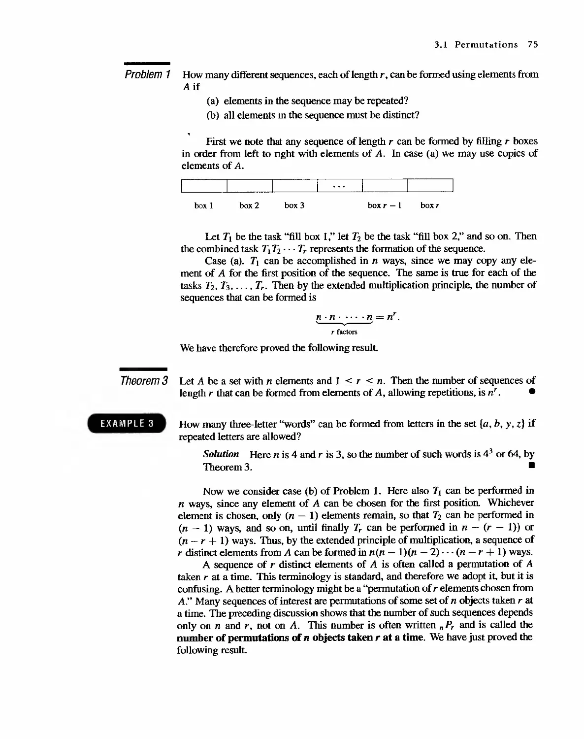
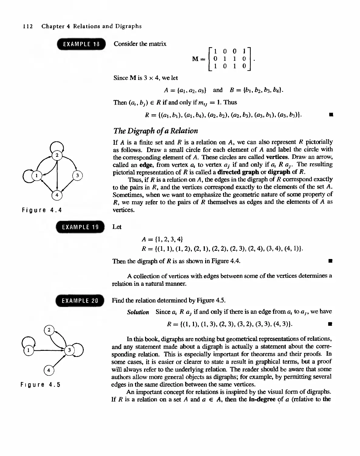
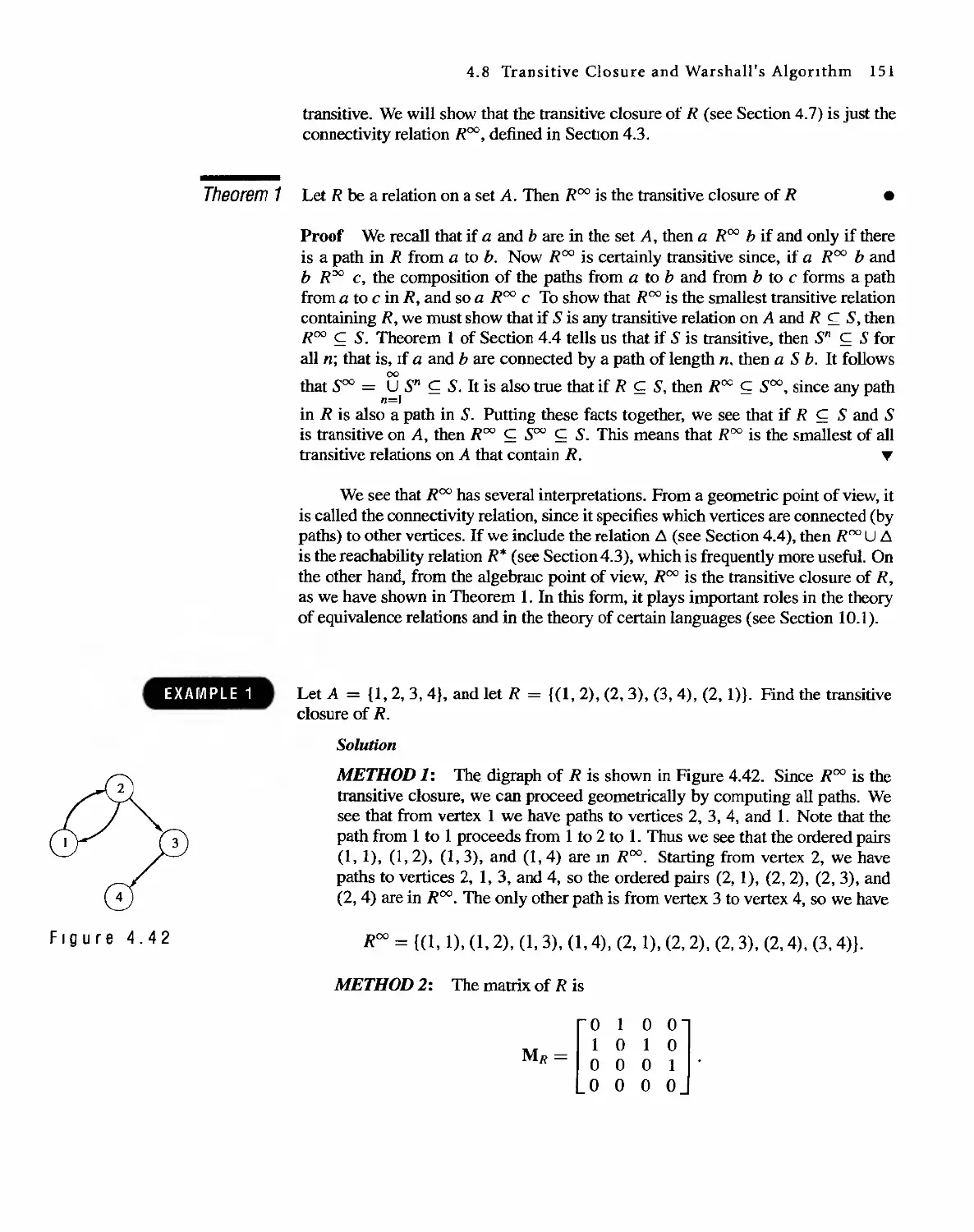
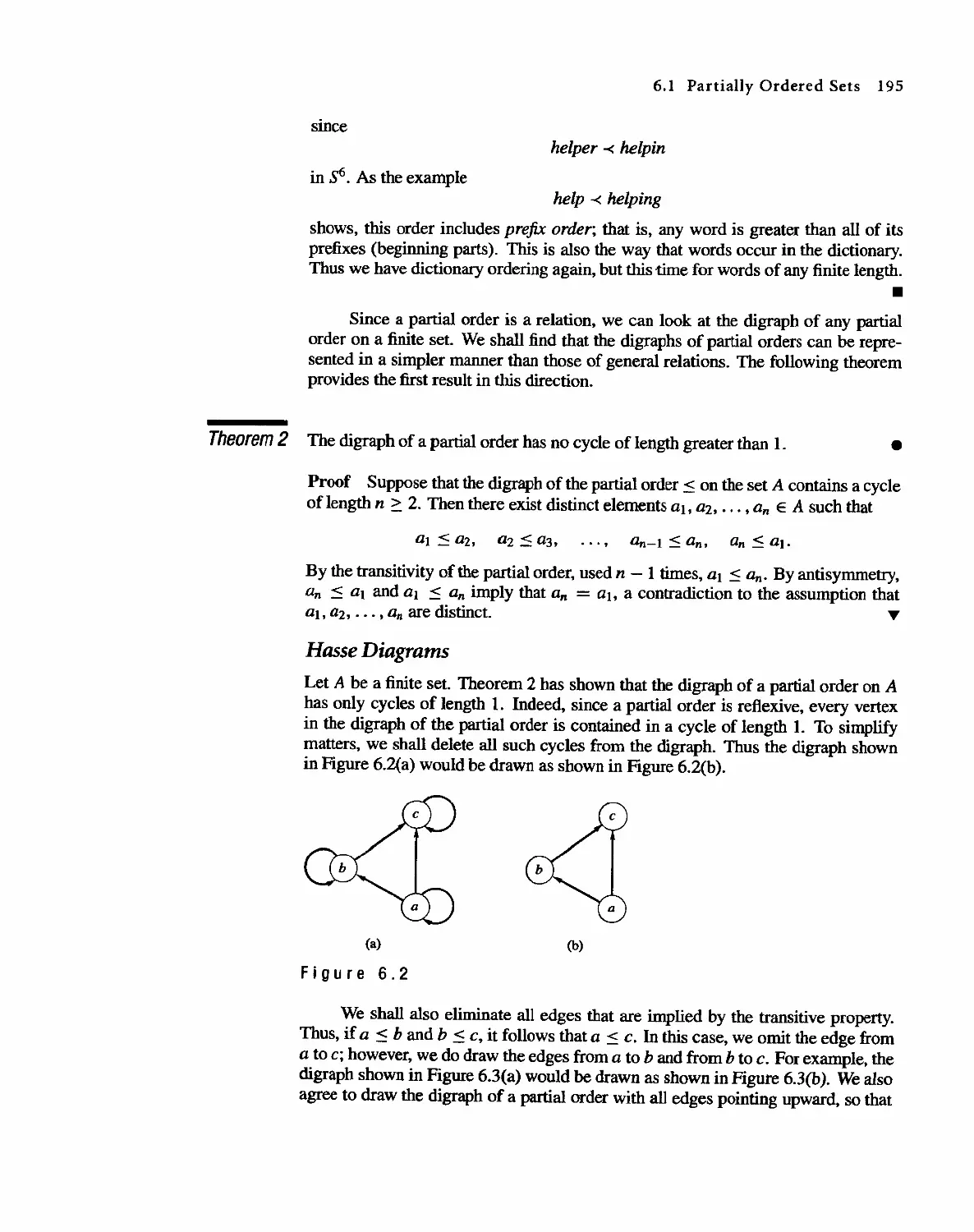
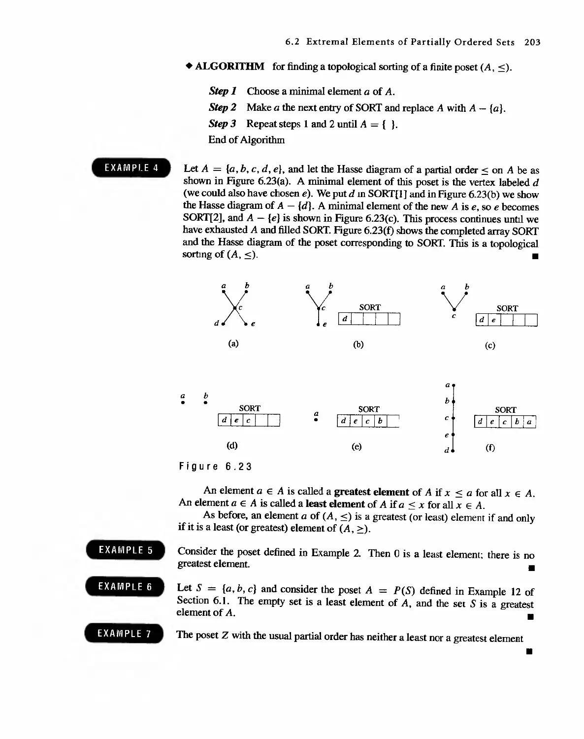
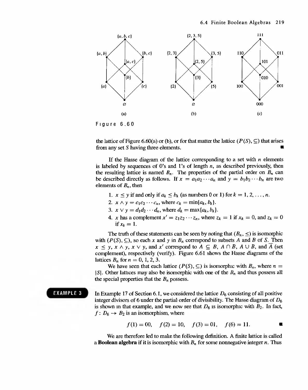
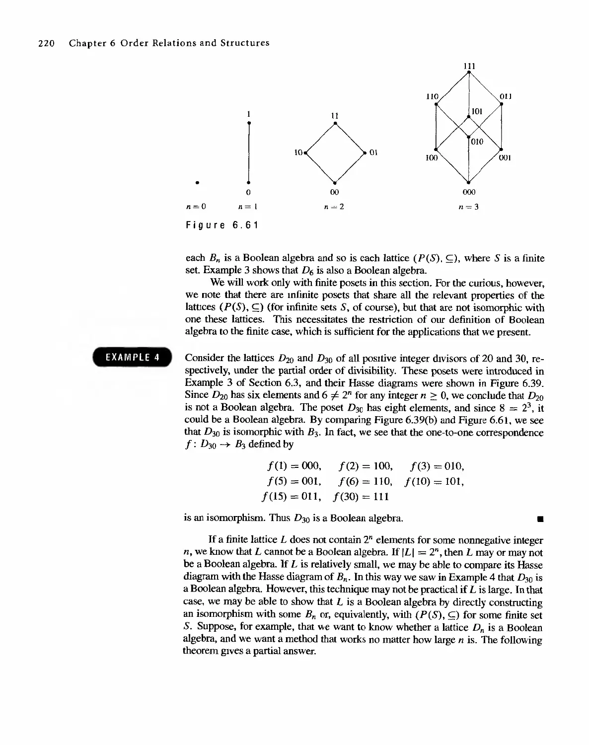
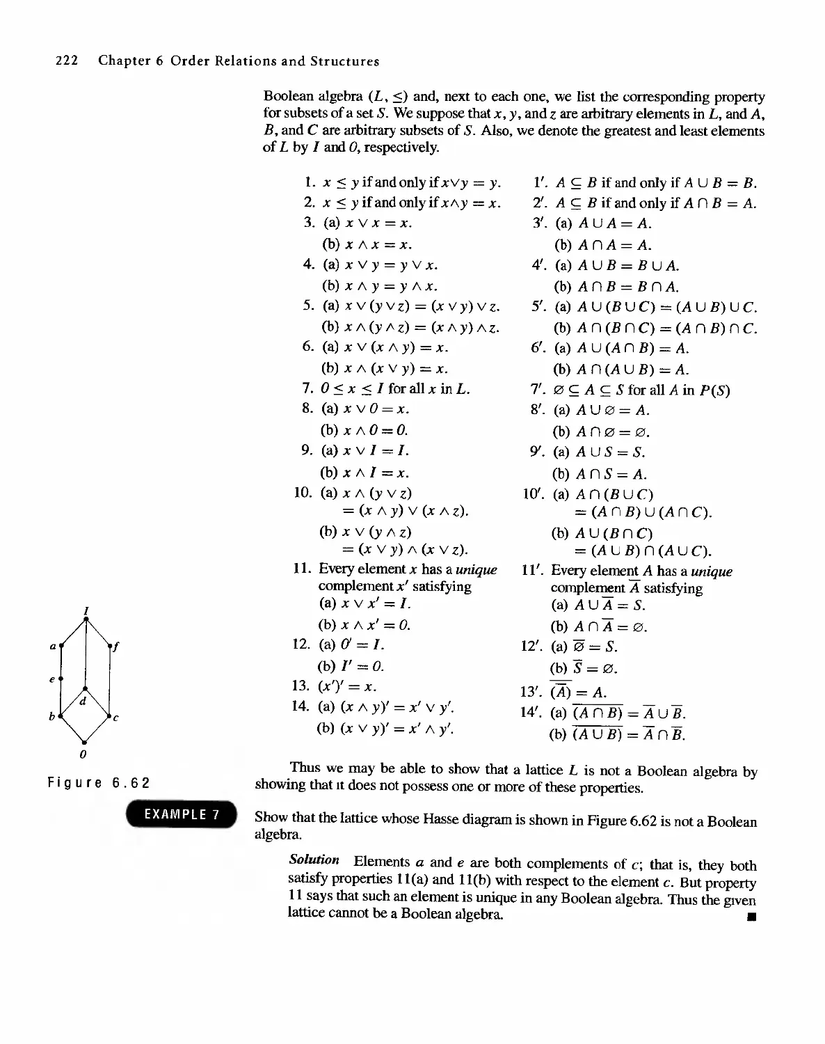
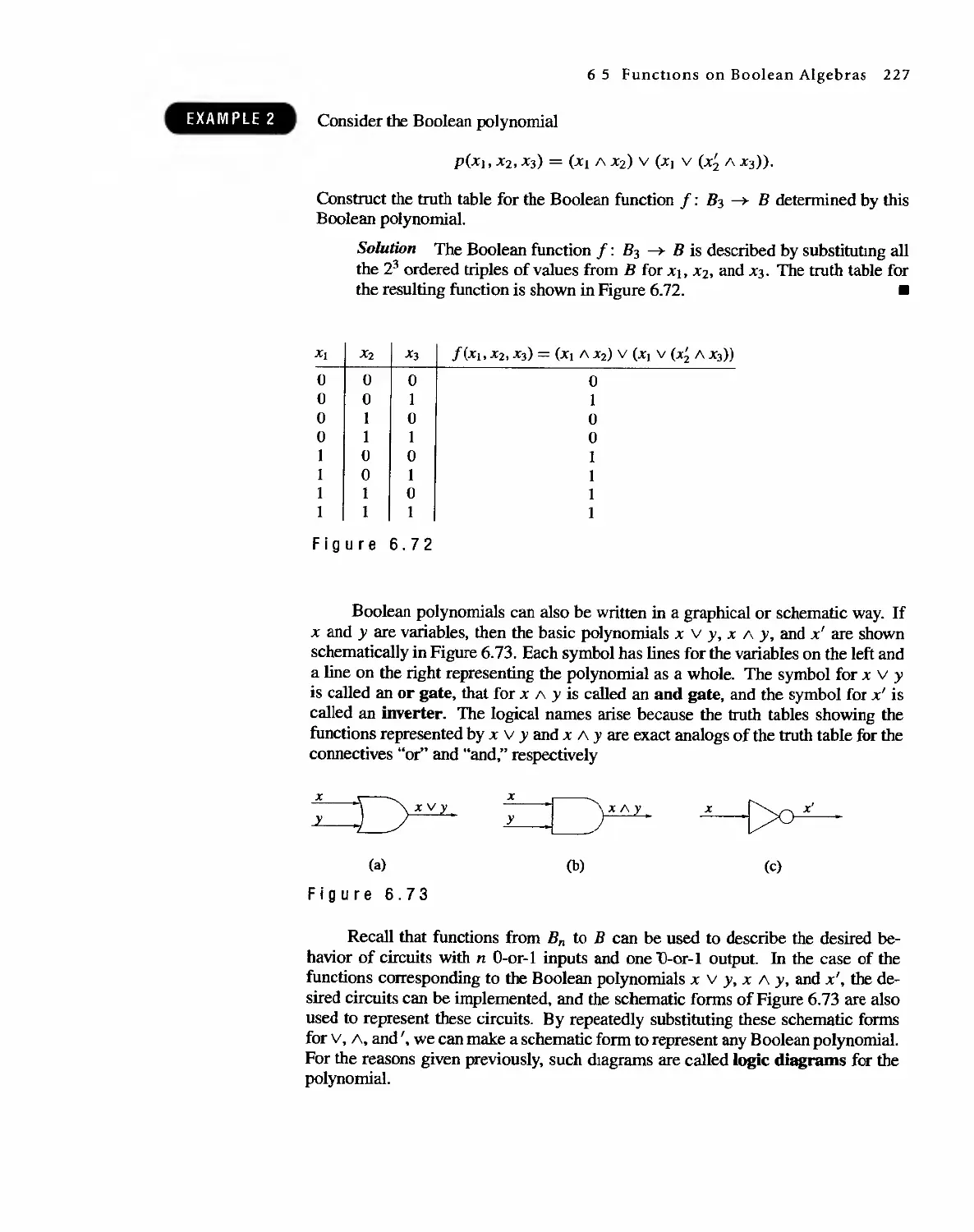
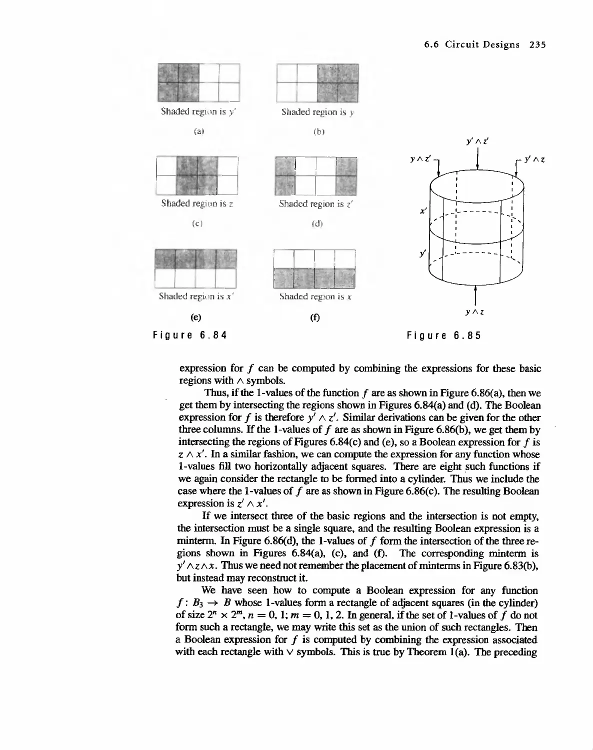
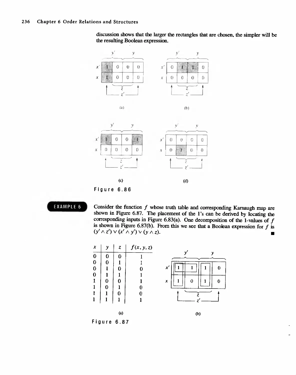
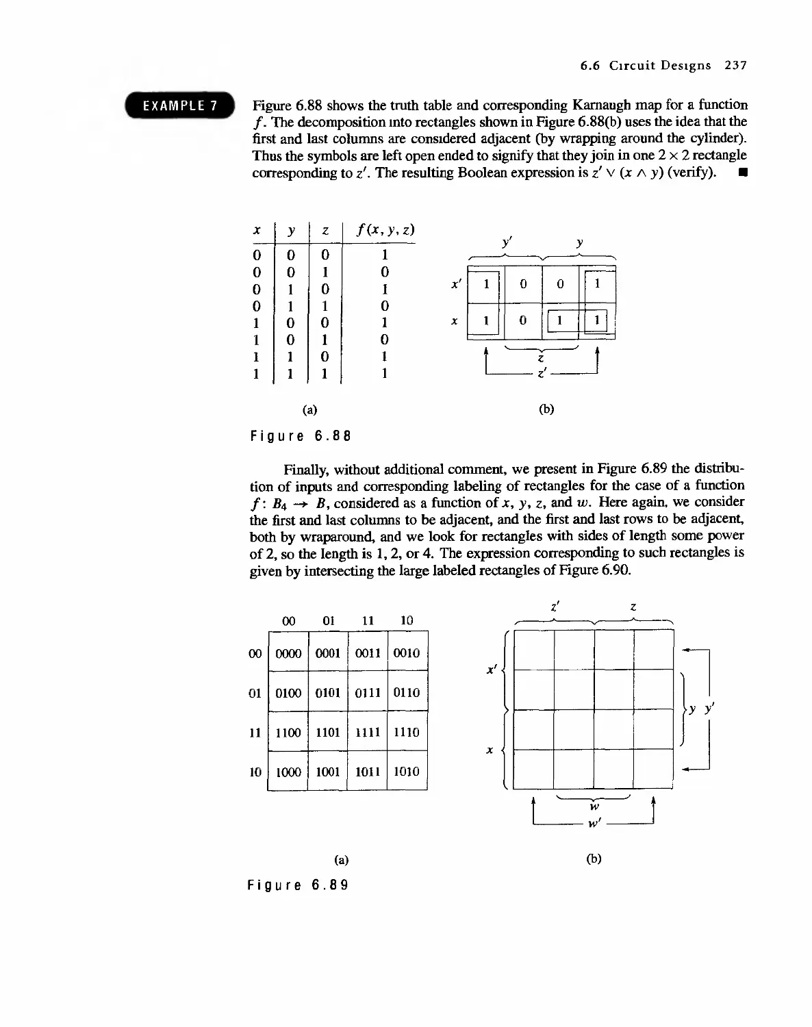
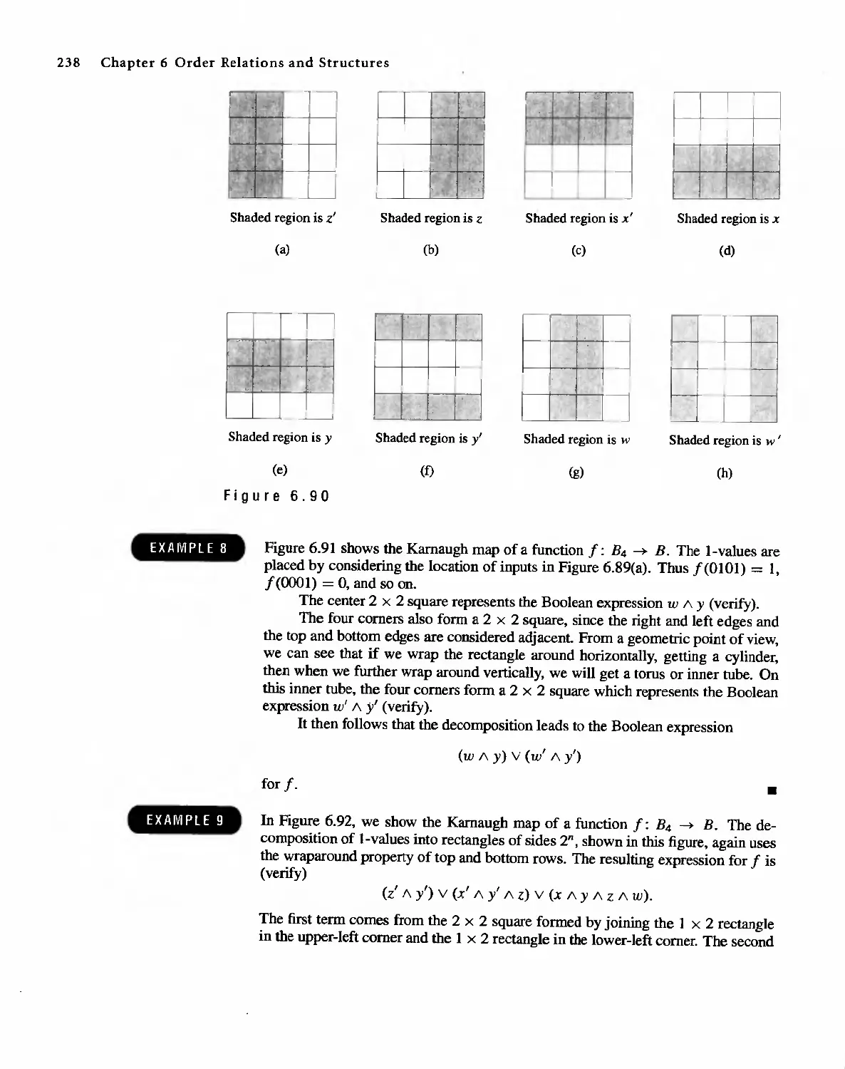
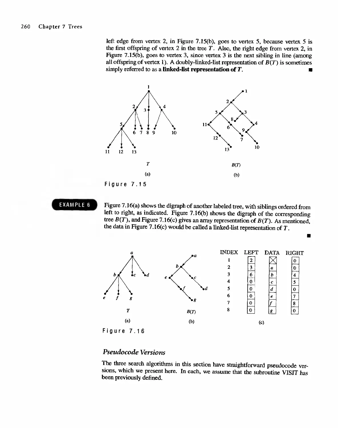
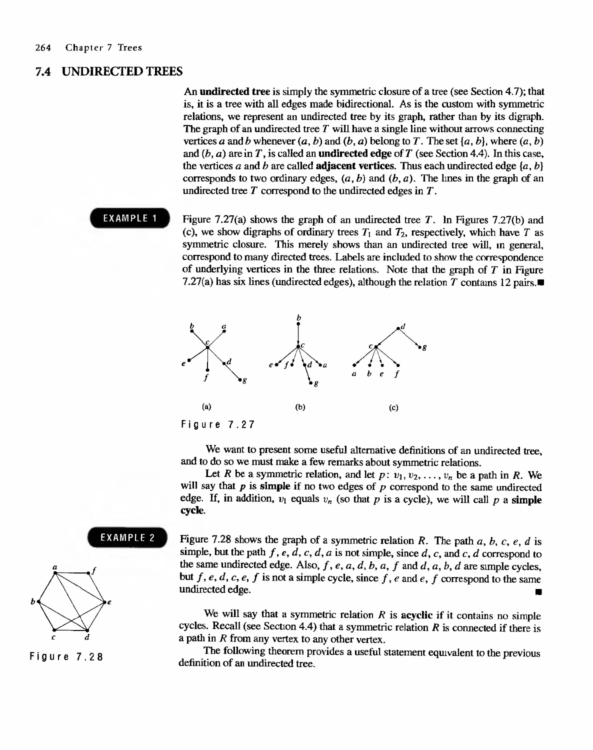
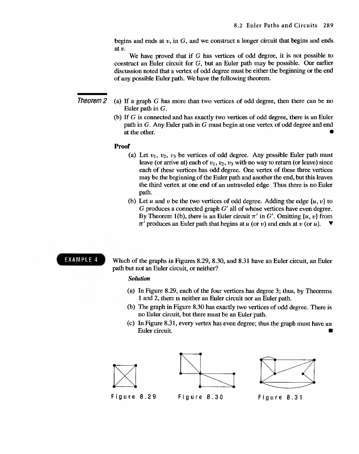
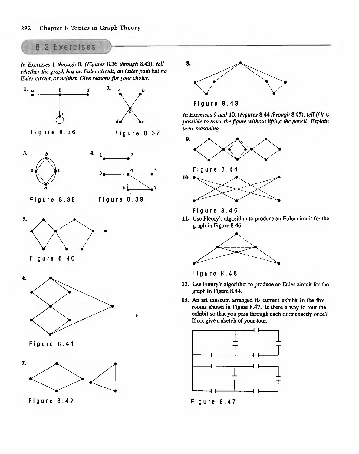
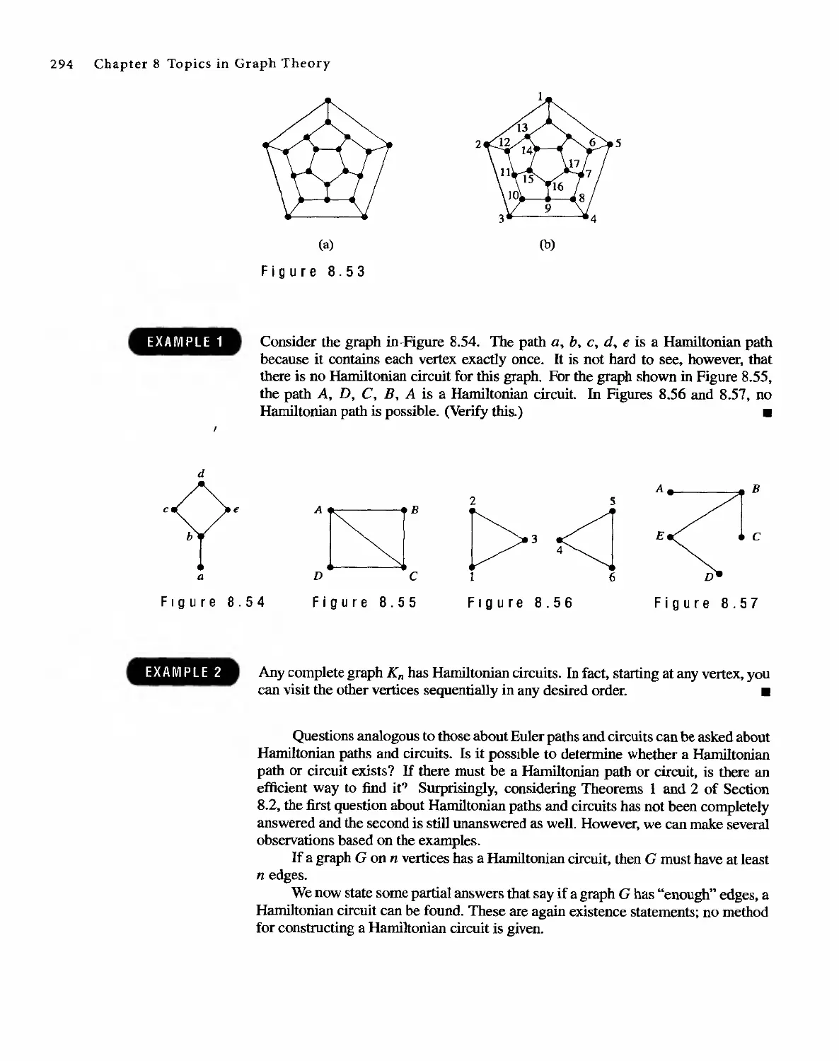
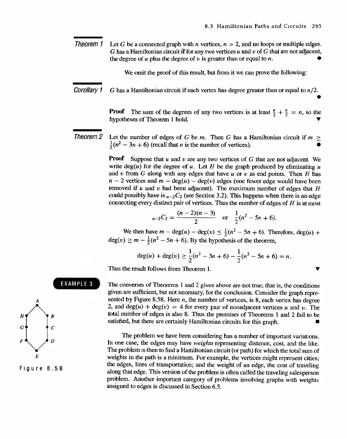
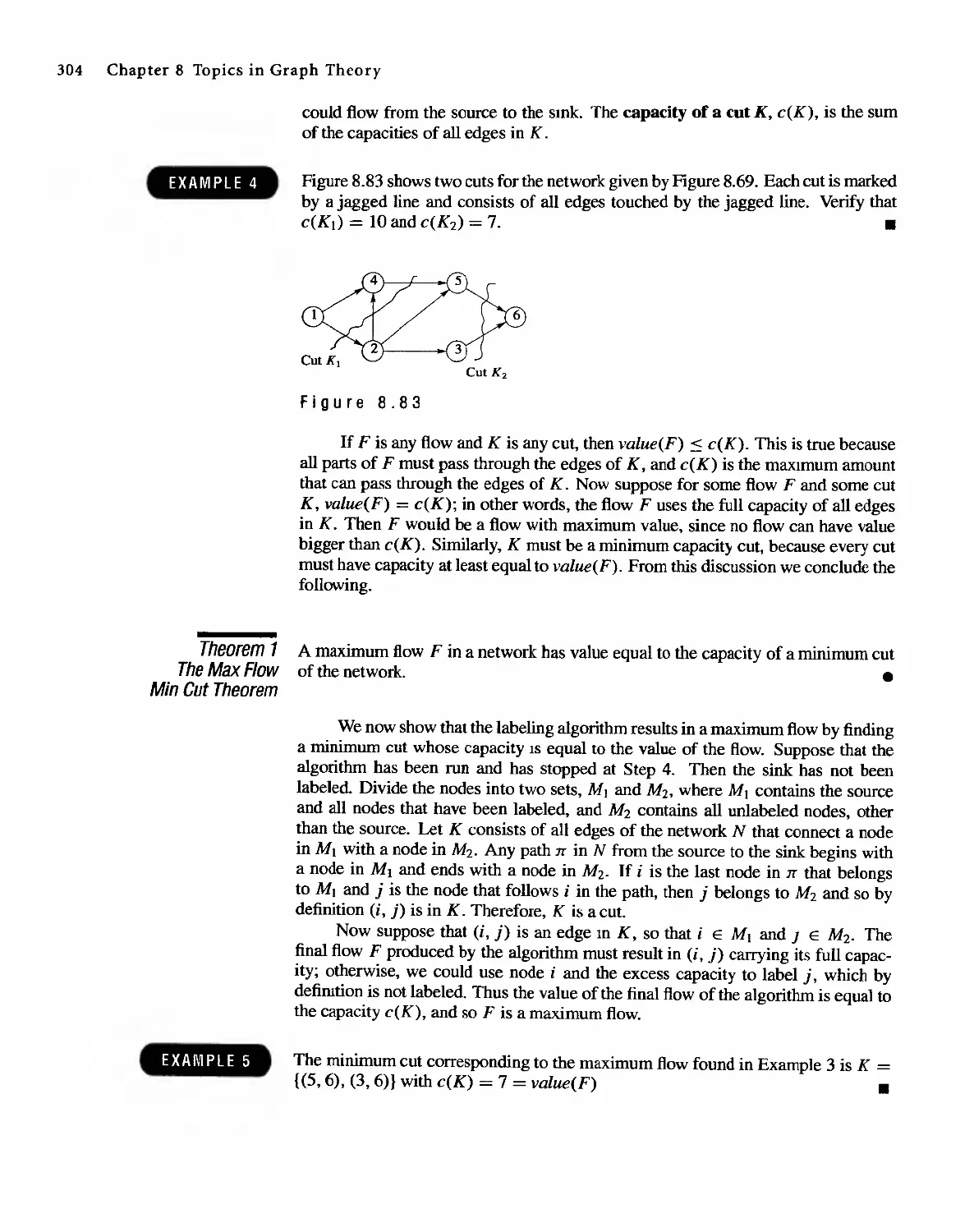
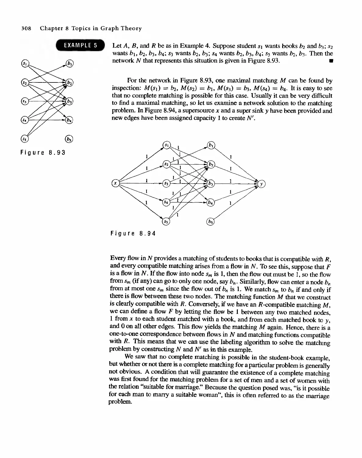
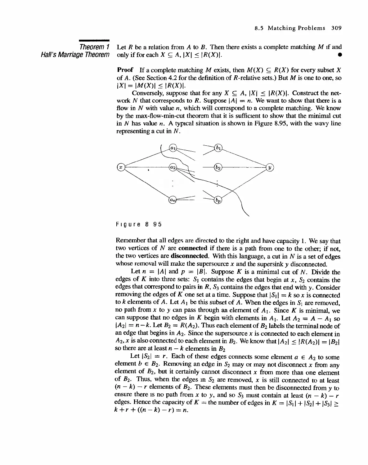
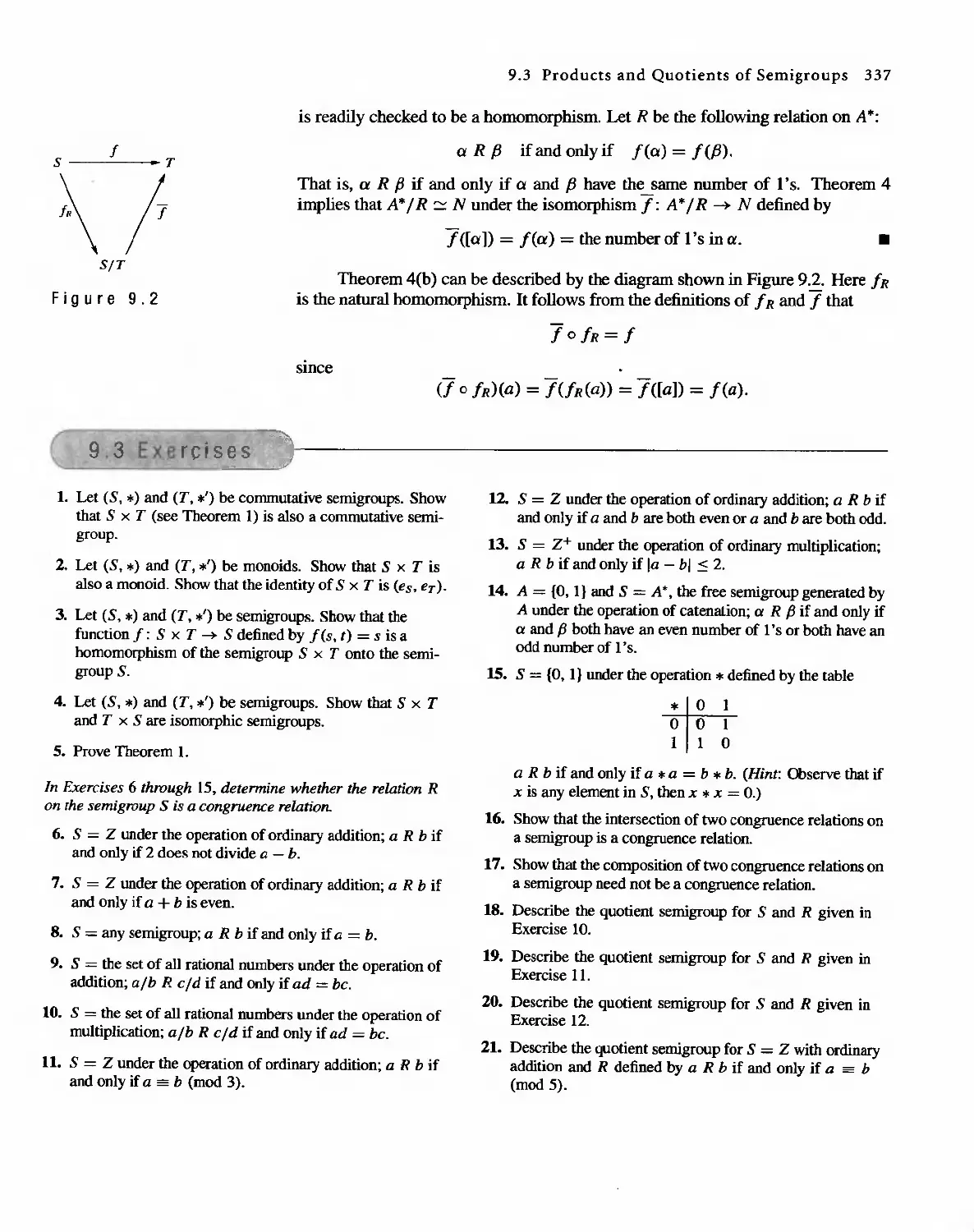
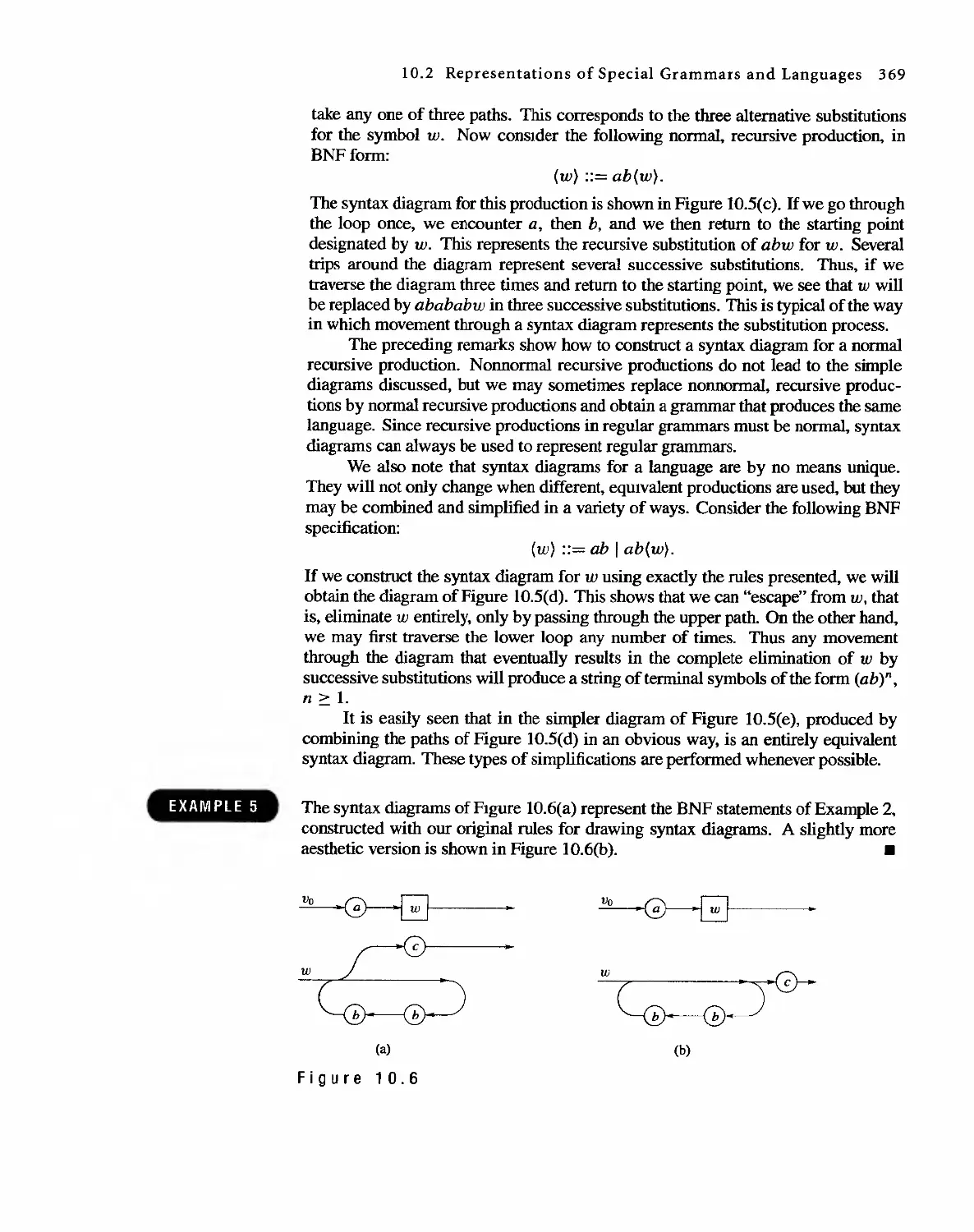
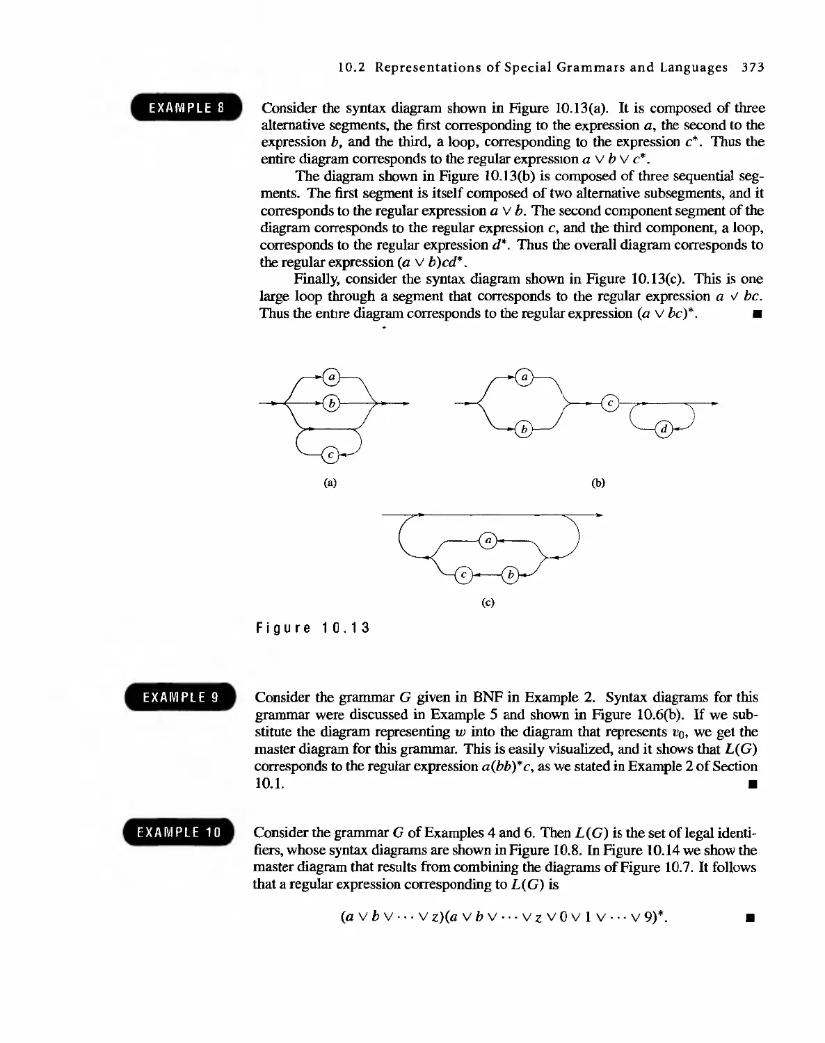
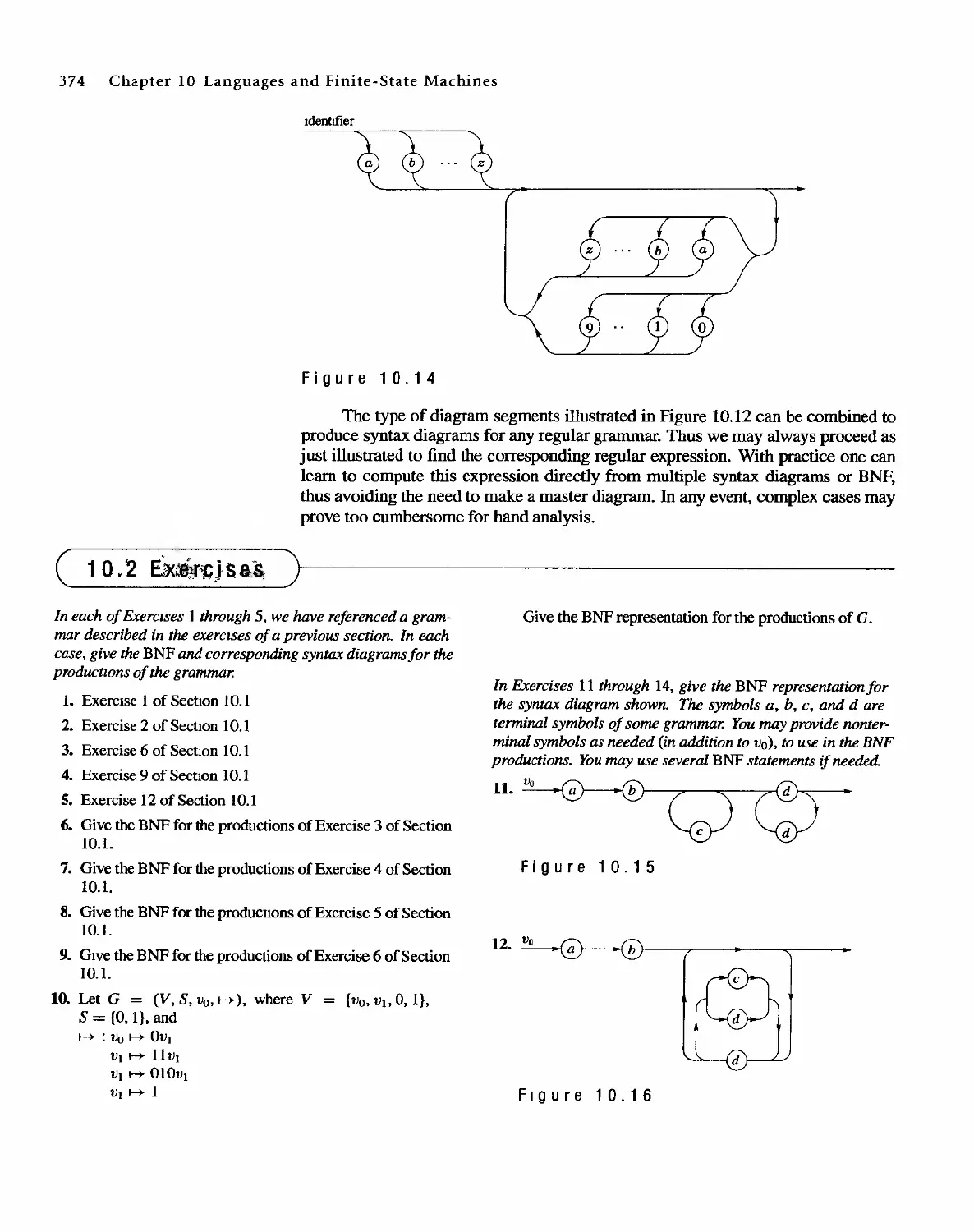
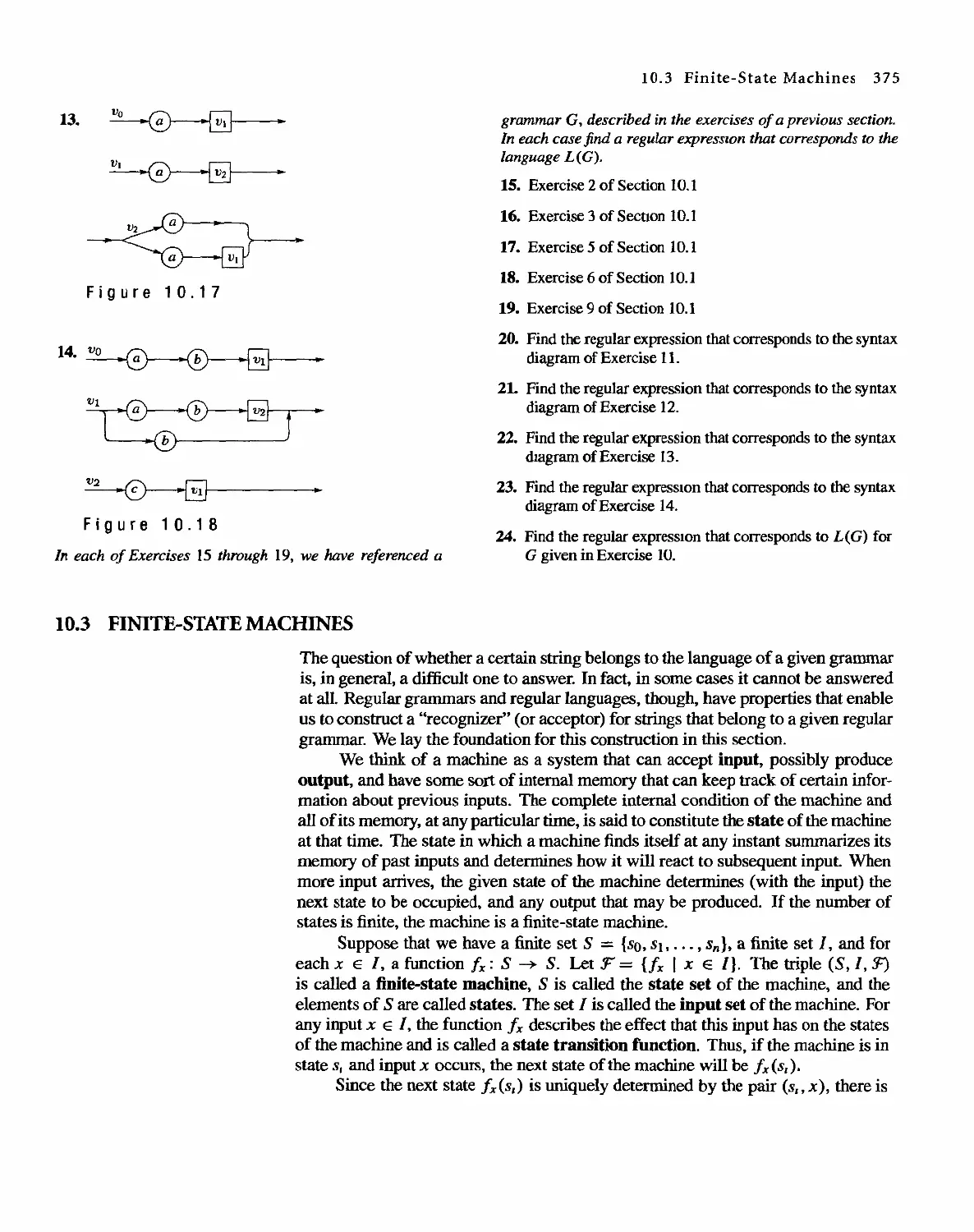
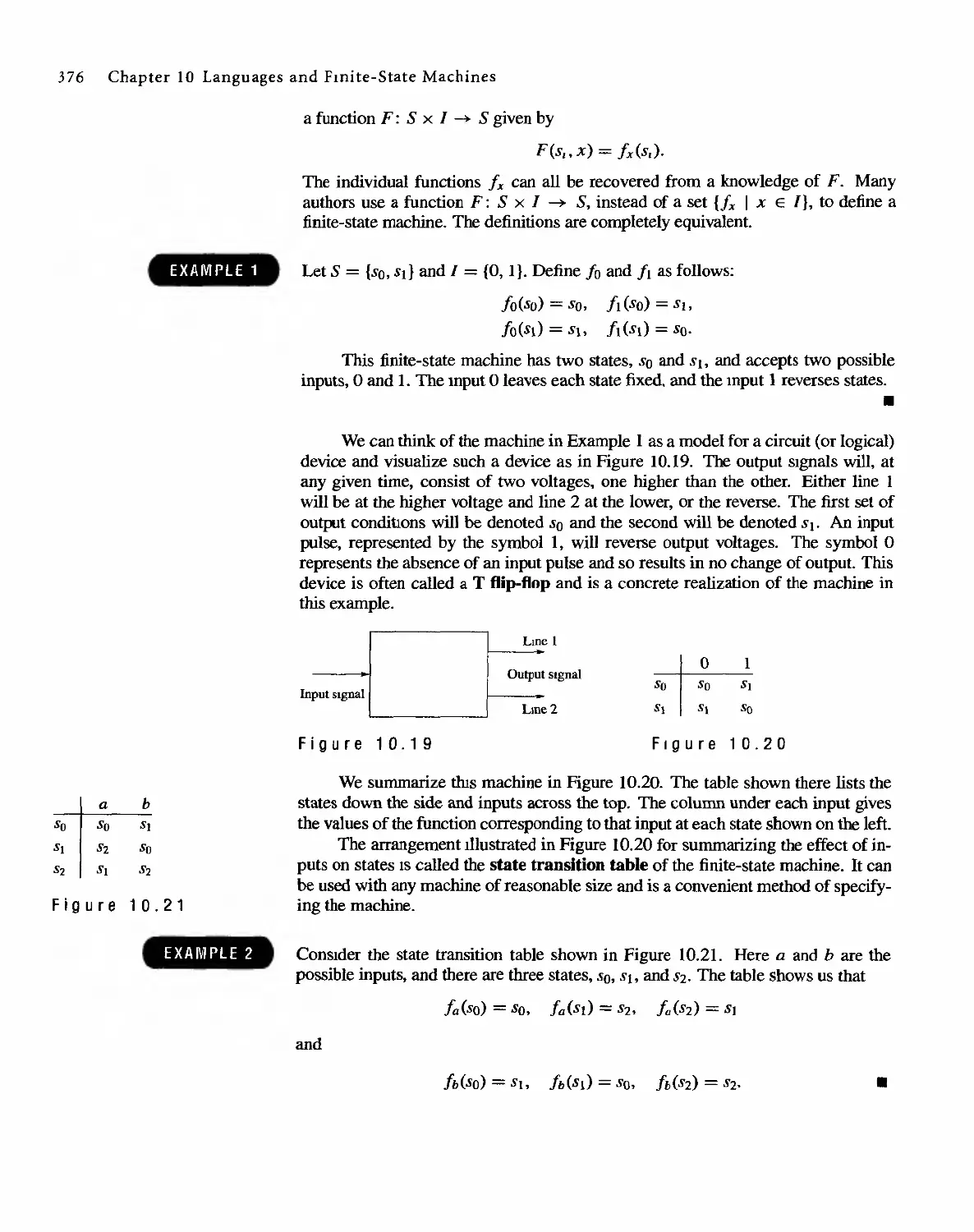
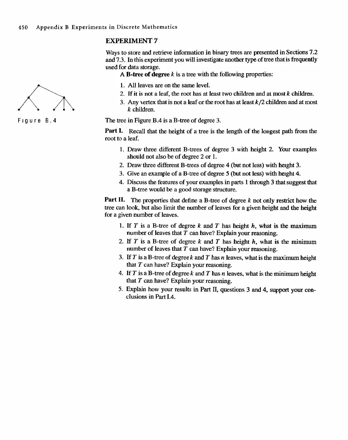
Текст
DISCRETE MATHEMATICAL
STRUCTURES
( Fourth Edition)
Bernard Kolman
Robert C. Busby
Sharon Cutler Ross
. Pearson Education
01-2001-2169
English Reprint Copyright @ 2001 by PEARSON EDUCATION NORTH ASIA LIMIED and HIGHER
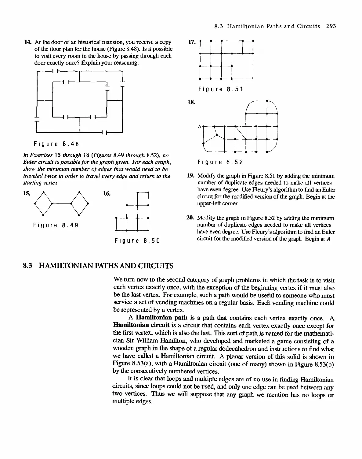
EDUCATION PRESS
Discrete Mathematical Structure from Prentice HaU's edition of the work
Discrete Mathematical Structure, 4th edition by Bernard Kolman, Robert C. Busby, Sharon Cutler
Ross, Copyright (9 2001,1996
All Rights Reserved
Published by arrangement with Prentice Hall, Inc. t a Pearson Education company
This edition is authorized for sale only in the People's Republic of China (excluding the SpecIal
Administrative Regions of Hong Kong and Macau)
To the memory of Lillie
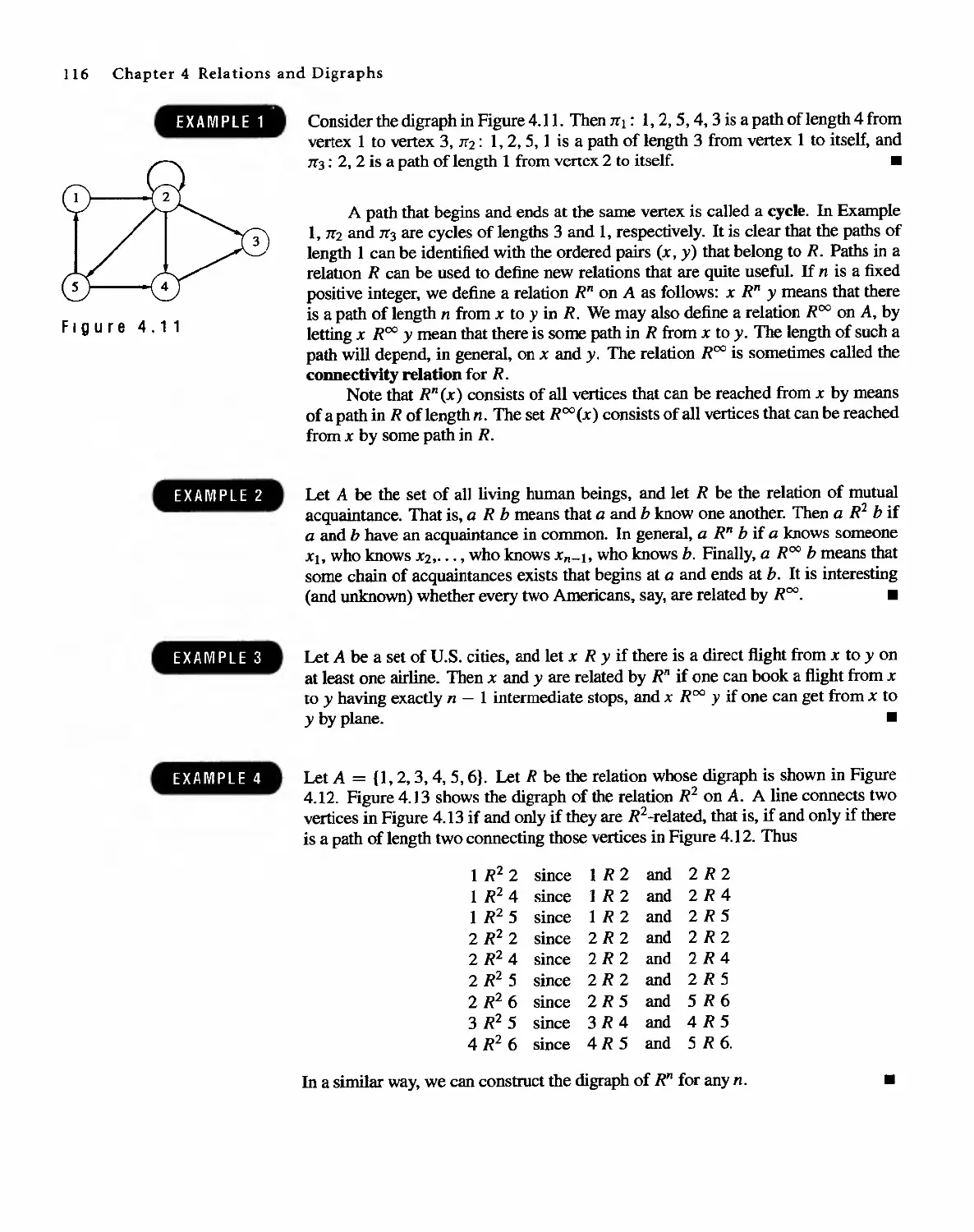
B.K.
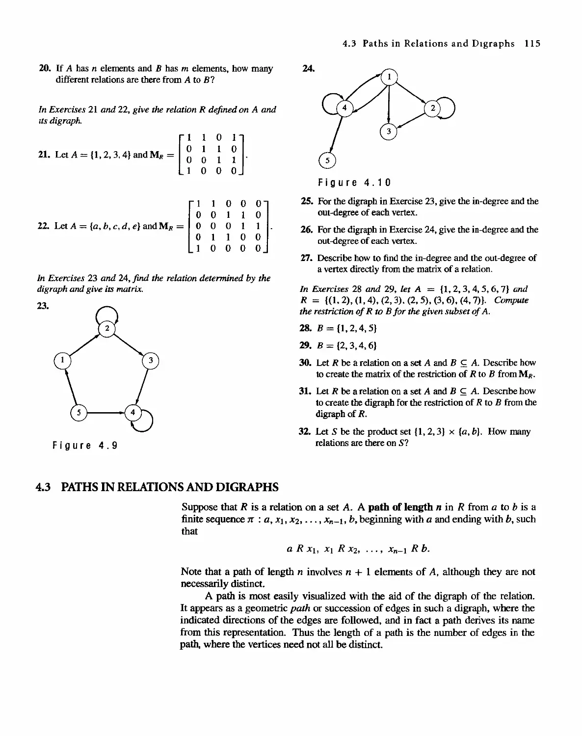
To my wife, Patricia, and our sons, Robert and Scott
R. C.B.
To Bill and bill
S. C.R.
. .
,:\';.... \',. ',' : , :.J '.'>.,
'. ." I" '. .
.' . .tv . " .
.. ' If4 1. ..
,,( . 'i:: .tr.. .f " .
. "\ ,;.,'11If 't
"I .I',, .... .: ,. 'f.'- II. . .
.... .," ... . ; 'eL '
'. '.. 4i111t.. . A
> .' '" t. } Ie ,.. . '..f
.¥ "!<.......
,. . 'f' 'IIi' ..'
".. . k' . " 1.,,' -:
" , . , . {i 'r}: :
.., \" . t: J'1. '\ .
;.f ::.; \. : ". . ; \.;
:. ... < . . . : ;'&1 ! · .,
' . t .. ' ,:' , t .'''.. }.! ':
.: t f.,,; '; .,
. "j .. '. . ', . " . ' , ,. \f:.
. , - \ ..., ... \ _ J"
..r ' ....,
'''< ,\' , "'\ .-;. ....
,. -f .t.... '- ' . , .. ." ;
, . 4' . __ ',' . . i-. ' .'
. j. ."1' .. (T
" ".... ..,
':'(': . '>I. i ;.; l t ':
.".:\ 'f\ \oi' "; : " i...
:\' \ . 1 . . '.'f. ;,:'.
. . - \ '..
. '1f"-.:.. .;: . 't" 0: I. 'J. t '".
f .l. p£'IJ Jj; . .:. Ii
,. :. --4\ $ '( (t """. ; J"
i ti. ': ,: ... '\; ., . !
...1 . It" t: . .. ,\ ..'
. . \ , <
{, \:; .. ', ' :-' '
:>" .... .t: ..' ..: .
.' ..." of. '!
;- , . h. 't" AI< .:
'I.."..'. . .. '-.. '"
, , '.. i .# .'" ,:, ".
y ' ';/:Jf. ,h ",
f,..\ , .. ;" f '. ;. . }J'- <
. . -' .' A' Ii",.
't . .,,' ', ' 'M'.
...... .*..... , ,\ ....
'., -! I .. . u (
" i; >. ' " '
,. . " ... . ... ..-'
.... .: ," ,_ \.";...... :0..
... '". -r:" --t
f .' ::. . A.... .'
. . ,< ..,. ) . 'Ii t
. . ..."'....
. f! - " j
' .( ,' ti ':., :i >::
:....,.. \!! ,'. .. '.
,-1; .,., .,iF " '. 1. .: -.. .
, . -. '. 4, ". :'t. :':
'.' ){,- \ r4',, ;,
: ' ' " V:: . f' . ., '..,'"
. , "".,
'. < '.., .-" &' =.;
. ',. '.' 04... ." 4 t' ,. ;t
: · . \ "Ii " ,- '.-
. .. {. : "t". '4i 1l: .. i' :,
. \:; lit. -,,' .
i 1 I ... <" :;" ;. . ) ' .., ::
,." ."' . ',l"" ." ,', t:. I1r \o ..-
". .,. . '. .... '4 ..... . i ? . 4 .'
J . fl' . tr ' I.:: ":
: .. if' ,1-. . . \ ' ' .wi, ;,'
, .; 'i ':...: ' ,.";'p, ".::
. _.... .
'... < . .. -"",.1' . '.. '.
to. . t j:' I .:... :
.' ,,') :£ . . .. '.'
. ' , ." '0' " .'
:..'f:;..., . tOt'" .. '-"'\. " \ '
-. .. ,,=;IC . . "t "
, . " .... - .:,. ,.
'.. \. 'j . .. , .
}\ . '. 'f ",. ,
: ..:..:..., ,,' "' i', ,t '..f
, ,('...... " .'
..... . ...t:.t,. :.:. C".4i:.-.... p.JI..:.
PREFACE
Discrete mathematics is a difficult course to teach and to study at the freshman and
sophomore level for several reasons. It is a hybrid course. Its content is mathemat-
ics. but many of its applications and more than half its students are from computer
science. Thus careful motivation of topics and previews of applications are im-
portant and necessary strategies. Moreover, the number of substantive and diverse
topics covered in the course is high, so that student must absorb them Tather quickly.
At the same time, the student may also be expected to develop proof-writing skills.
APPROACH
First, we have limited both the areas covered and the depth of coverage to what we
deemed prudent in a first course taught at the freshman and sophomore level. We
have identified a set of topics that we feel are of genuine use in computer science
and elsewhere and that can be presented in a logically coherent fashion. We have
presented an introduction to these topics along with an indication of how they can
be pursued in greater depth.
For example, we cover the simpler finite-state machines, not Turing machines.
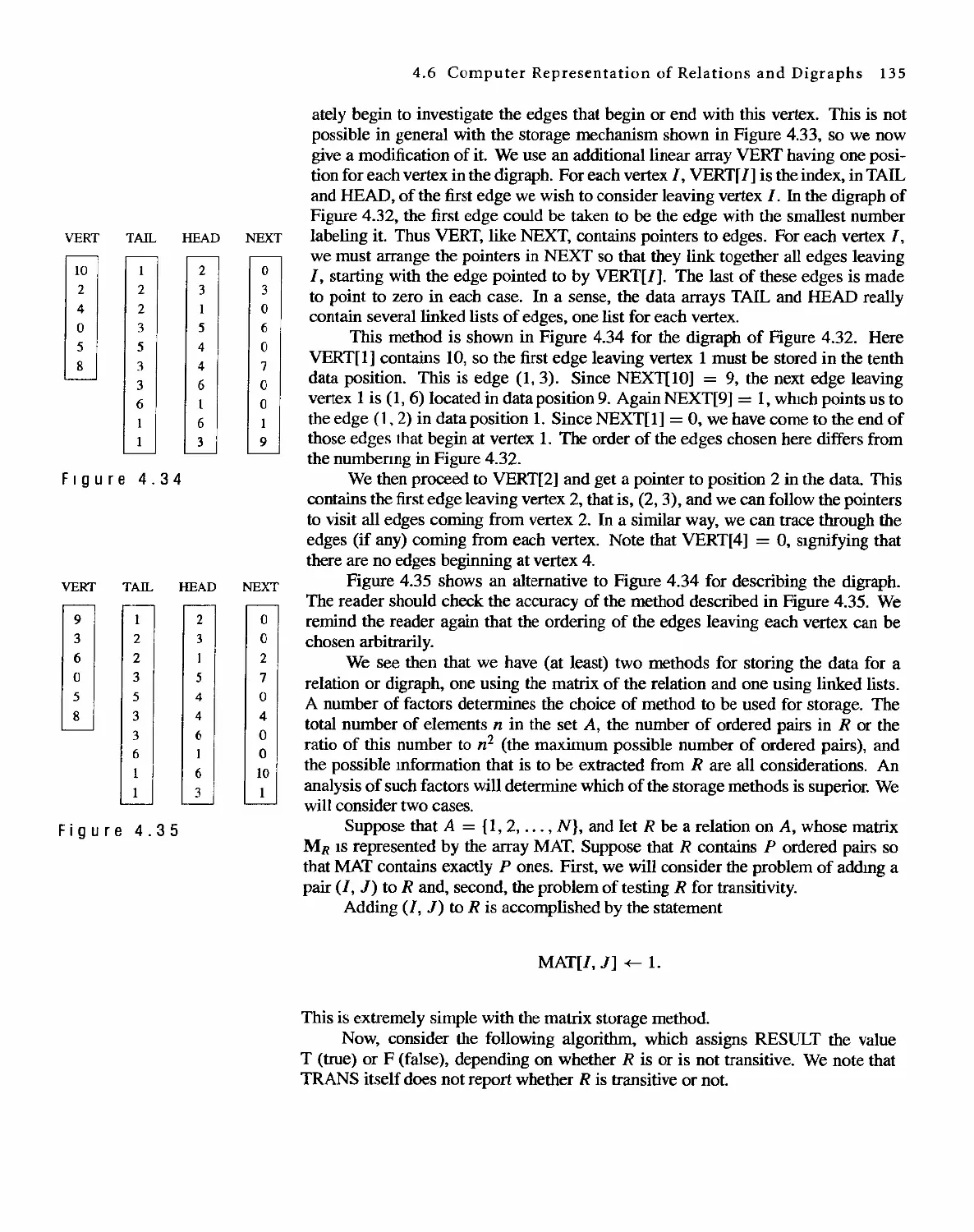
We have limited the coverage of abstract algebra to a discussion of semigroups and
groups and have given application of these to the important topics of finite-state
machines and error-detecting and error-correcting codes. Error-correcting codes, in
turn, have been primarily restricted to simple linear codes.
Second, the material has been organized and interrelated to minimize the mass
of definitions and the abstraction of some of the theory. Relations and digraphs are
treated as two aspects of the same fundamental mathematical idea, with a directed
graph being a pictorial representation of a relation. This fundamental idea is then
used as the basis of virtually all the concepts introduced in the book, including
functions, partial orders. graphs, and algebraic structures. Whenever possible, each
new idea introduced in the text uses previously encountered material and, in turn, is
developed in such a way that it simplifies the more complex ideas that follow. Thus
partial orders, lattices, and Boolean algebras develop from general relations. This
material in turn leads naturally to other algebraic structures.
.
Xl
xu Preface
WHAT IS NEW IN THE EOU UTI I EDITION
We continue to be pleased by the reception given to earlier editions of this book.
We still beheve that the book works well in the classroom because of the unifying
role played by two key concepts: relations and digraphs. For this edition we have
modified the order of topics slightly and made extensive revisions of the exercise
sets. The d1scourse on proof has been expanded in several ways. One of tbese is
the insertion of comments on nearly every proof in the book. Whatever changes we
have made, our goal continues to be that of maximizing the clarity of presentation.
As the audience for an introductory discrete mathematics course changes and as the
course is increasingly used as a bridge course, we have added the following features.
. A new section, Transport Networks, introduces this topic using ideas from
Chapter 4.
. A new section, Matching Problems, applies the techniques of transport net-
wolks to a broad class of problems.
. The section on mathematical induction now includes the strong form of in-
duction as well.
. The discussion of proofs and proof techniques is now woven throughout the
book with comments on most proofs, more exercises related to the mechanics
of proving statements, and Tips for Proofs sections. Tips for Proofs highlight
the types of proofs commonly seen for that chapter's material and methods for
selecting fruitful proof strategies.
. A Self-Test is provided for each chapter with answers for all problems given
at the back of the book.
. Exercise Sets have a broader range of problems: more routine problems and
more challenging problems. More exercises focus on the mechanics of proof
and proof techniques. As with writing in general, students learn to write proofs
not only by reading, analyzing, and recognizing the structure of proofs, but
especially by writing, re-writing t and writing more proofs themselves.
EXERCISES
The exercises form an integral part of the book. Many are computational in nature,
whereas others are of a theoretical type. Many of the latter and the experiments,
to be further described below, require verbal solutions. Exercises to help develop
proof-writing skills ask the student to analyze proofs, amplify arguments t or com-
plete partial proofs. Answers to all odd-numbered exercises appear in the back of
the book. Solutions to all exercises appear in the Instructor's ManuaI, which is
available (to instructors only) gratis from the publisher. The Instructor's Manual
also includes notes on the pedagogical ideas underlying each chapter, goals and
grading guidelines for the experiments further described below, and a test bank.
EXPERIMENTS
Appendix B contains a number of assignments that we call experiments. These
provide an opportunity for discovery and exploration, or a more-in-depth look at
Preface XIII
various topics discussed in the text. These are suitable for group work. Content
prerequisites for each experiment are given in the Instructor's Manual.
END OF CHAPTER MATERIAL
Each chapter contains Tips for Proofs, a summary of Key Ideas, a set of Coding
ExeICises, and a Self-Test covering the chapter's material.
CONTENT
Chapter 1 contains a miscellany of basic material required in the course. This in-
cludes sets, subsets, and their operations; sequences; division in the integers; matri-
ces; and mathematical structures. A goal of this chapter is to help students develop
skiUs in identifying patterns on many levels. Chapter 2 covers logic and related ma-
terial, including methods of proof and mathematical induction. Although the dis-
cussion of proof is based on this chapter, the commentary continues throughout the
book. Chapter 3, on counting, deals with permutations, combinations, the pigeon-
hole principle, elements of probability, and recurrence relations. Chapter 4 presents
basic types and properties of relations, along with their representation as directed
graphs. Connections with matrices and other data structures are also explored in
this chapter. The power of multiple representations for the concept of relation is
fully exploited. Chapter 5 deals with the notion of a function and gives important
examples of functions, including functions of special interest in computer science.
An introduction to the growth of functions is developed.
Chapter 6 covers partially ordered sets, including lattices and Boolean alge-
bras. Chapter 7 introduces directed and undirected trees along with applications of
these ideas. Elementary graph theory is the focus of Chapter 8. New to this edi-
tion are sections on Transport Networks and Matching Problems; these build on the
foundation of Chapter 4.
In Chapter 9 we give the basic theory of seIDlgroups and groups. These ideas
are applied in Chapters 10 and 11. Chapter 10 is devoted to finite-state machines.
It complements and makes effective use of ideas developed in previous chapters.
Chapter 11 treats the subject of binary coding.
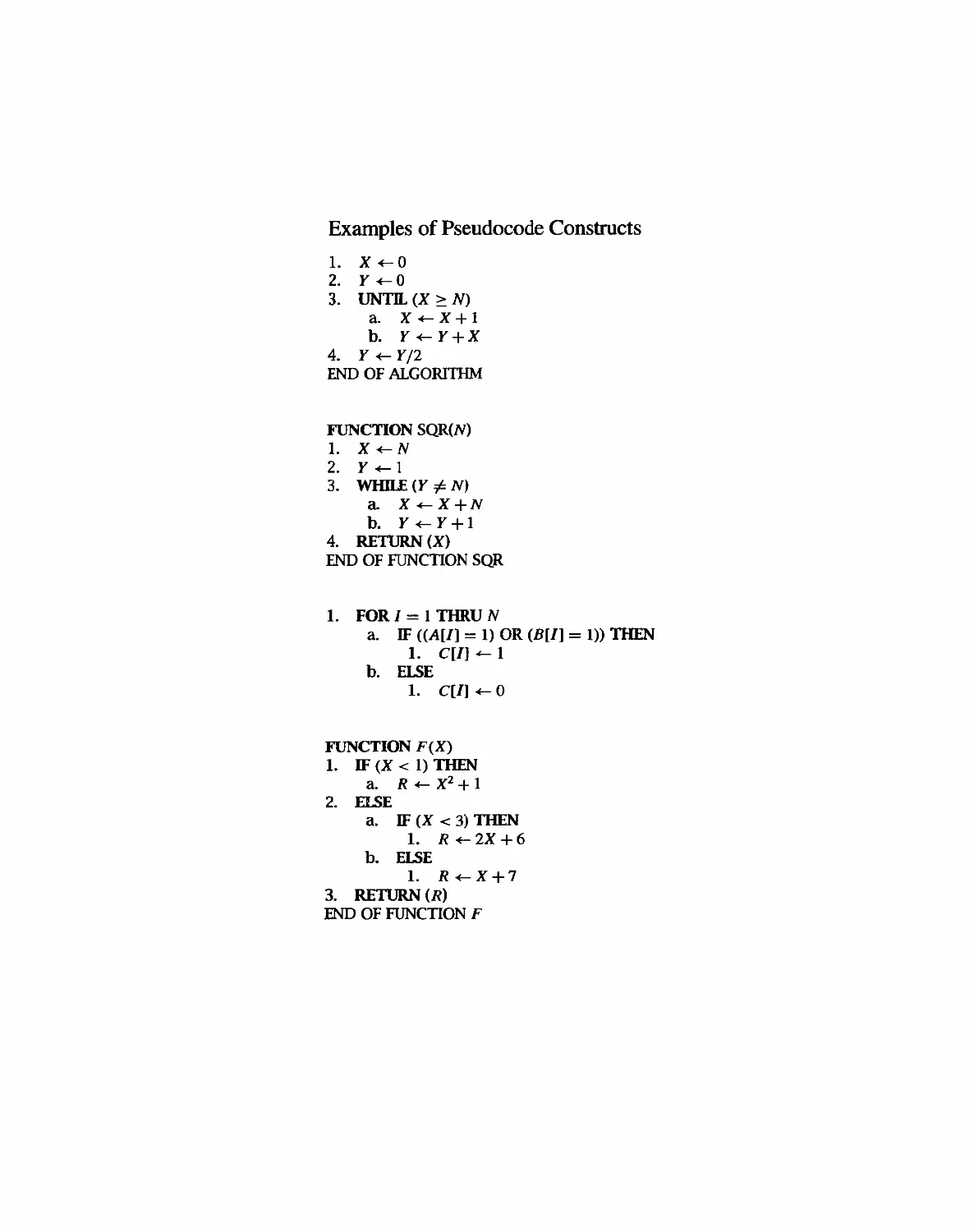
Appendix A discusses algorithms and pseudocode. The simplified pseudocode
presented here is used in some text examples and exercises; these may be omitted
without loss of continuity. Appendix B gives a collection of experiments dealing
with extensions or previews of topics in various parts of the course.
CSE OF THIS TEXT
This text can be used by students in mathematics as an introduction to the funda-
mental ideas of discrete mathematics, and as a foundation for the development of
more advanced mathematical concepts. If used in this waYt the topics dealing with
specific computer science applications can be ignored or selected independently as
important examples. The text can also be used in a computer science or computer
engineering curriculum to present the foundations of many basic computer-related
concepts, and provide a coherent development and common theme for these ideas.
Xl V Preface
ACKNOWLEDGMENTS
The instructor can easily develop a suitable course by referring to the chapter pre-
requisites, which identify material needed by that chapter.
We are pleased to express our thanks to the following reviewers of the first three edi-
tions: Harold Fredrickson t Naval Postgraduate School; Thomas E. Gerasch t George
Mason University; Samuel 1. Wiley, La Salle College; Kenneth B. Reid, Louisiana
Sate University; Ron Sandstrom, Fort Hays State University; Richard H. Austing,
University of Maryland; Nina Edelman, Temple University; Paul Gormley, Vil-
lanova University; Hennan Gollwitzer and Loren N. Argabright, both at DrexeJ
University; Bill Sands. University of Calgaryt who brought to our attention a num-
ber of errors in the second edition; Moshe Dror, University of Arizona, Tucson;
Lloyd Gavin, California State University at Sacramento; Robert H. Gilman, Stevens
Institute of Technology; Earl E. Kymala, California State University at Sacramento;
and Art Lew, University of Hawaii, Honolulu; and of the fourth edition: Ashok
T. Amin, University of Alabama at Huntsville; Donald S. Hart. Rochester Institute
of Technology; Minhua Liu, William Rainey Harper College; Charles Parry, VIr-
ginia Polytechnic Institute & University; Arthur T. Poet Temple University; Suk
Jai Seo, University of Alabama at Huntsville; Paul Weiner. St. Mary's University
of Minnesota. The suggestions t comments t and criticisms of these people greatly
improved the manuscript.
We thank Dennis R. KIetzing, Stetson University. who carefully typeset the
entire manuscript; Nina Edelman. Temple University. for critically reading page
proofs; Blaise DeSesa, Allentown College of St. Frances de Sales, who checked the
answers and solutions to all the exercises in the book; and instructors and students
from many institutions in the United Stares and other countries, for sharing with us
their experiences with the book and for offering helpful suggestions.
Finally, a sincere expression of thanks goes to Betsy Williams, George Lo-
bell t Gale Epps, and the entire staff at Prentice Hall for their enthusiasm t interest,
and unfailing cooperation during the conception t design, production, and marketing
phases of this edition.
B.K
R.C.B.
S.C.R.
, ' ," , i' ' , ,;L.,j.i1 ;'
" ., ),' ' ,of. !,
, ,yi ,.. ,it',.:, ,.\L :- 'lJ 'f"
-." ,'.' ,( .. " " , ' {j. ,
f .... - ..... .;.". . I : ..
' " '.. "'," ", " ,: ,', .,. "
..' ..... ". . .. .'< . . . . tt... .
1 . . . z ...... _ ,:.
, '. ( :.-': ' " ",," .
. t1 ; . r"; '.. : , 0 '''I<'',, ' '
. .. :' , I"'-:" ':: ',>' .; 't. ;.'
. ...',.." '.f . '." -'.
;v.. . ',:' ,', -: . .. \t ' " t ' , .
:....IL-\ ',:' ."..
:- ' ..,.
: ' ' ..., '. , .
. '.. ." · ,," J;-
..' . " tIL:'f t . . :
, '..., r' " 'J, '.
t. " ":",fIf" . ' ' , t. ' , ", .' :.,
.._' \ < ' "1 J . . ,,;, -
,: , . ¥,! , , '" :';' : f '" ', ,; 't. . , ';:, ,
.. .b. Y' . ".i. ",
, c' ' ; , ',:.;, L . ' ,' ["
<t .. ". '."",
. - :.,"':- . . . ,.. .1
' I ;' ;'" :-. } > < A:,; . : ',., ':\ ;:
. . ..", . .... "i
, ,'it " , " " ' ,;', ,::'
',' ' "T" 1 ".
:\i., :,' '-:: ,,'''';.'' ":';'1'"
' t' I "" 'i ;" '" ,. ' ,',' ,»"
V ',:' :, " ,11 = ',< 'it J
f, '. ', , , ':. ': " -" c'
.... .... . . ,.
'" ' " . i- . ' t
,! . ..' ' '1" :1tt' ,':f.,'.., \ ...,' ;,
,: . ...« . "." ", .. .
. ' ......."... t' , .
, . "v _:r . ,;':..' ' ) >".a < :,
" t' " '\, " T' ", ,.
., :' '. "'4 I : ,:-.,.:' '; ,:..; ,-::
I(V" -.' -¥'- ."'.. "J;' "J' '.,.
...' ' ,' , . , ' .: . " '41:.:, ", r
.TJ "." . '!; ','1. . ::'. '. > :
: :., { ;, " f. :, ,':
1'\W';:,j 'iX-,.,,:" ' "" .: ' Ji,., -.i
, '1' ..".' .'., "I- : ':=-
, " if:,"" " " .' -
II'. > .. ;- ,-", ..',", :-.' ' .--
, : 1 'It ..,.,. \ .
, '. ...' .J
iit : ' .':' " ' ;,I:J>::: '¥. ';
-.. . ' , , ;,:. ;. )-: .: , _; ,.,' , 4 ;
. . ," ..".. '"" " .,
." ", .,-', '" .'; ,'; !'.
';;:-,t'- : "/ ,. "" <')<' \ : ;!
. ..'. , ',',";,' ,iii>, 't
..'.... ........ . . ..y. '\<t
" . ,",:--\ . f ':'<
...... ,'" ".. .. .
"': '. '..., .', ,:y
, ;if> .. ," , It .
, ". " :',; ' * ' ,'" : .,: :r' I '
, ' ',' , ' '-' ifr. ,
. r ...". '",'" J_:. ,:..
,', , ,!,,',',, , '.. f'
, it:' ",':$t '.' - ", ':'11' ' t'...'
"'-'1-;,' ,.,,:.' " , ' 'J '':'' ?.., '\, "",
f,'" , <. :. "' " ,'" ,':-, : ..
t',. __"j:' ,.' '¥ /,,,'d ", '...;
" ,1: " , " ""...., "f
,. -. . '.r;'
, " " , ,', . ;,;.
"\ " <'. . ' . < "" '<"\;.
f' '> !' I ( ' '.f! .. ..".... ";'
". . a,"
j .:-:" ' ") r,! f#. ';f. ':
,: : ,. ,, M '9,,,,
--- ...... ,I., '" __ .
CONTENTS
Preface
.
XI
1 Fundamentals I
1.1 Sets and Subsets 1
1.2 Operations on Sets 5
1.3 Sequences 13
1.4 Division in the Integers 21
1.5 Matrices 30
1.6 Mathematical Structures 38
2 Logic 46
2.1 Propositions and Logical Operations
2.2 Conditional Statements 52
2.3 Methods of Proof 58
2.4 Mathematical Induction 64
46
3 Counting 73
3.1
3.2
3.3
3.4
3.5
Permutations 73
Combinations 78
Pigeonhole Principle
Elements of Probability
Recurrence Relations
83
86
95
VB
VBl Contents
4
5
6
7
8
Relations and Digraphs
103
4.1 Product Sets and Partitions 103
4.2 Relations and Digraphs 107
4.3 Paths in Relations and Digraphs 115
4.4 Properties of Relations 121
4.5 Equivalence Relations 128
4.6 Computer Representation of Relations and Digraphs 133
4.7 Operations on Relations 140
4.8 Transitive Closure and Warshall's Algorithm 150
Functions
161
5.1 Functions 161
5.2 Functions for Computer Science 170
5.3 Growth of Functions 175
5.4 Permutation Functions 180
Order Relations and Structures
191
6.1 Partially Ordered Sets 191
6.2 Extrema] Elements of Partially Ordered Sets 202
6.3 Lattices 207
6.4 Finite Boolean Algebras 217
6.5 Functions on Boolean Algebras 225
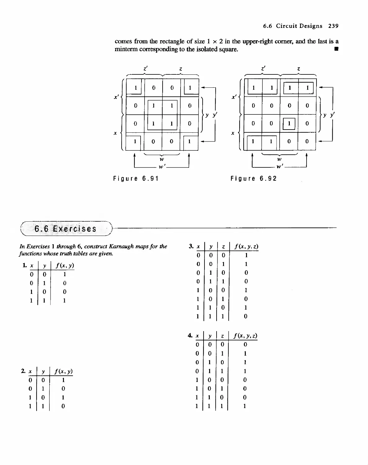
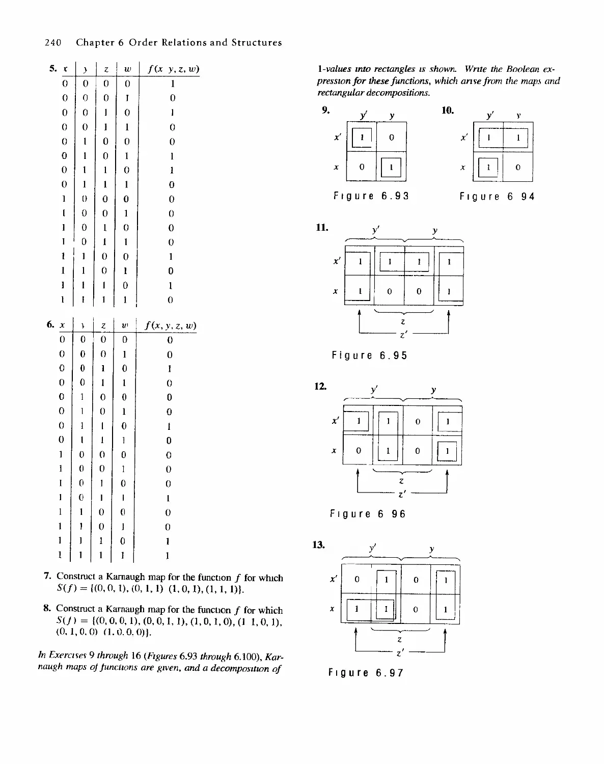
6.6 Circuit Designs 229
Trees
245
7.1 Trees 245
7.2 Labeled Trees 250
7.3 Tree Searching 254
7.4 Undirected Trees 264
7.s Minimal Spanning Trees 271
Topics in Graph Theory
280
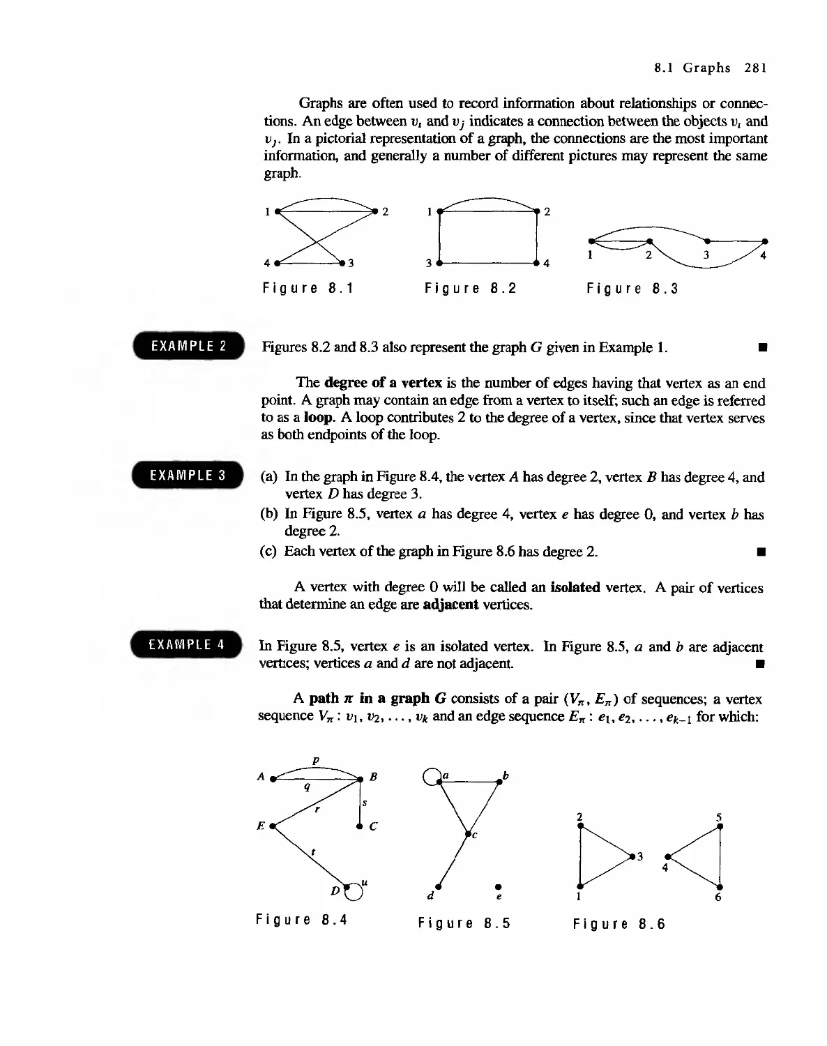
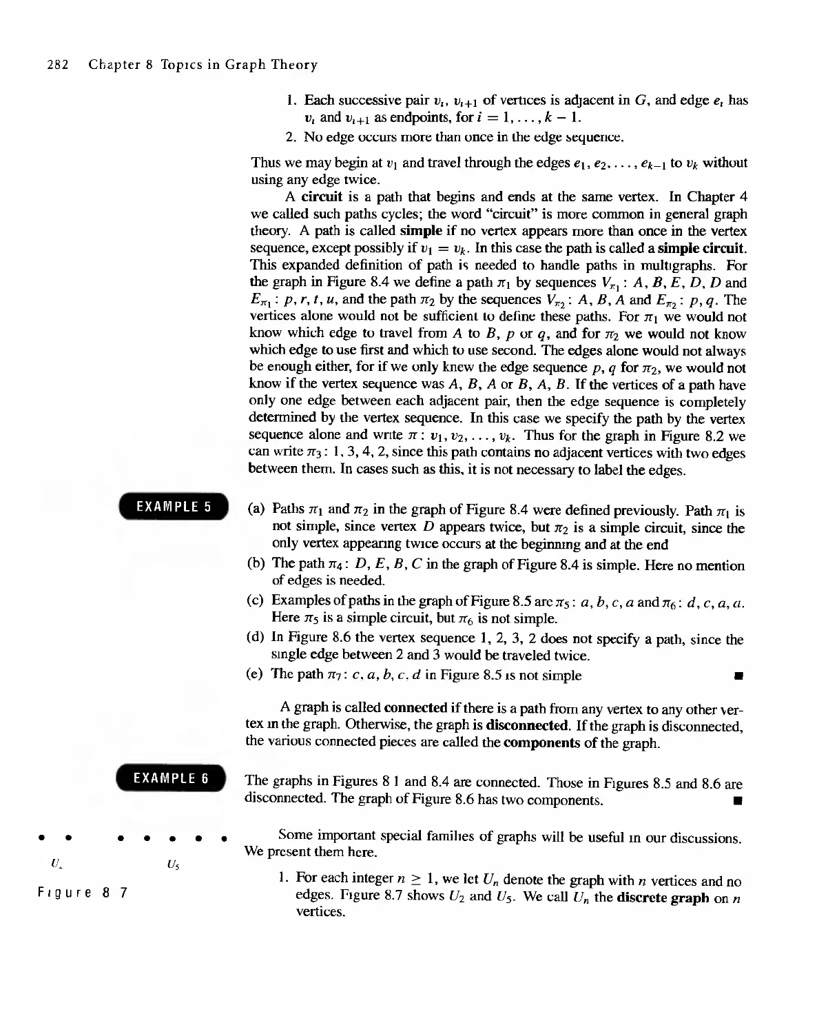
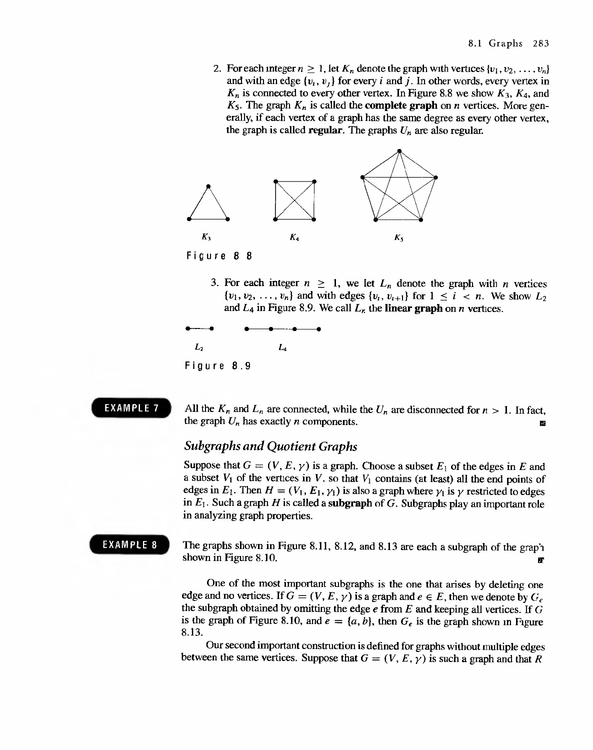
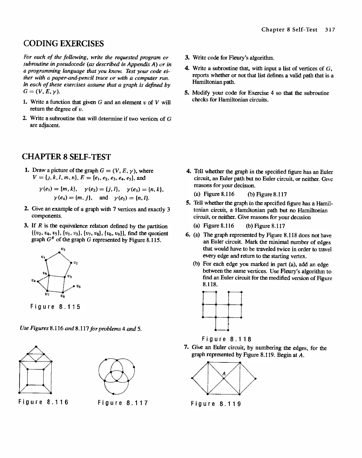
8.1 Graphs 280
8.2 Euler Paths and Circuits 286
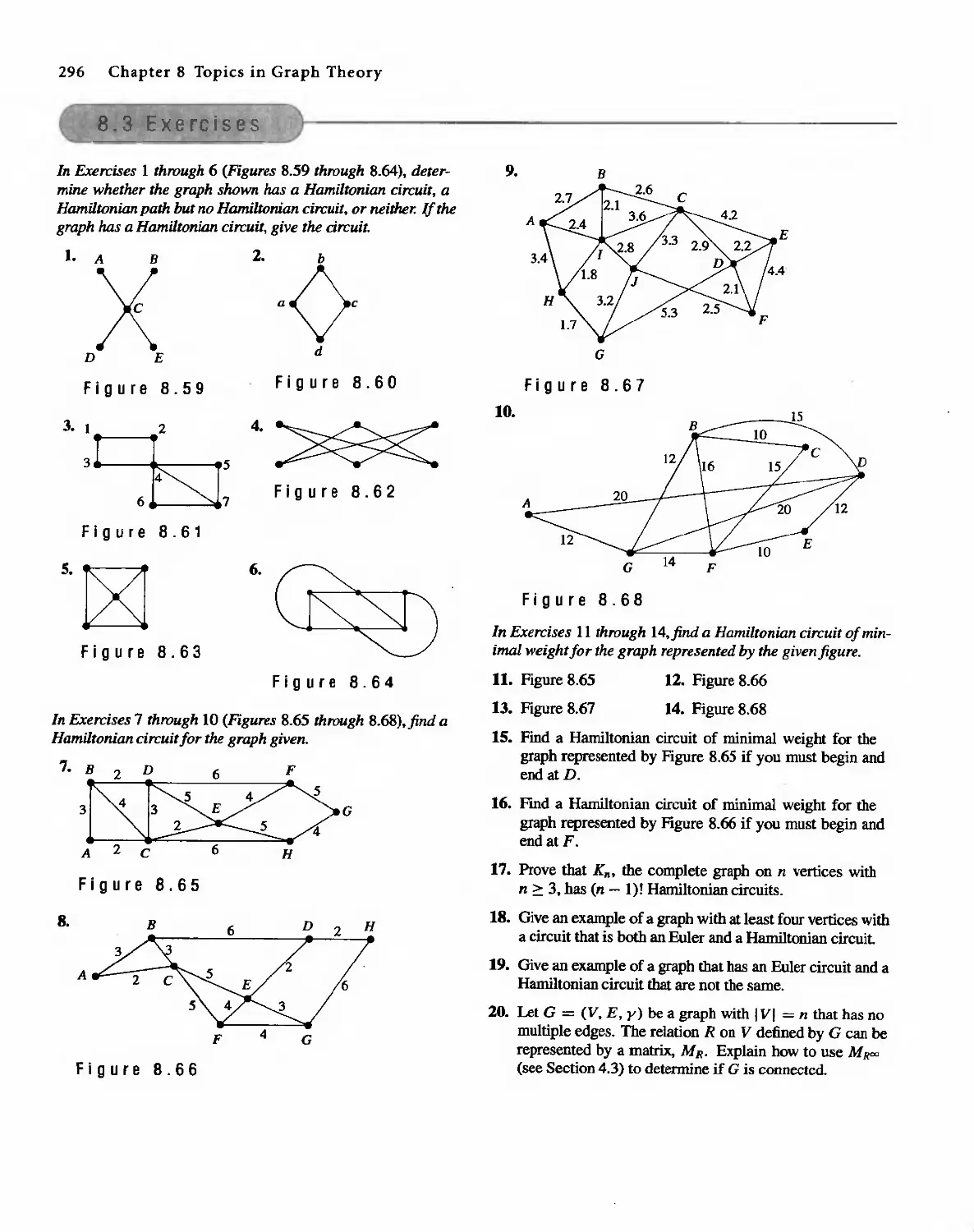
8.3 Hamiltonian Paths and Circuits 293
804 Transport Networks 297
Contents IX
8.5
8.6
Matching Problems
Coloring Graphs
305
311
9 Semigroups and Groups 319
9.1 Binary Operations Revisited 319
9.2 Semigroups 324
9.3 Products and Quotients of Sernigroups 331
9.4 GrOUDS 338
9.5 Products and Quotients of Groups 349
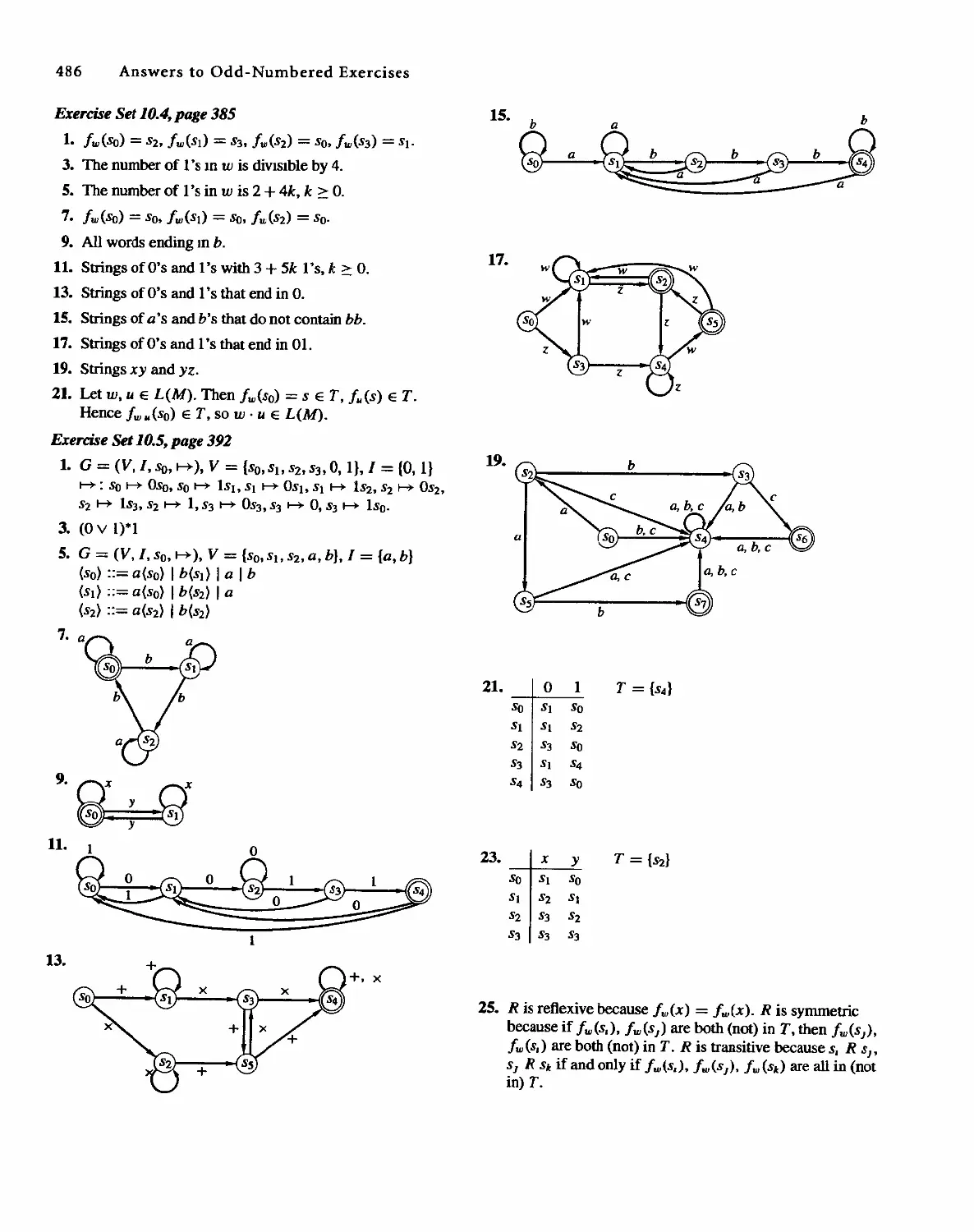
1 0 Languages and Finite-State Machines 357
10.1 Languages 357
10.2 Representations of Special Grammars and Languages 366
10.3 Finite-State Machines 375
10.4 Semigroups, Machines, and Languages 381
10.5 Machines and Regular Languages 386
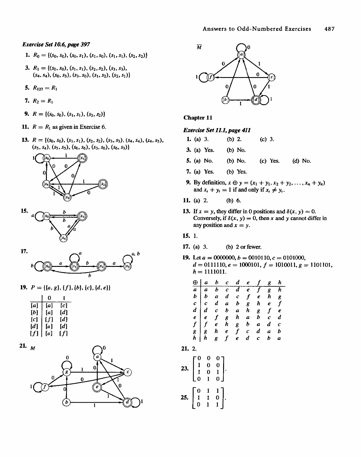
10.6 Simplification of Machines 393
11 Groups and Coding 401
11.1 Coding of Binary Information and Error Detection 401
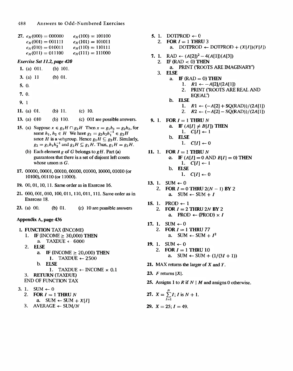
11.2 Decoding and Error Correction 413
Appendix A: Algorithms and Pseudocode 425
Appendix B: Experiments in Discrete Mathematics 438
Answers to Odd-Numbered Exercises 455
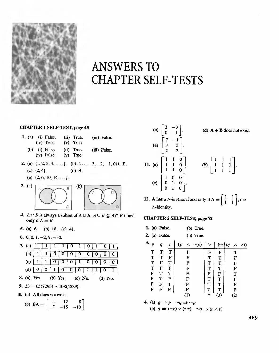
Answers to Chapter SeH- Tests 489
Index 502
. ,, f.; '1
;, '....t
to ' kl'
- -,
,. .'J"'f. .
,. ,
...i' v
.. \\
J,
"t
..
.
'-
I
-, ..
"'f
...
,
.ittt
.
,
.
..
,
11-/Jt'
c
'\ t
.. .
'
r
'
'I- f
...
"
t
t
t
'to .,.
t
....... -#
'!k.
If t
M
, ,
....
. .\
>
,
iT
N
..
..
."
r
"
\
.,.
f'
...
. . "' ft.. c
j.
..
11
" 1
OJ
. 3<
'-! .
. ..:J
'6
"
..
'If
"
\
"J \
,
<i:o
.
...
..)( ..
....,.'.... A
.
.
'!f'
J "
" J
, ,.
, r'
a
,
.
1 , .
&
....\
.... -;"
"
"Jr. :t:
. .. ..
t:,
. t' -'
.
.
FUNDAMENTALS
/''-0 '-'f[H i.,t It'::;: nlt'n' arc 110 '/OPlIO[ prcn'llui5iiC:, /tH' llri I'Jwflcr,' {he rcada
! '.II,'our< -':'l-d to rClill tarcrull\' and work fl1roll h all c\:amp/cs.,
.. . ....
In this chapter we intrQduce some of the basic tools of discrete malhematics.
We begin with sets. subsets. and their operations. notions with which you
may a1readv be famiJiar. Next Wt deal with sequences, using both explicit and
recursive patterns. Then we review some of the basic divi ibility properues
of the integers. Finally we introduce matrkes and matrix operations. This
gives us the background needed to begin our exploration of mathematical
Slruct ures.
1.1 SETS AND SUBSETS
Sets
A set is any well-defined collection of objects called the elements or members of
the set. For example, the collection of all wooden chairs, the collection of all one-
legged black birds, or the collection of real numbers between zero and one is each a
set. Well-defined just means that it is possible to decide if a given object belongs to
the collection or not. Almost all mathematical objects are first of all sets, regardless
of any additional properties they may possess. Thus set theory is, in a sense t the
foundation on which virtually all of mathematics is constructed. In spite of this, set
theory (at least the informal brand we need) is quite easy to learn and use.
One way of describing a set that has a finite number of elements is by listing
the elements of the set between braces. Thus the set of all positive integers that are
less than 4 can be written as
{I, 2, 3}.
(I)
The order in which the elements of a set are listed is not important. Thus
{I, 3, 2}, {3,2, I}, {3,l. 2}, {2, I, 3}, and {2, 3, I} are all representations of the set
given in (1). Moreover, repeated elements in the listing of the elements of a set can
be ignored. Thus, {I, J, 2, 3, I} is another representation of the set given in (I).
We use uppercase letters such as A, B, C -to denote sets, and lowercase letters
such as a, ht c. x, y, z, t to denote the members (or elements) of sets.
.
1
2 Chapter 1 Fundamentals
EXAMPLE 1
EXAMPLE 2
EXAMPLE 3
EXAMPLE 4
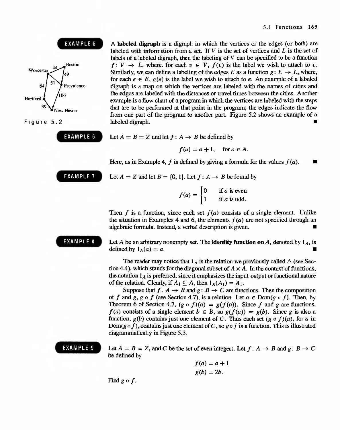
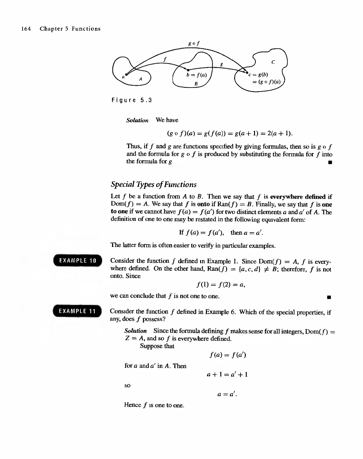
EXAMPLE 5
EXAMPLE 6
We indicate the fact that x is an element of the set A by writing x E A, and
we indicate the fact that x is not an element of A by writing x tfi A.
Let A = {I,3,5, 7}. Then 1 E A, 3 E A, but 2 tfi A.
.
Sometimes it is inconvenient or impossible to describe a set by listing all its
elements. Another useful way to define a set is by specifying a property that the
elements of the set have in conunon. We use the notation P(x) to denote a sentence
or statement P concerning the variable object x. The set defined by P(x), written
{x I P(x)}. is just the collection of all objects for which P is sensible and true. For
example t {x I x is a positive integer less than 4} is the set {I. 2, 3} described in (I)
by listing its elements.
The set consisting of all the letters in the word "byte" can be denoted by {b. Y. t, e}
or by {x I x is a letter in the word "byte"}. .
We introduce here several sets and their notations that will be used throughout this
book.
(a) Z+ = {x I x is a positive integer}.
Thus Z+ consists of the numbers used for counting: I, 2, 3 . . . .
(b) N = {x I x is a positive integer or zero}.
Thus N consists of the positive integers and zero: 0, I, 2, . . . .
(c) Z = {x I x is an integer}.
Thus Z consists of all the integers: ..., -3, -2, -1.0, 1,2,3. . . ..
(d) Q = {x I x is a rational number}.
Thus Q consists of numbers that can be written as a . where a and b are
b
integers and b is not O.
(e) R = {x I x is a real number}.
(f) The set that has no elements in it is denoted either by { } or the symbol 0
and is called the empty set. .
Since the square of a real number is always nonnegative t
{x I x is a real number and x 2 = -I} = 0.
.
Sets are completely known when their members are all known. Thus we say
two sets A and B are equal if they have the same elements t and we write A = B.
If A = {I, 2, 3} and B = {x I x is a positive integer and x 2 < I2}, then A = B. .
If A = {BASIC. PASCAL. ADA} and B = {ADA, BASIC, PASCAL}, then A = B.
.
A C B
4$bB
Figure 1.1
EXAMPLE 7
EXAMPLE 8
EXAMPLE 9
EXAMPLE 10
u
Figure 1.2
EXAMPLE 11
1.1 Sets and Subsets 3
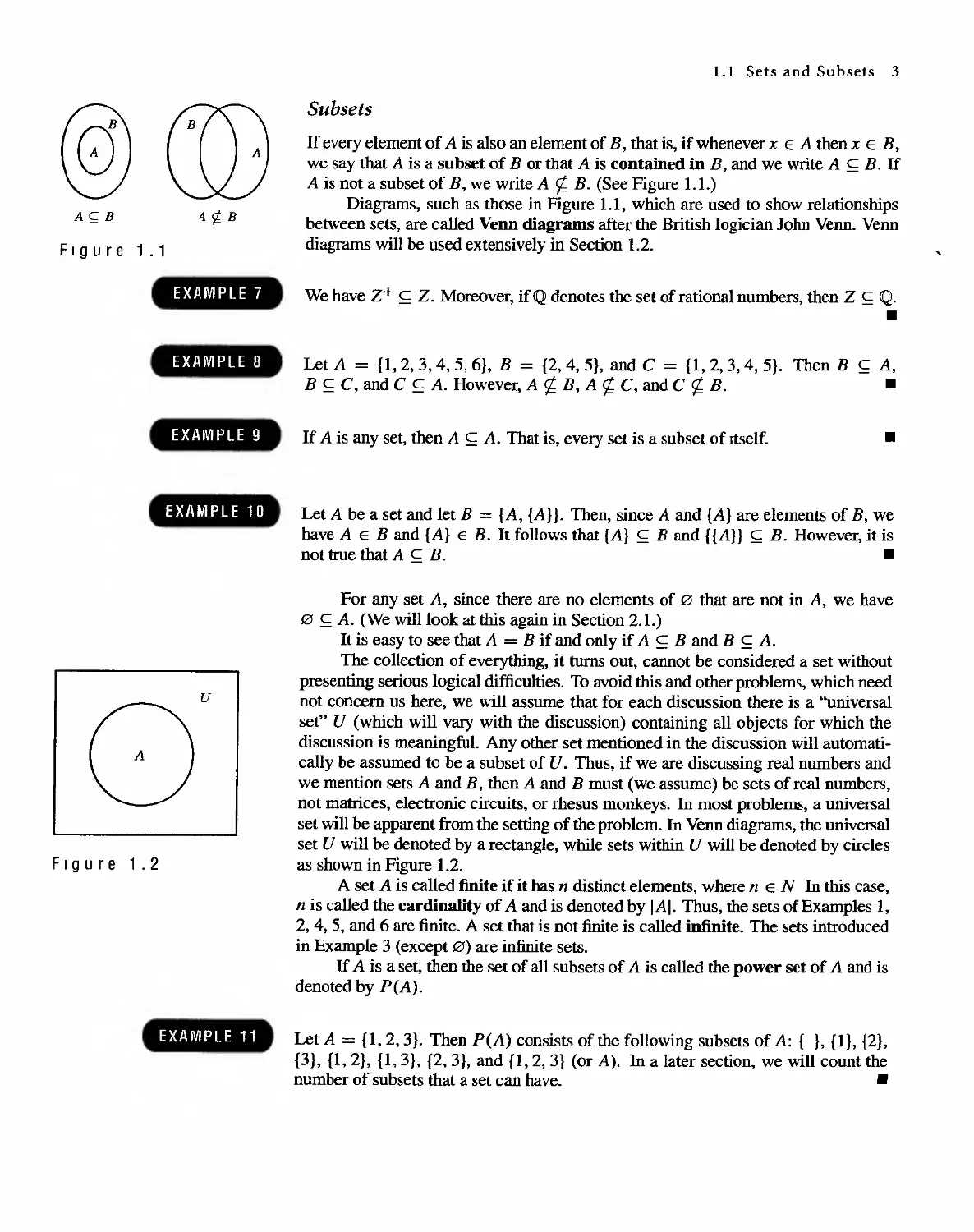
Subsets
If every element of A is also an element of B, that is, if whenever x E A then x E B,
we say that A is a subset of B or that A is contained in B, and we write A C B. If
A is not a subset of B, we write A rt B. (See Figure 1.1.)
Diagrams, such as those in Figure 1.1, which are used to show relationships
between sets, are called Venn diagrams after the British logician John Venn. Venn
diagrams will be used extensively in Section 1.2.
....
We have Z+ c Z. Moreover, if Q denotes the set of rational numbers, then Z C Q.
.
Let A = 0,2,3,4,5, 6}, B = {2, 4, 5}, and C = {I, 2, 3,4, 5}. Then B C A,
B C C, and C C A. However, A rt B tArt C, and C rt B. .
If A is any set, then A C A. That is, every set is a subset of Itself.
.
Let A be a set and let B = {A, {A}}. Then, since A and {A} are elements of B, we
have A E B and {A} E B. It follows that {A} C B and {{A}} C B. However, it is
not true that A C B. .
For any set A, since there are no elements of 0 that are not in A, we have
o c A. (We will look at this again in Section 2.1.)
It is easy to see that A = B if and only if A C Band B C A.
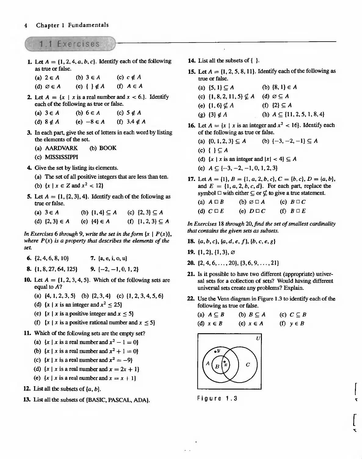
The collection of everything, it turns out, cannot be considered a set without
presenting serious logical difficulties. To avoid this and other problems, which need
not concern us here, we will assume that for each discussion there is a "universal
set" U (which will vary with the discussion) containing all objects for which the
discussion is meaningful. Any other set mentioned in the discussion will automati-
cally be assumed to be a subset of U. Thus, if we are discussing real numbers and
we mention sets A and B, then A and B must (we assume) be sets of real numbers,
not matrices t electronic circuits, or rhesus monkeys. In most problems, a universal
set will be apparent from the setting of the problem. In Venn diagrams, the universal
set U will be denoted by a rectangle, while sets within U will be denoted by circles
as shown in Figure 1.2.
A set A is called finite if it has n distinct elements, where n E N In this case,
n is called the cardinality of A and is denoted by IAI. Thus, the sets of Examples 1,
2, 4t 5, and 6 are finite. A set that is not finite is called infinite. The ets introduced
in Example 3 (except 0) are infinite sets.
If A is a set, then the set of all subsets of A is called the power set of A and is
denoted by P(A).
Let A = {l. 2, 3}. Then P(A) consists of the following subsets of A: ( }, {I}, {2},
{3}, {I, 2}, {l, 3}, {2, 3}, and {I, 2, 3} (or A). In a later section, we will count the
number of subsets that a set can have. .
4 Chapter 1 Fundamentals
1.1 Exercises
1. Let A = {I, 2, 4, a, b. c}. Identify each of the following
as true or false.
(a) 2 E A (b) 3 E A (c) c f/. A
(d) 0 E A (e) { } f/. A (t) A E A
2. Let A = {x I x is a real number and x < 6.}. Identify
each of the following as true or false.
(a) 3 E A (b) 6 E A (c) 5 f/. A
(d) 8 f/. A (e) -8 E A (t) 3.4 f/. A
3. In each part. give the set of letters in each word by listing
the elements of the set.
(b) BOOK
(a) AARDVARK
(c) MISSISSIPPI
4. Give the set by listing its elements.
(a) The set of all positive integers that are less than ten.
(b) {x I x E Z and x 2 < 12}
s. Let A = {I, {2. 3}, 4}. Identify each of the following as
true or false.
(a) 3 E A
(d) {2,3} E A
(b) {I,4} C A
(e) {4} E A
(c) {2, 3} C A
(t) {I, 2, 3} C A
In Exercises 6 through 9, write the set in theform {x I P(x)},
where P(x) is a property that describes the elements of the
set.
6. {2, 4, 6, 8, lO}
8. {l, 8, 27, 64, 125}
7. [a, e, i, 0, u}
9. [-2, -1,0, 1, 2}
10. Let A = {I, 2, 3,4, 5}. Which of the following setS are
equal to A?
(a) {4, 1,2,3, 5} (b) {2, 3, 4} (c) {I, 2, 3,4,5, 6}
(d) {x I x is an integer and x 2 < 25}
(e, {x I x is a positive integer and x < 5}
(t) {x I x is a positive rational number and x < 5}
11. Which of the following sets are the empty set?
(a) {x I x is a real number and x 2 - 1 = O}
(b) {x I x is a real number and x 2 + 1 = O}
(c) {x I x is a real number and x 2 = -9}
(d) {x I x is a real number and x = 2x + I}
(e) {x I x is a real number and x = x + I}
12. List all the subsets of {a, b}.
13. List all the subsets of {BASIC, PASCAL, ADA}.
14. List all the subsets of { }.
15. Let A = {I, 2, 5, 8, H}. Identify each of the following as
true or false.
(a) {5, I} C A
(c) {I, 8, 2,11, 5} i A
(e) {I,6} 't A
(g) {3} f/. A
(b) {8, I} E A
(d) 0 C A
(t) {2} C A
(h) A C {ll, 2, 5, 1,8, 4}
16. Let A = {x I x is an integer and x 2 < 16}. Identify each
of the following as true or false.
(a) to, 1,2, 3} C A (b) {-3, -2, -I} C A
(c) { } C A
(d) {x I x is an integer and Ixl < 4} c A
(e) A C {-3, -2, -1,0, 1,2, 3}
17. Let A = {l}, B = {I, a, 2, b, c}, C = {b, c}, D = {a, b},
and E = {I, a, 2, b, c, d}. For each part, replace the
symbol 0 with either C or 't to give a true statement.
(a) A 0 B (b) 00 A (c) B 0 C
(d) C 0 E (e) DOC (f) B 0 E
In Exercises 18 through 20, find the set of smallest cardinality
that contains the given sets as subsets.
18. {a, b, c}, {a, d, e, f}, {b, c, e, g}
19. {I, 2}, {I, 3}, 0
20. {2, 4, 6, .... 20}, {3, 6,9, .. ., 21}
21. Is it possible to have two different (appropriate) univer-
sal sets for a collection of sets? Would having different
universal sets create any problems? Explain.
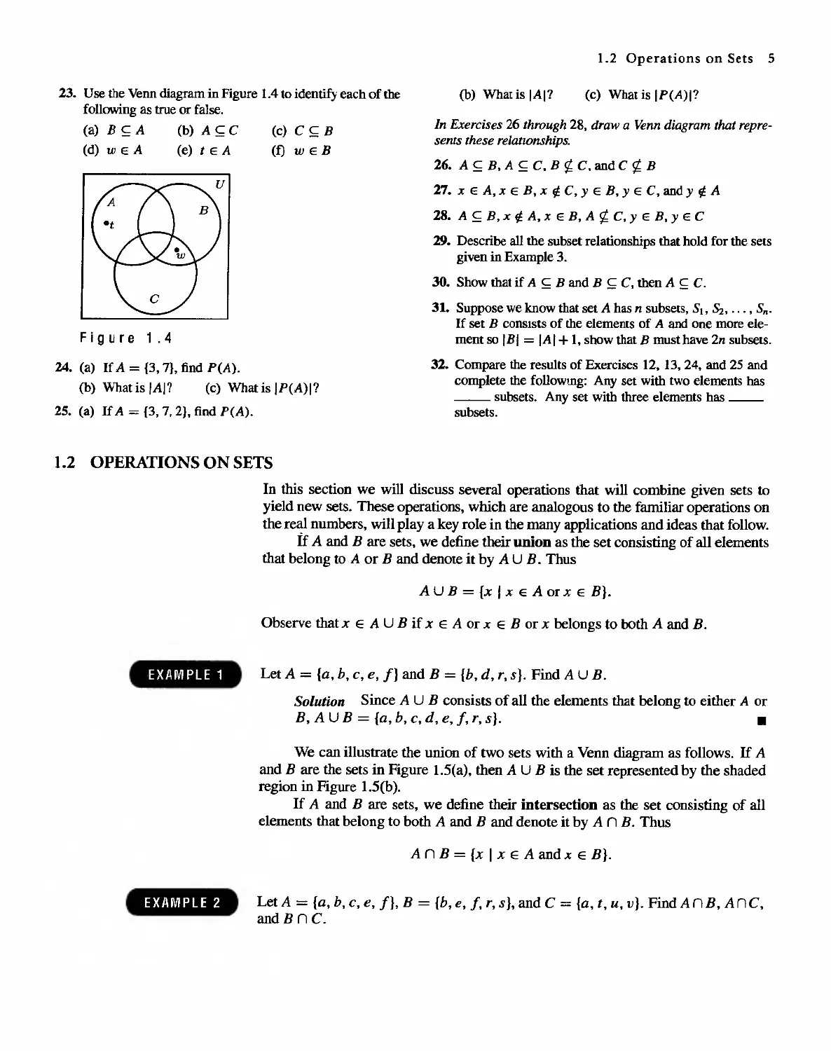
22. Use the Venn diagram in Figure 1.3 to identify each of the
following as true or false.
(a) A C B (b) B C A
(d) x E B (e) x E A
(c) C C B
(f) Y E B
u
r
Figure 1.3
[
1.2 Operations on Sets 5
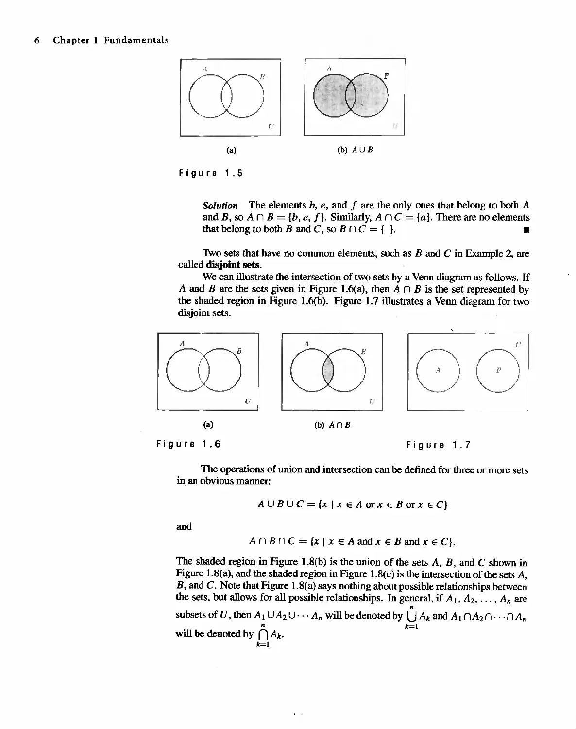
23. Use the Venn diagram in Figure 1.4 to identify each of the
following as true or false.
(a) B C A (b) A c C
(d) W E A (e) tEA
(b) What is IAI?
(c) What is IP(A)I?
(c) C C B
(f) wEB
In Exercises 26 through 28, draw a Venn diagram that repre-
sents these relatIOnships.
26. A C B, A C C. B i C. and C i B
27. x E A, x E B, x fj. C, Y E B, y E C, and y fj. A
28. A C B, x fj. A, x E B, Ai C, y E B, Y E C
29. Describe all the subset relationships that hold for the sets
given in Example 3.
30. Show that if A C Band B C C, then A c C.
31. Suppose we know that set A has n subsets, SI, S2, . . . , Sn.
If set B COnsISts of the elements of A and one more ele-
ment so I BI = IA I + I, show that B must have 2n subsets.
32. Compare the results of Exercises 12, 13,24, and 25 and
complete the followmg: Any set with two elements has
subsets. Any set with three elements has
subsets.
Figure 1.4
24. (a) If A = {3, 7}, find peA).
(b) What is IAI? (c) What is IP(A)I?
25. (a) If A = {3, 7, 2}, find peA).
1.2 OPERATIONS ON SETS
In this section we will discuss several operations that will combine given sets to
yield new sets. These operations, which are analogous to the familiar operations on
the re l numbers, will playa key role in the many applications and ideas that follow.
If A and B are sets, we define their union as the set consisting of all elements
that belong to A or B and denOte it by A U B. Thus
Au B = {x I x E A or x E B}.
Observe that x E AU B if x E A or x E B or x belongs to both A and B.
,E X AMP L E 1
Let A = {a. b, c, e, f] and B = {b, d, r, s}. Find A U B.
Solution Since A U B consists of all the elements that belong to either A or
B,AUB = {a,b,c,d.e,f,r,s}. .
We can illustrate the union of two sets with a Venn diagram as follows. If A
and B are the sets in Figure 1.5(a). then AU B is the set represented by the shaded
region in Figure 1.5(b).
If A and B are sets, we define their intersection as the set consisting of all
elements that belong to both A and B and denote it by A n B. Thus
An B = {x I x E A and x E B}.
EXAMPLE 2
Let A = {a, b, c, e, f}, B = {b, e, f, r, s}, and C = {a, t, u, v}. Find A n B, AnC,
and B n C_
6 Chapter 1 Fundamentals
,\
A
l'
(a)
(b) AU B
Figure 1.5
Solution The elements h, e, and f are the only ones that belong to both A
and B, so A n B = {h, e, fl. Similarly, An C = {a}. There are no elements
that belong to both Band C, so B n C = { }. .
Two sets that have no common elements, such as B and C in Example 2, are
called disjoint sets.
We can illustrate the intersection of two sets by a Venn diagram as follows. If
A and B are the sets given in Figure 1.6( a), then A n B is the set represented by
the shaded region in Figure 1.6(b). Figure 1.7 illustrates a Venn diagram for two
disjoint sets.
,
:1
\
['
u
l.
(a)
Figure 1.6
(b) A n B
Figure 1.7
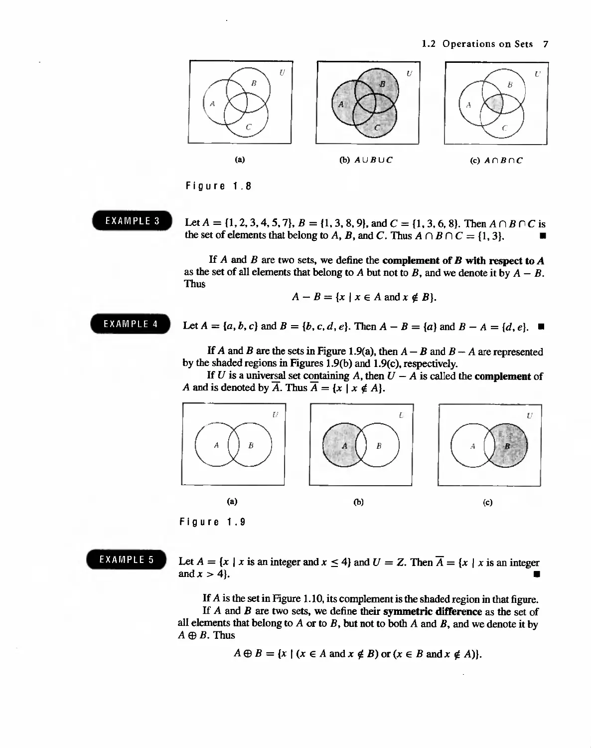
The operations of union and intersection can be defined for three or more sets
in an obvious manner:
A U B U C = {x I x E A or x E B or x E C}
and
An B n C = {x I x E A and x E B and x E C}.
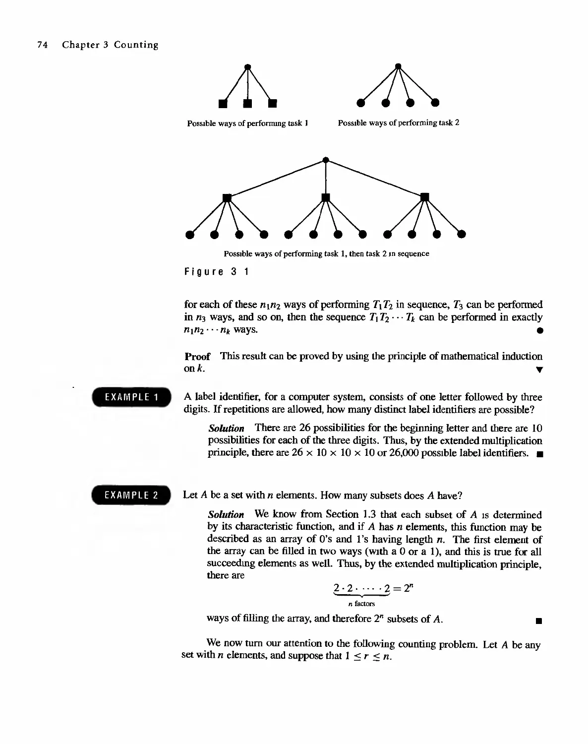
The shaded region in Figure 1.8(b) is the union of the sets A, B, and C shown in
Figure 1.8( a), and the shaded region in Figure 1.8( c) is the intersection of the sets A,
B, and C. Note that Figure 1.8(a) says nothing about possible relationships between
the sets. but allows for all possible relationships. In general, if AI, A z . ..., An are
n
subsets of U, then Al UA 2 U. . . An will be denoted by U Ak and Al nA 2 n. . . nA n
n k=I
will be denoted by n Ak.
k=I
EXAMPLE 3
EXAMPLE 4
EXAMPLE 5
1.2 Operations on Sets 7
L"
u
u
(a)
(b) A U B U C
(c) A n B n C
Figure 1.8
Let A = {l, 2, 3,4,5, 7}, B = U, 3,8, 9}, and C = {l, 3, 6, 8}. Then A n B n Cis
the set of elements that belong to A, Bt and C. Thus An B n C = {I, 3}. .
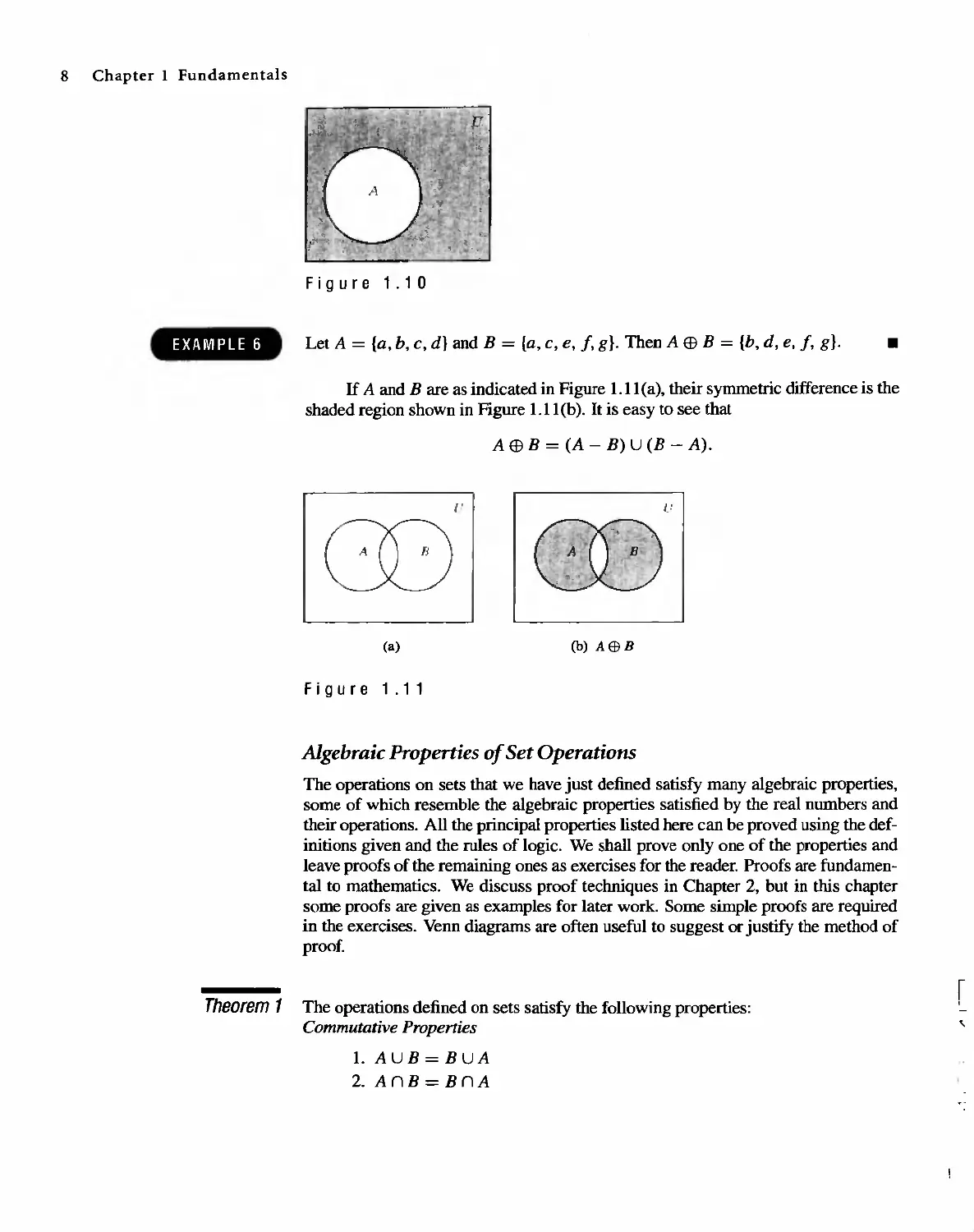
If A and B are two sets t we define the complement of B with respect to A
as the set of all elements that belong to A but not to B, and we denote it by A - B.
Thus
A - B = {x I x E A and x fj B}.
Let A = (a, b, c} and B = {b, c, d, e}. Then A - B = {a} and B - A = {d, e}. .
If A and B are the sets in Figure 1.9(a), then A - B and B - A are represented
by the shaded regions in Figures 1.9(b) and 1.9(c), respectively.
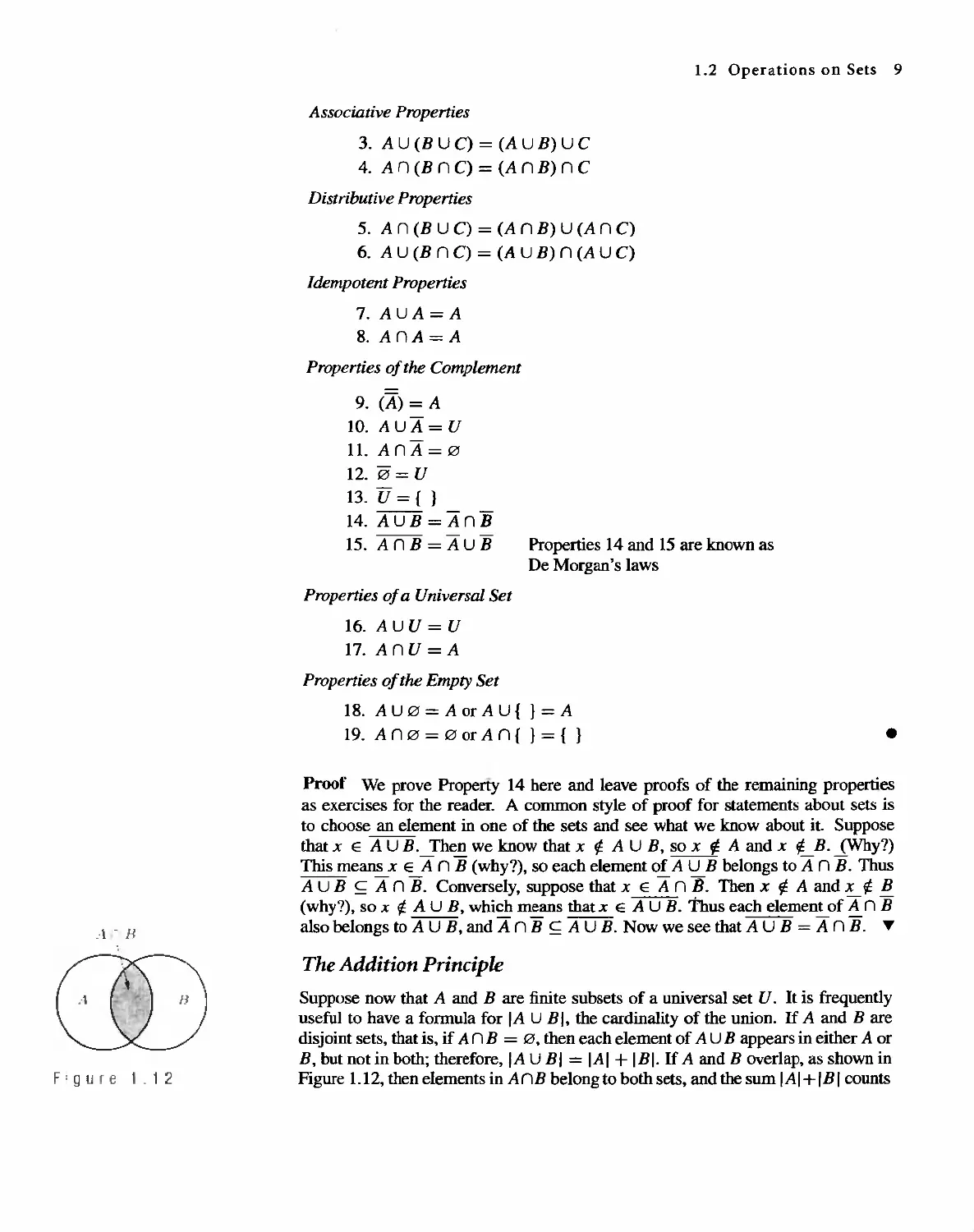
If U is a universal set containing A, then U - A is called the complement of
A and is denoted by A. Thus A = {x I x A}.
{.'
[
u
(a)
Figure 1.9
(b)
(c)
Let A = {x I x is an integer and x < 4} and U = Z. Then A = {x I x is an integer
and x > 4}. .
If A is the set in Figure 1.10, its complement is the shaded region in that figure.
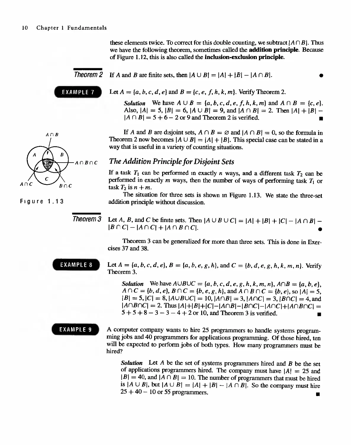
If A and B are two sets, we define their symmetric difference as the set of
all elements that belong to A or to B t but not to both A and Bt and we denote it by
A EB B. Thus
AEB B = {x I (x E A and x fj B) or (x E B andx fj A)}.
8 Chapter 1 Fundamentals
" ..
.. - "
I
.
11
...
. ,
;0\:
<
.
.
-. :: _...
;.,
..¥
,
1'''' ..
L
,
Figure 1.10
EXAMPLE 6
Let A = {a, b, C, d} and B = {a, C, e, I, g}. Then A ffi B = {b, d, e, I, g}.
.
If A and B are as indicated in Figure 1.II(a), their symmetric difference is the
shaded region shown in Figure 1.11 (b). It is easy to see that
A ffi B = (A - B) U (B - A).
l' ,
u
.
B
(a)
(b) A $ B
Figure 1.11
Algebraic Properties of Set Operations
The operations on sets that we have just defined satisfy many algebraic properties,
some of which resemble the algebraic properties satisfied by the real numbers and
their operations. All the principal properties listed here can be proved using the def-
initions given and the rules of logic. We shall prove only one of the properties and
leave proofs of the remaining ones as exercises for the reader. Proofs are fundamen-
tal to mathematics. We discuss proof techniques in Chapter 2, but in this chapter
some proofs are given as examples for later work. Some simple proofs are required
in the exercises. Venn diagrams are often useful to suggest or justify the method of
proof.
Theorem 1 The operations defined on sets satisfy the following properties:
Commutative Properties
r
,
LAUB=BUA
2. A n B = B n A
1.2 Operations on Sets 9
Associative Properties
3. AU (B U C) = (A U B) U C
4. An (B n C) = (A n B) n C
Distributive Properties
5. A n (B U C) = (A n B) U (A n C)
6. AU (B n C) = (A U B) n (A U C)
Idempotent Properties
7. A U A = A
8. A n A = A
Properties of the Complement
9, (A) = A
10. A U A = U
11. AnA=0
12. 0 = U
13. U = { }
14. AU B = An B
- -
15. A n B = A U B
Properties 14 and 15 are known as
De Morgan's laws
Properties of a Universal Set
16. A U U = U
17. AnU=A
Properties of the Empty Set
18. A U 0 = A or A U { } = A
19. An 0 = 0 or An { } = { }
.
_,\ - n
Proof We prove Property 14 here and leave proofs of the remaining properties
as exercises for the reader. A common style of proof for statements about sets is
to choose an elem ent in one of the sets and see what we know about it. Suppose
that x E AU B. Then we know that x A U B, so x rj A and x rt B. (Why?)
This m eans x E A n B (why?), so each element of A U B belongs to A n B . Thus
A U B cA n B . Conversely, suppose that x E A n B. Then x r;. A and £ B
(why?), so x Au B , whi ch mean s that x E AU B. Thus ea ch elem e nt o f A n B
also belongs to A U B, and A n B C A U B. Now we see that A U B = A n B. ...
The Addition Principle
Suppose now that A and B are finite subsets of a universal set U. It is frequently
useful to have a formula for IA UBI. the cardinality of the union. If A and Bare
disjoint sets, that is, if An B = 0, then each element of A U B appears in either A or
B, but not in both; therefore, I A UBI = 1 A I + 1 B I. If A and B overlap, as shown in
Figure 1.12, then elements in AnB belong to both sets, and the sum IAI+IBI counts
f;Qure 1-12
10 Chapter 1 Fundamentals
these elements twice. To correct for this double counting, we subtract 1 An B I. Thus
we have the following theorem, sometimes called the addition principle. Because
of Figure 1.12. this is also called the inclusion-exclusion principle.
Theorem 2 If A and B are finite sets. then IA U BI = IAI + IBI-IA n BI.
.
Let A = {a, b, e, d, e} and B = {e, e, J. h, k. mI. Verify Theorem 2.
Solution We have A U B = {a, b. e, d, e, f, h, k, m} and A n B = {e, e}.
Also, IAI = 5, IBI = 6t IA UBI = 9, and IA n BI = 2. Then IAI + IBI-
IA n BI = 5 + 6 - 2 or 9 and Theorem 2 is verified. .
,EXAMPLE 7
AnB
Figure 1.13
If A and B are dIsjoint sets, A n B = 0 and I A n B I = 0, so the formula in
Theorem 2 now becomes I A U BI = I A I + I B I. This special case can be stated in a
way that is useful in a variety of counting situations.
AnBnc
The Addition Principle for Disjoint Sets
If a task Tl can be perfonned In exactly n ways, and a different task T 2 can be
performed in exactly m ways, then the number of ways of perfonning task Tl or
task T 2 is n +m.
The situation for three sets is shown m Figure 1.13. We state the three-set
addition principle without discussion.
Theorem 3 Let A, B, and C be fimte sets. Then IA U B U CI = IAI + IBI + ICI- IA n BI-
IB (I CI - IA n CI + IA n B n CI. .
Theorem 3 can be generalized for more than three sets. This is done in Exer-
cises 37 and 38.
Let A = {a, b, e, d, e}, B = {a, b, e, g, h}, and C = {b. d, e, g, h, k, m, n}. Verify
Theorem 3.
Solution We have AUBUC = {a,b,e,d,e,g,h,k,m,n},AnB = {a.b,e},
An C = {h, d, e}, B n C = {b, e, g, hI, and An B n c = {b, e}, so IAI = 5,
IBI = 5, ICI = 8, IAUBUC/ = 10, IAnBI = 3, IAncl = 3, IBnCI = 4, and
IAnBnCI = 2. Thus IAI+IBI+lcl-IAnBI-IBnCI-IAnCI+IAnBncl =
5 + 5 + 8 - 3 - 3 - 4 + 2 or 10, and Theorem 3 is verified. .
EXAMPLE 8
A computer company wants to hire 25 programmers to handle systems program-
ming jobs and 40 programmers for applications programming. Of those hired, ten
will be expected to perform jobs of both types. How many programmers must be
hired?
Solution Let A be the set of systems programmers hired and B be the set
of applications programmers hired. The company must have I A I = 25 and
I B I = 40, and I A n B I = 10. The number of programmers that must be hired
is IA UBI. but IA U BI = IAI + IBI -JA n BI. SO the company must hire
25 + 40 - 10 or 5S programmers. _
EXAMPLE 9
EXAMPLE 10
( 1.2 Exer.ci.ses )
1.2 Operations on Sets 11
A survey has been taken on methods of commuter travel Each respondent was
asked to check BUS. TRAIN, or AUTOMOBll..E as a major method of traveling
to work. More than one answer was pennitted. The results reported were as fol-
lows: BUS, 30 people; TRAIN, 35 people; AUTOMOBILE, 100 people; BUS and
TRAIN, 15 people; BUS and AUTOMOBll..E, 15 people; TRAIN and AUTOMO-
Bll..E, 20 people; and all three methods, 5 people. How many people completed a
survey fonn?
Solution Let B, T, and A be the sets of people who checked BUS, TRAIN,
and AUTOMOB E, respectively. We know IBI = 30, IT I = 35, IAI = 100,
IB n T ' == 15, IB n AI = 15, IT n AI = 20, and IB n T n AI == 5 SO
IB/ + /T/+ /A/-/B nTI-/BnAI-/TnA/ + lBn TnAI = 30+35+
100 - 15 - 15 - 20 + 5 or 120 is IA U B U CI, the number of people who
responded. .
In Exercises 1 through 4, let U = {a, b, c, d, e, f, 8, h, k},
A = {a. b, c, g}. B :::: {d, e, J. g}. C = {a, c, f}, and
D = {j,h,k}.
1. Compute
(a) A U B (b) B U C
(d) BnD (e) (AUB)-e
(g) A (h) A EB B
U) (A n B) - e
2. Compute
(a) A U D
(d) AnD
(f) B - e
(I) c Ef1 D
(c) A n C
(f) A - B
(i) A ffi C
(d) B U e (e) Anc (f) AnD
(g) B nc (h) cnD
6. Compute
(a) A - B (b) B-A (c) C-D
(d) C (e) A (f) AEBB
(g) C $ D (h) BEBC
7. Compute
(a) A UBUe (b) AnBne
(c) A n (B U C) (d) (A U B) n D
(e) A U B (t) AnB
8. Compute
(a) BUeUD (b) BnenD
(c) A U A (d) AnA
(e) A U A (f) An (C U D)
(b) BUD (c) enD
(e) (A U B) - (C U B)
(g) B (h) C - B
(J) (A n B) - (B n D)
3. Compute
(a) A U B U C
(c) A n (B U C)
(e) A U B
(b) AnBnc
(d) (A U B) n C
(f) A n B
In Exercises 5 through 8, let U = {I. 2, 3, 4. 5. 6, 7,8. 9},
A = {l, 2, 4. 6. 8}, B = {2. 4, 5, 9}, C = {x I x is a positive
integer and x 2 < 16}, and D = {7, 8J.
5. Compute
(a) A U B
4. Compute
(a) A U 0
(d) en{ }
(b) A U U
(e) e U D
(b) A U e
(c) B U B
(f) enD
In ExercIses 9 and 10, let U = {a, b, c, d. e. J, g, h},
A = {a, c, f, g}, B == {a, e}, and C = {b. h}.
9. Compute
(a) A
(d) A n B
(b) B
(e) U
(c) A U B
(f) A - B
10. Compute
- -
(a) A n B
(d) C n e
(b) B U C
(e) A ffi B
(c) A U A
(f) B $ C
(c) A U D
11. Let U be the set of real numbers, A = {x I x is a solution
of x 2 - 1 = O}, and B = {- I, 4}. Compute
(a) A (b) B (c) AU B (d) An B
12 Chapter 1 Fundamentals
In Exercises 12 and 13. refer to Figure 1.14.
u
Figure 1.14
12. Identify the following as true or false.
(a) yEA n B (b) x E B U C
(c) wEB n C (d) u rt C
13. Identify the following as true or false.
(a) x E A n B n C (b) yEA U B U C
(c) Z E A n C (d) v E B n C
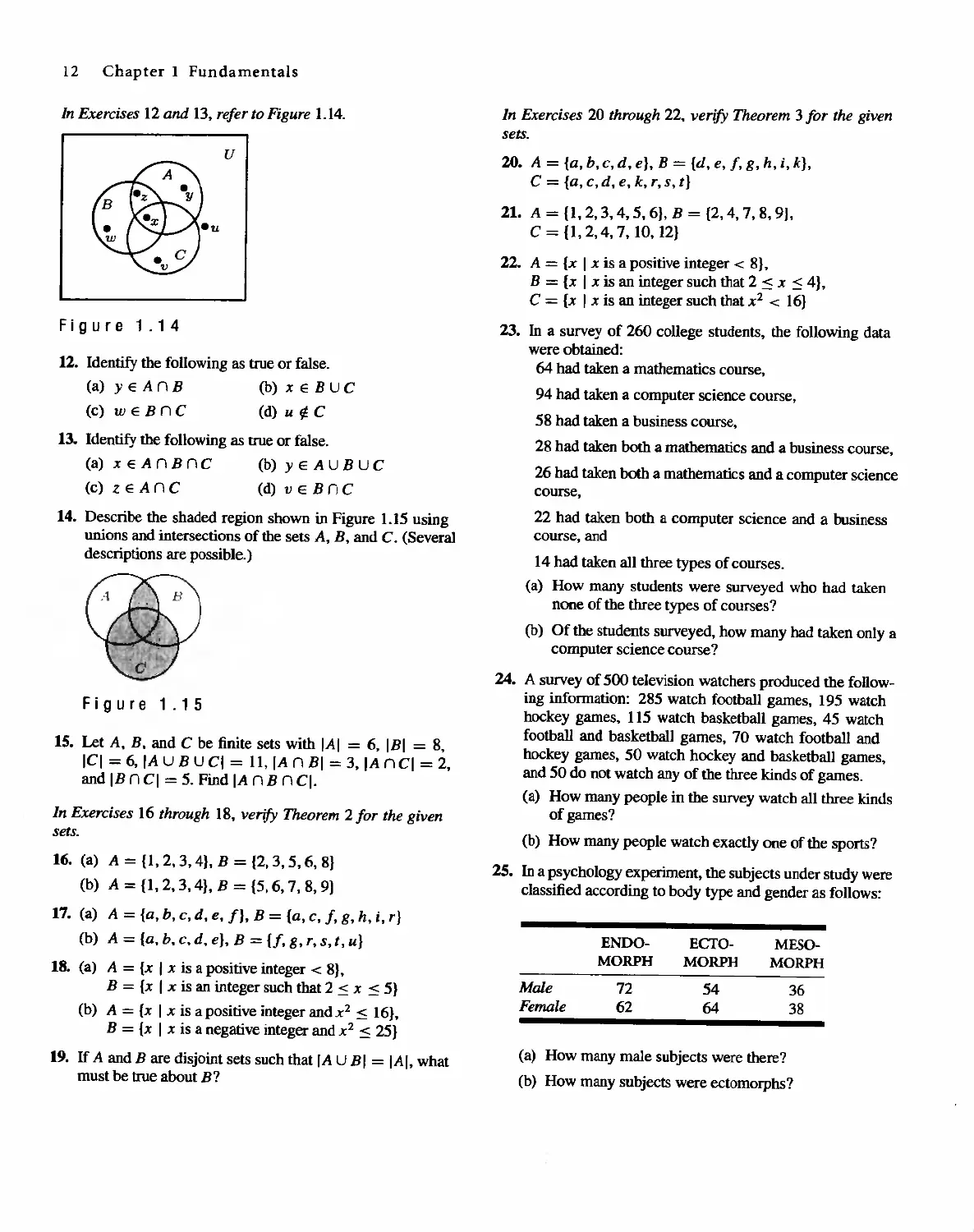
14. Describe the shaded region shown in Figure 1.15 using
unions and intersections of the sets A. B. and C. (Sever81
descriptions are possible.)
Figure 1.15
15. Let A. B. and C be finite sets with IAI = 6, IBI = 8,
IC! = 6, IA U B U q = 11, IA n BI = 3, IA n q = 2,
and IB nq = 5. Find IA nB nq.
In Exercises 16 through 18. verify Theorem 2 for the given
sets.
16. (a) A = {I, 2, 3, 4}, B = {2, 3, 5, 6, 8}
(b) A = {I, 2, 3, 4}, B = {5, 6, 7,8, 9}
17. (a) A = {a, h, c, d, e, fl, B = {a, c, i, g, h, i, r}
(b) A = {a, b. c. d. e}, B = if, 8, r, s.t, u}
18. (a) A = {x I x is a positive integer < 8},
B = {x I x is an integer such that 2 < x < 5}
(b) A = {x I x is a positive integer andx 2 < 16},
B = {x I x is a negative integer and x 2 < 25}
19. If A and B are disjoint sets such that IA U BI = IAI, what
must be true about B?
In Exercises 20 through 22, verify Theorem 3 for the given
sets.
20. A = {a, h, c, d, e}, B = {d, e, t, g, h, i, k},
C = {a,c,d,e,k,r,s,t}
21. A = {I, 2, 3. 4,5, 6}, B = {2, 4, 7,8, 9},
C = {I, 2,4, 7, lO,12}
22. A = {x I x is a positive integer < 8},
B = {x I x is an integer such that 2 < x < 4},
C = {x I x is an integer such that x 2 < 16}
23. In a survey of 260 college students, the following data
were obtained:
64 had taken a mathematics course,
94 had taken a computer science course,
58 had taken a business course,
28 had taken both a mathematics and a business course,
26 had taken both a mathematics and a computer science
course,
22 had taken both a computer science and a business
course, and
14 had taken 811 three types of courses.
(a) How many students were surveyed who had taken
none of the three types of courses?
(b) Of the students surveyed, how many had taken only a
computer science course?
24. A survey of 500 television watchers produced the follow-
ing information: 285 watch football games, 195 watch
hockey games, 115 watch basketb811 games, 45 watch
football and basketball games, 70 watch football and
hockey games, 50 watch hockey and basketball games,
and 50 do not watch any of the three kinds of games.
(a) How many people in the survey watch 811 three kinds
of games?
(b) How many people watch exactly one of the sports?
25. In a psychology experiment, the subjects under study were
classified according to body type and gender as follows:
Male
Female
ENDO-
MORPH
72
62
MESO-
MORPH
36
38
ECTO-
MORPH
54
64
(a) How many male subjects were there?
(b) How many subjects were ectomorphs?
(c) How many subjects were either female or endo-
morphs?
(d) How many subjects were not ma]e mesomorphs?
(e) How many subjects were either male, ectomorph, or
mesomorph?
26. Complete the following proof that A C A U B. Suppose
x E A. Then x E A U B, because . Thus by the
definitIon of subset A C A U B.
27. Complete the following proof that A '1 B C A. Suppose
x E A n B. Then x belongs to . Thus A n B C A.
28. (a) Draw a Venn diagram to represent the situation
C C A and C C B.
(b) To prove C C A U B. we should choose an element
from which set?
(c) Prove that if that if C C A and C C B, then
C C AU B.
29. (a) Draw a Venn diagram to represent the situation
A C C and B C C.
1.3 SEQUENCES
1.3 Sequences 13
(b) To prove A U B C C, we should choose an element
from which set?
(c) Prove that if A C C and B C C, then A U B C C
30. Prove that A - (A - B) C B.
31. Suppose that A ffi B = A ffi C. Does this guarantee that
B = C? Justify your conclusion.
32. Prove that A - B = A n B.
33. If AU B = AU C, must B = C? Explain.
34. If An B = An C, must B = C? Explain.
35. Prove that if A C B and C C D, then A U C C BUD
andAnC C B nD.
36. When is A - B = B - A? Explain.
37. Explain the last tenn in the sum in Theorem 3. Why is
IA n B n CI added and IB n q subtracted?
38. (a) Write the four-set version of Theorem 3; that is,
IA U B U C U DI = .. . .
(b) Describe in words the n-set version of Theorem 3.
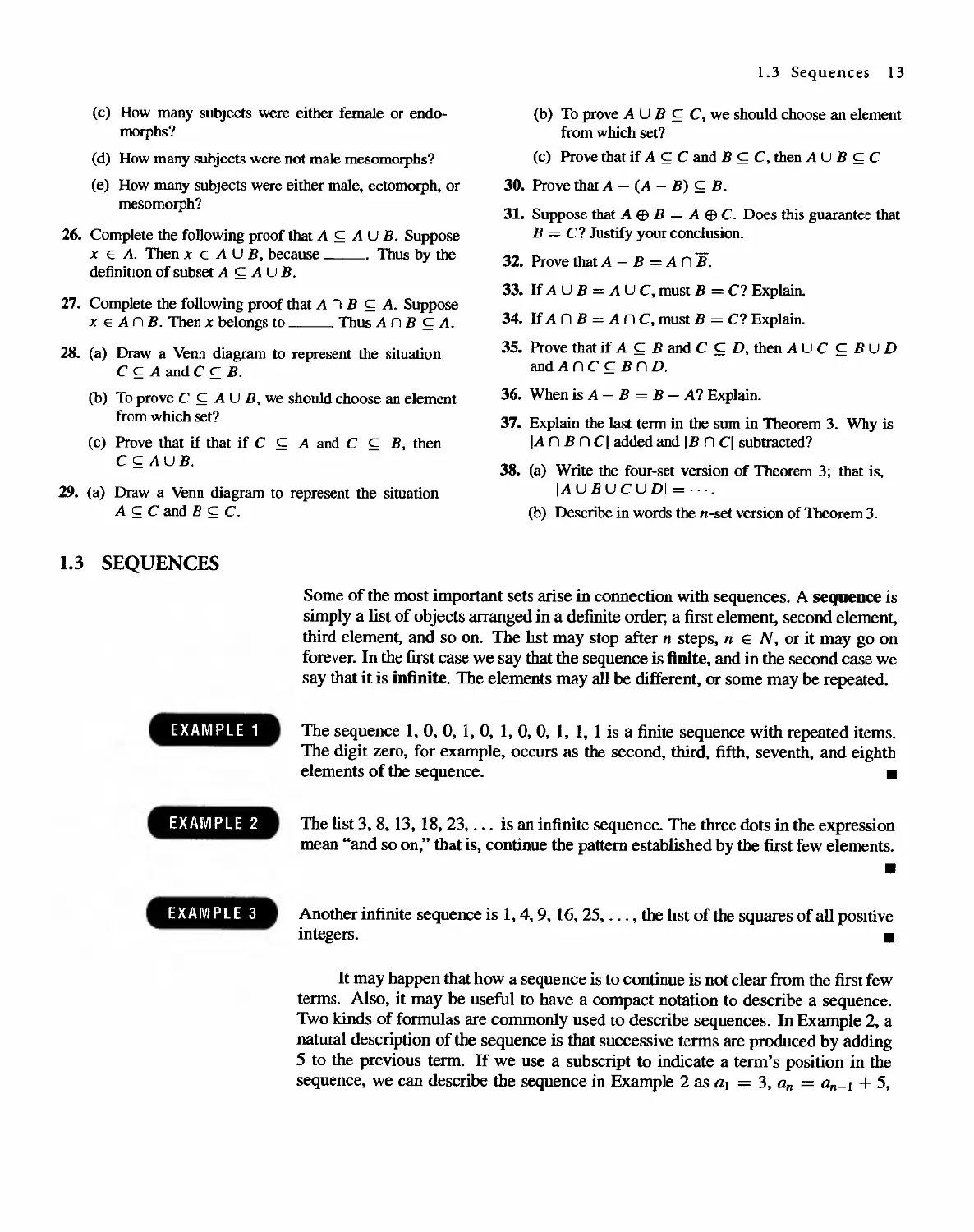
Some of the most important sets arise in connection with sequences. A sequence is
simply a list of objects arranged in a definite order; a first element, second element,
third element, and so on. The lIst may stop after n steps, n EN, or it may go on
forever. In the first case we say that the sequence is finite, and in the second case we
say that it is infinite. The elements may all be different, or some may be repeated.
EXAMPLE 1
The sequence 1, 0, 0, 1, 0, 1, 0, 0, 1, 1, 1 is a finite sequence with repeated items.
The digit zero, for example, occurs as the second, third. fifth. seventh, and eighth
elements of the sequence. _
EXAMPLE 2
The list 3.8. 13, 18,23, . " is an infinite sequence. The three dots in the expression
mean "and so on," that is, continue the pattern established by the first few elements.
-
Another infinite sequence is 1,4,9, 16, 25, . . . , the list of the squares of all posItive
integers. _
EXAMPLE 3
It may happen that how a sequence is to continue is not clear from the first few
terms. Also, it may be useful to have a compact notation to describe a sequence.
Two kinds of formulas are commonly used to describe sequences. In Example 2, a
natural description of the sequence is that successive terms are produced by adding
5 to the previous term. If we use a subscript to indicate a term's position in the
sequence, we can describe the sequence in Example 2 as aI = 3, an = an-l + 5,
14 Chapter 1 Fundamentals
EXAMPLE 4
EXAMPLE 5
EXAMPLE 6
EXAMPLE 7
EXAMPLE 8
EXAMPLE 9
EXAMPLE 10
EXAMPLE 11
2 < n < 00. A fonnula, like this one. that refers to previous tenns to define the next
term is called recursive. Every recursive fonnula must include a starting place.
On the other hand, in Example 3 it is easy to describe a tenn using only its
position number. In the nth position is the square of n; b n = n 2 , 1 < n < 00.
ThIS type of fonnula is called explicit, because it tells us exactly what value any
particular term has.
The recursive formula c} = 5, C n = 2C n -b 2 < n < 6t defines the finite sequence
5, ] 0, 20 t 40, 80, 160. .
The infinite sequence 3, 7, 11, 15, 19, 23, . .. can be defined by the recursive for-
mula d 1 = 3, d n = d n - 1 + 4. .
The explicit fonnula Sn = (-4)n, 1 < n < 00, describes the infinite sequence
-4.16, -64. 256..... .
The finite sequence 87, 82, 77, 72, 67 can be defined by the explicit formula
t n = 92 - 5n, 1 < n 5. .
An ordinary English word such as "sturdy" can be viewed as the finite sequence
s, u, r, d, y
composed of letters from the ordinary English alphabet.
.
In examples such as Example 8t it is common to omit the commas and write
the word in the usual way, if no confusion results. Similarly, even a meaningless
word such as "abacabcd" may be regarded as a finite sequence of length 8. Se-
quences of letters or other symbols, written without the cornmas t are also referred
to as strings.
An infinite string such as abababab. .. may be regarded as the infinite sequence a,
b, a, b. a, b, . . . . .
The sentence "now is the time for the tese' can be regarded as a finite sequence of
English words: now, is, the, time, fort the, test. Here the elements of the sequence
are themselves words of varying length, so we would not be able simply to omit the
commas. The custom is to use spaces instead of commas in this case. .
The set corresponding to a sequence is simply the set of all distinct elements
in the sequence. Note that an essential feature of a sequence is the order in which
the elements are listed. However. the order in which the elements of a set are listed
is of no significance at alL
(a) The set corresponding to the sequence in Example 3 is {l,4, 9,16,25,.. .}.
(b) The set corresponding to the sequence in Example 9 is simply {a. b}. .
1.3 Sequences 15
The idea of a sequence is important in computer science, where a sequence is
sometimes called a linear array or list. We will make a slight but useful distinction
between a sequence and an array, and use a slightly different notation. If we have
a sequence S: Sl, S2, S3, . . . , we think of all the elements of S as completely deter-
mined. The element S4, for example, is some fixed element of S, located in position
four Moreover, if we change any of the elements, we have a new sequence and will
probably name it something other than S. Thus if we begin with the finite sequence
S: 0, 1,2,3.2, 1, 1 and we change the 3 to a 4, getting 0, 1,2,4,2, 1, L we would
think of this as a different sequence, say S'.
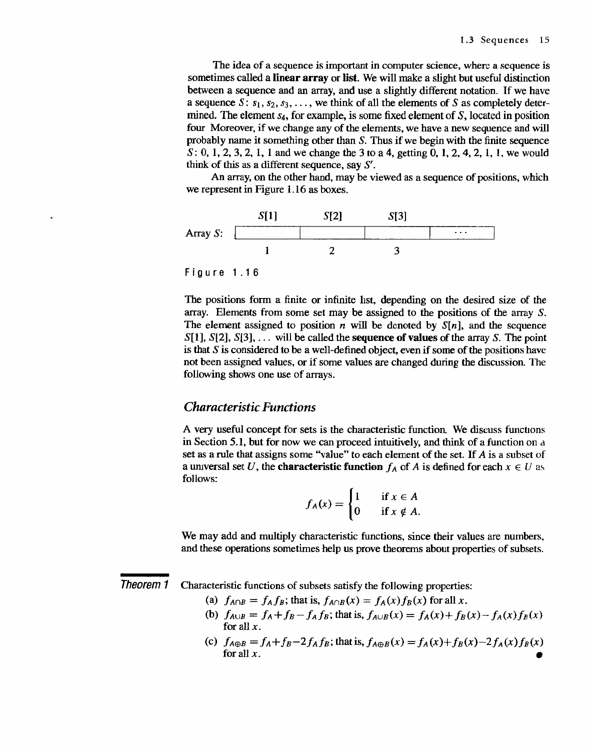
An array, on the other hand, may be viewed as a sequence of positions, which
we represent in Figure 1.16 as boxes.
S[I]
S[2]
S[3]
Array S:
1
2
3
Figure 1.16
The positions form a finite or infinite I1st, depending on the desired size of the
array. Elements from some set may be assigned to the positions of the array S.
The element assigned to position n will be denoted by S[n], and the sequence
S[1], S[2], S[3], . .. will be called the sequence of values of the array S. The point
is that S is considered to be a well-defined object, even if some of the positions have
not been assigned values, or if some values are changed during the discussion. The
following shows one use of arrays.
Characteristic Functions
A very useful concept for sets is the characteristic function. We discuss functIOns
in Section 5.1, but for now we can proceed intuitively, and think of a function on d
set as a rule that assigns some "value" to each element of the set. If A is a subset of
a umversal set U, the characteristic function fA of A is defined for each x E U a
follows:
fA (x) = {
ifxEA
if x f/: A.
We may add and multiply characteristic functions. since their values are numbers.
and these operations sometimes help us prove theorems about properties of subsets.
Theorem 1 Characteristic functions of subsets satisfy the following properties:
(a) fAnB = fAfB; that is, fAnB(X) = fA (X)fB(X) forallx.
(b) fAUB = fA+ fB- fAfB; that is, fAUB(X) = fA (x) + fB(X)- fA (X)fB(X)
for all x.
(c) fA(!}B = fA+ fB-2fAfB; that is, fA(!}B(X) = fA (x)+ fB(X)-2fA (X)fB(X)
for all x. .
16 Chapter 1 Fundamentals
Proof
(a) fA(X)fB(X) equals 1 if and only if both !A(X) and !B(X) are equal to 1,
and this happens if and only if x is in A and x is in B, that is, x is in A n B.
Since IAfB is I on A n B and 0 otherwise, it must be fAnB.
(b) If x E A, then fA (x) = 1, so fA (x) + fB(X) - fA (x) fB (x) = 1 + fB(X)-
fB(X) = 1. Similarly. when x E B, fA(X) + fB(X) - fA(X)fB(X) = 1.
If x is not in A or B, then fA(X) and IB{X) are 0, so fA(X) + IB(X) -
fA(X)fB(X) = O. Thus fA + IB - fAfB is 1 on A U B and 0 otherwise,
so It must be fAUB.
(c) We leave the proof of (c) as an exercise. .
Note that the proof of Theorem 4 proceeds by direct application of the defini-
tion of the characteristic function.
Computer Representation of Sets and Subsets
Another use of characteristic functions IS in representing sets in a computer. To
represent a set in a computer, the elements of the set must be arranged in a sequence,
The particular sequence selected is of no importance. When we list the set A =
{a, b, c, . . . , r} we nonnally assume no particular ordering of the elements in A.
Let us identify for now the set A with the sequence a, b, c, . . . , r.
When a universal set U is finite, say U = {Xl, XZ, . . . , x n }, and A is a subset
of U, then the characteristic function assigns 1 to an element that belongs to A and 0
to an element that does not belong to A. Thus I A can be represented by a sequence
of O's and I's of length n.
EXAMPLE 12
Let U = {I, 2,3,4,5, 6}, A = {I,2}, B = {2,4, 6}, and C = {4, 5, 6}. Then
fA (x) has value I when x is 1 or 2, and otherwise is O. Hence fA corresponds to
the sequence 1, I, 0, 0, 0, O. In a similar way, tbe finite sequence 0, 1, 0, 1, 0, I
represents fB and 0, 0,0, 1, 1, 1 represents fe. .
Any set with n elements can be arranged in a sequence of length n, so each
of its subsets corresponds to a sequence of zeros and ones of length n, representing
the characteristic functIOn of that subset. This fact allows us to represent a universal
set in a computer as an array A of length n. Assignment of a zero or one to each
location A[k] of the array specifies a unique subset of U.
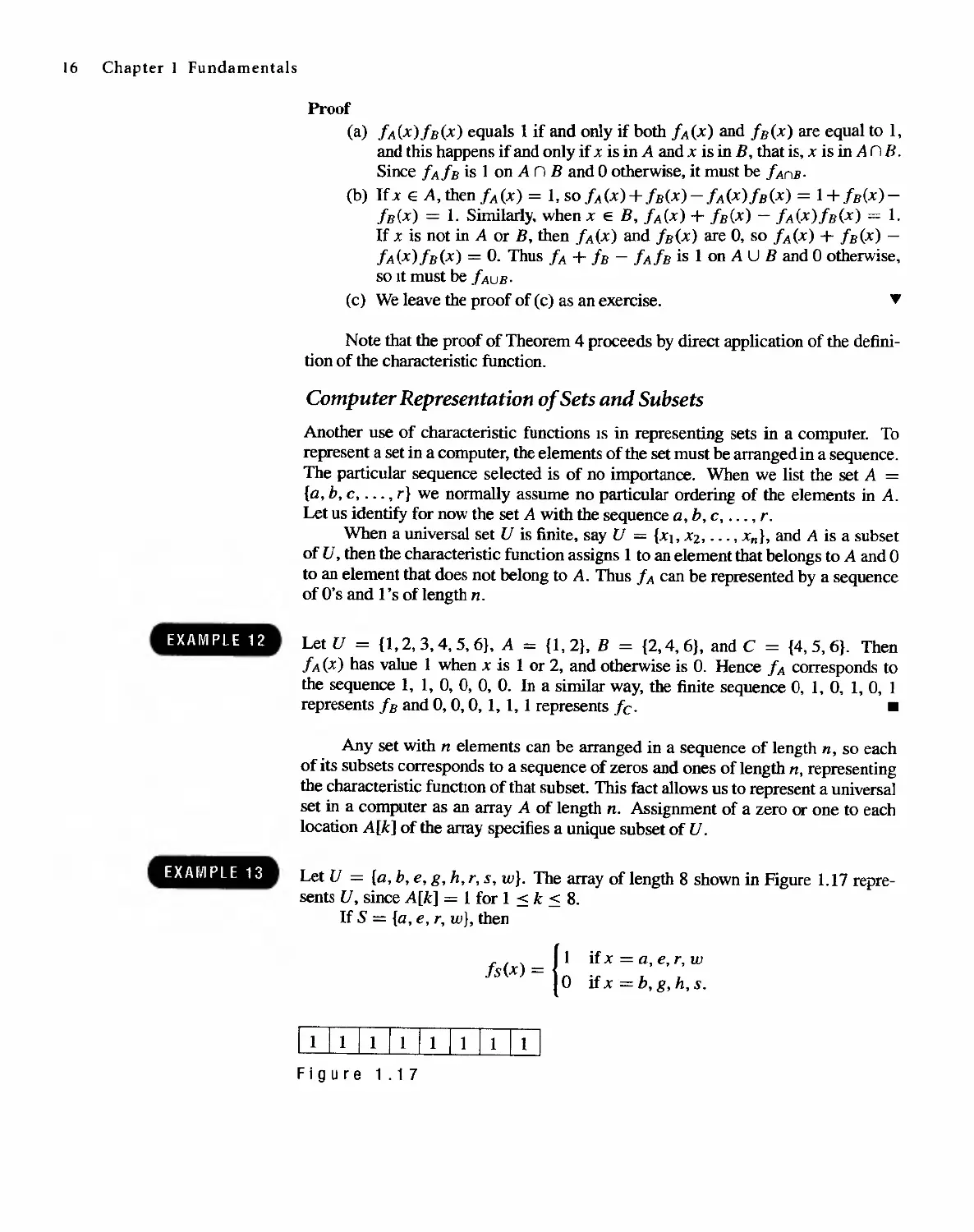
EXAMPLE 13
Let U = {a, b, e, g, h, r, s, wI. The array of length 8 shown in Figure 1.17 repre-
sents U, since A[k] = I for 1 < k < 8.
If S = {a, e, r, w}, then
fs(x) = g
if x = a, e, r, w
ifx=b,g,h,s.
11 [!]I WI [J]1 [!]
Figure 1.17
EXAMPLE 14
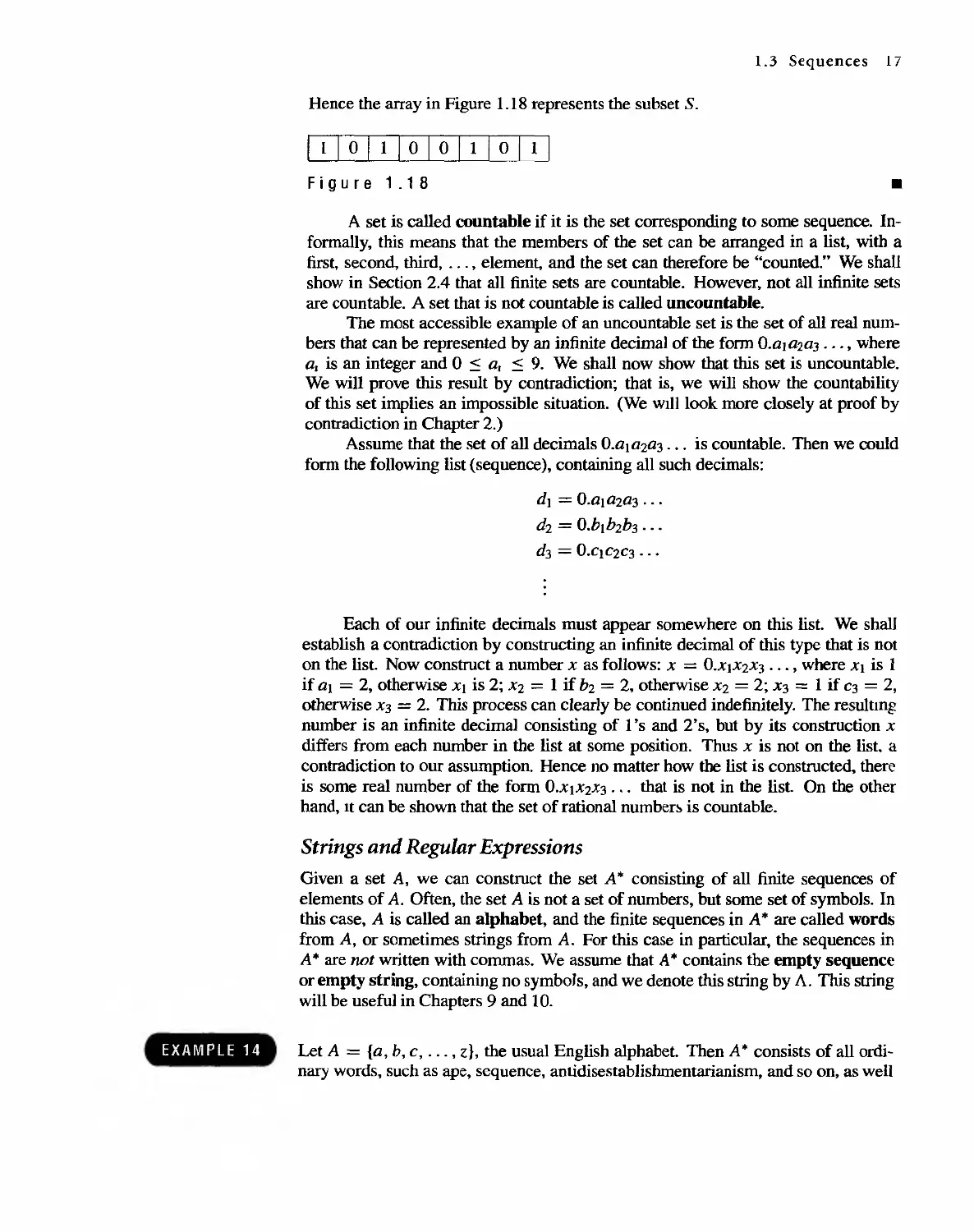
1.3 Sequences 17
Hence the array in Figure 1.18 represents the subset S.
1 1 1 0 1 1 [IJOITJO[O
Figure 1.18
.
A set is called countable if it is the set corresponding to some sequence. In-
fonnally, this means that the members of the set can be arranged in a list, with a
first, second, third, . . . , element. and the set can therefore be "counted." We shall
show in Section 2.4 that all finite sets are countable. However. not all infinite sets
are countable. A set that is not countable is called uncountable.
The most accessible example of an uncountable set is the set of all real num-
bers that can be represented by an infinite decima} of the fonn G.al a2a] . . ., where
a 1 is an integer and 0 < a , < 9. We shall now show that this set is uncountable.
We will prove this result by contradiction; that is, we will show the countability
of this set implies an impossible situation. (We wllllook more closely at proof by
contradiction in Chapter 2.)
Assume that the set of all decimals O.al a2a3 . .. is countable. Then we could
form the following list (sequence), containing all such decimals:
d] = O.a]a2a3 . . .
d2 = O.b r b 2 b3 .. .
d3 = 0.C]C2 C 3 . ..
.
.
Each of our infinite decimals must appear somewhere on this list. We shall
establish a contradiction by constructing an infinite decimal of this type that is not
on the list. Now construct a number x as follows: x = 0.XlX2X3 ..., where Xl is I
if a] = 2, otherwise Xl is 2; X2 = 1 if b2 = 2, otherwise X2 = 2; X3 == 1 if C3 = 2,
otherwise X3 = 2. This process can clearly be continued indefinitely. The resultmg
number is an infinite decima} consisting of 1 's and 2's, but by its construction X
differs from each number in the list at some position. Thus X is not on the list. a
contradiction to our assumption. Hence no matter how the list is constructed. there
is some real number of the form O.XlX2X3 . .. that is not in the list On the other
hand, It can be shown that the set of rational number is countable.
Strings and Regular Expressions
Given a set A, we can construct the set A'" consisting of all finite sequences of
elements of A. Often, the set A is not a set of numbers, but some set of symbols. In
this case, A is called an alphabet, and the finite sequences in A * are called words
from A, or sometimes strings from A. For this case in particular. the sequences in
A * are not written with commas. We assume that A * contains the empty sequence
or empty string, containing no symbols, and we denote this string by A. This string
will be useful in Chapters 9 and 10.
Let A = {a, b, c, . . . , d, the usual English alphabet. Then A * consists of all ordi-
nary words, such as ape, sequence, antidisestablishmentarianism, and so on, as well
18 Chapter 1 Fundamentals
EXAMPLE 15
EXAMPLE 16
as "words" such as yxaloble, zigadongdong, cay, and pqrst. All finire sequences
from A are in A *, whether they have meaning or not. .
If WI = SIS2S3 .. . Sn and W2 = tIt2t3 .. . tk are elements of A * for some set A,
we define the catenation of WI and W2 as the sequence SISZS3 . . . SntIt2t3 .., tk. The
catenation of WI with W2 is written as WI . W2 or WI W2, and is another element of
A* Note that if W belongs to A*, then w. A = wand A. w = w. This property is
convenient and is one of the main reasons for defining the empty string A.
Let A = {John, Sam, Jane, swims, runs, well, quickly, slowly}. Then A * con-
tains real sentences such as "Jane swims quickly" and "Sam runs well," as well as
nonsense sentences such as "Well swims Jane slowly John." Here we separate the
elements in each sequence with spaces. This is often done when the elements of A
are words. .
The idea of a recursive formula for a sequence is useful in more general set-
tings as well In the fonnallanguages and the finite state machines we discuss in
Chapter 10, the concept of regular expression plays an important role, and regu-
lar expressions are defined recursively. A regular expression over A is a string
constructed from the elements of A and the symbols (, ), V,*, A, according to the
following definition.
RE 1. The symbol A is a regular expression.
RE2. If x E A, the symbol x is a regular expression.
RE3. H a and f3 are regular expressions, then the expression af3 is regular.
RE4. If a and 13 are regular expressions, then the expression (a v 13) is regular.
RE5. If a is a regular expression, then the expression (a)* is regular.
Note here that REI and RE2 provide initial regular expressions. The other
parts of the definition are used repetitively to define successively larger sets of reg-
ular expressions from those already defined. Thus the definition IS recursive,
By convention, if the regular expression a consists of a single symbol x, where
x E A, or if a begins and ends with parentheses, then we write (a)* simply as a*.
When no confusion results, we will refer to a regular expression over A simply as a
reguJar expression (omitting reference to A).
Let A = {O, I}. Show that the following expressions are all regular expressions over
A.
(a) 0*(0 v 1)*
(b) 00*(0 v 1)*1
(c) (01)*(01 v 1*)
Solution
(a) By RE2, 0 and I are regular expressions. Thus (0 V 1) is regular by RE4,
and so 0* and (0 v 1)* are regular by RE5 (and the convention mentioned
previously). Finally, we see that 0*(0 V 1)* is regular by RE3.
EXAMPLE 17
EXAMPLE 18
1.3 Sequences 19
(b) We know that 0, I, and 0*(0 v 1)* are all regular. Thus, using RE3 twice,
00*(0 V 1)*1 must be regular.
(c) By RE3, 01 is a regular expression. Since 1* is regular, (01 v I *) is regular
by RE4, and (01) *is regular by RE5. Then the regularity of (0 I) * (0 I v 1 *)
follows from RE3. .
Associated with each regular expression over A, there is a corresponding sub-
set of A *. Such sets are called regular subsets of A * or Just reguJsr sets if no
reference to A is needed. To compute the regular et corresponding to a regular
expression, we use the following correspondence rules.
I, The expression A corresponds to the set {A}, where A is the empty string
in A*.
2. If x E A, then the regular expression x corresponds to the set {x}.
3. If [i and f3 are regular expressions corresponding to the subsets M and N
of A*, then af3 corresponds to M . N = {s . tis E M and tEN}. Thus
M . N is the set of all catenations of strings in M with strings in N.
4. If the regular expressions [i and fJ correspond to the subsets M and N of
A*, then (a v fJ) corresponds to M UN.
5. If the regular expression [i corresponds to the subset M of A *, then ([i) *
corresponds to the set M*. Note that M is a set of strings from A. Elements
from M* are finite sequences of such strings, and thus may themselves be
interpreted as strings from A. Note also that we always have A E M*
Let A = {a, b, c}. Then the regular expression a* corresponds to the set of all
finite sequences of a's. such as aaa, aaaaaaa. and so on. The regular expression
a (bve) corresponds to the set lab, ae} C A*. Finally. the regular expression ab(be) *
corresponds to the set of all strings that begin with ab, and then repeat the symbols
be n times, where n > 0, This set includes the strings ah. abbcbc, abbcbcbcbc, and
so on. .
Let A = to, I}. Find the regular sets corresponding to the three regular expressions
in Example 16.
Solution
(a) The set corresponding to 0*(0 v 1)* consists of all sequences of O's and
l's. Thus, the set is A*.
(b) The expression 00*(0 v 1)*1 corresponds to the set of all sequences ofO's
and l' s that begin with at least one 0 and end with at least one 1.
(c) The expression (01)*(01 v 1*) corresponds to the set of all sequences
of O's and l's that either repeat the string 01 a total of n > I times, or
begin with a total of n > 0 repetitions of 01 and end with some number
k > 0 of 1 'so This set includes, for example, the strings 111], 01, 01 01 01,
0101010111111, and OIl. .
20 Chapter 1 Fundamentals
1 } .. I '". It)
'11":-3 :E x'etci s 'e s
In Exercises 1 through 4. give the set corresponding to the
sequence.
1. 1,2, 1,2, 1,2, 1,2, 1
2. O. 2. 4. 6. 8, 10. ' ..
3. aabbecddee...zz
4. abbce c<!ddd
5. Give three different sequences that have {x, y. z} as a
corresponding set.
6. Give three different sequences that have {I, 2, 3, ... , } as
a corresponding set.
In Exercises 7 through 10, write out the first four terms (begin
with n = 1) of the sequence whose general term is given.
7. an = 5"
8. b" = 3n 2 + 2n - 6
9. CI = 2.5, C n = CII-I + 1.5
10. d l = -3, d n = -2d n - 1 + 1
In Exercises 11 through 16, write aformulafor the nth term of
the sequence. Identify your formula as recursive or explicit.
11.1,3,5,7,...
12. 0, 3. 8. 15,24, 35, ..
13. 1, -1, 1. -1,1, -1,...
14. 0, 2, O. 2, 0, 2, . . .
15. 1,4, 7, 10, 13, 16
16 1 1 1 1 I
. , 2' 4' ii' 16 ' . . .
17. Write an explicit formula for the sequence 2,5,8, II,
14. 17. . . ..
18. Write a recursive fannula for the sequence 2, 5, 7, 12,
19,31,.. ..
19. Let A = {x I x is a real number and 0 < x < I},
B = {x I x is a real number and x 2 + 1 = O}.
C = {x I x = 4m, m E Z}, D = {(x,3) I x IS an
English word whose length is 3}, and E = {x I x E Z
and x 2 S l00}. Identify each set as fimte, countable, or
uncountable.
20. Let A = lab, be, bal. In each part, tell whether the string
belongs to A *.
(a) ababah (b) ahe (c) abba
(d) abbcbaba (e) bcabbab (f) abbbcba
21. Let U = {FORTRAN, PASCAL, ADA, COBOL, LISP,
BASIC, C++, FORTH], B = {C++ BASIC, ADA},
C = {PASCAL, ADA, LISP, C++}. D = {FORTRAN.
PASCAL, ADA. BASIC, FORTH}, E = {PASCAL,
ADA, COBOL. LISP, C++}. In each of the following,
represent the given set by an array of zeros and ones.
(a) B U C (b) enD
(c) B n (D n E) (d) B U E
(e) C n (B U E)
22. Let U = {b,d,e,g.h,k,m.n}, B = {b}, C _
{d, g. m, n}, and D = {d, k, n}.
(a) Whatts fB(b)? (b) What is fde)?
(c) Find the sequences of length 8 that correspond to fB,
fe, and fv.
(d) Represent B U C, CUD, and enD by arrays of
zeros and ones.
23. Complete the proof that fAeB = fA + fB - 2fAfB
[Theorem 4(c)]. Suppose x E A and x fj B. Then
fA (x) = ,fB(x) = ,and
[A(x)fB(X) = , so h(x)+ fB (x)-2/A (x) fB (x) =
. Now suppose x fj A and x E B. Then fA (x) =
, fB(X) = , and !A(x)fB(X) = , so
!A(X) + IB(x) - 2fA(x)fB(X) = . The remaining
case to check is x fj A ffi B. If x (j A ffi B, then x E
and hex) + fB(X) - 2fA(X)fn(X) = . Explain
how these steps prove Theorem 4( c)
24. Using charactenstic functIons, prove that (A E9 B) E9 C =
A ffi (B E9 C).
25. Let A = {+, x, a, b}. Show that the following expres-
sions are regular over A.
(a) a + b(ab)'"(a x h V a)
(b) a +b x (a* vb)
(c) (a*b V +)'" V x h*
In Exercises 26 and 27, let A = {a, b, c}. In each exercise
a string zn A * is listed, and a regular expression over A. In
each case, tell whether or not the string on the left belongs to
the regular set corresponding to the regular expression on the
right.
26. (a) ac a*b*c (b) abcc (abe v c)*
(c) aaabc «a V b) V c)*
27. (a) ac (a*b V c) (b) abab (ab)*c
(c) aaccc (a. V b)c*
28. Give three expressions that are not regular over the A
given for Exercise 26.
29. Let A = {p, q. r}. Give the regular set corresponding to
the regular expression given.
(a) (p v q)rq* (b) p(qq)*r
30. Let S = to, I}. Give the regular expression corresponding
to the regular set given.
(a) tOO, 010, 0110, 011110, .. . }
(b) to. 001, 000,00001,00000,0000001, ...}
31. We define T -numbers recursively as follows:
1. 0 is aT-number.
2. If X is aT-number, X + 3 is aT-number.
Write a description of the set of T -numbers.
32. Define an S-number by
1. 8 is an S-number.
2. If X is an S-number and Y is a multiple of X, then Y
is an S-number.
1.4 DIVISION IN THE INTEGERS
1.4 Division in the Integers 21
3. If X is an S-number and X is a multiple of Y. then Y
is an S-number.
Describe the set of S-numbers.
33. Let F be a function defined for all nonnegative integers
by the following recursive definition.
F(O) = 0, F(1) = 1
F(N + 2) = 2F(N) + F(N + 1), N > 0
Compute the first six values of F; that is. write the values
of F(N) for N = 0, I, 2. 3,4,5.
34. Let G be a function defined for all nonnegative integers
by the followmg recursive definition.
G(O) = 1, G(1) = 2
G(N + 2) = G(N)2 + G(N + 1), N > 0
Compute the first five values of G_
We shall now discuss some results needed later about division and factoring in the
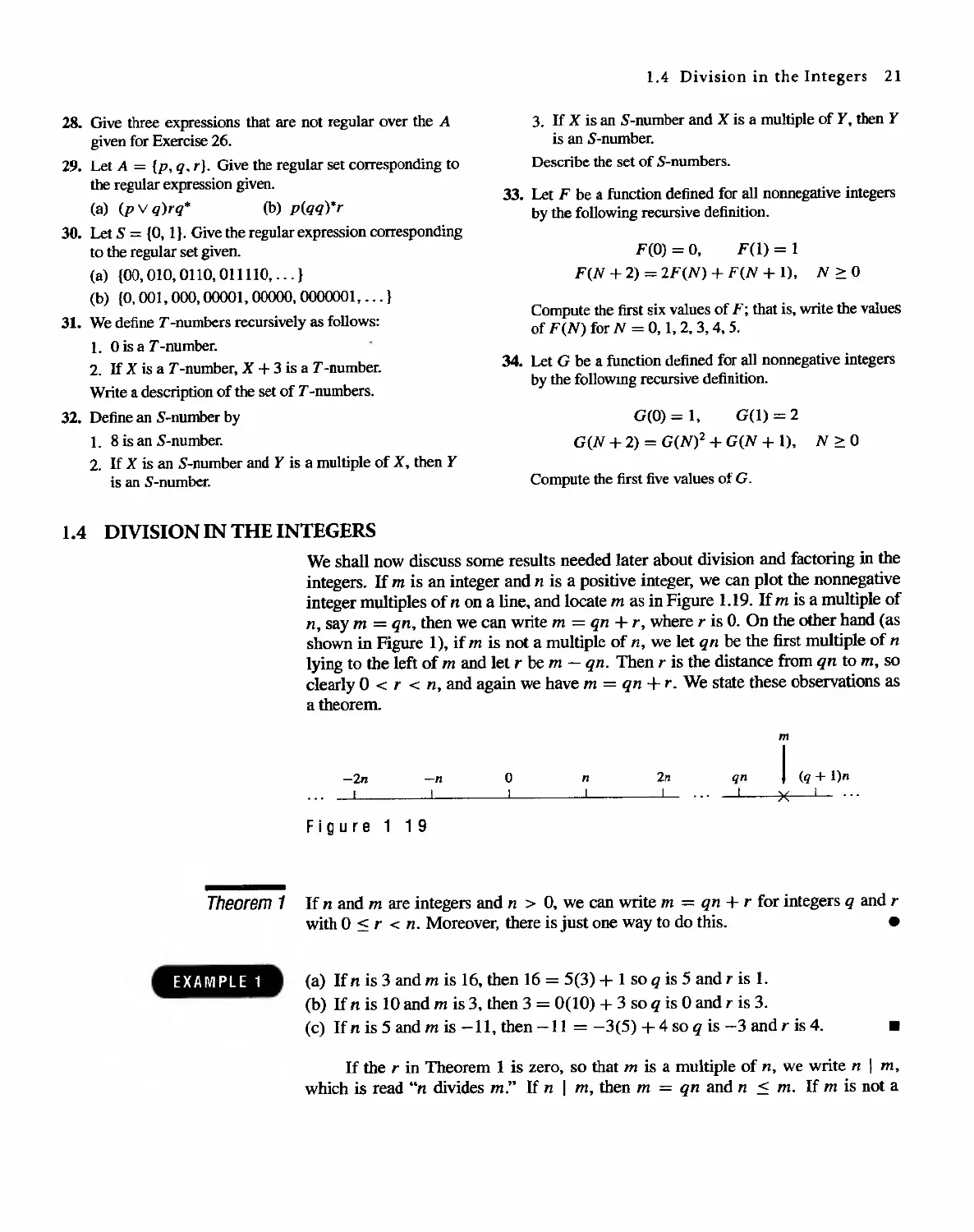
integers. If m is an integer and n is a positive integer, we can plot the nonnegative
integer multiples of n on a line. and locate m as in Figure 1.19. If m is a multiple of
n, say m = qn, then we can write m = qn + r, where r is O. On the other hand (as
shown in Figure I), if m is not a multiple of n, we let qn be the first multiple of n
lying to the left of m and let r be m - qn. Then r is the distance from qn to m. so
clearly 0 < r < n, and again we have m = qn + r. We state these observations as
a theorem.
m
-2n -n 0 n 2n qn I (q + l)n
I I I I I I X I
Figure 1 1 9
Theorem 1 If n and m are integers and n > O. we can write m = qn + r for integers q and r
with 0 < r < n. Moreover, there is just one way to do this. .
(a) If n is 3 and m is 16, then 16 = 5(3) + 1 so q is 5 and r is 1.
(b) If n is 10 and m is 3. then 3 = 0(10) + 3 so q is 0 and r is 3.
(c) If n is 5 and m is -11, then -11 = -3(5) + 4 so q is -3 and r is 4.
EXAMPLE 1
.
If the r in Theorem 1 is zero, so that m is a multiple of n, we write n I m,
which is read "n divides m." If n I m, then m = qn and n < m. If m is not a
22 Chapter 1 Fundamentals
multiple of n, we wnte n t m, which is read "n does not divide m." We now prove
some simple properties of divisibility.
Theorem 2 Let a, b, and e be integers.
(a) !fa I banda I e, then a I (b + c).
(b) Ifa I banda I c, where b > c, then a I (b - c).
(c) If a I b or a Ie, then a I be.
(d) Ifa I b andb I e, then a ! e.
.
Proof
(a) If a I b and a I e, then b = k}a and e = k2a for integers k 1 and k2. So
b+c= (k 1 +k 2 )aanda I (b+e).
(b) This can be proved in exactly the same way as (a).
(c) As in (a), we have b = k1a or e = k2a. Then either be = klae or
be = k2ab, so in either case be is a multiple of a and a I be.
(d) If a I band b I c, we have b = k1a and e = k2b, so e = k 2 b = k 2 (k 1 a) =
(k 2 kl)a and hence a Ie. ...
Note that again we have a proof that proceeds directly from a definition by
restating the original conditions. As a consequence of Theorem 2, we have that if
a I b and a I e, then a I (mb + ne), for any integers m and n.
A number p > 1 m z+ IS called prime if the only positive integers that divide
p are p and 1.
EXAMPLE 2
The numbers 2,3,5, 7, 11, and 13 are prime, while 4, 10, 16, and 21 are not prime.
.
It is easy to write a set of steps, or an algorithm*, to determine if a positive
integer n > 1 is a prime number. First we check to see if n IS 2. If n > 2, we could
divide by every integer from 2 to n - 1, and if none of these is a diVISor of n, then
n is prime. To make the process more efficient, we note that if mk = n, then either
m or k is les than or equal to . ThIs means that if n is not prime. it has a divisor
k satisfying the inequality I < k < ,Jii., so we need only test for divisors in this
range. Also, if n has any even number as a divisor, it must have 2 as a divisor. Thus
after checking for divisibility by 2, we may skip all even integers.
. ALGORITHM to test whether an integer N > 1 is prime:
Step 1 Check whether N is 2. If so, N is prune. If not, proceed to
Step 2 Check whether 2 I N - If so, N is not prime; otherwise, proceed to
Step 3 Compute the largest integer K < ,IN. Then
Step 4 Check whether DIN, where D is any odd number such that
I < D < K. If D ! N, then N is not prime; otherwise, N is prime.
* Algorithms are discussed in AppendIx A.
1.4 DIvision in the Integers 23
Testing whether an integer is prime is a common task for computers. The algorithm
given here is too inefficient for testing very large numbers, but there are many other
algorithms for testing whether an integer is prime.
Theorem 3 Every positive integer n > 1 can be written uniquely as p I p;2 . . . P;'s, where
PI < P2 < ... < Ps are distinct primes that divide n and the k's are positive
integers giving the number of times each prime occurs as a factor of n. .
We leave the proof of Theorem 3 to Section 2.4, but we give several illustra-
tions.
EXAMPLE J
(a) 9 = 3 ' 3 = 3 2
(b) 24 = 8 . 3 = 2 . 2 . 2 . 3 = 2 3 . 3
(c) 30 = 2 . 3 . 5
.
Greatest Common Divisor
If a, b, and k are in Z+, and k I a and k I b, we say that k is a common divisor
of a and b. If d is the largest such k, d is called the greatest common divisor, or
GCD, of a and b, and we write d = GCD(a, b). This number has some interesting
properties. It can be written as a combination of a and b, and it is not only larger
than all the other common divisors, it is a multiple of each of them.
Theorem 4 If d is GCD(a. b). then
(a) d = sa+tbforsomeintegerssandt. (These are not necessarily positive.)
(b) If c is any other common divisor of a and b, then c I d. .
Proof Let x be the smallest positive integer that can be written as sa + tb for
some integers s and t. and let c be a common divisor of a and b. SInce c I a and
c I b, it follows from Theorem 2 that c I x, so c < x. If we can show that x is a
common divisor of a and b, it will then be the greatest common divisor of a and b
and both parts of the theorem will have been proved. By Theorem 1, a = q x + r
with 0 < r < x. Solving for r, we have
r = a - qx = a - q(sa + tb) = a - qsa - qtb = (1 - qs)a + (-qt)b.
If r is not zero, then since r < x and r is the sum of a multIple of a and a multiple
of b, we will have a contradiction to the fact that x is the smallest positive number
that is a sum of multiples of a and b. Thus r must be 0 and x I a. In the same way
we can show that x I b, and this completes the proof.
This proof is more complex than the earlier ones. At this stage you should
focus on understanding the details of each step. We will discuss the structure of this
proof later.
From the definition of greatest common divisor and Theorem 4(b). we have
the following result: Let a, b. and d be in Z+. The integer d is the greatest common
divisor of a and b if and only if
24 Chapter 1 Fundamentals
(a) d I a andd I b.
(b) Whenever c I a and c I ht then c I d.
EXAMPLE 4
(a) The common divisors of 12 and 30 are 1,2,3, and 6, so that
GCD(12,30) = 6 and 6 = 1 .30 + (-2) .12.
(b) It is clear that GCD(17, 95) = 1 since 17 is prime and 17 f 95, and the reader
may verify that 1 = 28. 17 + (-5).95. .
If GCD(a, b) = I, as in Example 4(b), we say a and b are relatively prime.
One remaining question is that of how to compute the GCD conveniently in
generaL Repeated application of Theorem 1 provides the key to doing this.
We now present a procedure, called the Euclidean algorithm, for finding
GCD(a, b). Suppose that a > b > 0 (otherwise interchange a and b). Then by
Theorem 1, we may write
a = k l b + rl,
where k l is in Z+ and 0 < rl < b.
(1)
Now Theorem 2 tells us that if n divides a and b, then it must divide rt. since
r] = a - k1b. Similarly, if n divides band r], then it must divide a. We see that
the common divisors of a and b are the same as the common divisors of b and rl.
so GCD(a, b) = GCD(b, rl)'
We now continue using Theorem 1 as follows:
divide b by rl: b = k2rl + rz o < r2 < rl
divide rj by r2: rl = k 3 r 2 + r3 o < r] < r2
divide r2 by r3: r2 = k4 r 3 + r4 o < r4 < r3
. . (2)
. . .
. .
divide r n -2 by rn-l: r n -2 = knrn-l + r n o < r n < rn-l
divide rn-l by rn: rn-l = kn+lrn + rn+l o < rn+l < rn.
Since a > b > rl > r2 > r3 > r4 > ..., the remainder will eventually become
zero, so at some point we have rn+l = O.
We now show that r n = GCD(a, b). We saw previously that
GCD(a, b) = GCD(b. rI).
Repeating tlus argument with b and rl, v,e see that
GCD(b, rl) = GCD(rl, r2).
Upon continuing, we have
GCD(a. b) = GCD(b, 'I) = GCD(rl. r2) = ... = GCD(rn_l, rn).
Since rn-l = kn+1r n , we see that GCD(rn_l, rn) = r n - Hence r n = GCD(a, b).
1.4 Division in the Integers 25
EXAMPLE 5
Let a be 190 and b be 34. Then, using the Euclidean algorithm. we
dIVIde 190 by 34:
divide 34 by 20:
divide 20 by 14:
divide 14 by 6:
divide 6 by 2:
190 = 5 . 34 + 20
34 = I . 20 + 14
20 = 1 . 14 + 6
14 = 2 . 6 + 2
6=3.2+0
so GCD(190, 34) = 2, the last of the nonzero divisors.
.
In Theorem 4(a), we observed that if d = GCD(a, b), we can find integers s
and t such that d = sa + t b. The integers s and t can be found as follows. Solve
the next-to-Iast equation in (2) for r n :
r n = r n -2 - knrn-l.
(3)
Now solve the second-to-Iast equation in (2), r n -3 = kn-1Tn-2 + rn-l for rn-l:
rn-l = r n -3 - k n - 1 T n-2
and substitute this expression in (3):
Tn = r n -2 - k n [r n -3 - k n - 1 r n -2].
Continue to work up through the equations in (2) and (1), replacing r l by an expres-
sion involving r,-l and r,-2, and finally arriving at an expression involving only a
andb.
EXAMPLE 6
(a) Let a = 190 and b = 34 as in Example 5. Then
GCD(190.34) = 2 = 14 - 2(6)
= 14 - 2[20 - 1(14)]
= 3(14) - 2(20)
= 3[34 - 1 (20)] - 2(20)
= 3(34) - 5(190 - 5.34)
= 28(34) - 5(190)
6 = 20 - I .14
14 = 34 - 1 . 20
20 = 190 - 5 . 34
Hence s = -5 and 1 = 28. Note that the key is to carry out the arithmetic only
partially.
(b) Let a = 108 and b = 60. Then
GCD(108,60) = 12 = 60 - 1(48)
= 60 - 1[108 - 1(60)] 48 = 108 - 1 .60
= 2(60) - 108.
Hence s = -1 and t = 2. .
Theorem 5 If a and b are in Z+, then GCD(a, b) = GCD(b, b:f: a). .
26 Chapter 1 Fundamentals
Proof If c divides a and b, it divides b:l::a, by Theorem 2. Since a = b- (b-a) ,
-b + (b + a), we see, also by Theorem 2, that a common divisor of band b::f: a
also divides a and b. Smce a and b have the same common divisors as b and b ::f: a,
they must have the same greatest common divisor. T
This is another direct proof, but one that uses a previous theorem as well as
definitions.
Least Common Multiple
If a, b, and k are in Z4-, and a I k, b I k. we say k IS a common multiple of a and
b. The smallest such k, call it c, is called the least common multiple, or LCM, of a
and b, and we write c = LCM(a, b). The following result shows that we can obtain
the least common multiple from the grLatest common divisor, so we do not need a
separate procedure for finding the least common multiple.
Theorem 6 If a and b are two positive integers, then GCD(a, b) . LCM(a, b) = ab. .
Proof Let Pi, P2, . . . , Pk be all the prime factors of either a or b. Then we can
write
a = p l p 2. . p%k and b = ptl p 2 . . . p: k
where some of the a, and b , may be zero. It then follows that
GCD( b) - mm(aI,bI) rnm(aZ.b2) nun{ak,bk)
a, - PI P2 . . . Pk
and
LCM( b) - max(a}.b}) max(az,bz) max(ak.bk)
a, - PI P2 . . . Pk .
Hence
GCD( b) . LCM( b) - al+ b l a2+ b 2... ak+bk
a, a, - PI P2 Pk
( al a2 ak ) ( bl b2 b k )
= PI P2 ... Pk . PI P2 ... Pk
= ab. 'Y
EXAMPLE 7
Let a = 540 and b = 504. Factoring a and b into primes, we obtain
a = 540 = 2 2 . 3 3 . 5 and b = 504 = 2 3 . 3 2 . 7.
Thus all the prime numbers that are factors of either a or b are PI = 2, P2 = 3,
P3 = 5, and P4 = 7. Then a = 2 2 . 3 3 .5 1 .7° and b = 2 3 .3 2 .5° .7 1 . We then have
GCD(540, 504) = 2 rnm (2,3) .3 Ulln (3.2) . 5 Ulln (1.0) .7 nun (0.i)
= 2 2 . 3 2 . 50 . 70
= 2 2 . 3 2 or 36.
EXAMPLE 8
EXAMPLE 9
1.4 Division in the Integers 27
Also,
LCM(S40, S04) = 2 max (2,3) . 3 max (3,2) . SInaX(l,O) . 7 JWlX (O 1)
= 2 3 .3 3 . SI .7 1 or 7S60.
Then
GCD(540, S04). LCM(540, S04) = 36. 7S60 = 272,160 = 540. S04.
As a verification, we can also compute GCD(S40, S04) by the Euclidean algorithm
and obtain the same result. -
If n and m are integers and n ;> 1, Theorem 1 tells us we can wnte m = qn +r ,
o < r < n. Sometimes the remainder r is more important than the quotient q.
If the time is now 4 o'clock, what time will it be 10 1 hours from now?
Solution Letn = 12 andm = 4+101 or 10S. Then we have IOS = 8.12+9.
The remainder 9 answers the questlon. In 101 hours it will be 9 o'clock. -
For each n E Z+, we define a function In' the mod-n function, as follows: If
z is a nonnegative integer, In (z) = r, the remainder when z is divided by n. (Again,
functions are formally defined in Section 5.1, but as in Section 1.3, we need only
think of a function as a rule that assigns some "value" to each member of a set.) The
naming of these functions is made clear in Section 4.S.
(a) /3(14) = 2, because 14 = 4.3 + 2 and 14 = 2 (mod 3).
(b) /7(1S3) = 6
-
Pseudocode Versions
An alternative to expressing an algorithm in ordinary English as we did in this sec-
tion is to express it in something like a computer language. 1broughout the book
we use a pseudocode language, which is described fully in Appendix A. Here we
give pseudocode versions for an algorithm that determines if an integer is prime and
for an algorithm that calculates the greatest common divisor of two integers.
In the pseudocode for the algorithm to determine if an integer is prime, we
assume the existence of functions SQR and INT, where SQR(N) returns the greatest
integer not exceeding -IN, and INT(X) returns the greatest integer not exceeding
X. For example, SQR(10) = 3, SQR(2S) = S, INT(7.124) = 7, andINT(8) = 8.
SUBROUTINE PRIME(N)
1. IF (N = 2) THEN
a. PRINT ('PRIME')
b. RE11JRN
2. ElSE
a. IF (N /2 = INT(N /2» THEN
1. PRINT ('NOT PRIME')
2. RETIJRN
28 Chapter] Fundamentals
EXAM PLE 10
b. ELSE
1. FOR D = 3 THRU SQR(N) BY 2
a. IF (N / D = INT(N / D)) THEN
1. PRINT ('NOT PRIME')
2. RETURN
2. PRINT ('PRIME')
3. RETURN
END OF SUBROUTINE PRIME
The following gives a pseudocode program for finding the greatest common
divisor of two positive integers. This procedure is different from the Euclidean
algorithm, but in Chapter 2, we will see how to prove that this algorithm does indeed
find the greatest common divisor.
FUNCTION GCD(X, Y)
1. WHILE (X"# Y)
a. IF (X > Y) TIfEN
1. X+-X-Y
b. ELSE
1. Y +-y-x
2. RETURN (X)
END OF FUNCTION GCD
Use the pseudocode for GCD to calculate the greatest common divisor of 190 and
34 (Example 5).
Solution The following table gives the values of X, Y, X - Y, or Y - X as
we go through the program.
x y X-y y-X
190 34 156
156 34 122
122 34 88
88 34 54
54 34 20
20 34 14
20 14 6
6 14 8
6 8 2
6 2 4
4 2 2
2 2
Since the last value of X is 2, the greatest common divisor of 190 and 34 is 2.
.
C 1.4 Exercises)
1.4 Division in the Integers 29
In Exercises 1 through 4,for the given integers m and n. write
m as qn + r, with 0 < r < n. .
1. m = 20, n = 3
2. m = 64. n = 37
3. m = 3, n = 22
4. m = 48, n = 12
5. Write each integer as a product of powers of primes (as in
Theorem 3).
(a) 828
(d) 1125
(b) 1666
(e) 107
(c) 1781
In Exercises 6 through 9,find the greatest common divisor d
of the integers a and b, and write d as sa + tb.
6. a=60,b= 100
7. a = 45, b = 33
8. a = 34, b = 58
9. a = 77, b = 128
In Exercises 10 through 13, find the least common multiple of
the integers.
10. 72. 108
11. 150, 70
12. 175. 245
13. 32, 27
14. If f is the mod-7 function, compute each of the following.
(a) f(17) (b) 1(48) (c) 1(1207)
(d) j (130) (e) f(93) (f) 1(169)
15. If f is the mod-II function, compute each of the follow-
mg.
(a) f(39)
(d) f(573)
(b) f(386)
(e) 2f(87)
(c) 1(1232)
(f) 1(175) + 4
16. If g is the mod-5 function, solve each of the following.
(a) g(n) = 2 (b) g(n) = 4
17. If g is the mod-6 function, solve each of the following.
(a) g(n) = 3 (b) g(n) = 1
18. Complete the following proof. Let a and b be integers. If
p is a prime and p I ab, then p I a or p I b. We need
to show that if p t a, then p must divide b. If p 1 a,
then GCD(a. p) = 1, because . By Theorem 4, we
can write I = sa + tp for some integers s and t. Then
b = sab + tpb. (Why?) Then p must divide sab + tpb,
because . So p lb. (Why?)
19. Show that if GCD(a, c) = 1 and c I ab, then c I b.
(Hint: Model the proof on the one in Exercise 18.)
20. Show that if GCD(a, c) = 1, a I m, and elm. then
ac I m. (Hint: Use Exercise 19.)
21. Show that if d = GCD(a, b), a I b, and c I b, then
ac I bd.
22. Show that GCD(ca. cb) = cGCD(a. b).
23. Show that LCM(a, ab) = ab.
24. Show that If GCD(a, b) = 1, then LCM(a. b) = ab.
25. Let c = LCM(a, b). Show that if a I k and b I k, then
elk.
26. Prove that If a and b are positi,,'e integers such that a I b
and b I a, then a = b
27. Let a be an integer and let p be a positive integer. Prove
that if pia. then p = GCD(a, p).
28. Theorem 2(c) says that if a I b or a I c, then a I be. Is the
converse true; that is, if a I be, then a I b or a ! c? Justify
your conclusion.
29. Prove that if m and n are relatively prime and mn IS a
perfect square, then m and n are each perfect squares.
30. Is the statement in Exercise 29 true for cubes? For any
fixed power? Justify your conclusion.
In Exercises 31 through 33, let U = {l, 2, 3..., 1689},
A = {x I x E U and 3 I x}, B = {y lyE U and 5 I y}, and
C = {Z I Z E U and 111 z}. Compute each of the following.
31. (a) IAI
(b) IBI
(c) ICI
32. (a) The number of elements in U that are divisible by 15
(b) The number of elements of U that are divisible by
165
(c) The number of elements of U that are divisible by 55
33. Use the results of Exercises 31 and 32 to compute each of
the following.
(a) IA U B/ (b) IA U B U C/
30 Chapter 1 Fundamentals
1.5 MATRICES
A matrix is a rectangular array of numbers arranged in m horizontal rows and n
vertical columns:
all al2 al n
a21 a22 a2n
A= . . (1)
. . .
. . .
amI a m 2 a mn
The itb row of A is [azl a,2
all
a2)
... ain],] < i < m, and thejth column of A is
, 1 < j < n. We say that A is m by n, written m x n_ If m = n, we say A
am)
is a square matrix of order n and that the numbers all, a22, . . . , ann form the main
diagonal of A. We refer to the number a,), which is in the i th row and j th column
of A as the i, jtb element of A or as the (i, j) entry of A, and we often write (1)
as A = [ a'l ].
EXAMPLE 1 Let
A=[ 3 ], B= [ n c = [I -1 3 4]
-1
-1 1 0 -I
D= 2 , and E= -1 2 3
0 2 4 5
Then A is 2 x 3 with al2 = 3 and a23 = 2, B is 2 x 2 with b 21 = 4. C is 1 x 4,
D is 3 x 1, and E is 3 x 3. .
A square matrix A = [at) ] for which every entry off the main diagonal is
zero, that is, a'l = 0 for i :1= j, is called a diagonal matrix.
EXAMPLE 2 Each of the following is a diagonal matrix.
F= [ n 2 0 0 0 0 0
G= 0 -3 0 . and H= 0 7 0
0 0 5 0 0 6
.
Matrices are used in many applications in computer science, and we shall see
them in our study of relations and graphs. At this point we present the following
simple application showing how matrices can be used to display data in a tabular
form.
1.5 Matrices 31
EXAMPLE 3
The following matrix gives the airline distances between the cities indicated.
London
Madrid
New York
Tokyo
London
o
785
3469
5959
Madrid
785
o
3593
6706
New York
3469
3593
o
6757
Tokyo
5959
6706
6757
o
&I
Two m x n matrices A = [a , ) J and B = [hi)] are said to be equal if
a'l = hi)' I :s: i .:s: m, I < j < n; that is, if corresponding elements are the same.
Notice how easy it is to state the definition using generic elements a'l' hi)
EXAMPLE 4 If
A=
2 -3 -1
052
4 -4 6
and B =
2 x-I
y 5 2
4 -4 z
.
then A = 8 if and only if x = -3, y = 0, and z = 6.
II
If A = [ a , ) ] and B = [ hi) ] are m x n matrices, then the sum of A and B is
the matrix C = [ e,) ] defined by e , ) = a'l + h,), 1 < i < m, I < j < n. That is, C
IS obtamed by adding the corresponding elements of A and B. Once again the use
of generic elements makes it easy to state the definition.
EXAMPLE 5
[ 3 4 -1 ] [ 4 5 3 ]
Let A = 5 0 -2 and 8 = 0 -3 2. Then
[ 3+4 4+5 -1+3 ] [ 7
A + 8 = 5 + 0 0 + (-3) - 2 + 2 = 5
9
-3
n
.
Observe that the sum of the matrices A and B is defined only when A and B
have the same number of rows and the same number of columns. We agree to write
A + 8 only when the sum is defined.
A matrix all of whose entries are zero is called a zero matrix and is denoted
byO.
EXAMPLE 6
Each of the following is a zero matrix.
[g g]
[g g g]
000
000
000
II
The following theorem gives some basic properties of matrix addition; the
proofs are omitted.
Theorem 1 (a) A + B = 8 + A.
(b) (A + B) + C = A + (8 + C).
(c) A + 0 = 0 + A = A.
.
32 Chapter 1 Fundamentals
-
all al2 . . . alp
- .....
a21 a22 -. . alp bl1 b 1 2 " . bI} . , . bIn
. . . b 21 b 22 bz) b 2n
. . . . . . . . .
. . .
-
-
rail . . . .
a l 2 . . . alp I-- . . . .
. . . .
. . . bpI b p2 b pj b pTl
. . . .. . . .
. . .
- - L-
amI a m 2 . . . amp
- -
azt bzt ....
az2 b l 2
. .
. .
. .
"-
alp blp
.
.
Cn . . . Cl n
C22 . . . C2n
. e l ) .
. .
C m 2 . . . C mTl
Cll
C21
Cml
Multiply correspondmg
elements together and
add the results to
form c l )'
Figure 1.20
If A = [ al) ] is an m x p matrix and B = [ b l ) ] is a p x n matrix, then the
product of A and B, denoted AD. is the m x n matrix C = [ c l ) ] defined by
e l ) = alIbI) + a'2b2) + '" + alpb p )
1 < i < m, I < j < n.
(2)
Let us explain (2) in more detail. The elements ad, a 1 2. ., '. alp fonn the ith row of
A, and the elements b I ), bz], . . . , bPi form the jth column of B. Then (2) states that
for any i and j, the element c ' ) of C = AB can be computed in the following way,
illustrated in Figure 1.20,
1. Select row i of A and column j of B, and place them side by side.
2. Multiply corresponding entries and add all the products.
EXAMPLE 7
Let A = [i
3 -4 ]
2 3 and B =
3 1
- 2 2. Then
5 -3
AB _ [ (2)(3) + (3)(-2) + (-4)(5)
- (1)(3) + (2)(-2) + (3)(5)
_ [ -20 20 ]
- 14 -4 .
(2)(1) + (3)(2) + (-4){ -3) ]
(1)(1) + (2)(2) + (3)(-3)
.
An array of dimension two is a modification of the Idea of a matrix, in the
same way that a linear array is a modificatIon of the idea of a sequence. By an m x n
array A we will mean an m x n matrix A of mn positions. We may assign numbers
to these positIons later, make further changes in these assignments t and still refer
to the array as A. This is a model fOT two-dimensional storage of infonnation in a
1.5 Matrices 33
computer. The number assigned to row i and column j of an array A will be denoted
A[i, j].
As we have seen, the properties of matrix addition resemble the familiar prop-
erties for the addition of real numbers. However, some of the properties of matrix
multiplication do not resemble those of real number multiplication. First, observe
that if A is an m x p matrix and B is a p x n matrix t then AB can be computed and
is an m x n matrix. As for BA, we have the following four possibilities:
1. BA may not be defined; we may have n :/;: m.
2. BA may be defined and then BA is p x p, while AB is m x m and p f. m.
Thus AB and BA are not equal.
3. AB and BA may both be the same size, but not be equal as matrices.
4. AB = BA.
We agree as before to write AB only when the product is defined.
EXAMPLE 8
[ 2 1 ] [ 1 -I ] [ 4 -5 ]
Let A = 3 -2 and B = 2 -3 . Then AD = -1 3
[ -I 3 ]
BA = -5 8 .
and
.
The basic properties of matrix multiplication are given by the following
theorem.
Theorem 2 (a) A(BC) = (AB)C.
(b) A(B+ C) = AB+AC.
(c) (A+B)C = AC+BC.
.
The n x n diagonal matrix
1 0 0
0 I 0
1= . . ,
. .
. .
0 0 1
all of whose diagonal elements are 1, is called the identity matrix of order n. If A
is an m x n matrix, it is easy to verify that ImA = Aln = A. IT A is an n x n matrix
and p is a positive integer, we define
AP = A. A... A and AO = In.
'- .
v
P factors
If p and q are nonnegative integers, we can prove the following laws of exponents
for matrices:
AP Aq = Ap+q and (AP)q = AM.
Observe that the rule (AB)P = APBP does not hold for square matrices. However,
if AB = BA, then (AB)P = APBP.
34 Chapter 1 Fundamentals
If A = [ al) ] is an m x n matrix, then the n x m matrix AT :::: [ a ], where
a,T = a)" 1 < i < m, 1 j n, is called the transpose of A. Thus the transpose
of A is obtained by interchanging the rows and columns of A.
Let A = [ -3 ] and B = 3 4 5
EXAMPLE 9 1 2 -I 0 . Then
1 6 -2
2 6 3 2 1
AT = -3 I and B T = 4 -1 6
5 3 5 0 -2 .
The following theorem summarizes the basic properties of the transpose oper-
ation.
Theorem 3 IT A and B are matrices. then
(a) (A T)T = A.
(b) (A+B)T =AT +B T .
(c) (AB)T = B T AT.
.
A matrix A = [ a'J ] is called symmetric if AT = A. Thus, if A is symmetric,
it must be a square matrix. It is easy to show that A is symmetric if and only if
a,) == a),. That is, A is symmetric if and only if the entries of A are symmetric with
respect to the main diagonal of A.
EXAMPLE 10
1 2 -3 I
If A == 2 4 5 and B = 2
-3 5 6 3
is not symmetric.
2 -3
4 0, then A is symmetric and B
2 I
.
Boolean Matrix Operations
A Boolean matrix is an m x n matrix whose entries are either zero or one. We
shall now define three operations on Boolean matrices that have useful applications
in Chapter 4.
Let A = [a,)] and B = [b , )] be m x n Boolean matrices. We define
A v B = C = [ e , ) ], the join of A and B, by
C,} = {
if aij = 1 or b,) = I
if a'l and b,) are both 0
and A 1\ B = D = [ d,) J, the meet of A and B. by
d,} = {
if a,j and bl] are both I
if a,) = 0 or hi) = O.
1.5 Matrices 35
Note that these operations are only possible when A and B have the same size, just
as in the case of matrix addition. Instead of adding corresponding elements in A
and B, to compute the entries of the result, we simply examine the corresponding
elements for particular patterns.
I 0 1 1 1 0
EXAMPLE 11 Let A = 0 1 1 and B = 1 0 1
] 1 0 0 0 1
0 0 0 1 1 0
(a) Compute A vB. (b) Compute A 1\ B.
Solution
(a) Let A v B = [e , )]. Then, since a43 and b 4 3 are both 0, we see that
e43 = O. In all other cases, either a'l or b , ) is 1, so e l ) is also 1. Thus
AvB=
1 I 1
1 1 1
1 1 1
1 1 0
(b) Let A 1\ B = [ d l ) ]. Then, since all and b ll are both 1, dll = 1, and since
a23 and b 23 are both 1, d 23 = 1. In all other cases, either a'l or b l ) is 0, so
d i ) = O. Thus
AI\B=
100
001
000
000
.
Finally, suppose that A = [ a'l ] is an m x p Boolean matrix and B = [ h,) ] is
a p x n Boolean matrix. Notice that the condition on the sizes of A and B is exactly
the condition needed to fonn the matrix product AD. We now define another kind
of product.
The Boolean product of A and B, denoted A0B, is the m x n Boolean matrix
C = [ e , ) ] defined by
c') = {
if alk = 1 and b k ) = 1 for some k, 1 < k < P
otherwise.
This multiplication is similar to ordinary matrix multiplication. The preceding for-
mula states that for any i and j the element e , ) of C = A 0 B can be computed in
the following way, as illustrated in Figure 1.21. (Compare this with Figure 1.20.)
1. Select row i of A and column j of B, and arrange them side by side.
2. Compare corresponding entries. If even a single pair of corresponding en-
tries consists of two 1 's, then e'l = 1. If this is not the case, then e , ) = O.
We can easily perlonn the indicated comparisons and checks for each posi-
tion of the Boolean product. Thus, at least for human beings, the computation of
elements in A 0 B is considerably easier than the computation of elements in AB.
36 Chapter 1 Fundamentals
-
all al2 . . . alp
- - ...
a21 a22 . . . a2p bu b 12 . . . bl} . . . bIn
. . . bZI b22 b2j b 2n
. . . . . . . . .
. . .
0 -
a,p 1 . . . .
all a , 2 . . . - . . . .
. . . .
. . . bpI b p 2 bpj b pn
. . . . . . . .
. .
- - I-
ami a m 2 . . . amp
-
,
ail b rl -
an b,2
. .
. .
. .
-
a,p b ,p
Figure 1.21
EXAMPLE 12
Let A =
1 1 0
o 1 0
1 1 0
o 0 1
and B =
1 0 0 0
o 1 1 0 . Compute A 0 B.
101 1
Cll Cl2 . . . Cln
C21 C22 C2n
. . .
. . Cij .
. . .
Cml C m 2 . . . C mn
If any corresponding pair
of entries are both
equal to I, then C,j = 1;
otherwise c 'l = O.
Solution Let A 0 B = [ e,j ]. Then ell = 1, since row I of A and column
1 of B each have a 1 as the first entry. Similarly, el2 = 1, since a12 = I and
b22 = 1; that is, the first row of A and the second column of 8 have a 1 in
the second position. In a similar way we see that en = I. On the other hand,
e14 = 0, since row 1 of A and column 4 ofB do not have common l's in any
position. Proceeding in this way, we obtain
A0B=
1 110
o 1 1 0
1 110
1 0 1 1
.
The following theorem, whose proof is left as an exercise, summarizes the
basic properties of the Boolean matrix operations just defined.
Theorem 4 If A, B, and C are Boolean matrices of compatible sizes, then
L (a) A v B = B v A.
(b) A 1\ B = B 1\ A.
2. (a) (A v B) v C = A v (B v C).
(b) (A 1\ B) 1\ C = A 1\ (B J\ C).
1.5 Matrices 37
3. (a) A /\ (B Y C) = (A /\ B) v (A /\ C).
(b) A v (B 1\ C) = (A v B) /\ (A v C).
4. (A 0 B) 8 C = A 0 (B 0 C).
.
C 1.5 Exe rC;tsEfs -)
[ 3 -2
1. Let A = 4 1
234
C = 5 6-1
208
(a) What is a12, an, a23?
(b) What is b ll , b 31 ?
(c) What is Cn, C23, C33?
(d) List the elements on the main diagonal of C.
2. Which of the following are diagonal matrices?
[ 30 0
(a) A = ] (b) B = 0 -2 0
005
;].B=
3
-2 . and
4
5. If possible, compute each of the following.
(a) C + E (b) AB
(c) CB +F (d) AB + DF
6. If possible, compute each of the following.
(a) A(BD) and (AB)D
(b) AlC + E) and AC + AE
(c) FD+AB
000
(c) C = 0 0 0
000
(d) D= - - ]
003
400
(e) E = 0 4 0
004
3. If [ + + ] = [16 ]. find a, b, c, and d.
4. If [ a + 2b 2a - b ] = [ 4 - - 3 2 ] , find a, b, c, and d.
2c+d c-2d 4
7. If possible, compute each of the following.
(a) EB+FA
(b) A(B +D) and AD + AD
(c) (F + D)A (d) AC + DE
8. If possible, compute each of the following.
(a) AT and (AT)T
(b) (C + E)T and CT + E T
(c) (AB)T and BT AT (d) (BTC) + A
9. H possible, compute each of the following.
(a) AT (D + F) (b) (BC)T and CTB T
(c) (B T + A)C (d) (DT + E)F
10. Compute D3.
11. Let A be an m x n matrix. Show that IIIIA = AIn = A.
(Hint: Choose a generic element of LnA.)
12. Let A = [; _ ] and B = [ - l Show that
AB :/= BA.
In Exercises 5 through 10, let
A = [ ; _ ] , B =
o 1
1 2 t
2 3
3 0 0
13. Let A = 0 -2 0
o 0 4
(a) Compute A 3 . (b) What is A k ?
14. Show that AO = 0 for any matrix A.
15. Show that = In.
16. (a) Show that if A has a row of zeros, then AB has a
corresponding row of zeros (Hint: Use the generic
element definition of AD given in this section.)
C=
1 -2 3 [ -3 i],
4 2 5 , D= 4
3 1 2
3 2 -I [ -2 ;] .
5 4 -3 , F= 4
0 I 2
E=
38 Chapter 1 Fundamentals
(b) Show that if B has a colwnn of zeros, then AD has a
corresponding column of zeros.
17. Show that the jtl1 column of the matrix product AD is
equal to [he matnx product ABJ, where BJ is the jth
column of B.
18. If 0 ]S the 2 x 2 zero matrix, find two 2 x 2 matrices A
and B, with A -1= 0 and B :f: 0, such that AD = O.
19. If A = [ J. show thatA 2 = 1 2 .
20. Detennine all 2 x 2 matrices A = [ ] such that
A 2 =12.'
21. Let A and B be symmetric matrices.
(a) Show that A + B is also symmetric.
(b) Is AB also symmetnc?
22. Let A be an n x n matrix.
(a) Show that AA T and AT A are symmetric.
(b) Show that A + A T IS symmetric.
23. Prove Theorem 3. (Hint: For part (c), show that the I, Jth
element of (AB)T equals the i. jth element ofB T AT.)
In ExerClses 24 and 25, compute A V B, A 1\ B, and A (:) B for
the given matrices A and B.
24. (a) A = [ J. B= [ ]
(b) A = [ J B= [ ]
(c) A = [ l B= [ ]
I 0 0 I 1 1
25. (a) A = 0 1 I , B= 0 0 1
1 0 0 I 0 1
1.6 MATHEMATICAL STRUCTURES
(b) A = [! 0 H B= [: 1 n
1 1
0 0
1 0 0 1 1 ]
(c) A = 0 0 1 , B= 1 1 1
1 0 I 1 0 0
26. Complete the following proofs.
(a) A V A = A. Proof: Let b J } be an element of A V A. If
b JJ = 0, then a'l = , because . If b J ] = 1,
then llz] = because . Hence b,} = a,} for
each i, j pair.
(b) A 1\ A = A. Proof: Let b , } be an element of A 1\ A.
If b JJ = 0, then . If b J } = I, then
(Explam.) Hence b JJ = a JJ for each i, j pair.
27. Show that A V B = B v A.
28. Show that A 1\ B = .B 1\ A.
29. Show that A v (B v C) = (A v B) v C.
30. Show that A 1\ (8 1\ C) = (A 1\ B) 1\ C.
31. Show that A (:) (D (:) C) = (A (:) B) (:) C.
32. Show that A 1\ (B v C) = (A 1\ B) v (A 1\ C).
33. Show that A V (D 1\ C) = (A v B) 1\ (A v C).
34. What fact does Example 8 illustrate?
35. Let A = [ a JJ ] and B = [ b J } ] be two n x n matrices and
let C = [ CJ] ] represent AD. Prove that if k IS an integer
and k I u J ] for all i, j, then k I cJj for all i, J.
36. Let p be a prime number with p > 2, and let A and B be
matrices all of whose entrles are Integers. Suppose that
p divIdes all the entries of A + B and all the entries of
A - B, Prove that p dIvides all the entries of A and all the
entrles of B
A situation we have seen several times in this chapter, and will see many more times
in later chapters, is the following. A new kind of mathematical object is defined;
for example, a set or a matrix. Then notation is introduced for representing the new
type of object and a way to detennine whether two objects are the same is described.
Usually the next topic is ways to classify objects of the new type; for example, finite
or infinite for sets, and Boolean or symmetric for matrices Then operations are
defined for the objects and the properties of these operations are examined.
A collection of objects with operations defined on them and the accompanying
properties fonn a mathematical structure or system. In this book we deal only
with discrete mathematical structures.
EXAMPLE 1
EXAMPLE 2
EXAMPLE 3
EXAMPLE 4
EXAMPLE 5
EXAMPLE 6
EXAMPLE 7
1.6 Mathematical Structures 39
The collection of sets with the operations of union, intersection, and complement
and their accompanying propertIes is a (mscrete) mathematical structure. We denote
this structure by [sets, U, n, -]. -
The collection of 3 x 3 matrices with the operations of addition, multiplication, and
transpose is a mathematical structure denoted by [3 x 3 matrices, +, *, T]. _
An Important property we have not identified before is closure. A structure
is closed with respect to an operation if that operation always produces another
member of the collection of objects.
The structure [5 x 5 matrices, +, *, T] is closed with respect to addition because the
sum of two 5 x 5 matnces is another 5 x 5 matrix. -
The structure [odd integers, +, *] is not closed WIth respect to addition. The um
of two odd integers is an even integer. TIns structure does have the closure property
for multiplication, since the product of two odd numbers is an odd number. _
An operation that combines two objects is a binary operation. An operation
that requires only one object is a unary operation. Binary operations often have
similar properties, as we have seen earlier.
(a) Set intersection is a binary operation since it combines two sets to produce a
new set.
Producing the transpose of matrix is a unary operation. -
Common propertIes have been given names. For example, if the order of the
objects does not affect the outcome of a binary operation, we say that the operation
is commutative. That is, if x 0 y = y 0 x, where 0 is some binary operation, 0 is
commutative.
(a) Join and meet for Boolean matrices are commutative operations.
A v B = B v A and A A B = B 1\ A.
(b) Ordinary matrix multiplication is not a commutative operation. AD -=I BA. -
Note that when we sayan operation has a property, this means that the state-
ment of the property is true when the operation is used with any objects in the
structure. If there is even one case when the statement is not true, the operation
does not have that property. If 0 is a binary operation, then 0 is associative or has
the associative property if
(x 0 y) 0 z = x 0 (y 0 z).
Set union is an associative operation, since (A U B) U C = A U (B U C) is always
true. -
40 Chapter 1 Fundamentals
If a mathematical structure has two binary operations, say 0 and \1, a dis-
tributive property has the following pattern:
x 0 (y \1 Z) = (x 0 y) \1 (x 0 Z).
EXAMPLE 8
(a) We are familiar with the distributive property for real numbers; if a, b, and c
are real numbers, then a. (b + c) = a. b + a. c. Note that because we have an
agreement about real number arithmetic to multiply before adding, parentheses
are not needed on the right-hand side.
(b) The structure [sets, U, n, -] has two distributive properties:
A U (B () C) = (A U B) n (A U C)
and
A n (B U C) = (A n B) U (A n C).
.
Several of the structures we have seen have a unary operation and two binary
operations. For such structures we can ask whether De Morgan's laws are properties
of the system. If the unary operation is * and the binary operations are 0 and \1,
then De Morgan's laws are
(x 0 y)* = x* \l y* and (x \J y)'" = x* 0 y*,
EXAMPLE 9
(a) As we saw in Sec tion 1.2, sets ati sfy De Morgan 's l aw s for union, intersection,
and complement: (A U B) = An B and (A n B) = AU B.
(b) The stru cture [real numbers, +, *, FJ does not satisfy De Morgan's laws,
since ,J x + y f:= -IX * -/Y. .
A structure with a binary operation 0 may contain a distinguished object e,
with the property x 0 e = eO x = x for all x in the collection. We calI e an identity
for o. In fact, an identity for an operation must be unique.
Theorem 1 If e is an identity for a binary operation 0, then e is unique.
.
Proof Assume another object i also has the identity property, so x 0 i = i Ox = x.
Then eO i = e, but since e is an identity for 0, i 0 e = eO i = i. Thus, i = e.
There is at most one object with the identity property for o. ..
This is one of our first examples of a proof that does not proceed directly. We
assumed that there were two identity elements and showed that they ere in fact the
same element.
EXAMPLE 10
For [n x n matrices, +, *, T]t In is the identity for matrix multiplication and the
n x n zero matrix is the identity for matrix addition. .
If a binary operation 0 has an identity e, we say y is a o-inverse of x If
x 0 y = y 0 x = e.
1.6 Mathematical Structures 41
Theorem 2 If 0 is an associative operation and x has aD-inverse y, then y is unique. .
EXAMPLE 11
EXAMPLE 12
Proof Assume there is another D-inverse for x, say z. Then (zDx)Oy = eOy = y
and z 0 (x 0 y) = z 0 e = z. Smce 0 is associative, (z 0 x) 0 y = z 0 (x 0 y) and
so y = z. ..
(a) In the structure [3 x3 matrices, +, *,T], each matrix A = [ a'J ] has a +-inverse.
or additive inverse, -A = [ -a'J ].
(b) In the structure [integers, +, *], only the integers 1 and -1 have multiplicative
inverses. _
Let 0, \I, and * be defined for the set {a, I} by the following tables.
o 0 1 \I 0 1 x* x
001 000 01
110 101 10
Thus 1 0 0 = I, 0 \I 1 = 0, and 1 * = O. Determine if each of the following is true
for [{O, I}, 0, "1, *].
(a) 0 is commutative. (b) \l is associative.
(c) De Morgan's laws hold.
(d) Two distributive properties hold for the structure.
Solution
(a) The statement x 0 y = yO x must be true for all choices of x and y. Here
there is only one case to check: Is 00 1 = 1 00 true? Since both 001
and 1 0 0 are 1, 0 is commutative.
(b) The eight possible cases to be checked are left as an exercise. See Exercise
6(b).
(c) (000)* = O. = 1 0* \I 0* = 1 \II = 1.
(00 1)* = 1* = 0 0'" \11* = 1 \I 0 = O.
(101)* = 0* = 1 1* \11* = 0 \I 0 = O.
The last pair shows that De Morgan's laws do not hold in this structure.
(d) One possible distributJve property is x 0 (y \I z) = (x 0 y) \I (x 0 z).
We must check all possible cases. One way to organize this is shown in a
table.
x y z y\lz x 0 (y \I z) xOy x Oz (x 0 y) "1 (x 0 z)
0 0 0 0 0 0 0 0
0 0 1 0 0 0 I 0
0 1 0 0 0 1 0 0
0 I 1 1 1 1 I 1
1 0 0 0 1 1 1 1
1 0 1 0 1 1 0 0
1 1 0 0 1 0 1 0
1 1 1 I 0 0 0 0
(A)
(B)
42 Chapter 1 Fundamentals
Since columns (A) and (B) are not identical, this possible distribu-
tive property does not hold in this structure. The check for the other dis-
tributive property is Exercise 7. .
In later sections, we will find it useful to consider mathematical structures
themselves as objects and to classify them according to the properties associated
with their operations.
In Exercises 1 and 2, tell whether the structure has the closure
property with respect to the operation.
1. (a) [sets, U, n, -] union
(b) [sets, U, n, -] complement
2. (a) [4 x 4 matrices, +, *, 1] multiplication
(b) [3 x 5 matrices, +, *, 1] transpose
In Exercises 3 and 4, tell whether the structure has the closure
property with respect to the operation.
3. (a) [integers, +, -, *, +) division
(b) [A" catenation) catenation
4. (a) [n x n Boolean matrices, v, 1\, T) meet
(b) [prime numbers, +, *] addition
s. Show that Ea is a commutative operation for sets.
6. Using the definitions in Example 12, (a) show that 0 is
associative. (b) Show that 'iJ is associative.
7. Using the definitions in Example 12, determine if the
other possible distributive property holds.
8. Give the identity element, if one exists, for each binary
operation in the given structure.
(a) (real numbers, +, *, J]
(b) [sets, U, n, -)
(c) [{O, I}, 0, 'iJ, *] as defined in Example 12
(d) [subsets of a finite set A, Ea, -]
9. Give the identity element, if one exists, for each binary
operation in the structure [5 x 5 Boolean matrices, v, 1\,
0].
In Exercises 10 through 16, use the structure S _
[n x n diagonal matrices, +. *. T).
10. Show that S is closed with respect to addition.
11. Show that S is closed with respect to multiplication.
12. Show that S is closed with respect to the transpose opera-
tion.
13. Does S have an identity for addition? If so, what is It?
14. Does S have an identity for multiplication? If so, what is
It?
IS. Let A be an n x n diagonal matrix. Describe the additive
inverse of A.
16. Let A be an n x n dIagonal matrix. Describe the multI-
plicative inverse of A
In Exercises 17 through 23, use the structure R =
[M, +, *, T]. where M is the set of matrices of the fonn
[ g], where a is a real number.
17. Show that R is closed with respect to addition.
18. Show that R is closed with respect to multiplication.
19. Show that R is closed with respect to the transpose opera-
tion.
20. Does R ha\'e an idenl1ty for addItIon? If so, what is it?
21. Does R have an identIty fOT multiplication? If so, wbat is
it?
22. Let A be an element of M. Describe the additive inverse
forA.
23. Let A be an element of M. Describe the multiplicative
inverse for A.
In Exercises 24 through 28, let R = [Q, 0], where x 0 Y =
x ; Y . Determine which of the following properties hold for
this structure:
24. Closure
25. Commutative
26. Associative
27. An identity element
Key Ideas for Review 43
28. An inverse for every element
29. Let R = [2 x 1 matrices v), where
1 enrry of 8 to O. Let R = [5 x 5 Boolean matrices, /\,
v, comp]. Do De Morgan' s laws hold for R? Justifyyour
answer.
v
x+w
-
- y+z+l .
The properties of a mathematical structure can be used to
rewrite expressions just as is done in ordinary algebra. In Ex-
ercises 31 through 34, rewrite the given expre5sion to produce
the requested result.
x w
y z
Determine which of the following properties hold for this
structure:
(a) Closure (b) Commutative
(c) Associative
(d) An identity element
(e) An inverse for every element
30. For a Boolean matrix 8, we define comp 8 to be the ma-
trix formed by changing each 0 entry of B to 1 and each
-
31. (A U B) n (A U B) one set, no operations
32. (A n B) n A two sets, two operations
- -
33. (A U B) U (A n B) two sets 9 two operations
34. (A U B) n (A U B) one set, no operations
TIP.S FOR PRO()FS
Many exercises in Ibis chapter ask Ihat you show, provc, or ver*
if)' a statemeol. To show or prove a statement meaDS 10 gi"e 8
written explanation demonstra1:irJa that me statement is always
tlUe. To verify a statement in dlis means to check its bUth
for a particular case: see.. for example. Section I 2 Exercises 14
and 16.
Most proofs requited in this chapter proceed directly
from the given, conditions using definitions aDd previously
proven fseo; an example is Section 1.4 p 2.. A pow-
erful fool for constructing a proof is to daOOSEt8generiC object
of the type in the statement and to see what you knmv about this
object , Remember mat you must explain why the statement is
always trUe so choosing a specific object will only verify the
stalemeDt ferr tbat ject.
The most common way 10 show that two sets are equal is
to show each is a, subset of the 'other (Section, I 21' ' I).
In proving statements &boU1 sell or matrix ' . by
to work at the level of object Il8DJea rather Ihan at the element
or entry-Ieve]. For examplcs Section lopS, Exercise 22 is more
easily proved by using me 'facts that if A is sy'mmetric. Iben
A T A and 1beorem 3 rather than by using the fact that if
A [ t1Ji ] is 5 · dten tJ;j aJI Co.-each; and j.
One other style of direct proofis seen in Section l. Ex-
ample 12;. S ,- we sbow the s ' is always true by
examining aD poUible eases..
KEY IDEAS FOR REVIEW
. Set: a well-defined collection of objects
. 0 (empty set): the set with no elements
. EquaJ sets: sets with the same elements
. A B (A is a subset of B): Every element of A is an
element of B.
. lA' (cardinality of A): the number of elements of A
. Infinite set: see page 3
. P(A) (power set of A): the set of all subsets of A
. A U B (union of A and B): Ix I x E A or x E B}
. A n B {intersection of A and B):{x I x E A and x E B}
. Disjoint sets: two sets with no elements in common
. A - B (complement of B with respect to A):
{x I x E A and x " B}
-
. A (complement of A): {x I x " A}
. Algebraic properties of set operations: see pages 8-9
. Theorem (the addition principle): If A and B are finite sets,
then IA U BI;;;; IAI + IBI-IA nBI.
. Theorem (the three-set addition principle): If A B, and C
are finite sets, then JA U B U CI = IA[ + IBI + ICI -
IA n BI - IA n CI - 18 n CI + IA n B n CI.
. Inclusion-Exclusion Principle: see page 10
. Sequence: list of objects arranged in a definite order
44 Chapter I Fundamentals
· Recursive fonnula: fonnula that uses previously defined
tenns
· Explicit fonnula: formula that does not use previously
defined tenns
· Linear array: see page 15
· Characteristic function of a set A: fA (x) =
1 ifxeA
o ifxJ;A
· A + B: the matrix obtained by adding corresponding entries
of A and B
· Zero matrix: a matrix all of whose entries are zero
· AB: see page 32
· In (identity matrix): a square matrix with ones on the diag-
onal and zeros elsewhere
· AT: the matrix obtained from A by interchanging the rows
and columns of A
. Symmetric matrix: AT = A
· Array of dimension 2. see page 32
· Boolean matrix: a matnx whose entries are either one or
zero
· A v B: seepage 34
· A " B: see page 34
· A 0 B: see page 35
· Properties of Boolean matrix operations: see page 36
· Mathematical structure: a collection of objects with opera-
tions defined on them and the accompanying properties
· Binary operation: an operation that combines two objects
· Unary operation: an operation that requires only one object
· Closure property: each application of the operation pro-
duces another object in the collection
· Associative property: (x 0 y) 0 z = x 0 (y 0 z)
· Distributive property: x 0 (y V z) = (x 0 y) V (x 0 z)
· De Morgan's laws: (x 0 y)* = x. V y. and
(x V y)* = x. 0 y.
· Identity for 0: an element e such that x 0 e = e 0 x = x
for all x in the structure
· D-inverse for x: an element y such that x 0 Y = Y 0 x = e,
where e is the identity for 0
· Countable set: a set that corresponds to a sequence
· Word: finite sequence of elements of A
· Regular expression: see page 18
· Theorem: If n and m are integers and n > 0, we can write
m = qn + r for integers q and r with 0 r < n. Moreover,
there is Just one way to do this.
· GCD(a, b): d = GCD(a, b) if d I a, d I b, and d is the
largest common divisor of a and b.
· Theorem: If d IS GCD(a, b), then
(a) d = sa + tb for some integers sandt.
(b) If c I a and c I b, then c I d.
· Relatively prime: two integers a and b with GCD(a, b) = ]
· Euclidean algorithm: method used to find GCD(a, b); see
page 24
· LCM(a, b): c = LCM(a, b) if a I c, b I c, and c is the
smallest common multiple of a and b
· GCD(a, b) .. LCM(a, b) = ab
· mod-n function: fn(z) = T, where r is the remainder when
Z is divided by n
· Matrix: rectangular array of numbers
· Size of a matrix: A is m x n if it has m rows and n columns
· DiagonaJ matrix: a square matrix with zero entries off the
main diagonal
· EquaJ matrices: matrices of the same size whose corre-
sponding entries are equal
CODING EXERCISES
For each of the following, write the requested program or sub-
routine in pseudocode (as described in Appendix A) or in a
programming language that you know. Test your code either
with a paper-and-pencil trace or with a computer run.
In Exercises 1 through 3, assume that A and B are finite
sets of integers. Write a subroutine to compute the specified
set.
4. Consider the sequence recursively defined by g (0) = 1,
g(l) = -1, g(n) = 3g(n - 1) - 2g(n - 2)
(a) Write a subroutine that will print the first 20 terms of
the sequence.
(b) Wnte a subroutine that will print the first n tenns of the
sequence. The user should be able to supply the value
of n at runtime.
S. Write a subroutine to find the least common multiple of two
positive integers.
1. AUB
2. AnB
3. A-B
Chapter 1 Self-Test 45
CHAPTER 1 SELF-TEST
1. Let A = {x I x is areal number and 0 < x < 1}9
B = {x I x is a rew number and x 2 + 1 = OJ,
C = {x I x = 4m, m E Z}, D = (0, 2, 4, 6, ..), and
E = {x I x E Z and x 2 lOO}.
(a) Tell if each of the following is true or false.
(i) C D (ii) {4, 16} C
(iii) {4, 16) E (iv) D D
(v) B 0
(b) Tell if each of the following is true or false.
(i) C n E i (C U E)
(ii) 0 (A n B) (iii) enD = D
(iv) CUE D
(v) AnD S; A n c
2. Let A = {x I x = 2n, n E Z+},
B = {x I x = 2n+l,n E Z+},C = {x r x =4n,n E z+),
and D = {x I x(x 2 - 6x + 8) = 0, x E Z}. Use Z as the
universal set and find
6. Define a sequence as follows: Do = 0, at = 0,
a" = I - 3a ll -1 + 2£2"-2. Compute the first SIX terms of
this sequence.
7. Let U = {a, b, c, d, e, I, g, h, i, j}, A = {a, b, d, f},
B = {a, b c, h, j}, C = {b, c, f, h, i}, and D = {g, h}.
Represent each of the following sets by an array of zeros
and ones.
(a) A U B (b) A n B
-
(c) A n (B U C) (d) (A n B) U D
8. Let I = {a, b, c}. In each part that follows is listed a
string in 1* and a regular expression over I. For each, state
whether the string belongs to the regu1ar set cOlTesponding
to the expression.
(a) ab a*bc.
(c) be (ab*) v c)
(b) acbb
(d) abaca
«acb) v b)*
(ab)*ac
-
9. Use the Euclidean algorithm to compute GCD( 4389, 7293)
and write it as s(7293) + t(4389).
26420
10. Let A = -I 3 2 andB = -3 I . Compute, if
possible, each of the following.
(a) AB (b) BA
(c) OT (d) A+B
(e) A TO
-
(a) A U B
(c) (A n D) ffi (A n B)
(e) A - C
(b) A
(d) A U C
3. Draw a Venn diagram to represent (a) A n B and
- -
(b) A n B.
4. Under what conditions will A n B = A U B?
S. Suppose that 109 of the 150 mathematics students at Verys-
mall College take at least one of the following computer
languages: PASCAL, BASIC, C++. Suppose 45 study
BASIC, 61 study PASCAL, 53 study C++, 18 study
BASIC and PASCAL, 15 study BASIC and C++, and 23
study PASCAL and C++ .
(a) How many students study all three languages?
(b) How many students study oruy BASIC?
(c) How many students do not study any of the languages?
1 0 I I 1 0
11. Let C = 1 I 0 andD= 0 1 0 .
0 I 1 I I 0
Compute each of the following.
(a) C 0 D (b) C v D (c) CAD
12. Let S = [2 x 2 Boolean matrices, A, v 0] and A be a
2 x 2 Boolean matrix. Describe the A-inverse of A in S.
; . .. ....:;
J t " ; .... 'tt ." ;\i
,"" .. .. Ii.... - l!-
,e; ..
. J' .II 1t ,
.
.." f' . f "
. ' I
..
, .
or
.. . .."
; I' ,
.. ...
J '% I, \ *
..\.
'" ,;; ., ..
. C !
.. .. ."\ .: ,
,' ' ' \ .
, 1.
. \""',
'.. . ..
'.I.., tt '.t '\.
n\..' ::f.'\-.
. ,.. .. 't ' l'
.. t_
"',
..
LOGI C
.
.....
.
"
.
t.
P: IT( I/ isiff5: CI1I l'tcr 1
t.y ..
,
:
"t. "
,
'
,
-.
..
I
.,
\
Logic is the discipline that deals with the methods of reasoning. On an ele-
mf.'ntaTY level, logic provides Tulcs and techniques for detennining whether
a given argument is valid. Logical reasoning is U5ed in mathematics to prove
theorems. in computer science to verify the correctness of programs and to
prov!! theorems, in the natura) and physical sciences to d['aw conclusions from
experiments. in the sodal sciences, and in our everyday lives to sotve a mul-
titude of pTOblems. Indeed. we are const:mtlv using logical reasoning. In this"
chapter We discuss a f w of the basic ideas.
.
. .
, . --
"
..
,)
-iI...
.
.....
. . 't
f
' . ' r P
v eo .
! ..,
*
:1
;1
2.1 PROPOSITIONS AND LOGICAL OPERATIONS
.
,
A 11 ..'
)-
A statement or proposition is a declarative sentence that is either true or false, but
not both:
.
: f' --' J
.'?!. / '.J
II ';''/,', "
r'" ,I
.'
,,\
.,
J
EXAM PLE 1
.
...
.......
. j ..
, -- t
,.
Which of the following are statements?
(a) The earth is round.
(b) 2+3=5
(c) Do you speak English?
(d) 3 - x = 5
(e) Take two aspirins.
(f) The temperature on the surface of the planet Venus is ROOD F
(g) The sun will come out tomorrow.
Solutwn
....
..
, ..-
.
.
'"'
\
"",
"
..
.
i'
.
.
1
1-
'1t
+'
.
\ . "1.
r ... "IIi I'
:a..
"
'l
A
,I t
.
(a) and (b) are statements that happen to be true.
(c) is a question, so it is not a statement.
(d) is a declarative sentence, but not a statement. since it is true or false de-
pending on the value of x.
( e) is not a statement; it is a command.
,
,
.
.'
.
, t
9 'Jh,1f
.. 4t»
Table 2.1
p ""P
T F
F T
EXAMPLE 2
Table 2.2
P q pl\q
T T T
T F F
F T F
F F F
EXAMPLE 3
2.1 Propositions and Logical Operations 47
(t) is a declarative sentence whose truth or falsity we do not know at this
time; however, we can in principle determine if it is true or false, so it IS a
statement.
(g) is a statement since it is either true or false, but not both, although we
would have to wait until tomorrow to find out if it is true or false. _
Logical Connectives and Compound Statements
In mathematIcs, the letters x, y, z, . .. often denote variables that can be replaced
by real numbers, and these variables can be combined with the familiar operations
+, x, -, and -;-. In logic, the letters p, q, r, ... denote propositional variables;
that is, variables that can be replaced by statements. Thus we can write p: The
sun is shining today. q: It is cold. Statements or propositional variables can be
combined by logical connectives to obtain compound statements. For example,
we may combine the preceding statements by the connective and to fonn the com-
pound statement p and q: The sun is shining and it is cold. The truth value of
a compound statement depends only on the truth values of the statements being
combined and on the types of connectives being used. We shall look at the most
important connectives.
If p is a statement, the negation of p is the statement not p, denoted by "-' p.
Thus "-' p is the statement "it is not the case that p." From this definition, it follows
that if p is true, then "-' p is false, and if p is false, then "-' p is true. The truth
value of "-' p relative to p is given in Table 2.1. Such a table, giving the truth values
of a compound statement in tenns of its component parts, is called a truth table.
Strictly speaking, not IS not a connective, since it does not join two statements, and
"-' p is not really a compound statement. However, not is a unary operation for the
collection of statements and "'pis a statement if pis.
Give the negation of the following statements:
(a) p: 2 + 3 > ]
Solution
(b) q: It is cold.
(a) '" p: 2 + 3 is not greater than L That is, "-' p: 2 + 3 < 1. Smce p is true
in this case, ""pis false.
(b) "'-'q' It is not the case that it is cold. More simply, .......q: It is not cold. .
If p and q are statements, the conjunction of p and q is the compound state-
ment "p and q," denoted by p /\ q. The connective and is denoted by the symbol /\,
In the language of Section 1.6. and is a binary operation on the set of statements.
The compound statement p /\ q is true when both p and q are true; otherwise, it is
false. The truth values of p /\ q in terms of the truth values of p and q are given in
the truth table shown in Table 2.2. Observe that in giving the truth table of p /\ q we
need to look at four possible cases. This follows from the fact that each of p and q
can be true or false.
Form the conjunction of p and q for each of the following.
(a) p: It is snowing. q: I am cold.
48 Chapter 2 Logic
Table 2.3
p q pVq
T T T
T F T
F T T
F F F
EXAMPLE 4
(b) p: 2 < 3
( c) p: It is snowing.
q: -5 > -8
q: 3 < 5
Solution
(a) p 1\ q: It is snowing and I am cold.
(b) p 1\ q. 2 < 3 and -5 > - 8
(c) P 1\ q: It is snowing and 3 < 5.
-
Example 3(c) shows that in logic, unlike in everyday English, we may join
two totally unrelated statements by the connective and.
If p and q are statements, the disjunction of p and q is the compound state-
ment .. p or q;' denoted by p v q. The connective or is denoted by the symbol v.
The compound statement p v q is true if at least one of p or q is true; it is false
when both p and q are false. The truth values of p v q are given in the truth table
shown in Table 2.3.
Form the disjunction of p and q for each of the following.
(a) p: 2 is a positive integer q: .J2 is a rational number,
(b) p: 2 + 3 ::/= 5 q: London is the capital of France.
Solution
(a) p v q: 2 is a positive integer or -J2 is a rational number. Since p is true,
the disjunction p v q is true, even though q is false.
(b) p v q: 2 + 3 ::/= 5 or London is the capital of France. Since both p and q
are false, p v q is false. _
Example 4(b) shows that in logic, unlike in ordinary English, we may join two
lotall y unrelated statements by the connective or.
The connective or is more complicated than the connective and because it is
used in two different ways in English. Suppose that we say "I left for Spain on
Monday or I left for Spain on Friday." In this compound statement we have the
disjunction of the statements p: I left for Spain on Monday and q: 1 left for Spain
on Friday. Of course, exactly one of the two possibilities occurred. Both could not
have occurred. so the connective or is being used in an exclusive sense. On the
other hand, consider the disjunction "I passed mathematics or 1 failed French." In
this case, at least one of the two possibilities occUlTed. However. both could have
occurred, so the connective or is being used in an inclusive sense. In mathematics
and computer science we agree to use the connective or always in the inclusive
manner.
In general, a compound statement may have many component parts, each of
which is itself a statement, represented by some propositional variable. The state-
ment s: pV (q 1\ (pVr) involves three propositions, p, qt and r, each of which may
independently be true or false. There are altogether 2 3 or 8 possible combinations
of truth values for p, q, and r, and a truth table for s must give the truth or falsity
of in all these cases. If a compound statement s contaIns n component statements,
there will need to be 2 11 rows in the truth table for s. (In Section 3.1 we look at how
to count the possibilities in such cases,) Such a truth table may be systematically
constructed in the following way.
EXAMPLE 5
EXAMPLE 6
EXAMPLE 7
2.1 Propositions and Logical Operations 49
STEP 1: The first n columns of the table are labeled by the component propOSI-
tional variables. Further columns are included for aU intennediate combinations of
the variables, culminating in a column for the full statement.
STEP 2: Under each of the first n headings, we list the 2 n possible n-tuples of
truth values for the n component statements.
STEP 3: For each of the remaining columns, we compute, in sequence, the re-
maining truth values.
Make a truth table for the statement (p 1\ q) V ("" p).
Solution Because two propositions are involved, the truth table will have 2 2
or 4 rows. In the first two columns we list all possible pairs of truth values for
p and q. The numbers below the remaining columns show the order in which
the columns were filled.
p q pl\q V "'P
T T T T F
T F F F F
F T F T T
F F F T T
(1) (3) (2)
.
Quantifiers
In Section 1.1, we defined sets by specifying a property P(x) that elements of the
set have in common. Thus, an element of {x I P(x)} is an object t for which the
statement pet) is true. Such a sentence P(x) is called a predicate, because in En-
glish the property is grammatically a predicate. P(x) is also called a propositional
function, because each choice of x produces a proposition P(x) that is either true
or false. Another use of predicates is in programming. Two common constructions
are "ifP(x), then execute certain steps" and "while Q(x), do specified actions." The
predicates P(x) and Q(x) are called the guards for the block of programming code.
Often the guard for a block is a conjunction or disjunction.
Let A = {x I x is an integer less than 8}. Here P(x) is the sentence "x is an integer
less than 8." The common property is "is an integer less than 8." Since pel) is true,
1 EA. .
The universal quantification of a predicate P(x) is the statement "For aU
values of x, P(x) is true." We assume here that only values of x that make sense in
P(x) are considered. The universal quantification of P(x) is denoted "Ix P(x). The
symbol "I is called the universal quantifier.
(a) The sentence P(x): - ( -x) = x is a predicate that makes sense for real numbers
x. The universal quantification of P(x), "Ix P(x), is a true statement, because
for all real numbers, - ( -x) = x.
(b) Let Q(x): x + I < 4. Then "Ix Q(x) is a false statement, because Q(5) is not
true. .
50 Chapter 2 LOgIC
EXAMPLE 8
EXAMPLE 9
EXAMPLE 10
Universal quantification can also be stated in English as ufor every x," "every
x," or "for any x."
A predicate may contain several variables. Universal quantification may be
applied to each of the variables. For example, a commutative property can be ex-
pressed as "Ix Vy x 0 y = yO x. The order in which the universal quantifiers are
considered does not change the truth value. Often mathematical statements contain
implied universal quantifications (for example in Theorem 1, Section 1.2).
In some situations we only require that there be at least one value for which the
predIcate is true. The existential quantification of a predicate P(x) is the statement
UThere exists a value of x for which P(x) is true." The existential quantification of
P(x) is denoted 3x P(x). The symbol 3 is called the existential quantifier.
(a) Let Q(x): x + 1 < 4. The existential quantification ofQ(x), 3xQ(x), is a true
statement, because Q(2) is a true statement.
(b) The statement 3y y + 2 = y is false. There is no value of y for which the
propositional function y + 2 = Y produces a true statement. .
In EnglIsh 3x can also be read "there is an x;' "there is some x ," "there exists
an x," or "there is at least one x. n
Existential quantification may be applied to several variables in a predicate and
the order in which the quantifications are considered does not affect the truth value.
For a predicate with several vanables we may apply both universal and existential
quantification. In this case the order does matter.
Let A and B be n x n matrices.
(a) The statement VA 3B A + B = In is read "for every A there is a B such
that A + B = In" For a given A = [ a'l ], define 8 = [ b , ) ] as follows:
b u = 1 - au. I < i < n and b , ) = -a'l' i =1= j, 1 < I < n, I < j < n.
Then A + B = In and we have shown that VA 3B A + B = In is a true
statement.
(b) 3B VA A + 8 = In is the statement "there is a B such that for all A
A + B = In." This statement is false; no single B has this property for aU
A's.
(c) 3B VA A + B = A is true. What is the value for B that makes the statement
tlUe .
Let p: "Ix P(x). The negation of p is false when p is true, and true when p is
false. For p to be false there must be at least one value of x for which P(x) is false.
Thus, pis false if 3x .-vP(x) is true. On the other hand, if 3x "'-'P(x) is false, then
for every x, "'-'P(x) is false; that is, "Ix P(x) is true.
(a) Let p: For all positive integers n, n 2 + 41n + 41 is a prime number. Then ""P
is There is at least one positive integer n for which n 2 + 41n + 41 is not prime.
(b) Let q: There is some integer k for which 12 = 3k. Then ""q: For all integers k.
12 =1= 3k. .
C 2. t .,tX'.icig,:es )
2.1 PropositIOns and Logical Operations 51
1. Which of the following are statements?
(a) Is 2 a positive number?
(b) x 2 + x + 1 = 0
( c) Study logic
(d) There will be snow In January.
(e) If stock prices fall, then I will lose money.
2. Give the negation of each of the following statements.
(a) 2+ 7 < 11
(b) 2 IS an even integer and 8 is an odd integer.
3. Give the negation of each of the following statements.
(a) It will rain tomorrow or it will snow tomorrow.
(b) If you drive, then I will walk.
4. In each of the following, fonn the conjunction and the
disjunction of p and q.
(a) p: 3 + 1 < 5
(b) p: I am rich
q: 7 = 3 x 6
q: I am happy.
5. In each of the following, form the conjunction and the
dIsjunCtion of p and q.
(a) p: I will drive my car. q: I wIll be late.
(b) p. NUM > 10 q: NUM < 15
6. Determine the truth or falsity of each of the following
statements
(a) 2 < 3 and 3 is a positive integer.
(b) 2 > 3 and 3 IS a positive integer.
(c) 2 < 3 and 3 is not a positive integer.
(d) 2 > 3 and 3 IS not a positive integer,
7. Detennine the truth or falsity of each of the following
statements.
(a) 2 < 3 or 3 is a positive integer.
(b) 2 > 3 or 3 is a positive lllteger.
(c) 2 < 3 or 3 is not a positive integer.
(d) 2 > 3 or 3 is not a positIve integer.
In Exercises 8 and 9,find the truth value of each propositIOn if
p and r are true and q IS false.
8. (a) ""P /\ ""q
(c) P V q V r
9. (a) ""p/\(qVr)
(c) (r 1\ ""q) V (p V r)
(b) ("-'p v q) /\ r
(d) "-'(p v q) /\ r
(b) p /\ (""(q V ""r»
(d) (q /\ r) /\ (p v""r)
10. Which of the following statements IS the negation of the
statement "2 IS even and -3 is negative"?
(a) 2 is even and -3 is not negative.
(b) 2 is odd and -3 is not negative.
(c) 2 is even or -3 is not negative.
(d) 2 is odd or -3 is not negatIve.
11. Which of the following statements is the negation of the
statement "21S even or -3 is negative"?
(a) 2 is even or -3 is not negatIve
(b) 2 is odd or -3 is not negatIve.
(c) 2 is even and -3 IS not negatIve.
(d) 2 is odd and -31S not negative.
In Exercises 12 and 13 use p. Today zs Monday, q: The grass
is wet; and r: The dish ran away with the spoon
12. Write each of the followmg in tenns of p, q, r, and lOgICal
connectives.
(a) Today is Monday and the dish did not run away with
the spoon.
(b) Either the grass IS wet or today is Monday.
(c) Today is not Monday and the grass is dry.
(d) The dISh ran away with the spoon, but the grass is
wet.
13. Write an Engbsh sentence that corresponds to each of the
following.
(a) ""r /\ q
(c) ""(p v q)
(b) "'"q V r
(d) p v ""r
In Exercises 14 through 19, use P(x). x is even; Q(x): x IS a
prime number; R(x, y): x + y is even. The van abies x and y
represent integers.
14. Write an English sentence corresponding to each of the
followmg.
(a) \Ix P(x) (b) 3x Q(x)
15. Wnte an EnglIsh sentence correspondmg to each of the
following.
(a) \Ix 3y R(x. y) (b) 3x \ly R(x, y)
16. Write an English sentence corresponding to each of the
following.
(a) \Ix ("-'Q(x» (b) 3y ("'P(y»
52 Chapter 2 Logic
17. Write an English sentence correspondmg to each of the
following.
(a) ""(3x P(x» (b) "'"(\Ix Q(x»
18. Write each of the following in terms of P(x), Q(x),
R(x I y), logical connectives, and quantifiers.
(a) Every integer is an odd integer.
(b) The sum of any two integers is an even number.
(c) There are no even prime numbers.
(d) Every integer is even or a prime.
19. Determme the truth value of each statement given in Ex-
ercises 14 through 18.
In Exercises 20 through 23, make a truth table for the state-
ment,
20. ("'"p A q) V P
21. (p v q) v ""q
22. (p v q) /\ r
23. ("'"pVq)/\"'"r
For Exercises 24 through 26, define p t q to be a true state-
ment if neither p nor q is true.
2.2 CONDITIONAL STATEMENTS
p q p.,l.q
T T F
T F F
F T F
F F T
24. Make a truth table for (p t q) t r_
25. Make a truth table for (p J. q) 1\ (p t r).
26. Make a truth table for (p t q) .!- (p ..t. r).
For Exercises 27 through 29, define p b. q to be true if either p
or q, but not both, IS true. Make a trurh table for the statement.
27. (a) p b. q (b) p D, "'"P
28. (p I\q) lJ P
29. (p lJ q) b. (q b. r)
In Exercises 30 and 31, revision of the given programming
block is needed. Replace the guard P(x) with -P(x).
30. IF (x -=1= max and y > 4) THEN take action
31. WHILE (key = "open" or t < limit) take actIon
If p and q are statements, the compound statement 'if p then q,' denoted p :::} q, IS
called a conditional statement, or implication. The statement p is called the an-
tecedent or hypothesis, and the statement q is called the consequent or conclusion.
The connective if . .. then is denoted by the symbol =>.
EXAMPLE 1
Write the implication p =} q for each of the following.
(a) p: I am hungry. q: I will eat.
(b) p: It is snowing. q: 3 + 5 = 8
Solution
(a) If I am hungry, then I will eat.
(b) If it is snowing, then 3 + 5 = 8.
.
Example 1 (b) shows that in logic we use conditional statements in a more
general sense than is customary. Thus in English, when we say "if p then q," we are
tacitly assuming there is a cause-and-effect relationship between p and q. That is,
we would never use the statement in Example 1 (b) in ordinary English, since there
is no way statement p can have any effect on statement q.
In logic, implication is used in a much weaker sense. To say the compounc.
statement p => q is true simply asserts that if p is true, then q wiU also be found to
be true. In other words, p => q says onl}' that we wiU not have p true and q false
Table 2.4
p q p=>q
T T T
T F F
F T T
F F T
EXAMPLE 2
Table 2.5
p q p q
T T T
T F F
F T F
F F T
EXAMPLE 3
EXAMPLE 4
2.2 Conditional Statements 53
at the same time. It does not say that p "caused" q in the usual sense. Table 2.4
describes the truth values of p =} q in terms of the truth of p and q. Notice that
p => q is considered false only if p is true and q IS false. In particular, if p is false,
then p =} q is true for any q. This fact is sometimes described by the statement:
"A false hypothesis implies any conclusIOn." This statement is misleading, since it
seems to say that if the hypothesis is false, the conclusion must be true, an obviously
silly statement. Similarly, if q is true, then p :::} q win be true for any statement
p. The implication "If 2 + 2 = 5, then I am the king of England" is true, simply
because p: 2 + 2 = 5 is false, so it is not the case that p is true and q is false
simultaneously.
In the English language, and in mathematics, each of the following expres-
sions is an equivalent form of the conditional statement p => q: p implies q; q. if p;
p only if q; p is a sufficient condition for q; q is a necessary condition for p.
If p => q is an implication, then the converse of p :::} q is the imphcanon
q => p, and the contrapositive of p => q is the implication "Vq => rv p.
Give the converse and the contrapositive of the implication "If it is raimng, then I
get wet."
Solution We have p: It IS raining, and q: I get wet. The converse is q => p:
If I get wet, then it is raining. The contrapositive is "Vq :::} "V p: If I do not get
wet, then it is not raining. .
If p and q are statements, the compound statement p If and only if q, denoted
by p <=> q, is called an equivalence or biconditional. The connectIve if and only
if is denoted by the symbol -<:>. The truth values of p <=> q are given in Table 2.5.
Observe that p q IS true only when both p and q are true or when both p and
q are false. The equivalence p -# q can also be stated as p is a necessary and
sufficient condition for q.
Is the following equivalence a true statement? 3 > 2 if and only if 0 < 3 - 2.
Solution Let p be the statement 3 > 2 and let q be the statement 0 < 3 - 2.
Since both p and q are true, we conclude that p -# q is true. .
Compute the truth table of the statement (p ::::} q) {:} ("Vq => "" P ).
Solution The following table is constructed using steps 1, 2, and 3 as gIVen
in Section 2.1. The numbers below the columns show the order in which they
were constructed.
p q p:::}q ""q ""p rv q :::} rv p (p :::} q) -# ("'q :::} "Vp)
T T T F F T T
T F F T F F T
F T T F T T T
F F T T T T T
(1)
(2) (3)
.
(4)
(5)
54 Chapter 2 Logic
EXAMPLE 5
EXAMPLE 6
EXAMPLE 7
A statement that is true for all possible values of its propositional variables is
called a tautology. A statement that is always false is caUed a contradiction or an
absurdity, and a statement that can be either true or false. depending on the truth
values of its propositional variables, is called a contingency.
(a) The statement in Example 4 is a tautology.
(b) The statement p A '" P is an absurdity. (Verify this.)
(c) The statement (p =} q) 1\ (p V q) is a contmgency.
.
We have now defined a new mathematical structure with two binary opera-
tions and one unary operation, [propositions, /\, V, "'1. It makes no sense to say two
propositions are equal; instead we say p and q are logically equivalent, or simply
equivalent, if p # q is a tautology. When an equivalence is shown to be a tautol-
ogy, this means its two component parts are always either both true or both false,
for any values of the propositional variables. Thus the two sides are simply different
ways of makmg the same statement and can be regarded as "equal." We denote that
p is equivalent to q by p = q. Now we can adapt our properties for operations to
say this structure has a property if using equivalent in place of equal gives a true
statement.
The binary operation v has the commutative property; that IS, p V q == q V p. The
truth table for (p V q) # (q V p) shows the statement is a tautology.
p q p vq qvp (p v q) {} (q V p)
T T T T T
T F T T T
F T T T T
F F F F T
.
Another way to use a truth table to determine if two statements are equivalent
IS to construct a column for each statement and compare these to see if they are
identical. In Example 6 the third and fourth columns are identical, and this will
guarantee that the statements they represent are equivalent.
Forming p =} q from p and q is another binary operation for statements, but
we can express it in terms of the operations in Section 2. L
The conditional statement p =} q is equivalent to ('" p) V q. Columns 1 and 3 in
the following table show that for any truth values of p and q, p q and ('" p) V q
have the same truth values.
p q p=:}q "'p Vq
T T T F T
T F F F F
F T T T T
F F T T T
(1)
(2) (3)
.
2.2 Conditional Statements 55
The structure [propositions, /\, V, ""] has many of the same properties as the
structure [sets, U, n, -].
Theorem 1 The operations for propositions have the following properties.
Commutative Properties
1. pvq = qVp
2. p/\q=q/\P
Associative Properties
3. P V (q v r) = (p V q) V r
4. p /\ (q /\ r) == (p /\ q) /\ r
Distnbutive Properties
5. p v q /\ r) = (p V q) /\ (p V r)
6. p j\ (q V r) = (p /\ q) V (p /\ r)
Idempotent Properties
7. p V P = P
8. p /\ P = P
Properties of Negation
9. "'("" p) = P
10. ""(p V q) = ("'p) /\ (-vq)
11. "'(p /\ q) = ("'p) V ("'q)
10 and 11 are De Morgan's laws
.
Proof We have proved Propeny 1 in Example 6. The remaining properties may
be proved the same way and are left for the reader as exercises. ...
Truth tables can be used to prove statements about propositions, because in a
truth table all possible cases are examined
The implication operation also has a number of important properties.
Theorem 2 (a) (p => q) == «"'p) V q)
(b) (p => q) = ("'q => '" p)
(c) (p * q) = «p => q) /\ (q => p»
(d) ""(p => q) = (p /\ "'q)
(e) "'(p * q) = «p /\ "'q) V (q /\ ""p»
.
Proof
(a) was proved in Example 7 and (b) was proved in Example 4. Notice that
(b) says a conditional statement is equivalent to its contrapositive.
(d) gives an alternate version for the negation of a conditional statement. This
could be proved using truth tables, but It can also be proved by using
previously proven facts. Since (p => q) = «"'p) V q), the negation
56 Chapter 2 Logic
of p =} q must be equivalent to ""« "-' p) V q). By De Morgan's laws,
""« "" p) \I q) = (ry( "" p» 1\ ("'q) or p 1\ (""q). Thus, '""'(p =} q) =
(p 1\ "'q).
The remaining parts of Theorem 2 are left as exercises. ...
Theorem 3 states two results from Section 2.1, and several other propertIes for
the universal and existential quantifiers.
Theorem 3 (a) "'('rIx P(x» == 3x ""P(x)
(b) "-'(3x P(x» = 'Ix ("-'P(x»
(c) 3x (P(x) :::} Q(x» == 'Ix P(x) :::} 3x Q(x)
(d) 3x P(x) :::} 'Ix Q(x) = 'Ix (P(x) :::} Q(x»
(e) 3x (P(x) V Q(x» = 3x P(x) V 3x Q(x)
(f) 'Ix (P(x) 1\ Q(x» = 'Ix P{x) 1\ 'Ix Q(x)
(g) «('rIx P(x» V ('rIx Q(x»)) => 'Ix (P(x) V Q(x» is a tautology.
(h) 3x (P(x) 1\ Q(x» :::} 3x P(x) 1\ 3x Q(x) is a tautology.
.
The following theorem gives several important tautologies that are implica-
tions. These are used extensively in proving results in mathematics and computer
science and we will illustrate them in Section 2.3.
Theorem 4 Each of the following is a tautology.
( a ) (p 1\ q) :::} p
(c) p => (p V q)
(e) "v p :::} (p =} q)
(g) (p 1\ (p =} q» =:} q
(i) (""q 1\ (p :::} q» :::} "-' p
(b) (p 1\ q) =:} q
(d) q :::} (p v q)
(f) ""(p:::} q) :::} P
(h) ("'p!\ (p V q» :::} q
G) «p =:} q) 1\ (q =} r» =:} (p :::} r) .
c
,. "" '"' ", ,
..,." '" .',
2 2' o/" ', Gi .
' * ... # '(
)
in ExercIses 1 and 2 use the following: p: I am awake; q: I
work hard; r. I dream of home.
1. Write each of the following statements In terms of p, q. r,
and lOgICal connectIves,
(a) I am awake implies that I work hard.
(b) I dream of home only if I am awake.
(c) Working hard IS sufficient for me to be awake.
Cd) Bemg awake I necessary for me not to dream of
home.
2. Write each of the foHowing statements in tenns of p, q, r.
and logical connecti"es.
(a) I am not awake if and only If I dream of home,
(b) If I dream of home. then I am awake and I work hard.
(c) I do not work hard only if I am awake and I do not
dream of home.
(d) Not being awake and drearrung of home IS sufficIent
for me to work hard
3. State the converse of each of the followmg implications.
(a) If 2 + 2 = 4, then I am not the Queen of England.
(b) If I am not PresIdent of the Umted Sates, then I will
walk to work.
(c) If! am late. then I did not take the train to work.
(d) If I have time and I am not too tired, then I will go to
the <;;tore.
(e) If I have enough money, then I will buy a car and I
wIll bm d house.
J
4. State the contrapositive of each ImplicatIon in Exercise 3.
5. Determine the truth value for each of the following state-
ments.
(a) If 2 IS even, then New York has a large population.
(b) If 2IS even, then New York has a small populatIon.
(c) If 2IS odd. then New York has a large populatIon
(d) If 2IS odd, then New York has a small population
In Exercises 6 and 7. let p, q, and r be the following state-
ments. p' I wzll study dzscrete structure; q' I will go to a
movie; r: I am m a good mood,
6. Write the followmg statements ill terms of p, q. r, and
logical connectives.
(a) If I am not in a good mood, then I wIll go to a mOVIe,
(b) I Will not go to a mOVIe and I wIll !>tudy discrete
structures.
(c) I will go to a mOVIe only If I will not study dIscrete
<;tructures.
{d) If I will not study dIscrete structures, then I am not in
a good mood.
7. Wnte Enghsh sentences corresponding to the followmg
statements.
(a) ((""p) 1\ q) =?- r
(b) r =?- (pVq)
(c) (""r) =?- « ""q V p)
(d) (q 1\ (""p» {:} r
In Exercises 8 and 9, let p, q, r, and s be the following state-
ments: p: 4> 1, q' 4 < 5; r. 3 < 3, s' 2 > 2
8. Write the following statements m terms of p, q, r, and
lOgICal connectIves.
(a) Either 4 > 1 or4 < 5.
(b) If3 < 4, then 2> 2.
(c) It IS not the case that 2 > 2 or 4 > 1
9. Wnte EnglIsh sentences correspondmg to the following
statements.
(a) (p /\ s) ==* q
(b) rv(r 1\ q)
(c) ("-'r) =} p
2.2 Conditional Statements 57
In Exercises 10 through 12, construct truth tables to deterrmne
whether the given statement lS a tautology, a contmgency, or
an absurdity
10. (a) P/\"'p
11. (a) p:::::} (q :::::} p)
12. (a) (q 1\ p) V (q 1\ "'p)
(b) (pl\q):::::} p
(b) q V ("'q /\ p)
(b) q:::::} (q :::::} p)
(c) p:::::} (q 1\ p)
13. If p :::::} q IS false, can you determine the truth value of
(-"'(p 1\ q» :::::} q? Explain your answer.
14. If p :::::} q IS false, can you determine the truth value of
(-... p) v (p <:} q)? Explain your answer.
In Exercises 15 and 16,fimJ the truth value of each statement
if p and q are true and r, S, and t are false.
15. (a) "-'(p:::} q) (b) (-"'p):::::} r
(c) (p:::} s) 1\ (s =} t) (d) t =} rv q
16. (a) ("'q):::::} (r :::::} (r =} (p v s»
(b) p =} (r => q)
(c) (q:::::} (r s» 1\ «p =} s) => ("-'t»
(d) (r 1\ S 1\ t) :::::} (p V q)
17. 'Cse the defimtion of p ..j.. q given for ExercIse 24 in Sec-
tion 2.1 and show that «p -i p) ..j.. (q -i q) is equivalent
to p 1\ q.
18. Wnte the negatIon of each of the following In good En-
ghsh.
(a) The weather is bad and I WIn not go to work.
(b) If Carol IS not sick. then if she goes to the pIcmc, she
wIll have a good time.
(c) I will not WIn the game or I wIll not enter the contest.
19. ConsIder the folloWIng condItional statement:
p' If the flood destroys my house or the fire de-
stroys my house, then my msurance company
wIll pay me.
(a) Which of the followmg is the converse of p?
(b) Which of the followmg is the contrapOSIl1Ve of p?
(i) If my insurance company pays me, then the flood
destroys my house or the fire destroys my house.
(ii) If my msurance company pays me, then the
Rood de<;;troys my house and the fire destroys
mv house.
-
(ui) If my Insurance company does not pay me, then
the flood does not destroy my hou<;e or the fire
does not destroy my house
58 Chapter 2 Logic
(iv) If my insurance company does not pay me, then
the flood does not destroy my house and the fire
does not destroy my house
20. Prove Theorem 1 part 6.
21. Prove Theorem 1 part II.
22. Prove Theorem 2 part e.
23. Prove Theorem 3 part e.
24. Prove Theorem 3 part f.
25. Prove Theorem 4 part a,
26. Prove Theorem 4 part d.
27. Prove Theorem 4 part g.
28. Prove Theorem 4 part j.
2.3 METHODS OF PROOF
Some methods of proof we have already used are direct proofs using genenc ele-
ments, definitions, and previously proven facts. and proofs by cases, such as exam-
ining all possible truth value situations in a truth table. Here we look at proofs in
more detail.
If an implication P => q is a tautology, where P and q may be compound
statements involving any number of propositional variables, we say that q logically
follows from p. Suppose that an implication of the fonn (PI A P2 A . . . A Pn) ::::} q
is a tautology. Then this Implication is true regardless of the truth values of any of
its components. In this case, we say that q logically follows from Pl. Pz. . . . . Pn.
When q logically follows from PI, pz,. ., Pn, we write
PI
P2
Pn
q
where the symbol.', means therefore. Tills means if we know that PI is true, pz is
true, . . . , and Pn is true, then we know q is true.
VIrtually all mathematical theorems are composed of implications of the type
(PI 1\ P2 1\ . . . 1\ Pn) => q.
The Pr'S are called the hypotheses or premises, and q is called the conclusion. To
"prove the theorem" means to show that the implication is a tautology. Note that
we are not trying to show that q (the conclusion) is true, but only that q will be
true if all the P, are true. For this reason. mathematical proofs often begin with
the statement "suppose that PI, P2, . . ., and P7I are true' and conclude with the
statement "therefore, q is true." The proof does not show that q is true, but simply
shows that q has to be true if the Pr are all true.
Arguments based on tautologies represent universally correct methods of rea-
somng. Their validity depends only on the fonn of the statements involved and not
on the truth values of the variables they contain. Such arguments are called ruJes
of inference. The various steps in a mathematical proof of a theorem must follow
from the use of various rules of inference, and a mathematical proof of a theorem
must begin with the hypotheses, proceed through various steps. each justified by
some rule of inference, and arrive at the conclusion.
EXAMPLE 1
EXAMPLE 2
EXAMPLE 3
EXAMPLE 4
2.3 Methods of Proof 59
According to Theorem 30) of the last section, «p :::} q) 1\ (q :::} r» =} (p =} r) is
a tautology. Thus the argument
p=}q
q r
p:::}r
is universally valid, and so is a rule of inference.
-
Is the following argument valid?
If you invest in the stock market, then you will get rich.
If you get rich, then you will be happy.
. .. If you invest in the stock market, then you will be happy.
Solution The argument is of the form given in Example 1, hence the argu-
ment is valid, although the conclusion may be false. -
The tautology (p {;> q) {;> «p q) 1\ (q :::} p) is Theorem 2(c), Section 2.2.
Thus both of the following arguments are valid.
p{;>q
(p :::} q) !\ (q => p)
p=}q
q=}p
.. p{:}q
-
Some mathematical theorems are eqwvalences; that is. they are of the form
p {} q. They are usually stated p if and only if q. By Example 3, the proof of such
a theorem is logically equivalent with proving both p =} q and q =} p, and tIns is
almost always the way in which equivalences are proved. We first assume that p is
true, and show that q must then be true; next we assume that q is true and show that
p must then be true.
A very important rule of inference is
P
p:::}q
q.
That is, p is true, and p =} q is true, so q is true. 1his follows from Theorem 4(g),
Section 2.2.
Some rules of inference were gIven Latin names by classIcal scholars. Theo-
rem 4(g) is referred to as modus ponens, or loosely, the method of asserting.
Is the following argument valid?
Smoking is healthy.
If smoking is healthy, then cigarettes are prescribed by physicians.
Cigarettes are prescribed by physicians.
Solution The argument is valid since it is of the form modus ponens. How-
ever. the conclusion is false. Observe that the first premise p. smoking is
healthy is false. The second premise p :::} q is then true and (p !\ (p :::} q».
the conjunction of the two premises, is false. -
60 Chapter 2 Logic
EXAM PLE 5
EXAMPLE 6
Is the following argument valid?
If taxes are lowered, then income rises.
Income rises.
Taxes are lowered.
Solution Let p: taxes are lowered and q: income rises. Then the argument
is of the form
p q
q
p.
Assume that P ==} q and q are both true. Now P => q may be true with P
being false. Then the conclusion p is false. Hence the argument is not valid.
Another approach to answering this question is to venfy whether the statement
«p :=} q) 1\ q) logically implies the statement p. A truth table shows this is
not the case. (Verify this.) .
An important proof technique, called an indirect method of proof, follows
from the tautology (p => q) -<=> «"-'q) :=} ("-'p». This states, as we prevIously
mentioned, that an implication is equivalent to Its contrapositive. Thus to prove
P => q indirectlYt we assume q is false (the statement "-'q) and show that P is then
false (the statement'" p),
Let n be an mteger. Prove that if n 2 is odd, then n is odd.
Solution Let p: n 2 is odd and q: n is odd. We have to prove that p :=} q
is true Instead, we prove the contrapositive "-'q => "-' p. Thus suppose that
n is not odd, so that n is even. Then n = 2k, where k is an integer. We have
n 2 = (2k)2 = 4k 2 = 2(2k 2 ), so n 2 is even. We thus show that if n is even,
then n 2 is even, which is the contrapositive of the given statement. Hence the
given statement has been proved. .
Another important proof technique is proof by contradiction. This method
is based on the tautology «p => q) 1\ ("'q» :=} ("'p). Thus the rule of inference
p=>q
"'q
""P
is valid. Informally, this states that if a statement p implies a false statement q,
then p must be false. This is often applied to the case where q is an absurdIty or
contradiction. that is. a statement that is always false. An example is given by taking
q as the contradiction r /\ ("'-'r). Thus any statement that implies a contradiction
must be false. In order to use proof by contradiction, suppose we wish to show that
a statement q logically follows from statements PI, P2, . . . . Pn. Assume that "'q is
true (that iS t q is false) as an extra hypothesis, and that PI, P2, . . . , Pn are also true.
If this enlarged hypothesis PI 1\ P2 1\ . . . /\ Pn 1\ ("'q) implIes a contradiction, then
at least one of the statements PI, P2, "', Pn, <-vq must be false. This means that if
all the P, 's are true t then "'q must be false, so q must be true. Thus q follows from
PI, [J2, . . . , Pn. This is proof by contradiction.
, EXAMPLE 7
.EXAMPlE 8
2.3 Methods of Proof 61
Prove there is no rational number p / q whose square is 2. In other words. show -12
is irrational.
Solution This statement is a good candidate for proof by contradicrion, be-
cause we could not check all possible rational numbers to demonstrate that
none had a square equal to 2. Assume (p / q)2 = 2 for some integers P and q,
which have no common factors. If the original choice of p / q is not in lowest
terms, we can replace it WIth its equivalent lowest-term form. Then p2 = 2q2,
so p2 is even. This implies P is even. since the square of an odd number is
odd. Thus, P = 2n for some integer n. We see that 2 q 2 = p2 = (2n)2 = 4n 2 ,
so q2 = 2n 2 . Thus q2 is even. and so q is even. We now have that both p and
q are even, and therefore have a common factor 2. This is a contradiction to
the assumption. Thus the assumption must be false. _
We have presented several rules of inference and logical equivalences that
correspond to valid proof techniques. In order to prove a theorem of the (typical)
form (PI 1\ P2 1\ . . . /\ Pn) => q, we begin with the hypothesIs PI, P2, . . . , Pn and
show that some result 71 logically follows. Then, using PI, P2, . . . , pn, 7 I, we show
that some other statement r2 logically follows. We continue this process, producing
intennediate statements rl, r2, . , . , rko called steps in the proof, until we can finally
shows that the conclusion q logically follows from PI, P2,..., Pn, rl, r2,..., rk.
Each logical step must be justified by some valid proof technique, based on the rules
of inference we have developed, or on some other rules that come from tautological
implications we have not discussed. At any stage, we can replace a statement that
needs to be derived by its contrapositive statement, or any other equivalent form.
In practice, the construction of proofs is an art and must be learned in part
from observation and experience. The choice of intermediate steps and methods of
deriving them is a creative activity that cannot be precisely described, But a few
simple techniques are applicable to a wide variety of settings. We will focus on
these techniques throughout the book. The "Tips for Proofs" notes at the end of
each chapter highlights the methods most useful for that chapter's material.
Let m and n be integers. Prove that n 2 = m 2 if and only if m = n or m = -no
Solution Let us analyze the proof as we present it. Suppose P is the state-
ment n 2 = m 2 , q is the statement m = n, and r is the statement m = -no
Then we wish to prove the theorem p -# (q v r). We know from previous
discussion that we may instead prove s; p (q V r) and t: (q V r) => pare
true. Thus we assume that either q: m = n or r: m = -n is true. If q is true,
then m 2 = n 2 , and if r is true, then m 2 = (_n)2 = n 2 , so in either case p is
true. We have therefore shown that the implication t: (q V r) p is true.
Now we must prove that s: P => (q V r) is true; that is, we assume P
and try to prove either q or r. If p is true, then n 2 = m 2 , so m 2 - n 2 = O. But
m 2 -n 2 = (m-n)(m+n). Ifrl is the intermediate statement (m-n)(m+n) =
0, we have shown P => rl is true. We now show that rl (q V r) is
true, by showing that the contrapositive "-'(q V r) ("-'rl) IS true. Now
"-'(q v r) is equivalent to (rvq) 1\ ("-'r), so we show that ("'q) /\ (rvr) =} (rvrl).
Thus t if ("-'q): m 1= n and ("-'r): m 1= -n are true, then (m - n) 1= 0 and
(m + n) 1= 0, so (m - n)(m + n) # 0 and rl is false. We have therefore shown
62 Chapter 2 Logic
that r] ::} (q V r) is true. Finally, from the truth of p =} rl and rl :::} (q v r),
we can conclude that p ::} (q V r) is true, and we are done. .
We do not usually analyze proofs in this detailed manner. We have done so
only to illustrate that proofs are devised by piecing together equivalences and valid
steps resulting from rules of inference. The amount of detail given in a proof de-
pends on who the reader is likely to be.
As a final remark, we remind the reader that many mathematical theorems
actually mean that the statement is true for all objects of a certain type. Sometimes
this is not evident. Thus the theorem in Example 8 really states that for all integers
m and n. m 2 = n 2 if and only if m = n or m = -no Similarly, the statement "If x
and Y are real numbers. and x =1= Y. then x < y or y < x" is a statement about all
real numbers x and y. To prove such a theorem. we must make sure that the steps in
the proof are valid for every real number. We could not assume, for example, that
x is 2, or that y is 7r or../3. This is why proofs often begm by selecting a generic
element, denoted by a variable. On the other han we know from Section 2.2 that
the negation of a statement of the form 'Ix P(x) is 3x "'-'P(x), so we need only find
a single example where the statement is false.
EXAMPLE 9
Prove or disprove the statement that if x and y are real numbers, (x 2 = l) <=>
(x = y).
Solution The statement can be restated in the form 'Ix Vy R(x. y). Thus, to
prove this result, we would need to provide steps, each of which would be true
for all x and y. To disprove the result, we need only find one example for
which the implication is false.
Since (-3)2 = 3 2 , but - 3 =1= 3, the result is false. Our example is called
a counterexample, and any other counterexample would do just as well. .
In summary, if a statement claims that a property holds for all objects of a
certain type, then to prove it t we must use steps that are valid for all objects of that
type and that do not make references to any particular object. To disprove such a
statement, we need only show one counterexample. that is, one particular object or
set of objects for which the Claim fails.
In Exercises 1 through 11. state whether the argument given is
valid or not. If it is valid, identify the tautology or tautologies
on which it is based.
3.
If I drive to work, then I will arrive tired.
I do not drive to work.
I will not anive tlred.
1.
If I drive to work, then I will arrive tired.
I am not tried when I amve at worlc
I do not drive to work.
4.
If I drive to work, then I will anive tired.
I drive to work.
I will arrive tired.
5.
I will become famous or I will not become a
writer.
I will become a writer.
I will become famous.
2.
If I drive to work, then I will anive tired.
I arnve at work tired.
I drive to work.
6. I wIll become famous or I wIll be a wnter.
I will not be a writer.
I wIll become famous.
7. If I try hard and I have talent, then I will become
a mUSICian.
If I become a musician, tben I will be happy.
If I will not be happy, then I did not try hard or,
I do not have talent.
8. If I graduate this semester, then I wIll have
passed the physics course.
If I do not study physics for 10 hours a week.
then I will not pass physics.
If I study physics for 10 hours a week, then I
cannot play volleyball.
If I play volleyball. I will not graduate tbls
semester.
9. If my plumbing plans do not meet tbe construc-
tlOn code, then I cannot build my house,
If I hire a licensed contractor, tben my plumbing
plans will meet the construction code.
I hire a licensed contractor.
I can build my house.
10. (a)
p v q (b)
"'q
p
(p =:} q) 1\ (q =} r)
(----q) 1\ r
p
----(p =} q)
P
""q
12. Prove that tbe sum of two even numbers is even.
13. Prove that the sum of two odd numbers IS even.
14. Prove that the structure [even integers, +, *] is closed with
respect to *.
15. Prove that the structure [odd integers, +. *] is closed with
respect to *.
16. Prove that n 2 is even if and only if n is even.
p=}q
""P
----q
11. (a)
(b)
17. Prove that A = B if and only if A C Band B C A.
18. Let A and B be subsets of a universal set U. Prove that
A C B if and only If B C A .
19. Show that
(a) A C B IS a necessary and sufficient condition for
AU B = B.
(b) A C B is a necessary and sufficIent condition for
An B = A.
2.3 Methods of Proof 63
20. Prove or disprove: n 2 + 41n + 41 is a prime number for
every integer n.
21. Prove or disprove: the sum of any five consecutive inte-
gers is divIsible by 5
22. Prove or disprove that 3 I (n 3 - n) for every positive
mteger n,
23. Determine if tbe following is a valid argument. Explam
your conclusIOn.
Prove: "Ix x 3 > x 2 .
Proof: "Ix x 2 > 0 so "Ix x 2 (x - 1) > O(x - 1) and
"Ix x 3 - x 2 > o. Hence "Ix x 3 > x 2 .
24. Determine if tbe following is a valid argument. Explam
your conclusion.
Prove: If A and B are matrices such that AB = 0, tben
either A = 0 orB = O.
Proof: There are two cases to consider: A = 0 or
A i= O. If A = 0, then we are done. If A i= 0, then
A-I (AB) = A-10 and (A -IA)B = 0 and B = O.
25. Detennine if tbe following is a vabd argument. Explam
your conclusion.
Let m and n be two relatively prime integers Prove that If
mn is a cube, then m and n are each cubes.
Proof: We first note that in the factorizatIon of any cube
into prime factors, each prime must have an exponent
that is a multiple of 3, Write m and n each as a product
. al a2 U.I: d bl b2 b)
of pnmes; m = PI P2 ... Pk an n = ql q2 ". q) .
Suppose m IS not a cube. Then at least one a. is not a
multiple of 3. Since each prime factor of mn must have an
exponent that is a multiple of 3, n must have a factor p 1
such that hi i= 0 and a, + hi is a multiple of 3. But this
means that m and n share a factor. PI' This comradicrs the
fact that m and n are relatIvely pnme.
26. Determine if tbe following IS a vabd argument Explain
your conclusion.
Prove: If x is an irrational number, then 1 - x is also an
irrational number,
Proof: Suppose 1 - x IS rational. Then we can write
a a
I - x as -, with G, b E Z. Now we have 1 - - = x and
b b
b - a . al b Th .. ill t
x = . a ratIon num er. IS IS a contra c lOn.
b
Hence, if x is irrational. so is 1 - x,
27. Prove that the sum of two prime numbers, each larger than
2, is not a pnme number.
28. Prove that if two lines are each perpendIcular to a thIrd
line In the plane, then the two lines are parallel
29. Prove that If x is a rational number and Y IS an matlona]
number. then x + y is an irrational number.
64 Chapter 2 Logic
2.4 MATHEMATICAL INDUCTION
Here we discuss another proof technique. Suppose the statement to be proved can
be put in the form Vn > no Pen), where no is some fixed integer. That is, suppose
we wish to show that P(n) is true for all integers n > no. The following result shows
how this can be done Suppose that (a) P(no) is true and (b) IfP(k) is true for some
k > nOt then P(k + 1) must also be true. Then pen) is true for all n no. This
result is called the principle of mathematical induction. Thus to prove the truth of
a statement \In > no pen), using the principle of mathematIcal induction, we must
begin by proving directly that the first proposition P(no) is true. This is called the
basis step of the induction and is generally very easy.
Then we must prove that P(k) =>- P(k + I) is a tautology for any chOIce of
k > no- Since the only case-where an implication is false is if the antecedent is
true and the consequent is false, this step is usually done by showing that if P(k)
were true, then P(k + I) would also have to be true. Note that this is not the same
as assuming that P(k) is true for some value of k. This step is called the induction
step, and some work will usually be required to show that the implication is always
true.
EXAMPLE 1
Show, by mathematical induction, that for all n > 1.
n(n + 1)
1+2+3+...+n= .
2
So/uiUm Let pen) be the predicate 1 + 2 + 3 + ... + n = n(n; 1) . In this
example. no = I.
Basis Step: We must first show that P(l) is true. pel) is the statement
1= 1(1+1)
2 I
which is clearly true.
Induction Step: We must now show that for k > I, if P(k) is true, then
P(k + 1) must also be true. We assume that for some fixed k > 1,
k(k + 1)
1+2+3+'..+k= .
2
(1)
We now wish to show the truth ofP(k + I):
1 + 2 + 3 + ... + (k + 1) = (k + I)«k + I) + 1)
2 .
The left-hand side of P(k + 1) can be written as 1 + 2 + 3 + . . . + k + (k + 1)
EXAMPLE 2
2.4 Mathematical Induction 65
and we have
(1 + 2 + 3 +... + k) + (k + I)
= k(k + I) + (k + I)
2
= (k + 1) [ + 1]
(k + I)(k + 2)
2
using (1) to replace 1 + 2 + . . . + k
factoring
(k + 1)((k+ 1) + 1)
-
2
the right-hand side ofP(k + 1)
Thus. we have shown the left-hand side of P(k + 1) equals the right-hand side
of P(k + 1). By the principle of mathematical induction, it follows that P(n)
is true for all n > l. .
Let At, A2, A3...., An be any n sets. We show by mathematical induction that
( UAi ) =n AI .
1==1 I==t
(This is an extended version of one of De Morgan's laws.) Let P(n) be the predicate
that the equality holds for any n sets. We prove by mathematical induction that for
all n > 1, P(n) is true.
Basis Step: P(1) is the statement AI = AI, which is obviously true.
Induction Step: We useP(k) to show P(k+ 1). The left-hand side ofP(k+ 1)
.
IS
( k+ I )
A, = Al U A2 U . .. U Ak U Ak+1
= (AI U A 2 U . . . U Ak) U Ak+I associative property of U
= (AI U A 2 U ... U Ak) n Ak+I by De Morgan's law for two sets
= ( n A.) n A k +1 usiJ)g P(k)
k+I
= n AI right-hand side of P(k + 1)
1==1
Thus. the implication P(k) P(k + 1) is a tautology, and by the principle of
mathematical induction P(n) is true for all n > 1. .
66 Chapter 2 Logic
EXAMPLE 3
EXAMPLE 4
We show by mathematical induction that any finit nonempty set is countable; that
is, it can be arranged in a list.
Let Pen) be the predicate that if A is any set with IAI = n > 1, then A is
countable. (See Chapter 1 for definitions.)
Basis Step: Here no is I, so we let A be any set with one element, say
A = {x}. In this case x forms a sequence all by itself whose set is A. so
P(1) is true.
Induction Step: We want to use the statement P(k) that if A is any set with
k elements, then A is countable. Now choose any set B with k + 1 ele-
ments and pick any element x in B. Since B - {x} is a set with k elements,
the induction hypothesis P(k) tells us there is a sequence XI, X2, . .. , Xk with
B - {x} as its corresponding set. The sequence XI, X2, ..., Xk, X then has B
as the corresponding set so B is countable. Smce B can be imy set with k + 1
elements, P(k + I) is true if P(k) is. Thus, by the principle of mathematical
.
induction, P(n) is true for all n > 1. .
In proving results by induction, you should not start by assuming that P(k + 1)
is true and attempting to manipulate this result until you arrive at a true statement.
This common mistake is always an incorrect use of the principle of mathematical
induction.
A natural connection exists between recursion and induction, because objects
that are recursively defined often use a natural sequence in their definition. Induction
is frequently the best, maybe the only, way to prove results about recursively defined
objects.
Consider the following recursive definition of the factorial function: I! = 1, n! =
n(n - I)!. n > L Suppose we wish to prove for all n > 1, n! > 2 n - 1 . We proceed
by mathematical induction. Let pen): n! > 2 n - l . Here no is 1.
Basis Step: P(I) is the statement I! > 2°. Since I! is 1, this statement is true.
Induction Step: We want to show P(k) => P(k + 1) is a tautology. It will be
a tautology if P(k) true guarantees P(k + 1) is true. Suppose k! > 2 k - 1 for
some k > I. Then by the recursive definition, the left side of P(k + I) is
(k + l)! = (k + l)k!
> (k + 1)2*-1
> 2 X 2*-1
= 2*
using P(k)
k + 1 > 2, since k > 1
right-hand side of P(k + I)
Thus, P(k + 1) is true. By the princIple of mathematical induction, it follows
that P(n) is true for all n > 1. .
The following example shows one way in which induction can be useful in
computer programming. The pseudocode used in this and following examples is
described in Appendix A.
2.4 Mathematical Induction 67
EXAMPLE 5
Consider the following function given in pseudocode.
FUNCTION SQ(A)
1. C 0
2. D 0
3. WHILE (D #= A)
a. C C+A
b. D D + 1
4. RETURN (C)
END OF FUNCTION SQ
The name of the function, SQ, suggests that it computes the square of A. Step
3b shows A must be a positive integer if the looping is to end. A few trials with
particular values of A will provide evidence that the function does carry out this
task. However suppose we now want to prove that SQ always computes the square
of the positive integer A, no matter how large A might be. We shall give a proof by
mathematical induction. For each integer n 2: 0, let C n and Dn be the values of the
vanables C and D, respectively, after passing through the WHILE loop n times. In
particular, Co and Do represent the values of the variables before looping starts. Let
P(n) be the predicate C n = A x Dn. We shall prove by induction that Vn 2: 0 P(n)
is hue. Here no is O.
Basis Step: P(O) is the statement Co = A x Do, which is true since the value
of both C and D is zero "after" zero passes through the WHILE loop.
Induction Step: We must now use
P(k): C k = A X Dk
(2)
to show that P(k + 1): C k + 1 = A X Dk+l. After a pass through the loop, C is
increased by A, and D is increased by 1, so C k + 1 = Ck+A and Dk-t-l = Dk+ 1.
left-hand side of P(k + 1): Ck+l = C k + A
= A X Dk + A
= A x (D k + I)
= A X Dk+ 1
using (2) to replace C k
factoring
right-hand side of
P(k + 1)
By the principle of mathematical induction. it follows that as long as looping
occurs, C n = A x Dn. The loop must tenninate. (Why?) When the loop
terminates, D = A, so C = A x A, or A 2 , and this is the value returned by
the function SQ. .
Example 5 illustrates the use of a loop invariant., a relationship between vari-
abIes that persists through all iterations of the loop. This technique for proving that
loops and programs do what is claimed they do is an important part of the theory
of algorithm verification. In Example 5 it is clear that the looping stops if A is a
positive integer, but for more complex cases, this may also be proved by induction.
EXAMPLE 6
Use the technique of Example 5 to prove that the pseudocode program given in
Section 1.4 does compute the greatest common divisor of two positive integers.
<tJ
68 Chapter 2 Logic
Solution Here is the pseudocode given earlier.
FUNCTION GCD(X, Y)
1. WIfiLE (X =f:. Y)
a IF (X > Y) THEN
1. X -(- X - Y
b. ELSE
I. Y +- Y - X
2. RETURN (X)
END OF FUNCTION GCD
We claim that if X and Y are positive integers, then OCD returns GCD(X, Y).
To prove this. let X n and Y n be the values of X and Y after n 2: 0 passes
through the WHll.E loop. We claim that P(n)- GCD(X n , Y n ) = GCD(X, Y) is
true for all n 2: 0, and we prove this by mathematical Induction. Here no is O.
Basis Step: Xo = X, Yo = Y, since these are the values of the vari-
ables before looping begins; thus P(O) is the statement GCD(Xo, Yo) =
GCD(X, Y), which is true.
Induction Step: Consider the left-hand side of P(k + 1), that is,
GCD(X k + 1 , Y k + 1 ). After the k + I pass through the loop, either Xk4-! =
X k and Y k + 1 = Yk-Xk or Xk+l = Xk- Y k and Y k + 1 = Y k . ThenifP(k):
GCD(X k , Y k ) = GCD(X, Y) is true, we have, by Theorem 5, Section
1.4, that GCD(X k + l , Y k + 1 ) = GCD(X k , Y k ) = GCD(X, Y). Thus, by
the principle of mathematical induction, P(n) is true for all n 2: O. The
exit condition for the loop is X n = Y n and we have GCD(Xn Y n ) = Xn..
Hence the function always returns the value GCD(X, Y). .
Strong Induction
A slightly different form of mathematical induction is easier to use in some
proofs.. In the strong form of mathematical induction, or strong induction, the
induction step is to show that
P(no) 1\ P(no + 1) A P(no + 2) A . . . A P(k) =} P(k + 1)
is a tautology.. As before, the only case we need to check is that if each P(J),
j = no, · · · , k is true, then P(k + 1) is true. The strong form of inductIon is equiva-
lent to the form we first presented so it is a matter of convenience wlnch we use in
a proof.
EXAMPLE 7
Prove that every positive integer n > 1 can be written uniquely as p l p;2 . . . p s ,
where the Pi are primes and PI < P2 < .. .. < ps. (Theorem 3 Section 1.4)
Proof (by strong induction)
Basis Step: Here no is 2. P(2) is clearly true, since 2 is pnme.
lnduction Step: We use P(2), P(3), . . . , P(k) to show P(k + I): k + ] can be
written uniquely as p l p;2 · · · p s, where the P, are primes and Pl < P2 <
· .. < PS. There are two cases to consider.. If k + 1 is a prime, then P(k + 1) is
2.4 Mathematical Induction 69
true. If k + ] is not prime, then k + I = 1m, 2 ::: I k, 2 m k. Using P(l)
andP(m}, wehavek = lm = q lq?".q:tr?r?.'r 1I = p lp;2...p;$,
where each P, = qj or Tic, PI < P2 < ... < ps, and if qj = Tic = Pi, then
a J = hJ + Ck, otherwise P, = qJ and at = hJ or Pi = Tic and ai = CIc. Since
the factorization of 1 and m are unique, so is the factorization of k + 1. .
2 . 4 E -&.r£.j) $
...
In Exercises 1 through 7, prove the statement is true by using
mathematical induction.
17. Prove by mathematicallnducnon that if AI, A29 · · .. , An
are any n sets. then
1. 2 + 4 + 6 + · · · + 2n = n(n + 1)
2. 1 2 + 3 2 + 52 + ... + (2n _ 1)2 = n(2n + 1 (2n - I)
3. 1 + 2 1 + 2 2 + · · · + 2 n = 2n+ 1 - 1
5n(n + 1)
4. 5 + 10 + 15 + .. · + 5n = 2
5. 1 2 + 2 2 + 3 2 + . . . + n2 = n(n + 1 2n + I)
an -1
6. 1 + a + a 2 + .. + a n - I =
a-I
a(I rn)
7. a + ar + ar 2 + -. + ar n - 1 = for r :/= 1
l-r
n 2 (n + 1)2 + 4
8. Let Pen}: 1 3 + 2 3 + 3 3 +. · + n 3 = 4 ·
(a) Use P(k) to show P(k + 1).
(b) Is pen) true for all n ::: I?
9. Let P(n): 1 + 5 + 9 + . · . + (4n - 3) = (2n + l)(n - 1).
(a) Use P(k) to show P(k + 1).
(b) Is pen) true for all n I?
10. Prove 1 + 2 n < 3 n for n 2: 2
11. Prove n < 2 n forn > I
(2n + 1)2
12. Provel+2+3+...+n< - 8
13. Find the least n for which the statement is ttue and then
prove that (1 + n 2 ) < 2 n _
14. Find the least n for which the statement is true and then
prove that IOn < 3 n .
15. Prove by mathematical inducbon that if a set A has n
elements, then peA) has 2 n elements.
16. Prove by mathematical induction that 3 I (n 3 - n) for
every positIve integer n.
n n
nAf = UA , .
1=1 .=1
18. Prove by mathematical induction that if A1, A2' . . . , An
and B are any n + 1 sets, then
n n
U A, n B = U(A , n B).
1=1 1=1
19. Prove by mathematical induction that if AI, A2, .. ,An
and B are any n + 1 sets, then
n n
nA, UB = neAr U B).
.=] 1=1
20. Let P(n) be the statement 2 I (2n - 1).
(a) Prove that P(k) =} P(k + 1) is a tautology.
(b) Show that P(n) is not true for any integer n.
(c) Do the results in (a) and (b) contradict the principle
of mathematical induction? Explain.
In Exercises 21 through 23.. prove the given statement about
matrices. Assume A is n x n.
21. (A) + A 2 + . . . + An)T = Af + AI + · · · + A;
22. A 2 A" = A2+n
23. Let A and B be square matrices. If AD = BA, then
(AB)IJ = Anon" for 1J 1.
24. Prove that any restaurant bill of $n. n 5, can be paid
exactly using only $2 and $5 bills.
25. Prove that every integer greater than 27 can be written as
Sa + 8b, where a, b E Z+.
26. Use induction to show that if p is a prime and p I an for
n > 1, then pia.
27. Prove that if GCD(a, b) = 1, then GCD(a lZ , b n ) = I for
all n 2: 1. (Hint: Use Exercise 26.)
70 Chapter 2 Logic
28. (a) Find the smallest posItive integer no such that
2 n (j > n .
(b) Prove 2" > n 2 for all n no.
Sit U +- Z
6. WHILE (W > 0)
a. Z < Z+U
b. W W - 1
7. RETURN
END OF SUBROUI1NE POWER
COMPUTES: Z = X X y 2
LOOP IN\l (first loop):
X + (X x W) = X x Y
LOOP INV (second loop):
X + (X x Y x W) = X X y2
(Hint: Use the value of Z at the end of the first loop in
loop 2.)
In ExercIses 29 through 34, show that the given algorithm,
correctly used. produces the output stated, by using mathe-
matical induction to prove the relationship indicated is a loop
invanant and checking values when the looping stops. All
variables represent nonnegative integers.
29. SUBROUTINE COMP(X, Y; Z)
1.. Z X
2.. W Y
3.. WHILE (W > 0)
a. Z +- Z + y
b. W W - 1
4.
END OF SUBROlITINE CO:MP
COMPlTfES: Z = X + y 2
LOOP INV : (Y x W) + Z = X + y2
30. SUBROUTINE DIFF (X Y; Z)
1. Z X
2. W Y
3. WHILE (W > 0)
a. Z Z - I
b. W W - 1
4. RETIJRN
END OF SUBROTITINE DIFF
COMPlITES: Z = X - y
LOOP INV : X - Z + W = Y
31. SUBROUTINE EXP2 (N, M; R)
1. R +- I
2. K 2M
3. WHILE (K > 0)
a. R RxN
b. K+-K-I
4. RETURN
END OF SUBROUTINE EXP2
COMPUTES: R = N 2M
LOOPINV : R x N K = N 2 M
33. SUBROUTINE DIY (X, Y)
1. IF (Y = 0) THEN
a. PRINT ('error Y = 0')
2. ELSE
a. R +- X
b. K 0
c. WHILE (K Y)
i. R+-R-Y
ii. K K + I
d. IF (R = 0) THEN
i. PRINT (&true')
e. ELSE
1. PRINT ('false')
3. RETIJRN
END OF SUBROUTINE DIY
COMPUTF5: TRUfH VALUE OF Y IX.
wOPmv :R+KxY=X
.
32. SUBROUfINE POWER (X, Y; Z)
1. Z 0
2. W Y
3. WIill..E (W > 0)
a. Z +-Z+X
b. W W - I
4. W Y - 1
34. SUBROUTINE SQS (X, Y; Z)
1. Z +- Y
2. W X
3. WHILE (W > 0)
a. Z Z + X
b. W W - 1
4. W +- Y - 1
5. WHILE (W > 0)
a. Z Z+X
b. W W - 1
6. RETIJRN
END OF SUBROUTINE SQS
COMPUTES: Z = X 2 X y2
LOOP INV (first loop):
Z + (X x W) = Y + X 2
LOOP INV (second loop):
Z + (Y x W) = X 2 + y 2
TIPS fOR PRO()FS
This chapter provides the fonnal basis for our proofs, although
most proofs are not so fonnal as the patterns given in Section
2.3. Two new IYpes of proofs are presented: indirect proofs and
induction proofs. Indircct proofs are based either on the pat-
tern (p ::::> q) A -q (proof by contradiction) or on the fact thai
(p :=:::> q) = ("-1/ ---"'p) (prove the contrapositive). There
are no hard and fast rules about when (0 use a direct or il1-
direct proof. One strategy is [0 proceed cptimisticalJy with a
direct proof. If that does not lead to anything useful. you may
be able to identify a coumerexamptc if I:he statemeru is in fact
false or start a new proof based on one of the indirect models.
Where the dif1]culry occurs in the attempted direct proof can of-
tell poinr (he way La go next. Rememher that a certai11 amount
KEY IDEAS FOR REVIEW
. Statement: declarative sentence that is either true or false,
but not both
. Propositional variable: letter denoting a statement
. Compound statement: statement obtained by combining
two or more statements by a logical connective
. Logical connectives: not ("'), and (A), or (v), if then (=}),
if and only if ( <=> ) _
. Conjunction: p 1\ q (p and q)
. Disjunction: p v q (p or q)
. Predicate (propositiol1al function): a sentence of the form
P(x)
. Universal quantification: "Ix P(x) [For all values of x, P(x)
is true.]
. Existential quantification: 3x P(x) [There exists an x such
that P(x) is true.]
. Conditional statement or implication: p =} q (if p then q);
p is the antecedent or hypothesis and q is the consequent or
conclusion
. Converse of p =} q: q =} p
. Contrapositive of p =} q: """q =} ,.... P
. Equivalence: p {:} q
. Tautology: a statement that is true for all possible values of
its propositional variables
Key Ideas for Review 71
of creativity is required for any proof
Statements thai are good candidates for proof by induc-
tion are ones that involve the counting or wboJe numbers in
some way, either to count something or to describe a pattern.
Examples of these are in Section 2.4. EJ.ercises I ] and 15. No-
Uf;C that for most of the induction proofs in Section 2.4. PO:)
is used early and then properties of operations and arithmetic
are used. but in proving loop invariants, the "arithmetic" comes
first then the use of P(k).
In provlflg statemems about propositions. uy to use the
propcrtJes of ogical operations (see Section 2.2. Theorem I for
some of these). Bui1ding rruth tables should be your s«ond-
choice strategy,
. Absurdity: a statement that is false for all possible values
of its propositional variables
. Contingency: a statement that may be true or false, depend-
ing on the truth values of its propositional variables
. p = q (Logically equivalent statements p and q): p {:} q
is a tautology
. Methods of proof:
q logically follows from p: see page 58
Rules of inference: see page 58
Modus ponens: see page 59
Indirect method: see page 60
Proof by contradiction: see page 60
. Counterexample: single instance that disproves a theorem
or proposition
. Principle of mathematical induction: Let no be a fixed in-
teger. Supp()se that for each integer n > no we have a
proposition P(n). Suppose that (8) P(no) is true and (b) If
P(k), then P(k + 1) is 8 tautology for every k > no. Then
the principle of mathematical induction stares that pen) is
true for all n no.
. Loop invariant: a statement that is true before and after
every pass through a progranurung loop
. Strong form of mathematical induction: see page 68
72 Chapter 2 Logic
CODING EXERCISES
For each of the following, write the requested program or sub-
routine in pseudocode (as described in Appendix A) or in a
programming language that you kno Test your cl!de either
with a paper-anti-pencil trace or with a computer run.
1. Write a program that will print a truth table for p A q.
2. Write a program that will print a truth table for (p v q) => r.
CHAPTER 2 SELF-TEST
1. Determine the truth value of the given statements If p IS
true and q is false.
(a) p 1\ q (b) p v '"'-.;q
2. Determine the truth value for each of the following state-
ments. Assume x, Y E Z.
(a) Vx, y x + y is even.
(b) 3xVy x + Y is even.
3. Make a truth table for (p A p) V (-"(q A r).
.
For questions 4 through 6, let p: 1 < -1, q: 121 = 1-21,
r: -3 < -1, and s. I < 3.
4. Write the symbolIc version of the converse and of the
contrapositive for each of the following propositIons.
(a) p q
(b) (rvr) v (rvs) q
(c) q p v s
5. Wnte the converse and the contrapositive of these propo-
sitions as English sentences.
6. Give the truth value of each proposition in Problem 4.
7. The English word "or n is sometimes used in the exclusive
sense meaning that either p or q, but not both, is true.
Make a truth table for this exclusive Of, xor.
3. Wnte a program that will print a truth table for any two-
variable propositional function.
4. Write a subroutine EQUIVALENT that determines if two
logical expressIons are equivalent.
S. Write a subroutine that determines if a logical expression is
a tautology, a contingency, Of an absurdity.
8. Let p: An Internet business is cheaper to start, q: I will
start an Internet business, and r: An Internet business
makes less money. For each of the following write the
argument in English sentences and also determine the va-
lldity of the argument.
(a) r => (q p)
-...p
. ( r) V ( q)
(b)
p=>q
q r
p
r
9. Suppose that m and n are integers such that n I m and
m f n AIe these hypotheses sufficIent to prove that
m = n? If so, give a proof. If not. supply a simple addI-
tional hypothesIs that will guarantee m = n and provIde a
proof.
10. Prove or disprove by giving a counterexample that the sum
of any three consecutive odd integers is divisi bIe by 6.
11. Use mathematical induction to prove that 4" -1 is dIvIsIble
by 3.
12.
Use mathematical induction to prove that ] + 2 + 3 +
(n + 1 )2
2 .
.. +
n<
,. .. ,
,
.
I
I
,
,
'Ir'
,
,
,t
..
,\
-
.
..
,
fJ
a
.
'
*
&
· COUNTING
.
"
Prerequisistes: Chapter 1
t
,
Techniques for counting are important in mathematics and in computer science,
especially in the analysis of algorithms. In Section 1.2, the addition principle
was introduced. In this chapter, we present other counting techniques, in
particular those for peffilutations and combinations, and we look a two application
of counting, the pigeonhole principle and probability. In addition. recurrence
relations, another tool for the analysis of computer programs, are discussed.
3.1 PERMUTATIONS
We begin with a simple but general result we will use frequently in this section and
elsewhere.
Theorem 1
Suppose that two tasks T 1 and T2 are to be performed in sequence. If TI can be
performed in n 1 ways, and for each of these ways T2 can be performed in nz ways,
then the sequence Tl T 2 can be performed in n 1 n2 ways. .
,
Proof Each choice of a method of performing T1 will result in a different way of
performing the task sequence. There are n 1 such methods, and for each of these
we may choose nz ways of performing T 2 . Thus, in all, there will be nln2 ways
of performing the sequence TI T2. See Figure 3.1 for the case where n 1 is 3 and n2
.
Theorem I is sometimes called the multiplication principle of counting.
(You should compare it carefully with the addition principle of counting from Sec-
tion 1.2.) It is an easy matter to extend the multiplication principle as follows.
Theorem 2
Suppose that tasks T 1 , T 2 , . . . , Tk are to be performed in sequence. If T J can be per-
formed in n( ways, and for each of these ways Tz can be performed in nz ways, and
73
.
74 Chapter 3 Counting
PossIble ways of performIng task ]
PossIble ways of performing task 2
PossIble ways ofperfonning task 1, then task 21D sequence
Figure 3 1
for each of these n 1 nz ways of performing Tl T2 in sequence, T3 can be perfonned
in n3 ways, and so on, then the sequence Tl T 2 . . . Tk can be performed in exactly
nln2 . . . nk ways. .
Proof This result can be proved by using the principle of mathematical induction
on k. ..
.
EXAMPLE 1
A label identifier, for a computer system, consists of one letter followed by three
digits. If repetitions are allowed, how many distinct label identifiers are possible?
Solution There are 26 possibilities for the beginning letter and there are 10
possibilities for each of the three digits. Thus, by the extended multiplication
principle, there are 26 x 10 x 10 x 10 or 26,000 possIble label identifiers. .
EXAMPLE 2
Let A be a set with n elements. How many subsets does A have?
Solution We know from Section 1.3 that each subset of A IS determined
by its characteristic function, and if A has n elements, this function may be
described as an array of O's and 1 's having length n. The first element of
the array can be filled in two ways (WIth a 0 or a 1), and this is true for all
succeemng elements as well. Thus, by the extended multiplication principle,
there are
2-2. ... .2=2 n
j
"V
n factors
ways of filling the array, and therefore 2 n subsets of A.
.
We now turn our attention to the following counting problem. Let A be any
set with n elements, and suppose that 1 S r S n.
3.1 Permutations 75
Problem 1 How many different sequences, each of length r, can be fonned using elements from
A if
(a) elements in the sequence may be repeated?
(b) all elements ill the sequence must be distinct?
"
First we note that any sequence of length r can be formed by filling r boxes
in order from left to nght with elements of A. In case (a) we may use copies of
elements of A.
I
. . .
box 1
box 2
box 3
box r - I
boxr
Let Tl be the task "fill box I," let Tz be the task I>j;fill box 2 9 " and so on. Then
the combined task Tl T 2 . . . Tr represents the formation of the sequence.
Case (a). T) can be accomplished in n ways, since we may copy anyele-
ment of A for the first position of the sequence. The same is true for each of the
tasks T2, T 3 , . . . , Tr. Then by the extended multiplication principle, the number of
sequences that can be formed is
r
n.n. ... .n=n.
\.. J
v
T factors
We have therefore proved the following result.
Theorem 3 Let A be a set with n elements and 1 < ,. < n. Then the number of sequences of
length r that can be formed from elements of A, allowing repetitions, is n T . .
EXAMPLE 3
How many three-letter "words" can be formed from letters in the set {a, b, y, z} if
repeated letters are allowed?
Solution Here n is 4 and r is 3, so the number of such words is 4 3 or 64, by
Theorem 3. ·
Now we consider case (b) of Problem 1. Here also TI can be performed in
n ways, since any element of A can be chosen for the first position. Whichever
element is chosen 9 only (n - 1) elements remain, so that Tz can be performed in
(n - 1) ways, and so on, until finally Tr can be performed in n - (r - 1») or
(n - r + 1) ways. Thus, by the extended principle of multiplication, a sequence of
r distinct elements from A can be formed in n(n - 1)(n - 2) . . . (n - r + 1) ways.
A sequence of r distinct elements of A is often called a permutation of A
taken r at a time. This tenninology is standard, and therefore we adopt it, but it is
confusing. A better tenninology might be a ''permutation of r elements chosen from
A. H Many sequences of interest are permutations of some set of n objects taken r at
a time. The preceding discussion shows that the number of such sequences depends
only on n and r, not on A. This number is often written n Pr and is called the
number of permutations of n objects taken r at 8 time. We have just proved the
following result.
76 Chapter 3 Counting
Theorem 4 If 1 S r S n, then n Pr, the number of permutations of n objects taken r at a time, is
n . (n - 1) . (n - 2). ... . (n - r + 1). .
EXAMPLE 4 Let A be {t, 2, 3, 4}. Then the sequences 124,421,341, and 243 are some permu-
tations of A taken 3 at a time. The sequences 12,43, 31, 24, and 21 are examples of
different pennutations of A taken two at a time. By Theorem 4, the total number of
permutations of A taken three at a time is 4 P 3 or 4. 3 . 2 or 24. The total; number of
permutations of A taken two at a time is 4 P 2 or 4 . 3 or 12. .
When r = n, we are counting the distinct arrangements of the elements of
At with IAI = n, into sequences of length n. Such a sequence is simply called
a permutation of A. In Chapter 5 we use the term "permutation'. in a slightly
different way to increase its unlity. The number of permutations of A is thus n Pn or
n . (n - 1) . (n - 2) . . .. .2. 1, if n > 1. This number is also written n! and is read
n factorial. Both nPr and n! are built-in functions on many calculators.
EXAM PLE 5 Let A be {a, b, c}. Then the possible permutations of A are the sequences abc.. acb.,
bac, bca, cab, and cba. .
For convenience, we define O! to be 1. Then for every n > 0 the number of
permutations of n objects is n!. If n 1 and 1 r < n, we can now give a more
compact form for nPr as follows:
n Pr = n . (n - 1) . (n - 2) . ... . (n - r + 1)
n.(n-l). ... .(n-r+l).(n-r).(n-r-l). ... .2.}
-
(n - r) . (n - r - 1). ... . 2 . 1
n!
-
-
(n - r)!
.
EXAMPLE 6
Let A consist of all 52 cards in an ordinary deck of playing cards. Suppose that
this deck is shuffled and a hand of five cards is dealt. A list of cards in this hand,
in the order in which they were dealt, is a permutation of A taken five at a time.
Examples would include AR, 3D, 5C, 2H, JS 2H 3H, SH, QH KD; JH, JD, JS,
4H, 4C, and 3D, 2H, AH, JS, SC. Note that the first and last hands are the same, but
they represent different permutations since they were dealt in a different order. The
number of permutations of A taken five at a time is 52 P 5 = or 52.51.50.49.48 or
311t875 2OO. This is the number of five-card hands that can be dealt if we consider
the order in which they were dealt. .
EXAMPLE 7
If A is the set in Example 5, then n is 3 and the number of permutations of A is 3!
or 6. Thus aU the permutations of A are listed in Example 5, as claimed. .
EXAMPLE 8
How many (.words" of three distinct letters can be formed from the letters of the
word MAST?
S l . h . 4! 4!
o ution T e number IS 4P3 = or - or 24.
(4-3)! I!
.
3.1 Permutations 77
In Example 8 if the word had been MASS, 4 P 3 would count as distinct some
permutations that cannot be distinguished. For example t if we tag the two 8's as
SI and S2, then SIA and S2ASI are two of the 24 permutations counted, but
without the tags t these are the same "word. n We have one more case to consider.
permutations with limited repeats.
EXAMPLE 9
How many distinguishable permutations of the letters in the word BANANA are
there?
Solution We begin by tagging the Ns and N's in order to distinguish between
them temporarily. For the letters B. A}, Nl, A2, N2, A3, there are 6! or 720
permutations. Some of these permutations are identical except for the order
in which the N's appear; for example, AIA2A3BNIN2 and AIA2A3BN2Nl. In
fact, the 720 permutations can be listed in pairs whose members differ only
in the order of the two Nts. This means that if the tags are dropped from
the N's only 7 O or 360 distinguishable permutations remain. Reasoning in
a similar way we see that these can be grouped in groups of 3! or 6 that dif-
fer only in the order of the three Ns. For example, one group of 6 consists
of BNNA1A2A3, BNNA1A3A2. BNNA2AIA3' BNNA2A3Al' BNNA3 A I A 2.
BNNA3A2At. Dropping the tags would change these 6 into the single per-
mutation BNNAAA. Thus, there are 3 O or 60 distinguishable permutations of
the letters of BANANA. .
The following theorem describes the general situation for pennutations with
limited repeats.
Theorem 5 The number of distinguishable permutations that can be formed from a collection
of n objects where the first object appears kl times, the second object k 2 times, and
so on, is
n!
k 1 !k 2 !...k t (
.
EXAMPLE 10
The number of distinguishable "words" that can be formed from the letters of
MISSISSIPPI is l' 1! ! 2! or 34,650. ·
( 3.1 Exercises)
1. A bank password consists of two letters of the English
alphabet followed by two digits. How many different
passwords are there?
3. A coin is tossed four times and the result of each toss is
recorded. How many different sequences of heads and
tails are possible?
4. A catered menu is to include a soup, a main course, a
dessert, and a beverage. Suppose a customer can select
from four soups, five main courses, three desserts, and two
beverages. How many different menus can be selected?
2. In a psychological experiment, a person must arrange a
square, a cube. a circle, a triangle, and a pentagon in a
row. How many different arrangements are possible?
.
78 Chapter 3 Counting
S. A fair six -sided dIe is tossed four times and the numbers
shown are recorded in a sequence. How many different
sequences are there?
19. How many different arrangements of the letters In the
word BOUGHT can be fonned if the vowels must be kept
next to each other?
20. Find the number of distinguishable permutations of the
letters in BOOLEAN.
21. Find the number of distinguishable permutations of the
letters in PASCAL.
22. Find the number of distinguishable permutations of the
letters in ASSOCIATIVE.
23. Find the number of distinguishable permutations of the
letters in REQUIREMENTS.
24. In how many ways can seven people be seated in a circle?
25. A bookshelf is to be used to dIsplay six new books. Sup-
pose there are eight computer science books and five
French books from which to choose. If we decide to show
fOUT computer science books and two French books and
we are required to keep the books in each subject together,
how many different displays are possible?
26. Three fair six-sided dice are tossed and the numbers show-
ing on the top faces are recorded as a triple. How many
different records are possible?
27. Prove that n . n-] P n - 1 = nPn.
28. Most versions of Pascal allow variable names to consist
of eight letters or digits with the requirement that the first
character must be a letter. How many eight-character
variable names are possible?
29. Until recently, U.S. telephone area codes were three-digIt
numbers whose middle digit was 0 or 1. Codes whose
last two digits are I' s are used fOT other purposes (for ex-
ample, 911). With these condittons how many area codes
were available?
30. How many Social Secunty numbers can be assigned at
anyone time? IdentIfy any assumptions you have made.
31. How many zeros are there at the end of 12'? at the end of
26'? at the end of 53!?
32. Give a procedure for determining the number of zeros at
the end of n!. Justify your procedure.
6. Let A = to, I}.
(a) How many strings of length three are there in A *?
(b) How many strings of length seven are there in A *?
7. (a) Compute the number of strings of length four in the
set corresponding to the regular expression (01)*1.
(b) Compute the number of strings of length five in the
set corresponding to the regular expression (01)*1.
8. Compute each of the following.
(a) 4 P 4 (b) 6 P S (c) 7 P 2
9. Compute each of the following.
(a) nPn-i (b) nPn-2 (c) n+lPn-1
In Exercises 10 through 13, compUle the number of perm uta-
tions of the given set
10. {r, s, t, u}
11. {1,2.3.4,5}
12. {a, b, 1,2,3, c}
13. {4, 7, 10, 13}
In Exercises 14 through 16, find the number of permutations
of A taken r at a time.
14. A = {I, 2, 3,4,5,6, 7), r = 3
IS. A = {a, b, c, d, e, f}, r = 2
16. A = {x I x is an integer and x 2 < 16}, r = 4
17. In how many ways can SIX men and SIX women be seated
in a row if
(a) any person may sit next to any other?
(b) men and Women must occupy alternate seats?
18. Fmd the number of different pennutatlons of the letters in
the word GROUP.
3.2 COMBINATIONS
The multiplication principle and the counting methods for permutations all apply to
situations where order matters.. In this section we look at some counting problems
where order does not matter.
Problem 2 Let A be any set with n elements and ] < r :5 n_ How many different subsets of A
are there, each with r elements?
3.2 CombInations 79
The traditional name for an r-element subset of an n-element set A i:-, a com-
bination of A, taken r at a time.
EXAMPLE 1
Let A = {I, 2, 3, 4}. The following are all distinct combinations of A, taken three
at a time: Al = {I, 2, 3}, A2 = {I, 2, 4}, A3 = {I, 3, 4}, A4 == {2, 3, 4}. Note that
these are subsets, not sequences. Thus Al = {2, 1, 3} = {2, 3, I} = {I, 3 2} =
{3, 1, 2} = {3, 2., I}. In other words, when it comeS to combinations, unlike permu-
tations, the order of the elements is irrelevant. -
EXAMPLE 2
Let A be the set of all 52 cards In an ordinary deck of playing cards. Then a combi-
nation of A, taken five at a time, is just a hand of five cards regardless of how these
cards were dealt. -
We now want to count the number of r-element subsets of an n-element set
A. This is most easily accompbshed by using what we aheady knO\\i about permu-
tations. Observe that each permutation of the elements of A, taken r at a time, can
be produced by perfonning the following two tasks in sequence.
TASK 1: Choose a subset B of A containing r elements.
TASK 2: Choose a particular pennutation of B.
We are trying to compute the number of ways to choose B. Call this number
C. Then task 1 can be performed in C ways, and task 2 can be performed In r! ways.
Thus the total number of ways of perfonning both tasks is, by the multiplication
principle, C . r!. But it is also nPr. Hence,
n!
C . r 1 - p. -
. - n , - -
(n - r)!
Therefore,
n!
C= .
r! (n - r)!
We have proved the following result.
Theorem 1 Let A be a set with IAI = n, and let] r n. Then the number of combinations
of the elements of A, taken r at a time, that is the number of r-element subsets of A
.
1S
n!
r! (n - r)!
.
.
Note again that the number of combinations of A, taken r at a time.. does not
depend on A, but only on n and r. This number is often written nC, and is called
the number of combinations of n objects taken T at a time. We have
n!
nC r = .
r!(n-r)!
This computation is a built-in function on many calculators.
80 Chapter 3 Counting
EXAMPLE 3
Compute the number of distinct five-card hands that can be dealt from a deck of 52
cards.
Solution This number is 52C5 because the order in which the cards were
dealt IS irrelevant. 52C5 = 5; ! or 2,598,960. Compare this number with the
number computed in Section 3..1, Example 6. .
In the discussion of permutations, we considered cases where repetitions are
allowed. We now look at one such case for combinations.
Consider the following situation. A radio station offers a prize of three CDs
from the Top Ten list.. The choice of CDs is left to the winner, and repeats are
allowed. The order in which the choices are made is irrelevant. To determine the
number of ways in which prize winners can make their choices, we use a problem-
solving technique we have used before; we model the situation with one we already
know how to handle.
Suppose choices are recorded by the station's voice mail system. After prop-
erly identifying herself, a winner is asked to press 1 if she wants CD number n and
to press 2 if she does not. If I is pressed, the system asks again about CD number
n. When 2 IS pressed, the system asks about the next CD on the list When three
1 's have been recorded, the system tells the caller the selected CDs will be shipped.
A record must be created for each of these calls. A record will be a sequence of
1 's and 2's. Clearly there will be three l's in the sequence. A sequence may con-
tain as many as nine 2's, for example, if the winner refuses the first nine CDs and
chooses three copies of CD number 10. Our model for counting the number of ways
a prize winner can choose her three CDs is the following. Each three-CD selection
can be represented by an array containing three l's and nine 2's or blanks, or a to-
tal of twelve cells. Some possible records are 222122122221 (selecting numbers
4, 6, 10), 121 Ibbbbbbbb (selecting number I and two copies of number 2), and
222222222111 (selecting three copies of number 10).. The number of ways to select
three cells of the array to hold I 's is 12C3 since the array has 3 + 9 or 12 cells and
the order in which this selection is made does not matter. The following theorem
generalizes this discussion..
Theorem 2 Suppose k selections are to be made from n items without regard to order and that
repeats are allowed, assuming at least k copies of each of the n items.. The number
of ways these selections can be made is (n+k-I)Ck. .
E X AMP l E 4 In how many ways can a prize winner choose three CDs from the Top Ten list if
repeats are allowed?
Solution Here n is 10 and k is 3. By Theorem 2, there are 10+3-1 C3 or 12 C 3
ways to make the selections. The prize winner can make the selection in 220
ways.. _
In general, when order matters, we count the number of sequences or permuta-
tions; when order does not matter, we count the number of subsets or combinatIons.
Some problems require that the counting of pennutations and combinations
be combined or supplemented by the direct use of the addition or the multiplication
principle.
3.2 Combinations 81
EXAMPLE 5
Suppose that a valid computer password consists of seven characters, the first of
which is a letter chosen from the set {A, B, C, D, E, F, G} and the remaining six
characters are letters chosen from the English alphabet or a digit. How many differ-
ent passwords are possible?
Solution A password can be constructed by performing the tasks TJ and T2
.
In sequence.
TASK 1: Choose a starting letter from the set given.
TASK 2: Choose a sequence of letter and digits. Repeats are allowed.
Task TI can be perfonned in 7C} or 7 ways. Since there are 26 letters and 10
digits that can be chosen for each of the remaining six characters, and since
repeats are allowed, task T2 can be performed in 36 6 or 2,176,782,336 ways.
By the multiplication principle, there are 7 . 2176782336 or 15,237,476,352
different passwords. -
EXAMPLE 6
How many different seven-person committees can be formed each containing three
women from an available set of 20 women and four men from an available set of 30
men?
Solution In this case a committee can be fanned by performing the following
two ta ks in succession:
TASK 1:
TASK 2:
Choose three women from the set of 20 women.
Choose four men from the set of 30 men.
Here order does not matter in the individual choices, so we are merely count-
ing the number of possible subsets. Thus task 1 can be perfonned in 20C3 or
1140 ways and task 2 can be performed in 30C4 or 27,405 ways. By the multi-
plication principle, there are (1140) (27405) or 31,241,700 different commit-
tees. .
=s:: 2 4E: }(:err &1 s e s
,
1. Compute each of the following.
(a) 7C7 (b) 7C4 (c) 16C5
2. Compute each of the following.
(a) IICn-1 (b) nCn-2 (c) n+lCn-1
3. Show that nC, = nCn-r.
4. In how many ways can a committee of three faculty mem-
bers and two students be selected from seven faculty
members and eight students? .
s. In how many ways can a six-card hand be dealt from a
deck of 52 cards?
6. At a certain college, the housing office has decided to ap-
point, for each floor, one male and one female residential
advisor. How many different pairs of advisors can be se-
lected for a seven-story building from 12 male candidates
and 15 female candidates?
7. A microcomputer manufacturer who is designing an ad-
vertising campaign is considering six magazines, three
newspapers, two television stations, and four radio sta-
tions. In how many ways can six advertisements be run
if
(a) all six are to be in magazines?
(b) two are to be in magazines, two are to be in newspa-
pers, one is to be on television, and one is to be on
radio?
8. How many different eight-card hands with five red cards
and three black cards can be dealt from a deck of 52 cards?
82 Chapter 3 Counting
9. (a) Prod the number of subsets of each possible size for a
set containing four elements.
(b) Find the number of subsets of each possible size for a
set containing n elements.
(a) How many different record sequences are possible?
(b) How many of the records in part (a) contain exactly
one six?
(c) How many of the records in part (a) contain exactly
two fours?
21. If n fair coins are tossed and the results recorded, how
many
(a) record sequences are possible?
(b) sequences contain exactly three taIls, assuming
n 2: 3?
(c) sequences contam exactly k heads, assuming n > k?
22. If n fau six-sided dice are tossed and the numbers showing
on top are recorded, how many
(a) record sequences are possible"}
(b) sequences contain exactly one six?
(c) sequences contam exactly four twos, assuming
n > 47
For Exercises 10 through 13 suppose that an urn contains 15
balls, of which eight are red and seven are black.
10. In how many ways can five balls be chosen so that
(a) all five are red?
(b) all five are black?
11. In how many ways can five balls be chosen so that
(a) two are red and three are black?
(b) three are red and two are black?
12. In how many ways can five balls be chosen so that at most
three are black?
13. In how many ways can five balls be chosen so that at least
two are red?
14. A committee of six people WIth one person designated as
chair of the committee is to be chosen How many differ-
ent committees of this type can be chosen from a group of
10 people?
15. A gIft certificate at a local bookstore allows the recip-
Ient to choose six books from the combined list of ten
best-selling fiction books and ten best-selling non-fiction
books. In how many different ways can the selection of
six books be made?
16. The coUege food plan allows a student to chose three
pIeces of fruit each day. The fruits avatlable are apples,
bananas 9 peaches, pears, and plums. For how many days
can a student make a different selection?
23. How many ways can you choose three of seven fiction
books and two of six non-fictIon books to take with you
on your vacation?
24. For the dri,ing part of your vacation you will take 6 of the
35 rock cassettes in your collection, 3 of the 22 classIcal
cassettes, and 1 of the 8 comedy cassettes In how ways
can you make your cholce(s)?
25. The array commonl} called Pascal's triangle can be de-
tined by giving enough InformatIon to establish its pattern.
1
1 1
2
1
1
17. Showthatn+]C r = nCr-l +n C ,.
18. (a) How many ways can a student choose eight out of ten
questions to answer on an exam?
(b) How many ways can a student choose eight out of
ten questions to answer on an exam if the first three
questions must be answered?
19. Five fair cOins are tossed and the results are recorded.
(a) How many different sequences of heads and tails are
possible?
(b) How many of the sequences in part (a) have exactly
one head recorded?
(c) How many of the sequences in part (a) have exactly
three heads recorded?
20. Three fatr six-sided dIce are tossed and the numbers show-
Ing on top are recorded.
1
3
3
1
1
4
6
4
1
(a) Write the next three rows ofPascaI's triangle.
(b) GIve a rule for building the next row from the prevI-
ous row(s).
26. Pascal's triangle can also be defined by an explIcit pattern
Use the results of ExercIses 9 and 25 to give an expl1clt
rule for buildIng the nth row of Pascal's triangle.
27. Explain the connections between Exercises 17, 25, and
26.
28. The list of numbers in any row of Pascal's tnangle reads
the same from left to right as it does from nght to left.
Such a sequence is called a palindrome. Use the results of
Exercise 26 to prove that each row of Pascal's triangle IS
a palIndrome.
3.3 Pigeonhole Principle 83
3.3 PIGEONHOLE PRINCIPLE
Theorem 1
The Pigeonhole Principle
EXAMPLE 1
EXAMPLE 2
EXAMPLE 3
In this section we inn-oduce another proof technique, one that makes use of the
counting methods we have discussed..
If n pigeons are assigned to m pigeonholes, and m < n, then at least one pigeonhole
contains two or more pigeons. .
Proof Suppose each pigeonhole contains at most I pigeon. Then at most m pi-
geons have been asslgned. But since m < n, not all pigeons have been assigned
pigeonholes. This is a contradiction. At least one pigeonhole contains two or more
pigeons. ,..
This informal and almost trivial sounding theorem is easy to use and has un-
expected power in proving interesting consequences..
If eight people are chosen in any way from some group, at least two of them will
have been born on the same day of the week. Here each person (pigeon) is assigned
to the day of the week (pigeonhole) on which he or she was born. Since there are
eight people and only seven days of the week, the pigeonhole principle tells us that
at least two people must be assigned to the same day of the week. .
Note that the pigeonhole principle provides an existence proof; there must be
an object or objects with a certain characteristic. In Example 1, this characteristic is
having been born on the same day of the week. The pigeonhole principle guarantees
that there are at least two people with this characteristic but gives no infonnation on
identifying these people. Only their existence is guaranteed. In contrast, a construc-
tive proof guarantees the existence of an object or objects with a certain characteris-
tic by actually constructing such an object or objects. For example, we could prove
that given two rational numbers p and q there is a rational number between them by
showing that p;-q. is between p and q.
In order to use the pigeonhole principle we must identify pigeons (objects)
and pigeonholes (categories of the desired characteristic) and be able to count the
number of pigeons and the number of pigeonholes.
Show that if any five numbers from 1 to 8 are chosen, then two of them will add
to 9.
Solution Construct four different sets, each containing two numbers that add
up to 9 as follows: At = (1, 8}, A2 = {2, 7}, A3 = {3, 6}, A4 = {4. 5}. Each
of the five numbers chosen must belong to one of these sets. Since there are
only four sets, the pigeonhole principle tells us that two of the chosen numbers
belong to the same set These numbers add up to 9. .
Show that if any 11 numbers are chosen from the set {I, 2, . . . , 20}, then one of
them will be a multiple of another.
84 Chapter 3 Counting
Solution The key to solvrng this problem is to create 10 or fewer pigeonholes
in such a way that each number chosen can be assigned to only one pigeon-
hole, and when x and y are assigned to the same pigeonhole we are guaranteed
that either x I y or y I x. Factors are a natural feature to explore. There are
eight prime numbers between 1 and 20, but knowing that x and }' are multiples
of the same prime will not guarantee that either x I y or y I x. We try again.
There are ten odd numbers between 1 and 20.. Every positive integer n can be
written as n = 2 k m, where m is odd and k O. This can be seen by simply
factoring all powers of 2 (if any) out of n. In this case let us call m the odd
part of n.. H 11 numbers are chosen from the set {I, 2, . . . , 20}, then two of
them must have the same odd part.. This follows from the pigeonhole principle
since there are 11 numbers (pigeons), but only 10 odd numbers between 1 and
20 (pigeonholes) that can be odd parts of these numbers.
Let n 1 and n2 be two chosen numbers with the same odd part. We must
have nl = 2 kl m and n2 = 2 k2 m, for some k 1 and k2.. If k 1 > k 2 , then nl is a
multiple of n2; otherwise, n 2 is a multiple of n 1. .
Figure 3.2
EXAMPLE 4
Consider the region shown in Figure 3.2. It is bounded by a regular hexagon whose
sides are of length 1 unit. Show that if any seven points are chosen in this region,
then two of them must be no farther apart than 1 unit.
Solution Divide the region into six equilateral triangles, as shown in Figure
3.3. If seven points are chosen in the region, we can assign each of them to
a triangle that contains it. If the point belongs to several triangles, arbitrarily
assign it to one of them. Then the seven points are assigned to six triangular
regions, so by the pigeonhole principle, at least two points must belong to the
same region.. These two cannot be more than one unit apart. (Why?) .
Figure 3.3
EXAMPLE 5
Shins numbered consecutively from 1 to 20 are worn by the 20 members of a bowl-
ing league. When any three of these members are chosen to be a team, the league
proposes to use the sum of their shirt numbers as a code nwnber for the team. Show
that if any eight of the 20 are selected, then from these eight one may form at least
two different teams havIng the same code number..
Solution From the eight selected bowlers, we can form a total of gC3 or 56
different teams.. These will play the role of pigeons.. The largest possible team
code number is 18 + 19 + 20 or 57, and the smallest possible is 1 + 2 + 3 or 6.
Thus only the 52 code numbers (pigeonholes) between 6 and 57 inclusive are
available for the 56 possible teams. By the pigeonhole principle, at least two
teams will have the same code number. The league should use another way to
assign team numbers. .
The Extended Pigeonhole Principle
Note that if there are m pigeonholes and more than 2m pigeons, three or more
pigeons will have to be assigned to at least one of the pigeonholes. (Consider the
most even distribution of pigeons you can make.) In general, if the number of
pigeons is much larger than the number of pigeonholes, Theorem 1 can be restated
to give a stronger conclusion.
3.3 Pigeonhole Principle 85
First a word about notation. If n and m are positive integers, then Ln/mJ
stands for the largest integer less than or equal to the rational number n/m. Thus
L3/2J is 1, L9/4J is 2, and l6/3J is 2.
Theorem 2 H n pigeons are assigned to m pigeonholes, then one of the pigeonholes must contain
The Extended at least L (n - 1)/ m J + 1 pigeons. .
Pigeonhole Principle
Proof (by contradiction) H each pigeonhole contains no more than L(n - 1)/mJ
pigeons t then there are at mOst m. L(n -l)/mJ < m. (n -1)/m = n - 1 pigeons in
all. This conU'adicts our hypothesis, so one of the pigeonholes must contain at least
l(n - 1)/mJ + I pigeons. ...
This proof by contradiction uses the fact that there are two ways to count,the
total number of pigeons, the original count n and as the product of the number of
pigeonholes times the number of pigeons per pigeonhole.
EXAMPLE 6
We give an extension of Example 1. Show that if any 30 people are selected, then
one may choose a subset of five so that all five were born on the same day of the
week.
Solution Assign each person to the day of the week on which she or he was
born. Then 30 pigeons are being assigned to 7 pigeonholes. By the extended
pigeonhole principle with n = 30 and m = 7. at least L (30 - 1)/7 J + 1 or 5
of the people must have been born on the same day of the week. -
EXAMPLE 7
Show that if 30 dictionaries in a library contain a total of 61,327 pages, then one of
the dictionaries must have at least 2045 pages.
Solution Let the pages be the pigeons and the dictionaries the pigeonholes_
Assign each page to the dictionary in which it appears. Then by the extended
pigeonhole principle, one dictionary must contain at least L61,326/30J + I or
2045 pages. -
( 3.3 Exercises)
1. If thirteen people are assembled in a room, show that at
least two of them must have their birthday in the same
month.
2 Show that if seven numbers from 1 to 12 are chosen. then
two of them will add up to 13.
3. Let T be an equilateral triangle whose sides are of length
I unit. Show that if any five points are chosen lying on
or inside the triangle, then two of them must be DO more
than ! unit apan.
4. Show that if any eight positive integers are chosen. two of
them will have the same remainder when divided by 7.
s. Shl'>w that if seven colors are used. to paint 50 bicycles, at
least eight bicycles will be the same color.
6. Ten people volunteer for a three-person committee. Every
possible committee of three that can be fonned from these
ten names is written on a slip of paper, one slip for each
possible committee, and the slips are put in ten hats. Show
that at least one hat contains 12 or more slips of paper.
'"
7. Six friends discover that they have a total of $21.61 with
them on a trip to the movies. Show that one or more of
them must have at least $3.61.
86 Chapter 3 Counting
8. A store has an introductory sale on 12 types of candy
bars. A customer may choose one bar of any five different
types and will be charged no more than $1.75. Show that
although different choices may cost different amounts,
there must be at least two different ways to choose SO that
the cost will be the same for both choices.
9. If the store in Exercise 8 allows repetitions in the choices,
show that there must be at least ten ways to make different
chOIces that have the same cost.
10. Show that there must be at least 90 ways to choose six
numbers from 1 to 15 so that all the choices have the same
sum.
t 1. How many friends must you have to guarantee at least five
of them will have birthdays in the same month?
12. Show that if five points are selected in a square whose
sides have length 1 Inch, at least two of the points must be
no more than ,J2 inches apart.
13. Let A be an 8 x 8 Boolean matrix. If the sum of the entries
in A is 51, prove that there is a row i and a column j in
A such that the entries in row i and in column j add up to
more than 13.
14. Write an exercise similar to Exercise 13 for a 12 x 12
Boolean matrix.
15. Prove that if any 14 numbers from 1 to 25 are chosen, then
one of them is a multiple of another.
3.4 ELEMENTS OF PROBABILITY
16. Twenty disks numbered 1 through 20 are placed face
down on a table. Disks are selected one at a time and
turned over until 10 disks have been chosen. [f two of the
disks add up to 21, the player loses. Is it possible to win
this game?
17. Suppose the game in Exercise 16 has been changed so that
12 disks are chosen. Is it possible to win this game?
18. Complete the following proof. It is not possible to arrange
the numbers I, 2, 3, . . . ,lOin a circle so that every tnple
of consecutively placed numbers has a sum less than 15.
Proof: In any arrangement of 1. 2, 3, . . . , 10 in a circle,
there are triples of consecutIvely placed numbers,
because . Each number appears In of these
tnples. If the sum of each triple were less than 15, then
the total sum of all triples would be less than times
15 or . But 1 + 2 + 3 + . . . + 10 is 55 and since each
number appears in triples, the total sum should be
times 55. This is a contradiction so not all triples
can have a sum less than 15.
19. Prove that any sequence of six numbers must contain a
subsequence whose sum is divIsible by SIX. (Hint: Con-
sider the sums Ct. CI +C2, CI +cz + c). . .. and the possIble
remainders when divIding by six.)
20. Prove that any sequence of numbers must contain a sub-
sequence whose sum IS divisible by n.
Another area where counting techniques are important is probability theory. In this
section we present a brief introduction to probability.
Many experiments do not yield exactly the same results when perfonned re-
peatedly. For example, if we toss a coin, we are not sure If we will get heads or
tails, and if we toss a die. we have no way of knowing which of the six possible
numbers will turn up. Experiments of this type are called probabilistic, in contrast
to deterministic experiments, whose outcome is always the same.
Sample Spaces
A set A consisting of all the outcomes of an experiment is called a sample space
of the experiment With a given experiment, we can often associate more than one
sample space, depending on what the observer chooses to record as an outcome.
EXAMPLE 1
Suppose that a nickel and a quarter are tossed in the air. We describe three possible
sample spaces that can be associated with this experiment.
1. If the observer decides to record as an outcome the number of heads ob-
served, the sample space is A = {O, 1, 2}.
EXAMPLE 2
EXAMPLE 3
EXAMPLE 4
3.4 Elements of Probability 87
2. If the observer decides to record the sequence of heads (H) and tails (T)
observed, listing the condition of the nickel first and then that of the quarter,
then the sample space is A = {HH, HT, TH, TT}.
3. If the observer decides to record the fact that the coins match (M) (both
heads or both tails) or do not match (N), then the sample space is A
{ . N}. .
We thus see that in addition to describing the expenment. we must indicate
exactly what the observer wishes to record. Then the set of all outcomes of this type
become the sample space for the experiment.
A sample space may contain a finite or an infinite number of outcomes, but in
this chapter, we need only finite sample spaces.
Determine the sample space for an experiment consisting of tossing a six-sided die
twice and recording the sequence of numbers showing on the top face of the die
after each toss.
Solution An outcome of the experiment can be represented by an ordered
pair of numbers (n, m), where n and m can be 1, 2, 3, 4, 5, or 6. Thus the
sample space A contains 6 x 6 or 36 elements (by the multiplication principle).
.
An experiment consists of drawing three coins in succession from a box cont ainin g
four pennies and five dimes, and recording the sequence of results. Determine the
sample space of this experiment.
Solution An outcome can be recorded as a sequence of length 3 constructed
from the letters P (penny) and D (dime). Thus the sample space A is {PPP,
PPD, FDP. PDD, DPP, DPD, DDP. DDD}. .
Events
A statement about the outcome of an experiment, which for a particular outcome
will be either true or false, is said to describe an event. Thus for Example 2, the
statements, "Each of the numbers recorded is less than 3" and "The sum of the
numbers recorded is 4" would describe events. The event described by a statement
is taken to be the set of all outcomes for which the statement is true. With this mter-
pretation, any event can be considered a subset of the sample space. Thus the event
E described by the first statement is E = {(I, 1), (1,2), (2, 1), (2, 2)}. Similarly,
the event F described by the second statement is F = {(1, 3), (2, 2), (3, I)}.
Consider the experiment in Example 2. Detennine the events described by each of
the following statements.
(a) The sum of the numbers showing on the top faces is 8.
(b) The sum of the numbers showing on the top faces is at least 10.
Solution
(a) The event consists of all ordered pairs whose sum is 8. Thus the event is
{(2, 6), (3,5). (4,4), (5,3), (6.2)}.
88 Chapter 3 Counting
EXAMPLE 5
EXAMPLE 6
(b) The event consists of all ordered pairs whose sum is 10, 11, or 12. Thus
the event is {(4, 6), (5,5), (5,6), (6,4), (6,5), (6, 6)}. .
If A is a sample space of an experiment, then A itself is an event called the
certain event and the empty subset of A is called the bnpossible event.
Since events are sets. we can combine them by applying the operations of
union. intersection, and complementation to form new events. The sample space A
is the universal set for these events. Thus if E and F are events, we can fonn the
new events E U F, E n F, and E. What do these new events mean in terms of the
experiment? An outcome of the experiment belongs to E U F when it belongs to E
or F (or both). In other words. the event E U F occurs exactly when E or F occurs.
Similarly, the event E n F occurs if and only if both E and F occur. Finally. E
occurs if and only if E does not occur.
Consider the experiment of tossmg a die and recording the number on the top face.
Let E be the event that the number is even and let F be the event that the number is
prime. Then E = {2, 4, 6} and F = {2, 3, 5}. The event that the number showing is
either even or prime is E U F = {2, 3, 4,5, 6}. The event that the number showing
is an even prim e is En F = {2}. Finally, the event that the number showing is
no t even is E - {I, 3, 5} and the eVent that the number showing is not prime is
F = {I, 4, 6}. .
Events E and F are said to be mutually exclusive or disjoint if E n F = { }.
If E and F are mutually exclusive events. then E and F cannot both occur at the
same time; if E occurs, then F does not occur. and if F occurs. then E does not. If
E1, E2, . . . , En are all events. then we say that these sets are mutually exclusive, or
disjoint, if each pair of them is mutually exclusive Again, this means that at most
one of the events can occur on any given outcome of the experiment.
Assigning Probabilities to Events
In probability theory, we assume that each event E has been assigned a number
p(E) called the probability of the event E. We now look at probabilities. We will
investigate ways in which they can be assigned, properties they must satisfy, and the
meaning that can be given to them.
The number p(E) reflects our assessment of the likelihood that the event E
will occur. More precisely, suppose the underlying experiment is performed repeat-
edly. and that after n such performances. the event E has occurred n E times. Then
the fraction IE = n E / n, called the frequency of occurrence of E in n trials, is a
measure of the likelihood that E will occur. When we assign the probability peE)
to the event E, it means that in our judgment or experience, we believe that the
fraction IE will tend ever closer to a certain number as n becomes larger, and that
p( E) is this number. Thus probabilities can be thought of as Idealized frequencies
of occurrence of events, to which actual frequencies of occurrence will tend when
the experiment is performed repeatedly.
Suppose an experiment is perfonned 2000 times, and the frequency of occurrence
IE of an event E is recorded after 100.500, 1000, and 2000 trials. Table 3.1 sum-
marizes the results.
3.4 Elements of Probability 89
Table 3.1
Number of Repetitions
of the Experiment
nE
IE = nE/n
0.48
0.518
0.496
0.501
100
500
1000
2000
48
259
496
1002
.
Based on this table, it appears that the frequency IE approaches ! as n becomes
larger. It could therefore be argued that p(E) should be set equal to !. On the other
hand, one might require more extensive evidence before assigning as the value of
p(E). In any case, this sort of evidence can never "prove" that p(E) is !. It only
serves to make this a plausible assumption. -
If probabilities assigned to various events are to represent meaningfully fre-
quencies of occurrence of the events, as explained previously, then they cannot be
assigned in a totally arbitrary way. They must satisfy certain conditions. In the first
place, since every frequency IE must satisfy the inequalities 0 < IE < 1, it is only
reasonable to assume that
PI: 0 < p(E) < 1 for every event E in A.
Also. since the event A must occur every time (every outcome belongs to A), and
the event 0 cannot occur, we assume that
P2: p(A) = 1 and p(0) = O.
Finally, if E 1 , Ez, . . . , Ek are mutually exclusive events, then
n(E]UE2U .UEk) = nE] + nE2 +... + nEk'
since only one of these events"can occur at a time. If we divide both sides of this
equatIon by n, we see that the frequencies of occurrence must satisfy a similar equa-
tion. We therefore assume
P3: P(EI UE2 U... U E k ) = p(Ed + p(Ez) +... + p(Ek)
whenever the events are mutually exclusive. If the probabilities are assigned to
all e'\ients in such a way that PI, P2, and P3 are always satIsfied, then we ha\oe a
probability space. We call PI, P2, and P3 the axioms for a probability space.
It is important to realize that mathematically, no demands are made on a proba-
bility space except those given by the probability axioms PI, P2, and P3. Probability
theory begins with all probabilities assigned, and then investigates consequences of
any relations between these probabilities. No mention is made of how the proba-
bilities were assigned. However, the mathematical conclusions will be useful in an
actual situation only if the probabilities assigned reflect what actually occurs in that
situation.
Experimentation is not the only way to determine reasonable probabilities for
events. The probability axioms can sometimes provide logical arguments for choos-
ing certain probabilities.
90 Chapter 3 Counting
EXAMPLE 7
EXAMPLE 8
Consider the experiment of tossing a coin and recording whether heads or tails re-
sults. Consider the events E: heads turns up and F: tails turns up. The mechanics
of the toss are not controllable in detail. Thus in the absence of any defect in the
coin that might unbalance it, one may argue that E and F are equally likely to occur.
There is a symmetry in the situation that makes it impossible to prefer one outcome
over the other. This argument lets us compute what the probabilities of E and F
must be.
We have assumed that peE) = p(F), and it is clear that E and F are mutually
exclusive events and A = E U F. Thus, using the properties P2 and P3, we see that
1 = peA) = p(E) + p(F) = 2p(E) since p(E) = p(F). This shows that
p(E) = = p(F). One may often assIgn appropriate probabilities to events by
combining the symmetry of situations WIth the axloms of probabilit). _
Finally, we will show that the problem of assigmng probabilities to events can
be reduced to the consideration of the simplest cases. Let A be a probability space.
We assume that A is finite, that is, A = {Xl, X2, . . . ,x n }. Then each event {Xk},
consisting of just one utcome, is called an elementary event. For simplicity, let us
write Pk = p({Xk}). Then Pk is called the elementary probability corresponding
to the outcome Xk. Since the elementary events are mutually exclusive and their
union is A, the axioms of probability tell us that
EPl: 0 < Pk < 1 for all k
EP2: PI + P2 + . . . + Pn = 1.
If E is any event in A, say E = {XI)' X 12 ' . . . . x 1m }, then we can write E =
{X'I }U{X ,2 }U. . .U{X ,m }. This means, by axiom P2, that p(E) = P'l + P' 2 +...+ P'm.
Thus if we know the elementary probabilities, then we can compute the probability
of any event E.
Suppose that an expenment has a sample space A = {I, 2. 3,4,5, 6} and that the
elementary probabilities have been determined as follows:
1
PI = 12 '
1
P2 = 12 '
1
Ps = 4 '
I
P6=-.
12
1
P3 = 3 '
]
P4 = 6 '
Let E be the event ''The outcome is an even number." Compute p(E).
Solution Since E = {2, 4, 6}, we see that
1 I 1
peE) = P2 + P4 + P6 = 12 + 6 + 12 or
]
3
In a similar way we can detennine the probability of any event in A. .
Thus we see that the problem of assIgning probabilities to all events in a con-
sistent way can be reduced to the problem of finding numbers PI, P2, ..., Pn that
satisfy EPI and EP2. Again, mathematically speaking, there are no other restric-
tions on the Pk'S. However, if the mathematical structure that results is to be useful
in a particular situation, then the Pk'S must reflect the actual behavior occurring in
that situation.
EXAMPLE 9
EXAM PLE 10
3.4 Elements of Probability 91
Equally Likely Outcomes
Let us assume that an outcomes in a sample space A are equally likely to occur.
This IS, of course. an assumption. and so cannot be proved. We would make such an
assumption if experimental evidence or symmetry indicated that it was appropriate
in a particular situation (see Example 7). Actually these situations arise commonly.
One additional piece of terminology is customary. Sometimes experiments involve
choosing an object. in a nondeterministic way. from some collection. If the selection
is made in such a way that all objects have an equal probability of being chosen, we
say that we have made a random selection or chosen an object at random from the
collection. We will often use this terminology to specify examples of experiments
with equally likely outcomes.
Suppose that IAI = n and these n outcomes are equally likely. Then the
elementary probabilities are all equal, and since they must add up to 1. this means
that each elementary probability is l/n. Now let E be an event that contains k
outcomes. say E = {x]. X2. . . . . xd. Since all elementary probabilities are 1/ n, we
must have
1 Ilk
p(E) = - + - + . . . + - = -.
n n n n
k summands
Since k = /EI. we have the following principle: If all outcomes are equally likely.
then for every event E
) _ I E I _ total number of outcomes in E
p(E - - - .
I A I total number of outcomes
In this case, the computation of probabilities reduces to counting numbers of el-
ements in sets. For thIS reason, the methods of counting discussed in the earlier
sections of this chapter are quite useful.
Choose four cards at random from a standard 52-card deck. What is the probability
that four kings will be chosen?
Solution The outcomes of this experiment are four-card hands; each is equally
likely to be chosen. The number of four-card hands is 52C4 or 270.725. Let
E be the event that all four cards are kings. The event E contains only one
outcome. Thus p(E) = 270 725 or approximately 0.000003694. This is an
extremely unlikely event. .
A box contains six red balls and four green balls. Four balls are selected at random
from the box. What is the probability that two of the selected balls wll] be red and
two will be green?
Solution The total number of outcomes IS the number of ways to select four
objects out often, without regard to order. This is lOC4 or 210. Now the event
E. that two of the balls are red and two of them are green. can be thought of
as the result of perfonning two tasks in succession.
TASK 1: Choose two red balls from the six red balls in the box.
TASK 2: Choose two green balls from the four green balls in the box.
92 Chapter 3 Counting
EXAMPLE 11
EXAMPLE 12
Task 1 can be done in 6C2 or 15 ways and task 2 can be done in 4C2 or 6 ways.
Thus, event E can occurin 15.6 or 90 ways, and therefore peE) = 2 or .
.
A fair SiX-SIded die is tossed three times and the resulting sequence of numbers is
recorded. What is the probabtlity of the event E that either all three numbers are
equal or none of them is a 4?
Solution Since the die is assumed to be fair, all outcomes are equally likely.
First, we compute the total number of outcomes of the experiment. TIris is the
number of sequences of length 3, allowing repetitions, that can be constructed
from the set {I, 2,3,4,5, 6}. This number is 6 3 or 216.
Event E cannot be described as the result of performing two successive
tasks as in Example 10. We can, however t write E as the union of two simpler
events. Let F be the event that all three numbers recorded are equal, and let G
be the event that none of the numbers recorded is a 4. Then E = F U G. By
the addition principle (Theorem 2, Section 1.2), IFUGI = IFI+IGI-IFnGI.
There are only six outcomes in which the numbers are equal, so I FI is 6.
The event G consists of all sequences of length 3 that can be formed from the
set {l, 2,3,5, 6}. Thus IGI is 53 or 125. FinallYt the event F n G consIsts of
all sequences for which the three numbers are equal and none is a 4. Clearly,
there are five ways for this to happen, so IF n GI is 5. Using the addition
principle, lEI = IF U GI = 6 + 125 - 5 or 126. Thus, we have p(E) = i
7
or 12 ' .
Consider again the experiment in Example 10, in which four balls are selected at
random from a box containing six red balls and four green balls.
(a) If E is the event that no more than two of the balls are red, compute the
probability of E.
(b) If F is the event that no more than three of the balls are red, compute the
probability of F.
Solution
(a) Here E can be decomposed as the union of mutually exclusive events. Let
Eo be the event that none of the chosen balls are red, let E 1 be the event
that exactly one of the chosen balls is red, and let E2 be the event that
exactly two of the chosen balls are red. Then Eo, El, and E2 are mutually
exclusive and E = Eo U E 1 U E2. Using the addition principle twice,
lEI = IEol + lEI I + I E 21. If none of the balls is red, then all four must be
green. Since there are only four green balls in the box, there is only one
way for event Eo to occur. Thus I Eol = 1. If one ball is red. then the other
three must be green. To make uch a choice t we must choose one red ball
from a set of six, and then three green balls from a set of four. Thus, the
number of outcomes in El is (6Cl)(4C3) or 24.
In exactly the same way, we can show that the number of outcomes
in E2 is (6C2)(4C2) or 90. Thus, lEI = 1 + 24 + 90 or 115. On the other
hand, the total number of ways of choosing four balls from the box is lOC4
or 210, so p(E) = or ;i .
3.4 Elements of Probability 93
(b) We could compute IFI In the same way we computed lEI in part (a), by
decomposing F into four mutually exclusive events. The analysis would,
however, be even longer than that of part (a). We choose instead to illus-
trate anot her approach that is frequently useful.
Let F be the complementary event to F. Since F and F are mutu-
allLexclusive and their union IS the sample space, we must have p(F) +
p(F) = 1. This formula holds for any event F and is used when the com-
plementary event is easier to analyze. This is the case here, since F is the
event that all four balls chosen are red. These four red balls can be chosen
from the six red balls in 6C4 or 15 ways, so p (F) = 2 1 io or l . This means
that p(F) = 1 - l or . -
A common use of probability in computer science IS in analyzing the effi-
ciency of algorithms. For example, this may be done by considering the number of
steps we "expect" the algorithm to execute on an "average" run. Here is a simple
case to consider. If a fair coin is tossed 500 times, we expect 250 ( . 500) heads
to occur. Of course, we would not be swprised if the number of heads were not
exactly 250. This idea leads to the following definition. The expected value of an
experiment is the sum of the value of each outcome times its probability. Roughly
speaking, the expected value describes the "average" value for a large number of
trials.
An array of length 10 is searched for a key word. The number of steps needed to
find it is recorded. Assuming that the key is equally likely to be in any position of
the array, the expected value of this experiment is 1 . 1 + 2. 1 + . . . + 10. l or
g . On the average, we can expect to find a key word in 5.5 steps. _
EXAM Pl E 13
C 3.4 E>(BtF£ fs.eS I )
In Exercises 1 through 4, describe the associated sample
space.
1. A coin IS tossed three times and the sequence of heads and
tails is recorded,
2. Two letters are selected simultaneously at random from
the letters a, b, c, d.
3. A sIlver urn and a copper urn contam blue, red, and green
balls. An urn is chosen at random and then a ball is
selected at random from tlus urn.
4. A box contains 12 items, four of which are defective. An
item is chosen at random and not replaced. This is contin-
ued until all four defective items have been selected. The
total number of items selected is recorded.
5. (a) Suppose that the sample space of an experiment is
{I, 2, 3}. Detennine all possible events.
(b) Let S be a sample space containing n elements. How
many events are there for the associated experiment?
In Exercises 6 through 8, use the following assumptions. A
card is selected at randomfrom a standard deck. Let E. F.
and G be the following events.
E: The card is black.
F: The card is a diamond.
G: The card is an ace.
Describe the following events in complete sentences.
6. (a) E U G
7. (a) E n G
8. (a) E U F U G
(b) En G
(b) E U F U G
(b) (F n G) U E
94 Chapter 3 Counting
In Exercises 9 and 10, assume that a die is tossed twice and the
numbers showmg on the top faces are recorded in sequence.
Determine the elements in each of the given events.
9. (a) At least one of the numbers is as,
(b) At least one of the numbers is an 8.
10. (a) The sum of the numbers is less than 7.
(b) The sum of the numbers is greater than 8.
11. A dIe is tossed and the number showing on the top face is
recorded. Let E, F, and G be the folJowing events.
E: The number is at least 3.
F: The number is at most 3.
G: The number is divisible by 2.
(a) Are E and F mutually exclusive? Justify your an-
swer.
(b) Are F and G mutually exclusive? Justify your an-
swer.
(c) Is E U F the certain event? Justify your answer.
(d) Is En F the impossible event? Justify your answer.
12. Let E be an event for an experiment with sample space A.
Show that
(a) E u E is the certain event.
(b) EnE is the impossible event.
13. A merncal team classifies people according to the follow-
Ing characteristics.
Drinking habits: drinks (d), abstaIns (a)
Income level: low (1), middle (m), upper (u)
Smoking habits: smoker (s), nonsmoker (n)
Let E, F, and G be the following events.
E: A person drinks.
F: A person's income level is low.
G: A person smokes.
List the elements in each of the following events
(a) E U F (b) E n F (c) (E U G) n F
In Exerdses 14 and IS,let S = fl, 2,3,4,5, 6} be the sample
space of an experiment and let
E = {I, 3, 4, 5}, F = {2, 3}. G = {4}.
14. Compute the events E U F, E n F, and F .
15. Compute the following events: E U F and F n G.
In Exercises 16 and 17. list the elementary events for the given
experiments.
16. A vowel is selected at random from the set of all vowels
a, e, i, 0, u.
17. A card is selected at random from a standard deck and it
is recorded whether the card is a club, spade, diamond, or
heart.
18. (a) What is the probability of correctly guessing a per-
son's four-digit PIN?
(b) People often use the four digits of their birthday
(MM-DD) to create a PIN. What is the probability
of correctly guessing a PIN created this way, if the
birthday is known?
19. When a certain defective die is tossed, the numbers from
I to 6 will be on the top face with the following probabil-
ities.
2
PI = 18 '
3
P2 = 18 '
4
ps = 18 '
3
P4 = 18
4
P3 = 18'
2
P6 = 18
Find the probability that
(a) an odd number is on top.
(b) a prime number IS on top.
(c) a number less than 51s on top.
(d) a number greater than 3 is on top.
20. Repeat Exercise 19, assuming that the die IS not defective.
21. Suppose that E and F are mutually exclusive events such
that p(E) = 0.3 and p(F) = 0.4. Find the probability
that
(a) E does not occur. (b) E and F occur.
(c) E or F occurs.
(d) E does not occur or F does not occur
22. Consider an experiment with sample space A
{XI, X2, X3,X4} forwbich
2
PI = -,
7
1
P3 = 7 '
1
P4= -.
7
3
P2= -,
7
Find the probability of the given event.
(a) E = {Xl, X2} (b) F = {XI. X3, X4}
23. There are four candidates for president. A. B, C, and D.
Suppose A is twice as likely to be elected as B, B is three
times as likely as C, and C and D are equally likely to be
elected. What is the probability of being elected for each
candidate?
24. The outcome of a particular game of chance IS an integer
from 1 to 5. Integers 1,2, and 3 are equally likely to oc-
cur, and mtegers 4 and 5 are equally likely to occur. The
probabIlIty that the outcome IS greater than 2 is . Find
the probability of each possible outcome.
25. A farr coin is tossed five times, What is the probability of
obtaimng three heads and two tails?
In ExerCIses 26 through 28, suppose a fair die is tossed and
the number showing on the top foce is recorded. Let E, F, and
G be the following events.
E. {l,2, 3,5}, F: {2,4}, G: {l,4,6}
Compute the probability of the event indicated.
26. (a) E U F
27. (a) En F
28. (a) E U G
(b) En F
(b) E U G
(b) E n G
29. Suppose two dice are tossed and the numbers on the top
faces recorded. What is the probability that
(a) a 4 was tossed?
(b) a prime number was tossed?
(c) the sum of the numbers is less than 5?
(d) the sum of the numbers is at least 7?
30. Suppose that two cards are selected at random from a
standard 52-card deck. What is the probability that both
cards are less than 10 and neither of them is red?
3.5 RECURRENCE RELATIONS
3.5 Recurrence Relations 95
31. Suppose that three balls are selected at random from an
urn contaming seven red balls and five black balls Com-
pute the probability that
(a) all three balls are red.
(b) at least two balls are black.
(c) at most two balls are black.
(d) at least one ball is red.
32. A fair die is tossed three times m sUcceSSIOn. Fmd the
probability that the three resulting numbers
(a) include exactly two 3 's.
(b) form an mcreasmg sequence.
(c) include at least one 3
(d) include at most one 3.
(e) include no 3's.
33. An array of length n is searched for a key word. On the
average, how many steps will it take to find the key?
34. How should the analysis in ExercIse 33 be changed If we
do not assume that the key word is In the array?
35. A game is played by rolling two dIce and paYIng the player
an amount (m dollars) equal to the sum of the numbers
on top if this is 10 or greater The player must pay $3 for
each game. What is the expected value of this game?
36. For the game described in ExercIse 35, what would be a
"fair" cost to play the game? JustIfy your answer.
The recursive definitions of sequences in Section 1.3 are examples of recurrence
relations. When the problem is to find an explicit fonnula for a recursively defined
sequence, the recursive fonnula is called a recurrence relation. Remember that to
define a sequence recursivelYt a recursive formula must be accompanied by infor-
mation about the beginning of the sequence. This information is called the initial
condition or conditions for the sequence.
EXAMPLE 1
(a) The recurrence relation an = a n -l + 3 with al = 4 recursively defines the
sequence 4, 7,10,13,... .
(b) The recurrence relation In = In-l + In-2, II = 12 = 1. defines the Fibonacci
sequence I, 1,2,3,5, 8, 13,21, . .. . The initial conditions are II = I and
12=1. .
Recurrence relations arise naturally in many counting problems and In analyz-
ing programming problems.
96 Chapter 3 Counting
EXAMPLE 2
EXAMPLE 3
EXAMPLE 4
EXAMPLE 5
Let A = {O, 1}. Give a recurrence relation for Cn, the number of strings of length n
in A * that do not contain adjacent O's.
Solution Since 0 and 1 are the only strings oflength 1, CI = 2. Also, C2 = 3;
the only such strings are 01, 10, 11. In general, any string w of length n - 1
that does not contain 00 can be catenated with 1 to form a string 1. w, a string
of length n that does not contain 00. The only other possible beginning for a
"good" string of length n is 01. But any of these strings must be of the form
01 . v, where v IS a "good" stnng of length n - 2. Hence, C n = Cn-l + C n -2
with the initial conditions CI = 2 and C2 = 3. .
Suppose we wish to print out all n-element sequences without repeats that can be
made from the set {I, 2, 3, ..., n}. One approach [0 this problem is to proceed
recursively as follows.
STEP 1: Produce a list of all sequences that can be made from {I, 2, 3,...,
n -I}.
STEP 2: For each sequence in step 1, Insert n in turn in each of the n available
places (at the front, at the end, and between every pair of numbers in the sequence),
prim the result, and remove n.
The number of insert-print-remove actions is the number of n-element sequences.
It is also clearly n times the number of sequences produced in step 1. Thus we have
number of n-element sequences = n x (number of (n - i)-sequences).
This gives a recursive formula for the number of n.element sequences. What is the
initial condition? .
One technique for finding an explicit formula for the sequence defined by a
recurrence relation is backtracking, as illustrated in the following example.
The recurrence relation an = an-l + 3 with al = 2 defines the sequence 2, 5, 8, . . . .
We backtrack the value of an by substituting the definition of an-lo a n -2, and so on
until a pattern is clear.
an = an-l +3
= (a n -2 + 3) + 3
= «a n -3 + 3) +3) + 3
an = an-l + 3
= a n -2 + 2 . 3
= a n -3 + 3 . 3
or
Eventually this process will produce
an = an-(n-l) + (n - 1) .3
= al + (n - 1) .3
= 2 + (n - I) .3.
An explicit fonnula for the sequence is an = 2 + (n - 1)3.
.
Backtrack to find an explicit formula for the sequence defined by the recurrence
relation b n = 2b n -1 + 1 with initial condition bl = 7.
"
EXAMP[E 6
3.5 Recurrence Relations 97
Solution We begin by substituting the definition of the previow term in the
defining fonnuIa.
b n = 2b n - 1 + 1
= 2(2b n - 2 + 1) + 1
= 2[2(2b n -3 + 1) + 1] + 1
= 2 3 b n -3 + 4 + 2 + 1
= 2 3 b n _3 + 2 2 + 2 1 + L
A pattern is emerging with these rewriting of b n . (Note: There are no set rules
for how to rewrite these expressions and a certain amount of experimentation
may be necessary.) The backtracking will end at
b n = 2 n - 1 b n _<n_l) + 2 n - 2 + 2 n - 3 + ... + 2 2 + 2 1 + 1
= 2 n - 1 b 1 + 2n-l - 1 Using Exercise 3, Section 2.4
= 7 . 2n-l + 2 n - 1 - 1 Using bl = 7
= 8 . 2n-1 - 1 or 2n+2 - 1. .
Two useful summing rules were proved in Section 2.4. We record them again
for use in this section.
an -1
S1. l+a+a 2 +a 3 +...+a n - l = .
a-I
n(n + 1)
S2. I + 2 + 3 + .. . + n = .
2
Backtracking may not reveal an explicit pattern for the sequence defined by
a recurrence relation. We now introduce a more general technique for solving a
recurrence relation. First we give a definition. A recurrence relation is a linear
homogeneous relation of degree k if it is of the fonn
an = rl a n -] + r2 a n-2 + . . . + rkan-k
with the rl's constants.
Note that on the right-hand side, the summands are each built the same (homoge-
neous) way as a multiple of one of the k (degree k) previous tenns (linear).
(a) The relation C n = (-2)cn-1 is a linear homogeneous recurrence relation of
degree 1.
(b) The relation an = an-l + 3 is not a linear homogeneous recurrence relation.
(c) The recurrence relation In = In-l + In-2 is a linear homogeneous relation of
degree 2.
(d) The recurrence relation gn = g -l + gn-2 is not a linear homogeneous relation.
.
For a linear homogeneous recurrence relation of degree k. an = rlQn-l +
r2a n -2 +. . . +rkan-k, we call the associated polynomial of degree k, xk = rlx k - l +
r2x k - 2 + . . . + rko its characteristic equation. The roots of the characteristic equa-
tion playa key role in the explicit fonnula for the sequence defined by the recurrence
98 Chapter 3 Counting
relation and the initial conditions. While the problem can be solved in general, we
give a theorem for degree 2 only. Here it is common to write the characteristic
equation as x 2 - rlx - r2 = 0
Theorem 1 (a) If the characteristic equation X2 - r]x - r2 = 0 of the recurrence relatIon an =
r]a n -] + r2an-2 has two distinct roots, s] and S2, then an = us + vs 2 ' where u
and v depend on the initial conditions, is the explicit fonnula for the sequence.
(b) If the characteristic equation x2 - rlx - r2 = 0 has a single root s, the explIcIt
fonnula is an = usn + vns n , where u and v depend on the initial conditions. .
Proof
(a) Suppose that s] and S2 are roots of x 2 - rlX - r2 = 0, so s? - r] s] - r2 = 0,
s - rl S2 - r2 = 0, and an = usi + vs , for n > 1. We show that this
definition of an defines the same sequence as an = rlan-I + r2an-2. First
we note that u and v are chosen so that ai = USl + VS2 and a2 = us? + vsi
and so the initial conditions are satisfied. Then
an = us? + vsf Split out s? and si.
- us n - 2 s 2 + V sn-2s2 Substitute for S2 1 and S 2 2 .
- 1 1 2 2
= us -2(rlsl + r2) + vs -2(rls2 + r2)
n-I n-2 n-] n-2
= rlus] + r2usl + rl VS 2 + r2vs2
( n-I + n-I ) + ( n-2 n-2 )
= rl uS I VS 2 '2 uS I + vS 2
= rlan-I + r2a n -2 Use definitions of a n -]
and a n -2.
(b) This part may be proved in a similar way.
This direct proof requires that we find a way to use what is known about Sl
and S2. We know something about sf and si, and this suggests the first step of the
algebraic rewriting. Finding a useful first step in a proof may involve some false
starts. Be persistent.
EXAMPLE 7
Find an explicit formula for the sequence defined by C n = 3c n - J - 2C n -2 with initial
conditions CI = 5 and C2 = 3.
Solution The recurrence relation C n = 3C n -l- 2c n - 2 is a linear homogeneous
relation of degree 2. Its associated equation is x2 = 3x - 2. Rewriting this as
x2 - 3x + 2 = 0, we see there are two roots, 1 and 2. Theorem lea) says we
can find U and v so that C] = u(l) + v(2) and C2 = u(l)2 + v(2)2. Solving
this 2 x 2 system yields u is 7 and v is - 1.
By Theorem I, we have C n = 7 . In + (-1) . 2 n or C n = 7 - 2 n . Note
that using C n = 3C n -l - 2C n -2 with initial conditions c) = 5 and C2 = 3, gIves
5, 3, -I, -9 as the first four terms of the sequence. The fonnula C n = 7 - 2 n
also produces 5,3, -I, -9 as the first four tenns. .
EXAMPLE 8
EXAMPLE 9
EXAMPLE 10
3.5 Recurrence Relations 99
Solve the recurrence relation d n = 2d n - I - d n -2 with initial condItions d 1 = 1.5
andd2 = 3.
Solution The associated equation for this linear homogeneous relation is
x 2 - 2x + 1 = O. This equation has one (multiple) root, L Thus, by Theo-
rem l(b), d n = u(l)n + vn(l)n. Using this fonnula and the imtial conchtions,
d 1 = 1.5 = u + v(1) and d2 = 3 = u + v(2), we find that u is 0 and v IS 1.5.
Then d n = 1.511. .
The FIbonacci sequence in Example l(b) is a well-known sequence whose
explicit fonnula took over two hundred years to find.
The Fibonacci sequence is defined by a linear homogeneous recurrence relation
of degree 2, so by Theorem I, the roots of the associated equation are needed to
describe the explicit fonnula for the sequence. From In = In-l + In-2 and It =
h = I, we have x 2 - x-I = O. Using the quadratic fonnula to obtain the roots,
we find
Sl =
1+-J5
2
I--J5
and S2 = .
2
It remains to derennine the u and v of Theorem 1. We solve
1 = u ( 1 +2.,/5 ) + v ( 1 -2.,/5 )
( I + -J5 ) 2 ( I _ -J5 ) 2
l=u +v
2 2
and
For the given initial conditions, u is )s and v is - )s . The explicit fonnula for the
Fibonacci sequence is
= ( 1 + -J5 ) n _ ( I _ .J5 ) n
In -J5 2 -J5 2
.
Sometimes properties of a recurrence relation are useful to know. Because of
the close connection between recurrence (recursion) and mathematical induction,
proofs of these properties by induction are common.
For the Fibonacci numbers in Example 1 (b), In < ( ) n. This gives a bound on how
fast the Fibonacci numbers grow.
Proof (by strong induction)
Basis Step: Here no is 1. P (1) is 1 < and this is clearly true.
100 Chapter 3 Counting
Induction Step: We use P(j), j < k to show P(k + 1): It+! < Gt+ l . Consider
the left-hand side of P(k + 1):
( 5 ) k ( 5 ) k-l
!k+! = !k + fk-l < 3 + 3
( 5 ) k-1 ( 5 )
= 3 3 + 1
= e f l G )
< G f' G Y
_ _ ( 5 3 ) k+l ,
the right-hand side of P(k + 1). .
( 3.5 Exercises)
In Exercises 1 through 6, give the first four terms and identify
the given recurrence relation as linear homogeneous or not. If
the relation is a linear homogeneous relation. give its degree.
1. an = 2.5a n -h al = 4
2. b n = -3b n _ 1 - 2b n - 2 , b l = -2, b 2 = 4
3. C n = 2 n C n _h CI = 3
4. d n = nd n - h d l = 2
S. en = 5 e n -J + 3. e) = 1
6. gn = ..j8 n-] + gn-2, g) = 1, g2 = 3
7. Let A = CO, I}. Give a recurrence relation for the number
of strings of length n in A * that do not contain 01.
8. Let A = {O, I}. GIve a recurrence relatlon for the number
of strings of length n in A * that do not contain 111.
9. On the first of each month Mr. Martinez deposits $100
in a savmgs account that pays 6% compounded monthly.
Assuming that no withdrawals are made, give a recurrence
relation for the total amount of money in the account at
the end of n months.
10. An annuity of $10,000 earns 8% compounded monthly.
Each month $250 IS withdrawn from the annuity. Write a
recurrence relation for the monthly balance at the end of
n months.
In Exercises 11 through 16, use the technique of backtracking
to find an explicit fonnula for the sequence defined by the
recurrence relation and initial condition( s).
11. an = 2 5a n _I' al = 4
12. b n = 5b n - 1 + 3, b l = 3
13. CII = Cn-I + n, CI = 4
14. d n = -1.1d n - b d l = 5
15. ell = en-I - 2, el = 0
16. gn = ngn-I, gl = 6
In Exercises 17 through 22, solve each of the recurrence rela-
tions.
17. an = 4a n - 1 + 5a n -2. al = 2, a2 = 6
18. b n = -3b n - 1 - 2b n - 2 . b l = -2, b 2 = 4
19. C n = -6C n _1 - 9C n -2, CI = 2.5, C2 = 4.7
20. d ll = 4d n - 1 - 4d n - z , d 1 = 1, d 2 = 7
21. en = 2e n _z, el = ,J2, ez = 6
22. gn = 2gn-1 - 2g n - z . g) = 1, gz = 4
23. Develop a general explicit formula for a nonhomogeneous
recurrence relation of the form an = ran-I + s. where r
and s are constants.
24. Test the results of Exercise 23 on Exercises 12 and 15.
25. Prove Theorem 1 (b). (Hint: Find the condition on rl and
r2 that guarantees that there is one solution s ,)
26. Solve the recurrence relation of Example 2.
27. Using the argument in Example 3 for "P r would produce
"P r = r . II. P r - I . But this is easily shown to be false for
nearly all choices of n and r . Explain why the argument
is not valid.
28. For the Fibonacci sequence, prove that for n > 2,
1,,2+1 - 111. 2 = 1,,-1/,,-.-2'
29. Solve the recurrence relation of Exercise 7.
30. Solve the recurrence relation of Exercise 9.
31. Use mathematical induction to prove that for the recur-
renl.'C relation bl! = b n - I + 2b n -2. hi = I, b2 = 3.
b n < Hr.
32. Use mathematica1 induction to prove that for the re-
rIPs FOR PROOFS
Proofs based 011 the pigconhole principle ar introduced in this
chapler. Two situations arc pmsib]e the pigeons and pigeon-
hojes are impHcitly ddined in the statemcm of the problem
(Section 33. Exercise 5, or YDU must cre,lIe pigeons and pi-
gconhnlcs by de!ining categories into whkh the objects must
tall (Sectjon 3.3. Exercisc!> 12 and ]3). In the tir..t ca!'olc. the
KEY IDEAS FOR REVIEW
. Theorem (The Multiplication Principle): Suppose two tasks
TI and T 2 are to be perfonned in sequence. If TI can be per-
formed in n 1 ways and for each of these ways T 2 can be
performed in nz ways, then the sequence Tl T 2 can be per-
fonned in nln2 ways.
. Theorem (The Extended Multiplication Principle): see
pages 73-74
. Theorem: Let A be a set with n elements and I < r < n.
Then the number of sequences of length r that can be
fanned from elements of A, allowing repetitions, is n' .
. Pennutation of n objects taken r at a time (I < r < n): a
sequence of length r formed from distinct elements
. Theorem: If I < r < n, then np,. the number of penn uta-
tions of n objects taken r at a time, is n . (n - 1) " (n - 2) .
. .. . ( n - r + 1 ) or n! .
(n ,r)!
. Pennutation: an arrangement of n elements of a set A into
a sequence of length n
. Theorem: The number of distinguishable pennutations that
can be fonned from a collection of n objects where the first
Key Ideas for Review 101
currence relation all = 2a n - 1 + an-z, al = 10,
az = 12.5 I a3n+h n > o.
33. Let AI, Az, A J . .. ., An+l each be a k x I< matrix. Let
C n be the number of ways to evaluate the product
Al x Az X A J X ... x An+l by choosing different or-
ders in which to do the n multiplications. Compute C I,
Cz, CJ, C 4 , Cs.
34. Give a recurrence relation for C n (defined in Exercise 33).
35. Verify that C n = 2ft C n is a possible solution to the recur-
n+I
rence relation of Exercise 34 by showing that this formula
produces the first five values as found in Exercise 33. (The
terms of this sequence are called the Catalan numbers.)
phrases .'at [east k OfljOC1S" "ha\'e the same property" identify
the pigeons (objects) and the labels on the pigeonholes (possi-
ble propertics)_
Proofs of sta'cment about "C, and If P, are u!;uaUy dirccl
proofr.; b"''ioed on (he definitions and elementary algebra, Re-
member that ..L tJirec( proof is generally the first approach to try.
object appears k] times, the second object 1<2 times. and so
. n'
on, IS 1'1 !k2!"'..kt!'
. Combination of n objects taken r at a time: a subset of r
elements taken from a set with n elements
. Theorem: Let A be a set with IAI = n and let I < r < n.
Then n C" the number of combinations of the elements of
A. taken r at a time, is r! (: r)! .
. Theorem: Suppose k selections are to be made from n items
without regard to order and that repeats are allowed. assum-
ing at least k copies of each of the n items. The number of
ways these selections can be made is (n+k-1)C k -
. The pigeonhole principle: see page 83
. The extended pigeonhole principle: see page 85
. Sample space: the set of all outcomes of an experiment
. Event: a subset of the sample space
. Certain event: an event certain to occur
. Impossible event: the empty subset of the sample space
. Mutually excJusive events: any two events E and F with
EnF={ }
102 Chapter 3 Counting
. f E: the frequency of occurrence of the event E in n trials
. peE): the probabilIty of event E
. Probability space: see page 89
. Elementary event: an event consisting of just one outcome
. Random selection: see page 91
. Expected value: the sum of the products (value of a,) .
(p(a,)) for aU outcomes a , of an expenment
CODING EXERCISES
For each of the following, write the requested program or sub-
routine in pseudocode (as described in Appendu A) or in a
programming language that you knOw. Test your code either
}'ylth a paper-and-pencil trace or with a computer run.
1. Write a subroutine that accepts two posItIve integers n and
r and if r < n. returns the number of permutations of n
objects taken r at a time.
2. Write a program that has as input positive integers n and r
and if r < n. prints the permutations of 1. 2, 3. .... n taken
r at a time.
CHAPTER 3 SELF-TEST
J. Compute the number of
(a) five-dIgIt binary numbers.
(b) five-card hands from a deck of 52 cards.
(c) dIStinct arrangements of the letters of DISCRETE.
2. A computer program is used to generate all possible six-
letter names for a new medication. Suppose that all the
letters of the English alphabet may be used. How many
possible names can be formed
(a) Ifthe letters are to be distinct?
(b) if exactly two letters are repeated?
3. A fair six-sided die is rolled five times. If the results of
each roll are recorded. how many
(a) record sequences are possible?
(b) record sequences begin 1, 2?
4. The IC Shoppe has 14 flavors of ice cream today. If you
allow repeats. how many different triple-scoop ice cream
cone" can be chosen? (The order in which the scooping is
JlJJ) lIoes not matter.)
5. The Spring Dance Committee must have 3 freshman and 5
sophomore members. If there are 23 eligIble freshman and
. Recurrence relation: a recursive fannula for a sequence
. Initial conditions: information about the beginning of a
recursively defined sequence
. Linear homogeneous relation of degree k: a recurrence re-
lation of the form an = rl an-I + r2an-2 + . . , + rkan-k with
the r, · s constants
. Characteristic equation: see page 97
· Catalan numbers: see page lot
3. Write a subroutine that accepts two positive 111tegers 11 and
r and if r < n, returns the number of combinations of n
objects taken r at a time.
4. Write a program that has as input positive integers nand r
and if r .:5 n, prints the combinations of 1, 2, 3, . . . , n taken
r at a time.
5. (a) Write a recursive subroutine that with input k prints the
first k Fibonacci numbers.
(b) Write a nonrecursive subroutine that with input k prints
the kth Fibonacci number.
18 eligible sophomores. how many different committees
are possible?
6. Show that 2nC2 = 2 . n C 2 + n 2 .
7. Pizza Quik always puts 50 pepperoni slices on a pepper-
oni pizza. If you cut a pepperom pizza into eight equal
size pieces. at least one piece must have pepperoni
slices Justify your answer.
8. Complete and prove the following statement. At least
months of the year must begin on the same day of
the week.
9. What is the probability that exactly two coins will land
heads up when five fair coins are tossed?
10. Letp(A) = 0.29, p(B) = 0.41, and p(AUB) = 0.65. Are
A and B mutually exclusive events? Justify your answer.
11. Solve the recurrence relation b n = 7b n - 1 -12b n -2, b I = 1,
b 2 =7,
12. Develop a formula for the solution of a recurrence relation
of the form an = man-l - 1, at = m.
..
.\\ A
· if"
.... ,
'.' .
r
'II
.
.,
t
. .-
.. .. ,.. ..
f.
..
III
'\
, \
.. .
, 1-
,
.
.1
. . -
i '
,
. .
\.
..
.
.
t:
.
-' ...
,f-
'4 ... . \\
f"J,.
t .
'4
"
· , t ..-,.. 1
f ..
.-
. ,,\ ,
'It' , ".
..
t
-.
. t'
t t.
.
..
1-
,
,
. . &.
,
iI
-!'
J
f If
..
, J
.
,
...
A
.. II
.. '1'
'\i f
, .
.. It- ,.", "
.;'.
d$ .."
'.. l: 4 J
\'. rjo
. ....
.1
. , "
, ,\ Of .. I
, -i- i,
. :.t.\. . . ( tr-""
\ 1. , ...
" . 01
') ...... ..
"t. ,..t j
" , - \ -
,. .t...
I .\
..1
I
I J
, I..
..
..
.
('
to
+'
....
..
't
.. I{
.1
. ,. ,
."
"
.
.
.
\
..
't
"
I
"W"-L
...
."'t
..a./f ....
RELATIONS AND DIGRAPHS
Pn.'I!'(II-II. llt!"..: Chllrler I tlnd !
Relationships between peoplt:. numbers, r;ets. and many other entities can
be formalized in the: idea of a binary relation. In tbis chapter we devdop
the cOl1cept of binary relation. and we give several geometric and algebraic
methods of representing such objects. We also discuss a variety of differeD I
properties that a binary relation may possess, aDd we inlroduce important
examples such as equivaJence relations. Finally, W introduce several useful
types of operntions that may be performtd on binary relations. We discuss
these operations from both a theoreticaJ and computational point of view.
4.1 PRODUCT SETS AND PARTITIONS
Product Sets
An ordered pair (a, b) is a listing of the objects a and b in a prescribed order, with
a appearing first and b appearing second. Thus an ordered pair is merely a sequence
of length 2. From our earlier discussion of sequences (see Section 1.3) it follows
that the ordered pairs (aI, hI) and (a2. b 2 ) are equal if and only if al = a2 and
b l = b 2 .
If A and B are two nonempty sets. we define the product set or Cartesian
product A x B as the set of all ordered pairs (a. b) with a E A and b E B. Thus
A x B = {(a. b) I a E A and b E BJ.
EXAM PLE 1
Let
A = {l,2, 3} and B = {r,s};
then
A x B = {(I, r), (1, s), (2, r), (2, s), (3, r), (3, s)}.
Observe that the elements of Ax B can be arranged in a convenient tabular array as
shown in Figure 4.1. .
103
104 Chapter 4 Relations and Digraphs
EXAMPLE 2
B
A r s
1 (1, r) (1, s)
2 (2, r) (2,s)
3 (3, r) (3, s)
Figure 4.1
If A and B are as in Example 1, then
B x A = {(r, 1), (s, 1), (r, 2), (s, 2), (r, 3), (s, 3)}.
-
Theorem 1 For any two finite, nonempty sets A and B, I A x B I = I A II B I.
.
EXAMPLE 3
EXAMPLE 4
EXAMPLE 5
Proof Suppose that IAI = m and IBI = n. To form an ordered pair (a, b), a E A
and b E B, we must perform two successive tasks. Task 1 is to choose a first
element from A, and task 2 is to choose a second element from B. There are m
ways to perform task 1 and n ways to perform task 2; so, by the multiplication
principle (see Section 3.1), there are m x n ways to form an ordered pair (a, b). In
other words, IA x BI = m . n = IAIIBI.
If A = B = lR, the set of all real numbers, then JR. x .!R, also denoted by lR 2 , IS the
set of all points in the plane. The ordered pair (a, b) gives the coordinates of a point
a _
A marketing research firm classifies a person according to the following two criteria:
Gender: male (m); female (f)
Highest level of education completed: elementary school (e);
high school (h); college (c); graduate school (g)
Let S = {m, f} and L = {e, h, c, g}. The product set S x L contains all
the categories into which the pq>ulation IS classified. Thus the classification ([, g)
represents a female wbo has completed graduate school. There are eight categones
in this classification scheme. _
We now define the Cartesian product of three or more nonempty sets by gen-
eralizing the earlier definition of the Cartesian product of two sets. That is. the
Cartesian product Al x A 2 X. . x Am of the nonempty sets AI, A2...., Am is the
set of all ordered m-tuples (a.. Q2. "', am), where a l E A lJ I = 1,2, ... . m. Thus
AI x Az x .. x Am = {(alt az, ... . am) I a l E A" i = 1,2, ., . , mI.
A software firm provides the following three characteristics for each program that it
sells.
Language: FORTRAN (f); PASCAL (p); LISP (I)
Memory: 2 meg (2); 4 meg (4); 8 meg (8)
4.1 Product Sets and Partitions 105
Operating system: UNIX (u); DOS (d)
Let L = {f. p,l}, M = {2,4, 8}, and 0 = {u, d}. Then the Cartesian product
L x M x 0 contams all the categories that descnbe a program. There are 3 . 3 . 2
or 18 categories in this classification scheme. -
Proceeding in a manner similar to that used to prove Theorem 1, using the
extended multiplication principle, we can show that if Al has nl elements, A2 has
nz elements. . . . , and Am has n m elements, then A 1 X Az x . . . x Am has n I .nz. . . . .n m
elements.
Partitions
A
A partition or quotient set of a nonempty set A is a collection :p of nonempty
subsets of A such that
1. Each element of A belongs to one of the sets in :P.
2. If Al and Az are distinct elements of:P, then Al n Az = 0.
The sets in !P are called the blocks or cells of the partition. Figure 4.2 shows
a partition 9'= {AI, Az, A3, A4, A5, A6, A 7 } into seven blocks.
Figure 4 2
EXAMPLE 6
Let A = {a, b, c, d, e, f, g, hI. Consider the following subsets of A:
Al = {a, b, C, d}, Az = {a, c, e, J, g, h}, A3 = {a, c, e. g},
A4 = {h, d}, A5 = {f, hI.
Then {AI, A 2 } is not a partition since Al nA z :/= 0. Also, {AI, A5} is not a partition
since e f/. Al and e f/- As. The collection :P = {A3, A4, A 5 } is a partition of A. -
EXAMPLE 7 Let
Z = set of all integers,
A I = set of all even integers, and
Az = set of all odd integers.
Then {AI, AzI is a partItion of Z.
-
Since the members of a partition of a set A are subsets of A, we see that
the partition is a subset of peA), the power set of A. That is, partitions can be
considered as particular kinds of subsets of P(A).
( 4.1 Exercises)
In Exercises 1 through 4, find x or y so that the statement is
true.
1. (a) (x, 3) = (4,3)
(b) (a, 3y) = (a, 9)
(b) (C++, PASCAL) = (y, x)
3. (a) (4x,6) = (16, y)
(b) (2x - 3. 3y - 1) = (5.5)
4. (a) (x 2 ,25) = (49, y) (b) (x, y) = (x 2 , y2)
2. (a) (3x + 1,2) = (7, 2)
106 Chapter 4 Relations and DIgraphs
Tn ExercIses 5 and 6, let A = {a, b} and B = {4, 5, 6}.
5. LIst the elements in
(a) A x B
6. List the elements in
(a) A x A (b) B x B
7. Let A = {Fine, Yang} and B = {presIdent, vice-president,
secretary, treasurer}. Give each of the following.
(a) A x B (b) B x A (c) A x A
8. A genetics experiment classifies fruit flies according to
the following twu LTIteria:
(b) B x A
Gender: male (m), female (f)
Wing span: short (s). medium (m). long (1)
(a) How many categories are there in thIS classIfication?
(b) List all the categories in tlus classification scheme.
9. A car manufacturer makes three different types of car
frames and two types of engines.
Frame type: sedan (s), coupe (c). van (v)
Engine type: gas (g), diesel (d)
List all possible models of cars.
10. If A = {a, b, c}, B = {I, 2}, and C = {#, *}. list all the
elements of Ax B xC.
U. If A has three elements and B has n > I elements, use
mathematical induction to prove that IA x B J = 3n.
In Exercises 12 and 13, let A = {a I a is a real number} and
B = {t, 2, 3}. Sketch the given set in the Cartesian plane.
12. AxB
13. BxA
In Exercises 14 and 15, let A = {a I a is a real number and
-2 < a < 3} and B = {b I b is a real number and I < b < 5.
Sketch the given set in the Cartesian plane.
14. A x B
15. B x A
16. Show that if Al has nl elements, Az has nz elements, and
A3 has n3 elements, then Al x Az X A3 has n] . nz . n3
elements.
17. If A C C and B C D. prove that A x B C C x D.
In Exercises 18 and 19, let A == {I, 2, 3, 4, 5, 6, 7, 8, 9, 1O}
and
Al = {I, 2, 3, 4},
A3 = {4, 5, 7, 9},
As = {8. 9, 1O},
Az = {5, 6, 7]
A4 = {4, 8, 10)
A6 = {l, 2, 3,6,8, 1O}.
18. Which of the following are partitions of A?
(a) {AI, Az, As} (b) {AI, A 3 , As}
19. Which of the following are partItIons of A?
(a) {A3, A 6 } (b) {Az, A 3 , A 4 }
20. If A I is the set of positive integers and Az is the set of all
negative integers, is {A], Az} a partition of Z? Explain
your conclusion.
For Exercises 21 through 23, use A = {a, b, c . . . , z}.
21. Give a partition fP of A such that I = 4 and one element
of fP contains only the letters needed to spell your first
name.
22. Give a partition fP of A such that I = 3 and each
element of fP contains at least five elements
23. Is It possible to have a partition :P of A such that
:P= {AI, Az,..., Aw} and Vi JAIl > 3?
24. If B = to, 3, 6, 9, . . . }. give a partItion of B containing
(a) two mfinite subsets.
(b) three mfinite subsets.
25. Ltst all partitions of A = {I, 2, 3}.
26. List all partitions of B = {a, b, c, d}.
27. The number of partitIons of a set with n elements into k
subsets satIsfies the recurrence relation
S(n, k) = S(n - 1. k - 1) + k . S(n - 1, k}
WIth mitia! conditions S(n, I} = S(n, n} = 1. Find the
number of partitions of a set with three elements into two
subsets, that is, S{3,2). Compare your result with the
results of Exercise 25.
28. find the number of partitions of a set with four elements
into two subsets using the recurrence relation m Exercise
27. Compare the result with the results of Exercise 26.
29. Let A. B. and C be subsets of U. Prove that A x (B UC) =
(A x B) U (A x C).
30. Use the sets A = {I, 2, 4}, B = {2, 5, 7}, and
C = {I, 3, 7} to investigate whether A x (B n C)
(A x B) n (A x C). Explain your conclusIons.
4.2 Relations and Digraphs 107
4.2 RELATIONS AND DIGRAPHS
The notion of a relation between two sets of objects is quite common and intuitively
clear (a formal definition will be given later). If A is the set of all living humans
males and B is the set of all living human females, then the relation F (father) can
be defined between A and B. Thus. if x E A and y E B, then x is related to y by the
relation F if x is the father of y, and we write x F y. Because order matters here,
we refer to F as a relation from A to B. We could also consider the relations S and
H from A to B by letting x S y mean that x is a son of y, and x H y mean that x is
the husband of y.
If A is the set of all real numbers, there are many commonly used relations
from A to A. An example is the relation "less than," which is usually denoted by
<, so that X is related to y if x < y, and the other order relations >, > , and < .
We see that a relation is often described verbally and may be denoted by a familiar
name or symbol. The problem with this approach is that we will need to discuss
any possible relation from one abstract set to another. Most of these relations have
no simple verbal description and no familiar name or symbol to remmd us of their
nature or properties. Furthermore, it is usually awkward, and sometimes nearly
impossible, to give any precise proofs of the properties that a relation satisfies if we
must deal with a verbal description of it.
To solve this problem, observe that the only thing that really matters about a
relation is that we know precisely which elements in A are related to which elements
in B. Thus suppose that A = {I, 2,3, 4} and R is a relation from A to A. If we know
that I R 2, 1 R 3, I R 4, 2 R 3,2 R 4, and 3 R 4, then we know everything we need
to know about R. Actually, R is the famillar relation <, "less than," but we need not
know this. It would be enough to be given the foregoing list of related pairs. Thus we
may say that R is completely known if we know all R-related pairs. We could then
write R = {(I, 2), (1,3), (1,4), (2, 3), (2,4), (3, 4)}, since R is essentially equal
to or completely specified by tIns set of ordered pairs. Each ordered pair specifies
that its first element is related to its second element, and all possible related pairs
are assumed to be given, at least in principle. This method of specifying a relation
does not require any special symbol or description and so is suitable for any relation
bet een any two sets. Note that from this point of view a relation from A to B is
simply a subset of Ax B (giving the related pairs), and, conversely, any subset of
A x B can be considered a relation, even if it is an unfaffilliar relation for which
we have no name or alternative description. We choose this approach for defining
relatIons.
Let A and B be nonempty sets. A relation R from A to B is a subset of
A x B. If R c A x B and (a, b) E R, we say that a is related to b by R, and we
also write aRb. If a is not related (0 b by R, we write a It b. Frequently, A and B
are equal. In this case, we often say that R c A x A is a relation on A, instead of
a relation from A to A.
Relations are extremely important in mathematics and its applications. It is
not an exaggeration to say that 90% of what will be discussed in the remainder of
this book will concern some type of object that may be considered a relation. We
now give a number of examples.
EXAMPLE 1
Let A = {l, 2, 3}
from A to B.
and B = {r, s}. Then R = {(l, r), (2, ), (3, r)] is a relation
.
108 Chapter 4 Relations and Digraphs
EXAMPLE 2
EXAMPLE 3
EXAMPLE 4
EXAMPLE 5
EXAMPLE 6
EXAMPLE 7
Let A and B be sets of real numbers. We define the following relation R (equals)
from A to B:
aRb if and only if a = b.
.
Let A = {I, 2, 3, 4, 5}. Define the following relation R (less than) on A:
aRb if and only if a < b.
Then
R = {(I, 2), (1,3), (1,4), (1,5), (2,3), (2,4), (2,5), (3,4), (3,5), (4.5)}. .
Let A = Z+, the set of all positIve integers. Define the following relation R on A:
aRb if and only if a divides b.
Then 4 R 12, but 5 R 7.
.
Let A be the set of all people in the world. We define the following relation R on A:
aRb if and only if there is a sequence ao, ai, . . . ,an of people such that ao = a.
an = band ai-l knows a , . i = 1. 2..... n (n will depend on a and b). .
Let A = Rt the set of real numbers. We define the following relation R on A:
x R y if and only if x and y satisfy the equation : + = 1.
The set R consists of all points on the ellipse shown in Figure 4.3.
.
y
(0,3)
(-2,0)
(2.0)
x
(0. -3)
Figure 4.3
Let A be the set of all possible inputs to a given computer program, and let B be the
set of all possible outputs from the same program. Define the following relation R
from A to B: aRb if and only if b is the output produced by the program when
input a is used. .
EXAMPLE 8
EXAMPLE 9
EXAMPLE 10
EXAMPLE 11
EXAMPLE 12
4.2 Relations and Digraphs 109
Let A = the set of all tines in the plane. Define the following relation R on A:
1 1 R 1 2 if and only if II is parallel to 1 2 ,
.
An airline services the five cities cI, c2, C3, q, and cs. Table 4.1 gives the cost (in
dollars) of going from c , to c). Thus the cost of going from C} to C3 is $100, while
the cost of going from C4 to C2 is $200.
Table 4.1
From Cl C2 C3 C4 Cs
Cl 140 100 150 200
C2 190 200 160 220
C3 110 180 190 250
C4 190 200 120 150
Cs 200 100 200 150
.
We now define the following relation R on the set of cities A = {CI, C2, C3, C4,
cst: c , R c J if and only if the cost of going from C 1 to c J is defined and less than or
equa1 to $180. Find R.
Solution The relation R is the subset of Ax A consisting of all cities (c " C J)'
where the cost of going from c , to c] is less than or equal to $180. Hence
R = {(c}, C2), (Cl, C3), (Cl. q), (C2, C4), (C3, cd, (C3, C2),
(C4, C3). (C4. cs), (C5, cz), (C5, C4)}. .
Sets Arising from Relations
Let R C A x B be a relation from A (0 B. We now define various important and
useful sets related to R.
The domain of R, denoted by Dom(R), is the set of elements in A that are
related to some element in B. In other words, Dom(R), a subset of A, is the set of
all first elements in the pairs that make up R. Similarly, we define the range of R,
denoted by Ran(R), to be the set of elements in B that are second elements of pairs
in R, that iS t all elements in B that are related to some element in A.
Elements of A that are not in Dom(R) are not involved in the relation R in any
way. This is also true for elements of B that are not in Ran( R).
If R is the relation defined in Example 1, then Dom(R) = A and Ran(R) = B. .
If R is the relation given in Example 3, then Dom(R) = {I, 2, 3, 4} and Ran(R) =
{2,3,4,5}. .
Let R be the relation of Example 6. Then Dom(R) = [-2.2] and Ran(R)
[-3,3]. Note that these sets are given in interval notation. .
110 Chapter 4 Relations and Digraphs
If R is a relation from A to B and x E A, we define R(x)t the R-relative set
of x, to be the set of all y in B with the property that x is R-related to y. Thus. in
symbols.
R(x) = {y E B I x R y}.
Similarly, if A] C A, then R(Ad. the R-relative set of At. is the set of all y in B
with the property that x is R -related to y for some x in A] That is.
R(Ad = {y E B I x R y for some x in Ad.
From the preceding definitions. we see that R(AI) is the union of the sets R(x).
where x E A]. The sets R (x) play an important role in the study of many types of
relations.
EXAMPLE 13
Let A = {a, b, e. d} and let R = {(a, a), (a, b), (b, c), (e, a), (d, c), (e, b)}. Then
R(a) = {a, b}, R(b) = {e}. and if Al = {e, d}, then R(A]) = {a, b, e}. .
EXAMPLE 14
Let R be the relation of Example 6, and let x E R. If x R y for some y, then
x 2 /4 + y2/9 = 1. We see that if x is not in the interval (-2. 2), then no y can
satisfy the preceding equation. since x 2 /4 > 1. Thus, In tlus case, R(x) = 0.
If x = -2. then xZ /4 = 1, so x can only be related to O. Thus R( -2) = {OJ.
Simil arly, R(2) = (OJ. Finally, if -2 < x < 2 and x R y, then we must have
y = J 9 - (9x z /4) or y = - J 9 - ( 9x z /4). as w e see by solving the equation
x 2 /4 + yZ/9 = I, so that R(x) = { J9 - (9x z /4), - J 9- (9x Z /4)}. Thus, for
example, R(l) = {(3-J3)/2, -(3-J3)/2}. .
The following theorem shows the behavior of the R -relative sets with regard
to basic set operations.
Theorem 1 Let R be a relation from A to B. and let Al and A2 be subsets of A. Then
(a) If Al C A2, then R(Ad C R(Az).
(b) R(A] U Az) = R(A]) U R(A z ).
(c) R(A] n Az) C R(A]) n R(A2). .
Proof
(a) If y E R(A]), then x R y for some x E A]. Since Al c A 2 , X E A 2 .
Thus. y E R(Az), which proves part (a).
(b) If y E R(A] U Az), then by definition x R y for some x in A] U A 2 . If x is
in A], then. since x R Y. we must have y E R (A I). By the same argument,
if x is in A 2 , then y E R(Az). In either case, y E R(AJ) U R(Az). Thus
we have shown that R(A] U A2) C R(A]) U R(A 2 ).
Conversely, since A] C (AI U Az), part (a) tells us thar R(Al) C
R(A I U Az). Similarly. R(A z ) C R(AI U Az). Thus R(A]) U R(A 2 ) C
R(AI U A2). and therefore part (b) is true.
(c) If y E R(AI n Az). then, for some x in Al n A2t x R y. Since x is in
both AI and Az, it follows that y is in both R(A I ) and R(A2); that is,
y E R(Ad n R(A z ). Thus part (c) holds. ...
4.2 Relations and Digraphs 111
The strategy of this proof is one we have seen man y times in earlier sectJ.ons:
Apply a relevant definition to a generic object.
Notice that Theorem 1 (c) does not claim equality of sets. See Exercise 18 for
conditions under which the two sets are equal. In the following example, we will
see that equality does not always hold.
EXAMPLE 15
Let A = Z, R be " < ," A} = to, 1, 2}, and A2 = {9, 13}. Then R(Ad consists of
all integers n such that 0 < n, or 1 < n. or 2 < n. Thus R(Ad = {O, 1.2, ...}.
Sirrularly, R(A2) = {9, 10, 11, ...}, so R(A}) n R(A2) = {9, 10, 11, ...}. On the
other hand, A} n A2 = 0; thus R(A} n A2) = 0. This shows that the containment
in Theorem 1(c) is not always an equality. .
EXAMPLE 16
Let A = {I. 2, 3} and B = {x, Y. Z, w, p, q}, and consider the relation R
{(I, x), (1, z), (2, w), (2, p). (2, q), (3, y)}. Let A} = {l, 2} and Az = {2, 3}. Then
R(A}) = {x, Z, w, p, q} and R(A 2 ) = {w. p, q, y}. Thus R(Ad U R(A2) = B.
Since Al U A2 = A, we see that R(AI U A2) = R(A) = B. as stated in Theorem
I(b), Also, R(AI) n R(A 2 ) = {w, p, q} = R({2}) = R(AI n A2), so in this case
equality does hold for the containment in Theorem l(c). .
It is a useful and easily seen fact that the sets R(a), for a in A, completely
determine a relation R. We state this fact precisely in the following theorem.
Theorem 2 Let Rand S be relations from A to B. If R(a) = S(a) for all a in A, then R = S..
Proof If aRb, then b E R(a). Therefore, b E Sea) and a S b. A completely
similar argument shows that, if a S b, then aRb. Thus R = S. ...
The Matrix of a Relation
We can represent a relation between two finite sets with a matrix as follows. If
A = {ai, a2, . . . , am} and B = {b l , b2, . . . , b n } are finite sets containing m and n
elements, respectively, and R is a relation from A to B, we represent R by the m x n
matrix M R = [m 'j ], which is defined by
{ I if (a" b j ) E R
mij= 0 if(a"bj)f/-R.
The matrix M R is called the matrix of R. Often M R provides an easy way to check
whether R has a given property.
EXAIVIPLE 17
Let R be the relation defined in Example I. Then the matrix of R is
1 0
M R = 0 1
1 0
.
Conversely, given sets A and B with IAI = m and lEI = n, an m x n ma-
trix whose entries are zeros and ones determines a relation, as is illustrated in the
following example.
112 Chapter 4 Relations and Digraphs
EXAMPLE 18
Consider the matrix
M=
1 0 0 1
o 1 1 0
1 0 1 0
.
Since M is 3 x 4, we let
A = {al,a2,a3} and B = {bl,b2,b 3 ,b 4 }.
Then (ai, b J ) E R if and only if m'J = 1. Thus
R = {(aI, b 1 ). (at. b 4 ). (a2, b 2 ). (a2, b3), (a3, b}), (a3, b3)}. .
The Digraph of a Relation
If A is a finite set and R is a relation on A, we can also represent R pictorially
as follows. Draw a small circle for each element of A and label the circle with
the corresponding element of A. These circles are called vertices. Draw an arrow,
called an edge, from vertex a, to vertex a j if and only if a, R a J. The resulting
pictorial representation of R is called a directed graph or digraph of R.
Thus, if R is a relation on A, the edges in the digraph of R correspond exactly
to the pairs in R, and the vertices correspond exactly to the elements of the set A.
Sometimes, when we want to emphasize the geometric nature of some property of
R, we may refer to the pairs of R themselves as edges and the elements of A as
vertices.
Figure 4.4
EXAMPLE 19
Let
A = {l, 2, 3, 4}
R = {(I, 1), (I, 2), (2, I), (2,2), (2,3), (2,4), (3,4), (4, I)}.
Then the digraph of R is as shown in Figure 4.4.
.
A collection of vertices with edges between some of the vertices determines a
relation in a natural manner.
EXAMPLE 20
Find the relation determined by Figure 4.5.
Solution Since a, R a J if and only if there is an edge from a, to a J' we have
R = {O, 1), (1,3), (2,3), (3,2), (3,3), (4, 3)}.
.
Figure 4.5
In this book, digraphs are nothing but geometrical representations of relations,
and any statement made about a digraph is actually a statement about the corre-
sponding relation. This is especially important for theorems and their proofs. In
some cases, it is easier or clearer to state a result in graphical tenns, but a proof
will always refer to the underlying relation. The reader should be aware that some
authors allow more general objects as digraphs; for example, by permitting several
edges in the same direction between the same vertices.
An important concept for relations is inspired by the visual form Qf digraphs.
If R is a relation on a set A and a E A, then the in-degree <?f a (relative to the
EXAMPLE 21
EXAMPLE 22
FIgure 4,6
EXAMPLE 23
4.2 Relations and Digraphs 113
relation R) is the number of b E A such that (b, a) E R. The out-degree of a is the
number of bE A such that (a, b) E R.
What this means, in terms of the digraph of R, is that the in-degree of a vertex
is the number of edges tenninating at the vertex. The out-degree of a vertex is the
number of edges leaving the vertex. Note that the out-degree of a is ,R(a)l.
Consider the digraph of Figure 4.4. Vertex 1 has in-degree 3 and out-degree 2. Also
consider the digraph shown in Figure 4.5. Vertex 3 has in-degree 4 and out-degree
2, while vertex. 4 has in-degree 0 and out-degree 1. .
Let A = {a, b, C, d}, and let R be the relation on A that has the matrix
1 000
o 1 0 0
I 1 1 0
o ] 0 1
MR=
Construct the digraph of R. and list in-degrees and out-degrees of all vertices.
Solution The digraph of R is shown in Figure 4.6. The following table gives
the in-degrees and out-degrees of all vertices. Note that the sum of aU in-
degrees must equal the sum of all out-degrees.
In-degree
Out-degree
a b C d
2 3 1 1
1 1 3 2
.
Let A = {I, 4, 5}, and let R be given by the digraph shown in Figure 4.7. Find M R
and R.
Figure 4.7
Solution
MR=
o I I
110
o 1 1
,
R = {(I, 4), (1,5), (4, 1), (4,4), (5,4), (5,5)}. .
If R is a relation on a set A, and B is a subset of A, the restriction of R to B
is R n (B x B). '
114 Chapter 4 Relations and Digraphs
Let A = {a, b; c, d, e, I} and R = {(a, a), (a, c), (b, c). (a, e), (b. e), (c, e)}. Let
B = {a, b, c}. Then
B x B = {(a, a), (a, b), (a, c), (b, a), (b, b), (b, c), (c, a), (c, b), (c, c)}
EXAMPLE 24
and the restriction of R to B is {(a, a), (a, c), (b. c)}.
f .. 4 . 2 '" E X ere e s --"
.
1. For the relation R defined in Example 4, which of the
following ordered pairs belong to R?
(a) (2,3) (b) (0,8) (c) (1,3)
(d) (6, 18) (e) (-6,24) (f) (8,0)
2. For the relation R defined in Example 6, which of the
following ordered pairs belong to R?
(a) (2,0) (b) (0,2)
(d) (0,0) (e) (1,3/Z.J3)
(c) (0.3)
(1) (1, 1)
3. Let A = Z+, the positive integers, and R be the relation
defined by aRb if and only if 2a < b + 1. Which of the
following ordered pairs belong to R?
(a) (2.2) (b) (3,2) (c) (6, 15)
(d) (1.1) (e) (15,6) (f) (n, n)
In Exercises 4 through 12,jind the domain, range, matrix, and,
when A = B, the digraph of the relation R.
4. A = {a, b, c. d}, B = {I. 2, 3},
R = (a, 1), (a, 2), (b, 1), (c. 2), (d, I)}
S. A = {IBM, COMPAQ, Dell, Gateway, Zenith},
B = [75OC, PS60, 450SV, 4/33S, 525SX, 466V,486SL}
R = (IBM, 75OC), (Dell, 466V), (COMPAQ, 450SV),
(Gateway, PS60)}
6. A = {I, 2, 3, 4}, B = {I, 4, 6,8, 9}; aRb if and only if
b=a 2 .
7. A = [1,2,3,4, 8} = B; aRb if and only if a = b.
8. A = {I, 2, 3,4, 8}, B = {I, 4,6, 9}; aRb if and only if
a lb.
9. A = (1,2,3.4, 6} = B; aRb if and only if a is a
multiple of b.
10. A = {I. 2, 3.4. 5} = B; aRb if and only if a < b.
11. A = {I, 3, 5, 7, 9}, B = {2,4, 6, 8}; aRb if and only if
b <a.
12. A = {I, 2, 3. 4, 8} = B; aRb if and only if a + b 9.
13. Let A = Z+, the positive integers, and R be the relation
defined by aRb if and only if there exists a k in Z+
so that a = b k (k depends on a and b). Which of the
following belong to R?
(a) (4, 16) (b) (1, 7) (c) (8,2)
(d) (3,3) (e) (2,8) (f) (2,32)
14. Let A = R.. Consider the following relation R on A:
aRb if and only if 2a + 3b = 6. Find Dom(R) and
Ran(R).
15. Let A = R. Consider the following relation R on A:
aRb if and only if a 2 + b 2 = 25. Find Dom(R) and
Ran(R).
16. Let R be the relation defined in Example 6. Find R(A I )
for each of the following.
( ) AI = U, 8} (b) AI = {3, 4, 5}
(c) Ai = { }
17. Let R be the relation defined in Exercise 9. Find each of
the following.
(a) R(3) (b) R(6) (c) R({2, 4, 6})
18. Let R be a relation from A to B. Prove that for all subsets
AI and A 2 of A
R(A I n Az) = R(A I ) n R(A 2 ) if and only if
R(a) n R(b) = {} for any distinct a, bin A.
19. Let A = R.. Give a description of the relation R specified
by the shaded region in Figure 4.8.
y
(0.2)
(3 2)
J:.
(3 0)
Figure 4.a
4.3 Paths in Relations and DIgraphs 115
20. If A has n elements and B has m elements, how many 24.
different relations are there from A to B?
In Exercises 21 and 22, give the relation R defined on A and
Its digraph.
1 1 0 1
21. Let A = {I, 2,3. 4} andM R = 0 1 1 0
0 0 1 I
1 0 0 0
Figure 4.10
I 1 0 0 0
o 0 1 1 0
22. Let A = {a.b,c,d,e}andM R = 0 0 0 1 1 .
o 1 I 0 0
1 000 0
25. For the digraph in Exercise 23. give the in-degree and the
out-degree of each vertex.
26. For the digraph in Exercise 24, give the in-degree and the
out -degree of each vertex.
27. Describe how to find the in-degree and the out-degree of
a vertex directly from the matrix of a relation.
In Exercises 23 and 24, find the relation determined by the
digraph and give its matrix.
23.
In Exercises 28 and 29. let A = {I. 2, 3. 4, 5, 6, 7} and
R = {(I. 2), (1,4). (2,3). (2, 5). (3. 6), (4,7)}. Compute
the restriction of R to B for tM given subset of A.
28. B = {l,2,4,5}
29. B = {2, 3,4, 6}
30. Let R be a relation on a set A and B C A. Describe how
to create the matrix of the restriction of R to B from MR.
31. Let R be a relation on a set A and B C A. Descnbe how
to create the digraph for the restriction of R to B from the
digraph of R.
32. Let S be the product set {I. 2. 3} x {a, bJ. How many
relations are there on S?
Figure 4.9
4.3 PATHS IN RELATIONS AND DIGRAPHS
Suppose that R is a relation on a set A. A path of length n in R from a to b is a
finite sequence Jr : a. Xl, X2, .. ., Xn-l. b, beginning with a and ending with b. such
that
a R XI, Xl R X2. .... Xn-l R b.
Note that a path of length n involves n + 1 elements of A, although they are not
necessarily distinct.
A path is most easily visualized with the aid of the digraph of the relation.
It appears as a geometric path or succession of edges in such a digraph, where the
indicated directions of the edges are followed. and in fact a path derives its name
from this representation. Thus the length of a path is the number of edges in the
path, where the vertices need not all be distinct.
116 Chapter 4 Relations and Digraphs
EXAMPLE 1
figure 4.11
EXAMPLE 2
EXAMPLE 3
EXAMPLE 4
Consider the digraph in Figure 4.1 L Then Jl'l: 1,2,5,4,3 is a path oflength4 from
vertex I to vertex 3, 1TZ: 1,2,5, I is a path of length 3 from vertex I to itself, and
Jl'3: 2, 2 is a path of length 1 from venex 2 to itself. .
A path that begins and ends at the same vertex is called a cycle. In Example
I, Jl'z and Jl'3 are cycles of lengths 3 and I, respectively. It is clear that the paths of
length I can be identified with the ordered pairs (x, y) that belong to R. Paths in a
relatIon R can be used to define new relations that are quite useful. If n is a fixed
positive integer. we define a relation R n on A as follows: x R n y means that there
is a path of length n from x to y in R. We may also define a relation Roo on A, by
letting x Roo y mean that there is some path in R from x to y. The length of such a
path will depend, in general, on x and y. The relation Roo is sometimes called the
connectivity relation for R.
Note that R n (x) consists of all vertices that can be reached from x by means
of a path in R oflength n. The set Roo (x) consists of all vertices that can be reached
from x by some path in R.
Let A be the set of all living human beings, and let R be the relation of mutual
acquaintance. That iS t aRb means that a and b know one another. Then a R 2 b if
a and b have an acquaintance in common. In general, a Rn b if a knows someone
xl. who knows xz,. . . , who knows Xn-h who knows b. Finally, a Roo b means that
some chain of acquaintances exists that begins at a and ends at b. It is interesting
(and unknown) whether every two Americans, say, are related by Roo. .
Let A be a set of u.s. cities, and let x R y if there is a direct flight from x to y on
at least one airline. Then x and y are related by R n if one can book a flight from x
to y having exactly n - I intermediate stops, and x Roo y if one can get from x to
y . .
Let A = {l, 2,3,4,5, 6}. Let R be the relation whose digraph is shown in Figure
4.12. Figure 4.13 shows the digraph of the relation R Z on A. A line connects two
vertices in Figure 4.13 if and only if they are RZ-related, that is, if and only if there
is a path of length two connecting those vertices in Figure 4.12. Thus
1 R 2 2 since IR2 and 2R2
I R Z 4 SInce ] R 2 and 2R4
I R 2 5 since lR2 and 2R5
2 R 2 2 since 2R2 and 2R2
2 R 2 4 . 2R2 and 2R4
SInce
2 R Z 5 since 2R2 and 2R5
2 R Z 6 . 2R5 and 5R6
SInce
3 R 2 5 since 3R4 and 4R5
4R z 6 SlDce 4R5 and 5 R 6.
In a similar way, we can construct the digraph of R n for any n.
.
4.3 Paths in Relations and Digraphs 117
5
D
Figure 4 12
Figure 4.13
EXAMPLE 5
Let A = {a, b, e, d, e} and
R = {(a, a), (a, b), (b, c), (c, e). (c, d), (d, eH.
Compute (a) R2; (b) Roo.
Solution (a) The digraph of R is shown in Figure 4.14.
b a R 2 a SInce aRa and a R a.
a R 2 b SInce aRa and aRb.
a R 2 c . aRb and b Re.
SInce
b R 2 e since bRe and eR e.
b R 2 d SInce bRe and e R d.
e R 2 e . eRd and d Re.
SlDce
Hence
Figure 4.14
R 2 = {(a, a), (a, b), (a, c), (b, e), (b, d), (e, e)}.
(b) To compute Roo, we need all ordered pairs of vertices for which there is
a path of any length from the first vertex to the second. From Figure 4.14
we see that
ROO = {(a, a), (a, b), (a, c), (a, d), (a, e), (b, c),
(b, d), (b, e), (e, d), (c, e), (d, e)}.
For example, (a, d) E Roo, since there is a path of length 3 from a to d:
a, b, e t d. Similarly, (a, e) E Roo, since there is a path of length 3 from a
to e: a, b t e, e as well as a path of length 4 from a to e: a, b, e, d, e. .
If I R I is large, it can be tedious and perhaps difficult to compute Roo. or even
R2t from the set representation of R. However, M R can be used to accomplish these
tasks more efficiently.
Let R be a relation on a finite set A = {ai, a2, . . . , an}, and let M R be the n x n
matrix representing R. We will show how the matrix M R 2, of R 2 , can be computed
from MR.
Theorem 1 If R is a relation on A = fa}, a2,..., an}, then M R 2 = M R 0MR (see Section 1.5).
.
118 Chapter 4 Relations and Digraphs
Proof Let M R = [mil] and M R 2 = [nil]. By definition, the i, jth element of
M R 0 M R is equal to I if and only if row i of M R and column j of M R have a 1 in
the same relative position, say position k. This means that m,k = 1 and mkl = 1 for
some k, 1 < k < n. By definition of the matrix M R , the preceding conditions mean
that a, R ak and ak R a l' Thus a, R 2 a l' and so n'l = 1. We have therefore shown
that position i, j of MR 0 M R is equal to I if and only if n'l = 1. This means that
M 0 M R = M R 2. ....
For brevity, we will usually denote M R 0 MR simply as (MR) (the symbol
o reminds us that this is not the usual matrix product).
EXAMPLE 6 Let A and R be as in Example 5. Then
1 1 0 0 0
0 0 I 0 0
MR= 0 0 0 1 1
0 0 0 0 I
0 0 0 0 0
From the preceding discussion, we see that
1 1 0 0 0 1 1 0 0 0
0 0 1 0 0 0 0 1 0 0
M R 2 = M R 0 M R = 0 0 0 1 1 0 0 0 0 I ]
0 0 0 0 I 0 0 0 0 1
0 0 0 0 0 0 0 0 0 0
I I 1 0 0
0 0 0 1 1
- 0 0 0 0 I
0 0 0 0 0
0 0 0 0 0
Computing M R2 directly from R 2 , we obtain the same result. .
We can see from Examples 5 and 6 that it is often easier to compute R 2 by
computing M R 0 M R instead of searching the digraph of R for all vertices that can
be joined by a path of length 2. Similarly, we can show that M R 3 = M R 0 (M R 0
M R ) = (MR) . In fact, we now show by induction that these two results can be
genera]jzed.
Theorem 2 For n > 2 and R a relation on a finite set A, we have
MRn = M R 0 M R 0 . . . 0 M R (n factors).
.
Proof Let P(n) be the assertion that the statement holds for an integer n > 2.
Basis Step: P(2) is true by Theorem 1.
4.3 Paths in Relations and Digraphs 119
Induction Step: We use P(k) to show P(k + 1). Consider the matrix MRk+I. Let
MRkH = [Xl) ], MRk = [Yl) ], and MR = [ m , ) ]. If XI) = I, we must have a path
of length k + 1 from a l to a). If we let as be the vertex that this path reaches just
before the last vertex a), then there is a path of length k from a , to as and a path of
length I from as to aj" Thus Yi.l' = I and m S ) = 1, so MRk 0 M R has a I in position
i, }. We can see, similarly, that if MRk <:) MR has a 1 in position i, j, then XI) = I.
This means that MRk+1 = MRk <:) MR.
Using
P(k): MRk = M R <:)... <:) M R (k factors),
we have
MRk+1 = MRk G MR = (M R <:) MR <:) . . . 0 M R ) <:) M R
and hence
P(k + I): MRk+l = M R <:)... 0MR GMR (k + 1 factors)
is true. Thus, by the principle of mathematical induction, P(n) is true for all n > 2.
This proves the theorem. As before, we write M R 0. . . 0 M R (n factors) as (MR)O.
....
Note that the key to an induction step is finding a useful connection between
P(k) and P(k + I)
Now that we know how to compute the matrix of the relation R n from the
matrix of R, we would like to see how to compute the matrix of Roo. We proceed
as follows. Suppose that R is a relation on a finite set A, and X E A, yEA.
We know that x Roo y means that X and Y are connected by a path in R of length
n for some n. In general, n will depend on X and Y, but, clearlYt x Roo Y if and
only if X R y or X R 2 Y or x R 3 y or. .. Thus the preceding statement tells us
00
that Roo = R U R 2 U R 3 U ... = URn. If R and S are relations on A, the
n=l
relation R US is defined by x (R US) Y if and only if x R y or x S y. (The relation
R US will be discussed in more detail in Section 4.7.) The reader may verify that
MRUS = M R V Ms, and we will show this in SectIon 4.7. Thus
MROO = M R V M R2 V M R 3 V . . . = MR V (MR) V (MR) V . .. .
The reachability relation R* of a relation R on a set A that has n elements
is defined as follows: x R* y means that x = y or x Roo y. The idea is that y is
reachable from x if either y is x or there is some path from x to y. It is easily seen
that M R * = MRoo V In' where In is the n x n identity matrix. Thus our discussion
shows that
M R * = In vM R V (MR) V (MR) v... .
Let 1l'1 : a, Xl, X2, . . . ,Xn-l, b be a path in a relation R oflengthn from a to b.
and let 1l'2: b, YI, Y2, . .. , Ym-l. c be a path in R of length m from b to c. Then the
composition Of1l'l and Tr2 is the path a, Xl, X2, ..., b, Yl. Y2. ..., Ym-l, c of length
n + m, which is denoted by 1l'2 0 Trl. This is a path from a to c.
120 Chapter 4 Relations and Digraphs
Figure 4.15
EXAMPLE 7
Consider the relation whose digraph is given in Figure 4.15 and the paths
1l'1: 1, 2, 3 and 1T:2: 3, 5, 6, 2. 4.
Then the composition of 1l'1 and 1l'2 is the path 1l'2 0 1T:l: 1, 2,3,5,6,2,4 from 1 to 4
of length 6. .
c
4.3.EKeJcises
... '""t' 1';1 ,
)
For Exercises 1 through 8, let R be the relation whose digraph
is given in Figure 4.16.
7. Find M R 2.
8. (a) Find ROO.
(b) Find MRoo.
Figure 4.16
For Exercises 9 through 16, let R be the relation whose di-
graph is given in Figure 4.17.
9. List all paths of length 1.
10. (a) List all paths of length 2 starting from vertex c.
(b) Find all paths of length 2.
11. (a) List all paths of length 3 starting from vertex a.
(b) Find all paths of length 3.
12. Find a cycle starting at vertex c.
13. Find a cycle starting at vertex d.
1. List all paths of length 1.
2. (a) List all paths of length 2 starting from venex 2.
(b) List all paths of length 2.
3. (a) List all paths of length 3 starting from vertex 3,
(b) List all paths of length 3.
4. Fmd a cycle starting at venex 2.
5. Find a cycle startmg at vertex 6.
6. Draw the digraph of R 2 .
Figure 4.17
14. Fmd a cycle startIng at vertex a.
15. Draw the digraph of R 2 .
16. Find M R 2. Is thIS result consistent with the result of
ExercIse 15?
17. (a) Find MRoo.
(b) Fmd Roo.
18. Let R and S be relations on a set A. Show that
M RUS = M R V Ms.
19. Let R be a relatlon on a set A that has n elements. Show
that MR. = MRoo V In. where In is the n x n identity
matrix.
In Exerclses 20 through 23, let R be the relation whose digraph
is glven in Figure 4.18.
20. If Jl'l: 1,2,4,3 and 1r2: 3,5,6,4, find the composition
Jl'2 0 Jl'l
21. If Jl'J: 1,7,5 and Jl'2: 5,6,7,4,3, find the composition
Trl Q J!l
22. If Jl'J : 3, 4. 5, 6. and 1f2' 6,7, 4. 3, 5, find the composition
Jl'2 0 Jl'r.
23. If Jl'l : 2, 3, 5, 6, 7, and Jl'2: 7, 5. 6,4, find the composition
Jl'2 0 Jl'1.
24. Let A = {I, 2, 3, 4, 5} and R be the relation defined by
aRb If and only If a < b.
(a) Compute R 2 and R 3 .
(b) Complete the following statement: a R 2 b if and only
if
(c) Complete the following statement: a R 3 b if and only
If
4.4 PROPERTIES OF RELATIONS
4.4 Properties of Relations 121
Figure 4.18
25. By Theorem I, MR (:) MR = M R 2 so that M R 0 M R shows
where there are paths of length 2 in the dIgraph of R. Let
M R =
1 I 1 1
001 0
o 100
o 1 1 1
What does MR . M R show? Justify your conclusion
26. Is it possible to generalIze the results of Exercise 25? For
example. does (MR)3 tell us anything useful about R?
27. Complete the following. The proof of Theorem 1 is
proof based on of matrices.
28. (a) What about the statement of Theorem 2 indicates that
an induction proof is appropriate?
(b) What is the centra11dea of the inductIon step in the
proof of Theorem 2?
In many applications to computer science and applied mathematics. we deal with
relations on a set A rather than relations from A to B. Moreover, these relations
often satisfy certain properties that will be discussed in this section.
Reflexive and [rreflexive Relations
A relation R on a set A is reflexive if (a, a) E R for all a E A, that is, if a R a for
all a EA. A relation R on a set A is irreflexive if a R a for every a EA.
Thus R is reflexive if every element a E A is related to itself and it is irreflex-
ive if no element is related to itself.
EXAMPLE 1
(a) Let 6. = {(a, a) I a E A}, so that D. is the relation of equality on the set A.
Then 6. is reflexive, since (a, a) E 6. for all a E A.
122 Chapter 4 RelatIons and Digraphs
(b) Let R = {(a, b) E A x A I a =1= b}, so that R is the relation of inequality on
the set A. Then R is irreflexive, since (a, a) rj. R for all a EA.
(c) Let A = {I, 2, 3}, and let R = {(I, 1), (1, 2)}. Then R is not reflexive since
(2, 2) rj. R and (3,3) rj. R. Also, R is not irreflexive, since (1, 1) E R.
(d) Let A be a nonempty set. Let R = 0 C A x A, the empty relation. Then R
is not reflexive, since (a, a) rj. R for all a E A (the empty set has no elements).
However, R is irreflexive. .
We can identify a reflexive or irreflexive relation by its matrix as follows. The
matrix of a reflexive relation must have all 1 's on its main diagonal, while the matrix
of an irreflexive relation must have all 0' s on its main diagonal.
Similarly, we can characterize the digraph of a reflexive or irreflexive relation
as follows. A reflexive relation has a cycle of length 1 at every vertex, while an
irreflexive relation has no cycles of length 1. Another useful way of saying the same
thing uses the equality relation !:1 on a set A: R is reflexive if and only if !:1 C R,
and R is irreflexive if and only if /). n R = 0.
Finally, we may note that if R is reflexive on a set A, then Dom(R)
Ran(R) = A.
Symmetric, Asymmetric, and Antisymmetric Relations
A relation R on a set A is symmetric if whenever aRb, then bRa. It then follows
that R is not symmetric if we have some a and b E A with aRb, but b Q. A
relation R on a set A is asymmetric if whenever aRb, then b It. a. It then follows
that R is not asymmetnc if we have some a and b E A with both aRb and bRa.
A relation R on a set A is antisymmetric if whenever aRb and bRa, then
a = b. The contrapositive of this definition is that R is antisymmetric if whenever
a =1= b, then a b or b a. It follows that R is not antisymmetric if we have a and
b in A, a =1= b, and both a R b andb R a.
Given a relation R, we shall want to detennine which properties hold for R.
Keep in mind the following remark: A property fails to hold in general if we can
find one situation where the property does not hold.
E X Mil P L E 2
Let A = Z. the set of integers. and let
R = {(a, b) E A x A I a < b}
so that R is the relation less than. Is R symmetric, asymmetric, or antisymmetric?
Solution
Symmetry: If a < b, then it is not true that b < a, so R is not symmetric.
Asymmetry: If a < b, then b {:. a (b is not less than a), so R is asym-
metric.
Antisymmetry: If a =1= b, then either a I- b or b {:. a, so that R is anti-
synnnetric. .
EXAMPLE 3
Let A be a set of people and let R = {(x, y) E A x A I x is a cousin of y}. Then R
is a symmetric relation (verify). .
EXAMPLE 4
EXAMPLE 5
EXAMPLE 6
4.4 Properties of Relations 123
Let A = {l. 2,3, 4} and let
R = {(I, 2), (2,2), (3,4), (4, 1)}.
Then R is not symmetric, since (1. 2) E R, but (2. I) rJ- R. Also, R is not asymmet-
ric, since (2, 2) E R. Finally, R is antisymmetric, since if a #- b, either (a, b) rt R
or (b, a) rJ- R. .
Let A = Z+, the set of positive integers t and let
R = {(at b) E A x A I a dividesb}.
Is R symmetric, asymmetric, or antisymmetric?
Solution If a I b, it does not follow that h I a, so R is not symmetric. For
example, 2 I 4, but 4 t 2.
If a = b = 3, say, then a R h and bRa, so R is not asymmetric.
If a I band b I a, then a = b, so R is antisymmetric. (See Exercise 26
in Section 1.4.) .
We now relate symmetric, asymmetric, and antisymmetric properties of a re-
lation to properties of its matrix. The matrix M R = [ mil ] of a symmetric relation
satisfies the property that
if m J } = 1, then mJI = 1.
Moreover, if m}1 = 0, then mil = O. Thus MR is a matrix such that each pair of
entries, symmetrically placed about the main diagonal t are either both 0 or both 1.
It follows that M R = M , so that M R is a symmetric matrix (see Section 1.5).
The matrix MR = [m J } ] of an asymmetric relation R satisfies the property
that
if ml} = 1, then mJI = o.
If R is asymmetric, it follows that mli = 0 for all i; that is, the main diagonal of the
matrix M R consists entirely of O's. This must be true since the asymmetric property
implies that if mu = It then m,i = 0, which is a contradiction.
Finally, the matnx M R = [ m J } ] of an antisymmetric relation R satisfies the
property that if i =1= j, then m , } = 0 or m JI = O.
Consider the matrices in Figure 4.19, each of which is the matrix of a relation, as
indicated.
Relations R 1 and R2 are symmetric since the matrices MR 1 and MR z are sym-
metric matrices. Relation R3 is antisyrnmetric, since no symmetrically situated,
off-diagonal positions of MR3 both contain I's. Such positions may both have O's,
however, and the diagonal elements are unrestricted. The relation R3 is not asym-
metric because MR3 has I's on the main diagonal.
Relation R4 has none of the three properties: M14 is not symmetric. The
. presence of the I' s in positions 4, I and I, 4 of MJ4 violates both asymmetry and
antisymmetry.
Finally, Rs is antisymmetric but not asymmetric, and R6 is both asymmetric
and antisymmetric. .
124 Chapter 4 Relations and Digraphs
0 I I 0
I 0 1 1 1 0 0
0 0 1 =MRI 1 0 I 1 =MR2
I 1 1 0 0 I I
EXAMPLE 7
(a) (b)
0 0 I 1
I I I 0 0 I 0
0 1 0 = MR 3 0 0 0 I =MJ4
0 0 0 1 0 0 0
(c) (d)
1 0 0 1 0 1 1 I
0 I I I =MRs 0 0 1 0 = MR 6
0 0 1 0 0 0 0 1
0 0 0 1 0 0 0 0
(e)
Figure 4.19
(f)
We now consider the digraphs of these three types of relations. H R is an
asymmetric relation t then the digraph of R cannot simultaneously have an edge
from vertex i to vertex j and an edge from vertex j to vertex i. This is true for any
i and j, and in particular if i equals j. Thus there can be no cycles of length 1, and
all edges are "one-way streets."
If R is an antisymmetric relation, then for different vertices i and j there
cannot be an edge from vertex i to vertex j and an edge from vertex j to vertex i.
When i = j t no condition is imposed. Thus there may be cycles of length 1, but
again all edges are "one way."
We consider the digraphs of symmetric relations in more detail.
The digraph of a symmetric relation R has the property that if there is an edge
from vertex i to vertex j, then there is an edge from vertex j to vertex i. Thus, if two
vertices are connected by an edge, they must always be connected in both directions.
Because of this, it is possible and quite useful to give a different representation of
a symmetric relation. We keep the vertices as they appear in the digraph, but if two
vertices a and b are connected by edges in each direction, we replace these two
edges with one undirected edge. or a "two-way street." This undirected edge is Just
a single line without arrows and connects a and b. The resulting diagram will be
called the graph of the symmetric relation. (Graph will be given a more general
meaning in Chapter 8.)
Let A = {a, b, c, d, e} and let R be the symmetric relation given by
R = {(a, b), (b, a), (a, c), (c, a), (b, c), (c, b),
(b, e), (e, b), (e t d), (d, e), (c, d), (d, c)J.
EXAMPLE 8
4.4 Properties of Relations 125
The usual digraph of R is shown in Figure 4.20(a), while Figure 4.20(b) shows the
graph of R. Note that each undirected edge corresponds to two ordered pairs in the
relation R. .
Digraph of R
(a)
Figure 4.20
Graph of R
(b)
An undirected edge between a and b. in the graph of a symmetric relation R,
corresponds to a set {a, b} such that (a, b) E R and (b. a) E R. Sometimes we will
also refer to such a set {a, b} as an undirected edge of the relation R and call a and
b adjacent vertices.
A symmetnc relation R on a set A is called connected if there is a path from
any element of A to any other element of A. This simply means that the graph of R
is all in one piece. In Figure 4.21 we show the graphs of two symmetric relations.
The graph in Figure 4.21(a) is connected. whereas that in Figure 4.21(b) is not
connected.
(a)
Figure 4.21
(b)
Transitive Relations
We say that a relation R on a set A is transitive if whenever aRb and b R c, then
aRc. It is often convenient to say what it means for a relatIon to be not transitive.
A relation R on A is not transitive if there exist a, b. and c in A so that aRb and
h R c, but a t c. If such a. b, and c do not exist t then R is transitive.
Let A = Z. the set of integers. and let R be the relation less than. To see whether
R is transitive, we assume that aRb and b R c. Thus a < b and b < c. It then
follows that a < c. so aRc. Hence R is transitive. .
126 Chapter 4 Relations and Digraphs
EXAMPLE 9
Let A = Z+ and let R be the relation considered in Example 5. Is R transitive?
Solution Suppose that aRb and b R c, so that a I band b I c. It then does
follow that a I c. [See Theorem 2(d) of Section 1.4.] Thus R is transitive. .
EXAMPLE 10
Let A = {l. 2,3, 4} and let
R = {(I, 2), (I, 3). (4,2)}.
Is R transitive?
Solution Since there are no elements a, b. and c in A such that aRb and
b R c, but a JJ.. c, we conclude that R is transitive. .
A relation R is transitive if and only if its matrix M R = [ m'l ] has the prop-
erty
if m,] = 1 and m]k = 1, then m,k = 1.
The left-hand side of this statement simply means that (MR) has a I in position i,
k. Thus the transitivity of R means that if (MR) has a 1 in any position, then M R
must have a] in the same position. Thus. in particular. if (MR) = M R , then R is
transitive. The converse is not true.
EXAMPLE 11
Let A = {I, 2, 3} and let R be the relation on A whose matnx is
111
M R = 0 0 1
o 0 1
Show that R is transitive.
Solution By direct computation, (MR) = MR; therefore, R is transitive. .
To see what transitivity means for the digraph of a relation, we translate the
definition of transitivity into geometric tenns.
If we consider particular vertices a and c. the conditions aRb and b R c
mean that there is a path of length 2 in R from a to c. In other words, a R 2 c.
Therefore, we may rephrase the definition of transitivity as follows: If a R 2 c, then
aRc; that is, R2 C R (as subsets of Ax A). In other words, if a and c are connected
by a path of length 2 in R, then they must be connected by a path of length 1.
We can slightly generalize the foregoing geometric characterization of trans i-
tivity as follows.
Theorem 1 A relation R is transitive if and only if it satisfies the following property: If there is
a path of length greater than 1 from vertex a to vertex b, there is a path of length
1 from a to b (that is. a is related to b). Algebraically stated, R is transitive if and
only if R n C R for all n > 1. .
Proof The proof is left to the reader.
.,.
4.4 Properties of Relations 127
It will be convenient to have a restatement of some of these relational proper-
ties in tenns of R -relative sets. We list these statements without proof.
Theorem 2 Let R be a relation on a set A. Then
(a) Reflexivity of R means that a E R(a) for all a in A.
(b) Symmetry of R means that a E R(b) ifandonlyifb E R(a).
(c) Transitivity of R means that if b E R(a) and C E R(b), then C E R(a). .
4.4 Ex e rc is e S
'
In Exercises I through 8, let A = {I, 2, 3, 4}. Determine
whether the relation is rejiexive, irrejiexive, symmetric, asym-
metric, antisymmetric, or transitive.
1. R = ({I, 1), (1,2), (2, I), (2,2), (3,3), (3,4),
(4,3), (4,4)}
2. R = {O, 2), (1,3), (1,4), (2,3), (2,4), (3, 4)}
3. R = {(1. 3), (1, 1), (3, I), (1,2), (3,3), (4, 4)}
4. R = {(I, 1), (2,2), (3, 3)}
S. R = 0
6. R=AxA
7. R = {O, 2), (1,3), (3. 1).0,1), (3,3). (3, 2),
0,4), (4,2), (3,4)}
8. R = {O, 3), (4,2), (2,4), (3, 1), (2, 2)}
In Exercises 9 and 10 (Figures 4.22 and 4.23), let A = {I, 2, 3,
4,5}. Determine whether the relation R whose digraph is
given is reflexive, irrefiexive, symmetric, asymmetric, antisym-
metric, or transitive.
9.
10.
2
4
Figure 4.23
Figure 4.22
In Exercises 11 and 12, let A = {I, 2, 3, 4}. Determine
whether the relation R whose matrix M R is given is reflexive,
irrejle:xive, symmetric, asymmetric, antisymmetric, or transi-
tive.
11.
o 101
1 0 1 1
o 100
1 1 0 0
12.
1 1 0 0
1 1 0 0
o 0 1 0
o 0 0 1
In Exercises 13 through 22 , determine whether the relation
R on the set A is reflexive, irrejiexive, symmetric, aSYnJl1l£tric.
antisymmetric, or transitive.
13. A = Z; aRb if and only if a < b + L
14. A = Z+; aRb if and only if la - bl < 2.
15. A = Z+; aRb if and only if a = b le for some k E Z+.
16. A = Z; aRb if and only if a + b is even.
17. A = Z; aRb if and only if la - bl = 2.
18. A = the set of real numbers; aRb if and only if
a 2 + b 2 = 4.
19. A = Z+; aRb if and only if GCD(a, b) = L In this
case, we say that a and b are relatively prime. (See
Section 1.4 for GCD.)
20. A = the set of all ordered pairs of real numbers;
(a. b) R (c. d) if and only if a = c.
21. S = {I, 2, 3, 4}, A = S x S; (a, b) R (c, d) if and only if
ad = be.
22. A is the set of all lines in the plane. II R 1 2 if and only if
h is parallel to 1 2 .
23. Let R be the following symmetric relation on the set
A={l,2,3,4,5}:
R = ({I, 2), (2, I), (3,4), (4, 3), (3,5), (5, 3),
(4,5), (5,4), (5, 5)}.
Draw the graph of R.
128 Chapter 4 Relations and Digraphs
24. Let A = {a, b, c. d} and let R be the symmetric relatIOn
R = {(a, b). (b, a), (a, c), (c, a), (a, d), (d, a)}
Draw the graph of R.
25. Con I}ider the graph of a symmetm. relatIon R on
A = {I. 2. 3,4,5,6. 7} shown 10 Figure 4.24. Determme
R (list all pairs).
27. Let R be a symmetnc relation given by its matnx M R
Describe a procedure for usmg M R to detennine if the
graph of R is connected
28. Let R be a relatlon on A and B C A. WhICh relational
properties of R would be mhented by the restriction of R
to B?
o
29. Prove or disprove that if a relation on a set A IS transttive
and IrreflexIve, then It is asymmetnc.
30. Prove or illsprove that if a relation R on A is transitive,
then R 2 IS also transitive.
Figure 4,24
26. ConsIder the graph ot a symmetnc relatlOn R on
A = {a, b. c. d. e} shown m FIgure 4 25. Determme
R (lIst all pairs).
31. Let R be a nonempty re1atlon on a set A. Suppose that R
IS symmetric and transitive. Show that R is not irreflexlve.
32. Prove that If a relation R on a set A is symmetric, then the
rclatlOn R 2 is al o symmetnc.
33. Prove by mduction that If a relatlon R on a set A is sym-
metnc, then R" is symmetric for n > 1.
34. Define a relatIOn on Z+ that IS reflexive, symmetnc, and
transltlve and has not been defined previously.
e
Figure 4.25
35. Give a dIfect proof of Theorem I of this sectlon.
4.5 EQUIVALENCE RELATIONS
A relation R on a set A is called an equivalence relation if it is reflexive, symmetric,
and transitive.
EXAMPLE 1
Let A be the set of all triangles In the plane and let R be the relation on A defined
as follows:
R = (Ca. b) E A x A I a is congruent to b}.
lt is easy to see that R is an equivalence relation.
.
EXAMPLE 2
Let A = {I, 2, 3, 4} and let
R = {(1, 1), (1,2), (2, 1), (2,2), (3,4), (4, 3), (3,3), (4,4)}.
It is easy to verify that R is an eqUivalence relation.
.
EXAMPLE 3
Let A = Z, the set of Integers, and let R be defined by aRb if and only if a < b.
Is R an equivalence relation?
EXAMPLE 4
EXAMPLE 5
4 5 Equivalence Relations 129
Solution Since a < a, R is reflexive. If a < b, it need not follow that b < a,
so R is not symmetric. Incidentally, R is transitive, since a < b and b < c
imply that a < c. We see that R is not an equivalence relation. _
Let A = Z and let
R = {(a, b) E A x A J a and b yield the same remainder when divided by 2}.
In this case, we call 2 the modulus and write a = b (mod 2). read "a is congruent
to b mod 2."
Show that congruence mod 2 is an equivalence relation.
Solution First, clearly a = a (mod 2). Thus R is reflexive.
Second, if a :::== b (mod 2), then a and b yield the same remainder when
divided by 2, sob == a (mod 2). R is symmetric.
Finally, suppose that a = b (mod 2) and b = c (mod 2). Then a, b, and
c yield the same remainder when divided by 2. Thus, a = c (mud 2). Hence
congruence mod 2 is an equivalence relation. _
Let A = Z and let n E Z+. We Fneralize the relation defined in Example 4 as
follows. Let
R = {(a, b) E A x A I a = b (mod n)}.
That is, a = b (mod n) if and only if a and b yield the same remainder when divided
by n. Proceeding exactly as in Example 4, we can show that congruence mod n is
an equivalence relation. .
We note that if a = b (mod n), then a = qn + rand b = tn + r and a - b is
a multiple of n. Thus, a == b (mod n) if and only If n ! (a - b).
Equivalence Relations and Partitions
The following result shows that if :P is a partition of a set A (see Section 4.1), then
9> can be used to construct an equivalence relation on A.
Theorem 1 Let:P be a partition of a set A. Recall that the sets in :P are called the blocks of 9'.
Define the relation R on A as follows:
aRb if and only if a and b are members of the same block.
Then R is an equivalence relation on A.
.
Proof
(1) If a E A, then clearly a is in the same block as itself; so a R a.
(2) If aRb, then a and b are in the same block; so bRa.
(3) If aRb and b R c, then a, b, and c must all lie in the same block of 9'.
Thus a R c.
Since R is reflexive, symmetric, and transitive, R is an equivalence relation. R will
be called the equivalence relation determined by 9'. ...
130 Chapter 4 Relations and Digraphs
EXAMPLE 6
Let A = {I, 2, 3, 4} and consider the partition :P = {{I, 2, 3}, {4}} of A. Find the
equivalence relation R on A detennined by :P.
Solution The blocks of :P are {I, 2, 3} and {4}. Each element in a block is
related to every other element in the same block and only to those elements.
Thus, in this case,
R = {(I, 1), (1,2), (1,3), (2, 1), (2,2), (2,3), (3, I), (3,2), (3,3), (4,4)}.
. .
If :P is a partition of A and R is the equivalence relation determined by :P,
then the blocks of :P can easily be described in terms of R If A 1 is a block of :P
and a E AI, we see by definition that A 1 consists of all elements x of A with a R x.
That is, Al = R(a). Thus the partition :PIS {R(a) I a E A}. In words, :Pconsists of
all distinct R-relative sets that arise from elements of A. For instance, in Example
6 the blocks {I, 2, 3} and {4} can be described, respectively, as R(l) and R(4). Of
course. {I. 2, 3} could also be described as R(2) or R(3), so this way of representing
the block<; 1 not unique.
The foregoing construction of equivalence relations from partitions is very
simple. We might be tempted to believe that few equivalence relations could be
produced in this way. The fact is, as we will now show, that all equivalence relations
on A can be produced from partitions.
We begin with the following result. Since its proof uses Theorem 2 of Section
4.4, the reader might first want to review that theorem.
Lemma I t
Let R be an equivalence relation on a set A, and let a E A and b E A. Then
aRb if and only if R(a) = R(b).
.
Proof First suppose that R(a) = R(b). Since R is reflexive, b E R(b); therefore,
bE R(a)t so a R b.
Conversely, suppose that aRb. Then note that
1. b E R(a) by definition. Therefore, since R is symmetric,
2. a E R(b), by Theorem2(b) of Section 4.4.
We must show that R(a) = R(b). First, choose an element x E R(b). Since
R is transitive, the fact that x E R(b)t together with (l)t implies by Theorem 2(c)
of Section 4.4 that x E R(a). Thus R(b) C R(a) Now choose y E R(a). This
fact and (2) imply, as before, that y E R(b). Thus R(a) C R(b), so we must have
R(a) = R(b). y
Note the two-part structure of the lemma's proof. Because we want to prove a
biconditional, p {:} q, we must show q =} p as wel1 as p =} q.
We now prove our main result.
Theorem 2 Let R be an equivalence relation on A, and let :P be the collection of all distinct
relative sets R(a) for a in A. Then :P is a partition of A, and R is the equivalence
relation detennined by :P. .
t A lemma is a theorem whose mam purpose is to aid in provmg some other theorem
EXAMPLE 7
EXAMPLE 8
4.5 EqUIvalence RelatIOns 131
Proof According to the definitIOn of a partition, we must show the following two
properties:
(a) Every element of A belongs to some relatIve set.
(b) If R(a) and R(b) are not identical, then R(a) n R(b) = 0.
Now property (a) is true, since a E R(a) by reflexivity of R. To show propeny (b)
we prove the following equivalent statement:
If R(a) n R(b) i= 0, then R(a) = R(b).
To prove this, we assume that C E R(a) I) R(b). Then aRc and b R c.
Since R IS symmetric, we have c R b. Then aRc and c R b, so, by transitIv-
ity of R, aRb. Lemma 1 then tells us that R(a) = R(b). We have now proved that
:P is a partition. By Lemma 1 we see that aRb if and only if a and b belong to the
same block of :P. Thus :P determines R, and the theorem is proved.
Note the use of the contrapositive in this proof.
If R is an equivalence relatIOn on A, then the sets R(a) are traditIonally called
equivalence classes of R. Some authors denote the class R(a) by [a] (see Section
9.3). The partltIon :P constructed III Theorem 2 therefore consists of all equivalence
classes of R, and this partition will be denoted by AIR. Recall that partitions of
A are also called quotient sets of A, and the notation AI R reminds us that :P is the
quotient set of A that IS constructed from and determines R.
Let R be the relation defined in Example 2. Determine AI R.
Solution From Example 2 we have R(1) = {l,2} = R(2). Also, R(3) =
{3,4} = R(4). Hence AIR = {{I, 2}, {3, 4}}. .
Let R be the equivalence relation defined in Example 4. Determine AIR.
Solution First, R(O) = {. . . , -6, -4, -2,0,2,4,6.8, ...}, the set of even
integers, since the remainder is zero when each of these numbers is divided
by 2. R(1) = {.. . , -5, -3, -1, 1,3,5, 7, " . }, the set of odd integers, since
each gives a remainder of 1 when divided by 2. Hence AIR consists of the set
of even integers and the set of odd Integers. .
From Examples 7 and 8 we can extract a general procedure for detenruning
partitions AIR for A finite or countable. The procedure is as follows
STEP 1: Choose any element of A and compute the equivalence class R(a).
STEP 2: If R(a) i= A, choose an element b, not included in R(a), and compute
the equivalence class R(b).
STEP 3: If A is not the union of previously computed equivalence classes, then
choose an element x of A that is not in any of those equivalence classes and compute
R(x).
STEP 4: Repeat step 3 until all elements of A are included in the computed equiv-
alence classes. If A is countable, this process could continue indefinitely. In that
case, continue until a pattern emerges that allows you to describe or give a formula
for all equivalence classes.
132 Chapter 4 Relations and Digraphs
In Exercises 1 and 2. let A = {a. b, c}. Determine whether
the relatIOn R whose matrix M R is given IS an equIValence
relatzon
100
1. M R = 0 1 1
o 1 I
1 0 1
2. M R = 0 1 0
o 0 1
In Exercises 3 and 4 (Figures 4.26 and 4.27). determine
whether the relatIOn R whose digraph is given is an equiv-
alence relation.
3.
10. A = the set of all people in the Social Security database;
aRb if and only if a and b have the same last name.
11. A = the set of all triangles in the plane; aRb if and only
if a is similar to b.
12. A = Z+ X Z+; (a, b) R (c, d) If and only If b = d.
13. If {{a, C, e}, {b, d, I}} is a partitIon of the set A = {a, b, c,
d, e, I}, determine the corresponding equivalence relation
R.
14. If {{I, 3, 5}, {2, 4}} is a partition of the set A = {I, 2,3,
4, 5}, determine the corresponding equivalence relation
R.
15. Let A and R be the set and relation defined in Example 5.
Compute AI R
16. Let A = {a, b, c, d, e} and R be the relation on A defined
by
I 1 1 0 1
I 1 I 0 1
Figure 4.26 M R = I 1 1 0 1
0 0 0 1 0
4. I 1 ] 0 ]
Figure 4.27
In Exercises 5 through 12, determine whether the relation R
on the set A IS an equivalence relation.
s. A = {a, b, c, d},
R = {(a, a), (b, a), (b, b), (c, c), (d, d), (d, c)}
6. A = {I, 2,3,4, 5}, R = ((I, 1), (1,2), (1, 3), (2, I),
(2, 2), (3, I), (2,3), (3, 3), (4,4), (3,2), (5, 5)}
7. A = {I, 2,3, 4}, R = (O, I), (1, 2), (2,1), (2,2), (3, I),
(3,3), (1,3), (4,1), (4,4)}
8. A = the set of all members of the Software-of-the-Month
Club; aRb if and only if a and b buy the same number
of programs.
9. A = the set of all members of the Software-of-the-Month
Club; aRb if and only if a and b buy the same programs.
.
Compute AI R.
17. Let S = {I, 2, 3, 4, 5} and A = S x S Define the fol-
lowmg relation R on A: (a, b) R (a', b') if and only if
ab' = a'b.
(a) Show that R is an equivalence relation
(b) Compute A I R.
18. Let S = {I, 2, 3, 4} and A = S x S. Define the £01-
lowmg relation R on A: (a, b) R (a', b') if and only if
a + b = a' + b'.
(a) Show that R is an equivalence relation.
(b) Compute AI R.
19. A relation R on a set A IS called circular if aRb and
b R c imply c R a. Show that R is reflexive and circular
if and only if it is an equivalence relation.
20. Show that if Rl and R 2 are eqUIvalence relations on A,
then Rl n R 2 is an equivalence relation on A.
21. Define an eqUIvalence relatlon R on Z, the set of integers,
different from that used in Examples 4 and 8 and whose
corresponding partition contains exactly two infinite sets.
22. Define an equivalence relation R on Z, the set of integers,
whose corresponding panition contalns exactly three infi-
nite sets.
4.6 Computer RepresentatIOn of Relations and Digraphs 133
In Exercises 23 and 24. use the following definition. Given an
equivalence relatlon R on a set where + IS defined. the sum
of R-re/ative sets, R{a) + R(b), IS {x I x = s + I, S E R(a),
t E R(b)}
23. Let R be the eqUlvaJence relatIOn m Example 4. Show
that R{a) + R(b) = R(a + b) for aJl a, b
24. Lct R be the equivalence relation m ExercIse 12. Show
that R(a) + R(b) = R(a + b) for all a, b
4.6 COMPUTER REPRESENTATION OF RELATIONS AND DIGRAPHS
Ds
'::'
The most straightforward method of storing data Items is to place them in a linear
list or array. This generally corresponds to putting consecutive data items in consec-
utively numbered storage locations in a computer memory. Figure 4.28 illustrates
this method for five data items Dl, . . . . Ds. The method is an efficIent use of space
and provides, at least at the level of most programming languages, random access to
the data. Thus the linear array might be A and the data would be in locations A[1],
A[2], A[3], A[4], A[5], and we would have access to any data item D, by simply
supplying its index i.
The main problem with this storage method is that we cannot insert new data
between existing data without moving a possibly large number of items. Thus, to
add another item E to the Jist in Figure 4.28 and place E between Dz and D3, we
would have to move D3 to A[4], D4 to A[5], and Ds to A[6], if room exists, and
then assign E to A [3].
An alternative method of representing this sequence is by a linked list. shown
in schematic fashion in Figure 4.29. The basic unit of information storage is the
storage cell. We imagine such cells to have room for two mformation items. The
first can be data (numbers or symbols), and the second item is a pointer, that is, a
number that tells us (points to) the location of the next cell to be considered. Thus
cells may be arranged sequentially, but the data items that they represent are not
assumed to be in the same sequence. Instead, we discover the proper data sequence
'by following the pointers from each item to the next.
As shown in Figure 4.29, we represent the storage cell as a partitioned box
I DATA , with a dot in the right-hand side representing a pointer. A Line is
drawn from each s uch dot to the cell that the corresponding pointer designates as
next. The symbol - means that data have ended and that no further pointers
need be followed.
In practice, the concept of a linked list may be implemented usmg two linear
arrays, a data array A and a pointer array P, as shown in Figure 4.30. Note that
once we have accessed the data in location A[i], then the number in location P[i]
gives, or points to, the mdex of A containing the next data item.
Thus, if we were at location A[3], accessing data item Dz, then location P[3]
would contain 5, since the next data item, D3, is located in A[5]. A zero in some
location of P signifies that no more data items eXlSt. In Figure 4.30, P[4] is zero
because A [4] contains Ds, the last data item. In this scheme, we need two arrays for
the data that we previously represented in a single array, and we have only sequential
access. Thus we cannot locate Dz directly, but must go through the links until we
come to it. The big advantage of this method, however, is that the actual physical
order of the data does not have to be the same as the logical, or natural, order. In the
preceding example, the natural order is DID2D3D4DS, but the data are not stored
this way. The links allow us to pass naturally through the data, no matter how they
are stored. Thus it is easy to add new items anY\\ihere. If we want to insert Jtem
Dr
D 2
D3
D4
Ds
Figure 4.28
D4
DI
D 2
D
Figure 4.29
D4 4
DI 3
A D 2 P 5
Ds 0
D3 1
figure 4.30
134 Chapter 4 Relations and Digraphs
START II]
D.
D,
D 2
D5
DJ
E
4
3
6
0
1
5
A P
Figure 4.31
Figure 4.32
START TAIL HEAD NEXT
1 3 9
2 3 10
2 1 4
3 5 8
5 4 1
3 4 3
3 6 0
6 1 7
1 6 6
1 2 5
Figure 4.33
E between D 2 and D 3 , we adjoin E to the end of the array A, change one pointer,
and adjoin another pointer, as shown in Figure 4.31. This approach can be used no
matter how long the list is. We should have one additional variable START holding
the index of the first data item. In Figures 4.30 and 4.31, START would contain 2
since Dl is in A [2].
It does not matter how large the data item is, within computer constraints, so
A might actually be a two-dlmensional array or matrix. The first row would hold
several numbers describmg the first data item, the second row would describe the
next item, and so on. The data can even be a pointer to the location of the actual data.
Some programming languages implement pointers directly, but there are situations
where it is advantageous to control linked lists directly as shown here.
The problem of storing information to represent a relation or its digraph also
has two solutions similar to those presented previously for simple data. In the first
place, we know from Section 4.2 that a relation R on A can be represented by an
n x n matrix M R if A has n elements. The matrix M R has entries that are 0 or
1. Then a straightforward way of representing R in a computer would be by an
n x n array having O's and I's stored in each location. Thus, if A = (1,2} and
R = {(I, 1), (1, 2), (2, 2)}, then
MR=[ n
and these data could be represented by a two-dimensional array MAT, where
MAT[I, 1] = 1, MAT[l, 2] = 1, MAT[2, 1] = 0, and MAT[2, 2] = 1.
A second method of storing data for relations and digraphs uses the linked list
idea described previously. For clarity, we use a graphical language. A linked list
will be constructed that contains all the edges of the digraph, that is, the ordered
pairs of numbers that determine those edges. The data can be represented by two
arrays, TAIL and HEAD, giving the beginning vertex and end vertex, respectively,
for all arrows. If we wish to make these edge data mto a linked list, we will also
need an array NEXT of pointers from each edge to the next edge.
Consider the relation whose digraph is shown in Figure 4.32. The vertices are
the integers 1 through 6 and we arbitrarily number the edges as shown. If we wish
to store the digraph in linked-list form so that the logical order coincides with the
numbering of edges, we can use a scheme such as that illustrated in Figure 4.33.
START contains 2, the index of the first data item, the edge (2,3) (this edge is
labeled with a 1 in Figure 4.32). This edge is stored in the second entries of TAIL
and HEAD, respectively. Since NEXT[2] contains 10, the next edge is the one
located in position 10 of TAIL and HEAD, that is, (1, 2) (labeled edge 2 in Figure
4.32).
NEXT[10] contains 5, so we go next to data position 5, which contains the
edge (5,4). This process continues until we reach edge (3.6) in data position 7.
This is the last edge, and this fact is indicated by having NEXT[7] contain O. We
use 0 as a pointer, indicating the absence of any more data.
If we trace through this process, we wilJ see that we encounter the edges in
exactly the order corresponding to their numbering. We can arrange, in a similar
way, to pass through the edges in any desired order.
This scheme and the numerous equivalent variations of it have important dis-
advantages. In many algorithms, it is efficient to locate a vertex and then immedi-
VERT TAIL HEAD NEXT
10 1 2 0
2 2 3 3
4 2 1 0
0 3 5 6
5 5 4 0
8 3 4 7
3 6 0
6 L 0
1 6 1
1 3 9
Figure 4.34
VERT TAIL HEAD NEXT
9 1 2 0
3 2 3 0
6 2 1 2
0 3 5 7
5 5 4 0
8 3 4 4
3 6 0
6 1 0
1 6 10
1 3 1
Figure 4.35
4,6 Computer Representation of Relations and Digraphs 135
ately begin to investigate the edges that begin or end with this vertex. This is not
possible in general with the storage mechanism shown in Figure 4.33. so we now
give a modification of it. We use an additional linear array VERT having one posi-
tion for each vertex in the digraph. For each vertex I, VERTf I] is the index, in TAIL
and HEAD, of the first edge we wish to consider leaving vertex I. In the digraph of
Figure 4.32, the first edge could be taken to be the edge with the smallest number
labeling it. Thus VERT, like NEXT, contains pointers to edges. For each vertex I,
we must arrange the pointers in NEXT so that they link together all edges leaving
I, starting with the edge pointed to by VERT[l]. The last of these edges is made
to point to zero in each case. In a sense, the data arrays TAIL and HEAD really
contain several linked lists of edges, one list for each vertex.
This method is shown in Figure 4.34 for the digraph of Figure 4.32. Here
VERTf 1] contains 10, so the first edge leaving vertex 1 must be stored in the tenth
data position. This is edge (1,3). Since NEXT[10] = 9, the next edge leaving
vertex 1 is (1,6) located in data position 9. Again NEXT[9] = 1, which points us to
the edge (1 , 2) in data position 1. Since NEXT[ 1] = 0, we have come to the end of
those edges that begin at vertex 1. The order of the edges chosen here differs from
the numbenng in Figure 4.32.
We then proceed to VERT[2] and get a pointer to position 2 in the data. This
contains the first edge leaving vertex 2, that is, (2,3), and we can follow the pointers
to visit all edges coming from vertex 2. In a similar way, we can trace through the
edges (if any) coming from each vertex. Note that VERT[4] = 0, sIgnifying that
there are no edges beginning at vertex 4.
Figure 4.35 shows an alternative to Figure 4.34 for describing the digraph.
The reader should check the accuracy of the method described in Figure 4.35. We
remind the reader again that the ordering of the edges leaving each vertex can be
chosen arbitrarily.
We see then that we have (at least) two methods for storing the data for a
relation or digraph, one using the matrix of the relation and one using linked lists.
A number of factors detennines the choice of method to be used for storage. The
total number of elements n in the set A, the number of ordered pairs in R or the
ratio of this number to n 2 (the maximum possible number of ordered pairs), and
the possible mfonnation that is to be extracted from R are all considerations. An
analysis of such factors will determine which of the storage methods is superior. We
will consider two cases.
Suppose that A = {I. 2, ..., N}, and let R be a relation on A, whose matrix
M R IS represented by the array MAT. Suppose that R contains P ordered pairs so
that MAT contains exactly P ones. First, we will consider the problem of addmg a
pair (I, J) to R and. second, the problem of testing R for transitivity.
Adding (I, J) to R is accomplished by the statement
MAT[I, J] +- 1.
This is extremely simple with the matrix storage method.
Now, consider the following algorithm, which assigns RESIJLT the value
T (true) or F (false). depending on whether R is or is not transitive. We note that
TRANS itself does not report whether R is transitive or not.
136 Chapter 4 Relations and Digraphs
AlGORITHM TRANS
1. RESULT T
2. FORI = 1 THRU N
a. FORJ = 1 THRU N
1. IF (MAT[I, J] = 1) THEN
a. FORK = 1 THRU N
1. IF (MAT[J, K] = 1 and MAT[l, K] = 0) THEN
a. RESULT F
END OF ALGORITHM TRANS
Here RESULT is originally set to T, and it is changed only If a situation is
found where (I, J) E Rand (1, K) E R, but (I, K) rt R (a situation that violates
transitivity).
We now provide a count of the number of steps required by algorithm TRANS.
Observe that I and J each range from 1 to N. If (I, J) is not in R, Vve only perform
the one test "IF MAT[ I, J] = 1," which will be false, and the rest of the algorithm
will not be executed. Smce N 2 - P ordered pairs do not belong to R, we have
N 2 - P steps that must be executed for such elements. If (I, J) E R, then the test
"IF MAT[I. J] = I" will be true and an additional loop
a. FORK = 1 THRU N
1. IF (MAT[J, K] = 1 and MAT[l, K] = 0) TIlEN
a. RESULT F
of N steps will be executed. Since R contains P ordered pairs, we have P N steps
for such elements. Thus the total number of steps required by algorithm TRANS is
T A = PN + (N 2 - P).
Suppose that P = kN 2 , where 0 < k < 1, since P must be between 0 and N 2 .
Then algorithm TRANS tests for transitivity in
TA = kN 3 + (1 - k)N 2
steps.
Now consider the same d1graph represented by our linked-list scheme using
VERT, TAIL, HEAD, and NEXT. First we deal wIth the problem of adding an edge
(I, J). We assume that TAIL, HEAD, and NEXT have additional unused position
available and that the total number of edges is counted by a variable P. Then the
following algorithm adds an edge (I, J) to the relation R,
ALGORITHM ADDEDGE
1. P P+l
2. TAIL[P] I
3. HEAD[P] J
4. NEXT[P] VERT[1]
S. VERT[1] +- P
END OF ALGORITHM ADDEDGE
Figure 4.36 shows the situation diagrammatically in pointer form, both before
and after the addition of edge (I, J). VERT[l] now points to the new edge, and the
4.6 Computer Representation of Relations and Digraphs 137
VERT TAll.. HEAD NEXT
n n n n
. .
-I ..I I I 0 1--+
U
lank lank
VERT
TAll..
HEAD
NEXT
n
n
n
n
3-
. !
u
r J 0 \
\
.
I J
Figure 4.36
pointer from that edge goes to the edge previously pointed to by VERT[ 1], that is,
(1,1'). This method is not too involved, but clearly the matrix storage method has
the advantage for the task of adding an edge.
ALGORITHM NEWTRANS
1. RESULT +-- T
2. FOR I = I THRU N
a. X +-- VERT[ I]
b. WHILE (X 1= 0)
I. J +-- HEAD[X]
2. Y +-- VERT[J]
3. wmLE (Y 1= 0)
a. K +-- HEAD[Y]
b. TEST +-- EDGE[ I, K]
c. IF (TEST) THEN
1. Y +- NEXT[Y]
d. ELSE
1. RESULT +-- F
2. Y +-- NEXT[Y]
4. X +-- NEXT[ X]
END OF ALGORITHM NEWTRANS
The reader should follow the steps of this algorithm with several simple ex-
amples' For each vertex I, it searches through all paths of Jength 2 beginning at I
138 Chapter 4 Relations and Digraphs
and checks these for transitivity. Thus it eventually checks each path of length 2
to see if there is an equivalent direct path. Algorithm NEWTRANS is somewhat
longer than algorithm TRANS, which corresponds to the matrix method of storage,
and NEWTRANS also uses the function EDGE; but it is much more like the human
method of determining the transitivity of R. Moreover, NEWTRANS may be more
efficient.
Let us analyze the average number of steps that algonthm NEWTRANS takes
to test for transitivity. Each of the P edges begIns at a unique vertex, so, on the
average, P / N = D edges begin at a vertex. It is not hard to see that a function
EDGE, such as needed in NEWTRANS, can be made to take an average of about D
steps, since It must check all edges beginning at a particular vertex. The main FOR
loop of NEWTRANS will be executed N times, and each subordinate WHILE
statement will average about D executions. Since the last WHILE calls EDGE
each time, we see that the entire algorithm will average about ND3 execution steps.
As before, we suppose that P = kN 2 with 0 < k < L Then NEWTRANS averages
about
( kN 2 ) 3
TL = N N = e N 4
steps.
Recall that algorithm TRANS, using matrix storage, required about T A = kN 3 +
(1 - k)N 2 steps.
Consider now the ratio TL/T A of the average number of steps needed with
linked storage versus the number of steps needed with matrix storage to test R for
transitivity. Thus
TL
T A
k 3 N 4
kN3 + (1 - k)N2
k 2 N
( 1 ) 1 .
1+ k -1 N
When k is close to 1, that is, when there are many edges, then TL/T A is nearly
N, so T L TAN, and the linked-list method averages N times as many steps as the
matrix-storage method. Thus the matrix-storage method is N times faster than the
linked-list method in most cases.
On the other hand, if k is very small, then TL/T A may be nearly zero. This
means that if the number of edges is small compared with N 2 , it is, on average,
considerably more efficient to test for transitivity In a linked-list storage method
than with adjacency matrix storage.
We have, of course, made some oversimplifications. All steps do not take the
same time to execute, and each algorithm to test for transitivity may be shortened
by halting the search when the first counterexample to transitivity is discovered. In
spite of this, the conclusions remain true and illustrate the important point that the
choice of a data structure to represent objects such as sets. relations. and digraphs
has an important effect on the efficiency with which information about the objects
may be extracted.
Virtually all relatlons and digraphs of practical importance are too large to
be explored by hand. Thus the computer storage of relations and the algorithmic
implementation of methods for exploring them are of great importance.
4.6 Computer Representation of Relations and Digraphs 139
( 4 . 6 f X>;( rtls e s )
1. Verify that the linked-list arrangement of Figure 4.35
correctly describes the digraph of Figure 4.32.
2. Construct a functlon EDGE(l, J} (m pseudocode) that
returns the value T (true) if the pair (I, J) is in R and F
(false) otherwise. Assume that the relatIOn R is given by
arrays VERT. TAIL, HEAD, and NEXT, as described in
tlus section,
7. ConsIder the following arrays,
VERT = [1,2,6,4]
TAIL = [1,2,2,4,4,3,4, 1]
HEAD = [2, 2, 3, 3, 4, 4, 1. 3]
NEXT = [8,3,0,5,7,0,0, OJ
3. Show that the function EDGE of Exercise 2 runs m an
average of D steps, where D = P / N, P IS the number of
edges of R, and N IS the number of vertices of R. (Hint:
Let PI] be the number of edges running from vertex I to
vertex J. Express the total number of steps executed by
EDGE for each parr of vertices and then average. Use the
fact that LL ) = P.)
1=1)=1
These describe a relauon R on the set A = {l, 2, 3, 4}
Compute both the digraph of R and the matnx MR'
8. The followmg arrays describe a relation R on the set
A = {I, 2, 3, 4, 5}. Compute both the digraph of R and
the matrix MR.
4. Let NUM be a linear array holdmg N posItive integers,
and let NEXT be a hnear array of the same length. Sup-
pose that START IS a pointer to a "first" integer in NUM.
and for each I. NEXT[I] points to the "next" integer in
NUM to be considered. If NEXT[I] = 0, the list ends.
Write a function LOOK(NUM, NEXT, START, N, K) in
pseudocode to search NUM using the pointers in NEXT
for an integer K. If K IS found, the position of K m NUM
is returned If not, LOOK prints "NOT FOUND."
VERT = [6, 2, 8, 7, 10]
TAIL = [2,2,2,2, I, 1,4,3,4,5]
HEAD = [4,3,5, 1,2,3,5,4,2,4]
NEXT = [3, 1,4,0,0,5,9,0,0,0]
5. Let A = {I, 2, 3,4} and let R = {(1, I), (1,2), (1, 3),
(2,3), (2,4), (3, I), (3,4), (4, 2)} be a relation on A.
Compute both the matrix M R and the values of arrays
VERT, TAIL, HEAD, and NEXT desribmg R as a bnked
lIst. You may lInk m any reasonable way.
9. Let A = {I, 2,3,4, 5} and let R be a relation on A such
that
1 0 0 1 0
0 1 I 0 0
M R = 0 0 0 I 0
I 0 I 0 1
0 1 0 0 I
Construct a lInked-list representation, VERT, TAIL,
HEAD, NEXT, for the relation R.
6. Let A = {I, 2, 3, 4} and let R be the relation whose di-
graph is shown In Figure 4.37. Descnbe arrays VERT,
TAIL, HEAD, and NEXT, settmg up a linked-list repre-
sentation of R, so that the edges out of each vertex are
reached In the list In Increasing order (relative to their
numbenng in Figure 4.37).
10. Let A = {a, b, c, d, e} and let R be a relation described
by
10010
o 0 1 1 0
M R = I I 0 0 1
o 101 0
1 000 1
Construct a lmked-list representation, VERT, TAIL,
HEAD, NEXT, for R.
3
2
11. Let A = {a, b, c, d} and let R be a relation on A such that
M R =
1 I
o I
o 1
1 1
o 1
1 0
1 1
1 1
Figure 4.37
Construct a Imked-list representation, VERT, TAIL,
HEAD, NEXT, for the relation R.
140 Chapter 4 Relations and DIgraphs
12. Let A = {F, M, R, W} and let R be a relation on A such
that
M R =
I 1 0 1
1 1 0 1
I I 1 I
1 I 0 I
Construct a linked-list representation. VERT, TAIL,
HEAD, NEXT, for the relation R.
4.7 OPERATIONS ON RELATIONS
Now that we have investigated the classification of relations by properties they do or
do not have, we next define some operations on relations. As descnbed in Section
1.6. relations, together with these operations, and the accompanying properties form
a mathematical structure.
Let R and S be relations from a set A to a set B. Then, if we remember that
R and S are simply subsets of x B, we can use set operations on R and S. For
example, the complement of R, R, is referred to as the complementary relation. It
is, of course, a relation from A to B that can be expressed simply in terms of R:
a R b if and only if aRb.
We can also form the intersection R n S and the union R U S of the relations R
and S. In relational terms, we see that a R n S b means that aRb and a S b. AU
our set-theoretic operations can be used in this way to produce new relations. The
reader should try to give a relational description of the relation R ffi S (see Section
1.2).
A different type of operation on a relation R from A to B is the formation of
the inverse, usually written R- 1 . The relation R- I is a relation from B to A (reverse
order from R) defined by
b R- 1 a if and only if aRb.
It is clear from this that (R-l)-I = R. It is not hard to see that Dom(R- i )
Ran(R) and Ran(R-I) = Dom(R). We leave these simple facts for the reader to
check.
EXAMPLE 1
Let A = {I, 2, 3, 4} and B = {a, b, c}. Let
R = {(I, a), (1, b), (2, b), (2, c), (3, b), (4, a)}
and
S = {(I, b), (2, e), (3, b), (4, b)}.
Compute (a) R; (b) R n S; (c) R US; and (d) R-I.
Solution
(a) We first find
A x B = {(I, a), (1, b), (1, e), (2, a), (2, b), (2, c), (3, a),
= (3, b), (3, c), (4, a), (4, b), (4, e)}.
Then the complement of R in A x B is
R = {(1, e), (2, a), (3, a), (3, e), (4, b), (4, c)}.
EXAMPLE 2
EXAMPLE 3
EXAMPLE 4
4.7 Operations on Relations 141
(b) We have R n S = {(I, b), (3, b), (2, e)}.
(c) We have
R U S = {(I, a), (1, b), (2, b), (2, c), (3, b), (4, a), (4, b)}.
(d) Since (x, y) E R- 1 if and only if (y, x) E R, we have
R- 1 = {(a, 1), (b, 1), (b, 2), (c, 2), (b, 3), (a, 4)}. .
Let A = JR. Let R be the relation < on A and let S be > . Then the complement of
R is the relation >, since a 1:. b means that a > b. Similarly, the complement of S
is <. On the other hand, R- I = S, since for any numbers a and b,
a R- 1 b ifandonl} if bRa if and only if b < a if and only if a > b.
Similarly, we have S-1 = R. Also, we note that R n S is the relation of equality,
since a (R n S) b if and only if a < b and a > b if and only if a = b. Since, for
any a and b, a < b or a > b must hold, we see that R U S = A x A; that is, R US
is the universal relation in which any a is related to any b. .
Let A = {a, b, e, d, e} and let Rand S be two relations on A whose corresponding
digraphs are shown in Figure 4.38. Then the reader can verify the following facts:
R = {(a, a), (b, b), (a, c), (b, a), (c, b), (e, d), (c, e), (e , a), (d, b),
(d. a), (d, e), (e, b), (e, a), (e, d), (e, c)}
R- 1 = {(b, a), (e, b), (c, c), (c, d), (d, d), (d, b), (c, b). (d, a), (e, e), (e, a)}
R n S = {(a, b), (b, e), (c, c»). .
R
s
Figure 4.38
Let A = {I. 2. 3} and let R and S be relations on A. Suppose that the matrices of R
and S are
101
M R = 0 I 1
000
o 1 1
and Ms = 1 I 0
010
142 Chapter 4 RelatIOns and Dlgraphs
Then we can verify that
0 1 0 1 0 0
M R = 1 0 0 M R -l = 0 1 0 .
,
1 1 1 1 1 0
0 0 1 1 1 I
M Rns = 0 1 0 , M RUS = 1 1 1
0 0 0 0 1 0 .
Example 4 illustrates some general facts. Recalling the operations on Boolean
matrices from Section 1.5, we can show (Exercise 27) that if R and S are relations
on set A, then
M Rns = M R /\ Ms
M RUS =MR vMs
M R -l = (MR)T.
Moreover, if M is a Boolean matrix, we define the complement M of M as the
matrix obtained from M by replacing every 1 in M by a 0 and every 0 by a 1. Thus,
if
I 0 0
M= 0 1 1 ,
1 0 0
then
0 I 1
M= 1 0 0
0 1 ]
We can also show (Exercise 27) that If R IS a relation on a set A, then
M R = MR'
We know that a symmetric relation is a relation R such that M R = (MR)T,
and since (MR)T = M R - 1 . we see that R is symmetric if and only if R = R- 1 .
We now prove a few useful properties about combinations of relations.
Theorem 1 Suppose that R and S are relations from A to B.
(a) If R C S, then R- 1 C S-l.
(b) If R C S, then S C R .
(c) (R n S)-I = R- 1 n S-l an d (R U S)-l = R- 1 US-I.
(d) R n S = R U S and R U S = R n S .
.
Proof Parts (b) and (d) are special cases of general set properties proved in Section
1.2.
We now prove part (a). Suppose that R C S and let (a, b) E R- 1 . Then
(b, a) E R. so (b, a) E S. This, in turn, implies that (a, b) E S-I Since each
element of R- 1 is in S-l, we are done.
4.7 Operations on Relations 143
We next prove part (c). For the first part, suppose that (a, b) E (R nS) -I. Then
(b, a) ERn S, so (b, a) E Rand (b, a) E S. This means that (a, b) E R- 1 and
(a, b) E 8- 1 , so (a, b) E R-l n S-I. The converse containment can be proved by
reversing the steps. A similar argument works to show that (R U S) -I = R -I U S-I .
...
The relations R and R- 1 can be used to check if R has the propertIes of rela-
tions that we presented in Section 4.4. For instance, we saw earlier that R is sym-
metric if and only if R = R- 1 . Here are some other connections between operations
on relations and properties of relations.
Theorem 2 Let Rand S be relations on a set A.
(a) If R is reflexive, so is R- 1 .
(b) If R and S are reflexive, then so are R n S and R U S.
(c) R is reflexive if and only If R is irreflexive.
.
Proof Let be the equality relation on A. We know that R is reflexIve if and only
if C R. Clearly, ./:). = ./:).-1, so if ./:). C R, then./:). = Do-I C R- 1 by Theorem
1, so R- 1 is also reflexive. This proves part (a). To prove part (b), we note that if
./:). C Rand t:.. C S, then Do e Rn S and fJ. C R US. To show part (c), we note that
a relation S is irreflexive if and only if S n Do = 0. Then R is reflexive if and only
if Do C R if and only if Do n R = 0 if and only if R is irreflexive. ...
EXAMPLE 5
Let A = {I, 2, 3} and consider the two refleXIve relatIons
R = {(1, 1), (1,2), (1. 3), (2,2), (3, 3)}
and
S = {(I, 1), (1, 2), (2, 2), (3,2), (3, 3)}.
Then
(a) R- J = {(1, 1), (2, 1), (3, I), (2,2), (3, 3)}; Rand R- 1 are both reflexive.
(b) R = {(2, 1), (2, 3), (3, 1), (3, 2)} is irreflexive while R is reflexive.
(c) R n S = {(I, 1), (1,2), (2, 2), (3, 3)} and R US = {(I, 1), (1, 2), (1,3),
(2,2), (3,2), (3, 3)} are both reflexive. _
Theorem 3 Let R be a relation on a set A. Then
(a) R is symmetric if and only if R = R-I.
(b) R IS anusymmetnc If and only If R n R- 1 C fJ..
(c) R is asymmetric if and only if R n R- 1 = 0,
.
Proof The proof is straightforward and IS left as an exercise.
...
144 Chapter 4 Relations and DIgraphs
Theorem 4 Let R and S be relations on A.
(a) If R is symmetric, so are R- 1 and R .
(b) If Rand S are symmetric t so are R n Sand R US.
.
Proof If R is symmetric, R = R-l and thus (R- 1 ) -1 = R = R- J, which means
that R- 1 is also symmetric. Also, (a, b) E (R) -l if and only if (b, a) E R if and
only if (b, a) 'I- R if and only if (a, b) f. R-l = R if and only if (a, b) E R, so R
is symmetric and part (a) is proved. The proof of part (b) follows immediately from
Theorem I(e). ...
EXAMPLE 6
Let A = {I, 2, 3} and consider the symmetric relations
R = {(I, 1), (1,2), (2, 1), (1,3), (3, I)}
and
S = {(I, 1), (1,2), (2, 1), (2,2), (3, 3)}.
Then
(a) R- 1 = {(I, 1), (2, 1), (1, 2), (3, 1), (1, 3)} and R = {(2, 2), (2,3), (3,2),
(3,3)}; R- J and R are symmetric.
(b) R n S = {(I, 1), (I, 2), (2, I)} and R US = {(I, 1), (1,2), (1,3), (2, I),
(2.2). (3, 1), (3, 3)}, which are both symmetric. _
Theorem 5 Let R and S be relations on A.
(a) (R n S)2 c R 2 n S2.
(b) If R and S are transitive, so is R n S.
(c) If Rand S are equivalence relations, so is R n S.
.
Proof We prove part (a) geometrically. We have a (R n S)2 b if and only if there
is a path of length 2 from a to b in R n S. Both edges of this path lie in R and in
S, so a R 2 b and a S2 b, which Implies that a (R 2 n S2) b. To show part (b), recall
from Section 4.4 that a relation T is transitive if and only if T 2 C T. If R and S are
transitive, then R 2 C R, S2 C S, so (R n S)2 c R 2 n S2 [by part (a)] e Rn S, so
R n S is transitive. We next prove part (c). Relations R and S are each reflexive,
symmetric, and transitive. The same properties hold for R n S from Theorems 2(b),
4(b), and 5(b), respectively. Hence R n S is an eqwvalence relation. ...
EXAMPLE 7
Let R and S be equivalence relations on a finite set A, and let AI Rand AIS be the
corresponding partitions (see Section 4.5). Since R n S is an equivalence relation, it
corresponds to a partition AI(R n S). We now describe AI(R n S) in terms of AIR
and A I S. Let W be a block of AI (R n S) and suppose that a and b belong to W.
Then a (R n S) b, so aRb and a S b. Thus a and b belong to the same block, say
X, of AI R and to the same block, say Y, of AIS. This means that W C X n Y. The
steps in this argument are reversible; therefore, W = X n Y. Thus we can directly
compute the partition A/(R n S) by fanning all possible intersections of blocks in
AI R with blocks in A/S. .
EXAMPLE 8
EXAMPLE 9
4.7 Operations on RelatIons 145
Closures
If R is a relation on a set A, it may well happen that R lacks some of the important
relational properties discussed in Section 4.4, especially reflexivity, symmetry, and
transitivity. If R does not possess a particular property, we may wish to add pairs to
R until we get a relation that does have the required property. Naturally, we want to
add as few new pairs as possible, so what we need to find is the smallest relation R I
on A that contains R and possesses the property we desire. Sometimes R 1 does not
exist. If a relation such as R I does exist, we call it the closure of R with respect to
the property in question.
Suppose that R is a relation on a set A, and R is not reflexive. This can only occur
because some pairs of the diagonal relation l:i are not in R. Thus R 1 = R U t11S the
smallest reflexive relation on A containing R; that is, the reflexive closure of R is
RU . .
Suppose now that R is a relation on A that is not symmetric. Then there must exist
pairs (x, y) in R such that (y, x) is not in R. Of course, (y, x) E R- 1 , so if R
is to be symmetric we must add all pairs from R- 1 ; that is, we must enlarge R to
R U R- 1 . Clearly, (R U R-1)-1 = R U R- 1 , so R U R- 1 is the smallest symmetric
relation co nt:!inin g R; that is, R U R- 1 is the symmetric closure of R.
If A = {a, b, c, d} and R = {(a, b), (b, c), (a, c), (c, d)}, then R-I = {(b, a),
(c, b), (c, a), (d, c)}, so the symmetric closure of R is
R U R- 1 = {(a, b), (b, a), (b, c), (c, b), (a, c), (c, a), (c, d), (d, c)}. .
The symmetric closure of a relation R is very easy to visualize geometrically.
All edges in the digraph of R become ''two-way stteets" In R U R-I. Thus the
graph of the symmetric closure of R is simply the digraph of R with all edges made
bidirectional. We show in Figure 4.39( a) the digraph of the relation R of Example
9. FIgure 4.39(b) shows the graph of the symmetric closure R U R- 1 .
The transitive closure of a relation R is the smallest transitive relation con-
taining R. We will discuss the transitive closure in the next section.
(a)
Figure 4.39
(b)
146 Chapter 4 Relations and Digraphs
Composition
Now suppose that A, B, and C are sets, R is a relation from A to B, and S is a
relation from B to C. We can then define a new relatIOn. the composition of R and
S, written S 0 R. The relation S 0 R is a relation from A to C and is defined as
follows. If a is in A and c is in C, then a (S 0 R) c if and only if for some b in B, we
ha"e aRb and b S c. In other words, a is related to c by S 0 R if we can get from
a to c in two stages: first to an intennediate vertex b by relation R and then from b
to c by relation S. The relation S 0 R might be thought of as .. S following R" since
it represents the combined effect of two relations, first R, then S.
EXAMPLE 10
Let A = {I, 2, 3, 4}, R = {(I, 2), (1, 1), (1,3), (2.4), (3, 2)}, and S = {(1,4),
(1,3), (2,3). (3, 1), (4, l)}. Since (1,2) E Rand (2,3) E S, we must have (1,3) E
S 0 R. Similarly, since (1, 1) E Rand (1,4) E S, we see that (1,4) E S 0 R.
Proceeding in this way, we find that So R = {(I, 4), (1,3), (1, 1), (2, 1), (3, 3)}. .
The following result shows how to compute relative sets for the composition
of two relations.
Theorem 6 Let R be a relation from A to B and let S be a relation from B to c. Then, if A 1 is
any subset of A, we have
(S 0 R)(Ad = S(R(Ad).
.
Proof If an element Z E C is in (S 0 R)(Ad, then x (S 0 R) z for some x in AI.
By the defimtIon of composItion, thIS means that x R y and y S z for some y in B.
Thus y E R(x), so Z E S(R(x) Since {x} C A}, Theorem lea) of Section 4.2 tells
us that S(R(x» C S(R(Ad). Hence z E S(R(A 1 »), so (S 0 R)(A 1 ) C S(R(A I »
Conversely, suppose that Z E S(R(A I »). Then Z E S(y) for some y in R(A I )
and, similarly, y E R(x) for some x in AI. This means that x R y and y S z, so
x (S 0 R) z. Thus z E (S 0 R)(AI)' so S(R(Al» C (S 0 R)(A}). Thi proves the
theorem. Y
EXAM PlE 11
Let A = {a, b, c} and let Rand S be relations on A whose matrices are
I 0 I I 0 0
M R = I 1 I Ms= 0 1 1
0 I 0 I 0 I
We see from the matrices that
(a, a) E R and (a, a) E S, so (a, a) E So R
(a, c) E R and (c, a) E S, so (a, a) E S 0 R
(a, c) E R and (c. c) E S, so (a,c)ESoR.
It is easlly seen that (a, b) r;. So R since. If we had (a, x) E R and (x, b) E S, then
matrix MR tells us that x would have to be a or c; but matrix Ms tells us that neither
(a, b) nor (c, b) is an element of S.
4.7 Operations on Relations 147
We see that the first row of M SoR is 1 0 1. The reader may show by similar
analysis that
101
MS oR = 1 1 1
011
We note that MS oR = M R 0 Ms (Verify this).
-
Example 11 illustrates a general and useful fact. Let A, B, and C be fillite sets
with n, p, and m elements, respectively, let R be a relation from A to B, and let S
be a relation from B to C. TheD R and S have Boolean matrices M R and Ms with
respective sizes n x p and p x m. Thus M R 0 Ms can be computed, and it equals
M soR .
To see this let A = {aI, ..., an}, B = {b I ,..., b p }, and C = {Cl, ..., cm}.
Also, suppose that M R = [r l ) ], Ms = [ Sl) ], and M SoR = [t l ) ]. Then t l ) = I
if and only if (ai, c) E S 0 R, which means that for some k, (ai, bd E Rand
(bk, c)) E S. In other words, rlk = I and ski = 1 for some k between I and p. This
condition is identical to the condition needed for M R 0 Ms to have a 1 in position
i, j, and thus M SoR and M R (:) Ms are equal.
In the special case where Rand S are equal, we have So R = R 2 and M SoR =
M R 2 = M R 0 M R , as was shown in Section 4.3.
EXAMPLE 12
Let us redo Example 10 using matrices. We see that
1 ] 1 0 0 0 I 1
M R = 0 0 0 1 and M s = 0 0 I 0
0 1 0 0 1 0 0 0
0 0 0 0 ] 0 0 0
Then
1 0 1 1
M R 0Ms = I 0 0 0
0 0 1 0 ,
0 0 0 0
so
So R = {(1, I), (1,3), (1,4), (2, 1), (3, 3)}
as we found before. In cases where the Dumber of pairs in Rand S is large, the
matrix method is much more reliable. _
Theorem 7 Let A, B, C, and D be sets, R a relation from A to B, S a relation from B to C, and
T a relation from C to D. Then
To (S 0 R) = (T 0 S) 0 R.
.
Proof The relations R, S, and T are determined by their Boolean matrices M R ,
Ms, and MTt respectively. As we showed after Example 11, the matrix of the
composition is the Boolean matrix product; that is, MS oR = M R 0 Ms. Thus
MTo(SoR) = M SoR 0 M T = (M R 0 Ms) 0 M T .
148 Chapter 4 Relations and Digraphs
Similarly,
M(ToS)oR = M R 0 (Ms 0 M T ).
Since Boolean matrix multiplication is associative [see Exercise 31 of Section 1.5],
we must have
(M R 0 M s) GMT = M R G(Ms GMT),
and therefore
MTo(SoR) = M(ToS)oR.
Then
T 0 (S 0 R) = (T 0 S) 0 R
since these relations have the same matrices.
...
The proof illustrates the advantage of having several ways to represent a rela-
tion. Here using the matrix of the relation produces a simple proof.
In general, R 0 S i= S 0 R, as shown in the following example.
EXAMPLE 13
Let A = {a,b}, R = {(a, a), (b,a), (b,b)}, and S = {(a, h), (b,a), (b,b)}. Then
So R = {(a, b), (b, a), (b, b)}, while R 0 S = {(a, a), (a, b), (b, a), (b, b)}.
.
Theorem 8 Let A, B, and C be sets, R a relation from A to B, and S a relation from B to C.
Then (S 0 R)-1 = R- 1 0 S-I. .
Proof Let c E C and a E A. Then (c, a) E (S 0 R)-1 if and only if (a, c) E So R,
that is, if and only if there is a b E B with (a, b) E R and (b, c) E S. Finally,
this is equivalent to the statement that (c, b) E S-l and (b, a) E R- 1 ; that is,
(c, a) E R- 1 0 S-I. ...
C 4.-7 Ex e; f s e s -)
In Exercises 1 and 2, let RandS be the given relations from
A to B. Compute (a) R ; (b) R n S; (c) R US; (d) S-I.
1. A = B = {l, 2, 3};
R = {(I, I), 0.2). (2,3), (3, I)};
S = {(2, 1), (3, 1), (3, 2), (3, 3)}.
2. A = {a.b, e}; B = {l, 2, 3};
R = {(a I 1), (b, 1), (c, 2), (e. 3)};
S = {(a, 1), (a, 2), (b, 1), (b,2)}.
3. Let A = a set of people. Let aRb if and only if a and
b are brothers; let as b if and only if a and b are sisters.
Describe R U S.
4. Let A = a set of people. Let aRb if and on1y if a is older
than b; let a S b if and only if a is a brother of b. Describe
RnS.
s. Let A = a set of people. Let aRb if and only if a is the
father of b; let a S b if and only if a is the mother of b.
Describe R U S.
6. Let A = {2, 3,6, 12} and let RandS be the following
relations on A: x R y if and only if2 I (x - y); x S y if
and only if31 (x - y). Compute
(a) R; (b) R n S; (c) R US; (d) S-l.
In Exercises 7 and 8, let R and S be two relatIOns whose
corresponding digraphs are shown in Figures 4.40 and 4.41.
Compute (a) R; (b) R n s; (c) R U S; (d) S-).
7.
3
R
s
Figure 4.4Q
8.
R s
Figure 4.41
In Exercises 9 and 10, let A = [1,2, 3} and B = {l, 2, 3, 4}.
Let R and S be the relations from A to B whose matrices are
given, Compute (a) S , (b) R n S; (c) R U S; (d) R- I .
1 1 0 I 0 1 1 0
9. M R = 0 0 0 1 , 1\' f s = 1 0 0 1
I 1 I 0 1 1 0 0
1 0 1 0 1 1 1 I
10. M R = 0 0 0 1 ,Ms= 0 0 0 1
1 1 1 0 0 1 0 1
In Exercises 11 and 12, let A = {I, 2, 3, 4} and B = {I, 2, 3}.
Given the matrices M R and Ms of the relations R and S from
A to B, compute (a) M Rns ; (b) M RUS ; (c) MR-l; (d) Ms.
] 0 I 0 1 0
1l.M R = 0 1 1 ,Ms= I 0 1
0 1 0 I 0 1
1 0 1 1 1 1
0 I 0 1 0 I
12. M R = 0 1 1 ,Ms= 1 0 1
0 0 1 0 1 0
1 1 1 0 1 0
4.7 Operations on Relations 149
13. Let A = B = {I, 2, 3, 4}, R = {(t, I), (1,3), (2, 3),
(3, 1),(4,2), (4, 4)}, and S = {(I, 2), (2,3), (3, 1), (3,2),
(4,3)}. Compute (a) M Rns ; (b) M Rus ; (c) MR-l; (d) Ms.
14. Let
A = {I, 2,3,4,5, 6},
R = {(1, 2), (1, 1), (2, 1), (2, 2), (3,3), (4,4).
(5,5), (5,6), (6,5), (6, 6)}, and
S = {(I, 1), (1,2), (1, 3), (2, 1), (2,2), (2,3),
(3, 1), (3,2), (3,3), (4, 6), (4,4), (6,4),
(6. 6), (5,5)}
be equivalence relations on A. Compute the partition
corresponding to R n S.
15. Let A = {a, b, c, d, e} and let the equivalence relations R
and S on A be given by
1 1 1 1 0
1 1 I 1 0
M R = 1 1 I 1 0
1 1 1 1 0
0 0 0 0 1
1 0 0 0 0
0 1 1 0 0
Ms= 0 1 I 0 0
0 0 0 1 1
0 0 0 1 I
Compute the partition of A corresponding to R n S.
16. Let A = {I, 2. 3. 4} and R = {(2, 1), (2,3), (3,2),
(3,3), (2,2), (4,2)}.
(a) Find the reflexive closure of R.
(b) Find the symmetric closure of R.
17. Let R be the relation whose matrix is
1 0 0 1 1
0 0 1 0 1
1 1 I 0 0
0 1 1 0 0
0 0 1 0 1
(a) Find the reflexive closure of R.
(b) Find the symmetric closure of R.
18. Explain why the concept of closure is not applicable for
irreflexivity, asymmetry, or antisymmetry.
150 Chapter 4 Relations and Digraphs
19. Let A = B = C = the set of real numbers. Let R and S
be the following relations from A to B and from B to C,
respectively:
R = {(a, b) I a < 2b}
S = {(b, c) I b < 3c}.
(a) Is (1, 5) E So R?
(b) Is (2,3) E So R?
(c) Descnbe So R.
20. Let A = {I, 2, 3, 4}. Let
R = {(1, 1), (1,2), (2, 3), (2,4), (3,4), (4, 1), (4, 2)}
S = {(3, 1), (4,4), (2, 3), (2,4), (1. 1), (1, 4)}.
(a) Is (1,3) E R 0 R?
(b) Is (4. 3) E S 0 R?
(c) Is (1. 1) E R 0 8?
(d) Compute R 0 R.
(e) Compute S 0 R.
(f) Compute R 0 S.
(g) Compute 80S.
21. (a) Which properties of relations on a set A are preserved
by composition? Prove your conclusion.
(b) If R and S are equivalence relations on a set A, is So R
an equivalence relation on A? Prove your conclusion.
In Exercises 22 and 23, let A = {I, 2, 3, 4, 5} and let M R and
Ms be the matrices of the relations RandS on A. Compute
(a) M RcR ; (b) M scR ; (c) M RoS ; (d) Mscs.
22.
I 0 1 1 1
0 1 1 0 0
M R = I 0 0 I 0 ,
1 0 1 0 0
0 1 I 1 1
1 0 0 1 0
1 0 I 0 0
Ms= 1 0 1 0 0
0 I 1 1 1
1 0 0 0 1
23.
1 1 0 0 I
0 0 0 1 0
M R = 1 1 0 0 1
0 1 0 1 1
1 0 0 0 0
0 0 0 1 1
1 0 0 0 1
Ms= 0 1 0 1 0
1 1 0 1 1
1 0 1 0 0
24. (a) Let R and S be relations on a set A. If R and S are
asymmetric, pro e or disprove that R n 8 and R U S
are asymmetric.
(b) Let Rand S be relations on a set A. If R and 5 are
antisymmetric, prove or disprove that R n 8 and R US
are anusymmetric.
25. Let R be a relation from A to B and let S and T be
relations from B to C Prove or disprove.
(a) (S U T) 0 R = (80 R) U (T 0 R)
(b) (S n T) 0 R == (50 R) n (T 0 R)
26. Let R and S be relations from A to B and let T be a rela-
tion from B to C. Show that if R C S, then ToR C T oS.
27. Show that if Rand S are relations on a set A, then
(a) M Rns = M R A Ms
(b) M RUS = M R vMs
(c) MR-t = (MRl
(d) M R = M R
28. Let R and S be relations on a set A. Prove that
(R n S)" C RII n sn, for n 1.
In Exercises 29 through 31, let R and S be relahons on a
finite set A. Describe how to form lhe digraph of the specified
relation directly from the digraphs of RandS.
29. R- 1
30. R n S
31. R U S
32. Prove Theorem 3.
4.8 TRANSITIVE CLOSURE AND WARSHALL'S ALGORITHM
Transitive Closure
In this section we consider a construction that has several interpretations and many
important applications. Suppose that R is a relation on a set A and that R is not
4.8 Transitive Closure and Warshall's Algonthm 151
transitive. We will show that the transitive closure of R (see Section 4.7) is just the
connectivity relation Roo, defined in SectIon 4.3.
Theorem 1 Let R be a relation on a set A. Then Roo is the transitive closure of R
.
Proof We recall that if a and b are in the set A, then a Roo b if and only if there
is a path in R from a to b. Now Roo is certainly transitive since, if a Roo band
b R c, the composition of the paths from a to b and from b to c forms a path
from a to c in R, and so a Roo c To show that Roo is the smallest transitive relation
containing R, we must show that if S is any transitive relation on A and R c S, then
Roo C S. Theorem 1 of Section 4.4 tells us that if S is transitive, then sn C S for
all n; that is, If a and b are connected by a path of length n. then a S b. It follows
00
that SOO = U sn C S. It is also true that if R C S, then Roo C SOO. since any path
n=J
in R is also a path in S. Putting these facts together, we see that if R C S and S
is transitive on A, then R= C S= C S. This means that ROO is the smallest of all
transitive relations on A that contain R. ".
We see that Roo has several interpretations. From a geometric point of view, it
is called the connectivity relation, since it specifies which vertices are connected (by
paths) to other vertices. If we include the relation l1 (see Section 4.4), then R rxJ U l1
is the reachability relation R* (see Section 4.3), which is frequently more useful. On
the other hand, from the algebralc point of view, Roo is the transitive closure of R,
as we have shown in Theorem 1. In this form, it plays important roles in the theory
of equivalence relations and in the theory of certain languages (see Section 10.1).
EXAMPLE 1
Let A = {I, 2, 3, 4}, and let R = {(I, 2), (2, 3), (3,4), (2, l)}. Find the transitive
closure of R.
Solution
3
METHOD 1: The digraph of R is shown in Figure 4.42. Since Roo is the
transitive closure. we can proceed geometrically by computing all paths. We
see that from vertex 1 we have paths to vertices 2, 3, 4, and 1. Note that the
path from 1 to 1 proceeds from 1 to 2 to 1. Thus we see that the ordered pairs
(1, 1), (1,2), (1,3), and (1,4) are 10 Roo. Starting from vertex 2, we have
paths to vertices 2, 1, 3, and 4, so the ordered pairs (2, 1), (2,2), (2,3), and
(2, 4) are in Roo. The only other path is from vertex 3 to vertex 4, so we have
Figure 4.42
Roo = {(1, 1), (1, 2), (1, 3), (1,4), (2, 1), (2, 2), (2,3), (2,4), (3, 4)}.
METHOD 2: The matrix of R is
0 I 0 0
M R = 1 0 1 0
0 0 0 I
0 0 0 0
152 Chapter 4 Relations and DIgraphs
We may proceed algebraically and compute the powers of MR. Thus
1 0 1 0 0 1 0 I
(MR) = 0 1 0 1 (MR) = 1 0 1 0
0 0 0 0 , 0 0 0 0 ,
0 0 0 0 0 0 0 0
1 0 1 0
(MR) = 0 1 0 1
0 0 0 0
0 0 0 0
Continuing in this way, we can see that (MR) equals (MR) If n is even and
equals (MR) if n is odd and greater than 1. Thus
1 1 1 1
111 1
000 I
000 0
MRoo = M R V (MR) V (MR) =
and this gives the same relation a Method 1.
.
In Example 1 we did not need to consider all powers R n to obtain Roo. This
observation is true whenever the set A is finite, as we will now prove.
Theorem 2 Let A be a set with IAI = n, and let R be a relation on A. Then
Roo = R U R 2 U . . . U R n .
In other words, powers of R greater than n are not needed to compute Roo. .
Proof Let a and b be in A, and suppose that a, x}, X2, ..., X m , b is a path from a
to bin R; that is, (a, Xl), (X}, X2), . .., (x m , b) are allin R. If XI and xl are the same
vertex, say i < j, then the path can be divided into three sections. First, a path from
a to XI' then a path from XI to x), and finally a path from x) to b. The middle path
is a cycle, since x, = x J' so we simply leave it out and put the remaining two paths
together. This gives us a shorrer path from a to b (see Figure 4.43).
Figure 4.43
Now teta, Xl, X2...., xk, b be the shortest path from a to b. If a ::I b, then all
vertices a, X}, X2. . .., Xk, b are distinct. Otherwise t the preceding discussion shows
that we could find a shorter path. Thus the length of the path is at most n - 1
(since IAI = n). If a = b, then for similar reasons, the vertices a, Xl, X2,..., Xk
are distinct. so the length of the path is at most n. In other words, if a Roo b, then
a Rk b, for some k, I < k < n. Thus R OCJ = R U R 2 U... URn. ...
Figure 4.44
4,8 TransItive Closure and Warshall's Algorithm 153
The methods used to solve Example 1 each have certain difficulties. The
graphical method is impractical for large sets and relations and is not systematic.
The matrix method can be used in general and is systematic enough to be pro-
grammed for a computer, but It is inefficient and, for large matrices, can be pro-
hibitively costly. Fortunately, a more efficient algorithm for computing transitive
closure is a\'aIlable. It IS known as WarshalL's algonthm, after Its creator, and we
describe it next.
Warshall's Algorithm
Let R be a relation on a set A = {al. a2,..., an} If Xl, X2...., X m is a path in R,
then any vertices other than Xl and X m are called interior vertices of the path. Now,
for 1 < k < n, we define a Boolean matrix W k as follows. W k has a 1 in posItion
i, j if and only if there is a path from a to a) in R whose interior ,ertices, if any,
come from the set {ai, a2, ..., ak}.
Since any vertex must come from the set {Q I , a2, . . . , an}, it follows that the
matrix W n has a 1 in position i, j if and only if some path in R connects a with
aJ" In other words, W n = MRoo. If we define Wo to be l\f R , then we will have a
sequence W 0, WI, . . ., W n whose first tenn is M R and whose last tenn is MROG. We
will show how to compute each matrix W k from the previous matrix W k-l. Then
we can begin wIth the matrix of R and proceed one step at a lime unnl, In n steps,
we reach the matrix of Roo. This procedure is called Warshall's algorithm. The
matrices Wk are different from the powers of the matrix M R , and this difference
results in a considerable savings of steps in the computation of the transitive closure
of R.
Suppose that Wk = [ t'i ] and W k - l = [ s ) ]. If t ) = I, then there must be a
path from a to a) whose interior vertices come from the set {a I , a2, .., Gk}' If the
vertex ak is not an interior vertex of this path, then all interior vertices must actually
come from the set (aI, a2, . . . ,ak-d, so s ) = 1. If Gk is an interior vertex of the
path, then the situation is as shown in Figure 4.44. As in the proof of Theorem 2,
we may assume that all interior vertices are distinct. Thus ak appears only once
in the path, so all interior vertices of subpaths 1 and 2 must come from the set
{a}, a2. . . . , ak-d. ThIs means that s k = 1 and Ski = L
Thus t J = 1 if and only if either
(1) S'j = 1 or
(2) S k = 1 and Skj = 1.
This IS the basis for WarshaIl's algorithm. If W k - I has a ] in position i, j then, by
(1), so will Wk. By (2), a new 1 can be added in position i. j of W k If and only if
column k of W k-l has a 1 in position i dnd row k of W k-I has a 1 in position j.
Thus we have the following procedure for computing W k from W k-l.
STEP 1: First transfer to W k alII's in W k-l-
STEP 2: List the locations PI, P2, . . ., in column k of W k - l , where the entry is
1, and the locations ql, q2, . . ., in row k of W k-I, where the entry in 1.
STEP 3: Put l's in all the positions P , q) of W k (if they are not already there).
l54 Chapter 4 Relations and Digraphs
EXAMPLE 2
Consider the relation R defined In Example 1. Then
WO=M R =
o 1 0 0
1 0 1 0
000 I
o 0 0 0
andn = 4.
First we find WI so that k = I. W 0 has l's In location 2 of column I and
location 2 of row 1. Thus WI is Just W 0 with a ne\\i 1 in position 2, 2.
WI =
o 1 0 0
1 1 1 0
000 1
o 0 0 0
Now we compute W 2 so that k = 2. We must consult column 2 and row 2 of
WI. Matrix WI has l' s in locations 1 and 2 of column 2 and locations 1, 2, and 3 of
row 2.
Thus, to obtain W 2 , we must put l's in positions 1, 1; 1,2; 1,3; 2, 1; 2,2; and
2,3 of matrix WI (if l's are not already there). We see that
W 2 =
1 1 I 0
1 I 1 0
000 I
000 0
Proceeding, we see that column 3 of W 2 has l's in locations 1 and 2, and row
3 of W2 has a 1 in location 4. To obtain W 3 , we must put l's in positions 1,4 and
2,4 of W2, so
W3=
] 1 1 1
1 1 1 1
000 1
000 0
Finally, W 3 has 1 's in locations 1,2,3 of column 4 and no l's in row 4, so no
new l's are added and MRoo = W 4 = W 3 . Thus we have obtained the same result
as in Example I. .
The procedure illustrated in Example 2 yields the following a1gorithm for
computing the matrix, CLOSURE, of the transitive closure of a relation R repre-
sented by the N x N matrix MAT.
ALGORITIIM WARS HALL
I. CLOSURE +- MAT
2. FOR K = 1 THRU N
a. FOR I = 1 TIIRU N
1. FOR J = I THRU N
a. CLOSURE [/. J] +- CLOSURE [/, J]
v (CLOSURE [I, K] /\ CLOSURE [K, J])
END OF ALGORITHM WARS HAIl
4.8 Transitive Closure and Warshall's Algorithm 155
This algorithm was set up to proceed exactly as we have outlined previously.
With some slight rearrangement of the steps, it can be made a little more efficient. If
we think of the testing and assignment line as one step, then algorithm WARSHALL
requires n 3 steps in all. The Boolean product of two n x n Boolean matrices A and B
also requires n 3 steps, since we must compute n 2 entries, and each of these requires
n comparisons. To compute all products (MR) ' (MR) ,.", (MR) , we require
n 3 (n - 1) steps, since we will need n - 1 matrix multiplications. The formula
MRoo = M R V (MR) V . . . V (MR)o'
(1)
if implemented directly, would require about n 4 steps without the final joins. Thus
Warshall's algorithm is a significant improvement over direct computation of MRoo
using formula (1).
An interesting application of the transitive closure is to equivalence relations.
We showed In Section 4.7 that if R and S are equivalence relations on a set A,
then R n S is also an equivalence relation on A. The relahon R n S is the largest
eqUlvalence relation contained in both R and S, since it is the largest subset of Ax A
contained in both R and S. We would like to know the smallest equivalence relation
that contains both R and S. The natural candidate is R U S, but this relation is not
necessarily transitive. The solution is given in the next theorem.
Theorem 3 If Rand S are equivalence relations on a set A, then the smallest equivalence relation
containing both R and S is (R U S)oo. .
Proof Recall that /). IS the relation of equality on A and that a relation is reflexive
if and only if it contams /).. Then /). C R, /). C S since both are reflexive, so
/). C R LJ S C (R u S)OO, and (R U S)OO is also reflexive.
Since Rand S are symmetric, R = R- 1 and S = S-l, so (R U S)-l =
R- 1 U S-l = R US, and R U S is also symmetric. Because of this, all paths in R U S
are "two-way streets," and it follows from the definitions that (R U S)OO must also be
symmetric. Since we already know that (R U S)OO is transitive, it is an equivalence
relation containing R US. It is the smallest one, because no smaller set containing
R U S can be transitive, by definition of the transitive closure. Y
EXAMPLE 3
Let A = {I, 2, 3, 4, 5}, R = {(I, 1), (1,2), (2, 1), (2,2), (3, 3), (3,4), (4, 3), (4,4),
(5, 5)}, and S = {(I, 1), (2,2), (3,3), (4,4), (4,5), (5,4), (5, 5)}. The reader may
verify that both R and S are equivalence relations. The partition A j R of A corre-
sponding to R is {{I, 2), {3, 4}, {5}}, and the partition AjS of A corresponding to S
is {{I}, {2}, {3}, {4, 5}}. Find the smallest equivalence relation containing Rand St
and compute the partition of A that it produces.
Solution We have
1 1 0 0 0 ] 0 0 0 0
1 1 0 0 0 0 1 0 0 0
M R = 0 0 1 1 0 and M s = 0 0 1 0 0 ,
0 0 1 I 0 0 0 0 1 1
0 0 0 0 1 0 0 0 1 1
156 Chapter 4 Relations and Digraphs
so
1 1 000
1 1 000
M RUS = M R vMs = 0 0 1 1 0
o 0 1 I I
o 0 0 1 1
We now compute M(RUS)oo by WarshaJrs algorithm. First, W o = M RUS .
We next compute W 10 so k = 1. Since W o has l's in locations I and 2 of
column 1 and in locations 1 and 2 of row 1, we find that no new I's must be
adjoined to WI. Thus
WI = Woo
We now compute W z , so k = 2. Since WI has I's in locations 1 and 2
of column 2 and in locations 1 and 2 of row 2, we find that no new I's must
be added to WI. Thus
,
W z = WI.
We next compute W 3 , so k = 3. Since Wz has 1 's in locations 3 and 4
of column 3 and in locations 3 and 4 of row 3, we find that no new I's must
be added to W z . Thus
W3 = W z .
Things change when we now compute W 4. Since W 3 has 1 's in locations
3,4, and 5 of column 4 and in locations 3, 4, and 5 of row 4, we must add new
1 's to W 3 in positions 3, 5, and 5, 3. Thus
1 1 0 0 0
1 1 000
W 4 = 0 0 1 1 1
o 0 1 1 1
o 0 1 I 1
The reader may verify that W 5 = W 4 and thus
(R U S)OO = {(I, 1), (1,2), (2, I), (2,2), (3, 3), (3, 4), (3,5), (4.3),
(4,4), (4,5), (5,3), (5,4), (5, 5)}.
The corresponding partition of A is then (verify) HI, 2}, {3, 4, 5}}, .
( 4. B ' Ex e' r c j s e s)
1. (a) Let A = {I, 2, 3} and let R = {(I, 1), (1,2), (2,3),
(1,3), (3, 1), (3, 2)}. Compute the matrix MRoo of the
transitive closure R by using the formula
MRoo = M R V (MR) V (MR) .
(b) List the relation Roo whose matrix was computed in
part (a).
2. For the relation R of Exercise 1, compute the transitive
closure Roo by using Warshall's algorithm.
3. Let A = {ab a2, a3, a4, as} and let R be a relation on A
whose matrix is
100 I 0
o 1 000
M R = 0 0 0 ] I = Woo
I 0 000
o 1 001
Compute WI. W 2 , and W 3 as in Warshall's algorithm.
4. Find Roo for the relation in Exercise 3.
5. Prove that If R is reflexive and transitive, then R/J = R for
alln.
6. Let R be a relation on a set A, and let S = R 2 . Prove that
if a, b E A, then a 8 00 b if and only if there is a path in R
from A to b having an even number of edges.
In Exercises 7 through 10, let A = {I, 2, 3. 4}. For the rela-
tion R whose matnx IS given, find the matrIX of the transitive
closure by using Warshall's algorithm.
7. M R =
100 1
1 100
001 0
000 1
8. M R =
1 100
100 0
000 0
001 0
9. M R =
100 I
o 1 1 0
o 1 1 0
100 1
10. M R =
000 1
1 0 0 1
010 1
001 0
In Exercises 11 and 12, let A - {I, 2, 3, 4, 5} and let R
and 8 be the equivalence relations on A whose matrices are
given. Compute the matrix of the smallest equivalence relation
contaimng R and S, and list the elements of this relation.
1 ] 100
1 I 1 0 0
11. M R = 1 1 1 0 0
o 0 0 1 1
o 0 0 1 1
1 0 0 0 0
o 1 1 1 0
Ms = 0 1 1 1 0
o 1 1 1 0
00001
1 0 0 0 0
0 1 1 0 0
12. M R = 0 1 I 0 0
0 0 0 1 1
0 0 0 1 1
1 1 0 0 0
1 1 0 0 0
Ms= 0 0 1 0 0
0 0 0 1 0
0 0 0 0 1
13. Compute AIR, AIS, and the partition of A that corre-
sponds to the equivalence relatIon found in Exercise 11.
4.8 Transitive Closure and Wars hall's Algorithm 157
14. Compute AIR, AI S, and the partition of A that corre-
sponds to the equivalence relation found in Exercise 12,
15. Examine the results of Example 3 and Exercises 13
and 14. Based on these, give a procedure for produc-
mg AI(R u S)OO from AIR and AIS. Explain why the
procedure works.
16. Why 1S the procedure developed In ExercIse 15 not a
replacement for Wars hall's algorithm?
17. Let A = {I, 2, 3. 4} and let Rand S be the relations on A
described by
0 0 0 1
M R = 0 0 0 0
0 1 0 0
0 0 1 0
and
1 1 0 0
Ms= 0 1 0 0
0 0 I 0
0 1 0 1
Use Warshall's algorithm to compute the transitive closure
of R U S.
18. Let A = {a, b, c, d, e} and let R and S be the relations on
A described by
1 0 I 0 1
0 0 0 1 0
M R = 1 0 0 0 0
0 0 I 1 0
1 0 I 0 0
and
0 1 0 1 0
1 1 0 0 1
Ms= 1 1 I 0 0
0 1 0 0 0
0 1 0 1 0
Use Warshall's algorithm to compute the lransitIve closure
of R U S.
19. Outline the slrategy of the proof of Theorem 1. What type
of proof is it?
20. Outline the strategy of the proof of Theorem 2, What type
of proof is it?
158 Chapter 4 Relations and Digraphs
TIPS FOR PRO()FS
Before beginning a proof, you should be able to restate the
stafement in your own words. Consider carefuUy wbat the state-
ment says. For example. Theorem J, Secllon 4. I, tells bow to
count the elements of IA x BI. Thus to prove it you shouJd try
to apply one of the counting methods from Chapter 3.
Many statements about relations are statemetU.s about
Ihem as sets, and the techniques of Chapler 1 can be used 10
prove them, As an example, consider Section 4.2. Theorem
f. Remember (hat a \"ery common way to show that two sets
are equal is show rhat each is a subset of the omer. We do
bave other representations for .relations, ton, and in some cases
a proof b ed on matrix or digraph ideas may be clearer. Also.
this chapter contains many facts aOOm relational propenjes. op_
erations 00 relations. and their interactioos, These facts can
fonn (he basis of a proof at the name level ratller mall at the
dement le\'eJ; sec. for example, SectiOfi 4.7, Theorem 2.
Man)"definitions in dtis chapter are biconditiona] state-
ments. A bIconditional. p jf and omy if q. i& generally proved in
KEY IDEAS FOR REVIEW
· A x B (product set or Cartesian product):
{(a,b) I a E A andb E B}
· IA x BI = IAIIBI
· Partition or quotient set; see page 105
· Relation from A to B: subset of A x B
· Domain and range of a relation: see page 109
· Relative sets R(a), a in A, and R(B), B a subset of A: see
page 110
· Matrix of a relation: see page III
· Digraph of a relation: pictorial representation of a relation:
see page 112
· Path of length n from a to b in a relation R: finite se-
quence a, Xl, X2, ..., XII_I. b such that a R Xl, Xl R X2.
. . . , Xn-l R b
.
· X Rn y (R a relation on A): There is a path of length n from
xtoyinR
· X ROO y (connectivity relation for R): Some path exists in
R from.x to y.
· Theorem: Mil" = M R 0 M R 0 . . . 0 M R (n factors)
· Properties of relations on a set A:
Reflexive (a, a) E R for all a E A
Irreflexive (a, a) f. R for all a E A
Symmetric (a, b) E R implies that (b, a) E R
Asymmetric (a, b) E R implies that (b, a) (j. R
two parts: Jf p then q and if q then p. This is done for Lemma
I. Section 4.5. A frequently used grammatical S{JUClUre is 10 in-
troduce the second part of the proof with the word c01C\lerse(v,
See Theorem «5. SectiOIl 4.7. OccasionaJly the proof of a bicon-
ditional is of the form p # q <:> r <=> . ,. <:> IIThe.orem 2{c),
Section 4.1].
Checking whether a relation is an equivalence relatiol'l or
bas a certain relationa1 property is the same as proving or dis-
proving the SLaLeme.nt R has the property P(x}. For this ason.
you must work with generic eJement1! or if R is small. check aU
cases.
Some exercises in this chapter ask you to analyze a proof
and outline its !!itrategy OJ identify it,> key points. These exer-
cises should help you develop the habit of looking at all proofs
for these features. Underslanding how proofs you read are car-
ried out will help you create proofs your lf. At [his point you
should be able [0 read a imple proof with underslandiI1g and
recognize its srructure.
Antisyrnmetric (a, b) E Rand (b, a) E R imply that
a=b
Transitive (a. b) E R and (b, e) E R imply that
(a, e) E R
· Graph of a symmetric relation: see page 124
· Adjacent vertices: see page 125
· Equivalence relation: reflexive. s)1I1ITIetric. and transitive
relation
· Equivalence relation determined by a partition: see
page 129
· Linked-list computer representalion of a relation: see
pages 134-135
· a R b (complement of R): a R b if and only if a JJ b
· R- 1 : (x, y) E R- I if and only if (y, x) E R
· R U S, R n S: see page 140
· M Rns = M R 1\ Ms
· M RUS = M R VMs
· M/{I = (MR)T
· M R = M R
· If Rand S are equivalence relations, so is R n S: see page
144
· R 0 S: see page 146
· M SoR = M R 0 Ms: see page 147
. Theorem: R= IS the smallest transitive relation on A that
con tams R: see page 151
. Theorem' If IAI = n, Roo = R U R 2 U .. uRn
. Warshall's algorithm: computes MJiOO efficiently;
CODING EXERCISES
For each of the followmg, wnte the requested program or sub-
routme m pseudocode (as described in Appendix A) or in a
programmmg language that you know. Test your code either
with a paper-and-pencil trace or with a com purer run.
1. Wnte a program CROSS WIth mput posItive integers m and
n and output the set A x B where A = fl, 2, 3,..., m} and
B = {I, 2,3, ..., n}.
2. (a) Write a subroutme that has as input the matnx of a rela-
tion and determines whether the relation is reflexive.
(b) Wnte a subroutine that has as input the matrix of a rela-
tion and determines whether the relation is symmetric.
CHAPTER 4 SELF-TEST
1. Let A = {2,5, 7}and B = {x I x E Z. andx 3 < loo},
(a) What IS JA x BI? (b) List A x B
2. Let A and B be su bsets o f the universal set U. Then
A x B c U x U. [s A x B = A x B ? Justify your answer.
3. Give all two-element partitIOns of {a, b, c, d, e}.
4. Let C = {2. 8, 14 18} Define a relation on C by x R y if
and only If x - y > 5
(a) Draw the digraph of R.
(b) Give MR'
5. Let B = fa, b, c, d} and R = {(a, a), (a, b). (b, c),
(c, d), (d, b)}
(a) Draw the digraphs of Rand R 2 .
(b) GIve M R and M R 2
(c) GIve MRoo.
6. Detemune whether the relatIon R on the set A is reflex-
Ive. irrefleXIve, symmetric, asymmetric, antisymmetric, or
transitive, If A = Z+, x R y if and only If x < 3y.
Chapter 4 Self-Test 159
see page 153
. Theorem: If R and S are equivalence relatIons on A,
(R U 8)00 is the smallest equivalence relation on A con-
taining both A and B.
3. Write a program that has as mput the matrix of a relation and
detennines whether the relation is an equivalence relation.
4. Let R and 8 be relations represented by matrices M R and
Ms, respectively. Write a subroutine to produce the matnx
of
(a) R U 8 (b) R n 8 (c) R 0 8
5. Let R be a relatIon represented by the matnx MR. Wnte a
subroutine to produce the matrix of
(a) R- 1 (b) R
7. Let D = {t, 2,3,4,5, 6} and R be the relatlon on D whose
matrix is
1 0 0 0 0 1
0 I 1 0 1 0
MR= 0 0 0 1 0 1
1 0 0 1 0 1
0 0 1 0 1 0
0 1 0 0 1 1
Determine whether R is reflexive, irreflexive, syrnmetnc.
asymmetric, antisymmetric, or transitive.
8. Suppose R is a relation on a set A and that R is asymmetnc.
Can R also be antisymmetnc? Must R be antlsyrnmetnc?
Explain your answers.
9. Let B = {I, 2, 3,4, 5}, A = B x B, and define R on A as
follows: (u, v) R (x, y) if and only If u - v = x - y.
(a) Prove that R is an equivalence relation.
(b) Find [(2, 3)].
(c) Compute AI R.
160 Chapter 4 RelatlOns and Digraphs
10. The followmg arrays descnbe a relatIon R on the set
A = (1,2,3, 4}. GIVe the matnx of R
VERT = [5,3,1, 8J
TAIL = [3,3,2,2, 1, 1,4,4]
HEAD = [1,4, 1,3,2,3,4,2]
NEXT = [2,0,4,0, 6,0, 0, 7]
R = {(a, b), (a, c), (b, c), (c, e), (e, a), (a, a), (d, en
and S = {(a, a), (a, b), (b, a), (c. c), (c, d), (d, e), (b, e),
(e, d)}.
(a) Give R- 1 . (b) Compute RoS.
12. Let R = {O, 4), (2, 1), (2.5). (2,4). (4.3). (5.3). (3. 2)}.
Use Warshall's algorithm to find the matrix of the connec-
tivity relation based on R.
11. Let Rand S be relatIOns on {a. b, c, d, e} where
..'
Ii ...
J
.
11 ,
>,
\.
I
. ..
..
4Y
-
..Ji
, ,,,
.... ,,
.
,,'Ii.: t
..."
.
.::; "
.
...
. ....... ..
. 'iff-- "
j, ,
. .,.
,
. .
,
,
Ii.
.\
\ l'f
.
.
\1 1.
t f
.
I
.
\'"
.
,',
.... ......
,.
". '.
I "
.
,.
. tl. '41
...
.... L t
-.).f. ;
f .-,
, .
.
,.
4
L
. "-,
....'..
. .....
\- . -... ,.
!it..
., :\.1
. .
. , ".
". \f "
. \,.,:'
,
- '.
"
.
I"
. ,'
..,
'. .
'-
"
.
..
1-
I.
.
"
. ,. \
, t:. .
\ 4 , 4 .
It 5 "''iMo,.f.
.t .. ,
. ....
. ,,
. . -
"'.i." .
"
"
..
.
.
,
, ..
'to
... -
..
-
-
r
"
II
'I
..
of
'V'
. .
I
..
;A "
) -
.
'1 : :1
-i- Ii-, .. '
.-..
., J-
,
..
FUNCTIONS
1 J, ,"'t'{j!i!5i!t'S: Lildpret I
In this chapter we focus our .attention on a special type of relation, a function,
that plays an important role in mathematics., computer science, and many
applications. We also definc some functions used in computer science and
examine the growth of funchons.
5.1 FUNCTIONS
In this section we define the notion of a function, a special type of relation. We study
its basic properties and then discuss several special types of functions. A number of
important applications of functions will occur in later sections of the book. so it is
essential to get a good grasp of the material in this section.
Let A and B be nonempty sets. A function f from A to B, which is denoted
f: A --* B, is a relation from A to B such that for all a E Dom(f). f(a), the
f -relative set of a, contains just one element of B. Naturally, if a is not in Dom(f),
then f(a) = 0. If f(a) = {b}, it is traditional to identify the set {b} with the ele-
ment b and write f(a) = b. We will follow this custom, since no confusion results.
The relation f can then be described as the set of pairs {(a, f{a)) I a E Dom(f)}.
Functions are also called mappings or transformations, since they can be geo-
metrically viewed as rules that assign to each element a E A the unique element
f(a) E B (see Figure 5.1). The element a is called an argument of the function f,
and f(a) is called the value of the function for the argument a and is also referred to
as the image of a under f. Figure 5. I is a schematic or pictorial display of our deft-
nition of a function, and we will use several other similar diagrams. They should not
be confused with the digraph of the relation f, which we will not generally display.
f
Figure 5.1
161
162 Chapter 5 Functions
EXAMPLE 1
EXAMPLE 2
EXAMPLE 3
EXAMPLE 4
Let A = {I, 2, 3, 4} and B = {a, b, c, d}, and let
1 = {(1, a), (2. a), (3, d), (4, cH.
Here we have
1(1) = a
/(2) = a
1(3) = d
1(4) = c.
Since each set 1 (n) is a single value, / is a function.
Note that the element a E B appears as the second element of two different
ordered pairs in I. This does not conflict with the definition of a function. Thus a
function may take the same value at two different elements of A. .
Let A = {I, 2, 3} and B = fx, y, z}. Consider the relations
R = {(I, x), (2, x)} and S = {(I, x), (1, y), (2, z), (3, y)}.
The relation S is not a function since S(1) = {x, y}. The relation R is a function
with Dom(R) = {I,2} and Ran(R) = {x}. .
Let P be a computer program that accepts an integer as input and produces an
integer as output. Let A = B = Z. Then P detennines a relation fp defined as
follows: (m, n) E Ip means that n is the output produced by program P when the
input is m.
It is clear that 1 p is a function, since any particular input corresponds to a
unique output. (We assume that computer results are reproducible; that is, they are
the same each time the program is run.) .
Example 3 can be generalized to a program with any set A of possible inputs
and set B of corresponding outputs. In general, therefore, we may think of functions
as input-output relations.
Let A = R be the set of real numbers, and let p(x) = ao + alX + ... + anx n be
a real polynomial. Then p may be viewed as a relation on R For each r in R we
determine the relative set p(r) by substituting r into the polynomial. Then, since all
relative sets p(r) are known, the relation p is determined. Since a unique value is
produced by this substitution, the relation p is actually a function. .
If the formula defining the function does not make sense for all elements of
A, then the domain of the function is taken to be the set of elements for A for which
the formula does make sense.
In elementary mathematics, thelonnula (in the case of Example 4, the polyno-
mial) is usually confused with the function it produces. This is not harmful, unless
the student comes to expect a formula for every type of function.
Suppose that, in the preceding construction, we used a formula that produced
more than one element in p(x), for example, p(x) = :i:.JX. Then the resulting
relation would not be a function. For this reason. in older texts, relations were
sometimes called multiple-valued functions,
EXAMPLE5
Boston
Hartford
Figure 5.2
EXAMPLE 6
EXAMPLE 7
EXAMPLE 8
EXAMPLE 9
5.1 FunctIOns 163
A labeled digraph is a digraph in which the vertices or the edges (or both) are
labeled with information from a set. If V is the set of vertices and L is the set of
labels of a labeled digraph, then the labeling of V can be specified to be a function
f: V -+ L. where. for each v E V, f(v) is the label we wish to attach to v.
Similarly, we can define a labeling of the edges E as a function g: E ---+ L, where,
for each e E E, g(e) is the label we wish to attach to e. An example of a labeled
digraph is a map on which the vertices are labeled with the names of cities and
the edges are labeled with the distances or travel times between the cities. Another
example is a flow chart of a program in which the vertices are labeled with the steps
that are to be perfonned at that point in the program; the edges indicate the flow
from one part of the program to another part. Figure 5.2 shows an example of a
labeled digraph. -
Let A = B = Z and let f: A ---+ B be defined by
f(a) = a + I, for a E A.
Here, as in Example 4, f is defined by giving a formula for the values f(a). -
Let A = Z and let B = to, I}. Let f: A -+ B be found by
I(a) = {
if a is even
if a is odd.
Then f is a function, since each set f(a) consists of a single element. Unlike
the situation in Examples 4 and 6, the elements f(a) are not specified through an
algebraic fonnula. Instead, a verbal description is given. -
Let A be an arbitrary non empty set. The identity function on A, denoted by 1 A, is
defined by IA(a) = a. -
The reader may notice that lA is the relation we previously called!:!:.. (see Sec-
tion 4.4), which stands for the diagonal subset of Ax A. In the context of functions,
the notation I A is preferred, since it emphasizes the input-output or functional nature
of the relation. Clearly, if Ai C A, then lA(Ai) = Ai.
Suppose that f. A -+ B and g: B ---+ C are functions. Then the composition
of f and g, g 0 f (see Section 4.7), is a relation Let a E Dom(g 0 f). Then, by
Theorem 6 of Section 4.7, (g 0 f)(a) = g(f(a)). Since f and g are functions,
f(a) consists of a single element b E B, so g(f(a» = g(b). Since g is also a
function, g(b) contains just one element of C. Thus each set (g 0 f)(a), for a in
Dom(g 0 f), contains just one element of C, so g 0 f is a function. This is illustrated
diagrammatically in Figure 5.3.
Let A = B = Z, and C be the set of even integers. Let f: A -+ Band g: B -+ C
be defined by
f(a) = a + I
g(b) = 2b.
Find g 0 f.
164 Chapter 5 Functions
EXAMPLE 10
EXAMPLE 11
got
c
b = tea)
B
c = g(b)
= (g 0 f)(a)
Figure 5.3
Solution We have
(g 0 f)(a) = g(f(a) = g(a + 1) = 2(a + 1).
Thus, if f and g are functJ.ons specIfied by giving formulas t then so is g 0 f
and the formula for g 0 f is produced by substituting the formula for f into
the fonnula for g .
Special Types of Functions
Let f be a function from A to B. Then we say that f (s everywhere defined if
Dom(f) = A. We say that f is onto if Ran(f) = B. Finally. we say that f is one
to one if we cannot have f(a) = f(a ' ) for two distinct elements a and a ' of A. The
definition of one to one may be restated in the following eqUivalent fonn:
If f(a) = f(a'), then a = a'.
The latter fonn is often easier to verify in particular examples.
Consider the function f defined In Example 1. Since Dom(f) = A, f is every-
where defined. On the other hand, Ran(f) = {a, c, d} -# B; therefore, f is not
onto. Since
f(1) = f(2) = a,
we can conclude that f is not one to one.
.
ConsIder the function f defined in Example 6. Which of the special properties, if
any. does f possess?
Solution Since the formula defining f makes sense for all integers. Dom(f) =
Z = A, and so f is everywhere defined.
Suppose that
f(a) = [(at)
for a and a' in A. Then
a + 1 = a ' + 1
so
I
a =a.
Hence f IS one to one.
EXAM PlE 12
EXAMPLE 13
5.1 FunctIons 165
To see if f is onto, let b be an arbitrary element of B. Can we find an
element a E A such that f(a) = b Since
f(a) = a + 1,
we need an element a in A such that
a + I = b.
Of course,
a=b-l
will satisfy the desired equation since b - 1 is in A. Hence Ran(f) = B;
ilierefore,[isonro. .
Let A = {aI, a2, a3}, B = {bl, b 2 , b3}, C = {cl, C2}, and D = {d l . d 2 , d 3 . d 4 }.
Consider the following four functions, from A to B, A to D, B to C, and D to B,
respectively.
(a) It :::: {(at, b2), (az, b3), (a3, b])}
(b) h = {(at. d2), (a2, d l ), (a3, d4)}
(c) h = {(bl. C2), (bz, C2). (llJ, CI)}
(d) 14 = {(d l . bl), (d z . b 2 ), (d3, bd}
Detennine whether each function is one to one. whether each function is onto. and
whether each function is everywhere defined.
Solution
(a) It is everywhere defined, one to one, and onto.
(b) h is everywhere defined and one to one, but not onto.
(c) !3 is everywhere defined and onto, but is not one to one.
(d) 14 is not everywhere defined, not one to one, and not onto.
.
If I: A B is a one-to-one function, then f associates to each element a of
Dom(/) an element b = I(a) of Ran(f). Every bin Ran{/) is matched, in this
way, with one and only one element of Dom(f). For this reason, such an I is often
called a bijection between Dom(/) and Ran(f). If I is also everywhere defined
and onto, ilien I is called a one-to-one correspondence between A and B.
Let:R be ilie set of all equivalence relations on a given set A, and let n be the set of
all partitions on A. Then we can define a function f: :R n as follows. For each
equivalence relation R on A, let I(R) = AIR, the partition of A that corresponds
to R. The discussion in Section 4.5 shows that f is a one-to-one correspondence
between :R and n. .
Invertible Functions
A function f A B is said to be invertible if its inverse relation, I-I, is also a
function. The next example shows iliat a function is not necessarily invertible.
166 Chapter 5 Functions
E X AMP L E 1 4 Let f be the function of Example 1. Then
f-l = {(a, 1), (a, 2), (d, 3), (c, 4)}.
We see that f-l is not a function, since f-l (a) = {l, 2}. .
The following theorem is frequently used.
Theorem 1 Let f: A B be a function.
(a) Then f-l is a function from B to A if and only if f is one to One.
If f-l is a function, then
(b) the function f-l is also one to one.
(c) f-l is everywhere defined if and only if f is onto.
(d) f-l is onto if and only if I is everywhere defined. .
Proof
(a) We prove the following equivalent statement.
f-l is not a function if and only if f is not one to one.
Suppose first that f-l is not a function. Then, for some b in B, f-l(b)
must contain at least two distinct elements, a] and a2. Then f (a]) = b =
f(a2), so f is not one to one.
Conversely, suppose that f is not one to one. Then feat) = f(a2)
= b for two distinct elements a] and a2 of A. Thus f-l(b) contalns both
al and a2, so f-l cannot be a function.
(b) Since (f-l)-I is the function f. part (a) shows that f-l is one to one.
(c) Recall that Dom(f-l) = Ran(f). Thus B = Dom(f-I) If and only if
B = Ran(f). In other words, f- I is everywhere defined if and only if f
.
IS onto.
(d) Since Ran(f-l) = Dom(f), A = Dom(f) if and only if A = Ran(f-l).
That is, f is everywhere defined if and only if f- I IS onto.
As an immediate consequence of Theorem 1, we see that if I is a one-to-
one correspondence between A and B, then f-l is a one-ta-one correspondence
between B and A. Note also that if f: A B is a one-to-one function, then the
equation b = I(a) is equivalentto a = f-l(b).
EXAMPLE 15
Consider the function I defined in Example 6. Since it is everywhere defined, one
to one t and onto, f is a one-to-one correspondence between A and B. Thus f is
invertible, and f-l is a one-to-one correspondence between B and A. .
EXAMPLE 16
Let IR be the set of real numbers, and let f: JR JR be defined by f (x) = x 2 . Is f
invertible?
Solution We must determine whether f is one to one. Since
f(2) = f( -2) = 4,
we conclude that f is not one to one. Hence f is not invertible.
.
5.1 Functions 167
There are some useful results concerning the composition of functions. We
summarize these in the following theorem.
Theorem 2 Let I: A B.be any function. Then
(a) IB 0 1= f.
(b) 1 0 lA = I.
If f is a one-to-one correspondence between A and B, then
(c) f-l 0 f = lA.
(d) 1 0 1- 1 = lB.
.
Proof
(a) (1B o/)(a) = IB(/(a» = I(a), for all a in Dom(/). Thus, by Theorem
2 of Section 4.2, I B 0 I = I.
(b) (/ 0 lA)(a) = 1(I A (a» = I(a), for alIa in Dom(/), so f 0 l A = f.
Suppose now that I is a one-to-one correspondence between A and B.
As we pointed out, the equation b = I(a) is equivalent to the equation
a = 1-1 (b). Since I and /-1 are both everywhere defined and onto. this
means' that, for all a in A and b in B, I(f-l (b» = b and I-I (I (a» = a.
Then
(c) For all a in A, lA(a) = a = f-l(/(a)) = (/- 1 o/)(a). Thus lA =
I-I 0 I.
(d) For all b in B, IB(b) = b = f(/- 1 (b» = (/0 1- 1 )(b). Thus IB =
/0 f-l.
Theorem 3 (a) Let/: A B andg: B A befunctionssuchthatgof = lA and fog::::: lB.
Then I is a one-to-one correspondence between A and B, g is a one-to-one
correspondence between B and A, and each is the inverse of the other.
(b) Let I: A B and g: B C be invertible. Then g 0 f is invertible, and
(g 0 1)-1 = I-log-I. .
Proof
(a) The assumptions mean that
g(/(a» = a and I(g(b» = b. for all a in A and bin B.
This shows in particular that Ran(/) ::::: B and Ran(g) = A. so each
function is onto. If I(al) = l(a2), thenal = g(/(al» = g(/(a2» = a2.
Thus I is one to one. In a similar way, we see that g is one to one. so
both I and 8 are invertible. Note that f-l is everywhere defined since
Dom(/- 1 ) = Ran(/) = B. Now. if b is any element in B,
1-1 (b) = 1- 1 (/(g(b» = (/- 1 0 I)g(b» = lA(g(b» = g(b).
Thus g = 1-1, so also I = (/- 1 )-1 = g-l. Then, since g and I are
onto, I-I and g-1 are onto, so I and g must be everywhere defined. This
proves all parts of part (a).
168 Chapter 5 Functions
(b) We know that (go/)-l = I-log-I, since this is true for any two relations.
Since g-l and 1-1 are functions by assumption, so is their composition,
and then (g 0 1)-1 is a function. Thus g 0 I is invertible. ..
EXAMPLE 17
Let A = B = JR, the set of real numbers. Let I: A -+ B be given by the formula
I(x) = 2x 3 - I and let g: B -+ A be given by
1 1
g(y) = 2:Y + 2:'
Show that I is a bijection between A and B and g is a bijection between B and A.
Solution Let x E A and y = j (x) = 2x 3 -1. Then (y+ 1) = x 3 ; therefore,
x = y + = g(y) = g(/(x» = (g 0 I)(x).
Thus g 0 I = l A . Similarly, log = 1 B , so by Theorem 3(a) both I and g
are bijections. -
As Example 17 shows, it is often easier to show that a function, such as I, is
one to one and onto by constructing an inverse instead of proceeding directly.
Finally, we discuss briefly some special results that hold when A and B are
finite sets. Let A = {at. . . . , an} and B = {b 1 . . . " b n }, and let I be a function from
A to B that is everywhere defined. If I is one to one t then l(a1), l(a2), . . . , jean)
are n distinct elements of B. Thus we must have all of B, so I is also onto. On the
other hand, if I is onto, then lead, . . ., I(a n ) fonn the entire set B, so they must
all be different. Hence I is also one to one. We have therefore shown the following:
Theorem 4 Let A and B be two finite sets with the same number of elements, and let I: A -+ B
be an everywhere defined function.
(a) If j is one to one, then I is onto.
(b) If f is onto, then I is one to one. .
Thus for finite sets A and B with the same number of elements. and particularly if
A = B, we need only prove that a function is one to one or onto to show that it is a
bijection. This is an application of the pigeonhole principle.
5.1 Exercl es
I. Let A = {a. b, c, d} and B = {I, 2, 3}. Determine
whether the relation R from A to B is a function. If it
is a function, give its range.
(a) R = {(a, 1), (b, 2), (c, 1), (d, 2)}
(b) R = {(a, I), (b, 2), (a, 2), (c, 1), (d, 2)}
2. Let A = {a, b, c, d} and B = {I, 2, 3}. Determine
whether the relation R from A to B is a function. If it
is a function, give its range.
(a) R = {(a. 3), (b. 2), (c, I)}
(b) R = {(a, 1), (b, I), (c. I), (d, I)}
3. Detennine whether the relation R from A to B is a func-
tIon.
A = the set of all reCIpIents of MedIcare III the Umted
States,
B = {x I x IS a nine-digit number},
aRb If b is a's SOCIal Security number.
4. Determine whether the relatIon R from A to B is a func-
tIon.
A = a set of people in the United States,
B = {x I x is a nine-digit number},
aRb If b is a's passport number.
In Exerclses 5 through 8, verify that the formula Ylelds a
functlon from A to B.
5. A = B = Z; f(a) = a 2
6. A = B = JR; f(a) = e G
7. A = JR, B = to, I}; let Z be the set of integers and note
that Z C JR. Then for any real number a, let
f(a) = {
If a fj. Z
if a E Z.
8. A = JR, B = Z; f(a) = the greatest integer less than or
equal to a.
9. Let A = B = C = JR, and let f: A -+ B, g: B -+ C be
defined by f(a) = a-I andg(b) = b 2 . Find
(a) (f 0 g)(2) (b) (g 0 f)(2)
(c) (g 0 f)(x) (d) (f 0 g)(x)
(e) (f 0 f)(y) (f) (g 0 g)(y)
10. Let A = B = C = JR, and let f: A -+ B, g: B -+ C be
defined by f(a) = a + 1 and g(b) = b 2 + 2. Find
(a) (gof)(-2) (b) (fog)(-2)
(c) (g 0 f)(x) (d) (f 0 g)(x)
(e) (f 0 f)(y) (f) (g 0 g)(y)
11. In each part, sets A and B and a function from A to B are
gIven. Detenrune whether the function is one to one or
onto (or both or neither).
(a) A = {I, 2, 3.4) = B;
f = [0. 1). (2,3), (3,4), (4, 2)}
(b) A = [1,2, 3}; B = {a, b, c, d};
f = {(I, a). (2, a), (3, c)}
12. In each part, sets A and B and a function from A to B are
given Detennine whether the function IS one to one or
onto (or both or neither).
5.1 Functions 169
(a) A = 0, . H; B = {x, y, z, w};
f= {( ,x),U,y),G,w)}
(b) A = {I. 1, 7, 0.06} , B = {po q};
f = {(1.1, p), (7. q), (0.06, pH
13. In each part, sets A and B and a function from A to B are
given. Determine whether the function is one to one or
onto (or both or neither).
(a) A = B = Z; f(a) = a-I
(b) A = JR, B = {x I x is real and x > OJ; f(a) = lal
14. In each part, sets A and B and a function from A to B are
gIven. Determine whether the function is one to one or
onto (or both or neither).
(a) A = JR x JR, B = JR; f«a, b» = a
(b) Let S = {l,2,3}, T = {a,b}. Let A = B = S x T
and let f be defined by fen, a) = (n, b), n = 1,2,3,
and fen, b) = (I, a), n = 1,2,3.
15. In each part, sets A and B and a function from A to B are
given. Determine whether the function is one to one or
onto (or both or neither).
(a) A = B = JR x JR; f«a, b» = (a + b, a - b)
(b) A = JR, B = {x I x is real and x > OJ; I(a) = a 2
16. Explain why Theorem l(a) is equivalent to "f-l is not a
functIon if and only if f is not one to one".
17. Letf: A -+ B andg: B -+ A. Verifythatg = f-I.
(a) A = B = JR; f(a) = ar , g(b) = 2b - I
(b) A = {x J x is real and x > OJ; B = {y I y is real and
y > -I}; I(a) = a 2 - 1, g(b) = -Jb + 1
18. Let I: A -+ Band g: B -+ A. Verify thatg = f-I.
(a) A = B = P(S), where S is a set. If X E peS), let
f(X) = X = g(X).
(b) A = B = {I, 2, 3, 4};
I = {(I, 4), (2, I), (3, 2), (4, 3)};
g = {(I, 2), (2,3), (3,4), (4, I)}
19. Let I be a function from A to B. Find f-l.
(a) A = {x I x is real and x > -I}; B {x I
x is real and x > OJ; I(a) = .va + 1
(b) A = B = JR; f(a) = a 3 + 1
20. Let I be a functIOn from A to B. Find f-I.
(a) A = B = IR; f(a) = 2a 3 -1
(b) A = B = fl, 2, 3, 4, 5};
f = {(I, 3). (2,2), (3,4), (4,5), (5, I)}
In Exercises 21 and 22, let I be afunctionfrom A = {I, 2,
3,4} to B = {a, b. c, d}. Determine whether f-l is afunction.
21. f = {(I, a), (2, a), (3, c), (4, d)}
170 Chapter 5 Functions
22. f = {O, a), (2,c), (3. h), (4, d)}
23. Let A = B = C = IR. and consider the functions
f: A B andg: B C defined by f(a) = 2a + 1,
g(h) = h13. Verify Theorem 3(b): (go 1)-1 = [-log-I.
24. If a set A has n elements, how many functions are there
from A to A?
25. If a set A has n elements, how many bijections are there
from A to A?
26. If A has m elements and B has n elements, how many
functions are there from A to B?
27. Complete the following proof.
If f. A B and g: B C are one-to-one functions,
then g 0 f is one to one.
Proof: Letal, a2 EA. Suppose (gof)(al) = (go/Ha2).
Then g(/(aI» = g(f(a2» and f(al) = f(a2)' because
. Thus al = a2, because . Hence g 0 f is
one to one.
28. Complete the following proof.
If f; A B and g: B C are onto functJons, then
g 0 f is onto.
Proof: Choose x E . Then there exists y E
suchthatg(y) = x. (Why?) Then there exists Z E
such that fez) = y (why?) and (80 fHz) = x. Hence,
g 0 1 is onto.
29. Let f A B and g: B C be functions. Show that if
g 0 f lS one to one, then f is one to one.
5.2 FUNCTIONS FOR COMPUTER SCIENCE
30. Let I: A -7 B and g: B C be functions. Show that if
g 0 f is onto, then g is onto.
31. Let A be a set, and let I; A A be a bijection. For any
integer k > 1, let fk = f 0 f 0'" 0 f (k factors), and let
f- k = f-I 0 f- l 0 . . . 0 f-I (k factors). Define fO to be
lA' Then In IS defined for all n E Z. For any a E A, let
D(a, f) = {fn(a) In E Z}. Prove that if at. a2 E A, and
D(al, I) n D(a2, f) '# 0, then D(al, f) = D(a2, f).
32. Let I: A B be a function with finite domain and
range. Suppose that I Dom(/)1 = n and I Ran(/)1 = m.
Prove that
(a) If [ is one to one, then m = n.
(b) If I is not one to one, then m < n.
33. Let IAI = IBI = n and let f: A B be an every-
where defined function. Prove that the following three
statements are equivalent.
(a) 1 is one to one.
(b) f is onto.
(c) 1 is a one-to-one correspondence (that is, f is one to
one and onto).
34. Give a one-to-one correspondence between Z+, the set
of positive integers, and A = {x I x is a positive even
integer} .
35. Give a one-to-one correspondence between Z+, the set
of positive integers, and A = {x I x is a positive odd
integer}.
36. Based on Exercises 34 and 35, does IZ+I = IAI = IBI?
Justify your conclusIOn.
In previous chapters, we introduced on an informal basis some functions commonly
used in computer science applIcations. In this section we review these and define
some others.
EXAMPLE 1
Let A be a subset of the universal set U = {Ut. U2, U3, .... un}. The characteristic
function of A is defined as a function from U to to, I} by the following:
{ I if U , E A
IA(U,) = 0
if U 1 Ft A.
If A = {4, 7, 9} and V = {I, 2, 3,..., to}, then fA (2) = 0, fA(4) = 1, /A(7) = 1,
and fA (12) is undefined. It is easy to check that fA is everywhere defined and onto.
but is not one to one. .
EXAMPLE 2
In Section 1.4 we defined a family of mod-n functions. one for each positive
integer n. Each fn is a function from the nonnegative integers to the set to. 1.2.3.
E X A rn P L E 3
EXAMPLE 4
EXAMPLE 5
EXAMPLE 6
EXAMPLE 7
5.2 Functions for Computer Science 171
..., n - I}. For a fixed n, any nonnegative integer z can be written as z = kn + r
with 0 < r < n. Then In (z) = r. We can also express r.f:lation as z == r
(mod n) (see Section 4.5). Each member of the mod function family is everywhere
defined and onto, but not one to one. -
Let A be the set of nonnegative integers, B = Z+, and let f: A ---+ B be defined by
f(n) = n!. -
The general version of the pigeonhole principle (Section 3.3) required the floor
function, which is defined for rational numbers as f(q) is the largest integer less
than or equal to q. Here again is an example of a function that is not defined by a
formula. The notation Lq J is often used for I (q). Thus
f(1.5) = L1.5J = 1. 1(-3) = L -3J = -3.
-
A function similar to that in Example 4 is the ceiling function, which is defined
for rational numbers as c( q) is the smallest integer greater than or equal to q. The
notation rq1 is often used for c(q). Thus
c(1.5) = f1.51 = 2, c( -3) = r -31 = -3.
-
Many common algebraic functions are used in computer science, often with
domains restricted to subsets of the integers.
(a) Any polynomial with integer coefficients, p, can be used to define a function on
Z as follows: If p(x) = ao + QtX + Q2X2 + ... + anx n and Z E Z, then fez) is
the value of p evaluated at z.
(b) Let A = B = Z+ and let J: A ---+ B be defined by fez) = 2 Z . We call f
the base 2 exponential function. Other bases may be used to define siIrular
functions.
(c) Let A = B = JR and let fn: A ---+ B be defined for each positive integer n > I
as fn (x) = logn (x), the logarithm to the base n of x. In computer science
applications, the bases 2 and 10 are particularly useful. -
In general, the unary operatIons discussed in previous sections can be used to
create functions similar to the function in Example 3. The sets A and B in the defi-
nition of a function need not be sets of numbers, as seen in the following examples.
(a) Let A be a finite set and define 1: A'" -+ Z as 1 (w) is the length of the string w
(see Section 1.3 for the definition of A. and strings).
(b) Let B be a finite subset of the universal set U and define pow( B) to be the power
set of B. Then pow is a function from V, the power set of U, to the power set
oiV.
(c) Let A = B = the set of all 2 x 2 matrices with real number entries and let
t (M) = MT, the transpose of M. Then t is everywhere defined, onto, and one
to one. -
172 Chapter 5 Functions
EXAM PLE 8
EXAMPLE 9
EXAMPLE 10
(a) For elements of Z+ x Z+, define g(z!, Z2) to be GCD(zt. Z2). Then g is a
function from Z+ x Z+ to Z+. The GCD of two numbers is defined in Section
1.4.
(b) In a similar fashion we can define m(Zl, Z2) to be LCM(Zl, Z2). .
Another type of function, a Boolean function, plays a key role in nearly all
computer programs. Let B = {true, false}. Then a function from a set A to B is
called a Boolean funcdon. The predicates in Section 2.1 are examples of Boolean
functions.
Let P(x): x is even and Q(y): y is odd. Then P and Q are functions from Z to B.
We see that P(4) is true and Q(4) is false. The predicate R(x, y): x is even or y is
odd is a Boolean function of two variables from Z x Z to B. Here R(3, 4) IS false
and R(6, 4) is true. .
Hashing Functions
In Section 4.6, two methods of storing the data for a relation or digraph in a com-
puter were presented. Here we consider a more general problem of storing data.
Suppose that we must store and later examine a large number of data records. cus-
tomer accounts for example. In general we do not know how many records we may
have to store at any given time. This suggests that linked-lIst storage is appropriate,
because storage space is only used when we assign a record to it and we are not
holding idle storage space. In order to examine a record we will have to be able to
find it, so storing the data in a single linked list may not be practical because look-
ing for an item may take a very long time (relatively speaking). One technique for
handling such storage problems is to create a number of linked lists and to provide a
method for deciding onto which list a new item should be linked. This method will
also detennine which list to search for a desired item. A key point is to attempt to
assign an item to one of the lists at random. (Remember from Section 3.4 that this
means each list has an equal chance of being selected.) This will have the effect of
making the lists roughly the same size and thus keep the searching time about the
same for any item.
Suppose we must maintain the customer records for a large company and will
store the information as computer records. We begin by assigning each customer
a unique seven-digit account number. A unique identifier for a record is called its
key. For now we will not consider exactly how and what infonnation will be stored
for each customer account, but will describe only the storage of a location in the
computer's memory where this infonnation will be found. In order to detennine
to which list a particular record should be assigned t we create a hashing function
from the set of keys to the set of list numbers. Hashing functions frequently use a
mod-n function, as shown in the next example.
Suppose that (approximately) 10.000 customer account records must be stored and
processed. The company's computer is capable of searching a list of 100 items in an
acceptable amount oftime. We decide to create 101 linked lists for storage, because
if the hashing function works well in "randomly" assigning records to lists, we
5.2 Functions for Computer Science 173
would expect to see roughly 100 records per list. We define a hashing function from
the set of seven-digit account numbers to the set {O, 1,2.3, . .., lOO} as follows:
hen) = n (mod 101).
That is, h is the mod- I 0 I function. Thus,
h(2473871) = 2473871 (mod 101) = 78.
TIlls means that the record with account number 247387 I will be assigned to list
78. Note that the range of h is the set to, 1,2, . . . , lOO}. .
Because the function h in Example 10 is not one to one, different account
numbers may be assigned to the same list by the hashing function. If the first posi-
tion on list 78 is already occupied when the record with key 2473871 is to be stored,
we say a collision has occurred. There are many methods for resolving collisions.
One very simple method that will be sufficient for our work is to insert the new
record at the end of the existing list. Using this metho<L when we wish to find a
record, its key will be hashed and the list h(key) will be searched sequentially.
Many other hashing functions are suitable for this situation. For example, we
may break the seven-digit account number into a three-digit number and a four-
digit number, add these, and then apply the mod 101 function. Many factors are
considered in addition to the number of records to be stored; the speed with which an
average-length list can be searched and the time needed to compute the list number
for an account are two possible factors to be taken into account. For reasons that
will not be discussed here, the modulus used in the mod function should be a prime.
Determining a "good" hashing function for a particular application is a challenging
task.
5.2 Exercises
L
1. Let I be the mod-1O function. Compute
(a) 1(417) (b) 1(38) (c) f(253)
2. Let f be the mod-tO function. Compute
(a) f(81) (b) f(316) (c) f(1057)
6. Compute each of the following.
(a) f2.781 (b) f -2.781
(d) f-17.31 (e) f21.51
(c) f141
(a) fA (i)
(b) IA(Y)
(c) fA(O)
In Exercises 7 and 8, compute the values indicated. Note that
if the domain of these functions is Z+, then each function is
the explicit formula for an infinite sequence. Thus sequences
can be viewed as a special type of function.
7. fen) = 3n 2 - 1
(a) 1(3)
(c) f(5)
(b) f(17)
(d) f(12)
In Exercises 3 and 4, use the universal set U = {a, b, c, ...,
y, z} and the characteristicfunctionfor the specijiedsubset to
compute t11£ requested function values.
3. A={a,e,i,o,u}
4. A = {m, n, 0, P. q, r, z}
(a) /B(a) (b) fB(m)
5. Compute each of the following.
(a) L2.78J (b) L -2.78J
(d) L-17.3J (e) L2L5J
(c) fB(s)
8. g(n) = 5 - 2n
(a) g(4)
(c) g(129)
(b) g(14)
(d) g(23)
(c) L14J
174 Chapter 5 Functions
9. Let !z(n) = 2 n . Compute each of the following,
(a) 12(1) (b) 12(3)
(c) fz(5) (d) fz(lO)
10. Let hen) = 3 n . Compute each of the following
(a) f3(2) (b) f3(3)
(c) f3(6) (d) h(8)
In Exercises 11 through 14, let Ig{x) = 1082(x).
11. Compute each of the following.
(a) 19(16) (b) 19(128)
(c) Ig(512) (d) Ig(1024)
12. For each of the following find the largest integer less than
or equal to the function value and the smallest integer
greater than or equal to the function value.
(a) Ig(lO) (b) [g(25)
13. For each of the following find the largest integer less than
or equal to the function value and the smallest integer
greater than or equal to the function value.
(a) Ig(50) (b) Ig(1oo)
14. For each of the following find the largest integer less than
or equal to the function value and the smallest integer
greater than or equal to the function value.
(a) Ig(256) (b) Ig(500)
15. Prove that the functlOn in Example 7(c), t: {2 x 2 matrices
with real entries} { 2 x 2 matrices with real entries} is
everywhere defined, onto, and one to one.
16. Let A = {a, b, c,d}. Let I be the function in Example
7(a).
(a) Prove that lIS everywhere defined.
(b) Prove that I is not one to one.
(c) Prove or disprove that lIS onto.
17. Let A be a set with n elements, S be the set of relations
on A, and M the set of n x n Boolean matrices. Define
f. S M by feR) = MR. Prove thaI f is a bijection
between S and M.
18. Let p be a Boolean variable. How many different Boolean
functions of p are there? How many different Boolean
functions of two Boolean variables are there?
19. BuIld a table to represent the Boolean function
f(x, y, z) = (x' /\ y) V z for aU possible values of
x, y, and z
20. Let P be the propositIonal function defined by P(x, y) =
(x V y) l\ "'y Evaluate each of the following.
(a) P(true, true)
(b) P(false, true)
(c) P(true, false)
21. Let Q be the propositional function defined by
Q(x): 3(y E Z+)(xy = 60). Evaluate each of the follow-
mg.
(a) Q(3)
(c) Q(-6)
(b) Q(7)
(d) Q(1S)
In Exercises 22 through 24, use the hashing functIOn h, whzch
take5 the first three digits of the account number as one num-
ber and the last four digits as another number. adds them, and
then applies the mod 59 junction.
22. Assume that there are 7500 customer records to be stored
using this hashing function.
(a) How many linked lists will be required for the storage
of these records?
(b) If an approximately even distribution IS achieved,
roughly how many records will be stored by each
linked list?
23. Determine to which list the given customer account should
be attached.
(a) 3759273 (b) 7149021 (c) 5167249
24. Determine which list to search to find the given customer
account.
(a) 2561384
(b) 6082376
(c) 4984620
25. Refer to Section 3.4, Exercise 33 for the average num-
ber of steps needed to search an array of length n for a
key. Suppose a hashing function based on mod k is used
to store m items. On average, how many steps will be
required on average to search for a key?
26. Use the characteristic function of a set to prove that if
IAI = n, then lpow(A)1 = 2 n .
Exercises 27 through 33 use ideas from this section to com-
plete a dzscusslOn begun in Section 3.5, Exerczses 33 through
35. Pairs of parentheses are often used in 17/ilthe17/iltzca[ ex-
pressions to indzcate the order in which operations are to be
done. A compiler (or interpreter)foraprogramming language
must check that pairs of parentheses are properly placed. Thzs
17/ilY involve a number of things. but one simple check is that
the number of left and right parentheses are equal and that
in reading from left to right the number of left parentheses is
always greater than or equal to the number of right parenthe-
ses read. An expresszon that passes this check is called well
formed. The task here is to count the number of well-fonned
strings ofn left and n right parentheses. This number is Cn,
the nth Catalan number.
5.3 Growth of FunctIOns 175
27. How many strings of n left and n right parentheses can be
made (not just well-formed ones)?
28. List all well-formed strings of n left and n right parenthe-
ses for n = 1, 2, 3. What are the values of Ct. C2. and
C 3 ?
29. We WIll count the strings that are not well formed by
makmg a one-to-one correspondence between them and
a set of easier to count strings. Suppose PI P2P3 . . . P2n
is not well formed; then there is a first P, that is a right
parenthesis and there are fewer left parentheses than right
parentheses in PI P2 . . . p,. How many fewer are there? So
to the right of P, the number of left parentheses is
than the number of right parentheses. Make a new string
q} q2 . . . q2n as follows:
be a first position j where the number of nght parentheses
is greater than the number of left parentheses. Why? So m
'}r2r3 ... r) there is one more nght than left parenthesis
Hence in '1+1 ... r2n. the number of left parentheses IS
than the number of right parentheses. Make a new
smng SISZ . . . S2n as follows:
Sk = Tk. k = 1, 2, . . . , j
and
s. = {i
If Tk = )
if rk = (
for k = j + 1, J + 2,..., 2n.
qJ=Pl' j=I,2,....l
This new string SIS2. . S2n has left and nght
parentheses Explain how you know SIS2 . . . S2n is not well
formed.
and
q, = {i
30.
This new string q} q2 . . . q2n has left and
nght parentheses. Explain your reasoning.
To complete the one-to-one correspondence between the
P and the q strings of Exercise 29. we must show that
any string with n - 1 left and n + 1 right parentheses can
be paired with exactly one string with n left and n right
parentheses that is not well formed. Let TI T2'3 . . . T2n con-
SIst of n - 1 left and n + 1 right parentheses. There must
31. Using the results of Exercises 29 and 3D, the number of
strings with n left and n right parentheses that are not well
formed is equal to the number of strings WIth n - 1 left
and n + 1 right parentheses. By Section 3 2. thiS number
IS
if PJ = )
if P J = (
for j = i + I, i + 2. . . . , 2n.
32. Use the results of Exercises 27 and 31 to give a formula
for C n , Confirm this result by comparing Its values wIth
those found in Exercise 28
33. Express C n using the notation fur combinatIons and wIth-
out this notation.
5.3 GROWTH OF FUNCTIONS
In the earlier discussion of computer representations of relations (Section 4.6), we
saw that one of the factors determining the choice of storage method is the efficiency
of handling the data. In the example of testing to see if a relation is transitive, the
average number of steps needed was computed for an algorithm with the relation
stored as a matrix and for an algorithm with the relation stored using a linked list.
The results were that it would take roughly kn 3 + (1 - k)n 2 steps using matrix
storage and k 3 n 4 steps using a linked list. where the relation contains kn 2 ordered
pairs. Although many details were ignored, these rough comparisons give enough
information to make some decisions about appropnate data storage. In this section
we apply some concepts from previous sections and lay the groundwork for more
sophisticated analysis of algorithms.
The idea of one function growing more rapidly than another arIses naturally
when working with functions. In this section we formalize this notion.
EXAMPLE 1
Let R be a relation on a set A with IAI = n and ,RI = !n 2 . If R is stored as a
matrix, then ten) = !n 3 + !n 2 is a function that describes (roughly) the average
number of steps needed to detennine if R is transitive using the algorithm TRANS
176 Chapter 5 Functions
EXAMPLE 2
EXAM PlE 3
(Section 4.6). Storing R with a linked list and using NEWTRANS, the average
number of steps needed is (roughly) given by s(n) = 4n 4 . Table 5.1 shows that s
grows faster than t.
Table 5.1
n ten) s(n)
10 550 1250
50 63,750 781,250
100 505,000 12,500,000 .
Let I and g be functions whose domains are subsets of Z+, the positive inte-
gers. We say that I is O(g), read "I is big-Oh of g," if there exist constants c and
k such that II(n)1 < c. Ig(n)1 for all n > k. If I is O(g), then I grows no faster
than g does.
The function I(n) = tn3 + n2 IS O(g) for g(n) = n 3 . To see this, consider
1 1 I 1
_n 3 + _n 2 < _n 3 + _n 3 ifn > 1.
2 2 -2 2'
Thus,
I 1
_n 3 + _n 2 < I . n 3 if n > 1.
2 2 - ,
Choosing I for c and I for k, 'We have shown that If(n)1 < c. Ig(n)1 for all n ::: I
and I is O(g). .
The reader can see from Example 2 that other choices of c, k, and even g are
possible. If If(n)1 < clg(n)1 for all n > k, then we have If(n)1 < C . Ig(n)1
for all n ::: k for any C > c, and If(n)! < c . Ig(n)/ for all n > K for any
K > k. For the function t in Example 2, tis O(h) for h(n) = dn 3 , if d > 1, since
It(n)/ < 1 . Ig(n)/ < Ih(n)l. Observe also that t i o (r(n» for r(n) = n 4 , because
n3 + tn 2 < n 3 < n 4 for all n > I. When analyzmg algorithms, we want to know
the "slowest growing" simple function g for which f is O(g).
It is common to replace g in 0 (g) with the fonnula that defines g. Thus we
write that tis 0(n 3 ). This is called big-O notation.
We say that I and g have the same order if f is 0 (g) and g is 0 (f).
Let f(n} = 3n 4 - Sn 2 and g(n) = n 4 be defined for positive integers n. Then I
and g have the same order. First.
3n 4 - Sn 2 < 3n 4 + Sn 2
< 3n 4 + 5n\
= 8n 4 .
If n > I
Let c = 8 and k = I, then /f(n)! < c . Jg(n)1 for all n > k. Thus f is O(g).
Conversely, n 4 = 3n 4 - 2n 4 < 3n 4 - Sn 2 if n > 2. This is because if n > 2, then
n 2 > , 2n 2 > 5, and 2n 4 > Sn 2 . Using 1 for c and 2 for k, we conclude thatg IS
O(I). .
5.3 Growth of FunctIOns 177
If I is O(g) but g is not O(I), we say that I is lower order than g or that I
grows more slowly than g.
EXAM PLE 4
The function I(n) = n 5 is lower order than g(n) = n 7 . Clearly, if n > I, then
n 5 < n 7 . Suppose that there eXIst c and k such that n 7 < cn s for all n > k. Choose
N so that N > k and N 2 > c. Then N 7 < cN s < N 2 . N 5 , but this is a contradIction.
Hence I is 0 (g), but g is not 0 (I), and I is lower order than g. This agrees wIth
our experience that n S grows more slowly than n 7 .
We define a relation 8, bIg-theta, on functions whose domains are subsets of
Z+ as f 8 g if and only if I and g have the same order.
Theorem 1 The relation 8, big-theta, is an equivalence relation.
.
Proof Clearly, 8 is reflexive since every funcnon has the same order as itself.
Because the definition of same order treats I and g in the same way, thIS definition
is symmetric and the relation 8 is symmetric.
To see thar 8 is transitive, suppose I and g have the same order. Then there
existci andk 1 with II(n)1 < c].lg(n)1 foralln > k i . and there existc2 andk2 wIth
Ig(n)1 < c2 . !/(n)1 for an n > k 2 . Suppose that 8 and h have the same order; then
there exist C3, k3 with Ig(n)1 < C3 . Ih(n)1 for all n > k 3 . and there exist C4. k4 wIth
Ih(n)1 < c4 . Ig(n)1 for all n > k4.
Then I/(n)1 < C] . Ig(n)1 < c} (C3 . Ih(n)1) if n > k} and n > k3. Thus
I/(n)1 < C}C3 . jh(n)1 for all n > maximum of k} and k3.
Similarly. [h(n)1 < C2C4 . I/(n)1 for all n > maximum of k 2 and k4. Thus f
and h have the same order and 8 is transitive. ...
The equivalence classes of 8 consist of functions that have the same order.
We use any simple function in the equivalence class to represent the order of all
functions in that class. One 8-class is said to be lower than another e-cl s If
a representanve function from the first is of lower order than one from the second
class. This means functions in the first class grow more slowly than those in the sec-
ond It is the 8-class of a function that gives the infonnation we need for algorithm
analysis.
EXAMPLE 5
All functions that have the same order as g(n) = n 3 are said to have order 8Cn 3 ).
The most common orders in computer science applications are 8(1), 8(n), 8tn 2 ),
8(n 3 ), 8 (lg(n», 8 (nlg(n», and 8(2 n ). Here 8(1) represents the class of constant
functions and 19 is the base 2 log function. The continuous versions of some of these
functlons are shown in Figure 5.4. .
EXAMPLE 6
Every logarithnllc function I(n) = logb(n) has the same order as g(n) = 19(n).
There is a logarithmic change-of-base identity
1 loga(x)
ogb(X) = loga(b)
178 Chapter 5 Functions
y=2 X
y=x
y=x 2
y = 19(x)
y=x 3
Figure 5.4
in which loga(b) is a constant. Thus
1
I 10g b (n) I < IIg(n) I
- Ig(b)
and, conversely,
Ilg(n)1 < 19(b) .llog b (n)l.
Hence g is O(I) and I is O(g)
.
It is sometimes necessary to combine functions that give the number of steps
required for pIeces of an algorithm as is done in the analysis of TRANS (Section
4.6), where functions are added, and in the analysis of NEWTRANS, where func-
tions are multiplied. There are some general rules regarding the ordering of the
8-equivalence classes that can be used to determme the class of many functions
and the class of the sum or product of previously classified functions.
Rules for Determining the 8-Class of a Function
1. 8(1) functions are constant and have zero growth, the slowest growth possi-
ble.
2. 8(lg(n» is lower than 8(n k ) if k > O. This means that any logarithmic
function grows more slowly than any power function with positive exponent.
3. 8(n a ) is lower than 8(n b ) If and only If 0 < a < b.
4. 8(a ll ) is lower than 8 (b ll ) if and only if 0 < a < b.
5. 8(n k ) is lower than 8(a n ) for any power n k and any a > 1. This means that
any exponential function with base greater than I grows more rapidly than any
power function.
6. If r is not zero, then 8 (r I) = e (I) for any function I.
In Exercises 1 and 2, let f be a function that describes the
number of steps required to carry out a certain algorithm. The
number of items to be processed is represented by n. For each
junction, describe what happens to the number of steps if the
number of items is doubled.
EXAMPLE 7
EXAMPLE 8
5.3 Exercises
1. (a) fen) = 1001
(c) fen) = 5n 2
5.3 Growth of Functions 179
7. If h is a nonzero function and 8(!) is lower than (or the same as) B(g), then
B(fh) is lower than (or the same as) 8(gh).
8. If eel) is lower than B(g), then e(! + g) = B(g).
Determine the e-class of each of the following.
(a) fen) = 4n 4 - 6n 7 + 25n 3
(b) g(n) = 19(n) - 3n
(c) hen) = 1.1 n + n 15
Solution
(a) By Rules 3, 6, and 8, the degree of the polynomial detennines the 8-class
of a polynomial function. 8(f) = 8(n 7).
(b) Using Rules 2,6, and 8, we have that 8(g) = 8(n).
(c) By Rules 5 and 8, 8(h) = B(1.l n ). .
Using the rules for ordering 8-classes, arrange the following in order from lowest
to highest.
8 (nlg(n» 8(1ooon 2 - n) 8 (nO.2) 8(1,000,000) 8(1.3 n ) 8(n + 107)
Solution 8(1,000,000) is the class of constant functions, so it is the first
on the list. By Rules 5 and 8t 8(n + 107) is lower than 8(1000n 1 - n),
but higher than 8(nO. 2 ). To determine the position of 8(nlg(n» on the list,
we apply Rules 2 and 7. These give that 8(nlg(n» is lower than 8(n 2 ) and
higher than 8(n). Rule 5 says that 8(1.3 n ) is the highest class on this list. In
order, the classes are
8(1,000,000) 8(nO.2) 8(n + 107)
8 (nlg(n» 8(I000n 2 - n) 8(1.3 n ).
.
The E)-class of a function that describes the number of steps performed by an
algorithm is frequently referred to as the running time of the algorithm. For exam-
ple, the algorithm TRANS-has an average running time of n 3 . In general, algorithms
with exponential running times are impractical for all but very small values of n. In
many cases the runnin g time of an algorithm is estimated by ex amini ng best, worst,
or average cases.
2. (a) fen) = 1.4lg(n)
(c) fen) = nlg(n)
(b) fen) = 2 n
(d) fen) = l00n 4
3. Show that g(n) = n! is O(nn).
4. Showthath(n) = 1 +2 + 3 +... +n is O(n 2 ).
S. Show that fen) = 8n + 19(n) is O(n).
6. Show that g(n) = n 2 (7n - 2) is D(n 3 ).
(b) fen) = 3n
(d) fen) = 2.5n 3
180 Chapter 5 Functions
7. Show that fen) = nlg(n) is O(g) for g(n) = n 2 , but that
g IS not 0 (f).
8. Show that fen) = n lOO is O(g) for g(n) = 2", but that g
IS not O(/).
9. Show that I and g have the same order for fen) =
Sn 2 +4n + 3 and g(n) = Il2 + lOOn.
10. Show that f and g have the same order for fen) = 19(n 3 )
and g(n) = log s (6n).
11. Determine which of the following are in the same 8-c1ass.
A functIon may be In a class by itself
II(n) = 5nlg(n), f2(n) = 6n 2 - 3n + 7,
hen) = 1.5", f4(n) = Ig(n 4 ),
fs(n) = 13,463. f6(n) = -15n,
hen) = 19(1g(n», fs(n) = 9n0 7 ,
f9(n) = n!, flO(n) = n + 19(n),
III (n) = ,In + 12n, f12(n) = 19(n!)
12. Order the 8-classes in ExercIse 11 from lowest to highest.
In Exercises 13 through 18, analyze the operation performed
by the given plece of pseudocode and wnte a functwn that
describes the number of steps required. Give the 8-class of
the junction.
13. 1.
2.
3.
14. 1.
2.
3.
15. 1.
2.
3.
A 1
B 1
UNTIL (B > 100)
a. B 2A - 2
b. A A + 3
X I
Y 100
WHILE (X < Y)
a. X X+2
b. Y ! Y
1+-1
X O
WHILE (l < N)
a. X +- X + 1
b. I -- I + 1
5.4 PERMUTATION FUNCTIONS
16. 1. SUM +- 0
2. FOR I = 0 TIIRU 2(N - I) BY 2
a. SUM SUM + I
17. Assume that N is a power of 2
1. X l
2. K +- N
3. WHILE (K > 1)
a. X 3X
b. K LK/2J
18. SUBROUTINE MATMUL(A,B,N,M.P,Q;C)
1. IF (M = P) THEN
a. FOR I = 1 THRU N
1. FOR i = 1 THRU Q
a. C[I, i] 0
b FOR K = I THRU M
1. C[l, i] +- C[l, i] +
(A[I, K] x B[K. iD
2. ELSE
a. CALL PRINT ('INCOMPATIBLE')
3. RETURN
END OF SUBROUTINE MATMUl
19. Determine the 8-c1ass of the function defined in Section
1.3, Exercise 33. What is the running time for computing
F(N)?
20. (a) Write a recurrence relation to count the number of
ways a 3 x 3 square can be placed on an n x n square
with the edges of the squares parallel.
(b) What is the running time of an algorithm that uses
the recurrence relation in (a) to count the number of
placements?
21. Prove Rule 3.
22. Prove Rule 7.
23. Prove that If 8(f) = 8(g) = 8(h), then t + IS O(h).
24. Prove that if 8(f) = 8(g) and c t= 0, then
G(cI) = 8(g).
In this section we discuss bijections from a set A to itself. Of special importance
is the case when A is finite. Bijections on a finite set occur in a wide variety of
applications in mathematics, computer SCIence, and physics.
A bijection from a set A to itself is called a permutation of A.
EXAMPLE 1
Let A = JR and let f: A A be defined by f(a) = 2a + 1. Since f is one to one
and onto (verify), it follows that f is a permutation of A. .
EXAMPLE 2
EXAMPLE 3
5.4 Permutation Functions 181
If A = {aI, az, . . . , an} IS a finite set and p is a bijection on A, we list the
elements of A and the corresponding function values p(aJ), p(az). . .., p(a n ) in
the following form:
( Q] az . . . an )
p(a]) p(az) ... p(a n ) .
(I)
Observe that (I) completely describes p since it gives the value of p for every
element of A. We often wnte
( al az . . . an )
p = p(al) p(az) ... p(a n ) .
Thus, if p is a permutation of a finite set A = {aI, a2, . . _ , an}, then the se-
quence p(ad, p(a2), .. . , p(a n ) is just a rearrangement of the elements of A and so
corresponds exactly to a permutation of A in the sense of Section 3.1.
Let A = {I, 2, 3}. Then all the permutations of A are
I A = 0 ; n.
P3=O ; i),
PI=O ; n,
P4=O n.
pz=( i ),
P5=O ; n
.
Using the permutations of Example 2, compute (a) p:; 1; (b) P1 ° P2.
Solution
(a) Viewing P4 as a function, we have
P4 = {(I, 3), (2, I), (3, 2)}
Then
p:;1 = {(3, I), (1,2), (2, 3)}
or, when written in increasing order of the first component of each ordered
pair, we have
pi I = {(I, 2), (2,3), (3, 1)J.
Thus
-1 ( 1 2 3 )
P4 = 2 3 I = P3.
(b) The function pz takes 1 to 2 and P3 takes 2 to 3, so P3 ° P2 takes 1 to 3.
Also, pz takes 2 to ] and P3 takes J to 2, so P3 ° pz takes 2 to 2. Finally,
pz takes 3 to 3 and P3 takes 3 to 1, so P3 0 pz takes 3 to 1. Thus
( 1 2 3 )
P3 0 P2= 32 I .
We may view the process of fonning P3 ° P2 as shown in Figure 5.5.
Observe that P3 0 pz = ps. .
182 Chapter 5 Functions
b T
b'_1
Figure 5.6
b l
123
P3 0 P2=
231
2 1
1 2 3
o
213
123
Figure 5.5
The composition of two permutations is another permutation, usually referred
to as the product of these permutations. In the remainder of this chapter, we will
follow this convention.
Theorem 1 If A = {aI, a2, . . _, an} is a set containing n elements, then there are
n! = n. (n - 1)...2.1 permutations of A. .
b 3
EXAMPLE 4
Proof This result follows from Theorem 4 of Section 3.1 by letting r = n.
Let hI, b 2 ,..., b r be r distinct elements of the set A = {at. a2,..., an}. The
permutation p: A A defined by
p(b l ) = b 2
p(b 2 ) = b 3
.
.
.
.
p(b r - I } = b r
pCb,) = b i
p(x) = x, if x E A, x fj. {b I , b 2 , .. . , b r },
is called a cyclic permutation of length r, or simply a cycle of length r, and will
be denoted by (bI, b 2 , ... , b r ). Do not confuse this terminology with that used
for cycles in a digraph (Section 4.3). The two concepts are different and we use
slightly different notations. If the elements b I , b2, . . . , b r are arranged unifonnly on
a circle, as shown in Figure 5.6, then a cycle p of length r moves these elements in
a clockwise direction so that b i is sent to b2, b 2 to b 3 ,. . ., b r - I to b r , and b r to b l .
All the other elements of A are left fixed by p.
Let A = {I, 2,3,4, 5}. The cycle (1,3,5) denotes the permutation
( I 2 3 4 5 )
3 254 1 . .
Observe that if p = (bI, b 2 , - . . , b r ) is a cycle of length r, then we can also
write p by starting with any b" 1 < i < r I and moving in a clockwise direction, as
shown in Figure 5.5. Thus, as cycles,
(3,5,8,2) = (5, 8, 2, 3) = (8,2,3,5) = (2,3,5,8).
Note also that the notation for a cycle does not include the number of elements
in the set A. Thus the cycle (3, 2,1,4) could be a permutation of the set {l, 2,3, 4}
5.4 Permutation Functions 183
or of {I, 2,3,4,5,6, 7, 8}. We need to be told explicitly the set on which a cycle is
defined. It follows from the definition that a cycle on a set A is of length 1 if and
only if it is the identity pennutation, 1 A.
Since cycles are pennutations. we can form their product. However, as we
show in the following example, the product of two cycles need not be a cycle.
EXAMPLE 5 Let A = {l, 2, 3,4,5, 6}. Compute (4, 1,3,5) 0 (5,6,3) and (5, 6,3) 0 (4, 1,3,5).
Solution We have
(4, 1,3,5) = (j 2 3 4 5 6)
2 5 1 4 6
and
(5, 6,3) = ( 2 3 4 5 ).
2 5 4 6
Then
(4, 1,3,5) 0 (5, 6, 3) = ( 2 3 4 5 6) (I 2 3 4 5 )
2 5 I 4 6 0 1 2 5 4 6
= ( 2 3 4 5 6)
2 4 1 6 5
and
(5,6,3) 0 (4, 1,3,5) = ( 2 3 4 5 noo 2 3 4 5 n
2 5 4 6 2 5 1 4
=0 2 3 4 5 ).
2 6 1 4
Observe that
(4, 1,3,5) 0 (5, 6, 3) # (5,6,3) 0 (4, 1,3,5)
and that neither product is a cycle. .
Two cycles of a set A are said to be disjoint if no element of A appears in both
cycles.
EXAMPLE 6
Let A = {I, 2, 3, 4, 5, 6}. Then the cycles (1, 2,5) and (3, 4,6) are disJoint, whereas
the cycles (1, 2, 5) and (2,4, 6) are not. .
It is not difficultto show that if PI = (ab a2, . . . , a r ) and P2 = (hI, b 2 , . . . , hs)
are disjoint cycles of A, then PI 0 P2 = P2 0 Pl. This can be seen by observing that
PI affects only the a's, while P2 affects only the b's.
We shall now present a fundamental theorem and t instead of giving its proof,
we shall give an example that imitates the proof.
Theorem 2 A permutation of a finite set that is not the identity or a cycle can be written as a
product of disjoint cycles of length > 2. .
184 Chapter 5 Functions
EXAMPLE 7
Write the permutation
( 1 2 3 4 5 6 7 8 )
p= 3 4 6 5 2 1 8 7
of the set A = {I, 2, 3, 4,5,6,7, 8} as a product of disjoint cycles.
Solution We start with I and find that p(1) = 3, p(3) = 6, and p(6) :::: 1, so
we have the cycle (1, 3, 6). Next we choose the first element of A that has not
appeared in a previous cycle. We choose 2, and we have p(2) = 4, p(4) = 5,
and p(5) = 2, so we obtain the cycle (2, 4, 5). We now choose 7, the first
element of A that has not appeared in a previous cycle. Since p(7) = 8 and
p(8) = 7, we obtain the cycle (7.8). We can then write p as a product of
disjoint cycles as
p = (7,8) 0 (2.4,5) 0 (1,3,6).
.
It is not difficult to show that in Theorem 2, when a permutation [s wntten as
a product of disjoint cycles, the product is unique except for the order of the cycles.
Even and Odd Permutations
A cycle of length 2 is called a transposition. That is, a transposition is a cycle
p = (aI' a J ), where p(az) = a] and pea) = a l .
Observe that if p = (al,a]) is a transposition of A. then pop = lA, the
identity permutation of A.
Every cycle can be written as a product of transpositions. In fact,
(bI, b 2 ,..., b r ) = (bI. b r ) 0 (bI. br-d 0'" 0 (b l , b3) 0 (bb b 2 ).
This case be verified by induction on r, as follows
Basis Step: If r = 2, then the cycle is just (bI, b2), which already has the proper
form.
Induction Step: We use P(k) to show P(k + 1). Let (b l , b 2 , . . ., bk, bk+d be a
cycle of length k + 1. Then (b}, , .. . ,bk, b k + I ) = (b I , b k +1) 0 (bI, b2, .. . . b k ).
as may be verified by computing the composition. Using P(k), (b l , b 2 , . . . ,b k ) =
(b I , b k ) 0 (bI, bk- do. . . 0 (bI. ). Thus. by substitution,
(bI. b 2 . . . . , b k + l ) = (bI. bk+t> 0 (b l . b k ) 0 . . . 0 (b I , b 3 )(bJ, b 2 ).
This completes the induction step. Thus, by the principle of mathematical induction.
the result holds for every cycle. For example,
(1,2,3,4,5) = (1,5) 0 (1.4) 0 (1, 3) 0 (1. 2).
We now obtain the following corollary of Theorem 2.
Corollary 1 Every permutation of a finite set with at least two elements can be written as a
product of transpositions. .
Observe that the transpositions in Corollary I need not be disjoint.
5.4 PermutatIon FunctIOns 185
EXAMPLE 8
Write the permutation p of Example 7 as a product of transpositions.
Solution We have
p = (7,8) 0 (2,4,5) 0 (1,3,6).
Since we can write
(1,3,6) = (1,6) 0 (1, 3)
(2,4,5) = (2,5) 0 (2,4),
we have
p = (7, 8) 0 (2, 5) 0 (2, 4) 0 (1, 6) 0 (1, 3).
.
We have observed that every cycle can be written as a product of transposi-
tions. However, this can be done in many different ways. For example,
(1,2,3) = (1,3) 0 (1, 2)
= (2, I) 0 (2, 3)
= (1,3) 0 (3,1) 0 (1, 3) 0 (1, 2) 0 (3,2) 0 (2, 3).
It then follows that every permutation on a set of two or more elements can be writ-
ten as a product of transpositions in many ways. However, the following theorem,
whose proof we omit, brings some order to the situation.
Theorem 3 If a permutation of a finite set can be written as a product of an even number of
transpositions, then it can never be written as a product of an odd number of trans-
positions, and conversely. _
A permutation of a finite set is called even if it can be written as a product
of an even number of transposItions, and it is caned odd if it can be written as a
product of an odd number of transpositions.
EXAMPLE 9
Is the pennutation
( 1 2 3 4
p= 2 4 5 7
5 (j 7 )
6 3 1
even or odd?
Solution We first write p as a product of disjoint cycles, obtaining
p = (3,5,6) 0 (1,2,4, 7).
(Verify this.)
Next we write each of the cycles as a product of transpositions:
(1,2,4, 7) = (1, 7) 0 (1, 4) 0 (1,2)
(3,5,6) = (3,6) 0 (3, 5).
Then
p = (3,6) 0 (3,5) 0 (1, 7) 0 (1. 4) 0 (1, 2).
Since p is a product of an odd number of transpositions, it is an odd pernmta-
tion. .
186 Chapter 5 Functions
From the definition of even and odd permutations. it follows (see Exercises 18
through 20) that
(a) The product of two even permutations is even.
(b) The product of two odd permutations is even.
(c) The product of an even and an odd permutation is odd.
Theorem 4 Let A = {aI, az, .... an} be a finite set with n elements. n > 2. There are n!/2 even
permutations and n! /2 odd permutations. .
Proof Let An be the set of all even pennutations of A, and let Bn be the set of
all odd permutations. We shall define a function f: An Bn, which we show is
one to one and onto, and this will show that An and Bn have the same number of
elements.
Since n > 2, we can choose a particular transpositIon qo of A. Say that
qo = (an-I, an). We now define the functIon f: An Bn by
f (p) = qo 0 P,
P E An.
Observe that if P E An, then P is an even permutation. so qo 0 P is an odd permuta-
tion and thus f(p) E Bn. Suppose now that PI and pz are in An and
f(pt> = f(pz).
Then
qO 0 PI = qO 0 pz.
We now compose each side of equation (2) with qo:
qo 0 (qO 0 PI) = qo 0 (qO 0 pz);
so, by the associative property,
(qO 0 qo) 0 PI = (qO 0 qo) 0 pz
(2)
or, since qO 0 qo = lA,
IA 0 PI = lA 0 pz
PI = P2.
Thus f is one to one.
Now letq E Bn. Then qo 0 q E An. and
f(qo 0 q) = qo 0 (qo 0 q) = (qO 0 qo) 0 q = IA 0 q = q,
which means that f is an onto function. Since f: An Bn is one to one and
onto, we conclude that An and Bn have the same number of elements. Note that
An n Bn = 0 since no permutation can be both even and odd. Also, by Theorem I,
IAn U Bn I = n!. Thus, by Theorem 2 of Section 1.2,
n! = IAn U Bnl = IAn I + IBnl-IAn n Bnl = 21Anl.
We then have
n!
IAn I = IBnl = -.
2
".
"
5.4 Exercises
j
1. Which of the following functions f: R R are permu-
tations of JR?
(a) f is defined by f(a) = a - 1.
(b) f is defined by f(a) = a 2 .
2. Which of the following functions f: R JR are permu-
tations of JR?
(a) f is defined by f (a) = a 3 .
(b) f is defined by f(a) = eO.
3. Which of the following functions f: Z Z are permu-
tations of Z?
(a) f is defined by f(a) = a + 1.
(b) f is defined by f(a) = (a - 1)2.
4. Which of the following functions f: Z Z are permu-
tations of Z?
(a) f is defined by f(a) = a 2 + 1-
(b) f is defined by f(a) = a 3 - 3.
IT! Exercises 5 through 8, lei A = {l, 2, 3, 4,5, 6} and
PI = ( 2 3 4 5 ),
4 1 2 6
P2=( 2 3 4 5 ),
3 1 5 4
P3=( 2 3 4 5 ).
3 2 5 4
5. Compute
(a) PI I (b) P3 0 PI
6. Compute
(a) (P2 0 PI) 0 P2 (b) PI 0 (P3 0 pi I )
7. Compute
(a) P3 I (b) PlIo pi I
8. Compute
(a) (fJ3 0 pz) 0 PI (b) P3 0 (P2 0 PI)-I
In Exercises 9 and to, let A = {I, 2, 3,4,5,6,7, 8l- Compute
tire products.
9. (a) (3,5, 7, 8) 0 (1,3,2)
(b) (2,6) 0 (3,5,7,8) 0 (2, 5, 3, 4)
10. (a) (t,4) 0 (2,4,5,6) 0 (1,4,6, 7)
(b) (5,8) 0 (1,2,3,4) 0 (3, 5,6, 7)
5.4 Permutation Functions 187
11. Let A = {a, b, c, d, e, f, g}. Compute the products.
(a) (a, f, g) 0 (b, c, d, e)
(b) (f, g) 0 (b, c, f) 0 (a, b, c)
In Exercises 12 and 13, let A = {t, 2,3,4,5,6,7, 8}. Write
each permutation as the product of disjoint cycles.
12. (a)
2 3
3 2
i ; :)
; :)
)
)
(
(b) (
( ; ; :
(b) ( ; i :
2 3
3 4
13. (a)
14. Let A = {a, b, c, d, e, f, g}. Write each permutation as
the product of disjoint cycles.
00 ( a bed e f g )
g d b a c f e
00 (: : : ; )
15. Let A = {I, 2, 3, 4, 5,6,7, 8}. Write each pennutation as
a product of transpositions.
(a) (2, 1,4,5,8,6) (b) (3, 1,6) 0 (4, 8,2,5)
In Exercises 16 and 17,let A = {t, 2, 3,4,5,6,7, 8}. Deter-
mine whether the permutation is even or odd.
16. (a) ( i : )
(b) ( ; i i : )
17. (a) (6, 4, 2, I, 5)
(b) (4,8) 0 (3, 5, 2, 1) 0 (2,4, 7, 1)
18. Prove that the product of two even pennutations is even.
19. Prove that the product of two odd permutations is even.
20. Prove that the product of an even and an odd permutation
is odd.
21. Let A = {I, 2,3,4, 5}. Let f = (5,2,3) and
g = (3,4,1) be permutations of A. Compute each of the
following and write the result as the product of disjoint
cycles. '
(a) fog (b) f- I og-1
188 Chapter 5 Functions
22. Show that if p is a permutation of a finite set A, then
p2 = pop is a permutation of A.
23. Let A = {I, 2, 3,4,5, 6} and
p=(
4 5
1 5
)
be a permutation of A.
(a) Write p as a product of disjoint cycles.
(b) Compute p-l. (c) Compute p2.
(d) Find the period of P, that is, the smallest positive
integer k such that pk = 1 A.
24. Let A = {I, 2, 3,4,5, 6} and
P=( ; ;
4 5 6 )
I 2 6
be a permutation of A.
(a) Write p as a product of disjoint cycles.
(b) Compute p-l. (c) Compute p2.
(d) Find the period of p, that is, the smallest positive
integer k such that pk = 1 A'
TIPS r()R PROOFS
Before beginning a proof, you nright find it helpful to consider
what the ..tatement does IlOl say. This can help clarify your
thinking about what facts and tools are available for the proof.
Consider Themem 4, Sectjnn 5,1_ It does nor sa}' tbat if f is.
une tu Olle, then f is onto. The additional facts that IAI = IBI
and that f is everywhere, defined wiU need 10 be used in the
proof.
To shov,. that a function is one to one or onto, we need to
use genenc elemenl... See Example 1 I, Section :5.1. Eimer the
defi[]itioIl or one lo-ol1encs or its unlIapositive may be u ed
to prove this propeny. We also have the fact that if f: A -+ B
KEY IDEAS FOR REVIEW
. Function: see page 161
. Identity function, lA: IA(a) = a
. One-to-one function I from A to B: a ::f:. a' implies
I(a) =f. I(a')
. Onto function I from A to B: Ran(f) = B
. Bijection: one-to-one and onto funC[ion
. One-to-one correspondence: onto, one-to-one, everywhere
25. (a) Use mathematical induction to show that if p is a
permutation of a finite set A, then p" = pop o. . .0 P
is a permutation of A for n E Z+.
(b) If A is a finite set and p is a permutation of A, show
that pm = l A for some m E Z+.
26. Let p be a permutation of a set A. Define the following
relation R on A: aRb if and only if p" (a) = b for some
n E Z. [po is defined as the identity permutation and
p-" is defined as (p -I)" .] Show that R is an equivalence
relation and describe the equivalence classes.
27. Build a composition table for the pennutations of
A = {I, 2, 3} given in Example 2.
28. Describe how to use the composition table in Exercise 27
to identify p-l for any permutation p of A,
29. Find all subsets of {lA. PI, Pz. P3, P4, PsI. the pennuta-
tions in Example 2, that satisfy the closure property for
composition.
30. For each permutation, p, of A in Example 2, determine its
order. How does this relate to the subset in Exercise 29 to
which P belongs?
is everywhere defined and IA! = 181 = n. then f is one to
one if and only if f is onLo. In addition, jf we wish to show
is one to one and onto. we may do this by c:on...t.ructing the ia-
verse funClion i-I. E'il:ablilihil1g a one-to-one correspondence
is a powerluJ counting strategy. because it allows us to count
a different set than the original one. For example, Theorem 4,
Sectjon 5A, aDd Exercises 29 through 31, Se tlon 5.2.
To prove that I and g have the same order or one is of
lower order than the other. the princ.pal tools aTe the rules for
f.)-cJasses or manipulation of inequalities (Se.ction 5.3. Exam-
p[es 2 and 3).
defined function
. If f is a func[ion from A to B, IE 0 I = I; f 0 I A = I
. If f is an invertible function from A to B, I-I 0 I = 1 A;
10/- 1 = 18
. (g 0 1)-1 = I-log-I
. Boolean function I; Ran(/) C {true. false}
. Hashing function: see page 172
· O(g) (blgOhofg) seepage 176.
· f and g ofthe same order: f is O(g) and g IS O(n
· Theorem: The relation 8, f 8 g if and only if f and g
have the same order, is an equivalence relatIon.
· Lower G-class: see page 177
· Rules for determining 8-c1ass of a function: see page 178
· Runnmg tIme of an algorithm: 8-class of a function that
describes the number of steps perfonned by the algorithm
· PermutatIon funcuon: a bijection from a set A to itself
· Theorem: If A is a set that has n elements, then there are n!
permutatIons of A.
· Cycle ofIength r; (b z . b z ,.... b r ); seepage 182
. Theorem: A permutatlon of a fimte set that is not the iden-
tity or a cycle can be written as a product of disjomt cycles.
. TransposItion: a cycle of length 2
CODING EXERCISES
For each of the following, write the requested program or sub-
routzne in pseudocode (as described in Appendix A) or in a
programming language that you know. Test your code either
with a paper-and-pencil trace or with a computer run.
1. Let U = {Ut, U2, ... . un} be the universal set for possible
mput sets. Write a function CHARFCN that given a set
as mput returns the characteristic function of the set as a
sequence.
2. Write a functIon TRANSPOSE that, given an n x n matrix,
returns its transpose.
CHAPTER 5 SELF-TEST
1. Let A = {a, b, c, d}, B = {I, 2, 3}, and R = {(a, 2),
(b, I), (c, 2), (d, 1)}. Is R a function? Is R- t a function?
Explain your answers.
2. Let A = B = IR. Let f: A --')- B be the function defined
by f(x) = -5x + 8. Show that f is one to one and onto.
3. Compute
(a) lI6.29 J
(b) l-1.6J
4. Compute
(a) r16.291
(b) r -1.61
5. Compute
(a) [g(1)
(b) Ig(64)
Chapter 5 Self- Test 189
. Corollary: Every pennutation of a finite set with at least
two elements can be written as a product of transposiuons.
· Even (odd) pennutation: one that can be written as a prod-
uct of an even (odd) number of transpositions
· Theorem: If a permutation of a finite set can be written
as a product of an even number of transpositions, then it
Can never be written as a product of an odd number of
transpositions, and conversely.
. The product of
(a) Two even permutations is even.
(b) Two odd permutations IS even.
(c) An even and an odd permutation is odd
. Theorem: If A is a set that has n elements, then there are
n!j2 even permutations and n!j2 odd permutatIons of A.
,
3. Write a program that writes a given permutanon as a product
of disjoint cycles.
4. Write a program that writes a given permutatIon as a product
of transpositions.
5. Use the program in Exercise 4 as a subroutine m a program
that determines whether a given pennutation is even or odd
6. Let Q be the propositional function defined by
Q(x): 3y xy = [ l
Evaluate Q ([ ]) and Q ([ ]).
7. Assume that 9,500 account records need to be stored using
the hashing function h, which takes the first two digits of
the account number as one number and the last four digits
as another number, adds them, and then applIes the moo-89
function.
(a) How many hnked lists WIn be needed?
190 Chapter 5 Functions
(b) H an approximately even distribution of records is
achieved, roughly how many records will be stored in
each linked list?
(c) Compute h(4738 10), h(125332), and h(308691).
8. Show that fen) = 2n 2 + 9n + 5 is O(n 2 ).
9. Determine the S-class of fen) = 19(n) + n 2 + 2 n .
10. Consider the following pseudocode.
1. X -E- 10
2. 1 -E- 0
3. UNTD... (1 > N)
a. X -E-X +1
b. 1 -E- 1 + 2
Write a function of N that describes the number of steps
required and give the S-class of the function.
11. Let A = {I, 2,3,4,5, 6} and let PI = (3,6,2) and
P2 = (5, 1,4) be permutations of A.
(a) Compute PI 0 P2 and write the result as a product of
cycles and as the product of transpositions.
(b) Compute PlIo P2 1 .
12. Let PI = (; ; 1
( I 2 3 4 5 6
P2= 632 ] 54
(a) Compute PI 0 P2
(b) Compute PI I .
(c) Is PI an even or odd permutation? Explain.
6 7 )
5 6 and
).
-.... t" 1
. " It
... ,
.
..
. .. " ' , I 411
.."
.
. I
", ,., \ .
-
. /'
, . l' .
..
..
.
t"
...
"
.
'"
\
#
.... a,I
- ,..'
,.
..
,
"
..
,
,
....
.....
...., .
,
, i
't
" ";
"
..
f -
,.
'\,
.
. II. 't
:, .
"
.
, ,.t
-..
.
... .'\
"" "
. to ' 'I
0.\ .-
)'
... . -.,
.. .. ,
I
J If .
". 1
I
J' ,
It ..
..It t '\
. ,-
"
\ ) '" ;".,
.
'*
Of
,
f
tt ..
.,
,-. .
j
'. , "
. * , 1. '
t .A. t..
L
':"
10. ,
'.
.. , \
.. ,\
.
j
,
}. ,
\..\ ...- I
\\ ,
1 "
I tr
. .", .
4 ... \ L
'.1."'" .." ,
t
......'
"
f l'
c ,
.. f'-'t' ,
\
,
· f
,
.... f
lit;
, t.
.
1
, ," tl
, '
.
t"
--- .. ft
,:l ,
1
..
., " j
....
, . "
..
ORDER RELATIONS AND
STRUCTURES
Prer 'iil/i:\li,' : Chapfer-1
In this chapter we study partially ordeRd sets. jncluding ]attices and Boolean
algebras. These 5Ullcwres are useful in set theory. algebra. sorting and search-
ing. and. especiaUy in the case of Boolean algebras. in the construction of
logical representations for computer circuits.
6.1 PARTIALLY ORDERED SETS
A relation R on a set A is called a partial order if R is reflexive, antisymmetric,
and transitive. The set A together with the partial order R is called a partially
ordered set, or simply a poset, and we will denote this poset by (A, R). Hthere is
no possibility of confusion about the partial order, we may refer to the poset simply
as A, rather than (A, R).
EXAM PlE 1
Let A be a collection of subsets of a set S. The relation C of set inclusion is a partial
order on A, so (A, C ) is a poset. .
EXAM PLE 2
Let Z+ be the set of positive integers. The usual relation < (less than or equal to) is
a partial order on Z+. as is > (greater than or equal to). .
EXAMPLE3
The relation of divisibility (a R b if and only if a I b) is a partial order on Z+. .
EXAMPLE4
Let!R be the set of all equivalence relations on a set A. Since !R consists of subsets
of Ax A, !R is a partially ordered set under the partial order of set containment.
IT Rand S are equivalence relations on A. the same property may be expressed in
191
192 Chapter 6 Order Relations and Structures
relational notation as follows.
R C S if and only if x R y implies x S y for all x t y in A.
Then (fR, C ) is a poset.
.
EXAMPLE 5
The relation < on Z+ is not a partial order t since it is not reflexive.
.
EXAMPLE (j
Let R be a partial order on a set A, and let R- 1 be the inverse relation of R. Then
R- 1 is also a partial order. To see this, we recall the characterization of reflexive t
antisymmetric, and transitive given in Section 4.4. If R has these three properties,
then A. C R, R n R- 1 C A.t and R 2 C R. By taking inverses t we have
A. = A.-I C R- 1 , R- 1 n (R- 1 )-1 = R- 1 n R C A., and (R- 1 )2 C R- 1 ,
so, by Section 4.4, R- 1 is reflexive, antisymmetric, and transitive. Thus R- 1 is also
a partial order. The poset (A, R- 1 ) is called the dual of the poset (At R), and the
partial order R- 1 is called the dual of the partial order R. .
The most familiar partial orders are the relations < and > on Z and R. For
this reason, when speaking in general of a partial order R on a set A, we shall often
use the symbols < or > for R. This makes the properties of R more familiar and
easier to remember. Thus the reader may see the symbol:::: used for many different
partIal orders on different sets. Do not nustake this to mean that these relations are
all the same or that they have anything to do with the familiar relation < on Z or
R. If it becomes absolutely necessary to distinguish partial orders from one another,
we may also use symbols such as < I' < 't > I t /, and so on, to denote partial orders.
We wilI observe the following convention. Whenever (At ) is a poset, we
will always use the symbol > for the partial order < -I, and thus (At » will be the
dual poset. Similarly, the dual ofposet (A, ::5 1 ) will be denoted by (A, > 1)' and the
dual of the poset (B, < ') will be denoted by (B, > '). Again, this convention is to
remind us of the familiar dual posets (Z, < ) and (Z, » , as well as theposets (JR, < )
and (R, » .
If (A, < ) is a poset, the elements a and b of A are said to be comparable if
a < b or b < a.
Observe that in a partially ordered set every pair of elements need not be compara-
ble. For example, consider the poset in Example 3. The elements 2 and 7 are not
comparable; since 2 f 7 and 7 f 2. Thus the word "partial" in partially ordered set
means that some elements may not be comparable. If every pair of elements in a
poset A is comparable t we say that A is a linearly ordered set t and the partial order
is called a linear order. We also say that A is a chain.
EXAMPLE 7
The poset of Example 2 is linearly ordered.
.
The following theorem is sometimes useful since it shows how to construct a
new poset from given posets.
6.1 Partially Ordered Sets 193
Theorem 1 If lA, < ) and (B, < ) are posets, then (A x B, < ) is a poset, with parual order <
defined by
(a, b) < (a'. b') if a < a ' in A and h < b ' in B.
Note that the symbol < is being used to denote three distinct partIal orders. The
reader should find it easy to determine which of the three is meant at any time. .
Proof If (a, h) E A x B. then (a, h) < (a, h) since a < a in A and b < bin B, so
< satisfies the reflexive property in A x B. Now suppose that (a, b) < (a', JI) and
(a', b') < (a, h), where a and a ' E A and h and b ' E B. Then
a < a' and a' < a in A
and
b :5 b' and h' < b in B.
Since A and B are posets, the antisymmetry of the partial orders on A and B implies
that
a = a ' and b = b ' .
Hence < satisfies the anti symmetry property in A x B.
Finally, suppose that
(a, b) :5 (a', b') and (d, b') :5 (a", b " ) ,
where a, a', a" E A, and b, b ' , b" E B. Then
a < a' and a ' < a"
- - ,
so a < a", by the transitive property of the partial order on A. Similarly,
h < b ' and h" < b"
- - ,
so b :s b", by the transitive property of the partial order on B. Hence
(a, b) < (a", b").
Consequently, the transitive property holds for the partial order on A x B, and we
conclude that A x B is a poset. T
The partial order < defined on the Cartesian product A x B is called the
product partial order.
If (A, :5) is a poset, we say that a < h if a < b but a #- b. Suppose now
that (A, :5) and (B < ) are posets. In Theorem 1 we have defined the product partial
order on A x B. Another useful partial order on A x B, denoted by -<. is defined as
follows:
(a, h) -< (a', b') if a < a' or if a = a' and b < b'.
This ordering is called lexicographic t or "dictionary" order. The ordering of the
elements in the first coordinate dominates, except in case of "ties t " when attention
passes to the second coordinate. If (A, < ) and (B, < ) are linearly ordered sets, then
the lexicographic order -< on A x B is also a linear order.
194 Chapter 6 Order Relations and Structures
EXAMPLE 8
P3
PI
P2
x
x = XI X = X2
Figure 6.1
EXAMPLE 9
EXAMPLE 10
Let A = IR, with the usual ordering < . Then the plane JRz = IR x JR may be given
leXlcographic order. This is illustrated in Figure 6.1. We see that the plane is linearly
ordered by lexicographic order. Each vertical line has the usual order. and points
on one line are less than points on a line farther to the right. Thus, in Figure 6.1,
PI -< P2t PI -< P3, and P2 -< P3. .
Lexicographic ordering is easily extended to Cartesian products Al x A 2 X
. . . x An as follows:
(01,a2. ...,a n ) -< (a .a;, ....a ) if and only if
,
al < al or
, d '
al = al an a2 < a 2 or
, , d '
a 1 = aI' a2 = a 2 , an a3 < a3 or . . .
" , d '
a1 = a 1 . a2 = Oz, . " , a n -l = a n -l an an < an'
Thus the first coordinate dominates except for equality, in which case we consider
the second coordinate. If equality holds again, we pass to the next coordinate, and
SOOD.
Let S = {a, h, . .., z} be the ordinary alphabet. linearly ordered in the usual way
(a < h, b c. . . . . y z). Then sn = S X S x . . . x S (n factors) can be identified
with the set of all words having length n. Lexicographic order on S" has the property
that if WI -< W2 (WI, W2 E sn), then WI would precede Wz in a dictionary listing.
This fact accounts for the name of the ordering.
Thus park -< part, help -< hind, jump -< mump. The third is true since j < m;
the second, since h = h. e < i; and the first is true since p = P, a = a, r = r,
k< .
If S is a poset, we can extend lexicographic order to S* (see Section 1.3) in
the following way.
If x = al a2 . . 'l2n and y = hI b 2 . . . hI:. are in S* with n < k, we say that x -< y
if (al...., an) -< (hI, ..., b n ) in S" under lexicographic ordering of sn.
In the previous paragraph. we use the fact that the n-tuple (at, az. . . ., an) E
sn, and the string al az . . . an E 8. are really the same sequence of length n, written
in two different notations. The notations differ for historical reasons, and we will
use them interchangeably depending on context.
Let 8 be {a, b, ,.., z}. ordered as usual Then S. is the set of all possible "words"
of any length, whether such words are meaningful or not.
Thus we have
help -< helping
in S. since
help -< help
in 8 4 . Similarly, we have
helper -< helping
6.1 Partially Ordered Sets 195
smce
helper -< he/pin
in S6. As the example
help -< helping
shows, this order includes prefix order; that is, any word is greater than all of its
prefixes (beginning parts). This is also the way that words occur in the dictionary.
Thus we have dictionary ordering again, but this time for words of any finite length.
.
Since a partial order is a relation, we can look at the digraph of any partial
order on a finite set. We shall find that the digraphs of partial orders can be repre-
sented in a simpler manner than those of general relations. The following theorem
provides the first result in this direction.
Theorem 2 The digraph of a partial order has no cycle of length greater than 1.
.
Proof Suppose that the digraph of the partial order < on the set A contains a cycle
of length n > 2. Then there exist distinct elements aI, a2, ..., an E A such that
al a2,
az < a3,
. . . ,
an-l < an,
an < al.
By the transitivity of the partial order. used n - 1 times. al < an. Byantisymrnetry,
an < al and al an imply that an = a}, a contradiction to the assumption that
aI, az, . . . , an are distinct. 'Y
Hasse Diagrams
Let A be a finite set. Theorem 2 has shown that the digraph of a partial order on A
has only cycles of length 1. Indeed, since a partial order is reflexive, every vertex
in the digraph of the partial order is contained in a cycle of length ]. To simplify
matters, we shall delete all such cycles from the digraph. Thus the digraph shown
in Figure 6.2(a) would be drawn as shown in Figure 6.2(b).
(a)
Figure 6.2
(b)
We shall also eliminate all edges that are implied by the transitive property.
Thus, if a < band b < c, it follows that a < c. In this case, we omit the edge from
a to c; however t we do draw the edges from a to b and from b to c. For example, the
digraph shown in Figure 6.3(a) would be drawn as shown in Figure 6.3(b). We also
agree to draw the digraph of a partial order with all edges pointing upward, so that
196 Chapter 6 Order Relations and Structures
c
b
a
(a)
Figure 6.3
(b)
Figure 6.4
arrows may be omitted from the edges. Finally, we replace the circles representing
the vertices by dots. Thus the diagram shown in Figure 6.4 gives the final form of
the digraph shown in Figure 6.2(a). The resulting diagram of a partial order, much
simpler than its digraph, is called the Hasse diagram of the partial order of the
poset. Since the Hasse diagram completely describes the associated partial order,
we shall find it to be a very useful tool.
EXAMPLE 11
Let A = {I, 2, 3,4, I2}. Consider the partial order of divisibility on A. That is, if a
and b E A, a ::: b if and only if a I b. Draw the Hasse diagram of the poset (A, < ).
Solution The Hasse diagram is shown in Figure 6.5. To emphasize the sim-
plicity of the Hasse diagram, we show in Figure 6.6 the digraph of the poset
in Figure 6.5. .
EXAMPLE 12
Let S = {a, b, e} and A = peS). Draw the Hasse diagram of the poset A with the
partial order C (set inclusion).
Solution We first determine A, obtaining
A = {0, {a}, fbI, Ie}, {a, b}, {a, c}, {b, e}, {a, b, e}}.
The Hasse diagram can then be drawn as shown in Figure 6.7.
.
Observe that the Hasse diagram of a finite linearly ordered set is always of the
form shown in Figure 6.8.
It is easily seen that if (A, < ) is a poset and (A, » is the dual poset, then the
Hasse diagram of (A, » is just the Hasse diagram of (A, < ) turned upside down.
EXAMPLE 13
Figure 6.9(a) shows the Hasse diagram of a poset (A, < ), where
A = (a, b, c, d, e, fl.
Figure 6.9(b) shows the Hasse diagram of the dual poset (A, » . Notice that, as
stated, each of these diagrams can be constructed by turning the other upside down.
.
EXAMPLE 14
6.1 Partially Ordered Sets 197
12
o
{a,b,e}
{h,e} {a,e}
4
3
2 {b} {a}
1
Figure 6 5
Figure 6.6
Figure 6.7
f
b
a
c
b
d
c
d
d
e
a b c
f (a)
Figure 6.8 Figure 6.9
f
(b)
Topological Sorting
If A is a poset with partial order < , we sometimes need to find a linear order -< for
the set A that will merely be an extension of the given partial order in the sense that
if a < b, then a -< b. The process of constructing a linear order such as -< is called
topological sorting. This problem might arise when we have to enter a finite poset
A into a computer. The elements of A must be entered in some order, and we might
want them entered so that the partial order is preserved. That iS t if a < b, then a is
entered before b. A topological sorting -< will give an order of entry of the elements
that meets this condition.
Give a topological sorting for the poset whose Hasse diagram is shown in Figure
6.10.
Solution The partial order -< whose Hasse diagram is shown in Figure 6. 11 (a)
is clearly a linear order. It is easy to see that every pair in < is also in the order
-<, so -< is a topological sorting of the partial order < . Figures 6. 11 (b) and (c)
show two other solutions to this problem. _
198 Chapter 6 Order Relations and Structures
f f f
g g
f e
d c
e
e
d b
g b
c g
d
b b
c
c
a lJ a
a (a) (b) (c)
Figure 6.10 Figure 6 . 1 1
Isomorphism
Let (A, < ) and (A', < ') be posets and let I: A ---+ AI be a one-to-one correspon-
dence between A and A'. The function I is called an isomorphism from (A, < ) to
(A', < ') if, for any a and b in A,
a S b if and only if I(a) < ' I(b).
If I: A ---* A' is an isomorphism, we say that (A. < ) and (A', < ') are isomorphic
posets.
EXAMPLE 15
Let A be the set Z+ of positive integers, and let < be the usual partial order on A
(see Example 2). Let A' be the set of positive even integers, and let < ' be the usual
partial order on A'. The function I: A -+ A' given by
I(a) = 2a
is an isomorphism from (A, < ) to (A', < ').
First, I is one to one since, if I(a) = I(b), then 2a = 2b, so a = b. Next,
Dom(/) = A, so I is everywhere defined. Finally, if C E A', then c = 2a for
some a E Z+; therefore, C = I(a). This shows that I is onto, so we see that I is
a one-to-one correspondence. Finally, if a and b are elements of A, then it is clear
that a < b if and only if 2a < 2b. Thus I is an isomorphism .
Suppose that f: A ---* A' is an isomorphism from a poset (A, < ) to a poset
(A', < '). Suppose also that B is a subset of A, and B' = I(B) is the corresponding
subset of A'. Then we see from the definition of isomorpl11sm that the following
principle must hold.
Theorem 3 If the elements of B have any property relating to one another or to other elements
Principle of Correspondence of A, and if this property can be defined entirely in terms of the relation < , then the
elements of B' must possess exactly the same property, defined in terms of < '. .
a
c
d
Figure 6.12
EXAMPLE 16
b
EXAMPLE 17
6.1 Partially Ordered Sets 199
Let (A, < ) be the poset whose Hasse diagram is shown in Figure 6.12, and suppose
that I is an isomorphism from (A, < ) to some other poset (A', < '). Note first that
d < x for any x in A Oater we will call an element such as d a "least element" of
A). Then the corresponding element I(d) in A' must satisfy the property I(d) < ' y
for all y in AI. As another example, note that a i b and b i a. Such a pair is called
incomparable in A. It then follows from the principle of correspondence that I(a)
and f(b) must be incomparable in A'. .
For a finite poset, one of the objects that is defined entirely in terms of the
partial order is its Hasse diagram. It follows from the principle of correspondence
that two. finite isomorphic posets must have the same Hasse diagrams.
To be precise, let (A, < ) and (A', :;::') be finite posets, let I: A --+ A' be a
one-to-one correspondence, and let H be any Hasse diagram of (A, < ). Then
1. If I is an isomorphism and each label a of H is replaced by I(a), then H
will become a Hasse diagram for (A', < ').
Conversely,
2. If H becomes a Hasse diagram for (A', < '), whenever each label a is re-
placed by I(a), then I is an isomorphism.
This justifies the name "isomorphism:' since isomorphic posets have the same (iso- )
"shape" (morph) as described by their Hasse diagrams.
Let A = {I, 2,3, 6} and let < be the relation I (divides). Figure 6. 13 (a) shows the
Hasse diagram for (A, < ). Let
AI = P({a, b}) = {0, {a}, {b}, {a, b}},
and let < ' be set containment, C . If f: A A' is defined by
1(1) = 0, 1(2) = {a}, 1(3) = {b}, 1(6) = {a, b},
then it is easily seen that I is a one-to-one correspondence. If each label a E A
of the Hasse diagram is replaced by I(a), the result is as shown in Figure 6. 13 (b).
Since this is clearly a Hasse diagram for (A', =:::'), the function I is an isomorphism.
.
6
{b}
2
{a}
3
1
o
(a)
Figure 6.13
(b)
200 Chapter 6 Order Relations and Structures
;)
. . Ie
6.1 Exercises
1. Detennine whether the relation R is a partial order on the
setA.
(a) A = Z, and aRb if and only if a = 2b.
(b) A = Z, and aRb if and only if b 2 I a.
2. Detennine whether the relation R is a partial order on the
setA.
(a) A = Z, and aRb if and only if a = b le for some
k E Z+. Note that k depends on a and b.
(b) A = IR, and aRb if and only if a < b.
3. Determine whether the relation R is a linear order on the
set A.
(a) A = IR. and aRb if and only if a < b.
(b) A = IR, and a R b if and only if a > b.
4. Detennine whether the relation R is a linear order on the
set A.
(a) A = peS), where S is a set. The relation R is set
inclusion.
(b) A = IR x IR, and (a. b) R (a'. b l ) if and only if a < a'
and b < b't where < is the usual partial order on IR.
S. On the set A = {a, b, c}, find all partial orders < in which
a < b.
6. What can you say about the relation R on a set A if R is a
partial order and an equivalence relation?
7. Outline the structure of the proof given for Theorem 1.
8. Outline the structure of the proof given for Theorem 2.
In Exercises 9 and 10. determine the Hasse diagram of the
relation R.
9. A = {1, 2, 3, 4}, R = {(I. 1), (1,2), (2, 2), (2.4). (1,3),
(3,3), (3,4), (1,4), (4, 4)}.
10. A = {a, b, c, d, e}. R = {(a, a), (b, b), (c, c), (a, c), (c, d),
(e, e), (a, d), (d, d), (a, e), (b, e), (b, d), (b, e), (e, e)}.
Describe the ordered pairs in the relation determined by the
Hasse diagram on the set A = {I, 2, 3, 4} in Figures 6.14 and
6.15.
11.
12. 4
4
3
3
2
2
1
1
Figure 6.14
Figure 6.15
In Exercises 13 and 14, determine the Hasse diagram of the
partial order having the given digraph (Figures 6.16 and
6.17).
13.
Figure 6.16
14.
Figure 6.17
15. Determine the Hasse diagram of the relation on A =
{I, 2, 3, 4, 5} whose matrix is shown.
1 1 1 1 1
o I 111
o 0 1 1 1
o 0 0 1 1
o 000 1
16. Determine the Hasse diagram of the relation on A =
{1,2, 3, 4, 5} whose matrix is shown.
1 0 1 1 1
o 1 1 1 1
o 0 1 1 1
00010
o 0 001
In Exercises 17 and 18, determine the matrix of the partial
order whose Hasse diagram is given (Figures 6.18 and 6.19).
17. 2 3 4 5
18. 4
5
2
3
1
Figure 6.18
1
Figure 6.19
19. Let A = {O, A, B, C, E, 0, M, P. SJ have the usual al-
phabettcal order, where 0 represents a "blank" character
and 0 < x for all x E A. Arrange the following in
lexicographic order (as elements of Ax A x A x A).
(a) MOPO (b) MOPE (c) CAPO
(d) MAPO (e) BASE (f) ACED
(g) MACE (h) CAPE
20. Let A = Z+ X Z+ have lexicographic order. Mark each
of the following as true or false.
(a) (2, 12) -< (5,3) (b) (3,6) -< (3,24)
(c) (4,8) -< (4,6) (d) (15,92) -< (12,3)
In Exercises 21 through 24, consider the partial order of divis-
ibility on the set A. Draw the Hasse diagram of the poset and
determine which posets are linearly ordered.
21. A = {1, 2, 3, 5, 6,10, 15, 3D}
22. A = {2, 4, 8, 16,32}
23. A = {3, 6, 12,36, 72}
24. A = {I. 2, 3,4,5,6, 10, 12. 15,30, 60}
25. Describe how to use M R to determine if R is a partial
order.
In Exercises 26 and 27, draw the Hasse diagram of a topolog-
Ical sorting of the given poset (Figures 6.20 and 6.21).
26. 8
7
5
2
1
Figure 6.20
6.1 Partially Ordered Sets 201
27.
9
2
8
1
4
Figure 6.21
28. If (A, =::;) is a poser and A' is a subset of A, show that
CA', < ') is also a poset, where < ' is the restriction of < to
A'.
29. Show that if R is a linear order on the set A, then R- 1 is
also a linear order on A.
30. A relation R on a set A is called a quasiorder if It is
transitive and irreflexive. Let A = P(S) be the power set
of a set S, and consider the following relation R on A:
U R T if and oruy if U c T (proper containment). Show
that R is a quasiorder.
31. Let A = {x I x is a real number and -5 < x < 20}. Show
that the usual relation < is a quasiorder (see Exercise 30)
onA.
32. If R is a quasiorder on A (see Exercise 30), prove that
R- I is also a quasiorder on A.
33. Modify the relation in Example 3 to produce a quasiorder
onZ+.
34. Let B = {2, 3, 6, 9, 12, 18, 24} and let A = B x B. Define
the following relation on A: (a, b) -< (a', b ' ) if and only
if a I a' and b < b ' , where < is the usual partial order.
Show that -< is a partlal order.
35. Let A = {I, 2, 3, 5, 6,10, 15, 3D} and consider the partial
order < of divisibility on A. That is, define a < b to mean
that a J b. Let A' = P(S), where S = fe, f, g}, be the
paset with partial order c. Show that (A, < ) and (A', C )
are Isomorphic.
36. Let A = {I, 2,4, 8} and let < be the partJ.al order of di-
visibility on A. Let A' = to, 1,2, 3} and let < ' be the
usual relation "less than or equal to" on integers. Show
that (A, :::;) and (A', < ') are isommphic posets.
202 Chapter 6 Order Relations and Structures
6.2 EXTREMAL ELEMENTS OF PARTIALLY ORDERED SETS
a)
Certain elements in a poset are of special Importance for many of the properties
and applications of posets. In this section we discuss these elements, and in later
sections we shall see the important role played by them. In this section we consider
a poset (A. < ).
An element a E A is called a maximal element of A if there is no element
c in A such that a < c (see Section 6.1). An element b E A is called a minimal
element of A if there is no element c in A such that c < b.
It follows immediately that, if (A, :::) is a poset and (A, » is its dual poset, an
element a E A is a maximal element of (A, » if and only if a is a minimal element
of (A. ). Also, a is a minimal element of (A, » if and only if it is a maximal
element of (A, < ).
b)
Figure 6.22
E X AMP L E 1 Consider the poset A whose Hasse diagram is shown in Figure 6.22. The elements
ab a2, and G3 are maximal elements of A, and the elements bI. b2, and b3 are
mimmal elements. Observe that, since there is no line between b 2 and , we can
conclude neither that b 3 < b 2 nor that b 2 :5 h3. _
E X AMP L E 2 Let A be the poset of nonnegative real numbers with the usual partial order < . Then
o is a minimal element of A. There are no maximal elements of A. .
E X AMP L E 3 The poset Z with the usual partial order < has no maximal elements and has no
minimal elements. _
Theorem 1 Let A be a finite nonempty poset with partial order < . Then A has at least one
maxImal element and at least one minimal element. .
Proof Let a be any element of A. If a is not maximal, we can find an element
al E A such that a < al. If al is not maximal, we can find an element a2 E A such
that al < a2. This argument cannot be continued indefinitely, since A is a finite set.
Thus we eventually obtain the finite chain
a < al < a2 < ... < ak-l < ak,
which cannot be extended. Hence we cannot have ak < b for any b E A, so ak is a
maximal element of (A, < ).
This same argument says that the dual po set (A, » has a maximal element,
so (A, < ) has a minimal element. ...
By using the concept of a minimal element, we can give an algorithm for
finding a topological sorting of a given finite poset (A, < ). We remark first that
if a E A and B = A - fa}, then B is also a poset under the restriction of < to
B x B (see Section 4.2). We then have the following algorithm, which produces
a linear array named SORT. We assume that SORT is ordered by increasing index,
that is. SORT[l] -< SORT[2] -< . . .. The relation -< on A defined in this way is a
topological sorting of (A, < ).
EXAMPLE 4
EXAMPLE 5
EXAMPLE 6
EXAMPLE 7
6.2 Extremal Elements of Partially Ordered Sets 203
. ALGORITHM for finding a topological sorting of a finite poset (A, < ).
Step 1 Choose a minimal element a of A.
Step 2 Make a the next entry of SORT and replace A with A - {a}.
Step 3 Repeat steps 1 and 2 until A = { }.
End of Algorithm
Let A = {a, b, c, d, e}, and let the Hasse diagram of a partial order < on A be as
shown in Figure 6.23(a). A minimal element of this poset is the vertex labeled d
(we could also have chosen e). We putd ill SORT[1] and in Figure 6.23(b) we show
the Hasse diagram of A - {d}. A minimal element of the new A is e, so e becomes
SORT[2], and A - Ie} is shown in Figure 6.23(c). This process continues untIl we
have exhausted A and filled SORT. Figure 6.23(t) shows the completed array SORT
and the Hasse diagram of the poset corresponding to SORT. This is a topological
sortIng of (A, < ). _
a b a b a b
c SORT V SORT
0IllJ c
d if if
(a) (b) (c)
a
a b b
. .
SORT SORT SORT
a c 0iliTIEJ
.
e
(d) (e) d (f)
Figure 6.23
An element a E A is called a greatest element of A if x < a for all x E A.
An element a E A is called a least element of A if a < x for all x E A.
As before, an element a of (A, < ) is a greatest (or least) element if and only
if it is a least (or greatest) element of (A, » .
Consider the poset defined in Example 2. Then 0 is a least element; there is no
greatest element. _
Let S = {a, b, c} and consider the poset A - peS) defined in Example 12 of
Section 6.1. The empty set is a least element of A, and the set S is a greatest
element of A. .
The poset Z with the usual partial order has neither a least nor a greatest element
.
204 Chapter 6 Order Relations and Structures
Theorem 2 A poset has at most one greatest element and at most one least element. .
EXAMPLE 8
h
f
8
d
e
a b
Figure 6.24
EXAMPLE 9
Proof Suppose that a and b are greatest elements of a poset A. Then, since b is a
greatest element, we have a < b. Similarly, since a is a greatest element, we have
b < a. Hence a = b by the antisymmetry property. Thus. if the poset has a greatest
element, it only has one such element. Since this fact is true for all posets, the dual
poset (A. » has at most one greatest element, so (A, < ) also has at most one least
element. ...
The greatest element of a poset, if it exists, is denoted by I and is often called
the unit element. Similarly, the least element of a poset, if it exists, is denoted by 0
and is often called the zero element.
Consider a poset and a subset B of A. An element a E A is called an upper
bound of B if b .:5 a for all b E B. An element a E A is called a lower bound of B
if a :5 b for all b E B.
Consider the poset A = {a, b. c, d. e, f, g, h}. whose Hasse diagram is shown in
Figure 6.24. Find all upper and lower bounds of the following subsets of A: (a)
Bl = {a, b}; (b) B2 = {c, d, e}.
Soluticn
(a) B 1 has no lower bounds; its upper bounds are c, d. e. f. g, and h.
(b) The upper bounds of B2 are I, g, and h; its lower bounds are c, a, and b.
.
As Example 8 shows, a subset B of a poset may or may not have upper or
lower bounds (in A). Moreover, an upper or lower bound of B mayor may not
belong to B itself.
Let A be a poset and B a subset of A. An element a E A is called a least
upper bound (LUB) of B if a is an upper bound of B and a < a', whenever a' is
an upper bound of B. Thus a = LUB(B) if b < a for all b E B, and if whenever
a' E A is also an upper bound of B, then a :::: a'.
Similarly, an element a E A is called a greatest lower bound (GLB) of B
if a is a lower bound of B and a' < at whenever a' is a lower bound of B. Thus
a = GLB(B) if a ::: b for all b E B, and if whenever a' E A is also a lower bound
of B, then a' < a.
As usual, upper bounds in (A, < ) correspond to lower bounds in (A, » (for
the same set of elements), and lower bounds in (A, < ) correspond to upper bounds
in (A. < ). Similar statements hold for greatest lower bounds and least upper bounds.
Let A be the poset considered in Example 8 with subsets Bl and B2 as defined in
that example Find all least upper bounds and all greatest lower bounds of (a) B 1 ;
(b) B 2 .
Solution
(a) Since Bl has no lower bounds, it has no greatest lower bounds. However,
LUB(B 1 ) = c.
11
1
Figure 6.25
6.2 Extremal Elements of Partially Ordered Sets 205
(b) Since the lower bounds of B2 are c, a, and b, we find that
GLB(B2) = c.
The upper bounds of B 2 are I, g, and h. Since I and g are not compara-
ble, we conclude that B2 has no least upper bound. -
Theorem 3 Let (A, < ) be a poset Then a subset B of A has at most one LUB and at most one
GLB. .
8
EXAMPLE 10
a
b
c
(a)
Figure 6.26
Theorem 4
a ' b '
(b)
EXAMPLE 11
Proof The proof is similar to the proof of Theorem 2.
'Y
We conclude this section with some remarks about LUB and GLB in a finite
poset A, as viewed from the Hasse diagram of A. Let B = {bI, b 2 , "" b r }. If
a = LUB(B), then a is the first vertex that can be reached from b I , b2, -", b r by
upward paths. Similarly, if a = GLB(B), then a is the first vertex that can be
reached from b l , b2, . . . ,b r by downward paths.
Let A = {1, 2, 3, 4, 5, . . . , II} be the poset whose Hasse diagram is shown in FIgure
6.25. Find the LUB and GLB of B = {6,7, 10}, if they exist.
Solution Exploring all upward paths from vertices 6, 7, and 10, we find that
LUB(R) = 10. Similarly, by examining all downward paths from 6, 7. and
10, we find that GLB(B) = 4. .
The next result follows immediately from the principle of correspondence (see
Section 6.1).
Suppose that (A, :5) and (A f , < f) are isomorphic posets under the isomorphism
f: A -). A f .
(a) If a is a maximal (minimal) element of (A, < ), then I(a) is a maximal
(minimal) element of (A f , < f).
(b) If a is the greatest (least) element of (A. < ), then I(a) is the greatest
(least) element of (A f , < f).
(c) If a is an upper bound (lower bound, least upper bound, greatest lower
bound) of a subset B of A, then I(a) is an upper bound (lower bound,
least upper bound, greatest lower bound) for the subset f (B) of A f .
(d) If every subset of (A, < ) has a LUB (GLB), then every subset of (A f , :5')
has a LUB (GLB). .
Show that the posets (A, < ) and (A', '), whose Hasse diagrams are shown in Fig-
ures 6.26(a) and (b), respectively, are not isomorphic.
Solution The two posets are not isomorphic because (A, :5) has a gredtest
element at while (A', < f) does not have a greatest element. We could also ar-
gue that they are not isomorphic because (A, < ) does not have a least element,
while (A', < f) does have a least element. _
206 Chapter 6 Order Relations and Structures
6 2 Exe r i es
In Exercises 1 through 8, determine all maximal and minimal
elements of the poset.
1.
2
g
3
5
f
2
d
e
1
6
c
b
a
Figure 6.27
Figure 6.28
3. e
4.
4
7
f
2 8
c
b
1 9
a
Figure 6.30
Figure 6,29
5. A = 1R with the usual partial order S
6. A = {x I x is a real number and 0 < x < I} with the
usual partial order < .
7. A = {x I x is a real number and 0 < x < I} with the
usual partial order < .
8. A = {2, 3, 4, 6, 8.24, 48} with the partial order of divisi-
bility.
In Exercises 9 through 16, determine the greatest and least
elements, if they exist, afthe poset.
9.
10.
f
e
d
a b
e
d
c
b
c
a
Figure 6.31
Figure 6.32
11. 4
12.
5
5
4
2
3
1
2
Figure 6.33
1
Figure 6_34
13. A = {x I x is a real number and 0 < x < I} with the
usual partial order < .
14. A = {x I x is a real number and 0 < x < I} with the
usual partial order < .
15. A = {2. 4, 6, 8, 12, 18, 24, 36. 72} with the partial order
of divisibility.
16. A = {2, 3.4, 6, 12, 18,24, 36} with the partial order of
divisibility.
In Exercises 17 and 18. determine if the statements are equiv-
alent. Justify your conctwion.
17. (a) If a E A is a maximal element, then there is no C E A
such that a < c.
(b) If a E A is a maximal element, then for all b EA.
b < a.
18. (a) If a E A is a minimal element, then there is no c E A
such that c < a.
(b) If a E A is a minimal element. then for all b E A,
a < b.
19. Determine if the given statement is true or false. Explain
your reasoning.
(a) A non-empty finite poset has a maximal element.
(b) A non-empty finite poset has a greatest element.
(c) A non-empty finite poset has a minimal element.
(d) A non-empty finite poset has a least element.
20. Prove that if (A. < ) has a greatest element, then (A, < )
has a unique greatest element.
21. Prove that if (A. < ) has a least element. then (A, < ) has a
unique least element.
22 Prove Theorem 3.
In Exercises 23 through 30 find, if they exist, (a) all upper
bounds of B; (b) all lower bounds of B; (c) the least upper
bound of B; (d) the greatest lower bound of B.
23. g
h
e
d
Q b
B = {c. d, e}
Figure 6.35
25. f
e
d
c
b
a
B = {b.c. d}
FIgure 6.37
6.3 LATTICES
EXAMPLE 1
EXAMPLE 2
EXAMPLE 3
6.3 Lattices 207
24. 4
5
27. lA, < ) IS the poset In Exercise 23, B = {h, g, h},
28. (a) (A, < ) IS the poset III ExercIse 26; B = {4, 6, 9}
(b) (A, < ) IS the poset in ExercIse 26; B = {3. 4, 8}.
29. A = R and < denotes the usual partIal order:
B = {x I x IS a real number and I < x < Z}.
1
2
B = p, 2. 3, 4, 5}
Figure 6.36
26. 5 8
30. A = R and < denotes the usual partial order;
B = {x I x is a real number and I < x < 2}.
4 9
31. Construct the Hasse dIagram of a topological sorting of
the poset Vihose Hasse diagram IS shown III Figure 6.35.
Use the algorithm SORT
32 Construct the Hasse dIagram of a topologIcal sorting of
the poset whose Hasse diagram IS shown in FIgure 6,36.
Use the algorithm SORT.
1
2
B = {3, 4, 6}
33. Let R be a partIal order on a finite set A. Descnbe how to
use M R to find the least and greatest elements of A If they
exist.
Figure 6.38
A lattice is a poset (L, < ) in which every subset {a, h J consisting of two elements
has a least upper bound and a greatest lower bound. We denote LUB({a, h}) by
a V b and call it the join of a and b. Similarly, we denote GLB({a, h}) by a A h
and call it the meet of a and h. Lattice structures often appear in computing and
matbematical applications. Observe that a lattice is a mathematical structure as
described in Section 1.6, with two binary operations, join and meet.
Let S be a set and let L = P (8). As we have seen, c , containment, is a partial order
on L. Let A and B belong to the poset (L, C ). Then A v B is the set A U B. To see
this, note that A C AU B, B C A U B, and, if A C C and B C C, then it follows
that A U B C C. Similarly, we can show that the element A A B in (L C ) is the set
An B. Thus, L is a lattice. .
Consider the poset (Z+, < ), where for a and h III Z+, a < h If and only It a I h.
Then L is a lattice in which the join and meet of a and h are their least common
multiple and greatest common divisor, respectively (see Section 1.4). That is,
a vb = LCM(a, h) and a A h = GCD(a, h).
.
Let n be a positive integer and let Dn be the set of all positIve divisors of n. Then
Dn is a lattice under the relation of divisibility as considered in Example 2. Thus,
if n = 20, we have D20 = {l, 2,4,5, 10, 20}. The Hasse diagram of D20 is shown
208 Chapter 6 Order Relations and Structures
20
30
4
10
6
]5
2
5
2
5
] ]
D20 D30
(a) (b)
Figure 6.39
in Figure 6.39(a). If n = 30, we have D30 = {l. 2,3,5,6, 10, 15, 3D}. The Hasse
diagram of D30 is shown in Figure 6.39(b). .
EXAMPLE 4
Which of the Hasse diagrams in FIgure 6.40 represent lattices?
Solution Hasse diagrams (a), (b), (d), and (e) represent lattices. Diagram (c)
does not represent a lattice because f V g does not exist. Diagram (f) does not
represent a lattice because neither d 1\ e nor b v c exht. DIagram (g) does not
represent a lattice because c 1\ d does not eXIst. .
d f g
e
c e
c c d
b d d
b
b c b
a
a
a a
(a) (b) (C) (d)
e
e d
e c
b d
b c
a
a a
(e) (f) (g)
Figure 6.40
EXAMPLE 5
6.3 Lattices 209
We have already observed in Example 4 of Section 6.1 that the set :R of all eqUIva-
lence relations on a set A is a poset under the partial order of set containment. We
can now conclude that 9? is a lattIce where the meet of the equivalence relations R
and S is their Intersection R n S and their join is (R U S)OO, the tranSItIve closure of
theIr union (see Section 4.8). .
Let (L, < ) be a poset and let (L, » be the dual po set. If (L, < ) is a lattice,
we can show that (L, » is also a lattice In fact, for any a and b in L, the least
upper bound of a and bIn (L, ::::) is equal to the greatest lower bound of a and b
III (L, » . Snnilarly, the greatest lower bound of a and bin (L, < ) is equal to the
least upper bound of a and bin (L, » . If L is a finite set, this property can easIly
be seen by examming the Hasse diagrams of the poset and its dual.
E X AMP l-E 6 Let S be a set and L = P (S). Then (L, C ) is a lattice, and its dual lattice IS
(L, =:» , where C is "contained In" and =:> is "contains." The discussion preceding
thi example then shows that In the poset (L, ::J ) the Join A v B is the set A n B,
and the meet A /\ B is the set AU B. .
Theorem 1 If (L I . < ) and (L2, < ) are lattices, then (L, < ) is a lattice, where L = LI X L2, and
the partial order < of L is the product partIal order .
, EXAMPLE 7
.
EXAMPLE 8
EXAMPLE 9
Proof We denote the join and meet in L 1 by v I and /\ I, respectively, and the join
and meet in L2 by V2 and /\2, respectively. We already know from Theorem 1 of
Sectlon 6.1 that L is a poset. We now need to show that if (aI, b}) and (a2, b z ) E L,
then (aI, b I ) v (a2, b2) and (aI, bd 1\ (a2. b2) exist in L. We leave it as an exercise
to verify that
(a I , br) v (02, b 2 ) = (a I VI a2, b I V2 b 2 )
(aI, br) /\ (02, b 2 ) = (a I /\1 az, b i /\z b2).
Thus L IS a lattice.
.
Let L I and L2 he the lattIces shown m Figures 6.41(a) and (b), respectively. Then
L = L I X L 2 IS the lattIce shown in Figure 6.41(c). .
Let (L, < ) be a lattIce. A nonempty subset S of L is called a sublattice of L
If a 'y b E S and a /\ b E S whenever a E S and b E S.
The lattice Dn of all positive divisors of n (see Example 3) is a sublattice of the
lattice Z+ under the relation of divIsibility (see Example 2). .
Consider the lattice L shown in Figure 642(a). The partially ordered subset Sb
shown in Figure 6.42(b) is not a sublattice of L since a /\ b f/. Sb. The partially
ordered subset Sc in Figure 6.42( c) is not a sublattice of L since a vb 1; Sc- Observe,
however, that Sc is a lattice when considered as a poset by itself. The partially
ordered subset Sd In Figure 6.42(d) is a sublattice of L. .
210 Chapter 6 Order RelatIons and Structures
(I. J 12)
(I.. a)
(I.. b)
IJ
1 2
a
b
(0.. a)
(0). b)
0) O 2 (0), O 2 )
L, L 2 L = L. X L 2
(a) (b) (c)
Figure 6 41
1
1
1
a
b
b
b
Q
b
a
Q
c
o
o
o
(a)
Figure 6.42
(b)
(c)
(d)
Isomorphic Lattices
If I: Ll --)- L 2 is an isomorphism from the poset (L1, < d to the poset (L2, < 2),
then Theorem 4 of Section 6.2 tells us that L I is a lattice if and only if L 2 IS a
lattice. In fact, if a and b are elements of Ll, then I(a A. b) = f(a) A. I(b) and
I(a v b) = I(a) V f(b). If two lattices are isomorphic, as posets, we say the} are
isomorphic lattices.
EXAMPLE 10
Let L be the lattice D 6 , and let L f be the lattice P (S) under the relation of contain-
ment, where S = {a, b}. These posets were discussed in Example 16 of Section
6.1, where they were shown to be isomorphic. Thus, since both are lattices, they are
isomorphic lattices. .
6.3 LattIces 211
If f: A B is a one-to-one correspondence from a lattice (A, < ) to a set B,
then we can use the function f to define a partial order < ' on B. If b] and b 2 are in
B, then b i = f(ad and b 2 = lea2) for some unique elements al anda2 of A.
Define b I < ' bz (in B) if and only if al < az (in A). If A and B are finite, then
we can describe this process geometrically as follows. Construct the Hasse diagram
for (A, < ). Then replace each label a by the corresponding element I(a) of B. The
result is the Hasse diagram of the partial order < ' on B.
When B is given the partial order < ', I will be an isomorplusm from the
poset (A, < ) to the poset (B, < '). To see this, note that I is already assumed to be
a one-to-one correspondence. The definition of < ' states that, for any a 1 and az in
A, a] < az if and only if l(aI) < ' I(az). Thus I is an isomorphism. Since (A, < )
is a lattice, so is (B, < '), and they are isomorphic lattices.
EXAMPLE 11
If A is a set, let :R be the set of all equivalence relations on A and let fl be the set
of all partitions on A. In Example 13 of Section 5.1 we constructed a one-to-one
correspondence f from :R to fl. In Example 4 of Section 6.1, we considered the
partial order C on :R. From this partial order we can construct, using f as explamed
before, a partLal order < ' on fl. By construction, if :PI and:P2 are partitions of A,
and Rl and Rz, respectively, are the eqUIvalence relations correspondIng to these
partitions, then:Pl < !Pz will mean that R] C Rz. Since we showed in Example
5 that (:R, C ) is a lattice, and we know that f is an isomorphism, it follows that
(fl, < ') is also a lattice. In Exercise 33 we describe the pamal order < ' directly In
terms of the partitions themselves. .
Properties of Lattices
Before proving a number of the properties of lattices, we recall the meaning of a V b
and a 1\ b.
1. a < a V b and b < a v b; a v b is an upper bound of a and b.
2. If a < c and b < c, then a vb < c; a V b is the least upper bound of a and
b.
1'. a /\ b < a and a 1\ b < b; a /\ b is a lower bound of a and b.
2'. If c < a and c < b, then c < a /\ b; a /\ b is the greatest lower bound of a
andb.
Theorem 2 Let L be a lattice. Then for every a and b III L,
(a) a V b = b if and only if a < b.
(b) a /\ b = a if and only if a < b.
(c) a 1\ b = a if and only if a vb = b.
.
Proof
(a) Suppose that a vb = b. Since a < a vb = b, we have a < b. Conversely,
if a < b, then, since b < b, b is an upper bound of a and b; so by definition
of least upper bound we have a v b < b. Since a V b is an upper bound,
b < a v b, so a V b = b.
212 Chapter 6 Order Relations and Structures
(b) The proof is analogous to the proof of part (a), and we leave it as an
exercise for the reader.
(c) The proof follows from parts (a) and (b). T
E)( AMP L E 12 Let L be a linearly ordered set. If a and bEL, then either a < b or b < a. It
follows from Theorem 2 that L is a lattIce, since every parr of elements has a least
upper bound and a greatest lower bound. .
Theorem 3 Let L be a lattice. Then
I. Idempotent Properties
(a) a Va = a
(b) a 1\ a = a
2. Commutative Properties
(a) a v b = b Va
(b) aAb=b/\a
3. Associative Properties
(a) a V (b v c) = (a V b) v c
(b) a A (b /\ c) = (a A b) /\ C
4. Absorption Properties
(a) a v (a /\ b) = a
(b) a I' (a vb) = a
.
Proof
I. The statements follow from the definition of LUB and GLB.
2. The definition of LUB and GLE treat a and b symmetrically, so the results
follow.
3. (a) From the definition of LUB, we have a < a v (b v c) and b v c <
a v (b v c). Moreover, b < b v c and c < b v c, so, by transitivity,
b < a v (b v c) and c < a v (b v c). Thus a V (b v c) is an upper bound
of a and b, so by defimuon of least upper bound we have
a vb < a V (b v c).
Since a V (b V c) is an upper bound of a V band c, we obtain
(a V b) v c < a v (b v c).
SilTIllarly, a v (b v c) < (a v b) v c. By the antisymmetry of < , property
3(a) follows.
(b) The proof is analogous to the proof of part (a) and we omit it.
4. (a) Since a /\ b < a and a < a, we see that a is an upper bound of a A b
and a; so a v (a /\ b) < a. On the other hand, by the definition of LUB, we
have a < a v (a /\ b), so a V (a 1\ b) = a.
(b) The proof is analogous to the proof of part (a) and we omit It. T
6.3 Lattices 213
It follows from property 3 that we can write a v (b ve) and (a v b) Ve merely
as a V b V e, and similarly for a /\ b /\ e. Moreover, we can write
LUB({al,aZ,...,a n }) as al vaz v.. van
GLB({al, aZ, ..., an}) as al /\ aZ /\ .. /\ an,
since we can show by induction that these joins and meets are independent of the
grouping of the tenns.
Theorem 4 Let L be a lattice Then, for every a, b, and e in L,
1. If a < b, then
(a) ave < bye.
(b) a 1\ e < b /\ e.
2. a < e and b < e if and only if a V b < e.
3. e < a and e < b if and only if e < a /\ b.
4. Ifa < b andc < d, then
(a) aVe < bvd.
(b) a /\ e < bAd.
.
Proof The proof is left as an exercise.
'Y
Special Types of Lattices
A lattice L is said to be bounded if it has a greatest element / and a least element 0
(see Section 6.2).
EXAMPLE 13
The lattice Z+ under the partial order of divisibility, as defined in Example 2, is not
a bounded lattice since it has a least element, the number I, but no greatest element.
.
EXAMPLE 14
The lattice Z under the partial order < is not bounded since it has neither a greatest
nor a least element. .
EXAMPLE 15
The lattice peS) of all subsets of a set S, as defined in Example I, is bounded. Its
greatest element is S and its least element is 0. .
If L is a bounded lattice, then for all a E A,
O < a < /
a V 0 = a, a /\ 0 = 0
a v I = I, a /\ I = a.
Theorem 5 Let L = {aI, az. ..., a,J be a finite lattice. Then L is bounded.
Proof The greatest element of L is al va2 v . .. Van, and its least element is
a I /\ a2 /\ . . . 1\ an. .
214 Chapter 6 Order Relations and Structures
d
Note that the proof of Theorem 5 is a constructive proof. We show that L is
bounded by constructing the greatest and the least elements.
A lattice L is called distributive if for any elements a, b, and c in L we have
the following distributive properties:
1. a A (b v c) = (a /\ b) V (a A c)
2. a V (b 1\ c) = (a V b) 1\ (a V c)
If L is not dIstributive, we say that L is nondistributive.
We leave it as an exercise to show that the distributive property holds when
any two of the elements a, b, or c are equal or when anyone of the elements is 0 or
I. This observation reduces the number of cases that must be checked in verifying
that a distributive property holds. However, verification of a distributive property is
generally a tedious task.
I
b
a
c
o
Figure 6.43
EXAMPLE 16
For a set S, the lattice P (S) is dIstributive, since union and intersection (the join and
meet, respectively) each satisfy the distributive property shown in Section 1.2. .
EXAMPLE 17
The lattice shown in Figure 6.43 is distributive, as can be seen by verifying the
distributive properties for all ordered triples chosen from the elements a, b, C,
.
EXAMPLE 18
Show that the lattices pictured in FIgure 6.44 are nondistributive.
Solution
(a) We have
I
a
I
a A (b v c) = a A I = a
b
a
while
c
(a 1\ b) V (a /\ c) = b v 0 = b.
c
(b) Observe that
o
o
a /\ (b V c) = a 1\ I = a
(a)
(b)
while
Figure 6.44
(a /\ b) V (a 1\ c) = 0 V 0 = O.
.
The nondistributive lattices discussed in Example 18 are useful for showing
that a given lattice is non distributive, as the following theorem. whose proof we
omit, asserts.
Theorem 6 A lattice L is nondistributive if and only if it contains a sublattice that is isomorphic
to one of the two lattices of Example 18. .
Theorem 6 can be used quite efficiently by inspecting the Hasse dIagram of L.
Let L be a bounded lattice with greatest element I and least element 0, and let
a E L. An element a' E L is called a complement of a if
a V a' = I and a /\ a' = O.
Observe that
(/ = I and ]' = O.
EXAMPLE 19
EXAMPLE 20
EXAMPLE 21
6.3 Lattices 215
The lattice L = P (S) is such that every element has a complement, since if A E L,
then its set complement A has the properties A V A = S and A A A = 0. That is,
the set complement is also the complement in the lattIce L. .
The lattices in Figure 6.44 each have the property that eveI) element has a comple-
ment. The element c in both cases has two complements, a and b. .
Consider the lattices D20 and D 30 discussed in Example 3 and shown in Figure 6.39.
Observe that every element in D30 has a complement. For example, if a = 5, then
a' = 6. However, the elements 2 and lOin Dzo have no complements. .
Examples 20 and 21 show that an element a in a lattice need not have a com-
plement. and it may have more than one complement. However, for a bounded
distnbutIve lattice, the situation is more restrictive, as shown by the following theo-
rem
Theorem 7 Let L be a bounded distributive lattice. If a complement exists, it is unique. .
EXAMPLE 22
EXAMPLE 23
Proof Let a' and a" be complements of the element a E L. Then
a va' = f,
a 1\ a l = 0,
Using the distributive laws, we obtain
a' = a' v 0 = a' V (a 1\ a")
= (a' va) 1\ (a' va")
= I 1\ (a' va") = a' vall.
a v a" = I
" 0
a/\a = .
Also,
a" = a" v 0 = a" V (a A a')
= (a" va) /\ (a" va')
= f /\ (a' va") = a' Va".
Hence a l = a".
..,.
The proof of Theorem 7 is a direct proof, but it is not obvious how the repre-
sentations of a l and a" were chosen. There is some trial and error involved in this
sort of proof, but we expect to use the hypothesis that L is bounded and that L is
distributive. An alternatIve proof IS outlined in Exercise 34,
A lattice L is called complemented if it is bounded and if every element in L
has a complement.
The lattice L = P (S) is complemented. Observe that in this case each element of L
has a unique complement, which can be seen directly or is implied by Theorem 7.
.
The lattices dIscussed in Example 20 and shown in Figure 6.44 are complemented.
In this case, the complements are not unique. _
216 Chapter 6 Order Relations and Structures
6.3 Exercise-
In Exercises I through 6 (Figures 6.45 through 6.50), deter-
mine whether the Hasse diagram represents a lattice.
1.
2. e
9. If LI and L 2 are the lattices shown in Figure 6,51, draw
the Hasse diagram of L I X L 2 with the product partial
order.
f
b l b 2
d
al a2
d f
LI L 2
c
Figure 6.51
a
a b
10. Complete the proof of Theorem 1 by verifying that
(aI' bd v (a2, b 2 ) = (at VI a2, b i V2 b 2 ) and
(a I ,b l ) 1\ (a2, b 2 ) = (a I 1\1 a2, b i 1\2 b 2 ).
Figure 6.45
Figure 6.46
3.
g
4.
g
11. Let L = peS) be the lattice of aU subsets of a set S nnder
the relation of containment. Let T be a subset of S. Show
that peT) is a sublattice of L.
f
e
12. Let L be a lattice and let a and b be elements of L such
that a < b. The interval [a, b] is defined as the set of
all x E L such that a < x < b. Prove that [a, b] is a
sublattice of L.
h
d
e
b
c
a
13. Show that a subset of a linearly ordered poset is a sublat-
tice.
a b
Figure 6.47
Figure 6.48
14. Find all sublattices of D 24 that contain at least five ele-
ments.
5.
g
6.
f
15. Give the Hasse diagrams of aU nonisomorphic lattices that
have one, two, three, four, or five elements.
e
f
d
16. Show that if a bounded lattice has two or more elements,
then 0 # I.
17. Prove Theorem 2(b).
b
c
b
18. Show that the lattice D" is distributive for any 71.
a
a
19. (a) In Example 17 (Figure 6.43), how many ordered
triples must be checked to see if the lattice is distribu-
tive?
Figure 6.49
Figure 6.50
7. Is the poset A = {2, 3. 6, 12,24,36, 72} under the rela-
tion of divisibility a lattice?
(b) In Example 18 (Figure 6.44), what is the maximum
number of ordered triples that would need to be
checked to show that the lattice is not distributive?
8. Amplify the explanations in the solution of Example 4 by
explaining why the specified object does not exist.
20. Show that a sUblattice of a distributive lattice is distribu-
tive.
21. Show that If L 1 and L 2 are dIstnbutIve lattIces, then
L = L J X L 2 is also distributive, where the order of L is
the product of the order In LJ and L 2
22. Prove that If a and b arc elements m a bounded, dlstnbu-
tlve lattIce and If a has a complement a i . then
a v (a' /\ b) = a v h
a /\ (a' vb) = a A b
23. Let L be a distributive lattice Show that If there eXIsts an
a with a 1\ x = a 1\ y and a v x = a v y, then x = y.
24. A lattice IS sazd to be modular If, for all a, b, c, a < c
implIes that a v (b 1\ c) = (a v b) 1\ C
(a) Show that a dIstnbuttvc lattIce IS modular
(b) Show that the lattice shown In FIgure 6.52 IS a nonrns-
tnbuuve lattIce [hat IS modular.
1
a
c
o
FIgure 6 52
25. Fmd the complement of each clement In D 42 .
In ExerClses 26 through 29 (Figures 6.53 through 6 56), de-
tennme whether each lattlce l. dlstributlve, complemented, or
both.
26.
e
27. f
g /'
c< e
b
a
Figure 6 54
b
a
Figure 6 53
6.4 FINITE BOOLEAN ALGEBRAS
6.4 Fmite Boolean Algebras 217
28. e 29. g
d
c e f
b
a
Figure 6.55 b c
a
Figure 6.56
30. Prove Theorem 4, part (2).
31. Let L be a bounded lattIce WIth at least two elements
Show that no element of L IS it own complement
32. Consider the complemented lattice shown In FIgure 6 57
GIve the complements of each clement.
e
b
c
a
Figure 6 57
33. Let /PI = {At. Az, J. /P 2 = {BI' B2. ...} be two parti-
tIons of a set S. Show that /PI < /P 2 (see the definitIOn In
Example 11) If and only if each A, is contamed in some
B)"
34. Complete the followmg proof of Theorem 7
Proof. Let a' and a" be complements of a E
a f = a' /\ I = . Also, a" = a" 1\ I =
L. Then
. Hence
, 1I
a =a.
In this section we discuss a certaIn type of lattice that has a great many applications
in computer science We have seen in Example 6 of Section 6.3 that if S is a set.
L = P(S), and C is the usual relation of containment, then the poset (L, C ) is a
lattIce. These lattices have many properties that are not shared by lattices in general.
For this reason they are easier to work with, and they play a more important role in
various applications.
We ilI restrIct our attention to the lattices (P(S), C ), where S is a finite set,
and we begin by finding all essentially different examples.
218 Chapter 6 Order RelatIOns and Structures
Theorem 1 If Sl = {Xl, X2, . . . , xn} and S2 = {Yt. )12, . .. , Yn} are any two finite sets with n el-
ements, then the lattices (P(S}), C ) and (P(S2). C ) are isomorphic. Consequently,
the Hasse diagrams of these lattices may be drawn identically.
Proof Arrange the sets as shown In Figure 6.58 so that each element of Sl is di-
rectly over the correspondingly numbered element III S2. For each subset A of Sf, let
f(A) be the subset of S2 consisting of all elements that correspond to the elements
of A. Figure 6.59 sho'Ws a typical subset A of Sl and the corresponding subset f(A)
of S2. It is easily seen that the function f is a one-to-one correspondence from sub-
sets of Sl to subsets of S2. Equally clear is the fact that if A and B are any subsets of
Sl, then A C B if and only if I(A) C f(B). We omit the details. Thus the lattices
(P(S{), C ) and (P(S2), C ) are isomorphic. _
A
r "'
51 : XI X2 x n Sl : Xl I Xz X3 X4 I .. . x n
] J J
Sz: YI Yz Yn S2 . Yl ) Yz Y3 Y4 I Yn
... /
y
f(A)
Figure 6.58 Figure 6.5 9
The essential point of this theorem is that the lattice (P(S), C ) is completely
determined as a poset by the number ISI and does not depend in any way on the
nature of the elements in S.
EXAMPLE 1
Figures 6.60(a) and (b) show Hasse diagrams for the lattices (P(S), C ) and
(P(T), C ), respectively, where S = {a, b, e} and T = {2, 3, 5}. It IS clear from
this figure that the two lattices are isomorphic. In fact, we see that one possible
isomorphism f: S -? T is given by
f({a}) = (2l,
J({a, b}) = {2, 3},
f({b}) = {3},
f({b, e}) = {3, 5},
f({a, h, cD = {2, 3, 5}
J({e}) = {5},
f({a, en = {2, 5},
f(0) = 0.
-
Thus, for each n = 0, 1,2, . ., , there is only one type of lattice havmg the
fonn (P(S), C ). This lattIce depends only on n, not on S, and It has 2 n elements, as
was shown in Example 2 of Section 3.1. Recall from Section 1.3 that if a set S has
n elements, then all subsets of S can be represented by sequences of O's and I's of
length n. We can therefore label the Hasse diagram of a lattice (P(S), C ) by such
sequences. In doing so, we free the diagram from dependence on a partIcular set S
and emphasize the fact that it depends only on n.
EXAMPLE 2
Figure 6.60(c) shows how the diagrams that appear in FIgures 6.60(a) and (b) can
be labeled by sequences of D's and 1 's. This labeling serves equally well to describe
EXAMPLE 3
6.4 Finite Boolean Algebras 219
{a,b. cJ
{2, 3. 5}
1I}
{a, bJ
[b , e}
{3.5}
{a}
001
{e}
{2}
{5}
100
o
000
o
(a)
Figure 6.60
(b)
(c)
the lattice of Figure 6.60(a) or (b), or for that matter the lattice (P (S), C ) that arises
from any set S having three elements. -
If the Hasse diagram of the lattice corresponding to a set with n elements
is labeled by sequences of O's and l's of length n, as described previously, then
the resulting lattice is named Bn. The properties of the partial order on Bn can
be described directly as follows. If x = a}a2'" an and y = b}b 2 ... b n are two
elements of En' then
1. x < y if and only if ak < b k (as numbers 0 or 1) for k = 1, 2, . . . , n.
2. x /\ Y = C}C2'" Cn, where Ck = rnin{ak, 4}.
3. x V y = d 1 d2'" dn, where d k = max{ak, b k }.
4. x has a complement x' = ZtZ2'" Zn, where Zk = 1 if Xk = 0, and Zk = 0
if Xk = L
The truth of these statements can be seen by noting that (Bn, < ) is isomorphic
with (P(S), C ), so each x and y in Bn correspond to subsets A and B of S._Then
x < y, x /\ y, x v y, and x' correspond to A C B, A n B, A U E, and A (set
complement), respectively (verify). Figure 6.61 shows the Hasse diagrams of the
lattices Bn for n = 0, 1, 2, 3.
We have seen that each lattice (P(S), C ) is isomorphIc with En, where n =
I SI. Other lattIces may also be isomorphic with one of the Bn and thus possess all
the special properties that the Bn possess.
In Example 17 of Section 6.1, we considered the lattice D6 consisting of all positive
integer divisors of 6 under the partial order of divisibility. The Hasse diagram of D6
is shown In that example, and we now see that D6 IS isomorpluc with B2. In fact,
f: D6 -+ B2 is an isomorphism, where
f(1) = 00, f(2) = 10, 1(3) = 01, f(6) = 11.
-
We are therefore led to make the following definition. A finite lattice is called
a Boolean algebra if it is isomorphic with Bn for some nonnegative integer n. Thus
220 Chapter 6 Order Relations and Structures
111
110
011
10
01
1
II
.
0 00 000
n=O n=l n=2 n=3
Figure 6.61
each B" is a Boolean algebra and so is each lattice (P(S), C ), where S is a finite
set Example 3 shows that D6 is also a Boolean algebra.
We will work only with finite posets in this section. For the curious, however,
we note that there are mfinite po sets tbat share all the relevant properties of the
lattIces (P(S), C ) (for infinite sets S, of course), but that are not isomorphic with
one these lattices. This necessitates the restriction of our definition of Boolean
algebra to the finite case, which is sufficient for the applications that we present.
EXAMPLE 4
Consider the lattices D20 and D30 of aU posItive integer dIvisors of 20 and 30, re-
spectively, under the panial order of divisibility. These posets were introduced in
Example 3 of Section 6.3, and their Hasse diagrams were shown in Figure 6.39.
Since D 2 0 has six elements and 6 =1= 2 n for any integer n > 0, we conclude that D20
is not a Boolean algebra. The poset D30 has eight elements, and since 8 == 2 3 , it
could be a Boolean algebra. By comparing Figure 6.39(b) and Figure 6.61. we see
that D30 is isomorphic with B3. In fact, we see that the one-to-one correspondence
f: D 3 0 -+ B3 defined by
f(l) = 000,
f(5) = 001.
1(15) = 011,
f(2) = 100,
1(6) = 110,
1(30) = 111
1(3) = 010,
f(10) = 101,
is an isomorphism. Thus D30 is a Boolean algebra.
.
If a finite lattice L does not contain 2 n elements for some nonnegative integer
n, we know that L cannot be a Boolean algebra. If ILl = 2", then L mayor may not
be a Boolean algebra. If L is relatively small, we may be able to compare its Hasse
diagram with the Hasse diagram of Bn. In this way we saw in Example 4 that D 30 is
a Boolean algebra. However, this technique may not be practical if L is large. In that
case, we may be able to show that L is a Boolean algebra by directly constructing
an isomorphism with some Bn or, equivalently, with (P(S), C ) for some finite set
S. Suppose, for example, that \\'e want to know whether a lattice Dn is a Boolean
algebra, and we want a method that works no matter how large n is. The following
theorem gIves a partial answer.
6.4 Finite Boolean Algebras 221
Theorem 2 Let
EXAMPLE 5
Theorem 3
Substitution Rule for
Boolean Algebras
EXAMPLE 6
n = PI P2 . . . Pk.
where the PI are distinct primes. Then Dn is a Boolean algebra.
.
Proof Let S = {PI, pz, . . . , Pk}. If T C S and aT IS the product of the primes m
T, then aT ! n. Any divisor of n must be of the fonn aT for some subset T of S
(where we let a0 = 1). The reader may verify that if V and T are subsets of S, V C
T If and only If ay I aT. Also, It follows from the proof of Theorem 6 of SectIon
1.4 that aYnT = av /\ aT = GCD(av, aT) and aYUT = ay VaT = LCM(av, aT)'
Thus the function f: peS) -+ Dn given by f(T) = aT is an isomorphism from
peS) to Dn. Since peS) is a Boolean algebra, so is Dn. ...
Since 210 = 2 . 3 . 5 . 7, 66 = 2 . 3 . 11, and 646 = 2 . 17 . 19, we see from Theorem
2 thac D21O, D 66 , and D646 are all Boolean algebras. _
In other cases of large lattIces L, we may be able to show that L IS not a
Boolean algebra by showing that the partial order of L does not have the necessary
properties. A Boolean algebra is isomorphic with some Bn and therefore with some
lattice (P(S), C ). Thus a Boolean algebra L must be a bounded lattice and a com-
plemented lattice (see Section 6 3). In other words. it will have a greatest element 1
corresponding to the set S and a least element 0 corresponding to the subset 0. Also,
every element x of L will have a complement x'. According to Example 16, Section
6.3, L must also be distributive. The principle of correspondence (see Section 6.1)
then tells us that the following rule holds.
Any fonnula Involving U or n that holds for arbitrary subsets of a set S will continue
to hold for arbitrary elements of a Boolean algebra L if /\ is substituted for n and v
for U. .
If L is any Boolean algebra and x, y, and z are in L, then the following three
properties hold.
1. (x')' = x Involution Property
2. (x /\ y)' = x' v y' }
De Morgan's Laws
3. (x V y)' = x' /\ y'
This IS true by the substitution rule for Boolean algebras, since we know that the
correspondmg fonnulas
1'. (A) = A
2'. (A n B) = A U B
3'. (A U B) = A n B
hold for arbitrary subsets A and B of a set S.
-
In a similar way, we can 11st other properties that must hold in any Boolean
algebra by the substitution rule. Next we summarize all the basic properties of a
222 Chapter 6 Order Relations and Structures
Boolean algebra (L. < ) and, next to each one. we list the corresponding property
for subsets of a set S. We suppose that x, y, and z are arbitrary elements in L, and A.
B, and C are arbitrary subsets of S. Also, we denote the greatest and least elements
of L by 1 and 0, respectively.
I
1. x < y ifandonlyifxvy = y.
2. x < y if and only if xJ\y = x.
3. (a) x V x = x.
(b) x I\X =X.
4. (a) x v y = y v x.
(b) x 1\ Y = Y 1\ x.
5. (a) xv(yvz) = (xvy)vz.
(b) XI\(YAz) = (Xl\y)/\z.
6. (a) x v (x 1\ y) = x.
(b) x /\ (x V y) = x.
7. 0 < x < 1 for all x in L.
8. (a) x v 0 = x.
(b) x 1\ 0 = O.
9. (a) x v I = 1.
(b) x 1\ 1 = x.
10. (a) x 1\ (y V z)
= (x 1\ y) V (x /\z).
(b) x v (y /\ z)
= (x v Y) A (x V z).
11. Every element x has a unique
complement x' satisfying
(a) x V x' = 1.
(b) x 1\ x' = o.
12. (a) 0' = 1.
(b) l' = o.
13. (x')' = x.
14. (a) (x /\ y)' = x' V y'.
(b) (x v y)' = x' 1\ y'.
f
a
e
b
c
o
1'. A C B if and only if AU B = B.
2'. A C B if and only if An B = A.
3'. (a) A U A = A.
(b) A n A = A.
4'. (a) A U B = B U A.
(b) A n B = B n A.
5'. (a) AU (B U C) = (A U B) U C.
(b) An (B n C) = (A n B) n C.
6'. (a) A U (A n B) = A.
(b) A n (A U B) = A.
7'.0 C A C S for all A in peS)
8'. (a) AU 0 = A.
(b) An 0 = 0.
9'. (a) AU S = S.
(b) An s = A.
10'. (3) An (B U C)
= (A n B) U (A n C).
(b) A U (B n C)
= (A U B) n (AUC).
11'. Every eleme nt A has a unique
comple me nt A satisfying
(a) A U A = S.
(b) A n A = 0.
12'. (a) 0 = S.
(b) S = 0.
13'. (A) = A.
14'. (a) (AnB) = A U B .
- -
(b) (A U B) = A n B.
Figure 6.62
Thus we may be able to show that a lattice L is not a Boolean algebra by
showing that It does not possess one or more of these properties.
EXAMPLE 7
Show that the lattice whose Hasse diagram is shown in Figure 6.62 is not a Boolean
algebra.
Solution Elements a and e are both complements of c; that is, they both
satisfy properties 11 (a) and II(b) with respect to the element c. But property
11 says that such an element is unique in any Boolean algebra. Thus the gIven
lattice cannot be a Boolean algebra. .
6.4 Finite Boolean Algebras 223
EXAMPLE 8
Show that if n is a positive integer and p2 I n, where p is a prime number, then Dn
is not a Boolean algebra.
Solution Suppose that p2 I n so that n = p2q for some positive integer q.
Since p is also a divisor of n, p is an element of Dn. Thus, by the remarks
given previously, if Dn is a Boolean algebra. then p must have a complement
p'. Then GCD(p, p') = I and LCM(p, p') = n. By Theorem 6 of Section
lA, pp' = n. so p' = nip = pq. This shows that GCD(p, pq) = 1. which
is impossible, since p and pq have p as a common divisor. Hence Dn cannot
be a Boolean algebra. .
If we combine Example 8 and Theorem 2, we see that Dn is a Boolean algebra
if and only if n is the product of distinct primes. that is, if and only if no prime
divides n more than once.
EXA M PL E 9 If n = 40, then n = 2 3 ,5, so 2 divides n three times. If n = 75, thenn = 3 .5 2 , so
5 divides n tWIce. Thus neither D 4 0 nor D75 are Boolean algebras. .
Let us summarize what we have shown about Boolean algebras. We may at-
tempt to show that a lattice L is a Boolean algebra by examming its Hasse diagram
or constructing directly an isomorphism between Land Bn or (P(S), C ). We may
attempt to show that L is not a Boolean algebra by checking the number of elements
in L or the properties of its partial order. If L is a Boolean algebra, then we may use
any ofthe properties I through 14 to manipulate or rewrite expressions involving el-
ements of L. Simply proceed as if the elements were subsets and the manipulations
were those that arise in set theory. We call such a lattice an algebra. because we
use properties 1 through 14 just as the properties of real numbers are used in high
school algebra.
From now on we will denote the Boolean algebra B 1 simply as B. Thus B
contains only the two elements 0 and 1. It is sometimes useful to know that any of
the Boolean algebras Bn can be described in tenns of B. The following theorem
gives this description.
Theorem 4 For any n > 1, Bn is the product B x B x . . . x B of B, n factors, where B x B x
. . . x B is given the product partial order. .
Proof By definition, Bn consists of all n-tuples of O's and 1 's. that is. all n-tuples
of elements from B. Thus, as a set, Bn is equal to B x B x .., x B (n factors).
Moreover, if .x = XIX2." X n and y = YIY2'.' Yn are two elements of Bn, then we
know that
x y if and only if Xk < Yk
for all k.
Thus Bn, identified with B x B x . . . x B (n factors), has the product partial order.
y
224 Chapter 6 Order Relations and Structures
C _w6- 4' E X e " c i"s , ' " )
In Exercises 1 through 10. determine whether the poset is a
Boolean algebra. Explain.
1.
2.
f
g
d
c
e
e
b
c
b
a
Figure 6.63
a
Figure 6.64
3. c
e
4. e
c
d
b
a
f
Figure 6.65
a
Figure 6.66
s.
6.
h
n
f
d
f
g
8
b
c
b
a
a
Figure 6.67
7. b
Figure 6.68
8.
d
b c
a
a
Figure 6.69
9. D385
Figure 6.70
10. D6{J
11. Are there any Boolean algebras having three elements?
Why or why not?
12. Show that in a Boolean algebra, for any a and b, a < b if
and only if b ' a ' .
13. Show that in a Boolean algebra, for any a and b, a = b if
and only if (a 1\ b') v (a' 1\ b) = O.
14. Show that in a Boolean algebra, for any a, b, and c, if
a < b, then a v c < b v c.
15. Show that in a Boolean algebra, for any a, b, and c, if
Q < b. then a 1\ c < b 1\ c.
16. Show that in a Boolean algebra the following statements
are equivalent for any a and b.
(a) a v b = b
(b) a 1\ b = a
(c) a ' vb = I
(d) a 1\ b' = 0
(e) a < b
17. Show that in a Boolean algebra, for any a and b,
(a 1\ b) V (a I\b') = a.
18. Show that in a Boolean algebra. for any a and b,
b 1\ (a Y (a' 1\ (b vb'») = b.
19. Show that in a Boolean algebra, for any a, b, and c,
(a 1\ b 1\ c) v (b 1\ c) = b 1\ C.
20. Show that in a Boolean algebra, for any a, b, and c,
((a v c) 1\ (b' v c», = (d v b) 1\ e'.
21. Show that in a Boolean algebra. for any a, h. and c, if
Q < b, then
a v (b 1\ c) = b 1\ (a v c).
22. Explain the connection between Examples 7 and 8.
For Exercises 23 through 26, let A = {a, b, c, d, e, I. g, h}
and R be the relation defined by
M R =
1 1 1
o 1 0
001
000
I I I
010
o 0 I
000
[
I 0 0 0 0
] 0 0 0 0
10000
I 0 0 0 0
1 ] I 1 I
10101
1 0 0 1 1
I 0 0 0 1
[
6.5 Functions on Boolean Algebras 225
23. Show that (A, R) is a poset. defined by
24. Does the poset (A, R) have a least element? a greatest 1 1 1 I 1 1 1 1
a 1 a 0 1 1 1 1
element? If so, identify them.
a a 1 0 1 1 1 1
25. Show that the poset (A, R) is complemented and give all M R = a a a 1 a 1 1 1
a a a 0 1 1 1 1
pairs of complements.
0 a 0 0 0 1 0 1
0 0 a 0 a 0 1 1
26. Prove or disprove that (A, R) is a Boolean algebra. 0 0 0 0 0 0 0 1
27. Let A = fa, b, c, d, e, I, g, h} and R be the relation Prove or disprove that (A, R) is a Boolean algebra.
6.5 FUNCTIONS ON BOOLEAN ALGEBRAS
Tables listing the values of a function f for all elements of Bm such as shown in
Figure 6.71 ( a), are often called truth tables for f. This is because they are analogous
with tables that arise in logic (see Section 2.1). Suppose that the Xk represent propo-
sitions, and [(Xl, X2, . . . , X n ) represents a compound sentence constructed from the
Xk'S. If we think of the value 0 for a sentence as meaning that the sentence is false,
and 1 as meaning that the sentence is true, then tables such as Figure 6.71(a) show
us how truth or falsity of f (Xl, X2, . . . ,x n ) depends on the truth or falsity of its
component sentences Xk. Thus such tables are called troth tables, even when they
arise in areas other than logic. such as in Boolean algebras.
Xl X2 X3 I(xl, X2, X3)
0 0 0 0
0 a 1 I
0 I 0 1
0 J 1 a
1 a 0 1
1 0 1 0
1 1 0 1
1 1 1 0
Xl
X2 I (X},
I
.
.
.
X n
X2, X3)
(a)
Figure 6.71
(b)
The reason that such functions are important is that, as shown schematically
in Figure 6. 71 (b), they may be used to represent the output requirements of a circuit
for any possIble input values. Thus each Xl represents an input circuit capable of
carrying two indicator voltages (one voltage for 0 and a different voltage for 1) The
function f represents the desired output response in all cases. Such requirements
occur at the design stage of all combinational and sequential computer circuitry.
Note carefully that the specification of a function f' Bn ---7 B simply lists
circuit requirements. It gives no indication of how these requirements can be met.
One important way of producing functions from Bn to B is by using Boolean poly-
nomials, which we now consider.
226 Chapter 6 Order Relations and Structures
Boolean Polynomials
Let Xl, X2, . . . t X n be a set of n symbols or variables. A Boolean polynomial
P(XI, X2, . . . ,x n ) in the variables Xk, is defined recursively as follows:
1. Xl, X2, . . . , X n are all Boolean polynomials.
2. The symbols 0 and 1 are Boolean polynomials.
3. If p(x}, X2, . .. t x n ) and q(xt. X2, . . . ,x n ) are two Boolean polynomials,
then so are
P(XI. X2,..., x n ) V q(XI, X2'..', x n )
and
P(XI, X2, . . . , x n ) /\ q(Xl, X2, . .., x n ).
4. If p(xt. X2, . . ., x n ) is a Boolean polynoIIllal, then so is
(P(XI. X2. . . . , x n »'.
By tradition, (0)' is denoted 0', (1)' is denoted I', and (Xk)' is denoted x .
5. There are no Boolean polynomials in the variables Xk other than those that
can be obtained by repeated use of rules 1, 2, 3t and 4.
Boolean polynomials are also called Boolean expressions.
EXAMPLE 1
The following are Boolean polynomials in the variables x, y, and z.
Pt(X, y,z) = (x V y) /\ Z
P2(X, Y. z) = (x V y') V (y /\ 1)
P3(X, y, z) = (x V (y' /\ z» v (x /\ (y /\ I»
P4(X, y, z) = (x V (y V l» /\ «x' /\ z)' /\ (y' V 0»
.
Ordinary polynoIIllals in several variables, such as x2y Z4, xy + yz + x2y2,
x3y3+xZ 4 , and so on, are generally interpreted as expressions representing algebraic
computations with unspecified numbers. As such, they are subject to the usual rules
of arithmetic. Thus the polynomials x2 + 2x + 1 and (x + l)(x + 1) are considered
equivalent, and so are x(xy + yz)(x + z) and x 3 y + 2x2yZ + xyz2, SInce in each
case we can turn one into the other with algebraic manipulation.
Similarly, Boolean polynomials may be interpreted as representing Boolean
computations with unspecified elements of B, that is, with O's and 1 'So As such,
these polynomials are subject to the rules of Boolean arithmetic, that is, to the rules
obeyed by /\, v, and ' in Boolean algebras. As with ordinary polynomials, two
Boolean polynomials are considered equivalent if we can turn one into the other
with Boolean manipulations.
In Section 5.1 we showed how ordinary polynomials could produce functions
by substitution. This process works whether the polynomials involve one or several
variables. Thus the polynomial x y + Y Z3 produces a function I: ]R3 -7 by letting
I(x, y, z) = xy + YZ3. For example, 1(3,4,2) = (3)(4) + (4)(2 3 ) or 44. In a
similar way, Boolean polynomials involving n variables produce functions from Bn
to B. These Boolean functions are a natural generalization of those introduced in
Section 5.2.
EXAM PlE 2
6 5 FunctIOns on Boolean Algebras 227
Consider the Boolean polynomial
P(Xl, X2, X3) = (Xl 1\ XZ) V (Xl V (X /\ X3».
Construct the truth table for the Boolean function f: B3 -+ B determined by this
Boolean polynomial.
Solution The Boolean function f: B3 -+ B is described by substitutmg all
the 2 3 ordered triples of values from B for XI. X2, and X3. The truth table for
the resulting function is shown in Figure 6.72. .
Xl X2 X3 I(Xl, X2, X3) = (Xl A X2) V (Xl V (X A X3»)
0 0 0 0
0 0 1 1
0 I 0 0
0 1 1 0
1 0 0 1
1 0 1 1
1 1 0 1
1 1 1 1
Figure 6.72
Boolean polynomials can also be written in a graphical or schematic way. If
X and y are variables, then the basic polynomials X v y, X /\ y, and x' are shown
schematically in Figure 6.73. Each symbol has lines for the variables on the left and
a line on the right representing the polynomial as a whole. The symbol for X v y
is called an or gate, that for x 1\ y is called an and gate, and the symbol for x' is
called an inverter. The logical names arise because the truth tables showing the
functions represented by x v y and x /\ y are exact analogs of the truth table for the
connectives "or" and "and," respectively
x J ) xV Y. x :1 ) XI\ Y. -[>0 x'
x
y y .
(a) (b) (c)
Figure 6.73
Recall that functions from Bn to B can be used to describe the desired be-
havior of circuits with n O-or-l inputs and one'D-or-1 output. In the case of the
functions corresponding to the Boolean polynomials x v y, X /\ y, and x', the de-
sired circuits can be implemented, and the schematic fonns of Figure 6.73 are also
used to represent these circuits. By repeatedly substituting these schematic fonns
for v, /\t and I, we can make a schematic fonn to represent any Boolean polynomial.
For the reasons given previously, such dIagrams are called logic diagrams for the
polynomial.
228 Chapter 6 Order Relations and Structures
EXAMPLE 3 Let
p(x, y, z) = (x 1\ y) V (y 1\ z').
Figure 6.74(a) shows the truth table for the corresponding function f= B3 B.
Figure 6.74(b) shows the logic diagram for p. .
x y z I(x, y, z) = (x /\ y) V (y /\ z')
0 0 0 0
0 0 1 0
0 1 0 1
0 1 1 0
1 0 0 0
1 0 1 0
1 1 0 1
1 1 1 1
(a)
x
xl\y
y
.X I\y/v.y I\'l'/
z' y 1\ z'
z
(b)
Figure 6.74
Suppose that p is a Boolean polynomial in 11 variables, and f is the corre-
sponding function from Bn to B. We know that f may be viewed as a description of
the behavior of a circuit having n inputs and one output. In the same way. the logic
diagram of p can be viewed as a description of the construction of such a cirwit.
at least in terms of and gates, or gates, and inverters. Thus if the function f, de-
scribing the desired behavior of a circuit. can be produced by a Boolean polynomial
p, then the logic diagram for p will give one way to construct a circuit having that
behavior. In general, many different polynomials will produce the same function.
The logic diagrams of these polynomials will represent alternative methods for con-
structing the desired circuit. It is almost impossible to overestimate the importance
of these facts for the study of computer circuitry. Nearly all circuit design is done
by software packages, but it is important to understand the basic principles of circuit
design outlined in this section and the next.
6.6 Circuit Designs 229
C 6.5 Exercises)
1. Consider the Boolean polynomial
p(x, y, z) = X A (y V z').
If B = {O, I}, compute the truth table of the function
f: BJ B defined by p.
2. Consider the Boolean polynomial
p(x, y, z) = (x v y) A (z V x').
If B =. {O, I}, compute the truth table of the function
f: BJ B defined by p.
3. Consider the Boolean polynomial
p(x, y, z) = (x A y') V (y A (x' V y».
If B = {O, I}, compute the truth table of the function
f: BJ -+- B defined by p.-
4. Consider the Boolean polynomial
p(x, y, z) = (x A y) V (x' A (y A z'»,
If B = {O, I}, compute the truth table of the function
f: BJ B defined by p.
12. (x' A y' A Z' A w) V (x' A lAW' A y/) V (w/ A x' /\ Y A
z') v (w AX' A Y A z'); two variables and three operations
13. Construct a logic diagram implementing the function / of
(a) Exercise 1. (b) Exercise 2.
14. Construct a logic diagram implementing the function f of
(a) Exercise 3. (b) Exercise 4.
15. Give the Boolean function described by the logic diagram
in Figure 6.75.
x
y
z
Figure 6.75
16. Give the Boolean function described by the logic diagram
in Figure 6.76.
x
In Exercises 5 through 8, apply the rules of Boolean arithmetic
to show that the given Boolean polynomials are equivalent.
5. (x v y) A (x' V y); y
6. x A (y V (i A (y V y'»); x
7. (z' v x) A «x A Y) V z) A (z' v y); X A Y
8. [(x A z) V (y' v Z)'] V [(y A Z) V (x A z')]; X V Y
y
z
Figure 6.76
In Exercises 9 through 12, rewrite the given Boolean polyno-
mial to obtain the requested format.
9. (x A y' A z) V (x /\ Y A Z); two variables and one operation
10. (z v (y A (x V x'» A (y A l)'; one variable
11. (y A z) V x' v (w A w'Y V (y A z'); two variables and two
operations
17. Use the properties of a Boolean algebra to refine the func-
tion in Exercise 15 to use" the minimal number of variables
and operations. Draw the logic diagram for the new func-
tion.
18. Use the properties of a Boolean algebra to refine the func-
tion in Exercise 16 to use the minimal number of variables
and operations. Draw the logic diagram for the new func-
tion.
6.6 CIRCUIT DESIGNS
In Section 6.5 we considered functions from Bn to B, where B is the Boolean alge-
bra {O, I}. We noted that such functions can represent input-output requirements for
models of many practical computer circuits. We also pointed out that if the function
is given by some Boolean expression, then we can construct a logic diagram for it
and thus model the implementation of the function. In this section we show that all
functions from Bn to B are given by Boolean expressions, and thus Jogic diagrams
.
230 Chapter 6 Order Relations and Structures
can be constructed for any such function. OUf discussion illustrates a method for
finding a Boolean expression that produces a given function.
If I: Bn -+ B, we will let S(/) = {b E Bn I I(b) = I}. We then have the
following result.
Theorem 1 Let f, 11, and 12 be three functions from Bn to B,
(a) If S(/) = S(/I) U 5(12), then f(b) = fI(b) v f2(b) for all b in B.
(b) If S(/) = 5(/1) n 5(12), then I(b) = II (b) /\ f2(b) for all b in B.
(v and /\ are LUB and GLB, respectively, in B.)
Proof
(a) Let bE Bn. If b E S(I), then, by the definition of S(/), I(b) = L Since
S(1) = 5(11) U 5(/2), either b E 5(/1) or b E 5(/2), or both. In any
case, II (b) v f2(b) = 1. Now, if b fj. S(/), then I(b) = O. This means
that II (b) v h(b) = O. Thus, for all b E Bn, I(b) = II (b) v f2(b).
(b) This part is proved in a manner completely analogous to that used in part
( . -
Recall that a function I: En -+ B can be viewed as a function I (XI, X2, . . . ,
x n ) ofn variables, each of which may assume the values 0 or 1. If E(XI, X2, .... x n )
is a Boolean expression, then the function that it produces is generated by substitut-
ing all combinations of 0'8 and l's for the X, 's in the expression.
EXAMPLE 1
Let II: B2 -+ B be produced by the expression E (x, y) = x', and let h: B 2 -+ B
be produced by the expression E (x, y) = y', Then the truth tables of h and h
are shown in Figures 6.77(a) and (b), respectively. Let I: B 2 -+ B be the function
whose truth table is shown m Figure 6.77(c). Clearly, S(f) = S(/I) U S(/2), since
II is 1 at the elements (0, 0) and (0, 1) of B 2 , 12 is 1 at the elements (0, 0) and
(1,0) of B2, and f is 1 at the elements (0,0), (0, I), and (1,0) of B 2 . By Theorem
1, I = II v h, so a Boolean expression that produces I is x' V y/. This is easily
verified. _
x y 11 (x, y) x y hex, y) x y lex, y)
0 0 1 0 0 1 0 0 1
0 1 1 0 1 0 0 1 1
1 0 0 1 0 1 1 0 1
1 1 0 1 1 0 1 1 0
(a) (b) (c)
Figure 6.77
It is not hard to show that any function I: Bn -+ B for which S(/) has
exactly one element is produced by a Boolean expression. Table 6.1 shows the
correspondence between functions of two variables that are 1 at just one element
and the Boolean expression that produces these functions.
6.6 Circuit Designs 231
Table 6.1
8(/)
{(O, O)}
{(O,1)}
{(I, 0»)
{(I, I)}
Expression Producing f
x' A y'
x' AY
x A y'
XAY
EXAMPLE 2
Let f: B 2 B be the function whose truth table is shown in Figure 6.78(a). This
function is equal to I only at the element (0, 1) of B 2 ; that is, S(/) = l (0, I)}. Thus
1 (x, y) = I only when x = 0 and y = I. This is also true for the expression
E (x, y) = x' A y, so f is produced by this expressIOn,
x y z f(x, y, z)
1 (x, y) 0 0 0 0
x y 0 0 1 0
0 0 ] 0 1 0 1
0 I 1 0 1 I 0
1 0 0 1 0 0 0
1 I 0 I 0 1 0
1 I 0 0
1 1 1 0
(a)
Figure 6.78
(b)
The function I: B3 -+ B whose truth table is shown in Figure 6. 78(b) has
S(/) = {(O, 1, I)}; that is, 1 equals I only when x = 0, y = 1, and z = L This is
also true for the Boolean expression Xl /\ Y /\ z, which must therefore produce f. .
If b E Bn, then b is a sequence (CI, C2, . . . . cn) of length n, where each Ck IS 0
or 1. Let Eb be the Boolean expression X l/\ X2 /\' . . X n , where xk = Xk when Ck = 1
and Xk = xi when Ck = o. Such an expression is called a minterm. Example 2
illustrates the fact that any function I: Bn B for which S(/) is a single element
of Bn is produced by a minterm expression. In fact, if S(/) = {b}, it is easily seen
that the mintenn expression Eb produces I. We then have the following result.
Theorem 2 Any function f: Bn -+ B is produced by a Boolean expression.
.
Proof Let S(/) = {bI, ' . .., b k }, and for each i, let f, : Bn -+ B be the functIon
defined by
f, (h,) = 1
f,(b) =0.
if b i= b , .
232 Chapter 6 Order Relations and Structures
Then S(f,) = {b,}, so S(/) = 5(11) U... S(/n) and by Theorem 1.
I = II V 12 V ... In.
By the precedIng discussion, each f, is produced by the minterm Eb,. Thus I
is produced by the Boolean expression
Ebl V E v . . . V Eb n
and this completes the proof.
...
EXAMPLE 3
Consider the function I: B3 ---+ B whose truth table is shown in Figure 6.79. Since
5(/) = {(D, I, 1), (1, 1, I)}, Theorem 2 shows that I is produced by the Boolean
expression E(x, y, z) = E(O,I,I) V E O ,1.1) = (x' /\ Y /\ z) V (x /\ Y /\ z). This
expression, however. is not the simplest Boolean expression that produces I Using
properties of Boolean algebras. we have
(x' /\ y /\ z) V (x /\ Y /\ z) = (x' v x) /\ () /\ z) = 1 /\ (y /\ z) = Y /\ Z.
x y z f(x, y, z)
0 0 0 0
0 0 1 0
0 1 0 0
0 1 1 1
1 0 0 0
1 0 1 0
1 1 0 0
1 1 1 1
Figure 6.79
Thus I is also produced by the simple expression y /\ Z.
.
The process of writing a function as an "or" combination of minterms and
simplifying the resulting expression can be systematized in various ways. We will
demonstrate a graphical procedure utilizing what is known as a Karnaugh map. This
procedure is easy for humans beings to use with functions I: Bn B, if n is not
too large. We will illustrate the method for n = 2, 3, and 4. If n is large or if a
programmable algonthm is desired. other techniques may be preferable.
We consider first the case where n = 2 so that I is a function of two variables,
say x and y. In Figure 6.80(a), we show a 2 x 2 matrix of squares WIth each square
containing one possible input b from B 2 . In Figure 6.80(b), we have replaced each
input b with the corresponding minterm Eb. The labeling of the squares in Figure
6.80 is for reference only. In the future we will not exhibit these labels, but we will
assume that the reader remembers their locations. In Figure 6.80(b), we note that
x' appears everywhere in the first row and x appears everywhere in the second row,
We label these rows accordingly, and we perform a similar labeling of the columns.
y' y
00 01 , x' /\ y' x' /\ Y
x
10 11 x x/\y' x/\y
(a) (b)
Figure 6.80
EXAMPLE 4
Let I: B 2 B be the function whose truth table is shown in Figure 6.81{a). In
Figure 6.8 I (b), we have arranged the values of I in the appropriate squares, and we
have kept the row and column labels. The resulting 2 x 2 array of O's and I's is
called the Karnaugh map of [. Since 5(/) = {(O, 0), CO, IH. the corresponding
expression for I is (x' /, y') V (x' /\ y) = x' /\ (y' V y) = x'. .
EXAMPLE 5
6.6 Circuit Designs 233
x y I(x, y)
0 0 I yl Y
0 1 I x' I I
I 0 0
1 I 0 x 0 0
Truth table of f Karnaugh map of f
(a) (b)
Figure 6.81
The outcome of Example 4 is typical. When the I-values of a function I: 8 2 --+
B exactly fill one row or one column, the label of that row or column gives the
Boolean expression for I. Of course, we already know that if the I -values of f fill
just one square, then f is produced by the corresponding minterm. It can be shown
that the larger the rectangle of I-values of I, the smaller the expression for I will
be. Finally, if the I-values of I do not lie in a rectangle, we can decompose these
values into the union of (possibly overlapping) rectangles. Then, by Theorem 1. the
Boolean expression for I can be found by computing the expressions corresponding
to each rectangle and combining them with v.
Consider the function I: B 2 --+ 8 whose truth table is shown in Figure 6.82( a).
In FIgure 6.82(b), we show the Karnaugh map of f and decompose the I-values
into the two indicated rectangles. The expression for the function having l's in
the horizontal rectangle is Xl (verify). The function having all its l's in the verti-
cal rectangle corresponds to the expression y' (venfy). Thus I corresponds to the
expression Xl v yl. In Figure 6.82(c), we show a different decomposition of the
I-values of f into rectangles. This decomposition is also correct, but it leads to
the more complex expression i v (x' 1\ y). We see that the decomposition into
rectangles is not unique and that we should try to use the largest possible rectangles.
.
x y I(x,y)
0 0 1
0 I I
1 0 I
I 1 0
(a)
Figure 6.82
y' Y y' Y
x' I I x' I [JJ
x I 0 x 1 0
(b)
(c)
We now turn to the case of a function f: B3 -+ B, which we consider to be
a function of Xt y, and z. We could proceed as in the case of two variables and
construct a cube of side 2 to contain the values of f. This would work, but three-
dimensional figures are awkward to draw and use, and the idea would not generalJ.ze.
234 Chapter 6 Order Relations and Structures
Instead, we use a rectangle of size 2 x 4. In Figures 6. 83( a) and (b), respectively,
we show the inputs (from B3) and corresponding minterms for each square of such
a rectangle.
o 0
o 1
1 1
1 0
o
]
0 0 0 0 0 I 0 I I 0 I 0
I 0 0 I 0 1 1 I 1 I I 0
(a)
I Y
Y
A A "
, " ,
x'
x' 1\ y' 1\ z' x' /\ y' 1\ Z x' 1\ Y 1\ Z x' 1\ Y /\ i'
x /\ y' /\ z' X /\ y' 1\ Z Xl\yl\z X /\ Y 1\ z'
x
"- ,
y
z
"- ./
z '
(b)
Figure 6.83
Consider the rectangular areas shown in FIgure 6.84. If the I-values for a
function f: B3 -+ B exactly fill one of the rectangles shown, then the Boolean
expression for this function is one of the six expressions x, y, z, x', y'. or z'. as
indicated in Figure 6.84.
Consider the situation shown in Figure 6. 84(a). Theorem I(a) shows that f
can be computed by joining all the minterms corresponding to squares of the region
with the symbol v. Thus f is produced by
(x' 1\ y' /\ Z') V (x' 1\ y' 1\ z) V (x 1\ )I' /\ Z/) V (x /\ y' 1\ z)
= «x' V x) 1\ (y' 1\ z'» v «x' v x) 1\ (y' /\ z»
= (1 /\ (y' 1\ z'» v (1 /\ ()' 1\ z)
= (y' /\ z') V (y' /\ z)
= y' /\ (z' v z) = y' 1\ 1 = y'.
A similar computation shows that the other five regions are correctly labeled.
If we think of the left and right edges of our basic rectangle as glued together
to make a cylinder. as we show in Figure 6.85, we can say that the six large regions
shown in Figure 6.84 consist of any two adjacent columns of the cylinder, or of the
top or bottom half-cylinder.
The six basic regions shown in Figure 6.84 are the only ones whose corre-
sponding Boolean expressions need be considered. That is why we used them to
label Figure 6.83(b). and we keep them as labels for all Karnaugh maps of functions
from B3 to B. Theorem 1 (b) tells us that, if the I-values of a function f: B3 B
form exactly the intersection of two or three of the basic six regions, then a Boolean
6.6 Circuit Designs 235
.
I ,' -.
, ,
Shaded re hm is y' Shaded re,gion i <;
(a'l (b)
y'l\i
1 I-i y 1\ z' y' 1\ Z
""jj
.::1 I- I
I
I
1
Shaded region is z Shaded region is z , I
X' - 1- _ _ _ _ _ _
_I
I -
(c) {d) , I I "
I I
1 I
I
y' _1- _ _ - _ _ _
-,
... , ,
"
J .
. ........ "-
......, .
Shaded regi,m is J:' , hadcd rcg on i5> :t;
(e) (f) y 1\ z
Figure 6.84 Figure 6.85
expression for f can be computed by combining the expressions for these basic
regions with A symbols.
Thus, if the I-values of the function f are as shown in Figure 6.86( a), then we
get them by intersecting the regions shown in Figures 6.84(a) and (d). The Boolean
expression for f is therefore y' A z'. Similar derivations can be given for the other
three columns. If the I-values of f are as shown in Figure 6. 86(b ), we get them by
intersecting the regions of Figures 6.84(c) and (e), so a Boolean expression for f is
Z A x'. In a similar fashion, we can compute the expression for any function whose
I-values fill two horizontally adjacent squares. There are eight :8uch functions if
we again consider the rectangle to be formed into a cylinder. Thus we include the
case where the I-values of f are as shown in Figure 6.86(c). The resulting Boolean
expression is z' A x'.
If we intersect three of the basic regions and the intersection is not empty,
the intersection must be a single square, and the resulting Boolean expression is a
minterm. In Figure 6.86( d), the I-values of f form the intersection of the three re-
gions shown in Figures 6. 84(a), (c), and (f). The corresponding nllnterm is
y' I\z AX. Thus we need not remember the placement of minterms in Figure 6.83(b).
but instead may reconstruct it.
We have seen how to compute a Boolean expression for any function
f = B3 ---+ B whose I-values form a rectangle of adjacent squares (in the cylinder)
of size 21/. X 2 m . n = O. 1; m = 0, 1,2. In general. if the set of I-values of f do not
form such a rectangle, we may write this set as the union of such rectangles. Then
a Boolean expression for f is computed by combining the expression associated
with each rectangle with v symbols. This is true by Theorem I (a). The preceding
236 Chapter 6 Order Relations and Structures
discussion shows that the larger the rectangles that are chosen. the simpler will be
the resulting Boolean expression.
VI .
V \' }
..-
A J't.. .r ""'"- - .............. - .A... ,
""-...... ...."
x
.1\- -: 0 0 (J
, .
.
l 0 0 0
..
.
I
X
0 I 1 0
-
. -
0 0 0 0
x".
x
"- - " ...... -.....-- ... I
.......
Z z
I
z' I
I '7'
....
fa)
(1:1)
)/
v
or'
v
-
v
.
..-
... -
..
........
"""
.......
""V"
...........
"'"
'['
-..
o 0 I
I
.x
'[ n 0 0
L
I '- .........
-
...
-'
....
o
\"
() (I 0 0
0
.
.
f) """' 1 0 0
,
- " ........ ........ . .
"'T
(,.
I J
z
(c)
Figure 6.86
(d)
EXAMPLE 6
Consider the function f whose truth table and corresponding Karnaugh map are
shown in Figure 6.87. The placement of the 1'8 can be derived by locating the
corresponding inputs in Figure 6.83(a). One decomposition of the I-values of !
is shown in Figure 6.87(b). From this we see that a Boolean expression for f is
(y'l\ z') V (x' 1\ y') v (y 1\ z). .
x y z !(x,y,z)
0 0 0 1
0 0 1 1
0 1 0 0 X'
0 1 1 1
1 0 0 1 x
1 0 1 0
I 1 0 0
1 1 1 1
y' y
r .A. ...A.... ""'"
-v-
I I 1 0
1 0 1 0
'-
yo
Z
Z'
,..j
(8)
Figure 6.87
(b)
-
6.6 CIrcuit DesIgns 237
EXAMPLE 7
Figure 6.88 shows the truth table and corresponding Karnaugh map for a function
f. The decomposition Into rectangles shown in Figure 6.88(b) uses the idea that the
first and last columns are consIdered adjacent (by wrapping around the cylinder).
Thus the symbols are left open ended to signify that they join in one 2 x 2 rectangle
corresponding to z'. The resulting Boolean expression is z' v (x /\ y) (verify). .
x y z f{x, y, z)
0 0 0 1
0 0 I 0
0 ] 0 I x'
0 1 1 0
1 0 0 1 x
1 0 1 0
1 1 0 1
1 1 1 1
y' Y
/' ..A... ........,..-- ..A... ""
I
r
1 0 0 1
I 0 1 1
'-- -v- ..;
Z
z'
(a)
Figure 6.88
(b)
Finally, without additional comment, we present in Figure 6.89 the distribu-
tion of inputs and corresponding labeling of rectangles for the case of a function
f: B4 B, considered as a function of x, y, z, and w.. Here again, we consider
the first and last columns to be adjacent, and the first and last rows to be adjacen
both by wraparound, and we look for rectangles with sides of length some power
of 2, so the length is 1, 2, or 4. The expression corresponding to such rectangles is
given by intersecting the large labeled rectangles of Figure 6.90.
00
01
11
10
z' Z
r ..Jo- ....r-- .A.. "
11
0000 0001 0011 0010
0100 0101 0111 0110
1100 1101 1111 1110
1000 1001 1011 1010
x'
y y'
00
01
x
10
'--
-y--
w
w'
J
(a)
Figure 6.89
(b)
238 Chapter 6 Order Relations and Structures
t
-
-.
I ., . [- - - r - --' r- - --l
1
..
. -
.
1
r
.
I
I
.
} .
-.
,
.
---
L
Shaded region is z'
Shaded region is z
Shaded region is x'
Shaded region is x
(a)
(b)
(c)
(d)
l I
-" ''''-
-.
.
L, . -
- ,
. t .
-
.
.
,', .....
.
.
. .
.
.
.
--'
. ;
Shaded region is y
Shaded region is y'
Shaded region is w
Shaded region is w I
(e)
Figure 6.90
(f)
(g)
(h)
EXAMPLE 8
Figure 6.91 shows the Karnaugh map of a function /: B4 B. The I-values are
placed by considering the location of inputs in Figure 6.89(a).. Thus /(0101) = I,
/(0001) = 0, and so on.
The center 2 x 2 square represents the Boolean expression w /\ y (verify).
The four corners also fonn a 2 x 2 square, since the right and left edges and
the top and bottom edges are considered adjacent. From a geometric point of view,
we can see that if we wrap the rectangle around horizontally, getting a cylinder,
then when we further wrap around vertically, we will get a torus or inner tube. On
this inner tube, the four corners fonn a 2 x 2 square which represents the Boolean
expression Wi 1\ y' (verify).
It then follows that the decomposition leads to the Boolean expression
(w A y) v (w' A y')
for /.
.
EXAMPLE 9
In Figure 6.92, we show the Kamaugh map of a function /: B4 B. The de-
composition of i-values into rectangles of sides 2 n J shown in this figure, again uses
the wraparound property of top and bottom rows. The resulting expression for / is
(verify)
(z'l\ y') V (x' A y' A z) v (x A Y A Z A W).
The first term comes from the 2 x 2 square formed by joining the ] x 2 rectangle
in the upper-left comer and the 1 x 2 rectangle in the lower-Jeft corner. The second
.
6.6 Circuit Designs 239
comes from the rectangle of size 1 )( 2 in the upper-right comer, and the last is a
minterm corresponding to the isolated square. .
zl Z Zl l
r ..A.. -A.... ---.... r ""'" .JII....... ,
X'
I 0 0 1
0 ] I 0
0 1 I 0
1 0 0 1
X'
I 1 1 1
0 0 0 0
0 0 1 0
1 1 0 0
y y'
y y'
x
x
'-- 1 '- 'V ./
--v-
W W
w' w'
Figure 6.91
Figure 6.92
---
/ -
\. -6. 6_ :Ex.e rcJ s-e s
-
- --- , - ,- - -,
- t-
./
In Exercises 1 through 6, construct Karnaugh maps for the 3. x y z I(x, y, z)
functions whose truth tables are given. 0 0 0 I
1. x y I (x, y) 0 0 1 1
0 0 I 0 1 0 0
0 1 0 0 1 1 0
1 0 0 1 0 0 1
1 I 1 1 0 1 0
1 1 0 1
1 1 1 0
4. x y Z I(Xt y, z)
0 0 0 0
0 0 1 1
0 1 0 1
2. x y I (x, y) 0 I 1 1
0 0 1 1 0 0 0
0 1 0 1 0 1 0
1 0 1 1 1 0 0
1 I 0 1 1 1 1
240 Chapter 6 Order Relations and Structures
t } z W f(x y, z, w)
0 0 0 0 1
0 0 0 J 0
0 0 ] 0 ]
0 0 ] 1 0
0 I 0 0 0
0 I 0 1 1
0 1 1 0 I
0 1 I 1 0
1 0 0 0 0
I 0 0 1 0
I 0 1 0 0
I
1 I 0 1 1 0
1 I ] 0 0 1
1 ] 0 1 0
I 1 I 0 1
1 1 ] I 1 0
I
5. I-values Into rectangles IS shown.. Write the Bo()lean ex-
pression for these functions, which an se from the map5 and
rectangular decompositions..
6.
9.
10.
y'
y'
y
).'
Xl
,
x
I
o
I
1
o
1
1
o
x
x
Figure 6.93
Figure 6 94
11.
y'
""-
y
.A...
.....
r
-
X'
I I I 1
1 0 0 I
x
x ), z v' f(x, y, z, w)
0 0 0 0 0
0 0 0 1 0
0 0 1 0 I
0 0 I I 0
0 ] 0 0 0
0 1 0 1 0
0 1 l 0 I
0 1 1 1 0
1 0 0 0 0
1 0 0 1 0
I 0 J 0 0
] 0 I J 1
1 I 1 0 0 0
] ] 0 ] 0
1 1 I 0 1
1 ] 1 1 ]
'-- -"..- ./
Z
z'
Figure 6.95
12.
yJ Y
r A.. ........
.......
X'
] 1 0 ]
0 1 0 1
x
'--- -y- -'
z
z'
Figure 6 96
13.
v'
"'
.A.
y
-"-- Ii.
""
r
Xl
.-- I
0 1 0 1
1 I 0 1
7. Construct a Karnaugh map for the functIon f for WhICh
S(f) == {(O, o 1), (0,1,1) (1,0,1), (1,1, I)}.
8. Construct a Karnaugh map for the functIon f for which
S"( J) == {( 0, 0, 0, 1), (0, 0, 1, J), (1, 0, 1, 0), (] 1, 0, 1)
(0. 1, O. 0) (1. l). O. O)}..
In Exercise\' 9 through 16 (Figures 6.93 through 6.]00), Kar-
naugh maps oj functIons are given, and a decomposition of
x
\.... J
---y-
Z
,
Z
Figure 6.97
"
Key Ideas for Review 241
14.
y'
y
16.
Zl Z
r .A.. ....., .A "
r
.Jt.....
.A
......
x'
1 I I 1
0 0 I 0
X'
1 1 0 ]
1 1 0 J
0 0 0 0
1 "0 0 I
y y'
x
..... ."..- ./
Z
Z' X
Figure 6.98
'-- -."..- ..;
W
W
15.
,
Z Z
r --A- .A. "'"
Figure 6.100
x'
0 0 I 1
0 0 I I
1 0 0 1
0 I 1 0
y y'
.
In Exercises 17 through 24, use the Karnaugh map method to
find a Boolean expression/or the function f.
17. Let f be the function of Exercise 1.
18. Let f be the function of Exercise 2.
19. Let f be the function of Exercise 3.
20. Let f be the function of Exercise 4.
21. Let f be the function of Exercise 5.
22. Let f be the function of Exercise 6.
23. Let f be the function of Exercise 7.
24. Let f be the function of Exercise 8.
x
" -....,.. .../
W
w'
Figure 6.99
TIPS FOR PROOFS
S[a(eroents of rhe form vx P{x) or -...(3.);'1 Q(x») are candidates
f()T prt)()f b}! c( )nlradiction si,nce it is natura] 10 explore whaf
would happen if there were an object that di(1 not have property
P or if there were an object with property Q.. This situation is
seen in Theorem 2 Section 6'r 1 StatemenL about finite sets
also often lend themse.I\ cs to i ndircct proof . as seen in Theo-
rem I!I Seclion 6.2.
Many cxampJes and exercises in this chapter & k that you
check whether a specified ]attice is a Boolean a1g,ebra or not.
Rcmember that [his I the same a proving that Ihe; lattice is
a Boolean a1ge,bra. The facl Lhal [he number of elelnects is a
pt.lwer of 2, is a necessary condition., but not a sufficient condi-
tion - This means rhat if the, number of elements is not a power
of 2, the lattice is not 8 Boolean but there are lattices
vlith 2" elements tbat, are not Boolean aJ8ebras The check on
a divisibility lattice D. is an easy one and worth memoriling
If the Hasse diagram is .'small." then comparing it wi[h !hose
of the Brr' is an efficienr way to carry out the check. Attempt
ing to eonstroct an isomorphism between the given lattice and 8.
kno,wn Boolean algebra is the next most efficient methOO.. .As a
last resort 7 try to verify Ihat the properties of a. I)()()lean algebra
ate. satisfied by the lanice. But be sensible about this Try the-
singlen cases fitsl-there is, a unique least element 0:, There is
11 unique ,greatest eleme.nt I; U = I; and, :so on--not those that
require working through lots of cases such as the associative
propeny for 1\.
242 Chapter 6 Order Relations and Structures
KEY IDEAS FOR REVIEW
. PartIal order on a set: relation that is reflexive antisymmet-
Tic, and transitive
. Partially ordered set or poset: set together with a partial
order
· LInearly ordered set: partia11y ordered set in which every
pair of elements is comparable
· Theorem: If A and Bare posets, then A x B is a poset with
the product partial order. ·
· Dual of a poset (A, ): the poset (A, ), where 2: denotes
the in\ierse of <
--
3. (a) a V (b V c) = (a v b) v c
(b) a 1\ (b 1\ c) = (a 1\ b) 1\ c
4. (a) a V (a A b) = a
(b) aA(avb)=a
· Theorem: Let L be a lattice, and a, b 9 eEL.
1. If a :5 b, then
(a) a v c :5 b v c
(b) a 1\ c b 1\ C
2. a c and b c if and only if a V b ::s c
3. c a and c b If and only if c a 1\ b
4. If a b and c d, then
(a) a v c :5 b V d
(b) a A c bAd
· Isomorphic lattices: see page 210
· Bounded lattices: lattice that has a greatest element I and a
least element 0
· Theorem: A finite lattice is bounded.
· Distributive lattice: lattice that satIsfies the distributIve
laws:
. Hasse diagram: see page 196
· Topological sorting: see page 197
· IsomorphIsm of posets: see page 198
· Maximal (minimal) element of a poset: see page 202
· Theorem: A finite nonempty poset has at least one maxima]
element and at least one minimal element.
· Greatest (least) element of a poset A: see page 203
· Theorem: A poset has at most one greatest element and at
most one least element.
· Upper (lower) bound of subset B ofposet A: element a E A
such that b a (a b) for all b E B
· Least upper bound (greatest lower bound) of subset B of
poset A: element a E A such that a IS an upper (lower)
bound of B and a a' (a' :5 a), where a' is any upper
(lower) bound of B
· LattIce: a poset in which every subset consisting of two
elements has a I UB and a OLB
· Theorem: If Ll and Lz are lattices, then L = LI X Lz is a
lattIce.
· Theorem: Let L be a lattice, and a, bEL. Then
(a) a V b = b if and only if a b.
(b) a 1\ b = a if and only if a b.
(c) a 1\ b = a if and only if a v b = b.
· Theorem: Let L be a lattice. Then
). (a) aVa =a
(b) a 1\ a = a
2. (a) a v b := b v a
(b) a 1\ b = b 1\ a
a A (b V c) = (a A b) v (a A C)9
a V (b A c) = (a V b) 1\ (a V c).
· Complement of a: element a' E L (bounded latuce) such
that
a V at = I and a 1\ at == o.
· Theorem: Let L be a bounded dIstnbutive lattice. If a
complement exists, it is unique.
· Complemented lattice: bounded lattice in which every ele-
ment has a complement
· Boolean algebra. a lattIce isomorphIc wIth (P(S), ) for
some finite set S
· Properties of a Boolean algebra: see page 222
· Truth tables: see page 225
· Boolean expression: see page 226
· Mlntenn: a Boolean expression of the form x lAx 2A. · .Ax n,
where each Xic is either Xi or x
· Theorem: Any function f: Bn B is produced by a
Boolean expression.
· Karnaugh map: see page 232
Chapter 6 Self- Test 243
CODING EXERCISES
For each of the following, write the requested program or sub-
routine in pseudocode (as described in Appendix A) or in a
programming language that you knom Test your code either
with a paper-and-pencil trace or with a computer TUn.
.
1. Write a subroutine that determines if a relation R repre-
sented by its matrix is a pamal order.
3. (a) Write a function that computes x 1\ y.
(b) Write a function that computes x V y.
(c) Write a function that computes x'.
4. Write a subroutine that given x produces the corresponding
O11nterm.
For Exercises 2 through 4, let
Bn = ((XI, X2, X3,.. ., x n ) I XJ E to, I)} and x, y E Bn.
2. Write a subroutine that detennines if x y.
5. Let B = {O, I} A Write a program that prints a truth ta-
ble for the function f: B3 ) B defined by p(x" y, z) =
(x 1\ y') V (y 1\ (x'v y».
CHAPTER 6 SELF-TEST
1. Determine whether the given relation is a partial order.
Explain your answer.
(a) A IS any set; aRb if and only if a = b.
(b) A is the set of parallel lines in the plane; II R 1 2 if and
only if I} coincides with 1 2 Or I) is parallel tc 1 2 .
2. Given the Hasse diagram in Figure 6.101,
(a) draw the digraph of the partial order R defined;
(b) draw the Hasse diagram of the partial order R- I .
7. Let A = {a, b, c, d} and R be a relation on A whose matnx
.
IS
101 1
o 1 1 1
001 1
000 1
(a) Prove that R is a partial order.
(b) Draw the Hasse diagram of RA
8. Let L be a lattice. Prove that for every a. b, and c in L, if
a b and c ::; d., then a v c b v d and a 1\ c :s: b 1\ d.
M R =
..
a
Xl
c
f
9. Consider the Hasse diagrams given in Figure 6.103.
(a) Which of these posets are not lattices? Explain.
(b) Which of these posets are not Boolean algebras? Ex-
plain.
X3 X4
b
d
e
Figure 6.101
Figure 6.102
e
d e d
b c b
. . c b c
.
a a a a
3. Let (A, :s:) be the poset whose Hasse diagram is given in
Figure 6.102.
(3) Find all minimal and maximal elements of A.
(b) Find the least and greatest elements of A.
4. Let A = {2, 3, 4, 6, 8, 12, 24, 48} and denote the partial
order of divisibility; B = {4, 6, 12). Find, if they exist,
(a) all upper bounds of B;
(b) all lower bounds of B;
(c) the least upper bound of B;
(d) the greatest lower bound of B.
5. Show that a linearly ordered poset is a distributive lattice.
t). Find the complement of each element in DIOS.
Figure 6.103
10. Let (D 63 , :5) be the lattice of all positive divisors of 63 and
x ::s y means x I y.
(a) Draw the Hasse diagram of the lattice.
(b) Prove or disprove the statement: (D63, ) is a Boolean
algebra.
11. (a) Write the Boolean expression represented by the logic
diagram in Figure 6.104.
244 Chapter 6 Order ReIations and Structures
(b) Use the rules of Boolean arithmetic to find an expres-
sion using fewer operations that IS equivalent to the
expression found in part (a).
(c) Draw a logic diagram for the expression found in
part (b).
z
12. Use the Karnaugh map method to find a Boolean expres-
SIon for the function f whose truth table is as follows.
x y z f(x, y, z)
o 0 0 0
o 0 1 0
o 1 0 1
o 1 1 0
1 0 0 1
1 0 1 1
I 1 0 1
111 0
x
y
Figure 6.104
I
.
'. J\i '.
L ,t ... - r'F«i
.", f;.." . '"
. ,., .,. ", ,
-, ) CI;t l'-
1" -. I
? : ' , ..
, .1 '!- " M 'I- t ,;1. ,
-tt" i..
' '"1-:1 '.
1'", ,i I r.... '-
... ,, "-l
.,i' l' J;I .. ,
- ,, \ - £.)r '. ::, f "I
'i. E' .. \1t' .
, "."" .' ...
.. ,..... -',",
.."'" ,_" i '10
... t-'" .
, .... .
Ii " ... ".,.
__ .. ., 1f t , J
.. 10 i. . ,
,. t ,.
... '!" If ,
\.... 1
t. 'Jo .
} i ; ";'" t (- - "': 1
,..
,
-"' ,
TREES
Prcr qUiSlt!!S: Chapter.J
In this chapter we study a speciai type of re!ati\)n that I cX(('rfi )Jlallr useful
in a variety of compukr sLience appli.:..ations and that is llsuilll I ep resented
by its digraph. These relations arc essentiaJ for the (onstrunttm at data bases
and language compilers, to name just two impou.mt <1rea . They are caned
trees ur sometimes rooted trees, bec.ause or the . ppeafoln('(' of Their digraph:..
.'
f
4:
.,.
,...
-
,.
J
- J
, J
7.1 TREES
II
'..
..
J
.} ,
,... '1bx ,
._f, .,.' ,t= _ ,i
, ..
. t, J"_. \;:,
\ . .
.,, }.J) , i
t' t
f.-K. .".I-
... ..3
) - ,".;....., .j \ ,
.i ..
1iJ!If" "
"., ' t r .," 1
.,. \ . '1
.l 1tf, r
,;J... ' ..
" \.
.
Let A be a set, and let T be a relation on A. We say that T is a tree if there is a
vertex Vo in A with the property that there exists a unique path in T from Vo to every
other vertex in A, but no path from Vo to Va.
We show below that the vertex vo, described in the definition of a tree, is
unique. It is often called the root of the tree T, and T is then referred to as a rooted
tree. We write (T, Va) to denote a rooted tree T with root vo.
If (T, vo) is a rooted tree on the set A, an element v of A will often be referred
to as a vertex in T. This terminology simplifies the discussion, since it often happens
that the underlying set A of T is of no importance.
To help us see the nature of trees. we will prove some simple properties satis-
fied by trees.
I
tJ.
; ..!
.. #-
t
.I
Theorem 1
Let (T, vo) be a rooted tree. Then
(a) There are no cycles in T.
(b) Vo is the only root of T.
(c) Each vertex in T, other than vo. has in-degree one, and Vo has in-degree
Z ·
""".. iii
£ \ ,.
"'7 }. '"
. , .L" t! ,Ii' I
T" ." ·
, -..
l:t . . ,
:: .. ,: ..i.... I
.. ,. h
tfI" ., _:
j; .'.- c:. - J
..... ...- , 4("_' - \' \ ff I
"'" fr /tlr IF ,f
. "
Proof
(a) Suppose that there is a cycle q in T, beginning and ending at vertex v. By
definition of a tree. we know that v '# vo. and there must be a path p from
245
246 Chapter 7 Trees
Vo to v. Then q 0 p (see Section 4.3) is a path from Vo to v that is different
from p, and this contradicts the definition of a tree.
(b) If vb is another root of T, there is a path p from Vo to vb and a path q from
vb to Vo (since v is a root). Then q 0 p is a cycle from Vo to vo, and this is
impossible by definitIon. Hence the vertex Vo is the unique root.
(c) Let WI be a vertex in T other than vo. Then there is a unique path
vo, . . .. Vk, WI from Vo to WI in T. This means that (Vk. wd E T, so
WI has in-degree at least one. If the in-degree of WI is more than one,
there must be distinct vertices W2 and W3 such that (W2, WI) and (W3, WI)
are both in T. If W2 :f::. Vo and W3 :f= vo, there are paths P2 from Vo to W2
and P3 from Vo to W3, by definition. Then (W2, WI) 0 P2 and (W3, WI) 0 P3
are two different paths from Vo to WI t and this contradicts the definition
of a tree with root vo. Hence, the in-degree of WI is one. We leave it as an
exercise to complete the proof if W2 = Vo or W3 = Vo and to show that Vo
has in-degree zero. ...
Theorem 1 summarizes the geometric properties of a tree. With these proper-
ties in mind, we can see how the digraph of a typical tree must look.
Let us first draw the root Vo. No edges enter Vo. but several may leave, and
we draw these edges downward. The terminal vertices of the edges beginning at Vo
will be called the level! vertices. while Vo will be said to be at level O. Also, Vo
is sometimes called the parent of these level 1 vertices, and the level I vertices are
called the offspring of Vo. This is shown in Figure 7.I(a). Each vertex at level I
has no other edges entering it. by part (c) of Theorem It but each of these vertices
may have edges leaving the vertex. The edges leaving a vertex of level 1 are drawn
downward and tenninate at various vertices, which are said to be at level 2. Figure
7.I(b) shows the situation at this point. A parent-offspring relationship holds also
for these levels (and at every consecutive pair of levels). For example, V3 would
be called the parent of the three offspring V7. Vs, and V9. The offspring of anyone
vertex are sometimes called siblings.
The process above continues for as many levels as are required to complete
the digraph. If we view the digraph upside down, we will see why these relations
are called trees. The largest level number of a tree is called the height of the tree.
We should note that a tree may have infinitely many levels and that any level
V9 Level 2
(a)
Figure 7.1
(b)
7.1 Trees 247
other than level 0 may contain an infinite number of vertices. In fact, any vertex
could have infinitely many offspring. However, in all OUT future discussions, trees
will be assumed to have a finite number of vertices. Thus the trees will always have
a bottom (highest-numbered) level consisting of vertices with no offspring. The
vertices of the tree that have no offspring are called the leaves of the tree.
The vertices of a tree that lie at anyone level simply form a set of vertices in
A. Often, however t it is useful to suppose that the offspring of each vertex of the
tree are linearly ordered. Thus. if a vertex v has fOUT offspring, we may assume
that they are ordered, so we may refer to them as the first, second, third, or fourth
offspring of v. Whenever we draw the digraph of a tree, we automatically assume
some ordering at each level by arranging offspring from left to right. Such a tree will
be called an ordered tree. Generally, ordering of offspring in a tree is not explIcitly
mentioned. If ordering is needed, it is usually introduced at the time when the need
arises, and it often is specified by the way the digraph of the tree is drawn. The
following relational properties of trees are easily verified.
Theorem 2 Let (T, vo) be a rooted tree on a set A. Then
(a) T is irreftexlve.
(b) T is asymmetric.
(c) If (a, b) E T and (b, c) E T, then (a, c) T, for all a, b, and c in A. .
EXAMPLE 1
EXAMPLE 2
Figure 7.2
Proof The proof is left as an exercise.
...
Let A be the set of all female descendants of a given woman vo. We now define the
following relation T on A: If VI and V2 are elements of A, then VI T V2 if and only
if VI is the mother of V2. The relation T on A is a rooted tree with root vo. .
Let A = {VI, V2. V3, V4, VS, V6, V7, Vs, VI}, VlO] and let T = {(V2, V3), (V2. VI),
(V4, Vs), (V4, V6), (Vs, vg), (V6, V7), (V4, V2), (V7, V9), (V7, VlO)}. Show that T is a
rooted tree and identify the root.
Solution Since no p"&1 tin at vertices VI, V3. Vg, v9, and VlO, these vertices
cannot be roots of a e. .re are no paths from vertices V6, V7, V2, and Vs to
vertex V4, so we must ell ate these vertices as possible roots Thus, if T is
a rooted tree, its root must be vertex V4. It is easy to show that there is a path
from V4 to every other vertex. For example t the path V4, V6, V7, V9 leads from
V4 to V9. since (V4. V6). (V6, V7). and (V7, V9) are all in T. We draw the digraph
of T, beginning with vertex. V4, and with edges shown downward. The result
is shown in Figure 7.2. A quick inspection of this digraph shows that paths
from vertex V4 to every other vertex are unique, and there are no paths from
V4 to V4. Thus T is a tree with root V4. .
If n is a positive integer, we say that a tree T is an n-tree if every vertex has at
most n offspnng. H all vertices of T. other than the leaves, have exactly n offspring,
we say that T is a complete n-tree. In particular, a 2-tree is often called a binary
tree, and a complete 2-tree is often called a complete binary tree.
248 Chapter 7 Trees
Theorem 3
1]5
Vg
Figure 7.3
EXAMPLE 3
(
0- .... }it}.y #> f ...
7./l Ex&_rc:i ses
Binary trees are extremely important, since there are efficient methods of Im-
plementing them and searching through them on computers. We WIll see some of
these methods in Section 7.3, and we wilI also see that an) tree can be lepre:-.t:nted
as a binary tree.
Let (T, vo) be a rooted tree on the set A, and let v be a vertex of T. Let B be
the set consistmg of v and all its descendants. that is, all vertices of T that can be
reached by a path beginning at v. Observe that B C A Let T ( v) be the restrictIon
of the relation T to B, that is, Tn (B x B) (see Section 4.2). In other words, T(v)
is the tree that results from T in the following way. Delete all vertice that are not
descendants of v and all edges that do not begin or end at any uch vertex. Then we
have the following result.
If (T, vo) is a rooted tree and vET, then T(v) is also a rooted tree wIth root L. We
will say that T ( v) is fue suhtree of T beginning at v. .
Proof By definition of T ( v), we see that there IS a path from v to every other
vertex in T (v). If there is a vertex w in T (v) such that there are two distinct paths q
and q' from v to w, and if p IS the path In T trom Vo to v, then q 0 p and q' 0 p ,",ould
be two distinct paths in T from Vo to w. This is impossible, since T IS a tree WIth
root vo. Thus each path from v to another vertex w in T (v) must be umque. Also. If
q is a cycle at v in T(v), then q is also a cycle In T. This contradIcts Theorem lea);
therefore, q cannot exist. It follows that T (v) is a tree with root v. ...
Subtrees and sublattices (Section 6.3) are examples of substructures of a math-
ematical structure. In general, if a set A and a collection of operatJ.ons and then
propertIes form a mathematical structure (Section 1.6). then a substructure of the
same type is a subset of A with the same operations that satisfies all the propertIes
that define this type of structure. Thio;; concept is used again in Chapter 9.
Consider the tree T of Example 2. This tree has root V4 and is shown in Figure 7 2.
In Figure 7.3 we have drawn the subtrees Tevs), T(V2), and T(V6) of T. .
)
,
In Exercises 1 through 8, each relation R is defined on the set
A In each case determine if R IS a tree and, if it is, find the
root.
R = {(2, 1), (3. 4), (5 2), (6,5) (6.3)}
5. A={I,2,3,4.5,6}
R = {(I, I), (2,1), (2,3), (3,4). (4, 5), (4.6)}
6. A = {I, 2, 3,4,5, 6J
R = {(I, 2), (1, 3). (4,5), (4,6)}
7. A={t,u,v,w,x,y,z}
R = let, U), (u, w), (u, x), (u, v), (v, Z), (v, y)}
8. A = {u, v, w, x, y, z}
R = {(u, x), (u, v), (w, v), (x, Z), (x. y)}
1. A = {a,b, e, d, e}
R = {(a, d), (b, c), (e, a), (d, e)}
2. A = {a,b,e,d,e}
R = {(a, b), (b, e), (e, d), (d, b), (c, a)}
3. A={a,b,e,d,e,f}
R = {(a. b), (e, e), (f, a), (f, c), (f, d)}
4. A={1,2,3,4,5,6}
Tn Exercises 9 through 13, consider the rooted tree (T, vo)
shown En Figure 7 4.
Vl2
VIO
(T, vo)
Figure 7 4
9. (a) List alllevel-3 vertices.
(b) List all leaves.
10. (a) What are the sIbhngs of Vg?
(b) What are the descendants of vs?
11. (a) Compute the tree T(V2)
(b) Compute the tree T (V3)
12. (a) What is the heIght of (T, vo)?
(b) What IS the heIght of T ( V3) 'J
13. Is (T, LO) an n-tree? If so, for what integer n? Is (T, vo) a
complete n-tree? It so, for what mteger n?
Tn EXerCI,\es 14 through 18, consider the rooted tree (T, vo)
shown En Figure 7 5.
14. (a) List all level-4 vertIces.
(b) LI<>t allleave
15. (a) What are the siblIngs of V2?
(b) What are the descendants of V2 ?
16. (a) Compute the tree T(V4).
(b) Compute the tree T(V2)'
17. (a) What IS the height of (T, vo)?
7 1 Trees 249
(b) What is the heIght of T(V4)?
VI5
VIO
(T, uo)
FIgure 7.5
18. What is the mimmal number of vertIces that would need
to be added to make (T, vo) a complete 3-tree? Draw the
new tree.
19. Show that the maximum number of vertices m a binary
tree of height n is 2n+1 - 1
20. If T is a complete n-tree with exactly three levels, prove
that the number of vertIces of T must be 1 + kn, where
2 < k < n+l
21. Let T be a complete n-tree with m vertIces of WhICh k are
nonleaves and I arc leaves. (That is, m = k + I) Prove
that m = nk + ] and I = (n - I)k + 1.
22. Prove Theorem 2(a).
23. Prove Thevrem 2(b).
24. Prove Theorem 2(c).
25. Let T be a tree Suppose that T has r vertices and sedges
Fmd a formula relatmg r to s.
26. Draw all possIble unordered trees on the set S = {a, b, c}
27. What IS the maximum height for a tree on S =
{a, b, c, d, e}? Explain.
28. What is the maximum heIght for a complete bmary tree
on S = {a, b, c, d, e}?
29. Show that if (T, vo) is a rooted tree, then Vo has in-degree
zero.
250 Chapter 7 Trees
7.2 LABELED TREES
+
3
2 x x
2 3
Figure 7.6
It is sometimes useful to label the vertices or edges of a digraph to indicate that
the digraph is being used for a particular purpose. This is especially true for many
uses of trees in computer science. We will now give a series of examples in which
the sets of vertices of the trees are not important, but rather the utility of the tree is
best emphasized by the labels on these vertices. Thus we will represent the vertices
simply as dots and show the label of each vertex next to the dot representing that
vertex.
Consider the fully parenthesized, algebraic expression
(3 - (2 x x» + «x - 2) - (3 + x».
x
We assume, in such an expression, that no operation such as -, +, x, or -:- can
be performed until both of its arguments have been evaluated, that is, until all com-
putations inside both the left and right arguments have been performed. Therefore,
we cannot perform the central addition until we have evaluated (3 - (2 xx)) and
«x - 2) - (3 +x). We cannot perform the central subtraction in «x -2) - (3+x))
until we evaluate (x - 2) and (3 + x), and so on. It is easy to see that each such
expression has a central operator. corresponding to the last computation that can
be performed. Thus + is central to the main expression above, - is central to
(3 - (2 x x», and so on. An important graphical representation of such an ex-
pression is as a labeled binary tree. In this tree the root is labeled with the central
operator of the main expression. The two offspring of the root are labeled with the
central operator of the expressions for the left and right arguments, respectively. If
either argument is a constant or variable, instead of an expression, this constant or
variable is used to label the corresponding offspring vertex. This process continues
until the expression is exhausted. Figure 7.6 shows the tree for the original expres-
sion of this example. To illustrate the technique further, we have shown in Figure
7.7 the tree corresponding to the full parenthesized expression
«3 x (1 - x» -:- «4 + (7 - (y + 2») x (7 + (x -:- y»))).
3
y
Figure 7.7
Our next example of a labeled tree is Important for the computer implementa-
tion of a tree data structure. We start with an n-tree (T, vo). Each vertex in T has at
L
L
Figure 7.9
7.2 Labeled Trees 251
most n offspring. We imagine that each vertex potentially has exactly n offspring,
which would be ordered from I to n, but that some of the offspring in the sequence
may be missing. The remaining offspring are labeled with the position that they
occupy in the hypothetical sequence. Thus the offspring of any vertex are labeled
with distinct numbers from the set {I, 2, . . . , n}.
Such a labeled digraph is sometimes called positional. and we will also use
this tenn. Note that positional trees are also ordered trees. When drawing the di-
graphs of a positional tree, we will imagine that the n offspring POSItiOns for each
vertex are ananged symmetrically below the vertex, and we place in its appropriate
position each offspring that actually occurs.
Figure 7.8 shows the digraph of a positiona13-tree, with aU actually occurring
posItions labeled. If offspring 1 of any vertex v actually exists, the edge from v
to that offspring is drawn sloping to the left. Offspring 2 of any vertex v is drawn
vertically downward from v, whenever it occurs. Similarly, offspring labeted 3 will
be drawn to the right. Naturally, the root is not labeled, since it is not an offspring.
3
1
3
3
Figure 7.8
The positional binary tree is of special importance. In this case, for obvious
reasons, the positions for potentIal offspring are often labeled left and right, instead
of 1 and 2. Figure 7.9 shows the digraph of a positional binary tree, with offspring
labeled L for left and R for right. Labeled trees may have several sets of labels, all
in force simultaneously. We will usually omit the left -right labels on a positional
binary tree in order to emphasize other useful labels. The positions of the offspring
will then be indicated by the direction of the edges, as we ha\le drawn them in Figure
7.9.
Computer Representation of Binary Positional Trees
In Section 4.6, we discussed an idealized infonnation storage unit called a cell. A
cell contains two items. One is data of some sort and the other is a pointer to the
next cell, that is, an address where the next cell is located. A collection of such cells.
linked together by their pointers t is called a linked list. The discussion in Section
4.6 included both a graphical representation of linked lists, and an implementation
of them that used arrays.
We need here an extended version of this concept, called a doubly linked
list, in which each cell contains two pointers and a data item. We use the pictorial
252 Chapter 7 Trees
symbol to represent these new cells. The center space represents
data storage and the two pointers, called the left pointer and the right po inte r. are
represented as before by dots and arro,",s. Once again we use the symbol . for
a pointer signifying no additional data. Sometimes a doubly linked list is arranged
so that each cell points to both the next cell and the previous cell. This is useful if
we want to search tluough a set of data items in either direction. Our use of doubly
linked lists here is very different. We will use them to represent bmary posItional
labeled trees. Each cell will correspond to a vertex, and the data part can contain
a label for the vertex or a pointer to such a label. The left and right pointers will
direct us to the left and right offspring ve rtices, if they exist. If either offspring fails
to exist, the corresponding pointer will be . .
We implement this representation by using three arrays: LEFT holds pointers
to the left offspring, RIGHT holds the pointers to the right offspring, and DATA
holds infonnation or labels related to each vertex. or pointers to such infonnation.
The value 0, used as a pointer, will signify that the corresponding offspring does not
exist. To the linked list and the arrays we add a starting entry that points to the root
of the tree.
EXAMPLE 1
We consider again the positional binary tree shown in Figure 7.6. In Figure 7.1 O( a).
we represent this tree as a doubly linked list. in symbolic form. In Figure 7.1 O(b). we
show the implementation of this list as a sequence of three arrays (see also Section
4.6). The first row of these arrays is just a starting point whose left pointer points
to the root of the tree. As an example of how to intetpret the three arrays, consider
the fifth entry in the array DATA, which is x. The fifth entry in LEFT is 6, which
means that the left offspring of x is the sixth entry in DATA, or 2. Similarly, the
fifth entry in RIGHT is 7, so the right offspring of x is the seventh entry in DATA,
orx. .
INDEX LEFT DATA RIGHT
- ] 2 0
2 3 + 8
3 4 5
J x 4 0 3 0
5 6 x 7
6 0 2 0
7 0 x 0
8 9 ]2
-
9 ]Q 11
10 0 x 0
2
Il 0 2 0
- - -=- .
12 13 + 14
13 0 3 0
14 0 x 0
- - - - -
(a) (b)
Figure 7 .1 0
7.2 Labeled Trees 253
EXAMPLE 2
Now consider the tree of Figure 7.7. We represent this tree in Figure 7.11(a) as
a doubly linked list. As before, Figure 7.11 (b) shows the implementation of this
linked list in three arrays. Again, the first entry is a starting pOInt whose left pointer
points to the root of the tree. We have listed the vertices in a somewhat unnatural
order to show that. if the pointers are correctly determined, any ordering of vertices
can be used. .
INDEX LEFT DATA RIGHT
1 7 0
f Start 2 0 3 0
3 2 x 5
I 4 0 I 0
I
5 4 6
6 0 x 0
J + G "j ' G . I Y q} 7 3 15
8 0 4 0
I
I 9 8 + II
I f11 7 I x
I 10 0 7 0
I II 10 13
I [fl
, 2 12 0 0
j Y
13 12 + 14
14 0 2 0
x G x 4 !!J 7 l!J Y 15 9 x 17
16 0 7 0
I 17 16 + 19
,
Ii:J 3 I [1] 1 18 0 x I I
-=- 19 18 .
20 0 Y
L:::.....J
(a) (b)
Figure 7 . 1 1
C 7.2 EXerCiSeS)
1. (7 + (6 - 2» - (x - (y - 4»
1. (x + (y - (x + y») x «37(2 x 7» x 4)
3. 3 - (x+ (6 x (47 (2 - 3»»
4. « (2 x 7) + x) -+- y) -+- (3 - II)
5. «2+x) - (2 x x» - (x -2)
6. (11 - (11 x (11 + 11») + (11 + (11 x 11»
7. (3 - (2 - (11 - (9 - 4»» 7 (2 + (3 + (4 + 7»)
8. (x -+- y) -+- «x x 3) - (z -+- 4»
9. «2 x x) + (3 - (4 x x») + (x - (3 x I I»
10. «1 + 1) + (1 - 2» -;- «2 - x) + I)
In Exercises 1 through 10, con.struct the tree of the algebraic
expreSSIOn,
11. Construct the chgraphs of all distmct binary positional
trees having three or fewer edges and height 2.
12. How many distinct bmary positional trees are there wIth
height 2?
13. How many dIStinct positional 3-trees are there wIth heIght
2?
254 Chapter 7 Trees
14. Construct the digraphs of all distinct positional 3-trees INDEX LEFT DATA RIGHT
having two or fewer edges. 1 7 0
2 0 c 9
15. The following is the doubly linked list representation of 3 2 a 6
4 0 t 0
a binary positiona1labeled tree. Construct the digraph of 5 0 s 0
this tree with each vertex labeled as indicated. 6 10 a 11
7 3 n 8
INDEX LEFT DATA RIGHT 8 4 d 13
I 8 0 9 0 f 0
2 5 D 7 10 0 r 0
3 9 E 0 11 0 0 0
4 2 C 3 12 0 0
g
5 0 F 0 13 12 s 5
6 0 B 4
7 0 G 0 18. Give arrays LEFT, DATA, and RIGHT describing the tree
8 6 A 0 given in Figure 7.12 as a doubly linked list.
9 0 H 0
1
4
10
16. The following is the doubly linked list representation of
a binary positional labeled tree. Construct the dIgraph of
this tree with each vertex labeled as indicated.
INDEX
1
2
3
4
5
6
7
8
9
10
LEFT
9
10
o
8
3
o
o
o
6
o
DATA RIGHT
o
M 7
Q 0
T 0
V 4
X 2
K 0
D 0
G 5
C 0
]2
11
Figure 7.12
In Exercises 19 through 22, give arrays LEFT, DATA, and
RIGHT describing the tree created in the indicated exercise.
19. Exercise 1
20. Exercise 4
21. Exercise 5
22. Exercise 8
17. The following is the doubly linked list representation of
a binary positional labeled tree. Construct the digraph of
this tree with each vertex labeled as indicated.
h3 TREESEARCHING
There are many occasions when it is useful to consider each vertex of a tree T ex-
actly once in some specific order. As each successive vertex is encountered, we may
wish to take some action or perfonn some computation appropriate to the applica-
tion being represented by the tree. For example, if the tree T is labeled, the label
on each vertex may be displayed If T is the tree of an algebraic expression, then at
each vertex we may want to perfonn the computation indicated by the operator that
labels that vertex. Performing appropriate tasks at a vertex will be called visiting
EXAMPLE 1
7.3 Tree Searching 255
the vertex. This IS a convenient, nonspecIfic term that allows us to write algorithms
without giving the details of what constitutes a "visit" in each particular case.
The process of visiting each vertex of a tree in some specific order will be
called searching the tree or perfonning a tree search. In some texts, thIS process is
called walking or traversing the tree.
Let us cun ider tree searche on binary positional trees. Recall that In a binary
positional tree each vertex has two potential offspnng. We denote these potential
offspring by VL (the left offspring) and VR (the right offspring), and either or both
may be missing. If a binary tree T is not positional. it may always be labeled so that
it becomes positionaL
Let T be a binary positional tree WIth root v. Then, if v L exists. the subtree
T(vd (see Section 7.1) will be called the left subtree of T, and if VR exists, the
subtree T(VR) will be called the right subtree of T.
Note that T (v L), if it exists, IS a posItIonal bmary tree wIth root v L, and sim-
ilarly T (v R) is a positional binary tree with root v R. This notation allows us to
specify searching algorithms in a natural and powerful recursive fonn. Recall that
recursive algorithms are those that refer to themselves. We first describe a method
of searching called a preorder search. For the moment, we leave the detaIls of vis-
iting a vertex of a tree unspecified. Consider the following algorithm for searclung
a positional binary tree T with root v.
. ALGORITHM PREORDER
Step 1 Visit v.
Step 2 If VL exists, then apply this algorithm to (T(vr), vr).
Step 3 If VR exists, then apply this algorithm to (T(VR). VR)'
End of Algonthm
Infonnally, we see that a preorder search of a tree consists of the followmg
three steps:
1. Visit the root.
2. Search the left subtree if it exists.
3. Search the right subuee if it exists
Let T be the labeled, positional bmary tree whose dIgraph IS shown In FIgure
7. 13(a). The root of this tree is the vertex labeled A. Suppose that, for any ver-
tex v of T, visiting v prints out the label of v. Let us now apply the pre order search
algorithm to this tree. Note first that if a tree consists only of one vertex, Its root,
then a search of this tree simply prints out the label of the root. In Figure 7 .13(b),
we have placed boxes around the subtrees of T and numbered these subtrees (in the
corner of the boxes) for convenient reference.
According to PREORDER, applied to T, we will visit the root and print A,
then search subtree 1, and then subtree 7. Applying PREORDER to subtree I results
in visiting the root of subtree I and printing B, then searching sub tree 2, and finally
searching subtree 4. The search of subtree 2 first print the symbol C and then
searche subtree 3. Subtree 3 has just one vertex, and so, as previously mentIOned, a
256 Chapter 7 Trees
EXAMPLE 2
A
D
L
(a)
A
-L
I
-J
2
5
4
10
6
9
II
8
1
7
(b)
Figure 7.13
search of this tree yields just the symbol D. Up to this point, the search has yielded
the string ABCD. Note that we have had to interrupt the search of each tree (except
subtree 3, which is a leaf of T) in order to apply the search procedure to a subtree.
Thus we cannot finish the search of T by searching subtree 7 until we apply the
search procedure to subtrees 2 and 4. We could not complete the search of subtree
2 until we search subtree 3, and so on. The bookkeeping brought about by these
interruptions produces the labels in the desired order, and recursion is a simple way
to specify tIns bookkeeping.
Returning to the search, we have completed searching subtree 2, and we now
must search subtree 4, since this is the right subtree of tree 1. Thus we print E and
search 5 and 6 in order. These searches produce F and G. The search of subtree
1 is now complete, and we go to subtree 7. Applying the same procedure, we can
see that the search of subtree 7 will ultimately produce the string HIJKL. The result,
then, of the complete search of T is to print the string ABCDEFGHIJKL. .
Consider the completely parenthesized expression (a - b) x (c + (d -:- e». Figure
7 .14( a) shows the digraph of the labeled, positional binary tree representation of
this expression. We apply the search procedure PREORDER to this tree, as we did
7.3 Tree Searching 257
x
de
7
e.
a. -b
2 3 1
e
8
6
4
(a)
(b)
FIgure 7.14
to the tree in Example 1. Figure 7 . 14(b) shows the various subtrees encountered in
the search. Proceeding as in Example 1 and supposing again that visiting v simply
prints out the label of v, we see that the string x - a b + c -;- d e is the result of the
search. This is the prefix or Polish form of the given algebraic expression. Once
agam, the numbering of the boxes in Figure 7 .14(b) hows the order in which the
algorithm PREORDER is applied to subtrees. .
The Polish fonn of an algebraic expression is interesting because it represents
the expression unambiguously, without the need for parentheses. To evaluate an
expression in Polish fonn. proceed as follows. Move from left to right until we find
a string of the fonn Fxy, where F is the symbol for a binary operation (+, -, x,
and so on) and x and y are numbers. Evaluate x F y and substitute the answer for
the string Fxy. Continue this procedure until only one number remains.
For example, in the preceding expression, suppose that a = 6, b = 4, C = 5,
d = 2, and e = 2. Then we are to evaluate x - 6 4 + 5 -;- 2 2. This is done in the
following sequence of steps.
3. x 2 + 5 1
4. x 26
5. 12
1. x-64+5-;.-22
2. x 2 + 5 -;- 2 2 since the first string of the correct type is - 6 4 and
6 -4 = 2
replacmg -;- 2 2 by 2 -;- 2 or 1
replacing + 5 1 by 5 -t ] or 6
replacing x 2 6 by 2 x 6
This example is one of the primary reasons for calling this type of search the pre-
order search, because here the operation symbol precedes the arguments.
Consider now the following infonnal descriptions of two other procedures for
searching a positional binary tree T with root v.
258 Chapter 7 Trees
EXAMPLE 3
EXAMPLE 4
. ALGORITHM INORDER
Step 1 Search the left subtree (T(VL), VL), ifit exists
Step 2 Visit the root, v.
Step 3 Search the right subtree (T(VR), VR), if it exists.
End of Algorithm
. ALGORITHM POSTORDER
Step 1 Search the left sub tree (T(vd, vd, if it exists.
Step 2 Search the right subtree (T (v R), V R ), If it exists.
Step 3 Visit the root, v.
End of Algorithm
As indicated by the narning of the algorithms, these searches are called, re-
spectively, the inorder and postorder searches. The names indicate when the root
of the (sub)tree is visited relative to when the left and right sub trees are searched.
Informally, in a preorder search, the order is root, left, right; for an inorder search,
it is left, root, right; and for a postorder search, it is left, right, root.
Consider the tree of Figure 7 .13(b) and apply the algonthm INORDER to search it.
FIrst we must search subtree 1. This requires us to first search subtree 2, and thIS
in turn requires us to search subtree 3. As before, a search of a tree with only one
vertex simply prints the label of the vertex. Thus D is the first symbol printed. The
search of subtree 2 continues by printing C and then stops, since there is no right
subtree at C. We then visit the rool of subtree ] and print B. and then proceed to
the search of sub tree 4, which yields F, E, and G, in that order. We then ViSit the
root of T and print A and proceed to search sub tree 7. The reader may complete the
analysis of the search of subtree 7 to show that the subtree YIelds the string lJHKL
Thus the complete search yields the string DCBFEGAIJHKL.
Suppose now that we apply algorithm POSTORDER to search the same tree.
Again, the search of a tree with just one vertex will yield the label of that vertex.
In general, we must search both the left and the right subtrees of a tree with root v
before we print out the label at v
Referring again to Figure 7 .13(b), we see that both subtree 1 and sub tree 7
must be searched before A is printed. Subtrees 2 and 4 must be searched before B
is printed, and so on.
The search of subtree 2 requires us to search subtree 3, and D is the first
symbol printed. The search of sub tree 2 continues by printing C. We now search
subtree 4, yielding F, G, and E. We next visit the root of subtree 1 and pnnt B.
Then we proceed with the search of subtree 7 and print the symbols J, I. L, K,
and H Finally, we visit the root of T and print A. Thus we print out the string
DCFGEBJILKHA. .
Let us now apply the inorder and postorder searches to the algebraic expression
tree of Example 2 (see Figure 7.14(a». The use of INORDER produces the string
EXAMPLE 5
7.3 Tree Searching 259
a - b x c + d -;- e. Notice that this is exactly the expression that we began with in
Example 2, with all parentheses removed. Since the algebraic symbols lIe between
their arguments, this is often called the infix notation, and this explains the name
INORDER. The preceding expression is ambiguous without parentheses, It could
have come from the expression a - (b x « c + d) -;.- e»), which would have produced
a different tree. Thus the tree cannot be recovered from the output of search proce-
dure INORDER, while it can be shown that the tree is recoverable from the Polish
form produced by PREORDER. For this reason, Polish notation is often better for
computer applications, although infix form is more familiar to human beings.
The use of search procedure POSTORDER on this tree produces the string ab
- cde -;- + x. This is the postfix or reverse Polish form of the expression. It is
evaluated in a manner siIDllar to that used for Polish form, except that the operator
symbol is after its arguments rather than before them. If a = 2, b = 1, c = 3,
d = 4, and e = 2, the preceding expression is evaluated in the followmg sequence
of steps.
1. 21-342-;.-+x
2. 1 3 4 2 -;- + x replacing 2 1 - by 2 - 1 or 1
3. 1 3 2 + x replacing 4 2 -;- by 4 -;- 2 or 2
4. I 5 x replacing 3 2 + by 3 + 2 or 5
5. 5 replacing 1 5 x by 1 x 5 or 5
.
Reverse Polish form is also parentheses free, and from it we can recover the
tree of the expression. It is used even more frequently than the Polish form and is
the method of evaluating expressions in some calculators.
Searching General Trees
Until now, we have only shown how to search binary positional trees. We now show
that any ordered tree T (see Section 7.1) may be represented as a binary positional
tree that, although different from T, captures all the structure of T and can be used
to re-create T. With the binary positional description of the tree, we may apply the
computer representation and search methods previously de"eloped. Since any tree
may be ordered, we can use this technique on any (finite) tree.
Let T be any ordered tree and let A be the set of vertices of T. Define a
binary positional tree B(T) on the set of vertices A. as follows. If v E A, then the
left offspring VL of v in B(T) is the first offspring of v in T (in the given order of
siblings in T), if it exists. The right offspring VR of v in B(T) is the next sibling of
v in T (in the given order of siblings in T), if it exists.
Figure 7.15(a) shows the digraph of a labeled tree T. We assume that each set of
siblings is ordered from left to right, as they are drawn. Thus the offspnng of vertex
1, that is, vertices 2, 3, and 4, are ordered with vertex 2 first, 3 second, and 4 third.
Similarly, the first offspring of vertex 5 is vertex 11, the second IS vertex 12, and the
third is vertex 13.
In Figure 7.1 5(b). we sho\\> the digraph of the corresponding bInary posItIOnal
tree, B(T). To obtain Figure 7.15(b), we sImply draw a left edge from each vertex
v to its first offspring (if v has offspring). Then we draw a right edge from each
vertex v to it next sibling (in the order given), if v has a next sibling, Thus the
260 Chapter 7 Trees
EXAMPLE 6
left edge from vertex 2, in Figure 7.15(b), goes to vertex 5, because vertex 5 is
the first offspring of vertex 2 in the tree T. Also, the right edge from vertex 2, in
Figure 7.15(b), goes to vertex 3, since vertex 3 is the next sibling in line (among
all offspring of vertex 1). A doubly-linked-list representation of B(T) is sometimes
simply referred to as a linked-Dst representation of T. .
1
3
11
8 9 10
11 12 13
T
B(1)
(b)
(a)
Figure 7.15
Figure 7. 16(a) shows the digraph of another labeled tree, with siblings ordered from
left to righ 4 as indicated. Figure 7 .16(b) shows the digraph of the corresponding
tree B(T), and Figure 7. 16(c) gives an array representation of B(T). As mentioned,
the data in Figure 7.16( c) would be called a linked-list representation of T.
.
a INDEX LEFT DATA RIGHT
1 2 0
2 3 a 0
d 3 6 b 4
e
4 0 c 5
5 0 d 0
f 6 0 e 7
e g
7 0 f 8
T B(1) 8 0 g 0
(a) (b) (c)
Figure 7.16
Pseudocode Versions
The three search algorithms in this section have straightforward pseudocode ver-
sions, which we present here. In each, we assume that the subroutine VISIT has
been previously defined.
7.3 Tree Searching 261
SUBROUTINE PREORDER(T ,v)
1. CAlL VISIT (v)
2. IF (VL exists) THEN
a. CAll. PREORDER(T(vr), vL>
3. IF (VR exists) THEN
a. CALL PREORDER(T (v R), V R)
4. RETURN
END OF SUBROUTINE PREORDER
SUBROUTINE INORDER(T,v)
1. IF (VL exists) THEN
a_ CAll. INORDER(T(VL), VL)
2. CAlL VISIT(v)
3. IF (VR exists) THEN
a. CAll.INORDER(T(VR), VR)
4. RETURN
END OF SUBROUTINE INORDER
SUBROUTINE POSTORDER(T,v)
1. IF (VL exists) THEN
a. CAIl.POSTORDER(T(vd, vL>
2. IF (VR exists) THEN
a. CAll. POSTORDER(T(VR), VR)
3. CALL VISIT(v)
4. RETIJRN
END OF SUBROUTINE POSTORDER
7.3 Exercises
.
In Exercises 1 through 5 (Figures 7.17 through 7.21), the di- 3. a
graphs of labeled. positional binary trees are shown. In each
case we suppose that visiting a node results in printing out
the label of that node. For each exercise, show the result of
performing a preorder search of the tree whose digraph is
shown.
1. x 2. 8 h j f
x
Figure 7.1 9
y 2
4. 1
2
Figure 7.1 8
Figure 7 . 1 7
6 7
Figure 7 . 2 0
262 Chapter 7 Trees
5. 1
T
1. ONE 7. I
2. COW 8. A
A R 4 3. SEE 9. I
E 4. NEVER 10. I
10 5. PURPLE 1 L SAW
6. NEVER 12. HOPE
11 12
J
Z w Figure 7.22
T
In Exercises 17 and 18, evaluate the expression, which is given
In Polzsh. or prefix, notatIOn.
17. x - + 34 - 72-+ 12 x 3 - 64
Figure 7.21
fn Exercises 6 through 12, Vlsltmg a node means printing out
the label of the node.
6. Show the result of perfonrung an inorder search of the
tree shown in FIgure 7.17.
18. -+ - x 3.x x 4 y + 15 x 2 - 6 y, where x IS 2 and y is 3,
In Exercises 19 and 20, evaluate the expression, which is given
in reverse Polish, or postfix, notation.
7. Show the result of performing an inorder search of the
tree shown in Figure 7.18.
19. 4 3 2 -+ - 5 x 4 2 x 5 x 3 -+ -;-
8. Show the result of perfornung an inorder search of the
tree shown in Figure 7.19.
20. x 2 - 3 + 2 3 y + - w 3 - x 7. where .x is 7, y IS 2, and
wis1.
9. Show the result of perfornung an morder search of the
tree shown m FIgure 7 20.
21. Draw a binary tree whose preorder search produces the
string JBACDIHEGF
10. Show the result of perfornung an incrder search of the
tree shown m FIgure 7.21.
22. Draw a binary tree whose preorder search produces the
string CATSANDDOGS.
11. Show the result of performmg a postorder search of the
tree shown III Figure 7.17.
23. Draw a bmary tree whose postorder search produces the
string SEARCHING.
12. Show the result of perfornring a postorder search of the
tree shown in Figure 7 18
24. Draw a binary tree whose postorder search produces the
stnng TREEHOUSE.
13. Show the result of performing a postorder search of the
tree shown III Figure 7.19.
25. (a) Every bmary tree whose preorder search produces the
string JBACDIHEGF must have 10 vertices. What
else do the trees have in common?
14. Show the result of performing a postorder search of the
tree shown III Figure 7.20.
(b) Every binary tree whose postorder search produces
the string SEARCHING must have 9 vertIceS. What
else do the trees have in common?
15. Show the result of performing a postorder search of the
tree shown III Figure 7 21
26. Show that any element of the strIng ABCDEF may be the
root of a bmary tree whose inorder search produces thIS
string
16. ConsIder the tree dIgraph shown m Figure 7.22 and the
following lIst of words. Suppose that VIsItmg a node of
thIS tree means pnntmg out the word corresponding to the
number that labels that node. Pnnt out the sentence that
results from domg a postorder search of the tree.
In Exercises 27 and 28 (Figures 7.23 and 7.24), draw the
digraph of the binary positional tree B(T) that corresponds
to the tree shown Label the vertices of B(T) to show their
correspondence to the vertices ofT.
27.
s
v
z
28.
Figure 7 23
A
R
s
HM
Figure 7.24
In Exercises 29 and 30, we give, In array form, the doubly-
linked-list representation of a labeled tree T (not binary).
Draw the digraph of both the labeled binary tree B(T) actu-
ally stored in the arrays and the labeled tree T of which B (T)
IS the binary representation.
29.
INDEX LEFT DATA RIGHT
1 2 >< 0
2 3 a 0
3 4 b 5
4 6 c 7
5 8 d 0
6 0 e 10
7 0 f 0
8 0 g 11
9 0 h 0
10 0 i 9
11 0 J 12
12 0 k 0
30.
INDEX LEFT DATA RIGH
1 12 >< 0
2 0 T 0
3 0 W 0
4 2 0 3
5 0 B 0
6 0 R 0
7 0 A 0
8 6 N 7
9 5 C 8
10 4 H 9
11 0 E 10
12 11 S 0
T
7.3 Tree Searching 263
In Exercises 31 and 32 (Figures 725 and 7.26), consider the
digraph of the labeled binary posltlOnal tree shown. If this
tree is the binary form B(T) of some tree T, draw the dzgraph
of the labeled tree T.
31.
Q
J
f
Figure 7.25
32.
S2
iE'
Figure 7.26
33. Finding information stored in a binary tree IS a common
task We can Improve the efficiency of such a search by
having a "balanced" tree An AVL tree, (T, vo), is a b1-
nary tree where for each vET, the height of T(vd and
the height of T(VR) dIffer by at most one For the gIven
height, draw an AVL tree usmg the smallest possible
number of vertIces.
(a) he = 0
(b) ht = 1
(c) ht = 2
(d) ht = 3
34. Write a recurrence relation for AVL n . the ffilmmum num-
ber of vertices needed for anAVL tree of heIght n. Justify
your recurrence relation by giving a procedure for form-
ing an AVL tree of height k with a minimum number of
vertices from smaller AVL trees wIth mimmal numbers of
vertIces.
264 Chapter 7 Trees
7.4 UNDIRECTED TREES
An undirected tree is simply the symmetric closure of a tree (see Section 4.7); that
is, it is a tree with all edges made bidirectional. As is the custom wjth symmetric
relations, we represent an undirected tree by its graph, rather than by its digraph.
The graph of an undirected tree T will have a single line without arrows connecting
vertices a andb whenever (a, b) and (b, a) belong to T. The set {a, b}, where (a, b)
and (b, a) are in T, is called an undirected edge ofT (see Section 4.4). In this case,
the vertices a and b are called adjacent vertices. Thus each undirected edge {a, b}
corresponds to two ordinary edges, (a, b) and (b, a). The lmes in the graph of an
undirected tree T correspond to the undirected edges in T.
EXAMPLE 1
Figure 7.27(a) shows the graph of an undirected tree T. In Figures 7.27(b) and
(c), we show digraphs of ordinary trees TI and T 2 , respectively, which have T as
symmetric closure. This merely shows than an undirected tree will, III general,
correspond to many directed trees. Labels are included to show the corre pondence
of underlying vertices in the three relation . Note that the graph of T in Figure
7.27(a) has six lines (undirected edges), although the relation T contaIns 12 pairs..
b
e
c
8
Q b e f
g
-8
(a)
Figure 7.27
(b)
(c)
We want to present some useful alternative definitions of an undirected tree,
and to do so we must make a few remarks about symmetric relations.
Let R be a symmetric relation, and let p: VI, V2, . . . , V n be a path in R. We
wil1 say that p is simple if no two edges of p correspond to the same undirected
edge. If, in addition, VI equals V n (so that p is a cycle), we will call p a simple
cycle.
EXAMPLE 2
Figure 7.28 shows the graph of a symmetric relation R. The path a, b, c, e, d is
simple, but the path f, e, d, c, d, a is not simple, since d t c, and c, d correspond to
the same undirected edge. Also, f, e, a, d, b, a, f and d, a, b, d are sImple cycles,
but f, e, d, c, e, f is not a simple cycle, since f, e and e, f correspond to the same
undirected edge. .
a
b
e
c d
We will say that a symmetric relation R is acyclic if it contains no simple
cycles. Recall (see SectIon 4.4) that a symmetric relation R is connected if there is
a path in R from any vertex to any other vertex.
The following theorem provides a useful statement eqUIvalent to the previous
definition of an undirected tree.
Figure 7.28
7.4 Undirected Trees 265
Theorem 1 Let R be a symmetric relation on a set A. Then the following statements are equiv-
alent.
(a) R is an undirected tree.
(b) R is connected and acyclic. .
V1
VI ........
v, VA
V J
V?
(a)
(b)
Vo
Vo
\ J ,
Q a \
b b
(c) (d)
Figure 7.29
Proof We will prove that part (a) implies part (b), and we will omit the proof that
part (b) implies part (a). We suppose that R is an undirected tree, whIch means that
R is the symmetric closure of some tree T on A. Note first that if (a, b) E R, we
must have either (a, b) E T or (b, a) E T. In geometric terms, this means that every .
undrrected edge in the graph of R appears in the dIgraph of T, directed one way or
the other.
We will show by contradiction that R has no simple cycles. Suppose that R has
a simple cycle p: v}, t'2, . . . , V n , VI. For each edge (v" V J) In p, choose whichever
pair (v" v j ) or (v j' v,) is in T. The result is a closed figure with edges in T, where
each edge may be pointing in either direction. Now there are three possibilities.
Either all arrows point clockwise, as in Figure 7.29(a), all point counterclockwise,
or some pair must be as in Figure 7.29(b). Figure 7.29(b) is impossible, since in a
tree T every vertex (except the root) has in-degree I (see Theorem I of Section 7.1).
But either of the other two cases would mean that T contains a cycle, which is also
impossible. Thus the existence of the cycle p in R leads to a contradiction and so is
impossible.
We must also show that R is connected. Let Vo be the root of the tree T. Then,
if a and b are any vertices in A, there must be paths p from Vo to a and q from Vo
to b, as shown in Figure 7.29(c). Now all paths in T are reversible in R, so the path
q 0 p-l, shown in Figure 7.29(d), connects a with b in R, where p-I is the reverse
path of p. Since a and b are arbitraryt R is connected, and part (b) is proved. .
There are other useful characterizatIOns of undirected trees. We state two of
these without proof in the following theorem.
Theorem 2 Let R be a symmetric relation on a set A. Then R IS an undirected tree if and only
if either of the following statements is true.
(a) R is acyclic, and if any undirected edge is added to R, the new relation
will not be acyclic.
(b) R is connected, and if any undirected edge is removed from R, the new
relation will not be connected. .
Note that Theorems I and 2 tell us that an undirected tree must have exactly
the "right" number of edges; one too many and a cycle will be created; one too few
and the tree will become disconnected.
The following theorem will be useful in finding certain types of trees.
Theorem 3 A tree with n \ertices has n - 1 edges.
.
Proof Because a tree is connected, there must be at least n - 1 edges to connect
the n vertices. Suppose that there are more than n - I edges. Then either the root
266 Chapter 7 Trees
EXAMPLE 3
EXAMPLE 4
has in-degree 1 or some other vertex has in-degree at least 2. But by Theorem 1,
Section 7.1, rhis is impossible. Thus there are exactly n - 1 edges. ...
Spanning Trees of Connected Relations
If R is a symmetric, connected relation on a set A, we say that a tree T on A is a
spanning tree for R if T is a tree with exactly the same vertices as R and which
can be obtained from R by deleting some edges of R.
The symmetric relation R whose graph is shown III Figure 7.30(a) has the tree T ' ,
whose digraph is shown in Figure 7.30(b), as a spanning tree. Also, the tree T",
whose digraph is shown in Figure 7.30(c), is a spanning tree for R. Since R, T ' ,
and T" are all relations on the same set A, we have labeled the vertIces to show
the correspondence of elements. As this example Illustrates, spanning trees are not
.
a
a
a
c b c b
e dV e
f
T"
(c)
a
b
e
b
c
c
e
d
f
f f
R T'
(a) (1))
Figure 7.30
(dl
Sometimes there is interest in an undirected spanning tree for a symmetric
connected relation R. This is just the symmetric closure of a spanning tree. Figure
7.30(d) shows an undirected spanning tree for R that is derived from the spanning
tree of Figure 7.30(c). If R is a complicated relation that IS symmetric and con-
nected, it might be difficult to devise a scheme for searching R, that is, for visiting
each of its vertices once in some systematic manner. If R is reduced to a spanning
tree, the searching algorithms discussed in SectIOn 7.3 can be used.
Theorem 2(b) suggests an algorithm for finding an undirected spanning tree
for a relation R. Simply remove undirected edges from R until we reach a point
where removal of one more undirected edge wiU result in a relation that is not con-
nected. The result will be an undrrected spanning tree.
In Figure 7.31 (a), we repeat the graph of Figure 7 .30( a). We then show the re-
sult of successive removal of undirected edges. culminating in Figure 7 31 (f), the
undirected spanning tree, which agrees with Figure 7.30(d). .
This algorithm is fine for small relations whose graphs are easily drawn. For
large relations, perhaps stored in a computer, it is inefficient because at each stage
we must check for connectedness, and tlus in itself requires a complicated algo-
rithm. We now introduce a more efficient method, which also yields a spanrung
tree, rather than an undirected spanning tree.
EXAMPLE 5
7.4 UndIrected Trees 267
a
a
a
b
e
b
b
c
c
c
e
e
f
(a)
f
(b)
f
(C)
a
a
a
b
b
b
c
c
c
e
e
e
f
(d)
Figure 7.31
f
(e)
f
(f)
Let R be a relation on a set A, and let a, b E A. Let Ao = A - {a, b}, and
A' = Ao U {a'}, where a' is some new element not in A. Define a relation R' on
A' as follows Suppose u, v E A', u i= a', v i= a l . Let (a', u) E R ' if and only if
(a, u) E R or (b, u) E R. Let (u, a') E R' if and only if (u. a) E R or (u, b) E R,
Finally, let (u, v) E R' if and only if (u, v) E R. We say that R' is a result of
merging the vertices a and b.
Imagine, in the digraph of R, that the vertices are pins, and the edges are
elastic bands that can be shrunk to zero length. Now physically move pins a and
b together, shrinking the edge between them, if there is one, to zero length. The
resulting digraph is the digraph of R ' . If R is symmetric, we may perform the same
operation on the graph of R,
Figure 7.32(a) shows the graph of a symmetric relation R. In Figure 7 32(b), we
show the result of mergmg vertices Vo and VI into a new vertex vb. In Figure 7 .32( c),
we show the result of merging vertices vb and V2 of the relation whose graph IS
shown in Figure 7 .32(b) into a new vertex va. NotIce in Figure 7 .32( c) that the
undirected edges that were previously present between vb and Vs and between V2
and Vs have been combmed into one undirected edge. -
The algebraic form of this merging process is also very important. Let us
restrict our attention to symmetric relations and their graphs. We know from Section
4.2 how to construct the matrix of a relation R.
If R is a relation on A, we will temporarily refer to elements of A as vertIces
of R. Tlus will facIlitate the dIscussIOn.
Suppose now that vertices a and b of a relation R are merged into a new vertex
a' that replaces a and b to obtain the relation R'. To determine the matrix of R', we
proceed as follows.
268 Chapter 7 Trees
vo
1/
o
v"
o
VI
112
V2
Vs
V4 J
V3 V6 V3 V6 V3
(a) (b) (c)
Figure 7.32
STEP 1: Let row i represent vertex a and row J represent vertex b. Replace row
i by the join of rows i and j. The join oftwo n-tuples of D's and l's has a 1 in some
position exactly when either of those two n-tuples has a 1 in that position.
STEP 2: Replace column i by the join of columns i and j.
STEP 3: Restore the main diagonal to its original values m R.
STEP 4: Delete row j and column j.
We make the following observation regarding step 3. If e = (a, b) E R and
we merge a and b t then e would become a cycle of length 1 at a'. We do not want to
create this situation, since it does not correspond to "shrinkmg (a, b) to zero." Step
3 corrects for this occurrence.
EXAMPLE 6
Figure 7.33 gives the matrices for the corresponding symmetric relations whose
graphs are given in Figure 7.32. In Figure 7.33(b), we have merged vertices Vo and
VI into v . Note that this is done by taking the join of the first two rows and entering
the result in row 1, doing the same for the columns, then restoring the diagonal,
and removing row 2 and column 2. If vertices v and V2 in the graph whose matrix
is given by Figure 7 .33(b) are merged, the resulting graph has the matrix given by
Figure 7.33(c). .
Vo Vi V2 1.'3 V4 Vs V6 v' V2 V3 V4 Vs V6 v" V3 t'4 Vs V6
0 0
Vo 0 1 1 0 0 1 0 t" 0 1 1 1 1 0 v" 0 1 1 1 1
0 0
VI 1 0 0 1 1 0 0 V2 1 0 0 0 1 1 V3 1 0 0 0 0
V2 1 0 0 0 0 1 1 V3 1 0 0 0 0 0 V4 1 0 0 0 0
V3 0 1 0 0 0 0 0 V4 1 0 0 0 0 0 Vs 1 0 0 0 0
V4 0 1 0 0 0 0 0 Vs 1 1 0 0 0 0 V6 1 0 0 0 0
VCj 1 0 1 0 0 0 0 V6 0 1 0 0 0 0
V6 0 0 1 0 0 0 0
(a)
Figure 7.33
(b)
lC)
We can now give an algorithm for finding a spanning tree for a symmetric,
connected relation R on the set A = {VI, V2, . . . , V n }. The method is a special case
of an algorithm called Prim's algorithm. The steps are as follows:
7.4 Undirected Trees 269
STEP 1: Choose a vertex VI of R, and arrange the matrix of R so that the first row
corresponds to VI.
STEP 2: Choose a vertex V2 of R such that (vt. V2) E R. merge VI and V2 into a
new vertex v , representing {VI, V2} t and replace VI by v Compute the matrix of
the resulting relation R', Call the vertex v a merged vertex.
STEP 3: Repeat steps 1 and 2 on R' and on all subsequent relations until a relation
with a single vertex is obtained. At each step, keep a record of the set of original
vertices that is represented by each merged vertex.
STEP 4: Construct the spanning tree as follows. At each stage, when merging
vertices a and b, select an edge in R from one of the original venices represented
by a to one of the original vertices represented by b.
EXAMPLE 7
We apply Prim's algorithm to the symmetric relation whose graph is shown in Figure
7.34. In Table 7.1, we show the matrices that are obtained when the original set of
vertices is reduced by merging until a single vertex is obtained, and at each stage
we keep track of the set of original vertices represented by each merged vertex, as
well as of the new vertex that is about to be merged.
Q
b
c d Table 7.1
Figure 7.34 Original Vertices New Vertex
Represented by to Be Merged
Matrix Merged Vertices (with First Row)
a b c d
a 0 0 I I
b 0 0 1 1
I I 0 0 c
c
d 1 1 0 0
a' b d
a' 0 1 1
b 101
d 1 1 0
Q' {a,c}
b
a" d
" [ ]
a" {a, c, b}
d
a'"
alii [ 0 ]
alii { a C d b }
, , ,
The first vertex chosen is a, and we choose c as the vertex to be merged with
a, since there is a 1 at vertex c in row 1. We also select the edge (a, c) from the
original graph. At the second stage, there is a 1 at vertex b in row I, so we merge b
270 Chapter 7 Trees
a
b
with vertex a'. We select an edge in the original relation R from a vertex of {a, c}
to b, say (c, b). At the third stage, we have to merge d with vertex a". Again, we
need an edge in R from a vertex of {a, c, b} to d, say (a, d). The selected edges
(a, c), (c, b), and (a, d) form the spanning tree for R, which is shown in Figure
7.35. Note that the first vertex selected becomes the root of the spanning tree that is
constructed. .
c
d
Figure 7.35
7.4 Exercises
In Exercises 1 through 6, construct an undirected spanning
tree for the connected graph G by removing edges in succes-
sion. Show the graph a/the resulting undirected lree.
1. Let G be the graph shown in Figure 7,36.
4. Let G be the graph shown in Figure 7.39.
1
5
a
3
6
2
7
b
f
e
Figure 7.39
S. Let G be the graph shown in Figure 7.40.
a b c
c
d
Figure 7.36
e
2. Let G be the graph shown in Figure 7.37,
1
2.
Figure 7.40
6. Let G be the graph shown in Figure 7.41.
b
3
4
a
e
Figure 7.37
3. Let G be the graph shown in Figure 7.38.
g
a b
Figure 7.41
In Exercises 7 through 12 (Figures 7.36 through 7.41), use
Prim's algorithm to construct a spanning tree for the con-
nected graph shown. Use lhe indicated vertex as the root of
the tree and draw the digraph of the spanning tree produced.
7. Figure 7.36; use e as the root.
8. Figure 7.37; use 5 as the root.
c d
Figure 7.38
7.5 Mmimal Spanmng Trees 271
9. FIgure 7 38, use c as the root
10. Figure 7 39; use 4 as the root.
11. FIgure 7 40, use e as the root
12. FIgure 7 41, use d as the root
13. ConsIder the connected graph shown In FIgure 7 42 Show
the graphs of three dIfferent undirected spanning trees.
16. For the graph In Figure 7 45, give all spannmg trcl'''
.'\,'
.4. 1
ih
a
Az
.4.,
.4. 1
.4. 4
f
Figure 7 45
Figure 746
c
g
17. For the graph In Figure 7.46, gIve all spanmng trees.
FIgure 7.42
14. For the connected graph shown In FIgure 7.43, show the
graphs of all undirected spannIng trees
2
18. For the graph III Figure 747, how many dIfferent ,>pannlllg
trees are there?
1
3
.4. J
.4. 2 AI Az
I '\
.4. n , jA'
.' ..
A4 A3 As A4
FIgure 7 . 4 7 FIgure 7 .48
4
Figure 7 43
15. For the unduected tree shown In Figure 7 44, show the
dIgraphs of all "panmng trees. How many are there?
1
2
19. For the graph in Figure 7.48, how many dIfferent spanmng
trees are there?
20. State your conclusIOn for Figure 7 48 as a theorem C'nd
prove it
4
5
21. Prove that a symmetnc connected relation ha a undI-
rected spanmng tree
Figure 7 44
7.5 MINIMAL SPANNING TREES
In many appl1cations of symmetric connected relatIons, the (undIrected) graph of
the relation models a situation in which the edges as well as the vertIces carry in-
formation. A weighted graph is a graph for wruch each edge is labeled \\<ith a
numencal value called its weight.
EXAMPLE 1
The small town of SocIal Circle mamtains a system of walkmg trails between the
recreational areas in town. The system is modeled by the weIghted graph m FIgure
7.49, where the weIghts represent the distances in kilometers between site . B!
272 Chapter 7 Trees
B
3
H
c
A,
E
34
B
A
2
6
D
H
3
F
4
G
G
FIgure 7 50
Figure 7.49
EXAMPLE 2
A communicatIons company IS investigating the costs of upgrading links between
the relay stations it owns. The weighted graph in Figure 7.50 shows the stations and
the cost in millions of dollars for upgrading each link .
The weight of an edge (1 1 , v}) is sometimes referred to as the distance be-
tween vertices VI and v}, A vertex u is a nearest neighbor of vertex v if u and
v are adjacent and no other vertex is joined to v by an edge of lesser weight than
(u, v). Notice that, ungrammatically, v may have more than one nearest neighbor.
EXAMPLE 3
In the graph shown in Figure 7.49, vertex C is a nearest neIghbor of vertex A.
VertIces E and G are both nearest neighbors of vertex F. .
A vertex v is a nearest neighbor of a set of vertices V = {VI, V2, . . _ , Vk} in
a graph if v is adjacem to some member v, of V and no other vertex adjacent to a
member of V is joined by an edge of lesser weight than (v, VI)' This vertex v may
belong to V.
EXAMPLE 4
Referring to the graph gIven in Figure 7.50, let V = {C, E, J}. Then vertex D is a
nearest neighbor of V, because (D, E) has weight 2.2 and no other vertex adjacent
to C, E, or J is linked by an edge of lesser weight to one of these vertices. .
With applications of weighted graphs, it is often necessary to find an undi-
rected spanning tree for which the total weight of the edges in the tree IS as small
as possible. Such a spanning tree is called a minimal spanning tree. Prim's algo-
rithm (Section 7.4) can easily be adapted to produce a minimal spanning tree for a
weighted graph. We restate Prim's algorithm as it would be applied to a symmetric,
connected relation given by its undirected weighted graph.
· PRIM'S ALGORITHM Let R be a symmetric, connected relation with n ver-
tices.
Step 1 Choose a vertex VI of R. Let V = {VI} and E = { }.
7.5 Mlllimal Spanning Trees 273
Step 2 Choose a nearest neighbor VI of V that is adjacent to v], v} E V. and
for which the edge (VI' V J ) does not form a cycle with members of E.
Add VI to V and add (VI' Vi) to E.
Step 3 Repeat step 2 untlll E I = n - 1. Then V contains all n vertices of R,
and E contains the edges of a minimal spanning tree for R.
End of Algorithm
In this version of Prim's algorithm, we begin at any vertex of R and construct a
minimal spanning tree by adding an edge to a nearest neighbor of the set of vertices
already linked, as long as adding this edge does not complete a cycle. This is an
example of a greedy aIgorithm. At each stage we chose what is "best" based on
local conditions, rather than looking at the global situation. Greedy algorithms do
not always produce optimal solutions, but we can show that in this case the solution
is optimal.
Theorem 1 Prim's algorithm, as given, produces a minimal spanning tree for the relation. .
Proof Let R have n vertices. Let T be the spanning tree for R produced by Pnm's
algorithm. Suppose that the edges of T, in the order in which they were selected,
are tl, t2, . . . , tn-I. For each i from 1 to n - 1, we define 1', to be the tree with edges
tI, t2, . . . , t , and To = ( }. Then To C T] C ... C Tn-I = T. We now prove, by
mathematical induction, that each 1; is contained in a minimal spanning tree for R.
Basis Step: Clearly P(O): To = { } is contained in every minimal spanning tree
for R.
Induction Step: We use P(k): Tk is contained in a minimal spanning tree T' for R
to show P(k + 1): n+I is contained in a minimal spanning tree for R. By definition
we have {tI, t2, . . . , tk} C T'. If tk+ 1 also belongs to T', then T k +1 C T' and we have
P(k + 1) is true. If tk+1 does not belong to T', then T' U {tk+I} must contain a cycle.
(Why?) This cycle would be as shown in Figure 7.51 for some edges Sl, S2, ..., Sr
in T'. Now the edges of this cycle cannot all be from Tk or Tk+l would contain this
cycle. Let Sl be the edge with smallest index I that is not in Tk' Then Sl has one
vertex in the tree Tk and one not in Tk. This means that when tk+1 was chosen by
Prim's algorithm, S[ was also available. Thus the weight of s[ is at least as large as
that of tk+ 1. The spanning tree (T' - {Sl}) U {tk+ I} contains Tk+ 1. The weight of this
tree is less than or equal to the weight of T', so it is a minimal spanning tree for R.
Thus, P(k + 1) is true. So Tn-I = T is contained in a minimal spanning tree and
must in fact be that minimal spanning tree (Why?) 'Y
Sr
Figure 7.51
EXAMPLE 5
Social Circle, the town in Example 1, plans to pave some of the walking trails
to make them bicycle paths as well. As a first stage, the town wants to link all
the recreational areas with bicycle paths as cheaply as possible. Assuming that
construction costs are the same on all parts of the system, use Prim's algorithm to
find a plan for the town's paving.
Solution Referring to Figure 7.49, if we choose A as the first vertex the near-
est neighbor is C, 2 kilometers away. So (A, C) is the first edge selected.
274 Chapter 7 Trees
EXAMPLE 6
B
C
/21 -
! D
28
J
25
Figure 7 53
2.2
E
F
'1
C
B
AV
C
B
A
F
c
(a)
(b)
(c)
B D 2 H D 2 H
B
2 2
,1 5
2 3 A 2 C E
G F 4 G
(d) (e)
Figure 7.52
Considering the set of vertices {A, C}, B is the nearest neighbor, and we
may choose either (A, B) or (B, C) as the next edge Arbitrarily, we choose
(B. C). B is a nearest neighbor for {A, B. C}, but the only edge avaIlable
(A, B) would make a cycle, so we must move to a next nearest neighbor and
choose (C, F) [or (C, E)]. Figures 7.52(a) through (c) show the beginrung
steps and Figure 7.52(d) shows a possible final result. Figure 7.52(e) shows
a minimal spanning tree using Prim's algorithm beginning with vertex E. In
either case, the bicycle paths would cover 21 kilometers, _
A minimal spanning tree for the communication network in Example 2 may be
found by usmg Prim's algorithm beginning at any vertex. Figure 7.53 shows a
minimal spanning tree produced by beginning at I. The total cost of upgrading
these hnks would be $20,200,000. .
If a sYDll11etric connected relation R has n vertices, then Prim's algorithm has
running time 8(n z ). (This can be improved somewhat.) If R has relatively few
edges, a different algorithm may be more efficient. This is similar to the case for
determining whether a relation is transitive, as seen in SectIon 4.6. Kruskal's algo-
rithm i another example of a greedy algorithm that produces an optimal solutIon.
. KRUSKAL'S ALGORITHM Let R be a symmetric, connected relation with n
vertice and let S = {el, ez, . . . , ek} be the set of weighted edges of R.
Step 1 Choose an edge el in S of least weight. Let E = {e]}. Replace S
with S - fed.
Step 2 Select an edge e , In S of least weight that win not make a cycle with
members of E. Replace E WIth E U {e , J and S WIth S - {e,}.
Step 3 Repeat step 2 until I E I = n - 1.
End of Algonthm
EXAMPLE 7
EXAMPLE 8
c..
7.5 Exercises
, ,
7.5 Minimal Spanning Trees 275
Since R has n vertices, the n - 1 edges in E will form a spanning tree. The
selection process in step 2 guarantees that this is a minimal sp mni ng tree. (We
omit the proof.) RougWy speaking, the running time of Kruskal's algorithm is
e(k 19(k», where k is the number of edges in R.
A minimal spanning tree from Kruskal's algorithm for the walking trails in Example
1 is given in Figure 7.54. One sequence of edge selections is (D, E), (D, H),
(A, C), (A, B), (E, G), (E, F). and (C, E) for a total weight of 21 kilometers.
Naturally either of the algorithms for minimal spanning trees should produce trees
of the same weight. .
B
10
B D 2 H
D
2 A
5
A C
G 14 10
F G F
Figure 7.54 Figure 7.55
Use Kruska]'s algorithm to find a minim al spanning tree for the relation given by
the graph in Figure 7.55.
Solution Initially, there are two edges of least weight, (B, C) and (E, F).
Both of these are selected. Next there are three edges, (A, G), (R, G), and
(D. E), of weight 12. All of these may be added without creating any cycles.
Edge (F, G) of weight 14 is the remaining edge of least weight. Adding
(F, G) gives us six edges for a 7-vertex graph, so a minimal spanning tree has
been found. _
)
In Exerr::ises 1 through 6, use Prim's algorithm as given in
this section to find a minimal spanning tree for the connected
graph indicated. Use the specified vertex as the initial vertex.
1. Let G be the graph shown in Figure 7.49_ Begin at F.
B
D
F
G
4
A 2 C
H
2. Let G be the graph shown in Figure 7.50. Begin at A.
Figure 7.56
3. Let G be the graph shown in Figure 7.55. Begin at G.
s. Let G be the graph shown in Figure 7.57. Begin at K.
4. Let G be the graph shown in Figure 7.56. Begin at E.
6. Let G be the graph shown in Figure 7.57. Begin at M.
276
Chapter 7 Trees
A
H 22 J
2.3
G
K
26
23
3.7
B
37
L
E 19
1.7 23
43 D N M
27 1.7
c
Figure 7.57
In Exercises 7 through 9, use Kruskal's algorithm to find a
minimal spanning cree for the indicated graph.
7. Let G be the graph shown m Figure 7.50.
8. Let G be the graph shown In Figure 7.56,
9. Let G be the graph shown In Figure 7.57.
10. The distances between eight cities are gIven in the table
below. Use Kruskal's algorithm to find a minimal span-
ning tree whose vertices are these cities, What is the total
distance for the tree?
11. Suppose that in constructing a minimal spanning tree a
certain edge must be included. Give a modified version of
Kruskal's algorithm for this case.
12. Redo Exercise 10 with the requirement that the route from
Atlanta to Augusta must be included. How much longer
does tlns make the tree?
13. Modify Prim's algorithm to handle the case of finding a
maximal spanning tree if a certain edge must be included
in the tree.
14. Use the modification of Prim's algorithm developed in
Exercise 13 on the graph shown in Figure 7.57 if the edge
from D to L must be included in the tree.
15. Modify Kruskal's algorithm so that it will produce a max-
imal spanning tree, that is, one with the largest possible
sum of the weights.
16. Suppose that the graph in Figure 7 57 represents posslble
flows through a system of pipes. Find a spanning tree that
gives the maximum possible flow in this system.
17. Modify Prim's algorithm as given in this sectIon to find a
maximal spanning tree.
18. Use the modified Prim's algorithm from Exercise 17 to
find a maximal spanning tree for the graph in Figure 7.57.
19. In Example 5, two different minimal spanmng trees for
the same graph were displayed When wIll a weighted
graph have a unique minimal spanning tree? Give reasons
for your answer.
20. Give a simple condition on the weights of a graph that
wIll guarantee that there is a unique maxImal spannIng
tree for the graph.
21. Expand the proof of Theorem 1 by completIng the follow-
mg.
(a) T must have n - I edges. because
(b) T' U {lk+d must contain a cycle, because
(c) (T' - Cst!) U {tk+d is a spannmg tree for R, because
(d) If T is contained in a minimal spannmg tree for R,
then T must be that tree. Why?
Abbev1lle Aiken Allendale Anderson Asheville Athens Atlanta Augusta
Abbeville 69 121 309 113 70 135 63
Aiken 69 52 97 170 117 163 16
Allendale 121 52 149 222 160 206 59
Anderson 30 97 149 92 63 122 93
Asheville 113 170 222 92 155 204 174
Athens 70 117 160 63 155 66 101
Atlanta 135 163 206 122 204 66 147
Augusta 63 16 59 93 174 101 147
TIPS fOR PR()()tS
The umqueness of the root or of parhs from the root [0 other
lLIertkes forms the basis of many indirect proofs for statements
aOOut treeS. [See Theorem I(c). Section 7.1.] Counting ar-
guments are also cornmon in proofs about trees: for example.
Theorem 3. Section 7.4. BecatJse a tree. like a lattice. is a re-
lation with certain properties. the various facts and reprcscnta-
KEY IDEAS FOR REVIEW
. Tree: relation on a finite set A such that there exists a vertex
Vo E A with the property that there is a unique path from v.(}
to any other vertex in A and no path from Vo to vo.
. Root of tree: vertex Vo in the preceding definition
. Rooted tree (T, vo): tree T with root Vo
. Theorem. Let (T I vo) be a rooted tree. Then
(a) There are no cycles in T.
(b) Vo is the only root of T.
(c) Each vertex in T, other than vo, has in-degree one. and
Vo has in-degree zero.
. Level: see page 246
. Height of a tree: the largest level number of a tree
. Leaves: vertices having no offspring
. Theorem: Let T be a rooted tree on a set A. Then
(a) Tis irreflexive.
(b) T is asymmetric.
(c) If (a, b) E T and b, c) E T, then (a, c) rt T, for aU a,
b, and c in A.
. n-tree: tree in which every vertex has at most n offspring
. Complete n-tree: see page 247
. Binary tree: 2-tree
. Theorem. If (T. vo) is a rooted tree and vET. then T(v) is
also a rooted tree with root v.
. T (v): subtree of T beginning at v
. Positional binary tree: see page 251
. Computer representation of trees: see pages 251-252
. Preorder search: see page 255
CODING EXERCISES
For each of the following, write the requested program or sub-
routine in pseudocode (as described in Appendix A) or in a
programming language that you know. Test your code ljither
with a paper-and-pencil trace or with a computer run.
Coding Exercises 277
tions for rdations are aVaIlable to create proofs for tree theo-
rems. We see this in Theorem 2, Section 7,1. The development
of Prim's algorithm in Section 7,4 uses [he matrix representa-
tion of a relation: this representatioJi could be used in a proof
thai the running time of the algorithm is 6{n 2 ).
. Inorder search: see page 258
. Postorder search: see page 258
. Reverse Polish notation: see page 259
. Searching general trees: see page 259
. Linked-list representation of a tree: see page 260
. Undirected tree: symmetric closure of a tree
. Simple path: No two edges correspond to the same undi-
rected edge.
. Connected symmetric relation R: There is a path in R from
any vertex to any other vertex,
. Theorem: A tree with n vertices has n - 1 edges.
. Spanning tree for symmetric connected relation R: tree
reaching aU the vertices of R and whose edges are edges
ofR
. undirected spanning tree: symmetric closure of a spanning
tree
. Prim's algorithm: see pages 269-270
. Weighted graph: a graph whose edges are each labeled with
a Jiumerical value
. Distance between vertices Vi and v j: weight of (Vi, V j )
. Nearest neighbor of v: see page 272
. Minimal spanning tree: undirected spanning tree for which
the total weight of the edges is as small as possible
. Prim's algorithm (second version): see page 273
. Greedy algorithm: see page 273
. Kruskal's algorithm: see page 274
1. Use the arrays LEFf, DATA. RIGHT (Section 7.2) in a pro-
gram to store letters so that a postorder traversal of the tree
created will print the letters out in alphabetical order,
2. Write a program that with input an ordered tree has as OU[-
278 Chapter 7 Trees
put the correspondmg bmary posItional tree (as descnbed in
SectIOn 7.3).
:.;. Wnte a subroutine to carry out the merging of vertices as
dcscnbed m Prim's algorithm on page 268.
CHAPTER 7 SELF-TEST
1. Determme If the relation R = {(1, 7), (2,3), (4, 1),
(2,6), (4,5), (5,3), (4,2)} is a tree on the set A =
(1,2,3,4,5,6, 7) If it is a tree, what IS the root? If it
I not a tree, make the least number of changes necessary
to make It a tree and give the root
2. Cun ider (T, vo), the tree whose digraph is given m FIgure
758
Vo
L4
V9
V7
Figure 7.58
(a) What is the heIght of T?
(b) List the leaves of T
(c) How many subtrees of T contam V4?
(d) List the siblings of V7.
3. Let (T, vo) be a rooted tree. Prove that If any edge is
removed from T. then the resultIng relation cannot be a
tree.
4. Construct the labeled tree representing the algebraic ex-
preSSIOn
«(t' +3)(x +3) - (t' -2)(x -2» -;- (6x - 5» + (13 -In)).
5. The arrays LEFT, DATA, RIGHT gIve a doubly-linked-lIst
representation of a labeled binary, positIOnal tree. Con-
struct the dIgraph of thIS tree.
4. Wnte code for the second version of Prim's algorithm (Sec-
tion 7.5).
S. Write code for Kruskal's algorithm.
INDEX
I
2
3
4
5
6
7
8
9
10
LEFT
8
o
2
o
4
o
o
6
o
o
DATA
RIGHT
o
'i
o
o
7
9
o
3
10
o
S
T
R
U
C
T
U
R
E
6. Here to visit a vertex means to pnnt the contents of the
vertex
(a) Show the result ofperforrning a preorder search on the
tree constructed in Problem 5
(b) Show the results of perfonrung a postorder search on
the tree constructed In Problem 5.
7. Create a binary tree for which the results of perform-
ing a preorder search are SITREIS2S3E2D and for
which the results of performing a postorder search are
DE2S3S2EIRTSI Assume that to VISIt a vertex means to
print the contents of the vertex,
8. Draw a complete 3-tree WIth height 3 using the smalle<;t
possible number of vertIces
9. The dIgraph of a labeled, bInary positional tree IS shown In
Figure 7.59. Construct the digraph of the labeled ordered
tree T' such that T = B(T')
z
'-...
./ ''"''.. y
x""
',-
r
T
Figure 7 59
10. GIve an undrrected spanning tree for the relatIOn whose
graph IS gIven in Figure 7.60
B
G
H
.4.
E F
c
I
D
J
Figure 7.60
11. Use Pnm's greedy algonthm to find a nunimal spanmng
tree for the graph 10 Figure 761. Use vertex E as the
Chapter 7 e1t- Test 279
imtIal vertex and list the edges In the order In which they
are chosen.
A
6
c
E
F
D
7
B
Figure 7 61
12. Use Kruskal's algonthm to find a nummal spanning tree
for the graph 10 Figure 7 61. List the edges 10 the order In
WhICh they are chosen.
- ...,...
-. t .. ·
,"
- " i
I
-,
.. .
_f'
.
. .L... . ...
.... .
..,.
r
.
.. .
:
.-.-
.
".
-
!t
1 ) ....
'.
I
.
.
"'"J, ;.
,-
#
I
.
,.,
,.. ... .
.'
..
!IP',
.'
,
;;c
. (...,.
, 4'-'i . - '
.", "11 .
'\-. , 1,
, >II .
.
.
0\-
,"II \1f
. '- .
.... ...,
\. .
>
.
.-
f\
'Ji 'f:' _'_ .f!.t
.. .
"1 ... . , _
, 1,",. , _.t" t ."'"
. .; it... ,.\ '.,
i'\ " ,
.. \ ." ... '
. '" J.
, .' >
- ."
.
,l
'(
t
,.
"
1
l
.
- ,J; .
,t .
. "
.....,
"
.
, ...
L
...
\
.
il
!
. ITi
,f'
.'4
,
...
.
. "
\
",I t
. ,
,. ' . .. -...
" , ,
,
. .
.' .
«
-'. .... ,
..
, .
. . "
... ...
..
.. :-!.
.. ' .....
", .. ,-
TOPICS IN GRAPH THEORY
IJl'crcquisifes: (JUlpfCrs -' mul 5
Graph theory begins with very simple geometric ideas and has many powerful
applications. Some uses of graphs are di5'ussed in Chapters 4.6> and 7. In
those chapters a graph is associated with the digrapb of a symmetric relation.
Here we give an alternate definitlQn of graph that includes the more genera]
multigraphs and is more appropriate for the applications developed in this
chapter.
8.1 GRAPHS
A graph G consists of a finite set V of objects called vertices, a finite set E of
objects called edges, and a function y that assigns to each edge a subset {v, w}.
where v and w are venices (and may be the same). We will write G = (V, E, y)
when we need to name the parts of G. If e is an edge, and y(e) = {v. wI, we say
that e is an edge between v and w and that e is detennined by v and w. The vertices
v and w are called the end points of e. If there is only one edge between v and
w, we often identify e with the set {v, wI. This should cause no confusion. The
restriction that there are only a finite number of vertices may be dropped, but for the
discussion here all graphs have a finite number of vertices.
EXAMPLE 1
Let V = {I, 2. 3, 4} and E = tel. e2, e3. e4. es}. Let y be defined by
y(el) = y(es) = {I, 2}. y(e2) = {4,3}, y(e3) = {I, 3}, y(e4) = {2,4}.
Then G = (V, E, y) is a graph.
.
Graphs are usually represented by pictures using a point for each vertex and a
line for each edge. G in Example I is represented in Figure 8. L We usually omit
the names of the edges t since they have no intrinsic meaning. Also, we may want to
put other more useful labels on the edges. We sometimes omit the labels on vertices
as well if the graphical information is adequate for the discussion.
EXAMPLE 2
EXAMPLE 3
EXAMPLE 4
8.1 Graphs 281
Graphs are often used to record information about relationships or connec-
tions. An edge between VI and v j indicates a connection between the objects V, and
v}. In a pictorial representation of a graph, the connections are the most important
information, and generally a number of different pictures may represent the same
graph.
I 2 I 2
< p
4 3 4 I 2 3 4
Figure 8.1 Figure 8.2 Figure 8.3
Figures 8.2 and 8.3 also represent the graph G given in Example 1.
.
The degree of a vertex is the number of edges having that vertex as an end
point. A graph may contain an edge from a vertex to itself; such an edge is referred
to as a loop. A loop contributes 2 to the degree of a vertex, since that vertex serves
as both endpoints of the loop.
(a) In the graph in Figure 8.4, the vertex A has degree 2. vertex B has degree 4, and
vertex D has degree 3.
(b) In Figure 8.5, vertex a has degree 4, vertex e has degree 0, and vertex b has
degree 2.
(c) Each vertex of the graph in Figure 8.6 has degree 2. .
A vertex with degree 0 will be called an isolated vertex. A pair of vertices
that determine an edge are adjacent vertices.
In Figure 8.5, vertex e is an isolated vertex. In Figure 8.5, a and b are adjacent
vertIces; vertices a and d are not adjacent. .
A path 1C in a graph G consists of a pair (Vl!', El!') of sequences; a vertex
sequence Vl!' = VI. V2, ..., Vk and an edge sequence El!': el, e2. . . . ,ek-l for which:
p
A
B
b
2 5
E C
I 3
.
d e 1 6
Figure 8.4 Figure 8.5 Figure 8,6
282 Cbapter 8 TOpICS in Graph Theory
EXAM PLE 5
EXAMPLE 6
. . . . . . .
u u 5
FIgure 8 7
1. Each successive pair VI. V,+I of vertIces is adjacent in G, and edge e , has
V, and V,+I as endpoints, for i = I,..., k - L
2. No edge occurs more than once in the edge equence.
Thus we may begin at v] and travel through the edges el, ez, . . ., ek-l to Vk without
using any edge twice.
A circuit is a path that begins and ends at the same vertex. In Chapter 4
we called such paths cycles; the word "circuit" is more common in general graph
theory. A path is caIled simple if no vertex appears more than once in the vertex
sequence, except possibly if VI = Vk. In this case the path is called a simple circuit.
This expanded definition of path ie; needed to handle paths in multlgraphs. For
the graph in Figure 8.4 we define a path 7rI by sequences V nl : A, B, E, D, D and
E 'rl : p, r, t, u, and the path Jrz by the sequences V n2 : A, B, A and E n2 : p, q. The
vertices alone would not be sufficient to define these paths. For JrI we would not
know which edge to travel from A to B, P or q, and for Jrz we would not know
which edge to use first and which to use second. The edges alone would not always
be enough either, for if we only .knew the edge sequence p, q for Jrz, we would not
know if the vertex sequence was A, B, A or B, A, B. If the vertices of a path have
only one edge between each adjacent pair, then the edge sequence is completely
determined by the vertex sequence. In this case we specify the path by the vertex
sequence alone and wnte Jr: VI, Vz, . . . , Vk. Thus for the graph in Figure 8.2 we
can write Jr3: 1. 3, 4, 2, since this path contains no adjacent vertices with two edges
between them. In cases such as this. it is not necessary to label the edges,
(a) Paths Jrl and 7rz in the graph of Figure 8.4 were defined previously. Path Jrl is
not simple, since vertex D appears twice, but][z is a simple circuit, since the
only vertex appeanng tWIce occurs at the beginmng and at the end
(b) The path 1T4: D, E, B, C in the graph of Figure 8.4 is simple. Here no mention
of edges is needed.
(c) ExamplesofpathsinthegraphofFigure8,5areJr5: a,b,c,aand1T6: d,c,a,a.
Here Jr5 is a simple circuit, but Jr6 is not simple.
(d) In Figure 8.6 the vertex sequence I, 2, 3, 2 does not specify a path, since the
smgle edge between 2 and 3 would be traveled twice.
(e) The path 7r7: c. a, b, c. d in Figure 8.5 IS not simple _
A graph is called connected if there is a path from any vertex to any other \oer-
tex III the graph. Otherwise, the graph is disconnected. If the graph is disconnected,
the various connected pieces are called the components of the graph,
The graphs in Figures 8 I and 8.4 are connected. Those in FIgures 8.5 and 8.6 are
disconnected. The graph of Figure 8.6 has two components. _
Some important special famihes of graphs will be useful III our discussions.
We present them here.
1. For each integer n > I, we let Un denote the graph with n vertices and no
edges. FIgure 8.7 shows U z and Us. We call Un the discrete graph on n
vertices.
EXAMPLE 7
EXAMPLE 8
8.1 Graphs 283
2. For each mteger n > 1, let Kn denote the graph WIth vertIces {VI, V2, . .. . Vn}
and with an edge {V r , v]} for every i and j. In other words, every vertex in
Kn is connected to every other vertex. In Figure 8.8 we show K 3 , K4. and
K5' The graph Kn is called the complete graph on n vertices. More gen-
erally, if each vertex of a graph has the same degree as every other vertex,
the graph is called regular. The graphs Un are also regular.
K3
K4
K j
Figure 8 8
3. For each integer n > I, we let Ln denote the graph with n ve ices
{VI, V2, ..., v n } and with edges {v r , vr+d for I < i < n. We show L2
and L4 in Figure 8.9. We call Ln the linear graph on n vertIces,
. . . . . .
L 2 L4
Figure 8.9
All the Kn and Ln are connected, while the Un are disconnected for n > 1. In fact,
the graph Un has exactly n components. II
Subgraphs and Quotient Graphs
Suppose that G = (V, E, y) is a graph. Choose a subset E 1 of the edges in E and
a subset VI of the vertIces in V. so that VI contains (at least) all the end points of
edges in E 1. Then H = (VI, E 1 , Yl) is also a graph where Yl is Y restricted to edges
in EI' Such a graph H is called a subgraph of G. Subgraphs play an important role
in analyzing graph properties.
The graphs shown in Figure 8.11, 8.12, and 8.13 are each a subgraph of the grap'l
shown in Figure 8.10. I!I'
One of the most important subgraphs is the one that arises by deleting one
edge and no vertices. If G = (V, E, y) is a graph and e E E, then we denote by G e
the subgraph obtained by omitting the edge e from E and keeping all vertices. If G
is the graph of Figure 8.10, and e = {a, b}, then G e is the graph shown m FIgure
8.13.
Our second important construction is defined for graphs without multiple edges
between the same vertices. Suppose that G = (V, E, y) is such a graph and that R
284 Chapter 8 Topics in Graph Theory
a
b
b
a
b
i
f
i
/
I
I
h g h g h
d c d c d c d c
Figure 8.10 Figure 8.1 1 Figure 8.12 Figure 8 . 1 3
is an equivalence relation on the set V. Then we construct the quotient graph G R
in the following way. The vertices of G R are the equivalence classes of V produced
by R (see Section 4.5). If [v] and [w] are the equivalence classes of vertices v and
w of G. then there is an edge in G R from [v] to [w] if and only if some vertex in [v]
is connected to some vertex in [w] in the graph G. Informally, this just says that we
get G R by merging all the vertices in each equivalence class into a single vertex and
combining any edges that are superimposed by such a process.
EXAMPLE 9
Let G be the graph of Figure 8.14 (which has no multiple edges), and let R be the
equivalence relation on V defined by the partition
Ha, m, i}, {b, J, j}, {e, g, k}, {d, h, In.
Then G R is shown in Figure 8.15.
If S is also an equivalence relation on V defined by the partition
{{i, j, k, I}, {a, m}, if, b, e}, {d}, {g}, {h}},
then the quotient graph G S is shown in Figure 8.16,
.
[a] [b]
a b a b
m / [a] [h] m /
I j z]
1 k
h g
d [d] [e) [d] d
c c
Figure 8.14 Figure 8.15 Fig u re 8.16 Figure 8.17
Again, one of the most important cases arises from using just one edge. If e is
an edge between vertex v and vertex w in a graph G = {V, E, y}, then we consider
the equivalence relation whose partition consists of {v, w} and {v,}, for each V, =1= v,
Vi '1= w. That is, we merge v and w and leave everything else alone. The resulting
quotient graph is denoted G e . If G is the graph of Figure 8.14. and e = {i, j}, then
G e is the graph shown in Figure 8.17.
B.1 E ercises
8.1 Graphs 285
In Exercises 1 through 4 (Figures 8.18 through 8.21), give
V, the set of vertices, and E, the set of edges, for the graph
G = (V, E, y) given in Figures 8.18 through 8.21.
1. a
2. a
d
b
b
c
e
Figure 8.18
Figure 8.19
3.
4. 1
b
2
a
7
4
5
c
3
d
6
Figure 8.20
Figure 8.21
s. Draw a picture of the graph G = (V, E, y), where
V = {a, b, c, d, e}, E = (et. e2, e3, e4, es, e6J, and
y{eI) = y{es) = {a, c}, y(e2) = {a, d}, y(e3) = Ie, c},
y(e4) = {b. e}, and y(e6) = fe, d}.
6. Draw a picture of the graph G = {V, E, y), where
V = {a, b, e, d, e, f, g, hI, E = {elt e2,"', e9}, and
y{ed = {a, c}, y{e2) = {a, b}, y{e3) = {d, e},
y(e4) = {b, d}, y(es) = Ie, a}, y(e6) = Ie, d},
y{e7) = If, e}, y(es) = {e, g}, and y(e9) = If, g}.
7. Give the degree of each vertex in Figure 8.18.
8. Give the degree of each vertex in Figure 8.20.
9. List all paths that begin at a in Figure 8.19.
10. List three circuits that begin at 5 in Figure 8.21.
11. Draw the comple graph on seven vertices.
12. Consider Kn, the complete graph on n vertices. What is
the degree of each vertex?
13. Which of the graphs in Exercises 1 through 4 are regular?
14. Give an example of a regular, connected graph on six
vertices that is not complete.
15. Give an example of a graph on five vertices with exactly
two components.
16. Give an example of a graph that is regular, but not com-
plete, with eacb vertex having degree three.
For Exercises 17 through 20, use the graph G in Figure 8.22.
a
e
c
Figure 8.22
17. H R is the equivalence relation defined by the partition
({a, f}, Ie, b, d}, Ie}}, find the quotient graph, GR.
18. If R is the equivalence relation defined by the partition
{{a, b}, Ie}, {d}, {f, en, find the quotient graph, GR.
19. (a) Give the largest subgraph of G that does not contain
f.
(b) Give the largest subgraph of G that does not contain
a.
20. Let el be the edge between e and f. Draw the graph of
(a) Gel (b) Gel
For Exercises 21 and 22, use the graph G in Figure 8.23,
11
13
Figure 8.23
21. Let R = {(I, 1), (2, 2), (3,3), (4, 4), (5,5), (6, 6), (7, 7),
(S, 8), (9, 9), (IO, 10), (11, 11), (l2, 12), (13, 13),
(14, 14), (15, 15), (16, 16), (1, 10), (10, I), (3, 12),
(l2, 3), (5, 14), (14,5), (2, 11), (l1, 2), (4, 13), (13,4),
(6,15), (15, 6), (7,16), (16, 7), (8, 9), (9,8)}. Draw the
quotient graph GR.
22. Let R = ({I, 1), (2, 2), (3, 3), (4,4), (5, 5), (6,6), (7,7),
(8, 8), (9, 9), (IO, 10), (ll, 11), (12, 12), (13, 13),
(14, 14), (15, 15), (16, 16), (1, 2), (2, 1), (3,4), (4, 3),
(5,6), (6,5), (7, 8), (8, 7), (9, 16), (16, 9), (IO, 11),
(11, 10), (12, 13), (13, 12), (14, 15), (15, 14)}. Draw the
quotient graph GR.
286 Chapter 8 Topics in Graph Theory
23. Completc the following statement. Every linear graph on
n vertices must have edges. Explain your answer.
Y. What is the total number of edges in K'IJ the complete
graph on n vertices? Justify your answer.
25. ExplaIn how the definition of digraph m Chapter 4 differs
from the definition of graph in this section.
8.2 EULER PATHS AND CIRCUITS
26. Prove that if a graph G has no loops or multIple edges,
then twice the number of edges IS equal to the sum of the
degrees of all vertices.
27. Use the result of ExerCIse 26 to prove that If a graph G has
no loops Gr multiple edges, then the number of vertIces of
odd degree IS an even number.
In this section and the next, we consider broad categories of problems for which
graph theory is used. In the first type of problem, the task is to travel a path using
each edge of the graph exactly once. It mayor may not be necessary to begin and
end at the same vertex. A simple example of this is the common puzzle problem
that asks the solver to trace a geometric figure without lifting pencil from paper or
tracing an edge more than once.
A path in a graph G is called an Euler path if it includes every edge exactly
once. An Euler circuit is an Euler path that is a circuit. Leonhard Euler (1707-
1783) worked in many areas of mathematIcs. The names "Euler path" and "Euler
circuit" recognize his work with a problem called the Konigsberg Bndge problem.
EXAMPLE 1
Figure 8.24 shows the street map of a small neighborhood. A recycling ordinance
has been passed, and those responsible for picking up the recyclables must start
and end each trip by having the truck in the recycling terminal. The} would like to
plan the truck route so that the entire neighborhood can be covered and each street
need be traveled only once. A graph can be constructed having one vertex for each
intersection and an edge for each street between any two intersections. The problem
then is to find an Euler circuit for this graph. _
EXAMPLE 2
(a) An Euler path in Figure 8.25 is 7T: E, D, B, A, C, D.
(b) One Euler circuit in the graph of Figure 8.26 is 7T: 5,3,2, 1,3,4,5.
, --c-
"
.
(, '. - A
. "'.
,
7":.f ......
'
.
.;; .!
.. ,.
!f:
i'\ :- '''. .
-' '. 'r'< "
,
Figure 8.24
-
-,. ..... ..
.....1. 'r
1# ,
........ .
.. .. .. '.' :.'
".
, "
. ..;;
;c.. .1
...)" "
.",,-....
..--, "
""; 4",. ....
ffi Q
LJ
"
;,
:
..
...t.....
",
! V(.
! ...
,...
..<. .
-'
J' "',.
. -.t. ...
r:, ,"!.4w.. ..
.z: f t\
. \. ,
EXAMPLE 3
d
A
B
c
Figure 8.28
8.2 Euler Paths and Cucuits 287
E
2
4
c
A
Figure 8.25
5
1
Figure 8.26
A little experimentation will show that no Euler circuit is possible for the
graph in Figure 8.25. We also see that an Euler path is not possible for the graph in
Figure 8.6 in Section 8. L (Why?)
a b
[ ]
c Room A d RoomB
. . T
[ ]
f Room C g
h
T J [
D (OutsIde) I
Figure 8.27
e
J
T
Consider the floor plan of a three-room structure that is shown in Figure 8.27. Each
room is connected to every room that it shares a wall with and to the outside along
each wall. The problem is this: Is it possible to begin in a room or outside and
take a walk that goes through each door exactly once? This diagram can also be
formulated as a graph where each room and the outside constitute a vertex and an
edge corresponds to each door. A possible graph for this structure is shown in Figure
8.28. The translation of the problem is whether or not there exists an Euler path for
% .
Two questions arise naturally at this point. Is it possible to detennine whether
an Euler path or Euler circuit exists without actually finding it? If there must be an
Euler path or circuit, is there an efficient way to find one?
Consider again the graphs in Example 2. In Figure 8.25 the edge {D, E} must
be either the first or the last traveled, because there is no other way to travel to or
from vertex E This means that if G has a vertex of degree I, there cannot be an
Euler circuit, and if there is an Euler path, it must begin or end at this vertex. A
similar argument applies to any vertex v of odd degree, say 2n + 1. We may travel
in on one of these edges and out on another one n times, leaving one edge from v
288 Chapter 8 Topics in Graph Theory
untraveled. This last edge may be used for leaving v or arriving at v, but not both, so
a circuit cannot be completed. We have just shown the first of the following results.
Theorem 1 (a) If a graph G has a vertex of odd degree, there can be no Euler circuit in G.
(b) If G is a connected graph and every vertex has even degree, then there is an
Euler circuit in G. .
Proof
(b) Suppose that there are connected graphs where every vertex has even de-
gree, but there is no Euler circuit. Choose such a G with the smallest
number of edges. G must have more than one vertex since, if there were
only one vertex of even degree, there is clearly an Euler circuit.
We show first that G must have at least one circuit. If v is a fixed
vertex of G, then since G is connected and has more than one vertex, there
must be an edge between v and some other vertex VI. This IS a simple path
(of length 1) and so simple paths exist. Let 1'(0 be a simple path in G having
the longest possible length, and let its vertex sequence be VI, v2, . .. , VS.
Since V s has even degree and 1l'o uses only one edge that has V s as a vertex,
there must be an edge e not in 1'(0 that also has V s as a vertex. If the other
vertex of e is not one of the v,, then we could construct a simple path
longer than 1'(0, which is a contradiction. Thus e has some v, as Its other
vertex, and therefore we can construct a circuit V,, v , + I, . . . , v s , V, in G.
Since we now know that G has circuits, we may choose a circuit 1'(
in G that has the longest possible length Since we assumed that G has no
Euler circuits, 1'( cannot contain all the edges of G. Let G I be the graph
fonned from G by deleting all edges in 1l' (but no vertices). Since Jr is a
circuit, deleting its edges will reduce the degree of every vertex by 0 or
2, so G 1 is also a graph with all vertices of even degree. The graph G 1
may not be connected, but we can choose a largest connected component
(piece) and call this graph G z (G 2 may be G 1 ). Now G z has fewer edges
than G, and o (because of the way G wa chosen), G z must have an Euler
path 1'('.
If 1'(' passes through all the vertices on G, then 1'( and 1'(' clearly
have vertices in common. If not, then there must be an edge in G between
some vertex v' in 1'(', and some vertex v not in Jr'. Otherwise we could
not get from vertices In 1'(' to the other vertices in G, and G would not be
connected. Since e is not in 1'(', it must have been deleted when G I was
created from G, and so must be an edge in 1l'. Then v' is also in the vertex
sequence of 1'(, and so in any case 1'( and 1l" have at least one vertex v' in
common. We can then construct a circuit in G that is longer than Jr by
combining 1l' and 1'(' at v'. This is a contradiction, since 1'( was chosen to
be the longest possible circuit In G. Hence the eXistence of the graph G
always produces a contradiction, and so no such graph is possible. ....
The strategy of tills proof is one we have used before: Suppose there is a
largest (smallest) object and construct a larger (smaller) object of the same type
thereby creatIng a contradiction. Here we have 1'(. the longest possible circuit that
8.2 Euler Paths and Circuits 289
begins and ends at v, in G, and we construct a longer circuit that begins and ends
at v.
We have proved that if G has vertices of odd degree, it is not possible to
construct an Euler circuit for G. but an Euler path may be possible. Our earlier
discussion noted that a vertex of odd degree must be either the beginning or the end
of any possible Euler path. We have the following theorem.
Theorem 2 (a) If a graph G has more than two vertices of odd degree, then there can be no
Euler path in G.
(b) If G is connected and has exactly two vertices of odd degree, there is an Euler
path in G. Any Euler path in G must begin at one vertex of odd degree and end
at the other. .
Proof
(a) Let Vl, V2. V3 be vertices of odd degree. Any possible Euler path must
leave (or arrive at) each of Vt. V2, V3 with no way to return (or leave) since
each of these vertices has odd degree. One vertex of these three vertices
may be the beginning of the Euler path and another the end, but this leaves
the third vertex at one end of an untraveled edge Thus there is no Euler
path.
(b) Let u and v be the two vertices of odd degree. Adding the edge {u, v} to
G produces a connected graph G' all of whose vertices have even degree.
By Theorem 1 (b), there is an Euler circuit 7[' in G'. Omitting {u, v} from
7[' produces an Euler path that begins at u (or v) and ends at v (or u). ...
EXAMPLE 4
WhIch of the graphs in Figures 8.29,8.30, and 8.31 have an Euler circuit, an Euler
path but not an Euler circuit, or neither?
Solution
(a) In Figure 8.29, each of the four vertices has degree 3; thus, by Theorems
1 and 2, there IS neither an Euler circuit nor an Euler path.
(b) The graph in Figure 8.30 has exactly two vertices of odd degree. There is
no Euler circuit, but there must be an Euler path.
(c) In Figure 8.31, every vertex has even degree; thus the graph must have an
Euler circuit. .
Figure 8.29
Figure 8.30
Figure 8.31
290 Chapter 8 Topics in Graph Theory
EXAMPLE 5
Let us return to Example 3. We see that the four vertices have degrees 4. 4, 5. and 7,
respectively. Thus the problem can be solved by Theorem 2, that is, there is an Euler
path. One is shown in Figure 8.32. Using the labels of Figure 8.28, this path ]'( is
specified by V Jr : C, D, C, A, D, A, B, D, B, C and EJr: i, h, t, c, a, d, b, e, g, j.
.
]
oomB
[ T ]
Room C
] [ T
D (OutsIde)
Figure 8.32
b
A B
c e
D C
d
Figure B. 33
Theorems 1 and 2 are examples of existence theorems. They guarantee the ex-
istence of an object of a certain type. but they give no information on how to produce
the object. There is one hint in Theorem 2(b) about how to proceed. In Figure 8.33,
an Euler path must begin (or end) at B and end (or begin) at C. One possible Euler
path for this graph is specified by V Jr : B, A, D, C t A. B, C and E Jr : a, c, d, t, b, e.
We next give an algorithm that produces an Euler circuit for a connected graph
with no vertices of odd degree. We require an additional definition before stating the
algonthm. An edge is a bridge in a connected graph G if deleting it would create a
disconnected graph. For example, in the graph of Figure 8.4, Section 8.1, {B, E} is
a bridge.
. FLEURY'S ALGORITHM
Let G = (V, E, y) be a connected graph with each venex of even degree.
Step 1 Select an edge el that is not a bridge In G. Let its vertices be VI, V2.
Let]'( be specified by V Jr : V}, V2 and E Jr : el. Remove el from E and
VI and V2 from V to create G I .
Step 2 Suppose that V Jr : VI, V2, ..., Vk and E Jr : el, e2, . .. , ek-I have been
constructed so far t and that all of these edges and vertices have been
removed from V and E to fonn G k - I . Since Vk has even degree.
and ek-I ends there. there must be an edge ek in Gk-l that also
has Vk as a vertex. If there IS more than one such edge. select one
that is not a bridge for Gk-I. Denote the vertex of ek other than
Vk by Vk+h and extend V n and E Jr to V Jr : VI, Vl, . " , Vb vk+1 and
EJr: eI, e2, . . . , ek-l. eke
.
8.2 Euler Paths and Circuits 291
Step 3 Repeat Step 2 until no edges remain in E.
End of Algorithm
EXAMPLE 6
Use Fleury's algorithm to construct an Euler circuit for the graph in Figure 8.34.
A
c
E
G
D
H
Figure 8.34
Solution According to Step 1, we may begin anywhere. Arbitrarily choose
vertex A. We summarize the results of applying Step 2 repeatedly in Table 8.1.
Table 8.1
Current Path
Next Edge
Reasoning
7r:A
7r: A,B
7r: A,B,C
7r:A,B,C,A
7r:A,B,C,A,D
Jr: A, B, C, A, D, C
7r: A,B,C,A,D,C,E
7r:A,B,C,A,D,C,E,G
7r:A,B,C,A,D,C,E,G,F
Jr:A,B,C,A,D,C,E,G,F,E
7r:A,B.C,A,D,C,E,G,F,E,H
7r:A,B,C,A,D,C,E,G,F,E,HG
7r:A,B,C,A,D,C,E,G,F,E,H.G,A
{A, B}
{B,C}
{C,A}
{A, D}
{D, C}
{C,E}
{E, G}
{G,F}
{F,E}
{E, H}
{H,G}
{G. A}
No edge from A is a bridge. Choose anyone.
Only one edge from B remains.
No edge from C is a bridge. Choose anyone.
No edge from A is a bridge. Choose anyone.
Only one edge from D remains.
Only one edge from Cremains.
No edge from E IS a bridge. Choose anyone.
{A, G} is a bridge. Choose {G, F} or {G, H}.
Only one edge from F remains
Only one edge from E remains.
Only one edge from H remains.
Only one edge from G remains.
The edges In Figure 8.35 have been numbered in the order of their choice
in applying Step 2. In several places, other choices could have been made. In
general, if a graph has an Euler circuit, it is likely to have several different
Euler circuits. .
12
A
c
E
G
6
D
H
Figure 8.35
292 Chapter 8 Topics in Graph Theory
8.2 Exercises
In Exercises 1 through 8, (Figures 8.36 through 8.43), tell 8.
whether the graph has an Euler circuit, an Euler path but no
Euler circuit, or neither. Give reasons for your choice.
1. a
b
d
2.
a
b
c
Figure 8.43
In Exercises 9 and 10, (Figures 8.44 through 8.45), tell if it is
possible to trace the figure without lifting the pencil. Explain
.
your reasomng.
d
Figure 8.36
Figure 8.37
9.
3. b 4. 1 2
a c 3 4 5 Figure 8.44
10.
d 6 7
Figure 8.38 Figure 8.39
s.
Figure 8.45
11. Use Fleury's algorithm to produce an Euler circuit for the
graph in Figure 8.46.
Figure 8.40
6.
.
Figure 8.46
12. Use Fleury's algorithm to produce an Euler circuit for the
graph in Figure 8.44.
13. An art museum arranged its current exhibit in the five
rooms shown in Figure 8.47. Is there a way to tour the
exhibit so that you pass through each door exactly once?
If so, give a sketch of your tour.
7.
I
T
1
J
1
J
Figure 8.41
Figure 8.42
Figure 8.47
8.3 Hamiltonian Paths and Circuits 293
14. At the door of an historical mansion, you recehe a copy
of the floor plan for the house (Figure 8.48). Is it possible
to VIsit every room in the house by passing through each
door exactly once? Explain your reasornng.
; I
17.
I
; I
I
1
1..
Figure 8.51
18.
--
'1
T
A
Figure 8.48
In Exercises 15 through 18 (Figures 8.49 through 8.52), no
Euler circuit is possible for the graph gwen. For each graph,
show the minimum number of edges that would need to be
traveled twice in order to travel every ed1?e and return to the
staning venex.
Figure 8.52
15.
16.
19. ModIfy the graph in Figure 8.51 by adding the minimum
number of duplicate edges needed to make all vertIces
have even degree. Use Fleury's algorithm to find an Euler
cirewt for the modified version of the graph. Begin at the
upper-left corner.
Figure 8.50
20. Modify the graph In FIgure 8.52 by adding the mmimum
number of duplicate edges needed to make all vertices
have even degree. Use Fleury's algorithm to find an Euler
circuit for the modified version of the graph Begin at A
Figure 8.49
8.3 HAMILTONIAN PATHS AND CIRCUITS
We turn now to the second category of graph problems in which the task is to visit
each vertex exactly once, with the exception of the beginning vertex if it must also
be the last vertex. For example, such a path would be useful to someone who must
service a set of vending machines on a regular basis. Each vending machine could
be represented by a vertex.
A Hamiltonian path is a path that contains each vertex exactly once. A
Hamiltonian circuit is a circuit that contains each vertex exactly once except for
the first vertex, which is also the last. This sort of path is named for the mathemati-
cian Sir William Hamilton, who developed and marketed a game consisting of a
wooden graph in the shape of a regular dodecahedron and instructions to find what
we have called a Hamiltonian circuit. A planar version of this solid is shown in
Figure 8.53(a), with a Hamiltonian circuit (one of many) shown in Figure 8.53(b)
by the consecutively numbered vertices.
It is clear that loops and multiple edges are of no use in finding Hamiltonian
circuits, since loops could not be used t and only one edge can be used between any
two vertices. Thus we will suppose that any graph we mention has no loops or
multiple edges.
294 Chapter 8 Topics in Graph Theory
d
A B
2 5
c e A B
3 E C
Figure 8.54
EXAMPLE 1
a
EXAMPLE 2
5
2
(a)
Figure 8.53
(b)
Consider the graph in-Figure 8.54. The path a, b. c, d, e is a Hamiltonian path
because it contains each vertex exactly once. It is not hard to see, however, that
there is no Hamiltonian circuit for this graph. For the graph shown in Figure 8.55,
the path A, D, C, B, A is a Hamiltonian circuit. In Figures 8.56 and 8.57, no
Hamiltonian path is possible. (Verify this.) .
/
D
c
1
Figure 8.56
6
Figure 8.55
Figure 8.57
Any complete graph Kn has Hamiltonian c..ircuits. In fact, starting at any vertex, you
can visit the other vertices sequentially in any desired order. .
Questions analogous to those about Euler paths and circuits can be asked about
Hamiltonian paths and circuits. Is it possIble to determine whether a Hamiltonian
path or circuit exists? If there must be a Hamiltonian path or circuit, is there an
efficient way to find it? Surprisingly, considering Theorems 1 and 2 of Section
8.2, the first question about Hamiltonian paths and circuits has not been completely
answered and the second is still unanswered as well. However, we can make several
observations based on the examples.
If a graph G on n vertices has a Hamiltonian circuit, then G must have at least
n edges.
We now state some partial answers that say if a graph G has "enough" edges, a
Hamiltonian circuit can be found. These are again existence statements; no method
for constructing a Hamiltonian circuit is given.
8.3 Hamiltonian Paths and Clfcuits 295
Theorem 1 Let G be a connected graph with n vertices, n > 2, and no loops or multiple edges.
G has a Hamiltonian circuit if for any two vertices u and v of G that are not adjacent,
the degree of u plus the degree of v is greater than or equal to n. .
We omit the proof of this result, but from it we can prove the following:
Corollary 1 G has a Hamiltonian circuit if each vertex has degree greater than or equal to n /2.
.
Proof The sum of the degrees of any two vertices is at least i +
hypotheses of Theorem 1 hold.
= n, so the
...
Theorem 2 Let the number of edges of G be m. Then G has a Hamiltonian circuit if m >
(n2 - 3n + 6) (recall that n is the number of vertices). .
Proof Suppose that u and v are any two vertices of G that are not adjacent. We
write deg(u) for the degree of u. Let H be the graph produced by eliminating u
and v from G along wIth any edges that have u or v as end points. Then H has
n - 2 vertices and m - deg(u) - deg(v) edges (one fewer edge would have been
removed if u and v had been adjacent). The maximum number of edges that H
could possibly have is n-2C2 (see Section 3.2). This happens when there is an edge
connecting every distinct pair of vertices. Thus the number of edges of H is at most
(n - 2)(n - 3) ] 2
n-2 C 2 = 2 or 2 (n - 5n + 6).
We then have m - deg(u) - deg(v) < !(n 2 - 5n + 6). Therefore, deg(u) +
deg(v) 2: m -1(n 2 - 5n + 6). By the hypothesis of the theorem,
I 1
deg(u) + deg(v) > 2 (n 2 - 3n + 6) - 2 (n 2 - 5n + 6) = n.
Thus the result follows from Theorem 1. ...
EXAMPLE 3
The converses of Theorems 1 and 2 given above are not true; that is, the conditions
given are sufficient, but not necessary, for the conclusion. Consider the graph repre-
sented by Figure 8.58. Here n, the number of vertlces, is 8, each vertex has degree
2, and deg(u) + deg(v) = 4 for every parr of nonadjacent vertices u and v. The
total number of edges is also 8. Thus the premises of Theorems 1 and 2 fail to be
satisfied, but there are certainly Hamiltonian circuits for this graph. .
A
H
B
G C
E
The problem we have been considering has a number of important variatIons.
In one case, the edges may have weights representing distance, cost. and the like.
The problem IS then to find a Hamiltonian circuit (or path) for which the total sum of
weights in the path is a minimum. For example, the vertices might represent cities;
the edges, lines of transportation; and the weight of an edge, the cost of traveling
along that edge. This version of the problem is often called the traveling salesperson
problem. Another important category of problems involving graphs with weights
assigned to edges is discussed in Section 6.5.
F D
Figure 8.58
296 Chapter 8 Topics in Graph Theory
B.3 Ex ere j s e s
In Exercises 1 through 6 (Figures 8.59 through 8.64), deter-
mine whether the graph shown has a Hamiltonian circuit, a
Hamiltonian path but no Hamiltonian circuit. or neither. If the
graph has a Hamiltonian circuit, give the circuit.
D E d
Figure 8.59 Figure 8.60
3. 1 2 4.
3 5
6 7 Figure 8.62
Figure 8.61
S. 6.
1. A
B
Figure 8.63
2.
b
a
Figure 8.64
In Exercises 7 through 10 (Figures 8.65 through 8.68},find a
Hamiltonian circuit for the graph given.
7. B 2 D 6 F
3 G
A 2 C 6 H
Figure 8.65
8. B D 2 H
A
F
Figure 8.66
4
G
9.
B
A
E
G
Figure 8.67
10.
15
A
20
G
14
F
Figure 8.68
In Exercises 11 through 14, find a Hamiltonian circuit of min-
imal weight for the graph represented by the given figure.
11. Figure 8.65
13. Figure 8.67
12. Figure 8.66
14. Figure 8.68
15. Find a Hamiltonian circuit of minimal weight for the
graph represented by Figure 8.65 if you must begin and
end at D.
16. Find a Hamiltonian circuit of minimal weight for the
graph represented by Figure 8.66 if you must begin and
end at F.
17. Prove that Kn, the complete graph on n vertices with
n > 3, has (n - I)! Hamiltonian circuits.
18. Give an example of a graph with at least four vertices with
a circuit that is both an Euler and a Hamiltonian circuit.
19. Give an example of a graph that has an Euler circuit and a
Hamiltonian circuit that are not the same.
20. Let G = (V, E, y) be a graph with IVI = n that has no
multiple edges. The relation R on V defined by G can be
represented by a matrix, MR. Explain how to use M ROO
(see Section 4.3) to detennine if G is connected.
8.4 Transport Networks 297
8.4 TRANSPORT NETWORKS
Figure 8 69
(3,3)
(4,2)
(2,1)
l5,3)
(3,2)
Figure 8.70
EXAMPLE 1
We have previously examined several uses of labeled graphs. In this section we
return to the idea of a directed graph (digraph). An important use oflabeleddigraphs
is to model what are commonly called transport networks, Consider the labeled
digraph shown in Figure 8.69. This might represent a pipeline that carries water
from vertex 1 to vertex 6 as part of a municipal water system. The label on an
edge represents the maximum flow that can be passed through that edge and is
called the capacity of the edge. Many situations can be modeled in this way For
instance, Figure 8.69 might as easily represent an oil pipeline, a highway system,
a communications network, or an electric power grid. The vertices of a network
are usually called nodes and may denote pumping stations, shipping depots, relay
stations, or hIghway interchanges.
More formally, a transport network, or a network, is a connected digraph N
with the following properties:
(a) There is a unique node, the source, that has in-degree O. We generally
label the source node I.
(b) There is a unique node, the sink, that has out-degree O. If N has n nodes,
we generally label the sink as node n.
(c) The graph N is labeled. The label, C}, on edge (it j) is a nonnegative
number called the capacity of the edge.
For simplicity we also assume that all edges carry material in one direction only;
that is, if (i, J) is in N, then (j, i) is not.
Flows
The purpose of a network is to implement a flow of water, oil, electricity, traffic, or
whatever the network is designed to carry. Mathematically, a flow in a network N is
a function that assigns to each edge (i, j) of N a nonnegative number F,} that does
not exceed C l }. Intuitively. Fi} represents the amount of material passing through
the edge (i, j) when the flow is F. Informally, we refer to F,} as the flow through
edge (i, j). We also require that for each node other than the source and sink, the
sum of the Fik on edges entering node k must be equal to the sum of the Fk} on edges
leavlng node k. This means that material cannot accumulate. be created, dissipate,
or be lost at any node other than the source or the sink. This is called conservation
of flow. A consequence of this requirement is that the sum of the flows leaving the
source must equal the sum of the flows entering the sink. This sum is called the
value of the flow, written value(F). We can represent a flow F by labeling each
edge (i, j) with the pair (C il , F',/). A flow F in the netwoIkrepresented by Figure
8.69 is shown in Figure 8.70.
In Figure 8.70. flow is conserved at node 4 since there are input flows of size 2 and
1, and an output flow of size 3. (Verify that flow is conserved properly at the other
nodes.) Here value(F) = 5. .
298 Chapter 8 Topics in Graph Theory
Maximum Flows
For any network an Important problem is to determine the maximum value of a
flow through the network and to describe a flow that has the maximum value. For
obvious reasons this is commonly referred to the maximum flow problem.
EXAMPLE 2
Figure 8.71(a) shows a flow that has value 8. Three of the five edges are carrying
theIr maximum capacity. This seems to be a good flow function, but Figure 8. 71 (b)
shows a flow with value 10 for the same network. .
2
(6,6)
(2,2)
(4,4) (4,4)
3
(a) (b)
Figure 8 71
(2,2)
Example 2 shows that even for a small network, we need a systematic proce-
dure for solvmg the maximum flow problem. Examining the flow in Figure 8.71(a)
shows that using the edge from node 3 to node 2 as we did was a mistake. We should
reduce flow in edge (3,2) so that we can increase It in other edges.
Suppose that in some network N we have an edge (i, j) that is carrying a
flow of 5 units. If we want to reduce this flow to 3 units, we can imagine that it is
combined with a flow of two uruts in the opposite direction. Although edge (j, i) is
not in N, there is no hann in considering such a virtual flow as long as it only has
the effect of reducing the existing flow in the actual edge (i, j). Figure 8.72 displays
a portion of the flow shown in Figure 8.71(a).
The path Jr: 1,2,3,4 is not an actual path in this network, since (2,3) is not
an actual edge. However, n is a path in the symmetric closure of the network. (Refer
to Section 4.7 for symmetric closure.) Moreover, if we consider a virtual flow of
two unit through 1'[ , the effect on the network is to increase the flows through edges
(1, 2) and (3, 4) by two units and decrease the flow through edge (3, 2) by two units.
Thus, the flow of Figure 8.71(a) becomes the flow of Figure 8.71 (b).
We now describe this improvement in general terms. Let N be a network and
let G be the symmetric closure of N. Choose a path in G and an edge (i, j) in this
path If (i, j) belongs to N, then we say this edge has posItive excess capacity if
e'J = C ,j - F. J > O. If (i, j) is not an edge of N, then we are traveling this edge
in the wrong direction. In this case we say (i, j) has excess capacity e'l = Fll if
FJI > O. Then Increasmg flow through edge (i, j) will have the effect of reducing
FJI' We now give a procedure for solving a maximum flow problem.
(6,4)
Figure 8.72
A Maximum Flow Algorithm
The algorithm we present is due to Ford and Fulkerson and is often called the
labeling algorithm. The labeling referred to is an additional labeling of nodes. We
8.4 Transport Networks 299
have used integer capacities for simplicity, but Ford and Fulkerson show that this
algorithm will stop in a finite number of steps if the capacities are rational numbers.
Let N be a network with n nodes and G be the symmetric closure of N All
edges and paths used are in G. Begin with all flows set to 0 As we proceed, it will
be convenient to track the excess capacities in the edges and how they change rather
than tracking the increasing flows. When the algonthm terminates, it is easy to find
the maximum flow from the final excess capacities.
. THE LABELING ALGORITHM
Step 1 Let N] be the set of all nodes connected to the source by an edge with
positive excess capacity. Label each j in Nl with [EJ' I], where E)
is the excess capacityelJ of edge (1, j). The I in the label indicates
that j is connected to the source, node 1.
Step 2 Let node j in N] be the node with smallest node number and let
N2 (j) be the set of all unlabeled nodes. other than the source, that
are joined to node j and have positive excess capacity. Suppose that
node k is in N2 (j) and (j, k) is the edge with positive excess capacity.
Label node k with [Ek, n, where Ek is the minimum of EJ and the
excess capacity ejk of edge (j, k). When all the nodes in N 2 (j) are
labeled in this way, repeat this process for the other nodes in N 1 . Let
N2 = UJENI N 2 (J).
Note that after Step 1. we have labeled each node j in Nl with EJ' the amount
of material that can flow from the source to j through one edge and with the infor-
mation that this flow came from node 1. In Step 2. previously unlabeled nodes k
that can be reached from the source by a path j(: 1, j, k are labeled with [E k . j].
Here Ek is the maximum flow that can pass through]f since it is the smaller of the
amount that can reach J and the amount that can then pass on to k. Thus when Step
2 is finished, we have constructed two-step paths to all nodes in N 2 . The label for
each of these nodes records the total flow that can reach the node through the path
and its immediate predecessor in the path. We attempt to continue this construction
increasing the lengths of the paths until we reach the sink (if possible). Then the
total flow can be increased and we can retrace the path used for this increase.
Step 3 Repeat Step 2, labeling all previously unlabeled nodes N3 that can be
reached from a node in N2 by an edge having positive excess capac-
ity. Contlnue this process forming sets N 4 , Ns. ... until after a finite
number of steps either
(i) the sink has not been labeled and no other nodes can be labeled.
It can happen that no nodes have been labeled; remember that
the source is not labeled.
or
(ii) the sink has been labeled.
Step 4 In case (i), the algorithm terminates and the total flow then is a max-
imum flow. (We show this later.)
Step 5 In case (ii) the sink, node n, has been labeled with [En, m] where
300 Chapter 8 Topics in Graph Theory
En is the amount of extra flow that can be made to reach the sink
through a path lr. We examine 7r in reverse order. If edge (i, j) EN,
then we increase the flow in (i, j) by En and decreal\e the excess
capacity e'j by the same amount. Simultaneously, we increase the
excess capacity of the (virtual) edge (j, i) by En since there is that
much more flow in (i, j) to reverse. If, on the other hand, (i, j) f/: N,
we decrease the flow in (j, i) by En and increase its excess capacity
by En. We simultaneously decrease the excess capacity in (i, j) by
the same amount, since there is less flow in (i, j) to reverse. We now
have a new flow that is En units greater than before and we return to
Step 1.
EXAMPLE 3
Use the labeling algorithm to find a maxImum flow for the network in Figure 8.69.
Solution Figure 8.73 shows the network with initial capacities of all edges
in G. The initial flow in all edges is zero.
e45 = 3 eS4 = 0
5
en = 3 e32 = 0
e36 = 3
e63=O
e24=2
e42=O
Figure 8.73
STEP 1: Starting at the source, we can reach nodes 2 and 4 by edges having
excess capacity, so N I = {2, 4}. We label nodes 2 and 4 with the labels [5, I]
and [4, 1], respectively, as shown in Figure 8.74
[4,1]
e45 = 3 e d = 0
[5, t]
en = 3 e32 = 0
3
Figure 8.74
STEP 2: From node 2 we can reach nodes 5 and 3 using edges with positive
excess capacity. Node 5 is labeled with [2, 2] since only two additional units
of flow can pass through edge (2,5). Node 3 is labeled with [3,2] since only
8.4 Transport Networks 301
3 additional units of flow can pass through edge (2, 3). The result of this step
is shown in Figure 8.75.
[4, 1]
4
[2,2]
e4S = 3 eS4 = 0
[5, 1]
e23 = 3 e32 = 0
e36 = 3
e63 = 0
Figure 8.75
We cannot travel from node 4 to any unlabeled node by one edge. Thus,
N2 = {3, 5} and Step 2 is complete.
STEP 3: We repeat Step 2 using N2. We can reach the sink from node 3 and
3 units through edge (3, 6). Thus the sink is labeled with [3, 3]
STEP 5: We work backward through the path 1, 2, 3, 6 and ubtract 3 from
the excess capacity of each edge, indicating an increased flow through that
edge, and adding an equal amount to the excess capacities of the (virtual)
edges. We now return to Step 1 with the situation shown in Figure 8.76.
4
e4S = 3 eS4 = 0
eS6 = 4
e65=0
e24 = 2
e42=0
e2S = 2
e52 = 0
6
e23 = 0 e32 = 3
3
e36 = 3
e63=0
Figure 8.76
Proceeding as before, nodes 2 and 4 are labeled [2, 1] and [4, 1], respectively.
Note that £2 is now only 2 units. the new excess capacity of edge (I, 2). Node
2 can no longer be used to label node 3, since there is no excess capacity in the
edge (2, 3). But node 5 now will be labeled [2, 2]. Once again no unlabeled
node can be reached from node 4, so we move to Step 3. Here we can reach
node 6 from node 5 so node 6 is labeled with [2,5]. The final result of Step 3
is shown in Figure 8.77, and we have increased the flow by 2 units to a total
of 5 units.
We move to Step 5 again and work back along the path 1,2,5,6, subtracting
2 from the excess capacities of these edges and adding 2 to the capacities of
the corresponding (virtual) edges. We return to Step 1 with Figure 8.78.
302 Chapter 8 Topics in Graph Theory
[4, I}
4
e45 = 3 eS4 = 0
[2,2}
5
e24 = 2
e42=O
[2,5]
[2, I}
Figure 8.77
e23 = 0 e32 = 3
e36 = 0
e63=3
e45 = 3 eS4 = 0
5
e36 = 0
e63 = 3
1
e24 = 2
e42=O
e25 = 2
eS2 = 0
2
e23 = 0 e32 = 3
Figure 8.78
This time Steps 1 and 2 produce the following results. Only node 4 is labeled
from node 1, with [4. IJ. Node 5 is the only node labeled from node 4, with
[3,4]. Step 3 begins with Figure 8.79.
[4,1]
4
e45 = 3 eS4 = 0
[3,4J
5
1
e24 = 2
e42 = 0
e2!j = 0
eS2 = 2
e36 = 0
e63 = 3
e23 = 0 e32 = 3
Figure 8.79
At this point, node 5 could label node 2 using the excess capacity of edge
(5,2). (Verify that this would label node 2 with [2,5].) However, node 5 can
also be used to label the sink. The sink is labeled [2, 5] and the total flow
is increased to 7 units. In Step 5. we work back along the path 1,4,5.6,
adjusting excess capacities. We return to Step 1 with the configuration shown
in Figure 8.80.
8.4 Transport Networks 303
e45 = I e54 = 2
3
e24 = 2 e25 = 0
e42 = 0 e52 = 2
en = 0 e32 = 3
Figure 8.80
Verify that after Steps 1, 2, and 3, nodes 4, 5, and 2 have been labeled as
shown in Figure 8.81 and no further labeling is possible. The finallabelmg of
node 2 uses the virtual edge (5. 2).
[2, 1]
e45 = 1 e54 = 2
[1 4]
5
e56 = 0
e6S = 4
6
[1,5]
e23 = 0 e32 = 3
e36=O
e63 = 3
Figure 8.81
Thus, the final overall flow has value 7. By subtracting the final excess capac-
itye 'j of each edge (i, j) In N from the capacity C'j' the flow F that produces
the maximum value 7 can be seen in Figure 8.82. .
4
2
5
4
2
3
3
Figure 8.82
There remains the problem of showing that the labeling algorithm produces a
maximum flow. First, we define a cut in a network N as a set K of edges having
the property that every path from the source to the sink contains at least one edge
from K. In effect, a cut does "cut" a digraph into two pieces, one containing the
source and one containing the sink. If the edges of a cut were removed, nothing
304 Chapter 8 Topics in Graph Theory
EXAMPLE 4
Theorem 1
The Max Flow
Min Gllt Theorem
EXAMPLE 5
could flow from the source to the smk. The capacity of a cut K, c(K), is the sum
of the capacities of all edges in K.
Figure 8.83 shows two cuts for the network given by Figure 8.69. Each cut is marked
by a jagged line and consists of all edges touched by the jagged line. Verify that
C(KI) = 10 and c(K 2 ) = 7. _
CutK)
Cut K 2
Figure 8.83
If F is any flow and K is any cut, then value(F) < c(K). This is true because
all parts of F must pass through the edges of K, and c(K) is the maxImum amount
that can pass through the edges of K. Now suppose for some flow F and some cut
K, value(F) = c(K); in other words, the flow F uses the full capacity of all edges
in K. Then F would be a flow with maximum value, since no flow can have value
bigger than c(K). Similarly, K must be a minimum capacit} cut, because every cut
must have capacity at least equal to value(F). From this discussion we conclude the
following.
A maximum flow F in a network has value equal to the capacity of a minimum cut
of the network. .
We now show that the labeling algorithm results in a maximum flow by finding
a minimum cut whose capacity IS equal to the value of the flow. Suppose that the
algorithm has been run and has stopped at Step 4. Then the sink has not been
labeled. Divide the nodes into two sets, M 1 and M2, where M 1 contains the source
and all nodes that have been labeled, and M2 contains all unlabeled nodes, other
than the source. Let K consists of all edges of the network N that connect a node
in M 1 with a node in M 2 . Any path 1T in N from the source to the sink begins with
a node in M 1 and ends with a node in M2. If i is the last node in 1T that belongs
to M 1 and j is the node that follows i in the path, then j belongs to M 2 and so by
definition (i, j) is in K. Therefore, K is a cut.
Now suppose that (i, j) is an edge In K, so that i E M 1 and] E M 2 . The
final flow F produced by the algorithm must result in (i, j) carrying its full capac-
ity; otherwise, we could use node i and the excess capacity to label j, which by
defimtion is not labeled. Thus the value of the final flow of the algorithm is equal to
the capacity c(K), and so F is a maximum flow.
The minimum cut corresponding to the maximum flow found in Example 3 is K =
{(5, 6), (3, 6)} with c(K) = 7 = value(F) _
8.5 Matching Problems 305
.,/" to. ....... ;_.... .. "''I-'
8 4 eX :tr. t's'e $
<
/11 Exercises I through 4 (Figures 8.84 through 8.87), label
the network In the given figure with a flow that conserves flow
at each node, except the source and the smk. Each edge is
labeled with Its maximum capaCity.
5. The network shown in Figure 8.84
6. The network shown in Figure 8.85
7. The network shown in Figure 8.86
8. The network shown in Figure 8.87
1.
5
2
4
9. The network shown in Figure 8 88
Figure 8,84
2.
Figure 8.88
Figure 8,85
10. The network shown in Figure 8.89
3.
3
4
9
Figure 8.86
Figure 8.89
4.
3
5
In Exercises 11 through 16, find the minimum cut that corre-
sponds to the maximum flow for the given network,
11. The network of Exercise 5
12. The network of Exercise 6
1
6
6
13. The network of Exercise 7
Figure 8.87
14. The network of ExercIse 8
15. The network of ExercIse 9
16. The network of ExercIse 10
In Exercises 5 through 10, find a maximum flow zn the given
network by usmg the labeling algorithm.
8.5 MATCHING PROBLEMS
The definition of a transport network can be extended, and the concept of a maximal
flow in a network can be used to model situations that, at first glance, do not seem
to be network problems. We consider two examples in this section.
The first example is to allow a network to have multiple sources or multiple
306 Chapter 8 Topics in Graph Theory
2
4
3
7
Figure 8.90
sinks as many real networks do In the network N shown in Figure 8.90. nodes 1, 2,
and 3 are all sources, and nodes 6 and 7 are sinks. For example, the sources could
carry water from different pumping stations on a lake to two tanks (nodes 6-and 7)
that supply two towns' drinking water.
In a case like this, we want to maximize the flow from all sources taken to-
gether to all the sinks taken together. As before, a flow F consists of the quantities
F,J assigned to each edge (i, j). We require that flow be conserved at each node
that is not a source or a sink and that the flow in each edge not exceed the capacIty
of that edge. The value of the flow F, value ( F), is the sum of the flows in all edges
that come from any source. It is not hard to show that this value must equal the
sum of flows in all edges that lead to any sink. To find the maximal flow in a gen-
eral network N, we change the problem into a single-source, single-sink network
problem by enlarging N to N' as follows. We add two nodes, which we call a and
b. Node a is the source for Nt and is connected to all nodes that are sources in N.
Similarly, node b is the sink for N', and all nodes that were sinks in N are connected
to it. Nodes a and b are called, respectively, a supersource and a supersink. To
complete the new network we set the capacities of all new edges to some number
Co that is so large that no real flow through Nt can pass more than Co units through
any of the new edges. Some authors choose Co to be infinity.
EXAMPLE 1
An enlarged network N' for the network of Figure 8.90 is shown in Figure 8.91. We
have set Co to be 11, the sum of all capacities leavmg sources of N. .
2
Figure 8.91
By adding a supersource and a supersink (if necessary) to a network, we can
apply the labeling algorithm to find a maximal flow for the enlarged network. This
flow will also be maximal for the original network.
EXAMPLE 2
EXAMPLE 3
EXAMPLE 4
8.5 Matching Problems 307
Find the maximal flow for the network N given in Figure 8.90.
Solution Applying the labeling algorithm to the enlarged network N' given
in Figure 8.91 produces the result shown in Figure 8.92. (Verify.) The value
of this flow is 9. This is the maximal flow from nodes 1, 2, and 3 to nodes 6
and 7 in N. .
(2,2)
(2, 2)
(2, 1)
(2,2)
(3,3)
(11,3)
(4,4)
Figure 8.92
The Matching Problem
We consider now an important class of problems, matching problems, that can also
be modeled by network flows. We begin with two finite sets A and B and a relation
R from A to B. A matching function M is a one-to-one function from a subset of
A to a subset of B. We say a is matched with b if M(a) = b. A matching function
M is compatible with R if M C R; that is, if M (a) = b, then aRb.
Let A be a set of girls and B a set of boys attending a school dance. Define R by
aRb if and only if a knows b. A matching functIon M is defined from A to B by
M (a) = b if a and b dance the third dance together. M is compatible with R if each
girl knows her partner for the third dance. _
Let A = {SIt S2, S3, S4, ss} be a set of students working on a research project and
B = {bI, hz. lJ-j, b4. bs} be a set of reference books on reserve in the library for
the project. Define R by SI R bk if and only if student SI wants to sign out b k ,
A matching of students to books would be compatible with R if each student is
matched witb a book that he or she wants to sign out. .
Given any relation R from A to B, a matching M that is compatible with R is
called maximal if its domain is as large as possible and is complete if its domain is
A. In general, a matching problem is, given A, B, and R, find a maxlffiaJ matching
from A to B that is compatible with R. Somewhat swprisingly, matching problems
can be solved using networks. We create a network to model the situation by using
the elements of A as sources and the elements of B as sinks. There is an directed
edge (a, b) if and only if aRb. To complete the network, each edge is assigned
capacity L
308 Chapter 8 Topics in Graph Theory
EXAMPLE 5
Let A, B, and R be as in Example 4. Suppose student SI wants books h2 and b 3 ; S2
wants b I , b 2 . b3, b 4 ; 83 wants b 2 , ; S4 wants b 2 , b3, b 4 ; 85 wants hL., b3. Then the
network N that represents this situation is given in Figure 8.93. .
For the network in Figure 8.93, one maximal matchmg M can be found by
inspection: M(Sl) = , M(S2) = bI. M(S3) = b:3. M(S4) = b4. It is easy to see
that no complete matching is possible for this case. Usually it can be very difficult
to find a maximal matching, so let us examine a network solution to the matching
problem. In Figure 8.94, a supersource x and a super sink y have been provided and
new edges have been assigned capacity 1 to create N'.
@
Figure 8.93
Figure 8.94
Every flow in N provides a matching of students to books that is compatible with R,
and every compatible matching arises from a flow in N. To see this, suppose that F
is a flow in N. If the flow into node Sm is 1, then the flow out must be 1. so the flow
from Sm (if any) can go to only one node, say b n . Similarly, flow can enter a node b n
from at most one Sm since the flow out of b n is 1. We match 8m to b n if and only if
there is flow between these two nodes. The matching function M that we construct
is clearly compatible with R. Conversely, if we have an R -compatible matching M,
we can define a flow F by letting the flow be 1 between any two matched nodes.
1 from x to each student matched with a book, and from each matched book to y,
and 0 on all other edges. This flow yields the matching M again. Hence, there is a
one-to-one correspondence between flows in N and matching functions compatible
with R. This means that we can use the labeling algorithm to solve the matchmg
problem by constructing N and N' as in this example.
We saw that no complete matching is possible in the student-book example,
but whether or not there is a complete matching for a particular problem is generally
not obvious. A condition that will guarantee the existence of a complete matching
was first found for the matching problem for a set of men and a set of women with
the relation "suitable for marriage." Because the question posed was, "is it possible
for each man to many a suitable woman", this is often referred to as the marriage
problem.
Theorem 1
Hall's Marriage Theorem
8.5 Matching Problems 309
Let R be a relation from A to 8. Then there exists a complete matching M If and
only if for each X C A., IXI < !R(X)I. .
Proof If a complete matching M exists, then M(X) C R(X) for every subset X
of A. (See Section 4.2 for the definition of R-relative sets.) But M is one to one, so
IXI = IM(X)I < IR(X)I.
Conversely, suppose that for any X C A, IX I < IR(X)I. Construct the net-
work N that corresponds to R. Suppose IAI = n. We want to show that there is a
flow in N with value n, which will correspond to a complete matching. We know
by the max-flow-min-cut theorem that it is sufficIent to show that the minimal cut
in N has value n. A typIcal situation is shown in Figure 8.95, with the wavy line
representing a cut in N.
.
a
Figure 8 95
Remember that all edges are directed to the right and have capacity I. We say that
two vertices of N are connected if there is a path from one to the other; if not,
the two vertices are disconnected. With this language t a cut in N is a set of edges
whose removal will make the supersource x and the supersink y disconnected.
Let n = I A I and p = I B I. Suppose K is a minimal cut of N. Divide the
edges of K into three sets: 81 contains the edges that begin at x, 82 contains the
edges that correspond to pairs in R, 83 contains the edges that end with y. Consider
removing the edges of K one set at a time. Suppose that 1 S] I = k so x is connected
to k elements of A. Let Al be this subset of A. When the edges in 81 are removed,
no path from x to y can pass through an element of A 1. Since K is minimal, we
can suppose that no edges in K begin with elements in AI. Let A 2 = A - Al so
IA 2 1 = n -k. Let 82 = R(A 2 ). Thus each element of B2labels the tenninal node of
an edge that begins in A 2 . Since the supersource x is connected to each element in
A2, x is also connected to each element in 82. We know that IA 2 1 < IR(A 2 )1 = I B 21
so there are at least n - k elements in 8 2
Let 18 2 1 = r. Each of these edges connects some element a E A2 to some
element b E 82. Removing an edge in 82 mayor may not disconnect x from any
element of B2, but it certainly cannot disconnect x from more than one element
of B 2 . Thus, when the edges In 82 are removed, x is still connected to at least
(n - k) - r elements of 8 2 . These elements must then be disconnected from y to
ensure there IS no path from x to y, and so 83 must contain at least (n - k) - r
edges. Hence the capacity of K = the number of edges in K = 18 1 1 + 1821 + 1 8 31 >
k +r + ((n - k) - r) = n.
310 Chapter 8 Topics in Graph Theory
Since the cut that removes all edges beginning at x has capacity n, we see that
the minimal cut, and therefore the maximum flow, is exactly n. ...
Note that this is an example of an existence theorem; no method is given for
finding a complete matching, if one exists.
EXAMPLE 6
Let M R be the matrix of a marriage suitability relation between five men and five
women. Can each rn n marry a suitable woman?
1 1 0 0 0
o 0 0 I 1
MR = 1 0 1 0 0
o 0 1 0 1
01010
Solution We could construct an enlarged network N' to model this problem
and apply the labeling algorithm in order to answer the question. Instead,
we use Hall's marriage theorem. Note that each man considers exactly two
women suitable and each woman is considered suitable by exactly two men.
Consider the network that represents this problem. Let S be any subset of
the men and E be the set of edges that begin in S. Clearly lEI = 2/SI. Each
edge in E must tenninate in a node of R(S). But we know the number of edges
terminating at elements of R(S) is exactly 2IR(S)I. Thus t 21S1 < 2IR(S)I, and
so ISI < IR(S)I. By Hall's marriage theorem, a complete match is possible.
.
8.5 Exercises
.
1. For Example 5, find a different maximal matching. Is it 4. 5
possible to find a maximal matching where Ss is matched 1 4 7
with a book? 4
2. Verify that the labeling algorithm used on the network 2
of Figure 8.94 gives the maximal matching M (Sl) = b 2 ,
M (S2) = b l . M (S3) = S3. M (S4) = S4. 2
In Exercises 3 through 5 (Figures 8.96 through 8.98), find a Figure 8.97
maximum flow through the network.
3. 4 3 5. 8 5
1 3 6 1 3 6
2
5
5
7
2
3
Figure 8.96
Figure 8.98
8.6 Coloring Graphs 311
In Exercises 6 through 10, the matrix M R for a relation from 11. Which of the matchings found in Exercises 6 through 10
A to B is given. Find a maximal matching for A, B, and R. are complete matchings?
1 0 1 0 1 0 1 0 12. Let R be a relation from A to B with IAI = IB] = n
0 0 1 0 7. 0 I 0 1 Prove that if the number of ones in each column of M R
6. I 0 0 0 I 0 0 I is k and the number of ones in each row ofM R is k, then
1 I 0 1 0 1 1 0 there is a complete matching for A, B, and R
I 0 I 0 I I 0 1 0 1 13. Let R be a relation from A to B wIth IAI = IBI = n. Let
0 1 1 0 0 0 1 1 0 1
j be the maxImum number of ones in any column of M R
8. 0 0 1 0 0 9. 1 a 1 1 0
and k be the minimum number of ones in any row of M R
1 1 0 I I 1 I 0 1 a
Prove that if j =:; k, then there IS a complete matching for
0 0 1 0 0 0 1 0 1 1
A,B,andR.
1 0 I 0 1 1
0 I I 0 I 0 14. Let R be a relation from A to B with IAI = IBI = n.
I 0 I 1 0 0 Prove that a complete matching exists for A, B, and R if
10. t 1 0 I 0 1 each node in the network corresponding to A, B. and R
a 1 a 1 1 1 has degree at least . (Hint: Use a result from Section
0 0 1 0 0 1 8.3.)
8.6 COLORING GRAPHS
Suppose that G = (V, E. y) is a graph with no multiple edges, and C = {cI, Cz,
'" , cn} is any set of n "colors." Any function f. V ---+ C is called a coloring of
the graph G using n colors (or using the colors of C). For each vertex v, f(v)
is the color of v. As we usually present a graph pictorially, so we also think of a
coloring in the intuitive way of simply painting each.vertex with a color from C.
However, graph coloring problems have a wide variety of practical applications in
which "color" may have almost any meaning. For example, If the graph represents
a connected grid of cIties, each city can be marked with the name of the airline
havmg the most flights to and from that city. In this case, the vertices are cities and
the colors are airline names. Other examples are gIven later.
A coloring is proper if any two adjacent vertices v and w have different colors.
w
r
Let C = {r, w, b, y} so that n = 4. Figure 8.99 shows a graph G properly co]ored
with the colors from C in two different ways, One using three colors from C and
one using all four. We show the colors as labels, which helps to explain why we
avoid giving names to vertices. There are many ways to color this graph properly
with three or four colors, but it IS not hard to see that this cannot be done with two
or fewer colors. (Experiment to convince yourself that this is true.) .
EXAMPLE 1
r
r b w
w
r
The smallest number of colors needed to produce a proper coloring of a graph
G is called the chromatic number of G, denoted by X (G). For the graph G of
Figure 8.99, our discussion leads us to believe that X (G) = 3.
Of the many problems that can be viewed as graph-coloring problems, one of
the oldest is the map-coloring problem. Consider the map shown in FIgure 8.100.
A coloring of a map is a way to color each region (country, state, county,
province, etc,) so that no two distinct regions sharing a common border have the
same color. The map-coloring problem is to find the smallest number of colors
that can be used. We can view this problem as a proper graph-coloring problem as
Figure 8.99
312 Chapter 8 Topics in Graph Theory
EXAMPLE 2
A F
C E
Figure 8.101
EXAMPLE 3
.. . ..
. .,
Figure 8.100
follows. Given a map M, construct a graph G M with one vertex for each region and
an edge connecting any two vertices whose corresponding regions share a common
boundary. Then the proper colorings of G M correspond exactly to the colorings
ofM.
Consider the map M shown in Figure 8.100. Then GM is represented by Figure
8.101. .
The map-coloring problem dates back to the mid-nineteenth century and has
been an active object of research at various times since then. A conjecture was that
four colors are always enough to color any map drawn on a plane. This conjecture
was proved to be true In 1976 with the aid of computer computations performed on
almost 2,000 configurations of graphs. There is still no proof known that does not
depend on computer checking.
The graph corresponding to a map is an example of a planar graph, meaning
that it can be drawn in a plane so that no edges cross except at vertices. Figure 8.101
illustrates the planarity of the graph corresponding to the map of Figure 8.100. The
complete graph Ks is not planar, so graph-coloring problems are more general than
map-coloring problems. Later, we will see that five colors are required to color K5.
Graph-coloring problems also arise from counting problems.
Fifteen different foods are to be held in refrigerated compartments within the same
refrigerator, Some of them can be kept together, but other foods must be kept apart.
For example, spicy meats and cheeses should be kept separate from bland meats and
vegetables. Apples, eggs, and onions should be isolated or they will contaminate
many other foods. Butter, margarine, and cream cheese can be kept together, but
must be separated from foods with strong odors. We can construct a graph G as
follows. Construct one vertex for each food and connect two with an edge if they
must be kept in separate compartments in the refrigerator. Then X (G) is the smallest
number of separate containers needed to store the 15 foods properly. .
A similar method could be used to calculate the minimum number of labora-
tory drawers needed to store chemicals if we need to separate chemicals that will
react with one another if stored close to each other.
EXAMPLE 4
EXAM PLE 5
8.6 Coloring Graphs 313
Chromatic Polynomials
Closely related to the problem of computing X (G) is the problem of computIng the
total number of different proper colorings of a graph G using a set C = {c}. Cz,
. . ., cn} of colors.
If G is a graph and n > 0 is an integer, let Pc(n) be the number of ways to
color G properly using n or fewer colors. Since Pc (n) is a definite number for each
n, we see that Pc is a function. What may not be obvious is that P G IS a polynomial
in n. This can be shown in general and is clearly seen in the example of this section.
We call PG the chromatic polynomial of G.
Consider the linear graph L4 defined in Section 8.1 and shown in Figure 8.9. Sup-
pose that we have x colors. The first vertex can be colored with any color. No matter
how this is done, the second can be colored with any color that was not chosen for
vertex 1. Thus there are x-I choices for vertex 2. Vertex 3 can then be colored
with any of the x-I colors not used for vertex 2. A similar result hold for vertex 4
By the multiplication principle of counting (Section 3.1), the total number of proper
colorings is x(x - 1)3. Thus P L4 = x(x - 1)3, .
We can see from Example 4 that P L4 (0) = 0, P L4 (1) = 0, and P L4 (2)
2. Thus there are no proper colorings of L4 using zero colors (ob"iously) or one
color, and there are two using two colors. From this we see that X (L4) = 2. This
connection holds in general, and we have the following principle: If G is a graph
with no multiple edges, and Pc ic; the chromatic polynomial of G, then X (G) IS the
smallest positive integer x for which PG (x) =1= O.
An argument similar to the one given in Example 4 shows that for Ln' n > 1,
PL,. (x) = x (x - 1)n-l. Thus, by the above principle, X (L n ) = 2 for every n.
For any n > 1, consider the complete graph Kn defined in Section 8.1. Suppose
that we again have x colors to use in coloring Kn. If x < n, no proper coloring
is possible. So let x > n. Vertex VI can be colored with any of the x colors.
For vertex V2, only x-I remaIn SInce Vz is connected to VI. We can only color
V3 with x - 2 colors, since V3 is connected to VI and V2 and so the colors of VI
and V2 cannot be used again. Similarly, only x - 3 colors remain for V4 and so
on. Again using the multiplication principle of counting, we find that Px,. (x) =
x(x - l)(x - 2)... (x - n + I), This shows that X(K n ) = n. Note that if there are
at least n colors, then Px" (x) is the number of permutations of x objects taken n at
a time (see Section 3.1). .
Suppose that a graph G is not connected and that Gl and G z are two compo-
nents of G. This means that no vertex in G I is connected to any vertex in G 2 . Thus
any coloring of G I can be paired with any coloring of G2. This can be extended
to any number of components t so the multiplication principle of counting gives the
following result.
Theorem 1 If G is a disconnected graph with components G I , G z , ..., G m , then Pc(x)
P CI (X)PC2 (x) . . , PC m (x), the product ofthe chromatic polynomials for each com-
ponent. .
314 Chapter 8 TOpICS in Graph Theory
EXAMPLE 6
Let C be the graph shown in Figure 8.6. Then G has two components, each of
which is K3. The chromatic polynomial of K3 is x(x - I)(x - 2), x > 3. Thus,
by Theorem 1, Po(x) = x 2 (x - 1)2(X - 2)2. We see that X(C) = 3 and that the
number of distinct ways to color G using three colors is PG(3) = 36. If x is 4, then
the total number of proper colorings of G is 4 2 .3 2 .2 2 or 576. _
EXAMPLE 7
Consider the discrete graph Un of Section 8.1, having n vertices and no edges. All n
components are single points. The chromatic polynomial of a single point is x, so,
by Theorem 1, PUn (x) = x n . Thus X (D n ) = I as can also be seen directly. _
There is a useful theorem for computing chromatic polynomials using the sub-
graph and quotient graph constructions of Section 8.1. Let G = {V, E, y} be a
graph with no multiple edges, and let e E E, saye = {a, b). As in Section 8.1, let
G e be the subgraph of G obtained by deleting e, and let Ge be the quotient graph of
G obtained by merging the end points of e. Then we have the following result.
Theorem 2 With the preceding notation and using x colors,
Pc (x) = PGe(x) - Pc (x).
.
Proof Consider all the proper colorings of C e . They are of two types, those for
which a and b have different colors and those for which a and b have the same
color. Now a coloring of the first type is also a proper coloring for G, since a and
b are connected in G, and this coloring gives them different colors. On the other
hand, a coloring of G e of the second type corresponds to a proper coloring of G e .
In fact, since a and b are combined in G e , they must have the same color there. An
other vertices of G e have the same connections as in G. Thus we have proved that
PCe(x) = PG(x) + PGe(X) or PG(x) = PGe(x) - PGe(X).
EXAMPLE 8
Let us compute PG(x) for the graph G shown in Figure 8.102, using the edge e.
Then G e is K3 and G e has two components, one bemg a single point and the other
being K3- By Theorem I,
e
"
PCe(x) = x(x(x - I)(x - 2)) = x'(x - I)(x - 2),
if x > 2. Also.
PGe(X) = x(x - l)(x - 2),
Figure B 102
Thus, by Theorem 2, we see that
Pc(X) = x 2 (x - I)(x - 2) - x(x - I)(x - 2)
or
x(x - 1)2(x - 2).
Clearly, PG(1) = PG(2) = 0, and P G (3) = 12. This shows that x (G) = 3, .
:.6 Exercises
..
8.6 Coloring Graphs 315
In Exercises 1 through 4 (Figures 8.103 through 8.106), con-
struct a graph for the map given as done in Example 2.
1.
A - C
IB E
D
2.
Figure 8.103
3.
Figure 8.104
4.
NE
UT CO KS
AZ NM
Figure 8.105
Figure 8.106
In Exercises 5 through 8 (Figures 8.107 through 8.110), deter-
mine the chromatic number of the graph by inspection,
5.
Figure 8.107
7.
Figure 8.109
6.
Figure 8.108
8.
V n V2
V3
Figure 8.110
In Exercises 9 through 12, find the chromatic polynomial for
the graph represented by the given figure. Confirm each of
these by using the results of Exercises 5 through 8-
9. Figure 8.107
10. Figure 8.108
11. Figure 8.109
12. Figure 8.11 0
In Exercises 13 through 16 (Figures 8.111 through 8.114),find
the chromatic polynomial Po for the given graph and use Po
tofmd X(G).
13. 14.
Figure 8.111
Figure 8.112
15.
16.
Figure 8.113
Figure 8.114
17. Find Po and X(G) for the graph G of the map in Exer-
cise 1.
18. Find Po and X(G) for the graph G of the map in Exer-
cise 3.
19. Find Po and X(G) for the graph G of the map in Exercise
4. Consider using Theorem 2 to do this.
20. Let G be the graph represented by Figure 8.63, in Section
8.3 Exercises. Find Po and compute X(G).
21. Prove by mathematical induction that PLn (x) = x (x -
l)n-t, n > 1.
22. Prove that if G is a graph where the longest cycle has odd
length n and n is greater than 2, then X (G) < n + 1.
316 Chapter 8 Topics in Graph Theory
TIPS FOR PROOFS
No new proof 1echnique are introduced in this chapter. but
mOSl of those used pr-eviously make an appe.arance--direct, in-
direct by contradiction. malheffidtical induction. For statements
about graphs, a typical stmcrurc for a contradiction proof is 1<'1
examine the largest (or- smallest) object wilh certain properties
and show that if the statement were not lrue. then a larger (or
smaller) object with the same properties c(Juld be constructed.
This is the structure of thc proof of Theorem 1 (b). Section 8.2.
KEY IDEAS FOR REVIEW
. Graph: G = (V, E. y), where V is a finite set of objects,
called vertices. E is a set of objects, called edges. and y is
a function that assigns to each edge a two-element subset
ofV.
· Degree of a vertex: number of edges at the vertex
· Path: see page 281
· Circuit: path that begins and ends at the same vertex
· Simple path or circuit: see page 281
· Connected graph: There is a path from any vertex to any
other vertex.
· Subgraph: see page 283
· Euler path (circuit): path (circuit) that contains every edge
of the graph exactly once
· Theorem: (a) If a graph G has a vertex of odd degree. there
can be no Euler circuit in G. (b) If G is a connected graph
and every vertex has even degree, then there is an Euler-
circuit in G.
· Theorem: (a) If a graph G has more than two vertices of
odd degree, then there can be no Euler-path in G. (b) If Gis
connected and has exactly two vertices of odd degree, there
is an Euler- path in G.
· Bridge: edge whose deletion would cause the graph to
become disconnected
· Fleury's algorithm: see pages 290-291
· Hamiltonian path: path that includes each vertex of the
graph exactly once
· Hamiltonian circuit: circuit that includes each vertex ex-
actly once except for the first vertex. which is also the
last
· Theorem: Let G be a graph on n vertices with no loops or
multiple edges, n > 2. If for any two vertices u and v of G,
the degree of u plus the degree of v is at least n. then G has
a Hamiltonian circuit.
Often indirec( proo[.. are also existence proofs since they ttH us
only (hdt an {)bjett with certain propenies must CXi 1. bul not
how to cons!roct one. The proofs of Theorems I and 2 in Sec-
tion 8.2 arc of this type. Induction proofs are common in graph
theory. hecam e many theorems are stated in Ienns of the num-
ber- of vertices Of the number- of edge . Analysis of all possible
cases i., also common; the proof of the fuur- color lheurem that
was mentioned earlier is an extreme case of this te hnique,
· Theorem: Let G be a graph on n ,'ertices that has no loops
Of' multiple edges, n > 2. If the number of edges in G is at
least (n 2 - 3n + 6), then G has a Hamiltonian circuit.
. Transport network: see page 297
. Capacity: maximum flow that can be passed through an
edge
· Flow in a network: a function that assigns a flow to each
edge of a network
· Value of a flow: the sum of flows entering the sink
· Labeling algorithm: see page 299
· Cut in a network: set of edges in a network such that every
path from the source to (he sink contains at least one edge
in the set.
· Capacity of a cut: see page 304
· Max Flow Min Cut Theorem: A maximum flow in a net-
work has value equal to the capacity of a minimum cut of
the network
· Matching (function) M compatible with a relation R: a
one-to-one function such that M C R.
· Hall's marriage theorem: Let R be a relation from A to B.
There exists a complete matching M if and only if for each
X C A,IXI < IR(X)I.
· Coloring of a graph using n colors: see page 311
· Proper coloring of a graph: Adjacent edges have different
colors.
· Chromatic number- of a graphG. X (G): smallest number of
colors needed for a pmper- coloring of G
· Planar grnph: graph that can be drawn in a plane with no
crossing edges
· Chromatic polynomial of a graph G, P G : number of proper-
colorings of G in lenns of the number of colors available
CODING EXERCISES
For each of the following, write the requested program or
Jubroutine in pseudocode (as described in Appendix A) or in
a programming language that you know. Test your code ei-
ther with a paper-and-pencil trace or with a computer nm,
In each of these exercises assume that a graph is defined by
G=(V,E,y).
1. Write a function that given G and an element v of V wiU
return the degree of v.
2. Write a subroutine that will detennine if two vertices of G
are adjacent.
CHAPTER 8 SELF-TEST
1. Draw a picture of the graph G = (V, E. y), where
V = {J, k.l, m, TI}, E = {el. e2. e3. e4. es}. and
y(el) = [m, k}, y(e2) = {j, I}, y(e3) = in. k},
y(e4) = {m. j}, and y(es) = {n,I}.
2. Give an example of a graph with 7 vertices and exactly 3
components.
3. If R is the equivalence relatIon defined by the partition
{{V2, V4, vs}, {VI, V3}, {V1, Vs}, {V6, V9}), find the quotient
graph G R of the graph G represented by Figure 8.115.
Vs
VI
112
Vg
V4
V6
V7 Vs
Figure 8.11 5
Use Figures 8.116 and 8.117 for problems 4 and 5.
Figure 8.116
Figure 8.117
Chapter 8 Self-Test 317
3. Write code for Fleury's algorithm.
4. Write a subroutine that, with input a list of vertices of G.
reports whether or not that list defines a valid path that is a
Hamiltonian path.
5. Modify your code for Exercise 4 so that the subroutine
checks for Hamiltonian circuits.
4. Tell whether the graph in the specified figure has an Euler
circuit, an Euler path but no Euler circuit, or neither. GIve
reasons for your decision.
(a) Figure 8.116 (b) Figure 8.117
5. Tell whether the graph in the specified figure has a Hamil-
tonian circuit, a HaIIllltonian path but no Hamiltonian
circuit, or neither. Give reasons for your decIsion
(a) Figure 8.116 (b) Figure 8.117
6. (a) The graph represented by Figure 8.118 does not have
an Euler circuit. Mark the minimal number of edges
that would have to be traveled twice in order to travel
every edge and return to the starting vertex.
(b) For each edge you marked in part (a). add an edge
between the same vertices. Use Fleury's algorithm to
find an Euler circuit for the modified version of Figure
8.118.
Figure 8.118
7. Give an Euler circuit, by numbering the edges, for the
graph represented by FIgure 8.119. Begin at A.
Figure 8.119
318 Chapter 8 Topics in Graph Theory
8. Give a Hamiltonian circuit, by numbering the edges, for
the graph represented by FIgure 8.119.
9. Find a Hamiltonian circuit of minimal weight for the graph
represented by Figure 8.120.
2 5
1
1
2
2
5
2
Figure 8.120
10. Find a maximal flow in the network shown in Figure 8.121.
1
Figure 8.121
1
3
2
11. (a) Construct a graph for the map given in Figure 8.122.
(b) Detennine the number of colors required for a proper
coloring of the map.
Figure 8.122
12. Compute the chromatic polynomial for the graph con-
structed in Problem 11(a) and use it to prove the result of
Problem ll(b).
. ..
u
..
* to
. ..
I- t
.-
.
,. fir.
I
.
, " .
.. ..
-. -.. ..
.. . .' f,.
"'
\ \ .. ...
t if .
to ,,
,t J
, " , 1jt,
:" . ..
.. t
,
, ..
..
, I
t
,.
"
.
..
fit
. .
t
.'
I
c
r
"
.. .
..
(c
f. ,
'.
\.
t
'.I Wt. 1W
.-
'"
..."-i
. ..
i'
..
, , '
:,
f
, ft
;f t
,.'
.
.
..
,"
. "
.
& A
.
r ,
;
\'
. '
...
"
t-
'.
-Ii
...
. ..
,...
,,
<.
Ii '.
.,
.
I'
'...
'..
.....-t
.
.
VI. .
I ....
",...,.
'J! j
r.... \
'Po
..-
...,
ft. t-
'. y
.. ..
1 t . "
So-....
,
r
';
,
.
..
..; '.
' t
\
,
,
--
, ... Ii
$' ' ,
'\. .,
I'
..
.,)
It.
,
t.. ,
., Iii ,
,
'\..
--..
'(
c
.
.
.,
1-
f
"-
.. ..
":.'(I, ',1. ill
,.:t
I
....., ' -:
.' \t',f
of ,
Ii>o 'If
... ..
.
SEMIGROUPS AND GROUPS
PrOI'tjl,li5lrl'5: Chi1.rter 4, ,c;, (11:d (1
The notion of a mathematica] structure was intwduced in Section 1.6 J tl
the following chapters, other types of mathematicaJ sysh: ms were developed:
some. such as [propositions. /1.., V, ........ J. were not given specific names; but
others, such as Brit the BooJea.o algebra on n elements. were named. In this
chapter, we identify two more types of mathematical structures, scmigroups
and groups, Semigroups will be used in ollr study of finite state machines in
Chapter 10. We also develop the basic ideas of group theory. which we will
apply to coding theory in Chapter 11.
9.1 BINARY OPERATIONS REVISITED
We defined binary operations earlier (see Section 1.6) and noted in Section 5.2 that a
binary operation may be used to define a function. Here we turn the process around
and define a binary operation as a function with certain properties.
A binary operation on a setA is an everywhere defined function f: A x A
A. Observe the following properties that a binary operati n must satisfy:
1. Since Dom(l) = A x A. f assigns an element f (a, b) of A to each ordered
pair (a, b) in A x A. That is, the binary operation must be defined for each
ordered pair of elements of A.
2. Since a binary operation is a function, only one element of A is assigned to
each ordered pair.
Thus we can say that a binary operation is a rule that assigns to each ordered
pair of elements of A a unique element of A. The reader should note that this
definition is more restrictive than that given in Chapter 1, but we have made the
change to simplify the discussion in this chapter. We shall now turn to a number of
examples.
It is customary to denote binary operations by a symbol such as *. instead of
f. and to denote the element assigned to (a, b) by a * b [instead of *(a, b)]. It
should be emphasized that if a and b are elements in A, then a * b E A, and this
property is often described by saying that A is closed under the operation *.
319
320 Chapter 9 Semigroups and Groups
EXAMPLE 1
EXAM PLE 2
EXAMPLE 3
EXAMPLE 4
EXAMPLE 5
EXAMPLE 6
EXAMPLE 7
EXAMPLE 8
Let A = Z. Define a * b as a + b. Then * is a binary operation on Z.
.
Let A = JR. Define a * b as a / b. Then * is not a binary operation, since it is not
defined for every ordered pair of elements of A. For example, 3 * 0 is not defined,
since we cannot divide by zero. .
Let A = Z+. Define a * b as a-b. Then * is not a binary operation since it does
not assign an element of A to every ordered pair of elements of A; for example,
2 * 5 ft A. .
Let A = Z. Define a * b as a number less than both a and b. Then * is not a binary
operation, since it does not assign a unique element of A to each ordered pair of
elements of A; for example, 8 * 6 could be 5, 4,3, 1, and so on. Thus, in this case,
* would be a relation from A x A to A, but not a function. .
Let A = Z. Define a * bas max{a, b}. Then * is a binary operation; for example,
2 * 4 = 4, -3 * (-5) = -3. .
Let A = P(S), for some set S. If V and Ware subsets of S, define V * Was VU W.
Then * is a binary operation on A. Moreover, if we define V *' W as V n W, then
*' is another binary operation on A. .
As Example 6 shows, it is possible to define many binary operations on the
same set.
Let M be the set of all n x n Boolean matrices for a fixed n. Define A * B as A v B
(see Section 1.5). Then * is a binary operation. This is also true of A 1\ B. .
Let L be a lartice. Define a * b as a 1\ b (the greatest lower bound of a and b). Then
* is a binary operation on L This is also true of a v b (the least upper bound of a
and b). .
Tables
If A = {ai, a2, . . . , an} is a finite set, we can define a binary operation on A by
means of a table as shown in Figure 9.1. The entry in position i, j denotes the
element a l * a J'
EXAMPLE 9 Let A = {O, 1}. We define binary operations v and 1\ by the following tables:
V I 0 1 1\ 0 1
0 0 1 0 0 0
I I 1 1 1 0 1 .
EXAMPLE 10
EXAMPLE 11
EXAMPLE 12
9.1 Bmary Operations Revisited 321
* a] a2 a J an
a]
a2
.
.
a l a, * a J
an
Figure 9 1
If A = {a, b}, we shall now detenrune the number of binary operations that
can be defined on A. Every binary operation * on A can be described by a table
* a b
a
b
Since every blank can be filled in with the element a or b, we conclude that there
are 2 . 2 . 2 . 2 = 2 4 or 16 ways to complete the table. Thus, there are 16 binary
operations on A.
Properties of Binary Operations
Several of the properties defined for binary operations in Section 1.6 are of particular
importance in this chapter. We repeat them here.
A binary operation on a set A i aid to be commutative if
a*b=b*a
for all elements a and bin A.
The binary operation of addition on Z (as discussed in Example 1) is commutative.
.
The binary operation of subtraction on Z is not commutative, since
2 - 3 # 3 - 2.
.
A binary operation that is described by a table is commutative if and only if
the entries in the table are symmetric with respect to the main dIagonaL
Which of the following binary operations on A = {a, b, c, d} are commutative?
322 Chapter 9 Semigroups and Groups
EXAMPLE 13
EXAMPLE 14
EXAMPLE 15
EXAMPLE 16
* a b c d * a b c d
a a c b d a a c b d
b b c b a b c d b a
c c d b c c b b a c
d a a b b d d a c d
(a) (b)
Solution The operation in (a) is not commutative, since a * b is c while b * a
is b. The operation in (b) is commutative, since the entries in the table are
symmetric with respect to the main diagonal. .
A binary operation * on a set A is said to be associative if
a * (b * c) = (a * b) * c
for all elements a. b, and c in A.
The binary operation of addition on Z is associative.
.
The binary operation of subtraction on Z is not associative, since
2 - (3 - 5) i= (2 - 3) - 5.
.
Let L be a lattice. The binary operation defined by a * b = a 1\ b (see Example 8) is
commutative and associative. It also satisfies the idempotent property a 1\ a = a.
A partial converse of this example is also true, as shown in Example 16. .
Let * be a binary operation on a set A, and suppose that * satisfies the following
properties for any a, b, and c in A.
l.a=a*a
2. a * b = b * a
3. a * (b * c) = (a * b) * c
Define a relation < on A by
a < b if and only if a = a * b.
Idempotent property
Commutative property
Associative property
Show that (A. < ) is a poset, and for all a. b in A, GLB(a, b) = a * b.
Solution We must show that < is reflexive, anti symmetric, and transitive.
Since a = a * a, a < a for all a in A, and < is reflexive.
Now suppose that a < band b < a. Then, by definition and property 2,
a = a * b = b * a = b, so a = b. Thus < is antisymrnetric.
If a < b and b < c, then a = a * b = a * (b * c) = (a * b) * c = a * c,
so a < c and < is transitive.
9.1 Binary Operations Revisited 323
Finally, we must show that, for all a and b in A, a*b = al\b (the greatest
lower bound of a and b with respect to < ). We have a * b = a * (b * b) =
(a * b) * b, so a * J:j < b. In a similar way, we can show that a * b < a, so
a * b is a lower bound for a and b. Now, if c < a and c < b, then c = c * a
and c = c * b by definition. Thus c = (c * a) * b = c * (a * b), so c < a * b.
This shows that a * b is the greatest lower bound of a and b. .
9.1 Exercises
In Exercises I through 8, determine whether the description of
* is a valid definition of a binary operation on the set.
1. On JR, where a * b is ab (ordinary multiplication).
2. On Z+. where a * b is a/b.
3. On Z, where a * b is a b .
4. On Z+, where a * b is ab.
S. On Z+, where a * b is a-b.
6. On JR, where a * b is a-/b.
7. On JR, where a * b is the largest rational number that is
less than ab.
8. On Z, where a * b is 2a + b.
In Exercises 9 through 17, determine wMther the binary op-
eration * is commutative and whether it is associative on the
set.
9. On Z+, where a * b is a + b + 2.
10. On Z, where a * b is ab.
11. On JR. where a * b is a x Ibl.
12. On the set of nonzero real numbers, where a * b is a/b,
13. On JR. where a * b is the minimum of a and b.
14. On the set of n x n Boolean matrices, where A * B is
A 0 B (see Section 1.5).
15. On JR, where a * b is ab/3.
16. On JR, where a * b is ab + 2b.
17. On a lattice A, where a * b is a vb.
18. Fill in the following table so that the binary operation * is
commutative.
* a b c
a b
b c b a
c a c
19. Fill in the following table so that the binary operation * is
commutative and has the idempotent property.
* a b c
a c
b
c c a
20. Consider the binary operation * defined on the set
A = {a, b, c} by the following table.
* a b c
a b c b
b a b c
c cab
(a) Is * a commutative operation?
(b) Compute a * (b * c) and (a * b) * c.
(c) Is * an associative operation?
21. Consider the binary operation * defined on the set
A = {a. b, c, d} by the following table.
* a b c d
a a c b d
b d a b c,
c c d a a
d d b a c
Compute
(a) c * d and d * c.
(b) b * d and d * b.
(c) a * (b * c) and (a * b) * c.
(d) Is * commutative? associative?
In Exercises 22 and 23, complete the given mble so that the
binary operation * is associative.
22. * a b c d
a a b c d
b b a d c
c c d a b
d
324 Chapter 9 Semigroups and Groups
23. * a b c d
a b a c d
b b a c d
c
d d c c d
24. Let A be a set with n elements. How many binary opera-
tions can be defined on A?
25. Let A be a set with n elements. How many commutative
binary operations can be defined on A?
26. Let A = (a, b}.
(a) Make a table for each oCthe 16 binary operations that
can be defined on A.
(b) Usmg part (a), Identify the bmary operations on A
that are commutative.
9.2 SEMI GROUPS
EXAMPLE 1
EXAMPLE 2
EXAMPLE 3
EXAMPLE 4
EXAMPLE 5
EXAMPLE 6
27. Let A = (a, b}
(a) Using Exercise 26, identify the bmary operations on
A that are associatIve.
(b) Using Exercise 26, identify the binary operatIOns on
A that satisfy the Idempotent propert).
28. Let * be a binary operation on a set A, and suppose that
'" satisfies the Idempotent, commutative, and associative
propertIes, as dIscUSsed In Example 16. Define a relation
< on A by a < b if and only If b = a * b. Show that
(A, < ) is a poset and. for all a and b, LUB(a, b) = a * b.
29. Describe how the definition of a binary operatIon on a set
A is different from the definition of a binary operation
given in SectiOn 1.6. Explain also whether a binary oper-
ation on a set IS or is not a bInary operatIOn according to
the earlier definition.
In this section we define a simple mathematical structure, consisting of a set together
with a binary operation, that has many important applications.
A semigroup is a nonempty set 5 together with an associative binary opera-
tion * defined on S. We shall denote the semigroup by (S, *) or, when it is clear
what the operation * is, simply by S. We also refer to a * b ac;; the product of a and
b. The semigroup (S, *) is said to be commutative if * is a commutative operation.
It follows from Section 9.1 that (Z, +) is a commutative semigroup.
.
The set P (S), where S is a set, together with the operation of union is a commutative
semigroup. .
The set Z with the binary operation of subtraction is not a semigroup, since subtrac-
tion IS not associative. _
Let S be a fixed nonempty set, and let SS be the set of all functions f: S -4 S. If
f and g are elements of S5, we define f * g as fog, the composite function. Then
* is a binary operation on SS, and it follows from Section 4.7 that * is associative.
Hence (Ss, *) is a semigroup. The semigroup 5 s is not commutative. .
Let (L, < ) be a lattice. Define a binary operation on L by a * b = a v b. Then L is
.
a seIlligroup. .
Let A = {a 1 , a2, . . . , an} be a nonempty set. Recall from Section 1.3 that A * is
the set of all finite sequences of elements of A. That is, A * consists of all words
that can be fonned from the alphabet A. Let ex and fJ be elements of A *. Observe
that catenation is a binary operation . on A *. Recall that if ex = a 1 a2 . - . an and
9.2 Semigroups 325
fJ = b]b z . . . b h then a.fJ = a]aZ . . . anb]b Z . . . b k It is easy to see that if a, fJ, and
y are any elements of A *, then
a.(fJ.y) = (a.fJ).y
so that . is an associative binary operation, and (A *, .) is a semigroup. The semi-
group (A *, .) is called the free semigroup generated by A. .
In a semigroup (S, *) we can establish the following genera1ization of the
associative property; we omit the proof.
Theorem 1 If Q]. a2, . . ., an, n > 3, are arbItrary elements of a semigroup, then all products of
the elements aI, a2, . . ., an that can be formed by inserting meaningful parentheses
arbitrarily are equa1. .
E X AMP L E 7 Theorem I shows that the products
((a] * az) * a3) * a4, Q} * (az * (a3 * a4», (at * (az * Q3» * a4
are all equal.
.
If aI, az, ..., an are elements in a semigroup (S, *), we shall write their prod-
uct as
a l * a z * .. . * a
n.
omitting the parentheses.
An element e in a semigroup (S, *) is called an identity element if
e*a=a*e=a
for all a E S. As shown by Theorem 1, Section 1.6, an identity element must be
.
umque.
EXAMPLE 8
The number 0 is an identity in the semigroup (Z, +).
.
EXAMPLE 9
The semigroup (Z+. +) has no identity element.
.
A monoid is a semigroup (S. *) that has an identity.
EXAMPLE 10
The semigroup peS) defined in Example 2 has the Identity 0, since
0*A=0UA=A=AU0=A*0
for any element A E peS). Hence peS) is a monoid.
.
EXAM PLE 11
The semigroup SS defined in Example 4 has the identity Is. since
Is * f = Is 0 f = f 0 Is = f * Is
for any element f E SS. we see that SS is a monoid
.
326 Chapter 9 Semigroups and Groups
EXAMPLE 12
EXAMPLE 13
EXAMPLE 14
EXAMPLE 15
EXAM PLE 16
The semigroup A* defined in Example 6 is actually a monoid with identity A, the
empty sequence, since a.A = A. a = a for all a E A*. .
The set of all relations on a set A is a monoid under the operation of composition.
The identity element is the equality relation (see Section 4.7). .
Let (S, *) be a semi group and let T be a subset of S. If T is closed under the
operation * (that is, a * bET whenever a and b are elements of T), then (T, *) is
called a subsemigroup of (S. *). Similarly, let (S, *) be a monoid with identitye,
and let T be a nonempty subset of S. If T is closed under the operation * and e E T,
then (T, *) is called a submonoid of (S, *).
Observe that the associatIve property holds in any subset of a emigroup so
that a subsemigroup (T, *) of a semigroup (S, *) IS itself a semigroup. Similarly, a
submonoid of a monoid is itself a monoid.
If T is the set of all even integers, then (T, x) is a subsemigroup of the monoid
(Z, x), where x is ordinary multiplication, but it is not a submonoid since the
identity of Z, the number 1, does not belong to T. .
If (S, *) is a semi group, then (S, *) is a subsemigroup of (S, *). Similarly, let (8, *)
be a monoid. Then (S, *) is a sub monoid of (S, *), and if T = {e}, then (T, *) i
also a submonoid of (S, *). .
Suppose that (S, *) is a semi group, and let a E S. For n E Z+, we define the
powers of an recursively as follows:
a 1 = a, an = a n - 1 * a,
n > 2
Moreover, if (S, *) is a monoid, we also define
o
a = e.
It can be shown that if m and n are nonnegative integers, then
a m * an = a m + n .
(a) If (S, *) is a semigroup, a E S, and
T = {a l ! i E Z+},
then (T, *) is a sub semi group of (S, *).
(b) If (S, *) is a monoid, a E S. and
T = {a l liE Z+ or i = OJ,
then (T, *) is a submonoid of (S, *).
.
EXAMPLE 17
9.2 Semlgroups 327
Isomorphism and Homomorphism
An isomorphism between two posets was defined in Section 6.1 as a one-ta-one
correspondence that preserved order relations, the distinguishing feature of posets.
We now define an isomorphism between two seInlgroups as a one-to-one correspon-
dence that preserves the binary operations. In general, an isomorphism between two
mathematical structures of the same type should preserve the distinguishing features
of the structures.
Let (S, *) and (T, */) be two semigroups. A function f: S -)0 T is called an
isomorphism from (S, *) to (T. *') if it is a one-to-one correspondence from S to
T, and if
I(a * b) = f(a) *' f(b)
for all a and b in S.
If I is an isomorphIsm from (S, *) to (T, *'), then, since f is a one-to-one
correspondence, it follows from Theorem 1 of Section 5.1 that f-l exists and is a
one-to-one correspondence from T to S. We now show that I-I is an isomorphism
from (T, *') to (S, *). Let a' and b' be any elements of T. Since f is onto, we can
find elements a and b in S such that f(a) = a' and f(b) = b'. Then a = f-l(a')
and b = 1- 1 (b'). Now
f-l(a' *' b') = 1- 1 (f(a) *' f(b»
= f-l(f(a * b»
= (f-I 0 f)(a * b)
= a * b = f-I(a') * I-I(b').
Hence f-l is an isomorphism.
We now say that the semigroups (S, *) and (T, *') are isomorphic and we
write S :::: T.
To show that two semigfoups (S, *) and (T, *') are isomorphic, we use the
following procedure:
STEP 1: Define a function I; S T with Dom(f) = S.
STEP 2: Show that f is one-to-one.
STEP 3: Show that f is onto.
STEP 4: Show that f(a * b) = I(a) *' I(b).
Let T be the set of all even integers. Show that the semigroups (Z, +) and (T, + )
are isomorphic.
Solution
STEP 1: We define the function f: Z T by f(a) = 2a.
STEP 2: We now show tbat I is one-to-one as follows. Suppose that I(ad =
f(a2). Then 2al = 2a2, so at = a2. Hence f is one-to-one.
STEP 3: We next show that f is onto. Suppose that b is any even integer.
Then a = bl2 E Z and
I(a) = f(bIZ) = 2(bI2) = b,
so f is onto.
328 Chapter 9 Semigroups and Groups
STEP 4: We have
f(a+b) = 2(a+b) =2a+2b = I(a) + f(b).
Hence (Z, +) and (T, +) are isomorphic semigroups.
-
In general, it is rather straightforward to verify that a given function
f: S -+ T is or is not an isomorphism. However, it is generally more difficult
to show that two semigroups are isomorphic, because one has to create the isomor-
phism f.
As in the case of poset or lattice isomorphisms, when two semigroups (S, *)
and (T, *') are isomorphic, they can differ only in the nature of their elements; their
semigroup structures are identical. If S and T are finite semigroups, their respective
binary operations can be given by tables. Then S and T are isomorphic if we can
rearrange and relabel the elements of S so that its table is identical with that of T.
EXAMPLE 18
Let S = {a, b, e} and T = {x, y, z}. It is easy to verify that the followmg operation
tables give semigroup structures for S and T. respectively.
* a b e
a a b e
b b e a
c e a b
Let
* x y Z
x z..x y
y x y z
z y z x
I(a) = y
I(b) = x
fee) = z.
Replacing the elements in S by their images and rearranging the table. we obtain
exactly the table for T. Thus S and T are isomorphic. -
Theorem 2 Let (S, *) and (T, *') be monoids with identities e and e', respectively. Let
f: S -+ T be an isomorphism. Then f (e) = e'. .
Proof Let b be any element of T. Since I is onto, there is an element a in S such
that I(a) = b. Then
a=a*e
b = f(a) = f(a * e) = I(a) *' f(e)
= b *' fee).
Similarly, since a = e * a, b = fee) *' b. Thus for any bET,
b = b *' f(e) = fee) *' b,
which means that fee) is an identity for T. Thus since the identity IS unique. it
follows that f (e) = e'. T
H (S, *) and (T, *') are semigroups such that S has an identity and T does
not, it then follows from Theorem 2 that (S, *) and (T, *') cannot be isomorphic.
9.2 Sernigroups 329
EXAMPLE 19
Let T be the set of all even integers and let x be ordinary multiplication. Then the
semigroups (Z, x) and (T, x) are not isomorphIc, since Z has an identity and T
does not. .
,
By dropping the conditions of one to one and onto in the definition of an
isomorphism of two semigroups, we get another important method for comparing
the algebraic structures of the two semigroups.
Let (S, *) and (T, *') be two semigroups. An everywhere-defined function
f: S T is called a homomorphism from (S, *) to (T, *') if
I(a * b) = I(a) *' f(b)
for all a and b in S. If I is also onto, we say that T is a homomorphic image of S.
EXAMPLE 20
Let A = {O, I} and consider the semi groups (A*,.) and (A, +), where. is the
catenation operation and + is defined by the table
+ 0 1
o 0 1
110
Define the function I: A * A by
I ) { I if a has an odd number of 1 's
(a =
o if a has an even number of 1 's.
It is easy to verify that if a and {3 are any elements of A *, then
l(a.f3) = I(a) + 1(fJ).
Thus I is a homomorphism. The function f is onto since
1(0) = 0
l(l) = 1
but f is not an isomorphism, since it is not one to one.
.
The difference between an isomorphism and a homomorphism IS that an iso-
morphism must be one to one and onto. For both an isomorphism and a homomor-
phism, the image of a product is the product of the images.
The proof of the following theorem, which is left as an exercise for the reader,
is completely analogous to the proof of Theorem 2.
Theorem 3 Let (S, *) and (T, *') be monoids with identities e and e', respectively. Let
I: S T be a homomorphism from (S, *) onto (T, *'). Then I(e) = e'. .
Theorem 3 is a stronger, or more general, statement than Theorem 2, because
it requires fewer (weaker) conditions for the conclusion.
Theorem 3, together with the following two theorems, shows that, if a seIlli-
group (T, *') is a homomorphic image of the semigroup (S, *), then (T, *') has a
strong algebraic resemblance to (S, *).
330 Chapter 9 Semigroups and Groups
Theorem 4 Let f be a homomorphism from a semigroup (S, *) to a semigroup (T, *'). If S' is
a subsemigroup of (S, *), then
1(8') = {t E T I 1 = I(s) for some S E S'},
the image of S' under f, is a subsernigroup of (T, *').
.
Proof If t1 and t2 are any elements of I(S'), then there exist s] and S2 in S' with
t] = fest) and t2 = [(S2).
Then
t] *' t2 = I(S1) *' I(S2) = I(si * S2) = [(S3),
where S3 = SI * S2 E Sf. Hence t] *' l2 E [(S').
Thus I(S') is closed under the operation *'. Since the associative property
holds in T, it holds in f(S'), so [(S') is a subsemigroup of (T, *').
Theorem 5 If I is a homomorphism from a commutative semigroup (S, *) onto a semigroup
(T, *'), then (T, *') is also commutative. .
Proof Let II and 12 be any elements of T. Then there exist s] and S2 in S with
tl = I(SI) and t2 = f(s2)'
Therefore,
I} *' 12 = I(s}) *' !(S2) = I(s] * S2) = I(S2 * SI) = I(S2) *' I(s]) = 12 *' II.
Hence (T, *') is also commutative.
9.2 Ex r ises
1. Let A = {a, b}. Which of tbe following tables define a
semi group on A? Which define a monoid on A?
(a) * a b (b) * a b
a a b a a b
b a a b b b
2. Let A = {a, b}. Which of the following tables define a
semigroup on A? Which define a monoid on A?
(a) * a b (b) * a b
a b a a a b
b a b b b a
3. Let A = {a, b}. Which of the following tables define a
semigroup on A? Which define a monoid On A?
(a) * a b (b) * a b
a a a a b b
b b b b a a
In Exercises 4 through 14, determine whether the set together
with the binary operation is a semigroup, a monoid, or neither.
If it is a monoid, specify the identity. If it is a semigroup or a
monoid, determine if it is commutative.
4. Z+, where * is defined as ordinary mwtiplication.
5. Z-, where a * b is defined as max{a, b}.
6. Z+, where a * b is defined as GCD{a, b}.
7. Z+, where a * b is defined as a.
8. The nonzero real numbers, where * is ordinary multipli-
cation.
9. P(S), with S a set, where * is defined as intersection.
10. A Boolean algebra B, where a * b is defined as a A b.
11. S = {I, 2, 3, 6, 12}, where a * b is defined as GCD(a, b).
12. S = {I, 2, 3, 6, 9, 18}, where a * b is defined as
LCM(a, b).
13. Z. where a * b = a + b - ab.
ab
14. The even integers, where a * b is defined as '"2'
15. Does the following table define a semigroup?
* a b c
a e b a
b b e b
cab c
16. Does the following table define a seffilgroup?
* a b c
a a c b
b c b a
e b a c
17. Complete the following table to obtain a semi group.
* a b e
a cab
b a b c
e a
18. Complete the following table so that it defines a monoid.
* a b e d
a c d a b
b a b
c c
d b d a
19. Let S = {a, b}. Write the operatIon table for the serru-
group Ss. Is the senugroup commutative?
20. Let S = {a, b}. Write the operation table for the semi-
group (P(S), U),
9.3 Products and Quotients of Semlgroups 331
21. Let A = {a, b, e} and consIder the seffilgroup (A", .J,
where. IS the operation of catenatIon. If a = abae,
{3 = cba. and y = babe, compute
(a) (a.fJ).y (b) y.(a.a) (c) (y.fJ).a
22. Prove or disprove that the intersectIon of two subserru-
groups of a semigroup (S, *) is a subsemigroup of (S, *).
23. Prove or dIsprove that the intersectIon of two submonoids
of a monoid (S, *) is a submonoid of (S, *).
24. Let A = to, I}, and consIder the semigroup (A *, '),
where . is the operation of catenation. Let T be the subset
of A * consistIng of all sequences having an odd number
of l's. Is (T, .) a subsemigroup of (A, .)?
25. Let A = {a, b}. Are there two serrugroup (A, *) and
(A, *') that are not isomorphic?
26. An element x In a monOId is called an idempotent if
x 2 = X * X = x. Show that the set of aU idempotents m a
commutative monOid S IS a submonoid of S.
27. Let (SI, *1), (S2, *2) , and (S3, *3) be serrugroups and
f: SI -+ S2 and g: S2 -+ S3 be homomorphisms. Prove
that go f IS a homomorphism from St to S3.
28. Let (St, *), (S2, *'), and (S3, *") he c;emigroups, and let
f' SI -+ S2 and g: S2 -+ S3 be isomorphIsms. Show
that g 0 f: SI -+ S3 IS an isomorphism.
29. Which properties of f are used in the proof of Theorem 2?
30. Explain why the proof of Theorem I can be used as a
proof of Theorem 3.
31. Let R+ be the set of aU positive real numbers. Sho\\> that
the function f' R \- -+ R defined by f (x) = In x IS an
isomorphism of the senugroup (R+, x) to the seffilgroup
(R, +). where x and + are ordinary multiphcation and
addItIOn, respectIvely
9.3 PRODUCTS AND QUOTIENTS OF SEMIGROUPS
In this section we shall obtain new semigroups from existing semigroups.
Theorem 1 If (S, *) and (T, *') are semigroups, then (S x T, *") is a serrugroup, where *" is
defined by (SI, tl) *" (S2, t2) = (SI * S2, tl *' (2). .
Proof The proof is left as an exercise.
...
It follows at once from Theorem 1 that If S and T are monoids with identities
es and eTt respectively, then S x T is a monoid with identity (es, eT).
332 Chapter 9 Semigroups and Groups
We now turn to a discussion of equivalence relations on a seITI1group (S, *).
Since a semigroup is not merely a set, we shall find that certain equivalence relations
on a semigroup give additional information about the structure of the semigroup.
An equivalence relation R on the semigroup (S, *) is called a congruence
relation if
a R d and b R b' imply (a * b) R (a' * b').
EXAMPLE 1
Consider the semigroup (Z, +) and the equivalence relation R on Z defined by
aRb if and only if a = b (mod 2).
Recall that we discussed this equivalence relation in Section 4.5. Remember that if
a = b (mod 2), then 2 I (a - b). We now show that this relation is a congruence
relation as follows.
If
a = b (mod 2) and c = d (mod 2),
then 2 divides a - b and 2 divides c - d, so
a - b = 2m and c - d = 2n,
where m and n are in Z. Adding, we have
(a - b) + (c - d) = 2m + 2n
or
(a +c) - (b +d) = 2(m +n),
so
a + c == b + d (mod 2).
Hence the relation is a congruence relation.
.
EXAMPLE 2
Let A = {O, I} and consider the free semi group (A *, .) generated by A. Define the
following relation on A:
a R {3 if and only if a and {3 have the same number of 1 's.
Show that R is a congruence relation on (A"', .).
Solution We first show that R is an equivalence relatIOn. We have
1. a R a for any a E A *.
2. If a R {3, then a and {3 have the same number of l' s. so {3 R a.
3. If a R {3 and {3 R y, then a and {3 have the same number of l's and f3
and y have the same number of 1 's, so a and y have the same number
of 1 'so Hence a R y.
We next show that R is a congruence relation. Suppose that a R a' and
{3 R {3'. Then a and a' have the same number of l's and {3 and {3' have the
same number of 1 'so Since the number of 1 's in a. {3 is the sum of the number
9.3 Products and Quotients of Semlgroups 333
of l's in a and the number of l,s in f], we conclude that the number of l's in
a-f] is the same as the number of l's in a'.p'. Hence
(a.f]) R (a'./3')
and thus R is a congruence relation.
.
EXAMPLE 3
Consider the semigroup (Z, +), where + is ordinary addition. Let f(x)
x 2 - X - 2. We now define the following relation on Z:
aRb if and only if f(a) = f(b).
It is straightforward to verify that R is an equivalence relation on Z. However, R is
not a congruence relation since we have
-1 R 2
since f( -1) = [(2) = 0
and
-2 R 3
since f(-2) = f(3) = 4
but
(-1 + -2) R (2 +3)
since f( -3) = 10 and f(5) = 18.
.
Recall from Section 4.5 that an equivalence relation R on the semigroup (S, *)
determines a partition of S. We let [a] = R(a) be the equivalence class contain-
ing a and Sf R denote the set of aU equivalence classes. The notation [a] is more
traditional in this setting and produces less confusing computations.
Theorem 2 Let R be a congruence relation on the semigroup (S, *). Consider the relation @
from SIR x SIR to SIR in which the ordered pair ([a], [b]) is, for a and b in S,
related to [a * b].
(a) @ is a function from S / R x SIR to S / R, and as usual we denote @([a], [b])
by [a] @ [b]. Thus [a] @ [b] = [a * b].
(b) (Sf R, @) is a semigroup. .
Proof Suppose that ([a], [b]) = ([d], [b']). Then a R a ' and b Rb', so we must
have a * b R a ' * b', since R is a congruence relation. Thus [a * b] = Ta' * b']; that
iS t @ is a function. This means that @ is a binary operation on SIR.
Next, we must verify that @ is an associative operation. We have
[a] @ ([b] @ [e]) = [a] @ [b * e]
= [a * (b * e)]
= [(a * b) * e] by the associative property of * in S
= [a * b] @ [e]
= ([a] @ [b]) @ [el
Hence S / R is a semigroup. We call S / R the quotient semigroup or factor semi-
group. Observe that @ is a type of "quotient binary relation" on S / R that is con-
structed from the original binary relation * on S by the congruence relation R. 'f'
334 Chapter 9 Semigroups and Groups
Corollary 1 Let R be a congruence relation on the monoid (S, *). If we define the operation @
in Sf R by [a] @ [b] = [a * b], then (SIR, @) is a monoid. .
Proof If e is the identity in l S, *), then it is easy to verify that [e J is the identity in
(Sf R, @). Y
EXAMPLE 4
Consider the situation in Example 2. Since R is a congruence relation on the monoid
S = (A*, .), we conclude that (Sf R, 0) is a monoid, where
fa] 0 un = [a.,B].
.
EXAMPLE 5
As has already been pointed out in Section 4.5. we can repeat Example 4 of that
section with the positive integer n instead of 2. That is, we define the following
relatIOn on the semigroup (2, +):
aRb if and only if a = b (mod n).
Using exactly the same method as in Example 4 in Section 4.5, we show that R is an
equivalence relation amI. as in the case of n = 2, a = b (mod n) ImplIes n I (a - b).
Thus, if n is 4, then
2 = 6 (mod 4)
and 4 divides (2 - 6). We also leave it for the reader to show that = (mod n) is a
congruence relation on Z.
We now let n = 4 and we compute the equivalence classes detennined by the
congruence relation = (mod 4) on Z. We obtain
[0] = {..., -8, -4,0,4,8, 12, ..., } = [4] = [8] = ...
[1] = {..., -7, -3, 1,5,9, 13, ...} = [5] = [9] = ...
[2] == {... , -6, -2, 2, 6, 10, 14, . . . } = [6] = [10] = .. .
[3] == {, .. , -5, -1,3, 7, 11, 15, . .. } = [7] = [11] = .. . .
These are all the distinct equivalence classes that form the quotient set Z f = (mod 4).
It is customary to denote the quotient set Z f = (mod n) by Zn; Zn is a monoid with
operation E9 and identity [0]. We now determine the addition table for the semigroup
24 with operation EB.
EB [0] [1] [2] [3]
[0] [0] [1] [2] [3]
[IJ [1J [2J [3J [OJ
[2] [2] [3] [0] [1]
[3] [3] [0] [1] [2]
The entries in this table are obtained from
[a] E9 [b] = [a + b].
9.3 Products and Quotients of Semigroups 335
Thus
[1] EB [2] = [1 + 2] = [3]
[1] EB [3] = [1 + 3] = [4] = [0]
[2] EB [3] = [2 + 3] = [5] = [1]
[3] EB [3] = [3 + 3] = [6] = r2].
It can be shown that, in general, Zn has the 11 equivalence classes
[0], [1], [2], . . . , [n - 1]
and that
[a] EB [b] = [r],
where r is the remainder when a + b is divided by n. Thus, if n is 6,
[2] EB [3] = [5]
[3] EB [5] = [2]
[3] EB [3] = [0].
.
We shall now examine the connectIOn between the structure of a semigroup
(S, *) and the quotient semigroup (S/ R, @), where R is a congruence relatIon on
(S, *).
Theorem 3 Let R be a congruence relation on a semi group (S. *). and let (S/ R, @) be the
corresponding quotient semigroup. Then the function !R: S S / R defined by
fR(a) = [a]
is an onto homomorphism, called the natural homomorphism.
.
Proof If [a] E SIR, then !R(a) = [a], so fR is an onto function. Moreover, if a
and b are elements of S, then
!R(a * b) = [a * b] = [a] @ [b] = fR(a) @ !R(b),
so fR is a homomorphism.
".
Theorem 4 Let f: S T be a homomorphism of the semigroup (S, *) onto the semigroup
Fundamental (T, *'). Let R be the relation on S defined by aRb if and only if f(a) = f(b), for
Homomorphism Theorem a and b in S. Then
(a) R is a congruence relation.
(b) (T, *') and the quotient semigroup (SIR, ) are isomorphic. .
336 Chapter 9 Semigroups and Groups
Proof
(a) We show that R is an equivalence relatIon. First, a R a for every a E S,
since f(a) = f(a). Next, if aRb, then f(a) = f(b), so bRa. Finally,
If aRb and b R e, then f(a) = f(b) and f(b) = fee), so f(a) = fee)
and aRe. Hence R is an equivalence relation. Now suppose that a R al
and b RbI. Then
f(a) = f(al) and f(b) = f(bd.
Multiplying in T, we obtain
f(a) *' f(b) = f(ad *' f(bd.
Since f is a homomorphism, this last equation can be rewritten as
f(a * b) = f(al * bI).
Hence
(a*b) R (aI*bd
and R is a congruence relation.
(b) We now consider the relation f from SIR to T defined as follows:
f = {([a], f(a» I [a] E SIR}.
We first show that f is a function. Suppose that [a] = [a'] Then a R a',
so f(a) = fed), wmch implies that f IS a functIon. We may now write
f : SIR -+ T, where f ([a]) = f(a) for [a] E SIR.
We next show that f is one to one Suppose that J {[a]) = f ([a']).
Then
f(a) = f(a').
So a R a'. which implies that [a] = [a'l Hence f is one to one.
Now we show that f is onto. Suppose that bET. Since f is onto,
f(a) = b for some element a in S. Then
f([an = f(a) = b.
So J is onto.
Finally.
f([a] @ [b]) = f([a * bJ)
= f(a * b) = f(a) *' J(b)
= J ([a]) *' f ([b]).
Hence f is an isomorphism.
T
EXAMPLE 6
Let A = {O, I}, and consider the free semigroup A * generated by A under the
operation of catenation, Note that A * is a monoid with the empty string A as its
identity. Let N be the set of all nonnegative integers. Then N is a semigroup under
the operation of ordinary addition, denoted by (N. + ). The function f: A * -+ N
defined by
J(a) = the number of l's in a
is readily checked to be a homomorphism. Let R be the following relation on A *:
a R {3 if and only if f(a) = 1({3).
That is, a R f3 if and only if a and {3 have the same number of l' s. Theorem 4
implies that A * / R N under the isomorphism I : A * / R N defined by
S
f
· T
SIT
9.3 Products and Quotients of Semigroups 337
1 ([aD = I(a) = thenumberofl'sina.
.
Theorem 4(b) can be described by the diagram shown in Figure 9 .2. Here IR
is the natural homomorphism. It follows from the definitions of I R and I that
I 0 IR = I
Figure 9.2
.
SInce
.
(/ 0 IR)(a) = 1 (IR(a») = 1([aD = tea).
9 3 rei s_ s
1. Let (S, *) and (T, */) be commutative semigroups. Show
that S x T (see Theorem 1) is also a commutative serni-
group.
2. Let (S, *) and (T, */) be monoids. Show that S x T is
also a monoid. Show that the identity of S x T is (es, eT)'
3. Let (S, *) and (T, */) be sernigroups. Show that the
function f: S x T S defined by f(s, t) = s is a
homomorphism of the semigroup S x T onto the semi-
group S.
4. Let (S, *) and (T, */) be semigroups. Show that S x T
and T x S are isomorphic sernigroups.
5. Prove Theorem 1.
In Exercises 6 through 15, determine whether the relation R
on the semigroup S is a congruence relation.
6. S = Z under the operation of ordinary addition; aRb if
and only if 2 does not divide a-b.
7. S = Z under the operation of ordinary addition; aRb if
and only if a + b is even.
8. S = any sernigroup; aRb if and only if a = b.
9. S = the set of all rational numbers under the operation of
addition; a/b R e/d if and only if ad = be.
10. S = the set of all rational numbers under the operation of
multiplication; a/b R e/d if and only if ad = be,
n. S = Z under the operation of ordinary addition; aRb if
and only if a = b (mod 3).
12. S = Z under the operation of ordinary addition; aRb if
and only if a and b are both even or a and b are both odd.
13. S = Z+ under the operation of ordinary multiplication;
aRb if and only if la - bl < 2.
14. A = to, I} and S = A oj.. the free semigroup generated by
A under the operation of catenation; ex R f3 if and only if
ex and f3 both have an even number of 1 's or both have an
odd number of l's.
15. S = {O, I} under the operation * defined by the table
* 0 I
o 0 I
1 1 0
aRb if and only if a * a = b * b. (Hint: Observe that if
x is any element in S, then x * x = 0.)
16. Show that the intersection of two congruence relations on
a sernigroup is a congruence relation.
17. Show that the composition of two congruence relations on
a sernigroup need not be a congruence relation.
18. Describe the quotient semigroup for S and R given in
Exercise 10.
19. Describe the quotient sernigroup for S and R given in
Exercise 11.
20. Describe the quotient sernigroup for S and R given in
Exercise 12.
21. Describe the quotient semi group for S = Z with ordinary
addition and R defined by aRb if and only if a = b
(mod 5).
338 Chapter 9 Semigroups and Groups
* a b c d
a a b c d
b b a d c
c c d a h
d d c b a
Consider the congruence relation R = {(e, e), (e , a),
. , , , , , . . , . , }m
(a) Write the operation table of the quotient monoid Sj R.
(b) Describe the natural homomorphism fR' S SjR.
22. ConsIder the semigroup S = {a, b, c, d} with the follow-
Ing operatIOn table,
* e a b c
e e a b c
a a e b c
b b c b c
c c b b c
24. Let A = {O, I} and consider the free seIDl group A * gener-
ated by A under the operation of catenation. Let N be the
semigroup of all nonnegative integers under the operation
of ordinary addition.
(a) Verify that the function f: A* N, defined by
f(a) = the number of digits rn a, IS a homomor-
phism.
(b) Let R be the following relation on A *, a R f3 if and
only if f(a) = f(ft). Show that R IS a congruence
relation on A *.
Consider the congruence relanon R = {(a , a), (a, b),
(b, a). (b , b), (c. c). (c. d), (d, c), (d, d)} on S.
(a) Write the operation table of the quotient seffilgroUp
SIR.
(b) Describe the natural homomorphism fR: S SjR,
23. Consider the monOid S = {e, a, b, c} with the following
operation table.
(c) Show that A * / R and N are isomorphic.
25. Describe the strategy of the proof of Theorem 4. Outline
the proof.
9.4 GROUPS
In this section we examine a special type of monoid, called a group, that has appli-
cations in every area where synnnetry occurs. Applications of groups can be found
in mathematics, physics, and chemistry, as well as in less obvious areas such as
sociology. Recent and exciting applications of group theory have arisen in fields
such as particle physics and in the solutions of puzzles such as Rubik's cube. In this
book, we shall present an important application of group theory to binary codes in
Secrion 11.2.
A group (G, *) is a monoid, with identity e, that has the additional property
that for every element a E G there exists an element a' E G such that a * a' =
a' * a = e. Thus a group is a set together with a bmary operation * on G such that
1. (a * b) * c = a * (b * c) for any elements a, b, and c in G.
2. There IS a umque element e in G such that
a*e=e*a
for any a E G.
3. For every a E G, there is an element a' E G, called an inverse of a, such
that
, /
a*a =a >l'a=e.
Observe that if (G, *) is a group, then * is a binary operation, so G must be
closed under *; that is.
a *b E G
for any elements a and bInG.
To simplify our notation. from now on when only one group (G, *) is under
consideration and there is no possibility of confusion, we shall write the product
a * b of the elements a and b in the group (G, *) simply as ab, and we shall also
refer to (G, *) simply as G.
9.4 Groups 339
A group G is said to be Abelian if ab = ba for all elements a and b in G.
EXAMPLE 1
The set of all integers Z with the operation of ordinary addition is an Abelian group.
If a E Z, then an inverse of a is its OpposIte -a. _
EXAMPLE 2
The set Z+ under the operation of ordinary multiplication is not a group since, for
example, the element 2 in Z+ has no inverse. However, tlus set together with the
given operation is a monoid. _
EXAMPLE 3
The set of all nonzero real numbers under the operation of ordinary multiplication
is a group. An inverse of a =1= 0 is tja. _
EXAMPLE 4
Let G be the set of all nonzero real numbers and let
ab
a*b=-
2.
Show that (G, *) is an Abelian group.
Solution We first verify that * is a binary operation. If a and b are elements
of G, then ab j2 is a nonzero real number and hence is in G. We next verify
associauvi . Since
( ab ) (ab)c
(a*b)*e= 2 *c= 4
and since
( be ) a (be) (ab)c
a * (b * c) = a * "2 = 4 = 4 '
the operation * is associative.
The number 2 is the identi in G, for if a E G, then
a * 2 = (a)(2) = a = (2)(a) = 2 * a.
2 2
Finally, if a E G, then a' = 4ja is an inverse of a. since
, _ 4 _ a(4ja) _ 2 - (4ja)(a) _ 4 _,
a*a -a*-- - - - *a-a *a.
a 2 2 a
Since a * b = b * a for all a and b in G. we conclude that G is an Abelian
group. _
Before proceeding with additional examples of groups, we develop several
important properties that are satisfied in any group G.
Theorem 1 Let G be a group. Each element a in G has only one inverse in G.
.
340 Chapter 9 Semigroups and Groups
Proof Let a' and a" be inverses of a. Then
a' (aa") = a' e = a'
and
(a' a )a" = ea" = a".
Hence, by associativIty,
, "
a =a.
'Y
From now on we shall denote the inverse of a by a-I. Thus in a group G we
have
-1 -1
aa = a a = e.
Theorem 2 Let G be a group and let a, b, and c be elements of G. Then
(a) ab = ac implies that b = c (left cancellation property).
(b) ba = ca implies that b = c (right cancellation property).
.
Proof
(a) Suppose that
ab = ac.
Multiplying both sides of this equation by a-Ion the left, we obtain
a-I (ab) = a-I (ac)
(a-1a}b = (a-1a)c
eb = ec
b=c
by associativity
by the definition of an inverse
by definition of an identity.
(b) The proof is similar to that of part (a).
'Y
Theorem 3 Let G be a group and let a and b be elements of G. Then
(a) (a-I)-l = a.
(b) (ab)-l = b-1a- 1 .
.
Proof
(a) We show that a acts as an inverse for a-I:
a-I a = aa- I = e.
Since the inverse of an element IS unique, we conclude that (a-I) -I = a.
(b) We easily verify that
(ab)(b-1a- 1 ) = a(b(b-1a- 1 )) = a«bb- 1 )a- 1 } = a(ea- 1 ) = aa- 1 = e
and, similarly,
(b- I a- 1 )(ab) = e,
so
(ab)-l = b-Ia- 1 .
'Y
9.4 Groups 341
Theorem 4 Let G be a group, and let a and b be elements of G. Then
(a) The equation ax = b has a unique solution in G.
(b) The equation ya = b has a unique solution in G.
Table 9.1 Table 9.2
e a e a
e e a e e a
a a a a e
.
Proof
(a) The element X = a-Ib is a solution of the equation ax = b, since
a(a-Ib) = (aa-I)b = eb = b.
Suppose now that Xl and X2 are two solutions of the equation ax = b.
Then
aXl = b and aX2 = b.
Hence
aXl = aX2.
Theorem 2 ImplIes that Xl = X2.
(b) The proof is similar to that of part (a).
.....
From our discussion of monoids, we know that if a group G has a finite
number of elements, then its binary operation can be given by a table, which is
generally called a multiplication table. The multIplication table of a group G =
{a}, az, ... , an} under the binary operation * must satisfy the following properties:
L The row labeled by e must be
aI, a2, . . . , an
and the column labeled by e must be
al
az
an.
2. From Theorem 4, it follows that each element b of the group must appear
exactly once in each row and column of the table Thus each row and
column is a permutation of the elements al. a2, . . . , an of G, and each row
(and each column) detennines a different permutation.
If G is a group that has a finite number of elements, we say that G is a finite
group, and the order of G is the number of elements I G I in G. We shall now
detennine the multiplication tables of all nonisomorphic groups of orders 1, 2, 3,
and 4.
If G is a group of order 1, then G = Ie}, and we have ee = e. Now let
G = (e, a} be a group of order 2. Then we obtain a multiplication table (Table 9.1)
where we need to fill in the blank. The blank: can be filled in by e or by a. Since
there can be no repeats in any row or column, we must write e in the blank. The
multiplication table shown in Table 9.2 satisfies the associativity property and the
other properties of a group, so it is the multiplication table of a group of order 2.
342 Chapter 9 Semigroups and Groups
Table 9.3
e a b
e e a b
a a
b b
Table 9.4
e a b
e e a b
a a b e
b b e a
Next, let G = fe, a, b} be a group of order 3. We have a multiplication table
(Table 9.3) where we must fill in four blanks. A little experimentation shows that
we can only complete the table as shown in Table 9.4. It can be shown (a tedious
task) that Table 9.4 satisfies the associative property and the other properties of a
group. Thus it is the multiplication table of a group of order 3. Observe that the
groups of orders 1, 2, and 3 are also Abelian and that there IS just one group of each
order for a fixed labelIng of the elements.
We next come to a group G = {e, a, b, c} of order 4. It is not illfficult to show
that the possIble multiplication table for G can be completed as shown in Tables 9.5
through 9.8. It can be shown that each of these tables satisfies the associative prop-
erty and the other properties of a group. Thus there are four possible multiplication
tables for a group of order 4. Again, observe that a group of order 4 is Abelian. We
shall return to groups of order 4 toward the end of this section, where we shall see
that there are only two and not four different nonisomorphic groups of order 4.
Table 9.5 Table 9.6
e a b c e a b c
e e a b c e e a b c
a a e c b a a e c h
b b c e a b b c a e
c c b a e c c b e a
Table 9.7 Table 9.8
e a b c e a b c
e e a b c e e a b c
a a b c e a a c e b
b b c e a b b e c a
c c e a b c c b a e
EXAMPLE 5
Let B = {O, I}, and let + be the operation defined on B as follows:
+ 0 1
o 0 1
110
Then B is a group. In this group, every element is its own inverse.
.
We next turn to an important example of a group.
EXAMPLE 6
Consider the equilateral triangle shown in Figure 9.3 with vertices 1, 2, and 3. A
symmetry of the triangle (or of any geometrical figure) is a one-to-one correspon-
dence from the set of points forming the triangle (the geometrical figure) to itself
that preserves the distance between adjacent points. Since the triangle IS determined
by its vertices, a symmetry of the triangle is merely a permutation of the vertices
that preserves the distance between adjacent points. Let II. [2, and 13 be the angle
3
1 13
Figure 9.3
9.4 Groups 343
bisectors of the corresponding angles as shown in Figure 9.3, and let 0 be their
point of intersection.
We now describe the symmetries of this triangle. First, there is a counter-
clockwise rotation 12 of the triangle about 0 through 120°. Then 12 can be written
(see Section 5.3) as the permutation
( 1 2 3 )
12= 2 3 1 .
2
We next obtain a counterclockwise rotation 13 about 0 through 240°, which can be
written as the permutation
( 1 2 3 )
/3= 3 1 2 .
Finally, there is a counterclockwise rotation II about 0 through 360°, which can be
written as the permutation
( 1 2 3 )
fl= 1 2 3 .
Of course, it can also be viewed as the result of rotating the tnangle about 0
through 0°.
We may also obtain three additional symmetries of the triangle, gl. g2, and
g3, by reflecting about the lines It. lz, and 1 3 , respectively. We may denote these
reflections as the following permutations:
( 1 2 3 )
gl = 1 3 2 '
( 1 2 3 )
g2= 321 '
( 1 2 3 )
g3 = 2 1 3 .
Observe that the set of all symmetries of the triangle is described by the set of
permutations of the set {l, 2, 3}, which is considered in Section 5.3 and is denoted
by S3. Thus
S3 = {fI. /2, /3, gl. g2, g3}.
We now introduce the operation *,followed by, on the set S3, and we obtain
the multiplication table shown in Table 9,9.
Table 9.9
* II 12 i3 81 82 g
fi 11 12 i3 81 82 g3
i2 12 /3 il 83 81 g2
13 /3 il 12 82 83 g.
81 81 82 83 il h h
82 82 83 81 13 /1 h
83 83 81 82 12 h fl
Each of the entries in this table can be obtained in one of two ways: algebraically
or geometrically. For example, suppose that we want to compute h * g2. Geo-
metrically. we proceed as in Figure 9.4. Note that "followed by" here refers to the
geometric order. To compute 12 * g2 algebraically, we compute 12 0 g2.
344 Chapter 9 Semigroups and Groups
n 0°0 ; i)=(: ;)=81
and find that h * 82 = gl.
Since composition of functions is always associative, we see that * is an asso-
ciative operation on 83. Observe that 11 is the identity in 83 and that every element
of 8 3 has a unique inverse in 83. For example, 1 2 - 1 = /3. Hence 83 is a group called
the group of symmetries of the triangle. Observe that S3 is the first example that
we have given of a group that is not Abelian. _
3
2
2
1
13
2
1 2
1
l2
3
3
1
GIven triangle
Tnangle resulting after
applying h.
Tnangle resultmg after applymg
82 to the tnangle at the left
Figure 9.4
EXAMPLE 7
The set of all pennutations of n elements IS a group of order n! under the operation
of composition. This group is called the symmetric group on n letters and is
denoted by Sn. We have seen that 83 also represents the group of symmetries of the
equilateral triangle. .
As in Example 6, we can also consider the group of symmetries of a square.
However, it turns out that this group is of order 8, so it does not agree with the group
S4, whose order is 4! = 24.
EXAMPLE 8
In Section 9.3 we discussed the monoid Zn. We now show that Zn is a group as
follows. Let [a] E Zn. Then we may assume that 0 < a < n. Moreover, [n - a] E
Zn and since
[a] ED [n - a] = [a +n - a] = en] = [0],
we conclude that [n - a] is the inverse of [a]. Thus, if n is 6, then [2] is the inverse
of [4]. Observe that Zn is an Abelian group. .
We next turn to a discussion of Important subsets of a group. Let H be a subset
of a group G such that
(a) The identity e of G belongs to H.
(b) If a and b belong to H, then ab E H.
(c) If a E H, then a-I E H.
Then H is called a subgroup of G. Part (b) says that H is a subsemigroup of
G. Thus a subgroup of G can be viewed as a subsemigroup having properties (a)
and (c).
EXAMPLE 9
EXAMPLE 10
EXAMPLE 11
EXAMPLE 12
EXAMPLE 13
9.4 Groups 345
Observe that if 0 is a group and H is a subgroup of 0, then H is also a group
with respect to the operation in 0, since the associative property in G also holds in
H.
Let G be a group. Then G and H = {e} are subgroups of G, called the trivial
subgroups of O. .
Consider S3. the group of symmetries of the equilateral triangle, whose multipli-
catIOn table is shown in Table 9.9. It is easy to verify that H = {II, 12, h} is a
subgroup of S3. .
Let An be the set of all even pennutations (see Section 5.4) in the group Sn. It can
be shown from the definition of even pennutation that An is a subgroup of Sn, called
the alternating group on n letters, .
Let G be a group and let a E G. Since a group is a monoid, we have already defined,
in Section 9.2, an for n E Z+ as aa . . 'a (n factors), and aO as e. If n is a negative
integer, we now define a- n as a-la-I. . . a-I (n factors). Then, if nand m are any
integers, we have
ana m = a n + m .
It is easy to show that
H = {d liE Z}
is a subgroup of G.
.
Let (G, *) and (0', *') be two groups. Since groups are also semigroups, we
can consider isomorphisms and homomorphisms from (0, *) to (G', *').
Since an isomorphism must be a one-to-one and onto function, it follows that
two groups whose orders are unequal cannot possibly be isomorphic.
Let 0 be the group of real numbers under additIon, and let 0' be the group of
positive real numbers under multiplication. Let f: 0 4- G' be defined by f (x) =
eX. We now show that I is an isomorphism.
If I(a) = f(b), so that e D = e h t then a = b. Thus f is one to one. If c E G',
then Inc E G and
f(Inc) = e 1nc = c,
so I is onto. FinallYt
f(a + b) = e D + b = eDe h = f(a)f(b).
Hence f is an isomorphism.
.
346 Chapter 9 Semigroups and Groups
EXAMPLE 14
EXAMPLE 15
Let G be the symmetric group of n letters, and let G' be the group B defined in
Example 5. Let I: G G' be defined as follows: for pEG,
I (p) = { 0 f p E An
1 If P rt An.
(the subgroup of all even pennutations in G)
Then I is a homomorphism.
.
Let G be the group of integers under addition, and let G' be the group Zn as dis-
cussed in Example 8. Let I: G G' be defined as follows: If m E G, then
I(m) = [r], where r is the remainder when m is divided by n. We now show that
I is a homomorphism of G onto G'.
Let [r] E Zn' Then we may assume that 0 < r < n, so
r = 0 . n + r,
which means that the remainder when r is divided by n is r. Hence
I(r) = [r]
and thus I is onto.
Next, let a and b be elements of G expressed as
a = q}n + r},
b = q2n + r2,
where 0 .:S rl < n, and rl and ql are integers
where 0 < r2 < n, and r2 and q2 are integers
(1)
(2)
so that
I(a) = [rd and I(b) = [r2].
Then
I(a) + I(b) = [rd + [r2J = [r} + r2].
To find [ri + r2], we need the remainder when rl + r2 is divided by n. Write
rl + r2 = q3 n + T3,
where 0 < r3 < n, and r3 and q3 are integers.
Thus
I{a) + I(b) = [r3].
Adding, we have
a + b = qln + q2n + r} + r2 = (ql + q2 + q3)n + r3,
so
I(a + b) = [rl + r2] = [r3].
Hence
I(a + b) = I(a) + I(b).
which implies that I is a homomorphism.
Note that when n is 2, f assIgns each even integer to [0] and each odd integer
to [1]. .
9.4 Groups 347
Theorem 5 Let (G, *) and (G', *') be two groups, and let f: G G ' be a homomorphism
from G to G'.
(a) If e is the identity in G and e' is the identity in G', then fee) = e'.
(b) If a E G, then f(a- I ) = (f(a»-I.
(c) If H is a subgroup of G, then
EXAMPLE 15
EXAM PLE 17
f(H) = {f(h) I h E H}
is a subgroup of G ' .
.
Proof
(a) Letx = f(e). Then
x *' x = fee) *' fee) = f(e * e) = fee) = x,
so x *' x = x. Multiplying both sides by x-Ion the right, we obtain
I , -I I -I ,
x=x*x*x =x*x =e.
Thus f(e) = e'.
(b) a * a-I = e, so
f(a * a-I) = fee) = e' by part (a)
or
f(a) *' f(a-I) = e' since f is a homomorphism.
Similarly,
f(a-I) *' f(a) = e'.
Hence f(a- I ) = (f(a»-I.
(c) This follows from Theorem 4 of Section 9.2 and parts (a) and (b).
The groups 83 and Z6 are both of order 6. However, 8 3 is not Abelian and Z6 is
Abelian. Hence they are not isomorphic. Remember that an isomorphism preserves
all properties defined in terms of the group operations. .
Earlier in this section we found four possible multiplication tables (Tables 9.5
through 9.8) for a group or order 4. We now show that the groups with multipli-
catIOn Tables 9.6, 9.7, and 9.8 are isomorphic as follows. Let G = Ie, a, b, e} be
the group whose multiplication table is Table 9.6, and let G ' = {e', ai, b ' . e / } be the
group whose multiplication table is Table 9.7. where we put primes on every entry
in this last table. Let I: G -+ G' be defined by fee) = e ' , f(a) = b', f(b) = ai,
I (e) = e'. We can then verify that under this renaming of elements the two ta-
bles become identical, so the corresponding groups are isomorphic. Similarly, let
G" = {e", a", b", c"} be the group whose multiplication table is Table 9.8, where
we put double primes on every entry in this last table. Let g: G -+ G" be defined
by gee) = e", g(a) = e", g(b) = b"t gee) = a". We can then verify that under this
renaming of elements the two tables become identical, so the corresponding groups
areisomorphic. That is, the groups given by Tables 9.6, 9.7. and 9.8 are isomorphic.
348 Chapter 9 Semigroups and Groups
Now, how can we be sure that Tables 9.5 and 9.6 do not yield isomorphic
groups? Observe that if x is any element in the group detenruned by Table 9.5, then
x 2 = e. If the groups were isomorphic, then the group determined by Table 9.6
would have the same property. Since it does not, we conclude that these groups are
not isomorphic. Thus there are exactly two nonisomorphic groups of order 4.
The group with multiplicatIon Table 9.5 is called the Klein 4 group and It is
denoted by V. The one with multiplication Table 96,9.7, or 9.8 is denoted by Z4,
since a relabeling of the elements of Z4 results in this multiplication table. .
(
)
9 . 4 E X 6<r c i.s e s
,
,
In Exercises 1 through 11, determine whether the set together
with the binary operation is a group. If it is a group, determine
if It is Abelian; specify the identity and the inverse of a generic
element.
1. Z, where * is ordinary multiplication.
2. Z, where * IS ordinary subtraction.
3. Q, the set of all rational numbers under the operation of
addition.
4. Q, the set of all rational numbers under the operation of
IIlultijJli(A[tion.
5. JR, under the operatIon of multiplication.
6. :JR, where a * b = a + b + 2.
7. Z..., under the operation of addition.
8. The real numbers that are not equal to -1, where
a * b = a + b + ab.
9. The set of odd integers under the operation of IIlultiplica-
tIon.
10. The set of all m x n matrices under the operation of matrix
addition.
11. If S is anonempty set, the set peS). where A*B = A$B.
(See Section 1.2.)
12. Let S = {x I x is areal number and x ::f= 0, x -:F -I}. Con-
sider the following functions j;: S -+ S, I = 1, 2, . . . . 6:
flex) = x,
1
f3(X) = -
x
f2 (x) = I - x,
I
f4(X) = ,
I-x
I
fs (x) = 1 - -,
x
X
f6(X) = x-I
Show that G = {f}, fz, 13, f4' fs, f6} is a group under the
operation o composition. Give the multiplication table
ofG.
13. Consider S3, the group of symmetries of the equilateral
triangle, and the group in Exercise 12. Prove or disprove
that these two groups are isomorphic.
14. Show that the mapping in Example 14 i a homomor-
phism.
15. Let G be the groujJ defined in Example 4. Solve the
fonowing equatIOns:
(a) 3 * x = 4 (b) y * 5 = -2
16. Let G be a group with Identity e. Show that If a Z = e for
all a in G, then G is Abelian.
17. Consider the square shown in Figure 9.5.
4
3
1
2
Figure 9.5
The syrnmetnes of the square are as follows:
Rotations ft, Jz, /3, and i4 through 0°,90°, 180°,
and 270 0 , respectively
is and f6, reflections about the lines v and h, respec-
tively
h and is. reflections about the diagonals d l and d z ,
respectively
Wnte the multiplication table of D 4 , the group of symme-
tries of the square.
18. Let G be a group Show by mathematical induction that if
ab = ba, then (ab)n = anb n for n E Z+.
19. Let G be a finite group with identity e, and let a be an ar-
bitrary element of G. Prove that there exists a nonnegative
mteger n such that an = e.
20. Let G be the nonzero integers under the operation of
multiphcatIon, and let H = {31'1 In E Z}. Is H a subgroup
ofG?
21. Let G be the group of integers under the operation of
addItion, and let H = {3k I k E Z}. Is H a subgroup of
G?
22. Let G be an Abelian group with identity e, and let
H = {x I x 2 = e}. Show that H IS a subgroup of
G.
23. Let G be a group, and let H = {x I x E G and xy = yx
for all y E G}. Prove that H is a subgroup of G.
24. Let G be a group and let a E G. Define Ha = {x I x E G
and xa = ax}. Prove that Ha is a subgroup of G.
25. Let An be the set of all even permutations in Sit. Show
that An is a subgroup of Sn.
26. Let H and K be subgroups of a group G.
(a) Prove that H n K is a subgroup of G.
(b) Show that H U K need not be a subgroup of G.
27. Find all subgroups of the group given in Exercise 17.
9.5 Products and Quotients of Groups 349
28. Let G be an Abelian group and n a fixed integer. Prove
that the function f: G G defined by f(a) = an, for
a E G. is a homomorphism.
29. Prove that the function f(x) = Ix I is a homomorphism
from the group G of nonzero real numbers under multi-
plication to the group G' of positive real numbers under
multiplication.
30. Let G be a group with identity e. Show that the functIon
f: G G defined by I(a) = e for all a EGis a
homomorphism.
31. Let G be a group. Show that the function f: G G
defined by I(a) = t? is a homomorphism if and only if
G IS Abelian.
32. Let G be a group. Show that the function f: G G
defined by f(a) = a-I is an isomorphism if and only if
G is Abelian.
33. Let G be a group and let a be a fixed element of G. Show
that the function fa: G G defined by fa (x) = axa- l ,
for x E G, is an isomorphism.
34. Let G = {e, a, a 2 , a 3 , a 4 , a 5 } be a group under the opera-
non of a'aI = aT, where i + j = r (mod 6). Prove that
G and Z6 are isomorphic.
9.5 PRODUCTS AND QUOTIENTS OF GROUPS
In this section, we shall obtain new groups from other groups by using the ideas
of product and quotient. Since a group has more structure than a semigroup, our
results will be deeper than analogous results for semigroups as discussed in Section
9.3.
Theorem 1 If G 1 and G 2 are groups, then G = G 1 X G 2 is a group with binary operation defined
by
(at. bl)(a2, b 2 ) = (ala2, b 1 b 2 ).
.
Proof By Theorem I, Section 9.3, we have that G is a semigroup. The existence
of an identity and inverses is easy to verify.
EXAMPLE 1
Let Gland G 2 .!>e the_group Z2. For simplicity of notation, we shall write the ele-
ments of Z2 as 0 and 1, respectively, instead of [0] and [1]. Then the multiplication
table of G = G 1 X G 2 is given in Table 9.10.
Since G is a group of order 4, it must be isomorphic to V or to 24 (see Section
9.4), the only groups of order 4. By looking at the multiplication tables, we see
that the functIon f: V Z2 X Z2 defined by f(e) = (0 . O) t f(a) = (1. 0) ,
f(b) = (0, I), and f(c) = (l, I) is an isomorphism. .
350 Chapter 9 Semigroups and Groups
Table 9.10 Multi lication Table of Z2 x Z2
(0,0) (1, 0) (0, 1) (1.1)
(0.0) (0,0) (1,0) (0.1) (1.1)
(1,0) (1.0) (0,0) (1, 1) (0, 1)
(0.1) (0, 1) (1. 1) (0 , 0) (1. 0)
- -
(1, 1) (1,1) (0, I) (1,0) (0,0)
If we repeat Example I with Z2 and Z3, we find that Z2 x Z3 ::: Z6. It can be
shown, in general, that Zm x Zn ::::: Zmn if and only if GCD(m. n) = I, that is, if
and only if m and n are relatively prime.
Theorem 1 can obviously be extended to show that if G I , G 2 , ..., G II are
groups, then G = G 1 X G 2 X ... G n is also a group.
EXAMPLE 2
Let B = to, I} be the group defined in Example 5 of Section 9.4, where + is defined
as follows:
+ 0 I
o 0 1
1 I 0
Then B n = B x B x .,. x B (n factors) is a group with operation EB defined by
(Xl, X2..... x n ) EB (YI, Y2, ..., Yn) = (Xl + YI. X2 + Y2, ..., X n + Yn).
The identity of B n is (0.0, . . . , 0), and every element is its own inverse. This group
is essentially the same as the Boolean algebra Bn defined in Section 6.4, but the
binary operation is very different from 1\ and v. .
A congruence relation on a group is simply a congruence relation on the group
when it is viewed as a semigroup. We now discuss quotient structures determined
by a congruence relation on a group.
Theorem 2 Let R be a congruence relation on the group (G, *). Then the semigroup (G / R, @)
is a group, where the operation @ is defined on G / R by
[a] @ [b] = [a * b] (see Section 9.3).
.
Proof Since a group is a monoid, we know from Corollary 1 of Section 9.3 that
G / R is a monoid. We need to show that each element of G I R has an inverse. Let
[a] E G/ R. Then [a-I] E G / R, and
[a] @ la-I] = La * a-I] = [e].
So [ar l = [a-I]. Hence (G/ R, @) is a group. .
Since the definitions of homomorphism, isomorphism, and congruence for
groups involve only the semigroup and monoid structure of groups, the following
corollary is an immediate consequence of Theorems 3 and 4 of Section 9.3.
9.5 Products and Quotients of Groups 351
Corollary 1 (a) If R is a congruence relation on a group G, then the function IR: G Gj R,
given by IR(a) = [a], is a group homomorphism.
(b) If f: G G' is a homomorphism from the group (G, *) onto the group
(G'. *'), and R is the relation defined on G by aRb if and only if f (a) = f (b),
for a andb in G. then
1. R is a congruence relation.
2. The function I : GjR G', given by 1 ([aD = f(a), is an isomorphism
from the group (Gj R, @) onto the group (G', *'). .
Congruence relations on groups have a very special form, which we will now
develop. Let H be a subgroup of a group G, and let a E G. The left coset of H
in G determined by a is the set aH = {ah I h E H}. The right coset of H in G
determined by a is the set H a = {ha I h E H}. Finally, we will say that a subgroup
H of G is normal if aH = Ha for all a In G.
Warning: If Ha = aH, it does not follow that, for h E H and a E G.
ha = ah. It does follows that ha = ah', where h' is some dement in H.
rf H is a subgroup of G, we shall need in some apphcations to compute all
the left cosets of H in G. First, suppose that a E H. Then a H C H, since H IS a
subgroup of G; moreover, if h E H, then h = ah', where h' = a-1h E H, so that
H C aH. Thus, if a E H. then aH = H. This means that, when finding all the
cosets of H, we need not compute aH for a E H, since it will always be H.
,
EXAMPLE 3
Let G be the symmetric group S3 discussed in Example 6 of Section 9 4. The subset
H = {II, g2} is a subgroup of G. Compute all the distinct left cosets of H in G.
Solution If a E H, then a H = H. Thus
I] H = g2H = H.
Also.
hH = {f2,gIJ
f3H = {f3, g3}
g]H = {g], h} = hH
g3 H = {g3, h} = hH.
The distinct left cosets of H in G are H, hH, and hH.
.
EXAMPLE 4
Let G and H be as in Example 3 Then the right coset Hh = [12, g3}. In Example
3 we saw that hH = {h, gd. It follows that H is not a normal subgroup of G. .
EXAMPLE 5
Show that if G is an Abelian group. then every subgroup of G is a normal subgroup.
Solution Let H be a subgroup of G and let a E G and h E H. Then
ha = ah, so H a = aH, which implies that H is a normal subgroup of G. .
352 Chapter 9 Semlgroups and Groups
Theorem 3 Let R be a congruence relation on a group G, and let H = [e], the equivalence class
containing the identity. Then H is a nonnal subgroup of G and, for each a E G,
[a]=aH=Ha. -
Proof Let a and b be any elements in G. Since R is an equivalence relation,
b E [a] if and only if [b] = [a]. Also, G / R is a group by Theorem 2. Therefore,
[b] = [a] if and only If [el = [a]-l[b] = [a-1b]. Thus b E [a] if and only if
H = [e] = [a-1b]. That is, b E [a] if and only if a-Ib E H or b E aH. This
proves that [a] = aH for every a E G. We can show similarly that b E [a] if and
only if H = [e] = [b]fa]-I = [ba-I]. This is equivalenttothe statement [a] = Ha.
Thus [a] = aH = Ha, and H is normal. ..
Combining Theorem 3 with Corollary 1. we see that In this case the quotient
group G / R consists of all the left cosets of N = [e]. The operation in G / R is given
by
(aN)(bN) = [a] @ [b] = Lab] = abN
and the function fR: G -+ Gj R, defined by fR(a) = aN, is a homomorphism
from G onto G / R. For this reason, we will often write G / R as G / N.
We next consider the question of whether every normal subgroup of a group
G is the equivalence class of the identity of G for some congruence relation.
Theorem 4 Let N be a normal subgroup of a group G, and let R be the following relation on G:
aRb if and only if a-Ib E N.
Then
(a) R is a congruence relation on G.
(b) N is the equivalence class [e] relative to R. where e is the identity of G.
Proof
(a) Let a E G. Then a R a, SInce a-I a = e E N, so R is reflexive. Next,
suppose that aRb, so that a-Ib E N. Then (a-1b)-1 = b-1a E N,
so bRa. Hence R is symmetric. Finally, suppose that aRb and b R c.
Then a-1b E N and b-Ic E N. Then (a-Ib)(b-Ic) = a-Ie E N, so
aRc. Hence R is transitive. Thus R is an equivalence relation on G.
Next we show that R is a congruence relation on G. Suppose that
aRb and c R d. Then a-Ib E Nand c-1d E N. Since N is nonnal,
Nd = dN; that is, for any nI E N, nId = dn2 for some n2 E N. In
particular, since a-Ib E N. we have a-Ibd = dn2 for some n2 E N.
Then (ae)-Ibd = (c-Ia-I)(bd) = c-I(a-Ib)d = (c- I d)n2 E N, so
ac R bd. Hence R is a congruence relation on G.
(b) Suppose that x E N. Then x-Ie = x-I E N since N is a subgroup. so
x R e and therefore x E [e]. Thus N C; [e]. Conversely, if x E [e], then
x R e, so x-Ie = x-I E N. Then x E Nand Le] C N. Hence N = [e]. ..
We see, thanks to Theorems 3 and 4, that if G is any group. then the equiv-
alence classes with respect to a congruence relation on G are always the cosets of
9.5 Products and Quotients of Groups 353
some normal subgroup of G. Conversely, the cosets of any normal subgroup of
G are just the equivalence classes with respect to some congruence relation on G.
We may now, therefore, translate Corollary l(b) as follows: Let I be a homomor-
phism from a group (G, *) onto a group (G', *'), and let the kernel of I, ker(/),
be defined by
Then
ker(f) = {a E G I I(a) = e'l.
(a) ker(/) is a normal subgroup of G.
(b) The quotient group G / ker(/) is isomorphic to G I .
This follows from Corollary 1 and Theorem 3, since if R is the congruence relation
on G given by
aRb if and only if I(a) = I(b),
then it is easy to show that ker(f) = [e].
EXAMPLE 6
Consider the homomorphism I from Z onto Zn defined by
I(m) = [r],
where r is the remainder when m is divided by n. (See Example 15 of Section 9.4.)
Find ker(/).
Solution An integer m in Z belongs to ker(f) if and only if I (m) = [O]t that
is, if and only if m is a multiple of n. Hence ker(/) = nZ. .
''" .:,J> ': .. ,. Ij '" -'..... <<"'.-
f' t....... -",r. 4. "" I """
91 ;1. & . ;'. ..\. L ",'I
a . 0.: " . 4
to . .. '" -. . ... y..!...
'. r "'" .....:1 .;. .'i.r f '<;";) & ,, .' 4 .;: -:..-:. , 'I.
. - .... "\r""'. "1'.& . A.
1. Write the multiplication table for the group Z2 x Z3.
2. Prove that if G and G' are Abelian groups, then G x G' is
an Abelian group.
3. Let G I and G 2 be groups. Prove that G 1 x G 2 and G 2 x G I
are isomorphic.
4. Let G I and G 2 be groups. Show that the function
f: G 1 x G 2 -+ Gl defined by f(a, b) = a, fora E G I
and b E G 2 , is a homomorphism.
5. Detenrune the operatIOnal table of the quotient group
Z/3Z, where Z has operation +.
6. Let Z be the group of integers under the operation of ad-
ditIOn. Prove that the function f: Z x Z -+ Z defined by
f(a, b) = a + b is a homomorphism.
7. Let G = Z4. Determine all the left cosets of H = {[O]}
In G.
8. Let G = Z4. Determine all the left cosets of H =
([OJ, [2]) In G.
9. Let G = Z4. Determine all the left cosets of H =
{[OJ, [1], [2], [3]} in G.
10. Let G = S3. Determine all the left cosets of H = {ft. gd
in G.
11. Let G = S3 Determine all the left cosets of H = {fl. g3}
in G.
12. Let G = S3. Determine all the left cosets of H =
{It. 12, h} in G.
13. Let G = S3. DetefIIl1ne all the left cosets of H = {fd
in G.
14. Let G = 53. Determine all the left cosets of H =
{fl' 12, 13, gl, g2,g3} in G.
15. Let G = Zs Determine all the left cosets of H =
{[OJ, [4]} in G.
16. Let G = Z8 Determine all the left cosets of H =
{[OJ, [2], [4], [6]} in G
354 Chapter 9 Semigroups and Groups
17. Let Z be the group of integers under the operation of
addition, and let G = Z x Z. Consider the subgroup
H = {(x, y) I x = y} of G. Describe the left cosets of H
in G.
18. Let N be a subgroup of a group G, and let a E G. Define
a-1Na = {a-1na In EN}.
Prove that N is a nonnal subgroup of G if and only if
a-1Na = N for an a E G.
19. Let N be a subgroup of group G. Prove that N is a normal
subgroup of G if and only if a-I N a C N for ail a E G.
20. Find all the nonnal subgroups of 53'
21. Find all the nonnal subgroups of D4. (See Exercise 17 of
Section 9.4.)
22. Let G be a group, and let H = {x I x E G and xa = ax
for all a E G}. Show that H is a normal subgroup of G.
23. Lei H be a subgroup of a group G. Prove that every left
coset aH of H has the same number of elements as H
by showing that the function fa: H 4' a H defined by
fa (h) = ah, for h E H, is one to one and onto.
24. Let Hand K be nonnal subgroups of G. Show that H n K
is a nonna! subgroup of G.
rIPs FOR PROOFS
The proofs in this chapter are mosdy simple direct proofs.
in pan because we have introduced several new mathematical
structures (scmiEfOup, monoids, groups. AbeJian groups). With
a new structure we first explore the simple consequences of the
definitions; for example, Theorem I, Section 9.2. HO\),.lever.
proofs of uniqueness are frequently indirecI as in Theorems I
and 4 in Section 9.4.
The idea of a substructure appears several times in this
ctlapter. In general. to prove that a subset ronns a substruc-
(ure of a mathematical structure. we show that the subset to-
get1ler wilh the operation(s) satisfy the dcfiniliol1 oHhis type of
KEY IDEAS FOR REVIEW
. Binary operation on A: everywhere defined function
f: A x A -+ A
. Commutative binary operation: a * b = b * a
. Associative binary operation: a * (b * c) = (a * b) * c
. Semigroup: nonempty set S LOgether with an associative
binary operation * defined on S
25. Let G be a group and H a subgroup of G. Let S be the
set of ail left cosets of H in G, and lei T be the set of all
right coselS of H in G. Prove that the function f: S -+ T
defined by f(aH) = Ha- 1 is one to one and onto.
26. Let G I and G2 be groups. Let f: G 1 X G 2 -+ G 2 be
the homomorphism from G 1 X G2 onto G z given by
f «gl , 82» = gz. Compute ker(f).
27. Let f be a homomorphism from a group G I onto a group
Gz. and suppose that G z is Abelian. Show that ker(f)
contains all elements of G I of the form aba-1b- 1 , where
a and b are arbitrary in G\.
28. Let G be an Abelian group and N a subgroup of G. Prove
that G / N is an Abelian group.
29. Let H be a subgroup of the finite group G and suppose
that there are only two left cosets of H in G. Prove that
H is a normal subgroup of G.
30. Let H and N be subgroups of the group G. Prove that if
N is a normal subgroup of G, then H n N is a normal
subgroup of H.
31. Let f: G -+ G' be a group homomorphism. Prove that
f is one to one if and only if ker(f) = (e).
structure. But any global property such as associativity is in-
herited by the sunset so we need only check closure properties
and properties invul ving i'lpecia] elements. Thus, to show tha
a suhset is a subgroup, we check closure for the multiplication.
thaI the identity belongs to the subset, and thai me inverse of
each element in the subset belongs to the subset.
Isomorphism is a powerful tool for proving statements.
since. roughly speaking, establishing an isomorphism between
two structures allows us to transfer knowledge aboUl oille struc-
lure lo the other. This can be seen in Theorem 4. Section 9.2.
. Monoid: sernigroup that has an identity
. Subsemigroup (T, *) ofsemigroup (S, *): T is a nonempty
subset of 5 and a * bET whenever a and b are in T.
. Submonoid (T, *) of monoid (5. *): T is a nonempty sub-
set of S, e E T, and a * bET whenever a and bare
in T. ...
. Isomorphism: see page 327
. Homomorphism: see page 329
. Theorem. Let (8, *) and (T, *') be monoids with identities
e and e', respectively, and suppose that f: S T is an
isomorphism. Then f (e) = e'.
. Theorem: If (S, *) and (T, *') are semigroups, then
(S x T, */1) is a semigroup, where */1 is defined by
(Sit tx) *" (S2, Iz) = (s( * S2, II *' t2).
. Congruence relatIon R on semigroup (8, *): equiva-
lence relatIOn R such that a R a' and b R b' imply that
(a * b) R (a' * b')
. Theorem: Let R be a congruence relation on the semigroup
(S, *). Define the operation @ in SIR as follows:
[a] @ [b] = [a * b].
Then (SIR, @) is a semigroup.
. Quotient semigroup or factor semigroup SIR: see page 333
· Zn: see page 334
. Theorem (fundamental homomorphism theorem): Let
f: S -)- T be a homomorphism of the semigroup (S, *)
onto the semigroup (T, *'). Let R be the relation on S
defined by aRb if and only if f(a) = f(b), for a and bin
S. Then
(a) R is a congruence relation.
(b) T is isomorplnc to 81 R.
. Group (G, *): monoid with identity e such that for ev-
ery a E G there exists a' E G with the property that
, -' -
a * a - a * a-e.
. Theorem: Let G be a group, and let a, b, and c be elements
of G. Then
CODING EXERCISES
For each of the followmg, write the requested program or sub-
routlne in pseudocode (as descrLbed In Appendzx A) or m a
programming language that you know. Test your code either
with a paper-and-pencil trace or with a computer run
Let Z" be as defined In Section 9.3.
1. Write a function SUM that takes two elements of Zn, [x]
and [y] and returns their sum [x] E9 [y]. The user should be
able to input a choice for n.
Coding Exercises 355
(a) ab = ac implies that b = c (left cancellatIon property).
(b) ba = ca Implies that b = c (right cancellation prop-
erty ).
.
· Theorem: Let G be a group, and let a and b be elements of
G. Then
(a) (a-I)-I = a.
(b) (ab)-l = b-1a- I .
. Order of a group G: I G I, the number of elements in G
· S,,: the symmetric group on n letters
· Subgroup: see page 344
· Theorem: Let R be a congruence relation on the group
(G, *). Then the semigroup (G / R, @) is a group, where
the operation @ is defined in G I R by
[a] @ [b] = [a * b].
. Left co et aH of H in G determined by a' {ah I h E H}
. Nonnal subgroup: subgroup H such that aH = Ha for all
amG
· Theorem: Let R be a congruence relation on a group G, and
let H = [e], the equivalence class containing the identity.
Then H is a nonnal subgroup of G and, for each a E G,
[a] =aH =Ha.
. Theorem: Let N be a normal subgroup of a group G, and
let R be the following relation on G:
aRb if and only if a-1b EN.
Then
(a) R is a congruence relation on G.
(b) N is the equivalence class [e] relative to R, where e is
the idennty of G.
2. Let H = {[O], [2]}. Write a subroutine that computes the
left cosets of H in Z6'
3. Let H = {[OJ, [2], [4], [6J}. Write a subroutine that com-
putes the right cosets of H in Zs.
4. Write a program that gIven a finite operation table will
determine if the operation satisfies the associative property.
5. Wme a program that gh.en a finite group G and a subgroup
H determines if H is a nonnal subgroup of G.
356 Chapter 9 Semigroups and Groups
CHAPTER 9 SELF-TEST
1. For each of the following, determine whether the descrip-
tion of * is a valid definition of a binary operation on the
given set,
(a) On the set of 2 x 2 Boolean matnces. where A * B =
[ (a , ) + b , }) (mod 2) ]
(b) On the set of even integers. where a * b = a + b
(c) On Z+, where a * b = 2 ab
2. Complete the operational table so that * is a commutative
and idempotent binary operation.
* a b c
a e
b
e b
3. Let Q be the set of rational numbers and define a * b =
a + b - ab
(a) Is (Q, *) a monoid? Justify your answer.
(b) If (Q, *) is a monoid, which elements of Q have an
inverse?
4. Detemune whether the set together with the operation is a
sernigroup, a monoid, or neither for each of the pairs given
in Exercise I.
5. Let A = {O, I}, and consider the sernigroup (A*, .),
where . is the operation of catenation. Define a relation R
on this semigroup by ex R f3 if and only if ex and fi have the
same length. Prove that R is a congruence relation.
6. Let G be a group and define I: G G by f(a) = a-I.
Is I a homomorphism? Justify your answer.
7. Let G be the group whose multiplication table is given
below and let H be the subgroup {e, d, e}.
* e a b e d f
e e a b e d f
a a e e b f d
b b d e I a c
e e I a d e b
d d b f e e a
I I e d a b e
Find the right cosets of H in G.
8. Let I: G 1 G 2 be a homomorphism from the group
(G lo *1) onto the group (G 2 , *2). If N is a nonnal sub-
group of G], show that its image feN) is a nonnal sub-
group of G 2 .
9. Let G be a group with identity e. Show that if x 2 = x for
some x in G, then x = e.
10. Let G be the group of integers under the operatIOn of ad-
dition and G' be the group of all even integers under the
operation of addition. Show that the function f: G G'
defined by I(a) = 2a is an isomorphism.
11. Let Ht, H2, . . . I Hk be subgroups of a group G. Prove that
k
n If, is also a subgroup of G.
1=1
12. Let G be the group of all nonzero real numbers under
the operation of multiplication and consider the subgroup
H = {3n I n E Z} of G. Detenmne all the left co sets of H
inG.
\ .. 4
. l .
. .
, "
"
. .. > . ...
t
. .. !
, oi
" ,
. .... "
, . ; .
,-
..
. .
,
'\f \
.
. ..
" " .
.
I ".
\ .'
. . ",\.,
.... t ,
,
,. \, "
o "
..,. , ,
...
t 1r,
. " ,
t ,
. ..
.,', '
. t [" 1
".
fa 1.
) .. t\ ,
.
0
. \,
. .....
W .
..
,I
f
a.
t .,
t \ ,
.. ,.
.'
'.
10
\ I
"!
. at
7-
.
...
\
, ,
.
\
.
.
\
, ..
'.
!I
.
LANGUAGES AND
FINITE-STATE MACHINES
Prerequisites: Chapters 7 and 9
Tn this chapter we mtroduce to the study of forma [ IaI1guages aad develop an-
other mathematicaJ structure, phrase structure gram mars, a simpJe device for
the construction of useful formal languages. We alsoe",amine several popular
methods for representing these grammars.
10.1 (J(]i\(JES
In Section 1.3 t we considered the set S" consisting of all finite strings of elements
from the set S. There are many possible interpretations of the elements of S*, de;.
pending on the nature of S. If we think of S as a set of "words." then S* may be
regarded as the collection of all possible "sentences" fonned from words in S. Of
course, such "sentences" do not have to be meaningful or even sensibly constructed.
We may think of a language as a complete specification, at least in principle, of three
things. First, there must be a set S consisting of all "words" that are to be regarded
as being part of the language. Second. a subset of S* must be designated as the set
of "properly constructed sentences" in the language. The meaning of this term will
depend very much on the language being constructed. Finally. it must be detennined
which of the properly constructed sentences have meaning and what the meaning is.
Suppose, for example, that S consists of all English words. The specification
of a properly constructed sentence involves the complete rules of English grammar;
the meaning of a sentence is detennined by this construction and by the meaning of
the words. The sentence
"Going to the store John George to sing."
is a string in S*, but is not a properly constructed sentence. The arrangement of
nouns and verb phrases is illegal. On the other hand, the sentence
"Noiseless blue sounds sit cross-legged under the mountaintop."
is properly constructed t but completely meaningless.
For another example, S may consist of the integers, the symbols +, -, x.
and 7, and left and right parentheses. We will obtain a language if we designate
357
358 Chapter 10 Languages and FInite-State Machines
as proper those strings in S* that represent unambiguously parenthesized algebraic
expressions. Thus
((3 - 2) + (4 x 7» -7- 9 and (7 - (8 - (9 - 10»)
are properly constructed "sentences" in this language. On the other hand, (2 - 3» +
4, 4 - 3 - 2, and )2 + (3 - ) x 4 are not properly constructed. The first has too
many parentheses, the second has too few (we do not know which subtraction to
perform first), and the third has parentheses and numbers completely out of place.
All properly constructed expressions have meaning except those involving divIsion
by zero. The meaning of an expression is the rational number it represents. Thus
the meaning of ((2 - 1) -7- 3) + (4 x 6) is 73/3, while 2 + (3..;-.0) and (4+ 2) - (0..;-.0)
are not meaningful.
The specification of the proper construction of sentences is called the syntax
of a language. The specification of the meaning of sentences is called the seman-
tics of a language. Among the languages that are of fundamental illlportance in
computer science are the programming languages. These include BASIC, FOR-
TRAN, JAVA, PASCAL, C++, LISP, ADA, FORTH, and many other general and
special-purpose languages. When they are taught to program in some programming
language, people are actually taught the syntax of the language. In a compiled lan-
guage such as FORTRAN, most mistakes in syntax are detected by the compiler,
and appropriate error messages are generated. The semantics of a programming
language forms a much more difficult and advanced topic of study. The meaning of
a line of programming is taken to be the entire sequence of events that takes place
inside the computer as a result of executing or interpreting that line.
We will not deal with semantics at all. We will study the syntax of a class of
languages called phrase structure grammars. Although these are not nearly complex
enough to include natural languages such as English, they are general enough to
encompass many languages of importance in computer science. This includes most
aspects of programming languages, although the complete specification of some
higher-level programming languages exceeds the scope of these grammars. On the
other hand, phrase structure grammars are simple enough to be studIed preciselYt
since the syntax is determined by substitution rules. The grammars that will occupy
most of our attention lead to interesting examples of labeled trees.
Grammars
A phrase structure grammar G is defined to be a 4-tuple (V, S, VO, 1---+), where V
is a finite set, S is a subset of V, Vo E V - S, and 1---+ is a finite relation on V*. The
idea here is that S is, as discussed previously, the set of all allowed "words u in the
language, and V consists of S together with some other symbols. The element Vo of
V is a starting point for the substitutions, which will shortly be discussed. Finally,
the relation t---+ on V* specifies allowable replacements, in the sense that, if w 1---+ w',
we may replace w by w' whenever the string w occurs, either alone or as a substring
of some other string. Traditionally, the statement w 1---+ w' is called a production of
G. Then w and w' are tenned the left and right sides of the production, respectively.
We assume that no production of G has the empty smng A as its left side. We will
call the production relation of G.
With these ingredients, we can introduce a substitution relation, denoted by
=}, on V*. We let x => y mean that x = I . w . r, y = 1 . w' . r, and w 1---+ w',
EXAMPLE 1
10.1 Languages 359
where I and r are completely arbitrary strIngs in V.. In other words, x ::::} y means
that y results from x by using one of the allowed productions to replace part or all
of x. The relation =} is usually called direct derivability. Finally, we let ::::}oo be
the transitive closure of =} (see Section 4.3), and we say that a string win S* is a
syntactically correct sentence if and only if Vo ::::} 00 w. In more detail. this says that
a string w is a properly constructed sentence if w is in S*, not just in V., and if we
can get from Vo to w by making a finite number of substitutions. This may seem
complicated, but it is really a simple idea, as the following examples will show.
If G = (V, S, Vo, 1-+) is a phrase structure grammar, we will call S the set
of terminal symbols and N = V - S the set of nonterminal symbols. Note that
V = SUN.
The reader should be warned that other texts have slight variations of the def-
initions and notations that we have used for phrase structure grammars.
Let S = {John, Jill, drives, jogs, carelesslYt rapidly, frequently}, N = {sentence,
noun, verphrase t verb, adverb}, and let V = SUN. Let Vo = sentence, and suppose
that the relation 1-+ on V* is described by
sentence 1-+ noun verbphrase
noun 1-+ John
noun 1-+ Jill
verbphrase 1-+ verb adverb
verb 1-+ drives
verb 1-+ jogs
adverb 1-+ carelessly
adverb 1-+ rapidly
adverb 1-+ frequently
The set S contains all the allowed words In the language; N consists of words that
describe parts of sentences but that are not actually contained in the language.
We claim that the sentence "Jill drives frequently," which we will denote by
W t is an allowable or syntactically correct sentence in this language. To prove this,
we consider the following sequence of stnngs in V*.
sentence
noun
Jill
Jill
Jill
Jill
verbphrase
verbphrase
verb
drives
drives
adverb
adverb
frequently
Now each of these strings follows from the preceding one by using a production
to make a partial or complete substitution. In other words, each string is related to
the following string by the relation ::::}, so sentence =}oo w. By definition then, W
is syntactically correct since, for this example, Vo is sentence. In phrase structure
grammars, correct syntax simply refers to the process by which a sentence is formed,
nothing else. -
It should be noted that the sequence of substitutions that produces a valid
sentence, a sequence that will be called a derivation of the sentence, is not unique.
360 Chapter 10 Languages and Finite-State Machines
The following derivation produces the sentence w of Example 1 but IS not identical
with the derivation given there.
sentence
noun
noun
noun
noun
Jill
verbphrase
verb
verb
drives
drives
adverb
frequently
frequently
frequently
The set of all properly constructed sentences that can be produced using a
grammar G is called the language of G and is denoted by L (G). The language
of the grammar given in Example 1 is a somewhat simple-minded sublanguage of
English, and it contains exactly 12 sentences. The reader can verify that "John jogs
carelessly" is in the language L(G) oftlns grammar, while "JilI frequently jogs" is
not1OL(G).
It is also true that many different phrase structure grammars may produce
the same language; that is, they have exactly the same set of syntactically correct
sentences. Thus a grammar cannot be reconstructed from its language. In Section
10.2 we will give examples in which different grammars are used to construct the
same language.
Example I illustrates the process of derivation of a sentence in a phrase struc-
ture grammar. Another method that may sometimes be used to show the derivation
process is the construction of a derivation tree for the sentence. The starting sym-
bol, vo, is taken as the label for the root of this tree. The level-1 vertices correspond
to and are labeled in order by the various words mvolved 10 the first substitution
for Vo. Then the offspring of each vertex, at every succeeding level, are labeled
by the various words (If any) that are substituted for that vertex the next time it is
subjected to substitution. Consider, for example, the first derivation of sentence w
in Example I, Its derivation tree begins with "sentence," and the next-level vertices
correspond to "noun" and "verbphrase" since the first substitution replaces the word
"sentence" with the string "noun verbphrase." This part of the tree is shown in Fig-
ure 1O.I(a). Next, we substitute "Jill" for "noun," and the tree becomes as shown
in Figure 10.1(b). The next_ two substitutions, "verb adverb" for "verbphrase" and
"drives" for "verb t " extend the tree as shown in Figures 10.1 (c) and (d). Finally, the
tree is completed with the substitution of "frequently" for "adverb." The finished
derivation tree is shown in Figure 10.1(e).
The second derivation sequence, given in Example 1 for the sentence w, yields
a derivation tree in the stages shown in Figure 10.2 on page 362. Notice that the
same tree results in both figures. Thus these two derivations yield the same tree,
and the differing orders of substitution simply create the tree in different ways. The
sentence being derived labels the leaves of the resulting tree.
EXAMPLE 2
Let V = {vo, W, a, b, c}, S = {a, b, c}t and let be the relation on V* given by
1. vo 1---+ aw.
2. w J---+ bbw.
3. W J---+ c.
Consider the phrase structure grammar G = (V, S, Vo, ). To derive a sen-
tence of L(G)t it is necessary to perform successive substitutions, using (I), (2),
EXAMPLE 3
10.1 Languages 361
sentence
adverb
sentence
noun
noun
verbphrase
noun
verbphrase
verbphrase
Jill JIll
(a) (b)
(c)
'\entence
sentence
noun
Jill verb
adverb
verbphrase
noun
adverb
Jm
dnves
dnves
frequently
(d)
(e)
Figure 10,1
and (3), until all symbols are eliminated other than the terminal symbols a, b, and
c. Since we begin with the symbol vo, we must first use production (1), or we could
never eliminate Vo. This first substitution results in the string aw. We may now
use (2) or (3) to substitute for w. If we use production (2), the result will contain
a w. Thus one application of (2) to aw produces the string ab 2 w (here b n means n
consecutive b's). If we use (2) again, we will have the string ab 4 w. We may use
production (2) any number of tlmes, but we will finally have to use production 3
to eliminate the symbol w. Once we use (3). only tenninal symbols remain, so the
process ends. We may summarize this analysis by saying that L (G) is the subset
of S* corresponding to the regular expression a(bb)*c (see Section 1.3). Thus the
word ab 6 c is in the language of G. and its derivation tree is shown in Figure 10.3.
Note that. unlike the tree of Example 1, the derivation tree for ab 6 c is not a binary
tree. .
Let V = {vo, w, a, b, c}, S = {a, b, c}, and let 1---+ be a relation on V* given by
1. Vo 1---+ avob.
3. abw 1---+ c.
2. vob 1---+ bw.
Let G = (V, S, VO, 1---+) be the corresponding phrase structure grammar. As we did
in Example 2. we determine the fonn of allowable sentences in L(G).
Since we must begin with the symbol Vo alone. we must use production (1)
first We may continue to use (1) any number of times, but we must eventually use
production (2) to eliminate Vo. Repeated use of (1) will result in a string of the fonn
anvobn; that is, there are equal numbers of a's and b's. When (2) is used repeatedly.
the result is a string of the fonn am(abw)b m with m > o. At this point the only
362 Chapter 10 Languages and FmIte-State Machines
sentence
sentence
noun
verbphrase
verbphrase
noun
adverb
. adverb
frequently
(a)
(b)
(c)
sentence
,erbphrase
noun
verbphrase
verb
adverb
JIll
verb
adverb
dnves _
frequency
dnves
frequently
(d)
Figure 10.2
(e)
Vo
a
w
c
Figure 10,3
production that can be used is (3), and we must use it to remove the nontenruna1
symbol w. The use of (3) finishes the substitution process and produces a string in
S*. Thus the a110wable sentences L(G) of the grammar G all have the form w =
ancb n , where Il > O. In this case it can be shown that L(G) does not correspond to
a regular expression over S. .
10.] Languages 363
Another interesting feature of the grammar in Example 3 is that the deriva-
tions of the sentences cannot be expressed as trees. Our construction of derivation
trees works only when the left-hand sides of all productions used consist of single,
nonterminal symbols. The left-hand sides of the productions in Example 3 do not
ha'\ie this simple form. Although it is possible to construct a graphical represen-
tation of these derivations, the resulting digraph would not be a tree. Many other
problems can arise if no restrictions are placed on the productions. For this reason,
a classification of phrase structure grammars has been devised.
Let G = (V, S, VO, 1---+) be a phrase structure grammar. Then \\Ie say that G is
TYPE 0: if no restrictions are placed on the productions of G
TYPE 1: if for any production WI 1--+ W2, the length of WI is less than or equal to
the length of W2 (where the length of a string is the number of words in that string)
TYPE 2: if the left-hand side of each production is a single, nontenninal symbol
and the right-hand side consists of one or more symbols
TYPE 3: if the left-hand side of each production is a single. non terminal symbol
and the right-hand side has one or more symbols, including at most one nonterminal
symbol, which must be at the extreme right of the string
In each of the preceding types, we permit the inclusion of the trivial production
Vo J--+ A, where A represents the empty string. This is an exception to the defining
rule for types I, 2, and 3, but it is included so that the empty string can be made part
of the language. This avoids constant consideration of unimponant special cases.
It follows from the definition that each type of grammar is a special case of
the type preceding it. Example I is a type 2 grammar, Example 2 is type 3. and
Example 3 is type O. Grammars of types 0 or I are quite difficult to study and
little is known about them. They include many pathological examples that are of
no known practical use. We will restrict further consideration of grammars to types
2 and 3. These types have derivation trees for the sentences of their languages,
and they are sufficiently complex to describe many aspects of actual programming
languages. Type 2 grammars are sometimes called context free grammars, since
the symbols on the left of the productions are substituted for wherever they occur.
On the other hand, a production of the type I . W . r t---+ I . w' . r (which could not
occur in a type 2 grammar) is called context sensitive, since w' is substituted for W
only in the context where it is surrounded by the sttings I and r. Type 3 grammars
have a very close relatIonship with finite-state machines. (See Section 10.3.) Type
3 grammars are also called regular grammars.
A language will be called type 2 or type 3 if there is a grammar of type 2
or type 3 that produces it. This concept can cause problems. Even if a language
is produced by a non-type-2 grammar, it is possible that some type 2 grammar also
produces this same language. In this case, the language is type 2. The same situation
may arise in the case of type 3 grammars.
The process we have considered in this sectlon, namely deriving a sentence
within a grammar, has a converse process. The converse process involves taking a
sentence and verifying that it is syntactically correct in some grammar G by con-
structmg a denvation tree that will produce It. ThIs process is called parsing the
sentence, and the resulting derivation tree is often called the parse tree of the sen-
tence, Parsing is of fundamental importance for compilers and other forms of lan-
guage translation. A sentence in one language is parsed to show its structure, and a
364 Chapter 10 Languages and Fmite-State Machines
tree is constructed. The tree is then searched and t at each step, corresponding sen-
tences are generated in another language In this way a C++ program, for example,
is compiled into a machine-language program. The contents of this section and the
next two sections are essential to the compiling process, but the complete details
must be left to a more advanced course.
tQ.1'-f*:.f€ : ,S J
,.' ,P",/ .. Y i ..
In Exercises 1 through 7, a grammar G is specified, In each
case describe precisely the language, L(G), produced by this
grammar; that IS, describe all syntactically correct "sen-
tences "
1. G = (V, S, VO, 1-+)
V = {va, V), x, y, d, S = {x, y, z}
1-+ : Vo 1-+ XVo
Vo 1-+ yVI
VI 1-+ YVI
VI 1-+ Z
7. G=(V,S,Vo,l-+)
V = {vo, V.. Vz, x, y, z}, S = {x, y, z}
1-+ : Vo 1-+ VOVI
VOVI 1-+ V2VO
V2VO 1-+ xy
V2 1-+ X
VI 1-+ Z
2. G = (V, S, VA, 1-+)
V = {vo, a}, S = {a}
1-+ : Vo 1-+ aavo
Vo 1-+ aa
8. For each grammar in Exercises 1 through 7, state whether
the grammar is type 1,2, or 3.
9. Let G = (V, S, /,1-+), where
V = {I, L, D, W,a, b, c, 0,1,2,3,4,5,6,7,8, 9}
S = {a, b, C, 0,1,2,3,4,5,6,7,8, 9}
3. G = (V, S, Vo,l-+)
V = {vo,a,b}, S={a,b}
1-+ : Vo 1-+ aavo
Vo r-+ a
V(J t---7 b
1-+ is given by
1. II-+L 8. Lt---7b
2. 11-+ LW 9. LI-+c
3. W 1-+ LW 10. DI-+O
4. W 1-+ DW 11. DI-+l
5, WI-+L
6. WI-+D 19, DI-+9
7. LI-+a
4. G = 0', S, VO, 1-+)
V = {to,X, y, d, S = {x, y, z}
1-+ : Vo 1-+ XVo
Vo 1-+ yvo
Vo 1-+ Z
Which of the following statements are true for this gram-
mar?
5. G = (V, S, VO, 1-+)
V = {va, VI, 112, a, +, (,)},
S = {(.). a, +}
1-+ : Vo 1-+ (vo) (where left and right parentheses
are symbols from S)
Vo 1-+ a + VI
VI 1-+ a + V2
VZl-+a+v2
V2 1-+ a
(a) ab092 E L(G)
(b) 2a3b E L(G)
(c) aaaa E L(G)
(d) I ==> a
(e) I ==>00 ab
(f) DW ==} 2
(g) DW ==}oo 2
(h) W::}oo 2abc
(i) W ==>00 ba2e
10. Draw a derivation tree for ab3 in the grammar of Exer-
cise 9.
6. G = (V, S. VO, 1-+)
V = {va, VI, a, b}, S = {a, b}
1-+ : Vo 1-+ aVI
VI 1-+ bvo
VI 1-+ a
11. If G is the grammar of Exercise 9, describe L(G).
12. Let G = (V, S, VO, 1-+) where
V = {vo, VI, V2, a, b, c}, S = {a, b, c}
1-+ : Vo 1-+ aa Vo
Vo 1-+ bVI
VI 1-+ cV2b
VI 1-+ cb
V2 r-+ bbv2
V2 1---+ bb
State which of the following are in L(G).
(a) aabcb
(b) abbcb
(c) aaaabcbb
(d) aaaabcbbb
(e) abcbbbbb
13. If G is the grammar of Exercise 12, describe L(G).
14. Draw a denvation tree for the string a B in the grammar of
ExercIse 2.
15. Give two distinct derivations (sequences of substitutions
that start at vo) for the stnng xyz E L(G), where G is the
grammar of Exercise 7.
16. Let G be the grammar of Exercise 5, Can y(Ju give
two distinct derivations (see Exercise 15) for the string
«a+a+a»?
17. Let G be the grammar of Exercise 9, Give two distinct
derivatIons (see Exerci.se 15) of the string al00.
In Exercises 18 through 24, construct a phrase structure gram-
mar G such that the language, L(G), of G is equal to the
language L
18. L = {a" b" I n > l}
19. L = {stnngs of O's and 1 's with an equal number n > 0
ofO's and 1 's}
20. L = {anb m In > I, m > I}
21. L = {anb" I n > 3}
22. L = {anb m In > I, m 3}
23. L = {xnym In > 2, m nonnegative and even}
24. L = {x" ym I n even, m positive and odd}
In Exercises 25 and 26, let V = {vo, VI, V2, V3}, S = {a}, and
let 1-+ be the relation on V* given by
L Vo 1-+ aVl
4. V2 1-+ a
2. VI 1-+ aV2
5. V3 H aVI
3. V2 H aV3
Let G = (V. S, VO, 1-+).
10.1 Languages 365
25. Complete the following proof that each (aaa)" n > 1
belongs to L( G).
Proof: Basis Step: For n = 1, aaa IS produced by
Hence aaa E L(G).
Induction Step: We use P(k): (aaa)k is in L(G) to show
P(k+l): (aaa)k+I isinL(G), If (aaa)k = a 3k is in L(G),
then we must have applied to . Instead we
may use production rule to produce a3kav3. (Com-
plete the derivation of aaa 3k + 3 ) Hence (aaa)3(k+1) is in
L(G).
26. Complete the followmg proof that any string in L( G) is
of the form (aaa)1I.
Proof: Clearly all strings in L(G) are of the form a',
1 < i, because . Let pen): If a ' is m L(G) and
3n < i < 3(n + 1), then i = 3(n + 1).
Basis Step For n = 0, suppose a ' is in L(G) and
It is easy to see that the smallest possible I with these
production rules is 3. Hence P(O) is true.
Induction Step: Let k > 1. We use P(k): to show
P(k + 1): . Suppose 3(k + 1) < I < 3(k + 2)
We know that a ' must have been produced from
by productIon rule . But at the step just before that
we must have used production rule on d-2Vl The
string a ' - 2 v] could not have been produced usmg produc-
tion rule 1, because , but was produced from
Since3(k+l) < i < 3(k+2), wehave3k < l < 3(k+1).
By P(k),
27. Let G I and G2 be regular grammars with languages
Ll and L 2 respectively, Define a new language L3 =
{WI' Wz I WI E LI and W2 E L 2 }. Describe how to create
a regular grammar for L3 from Gland Gz.
28. Complete the following proof that no regular grammar G
can produce the language of Exercise 18.
Proof: Suppose that there is a regular grammar G =
(V, S, Vo, ) with n nontenninals. L(G) must contain
exactly the strIngs of the fonn a'b ' . But since G is reg-
ular, in the derivation of a' b ' we must have wIth
some nontenninal V J' But with only n nontennmals, there
must be at least two strings (1) and (2) with the
same nonterminals. (Why?) There is no way to guarantee
that using the production rules on (1) and (2) will produce
exactly h 's from (1) and exactly h 's from (2).
Hence there is nO such regular grammar G
366 Chapter 10 Languages and FInIte-State Machines
10.2 REPRESENTATIONS OF SPECIAL GRAMMARS AND LANGUAGES
BNF Notation
For type 2 grammars (which include type 3 grammars), there are some useful, alter-
native methods of displaying the productions. A commonly encountered alternative
is called the BNF notation (for Backus-Naur form). We know that the left-hand
sides of all productions in a type 2 grammar are singlet nontermina] symbols. For
any such symbol w, we combine all productions having w as the left-hand side. The
symbol w remains on the left, and all right-hand sides associated with w are listed
together, separated by the symbol I. The relational symbol t-+ is replaced by the
symbol ::=. Finally, the nonterminal symbols, wherever they occur, are enclosed
in pointed brackets ( ). This has the additional advantage that nonterminal symbols
may be permitted to have embedded spaces. Thus (wordl word2) shows that the
string between the brackets is to be treated as one "word," not as two words. That
is, we may use the space as a convenient and legitimate "letter" in a word, as long
as we use pointed brackets to delimit the words.
EXAMPLE 1
In ENF notation, the productions of Example 1 of Section 10.1 appear as follows.
(sentence) :;= (noun){verbphrase)
(noun) ::= John I Jill
(verbphrase) ::= (verb) (adverb)
(verb) ::= drives I jogs
(adverb) ::= carelessly I rapidly I frequently
.
EXAMPLE 2
In ENF notation, the productions of Example 2 of Section 10.1 appear as follows.
(vo) ::= a{w)
(w) ::= bb(w) I c
.
Note that the left-hand side of a production may also appear in one of the
strings on the right-hand side. Thus, in the second line of Example 2, (w) appears
on the left, and it appears in the string bb{w) on the right. When this happens,
we say that the corresponding production w t-+ bbw is recursive. If a recursive
production has w as left-hand side, we will say that the production is nonna} if
w appears only once on the right -hand side and is the rightmost symbol. Other
nonterminal symbols may also appear on the right side. The recursive production
w t-+ bbw given in Example 2 is normal. Note that any recursive production that
appears in a type 3 (regular) grammar is nonnal, by the definition of type 3.
EXAMPLE 3
BNF notation is often used to specify actual programming languages. PASCAL and
many other languages had their grammars given in ENF initially. In this example,
we consider a small subset of PASCAL's grammar. This subset describes the syntax
of decimal numbers and can be viewed as a mini-granunar whose corresponding
language consists precisely of all properly formed decimal numbers.
EXAMPLE 4
10.2 Representations of Special Grammars and Languages 367
Let S = {O, 1,2,3,4,5,6, 7,8,9, .}. Let V be the umon of S with the set
N = {decimal-number, decimal-fraction, unsigned-integer, digit}.
Then let G be the grammar with symbol sets V and S, with starting symbol "decimal-
number" and with productions given in BNF fonn as follows=
1. (decimal-number) ::= (unsigned-integer) I {decimal-fraction} I
(unsigned-integer) (decimal-fraction)
2. (decimal-fraction) ::= .(unsigned-integer)
3. (unsigned-integer) ::= (digit) I (digit) (unsigned-integer)
4. (digit) =:= 0 /1 I 2 / 3 I 4 I 5 I 6 I 7 / 8 / 9
Figure 10.4 shows a derivation tree, in this grammar, for the decimal number
23.14. Notice that the BNF statement numbered 3 is recursive in the second part
of its right-hand side. That is, the production "unsigned-integer digit unsigned-
integer" is recursive, and it is also nonnal. In general, we know that many different
grammars may produce the same language. If the line numbered 3 were replaced
by the line
3'. (unsigned-integer) ::= (digit) I (unsigned-integer){digit)
we would have a different grammar that produced exactly the same language, namely
the correctly formed decimal numbers. However, this grammar contains a produc-
tion that is recursive but not normal. ·
unsigned-Illteger
unslgned-mteger
2
digit
1
3
4
Figure 10.4
As in Example 3, we give a grammar that specifies a piece of several actual program-
ming languages. In these languages, an identifier (a name for a variable, function,
subroutine, and so on) must be composed of letters and digits and must begin with a
letter. The following grammar, with productions given in BNF, has precisely these
identifiers as its language.
G = (V, 5, identifier, )
N = {identifier, remaining, dIgit, letter}
S = {a, b, c, . . . , z, 0, 1,2,3, . .. , 9},
V=NUS
368 Chapter 10 Languages and FInite-State Machines
1. (identifier) ::= (letter) I (letter){remaining)
2. (remaining) ::= (letter) I (digit) ! (letter)(remaining) I {diglt}(remaining}
3. (letter) ::= a I b Ie.. I z
4. (digit) ::= 0 I I 2 I 3 I 4 I 5 I 6 I 7 I 8 19
Agam we see that the productions "remaining t--+ letter remaining" and "remaining
t--+ digit remaining," occurring in BNF statement 2, are recursive and nonnal. .
Syntax Diagrams
A second alternative method for displaying the productions in some type 2 gram-
mars is the syntax diagram. This is a pictorial display of the productions that allows
the user to view the substitutions dynamically, that is, to view them as movement
through the diagram. We will illustrate, in Figure 10.5, the diagrams that result from
translating typical sets of productions, usually all the productions appearing on the
right-hand side of some BNF statement.
A BNF statement that involves just a single production, such as (w) ::=
(WI)(W2){W3}, will result in the diagram shown In Figure 10.5(a). The symbols
(words) that make up the right-hand side of the production are drawn in sequence
from left to right. The arrows indicate the direction in which to move to accomplish
a substitution, while the label w indicates that we are substituting for the symbol w.
Finally, the rectangles enclosing WI, w2, and W3 denote the fact that these are non-
terminal symbols. If terminal symbols were present, they would instead be enclosed
in circles or ellipses. Figure I 0.5(b) shows the situation when there are several pro-
ductions with the same left -hand side. This figure is a syntax diagram translation of
the following BNF specification:
(W) ::= (WI) (W2) I (wda I bC{W2)
(where a, b. and C are tenninal symbols). Here the diagram shows that when we
substitute for w, by moving through the figure in the direction of the arrows, we may
WI W2
W -[;] .[;] -[;] w
. WI a
W2
la) (b)
W
W
W
-0
-(1)
)-
. .
G). )
(
(c)
(d)
(e)
Figure 10.5
EXAMPLE 5
10.2 Representations of Special Grammars and Languages 369
take anyone of three paths. This corresponds to the three alternative substitutions
for the symbol w. Now consIder the following nonnal, recursive production, in
BNF fonn:
(w) ::= ab(w}.
The syntax diagram for this production is shown in Figure 1 O.5( c). If we go through
the loop once, we encounter a, then b, and we then return to the starting point
designated by w. This represents the recursive substitution of abw for w. Several
trips around the diagram represent several successive substitutions. Thus, if we
traverse the diagram three times and return to the starting point, we see that W will
be replaced by abababw in three successive substitutions. This is typical of the way
in which movement through a syntax diagram represents the substitution process.
The preceding remarks show how to construct a syntax diagram for a normal
recursive production. Nonnonnal recursive productions do not lead to the simple
diagrams discussed, but we may sometimes replace nonnonnal, recursive produc-
tions by nonnal recursive productions and obtain a grammar that produces the same
language. Since recursive productions in regular grammars must be normal, syntax
diagrams can always be used to represent regular grammars.
We also note that syntax diagrams for a language are by no means unique.
They will not only change when different, eqUIvalent productions are used, but they
may be combined and simplified in a variety of ways. Consider the following BNF
specification:
{w} ::= ab I ab{w).
If we construct the syntax diagram for w using exactly the rules presented, we will
obtain the diagram of Figure 1O.5(d). This shows that we can "escape" from W, that
is, eliminate w entirely, only by passing through the upper path. On the other hand,
we may first traverse the lower loop any number of times. Thus any movement
through the diagram that eventually results in the complete elimination of w by
successive substitutions will produce a string of terminal symbols of the form (ab)n ,
n > 1.
It is easily seen that in the simpler diagram of Figure lO.5(e), produced by
combining the paths of Figure lO.5(d) in an obvious waYt is an entirely equivalent
syntax diagram. These types of simplifications are performed whenever possible.
The syntax diagrams of FIgure 1O.6(a) represent the BNF statements of Example 2,
constructed with our original rules for drawing syntax diagrams. A slightly more
aesthetic version is shown in Figure 10.6(b). .
Vo
.
..G
Vo
.8
.
..
w
w
· )"0-
(])-
.
(a)
Figure 10.6
(b)
370 Chapter 10 Languages and Finite-State Machines
EXAMPLE 6
Consider the BNF statements I. 2, 3, and 4 of Example 4. The direct translation
into syntax diagrams is shown in Figure 10.7. In Figure 10.8 we combine the first
two diagrams of Figure 10.7 and simplify the result. We thus eliminate the symbol
"remaining," and we arrive at the customary syntax diagrams for identifiers. .
letter
letter
Identifier
letter
remammg
re mamm g
digit
letter
dIgIt
Figure 10 7
identifier
letter
letter
digIt
letter
digit
Figure 10.8
EXAM PLE 7
The productions of Example 3. for well-formed decimal numbers, are shown in
syntax diagram form in Figure 10.9. Figure 10.10 shows the result of substituting
the diagram for "unsigned-integer" into that for "decimal-number" and "decimal-
fraction." In Figure 10.11 (see p. 372) the process of substitution is carried one step
further. Although this is not usually done, it does illustrate the fact that we can be
very flexible in designing syntax diagrams. .
If we were to take the extreme case and combine the diagrams of Figure
10.11 into one huge diagram. that diagram would contain only terminal symbols.
In that case a valid "decimal-number" would be any string that resulted trom mov-
ing through the diagram, recording each symbol encountered in the order in which
it was encountered, and eventually exiting to the right.
10.2 Representations of Special Grammars and Languages 371
decimal number
decunal-iraction
unsigned-integer
unsigned-integer
decIrnal-fraCtiOD
decimal-number
- 8 -I unsigned-integer I
..
unsi
digit
di it
Figure 10.9
decimal-number
digit
decimal-fraction
digit dec1l1lal-fraction
decimal-fraction
-8
( -I
digit
..
)
.
di it
Figure 10.10
Regular Grammars and Regular Expressions
There is a close connection between the language of a regular grammar and a regular
expression (see Section 1.3). We state the following theorem without proof.
Theorem 1 Let S be a finite set, and L C S*. Then L is a regular set if and only if L = L(G)
for some regular grammar G = (V, S, VO, t---+-). .
Theorem 1 tells us that the language L(G) of a regular grammar G must be
the set corresponding to some regular expression over S, but it does not ten us how
to find such a regular expression. If the relation t-+ of G is specified in BNF or syn-
tax diagram fonn, we may compute the regular expression desired in a reasonably
372 Chapter 10 Languages and Finite-State Machines
deCImal-number
dIgit
dIgit
dIgIt
dIgIt
di it
Figure 10.11
straIghtforward way. Suppose, for example, that G = (V, S, VO, t---+) and that t---+ is
specified by a set of syntax diagrams. As we previously mentioned, it is possible
to combine all the syntax diagrams into one large diagram that represents Vo and
involves only tenninaI symbols. We will call the result the master diagram of G.
Consider the following rules of correspondence between regular expressions and
parts, or segments, of the master diagram of G.
I. Terminal symbols of the diagram correspond to themselves, as regular ex-
.
presslOns.
2. If a segment D of the diagram is composed of two segments Dl and D 2
in sequence, as shown in Figure lO.12(a), and if Dl and D 2 correspond to
regular expressions al and a2, respectively, then D corresponds to at" a2
3. If a segment D of the dIagram is composed of alternative segments Dt and
D 2 , as shown in Figure 1 O.12(b), and if Dl and Dz correspond to regular
expressions al and a2, respectively, then D corresponds to at va2.
4. If a segment D of the diagram is a loop through a segment D 1 , as shown in
Figure IO.12(c), and if Dl corresponds to the regular expression a, then D
corresponds to a..
C. ) ·
-
(a)
Figure 10.12
(b)
(c)
Rules 2 and 3 extend to any finite number of segments D, of the diagram.
Using the foregoing rules, we may construct the single expression that corresponds
to the master diagram as a whole. This expression is the regular expTe ion that
corresponds to L(G).
EXAMPLE 8
EXAMPLE 9
EXAMPLE 10
10.2 Representations of Special Grammars and Languages 373
Consider the syntax diagram shown in Figure 10. 13 (a). It is composed of three
alternative segments, the first corresponding to the expression a, the second to the
expression b, and the third, a loop, corresponding to the expression e*. Thus the
entire diagram corresponds to the regular expressIOn a V b V e*.
The diagram shown in Figure I 0.13(b) is composed of three sequential seg-
ments. The first segment is itself composed of two alternative subsegments, and it
corresponds to the regular expression a vb. The second component segment of the
diagram corresponds to the regular expres ion c, and the third component, a loop,
corresponds to the regular expression d*. Thus the overall diagram corresponds to
the regular expression (a V b )ed*.
Finally, consider the syntax diagram shown in Figure 10. 13(c). This is one
large loop through a segment that corresponds to the regular expression a v be.
Thus the entrre diagram corresponds to the regular expression (a V be)*. .
.
>'0
..
(a)
(b)
(c)
Figure 10.13
Consider the grammar G given in BNF in Example 2. Syntax diagrams for this
grammar were discussed in Example 5 and shown in Figure IO.6(b). If we sub-
stitute the diagram representing w into the diagram that represents vo, we get the
master diagram for this grammar. This is easily visualized, and it shows that L( G)
corresponds to the regular expression a(bb)*c, as we stated in Example 2 of Section
10.1. .
Consider the grammar G of Examples 4 and 6. Then L (G) is the set of legal identi-
fiers, whose syntax diagrams are shown in Figure 10.8. In Figure 10.14 we show the
master diagram that results from combining the diagrams of Figure 10.7. It follows
that a regular expression corresponding to L( G) is
(a V b V .. . V z)(a V b V .. . V Z V 0 V I V . .. V 9)*.
.
374 Chapter 10 Languages and Finite-State Machines
Identifier
Figure 10.14
The type of diagram segments illustrated in Figure 10.12 can be combined to
produce syntax diagrams for any regular grammar. Thus we may always proceed as
just illustrated to find the corresponding regular expression. With practice one can
learn to compute this expression directly from multiple syntax diagrams or BNF,
thus avoiding the need to make a master diagram. In any event, complex cases may
prove too cumbersome for hand analysis.
( 10. 2 8x 'JijS8$ )
/11 each of Exercises] through 5. we have referenced a gram-
mar described il1 the exercises oj a previous section. In each
case, give the BNF and corresponding SYl1tax diagramsfor the
productIOns of the grammar.
1. ExercIse 1 of SectIon 10.1
2. Exercise 2 of SectIon 10.1
3. Exercise 6 of Section 10.1
4. Exercise 9 of SectIon 10.1
S. Exercise 12 of Section 10.1
6. Give the BNF for the productions of Exercise 3 of Section
10.1.
7. Give the BNF for the productions of Exercise 4 of Section
10.1.
8. Give the BNF for the productlons of Exercise 5 of Section
10.1.
9. GIve the BNF for the productions of Exercise 6 of Section
10.1.
10. Let G = (V, S, VO, H-), where V = {vo, VI. 0, I},
S = to, I}, and
H- : Vo H- Ov]
VI H- Ilv]
V] OlOVI
VI H- 1
Give the BNF representation for the productions of G.
In Exercises 11 through 14, give the BNF representationfor
the syntax diagram shown, The symbols a, b. c. and dare
terminal symbols of some grammar. You may provide nonter-
minal symbols as needed (in additiol1 to vo). to use in the BNF
productions. You may use several BNF statements if needed.
11. Vo
Figure 10.15
12. Vo
d
Figure 10.16
13. Va -0 -5]
VI ,,0 ..GJ
, :
Figure 10.17
14. Vo
,,0
-0
"'1'0 -(£)
-0
V2..0 GJ
Figure 10.18
GJ--J
10.3 Finite-State Machines 375
-
grammar G, described in the exercises of a previous section.
In each case find a regular expresslOlZ that corresponds to the
language L (G).
15. Exercise 2 of SectiGn 10.1
-
16. Exercise 3 of Section 10.1
17. Exercise 5 of Section 10.1
18. Exercise 6 of Section 10.1
19. Exercise 9 of Section 10.1
20. Find the regular expression that corresponds to the syntax
diagram of Exercise 11.
21. Find the regular expression that corresponds to the syntax
diagram of Exercise 12.
22. Find the regular expression that corresponds to the syntax
dIagram of Exercise 13.
23. Find the regular expressIon that corresponds to the syntax
diagram of Exercise 14.
24. Find the regular expressIon that corresponds to L(G) for
G given in Exercise 10.
..
-
.
In each of Exercises 15 through 19, we have referenced a
10.3 FINITE-STATE MACHINES
The question of whether a certain string belongs to the language of a given grammar
is, in general t a difficult one to answer. In fact, in some cases it cannot be answered
at all. Regular grammars and regular languages, though, have properties that enable
us to construct a "recognizer" (or acceptor) for strings that belong to a given regular
grammar. We lay the foundation for this construction in this section.
We think of a machine as a system that can accept input, possibly produce
output, and have some sort of internal memory that can keep track of certain infor-
mation about previous inputs. The complete internal condition of the machine and
all of its memory, at any particular time, is said to constitute the state of the machine
at that time. The state in which a machine finds itself at any instant summarizes its
memory of past inputs and determines how it will react to subsequent input When
more input arrives, the given state of the machine determines (with the input) the
next state to be occupied. and any output that may be produced. If the number of
states is finite, the machine is a finite-state machine.
Suppose that we have a finite set S = {so, S1, . . . , snh a finite set I, and for
each x E I, a function Ix: S S. Let:F = {Ix I x E II. The triple (S, I.:F)
is called a finite-state machine, S is called the state set of the machine, and the
elements of S are called states. The set I is called the input set of the machine. For
any input x E I. the function fx describes the effect that this input has on the states
of the machine and is caned a state transition function. Thus, if the machine is in
state SI and input x occurs, the next state of the machine will be fx (s,).
Since the next state fx (Sf) is uniquely determined by the pair (S" X), there is
376 Chapter 10 Languages and Fmite-State Machines
a function F: S x I -+ S given by
F(sl' x) = Ix(sl)'
The individual functions Ix can all be recovered from a knowledge of F. Many
authors use a function F: S x I S, instead of a set {Ix I x E T}, to define a
finite-state machine. The definitions are completely equivalent.
EXAMPLE 1
Let S = {so, sd and 1= to, I}. Define fo and it as follows:
lo(so) = so, II (so) = SI,
fo(sd = SJ, fl (sd = so.
This finite-state machine has two states, So and SI, and accepts two possible
inputs, 0 and 1. The mput 0 leaves each state fixed. and the mput 1 reverses states.
.
We can think of the machine in Example I as a model for a circuit (or logical)
device and visualize such a device as in Figure 10.19. The output sIgnals will, at
any given time, consist of two voltages, one higher than the other. Either line I
will be at the higher voltage and line 2 at the lower, or the reverse. The first set of
output conditlons wm be denoted So and the second will be denoted SI' An input
pulse, represented by the symbol 1, will reverse output voltages. The symbol 0
represents the absence of an input pulse and so results in no change of output. This
device is often called a T flip-flop and is a concrete realization of the machine in
this example.
Lmel
0 1
Output signal So So S]
Lme2 S] S] So
Figure 1 0.20
Input signal
Figure 10.19
a b
So So S]
S] S2 So
S2 SI S2
Figure 1 0.21
We summarize tlns machine in Figure 10.20. The table shown there lists the
states down the side and inputs across the top. The column under each input gives
the values of the function corresponding to that input at each state shown on the left.
The arrangement Illustrated in Figure 10.20 for summarizing the effect of in-
puts on states IS called the state transition table of the finite-state machine. It can
be used with any machine of reasonable size and is a convenient method of specify-
ing the machine.
EXAMPLE 2
ConsIder the state transition table shown in Figure 10.21. Here Q and b are the
possible inputs, and there are three states, So, S1, and S2. The table shows us that
la(so) = So, fa(sd = S2, h(S2) = s]
and
fb(SO) = SI, fb (sd = so, fb(S2) = S2. .
Figure 10.22
EXAMPLE 3
EXAMPLE 4
10.3 Finite-State Machines 377
If M is a finite-state machine with states S, mputs I, and state transition func-
tions {fx I x E I}, we can detennine a relation RM on S in a natural way. If S ,
sJ E S, we say that SI RM sJ if there is an input x so that fAs') = SF
Thus s RM sJ means that if the machine is in state SI, there is some input
x E I that, if received next, will put the machme in state sJ' The relation RM
permits us to describe the machine M as a labeled digraph of the relation RM on S,
where each edge is labeled by the set of all inputs that cause the machine to change
states as indicated by that edge
Consider the machine of Example 2. Figure 10.22 shows the digraph of the relation
R M , with each edge labeled appropriately. Notice that the entire structure of M can
be recovered from this digraph, since edges and their labels indicate where each
input sends each tate _
Consider the machine M whose table is shown in Figure 1O.23(a). The digraph of
RM is then shown in Figure I 0.23(b), with edges labeled appropriately. -
a b c
So So So So
SI Sz S3 Sz
S2 SJ So S3
S3 I S3 S2 S3 a,c
(a)
Figure 10.23
(b)
Note that an edge may be labeled by more than one input, since several inputs
may cause the same change of state. The reader will observe that every input must
be part of the label of exactly one edge out of each state. This is a genera) property
that holds for the labeled digraphs of aU finite-state machines. For brevity, we will
refer to the labeled digraph of a machine M simply as the digraph of M.
It is possible to add a variety of extra features to a finite-state machine in order
to increase the utility of the concept. A simple t yet very useful extension results in
what is often called a Moore machine, or recognition machine, which is defined
as a sequence (S, I, :F: So, T), where (S, I, :F) constitutes a finite-state machine,
So E S and T c S. The state So is called the starting state of M, and it will be used
to represent the condition of the machine before it receives any input. The set T is
called the set of acceptance states of M _ These states will be used in Section 10.4
in connection with language recognition.
When the diagraph of a Moore machine is drawn, the acceptance states are
indicated with two concentric circles, instead of one. No special notation will be
used on these digraphs for the starting state, but unless otherwise specified, this
state will be named So-
378 Chapter 10 Languages and FIlllte-State Machines
EXAMPLE 5
Let M be the Moore machine (S, /, :F, So, T), where (S, /,:F) is the finite-state
machine of Figure 10.23 and T = {St, S3}. Figure 10.24 shows the digraph of M.
.
a,c
Machine Congruence and Quotient Machines
Let M = (S, /, :F) be a finite-state machine, and suppose that R is an equivalence
relation on S We say that R is a machine congruence on M if, for any s, t E S,
s R t implies that Ix (s) R Ix (t) for all x E /. In other words, R is a machine
congruence if R -equivalent pairs of states are always taken into R -equivalent pairs
of stat es by every input in /. If R is a machine congruence on M = (S, /,:F),
w e let S = Sf R be the partition of S corresponding to R (see Section 4.5). Then
S = Us] I S E S}.
- -
For any input x E /, consider the relation I x on S defined by
Figure 10,24
fx = {([s], [fAs)])}.
If [s] = [t], then-.! R t; therefore, Ix(sl R fA t), so [Ix(s)] = [ /A t)]. This shows
that the relation I x is a function from S to S, and we may write I x ([s]) = [Ix (s)]
for all equivalence classes [s] in S . If we let :F = { f x I x E I}, then the triple
- - -
M = (S, /, :F) is a fini te-s tate machine called the quotient of M corresponding to
R. We will also denote M by M / R.
Generally, a quotient machine will be simpler than the original machine. We
will show in Section 10.6 that it ts often possible to find a simpler quotient machine
that will replace the original machine for certain purposes.
EXAMPLE 6
Let M be the finite-state machine whose state transition table is shown in Figure
10.25. Then S = {so, SI, S2, S3, S4, S5}. Let R be the equivalence relation on S
whose matrix is
1 0 1 0 0 0
o ] 0 1 0 1
101 000
R = 0 ] 0 1 0 I
000 0 1 0
o 101 0 1
Then we have Sf R = {[So], [s11, [S4]}' where
[soJ = {So, S2} = [S2],
[sd = {St, S3, S5} = [S3] = [S5],
and
[s41 = {S4}.
We check that R is a machine congruence, The state transition table in Figure 10.25
shows that la takes each element of [SI] to an element of [S,] for i = 0, 1.4. Also, Ib
takes each element of [so] to an element of [S4], each element of [s11 to an element
of [so], and each element of [S4] to an element of [sd. These observations show that
R is a machine congruence; the state transition table of the quotient machine M / R
is shown in Figure 10.26. .
EXAMPLE 7
a
a
a
Figure 10.29
EXAM PLE 8
10.3 Finite-State Machines 379
a b
So So S4
Sl Sl So
S2 S2 S4 a b
S3 Ss S2 [so] [so] [S4]
S4 S4 S3 [srJ [srJ [so]
Ss S3 S2 [S4] [S4] [s:d
Figure 1 0.25 Figure 10.26
Let I = to, I}, S = {so, SI. S2, S3, S4, SS, S6, S7}, and M = (S, I. :F), the finite-state
machine whose digraph is shown in Figure 10.27.
o
o
I
S3
0 0 0
0 0 1 0
S4 1
1 1
1 0
Figure 1 0 .27 Figure 1 0.2 B
Suppose that R IS the equivalence relation whose corresponding partition of
S, SIR, is {{so, S4}, {St, S2, ss}, {S6}, {S3,S?}}. Then it is easily checked, from the
digraph of Figure 10.27, that R is a machine congruence. To obtain the digraph of
the quotient machine M, draw a vertex for each equivalence class, [so] = {so, S4},
[stJ = {st. S2, ss}, [S6] = {S6}, [S3] = {S3. S7}. and construct an edge from [s,] to [s)]
if there iS t in the original digraph, an edge from some vertex in [s,] to some vertex
in [s)]. In tlns case, the constructed edge is labeled with all inputs that take some
vertex in [sJ to some vertex in [s)]. Figure 10.28 shows the result. The procedure
illustrated in this example works in general. _
If M = (S, I, :F.!..o, T) is a Moore machine, and R is a m a chin e con grue nce
on M, then we may let T = Ht] I t E T}. Here. the sequence M = (S, I,!F, [so], T)
is a Moore machine. In other words, we comput e th e usual quotient machine M I R;
then we designate [so] as a starting state, and let T be the set of equivalence classes
of acceptance states. The resulting Moore machine M , constructed tlris way, will be
called the quotient Moore machine of M.
Consider the Moore machine (S, I, !F, so. T). where (S, I, :F) is the finite-state ma-
chine of Example 6 and T is the set {s I , S3, S4}. The digraph of the resulting quotient
Moore machine is shown in Figure 10.29. .
380 Chapter 10 Languages and Finite-State Machines
C 1 0.3 Exercises )
In Exercises 1 through 6, draw the digraph of the machine 10. a b
whose state transition table is shown. Remember to label the a
edges with the appropriate inputs, b
1. 0 1 2. 0 1 2 a
So So S} So SI So S2 Figure 10.33
s) s) S2 S} So So S}
S2 52 So S2 S2 So S2 11. a b
3. a b 4. a" b
So s} So So S( So
s} S2 So S( S2 SI
c
S2 S2 So S2 S3 S2
S3 S3 S3
a, b
5. a b c 6. 0 1 2
c
So So S} S2 So So S2 SI
SI 52 S} SI s} SI S3 S2 Figure 10.34
S2 5} SI 52 S2 S2 S} S3 12.
S3 52 So 51 S3 S3 S3 S2 1 0
In Exercises 7 through 12 (Figures 10.30 through 10.35), 0
construct the state transition table of the finite-state machine
whose digraph is shown. . 1
7. a b
0 1
a, b
a
Figure 1 0.30
8. 0
1
1 Figure 1 0.35
1
13. Let M = (S, I, :F) be a finite-state machine, Define
a relation R on I as follows: x} R X2 if and only if
fXI (s) = fxz(s) for every s in S. Show that R is an
equivalence relation on I.
0, I
14. Let (S, *) be a finite sernigroup. Then we may consider
the machine (S, S, :F), where :F = {fx I XES}, and
fx(Y) = x * Y for all x, yES. Thus we have a finite-state
machine in which the state set and the input are the same.
Define a relation R on S as follows: x R y if and only if
there is some Z E S such that hex) = y. Show that R is
transitive.
Figure 10.31
9. F
F
15. Consider a finite group (S, *) and let (S, S, :F) be the
finite-state machine constructed in Exercise 14. Show that
if R is the relation defined in Exercise 14, then R is an
equivalence relation,
Figure 10.32
lOA Semigroups, Machines, and Languages 381
16. Let I = {O. I} and S = {a, b}. Construct all possible state
transition tables of finite-state machines that have
S as state set and I as mput set.
17. Consider the machine whose state transition table is
o 1
1 1 4
232
323
441
Here S = {I, 2, 3, 4}.
(a) Show that R = {(1, I), (1,4), (4, 1), (4,4), (2,2),
(2. 3), (3, 2). (3, 3)} is a machine congruence.
(b) Construct the state transition table for the correspond-
mg quotient machine.
18. ConsIder the machine whose state transitIon table IS
is a machine congruence, Draw the digraph of the corre-
sponding quotient Moore machine.
o
o
o
Figure 10.36
a b c
So So SI S3
S1 So SI S2
S2 S2 S3 So
S3 S2 S2 So
20. Consider the Moore machine whose digraph is shown in
Figure 10.37. Show that the relation R on S whose matrix
is
Let R = {(so, sd, (so, so), (SI, sr), (s}, so), (S3, S2), (S2, S2),
(S3, S3), (S2, S3)}'
(a) Show that R IS a machine congruence.
(b) Construct the digraph for the corresponding quotient
machine.
19. Consider the Moore machine whose digraph is shown in
Figure 10.36. Show that the relation R on S whose matrix
IS
10000
o 1 000
M R = 0 0 1 1 I
o 0 1 1 1
o 0 1 1 1
is a machine congruence. Draw the digraph of the corre-
sponding quotient Moore machine.
So
1
1
1 0 0 0 I 0
0 1 0 0 0 1
M R = 0 0 1 1 0 0
0 0 1 1 0 0 0
1 0 0 0 1 0
0 1 0 0 0 1 Figure 10.37
10.4 SEMI GROUPS) MACHINES) AND LANGUAGES
Let M = (S, I, :F) be a finite-state machine with state set S = {so, St. . . . , sn}, input
set I, and state ttansition functions :F = {Ix I x E I}.
We will associate with M two monoids, whose construction we recall from
Seeton 9.2. First, there is the free monoid [* on the input set I. This monoid
consists of all finite sequences (or "strings" or "words") from I, with catenation
as its binary operation. The identity is the empty string A. Second. we have the
monoid SS, which consists of all functions from S to S and which has function
composition as its binary operation. The identity in SS is the function Is defined by
Is(s) = s, for all sin S.
If w = XIX2 . . . X n E I*. we let fw = IXn olXn_l o. . . 0 IXI' the composition of
the functions IXn' IXn-I' . . . , IXI' Also we define /1., to be Is. In this way we assign
382 Chapter 10 Languages and FInite-State Machines
EXAMPLE 1
EXAMPLE 2
o
1
(0: 0,
o
Figure 10.38
an element I w of SS to each element w of J*. If we tlrink of each Ix as the effect of
the input x on the states of the machine M. then Iw represents the combined effect
of all the input letters in the word w. received in the sequence specified by w. We
call Iw the state transition function corresponding to w.
Let M = (S, I, :F), where S = {so, SI, S2}, I = CO, I}. and :F is given by the
following state transition table.
o I
So
S}
S2
So
S2
$1
s]
S2
So
Let w = 011 E l"'. Then
Iw(so) = (ft 0 11 0 lo)(so) = 11 (ft (/o(so)))
= II (II (So)) = II (SI) = S2.
Similarly,
Iw(SI) = 11 (11 (/O(SI)) = 11 (/1 (S2)) = II (so) = SI
and
Iw(S2) = I] (11 (10 (S2»)) = 11 (/1 (SI)) = /1 (S2) = So.
.
Let us consider the same machine M as in Example 1 and examine the problem of
computing Iw a little differently. In Example 1 we used the definition directly, and
for a large machine we would program an algorithm to compute the values of I w
in just that way. However, if the machine is of moderate size t we may find another
procedure to be preferable.
We begin by drawing the digraph of the machine M as shown in Figure 10.38.
We may use this digraph to compute word transition functions by just following the
edges corresponding to successive input letter transitions. Thus, to compute f w(so),
we start at state So and see that input 0 takes us to state So. The input I that follows
takes us on to state SI. and the final input of I takes us to S2. Thus fw(so) = S2, as
before.
Let us compute fw " where w' = 01011. The successive transitions of So are
o 1 011
So So SI S2 ---+ So SI,
so Iw'(so) = SI. Similar displays show that fw,(sd = S2 and Iw'(S2) = So. .
This method of interpreting word transition functions such as / w and f w' is
useful in designing machines that have word transitions possessing certain desired
properties. This is a crucial step in the practical application of the theory and we
will consider It in the next section.
Let M = (S, I,:F) be a finite-state machine. We define a function T from 1*
to Ss. If w is a string in 1*, let T(w) = fw as defined previously. Then we have the
following result.
10.4 Semigroups, Machines. and Languages 383
Theorem 1 (a) If WI and W2 are in /*, then T(WI . W2) = T(W2) 0 T(w}).
(b) If .M = T (/*), then .M is a submonoid of SS.
.
Proof
(a) Let WI = XIX2". Xl< and W2 = YIY2'.. Ym be two strings in [*. Then
T(WI . W2) = T(XIX2". XkYIY2." Ym)
= (fYm 0 !Ym-l 0".0 !YI) 0 (fxk 0 fXk-1 0..' 0 fx))
= T(W2) 0 T(Wl)'
Also, T(A) = Is by definition. Thus T IS a monoid homomorphIsm.
(b) Part (a) shows that if ! and g are in .M, then fog and go f are in.M. Thus
..M is a subsemigroup of SS. Since Is = T(A). Is E ..M. Thus.M is a
submonoid of SS. The monoid.M is called the monoid of the machine M.
...
EXAMPLE 3
Let S = {so. SI. S2} and I = {a, b, d}. Consider the finite-state machine M
(S. I.:F) defined by the digraph shown in Figure 10.39. Compute the functions
fbad, fadd, and fbadadd, and verify that
f add 0 fbad = !b (ldnd4 .
Solution !bad is computed by the following sequence of ttansitions:
a,b
b a
d-ftafi)
d b.d
Figure 10.39
bad
So So So SI
bad
S I ----+ SI ----+ S2 ----+ S}
bad
S2 ----+ S} ----+ S2 ----+ SI.
Thus fbad(SO) = S{, !bad(S}) = SI, and fbad(S2) = Sl.
Similarly, for f add.
add
So ----+ So SI So
add
SI S2 S} ----+ So
add
S2 S2 ----+ S} So,
so fadd(s,) = So for i = 0, 1.2. A similar computation shows that
fbadadd(SO) = So,
f/JQ4oAd (S}) = So,
!badadd(S2) = So
and the same results hold for !add 0 !bad. In fac
(/add 0 fbad) (so) = /add(fbad(SO» = fadd(sI) = So
(fadd 0 fbad)(SI) = fadd(!bad(SI» = fadd(st> = So
(fadd 0 !bad)(S2) = fadd(!bad(S2» = fadd(sd = So.
.
EXAMPLE 4
Consider the machine whose graph is shown in Figure t 0.40. Show that fu (so) = So
if and only if W has 3n 1 's for some n > O.
384 Chapter 10 Languages and Finite-State Machines
o
Figure 10.40
Solution FromFigure 10.40 we see that 10 = Is, so the D's in a string W E 1*
have no effect on Iw. Thus, if W is w with all D's removed, then Iw = Iw . Let
l(w) denote the length of w, that is, the number of digits in w. Then l( w ) is
the number if l's in w, for all W E 1*. For each n > 0, consider the statement
P(n): Let w E I* and let l( w ) = m.
(a) If m = 3n, then Iw(so) = so.
(b) If m = 3n + 1, then Iw(so) = SI.
(c) Ifm = 3n + 2, then Iw(so) = S2.
We prove by mathematical induction that P(n) is true for all n > O.
Basis Step: Suppose that n = O. In case (a), m = 0; therefore, w has no
l's and fw(so) = 1s(so) = so. In case (b), m = I, so w = 1 and Iw(so) =
/w (so) = /1 (so) = SI. Finally, in case (c), m = 2, so w = 11, and Iw(so) =
/w (so) = III (so) = 11 (s.) = S2.
Induction Step: We must use P(k) to show P(k+ 1). Let W E 1*, and denote
1(fiJ) by m. In case (a)t m = 3(k + I) = 3k + 3; therefore, w = w' . HI,
where l(w ' ) = 3k. Then /w'(so) = So by P(k), part (a), and /Ul (so) = So by
direct computation t so /w cso) = /w,(!tu(so» = /w'(so) = So. Cases (b) and
(c) are handled in the same way. Thus P(k + 1) is true.
By mathematical induction, pen) is true for all n > 0, so Iw(so) = So if
and only if the number of l's in w is a multiple of 3. .
Suppose now that (S, I,:F, So, T) is a Moore machine. As in Section 10.1, we
may think of certain subsets of 1* as "languages" with "words" from 1. Using M,
we can define such a subset, which we wIll denote by L(M), and call the language
of the machine M. Define L(M) to be the set of all w E 1* such that Iw(so) E T.
In other words, L(M) consists of all strings that, when used as input to the machine,
cause the starting state So to move to an acceptance state in T. Thus. in this sense,
M accepts the string. It is for this reason that the states in T were named acceptance
states in Section 10.3.
Let M = (S, I, :F, so, T) be the Moore machine in which (S, I, :F) is the finite-state
machine whose digraph is shown in Figure lOAD, and T = {sd. The discussion of
Example 4 shows that /w(so) = SI if and only if the number of l's in w is of the
form 3n + 1 for some n > O. Thus L(M) is exactly the set of all strings with 3n + I
] 's for some n > O. .
EXAMPLE 5
EXAMPLE 6
a
a
b
b
Figure 10.41
G,b
Consider the Moore machine M whose digraph is shown in Figure 10.41. Here
state So is the starting state, and T = {S2}. What is L(M)? Clearly, the input set is
I = {a. b}. Observe that, in order for a string w to cause a transition from So to S2. w
must contain at least two b's. After reaching S2, any additional letters have no effect.
Thus L(M) is the set of all strings having two or more b's. We see, for example,
that laabaa(so) = SI, so aabaa is rejected. On the other hand, /abaab(SO) = S2, so
abaab is accepted. .
( 1 0 . 4 E x ere i s e s )
10.4 Semigroups, Machines, and Languages 385
In ExercI e5 1 through 5, we refer to the finite-state machine
whose state transition table IS
11.
o
o
1
0 1
So So Sl
Sl Sl \'2
S2 S2 S3
S3 s3 So 0 0
1. LIst the values of the transitIon function f w for w
01001
2. List the values of the transItion function I w for w
11100
3. DescrIbe the set of binary words (sequences of D's and
1 's) w having the property that Iw(so) = So.
4. Descnbe the set of binary words w having the property
that fw = 1010.
5. Descnbe the set of bmary words w having the property
that Iw(so) = S2.
In Exercises 6 through 10, we refer to the finite-state machine
whose digraph is shown in Figure 10.42.
b
a
b
Frgure 10.42
6. LIst the values of the transition function fw for w = abba
7. LIst the values of the transition function fw for w -
babab
8. Describe the set of words w having the property that
fw(so) = 52-
9. Describe the set of words w having the property that
fw(so) = \'0.
10. Describe the set of words w having the property that
fw = faba'
In Exercises Illhrough 15, describe (in words) the language
accepted by the Moore machines whose digraphs are given in
Fzgures 10 43 through 10.47.
Figure 10,43
12. 0
o
0
Figure 1 0.44
13. I 0
(@c- o
1
Figure 1 0.45
14. 1 0 0,1
Q .ti) I .-:.@ 0 .@
1
Figure 1 0.46
15. a a,b
ce: b cfiJ
-=:e b
a
Figure 1 0.47
H 6 Chapter 10 Languages and FmIte-State Machmes
In Exerclses 16 through 20, descnbe (m words) the language 19. x y Z
accepted by the Moore machme whose slate table lS given. So Sl S3 S4
The startmg state IS So, and the set T of acceptance states is SI S4 S2 S4 T = {S2}
shown. S2 S4 S4 S4
16. 0 1 S3 S4 S4 S2
S4 S4 S4 S4
So SI S2
SI Sl s T = {S2} 20.
, x y
S2 S2 SJ \'0 \'1 \'2
17. 0 1 SI S3 S2 T = {SI> S2}
So SI So S2 SI S2
s. S. S2 T = {S2} S3 S3 S3
S2 SI So
18. 0 1 21. Let M = {S, 1,:F, so. T} be a Moore machIne. Suppose
So So SI T = {sd that if sET and W E 1*, then fwCs) E T. Prove that
L(M) is a subsernigroup of (/*. '), where is catenation.
SI So Sl
10.5 MACHINES AND REGULAR LANGUAGES
Let M = (5, I. :F, so, T) be a Moore machine. In Section lOA we defined the
language L(M) of the machine M. It is natural to ask if there is a connection
between such a language and the languages of phrase structure grammars, discussed
in Section 10.1. The following theorem, due to S. Kleene, describes the connection.
Theorem 1 Let 1 be a set and let L c 1*. Then L IS a type 3 language; that is, L = L(G),
where G is a type 3 grammar having I as its set oftenninal symbols, if and only if
L = L(M) for some Moore machine M = (5. I,:F, So. T). .
We stated in Section 10.2 that a set L C [* is a type 3 language if and only
if L is a regular set, that is, if and only if L corresponds to some regular expression
over I. This leads to the following corollary of Theorem 1.
Corollary 1 Let I be a set and let L C I*. Then L = L (M) for some Moore machine M =
(S, I, :F, so, T) if and only if L is a regular set. .
We will not give a complete and detailed proof of Theorem 1. However, it
is easy to give a construction that produces a type 3 grammar from a given Moore
machine. This is done in such a way that the grammar and the machine have the
same language, Let M = (S, I, :F, so, T) be a given Moore machine. We construct
a type 3 grammar G = (V, I, So, r-+) as follows. Let V = IUS; that is, [ will be
the set of terminal symbols for G, while S will be the set of nonterminal symbols.
Let Sf and sJ be in S, and x E I. We write Sf r-+ XS j ' if Ix (S/) = Sj' that is, if the
mput x takes state s, to S j' We also write s, r-+ x if Ix (s,) E T, that is, if the input
x takes the state s, to some acceptance state. Now let r-+ be the relation detennined
by the preceding two conditions and take this relation as the productIon relatIOn of
G.
The grammar G constructed above has the same language as M. Suppose, for
example, that w = XIX2X3 E I*. The string w is in L(M) if and only if /w(so) =
o
EXAM PLE 1
EXAMPLE 2
I
I
o
Figure 10.48
10.5 Machines and Regular Languages 3S7
!JC3(!JC2(!JCI(SO))) E T. Let a = !JCl(so),b = !x2(a),andc = !x3(b),where
c = !w (so) is in T. Then the rules given for constructing tell us that
1. So Xla
2. a X2b
3. b X3
are all productions in G. The last one occurs because C E T. If we begin wIth So
and substitute, using (1), (2), and (3) in succeSSion, we see that So =}* XlX2X3 = W
(see Section 10.1), so W E L(G). A similar argument works for any string in
L(M), so L(M) C L(G). If we reverse the argument, we can see that we aIsohave
L(G) C L(M). Thus M and G have the same language.
Consider the Moore machine M shown in Figure 10.41. Construct a type 3 grammar
G such that L(G) = L(M). Also, find a regular expression over I = {a, b} that
corresponds to L(M).
Solution Let I = {a, b}, S = {so, SI, S2}' and V = IUS. We construct the
grammar (V, 1, so, r--+), where r--+ is described as follows:
: So r--+ aso
So bS I
SI r--+ aSl
SI r--+ bS2
S2 r--+ aS2.
S2 bS2
Sl b
S2 r--+ a
S2 r--+ b
The production relation is constructed as we indicated previously; there-
fore, L(M) = L(G).
Ifwe consult Figure 10.41, we see that a string W E L(M) has the fol-
lowing properties. Any number n > 0 of a's can occur at the beginning of w.
At some point, a b must occur in order to cause the transition from So to Sl. Af-
ter this b, any number k > 0 of a's may occur, followed by another b to cause
transition to S2. The remainder of w, if any, is completely arbitrary, since the
machine cannot leave S2 after once entering this state. From this description
we can readily see that L(M) corresponds to the regular expression
a*ba*b(a v b)*.
.
Consider the Moore machine whose digraph is shown in Figure 10.48. Describe in
words the language L(M). Then construct the regular expression thaI corresponds
to L(M) and describe the production of the corresponding grammar G in BNF form.
Solution It is clear that O's in the input string have no effect on the states [f
an input string w has an odd number of ] , s, then! w (so) = Sl. If w has an even
number of 1 's, then !w(so) = So. Since T = lsd, we see that L(M) consists
of all w in [* that have an odd number of I' s.
We now find the regular expression corresponding to L(M). Any input
string correspondmg to the expression 0* 1 0* will be accepted, since it wilI
have exactly one 1. If an input w begins in this way, but has more 1 's, then the
additional ones must come in pairs, with any number of O's allowed between,
388 Chapter 10 Languages and FWlte-State Machines
EXAM PLE 3
or after each pall' of l's. The previous sentence describes the set of strings
corresponding to the expression (10*10*)*. Thus L(M) corresponds to the
regular expression
0* 10*(10* 10*)*.
Finally, the type 3 grammar constructed from M is G = (V, I, So. )
with V = IUS. The BNF of the relation is
{So} ::= O{so} I 1 {sd I 1
(st> ::= O(Sl) I l(so) ! 0
.
Occasionally, we may need to determine the function performed by a given
Moore machme, as we did in the precedmg examples. More commonly, however,
it is necessary to construct a machine that will perform a given task. This task may
be defined by giving a verbal description, a regular expression, or an equivalent
type 3 grammar, perhaps in BNF or with a syntax diagram. There are systematic.
almost mechanical ways to construct such a machine. Most of these use the concept
of nondeterministic machines and employ a tedious translation process from such
machines to the Moore machines that we have discussed. If the task of the machine
is not too complex, we may use simple reasoning to construct the machine in steps,
usually in the form of its digraph. Whichever method is used, the resulting machine
may be quite inefficient; for example, it may have unneeded states. In Section 10.6,
we will give a procedure for constructing an equivalent machine that may be much
more efficient.
Construct a Moore machine M that wilJ accept exactly the string 00 I from input
strings ofO'sand l's. In other words. 1 = {O. I} and L(M) = {DOl}.
Solution We must begin with a starting state so. If w is an input string of O's
and l's and if w begins with a 0, then w may be accepted (depending on the re-
mainder of its components). Thus one step toward acceptance has been taken.
and there needs to be a state Sl that corresponds to this step. We therefore be-
gin as in Figure lO.49( a). If we next receive another 0, we have progressed one
more step toward acceptance. We therefore construct another state S2 and let
o give a transition from Sl to S2. State Sl represents the condition Ufirst symbol
of input is a 0," whereas state S2 represents the condition "first two symbols
of the input are 00." This situation is shown in Figure 1 0.49(b). Finally, if the
third input symbol is a 1. we move to an acceptance state, as shown in Figure
I 0.49( c). Any other beginning sequence of input digits or any additional dIgits
will move us to a "failure state" S4 from which there is no escape Thus Figure
I 0.49( d) shows the completed machine. .
The process illustrated in Example 3 is difficult to describe precisely or to
generalize. We try to construct states representing each successive stage of input
complexity leading up to an acceptable string. There must also be states indicating
the ways in which a promising input pattern may be destroyed when a certain sym-
bol is received. If the machine is to recognize several, essentially dIfferent types
of input, then we will need to construct separate branches corresponding to each
EXAMPLE 4
o
1
o
Figure 10.50
o
o
Figure 10.51
10.5 Machines and Regular Languages 389
@---2-@
@ 0 .@ 0 @
(a)
(b)
@
o
o .@
1 .@
-@
(c)
Figure 10.49
(d)
type of input. This process may result is some redundancy, but the machine can be
simplified later.
Let I = {O, I}. Construct a Moore machine that accepts those input sequences w
that contain the string 01 or the string to anywhere within them. In other words,
we are to accept exactly those strings that do not consist entirely of O's or entirely
of I' s.
Solution This is a simple example in which, whatever input digit is received
first, a string will be accepted if and only if the other digit is eventually re-
ceived. There must be a starting state So, states Sl and S2 corresponding re-
spectively to first receiving a 0 or 1, and (acceptance) states S3 and S4, which
will be reached if and when the other digit is received. Having once reached
an acceptance state, the machine stays in that state. Thus we construct the
digraph of this machine as shown in Figure 10.50. .
In Example 3, once an acceptance state is reached, any additional input will
cause a permanent transition to a nonaccepting state. In Example 4, once an ac-
ceptance state is reached, any additional input will have no effect. Sometimes the
situation is between these two extremes. As input is received t the machine may re-
peatedly enter and leave acceptance states. Consider the Moore machine M whose
digraph is shown in Figure 10.51. This machine is a slight modification of the finite-
state machine given in Example 4 of Section 10.4. We know from that example that
W E L(M) if and only if the number of I's in w is of the form 3n, n O. As
input symbols are received, M may enter and leave So repeatedly. The conceptual
states "one I has been received" and "four 1 's have been received" may both be
represented by St. When constructing machines, we should keep in mind the fact
that a state, previously defined to represent one conceptual input condition, may be
used for a new input condition if these two conditions represent the same degree of
progress of the input stream toward acceptance. The next example Illustrates this
fact.
390 Chapter 10 Languages and Finite-State MachInes
EXAMPLE 5
Construct a Moore machine that accepts exactly those input strings of x's and y's
that end in )y.
Solution Again we need a starting state So. If the input string begins with a y,
we progress one step to a new state SI C'last mput component received is a y").
On the other hand, If the mput begins with an x. we have made no progress
toward acceptance. Thus we may suppose that M is again in state So. This
situation is shown in Figure 10.52(a). If, while in state SI, a y is received, we
progress to an acceptance state Sz ("last two symbols of input received were
y'g"). If instead the input received IS an x, we must again receive two y's in
order to be in an acceptance state. Thus we may again regard this as a return
to state So. The situation at this point is shown in Figure I 0.52(b). Having
reached state Sz, an additional input of y will have no effect, but an input of x
will necessitate two more y's for acceptance. Thus we can agaln regard M as
being in state So. The final Moore machine is shown in Figure 1O.52(c). .
x X x Y
So y SI y y -@ y SI
x x
X
,
(a) (b) (c)
Figure 10.52
We have not mentioned the question of implementatIon of finite-state ma-
chines. Indeed, many such machines, including all digital computers, are imple-
mented as hardware devices, that is, as electronic circuitry There are, however,
many occasions when finite-state machines are simulated in software. This is fre-
quently seen in compilers and interpreters, for which Moore machines may be pro-
grammed to retrieve and interpret words and symbols in an input string. We prm-ide
just a hint of the techniques available by simulating the machine of Example 2 in
pseudocode. The reader should refer back to Example 2 and Figure 10.48 for the
details of the machine. The following subroutine gIves a pseudocode program for
this machine.
This program uses a subroutine INPUT to get the next 0 or 1 in variable X
and assumes that a logical variable EOI will be set true when no further input is
available. The variable RESULT will be true if the input string contains an odd
number of I t s ; otherwise, it will be false.
SUBROUTINE ODD ONES (RESULT)
1. EOI -r F
2. RESULT F
3. STATE *- 0
4. UNTn. (EOI)
a. CALL INPUT (X, EOI)
1. IF (EOI = F) THEN
a. IF (STATE = 0) mEN
10.5 Machines and Regular Languages 391
1. IF (X = 1) THEN
a. RESULT T
b. STATE + 1
b. ELSE
1. IF (X = 1) THEN
a. RESULT F
b. STATE 0
5. RETURN
END OF SUBROUTINE ODDONES
In this particular coding technique, a state is denoted by a variable that may be
assigned different values depending on input and whose values then detennine other
effects of the input. An alternatIve procedure is to represent a state by a particular
location in code. This location then detennines the effect of input and the branch
to a new location (subsequent state). The foHowing subroutine shows the same
subroutine ODDONES coded in this alternative way.
SUBROUTINE ODD ONES (RESULT) version 2
L RESULT +- F
SO: 2. CALL INPUT (X, E01)
3. IF (EOI) THEN
a. RETURN
4. ELSE
a. IF (X = I) IHEN
1. RESULT +- T
2. GO TO Sl
b. ELSE
1. GO TO SO
51: 5. CALL INPUT (X, EOI)
6. IF (EOD THEN
a. RETURN
7. ElSE
a. IF (X = 1) THEN
L RESULT +- F
2. GO TO SO
b. ELSE
1. GO TO Sl
END OF SUBROUTINE ODDONES version 2
It is awkward to avoid GO TO statements in this approach, and we have used
them. In languages with multiple GO TO statements, such as FORTRAN's indexed
GO TO or PASCAL's CASE statement, this method may be particularly efficient
for finite-state machines with a fairly large number of states. In such cases, the first
method may become quite cumbersome.
392 Chapter 10 Languages and Fmite-State Machines
( 10.$ *i":. )
1. Let M be the Moore machine of Figure 10.53 Con-
struct a type 3 grammar G = (V, I, so, H> ). such that
L(M) = L(G).
o
In Exercises 6 through 20, construct the digraph of a Moore
machine that accepts the input strings described and no others.
6. Inputs a, b: strings where the number of a's and the
number of b's are the same
7. Inputs a, b: StrIngs where the number of b's IS divisible
by3
o
8. Inputs a, b strings where the number of a's IS even and
the number of b's is a multiple of 3
9. Inputs x, y: strings that have an even number of y's
10. Inputs 0, 1: strings that contain 0011
11. Inputs 0, 1: strings that end with 00 II
12. Inputs 0, : strings that contain 06. or D
13. Inputs +, x: strIngs that contain + x x or x + +
o
Figure 10,53
2. Let M be the Moore machine of Figure 10.54. Give a
regular expressIOn over I = to, I}, wluch corresponds to
the language L (M).
1
COCO
14. Inputs w, z: strIngs that contain wz or zzw
o
15. Inputs a, b: strIngs that conrain ab and end m bbb
16. Inputs +, x: strIngs that end in + x x
I
Figure 10.54
3. Let M be the Moore machine of Exercise 18, Section
lOA. GIVe a regular expressiOn over I = {O, I}, which
corresponds to the language L (M).
4. Let M be the Moore machine of Figure 10,55. Con-
struct a type 3 grammar G = (V, I, so, ), such that
L(M) = L(G). Describe H> In BNF.
I 0
,@
I
17. Inputs w, z: strings that end in wz or ZZW
18. Inputs 0, 1.2: the string 0120
19. Inputs a, b, c: the strIngs aab or abc
20. Inputs x, y, z: the strings xzx or}x or zyx
l
0, I
o .@
In Exercises 21 through 25, construct the state table of a
Moore machine that recognizes the given input strings and no
others,
Figure 10.55
5. Let M be the Moore machine of Figure 10.56. Con-
struct a type 3 grammar G = (V, I, so, ). such that
L(M) = L(G). Describe H> in BNF.
21. Inputs 0, 1: strings endmg in 01 01
22. Inputs a, b: strings where the number of b's IS divisIble
by4
a b a, b
C@:= -:e b .@)
a
Figure 10.56
23. Inputs x, y: strings havlllg exactl} twO x's
24. Inputs a, b: strings that do not have two successive b's
25. Let.M. = (5, I, :.F, so. T) be a Moore machine. Define a
relation R on 5 as follows: s, R 5J if and only if fw(s,)
and fw(sJ) either both belong to T or neither does, for
every W E 1"'. Show that R IS an equivalence relation on
S.
10.6 Simplification of Machines 393
10.6 SIMPLIFICATION OF MACHINES
As we have seen, the method in Section 10.5 for the construction of a finite-state
machine to perform a given task is as much an art as a science. Generally, graphical
methods are first used, and states are constructed for all intermediate steps in the
process. Not surprisingly, a machine constructed in this way may not be efficient,
and we need to find a method for obtaining an equivalent, more efficient machine.
Fortunately, a method is available that is systematic (and can be computerized), and
this method will take any correct machine, however redundant it is, and produce an
equivalent machine that is usually more efficient. Here we will use the number of
states as our measure of efficiency. We will demonstrate this technique for Moore
machines, but the principles extend, with small changes, to various other types of
finite-state machines. Let (S, I, :F, So, T) be a Moore machine. We define a relation
R on S as follows: For any S, t E Sand w E [*, we say that s and t are w-
compatible if /wCs) and /w(t) both belong to T, or neither does. Let S R t mean
that s and t are w-compatible for all w E 1*.
Theorem 1 Let (S, I, s=: So, T) be a Moore machine, and let R be the relation defined previ-
ously.
(a) R is an equivalence relation on S.
(b) R is a machine congruence (see Section 10.3). .
Proof
(a) R is clearly reflexive and symmetric. Suppose now that s R t and t R u
for s, t, and u in S, and let w E 1*. Then s and t are w-compatible, as
are t and u, so if we consider fw( s), /w(t), /w(U), it follows that either
all belong to T or all belong to T, the complement of T. Thus sand u
are w-compatible, so R is transitive, and therefore R is an equivalence
relation,
(b) We must show that if s and t are in S and x E I, then SRI implies that
/As) R /x(t). To show this, let w E 1*, and let Wi = X . W (. is the
operati on of catenation). Since s R t, /w/(s) and fwl(t) are both in T or
both in T. But /wl(s) = /x.w(s) = /w(/x(s)) and /wl(t) = /x wet) =
/w(/At), so /x(S) and /At) are w-compatible. Since w is arbitrary in
1*, /x(s) R fx(t). ...
_ Since R is machine congruence, we may form the quotie nt M oore machine
M = (Sf R, /, :F, [So], T / R) as in Section 10.3. The machine M is the efficient
verSIOn of M that we have promised. We will show that M is equivalent to M,
meaning that L(M) = L(M).
EXAMPLE 1
Consider the Moore machine whose digraph is shown in Figure 10.57. In this ma-
chine I = {O, 1}.-.Ihe starting state is So, and T = {S2, S3}. Let us compute the
quotJ.ent machine M. First, we see that So R s}. In fact, / w (so) E T if and only IT W
contains at least one I, and / w (Sl) E T under precisely the same condItion. Thus So
and SI are w-compatible for all W E 1*. Now S2 .ll So and S3 R So, since /0(S2) E T.
/0(S3) E T. but /o(so) fj T. This implies that {so. s11 is one R-equivalence class.
394 Chapter 10 Languages and Fmite-State Machines
0
1
So
0 0
1 0,1
1 [
Figure 1 0.57 FIgure 1 0,58
Also S2 R S3, SInce fw(sz) E T and fw(S3) E T for all W E I*. This proves that
SI R = {{so, sIl, {S2, S3}} = [[so], [S2]}.
Also note that T I R = {[S2]}. The resulting quotient Moore machine M IS equivalent
to M and its digraph is shown in Figure 10.58. .
In this case it is clear that M and M are equivalent since each accepts a word
w if and only If w has at least one 1. In general, we have the following result.
Theorem 2 Let M = (S, I, s=: so, T) be a Moore machine, let R be the equivalence relation
defined above, and let M (SIR, I, T. [so], T I R) be the corresponding quotient
Moore machine. Then L(M) = L(M). .
Proof Suppose that w is accepted by M so that /w(so) E T. Then f w([soD -
[fw(so)] E T / R; that is, M als o ac cepts w.
Conversely, suppose that M accepts w so that f w([so]) = [fw(so)] is in TIR.
This means that t R fw(so) for some element tin T. By definition of R, we know
that t and /w(so) are w'-compatible for every w' E 1*. When w' is A, the empty
s tring , then fw = Is, so t = fw,(t) and fw(so) = fw'(fw(so» are both in T or both
in T. Since t E T, we must have fw(so) E T, so M accepts w. ..
Thus we see that after initially deslgnin he Moore machine M, we may
compute R and pass to the quotient machine M = M / R, thereby obtaining an
equivalent machine that may be considerably more efficient, in the sense that it may
have many fewer states Often the quotient machine is one that would have been
difficult to discover at the outset.
We now need an algorithm for computing the relation R. In Example 1 we
found R by direct analysis of input, but this example was chosen to be particularly
simple. In general, a direct analysis wilJ be very difficult. We now define and
Investigate a set of relations that provides an effecti\le method for computing R.
If k is a nonnegative integer, we define a relation Rk on S, the state set of a
Moore machine (S, I, :F, So, T). If w E 1*, recall that 1 ( w) is the length of the string
w, that is, the number of symbols in w. Note that leA) = O. Now, if s and I E S,
we let s Rk t mean that sand tare w-compatible for all w E 1* with l(w) < k. The
relations Rk are not machine congruences but are successive approximations to the
desired congruence R.
10.6 Simplification of Machines 395
Theorem 3 (a) Rk+! C Rk for all k > O.
(b) Each Rk is an equivalence relation.
(c) R C Rk for all k > O.
.
Proof If s, t E S, and s and t are w-compatible for all W E 1* or for all w with
l(w) < k + I, then in either case s and t are compatible for all w with l(w) < k.
This proves parts (a) and (c). The proof of part (b) is similar to the proof of Theorem
1 (a), and we omit it. .".
The key result for computing the relations Rk recursively is the following
theorem.
Theorem 4 (a) Sf Ro = {T, T}, \Jfhere T is the complement of T.
(b) Let k be a nonnegative integer and s, t E S. Then s Rk+l t if and only if
(1) s Rk t.
(2) fxCs) Rk fx(t) for all x E I. .
Proof
(a) Since only A has length --2, it follows that s Ro t if and onl y if both s and
t are in T or both are III T. This proves that Sf Ro = {T, T}.
(b) Let w E 1* be such that l(w) < k + 1. Then w = x . w', for some x E I
and for some w' E 1* with l(w') < k. Conversely, if any x E 1 and
w' E 1* with l (w') < k are chosen, the resulting string w = x . w' has
length less than or equal to k + 1.
Now fw(s) = Ix w'(S) = fw'(fX<s) and Iw(t) = /w,(fxCt) for
any s, t in S. This shows that s and t are w-compatible for any w E [*
with l(w) < k + I if and only if fxCs) and fx(t) are, for all x E 1, w'-
compatible, for any w' with l(w') < k. That is, s Rk+l t if and only if
fxCs) Rk fx(t) for all x E [.
Now either of these equivalent conditions implies that s Rk t, since
Rk+l C Rk, so we have proved the theorem. ...
This result says that we may find the partitions Pk, corresponding to the rela-
tions Rh by the followmg recursive method:
STEP 1: Begin with Po = {T, T}.
STEP 2: Having reached partition Pk = {At, A2,..., Am}, examine each equiv-
alence class A, and break it into pieces where two elements s and t of A, fall into
the same piece if all inputs x take both sand t into the same subset A 1 (depending
on x).
STEP 3: The new parotion of S, obtained by taking all pieces of an the A" will
be Pk+!.
The final step in this method, telling us when to stop, is given by the following
result.
396 Chapter 10 Languages and FInite-State Machines
Theorem 5 If Rk = Rk+l for any nonnegative integer k, then Rk = R.
EXAMPLE 2
EXAMPLE 3
1
I
o
o
Figure 10.59
.
Proof Suppose that Rk = Rk+l. Then, by Theorem 4, s Rk+Z t If and only if
fAs) Rk+l fx(t) for all x E I, or (since Rk = Rk+d if and only if Jx(s) Rk fxCt)
for all x E I. This happens if and only if s Rk+l t. Thus Rk+2 = Rk+l = Rk.
By induction, it follows that Rk = Rn for all n > k. Now it is easy to see that
00
R = n Rn, since every string w in [* must have some finite length. Since R I
n::::O
Rz . . . Rk = Rk+l = . . . , the intersection of the Rn's is exactly Rk, so R = Rk'
T
A procedure for reducing a given Moore machine to an equivalent machine is
as follows.
STEP 1: Start with the partition Po = {T. T}.
STEP 2: Construct successive partitions Pl. pz. . .. corresponding to the equiva-
lence relations RI, R2. . .. by using the method outlined after Theorem 4.
STEP 3: Whenever P k = Pk+l, stop. The resulting partition P = Pk corresponds
to the relation R.
STEP 4: The resulting quotient machine is equivalent to the given Moore ma-
chine.
Consider the machine of Example L Here S = {so, s}, Sz, S3} and T = {sz. S3}'
We use the preceding method to compute an equivalent quotient machine. First,
Po = {{so, sd, {sz. S3}}. We must decompose this partition in order to find Pl'
Consider first the set {so, sd. Input 0 takes each of these states into {so. sd. Input
1 takes both So and Sl into {S2. S3}. Thus the equivalence class {so. stJ does not
decompose in passing to Pl' We also see that input 0 takes both Sz and S3 into
{sz, S3} and input 1 takes both S2 and S3 into {sz, S3}. Again, the equivalence class
{S2, S3} does not decompose in passing to Pl. This means that PI = Po, so Po
corresponds to the congruence R. We found this result directly in Example 1. .
Let M be the Moore machine shown in FIgure 10. 59. Find the relation R and draw
the digraph of the corresponding quotient machine M.
Solution The partition Po = {T, T} = {{so, ss}, is}, Sz, S3, S4}}. Consider
first the set {so, S5}. Input 0 carries both So and Ss into T, and input 1 carries
both into T. TI1U {so, ss} does not decompose further in p ass ing to Pl. Next
consider the set T = {SI. sz. S3, S4}' State s] is carried to T by input 0 and
to T by input 1. This is also true for state S4, but not for S2 and S3; so the
equi va lence class of Sl in PI will be {Sl. S4}. Since states S2 and S3 are carried
in to T by inputs 0 and 1, they will also fonn an equivalence class in Pl. Thus
T has decomposed into the subsets {Sl, S4} and {sz, S3} in passing to PI, and
PI = {{so. ss}, {s). S4}, {S2, S3}}.
To find Pz, we must examine each subset of PI in turn. Consider {so, ss}.
Input 0 takes So and Ss to {so, ss}, and input 1 takes each of them to {s!> s4J.
This means that {so, ss} does not further decompose in passing to Pz. A similar
10.6 Simplification of Machines 397
0 1
I 0
1 . 0
Figure 1 0.60
argument shows that neither of the sets Is}, S4} and {S2, S3} decomposes, so
that P2 = Pl. Hence PI corresponds to R. The resulting quotient machine is
shown in Figure 10.60. It can be shown (we omit the proof) that each of these
machines will accept a string w = b r b2 . . . b n in to, 1}* if and only if w is the
binary representation of a number that is divisible by 3. .
C 1 G . £ 'E e'rGt8 !, )
In Exercises] through 8.find the specified relation Rk for the
Moore machine whose digraph IS given.
8. Find R] for the Moore machine depicted by Figure 10.64.
1. Find Ro.
O@ I . 1 @ 0 @
I
Figure 1 0 .61
2. Find R1,for the Moore machine depicted by Figure 10.61.
3. Find Rl for the Moore machine depicted by Figure 10.62.
Figure 10.64
9. Find R for the machine of Exercise 1.
b
10. Find R for the machine of Exercise 3.
11. Find R for the machine of Exercise 6.
12. Find R for the Moore machine depicted by Figure 10.65.
Figure 10.62
4. Fmd Rz for the machme of Exercise 3.
5. Find R127 for the machine of Exercise 3.
6. Find Rl for the Moore machine depicted by Figure 10.63.
I
b a
13. Fmd the relation R and construct the digraph of the cor-
responding equivalent quotient machine for the Moore
I machine whose digraph is shown in Figure 10.64.
b
So
Figure 10.65
o I
Figure 10.63
In Exercises 14 through 17. draw the digraph of the quotient
machine M for the given machine.
14. The machine of Exercise 1
7. Find Rz for the machine of Exercise 6.
398 Chapter 10 Languages and Finite-State Machines
15. The machine of Exercise 3
16. The machine of Exercise 6
17. The machine of Exercise 12
IT! Exercises 18 and 19,find the partition corresponding 10 the
relation R. and construct the state table of the correspond-
ing quotient machine that is equivalent to the Moore machine
whose stale table is shown.
18. 0 1
So S5 S2
SI S6 S2
S2 So S4 T = {S2}
s] S3 S5
S4 S6 S2
S5 S3 So
S6 S] SI
TIPS I-()R PROl)tS
The pro..)f techniques of Chapter 2 are sufficient tu l1andle an
the proofs we have pre!>en ed up t(J this point These techniques
should be very familiar 10 you by now. Direct proofs using def-
inilinns ami pre\:iollsl)' proven results are u uaJJy Ihe first strat-
egy to (1)'- Example 4, Section 10.4, uses an induction proof.
because the <;tatcment lO be proved is of the fonn P(I'1). " > O.
The form of Lhe statement is often a due [0 what proof SlJ'aL-
egy to choosc_ A<:. another example, you should recognize that
KEY IDEAS FOR REVIEW
· Phrase structure grammar (V. S, VA, i'-4): see page 358
. Production: a statement w WI, where (w, w') E
. Direct derivability: see page 359
. Termina1 symbols: the elements of S
. Nonterminal symbols: the elements of V - S
. Derivation of a sentence: substitution process that produces
a valid sentence
. Language of a grammar G: set of all properly constructed
sentences that can be produced from G
. Derivation tree for a sentence: see page 360
. Types 0, 1, 2. 3 phrase structure grammars: see page 363
· Context-free grammar: type 2 grammar
. Regular grammar: type 3 grammar
· Parsing: process of obtaining a derivation tree that will
produce a given sentence
19. 0 1
a a c
b g d
c I e So =a
d a d T = {d, e}
e a d
I g I
g g c
20. Draw the digraph of the Moore machine whose state table
is given in Exer cise 18. Also, draw the digraph of the
quotient machine M.
21. Draw the digraph of the Moore machine whose state table
is given in Exercise 19. Also, draw the digraph of the
quotient machine M .
phrases such as "at )cast [wo" in the theorem or statement may
make it a good candidate for a pigeonhole proof. (See Exercise
28. Section I 0,1.) Even when you have a good idea which proof
technique wiJI be useful. there ]s still likely to be some lrial and
error involved jf] developing the proof. Just how to use a def-
ioition or which previous thCQrem is applicable is not always
obvious. but persistence is 31so a powerful tool for producing a
proof.
· BNF notation: see page 366
. Syntax diagram: see page 368
. Theorem: Let S be a finite set, and L c S*. Then L is
a regular set if and only if L = L(G) for some regular
grammar G = (V, S. VO. i'-4).
. Finite-state machine: (S, I, :F), where S is a finite set of
states, I is a set of inputs. and :F = {Ix I x E I}
. State transition tables: see page 376
· R M : Sj RM Sj, if there is an input x so that IAsj) = Sj
. Moore machine: M = (S, I,:F. so, T), where So E S is the
starting state and T C S is the set of acceptance states
. Machine congruence Ron M: For any s. t E S. .f R t
implies that Ix(s) R Ix(t) for all x E I.
. Quotient of M corresponding to R: see page 378
· State transitIOn function fw, W = XIX2" . x,,:
fw = fX n 0 fXn-1 0 . . . 0 fxl' It.. = Is
· Theorem Let M = (S, I,:F) be a finite-state machine. De-
fine T: 1* SS by T(w) = fw, w i= A, and T(A) = Is.
Then
(a) Ifwlandw2areinI*,thenT(wI,w2) = T(W2)oT(WI).
(b) If.At = T(I*), then.At is a submonOld of SS.
. Monoid of a machine: .At in the preceding theorem
CODING EXERCISES
For each of the following, wnte the requested program or sub-
routine in pseudocode (as described in Appendix A) or in a
programming language that you knoMl. Test your code either
with a paper-and-pencil trace or with a computer run.
1. Let M = (S, I,:F) be a finite state machine where
S = {so, sIl, I = {O, I}, and .1" is given by the follow-
ing state transition table:
o
I
SI
So
So
Sl
So
Sl
Write a subroutme that given a state and an input returns the
next state of the machine.
2. Write a function ST _ TRANS that takes a word w, a string
of O's and 1 's, and a state s and returns fw(s), the state
transition function corresp.onding to W evaluated at s.
CHAPTER 10 SELF-TEST
1. Let G = (V, S, Va, ) be a phrase structure grammar with
V = {vo, VI, a, b, c, d}, S = {a, b, c, d}, and
: Vo avob Vo 1-+ VI VI CVI VI 1-+ d.
Tell whether each of the following is true or false.
(a) abed E L(G)
(b) aaaVl bbb=} * aaaCCVI bbb
(c) ccccd E L(G)
(d) aVIb aedb
2. Describe precisely L(G), the language of G as given in
Problem 1.
3. Let G = (V, S, VO, H- ) be a phrase structure granunar with
Chapter 10 Self-Test 399
. w-compatible: see page 393
. Equivalent machines M and N: L(M) = L(N)
. 1 (w): length of the string w
. Language accepted by M: L(M) = {w E 1* I fw(so) E T}
. Theorem: Let I be a set and L c 1*. Then L is a type 3
language, that is, L = L(G) if and only if L = L(M) for
some Moore machine M.
3. Let M = (S,I,:F) be a Moore machine where S =
{SO,SI,S2}, I = {O,l}, T = {S2} and .1"is given by the
following state transition table:
o 1
So
SI
S2
SI
S2
So
So
S2
SI
Write a program that determines if a given word w is in
L(M).
4. Write a subroutine that sffilUlates the Moore machine given
m Exercise 2, Sectlon 10.5.
S. Write a subroutine that sImulates the Moore machme given
in Exercise 4, Section 10 5.
V = {vo, VI, 1,2,3,4, 5}, S = {I, 2,3,4, 5} and
1-+ : Vo 1-+ 1 VI
VI 1-+ I VI
VI 4VI
Vo 1-+ 3VI
VI 2VI
VI 5VI
Vo J--+ 5VI
VI 1-+ 3VI
VI 2
(a) Draw the syntax diagram for the productions of G.
(b) Give the BNF for the productions of G.
4. Describe the language of G as given in Problem 3.
5. Construct a phrase structure grammar G such that L (G) =
{0"10"' In > 0, m > I}.
6. Consider the finite-state machine whose state transitiOn
400 Chapter 10 Languages and Finite-State Machines
table IS
(a) Show that R = {(so, so), (SI, sd, (S2, S2), (S3, S3),
a b (S4, S4), (Ss, Ss), (S6, S6), (S7, S7), (Sb S2), (SJ, S4),
So So Sl (S2, SI), (S2, S4), (S4, St), (S4, S2), (Ss, S6), (S6, Ss)} IS
Sl Sl S2 a machine congruence.
S2 S2 S3 (b) Draw the digraph of the corresponding quotient Moore
S3 S3 So machine
Construct the digraph of this machine.
7. Descnbe the language accepted by the Moore machine
whose digraph is given in Figure 10.66.
1
1
9. For the machine described in Problem 6, describe all words
w in {a, b}* such that /w(so) = So.
10. Construct a Moore machine that accepts a string of O's and
1 's if and only If the string has exactly two 1 's,
11. Consider the Moore machine M whose digraph is given
In Figure 10.68. Define Rh k = 0, 1,2,.... as follows:
s Rk t if and only if s and t are w-compatible for all
w E to, l}* with length of w < k.
a,e
Figure 10.66
8. Consider the Moore machine M whose dIgraph is gIven In
Figure 10.67.
Figure 10.68
a,e a,e
(a) Give the matrix of Ro.
(b) List the elements of R 1.
12. Usmg the machine M and the definitions In Problem 11,
(a) Find the smallest k such that Rk = Rk+ 1.
(b) Let R = Rk for the k found in part (a) and draw the
digraph of M / R,
Figure 10.67
. .
\ t .. t
'I ,
. .... ..
4.' w
I .
. ,.
. .
. t <It \ "';
.. t
v .
.....
"
.
'...
1ft ,. ,
II' t .
.
f'
.
1 !
j', '"
; :«
. . .4
";,
.
c \"
J' t' I
. "
J
... ,
'\ . . '$
(\ .
..
, .
'i,
t\ .
.
1 'II 1
,1IiL J
L
. "
.
'"
i
"
,. \ '"
'j, ....
1!1, ..,' t
',#
I- , .
t"
" l'
.. f' " .
\: ,.
.\
GROUPS AND CODING
Prcrequisires: CharIer 9
In today's modern world of communication. data items are constantly be-
ing transmitted from point to point- This tran&mission may rang from the
simple task of a computer terminal interacting with the mai.nframe computer
located 200 feet away, to the more complicated task of sending a signal thou-
sands of miles away via a sateUi[e that is parked in an orbit 10.000 mdes from
the earth. or to i1 telephone call or letter 10 another part of the country. The
bask probJem in transmission of data is that of receiving [he data as sent and
not receiving a distort d piece of data. Distortion can be caused by a number
of factors.
Coding theory has developed r.echniques for introducing redundant in-
formation in transmitted data that h lp in detectiDg. and sometimes in cor-
recting, erron. Some of these techniques makt- use of group theory. We
pr nt 8 brief introduction to these ideas in this chapter.
11.1 CODING OF BINARY INFORMATION AND
ERROR DETECTION
, ,
t.
!
)
..
f .\
:>
,
( ...
-f, . .
,.
.
.- .
The basic unit of information, called a message, is a finite sequence of characters
from a finite alphabet. We shall choose as our alphabet the set B = to, I}. Every
character or symbol that we want to transmit is now represented as a sequence of m
elements from B. Tbat is, every character or symbol is represented in binary form.
Our basic unit of information, caned a word. is a sequence of m O's and 1 'so
Tbe set B is a group under the binary operation + whose table is shown in
Table 11.1. (See Example 5 of Section 9.4.)
Table 11.1
+ 0 1
o 0 1
1 I 0
If we think of B as the group Z2, then + is merely mod 2 addition. It follows from
Theorem 1 of Section 9.5 that Bm = B x B x ... x B (m factors) is a group under
. 401
...
402 Chapter 11 Groups and Coding
the operation EB defined by
(Xl, Xl, . . . , X m ) EB (YI, Yl, . . . , Ym) = (Xl + YI, Xl + Y2, . . . , X m + Ym).
This group has been introduced in Example 2 of Section 9.5. Its identity is 0 =
(0, 0, . . . , 0) and every element is its own inverse. An element in B m will be written
as (b l , b l , .. ., b m ) or more simply as blbl .' . b m . Observe that B m has 2 m elements.
That IS, the order of the group B m is 2 m .
Figure 11.1 shows the baSIC process of sending a word from one point to
another point over a transmission channel. An element X E B m is sent through
the transmission channel and is received as an element Xt E B m . In actual practice,
the transmission channel may suffer disturbances, which are generally called noise,
due to weather interference, electrical problems, and so on, that may cause a 0 to
be received as a I, or Vice versa. This erroneous transmission of digits in a word
being sent may give rise to the situation where the word received is different from
the word that was sent; that is. X :/=- Xl. If an error does occur, then Xt could be any
element of B m .
Word Word
xE Em Xt E B Tn
transmItted TransmissIOn channel receIVed
Figure 11.1
The basic task in the transmission of information is to reduce the likelihood of
receiving a word that differs from the word that was sent. This is done as follows.
We first choose an integer n > m and a one-to-one function e: B m En. The
function e is called an (m, n) encoding function, and we view it as a means of
representing every word in B m as a word in B n . If b E Em. then e(b) is called
the code word representing b. The additional O's and }'s can provide the means to
detect or correct errors produced in the transmission channel.
We now transmit the code words by means of a transmission channel. Then
each code word X = e(b) is received as the word Xt in Bn. This situation is illus-
trated in Figure 11.2.
Word b E B m Encoded word Word Xt E Bn
to be sent x = €(b) E Bn received
e Transmission channel
Figure 11.2
Observe that we want an encoding function e to be one to one so that different
words in B m will be assigned different code words.
If the transmission channel IS noiseless, then Xt = X for all X in En. In this
case X = e(b) is received for each b E B m , and since e is a known function, b may
be identified.
In general, errors in transmission do occur. We will say that the code word
X = e(b) has been transmitted with k or fewer errors if x and Xl differ in at least 1
but no more than k positions.
EXAMPLE 1
EXAMPLE 2
Parity Check Code
EXAMPLE 3
11.1 Coding of Binary Information and Error Detection 403
Let e: B m -+ B n be an (m, n) encoding function. We say that e detects k or
fewer errors if whenever x = e(b) is transmitted with k or fewer errors, then Xt is
nol a code word (thus Xl could not be x and therefore could not have been correctly
transmitted). For X E B n , the number of l's in x is called the weight of x and is
denoted by Ix I.
Find the weight of each of the following words in B5:
(a) x = 01000; (b) x = 11100; (c) x = 00000; (d) x = 11111.
Solution
(a) Ixl = I. (b) Ixl = 3. (c) Ixl = o. (d) Ixl = 5.
.
The following encoding functIon e: B m -+ Bm+l is called the parity (m, m + 1)
check code: If b = bi b 2 . . . b m E B m , define
e(b) = b 1 b2" . bmb m + 1 ,
where
b _ { o if Ibl is even
m+l - I if Ibl is odd.
Observe that b m + 1 is zero if and only if the number of l's in b is an even number.
It then follows that every code word e(b) has even weight. A single error in the
transmission of a code word wIll change the received word to a word of odd weight
and therefore can be detected. In the same way we see that any odd number of errors
can be detected.
For a concrete illustration of this encoding function. let m = 3. Then
e (000) = 0000
e(OOI) = 0011
e(010) = 0101
e(OlI) = 0110
e(IOO) = 1001
e(lOI) = 1010
e(lIO) = 1100
e(IlI) = 11Il
Suppose now that b = 11 L Then x = e(b) = 1111. If the transmission channel
transmits x as Xl = 1101, then IXI I = 3, and we know that an odd number of errors
(at least one) has occurred. _
code words.
It should be noted that if the received word has even weight, then we cannot
conclude that the code word was transmitted correctlYt since this encoding function
does not detect an even number of errors. Despite this limitation, the parity check
code is widely used.
Consider the following (m, 3m) encoding function e: B m B 3m . If
b = bi b2 . . . b m E B m ,
404 Chapter II Groups and Codmg
EXAMPLE 4
Theorem 1
Properties of the
Distance Function
define
e(b) = e(b 1 b2" .b m ) = b 1 b2" .b m b J b 2 .. .b m h J b2" .b m .
That is, the encoding function e repeats each word of B m three times. For a concrete
example, let m = 3. Then
e(OOO) = OOOOOOOOO
e(ool) = 001001001
e(010) = 010010010
e(011) = 011011011
e(100) = 100100100
e(101) = 101101101
e(llO) = 110110110
e(111) = 111111111
code words.
Suppose now that b = OIl. Then e(Oll) = 011 0 11011. Assume now that the
transmission channel makes an error in the underlined digit and that we receive the
word 011111011. This is not a code word, so we have detected the error. It is not
hard to see that any single error and any two errors can be detected. .
Let x and y be words in B m . The H ammi ng distance (x. y) between x and
y is the weight, Ix E9 yl, of x E9 y. Thus the distance between x = XIX2" 'X m and
y = Yl Y2 . . . Ym is the number of values of i such that Xi # y" that is, the number
of positions in which x and y differ. Using the weight of x EB y is a convenient way
to count the number of different positions.
Find the distance between x and y:
(a) x = 110110. y = 000101.
(b) x = 001100, y = 010110.
Solution
(a) x Eey = 110<'Hl, so Ix E9 YI = 4.
(b) x E9 y = 011010 t so Ix E9 yl = 3.
.
Let x, y. and z be elements of B m . Then
(a) (x, y) = (y. x).
(b) (x, y) > O.
(c) (x, y) = 0 if and only if x = y.
(d) (x. y) < (x. z) + (z, y).
.
Proof Properties (a), (b), and (c) are simple to prove and are left as exercises.
(d) For a and b in B m .
la E9 hi < lal + Ibl.
11.1 Coding of Binary Information and Error Detection 405
since at any position where a an d b differ one of them must contain a 1.
AIso, if a E B m , then a E9 a = 0, the identity element in B m . Then
8(x, y) = Ix E9 yl = Ix E9 0 E9 yl = Ix EB z E9 z EB yl
< Ix E9 zl + Iz E9 yl
=8(x,z)+«5(z,y). 'Y
The minimum distance of an encoding function e: Bm Bn is the mini-
mum of the distances between all distinct pairs of code words; that is,
min{8(e(x), e(y» I x, y E B m }.
EXAMPLE 5
Consider the following (2, 5) encoding function e:
e(OO) = 00000
e(10) = 00111
e(OI) = 01110
e(l1) = 11111
code words.
The minimum distance is 2t as can be checked by computing the minimum of the
distances between all six distinct pairs of code words. .
Theorem 2 An (m, n) encoding function e: B m B n can detect k or fewer errors if and only
if its minimum distance is at least k + I. .
Proof Suppose that the minimum distance between any two code words is at least
k + 1. Let b E B m , and let x = e(b) E Bn be the code word representing b. Then
x is transmitted and is received as Xt. If Xt were a code word different from x, then
8(x, Xt) > k + I, so x would be transmitted with k + I or more errors. Thus t if x is
transmitted with k or fewer errors, then Xt cannot be a code word. TIns means that
e can detect k or fewer errors.
Conversely, suppose that the minimum distance between code words is r < k,
and let x and y be code words with 8 (x, y) = r. If X r = y, that is, if x is transmitted
and is mistakenly received as y, then r < k errors bave been committed and have
not been detected. Thus it is not true that e can detect k or fewer errors. ...
EXAMPLE 6
Consider the (3, 8) encoding function e: B 3 -+ B 8 defined by
e(ooo) = 00000000
e(OOI) = 10111000
e(OIO) = 00101101
e(OII) = 10010101
e(100) = 10100100
e(101) = 10001001
e(110) = 00011100
e(111) = 00110001
code words.
How many errors will e detect?
406 Chapter 11 Groups and Coding
Solution The minimum distance of e is 3, as can be checked by computing
the minimu m of the distances between all 28 distinct pairs of code words. By
Theorem 2, the code will detect k or fewer errors if and only if its minimum
distance is at least k + 1. Since the minimum distance is 3, we have 3 > k + 1
or k < 2. Thus the code will detect two or fewer errors. .
Group Codes
So far, we have not made use of the fact that (B n , (1) is a group. We shall now
consider an encoding function that makes use of this property of B n .
An (m, n) encoding function e: B m -+ B n is caUed a group €ode if
e(B m ) = {e(h) I h E B m } = Ran(e)
is a subgroup of Bn.
Recall from the definition of subgroup given in Section 9.4 that N is a sub-
group of BI! if (a) the identity of Bn is in N, (b) if x and y belong to N, then
x $ YEN, and (c) if x is in N, then its inverse is in N. Property (c) need not be
checked here, since every element in B n is its own inverse. Moreover, since B n is
Abelian t every subgroup of B n is a normal subgroup.
EXAMPLE 7
Consider the (3. 6) encoding function e: B 3 -+ B 6 defined by
e(OOO) = 000000
e(ool) = 001100
e(010) = 010011
e(Oll) = 011111
e(1oo) = 100101
e(101) = 101001
e(110) = 110110
e(l11) = 111010
code words.
Show that this encoding function is a group code.
Solution We must show that the set of all code words
N= {OOOOOO, 001100,010011, 011111. 100101, 101001, IlOilO, 111010}
is a subgroup of 8 6 . This is done by first noting that the identity of B6 belongs
to N. Next we verify, by trying all possibilities, that if x and y are elements in
N, then x 61 y is in N. Hence N is a subgroup of B 6 , and the given encoding
function is a group code. .
The strategy of the next proof is similar to the way we often show two sets A
and B are the same by showing that A C B and 8 C A. Here we show that = TJ
by proving < TJ and TJ .
Theorem 3 Let e: Bm -4 Bn be a group code. The minimu m distance of e is the minim um
weight of a nonzero code word. .
Table 11.2
. 0 1
o 0 0
1 0 1
EXAMPLE 8
11.1 Coding of Binary Information and Error Detection 407
Proof Let 8 be the minimum distance of the group code, and suppose that 8 =
8(x, y), where x and yare distinct code words. Also, let TJ be the minimum weight
of a nonzero code word and suppose that TJ = I z I for a code word z. Since e is a
group code, x ffi y is a nonzero code word. Thus
8 = 8(x, y) = Ix ffi yl > TJ.
On the other hand, since 0 and z are distinct code words,
TJ = Izi = Iz E9 01 = 8(z, 0) > 8.
Hence TJ = 8.
T
One advantage of a group code is given in the following example.
The minimum distance of the group code in Example 7 is 2, since by Theorem 3
this distance is equal to the smallest number of I's in any of the seven nonzero code
words. To check this directly would require 28 different calculations. .
We shall now take a brief look at a procedure for generating group codes.
First, we need several additional results on Boolean matrices. Consider the set B
with operation + defined in Table 11.1. Now let D = [d , } ] and E = [e , } ] be
m x n Boolean matrices. We define the mod-2 sum D EB E as the m x n Boolean
matrix F = [h} ], where
h} = d 'J + e'l'
I < i < m, 1 < j < n.
(Here + is addition in B.)
EXAMPLE 9 We have
I 0 I I 1 1 0 I 1 + I 0+] 1+0 1 + I
0 1 1 0 EB 1 I 0 1 0+1 1 + 1 1+0 0+1
I 0 0 1 0 1 I 1 1+0 0+1 0+1 1+1
0 I 1 0
1 0 1 1
1 1 I 0
Observe that if F = D EB E, then h} is zero when both d 'J and e'l are zero or both
are one. .
Next, consider the set B = to, I} with the binary operation given in Table
1 1.2. This operation bas been seen earlier in a different setting and with a different
symboL In Chapter 6 it was shown that B is the unique Boolean algebra with two
elements. In particular, B is a lattice with partial order < defined by 0 < 0, 0 :S 1,
1 < 1. Then the reader may easily check that if a and b are any two elements of B,
a.b=aAb
(the greatest lower bound of a and b).
Thus Table 11.2 for. is just a copy of the table for /\.
408 Chapter 11 Groups and Coding
Let D = [ d , } ] be an m x p Boolean matrix, and let E = [ e'l ] be a p x n
Boolean matrix. We define the mod-2 Boolean product D * E as the m x n matrix
F = [ h} ], where
h} = d ll . el} + d ,2 . e2} +... + d,p' e p },
1 < i < m, 1 < j < n.
This type of multiplication is illustrated in Figure I I .3. Compare this with similar
figures in Section 1.5.
. -
au al2 . . . alp
- -
a21 a22 . . . a2p b ll b12 . . . b l } . . . bIn
. . . b 21 b 22 b 2 } b 2n
. . . . . . . . .
. . .
-
* -
. . . .
all a , 2 .. . a,p . . . .
. . .
. . . bpI b p2 bpi b pn
. . . . . . . . .
. . .
-
amI a m 2 . . . amp
-
a,l b l } -
a , 2 b 2 }
. .
. .
. .
a,p bpi L.
Cll cl2 Cl n
C21 c22 c2n
c , )
cml C m 2 .. . c mn
If an odd number of
correspondmg pam; ConSISts of
two 1 s, then e , ) = 1,
and If an even number
consIsts of two 1 s, then
e , } = 0
Figure 11.3
EXAMPLE 10
We have
[0 1 I I 0 ]
1 *
1 0
1 1
o I
= [ 1.1+1,1+0.0 1.0+1.]+0.1 ]
0.1+].1+1.0 0.0+1.]+1.1
=[ n
.
The proof of the following theorem is left as an exercise.
Theorem 4 Let D and E be m x p Boolean matrices, and let F be a p x n Boolean matrix. Then
(D 61 E) * F = (D * F) EB (E * F).
That is, a distributive property holds for EB and *.
.
We shall now consider the element x = XIX2'" X n E BII as the ] x n matrix
[Xl X2 ... x n ].
11.1 Coding of Binary InformatIOn and Error DetectIOn 409
Theorem 5 Let m and n be nonnegative integers with m < n, T = n - m, and let H be an n x T
Boolean matrix. Then the function In: En ---+ B r defined by
In (x) =x *8,
X E B n
is a homomorphism from the group B n to the group B r .
.
Proof If x and Y are elements in B n . then
In(x ffi y) = (x ffi y) * H
= (x * H) EEl (y * H)
= IH(X) ffi IH(y).
by Theorem 4
Hence In is a homomorphism from Bn to B r .
"
Corollary 1 Let m, n, r, H, and In be as in Theorem 5. Then
N = {x E B n I x * H = O}
is a normal subgroup of B n .
.
Proof It follows from the results in Section 9.5 that N is the kernel of the homo-
morphism In. so it is a normal subgroup of B n . .
Let m < n and r = n - m. An n x r Boolean matrix
h ll h I2 h Ir
h 21 h 22 h 2r
. . .
. . .
. . .
H= hml h m 2 h mr
,
1 0 0
0 1 0
n - m = r rows . .
. . .
. . .
0 0 1
whose last r rows form the r x r identity matrix, is called a parity check matrix.
We use H to define an encoding function en: B m ---+ B n . If b = b 1 b 2 ... b m , let
x = en (b) = b I b 2 . . . bmXIX2 . . . Xr. where
Xl = b I . hu + b 2 . h 21 + ... + b m . hml
X2 = bi . h 12 + b 2 . hZ 2 + . . . + b m . h m 2
.
.
.
(1)
X r = b i . hIT + b 2 . hZ r + ..' + b m . h mr .
Theorem 6 Let x = YIY2'" YmXI ... X r E B n . Then x * H = 0 if and only if x = eH(b) for
some b E B m . .
410 Chapter 11 Groups and Coding
Proof Suppose that x * H = O. Then
YI . h l1 + Y2 . h 21 + ... + Ym . h ml + Xl = 0
YI . h 12 + Y2 . h Z2 + .. + Ym . h m2 + X2 = 0
.
YI h Ir + Y2 . h Zr + . . . + Ym . h mr + X r = O.
The first equation is of the fonn
a+xI =0, wherea=y] .h1] +Y2.h21+"'+Ym.hml.
Adding a to both sides. we obtain
a + (a + Xl) = a + 0 = a
(a+a)+x] =a
O+XI = a since a +a = 0
Xl = a.
This can be done for each row; therefore,
Xz = YI . hrz + Y2 . h 2z + . . . + Ym . h mz ,
I < i r.
Letung hI = Yh b 2 = Y2, ..., b m = Ym, we see that xI, xz,..., x r satisfy the
equations in (1). Thus b = b l b 2 .. . b m E Bm and x = eH(b).
Conversely, if x = eH(b), the equations in (1) can be rewritten by adding X z
to both sides of the ith equation, i = 1, 2, . . . , n, as
b l . h 1l + b 2 . h 21 + . . . + b m . h m1 + Xl = 0
b l . h 12 + b 2 . h Z2 + . . . + b m . h m2 + X2 = 0
.
.
b I . h lr + b 2 . h 2r + . . . + b m . h mr + X r = 0,
which shows x * H = O.
..
Corollary 2 eH(B m ) = {eH(b) I b E Bm}is a subgroup of B n .
.
Proof The result follows from the observation that
eH(B m ) = ker(/H)
and from Corollary 1. Thus e H is a group code.
EXAMPLE 11
Let m = 2, n = 5, and
1 1 0
011
H= 1 0 0
010
001
Determine the group code e H: B 2 B 5 .
11.1 Coding of Binary Information and Error Detection 411
Solution We have B 2 = (00, 10,01, ll). Then
e(OO) = OOXIX2X3,
where Xl, xz, and X3 are determined by the equations in (1). Thus
Xl = X2 = X3 = 0
and
e (00) = 00000.
Next
e(lO) = IOXIX2X3.
Using the equations in (1) with b l = 1 and b 2 = 0, we obtain
Xl = 1 . 1 + ° . 0 = 1
X2 = 1 . 1 + 0 . 1 = 1
X3 = 1 . 0 + 0 . 1 = O.
Thus Xl = 1, X2 = 1, and X3 = 0, so
e(10) = 10110.
Similarly (verify),
,j
-
e(Ol) = 01011
e(l1) = 11101.
.
11.1 Exercises
Find the weights of the given words.
1. (a) 1011
2. (a) 011101
(b) 0110
(b) 11111
(c) 1110
(c) 010101
6. Consider the (m, 3m) encoding function of Example 3,
where m = 4. For each of the received words, determine
whether an error will be detected.
(a) 011010011111 (b) 110110010110
7. Consider the (m.3m) encoding function of Example 3,
where m = 4. For each of the received words, determine
whether an error will be detected.
(a) 010010110010 (b) 001001111001
8. Explain how Ix E9 yl counts the number of positions in
which x and y differ.
9. Find the distance between X and y.
(a) x = 1100010, y = 1010001
(b) x = 0100110, y = 0110010
10. Find the distance between x and y.
(a) X = 00111001, y = 10101001
(b) X = 11010010, y = 00100111
3. Consider the (3,4) parity check code. For each of the
received words, determine whether an error will be
detected.
(a) 0100
(b) 1100
4. Consider the (3,4) parity check code. For each of the
received words. determine whether an error will be
detected.
(a) 0010 (b) 1001
5. Consider the (6, 7) parity check code. For each of the
received words, determine whether an error will be
detected.
(a) 1101010
(c) 0011111
(b) 1010011
(d) 1001101
412 Chapter 11 Groups and Coding
11. (a) Prove Theorem l(a).
(b) Prove Theorem 1(b).
12. Prove Theorem l(c).
13. Find the minimum distance of the (2,4) encodmg func-
tion e.
e(OO) = 0000
e(OI) = 1011
19. Find the minimum distance of the group code defined in
Exercise 17.
20. Find the minimum distance of the group code defined in
Exercise 18.
e(lO) = 0110
e(11) = 1100
21. Compute
[ 1 ]e[ 1 l
1 1
22. Compute
1 0 1 1 0 1
1 1 0 e 0 1 0
0 1 0 1 1 ]
0 1 1 0 0 1
23. Compute
1 0 * [ 1 l
1 1
1
0 1
24. Compute
1 0 1 1 1 0
0 1 1 * 0 1 1
1 0 1 1 0 1
25. Let
0 1 1
0 1 1
H= 1 0 0
0 1 0
0 0 1
14. Find the minimum distance of the (3, 8) encodmg func-
tion e.
e(OOO) = OOOOOOOO
e(OOI) = 01110010
e(OIO) = 10011100
e(OI1) = 01110001
e(I00) = 01100101
e(lOl) = 10110000
e(110) = 11110000
e(111) = 00001111
15. Consider the (2, 6) encoding function e.
e(OO) = 00000o
e(OI) = 011110
e(lO) = 101010
e(11) = 111000
(a) Find the minimum distance of e.
(b) How many errors will e detect?
16. Consider the (3, 9) encoding function e.
.
e(OOO) = 0OOOOOOOO
e{OOI) = 011100101
e(OlO) = 010101000
e{OII) = 110010001
e(I00) = 010011010
e(101) = 111101011
e(llO) = 001011000
e(111) = 110000111
(a) Find the minimum distance of e.
(b) How many errors will e detect?
17. Show that the (2, 5) encoding function e: B 2 B 5
defined by
e(OO) = 00000
e(OI) = 01110
e(lO) = 10101
e(ll) = 1l01l
be a parity check matrix. Determine the (2, 5) group code
function e H: B 2 B 5 .
26. Let
1 0 0
B 1 0 1 1
H= 1 1 1
1 0 0
0 1 0
0 0 1
is a group code.
18. Show that the (3, 7) encoding function e: B 3 ---+
defined by
e(OOO) = 00000oo
e(OOI) = 0010110
e(01O) = 0101000
e(Oll) = 0111110
is a group code.
e(I00) = 1000101
e(101) = 1010011
e(110) = 1101101
e(I11) = 1111011
be a parity check matrix. Determine the (3, 6) group code
eH: B 3 ---+ B 6 .
27. Prove Theorem 4.
11.2 Decoding and Error Correction 413
11.2 DECODING AND ERROR CORRECTION
Consider an (m, n) encoding function e: B m B n . Once the encoded word x =
e(b) E B n , for b E Bm. is received as the word Xr, we are faced with the problem of
identifying the word b that was the original message.
An onto function d: Bn Bm is called an (n, m) decoding function associ-
ated with e if d (Xt) = b ' E B m is such that when the transmission channel has no
noise, then b ' = b. that is.
doe=IBm,
..
where I Bm is the identity function on B m . The decoding function d is required to be
onto so that every received word can be decoded to give a word in B m . It decodes
properly received words correctly. but the decoding of improperly received words
mayor may not be correct.
EXAMPLE 1
Consider the parity check code that is defined in Example 2 of Section 11.1. We now
define the decoding function d: Bm+l Bm.lfy = YIY2'" YmYm+1 E Bm+l, then
d(y) = YIY2'" Ym'
Observe that if b = hI b 2 . . . b m E B m . then
(d 0 e) (b) = d(e(b» = b.
sodoe=lBm.
For a concrete example t let m = 4.
d(IIOOI) = IIoo.
Then we obtain d(lOOIO) = 1001 and
.
Let e be an (m, n) encoding function and let d be an (n, m) decoding function
associated with e. We say that the pair (e, d) corrects k or fewer errors if whenever
x = e( b) is transmitted correct! y or with k or fewer errors and Xt is received, then
d(Xt) = b. Thus Xt is decoded as the correct message b.
EXAMPLE 2
Consider the (m, 3m) encoding function defined in Example 3 of Section 11.1. We
now define the decoding function d: B 3m B m . Let
Y = YIY2.' . YmYm+l . . . YZmYZm+l . . . Y3m'
Then
d(y) = ZlZ2 . . . Zm,
where
if {YI' Yl+m, YI+2m} has atleasttwo 1 's
if {YI, Y,+m, YI+2m} has less than two l's.
That is, the decoding function d examines the ith digit in each of the three blocks
transmitted. The digit that occurs at least twice in these three blocks is chosen as
the decoded ith digit. For a concrete example t let m = 3. Then
z,= g
e(lOO) = 100100100
e(Oll) = OII011011
e(OOI) = 001001001.
414 Chapter 11 Groups and Coding
Suppose now that b = OIl. Then e(Ol1) = 011 0 11011. Assume now that the
transmission channel makes an error in the underlined digit and that we receive the
word Xt = 011111011. Then, since the first digits in two out of the three blocks are
0, the first digit is decoded as O. Similarly, the second digit is decoded as 1, since all
three second digits in the three blocks are 1. Finally, the third digit is also decoded
as 1, for the analogous reason. Hence d (Xt) = 011; that iS t the decoded word is 011,
which is the word that was sent. Therefore, the single error has been corrected. A
similar analysis shows that, if e is this (m, 3m) code for any value of In and d is as
defined t then (e, d) corrects any single error. .
Given an (m, n) encoding function e: Bm En, we often need to determine
an (n, m) decoding function d: Bn -+ Bm associated with e. We now discuss a
method, called the maximum likelihood technique, for determining a decoding
function d for a given e.
Since B m has 2 m elements, there are 2 m code words in B n . We first list the
code words in a fixed order:
X (I) , X (2) , . . . , X (2 m ) .
If the received word is XI. we compute (X(f), Xt) for 1 i 2 m and choose the
first code word, say it is x(s), such that
min { (X(l), x,)} = (x(s), x,),
I < , < 2 m
That is, Xes) is a code word that is closest to Xt and the first in the list. If xes) = e(b),
we define the maximum likelihood decoding function d associated with e by
d(xt) = b.
Observe that d depends on the particular order in which the code words in e(B n )
are listed. If the code words are listed in a different order, we may obtain a different
maximum likelihood decoding function d associated with e.
Theorem 1 Suppose that e is an (m, n) encoding function and d is a maximum likelihood de-
coding function associated with e. Then (e, d) can correct k or fewer errors if and
only if the minimum distance of e is at least 2k + 1. .
Proof Assume that the minimum distance of e is at least 2k + 1. Let b E B m
and x = e (b) E B n . Suppose that x is transmitted with k or fewer errors, and Xt is
received. This means that (x, Xt) < k. If z is any other code word, then
2k + 1 < Sex, z) < (x. Xt) + (Xt, z) < k + d(x" z).
Thus (x t , z) > 2k + 1 - k = k + 1. This means that x is the unique code word that
is closestto XI> so d (Xt) = b. Hence (e, d) corrects k or fewer errors.
Conversely, assume that the minimum distance between code words is r < 2k,
and let x = e(b) and x' = e(b ' ) be code words with (x, x') = r. Suppose that
x' precedes x in the list of code words used to define d. Write x = b I b 2 . . . b n ,
x' = b b; . . . b . Then b l i= b: for exactly r integers i between 1 and n. Assume,
for simplicity, that b i i= b . b 2 i= b;, ..., b r i= b , but b , = b when i > r. Any
other case is handled in the same way.
11.2 Decoding and Error Correction 415
(a) Suppose that r < k. If x is transmitted as x, = x', then r :S k errors have
been committed, but d(xt) = b'; so (e, d) has not corrected the r errors.
(b) Suppose that k + 1 < r < 2k, and let
y = b b . . . b bk+ 1 . . . b n .
If x is transmitted as Xl = y, then l)(Xt, x') = r - k k and 8(x" x) > k.
Thus x' is at least as close to Xt as x is, and x' precedes x in the list of code
words; so d(XI) =1= b. Then we have committed k errors, which (e, d) has
not corrected. ..
EXAMPLE 3
Let e be the (3, 8) encoding function defined in Example 6 of Section 11.1, and let
d be an (8, 3) maximum likelihood decoding function associated with e. How many
errors can (e, d) correct?
Solution Since the minimum distance of e is 3, \\Ie have 3 > 2k + 1, so
k S 1. Thus (e, d) can correct one error. .
We now discuss a simple and effective technique for detennining a maxunum
likelihood decoding function associated with a given group code. First, we prove
the following result.
Theorem 2 If K is a finite subgroup of a group G. then every left coset of K in G has exactly
as many elements as K _ .
Proof Let aK be a left coset of KinG, where a E G. Consider the function
f: K -+ aK defined by
f(k) = ak,
for k E K.
We show that f is one to one and onto.
To show that f is one to one, we assume that
f(kt) = f(k 2 ),
k l , k 2 E K.
Then
ak! = ak2.
By Theorem 2 of Section 9.4, k l = k 2 . Hence f is one to one.
To show that f is onto, let b be an arbitrary element in aK. Then b = ak for
some k E K. We now have
f(k) =ak = b,
so f is onto. Since f is one to one and onto, K and a K have the same number of
elements. ..
Let e: B ffl -+ B n be an (m, n) encoding function that is a group code. Thus
the set N of code words in B n is a subgroup of BIZ whose order is 2 m , say N =
{X (1) ,x(2), . .. , x(2"')}.
416 Chapter 11 Groups and Coding
Suppose that the code word x = e(b) is transmitted and that the word Xt is
received. The left coset of Xt is
Xt(BN = {Ei,E2' ...,E2m},
where E, = Xt EB xCi). The distance fromxt to code word X(I) isjust lEI I, the weight
of £,. Thus, if EJ is a coset member with smallest weight t then xc}) must be a code
word that is closestto X,. In this case t xu) = 0 EB xCl) = x, EB x, EB xU) = Xt EB EJ'
An element EJ' having smallest weight, is called a coset leader. Note that a coset
leader need not be unique.
If e: Em ---+ Ell is a group code, we now state the following procedure for
obtaining a maximum likelihood decoding function associated with e.
STEP 1: Determine all the left cosets of N = e(E m ) in B n .
STEP 2: For each coset, find a coset leader (a word of least weight). Steps I and
2 can be carried out in a systematic tabular manner that will be described later,
STEP 3: If the word Xt is received, determine the coset of N to wmch XI belongs.
Since N is a normal subgroup of En, it follows from Theorems 3 and 4 of Section
9.5 that the cosets of N fonn a partition of Bn, so each element of En belongs to
one and only one coset of N in B n . Moreover, there are 2" 12 m or 2 r distinct cosets
of N in B n .
STEP 4: Let E be a coset leader for the coset determined in Step 3 Compute
x = Xt EB E. If x = e(b), we let d(x,) = b. That is, we decode Xt as b.
To implement the foregoing procedure, we must keep a complete list of all the
cosets of N in En, usually in tabular form, with each row of the table containing
one coset. We identify a coset leader in each row. Then, when a word Xr is received,
we locate the row that contains it, find the coset leader for that row, and add it to
Xt. This gives us the code word closest to X,. We can eliromate the need for these
additions if we construct a more systematic table.
Before illustrating with an example, we make several observations. Let
N = {X(l) , X (2) , .. ., x C2m )}.
where x(l) is 0, the identity of En.
Steps 1 and 2 in the preceding decoding algorithm are carried out as follows.
First, list all the elements of N in a row, starting with the identity 0 at the left. Thus
we have
o X (2) X (3)
(2 m )
X .
- -
This ro }s the coset [0], and it has 0 as its coset leader. For this reason we will also
refer to 0 as El. Now choose any word y in Bn that has not been listed in the first
row. List the elements of the coset y EB N as the second row. This coset also has 2 m
elements. Thus we have the two rows
o X (2)
Y EB 0 Y EB x(2)
X (3 )
Y EB x(3)
(2 m )
X
. .. y EB x(2 m ).
In the coset y $ N, pick an element of least weight, a coset leader, which we denote
by E (2). In case of ties, choose any element of least weight. Recall from Section 9.5
that, since E(2) E Y EB N, we have y EfJ N = E(2) EB N. This means that every word
EXAMPLE 4
11.2 Decoding and Error Correction 417
in the second row can be written as € (2) EB \J. \J EN. Now rewrite the second row as
fonows:
E(2) E(2) EB x(2) (;(2) ffi x(3) .. E(2) (£I x(2 m )
with E(2) in the leftmost position,
Next. choose another element z in B n that has not yet been listed in either of
the first two rows and fonn the third row (z EB xC}»), 1 < j < 2 m (another coset of
N in B n ). This row can be rewritten in the fonn
E(3) E(3) EB x(2) E(3) EB x(3) . . - E(3) EB X (2 m ) ,
where E (3) is a coset leader for the row.
Continue this process until aU elements of B n have been listed. The resulting
Table 11.3 is called a decoding table. Notice that it contains 2 r rows, one for each
coset of N. If we receive the word Xt, we locate it in the table. If x is the element of
N that is at the top of the colunm containing Xt. then x is the code word closest to
Xt- Thus, if x = e(b), we let d(x,) = b.
Table 11.3
0 X (2) X(3) - - x(2m-n
E(2) f (2) EB x(2) E(2) EB X(3) , , E(2) EB x(2 m -l)
- . . .
. . . .
. . . .
(2') E(2') EB X{2) E(2') EB X(3) .. . E(2') EB X(zm-I)
E
Consider the (3, 6) group code defined in Example 7 of Section 11. L Here
N = {OOOOOO,001100.010011,011111. 100101, 101001, 110110, 111010}
= (x O ). X (2) , .. _. x(8)}
as defined in Example I. We now implement the decoding procedure for e as fol-
lows.
STEPS 1 and 2: Determine all the left cosets of N in 8 6 , as rows of a table. For
each row i, locate the coset leader E " and rewrite the row in the order
E, , E, ffi 001100. El ffiOlOOll, . . , El EB 111010.
The result is shown in Table 11.4.
Table 11.4
00000o 001100 010011 011111 100101 101001 110110 111010
000001 001101 010010 011110 100100 101000 110111 111011
000010 001110 010001 011101 ]00111 101011 ]10100 111000
000100 00 1 000 0l0l11 011011 100001 101101 110010 111110
01 0000 011100 000011 001111 110101 111001 100110 101010
100000 101100 110011 111111 000 10 1 001001 010110 011010
00011 0 001010 010101 011001 100011 101111 11 0000 111100
010100 011000 000111 001011 11 0001 111101 100010 101110
418 Chapter 11 Groups and Codmg
STEPS 3 and 4: If we receive the word 000101, we decode it by first locating it
in the decoding table: it appears in the fifth column, where it is underlined. The
word at the top of the fifth column is 100101. Since e(1oo) = 100101, we decode
000101 as 100. Similarly, if we receive the word 010101, we first locate it in the
third column of the decoding table, where it is underlined twice. The word at the
top of the third column is 010011. Since e(OIO) = 010011, we decode 010101 as
010.
We make the following observations for this example. In detennining the
decoding table in Steps 1 and 2, there was more than one candidate for coset leader
of the last two cosets. In row 7 we chose 00110 as coset leader. If we had chosen
001010 instead, row 7 would have appeared in the rearranged fonn
001010 001010 EB 001100
001010 ffi 111010
or
001010 000110 011001 010101 101111 100011 111100 110000.
The new decoding table is shown in Table 11.5.
Table 1].5
00000o 001100 010011 011111 100101 101001 110110 111010
00000 1 001101 010010 011110 100100 101000 110111 111011
000010 001110 010001 011101 100111 101011 110100 111000
000100 001000 010111 011011 ]00001 101101 110010 111110
01 0000 011100 000011 001111 n0101 111001 100110 101010
100000 101100 110011 1111lJ 00010 1 001001 010110 011010
001010 00011 0 011001 010101 101111 100011 111100 11 0000
010100 011000 000111 00 10 1] 11 000 1 111101 100010 101110
Now, if we receive the word 010101, we first locate it in thefourth column of
Table 11.5. The word at the top of the fourth column is 011111. Since e(Ol1) =
011111, we decode 010101 as OIL .
Suppose that the (m, n) group code is eH: B m B n , where H is a given
parity check matrix. In this case, the decoding technique above can be simplified.
We now turn to a discussion of this situation.
Recall from Section 11.1 that r = n - m,
h 11 h 12 . . . h Ir
h21 h 22 . . . h Zr
. .
. .
.
H=
h mI h m2 . . . h mr
1
o
o
1
. . .
o
o
.
. .
. .
o
o
. . .
1
] 1.2 Decodmg and Error Correction 419
and the function f H: Bf! -+ B r defined by
fH(X) = x * H
is a homomorphism from the group B n to the group B r .
Theorem 3 If m, n, r, H, and fH are as defined, then fH is onto.
.
Proof Let b = b i b 2 . . . b r be any element in B r . Letting
x = 00 . , . 0 b l b 2 . . b r
'--v-'
mO's
we obtain x * H = b. Thus fH(X) = b, so fH is onto.
'Y
It follows from Corollary 1 of SectIon 9.5 that B r and Bf! / N are Isomorphic,
where N = ker(f H) = e H (B m ), under the isomorphism g: B n / N -+ Br defined
by
g(xN) = !H(X) = x * H.
The element x * H is called the syndrome of x. We now have the following
result.
Theorem 4 Let x and Y be elements in B n . Then x and y lie in the same left coset of N in B n if
and only if f H (x) = f H (y), that is, if and only if they have the same syndrome. .
Proof It follows from Theorem 4 of Section 9.5 that x and y lie in the same left
coset of N In B" if and only If x ffi y = (-x) ffi yEN. Since N = ker(fH),
x EB yEN if and only if
fH(X EB y) = OB'
fH(X) E9 fH(Y) = DB'
fH(X) = fH(Y).
'Y
In this case, the decoding procedure given previously can be modified as fol-
lows. Suppose that we compute the syndrome of each coset leader. If the word Xt is
received, we also compute fH(Xt), the syndrome of Xt. By comparing fH(Xt) and
the syndromes of the coset leaders, we find the coset in which Xt lies. Suppose that
a coset leader of this coset is E. We now compute x = Xt EB E. If x = e(b), we then
decode Xt as b. Thus we need only the coset leaders and their syndromes in order to
decode. We state the new procedure in detaIl.
STEP 1: Determine allleft cosets of N = e H (B m ) in B n .
STEP 2: For each coset, find a coset leader, and compute the syndrome of each
leader.
STEP 3: If Xt is received, compute the syndrome of Xt and find the coset leader E
having the same syndrome. Then Xt ffi E = x is a code word eH(b), and d(Xt) = b.
420 Chapter 11 Groups and Coding
For this procedure, we do not need to keep a table of cosets, and we can avoid
the work of computing a decoding table. Simply list all cosets once, in any order,
and select a coset leader from each coset. Then keep a table of these coset leaders
and their syndromes. The foregoing procedure is easily implemented with such a
table.
EXAMPLE 5
Consider the parity check matrix
1 1 0
1 0 1
H= 0 1 1
1 0 0
0 1 0
0 0 1
Table 11.6
Syndrome
of Coset
Leader
000
001
010
011
100
101
110
111
and the (3, 6) group e H: 8 3 8 6 . Then
e (000) = 00000o
e(OOI) = 001011
e(OIO) = 010101
e(Ol1) = 011110
e(100) = 100110
e(10l) = 101101
eCHO) = 110011
e(ll1) = 111000
code words.
Thus
Coset
Leader
00000o
000001
000010
001000
000100
010000
100000
001100
N = {OOOOOO, 001011,010101,011110, 100110,101101, 110011, 111000}.
We now implement the decoding procedure as follows.
In Table 11.6 we give only the coset leaders together with their syndromes.
Suppose now that we receive the word 001110. We compute the syndrome of Xt =
001110, obtaining !H(Xt) = Xt * H = 101, which is the sixth entry in the first
column of Table 11.6. This means that Xt lies in the coset whose leader is € =
010000. We compute x = Xt EB E = 001110 EB 010000 = 011110. Since e(Oll) =
011110, we decode 001110 as OIl. .
c 11 . 2 . , _\[ !se s .)
,
1. Let d be the (4, 3) decoding function defined by letting m
be 3 in Example I. Determine d (y) for the word y in B 4 ,
(a) y = 0110 (b) y = 1011
3. Let d be the (6, 2) decoding function defined in Ex-
ample 2. Determine d(y) for the word y in B 6 .
(a) y = 111011 (b) y = 010100
4. Let d be the (9, 3) decoding function defined in the same
way as the decoding function in Example 2. Determine
d(y) for the word y in B 9 .
(a) y = 101111101 (b) y = 100111100
2. Let d be the (6, 5) decoding function defined by letting m
be 5 in Example 1. Determine d (y) for the word y in B 6 .
(a) y = 001101 (b) y = 110100
In Exercises 5 through 10, let e be the indicated encoding
Junction and let d be an associated maximum likelihood de-
codmg function. Determine the number of errors that (e, d)
will correct.
5. e is the encoding function in Exercise 13 of Section 11.1.
6. e is the encoding function in Exercise 14 of Section 11.1.
7. e is the encoding function in Exercise 15 of Section 11.1.
8. e is the encoding function in Exercise 16 of Section 11.1.
9. e is the encoding function in Exercise 17 of Section 11.1.
10. e is the encoding function in Exercise 18 of Section 11.1.
11. Consider the group code defined in Exercise 17 of Sec-
tion 11.1 Decode the following words relative to a maxi-
mum likelihood decoding function.
(a) 11110 (b) 10011 (c) 10100
12. Consider the (2,4) group encoding function e: B 2 B 4
defined by
e(OO) = 0000
e(OI) = 0111
e(10) = 1001
e(ll) = III I.
Decode the following words relative to a maximum like-
lihood decoding function.
(a) 0011 (b) lOll (c) llll
13. Consider the (3, 5) group encoding function e: B 3 n S
defined by
e(OOO) = 00000
e(OOI) = 00110
e(OIO) = 01001
e(Oll) = OIl II
e(100) = 10011
e(101) = 10101
e(1lO) = 11010
e(lll) = 11100.
Decode the following words relative to a maximum like-
lihood decoding function.
(a) HOOI (b) 01010 (c) 00111
14. Consider the (3, 6) group encoding function e: B 3 8 6
defined by
11.2 Decoding and Error Correction 421
(a) Prove that if gl and g2 are elements of G, then either
81H=g2HorglHng2H={ }.
(b) Use the result of part (a) to show that the left CDsets
of H form a partition of G
In Exercises 16 through 18, determine the coset leaders for
N = eH(Bm)for the given parity check matrix H.
1 1
16. H = 1 0
1 0
0 1
0 1 1
1 0 1
17. H = 1 0 0
0 1 0
0 0 1
1 0 0
t 1 0
18. H = 0 1 1
1 0 0
0 1 0
0 0 1
In Exercises 19 through 21, compute the syndrome for each
coset leader found in the specified exercise.
19. Exercise 16.
20. Exercise 17.
21. Exercise 18.
22. Let
1 1
I 0
1 0
o 1
be a parity check matrix. Decode the following words
relative to a maximum likelihood decoding function.
(a) 0101 (b) 1010 (c) 1101
H=
e(OOO) = 00000o e(100) = 100101 23. Let
0 1 1
e(001) = 000110 e(10l) = 100011 1 0 1
e(OIO) = 010010 e(110) = 110111 H= 1 0 0
e(011) = 010100 e(lll) = 110001. 0 I 0
0 0 1
Decode the following words relative to a maxImum hke-
lihood decoding function.
(a) OllllO (b) 101011 (c) 110010
15. Let G be a group and H a subgroup of G.
be a parity check matrix. Decode the followmg words
relative to a maximum likelihood decoding function asso-
ciated with e H'
(a) 10100
(b) 01101
(c) 11011
422 Chapter 11 Groups and Coding
24. Let
H=
1 a 0
110
all
1 a a
a 1 0
a a 1
TIPS FOR PROOFS
Ine proofs in this chapter rely heavily on earlier results. Man)'
of the concepts developed throughout the book are applied here
10 the problems of coding and decoding. In Section 1 L J, we
pointed out the similarity of proving two numbers equaJ fo
proving two selS are the same. AnaJogous proofs could be de-
veloped for any relarion that has the antisymme(rlc property as
KEY IDEAS FOR REVIEW
· Message: finite sequence of characters from a finite alpha-
bet
· Word: sequence of a's and l's
· (m, n) encoding function: one-to-one function
e: B m B", m < "
. Code word: element in Ran(e)
· Weight of x.lxl: number of l's in x
· Parity check code: see page 403
· Hamming distance between x and y. 45 (x , y): Ix EB yl
· Theorem (Properties of the Distance Function): Let x, y,
and z be elements of Bm. Then
(a) 45(x. y) = 45(y, x).
(b) 45(x, y) > O.
(c) 45 (x ,y) = a if and only if x = y.
(d) 45(x, y) < 45 (x. z) + 8(z, y).
· Minimum distance of an (m, n) encoding function: min-
imum of the distances between all distinct pairs of code
words
· Theorem: An (m, n) encOOing function e: B m B" can
detect k or fewer errors if and only if its minimum distance
is at least k + L
. Group code: (rn. n) encoding function e: Bm B" such
that e(B'") = {e(b) I bE B m } is a subgroup of B"
be a parity check matrix. Decode the following words
relative to a maximum likelihood decOOing function asso-
ciated with e H.
(a) 011001
(b) 101011
(c) 111010
"is Jc than" and '-is a subset of' do.
. [n Section 11.2. Theorem 2 we use a one-to-one, onLo
function to "match" the elements of two sets in orde,r to show
mar they have the same Ilumber of elements. This is also (3,
technique that can be used in solving counting problems if the
cardinality of ODe of the sets used is known.
· Theorem: The minimum distance of a group code is the
minimum weight of a nonzero code word.
· Mod-2 sum of Boolean matrices D and E. D EB E: see page
407
. Mod-2 Boolean product of Boolean matrices D and E,
D * E: see page 408
. Theorem: Let m and n be nonnegative integers with m < n,
r = " - m, and let H be an n x r Boolean matrix. Then the
function fH: B" B r defined by
fH(X)=x.H,
x E B"
is a homomorphism from the group B" to the group B r .
. Group code eH corresponding to parity check matrix H: see
page 409
. (n, m) decoding function: see page 413
· Maximum likelihood decoding function associated with e:
see page 414
· Theorem: Suppose that e is an (m, n) encoding function
and d is a maximum likelihood decoding function associ-
ated with e. Then (e. d) can correct k or fewer errors if and
only if the minimum distance is at least 2k + 1.
· Decoding procedure for a group code: see page 416
· Decoding procedure for a group code given by a parity
check matrix: see page 419
CODING EXERCISES
For each of the following, wnte the requested program or sub-
routme in pseudocode (as described in Appendix A) or In a
programmmg language that you know. Test your code either
with a paper-and-pencil trace or 11 tth a Lomputer run.
1. Wnte a function that finds the weight of a word in Bn.
2. Wnte a subroutine that computes the Hammmg distance
between two words in B n .
3. Let M and N be Boolean matrIces of SIze n x fJ, Wnte a
CHAPTER 11 SELF-TEST
1. ConSIder the (3, 4) parity check code For each of the re-
ceived words, determine whether an error WIll be detecterl.
(a) 1101 (b) 1010 (c) 1111 (d) 001 1
2. Consider the (m, 3m) encodmg function with m = 4. For
each of the received words, determine whether an error
w1l1 be detected.
(a) 001100100011
(c) 01011101001 I
3. Let e be the (3, 5) encoding function defined by
(b) 110111001101
e(OOO) = 0000
e(OOI) = 11110
e(OlO) = 01101
e(OlI) = 10011
e(100) = 01010
e(lOl) = 10100
e(110) = 00111
e(111) = 11001.
Chapter 11 Self-Test 423
program that gIven M and N returns theIr mod-2 Boolean
product.
4. Wnte a subroutine to sImulate the (m, 3m)-encoding func-
tion e: Bm --'" B3m described in Example 3, SectIon 11,1,
5. Wnte a subroutme to simulate the decoding function d for
the encodmg function of Exercise 4 as described in Example
2, Section 11 2.
How many errors will e detect?
4. Show that the (3,5) encoding function In Problem 3 IS a
group code.
5. Let e be the encoding function defined in Problem 3 and let
d be an assocIated maximum likelihood decodmg function.
Determine the number of errors that (e, d) wIll correct.
6. Let
1 I
H= 0 1
1 0
0 1
be a parity check matrix. Decode 0110 relatIve to a maxI-
mum likelihood decodmg function associated with e H.
t: '
. ,
:.
.... '.
i
, ,
, , '
,'.' t. '.
.',.. ','
'.JI-;. ':
. . . t
. '
:/'" "
.: _AC
" -.,t
. -,. ,"
, . '. .
. ' ':-.
" , . '_y , ' 'ft_ . '
. . ' .... It
.',,. ':, " 8: ' . t J, ""';> .,'
1 . -it. ; .
. . .... ..
(' .....
''\: ':" ' ' "'tj;', . ,'-
.. "". .. .' .- ': : ,:'... ,'-t,
- , '':: ':, ' ..,-' , .'- : :.\\ ' '.- , .-:' ,
r. ' ., .; f .
, ,'" ' ..'j'," ' tC " ,'.',', ' , : ,
. ' . ., .
", ," Jr, . . '. . .. ...
" . .:. :,.' - 1t,,;.c..'
Appendix A
ALGORITHMS
AND PSEUDOCODE
ALGORITHMS
An algorithm is a complete list of the step necessary to perfonn a task or compu-
tation. The steps in an algorithm may be general descriptions, leaving much detail
(0 be filled in, or they may be totally precise descriptions of every detail.
EXAMPLE 1
A recipe for baking a cake can be viewed as an algorithm. It might be written as
follows.
1 ADD MILK TO CAKE MIX
2 ADD EGG TO CAKE MIX AND MILK.
3 BEAT MIXTURE FOR 2 MINUTES.
4 POUR MIXTURE INTO PAN AND COOK IN OVEN FOR 40
MINUTES AT 350°F.
End of Algorithm
It is a good idea to add the last line so that there can be no mi take about
where the algorithm ends. The preceding algorithm is fairly general and assumes
that the user under tand!o. how to pour milk, break an egg, set controls on an oven,
and perform a host of other unspecified actions. If these steps were aU included,
the algorithm would be much more detailed, but long and unwieldy. One possible
solution, if the added detail is necessary, is to group collections of related steps into
other algorithms that we call subroutines and simply refer to these subroutines at
appropriate points in the main algorithm. We hasten to point out that we are using
the tenn "subroutine" in the general sense of an algorithm whose primary purpose
is to fonn part of a more general algorithm. We do not give the teon the precise
meaning that it would have In a computer programming language. Subroutine
are given names, and when an algorithm wishes the steps in a subroutine to be
perfonned, it signifies this by calling the subroutine. We will specify this by a
statement CALL NAME, where NAME is the name of the subroutine. .
425
426 AppendIx A Algorithms and Pseudocode
EXAMPLE 2
Consider the following version of Example 1, which uses subroutines to add detail.
Let us title this algorithm BAKECAKE.
. ALGORITHM BAKECAKE
1 CALL ADDMILK
2 CALL ADDEGG
3 CALL BEAT(2)
4 CALL COOK(OVEN, 40, 350)
End of Algorithm BAKECAKE
The subroutines of this example will gIve the details of each step. For exam-
ple, subroutine ADDEGG might consist of the foHowing general steps.
. SUBROUTINE ADDEGG
1 Remove egg from carton.
2 Break egg on edge of bowl.
3 Drop egg, without shell, into bowl.
4 RETURN
End of Subroutine ADDEGG
Of course, these steps could be broken into substeps, which themselves could
be implemented as subroutines. The purpose of Step 4, the "return" statement, is
to sIgnify that one should continue with the original algorithm that "called" the
subroutine. _
Our primary concern is with algorithms to implement mathematical computa-
tIons, Investigate mathematical questions, manipulate strings or sequences of sym-
bols and numbers, move data from place to place In arrays, and so on. Sometimes
the algorithms will be of a general nature, suitable for human use, and sometunes
they will be stated in a formal, detailed way suitable for programming in a computer
language. Later in this appendix we will describe a reasonable language for stating
algorithms.
It often happens that a test is performed at some point in an algorithm, and the
result of this test determines which of two sets of steps will be performed next. Such
a test and the resulting decision to begin performing a certain set of instructions will
be called a branch.
EXAMPLE 3
Consider the following algorithm for deciding whether to study for a "discrete struc-
tures" test.
. ALGORITHM FLIP
1 Toss a coin.
EXAMPLE 4
Algonthms and Pseudocode 427
2 IF the result is "heads," GO TO 5_
3 Study for test.
4 GO TO 6.
5 See a show.
6 Take test next day.
End of ALGORITHM FLIP
.
Note that the branching is accomplIshed by GO TO statements, which direct
the user to the next instruction to be performed, in case it is not the next instruction
in sequence. In the past, especially for algorithms written in computer program-
ming languages such as FORTRAN, the GO TO statement was universally used to
describe branches. Since then there have been many advances in the art of algo-
rithm and computer program design. Out of this experience has come the view that
the mdiscriminate use of GO TO statements to branch from one instruction to any
other instruction leads to algorithms (and computer programs) that are difficult to
understand, hard to modify, and prone to error. Also, recent techniques for actually
proving that an algorithm or program does what it is supposed to do will not work
in the presence of unrestricted GO TO statements.
In light of the foregoing remarks, it is a widely held view that algorithms
should be structured. This term refers to a variety of restrictions on branching,
which help to overcome difficulties posed by the GO TO statement. In a structured
branch, the test condition follows an IF statement. When the test is true, the in-
structions following a THEN statement are performed. Otherwise, the instructions
following an ELSE statement are performed.
Consider again the algorithm FLIP described in Example 3. The following is a
structured version of FLIP.
. ALGORITHM FLIP
1 Toss a coin.
2 IF (heads) THEN
a Study for test.
3 ELSE
a See a show.
4 Take test next day.
End of ALGORITHM FLIP
This algorithm is easy to read and is formulated without GO TO statements.
In fact, it does not require numbering or lettering of the steps, but we keep these to
set off and emphasize the instructions. Of course, the algorithm FLIP of Example 3
is not very different from that of Example 4. The point is that the GO TO statement
has the potential for abuse, which is eliminated in the structured form. .
428 Appendix A Algorithms and Pseudocode
Another comm<Jnly encountered situation that calls for a branch is the loop,
in wr..ich a set of instructions is repeatedly followed either for a definite number of
times or until some condition is encountered. In structured algorithms. a loop may
be formulated as shown in the following example.
EXAMPLE 5
The following algorithm describes the process of mailing 50 invitations.
. ALGORITHM INVITATIONS
1 COUNT +- 50
2 WHILE (COUNT> 0)
a Address envelope.
b Insert invitation in envelope.
c Place stamp on envelope.
d COUNT +- COUNT - 1
3 Place envelopes in matlbox.
End of ALGORITHM INVITATIONS
In this algorithm, the variable COUNT is first assigned the value 50. The sym-
bol +- may be read "is assigned." The loop is handled by the WHILE statement.
The condition COUNT> 0 is checked, and as long as it is true, statements a through
d are performed. When COUNT = 0 (after 50 steps), the looping stops. .
Later in this appendix we will give the details of this and other methods of
looping, which are generally considered to be structured. In structured algorithms.
the only deviations permitted from a normal, sequential execution of steps are those
given by loops or iteratIons and those resulting from the use of the IF - THEN-ELSE
construction. Use of the latter construction for branching is called selection.
In this book we will need to describe numerous algorithms, many of which
are highly technical. Descriptions of these algorithms in ordinary English may be
feasible, and in many cases we will give such descriptions. However, it is often
easier to get an overview of an algorithm if it is presented in a concise, symbolic
fonn. Some authors use diagrammatic representations called flow charts for this
purpose. Figure A.I shows a flow chart for the algorithm given in Example 4. These
diagrams have a certain appeal and are still used in the computer programming field,
but many believe that they are undesirable since they are more in accord with older
programming practice than with structured programming ideas.
The other alternative is to express algorithms in a way that resembles a com-
puter programming language or to use an actual programming language such as
PASCAL. We choose to use a pseudocode language rather than an actual program-
ming language, and the earlier examples of this section provide a hint as to the
structure of tIns pseudocode form. There are several reasons for making this choice.
First, know ledge of a programming language is not necessary for the understanding
of the contents of this book. The fine details of a programming language are neces-
sary for communication with a computer but may serve only to obscure the descrip-
tion of an alg<Jrithrn. Moreover, we feel that the algorithms should be expressed in
Algorithms and Pseudocode 429
BEGIN
Toss coin
F
T
See show
Study for test
Take test
STOP
Figure A.1
such a way that an easy translation to any desired computer prograrrumng language
is possible. Pseudocode is very simple to learn and easy to use, and it in no way
interferes with one's learning of an actual programming language.
The second reason for using pseudocode is the fact that many professional
programmers believe that developing and maintaining pseudocode versions of a
program, before and after translation to an actual programming language, encourage
good programming practice and aid in developing and modifying programs. We feel
that the student should see a pseudocode in use for this reason. The pseudocode de-
scribed is largely taken from Rader (Advanced Software Design Technzques, Petro-
celli, New York, 1968) and has seen service in a practical programming environ-
ment. We have made certam cosmetic changes in the interest of pedagogy.
One warning is in order. An algorithm written in pseudocode may, if it is
finely detailed, be very reminiscent of a computer program. This is deliberate, even
to the use of terms like SUBROUTINE and the statement RETURN at the end of a
subroutine to signify that we should return to the steps of the main algorithm. Also,
the actual programming of algorithms is facilitated by the similarity of pseudocode
to a programming language. However, always remember that a pseudocode algo-
rithm is not a computer program. It is meant for humans, not machines, and we
are only obliged to include sufficient detail to make the algorithm clear to human
readers.
PSEUDOCODE
In pseudocode t successive steps are usually labeled with consecutive numbers. If a
step begins a selection or a loopt several succeeding steps may be considered sub or-
430 Appendix A Algorithms and Pseudocode
dinate to tlns step (for example, the body of a loop). Subordinate lines are indented
several spaces and labeled with consecutive letters instead of numbers. If these steps
had subordinates, they in turn would be indented and labeled with numbers. We use
only consecutive numbers or letters as labels, and we alternate them in succeed-
ing levels of subordination. A typical structuring of steps with subordinate steps is
illustrated in the following. .
1. line 1
a. line 2
b. line 3
1. line 4
2. line 5
c. line 6
2. line 7
3. line 8
a. line 9
L line 10
b. line 11
4. line 12
Steps that have the same degree of indentation will be said to be at the same
level. Thus the next line at the level of line 1 is line 7, while the next line at the level
of line 3 is line 6, and so on.
Selection in pseudocode is expressed with the form IF-THEN-ELSE, as fol-
lows:
L IF (CONDm ON) TIlEN
I true-block I
2. ELSE
I false-block I
The true- and false-blocks (to be executed respectively when CONDITION is
true and CONDITION is false) may contain any legitimate pseudocode including
selections or iterations. Sometimes we WIll omit statement 2, the ELSE statement,
and the false-block. In this case, the true-block is executed only when CONDITION
IS true and then, whether CONDITION is true or false, control passes to the next
statement that is at the same level as statement 1.
EXAMPLE 6
Consider the following statements in pseudocode. Assume that X is a rational num-
ber.
L IF (X > 13,000) THEN
a. y X + 0.02(X - 13,000)
2. ELSE
a. y X +0.03X
In statement 1, CONDITION is: X > 13,000. If X is greater than 13,000,
then Y is computed by the formula
X + 0.02(X - 13,000),
EXAMPLE 7
.
Algonthms and Pseudocode 431
while if X < 13,000, then Y is computed by the formula
X +O.03X.
.
We will use the ordinary symbols of mathematics to express algebraic rela-
tionships and conditions in pseudocode. The symbols +, -, x, and I wIll be used
for the basic arithmetic operations. and the symbols <. >, < , > , =, and f=. will be
used for testing conditions. The number X raised to the power Y will be denoted by
X Y, the square of a number A will be denoted by A2, and so OD. Moreover, products
such as 3 x A will be denoted by 3A, and so on, when no confusion is possible.
We wi1l use a left arrow, +-, rather than the equal sign, for assignments of
values to variables. Thus, as in Example 6, the expression Y +- X + O.03X means
that Y is assigned the value specified by the right-hand side. The use of = for this
purpose conflicts with the use of this symbol for testing conditions. Thus X = X + 1
could either be an assIgnment or a question about the number X. The use of +-
avoids this problem.
A fundamental way to express iteration expressions in pseudocode is the
WillLE fonn:
L WHILE (COND mON)
I repeat-block I
Here CONDITION is tested and, if true, the block of pseudocode following it
is executed. This process is repeated until CONDmON becomes false, after which
control passes to the next statement that is at the same level as statement 1.
Consider the following algorithm in pseudocode; N is assumed to be a posItive
integer.
1 X+-O
2 Y+-O
3 WHILE (X < N)
a X+-X+l
b Y+-Y+X
4 y +- Y /2
End of ALGORITHM
In this algorithm. CONDITION is X < N. As long as CONDITION is true.
that is, as long as X < N, statements a and b will be executed repeatedly. As soon
as CONDITION is false, that is, as soon as X = N, statement 4 will be executed.
This means that the WHILE loop is executed N times and the algorithm computes
1+2+...+N
2
,
which is the value of variable Y at the completion of the algonthm.
.
..32 Appendix A Algorithms and Pseudocode
A simple modification of the WHILE form called the UNTIL form is useful
and we include it, although it could be replaced by completely equivalent statements
using WHILE. This construction is
1. UNTIL (COND mON)
I repeat-block I
Here the loop continues to be executed until the condition is true; that is, continues
only as long as the condition is false. Also, CONDmON is tested after the repeat-
block rather than before, so the block must be repeated at least once.
EXAMPLE 8
The algorithm given in Example 7 could also be written with an UNTIL statement
as follows:
1 X+-O
2 Y+-O
3 UNTIL (X > N)
a X+-X+l
b Y+-Y+X
4 Y +- Y /2
End of ALGORITHM
In this algorithm, the CONDmON X > N is tested at the completion of Step
3. If it is false, the body of Step 3 is repeated. Tl11s process continues until the test
reveals that CONDITION is true (when X = N). At that time Step 4 is immediately
executed. .
The UNTIL form of iteration is a convenience and could be formulated with
a WHILE statement. The form
1. UNTIL (C ONDmON)
I block 11
is actually equivalent to the form
L I block 11
2. WHILE (C ONDmON = FALSE)
I block 1 I
In each case, the Instructions in block I are followed once, regardless of CON-
DITION. After this, CONDITION is checked, and, if it is true, the process stops,
otherwise, block I instructions are followed again. This procedure of checldng
CONDITION and then repeating instructions in block I if CONDITION is false is
continued until CONDITION is true. Since both forms produce the same results,
they are equivalent.
The other form of iteration is the one most like a traditional DO loop, and we
express it as a FOR statement:
EXAMPLE 9
EXAMPLE 10
Algorithms and Pseudocode 433
1. FOR VAR = X THRU Y [BY Z]
I repeat-block I
In this fonn, V AR is an integer variable used to count the number of times the
instructions in repeat-block have been followed. X, Y, and Z, if desired. are either
integers or expressions whose computed values are integers. The vanable V AR
begins at X and increases Z units at a time (Z is 1 if not specified). After each
increase in X, the repeat-block is executed as long as the new value of X is not
greater than Y. The conditions on V AR, specified by X. Y, and Z, are checked
before each repetition of the instructions in the block. The block is repeated only if
those conditions are true. The brackets around BY Z are not part of the statement.
but simply mean that this part is optional and may be omitted. Note that the repeat
block is always executed at least once, since no check is made until X is changed.
The pseudocode statement
FOR VAR = 2 THRU IOBY 3
will cause the repeat-block to be executed three tImes, corresponding to VAR = 2,
5, 8. The process ends then, since the next value of VAR would be I I. which is
greater than 10. .
We wi1l use lines of pseudocode by themselves to illustrate different parts of
a computation. However, when the code represents a complete thought, we may
choose to designate it as an algorithm, a subroutine, or a function.
A set of instructions that will primarily be used at various places by other
algorithms is often designated as a subroutine. A subroutine is given a name for
reference, a list of input variables, which it will receive from other algorithms. and
output variables, which it will pass on to the algonthms that use it. A typical title of
a subroutine is
SUBROUTINE NAME (A, B, .. . ; X, Y, ...)
The values of the input variables are assumed to be supplied to the subroutine
when it is used. Here NAME is a name generally chosen as a memory aid for the
task performed by the subroutine; A, B, and so on, are input variables; and X, Y,
and so on, are output variables. The semicolon is used to separate input variables
from output variables.
A subroutine will end with the statement RETURN. As we remarked earlier
in this section, this simply reminds us to return to the algorithm (if any) that i using
the subroutine.
An algorithm uses a subroutine by mcluding the statement
CALL NAME (A, B, . . . ; X, Y, . . . )
where NAME is a subroutine and the input variables A, B, and so on have all been
assigned values. This process was also illustrated in earlier examples.
The following subroutine computes the square of a positive mteger N by successive
additions.
434 Appendix A Algonthms and Pseudocode
. SUBROUTINE SQR(N; X)
1 X N
2 Y+-l
3 WHILE (Y =1= N)
a X X+N
b Y+-Y+l
4 RETURN
End of SUBROUTINE SQR
If the result of the steps performed by a subroutine is a single number, we may
call the subroutine FUNCTION. In this case, we title such a program as follows:
FUNCTION NAME (A, B, C,...)
where NAME is the name of the function and A, B, C, . " are input variables. We
also specify the value to be returned as follows:
RETURN (Y)
where Y is the value to be returned.
The name FUNCTION is used because such subroutines remind us of familiar
functions such as sin(x), log (x ), and so on. When an algorithm requires the use of a
function defined elsewhere, it simply uses the function in the familiar way and does
not use the phrase CALL. Thus, if a function FNI has been defined, the following
steps of pseudocode will compute I plus the value of the function FNI at 3X + 1.
I. Y +- 3X + 1
2. Y +- 1 +FNI(Y)
EXAMPLE 11
The program given in Example 10 can be written as a function as follows:
. FUNCTION SQR(N)
I X+-N
2 Y+-I
3 WHILE (Y i= N)
a X+-X+N
b Y+-Y+l
4 RETURN (X)
End of FUNCTION SQR
.
Variables such as Y in Examples 10 and 11 are called local variables, smce
they are used only by the algorithm in its computatIOns and are not part of input or
output.
EXAMPLE 12
EXAMPLE 13
Algonthms and Pseudocode 435
We will have many occasions to use linear arrays, as we need to be able to
incorporate them into algorithms written in pseudocode. An array A will have loca-
tions indicated by A[l], A[2], A[3], . .. (as we noted in Section 1.3) and we will use
this notation in pseudocode statements. Later, we will introduce arrays with more
dimensions. In most actual programming languages, such arrays must be introduced
by dimension statements or declaratIons, which indicate the maximum number of
locations that may be used in the array and the nature of the data to be stored. In
pseudocode we will not require such statements, and the presence of brackets after
a variables will indicate that the variable names an array.
Suppose that X[l], X[2]. ..., X[N] contain real numbers and that we want to ex-
hibit the maximum such number. The following instructions will do that.
1. MAX +- X[I]
2. FOR I = 2 THRU N
a. IF (MAX < XCI)) THEN
1. MAX X[l]
3. RETIJRN (MAX)
.
Suppose that A[I]. A[2], . . . . A[N] contain O's and l's so that A represents a subset
(which we will also call A) of a universal set U with N elements (see Section 1.3).
Similarly, a subset B of U is represented by another array, B[l]. B[2]. . .. . B[N].
The following pseudocode will compute the representation of the union C = A U B
and store it in locations C[I], C[2], . .. , C[N] of an array C.
1. FOR I = I THRU N
a. IF (A[l] = I) OR (B[l] = 1») THEN
] C[lJ 1
b. ELSE
1. C[l] +- 0
.
We will find it convenient to include a PRINT statement in the pseudocode.
The construction is
1. PRINT ('message')
This statement will cause 'message' to be printed. Here we do not specify whether
the printing is done on the computer screen or on paper.
Finally, we do include a GO TO statement to direct attention to some other
point in the algorithm. The usage would be GO TO LABEL, where LABEL IS a
name assigned to some line of the algorithm. If that line had the number I, for
example. then the line would have to begin
LABEL: I . . .
We avoid the GO TO statement when possible. but there are times when the
GO TO statement is extremely useful, for example. to exit a loop prematurely if
certain conditIons are detected.
436 Appendix A Algorithms and Pseudocode
(
Exe:r'cises
. .
)
In Exercises 1 through 8, write the steps in pseudocode needed
to perform the task descrIbed.
1. In a certain country, the tax structure is as follows. An in-
come of $30,000 or more results in $6000 tax, an income
of $20,000 to $30.000 pays $2500 tax, and an income
of less than $20,000 pays a 10% tax. Write a function
TAX that accepts a variable INCOME and outputs the tax
appropriate to that Income
2. Table A I shows brokerage commissions for finn X based
on both price per share and number of shares purchased.
Table A.I Commission Schedule (per share)
Less Than $150/Share
$ 150/Share or More
$3.25 $2.75
$2 75 $2.50
Less than 100 shares
100 shares or more
Write a subroutine COMM WIth input variables NUM-
BER and PRICE (giving number of shares purchased
and price per share) and output variable FEE giving the
total commission for the transaction (not the per share
commission).
3. Let X], X 2 , ..., X N be a set of numbers. Write the steps
needed to compute the sum and the average of the num-
bers.
4. Write an algorithm to compute the sum of cubes of all
numbers from 1 to N (that is, 1 3 + 2 3 + 3 3 + . . . + N 3 ).
S. Suppose that the array X consists of real numbers X[l].
X[2], X[3] and the array Y consists of real numbers Y[I].
f[2]. f[3]. Write an algorithm to compute
X[I]Y[I] + X[2]Y[2] + X[3]Y[3].
6. Let the array A[1], A[2], . . . , A[N] contain the coeffi-
cients aI, a2. . , aN of a polynomial E ] a,x'. Write a
subroutme that has the array A and variables N and X as
inputs and has the value of the polynomial at X as output.
7. Let A[l], A[2], A[3] be the coefficients of a quadratic
equation ax 2 + bx + c = 0 (that is, A[1] contains a.
A[2] contains b, and A[3] contains c). Write an algorithm
that computes the roots Rl and R2 of the equation if they
are real and distinct. If the roots are real and equal, the
value should be assigned to R 1 and a message pnnted. If
the roots are not real, an appropriate message should be
printed and computation halted. You may use the function
SQRT (which returns the square root of any nonnegative
number X).
8. Let [a], a2), [a2. a3),"', [aN-h aN] be N adjacent in-
tervals on the real line. If A[1], ... . A[N] contain the
numbers alt . . . , an. respectively, and X is a real number,
write an algorithm that computes a variable INTERVAL
as follows: If X is not between al and aN, INTERVAL
= 0, however, if X is in the ith interval, then INTERVAL
= i. Thus INTERVAL specifies which interval (if any)
contains the number X.
In Exercises 9 through 12, let A and B be a"ays of length
N that contain 0' s and l's, and suppose they represent sub-
sets (which we also call A and B) of some universal set U
with N elements. Write algorithms that specify an array C
representing the set indicated.
9. C = A €a B
10. C = A n B
11. C= A n B
12. C = A n (A €a B)
In Exercises 13 through 20, write pseudocode programs to
compute the quantity specified. Here N is a positive integer.
13. The sum of the first N nonnegatIve even Integers
14. The sum of the first N nonnegatIve odd integers
15. The product of the first N positive even integers
16. The product of the first N positive odd integers
17. The sum of the squares of the first 77 positive integers
18. The sum of the cubes of the first 23 positive integers
19. The sum of the first 10 terms of the series
00 1
3n + 1
20. The smallest number of tenns of the series
00 1
L n+l
n=1
whose sum exceeds 5
In Exercises 21 through 25, describe what is accomplished
by the pseudocode. Unspecified inputs or variables X and Y
represent rational numbers, while Nand M represent integers.
21. SUBROUTINE MAX (X, Y; Z)
1. Z+-X
2. IF (X < Y) THEN
a. Z +- Y
3. RETIJRN
END OF SUBROUTINE MAX
22.1. X+-O
2. 1+-1
3. WHILE (X < 10)
a. X X + (1//)
b. I +- I + 1
23. FUNCTION F(X)
1. IF (X < 0) THEN
a R +- -X
2. ELSE
a. R+-X
3. RETIJRN (R)
END OF FUNCTION F
24. FUNCTION F(X)
1. IF (X < 0) THEN
a. R +- X 2 + I
2. ELSE
a. IF (X < 3) THEN
1. R +- 2X + 6
b. ELSE
L R X+7
3. RETIJRN (R)
END OF FUNCTION F
25. 1. IF (M < N) THEN
a. R+-O
2. ELSE
a. K+-N
b. WHILE (K < M)
1. K K+N
c. IF (K = M) TIlEN
1. R+-l
3. ELSE
1. R+-O
Algorithms and Pseudocode 437
/n Exercises 26 through 30, give the value of all variables
at the time when the given set of instructions tenninates. N
always represents a positive integer.
26.1. I l
2. X 0
3. WHILE (I < N)
a. X+-X+l
b. I +- I + 1
27. 1. I +- 1
2. X O
3. WHILE (I < N)
a. X X+I
b. 1 1+1
28.1. A+-l
2. B +- 1
3. UNTll. (B > 100)
a. B+-2A-2
b. A +- A + 3
29. l. FOR I = 1 THRU 50 BY 2
a. X+-O
b. X +- X + I
2. IF (X < 50) THEN
a. X +- 25
3. ElSE
a. X+-O
30. 1. X +- I
2. Y 100
3. WHILE (X < Y)
a. X +- X + 2
b. Y +- Y
ac i \ {,If ,-., :. " ::r tt f; I '-'
4 " . .....' , ' .;.,.,
.. , -.. -\'
, '., , '"" . f. ; tj '
, , ...,1' !." , \
:: ...-; .. . - '" .. ,& t
'- ; . -: ..-":. " :kiA .. .:' '..
50,,, ..' '. - -: :;,-<; , i..' ,:-
.,... ........ .
Ii' '..
,....,..\ .....:;..
, '-< . f; , ' ' ' '" , , ,
,. : ' ,'> ":,' '-j' ,',
..' " ': ''';', ;, f., , '.' ' , ,'. 1 :
Ji;.,' ," , "', , ," ,
, ,,', " ." :',
,:" "". ',,' ".' , ;"\ ,;- . ....#-0.
" , ' "'< , '; .-'.. ,
t. ,' j'" <_" ." '. , i"
. f. :>:: \ '.'! . ',:'t !
, -, ';; "<\ " ',.."...
, 'V \. ; " ,', ::;t
. }"'t ,c', .'t'
., ,,:'<:,,: ,: ,;';,i,',': '" ,
t ., <0. .":
. , , " ",...., ',; ";") ';, l
. ',,' "... ,' i .. _ '
. .. ). . 'v'" .,"
, ". ',-i:', ' . .'
': '...;' ( ,... ',',
' , ' ',,' "', ,':;, "': 1"
'. ... ..:,.,... .:.. . .,.... :-' ... ":
... .... y' "" 1;". . . . ",
t. ,t > ' . ' ,... ., ' - "
.... - .' ,," ,... 1', 1
"'" ,f' '1 .'...! ' '
t ': ', :' ';.',:':.i - \ "'
. ' ',' .., " "-1",t,..
...: 4!- .ft.. . 1:;.t .'..
t ;'. Ii ", , ,." ..:
" < ., N ' \ ,," io'\ iI!'
" ' r
_ i: '/" I ""." "'"
'.:,,' .., .: J. .' ,
"- ;j " .: ", '\ ". \# "; ..I,':
" ,' '. ' ,,#\ . :'Ii \ :f
'>;1' ) , vf: .,t. >,j.i' ::'
f ' :i r,,' ii\:,
..' " ''!j.: :, (' t ': ' ,J .»
,''4 , . ..... . "
, ' "'.' ...v; ," '
\ ,,- '. '-y ,
;' '.1.I.. (: .! "
" ....ii.' $I. , ..
. '.. - -'.. " "
, ' . ' f '
";" ,
. .' .r-. _
. " .....1 , '.... ,
,.J( , " .. I :'!'" :ill' '
:q,. "" " " .". dE
"' V' ,iT ,'", ...,..,
. ' -
> . '( : ,:, '; \-::
\)' ""t "'I.., " . ,
, , t. \, .. J
,:,' ,. ... '.. .: f", ,.., ',',/
, , l :; (, .A"". ,?
" j 'i , ',"', \ '
, " J.- 11, -t'" .
, -f' :. " 1
' , ' -""""- ,. ; ...... . ,', """ , "
Jt( ::IP ,:$'.".:,. .. .
1';1 .."" ,," ::.. ;.;;J '" ";l' .',
Appendix B
EXPERIMENTS IN
DISCRETE MATHEMATICS
EXPERIMENT 1
In this experiment you will investigate a family of mathematical structures and clas-
sify family members according to certain properties that they have or do not have.
In Section 1.4, we define x = r (mod n) if x = kn + r with 0 < r < n - 1. This
idea is used to define operations in the family of structures to be studied. There wilJ
be one member of the family for each positive integer n. Each member of the family
has two operations defined as follows:
a EBn b = a + b (mod n), a n b = ab (mod n).
For example, 5 ffi3 8 = 13 (mod 3) = I. because 13 = 4.3 + I and 4 s 8 =
32 (mod 5) = 2. The result of each operation mod n must be a number between
o and n - I (inclusive). so to satisfy the closure property for each operation we
restrict the objects in the structure based on mod n to 0, I, 2, . . . , n - 1. Let Zn =
HI, 2, 3, ..., n - I}, ffi n , @n]. The Zn are the family of structures to be studied.
Part I. Some examples need to be collected to begin the investigation.
I. Compute each of the following.
(a) 7 ffi8 5 (b) 4 EB6 2
(c) 2 ffi4 3 (d) 1 EBs 3
(e) 6 ffi7 6 (f) 7 08 5
(g) 4 6 2 (h) 2 04 3
(i) 1 @s 3 U) 6 07 6
2. Construct an operation table for ffi n and an operation table for @n for
n = 2, 3, 4, 5, 6. There will be a total of 10 tables. These will be used in
Part II.
Part II. Properties that a mathematical structure can have are presented in Section
1.6. In this part you will see if some of these properties are satIsfied by Zn for
selected values of n.
1. Is ffi n corrunutative for n = 2, 3, 4, 5, 6? Explain how you made your
decisions.
Experiment 1 439
2. Is EBn associative for n = 2, 3, 4, 5, 6? Explain how you made your
decisions.
3. Is there an identity for ffi n in Zn for n = 2, 3, 4, 5, 6? If so, gIve the
identity.
4. Does each element of Zn have an EBn-inverse for n = 4, 5, 6? If so, let-z
denote the EBn-inverse of z and define a en b = a ffin (-b) and construct
a en table.
5. Solve each of the following equations.
(a) 3 EB4 x = 2 (b) 3 EBs x = 2 (c) 36:)6 X = 2
6. Is n commutative for n = 2, 3, 4, 5, 6? Explain how you made your
decisions.
7. Is n associative for n = 2, 3, 4, 5, 6? Explain how you made your
decisions.
8. Is there an identity for 0n in Zn for n = 2, 3, 4, 5, 6? If so, give the
identity.
9_ Does each element of Zn have an 0n -inverse for n = 4, 5, 6? If so, let 1/ z
denote the n -inverse of z and define a 0n b = a n (1/ b) and construct
a 0n table.
10. Solve each of the following equations.
(a) 2 0n x = 0 for n = 3, 4, 5, 6
(b) x 0n 3 = 2 for n = 4, 5, 6, 7
(c) 20n x = I for n = 3,4,5.6
Part III. Here you will develop some genera1 conclusions about the family of Zn.
1. Let a E Zn and a 1= O. Tell how to compute -a using n and a.
2. For which positive integers k does a k x = 1 have a unique solution for
each a, 0 < a < k - I?
3. For which positive integers k does a k x = 1 not have a unique solution
for each a, 0 < a < k - I?
4. Test your conjectures from questions 2 and 3 for k = 9, 10, and 11. If
necessary, revise your answers for questions 2 and 3.
5. If a 0k x = 1 does not have a unique solution for each a, 0 < a < k - I,
describe the relationship between a and k that guarantees that
(a) There are no solutions to a 0k x = 1.
(b) There is more than one solution to a 0k x = I.
6. Describe k such that the following statement is true for Zk.
a 0k b = 0 only if a = 0 or b = 0
440 Appendix B Experiments in Discrete Mathematics
EXPERIMENT 2
Many games and puzzles use strategies based on the rules of mathematical logic
developed in Chapter 2. We begin here with a simple puzzle situation: Construct an
object from beads and wires that satisfies some given conditions. After investigating
this object. you will prove that it satisfies certain properties.
Part I. Here are the conditions for the first object.
(a) You must use exactly three beads.
(b) There is exactly one wire between every pair of beads.
(c) Not all beads can be on the same WIre.
(d) Any pair of wires has at least one bead in common.
I. Draw a picture of the object.
2. Your object might not be the only one possible, so the following statements
are to be proved refening only to the conditions and not to your object.
Tl. Any two wires have at most one bead in common.
T2. There are exactly three wires.
T3. No bead is on all the wires.
Part II. Here are the conditions for the second object.
(a) You must use at least one bead.
(b) Every wire has exactly two beads on it.
(c) Every bead is on exactly two wires.
(d) Given a wire. there are exactly three other distinct wires that have no
beads in common with the given wire.
I. Draw a picture of the object.
2. Your object might not be the only one possible, so the following statements
are to be proved referring only to the conditions and not to your object.
TI. There is at least one wire.
T2. Given a wire there are exactly two other wires that have a bead in
cornmon with the given wire.
T3. There are exactly wires.
T4. There are exactly beads.
Part lli. The two objects you created in Parts I and II can be viewed in a number
of ways. Instead of beads and wires. consider player and two-person teams, or
substitute the words point and line for bead and wire.
I. Translate the statements Tl, T2, and T3 in Part I into statemenl about
players and two-person teams.
2. Translate the conditions (a)-{d) given in Part II into statement about points
and lines.
3. The type of object created here is often called a finite geometry, because
each has a finite number of points and lines, What common geometnc
concept is described in condition (d) of Part n?
Experiment 2 44]
4. The Acian Bolex Tournament will be played soon. Determine the number
of players needed and the number of teams that will be fonned according
to these ancient rules for bolex.
(a) A team must consIst of exactly three players.
(b) Two players may be on at most one team in common.
(c) Each player must be on at least three teams.
(d) Not all the players can be on the same team.
(e) At least one team must be fonned.
(f) If a player is not on a given team, then the player must be on exactly
one team that has no members in common with the given team.
442 AppendIx B Experiments in DIscrete MathematIcs
EXPERIMENT 3
An old folktale says that in a faraway monastery there is a platform \\-ith three large
posts on it and when the world began there were 64 golden disks stacked on one of
the posts. The disks are all of different sizes arranged in order from largest at the
bottom to smallest at the top. The disks are being moved from the original post to
another according to the following rules:
1. One disk at a time is moved from one post to another.
2. A larger disk may never rest on top of a smaller disk.
3. A disk is either on a post or in motion from one post to another.
When the monks have finished moving the disks from the original post to one
of the others, the world will end. How long will the world exist?
A useful strategy is to try out smaller cases and look for patterns. Let Nk be
the minimum number of moves that are needed to move k disks from one post to
another. Then Nt is 1 and N z is 3. (Verif) this.)
1. By experimenting, find N3, N 4 . Ns.
2. Describe a recursive process for transferring k disks from post 1 to post 3.
Write an algorithm to carry out your process.
3. Use the recursive process in part 2 to develop a recurrence relation for N k .
4. Solve the recurrence relation in part 3 and verify the solution by companng
the results produced by the solution and the values found in part 1.
5. From part 4 you have an explicit formula for Nk. Use mathematical induc-
tion to prove that this statement is true.
6. If the monks move one disk per second and never make a mistake. how
long (to the nearest year) wIll the world exist?
Experiment 4 443
EXPERIMENT 4
Equivalence relations and partial orders are defined as relations with certain prop-
erties. In this experiment, you will investigate compatibility relations that are also
defined by the relation properties they have. A compatibility relation is a relation
that is reflexive and symmetric. Every equivalence relation is a compatibility re-
lation, but here you will focus on compatibility relations that are not equivalence
relations.
Part I.
1. Verify that the relation R on A is a compatibility relation.
(a) A is the set of students at your college; x R y if and only if x and y
have taken the same course.
(b) A is the set of all triangles; x R y if and only if x and y have an angle
with the same measure.
(c) A = {I, 2, 3,4, 5}; R = {(I, 1), (2, 2), (3,3), (4,4), (5,5), (2,3),
(3,2), (4, I), (1,4), (2,4), (4, 2), (1,2), (2, I), (4.5), (5,4), (1,3),
(3, I)}.
2. In Part 1.1 (c), the relation is given as a set of ordered pairs. A relation can
also be represented by a matrix or a digraph. Describe how to detenrune if
R is a compatibility relation using its
(a) Mattix.
(b) Digraph.
3. Give another example of a compatibility relation that is not an equivalence
relation.
Part II. Every relation has several associated relations that mayor may not share
its properties.
1. If R is a compatibility relation. is R -l , the inverse of R, also a compatibility
relation? If so, prove this. If not, give a counterexample.
2. If R is a compatibility relation, is R, the complement of R, also a compat-
ibility relation? Ifso. prove this. If not, give a counterexample.
3. If Rand S are compatibility relations, is RoS also a compatibility relation?
If so. prove this. If not, give a counterexample.
Part III. In Section 4.5, we showed that each equivalence relation R on a set A
gives a partition of A. A compatibility relation R on a set A gives instead a cov-
ering of A. A covering of A is a set of subsets of A, {Al, A 2 , ..., Ad. such that
k
U A, = A. We define a maximal compatibility block to be a subset B of A with
1=1
each element of B related by R to every other element of B, and no element of A - B
is R-related to every element of B. For example, in Pan I.1(c), the sets {I, 2, 3} and
{I, 2, 4} are maximal compatibility blocks. The set of all maximal compatibility
blocks relative to a compatibility relation R fonns a covering of A.
1. Give all maximal compatibility blocks for the relation in Part 1.1 ( c). Verify
that they fonn a covering of A.
444 Appendix B Experiments in Discrete Mathematics
2. Describe the maximal compatibility blocks for the relation in Part I.I(b).
The set of all maximal compatibility blocks form a covering of A. Is this
covering also a partition for this example? Explain
3. The digraph of a compatibility relation R can be simplified by omitting the
loop at each vertex and using a single edge with no arrow between related
vertices.
(a) Draw the simplified graph for the relation in Part 1.1 (c).
(b) Describe how to find the maximal compatibility blocks of a compati-
bility relation, given its simplified graph.
4. Find the covering of A associated with the relation whose simplified graph
. . .
IS gIven m
(a) Figure B.l.
(b) Figure B.2.
(c) Figure B.3.
1
1 2 2
2 4
3 5 3 4
1 5
6 7 5 6
Figure 8.1 Figure 8.2 Figure 8.3
5. Given the following covering of A, produce an associated compatibility re-
lation R; that is, one whose maxunal compatibility blocks are the elements
of the covering.
{{I, 2}. {l, 3,6, 7}, {4, 5, 1 I}, {5, to}, {8,5}, {2, 8, 9}. {3, 9}, {9, IOn
Is there another compatibility relation that would produce the same cover-
ing of A?
Experiment 5 445
EXPERIMENT 5
The O-class of a function that describes the number of steps perfonned by an algo-
rithm is referred to as the running time of the algorithm. In this experiment you
will analyze several algorithms. presented in pseudocode, to determine their running
times.
Part I. The first algorithm is one method for computing the product of two n x n
matrices. Assume that the matrices are each stored in an array of dimension 2 and
that A[i, j] holds the element of A in row i and column j.
. ALGORITHM MATMUL(A, B; C)
1. FOR I = I 11IRU N
a. FOR J = I THRU N
1. C[I, J] +- 0
2. FOR K = 1 THRU N
a. C[I, J] +- C[I. J] + A[I, K] x B[K. J]
END OFMATMUL
Assume that each asSIgnment of a value, each addition, and each element multipli-
catIon take the same fixed amount of time.
1. How many assignments will be done in the second FOR loop?
2. How many element multiplications are done in the third FOR loop?
3. What is the running time of MATMUL? Justify your answer.
Part II. The following recursive algonthm will compute n! for any positive inte-
gern.
. ALGORITHM FAC(N)
1. IF (N = 1) THEN
a. A +- 1
2. ELSE
a. A +- N x FAC(N - 1)
3. RETURN (A)
END OF FAC
1. Let Sn be the number of steps needed to calculate n! using FAC. Write a
recurrence relation for Sn in tenns of Sn-l.
2. Solye the recurrence relation in part I and use the result to determine the
running time of FAC.
Part III. The function SEEK will give the cell in which a specified value is stored
in cells i through i + n - 1 (inclusive) of an array A. Assume that i > 1.
FUNCTION SFEK(lTEM, I, 1+ N-1)
1. CELL +- 0
2. FOR J = I THRU I + N - 1
a. IF (A[ J] = ITEM) THEN
446 Appendix B Experiments In DIscrete Mathematics
b. CELL +- J
3. RETURN (CELL)
END OF FUNCTION SEEK
1. How many cells are there from A[i] to A[i + n - 1] (inclusive)?
2. Give a verbal description of how SEEK operates.
3. What is the running time of SEEK? Justify your answer.
Part I'\t: The algorithm HUNT will give the cell in which a specified value is stored
in cells i through i +n -1 (inclusive) of an array A. Assume that i > 1. To simplify
the analysis of this algorithm, assume that n, the number of cells to be inspected, is
a power of 2.
. ALGORITHM HUNT (ITEM, I, I + N - 1)
1. CELL +- 0
2. IF (N = 1 AND A[/] = ITEM) THEN
a. CELL I
3. ELSE
a. CELLI HUNT(ITEM, I. I + N /2 - 1)
b. CELL2 HUNT(lTEM. I + N /2. I + N - 1)
4. IF (CELLI i= 0) THEN
a. CELL CELLI
S. ELSE
a. CELL +- CELL2
6. REI1JRN (CELL)
END OF HUNT
1. Give a verbal description of how HUNT operates.
2. What is the running time of HUNT? Justify your answer.
3. Under what circumstances would it be better to use SEEK (Part ill) rather
than HUNT? When would It be better to use HUNT rather than SEEK?
Experiment 6 447
EXPERIMENT 6
The purpose of this experiment is to introduce the concept of a Markov chain. The
investigations will use your knowledge of probability and matrices.
Suppose that the weather in Ada is either rainy or dry We say that the weather
has two possible states. As a result of extensive record keeping, it has been deter-
mined that the probability of a rainy day following a dry day is t, and the probability
of a rainy day following a rainy day is . If we know the weather today, then we
can predict the probability that it is rainy tomorrow. In fact, if we know the state
in which the weather is today, then we can predict the probability for each possible
state tomorrow. A Markov chain is a process in which the probability of a system's
being in a particular state at a given observation period depends only on its state at
the immediate preceding observation period. Let t , ) be the probabihty that if the
system is in state j at a certain observation period it will be in state i at the next pe-
riod; t,) is called a transition probability. It is convenient to arrange the transition
probabilities for a system with n possible states as an n x n transition matrix. A
transition matrix for Ada's weather is
o R
T= [f n:
1. What is the sum of the entries in each column of T? Explain why this must
be the same for each column of any transition matrix.
The transition matrix of a Markov chain can be used to determine the proba-
bility of the system being in any of its n possible states at future times. Let
(k)
PI
(k)
P2
p(k) =
p k)
denote the state vector of the Markov chain at the observation period k, where p k)
is the probability that the system is in state j at the observation period k. The state
vector p(O) is called the initial state vector.
2. Suppose today, a Wednesday, is dry in Ada and this is observatIon period O.
(a) Give the initial state vector for the system.
(b) What is the probability that it will be dry tomorrow? What IS the prob-
ability that it will be rainy tomorrow? Give p(l).
(c) Compute TpW). What is the relationship between TP(O) and p(l)?
It can be shown that, in general, p(k) = Tkp(O). Thus the transition matrix and
the initial state vector completely determine every other state vector.
3. Using the initial state vector from part 2, what is the state vector for
(a) Friday?
(b) Sunday?
448 Appendix B Experiments in DIscrete MathematIcs
(c) Monday?
(d) What appears to be the long-term behavior of this system?
In some cases the Markov chain reaches an equilibrium state, because the state
vectors converge to a fixed vector. This vector is called the steady-state vector.
The most commOn use of Markov chains is to determine long-term behavior, so it
is important to know if a particular Markov chain has a steady-state vector.
4. Let
T=
o I
I 0
and p(O) =
1
3
2
3'
Compute enough state vectors to determine the long-term behavior of this
Markov chain
A transition matrix T of a Markov chain is called regular if all the entries m
some power of T are positive. If a Markov chain has a regular transition matrix,
then the process has a steady-state vector, One way to find the steady-state vector,
if it exists, is to proceed as in part 3; that is, calculate enough successive state
vectors to identify the vector to which they are converging. Another method requires
the solution of a system of linear equations. The steady-state vector U mus[ be a
solution of the matrix equation TU = U, and the entries of U have sum equal to I.
5. Verify that the transition matrix for the weather in Ada is regular and that
the transition matrix in part 4 is not regular.
6. Solve
2 1
3 2
1 1
3' 2
x
x
y
y
with the condition that x + y = I. Compare your solution wIth the results
of part 3.
7. Consider a plant that can have red (R), pink (P), or white (W) flowers de-
pending On the genotypes RR, RW, and WW. When we cross each of these
genotypes with genotype RW, we have the following transition matrix.
Flowers of parent plant
R p W
R 0.5 0.25 0.0
Flowers of p 0.5 0.50 0.5
offspnng plant
W 0.0 0.25 0.5
Suppose that each successive generation is produced by crossing only with
plants of RW genotype.
(a) Will the process reach an equilibrium state? Why or why not?
(b) If there is a steady-state vector for this Markov chain, what are the
long-term percentages of plants with red, pmk, and whIte flowers?
8. In Acia there are two companies that produce widgets, Widgets, Inc., and
Acia Widgets. Each year Widgets, Inc., keeps one-fourth of its customers
while three-fourths switch to Ada Widgets. Each year Ada Widgets keeps
Experiment 6 449
two-thirds of its customers and one-third switch to Widgets, Inc. Both
companies began business the same year and in that first year Widgets, Inc.
had three-fifths of the market and Ada Widgets had the other two-fifths of
the market. Under these conditions, will Ada Widgets ever run Widgets,
Inc., out of business? Justify your answer.
450 Appendix B Experiments in Discrete Mathematics
EXPERIMENT 7
Figure 8.4
Ways to store and retrieve infonnation in binary trees are presented in Sections 7.2
and 7.3. In this experiment you will investigate another type of tree that is frequently
used for data storage.
A B-tree of degree k is a tree with the following properties:
1. All leaves are on the same level.
2. If it is not a leaf. the root has at least two children and at most k children.
3. Any \>ertex that is not a leaf or the root has at least k/2 children and at most
k children.
The tree in Figure B.4 is a B-tree of degree 3.
Part I. Recall that the height of a tree is the length of the longest path from the
root to a leaf.
1. Draw three different B-trees of degree 3 with height 2. Your examples
should not also be of degree 2 or 1.
2. Draw three different B-trees of degree 4 (but not less) with heIght 3.
3. Give an example of a B-tree of degree 5 (but not less) with heIght 4.
4. Discuss the features of your examples in parts I through 3 that suggest that
a B-tIee would be a good storage structure.
Part II. The properties that define a B-tree of degree k not only restrict how the
tIee can look. but also limit the number of leaves for a given height and the height
for a given number of leaves.
1. If T is a B-tIee of degree k and T has height h, what is the maximum
number of leaves that T can have? Explain your reasoning.
2. If T is a B-tIee of degree k and T has height h, what is the minimum
number of leaves that T can have? Explain your reasoning.
3. If T is a B-tree of degree k and T has n leaves. what is the maximum height
that T can have? Explain your reasoning.
4. If T is a B-tree of degree k and T has n leaves. what is the minimum height
that T can have? Explain your reasoning.
S. Explain how your results in Part TIt questions 3 and 4. support your con-
clusions in Part 14.
ExperIment 8 451
EXPERIMENT 8
The purpose of this experiment is to investigate relationships among groups, sub-
groups, and elements. FIve groups are gIven as examples to use in the InvestIgatIon.
You may decide to look at other groups as well to test your conjectures.
S3 is the group of permutations of {I, 2, 3} with the operatIon of compo-
sition. It is also the group of symmetries of a triangle. (See Section
9.4.)
D4 is the group of symmetries of a square. (This group is presented in Ex-
ercise 17, Section 9.4.)
S4 is the group of permutations of {I, 2, 3, 4} with the operation of compo-
sition.
G 1 is the group whose multiplication table is given in Table B.1.
G2 is the group whose multiplication table is given in Table B-2.
You may find it helpful to write out the multiplication tables for S3, D4, and S4.
Table B.l
1 2 3 4 5 6 7 8
1 1 2 3 4 5 6 7 8 Table B.2
2 2 5 4 7 6 1 8 3
3 3 8 5 2 7 4 1 6 1 2 3 4 5
4 4 3 6 5 8 7 2 1 1 J 2 3 4 5
5 5 6 7 8 1 2 3 4 2 2 3 4 5 1
6 6 1 8 3 2 5 4 7 3 3 4 5 1 2
7 7 4 1 6 3 8 5 2 4 4 5 1 2 3
8 8 7 2 1 4 3 6 5 5 5 J 2 3 4
1. Identify the identity element e for each of the five groups.
2. For each of the five groups, do the following. For each element g in the
group, find the smallest k for which gk = e, the identity. This number k is
called the order of g.
3. What is the relationship between the order of an element of a group and the
order of the group? (The order of a group is the number of elements.)
4. For each of the five groups, find all subgroups of the group.
5. A group is called cyclic if its elements are the powers of one of the ele-
ments. Identify any cyclic groups among the subgroups of each group.
6. What is the relationship between the order of a subgroup and the order of
the group?
7. The groups G] and D4 are both of order 8. Are they isomorphic? Explain
.
your reasomng.
452 Appendix B Experiments in Discrete MathematIcs
EXPERIMENT 9
Moore machines (Section 10.3) are examples of finite-state automata that recognize
regular languages. Many computer languages, however, are not regular (type 3), but
are context free (type 2). For example, a computer language may include expres-
sions using balanced parentheses (a right parenthesis for every left parenthesis). A
Moore machine has no way to keep track of how many left parentheses have been
read to determine if the same number of right parentheses have also been read. A
finite-state machine that includes a feature to do this is called a pushdown automa-
ton.
A pushdown automaton is a sequence (S, I, F, So, T) in which S is a set of
states, T is a subset of S and is the set of final states, So E S is the start state, l is
the input set, and F is a function from S x 1 x 1* to S x J*. Roughly speaking, the
finite-state machine can create a string of elements from the input set to serve as its
memory. This string may be the empty string A. Tbe transition function F uses the
current state, the input. and the string to detennine the next state and the next string.
For example, F(S3, a, w) = (S2, w') means that if the machine is in state S3 with
current memory string w and a is read, the machine will move to state S2 with new
string w'. In actual practice there are only two ways to change the memory string:
(I) From w to bw for some b in I; this is called pushing b on the stack.
(2) From bw to w for some b in I; this is called popping b off the stack.
A pushdown automaton accepts a string v if this input causes the machine to move
from So with memory string A to a final state sJ with memory string A.
I. Construct a Moore machine that will accept strings of the fonn om 1 n,
m > 0, n > 0, and no others.
2. Explain why the Moore machine in part I cannot be modified to accept
strings of the fann on In t n > 0, and no others.
3. Let P = (S, I, F, So. T) with S = {so, sd, [ = to. I}, T = lsd, and
F(so, 0, w) = (so, Ow). F(so, 1. Ow) = (SI. w),
F(SI, l,Ow) = (SI, w)
where w is any string in [*. Show that P accepts strings of the form on 1 n .
n > 0, and no others.
4. Let I = {a, b, c} amd w E {a, b}*. We define w R to be the string formed
by the elements of w in reverse order. For example, if w is aabab, then
w R is babaa. Design a pushdown automaton that will accept strings of the
form wcw R , and no others.
5. Let G = (V, S, so. t-+) be a phrase structure grammar with V = {vo, w, a.
b, c}t S = {a, b, c}, and
t---7: Vo t---7 avob, vob t-+ bw, abw t-+ c.
(a) Describe the language L(G).
(b) Design a pushdown automaton whose language is L(G). That is, it
only accepts strings in L(G).
P3
PI
Figure B 5
PI
P 2
P'j
P 4
Figure B.6
Experiment 10 453
EXPERIMENT 10
P 4
Suppose that there are n individuals PI, P2, ..., Pn some of whom can influence
each other in making decisions. If P3 influences Pj, it mayor may not be true that
P 5 influences P 3 . In Figure B.5 we have drawn a digraph to describe the influence
re1ation among the six members of a design team. Notice that the digraph has no
loops; an individual does not influence herself or himself.
L (a) Give the matrix for this relation.
(b) Is there a leader in this design group? Justify your answer.
The relation described by the digraph in Figure B.5 is not transitive, but we
can speak of two-stage influence. We say PI has two-stage influence on PJ if there
is a path of length 2 from Pi to Pj' Similarly, P, has r-stage influence on Pj if there
is a path of length r from P, to Pj' In Section 4.3, a method for determining whether
a path of length r exists from PI to Pj is presented.
2. Use the matnx for the relation described by Figure B.5 to deternune whether
PI has two-stage influence on Pj for each ordered pair of distinct members
of the design team.
3. Consider a communication network among five sites with matrix
o 1 000
o 0 101
o 0 0 I 0
I I 0 0 0
00110
(a) Can P3 get a message to Pj in at most two stages?
(b) What is the minimum number of stages that will guarantee that every
site can get a message to any other different site?
(c) What is the minimum number of stages that will guarantee that every
site can get a message to any site including itself?
A dictionary defines a clique as a small exclusive group of people. In study-
ing organizational structures, we often find subsets of people in which any pair of
inmviduals is related, and we borrow the word clique for such a subset. A clique in
an influence digraph is a subset S of vertices such that
(1) ISI > 3.
(2) If P, and Pj are in S, then PI influences Pj and Pj influences p,.
(3) S is the largest subset that satIsfies (2).
4. Identify all cliques in the digraph in Figure B.6.
If the digraph is small, cliques can be identified by inspection of the digraph.
In general, it can be difficult to determine cliques using only the digraph. The algo-
rithm CLIQUE identifies which vertices belong to cliques for an influence relation
given by its matrix.
454 AppendIX B ExperIments in DIscrete Mathematics
. ALGORITHM CLIQUE
1 If A = [ a'l ] is the matrix of the influence relation, construct the matrix
S = [Sl)] as follows: S'i = S)l = I if and only if a'l = a)i = 1.
Otherwise, Si} = o.
2 Compute S <::) S <::) S = C = [ c IJ ].
3 PI belongs to a clique if and only if Cll is positive.
End of CLIQUE
5. Use CLIQUE and the matrix for the digraph in Figure B.6 to determine
which vertices belong to a clique. Verify that this is consistent with your
results for part 3. Explain why CLIQUE works.
6. Five people have been stationed on a remote island to operate a weather
station. The following social interactions have been observed:
P l gets along with P2, P3, and P4.
Pz gets along with Pl, P 3t and Ps.
P 3 gets along with PI. P 2 , and P 4 -
P4 gets along with P3 and Ps.
Ps gets along with P 4 .
IdentIfy any chques in this set of people.
7. Another application of cliques is in dete rminin g the chromatic number of
a graph. (See Section 8.6.) Explain how knowing the cliques in a graph G
can be used to find X (G).
f;' ", , :rl'''f'.' , ", 1-... ';;,1!': ',;
) ,." ,", f&' "... ,-
'". ,,,, ,,,,
'.- : \ ' " '\ 1 " ': ,I
'>L '" ' \ ' .. -"'.... '
' ,;' ,..,tL :", :,It ,., %,'f T I;
,, 't f , ;, ., ' I '
, '.. '- .....i ' ,"'J
, .4( ....' .L ' ,
. \, , ' ." "...,Of :i\ , ; ,.,
t _4 *' ,""':, ,
! { , ',., '.. , !'
, " ,'--f". '. , ." -
4 ,r .
,;/; ,.
. '. 'S"
1it .. ..
.It "... i .1-
:.'_ ; r: .'., " ;" " J.
, ,.' . 'i,!: ..\: '., 'Jo ,i, .I ; .
.... '\../ ."... ...
of ..ii< t- .
. - .
...
,
ANSWERS TO
ODD-NUMBERED EXERCISES
NarE: We have n()t mcluded "solutions" for Coding Exercises for several reasons. We believe each department (or Instructor)
should have very specific programming standards and any code we presented would certainly violate someone's standards and set
up unneces ary conflicts. More importantly, different programming languages suppon different constructions and what is a good
choice In one can be a very bad one in another.
CHAPTER 1
Exercise Set l.It page 4
1. (a) True. (b) False.
(d) False. (e) True.
23. (a) False. (b) False (c) Insufficient mformation.
(d) False. (e) True. (f) True.
25. (a) n }, [3}, {7}, {2}. {3, 7}, {3, 2}, {7, 2}, {3, 7, 2}}.
(b) 3. (c) 8.
27. is one solution
A
(c) False
(f) False
(c) False
(f) False
3. (a) {A, R, D, V, K}. (b) {B, 0, K].
(c) {M. I. S. Pl.
5. (a) False.
(d) True
(b) True.
(e) False.
7. [x I x IS a vowel}
9. [x I x E Z and x 2 < 5}
11. (b), (c). (e).
13. { }, {BASIC}, {PASCAL}, {ADA}, {BASIC, PASCAL},
{BASIC. ADA}, {PASCAL. ADA}, {BASIC, PASCAL,
ADA}.
29. 0 C Z+ C N c Z C Q C R.
31. Let b E B. b ft A. Each subset of B eIther contams b or It
does not. Let B} be a subset of B. If it doesn't contain b,
then B} is one of the 51' If it contains b, then the elements
of B} are all the elements of one of the 5 J and b. In this
case B} is not one of the 5 J . and B has exactly 2n subsets.
Exercise Set 1.2, page 11
15. (a) True.
(d) True.
(g) True.
17. (a) C
(d) C
19. {I, 2. 3}
(b) False.
(e) True.
(h) True.
(b) C
(e) %
(c) False.
(f) True.
1. (a) {a, b, e. d, e, f, g}.
(c) (a, c)
(e) {b, g, d, e}.
(g) {d, e, f, h, k}.
(i) {b, g, fl.
3. (a) {a, b, c, d, e, f, g}.
(e) {a, c, g}.
(e) {h, k}.
s. (a) {1.2,4,5,6,8,9}.
(c) %
(f) C
21. Yes. Yes. the complement of a set would not be defined
unambiguuu ly.
(b) {a, e. d, e. f. g}.
(d) {I}
(f) {a, b, e}.
(h) {a, b, e, d, e, fl.
(j) {g}.
(b) { }.
(d) {a, c, fl.
(f) [a. b, e. d, e, f, h, k}.
(b) [1,2,3,4,6, 8}.
455
456 Answers to Odd-Numbered Exercises
(c) {I, 2, 4, 6, 7, 8}.
(e) {I. 2, 4}.
(g) {2.4}
7. (a) {I. 2,3,4,5,6,8, 9}.
(c) {I. 2. 4}.
(e) {3,7}.
9. (a) {b,d,e.h}.
(c) {b, d. hI.
(e) { }.
(d) {I, 2, 3, 4,5. 9}.
(f) {8}.
(h) { }.
(b) {2,4}.
(d) {8}.
(t) {I, 3, 5,6, 7.8. 9}.
(b) {b, c. d, I. g. hI.
(d) {b, c. d, e, f. g, h}.
(f) {c, I. g}.
II. (a) All real numbers except -1 and 1.
(b) All real numbers except -1 and 4.
(c) All real numbers except -I, 1. and 4,
(d) All real numbers except -1.
13. (a) True. (b) True. (c) False. (d) False.
15. I.
17. (a) IA UBI = 10, IAI = 6, IBI = 7, IA n BI = 3. Hence
IA U BI = IAI + IBI-IA n BI.
(b) IA U BI = lI,lAI = 5.IBI = 6, IA n BI = 0, Hence
IAUBI = IAI + IBI-IA nBI.
19. B must be the empty set.
21. IAI = 6, IBI = 5, Ie! = 6, IA n BI = 2, IA n CI = 3.
IB n CI = 3, IA n B n C/ = 2, IA U B U CI = 11. Hence
IA U B U CI = IAI + IBI + ICI - IA n BI -IA n CI
-IB n CI + IA n B n CI.
23. (a) 106. (b) 60.
25. (a) 162. (b) 118. (c) 236.
(d) 290. (e) 264.
27. A and to B.
29. (a)
(b)AUB.
(c) Letx E AU B. Then x E A or x E B. Since A C C
and B C C, x E A or x E B means that x E C. Hence
AUB c C.
31. Yes. Suppose x E B. Either x E A or x 't A. If x E A,
then x 't A ffi B = A ffi C. But then x must be in C. If
x 't A, then x E A ffi B = A ffi C, and again x must be in
C. So B c C. A similar argument shows that C C B, so
B=C.
33. No. Let A = {t, 2. 3}, B = {4}, and C = {3, 4}. Then
A U B = A U C and B i= C.
35. (a) Let x E AU C. Then x E A or x E C, so x E B or
xED and x E BUD. Hence A U C c BUD.
(b) Let x E A n c. Then x E A and x E C, so x E B and
XED. Hence x E B n D. Thus A n C C B n D.
37. We must subtract IB n C/. because each element in B n C
has been counted twice in IAI + IBI + IC!. But when we
subtract both IB n C! and IA n q, we have uuncounted"
all the elements of C that also belong to B and A. These
(and the similar elements of A and B) are counted again
by adding IA n B n CI.
Exercise Set 1.3, page 20
1. {I,2}.
3. {a, b, c, . . . , z}.
5. Possible answers include xyzxyz. . . . xxyyzzxxyyzz, and
yzxyzx. . . .
7. 5.25. 125.625.
9. 25,4,5.5,7.
11. an = an-l + 2, al = 1. recursive; an = 2n - I, explIcit.
13. C n = (_l) n -rl , exphcit
15. en = en-l + 3, e) = 1, recursIve
17. a r = 2 + 3(n - 1).
19. A, uncountable; B, finite; C, countable; D, fimte; E,
finite.
21. (a) 01101110.
(c) 00100000.
(e) 00010100.
23. IA(X) = 1; hex) = 0, h(x)fB(x) = 0;
hex) + IB(X) - 2fA(X)h(x) = 1
IA(X) = 0; IB(x) = 1. iA(X)IB(X) = 0;
hex) + iBeX) - 2iA(X)fB(X) = 1.
x E A n B or x 't A U B;
fA(X) + IB(X) - 2IA(X)/B(X) = O.
(b) 01100000.
(d) 1111101 I.
25. (a) a and b are regular by RE2. ab is then regular by RE3
and so by RES. (ab)* is regular. Applying RE2 and
RE3, we have a + b(ab)* and a x b are regular. By
RE4, (a x b va) is regular. Using RE3,
a + b(ab)*(a x b v a) is regular.
(b) By RE2, a, b, +, x are regular. By RES, a* is regular;
(a* v b) is regular by RE4. Using RE3. we have
a + b x (a'" V b) is regular.
(c) By RE2. a, b, v, + are regular. Thus, by RES, a* and
b* are regular. Using RE3, we have a*b and xab* are
regular. By RE4, (a*b V +) is regular. By RE5,
(a*b v +)* is regular. And finally, by RE4,
«a*b v +)* v xab*) is regular.
27. (a) No. (e) No. (c) Yes.
29. (a) {pr, prq, prqq, ... ; qr, qrq, qrqq, ...}.
(b) {pr, pqqr, pqqqqr, ...}.
31. T-numbers fonn the sequence 0,3,6,9, .... The
T-numbers are the nonnegative multiples of 3.
33. 0, 1, 1,3,5, 11.
Exercise Set 1.4, page 29
1. 20 = 6. 3 + 2.
3. 3 = 0 . 22 + 3.
5. (a) 828 = 2 2 . 3 2 . 23.
(c) 1781 = 13 . 137.
(e) 1m.
7. d = 3, 3 = 3 .45 - 4 . 33.
9. d = 1; 1 = 5.77 - 3.128.
11. 1050.
(b) 1666 = 2.7 2 . 17.
(d) 1125 = 3 2 .5 3 .
13. 864.
15. (a) 6. (b) 1.
(d) 1. (e) 20.
17. (a) {3,9, 15,21, . . . }.
(c) O.
(0 14.
(b) {1,7, 13, 19, ...}
19. If GCD(a, c) = I, there are integers s, t such that
I = sa + tc. Thus b = sab + tcb. Since c I ab and c I c.
we have c I (sab + tcb). That is, c I b
21. Since a I b and c I b, ac ! ab and ac I bb. We can write d
as sa + tb and bd = sab + tbb. Because ac divides both
sab and tbb, ac also divides bd.
23. Clearly, a I ab and ab I ab, so ab IS a common multIple of
a and ab. No smaller multiple of ab exists, so
ab = LCM(a, ab).
25. Let a = p 1 p;2 . . . p n , b = pfl p 2 . . . p:n. and
k = p l p 2 . . . P:", where some of the ai' b" and k, may
be zero Smce a I k, k, > a" I = 1,2,..., n and since
b I k, k, > b " i = I, 2, . . . ,n. If c = LCM(a, b), then
c = p l p 2 . - . p n, where c, = max(a" b , ). Then k, 2: c"
i = 1,2, ..., nand c I k.
27. p I a and pip, so p is a common divisor of a and p.
Hence p I GCD(a, p). ButGCD(a, p) I p, so
GCD(a, p) = p. (See Exercise 26.)
Answers to Odd-Numbered Exercises 457
29 C . de al °2 ok d hI bJ th
. onSl r m = PI P2 ... Pk an n = qi q2 ... q" e
prime factorizations of m and n. Since GCD(m, n) = I,
{PI, P2,.... Pk} n {qt. q2. - - -. q,} = { }. Thus for mn to
be a perfect square, each a , and b J must be even. But this
means m and n are each perfect squares.
31. (a) 563.
33. (a) 788.
(b) 337.
(b) 870.
(c) 153.
Exercise Set 1.5, page 37
1. (a) -2, 1,2. (b) 3, 4
(d) 2, 6, 8.
(c) 4, -1, 8.
3. a is 3, b is 1, c is 8, and d is - 2.
4 0 2
5. (a) 9 6 2
324
(b) AB = [ _
13 ]
o .
(c) Not possible. (d) [ J.
7. (a) ED is 3 x 2 and FA is 2 x 3, the sum is undefined.
(b) B + D does not exist.
[ 10 0 -25 ]
(c) 40 14 12. (d) DE does not exist.
22 34
9. (a) 3 11. (b) BC is not defined.
-31 3
(c) [ 25 5 26 ]
20 -3 32 .
(d) DT + E is not defined.
11. Let B = [ b Jk ] = I".A. Then bJIe = E 'l' I il,all', for
1 < j < m and 1 < k < n. But i]} = 1 and i Jl = 0 if
j i= 1. Hence b jk = iJJajk, 1 < j < m, 1 < k < n. This
means B = ImA = A. Similarly, if C = Al,. = [ Cjk ],
cjk = E : I QJdllc = ajkiJ:k = aJk for I < j m,
1 < k < n.
13. A3 =
27 0 0 3 3 0 0
0 -8 0 or 0 ( - 2)3 0 ,
0 0 64 0 0 4 3
3 k 0 0
0 (-2)'t 0 .
0 0 4 k
A k =
15. The entries of I satisfy i ) = i jk. But i JIe = 1 if j = k
and is 0 otherwise. Thus i J = llf k = j and is 0 if k f:. j
for I < j n, 1 < k < n.
458 Answers to Odd-Numbered Exercises
17. The }th column of AD has entries e,) = 1:;=1 a1lebk)" Let
D = [ d , ] ] = AB), where B) IS the jth column of B.
Then d , } = L:=l a,mb m } = e , )"
19. A 2 = [ ] = 1 2 .
21. (a) (A + B)T = AT + B T by Theorem 3. Since A and B
are symmetric, AT + B T = A + B and A + B is also
symmetric.
(b) (AB)T = BT A T = BA, but this may not be AB, SO
AD may not be symmetric. Let A = [; ] and
B = [ _ i - ; ]. Then AB is not symmetric.
23. (a) The I, Jth element of (ATl is the j, ith element of
AT. But the j, ith element of AT is the i, jth element
of A. Thus (AT)T = A.
(b) The i, jth element of (A t- B)T is the j, ith element
of A + B, a}1 + bJl" But this is the sum of the j, ith
entry of A and the j, ith entry of B. It is also the sum
of the i. jth entry of AT and the i, jth entry ofBT.
Thus (A + B)T = AT + B T .
(c) Let C = [e , ) ] = (AB)T. Then e'l = L;=1 U)kbkh
thej. ith entry of AB. Let D = [d , ) ] = BT AT, then
n n n
d , ] = Lb:ka ) = L b b a }/c = La}leb kl = e,l'
1e=1 k=] k=I
Hence (AB)T = B T AT.
25. (a) A v B =
AQB=
(b) AvB=
A0B=
(c) A v B =
A0B=
I I 1
0 I I ;AAB=
1 0 1
1 1 1
0 0 1
1 1 1
0 1 I
1 1 0 .AAB=
1 0 1
1 0 1
1 1 1
0 1 1
1 1 1
1 1 1 ;AAB=
1 0 1
1 1 1
1 0 0
1 1 1
1 0 0
o 0 1 .
,
1 0 0
27. Let C = [ e,) ] = A v B and D = [ d,} ] = B v A.
_ { I a JJ = 1 or b JJ = 1 _ d
c J } - - IJ
o au = 0 = b,}
Hence C = D.
29. Let [ d , ) ] = B v C, [ e'l ] = A v (B v C).
[ f,) ] = A v B, and [ gJ} ] = (A v B) v C. Then
{ I b,} = 1 or cfJ = 1
d 'J = 0
otherwise
{ I a , ) = 1 or d , ) = 1
e 'J = 0
otherwise
But this means d , ) = ] if a , ) = 1 or b , ) = 1 or e , ) = I and
d J } = 0 otherwise.
{ I a'l = 1 or b , ) = 1
f,} = 0 othervvise
{ If,} = 1 or e , ) = 1
gJJ = 0 otherwise
But this means g,} = 1 if a'l = 1 or b,} = 1 or C ' } = 1 and
g'J = 0 otherwise. Hence A v (B v C) = (A v B) v C.
31. Let [ d , } ] = B 0 C. [ e J } ] = A 0 (B 0 C),
[ f,J ] = A 0 B. and [g,} ] = (A 0 B) 0 C. Then
d , = { I bile = CleJ for some k
} 0 otherwise
and
{ I a" = 1 = d 'J for some 1
e'l = 0 otherwise
But this means
e" = { azl = 1 = bile = ele) for some k.l
otherwise.
0 0 1
1 1 0 . f" = { aile = 1 = b le } for some k
.
1 0 0 otherwise
and
g" = { f,1 = 1 = Ci) for some 1
otherwise
1 0 0
But then
0 0 1 .
.
1 0 0 g" = { a,1e = 1 = b k1 = CiJ for some k, 1
otherwise
and A 0 (B 0 C) = (A <::) B) 0 C.
33. An argument similar to that in Exercise 32 shows that
A v (B A C) = (A v B) A (A v C).
n
35. Since e , ] = La,tb,) and k I all for any i and t, k divides
,=[
each tenn in e , ), and thus k I e , ) for all i and j.
Exercise Set 1.6, page 42
1. (a) Yes. (b) Yes.
3. (a) No. (b) Yes.
5. A ffi B = {x I (x E A U B) and (x A n B)} =
{x I (x E B U A) and (x B n A)} = B ffi A.
7.
xyz yOz x 'iJ (y 0 z) xV'y x 'iJ'l. (x 'iJ y) 0 (x \l z)
000 0 0 0 0 0
001 1 0 0 0 0
010 1 0 0 0 0
o 1 1 0 0 0 0 0
1 00 0 0 0 0 0
101 I 1 0 1 I
110 1 1 1 0 I
1 1 1 0 0 1 1 0
(A) (B)
Since columns (A) and (B) are identical, the distributive
property x 'iJ (y 0 z) = (x \l y) 0 (x \l z) holds.
9. 5 x 5 zero matrix for v; 5 x 5 matrix of 1 's for A, Is for 0.
11. Let A, B be n x n diagonal matrices. Let [ e , ) ] = AD.
Then e'l = L =1 a'kbk), but a,le = 0 if i i= k. Hence
e , ) = alib,). But b , ] = 0 If I =I=- j. Thus e , ) = 0 If I i= J
and AB is an n x n diagonal matrix.
13. Yes. the n x n zero matrix, which is a diagonal matrix.
15. -A is the diagonal matrix with i, i th entry -an.
17. [ ] + [ g] or [ a b ] belongs to M.
19. [ g ] T or [ ] belongs to M.
21. Yes, [ ]. By Exercise 16, we see this is the identity
and 1 E 1R.
23. Ifa #0, thenA- 1 = U n
25. Yes.
27. No.
29. (a) Yes.
(b) Yes.
(c) Yes.
Answers to Odd-Numbered Exercises 459
(d) Yes, [ - J.
31. A.
33. AnB.
(e) Yes, [ _; x 2 J.
Chapter 2
Exercise Set 2.1, page 51
1. (b), (d), and (e) are statements.
3. (a) It will not rain tomorrow and it will not snow
tomorrow.
(b) It is not the case that if you drive, I will walk.
5. (a) I will drive my car and I wilJ be late.
I will drive my car or I will be late.
(b) 10 < NUM < 15.
NUM> 100rNUM < 15
7. (a) True. (b) True. (c) True. (d) False.
9. (a) False. (b) True. (c) True (d) False
11. (d) is the negation.
13. (a) The dish did not run away wIth the spoon and the
grass is wet.
(b) The grass is dry or the dish ran away with the spoon.
(c) It is not true that today is Monday or the grass is wet.
(d) Today is Monday or the dish did not run away with
the spoon.
15. (a) For all x there exists a y such that x + y is even.
(b) There eXIsts an x such that, for all y, x + Y IS even.
17. (a) It is not true that there is an x such that x IS even.
(b) It is not true that, for all x, x is a prime number.
19. 14: (a) False. (b) True.
15: (a) True. (b) False.
16: (a) False, (b) True.
17: (a) False. (b) True.
18: (a) False. (b) False. (c) False. (d) False.
21. p q (p v q) v "'q
T T T T F
T F T T T
F T T T F
F F F T T
(1) t (2)
460 Answers to Odd-Numbered Exercises
23. P q r ("'p v q) /\ "'r
T T T T F
T T F T T
T F T F F
T F F F F
F T T T F
F T F T T
F F T T F
F F F T T
(1) t
25. p q r (p q) /\ (p + r)
T T T F F F
T T F F F F
T F T F F F
T F F F F F
F T T F F F
F T F F F T
F F T T F F
F F F T T T
(1) t (2)
27. (a) p q p q (b) p p "'P
T T F T T F
T F T F T T
F T T t
F F F
29. p q r (p q) (q bor)
T T T F F F
T T F F T T
T F T T F T
T F F T T F
F T T T T F
F T F T F T
F F T F T T
F F F F F F
(1) t (2)
31. (keY:f: "open") and (t > limit)
Exercise Set 22, page 56
1. (a) p => q. (b) r => p.
(c) q => p. (d) "'r => p.
3. (a) If! am not the Queen of England, then 2 + 2 = 4.
(b) If] walk to work, then I am not the President of the
United States.
(c) If I did not take the train to work, then I am late.
(d) If I go to the store, then I have time and I am not too
tired.
( e) If I buy a car and I buy a house, then I have enough
money.
5. (a) True.
(c) True.
(b) False.
(d) True.
7. (a) If I do not study discrete structures and I go to a
movie. then I am ill a good mood.
(b) If I am ill a good mood, then I will study discrete
structures or I will go to a movie.
(c) If I am not in a good mood. then I will not go to a
movie or I will study discrete structures.
(d) I will go to a mOVIe and I will not study discrete
structures If and only If I am In a good mood.
9. (a) If 4 > 1 and 2 > 2, then 4 < 5.
(b) It is not true that 3 :5 3 and 4 < 5.
(e) If 3 > 3. then 4 > 1.
11. (a) p q p=> (q => p)
T T T T
T F T T
F T T F
F F T T
t
. tautology
(b) p q q=> (q => p)
T T T T
T F T T
F T F F
F F T T
t
contingency
13. Yes. If p => q is false, then p is true and q is false. Hence
p /\ q is false, "'(p /\ q) is true, and (""(p A q» => q is
false.
15. (a) False. (b) True. (c) False. (d) True.
17.
p q P/\q (p p) (q q)
T T T F T F
T F F F F T
F T F T F F
F F F T F T
(A) (B)
Since columns (A) and (B) are the same, the statements
are equivalent.
19. (a) (i).
(b) (iv).
21.
p q "-' (p /\ q) rvp V "-q
T T F T F F F
T F T F F T T
F T T F T T F
F F T F T T T
(1\) (J3)
Because columns (1\) and (B) are the same, the statements
are eqUIvalent.
23. The statement 3x(P(x) v Q(x» is true If and only if 3x
such that either P(x) or Q(x) is true, but this means either
3x P(x) or 3x Q(x) is true. ThIS holds If and only If
3x P(x) v 3x Q(x) IS true.
25. p q (p /\ q) => p
T T T T
T F F T
F T F T
F F F T
t
27. p
T
T
F
F
(p =} q»
T
F
T
T
(p /\
T
F
F
F
=}q
T
T
T
T
t
q
T
F
T
F
Exercise Set 2.3, page 62
1. Valid: «d =} t) 1\ "-t) =} "'d.
3. Invalid
5. Valid: «/ v "'w) /\ w) =} f
7. Valid: [(ht =} m) /\ (m =} hp)] =} ['"'-'hp =} "'ht].
9. InvalId.
lI. (a) InvalId
(b) Valid: (rv(p =} q) /\ p) =} rvq
13. Suppose m and n are odd numbers. Then there exist
integers J and k such that m = 2j + 1 and n = 2k + 1.
m + n = 2J + 1 + 2k + 1 = 2J + 2k + 2 = 2(j + k + 1).
Smce j + k + 1 is an integer, m + n is even.
15. Suppose that m and n are odd. Then there exit integers j
and k such that m = 2j + 1 and n = 2k + 1.
m 'n = 2J . 2k + 2j + 2k + 1 = 2(2Jk + j + k) + 1.
Smce 2J k + j + k is an integer, m . n IS odd and the
system IS closed with respect to multiplication.
17. If A = B, then, clearly, A C Band B C A. If A C Band
B C A, then A C B C A and B must be the same as A.
19. (a) If A C B, then A U B C B. But B C A U B. Hence
A U B = B If A U B = B, then since A C A U B, we
have A C B.
Answers to Odd-Numbered Exercises 461
(b) If A C B, then A c An B. But A n B C A. Hence
A n B = A. If An B = A, then since A n B C B, we
have A C B.
21. l\ny five consecutive mtegers can be represented by n,
n + I, n + 2, n + 3,11 + 4. TheIr sum is 5n + 10 or
5(n + 2). This IS clearly divisible by 5.
23. Invalid. Multiplying by x - I mayor may not preserve the
order of the inequality.
25. Valid.
27. Let x and y be prime numbers, each larger than 2. Then x
and y are odd and theIr sum is even (Exercise 13). The
only even prime is 2, so x + Y IS not a prime.
29. Suppose x + y is rational. Then there are integers a and b
such that x + y = . Since x is rational, we can write
x = J with Integers e and d. But now
y = x + Y - x = - , y = adb bc . J30th ad - be and bd
are integers This is a contradictIon SInce y IS an IrratIonal
number and cannot be expressed as the quotIent of two
integers.
Exercise Set 2.4, page 69
Note: Only the outlines of the inductton proofs are given.
These are not complete proofs.
I. Basis step: n = 1 P(1): 2(1) = 1 (1 + 1) is true.
Induction step: P(k): 2 + 4 +.. + 2k = k(k + 1).
P(k + 1): 2 + 4 + ... + 2(k + 1) = (k + l)(k + 2)
LHS of P(k + 1): 2 + 4 + . . . + 2k + 2(k + 1) =
k(k + 1) + 2(k + 1) = (k + l)(k + 2)
RHS ofP(k + 1).
3. J3asis step: n = 0 P(D): 2° = 2[)+1 - 1 is true.
Induction step: LHS of P(k + 1)
1 + 2 1 + 2 2 + . . . + 2/c + 2 k +1 = (2k+I - 1) + 2k+1 =
2.2k+1 - 1 = 2 1c + 2 -1 RHS ofP(k + 1).
. 2 1(1 + 1)(2 + 1) .
5. J3asiS step: n = 1 P{l). 1 = IS true.
6
Induction step: LHS ofP(k + I)"
1 2 + 2 2 +... + k 2 + (k + 1)2
k(k + 1)(2k + 1) 2
= 6 +(k+J)
= (k + 1) ( k(2 + 1) + (k + 1))
= k + 1 (2k 2 + k + 6(k + 1)
6
= k + 1 (2e + 7k + 6)
6
462 Answers to Odd-Numbered Exercises
(k + I)(k + 2)(2k + 3)
-
6
(k + 1)«k + 1) + 1)(2(k + 1) + 1)
6
19. Basis step: n = I P{I): Al U B = A] U B is true.
Induction step: LHS ofP{k + I):
( kNAI ) U B = (( A AI ) 'I AHI ) U B
1=1 I-I
= (( Al A,) U B) n (A H1 U B)
(distributive property)
= C AI (A, U B») n (Ak+1 U B)
k+1
= n (A, U B) RHS ofP(k + 1).
1=1
RHS ofP{k + I).
a(1-r 1 ) .
7. Basis step: n = I P(1): a = IS true.
I-r
Induction step: LHS ofP(k + 1):
a(1 - rk)
a + ar + . . . + ark-I + ark = + ark =
I-r
a - ark + ark - ar HI a(1 - rHI)
- RHS of
I-r I-r
P(k + I).
9. (a) LHSofP(k+I): 1+5+9+...+(4{k+I)-3)=
(2k + I)(k - I) + 4{k + 1) - 3 = 2k 2 + 3k =
(2k + 3)(k) = (2{k + 1) + I)({k + I) + 1) RHS of
P(k + 1).
(b) No; P(l): 1 = (2. 1 + 1)(1 - I) IS false.
11. Basis step: n = 2 P(2): 2 < 2 2 is true.
Induction step: LHS of P(k + I):
k + 1 < 2 k + I < 2 k + 2 k = 2 . 2 k = 2k+1 RHS of
P(k + 1).
13. Basis step: n = 5 P(5): 1 + 52 < 2 5 is true.
Induction step: LHS ofP{k + 1):
1 + (k + 1)2 = k 2 + 1 + 2k + 1 < 2 k + 2k + 1 <
2 k + k 2 + 1 < 2 k + 2 k = 2. 2 k = 2 HI RHS ofP(k + 1).
15. Basis step: n = 0 A = { } and peA) = {( n, so
W(A)I = 2 0 and P(O) IS true.
Induction step: Use P(k): IflAI = k, then IP{A)I = 2 k to
show P(k + 1): IflAI = k + 1, then IP(A)] = 2 k +1.
Suppose that IAI = k + 1. Set aside one element x of A.
Then IA - {xli = k and A - {x} has 2 k subsets. These
subsets are also subsets of A. We can form another 2 k
subsets of A by forming the union of {x} with each subset
of A - {x}. None of these subsets are duplIcates. Now A
has 2 k + 2 k , or 2k+l. subsets
17. Basis step: n = 1 P(I): AI = Al is true.
Induction step: LHS of P(k + 1):
: : A, = (OIA J) n Ak+1
k
= n A, U A HI (De Morgan's laws)
J=I
= ( j A J ) U Ak+1
1=1
k+l_
= U A J RHS ofP(k + I).
J=I
21. Basis step: n = 1 P(1): Ai = Ai IS true.
Induction step: LHS ofP{k + 1)
(AI + A 2 + . . . + Ak + Ak+I)T =
(AJ +A2+" .+Ak)T +AI+I = Ai +Af + . .+AI +AIH
RHS of P{k + 1).
23. Basis step: n = 1 P(1): (AB)J = A 1 .W IS true.
InductIon step: LHS ofP{k + I)
(AB)k+1 = (AB)(AB)k = AB.AkBk = BA.AkB k =
A.AkB.Bk = AHI.BHI RHS ofP(k + 1).
25. Basis step: n = 28 P(28): 28 can be written as
5 4+8.1.
Induction step: We use P{j) for J = 28, 29. ... , k to show
P(k + 1). Consider k + 1 = (k + 1 - 5) + 5 = (k - 4) + 5.
P(k - 4) guarantees that k - 4 = 5a' + 8b, a f , b in Z+.
Hence, k + 1 = 5a + 8b, a, b in Z+.
27. Basis step: n = 1 P(1): IfGCD(a, b) = I, then
GCD(a l , b l ) = 1 is true.
Induction step: Suppose GCD(a, b) = I. Let
d = GCD(ak+l, b k +1). If d -::/= 1, then let p be a prime
factor of d. Then p I a HI and p I b HI . By Exercise 24,
p I a and p I b. But tillS is a contradiction. Hence d must
bel.
29. Loop Illvariant check:
Basis step: n = 0 P(O): Y x W o + Zo = X + y2 is true
because W o = Y and Zo = X.
Induction step: LHS ofP(k + I): Y x W k + 1 + ZHI =
Y X (W k - 1) + (Zk + Y) = Y X W k + Zk = X + y 2
RHS ofP{k + I).
Exit condition check: When W = 0,
Y x W + Z = X + y 2 yields Z = X + y2.
31. Loop invariant check:
Basis step: n = 0 P{O): Ro x NKo = N 2M is true,
because Ro = 1 and Ko = 2M.
Induction step: LHS of P(k + 1):
R k +1 x NKlc+l = (Rk X N) X N K k- 1 = Rk X NKk = N 2M
RHS ofP(k + 1).
Exit condition check: When K = 0, R X N K = N 2M
yields R x NO = N 2M or R = N 2M .
33. Loop invariant check:
Basis step: n = 0 P(O): Ro + Ko x Y = X is true,
because Ro = X and Ko = O.
Induction step: LHS ofP(k + 1): Rk+1 + K H1 x Y =
(Rlc - Y) + (K k + 1) x Y = Rk + Kk x Y = X RHS of
P(k + 1)
Exit condition check: R < Y. R + K x Y = X and
R = 0 if and only if Y I X.
.
Chapter 3
Exercise Set 3.1, page 77
1. 67,600.
3. 16.
5. 1296.
7. (a) O. (b) 1.
9. (a) n!
n!
(b) 2
(n + I)!
(c) 2
11. 120.
13. 4! or 24.
15. 30.
17. (a) 479,001,600.
19. 240.
21. 360.
23. 39,916,800
25. 67,200.
'1:1. n. n-1P n - 1 = n. (n - 1)(n - 2).. .2.1 = n! = nPn.
(b) 1,036,800.
29. 190.
31. 2; 6; 12.
Exercise Stt 3.2, page 81
1. (a) 1. (b) 35.
(c) 4368.
n!
3. nC,. =
r!(n - r)!
5. 20.358.520
7. (a) l. (b) 360.
n!
= nCn- r .
(n - (n - r»!(n - r)!
9. (a) One of size 0, 4 of size 1, 6 of size 2, 4 of size 3, and
1 of size 4.
(b) For each r, 0 < r < n, there are nCr subsets of size r.
11. (a) 980.
13. 2702.
15. 177,100
(b) 1176.
Answers to Odd-Numbered Exercises 463
n! n!
17. nCr-1 + nCr = +
(r - I)! (n - (r - I»! r! (n - r)!
n!r + n! (n - r + 1) n! en + 1)
r! (n - r + I)! r! (n + 1 - r)!
(n + I)! _ C
- n+1 ,..
r! (n + 1 - r)!
19. (a) 32. (b) 5. (c) 10.
21. (a) 2 n . (b) nC3. (c) nCk.
23. 525.
25. (a) 1 5 10 10 5 1
] 6 15 20 15 6 1
1 7 21 35 35 21 7 1
(b) Begin the row with a 1; write the sum of each
consecutive pair of numbers in the previous row,
moving left to right; end the row with a 1.
27. Exercise 17 shows another way to express the results of
Exercise 25(b) and Exercise 26.
Exercise Set 3.3, page 85
1. Let the birth months play the role of the pigeons and the
calendar months, the pigeonholes. Then there are 13
pigeons and 12 pigeonholes. By the pigeonhole principle,
at least two people were born in the same month.
3.
A
c
B
m2
m)
m], m2, m3 are the midpoints of sides AC, AB, and BC,
respectively. Let the four small triangles created be the
pIgeonholes. For any five points in or on triangle ABC, at
least two must be in or on the same small triangle and thus
are no more than unit apart.
5. By the extended pigeonhole principle, at least
l(50 - 1)/7J + 1 or 8 will be the same color.
7. Let 2161 cents be the pigeons and the six friends, the
pigeonholes. Then at least one friend has
l(2161 - 1)/6J + 1 or 361 cents.
9. If repetitions are allowed, there are 16C or 4368 choices.
At least L 4367/175 J + 1, or 25, choices have the same
cost.
11. You must have at least 49 friends.
464 Answers to Odd-Numbered Exercises
13. Consider the first eight rows, one row must have at least 7
ones since there are 51 ones ill all Similarly, there is a
column with at least 7 ones The sum of the entries In this
row and this column is at least 14.
15. Label the pIgeonholes with 1,3,5, ....25, the odd
numbers between 1 and 25 inclusive. Assign each of the
selected 14 numbers to the pigeonhole labeled with its odd
part. There are only 13 pigeonholes, so two numbers must
have the same odd part One is a multiple of the other,
17. No. At least one parr of the 12 disks must add up to 21.
19. ConsIder the six sums CI, CI + cz, Cl + Cz + C3, "',
CI + Cz + C3 + C4 + C5 + C6. If one of these has remainder
o when divided b) 6, then we are done If none have
remamder 0 when divided by 6, then two of them must
gIve the same remainder. The positive dIfference of these
two is a subsequence whose sum is divisible by 6.
Exercise Set 3.4, page 93
1. {HHH, HHT, HTH, THH, HIT, THT, TfH, 'l'i'i'} .
3. {sb, sr, sg, cb, cr, eg}.
5. (a) { }. {I}, {2}, {3}, {2, 3}, {I, 2}, {I, 3}, {I, 2, 3}.
(b) 2 n .
7. (a) The card is a red ace.
(b) The card is black or a diamond or an ace.
9. (a) {(5, 1), (5,2), (5, 3), (5,4), (5,5), (5, 6),
(1,5), (2,5), (3, 5), (4, 5), (6, 5)}.
(b) { }
11. (a) No, 3 satIsfies both descnptions,
(b) No, 2 satisfies both descnpnons.
(c) Yes, E U F = {3, 4, 5, 1,2, 3}.
(d) No, E n F = {3}.
13. (a) {dls, dln, dms, dmn, dus, dun, als, aln}.
(b) {als, aln}.
(c) {dls, dIn, als}.
15. E U F = {2, 6, 3}, F n G = {4},
17. {club}, {spade}, {diamond), {heart}.
19. (a) . (b) (c) . (d):8'
21. (a) 0.7. (b) O. (c) 07. (d) 1.
23. peA) = 1 6 1 ' pCB) = 1 3 1 ' p(C) = 1\ ' p(D) = 111 '
25. .
27. (a) i
29. (a) .
(b) L
(b) .
(c) 3 6 6'
(d) ,
31. (a) 1io ' (b) :2 ' (c) ; .
n+l
33. 2 .
35. - dollars.
Exercise Set 3.5, page 100
1. Yes, degree 1.
3. No,
5. No.
7. SJ = 2, Sz = 3, Sn = Sn 1 + 1
9. AI = 100(1 + °Ir: ). An = (1 + °I ) (An_1 + 100).
11. an = 4(2.5y-I,
n(n + 1)
13. C n = 3 + 2 .
IS. en = -2(n - I),
17. an = 10 .5 n - ig (-IY.
19. C n = _ 1 7 (_3)n + 1 2 n(_3)n.
21. en = 2( -J2)n + (_-J2)n.
(d) ; .
( n-l 1 )
23. an = rn-Ial +s r - .
r - 1
25. For x 2 - TIX - rz = Oto have a umque solution, s, we
rl
must have r; = -4r2. Then S = -. We now show that
2
a" = usn + vns n defines the same sequence as
an = rlan-I + rzan-z when u and u are chosen so that
al = us + us and az = us z + 2us z . Consider
an = usn + uns n
= (us n - z + u(n - 1)sn-Z)sz + usn
= (us n - Z + u{n - l)sn-z)(ris + rz) + usn
= rl (us n - I + u{n - l)sn-I)
+ Tz{US n - 2 + u{n - 2)sn-z) + rz'LS n - z + usn
= rIa n -l + Tzan-2 + vs n - 2 (r2 + sz)
= rian-l + rzan-z since r2 + SZ = O.
27. There are r places to msert an element in a sequence of
length r - I, but there are n - (r - 1) different elements
that could be used for the insertion.
29. AI = 100(1.005),
An = lOO(1.005)n + 20,100{1.005 n - 1 - 1).
31. Basis step: n = 1 P(1): b i < is true, because bi is 1.
Induction step: LHS of P(k + 1):
b k +1 = bk + 2b k - 1 < ( t + 2 nt- I = (D k - I G + 2) =
a)k-I G) < (n k - 1 ( ) = (Dk+l RHS ofP{k + 1).
33. C 1 = 1, C z = 1, C 3 = 2, C 4 = 5, C 5 = 14.
Chapter 4
Exercise Set 4.1, page 105
1. (a) x is 4.
(b) y is 3.
3. (a) x is 4; y is 6.
(b) x is 4; y is 2.
5. (a) ({a, 4), (a, 5), (a, 6), (b 4), (b, 5), (b, 6)}.
(b) {(4, a), (5, a), (6, a), (4, b), (5, b), (6, b)}.
7. (a) {(Fine, president), (Fine, vIce-president),
(Fine, secretary), (Fine, treasurer). (Yang, president),
(Yang, vice-president), (Yang, secretary),
(Yang, treasurer)}.
(b) {(president, Fine), (vice-president. Fine),
(secretary, Fine), (treasurer, Fine), (presIdent. Yang),
(vice-president, Yang), (secretary, Yang),
(treasurer, Yang)}.
(c) {(Fine, Fine), (Fine, Yang), (Yang, Fine),
(Yang, Yang)}.
9. gs,ds,gc,dc,gv,dv.
11. (outline) Basis step: n = 1 P(1): If IAI = 3 and IBI = 1,
then IA x BI = 3. A x B = {(ai, *), (az, *), (a3, *)}.
Clearly, IA x B I = 3.
Induction step: Suppose IBI = k > 1. Let x E Band
C = B - {x}. Then ICI = k - 1 > I and using P(k), we
have IA xCI = 3(k - 1). IA x {x}! = 3. Since
(A x C) n (A x {x}) = { } and
(A x C) U (A x Ix}) = A x B, fAx BI = 3(k - 1) + 3
or3k.
13.
y
(3.5)
(1.2
(2.1)
(1.0
x
(2,0)
(3, -4)
Answers to Odd- Numbered Exercises 465
15.
y
(1,3) (5,3)
x
(1. - 2)
(5. -2)
17. Let (x, y) E A x B, then x E A and y E B. Smce A c C
and B c D, X E Candy ED. Hence (x, y) E C x D.
19. (a) Yes. (b) No.
21. Answers will vary.
23. No, IAI = 26,
25. {{I}, {2}. {3}}, {{I}, {2, 3}}, {{2}, {l, 3}}, {{3}. {I, 2}},
HI. 2, 3}}.
27. 3. There are 3 2-element partitions listed in the solution to
Exercise 25
29. Let (x, y) E A x (B U C). Then x E A, y E B U C.
Hence (x, y) E A x B or (x, y) E A x C. Thus
A x (B U C) C (A x B) U (A x C). Let
(x, y) E (A x B) U (A x C). Then x E A, y E B or
y E C. Hence y E B U C and (x, y) E A x (B U C). So,
(A x B) U (A x C) C A x (B U C)
Exercise Set 4.2, page 114
1. (a) No. (b) No. (c) Yes.
(d) Yes. (e) Yes. (f) Yes.
3. (a) No. (b) No. (c) Yes.
(d) Yes. (e) No. (f) Only ifn = 1.
5. Domain: {IBM, Dell, COMPAQ, Gateway],
Range: {75OC, 466 450SV, PS60};
1 000 000
0010000
0000010.
o 100 000
o 000 000
7. Domain: {I, 2, 3.4, 8}, Range: {I, 2.3,4, 8};
1 000 0
o 1 000
00100
o 0 0 1 0
o 000 1
466 Answers to Odd-Numbered Exercises
@ @
cf)
(j) @
6
25. Vertex ] 2 3 4 5
In-degree ] 2 ] 3 0
Out-degree 1 2 1 1 2
27. The in-degree of a vertex is the number of ones in the
column labeled by that vertex. The out-degree of a vertex
is the number of ones m the row labeled by that vertex.
29. {(2,3), (3, 6)}.
31. Delete any vertex labeled by an element of A - B. Then
delete any edges that do not point to a vertex.
Exercise Set 4.3 1 poge 120
1. 1,2 1,6 2,3 3,3 3,4 4,3 4,5 4, 1 6,4.
3. (a) 3, 3, 3, 3 3, 3, 4, 3 3, 3, 4, 5 3,4, 1. 6
3, 4, I, 2 3, 4, 3, 3 3,4, 3, 4 3, 3,4, 1
3, 3, 3, 4.
(b) In additlon to those in part (a), 1,2,3,3
1,2,3,41,6,4,11,6,4,52,3,3,3
2, 3, 3, 4 2, 3, 4, 3 2, 3, 4, 5 4, 1, 2, 3
4, 1,6,4 6,4,3,3 6,4.3,4 6,4. 1,2
6, 4, 1, 6 I, 6, 4, 3 2, 3, 4, I 4, 3, 3, 3
4, 3, 4, 3 4, 3, 4, I 4, 3, 4, 5 4, 3, 3, 4.
5. One is 6, 4, I, 6.
o 0 1 1 0 0
o 0 I 1 0 0
I 0 1 1 1 0
0 1 1 1 0 1
o 0 0 0 0 0
1 0 1 0 I 0
9. a.c a,b b,b b.i c,d e,e d,c d,b
e,i I,d.
11. (a) a, c, d, C a, c, d, b a, c, e, i a, b, b, b
a, b, b, / a, b, /, d.
{b} In addition to those in part (a), b, b, b, b
b, b, b, / b, b, /, d b, i, d, b b, i, d, c
c, d, c, d c, d, c, e c, d, b, b c, d, b, i
c,e,i,d d,c,d,c d.c,e.f d,b.b,b
d,b,b,/ d,b,/,d d,e,d,b e,/,d,b
e,i,d,c i,d,c,d i,d,c,e f,d,b,b
i,d,b,/,
13. One is d. b, f. d.
15.
9. Domain: {I, 2,3,4. 6}, Range: fl. 2. 3, 4, 6};
1 0 0 0 0
1 1 0 0 0
10100
1 1 0 1 0
1 1 1 0 1
11. Domain: (3, 5, 7. 9), Range: f2, 4,6, 8};
000 0
100 0
1 100
I 1 I 0
1 1 1 I
13. (a) No (b) No, (c) Yes
(d) Yes. (e) No. (f) No.
15. Dom(R) = [-5,5], Ran(R) = [-5,5].
17. (a) (1,3}. (b) {1,2,3,6), (c) l1.2,4,3.6}.
19. aRb if and only If 0 < a < 3 and 0 < b < 2.
21. R =
{(1, I), (1, 2), (1,4), (2,2), (2, 3), (3,3). (3, 4), (4, I)}.
23. R = {(I. 2), (2,2), (2, 3). (3,4), (4,4), (5. 1), (5, 4)}.
] 000 0
o 1 1 0 0
000 I 0
o 0 0 1 0
1 0 0 1 0
.
o I ] 1 1 1
011 1 ] 1
011 111
17. (a) 0 I 1 1 1 1
o I 1 1 I 1
o 1 111 1
(b) {(a, c), (a, d), (a, b), (a, e), (a, 1), (h, h),
(h, c), (h, d), (b, e), (b, j), (c, h), (c, c),
(c, d), (c, e), (c, f), (d, b), (d, c), (d, d),
(d, e), (d, f), (e, h), (e, c), (e, d), (e, e),
(e. j), (f, b), (f, c), (f, d), (f, e), (f, f)}.
19. Xl R* x} if and only if X, = X} or Xl R" X} for some n.
The i, jth entry of MR. is I if and only if i = j or the
00
I. } th entry of MRn is 1 for some n. Since Roo = U R k ,
k=I
the I, jth entry of M R* is 1 if and only if i = j or the
I, jth entry ofMRco is 1. Hence MR. = In V MRoo.
21. 1,7,5.6.7,4,3.
23. 2, 3, 5, 6. 7. 5, 6, 4
25. The i j -entry of M R . M R is the number of paths from i to
} of length two, because it IS also the number of k's such
that a,k = b k } = 1.
27. Direct; Boolean multiplication.
Exercise Set 4.4, page 127
1. ReflexIve, symmetric, transitive.
3. None.
5. Irreflexive, symmetric. asymmetric, antisymmetric,
transitive.
7. Transitive,
9. Antlsymmetric, transitive.
11. IrreflexJVe, symmetric.
13. Reflexive.
15. Reflexive, antisymmetric, transitive.
17. Irreflexive, symmetric,
19. Symmetric.
21. Reflexive. symmetric. transitive.
23.
2
1
2S. {(I, 5), (5, 1), (1,6), (6, I), (5,6), (6,5), (1, 2),
(2, 1), (2,7), (7, 2), (2,3), (3, 2)}.
Answers to Odd-Numbered Exercises 467
27. Let ab az, . . . , an be the elements ofthe base set. The
graph of R is connected if for each a l . there is a 1 in the
lth column of (MR) for some k.
29. Let R be transitive and irreflexive. Suppose aRb and
bRa. Then a R a since R is transitive. But this
contradicts the fact that R is irreflexive. Hence R is
asymmetric.
31. Let R -=F { } be symmetric and transinve. There exists
(x, y) E Rand (y, x) E R. Since R IS transitive, we have
(x, x) E R, and R is not irreflexive.
33. (Outline) Basis step: n = 1 P(I): If R is symmetric,
then R 1 is symmetric is true.
Induction step: Use P(k): If R IS symmetnc. then R k IS
symmetric to show P(k + 1). Suppose that a R k +1 b.
Then there is acE A such that a R k c and c R b. We
have h R c and c R k a. Hence b RHI a.
35. First, suppose R is transitive. Let a R n b, n > 1. Then
there is a path a, Xt. xz, ... ,Xn-l, b in R. Since R IS
transitive, we have a R Xl A Xl R X2 ===} a R X2;
a R X2 A X2 R X3 ===} a R X3, . . . ;
a R Xn-l AXn-1 R h ===} aRb. Hence J?I C R, n > L
Conversely. if R n C R, n > I, then R 2 C R and R is
transitive.
Exercise Set 4.5, page 132
1. Yes.
3. Yes.
5. No.
7. No.
9. Yes.
11. Yes.
13. {(a, a), (a, c), (a, e), (c, a), (c, c), (c, e), (e, a).
(e, c), (e, e), (b, h), (b, f), (b, d), (d, b), (d, d),
(d, f), (f, b), (f, d), (f, f)}.
15. {{..., -3, -1, 1,3,5,... }, t..., -4, -2,0,2,4, ...}}
17. (a) (a, h) R (a, h) because ab = ba. Hence R is
reflexive. If (a, h) R (a', b'), then ab ' = ba'. Then
a'h = b'a and (ai, b ' ) R (a, b). Hence R is
symmetric. Now suppose that (a, b) R (a f , b') and
(a', h') R (a", b"). Then ab' = ba' and a'b" = bfa"
b ' a" a" a"
b " b ' b I b "
a = a- = a - = a - = a.
a' a' a'
Hence (a, h) R (a", h") and R is transitive.
468 Answers to Odd-Numbered Exercises
(b) {{(t, 1), (2,2), (3, 3), (4,4), (5, 5)}, {(I, 2), (2, 4)},
{(I, 3)}. {(I, 4)}, {(I, 5)}, {(2, I), (4,2H,
{(2, 3)}, {(2, 5)}, {(3, I)}, {(3, 2)}, {(3, 4)},
{(3, 5)}. {(4, I)}, {(4, 3)}, {(4, 5)}, {(5, IH,
{(5, 2)}, {(5, 3)}, {(5, 4))}.
19. Let R be reflexive and circular. If aRb, then aRb and
b R b, so bRa, Hence R is symmetric. If aRb and
b R c, then eRa But R IS symmetrIc, so aRc, and R IS
transitive.
Let R be an equivalence relatIon. Then R is reflexive, If
aRb and b R c, then aRc (transitivity) and eRa
(symmetry), so R is also circular.
21. aRb If and only if ab > O.
23. If z is even (or odd), then R(z) is the set of even (or odd)
integers Thus, If a and b are both even (or odd), then
R(a) + R(b) = {x I x = s + t, S E R(a}, t E R(b)} =
{x I x is even} = R(a + b). If a and b have opposite
parity, then R(a} + R(b} = {x I x = s + t, S E R(a),
t E R(b)} = {x I x is odd} = R(a + b).
Exercise Set 4.6, page 139
1. VERT[l] = 9 (I,6) NEXT[9] = 10 (I,3)
NEXT[lO] = 1 (1. 2) NEXT[I] = 0
VERT[2] = 3 (2, 1) NEXT[3] = 2 (2,3)
NEXT[2] = 0
VERT[3] = 6 (3,4) NEXT[6] = 4 (3,5)
NEXT[4] = 7 (3,6) NEXT[7] = 0
VERT[4] = 0
VERT[5] = 5 (5,4) NEXT[5] = 0
VERT[6] = 8 (6,1) NEXT[8] = 0
3. On average, EDGE must look at the average number of
edges from any vertex. If R has P edges and N vertices,
. L ) P
then EDGE exannnes = - edges on average.
N N
5.
V ERT TAIL HEAD NEXT
1 1 I 2
4 1 2 3
6 1 3 0
8 2 3 5
2 4 0
3 1 7
3 4 0
4 2 0
1 1 1 0
001 1
100 1
o 100
7.
o 1 1 0
o 1 1 0
o 0 0 1
1 0 1 1
9. VERT TAll- HEAD NEXT
1 1 1 2
3 1 4 0
5 2 2 4
6 2 3 0
9 3 4 0
4 1 7
4 3 8
4 5 0
5 2 10
5 5 0
1I. VERT TAIL HEAD NEXT
1 a a 2
4 a b 3
6 a d 0
9 b b 5
b c 0
c b 7
c c 8
c d 0
d a 10
d b 11
d c 12
d d 0
Exercise Set 4.7, page 148
1. (a) {(I, 3), (2, I), (2,2), (3,2), (3, 3)}.
(b) {(3, I)}.
(e) {(I, 1), (1,2). (2,1), (2, 3), (3,1), (3,2), (3, 3)}.
(d) {(I, 2), (1, 3), (2,3), (3, 3)}.
3. {(a, b) I a, b are sisters or a. b are brothers}.
5. a (R U S) b If and only if a is a parent of b.
7. (a) {(2, 1), (3,1), (3,2), (3, 3), (4,2), (4.3),
(4,4), (I, 4)}.
(b) {(I, 1),0,2), (2,2), (2, 3), (2,4), (4, 1), (3, 4)}.
(c) {(I, I), (1,2), (1,3), (1,4), (2,2), (2, 3), (2,4),
(3, I), (3,2), (3,4), (4, I), (4, 4)}.
(d) {(I, 1), (2, I), (2,2), (1,4), (4, 1), (2,3), (3,2),
(1, 3), (4, 2), (3,4), (4, 4)}.
9. (a) {(I, 1), (1,4), (2,2), (2,3), (3,3), (3, 4)}.
(b) {(I, 2), (2,4), (3,1), (3, 2)},
(c) {(I, 1), (1,2),0,3), (1,4), (2, 1), (2,4), (3, 1), (b)
(3,2), (3, 3)}.
(d) {(I. 1), (2, 1), (4. 1), (4.2), (1, 3), (2. 3). (3, 3)}.
0 0 0 1 1 1
11. (a) 0 0 1 (b) 1 1 ]
0 0 0 ] 1 1 (c)
1 0 ] 1 1 ]
1 0 0 1 1 0 1
0 1 0
(c) 0 I I 0 (d) 0 1 0
1 1 0 I 0 0 0
(d)
0000 1110
1 ( 0 0 1 0 ( b ) 0 0 1 0
3. a) 1 0 0 0 1 1 0 0
0000 0 III
1010 1011
0001 1101
(C) 1 1 0 O' (d) 0 0 1 1
0001 1101
IS. R n S = {(a, a), (b, b), (b, c), (c, b), (c, c), (d, d), (e, e)}
{{a}, {b, c}, {d}, {e}}.
17. (a) {(a, a), (a, d), (a, e), (b, b). (b, c), (b. e), (c, a),
(c, b), (c, c), (d, b), (d, c), (d. d), (e. c), (e, e)}
(b) {(a, a), (a, d), (d, a), (a, e), (e, 0), (b, c). (c, b),
(b. e), (e, b), (c. a), (a. c), (c, c), (d, b), (b. d), (d, c).
(c, d). (e, c), (c, e), (e, e)}
19. (a) Yes. (b) Yes
(c) x (S 0 R) y If and only if x < 6y
21. (a) Reflexive 0 R a A a Sa=> a So R a.
Irreflexive No 1 R 2 A 2 S 1 ==> 1 S 0 R 1.
Symmetric No 1 R 3. 3 R 1, 3 S 2. 2 S 3
==> 1 S 0 R 2, but 2 S a R 1.
Asynunetric No R = {(I. 2), (3. 4)} and
S = {(2, 3), (4, I)} provide a counterexample.
Antisyrnmetric No R = {(a, b), (c, d)} and
S = {(b, c), (d, a)} provide a counterexample.
Transitive No R = {(a, d). (b, e)} and
S = {( d, b), (e , c)} provide a counterexample.
(b) No. syrnmetnc and transitive properties are not
preserved.
1 101 1
o 101 1
23. (a) 1 1 0 1 1
1 101 1
] 100 1
Answers to Odd-Numbered Exercises 469
1 0 1 1 1
1 1 0 1 I
I 0 ] 1 ]
1 1 ] 1 1
0 0 0 1 1
1 1 0 1 1
1 ( 0 0 I
0 1 0 1 1
1 L 0 1 1
1 1 0 0 1
1 1 1 1 ]
1 0 1 1 1
1 1 0 1 1
1 ] 1 1 1
0 1 0 1 1
25. (a) Let (x. y) E (S u T) 0 R. Then x R z, z S UTy for
some z E B. Either z S y or z T y and x S oRyor
x ToRy, Hence (x, y) E So RUT 0 R. Now let
(x, y) E So RUT 0 R. Say (x, y) E ToR. Then
x R z, z T y for some z E B. Thus z S UTy and
(x,y) E (SUT)oR.
(b) Let R = {(x, z), (x, m)}, S = {(z, y)}, and
T = {(m, y)}. Then (x, y) E (S 0 R) n (T 0 R), but
(S n T) 0 R = { }.
27. (a) Let M Rns = [ m'J ], M R = [ r.] ], Ms = [ sl) ].
m l ] = 1 if and only if (i, j) ERn S. (i, J) E R if and
only if r,] = 1 and (i, j) E S if and only if s'] = 1.
But this happens if and only if the i, jth entry of
M R AMs is 1-
(b) Let M RUS = [ m lJ ], M R = [ rl) ], Ms = [ SI) ].
m l ] = 1 if and only if (i, j) E R U S. (i, J) E R if and
only if r l ) = 1 or (i, j) E S if and only if Sl) = 1. But
this happens if and only if the i, jth entry of
M R vMs is 1.
(c) The i, jth entry ofM R -1 is 1 if and only if
(i, j) E R- 1 if and only if (j, i) E R if and only If the
j, ith entry of M R is 1 if and only if the i, jth entry of
Mk is 1.
(d) The i. jth entry of M R is 1 if and only if (z, j) E R if
and only If (i, j) f/. R if and only if the i, jth entry of
M R is 0 if and only if the i. jth entry of M R is 1
29. To form the digraph of R- 1 , reverse the arrows in the
digraph of R.
31. The edges ofthe digraph of R LJ S are the e.dges that
appear on either the digraph of R or the digraph of S.
470 Answers to Odd-Numbered Exercises
Exercise Sel4.8, page 156
1 1 1
1. (a) 1 1 1 .
1 1 1
(b) (O, I), (1,2), (1.3), (2, I), (2.2), (2, 3),
(3. I), (3,2), (3. 3)}.
10010
o 1 0 0 0
3. WI = 0 0 0 1 1 , W 2 = WI = W 3 .
10010
o 100 1
S. Let R be reflexive and transitive. Suppose that x R n y.
Then x, at. a2. . . . , an_I, Y is a path oflength n from x to
y. x R al 1\ al R a2 =? x R a2. Similarly, we have
x R ak 1\ ale R ak+I :::::} x R ak+) and finally
x R an-l 1\ an_I R y =? x R y. Hence R" C R. If x R y.
then since R is reflexive we can build a path of length n,
x, x. x. .., x, y from x to y and x Rn y.
1 0 0 1
110 1
001 0
000 I
100 1
o 1 1 0
o 1 ] 0
1 0 0 1
11. A x A.
7.
9.
13. AIR = {{I. 2, 3}, {4, 5}}, AIS = {{I}, {2. 3, 4}, {5}},
AI(R U S)OO = A.
15. The collection of elements in A I R and A IS can be
separated into sub-collections of non-disjoint sets Each
element of A I (R U Sy X ) is the union of the sets in one of
these sub--collections.
17. {(I, 1), (1,2), (1,4), (2,2), (3,2), (3,3), (4,2),
(4.3). (4.4). (1, 3)}.
19. We first show Roo IS transitive. Then we show it is the
smallest relation that contains R. It is a direct proof.
Chapter 5
Exercise Set 5.1, page 168
1. (a) Yes. Ran{R} = {I, 2}.
3. Yes.
(b) No.
S. Each integer has a unique square that is also an integer.
7. Each r E IR is either an integer or it is not.
9. (a) 3 (b) 1 (c) (x - 1)2
(d) x 2 - 1 (e) y - 2 (1) y4
11. (a) Both. (b) Neither.
13. (a) Both. (b) Onto.
15. (a) Both. (b) Onto.
( a+ 1 ) ( a + 1 )
17. (a) (g 0 f)(a) = g 2 = 2 2 - 1 = a.
(b) (g 0 f) (a) = g{a 2 - 1) = ../a 2 + 1 - 1 = lal = a,
since a > O.
19. (a) f-I(b) = b 2 - 1
(b) f-l(b) = ,{fb - 1
21. No. (a, 1), (a,2) E f-I.
2a + 1 3c - 1
23. (g 0 f) (a) = 3 ; (g 0 f)-I (e) = ;
b-l 2
f-I{b) = ; g-I{C) = 3c;
2
3c-l
(f-I 0 g-I)(C) = f-l(3c) = 2 .
25. nL
27. g is one to one; f is one to one.
29. Let go f be one to one. Suppose f(a) = f(b). Then
(g 0 f)(a) = (g 0 f)(b) and a = b. Hence f IS one to one,
31. Suppose O(al. f} n O(a2. f) #- { }. Then
fie! (aI) = fIe 2 {a2} for some k 1 and k 2 .
(f-lel 0 t k2 )(al) = al = t leZ - 1e1 (Q2). Hence
al E O{a2, f) and fn(a) E o {al. f) for all n. Similarly.
fn (a2) E 0 (at, f) for all n. Thus 0 (ai, f) = 0 (az, f).
33. Since f is everywhere defined, Dom{f) = A. Suppose f
is one to one. Then by Exercise 32.
I Ran{f)1 = I Dom{f) I = n. Since IBI = n, Ran{f) = B
and f is onto. Next, suppose f is onto. Then
Ran(f} = B,I Ran(f)1 = n and IDo {f)1 = n. By
Exercise 32, f must be one to one. Since (a) and (b) are
equivalent, (a) and (b) are each equivalent to (c).
35. One possible one-to-one correspondence is g: Z+ ---+ B:
z -4 2z + 1.
Exercise Set 5.2, page 173
1. (a) 7, (b) 8.
3. (a) 1. (b) O.
5. (a) 2. (b) -3.
(d) -18. (e) 21.
7. (a) 26. (b) 866.
9. (a) 2. (b) 8.
11. (a) 4. (b) 7.
13. (a) 5; 6 (b) 6; 7
(c) 3.
. (c) 1.
(c) 14.
(c) 74.
(c) 32.
(c) 9.
(d) 431.
(d) 1024,
(d) 10.
15. For any 5 x 5 matrix M, M T exists so t IS everywhere
defined. [f M is a 5 x 5 matrix, then I (M T ) = M, so t is
onto. Suppose M T = NT. Then (MTf = (NTl; that is,
M = N and t is one to one.
17. Every relation R on A defines a unique matrix M R SO f is
everywhere defined and one to one. Any n x n Boolean
matrix M defines a relation on A so f is onto.
19. x y z lex, y, z)
T T T T
T T F F
T F T T
T F F F
F T T T
F T F T
F F T T
F F F F
21. (a) True, (b) False, (c) False. (d) True.
23. (a) 3] (b) O. (c) 36.
25. l ; +2J
2
27. 2nCn.
29. There can be only one fewer, since p, is the first such p);
one more, n - 1 left and n + 1 right
31. 2nC,,-1
33. 2n C n , (2n)!
n + 1 n! (n + 1)!
Exercise Set 5.3, page 179
1. (a) The number of steps remains 1001.
(b) The number of steps doubles.
(c) The number of steps quadruples.
Cd) The number of steps increases eightfold.
3. In!1 = In(n - l)(n - 2)...2. II < 1 In. n... nl, n > 1.
Answers to Odd- Numbered Exercises 471
5. 18n + 19(n) 1 < 18n +nl = 91nl, n > 1.
7. In 19(n) I < In. nl = n 2 , n > 1. Suppose there exist c and
k such thatn 2 < c. nlg(n), n k. Choose N > k With
N > c. Ig(N). Then N 2 < C . N . Ig(N) < N 2 , a
contradiction.
9. 15n 2 + 4n + 31 < 15n 2 + 500nl. n > 1;
15n 2 + 500nl < 51n 2 + lOOnl. We have
In 2 + loonl = In 2 +4. 25nl In 2 + 4n 2 1. n ::: 25. But
15n 2 1 < 15n 2 + 4n + 31,
11. {f;s}, {f6, 110, lu}, (f1}, Lh}. {/s}, lit}, {/2}, lh}, {hJ,
{f12}.
13. f(n)=2+18.6+10rlll 0(1)
15. fen) = 2 + n . 5 + lor fen) = 3 + 5n O(n)
17. fen) = 2 + 41g(n) O(/gn)
19. 0(2 n ).
21. Suppose a < b. Then n G < n h . n > 1. Suppose
n b < c. n a , for n k. Choose N > k with N h - a > c.
Then N h < C . N a < Nh-a . N a = N h , a contradiction.
23. There exist Clo k}, C2, k 2 such that
If(n) + g(n)1 < If(n)1 + Ig(n)1 < cdh(n)! + c2/h(n)l,
n > max{k 1 , k 2 }. Thus f + g is O(h).
Exercise Set 5.4, page 187
1. (a) Yes. (b) No.
3. (a) Yes. (b) No.
S. (a) ( 2 3 4 5 }
4 1 2 6
(b) ( 2 3 4 5 ).
5 6 3 I
7. (a) ( 2 3 4 5 ).
3 2 5 4
(b) (: 2 3 4 5 }
3 4 6 2
9. (a) (1,5,7,8,3,2). (b) (2, 7,8,3.4,6).
11. (a) (a, f, g) 0 (b, c, d, e).
(b) (a, c) 0 (b, g, f).
13. (a) (1,6.3,7,2,5,4,8).
(b) (5,6,7.8) 0 (1,2.3).
15. (a) (2,6) 0 (2, 8) 0 (2,5) 0 (2, 4) 0 (2, 1).
(b) (3,6) 0 (3, 1) 0 (4,5) 0 (4, 2) 0 (4, 8).
17. (a) Even. (b) Odd
472 Answers to Odd-Numbered Exercises
19. Suppose PI IS the product of 2k I + 1 transpositions and P2
IS the product of 2k 2 + 1 transpositions. Then P2 0 PI can
be written as the product of2(k i + k 2 ) + 2 transpositions
By Theorem 3, P2 0 PI is e\>en.
21. (a) (1,5, 2, 3,4)
(b) (1,4,2,5,3)
23. (a) (1,2,4).
2
1
(b) (
(c) (
(d) 3.
3 4 5
325
).
).
234 5
1 325
25. (a) Basis step: n = 1 If P is a permutation of a finite set
A, then pI is a permutation of A is true.
Induction step: The proof in Exercise 16 shows that if
pn-I is a permutation of A, then p"-I 0 P is a
pennutation of A. Hence p" is a permutation of A.
(b) If IAI = n, then there are n! permutations of A.
Hence, the sequence 1 A, p, p2, p3, . .. is finite and
p' = pl for some i =1= j. Suppose i < j. Then
p- I 0 pI = IA = p- I 0 pl. So pl-I = lA, j - i E Z.
27. IA PI P2 P3 P4 P5
I A IA PI P2 P3 P4 ps
PI PI lA P4 ps P2 P3
P2 P2 P3 IA PI p P4
P3 P3 P2 ps P4 l A PI
P4 P4 ps PI I A P3 P2
ps Ps P4 P3 P2 PI l A
29. {tAl, {lA, PI}, {lA, P2}, {lA, PsI, {lA, P3, P4},
{lA, PI. P2, P3, P4, PsI.
Chapter 6
9.
4
2
3
1
11. {(I, 1), (2,2), (3,3), (4,4), (1,3), (1,4), (2,3), (2,4),
(3,4)}.
13.
e
15. 5
4
3
2
1
1 1 1 I 1
0 1 0 0 0
17. 0 0 1 0 0
0 0 0 1 0
0 0 0 0 1
19. ACE, BASE, CAP, CAPE, MACE, MAP, MOP, MOPE
21. 30
10 15
2 3
Exercise Set 6.1, page 200 1
1. (a) No, (b) No.
3. (a) Yes
(b) Yes.
5. {(a, a), (b, b), (c, c), (a, b)},
{(a, a), (b, b), (c, c), (a, b), (a, c)},
{(a, a), (b, b), (c, c), (a, b), (c, b)},
{(a, a), (b, b), (c, c), (a, b), (b, c), (a, c)},
{(a, a), (b, b), (c, c), (a, b), (c, b), (c, a)},
{(a, a), (b, b), (c, c), (a, c), (c, b), (a, b)},
7. The structure of the proof is to check directly each of the
three properties required for a partial order,
23. linear 72
36
12
6
3
25. If the main dIagonal ofM R is aliI's, then R IS reflexive. If
M R 0 M R = M R , then R IS transItive. If a'l = I, 1 :f= ] In
M R , then a}l must be 0 in order for R to be anti symmetric.
27. 9
8
7
6
5
3
2
1
4
29. For every a, b E A, either aRb or bRa. Hence either
b R- I a or a R- I b. and R- I is a linear order.
31. Supposex < y, y < l,X, y, lEA. Then X < l so < is
transitIve. Clearly, x {:. x, x E A; < is irrefiexive. Thus <
is a quasiorder.
33. aRb if and only if a I b and a ¥=- b.
35.
30
fe, f. g)
10
{g}
15
Ie, f)
If,g}
2
3
{e)
1
{ }
Define F as follows: F(1) = { }; F(2) = tel;
F(5) = {f}; F(3) = {g}; F(IO) = (e, f}; F(6) = fe, g};
F(15) = {I, g}; F(30) = fe, I, g}.
Exercise Set 6.2, page 206
1. Maximal: 3,5; Minimal: 1,6.
3. Maximal: e, I; Minimal: a.
5. Maximal: none; Minimal: none.
7. Maximal: 1; Minimal: none.
9. Greatest: I; Least: a.
11. No greatest or least.
13. Greatest: none; Least: none.
IS. Greatest. 72; Least 2
17. No, a may be maximal and there be an element of A, b,
such that a and b are incomparable.
19. (a) True. There cannot be al < a2 < ., since A is finite.
(b) False. Not all elements have to be comparable.
(c) True. There cannot be . .. ,a2, al since A is finite.
Answers to Odd-Numbered Exercises 473
(d) False. Not all elements have to be comparable.
21. Suppose a and b are least elements of (A, < ). Then a < b
and b < a. Since < is antisymmernc, a = b. Note: ThIs IS
a restatement of Theorem 2.
23. (a) I,g,h. (b) a,b,c.
25. (a) d, e, f. (b) b. a
27. (a) None. (b) b
29. (a) x E [2, (0).
(c) 2.
(c) I.
(c) d.
(c) None,
(d) c.
(d) b.
(d) b,
(b) x E (-00, 1].
(d) 1.
31. h
g
f
e
d
c
b
(J
33. The least element of A is the label on the row that is all
ones. The greatest element of A IS the label on the column
that is all ones.
Exercise Set 6.3, page 216
1. Yes, all the properties are satisfied.
3. No, GLB({e, b}) does not exist.
5. Yes. all the properties are satisfied.
7. No.
9.
(bl. b2)
(al. b2)
(bl. a2)
(aI, a2)
11. For each T I , T2 C T. TI n T 2 and TI U T2 are subsets of T
so peT) IS a sublattlce of peS).
13. For any elements x, y of a linearly ordered poset, x < y or
y < x. Say x < y. Then x = x 1\ y and y = x V y. Hence
any subset of linearly ordered poset is a sublattice.
15.. I
<j>
<>
474 Answers to Odd-Numbered Exercises
17. Suppose a A b = a.
a < a vb = (a A b) V b = (a V b) A b < b. Thus a < b.
Suppose a < b. a A b < a and a < a. a < b gives
a < a A b. Hence a Ab = a.
19. (a) 12. Figure 6.44(a): 3 Figure 6.44(b}: 3.
21. (alt a2)I\«b.. b 2 )v(clt C2» = (a.. a2)A(b l VClt b Z VC2) =
(al A (b l V CI), a2 A (b z V C2» =
«a. 1\ bd v (at 1\ cd, (a2 A b2) v (a2 1\ C2» =
«ai, a2) A (b lt b z » V «alt a2) A (Clt cz».
A similar argument establishes the other distributive
property.
23. Suppose a A x = a A y and a v x = a v y. Then
y < yv I\ = A V A =YI\ V =
y A (a v x) = (y 1\ a) V (y 1\ x) = (a A x) V (y A x) =
x A (a V y) < x. Hence y < x, A similar argument shows
x < y. Thus x = y.
25. ]' = 42,42' = 1,2 ' = 21.2]' = 2, 3 ' = 14. 14 ' = 3.
7' = 6, 6' = 7.
27. Neither,
29. DistrIbutIve. but not complemented.
31. If x = x', then x = x v x = I and x = x A x = O. But by
Exercise 11. 0 :/: 1. Hence, x :/: x'.
33. Suppose:P 1 < :P 2 Then RI c R2. Letx E A,. Then
A, = {y I a Rl y} and A, C {y I X R 2 y} = BJ where
x E B}. Suppose each A, C Bj" Then x R] y implies
x R 2 y and RI C Rz. Thus :PI < :P z .
Exercise Set 6.4, page 224
1. No, it has 6 elements. not 2 n elements.
3. No, it has 6 elements, not 2 n elements.
5. Yes, it is BJ.
7. Yes, it is Bt.
9. Yes; 385 = 5 . 7 . 11.
II. No, each Boolean algebra must have 2 n elements.
13. Suppose a = b.
(a A b') V (a ' A b) = (b A b') V (a ' A a) = 0 V 0 = O.
Suppose (a A b') V (a ' A b) = O. Then a /\ b l = 0 and
a ' A b = O. We have I = {f = (a A b')' = a' V b. So a' is
the complement of b; b' = a',
15. Suppose a < b. Then a A C < a < b and a A C < C so
a A C .:5 b A C.
17. (a A b) V (a A b') = a A (b vb') = a /\ I = a.
19. (al\bAc)v(bAC) = (a V I)A(bAc) = 1 A (bAC) = bAC.
21. Suppose a .5 b. Then
a V (b A c) = (a V b) A (a V c) = b A (a V c).
23. R is reflexive because mIl = 1, i = 1,2, .. ,8. R is
antisymmetric since if m,} = 1 and i :/: j, then m JI = O.
R is transitive. because M R 0 M R shows that R Z C R.
25. Complement pairs are a, h; b. g; c. f; d. e. Since each
element has a unique complement, (A, R) is
complemented.
27. (A. R) is not a Boolean algebra; complements are not
unique.
Exercise Set 6.5, page 229
1. x y Z XA (y V Z')
0 0 0 0 1
0 0 1 0 0
0 1 0 0 1
0 1 1 0 1
1 0 0 1 1
1 0 ] 0 0
1 I 0 1 1
1 1 1 1 1
t
3. x y z (x v i) V (y A (x' V y)
0 0 0 0 0 0 1
0 0 1 0 0 0 1
0 1 0 0 1 1 1
0 1 1 0 1 1 1
1 0 0 1 1 0 0
1 0 1 1 1 0 0
1 1 0 0 1 1 1
1 1 1 0 I 1 1
(1) (4) (3) (2)
s. (x v y) /\ (x' V y) = (x A Xl) V Y = 0 V Y = y.
7. (z' v x) A «x A y) v z) A (Z' V y» =
(z'v (x A y» A «x A y) V z) = (x A y) V (Z' 1\ z) =
(x /\ y) V 0 = X A y.
9. x /\ Z.
11. y V X'.
13. (a} x
x 1\ (y V z')
y
y v z'
z
z'
Answers to Odd-Numbered Exercises 475
(b) y
xvy
(x v y) /\ (x' v z)
13. (Z' A y) V (x /\ y') v (y' A Z)
15. (Z AX') V (W' AX Ay) V (W AX A y')
17. (x' 1\ y') V (x A y)
19. (x' A yJ) V (X /\ z')
21. z
x
x'vz
z
15. (x v (y /\ z»' v z'
17. «x v y) /\ z)'
23. (x' /\ y' A W') V (y A Z A W') v (x' A z' A Y /\ W)
x
y
(x V y) /\ Z
«x v y) /\ z)'
Chapter 7
z
Exercise Set 7.1, page 248
1. Yes. the root is b.
Exercise Set 6.6, page 239
1. y' y
x' IT] 0
x 0 0]
3. y' y
, . " . ,
x' I 1 0 0
x 1 0 0 I
L =:J
y
z
z'
5. z' z
, -v ,
3. Ye he root is f.
5. Nt,
7. Yes. the root is t.
9. (a) VI2, VIO. Vn. Vn, V14.
(b) VlO, Vn. Vs. V12. V7. VIS. V14. V9.
11. (a)
Vl2
x'
I I 0 0 I
0 0] 0 I
-
I I 0 0 I
0 0 0 0
(b)
x
il
y y'
t = , =:J
I
7. y' y 13.
, ,
x'
0 I I 0
0 I 1 0
(T. vo) may be an n-tree for n > 3. It IS not a complete
3-tree.
x
15. (a) VI. tIJ.
(b) V6. V7, vs, VI3, V14. V16. VIO.
L , =:J
17. (a) 4.
(b) 2.
9. (x' /\ y') V (x A Y)
11. z' v (x' /\ z)
19. The maximum number of vertices in a binary tree of
height n is 1 + 2 + 2 2 + 2 3 + . . . + 2" = 2"+1 - 1. (See
Section 3.5, page 97.)
476 Answers to Odd-Numbered Exercises
21. The total number of vertices is 1 + kn, where k is the
number of non-leaves and 1 counts the root, because every
vertex except the root is an offspring. Smce I = m - k,
I = I + kn - k or 1 + k(n - 1).
23. If both v T u and u Tv. then v, u. v is a cycle in T. Thus
v T u implies u 1 v. T is asymmetric.
25. Each vertex except the root has in-degree 1. Thus
s=r-l.
27. 4. The tree of maximum height has one vertex on each
level.
29. Assume that the in-degree of Vo i= O. Then there is a cycle
that begins and ends at vo. This is impossible. Hence the
in-degree of Vo must be O.
Exercise Set 7.2, page 253
1.
7
6
2
y
4
3.
3
3
5.
x A.
I \ x 2
2
x 2
x
11.
7.
3
9.
4 x
7
13. 721.
15.
17.
E
F GH
n
f r
o
g
s
..
19. LEFf
2
3
5
9
o
7
o
o
o
11
o
o
21. LEFf
2
3
5
9
7
11
o
o
o
o
o
o
Answers to Odd-Numbered ExerCIses 477
DATA RIGHT
o
4
+ 6
10
7 0
8
6 0
2 0
x 0
12
y 0
4 0
23. G
E A
25. (a) The root must be labeled J; if J has a left child, it
must be labeled B. otherwise the right child is
labeled B.
(b) The root must be labeled G; if G has a left child, It
must be labeled N, otherwise the right child is
labeled N.
DATA RIGHT
o
4
6
10
+ 8
x 12
2 0
x 0
x 0
2 0
2 0
x 0
27.
s
u
z
29.
B(T)
T
Exercise Set 7.3, page 261
1. x y s Z t u v
3. a beg hid k e j f
S. TSAMZWEDQMLCKFNTRGJ
7. 2 + 3 - 1 x 2
9. 6 4 2 I 3 5 7
e I
11. s y v u t Z x
13. g h C l b kj fed a
15. ZWMADQESCNTFKUGRMT
17. 4
19.
21.
k
h
31.
a
J
f
/ "'x d
/ e
J g
33. (a). Va
I
(b) / '"
(c)
G
478 Answers to Odd-Numbered Exercises
(d) IX 2 1 2 1 2
/ 4 5 4 5 4 5
IX 2 IX 2
Exercise Sft 7.4, page 270 4 5 4 5
1. Q 17.
A, :JA' A'U A '
b f
A4 AJ A4 A3
c e
d A'C A ' A'n A '
3. "F::: b A4 A3 A4 A3
C d 19. n
s. Q b c
21. Prim's algorithm will produce a spanning tree; its
symmetric closure is an undirected spanning tree for the
e relatIon.
7. e f
Exercise Set 7.5, page 275
d a 1.
B R
c b
9. A
CUd
Q b
11. 3. A B C
e
c b V / D
G F E
d 5.
H J
A G
a
K
13. b b B
e e
C L
a f a
E
c g c g
D N
b e
"(0 1 7. B C E
D
A F
c g
R J
IS. There are 5 spannmg trees.
9.
H
G
J
A
K
c
L
E
D N
11. Suppose e r is the required edge. Let
S = {el, e2,..., ek} - fer} and E = {erJ. Now apply
Kruskal's algorithm to Sand E.
13. Suppose (v r , V s ) IS the edge to be included.
Step 1. Let V = {v r } and E = {(V n v s )}. Steps 2 and 3
are unchanged.
IS. Change Step 1 to read "Choose an edge el in S of greatest
weight."
17. Define v to be a farthest vertex of V = {vt. V2. ... , Vk} if
v is adjacent to some v, in V and no other vertex is joined
to a member of V by an edge of greater weight than
(v, v,) In Step 2 replace "nearest" with "furthest."
19. If each edge has a dIstinct weight. there will be a unique
minimal spanning tree since only one choice can be made
at each step.
21. (a) T is a tree WIth n vertices. (Theorem 3. Section 7.4)
(b) T' U {tk+d would have n vertices and n distinct edges.
(Theorem 2, Section 7.4)
(c) it is connected and acyclic (Theorem I, Section 7.4)
(d) T IS a spanning tree for R.
Chapter 8
Exercise Set 8.1, page 285
1. V = {a, b, c, d}, E = {fa, h}, {b. c}, {b, d}. {c, en
3. V = {a, b, c, d}, E = {{a, h}, {b, c}, {d, a}, {d, en. All
edges are double edges.
S.
a
b
d
7. Degree of a IS 2; degree of b is 3; degree of cis 3; degree
of d is 1.
9. a, c; a. b. c; a, c. d; a, c, e.
Answers to Odd-Numbered Exercises 479
lI.
13. Only the graph given in Exercise 3 is regular.
15. One possible solution is .
.
17. fa, f)
Ie, b, d}
19. (a) (b)
a
e e
c c
21. {3, I2}
{I. to}
{5. 14}
{7 I 16}
23. n - 1. The two "endpoints" have degree 1; the other n - 2
vertices each have degree 2. Hence the number of edges is
2(1) + 2(n - 2)
2
or n - I, since each edge is counted twice in the sum of
the degrees.
25. In a digraph there are no multiple edges between vertices.
In a graph. the edges are not directed.
27. The sum of the degrees of all vertices with even degree is
clearly even. Thus the sum of the degrees of all vertices of
odd degree must also be even (using Exercise 26). But if
there were an odd number of vertices of odd degree. the
sum of their degrees would be odd, a contradiction.
480 Answers to Odd-Numbered Exercises
Exercise Set 8.2, page 292
1. Neither. There are 4 vertices of odd degree
3. Euler circUIt All vertices have even degree
S. Euler path only, since exactly two vertices have odd
degree.
7. NeIther The graph is disconnected.
9. Yes, all vertIces have even degree.
11.
A,B,D,F,G,H,E,C.A
A.B,C,E,D,F,J,G,H,I,A
11. C. A. B, D. F, G, H, E, C
111,H,G,J.F,D,E,C.B.A.I
IS. D. B, A. C, E. H. G, F, D
17. Choose any vertex, VI> In K", n > 3 Choose anyone of
the n - 1 edges with VI as an endpoint. Follow this edge
to V2. Here we have n - 2 edges from which to choose.
Continuing in tlus way we see there are
(n - l){n - 2)...3.2. 1 Hamiltonian circuits we can
choose.
IS one possIble answer
13. Yes. Note that if a cIfcuit is reqmred, it IS not possIble.
19. One example is
<1><I>
Exercise Set 8.4, page 305
1. One possible solution is
2
15. One more edge.
'-
-_...-
3. One possible solution is
(4.4)
(5,3)
17. 7. One possIble solution.
}J!
, ,
3 , 4
,
3 27 14 13 5
,
,
10
, 6
3 2 : 8
,
,
'- , 24 7
34 33
S. value(F) = 6
2
19. See the solution for Exercise 17. The consecutively
numbered edges are one possIble circUlt
Exercise Set 8.3, page 296
1. Neither
3. Hamiltonian path, but no Harrultonian circuit.
s. Hamiltoruan ciremt.
7. value{F) = 13
(4.4)
(5,2)
9. value(F) = 16
(9,3)
(7,0)
(10,8)
(8,2)
(8,S)
11. {(l, 2), (1. 3)}
13. {(2, 4), (3, 6), (5, 6)}
15. {(2, 5), (3,5), (6.8), (7, 8)}
Exercise Set 8.5, page 310
1. Yes. M(S2) = bJ, M(S3) = b 3 , M(S4) = b 4 , M(S5) = b 2 .
3. value(F) = 9
(4,3)
1
3
(3,3)
6
(2.2) 5 (3,2) 7
S. value(F) = 17
(8.7) (5,5)
(2,2)
(3.3) (4,4)
2
(3,3) (4,0)
7. {(a, 1), (b, 2), (c, 4), (d. 3)} is a maximal matching.
9. {(a, 5), (b, 2), (c, 3), (d, I), (e, 4)} is a maximal
matdnng.
11. The rnatchings in Exercises 7. 9, and 10 are complete.
13. Let S be any subset of A and E the set of edges that begin
in S. Then klSI < IE!. Each edge in E must terminate in
a node of R(S). There are at most jIR(s)1 such nodes.
Since J < k, jlSI < klSI < jIR(S)1 and ISI IR(S)I. By
Hall's marriage theorem, there is a complete matchmg for
A, B, and R.
Exercise Set 8.6, page 315
1. A
c
B
E
Answers to Odd-Numbered ExerCises 481
3. ME
NH MA
VT
5. 2.
7. 2.
9. Pdx) = x(x - 1)(x 2 - 3x + 3); PG{O) = PG(l) = 0,
P G (2) = 2.
11. Pdx) = x(x - 1){x 4 - 5x 3 + lOx 2 - lOx + 5);
PdO) = PoCl) = O. Pd2) = 2.
13. PG(x) = x(x - l){x - 2)2; X(G) = 3.
15. Pdx) = x(x - l){x - 2){x - 3); X(G) = 4.
17. PoCx) = x{x - l){x - 2)3; X(G) = 3.
19. PG(x) = x{x - l)2(X - 2){x 2 - 3x + 3}; X(G) = 3
21. (outline) BasIs Step: n = 1 P(1): P L1 (x) = x is true,
because LI consists of a single vertex.
Induction Step: We use P{k) to show P{k + 1). Let
G = LA:+1 and e be an edge {u. v} with deg(v) = 1. Then
G e has two components, LA: and v. Using Theorem I and
P(k), we have P G " (x) = X . x(x - 1)k-I, Merging v wIth
u gives G e = LA:. Thus PG'(x) = x(x _l)k-I. By
Theorem 2, P LkH (x) = x 2 (x - l)k-1 - x(x - l)k-1 =
x(x - l)k-I(X - 1) or x(x - l)k.
Chapter 9
Exercise Set 9.1, page 323
I. Yes.
3. No.
S. No.
7. No.
9. Commutative. assocIative.
11. Not commutatIve. assocIative
13. CommutatIve, associative.
15. Commutative, assocIative.
17. Commutative, associatIve.
19. One solution is
* a b c
a ace
b c b a
c cae
482 Answers to Odd-Numbered Exercises
21. (a) a. a. (b) c, b. (c) c, a (d) Neither
23. * a b C d
a a b C d
b b a C d
C c d C d
d d c c d
II(n;l) . .
25. n commutative operatIons.
27. (a) Associative: (1), (5), (8). (9), (to), (l1), (15), (16).
(b) Idempotent: (5), (10). (II). (15).
29. A binary operation on a set S must be defined for every a,
bin S. According to the earlier definition, a * b may be
undefined for some a, b m S. Any binary operation on a
set S is a binary operation in the sense of Section 1.6.
Exercise Set 9.2 1 page 330
1. Sernigroup: (b) monoid: (b)
3. Sernigroup: (a)
monoid: neither
5. Monoid: identity is 1; commutative.
7. Sernigroup
9. Monoid' identity is S: commutative
11. Monoid: identity is 12; commutative.
13. Monoid: identity is 0; commutative.
15. Neither.
17. * a b C
a C a b
b a b C
c b C a
19. Let It (a) = a, 11 (b) = a; Iz{a) = a, Iz{b) = b;
13{a) = b, 13{b) = a; 14(a) = b. 14{b) = b. These are
the only functions on S. It is not commutative.
0/112 f3/4
II II II 14 14
fz II fz 13 14
!3 11 13 12 I,
/4 II /4 14 /4
21. (a) abaccbababc.
(b) babcabacabac
(c) babccbaabac.
23. By ExercIse 22, we need only check that e E SI n Sz. But
e E Sl and e E Sz, because each is a submonoid of (S. *).
25. Yes. Referto Exercise 1.
27. Let x, y E SI
(g 0 f)(x *1 y) = g{f(x *1 y»
= g(f(x) *z fey»
= g{f(x») *3 g{/(y»
= (g 0 f)(x) *3 (g o/)(y).
Hence g 0 f is a homomorphism from (SI, *d to (S3, *3)'
29. Onto; homomorphIsm.
31. Let x, y E m.+. In(x * y) = In(x) + In(y) so In is a
homomorphism. Suppose x E m. Then eX E JR+ and
In{e X ) = x so In is onto JR+. Suppose In(x) = In{y); then
eln(x) = eln(y) and x = y. Hence In is one to one and an
isomorphism between (]R+. x) and (JR, +).
Exercise Set 9.3, page 337
1. Let (SI> tl), (S2, t2) E S x T.
'1 ) ( ' ) " . b .
(s], tI) * (S2,1z = SI * Sz. t] * tz so * IS a mary
operation. Consider (SI, tl) *" «S2, t ) *" (S3. t3» =
(SI, [I) *" {sz *S3, Iz *' (3) = {SI * (S2 * S3), tl *' (tz *' (3» =
(CSt *Sz) *S3, (tl *' tz) *' (3) = {(SI> 'I) *11 (Sz, t2» *" (S3, (3).
Thus (S x T. *") is a semigroup. (SI, II) *" (S2, tz) =
(SI * S2, tl *1 tz) = {sz * S], 1z *' (1) = (sz, (2) *" (SI, tt>.
Hence *" is commutative.
3. Let (\'1, td, (S2. t2) E S x T. Then l«sl. 1d *" (S2, t2» =
f{si * S2, It *' (2) = SI * Sz = f(s], 11) * /(sz, (z). f is a
homomorphism.
5. *" IS a bmary operatIOn, because both * and *' are.
Consider (SI' tl) *" «S2, (z) *" (S3, t3».
(SI, tl) *" ({sz. tz) *" (S3, (3» = (SI, tl) *'1 (sz * S3, 1z *' (3)
= (s, * (S2 * S3), tl *' (tz *' (3»
= {(SI * S2) * 53. (tl *' tz) *' (3»
= «St> t]) *" (sz, (2» *" (S3, '3)
Thus, *" is associative.
7. Yes.
9. Yes.
n. Yes.
13. No.
IS. Yes.
17. By Exercise 21, Section 4.7, we have that the compositIon
of two equivalence relations need not be an equivalence
relation.
19. SIR = {[OJ, [I]}, [0] = to, :1:2, ::1:4, ...},
[1] = {:l:I, :1:3, :1:5, ...}
ffi [OJ [lJ
[0] [OJ [1]
[1] [1] [0]
21. SIR = {[OJ, [1], [2], [3], [4]},
[a] = {z I z =5k+a.k E Z},a =0,1,2.3,4.
[OJ (11 [2] [3] [4]
[0] [1] [2] [3] [4]
[1] [2] [3] [4] [OJ
[2] [3] [4] [0] [1]
[3] [4] [0] [1] [2]
[4] [0] [1] [2] [3]
[a] [b]
[a] [a] [b]
[b] [b] [b]
(b) fRee) = [al = fR(a). fR(b) = [b] = fRee).
ffi
[OJ
[1]
[2]
[3]
[4]
23. (a)
25. ThIS IS a direct proof. For part (a), we check the three
properties for an equivalence relation and then the
property fo a congruence relation. In part (b), we first
check that 1 IS a functIOn and then the propertles of an
isomorphism are confirmed.
Exercise Set 9.4, page 348
I. No.
3. Yes; abelian; identity is 0; a-I is -a.
5. No.
7. No.
9. No.
11. Yes; abelian; identity is { }; a-I is a.
13. Since 8t, gz, g3 in S3 each have order 2, they must be
paired somehow WIth Jz,!3, f4 of Example 12 tftbe
groups are isomorphic. But no rearrangement of the
columns and rows labeled fz, h, f4 in Example 12 will
give the "block" pattern shown by gh 8z, 83 in the table
for S3' Hence the groups are not isomorphic.
15. (a) .
17. 0 JI
II JI
Jz fz
13 h
14 14
Is Is
f6 16
!7 h
Is /s
(b) 4 .
Iz f3 14 Is 16 !7 Is
fz!3lalsf6h/s
h 14 II Is 17 15 16
14 II Iz 16 Is Is 17
fl 12 13 17 Is 16 Is
hf6/s/lhfzl4
IsJ5hl3/1/4h
ff. f8 Is f4 Iz fl f3
fs f7 16 12 14 h II
19. Consider the sequence e, a, a Z , a 3 , . .. . Smce G is finite,
not all terms of this sequence can be distinct; that is, for
some I < l,a' =a 1 . Then {a-Iya' = (a- I )'a 1 and
e = a)-' . Note that j - i > O.
21. Yes.
Answers to Odd-Numbered Exercises 483
23. Clearly, e E H. Let a, bE H. Consider
(ab)y = a(by) = a{yb) = {ay)b = (ya)b = y(ah)
Vy E G. Hence H is closed under multiphcation and is a
subgroup of G.
25. The identity permutation is an even permutation. If PI and
pz are even permutations, then each can be written as the
product of an even number of transpositions. Then PI 0 pz
can be written as the product of these representations of
PI and P2. But this gives PI 0 pz as the product of an even
number of transpositions. Thus PI 0 PZ E An and An is a
subgroup of Sn.
27. {/d, If}, 12, h, la}, {ft. h. fs, 16}, {II, h, 17, h},
{fl, fs}, {fl, f6}, {ji, fl}, {lit 17}' {fit Is}. D4.
29. Ixyl = Ixl' Iyl. Thus I(xy) = f{x)f(y).
31. Suppose f: G G: a ---+ a 2 is a homomorphism. Then
I(ab) = I{a)f(b) or {ab)z = a 2 b z . Hence
a-I (abab)b- 1 = a-I (azbZ)b- 1 and ba = ab. Suppose G
is abelian By Exercise 18, f{ab) = l(a)/(b).
33. Let x, y E G.
la(xy) = axya- 1 = axa-laya- 1 = la(x)fa(y). fa is a
homomorphism. Suppose x E G. Then
la(a-Ixa) = aa-Ixua- I = x so la is onto. Suppose
la(x) = la(Y), then axa- 1 = aya- 1 . Now
a-1(axa-1)a = a-I (aya-1)a and x = y. Thus fQ is one
to one and an isomorphism.
Exercise Set 9.5, page 353
- - (1. 0) (1, 2)
1. (0, 0) (0, 1) (0,2) (I,I)
(0, 0) (O,O) (0, 1) (0,2) (1, 0) (1, 1) (t,2)
- - (1, 1)
CO, I) (0, 1) (0,2) (0.0) (1,2) (1, 0)
(0,2) (0,2) (0 , 0) (0, 1) (1,2) (1,0) (1, 1)
(1,0) (1,0) (1, T) (1, 2) (O , 0) (0,1) (0, 2)
(I, I) (1, 1) (I, 2) (1,0) (0, I) (0,2) (0,0)
(1,2) (I, 2) (1,0) (1, 1) (0,2) (0,0) (0.1)
3. Define I: G I G z : (gl> gz) (gz, gl). By Exercise 4,
Sectlon 9.3, I IS an isomorphism.
5. [0] [1] [2]
[0] [0] [1] [2]
[1] [1] [2] [0]
[2] [2J [0] (1]
7. {[O]}, {[I]}, {[2]}, {[3J}.
9. ([OJ, [1], [2], [31).
11. {fl, 83}, {fz, gz}, {f3. gIl.
13. {/d, {f2}, {f3}, {gd, {gz}, {g3}.
484 Answers to Odd-Numbered Exercises
15. {[OJ, [4]}, {[I], [5]}, {[2], [6]}, {[3], [7]}.
17. (em +x,n + x) I x E Z} for{m,n) E Z x Z.
19. If N is a nonnal subgroup of G, Exercise 12 shows that
a-I Na e N for all a E G.
Suppose a-I N a c N for all a E G. Again the proof in
Exercise 12 shows that N is a nonnal subgroup of G.
21. {fd. {fl> hI, {ft. /J, fs, f6}, {fl, 12, /3, f4},
{ft, 13, 17, fs}. D4
23. Suppose fa(ht> = la{h 2 ). Then ah 1 = ah 2 and
a-I (ahd = a 1 (ah 2 ). Hence hI = h 2 and fa is one to
one. Let x EaR. Then x = ah. hER and fa (h) = x.
Thus fa IS onto and smce it is everywhere defined as well,
Ia IS a one-to-one correspondence between R and a H.
Hence IHI = laRI
25. Suppose feaR) = f(bR). Then Ra- 1 = Hb- 1 and
a-I = hb- I , h E H. Hence a = bh- 1 E bH so
aH C bR. Similarly, bH C aR so aR = bH. This
means f is one to one. H R c is a right coset of R, then
f{c- 1 R) = Hc so f is also onto.
27. Consider f(aba- I b- 1 ) = f{a)f(b)f{a- l )f{b- 1 ) =
f(a)f{a- 1 )f{b)f(b- 1 ) = f(a)(f(a»-I f{b)(f(b»-I
(by Theorem 5. Section 9.4) = ee = e. Hence
(aba-1b- 1 I a, bin Gd C ker(f)
29. Let a fj R. The left cosets of Rare Hand aH. The right
cosets are Hand Ha. H n aR = R n Ha = { } and
H U aR = H U Ha. Thus aR = Ra. Since
a E R:::} aR = H. we havexR = H:x \Ix E G. H is a
nonnal subgroup of G.
31. Suppose I: G 0' is one to one. Let x E ker(!). Then
f(x) = e' = fee). Thus x = e and ker(f) = tel.
Conversely suppose ker(f) = tel. If f(8d = f(82) then
f(818;1) = f(81)f(8z l ) = 1(81)(f(82»-1 =
f(81)(f(81»-1 = e. Hence 8182'1 E ker(f). Thus
8182'1 = e and 81 = 82. Hence f is one to one.
Chapter 10
Exercise SerIO.l, page 364
1. {X'"y"z, m > O. n > I}.
3. {a 2 "+I. n > O} U {a 2n b, n > OJ.
S. {«oo. (a + a + ... + a). 00)' k > 0, n > 3}.
'-v--" v '
k lIa k
7. {xmyz",m > t,n > OJ.
9. (a), (c), (e), (h). (i).
11. L(G) IS the set of strings from {a, b, c, 1. 2, . . . , 9, O}*
that begin with a, b, or c.
13. L(G) = {{aa)"bc!(bb)Jb k , n 2: 0, k > I, j > OJ.
15. Vo
VOVI
Vo VI VI
V2 V OZ
xyz
Vo
VOVI
V2 V O V I
X)'VI
X)'Z
17. 1
LW
aW
aDW
atW
atDW
atDD
alOD
a 100
I
LW
LDW
LDDW
LDDD
aDDD
alDD
aLOD
aloo
19. G = (V. S, Vo, 1--+), V = {vo, V10 0, l}, S = to, I}
1--+ Vo 1--+ Ov] I, Vo 1--+ 1 VI 0, VI H Ov l l, VI 1---+ 1 VI 0,
VI 1--+ 01. VI t-+ 10
21. G = (V, S, VO, 1--+), V = {vo, V10 a, b}, S = [a, b}
1--+: Vo 1--+ aavlbb. VI 1---+ avlb, VI 1--+ ab
23. G = (V, S, VO, 1--+), V = {vo, x, y}, S = {x, y}
1--+: Vo 1--+ VoYY. Vo 1--+ xVo, Vo 1--+ xx
25. By using production rules I, 2, and 4; productlon rule 4 to
a 3k - 1 v . 3' a 3k av ----. a 3k +I v ----. a 3k + 2 v ----. a 3 (k+I)
2" 3 --r I --r 2 --r .
27. Let G I = (VI> 8 10 vo, HI) and G 2 = (V 2 , S2, V , 1--+2)'
Define G = (VI U V 2 , SI U S2, Va, 1--+) as follows. If
V J 1---+1 WVko then V J 1--+ WVk' If V, 1--+1 W where W consIsts
of terminal symbols, then V J 1--+ WV . All productions in
'-+2 become productions in .-+.
Exercise Set 10.2, page 374
1. (va) .:= x (va) I y(vI)
(VI) ::= y(vI) I z
Va ) 0
VI )-0
Lg.
.. ..
..
3. (vo) ::= a(Vl)
(VI) ::= b(vo) I a
Va (';;\
"' 6
.
..
VI
Answers to Odd-Numbered ExerCIses 485
S. (Vo) ::= aa(vo) I b(vI)
(VI) ::= c(v2)b I cb
(VZ) ::= bb(vz) I bb
VD "0-- "
7. a b
So SI SI
SI SJ S2
S2 So S2
VI .. 0 .. @
.)
9. T F
So SI So
SI SI S]
S2 SI S2
V2
C )
7. (vo) . = x(vo) I y(vo) I z
9. (vo): = a(vl)
(VI) = b(vo} I a
lI. (vo) = ab(v.}
(VI) . = C(VI} I (V2)
(vz) : = dd(V2) I d
13. (vo)' = a(VI}
(VI) : = a(V2}
(Vz) :.= a(VI} I a
IS. {aa)*aa
17. (O*{a + a + (a + )*a())*. Note: Right and left
parentheses must be matched.
19. (a v b v c)(a v b v c v 0 v 1 v .. . v 9)"
21. abed v (d(c v d)d))*
23. ab{abc)ftb, n > 1.
..
..
11. a b c
So So S[ Sz
SI Sz S[ S3
Sz S3 S3 SI
83 S3 S3 S2
13. Letx E I. Certainly fx(s) = fxCs) foraUs E S. Thus
x R x and R is reflexive.
Suppose x R y. Then fxCs) = [yes) Vs E S. But then
y R x and R is symmetric.
Suppose x R y. y R z. Then fxCs) = [yes) = fzCs).
Vs E S. Hence x R z and R is transitive.
Exercise Set 10.3, page 380
1.
15. Using Exercise 14. we need only show that R is reflexive
and symmetric. Let S E S s = e * s so fees) = sand
s R s. Suppose x R y. Then hex) = y for some z E S.
Y = z * x=> Z-I * Y = x and thus fc1(y) = x. Hence
y R x and R is symmetric.
1
1
17. (a) Inspection ofM R shows that R is reflexive and
symmetric. Since M R 0 M R = MR. R is transitive.
Thus R is an equivalence relation. The table below
shows that it is a machine congruence.
1
(b) 0 1
[1] [1] [1]
[2] [2] [2]
5.
b. c
19. Inspection of M R shows that R is reflexive and
symmetric. Since M R 0 M R = MR. R is transitive. Thus
R is an equivalence relation. The digraph below shows
that it is a machine congruence.
01 0
1
o
486 Answers to Odd-Numbered Exercises
Exercise Set 10.4, page 385
1. fw{so) = S2, fw{Sl) = S3, fw(S2) = So, fw{S3) = SI'
3. The number of 1 's In W is divIsIble by 4.
S. The number of l's in w is 2 + 4k, k > O.
7. fw{so) = So, I,As!) = So, Iw{s2) = So.
9. All words ending In b.
11. Strings of O's and 1 's with 3 + 5k l's, k O.
13. Strings of O's and l's that end in O.
IS. Strings of a's and b'g that do not contain bb.
17. Strings of O's and 1 's that end in 01.
19. Strings xy and yz.
21. Let w, U E L{M). Then fw(80) = sET, fu{s) E T.
Hence /wu{so) E T, so w. U E L(M).
Exercise Set 10.5, page 392
1. G = (V. I, So, J----+), V = {so, S10 S2. S3, 0, I}, 1= {Of I}
: So OSo, So Is l , s! OSlo SI t--+ 1S2, S2 t--+ OS2,
S2 t--+ Is 3 , S2 I, S3 OS3, S3 1--+ 0, S3 f--i> Iso.
15.
b
a
b
a
b
S2
b
83
b
a
a
a
17.
w
z
z
19.
b
3. (0 V 0*1
S. G = (V, I, So, t--+), V = {so, Sh S2, a, b}, I = {a, b}
(so) ::= a{so} I b{sd I a I b
{SI} ::= a{so} I b{S2} I a
(S2) ::= a{s2} I b(S2}
a
a, b, C
a, b,c
b
21. 0 1 T = {S4}
So S} So
S} S} S2
S2 S3 So
S3 SI S4
9. JJ' S4 S3 So
y
y
11. 1 0 23. T = {S2}
X y
0 0 1 1 So SI So
So 1 SI SI s2 s}
0 0
S2 S3 s2
1 S3 S3 S3
13.
+, X
X x
25. R is reflexive because Iw(x) = Iwex). R is symmetric
because if fw(s,), Iw{sJ) are both (not) in T, then fw{s),
fw{s,) are both (not) in T. R is transitive because s, R 8),
+ SJ R SA: if and only if Iw(s,). Iw(s), fw{Sk) are all in (not
in) T.
Answers to Odd-Numbered Exercises 487
Exercise Set 10.6, page 397
1. Ro = {(so, so), (so, St), (St, so), (St, St), (S2, S2)}
3. Rt = {(so, so), (st. St), (S2, S2), (S3, S3),
(S4. S4), (so, S3), (S3. so), (st. S2), (S2, St)}
1
S. R t27 = Rt
7. R 2 = Rl
9. R = {(so, so), (st. St), (S2' S2)}
Chapter 11
11. R = Rl as given in Exercise 6.
13. R = {(so, so), (st. Sl), (S2' S2), (S3, S3), (S4, S4), (S4, ss),
(ss, S4), (ss, S5), (S6, S6), (S3. S6), (S6, S3)}
1
1
Exercise Set 11.1, page 411
1. (a) 3. (b) 2. (c) 3.
3. (a) Yes. (b) No.
S. (a) No. (b) No. (c) Yes.
7. (a) Yes. (b) Yes.
9. By definition, x ffi y = (Xl + Yt. X2 + Y2, . . . ,XII + YII)
and x, + y, = 1 if and only if X, -:/= y,.
(d) No.
a
11. (a) 2. (b) 6.
13. If X = y, they differin 0 positions and 45 (x, y) = o.
Conversely. if 45 (x, y) = O. then x and y cannot differ in
any position and X = y.
IS.
15. L
17. (a) 3. (b) 2 or fewer.
17. a b
b oe.. a . b . Q 19. Let 0 = 00000oo, b = 0010110, e = 0101000,
a d = 0111110, e = 1000101, f = 1010011, g = 1101101.
h = 1111011.
b
ffi 0 b e d e f g h
19. P = {{a, g}, {f}, {b}, {e}, {d, ell 0 0 b e d e f g h
0 l b b a d e f e h g
[0] [0] [e] e e d 0 b g h e f
[b] [a] [d] d d e b 0 h g f e
[e] [f] Cd] e e f g h 0 b e d
[d] [a] [d] f f e h g b 0 d e
[f] [a] [11 g g h e f e d 0 b
h h g f e d e b 0
21. M 21. 2.
0 0 0 0
23. 1 0 0
1 1 0 1
0 0 1 0
1 I 1
0
25. t t 0
1 0 1 1
488 Answers to Odd-l\umbered Exercises
27. eH(OOO) = 000000
eH(OOI) = 00111 I
eH(OIO) = 010011
eH(01 I) = 011100
eHOOO) = 100100
eH(1Ol) = 101011
el/(llO) = 110111
eH(ll1) = 111000
Exercise Set 11.2, page 420
1. (a) OIl. (b) 101.
3. (a) 11 (b) 01.
s. O.
7. O.
9. 1
11. (a) 01. (b) I I. (c) 10,
13. (a) 010 (b) 110. (c) 001 are possible answers.
15. (a) Suppose x E 81H n 8zH Then x = 81hl = 8zhz, for
some hI. h z E H We have 81 = 82h2h 1 E 8zH
smce H is a o,ubgroup. Hence 81H c 82H. Siffillarly,
8z = 81 h l h :;1 and 8zH C 81H. Thus, 8 I H = 82H.
(b) Each element 8 of G belongs to g H. Part (a)
guarantees that there is a set of disjomt left cosets
whose umon IS G.
17. 00000,00001,00010,00100,01000, 10000,01010 (or
101(0),00110 (or 11000).
19. 00, Ol, 10, I I. Same order as in ExerCIse 16.
21. 000,001,010, 100,011, 110,011, 111. Same order as in
ExercIse 18.
23. (a) 00.
(b) OJ.
(c) 10 are possible answers
Appendix A, page 436
1. FUNCTION TAX (INCOME)
1. IF (INCOME?: 30,000) THEN
a. TAXDUE +- 6000
2. ELSE
a. IF (INCOME > 20,000) THEN
1. TAXDUE 2500
b. ELSE
1. TAXDUE INCOME x 0.1
3. RETURN (TAXDUE)
END OF FUNCTION TAX
3. L SUM 0
2. FOR / = 1 THRU N
a. SUM SUM + X[I]
3. AVERAGE +- SUM/N
S. 1. DOTPROD +- 0
2. FOR / = 1 THRU 3
a. DOTPROD +- DOTPROD + (X[/])(Y[I])
7. 1. RAD +- (A [2])2 - 4(A[I])(A[3])
2. IF (RAD < 0) THEN
a. PRINT ('ROOTS ARE IMAGINARY')
3. ELSE
a. IF (RAD = 0) THEN
1. R1 +- -A[2]/(2A[l])
2. PRINT ('ROOTS ARE REAL AND
EQUAL')
b. ELSE
1. RI +- (-A[2] + SQ(RAD»/(2A[1])
2. R2 +- (-A[2] - SQ(RAD»/(2A[1])
9. 1. FOR / = 1 THRU N
a. IF (A[I] -1= B[I]) THEN
1. C[/] +- 1
b. ELSE
1. C[I] +- 0
11. 1. FOR / = 1 THRU N
ii. IF (A[I] = 0 AND B[I] = 0) THEN
1. C[I] +- 1
b. ELSE
1. C[I] +- 0
13. 1. SUM +- 0
2. FOR / = 0 THRU 2(N - 1) BY 2
a. SUM +- SUM + /
15. 1. PROD +- 1
2. FOR / = 2 THRU 2N BY 2
a. PROD +- (PROD) x /
17. 1. SUM +- 0
2. FORI = 1 THRU 77
a. SUM +- SUM + /2
19. 1. SUM +- 0
2. FOR / = 1 THRU 10
a. SUM +- SUM + 0/(3/ + 1)
21. MAX returns the larger of X and Y.
23. F returns 1 X I.
25. Assigns 1 to R if N I M and assigns 0 otherwise.
N
27. X = 'LJ; I is N + L
1=1
29. X = 25; / = 49.
.
.
.
.
II-
"
t:
ANSWERS TO
CHAPTER SELF-TESTS
f
"
.
..
. ,
.
CHAPTER 1 SELF-TEST, page 45
1. (a) (i) False. (ii) True. (iii) False.
(iv) True. (v) True.
(b) (i) False. (ii) True. (iii) False.
(iv) False. (v) True.
2. (a) {1,2.3,4,...,}. (b) {...,-3,-2,-1,0}UB.
(c) {2.4}. (d) A.
(e) {2.6. 10. 14, . . . }.
3. (a) (b)
(c) [ -3] (d) A + B does not exist.
1 .
7 -1
(e) 3 3 .
2 2
1 1 0 1 1 1
11. (a) 1 1 0 (b) 1 1 0
I 1 0 1 I 1
1 0 0
(c) 0 1 0 .
0 1 0
12. A has a I\-inverse if and only if A = [ ; ; J. the
A-identity.
l U
4. An B is always a subset of AU B. AU B c An B if and CHAPTER 2 SELF-TEST, page 72
only if A = B_
5. (a) 6. (b) 18, (c) 41.
6. O. o. 1. -2,9. -30.
7. (a) 1
(b)
(c)
(d)
8. (a) Yes. (b) Yes. (c) No.
9. 33 = 65(7293) - 108(4389).
10. (a) AB does not exist.
(b) BA = [ - j _ ; -1 l
1. (a) False.
2. (a) False.
3.
(b) True.
(b) True.
(d) No.
p q r (p 1\ ""-'p) V (",,-, (q 1\ r»
T T T F F F T
T T F F T T F
T F T F T T F
T F F F T T F
F T T F F F T
F T F F T T F
F F T F T T F
F F F F T T F
(1) t (3)
4. (a) q => P "'"q => "'" P
(b) q ("-'7) V ("'"s) "'"q => (r 1\ s)
(2)
489
490 Answers to Chapter Self-Tests
(c) (pvs)=*q ("'pl\,o"s)=*"'q
S. (a) If 121 = 1-21, then 1 < -1.
If 121 =/; 1-21. then 1 -1.
(b) If 121 = 1-2/, then either -3 > -] or 1 > 3.
If 121 =/; 1-21. then -3 < -1 and I < 3.
(c) If I < -lor 1 < 3, then /2/ = 1-2/.
If I > -I and I 2: 3, then 121 =/; 1-21.
6. (a) False True
(b) False True
(c) True True
7. p q pxorq
T T F
T F T
F T T
F F F
8. (a) If an Internet business makes less money, then if I
start an Internet business, then an Internet business is
cheaper to start. An Internet business is not cheaper to
start. Therefore, either an Internet business does not
make less money or I do not start an Internet business.
Valid.
(b) If an Internet business is cheaper to start, then I will
start an Internet business. If I start an Internet
business, then an Internet business will make less
money. An Internet busmess is cheaper to start.
Therefore, an Internet business will make less money.
Valid.
9. No, consider 6 I -6 and -6 I 6. If both m and n are
positive (or negatlve), then n I m and m I n guarantees
thatn = m.
to. Consider 7, 9, and 11. These are three consecutive odd
integers whose sum is not dIvisible by 6.
11. Basis Step: n = O. P(O): 4° - 1 is divisible by 3 is true
since 3 I o.
Induction Step: We use P(k): 3 divides 4 k - 1 to show
P(k + 1): 3 divides 4k+1 - L Consider
4 k + 1 - 1 = 4(4 k - 1) + 3. By P(k), 31 (4 k - 1) and we
have 4 1 +] - I = 3(a + 1) where a = 4 k - 1. So
3 I (4k+l - 1).
. (1 + 1)2 .
12. BasIs Step: n = 1. P(1): 1 < IS ttue.
2
Induction Step: We use P(k):
(k + 1)2
1+2+3+...+k <
2
to show P(k + 1):
(k + 2)2
1 + 2 + . . . + (k + 1) <
2 .
LHS ofP(k + 1):
(k + 1)2
1 + 2 + 3 + . .. + k + (k + 1) < + (k + 1)
2
k 2 + 4k + 3
2
k 2 +4k+4
2
(k + 2)2
2
<
the RHS ofP(k + I).
CHAPTER 3 SELF-TEST, page 102
1. (a) 32.
2. (a) 165,765,600.
3. (a) 7776.
4. 560.
S. 15,173,928.
(b) 2.598,960.
(b) 118,404.002.
(b) 216.
(c) 20.160.
n! 2 2 . n! + 2! (n - 2)! n 2
6. 2. + n =
(n - 2)!2! (n - 2)! 2!
(n - 2)!n(n -1 +n)
(n - 2)!
(2n - 2)' 2
= n(2n - 1). . -
(2n - 2)! 2
(2n)!
2! (2n - 2)!
= 2nC 2 .
7. L 58° J + 1 = 7 pieces. assuming the pepperoni slices are
not cut.
8. At least two months must begin on the same day of the
week. Let the seven days of the week be the pigeonholes
and the twelve months of the year, the pigeons. Then by
the pigeonhole principle, at least l r; J + 1, or 2, months
begin on the same day of the week.
9 10
. 32"
10. No, p(A n B) = peA) + pCB) - peA U B) =
0.29 + 0.41 - 0.65 = 0.05.
11. b n = _3 ft + 4 ft .
12 a - m n-1 a m n-2 m ft-3 m 2 I -
.,,- 1- - -.....- --
m ft - 1 - 1
m ft -
m -I
CHAPTER 4 SELF-TEST, page 159
1. (a) 12
(b) {(2, 1), (2, 2), (2, 3), (2, 4), (5, 1), (5, 2), (5,3),
(5,4), (7, I), (7, 2), (7, 3), {7, 4)J.
2. Let U = {I, 2, 3,4, 5}, A = {I, 2, 3}, B = {2, 3}. Then
(2. 5) E A x B, but (2, 5) f/. A x B.
3. {{a, b, e}, {d, e}}, {{a, b, d}, {e, e}}, {(a, b, e}, {e, d}},
{{b, e. d}, {a, eH, {{b, e, e}, {a, d}}, {(b, d, e}, {a, eH,
{{e, d, e}, {a, b}}, {{a, e, d}, {b, e}}, {[a, e, e}, {h, d}},
{{a, d, e}, {b, e}}, {{a, b, e, dl, {e}}, {[a, b, d, e}, {eH,
{{b, e, d, e}, {a}}, {{a. b. e, e}, {d}}, {{a, e, d, e}, {b}}.
000 0
1 000
1 1 0 0
1 1 0 0
4. (a)
(b)
5. (a)
b
1 1 0 0
(b) M R = 0 0 1 0
0 0 0 1
0 1 0 0
1 1 1 0
M R 2 = 0 0 0 1
0 1 0 0
0 0 1 0
1 1 1 1
(c) MRoo = 0 1 1 1
0 1 L 1 .
0 1 1 1
6. Reflexive, not irreflexive, not symmetrIc, not asymmetric,
not anti symmetric, not transItive.
7. Not reflexive, not irreflexive, not symmetric, not
asymmetric, anti symmetric. not transItIve.
8. Since aRb implies bRa, aRb /\ bRa is always false.
Hence aRb /\ bRa =? a = b is always true. R must be
antisymmetric.
Answers to Chapter Self- Tests 491
9. (a) (u. v) R (u, v) since u - v = u - v is true. Thus R is
reflexive. If (u, v) R (x, y), then u - v = x - y and
(x, y) R Cu. v). Thus R is symmetric.
If ({u, v) R (x, y» /\ ({x, y) R (w, z», then
u - v = x - y = w - Z and (u, v) R (w, z). Hence,
R is transitive.
(b) [(2,3)] = {(2, 3), (I, 2), (3,4), (4,5)}.
(c) AIR = ([{2, 3)], [(2, 4)], [(2, 5)], [{2, 2)], [(2, 1)],
[(3, 1)], [(4, 1)], [(5, 1», [{I, 5)]}.
o 1 1 0
1 0 1 0
10. M R = 1 0 0 1
o 1 0 1
11. (a) R- I = ({a, a), (a, e), (b, a), (e, a), (e, b),
(e, d). (e, e)}.
(b) R 0 S = ({a, a), (a, b), (a, c), (a, d), (a, e), (b, c),
(b. d), (e, d), (d, c), (d, d), (e, a), (e, b)}.
I 1 1 1 1
111 I 1
12. MRoo = I I 1 1 1
1 1 1 1 1
1 1 1 1 1
CHAPTER 5 SELF-TEST, page 189
1. (a) Yes. IR(x)1 = 1, x E A.
(b) No, (1, b), (1, d) E R- I .
2. Suppose f(a) = f(b). then -5a + 8 = -5b + 8. But
then a = b so f is one to one. Let r E JR. Then
( 7 - 8 ) ( r - 8 )
f -5 = -5 -5 + 8 = r - 8 + 8 = r.
So f is onto.
3. (a) 16.
4. (a) 17.
5. (a) O.
(b) -2.
(b)-I.
(b) 6.
6. True; false.
7. (a) 90.
(b) 106.
(c) 30; 4; 88.
8. 2n 2 + 9n + 5 < 2n 2 +n2 + n 2 , n > 9. Choose 4 for c and
9 for k. Then 12n 2 + 9n + 51 :s 41n 2 1, n > 9.
9. 8(2 11 ).
10. feN) = 2 + 5 ( N ; 1 ); 8(n).
11. (a) (I, 4, 5) 0 (2, 3, 6) (I, 5) 0 (I, 4) 0 (2, 6) 0 (2, 3)
492 Answers to Chapter Self- Tests
(b) (2,6,3) 0 (1, 5, 4).
12. (a) ( ; ).
) (4 1 2 3 4 5 6 7 )
325671.
(c) PI = (1,7,6,5,4) 0 (2, 3) =
(1,4) 0 (1,5) 0 (1,6) 0 (1, 7) 0 (2,3) odd.
CHAPTER 6 SELF-TEST, page 243
1. (a) R IS reflexive, antisyrnmetric, and transitive. Hence,
R is a partial order on A.
(b) R i.. reflexive and transitive, but not anti symmetric.
R is not a partial order.
2. (a)
(b)
XI
X2
X3
X4
3. (a) Minimal: d, e maxImal: a.
(b) Least. none greatest: a.
4. (a) Upper bounds: 12,24,48
(b) Lower bounds: 2.
(c) LUB(B) = 12. (d) GLB(B) = 2.
5. (a) a 1\ (b v c) = { a If a < b v c or a b, c (1)
b V c If b V c < a or b, c < a (2)
Th { a Va or a (1)
us, (a A b) V (a A c) = b V c (2)
(b) aV(bAC)= { a f(bAc) < aorb,c a
b A c If a < (b 1\ c) or a < b, c
Thus, (a V b) A (a V c) = { a b A a or a (3)
1\ c (4)
6. l' = 105; 3' = 35. 5' = 21; 7' = 15; 15' = 7; 21' = 5;
35' = 3, 105' = 1.
(3)
(4)
7. (a) R IS reflexive, because the main diagonal of M R is all
ones. R is antJ.symmetric, because if m'l = 1, then
m), = o. M R 2 = M R , so R is transitive.
(b) d
c
a
b
8. Since a S b < b V d and c < d < b V d, we have
a V c < by d. (a V c is the LUB of a and c.) Also,
a A c :::: a ::: b and a A c < c < d since a 1\ c is the GLB
of a and c. Thus, a 1\ c < b 1\ d
9. (a) (1) and (3) are not lattices; b Y c does not exist.
(2) and (4) are lattices.
(b) (1), (2), and (3) are not Boolean algebras; the number
of vertices is not a power oi2. (4) is B3.
10. (a)
63
9
21
3
7
1
(b) D63 is not a Boolean algebra; there are 6 elements.
u. (a) «x A Y) V (y A Z»'.
(c) X
(b) (y 1\ (x V z'»'.
[>Y-
z
y
12. (x A y') V (y Y Z').
CHAPTER 7 SELF-TEST, page 278
1. It is not a tree; deleting either (2, 3) or (5,3) will give a
tree with root 4.
2. (a) 4.
(c) 4.
(b) V4, VlO, V6, V9, VB.
Cd) V6, Vs.
3. Every edge (v" vJ) in (T, vo) belongs to a umque path
from Vo to v J. Hence removing (v" V J) would mean there
is no path from Vo to v J .
4.
X 3x 3x 2x
2
Answers to Chapter Self-Tests 493
c
CHAPTER 8 SELF-TEST, page 317
5.
1.
J
I
m
k
n
T
2. One solutIOn IS
6. (a) UCRETSURT
7.
(b) ERCRTUSTU
<J.[>
3. [vd
[V7]
4. (a)
8.
(b)
5. (a)
(b)
6. (a)
9. q
[V2]
[V6]
Neither an Euler circuit nor path. There are more than
2 vertices of odd degree.
An Euler circuit. All vertices have even degree.
A Hanultoman circuit.
A Hanultoman path. but not a circuit.
y
(b) One solutIon is
19
2 11
21 14 12
20 15 13
3 16
lIS 17 1
4 6
10
10. One solution is
A B
>
22
9
G
H
8
t t. FA. AD. AG. GC. GB. BF
A
5
7. One solution IS
E
F
D
B
12. GC,AD. GB, GA,BF,AE
A
8. One solution is
E
F
4
D
B
494 Answers to Chapter Self-Tests
9.
2
2
1
2
5
2
10. value( F) = 6.
(3,3)
(2,2)
11. (a)
A
lJ
c
(b) 3.
12. PG(x) = x(x - l)(x - 2)3
PG(O) = PG(I) = Po(2) = 0, P G (3) = 6.
D
CHAPTER 9 SELF-TEST, page 356
1. (a) Yes, A * B is well-defined for all 2 x 2 Boolean
matrices.
(b) Yes, this is ordinary addition for even numbers.
(c) Yes, 2 ab is defined uniquely for all a, b in Z-t.
2. *
a
a b
where 0 represents a, b, or e.
e
o
b b
b
a e
b e
e 0
e
3. (a) If a, b E Q, then a * b is also a rational number.
a * (b * e) = a * (b + e - be)
= a + (b + e - be) - a(b + e - be)
= a + b + e - be - ab - ae + abe.
(a * b) * e = (a + b - ab) * e
= a +b-ab+e - (a + b- ab)c
= a +b+e -ab -ae- be+abe.
Hence, * is associative. Zero is the identity for (Q, *)
which is a monoid.
(b) [f a -=1= 1, then
a* =a+ -a ( )
a:l a:l a:l
a 2 - a + a - a 2
a-I
=0.
Thus all rational numbers except I have a *-inverse.
4. (a) and (b) are monoids. (c) is neither.
5. R has previously been shown to be an equivalence
relation, because it is equality for the string lengths.
Suppose aRb and a R f3, then length(a . a) =
length(a) + length(a) = length(b) + length(f3) =
length(b . (3). Thus a . aRb. f3 and R is a congruence
relation.
6. No, f(ab) = (abr 1 = b- 1 a- 1 =1= f(a) . J(b).
7. {c,d,e} = H = He = He = Hd;
Ha = (a,b, f} = Hb = Hf.
8. Let g E G 2 and n E feN}. Since f is onto, there is a
g' E G 1 such that f(g') = g. Sincen E f(N), there is an
n' E N such that fen') = n. Then
gll = f(g')[(n') = f(g'n'). N is nonnal in G 1 so
g'n' = n" g' for some 11" E N. Then
f(g'n') = J(n"g') = f(n")f(g') = f(n"}g E f(N)g.
Thus g. feN) C f(N). g. Similarly, we can show
f(N). g C g. feN) and hence g. feN) = feN) . g for
all g E G 2 .
9. Supposex 2 = x. Thenx-I(xx) = X-IX and (x-Ix)x = e.
So x = e.
lOA f(a + b) = 2(a + b) = 2a + 2b = f(a) + f(b) so f is a
homomorphism. For any even integer n, n = 2k, k E Z,
and f(k} = n so f is onto. Suppose f(a) = f(b}. Then
2a = 2b and a = b. Hence f is one to one.
k
11. Since the identity e belongs to every subgroup, e E n H..
.=1
Ie
Suppose hand h' belong to nH,. Then h, h', and hh'
,=1
k k
belong to each H, and hh' E n H.. Let hEn H,. Then h
,=1 .=1
and h -1 belong to each H" since each H, is a subgroup of
Ie
G and so h- 1 E nH,.
,=1
12. The left co sets of H are r H = {r . 3" , n E Z} for each
r =f:. 3 k , k E Z, and H itself.
Answers to Chapter Self- Tests 495
CHAPTERIOSEL TES page399
I. (a) Fal"e (b) True. (c) True. (d) False.
2. L(G) = {ancmdb n , n > O,m > OJ.
3. (a)
9. Stnngs with exactly 4k, k > 0, b's.
10.
lJ(
1
1
1
o
o
o
0, 1
VI
1 I 0 0
1 1 0 0
11. M = 0 0 1 1
o 0 1 1
R] = {(so, so), (s.. SI), (S2' S2), (S3, S3), (sz, S3), (S3, S2) J.
12. (a) k = I
(b) R = {(so. so), (Sb S.). (S2. S2). (S3, S3). (S2, S3).
(S3. S2)}.
(b) (vo) ::= l(v[) I 3(v.) 15(v.)
(VI) := l(v[) I 2(vd 13{v]} 14{v]} I 5{v]) 12
4. L(G) = {(I v 3 v 5)(1 v 2 v 3 v 4 v 5)n2. n > OJ.
5. G = (V, S. Vo. t-+) with V = {Vo, VI, 0, I}, S :::; {Of I},
and t-+. Vo t-+ OVo. Vo t-+ 1 Vb v] t-+ Ov.. VI O.
1
6.
CHAPTER 11 SELF-TEST, page 423
1. (a) Yes. (b) No (c) No. (d) No.
2. (a) Yes. (b) Yes. (c) Yes,
3. One.
7. Strings of O's and l's WIth 3k + I zeros, k > O. 4. Let c] = 00000. C2 = lIllO, C3 = 01101, C4 = 10011,
8. (a) R IS easIly seen to be an equivalence relation with Cs = 01010. C6 = 10100, C7 = 00111, Cs = 11001.
equivalence classes {so}, {S3}, {s}, S2, S4}, {ss, S6}, and ffi C] Cz C3 C4 Cs C6 C7 Cs
{s-. }. C] CI Cz C3 C4 Cs C6 C7 Cs
a b C C2 C2 CI C4 C3 C6 Cs Cs C7
[so] [sd [s.J [S3] C3 C3 C4 c) C2 C7 Cs Cs C6
[sd [sd [S5] [s11 C4 C4 C3 C2 C] Cs C7 C6 Cs
[S3] [S3] [s.] [S3J Cs Cs C6 C7 Cs CI C2 C3 C4
[S5] [S7] [S5] [S7] C6 C6 Cs Cs C7 C2 CI C4 C3
[S7] [S7] [S7] [S7] C7 C7 Cg C5 C6 C3 C4 CI Cz
(b) Cg Cs C7 C6 Cs C4 C3 C2 CI
The table shows this subset is closed for EEl. contains the
identity for B S , and contams the inverse of each element.
a, c
5. O.
a,b, c
6. 11.
A
Abehan group, 339
AbsorptIon propertIes of a lattIce, 212, 222
Absurdity, 54
Acceptan<.e state, 377
ALydlC symmetric relation, 264
Addition pnnclple, 9
for dlsjomt sets, 10
Adjacent vertiCeS, 125, 264, 281
Algonthm(s), 22, 425
branLh of, 426
Euclidean, 24
Fleury's, 290-291
greedy, 273
Kruskal's, 274
labeling, 299
Pnm's, 268-269,273
runmng time of, 179,445
structured, 427
ubroutine of, 425
Warshall's, 153
Alphabet, 17
Alternatmg group on 11 letters, 345
And gate, 227
Antecedent statement, 52
Antlsymmetnc relation, 122
Argument of a functIon, 161
Array
of dImensIon two, 32
lmear, ] 5
m by n, 32
Assodatlve operatIon, 39, 322
AssoCiative property, 39
AssociatIve properties
of a Boolean algebra, 222
of a lattIce, 212
ofloglCal operations, ';5
of set operations, 9
: ", , >JWI:
. ."
,1-,
,
:
"
INDEX
AsymmetrIc relation, 122
Automaton, pushdown, 452
AVL tree, 263
AXIOms for probability space, 89
product of, 35
Boolean matnx, 34
complement of, 142
Boolean polynomial, 226
Boolean product, 35
mod-2,408
Boolean sum (mod 2) of matrices, 407
Bound
greatest lower, 204
least upper, 204
lower, 204
upper, 204
Bounded lattIce, 213
Branch of an algorithm, 426
Bridge, 290
B-tree of degree k, 450
B
Backus-Naur notation, 366
Backtrackmg, 96
Base 2 exponential function, 171
Basis step of inductIOn, 64
BicondItional statement, 53
Bijection, 165
Binary operation, 39, 319
assOciatIve, 39, 322
commutative, 39, 321
idempotent property of, 322
identIty of, 40
on a set, 319
Bmary tree, 247
complete, 247
positional,251
Block
maXImal compatibility, 443
of ci partItIOn, 105
BNF notation, 366
Boolean algebra, 219
De Morgan's laws for, 221
involutIOn property of, 221
propertIes of, 222
substitution rule for, 221
Boolean expression, 226
Boolean function, 172
Boolean matrices
join of, 34
meet of. 34
mod-2 product of, 408
mod-2 sum of. 407
C
CALL statement, 425, 433
Cancellation property
left, 340
nght, 340
CapaCIty
of a cut, 304
of a flow, 297
CardinalIty of a set, 3
Cartesian product, 103, 104
Catalan numbers, 101, 174-175
Catenation of strings, 18
Ceiling functIOn, 171
Cell
of a partition, 105
storage, 133
Central operator, 250
Certain event, 88
Chain, 192
Markov, 447
497
498 Index
CharacterIstIC equatIOn, 97
Characteristic function of a set, 15, 170
Chosen at random, 91
Chromatic number, 311
ChromatIC polynomial, 313
CIrCUIt, 282
Euler, 284
Hamiltoman, 293
sImple, 282
CIrcular relatiOn, 132
Class
lower, of functions, 177
ClIque, 453
Closed with respect to an operation, 39,
319
Closure
of an operatIon, 39
reflexIVe, 145
of a relatiOn, 145
symmetric, 145
transItive, 145, 151
Code
group, 406
panty check, 403
Code word, 402
CollisIon, 173
Colonng of a graph, 3 11
proper, 311
Column of a matrIX, 30
CombmatiOn of n objects taken r at a
tIme, 79
number of, 79
with repeats, 80
Common divisor, 23
greatest, 23
Common multIple, 26
least, 26
CommutatIve operation, 39,321
CommutatIve properties
ofalatUce,212,222
OflOgical operations, 55
of set operatIons, 8
Comparable elements of a poset, 192
wmpatible matching, 307
CompatIbility
maximal block, 443
relatiOn, 443
Compatible strings, 393
Complement
of a Boolean matrix, 142
of an element of a lattice, 214
properties of, 9
of a set, 7
of a set B with respect to A, 7
Complementary relation, 140
Complemented lattice, 215
Complete binary tree, 247
Complete graph, 283
Complete matchmg, 307
Complete n-tree, 247
Component of a graph, 282
Composition
of paths, 119
of permutatiOns, 182
of relatIons, 146
Compound statement, 47
Computer representatiOn
of a digraph, 134-135
of a positional bmary tree, 251-252
of a relatiOn, 134-135
of a set, 16
of a tree, 260
Conclusion, 58
of an Imphcation,52
Conditional statement, 52
Conditions for a recurrence relatIon, 95
Congruence
machme, 378
moda,129
relation, 332, 350
Congruent to r mod a, 129
Conjunction of statements (propositions),
47
Connected graph, 282
Connected symmetnc relatIon, 125
Connected vertices, 309
Connective, 47
ConnectIVIty relation, 116
Consequent Statement, 52
ConservatIon of flow, 297
Constructive proof, 83
Context-free grammars, 363
Context-sensItive grammars, 363
Contingency, 54
Contradiction, 54
proof by, 60
Contrapositive of an ImplicatIOn, 53
Converse of an implication, 53
Corrects k or fewer errors, 413
Correspondence
one to one between A and B, 145
principle, 198
Coset
leader, 416
left, ofa subgroup, 351
right, of a subgroup, 35J
Countable set, 17
Counterexample, 62
Counting
multiplication pnnciple of, 73
Covering of a set, 443
Cut, 303
capacity of, 304
Cycle(s),116 I
disjoint, 183
as a pennutation,182
sImple, 264
Cyclic
group, 451
permutation, 182
D
Decodmg functIon, 413
maximum likelihood, 414
Decoding table, 417
Degree of a vertex, 281
De Morgan's laws
for Boolean algebras, 221
for mathematical structures, 40
for sets, 9
for statements, 55
DenvatiOn of a sentence, 359
DenvatIon tree, 360
Descendants of a vertex, 248
Detect k or fewer errors, 403
Deterministic, 86
Diagonal
main, of a matrix, 30
matrix, 30
Diagram
Hasse, 196
logic, 227
master, 372
syntax, 368
Venn, 3
Digraph,112
cycle in, 116
edge of, 112
of a finite-state machme, 377
labeled, 163
path m, 115
ofa relation, 112
vertex of. 112
Direct derivabihty, 359
Directed graph; see Digraph
Disconnected graph, 282
Disconnected vertices, 309
Discrete graph, 282
Disjoint
cycles, 183
events, 88
sets, 6
Disjunction of statements (propositions),
48
Distance
function, 404
Hamming, 404
mmimum, of an encoding function, 405
between vertices, 272
Distributive lattice, 214
Distributive propertIes
of a lattice, 214, 222
oflogical operations, 55
of set operatIons, 9
DIstnbutive property, 40
DIvIdes, 21
DIvIsor
common, 23
greatest common, 23
Domam of a relation, 109
Doubly linked lIst, 251
Dual partial order, 192
Dual poset, 192
detects k Or fewer, 403
k or fewer, 402
Euclidean algorithm, 24
Euler circuit, 286
Euler path, 286
Even permutation, 185
Event(s),87
certain, 88
disJomt, 88
elementary, 90
frequency of occurrence, 88
unpossible, 88
mutually exclusive, 88
probabilIty of, 88
Everywhere-defined function, 164
EXIstence proof, 83
Existential quantificatIon, 50
Expected value, 93
Explicit formula, 14
Exponential function
base 2, 171
ExpressIon
Boolean, 226
regular, 18
over A, 18
E
Edge, 112, 280
capacIty of, 297
end points of, 280
undirected, 125, 264
weight of, 271, 295
Element
complement of) 214
greatest, of a poset, 203
Idempotent, 331
IdentIty, 325
inverse of, 338
least, of a poset, 203
of a matrIX, 30
maximal, of a poset, 202
minimal, of a poset, 202
order of, 451
of a set, 1
syndrome of, 419
unit, of a poset, 204
zero, of a poset, 204
Elementary event, 90
Elementary probability, 90
Empty relatIon, 122
Empty sequence, 17
Empty set, 2
properties of, 9
Empty string, 17
Encoding functIon, 402
End pomts, 280
Entry
of a matnx, 30
Equality
of matrices, 31
ofrelation, 121
of sets, 2
Equally likely outcomes, 91
Equivalence, 53
EqUIvalence classes of an equivalence
relation, 131
Equivalence relation, 128
detennined by a partition, 129
Equivalent machines, 393
EquIvalent statements. 54
Errors
corrects k or fewer, 413
F
Factor semigroup, 333
Factorial n) 76
Fibonacci sequence. 95, 99
Finite group, 341
Fmite sequence, 13
Finite set, 3
Finite-state machine, 375
congruence on) 378
digraph of, 377
input set of, 375
monoid of, 383
quotient of, 378
state of, 375
state set of, 375
state transition table of, 376
Fleury's algonthm, 290-291
Floor function, 171
Flow) 297
conservation of, 297
value of, 297
Flow chart, 428
Formula
explicit, 14
recursive, 14
FOR statement, 432-433
Free monoid, 382
Free semigroup, 325
Frequency of occurrence of E in 11 trials, 88
Function, 161
argument of, 161
Index 499
base 2 exponential, 171
Boolean, 172
ceiling, 171
characteristic, of a set, 15. 170
decoding associated with e,413
distance, 404
encoding, 402
everywhere defined, 164
floor, 171
hashmg, 172
Identity, 163
Invertible, 165
log base, 171
matchmg, 307
maximum likehhood decoding, 414
mod n, 27,170
one to one, 164
onto, 164
permutation, 180
propositional, 49
state transition, 375
correspondmg to a stnng, 382
value of, 161
FUNCTION statement, 434
Fundamental homomorphism theorem,
335
G
Gate
and,227
or, 227
GO TO statement, 427,435
Grammar, 358
context-free, 363
context sensItive, 363
phrase structure, 358
regular, 363
Type n (n = 0, 1) 2) 3). 363
Graph, 280
chromatic number of, 311
coloring of, 31 ]
complete, 283
components of, 282
connected, 282
disconnected, 282
discrete, 282
linear, 283
path In, 281
planar, 312
quotient, 284
regular, 283
sub-, 283
of a symmetrIC relation, 124
weighted, 271
Greatest common divisor, 23
Greatest element of a poset. 203
Greatest lower bound, 204
500 Index
Greedyalgonthm. 273
Group (s). 338
Abelian. 339
alternating. on n letters, 345
code, 406
cychc, 451
timte, 341
inverse in, 338
Klein 4. 348
normal subgroup of, 351
order of, 341
product of, 349
quotient, 350
subgroup of, 344
symmetric, on n letters, 344
of symmetries of the triangle, 344
Group code, 406
Guard, 49
H
Hall's Marnage theorem, 309
Hamiltonian circuit, 293
Hamiltonian path. 293
Hamming distance, 404
Hashmg function, 172
Hasse diagram, 196
Helght of a tree. 246
Homogeneous linear relation of degree k,
97
HomomorphlC lmage, 329
Homomorphism
fundamental theorem. 335
kernel of. 353
natural, 353
of semigroups, 329
Hypotheses, 58
HypothesIs, 52
I
Idempotent element, 331
Idempotent properties
of a bmary operation, 322
of a lattIce, 212
of logIcal operations, 55
of a set, 9
IdentIty
of a binary operation, 40
element, 325
function, 163
matrIX,33
IF THEN ELSE statement, 427, 430
Image
homomorphic, 329
Image of a, 161
Implication, 52
contraposItive of, 53
converse of. 53
Impossible event, 88
Inclusion-exclusion principle, 10
Incomparable elements of a poset, 199
In-degree of a vertex, 112
Indirect method of proof, 60
Induction
principle of mathematical, 64
strong form of, 68
Induction step, 64
Inequality relation, 122
Inference
rules of. 58
Infinite sequence, 13
Infinite set, 3
Infix notation, 259
Influence
two-stage, 453
Initial conditions for a recurrence relation,
95
Inorder search of a tree, 258
Input of a machine, 375
Input-output relation, 162
Input set of a machine, 375
Interior vertices of a path, 153
Intersection of sets,S
Interval m a lattice, 216
Invariant
of a loop, 67
Inverse
of a binary operation, 40
of an element, 338
relation, 140
Inverter, 227
Invertible function, 165
Involution property m a Boolean algebra,
221
Irreflexive relation, 121
Isolated vertex, 281
Isomorphic lattices, 209
Isomorphic posets, 198
Isomorphic semigroups. 327
Isomorphism, 198, 327
J
Join of two elements in a lattice, 207
Join of two matrices, 34
K
Kamaugh map, 232
Kernel, 353
Key, 172
Klein 4 group, 348
Kruskal's algonthm, 274
k or fewer errors, 402, 413
L
Labeled digraph, 163
Labeled tree, 250
Labeling algorithm, 299
Language
of a Moore machine, 384
of a phrase structure grammar, 360
semantIcs of. 358
syntax of, 358
Type n (n = 0,1,2,3),363
Lattice(s),207
absorption properties of, 212
associative properties of, 212
commutative properties of, 212
bounded,213
complemented, 214
distributive, 214
distributive properties of, 214
Idempotent properties of, 212
isomorphic, 210
modular, 217
nondistributive, 214
sub-, 209
Laws
De Morgan's, 9,40,55,221
Least common multIple, 26
Least element of a poset, 203
Least upper bound, 204
Leaves of a tree, 247
Left cancellation property, 340
Left coset ofa subgroup, 351
Left pomter, 252
Left sIde of production, 358
Left subtree, 255
Lemma, 130
Length
of d path, 115
of a string, 363, 384
Less than relation, 122
Level
same, 430
in a tree, 246
Level n vertices, 246
Lexicographic order, 193
19, log base 2 function. 174
LikelIhood
maximum decoding functIOn, 414
maximum techmque, 414
Linear array, 15
Linear graph, 283
Linear homogeneous relation of degree k,
97
Linear order, 192
Linearly ordered set, 192
Linked-list representation
oCa relation, 134-135
of a sequence, 133
of a tree, 260
List, 15
doubly Jinked, 251
lmked, 133
Local variable, 434
Log base 2 function, 171, 174
Logle diagram, 227
Logic gate, 227
LogIcal connectIves, 47-49
LogICally follows, 58
Logically equivalent propositions
(statements),54
Loop, 281,428
Loop invarIant, 67
Lower bound, 204
Lower class, 177
Lower order, 177
M
m x n, 30
Machine( <;)
acceptance state, 377
congruence, 378
digraph of, 377
equivalent, 393
finite-state, 375
mput(s) of, 375
Input set of, 375
language of, 384
monoid of, 383
Moore, 377
output of. 375
quotient, 378
quotient Moore, 379
recognition, 377
starting state of, 377
state of, 375
state set of, 375
state transition function of, 375
state transition table of, 376
MaIn dIagonal of a matrix, 30
Map
Karnaugh,232
Mapping, 161
Markov chain, 447
state vector of, 447
Master diagram of a regular grammar, 372
Matching
compatible with a relation, 307
complete, 307
function, 307
maXImal, 307
problem, 307
Mathematical structure, 38
Mathematical system, 38
Mathematical mductlOn
principle of, 64
strong form of, 68
Matrices
Boolean product of. 35
equal, 31
join of, 35
meet of. 35
mod-2 sum of, 407
mod-2 Boolean product of, 408
product of, 32
sum of. 31
Matrix, 30
Boolean, 34
Boolean, complement of, 142
column of, 30
diagonal, 30
element of, 30
identity, 33
(i,J,th element of. 30
(i, J) entry of, 30
main diagonal of, 30
panty check, 409
of a relation, 11]
regular, 448
row of, 30
square, 30
symmetric, 34
transition, 447
transpose of. 34
zero, 31
Max Flow Min Cut Theorem, 304
Maximal compatIbility block, 443
Maxnnal element of a poset, 202
Maximal matching, 307
Maximum likelihood decoding function,
414
Maximum likelihood technique, 414
Meet
of two elements in a lattice, 207
of two matrices, 34
Message, 40 1
Minimal element of a poset, 202
Minimal spanning tree, 272
Minimum distance of an encoding
function, 405
Minterm, 231
Mod-2 Boolean product, 408
Mod-2 sum, 407
Mod-Pi function, 27,170-171
Mod lattice,217
Modulus, 129
Modus ponens, 59
Monoid, 325
free, 382
idempotent element in, 331
of a machine, 381
sub-, 326
Moore machIne, 377
acceptance state of, 377
Index 501
language of, 384
quotient, 379
starting state of, 377
Multiple
common, 26
least common. 26
Multiplication pnnciple of counting, 73
Multiplication table, 341
Mutually exclusive events, 88
N
Natural homomorphism, 335
Negation
properties of, 55
of a statement, 47
Neighbor
nearest, of a vertex, 272
nearest, of a set of vertices, 272
Network. 297
cut in, 304
flow in. 297
Noise, 402
Nondistributive lattice, 214
Nonterminal symbol, 359
Normal subgroup, 351
Normal production, 363
Notation
Backus-Naur, 366
infix, 259
postfix, 259
prefix, 257
n-tree, 247
complete, 247
o
o (big oh). 176
Odd permutation, 185
Offspring of a vertex in a tree, 246
One-to-one correspondence between A
and B. 165
One-to-one function, 164
Onto function, 164
Operation, 39, 319
associative, 39.322
binary, 39
on a set, 319
commutarive,39,321
Idempotent property ofbmary, 322
table, 321
unary. 39
Order
of an element in a group, 451
of a group, 341
lexIcographic, 193
linear, 192
lower, 177
502 Index
Order (Continued)
partIal, 191
product partial, 193
same, 176
Ordered palr, 103
Ordered tree, 247
Or gate, 227
Outcome(s),86
equally lIkely, 91
Out-degree of a vertex, 113
Output of a machine, 37S
p
Palindrome, 82
Parent, 246
Panty check code, 403
Panty check matrIX, 409
Parse tree, 363
Parsmg a sentence, 363
Partial order, 19]
dual, 192
product, 193
Partially ordered set, 191
Partition, 105
block of. 105
cell of. 105
Pascal's triangle, 82
Path(s)
composition of, 119
Euler, 284
m a graph, 281
Harmltonian, 293
mtenor vertices of, 153
length of, 11 5
in relatIons, 115
sunple, 264, 282
Permutation(s), 76
cyclic, 182
even, 185
funcnon,180
of n objects taken r at a time, number
of, 75
odd, 185
product of, 182
With lnnited repeats, 77
Phrase structure grammar, 358
denvation In, 359
language of, 360
nontermmal symbol of, 359
production of, 358
production relation of. 358
regular, 363
termmal symbol of, 359
Type n, (n = 0, I, 2,3),363
PIgeonhole princIple, 83
extended, 85
Planar graph, 312
Pomter,133
left, 252
right, 252
PolIsh form, 257
reverse, 259
Polynomial
Boolean, 226
chromatlC, 313
Poset(s), 191
dual. 192
greatest element of, 203
Hasse dIagram of, 196
IsomorphIC,19B
least element of, 203
lmearlyordered, 192
maximal element, 202
minimal element of, 202
unit element of, 204
zero element of, 204
Positional tree, 25 I
bmary, 251
Postfix form, 259
Postorder search, 258
Power set of a set, 3
Predicate, 49
Prefix form, 257
Premises, S8
Pre order search of a tree, 255
Prime
relativeJy, 24, 127
Prime number, 22
Prnn'salgorIthrn,26&-269,273
Principle
addition, 9
of correspondence, 198
extended pigeonhole, 85
of mathematical induction, 64
multiplIcatIon, of counting, 73
pigeonhole, 83
PRINT statement, 435
Probabilistic, 86
Probability
,
elementary, 90
of an event, 88
space, axioms for, 89
transItion, 447
Product
Boolean, of two matrices, 35
Cartesian, 103, 104
of two groups, 349
of two matrices, 32
of two permutations, 182
of two semigroups, 331
mod-2 Boolean, 408
partial order, 193,209
in a semigroup, 324
set, 103
Production, 358
left,358
nonnal, 366
recursIve, 366
right, 358
ProductIon relation, 358
Proof
constructive, 83
by contradiction, 60
existence, 83
indhectmethod,60
steps in, 61
Proper coloring of a graph, 311
Property
absorption, 212
assocIative, 9,39,55,212,322
cancellation, 340
closure, 39
conrrnutative, 8, 39,55,212,321
of the dIstance function, 404
disuibutive. 9,40, 55,214
of the empty set, 9
idempotent, 9, 55, 212, 322
Proposition(s),46
conjunction of, 47
disjunction of, 48
equivalent, 54
logically equivalent, 54
negation of, 47
Propositional functIon. 49
Propositional variable, 47
Prove a theorem, 58
Pseudocode, 27,428,429-430
Pushdown automaton. 452
Q
Quantification
existential, 50
universal, 49
Quantifiers, 49-50
Quasiorder. 201
Quotient
finite-state machine, 378
graph, 284
group, 250
Moore machine, 379
semigroup. 333
set, 105, 131
of an equivalence relation, 131
R
Random selection, 91
Range of a relatIon, J 09
Reachability relation, 1 19
RecognItion machine; see Moore machine
Recurrence relation, 95
characteristic equation of. 97
lInear homogeneous of degree k, 97
Recursive formula, 14; see also Recurrence
relation
RecursIve productIon. 363
Reflexive dosure of a relatIOn, 145
RefleXive relatIon, 121
Regular expreSSIOn, 18,371
over A, 18
Regular grammar, 363, 371
Regular graph, 283
Regular Markov chain, 448
Regular set, 19,371
Regular subset, 19
RelatlOn(s), 107
on A, 107
from A to B, 107
acyclic symmetric, 264
antlsymmetnc, 122
asymmetnc, 122
cIrcular, 132
closure of, 145
compatibIlity, 443
complementary, 140
composition of, 146
computer representatIOn of. 134-135
congruence, 332,350
connected symmetnc, 125
connectnity, 116
digraph of, 112
domatn of. 109
empty, 122
equality, 121
eqUIvalence, 128
classes of, 13]
determmed by partItion, 129
graph of symmetric, 124
mequality, 122
Input-output, 162
mverse, 140
irref1exlVe, 121
less than, 122
lmear homogeneous, of degree k, 97
matrix of. 111
partial order, 191
path in, 115
production, 358
quasiorder, 201
range of, 109
reachabllIty, 119
recurrence, 95
refleXive, 121
reflexive dosure of, 145
restrictIon of, 113
on a set, 107
symmetrIc, 122
symmetric closure of, 145
trdn itIve, 125
transitive closure of. 145, 151
Re1atnely prIme, 24, 127
Restriction of a relatIOn, 113
RETURN statement, 434
Reverse Pohsh form, 259
Right cancellation property, 340
RIght coset of a subgroup, 351
Right pomter, 252
Right side of a production, 358
Right subtree, 255
Root of a tree, 245
Rooted tree, 245
Row of a matrIX, 30
R-relatlVe set
of A. 110
of x, no
Rules of mference, 58
Running time of an algorithm, 179. 445
S
Same level, 430
Same order, 176
Sample space, 86
Search
morcier. 258
postorder, 258
preorder, 255
tree, 255
Searching a tree, 255
Selection, 428
random, 91
Semantics of a language, 358
Semigroup(s), 324
factor. 333
free, 325
homomorphism, 329
isomorphlC,327
isomorphism, 327
product of, 331
quotient, 333
sub-, 326
Sentence parsing, 363
Sequence, 13
empty, 17
FibonaccI, 95, 99
finite, 13
infinite, I 3
mitial conditions for, 95
set corresponding to, 14
of values, 15
Set(s), 1
alphabet, 17
binary operation on, 319
cardinality of, 3
characterIstic function of, 15
closed, 319
combmatlOn of. taken r at a time, 79
complement of, 7
Index 503
complement of B wIth respect to A, 7
contained m, 3
corresponding to a sequence, 14
countable, 17
dIsJoint, 6
element of, ]
empty, 2
equal. 2
finite, 3
mfinIte, 3
mput. of a machIne. 375
mtersection of,S
lmearly ordered, 192
member of, I
mutually e}.clusive, 88
operatIons, properties of, 8-9
partIally ordered, 191
partItion of, 105
permutation of. 75
power set of, 3
product, 103
quotIent, 105, 131
regular, 19
regular expression over. 18,371
R-relative, no
state, of a machme, 375
stnngs from, 17
subset of, 3
symmetric difference of, 7
uncountable, 17
UnIon of. 5
unIversal, 3
Venn diagram of, 3
Sibling of a vertex, 246
Simple circuit, 282
Simple cycle, 264
Simple path, 264, 282
Smk, 297
Sorting
topological, 197
Source, 297
Space
probability, 89
aX:IOms for, 89
sample. 86
Spanning tree. 266
minimal, 272
undirected, 266
Square matrix, 30
Starting state, 377
State(s), 375.447
acceptance, 377
set of a machine, 375
startmg, 377
transitIon functron, 375, 382
transition table. 376
of a finite-state machine, 375
vector. of a Markov chain, 447
504 Index
Statement(s),46
CALL, 425, 433
compound,47
conditional, 52
conjunction of, 47
contradictIon of, 54
contraposltlve of, 53
converse of, 53
disJunction of, 48
equivalent, 54
FOR, 432-433
GO TO, 427, 435
IF THEN ELSE, 427,430
lOgically equivalent, 54
logically following from, 58
negation of, 47
PRINT, 435
RETURN,434
UNTIL, 432
WHILE, 428, 431
Steady-state vector, 448
Steps in proof, 61
Storage cell, 133
Strmg(s), 14, 17
catenatIOn of, 18
compatible, 393
empty, 17
length, 363, 384
Structure, mathematical, 38
Structured algonthm, 427
Subgraph, 283
Subgroup, 344
coset of, 351
normal, 351
trIVIal, 345
Sublattice, 209
Sub monoid, 326
Subroutme, 425, 433
SUBROUTINE statement, 426, 433
Subsemlgroup, 326
Subset, 3
regular, 19
Substitution rule for Boolean algebras, 221
Subtree
corresponding to a vertex, 248
left, 255
nght, 255
of a tree, 248
Sum
of matrices, 31
mod-2,407
Supersink, 306
Supersource, 306
SymmetrIc closure of a relation, 145
Symmetric difference, of two sets, 7
Symmetric group on n letters. 344
SymmetrIc matnx, 34
Symmetric relation, 122
acyclIc, 264
graph of, 124
Symmetry of a figure, 342
Syndrome of an element, 419
Syntax
diagram, 368
of a language, 358
System, mathematical, 3B
T
Table
binary operation, 321
decoding, 417
multiplication, 341
state transition, 376
truth,47,225
Tautology, 54
Terminal symbol, 359
Tflip-flop, 376
Theta class, 177
Time
running, of an algorithm, 179, 445
Topological sorting, 197
Towers of Hanoi, 442
Transformation, 163
Transition
matrix, 447
probability, 447
Transition function
state, 375, 382
state correspondmg to a stnng, 382
Transitive closure of a relation, 145, 151
Transitive relation, 125
Transport network, 297
Transpose of a matrix, 34
Transposition, 184
Traveling Salesperson Problem, 295
Traversing a tree, 255
Tree(s), 245
AVL, 263
binary, 247
B-tree of degree k, 450
complete binary, 247
complete n-tree, 247
computer representation of positional
binary, 251-252
derivation, 360
height of, 246
morder search of, 258
labeled, 250
leaves of, 247
linked list representation of, 260
minimal spanning, 272
n-tree, 247
ordered, 247
parse, 363
positional, 251
positional bmary, 251
postorder search of, 25B
preorder search of, 255
root of, 245
rooted, 245
search, 255
searchmg, 255
spannmg, 266
subtree of, 248, 255
traversmg, 255
undirected, 264
edge m, 264
spannmg, 266
vertex of, 245
walking, 255
Truth table, 47, 225
Two-stage mfluence, 453
Type n (n = 0, 1,2,3)
language, 363
phrase structure grammar, 363
U
Unary operatIon, 39
Uncountable set, 17
Undirected edge, 125.264
Unduected spanning tree, 266
Undirected tree, 264
Union of sets,S
Umt element of a poset, 204
Universal quantification, 49
Umversal set, 3
properties of, 9
UNTIL statement, 432
Upper bound, 204
V
Value of the flow, 297
Value of a functIOn, 161
Vanable
local, 434
Vector
state, 447
steady-state, 448
Venn, John, 3
Venn diagram, 3
Vertex, 112,280
degree of, 281
descendants of, 248
in-degree of, 112
Isolated, 28 I
level n, 246
nearest neighbor of, 272
offspnng of, 246
out -degree of, 1 13
subtree beginnmg with, 248
in a tree T, 248
Index 505
Vlsltmg, 254
Vertices
adjacent, 125, 264, 281
connected, 309
disconnected, 309
distance between, 272
mtenor, of a path, 153
nearest neighbor of, 272
W
Word, 17,401
code, 402
weight of, 403
Walking a tree, 255
Warshall's algorithm, 153
Weight
of an edge, 271,295
of a word, 403
Weighted graph, 271
WHILE statement, 428, 432
z
Zero
element of a poset, 204
matrIX, 31
Chapter 1
a,b,c,x,y,z
E
Z+
N
Z
Q
JR
0, {}
C
u
IAI
peA)
AUB
AnB
A-B
A
AEaB
A*
A
n 1m
GCD(a. b)
LCM(a, b)
AT
AvD
AI\D
A0D
Chapter 2
""P
pl\q
pVq
V
3
p q
p = q
List of Frequently Used Symbols
Chapter 3
elements of a set, p. 1
belongs to, p. 2
the set of positive integers, p. 2
the set of nonnegative integers, p 2
the set of integers, p. 2
the set of rational numbers, p. 2
the set of real numbers, p, 2
the empty set, p. 2
IS contained in, p. 3
the universal set, p 3
the cardinality of A, p, 3
the set of all subsets of A, p.3
the union of sets A and B, P 5
the intersection of sets A and B,
p.5
the complement of B with respect
to A, p. 7
the complement of A, p. 7
the symmetnc dIfference of sets A
andB,p.7
the set of all finite sequences of
elements of A, p. 17
the empty sequence or string, p.17
n divides m, p. 21
the greatest common divisor of a
and b, p. 23
the least common multiple of a and
b, p. 26
the transpose of the matrix A, p. 34
the join of A and B, p. 34
the meet of A and D, p. 34
the Boolean product of A and D,
p.35
nPr
nCr
peE)
IE
Chapter 4
AxB
R(x)
R(A)
M R
ROO
R*
b.
= b (mod n)
[a]
AIR
SoR
Chapter 5
lA
i-I
IA
LxJ
not p, p 47
p and q, p. 47
p or q, p. 48
for all, p. 49
there eXIsts, p. 50
p implies q, p. 52
p is equivalent to q, p. 54
rxl
O(n
8(/)
( a] a2 . an )
pea]) p(a2) . , , pea,,)
n!
the number of permutations of n
obJect taken r at a tIme, p. 75
n-factorial, p. 76
the number of combinations of n
objects taken r at a tIme, p. 79
the probability of the event E, P 88
the frequency of occurrence of
event E, p 88
the Cartesian product of A and B,
p.103
the R-relative set of x, p. 110
the R-relative set of A, p. 110
the matrix of R, p. 111
the connectIvity relatIon of R, the
transitivIty closure of R, p. 116
the reachability relation of R,
p. 119
the relation of eqUalIty, p 121
congruent to b mod n, p. 129
the equivalence class of a, p. 131
a partition of set A.determined by
the equivalence relation R on A,
p. 131
the composition of Rand S, p. 146
the identity function on A, p, 163
the inverse of the function i, p. 165
the characteristic function of a set
A, p. 170
the largest integer less than or equal
to x, p 171
the smallest integer greater than or
equal to x, p. 171
the order of a function I. p. 176
the 8-class of a function I, p. 177
permutation of the set
A = {at, a2. ..., an}, p, 181
Chapter 6
< a partIal order relation. p. 192
a vb, LUB(a, b) the least upper bound of a and b.
p.207
a A b, GLB(a, b) the greatest lower bound of a and b.
p.207
a' the complement of a, p. 214
En Boolean algebra, p 219
x
y
:n x 1\ Y.. and gate, p. 227
x
y
:D xVY .
__ or gate, p. 227
x
-[)o
..
inverter{ crr),p.227
x
Chapter 7
(T, vo) the tree with root vo, p. 245
T(v) the subtree of T with root v, p 248
Chapter 8
(V, E, y) the graph with vertices in V and
edges in E, P 280
Un the discrete graph on n vertices,
p.282
Kn the complete graph on n vertIces,
p.283
Ln the linear graph on n vertices,
p.283
G e the subgraph obtamed by omitting e
from G, p. 283
G R the quotient graph with respect to
R,p.284
el} excess capacity of edge (i, J),
p.299
x(G) the chromatic number of G. p. 311
P G the chromatic polynomial of G,
p.313
Chapter 9
SS the set of all functIOns from S to S,
p,324
SjR the quotient senugroup of a
sernigroup S, p, 333
Zn the quotient set Z/ == (mod n),
p.334
IR natural homomorphism of S onto
SjR,p,335
aH a left coset of H in G. p. 351
Chapter 10
(V, S, Vo. 1-+) phrase structure grammar, p. 358
=} dITectderivabilky,p,359
() "- BNF specIfication of a grammar,
u-
p.366
L(G) the language of G. p. 360
:F the set of transition functions of a
finite-state machine, p. 375
(S,/,J:) a fimte-state machine, p, 375
Ix the transItion functIon
corresponding to mput x, p. 375
(S, I, So, T) Moore machine, p. 377
MjR quotient machine of machine M,
p.379
l(w) the length of a string w, p. 384
Chapter 11
e an (m, n) encoding function, p. 402
8(x, y) the distance between the words x
and y. p. 404
AffiB the mod 2 sum of A and B, p.407
A*B the mod 2 Boolean product of A
and B, p. 408
d an (n. m) decoding function, p. 413
€} a coset leader. p. 416
x*H the syndrome of x, p, 419
Examples of Pseudocode Constructs
1. X+-O
2. y+-o
3. UNTH. (X > N)
a. X+-X+l
b. Y +- Y + X
4. Y +- Y /2
END OF ALGORITIIM
FUNCTION SQR(N)
1. X+-N
2. Y +- 1
3. WHILE (Y # N)
a. X+-X+N
b. Y +- Y + 1
4. RE11JRN (X)
END OF FUNCTION SQR
1. FORI = 1 THRU N
a. IF «A[l) = 1) OR (B[l] = 1» THEN
1. C[l] 4- 1
b. ELSE
1. C[l] +- 0
FUNCTION F(X)
1. IF (X < I) THEN
a. R +- X 2 + 1
2. ELSE
a. IF (X < 3) THEN
1. R +- 2X + 6
b. ELSE
1. R+-X+7
3. RE11JRN (R)
END OF RJNCTION F
Examples of BNF and Syntax. Diagrams
G = (V, S, identifier, )
N = {Identifier, remaining, digit, letter}
S = {a, b, c, . . . , z, 0, 1,2,3, . . . , 9}
V = NUS
1. {identifier} ::= {letter} I (letter) (remaining)
2. (remaining) ::= {letter} I (digit) I (letter)
(remaining) I {digit} {remaining>
3. {letter} ::= a I b I c I ,.. I z
4. {digit} := 0 I 1 I 2 I 3 I 4 I 5 I 6 I 7 I 8 I 9
identIfier
letter
letter
remaining
letter
digIt
letter
digit