/


Автор: Matousek J.
Теги: mathematics geometry higher mathematics applied mathematics discrete geometry lectures
Год: 2002


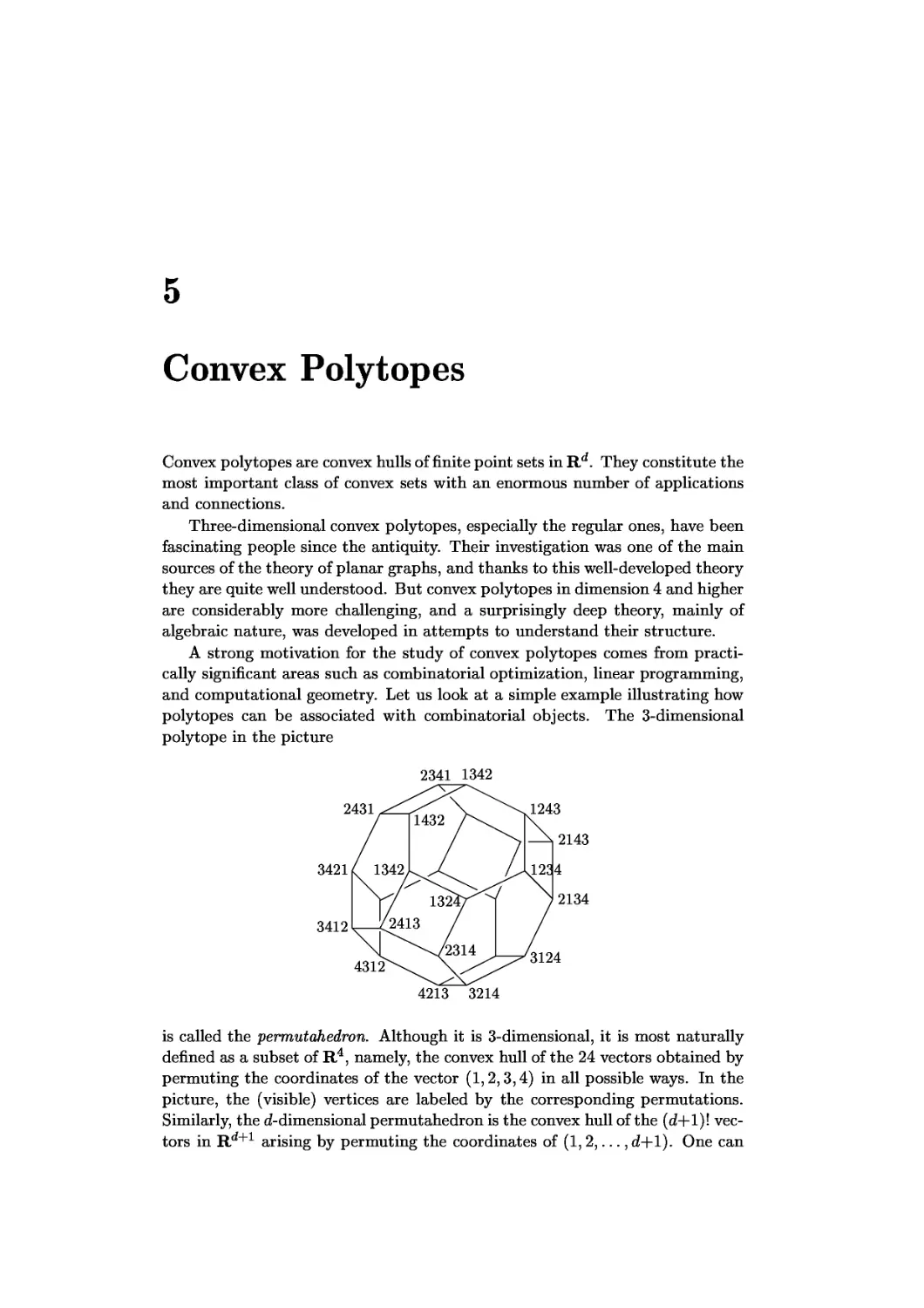
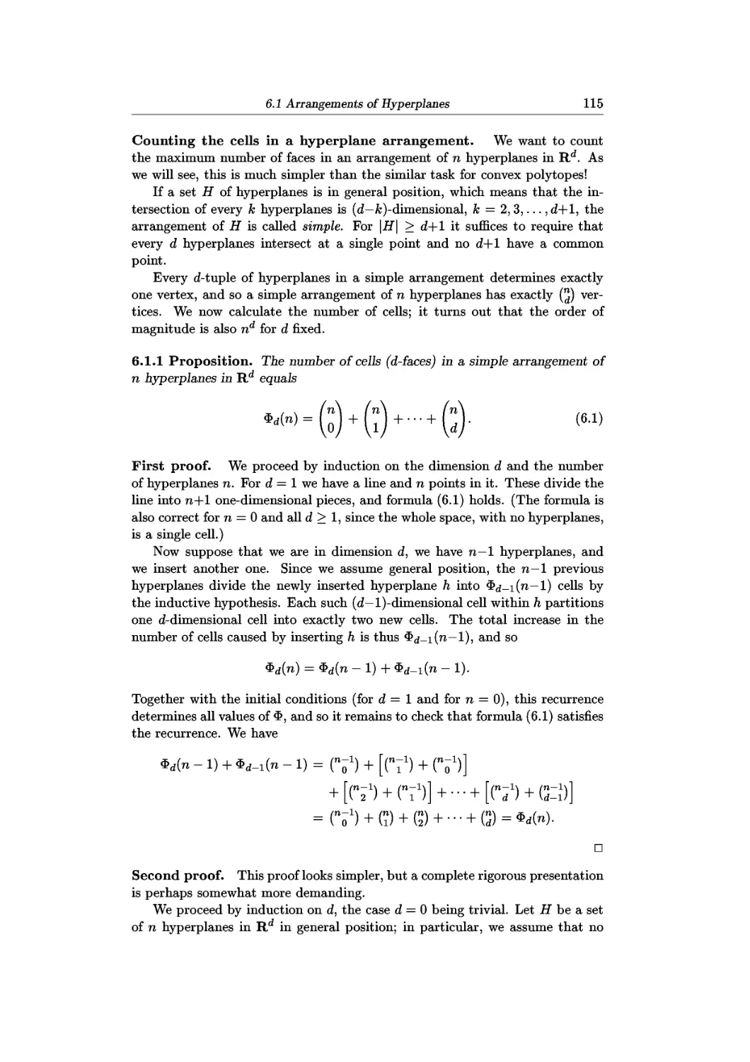
Текст
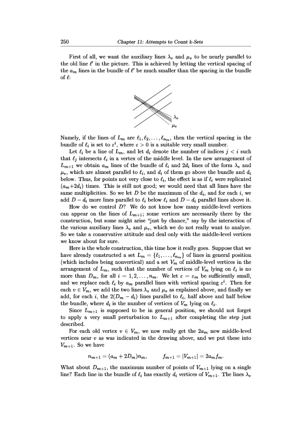
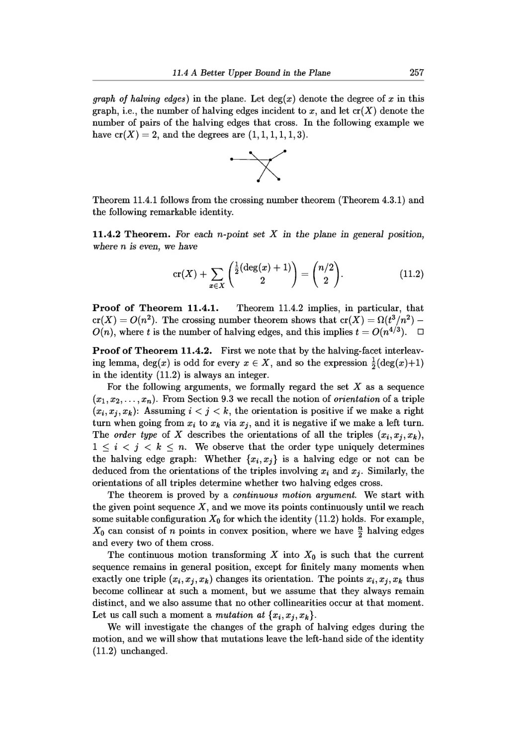
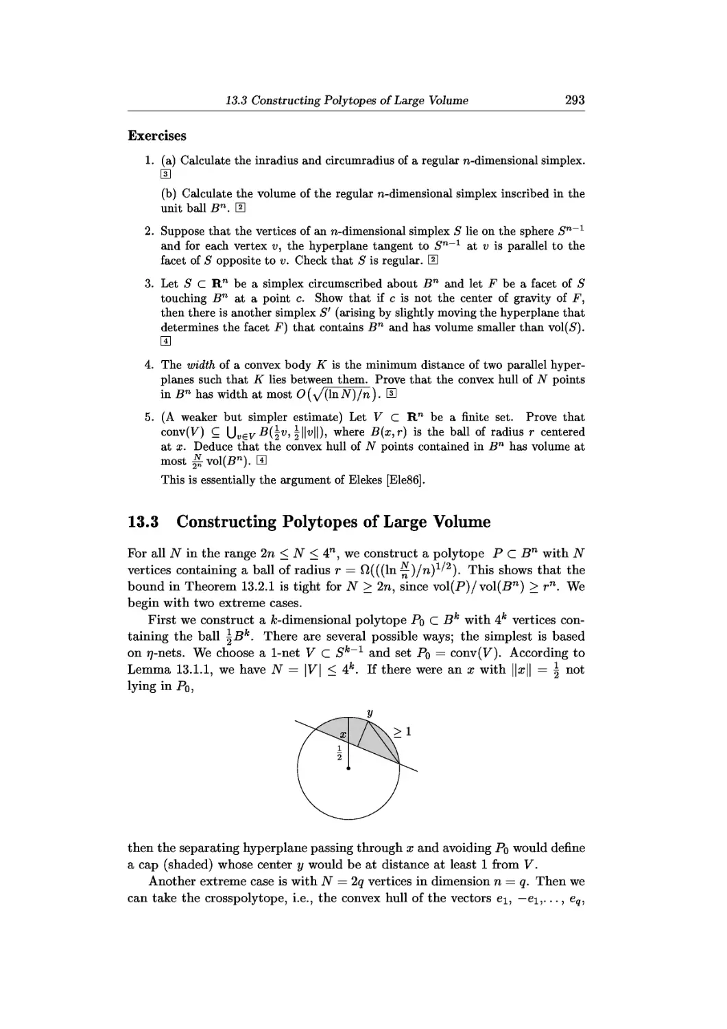
From the Preface
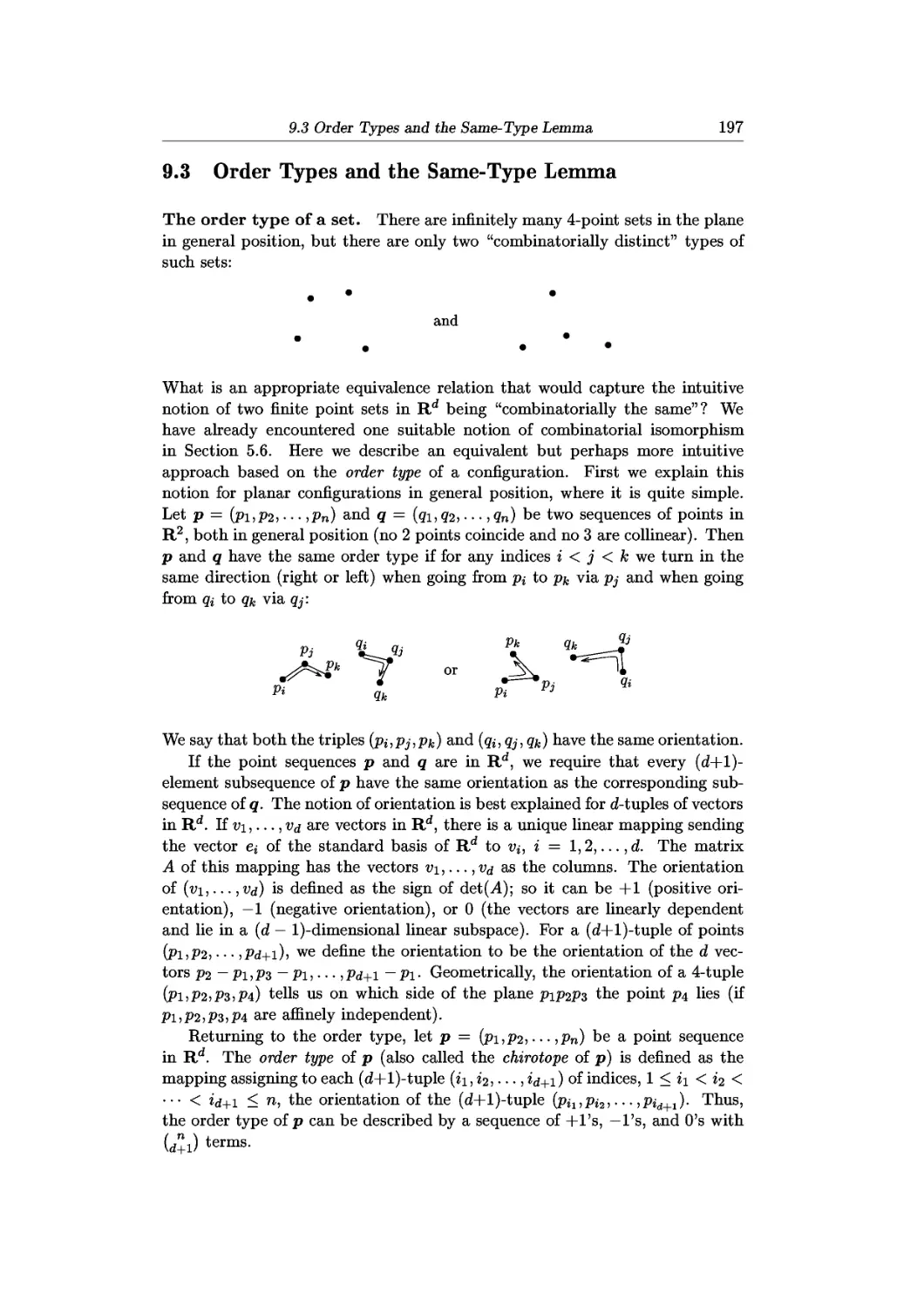
Questions in discrete geometry typically involve finite sets of points, lines, circles, planes, or other simple geometric objects. For example, one can
ask, what is the largest number of regions into which n lines can partition the plane, or what is the minimum possible number of distinct distances
occurring among n points in the plane (the former question is easy, the latter one is hard). More complicated objects are investigated too, such as
convex polytopes or finite families of convex sets. The emphasis is on "combinatorial" properties: which of the given objects intersect, or how
many points are needed to intersect all of them, and so on. Characteristics like angle, distance, curvature, or volume, ubiquitous in other areas of
geometry, are usually not of primary interest, although they can serve as useful tools.
Many questions in discrete geometry are very natural and worth studying for their own sake. Some of them, such as the structure of 3-dimensional
convex polytopes, go back to the Antiquity, and a lot of them are motivated by other areas of mathematics. To a working mathematician or
computer scientist, the contemporary discrete geometry offers results and techniques of great diversity, a useful enhancement of the "bag of
tricks" for attacking problems in her or his field.
This book is primarily an introductory textbook. It does not require any special background besides the usual undergraduate mathematics (linear
algebra, calculus, and a little of combinatorics, graph theory, and probability). It should be accessible to early graduate students, although mastering
the more advanced proofs probably needs some mathematical maturity. The first and main part of each section is intended for teaching in class. I
have actually taught most of the material, mainly in an advanced course in Prague whose contents varied over the years.
The book can also serve as a collection of surveys in several narrower subfields of discrete geometry where, as far as I know, no adequate recent
treatment was available. The sections are accompanied by bibliographic notes and extending remarks. For well-established material, such as
convex polytopes, these parts usually refer to the original sources, point to modern treatments and surveys, and present a sample of key results in
the area. For the less well-covered topics, I have aimed at surveying most of the important recent results. For some of them, proof outlines are
provided, which should convey the main ideas and make it easy to fill in the details from the original source.
Convexity
We begin with a review of basic geometric notions such as hyperplanes and affine
subspaces in Rd, and we spend some time by discussing the notion of general
position. Then we consider fundamental properties of convex sets in Rd, such
as a theorem about the separation of disjoint convex sets by a hyperplane and
Helly's theorem.
1.1 Linear and Affine Subspaces, General Position
Linear subspaces. Let Rd denote the d-dimensional Euclidean space. The
points are d-tuples of real numbers, x — (x\,X2, ¦ ¦ ¦, xj).
The space Rd is a vector space, and so we may speak of linear subspaces,
linear dependence of points, linear span of a set, and so on. A linear subspace of
Rd is a subset closed under addition of vectors and under multiplication by real
numbers. What is the geometric meaning? For instance, the linear subspaces
of R2 are the origin itself, all lines passing through the origin, and the whole of
R2. In R3, we have the origin, all lines and planes passing through the origin,
and R3.
Affine notions. An arbitrary line in R2, say, is not a linear subspace unless
it passes through 0. General lines are what are called affine subspaces. An
affine subspace of Rd has the form x + L, where x € Rd is some vector and L
is a linear subspace of Rd. Having defined affine subspaces, the other "affine"
notions can be constructed by imitating the "linear" notions.
What is the affine hull of a set X С Rd? It is the intersection of all affine
subspaces of Rd containing X. As is well known, the linear span of a set X can
be described as the set of all linear combinations of points of X. What is an
affine combination of points a-\_, 0,2, ¦ ¦ ¦, an € Rd that would play an analogous
role? To see this, we translate the whole set by — an, so that an becomes the
origin, we make a linear combination, and we translate back by +an. This yields
an expression of the form /3i(ai — an) + /Зг(а2 — o-n) + • • • + Pn{a-n — o-n) + o-n —
Piai + /5г«2H 1-/3n_ian_i + A -/?i -/32 Pn-i)an, where /3b ..., /3n are
arbitrary real numbers. Thus, an affine combination of points a\,...,an € Rd
Chapter 1: Convexity
is an expression of the form
Ч h апап, where a\,..., an € R and a\ -\ \- an — 1.
Then indeed, it is not hard to check that the affine hull of X is the set of all
affine combinations of points of X.
The affine dependence of points a\,..., an means that one of them can be
written as an affine combination of the others. This is the same as the existence
of real numbers ol\,ol2,- ¦ -OLn, at least one of them nonzero, such that both
a\a\ + 0*20,2 -\ h anan — 0 and ct\ + аг Ч \- an — 0.
(Note the difference: In an affine combination, the ctj sum to 1, while in an
affine dependence, they sum to 0.)
Affine dependence of a\,..., an is equivalent to linear dependence of the
n—1 vectors a,\ — an, a,2 — an,..., an-\ — an. Therefore, the maximum possible
number of affinely independent points in Rd is d+1.
Another way of expressing affine dependence uses "lifting" one dimension
higher. Let bj = (а$, 1) be the vector in Rd+1 obtained by appending a new
coordinate equal to 1 to a;; then a\,..., an are affinely dependent if and only if
bi,... ,bn are linearly dependent. This correspondence of affine notions in Rd
with linear notions in R "*~1 is quite general. For example, if we identify R2
with the plane Ж3 = 1 in R3 as in the picture,
then we obtain a bijective correspondence of the fc-dimensional linear subspaces
of R3 that do not lie in the plane Ж3 = 0 with (k—l)-dimensional affine sub-
spaces of R2. The drawing shows a 2-dimensional linear subspace of R3 and the
corresponding line in the plane Ж3 = 1. (The same works for affine subspaces
of Rd and linear subspaces of Rd+1 not contained in the subspace 2^+1 = 0.)
This correspondence also leads directly to extending the affine plane R2 into
the projective plane: To the points of R2 corresponding to nonhorizontal lines
through 0 in R3 we add points "at infinity," that correspond to horizontal lines
through 0 in R3. But in this book we remain in the affine space most of the
time, and we do not use the projective notions.
Let ai,a,2, ¦ ¦ ¦ ,а^+1 be points in Rd, and let A be the d x d matrix with
aj — а^+i as the ith column, i — 1,2, ...,d. Then ai,...,ad+i are affinely
independent if and only if A has d linearly independent columns, and this is
equivalent to det(.A) ф 0. We have a useful criterion of affine independence
using a determinant.
1.1 Linear and АШпе Subspaces, General Position
Affine subspaces of Rd of certain dimensions have special names. A (d—1)-
dimensional affine subspace of Rd is called a hyperplane (while the word plane
usually means a 2-dimensional subspace of Rd for any d). One-dimensional
subspaces are lines, and a ft-dimensional affine subspace is often called a k-flat.
A hyperplane is usually specified by a single linear equation of the form
a\X\ + агжг + • • • + adxd — °- We usually write the left-hand side as the scalar
product (a, x). So a hyperplane can be expressed as the set {x E Rd: (a, x) — b}
where a E Rd \ {0} and b E R. A (closed) half-space in Rd is a set of the form
{x E Kd: (a, x) > b} for some a E Rd\{0}; the hyperplane {x E Kd: (a, x) — b}
is its boundary.
General ft-flats can be given either as intersections of hyperplanes or as
affine images of Rk (parametric expression). In the first case, an intersection
of ft hyperplanes can also be viewed as a solution to a system Ax — b of linear
equations, where x E Rd is regarded as a column vector, A is a к х d matrix,
and b E Rfc. (As a rule, in formulas involving matrices, we interpret points of
Rd as column vectors.)
An affine mapping f: Rk —? Rd has the form /:y i-> By + с for some d x к
matrix В and some с € Rd, so it is a composition of a linear map with a
translation. The image of / is a ft'-flat for some k' < mm(k,d). This k' equals
the rank of the matrix B.
General position. "We assume that the points (lines, hyperplanes,...) are
in general position." This magical phrase appears in many proofs. Intuitively,
general position means that no "unlikely coincidences" happen in the considered
configuration. For example, if 3 points are chosen in the plane without any
special intention, "randomly," they are unlikely to lie on a common line. For a
planar point set in general position, we always require that no three of its points
be collinear. For points in Rd in general position, we assume similarly that no
unnecessary affine dependencies exist: No к < d+1 points lie in a common
(ft—2)-flat. For lines in the plane in general position, we postulate that no 3
lines have a common point and no 2 are parallel.
The precise meaning of general position is not fully standard: It may depend
on the particular context, and to the usual conditions mentioned above we
sometimes add others where convenient. For example, for a planar point set
in general position we can also suppose that no two points have the same x-
coordinate.
What conditions are suitable for including into a "general position" assump-
assumption? In other words, what can be considered as an unlikely coincidence? For
example, let X be an га-point set in the plane, and let the coordinates of the
ith point be (x{, yi). Then the vector v(X) — (xi, X2, ¦ ¦ ¦, xn, yi,y2, ¦ ¦ ¦, Уп) can
be regarded as a point of R2n. For a configuration X in which x\ — X2, i.e., the
first and second points have the same ж-coordinate, the point v(X) lies on the
hyperplane {x\ — X2} in R2n. The configurations X where some two points
share the ж-coordinate thus correspond to the union of Q) hyperplanes in R2n.
Since a hyperplane in R2n has Bra-dimensional) measure zero, almost all points
of R2n correspond to planar configurations X with all the points having distinct
ж-coordinates. In particular, if X is any га-point planar configuration and e > 0
8 Chapter 1: Convexity
is any given real number, then there is a configuration X', obtained from X by
moving each point by distance at most e, such that all points of X' have distinct
ж-coordinates. Not only that: almost all small movements (perturbations) of X
result in X' with this property.
This is the key property of general position: configurations in general po-
position lie arbitrarily close to any given configuration (and they abound in any
small neighborhood of any given configuration). Here is a fairly general type
of condition with this property. Suppose that a configuration X is specified by
a vector t — (?1, ?2, • • •, tm) of m real numbers (coordinates). The objects of X
can be points in Rd, in which case m — dn and the tj are the coordinates of
the points, but they can also be circles in the plane, with m — Зга and the tj
expressing the center and the radius of each circle, and so on. The general posi-
position condition we can put on the configuration X isp(t) — p(ti,t2, ¦ ¦ ¦,tm) ф О,
where p is some nonzero polynomial in m variables. Here we use the following
well-known fact (a consequence of Sard's theorem; see, e.g., Bredon [Bre93],
Appendix C): For any nonzero m-variate polynomial p{t\,..., tm), the zero set
{t E RTO: p{t) — 0} has measure 0 in RTO.
Therefore, almost all configurations X satisfy p(t) ф 0. So any condition
that can be expressed as p(t) ф 0 for a certain polynomial p'mm real variables,
or, more generally, as pi(t) ф 0 or P2{t) Ф 0 or ..., for finitely or countably
many polynomials pi,P2, ¦ ¦ -, can be included in a general position assumption.
For example, let X be an га-point set in Rd, and let us consider the condition
"no d+1 points of X lie in a common hyperplane." In other words, no d+1
points should be affinely dependent. As we know, the affine dependence of d+1
points means that a suitable d x d determinant equals 0. This determinant is
a polynomial (of degree d) in the coordinates of these d+1 points. Introducing
one polynomial for every (d+l)-tuple of the points, we obtain (Jl-^) polynomials
such that at least one of them is 0 for any configuration X with d+1 points
in a common hyperplane. Other usual conditions for general position can be
expressed similarly.
In many proofs, assuming general position simplifies matters considerably.
But what do we do with configurations Xq that are not in general position?
We have to argue, somehow, that if the statement being proved is valid for
configurations X arbitrarily close to our Xq, then it must be valid for Xq itself,
too. Such proofs, usually called perturbation arguments, are often rather simple,
and almost always somewhat boring. But sometimes they can be tricky, and
one should not underestimate them, no matter how tempting this may be. A
nontrivial example will be demonstrated in Section 5.5 (Lemma 5.5.4).
Exercises
1. Verify that the affine hull of a set X С Rd equals the set of all affine combinations
of points of X. В
2. Let A be a 2 x 3 matrix and let b ? R2. Interpret the solution of the system
Ax = b geometrically (in most cases, as an intersection of two planes) and discuss
the possible cases in algebraic and geometric terms. S
3. (a) What are the possible intersections of two B-dimensional) planes in R4?
1.2 Convex Sets, Convex Combinations, Separation
What is the "typical" case (general position)? What about two hyperplanes in
R4? S
(b) Objects in R4 can sometimes be "visualized" as objects in R3 moving in time
(so time is interpreted as the fourth coordinate). Try to visualize the intersection
of two planes in R4 discussed (a) in this way.
1.2 Convex Sets, Convex Combinations, Separation
Intuitively, a set is convex if its surface has no "dips":
¦ not allowed in a convex set
1.2.1 Definition (Convex set). A set С С R<* is convex if for every two
points x,y € С the whole segment xy is also contained in C. In other words,
for every t € [0,1], the point tx + A — t)y belongs to C.
The intersection of an arbitrary family of convex sets is obviously convex.
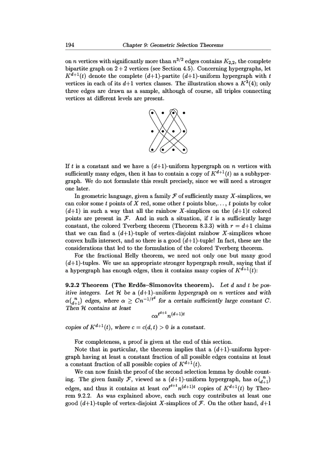
So we can define the convex hull of a set X С Rd, denoted by conv(-X"), as the
intersection of all convex sets in Rd containing X. Here is a planar example
with a finite X:
conv(X)
An alternative description of the convex hull can be given using convex
combinations.
1.2.2 Claim. A point x belongs to conv(-X") if and only if there exist points
xi, X2, ¦ ¦ ¦ xn € X and nonnegative real numbers t\, ?2, ¦ ¦ ¦, tn with Y2=i U — 1
such that x — Ya=i Ux%.
The expression Ya=i U%i as in the claim is called a convex combination of
the points xi,X2,- ¦ ¦ ,xn. (Compare this with the definitions of linear and affine
combinations.)
Sketch of proof. Each convex combination of points of X must lie in
conv(.X"): For n — 2 this is by definition, and for larger n by induction. Con-
Conversely, the set of all convex combinations obviously contains X and it is convex.
?
In Hd, it is sufficient to consider convex combinations involving at most d+1
points:
1.2.3 Theorem (Caratheodory's theorem). Let X С Rd. Then each
point of conv(X) is a convex combination of at most d+1 points of X.
10 Chapter 1: Convexity
For example, in the plane, conv(-X") is the union of all triangles with vertices
at points of X. The proof of the theorem is left as an exercise to the subsequent
section.
A basic result about convex sets is the separability of disjoint convex sets
by a hyperplane.
1.2.4 Theorem (Separation theorem). Let C, D С Kd be convex sets with
С П D — 0. Then there exists a hyperplane h such that С lies in one of the
closed half-spaces determined by h, and D lies in the opposite closed half-space.
In other words, there exist a unit vector а € Rd and a number b € R such that
for all x € С we have (a, x) > b, and for all x € D we have (a, x) < b.
If С and D are closed and at least one of them is bounded, they can be
separated strictly; in such a way that СП ft = D П ft = 0.
In particular, a closed convex set can be strictly separated from a point.
This implies that the convex hull of a closed set X equals the intersection of all
closed half-spaces containing X.
Sketch of proof. First assume that С and D are compact (i.e., closed and
bounded). Then the Cartesian product С х D is a compact space, too, and the
distance function (x, у) i->- \\x — y\\ attains its minimum on С х D. That is,
there exist points p € С and q € D such that the distance of С and D equals
the distance of p and q.
The desired separating hyperplane h can be taken as the one perpendicular
to the segment pq and passing through its midpoint:
It is easy to check that h indeed avoids both С and D.
If D is compact and С closed, we can intersect С with a large ball and get
a compact set С. If the ball is sufficiently large, then С and С have the same
distance to D. So the distance of С and D is attained at some p € С and
q € D, and we can use the previous argument.
For arbitrary disjoint convex sets С and D, we choose a sequence C\ С
Сг ^ Сз С • • • of compact convex subsets of С with (JnLi Cn — C. For
example, assuming that 0 € C, we can let Cn be the intersection of the closure
of A — ^)C with the ball of radius n centered at 0. A similar sequence D\ С
ZJ ^ ••• is chosen for D, and we let hn — {x € Rd: (an,x) — bn} be a
hyperplane separating Cn from Dn, where an is a unit vector and bn € R.
The sequence (bn)^=1 is bounded, and by compactness, the sequence of (d+1)-
component vectors (an,bn) € Rd+1 has a cluster point (a, b). One can verify,
1.2 Convex Sets, Convex Combinations, Separation 11
by contradiction, that the hyperplane h — {x € Rd: (a, x) — b} separates С
and D (nonstrictly). ?
The importance of the separation theorem is documented by its presence
in several branches of mathematics in various disguises. Its home territory is
probably functional analysis, where it is formulated and proved for infinite-
dimensional spaces; essentially it is the so-called Hahn-Banach theorem. The
usual functional-analytic proof is different from the one we gave, and in a way
it is more elegant and conceptual. The proof sketched above uses more special
properties of Rd, but it is quite short and intuitive in the case of compact С
and D.
Connection to linear programming. A basic result in the theory of linear
programming is the Farkas lemma. It is a special case of the duality of linear
programming (discussed in Section 10.1) as well as the key step in its proof.
1.2.5 Lemma (Farkas lemma, one of many versions). For every d x n
real matrix A, exactly one of the following cases occurs:
(i) The system of linear equations Ax — 0 has a nontrivial nonnegative so-
solution x € R™ (all components of x are nonnegative and at least one of
them is strictly positive).
(ii) There exists а у € Rd such that yTA is a vector with all entries strictly
negative. Thus, if we multiply the j th equation in the system Ax — 0 by yj
and add these equations together, we obtain an equation that obviously
has no nontrivial nonnegative solution, since all the coefficients on the
left-hand sides are strictly negative, while the right-hand side is 0.
Proof. Let us see why this is yet another version of the separation theorem.
Let V С Rd be the set of n points given by the column vectors of the matrix A.
We distinguish two cases: Either 0 € conv(F) or 0 ^ conv(F).
In the former case, we know that 0 is a convex combination of the points
of V, and the coefficients of this convex combination determine a nontrivial
nonnegative solution to Ax — 0.
In the latter case, there exists a hyperplane strictly separating V from 0,
i.e., a unit vector у ? Rd such that (y,v) < (y,0) — 0 for each v € V. This is
just the у from the second alternative in the Farkas lemma. ?
Bibliography and remarks. Most of the material in this chapter is quite old
and can be found in many surveys and textbooks. Providing historical accounts
of such well-covered areas is not among the goals of this book, and so we mention
only a few references for the specific results discussed in the text and add some
remarks concerning related results.
The concept of convexity and the rudiments of convex geometry have been
around since antiquity. The initial chapter of the Handbook of Convex Geometry
[GW93] succinctly describes the history, and the handbook can be recommended
as the basic source on questions related to convexity, although knowledge has pro-
progressed significantly since its publication.
12 Chapter 1: Convexity
For an introduction to functional analysis, including the Hahn-Banach theo-
theorem, see Rudin [Rud91], for example. The Farkas lemma originated in [Far94]
(nineteenth century!). More on the history of the duality of linear programming
can be found, e.g., in Schrijver's book [Sch86].
As for the origins, generalizations, and applications of Caratheodory's theorem,
as well as of Radon's lemma and Helly's theorem discussed in the subsequent sec-
sections, a recommendable survey is Eckhoff [Eck93], and an older well-known source
is Danzer, Griinbaum, and Klee [DGK63].
Caratheodory's theorem comes from the paper [CarO7], concerning power series
and harmonic analysis. A somewhat similar theorem, due to Steinitz [Stel6], asserts
that if я lies in the interior of conv(X) for an X С Rd, then it also lies in the interior
of сопу(У) for some Y С X with \Y\ < 2d. Bonnice and Klee [BK63] proved a
common generalization of both these theorems: Any fc-interior point of X is a k-
interior point of Y for some Y С X with at most maxBfc, d+1) points, where x is
called a k-interior point of X if it lies in the relative interior of the convex hull of
some fc+1 affinely independent points of X.
Exercises
1. Give a detailed proof of Claim 1.2.2. В
2. Write down a detailed proof of the separation theorem. S
3. Find an example of two disjoint closed convex sets in the plane that are not
strictly separable. Ш
4. Let /: Rd -> Rfc be an affine map.
(a) Prove that if С С Rd is convex, then f(C) is convex as well. Is the preimage
of a convex set always convex? В
(b) For X С Rd arbitrary, prove that conv(/(X)) = conv(/(X)). Ш
5. Let X С Rd. Prove that diam(conv(X)) = diam(X), where the diameter
diam(y) of a set Y is sup{||# — y\\: x, у ? Y}. S
6. A set С С Rd is a convex cone if it is convex and for each x ? C, the ray Ox is
fully contained in C.
(a) Analogously to the convex and affine hulls, define the appropriate "conic
hull" and the corresponding notion of "combination" (analogous to the convex
and affine combinations). S
(b) Let С be a convex cone in Rd and b e" С a point. Prove that there exists a
vector о with (a, x) > 0 for all x ? С and (a, b) < 0. S
7. (Variations on the Farkas lemma) Let A be a d x n matrix and let b ? Rd.
(a) Prove that the system Ax = b has a nonnegative solution x ? R™ if and only
if every у ? Rd satisfying yTA > 0 also satisfies yTb > 0. S
(b) Prove that the system of inequalities Ax < b has a nonnegative solution x if
and only if every nonnegative у ? Rd with yTA > 0 also satisfies yTb > 0. S
8. (a) Let С С Rd be a compact convex set with a nonempty interior, and let p ? С
be an interior point. Show that there exists a line I passing through p such that
the segment l П С is at least as long as any segment parallel to I and contained
inC. Ш
(b) Show that (a) may fail for С compact but not convex. Ш
1.3 Radon's Lemma and Helly's Theorem 13
1.3 Radon's Lemma and Helly's Theorem
Caratheodory's theorem from the previous section, together with Radon's lemma
and Helly's theorem presented here, are three basic properties of convexity in
Rd involving the dimension. We begin with Radon's lemma.
1.3.1 Theorem (Radon's lemma). Let A be a set of d+2 points in Kd.
Then there exist two disjoint subsets A\,A2 С A such that
conv(Ai) П conv(A2) ф 0.
A point x € conv(-Ai) П conv(.A2), where A\ and A2 are as in the theorem,
is called a Radon point of A, and the pair [A\,A2) is called a Radon partition
of A (it is easily seen that we can require A\ U A2 — A).
Here are two possible cases in the plane:
Proof. Let A — {ai,a2, ¦ ¦ ¦, а^+г}- These d+2 points are necessarily affinely
dependent. That is, there exist real numbers a\,... ,а^+2) not all of them 0,
such that Y,i=i ai = 0 and Yd=? «№ = 0.
Set P — {i: щ > 0} and N — {i: ац < 0}. Both P and N are nonempty. We
claim that P and N determine the desired subsets. Let us put A\ — {af. i € P}
and A2 — {af. i € N}. We are going to exhibit a point x that is contained in
the convex hulls of both these sets.
Put 5 = YlieP ai] we also have S — — YlieN ai- Then we define
ft*. A.1)
Since Yli=i aiai — 0 — YlieP aiai + YlieN aiaii we also have
The coefficients of the щ in A.1) are nonnegative and sum to 1, so ж is a
convex combination of points of A\. Similarly A.2) expresses ж as a convex
combination of points of A2. ?
Helly's theorem is one of the most famous results of a combinatorial nature
about convex sets.
1.3.2 Theorem (Helly's theorem). Let Ci, C2,... ,Cnbe convex sets in Kd,
n > d+1. Suppose that the intersection of every d+1 of these sets is nonempty.
Then the intersection of all the Ci is nonempty.
14 Chapter 1: Convexity
The first nontrivial case states that if every 3 among 4 convex sets in the
plane intersect, then there is a point common to all 4 sets. This can be proved
by an elementary geometric argument, perhaps distinguishing a few cases, and
the reader may want to try to find a proof before reading further.
In a contrapositive form, Helly's theorem guarantees that whenever C\, C2, ¦ ¦ ¦, Cn
are convex sets with ПГ=1 ^» — 0> then this is witnessed by some at most d+1
sets with empty intersection among the C%. In this way, many proofs are greatly
simplified, since in planar problems, say, one can deal with 3 convex sets instead
of an arbitrary number, as is amply illustrated in the exercises below.
It is very tempting and quite usual to formulate Helly's theorem as follows:
"If every d+1 among n convex sets in R intersect, then all the sets inter-
intersect." But, strictly speaking, this is false, for a trivial reason: For d > 2, the
assumption as stated here is met by n — 2 disjoint convex sets.
Proof of Helly's theorem. (Using Radon's lemma.) For a fixed d, we
proceed by induction on n. The case n — d+1 is clear, so we suppose that n >
d+1 and that the statement of Helly's theorem holds for smaller n. Actually,
n — d+1 is the crucial case; the result for larger n follows at once by a simple
induction.
Consider sets C\,C2,---,Cn satisfying the assumptions. If we leave out
any one of these sets, the remaining sets have a nonempty intersection by the
inductive assumption. Let us fix a point щ E C\j^i Cj and consider the points
0,1,0,2,... ,а^+2 • By Radon's lemma, there exist disjoint index sets I\,l2 С
{1,2,..., d+1} such that
conv({aj: i E Д}) П conv({aj: i E h}) ф 0-
We pick a point x in this intersection. The following picture illustrates the case
d — 1 and n — 4:
We claim that x lies in the intersection of all the Cj. Consider some i E
{1,2,..., n}; then i g I\ or i g I2. In the former case, each Oj with j E I\ lies
in d, and so ж € conv({aj: j E h}) С С{. For i g /2 we similarly conclude
that x E conv({a,-: j E I2}) С Q. Therefore x E fl"=i С»- п
An infinite version of Helly's theorem. If we have an infinite collection
of convex sets in Rd such that any d+1 of them have a common point, the
entire collection still need not have a common point. Two examples in R1 are
the families of intervals {@,1/n): n — 1,1,...} and {[n, 00): n — 1,1,...}. The
sets in the first example are not closed, and the second example uses unbounded
sets. For compact (i.e., closed and bounded) sets, the theorem holds:
1.3 Radon's Lemma and Helly's Theorem 15
1.3.3 Theorem (Infinite version of Helly's theorem). Let С be an ar-
arbitrary infinite family of compact convex sets in Rd such that any d+1 of the
sets have a nonempty intersection. Then all the sets of С have a nonempty
intersection.
Proof. By Helly's theorem, any finite subfamily of С has a nonempty inter-
intersection. By a basic property of compactness, if we have an arbitrary family of
compact sets such that each of its finite subfamilies has a nonempty intersec-
intersection, then the entire family has a nonempty intersection. ?
Several nice applications of Helly's theorem are indicated in the exercises
below, and we will meet a few more later in this book.
Bibliography and remarks. Helly proved Theorem 1.3.2 in 1913 and commu-
communicated it to Radon, who published a proof in [Rad21]. This proof uses Radon's
lemma, although the statement wasn't explicitly formulated in Radon's paper.
References to many other proofs and generalizations can be found in the already
mentioned surveys [Eck93] and [DGK63].
Helly's theorem inspired a whole industry of Helly-type theorems. A family В
of sets is said to have Helly number h if the following holds: Whenever a finite
subfamily T С В is such that every h or fewer sets of T have a common point,
then P| T ф 0. So Helly's theorem says that the family of all convex sets in Rd
has Helly number d+1. More generally, let P be some property of families of sets
that is hereditary, meaning that if T has property P and T' С F, then T' has P
as well. A family В is said to have Helly number h with respect to P if for every
finite T С В, all subfamilies of T of size at most h having P implies J7 having P.
That is, the absence of P is always witnessed by some at most h sets, so it is a
"local" property.
Exercises
1. Prove Caratheodory's theorem (you may use Radon's lemma). Ш
2. Let К С Rd be a convex set and let C\,..., С„ С Rd, n > d+1, be convex sets
such that the intersection of every d+1 of them contains a translated copy of K.
Prove that then the intersection of all the sets Cj also contains a translated copy
ofK. В
This result was noted by Vincensini [Vin39] and by Klee [Kle53].
3. Find an example of 4 convex sets in the plane such that the intersection of each
3 of them contains a segment of length 1, but the intersection of all 4 contains
no segment of length 1. Ш
4. A strip of width w is a part of the plane bounded by two parallel lines at distance
w. The width of a set X С R2 is the smallest width of a strip containing X.
(a) Prove that a compact convex set of width 1 contains a segment of length 1
of every direction. S
(b) Let {Ci,C2,. ..,Cn} be closed convex sets in the plane, n > 3, such that
the intersection of every 3 of them has width at least 1. Prove that П"=1 С» has
width at least 1. S
The result as in (b), for arbitrary dimension d, was proved by Sallee [Sal75], and
a simple argument using Helly's theorem was noted by Buchman and Valentine
[BV82].
16 Chapter 1: Convexity
5. Statement: Each set X С R2 of diameter at most 1 (i.e., any 2 points have
distance at most 1) is contained in some disc of radius l/\/3.
(a) Prove the statement for 3-element sets X. В
(b) Prove the statement for all finite sets X. S
(c) Generalize the statement to Rd: determine the smallest r = r(d) such that
every set of diameter 1 in Rd is contained in a ball of radius r (prove your claim).
Ш
The result as in (c) is due to Jung; see [DGK63].
6. (a) Prove that if the intersection of each 4 or fewer among convex sets Ci,...,Cn С
R2 contains a ray then П™=1 С« also contains a ray. Ш
(b) Show that the number 4 in (a) cannot be replaced by 3. S
This result, and an analogous one in Rd with the Helly number 2d, are due to
Katchalski [Kat78].
7. For a set X С R2 and a point x e X, let us denote by V(x) the set of all points
у ? X that can "see" x, i.e., points such that the segment xy is contained in X.
The kernel of X is defined as the set of all points x ? X such that V(x) = X. A
set with a nonempty kernel is called star-shaped.
(a) Prove that the kernel of any set is convex. Ш
(b) Prove that if V(x) П V(y) П V(z) Ф 0 for every x,y,z ? X and X is compact,
then X is star-shaped. That is, if every 3 paintings in a (planar) art gallery can be
seen at the same time from some location (possibly different for different triples
of paintings), then all paintings can be seen simultaneously from somewhere. If
it helps, assume that X is a polygon. S
(c) Construct a nonempty set ICR2 such that each of its finite subsets can be
seen from some point of X but X is not star-shaped. S
The result in (b), as well as the d-dimensional generalization (with every d+1
regions V(x) intersecting), is called Krasnosel'skii's theorem; see [Eck93] for ref-
references and related results.
8. In the situation of Radon's lemma (A is a (d+2)-point set in Rd), call a point
x ? Rd a Radon point of A if it is contained in convex hulls of two disjoint subsets
of A. Prove that if A is in general position (no d+1 points affinely dependent),
then its Radon point is unique. S
9. (a) Let I,FcR2 be finite point sets, and suppose that for every subset S С
XliY of at most 4 points, Sf)X can be separated (strictly) by a line from Sf)Y.
Prove that X and Y are line-separable. S
(b) Extend (a) to sets X,Y С Rd, with \S\ < d+2. В
The result (b) is called Kirchberger's theorem [KirO3].
1.4 Centerpoint and Ham Sandwich
We prove an interesting result as an application of Helly's theorem.
1.4.1 Definition (Centerpoint). Let X be an n-point set in Kd. A point
x € Rd is called a centerpoint of X if each closed half-space containing x
contains at least ^щ- points of X.
1.4 Centerpoint and Ham Sandwich 17
Let us stress that one set may generally have many centerpoints, and a
centerpoint need not belong to X.
The notion of centerpoint can be viewed as a generalization of the median of
one-dimensional data. Suppose that x\,..., xn € R are results of measurements
of an unknown real parameter x. How do we estimate x from the Xj? We can
use the arithmetic mean, but if one of the measurements is completely wrong
(say, 100 times larger than the others), we may get quite a bad estimate. A
more "robust" estimate is a median, i.e., a point x such that at least ^ of the X{
lie in the interval (—oo, x] and at least ^ of them lie in [x, oo). The centerpoint
can be regarded as a generalization of the median for higher-dimensional data.
In the definition of centerpoint we could replace the fraction ^- by some
other parameter a € @,1). For a > ^-, such an "a-centerpoint" need not
always exist: Take d+1 points in general position for X. With a = ^щ- as in
the definition above, a centerpoint always exists, as we prove next.
Centerpoints are important, for example, in some algorithms of divide-and-
conquer type, where they help divide the considered problem into smaller sub-
problems. Since no really efficient algorithms are known for finding "exact"
centerpoints, the algorithms often use a-centerpoints with a suitable a < ^-,
which are easier to find.
1.4.2 Theorem (Centerpoint theorem). Each unite point set in Kd has at
least one centerpoint.
Proof. First we note an equivalent definition of a centerpoint: ж is a
centerpoint of X if and only if it lies in each open half-space 7 such that
4
We would like to apply Helly's theorem to conclude that all these open
half-spaces intersect. But we cannot proceed directly, since we have infinitely
many half-spaces and they are open and unbounded. Instead of such an open
half-space 7, we thus consider the compact convex set conv(-X" П 7) С 7.
convG П X)
Letting 7 run through all open half-spaces 7 with \X f | -у| > ^- n, we obtain a
family С of compact convex sets. Each of them contains more than -A^n points
of X, and so the intersection of any d+1 of them contains at least one point
of X. The family С consists of finitely many distinct sets (since X has finitely
many distinct subsets), and so П С ф 0 by Helly's theorem. Each point in this
intersection is a centerpoint. ?
In the definition of a centerpoint we can regard the finite set X as defining
a distribution of mass in RA The centerpoint theorem asserts that for some
point x, any half-space containing x encloses at least ^- of the total mass. It is
18 Chapter 1: Convexity
not difficult to show that this remains valid for continuous mass distributions,
or even for arbitrary Borel probability measures on Rd (Exercise 1).
Ham-sandwich theorem and its relatives. Here is another important re-
result, not much related to convexity but with a flavor resembling the centerpoint
theorem.
1.4.3 Theorem (Ham-sandwich theorem). Every d unite sets in Hd can
be simultaneously bisected by a hyperplane. A hyperplane h bisects a unite set
A if each of the open half-spaces defined by h contains at most \\A\/2\ points
of A.
This theorem is usually proved via continuous mass distributions using a
tool from algebraic topology: the Borsuk-Ulam theorem. Here we omit a proof.
Note that if A{ has an odd number of points, then every h bisecting A{
passes through a point of A{. Thus if A\,..., A^ all have odd sizes and their
union is in general position, then every hyperplane simultaneously bisecting
them is determined by d points, one of each A{. In particular, there are only
finitely many such hyperplanes.
Again, an analogous ham-sandwich theorem holds for arbitrary d Borel
probability measures in Rd.
Center transversal theorem. There can be beautiful new things to discover
even in well-studied areas of mathematics. A good example is the following
recent result, which "interpolates" between the centerpoint theorem and the
ham-sandwich theorem.
1.4.4 Theorem (Center transversal theorem). Let 1 < ft < d and let
Ai,A2,..., Ak be unite point sets in Kd. Then there exists a (k—l)-uat f such
that for every hyperplane h containing f, both the closed half-spaces deuned
by h contain at least d_j,+2\Ai\ points of A4, г — 1,2,..., к.
The ham-sandwich theorem is obtained for к — d and the centerpoint the-
theorem for ft = 1. The proof, which we again have to omit, is based on a result
of algebraic topology, too, but it uses a considerably more advanced machinery
than the ham-sandwich theorem. However, the weaker result with -Л^ instead
°f d-k+2 1S easv *° Provei see Exercise 2.
Bibliography and remarks. The centerpoint theorem was established by
Rado [Rad47]. According to Steinlein's survey [Ste85], the ham-sandwich theorem
was conjectured by Steinhaus (who also invented the popular 3-dimensional inter-
interpretation, namely, that the ham, the cheese, and the bread in any ham sandwich
can be simultaneously bisected by a single straight motion of the knife) and proved
by Banach. The Center Transversal theorem was found by Dol'nikov [БоГ92] and,
independently, by Zivaljevic and Vrecica [ZV90].
Significant effort has been devoted to efficient algorithms for finding (approxi-
(approximate) centerpoints and ham-sandwich cuts (i.e., hyperplanes as in the ham-sandwich
theorem). In the plane, a ham-sandwich cut for two n-point sets can be computed
in linear time (Lo, Matousek, and Steiger [LMS94]). In a higher but fixed dimen-
dimension, the complexity of the best exact algorithms is currently slightly better than
0{nd~l). A centerpoint in the plane, too, can be found in linear time (Jadhav
1.4 Centerpoint and Ham Sandwich 19
and Mukhopadhyay [JM94]). Both approximate ham-sandwich cuts (in the ratio
1 : 1+e for a fixed e > 0) and approximate centerpoints ((щг[— e)-centerpoints) can
be computed in time O(n) for every fixed dimension d and every fixed e > 0, but
the constant depends exponentially on d, and the algorithms are impractical if the
dimension is not quite small. A practically efficient randomized algorithm for com-
computing approximate centerpoints in high dimensions (a-centerpoints with a rs 1/d2)
was given by Clarkson, Eppstein, Miller, Sturtivant, and Teng [CEM+96].
Exercises
1. (Centerpoints for general mass distributions)
(a) Let fj, be a Borel probability measure on Rd; that is, ?t(Rd) = 1 and each
open set is measurable. Show that for each open half-space 7 with /г G) > t there
exists a compact set С С 7 with fj,(C) > t. S
(b) Prove that each Borel probability measure in Rd has a centerpoint (use (a)
and the infinite Helly's theorem). В
2. Prove that for any к finite sets Ai,...,Ak С Rd, where 1 < к < d, there exists a
(k—l)-flat such that every hyperplane containing it has at least щ^ \А^\ points
of Ai in both of its closed half-spaces for all i = 1,2,..., к. Ш
Lattices and Minkowski's
Theorem
This chapter is a quick excursion into the geometry of numbers, a field where
number-theoretic results are proved by geometric arguments, often using prop-
properties of convex bodies in Rd. We formulate the simple but beautiful theorem of
Minkowski on the existence of a nonzero lattice point in every symmetric convex
body of sufficiently large volume. We derive several consequences, concluding
with a geometric proof of the famous theorem of Lagrange claiming that every
natural number can be written as the sum of at most 4 squares.
2.1 Minkowski's Theorem
In this section we consider the integer lattice Zd, and so a lattice point is a point
in Hd with integer coordinates. The following theorem can be used in many
interesting situations to establish the existence of lattice points with certain
properties.
2.1.1 Theorem (Minkowski's theorem). Let С С Rd be symmetric (around
the origin, i.e., С = —С), convex, bounded, and suppose that vol(C) > 2d.
Then С contains at least one lattice point different from 0.
Proof. We put С = \C = {\x: x G C}.
Claim: There exists a nonzero integer vector и G Zd \ {0} such that С П (С +
v) ф 0; i.e., С and a translate of С by an integer vector intersect.
Proof. By contradiction; suppose the claim is false. Let R be a large
integer number. Consider the family С of translates of С by the
integer vectors in the cube [-R, R]d: С = {C'+v: v G [-R, R]dDZd},
as is indicated in the drawing (C is painted in gray).
22
Chapter 2: Lattices and Minkowski's Theorem
Each such translate is disjoint from C", and thus every two of these
translates are disjoint as well. They are all contained in the enlarged
cube К = [-R - D,R + D]d, where D denotes the diameter of C".
Hence
vol(K) = BR + 2D)d > |C| vol(C') = BД + l)d vol(C'),
and
The expression on the right-hand side is arbitrarily close to 1 for
sufficiently large R. On the other hand, vol(C') = 2"dvol(C) > 1 is
a fixed number exceeding 1 by a certain amount independent of R,
a contradiction. The claim thus holds. ?
Now let us fix a v G Zd as in the claim and let us choose a point x G
С П (C + v). Then we have x — v E C, and since С is symmetric, we obtain
v — x G С. Since С is convex, the midpoint of the segment x(v — x) lies in С
too, and so we have \x + \{v — x) = \v G С. This means that v G C, which
proves Minkowski's theorem. ?
2.1.2 Example (About a regular forest). Let К be a circle of diameter 26
(meters, say) centered at the origin. Trees of diameter 0.16 grow at each lattice
point within К except for the origin, which is where you are standing. Prove
that you cannot see outside this miniforest.
2.1 Minkowski's Theorem
23
Proof. Suppose than one could see outside along some line t passing through
the origin. This means that the strip 5 of width 0.16 with t as the middle
line contains no lattice point in К except for the origin. In other words, the
symmetric convex set С = К П 5 contains no lattice points but the origin. But
as is easy to calculate, vol(C) > 4, which contradicts Minkowski's theorem. ?
2.1.3 Proposition (Approximating an irrational number by a frac-
fraction). Let a ? @,1) be a real number and N a natural number. Then there
exists a pair of natural numbers m, n such that n < N and
m
а —
n
nN
This proposition implies that there are infinitely many pairs m,n such that
\a — ™ | < 1/ra2 (Exercise 4). This is a basic and well-known result in elementary
number theory. It can also be proved using the pigeonhole principle.
The proposition has an analogue concerning the approximation of several
numbers a\,..., otf. by fractions with a common denominator (see Exercise 5),
and there a proof via Minkowski's theorem seems to be the simplest.
Proof of Proposition 2.1.3. Consider the set
С = {(x,y) E R2: -N - \ < x < N + \, \ax - y\ < ^
у = ax
This is a symmetric convex set of area BN+l)^ > 4, and therefore it contains
some nonzero integer lattice point (n, m). By symmetry, we may assume n > 0.
The definition of С gives n < N and \an — m\<jj. In other words, \a — ^| <
-^. ?
24 Chapter 2: Lattices and Minkowski's Theorem
Bibliography and remarks. The name "geometry of numbers" was coined by
Minkowski, who initiated a systematic study of this field (although related ideas
appeared in earlier works). He proved Theorem 2.1.1, in a more general form
mentioned later on, in 1891 (see [Min96]). His first application was a theorem
on simultaneously making linear forms small (Exercise 2.2A). While geometry
of numbers originated as a tool in number theory, for questions in Diophantine
approximation and quadratic forms, today it also plays a significant role in several
other diverse areas, such as coding theory, cryptography, the theory of uniform
distribution, and numerical integration.
Theorem 2.1.1 is often called Minkowski's first theorem. What is, then, Minkowski's
second theorem? We answer this natural question in the notes to Section 2.2, where
we also review a few more of the basic results in the geometry of numbers and point
to some interesting connections and directions of research.
Most of our exposition in this chapter follows a similar chapter in Pach and
Agarwal [PA95]. Older books on the geometry of numbers are Cassels [Cas59] and
Gruber and Lekkerkerker [GL87]. A pleasant but somewhat aged introduction is
Siegel [Sie89]. The Gruber [Gru93] provides a concise recent overview.
Exercises
1. Prove: If С С Rd is convex, symmetric around the origin, bounded, and such
that vol(C) > k2d, then С contains at least 2k lattice points. S
2. By the method of the proof of Minkowski's theorem, show the following result
(Blichtfeld; Van der Corput): If S С Rd is measurable and vol(S) > k, then
there are points sy,s2,..., Sk ? S with all s« — Sj ? Zd, 1 < i, j < k. S
3. Show that the boundedness of С in Minkowski's theorem is not really necessary.
Ш
4. (a) Verify the claim made after Example 2.1.3, namely, that for any irrational а
there are infinitely many pairs m,n such that \a — m/n\ < 1/n2. Ш
(b) Prove that for a = \/2 there are only finitely many pairs m,n with \a —
m/n\ < l/4n2. S
(c) Show that for any algebraic irrational number a (i.e., a root of a univariate
polynomial with integer coefficients) there exists a constant D such that \a —
m/n\ < l/nD holds for finitely many pairs (m,n) only. Conclude that, for
example, the number X^i 2~** is not algebraic. Ш
5. (a) Let ay, a2 ? @,1) be real numbers. Prove that for a given N ? N there exist
mi,m2,n ? N, n < N, such that \at - ^-| < ^Л^, i = 1,2. Ш
(b) Formulate and prove an analogous result for the simultaneous approximation
of d real numbers by rationale with a common denominator. S (This is a result
of Dirichlet [Dir42].)
6. Let if С R2 be a compact convex set of area a and let я be a point chosen
uniformly at random in [0,1J.
(a) Prove that the expected number of points of Z2 in the set К + x equals a. S
(b) Show that with probability at least I — a, К + x contains no point of Z2. Ш
2.2 General Lattices 25
2.2 General Lattices
Let zi, z2, • • •, zd be a d-tuple of linearly independent vectors in Rd. We define
the lattice with basis {zi,z2, • • •, zd} as the set of all linear combinations of the
Z{ with integer coefficients; that is,
A = A(zi,z2,...,zd) = {iiZi + i2z2-\ Y%dZd: {k,i2, ¦ ¦ ¦ ,id) G Zd}.
Let us remark that this lattice has in general many different bases. For instance,
the sets {@,1), A,0)} and {A,0), C,1)} are both bases of the "standard" lat-
lattice Z2.
Let us form adxd matrix Z with the vectors z-\_,... ,zd as columns. We
define the determinant of the lattice A = A(z-\_,z2,..., Zd) as det Л = | det Z\.
Geometrically, det Л is the volume of the parallelepiped {ai^i + 02^2 + • • • +
adzd: at,...,adE [0,1]}:
(the proof is left to Exercise 1). The number det Л is indeed a property of the
lattice Л (as a point set) and it does not depend on the choice of the basis of Л
(Exercise 2). It is not difficult to show that if Z is the matrix of some basis of
Л, then the matrix of every basis of Л has the form BU, where U is an integer
matrix with determinant ±1.
2.2.1 Theorem (Minkowski's theorem for general lattices). Let A be а
lattice in Rd, and let С С Rd be a symmetric convex set with vol(C) > 2d det Л.
Then С contains a point of A different from 0.
Proof. Let {zi,..., zd} be a basis of Л. We define a linear mapping /: Hd —>
Rd by f(xi, x2,..., xd) = X\Z\ + x2z2 + • • • + xdzd. Then / is a bijection and
Л = f(Zd). For any convex set X, we have vol(/(X)) = det(A) vol(X). (Sketch
of proof: This holds if X is a cube, and a convex set can be approximated by a
disjoint union of sufficiently small cubes with arbitrary precision.) Let us put
C' = f~1(C). This is a symmetric convex set with vol(C') = vol(C)/detA >
2d. Minkowski's theorem provides a nonzero vector v G С П Zd, and f(v) is the
desired point as in the theorem. ?
A seemingly more general definition of a lattice. What if we consider
integer linear combinations of more than d vectors in Rd? Some caution is
necessary: If we take d = 1 and the vectors v\ = A), v2 = (\/2), then the integer
linear combinations iiVi + гг^г are dense in the real line (by Example 2.1.3),
and such a set is not what we would like to call a lattice.
In order to exclude such pathology, we define a discrete subgroup of Rd as
a set Л С Rd such that whenever x, у G Л, then also x — у G Л, and such that
26 Chapter 2: Lattices and Minkowski's Theorem
the distance of any two distinct points of Л is at least S, for some fixed positive
real number S > 0.
It can be shown, for instance, that if v-\_,V2, • • •, vn G Rd are vectors with
rational coordinates, then the set Л of all their integer linear combinations is
a discrete subgroup of Rd (Exercise 3). As the following theorem shows, any
discrete subgroup of Rd whose linear span is all of Rd is a lattice in the sense
of the definition given at the beginning of this section.
2.2.2 Theorem (Lattice basis theorem). Let Л С Rd be a discrete sub-
subgroup of Rd whose linear span is Rd. Then Л has a basis; that is, there exist d
linearly independent vectors z\, 22, • • •, Zd G Rd such that Л = A(z-\_,Z2, • • •, Zd).
Proof. We proceed by induction. For some i, 1 < i < d+l, suppose that
linearly independent vectors 21,22, • • •, ?»-i G Л with the following property
have already been constructed. If Fi-i denotes the (г—l)-dimensional subspace
spanned by 21,..., 2j_i, then all points of Л lying in Fj_i can be written as
integer linear combinations of 21,..., 2j_i. For г = d+l, this gives the statement
of the theorem.
So consider an г < d. Since Л generates Rd, there exists a vector w G Л
not lying in the subspace i^-i. Let P be the г-dimensional parallelepiped
determined by 21,22,..., 2j-i and by w: P = {ol\Z\ + 0:222 H + «i-i^i-i +
Oiiiv: ai,..., ац G [0,1]}. Among all the (finitely many) points of Л lying in P
but not in F{-i, choose one nearest to i^_i and call it z%, as in the picture:
w
Note that if the points of Л П P are written in the form ai2i + «2^2 + • • • +
oti-\Zi-\ + ol{W, then Z{ is one with the smallest щ. It remains to show that
21,22,..., 2j have the required property.
So let v G Л be a point lying in Fi (the linear span of z\,...,zi). We
can write v = fi\Z\ + /Зг^г + • • • + PiZi for some real numbers /?i,..., /%. Let
7j be the fractional part of /3j, j = 1,2,...,г; that is, jj = /3j — [/3j\. Put
v' = 7121 + 72^2 + • • • + 7»2j. This point also lies in Л (since v and v' differ by
an integer linear combination of vectors of Л). We have 0 < 7^ < 1, and hence
v' lies in the parallelepiped P. Therefore, we must have 7$ = 0, for otherwise,
v' would be nearer to i^_i than щ. Hence v' G Л П i^-i, and by the inductive
hypothesis, we also get that all the other jj are 0. So all the /3j are in fact
integer coefficients, and the inductive step is finished. ?
Therefore, a lattice can also be defined as a full-dimensional discrete sub-
subgroup of Rd.
2.2 General Lattices 27
Bibliography and remarks. First we mention several fundamental theorems
in the "classical" geometry of numbers.
Lattice packing and the Minkowski-Hlawka theorem. For a compact С С Rd, the
lattice constant A(C) is defined as min{det(A): ЛПС = {0}}, where the minimum
is over all lattices Л in Rd (it can be shown by a suitable compactness argument,
known as the compactness theorem of Mahler, that the minimum is attained). The
ratio vol(C)/A(C) is the smallest number D = D(C) for which the Minkowski-like
result holds: Whenever det(A) > D, we have СПЛ / {0}. It is also easy to
check that 2~dD{C) equals the maximum density of a lattice packing ofC; i.e., the
fraction of Rd that can be filled by the set С+A for some lattice Л such that all the
translates C+v, v ? Л, have pairwise disjoint interiors. A basic result (obtained by
an averaging argument) is the Minkowski-Hlawka theorem, which shows that D > 1
for all star-shaped compact sets C. If С is star-shaped and symmetric, then we
have the improved lower bound (better packing) D > 2?(d) = 2 XI^Li n~d- This
brings us to the fascinating field of lattice packings, which we do not pursue in this
book; a nice geometric introduction is in the first half of the book Pach and Agarwal
[PA95], and an authoritative reference is Conway and Sloane [CS99]. Let us remark
that the lattice constant (and hence the maximum lattice packing density) is not
known in general even for Euclidean spheres, and many ingenious constructions
and arguments have been developed for packing them efficiently. These problems
also have close connections to error-correcting codes.
Successive minima and Minkowski's second theorem. Let С С Rd be a con-
convex body containing 0 in the interior and let Л С Rd be a lattice. The ith
successive minimum of С with respect to A, denoted by A« = Aj(C, A), is the
infimum of the scaling factors A > 0 such that AC contains at least г linearly
independent vectors of A. In particular, Ai is the smallest number for which
AiC contains a nonzero lattice vector, and Minkowski's theorem guarantees that
Xf < 2ddet(A)/vol(C). Minkowski's second theorem asserts Bd/d\) det(A) <
AiA2 • • • Ad • vol(C) < 2d det(A).
Computing lattice points in convex bodies. Minkowski's theorem provides the
existence of nonzero lattice points in certain convex bodies. Given one of these
bodies, how efficiently can one actually compute a nonzero lattice point in it?
More generally, given a convex body in Rd, how difficult is it to decide whether it
contains a lattice point, or to count all lattice points? For simplicity, we consider
only the integer lattice Zd here.
First, if the dimension d is considered as a constant, such problems can be solved
efficiently, at least in theory. An algorithm due to Lenstra [Len83] finds in polyno-
polynomial time an integer point, if one exists, in a given convex polytope in Rd, d fixed
(the ideas are also explained in many other sources, e.g., [GLS88], [Lov86], [Sch86],
[Bar97]). More recently, Barvinok [Bar93] (or see [Bar97]) provided a polynomial-
time algorithm for counting the integer points in a given fixed-dimensional convex
polytope. Both algorithms are nice and certainly nontrivial, and especially the
latter can be recommended as a neat application of classical mathematical results
in a new context.
On the other hand, if the dimension d is considered as a part of the input then
(exact) calculations with lattices tend to be algorithmically difficult. Most of the
difficult problems of combinatorial optimization can be formulated as instances of
integer programming, where a given linear function should be minimized over the
set of integer points in a given convex polytope. This problem is well known to
be NP-hard, and so is the problem of deciding whether a given convex polytope
contains an integer point (both problems are actually polynomially equivalent).
For an introduction to integer programming see, e.g., Schrijver [Sch86].
28 Chapter 2: Lattices and Minkowski's Theorem
Some much more special problems concerning lattices have also been shown
to be algorithmically difficult. For example, finding a shortest (nonzero) vector
in a given lattice Л specified by a basis is NP-hard (with respect to randomized
polynomial-time reductions). (In the notation introduced above, we are asking for
\i(Bd, Л), the first successive minimum of the ball. This took quite some time to
prove (Micciancio [Mic98] has obtained the strongest result to date, inapproxima-
bility up to the factor of \/2, building on earlier work mainly of Ajtai), although
the analogous hardness result for the shortest vector in the maximum norm (i.e.,
Ai([— 1, l]d, Л)) has been known for a long time.
Basis reduction and applications. Although finding the shortest vector of a lattice
Л is algorithmically difficult, the shortest vector can be approximated in the fol-
following sense. For every e > 0 there is a polynomial-time algorithm which, given a
basis of a lattice Л in Rd, computes a nonzero vector of Л whose length is at most
A + e)d times the length of the shortest vector of Л; this was proved by Schnorr
[Sch87]. The first result of this type, with a worse bound on the approximation
factor, was obtained in the seminal work of Lenstra, Lenstra, and Lovasz [LLL82].
The LLL algorithm, as it is called, computes not only a single short vector but a
whole "short" basis of Л.
The key notion in the algorithm is that of a reduced basis of Л; intuitively, this
means a basis that cannot be much improved (made significantly shorter) by a sim-
simple local transformation. There are many technically different notions of reduced
bases. Some of them are classical and have been considered by mathematicians
such as Gauss and Lagrange. The definition of the Lovdsz-reduced basis used in the
LLL algorithm is sufficiently relaxed so that a reduced basis can be computed from
any initial basis by polynomially many local improvements, and, at the same time,
is strong enough to guarantee that a reduced basis is relatively short. These results
are covered in many sources; the thin book by Lovasz [Lov86] can still be recom-
recommended as a delightful introduction. Numerous refinements of the LLL algorithm,
as well as efficient implementations, are available.
We sketch an ingenious application of the LLL algorithm for polynomial factor-
factorization (from Kannan, Lenstra, and Lovasz [KLL88]; the original LLL technique is
somewhat different). Assume for simplicity that we want to factor a monic polyno-
polynomial p(x) ? Z[x] (integer coefficients, leading coefficient 1) into a product of factors
irreducible over Z[x]. By numerical methods we can compute a root a of p(x) with
very high precision. If we can find the minimal polynomial of a, i.e., the lowest-
degree monic polynomial q(x) ? Z[x] with q(a) = 0, then we are done, since q(x) is
irreducible and divides p{x). Let us write q(x) = xd + ad-\xd~1 Л 1- oo- Let К
be a large number and let us consider the d-dimensional lattice Л in Rd+1 with ba-
basis (K, 1,0,...,0), (Ka,0,1,0,...,0), (Ka2,0,0,1,0,...,0),..., (Kad,0,...,0,1).
Combining the basis vectors with the coefficients oo, oi,..., aa-i, 1, respectively,
we obtain the vector vo = @,oo,oi,.. .,a<j_i, 1) ? Л. It turns out that if К is
sufficiently large compared to the о,, then vo is the shortest nonzero vector, and
moreover, every vector not much longer than vo is a multiple of vo- The LLL algo-
algorithm applied to Л thus finds vo, and this yields q(x). Of course, we do not know
the degree of q{x), but we can test all possible degrees one by one, and the required
magnitude of К can be estimated from the coefficients of p{x).
The LLL algorithm has been used for the knapsack problem and for the subset
sum problem. Typically, the applications are problems where one needs to express
a given number (or vector) as a linear combination of given numbers (or vectors)
with small integer coefficients. For example, the subset sum problem asks, for given
integers oi, 02,..., an and b, for a subset / С {1,2,..., n} with Y^iei °» = &! i-e-> &
should be expressed as a linear combination of the о« with 0/1 coefficients. These
2.3 An Application in Number Theory 29
and many other significant applications can be found in Grotschel, Lovasz, and
Schrijver [GLS88]. In cryptography, several cryptographic systems proposed in the
literature were broken with the help of the LLL algorithm (references are listed,
e.g., in [GLS88], [Dwo97]). On the other hand, lattices play a prominent role in
recent constructions, mainly due to Ajtai, of new cryptographic systems. While
currently the security of every known efficient cryptographic system depends on
an (unproven) assumption of hardness of a certain computational problem, Ajtai's
methods suffice with a considerably weaker and more plausible assumption than
those required by the previous systems (see [Ajt98] or [Dwo97] for an introduction).
Exercises
1. Let vi,...,Vd be linearly independent vectors in Rd. Form a matrix A with
vi,..., Vd as rows. Prove that | det A\ is equal to the volume of the parallelepiped
+ CX2V2 + ¦ ¦ ¦ + adVd'- ai,...,ad ? [0,1]}. (You may want to start with
2. Prove that if z\,..., z«j and z[,...,z'd are vectors in Rd such that A(zi,. ..,Zd) =
A(z[,..., z'd), then I det Z\ = | det Z'\, where Z is the dxd matrix with the z% as
columns, and similarly for Z'. S
3. Prove that for n rational vectors vi,... ,vn, the set Л = {iiVi + «2^2 + • • • +
invn'- ii,«2> • • • >in ? Z} is a discrete subgroup of Rd. S
4. (Minkowski's theorem on linear forms) Prove the following from Minkowski's
theorem: Let ?i(x) = XIjLi aijxj be linear forms in d variables, i = 1,2,..., d,
such that the dxd matrix (oy)^- has determinant 1. Let bi,..., b<* be positive
real numbers with bib2 ¦¦¦bd = 1. Then there exists a nonzero integer vector
z g Zd \ {0} with \ti{z)\ < h for all i = 1,2,..., d. Ш
2.3 An Application in Number Theory
We prove one nontrivial result of elementary number theory. The proof via
Minkowski's theorem is one of several possible proofs. Another proof uses the
pigeonhole principle in a clever way.
2.3.1 Theorem (Two-square theorem). Each prime p = I(mod4) can be
written as a sum of two squares: p = a2 + b2, a,b G Z.
Let F = GF{p) stand for the field of residue classes modulo p, and let
F* = F\ {0}. An element a G F* is called a quadratic residue modulo p if there
exists an x G F* with x2 = a (modp). Otherwise, a is a quadratic nonresidue.
2.3.2 Lemma. Ир is a prime with p = 1 (mod 4) then —I is a quadratic residue
modulo p.
Proof. The equation i2 = 1 has two solutions in the field F, namely i = 1
and i = — 1. Hence for any i ф ±1 there exists exactly one j ф i with ij = 1
(namely, j = г, the inverse element in F), and all the elements of F* \ {—1,1}
can be divided into pairs such that the product of elements in each pair is 1.
Therefore, (p-l)\ = 1 • 2 • • • (p-1) = -1 (modp).
30 Chapter 2: Lattices and Minkowski's Theorem
For a contradiction, suppose that the equation i2 = — 1 has no solution in
F. Then all the elements of F* can be divided into pairs such that the product
of the elements in each pair is —1. The number of pairs is (p—1)/2, which is an
even number. Hence (p— 1)! = (—1)(Р~гУ2 = 1, a contradiction. ?
Proof of Theorem 2.3.1. By the lemma, we can choose a number q such
that q2 = —l(modp). Consider the lattice Л = K(z\,Z2), where z\ = (l,q)
and %2 = @,p). We have detA = p. We use Minkowski's theorem for general
lattices (Theorem 2.2.1) for the disk С = {(x,y) G R2: x2 + y2 < 2p}. The
area of С is 2ттр > Ар = 4det Л, and so С contains a point (a, b) G Л \ {0}. We
have 0 < a2 + b2 < 2p. At the same time, (a, b) = iz\ + JZ2 for some i,j G Z,
which means that а = i,b = iq + jp. We calculate a2 + b2 = i2 + (iq + jpJ =
i2 + i2q2 + 2iqjp + j2p2 = г2A + q2) = 0 (modp). Therefore a2 + b2 = p. ?
Bibliography and remarks. The fact that every prime congruent to 1 mod
4 can be written as the sum of two squares was already known to Fermat (a more
rigorous proof was given by Euler). The possibility of expressing every natural
number as a sum of at most 4 squares was proved by Lagrange in 1770, as a part
of his work on quadratic forms.
Exercises
1. (Lagrange's four-square theorem) Let p be a prime.
(a) Show that there exist integers o, b with o2 + b2 = — 1 (modp). S
(b) Show that the set Л = {(x,y,z,t) ? Z4: z = ax + by (modp), t = bx —
ay (modp)} is a lattice, and compute det(A). Ш
(c) Show the existence of a nonzero point of Л in a ball of a suitable radius, and
infer that p can be written as a sum of 4 squares of integers. S
(d) Show that any natural number can be written as a sum of 4 squares of
integers. S
Convex Independent Subsets
Here we consider geometric Ramsey-type results about finite point sets in the
plane. Ramsey-type theorems are generally statements of the following type:
Every sufficiently large structure of a given type contains a "regular" substruc-
substructure of a prescribed size. In the forthcoming Erdos-Szekeres theorem (The-
(Theorem 3.1.3), the "structure of a given type" is simply a finite set of points in
general position in R2, and the "regular substructure" is a set of points forming
the vertex set of a convex polygon, as is indicated in the picture:
A prototype of Ramsey-type results is Ramsey's theorem itself: For every
choice of natural numbers p, r, n, there exists a natural number N such that
whenever X is an N-element set and c: (*) -> {1,2, ...,r} is an arbitrary
coloring of the system of all p-element subsets ofX byr colors, then there is an
n-element subset Y С X such that all the p-tuples in ( ) have the same color.
The most famous special case is withp = r — 2, where B) is interpreted as the
edge set of the complete graph Kj$ on N vertices. Ramsey's theorem asserts
that if each of the edges of Kj$ is colored red or blue, we can always find a
complete subgraph on n vertices with all edges red or all edges blue.
Many of the geometric Ramsey-type theorems, including the Erdos-Szekeres
theorem, can be derived from Ramsey's theorem. But the quantitative bound
for the N in Ramsey's theorem is very large, and consequently, the size of the
"regular" configurations guaranteed by proofs via Ramsey's theorem is very
small. Other proofs tailored to the particular problems and using more of their
geometric structure often yield much better quantitative results.
32 Chapter 3: Convex Independent Subsets
3.1 The Erdos-Szekeres Theorem
3.1.1 Definition (Convex independent set). We say that a set X С Hd is
convex independent if for every x ? X, we have x g conv(-X" \ {x}).
The phrase "in convex position" is sometimes used synonymously with "con-
"convex independent." In the plane, a finite convex independent set is the set of
vertices of a convex polygon. We will discuss results concerning the occurrence
of convex independent subsets in sufficiently large point sets. Here is a simple
example of such a statement.
3.1.2 Proposition. Among any 5 points in the plane in general position (no
3 collinear), we can find 4 points forming a convex independent set.
Proof. If the convex hull has 4 or 5 vertices, we are done. Otherwise, we have
a triangle with two points inside, and the two interior points together with one
of the sides of the triangle define a convex quadrilateral. ?
Next, we prove a general result.
3.1.3 Theorem (Erdos—Szekeres theorem). For every natural number к
there exists a number n(k) such that any n(k)-point set X с R2 in general
position contains a k-point convex independent subset.
First proof (using Ramsey's theorem and Proposition 3.1.2). Color a
4-tuple T С X red if its four points are convex independent and blue otherwise.
If n is sufficiently large, Ramsey's theorem provides a fc-point subset Y С X
such that all 4-tuples from Y have the same color. But for к > 5 this color
cannot be blue, because any 5 points determine at least one red 4-tuple. Conse-
Consequently, Y is convex independent, since every 4 of its points are (Caratheodory's
theorem). ?
Next, we give an inductive proof; it yields an almost tight bound for n(k).
Second proof of the Erdos—Szekeres theorem. In this proof, by a set
in general position we mean a set with no 3 points on a common line and no
2 points having the same ж-coordinate. The latter can always be achieved by
rotating the coordinate system.
Let X be a finite point set in the plane in general position. We call X a
cup if X is convex independent and its convex hull is bounded from above by
a single edge (in other words, if the points of X lie on the graph of a convex
function).
Similarly, we define a cap, with a single edge bounding the convex hull from
below.
V.
3.1 Tie Erdos-Szekeres Theorem
33
A fc-cap is a cap with к points, and similarly for an ^-cup.
We define f(k,?) as the smallest number N such than any JV-point set in
general position contains a fc-cup or an ^-cap. By induction on к and ?, we
prove the following formula for f(k, ?):
№,?)<
+ 1.
C.1)
Theorem 3.1.3 clearly follows from this, with n(k) < f(k, k). For к < 2 or i < 2
the formula holds. Thus, let k, ? > 3, and consider a set P in general position
with N — f{k—l,?) + f(k,?—l)—l points. We prove that it contains a fc-cup or
an ?cap. This will establish the inequality f(k,?) < f(k-l,?) + f(k,?-l)-l,
and then C.1) follows by induction; we leave the simple manipulation of bino-
binomial coefficients to the reader.
Suppose that there is no ^-cap in X. Let E С X be the set of points p E X
such that X contains a (k—l)-cup ending with p.
We have \E\ > N - f(k-l,?) + 1 = f(k,?-l), because X\E contains no
(fc-l)-cup and so \X\E\< f(k-l, ?).
Either the set E contains a fc-cup, and then we are done, or there is an
{?— l)-cap. The first point p of such an {?—l)-cap is, by the definition of E, the
last point of some (k—l)-cup in X, and in this situation, either the cup or the
cap can be extended by one point:
fc-1
-1
fc-1 t-\
p-
i
¦¦' p
V •
¦•
\
'i
or
\
*•-
_.m щ
r~" "*•-,
P
This finishes the inductive step.
?
A lower bound for sets without fe-cups and ^-caps. Interestingly, the
bound for f(k,?) proved above is tight, not only asymptotically but exactly!
This means, in particular, that there are га-point planar sets in general position
where any convex independent subset has at most O(logra) points, which is
somewhat surprising at first sight.
An example of a set X^ of ( jj_^4) points in general position with no fc-cup
and no ^-cap can be constructed, again by induction on k + ?. If к < 2 or ? < 2,
then Xjf^ can be taken as a one-point set.
Supposing both к > 3 and ? > 3, the set X^ is obtained from the sets
L — Xf,_it? and R — Xf,t?_i according to the following picture:
34 Chapter 3: Convex Independent Subsets
The set L is placed to the left of R in such a way that all lines determined by
pairs of points in L go below R and all lines determined by pairs of points of R
go above L.
Consider a cup С in the set X^^ thus constructed. If С П L — 0, then
\C\ < ft—1 by the assumption on R. If С П L ф 0, then С has at most 1 point
in R, and since no cup in L has more than ft—2 points, we get \C\ < ft—1 as
well. The argument for caps is symmetric.
We have |-X"fc/| = |X^._1^| + |X^.^_1|, and the formula for |-X"^.^| follows by
induction; the calculation is almost the same as in the previous proof. ?
Determining the exact value of ra(ft) in the Erdos-Szekeres theorem is much
more challenging. Here are the best known bounds:
2*-2 + 1 < n(k) < (^
The upper bound is a small improvement over the bound /(ft, ft) derived above;
see Exercise 5. The lower bound results from an inductive construction slightly
more complicated than that of X^^.
Bibliography and remarks. A recent survey of the topics discussed in the
present chapter is Morris and Soltan [MSOO].
The Erdos-Szekeres theorem was one of the first Ramsey-type results [ES35],
and Erdos and Szekeres independently rediscovered the general Ramsey's theorem
at that occasion. Still another proof, also using Ramsey's theorem, was noted
by Tarsi: Let the points of X be numbered xi,X2, ¦ ¦ ¦ ,xn, and color the triple
{xi, Xj, Xk}, г < j < k, red if we make a right turn when going from Xi to Xk via
Xj, and blue if we make a left turn. It is not difficult to check that a homogeneous
subset, with all triples having the same color, is in convex position.
The original upper bound of n(k) < B^Г24)+1 ^от [ES35] has been improved
only recently and very slightly; the last improvement to the bound stated in the
text above is due to Toth1 and Valtr [TV98].
The Erdos-Szekeres theorem was generalized to planar convex sets. The fol-
following somewhat misleading term is used: A family of pairwise disjoint convex sets
is in general position if no set is contained in the convex hull of the union of two
other sets of the family. For every к there exists n such that in any family of n
pairwise disjoint convex sets in the plane in general position, there are к sets in
convex position, meaning that none of them is contained in the convex hull of the
union of the others. This was shown by Bisztriczky and G. Fejes Toth [BT89] and,
with a different proof and better quantitative bound, by Pach and Toth [PT98].
The assumption of general position is necessary.
An interesting problem is the generalization of the Erdos-Szekeres theorem
to Rd, d > 3. The existence of rid{k) such that every rid{k) points in Rd in
general position contain a fe-point subset in convex position is easy to see (Exer-
(Exercise 4), but the order of magnitude is wide open. The current best upper bound
nd{k) < Bfefc^d~1)+^ [KarOl] slightly improves the immediate bound. Fiiredi [un-
[unpublished] conjectured that n3(k) < e°^\ If true, this would be best possible:
A construction of Karolyi and Valtr [KV01] shows that for every fixed d > 3,
lrThe reader should be warned that four mathematicians named Toth are mentioned
throughout the book. For two of them, the surname is actually Fejes Toth (Laszlo and
Gabor), and for the other two it is just Toth (Geza and Csaba).
3.2 Horton Sets 35
rid(k) > eCdk with a suitable c«j > 0. The construction starts with a one-
point set Xo, and Xi+1 is obtained from Xt by replacing each point x ? X, by
the two points a; - (ef, ef,. ..,?») and a; + (ef, ef, ...,?»), with ?; > 0 suffi-
sufficiently small, and then perturbing the resulting set very slightly, so that Xj+i is
in suitable general position. We have |X,| = 2l, and the key lemma asserts that
mc(X,_|_i) < mc(Xi) + mcGr(X,)), where mc(X) denotes the maximum size of a
convex independent subset of X and тг is the projection to the hyperplane {xd = 0}.
Another interesting generalization of the Erdos-Szekeres theorem to Rd is men-
mentioned in Exercise 5.4.3.
The bounds in the Erdos-Szekeres theorem were also investigated for special
point sets, namely, for the so-called dense sets in the plane. An n-point X С R2
is called c-dense if the ratio of the maximum and minimum distances of points in
X is at most Cy/n. For every planar n-point set, this ratio is at least coy/n for
a suitable constant Co > 0, as an easy volume argument shows, and so the dense
sets are quite well spread. Improving on slightly weaker results of Alon, Katchalski,
and Pulleyblank [AKP89], Valtr [Val92a] showed, by a probabilistic argument, that
every c-dense n-point set in general position contains a convex independent subset
of at least cin1/3 points, for some ci > 0 depending on c, and he proved that this
bound is asymptotically optimal. Simplified proofs, as well as many other results
on dense sets, can be found in Valtr's thesis [Val94].
Exercises
1. Find a configuration of 8 points in general position in the plane with no 5 convex
independent points (thereby showing that nE) > 9). S
2. Prove that the set {(«, j); i = 1,2,..., m, j = 1,2,..., m} contains no convex
independent subset with more that Cm2/3 points (with С some constant inde-
independent of m). Ш
3. Prove that for each к there exists n(k) such that each n(fe)-point set in the plane
contains a fe-point convex independent subset or к points lying on a common
line. S
4. Prove an Erdos-Szekeres theorem in Rd: For every к there exists n = rid(k) such
that any n points in Rd in general position contain a fe-point convex independent
subset. S
5. (A small improvement on the upper bound on n(k)) Let X С Rd be a planar
set in general position with f(k, t)+\ points, where / is as in the second proof
of Erdos-Szekeres, and let t be the (unique) topmost point of X. Prove that X
contains a k-cup with respect to t or an i-cap with respect to t, where a cup with
respect to t is a subset Y С X\{t} such that Y U {t} is in convex position, and
a cap with respect to t is a subset Y С X \ {t} such that {x, y, z, t} is not in
convex position for any triple {x,y,z} С Y. Infer that n(k) < f(k—l,k)+l. S
6. Show that the construction of Xk^ described in the text can be realized on a
polynomial-size grid. That is, if we let n = |Xfc,^|, we may suppose that the
coordinates of all points in Xf.^ are integers between 1 and nc with a suitable
constant с (This was observed by Valtr.) S
3.2 Horton Sets
Let X be a set in Rd. A fc-point set Y С X is called a k-hole in X if Y is convex
independent and conv(Y") f]X — Y. In the plane, Y determines a convex fc-gon
36
Chapter 3: Convex Independent Subsets
with no points of X inside. Erdos raised the question about the rather natural
strengthening of the Erdos-Szekeres theorem: Is it true that for every к there
exists an n(k) such that any ra(fc)-point set in the plane in general position has
a fc-hole?
A construction due to Horton, whose streamlined version we present below,
shows that this is false for к > 7: There are arbitrarily large sets without a
7-hole. On the other hand, a positive result holds for к < 5. For к — 6, the
answer is not known, and this -hole problem" appears quite challenging.
3.2.1 Proposition (The existence of a 5-hole). Every sufficiently large
planar point set in general position contains a 5-hole.
Proof. By the Erdos-Szekeres theorem, we may assume that there exists
a 6-point convex independent subset of our set X. Consider a 6-point convex
independent subset H С X with the smallest possible 1-Х" П conv(H)\. Let
/ = conv(.ff) П (X \ H) be the points inside the convex hull of H.
• If / = 0, we have a 6-hole.
• If there is one point x in /, we consider a diagonal that partitions the
hexagon into two quadrilaterals:
The point x lies in one of these quadrilaterals, and the vertices of the
other quadrilateral together with x form a 5-hole.
If |/| > 2, we choose an edge xy of conv(/). Let 7 be an open half-plane
bounded by the line xy and containing no points of / (it is determined
uniquely unless |/| = 2).
If I7 П H\ > 3, we get a 5-hole formed by x, y, and 3 points of 7 П H.
For 17 П H\ < 2, we have one of the two cases indicated in the following
picture:
'¦7
By replacing и and о by ж and у in the left situation, or и by ж in the
right situation, we obtain a 6-point convex independent set having fewer
points inside than H, which is a contradiction. ?
3.2 Horton Sets 37
3.2.2 Theorem (Seven-hole theorem). There exist arbitrarily large unite
sets in the plane in general position without a 7-hole.
The sets constructed in the proof have other interesting properties as well.
Definitions. Let X and Y be finite sets in the plane. We say that X is high
above Y (and that Y is deep below X) if the following hold:
(i) No line determined by two points of X U Y is vertical,
(ii) Each line determined by two points of X lies above all the points of Y.
(iii) Each line determined by two points of Y lies below all the points of X.
For a set X — {x\,X2, ¦ ¦ ¦, xn}, with no two points having equal ж-coordinates
and with notation chosen so that the ж-coordinates of the Xi increase with i,
we define the sets Xq — {x2, Ж4,...} (consisting of the points with even indices)
and X\ — {x\,xz,...} (consisting of the points with odd indices).
A finite set Я С R2 is a Horton set ii \H\ < 1, or the following conditions
hold: \H\ > 1, both Щ and Нг are Horton sets, and Нг lies high above Щ or
Щ lies high above H\.
3.2.3 Lemma. For every n > 1, an n-point Horton set exists.
Proof. We note that one can produce a smaller Horton set from a larger one
by deleting points from the right. We construct H^k\ a Horton set of size 2k,
by induction.
We define Я(о) as the point @,0). Suppose that we can construct a Horton
set HW with 2k points whose ж-coordinates are 0,1,..., 2k — 1. The induction
step goes as follows.
Let A — 2Н№ (i.e., ifW expanded twice), and В — A+ (l,ftfc), where h^
is a sufficiently large number. We set H(k+1) — AU В. It is easily seen that if
hk is large enough, В lies high above A, and so H^k+1^ is Horton as well. The
set tf C) looks like this:
?
Closedness from above and from below. A set X in R2 is r-closed from
above if for any r-cup in X there exists a point in X lying above the r-cup
(i.e., above the bottom part of its convex hull).
a point of
X here
r = 4
38 Chapter 3: Convex Independent Subsets
Similarly, we define a set r-closed from below using r-caps.
3.2.4 Lemma. Every Horton set is both A-closed from above and A-closed from
below.
Proof. We proceed by induction on the size of the Horton set. Let H be a
Horton set, and assume that Щ lies deep below Hi (the other possible case is
analogous). Let С С Я be a 4-cup.
If С С Щ or С С Hi, then a point closing С from above exists by the
inductive hypothesis. Thus, let С П Щ Ф 0 Ф С П Яь
The cup C may have at most 2 points in Hi (the upper part): If there were
3 points, say a,b,c (in left-to-right order), then Щ lies below the lines ab and
be, and so the remaining point of C, which was supposed to lie in Щ, cannot
form a cup with {a, b, c}:
This means that С has at least 2 points, a and b, in the lower part Щ.
Since the points of Щ and Hi alternate along the ж-axis, there is a point
с 6 Hi between a and b in the ordering by ж-coordinates. This с is above the
segment ab, and so it closes the cup С from above. We argue similarly for a
4-cap. ?
3.2.5 Proposition. No Horton set contains a 7-hole.
Proof. (Very similar to the previous one.) For contradiction, suppose there
is a 7-hole X in the considered Horton set H. If X С Щ or X С Нг, we
use induction. Otherwise, we select the part (Hq or Hi) containing the larger
portion of X; this has at least 4 points of X. If this part is, say, Щ, and it lies
deep below Hi, these 4 points must form a cup in Щ, for if some 3 of them
were a cap, no point of Hi could complete them to a convex independent set.
By Lemma 3.2.4, Щ (being a Horton set) contains a point closing the 4-cup
from above. Such a point must be contained in the convex hull of the 7-hole
X, a contradiction. ?
Bibliography and remarks. The existence of a 5-hole in every 10-point
planar set in general position was proved by Harborth [Har79]. Horton [Hor83]
constructed arbitrarily large sets without a 7-hole; we followed a presentation of
his construction according to Valtr [Val92a].
The question of existence of fe-holes can be generalized to point sets in Rd.
Valtr [Val92b] proved that Bd+l)-holes exist in all sufficiently large sets in general
position in Rd, and he constructed arbitrarily large sets without fe-holes for к >
2d-1(P(d-l)+l), where P(d-1) is the product of the first d-1 primes. We outline
3.2 Horton Sets 39
the construction. Let Я be a finite set in Rd, d > 2, in general position (no d+1
on a common hyperplane and no two sharing the value of any coordinate). Let
H = {xi, X2, ¦ ¦ ¦, xn} be enumeration of Я by increasing first coordinate, and let
Щ,г = {xi- i =т (mod q)}. Let px = 2,p2 = 3,... ,pd-i be the first d— 1 primes,
and let us write p = Pd-i for brevity. The set Я is called d-Horton if
(i) its projection on the first d— 1 coordinates is a (d— 1)-Horton set in If* (where
all sets in R1 are 1-Horton), and
(ii) either \H\ < 1 or all the sets ЯР;Г are d-Horton, r = 0,1,... ,p— 1, and for every
subset / С {0,1,... ,p—1} of at least two indices, there is a partition I = JUK,
JФ$фК, such that (Jre j Hp,r lies high above \JreK ЯР;Г.
Here A lies high above В if every hyperplane determined by d points of A lies
above В (in the direction of the dth coordinate) and vice versa. Arbitrarily large
d-Horton sets can be constructed by induction: We first construct the (d—l)-di-
mensional projection, and then we determine the dth coordinates suitably to meet
condition (ii). The nonexistence of large holes is proved using an appropriate
generalization of r-closedness from above and from below.
Since large sets generally need not contain fe-holes, it is natural to look for other,
less special, configurations. Bialostocki, Dierker, and Voxman [BDV91] proved the
existence of k-holes modulo q: For every q and for all k > q+2, each sufficiently
large set X (in terms of q and k) in general position contains a fe-point convex
independent subset У such that the number of points of X in the interior of conv(y)
is divisible by q; see Exercise 6. Karolyi, Pach, and T6th [KPT01] obtained a
similar result with the weaker condition k > | q + 0A). They also showed that
every sufficiently large 1-almost convex set in the plane contains a fe-hole, and Valtr
[ValOl] extended this to fe-almost convex sets, where X is fe-almost convex if no
triangle with vertices at points of X contains more than k points of X inside.
Exercises
1. Prove that an n-point Horton set contains no convex independent subset with
more than 41og2 n points. S
2. Find a configuration of 9 points in the plane in general position with no 5-hole.
a
3. Prove that every sufficiently large set in general position in R3 has a 7-hole. S
4. Let Я be a Horton set and let k>7. Prove that if У С Я is a fe-point subset in
convex position, then |ЯПсошг(У)| > 2L^/4J. Thus, not only does Я contain no
fe-holes, but each convex fe-gon has even exponentially many points inside. Ш
This result is due to Nyklova [NykOO], who proved exact bounds for Horton
sets and observed that the number of points inside each convex fe-gon can be
somewhat increased by replacing each point of a Horton set by a tiny copy of a
small Horton set.
5. Call a set X С R2 in general position almost convex if no triangle with vertices
at points of X contains more than 1 point of X in its interior. Let X С R2 be
a finite set in general position such that no triangle with vertices at vertices of
conv(X) contains more than 1 point of X. Prove that X is almost convex. S
6. (a) Let q > 2 be an integer and let k = mq+2 for an integer m > 1. Prove
that every sufficiently large set X с R2 in general position contains a fe-point
convex independent subset У such that the number of points of X in the interior
of conv(y) is divisible by q. Use Ramsey's theorem for triples. Ш
(b) Extend the result of (a) to all k > q + 2. S
Incidence Problems
In this chapter we study a very natural problem of combinatorial geometry: the
maximum possible number of incidences between m points and n lines in the
plane. In addition to its mathematical appeal, this problem and its relatives are
significant in the analysis of several basic geometric algorithms. In the proofs
we encounter number-theoretic arguments, results about graph drawing, the
probabilistic method, forbidden subgraphs, and line arrangements.
4.1 Formulation
Point—line incidences. Consider a set P of m points and a set L of n lines
in the plane. What is the maximum possible number of their incidences, i.e.,
pairs (p, t) such that p € P, t € L, and p lies on 11 We denote the number of
incidences for specific P and L by I(P, L), and we let I(m, n) be the maximum
of I(P, L) over all choices of an m-element P and an га-element L. For example,
the following picture illustrates that /C,3) > 6,
and it is not hard to see that actually /C,3) = 6.
A trivial upper bound is I(m, n) < mn, but it it can never be attained
unless m — 1 or n — 1. In fact, if m has a similar order of magnitude as n then
I(m, n) is asymptotically much smaller than mn. The order of magnitude is
known exactly:
4.1.1 Theorem (Szemeredi—Trotter theorem). Forallm,n > 1, we have
I(m, n) — O(m2/3ra2/3 + m + n), and this bound is asymptotically tight.
We give two proofs in the sequel, one simpler and one including techniques
useful in more general situations. We will mostly consider only the most inter-
interesting case m — n. The general case needs no new ideas but only a little more
complicated calculation.
42 Chapter 4: Incidence Problems
Of course, the problem of point-line incidences can be generalized in many
ways. We can consider incidences between points and hyperplanes in higher
dimensions, or between points in the plane and some family of curves, and so
on. A particularly interesting case is that of points and unit circles, which is
closely related to counting unit distances.
Unit distances and distinct distances. Let U(n) denote the maximum
possible number of pairs of points with unit distance in an га-point set in the
plane. For n < 3 we have U(n) — (™) (all distances can be 1), but already for
n — 4 at most 5 of the 6 distances can be 1; i.e., ?7D) = 5:
We are interested in the asymptotic behavior of the function U(n) for n -> oo.
This can also be reformulated as an incidence problem. Namely, consider an
га-point set P and draw a unit circle around each point of p, thereby obtaining
a set С of n unit circles. Each pair of points at unit distance contributes
two point-circle incidences, and hence U(n) < ^IiCirc(n,n), where Лагс!"^™)
denotes the maximum possible number of incidences between m points and n
unit circles.
Unlike the case of point-line incidences, the correct order of magnitude of
U(n) is not known. An upper bound of O(ra4/3) can be obtained by modifying
proofs of the Szemeredi-Trotter theorem. But the best known lower bound is
U(n) > ^i+ci/ioglogn^ for some positive constant сг; this is superlinear in n but
grows more slowly than n1+? for every fixed e > 0.
A related quantity is the minimum possible number of distinct distances
determined by n points in the plane; formally,
9(n)= min, \{dist(x,y): x,y E P}\.
PCR2: \P\=n
Clearly, g(n) > (^)/U(n), and so the bound U(n) — O(ra4/3) mentioned above
gives g(n) — f2(ra2/3). This has been improved several times, and the current
best lower bound is approximately Г2(га0863). The best known upper bound is
Arrangements of lines. We need to introduce some terminology concerning
line arrangements. Consider a finite set L of lines in the plane. They divide the
plane into convex subsets of various dimensions, as is indicated in the following
picture with 4 lines:
4.1 Formulation 43
The intersections of the lines, indicated by black dots, are called the vertices.
By removing all the vertices lying on a line ? € L, the line is split into two
unbounded rays and several segments, and these parts are the edges. Finally, by
deleting all the lines of L, the plane is divided into open convex polygons, called
the cells. In Chapter 6 we will study arrangements of lines and hyperplanes
further, but here we need only this basic terminology and (later) the simple fact
that an arrangement of n lines in general position has (™) vertices, n2 edges, and
(™)+ra+l cells. For the time being, the reader can regard this as an exercise,
or wait until Chapter 6 for a proof.
Many cells in arrangements. What is the maximum total number of
vertices of m distinct cells in an arrangement of n lines in the plane? Let
us denote this number by K(m, n). A simple construction shows that the
maximum number of incidences I(m, n) is asymptotically bounded from above
by K(m, n); more exactly, we have I(m, n) < | K(m, 2n). To see this, consider
a set P of m points and a set L of n lines realizing I{m,n), and replace each
line ? € L by a pair of lines ?', ?" parallel to ? and lying at distance s from ?:
If e > 0 is sufficiently small, then a point p € P incident to к lines in the
original arrangement now lies in a tiny cell with 2k vertices in the modified
arrangement.
It turns out that K(m, n) has the same order of magnitude as I(m, n), and
the upper bound can be obtained by methods similar to those used for I(m, n).
In higher-dimensional problems, even determining the maximum possible com-
complexity of a single cell can be quite challenging. For example, the maximum
complexity of a single cell in an arrangement of n hyperplanes is described by
the so-called upper bound theorem from the 1970s, which will be discussed in
Chapter 5.
Bibliography and remarks. This chapter is partially based on a nice presen-
presentation of the discussed topics in the book by Pach and Agarwal [PA95], which we
recommend as a source of additional information concerning history, bibliographic
references, and various related problems. But we also include some newer results
and techniques discovered since the publication of that book.
The following neat problem concerning point-line incidences was posed by
Sylvester [Syl93] in 1893: Prove that it is impossible to arrange a finite num-
number of points in the plane so that a line through every two of them passes through
a third, unless they all lie on the same line. This problem remained unsolved until
1933, when it was asked again by Erdos and solved shortly afterward by Gallai.
The solution shows, in particular, that it is impossible to embed the points of a
finite projective plane T into R2 in such a way that points of each line of T lie on
a straight line in R2. For example, the well-known drawing of the Fano plane of
order 3 has to contain a curved line:
44 Chapter 4: Incidence Problems
Recently Pinchasi [PinO2] proved the following conjecture of Bezdek, resembling
Sylvester's problem: For every finite family of at least 5 unit circles in the plane,
every two of them intersecting, there exists an intersection point common to exactly
2 of the circles.
The problems of estimating the maximum number of point-line incidences, the
maximum number of unit distances, and the minimum number of distinct distances
were raised by Erdos [Erd46]. For point-line incidences, he proved the lower bound
I(m,n) = fi(m2/3n2/3 + m + n) (see Section 4.2) and conjectured it to be the
right order of magnitude. This was first proved by Szemeredi and Trotter [ST83].
Simpler proofs were found later by Clarkson, Edelsbrunner, Guibas, Sharir, and
Welzl [CEG+90], by Szekely [Sze97], and by Aronov and Sharir [ASOla]; they are
quite different from one another, and we discuss them all in this chapter.
Toth [TotOla] proved the analogy of the Szemeredi-Trotter theorem for the
complex plane; he used the original Szemeredi-Trotter technique, since none of the
simpler proofs seems to work there.
A beautiful application of techniques of Clarkson et al. [CEG+90] in geometric
measure theory can be found in Wolff [Wol97]. This paper deals with a variation
of the Какеуа problem: It shows that any Borel set in the plane containing a circle
of every radius has Hausdorff dimension 2.
For unit distances in the plane Erdos [Erd46] established the lower bound
U(n) = fi(n1+c/loglog") (Section 4.2) and again conjectured it to be tight, but
the best known upper bound remains O(n4/3). This was first shown by Spencer,
Szemeredi, and Trotter [SST84], and it can be re-proved by modifying each of
the proofs mentioned above for point-line incidences. Further improvement of the
upper bound probably needs different, more "algebraic," methods, which would
use the "circularity" in a strong way, not just in the form of simple combinatorial
axioms (such as that two points determine at most two unit circles).
For the analogous problem of unit distances among n points in R3, Erdos
[Erd60] proved fi(n4/3 loglogn) from below and O(n5/3) from above. The example
for the lower bound is the grid {1,2,..., [n1/3]}3 appropriately scaled; the bound
fi(n4/3) is entirely straightforward, and the extra loglogn factor needs further
number-theoretic considerations. The upper bound follows by an argument with
forbidden K3y3; similar proofs are shown in Section 4.5. The current best bound
is close to О(пУ2); more precisely, it is n3/22o(«2(n)) [CEG+90]. Here the func-
function a(n), to be defined in Section 7.2, grows extremely slowly, more slowly than
logn, loglogn, log loglogn, etc. In dimensions 4 and higher, the number of unit
distances can be fi(n2) (Exercise 2). Here even the constant at the leading term is
known; see [PA95]. Among other results related to the unit-distance problems and
considering point sets with various restrictions, we mention a neat construction of
Erdos, Hickerson, and Pach [EHP89] showing that, for every a ? @,2), there is an
n-point set on the 2-dimensional unit sphere with the distance a occurring at least
fi(nlog* n) times (the special distance y/2 can even occur fi(n4/3) times), and the
annoying (and still unsolved) problem of Erdos and Moser, whether the number
of unit distances in an n-point planar set in convex position is always bounded by
O(n) (see [PA95] for partial results and references).
For distinct distances in the plane, the best known upper bound, due to Erdos,
is O(n/\/logn). This bound is attained for the y/nXy/n square grid. After a series
of increases of the lower bound (Moser [Mos52], Chung [Chu84], Beck [Bec83],
4.1 Formulation 45
Clarkson et al. [CEG+90], Chung, Szemeredi, and Trotter [CST92], Szekely [Sze97],
Solymosi and Toth [ST01]) the current record is п{пА/^-г/^-е) for every fixed
e > 0 (the exponent is approximately 0.863) by Tardos [TarOl], who improved a
number-theoretic lemma in the Solymosi-Toth proof. Aronov and Sharir [ASOlb]
obtained the lower bound of approximately n0526 for distinct distances in R3.
Another challenging quantity is the number /Circ(w, n) of incidences ofm points
with n arbitrary circles in the plane. The lower bound for point-line incidences
can be converted to an example with m points, n circles, and fi(m2/3n2/3 +m + n)
incidences, but in the case of /Circ(w, n), this lower bound is not the best possible
for all m and n: Consider an example of an n-point set with t = O{n/y/\ogn)
distinct distances and draw the t circles with these distances as radii around each
point; the resulting tn = o(n2) circles have fi(n2) incidences with the n points.
The current record in the upper bound is due to Aronov and Sharir [ASOla], and
for m = n it yields ICirc(n,n) = O(n15/11+?) = O(n1364). A little more about their
approach is mentioned in the notes to Section 4.5, including an outline of a proof
of a weaker bound ICivc{n,n) = O(n1A). Two other methods for obtaining upper
bounds are indicated in Exercises 4.4.2 and 4.6.4.
More generally, one can consider I(P, Г), the number of incidences between an
m-point P С R2 and a family Г of n planar curves. Pach and Sharir [PS98a] proved
by Szekely's method that if Г is a family of curves with к degrees of freedom and
multiplicity type s, meaning that for any к points there are at most s curves of Г
passing through all of them and no two curves intersect in more than к points, then
|/(P, Г) | = О (m*^2*-1^1-1/^-1) + m + n), with the constant of proportionality
depending on к and s. Earlier [PS92], they proved the same bound with some
additional technical assumptions on the family Г by the technique of Clarkson
et al. [CEG+90]. Most likely this bound is not tight for к > 3. Aronov and
Sharir [ASOla] improved the bound slightly for Г a family of graphs of univariate
polynomials of degree at most k. The best known lower bound is mentioned in the
notes to Section 4.2 below.
Point-plane incidences. Considering n points on a line in R3 and m planes
containing that line, we see that the number of incidences can be mn without
further assumptions on the position of the points and/or planes. Agarwal and
Aronov [AA92] proved the upper bound 0{rr?lbrfilb +m + n) for the number of
incidences between m planes and n points in R3 if no 3 of the points are collinear,
slightly improving on a result of Edelsbrunner, Guibas, and Sharir [EGS90]. In
dimension d, the maximum number of incidences of n hyperplanes with m vertices
of their arrangement is O(m2/3nd/3 + пй~г) [АА92], and this is tight for m > nd~2
(for smaller m, the trivial 0(mn) bound is tight).
The complexity of many cells in an arrangement of lines was first studied by
Canham [Can69], who proved K(m,n) = O(m2 + n), using the fact that two
cells can have at most 4 lines incident to both of them (essentially a "forbidden
К2,5" argument; see Section 4.5). The tight bound 0{т2/3п2/3 +т + п) was first
achieved by Clarkson et al. [CEG+90]. Among results for the complexity of m
cells in other types of arrangements we mention the bound 0{m2/3n2/3 + na(n) +
nlogm) for segments by Aronov, Edelsbrunner, Guibas, and Sharir [AEGS92],
O(m2/3n2/3a(nI/3 + n) for unit circles [CEG+90] (improved to O(m2/3n2/3) +
n) by Agarwal, Aronov, and Sharir [AAS01]), O(m3/5n4/52°-4a(") + n) for arbi-
arbitrary circles [CEG+90] (also improved in [AAS01]; see the notes to Section 4.5),
0{т21ъп + n2) for planes in R3 by Agarwal and Aronov [AA92] (which is tight),
and O(m1/2nd/2(logn)(Ld/2J-1)/2) for hyperplanes in Rd by Aronov, Matousek,
and Sharir [AMS94]. If one counts only facets of m cells in an arrangement of n
hyperplanes in Rd, then the tight bound is O(m2/3nd/3 + n**) [AA92]. A few
46 Chapter 4: Incidence Problems
more references on this topic can be found in Agarwal and Sharir [ASOOa].
The number of similar copies of a configuration. The problem of unit distances
can be rephrased as follows. Let К denote a set consisting of two points in the plane
with unit distance. What is the maximum number of congruent copies of К that can
occur in an n-point set in the plane? This reformulation opens the way to various
interesting generalizations, where one can vary K, or one can consider homothetic
or similar copies of K, and so on. Elekes's survey [EleOl] nicely describes these
problems, their relation to the incidence bounds, and other connections. Here we
sketch some of the main developments.
Beautiful results were obtained by Laczkovich and Ruzsa [LR97], who investi-
investigated the maximum number of similar copies of a given finite configuration К that
can be contained in an n-point set in the plane. Earlier, Elekes and Erdos [EE94]
proved that this number is fi(n2~(logn' °) for all K, where с > 0 depends on K,
and it is fi(n2) whenever all the coordinates of the points in К are algebraic num-
numbers. Building on these results, Laczkovich and Ruzsa proved that the maximum
number of similar copies of К is fi(n2) if and only if the cross-ratio of every 4 points
of К is algebraic, where the cross-ratio of points a,b,c,d ? R2 equals |5f • |5|,
with a, b, c, d interpreted as complex numbers in this formula.
Their proof makes use of very nice results from the additive theory of numbers,
most notably a theorem of Freiman [Fre73] (also see Ruzsa [Ruz94]): If A is a set
of n integers such that \A + A\ < en, where A + A = {a + b: a,b ? A} and c> 0 is a
constant, then A is contained in a d-dimensional generalized arithmetic progression
of size at most Cn, with С and d depending on с only. Here a d-dimensional
generalized arithmetic progression is a set of integers of the form {zo + iiQi + *2<72 +
\-idQd- h = 0,1,... ,ni, i2 = 0,1,... ,n2,... ,id = 0,1,... ,nd} for some integers
zo and «ft., <72> •••)<&• It is easy to see that \A + A\ < Cd\A\ for every d-dimension-
al generalized arithmetic progression, and Freiman's theorem is a sort of converse
statement: If \A + A\ = O(\A\), then A is not too far from a generalized arithmetic
progression. (Freiman's theorem has also been used for incidence-related problems
by Erdos, Fiiredi, Pach, and Ruzsa [EFPR93], and Gowers's paper [Gow98] is an
impressive application of results of this type in combinatorial number theory.)
Polynomials attaining O(n) values on Cartesian products. Interesting results re-
related to those of Freiman, as well as to incidence problems, were obtained in a
series of papers by Elekes and his coworkers (they are described in the already
mentioned survey [EleOl]). Perhaps even more significant than the particular re-
results is the direction of research opened by them, combining algebraic and com-
combinatorial tools. Let us begin with a conjecture of Purdy proved by Elekes and
Ronyai [EROO] as a consequence of their theorems. Let P be a set of n distinct
points lying on a line и С R2, let Q be a set of n distinct points lying on a line
v С R2, and let Dist(P,<2) = {||p - g||: p ? P,q ? Q}. If, for example, и and v
are parallel and if both P and Q are placed with equal spacing along their lines,
then | Dist(P, Q)\ < 2n. Another such case is P = {(y/i,0): г = 1,2, ...,n} and
Q = {@, Vj): j = 1,2, ...,n}: This time и and v are perpendicular, and again
|Dist(P, Q)\ < 2n. According to Purdy's conjecture, these are the only possible
positions of и and v if the number of distances is linear: For every С > 0 there
is an no such that if n > no and | Dist(P,Q)\ < Cn, then и and v are parallel or
perpendicular.
If we parameterize the line и by a real parameter x, and v by y, and denote the
cosine of the angle of и and v by A, then Purdy's conjecture can be reformulated
in algebraic terms as follows: Whenever X, Y С R are n-point sets such that the
polynomial F(x, y) = x2 + y2 + 2\xy attains at most Cn distinct values on X x Y,
i.e., \{F(x,y): x ? X, у ? Y}\ < Cn, then necessarily A = 0 or A = ±1, provided
4.1 Formulation 47
that n > no(C).
Elekes and Ronyai [EROO] characterized all bivariate polynomials F(x, y) that
attain only O(n) values on Cartesian products X x Y. For every C, d there exists an
no such that if F(x, y) is a bivariate polynomial of degree at most d and X, Y С R
are n-point sets, n > щ, such that F(x,y) attains at most Cn distinct values on
X x Y, then F(x, y) has one of the two special forms f(g(x) +h(y)) or f(g(x)h(y)),
where /, g, h are univariate polynomials. In fact, we need not consider the whole
X x Y; it suffices to assume that F attains at most Cn values on an arbitrary subset
of Sn2 pairs from X x Y (with no depending on S, too). A similar result holds for a
bivariate rational function F(x, y), with one more special form to consider, namely
F(x, y) = f((g(x) + h(y))/(l - g(x)h(y))).
We indicate a proof only for the special case of the polynomial F(x, y) = x2 +
y2 + 2Xxy from Purdy's conjecture (following Elekes [Ele99]); the basic idea of the
general case is similar, but several more tools are needed, especially from elementary
algebraic geometry. So let Z = F(X, Y) be the set of values attained by F onXxY.
For each yt ? Y, put fi(x) = F(x,yi), and define the family Г = {7^: i,j =
1,2, ...,n, г Ф j} of planar curves by 7^ = {(fi(t),fj(t)): t ? R} (this is the
key trick). Each 7^ contains at least § points of Z x Z, since among the n
points (fi(xk), fj(%k))> %k ? X, no 3 can coincide, because the /j are quadratic
polynomials. Moreover, a straightforward (although lengthy) calculation using
resultants verifies that for A e" {0, ±1}, at most 8 distinct curves 7^ can pass
through any two given distinct points o, b ? R2. Consequently, Г contains at least
\n2 distinct curves. Using the bound of Pach and Sharir [PS92], [PS98a] on the
number of incidences between points and algebraic curves mentioned above, with
Z x Z as the points and the at least |n2 distinct curves of Г as the curves, we obtain
that \Z\ = fi(n5/4). So there is even a significant gap: Either A ? {0,±l}, and
then F(X, Y) can have only 2n distinct elements for suitable X, Y, or A e" {0, ±1}
and then \F(X,Y)\ = fi(n5/4) for all X,Y.
Perhaps this latter bound can be improved to fi(n2~?) for every e > 0 (so there
would be an almost-dichotomy: either the number of values of F can be linear,
or it has to be always near-quadratic). On the other hand, it is known that the
polynomial x2 + y2 + xy attains only O(n2/y/logn) distinct values for x, у ranging
over {1,2, ...,n}, and so the bound need not always be linear or quadratic. It
seems likely that in the general case of the Elekes-Ronyai theorem the number of
values attained by F should be near-quadratic unless F is one of the special forms.
Further generalizations of the Elekes-Ronyai theorem were obtained by Elekes
and Szabo; see [EleOl].
Exercises
1. Let /lcirc(^) n) be the maximum number of incidences of m points with n unit
circles and let U(n) be the maximum number of unit distances for an n-point
set.
(a) Prove that /icircBn,2n) = O(IlciTC(n,n)). Ш
(b) We have seen that U(n) < |/iCirc(")")- Prove that /iCirc(")") = O(U(n)).
a
2. Show that an n-point set in R4 may determine fi(n2) unit distances. Ш
3. Prove that if X с Rd is a set where every two points have distance 1, then
|X| < d+1. S
4. What can be said about the maximum possible number of incidences of n lines
in R3 with m points? В
48 Chapter 4: Incidence Problems
5. Use the Szemeredi-Trotter theorem to show that n points in the plane determine
at most
(a) O(n7/3) triangles of unit area, S
(b) O(n7/3) triangles with a given fixed angle а. S
The result in (a) was first proved by Erdos and Purdy [EP71]. As for (b), Pach
and Sharir [PS92] proved the better bound O(n2 logn); also see [PA95].
6. (a) Using the Szemeredi-Trotter theorem, show that the maximum possible num-
number of distinct lines such that each of them contains at least к points of a given
m-point set P in the plane is O(m2/k3 + т/к). В
(b) Prove that such lines have at most O(m2/k2 + m) incidences with P. S
7. (Many points on a line or many lines)
(a) Let P be an m-point set in the plane and let к < \fm be an integer parameter.
Prove (using Exercise 6, say) that at most 0{m2/k) pairs of points of P lie on
lines containing at least к and at most y/m points of P. S
(b) Similarly, for К > у/т, the number of pairs lying on lines with at least y/m
and at most К points is О (Km). S
(c) Prove the following theorem of Beck [Bec83]: There is a constant c> 0 such
that for any n-point P С R2, at least en2 distinct lines are determined by P or
there is a line containing at least en points of P. В
(d) Derive that there exists a constant с > 0 such that for every n-point set P
in the plane that does not lie on a single line there exists a point p ? P lying on
at least en distinct lines determined by points of P. Ш
Part (d) is a weak form of the Dirac-Motzkin conjecture; the full conjecture, still
unsolved, is the same assertion with с = |.
8. (Many distinct radii)
(a) Assume that /Circ(w>rc) = O(man^ +m + n) for some constants a < 1 and
/3 < 1, where /Circ(*n> n) is the maximum number of incidences of m points with n
circles in the plane. In analogy with to Exercise 7, derive that there is a constant
с > 0 such that for any n-point set P С R2, there are at least en3 distinct circles
containing at least 3 points of P each or there is a circle or line containing at
least en points of P. S
(b) Using (a), prove the following result of Elekes (an answer to a question of
Balog): For any n-point set P С R2 not lying on a common circle or line, the
circles determined by P (i.e., those containing 3 or more points of P) have fi(n)
distinct radii. Ш
(c) Find an example of an n-point set with only O(n) distinct radii. S
9. (Sums and products cannot both be few) Let А с R be a set of n distinct real
numbers and let S = A + A = {a + b: a,b ? A} and P = A ¦ A = {ab: a,b ? A}.
(a) Check that each of the n2 lines {(x, y) ? R2: у = a(x — b)}, a,b ? A, contains
at least n distinct points of S x P. Ш
(b) Conclude using Exercise 6 that |5xP| = fi(n5/2), and consequently, max(|5|, \P)
fi(n5/4); i.e., the set of sums and the set of products can never both have almost
linear size. В (This is a theorem of Elekes [Ele97] improving previous results on
a problem raised by Erdos and Szemeredi.)
10. (a) Find n-point sets in the plane that contain fi(n2) similar copies of the vertex
set of an equilateral triangle. Ш
4.2 Lower Bounds: Incidences and Unit Distances 49
(b) Verify that the following set Pm has n = O(m4) points and contains fi(n2)
similar copies of the vertex set of a regular pentagon: Identify R2 with the
complex plane C, let w = e27"/5 denote a primitive 5th root of unity, and put
iiw1 +«з^3: io,i\,ii,iz ? Z, \ij\ < m}.
m
The example in (b) is from Elekes and Erdos [EE94], and the set Poo is called a
pentagonal pseudolattice. The following picture shows P<z:
4.2 Lower Bounds: Incidences and Unit Distances
4.2.1 Proposition (Many point-line incidences). We have I(n,n) —
f2(ra4'3), and so the upper bound for the maximum number of incidences of
n points and n lines in the plane in the Szemeredi-Trotter theorem is asymp-
asymptotically optimal.
It is not easy to come up with good constructions "by hand." Small cases
do not seem to be helpful for discovering a general pattern. Surprisingly, an
asymptotically optimal construction is quite simple. The appropriate lower
bound for I(m,n) with n ф m is obtained similarly (Exercise 1).
Proof. For simplicity, we suppose that n — 4fc3 for a natural number k.
For the point set P, we choose the к x 4fc2 grid; i.e., we set P — {(i,j): i —
0,1, 2,..., ft—1, j — 0,1,..., 4ft2 —1}. The set L consists of all the lines with
equations у — ах + b, where а — 0,1,..., 2ft—1 and b — 0,1,..., 2ft2—1. These
are n lines, as it should be. For x € [0, ft), we have ах+b < ak+b < 2ft2 + 2ft2 =
4ft2. Therefore, for each i — 0,1,..., ft—1, each line of L contains a point of P
with the ж-coordinate equal to i, and so I(P, L) > ft • \L\ — ^ ra4'3. ?
Next, we consider unit distances, where the construction is equally simple
but the analysis uses considerable number-theoretic tools.
4.2.2 Theorem (Many unit distances). For all n > 2, there exist configu-
configurations ofn points in the plane determining at least n1+cillog log " unit distances,
with a positive constant c\.
50 Chapter 4: Incidence Problems
A configuration with the asymptotically largest known number of unit dis-
distances is а л/пХл/п regular grid with a suitably chosen step. Here unit distances
are related to the number of possible representations of an integer as a sum of
two squares. We begin with the following claim:
4.2.3 Lemma. Let p\ < ръ < • • • < pr be primes of the form Ak+1, and put
M — P1P2 • • -pr- Then M can be expressed as a sum of two squares of integers
in at least 2r ways.
Proof. As we know from Theorem 2.3.1, each pj can be written as a sum of
two squares: pj — a2+b2. In the sequel, we work with the ring Z[i], the so-called
Gaussian integers, consisting of all complex numbers и + iv, where u, v € Z.
We use the fact that each element of Z[i] can be uniquely factored into primes.
Prom algebra, we recall that a prime in the ring Z[i] is an element 7 € Z[i] such
that whenever 7 = 7172 with 71,72 G Z[i], then \ji\ — 1 or |-/21 — 1- Both
existence and uniqueness of prime factorization follows from the fact that Z[i]
is a Euclidean ring (see an introductory course on algebra for an explanation
of these notions).
Let us put otj — aj+i bj, and let ocj — a,j—i bj be the complex conjugate of aj.
We have otjuj — (aj + ibj)(a,j — i bj) — aj + Щ — Pj. Let us choose an arbitrary
subset J С / = {1,2,... , r} and define Aj + iBj — (jlj^jocjj (jlje^juj)-
Then Aj - iBj = (jljeJ^j) (jljei\Jaj)> and hence M = (Aj + iBj)(Aj -
iBj) — Aj + Bj. This gives one expression of the number M as a sum of two
squares. It remains to prove that for two sets J ф J', Aj + \Bj ф Aj< + iBji.
To this end, it suffices to show that all the aj and ocj are primes in Z[i]. Then
the numbers Aj + \Bj and Aji + \Bji are distinct since they have distinct prime
factorizations. (No aj or aj can be obtained from another one by multiplying
it by a unit of the ring Z[i]: The units are only the elements 1, —1, i, and —i.)
So suppose that aj — 7172, 71,72 €E Z[i]. We have pj — ajdij — 71727172 =
|7i|2|72|2- Now, |7i|2 and I72I2 are both integers, and since pj is a prime, we
get that I71I = 1 or I72I = 1. ?
Next, we need to know that the primes of the form 4&+1 are sufficiently
dense. First we recall the well-known prime number theorem: If тг(га) denotes
the number of primes not exceeding n, then
Th
n(n) — A + o(l))- as n —>¦ 00.
Inn
Proofs of this fact are quite complicated; on the other hand, it is not so hard
to prove weaker bounds en/logn < тг(га) < Cn/logn for suitable positive
constants с, С
We consider primes in the arithmetic progression 1,5,9,..., 4&+1,.... A
famous theorem of Dirichlet asserts that every arithmetic progression contains
infinitely many primes unless this is impossible for a trivial reason, namely,
unless all the terms have a nontrivial common divisor. The following theorem
is still stronger:
4.2 Lower Bounds: Incidences and Unit Distances 51
4.2.4 Theorem. Let d and a be relatively prime natural numbers, and let
nd,a{n) be the number of primes of the form a+kd (k — 0,1,2,...) not exceeding
n. We have
1 n
where ip denotes the Euler function: ip(d)is the number of integers between 1
and d that are relatively prime to d.
For every d > 2, there are <p{d) residue classes modulo d that can possi-
possibly contain primes. The theorem shows that the primes are quite uniformly
distributed among these residue classes.
The proof of the theorem is not simple, and we omit it, but it is very nice
and we can only recommend to the reader to look it up in a textbook on number
theory.
Proof of the lower bound for unit distances (Theorem 4.2.2). Let us
suppose that n is a square. For the set P we choose the points of the л/п х л/п
grid with step l/\/M, where M is the product of the first r—1 primes of the
form 4&+1, and r is chosen as the largest number such that M < j.
It is easy to see that each point of the grid participates in at least as many
unit distances as there are representations of M as a sum of two squares of
nonnegative integers. Since one representation by a sum of two squares of
nonnegative integers corresponds to at most 4 representations by a sum of two
squares of arbitrary integers (the signs can be chosen in 4 ways), we have at
least 2r~1/16 unit distances by Lemma 4.2.3.
By the choice of r, we have 4pip2• • -Pr-i < n < 4pip2---pr, and hence
2r < n and pr > (^I/r. Further, we obtain, by Theorem 4.2.4, r — щ^(рг) >
(^ — o(l))pr/logpr > т/р^ > n1/3r for sufficiently large n, and thus r3r > n.
Taking logarithms, we have 3rlogr > logra, and hence r > logra/C1ogr) >
logra/C1oglogra). The number of unit distances is at least n2r~4 > „i+ci/ioglogn
as Theorem 4.2.2 claims. Let us remark that for sufficiently large n the constant
c\ can be made as close to 1 as desired. ?
Bibliography and remarks. Proposition 4.2.1 is due to Erdos [Erd46].
His example is outlined in Exercise 2 (also see [PA95]); the analysis requires a
bit of number theory. The simpler example in the text is from Elekes [EleOl].
Its extension provides the best known lower bound for the number of incidences
between m points and n > m^'/2 curves with к degrees of freedom: For a
parameter t < тг1к, let P = {(i,j): 0 < i < t, 0 < j < f}, and let Г consist of the
graphs of the polynomials XI*=o atxl w^tn ог = 0,1,..., [^йрг] > ^ = 0> 1> • • • > k—1.
Theorem 4.2.2 is due to Erdos [Erd46], and the proof uses ingredients well
known in number theory. The prime number theorem (and also Theorem 4.2.4)
was proved in 1896, by de la Valee Poussin and independently by Hadamard (see
Narkiewicz [NarOO]).
Exercises
1. By extending the example in the text, prove that for all m, n with n2 <m and
m2 < n, we have I(m,n) = fi(n2/3m2/3). Ш
52 Chapter 4: Incidence Problems
2. (Another example for incidences) Suppose that n = At6 for an integer t > 1 and
let P = {(i,j): 0 <i,j < y/n}. Let S = {(а,Ь),а,Ь = 1,2,..., t, gcd(o,b) = 1},
where gcd(o, b) denotes the greatest common divisor of a and b. For each point
p ? P, consider the lines passing through p with slope а/b, for all pairs (o, b) ? S.
Let L be the union of all the lines thus obtained for all points p ? P.
(a) Check that \L\ < п. В
(b) Prove that |5| > ct2 for a suitable positive constant с > 0, and infer that
^ Ш
4.3 Point-Line Incidences via Crossing Numbers
Here we present a very simple proof of the Szemeredi-Trotter theorem based
on a result concerning graph drawing. We need the notion of the crossing
number of a graph G; this is the minimum possible number of edge crossings
in a drawing of G. To make this rigorous, let us first recall a formal definition
of a drawing.
An arc is the image of a continuous injective map [0,1] -? R2. A drawing
of a graph G is a mapping that assigns to each vertex of G a point in the plane
(distinct vertices being assigned distinct points) and to each edge of G an arc
connecting the corresponding two (images of) vertices and not incident to any
other vertex. We do not insist that the drawing be planar, so the arcs are
allowed to cross. A crossing is a point common to at least two arcs but distinct
from all vertices. In this section we will actually deal only with drawings where
each edge is represented by a straight segment.
Let G be a graph (or multigraph). The crossing number of a drawing of
G in the plane is the number of crossings in the considered drawing, where a
crossing incident to к > 2 edges is counted B) times. So a drawing is planar
if and only if its crossing number is 0. The crossing number of the graph G is
the smallest possible crossing number of a drawing of G; we denote it by cr(G).
For example, cr(Ks) — 1:
As is well known, for n > 2, a planar graph with n vertices has at most Зга—6
edges. This can be rephrased as follows: If the number of edges is at least Зга—5
then cr(G) > 0. The following theorem can be viewed as a generalization of
this fact.
4.3.1 Theorem (Crossing number theorem). Let G — {V,E) be a simple
graph (no multiple edges). Then
(the constant щ can be improved by a more careful calculation).
4.3 Point-Line Incidences via Crossing Numbers 53
The lower bound in this theorem is asymptotically tight; i.e., there exist
graphs with ra vertices, m edges, and crossing number O(m3/ra2); see Exercise 1.
The assumption that the graph is simple cannot be omitted.
For a proof of this theorem, we need a simple lemma:
4.3.2 Lemma. The crossing number of any simple graph G — (V, E) is at least
\E\-Z\V\.
Proof. If \E\ > 3| V| and some drawing of the graph had fewer than \E\ — 3| V|
crossings, then we could delete one edge from each crossing and obtain a planar
graph with more than 3|F| edges. ?
Proof of Theorem 4.3.1. Consider some drawing of a graph G — {V,E)
with ra vertices, m edges, and crossing number x. We may assume m > 4ra,
for otherwise, the claimed bound is negative. Let p € @,1) be a parameter;
later on we set it to a suitable value. We choose a random subset V' С V by
including each vertex v € V into V' independently with probability p. Let G'
be the subgraph of G induced by the subset V'. Put ra' = |F'|, m' = \E(G')\,
and let x1 be the crossing number of the graph G' in the drawing "inherited"
from the considered drawing of G. The expectation of ra' is E[ra'] = np. The
probability that a given edge appears in E(G') is p2, and hence E[m'] = mp2,
and similarly we get Е[ж'] = xp4. At the same time, by Lemma 4.3.2 we always
have x' > m! — Зга', and so this relation holds for the expectations as well:
E[x'] > E[m'] - 3E[ra']. So we have xp4 > mp2 - Згар. Setting p = ^ (which is
at most 1 since we assume m > 4ra), we calculate that
-64^--
The crossing number theorem is proved. ?
Proof of the Szemeredi—Trotter theorem (Theorem 4.1.1). We consider
a set P of m points and a set L of ra lines in the plane realizing the maximum
number of incidences I(m, ra). We define a certain topological graph G — (V, E),
that is, a graph together with its drawing in the plane. Each point p € P
becomes a vertex of G, and two points p,q € P are connected by an edge if
they lie on a common line t € L next to one another. So we have a drawing
of G where the edges are straight segments. This is illustrated below, with G
drawn thick:
If a line I € L contains к > 1 points of P, then it contributes ft—1 edges to
P, and hence I(m, ra) = \E\ + ra. Since the edges are parts of the ra lines, at
most Q) pairs may cross: cr(G) < Q)- On the other hand, from the crossing
54 Chapter 4: Incidence Problems
number theorem 4.3.1 we get cr(G) > щ • \E\3/m2 -m. So щ • \E\3/m2 - m <
cr(G) < (g), and a calculation gives \E\ — O(ra2/3m2/3 + m). This proves the
Szemeredi-Trotter theorem. П
The best known upper bound on the number of unit distances, U(n) —
O(ra4'3), can be proved along similar lines; see Exercise 2.
Bibliography and remarks. The presented proof of the Szemeredi-Trotter
theorem is due to Szekely [Sze97].
The crossing number theorem was proved by Ajtai, Chvatal, Newborn, and
Szemeredi [ACNS82] and independently by Leighton [Lei84]. This result belongs
to the theory of geometric graphs, which studies the properties of graphs drawn in
the plane (most often with edges drawn as straight segments). A nice introduction
to this area is given in Pach and Agarwal [PA95], and a newer survey is Pach
[Pac99]. In the rest of this section we mention mainly some of the more recent
results.
Pach and Toth [PT97] improved the constant ^ in Theorem 4.3.1 to approx-
approximately 0.0296, which is already within a factor of 2.01 of the best known upper
bound (obtained by connecting all pairs of points of distance at most d in a regular
л/п x n/n grid, for a suitable d). The improvement is achieved by establishing a
better version of Lemma 4.3.2, namely, cr(G) > 5\E\ - 25|F| for \E\ > 7\V\ - 14.
Pach, Spencer, and Toth [PST00] proved that for graphs with certain forbidden
subgraphs, the bound can be improved substantially: For example, if G has n
vertices, m edges, and contains no cycle of length 4, then cr(G) = U(m4/n3) for
m > 400n, which is asymptotically tight. Generally, let Q be a class of graphs that
is monotone (closed under adding edges) and such that any n-vertex graph in Q
has at most O(n1+a) edges, for some a G @,1). Then cr(G) > cm2+1/a/n1+1/a
for any G ? Q with n vertices and m > Cn log2 n edges, with suitable constants
С, с > 0 depending on Q. The proof applies a generally useful lower bound on the
crossing number, which we outline next. Let bw(G) denote the bisection width of
G, i.e., the minimum number of edges connecting V\ and V2, over all partitions
(VUV2) of V(G) with |Vi|, IV2I > I |V(G)|. Leighton [Lei83] proved that cr(G) =
fi(bw(GJ) — |F(G)| for any graph G of maximum degree bounded by a constant.
Pach, Shahrokhi, and Szegedy [PSS96], and independently Sykora and Vrt'o [SV94],
extended this to graphs with arbitrary degrees:
cr(G)=fi(bw(GJ)-l ? degG(«J, D.1)
v€V(G)
where degG (v) is the degree of v in G. The proof uses the following version, due
to Gazit and Miller [GM90], of the well-known Lipton-Tarjan separator theorem
for planar graphs: For any planar graph H and any nonnegative weight function
w: V(H) -> [0, |] with XIueWH) w(v) = 1> one can delete at most 1.58.. f
edges in such a way that the total weight of vertices in each component of the re-
resulting graph is at most |. To deduce D.1), consider a drawing of G with the
minimum number of crossings, replace each crossing by a vertex of degree 4, assign
weight 0 to these vertices and weight штщ to the original vertices, and apply the
separator theorem (see, e.g., [PA95] for a more detailed account). Djidjev and Vrfo
[DV02] have recently strengthened D.1), replacing bw(G) by the cutwidth of G.
To define the cutwidth, we consider an injective mapping /: V(G) -> R. Each edge
corresponds to a closed interval, and we find the maximum number of these inter-
intervals with a common interior point. The cutwidth is the minimum of this quantity
over all /.
4.3 Point-Line Incidences via Crossing Numbers 55
To derive the result of Pach et al. [PSTOO] on the crossing number of graphs
with forbidden subgraphs mentioned above from D.1), we consider a graph G ? Q
with n vertices and m edges. If cr(G) is small, then the bisection width is small, so
G can be cut into two parts of almost equal size by removing not too many edges.
For each of these parts, we bisect again, and so on, until parts of some suitable
size s (depending on n and m) are reached. By the assumption on Q, each of the
resulting parts has O(s1+a) edges, and so there are O(nsa) edges within the parts.
This number of edges plus the number of edges deleted in the bisections add up to
m, and this provides an inequality relating cr(G) to n and m; see [PSTOO] for the
calculations.
The notion of crossing number is a subtle one. Actually, one can give several
natural definitions; a study of various notions and of their relations was made by
Pach and Toth [PTOO]. Besides counting the crossings, as we did in the definition
of cr(G), one can count the number of (unordered) pairs of edges that cross; the
resulting notion is called the pair-wise crossing number in [PTOO] and we denote
it by pair-cr(G). We always have pair-cr(G) < cr(G), but since two edges (arcs)
are allowed to cross several times, it is not clear whether pair-cr(G) = cr(G) for
all graphs G, and currently this seems to be a challenging open problem (see Ex-
Exercise 4 for a typical false attempt at a proof). A simple argument shows that
cr(G) < 2pair-cr(GJ (Exercise 4(c)). A stronger claim, proved in [PTOO], is
cr(G) < 2odd-cr(GJ, where odd-cr(G) is the odd-crossing number of G, count-
counting the number of pairs of edges that cross an odd number of times. An inspiration
for their proof is a theorem of Hanani and Tutte claiming that a graph G is planar
if and only if odd-cr(G) = 0. In a drawing of G, call an edge e even if there is no
edge crossed by e an odd number of times. Pach and Toth show, by a somewhat
complicated proof, that if we consider a drawing of G and let Eo be the set of
the even edges, then there is another drawing of G in which the edges of Eo are
involved in no crossings at all. The inequality cr(G) < 2 odd-cr(GJ then follows
by an argument similar to that in Exercise 4(c).
Finally, let us remark that if we consider rectilinear drawings (where each edge is
drawn as a straight segment), then the resulting rectilinear crossing number can be
much larger than any of the crossing numbers considered above: Graphs are known
with cr(G) = 4 and arbitrarily large rectilinear crossing numbers (Bienstock and
Dean [BD93]).
Exercises
1. Show that for any n and m, 5n < m < (™), there exist graphs with n vertices,
m edges, and crossing number O(m3/n2). S
2. In a manner similar to the above proof for point-line incidences, prove the bound
-ficirc(^) n) = O(n4/3), where /icirc(^> n) denotes the maximum possible number
of incidences between m points and n unit circles in the plane (be careful in
handling possible multiple edges in the considered topological graph!). S
3. Let К(n, m) denote the maximum total number of edges of m distinct cells in
an arrangement of n lines in the plane. Prove К(n,m) = O(n2/3m2/3 +n + m)
using the method of the present section (it may be convenient to classify edges
into top and bottom ones and bound each type separately). S
4. (a) Prove that in a drawing of G with the smallest possible number of crossings,
no two edges cross more than once. S
(b) Explain why the result in (a) does not imply that pair-cr(G) = cr(G) (where
pair-cr(G) is the minimum number of pairs of crossing edges in a drawing of G).
56 Chapter 4: Incidence Problems
(c) Prove that if G is a graph with pair-cr(G) = k, then cr(G) < B2fc). Ш
4.4 Distinct Distances via Crossing Numbers
Here we use the methods from the preceding sections to establish a lower bound
on the number of distinct distances determined by an га-point set in the plane.
We do not go for the best known bound, whose proof is too complicated for our
purposes, but in the notes below we indicate how the improvement is achieved.
4.4.1 Proposition (Distinct distances in R2). The minimum number
g(n) of distinct distances determined by an n-point set in the plane satisfies
g(n) = ft
Proof. Fix an га-point set P, and let t be the number of distinct distances
determined by P. This means that for each point p € P, all the other points
are contained in t circles centered at p (the radii correspond to the t distances
appearing in P).
These tn circles obtained for all the n points of P have n(n—1) incidences
with the points of P. The first idea is to bound this number of incidences from
above in terms of n and t, in a way similar to the proof of the Szemeredi-Trotter
theorem in the preceding section, which yields a lower bound for t.
First we delete all circles with at most 2 points on them (the innermost circle
and the second outermost circle in the above picture). We have destroyed at
most 2nt incidences, and so still almost n2 incidences remain (we may assume
that t is much smaller than n, for otherwise, there is nothing to prove). Now we
define a graph G: The vertices are the points of P and the edges are the arcs of
the circles between the points. This graph has n vertices, almost n2 edges, and
there are at most t2n2 crossings because every two circles intersect in at most
2 points.
Now if we could apply the crossing number theorem to this graph, we would
get that with n vertices and n2 edges there must be at least Г2(габ/га2) = Г2(га4)
crossings, and so t — ?l(n) would follow. This, of course, is too good to be true,
and indeed we cannot use the crossing number theorem directly because our
graph may have multiple edges: Two points can be connected by several arcs.
A multigraph can have arbitrarily many edges even if it is planar. But if we have
a bound on the maximum edge multiplicity, we can still infer a lower bound on
the crossing number:
4.4 Distinct Distances via Crossing Numbers 57
4.4.2 Lemma. Let G — (V, E) be a multigraph with maximum edge multi-
multiplicity k. Then
We defer the proof to the end of this section.
In the graph G defined above, it appears that the maximum edge multiplicity
can be as high as t. If we used Lemma 4.4.2 with к — t in the manner indicated
above, we would get only the estimate t — f2(ra2/3).
The next idea is to deal with the edges of very high multiplicity separately.
Namely, we observe that if a pair {u, v} of points is connected by к arcs, then
the centers of these arcs lie on the symmetry axis tuv of the segment uv:
So the line iuv has at least к incidences with the points of P. But the Szemeredi-
Trotter theorem tells us that there cannot be too many distinct lines, each
incident to many points of P. Let us make this precise.
By a consequence of the Szemeredi-Trotter theorem stated in Exercise 4.1.6(b),
lines containing at least к points of P each have altogether no more than
0{n2/k2 + n) incidences with P.
Let M be the set of pairs {u, v} of vertices of G connected by at least к
edges in G, and let E be the set of edges (arcs) connecting these pairs. Each
edge in E connecting the pair {u, v} contributes one incidence of the bisecting
line iuv with a point p € P. On the other hand, one incidence of such p with
some tuv can correspond to at most It edges of E, because at most t circles are
centered at p, and so tuv intersects at most It arcs with center p. So we have
\E\ = 0{tn2/k2 + tn).
Let us set к as large as possible but so that \E\ < \n2, i.e., к — C\/i for a
sufficiently large constant C. If we delete all edges of E, the remaining graph
still has Г2(га2) edges, but the maximum multiplicity is now below k. We can
finally apply Lemma 4.4.2: With n vertices, Г2(га2) edges, and edge multiplicity
at most к — O(\/t), we have at least Г2(га4/\/?) crossings. This number must
be below t2n2, which yields t — Г2(га4'5) as claimed. ?
Proof of Lemma 4.4.2. Consider a fixed drawing of G. We choose a
subgraph G' of G by the following random experiment. In the first stage, we
consider each edge of G independently, and we delete it with probability 1 — ^.
In the second stage, we delete all the remaining multiple edges, and this gives
G', which has n vertices, m! edges, and x' crossing pairs of edges. Consider the
probability pe that a fixed edge e E E remains in G'. Clearly pe < \- On the
other hand, if e was one of к' < к edges connecting the same pair of vertices,
58 Chapter 4: Incidence Problems
then the probability that e survives the first stage while all the other edges
connecting its two vertices are deleted is
к \ к) ~ Зк
(since A - l/kf'1 > \). We get E[m'] > \E\/3k and Е[ж'] < x/k2. Applying
the crossing number theorem for the graph G' and taking expectations, we have
„г л 1 E[m'3]
Еж' >пЧ^
64
64 n2
By convexity (Jensen's inequality), we have E[m'3] > (E[m']K = п(\Е\3/к3).
Plugging this plus the bound Е[ж'] < x/k2 into the above formula, we get
and the lemma follows. ?
Bibliography and remarks. The proof presented above is, with minor mod-
modifications, that of Szekely [Sze97]. The bound has subsequently been improved
by Solymosi and Toth [ST01] to fi(n6/7) and then by Tardos [TarOl] to (approxi-
(approximately) fi(n0-863).
The weakest point of the proof shown above seems to be the lower bound on
the number of incidences between the points of P and the "rich" bisectors tuv
({u, v} being the pairs connected by к or more edges). We counted as if each such
incidence could be responsible for as many as t edges. While this does not look
geometrically very plausible, it seems hard to exclude such a possibility directly.
Instead, Solymosi and Toth prove a better lower bound for the number of incidences
of P with the rich bisectors differently; they show that if there are many edges with
multiplicity at least k, then each of fi(n) suitable points is incident to many (namely
u(n/t3/2) in their proof) rich bisectors. We outline this argument.
We need to modify the definition of the graph G. The new definition uses an
auxiliary parameter r (a constant, with r = 3 in the original Solymosi-Toth proof).
First, we note that by the theorem of Beck mentioned in Exercise 4.1.7, there is a
subset P' С P of fi(n) points such that each p ? P' sees the other points of P in
fi(n) distinct directions. For each p ? P', we draw the t circles around p. If several
points of P are visible from p in the same direction, we temporarily delete all of
them but one. Then, on each circle, we group the remaining points into groups by
r consecutive points, and on each circle we delete the at most r—1 leftover points
fitting in no such group. This still leaves fi(n) r-point groups on the circles centered
at p.
Next, we consider one such r-point group and all the (?) bisecting lines of its
points. If at least one of these bisectors, call it tuv, contains fewer than к points
of P (k being a suitable threshold), then we add the arc connecting и and v as an
edge of G:
: If this bisector has at most к points of P,
then the arc {u, v} is added to G.
4.4 Distinct Distances via Crossing Numbers 59
(This is not quite in agreement with our definition of a graph drawing, since the arc
may pass though other vertices of G, but it is easy to check that if we permit arcs
through vertices and modify the definition of the crossing number appropriately,
Lemma 4.4.2 remains valid.) The groups where every bisector contains at least к
points of P (call them rich groups) do not contribute any edges of G.
Setting к = an2 /t2 for a small constant a, we argue by Lemma 4.4.2 that G
has at most fin2 edges for a small fi = fi(a) > 0. It follows that most of the
r-point groups must be rich, and so there is a subset P" С Р' of fi(n) points, each
of them possessing fi(n) rich groups on its circles. It remains to prove that each
point p ? P" is incident to many rich bisectors. We divide the plane around p
into angular sectors such that each sector contains about Srt points (of the fi(n)
points in the rich groups belonging to p). Each sector contains at least t complete
rich groups (since there are t circles, and so the sector's boundaries cut through
at most 2t groups), and we claim that it has to contain many rich bisectors. This
leads to the following number-theoretic problem: we have tr distinct real numbers
(corresponding to the angles of the points in the sector as seen from p), arranged
into t groups by r numbers, and we form all the (?) arithmetic averages of the pairs
in each group (corresponding to the rich bisectors of the group). This yields ?(?)
real numbers, and we want to know how many of them must be distinct.
It is not hard to see that for r = 3, there must be at least u(t1/3) distinct
numbers, because the three averages (o + 6)/2, (o + c)/2, and (b + c)/2 determine
the numbers a, b, с uniquely. It follows, still for r = 3, that each of the fi(f) sectors
has fi^1/3) distinct bisectors, and so each point in P" has ?l(n/t2/3) incidences
with the rich lines. Applying Szemeredi-Trotter now yields the Solymosi-Toth
bound of t = fi(n6/7) distinct distances.
Tardos [TarOl] considered the number-theoretic problem above for larger r, and
he proved, by a complicated argument, that for r large but fixed, the number of
distinct pairwise averages is u(tl/e+e), with e -> 0 as r -> oo. Plugging this into
the proof leads to the current best bound mentioned above. An example by Ruzsa
shows that the number of distinct pairwise averages can be О(уД) for any fixed r,
and it follows that the Solymosi-Toth method as is cannot provide a bound better
than fi(n8/9). But surely one can look forward to the further continuation of the
adventure of distinct distances.
Exercises
1. Let -/circ(w>^) be the maximum number of incidences between m points and n
arbitrary circles in the plane. Fill in the details of the following approach to
bounding ICiTc{n, n). Let К be a set of n circles, С the set of their centers, and
P a set of n points.
(a) First, assume that the centers of the circles are mutually distinct, i.e., \C\ =
\K\. Proceed as in the proof in the text: Remove circles with at most 2 incidences,
and let the others define a drawing of a multigraph G with vertex set P and
arcs of the circles as edges. Handle the edges with multiplicity к or larger via
Szemeredi-Trotter, using the incidences of the bisectors with the set C, and
those with multiplicity < к by Lemma 4.4.2. Balance к suitably. What bound
is obtained for the total number of incidences? S
(b) Extend the argument to handle concentric circles too. S
2. This exercise provides another bound for ICiTC{n, n), the maximum possible num-
number of incidences between n arbitrary circles and n points in the plane. Let К
be the set of circles and P the set of points. Let Pi be the points with at least
di = 2i and fewer than 2*+1 incidences; we will argue for each Pt separately.
60 Chapter 4: Incidence Problems
Define the multigraph G on Pt as usual, with arcs of circles of К connecting neigh-
neighboring points of Pi (the circles with at most 2 incidences with Pt are deleted).
Let E be the set of edges of G. For a point и ? Pi, let N(u) be the set of
its neighboring points, and for а о ? N(u), let fj,(u, v) be the number of edges
connecting и and v. For an edge e, define its partner edge as the edge following
after e clockwise around its circle.
(a) Show that for each и ? Pu \{v ? N(u): n(u,v) > 4у^}| < \fdij2. Ш
(b) Let Eh С Е be the edges of multiplicity at least 4у/сЦ. Argue that for at
least | of the edges in Eh, their partner edges do not belong to Eh, and hence
\\\ (\\)lE
(c) Delete the edges of Eh from the graph, and apply Lemma 4.4.2 to bound
\E\Eh\. What overall bound does all this give for ICivc{n, n)? В
A similar proof appears in Pach and Sharir [PS98a] (for the more general case
of curves mentioned in the notes to Section 4.1).
4.5 Point-Line Incidences via Cuttings
Here we explain another proof of the upper bound I(n, n) — O(ra4/3) for point-
line incidences. The technique is quite different. It leads to an efficient al-
algorithm and seems more generally applicable than the one with the crossing
number theorem.
4.5.1 Lemma (A worse but useful bound).
I(m,n) - 0{n^/m + m), D.2)
I(m,n) = 0(my/n + n). D.3)
Proof. There are at most Q) crossing pairs of lines in total. On the other
hand, a point щ € P with di incidences "consumes" B*) crossing pairs (their
intersections all lie at pi). Therefore, YaLi B) — B)-
We want to bound XI^Li di from above. Since points with no incidences can
be deleted from P in advance, we may assume di > 1 for all i, and then we
have B*) > (dj—1J/2. By the Cauchy-Schwarz inequality,
-1) <
\
m > (di-1 2 <
к
\
and hence XIdi — 0(пл/т + т).
The other inequality in the lemma can be proved similarly by looking at
pairs of points on each line. Alternatively, the equality I(n, m) — I(m, n) for
all m, n follows using the geometric duality introduced in Section 5.1. ?
Forbidden subgraph arguments. For integers r, s > 1, let Kr>s denote the
complete bipartite graph on r + s vertices; the picture shows ^3,4:
4.5 Point-Line Incidences via Cuttings 61
The above proof can be expressed using graphs with forbidden 1^2,2 as a sub-
subgraph and thus put into the context of extremal graph theory.
A typical question in extremal graph theory is the maximum possible num-
number of edges of a (simple) graph on n vertices that does not contain a given
forbidden subgraph, such as Kip,- Here the subgraph is understood in a non-
induced sense: For example, the complete graph K4 does contain Kip as a
subgraph. More generally, one can forbid all subgraphs from a finite or infinite
family JF of graphs, or consider "containment" relations other than being a
subgraph, such as "being a minor."
If the forbidden subgraph H is not bipartite, then, for example, the complete
bipartite graph Кп>п has 2ra vertices, n2 edges, and no subgraph isomorphic to
H. This shows that forbidding a nonbipartite H does not reduce the maximum
number of edges too significantly, and the order of magnitude remains quadratic.
On the other hand, forbidding Kr>s with some fixed r and s decreases the
exponent of n, and forbidden bipartite subgraphs are the key to many estimates
in incidence problems and elsewhere.
4.5.2 Theorem (Kovari—Sos—Turan theorem). Let r < s be fixed natu-
natural numbers. Then any graph on n vertices containing no Kr>s as a subgraph
has at most O(n2~1'r) edges.
If G is a bipartite graph with color classes of sizes m and n containing no
subgraph Kr>s with the r vertices in the class of size m and the s vertices in the
class of size n, then
\E(G)\ = О (min(mra1-1/'' + n, m1/^ + m)) .
(In both parts, the constant of proportionality depends on r and s.)
Note that in the second part of the theorem, the situation is not symmetric:
By forbidding the "reverse" placement of Kr>s, we get a different bound in
general.
The upper bound in the theorem is suspected to be tight, but a matching
lower bound is known only for some special values of r and s, in particular for
r < 3 (and all s > r).
To see the relevance of forbidden Kip to the point-line incidences, we con-
consider a set P of points and a set L of lines and we define a bipartite graph with
vertex set P Li L and with edges corresponding to incidences. An edge {p, ?}
means that the point p lies on the line I. So the number of incidences equals
the number of edges. Since two points determine a line, this graph contains
no Kifi as a subgraph: Its presence would mean that two distinct lines both
contain the same two distinct points. The Kovari-S6s-Turan theorem thus im-
immediately implies Lemma 4.5.1, and the above proof of this lemma is the usual
proof of that theorem, for the special case r — s — 2, rephrased in terms of
points and lines.
As was noted above, for arbitrary bipartite graphs with forbidden K22, not
necessarily being incidence graphs of points and lines in the plane, the bound in
the Kovari-S6s-Turan theorem cannot be improved. So, in order to do better
62
Chapter 4: Incidence Problems
for point-line incidences, one has to use some more geometry than just the
excluded Kip,- In fact, this was one of the motivations of the problem of point-
line incidences: In a finite projective plane of order q, we have n — q2+q+l
points, n lines, and (q+l)n rs га3/2 incidences, and so the Szemeredi-Trotter
theorem strongly distinguishes the Euclidean plane from finite projective planes
in a combinatorial sense.
Proof of the Szemeredi—Trotter theorem (Theorem 4.1.1) for m = n.
The bound from Lemma 4.5.1 is weaker than the tight Szemeredi-Trotter
bound, but it is tight if n2 < m or m2 < n. The idea of the present proof
is to convert the "balanced" case (n points and n lines) into a collection of
"unbalanced" subproblems, for which Lemma 4.5.1 is optimal. We apply the
following important result:
4.5.3 Lemma (Cutting lemma ). Let L be a set ofn lines in the plane, and
let r be a parameter, 1 < r < n. Then the plane can be subdivided into t gen-
generalized triangles (this means intersections of three half-planes) A±, Д2,..., Д<
in such a way that the interior of each Д$ is intersected by at most " lines of
L, and we have t < Cr2 for a certain constant С independent ofn and r.
Such a collection Д1
may look like this, for example:
Ai
The lines of L are not shown.
In order to express ourselves more economically, we introduce the following
terminology. A cutting is a subdivision of the plane into finitely many general-
generalized triangles. (We sometimes omit the adjective "generalized" in the sequel.)
A given cutting is a ^-cutting for a set Loin lines if the interior of each triangle
of the cutting is intersected by at most " lines of L.
Proofs of the cutting lemma will be discussed later, and now we continue
the proof of the Szemeredi-Trotter theorem.
Let P be the considered га-point set, L the set of n lines, and I(P, L) the
number of their incidences. We fix a "magic" value r — ra1/3, and we divide
the plane into t — O(r2) — O(n2'3) generalized triangles Д1,..., Д< so that the
interior of each Д$ is intersected by at most n/r — ra2/3 lines of L, according to
the cutting lemma .
Let Pi denote the points of P lying inside Д$ or on its boundary but not at
the vertices of Д$, and let L$ be the set of lines of L intersecting the interior of
Дг. The pairs (Li, Pi) define the desired "unbalanced" subproblems. We have
4.5 Point-Line Incidences via Cuttings 63
\Li\ < ra2'3, and while the size of the Pi may vary, the average |Pj| is j rs га1'3,
which is about the square root of the size of L$.
We have to be a little careful, since not all incidences of L and P are
necessarily included among the incidences of some Li and Pj. One exceptional
case is a point p € P not appearing in any of the Pi.
Such a point has to be the vertex of some Aj, and so there are no more than 3t
such exceptional points. These points have at most /(ra, 3t) incidences with the
lines of L. Another exceptional case is a line of L containing a side of Aj but
not intersecting its interior and therefore not included in Li, although it may
be incident with some points on the boundary of Aj.
There are at most 3t such exceptional lines, and they have at most ICt, ra)
incidences with the points of P. So we have
t
I(L, P) < /(ra, 3t) + ICt, ra) + ? I{LU Pi).
i=l
By Lemma 4.5.1, I(n,3t) and ICt,ra) are both bounded by O(ii/ra + ra) =
O(ra7/6) <C ra4/3, and it remains to estimate the main term. We have |Lj| < ra2/3
and Y%=i \Pi\ ^ 2ra, since each point of P goes into at most two Pi. Using the
bound D.2) for each I(Li,Pi) we obtain
t
E
This finally shows that /(ra, ra) = O(ra4/3). ?
Bibliography and remarks. The bound in Lemma 4.5.1 using excluded -Кг,2
is due to Erdos [Erd46].
Determining the maximum possible number of edges in a A^-free bipartite
graph with given sizes of the two color classes is known as the Zarankiewicz problem.
The general upper bound given in the text was shown by Kovari, Sos, and Turan
[KST54]. For a long time, matching lower bounds (constructions) were known only
for r < 3 and all s > r (in these cases, even the constant in the leading term is known
exactly; see Fiiredi [Fiir96] for some of these results and references). In particular,
К2,2-free graphs on n vertices with fi(n3/2) edges are provided by incidence graphs
64 Chapter 4: Incidence Problems
of finite projective planes, and -Ki3-free graphs on n vertices with fi(n5/3) edges
were obtained by Brown [Вгобб]. His construction is the "distance-fc graph" in the
3-dimensional affine space over finite fields of order q = — 1 mod 4, for a suitable
к = k(q). Recently, Kollar, Ronyai, and Szabo [KRS96] constructed asymptotically
optimal -K^g-free graphs for s very large compared to r, namely s > r!+l, using
results of algebraic geometry. This was slightly improved by Alon, Ronyai, and
Szabo [ARS99] to s > (r—1)!+1. They also obtained an alternative to Brown's
construction of _К"з,з-ггее graphs with a better constant, and asymptotically tight
lower bounds for some "asymmetric" instances of the Zarankiewicz problem, where
one wants a A^-free bipartite graph with color classes of sizes n and m (with the
"orientation" of the forbidden Kr>s fixed).
The approach to incidence problems using cuttings first appeared in a seminal
paper of Clarkson, Edelsbrunner, Guibas, Sharir, and Welzl [CEG+90], based on
probabilistic methods developed in computational geometry ([Cla87], [HW87], and
[CS89] are among the most influential papers in this development). Clarkson et al.
did not use cuttings in our sense but certain "cuttings on the average." Namely,
if щ is the number of lines intersecting the interior of Д,, then their cuttings
have t = O(r2) triangles and satisfy XI*=i n\ < ^(c) ' r2(^)c> where с > 1 is an
integer constant, which can be selected as needed for each particular application,
and C(c) is a constant depending on с This means that the cth degree average of
the щ is, up to a constant, the same as if all the щ were O("). Technically, these
"cuttings on the average" can replace the optimal ^-cuttings in most applications.
Clarkson et al. [CEG+90] proved numerous results on various incidence problems
and many-cells problems by this method; see the notes to Section 4.1.
The cutting lemma was first proved by Chazelle and Friedman [CF90] and,
independently, by Matousek [Mat90a]. The former proof yields an optimal cutting
lemma in every fixed dimension and will be discussed in Section 6.5, while the
latter proof applies only to planar cutting and is presented in Section 4.7. A third,
substantially different, proof was discovered by Chazelle [Cha93a].
Yet another proof of the Szemeredi-Trotter theorem was recently found by Aronov
and Sharir (it is a simplification of the techniques in [ASOla]). It is based on the
case d = 2 of the following partition theorem of Matousek [Mat92]: For every
n-point set X С Rd, d fixed, and every r, 1 < r < n, there exists a partition
X = Xx U X2 U • • • U Xt, t = O(r), such that * < |Х*| < ^ for all i and no
hyperplane h crosses more than 0{r1~1/d) of the sets X^. Here h crossing Xi
means that Xt is not completely contained in one of the open half-spaces defined
by h or in h itself.1 This result is proved using the d-dimensional cutting lemma (see
Section 4.6). The bound 0{rl~lld) is asymptotically the best possible in general.
To use this result for bounding I(L,P), where L is a set of n lines and P a
set of n points in the plane, we let X = Vo (L) be the set of points dual to the
lines of L (see Section 5.1). We apply the partition theorem to X with r = n2/3
and dualize back, which yields a partition L = Li U L2 U • • • U Lt, t = O(r), with
I-M « 7 = n1/3. The crossing condition implies that no point p is incident to
lines from more than O(^/r) of the Lt, not counting the pathological Lt where p is
common to all the lines of Li.
We consider the incidences of a point p ? P with the lines of 1ц. The г where
p lies on at most one line of 1ц contribute at most O(^/r) incidences, which gives
a total of O(ny/r) = O(n4/'3) for all p e P. On the other hand, if p lies on at least
two lines of Li then it is a vertex of the arrangement of Lt. As is easy to show,
the number of incidences of к lines with the vertices of their arrangement is О (к2)
XA slightly stronger result is proved in [Mat92]: For every X, we can choose a relatively
open simplex «r» D Xi, and no h crosses more than (^(r1^) of the «r».
4.6 A Weaker Cutting Lemma 65
(Exercise 6.1.6), and so the total contribution from these cases is Q3 IM)
O(n2/r) = O(n4/3). This proves the balanced case of Szemeredi-Trotter, and the
unbalanced case works in the same way with an appropriate choice of r. Unlike the
previous proofs, this one does not directly apply with pseudolines instead of lines.
Improved point-circle incidences. A similar method also proves that ICiTC{n,n) =
O(nlA) (see Exercise 4.4.2 for another proof). Circles are dualized to points and
points to surfaces of cones in R3, and the appropriate partition theorem holds as
well, with no surface of a cone crossing more than O(r2/3) of the subsets Xt.
Aronov and Sharir [ASOla] improved the bound to /Circ(w>rc) = O(m2/3n2/3 +
m) for large m, namely m > „(в-зе)/D-9е^ andto/circ(m,n) = O(mF+3?)/11n(9-?)/11+
n) for the smaller m (here, as usual, e > 0 can be chosen arbitrarily small, influ-
influencing the constants of proportionality). Agarwal et al. [AAS01] obtained almost
the same bounds for the maximum complexity of m cells in an arrangement of n
circles.
A key ingredient in the Aronov-Sharir proof are results on the following ques-
question of independent interest. Given a family of n curves in the plane, into how
many pieces ("pseudosegments") must we cut them, in the worst case, so that no
two pieces intersect more than once? This problem, first studied by Tamaki and
Tokuyama [TT98], will be briefly discussed in the notes to Section 11.1. For the
curves being circles, Aronov and Sharir [ASOla] obtained the estimate O(n3/2+?),
improving on several previous results.
To bound the number I(P, C) of incidences of an m-point set P and a set С
of n circles, we delete the circles containing at most 2 points, we cut the circles
into O(n3/2+?) pieces as above, and we define a graph with vertex set P and with
edges being the circle arcs that connect consecutive points along the pieces. The
number of edges is at least I(P,C) — O(n3/2+?). The crossing number theorem
applies (since the graph is simple) and yields I(P,C) = 0{т21гт?1г + n3/2+?),
which is tight for m about n5/4 and larger. For smaller m, Aronov and Sharir use
the method with partition in the dual space outlined above to divide the original
problem into smaller subproblems, and for these they use the bound just mentioned.
Exercises
1. Let /icirc(^) n) be the maximum number of incidences between m points and n
unit circles in the plane. Prove that /iCirc(^>^) = 0{my/n + n) by the method
of Lemma 4.5.1. В
2. Let -/circ(w> n) be the maximum possible number of incidences between m points
and n arbitrary circles in the plane. Prove that /Circ(^)^) = O(riy/m + n) and
/circ(m,n) = 0(тп21ъ +п). В
4.6 A Weaker Cutting Lemma
Here we prove a version of the cutting lemma (Lemma 4.5.3) with a slightly
worse bound on the number of the Aj. The proof uses the probabilistic method
and the argument is very simple and general. We will improve on it later and
obtain tight bounds in a more general setting in Section 6.5. In Section 4.7
below we give another, self-contained, elementary geometric proof of the planar
cutting lemma .
Here we are going to prove that every set of n lines admits a ^-cutting
consisting of O(r2 log2 n) triangles. But first let us see why at least f2(r2)
66
Chapter 4: Incidence Problems
triangles are necessary.
A lower bound. Consider n lines in general position. Their arrangement
has, as we know, (I^+n+l > n2 /2 cells. On the other hand, considering a
triangle Д$ whose interior is intersected by к < " lines (k > 1), we see that Д$
is divided into at most B)+k+l < 2k2 cells. Since each cell of the arrangement
has to show up in the interior of at least one triangle Aj, the number of triangles
is at least ra2/4fc2 = f2(r2). Hence the cutting lemma is asymptotically optimal
for r —>¦ oo.
Proof of a weaker version of the cutting lemma (Lemma 4.5.3). We
select a random sample 5 С L of the given lines. We make s independent
random draws, drawing a random line from L each time. These are draws with
replacement: One line can be selected several times, and so 5 may have fewer
than s lines.
Consider the arrangement of 5. Partition the cells that are not (generalized)
triangles by adding some suitable diagonals, as illustrated below:
lines of S
added diagonals
lines of L \ S
This creates (generalized) triangles A±, A2,..., At with t — O(s2) (since we
have a drawing of a planar graph with (^)+l vertices; also see Exercise 2).
4.6.1 Lemma. For s — 6r Inn, the following holds with a positive probability:
The Ai form a —cutting for L; that is, the interior of no Aj is intersected by
more than " lines of L.
This implies the promised weaker version of the cutting lemma: Since the
probability of the sample 5 being good is positive, there exists at least one good
5 that yields the desired collection of triangles.
Proof of Lemma 4.6.1. Let us say that a triangle T is dangerous if its
interior is intersected by at least к — " lines of L. We fix some arbitrary
dangerous triangle T. What is the probability that no line of the sample 5
intersects the interior of T? We select a random line s times. The probability
that we never hit one of the к lines intersecting the interior of T is at most
A — k/n)s. Using the well-known inequality 1+x < ex, we can bound this
probability by e~ksln = e~6]nn = n~6.
4.6 A Weaker Cutting Lemma 67
Call a triangle T interesting (for L) if it can appear in a triangulation for
some sample S С L. Any interesting triangle has vertices at some three vertices
of the arrangement of L, and hence there are fewer than ra6 interesting trian-
triangles.2 Therefore, with a positive probability, a random sample 5 intersects the
interiors of all the dangerous interesting triangles simultaneously. In particular,
none of the triangles Aj appearing in the triangulation of such a sample 5 can
be dangerous. This proves Lemma 4.6.1. ?
More sophisticated probabilistic reasoning shows that it is sufficient to
choose s — const • rlogr in Lemma 4.6.1, instead of const • rlogra, and still,
with a positive probability no interesting dangerous triangle is missed by 5
(see Section 6.5 and also Exercise 10.3.4). This improvement is important for
r small, say constant: it shows that the number of triangles in a ^-cutting can
be bounded independent of n.
To prove the asymptotically tight bound O(r2) by a random sampling ar-
argument seems considerably more complicated and we will discuss this in Sec-
Section 6.5.
Bibliography and remarks. The ideas in the above proof of the weaker
cutting lemma can be traced back at least to early papers of Clarkson (such as
[Cla87]) on random sampling in computational geometry. The presented proof was
constructed ex post facto for didactic purposes; the cutting lemma was first proved,
as far as I know, in a stronger form (with logr instead of logn).
Exercises
1. Calculate the exact expected size of S, a sample drawn from n elements by s
independent random draws with replacements. S
2. Calculate the number of (generalized) triangles arising by triangulating an ar-
arrangement of n lines in the plane in general position. (First, specify how exactly
the unbounded cells are triangulated.) S
3. (A cutting lemma for circles) Consider a set К of n circles in the plane. Select a
sample S С К by s independent random draws with replacement. Consider the
arrangement of S, and construct its vertical decomposition; that is, from each
vertex extend vertical segments upwards and downwards until they hit a circle
of S (or all the way to infinity). Similarly extend vertical segments from the
leftmost and rightmost points of each circle.
(a) Show that this partitions the plane into O(s2) "circular trapezoids" (shapes
bounded by at most two vertical segments and at most two circular arcs). S
(b) Show that for s = Crlnn with a sufficiently large constant C, there is
a positive probability that the sample S intersects all the dangerous interesting
circular trapezoids, where "dangerous" and "interesting" are defined analogously
to the definitions in the proof of the weaker version of the cutting lemma . S
4. Using Exercises 3 and 4.5.1, show that the number of unit distances determined
by n points in the plane is O(n4/3 log2'3 n). S
2The unbounded triangles have only 1 or 2 vertices, but they are completely determined
by their two unbounded rays, and so their number is at most n2.
68
Chapter 4: Incidence Problems
5. Using Exercises 3 and 4.5.2, show that ICivc{n,n) = O(nlAlogcn) (for some
constant c), where ICivc{m,n) is the maximum possible number of incidences
between m points and n arbitrary circles in the plane. S
4.7 The Cutting Lemma: a Tight Bound
Here we prove the cutting lemma in full strength. The proof is simple and
elementary, but it does not seem to generalize to higher-dimensional situations.
For simplicity, we suppose that the given set L of n lines is in general
position. (If not, perturb it slightly to get general position, construct the ?-
cutting, and perturb back; this gives a ^-cutting for the original collection of
lines; we omit the details.) First we need some definitions and observations
concerning levels.
Levels and their simplifications. Let L be a fixed finite set of lines in the
plane; we assume that no line of L is vertical. The level of a point x € R2 is
defined as the number of lines of L lying strictly below x.
We note that the level of all points of an (open) cell of the arrangement of
L is the same, and similarly for a (relatively open) edge. On the other hand,
the level of an edge can differ from the levels of its endpoints, for example.
We define the level к of the arrangement of L, where 0 < к < п, as the set
Ek of all edges of the arrangement of L having level exactly k. These edges plus
their endpoints form an ж-monotone polygonal line, where ж-monotone means
that each vertical line intersects it at exactly one point.
It is easy to see that the level к makes a turn at each endpoint of its edges;
it looks somewhat like this:
The level к is drawn thick, while the thin segments are pieces of lines of L and
they do not belong to the level k.
Let eo, ei,..., e< be the edges of Ek numbered from left to right; eo and e<
are the unbounded rays. Let us fix a point pi in the interior of ej. For an integer
parameter q > 2, we define the q-simplification of the level к as the monotone
polygonal line containing the left part of eo up to the point po, the segments
PoPq, PqP2q,---, P [(t-i) / q] qPu and the part of et to the right of pt. Thus, the
^-simplification has at most ^+2 edges. Here is an illustration for t — 9, q — 4:
Pi
P9
4.7 The Cutting Lemma: a Tight Bound 69
(We could have defined the ^-simplification by connecting every qth vertex of
the level, but the present way makes some future considerations a little simpler.)
4.7.1 Lemma.
(i) The portion П of the level к (considered as a polygonal line) between the
points pj and Pj+q is intersected by at most q+1 lines of L.
(ii) The segment pjPj+q is intersected by at most q+1 lines of L.
(iii) The q-simpliucation of the level к is contained in the strip between the
levels к - \q/2~] and к + \q/Z\.
Proof. Part (i) is obvious: Each line of L intersecting П contains one of
the edges ej, ej+±,..., ej+q. As for (ii), П is connected, and hence all lines
intersecting its convex hull must intersect П itself as well. The segment PjPj+q
is contained in conv(II).
Concerning (iii), imagine walking along some segment PjPj+q of the q-
simplification. We start at an endpoint, which has level k. Our current level
may change only as we cross lines of L. Moreover, having traversed the whole
segment we must be back to level k. Thus, to get from level к to к + i and back
to к we need to cross at least Ii lines on the way. Prom this and (ii), Ii < q+1,
and hence i < |_(g+l)/2j = \q/2]. ?
Proof of the cutting lemma for lines in general position. Let r be
the given parameter. If r — Г2(га), then it suffices to produce a 0-cutting of size
O(n2) by simply triangulating the arrangement of L. Hence we may assume
that r is much smaller than n.
Set q — [ra/10r]. Divide the levels Eq, E±,..., En-\ into q groups: The ith
group contains all Ej with j congruent to i modulo q (i — 0,1,... ,q—1). Since
the total number of edges in the arrangement is n2, there is an i such that the
ith group contains at most n2/q edges. We fix one such i; from now on, we
consider only the levels i, q+i, 2q+i,..., and we construct the desired ^-cutting
from them.
Let Pj be the ^-simplification of the level jq+i. If Ejq+i has rrij edges,
then Pj has at most rrij/q + 3 edges, and the total number of edges of the Pj,
j - 0,1,..., [(n-l)/q\, can be estimated by n2/q2 + 3(n/q+l) - O(n2/q2).
We note that the polygonal chains Pj never intersect properly: If they did, a
vertex of some Pj, which has level qj + i, would be above Pj+i, and this is ruled
out by Lemma 4.7.1(iii).
We form the vertical decomposition for the Pj; that is, we extend vertical
segments from each vertex of Pj upwards and downwards until they hit Pj-i
and
70
Chapter 4: Incidence Problems
i+i
This subdivides the plane into O(n2/q2) — O(r2) trapezoids.
We claim that each such trapezoid is intersected by at most " lines of L. We
look at a trapezoid in the strip between Pj and Pj+i- By Lemma 4.7.1(iii), it
lies between the levels qj + i— \q/2~\ and q(j+l) + i+ \q/2], and therefore, each
of its vertical sides is intersected by no more than 3q lines. The bottom side
is a part of an edge of Pj, and consequently, it is intersected by no more than
q+1 lines; similarly for the top side. Hence the number of lines intersecting the
considered trapezoid is certainly at most lOq < ". (A more careful analysis
shows that one trapezoid is in fact intersected by at most 1q + 0A) lines; see
Exercise 1.)
Finally, a --cutting can be obtained by subdividing each trapezoid into two
triangles by a diagonal. But let us remark that for applications of --cuttings,
trapezoids are usually as good as triangles. ?
Bibliography and remarks. The basic ideas of the presented proof are from
[Mat90a], and the presentation basically follows [Mat98]. The latter paper provides
some estimates for the number of triangles or trapezoids in a ^-cutting, as r —> oo:
For example, at least 2.54A — o(l))r2 trapezoids are sometimes necessary, and
8(l+o(l))r2 trapezoids always suffice. The notion of levels and their simplifications,
as well as Lemma 4.7.1, are due to Edelsbrunner and Welzl [EW86].
Exercises
1. (a) Verify that each trapezoid arising in the described construction is intersected
by at most 2.5q + 0A) lines. Setting q appropriately, show that the plane can
subdivided into 12.5r2 + O(r) trapezoids, each intersected by at most ™ lines,
assuming 1 -С г -С п. В
(b) Improve the bounds from (a) to 2q + 0A) and 8r2 + O(r), respectively. Ш
Convex Polytopes
Convex polytopes are convex hulls of finite point sets in Rd. They constitute the
most important class of convex sets with an enormous number of applications
and connections.
Three-dimensional convex polytopes, especially the regular ones, have been
fascinating people since the antiquity. Their investigation was one of the main
sources of the theory of planar graphs, and thanks to this well-developed theory
they are quite well understood. But convex polytopes in dimension 4 and higher
are considerably more challenging, and a surprisingly deep theory, mainly of
algebraic nature, was developed in attempts to understand their structure.
A strong motivation for the study of convex polytopes comes from practi-
practically significant areas such as combinatorial optimization, linear programming,
and computational geometry. Let us look at a simple example illustrating how
polytopes can be associated with combinatorial objects. The 3-dimensional
polytope in the picture
2341 1342
2431
1243
3421
3412
2143
2134
4312
3124
4213 3214
is called the permutahedron. Although it is 3-dimensional, it is most naturally
defined as a subset of R4, namely, the convex hull of the 24 vectors obtained by
permuting the coordinates of the vector A,2,3,4) in all possible ways. In the
picture, the (visible) vertices are labeled by the corresponding permutations.
Similarly, the d-dimensional permutahedron is the convex hull of the (d+1)! vec-
vectors in Rd+1 arising by permuting the coordinates of A,2,..., d+1). One can
72 Chapter 5: Convex Polytopes
observe that the edges of the polytope connect exactly pairs of permutations
differing by a transposition of two adjacent numbers, and a closer examina-
examination reveals other connections between the structure of the permutahedron and
properties of permutations.
There are many other, more sophisticated, examples of convex polytopes
assigned to combinatorial and geometric objects such as graphs, partially or-
ordered sets, classes of metric spaces, or triangulations of a given point set. In
many cases, such convex polytopes are a key tool for proving hard theorems
about the original objects or for obtaining efficient algorithms. Two impressive
examples are discussed in Chapter 12, and several others are scattered in other
chapters.
The present chapter should convey some initial working knowledge of convex
polytopes for a nonpolytopist. It is just a small sample of an extensive theory.
A more comprehensive modern introduction is the book by Ziegler [Zie94].
5.1 Geometric Duality
First we discuss geometric duality, a simple technical tool indispensable in the
study of convex polytopes and handy in many other situations. We begin with
a simple motivating question.
How can we visualize the set of all lines intersecting a convex pentagon as
in the picture?
A suitable way is provided by line-point duality.
5.1.1 Definition (Duality transform). The (geometric) duality transform
is a mapping denoted by ?>o- To a point а € Rd \ {0} it assigns the hyperplane
V0{a) = {x?-Rd: {a,x) = l},
and to a hyperplane h not passing through the origin, which can be uniquely
written in the form h — {x € Rd: (a, x) — 1), it assigns the point T>o(h) =o?
Rd \ {0}.
Here is the geometric meaning of the duality transform. If a is a point at
distance S from 0, then 2>o(a) is the hyperplane perpendicular to the line 0a and
intersecting that line at distance ^ from 0, in the direction from 0 towards a.
5.1 Geometric Duality
73
A nice interpretation of duality is obtained by working in Rd+1 and identi-
identifying the "primal" Rd with the hyperplane тг = {x € Rd+1: a;d+i = 1} and the
"dual" Rd with the hyperplane p — {x € Rd+1: xj+i = — 1}. The hyperplane
dual to a point a € тг is produced as follows: We construct the hyperplane in
Rd+1 perpendicular to Oa and containing 0, and we intersect it with p. Here is
an illustration for d — 2:
In this way, the duality T>q can be naturally extended to fc-flats in Rd, whose
duals are [d—k—l)-flats. Namely, given a fc-flat / С тг, we consider the (fc+1)-
flat F through 0 and /, we construct the orthogonal complement of F, and we
intersect it with p, obtaining ?>о(/).
Let us consider the pentagon drawn above and place it so that the origin
lies in the interior. Let V{ — ?>o(^i)> where ?{ is the line containing the side
ajOi+i. Then the points dual to the lines intersecting the pentagon а\п2 ... 05
fill exactly the exterior of the convex pentagon v\V2 ¦ ¦ ¦ v§:
V1=V0(i1)
"-<¦ «3
This follows easily from the properties of duality listed below (of course, there
is nothing special about a pentagon here). Thus, the considered set of lines can
be nicely described in the dual plane. A similar passage from lines to points or
back is useful in many geometric or computational problems.
Properties of the duality transform. Let p be a point of Rd distinct from
the origin and let ft be a hyperplane in Rd not containing the origin. Let h~
stand for the closed half-space bounded by h and containing the origin, while
h+ denotes the other closed half-space bounded by h. That is, if h — {x €
Rd: (a, x) = 1}, then h~ = {x € Rd: (a, x) < 1}.
5.1.2 Lemma (Duality preserves incidences).
(i) p € h if and only ifD0(h) € V0(p).
(ii) p € h~ if and only ifD0(h) € ?>o(p)~-
74 Chapter 5: Convex Polytopes
Proof. (i) Let h — {x € Rd: {a,x) — 1}. Then p € ft means (a,p) = 1.
Now, T>o(h) is the point a, and T>o(p) is the hyperplane {j/ € Rd: (j/,p) = 1},
and hence T>q{K) — a € ?>o(p) also means just (a,p) = 1. Part (ii) is proved
similarly. П
5.1.3 Definition (Dual set). For a set X С Rd, we define the set dual to X,
denoted by X*, as follows:
X* = {y € Rd: (x, y) < 1 for all x € X} .
Another common name used for the duality is polarity, the dual set would
then be called the polar set. Sometimes it is denoted by X°.
Geometrically, X* is the intersection of all half-spaces of the form T>q{x)~
with x € X. Or in other words, X* consists of the origin plus all points у such
that X С T>o(y)~. For example, if X is the pentagon сцаг ... 05 drawn above,
then X* is the pentagon v±V2 ¦ ¦ ¦ v§.
For any set X, the set X* is obviously closed and convex and contains the
origin. Using the separation theorem (Theorem 1.2.4), it is easily shown that
for any set X С Rd, the set (X*)* is the closure conv(X U {0}). In particular,
for a closed convex set containing the origin we have (X*)* — X (Exercise 3).
For a hyperplane h, the dual set h* is different from the point ©o(ft)-1
For readers familiar with the duality of planar graphs, let us remark that it
is closely related to the geometric duality applied to convex polytopes in R3.
For example, the next drawing illustrates a planar graph and its dual graph
(dashed):
-jb
Later we will see that these are graphs of the 3-dimensional cube and of the
regular octahedron, which are polytopes dual to each other in the sense defined
above. A similar relation holds for all 3-dimensional polytopes and their graphs.
Other variants of duality. The duality transform Vq defined above is
just one of a class of geometric transforms with similar properties. For some
purposes, other such transforms (dualities) are more convenient. A particu-
particularly important duality, denoted by V, corresponds to moving the origin to the
"minus infinity" of the a^-axis (the a^-axis is considered vertical). A formal
definition is as follows.
5.1.4 Definition (Another duality). A nonvertical hyperplane h can be
uniquely written in the form h — {x € Rd: Xd — a±x± + • • • + ad-iXd-i — ad}-
We set T>{h) — (a±,..., а^-i, a^). Conversely, the point a — (a±,..., a^-i, a^)
maps back to h.
1In the literature, however, the "star" notation is sometimes also used for the dual point
or hyperplane, so for a point p, the hyperplane T>o(p) would be denoted by p*, and similarly
h* may stand for T>o(h).
5.2 H-Polytopes and V-Polytopes 75
The property (i) of Lemma 5.1.2 holds for this V, and an analogue of (ii)
is:
(ii') A point p lies above a hyperplane h if and only if the point T>{h) lies above
the hyperplane V(p).
Exercises
1. Let С = {x € Rd: \xi\-\ h |a;<j| < 1}. Show that C* is the d-dimensional cube
{x € Rd: max\xi\ < 1}. Picture both bodies for d = 3. В
2. Prove the assertion made in the text about the lines intersecting a convex pen-
pentagon. В
3. Show that for any X С Rd, (X*)* equals the closure of conv(X U {0}), where
X* stands for the dual set to X. В
4. Let С С Rd be a convex set. Prove that C* is bounded if and only if 0 lies in
the interior of С. В
5. Show that С = С* if and only if С is the unit ball centered at the origin. В
6. (a) Let С = conv(X) С Rd. Prove that C* = f\x?X V0(x)~. В
(b) Show that if С = f]h?Hh~, where Я is a collection of hyperplanes not
passing through 0, and if С is bounded, then C* = comr{T>o(h): h € H}. В
(c) What is the right analogue of (b) if С is unbounded? В
7. What is the dual set h* for a hyperplane h, and what about ft**? В
8. Verify the geometric interpretation of the duality Vq outlined in the text (using
the embeddings of Rd into Rd+1). В
9. (a) Let s be a segment in the plane. Describe the set of all points dual to lines
intersecting s. Ш
(b) Consider n > 3 segments in the plane, such that none of them contains 0 but
they all lie on lines passing through 0. Show that if every 3 among such segments
can be intersected by a single line, then all the segments can be simultaneously
intersected by a line. В
(c) Show that the assumption in (b) that the extensions of the segments pass
through 0 is essential: For each n > 1, construct n+1 pairwise disjoint segments
in the plane that cannot be simultaneously intersected by a line but every n of
them can (such an example was first found by Hadwiger and Debrunner). Ш
5.2 ff-Polytopes and V-Polytopes
A convex polytope in the plane is a convex polygon. Famous examples of
convex polytopes in R3 are the Platonic solids: regular tetrahedron, cube,
regular octahedron, regular dodecahedron, and regular icosahedron. A convex
polytope in R3 is a convex set bounded by finitely many convex polygons. Such
a set can be regarded as a convex hull of a finite point set, or as an intersection
of finitely many half-spaces. We thus define two types of convex polytopes,
based on these two views.
76 Chapter 5: Convex Polytopes
5.2.1 Definition (iT-polytope and V-polytope). An Я-polyhedron is an
intersection of finitely many closed half-spaces in some Rd. An J?-polytope is
a bounded H-polyhedron.
A У-polytope is the convex hull of a finite point set in R .
A basic theorem about convex polytopes claims that from the mathematical
point of view, J?-polytopes and F-polytopes are equivalent.
5.2.2 Theorem. Each V-polytope is an H-polytope. Each H-polytope is a
V-polytope.
This is one of the theorems that may look "obvious" and whose proof needs
no particularly clever idea but does require some work. In the present case, we
do not intend to avoid it. Actually, we have quite a neat proof in store, but we
postpone it to the end of this section.
Although J?-polytopes and F-polytopes are mathematically equivalent, there
is an enormous difference between them from the computational point of view.
That is, it matters a lot whether a convex polytope is given to us as a convex
hull of a finite set or as an intersection of half-spaces. For example, given a set
of n points specifying a F-polytope, how do we find its representation as an
.ff-polytope? It is not hard to come up with some algorithm, but the problem
is to find an efficient algorithm that would allow one to handle large real-world
problems. This algorithmic question is not yet satisfactorily solved. Moreover,
in some cases the number of required half-spaces may be astronomically large
compared to the number n of points, as we will see later in this chapter.
As another illustration of the computational difference between F-polytopes
and .ff-polytopes, we consider the maximization of a given linear function over
a given polytope. For F-polytopes it is a trivial problem, since it suffices to
substitute all points of V into the given linear function and select the maximum
of the resulting values. But maximizing a linear function over the intersection
of a collection of half-spaces is the basic problem of linear programming, and it
is certainly nontrivial.
Terminology. The usual terminology does not distinguish F-polytopes and
.ff-polytopes. A convex polytope means a point set in Rd that is a F-polytope
(and thus also an J?-polytope). An arbitrary, possibly unbounded, J?-poly-
hedron is called a convex polyhedron. All polytopes and polyhedra considered
in this chapter are convex, and so the adjective "convex" is often omitted.
The dimension of a convex polyhedron is the dimension of its affine hull.
It is the smallest dimension of a Euclidean space containing a congruent copy
of P.
Basic examples. One of the easiest classes of polytopes is that of cubes. The
d-dimensional cube as a point set is the Cartesian product [—1, l]d.
d=l d=2 d=S
5.2 H-Polytopes and V-Polytopes
77
As a F-polytope, the d-dimensional cube is the convex hull of the set {—1, l}d
Bd points), and as an JJ-polytope, it can be described by the inequalities — 1 <
X{ < 1, i — 1,2,..., d, i.e., by 2d half-spaces. We note that it is also the unit
ball of the maximum norm ||ж||оо — maxj \x{\.
Another important example is the class of crosspolytopes (or generalized oc-
tahedra). The d-dimensional crosspolytope is the convex hull of the "coordinate
cross," i.e., conv{ei, — e±, ег, —ег,..., e^, — e^}, where e±,..., e^ are the vectors
of the standard orthonormal basis.
d = 2
d =
It is also the unit ball of the ^i-norm ||a;||i = Sj=i \xi\ ¦ As an J?-polytope,
it can be expressed by the 2d half-spaces of the form {a, <I, where a runs
through all vectors in {—1, l}d.
The polytopes with the smallest possible number of vertices (for a given
dimension) are called simplices.
5.2.3 Definition (Simplex). A simplex is the convex hull of an affinely in-
independent point set in some Hd.
A d-dimensional simplex in Rd can also be represented as an intersection of
d+1 half-spaces, as is not difficult to check.
A regular d-dimensional simplex is the convex hull of d+1 points with all
pairs of points having equal distances.
d = 0
d =
d = 2
Unlike cubes and crosspolytopes, d-dimensional regular simplices do not have
a very nice coordinate representation in Rd. The simplest and most useful
representation lives one dimension higher: The convex hull of the d+1 vec-
vectors e±,..., e^+i of the standard orthonormal basis in Rd+1 is a d-dimensional
regular simplex with side length y/2.
1@,0,1)
A,0,0)
'@,1,0)
78 Chapter 5: Convex Polytopes
Proof of Theorem 5.2.2 (equivalence of iT-polytopes and V-poly-
topes). We first show that any JJ-polytope is also a F-polytope. We proceed
by induction on d. The case d — 1 being trivial, we suppose that d > 2.
So let Г be a finite collection of closed half-spaces in Rd such that P — f) Г
is nonempty and bounded. For each 7 € Г, let F-y — P П #7 be the intersection
of P with the bounding hyperplane of 7. Each nonempty Fy is an J?-polytope
of dimension at most d— 1 (correct?), and so it is the convex hull of a finite set
Vy С Fy by the inductive hypothesis.
We claim that P — conv(F), where V — L^er Vy Let x ? P and let I be
a line passing through x. The intersection l П P is a segment; let у and z be
its endpoints. There are а,^еГ such that у € Fa and zeF^ (if у were not
on the boundary of any 7 € Г, we could continue along I a little further within
v F
We have у € conv(Fa) and z € conv(V^), and thus ж € conv(FaUV^) С conv(F).
We have proved that any JJ-polytope is a F-polytope, and it remains to
show that a F-polytope can be expressed as the intersection of finitely many
half-spaces. This follows easily by duality (and implicitly uses the separation
theorem).
Let P — conv(F) with V finite, and assume that 0 is an interior point
of P. By Exercise 5.1.6(a), the dual body P* equals П«еУ ^o{v)~, and by
Exercise 5.1.4 it is bounded. By what we have already proved, P* is a F-poly-
tope, and by Exercise 5.1.6(a) again, P — (P*)* is the intersection of finitely
many half-spaces. ?
Bibliography and remarks. The theory of convex polytopes is a well-
developed area covered in numerous books and surveys, such as the already rec-
recommended recent monograph [Zie94] (with addenda and updates on the web page
of its author), the very influential book by Grunbaum [Gru67], the chapters on
polytopes in the handbooks of discrete and computational geometry [GO97], of
convex geometry [GW93], and of combinatorics [GGL95], or the books McMullen
and Shephard [MS71] and Br0nsted [Br083], concentrating on questions about the
numbers of faces. Recent progress in combinatorial and computational polytope
theory is reflected in the collection [KZOO]. For analyzing examples, one should
be aware of (free) software systems for manipulating convex polytopes, such as
polymake by Gawrilow and Joswig [GJOO].
Interesting discoveries about 3-dimensional convex polytopes were already made
in ancient Greece. The treatise by Schlafli [SchOl] written in 1850-52 is usually
mentioned as the beginning of modern theory, and several books were published
around the turn of the century. We refer to Grunbaum [Gru67], Schrijver [Sch86],
and to the other sources mentioned above for historical accounts.
The permutahedron mentioned in the introduction to this chapter was consid-
considered by Schoute [Schll], and it arises by at least two other quite different and
natural constructions (see [Zie94]).
5.3 Faces of a Convex Polytope 79
There are several ways of proving the equivalence of Я-polytopes and F-poly-
topes. Ours is inspired by a proof by Edmonds, as presented in Fukuda's lecture
notes (ETH Zurich). A classical algorithmic proof is provided by the Fourier-
Motzkin elimination procedure, which proceeds by projections on coordinate hy-
perplanes; see [Zie94] for a detailed exposition. The double-description method is
a similar algorithm formulated in the dual setting, and it is still one of the most
efficient known computational methods. We will say a little more about the algo-
algorithmic problem of expressing the convex hull of a finite set as the intersection of
half-spaces in the notes to Section 5.5.
One may ask, what is a "vertex description" of an unbounded H-polyhedron?
Of course, it is not the convex hull of a finite set, but it can be expressed as the
Minkowski sum P + C, where P is a F-polytope and С is a convex cone described
as the convex hull of finitely many rays emanating from 0.
Exercises
1. Verify that a d-dimensional simplex in Rd can be expressed as the intersection
of d+l half-spaces. В
2. (a) Show that every convex polytope in Rd is an orthogonal projection of a
simplex of a sufficiently large dimension onto the space Rd (which we consider
embedded as a d-flat in some R"). S
(b) Prove that every convex polytope P symmetric about 0 (i.e., with P = —P)
is the affine image of a crosspolytope of a sufficiently large dimension. S
5.3 Faces of a Convex Polytope
The surface of the 3-dimensional cube consists of 8 "corner" points called ver-
vertices, 12 edges, and 6 squares called facets. According to the perhaps more usual
terminology in 3-dimensional geometry, the facets would be called faces. But in
the theory of convex polytopes, the word face has a slightly different meaning,
defined below. For the cube, not only the squares but also the vertices and the
edges are all called faces of the cube.
5.3.1 Definition (Face). A face of a convex polytope P is defined as
• either P itself, or
• a subset of P of the form P П ft, where ft is a hyperplane such that P is
fully contained in one of the closed half-spaces determined by ft.
80 Chapter 5: Convex Polytopes
We observe that each face of P is a convex polytope. This is because P
is the intersection of finitely many half-spaces and h is the intersection of two
half-spaces, so the face is an JJ-polyhedron, and moreover, it is bounded.
If P is a polytope of dimension d, then its faces have dimensions — 1, 0,
1,..., d, where —1 is, by definition, the dimension of the empty set. A face of
dimension j is also called a j'-face.
Names of faces. The 0-faces are called vertices, the l-faces are called
edges, and the (d— l)-faces of a d-dimensional polytope are called facets. The
(d—2)-faces of a d-dimensional polytope are ridges; in the familiar 3-dimension-
al situation, edges = ridges. For example, the 3-dimensional cube has 28 faces
in total: the empty face, 8 vertices, 12 edges, 6 facets, and the whole cube.
The following proposition shows that each F-polytope is the convex hull of
its vertices, and that the faces can be described combinatorially: They are the
convex hulls of certain subsets of vertices. This includes some intuitive facts
such as that each edge connects two vertices.
A helpful notion is that of an extremal point of a set: For a set X С Rd, a
point x € X is extremal if x 0 conv(X \ {x}).
5.3.2 Proposition. Let P С Rd be a (bounded) convex polytope.
(i) ("Vertices are extremal") The extremal points ofP are exactly its vertices,
and P is the convex hull of its vertices.
(ii) ("Face of a face is a face") Let F be a face of P. The vertices of F are
exactly those vertices of P that lie in F. More generally, the faces of F
are exactly those faces of P that are contained in F.
The proof is not essential for our further considerations, and it is given at the
end of this section (but Exercise 8 below illustrates that things are not quite as
simple as it might perhaps seem). The proposition has an appropriate analogue
for polyhedra, but in order to avoid technicalities, we treat the bounded case
only.
Graphs of polytopes. Each 1-dimensional face, or edge, of a convex polytope
has exactly two vertices. We can thus define the graph G(P) of a polytope P
in the natural way: The vertices of the polytope are vertices of the graph, and
two vertices are connected by an edge in the graph if they are vertices of the
same edge of P. (The terms "vertices" and "edges" for graphs actually come
from the corresponding notions for 3-dimensional convex polytopes.) Here is an
example of a 3-dimensional polytope, the regular octahedron, with its graph:
For polytopes in R3, the graph is always planar: Project the polytope from
its interior point onto a circumscribed sphere, and then make a "cartographic
5.3 Faces of a Convex Polytope 81
map" of this sphere, say by stereographic projection. Moreover, it can be shown
that the graph is vertex 3-connected. (A graph G is called vertex k-connected
if |V((j)| > k+1 and deleting any at most k—1 vertices leaves G connected.)
Nicely enough, these properties characterize graphs of convex 3-polytopes:
5.3.3 Theorem (Steinitz theorem). A unite graph is isomorphic to the
graph of a 3-dimensional convex polytope if and only if it is planar and vertex
3-connected.
We omit a proof of the considerably harder "if" part (exhibiting a poly-
polytope for every vertex 3-connected planar graph); all known proofs are quite
complicated.
Graphs of higher-dimensional polytopes probably have no nice description
comparable to the 3-dimensional case, and it is likely that the problem of decid-
deciding whether a given graph is isomorphic to a graph of a 4-dimensional convex
polytope is NP-hard. It is known that the graph of every d-dimensional poly-
polytope is vertex d-connected (Balinski's theorem), but this is only a necessary
condition.
Examples. A d-dimensional simplex has been defined as the convex hull of
a (d+l)-point affinely independent set V. It is easy to see that each subset of
V determines a face of the simplex. Thus, there are (^.i) faces of dimension k,
k--l,0,...,d, and 2d+1 faces in total.
The d-dimensional crosspolytope has V — {e±, —e±,... ,е^, —е^} as the ver-
vertex set. A proper subset F С V determines a face if and only if there is no i
such that both ej € F and — ej € F (Exercise 2). It follows that there are 3d+l
faces, including the empty one and the whole crosspolytope.
The nonempty faces of the d-dimensional cube [— 1, l]d correspond to vectors
v € {—1,1,0}d. The face corresponding to such v has the vertex set {u €
{—l,l}d: щ — V{ for all i with V{ ф 0}. Geometrically, the vector v is the
center of gravity of its face.
The face lattice. Let T{P) be the set of all faces of a (bounded) convex
polytope P (including the empty face 0 of dimension —1). We consider the
partial ordering of T{P) by inclusion.
5.3.4 Definition (Combinatorial equivalence). Two convex polytopes P
and Q are called combinatorially equivalent if T{P) and T{Q) are isomorphic
as partially ordered sets.
We are going to state some properties of the partially ordered set
without proofs. These are not difficult and can be found in [Zie94].
It turns out that T(P) is a lattice (a partially ordered set satisfying addi-
additional axioms). We recall that this means the following two conditions:
• Meets condition: For any two faces F, G ? F{P), there exists a face
M € F{P), called the meet of F and G, that is contained in both F and
G and contains all other faces contained in both F and G.
82
Chapter 5: Convex Polytopes
• Joins condition: For any two faces F, G ? F{P), there exists a face
J ? ^{P), called the join of F and G, that contains both F and G and
is contained in all other faces containing both F and G.
The meet of two faces is their geometric intersection F П G.
For verifying the joins and meets conditions, it may be helpful to know
that for a finite partially ordered set possessing the minimum element and the
maximum element, the meets condition is equivalent to the joins condition, and
so it is enough to check only one of the conditions.
Here is the face lattice of a 3-dimensional pyramid:
1234
The vertices are numbered 1-5, and the faces are labeled by the vertex sets.
The face lattice is graded, meaning that every maximal chain has the same
length (the rank of a face F is dim(F)+l). Quite obviously, it is atomic:
Every face is the join of its vertices. A little less obviously, it is coatomic;
that is, every face is the meet (intersection) of the facets containing it. An
important consequence is that combinatorial type of a polytope is determined
by the vertex-facet incidences. More precisely, if we know the dimension and
all subsets of vertices that are vertex sets of facets (but without knowing the
coordinates of the vertices, of course), we can uniquely reconstruct the whole
face lattice in a simple and purely combinatorial way.
Face lattices of convex polytopes have several other nice properties, but no
full algebraic characterization is known, and the problem of deciding whether a
given lattice is a face lattice is algorithmically difficult (even for 4-dimensional
polytopes).
The face lattice can be a suitable representation of a convex polytope in
a computer. Each j-face is connected by pointers to its (j—l)-faces and to
the (j+l)-faces containing it. On the other hand, it is a somewhat redundant
representation: Recall that the vertex-facet incidences already contain the full
information, and for some applications, even less data may be sufficient, say
the graph of the polytope.
The dual polytope. Let P be a convex polytope containing the origin in its
interior. Then the dual set P* is also a polytope; we have verified this in the
proof of Theorem 5.2.2.
5.3.5 Proposition. For each j — — 1,0,..., d, the j-faces of P are in a bijec-
tive correspondence with the (d—j—l)-faces of P*. This correspondence also
5.3 Faces of a Convex Polytope 83
reverses inclusion; in particular, the face lattice of P* arises by turning the face
lattice of P upside down.
Again we refer to the reader's diligence or to [Zie94] for a proof. Let us
examine a few examples instead.
Among the five regular Platonic solids, the cube and the octahedron are
dual to each other, the dodecahedron and the icosahedron are also dual, and
the tetrahedron is dual to itself. More generally, if we have a 3-dimensional
convex polytope and G is its graph, then the graph of the dual polytope is the
dual graph to G, in the usual graph-theoretic sense. The dual of a d-simplex is
a d-simplex, and the d-dimensional cube and the d-dimensional crosspolytope
are dual to each other.
We conclude with two notions of polytopes "in general position."
5.3.6 Definition (Simple and simplicial polytopes). A polytope P is
called simplicial if each of its facets is a simplex (this happens, in particular, if
the vertices of P are in general position, but general position is not necessary).
A d-dimensional polytope P is called simple if each of its vertices is contained
in exactly d facets.
The faces of a simplex are again simplices, and so each proper face of a
simplicial polytope is a simplex. Among the five Platonic solids, the tetrahe-
tetrahedron, the octahedron, and the icosahedron are simplicial; and the tetrahedron,
the cube, and the dodecahedron are simple. Crosspolytopes are simplicial, and
cubes are simple. An example of a polytope that is neither simplicial nor simple
is the 4-sided pyramid used in the illustration of the face lattice.
The dual of a simple polytope is simplicial, and vice versa. For a simple d-di-
d-dimensional polytope, a small neighborhood of each vertex looks combinatorially
like a neighborhood of a vertex of the d-dimensional cube. Thus, for each
vertex и of a d-dimensional simple polytope, there are d edges emanating from
v, and each fc-tuple of these edges uniquely determines one fc-face incident to v.
Consequently, v belongs to (k) fc-faces, к — 0,1,..., d.
Proof of Proposition 5.3.2. In (i) ("vertices are extremal"), we assume
that P is the convex hull of a finite point set. Among all such sets, we fix one
that is inclusion-minimal and call it Vo. Let Vv be the vertex set of P, and let
Ve be the set of all extremal points of P. We prove that Vo — Vv — Ve, which
gives (i). We have Ve С Vo by the definition of an extremal point.
Next, we show that Vv С Ve. If v ? Vv is a vertex of P, then there is
a hyperplane h with P П h — {v}, and all of P \ {v} lies in one of the open
half-spaces defined by h. Hence P \ {v} is convex, which means that v is an
extremal point of P, and so Vv CVe.
Finally we verify Vo С Vv. Let v ? Vo! by the inclusion-minimality of Vo,
we get that v 0 С — conv(Vo \ {v})- Since С and {v} are disjoint compact
convex sets, they can be strictly separated by a hyperplane h. Let hv be the
hyperplane parallel to h and containing v; this hv has all points of Vo \ {v} on
one side.
84 Chapter 5: Convex Polytopes
We want to show that P П hv — {v} (then и is a vertex of P and we are
done). The set P\hv — conv(Vo) \ hv, being the intersection of a convex set
with an open half-space, is convex. Any segment vx, where x € P\hv, shares
only the point v with the hyperplane hv, and so (P \ hv) U {v} is convex as
well. Since this set contains Vq and is convex, it contains P — conv(Vb)> and so
Pnhv — {v} indeed.
As for (ii) ("face of a face is a face"), it is clear that a face G of P contained
in F is a face of F too (use the same witnessing hyperplane). For the reverse
direction, we begin with the case of vertices. By a consideration similar to that
at the end of the proof of (i), we see that F — conv(F) П ft — conv(F П ft).
Hence all the extremal points of F, which by (i) are exactly the vertices of F,
are in V.
Finally, let F be a face of P defined by a hyperplane ft, and let G С F be
a face of F defined by a hyperplane g within ft; that is, g is a (d—2)-dimen-
sional afiine subspace of ft with G — g П F and with all of F on one side. Let
7 be the closed half-space bounded by ft with P С 7. We start rotating the
boundary ft of 7 around g in the direction such that the rotated half-space 7'
still contains F.
If we rotate by a sufficiently small amount, then all the vertices of P not lying
in F are still in the interior of 7'. At the same time, the interior of 7' contains
all the vertices of F not lying in G, while all the vertices of G remain on the
boundary ft' of 7'. So ft' defines a face of P (since all of P is on one side), and
this face has the same vertex set as G, and so it equals G by the first part of
(ii) proved above. ?
Bibliography and remarks. Most of the material in this section is quite old,
and we restrict ourselves to a few comments and remarks on recent developments.
Graphs of polytopes. The Steinitz theorem was published in [Ste22]. A proof (of
the harder implication) can be found in [Zie94]. In this type of proof, one starts
with the planar graph К4, which is obviously realizable as a graph of a 3-dimen-
sional polytope, and creates the given 3-connected planar graph by a sequence of
suitable elementary operations, the so-called AY transformations, which are shown
to preserve the realizability. Another type of proof first finds a suitable straight
edge planar drawing of the given graph G and then shows that the vertices of such
a drawing can be lifted to R3 to form the appropriate polytope. The drawings
needed here are "rubber band" drawings: Pin down the vertices of an outer face
5.3 Faces of a Convex Polytope 85
and think of the edges as rubber bands of various strengths, which left alone would
contract to points. Then the equilibrium position, where the forces at every inner
vertex add up to 0, specifies the drawing (see e.g. Richter-Gebert [RG97] for a
presentation). These ideas go back to Maxwell; the result about the equilibrium
position specifying straight edge drawing for every 3-connected planar graph was
proved by Tutte [Tut60]. Very interesting related results about graphs with higher
connectivity are due to Linial, Lovasz, and Wigderson [LW88]. Another way of
obtaining suitable drawings is via Koebe's representation theorem (see, e.g., [PA95]
for an exposition): Every planar graph G can be represented by touching circles;
that is, every vertex v € V(G) can be assigned a circular disk in the plane in such
a way that the disks have pairwise disjoint interiors and two of them touch if and
only if their two vertices are connected by an edge.
On the other hand, Koebe's theorem follows easily from a stronger version of the
Steinitz theorem due to Andreev: Every 3-connected planar graph has a cage rep-
representation, i.e., as the graph of a 3-dimensional convex polytope P whose edges
are all tangent to the unit sphere (each vertex of P can see a cap of the unit sphere,
and a suitable stereographic projection of these caps yields the disks as in Koebe's
theorem). These beautiful results, as well as several others along these lines, would
certainly deserve to be included in a book like this, but here they are not for space
and time reasons.
A result of Blind and Mani-Levitska, with a beautiful simple new proof by Kalai
[Kal88], shows that a simple polytope is determined by its dimension and its graph;
that is, if two d-dimensional simple polytopes P and Q have isomorphic graphs,
then they are combinatorially equivalent.
One of the most challenging problems about graphs of convex polytopes is the
Hirsch conjecture. In its basic form, it states that the graph of any d-dimen-
sional polytope with n facets has diameter at most n—d; i.e., every two vertices
can be connected by a path of at most n—d edges. This conjecture is implied by
its special case with n = 2d, the so-called d-step conjecture. There are several
variants of the Hirsch conjecture. Some of them are known to be false, such as the
Hirsch conjecture for d-dimensional polyhedra with n-facets; their graph can have
diameter at least n—d+[d/5\. But even here the conjecture fails just by a little,
while the crucial and wide open question is whether the diameter of the graph can
be bounded by a fixed polynomial in d and n.
The Hirsch conjecture is motivated by linear programming (and it was published
in Dantzig's book [Dan63]), since the running time of all variants of the simplex
algorithm is bounded from below by the number of edges that must be traversed
in order to get from the starting vertex of the polyhedron of admissible solutions
to the optimum vertex.
The best upper bound is due to Kalai. He published several papers on this
subject, successively improving and simplifying his arguments, and this sequence is
concluded with [Kal92]. He proves the following: Let P be a convex polyhedron in
Rd with n facets. Assume that no edge ofP is horizontal and that P has a (unique)
topmost vertex w. Then from every vertex v of P there is a path to w consisting
86 Chapter 5: Convex Polytopes
of at most f{d,n) < 2n(d+L1°g_21"J) < 2nlo^d+1 edges and going upward all the
time. The proof is quite short and uses only very simple properties of polytopes
(also see [Zie94] or [Kal97]).
Kalai [Kal92] also discovered a randomized variant of the simplex algorithm for
linear programming for which the expected number of pivot steps, for every linear
program with n constraints in Rd, is bounded by a subexponential function of n
and d, namely by n°^\ All the previous worst-case bounds were exponential.
Interestingly, essentially the same algorithm (in a dual setting) was found by Sharir
and Welzl and a little later analyzed in [MSW96], independent of Kalai's work and
at almost the same time, but coming from a quite different direction. The Sharir-
Welzl algorithm is formulated in an abstract framework, and it can be used for
many other optimization problems besides linear programming.
Realizations of polytopes. By a realization of a d-dimensional polytope P we
mean any polytope Q С Rd that is combinatorially equivalent to P. The proof of
Steinitz's theorem shows that every 3-dimensional polytope has a realization whose
vertices have integer coordinates. For 3-polytopes with n vertices, Richter-Gebert
[RG97] proved that the vertex coordinates can be chosen as positive integers no
larger than 218™ , and if the polytope has at least one triangular facet, the upper
bound becomes 43™ (a previous, slightly worse, estimate was given by Onn and
Sturmfels [OS94]). No nontrivial lower bounds seem to be known. Let us remark
that for straight edge drawings of planar graphs, the vertices of every n- vertex graph
can be placed on a grid with side O(n). This was first proved by de Fraysseix, Pach,
and Pollack [dFPP90] with the Bn-4) x (n-2) grid, and re-proved by Schnyder
[Sch90] by a different method, with the (n—1) x (n—1) grid; see also Kant [Kan96]
for more recent results in this direction.
For higher-dimensional polytopes, the situation is strikingly different. Although
all simple polytopes and all simplicial polytopes can be realized with integer vertex
coordinates, there are 4-dimensional polytopes for which every realization requires
irrational coordinates (we will see an 8-dimensional example in Section 5.6). There
are also 4-dimensional n-vertex polytopes for which every realization with integer
coordinates uses doubly exponential coordinates, of order 22 " . There are nu-
numerous other results indicating that the polytopes of dimension 4 and higher are
complicated. For example, the problem of deciding whether a given finite lattice is
isomorphic to the face lattice of a 4-dimensional polytope is algorithmically diffi-
difficult; it is polynomially equivalent to the problem of deciding whether a system of
polynomial inequalities with integer coefficients in n variables has a solution. This
latter problem is known to be NP-hard, but most likely it is even harder; the best
known algorithm needs exponential time and polynomial space. An overview of
such results, and references to previous work on which they are built, can be found
in Richter-Gebert [RG99], and detailed proofs in [RG97]. Section 6.2 contains a
few more remarks on realizability (see, in particular, Exercise 6.2.3).
Exercises
1. Verify that if V С Rd is affinely independent, then each subset F C.V determines
a face of the simplex conv(F). S
2. Verify the description of the faces of the cube and of the crosspolytope given in
the text. В
3. Consider the (n—1)-dimensional permutahedron as defined in the introduction
to this chapter.
5.4 Many Faces: Tie Cyclic Polytopes 87
(a) Verify that it really has n! vertices corresponding to the permutations of
{i,2,...,n}. a
(b) Describe all faces of the permutahedron combinatorially (what sets of per-
permutations are vertex sets of faces?). S
(c) Determine the dimensions of the faces found in (b). In particular, show that
the facets correspond to ordered partitions (A,B) of {1,2,...,n}, A,B ф%, and
count them. S
4. Using Proposition 5.3.2, prove the following:
(a) If F is a face of a convex polytope P, then F is the intersection of P with
the affine hull of F. В
(b) If F and G are faces of a convex polytope P, then F П G is a face, too. Ш
5. Let P be a convex polytope in R3 containing the origin as an interior point, and
let F be a j-face of P, j = 0,1,2.
(a) Give a precise definition of the face F' of the dual polytope P* corresponding
to F (i.e., describe F' as a subset of R3). В
(b) Verify that F' is indeed a face of P*. В
6. Let V С Rd be the vertex set of a convex polytope and let U С V. Prove that U
is the vertex set of a face of conv(F) if and only if the affine hull of U is disjoint
fromconv(F\C/). В
7. Prove that the graph of any 3-dimensional convex polytope is 3-connected; i.e.,
removing any 2 vertices leaves the graph connected. В
8. Let С be a convex set. Call a point a; € С exposed if there is a hyperplane
h with С П h = {x} and all the rest of С on one side. For convex polytopes,
exposed points are exactly the vertices, and we have shown that any extremal
point is also exposed. Find an example of a compact convex set С С R2 with
an extremal point that is not exposed. В
9. (On extremal points) For a set X С Rd, let ex(X) = {x € X: x g conv(X\{a;})}
denote the set of extremal points of X.
(a) Find a convex set С С Rd with С Ф conv(ex(C)). Ш
(b) Find a compact convex С С R3 for which ex(C) is not closed. Ш
5.4 Many Faces: The Cyclic Polytopes
A convex polytope P can be given to us by the list of vertices. How difficult
is it to recover the full face lattice, or, more modestly, a representation of P
as an intersection of half-spaces? The first question to ask is how large the
face lattice or the collection of half-spaces can be, compared to the number of
vertices. That is, what is the maximum total number of faces, or the maximum
number of facets, of a convex polytope in Rd with n vertices? The dual question
is, of course, the maximum number of faces or vertices of a bounded intersection
of n half-spaces in Rd.
Let fj — fj{P) denote the number of j-faces of a polytope P. The vector
(Л) /i> • • • > fd) is called the f-vector of P. We thus assume fo — n and we are
interested in estimating the maximum value of fd-i and of Y^t=o fk-
Chapter 5: Convex Polytopes
In dimensions 2 and 3, the situation is simple and favorable. For d — 2, our
polytope is a convex polygon with ra vertices and ra edges, and so fo — fi — n,
/2 = 1. The /-vector is even determined uniquely.
A 3-dimensional polytope can be regarded as a drawing of a planar graph,
in our case with ra vertices. By well-known results for planar graphs, we have
/1 < Зга—6 and /2 < 2ra—4. Equalities hold if and only if the polytope is
simplicial (all facets are triangles).
In both cases the total number of faces is linear in ra. But as the dimension
grows, polytopes become much more complicated. First of all, even the total
number of faces of the most innocent convex polytope, the d-dimensional sim-
simplex, is exponential in d. But here we consider d fixed and relatively small, and
we investigate the dependence on the number of vertices ra.
Still, as we will see, for every ra > 5 there is a 4-dimensional convex polytope
with ra vertices and with every two vertices connected by an edge, i.e., with Q)
edges! This looks counterintuitive, but our intuition is based on the 3-dimen-
3-dimensional case. In any fixed dimension d, the number of facets can be of order
raLd'2J, which is rather disappointing for someone wishing to handle convex
polytopes efficiently. On the other hand, complete desperation is perhaps not
appropriate: Certainly not all polytopes exhibit this very bad behavior. For
example, it is known that if we choose ra points uniformly at random in the unit
ball Bd, then the expected number of faces of their convex hull is only o(ra), for
every fixed d.
It turns out that the number of faces for a given dimension and number of
vertices is the largest possible for so-called cyclic polytopes, to be introduced
next. First we define a very useful curve in Rd.
5.4.1 Definition (Moment curve). The curve 7 = {(t, t2,..., td): teR} in
Rd is called the moment curve.
5.4.2 Lemma. Any byperplane h intersects the moment curve 7 in at most d
points. If there are d intersections, then h cannot be tangent to 7, and thus at
each intersection, 7 passes from one side of h to the other.
Proof. A hyperplane h can be expressed by the equation (a, x) — b, or in
coordinates a\x\+022:2H \-a>dXd — b. A point of 7 has the form (t,t2,... ,td),
and if it lies in h, we obtain ait + atf? H \- ddtd — 6 = 0. This means that t is
a root of a nonzero polynomial Ph{t) of degree at most d, and hence the number
of intersections of h with 7 is at most d. If there are d distinct roots, then they
must be all simple. At a simple root, the polynomial Ph{t) changes sign, and
this means that the curve 7 passes from one side of h to the other. ?
As a corollary, we see that every d points of the moment curve are affinely
independent, for otherwise, we could pass a hyperplane through them plus one
more point of 7. So the moment curve readily supplies explicit examples of
point sets in general position.
5.4.3 Definition (Cyclic polytope). The convex hull of finitely many points
on the moment curve is called a cyclic polytope.
5.4 Many Faces: Tie Cyclic Polytopes 89
How many facets does a cyclic polytope have? Each facet is determined by
a d-tuple of vertices, and distinct d-tuples determine distinct facets. Here is a
criterion telling us exactly which d-tuples determine facets.
5.4.4 Proposition (Gale's evenness criterion). Let V be the vertex set
of a cyclic polytope P considered with the linear ordering < along the mo-
moment curve (larger vertices have larger values of the parameter t). Let F —
{ui, г?2, • • •, Vd} С V be a d-tuple of vertices of P, where v± < V2 < ¦ ¦ ¦ < Vd-
Then F determines a facet of P if and only if for any two vertices u,v ?V\F,
the number of vertices V{ ? F with и < V{ < v is even.
Proof. Let Hf be the hyperplane affinely spanned by F. Then F determines
a facet if and only if all the points of V \ F lie on the same side of Jif-
Since the moment curve 7 intersects Hf in exactly d points, namely at
the points of F, it is partitioned into d+1 pieces, say 70, ...,7^, each lying
completely in one of the half-spaces, as is indicated in the drawing:
7i
Hence, if the vertices of V \ F are all contained in the odd-numbered pieces
7iO3) •••> as in *ne picture, or if they are all contained in the even-numbered
pieces 7o,72>---> then F determines a facet. This condition is equivalent to
Gale's criterion. ?
Now we can count the facets.
5.4.5 Theorem. The number of facets of a d-dimensional cyclic polytope with
n vertices (n > d+1) is
For fixed d, this has the order of magnitude
Proof. The number of facets equals the number of ways of placing d black
circles and n — d white circles in a row in such a way that we have an even
number of black circles between each two white circles.
Let us say that an arrangement of black and white circles is paired if any
contiguous segment of black circles has an even length (the arrangements per-
permitted by Gale's criterion need not be paired because of the initial and final
segments). The number of paired arrangements of 2k black circles and n — 2k
90 Chapter 5: Convex Polytopes
white circles is (n~j,k), since by deleting every second black circle we get a one-
to-one correspondence with selections of the positions of к black circles among
n — к possible positions.
Let us return to the original problem, and first consider an odd d — 2k+l.
In a valid arrangement of circles, we must have an odd number of consecutive
black circles at the beginning or at the end (but not both). In the former case,
we delete the initial black circle, and we get a paired arrangement of 2k black
and n—l—2k white circles. In the latter case, we similarly delete the black
circle at the end and again get a paired arrangement as in the first case. This
establishes the formula in the theorem for odd d.
For even d — 2k, the number of initial consecutive black circles is either
odd or even. In the even case, we have a paired arrangement, which contributes
(™fcfc) possibilities. In the odd case, we also have an odd number of consecutive
black circles at the end, and so by deleting the first and last black circles we
obtain a paired arrangement of 2(k—1) black circles and n—2k white circles.
This contributes ("^_7 ) possibilities. ?
Bibliography and remarks. The convex hull of the moment curve was studied
by by Caratheodory [CarO7]. In the 1950s, Gale constructed neighborly polytopes
by induction. Cyclic polytopes and the evenness criterion appear in Gale [Gal63].
The moment curve is an important object in many other branches besides the
theory of convex polytopes. For example, in elementary algebraic topology it is
used for proving that every (at most countable) d-dimensional simplicial complex
has a geometric realization in R2d+1.
Convex hulls of random sets. Barany [Bar89] proved that if n points are chosen
uniformly and independently at random from a fixed d-dimensional convex polytope
К (for example, the unit cube), then the number of fc-dimensional faces of their
convex hull has the order (logn)** for every fixed d and k, 0 < к < d—1 (the
constant of proportionality depending on d, k, and K). If if is a smooth convex
body (such as the unit ball), then the order of magnitude is n^d~l^^d+l\ again
with d, k, and К fixed. For more references and wider context see, e.g., Weil and
Wieacker [WW93].
Exercises
1. (a) Show that if V is a finite subset of the moment curve, then all the points of
V are extreme in conv(F); that is, they are vertices of the corresponding cyclic
polytope. @
(b) Show that any two cyclic polytopes in Rd with n vertices are combinatorially
the same: They have isomorphic face lattices. Thus, we can speak of the cyclic
polytope. S
2. (Another curve like 7) Let /3 С Rd be the curve {(щ;, ^, • • •, ^): t € R, t >
0}. Show that any hyperplane intersects ft in at most d points (and if there are d
intersections, then there is no tangency), and conclude that any n distinct points
on ft form the vertex set of a polytope combinatorially isomorphic to the cyclic
polytope. Ш (Let us remark that many other curves have these properties as
well; the moment curve is just the most convenient example.)
3. (Universality of the cyclic polytope)
(a) Let xi,..., xn be points in Rd. Let гц denote the vector arising by appending
1 as the (d+l)st component of Xi. Show that if the determinants of all matrices
5.5 Tie Upper Bound Theorem 91
with columns y^,..., ytd+1, for all choices of indices ii < i2 < ¦ ¦ ¦ < id+i, have
the same nonzero sign, then xi,...,xn form the vertex set of a convex polytope
combinatorially equivalent to the n-vertex cyclic polytope in Rd. Ш
(b) Show that for any integers n and d there exists N such that among any N
points in Rd in general position, one can choose n points forming the vertex set
of a convex polytope combinatorially equivalent to the n-vertex cyclic polytope.
S (This can be seen as a d-dimensional generalization of the Erdos-Szekeres
theorem.)
4. Prove that if n is sufficiently large in terms of d, then for every set of n points
in Rd in general position, one can choose d+1 simplices of dimension d with
vertices at some of these points such that any hyperplane avoids at least one of
these simplices. Use Exercise 3. S
This exercise is a special case of a problem raised by Lovasz, and it was commu-
communicated to me by Barany. A detailed solution can be found in [BVS+99].
5. Show that for cyclic polytopes in dimensions 4 and higher, every pair of vertices
is connected by an edge. For dimension 4 and two arbitrary vertices, write out
explicitly the equation of a hyperplane intersecting the cyclic polytope exactly
in this edge. В
6. Determine the /-vector of a cyclic polytope with n vertices in dimensions 4, 5,
and 6. В
5.5 The Upper Bound Theorem
The upper bound theorem, one of the earlier major achievements of the theory
of convex polytopes, claims that the cyclic polytope has the largest possible
number of faces.
5.5.1 Theorem (Upper bound theorem). Among all d-dimensional convex
polytopes with n vertices, the cyclic polytope maximizes the number of faces
of each dimension.
In this section we prove only an approximate result, which gives the correct
order of magnitude for the maximum number of facets.
5.5.2 Proposition (Asymptotic upper bound theorem). A d-dimension-
d-dimensional convex polytope with n vertices has at most 2 (, Л2,) facets and no more than
2d+1(|d/2l) f&ces in total. For d fixed, both quantities thus have the order of
magnitude nLd/2J.
First we establish this proposition for simplicial polytopes, in the following
form.
5.5.3 Proposition. Let P be a d-dimensional simplicial polytope. Then
(a) fo(P) + fi(P) + ¦¦¦ + fd(P) < 2d/d_i(P), and
(b) fd-i(P)<2f[d/2i_1(P).
92 Chapter 5: Convex Polytopes
This implies Proposition 5.5.2 for simplicial polytopes, since the number
of (|_d/2j— l)-faces is certainly no bigger than (|d/2|)> the number of all |_cZ/2j-
tuples of vertices.
Proof of Proposition 5.5.3. We pass to the dual polytope P*, which is sim-
simple. Now we need to prove ?*=o/*(p*) < 2df0{P*) and /0(P*) < 2/[d/2l(P*).
Each face of P* has at least one vertex, and every vertex of a simple d-poly-
tope is incident to 2d faces, which gives the first inequality.
We now bound the number of vertices in terms of the number of |"d/2] -faces.
This is the heart of the proof, and it shows where the mysterious exponent [d/2\
comes from.
Let us rotate the polytope P* so that no two vertices share the a^-coordinate
(i.e., no two vertices have the same vertical level).
Consider a vertex v with the d edges emanating from it. By the pigeonhole
principle, there are at least \d/2~\ edges directed downwards or at least \d/2~\
edges directed upwards. In the former case, every \d/2~\ -tuple of edges going
up determines a [d/2] -face for which v is the lowest vertex. In the latter case,
every [d/2]-tuple of edges going down determines a |"d/2]-face for which v
is the highest vertex. Here is an illustration, unfortunately for the not too
interesting 3-dimensional case, showing a situation with 2 edges going up and
the corresponding 2-dimensional face having v as the lowest vertex:
We have exhibited at least one [d/2] -face for which v is the lowest vertex or the
highest vertex. Since the lowest vertex and the highest vertex are unique for
each face, the number of vertices is no more than twice the number of |"d/2"|-
faces. ?
Warning. For simple polytopes, the total combinatorial complexity is propor-
proportional to the number of vertices, and for simplicial polytopes it is proportional
to the number of facets (considering the dimension fixed, that is). For poly-
polytopes that are neither simple nor simplicial, the number of faces of intermediate
dimensions can have larger order of magnitude than both the number of facets
and the number of vertices; see Exercise 1.
Nonsimplicial polytopes. To prove the asymptotic upper bound theorem,
it remains to deal with nonsimplicial polytopes. This is done by a perturbation
argument, similar to numerous other results where general position is convenient
for the proof but where we want to show that the result holds in degenerate cases
as well. In most instances in this book, the details of perturbation arguments
are omitted, but here we make an exception, since the proof seems somewhat
nontrivial.
5.5.4 Lemma. For any d-dimensional convex polytope P there exists a d-di-
mensional simplicial polytope Q with fo(P) — fo{Q) and fk{Q) > fk{P) &>r a^
5.5 The Upper Bound Theorem 93
Proof. The basic idea is very simple: Move (perturb) every vertex of P by
a very small amount, in such a way that the vertices are in general position,
and show that each fc-face of P gives rise to at least one fc-face of the perturbed
polytope. There are several ways of doing this proof.
We process the vertices one by one. Let V be the vertex set of P and let
v € V. The operation of e-pushing v is as follows: We choose a point v' lying in
the interior of P, at distance at most e from v, and on no hyperplane determined
by the points of V, and we set V — (V \ {v}) U {«'}. If we successively e^-push
each vertex v of the polytope, the resulting vertex set is in general position and
we have a simple polytope.
It remains to show that for any polytope P with vertex set V and any v € V,
there is an e > 0 such that e-pushing v does not decrease the number of faces.
Let U С V be the vertex set of a fc-face of P, 0 < к < d-1, and let V
arise from V by e-pushing v. If v ? U, then no doubt, U determines a face of
conv(V), and so we assume that v € U. First suppose that v lies in the affine
hull of U \ {v}; we claim that then U \ {v} determines a fc-face of conv(V).
This follows easily from the criterion in Exercise 5.3.6: A subset U С V is the
vertex set of a face of conv(F) if and only if the affine hull of U is disjoint from
conv(F\?7). We leave a detailed argument to the reader (one must use the fact
that v is pushed inside).
If v lies outside of the affine hull of U \ {v}, then we want to show that
U' = (U\ {v}) U {г/} determines a fc-face of conv(V'). The affine hull of U
is disjoint from the compact set conv(F \ U). If we move v continuously by a
sufficiently small amount, the affine hull of U moves continuously, and so there
is an e > 0 such that if we move v within e from its original position, the
considered affine hull and conv(F \ U) remain disjoint. ?
The /i-vector and such. Here we introduce some notions extremely useful
for deeper study of the /-vectors of convex polytopes. In particular, they are
crucial in proofs of the (exact) upper bound theorem.
Let us go back to the setting of the proof of Proposition 5.5.3. There we
considered a simple polytope that used to be called P* but now, for simplicity,
let us call it P. It is positioned in Rd in such a way that no edge is horizontal,
and so for each vertex v, there are some iv edges going upwards and d — iv edges
going downwards.
The central definition is this: The h-vector of P is (fto, fti,..., hd), where ftj
is the number of vertices v with exactly i edges going upwards. So, for example,
we have ho — hd — 1.
Next, we relate the ft-vector to the /-vector. Each vertex v is the lowest
vertex for exactly (l%) faces of dimension k, and each fc-face has exactly one
lowest vertex, and so
(for г < к we have Q) =0). So the ft-vector determines the /-vector. Less
obviously, the ft-vector can be uniquely reconstructed from the /-vector! A
quick way of seeing this is via generating functions: If f(x) is the polynomial
94 Chapter 5: Convex Polytopes
J2t=ofkxk and h{x) — Yfi=QhiXli then E.1) translates to f(x) — h(x+l), and
therefore h(x) — f(x—l). Explicitly, we have
E.2)
k=0 W
We have defined the ft-vector using one particular choice of the vertical
direction, but now we know that it is determined by the /-vector and thus
independent of the chosen direction. By turning P upside down, we see that
hi — hd-i for all i — 0,1,..., d.
These equalities are known as the Dehn-Sommerville relations. They include
the usual Euler formula /o + /2 = /1 + 2 for 3-dimensional polytopes.
Let us stress once again that all we have said about ft-vectors concerns only
simple polytopes. For a simplicial polytope P, the ft-vector can now be defined
as the ft-vector of the dual simple polytope P*. Explicitly,
The upper bound theorem has the following neat reformulation in terms of
ft-vectors: For any d-dimensional simplicial polytope with fo = n vertices, we
have
ft/n_d_H_i\ . = Mj_>Ld/2J_ E3)
Proving the upper bound theorem is not one of our main topics, but an outline
of a proof can be found in this book. It starts in the next section and finishes in
Exercise 11.3.6, and it is not among the most direct possible proofs. Deriving
the upper bound theorem from E.3) is a pure and direct calculation, verifying
that the ft-vector of the cyclic polytope satisfies E.3) with equality. We omit
this part.
Bibliography and remarks. The upper bound theorem was conjectured
by Motzkin in 1957 and proved by McMullen [McM70]. Many partial results have
been obtained in the meantime. Perhaps most notably, Klee [Kle64] found a simple
proof for polytopes with not too few vertices (at least about d2 vertices in dimen-
dimension d). That proof applies to simplicial complexes much more general than the
boundary complexes of simplicial polytopes: It works for Eulerian pseudomanifolds
and, in particular, for all simplicial spheres, i.e., simplicial complexes homeomor-
phic to Sd~l. Presentations of McMullen's proof and Klee's proof can be found in
Ziegler's book [Zie94]. A nice variation was described by Alon and Kalai [AK85].
Another proof, based on linear programming duality and results on hyperplane
arrangements, was given by Clarkson [Cla93]. An elegant presentation of similar
ideas, using the Gale transform discussed below in Section 5.6, can be found in
Welzl [WelOl] and in Exercises 11.3.5 and 11.3.6. Our exposition of the asymptotic
upper bound theorem is based on Seidel [Sei95].
The ordering of the vertices of a simple polytope P by their height in the def-
definition of the h-vector corresponds to a linear ordering of the facets of P*. This
5.5 Tie Upper Bound Theorem 95
ordering of the facets is a shelling. Shelling, even in the strictly peaceful mathe-
mathematical sense, is quite important, also beyond the realm of convex polytopes. Let
К be a finite cell complex whose cells are convex polytopes (such as the boundary
complex of a convex polytope), and suppose that all maximal cells have the same
dimension k. Such K. is called shellable if к = 0 or к > 1 and K. has a shelling. A
shelling of K. is an enumeration Fi,F2,...,Fn of the facets (maximum-dimension
cells) of K. such that (i) the boundary complex of Fi is shellable, and (ii) for every
i > 1, there is a shelling of the complex Fi П Uj=i ^i tnat can be extended to a
shelling of the boundary complex of Fi. The boundary complex of a convex poly-
polytope is homeomorphic to a sphere, and a shelling builds the sphere in such a way
that each new cell is glued by contractible part of its boundary to the previously
built part, except for the last cell, which closes the remaining hole.
McMullen's proof of the upper bound theorem does not generalize to simplicial
spheres (i.e., finite simplicial complexes homeomorphic to spheres), for example
because they need not be shellable, counterintuitive as this may look. The upper
bound theorem for them was proved by Stanley [Sta75] using much heavier algebraic
and algebraic-topological tools.
An interesting extension of the upper bound theorem was found by Kalai
[Kal91]. Let P be a simplicial d-dimensional polytope. All proper faces of P
are simplices, and so the boundary is a simplicial complex. Let К be any subcom-
plex of the boundary (a subset of the proper faces of P such that if F € K, then
all faces of F also lie in K). The strong upper bound theorem, as Kalai's result is
called, asserts that if if has at least as many (d— l)-faces as the d-dimensional cyclic
polytope on n vertices, then К has at least as many fc-faces as that cyclic polytope,
for all к = 0,1,..., d—1. (Note that we do not assume that P has n vertices!) The
proof uses methods developed for the proof of the ^-theorem mentioned below as
well as Kalai's technique of algebraic shifting.
Another major achievement concerning the /-vectors of polytopes is the so-
called g-theorem. The inventive name g-vector of a d-dimensional simple polytope
refers to the vector (ffo,ffi,---,ff|d/2j)> where g0 = h0 and g% = hi - Ы-i, i =
1,2,..., [d/2\. The ^-theorem characterizes all possible integer vectors that can
appear as the g-vector of a d-dimensional simple (or simplicial) polytope. Since
the g-vector uniquely determines the /-vector, we have a complete characterization
of /-vectors of simple polytopes. In particular, the ^-theorem guarantees that all
the components of the g-vector are always nonnegative (this fact is known as the
generalized lower bound theorem), and therefore the h-vector is unimodal: We have
ho < hi < ¦ ¦ ¦ < ft|_<*/2j = hid/2] > • • • > hd- (On the other hand, the /-vector of a
simple polytope need not be unimodal; more exactly, it is unimodal in dimensions
up to 19, and there are 20-dimensional nonunimodal examples.) We again refer to
[Zie94] for a full statement of the ^-theorem. The proof has two independent parts;
one of them, due to Billera and Lee [BL81], constructs suitable polytopes, and the
other part, first proved by Stanley [Sta80], shows certain inequalities for all simple
polytopes. For studying the most elementary proof of the second part currently
available, one can start with McMullen [McM96] and continue with [McM93].
For nonsimple (and nonsimplicial) polytopes, a characterization of possible /-
vectors remains elusive. It seems, anyway, that the flag vector might be a more
appropriate parameter for nonsimple polytopes. The flag vector counts, for every
к = 1,2,...,d and for every ii < i2 < ¦¦ ¦ < ik, the number of chains Fi С F2 С
• • • С Fk, where Fi,...,Fk are faces with dim(Fj) = ij (such a chain is called a
flag).
No analogue of the upper bound theorem is known for centrally symmetric
polytopes. A few results concerning their face counts, obtained by methods quite
different from the ones for arbitrary polytopes, will be mentioned in Section 14.5.
96 Chapter 5: Convex Polytopes
The proof of Lemma 5.5.4 by pushing vertices inside is similar to an argument
in Klee [Kle64], but he proves more and presents the proof in more detail.
Convex hull computation. What does it mean to compute the convex hull of a given
n-point set V С Rd? One possible answer, briefly touched upon in the notes to
Section 5.2, is to express conv(F) as the intersection of half-spaces and to compute
the vertex sets of all facets. (As we know, the face lattice can be reconstructed
from this information purely combinatorially; see Kaibel and Pfetsch [KP01] for an
efficient algorithm.) Of course, for some applications it may be sufficient to know
much less about the convex hull, say only the graph of the poly tope or only the
list of its vertices, but here we will discuss only algorithms for computing all the
vertex-facet incidences or the whole face lattice. For a more detailed overview of
convex hull algorithms see, e.g., Seidel [Sei97].
For the dimension d considered fixed, there is a quite simple and practical ran-
randomized algorithm. It computes the convex hull of n points in Rd in expected time
0(nLd/2J +nlogn) (Seidel [Sei91], simplifying Clarkson and Shor [CS89]), and also
a very complicated but deterministic algorithm with the same asymptotic running
time (Chazelle [Cha93b]; somewhat simplified in Bronnimann, Chazelle, and Ma-
tousek [BCM99]). This is worst-case optimal, since an n-vertex polytope may have
about nLd/2J facets. There are also output-sensitive algorithms, whose running time
depends on the total number / of faces of the resulting polytope. Recent results
in this direction, including an algorithm that computes the convex hull of n points
in general position in Rd {d fixed) in time O(nlog/ + (n/I-1/(Ld/2J+i)(iogn)c(d)),
can be found in Chan [ChaOOb].
Still, none of the known algorithms is theoretically fully satisfactory, and prac-
practical computation of convex hulls even in moderate dimensions, say 10 or 20, can be
quite challenging. Some of the algorithms are too complicated and with too large
constants hidden in the asymptotic notation to be of practical value. Algorithms
requiring general position of the points are problematic for highly degenerate point
configurations (which appear in many applications), since small perturbations used
to achieve general position often increase the number of faces tremendously. Some
of the randomized algorithms compute intermediate polytopes that can have many
more faces than the final result. Often we are interested just in the vertex-facet
incidences, but many algorithms compute all faces, whose number can be much
larger, or even a triangulation of every face, which may again increase the com-
complexity. Such problems of existing algorithms are discussed in Avis, Bremner, and
Seidel [ABS97].
For actual computations, simple and theoretically suboptimal algorithms are
often preferable. One of them is the double-description method mentioned earlier,
and another algorithm that seems to behave well in many difficult instances is
the reverse search of Avis and Fukuda [AF92]. It enumerates the vertices of the
intersection of a given set H of half-spaces one by one, using quite small storage.
Conceptually, one thinks of optimizing a generic linear function over |~) H by a
simplex algorithm with Bland's rule. This defines a spanning tree in the graph of
the polytope, and this tree is searched depth-first starting from the optimum vertex,
essentially by running the simplex algorithm "backwards." The main problem of
this algorithm is with degenerate vertices of high degree, which may correspond to
an enormous number of bases in the simplex algorithm.
Also, it sometimes helps if one knows some special properties of the convex hull
in a particular problem, say many symmetries. For example, very extensive com-
computations of convex hulls were performed by Deza, Fukuda, Pasechnik, and Sato
[DFPS00], who studied the metric polytope. Before we define this interesting poly-
polytope, let us first introduce the metric cone Mn. This is a set in R,U) representing all
5.6 Tie Gale Transform 97
metrics on {1,2,..., n}, where the coordinate x^jy specifies the distance of i to j,
1 < i < j' < n. So М„ is defined by the triangle inequalities x^jy + #{j,fc} < #{г,/ь}!
where i, j, к are three distinct indices. The metric polytope mn is the subset of Mn
defined by the additional inequalities saying that the perimeter of each triangle is
at most 2, namely x^j^ + X{jtk} + #{j,/b} < 2. Deza et al. were able to enumerate
all the approximately 1.5 • 109 vertices of the 28-dimensional polytope т$; this may
give some idea of the extent of these computational problems. Without using many
symmetries of mn, a polytope of this size would currently be out of reach. Such
computations might provide insight into various conjectures concerning the metric
polytope, which are important for combinatorial optimization problems (see, e.g.,
Deza and Laurent [DL97] for background).
Exercises
1. (a) Let P be a fc-dimensional convex polytope in Rfc, and Q an ^-dimensional
convex polytope in Re. Show that the Cartesian product P x Q с Rk+e is a
convex polytope of dimension к + i. S
(b) If F is an г-face of P, and G is a j-face of Q, i,j > 0, then F x G is an
(i + j)-face of P x Q. Moreover, this yields all the nonempty faces of P x Q. В
(c) Using the product of suitable polytopes, find an example of a "fat-lattice"
polytope, i.e., a polytope for which the total number of faces has a larger order
of magnitude than the number of vertices plus the number of facets together (the
dimension should be a constant). В
(d) Show that the following yields a 5-dimensional fat-lattice polytope: The
convex hull of two regular n-gons whose affine hulls are skew 2-flats in R5. В
For recent results on fat-lattice polytopes see Eppstein, Kuperberg, and Ziegler
[EKZ01].
5.6 The Gale Transform
On a very general level, the Gale transform resembles the duality transform
defined in Section 5.1. Both convert a (finite) geometric configuration into
another geometric configuration, and they may help uncover some properties of
the original configuration by making them more apparent, or easier to visualize,
in the new configuration. The Gale transform is more complicated to explain
and probably more difficult to get used to, but it seems worth the effort. It
was invented for studying high-dimensional convex polytopes, and recently it
has been used for solving problems about point configurations by relating them
to advanced theorems on convex polytopes. It is also closely related to the
duality of linear programming (see Section 10.1), but we will not elaborate on
this connection here.
The Gale transform assigns to a sequence a = (ai, аг, • • •, an) of n > d+1
points in Rd another sequence g — (gi,g2, ¦ ¦ ¦ ,9n) of n points. The points
g~i,g~2, ¦ ¦ ¦ ,gn live in a different dimension, namely in R""'*. For example, n
points in the plane are transformed to n points in R"~3 and vice versa. In
the literature one finds many results about fc-dimensional polytopes with fc+3
or fc+4 vertices; this is because their vertex sets have a low-dimensional Gale
transform.
98
Chapter 5: Convex Polytopes
Let us stress that the Gale transform operates on sequences, not individual
points: We cannot say what gi is without knowing all of ai,a2, ¦ ¦ ¦ ,an. We
also require that the affine hull of the <ц be the whole Rd; otherwise, the Gale
transform is not defined. (On the other hand, we do not need any sort of general
position and some of the щ may even coincide.)
The reader might wonder why the points of the Gale transform are written
with bars. This is to indicate that they should be interpreted as vectors in a
vector space, rather than as points in an affine space. As we will see, "affine"
properties of the sequence a, such as affine dependencies, correspond to "linear"
properties of the Gale transform, such as linear dependencies.
In order to obtain the Gale transform of a, we first convert the щ into
(d+l)-dimensional vectors: щ € Rd+1 is obtained from <ц by appending a
(d+l)st coordinate equal to 1. This is the embedding Rd —>• Rd+1 often used
for relating affine notions in Rd to linear notions in Rd+1; see Section 1.1.
Let A be the d x n matrix with щ as the ith column. Since we assume that
there are d+1 affinely independent points in a, the matrix A has rank d+1,
and so the vector space V generated by the rows of A is a (d+l)-dimensional
subspace of R". We let V1- be the orthogonal complement of V in R"; that is,
V-1- = {w € R": (w,u;> = 0 for all v <E V}. We have dim(F-L) = n-d-1. Let
us choose some basis (bi, b?,, ¦ ¦ ¦, bn_d-i) of VL, and let В be the (n—d—1) x n
matrix with bj as the jth row. Finally, we let g~i € R™"** be the ith column
of B. The sequence g — (g~i,g~2, ¦ ¦ ¦ ,9n) is the Gale transform of a. Here is а
pictorial summary:
n
oi ... an
point sequence
1
1
1
1
1
1
1
1
1
-> d+1
n-d-1
basis of
orthogonal
complement
Gale transform
9i
9n
5.6.1 Observation.
(i) (The Gale transform is determined up to linear isomorphism) In the con-
construction ofg, we can choose an arbitrary basis ofV-1. Choosing a dif-
different basis corresponds to multiplying the matrix В from the left by a
nonsingular (n—d—1) x (n—d—1) matrix T (Exercise 1), and this means
transforming (gi, ¦ ¦ ¦ ,gn) by a linear isomorphism ofRn~d~1.
(ii) A sequence g in R""** is the Gale transform of some a if and only if it
spans R""** and has 0 as the center of gravity: Y%=i 9i — 0-
(iii) Let us consider a sequence д in R""'* satisfying the condition in (ii). If
we interpret it as a point sequence (breaking the convention that the result
of the Gale transform should be thought of as a sequence of vectors), apply
the Gale transform to it, again consider the result as a point sequence,
and apply the Gale transform the second time, we recover the original g,
up to linear isomorphism (Exercise 5).
5.6 Tie Gale Transform 99
Two ways of probing a configuration. We would like to set up a dictionary
for translating between geometric properties of a sequence a and those of its
Gale transform. First we discuss how some familiar geometric properties of a
configuration of points or vectors are reflected in the values of afline or linear
functions on the configuration, and how they manifest themselves in affine or
linear dependencies. For a sequence а — (ai,...,an) of vectors in Rd+1, we
define two vector subspaces of R":
LinVal(a) = {(/(ai), /(a2), • • •, f(an)): f: Rd+1 -)• R is a linear function},
LinDep(a) = {a G R": aiai + 0202 H Ь апап — 0}.
For a point sequence a = (а±,... ,an), we then let AffVal(a) = LinVal(a) and
AffDep(a) = LinDep(a), where a is obtained from a as above, by appending
l's. Another description is
AffVal(a) = {(/(ai), /(a2),..., f{an)): /: Rd ->• R is an affine function},
AffDep(a) = {a € R": aiai H h anan = 0,ац-\ han = 0}.
The knowledge of LinVal(a) tells us a lot about a, and we only have to learn
to decode the information. As usual, we assume that a linearly spans all of
Each nonzero linear function /: Rd+1 ->• R determines the linear hyperplane
hf — {x € Rd+1: f(x) — 0} (by a linear hyperplane we mean a hyperplane
passing through 0). This hf is oriented (one of its half-spaces is positive and
the other negative), and the sign of /(aj) determines whether ai lies on hf, on
its positive side, or on its negative side.
f(x) > 0
hf. f(x) = 0
a4
We begin our decoding of the properties of a with the property "spanning a
linear hyperplane." That is, we choose our favorite index set / С {1, 2,..., га},
and we ask whether the points of the subsequence a/ = (a^: i € /) span a linear
hyperplane. First, we observe that they lie in a common linear hyperplane if
and only if there is a nonzero <p € LinVal(a) such that <pi — 0 for all i € /.
It could still happen that all of aj lies in a lower-dimensional linear subspace.
Using the assumption that a spans Rd+1, it is not difficult to see that a/ spans
a linear hyperplane if and only if all <p € LinVal(a) that vanish on a/ have
identical zero sets; that is, the set {г: <pi — 0} is the same for all such (p. If we
know that a/ spans a linear hyperplane, we can also see how the other vectors
in a are distributed with respect to this linear hyperplane.
Analogously, knowing AffVal(a), we can determine which subsequences of
a span (affine) hyperplanes and how the other points are partitioned by these
hyperplanes. For example, we can tell whether there are some d+1 points on
100 Chapter 5: Convex Polytopes
a common hyperplane, and so we know whether a is in general position. As a
more complicated example, let P — conv(a). We can read off from AffVal(a)
which of the aj are the vertices of P, and also the whole face lattice of P
(Exercise 6).
Similar information can be inferred from AffDep(a) (exactly the same in-
information, in fact, since AffDep(a) = AffVal(a)-1-; see Exercise 7). For an
a G AffDep(a) let /+(a) = {г € {1,2, ...,ra}: a* > 0} and /-(a) = {г €
{1, 2,..., га}: oti < 0}. As we learned in the proof of Radon's lemma (Lemma 1.3.1),
I+ = !+{&) and J_ = !-{&) correspond to Radon partitions of a. Namely,
Eie/+ oiiui = Еге/_(-"г)аЬ and dividing by Eie/+ «» = Eie/_ (-«»), we have
convex combinations on both sides, and so conv(a/+) П conv(a/_) ф 0. Con-
Conversely, if I\ and h are disjoint index sets with conv(a/2) П conv(a/2) ф 0,
then there is a nonzero а € AffDep(a) with /+(a) С Д and I-{а) С 1^. For
example, ai is a vertex of conv(a) if and only if there is no а ? AffDep(a) with
1+{а) = {г}.
For a sequence a of vectors, linear dependencies correspond to expressing
0 as a convex combination. Namely, for disjoint index sets I\ and I2, we have
0 € conv({aj: г € Д} U {—дц: i € /2}) if and only if there is a nonzero а €
LinDep(a) with /+(a) С Д and 1-{а) С I2.
Together with these geometric interpretations of LinVal(a), AffVal(a), LinDep(a),
and AffDep(a), the following lemma (whose proof is left to Exercise 8) allows us
to translate properties of point configurations to those of their Gale transforms.
5.6.2 Lemma. Let a be a sequence of ra points in Rd whose points a&nely
span Rd, and let g be its Gale transform. Then LinVal(g) = AffDep(a) and
LinDep(g) = AffVal(a). ?
So a Radon partition of a corresponds to a partition of g by a linear hyper-
hyperplane, and a partition of a by a hyperplane translates to a linear dependence
(i.e. a "linear Radon partition") of g.
Let us list several interesting connections, again leaving the simple but in-
instructive proofs to the reader.
5.6.3 Corollary (Dictionary of the Gale transform).
(i) (Lying in a common hyperplane) For every (d+l)-point index set I C
{1,2,..., га}, the points ац with i € / lie in a common hyperplane if and
only if all the vectors gj with j $. I He in a common linear hyperplane.
(ii) (General position) In particular, the points of a are in general position
(no d+1 on a common hyperplane) if and only if every ra—d— 1 vectors
among §i,- ¦ ¦ ,gn span H.""** (which is a natural condition of general
position for vectors).
(iii) (Faces of the convex hull) The points сц with г € / are contained in
a common facet of P — conv(a) if and only if 0 € conv{«fy-: j 0 /}. In
particular, ifP is a simplicial polytope, then its k-faces exactly correspond
to complements of the (n—k—l)-element subsets of § containing 0 in the
convex hull.
5.6 Tie Gale Transform
101
(iv) (Convex independence) The Oj form a convex independent set if and only
if there is no oriented linear hyperplane with exactly one of the g~j on the
positive side.
Here is, finally, a picture of a 3-dimensional convex polytope with 6 vertices
and the (planar) Gale transform of its vertex set:
o4
9i
For example, the facet ai020506 is reflected by the complementary pair 33,34 of
parallel oppositely oriented vectors, and so on.
Signs suffice. As was noted above, in order to find out whether some Oj is a
vertex of conv(a), we ask whether there is an a € AffDep(a) with /+(a) = {г}.
Only the signs of the vectors in AffDep(a) are important here, and this is the
case with all the combinatorial-geometric information about point sequences
or vector sequences in Corollary 5.6.3. For such purposes, the knowledge of
sgn(AffDep(a)) = {(sgn(ai),... ,sgn(an)): a € AffDep(a)} is as good as the
knowledge of AffDep(a).
We can thus declare two sequences a and b combinatorially isomorphic if
sgn(AffDep(a)) = sgn(AffDep(b)) and sgn(AffVal(a)) = sgn(AffVal(b)).2 We
will hear a little more about this notion of combinatorial isomorphism in Sec-
Section 9.3 when we discuss order types, and also in the notes to Section 6.2 in
connection with oriented matroids.
Here we need only one very special case: If g — (gi,..., gn) is a sequence of
vectors, ?1, ...,?„ > 0 are positive real numbers, and g' — (tigi,..., tngn), then
clearly,
sgn(LinVal(g)) = sgn(LinVal(g')) and sgn(LinDep(g)) = sgn(LinDep(g'))>
and so g and g' are combinatorially isomorphic vector configurations.
Affine Gale diagrams. We have seen a certain asymmetry of the Gale
transform: While the sequence a is interpreted affinely, as a point sequence, its
Gale transform needs to be interpreted linearly, as a sequence of vectors (with
0 playing a special role). Could one reduce the dimension of g by 1 and pass
to an "affine version" of the Gale transform? This is indeed possible, but one
has to distinguish "positive" and "negative" points in the affine version.
Let g be the Gale transform of some a, gi,... ,gn € Ип~а~г. Let us assume
for simplicity that all the g~i are nonzero. We choose a hyperplane h not parallel
to any of the g~i and not passing through 0, and we project the g~i centrally from
0 into h, obtaining points gi,... ,gn € h = R"~d~2. If gi lies on the same side
of 0 as gi, i.e., if gi — Ug~i with ti > 0, we set Gj = +1, and call gi a positive
2It is nontrivial but true that either of these equalities implies the other one.
102
Chapter 5: Convex Polytopes
point. For gi lying on the other side of 0 than gi we let <j{ — — 1 and we call
gi a negative point. Here is an example with the 2-dimensional Gale transform
from the previous drawing:
9з
9i,96 93,9a 92 9ь
—© W) О—•-
affine Gale diagram
The positive gi are marked by full circles, the negative ones by empty circles, and
we have borrowed the (incomplete) yin-yang symbol for marking the positions
shared by one positive and one negative point. This sequence g of positive
and negative points in R"~d~2, or more formally the pair (g,a), is called an
affine Gale diagram of a. It conveys the same combinatorial information as
g, although we cannot reconstruct a from it up to linear isomorphism, as was
the case with g. (For this reason, we speak of Gale diagram rather than Gale
transform.) One has to get used to interpreting the positive and negative points
properly. If we put
AffVal(ff, a) =
),..., anf(gn)): /: R
""d
AffDep(ff, a) = {a e R": ??=1 <пат = О,
= О, ?"=i
R affine},
а{ = о},
then, as is easily checked,
sgn(AffDep(g,a)) = sgn(LinDep(g)) and sgn(AffVal(gr,(j)) = sgn(LinVal(g)).
Here is a reinterpretation of Corollary 5.6.3 in terms of the affine Gale diagram.
5.6.4 Proposition (Dictionary of affine Gale diagrams). Let a be a
sequence ofn points in Hd, let g be the Gale transform of a, and assume that
all the g~i are nonzero. Let (g, a) be an affine Gale diagram of a in R"~d~2.
(i) A subsequence a/ lies in a common facet of conv(a) if and only if conv({gj: j
/, oj = 1}) П conv(fo: j ? I, oj = -1}) ф 0.
(ii) The points of a are in convex position if and only if for every oriented
hyperplane in Hn~d~2, the number of positive points of g on its positive
side plus the number of negative points of д on its negative side is at
least 2. ?
So far we have assumed that gi ф 0 for all i. This need not hold in general,
and points g~i = 0 need a special treatment in the affine Gale diagram: They are
called the special points, and for a full specification of the affine Gale diagram,
we draw the positive and negative points and give the number of special points.
It is easy to find out how the presence of special points influences the conditions
in the previous proposition.
5.6 Tie Gale Transform 103
A nonrational polytope. Configurations of fc+4 points in Rfc have planar
affine Gale diagrams. This leads to many interesting constructions of fc-dimen-
sional convex polytopes with fc+4 vertices. Here we give just one example: an
8-dimensional polytope with 12 vertices that cannot be realized with rational
coordinates; that is, no polytope with isomorphic face lattice has all vertex
coordinates rational. First one has to become convinced that if 9 distinct points
are placed in R2 so that they are not all coUinear and there are coUinear triples
and 4-tuples as is marked by segments in the left drawing below,
96,99
then not all coordinates of the points can be rational. We omit the proof, which
has little to do with the Gale transform or convex polytopes.
Next, we declare some points negative, some positive, and some both pos-
positive and negative, as in the right drawing, obtaining 12 points. These points
have a chance of being an affine Gale diagram of the vertex set of an 8-di-
8-dimensional convex polytope, since condition (ii) in Proposition 5.6.4 is sat-
satisfied. How do we construct such a polytope? For gi = (xi,yi), we put
<ji = (Uxi,Uyi,U) € R3, choosing U > 0 for positive gi and U < 0 for neg-
negative U, in such a way that Y,}=i 9i = 0. Then the Gale transform of g is the
vertex set of the desired convex polytope P (see Observation 5.6.1(ii) and (iii)).
Let P' be some convex polytope with an isomorphic face lattice and let
(g1, a') be an affine Gale diagram of its vertex set a'. We have, for example, g'7 =
д'1О because {a'f. i ф- 7,10} form a facet of P', and similarly for the other point
coincidences. The triple g'i,gi2,98 (where g'8 is positive) is coUinear, because
{a'f i ф 1,8,12} is a facet. In this way, we see that the point coincidences
and collinearities are preserved, and so no affine Gale diagram of P' can have
all coordinates rational. At the same time, by checking the definition, we see
that a point sequence with rational coordinates has at least one affine Gale
diagram with rational coordinates. Thus, P cannot be realized with rational
coordinates.
Bibliography and remarks. Gale diagrams and the Gale transform emerged
from the work of Gale [Gal56] and were further developed by Perles, as is doc-
documented in [Gru67] (also see, e.g., [MS71]). Our exposition essentially follows
Ziegler's book [Zie94] (his treatment is combined with an introduction to oriented
matroids). We aim at concreteness, and so, for example, the Gale transform is
defined using the orthogonal complement, although it might be mathematically
more elegant to work with the annihilator in the dual space (Rn)*, and so on. The
construction of an irrational 8-polytope is due to Perles.
In Section 11.3 (Exercise 6) we mention an interpretation of the /i-vector of
a simplicial convex polytope via the Gale transform. Using this correspondence,
Wagner and Welzl [WW01] found an interesting continuous analogue of the upper
104 Chapter 5: Convex Polytopes
bound theorem, which speaks about probability distributions in Rd. For other
recent applications of a similar correspondence see the notes to Section 11.3.
Exercises
1. Let В be а к x n matrix of rank к <n. Check that for any к x n matrix B' whose
rows generate the same vector space as the rows of B, there exists a nonsingular
к x к matrix T with В' = ТВ. Infer that if g = (gi,...,gn) is a Gale transform
of a, then any other Gale transform of a has the form (Tgi, Tg2, ¦¦¦, Tgn) for a
nonsingular square matrix T. В
2. Let a be a sequence of d+1 affinely independent points in Rd. What is the Gale
transform of a, and what are AffVal(a) and AffDep(a)? Ш
3. Let g be a Gale transform of the vertex set of a convex polytope P С Rd, and
let h be obtained from g by appending the zero vector. Check that h is again
a Gale transform of a convex independent set. What is the relation of this set
toP? В
4. Using affine Gale diagrams, count the number of classes of combinatorial equiv-
equivalence of d-dimensional convex polytopes with d+2 vertices. How many of them
are simple, and how many simplicial? В
5. Verify the characterization in Observation 5.6.1(ii) of sequences g in R™"**
that are Gale transforms of some a, and check that if the Gale transform is
applied twice to such g, we obtain g up to linear isomorphism. В
6. Let a = (oi,..., an) be a point sequence in Rd whose affine hull is all of Rd,
and let P = conv{oi,..., an}.
Given AffVal(a), explain how we can determine which of the щ are the vertices
of P and how we reconstruct the face lattice of P. В
7. Let a be a sequence of n vectors in Rd+1 that spans Rd+1.
(a) Find dimLinVal(a) and dimLinDep(a). В
(b) Check that LinVal(a) is the orthogonal complement of LinDep(a). В
8. Prove Lemma 5.6.2. В
9. Verify Corollary 5.6.3. В
5.7 Voronoi Diagrams
Consider a finite set P С Rd. For each point p € P, we define a region reg(p),
which is the "sphere of influence" of the point p: It consists of the points x € Rd
for which p is the closest point among the points of P. Formally,
reg(p) = {x € Rd: dist(a;,p) < dist(x,q) for all q € P},
where dist(a;, y) denotes the Euclidean distance of the points x and y. The
Voronoi diagram of P is the set of all regions reg(p) for p € P. (More precisely,
it is the cell complex induced by these regions; that is, every intersection of a
subset of the regions is a face of the Voronoi diagram.) Here an example of the
Voronoi diagram of a point set in the plane:
5.7 Voronoi Diagrams
105
(Of course, the Voronoi diagram is clipped by a rectangle so that it fits into a
finite page.) The points of P are traditionally called the sites in the context of
Voronoi diagrams.
5.7.1 Observation. Each region reg(p) is a convex polyhedron with at most
\P\-l facets.
reg(p) = f] {x: dist(x,p) <
Indeed,
is an intersection of \P\ — 1 half-spaces.
?
For d = 2, a Voronoi diagram of n points is a subdivision of the plane
into n convex polygons (some of them are unbounded). It can be regarded as
a drawing of a planar graph (with one vertex at the infinity, say), and hence
it has a linear combinatorial complexity: n regions, O(n) vertices, and O(n)
edges.
In the literature the Voronoi diagram also appears under various other
names, such as the Dirichlet tessellation.
Examples of applications. Voronoi diagrams have been reinvented and
used in various branches of science. Sometimes the connections are surprising.
For instance, in archaeology, Voronoi diagrams help study cultural influences.
Here we mention a few applications, mostly algorithmic.
• ("Post office problem" or nearest neighbor searching) Given a point set P
in the plane, we want to construct a data structure that finds the point
of P nearest to a given query point x as quickly as possible. This prob-
problem arises directly in some practical situations or, more significantly, as a
subroutine in more complicated problems. The query can be answered by
determining the region of the Voronoi diagram of P containing x. For this
problem (point location in a subdivision of the plane), efficient data struc-
structures are known; see, e.g., the book [dBvKOS97] or other introductory
texts on computational geometry.
106
Chapter 5: Convex Polytopes
(Robot motion planning) Consider a disk-shaped robot in the plane. It
should pass among a set P of point obstacles, getting from a given start
position to a given target position and touching none of the obstacles.
•
1
~N
Of
51 -Г
•i
**• .*'.
.. • \
!
""\ •
¦ *l
¦)--. •
*!
;
!
•
If such a passage is possible at all, the robot can always walk along the
edges of the Voronoi diagram of P, except for the initial and final segments
of the tour. This allows one to reduce the robot motion problem to a graph
search problem: We define a subgraph of the Voronoi diagram consisting
of the edges that are passable for the robot.
(A nice triangulation: the Delaunay triangulation) Let P С R2 be a finite
point set. In many applications one needs to construct a triangulation of
P (that is, to subdivide conv(P) into triangles with vertices at the points
of P) in such a way that the triangles are not too skinny. Of course,
for some sets, some skinny triangles are necessary, but we want to avoid
them as much as possible. One particular triangulation that is usually
very good, and provably optimal with respect to several natural criteria,
is obtained as the dual graph to the Voronoi diagram of P. Two points
of P are connected by an edge if and only if their Voronoi regions share
an edge.
If no 4 points of P lie on a common circle then this indeed defines a
triangulation, called the Delaunay triangulation3 of P; see Exercise 5.
The definition extends to points sets in Rd in a straightforward manner.
(Interpolation) Suppose that /: R2 —У R is some smooth function whose
values are known to us only at the points of a finite set P С R2. We would
like to interpolate / over the whole polygon conv(P). Of course, we cannot
Being a transcription from Russian, the spelling of Delaunay's name varies in the litera-
literature. For example, in crystallography literature he is usually spelled "Delone."
5.7 Voronoi Diagrams
107
really tell what / looks like outside P, but still we want a reasonable
interpolation rule that provides a nice smooth function with the given
values at P. Multidimensional interpolation is an extensive semiempirical
discipline, which we do not seriously consider here; we explain only one
elegant method based on Voronoi diagrams. To compute the interpolated
value at a point x € conv(P), we construct the Voronoi diagram of P,
and we overlay it with the Voronoi diagram of P U {x}.
The region of the new point x cuts off portions of the regions of some of
the old points. Let wp be the area of the part of reg(p) in the Voronoi
diagram of P that belongs to reg(x) after inserting x. The interpolated
value f(x) is
wn
An analogous method can be used in higher dimensions, too.
Relation of Voronoi diagrams to convex polyhedra. We now show that
Voronoi diagrams in Rd correspond to certain convex polyhedra in Rd+1.
First we define the unit paraboloid in Rd+1:
U = {x € Rd+1: xd+1 = x\ + x\ + • • • + x2d}.
For d = 1, U is a parabola in the plane.
In the sequel, let us imagine the space Rd as the hyperplane a^+i = 0 in
Rd+1. For a point p = (pi,---,Pd) € Rd, let e(p) denote the hyperplane in
Rd+1 with equation
Xd+i = tyixi + 2p2x2 H h 2pdxd -p\-p\ p\-
Geometrically, e(p) is the hyperplane tangent to the paraboloid U at the point
u(p) = (pi,P2, ¦ ¦ ¦ ,Pd,Pi + • • • + Pd) lying vertically above p. It is perhaps
easier to remember this geometric definition of e(p) and derive its equation by
differentiation when needed. On the other hand, in the forthcoming proof we
start out from the equation of e(p), and as a by-product, we will see that e(p)
is the tangent to U at u(p) as claimed.
5.7.2 Proposition. Let p, x € Rd be points and let u(x) be the point of U
vertically above x. Then u(x) lies above the byperplane e(p) or on it, and the
vertical distance ofu(x) to e(p) is S2, where S = dist(a;,p).
108
Chapter 5: Convex Polytopes
= 0
Proof. We just substitute into the equations of U and of e(p). The a;d+i-co-
ordinate of u{x) is x\ + • • • + a;^, while the a^+i-coordinate of the point of e(p)
above x is 2p\x\ + • • • + 2pd%d — p\ — • • • — p\- The difference is (x\ — p\J +
= S2. ?
Let ?(p) denote the half-space lying above the hyperplane e(p). Consider
an га-point set P С Rd. By Proposition 5.7.2, x ? reg(p) holds if and only if
e(p) is vertically closest to U at a; among all e(q), q G P. Here is what we have
derived:
5.7.3 Corollary. The Voronoi diagram of P is the vertical projection of the
facets of the polyhedron f\pep ?(p) onto the hyperplane Xd+i =0. ?
Here is an illustration for a planar Voronoi diagram:
5.7.4 Corollary. The maximum total number of faces of all regions of the
Voronoi diagram of an n-point set in Hd is O(n^d^2^).
Proof. We know that the combinatorial complexity of the Voronoi diagram
equals the combinatorial complexity of an i?-polyhedron with at most n facets
in Rd+1. By intersecting this -ff-polyhedron with a large simplex we can obtain
a bounded polytope with at most n+d+2 facets, and we have not decreased the
number of faces compared to the original .ff-polyhedron. Then the dual version
of the asymptotic upper bound theorem (Theorem 5.5.2) implies that the total
number of faces is 0(пГ«*/21), since [(d+l)/2\ = \d/2]. ?
The convex polyhedra in Rd+1 obtained from Voronoi diagrams in Rd by
the above construction are rather special, and so a lower bound for the com-
combinatorial complexity of convex polytopes cannot be automatically transferred
5.7 Voronoi Diagrams 109
to Voronoi diagrams. But it turns out that the number of vertices of a Voronoi
diagram on n points in Rd can really be of order ra^/2l (Exercise 2).
Let us remark that the trick used for transforming Voronoi diagrams to
convex polyhedra is an example of a more general technique, called linearization
or Veronese mapping, which will be discussed a little more in Section 10.3. This
method sometimes allows us to convert a problem about algebraic curves or
surfaces of bounded degree to a problem about fe-flats in a suitable higher-di-
higher-dimensional space.
The farthest-point Voronoi diagram. The projection of the .ff-polyhedron
f|pep ?(p)op, where 70p denotes the half-space opposite to 7, forms the farthest-
neighbor Voronoi diagram, in which each point p € P is assigned the regions
of points for which it is the farthest point. It can be shown that all nonempty
regions of this diagram are unbounded and they correspond precisely to the
points appearing on the surface of conv(P).
Bibliography and remarks. The concept of Voronoi diagrams independently
emerged in various fields of science, for example as the medial axis transform in
biology and physiology, the Wigner-Seitz zones in chemistry and physics, the do-
domains of action in crystallography, and the Thiessen polygons in meteorology and
geography. Apparently, the earliest documented reference to Voronoi diagrams is a
picture in the famous Principia Philosopiae by Descartes from 1644 (that picture
actually seems to show a power diagram, a generalization of the Voronoi diagram to
sites with different strengths of influence). Mathematically, Voronoi diagrams were
first introduced by Dirichlet [Dir50] and by Voronoi [Vor08] for the investigation of
quadratic forms. For more information on the interesting history and a surprising
variety of applications we refer to several surveys: Aurenhammer and Klein [АК00],
Aurenhammer [Aur91], and the book Okabe, Boots, and Sugihara [OBS92]. Every
computational geometry textbook also has at least a chapter devoted to Voronoi
diagrams, and most papers on this subject appear in computational geometry.
The Delaunay triangulation (or, more correctly, the Delaunay tessellation, since
it need not be a triangulation in general) was first considered by Voronoi as the
dual to the Voronoi diagram, and later by Delaunay [Del34] with the definition
given in Exercise 5(b) below. The Delaunay triangulation of a planar point set P
optimizes several quality measures among all triangulations of P: It maximizes the
minimum angle occurring in any triangle, minimizes the maximum circumradius of
the triangles, maximizes the sum of inradii, and so on (see [АК00] for references).
Such optimality properties can usually be proved by local flipping. We consider an
arbitrary triangulation T of a given finite P С R2 (say with no 4 cocircular points).
If there is a 4-point Q С Р such that conv(<9) is a quadrilateral triangulated by
two triangles of T but in such a way that these two triangles are not the Delaunay
triangulation of Q, then the diagonal of Q can be flipped:
not locally / /\ 1оса11У
Delaunay
It can be shown that every sequence of such local flips is finite and finishes with
the Delaunay triangulation of P (Exercise 7). This procedure has an analogue in
higher dimensions, where it gives a simple and practically successful algorithm for
computing Delaunay triangulations (and Voronoi diagrams); see, e.g., Edelsbrunner
and Shah [ES96].
110 Chapter 5: Convex Polytopes
Generalizations of Voronoi diagrams. The example in the text with robot motion
planning, as well as other applications, motivates various notions of generalized
Voronoi diagrams. First, instead of the Euclidean distance, one can take various
other distance functions, say the ?p-metrics. Second, instead of the spheres of in-
influence of points, we can consider the spheres of influence of other sites, such as
disjoint polygons (this is what we get if we have a circular robot moving amidst
polygonal obstacles). We do not attempt to survey the numerous results concern-
concerning such generalizations, again referring to [АК00]. Results on the combinatorial
complexity of Voronoi diagrams under non-Euclidean metrics and/or for nonpoint
sites will be mentioned in the notes to Section 7.7.
In another, very general, approach to Voronoi diagrams, one takes the Voronoi
diagram induced by two objects as a primitive notion. So for every two objects we
are given a partition of space into two regions separated by a bisector, and Voronoi
diagrams for more than two objects are built using the 2-partitions for all pairs.
If one postulates a few geometric properties of the bisectors, one gets a reasonable
theory of Voronoi diagrams (the so-called abstract Voronoi diagrams), including
efficient algorithms. So, for example, we do not even need a notion of distance at
this level of generality. Abstract Voronoi diagrams (in the plane) were suggested
by Klein [Kle89].
A geometrically significant generalization of the Euclidean Voronoi diagram is
the power diagram: Each point p ? P is assigned a real weight w(p), and reg(P) =
{x ? Rd: \\x — p\\2 — w(p) < \\x — q\\2 — w(q) for all q ? P}. While Voronoi diagrams
in Rd are projections of certain convex polyhedra in Rd+1, the projection into Rd
of every intersection of finitely many nonvertical upper half-spaces in Rd+1 is a
power diagram. Moreover, a hyperplane section of a power diagram is again a
power diagram. Several other generalized Voronoi diagrams in Rd (for example,
with multiplicative weights of the sites) can be obtained by intersecting a suitable
power diagram in Rd+1 with a simple surface and projecting into Rd, which yields
fast algorithms; see Aurenhammer and Imai [AI88].
Another generalization are higher- order Voronoi diagrams. The fcth-order Voronoi
diagram of a finite point set P assigns to each fc-point TCP the region reg(T)
consisting of all x ? Rd for which the points of T are the к nearest neighbors of x
in P. The usual Voronoi diagram arises for к = 1, and the farthest-point Voronoi
diagram for к = \P\ — 1. The fcth-order Voronoi diagram of P С Rd is the pro-
projection of the kth level facets in the arrangement of the hyperplanes e(p), p ? P
(see Chapter 6 for these notions). Lee [Lee82] proved that the fcth-order Voronoi
diagram of n points in the plane has combinatorial complexity O(k(n—k)); this is
better than the maximum possible complexity of level к in an arrangement of n
arbitrary planes in R3.
Applications of Voronoi diagrams are too numerous to be listed here, and we add
only a few remarks to those already mentioned in the text. Using point location
in Voronoi diagrams as in the post office problem, several basic computational
problems in the plane can be solved efficiently, such as finding the closest pair in a
point set or the largest disk contained in a given polygon and not containing any
of the given points.
Besides providing good triangulations, the Delaunay triangulation contains sev-
several other interesting graphs as subgraphs, such as a minimum spanning tree of a
given point set (Exercise 6). In the plane, this leads to an O(nlogn) algorithm for
the minimum spanning tree. In R3, subcomplexes of the Delaunay triangulation,
the so-called a-complexes, have been successfully used in molecular modeling (see,
e.g., Edelsbrunner [Ede98]); they allow one to quickly answer questions such as,
"how many tunnels and voids are there in the given molecule?"
5.7 Voronoi Diagrams 111
Robot motion planning using Voronoi diagrams (or, more generally, the retrac-
retraction approach, where the whole free space for the robot is replaced by some suitable
low-dimensional skeleton) was first considered by O'Dunlaig and Yap [OY85]. Al-
Algorithmic motion planning is an extensive discipline with innumerable variants of
the problem. For a brief introduction from the computational-geometric point of
view see, e.g., [dBvKOS97]; among several monographs we mention Laumond and
Overmars [LO96] and Latombe [Lat91].
The spatial interpolation of functions using Voronoi diagrams was considered
by Sibson [Sib81].
Exercises
1. Prove that the region reg(p) of a point p in the Voronoi diagram of a finite point
set P С Rd is unbounded if and only if p lies on the surface of conv(P). S
2. (a) Show that the Voronoi diagram of the 2n-point set {Ц, 0,0): г = 1,2,..., n}U
{@,1, i): j = 1,2,..., n} in R3 has fi(n2) vertices. В
(b) Let d = 2k+l be odd, let ei,..., e«j be vectors of the standard orthonormal
basis in Rd, and let eo stand for the zero vector. For г = 0,1,..., к and j =
1,2,...,n, let pitj = в2г + ^e2j+i. Prove that for every choice of jo,ji, •• -,jk ?
{1,2,..., n}, there is a point in Rd for which the nearest points among the pij
are exactly Po,jo>Pi,ji> • • • iPk,jk- Conclude that the Voronoi diagram of the pij
has combinatorial complexity Cl(nk) = Cl(n№/2^). В
3. (Voronoi diagram of flats) Let ?i,... ,?<*_i be small distinct positive numbers
and for г = 1,2, ...,d— 1 and j = 1,2,..., n, let Fitj be the (d—2)-flat {x ?
Rd: Xi = j,Xd = Si}. For every choice of ji, j2, •• -,jd-i ? {1,2,. ..,n}, find a
point in Rd for which the nearest sites (under the Euclidean distance) among the
Fitj are exactly Fi^ ,F2j2,..., Fd_ijd_1. Conclude that the Voronoi diagram of
the Fitj has combinatorial complexity fi(nd~1). В
This example is from Aronov [AroOO].
4. For a finite point set in the plane, define the farthest-point Voronoi diagram as
indicated in the text, verify the claimed correspondence with a convex polyhedron
in R3, and prove that all nonempty regions are unbounded. В
5. (Delaunay triangulation) Let P be a finite point set in the plane with no 3 points
collinear and no 4 points cocircular.
(a) Prove that the dual graph of the Voronoi diagram of P, where two points
p,q ? P are connected by a straight edge if and only if the boundaries of reg(p)
and reg(q) share a segment, is a plane graph where the outer face is the comple-
complement of conv(P) and every inner face is a triangle. В
(b) Define a graph on P as follows: Two points p and q are connected by an edge
if and only if there exists a circular disk with both p and q on the boundary and
with no point of P in its interior. Prove that this graph is the same as in (a),
and so we have an alternative definition of the Delaunay triangulation. В
6. (Delaunay triangulation and minimum spanning tree) Let P С R2 be a finite
point set with no 3 points collinear and no 4 cocircular. Let T be a spanning
tree of minimum total edge length in the complete graph with the vertex set P,
where the length of an edge is just its Euclidean length. Prove that all edges of
T are also edges of the Delaunay triangulation of P. В
7. (Delaunay triangulation by local flipping) Let P С R2 be an n-point set with
no 3 points collinear and no 4 cocircular. Let T be an arbitrary triangulation of
112 Chapter 5: Convex Poly topes
conv(P). Suppose that triangulations 71, 7г, • • • are obtained from T by succes-
successive local flips as described in the notes above (in each step, we select a convex
quadrilateral in the current triangulation partitioned into two triangles in a way
that is not the Delaunay triangulation of the four vertices and we flip the diagonal
of the quadrilateral).
(a) Prove that the sequence of triangulations is always finite (and give as good
an estimate for its maximum length as you can). В
(b) Show that if no local flipping is possible, then the current triangulation is
the Delaunay triangulation of P. Ш
8. Consider a finite set of disjoint segments in the plane. What types of curves may
bound the regions in their Voronoi diagram? The region of a given segment is
the set of points for which this segment is a closest one. S
9. Let A and В be two finite point sets in the plane. Choose oo ? A arbitrarily.
Having defined oo,..., о« and bi,..., bj_i, define bi+i as a point of B\{bi,..., bj}
nearest to Oj, and Oj+i as a point of A \ {oo,..., о«} nearest to bj+i. Continue
until one of the sets becomes empty. Prove that at least one of the pairs (oj, bj+i),
(bj+i, Oj+i), г = 0,1,2,..., realizes the shortest distance between a point of A and
a point of B. (This was used by Eppstein [Epp95] in some dynamical geometric
algorithms.) В
10. (a) Let С be any circle in the plane хз = 0 (in R3). Show that there exists a
half-space h such that С is the vertical projection of the set h П U onto хз = О,
where U = {x ? R3: хз = x\ + x\} is the unit paraboloid. Ш
(b) Consider n arbitrary circular disks Ki,..., Kn in the plane. Show that there
exist only O(n) intersections of their boundaries that lie inside no other Kt (this
means that the boundary of the union of the Kt consists of O(n) circular arcs).
В
11. Define a "spherical polytope" as an intersection of n balls in R3 (such an object
has facets, edges, and vertices similar to an ordinary convex polytope).
(a) Show that any such spherical polytope in R3 has O(n2) faces. You may
assume that the spheres are in general position. Ш
(b) Find an example of an intersection of n balls having quadratically many
vertices. В
(c) Show that the intersection of n unit balls has O(n) complexity only. Ш
6
Number of Faces in Arrangements
Arrangements of lines in the plane and their higher-dimensional generalization,
arrangements of hyperplanes in Rd, are a basic geometric structure whose sig-
significance is comparable to that of convex polytopes. In fact, arrangements and
convex polytopes are quite closely related: A cell in a hyperplane arrangement
is a convex polyhedron, and conversely, each hyperplane arrangement in Rd
corresponds canonically to a convex polytope in Rd+1 of a special type, the
so-called zonotope. But as is often the case with different representations of
the same mathematical structure, convex polytopes and arrangements of hy-
hyperplanes emphasize different aspects of the structure and lead to different
questions.
Whenever we have a problem involving a finite point set in Rd and parti-
partitions of the set by hyperplanes, we can use geometric duality, and we obtain a
problem concerning a hyperplane arrangement. Arrangements appear in many
other contexts as well; for example, some models of molecules give rise to ar-
arrangements of spheres in R3, and automatic planning of the motion of a robot
among obstacles involves, implicitly or explicitly, arrangements of surfaces in
higher-dimensional spaces.
Arrangements of hyperplanes have been investigated for a long time from
various points of view. In several classical areas of mathematics one is mainly
interested in topological and algebraic properties of the whole arrangement.
Hyperplane arrangements are related to such marvelous objects as Lie algebras,
root systems, and Coxeter groups. In the theory of oriented matroids one
studies the systems of sign vectors associated to hyperplane arrangements in
an abstract axiomatic setting.
We are going to concentrate on estimating the combinatorial complexity
(number of faces) in arrangements and neglect all the other directions.
General probabilistic techniques for bounding the complexity of geometric
configurations constitute the second main theme of this chapter. These meth-
methods have been successful in attacking many more problems than can even be
mentioned in this book. We begin with a simple but powerful sampling ar-
argument in Section 6.3 (somewhat resembling the proof of the crossing number
theorem), add more tricks in Section 6.4, and finish with quite a sophisticated
method, demonstrated on a construction of optimal ^-cuttings, in Section 6.5.
114 Chapter 6: Number of Faces in Arrangements
6.1 Arrangements of Hyperplanes
We recall from Section 4.1 that for a finite set H of lines in the plane, the
arrangement of H is a partition of the plane into relatively open convex subsets,
the faces of the arrangement. In this particular case, the faces are the vertices
@-faces), the edges (l-faces), and the cells B-faces).1
An arrangement of a finite set H of hyperplanes in Rd is again a partition
of Rd into relatively open convex faces. Their dimensions are 0 through d. As
in the plane, the 0-faces are called vertices, the l-faces edges, and the d-faces
cells. Sometimes the (d— l)-faces are referred to as facets.
The cells are the connected components of Rd \ (J H. To obtain the facets,
we consider the (d— l)-dimensional arrangements induced in the hyperplanes of
H by their intersections with the other hyperplanes. That is, for each ft G H
we take the connected components of ft \ {Jh'eH-.h'^h^'- To obtain fe-faces,
we consider every possible fe-flat L defined as the intersection of some d—k
hyperplanes of H. The fe-faces of the arrangement lying within L are the
connected components of L \ [J(H \ Hl), where Hi, = {ft € H: L С ft}.
Remark on sign vectors. A face of the arrangement of H can be described
by its sign vector. First we need to fix the orientation of each hyperplane
h ? H. Each h ? H partitions Rd into three regions: ft itself and the two
open half-spaces determined by it. We choose one of these open half-spaces as
positive and denote it by ft®, and we let the other one be negative, denoted by
fte.
Let F be a face of the arrangement of H. We define the sign vector of F
(with respect to the chosen orientations of the hyperplanes) as a(F) = {a^: h ?
H), where
Г +1 if F С h®,
ah = \ 0 if F С ft,
[ -1 ifFCfte.
The sign vector determines the face F, since we have F = Плея ^l<Th > where
ft0 = ft, ft1 = ft®, and ft = fte. The following drawing shows the sign vectors
of the marked faces in a line arrangement. Only the signs are shown, and the
positive half-planes lie above their lines.
Лз
Of course, not all possible sign vectors correspond to nonempty faces. For n
lines, there are 3n sign vectors but only O(n2) faces, as we will derive below.
1This terminology is not unified in the literature. What we call faces are sometimes referred
to as cells @-cells, l-cells, and 2-cells).
6.1 Arrangements of Hyperplanes 115
Counting the cells in a hyperplane arrangement. We want to count
the maximum number of faces in an arrangement of n hyperplanes in Rd. As
we will see, this is much simpler than the similar task for convex polytopes!
If a set H of hyperplanes is in general position, which means that the in-
intersection of every к hyperplanes is (d—fe)-dimensional, к = 2, 3,..., d+1, the
arrangement of H is called simple. For \H\ > d+1 it suffices to require that
every d hyperplanes intersect at a single point and no d+1 have a common
point.
Every d-tuple of hyperplanes in a simple arrangement determines exactly
one vertex, and so a simple arrangement of n hyperplanes has exactly Q) ver-
vertices. We now calculate the number of cells; it turns out that the order of
magnitude is also nd for d fixed.
6.1.1 Proposition. The number of cells (d-faces) in a simple arrangement of
n hyperplanes in Rd equals
First proof. We proceed by induction on the dimension d and the number
of hyperplanes n. For d = 1 we have a line and n points in it. These divide the
line into n+1 one-dimensional pieces, and formula F.1) holds. (The formula is
also correct for n = 0 and all d > 1, since the whole space, with no hyperplanes,
is a single cell.)
Now suppose that we are in dimension d, we have n—1 hyperplanes, and
we insert another one. Since we assume general position, the n—1 previous
hyperplanes divide the newly inserted hyperplane h into <I>d_i(ra—1) cells by
the inductive hypothesis. Each such (d—l)-dimensional cell within h partitions
one d-dimensional cell into exactly two new cells. The total increase in the
number of cells caused by inserting h is thus $d-i(n—1), and so
Ып) = Ып - 1) + ®d-i{n - 1)-
Together with the initial conditions (for d = 1 and for n = 0), this recurrence
determines all values of Ф, and so it remains to check that formula F.1) satisfies
the recurrence. We have
Ып - 1) + Ф„_1(п - 1) = (V) + [Г,1) + Го1)]
+ [(В21) + (ПГ1)] + - + [(ВЛ + C:11)]
= Го1)+ (?) + G) + - + C) = **(»)•
?
Second proof. This proof looks simpler, but a complete rigorous presentation
is perhaps somewhat more demanding.
We proceed by induction on d, the case d = 0 being trivial. Let H be a set
of n hyperplanes in Rd in general position; in particular, we assume that no
116 Chapter 6: Number of Faces in Arrangements
hyperplane of H is horizontal and no two vertices of the arrangement have the
same vertical level (a^-coordinate).
Let д be an auxiliary horizontal hyperplane lying below all the vertices. A
cell of the arrangement of H either is bounded from below, and in this case it
has a unique lowest vertex, or is not bounded from below, and then it intersects
д. The number of cells of the former type is the same as the number of vertices,
which is Q). The cells of the latter type correspond to the cells in the (d—1)-
dimensional arrangement induced within д by the hyperplanes of H, and their
number is thus <I?d-i(ra). ?
What is the number of faces of the intermediate dimensions 1,2,..., d— 1 in
a simple arrangement of n hyperplanes? This is not difficult to calculate using
Proposition 6.1.1 (Exercise 1); the main conclusion is that the total number of
faces is O(nd) for a fixed d.
What about nonsimple arrangements? It turns out that a simple arrange-
arrangement of n hyperplanes maximizes the number of faces of each dimension among
arrangements of n hyperplanes. This can be verified by a perturbation argu-
argument, which is considerably simpler than the one for convex polytopes (Lemma 5.5.4),
and which we omit.
Bibliography and remarks. The paper of Steiner [Ste26] from 1826 gives for-
formulas for the number of faces in arrangements of lines, circles, planes, and spheres.
Of course, his results have been extended in many ways since then (see, e.g., Za-
slavsky [Zas75]). An early monograph on arrangements is Griinbaum [Grii72].
The questions considered in the subsequent sections, such as the combinatorial
complexity of certain parts of arrangements, have been studied mainly in the last
twenty years or so. A recent survey discussing a large part of the material of
this chapter and providing many more facts and references is Agarwal and Sharir
[ASOOa].
The algebraic and topological investigation of hyperplane arrangements (both
in real and complex spaces) is reflected in the book Orlik and Terao [OT91]. Let
us remark that in these areas, one usually considers central arrangements of hyper-
hyperplanes, where all the hyperplanes pass through the origin (and so they are linear
subspaces of the underlying vector space). If such a central arrangement in Rd is
intersected with a generic hyperplane not passing through the origin, one obtains
a (d— l)-dimensional "affine" arrangement such as those considered by us. The
correspondence is bijective, and so these two views of arrangements are not very
different, but for many results, the formulation with central arrangements is more
elegant.
The correspondence of arrangements to zonotopes is thoroughly explained in
Ziegler [Zie94].
Exercises
1. (a) Count the number of faces of dimensions 1 and 2 for a simple arrangement
of n planes in R3. S
(b) Express the number of fc-faces in a simple arrangement of n hyperplanes in
Rd. a
2. Prove that the number of unbounded cells in an arrangement of n hyperplanes
in Rd is O(nd-1) (for a fixed d). В
6.2 Arrangements of Other Geometric Objects 117
3. (a) Check that an arrangement of d or fewer hyperplanes in Rd has no bounded
cell. В
(b) Prove that an arrangement of d+1 hyperplanes in general position in Rd has
exactly one bounded cell. В
4. How many d-dimensional cells are there in the arrangement of the (f) hyper-
hyperplanes in Rd with equations {xi = Xj}, where 1 < г < j < d? В
5. How many d-dimensional cells are there in the arrangement of the hyperplanes
in Rd with the equations {x^ — Xj = 0}, {x^ — Xj = 1}, and {x^ — Xj = —1},
where 1 < i < j < dl В
6. (Flags in arrangements)
(a) Let Я be a set of n lines in the plane, and let V be the set of vertices of
their arrangement. Prove that the number of pairs {v,h) with v ? V, h ? H,
and v ? h, i.e., the number of incidences I(V, H), is bounded by O(n2). (Note
that this is trivially true for simple arrangements.) В
(b) Prove that the maximum number of d-tuples (Fo, i*i,..., F^) in an arrange-
arrangement of n hyperplanes in Rd, where Ft is an i-dimensional face and i*j_i is
contained in the closure of Ft, is O(nd) (d fixed). Such d-tuples are sometimes
called flags of the arrangement. В
7. Let P = {px,... ,pn} be a point set in the plane. Let us say that points x, у
have the same view of P if the points of P are visible in the same cyclic order
from them. If rotating light rays emanate from x and from y, the points of P
are lit in the same order by these rays. We assume that neither x nor у is in P
and that neither of them can see two points of P in occlusion.
(a) Show that the maximum possible number of points with mutually distinct
views of P isO(n4). В
(b) Show that the bound in (a) cannot be improved in general. Ш
6.2 Arrangements of Other Geometric Objects
Arrangements can be defined not only for hyperplanes but also for other geomet-
geometric objects. For example, what is the arrangement of a finite set H of segments
in the plane? As in the case of lines, it is a decomposition of the plane into faces
of dimension 0,1, 2: the vertices, the edges, and the cells, respectively. The ver-
vertices are the intersections of the segments, the edges are the portions of the
segments after removing the vertices, and the cells B-faces) are the connected
components of R2 \ (J H. (Note that the endpoints of the segments are not
included among the vertices.) While the cells of line arrangements are convex
polygons, those in arrangements of segments can be complicated regions, even
with holes:
It is almost obvious that the total number of faces of the arrangement of n
segments is at most O(n2). What is the maximum number of edges on the
118 Chapter 6: Number of Faces in Arrangements
boundary of a single cell in such an arrangements? This seemingly innocuous
question is surprisingly difficult, and most of Chapter 7 revolves around it.
Let us now present the definition of the arrangement for arbitrary sets
At, A2,... ,An С Rd. The arrangement is a subdivision of space into con-
connected pieces again called the faces. Each face is an inclusion-maximal con-
connected set that "crosses no boundary." More precisely, first we define an
equivalence relation ss on Rd: We put x и у whenever x and у lie in the
same subcollection of the Ai, that is, whenever {i: x ? Ai} = {i: у ? Ai}.
So for each / С {1,2,..., n}, we have one possible equivalence class, namely
{x ? Rd: x ? Ai 4$ i ? 1} (this is like a field in the Venn diagram of the Ai).
But in typical geometric situations, most of the classes are empty. The faces
of the arrangement of the Ai are the connected components of the equivalence
classes. The reader is invited to check that for both hyperplane arrangements
and arrangements of segments this definition coincides with the earlier ones.
Arrangements of algebraic surfaces. Quite often one needs to con-
consider arrangements of the zero sets of polynomials. Let pi(xi, X2, ¦ ¦ ¦, #d),...,
pn{xi,X2, ¦ ¦ ¦ ,Xd) be polynomials with real coefficients in d variables, and let
Zi = {x ? Rd: pi(x) = 0} be the zero set of pi. Let D denote the maximum
of the degrees of the pf, when speaking of the arrangement of Z\,..., Zn, one
usually assumes that D is bounded by some (small) constant. Without a bound
on D, even a single Zi can have arbitrarily many connected components.
In many cases, the Zi are algebraic surfaces, such as ellipsoids, paraboloids,
etc., but since we are in the real domain, sometimes they need not look like
surfaces at all. For example, the zero set of the polynomial p(xi, X2) = x\ + x\
consists of the single point @,0). Although it is sometimes convenient to think
of the Zi as surfaces, the results stated below apply to zero sets of arbitrary
polynomials of bounded degree.
It is known that if both d and D are considered as constants, the maxi-
maximum number of faces in the arrangement of Z\, Z2, • • •, Zn as above is at most
O(nd). This is one of the most useful results about arrangements, with many
surprising applications (a few are outlined below and in the exercises). In the
literature one often finds a (formally weaker) version dealing with sign patterns
of the polynomials pi. A vector a ? {—1,0,+l}n is called a sign pattern of
pi,P2, ¦ ¦ ¦ ,pn if there exists an x ? Rd such that the sign of Pi(x) is ai, for all
i = l,2,...,n. Trivially, the number of sign patterns for any n polynomials is
at most 3n. For d = 1, it is easy to see that the actual number of sign patterns
is much smaller, namely at most 2nD + l (Exercise 1). It is not so easy to prove,
but still true, that there are at most C(d, D) ¦ nd sign patterns in dimension
d. This result is generally called the Milnor-Thom theorem (and it was appar-
apparently first proved by Oleinik and Petrovskii, which fits the usual pattern in the
history of mathematics). Here is a more precise (and more recent) version of
this result, where the dependence on D and d is specified quite precisely.
6.2.1 Theorem (Number of sign patterns). Let pi,p2, ¦ ¦ ¦ ,Pn be d-variate
real polynomials of degree at most D. The number of faces in the arrangement
of their zero sets Z\, Z2, ¦ ¦ ¦, Zn С Rd, and consequently the number of sign
patterns ofpi, ...,pn as well is at most 2{2D)d ?f=o 2*Dпг+1). For n > d > 2,
6.2 Arrangements of Other Geometric Objects 119
this expression is bounded by
/50-PraV
\ d )
Proofs of these results are not included here because they would require at
least one more chapter. They belong to the field of real algebraic geometry.
The classical, deep, and extremely extensive field of algebraic geometry mostly
studies algebraic varieties over algebraically closed fields, such as the complex
numbers (and the questions of combinatorial complexity in our sense are not
among its main interests). Real algebraic geometry investigates algebraic va-
varieties and related concepts over the real numbers or other real-closed fields;
the presence of ordering and the missing roots of polynomials make its flavor
distinctly different.
Arrangements of pseudolines. An arrangement of pseudolines is a natural
generalization of an arrangement of lines. Lines are replaced by curves, but
we insist that these curves behave, in a suitable sense, like lines: For example,
no two of them intersect more than once. This kind of generalization is quite
different from, say, arrangements of planar algebraic curves, and so it perhaps
does not quite belong to the present section. But besides mentioning pseudoline
arrangements as a useful and interesting concept, we also need them for a
(typical) example of application of Theorem 6.2.1, and so we kill two birds with
one stone by discussing them here.
An (affine) arrangement of pseudolines can be defined as the arrangement
of a finite collection of curves in the plane that satisfy the following conditions:
(i) Each curve is ш-monotone and unbounded in both directions; in other
words, it intersects each vertical line in exactly one point.
(ii) Every two of the curves intersect in exactly one point and they cross at
the intersection. (We do not permit "parallel" pseudolines, for they would
complicate the definition unnecessarily.J
The curves are called pseudolines, but while "being a line" is an absolute notion,
"being a pseudoline" makes sense only with respect to a given collection of
curves.
Here is an example of a (simple) arrangement of 5 pseudolines:
2This "affine" definition is a little artificial, and we use it only because we do not want to
assume the reader's familiarity with the topology of the projective plane. In the literature one
usually considers arrangements of pseudolines in the projective plane, where the definition
is very natural: Each pseudoline is a closed curve whose removal does not disconnect the
projective plane, and every two pseudolines intersect exactly once (which already implies that
they cross at the intersection point). Moreover, one often adds the condition that the curves
do not form a single pencil; i.e., not all of them have a common point, since otherwise, one
would have to exclude the case of a pencil in the formulation of many theorems. But here we
are not going to study pseudoline arrangements in any depth.
120 Chapter 6: Number of Faces in Arrangements
Much of what we have proved for arrangements of lines is true for arrangements
of pseudolines as well. This holds for the maximum number of vertices, edges,
and cells, but also for more sophisticated results like the Szemeredi-Trotter
theorem on the maximum number of incidences of m points and n lines; these
results have proofs that do not use any properties of straight lines not shared
by pseudolines.
One might be tempted to say that pseudolines are curves that behave topo-
logically like lines, but as we will see below, in at least one sense this is pro-
profoundly wrong. The correct statement is that every two of them behave topo-
logically like two lines, but arrangements of pseudolines are more general than
arrangements of lines.
We should first point out that there is no problem with the "local" struc-
structure of the pseudolines, since each pseudoline arrangement can be redrawn
equivalently (in a sense defined precisely below) by polygonal lines, as a wiring
diagram:
The difference between pseudoline arrangements and line arrangements is of a
more global nature.
The arrangement of 5 pseudolines drawn above can be realized by straight
lines:
What is the meaning of "realization by straight lines"? To this end, we need
a suitable notion of equivalence of two arrangements of pseudolines. There are
several technically different possibilities; we again use an "afiine" notion, one
that is very simple to state but not the most common. Let H be a collection of
n pseudolines. We number the pseudolines 1, 2,..., n in the order in which they
appear on the left of the arrangement, say from the bottom to the top. For each
i, we write down the numbers of the other pseudolines in the order they are
encountered along the pseudoline i from left to right. For a simple arrangement
we obtain a permutation ttj of {1,2,..., n} \ {i} for each i. For the arrangement
in the pictures, we have tti = B,3,5,4), тгг = A,5,4,3), тгз = A,5,4,2),
7Г4 = E,1,3,2), and 7Г5 = D,1,3,2). For a nonsimple arrangement, some of
the ttj are linear quasiorderings, meaning that several consecutive numbers can
be chunked together. We call two arrangements affinely isomorphic if they
yield the same tti, ..., тгп, i.e., if each pseudoline meets the others in the same
6.2 Arrangements of Other Geometric Objects 121
(quasi)order as the corresponding pseudoline in the other arrangement. Two
affinely isomorphic pseudoline arrangements can be converted one to another
by a suitable homeomorphism of the plane.3
An arrangement of pseudolines is stretchable if it is affinely isomorphic to an
arrangement of straight lines.4 It turns out that all arrangements of 8 or fewer
pseudolines are stretchable, but there exists a nonstretchable arrangement of 9
pseudolines:
The proof of nonstretchability is based on the Pappus theorem in projective
geometry, which states that if 8 straight lines intersect as in the drawing, then
the points p, q, and r are collinear. By modifying this arrangement suitably,
one can obtain a simple nonstretchable arrangement of 9 pseudolines as well.
Next, we show that most of the simple pseudoline arrangements are non-
nonstretchable. The following construction shows that the number of isomorphism
classes of simple arrangements of n pseudolines is at least 2n(n ):
We have m ss |, and the lines h\,..., hm and g\,..., gm form a regular grid.
Each of the about | pseudolines pi in the middle passes near tt(n) vertices of
3The more usual notion of isomorphism of pseudoline arrangements is defined for arrange-
arrangements in the projective plane. The arrangement of H is isomorphic to the arrangement of H'
if there exists a homeomorphism ip of the projective plane onto itself such that each pseudoline
h 6 H is mapped to a pseudoline ip(h) 6 H'. For affinely isomorphic arrangements in the
affine plane, the corresponding arrangements in the projective plane are isomorphic, but the
isomorphism in the projective plane also allows for mirror reflection and for "relocating the
infinity." Combinatorially, the isomorphism in the projective plane can be described using the
(quasi)orderings tti, ..., жп as well. Here the тг» have to agree only up to a possible reversal
and cyclic shift for each i, and also the numbering of the pseudolines by l,2,...,n is not
canonical.
We also remark that two arrangements of lines are isomorphic if and only if the dual point
configurations have the same order type, up to a mirror reflection of the whole configuration
(order types are discussed in Section 9.3).
4For isomorphism in the projective plane, one gets an equivalent notion of stretchability.
122 Chapter 6: Number of Faces in Arrangements
this grid, and for each such vertex it has a choice of going below it or above.
This gives 2n(n ) possibilities in total.
Now we use Theorem 6.2.1 to estimate the number of nonisomorphic sim-
simple arrangements of n straight lines. Let the lines be ?i,...,?n, where i{
has the equation у = щх + 6j and oi > 02 > • • • > on. The ^-coordinate
of the intersection l{ П tj is o* J.. To determine the ordering ttj of the in-
intersections along ti, it suffices to know the ordering of the ^-coordinates of
these intersections, and this can be inferred from the signs of the polynomials
Pijk{a» h, o>j,bj,ak, bk) = {h - bj)(ak -сц) - {h - bk){uj - щ). So the number of
nonisomorphic arrangements of n lines is no larger than the number of possible
sign patterns of the O(ra3) polynomials pijk in the 2ra variables 01, bi,..., an, bn,
and Theorem 6.2.1 yields the upper bound of 2°(nlosn). For large n, this is a
negligible fraction of the total number of simple pseudoline arrangements. (Sim-
(Similar considerations apply to nonsimple arrangements as well.)
The problem of deciding the stretchability of a given pseudoline arrangement
has been shown to be algorithmically difficult (at least NP-hard). One can easily
encounter this problem when thinking about line arrangements and drawing
pictures: What we draw by hand are really pseudolines, not lines, and even
with the help of a ruler it may be almost impossible to decide experimentally
whether a given arrangement can really be drawn with straight lines. But there
are computational methods that can decide stretchability in reasonable time at
least for moderate numbers of lines.
Bibliography and remarks. A comprehensive account of real algebraic geome-
geometry is Bochnak, Coste, and Roy [BCR98]. Among the many available introductions
to the "classical" algebraic geometry we mention the lively book Cox, Little, and
О'Shea [CLO92].
The original bounds on the number of sign patterns, less precise than Theo-
Theorem 6.2.1 but still implying the O(nd) bound for fixed d, were given independently
by Oleinik and Petrovskii [OP49], Milnor [Mil64], and Thorn [Tho65]. Warren
[War68] proved that the number of d-dimensional cells in the arrangement as in
Theorem 6.2.1, and consequently the number of sign patterns consisting of ±l's
only, is at most 2BD)d^i=0 2г("). The extension to faces of all dimensions, and
to sign patterns including O's, was obtained by Pollack and Roy [PR93].
Sometimes we have polynomials in many variables, but we are interested only in
sign patterns attained at points that satisfy some additional algebraic conditions.
Such a situation is covered by a result of Basu, Pollack, and Roy [BPR96]: The
number of sign patterns attained by n polynomials of degree at most D on a k-
dimensional algebraic variety V С Rd, where V can be defined by polynomials of
degree at most D, is at most {fyO{D)d.
While bounding the number of sign patterns of multivariate polynomials ap-
appears complicated, there is a beautiful short proof of an almost tight bound on the
number of zero patterns, due to Ronyai, Babai, and Ganapathy [RBG01], which
we now sketch (in the simplest form, giving a slightly suboptimal result). A vector
С ? {0,1}™ is a zero pattern of d-variate polynomials Pi,- ¦¦ ,pn with coefficients
in a field F if there exists an x = x(C) ? Fd with Pi{x) = 0 exactly for the г with
Q = 0. We show that if all the pi have degree at most D, then the number of zero
patterns cannot exceed (DnJ~d) • For each zero pattern ?, let q^ be the polynomial
Xii-c-toPi- We have degg^ < Dn. Let us consider the q$ as elements of the vector
space L of all d-variate polynomials over F of degree at most Dn. Using the basis
6.2 Arrangements of Other Geometric Objects 123
of L consisting of all monomials of degree at most Dn, we obtain dim L < (^
It remains to verify that the q^ are linearly independent (assuming that no pi is
identically 0). Suppose that X<aC<?C = 0 with a^ ? F not all 0. Choose a zero
pattern ? with a^ Ф 0 and with the largest possible number of 0's, and substitute
x(?) into ^> &c<lc- This yields a^ = 0, a contradiction.
Pseudoline arrangements. The founding paper is Levi [Lev26], where, among
others, the nonstretchable arrangement of 9 lines drawn above was presented. A
concise survey was written by Goodman [Goo97].
Pseudoline arrangements, besides being very natural, have also turned out to
be a fruitful generalization of line arrangements. Some problems concerning line
arrangements or point configurations were first solved only in the more general
setting of pseudoline arrangements, and certain algorithms for line arrangements,
the so-called topological sweep methods, use an auxiliary pseudoline to speed up
the computation; see [Goo97].
Infinite families of pseudolines have been considered as well, and even topolog-
topological planes, which are analogues of the projective plane but made of pseudolines.
It is known that every finite configuration of pseudolines can be extended to a
topological plane, and there are uncountably many distinct topological planes; see
Goodman, Pollack, Wenger, and Zamfirescu [GPWZ94].
Oriented matroids. The possibility of representing each pseudoline arrangement
by a wiring diagram makes it clear that a pseudoline arrangement can also be
considered as a purely combinatorial object. The appropriate combinatorial coun-
counterpart of a pseudoline arrangement is called an oriented matroid of rank 3. More
generally, similar to arrangements of pseudolines, one can define arrangements of
pseudohyperplanes in Rd, and these are combinatorially captured by oriented ma-
matroids of rank d+1. Here the rank is one higher than the space dimension, because
an oriented matroid of rank d is usually viewed as a combinatorial abstraction of a
central arrangement of hyperplanes in Rd (with all hyperplanes passing through 0).
There are several different but equivalent definitions of an oriented matroid.
We present a definition in the so-called covector form. An oriented matroid is a set
V* С {—1,0,1}™ that is symmetric (v ? V* implies — v ? V*), contains the zero
vector, and satisfies the following two more complicated conditions:
• (Closed under composition) If u, v ? V*, then и о v ? V*, where (и о v)i = щ if
щ Ф 0 and (и о v)i = Vi if щ = 0.
• (Admits elimination) If u, v ? V* and j ? S(u, v) = {г: щ = —Vi Ф 0}, then there
exists w ? V* such that Wj = 0 and Wi = (и о v)i for all г e" S(u, v).
The rank of an oriented matroid V* is the largest r such that there is an increasing
chain vi -< v2 -< • • • -< vr, Vi ? V*, where и ¦< v means щ ¦< Vi for all г and where
0 -< 1 and 0 -< —1. At first sight, all this may look quite mysterious, but it becomes
much clearer if one thinks of a basic example, where V* is the set of sign vectors
of all faces of a central arrangement of hyperplanes in Rd.
It turns out that every oriented matroid of rank 3 corresponds to an arrange-
arrangement of pseudolines. More generally, Lawrence's representation theorem asserts
that every oriented matroid of rank d comes from some central arrangement of
pseudohyperplanes in Rd, and so the purely combinatorial notion of oriented ma-
matroid corresponds, essentially uniquely, to the topological notion of a (central) ar-
arrangement of pseudohyperplanes.5
Oriented matroids are also naturally obtained from configurations of points or
vectors. In the notation of Section 5.6 (Gale transform), if a is a sequence of n
5The correspondence need not really be one-to-one. For example, the oriented matroids of
two projectively isomorphic pseudoline arrangements agree only up to reorientation.
124 Chapter 6: Number of Faces in Arrangements
vectors in Rr, then both the sets sgn(LinVal(a)) and sgn(LinDep(a)) are oriented
matroids in the sense of the above definition. The first one has rank r, and the
second, rank n—r.
We are not going to say much more about oriented matroids, referring to Ziegler
[Zie94] for a quick introduction and to Bjorner, Las Vergnas, Sturmfels, White, and
Ziegler [BVS+99] for a comprehensive account.
Stretchability. The following results illustrate the surprising difficulty of the
stretchability problem for pseudoline arrangements. They are analogous to the
statements about realizability of 4-dimensional convex polytopes mentioned in Sec-
Section 5.3, and they were actually found much earlier.
Certain (simple) stretchable arrangements of n pseudolines require coefficients
with 2n(") digits in the equations of the lines, in every straight-line realization
(Goodman, Pollack, and Sturmfels [GPS90]). Deciding the stretchability of a given
pseudoline arrangement is NP-hard (Shor [Sho91] has a relatively simple proof),
and in fact, it is polynomially equivalent to the problem of solvability of a system
of polynomial inequalities with integer coefficients. This follows from results of
Mnev, published in Russian in 1985 (proofs were only sketched; see [Mne89] for
an English version). This work went unnoticed in the West for some time, and so
some of the results were rediscovered by other authors.
Although detailed proofs of such theorems are technically demanding, the prin-
principle is rather simple. Given two real numbers, suitably represented by geometric
quantities, one can produce their sum and their product by classical geometric
constructions by ruler. (Since ruler constructions are invariant under projective
transformations, the numbers are represented as cross-ratios.) By composing such
constructions, one can express the solvability of p(xi,..., xn) = 0, for a given n-
variate polynomial p with integer coefficients, by the stretchability of a suitable
arrangement in the projective plane. Dealing with inequalities and passing to sim-
simple arrangements is somewhat more complicated, but the idea is similar.
Practical algorithms for deciding stretchability have been studied extensively
by Bokowski and Sturmfels [BS89] and by Richter-Gebert (see, e.g., [RG99]).
Mnev [Mne89] was mainly interested in the realization spaces of arrangements.
Let Я be a fixed stretchable arrangement. Each straight-line arrangement H'
affinely isomorphic to H can be represented by a point in R2n, with the 2n coordi-
coordinates specifying the coefficients in the equations of the lines of H'. Considering all
possible H' for a given H, we obtain a subset of R2n. For some time it was con-
conjectured that this set, the realization space of H, has to be path-connected, which
would mean that one straight-line realization could be converted to any other by a
continuous motion while retaining the affine isomorphism type.6 Not only is this
false, but the realization space can have arbitrarily many components. In a suit-
suitable sense, it can even have arbitrary topological type. Whenever А С R™ is a set
definable by a formula involving finitely many polynomial inequalities with integer
coefficients, Boolean connectives, and quantifiers, there is a line arrangement whose
realization space S is homotopy equivalent to A (Mnev's main result actually talks
about the stronger notion of stable equivalence of S and A; see, e.g., [Goo97] or
[BVS+99]). Similar theorems were proved by Richter-Gebert for the realization
spaces of 4-dimensional polytopes [RG99], [RG97].
These results for arrangements and polytopes can be regarded as instances of
a vague but probably quite general principle: "Almost none of the combinatorially
eIn fact, these questions have been studied mainly for the isomorphism of arrangements in
the projective plane. There one has to be a little careful, since a mirror reflection can easily
make the realization space disconnected, and so the mirror reflection (or the whole action of
the general linear group) is factored out first.
6.2 Arrangements of Other Geometric Objects 125
imaginable geometric configurations are geometrically realizable, and it is difficult
to decide which ones are." Of course, there are exceptions, such as the graphs of
3-dimensional convex polytopes.
Encoding pseudoline arrangements. The lower bound 2fi(™ ' for the number of
isomorphism classes of pseudoline arrangements is asymptotically tight. Felsner
[Fel97] found a nice encoding of such an arrangement by an n x n matrix of O's and
l's, from which the isomorphism type can be reconstructed: The entry (г, j) of the
matrix is 1 iff the j'th leftmost crossing along the pseudoline number i is with a
pseudoline whose number к is larger than i.
Exercises
1. Let pi{x),... ,pn{x) be univariate real polynomials of degree at most D. Check
that the number of sign patterns of the pi is at most 2nD+l. В
2. (Intersection graphs) Let S be a set of n line segments in the plane. The inter-
intersection graph of S is the graph on n vertices, which correspond to the segments
of S, with two vertices connected by an edge if and only if the corresponding two
segments intersect.
(a) Prove that the graph obtained from K5 by subdividing each edge exactly
once is not the intersection graph of segments in the plane (and not even the
intersection graph of any arcwise connected sets in the plane). Ш
(b) Use Theorem 6.2.1 to prove that most graphs are not intersection graphs
of segments: While the total number of graphs on n given vertices is 2^) =
2™ /2+°(")) only 2°(nlo8") of them are intersection graphs of segments (be careful
about collinear segments!). В
(c) Show that the number of (isomorphism classes of) intersection graphs of
planar arcwise connected sets, and even of planar convex sets, on n vertices
cannot be bounded by 2°(nl°en\ (The right order of magnitude does not seem
to be known for either of these classes of intersection graphs.) Ш
3. (Number of combinatorially distinct simplicial convex polytopes) Use Theo-
Theorem 6.2.1 to prove that for every dimension d > 3 there exists Cd > 0 such
that the number of combinatorial types of simplicial polytopes in Rd with n
vertices is at most 2Cdnl°sn. (The combinatorial equivalence means isomorphic
face lattices; see Definition 5.3.4.) Ш
Such a result was proved by Alon [Alo86b] and by Goodman and Pollack [GP86].
4. (Sign patterns of matrices and rank) Let A be a real n x n matrix. The sign
matrix <j(A) is the n x n matrix with entries in {—1,0, +1} given by the signs
of the corresponding entries in A.
(a) Check that A has rank at most q if and only if there exist n x q matrices U
and V with A = UVT. В
(b) Estimate the number of distinct sign matrices of rank q using Theorem 6.2.1,
and conclude that there exists an n x n matrix S containing only entries +1 and
—1 such that any real matrix A with a(A) = S has rank at least en, with a
suitable constant с > 0. В
The result in (b) is from Alon, Frankl, and Rodl [AFR85] (for another application
see [Mat96b]).
5. (Extendible pseudosegments) A family of pseudosegments is a finite collection
S = {si, S2,..., sn} of curves in the plane such that each s, is ж-monotone and
its vertical projection on the я-axis is a closed interval, every two curves in the
126 Chapter 6: Number of Faces in Arrangements
family intersect at most once, and whenever they intersect they cross (tangential
contacts are not allowed). Such an S is called extendible if there is a family
L = {?i,..., tn} of pseudolines such that s, С ?,, г = 1,2,..., п.
(a) Find an example of a nonextendible family of 3 pseudosegments. E
(b) Define an oriented graph G with vertex set S and with an edge from s, to Sj
if Si Hsj Ф 0 and s, is below Sj on the left of their intersection. Check that if S
is extendible, then G is acyclic. E
(c) Prove that, conversely, if G is acyclic, then S is extendible. Extend the
pseudosegments one by one, maintaining the acyclicity of G. В
(d) Let Ц be the projection of s, on the a>axis. Show that if for every г < j,
Ц n /,- = 0 or Ц С /; or /,- С /j, then G is acyclic, and hence S is extendible. S
(e) Given a family of closed intervals Ii,...,In С R, show that each interval
in the family can be partitioned into at most O(logn) subintervals in such a
way that the resulting family of subintervals has the property as in (d). This
implies that an arbitrary family of n pseudosegments can be cut into a family of
O(nlogn) extendible pseudosegments. В
These notions and results are from Chan [ChaOOa].
6.3 Number of Vertices of Level at Most к
In this section and the next one we investigate the maximum number of faces
in certain naturally defined portions of hyperplane arrangements. We consider
only simple arrangements, and we omit the (usually routine) perturbation ar-
arguments showing that simple arrangements maximize the investigated quantity.
Let Я be a finite set of hyperplanes in Rd, and assume that none of them is
vertical, i.e., parallel to the a^-axis. The level of a point x G Rd is the number
of hyperplanes of H lying strictly below x (the hyperplanes passing through x,
if any, are not counted). This extends the definition for lines from Section 4.7.
We are interested in the maximum possible number of vertices of level at
most к in a simple arrangement of n hyperplanes. The following drawing shows
the region of all points of level at most 2 in an arrangement of lines; we want
to count the vertices lying in the region or on its boundary.
The vertices of level 0 are the vertices of the cell lying below all the hy-
hyperplanes, and since this cell is the intersection of at most n half-spaces, it
has at most O(nLd/2J) vertices, by the asymptotic upper bound theorem (The-
(Theorem 5.5.2). Prom this result we derive a bound on the maximum number of
vertices of level at most k. The elegant probabilistic technique used in the proof
is generally applicable and probably more important than the particular result
itself.
6.3 Number of Vertices of Level at Most к 127
6.3.1 Theorem (Clarkson's theorem on levels). The total number of
vertices of level at most к in an arrangement ofn hyperplanes in Rd is at most
with the constant of proportionality depending on d.
We are going to prove the theorem for simple arrangements only. The gen-
general case can be derived from the result for simple arrangements by a standard
perturbation argument. But let us stress that the simplicity of the arrangement
is essential for the forthcoming proof.
For all к @ < к < п — d), the bound is tight in the worst case. To see
this for ft > 1, consider a set of | hyperplanes such that the lower unbounded
cell in their arrangement is a convex polyhedron with Г2((^)Ld/2J) vertices, and
replace each of the hyperplanes by ft very close parallel hyperplanes. Then each
vertex of level 0 in the original arrangement gives rise to u(kd) vertices of level
at most ft in the new arrangement.
A much more challenging problem is to estimate the maximum possible
number of vertices of level exactly ft. This will be discussed in Chapter 11.
One of the main motivations that led to Clarkson's theorem on levels was
an algorithmic problem. Given an n-point set P С Rd, we want to construct a
data structure for fast answering of queries of the following type: For a query
point x ? Rd and an integer t, report the t points of P that lie nearest to x.
Clarkson's theorem on levels is needed for bounding the maximum amount
of memory used by a certain efficient algorithm. The connection is not entirely
simple. It uses the lifting transform described in Section 5.7, relating the al-
algorithmic problem in Rd to the complexity of levels in Rd+1, and we do not
discuss it here.
Proof of Theorem 6.3.1 for d = 2. First we demonstrate this special case,
for which the calculations are somewhat simpler.
Let H be a set of n lines in general position in the plane. Let p denote a
certain suitable number in the interval @,1) whose value will be determined
at the end of the proof. Let us imagine the following random experiment. We
choose a subset R С H at random, by including each line h ? H into R with
probability p, the choices being independent for distinct lines h.
Let us consider the arrangement of R, temporarily discarding all the other
lines, and let f(R) denote the number of vertices of level 0 in the arrangement
of R. Since R is random, / is a random variable. We estimate the expectation
of /, denoted by E[/], in two ways.
First, we have f(R) < \R\ for any specific set R, and hence E[/] < Е[|Д|] =
pn.
Now we estimate E[/] differently: We bound it from below using the number
of vertices of the arrangement of H of level at most ft. For each vertex v of
the arrangement of H, we define an event Av meaning uv becomes one of the
vertices of level 0 in the arrangement of R." That is, Av occurs if v contributes 1
to the value of /. The event Av occurs if and only if the following two conditions
are satisfied:
128 Chapter 6: Number of Faces in Arrangements
• Both lines determining the vertex v lie in R.
• None of the lines of H lying below v falls into R.
these must be in R
У these must not be in R
We deduce that ProbfA,] = p2(l - p)^v\ where ?(v) denotes the level of the
vertex v.
Let V be the set of all vertices of the arrangement of H, and let V<k Q V
be the set of vertices of level at most к, whose cardinality we want to estimate.
We have
e[/] = ?Pro4A>] > ? Prob[A,]
vev vev<k
= ? p2(l-p)^> 2 P2(l-p)k = \V<k\-p2(l-p)k.
vev<k vev<k
Altogether we have derived np > E[/] > \V<k\ "P2(l —p)k, and so
Let us now choose the number p so as to minimize the right-hand side. A
convenient value is p = ^^; it does not yield the exact minimum, but it
comes close. We have A — ^гт) > e > | for all к > 1. This leads to
|V<*| < 3{k+l)n. ?
Proof for an arbitrary dimension. The idea of the proof is the same as
above. As for the technical realization, there are at least two possible routes.
The first is to retain the same probability distribution for selecting the sample R
(picking each hyperplane of the given set H independently with probability p);
in this case, most of the proof remains as before, but we need a lemma showing
that E[|i?|Ld/2J] = O((pn)Ld/2J). This is not difficult to prove, either from
a Chernoff-type inequality or by elementary calculations (see Exercises 6.5.2
and 6.5.3).
The second possibility, which we use here, is to change the probability dis-
distribution. Namely, we define an integer parameter r and choose a random
r-element subset R С Н, with all the (") subsets being equally probable.
With this new way of choosing R, we proceed as in the proof for d = 2. We
define f(R) as the number of vertices of level 0 in the arrangement of R and
estimate E[/] in two ways. On the one hand, we have f(R) = O(rLd/2J) for all
R, and so
The notation V for the set of all vertices of the arrangement of H, V<k fc>r
the vertices of level at most к, and Av for the event uv is a vertex of level 0 in
the arrangement of R," is as in the previous proof. The conditions for Av are
6.3 Number of Vertices of Level at Most к 129
• All the d hyperplanes defining the vertex v fall into R.
• None of the hyperplanes of H lying below v fall into R.
So if i = ?{v) is the level of v, then
m-d-l\
РгоЬ[Л] = ^*Л
For brevity, we denote this quantity by P{?). We note that it is a decreasing
function of i. Therefore,
vev
Combining with E[/] = O(rLd/2J) derived earlier, we obtain
An appropriate value for the parameter r is r = Lfc+rJ- (This is not sur-
surprising, since in the previous proof, the size of R was concentrated around
pn = j^i') Then we have the following estimate:
6.3.2 Lemma. Suppose that 1 < к < ^ - 1, which implies Id < r < §. Then
P(k) > cd(k+l)-d
for a suitable Cd > 0 depending only on d.
We postpone the proof of the lemma a little and finish the proof of The-
Theorem 6.3.1. We want to substitute the bound from the lemma into F.2). In
order to meet the assumptions of the lemma, we must restrict the range of к
somewhat. But if, say, к > ^, then the bound claimed by the theorem is of
order nd and thus trivial, and for к = 0 we already know that the theorem
holds. So we may assume 1 < fe < ^ — 1, and we have
l)~d = О
This establishes the theorem. ?
Proof of Lemma 6.3.2.
m—d—k\
P(k) ={ r~d '
0
{n-d-k){n-d-k-l) ¦ ¦ ¦ {n-k-r+1)
r(r-l) • • • (r-d+1)
n(n—1) • • • (n—r+1)
r(r—1) • • • (r—d+1) n—d—k n—d—k—1 n—k—r+1
n(n—1) • • • (n—d+1) n—d n—d—1 n—r+1
к \ (х_ к
n — dj\ n — d — 1/ V n — r + 1
n-r + l
130 Chapter 6: Number of Faces in Arrangements
Now, r- > (^ - l)/n > щ±щ (since fc < f, say) and 1 - ^ > 1 - f (a
somewhat finer calculation actually gives 1 — ^±1 here). Since к < j, we can
use the inequality 1-х > e~2x valid for x ? [0, |], and we arrive at
Lemma 6.3.2 is proved. ?
Levels in arrangements. Besides vertices, we can consider all faces of level
at most k, where the level of a face is the (common) level of all of its points.
Using Theorem 6.3.1, it is not hard to prove that the number of all faces of
level at most к in an arrangement of n hyperplanes is O(«Ld/2J (fe+l)l"d/2l).
In the literature one often speaks about the level к in an arrangement of
hyperplanes, meaning the boundary of the region of all points of level at most k.
This is a polyhedral surface and each vertical line intersects it in exactly one
point. It is a subcomplex of the arrangement; note that it may also contain
faces of level different from k. In Section 4.7 we considered such levels in
arrangements of lines.
Bibliography and remarks. Clarkson's theorem on levels was first proved in
Clarkson [Cla88a] (see Clarkson and Shor [CS89] for the journal version). The ele-
elegant proof technique has many other applications, and we will meet it several more
times, combined with additional tricks into sophisticated arguments. The theorem
can be formulated in an abstract framework outlined in the notes to Section 6.5.
New variations on the basic method were noted by Sharir [ShaOl] (see Exercises 4
and 5).
In the planar case, the O(nk) bound on the complexity of levels 0 through к was
known before Clarkson's paper, apparently first proved by Goodman and Pollack
[GP84]. Alon and Gyori [AG86] determined the exact constant of proportionality
(which Clarkson's proof in the present form cannot provide). Welzl [WelOl] proved
an exact upper bound in R3; see the notes to Section 11.3 for a little more about
his method. Several other related references can be found, e.g., in Agarwal and
Sharir [ASOOa].
Exercises
1. Show that for n hyperplanes in Rd in general position, the total number of
vertices of levels k, k+1,..., n-d is at most 0(nLd/2J (n-k) Г**/21). В
2. (a) Consider n lines in the plane in general position (their arrangement is simple).
Call a vertex v of their arrangement an extreme if one of its defining lines has
a positive slope and the other one has a negative slope. Prove that there are
at most O((k+1J) extremes of level at most k. Imitate the proof of Clarkson's
theorem on levels. S
(b) Show that the bound in (a) cannot be improved in general. E
3. Let Ki,..., Kn be circular disks in the plane. Show that the number of intersec-
intersections of their boundary circles that are contained in at most к disks is bounded
by O(nk). Use the result of Exercise 5.7.10 and assume general position if con-
convenient. В
4. Let L be & set of n nonvertical lines in the plane in general position.
6.4 The Zone Theorem 131
(a) Let W be an arbitrary subset of vertices of the arrangement of L, and let
Xw be the number of pairs (v, ?), where v ? W, ? ? L, and ? goes (strictly)
below v. For every real number p ? @,1), prove that Xw > р!^! — p~2n. В
(b) Let W be a set of vertices in the arrangement of L such that no line of L
lies strictly below more than к vertices of W, where к > 1. Use (a) to prove
\W\ = O(nVk). В
(c) Check that the bound in (b) is tight for all к < §. В
This exercise and the next one are from Sharir [ShaOl].
5. Let P be an n-point set in the plane in general position (no 4 points on a common
circle). Let С be a set of circles such that each circle in С passes through 3
points of P and contains no more than к points of P in its interior. Prove that
\C\ < O(nk2/3), by an approach analogous to that of Exercise 4. В
6.4 The Zone Theorem
Let Я be a set of n hyperplanes in Rd, and let g be a hyperplane that may or
may not lie in H. The zone of g is the set of the faces of the arrangement of
H that can see g. Here we imagine that the hyperplanes of H are opaque, and
so we say that a face F can see the hyperplane g if there are points x ? F and
у G g such that the open segment xy is not intersected by any hyperplane of H
(the face F is considered relatively open). Let us note that it does not matter
which point x G F we choose: Either all of them can see g or none can. The
picture shows the zone in a line arrangement:
The following result bounds the maximum complexity of the zone. In the
proof we will meet another interesting random sampling technique.
6.4.1 Theorem (Zone theorem). The number of faces in the zone of any
hyperplane in an arrangement of n hyperplanes in Rd is 0{nd~1), with the
constant of proportionality depending on d.
We prove the result only for simple arrangements; the general case follows,
as usual, by a perturbation argument. Let us also assume that д $ H and that
H U {д} is in general position.
It is clear that the zone has O(nd~1) cells, because each (d— l)-dimensional
cell of the (d—l)-dimensional arrangement within д is intersects only one d-di-
mensional cell of the zone. On the other hand, this information is not sufficient
132 Chapter 6: Number of Faces in Arrangements
to conclude that the total number of vertices of these cells is O(nd~1): For ex-
example, as we know from Chapter 4, n arbitrarily chosen cells in an arrangement
of n lines in the plane can together have as many as f2(n4/3) vertices.
Proof. We proceed by induction on the dimension d. The base case is d = 2;
it requires a separate treatment and does not follow from the trivial case d = 1
by the inductive argument shown below.
The case d = 2. (For another proof see Exercise 7.1.5.) Let Я be a set of n
lines in the plane in general position. We consider the zone of a line д. Since a
convex polygon has the same number of vertices and edges, it suffices to bound
the total number of 1-faces (edges) visible from the line д.
Imagine д drawn horizontally. We count the number of visible edges lying
above д. Among those, at most n intersect the line g, since each line of H gives
rise to at most one such edge. The others are disjoint from g.
Consider an edge uv disjoint from g and visible from a point of g. Let h G H
be the line containing uv, and let a be the intersection of h with g:
...-TU
Let the notation be chosen in such a way that и is closer to a than v, and let
i ? H be the second line (besides h) defining the vertex u. Let b denote the
intersection i П g. Let us call the edge uv a right edge of the line i if the point
b lies to the right of a, and a left edge of the line ? if b lies to the left of a.
We show that for each line i there exists at most one right edge. If it were
not the case, there would exist two edges, uv and xy, where и lies lower than
x, which would both be right edges of ?, as in the above drawing. The edge xy
should see some point of the line g, but the part of g lying to the right of a is
obscured by the line h, and the part left of a is obscured by the line i. This
contradiction shows that the total number of right edges is at most n.
Symmetrically, we see that the number of left edges in the zone is at most n.
The same bounds are obtained for edges of the zone lying below g. Altogether
we have at most O(n) edges in the zone, and the 2-dimensional case of the zone
theorem is proved.
The case d > 2. Here we make the inductive step from d—1 to d. We assume
that the total number of faces of a zone in Rd-1 is O(nd~2), and we want to
bound the total number of zone faces in Rd.
The first idea is to proceed by induction on n, bounding the maximum
possible number of new faces created by adding a new hyperplane to n—1 given
ones. However, it is easy to find examples showing that the number of faces
can increase roughly by nd~1, and so this straightforward approach fails.
6.4 The Zone Theorem 133
In the actual proof, we use a clever averaging argument. First, we demon-
demonstrate the method for the slightly simpler case of counting only the facets (i.e.,
[d—l)-faces) of the zone.
Let f(n) denote the maximum possible number of (d— l)-faces in the zone
in an arrangement of n hyperplanes in Rd (the dimension d is not shown in the
notation in order to keep it simple). Let H be an arrangement and g a base
hyperplane such that f(n) is attained for them.
We consider the following random experiment. Color a randomly chosen
hyperplane ft G H red and the other hyperplanes of H blue. We investigate the
expected number of blue facets of the zone, where a facet is blue if it lies in a
blue hyperplane.
On the one hand, any facet has probability ^^ of becoming blue, and hence
the expected number of blue facets is n^Lf{n).
We bound the expected number of blue facets in a different way. First, we
consider the arrangement of blue hyperplanes only; it has at most f(n—1) blue
facets in the zone by the inductive hypothesis. Next, we add the red hyperplane,
and we look by how much the number of blue facets in the zone can increase.
A new blue facet can arise by adding the red hyperplane only if the red
hyperplane slices some existing blue facet F into two parts Fi and F2, as is
indicated in the picture:
gnh
This increases the number of blue facets in the zone only if both i*i and F2 are
visible from g. In such a case we look at the situation within the hyperplane ft;
we claim that F П ft is visible from g П ft.
Let С be a cell of the zone in the arrangement of the blue hyperplanes
having F on the boundary. We want to exhibit a segment connecting F П ft to
g П ft within C. If x\ G F\ sees a point yi & g and X2 € F2 sees 2/2 ? g, then the
whole interior of the tetrahedron Х1Х2У1У2 is contained in C. The intersection
of this tetrahedron with the hyperplane ft contains a segment witnessing the
visibility of g П ft from F П ft.
If we intersect all the blue hyperplanes and the hyperplane g with the red
hyperplane ft, we get a (d— l)-dimensional arrangement, in which F П ft is a
facet in the zone of the (d—2)-dimensional hyperplane g П ft. By the inductive
hypothesis, this zone has O(nd~2) facets. Hence, adding ft increases the number
134 Chapter 6: Number of Faces in Arrangements
of blue facets of the zone by O(nd~2), and so the total number of blue facets
after h has been added is never more than f(n—1) + O(nd~2).
We have derived the following inequality:
It implies f(n) = 0{nd~x), as we will demonstrate later for a slightly more
general recurrence.
The previous considerations can be generalized for (d—fe)-faces, where 1 <
к < d—2. Let fj(n) denote the maximum possible number of j-faces in the
zone for n hyperplanes in dimension d. Let H be a collection of n hyperplanes
where fd-k{n) is attained.
As before, we color one randomly chosen hyperplane h G H red and the
others blue. A (d—fe)-face is blue if its relative interior is disjoint from the red
hyperplane. Then the probability of a fixed (d—fe)-face being blue is n^, and
the expected number of blue (d—fe)-faces in the zone is at most ^i^fd-kin)-
On the other hand, we find that by adding the red hyperplane, the number of
blue (d—fe)-faces can increase by at most O(nd~2), by the inductive hypothesis
and by an argument similar to the case of facets. This yields the recurrence
^ d-2)
^ fd-k{n) < fd-k{n-l) + O(nd-2).
We use the substitution ip(n) = n(n_^~ff_fc+14, which transforms our recur-
recurrence to ip(n) < ip(n—l) + O(nd~k~2). We assume к < d—\ (so the con-
considered faces must not be edges or vertices). Then the last recurrence yields
<p{n) = 0{nd-k-1), and hence fd-k{n) = O^).
For the case к = d—\ (edges), we would get only the bound /i(n) =
O(nd~1 log n) by this method. So the number of edges and vertices must be
bounded by a separate argument, and we also have to argue separately for the
planar case.
We are going to show that the number of vertices of the zone is at most
proportional to the number of the 2-faces of the zone. Every vertex is contained
in some 3-face of the zone. Within each such 3-face, the number of vertices is
at most 3 times the number of 2-faces, because the 3-face is a 3-dimensional
convex polyhedron. Since our arrangement is simple, each 2-face is contained
in a bounded number of 3-faces. It follows that the total number of vertices
is at most proportional to /г(и) = O(nd~1). The analogous bound for edges
follows immediately from the bound for vertices. ?
Zones in other arrangements. The maximum complexity of a zone can be
investigated for objects other than hyperplanes. We can consider two classes 2
and Л of geometric objects in Rd and ask for the maximum complexity of the
zone of а С ? 2 in the arrangement of n objects oi, 02, • • •, an ? Л. This leads
to a wide variety of problems. For some of them, interesting results have been
obtained by extending the technique shown above.
6.4 The Zone Theorem 135
Most notably, if С is a fe-flat in Rd, 0 < к < d, or more generally, a k-di-
mensional algebraic variety in Rd of degree bounded by a constant, then the
zone of С in an arrangement of n hyperplanes has complexity at most
О (n
L(d+*)/2J
(log пУ
where /? = 1 for d + к odd and /? = 0 for d + fe even. (The logarithmic factor
seems likely to be superfluous in this bound; perhaps a more sophisticated
proof could eliminate it.) With ? being a fe-flat, this result can be viewed as
an interpolation between the asymptotic upper bound theorem and the zone
theorem: For к = 0, with ? being a single point, we consider the complexity
of a single cell, while for к = d— 1, we have the zone of a hyperplane. The key
ideas of the proof are outlined in the notes below; for a full proof we refer to
the literature.
A simple trick relates the zone problem to another question, the maximum
complexity of a single cell in an arrangement. For example, what is the com-
complexity of the zone of a segment С m an arrangement of n line segments? On
the one hand, С can be chosen as a single point, and so the maximum zone com-
complexity is at least the maximum possible complexity of a cell in an arrangement
of n segments. On the other hand, the complexity of the zone of ? is no more
than the maximum cell complexity in an arrangement of In segments, since we
can split each segment by making a tiny hole near the intersection with ?:
A similar reduction works for the zone of a triangle in an arrangement of trian-
triangles in R3 and in many other cases. Results presented in Section 7.6 will show
that under quite general assumptions, the zone complexity in dimension d is no
more than O(nd~1+?), for an arbitrarily small (but fixed) e > 0.
Bibliography and remarks. The two-dimensional zone theorem was es-
established by Chazelle, Guibas, and Lee [CGL85], with the proof shown above,
and independently by Edelsbrunner, O'Rourke, and Seidel [EOS86] by a different
method. The first correct proof of the general d-dimensional case, essentially the
one presented here, is due to Edelsbrunner, Seidel, and Sharir [ESS93]. The main
ingredients of the technique were previously developed by Sharir and his coauthors
in several papers.
Bern, Eppstein, Plassman, and Yao [BEPY91] determined the best constant in
the planar zone theorem: The zone of a line in an arrangement of n lines has at
most 5.5n edges. They also showed that the zone of a convex fc-gon has complexity
O(n + k2).
The extension of the zone theorem to the zone of a fc-dimensional algebraic
variety in a hyperplane arrangement, as mentioned in the text, was proved by
Aronov, Pellegrini, and Sharir [APS93]. They also obtained the same bound with
? being the relative boundary of a (fc+l)-dimensional convex set in Rd.
136 Chapter 6: Number of Faces in Arrangements
The problem with the zone of a curved surface that did not exist for the zone
of a hyperplane is that a face F of the zone of ? can be split by a newly inserted
hyperplane h into two subfaces Fi and F2, both of them lying in the zone, without
h<~\ F being in the zone of С Л h, as is illustrated below:
"¦ x
It turns out that each face F split by h in this way is adjacent to a facet in h that
can be seen from ? from both sides; such a facet is called a popular facet of the
zone. In order to set up a suitable recurrence for the number of faces in the zone,
one needs to bound the total complexity of all popular facets. This is again done
by a technique similar to the proof of the zone theorem in the text. The concept of
popular facet needs to be generalized to a popular j-face, which is a j-dimensional
face F that can be seen from ? in all the 2d~-7 "sectors" determined by the d — j
hyperplanes defining F. The key observation is that if a blue popular j-face is split
into two new popular j-faces by the new red hyperplane, then this can be charged
to a popular (j—l)-face within h, as the following picture illustrates for j = 1:
h
This is used to set up recurrences for the numbers of popular j-faces.
Exercises
1. (Sum of squares of cell complexities)
(a) Let С be the set of all cells of an arrangement of a set H of n hyperplanes in
Rd. For d = 2,3, prove that Ecec/o(c'J = O(nd), where/0(C) is the number
of vertices of the cell С. В
(b) Use the technique explained in this section to prove 2сбс/о(СJ = 0(ra(i(logn)l-(i/2J~1)
for every fixed d > 3 (or a similar bound with a larger constant in the exponent
of log n if it helps). В
The result in (b) is from Aronov, Matousek, and Sharir [AMS94].
2. Define the (<fc)-zone of a hyperplane д in an arrangement of hyperplanes as the
collection of all faces for which some point x of their relative interior can be
connected to some point у ? д so that the interior of the segment xy intersects
at most к hyperplanes.
(a) By the technique of Section 6.3 (Clarkson's theorem on levels), show that
the number of vertices of the (<fc)-zone is O(nd~1k). В
(b) Show that the bound in (a) cannot be improved in general. В
3. In this exercise we aim at bounding K(n, n), the maximum total number of edges
of n distinct cells in an arrangement of n lines in the plane, using the cutting
lemma as in Section 4.5 (this proof is due to Clarkson, Edelsbrunner, Guibas,
Sharir, and Welzl [CEG+90]). Let L be a set of n lines in general position.
(a) Prove the bound K(n,m) = 0{пфп + т). В
(b) Prove K(n,n) = О(п4/3) using the cutting lemma. Ш
6.5 The Cutting Lemma Revisited 137
4. Consider a set H of n planes in R3 in general position and a sphere S (the surface
of a ball).
(a) Show that S intersects at most O(n2) cells of the arrangement of H. В
(b) Using (a) and Exercise 1, prove that the zone of S in the arrangement of H
has at most O(n5/'2) vertices. Ш (This is just an upper bound; the correct order
of magnitude is about n2.)
6.5 The Cutting Lemma Revisited
Here we present the most advanced version of the random sampling technique.
It combines the approach to the weak cutting lemma (Section 4.6) with ingre-
ingredients from the proof of Clarkson's theorem on levels and additional ideas.
We are going to re-prove the cutting lemma 4.5.3: For every set H of n
lines in the plane and every r > 1 there exists a —cutting for H of size O(r2),
i.e., a subdivision of the plane into O(r2) generalized triangles Ai,..., At such
that the interior of each Д$ is intersected by at most " lines of H. The proof
uses random sampling, and unlike the elementary proof in Section 4.7, it can
be generalized to higher dimensions without much trouble. We first give a
complete proof for the planar case and then we discuss the generalizations.
Throughout this section we assume that H is in general position. A per-
perturbation argument mentioned in Section 4.7 can be used to derive the cutting
lemma for an arbitrary H.
The first idea is as in the proof of a weaker cutting lemma by random
sampling in Section 4.6: We pick a random sample 5 of a suitable size and
triangulate its arrangement.
The subsequent calculations become simpler and more elegant if we choose
S by independent Bernoulli trials. That is, instead of picking s random lines
with repetitions as in Section 4.6, we fix a probability p = ^ and we include each
line h ? H into S with probability p, the decisions being mutually independent
(this is as in the proof of the planar case of Clarkson's theorem on levels).
These two ways of random sampling (by s random draws with repetitions and
by independent trials with success probability ^) can usually be thought of
as nearly the same; although the actual calculations differ significantly, their
results tend to be similar.
Sampling and triangulation alone do not work. Considerations simi-
similar to those in Section 4.6 show that with probability close to 1, none of the
triangles in the triangulation for the random sample S as above is intersected
by more than C" logn lines of H, for a suitable constant C. Later we will see
that a similar statement is true with C"logs instead of C"logn. But it is
not generally true with C", for any С independent of s and n. So the most
direct road to an optimal —cutting, namely choosing const • r random lines and
triangulating their arrangement, is impassable.
To see this, consider a 1-dimensional situation, where H = {hi,... ,hn} is
a set of n points in R (or if you prefer, look at the part of a 2-dimensional
arrangement along one of the lines). For simplicity, let us set s = §; then
p = \, and we can imagine that we toss a fair coin n times and we include hi
138 Chapter 6: Number of Faces in Arrangements
into S if the ith toss is heads. The picture illustrates the result of 30 tosses,
with black dots indicating heads:
o#o##oo#o#oo#oo#o###o###ooo##o
We are interested in the length of the longest consecutive run of tails (empty
circles). For к is fixed, it is very likely that к consecutive tails show up in a
sequence of n tosses for n sufficiently large. Indeed, if we divide the tosses into
blocks of length к (suppose for simplicity that n is divisible by k),
oooooooooooooooooooooooooooooo
I I I I I I I I I I I
then in each block, we have probability 2 k of receiving all tails. The blocks
are mutually independent, and so the probability of not obtaining all tails in
any of the ^ blocks is A — 2~k)n/k. For к fixed and n —? oo this goes to 0, and
a more careful calculation shows that for к = |_| log2 n\ we have exponentially
small probability of not receiving any block of к consecutive tails (Exercise 1).
So a sequence of n tosses is very likely to contain about log n consecutive tails.
(Sequences produced by humans that are intended to look random usually do
not have this property; they tend to be "too uniform.") Similarly, for a smaller
s, if we make a circle black with probability ^, then the longest run typically
has about " log s consecutive empty circles.
Of course, in the one-dimensional situation one can define much more uni-
uniform samples, say by making every "th circle black. But it is not clear how
one could produce such "more uniform" samples for lines in the plane or for
hyperplanes in Rd.
The strategy: a two-level decomposition. Instead of trying to select
better samples we construct a ^-cutting for H in two stages. First we take a
sample S with probability p = ^ and triangulate the arrangement, obtaining
a collection T of triangles. (The expected number of triangles is O(r2), as we
will verify later.) Typically, T is not yet a ^-cutting. Let /(Д) denote the set
of lines of H intersecting the interior of a triangle Д G T and let пд = |/(A)|.
We define the excess of a triangle Д G T as ?д = пд • ^.
If ^д < 1, then пд < " and Д is a good citizen: It can be included into
the final ^-cutting as is. On the other hand, if ?д > 1, then Д needs further
treatment: We subdivide it into a collection of finer triangles such that each of
them is intersected by at most " lines of H. We do it in a seemingly naive way:
We consider the whole arrangement of /(Д), temporarily ignoring Д, and we
construct a ^-cutting for it. Then we intersect the triangles of this ^-cutting
with Д, which can produce triangles but also quadrilaterals, pentagons, and
hexagons. Each of these convex polygons is further subdivided into triangles,
as is illustrated below:
6.5 The Cutting Lemma Revisited
139
a ^-cutting restrict to Д and triangulate
Note that each triangle in the ^-cutting is intersected by at most j^ = "
lines of /(Д). Therefore, the triangles obtained within Д are valid triangles of
a ^-cutting for H. The final ^-cutting for H is constructed by subdividing each
Д ? T with excess greater than 1 in the indicated manner and taking all the
resulting triangles together.
How do we make the required ^-cuttings for the ДД)? We do not yet have
any suitable way of doing this unless we use the cutting lemma itself, which
we do not want, of course. Fortunately, as a by-product of the subsequent
considerations, we obtain a method for directly constructing slightly suboptimal
cuttings:
6.5.1 Lemma (A suboptimal cutting lemma). For every unite collec-
collection of lines and any и > 1, there exists a ^-cutting consisting of at most
К(ulog(u+l)J triangles, where К is a suitable constant.
If we employ this lemma for producing the ^-cuttings, we can estimate the
number of triangles in the resulting ^-cutting in terms of the excesses of the
triangles in T: The total number of triangles is bounded by
F.3)
Aer
The key insight for the proof of the cutting lemma is that although we
typically do have triangles Д G T with excess as large as about logr, they
are very few. More precisely, we show that under suitable assumptions, the
expected number of triangles in T with excess t or larger decreases exponentially
as a function of t. This will take care of both estimating F.3) by O(r2) and
establishing Lemma 6.5.1.
Good and bad triangulations. Our collection T of triangles is obtained
by triangulating the cells in the arrangement of the random sample S. Now
is the time to specify how exactly the cells are triangulated, since not every
triangulation works. To see this, consider a set H of n lines, each of them
touching the unit circle, and let 5 be a random sample, again for simplicity
with probability p = \. We have learned that such a sample is very likely to
leave a gap of about logn unselected lines (as we go along the unit circle). If we
maliciously triangulate the central cell in the arrangement of S by the diagonals
from the vertex near such a large gap,
140
Chapter 6: Number of Faces in Arrangements
all these about § triangles have excess about log n; this is way too large for our
purposes.
The triangulation thus cannot be quite arbitrary. For the subsequent proof,
it has to satisfy simple axioms. In the planar case, it is actually technically
easier not to triangulate but to construct the vertical decomposition of the
arrangement of S. We erect vertical segments upwards and downwards from
each vertex in the arrangement of S and extend them until they meet another
line (or all the way to infinity):
So far we have been speaking of triangles, and now we have trapezoids, but
the difference is immaterial, since we can always split each trapezoid into two
triangles if we wish. Let T(S) denote the set of (generalized) trapezoids in the
vertical decomposition of S. As before, /(Д) is the set of lines of H intersecting
the interior of a trapezoid Д.
6.5.2 Proposition (Trapezoids with large excess are rare). Let H be а
fixed set of n lines in general position, let p = ?, where 1 < r < §, Jet S be
a random sample drawn from H by independent Bernoulli trials with success
probability p, and let t > 0 be a real parameter. Let T{S)>t denote the set of
trapezoids in A ? T(S) with excess at least t, i.e., with |/(Д)| > ?". Then the
expected number of trapezoids in T{S)>t is bounded as follows:
E[|T(S)>(|]<C.2-V2
for a suitable absolute constant C.
First let us see how this result can be applied.
6.5 The Cutting Lemma Revisited 141
Proof of the suboptimal cutting lemma 6.5.1. To obtain a ^-cutting
for H, we set r = Aulog(u+1) for a sufficiently large constant A and choose a
sample S as in Proposition 6.5.2.
By that proposition with t = 0, we have E[|TE)|] < Br2 for a suit-
suitable constant B. By the same proposition with t = Alog(u+1), we have
E[|TE)>f|] < 3 if A is sufficiently large. By linearity of expectation, we obtain
E
So there exists a sample 5 with both \T(S)\ < 2Br2 and \T(S)>t\ = 0. This
means that we have a ^-cutting into O(r2) = O((ulog(u+1)J) trapezoids. ?
For an alternative proof of Lemma 6.5.1 see Exercise 10.3.4.
Proof of the cutting lemma (Lemma 4.5.3). Most of the proof has
already been described. To produce a ^-cutting, we pick a random sample S
with probability p = ?, we let T = T(S) be its vertical decomposition, and we
refine each trapezoid Д G T with excess ?д > 1 using an auxiliary ^-cutting.
The size of the resulting ^-cutting is bounded by F.3). So it suffices to estimate
the expected value of that expression using Proposition 6.5.2:
e
(as
i=0
i=0
oo
i=0
= O(r2).
The cutting lemma is proved. ?
Note that it was not important that the suboptimal cutting lemma is near-
optimal: Any bound subexponential in и for the size of a ^-cutting would do.
In particular, for any fixed с > 1, the expected cth-degree average of the excess
is only a constant.
For the proof of Proposition 6.5.2, we need several definitions and some
simple properties of the vertical decomposition. Let Я be a fixed set of lines in
general position, and let Reg = (Jsch T(S) be the set of all trapezoids that can
ever appear in the vertical decomposition for some S С Н (including 5 = 0).
For a trapezoid Д G Reg, let D(A) be the set of the lines of H incident to at
142
Chapter 6: Number of Faces in Arrangements
least one vertex of Д. By the general-position assumption, we have |Z)(A)| < 4
for all Д. The various possible cases, up to symmetry, are drawn below; the
picture shows the lines of D(A) with Д marked in gray:
The set D(A) is called the defining set of Д. Note that the same defining set
can belong to several trapezoids.
Now we list the properties required for the proof; some of them are obvious
or have already been noted.
(CO) We have |1>(Д)| < 4 for all Д G Reg. Moreover, any set So С Я is the
defining set for at most a constant number of Д G Reg (certainly no more
than the maximum of |TEo)| f°r \^o\ < 4).
(Cl) For any Д G T(S), we have D(A) С S (the defining set must be present)
and S П I(A) = 0 (no intersecting line may be present).
(C2) For any Д G Reg and any 5 С Я such that D(A) С S and /(Д) П S = 0,
we have Д G T(S).
(C3) For every S С Я, we have \T{S)\ = 0{\S\2 + 1). To see this, think of
adding the vertical segments to the arrangement of S one by one: Each
of them splits an existing region in two.
The most interesting condition is (C2), which says that the vertical decom-
decomposition is defined "locally." It implies, in particular, that Д is one of the
trapezoids in the vertical decomposition of its defining set. More generally, it
says that Д G Reg is present in T(S) whenever it is not excluded for simple
local reasons (which can be checked by looking only at Д). Checking (C2) in
our situation is easy, and we leave it to the reader. Also note that it is (C2)
that is generally violated for the mischievous triangulation considered earlier.
Proof of Proposition 6.5.2. First we prove that if 5 С Я is a random
sample drawn with probability p = ^, 0 < r < n, then
This takes care of the case t < 1 in the proposition. By (C3), we have |TE)| =
O(|5|2 + l) for every fixed 5, and so it suffices to show that E[|S|2] = O(r2 + 1).
Now, \S\ is the sum of independent random variables, each of them attaining
value 1 with probability p and value 0 with probability 1 — p, and it is easy to
check that E[|5|2] <r2 + r (Exercise 2(a)).
6.5 The Cutting Lemma Revisited 143
Next, we assume t > 1. Let S С Н be a random sample drawn with
probability p. We observe that the conditions (Cl) and (C2) allow us to express
the probability p(A) that a certain trapezoid Д G Reg appears in the vertical
decomposition T(S): Since Д appears if and only if all lines of D(A) are selected
into S and none of /(Д) is selected, we have
(An analogous formula appeared in the proof of the planar Clarkson's theorem
on levels, and one can say that the technique of that proof is developed one step
further in the present proof.) If we write Reg>t = {Д ? Reg: |/(Д)| > ?"} for
the set of all potential trapezoids with excess at least t, the expected number
of trapezoids in T(S)>t can be written as
B[\T(S)>t\}= ? „(Д). F.5)
It seems difficult to estimate this sum directly; the trick is to compare it with a
similar sum obtained for the expected number of trapezoids for another sample.
We define another probability p = |, and we let S be a sample drawn
from H by Bernoulli trials with success probability p. On the one hand, we
have E[|TE)|] = O(r2/t2 + 1) by F.4). On the other hand, setting p(A) =
ll 11 we have, in analogy to F.5),
p(A)
AeReg AeReg>t
AeReg>t
V r,(A\ . *"•"' •> F.rirr.<?WJl . R F.6)
where
Now R can be bounded from below. For every Д G Reg>t, we have |/(Д)| > t^
and |-О(Д)| < 4, and so
pj&j = \p) K^p) ~l Ir^pj
We use 1 — p < e~p (this holds for all real p) and 1 — p > e~2p (this is true for
all p G [0, |], and we have p < p < ^). Therefore R > t~Ael~2. Substituting
into F.6), we finally derive
j-j — II» % '-• / I I 2 v v '-' 1 .Л I ¦*- ¦ 2 *—^ * ™
it
for a sufficiently large constant С (the proposition assumes r > 1). Proposi-
Proposition 6.5.2 is proved. ?
The following can be proved by the same technique:
144 Chapter 6: Number of Faces in Arrangements
6.5.3 Theorem (Cutting lemma for arbitrary dimension). Let d > 1
be a fixed integer, let H be a set of n hyperplanes in Rd, and let r be a
parameter, 1 < r < n. Then there exists a —cutting for H of size O(rd); that
is, a subdivision of Rd into O(rd) generalized simplices such that the interior
of each simplex is intersected by at most " hyperplanes of H.
The only new part of the proof is the construction of a suitable triangu-
triangulation scheme that plays the role of T(S). A vertical decomposition does not
work. More precisely, it is not known whether the vertical decomposition of an
arrangement of n hyperplanes in Rd always has at most O(nd) cells (prisms);
this would be needed as the analogue of condition (C3). Instead one can use
the bottom-vertex triangulation, which we define next.
First we specify the bottom-vertex triangulation of a fe-dimensional convex
polytope P С Rd, 1 < к < d, by induction on k. For к = 1, P is a line segment,
and the triangulation consists of P itself. For к > 1, we let v be the vertex of
P with the smallest last coordinate (the "bottom vertex"); ties can be broken
by lexicographic ordering of the coordinate vectors. We triangulate all proper
faces of P inductively, and we add the simplices obtained by erecting the cone
with apex v over all simplices in the triangulations of the faces not containing v.
j _ 2 'N ' x/ d — 3
It is not difficult to check that this yields a triangulation of P (even a simplicial
complex, although this is not needed in the present proof), and that if P is
a simple polytope, then the total number of simplices in this triangulation
is at most proportional to the number of vertices of P (with the constant of
proportionality depending on d); see Exercise 4.
All the bounded cells of the arrangement of S are triangulated in this way.
Some care is needed for the unbounded cells, and several ways are available.
One of the simplest is to intersect the arrangement with a sufficiently large box
containing all the vertices and construct the ?-cutting only inside that box.
This is sufficient for most applications of ^-cuttings. Alternatively (and almost
equivalently), we can consider the whole arrangement in the projective d-space
instead of Rd. We omit a detailed discussion of this aspect.
In this way we obtain a triangulation T(S) for every subset S of the given
set of hyperplanes. The analogue of (C3) is \T{S)\ = 0{\S\d +1), which follows
(assuming H in general position) because the number of simplices in each cell
is proportional to the number of its vertices, and the total number of vertices
is O(\S\d).
The set /(Д) are all hyperplanes intersecting the interior of a simplex Д,
and D(A) consists of all the hyperplanes incident to at least one vertex of
Д. We again need to assume that our hyperplanes are in general position.
6.5 The Cutting Lemma Revisited 145
Then, obviously, |Z)(A)| < d(d+l), and a more careful argument shows that
|Z)(A)| < 2 • ^ne important thing is that an analogue of (CO) holds,
namely, that both |.D(A)| and the number of Д with a given D(A) are bounded
by constants.
The condition (Cl) holds trivially. The "locality" condition (C2) does need
some work, although it is not too difficult, and we refer to Chazelle and Fried-
Friedman [CF90] for a detailed argument.
With (C0)-(C3) in place, the whole proof proceeds exactly as in the planar
case. To get the analogue of F.4), namely E[|TE)|] = O(rd+1), we need
the fact that E\\S\d\ = O(rd) (this is what we avoided in the proof of the
higher-dimensional Clarkson's theorem on levels by passing to another way of
sampling); see Exercise 2(b) or 3.
Further generalizations. An analogue of Proposition 6.5.2 can be derived
from conditions (C0)-(C3) in a general abstract framework. It provides optimal
^-cuttings not only for arrangements of hyperplanes but also in other situations,
whenever one can define a suitable decomposition scheme satisfying (C0)-(C3)
and bound the maximum number of cells in the decomposition (the latter is
a challenging open problem for arrangements of bounded-degree algebraic sur-
surfaces). The significance of Proposition 6.5.2 reaches beyond the construction
of cuttings; its variations have been used extensively, mainly in the analysis of
geometric algorithms. We are going to encounter a combinatorial application
in Chapter 11.
Bibliography and remarks. The proof of the cutting lemma as in this
section (with a different way of sampling) is due to Chazelle and Friedman [CF90].
Analogues of Proposition 6.5.2, or more precisely the consequence stating that the
expectation of the cth degree average of the excess is bounded by a constant, were
first proved and applied by Clarkson [Cla88a] (see Clarkson and Shor [CS89] for
the journal version). Since then, they became one of the indispensable tools in
the analysis of randomized geometric algorithms, as is illustrated by the book by
Mulmuley [Mul93a], for example, as well as by many newer papers.
The bottom-vertex triangulation (also called the canonical triangulation in some
papers) was defined in Clarkson [Cla88b].
Proposition 6.5.2 can be formulated and proved in an abstract framework, where
Я and Reg are some finite sets and T: 2H -> 2Де», /: Reg -> 2H, and D: Reg -> 2H
are mappings satisfying (CO) (with some constants), (Cl), (C2), and an analogue
of (C3) that bounds the expected size of T{S) for a random S С Я by a suitable
function of r, typically by O(rk) for some real constant к > 1. The conclusion
is E[|TE)>t|] — ОB~*гк). Very similar abstract frameworks are discussed in
Mulmuley [Mul93a] and in De Berg, Van Kreveld, Overmars, and Schwarzkopf
[dBvKOS97].
The axiom (C2) can be weakened to the following:
(C2') If Д g T(S) and S' С S satisfies ?>(Д) С S', then Д g T(S'). That is,
Д cannot be destroyed by deleting elements of S unless we delete an element of
D(A).
A typical situation where (C2') holds although (C2) fails is that in which Я is a
set of lines in the plane and T{S) are the trapezoids in the vertical decomposition
of the cell in the arrangement of S that contains some fixed point, say 0. Then Д
can be made to disappear by adding a line to S even if that line does not intersect
146 Chapter 6: Number of Faces in Arrangements
Д, as is illustrated below:
This weaker axiom was first used instead of (C2) by Chazelle, Edelsbrunner, Guibas,
Sharir, and Snoeyink [CEG+93]. For a proof of a counterpart of Proposition 6.5.2
under (C2') see Agarwal, Matousek, and Schwarzkopf [AMS98].
Yet another proof of the cutting lemma in arbitrary dimension was invented
by Chazelle [Cha93a]. An outline of the argument can also be found in Chazelle's
book [ChaOOc] or in the chapter by Matousek in [SUOO].
Both the proofs of the higher-dimensional cutting lemma depend crucially on
the fact that the arrangement of n hyperplanes in Rd, d fixed, can be triangu-
triangulated using O(nd) simplices. As was explained in Section 6.2, the arrangement
of n bounded-degree algebraic surfaces in Rd has O(nd) faces in total, but the
faces can be arbitrarily complicated. A challenging open problem is whether each
face can be further decomposed into "simple" pieces (each of them defined by a
constant-bounded number of bounded-degree algebraic inequalities) such that the
total number of pieces for the whole arrangement is O(nd) or not much larger.
This is easy for d — 2 (the vertical decomposition will do), but dimension 3 is
already quite challenging. Chazelle, Edelsbrunner, Guibas, and Sharir [CEGS89]
found a general argument which provides an O(n2d~2) bound in dimension d using
a suitable vertical decomposition. By proving a near-optimal bound in the 3-di-
mensional case and using it as a basis of the induction, they obtained the bound
of O(n2d~3f3(n)), where /3 is a very slowly growing function (much smaller than
log*n). Recently Koltun [KolOl] established a near-tight bound in the 4-dimen-
sional situation, which pushed the general bound to O(n2d~4+S) for every fixed
d>4.
This decomposition problem is the main obstacle to proving an optimal or near-
optimal cutting lemma for arrangements of algebraic surfaces. For some special
cases, say for an arrangement of spheres in Rd, optimal decompositions are known
and an optimal cutting lemma can be obtained. In general, if one can prove a
bound of O(na) for the number of pieces in the decomposition, then the techniques
of Chapter 10 yield ^-cuttings of size O(ra log" r), and if, moreover, the locality
condition (C2) can be guaranteed, then the method of the present section leads to
^-cuttings of size O(ra).
Exercises
1. Estimate the largest к — k(n) such that in a row of n tosses of a fair coin we
obtain к consecutive tails with probability at least |. In particular, using the
trick with blocks in the text, check that for к — [f log2 n\, the probability of not
getting all tails in any of the blocks is exponentially small (as a function of n).
H
2. Let X — X1 + X2 + 1- Xn, where the Xt are independent random variables,
each attaining the value 1 with probability p and the value 0 with probability
1-p.
(a) Calculate E [X2]. H
(b) Prove that for every integer d > 1 there exists Cd such that E[Xd] <
(np + Cd)d- (You can use a Chernoff-type inequality, or prove by induction that
6.5 The Cutting Lemma Revisited 147
E [(X + a)d] < (np + d + a)d for all nonnegative integers n, d, and a.) S
(c) Use (b) to prove that E[Xa] < (np + ca)a also holds for nonintegral a > 1.
Ш
3. Let X — X1 + X2 H 1- Xn be as in the previous exercise. Show that E[ (*) ] —
Pd^d) (where d > 0 is an integer) and conclude that E [Xd] < Cd(np)d for np> d
and a suitable q > 0. S
4. Let P be a d-dimensional simple convex polytope. Prove that the bottom-vertex
triangulation of P has at most C^fo (P) simplices, where C^ depends only on d
and /o(-P) denotes the number of vertices of P. Ш
9
Geometric Selection Theorems
As in Chapter 3, the common theme of this chapter is geometric Ramsey theory.
Given n points, or other geometric objects, where n is large, we want to select
a not too small subset forming a configuration that is "regular" in some sense.
As was the case for the Erdos-Szekeres theorem, it is not difficult to prove
the existence of a "regular" configuration via Ramsey's theorem in some of
the subsequent results, but the size of that configuration is very small. The
proofs we are going to present give much better bounds. In many cases we
obtain "positive-fraction theorems": The regular configuration has size at least
en, where n is the number of the given objects and с is a positive constant
independent of n.
In the proofs we encounter important purely combinatorial results: a weak
version of the Szemeredi regularity lemma and a theorem of Erdos and Si-
monovits on the number of complete fc-partite subhypergraphs in dense k-
uniform hypergraphs. We also apply tools from Chapter 8, such as Tverberg's
theorem.
9.1 A Point in Many Simplices: The First Selection Lemma
Consider n points in the plane in general position, and draw all the Q) triangles
with vertices at the given points. Then there exists a point of the plane common
to at least | Q) of these triangles. Here | is the optimal constant; the proof
below, which establishes a similar statement in arbitrary dimension, gives a
considerably smaller constant.
For easier formulations we introduce the following terminology: If X С Rd is
a finite set, an X-simplex is the convex hull of some (d+l)-tuple of points of X.
We make the convention that X-simplices are in bijective correspondence with
their vertex sets. This means that two X-simplices determined by two distinct
(d+l)-point subsets of X are considered different even if they coincide as subsets
of Rd. Thus, the X-simplices form a multiset in general. This concerns only sets
X in degenerate positions; if X is in general position, then distinct (d+l)-point
sets have distinct convex hulls.
9.1.1 Theorem (First selection lemma). Let X be an n-point set in Rd.
190 Chapter 9: Geometric Selection Theorems
Then there exists a point а € Rd (not necessarily belonging to X) contained in
at least Cd{J^_^} X-simplices, where Cd > 0 is a constant depending only on the
dimension d.
The best possible value of Cd is not known, except for the planar case. The
first proof below shows that for n very large, we may take Cd ~ (d+l)~(d+1).
The first proof: from Tverberg and colorful Caratheodory. We
may suppose that n is sufficiently large (n > щ for a given constant no), for
otherwise we can set Cd to be sufficiently small and choose a point contained in
a single X-simplex.
Put r = \n/(d + I)]. By Tverberg's theorem (Theorem 8.3.1), there exist
r pairwise disjoint sets M\,...,Mr С X whose convex hulls all have a point in
common; call this point a. (A typical Mj has d+1 points, but some of them
may be smaller.)
We want show that the point a is contained in many X-simplices (so far we
have const • n and we need const • nd+1).
Let J = {jo,... ,jd} С {1,2,..., r} be a set of d+1 indices. We apply the
colorful Caratheodory's theorem (Theorem 8.2.1) for the (d+1) "color" sets
Mj0,..., Mjd, which all contain a in their convex hull. This yields a rainbow
X-simplex Sj containing a and having one vertex from each of the M^, as
illustrated below:
If J' Ф J are two (d+l)-tuples of indices, then Sj Ф Sji. Hence the number
of X-simplices containing the point a is at least
\n/(d+l)]\
J ~
For n sufficiently large, say n > 2d(d+l), this is at least {d+l)-{d+1J-d{dn+^).
U
The second proof: from fractional Helly. Let T denote the family of
all X-simplices. Put N = \F\ = (^J. We want to apply the fractional Helly
theorem (Theorem 8.1.1) to T. Call a (d+l)-tuple of sets of T good if its d+1
sets have a common point. To prove the first selection lemma, it suffices to show
that there are at least «(^J good (d+l)-tuples for some а > 0 independent of
9.1 A Point in Many Simplices: The First Selection Lemma 191
n, since then the fractional Helly theorem provides a point common to at least
ДЛГ members of T.
Set t = (d+1J and consider a t-point set Y С X. Using Tverberg's theo-
theorem, we find that Y can be partitioned into d+1 pairwise disjoint sets, of size
d+1 each, whose convex hulls have a common point. (Tverberg's theorem does
not guarantee that the parts have size d+1, but if they don't, we can move
points from the larger parts to the smaller ones, using Caratheodory's theo-
theorem.) Therefore, each t-po'mt Y С X provides at least one good (d+l)-tuple of
members of T. Moreover, the members of this good (d+l)-tuple are pairwise
vertex-disjoint, and therefore the (d+l)-tuple uniquely determines Y. It follows
that the number of good (d+l)-tuples is at least (") = fi(n(d+1J) > а(^). ?
In the first proof we have used Tverberg's theorem for a large point set, while
in the second proof we applied it only to configurations of bounded size. For the
latter application, if we do not care about the constant of proportionality in the
first selection lemma, a weaker version of Tverberg's theorem sufHces, namely
the finiteness of T(d, d+1), which can be proved by quite simple arguments, as
we have seen.
The relation of Tverberg's theorem to the first selection lemma in the second
proof somewhat resembles the derivation of macroscopic properties in physics
(pressure, temperature, etc.) from microscopic properties (laws of motion of
molecules, say). From the information about small (microscopic) configurations
we obtained a global (macroscopic) result, saying that a significant portion of
the X-simplices have a common point.
A point in the interior of many X-simplices. In applications of the
first selection lemma (or its relatives) we often need to know that there is a
point contained in the interior of many of the X-simplices. To assert anything
like that, we have to assume some kind of nondegenerate position of X. The
following lemma helps in most cases.
9.1.2 Lemma. Let X С Rd be a set of n > d+1 points in general position,
meaning that no d+1 points of X lie on a common hyperplane, and let "K be
the set of the Q) hyperplanes determined by the points of X. Then no point
а € Rd is contained in more than dnd~x hyperplanes ofH. Consequently, at
most O(nd) X-simplices have a on their boundary.
Proof. For each d-tuple S whose hyperplane contains a, we choose an
inclusion-minimal set K(S) С S whose afHne hull contains a. We claim that if
|KEi)| = \K{S2)\ = k, then either KEi) = K{S2) or К (Si) and K{S2) share
at most k—2 points.
Indeed, if -FC(Si) = {x1,...,xk-1,xk} and K(S2) = {х1,...,хк-1}ук},
%k Ф 2/fc) then the afHne hulls of K{S\) and K(S2) are distinct, for otherwise,we
would have fc+1 points in a common (к—l)-flat, contradicting the general po-
position of X. But then the affine hulls intersect in the (к—2)-flat generated by
xi,..., хк-1 and containing a, and K(S\) and K(S2) are not inclusion-minimal.
Therefore, the first к—1 points of K(S) determine the last one uniquely, and
the number of distinct sets of the form K(S) of cardinality к is at most пк~г.
192 Chapter 9: Geometric Selection Theorems
The number of hyperplanes determined by X and containing a given fc-point
set К С X is at most nd~k, and the lemma follows by summing over k. ?
Bibliography and remarks. The planar version of the first selection lemma,
with the best possible constant §, was proved by Boros and Fiiredi [BF84]. A
generalization to an arbitrary dimension, with the first of the two proofs given
above, was found by Barany [Bar82]. The idea of the proof of Lemma 9.1.2 was
communicated to me by Janos Pach.
Boros and Fiiredi [BF84] actually showed that any centerpoint of X works;
that is, it is contained in at least §(") X-triangles. Wagner and Welzl (private
communication) observed that a centerpoint works in every fixed dimension, being
common to at least ^(^"J X-simplices. This follows from known results on the
face numbers of convex polytopes using the Gale transform, and it provides yet
another proof of the first selection lemma, yielding a slightly better value of the
constant Cd than that provided by Barany's proof. Moreover, for a centrally sym-
symmetric point set X this method implies that the origin is contained in the largest
possible number of X-simplices.
As for lower bounds, it is known that no n-point X С Rd in general position
has a point common to more than ^(^"J X-simplices [Bar82]. It seems that
suitable sets might provide stronger lower bounds, but no results in this direction
are known.
9.2 The Second Selection Lemma
In this section we continue using the term X-simplex in the sense of Section 9.1;
that is, an X-simplex is the convex hull of a (d+l)-point subset of X. In that
section we saw that if X is a set in Rd and we consider all the X-simplices,
then at least a fixed fraction of them have a point in common.
What if we do not have all, but many X-simplices, some a-fraction of all?
It turns out that still many of them must have a point in common, as stated in
the second selection lemma below.
9.2.1 Theorem (Second selection lemma). Let X be an n-point set in
Rd and let T be a family ofa(d"^) X-simplices, where a € @,1] is a parameter.
Then there exists a point contained in at least
X-simplices ofF, where с = c(d) > 0 and Sd are constants.
This result is already interesting for a fixed. But for the application that
motivated the discovery of the second selection lemma, namely, trying to bound
the number of fc-sets (see Chapter 11), the dependence of the bound on a is
important, and it would be nice to determine the best possible values of the
exponent sj.
For d = 1 it is not too difficult to obtain an asymptotically sharp bound (see
Exercise 1). For d = 2 the best known bound (probably still not sharp) is as fol-
follows: If \F\ = n3~l>, then there is a point contained in at least fl(n3~3l>/ log5 n)
X-triangles of T. In the parameterization as in Theorem 9.2.1, this means that
9.2 The Second Selection Lemma 193
S2 can be taken arbitrarily close to 3, provided that a is sufficiently small, say
а < n~s for some 5 > 0. For higher dimensions, the best known proof gives
Hypergraphs. It is convenient to formulate some of the subsequent con-
considerations in the language of hypergraphs. Hypergraphs are a generalization
of graphs where edges can have more than 2 points (from another point of
view, a hypergraph is synonymous with a set system). A hypergmph is a pair
H = (V, E), where V is the vertex set and E С 2V is a system of subsets of V,
the edge set. A k-uniform hypergraph has all edges of size к (so a graph is a 2-
uniform hypergraph). А к-partite hypergraph is one where the vertex set can be
partitioned into к subsets V\, V2,..., V&, the classes, so that each edge contains
at most one point from each V{. The notions of subhypergraph and isomorphism
are defined analogously to these for graphs. A subhypergraph is obtained by
deleting some vertices and some edges (all edges containing the deleted vertices,
but possibly more). An isomorphism is a bijection of the vertex sets that maps
edges to edges in both directions (a renaming of the vertices).
Proof of the second selection lemma. The proof is somewhat similar
to the second proof of the first selection lemma (Theorem 9.1.1). We again
use the fractional Helly theorem. We need to show that many (d+l)-tuples of
X-simplices of T are good (have nonempty intersections).
We can view T as a (d+l)-uniform hypergraph. That is, we regard X as
the vertex set and each X-simplex corresponds to an edge, i.e., a subset of X
of size d+1. This hypergraph captures the "combinatorial type" of the family
T, and a specific placement of the points of X in Rd then gives a concrete
"geometric realization" of T.
First, let us concentrate on the simpler task of exhibiting at least one good
(d+l)-tuple; even this seems quite nontrivial. Why cannot we proceed as in the
second proof of the first selection lemma? Let us give a concrete example with
d = 2. Following that proof, we would consider 9 points in R2, and Tverberg's
theorem would provide a partition into triples with intersecting convex hulls:
But it can easily happen that one of these triples, say {a, b, c}, is not an edge
of our hypergraph. Tverberg's theorem gives us no additional information on
which triples appear in the partition, and so this argument would guarantee a
good triple only if all the triples on the considered 9 points were contained in
T. Unfortunately, a 3-uniform hypergraph on n vertices can contain more than
half of all possible (jj) triples without containing all triples on some 9 points
(even on 4 points). This is a "higher-dimensional" version of the fact that
the complete bipartite graph on ^ + ^ vertices has about \ n2 edges without
containing a triangle.
Hypergraphs with many edges need not contain complete hypergraphs, but
they have to contain complete multipartite hypergraphs. For example, a graph
194 Chapter 9: Geometric Selection Theorems
on n vertices with significantly more than n3/2 edges contains К2,2> the complete
bipartite graph on 2 + 2 vertices (see Section 4.5). Concerning hypergraphs, let
Kd+1(t) denote the complete (d+l)-partite (d+l)-uniform hypergraph with t
vertices in each of its d+1 vertex classes. The illustration shows a K3(A); only
three edges are drawn as a sample, although of course, all triples connecting
vertices at different levels are present.
If t is a constant and we have a (d+l)-uniform hypergraph on n vertices with
sufficiently many edges, then it has to contain a copy of Kd+1(t) as a subhyper-
graph. We do not formulate this result precisely, since we will need a stronger
one later.
In geometric language, given a family T of sufficiently many X-simplices, we
can color some t points of X red, some other t points blue,..., t points by color
(d+1) in such a way that all the rainbow X-simplices on the (d+l)t colored
points are present in T. And in such a situation, if t is a sufficiently large
constant, the colored Tverberg theorem (Theorem 8.3.3) with r = d+1 claims
that we can find a (d+l)-tuple of vertex-disjoint rainbow X-simplices whose
convex hulls intersect, and so there is a good (d+l)-tuple! In fact, these are the
considerations that led to the formulation of the colored Tverberg theorem.
For the fractional Helly theorem, we need not only one but many good
(d+l)-tuples. We use an appropriate stronger hypergraph result, saying that if
a hypergraph has enough edges, then it contains many copies of Kd+1(t):
9.2.2 Theorem (The Erdos-Simonovits theorem). Let d and t be pos-
positive integers. Let W be a (d+l)-uniform hypergraph on n vertices and with
a(d+i) edges, where а > Сп~г/г for a certain sufficiently large constant C.
Then "K contains at least
copies ofKd+1(t), where с = c(d, t) > 0 is a constant.
For completeness, a proof is given at the end of this section.
Note that in particular, the theorem implies that a (d+l)-uniform hyper-
hypergraph having at least a constant fraction of all possible edges contains at least
a constant fraction of all possible copies of Kd+1(t).
We can now finish the proof of the second selection lemma by double count-
counting. The given family T, viewed as a (d+l)-uniform hypergraph, has a(d)
edges, and thus it contains at least саг n(d+1)* copies of Kd+1(t) by Theo-
Theorem 9.2.2. As was explained above, each such copy contributes at least one
good (d+l)-tuple of vertex-disjoint X-simplices of T. On the other hand, d+1
9.2 The Second Selection Lemma 195
vertex-disjoint X-simplices have together (d+1J vertices, and hence their ver-
vertex set can be extended to a vertex set of some Kd+1(t) (which has t(d+l)
vertices) in at most n*(d+1)-(d+1) = w(*-d-i)(d+i) ways. This is the maximum
number of copies of Kd+1(t) that can give rise to the same good (d+l)-tuple.
Hence there are at least саг md+1) good (d+l)-tuples of X-simplices of T.
By the fractional Helly theorem, at least da1 + nd+1 X-simplices of T share a
common point, with d = d(d) > 0. This proves the second selection lemma,
with the exponent sd < Dd+l)d+1. ?
Proof of the Erdos—Simonovits theorem (Theorem 9.2.2). By induc-
induction on k, we are going to show that a fc-uniform hypergraph on n vertices and
with m edges contains at least fk(n,m) copies of Kk(t), where
fk{n,m) = cknl
with Ck > 0 and Ck suitable constants depending on к and also on t (t is not
shown in the notation, since it remains fixed). This claim with к = d+1 implies
the Erdos-Simonovits theorem.
For к = 1, the claim holds.
So let к > 1 and let M be k-uniform with vertex set V, \V\ = n, and edge
set E, \E\ = m. For a vertex v G V, define a (k—l)-uniform hypergraph %„
on V, whose edges are all edges of V. that contain v, but with v deleted; that
is, nv = (V,{e \ {v}: e G E,v G e}). Further, let W be the (fc-l)-uniform
hypergraph whose edge set is the union of the edge sets of all the %v.
Let /C denote the set of all copies of the complete (k—l)-partite hypergraph
Kk~l{t) in H1. The key notion in the proof is that of an extending vertex for a
copy К G /C: A vertex v G V is extending for а К G /C if К is contained in %„,
or in other words, if for each edge e of K, eO{v} is an edge in M. The picture
below shows a K2B) and an extending vertex for it (in a 3-regular hypergraph).
The idea is to count the number of all pairs (K, v), where К G /C and v is an
extending vertex of K, in two ways.
On the one hand, if a fixed copy К G /C has qK extending vertices, then it
contributes (qf) distinct copies of Kk{i) in %. We note that one copy of Kk{i)
comes from at most 0A) distinct К G /C in this way, and therefore it sufHces
to bound Y,KeK (qf) fr°m below.
On the other hand, for a fixed vertex v, the hypergraph %„ contains at
least fk-i{n,mv) copies К G /C by the inductive assumption, where mv is the
number of edges of %v. Hence
X) 9k > X) fk-i(n,mv).
KEK vEV
196 Chapter 9: Geometric Selection Theorems
Using Ylvev mv = km, the convexity of fk-i in the second variable, and
Jensen's inequality (see page ??), we obtain
X) Чк > n fk-i{n, km/n). (9.1)
кек
To conclude the proof, we define a convex function extending the binomial
coefficient (*) to the domain R:
( 0 for x < t - 1,
9{x) = | .(.-!)..(
We want to bound ^2кек9(як) from below, and we have the bound (9.1) for
YliceicQK- Using the bound |/C| < n*^) (clear, since Kk~l{t) has t(k—1)
vertices) and Jensen's inequality, we derive that the number of copies of Kk(t)
in H is at least
t{k-i)n /n/fc_i(n,fcm/n)N
cn 3{ nt(k-i)
A calculation finishes the induction step; we omit the details. ?
Bibliography and remarks. The second selection lemma was conjectured, and
proved in the planar case, by Barany, Fiiredi, and Lovasz [BFL90]. The missing
part for higher dimensions was the colored Tverberg theorem (discussed in Sec-
Section 8.3). A proof for the planar case by a different technique, with considerably
better quantitative bounds than can be obtained by the method shown above, was
given by Aronov, Chazelle, Edelsbrunner, Guibas, Sharir, and Wenger [ACE+91]
(the bounds were mentioned in the text). The full proof of the second selection
lemma for arbitrary dimension appears in Alon, Barany, Fiiredi, and Kleitman
[ABFK92].
Several other "selection lemmas," sometimes involving geometric objects other
than simplices, were proved by Chazelle, Edelsbrunner, Guibas, Herschberger, Sei-
del, and Sharir [CEG+94].
Theorem 9.2.2 is from Erdos and Simonovits [ES83].
Exercises
1. (a) Prove a one-dimensional selection lemma: Given an n-point set X С R and a
family T of а (^) X-intervals, there exists a point common to fi(a2 B)) intervals
of T. What is the best value of the constant of proportionality you can get? S
(b) Show that this result is sharp (up to the value of the multiplicative constant)
in the full range of а. Ш
2. (a) Show that the exponent S2 in the second selection lemma in the plane cannot
be smaller than 2. Ш
(b) Show that S3 > 2. Ш Can you also show that Sd > 2?
(c) Show that the proof method via the fractional Helly theorem cannot give a
better value of S2 than 3 in Theorem 9.2.1. That is, construct an n-point set and
a(") triangles on it in such a way that no more than O(a5n9) triples of these
triangles have a point in common. H
9.3 Order Types and the Same-Type Lemma 197
9.3 Order Types and the Same-Type Lemma
The order type of a set. There are infinitely many 4-point sets in the plane
in general position, but there are only two "combinatorially distinct" types of
such sets:
and
What is an appropriate equivalence relation that would capture the intuitive
notion of two finite point sets in Rd being "combinatorially the same"? We
have already encountered one suitable notion of combinatorial isomorphism
in Section 5.6. Here we describe an equivalent but perhaps more intuitive
approach based on the order type of a configuration. First we explain this
notion for planar configurations in general position, where it is quite simple.
Let p = (pi,P2, • • • ,Pn) and q = (#1, #2, • • •, 4n) be two sequences of points in
R2, both in general position (no 2 points coincide and no 3 are collinear). Then
p and q have the same order type if for any indices г < j < к we turn in the
same direction (right or left) when going from pi to pk via pj and when going
from qi to qk via qf.
Pi
V
We say that both the triples (pi,Pj,Pk) and (qi, qj,qk) have the same orientation.
If the point sequences p and q are in Rd, we require that every (d+1)-
element subsequence of p have the same orientation as the corresponding sub-
subsequence of q. The notion of orientation is best explained for d-tuples of vectors
in Rd. If vi,..., Vd are vectors in Rd, there is a unique linear mapping sending
the vector e$ of the standard basis of Rd to Vi, i = 1,2,..., d. The matrix
A of this mapping has the vectors v\,..., Vd as the columns. The orientation
of (vi,... ,Vd) is defined as the sign of det(A); so it can be +1 (positive ori-
orientation), —1 (negative orientation), or 0 (the vectors are linearly dependent
and lie in a (d — l)-dimensional linear subspace). For a (d+l)-tuple of points
(j>i>P2, • • • ,Pd+i)> we define the orientation to be the orientation of the d vec-
vectors pi — р\,Ръ — Pi,... ,Pd+i — Pi- Geometrically, the orientation of a 4-tuple
(РъР2,Рз,Р4) tells us on which side of the plane P1P2P3 the point p\ lies (if
РъР2,Рз,Р4 are afHnely independent).
Returning to the order type, let p = (pi,P2, • • • ,Pn) be a point sequence
in Rd. The order type of p (also called the chirotope of p) is defined as the
mapping assigning to each (d+l)-tuple («i, «2, • • •, id+i) of indices, 1 < i\ < ii <
••• < id+i < n, the orientation of the (d+l)-tuple (pi!,Pi2> • • • >Pid+i)- Thus,
the order type of p can be described by a sequence of +l's, — l's, and O's with
(d+i) terms-
198 Chapter 9: Geometric Selection Theorems
The order type makes good sense only for point sequences in Rd containing
some d+1 affinely independent points. Then one can read off various properties
of the sequence from its order type, such as general position, convex position,
and so on; see Exercise 1.
In this section we prove a powerful Ramsey-type result concerning order
types, called the same-type lemma.
Same-type transversals. Let (Yi, Y2, • • •, Ym) be an m-tuple of finite sets in
Rd. By a transversal of this m-tuple we mean any m-tuple B/1,2/2, • • •, Ут) such
that yi € Yi for all i. We say that (Yi, У2, • • •, Ym) has same-type transversals if
all of its transversals have the same order type. Here is an example of 4 planar
sets with same-type transversals:
Y3
Y4\
\ Y2
If (Xi, X2,..., Xm) are very large finite sets such that Хг0--- ilXm is in
general position,1 we can find not too small subsets Yi С Хг,..., Ym С Хт such
that (Yi,..., Ym) has same-type transversals. To see this, color each transversal
of (Xi, Хч-,..., Xm) by its order type. Since the number of possible order types
of an m-point set in general position cannot exceed r = 2W1/, we have a
coloring of the edges of the complete m-partite hypergraph on (Xi,... ,Xm)
by r colors. By the Erdos-Simonovits theorem (Theorem 9.2.2), there are sets
Yi С Xi, not too small, such that all edges induced by Yi U • • • U Ym have the
same color, i.e., (Yi,..., Ym) has same-type transversals.
As is the case for many other geometric applications of Ramsey-type theo-
theorems, this result can be quantitatively improved tremendously by a geometric
argument: For m and d fixed, the size of the sets Yi can be made a constant
fraction of \Xi\.
9.3.1 Theorem (Same-type lemma). For any integers d,m > 1, there
exists с = c(d,m) > 0 such that the following holds. Let Xi,X2,... ,Xm be
finite sets in Rd such that XiLJ • • • L)Xm is in general position. Then there are
Yi С Xi,..., Ym С Xm such that the m-tuple (Yi, Y2, • • •, Ym) has same-type
transversals and \Yt\ > c\Xi\ for all г = 1,2,..., m.
Proof. First we observe that it is sufficient to prove the same-type lemma for
m = d+1. For larger m, we begin with (Xi, X2,..., Xm) as the current m-tuple
of sets. Then we go through all (d+l)-tuples («i,«2, • • • ,«d+i) of indices, and
if (Zi,..., Zm) is the current m-tuple of sets, we apply the same-type lemma
to the (d+l)-tuple (Z^,... ,Zid+1). These sets are replaced by smaller sets
xThis is a shorthand for saying that X, flXj =0 for all i ф j and X\ U • • • U Xm is in
general position.
9.3 Order Types and the Same-Type Lemma 199
{Z[V...,Z\ ) such that this (d+l)-tuple has same-type transversals. After
this step is executed for all (d+l)-tuples of indices, the resulting current m-
tuple of sets has same-type transversals.
This method gives the rather small lower bound
c(d,m) ^c
To handle the crucial case m = d+1, we will use the following criterion for
a (d+l)-tuple of sets having same-type transversals.
9.3.2 Lemma. Let C\, C2, ..., Са+i Q R-d be convex sets. The following two
conditions are equivalent:
(i) There is no hyperplane simultaneously intersecting all of C\, C2, • • •, C
(ii) For each nonempty index set I С {1,2,..., d+1}, the sets (Jie/ C»
\}j0 Cj can be strictly separated by a hyperplane.
Moreover, if Xi,X2,... ,Ха+г С Rd are Unite sets such that the sets Ci =
conv(Xi) have property (i) (and (ii)), then (Xi,..., -Xd+i) has same-type transver-
transversals.
In particular, planar convex sets С\,С2,С$ have no line transversal if and
only if each of them can be separated by a line from the other two. The proof
of this neat result is left to Exercise 3. We will not need the assertion that (i)
implies (ii).
Same-type lemma for d+1 sets. To prove the same-type lemma for the
case m = d+1, it now suffices to choose the sets YJ С Xi in such a way that
their convex hulls are separated in the sense of (ii) in Lemma 9.3.2. This can be
done by an iterative application of the ham-sandwich theorem (Theorem 1.4.3).
Suppose that for some nonempty index set I С {1,2,..., d + 1}, the sets
conv(\jieI Xi) and convOJjgj Xj) cannot be separated by a hyperplane. For
notational convenience, we assume that d+1 € I. Let ft be a hyperplane si-
simultaneously bisecting X\,X2,...,Xd, whose existence is guaranteed by the
ham-sandwich theorem. Let 7 be a closed half-space bounded by h and con-
containing at least half of the points of Xd+\. For all ie/, including i = d+1, we
discard the points of Xi not lying in 7, and for j g I we throw away the points
of Xj that lie in the interior of 7 (note that points on h are never discarded);
see Figure 9.1.
We claim that union of the resulting sets with indices in / is now strictly
separated from the union of the remaining sets. If h contains no points of the
sets, then it is a separating hyperplane. Otherwise, let the points contained in
h be ai,...,at; we have t < d by the general position assumption. For each
aj, choose a point a'- very near to a,j. If aj lies in some Xi with i € /, then a'-
is chosen in the complement of 7, and otherwise, it is chosen in the interior of
7. We let h! be a hyperplane passing through a[,... ,a't and lying very close
to h. Then h' is the desired separating hyperplane, provided that the a'- are
sufficiently close to the corresponding aj, as in the picture below:
200 Chapter 9: Geometric Selection Theorems
7 ,--¦¦
Xl \ '
initial sets
f \
I \
/ = {2,3} / = {1,3} result
Figure 9.1: Proof of the same-type lemma for d = 2, m = 3.
U 11)
Thus, we have "killed" the index set /, at the price of halving the sizes of the
current sets; more precisely, the size of a set X{ is reduced from \X{\ to |"|Xj|/2]
(or larger). We can continue with the other index sets in the same manner.
After no more than 2d~l halvings, we obtain sets satisfying the separation
condition and thus having same-type transversals. The same-type lemma is
proved. The lower bound for c(d, d+1) is doubly exponential, roughly 2~2 . ?
A simple application. We recall that by the Erdos-Szekeres theorem,
for any natural number к there is a natural number n = n(k) such that any
n-point set in the plane in general position contains a subset of к points in
convex position (forming the vertices of a convex fc-gon). The same-type lemma
immediately gives the following result:
9.3.3 Theorem (Positive-fraction Erdos-Szekeres theorem). For ev-
every integer к > 4 there is a constant cp, > 0 such that every sufficiently large
Unite set IcR2 in general position contains к disjoint subsets Yi,..., Y^, of
size at least с^\Х\ each, such that each transversal of (Yi,..., !&) is in convex
position.
Proof. Let n = n(k) be the number as in the Erdos-Szekeres theorem. We
partition X into n sets Xi,...,Xn of almost equal sizes, and we apply the
9.3 Order Types and the Same-Type Lemma 201
same-type lemma to them, obtaining sets Y"i,..., Yn, Y{ С Xi, with same-type
transversals. Let (yi,..., yn) be a transversal of (Yi,..., Yn). By the Erdos-
Szekeres theorem, there are i\ < 12 < • • • < ik such that y^,..., j/jfc are in
convex position. Then У^,..., Y^ are as required in the theorem. ?
Bibliography and remarks. For more information on order types, the reader
can consult the survey by Goodman and Pollack [GP93]. The same-type lemma is
from Barany and Valtr [BV98], and a very similar idea was used by Pach [Pac98].
Barany and Valtr proved the positive-fraction Erdos-Szekeres theorem (the case
к = 4 was established earlier by Nielsen), and they gave several more applications
of the same-type lemma, such as a positive-fraction Radon lemma and a positive-
fraction Tverberg theorem.
Another, simple proof of the positive-fraction Erdos-Szekeres theorem was found
by Pach and Solymosi [PS98b]; see Exercise 4 for an outline.
The equivalence of (i) and (ii) in Lemma 9.3.2 is from Goodman, Pollack, and
Wenger [GPW96].
A nice strengthening of the same-type lemma was proved by Por [P6rO2]: In-
Instead of just selecting а У from each Xj, the X, can be completely partitioned into
such Yf. That is, for every d and m there exists n = n{d,m) such that whenever
Xu X2,..., Xm С Rd are finite sets with \XX\ = \X2\ = ¦ ¦ ¦ = \Xm\ and with ' X;
in general position, there are partitions X, = УхОУгО-'-иУп, г = 1,2, ...,m,
such that for each j = 1,2,..., n, the sets Уц, Y2j,..., Ymj have the same size and
same-type transversals. Schematically:
j = 1 2 3 ... n
1 1 1 1 m Xi
1 1 1 1 m x2
1 1 1 1 m x3
1 1 1 1 ~n~\ x4
(the sets in each column have same-type transversals). For the proof, one first
observes that it suffices to prove the existence of n(d, d+1); the larger m follow as
in the proof of the same-type lemma, by refining the partitions for every {d+1)-
tuple of the indices г. The key step is showing n(d,d+1) < 2n(d—l,d+l). The
Xi are projected on a generic hyperplane h and the appropriate partitions are
found for the projections by induction. Let X\ С h be the projection of X,, let
Y{,... ,y/d+1) be one of the "columns" in the partitions of the X- (we omit the
index j for simpler notation), let к = |У/|, and let У, С X, be the preimage of У/.
As far as separation by hyperplanes is concerned, the У/ behave like d+1 points in
general position in If*, and so there is only one inseparable (Radon) partition
(see Exercise 1.3.8), i.e., an / С {1,2,.. .,d+l} (unique up to complementation)
such that \JieIYi cannot be separated from LW/^/- By an argument resembling
proofs of the ham-sandwich theorem, it can be shown that there is a half-space 7
in Rd and a number &i such that I7 П У,| = &i for г ? / and I7 П У,| = к — ki for
i & I. Letting Zt = Yi П 7 for i ? I and Z{ = Yi \ 7 for i ? / and Tj = YJ \ Zh one
obtains that {Zi,..., Z^+i) satisfy condition (ii) in Lemma 9.3.2, and so they have
same-type transversals, and similarly for the T,. A 2-dimensional picture illustrates
the construction:
202
Chapter 9: Geometric Selection Theorems
= {1,3}
The problem of estimating n(d, m) (the proof produces a doubly exponential bound)
is interesting even for d = 1, and there Por showed, by ingenious arguments, that
n(l,m) = 0(m2).
Exercises
1. Let p = (pi,P2,---,pn) be a sequence of points in Rd containing d+1 affinely
independent points. Explain how we can decide the following questions, knowing
the order type of p and nothing else about it:
(a) Is it true that for every к points among the pi, к = 2,3,..., d+1, the affine
hull has the maximum dimension k—1? Ш
(b) Does pd+2 lie in conv({pi,... ,Pd+i})? S
(c) Are the points pi,... ,pn convex independent (i.e., is each of them a vertex
of their convex hull)? Ш
2. Let p = (pi,P2,---,pn) be a sequence of points in Rd whose affine hull is the
whole of Rd. Explain how we can determine the order type of p, up to a global
change of all signs, from the knowledge of sgn(Af(Val(p)) (the signs of affine
functions on the pi\ see Section 5.6). Ш
(Conversely, sgn(Af(Val(p)) can be reconstructed from the order type, but the
proof is more complicated; see, e.g., [BVS+99].)
3. (a) Prove that in the setting of Lemma 9.3.2, if the convex hulls of the X,
have property (i), then (Xl, ..., X^+i) has same-type transversals. Proceed by
contradiction. S
(b) Prove that property (ii) (separation) implies property (i) (no hyperplane
transversal). Proceed by contradiction and use Radon's lemma. S
(c) Prove that (i) implies (ii). Ш
4. Let к > 3 be a fixed integer.
(a) Show that for n sufficiently large, any n-point set X in general position in the
plane contains at least cn2k convex independent subsets of size 2k, for a suitable
с = c(k) > 0. S
(b) Let S = {pi,P2, ¦ ¦ ¦ ,P2k} be a convex independent subset of X, where the
points are numbered along the circumference of the convex hull in a clockwise
order, say. The holder of S is the set H(S) = {рг,рз,... ,p2k-i}- Show that
there is a set H that is the holder of at least п(пк) sets S. Ш
(c) Derive that each of the indicated triangular regions of such an H contain
fi(n) points of X:
9.4 A Hypergraph Regularity Lemma 203
Infer the positive-fraction Erdos-Szekeres theorem in the plane. Ш
(d) Show that the positive-fraction Erdos-Szekeres theorem in higher dimensions
is implied by the planar version. Ш
5. (A Ramsey-type theorem for segments)
(a) Let L be a set of n lines and P a set of n points in the plane, both in general
position and with no point of P lying on any line of L. Prove that we can select
subsets L' С L, \L'\ > an, and P' С P, \P'\ > an, such that P' lies in a single
cell of the arrangement of L' (where a > 0 is a suitable absolute constant). You
can use the same-type lemma for m = 3 (or an elementary argument). Ш
(b) Given a set S of n segments and a set Loin lines in the plane, both in general
position and with no endpoint of a segment lying on any of the lines, show that
there exist S' С S and L' С L, \S'\, \L'\ > /3n, with a suitable constant /3 > 0,
such that either each segment of S' intersects each line of L' or all segments of
S' are disjoint from all lines of L'. S
(c) Given a set Roin red segments and a set В of n blue segments in the plane,
with R(jB in general position, prove that there are subsets R' СЙ, \R'\ > jn,
and В' С В, \В'\ > jn, such that either each segment of R' intersects each
segment of B' or each segment of R' is disjoint from each segment of B' G > 0
is another absolute constant). S
The result in (c) is due to Pach and Solymosi [PS01].
9.4 A Hypergraph Regularity Lemma
Here we consider a fine tool from the theory of hypergraphs, which we will need
for yet another version of the selection lemma in the subsequent section. It is
a result inspired by the famous Szemeredi regularity lemma for graphs. Very
roughly speaking, the Szemeredi regularity lemma says that for given e > 0, the
vertex set of any sufiiciently large graph G can be partitioned into some number,
not too small and not too large, of parts in such a way that the bipartite graphs
between "most" pairs of the parts look like random bipartite graphs, up to an
"error" bounded by e. An exact formulation is rather complicated and is given
in the notes below. The result discussed here is a hypergraph analogue of a
weak version of the Szemeredi regularity lemma. It is easier to prove than the
Szemeredi regularity lemma.
Let "K = {X,E) be a fc-partite hypergraph whose vertex set is the union
of к pairwise disjoint n-element sets X\,X2,... ,Xk, and whose edges are k-
tuples containing precisely one element from each Xj. For subsets Yi С Xi,
i = 1,2,..., k, let e(Yi,..., Yk) denote the number of edges of V. contained
in Yi U • • • U Yfc. In this notation, the total number of edges of V. is equal to
е(Хг,...,Хк). Further, let
p(Y1,...,Yk) =
204 Chapter 9: Geometric Selection Theorems
denote the density of the subhypergraph induced by the Y{.
9.4.1 Theorem (Weak regularity lemma for hypergraphs). Let V. be
a k-partite hypergraph as above, and suppose that p('H) > /3 for some /3 > 0.
Let 0 < ? < \. Suppose that n is sufficiently large in terms of к, /3, and e.
Then there exist subsets Yi С Xi of equal size |Yi| = s > [3ll? n, i =
1,2,..., k, such that
(i) (High density) p(Ylt..., Yk) > 13, and
(ii) (Edges on all large subsets) e(Z\,..., Z&) > 0 for any Z{ С Y{ with \Zi\>
es,i = l,2,...,k.
The following scheme illustrates the situation (but of course, the vertices of
the Yi and Z{ need not be contiguous).
Yi
for all Zi,..., Zk there exists an edge
Proof. Intuitively, the sets Yi should be selected in such a way that the sub-
subhypergraph induced by them is as dense as possible. We then want to show
that if there were Zi,...,Zk of size at least es with no edges on them, we could
replace the Yi by sets with a still larger density. But if we looked at the usual
density p(Yi,..., Y^), we would typically get too small sets У». The trick is to
look at a modified density parameter that slightly favors larger sets. Thus, we
define the magical density n(Yi,..., Y^) by
We choose Yi,...,!*, Yi С Xi, as sets of equal size that have the maximum
possible magical density /j,(Yi, ..., Yj,). We denote the common size |Y"i| = • • • =
1П | by a.
First we derive the condition (i) in the theorem for this choice of the Yi. We
have
9.4 A Hypergraph Regularity Lemma 205
and so e(Yi,..., Yk) > fisk, which verifies (i). Since obviously e(Yi,..., Yk) <
sk, we have д(У1,..., Yk) < se . Combining with fi(Yi,..., Yk) > fin6 derived
above, we also obtain that s > fi1'6 n.
It remains to prove (ii). Since es is a large number by the assumptions,
rounding it up to an integer does not matter in the subsequent calculations
(as can be checked by a simple but somewhat tedious analysis). In order to
simplify matters, we will thus assume that es is an integer, and we let Z\ С
Y\,..., Zk С Yk be es-element sets. We want to prove e{Z\,..., Z&) > 0. We
have
(9.2)
-e(Y1\Z1,Y2,Y3,...,Yk)
-e{Zl,Z2,Z3,...,Yk\Zk).
We want to show that the negative terms are not too large, using the assump-
assumption that the magical density of Y\,..., Yk is maximum. The problem is that
Yi,...,Yk maximize the magical density only among the sets of equal size, while
we have sets of different sizes in the terms. To get back to sets of equal size, we
use the following observation. If, say, Ri is a randomly chosen subset of Y\ of
some given size r, we have
B[p(R1,Y2,...,Yk)]=p(Y1,...,Yk),
where E[-] denotes the expectation with respect to the random choice of an
r-element Ri C7j. This preservation of density by choosing a random subset
is quite intuitive, and it is not difficult to verify it by counting (Exercise 1). For
estimating the term e(Yi \ Z\, Y2,..., Yk), we use random subsets R2,..., Rk of
size A—e)s of Y2,..., Yk, respectively. Thus,
= (l-e)skB[p(Y1\Z1,R2,...,Rk)].
Now for any choice of R2,..., Rk, we have
Therefore,
To estimate the term e(Zi, Z2,..., Zj_i, Yi \ Zj, Yi+i,..., Yk), we use random
subsets Ri С Yi \ Z{ and Ri+i С ii+i,..., Rk С Yk, this time all of size ?s. A
similar calculation as before yields
e(Zx,Z2,.. .,Zi-UYi \ Zi,Yi+1, ...,Yk)< e*^! - e)e{Y1,.. .,Yk).
206 Chapter 9: Geometric Selection Theorems
(This estimate is also valid for i = 1, but it is worse than the one derived above
and it would not suffice in the subsequent calculation.) From (9.2) we obtain
that e(Zi,..., Zk) is at least e(Y\,...,!*) multiplied by the factor
к
1 - A - e) - A - ?)?-?* Y, ?i~l = ?~ ?l~?k i1 ~ ?к~г)
i=2
mi)
> o.
Theorem 9.4.1 is proved. ?
Bibliography and remarks. The Szemeredi regularity lemma is from [Sze78],
and in its full glory it goes as follows: For every e > 0 and for every k0, there exist К
and щ such that every graph G опп>щ vertices has a partition (Vo,Vi,...,Vk)
of the vertex set into k+1 parts, k0 < к < К, where \Vo\ < en, \Vi\ = |1^| =
••• = |Vfc| = m, and ail but at most ek2 of the (%) pairs {Vi,Vj} are e-regular,
which means that for every А С V, and В С Vj with \A\, \B\ > em we have
\p(A,B) — p{Vi,Vj)\ < e. Understanding the idea of the proof is easier than
understanding the statement. The regularity lemma is an extremely powerful tool
in modern combinatorics. A survey of applications and variations can be found in
Komlos and Simonovits [KS96].
Our presentation of Theorem 9.4.1 essentially follows Pach [Pac98], whose treat-
treatment is an adaptation of an approach of Komlos and Sos.
One can formulate various hypergraph analogues of the Szemeredi regularity
lemma in its full strength. For instance, for a 3-uniform hypergraph, one can de-
define a triple Vi, V2, V2 of disjoint subsets of vertices to be e-regular if \p( Ai, A2, A3) —
p(Vi,V2,V3)| < e for every А, С V, with |A,| > ?|Vj|, and formulate a statement
about a partition of the vertex set of every 3-regular hypergraph in which almost
all triples of classes are ?-regular. Such a result indeed holds, but this formula-
formulation has significant shortcomings. For example, the Szemeredi regularity lemma
allows approximate counting of small subgraphs in the given graph (see Exercise 3
for a simple example), which is the key to many applications, but the notion of
?-regularity for triple systems just given does not work in this way (Exercise 4). A
technically quite complicated but powerful regularity lemma for 3-regular hyper-
graphs that does admit counting of small subhypergraphs was proved by Frankl and
Rodl [FR01]. The first insight is that for triple systems, one should not partition
only vertices but also pairs of vertices.
Let us mention a related innocent-looking problem of geometric flavor. For a
point c?5 = {l,2,..., n}d, we define a jack with center с as the set of all points of
S that differ from с in at most 1 coordinate. The problem, formulated by Szekely,
asks for the maximum possible cardinality of a system of jacks in S such that no
two jacks share a line (i.e., every two centers differ in at least 2 coordinates) and
no point is covered by d jacks. It is easily seen that no more than nd~x jacks can
be taken, and the problem is to prove an o(nd~1) bound for every fixed d. The
9.5 A Positive-Fraction Selection Lemma 207
results of Frankl and Rodl [FR01] imply this bound for d = 4, and recently Rodl
and Skokan announced a positive solution for d = 5 as well; these results are based
on sophisticated hypergraph regularity lemmas. A positive answer would imply
the famous theorem of Szemeredi on arithmetic progressions (see, e.g., Gowers
[Gow98] for recent work and references) and would probably provide a "purely
combinatorial" proof.
Exercises
1. Verify the equality E[p(Ri,Y2,...,Yk)] = p(Yi,..., Yk), where the expectation
is with respect to a random choice of an r-element Ri С Yi. Also derive the
other similar equalities used in the proof in the text. В
2. (Density Ramsey-type result for segments)
(a) Let с > 0 be a given positive constant. Using Exercise 9.3.5(c) and the weak
regularity lemma, prove that there exists /3 = /3(c) > 0 such that whenever R
and В are sets of segments in the plane with RGB in general position and such
that the number of pairs (r, b) with r ? R, b ? B, and г П b Ф 0 is at least en2,
then there are subsets R' С R and B'CB such that \R'\ > /3n, \B'\ > /3n, and
each r e R' intersects each b e B'. IE
(b) Prove the analogue of (a) for noncrossing pairs. Assuming at least en2 pairs
(r, b) with г П b = 0, select R' and B' of size 0n such that г П b = 0 for each
r e R' and b e В'. Ш
These results are from Pach and Solymosi [PS01].
3. (a) Let G = (V,E) be a graph, and let V be partitioned into classes Vl,V^,1^
of size m each. Suppose that there are no edges with both vertices in the same
Vi, that \p(Vi,Vj) — \\ < e for all г < j, and that each pair (Vi,Vj) is e-regular
(this means that \p(A,B) - p(Vi,Vj)\ < e for any А С V, and В С Vj with
\A\, \B\ > em). Prove that the number of triangles in G is (| + o(l))m3, where
the o(l) notation refers to e -> 0 (while m is considered arbitrary but sufficiently
large in terms of s). S
(b) Generalize (a) to counting the number of copies of K4, where G has 4 classes
Vi,..., Vi of equal size (if all the densities are about \, then the number should
be B + o(l))m4). В
4. For every e > 0 and for arbitrarily large m, construct a 3-uniform 4-partite
hypergraph with vertex classes Vi,...,Vi, each of size m, that contains no Щ3'
(the system of all triples on 4 vertices), but where \p(Vi, Vj,Vk) — \\ < ? for all
г < j < к and each triple (Vi,Vj,Vk) is ?-regular. The latter condition means
\p(Ai, Aj,Ak) - p(Vi,Vi,Vk)\ < ? for every A{ С Vit Aj С ^, Afc С Ffc of size at
least em. S
9.5 A Positive-Fraction Selection Lemma
Here we discuss a stronger version of the first selection lemma (Theorem 9.1.1).
Recall that for any n-point set X С Rd, the first selection lemma provides a
"heavily covered" point, that is, a point contained in at least a fixed fraction of
the (j+i) simplices with vertices in points of X. The theorem below shows that
we can even get a large collection of simplices with a quite special structure.
For example, in the plane, given n red points, n white points, and n blue points,
we can select j| red, j| white, and j| blue points in such a way that all the
208 Chapter 9: Geometric Selection Theorems
red-white-blue triangles for the resulting sets have a point in common. Here is
the d-dimensional generalization.
9.5.1 Theorem (Positive-fraction selection lemma). For all natural
numbers d, there exists с = c(d) > 0 with the following property. Let X\, X2,..., X^+i С
Rd be unite sets of equal size, with X1LJX2LJ • • -ОХ^+г in general position.
Then there is a point а € Rd and subsets Z\ С X\,..., Zd+i С Ха+i, with
\Zi\ > c\Xi\, such that the convex hull of every transversal of [Z\,..., Z^+i)
contains a.
As was remarked above, for d = 2, one can take с = ^. There is an
elementary and not too difficult proof (which the reader is invited to discover).
In higher dimensions, the only known proof uses the weak regularity lemma for
hypergraphs.
Proof. Let X = Xi U • • • U Х^+\. We may suppose that all the X{ are
large (for otherwise, one-point Zi will do). Let Tq be the set of all "rainbow"
X-simplices, i.e., of all transversals of (Xi,... ,Xa+i), where the transversals
are formally considered as sets for the moment. The size of Tq is, for d fixed,
at least a constant fraction of (L [) (here we use the assumptions that the Xi
are of equal size). Therefore, by the second selection lemma (Theorem 9.2.1),
there is a subset T\ С JF0 of at least /?nd+1 X-simplices containing a common
point a, where /3 = /?(d) > 0. (Note that we do not need the full power of
the second selection lemma here, since we deal with the complete (d+l)-partite
hypergraph.)
For the subsequent argument we need the common point a to lie in the inte-
interior of many of the X-simplices. One way of ensuring this would be to assume
a suitable strongly general position of X and use a perturbation argument for
arbitrary X. Another, perhaps simpler, way is to apply Lemma 9.1.2, which
guarantees that a lies on the boundary of at most O(nd) of the X-simplices of
T\. So we let Ti С Т\ be the X-simplices containing a in the interior, and for
a sufficiently large n we still have l^l > f3'nd+1.
Next, we consider the (d+l)-partite hypergraph V. with vertex set X and
edge set Ti- We let e = c(d,d + 2), where c(d, m) is as in the same-type lemma,
and we apply the weak regularity lemma (Theorem 9.4.1) to 'H. This yields
sets Ух С Xi,..., Yd+i С Xd+i, whose size is at least a fixed fraction of the
size of the Xi, and such that any subsets Z\ С Y\,..., Zd+\ С Y^+i of size at
least ?|Yi| induce an edge; this means that there is a rainbow X-simplex with
vertices in the Zi and containing the point a.
The argument is finished by applying the same-type lemma with the d+2
sets Yi, Y2,..., Yd+i and У^+г = {a}- We obtain sets Z\ С Ylr.., Za+i С
Yd+i and Za+2 = {a} with same-type transversals, and with \Zi\ > e\Yi\ for
i = 1,2, ...,d+l. (Indeed, the same-type lemma guarantees that at least
one point is selected even from an 1-point set.) Now either all transversals
of (Zi,..., Za+i) contain the point a in their convex hull or none does (use
Exercise 9.3.1(d)). But the latter possibility is excluded by the choice of the
Yi (by the weak regularity lemma). The positive-fraction selection lemma is
proved. ?
9.5 A Positive-Fraction Selection Lemma 209
It is amazing how many quite heavy tools are used in this proof. It would
be nice to find a more direct argument.
Bibliography and remarks. The planar case of Theorem 9.5.1 was proved by
Barany, Fiiredi, and Lovasz [BFL90] (with cB) > ^), and the result for arbitrary
dimension is due to Pach [Pac98].
11
Attempts to Count fe-Sets
Consider an n-point set X с Rd, and fix an integer k. Call a fc-point subset
S С X a k-set of X if there exists an open half-space 7 such that 5 = X П 7;
that is, 5 can be "cut off" by a hyperplane. In this chapter we want to estimate
the maximum possible number of fc-sets of an n-point set in Rd, as a function
of n and k.
This question is known as the k-set problem, and it seems to be extremely
challenging. Only partial results have been found so far, and there is a substan-
substantial gap between the upper and lower bounds even for the number of planar
fc-sets, in spite of considerable efforts by many researchers. So this chapter
presents work in progress, much more so than the other parts of this book. I
believe that the k-set problem deserves to be such an exception, since it has
stimulated several interesting directions of research, and the partial results have
elegant proofs.
11.1 Definitions and First Estimates
For technical reasons, we are going to investigate a quantity slightly different
from the number of fc-sets, which turns out to be asymptotically equivalent,
however.
First we consider a planar set X с R2 in general position. А к-facet of X
is a directed segment xy, x, у € X, such that exactly к points of X lie (strictly)
to the left of the directed line determined by x and y.
a 4-facet
Similarly, for X с Rd, a k-facet is an oriented (d— l)-dimensional simplex
with vertices xi,X2,---,x,j € X such that the hyperplane h determined by
xi,X2,- ¦ ¦ ,Xd has exactly к points of X (strictly) on its positive side. (The
242 Chapter 11: Attempts to Count k-Sets
orientation of the simplex means that one of the half-spaces determined by h
is designated as positive and the other one as negative.)
Let us stress that we consider k-facets only for sets X in general position (no
d+1 points on a common hyperplane). In such a case, the 0-facets are precisely
the facets of the convex hull of X, and this motivates the name fc-facet (so
k-facets are not fc-dimensional!).
A special case of fc-facets are the halving facets. These exist only if n — d
is even, and they are the ^^-facets; i.e., they have exactly the same number
of points on both sides of their hyperplane. Each halving facet appears as
an ^^-facet with both orientations, and so halving facets can be considered
unoriented. In the plane, instead of fc-facets and halving facets, one often speaks
of k-edges and halving edges. The drawing shows a planar point set with the
halving edges:
N
We let KFAC(X, k) denote the number of fc-facets of X, and KFACd(n, k) is
the maximum of KFAC (X, k) over all n-point sets X с Rd in general position.
Levels, fe-sets, and fe-facets. The maximum possible number of fc-sets is
attained for point sets in general position: Each k-set is defined by an open
half-space, and so a sufficiently small perturbation of X loses no fc-sets (while
it may create some new ones).
Next, we want to show that for sets in general position, the number of k-
facets and the number of fc-sets are closely related (although the exact relations
are not simple). The best way seems to be to view both notions in the dual
setting.
Let X с Rd be a finite set in general position. Let H = {V{x): x ? X} be
the collection of hyperplanes dual to the points of X, where V is the duality
"with the origin at хц = —oo" as defined in Section 5.1.
We may assume that each fc-set 5 of X is cut off by a nonvertical hyperplane
hs that does not pass through any point of X. If 5 lies below hs, then the dual
point ys = T>{hs) is a point lying on no hyperplane of H and having exactly
к hyperplanes of H below it. So ys lies in the interior of a cell at level к of
the arrangement of H. Similarly, if 5 lies above hs, then ys is in a cell at level
n—k. Moreover, if ys1 and ys2 lie in the same cell, then Si = 5г, and so fc-sets
exactly correspond to cells of level к and n—k.
Similarly, we find that the fc-facets of X correspond to vertices of the ar-
arrangement of H of levels к or n—k—d (we need to subtract d because of the d
hyperplanes passing through the vertex that are not counted in its level).
The arrangement of H has at most 0{nd~x) unbounded cells (Exercise 6.1.2).
Therefore, all but at most 0{nd~x) cells of level к have a topmost vertex, and
the level of such a vertex is between k—d+1 and k. On the other hand, every
vertex is the topmost vertex of at most one cell of level k. A similar relation
exists between cells of level n—k and vertices of level n—k—d. Therefore, the
number of fc-sets of X is at most 0{nd-x) + ?f=o KFAC(X, k-j). Conversely,
11.1 Definitions and First Estimates 243
KFAC(X, k) can be bounded in terms of the number of fc-sets; this we leave to
Exercise 2. From now on, we thus consider only estimating KFACd{n, k).
Viewing KFACd{n, k) in terms of the fc-level in a hyperplane arrangement,
we obtain some immediate bounds from the results of Section 6.3. The fc-level
has certainly no more vertices than all the levels 0 through к together, and
hence
KFACd(n, к) = О
by Theorem 6.3.1. On the other hand, the arrangements showing that Theo-
Theorem 6.3.1 is tight (constructed using cyclic polytopes) prove that for к < n/2,
we have
KFACd(n, k) =
this determines KFACd{n, k) up to a factor of k.
The levels 0 through n together have O(nd) vertices, and so for any par-
particular arrangement of n hyperplanes, if к is chosen at random, the expected
fc-level complexity is 0{nd~1). This means that a level with a substantially
higher complexity has to be exceptional, much bigger than most other levels.
It seems hard to imagine how this could happen. Indeed, it is widely believed
that KFACd(n, k) is never much larger than nd~l. On the other hand, levels
with somewhat larger complexity can appear, as we will see in Section 11.2.
Halving facets versus fe-facets. In the rest of this chapter we will mainly
consider bounds on the halving facets; that is, we will prove estimates for the
function
HFACd(n) = \ KFACd(n, ^), n-d even.
It is easy to see that for all k, we have KFACd(n, k) < 2 • HFACdBn + d) (Ex-
(Exercise 1). Thus, for proving asymptotic bounds on maxo<jfe<n_dKFACd(n, к),
it suffices to estimate the number of halving facets. It turns out that even
a stronger result is true: The following theorem shows that upper bounds on
HFACd(n) automatically provide upper bounds on KFACd(n, k) sensitive to k.
11.1.1 Theorem. Suppose that for some d and for all n, HFACd(n) can be
bounded by O(nd~Cd), for some constant Cd > 0. Then we have, for all к < ^^,
KFACd(n, k) = О
Proof. We use the method of the probabilistic proof of the cutting lemma
from Section 6.5 with only small modifications; we assume familiarity with that
proof. We work in the dual setting, and so we need to bound the number of
vertices of level к in the arrangement of a set H of n hyperplanes in general
position. Since for к bounded by a constant, the complexity of the k-level is
asymptotically determined by Clarkson's theorem on levels (Theorem 6.3.1),
we can assume 2 < к < ^.
We set r = ^ and p = ^ = |, and we let 5 С Н be a random sample
obtained by independent Bernoulli trials with success probability p. This time
we let T{S) denote the bottom-vertex triangulation of the bottom unbounded
cell of the arrangement of 5 (actually, in this case it seems simpler to use
244
Chapter 11: Attempts to Count k-Sets
the top-vertex triangulation instead of the bottom-vertex one); the rest of the
arrangement is ignored. (For d = 2, we can take the vertical decomposition
instead.) Here is a schematic illustration for the planar case:
— lines of S
T(S)
level к of H
The conditions (C0)-(C2) as in Section 6.5 are satisfied for this T{S) (in
(CO) we have constants depending on d, of course), and as for (C3), we have
\T{S)\ = O(|5|Ld/2J + 1) for all 5 С Я by the asymptotic upper bound theo-
theorem (Theorem 5.5.2) and by the properties of the bottom-vertex triangulation.
Thus, the analogy of Proposition 6.5.2 can be derived: For every t > 0, the
expected number of simplices with excess at least t in T{S) is bounded as
follows
E[|T(S)>*|] = О B"Vd/2J) = О B~*(f )Lrf/2J) . A1.1)
Let Vk denote the set of the vertices of level к in the arrangement of Я,
whose size we want to estimate, and let Vk(S) be the vertices in Vk that have
level 0 with respect to the arrangement of 5; i.e., they are covered by a simplex
of T{S).
First we claim that, typically, a significant fraction of the vertices of Vk
appears in Vk(S), namely, E[|VfcE)|] > ||Vfc|. For every v € Vk, the probability
that v € Vk{S), i.e., that none of the at most к hyperplanes below v goes into
5, is at least A — p)k = A — |)fc > |, and the claim follows.
It remains to bound E[|F^.E)|] from above. Let A € T{S) be a simplex
and let Яд be the set of all hyperplanes of Я intersecting A. Not all of these
hyperplanes have to intersect the interior of A (and thus be counted in the excess
of A), but since Я is in general position, there are at most a constant number of
such exceptional hyperplanes. We note that all the vertices in V*.E)nA have the
same level in the arrangement of Яд (it is к minus the number of hyperplanes
below A). By the assumption in the theorem, we thus have |VfcE) П A| =
0{\HA\d-cd) = 0{{tA^)d-c*) = 0{{tAk)d-c*), where tA is the excess of A.
Therefore,
Сл
; this is as in Section 6.5. We
Using A1.1), the sum is bounded by
have shown that
|V*| < 4E[|V*E)|] = О (n
and Theorem 11.1.1 is proved.
?
Bibliography and remarks. We summarize the bibliography of fe-sets here,
and in the subsequent sections we only mention the origins of the particular results
11.1 Definitions and First Estimates 245
described there. In the following we always assume к > 1, which allows us to write
к instead of k+1 in the bounds.
The first paper concerning fe-sets is by Lovasz [Lov71], who proved an O(n3/2)
bound for the number of halving edges. Straus (unpublished) showed an п(п logn)
lower bound. This appeared, together with the bound O(nVk) for planar fe-sets,
in Erdos, Lovasz, Simmons, and Straus [ELSS73]. The latter bound was indepen-
independently found by Edelsbrunner and Welzl [EW85]. It seems to be the natural bound
to come up with if one starts thinking about planar fe-sets; there are numerous
variations of the proof (see Agarwal, Aronov, Chan, and Sharir [AACS98]), and
breaking this barrier took quite a long time. The first progress was made by Pach,
Steiger, and Szemeredi [PSS92], who improved the upper bound by the tiny factor
of log* к. A significant breakthrough, and the current best planar upper bound of
O(nk1/3), was achieved by Dey [Dey98]. A simpler version of his proof, involving
new insights, was provided by Andrzejak, Aronov, Har-Peled, Seidel, and Welzl
[AAHP+98].
An improvement over the fl(nlogfe) lower bound [ELSS73] was obtained by
Toth [TotOlb], namely, KFAC2(n,fc) > пехр(с^Лор) for a constant с > 0 (a
similar bound was found by Klawe, Paterson, and Pippenger in the 1980s in an
unpublished manuscript, but only for the number of vertices of level к in an ar-
arrangement of n pseudolines in the plane).
The first nontrivial bound on fe-sets in higher dimension was proved by Barany,
Furedi, and Lovasz [BFL90]. They showed that HFAC3(n) = 0(n2"8). Their
method includes the main ingredients of most of the subsequent improvements;
in particular, they proved a planar version of the second selection lemma (Theo-
(Theorem 9.2.1) and conjectured the colored Tverberg theorem (see the notes to Sec-
Sections 8.3 and 9.2). Aronov, Chazelle, Edelsbrunner, Guibas, Sharir, and Wenger
[ACE+91] improved the bound for the planar second selection lemma (with a
new proof) and showed that HFACs(n) — 0(n8/3 Iog5^3n). A nontrivial upper
bound for every fixed dimension d, HFACd(n) — O(nd~Cd) for a suitable c^ > 0,
was obtained by Alon, Barany, Furedi, and Kleitman [ABFK92], following the
method of [BFL90] and using the recently established colored Tverberg theo-
theorem. Dey and Edelsbrunner [DE94] proved a slightly better 3-dimensional bound
НЕАСз(п) — 0(n8/3) by a direct and simple 3-dimensional argument avoiding the
use of a planar selection lemma (see Exercise 11.3.8). A new significant improve-
improvement to HFACs(n) — O(n25) was achieved by Sharir, Smorodinsky, and Tardos
[SST01]; their argument is sketched in the notes to Section 11.4.
Theorem 11.1.1 is due to Agarwal et al. [AACS98]. Their proof uses a way of
random sampling different from ours, but the idea is the same.
Another interesting result on planar fe-sets, due to Welzl [Wel86], is Y^keK KFAC (X, к)
О (nV^keK k) f°r every n-point set IcR2 and every index set К С {1,2,..., [n/2\}
(see Exercise 11.3.2). Using identities derived by Andrzejak et al. [AAHP+98]
(based on Dey's method), the bound can be improved to О I n(|K\ ¦ Y,keK fy );
this was communicated to me by Emo Welzl.
Edelsbrunner, Valtr, and Welzl [EVW97] showed that "dense" sets X, i.e., n-
point X с Rd such that the ratio of the maximum to minimum interpoint distance
is O(nl/d), cannot asymptotically maximize the number of fe-sets. For example,
in the plane, they proved that a bound of HFAC2(n) — O(n1+a) for arbitrary
sets implies that any n-point dense set has at most O(n1+al2) halving edges. Alt,
Felsner, Hurtado, and Noy [AFH+00] showed that if X С R2 is a set contained in
a union of С convex curves, then KFAC(X, к) — O(n) for all к, with the constant
of proportionality depending on C.
Several upper bounds concern the maximum combinatorial complexity of level
246 Chapter 11: Attempts to Count k-Sets
к for objects other than hyperplanes. For segments in the plane, the estimate
obtained by combining a result of Dey [Dey98] with the general tools in Agarwal et
al. [AACS98] is O(nfc1/3a(f)). Their method yields the same result for the level
к in an arrangement of n extendible pseudosegments (defined in Exercise 6.2.5).
For arbitrary pseudosegments, the result of Chan mentioned in that exercise (n
pseudosegments can be cut into O(nlogn) extendible pseudosegments) gives the
slightly worse bound 0{пкг1га{1) Iog2/3(fc+l)).
The study of levels in arrangements of curves with more than one pairwise
intersection was initiated by Tamaki and Tokuyama [TT98], who considered a
family of n parabolas in R2 (here is a neat motivation: Given n points in the
plane, each of them moving along a straight line with constant velocity, how many
times can the pair of points with median distance change?). They showed that n
parabolas can be cut into 0(n5/3) pieces in total so that the resulting collection
of curves is a family of pseudosegments (see Exercise 6). This idea of cutting
curves into pseudosegments proved to be of great importance for other problems
as well; see the notes to Section 4.5. Tamaki and Tokuyama obtained the bound of
O(n2-1/12) for the maximum complexity of the fe-level for n parabolas. Using the
tools from [AACS98] and a cutting into extendible pseudosegments, Chan [ChaOOa]
improved this bound to 0{пкг-2^ Iog2/3(fc+l)).
All these results can be transferred without much difficulty from parabolas to
pseudocircles, which are closed planar Jordan curves, every two intersecting at most
twice. Aronov and Sharir [ASOla] proved that if the curves are circles, then even
cutting into 0(n3/2+?) pseudosegments is possible (the best known lower bound is
fl(n4/3); see Exercise 5). This upper bound was extended by Nevo, Pach, Pinchasi,
and Sharir [NPPS01] to certain families of pseudocircles: The pseudocircles in the
family should be selected from a 3-parametric family of real algebraic curves and
satisfy an additional condition; for example, it suffices that their interiors can be
pierced by 0A) points (also see Alon, Last, Pinchasi, and Sharir [ALPS01] for
related things).
Tamaki and Tokuyama constructed a family of n curves with at most 3 pairwise
intersections that cannot be cut into fewer than fl(n2) pseudosegments, demon-
demonstrating that their approach cannot yield nontrivial bounds for the complexity of
levels for such general curves (Exercise 5). However, for graphs of polynomials
of degree at most s, Chan [ChaOOa] obtained a cutting into roughly O(n2~1/3" )
pseudosegments and consequently a nontrivial upper bound for levels. His bound
was improved by Nevo et al. [NPPS01].
As for higher-dimensional results, Katoh and Tokuyama [KT99] proved the
bound O(n2k2/3) for the complexity of the fe-level for n triangles in R3.
Bounds on fe-sets have surprising applications. For example, Dey's results for
planar fe-sets mentioned above imply that if G is a graph with n vertices and m
edges and each edge has weight that is a linear function of time, then the mini-
minimum spanning tree of G changes at most 0(mn1/3) times; see Eppstein [Epp98].
The number of fe-sets of the infinite set (Z^~)d (lattice points in the nonnegative
orthant) appears in computational algebra in connection with Grobner bases of
certain ideals. The bounds of O((klogk)d~l) and u(kd~llogk) for every fixed d,
as well as references, can be found in Wagner [WagOl].
Exercises
1. Verify that for all к and all dimensions d, KFACd(n, k) < 2 • HFACdBn + d). В
2. Show that every vertex in an arrangement of hyperplanes in general position is
the topmost vertex of exactly one cell. For X с Rd finite and in general position,
11.1 Definitions and First Estimates 247
bound KFAC(X, k) using the numbers of j-sets of X, к < j < k+d—1. S
3. Suppose that we have a construction that provides an n-point set in the plane
with at least /(n) halving edges for all even n. Show that this implies KFAC2 (n, k)
U([n/2k\fBk)) for all к < f. В
4. Suppose that for all even n, we can construct a planar n-point set with at least
/(n) halving edges. Show that one can construct n-point sets with fl(n/(n))
halving facets in R3 (for infinitely many n, say). Ш Can you extend the con-
construction to Rd, obtaining fl(nd~2/(n)) halving facets?
5. (Lower bounds for cutting curves into pseudosegments) In this exercise, Г is a
family of n curves in the plane, such as those considered in connection with
Davenport-Schinzel sequences: Each curve intersects every vertical line exactly
once, every two curves intersect at most s times, and no 3 have a common point.
(a) Construct such a family Г with s — 2 (a family of pseudoparabolas) whose
arrangement has fl(n4/3) empty lenses, where an empty lens is a bounded cell
of the arrangement of Г bounded by two of the curves. (The number of empty
lenses is obviously a lower bound for the number of cuts required to turn Г into
a family of pseudosegments.) S
(b) Construct a family Г with s — 3 and with fl(n2) empty lenses. В
6. (Cutting pseudoparabolas into pseudosegments) Let Г be a family of n pseu-
pseudoparabolas in the plane as in Exercise 5(a). For every two curves 7,7' ? Г
with exactly two intersection points, the lens defined by 7 and 7' consists of the
portions of 7 and 7' between their two intersection points, as indicated in the
picture:
7
У
(a) Let Л be a family of pairwise nonoverlapping lenses in the arrangement of
Г, where two lenses are nonoverlapping if they do not share any edge of the
arrangement (but they may intersect, or one may be enclosed in the other). The
goal is to bound the maximum size of Л. We define a bipartite graph G with
V(G) = Г x {0,1} and with E(G) consisting of all edges {G,0), G', 1)} such that
there is a lens in Л whose lower portion comes from 7 and upper portion from
7'. Prove that G contains no K3t4: and hence |Л| — 0(n5/3). Supposing that
АГз;4 were present, corresponding to "lower" curves 71,72,73 and "upper" curves
7i,..., 74, consider the upper envelope U of 71,72,73 and the lower envelope L
of 7i,..., 74. (A more careful argument shows that even АГз;з is excluded.) Ш
(b) Show that the graph G in (a) can contain a Ki,r for arbitrarily large г. Ш
(c) Given Г, define the lens set system (X, C) with X consisting of all bounded
edges of the arrangement of Г and the sets of С corresponding to lenses (each
lens contributes the set of arrangement edges contained in its two arcs). Check
that t{C) is the smallest number of cuts needed to convert Г into a collection of
pseudosegments, and that the result of (a) implies v(C) — 0(n5/3). Ш
(d) Using the method of the proof of Clarkson's theorem on levels and the in-
inequality in Exercise 10.1.4(a), prove that т(С) = O(n5/3). S
248 Chapter 11: Attempts to Count k-Sets
7. (The k-set polytope) Let X с Rd be an n-point set in general position and let
к ? {1,2,..., n—1}. The k-set polytope Qk{X) is the convex hull of the set
, \S\=
in Rd. Prove that the vertices of Qk(X) correspond bijectively to the fe-sets
ofX. Ш
The к-set polytope was introduced by Edelsbrunner, Valtr, and Welzl [EVW97].
It can be used for algorithmic enumeration of fe-sets, for example by the reverse
search method mentioned in the notes to Section 5.5.
11.2 Sets With Many Halving Edges
Here we are going to construct n-point planar sets with a superlinear number
of halving edges. It seems more intuitive to present the constructions in the
dual setting, that is, to construct arrangements of n lines with many vertices
of level *=2.
A simpler construction. We begin with a construction providing il(n log n)
vertices of the middle level.
By induction on m, we construct a set Lm of 2m lines in general position
with at least fm = (m+lJm vertices of the middle level (i.e., level г™-].).
We note that each line of Lm contains at least one of the middle-level vertices.
For m = 1 we take two nonvertical intersecting lines.
Let m > 1 and suppose that an Lm satisfying the above conditions has
already been constructed. First, we select a subset M с Lm of 2m~1 lines, and
to each line of ? € M we assign a vertex v(?) of the middle level lying on ?, in
such a way that v(?) ф v(?') for ? ф ?'. The selection can be done greedily: We
choose a line into M, take a vertex of the middle level on it, and exclude the
other line passing through that vertex from further consideration.
Next, we replace each line of Lm by a pair of lines, both almost parallel to
the original line. For a line ? € M, we let the two lines replacing ? intersect at
v(?). Each of the remaining lines is replaced by two almost parallel lines whose
intersection is not near to any vertex of the arrangement of Lm. This yields the
set I/m+i-
As the following picture shows, a middle-level vertex of the form v(?) yields
3 vertices of the new middle level (level 2m—1 in the arrangement of Lm+i):
v{t)
Each of the other middle-level vertices yields 2 vertices of the new middle level:
11.2 Sets With Many Halving Edges 249
Hence the number of middle-level vertices for Lm+i is at least 2/m + 2m~1 =
[{ J]1 U
A better construction. This construction is more complicated, but it shows
the lower bound
for the number of vertices of the middle level (and thus for the number of
halving edges). This bound is smaller than n1+s for every S > 0 but much
larger than n(log n)c for any constant с
For simplicity, we will deal only with values of n of a special form, thus
providing a lower bound for infinitely many n. Simple considerations show that
HFAC2(w) is nondecreasing, and this gives a bound for all n.
The construction is again inductive. We first explain the idea, and then we
describe it more formally.
In the first step, we let Lo consist of two intersecting nonvertical lines.
Suppose that after m steps, a set of lines Lm in general position has already
been constructed, with many vertices of the middle level. First we replace every
line t G Lm by am parallel lines; let us call these lines the bundle of L So if v is
a vertex of the middle level of Lm, we get am vertices of the middle level near
v after the replacement.
bundle of t
(am - 3)
bundle of ?'
Then we add two new lines А„ and /j,v as indicated in the next picture, and we
obtain 2am vertices of the middle level:
If nm = \Lm\ and fm is the number of vertices of the middle level in Lm, the
construction gives roughly nm+i w amnm + 2/m and /m+i w 2amfm. This
recurrence is good: With a suitable choice of the multiplicities am, it leads
to the claimed bound. But the construction as presented so far is not at all
guaranteed to work, because the new lines А„ and /j,v might mess up the levels
of the other vertices. We must make some extra provisions to get this under
control.
250 Chapter 11: Attempts to Count k-Sets
First of all, we want the auxiliary lines А„ and /j,v to be nearly parallel to
the old line ?' in the picture. This is achieved by letting the vertical spacing of
the am lines in the bundle of ?' be much smaller than the spacing in the bundle
oEl:
Namely, if the lines of Lm are 4,^2, • • • ,4im, then the vertical spacing in the
bundle of t{ is set to ?*, where e > 0 is a suitable very small number.
Let t{ be a line of Lm, and let dj denote the number of indices j < i such
that ?j intersects ti in a vertex of the middle level. In the new arrangement of
Lm+i we obtain am lines of the bundle of ti and 2dj lines of the form А„ and
/j,v, which are almost parallel to 4, and dj of them go above the bundle and dj
below. Thus, for points not very close to ?i, the effect is as if t{ were replicated
(am+2dj) times. This is still not good; we would need that all lines have the
same multiplicities. So we let D be the maximum of the dj, and for each г, we
add D — di more lines parallel to 4 below 4 and D — di parallel lines above it.
How do we control DI We do not know how many middle-level vertices
can appear on the lines of Lm+i; some vertices are necessarily there by the
construction, but some might arise "just by chance," say by the interaction of
the various auxiliary lines А„ and /j,v, which we do not really want to analyze.
So we take a conservative attitude and deal only with the middle-level vertices
we know about for sure.
Here is the whole construction, this time how it really goes. Suppose that we
have already constructed a set Lm = {?i,..., ?Пт } of lines in general position
(which includes being nonvertical) and a set Vm of middle-level vertices in the
arrangement of Lm, such that the number of vertices of Vm lying on 4 is no
more than Z)m, for all г = 1,2,... ,nm. We let e = em be sufficiently small,
and we replace each 4 by am parallel lines with vertical spacing ег. Then for
each v ? Vm, we add the two lines А„ and /j,v as explained above, and finally we
add, for each г, the 2(Dm — di) lines parallel to 4, half above and half below
the bundle, where dj is the number of vertices of Vm lying on 4-
Since Lm+i is supposed to be in general position, we should not forget
to apply a very small perturbation to Lm+i after completing the step just
described.
For each old vertex v ? Vm, we now really get the 2am new middle-level
vertices near v as was indicated in the drawing above, and we put these into
Vm+i. So we have
Пт+l = {urn + 2Dm)nm, fm+l = \Vm+l\ = 2amfm.
What about -Dm+i, the maximum number of points of Vm+i lying on a single
line? Each line in the bundle of 4 has exactly dj vertices of Fm+i- The lines А„
11.3 The Lovasz Lemma and Upper Bounds in All Dimensions 251
get 2am vertices of Fm+i, and the remaining auxiliary lines get none. So
Dm+1 = max(?>m,2am).
It remains to define the am, which are free parameters of the construction.
A good choice is to let am = ^Dm. Then we have Dq = 1, Dm = 8m, and
am = 4 • 8m. Prom the recurrences above, we further calculate
„ _ о am ol+2+-+(m-l) f _om ol+2+-+(m-l)
So lognm is O(m2), while log(/m/nm) = log (|(|)m) = п(т). We indeed have
fm>nm- ea(^lognm) as promised. П
Bibliography and remarks. The first construction is from Erdos et al.
[ELSS73] and the second one from Toth [TotOlb]. In the original papers, they are
phrased in the primal setting.
11.3 The Lovasz Lemma and Upper Bounds in All Dimen-
Dimensions
In this section we prove a basic property of the halving facets, usually called
the Lovasz lemma. It implies nontrivial upper bounds on the number of halving
facets, by a simple self-contained argument in the planar case and by the second
selection lemma (Theorem 9.2.1) in an arbitrary dimension. We prove a slightly
more precise version of the Lovasz lemma than is needed here, since we will use
it in a subsequent section. On the other hand, we consider only halving facets,
although similar results can be obtained for fc-facets as well. Sticking to halving
facets simplifies matters a little, since for other fc-facets one has to be careful
about the orientations.
Let X с Rd be an n-point set in general position with n — d even. Let T
be a (d— l)-point subset of X and let
VT = {x € X \ T: T U {x} is a halving facet of X}.
In the plane, T has a single point and Vt are the other endpoints of the halving
edges emanating from it. In 3 dimensions, conv(T) is a segment, and a typical
picture might look as follows:
where T = {<i, <г} and the triangles are halving facets.
Let /ibea hyperplane containing T and no point of X \ T. Since \X \ T\ is
odd, one of the open half-spaces determined by h, the larger half-space, contains
more points of X than the other, the smaller half-space.
252 Chapter 11: Attempts to Count k-Sets
11.3.1 Lemma (Halving-facet interleaving lemma). Every hyperplane
h as above "almost halves" the halving facets containing T. More precisely, if
r is the number of points ofVr in the smaller half-space ofh, then the larger
half-space contains exactly r+1 points ofVr-
Proof. To get a better picture, we project T and Vr to a 2-dimensional plane
p orthogonal to T. (For dimension 2, no projection is necessary, of course.) Let
the projection of T, which is a single point, be denoted by t and the projection
of Vt by V^,. Note that the points of Vr project to distinct points. The halving
facets containing T project to segments emanating from t. The hyperplane h
is projected to a line h', which we draw vertically in the following indication of
the situation in the plane p:
smaller half-space i larger half-space
rotation /
I a»
Ы
We claim that for any two angularly consecutive segments, such as at and bt,
the angle opposite the angle atb contains a point of VT (such as z). Indeed,
the hyperplane passing through t and a has exactly rt^L points of X in both
of its open half-spaces. If we start rotating it around T towards b, the point a
enters one of the open half-spaces (in the picture, the one below the rotating
hyperplane). But just before we reach b, that half-space again has ^^ points.
Hence there was a moment when the number of points in this half-space went
from ^^+1 to ^^, and this must have been a moment of reaching a suitable z.
This means that for every two consecutive points of VT, there is at least
one point of VT in the corresponding opposite wedge. There is actually exactly
one, for if there were two, their opposite wedge would have to contain another
point. Therefore, the numbers of points of Vr in the half-spaces determined by
h differ exactly by 1.
To finish the proof of the lemma, it remains to observe that if we start
rotating the hyperplane h around T in either direction, the first point of Vt
encountered must be in the larger half-space. So the larger half-space has one
more point of Vt than the smaller half-space. (Recall that the larger half-space
is defined with respect to X, and so we did not just parrot the definition here.)
?
11.3.2 Corollary (Lovasz lemma). Let X с Rd be an n-point set in
general position, and let ? be a line that is not parallel to any of the halving
facets of X. Then t intersects the relative interior of at most О(па~г) halving
facets of X.
11.3 The Lovasz Lemma and Upper Bounds in All Dimensions 253
Proof. We can move ? a little so that it intersects the relative interiors of
the same halving facets as before but intersects no boundary of a halving facet.
Next, we start translating ? in a suitably chosen direction. (In the plane there
are just two directions, and both of them will do.) The direction is selected
so that we never cross any (d — 3)-dimensional flat determined by the points
of X. To this end, we need to find a two-dimensional plane passing through
? and avoiding finitely many (d — 3)-dimensional flats in Rd, none of them
intersecting ?; this is always possible.
As we translate the line ?, the number of halving facets currently intersected
by ? may change only as ? crosses the boundary of a halving facet F, i.e.,
a (d—2)-dimensional face of F. By the halving-facet interleaving lemma, by
crossing one such face T, the number of intersected halving facets changes by 1.
After moving far enough, the translated line ? intersects no halving facet at
all. On its way, it crossed no more than 0{nd~l) boundaries, since there are
only О(па~г) simplices of dimension d—2 with vertices at X. This proves the
corollary. ?
11.3.3 Theorem. For each d > 2, the maximum number of halving facets
satisfies
where s^-i is an exponent for which the statement of the second selection lemma
(Theorem 9.2.1) holds in dimension d—1. In particular, in the plane we obtain
HFAC2(n) = O(n3/2).
For higher dimensions, this result shows that HFACd(w) is asymptotically
somewhat smaller than nd, but the proof method is inadequate for proving
bounds close to nd~l.
Theorem 11.3.3 is proved from Corollary 11.3.2 using the second selection
lemma. Let us first give a streamlined proof for the planar case, although later
on we will prove a considerably better planar bound.
Proof of Theorem 11.3.3 for d = 2. Let us project the points of X
vertically on the ж-axis, obtaining a set Y. The projections of the halving edges
of X define a system of intervals with endpoints in Y. By Corollary 11.3.2,
any point is contained in the interior of at most O(n) of these intervals, for
otherwise, a vertical line through that point would intersect too many halving
edges.
Mark every qth point of Y (with q a parameter to be set suitably later).
Divide the intervals into two classes: those containing some marked point in
their interior and those lying in a gap between two marked points. The number
of intervals of the first class is at most O(n) per marked point, i.e., at most
O(n2/q) in total. The number of intervals of the second class is no more than
(9^1) per gap, i.e., at most (^ + 1)(9^1) in total. Balancing both bounds by
setting q = \\/n~\, we get that the total number of halving edges is 0(n3/2) as
claimed. ?
Note that we have implicitly applied and proved a one-dimensional second
selection lemma (Exercise 9.2.1).
254 Chapter 11: Attempts to Count k-Sets
Proof of Theorem 11.3.3. We consider an n-point X с Rd. We project
X vertically into the coordinate hyperplane Xd = 0, obtaining a point set Y,
which we regard as lying in Rd-1. If the coordinate system is chosen suitably,
Y is in general position.
Each halving facet of X projects to a (d— l)-dimensional У-simplex in Rd-1;
let T be the family of these У-simplices. If we write \F\ = ckQ), then by the
second selection lemma, there exists a point a contained in at least caSd(^)
simplices of T. Only at most 0{nd~l) of these contain a in their boundary, by
Lemma 9.1.2, and the remaining ones have a in the interior. By the Lovasz
lemma (Corollary 11.3.2) applied on the vertical line in Rd passing through the
point a, we thus get ca^-i(^) = 0{nd-x). We calculate that \F\ = aQ =
0{nd~llSd-1) as claimed. ?
Bibliography and remarks. The planar version of the Lovasz lemma (Corol-
(Corollary 11.3.2) originated in Lovasz [Lov71]; the proof implicitly contains the halving-
facet interleaving lemma. A higher-dimensional version of the Lovasz lemma ap-
appeared in Barany, Fiiredi, and Lovasz [BFL90].
Welzl [WelOl] proved an exact version of the Lovasz lemma, as is outlined in
Exercises 5 and 6 below. This question is equivalent to the upper bound theorem
for convex polytopes, via the Gale transform. The connection of fe-facets and
h-vectors of convex polytopes was noted earlier by several authors (Lee [Lee91],
Clarkson [Cla93], and Mulmuley [Mul93b]), sometimes in a slightly different but
essentially equivalent form. Using this correspondence and the generalized lower
bound theorem mentioned in Section 5.5, Welzl also proved that the maximum
total number of j-facets with j < к for an n-point set in R3 (or, equivalently, the
maximum possible number of vertices of level at most к in an arrangement of n
planes in general position in R3) is attained for a set in convex position, from which
the exact maximum can be calculated. It also implies that in R3, a set in convex
position minimizes the number of halving facets (triangles).
An interesting connection of this result to another problem was discovered by
Sharir and Welzl [SW01]. They quickly derived the following theorem, which was
previously established by Pach and Pinchasi [PP01] by a difficult elementary proof:
IiR,B с R2 are n-point sets ("red" and "blue") with ROB in general position, then
there are at least n balanced lines, where a line ? is balanced if |i?n?| — |ВП€| — 1
and on both sides of ? the number of red points equals the number of blue points (for
odd n, the existence of at least one balanced line follows from the ham-sandwich
theorem). A proof based on Welzl's result in R3 mentioned above is outlined in
Exercise 4. Let us remark that conversely, the Pach-Pinchasi theorem implies the
generalized lower bound theorem for (d+4)-vertex polytopes in Rd.
Exercises
1. (a) Prove the following version the Lovasz lemma in the planar case: For a set
X с R2 in general position, every vertical line ? intersects the interiors of at
most k+1 of the k-edges. Ш
(b) Using (a), prove the bound КЕАСг(п,k) — O(ny/k+l) (without appealing
to Theorem 11.1.1). S
2. Let К С {1,2,..., [n/2\}. Using Exercise 1, prove that for any n-point set X с
R2 in general position, the total number of fe-edges with к ? К (or equivalently,
the total number of vertices of levels к ? К in an arrangement of n lines) is
11.3 The Lovasz Lemma and Upper Bounds in All Dimensions 255
at most О {n-\/Y^k?K k)• (Note that this is better than applying the bound
KFAC2(n,fc) = O(nVk) for each к ? К separately.) S
3. (Exact planar Lovasz lemma) Let X с R2 be a 2n-point set in general position,
and let ? be a vertical line having к points of X on the left and 2n—к points on
the right. Prove that ? crosses exactly min(fe, 2n—к) halving edges of X. S
4. Let X be a set of 2n+l points in R3 in general position, and let pi,p2, ¦ ¦ ¦ ,P2n+i
be the points of X listed by increasing height (^-coordinate).
(a) Using Exercise 3, check that if pk+i is a vertex of conv(X), then there are
exactly min(fe, 2n—к) halving triangles having pk+i as the middle-height vertex
(that is, the triangle is PiPk+iPj with г < k+1 < j). S
(b) Prove that every Bn+l)-point convex independent set X с R3 in general
position has at least n2 halving triangles. В
(c) Assuming that each Bn+l)-point set in R3 in general position has at least n2
halving triangles (which follows from (b) and the result mentioned in the notes
above about the number of halving triangles being minimized by a set in convex
position), infer that if X — {pi,... ,p2n+i} С R3 is in general position, then for
every к, there are always at least min(fe, 2n—к) halving triangles having Pk+i as
the middle-height vertex (even if Pk+i is not extremal in X). S
(d) Derive from (c) the result about balanced lines mentioned in the notes to this
section: IiR,B с R2 are n-point sets (red and blue points), with RUB in general
position, then there are at least n balanced lines ? (with |Д П ?\ — \B П ?\ — 1
and such that on both sides of ? the number of red points equals the number of
blue points). Embed R2 as the z — 1 plane in R3 and use a central projection
on the unit sphere in R3 centered at 0. S
See [SW01] for solutions and related results.
5. (Exact Lovasz lemma) Let X с Rd be an n-point set in general position and
let ? be a directed line disjoint from the convex hulls of all (d— l)-point subsets
of X. We think of ? as being vertical and directed upwards. We say that ? enters
a j-facet F if it passes through F from the positive side (the one with j points)
to the negative side. Let hj — hj(?,X) denote the number of j-facets entered
by ?, j — 0,1,..., n — d. Further, let Sk{?, X) be the number of (d + fe)-element
subsets SCI such that ? П convE) Ф 0.
(a) Prove that for every X and ? as above, Sk — Y^jZk (D^i- ®
(b) Use (a) to show that h0,..., /ira_d are uniquely determined by s0, s\,..., sn-d-
a
(c) Infer from (b) that if X' is a set in general position obtained from X by
translating each point in a direction parallel to ?, then hj(?,X) — hj(?,X') for
all j. Derive hj — hn-d-j. В
(d) Prove that for every x ? X and all j, we have hj(?,X\ {x}) < hj(?,X). S
(e) Choose x ? X uniformly at random. Check that E [ hj {?, X \ {x})] —
^=±hj + ^hj+1.m
(f) From (d) and (e), derive hj+\ < efuj, and conclude the exact Lovasz
lemma:
d-l\ fn-j-l\\
-i )>{ d-i ))
256 Chapter 11: Attempts to Count k-Sets
6. (The upper bound theorem and fe-facets) Let о — (ai, аг,..., ап) be a sequence
of n > d+1 convex independent points in Rd in general position, and let P be
the d-dimensional simplicial convex poly tope with vertex set {ai,..., а„}. Let
g — (gi,... ,gn) be the Gale transform of o, g~i,..., gn ? R™""*, and let 6; be a
point in Rra~d obtained from gi by appending a number ?; as the last coordinate,
where the U are chosen so that X — {6i,..., Ь„} is in general position.
(a) Let ? be the xra_d-axis in Rra~d oriented upwards, and let sfc — sfc(?,X)
and ftj — hj(?,X) be as in Exercise 5. Show that /fc(P) — Sd-k-\{?,X), к —
0,l,...,d-l. S
(b) Derive that hj(P) — hj(?,X), j — 0,1,...,d, where hj is as at the end
of Section 5.5, and thus (f) of the preceding exercise implies the upper bound
theorem in the formulation with the h-vector E.3). В
If (a) and (b) are applied to the cyclic polytopes, we get equality in the bound for
hj in Exercise 5(f). In fact, the reverse passage (from an X с Rra~d in general
position to a simplicial polytope in Rd) is possible as well (see [WelOl]), and so
the exact Lovasz lemma can also be derived from the upper bound theorem.
7. This exercise shows limits for what can be proved about fe-sets using Corol-
Corollary 11.3.2 alone.
(a) Construct an n-point set X с R2 and a collection of fl(n3/2) segments with
endpoints in X such that no line intersects more than O(n) of these segments.
a
(b) Construct an n-point set in R3 and a collection of fl(n5/2) triangles with
vertices at these points such that no line intersects more than O(n2) triangles.
Ш
8. (The Dey-Edelsbrunner proof of HFAC3(n) = 0(n8/3)) Let X be an n-point set
in R3 in general position (make a suitable general position assumption), and let
T be a collection of t triangles with vertices at points of X. By a crossing we
mean a pair (T, e), where T e T is a triangle and e is an edge of another triangle
from T, such that e intersects the interior of T in a single point (in particular, e
is vertex-disjoint from T).
(a) Show that if t > Cn2 for a suitable constant C, then two triangles sharing
exactly one vertex intersect in a segment, and conclude that at least one crossing
exists. Ш
(b) Show that at least t — Cn2 crossings exist. @
(c) Show that for t > Cn2, with С > С being a sufficiently large constant,
at least fl(?3/n4) crossings exist. Infer that there is an edge crossing u(t3/n6)
triangles. (Proceed as in the proof of the crossing number theorem.) S
(d) Use Corollary 11.3.2 to conclude that HFAC3(n) - O(n8/3). Ш
11.4 A Better Upper Bound in the Plane
Here we prove an improved bound on the number of halving edges in the plane.
11.4.1 Theorem. The maximum possible number of halving edges of an n-
point set in the plane is at most O(n4/3).
Let X be an n-point set in the plane in general position, and let us draw
all the halving edges as segments. In this way we get a drawing of a graph (the
11.4 A Better Upper Bound in the Plane 257
graph of halving edges) in the plane. Let deg(a;) denote the degree of x in this
graph, i.e., the number of halving edges incident to x, and let cr(X) denote the
number of pairs of the halving edges that cross. In the following example we
have cr(X) = 2, and the degrees are A,1,1,1,1,3).
N
Theorem 11.4.1 follows from the crossing number theorem (Theorem 4.3.1) and
the following remarkable identity.
11.4.2 Theorem. For each n-point set X in the plane in general position,
where n is even, we have
Proof of Theorem 11.4.1. Theorem 11.4.2 implies, in particular, that
cr(X) = O(n2). The crossing number theorem shows that cr(X) = fi(?3/n2) —
O(n), where t is the number of halving edges, and this implies t = O(n4/3). ?
Proof of Theorem 11.4.2. First we note that by the halving-facet interleav-
interleaving lemma, deg(a;) is odd for every x € X, and so the expression |(deg(a;)+l)
in the identity A1.2) is always an integer.
For the following arguments, we formally regard the set X as a sequence
(a;i, жг, • • •, xn). From Section 9.3 we recall the notion of orientation of a triple
(xi,Xj,Xk): Assuming i < j < k, the orientation is positive if we make a right
turn when going from x\ to Xf. via Xj, and it is negative if we make a left turn.
The order type of X describes the orientations of all the triples (xi,Xj,Xk),
l<i<j<k<n. We observe that the order type uniquely determines
the halving edge graph: Whether {x%,xj) is a halving edge or not can be
deduced from the orientations of the triples involving X{ and Xj. Similarly, the
orientations of all triples determine whether two halving edges cross.
The theorem is proved by a continuous motion argument. We start with
the given point sequence X, and we move its points continuously until we reach
some suitable configuration Xq for which the identity A1.2) holds. For example,
Xq can consist of n points in convex position, where we have | halving edges
and every two of them cross.
The continuous motion transforming X into Xq is such that the current
sequence remains in general position, except for finitely many moments when
exactly one triple (xi,Xj,Xk) changes its orientation. The points x^Xj^x^ thus
become collinear at such a moment, but we assume that they always remain
distinct, and we also assume that no other collinearities occur at that moment.
Let us call such a moment a mutation at {xi,Xj,x/f}.
We will investigate the changes of the graph of halving edges during the
motion, and we will show that mutations leave the left-hand side of the identity
A1.2) unchanged.
258
Chapter 11: Attempts to Count k-Sets
Both the graph and the crossings of its edges remain combinatorially un-
unchanged between the mutations. Moreover, some thought reveals that by a
mutation at {x, y, z}, only the halving edges with both endpoints among x, y, z
and their crossings with other edges can be affected; all the other halving edges
and crossings remain unchanged.
Let us first assume that {ж, у} is a halving edge before the mutation at
{x, y, z} and that z lies on the segment xy at the moment of collinearity:
->¦
We note that {x, z} and {y, z) cannot be halving edges before the mutation.
After the mutation, {x, y} ceases to be halving, while {x, z} and {y, z} become
halving.
Let deg(z) = 2r+l (before the mutation) and let h be the line passing
through z and parallel to xy. The larger side of h, i.e., the one with more
points of X, is the one containing x and y, and by the halving-facet interleaving
lemma, r+1 of the halving edges emanating from z go into the larger side of h
and thus cross xy. So the following changes in degrees and crossings are caused
by the mutation:
• deg(z), which was 2r+l, increases by 2, and
• cr(X) decreases by r+1.
It is easy to check that the left-hand side of the identity A1.2) remains the
same after this change.
What other mutations are possible? One is the mutation inverse to the one
discussed above, with z moving in the reverse direction. We show that there are
no other types of mutations affecting the graph of halving edges. Indeed, for
any mutation, the notation can be chosen so that z crosses over the segment xy.
Just before the mutation or just after it, it is not possible for {x, z} to be a
halving edge and {y, z} not. The last remaining possibility is a mutation with
no halving edge on {x, y, z}, which leaves the graph unchanged. Theorem 11.4.2
is proved. ?
Tight bounds for small n. Using the identity A1.2) and the fact that all
vertices of the graph of halving edges must have odd degrees, one can determine
the exact maximum number of halving edges for small point configurations
(Exercise 1). Figure 11.1 shows examples of configurations with the maximum
possible number of halving edges for n = 8, 10, and 12. These small examples
seem to be misleading in various respects: For example, we know that the
number maximum of halving edges is superlinear, and so the graph of halving
edges cannot be planar for large n, and yet all the small pictures are planar.
11.4 A Better Upper Bound in the Plane
259
Figure 11.1: Welzl's Little Devils.
Bibliography and remarks. Theorem 11.4.1 was first proved by Dey [Dey98],
who discovered the surprising role of the crossings of the halving edges. His proof
works partially in the dual setting, and it relies on a technique of decomposing the
fe-level in an arrangement into convex chains discussed in Agarwal et al. [AACS98].
The identity A1.2), with the resulting considerable simplification of Dey's proof,
were found by Andrzejak et al. [AAHP+98]. They also computed the exact maxi-
maximum number of halving edges up to n — 12 and proved results about fe-facets and
fe-sets in dimension 3.
Improved upper bound for k-sets in R3. We outline the argument of Sharir et
al. [SST01] proving that an n-point set X с R3 in general position has at most
O(n25) halving triangles. Let T be the set of halving triangles and let t — |T|. We
will count the number N of crossing pairs of triangles in T in two ways, where a
crossing pair looks like this:
The triangles share one vertex p, and the edge of T\ opposite to p intersects the
interior of T2.
The Lovasz lemma (Corollary 11.3.2: no line intersects more than O(n2) halving
triangles) implies N — O(n4). To see this, we first consider pairs (?, T), where ?
is a line spanned by two points p,q € X,t € T, and ? intersects the interior of T.
Each of the (™) lines ? contributes at most O(n2) pairs, and each pair (?, T) yields
at most 3 crossing pairs of triangles, one for each vertex of T.
Now we are going to show that N — U(t2/n) — O(tn), which together with
N — 0(n4) implies t — O(n25). Let p be a horizontal plane lying below all of X.
For asetAcR3, let A* denote the central projection of A from p into p. To bound
N from below, we consider each p € X in turn, and we associate to it a graph Gp
drawn in p. Let jp be the open half-space below the horizontal plane through p.
The vertex set of the geometric graph Gp is Vp — (X П 7P)*. Let 'Hp С Т be the
set of the halving triangles having p as the highest vertex, and let M.p С Т be the
triangles with p as the middle-height vertex. Each T € 'Hp contributes an edge of
Gp, namely, the segment T*:
q.<i
/_T\
T*
\r
r* /
Each T € Mp gives rise to an unbounded ray in Gp, namely, (T П 7P)*:
260 Chapter 11: Attempts to Count k-Sets
Formally, we can interpret such a ray as an edge connecting the vertex q* € Vp to
a special vertex at infinity.
Let mp — \HP\ + \MP\ be the total number of edges of Gp, including the rays,
and let rp — \MP\ be the number of rays. Write xp for the number of edge crossings
in the drawing of Gp. We have
P — 2t and
Pex Pex
because each T € T contributes to one 'Hp and one M.p. We note that N >
Spex xp> since an edge crossing in Gp corresponds to a crossing pair of triangles
with a common vertex p.
A lower bound for xp is obtained using a decomposition of Gp into convex
chains, which is an idea from Agarwal et al. [AACS98] (used in Dey's original
proof of the 0(n4/3) bound for planar halving edges). We fix a vertical direction in
p so that no edges of Gp are vertical. Each convex chain is a contiguous sequence
of (bounded or unbounded) edges of Gp that together form a graph of a convex
function defined on an interval. Each edge lies in exactly one convex chain. Let e
be an edge of Gp whose right end is a (finite) vertex v. We specify how the convex
chain containing e continues to the right of г»: It follows an edge e' going from v to
the right and turning upwards with respect to v but as little as possible.
If there is no e' like this, then the considered chain ends at v:
By the halving-facet interleaving lemma, the fan of edges emanating from v has
an "antipodal" structure: For every two angularly consecutive edges, the opposite
wedge contains exactly one edge. This implies that e is uniquely determined by
e', and so we have a well-defined decomposition of the edges of Gp into convex
chains. Moreover, exactly one convex chain begins or ends at each vertex. Thus,
the number cp of chains equals |(np + rp).
A lower bound for the number of edge crossings xp is the number of pairs
{Ci, C2} of chains such that an edge of C\ crosses an edge of Ci. The trick is to
estimate the number of pairs {Ci, C2} that do not cross in this way. There are two
possibilities for such pairs: C\ and C2 can be disjoint or they can cross at a vertex:
The number of pairs {C\,C<i\ crossing at a vertex is at most mpnp, because the
edge ei of C\ entering the crossing determines both C\ and the crossing vertex,
11.4 A Better Upper Bound in the Plane 261
and Ci can be specified by choosing one of the at most np edges incident to that
vertex. Finally, suppose that C\ and Ci are disjoint and Ci is above C\. If we fix
an edge ei of C\, then Ci is determined by the vertex where the line parallel to ei
translated upwards first hits Ci:
Ci
We obtain xp > (C2P) — 2mpnp, and a calculation leads to N > Y^,xp ~ ?l(t2/n) —
O(nt). This concludes the proof of the О(п2Ъ) bound for halving facets in R3.
Having already introduced the decomposition of the graph of halving edges
into convex chains as above, one can give an extremely simple alternative proof of
Theorem 11.4.1. Namely, the graph of halving edges is decomposed into at most
n convex chains and, similarly, into at most n concave chains. Any convex chain
intersects any concave chain in at most 2 points, and it follows that the number
of edge crossings in the graph of halving edges is O(n2). The application of the
crossing number theorem finishes the proof.
Exercises
1. (a) Find the maximum possible number of halving edges for n — 4 and n — 6,
and construct the corresponding configurations. S
(b) Check that the three graphs in Figure 11.1 are graphs of halving edges of the
depicted point sets. Ш
(c) Show that the configurations in Figure 11.1 maximize the number of halving
edges. Ш
13
Volumes in High Dimension
We begin with comparing the volume of the га-dimensional cube with the volume
of the unit ball inscribed in it, in order to realize that volumes of "familiar"
bodies behave quite differently in high dimensions from what the 3-dimensional
intuition suggests. Then we calculate that any convex polytope in the unit
ball Bn whose number of vertices is at most polynomial in ra occupies only a
tiny fraction of Bn in terms of volume. This has interesting consequences for
deterministic algorithms for approximating the volume of a given convex body:
If they look only at polynomially many points of the considered body, then
they are unable to distinguish a gigantic ball from a tiny polytope. Finally, we
prove a classical result, John's lemma, which states that for every ra-dimensional
symmetric convex body К there are two similar ellipsoids with ratio л/га such
that the smaller ellipsoid lies inside К and the larger one contains K. So, in
a very crude scale where the ratio л/га can be ignored, each symmetric convex
body looks like an ellipsoid.
Besides presenting nice and important results, this chapter could help the
reader in acquiring proficiency and intuition in geometric computations, which
are skills obtainable mainly by practice. Several calculations of nontrivial length
are presented in detail, and while some parts do not require any great ideas,
they still contain useful small tricks.
13.1 Volumes, Paradoxes of High Dimension, and Nets
In the next section we are going to estimate the volumes of various convex
polytopes. Here we start, more modestly, with the volumes of the simplest
bodies.
The ball in the cube. Let Vn denote the volume of the га-dimensional ball
Bn of unit radius. A neat way of calculating Vn is indicated in Exercise 2; the
result, which can be verified in various other ways and found in many books of
formulas, is
Vn = Г(
Here Г(ж) = /0°° tx~1e~t dt is the usual gamma function, with T(k+1) = k\ for
284
Chapter 13: Volumes in High Dimension
natural numbers k.
Let us compare the volume of the unit cube [0, l]n with that of the inscribed
ball (of radius ^).
(Using Exercise 1, the reader may want to add the crosspolytope inscribed in
both bodies to the comparison.) For dimension n = 3, the volume of the ball is
about 0.52, but for n = 11 it is already less than 10~3. Using Stirling's formula,
we find that it behaves roughly like (^p)n/2- For large n, the inscribed ball is
thus like a negligible dust particle in the cube, as far as the volume is concerned.
This can be experienced if one tries to generate random points uniformly
distributed in the unit ball Bn. A straightforward method is first to generate
a random point x in the cube [—1,1]", by producing n independent random
numbers x\,X2,...,xn € [—1,1]. If ||ж|| > 1, then x is discarded and the
experiment is repeated, and if ||ж|| < 1, then x is the desired random point
in the unit ball. This works reasonably in dimensions below 10, say, but in
dimension 20, we expect about 40 million discarded points for each accepted
point, and the method is rather useless.
Another way of comparing the ball and the cube is to picture the sizes of
the тг-dimensional ball having the same volume as the unit cube:
4 О
n = 2 n = 10
n = 50
For large n, the radius grows approximately like 0.24л/й. This indicates that
the тг-dimensional unit cube is actually quite a huge body; for example, its
diameter (the length of the longest diagonal) is yfn. Here is another example
illustrating the largeness of the unit cube quite vividly.
Balls enclosing a ball. Place balls of radius \ into each of the 2" vertices
of the unit cube [0, l]n so that they touch along the edges of the cube, and
consider the ball concentric with the cube and just touching the other balls:
Obviously, this ball is quite small, and it is fully contained in the cube, right?
No: Already for n = 5 it starts protruding out through the facets.
13.1 Volumes, Paradoxes of High Dimension, and Nets 285
Proper pictures. If a planar sketch of a high-dimensional convex body should
convey at least a partially correct intuition about the distribution of the mass,
say for the unit cube, it is perhaps best to give up the convexity in the drawing!
According to Milman [МП98], a "realistic" sketch of a high-dimensional convex
body might look like this:
Strange central sections: the Busemann—Petty problem. Let К and
L be convex bodies in Rn symmetric about 0, and suppose that for every
hyperplane h passing through 0, we have voln_i(.ftT П h) < voln_i(L П h). It
seems very plausible that this should imply vol(K) < vol(L); this conjecture of
Busemann and Petty used to be widely believed (after all, it was known that if
the volumes of the sections are equal for all h, then К = L). But as it turned
out, it is true only for n < 4, while in dimensions n > 5 it can fail! In fact,
for large dimensions, one of the counterexamples is the unit cube and the ball
of an appropriate radius: It is known that all sections of the unit cube have
volume at most s/2, while in large dimensions, the unit-volume ball has sections
of volume about л/ё.
Nets in a sphere. We conclude this section by introducing a generally useful
tool. Let 5n~1 = {x € Rn: ||ж|| = 1} denote the unit sphere in Rn (note that
S2 is the 2-dimensional sphere living in R3). We are given a number rj > 0, and
we want to place a reasonably small finite set N of points on Sn~x in such a way
that each x e Sn~x has some point of N at distance no larger than rj. Such an
N is called r]-dense in Sn~1. For example, the set N = {e±, —e±,... ,en, —en}
of the In orthonormal unit vectors of the standard basis is V^-dense. But it is
generally difficult to find good explicit constructions for arbitrary -q and n. The
following simple but clever existential argument yields an ?y-dense set whose
size has essentially the best possible order of magnitude.
Let us call a subset N С Sn~1 rj-separated if every two distinct points of N
have (Euclidean) distance greater than r]. In a sense, this is opposite to being
?y-dense.
In order to construct a small ?y-dense set, we start with the empty set and
keep adding points one by one. The trick is that we do not worry about rj-
density along the way, but we always keep the current set ^-separated. Clearly,
if no more points can be added, the current set must be ?y-dense.
The result of this algorithm is called an rj-net.1 That is, N С Sn~x is
an ?y-net if it is an inclusion-maximal ^-separated subset of 5"; i.e., if N
is ^-separated but N U {x} is not ^-separated for any x € 5n~1 \ N. (These
definitions apply to an arbitrary metric space in place of 5".) A volume
argument bounds the maximum size of an 77-net.
xNot to be confused with the notion of e-net considered in Chapter 10; unfortunately, the
same name is customarily used for two rather unrelated concepts.
286 Chapter 13: Volumes in High Dimension
13.1.1 Lemma (Size of r/-nets in the sphere). For each rj € @,1], any
rj-net N С 5n~1 satisfies
/4\n
* id ¦
Later on, we will check that for -q small, no ?y-dense set can be much smaller
(Exercise 14.1.3).
Proof. For each x € N, consider the ball of radius | centered at x. These
balls are all disjoint, and they are contained in the ball -8@,1 + rf) С В@,2).
Therefore, vol(B@,2)) > \N\ vol(B@,!})), and since vol(B@,r)) in R" is pro-
proportional to rn, the lemma follows. ?
Bibliography and remarks. Most of the material of this section is well
known and standard. As for the Busemann-Petty problem, which we are not going
to pursue any further in this book, information can be found, e.g., in Gardner,
Koldobski, and Schlumprecht [GKS99] (recent unified solution for all dimensions),
in Ball [Bal], or in the Handbook of Convex Geometry [GW93].
Exercises
1. Calculate the volume of the n-dimensional crosspolytope, i.e., the convex hull of
{ei, —ei,..., en, —en}, where e, is the ith vector in the standard basis of R™. В
2. (Ball volume via the Gaussian distribution)
(a) Let /„ = fRd в""* dx, where ||z|| = {x\ + ¦¦¦ + 4I/2 is the Euclidean
norm. Express /„ using 7i. S
(b) Express /„ using Vn = vol(Bn) and a suitable one-dimensional integral, by
considering the contribution to /„ of the spherical shell with inner radius r and
outer radius r + dr. S
(c) Calculate /„ by using (b) for n = 2 and (а). Ш
(d) Integrating by parts, set up a recurrence and calculate the integral appearing
in (b). Compute Vn. S
This calculation appears in Pisier [Pis89] (also see Ball [Bal97]).
3. Let X С Sn~x be such that every two points of X have (Euclidean) distance at
least л/2- Prove that \X\ < 2n. Ш
13.2 Hardness of Volume Approximation
The theorem in this section can be regarded as a variation on one of the "para-
"paradoxes of high dimension" mentioned in the previous section, namely that the
volume of the ball inscribed in the unit cube becomes negligible as the dimen-
dimension grows. The theorem addresses a dual situation: the volume of a convex
polytope inscribed in the unit ball.
13.2.1 Theorem. Let Bn denote the unit ball in Rn, and let P be a convex
polytope contained in Bn and having at most N vertices. Then
vol(P)
vol(Bn) - I n
13.2 Hardness of Volume Approximation 287
with an absolute constant C.
Thus, unless the number of vertices is exponential in n, the polytope is very
tiny compared to the ball.
For N > nenlc', the bound in the theorem is greater than 1, and so it
makes little sense, since we always have vol(P) < vol(Bn). Thus, a reasonable
range of N is n+1 < N < cN for some positive constant с > 0. It turns out
that the bound is tight in this range, up to the value of C, as discussed in the
next section. This may be surprising, since the elementary proof below makes
seemingly quite rough estimates.
Let us remark that the weaker bound
vol(B«) -\ n ) [ 6 >
is somewhat easier to prove than the one in Theorem 13.2.1. The difference
between these two bounds is immaterial for N > n2, say. It becomes significant,
for example, for comparing the largest possible volume of a polytope in Bn with
ra log ra vertices with the volume of the largest simplex in Bn.
Application to hardness of volume approximation. Computing or esti-
estimating the volume of a given convex body in Rn, with n large, is a fundamental
algorithmic problem. Many combinatorial counting problems can be reduced
to it, such as counting the number of linear extension of a given poset, as we
saw in Section 12.3. Since many of these counting problems are computation-
computationally intractable, one cannot expect to compute the volume precisely, and so
approximation up to some multiplicative factor is sought.
It turns out that no polynomial-time deterministic algorithm can generally
achieve approximation factor better than exponential in the dimension. A con-
concrete lower bound, derived with help of Theorem 13.2.1, is (c7i/log7i)n. This
can also be almost achieved: An algorithm is known with factor (dn)n.
In striking contrast to this, there are randomized polynomial-time algo-
algorithms that can approximate the volume within a factor of (l+?) for each fixed
? > 0 with high probability. Here "randomized" means that the algorithm
makes random decisions (like coin tosses) during its computation; it does not
imply any randomness of the input. These are marvelous developments, but
they are not treated in this book. We only briefly explain the relation of The-
Theorem 13.2.1 to the deterministic volume approximation.
To understand this connection, one needs to know how the input convex
body is presented to an algorithm. A general convex body cannot be exactly de-
described by finitely many parameters, so caution is certainly necessary. One way
of specifying certain convex bodies, namely, convex polytopes, is to give them
as convex hulls of finite point sets (F-presentation) or as intersections of finite
sets of half-spaces (H-presentation). But there are many other computation-
computationally important convex bodies that are not polytopes, or have no polynomial-size
F-presentation or .ff-presentation. We will meet an example in Section 15.5,
where the convex body lives in the space of n x n real matrices and is the
intersection of a polytope with the cone consisting of all positive semidefinite
matrices.
288 Chapter 13: Volumes in High Dimension
In order to abstract the considerations from the details of the presentation
of the input body, the oracle model was introduced for computation with convex
bodies. If if С Rn is a convex body, a membership oracle for К is, roughly
speaking, an algorithm (subroutine, black box) that for any given input point
x € Rn outputs YES if x € К and NO if ж 0 К.
This is simplified, because in order to be able to compute with the body,
one needs to assume more. Namely, К should contain a ball -8@, r) and be
contained in a ball B@,R), where R and r > 0 are written using at most
polynomially many digits. On the other hand, the oracle need not (and often
cannot) be exact, so a wrong answer is allowed for points very close to the
boundary. These are important but rather technical issues, and we will ignore
them. Let us note that a polynomial-time membership oracle can be constructed
for both F-presented and ^-presented polytopes, as well as for many other
bodies.
Let us now assume that a deterministic algorithm approximates the vol-
volume of each convex body given by a suitable membership oracle. First we
call the algorithm with К = Bn, the unit ball. The algorithm asks the or-
oracle about some points {x±,X2, ¦ ¦ ¦ ,%n}, gets the correct answers, and out-
outputs an estimate for vol(Bn). Next, we call the algorithm with the body
К = conv({a;i, ж2,..., х^} П Bn). The answers of the oracle are exactly the
same, and since the algorithm has no other information about the body К and
it is deterministic, it has to output the same volume estimate as it did for Bn.
But by Theorem 13.2.1, vol(Bn)/ vo\{K) > (cn/ln(N/n+l))n/2, and so the er-
error of the approximation must be at least this factor. If N, the number of oracle
calls, is polynomial in n, it follows that the error is at least (c'n/log n)n/2.
By more refined consideration, one can improve the lower bound to ap-
approximately the square of the quantity just given. The idea is to input the
dual body K* into the algorithm, too, for which it gets the same answers,
and then use a deep result (the inverse Blaschke-Santalo inequality) stating
that vol(K) vol(-K"*) > cn/n\ for any centrally symmetric ra-dimensional convex
body K, with an absolute constant с > 0 (some technical steps are omitted
here). This improvement is interesting because, as was remarked above, for
symmetric convex bodies it almost matches the performance of the best known
algorithm.
Idea of the proof of Theorem 13.2.1. Let V be the set of vertices of the
polytope P С Bn, \V\ = N. We choose a suitable parameter к < n and prove
that for every x € P, there is a fc-tuple J of points of V such that x is close to
conv(J). Then vol(P) is simply estimated as (^) times the maximum possible
volume of the appropriate neighborhood of the convex hull of к points in Bn.
Here is the first step towards realizing this program.
13.2.2 Lemma. Let S in Rn be an n-dimensional simplex, i.e., the convex
hull ofn+1 affinely independent points, and let R = R(S) and p = p(S) be the
circumradius and inradius of S, respectively, that is, the radius of the smallest
enclosing ball and of the largest inscribed ball. Then ^ > n.
13.2 Hardness of Volume Approximation 289
Proof. We first sketch the proof of an auxiliary claim: Among all simplices
contained in Bn, the regular simplex inscribed in Bn has the largest volume.
The volume of a simplex is proportional to the (n—l)-dimensional volume of
its base times the corresponding height. It follows that in a maximum-volume
simplex 5 inscribed in Bn, the hyperplane passing through a vertex v of 5 and
parallel to the facet of 5 not containing v is tangent to Bn, for otherwise, v
could be moved to increase the height:
base
It can be easily shown (Exercise 2) that this property characterizes the regular
simplex (so the regular simplex is even the unique maximum).
Another, slightly more difficult, argument shows that if 5 is a simplex of
minimum volume circumscribed about Bn, then each facet of 5 touches Bn at
its center of gravity (Exercise 3), and it follows that the volume is minimized
by the regular simplex circumscribed about Bn.
Let So С Вп be a simplex. We consider two auxiliary regular simplices Si
and S2, where Si is inscribed in Bn and S2 satisfies volE2) = volEo). Since
volEi) > volEo) = volE2), 5i is at least as big as S2, and so p(So) < pEr2) <
p(Si). A calculation shows that p{Si) = ^ (Exercise l(a)). ?
Let F be a j-dimensional simplex in Rn. We define the orthogonal p-
neighborhood Fp of F as the set of all x € Rn for which there is а у € F
such that the segment xy is orthogonal to F and \\x — y|| < p. The next draw-
drawing shows orthogonal neighborhoods in R3 of a 1-simplex and of a 2-simplex:
\\
The orthogonal p-neighborhood of F can be expressed as the Cartesian prod-
product of F with a p-ball of dimension n—j, and so voln(Fp) = volj(F) • pn~i ¦
13.2.3 Lemma. Let S be an n-dimensional simplex contained in Bn, let x € S,
and let к be an integer parameter, 1 < к < п. Then there is a k-tuple J of
affinely independent vertices of S such that x lies in the orthogonal p-neighbor-
hood of conv(J), where
p = p(n, k) =
'i=k
290 Chapter 13: Volumes in High Dimension
Proof. We proceed by induction on n — k. For n = k, this is Lemma 13.2.2:
Consider the largest ball centered at x and contained in 5; it has radius at most
^, it touches some facet F of 5 at a point y, and the segment xy is perpendicular
to F, witnessing x € Fi/n.
For к < n, using the case к = n, let 5' be a facet of 5 and x' € 5' a point
at distance at most ^ from 5' with xx' ± S'. By the inductive assumption, we
find a (k—l)-face F of 5' and a point у € F with \\x' — y\\ < p(n—l,k) and
x'y _L F. Here is an illustration for n = 3 and к = 2:
Then xx' _L x'y (because the whole of 5' is perpendicular to xx'), and so
\\x - y\\2 = \\x - x'\\2 + \\x' - y\\2 < p(n, kJ. Finally, xy _L F, since both the
vectors x' — у and x — x' lie in the orthogonal complement of the linear subspace
generated by F — y. ?
Proof of Theorem 13.2.1. By Caratheodory's theorem and Lemma 13.2.3,
P = conv(F) is covered by the union of all the orthogonal p-neighborhoods
conv(J)p, J € (^), where p = p(n, k) is as in the lemma. The maximum (k—1)-
dimensional volume of conv( J) is no larger than the (k—l)-dimensional volume
of the regular (fc—l)-simplex inscribed in Вк~г, which is
(*-l)/2
M{k-1) =
see Exercise l(b). (If we only want to prove the weaker estimate A3.1) and do
not care about the value of C, then M(k—1) can also be trivially estimated by
voh.-it-B*-1) or even by 2к~г.)
What remains is calculation. We have
We first estimate
i=k i=k ^ ' i=k
We now set
*=' n
(for obtaining the weaker estimate A3.1), the simpler value к = LnflvJ ^s more
convenient). We may assume that lniV is much smaller than n, for otherwise,
the bound in the theorem is trivially valid, and so к is larger than any suitable
constant. In particular, we can ignore the integer part in the definition of k.
13.2 Hardness of Volume Approximation 291
For estimating the various terms in A3.2), it is convenient to work with
the natural logarithm of the quantities. The logarithm of the bound we are
heading for is |(lnln(^+l) — Inn + 0A)), and so terms up to 0(n) can be
ignored if we do not care about the value of the constant C. Further, we find
that k\nk = k\nn — fclnln(^+l) = k\nn + 0{n). This is useful for estimating
In(fc!) = к In к - 0{k) = k\nn- 0{n).
Now, we can bound the logarithms of the terms in A3.2) one by one.
We have In (J) < klnN - ln(fc!) = fc(ln(f) + Inn) - ln(fc!) < n + klnn-
klnn + 0(n) = 0(n); this term is negligible. Next, \nM{k—1) contributes
about — ln(fc!) = —k\nn + 0(n). The main contribution comes from the term
lnp{n,k)n-k+1 < -(n-k) In Vk+O{n) = =(-Inn+InIn(^+l))+|lnn+O(n).
Finally In(voIr,_Jfc+i(Bn-*+1)/vol(Bn)) = 1п(Г(§+1)/Г(^§±±+1)) + 0{n) <
\nnkl2 + 0{n) = 11птг+0(?г). The term —k\nn originating from M(k—1) can-
cancels out nicely with the two terms | Inn, and altogether we obtain |(— Inn +
(^+l) + 0A)) as claimed in the theorem. ?
Bibliography and remarks. Our presentation of Theorem 13.2.1 mostly fol-
follows Barany and Fiiredi [BF87]. They pursued the hardness of deterministic vol-
volume approximation, inspired by an earlier result of Elekes [Ele86] (see Exercise 5).
They proved the weaker bound A3.1); the stronger bound in Theorem 13.2.1, in a
slightly different form, was obtained in their subsequent paper [BF88].
Theorem 13.2.1 was also derived by Carl and Pajor [CP88] from a work of Carl
[Car85] (they provide similar near-tight bounds for ?p-balls).
A dual version of Theorem 13.2.1 was independently discovered by Gluskin
[Glu89] and by Bourgain, Lindenstrauss, and Milman [BLM89]. The dual set-
setting deals with the minimum volume of the intersection of N symmetric slabs
in R™. Namely, let ui,U2,.. .,un € R™ be given (nonzero) vectors, and let
К = f\f=1{x € R": \(ut, x)\ < 1} (the width of the ith slab is ртц)• The dual ana-
analogue of Theorem 13.2.1 is this: Whenever all ||uj|| < 1, we have vol(Bn)/ vol(K) <
(^ln(^+l)) . A short and beautiful proof can be found in Ball's handbook
chapter [Bal]. There are also bounds based on the sum of norms of the щ. Namely,
for all p € [l.oo), we have vol^I/" > ~r=^, where R = (???1 IM|p)Vp
(Euclidean norms!), as was proved by Ball and Pajor [BP90]; it also follows from
Gluskin's work [Glu89]. For p = 2, this result was established earlier by Vaaler.
It has the following nice reformulation: The intersection of the cube [—1,1]^ with
any n-flat through 0 has n-dimensional volume at least 2™ (see [Bal] for more
information and related results).
The setting with slabs and that of Theorem 13.2.1 are connected by the Blaschke-
Santalo inequality2 and the inverse Blaschke-Santalo inequality. The former states
that vol(K)vol(K*) < vol(B™J < c"/nl for every centrally symmetric convex
body in R™ (or, more generally, for every convex body К having 0 as the center
of gravity). It allows one the passage from the setting with slabs to the setting of
Theorem 13.2.1: If the intersection of the slabs {x: \(щ, х)\ < 1} has large volume,
then conv{ui,..., ujv} has small volume. The inverse Blaschke-Santalo inequality,
as was mentioned in the text, asserts that vol(A') vol(K*) > cn/n\ for a suitable
с > 0, and it can thus be used for the reverse transition. It is much more difficult
2In the literature one often finds it as either Blaschke's inequality or Santalo's inequality.
Blaschke proved it for n < 3 and Santalo for all n; see, e.g., the chapter by Lutwak in the
Handbook of Convex Geometry [GW93].
292
Chapter 13: Volumes in High Dimension
than the Blaschke-Santalo inequality and it was proved by Bourgain and Milman;
see, e.g., [Mil98] for discussion and references.
Let us remark that the weaker bound (^(lniV)) is relatively easy to prove
in the dual setting with slabs (Exercise 14.1.4), which together with the Blaschke-
Santalo inequality gives A3.1).
Theorem 13.2.1 concerns the situation where vol(P) is small compared to vol(.Bra).
The smallest number of vertices of P such that vol(P) > A—e) vol(B") for a
small e > 0 was investigated by Gordon, Reisner, and Schiitt [GRS97]. In an ear-
earlier work they constructed polytopes with N vertices giving e = O(nN~2^n~1'1),
and in the paper mentioned they proved that this is asymptotically optimal for
N > (Cn)*™)/2, with a suitable constant C.
The oracle model for computation with convex bodies was introduced by Gro-
tschel, Lovasz, and Schrijver [GLS88]. A deterministic polynomial-time algorithm
approximating the volume of a convex body given by a suitable oracle (weak sep-
separation oracle) achieving the approximation factor n!(l+e), for every e > 0, was
given by Betke and Henk [BH93] (the geometric idea goes back at least to Macbeath
[Mac50]). The algorithm chooses an arbitrary direction v\ and finds the supporting
hyperplanes /i+ and h± of К perpendicular to vi. Let p+ and pf be contact points
of /i+ and /if with K. The next direction u2 is chosen perpendicular to the affine
hull of {pt,Pi}, etc.
After n steps, the n pairs of hyperplanes determine a parallelotope P D K, while
Q = conv{pf,pf,..., p+,p~} С К, and it is not hard to show that vol(P)/ vol(<9) <
n! (the extra factor A+e)" arises because the oracle is not exact).
The first polynomial-time randomized algorithm for approximating the volume
with arbitrary precision was discovered by Dyer, Frieze, and Kannan [DFK91]. Its
parameters have been improved many times since then; see, e.g., Kannan, Lovasz,
and Simonovits [KLS97]. A recent success of these methods is a polynomial-time
approximation algorithm for the permanent of a nonnegative matrix by Jerrum,
Sinclair, and Vigoda [JSV01].
By considerations partially indicated in Exercise 4, Barany and Fiiredi [BF87]
showed that in deterministic polynomial time one cannot approximate the width of
a convex body within a factor better than fl(^/n/logn). Brieden, Gritzmann,
Kannan, Klee, Lovasz, and Simonovits [BGK+99] provided a matching upper
bound (up to a constant), and they showed that in this case even randomized
algorithms are not more powerful. They also considered a variety of other param-
parameters of the convex body, such as diameter, inradius, and circumradius, attaining
similar results and improving many previous bounds from [GLS88].
Lemma 13.2.2 appears in Fejes Toth [T6t65].
13.3 Constructing Polytopes of Large Volume 293
Exercises
1. (a) Calculate the inradius and circumradius of a regular n-dimensional simplex.
В
(b) Calculate the volume of the regular n-dimensional simplex inscribed in the
unit ball Bn. В
2. Suppose that the vertices of an n-dimensional simplex S lie on the sphere Sn~1
and for each vertex v, the hyperplane tangent to Sn~1 at v is parallel to the
facet of S opposite to v. Check that S is regular. S
3. Let S С R™ be a simplex circumscribed about Bn and let F be a facet of S
touching Bn at a point c. Show that if с is not the center of gravity of F,
then there is another simplex S' (arising by slightly moving the hyperplane that
determines the facet F) that contains Bn and has volume smaller than volE).
Ш
4. The width of a convex body К is the minimum distance of two parallel hyper-
planes such that К lies between them. Prove that the convex hull of N points
in Bn has width at most O(^/(lniV)/n). S
5. (A weaker but simpler estimate) Let V С R™ be a finite set. Prove that
conv(F) С \Jv€V B{\v, \\\v\\), where B(x,r) is the ball of radius r centered
at x. Deduce that the convex hull of N points contained in Bn has volume at
most ?vol(Bn). Ш
This is essentially the argument of Elekes [Ele86].
13.3 Constructing Polytopes of Large Volume
For all N in the range 2n < N < 4", we construct a polytope P С Bn with N
vertices containing a ball of radius r = f2(((ln ^)jnI!2). This shows that the
bound in Theorem 13.2.1 is tight for N > 2n, since vol(P)/vol(Bn) > rn. We
begin with two extreme cases.
First we construct a fc-dimensional polytope Po С Вк with 4fc vertices con-
containing the ball \Bk. There are several possible ways; the simplest is based
on ?y-nets. We choose a 1-net V С 5fc~1 and set Po = conv(F). According to
Lemma 13.1.1, we have N = \V\ < 4fc. If there were an x with ||ж|| = \ not
lying in Po,
>1
then the separating hyperplane passing through x and avoiding Po would define
a cap (shaded) whose center у would be at distance at least 1 from V.
Another extreme case is with N = 2q vertices in dimension n = q. Then we
can take the crosspolytope, i.e., the convex hull of the vectors e±, —e±,..., eq,
294 Chapter 13: Volumes in High Dimension
—eq, where (ei,... ,eq) is the standard orthonormal basis. The radius of the
inscribed ball is r = 4= which matches the asserted formula.
Next, suppose that n = qk for integers q and к and set N = qAk. Prom
N = qAk = f 4* we have f = Ak/k > ek and к < lnf, and so q > n/ln%.
Hence it suffices to construct an iV-vertex polytope P С Вп containing the ball
rBn with r = jjj=;
The construction of P is a combination of the two constructions above. We
interpret Rn as the product Rfc x Rfc x • • • x Rfc (q factors). In each of the
copies of Hk, we choose a polytope Po with 4fc vertices as above, and we let P
be the convex hull of their union. More formally,
P = conv j@,0,..., 0, xi, x2, ¦ ¦ ¦, xk, 0,0,..., 0): (жь ..., xk) € V,
(i-l)fcx
where V is the vertex set of Po-
We want to show that P contains the ball rBn, r = ^y=. Let ж be a point
of norm ||ж|| < r and let x^ be the vector obtained from x by retaining the
coordinates in the zth block, i.e., in positions (г—l)fc+l,..., ik, and setting all
the other coordinates to 0. These x^ are pairwise orthogonal, and x lies in the
o-dimensional subspace spanned by them. Let г/М = f L be the vector of
z\\x II
length ^ in the direction of x^. Each y^ is contained in P, since Po contains
the ball of radius \. The convex hull of the y^ is a g-dimensional crosspolytope
of circumradius ^, and so it contains all vectors of norm ^V in the subspace
spanned by the x^%\ including x.
This construction assumes that n and N are of a special form, but it is not
difficult to extend the bounds to all n > 2 and all N in the range 2n < N < 4"
by monotonicity considerations; we omit the details. This proves that the bound
in Theorem 13.2.1 is tight up to the value of the constant С for 2n < N < 4".
?
Bibliography and remarks. Several proofs are known for the lower bound al-
almost matching Theorem 13.2.1 (Barany and Fiiredi [BF87], Carl and Pajor [CP88],
Kochol [Koc94]). In Barany and Fiiredi [BF87], the appropriate polytope is ob-
obtained essentially as the convex hull of N random points on 5™ (for technical
reasons, d special vertices are added), and the volume estimate is derived from an
exact formula for the expected surface measure of the convex hull of N random
points on 5™ due to Buchta, Miiller, and Tichy [BMT95].
The idea of the beautifully simple construction in the text is due to Kochol
[Koc94]. His treatment of the basic case with exponentially large N is different,
though: He takes points of a suitably scaled integer lattice contained in Bk for V,
which yields an efficient construction (unlike the argument with a 1-net used in the
text, which is only existential).
Exercises
1. (Polytopes in Bn with polynomially many facets)
13.4 Approximating Convex Bodies by Ellipsoids
295
(a) Show that the cube inscribed in the unit ball Bn, which is a convex polytope
with 2n facets, has volume of a larger order of magnitude than any convex
polytope in Bn with polynomially many vertices (and so, concerning volume,
"facets are better than vertices"). Э
(b) Prove that the inradius of any convex polytope with N facets contained in
Bn is at most O(^/(ln(iV/n+ l))/n) (and so, in this respect, facets are not
better than vertices). S
These observations are from Brieden and Kochol [BKOO].
13.4 Approximating Convex Bodies by Ellipsoids
One of the most important issues in the life of convex bodies is their approxima-
approximation by ellipsoids, since ellipsoids are in many respects the simplest imaginable
compact convex bodies. The following result tells us how well they can generally
be approximated (or how badly, depending on the point of view).
13.4.1 Theorem (John's lemma). Let К с Rn be a bounded closed
convex body with nonempty interior. Then there exists an ellipsoid Em such
that
С К С Eout,
where Eout is Em expanded from its center by the factor n. If К is symmetric
about the origin, then we have the improved approximation
EinCKC Eout =
Ei
Thus, К can be approximated from outside and from inside by similar
ellipsoids with ratio 1 : n, or 1 : y/n for the centrally symmetric case. Both
these ratios are the best possible in general, as is shown by К being the regular
simplex in the general case and the cube in the centrally symmetric case.
n • Ein
In order to work with ellipsoids, we need a rigorous definition. A suitable
one is to consider ellipsoids as affine images of the unit ball: If Bn denotes
the unit ball in Rn, an ellipsoid E is a set E = f{Bn), where /:Rn ->¦ Rn
is an affine map of the form f:x \-Ь Ax + с Here x is regarded as a column
vector, с € Rn is a translation vector, and Л is a nonsingular n x n matrix. A
very simple case is that of с = 0 and A a diagonal matrix with positive entries
a\, Gt2, - - -, an on the diagonal. Then
E=\x€B.n:
x\
xH
A3.3)
296 Chapter 13: Volumes in High Dimension
as is easy to check; this is an ellipsoid with center at 0 and with semiaxes
ai, a,2, ¦ ¦ ¦, an. In this case we have vo\{E) = а\п2 • • • an • vo\{Bn). An arbitrary
ellipsoid E can be brought to this form by a suitable translation and rotation
about the origin. In the language of linear algebra, this corresponds to diago-
nalizing a positive definite matrix using an orthonormal basis consisting of its
eigenvectors; see Exercise 1.
Proof of Theorem 13.4.1. In both cases in the theorem, E-m is chosen as
an ellipsoid of the largest possible volume contained in K. Easy compactness
considerations show that a maximum-volume ellipsoid exists. In fact, it is also
unique, but we will not prove this. (Alternatively, the proof can be done starting
with the smallest-volume ellipsoid enclosing K, but this has some technical
disadvantages. For example, its existence is not so obvious.)
We prove only the centrally symmetric case of John's lemma. The nonsym-
metric case follows the same idea but the calculations are different and more
complicated, and we leave them to Exercise 2.
So we suppose that К is symmetric about 0, and we fix the ellipsoid Е-ш of
maximum volume contained in K. It is easily seen that Е-ш can be assumed to
be symmetric, too. We make a linear transformation so that E-m becomes the
unit ball Bn. Assuming that the enlarged ball л/га ¦ Bn does not contain K, we
derive a contradiction by exhibiting an ellipsoid E' С К with vol(E') > vol(Bn).
We know that there is a point x E К with ||ж|| > л/га. For convenience, we
may suppose that x = (s, 0,0,..., 0), s > л/га. То finish the proof, we check
that the region R = conv(Bn U {—x, x})
—x
contains an ellipsoid E' of volume larger than vol(Bn).
The calculation is a little unpleasant but not so bad, after all. The region
R is a rotational body; all the sections by hyperplanes perpendicular to the
a;i-axis are balls. We naturally also choose E' with this property: The semiaxis
in the a;i-direction is some a > 1, while the slice with the hyperplane {x\ = 0}
is a ball of a suitable radius b < 1. We have vol(E') = аЬп~г vol(Bn), and so
we want to choose a and b such that abn~x > 1 and E' С R. By the rotational
symmetry, it suffices to consider the planar situation and make sure that the
ellipsis with semiaxes a and b is contained in the planar region depicted above.
In order to avoid direct computation of a tangent to the ellipsis, we multiply
the a;i-coordinate of all points by the factor ?. This turns our ellipsis into the
dashed ball of radius b:
13.4 Approximating Convex Bodies by Ellipsoids
297
A bit of trigonometry yields
t= S
а2-Ъ2
This leads to a2 = s2(l — b2) + b2. We now choose b just a little smaller than 1;
a suitable parameterization is b2 = 1-е for a small e > 0. We want to show
that dbn~1 > 1, and for convenience, we work with the square. We have
a2b2(n-l) = A + ф2 _ !))(!_?)""!.
The Maclaurin series of the right-hand side in the variable s is 1 + (s2 — n)s +
O(e2). Since s2 > n, the expression indeed exceeds 1 for all sufficiently small
? > 0. Theorem 13.4.1 is proved. ?
Bibliography and remarks. Theorem 13.4.1 was obtained by John [Joh48].
He actually proved a stronger statement, which can be quite useful in many appli-
applications. Roughly speaking, it says that the maximum-volume inscribed ellipsoid
has many points of contact with К that "fix" it within K. The statement and
proof are nicely explained in Ball [Bal97].
As was remarked in the text, the maximum-volume ellipsoid contained in К
is unique. The same is true for the minimum-volume enclosing ellipsoid of K;
a proof of the latter fact is outlined in Exercise 3. The uniqueness was proved
independently by several authors, and the oldest such results seem to be due to
Lowner (see Danzer, Griinbaum, and Klee [DGK63] for references). The minimum-
volume enclosing ellipsoid is sometimes called the Lowner-John ellipsoid, but in
other sources the same name refers to the maximum-volume inscribed ellipsoid.
The exact computation of the smallest enclosing ellipsoid for a given convex
body К is generally hard. For example, it is NP-hard to compute the smallest
enclosing ellipsoid of a given finite set if the dimension is a part of input (there
are linear-time algorithms for every fixed dimension; see, e.g., Matousek, Sharir,
and Welzl [MSW96]). But under suitable algorithmic assumptions on the way
that a convex body К is given (weak separation oracle), it is possible to compute
in polynomial time an enclosing ellipsoid such that its shrinking by a factor of
roughly n3/2 (roughly n in the centrally symmetric case) is contained in К (if К
is given as an ff-polytope, then these factors can be improved to the nearly worst-
case optimal n+1 and л/n+l, respectively). Finding such approximating ellipsoids
is a basic subroutine in other important algorithms; see Grotschel, Lovasz, and
Schrijver [GLS88] for more information.
There are several other significant ellipsoids associated with a given convex body
that approximate it in various ways; see, e.g., Lindenstrauss and Milman [LM93]
and Tomczak-Jaegermann [TJ89].
298 Chapter 13: Volumes in High Dimension
Exercises
1. Let ЕЪе the ellipsoid f(Bn), where f:x ^ Ax for an n xn nonsingular matrix A.
(a) Show that E = {x € R": xTBx < 1}. What is the matrix Bl В
(b) Recall or look up appropriate theorems in linear algebra, showing that there
is an orthonormal matrix T such that В' = ТВТ~г is a diagonal matrix with
the eigenvalues of В on the diagonal (check and use the fact that В is positive
definite in our case). В
(c) What is the geometric meaning of T, and what is the relation of the entries
of TBT-1 to the semiaxes of the ellipsoid El В
2. Prove the part of Theorem 13.4.1 dealing with not necessarily symmetric convex
bodies. В
3. (Uniqueness of the smallest enclosing ellipsoid) Let X С R™ be a bounded set
that is not contained in a hyperplane (i.e., it contains n+1 affinely independent
points). Let ?(X) be the set of all ellipsoids in R™ containing X.
(a) Prove that there exists an Eo € ?(X) with vol(_E0) = ini{vol(E): E € ?(X)}.
(Show that the infimum can be taken over a suitable compact subset of ?{X).)
Ш
(b) Let E1,E2 be ellipsoids in R"; check that after a suitable affine transfor-
transformation of coordinates, we may assume that E1 = {x € R": XIILi ^ ^ 1}
and E2 = {x € R": \\x - cf < 1}. Define E = {x € R": \ ?Г=1 % +
\ YJi=i(xi - °iJ < !}• Verify that Ег Г\Е2 С E, that E is an ellipsoid, and that
vol(E) > min(vol(?!i),vol(?!2)), with equality only if E1 = E2. Conclude that
the smallest-volume enclosing ellipsoid of X is unique. Ш
4. (Uniqueness of the smallest enclosing ball)
(a) In analogy with Exercise 3, prove that for every bounded set X С R™, there
exists a unique minimum-volume ball containing X. GO
(b) Show that if X С R™ is finite then the smallest enclosing ball is determined
by at most n+1 points of X; that is, there exists an at most (n+l)-point subset
of X whose smallest enclosing ball is the same as that of X. GO
5. (a) Let P С R2 be a convex polygon with n vertices. Prove that there are
three consecutive vertices of P such that the area of their convex hull is at most
O(n~3) times the area of P. Ш
(b) Using (a) and the fact that every triangle with vertices at integer points has
area at least \ (check!), prove that every convex n-gon with integral vertices has
area fi(n3). GO
Remark. Renyi and Sulanke [RS64] proved that the worst case in (a) is the
regular convex n-gon.
14
Measure Concentration and
Almost Spherical Sections
In the first two sections we are going to discuss measure concentration on a high-
dimensional unit sphere. Roughly speaking, measure concentration says that if
А С Sn~1 is a set occupying at least half of the sphere, then almost all points of
Sn~1 are quite close to A, at distance about O(ra~1/2). Measure concentration is
an extremely useful technical tool in high-dimensional geometry. Prom the point
of view of probability theory, it provides tail estimates for random variables
defined on 5", and in this respect it resembles Chernoff-type tail estimates for
the sums of independent random variables. But it is of a more general nature,
more like tail estimates for Lipschitz functions on discrete spaces obtained using
martingales.
The second main theme of this chapter is almost-spherical sections of con-
convex bodies. Given a convex body К С R™, we want to find a fc-dimensional
subspace L of R" such that К П L is almost spherical, i.e., it contains a ball
of some radius r and is contained in the concentric ball of radius (l+e)r. A
remarkable Ramsey-type result, Dvoretzky's theorem, shows that with к be-
being about e~2 log n, such a fc-dimensional almost-spherical section exists for
every K. We also include an application concerning convex polytopes, showing
that a high-dimensional centrally symmetric convex polytope cannot have both
a small number of vertices and a small number of facets.
Both measure concentration and the existence of almost-spherical sections
are truly high-dimensional phenomena, practically meaningless in the familiar
dimensions 2 and 3. The low-dimensional intuition is of little use here, but
perhaps by studying many results and examples one can develop intuition on
what to expect in high dimensions.
We present only a few selected results from an extensive and well-developed
theory of high-dimensional convexity. Most of it was built in the so-called local
theory of Banach spaces, which deals with the geometry of finite-dimensional
subspaces of various Banach spaces. In the literature, the theorems are usually
formulated in the language of Banach spaces, so instead of symmetric convex
bodies, one speaks about norms, and so on. Here we introduce some rudimen-
rudimentary terminology concerning normed spaces, but we express most of the notions
300 Chapter 14: Measure Concentration and Almost Spherical Sections
in geometric language, hoping to make it more accessible to nonspecialists in
Banach spaces. So, for example, in the formulation of Dvoretzky's theorem, we
do not speak about the Banach-Mazur distance to an inner product norm but
rather about almost spherical convex bodies. On the other hand, for a more
serious study of this theory, the language of normed spaces seems necessary.
14.1 Measure Concentration on the Sphere
Let P denote the usual surface measure on the unit Euclidean sphere 5",
scaled so that all of 5" has measure 1 (a rigorous definition will be men-
mentioned later). This P is a probability measure, and we often think of 5" as
a probability space. For a set А С 5", P[A] is the P-measure of A and also
the probability that a random point of 5" falls into A. The letter P should
suggest "probability of," and the notation P[A] is analogous to Prob[.A] used
elsewhere in the book.
Measure concentration on the sphere can be approached in two steps. The
first step is the observation, interesting but rather easy to prove, that for large
n, most of 5" lies quite close to the "equator." For example, the following
diagram shows the width of the band around the equator that contains 90% of
the measure, for various dimensions n:
n = 3 n = 11 n = 101
That is, if the width of the gray stripe is 2w, then
P [{x E S"-1: -w<xn< w}] = 0.9.
As we will see later, w is of order n~1'2 for large n. (Of course, one might
ask why the measure is concentrated just around the "equator" xn = 0. But,
counterintuitive as it may sound, it is concentrated around any equator, i.e.,
near any hyperplane containing the origin.)
The second, considerably deeper, step shows that the measure on 5"
is concentrated not only around the equator, but near the boundary of any
(measurable) subset А С 5" covering half of the sphere. Here is a precise
quantitative formulation.
14.1.1 Theorem (Measure concentration for the sphere). Let А С
5" be a measurable set with P[A] > \, and let At denote the t-neighborhood
of A, that is, the set of all x € 5" whose Euclidean distance to A is at most t.
Then
l-P[At] <2e-'2n/2.
14.1 Measure Concentration on the Sphere 301
Thus, if A occupies half of the sphere, almost all points of the sphere lie at
distance at most O(ra~1/2) from A; only extremely small reserves can vegetate
undisturbed by the nearness of A. (There is nothing very special about measure
\ here; see Exercise 1 for an analogous result with P[A] = а E @, |).) To
recover the concentration around the equator, it suffices to choose A as the
northern hemisphere and then as the southern hemisphere.
We present a simple and direct geometric proof of a slightly weaker version
of Theorem 14.1.1, with —<2ra/4 in the exponent instead of —t2n/2. It deals
with both the steps mentioned above in one stroke.
It is based on the Brunn-Minkowski inequality: vol(^I/" + vol(SI/" <
vol(A + 5I/" for any nonempty compact sets A,B С Rn (Theorem 12.2.2).
We actually use a slightly different version of the inequality, which resembles
the well known inequality between the arithmetic and geometric means, at least
optically:
B)) > ^/vol{A)vol{B). A4.1)
This is easily derived from the usual version: We have vol(|(.A +
тоЩЛ^ + тоЩВI/" = §(vol(j4I/n+vol(.BI/n) > {vol{A)vol{B)I/2n by
the inequality \ (a + b) > Vab-
Proof of a weaker version of Theorem 14.1.1. For a set А С 5",
we define A as the union of all the segments connecting the points of A to 0:
A = {ax: x € A, a € [0,1]} С Вп. Then we have
where ц{А) = vo\{A) j vo\{Bn) is the normalized volume of A; in fact, this can
be taken as the definition of P [A].
Let t E [0,1], let P[A] > |, and let В = 5" \ At. Then \\a - b\\ > t for all
a E A, be B.
14.1.2 Lemma. For any x eA and у eB, we have \\Ц&\\ < 1 - t2/8.
Proof of the lemma. Let x = ax, у = fly, x E А, у Е В:
First we calculate, by the Pythagorean theorem and by elementary
calculus,
x + y
< i/1- — < 1- —.
302
Chapter 14: Measure Concentration and Almost Spherical Sections
For passing to x and y, we may assume that /9 = 1. Then
x + y
2
OLX + y
2
x + y
2
The lemma is proved.
By the lemma, the set \{A + B) is contained in the ball of radius 1 — <2/8
around the origin. Applying Brunn-Minkowski in the form A4.1) to A and B,
we have
'l-f
B)) >
= JP[A] P[B] >
So
42n
P[B] < 2 1 - - <
?
Bibliography and remarks. The simple proof of the slightly weaker measure
concentration result for the sphere shown in this section is due to Arias-de-Reyna,
Ball, and Villa [ABV98]. More about the history of measure concentration and
related results will be mentioned in the next section.
Exercises
1. Derive the following from Theorem 14.1.1: If А С 5™ satisfies P[A] > a,
0 < a < |, then 1 - P[At] < 2e-(*-*°J"/2, where t0 is such that 2e-*o"/2 < a.
S
2. Let А, В с 5™ be measurable sets with distance at least It. Prove that
1шп(Р[,4] , 2/
3. Use Theorem 14.1.1 to show that any 1-dense set in the unit sphere Sn~l has at
least |e"/8 points. @
4. Let К = П^1{ж e R": Ku«;^)| < 1} be the intersection of symmetric slabs
determined by unit vectors ui,...,un ? Rn- Using Theorem 14.1.1, prove that
vol(Bn)/vol(K) < (f lniV)"/2 for a suitable constant С S
The relation to Theorem 13.2.1 is explained in the notes to Section 13.2.
14.2 Isoperimetric Inequalities and More on Concentration
The usual proof of Theorem 14.1.1 (measure concentration) has two steps. First,
P[At] is bounded for A the hemisphere (which is elementary calculus), and
second, it is shown that among all sets A of measure |, the hemisphere has the
smallest P [At]. The latter result is an example of an isoperimetric inequality.
Before we formulate this inequality, let us begin with the mother of all
isoperimetric inequalities, the one for planar geometric figures. It states that
among all planar geometric figures with a given perimeter, the circular disk
14.2 Isoperimetric Inequalities and More on Concentration 303
has the largest possible area. (This is well known but not so easy to prove
rigorously.) More general isoperimetric inequalities are usually formulated using
the volume of a neighborhood instead of "perimeter." They claim that among
all sets of a given volume in some metric space under consideration, a ball of
that volume has the smallest volume of the ^-neighborhood:
(In the picture, assuming that the dark areas are the same, the light gray area
is the smallest for the disk.) Letting t —> 0, one can get a statement involving
the perimeter or surface area. But the formulation with ^-neighborhood makes
sense even in spaces where "surface area" is not defined; it suffices to have a
metric and a measure on the considered space.
Here is this "neighborhood" form of isoperimetric inequality for the Eu-
Euclidean space R" with Lebesgue measure.
14.2.1 Proposition. For any compact set А С Rd and any t > 0, we have
> vol(Bt), where В is a ball of the same volume as A.
Although we do not need this particular result in the further development,
let us digress and mention a nice proof using the Brunn-Minkowski inequality
(Theorem 12.2.2).
Proof. By rescaling, we may assume that В is a ball of unit radius. Then
At = A + tB, and so
vol{At) = vol{A
?
For the sphere 5" with the usual Euclidean metric inherited from R", an
r-ball is a spherical cap, i.e., an intersection of 5" with a half-space. The
isoperimetric inequality states that for all measurable sets А С 5" and all
t > 0, we have P[At] > Р[СЦ, where С is a spherical cap with P[C] = P[A].
We are not going to prove this; no really simple proof seems to be known.
The measure concentration on the sphere (Theorem 14.1.1) is a rather direct
consequence of this isoperimetric inequality, by the argument already indicated
above. If P[A] = \, then P[At] > P[Ct], where С is a cap with P[C] = \, i.e.,
a hemisphere. Thus, it suffices to estimate the measure of the complementary
cap S" y
1Theorem 14.1.1 provides a good upper bound for the measure of a spherical cap, but
sometimes a lower bound is useful, too. Here are fairly precise estimates; for convenience they
are expressed with a different parameterization. Let С(т) — {x G S": xi > r} denote the
spherical cap of height 1 — r. Then for 0 < r < \Jijn, we have ^ < P[C(r)] < \, and for
304 Chapter 14: Measure Concentration and Almost Spherical Sections
Gaussian concentration. There are many other metric probability spaces
with measure concentration phenomena analogous to Theorem 14.1.1. Perhaps
the most important one is R" with the Euclidean metric and with the ra-di-
mensional Gaussian measure 7 given by
f
J A
This is a probability measure on R" corresponding to the га-dimensional normal
distribution. Let Z\,Z2,...,Zn be independent real random variables, each of
them with the standard normal distribution iV@,1), i.e., such that
<z] = -^ Г
J —
for all z € R. Then the vector (Z\, Z2,..., Zn) € R" is distributed accord-
according to the measure 7. This 7 is spherically symmetric; the density function
Bтг)~п'2е~"х" I2 depends only on the distance of x from the origin. The dis-
distance of a point chosen at random according to this distribution is sharply
concentrated around y/n, and in many respects, choosing a random point ac-
according to 7 is similar to choosing a random point from the uniform distribution
on the sphere y/nSn~1.
The isoperimetric inequality for the Gaussian measure claims that among
all sets A with given j(A), a half-space has the smallest possible measure of the
^-neighborhood. By simple calculation, this yields the corresponding theorem
about measure concentration for the Gaussian measure:
14.2.2 Theorem (Gaussian measure concentration). Let a measurable
set iCR" satisfy -/{A) > §. Then ~/{At) > 1 - e"*2/2.
Note that the dimension does not appear in this inequality, and indeed
the Gaussian concentration has infinite-dimensional versions as well. Measure
concentration on Sn~1, with slightly suboptimal constants, can be proved as an
easy consequence of the Gaussian concentration; see, for example, Milman and
Schechtman [MS86] (Appendix V) or Pisier [Pis89].
Most of the results in the sequel obtained using measure concentration on
the sphere can be derived from the Gaussian concentration as well. In more ad-
advanced applications the Gaussian concentration is often technically preferable,
but here we stick to the perhaps more intuitive measure concentration on the
sphere.
Other important "continuous" spaces with concentration results similar to
Theorem 14.1.1 include the га-dimensional torus (the га-fold Cartesian product
S1 x • • • x S1 С R2n) and the group SO(ra) of all rotations around the origin in
R" (see Section 14.4 for a little more about SO(ra)).
sjijn < т < 1, we have
1 _ r3)(»-D/3 < P[C(r)] 1 3(D/3
These formulas are taken from Brieden et al. [BGK+99].
14.2 Isoperimetric Inequalities and More on Concentration 305
Discrete metric spaces. Similar concentration inequalities also hold in
many discrete metric spaces encountered in combinatorics. One of the sim-
simplest examples is the га-dimensional Hamming cube Cn = {0,1}". The points
are га-component vectors of 0's and l's, and their Hamming distance is the
number of positions where they differ. The "volume" of a set А С {0,1}"
is defined as P[A] = ^|^4|- An r-ball В is the set of all 0/1 vectors that
differ from a given vector in at most r coordinates, and so its volume is
P[B] = 2~n A +(") + (") H 1- ("))¦ The isoperimetric inequality for the
Hamming cube, due to Harper, is exactly of the form announced above:
If А С Cn is any set with P[A] > P[B], then P[At] > P[Bt].
Of course, if A is an r-ball, then At is an (r+i)-ball and we have equality.
Suitable estimates (tail estimates for the binomial distribution in probability
theory) then give an analogue of Theorem 14.1.1:
14.2.3 Theorem (Measure concentration for the cube). Let А С Сп
satisfy P[A] > \. Then 1 - P[At] < е~г^2п.
This is very similar to the situation for 5", only the scaling is different:
While the Hamming cube Cn has diameter n, and the interesting range of t is
from about \fn to n, the sphere 5" has diameter 2, and the interesting t are
in the range from about -k= to 2.
Another significant discrete metric space with similar measure concentra-
concentration is the space Sn of all permutations of {1,2,..., n} (i.e., bijective mappings
{1, 2,..., n} —> {1,2,..., n}). The distance of two permutations p\ and p2 is
|{г: pi(i) Ф P2(i)}l> and *ne measure is the usual uniform probability measure
on Sn, where every single permutation has measure ^j. Here a measure concen-
concentration inequality reads 1-Р[Л] < e-(<-3V^J/8n for ац А С Sn with P[A] > \.
The expander graphs, to be discussed in Section 15.5, also offer an example of
spaces with measure concentration; see Exercise 15.5.7.
Bibliography and remarks. A modern treatment of measure concentration is
the book Ledoux [LedOl], to which we refer for more material and references. A con-
concise introduction to concentration of Lipschitz functions and discrete isoperimetric
inequalities, including some very recent material and combinatorial applications, is
contained in the second edition of the book by Alon and Spencer [ASOOd]. Older
material on measure concentration in discrete metric spaces, with martingale proofs
and several combinatorial examples, can be found in Bollobas's survey [Bol87]. For
isoperimetric inequalities and measure concentration on manifolds see also Gromov
[Gro98] (or Gromov's appendix in [MS86]).
The Euclidean isoperimetric inequality (the ball has the smallest surface for a
given volume) has a long and involved history. It has been "known" since antiquity,
but full and rigorous proofs were obtained only in the nineteenth century; see, e.g.,
Talenti [Tal93] for references. The quick proof via Brunn-Minkowski is taken from
Pisier [Pis89].
The exact isoperimetric inequality for the sphere was first proved (according to
[FLM77]) by Schmidt [Sch48]. Figiel, Lindenstrauss, and Milman [FLM77] have a
3-page proof based on symmetrization.
Measure concentration on the sphere and on other spaces was first recognized
as an important general tool in the local theory of Banach spaces, and its use was
306 Chapter 14: Measure Concentration and Almost Spherical Sections
mainly pioneered by Milman. Several nice surveys with numerous applications,
mainly in Banach spaces but also elsewhere, are available, such as Lindenstrauss
[Lin92], Lindenstrauss and Milman [LM93], Milman [Mil98], and some chapters of
the book Benyamini and Lindenstrauss [BL99].
The Gaussian isoperimetric inequality was obtained by Borell [Bor75] and in-
independently by Sudakov and Tsirel'son [ST74]. A proof can also be found in Pisier
[Pis89]. Ball [Bal97] derives a slightly weaker version of the Gaussian concen-
concentration directly using the Prekopa-Leindler inequality mentioned in the notes to
Section 12.2. The exact isoperimetric inequality for the Hamming cube is due to
Harper [Нагбб]. We will indicate a short proof of measure concentration for product
spaces, including the Hamming cube, in the notes to the next section.
More recently, very significant progress was made in the area of measure con-
concentration and similar inequalities, especially on product spaces, mainly associated
with the name of Talagrand; see, for instance, [Tal95] or the already mentioned
book [LedOl]. Talagrand's proof method, which works by establishing suitable
one-dimensional inequalities and extending them to product spaces by a clever in-
induction, also gives most of the concentration results previously obtained with the
help of martingales.
Many new isoperimetric and concentration inequalities, as well as new proofs of
known results, have been obtained by a function theoretic (as opposed to geometric)
approach. Here concentration inequalities are usually derived from other types of
inequalities, such as logarithmic Sobolev inequalities (estimating the entropy of a
random variable). One advantage of this is that while concentration inequalities
usually do not behave well under products, entropy estimates extend to products
automatically, and so it suffices to prove one-dimensional versions.
Reverse isoperimetric inequality. The smallest possible surface area of a set with
given volume is determined by the isoperimetric inequality. In the other direction,
the surface area can be arbitrarily large for a given volume, but a meaningful
question is obtained if one considers affine-equivalence classes of convex bodies.
The following reverse isoperimetric inequality was proved by Ball (see [Bal97] or
[Bal]): For every n-dimensional convex body С there exists an affine image С of
unit volume whose surface area is no larger than the surface area of the n-dimen-
n-dimensional unit-volume regular simplex. Among symmetric convex bodies, the extremal
body is the cube.
14.3 Concentration of Lipschitz Functions
Here we derive a form of the measure concentration that is very suitable for
applications. It says that any Lipschitz function on a high-dimensional sphere
is tightly concentrated around its expectation. (Any measurable real function
/: 5" —> R can be regarded as a random variable, and its expectation is given
We recall that a mapping / between metric spaces is C-Lipschitz, where
С > 0 is a real number, if the distance of f(x) and f(y) is never larger than
С times the distance of x and y. We first show that a 1-Lipschitz function
/:5n-1 —> R is concentrated around its median. The median of a real-valued
function / is defined as
med(/) = sup{< € R: P[/ < t] < §}.
Here P is the considered probability measure on the domain of /; in our case,
14.3 Concentration of Lipscbitz Functions 307
it is the normalized surface measure on 5". The notation P[/ <t] is the
usual probability-theory shorthand for P[{x € 5": f(x) < t}]. The following
lemma looks obvious, but an actual proof is perhaps not completely obvious:
14.3.1 Lemma. Let /: Г2 —^ R be a measurable function on a space п with a
probability measure P. Then
med(/)] < \ and P[/ > med(/)] < \.
Proof. The first inequality can be derived from the a-additivity of the
measure P:
oo
P[/ < med(/)] = Y, P НК/) - ^t < / < med(/) - \]
k=i
= supP[/<med(/)-i] <§.
The second inequality follows similarly. ?
We are ready to prove that any 1-Lipschitz function 5" —> R is concen-
concentrated around its median:
14.3.2 Theorem (Levy's lemma). Let f-.S4'1 -> R be 1-Lipschitz. Then
for all te [0,1],
P[/ > med(/) +1] < 2e-'2"/2 and P[/ < med(/) - t] < 2е~^2.
For example, on 99% of 5", the function / attains values deviating from
med(/) by at most 3.5га/2.
Proof. We prove only the first inequality. Let A = {x € 5": f(x) <
med(/)}. By Lemma 14.3.1, P[.A] > \. Since / is 1-Lipschitz, we have
f(x) < med(/) + t for all x € At- Therefore, by Theorem 14.1.1, we get
med(/) +1] < 1 - P[At] < 2e-*2"/2. ?
The median is generally difficult to compute. But for a 1-Lipschitz function,
it cannot be too far from the expectation, which is usually easier to estimate:
14.3.3 Proposition. Let f-.S™'1 ->Rbe 1-Lipschitz. Then
| med(/) - E[/] | < 12га/2.
Proof.
00 к
I me
< ? + . P [|/ - med(/)| > *
12га/2
k=0
308 Chapter 14: Measure Concentration and Almost Spherical Sections
(the numerical estimate of the last sum is not important; it is important that
it converges to some constant, which is obvious). ?
We derive a consequence of Levy's lemma on finding fc-dimensional sub-
spaces where a given Lipschitz function is almost constant. But first we need
some notions and results.
Random rotations and random subspaces. We want to speak about
a random fc-dimensional (linear) subspace of R". We thus need to specify a
probability measure on the set of all fc-dimensional linear subspaces of R" (the
so-called Grassmann manifold or Grassmannian). An elegant way of doing this
is via random rotations.
A rotation p is an isometry of R" fixing the origin and preserving the orien-
orientation. In algebraic terms, p is a linear mapping x н-> Ax given by an orthonor-
mal matrix A with determinant 1. The result of performing the rotation p on
the standard orthonormal basis (ei,..., en) in R" is an га-tuple of orthonormal
vectors, and these vectors are the columns of A.
The group of all rotations in R" around the origin with the operation of
composition (corresponding to multiplication of the matrices) is denoted by
SO(ra), which stands for the special orthogonal group. With the natural topol-
topology (obtained by regarding the corresponding matrices as points in R" ), it is
a compact group. By a general theorem in the theory of topological groups,
there is a unique Borel probability measure on SO(ra) (the Haar measure) that
is invariant under the action of the elements of SO(ra). Here is a more concrete
description of this probability measure. To obtain a random rotation p, we first
choose a vector a\ € Sn~1 uniformly at random. Then we pick a^ orthogonal
to a\\ this a,2 is drawn from the uniform distribution on the (n—2)-dimensional
sphere that is the intersection of 5" with the hyperplane perpendicular to
a\ and passing through 0. Then аз is chosen from the unit sphere within the
(n—2)-dimensional subspace perpendicular to a\ and аг, and so on.
In the sequel we need only the following intuitively obvious fact about a
random rotation p 6 SO(ra): For every fixed и € Sn~1, p(u) is a random vector
of S"-1. Therefore, if и € S™ is fixed, А С S™ is measurable, and p € SO(ra)
is random, then the probability of p(u) € A equals P[A].
Let Lq be the fc-dimensional subspace spanned by the first к coordinate
vectors ei, ег,..., e*. A random fc-dimensional linear subspace L С R" can be
defined as p(Lq), where p € SO(ra) is a random rotation.
By Levy's lemma, a 1-Lipschitz function on Sn~1 is "almost constant" on
a subset A occupying almost all of 5". Generally we do not know anything
about the shape of such an A. But the next proposition shows that the almost-
constant behavior can be guaranteed on the intersection of 5" with a linear
subspace of R" of relatively large dimension.
14.3.4 Proposition (Subspace where a Lipschitz function is almost
constant). Let f: 5" -^Rbea 1-Lipschitz function and let S € @,1]. Then
there is a linear subspace L С R" such that all values of f restricted to Sn~1f)L
14.3 Concentration of Lipschitz Functions 309
are in the interval [med(/) — 5, med(/) + <$] and
S2
dimL > —-—-——¦ • n — 1.
81(8/*)
Proof. Let Lq be the subspace spanned by the first к = |"ra<$2/81og| — 1]
coordinate vectors. Fix a |-net N (as defined above Lemma 13.1.1) in Sn~1DLo.
Let p E SO(ra) be a random rotation. For x E N, p(x) is a random point, and
so by Levy's lemma, the probability that \f{p{x)) — med(/)| > | for at least one
point x E N is no more than \N\ ¦ 4e~52n/8. Using the bound \N\ < (§)* from
Lemma 13.1.1, we calculate that with a positive probability, \f(y)—med(/)| < |
for all у E p{N).
We choose a p with this property and let L = p(Lq). For each x E 5" flL,
there is some у E p(N) with \\x — y\\ < |, and since / is 1-Lipschitz, we obtain
|/0r) - med(/)| < \f(x) - f(y)\ + \f(y) - med(/)| < S. ?
Bibliography and remarks. Levy's lemma and a measure concentration result
similar to Theorem 14.1.1 were found by Levy [Lev51].
Analogues of Levy's lemma for other spaces with measure concentration follow
by the same argument. On the other hand, a measure concentration inequality
for sets follows from concentration of Lipschitz functions (a Levy's lemma) on the
considered space (Exercise 1). For some spaces, concentration of Lipschitz functions
can be proved directly. Often this is done using martingales (see [LedOl], [ASOOd],
[MS86], [Bol87]). Here we outline a proof without martingales (following [LedOl])
for product spaces.
Let fi be a space with a probability measure P and a metric p. The Laplace
functional E = -Eq.p.p is a function @, oo) -> R defined by
E(X) = sup {E [ел/] : /: п -> R is 1-Lipschitz and E[/] = 0} .
First we show that a bound on E(\) implies concentration of Lipschitz functions.
Assume that E(\) < ea>?l2 for some a > 0 and all A > 0, and let /: fi -> R
be 1-Lipschitz. We may suppose that E[/] = 0. Using Markov's inequality for
the random variable Y = ex*, we have P[/ > t] = P[Y > etx] < E[Y]/etx <
E(X)/etx < ea>?l2-xt, and setting A = \ yields P[/ > t] < е~е12а.
Next, for some spaces, E(\) can be bounded directly. Here we show that if
(fi,p) has diameter at most 1, then E(\) < e~x I2. This can be proved by the
following elegant trick. First we note that eE^ < E[e^] for any /, by Jensen's
inequality in integral form, and so if E[/] = 0, then E[e~^] > 1. Then, for a
1-Lipschitz / with E[/] = 0, we calculate
Е[ел/
1 - f ex«<
a\ ( f
J \J
= I I ex{f{x)-f{y))$P{x)$P{y)
= E / / ww-fMV dP{x) dP{y).
-_n J J l-
310 Chapter 14: Measure Concentration and Almost Spherical Sections
For i even, we can bound the integrand by А*/г!, since \f{x) — f{y)\ < 1. For odd i,
the integral vanishes by symmetry. The resulting bound is X^o A2fe/Bfc)! < eA /2.
(If the diameter is D, then we obtain E(X) < е°2х^2.)
Finally, we prove that the Laplace functional is submultiplicative. Let (fii, Pi, pi)
and (O2,P2,p2) be spaces, let fi = fiixfi2, P = PixP2) and p = p\ + p2
(that is, p{{x,y),{x',y')) = pi{x,x') + Р2{у,у'))- We claim that Еп>р>р(Х) <
EnltpltPl(\) ¦ En2tp2tP2(\). To verify this, let /:fi -> R be 1-Lipschitz with
E[/] = 0, and set g(y) = Ex [f(x,y)] = JQi f(x,y) dPi(z). We observe that g,
being a weighted average of 1-Lipschitz functions, is 1-Lipschitz. We have
dP2(j/).
= f eX9{v)(f
JU2 KJu!
The function a^ f(x, y) — g(y) is 1-Lipschitz and has zero expectation for each y,
and the inner integral is at most EnltpltPl(\). Since g is 1-Lipschitz and E[#] = 0,
we have /n eXa^ dP2(j/) < Eq2>p2>P2(X) and we are done.
By combining the above, we obtain, among others, that if each of n spaces
(fij, Pj, pi) has diameter at most 1 and (fi, P, p) is the product, then P[/ > E[/] +t] <
e-t /2n for gjj 1-Lipschitz /: fi -> R. In particular, this applies to the Hamming
cube.
Proposition 14.3.4 is due to Milman [Mil69], [Mil71].
Exercises
1. Derive the measure concentration on the sphere (Theorem 14.1.1) from Levy's
lemma. S
14.4 Almost Spherical Sections: The First Steps
For a real number t > 1, we call a convex body К t-almost spherical if it contains
a (Euclidean) ball В of some radius r and it is contained in the concentric ball
of radius tr.
Given a centrally symmetric convex body К С R" and e > 0, we are interested
in finding a fc-dimensional (linear) subspace L, with к as large as possible, such
that the "section" К П L is (l+e)-almost spherical.
Ellipsoids. First we deal with ellipsoids, where the existence of large spherical
sections is not very surprising. But in the sequel it gives us additional freedom:
Instead of looking for a (l+e)-spherical section of a given convex body, we can
as well look for a (l+e)-ellipsoidal section, while losing only a factor of at most
14.4 Almost Spherical Sections: The First Steps 311
2 in the dimension. This means that we are free to transform a given body by
any (nonsingular) affine map, which is often convenient. Let us remark that
in the local theory of Banach spaces, almost-ellipsoidal sections are usually as
good as almost-spherical ones, and so the following lemma is often not even
mentioned.
14.4.1 Lemma (Ellipsoids have large spherical sections). For any Bk—1)-
dimensional ellipsoid E, there is a k-uat L passing through the center ofE such
that E П L is a Euclidean ball.
Proof. Let E = ix E R2*: Y^ti1 $ < A with 0 < ai < a2 < • • • < a2k-i-
We define the fc-dimensional linear subspace L by a system of к — 1 linear
equations. The ith equation is
-I
i = 1,2,..., k—1. It is chosen so that
Xj X2k_{ _ 1,2, 2 ч
2+2 - 2 \Xi + X2k-i)
ai a2k-i ak
for x € L. It follows that for x € L, we have x € E if and only if ||ж|| < а^,
and so E П L is a ball of radius a p.. The reader is invited to find a geometric
meaning of this proof and/or express it in the language of eigenvalues. ?
To make formulas simpler, we consider only the case e = 1 B-almost spher-
spherical sections) in the rest of this section. An arbitrary e > 0 can always be
handled very similarly.
The cube. The cube [—1,1]" is a good test case for finding almost-spherical
sections; it seems hard to imagine how a cube could have very round slices.
In some sense, this intuition is not totally wrong, since the almost-spherical
sections of a cube can have only logarithmic dimension, as we verify next. (But
the га-dimensional crosspolytope has (l+e)-spherical sections of dimension as
high as c(e)ra, and yet it does not look any rounder than the cube; so much for
the intuition.)
The intersection of the cube with a fc-dimensional linear subspace of R" is
a fc-dimensional convex polytope with at most 2k facets.
14.4.2 Lemma. Let P be a k-dimensional 2-almost spherical convex polytope.
Then P has at least \ ek/8 facets.
Therefore, any 2-almost spherical section of the cube has dimension at most
O(togn).
Proof of Lemma 14.4.2. After a suitable affine transform, we may assume
^Bk CPC Bk. Each point x E Sk~1 is separated from P by one of the facet
hyperplanes. For each facet F of P, the facet hyperplane hp cuts off a cap Cf
312 Chapter 14: Measure Concentration and Almost Spherical Sections
of Sk~1, and these caps together cover all of Sk~1. The cap Cp is at distance
at least \ from the hemisphere defined by the hyperplane h'F parallel to hp and
passing through 0.
By Theorem 14.1.1 (measure concentration), we have P[Cf] < 2e fc/8. ?
Next, we show that the га-dimensional cube actually does have 2-almost
spherical sections of dimension f2(log n). First we need a fc-dimensional 2-almost
spherical polytope with Ak facets. We note that if P is a convex polytope
with Bk С Р С tBk, then the dual polytope P* satisfies \Bk С Р* С Вк
(Exercise 1). So it suffices to construct a fc-dimensional 2-almost spherical
polytope with Ak vertices, and this was done in Section 13.3: We can take any
1-net in 5fc~1 as the vertex set. (Let us remark that an exponential lower bound
for the number of vertices also follows from Theorem 13.2.1.)
By at most doubling the number of facets, we may assume that our fc-di-
mensional 2-almost spherical polytope is centrally symmetric. It remains to
observe that every k-dimensional centrally symmetric convex polytope P with
2n facets is an аШпе image of the section [—1,1]" П L for a suitable k-di-
k-dimensional linear subspace L С R". Indeed, such a P can be expressed as
the intersection Г|"=1{ж 6 Rfc: |{aj,a;)| < 1}, where ±ai,..., ±an are suitably
normalized normal vectors of the facets of P. Let /:Rfc —> R" be the linear
map given by
f(x) =
Since P is bounded, the щ span all of Rfc, and so / has rank k. Conse-
Consequently, its image L = /(Rfc) is a fc-dimensional subspace of R". We have
P = /~1([— 1,1]"), and so the intersection [—1,1]" П L is the affine image of P.
We see that the га-dimensional cube has 2-almost ellipsoidal sections of di-
dimension ri(logra) (as well as 2-almost spherical sections, by Lemma 14.4.1).
Next, we make preparatory steps for finding almost-spherical sections of
arbitrary centrally symmetric convex bodies. These considerations are most
conveniently formulated in the language of norms.
Reminder on norms. We recall that a norm on a real vector space Z is a
mapping that assigns a nonnegative real number \\x\\z to each x € Z such that
ll^llz = 0 implies x = 0, ||o:a;||z = lal • \\x\\z for all a € R, and the triangle
inequality holds: ||ж + у||я < ||a;||z + ||y||z- (Since we have reserved || • || for the
Euclidean norm, we write other norms with various subscripts, or occasionally
we use the symbol | • |.)
Norms are in one-to-one correspondence with closed bounded convex bod-
bodies symmetric about 0 and containing 0 in their interior. Here we need only
14.4 Almost Spherical Sections: The First Steps 313
one direction of this correspondence: Given a convex body К with the listed
properties, we assign to it the norm || • \\к given by
f x
\\x\\k = min < t > 0: — € J
I *
Here is an illustration:
1Мк = з . у
It is easy to verify the axioms of the norm (the convexity of К is needed for
the triangle inequality). The body К is the unit ball of the norm || • ||#. The
norm of points decreases by blowing up the body K.
General body: the first attempt. Let К с R™ be a convex body defining
a norm (i.e., closed, bounded, symmetric, 0 in the interior). Let us define the
function fK'-Sn~1 -? R as the restriction of the norm || • \\к on Sn~1\ that is,
1к{х) = ||#||at- We note that К is i-almost spherical if (and only if) there is a
number a > 0 such that a < f(x) < ta for all x € Sn~x. So for finding a large
almost-spherical section of K, we need a linear subspace L such that / does
not vary too much on 5" П L, and this is where Proposition 14.3.4, about
subspaces where a Lipschitz function is almost constant, comes in.
Of course, that proposition has its assumptions, and one of them is that Jk
is 1-Lipschitz. A sufficient condition for that is that К should contain the unit
ball:
14.4.3 Observation. Suppose that the convex body К contains the R-ball
B@,R). Then \\x\\k < ^ll^ll f°T a^ x-> and the function x н-> \\x\\k is ^-Lip-
^-Lipschitz with respect to the Euclidean metric. ?
Then we can easily prove the following result.
14.4.4 Proposition. Let К С R" be a convex body defining a norm and such
that Bn С К, and let m = тей($к), where }к is as above. Then there exists
a 2-almost-spherical section of К of dimension at least
Proof. By Observation 14.4.3, Jk is 1-Lipschitz. Let us set S = у (note that
Bn С К also implies m < 1). Proposition 14.3.4 shows that there is a subspace
L such that Jk S §m, \тп\ on 5" П L, where
= Я (г-^ш) = П
314 Chapter 14: Measure Concentration and Almost Spherical Sections
The section К П L is 2-almost spherical. ?
A slight improvement. It turns out that the factor logB4/m) in the result
just proved can be eliminated by a refined argument, which uses the fact that
JK comes from a norm.
14.4.5 Theorem. With the assumptions as in Proposition 14.4.4, a 2-almost
spherical section exists of dimension at least /3nm2, where /3 > 0 is an absolute
constant.
Proof. The main new observation is that for our /#, we can afford a much
less dense net N in the proof of Proposition 14.3.4. Namely, it suffices to let N
be a ^-net in 5fc~1, where к = \f3m2n\.
If /3 > 0 is sufficiently small, Levy's lemma gives the existence of a rotation
p such that j|m < /at(j/) < Щт ^or a^ У ^ P(N); this is exactly as in the
proof of Proposition 14.3.4. It remains to verify |m < }k{x) < f m for all
x E Sn~x П L, where L = p(Lq). This is implied by the following claim with
а = Щт and | • | = || • \\к-
Claim. Let N be a \-net in Sk~1 with respect to the Euclidean metric, and
let | • | be a norm on Rk satisfying |a < \y\ < a for all у € N and for some
number а > 0. Then §a < \x\ < fa for all x € 5fc~1.
To prove the claim, we begin with the upper bound (this is where the new
trick lies). Let M = тах{|ж|: х € 5fc~1} and let xq € Sk~x be a point where
M is attained. Choose a, yo E N at distance at most ^ from xq, and let
z = {xq — yo)/\\xQ — j/o|| be the unit vector in the direction of xq — j/o- Then
M = \xo\ < \yo\ + \xo — j/oI < a + \\xo — yo\\ ¦ \z\ < а + \М. The resulting
inequality M < а + ^M yields M < |a.
The lower bound is now routine: If ж € Sk~1 and у Е N is at distance at
most ^ from it, then \x\ > \y\ — \x — y\ > |a — ^ • |a > |a. The claim, as well
as Theorem 14.4.5, is proved. ?
Theorem 14.4.5 yields almost-spherical sections of K, provided that we can
estimate med(//c) (after rescaling К so that Bn С К). We must warn that this
in itself does not yet give almost spherical sections for every К (Dvoretzky's
theorem), and another twist is needed, shown in Section 14.6. But in order to
reap some benefits from the hard work done up until now, we first explain an
application to convex polytopes.
Bibliography and remarks. As was remarked in the text, almost-spherical and
almost-ellipsoidal sections are seldom distinguished in the local theory of Banach
spaces, where symmetric convex bodies are considered up to isomorphism, i.e., up
to a nonsingular linear transform. If K± and K2 are symmetric convex bodies in
Rn, their Banach-Mazur distance d(Ki,K2) is defined as the smallest positive t
for which there is a linear transform T such that T{K{) С К2 С t ¦ T(K2). So a
symmetric convex body К is t-almost ellipsoidal if and only if d(K, Bn) < t. It
turns out that every two symmetric compact convex bodies Ki,K2 С Rn satisfy
d(Ki, K2) < *Jn. The logarithm of the Banach-Mazur distance is a metric on the
space of compact symmetric convex bodies in Rn.
14.5 Many Faces of Symmetric Poly topes 315
Lemma 14.4.1 appears in Dvoretzky [Dvo61]. Theorem 14.4.5 is from Figiel,
Lindenstrauss, and Milman [FLM77].
There are several ways of proving that the n-dimensional crosspolytope has al-
almost spherical sections of dimension fi(n) (but, perhaps surprisingly, no explicit
construction of such a section seems to be known). A method based on Theo-
Theorem 14.4.5 is indicated in Exercise 14.6.2. A somewhat more direct way, found by
Schechtman, is to let the section L be the image of the linear map /: Rcn -> Rn
whose matrix has entries ±1 chosen uniformly and independently at random (с > О
is a suitable small constant). The proof uses martingales (Azuma's inequality); see,
e.g., Milman and Schechtman [MS86]. The existence of a C-almost spherical section
of dimension |, with a suitable constant C, is a consequence of a theorem of Kashin:
If Bf denotes the crosspolytope and p is a random rotation, then Bf П p(-Bf) is
32-almost spherical with a positive probability; see Ball [Bal97] for an insightful
exposition. The previously mentioned methods do not provide a dimension this
large, but Kashin's result does not give A-He)-almost spherical sections for small e.
Exercises
1. Let К be a convex body containing 0 in its interior. Check that К С Вп if and
only if Bn С К* (recall that K* = {x ? Rfc: (x,y) < 1 for all у ? К}). Derive
that if Bk С К С tBk, then \Bk С К* С Вк. Ш
14.5 Many Faces of Symmetric Poly topes
Can an га-dimensional convex polytope have both few vertices and few facets?
Yes, an га-simplex has ra+1 vertices and ra+1 facets. What about a centrally
symmetric polytopel The га-dimensional cube has only 2ra facets but 2" vertices.
Its dual, the crosspolytope (regular octahedron for ra = 3), has few vertices but
many facets. It turns out that every centrally symmetric polytope has many
facets or many vertices.
14.5.1 Theorem. There is a constant a > 0 such that for any centrally sym-
symmetric n-dimensional convex polytope P, we have log fo(P) • log /n_i(P) > an
(recall that fo(P) denotes the number of vertices and /n_i(P) the number of
facets).
For the cube, the expression log /o(P) • log /n_i(P) is about nlogn, which is
even slightly larger than the lower bound in the theorem. However, polytopes
can be constructed with both log/o(P) and log/n_i(P) bounded by 0{\/n)
(Exercise 1).
Proof of Theorem 14.5.1. We use the dual polytope P* with /0(P) =
/n_i(P*), and we prove the theorem in the equivalent form log/n_i(P*) •
log/n_i(P)>cm.
John's lemma (Theorem 13.4.1) claims that for any symmetric convex body
K, there exists a (nonsingular) linear map that transforms К into a \/n-almost
spherical body. We can thus assume that the considered га-dimensional polytope
P is y/n-almost spherical (this is crucial for the proof).
After rescaling, we may suppose Bn С Р С \/nBn. Letting m = med(/p),
where fp is the restriction of || • \\p on 5" as usual, Theorem 14.4.5 tells us
316 Chapter 14: Measure Concentration and Almost Spherical Sections
that there is a linear subspace L of R" with P Г\ L being 2-almost spherical
and with dim(L) = ?l(nm2). Thus, since any fc-dimensional 2-almost spherical
polytope has еп№ facets, we have log/n_i(P) = Q(nm2).
Now, we look at P*. Since Bn С Р С \fnBn, by Exercise 14.4.1 we have
n-i/2Bn c p* c Bn In order to apply Theorem 14.4.5, we set P = <JnP*,
and obtain a 2-almost spherical section L of P of dimension ?l(nm2), where
m = med(/p). This implies log/n_i(P*) = Q,{nm2).
It remains to observe the following inequality:
14.5.2 Lemma. Let P be a polytope in R" defining a norm and let P* be the
dual polytope. Then we have med(/p)med(/p*) > 1.
We leave the easy proof as Exercise 2. Since m = med(fp*)/y/n, we finally
obtain
log/n_i(P).tog/n_i(P') = П(п2т2т2)
= ft(ramed(/pJmed(/P.J) = Щп).
This concludes the proof of Theorem 14.5.1. ?
Bibliography and remarks. Theorem 14.5.1, as well as the example in
Exercise 1, is due to Figiel, Lindenstrauss, and Milman [FLM77]. Most of the tools
in the proof come from earlier papers of Milman [Mil69], [Mil71].
Exercises
1. Construct an n-dimensional convex polytope P with log/o(-P) = fl(y/n) and
log/n_i(P) = п(,/п), thereby demonstrating that Theorem 14.5.1 is asymptot-
asymptotically optimal. Start with the interval [0,1] С R1, and alternate the operations
(•)* (passing to the dual polytope) and x (Cartesian product) suitably; see Ex-
Exercise 5.5.1 for some properties of the Cartesian product of polytopes. S
The polytopes obtained from [0,1] by a sequence of these operations are called
Hammer polytopes, and they form an important class of examples.
2. Let К be a bounded centrally symmetric convex body in Rn containing 0 in its
interior, and let K* be the dual body.
(a) Show that \\x\\K ¦ \\x\\K* > 1 for all x ? S". Ш
(b) Let f,g:Sn~l -> R be (measurable) functions with f{x)g(x) > 1 for all
x ? S"-1. Show that med(/) med^) > 1. В
14.6 Dvoretzky's Theorem
Here is the remarkable Ramsey-type result in high-dimensional convexity promised
at the beginning of this chapter.
14.6.1 Theorem (Dvoretzky's theorem). For any natural number к and
any real e > 0, there exists an integer n = n(k, e) with the following property.
For any n-dimensional centrally symmetric convex body К С R", there exists
a k-dimensional linear subspace LCR" such that the section К П L is A+e)-
almost spherical.
The best known estimates give n(k,e) = e°(k/? \
14.6 Dvoretzky's Theorem 317
Thus, no matter how "edgy" a high-dimensional К may be, there is always
a slice of not too small dimension that is almost a Euclidean ball. Another
way of expressing the statement is that any normed space of a sufficiently large
dimension contains a large subspace on which the norm is very close to the
Euclidean norm (with a suitable choice of a coordinate system in the subspace).
Note that the Euclidean norm is the only norm with this universal property,
since all sections of the Euclidean ball are again Euclidean balls.
As we saw in Section 14.4, the га-dimensional cube shows that the largest
dimension of a 2-almost spherical section is only O(logra) in the worst case.
The assumption that К is symmetric can in fact be omitted; it suffices to
require that 0 be an interior point of K. The proof of this more general version
is not much more difficult than the one shown below.
We prove Dvoretzky's theorem only for e = 1, since in Section 14.4 we
prepared the tools for this particular setting. But the general case is not very
different.
Preliminary considerations. Since affine transforms of К are practi-
practically for free in view of Lemma 14.4.1, we may assume that Bn С К С
л/пВп by John's lemma (Theorem 13.4.1). So the norm induced by К sat-
satisfies ra/2!^!! < \\x\\k < \\x\\ for all x. If Jk is the restriction of || • \\к to
Sn~1, we have the obvious bound med(/^) > ra/2. Immediate application
of Theorem 14.4.5 shows the existence of a 2-almost spherical section of К of
dimension f2(ramed(//rJ) = Г2A), so this approach gives nothing at all! On the
other hand, it just fails, and a small improvement in the order of magnitude of
the lower bound for med(/^) already yields Dvoretzky's theorem.
We will not try to improve the estimate for med(/^) directly. Instead,
we find a relatively large subspace Z С R™ such that the section К П Z can
be enclosed in a not too large parallelotope P. Then we estimate, by direct
computation, med(/p) (over the unit sphere in Z).
The selection of the subspace Z is known as the Dvoretzky-Rogers lemma.
We present a version with a particularly simple proof, where dim Z rs п/ log n.
(For our purposes, we would be satisfied with even much weaker estimates, say
dimZ > ns for some fixed 6 > 0, but on the other hand, another proof gives
even dimZ = §¦)
14.6.2 Lemma (A version of the Dvoretzky—Rogers lemma). Let К с
R" be a centrally symmetric convex body. Then there exist a linear subspace
Z С R" of dimension k = |_lo" nJ, an ortbonormal basis tti, U2,..., Щ of Z,
and a nonsingular linear transform T of R" such that if we let К = T(K) П Z,
then \\x\\pr < \\x\\ for all x € Z and ||wj||^ > \ for alii = 1, 2,... ,k.
Geometrically, the lemma asserts that К is sandwiched between the unit ball
Bk and a parallelotope P as in the picture:
318 Chapter 14: Measure Concentration and Almost Spherical Sections
(The lemma claims that the points 2щ are outside of К or on its boundary,
and P is obtained by separating these points from К by hyperplanes.)
Proof. By John's lemma, we may assume Bn С К С tBn, where t = л/п.
Interestingly, the full power of John's lemma is not needed here; the same proof
works with, say, t = n or t = ra10, only the bound for к would become worse by
a constant factor.
Let Xq = R" and Kq = K. Here is the main idea of the proof. The
current body K{ is enclosed between an inner ball and an outer ball. Either K{
approaches the inner ball sufficiently closely at "many" places, and in this case
we can construct the desired tti,... ,щ, or it stays away from the inner ball
on a "large" subspace. In the latter case, we can restrict to that subspace and
innate the inner ball. But since the outer ball remains the same, the inflation
of the inner ball cannot continue indefinitely. A precise argument follows; for
notational reasons, instead of inflating the inner ball, we will shrink the body
and the outer ball.
We consider the following condition:
(*) Each linear subspace Y С Xq with dim(Xo) — dim(y) < к
contains a vector и with ||tt|| = 1 and ||tt||jf0 > \-
This condition may or may not be satisfied. If it holds, we construct the or-
thonormal basis tti, «2,..., it* by an obvious induction. If it is not satisfied, we
obtain a subspace X\ of dimension greater than n — к such that ||a;||jf0 < ^\\x\\
for all x € X\. Thus, Kq П Xi is twice "more spherical" than Kq. Setting
Ki = \{Kq П Xi), we have
We again check the condition (*) with X\ and K\ instead of Xq and Kq. If it
holds, we find the щ within Xi, and if it does not, we obtain a subspace X2 of
dimension greater than n — 2k, etc. After the ith step, we have
This construction cannot proceed all the way to step i = Iq = [Iog2 n\ > since
2l° > t = y/n. Thus, the condition (*) must hold for Xjo_i at the latest. We
have dimXjo_i > n — (io — l)k > k, and so the required basis tti,..., up. can
be constructed. ?
The parallelotope is no worse than the cube. Prom now on, we work
within the subspace Z as in Lemma 14.6.2. For convenient notation, we assume
14.6 Dvoretzky's Theorem 319
that Z is all of R" and К is as К in the above lemma, i.e., Bn С К and ||wj||/r >
\, i = 1,2,... ,n, where u\,...,un is an orthonormal basis of R". (Note that
the reduction of the dimension from n to n/ log n is nearly insignificant for the
estimate of n(k, e) in Dvoretzky's theorem.)
The goal is to show that med(/#) = ?l(-\/(log n)/n), where /# is || • Un-
Unrestricted to 5". Instead of estimating med(/#), we bound the expectation
Since /к is 1-Lipschitz (we have Bn С К), the difference | med(/#) —
is O(n~1^2) by Proposition 14.3.3, which is negligible compared to the
lower bound we are heading for.
We have || • \\к > || • \\p, where P is the parallelotope as in the illustration
to Lemma 14.6.2. So we actually bound E[/p] from below.
First we show, by an averaging trick, that E[/p] > E[/c], where fc(x) =
11|ж||oo = \ max^ \xi\ is the norm induced by the cube С of side 4. The idea of
the averaging is to consider, together with a point x = Y^i=i aiui G 5", the
2" points of the form Y^=i <?{<Х{Щ, where a € {—1,1}" is a vector of signs. For
any measurable function /p: 5" —> R, we have
= 2"
The following lemma with V{ = а^щ and | • | = || • ||p implies that the integrand
on the left-hand side is always at least 2" maxj ||а$и$||р > 2" • | maxj |а^|, and
so indeed E[/p] > E[/c].
14.6.3 Lemma. Let v\,V2,..., vn be arbitrary vectors in a normed space with
norm | • |. Then
E aiVi
> 2" max \vi\.
The proof is left as Exercise 1. It remains to estimate E[/c] from below.
14.6.4 Lemma. For a suitable positive constant с and for all n we have
where ||ж||оо = maxj \xi\ is the t^ (or maximum) norm.
Note that once this lemma is proved, Dvoretzky's theorem (with e = 1)
follows from what we have already done and from Theorem 14.4.5.
Proof of Lemma 14.6.4. There are various proofs; a neat way is based on
the generally useful fact that the га-dimensional normal distribution is spher-
spherically symmetric around the origin. We use probabilistic terminology. Let
Z\, Z2,..., Zn be independent random variables, each of them with the stan-
standard normal distribution N@,1). As was mentioned in Section 14.1, the random
320 Chapter 14: Measure Concentration and Almost Spherical Sections
vector Z = (Zi, Z2,..., Zn) has a spherically symmetric (Gaussian) distribu-
z
\\z\\
tion, and consequently, the random variable тМп is uniformly distributed in
J". Thus
-\\z\U
We show first, that we have ||Z|| < \/3ra with probability at least |, and second,
that for a suitable constant c\ > 1, ||Z||oo > ci\/logra holds with probability at
least I. It follows that both these events occur simultaneously with probability
at least |, and so E[/c] > c^/log n/n as claimed.
As for the Euclidean norm ||Z||, we obtain E[||Z||2] = raE[Z2] = n, since an
iV@,1) random variable has variance 1. By Markov's inequality, Prob ||Z|| > \/3ra
Prob[||Z||2>3E[||Z||2]]<i.
Further, by the independence of the Z{ we have
<z]= Prob[|Zi| < z for alH = 1,2, ...,n]
z]n = (l -
We can estimate /~ e"*3/2 dt > //+1 e"*'''/2 dt > e~(z+1?I2. Thus, setting
z = л/Ьга-l, we have ProbfUZJIoo < z] < A - ^ ra/2)", which is below |
for sufficiently large n. Lemma 14.6.4 is proved. ?
Bibliography and remarks. Dvoretzky and Rogers [DR50] investigated the
so-called unconditional convergence in infinite-dimensional Banach spaces, and as
an auxiliary result, they proved a statement similar to Lemma 14.6.2, with the
dimension of the subspace about л/п. They used the largest inscribed ellipsoid
and a variational argument (somewhat similar to the proof of John's lemma). The
lemma actually holds with an |-dimensional subspace; for a proof due to Johnson,
again using the largest inscribed ellipsoid, see Benyamini and Lindenstrauss [BL99].
The proof of Lemma 14.6.2 presented in this section is from Figiel, Lindenstrauss,
and Milman [FLM77].
Dvoretzky's theorem was conjectured by Grothendieck [Gro56] and first proved
by Dvoretzky [Dvo59], [Dvo61]. His proof was quite complicated, and the estimate
for the dimension of the almost spherical section was somewhat worse than that in
Theorem 14.6.1. Since then, several other proofs have appeared; see Lindenstrauss
[Lin92] for an insightful summary. The proof shown above essentially follows Figiel
et al. [FLM77], who improved and streamlined Milman's proof [Mil71] based on
measure concentration. A modern proof using measure concentration for the Gaus-
Gaussian measure instead of that for the sphere can be found in Pisier [Pis89]. Gordon
[Gor88] has a proof with more probability-theoretic flavor, using certain inequalities
for Gaussian random variables (an extension of the so-called Slepian's lemma).
The dependence of the dimension of the almost spherical section on n is of order
logn, which is tight, as we have seen. In terms of e, the proof presented gives a
bound proportional to e2/log |, and the best known general bound is proportional
to e2 (Gordon [Gor88]).
A version of Dvoretzky's theorem for not necessarily symmetric convex bodies
was established by Larman and Mani [LM75], and Gordon's proof [Gor88] is also
formulated in this setting.
For x e R", let ||ж||р = (|a;i|p H h |ж„|рI/р denote the ^,-norm of x. Here
p ? [l,oo), and for the limit case p = 00 we have ЦжЦоо = max, \xi\. For not
14.6 Dvoretzky's Theorem 321
too large p, the unit balls of ^,-norms have much larger almost spherical sections
than is guaranteed by Dvoretzky's theorem. For p ? [1,2], the dimension of a
(l+e)-almost spherical section is cen, and for p > 2, it is cen2/p. These results
are obtained by the probabilistic method, and no explicitly given sections with
comparable dimensions seem to be known; see, e.g., [MS86]. There are many other
estimates on the dimension of almost spherical sections, for example in terms of the
so-called type and cotype of a Banach space, as well as bounds for the dimension
of almost spherical projections. For example, by a result of Milman, for any cen-
centrally symmetric n-dimensional convex body К there is a section of an orthogonal
projection of К that is (l+e)-almost spherical and has dimension at least c(s)n
(which is surprising, since both for sections alone and for projections alone the
dimension of an almost spherical section can be only logarithmic). Such things
and much more information can be found in the books Milman and Schechtman
[MS86], Pisier [Pis89], and Tomczak-Jaegermann [TJ89].
Exercises
1. Prove Lemma 14.6.3. Ш
2. (Large almost spherical sections of the crosspolytope) Use Theorem 14.4.5 and
the method of the proof of Lemma 14.6.4 for proving that the n-dimensional unit
ball of the 4-norm has a 2-almost spherical section of dimension at least en, for
a suitable constant c> 0. Ш
15
Embedding Finite Metric Spaces
into Normed Spaces
15.1 Introduction: Approximate Embeddings
We recall that a metric space is a pair (X, p), where X is a set and p:XxX—t
[0, oo) is a metric, satisfying the following axioms: p(x, у) — О if and only if
х = У, p{x, y) = p{y, x), and p(x, y) + p(y, z) > p(x, z).
A metric p on an га-point set X can be specified by an nxn matrix of real
numbers (actually (") numbers suffice because of the symmetry). Such tables
really arise, for example, in microbiology: X is a collection of bacterial strains,
and for every two strains, one can obtain their dissimilarity, which is some
measure of how much they differ. Dissimilarity can be computed by assessing
the reaction of the considered strains to various tests, or by comparing their
DNA, and so on.1 It is difficult to see any structure in a large table of numbers,
and so we would like to represent a given metric space in a more comprehensible
way.
For example, it would be very nice if we could assign to each x € X a point
f(x) in the plane in such a way that p(x, y) equals the Euclidean distance of
f(x) and f(y)- Such representation would allow us to see the structure of the
metric space: tight clusters, isolated points, and so on. Another advantage
would be that the metric would now be represented by only 2ra real numbers,
the coordinates of the n points in the plane, instead of (") numbers as before.
Moreover, many quantities concerning a point set in the plane can be computed
by efficient geometric algorithms, which are not available for an arbitrary metric
space.
This sounds very good, and indeed it is too good to be generally true: It
is easy to find examples of small metric spaces that cannot be represented in
this way by a planar point set. One example is 4 points, each two of them at
distance 1; such points cannot be found in the plane. On the other hand, they
exist in 3-dimensional Euclidean space.
"There are various measures of dissimilarity, and not all of them yield a metric, but many
do.
324 Chapter 15: Embedding Finite Metric Spaces into Normed Spaces
Perhaps less obviously, there are 4-point metric spaces that cannot be rep-
represented (exactly) in any Euclidean space. Here are two examples:
The metrics on these 4-point sets are given by the indicated graphs; that is,
the distance of two points is the number of edges of a shortest path connecting
them in the graph. For example, in the second picture, the center has distance
1 from the leaves, and the mutual distances of the leaves are 2.
So far we have considered isometric embeddings. A mapping f:X —> Y,
where X is a metric space with a metric p and У is a metric space with a
metric a, is called an isometric embedding if it preserves distances, i.e., if
<j(f(x),f(y)) — p(x,y) for all x, у € X. But in many applications we need
not insist on preserving the distance exactly; rather, we can allow some distor-
distortion, say by 10%. A notion of an approximate embedding is captured by the
following definition.
15.1.1 Definition (D-embedding of metric spaces). A mapping f:X ->
Y, where X is a metric space with a metric p and Y is a metric space with a
metric a, is called a D-embedding, where D > 1 is a real number, if there exists
a number r > 0 such that for all x, у € X,
r • p{x, y) < <r{f{x), f{y)) <Dr- p{x, y).
The inumum of the numbers D such that f is a D-embedding is called the
distortion of f.
Note that this definition permits scaling of all distances in the same ratio
r, in addition to the distortion of the individual distances by factors between 1
and D. If У is a Euclidean space (or a normed space), we can rescale the image
at will, and so we can choose the scaling factor r at our convenience.
Mappings with a bounded distortion are sometimes called Ы-Lipschitz map-
mappings. This is because the distortion of / can be equivalently defined using the
Lipschitz constants of / and of the inverse mapping /-1. Namely, if we define
the Lipschitz norm of / by ||/||ыР = snp{a(f(x),f(y))/p(x,y): x,y E X, x ф
у}, then the distortion of / equals ||/||ыр • ||/~1||ыр-
We are going to study the possibility of D-embedding of га-point metric
spaces into Euclidean spaces and into various normed spaces. As usual, we
cover only a small sample of results. Many of them are negative, showing that
certain metric spaces cannot be embedded too well. But in Section 15.2 we start
on an optimistic note: We present a surprising positive result of considerable
theoretical and practical importance. Before that, we review a few definitions
concerning ^-spaces.
The spaces ?p and ?*. For a point x € Rd and p € [1, oo), let
/Л \
l-rll — I V^ \<r-\P I
I lip — I / j F»! I
4=i '
15.1 Introduction: Approximate Embeddings 325
denote the lv-norm of x. Most of the time, we will consider the case p — 2, i.e.,
the usual Euclidean norm \\x\\2 — \\x\\. Another particularly important case is
p — 1, the ^i-norm (sometimes called the Manhattan distance). The ^-norm,
or maximum norm, is given by ||ж||оо — max, |ж$|. It is the limit of the ^p-norms
as p —> 00.
Let ?p denote the space Rd equipped with the ^p-norm. In particular, we
write t\ in order to stress that we mean Rd with the usual Euclidean norm.
Sometimes we are interested in embeddings into some space ?p, with p
given but without restrictions on the dimension d; for example, we can ask
whether there exists some Euclidean space into which a given metric space
embeds isometrically. Then it is convenient to speak about ?p, which is the
space of all infinite sequences x — {x\,X2,...) of real numbers with ||ж||р < oo,
where ||ж||р = (SiSi \xi\p) ¦ In particular, ?2 is the (separable) Hilbert space.
The space ?p contains each i? isometrically, and it can be shown that any finite
metric space isometrically embeddable into lv can be isometrically embedded
into ?p for some d. (In fact, every га-point subspace of tv can be isometrically
embedded into ?p with d < ("); see Exercise 15.5.2.)
Although the spaces ?p are interesting mathematical objects, we will not
really study them; we only use embeddability into ?p as a convenient shorthand
for embeddability into ?p for some d.
Bibliography and remarks. This chapter aims at providing an overview
of important results concerning low-distortion embeddings of finite metric spaces.
The scope is relatively narrow, and we almost do not discuss even closely related
areas, such as isometric embeddings. Another recent survey, with fewer proofs and
mainly focused on algorithmic aspects, is Indyk [IndOl].
For studying approximate embeddings, it may certainly be helpful to under-
understand isometric embeddings, and here extensive theory is available. For example,
several ingenious characterizations of isometric embeddability into li can be found
in old papers of Schoenberg (e.g., [Sch38], building on the work of mathematicians
like Menger and von Neumann). A recent book concerning isometric embeddings,
and embeddings into l\ in particular, is Deza and Laurent [DL97].
Another closely related area is the investigation of bi-Lipschitz maps, usually
(l+e)-embeddings with e > 0 small, defined on an open subset of a Euclidean
space (or a Banach space) and being local homeomorphisms. These mappings are
called quasi-isometries (the definition of a quasi-isometry is slightly more general,
though), and the main question is how close to an isometry such a mapping has
to be, in terms of the dimension and e; see Benyamini and Lindenstrauss [BL99],
Chapters 14 and 15, for an introduction.
Exercises
1. Consider the two 4-point examples presented above (the square and the star);
prove that they cannot be isometrically embedded into l\. S Can you determine
the minimum necessary distortion for embedding into Bp.
2. (a) Prove that a bijective mapping / between metric spaces is a D-embedding if
andonlyif||/||Lip.||/-1||Lip<JD. Ш
(b) Let (X,p) be a metric space, \X\ > 3. Prove that the distortion of an
embedding f:X—>Y, where (Y,a) is a metric space, equals the supremum of
326 Chapter 15: Embedding Finite Metric Spaces into Normed Spaces
the factors by which / "spoils" the ratios of distances; that is,
15.2 The Johnson-Lindenstrauss Flattening Lemma
It is easy to show that there is no isometric embedding of the vertex set V of
an га-dimensional regular simplex into a Euclidean space of dimension к < га.
In this sense, the (ra+l)-point set V С Щ 1S truly га-dimensional. The situation
changes drastically if we do not insist on exact isometry: As we will see, the set
V, and any other (ra+l)-point set in ^™, can be almost isometrically embedded
к — O(logra) only!
15.2.1 Theorem (Johnson—Lindenstrauss flattening lemma). Let X be
an n-point set in a Euclidean space (i.e., X С ?2), and let e € @,1] be given.
Then there exists a {l+e)-embedding of X into t\, where к — O(e~2 log ra).
This result shows that any metric question about ra points in P^ can be
considered for points in ?2 og , if we do not mind a distortion of the distances
by at most 10%, say. For example, to represent ra points of Щ m a computer,
we need to store n2 numbers. To store all of their distances, we need about
n2 numbers as well. But by the flattening lemma, we can store only O(ralogra)
numbers and still reconstruct any of the n2 distances with error at most 10%.
Various proofs of the flattening lemma, including the one below, provide ef-
efficient randomized algorithms that find the almost isometric embedding into |fc
quickly. Numerous algorithmic applications have recently been found: in fast
clustering of high-dimensional point sets, in approximate searching for near-
nearest neighbors, in approximate multiplication of matrices, and also in purely
graph-theoretic problems, such as approximating the bandwidth of a graph or
multicommodity flows.
The proof of Theorem 15.2.1 is based on the following lemma, of independent
interest.
15.2.2 Lemma (Concentration of the length of the projection). For a
unit vector x € Sn~1, let
be the length of the projection of x on the subspace Lq spanned by the first
к coordinates. Consider x € Sn~1 chosen at random. Then f(x) is sharply-
concentrated around a suitable number m — m(n, k):
P[f(x) >m + t]< 2e-*2"/2 and P[f(x) <m-t]< 2е~^2,
where P is the uniform probability measure on 5". For n larger than a
suitable constant and к > 10 In га, we have m > \\1^-
15.2 The Jobnson-Lindenstrauss Flattening Lemma 327
In the lemma, the fc-dimensional subspace is fixed and x is random. Equiv-
alently, if ж is a fixed unit vector and L is a random fc-dimensional subspace of
?2 (as introduced in Section 14.3), the length of the projection of x on L obeys
the bounds in the lemma.
Proof of Lemma 15.2.2. The orthogonal projection pii™ —> ^2 given
by (xi,..., xn) i-)- (xi,..., Xf.) is 1-Lipschitz, and so / is 1-Lipschitz as well.
Levy's lemma (Theorem 14.3.2) gives the tail estimates as in the lemma with
m — med(/). It remains to establish the lower bound for m. It is not impossibly
difficult to do it by elementary calculation (we need to find the measure of
a simple region on Sn~1). But we can also avoid the calculation by a trick
combined with a general measure concentration result.
For random x € 5", we have 1 = Е[||ж||2] = ?"
-, and so E[/2] = ?. We now show tfeatEj&^e ^MsSJflgSftfy
Е [/2] cannot be much larger than m2, and so m is not too small.
For any t > 0, we can estimate
- = E f/2l < P[/ < m + t] ¦ (m + tf + P[/ > m + t] ¦ max(/(iJ)
77, L J x
Let us set t — \Jkjbn. Since к > 10 In га, we have 2e~* ™/2 < ^, and from the
above inequality we calculate m > ^(k—2)/n — t > |^fkfn.
Let us remark that a more careful calculation shows that m — i/k~Jn+O(A^)
for all k. ?
Proof of the flattening lemma (Theorem 15.2.1). We may assume that
ra is sufficiently large. Let X С t^hea. given га-point set. We set к — 200e~2 lnra
(the constant can be improved). If к > п there is nothing to prove, so we assume
к < га. Let L be a random fc-dimensional linear subspace of ^" (obtained by a
random rotation of Lq).
The chosen L is a copy of $>• We let p: Щ —>• L be the orthogonal projection
onto L. Let m be the number around which ||р(ж)|| is concentrated, as in
Lemma 15.2.2. We prove that for any two distinct points x,y € ?%, the condition
A - §)m \\x - y\\ < \\p(x) - p(y)\\ < A + §)m \\x - y\\ A5.1)
is violated with probability at most ra~2. Since there are fewer than ra2 pairs of
distinct x, у € X, there exists some L such that A5.1) holds for all x, у € X. In
such a case, the mapping p is a .D-embedding of X jntri1#? D < s' 1_e/3 < 1+e
(for e < 1).
Let x and у be fixed. First we reformulate the condition A5.1). Let и —
x — у; since p is a linear mapping, we have p(x) — p(y) — p(u), and A5.1) can
be rewritten as A — |)m ||м|| < ||p(w)|| < A + |)m ||u||. This is invariant under
scaling, and so we may suppose that ||м|| = 1. The condition thus becomes
||p(«)|| -m < §m. A5.2)
328 Chapter 15: Embedding Finite Metric Spaces into Normed Spaces
By Lemma 15.2.2 and the remark following it, the probability of violating A5.2),
for и fixed and L random, is at most
This proves the Johnson-Lindenstrauss flattening lemma. ?
Alternative proofs. There are several variations of the proof, which are more
suitable from the computational point of view (if we really want to produce the
embedding into ^(logn)).
In the above proof we project the set X on a random fc-dimensional sub-
space L. Such an L can be chosen by selecting an orthonormal basis (bi, 62, • • •, bfc),
where Ь\,...,Ь^ is a random fc-tuple of unit orthogonal vectors. The coordi-
coordinates of the projection of x to L are the scalar products (bi, x),..., (bp,, x). It
turns out that the condition of orthogonality of the 6, can be dropped. That is,
we can pick unit vectors bi,..., b& € Sn~1 independently at random and define
a mapping p: X —? ?% Ъу x >-? ({bi, x),..., {Ь/,, x)). Using suitable concentration
results, one can verify that p is a (l+e)-embedding with probability close to 1.
The procedure of picking the 6, is computationally much simpler.
Another way is to choose each component of each 6, from the normal distri-
distribution iV@,1), all the nk choices of the components being independent. The
distribution of each 6, in R" is rotationally symmetric (as was mentioned in
Section 14.1). Therefore, for every fixed и € Sn~1, the scalar product Fj,m)
also has the normal distribution iV@,1) and ||р(м)||2, the squared length of the
image, has the distribution of X!i=i ^ti where the Z, are independent iV@,1).
This is the well known Chi-Square distribution with к degrees of freedom, and
a strong concentration result analogous to Lemma 15.2.2 can be found in books
on probability theory (or derived from general measure-concentration results for
the Gaussian measure or from Chernoff-type tail estimates). A still different
method, particularly easy to implement but with a more difficult proof, uses
independent random vectors bi € {—1,1}".
Bibliography and remarks. The flattening lemma is from Johnson and
Lindenstrauss [JL84]. They were interested in the following question: Given a
metric space Y, an n-point subspace X CY, and a 1-Lipschitz mapping f:X -> ?2,
what is the smallest С = C(n) such that there is always a C-Lipschitz mapping
f:Y -> ?2 extending /? They obtained the upper bound С = 0(\/logn), together
with an almost matching lower bound.
The alternative proof of the flattening lemma using independent normal ran-
random variables was given by Indyk and Motwani [IM98]. A streamlined exposition
of a similar proof can be found in Dasgupta and Gupta [DG99]. For more gen-
general concentration results and techniques using the Gaussian distribution see, e.g.,
[Pis89], [MS86].
Achlioptas [AchOl] proved that the components of the 6, can also be chosen
as independent uniform ±1 random variables. Here the distribution of (bi,u) does
depend on и but the proof shows that for every и ? 5™, the concentration of
||p(u)||2 is at least as strong as in the case of the normally distributed &,. This is
established by analyzing higher moments of the distribution.
The sharpest known upper bound on the dimension needed for a (l+e)-embedding
of an n-point Euclidean metric is ^4A + o(l))lnn, where o(l) is with respect to
15.3 Lower Bounds By Counting 329
e -> 0 [IM98], [DG99], [AchOl]. The main term is optimal for the current proof
method; see Exercises 3 and 15.3.4.
The Johnson-Lindenstrauss flattening lemma has been applied in many algo-
algorithms, both in theory and practice; see the survey [IndOl] or, for example, Klein-
berg [Kle97], Indyk and Motwani [IM98], Borodin, Ostrovsky, and Rabani [BOR99].
Exercises
1. Let x, у ? Sn~1 be two points chosen independently and uniformly at random.
Estimate their expected (Euclidean) distance, assuming that n is large. S
2. Let L С Rn be a fixed fc-dimensional linear subspace and let я be a random
point of Sn~1. Estimate the expected distance of x from L, assuming that n is
large. S
3. (Lower bound for the flattening lemma)
(a) Consider the n+1 points 0,ei,e2,.. -,en ? Rn (where the e, are the vec-
vectors of the standard orthonormal basis). Check that if these points with their
Euclidean distances are A+e)-embedded into 1%, then there exist unit vectors
v\,V2,...,vn ? Rfc with Kui)^)| < ЮОе for all г ^ j (the constant can be
improved). S
(b) Let A be an nxn symmetric real matrix with an = 1 for all i and \atj | < n/2
for all j,j, г ^ j. Prove that A has rank at least f. Ш
(c) Let A be an nxn real matrix of rank d, let к be a positive integer, and let В
be the nxn matrix with Ъц = акц. Prove that the rank of В is at most (fc^d) • S
(d) Using (a)-(c), prove that if the set as in (a) is A+e)-embedded into l\, where
/2 < e < \, then
/1 \
\e2 log i /
This proof is due to Alon (unpublished manuscript, Tel Aviv University).
15.3 Lower Bounds By Counting
In this section we explain a construction providing many "essentially different"
га-point metric spaces, and we derive a general lower bound on the minimum
distortion required to embed all these spaces into a d-dimensional normed space.
The key ingredient is a construction of graphs without short cycles.
Graphs without short cycles. The girth of a graph G is the length of the
shortest cycle in G. Let m(?, n) denote the maximum possible number of edges
of a simple graph on n vertices containing no cycle of length I or shorter, i.e.,
with girth at least t+1.
We have mB, n) — ("), since the complete graph Kn has girth 3. Next,
mC, n) is the maximum number of edges of a triangle-free graph on n vertices,
and it equals |_§J • [f 1 by Turan's theorem; the extremal example is the com-
complete bipartite graph K^n/2\, \n/i\ ¦ Another simple observation is that for all k,
mBk+l, n) > |mBfc, n). This is because any graph G has a bipartite subgraph
330 Chapter 15: Embedding Finite Metric Spaces into Normed Spaces
H that contains at least half of the edges of G? So it suffices to care about
even cycles and to consider I even, remembering that the bounds for I — 2k
and I — 2&+1 are almost the same up to a factor of 2.
Here is a simple general upper bound on m(?, n).
15.3.1 Lemma. For all n and I,
Proof. It suffices to consider even I — 2k. Let G be a graph with n vertices
and m — mBk,n) edges. The average degree is d — 2^. There is a subgraph
H С G with minimum degree at least 8 — \d. Indeed, by deleting a vertex of
degree smaller than 8 the average degree does not decrease, and so H can be
obtained by a repeated deletion of such vertices.
Let vq be a vertex of H. The crucial observation is that, since H has no cycle
of length 2k or shorter, the subgraph of H induced by all vertices at distance
at most к from vq is a tree:
The number of vertices in this tree is at least 1 + 8 + 8(8—1)-\ \-8(8—l)k~1 >
(8—l)k, and this is no more than n. So 8 < n1/k+l and m — \dn < 8n <
This simple argument yields essentially the best known upper bound. But
it was asymptotically matched only for a few small values of t, namely, for
I € {4,5, 6, 7,10,11}. For mD, n) and mE, n), we need bipartite graphs without
K2fl] these were briefly discussed in Section 4.5, and we recall that they can have
up to ra3/2 edges, as is witnessed by the finite projective plane. The remaining
listed cases use clever algebraic constructions.
For the other t, the record is also held by algebraic constructions; they are
not difficult to describe, but proving that they work needs quite deep mathe-
mathematics. For all I = 1 (mod4) (and not on the list above), they yield m(?,n) —
щп1+4/(зе-7)^ while for t = 3(mod4), they lead to m{?,n) = ft(ra1+4/C?-9)).
Here we prove a weaker but simple lower bound by the probabilistic method.
15.3.2 Lemma. For alH>3 and n > 2, we have
Of course, for odd t we obtain an Г2(га1+1/^~2)) bound by using the lemma
for 1-Х.
2To see this, divide the vertices of G into two classes A and В arbitrarily, and while there
is a vertex in one of the classes having more neighbors in its class than in the other class,
move such a vertex to the other class; the number of edges between A and В increases in each
step. For another proof, assign each vertex randomly to A or В and check that the expected
number of edges between A and В is | |
15.3 Lower Bounds By Counting 331
Proof. First we note that we may assume n > 4/ > 16, for otherwise, the
bound in the lemma is verified by a path, say.
We consider the random graph G(n,p) with n vertices, where each of the
(") possible edges is present with probability p, 0 < p < 1, and these choices
are mutually independent. The value of p is going to be chosen later.
Let E be the set of edges of G(n,p) and let F С E be the edges contained in
cycles of length ? or shorter. By deleting all edges of F from G(n,p), we obtain
a graph with no cycles of length ? or shorter. If we manage to show, for some
m, that the expectation E[|i?\.F|] is at least m, then there is an instance of
G(n,p) with \E\F\ > m, and so there exists a graph with n vertices, m edges,
and of girth greater than ?.
We have E[|i?|] = (")P- What is the probability that a fixed pair e = {u, v}
of vertices is an edge of F1 First, e must be an edge of G(n,p), which has
probability p, and second, there must be path of length between 2 and ?—1
connecting и and v. The probability that all the edges of a given potential
path of length к are present is pk, and there are fewer than nk~1 possible
paths from и to v of length k. Therefore, the probability of e € F is at most
Sfc=2^+lnfc1' which can be bounded by 2pene~2, provided that np > 2. Then
E[|F|] < (") • 2pe-ne-~2, and by the linearity of expectation, we have
ЩЕ \ F\] = Щ\Е\] - E[|F|] > О (l - 2p<" V-2) .
Now, we maximize this expression as a function of p; a somewhat rough but
simple choice is p = /^), which leads to E[|#\F|] > \n1+1l^-v> (the
constant can be improved somewhat). The assumption np > 2 follows from
n > 4/. Lemma 15.3.2 is proved. ?
There are several ways of proving a lower bound for m(?, n) similar to that
in Lemma 15.3.2, i.e., roughly n1+1^; one of the alternatives is indicated in
Exercise 1 below. But obtaining a significantly better bound in an elementary
way and improving on the best known bounds (of roughly ra1+4/M) remain
challenging open problems.
We now use the knowledge about graphs without short cycles in lower
bounds for distortion.
15.3.3 Proposition (Distortion versus dimension). Let Z be a d-dimen-
sional normed space, such as some ?<*, and suppose that all n-point metric spaces
can be D-embedded into Z. Let ? be an integer with D < ? < 5D (it is essential
that ? be strictly larger than D, while the upper bound is only for technical
convenience). Then
1 m{?,n)
d>
П
Proof. Let G be a graph with vertex set V — {vi,V2,...,vn} and with
m — m(?, n) edges. Let Q denote the set of all subgraphs H С G obtained
from G by deleting some edges (but retaining all vertices). For each H € Q, we
332 Chapter 15: Embedding Finite Metric Spaces into Normed Spaces
define a metric рн on the set V by рн{и, v) — min(^, du{u, v)), where du{u, v)
is the length of a shortest path connecting и and v in H.
The idea of the proof is that Q contains many essentially different metric
spaces, and if the dimension of Z were small, then there would not be sufficiently
many essentially different placements of n points in Z.
Suppose that for every H € G there exists a Z)-embedding fjj- {V, рн) -* Z.
By rescaling, we make sure that -^ рн{и, v) < ||/я(^) — /h(^)||z < Рн{и, v) for
all u, v € V. We may also assume that the images of all points are contained
in the ?-ball Bz{0,?) = {x € Z: \\x\\z < ?}¦
Set /3 = j(^-l). We have 0 < /3 < 1. Let N be a /?-net in Bz{0,e). The
notion of /?-net was defined above Lemma 13.1.1, and that lemma showed that a
/?-net in the (d— l)-dimensional Euclidean sphere has cardinality at most D )d.
Exactly the same volume argument proves that in our case \N\ < D)d-
For every H € Q, we define a new mapping дн- V —t N by letting gij{v) be
the nearest point to /я(^) in N (ties resolved arbitrarily). We prove that for
distinct H\,H2 € G, the mappings </#i and дщ are distinct.
The edge sets of H\ and H2 differ, so we can choose a pair u, v of vertices
that form an edge in one of them, say in Hi, and not in the other one (-#2)-
We have рн1 {и, v) — 1 while рн2 {и, v) — I, for otherwise, a u-v path in H%
of length smaller than I and the edge {u, v} would induce a cycle of length at
most I in G. Thus
\\9H,{u) - 9hM\\z < ||/Я1(«) - ShMWz + W < 1 + 2^
and
ЬнМ-ЯнШг > ||/я3(«) "/h3(«)||z -2/3 > ^ -2/3 = 1 + 2/3.
Therefore, ^нДи) # 5я2(и) or ^Hi(v) # 9h2{v)-
We have shown that there are at least \Q\ distinct mappings V —t N. The
number of all mappings V —>• N is |iV|", and so
\g\ = 2m < \щп < I ^
The bound in the proposition follows by calculation. ?
15.3.4 Corollary ("Incompressibility" of general metric spaces). If Z
is a normed space such that all n-point metric spaces can be D-embedded into
Z, where D > 1 is considered fixed and n —> oo, then we have
• dim Z - Щп) for D < 3,
• dim Z — Щл/п) for D < 5,
• dimZ = Щп1/3) for D < 7.
15.3 Lower Bounds By Counting 333
This follows from Proposition 15.3.3 by substituting the asymptotically op-
optimal bounds for mC, n), mE, n), and mG, n). The constant of proportionality
in the first bound goes to 0 as D —> 3, and similarly for the other bounds.
The corollary shows that there is no normed space of dimension significantly
smaller than n in which one could represent all га-point metric spaces with
distortion smaller than 3. So, for example, one cannot save much space by
representing a general га-point metric space by the coordinates of points in
some suitable normed space.
It is very surprising that, as we will see later, it is possible to 3-embed all
га-point metric spaces into a particular normed space of dimension close to л/п.
So the value 3 for the distortion is a real threshold! Similar thresholds occur
at the values 5 and 7. Most likely this continues for all odd integers D, but we
cannot prove this because of the lack of tight bounds for the number of edges
in graphs without short cycles.
Another consequence of Proposition 15.3.3 concerns embedding into Eu-
Euclidean spaces, without any restriction on dimension.
15.3.5 Proposition (Lower bound on embedding into Euclidean spaces).
For all n, there exist n-point metric spaces that cannot be embedded into ?2
(i.e., into any Euclidean space) with distortion smaller than с log nj log log n,
where с > 0 is a suitable positive constant.
Proof. If an га-point metric space is .D-embedded into ^"> then by the
Johnson-Lindenstrauss flattening lemma, it can be BZ))-embedded into t\ with
d < С log n for some specific constant C.
For contradiction, suppose that D < c\ log nj log log n with a sufficiently
small c\ > 0. Set I — \D and assume that I is an integer. By Lemma 15.3.2,
we have m(?,n) > ^ra1/^) > Ciralogra, where C\ can be made as large as
we wish by adjusting c\. So Proposition 15.3.3 gives d > ^ logra. If C\ > 5C,
we have a contradiction. ?
In the subsequent sections the lower bound in Proposition 15.3.5 will be
improved to f2(logra) by a completely different method, and then we will see
that this latter bound is tight.
Bibliography and remarks. The problem of constructing small graphs with
given girth and minimum degree has a rich history; see, e.g., Bollobas [Bol85] for
most of the earlier results.
In the proof of Lemma 15.3.1 we have derived that any graph of minimum degree
5 and girth 2k+l has at least 1 + 5 XIjJo i^~^Y vertices, and a similar lower bound
for girth 2k is 2 ^2^Iq E—1)\ Graphs attaining these bounds (they are called Moore
graphs for odd girth and generalized polygon graphs for even girth) are known to
exist only in very few cases (see, e.g., Biggs [Big93] for a nice exposition). Alon,
Hoory, and Linial [AHL01] proved by a neat argument using random walks that
the same formulas still bound the number of vertices from below if S is the average
degree (rather than minimum degree) of the graph. But none of this helps improve
the bound on m{l,n) by any substantial amount.
The proof of Lemma 15.3.2 is a variation on well known proofs by Erdos.
The constructions mentioned in the text attaining the asymptotically optimal
value of m{t,n) for several small t are due to Benson [Вепбб] (constructions with
334 Chapter 15: Embedding Finite Metric Spaces into Normed Spaces
similar properties appeared earlier in Tits [Tit59], where they were investigated
for different reasons). As for the other I, graphs with the parameters given in the
text were constructed by Lazebnik, Ustimenko, and Woldar [LUW95], [LUW96]
by algebraic methods, improving on earlier bounds (such as those in Lubotzky,
Phillips, Sarnak [LPS88]; also see the notes to Section 15.5).
Proposition 15.3.5 and the basic idea of Proposition 15.3.3 were invented by
Bourgain [Bou85]. The explicit use of graphs without short cycles and the detection
of the "thresholds" in the behavior of the dimension as a function of the distortion
appeared in Matousek [Mat96b].
Proposition 15.3.3 implies that a normed space that should accommodate all
n-point metric spaces with a given small distortion must have large dimension.
But what if we consider just one n-point metric space M, and we ask for the
minimum dimension of a normed space Z such that M can be D-embedded into
Z? Here Z can be "customized" to M, and the counting argument as in the proof
of Proposition 15.3.3 cannot work. By a nice different method, using the rank
of certain matrices, Arias-de-Reyna and Rodriguez-Piazza [AR92] proved that for
each D < 2, there are n-point metric spaces that do not D-embed into any normed
space of dimension below c(D)n, for some c(D) > 0. In [Mat96b] their technique
was extended, and it was shown that for any D > 1, the required dimension is at
least c([-Dj)n1/'2l-?)J, so for a fixed D it is at least a fixed power of n. The proof
again uses graphs without short cycles. An interesting open problem is whether
the possibility of selecting the norm in dependence on the metric can ever help
substantially. For example, we know that if we want one normed space for all n-
point metric spaces, then a linear dimension is needed for all distortions below 3.
But the lower bounds in [AR92], [Mat96b] for a customized normed space force
linear dimension only for distortion D < 2. Can every n-point metric space M be
2.99-embedded, say, into some normed space Z = Z(M) of dimension o(n)?
We have examined the tradeoff between dimension and distortion when the dis-
distortion is a fixed number. One may also ask for the minimum distortion if the
dimension d is fixed; this was considered in Matousek [Mat90b]. For fixed d, all
^p-norms on Rd are equivalent up to a constant, and so it suffices to consider em-
beddings into l\. Considering the n-point metric space with all distances equal to 1,
a simple volume argument shows that an embedding into l\ has distortion at least
О(га1/'*). The exponent can be improved by a factor of roughly 2; more precisely,
for any d > 1, there exist n-point metric spaces requiring distortion п (n1/!-^1)/2-!)
for embedding into l\ (these spaces are even isometrically embeddable into t%+1).
They are obtained by taking a g-dimensional simplicial complex that cannot be
embedded into R2? (a Van Kampen-Flores complex; for modern treatment see,
e.g., [Sar91] or [Ziv97]), considering a geometric realization of such a complex in
R2?+1, and filling it with points uniformly (taking an n-net within it for a suitable
n, in the metric sense); see Exercise 3 below for the case q = 1. For d = 1 and
d = 2, this bound is asymptotically tight, as can be shown by an inductive argument
[Mat90b]. It is also almost tight for all even d. An upper bound of 0{n2ld log3''2 n)
for the distortion is obtained by first embedding the considered metric space into
?% (Theorem 15.7.1), and then projecting on a random d-dimensional subspace;
the analysis is similar to the proof of the Johnson-Lindenstrauss flattening lemma.
It would be interesting to close the gap for odd d > 3; the case d = 1 suggests
that perhaps the lower bound might be the truth. It is also rather puzzling that
the (suspected) bound for the distortion for fixed dimension, D rs n1/l(d+1)/2ii
looks optically similar to the (suspected) bound for dimension given the distortion
(Corollary 15.3.4), d rs n1/'L(?)+1)/2J. Is this a pure coincidence, or is it trying to
tell us something?
15.3 Lower Bounds By Counting 335
Exercises
1. (Erdos-Sachs construction) This exercise indicates an elegant proof, by Erdos
and Sachs [ES63], of the existence of graphs without short cycles whose number
of edges is not much smaller than in Lemma 15.3.2 and that are regular. Let
I > 3 and 5 > 3.
(a) (Starting graph) For all 5 and I, construct a finite 5-regular graph GE, I)
with no cycles of length I or shorter; the number of vertices does not matter.
One possibility is by double induction: Construct GE+l,?) using GE,l) and
GE',t-l) with a suitable 5'. Ш
(b) Let G be a 5-regular graph of girth at least t+\ and let и and v be two
vertices of G at distance at least 1+2. Delete them together with their incident
edges, and connect their neighbors by a matching:
Check that the resulting graph still does not contain any cycle of length at most I.
a
(c) Show that starting with a graph as in (a) and reducing it by the operations
as in (b), we arrive at a 5-regular graph of girth 1+1 and with at most 1 + 5 +
5E—1) + • • • + 5E—1)? vertices. What is the resulting asymptotic lower bound
for m(n,?), with I fixed and n -> oo? Ш
2. (Sparse spanners) Let G be a graph with n vertices and with positive real weights
on edges, which represent the edge lengths. A subgraph H of G is called a t-
spanner of G if the distance of any two vertices u, v in H is no more than t
times their distance in G (both the distances are measured in the shortest-path
metric). Using Lemma 15.3.1, prove that for every G and every integer t > 2,
there exists a t-spanner with О (n1+1/ L*/2J) edges. Ш
3. Let Gn denote the graph arising from K5, the complete graph on 5 vertices, by
subdividing each edge n—1 times; that is, every two of the original vertices of K&
are connected by a path of length n. Prove that the vertex set of Gn, considered
as a metric space with the graph-theoretic distance, cannot be embedded into
the plane with distortion smaller than const ¦ n. GD
4. (Another lower bound for the flattening lemma)
(a) Given e e @, |) and n sufficiently large in terms of e, construct a collection
V of ordered n-tuples of points of l^ such that the distance of every two points in
each V ? V is between two suitable constants, no two V Ф V e V can have the
same (l+e)-embedding (that is, there are i,j such that the distances between
the ith point and the j'th point in V and in V differ by a factor of at least 1+e),
andlog|V| = fi(e-2nlogn). Ш
(b) Use (a) and the method of this section to prove a lower bound of п (e2^ i log n)
for the dimension in the Johnson-Lindenstrauss flattening lemma.
336 Chapter 15: Embedding Finite Metric Spaces into Normed Spaces
15.4 A Lower Bound for the Hamming Cube
We have established the existence of га-point metric spaces requiring the dis-
distortion close to log ra for embedding into ?2 (Proposition 15.3.5), but we have
not constructed any specific metric space with this property. In this section we
prove a weaker lower bound, only Щу/log n), but for a specific and very simple
space: the Hamming cube. Later on, we extend the proof method and exhibit
metric spaces with f2(logra) lower bound, which turns out to be optimal. We
recall that Cm denotes the space {0, l}m with the Hamming (or ?\) metric,
where the distance of two 0/1 sequences is the number of places where they
differ.
15.4.1 Theorem. Let m > 2 and n — 2m. Then there is no D-embedding of
the Hamming cube Cm into ?2 with D < л/т — ^/log2 n. That is, the natural
embedding, where we regard {0, l}m as a subspace of С?, is optimal.
The reader may remember, perhaps with some dissatisfaction, that at the
beginning of this chapter we mentioned the 4-cycle as an example of a metric
space that cannot be isometrically embedded into any Euclidean space, but we
gave no reason. Now, we are obliged to rectify this, because the 4-cycle is just
the 2-dimensional Hamming cube.
The intuitive reason why the 4-cycle cannot be embedded isometrically is
that if we embed the vertices so that the edges have the right length, then at
least one of the diagonals is too short. We make this precise using a slightly more
complicated notation than necessary, in anticipation of later developments.
Let V be a finite set, let p be a metric on V, and let E, F С B) be nonempty
sets of pairs of points of V. As our running example, V — {vi,..., V4} is the
set of vertices of the 4-cycle, p is the graph metric on it, E — {{^1,^2}, {^2, V3},
(V3) vi}i {vii vi}} are *пе edges, and F — {{^1,^3}, {^2,^4}} are the diagonals.
E
F
I v2
Let us introduce the abbreviated notation
p{u,vJ.
We consider the ratio
Re'f{p) =
the subscripts E, F will be omitted unless there is danger of confusion. For
our 4-cycle, R(p) is a kind of ratio of "diagonals to edges" but with quadratic
averages of distances, and it equals \/2 (right?).
Next, let /: V —t t^ be a D-embedding of the considered metric space into a
Euclidean space. This defines another metric a on V: <j(u,v) — \\f(u) — f(v)\\.
With the same E and F, let us now look at the ratio R(a).
15.4 A Lower Bound for the Hamming Cube 337
If / is a -D-embedding, then R(<j) > R(p)/D. But according to the idea
mentioned above, in any embedding of the 4-cycle into a Euclidean space, the
diagonals are always too short, and so R(<j) can be expected to be smaller
than \/2 in this case. This is confirmed by the following lemma, which (with
xi — f(vi)) shows that R(o~) < 1 and therefore D > \/2.
15.4.2 Lemma (Short diagonals lemma). Let xi,x2,xs,Xi be arbitrary
points in a Euclidean space. Then
\\X1 - X3\\2 + \\X2 - Xi\\2 < \\X\ - X2\\2 + \\X2 - X3\\2 + \\x3 - Xi\\2 + \\xi - X\\\2.
Proof. Four points can be assumed to lie in R3, so one could start some
stereometric calculations. But a better way is to observe that it suffices to
prove the lemma for points on the real line! Indeed, for the ж, in some Rd we
can write the 1-dimensional inequality for each coordinate and then add these
inequalities together. (This is the reason for using squares in the definition
of the ratio R{a): Squares of Euclidean distances split into the contributions
of individual coordinates, and so they are easier to handle than the distances
themselves.)
If the xi are real numbers, we calculate
(xi - x2J + (x2 - x3J + (x3 - XiJ + (x4 - xtJ - (xt - x3J - (x2 - XiJ
— {xi -x2 + x3 - XiJ > 0,
and this is the desired inequality. ?
Proof of Theorem 15.4.1. We proceed as in the 2-dimensional case. Let
V — {0, l}m be the vertex set of Cm, let p be the Hamming metric, let E be
the set of edges of the cube (pairs of points at distance 1), and let F be the
set of the long diagonals. The long diagonals are pairs of points at distance m,
or in other words, pairs {и,п}, и € V, where п is the vector arising from и by
changing 0's to l's and l's to 0's.
We have \E\ = m2m~1 and |F| = 2m~1, and we calculate Re,f{p) = л/т-
If a is a metric on V induced by some embedding f:V—? i2, we want to
show that Re,f{<?) < 1; this will give the theorem. So we need to prove that
cr2(F) < <J2{E). This follows from the inequality for the 4-cycle (Lemma 15.4.2)
by a convenient induction.
The basis for m — 2 is directly Lemma 15.4.2. For larger m, we divide
the vertex set V into two parts Vq and Vi, where Vq are the vectors with the
last component 0, i.e., of the form uO, и € {0,1}т~1. The set Vq induces an
(m—l)-dimensional subcube. Let Eq be its edge set and Fq the set of its long
diagonals; that is, Fq — {{и0,п0}: и € {0,1}7"}, and similarly for E\ and F\.
Let i?oi — E\ (Eq UEi) be the edges of the m-dimensional cube going between
the two subcubes. By induction, we have
G2(Fo) < o-2{E0) and а2{Ег) < <72(^).
For и € {0,1}т~1, we consider the quadrilateral with vertices uO, п0, Hi, ttl;
for и — 00, it is indicated in the picture:
338
Chapter 15: Embedding Finite Metric Spaces into Normed Spaces
110
000
Its sides are two edges of #oi, one diagonal from Fq and one from Fi, and
its diagonals are from F. If we write the inequality of Lemma 15.4.2 for this
quadrilateral and sum up over all such quadrilaterals (they are 2m~2, since и
and п yield the same quadrilaterals), we get
cr2(F) < ct2(E0i) + ct2(F0) + <72(^).
By the inductive assumption for the two subcubes, the right-hand side is at
most a2 (#01) + cr2 {Eo) + o2 {Ex) — а2 (Е). ?
Bibliography and remarks. Theorem 15.4.1, found by Enflo [Enf69], is
probably the first result showing an unbounded distortion for embeddings into
Euclidean spaces. Enflo considered the problem of uniform embeddability among
Banach spaces, and the distortion was an auxiliary device in his proof.
Exercises
1. Consider the second graph in the introductory section, the star with 3 leaves, and
prove a lower bound of A= for the distortion required to embed into a Euclidean
space. Follow the method used for the 4-cycle. S
2. (Planar graphs badly embeddable into I?) Let Gq,Gi,. .. be the following graphs:
О
Gj+i is obtained from G, by replacing each edge by a square with two new
vertices. Using the short diagonals lemma and the method of this section, prove
that any Euclidean embedding of Gm (with the graph metric) requires distortion
at least л/т+1. Ш
This result is due to Newman and Rabinovich [NR01].
3. (Almost Euclidean subspaces) Prove that for every к and e > 0 there exists n =
n(k, e) such that every n-point metric space (X, p) contains a fc-point subspace
that is (l+e)-embeddable into li- Use Ramsey's theorem. S
This result is due to Bourgain, Figiel, and Milman [BFM86]; it is a kind of
analogue of Dvoretzky's theorem for metric spaces.
15.5 A Tight Lower Bound via Expanders 339
15.5 A Tight Lower Bound via Expanders
Here we provide an explicit example of an га-point metric space that requires
distortion f2(log ra) for embedding into any Euclidean space. It is the vertex set
of a constant-degree expander G with the graph metric. In the proof we are
going to use bounds on the second eigenvalue of G, but for readers not familiar
with the important notion of expander graphs, we first include a little wider
background.
Roughly speaking, expanders are graphs that are sparse but well connected.
If a model of an expander is made with vertices being little balls and edges
being thin strings, it is difficult to tear off any subset of vertices, and the more
vertices we want to tear off, the larger effort that is needed.
More formally, we define the edge expansion (also called the conductance)
of a graph G = {V, E) as
ACV,1<\A\<1\V\),
where e(A, B) is the number of edges of G going between A and B. One can
say, still somewhat imprecisely, that a graph G is a good expander if $(G) is
not very small compared to the average degree of G.
In this section, we consider r-regular graphs for a suitable constant r > 3,
say r — 3. We need г-regular graphs with an arbitrary large number ra of vertices
and with edge expansion bounded below by a positive constant independent of
ra. Such graphs are usually called constant-degree expanders?
It is useful to note that, for example, the edge expansion of the raxra planar
square grid tends to 0 as ra —> oo. More generally, it is known that constant-
degree expanders cannot be planar; they must be much more tangled than
planar graphs.
The existence of constant-degree expanders is not difficult to prove by the
probabilistic method; for every fixed г > 3, random г-regular graphs provide
very good expanders. With considerable effort, explicit constructions have been
found as well; see the notes to this section.
Let us remark that several notions similar to edge expansion appear in the
literature, and each of them can be used for quantifying how good an expander
a given graph is (but they usually lead to an equivalent notion of a family
of constant-degree expanders). Often it is also useful to consider nonregular
expanders or expanders with larger than constant degree, but regular constant-
degree expanders are probably used most frequently.
Now, we pass to the second eigenvalue. For our purposes it is most conve-
convenient to talk about eigenvalues of the Laplacian of the considered graph. Let
G — {V,E) be an г-regular graph. The Laplacian matrix Lq of G is an raxra
matrix, ra = |F|, with both rows and columns indexed by the vertices of G,
3A rigorous definition should be formulated for an infinite family of graphs. A family
{Gi,G2,...} of r-regular graphs with |F(G»)| —^ooasi—^ooisa family of constant-degree
expanders if the edge expansion of all G» is bounded below by a positive constant independent
oft.
340 Chapter 15: Embedding Finite Metric Spaces into Normed Spaces
defined by
{r for и — v,
-1 if ифю and {u,v} € E{G),
0 otherwise.
It is a symmetric positive semidefinite real matrix, and it has n real eigenvalues
/ii — 0 < /Л2 < • • • < Mn- The second eigenvalue /12 — №{G) is a fundamental
parameter of the graph G.4
Somewhat similar to edge expansion, ^(G) describes how much G "holds
together," but in a different way. The edge expansion and ^(G) are related
but they do not determine each other. For every r-regular graph G, we have
> -\f- (see, e.g., Lovasz [Lov93], Exercise 11.31 for a proof) and
< 2<I?(G) (Exercise 6). Both the lower and the upper bound can al-
almost be attained for some graphs.
For our application below, we need the following fact: There are constants
r and /3 > 0 such that for sufficiently many values of n (say for at least one
n between 10fc and 10fc+1), there exists an n-vertex r-regular graph G with
M2(G) > 0. This follows from the existence results for constant-degree ex-
expanders mentioned above (random 3-regular graphs will do, for example), and
actually most of the known explicit constructions of expanders bound the sec-
second eigenvalue directly.
We are going to use the lower bound on ^(G) via the following fact:
For all real vectors (xv)v^v with Xlvev xv — 0, we
have xtLqx > [i2\\x\\.
To understand what is going on here, we recall that every symmetric real n x n
matrix has n real eigenvalues (not necessarily distinct), and the correspond-
corresponding n unit eigenvectors bi,b2,...,bn form an orthonormal basis of R". For
the matrix Lq, the unit eigenvector b\ belonging to the eigenvalue ^i = 0 is
n~1l2(l, 1,..., 1). So the condition Y^vev xv — 0 means the orthogonality of x
to bi, and we have x — YT
i=1 афг for suitable real щ with a\ — 0. We calculate,
using xTbi — ai,
xTLGx —
j=2 j=2 j=2 j=2
This proves A5.3), and we can also see that x — 62 yields equality in A5.3). So
we can write ^2 = min{xTLqx: \\x\\ — 1, X!t>eV xv — 0} (this is a special case of
the variational definition of eigenvalues discussed in many textbooks of linear
algebra).
Now, we are ready to prove the main result of this section.
4The notation /л, for the eigenvalues of Lg is not standard. We use it in order to distinguish
these eigenvalues from the eigenvalues Ai > Л2 > • • • > An of the adjacency matrix Ag usually-
considered in the literature, where (Ag)uv — 1 if {u, v} G E(G) and (Ag)Uv — 0 otherwise.
Here we deal exclusively with regular graphs, for which the eigenvalues of Ag are related to
those of Lg in a very simple way: A» = г—Цг, i — 1, 2 ..., n, for any r-regular graph.
15.5 A Tight Lower Bound via Expanders 341
15.5.1 Theorem (Expanders are badly embeddable into ?2)- Let G
be an r-regular graph on an n-element vertex set V with ^(G) > /3, where
r > 3 and /3 > 0 are constants, and let p be the shortest-path metric on V.
Then the metric space (V, p) cannot be D-embedded into a Euclidean space for
D < с log ra, where с = c(r, /3) > 0 is independent ofn.
Proof. We again consider the ratios Re,f{p) and Re,f{<?) as in the proof
for the cube (Theorem 15.4.1). This time we let E be the edge set of G, and
F — B) are all pairs of distinct vertices. In the graph metric all pairs in E
have distance 1, while most pairs in F have distance about logra, as we will
check below. On the other hand, it turns out that in any embedding into 1%
such that all the distances in E are at most 1, a typical distance in F is only
0A). The calculations follow.
We have p2{E) — \E\ — Щ-. To bound p2(F) from below, we observe that for
each vertex vq, there are at most l+r+r(r—1)H \-r{r—l)k~1 < rk+l vertices
at distance at most к from vq. So for к — logr ^^, at least half of the pairs in
F have distance more than k, and we obtain p {F) — ?l(n2k2) — ?l(n2 log2 n).
Thus
Re,f(p) - О {y/n ¦ logra) .
Let /: V —> (-2 be an embedding into a Euclidean space, and let a be the
metric induced by it on V. To prove the theorem, it suffices to show that
Re,f{&) — O(y/n); that is,
o2{F) = 0{no2{E)).
By the observation in the proof of Lemma 15.4.2 about splitting into coordi-
coordinates, it is enough to prove this inequality for a one-dimensional embedding.
So for every choice of real numbers {xv)v^y, we want to show that
(xu-xvJ = 0(n) ? (xu-xvJ. A5.4)
{u,v}eF {u,v}eE
By adding a suitable number to all the xv, we may assume that Xlvev xv — 0.
This does not change anything in A5.4), but it allows us to relate both sides
to the Euclidean norm of the vector x.
We calculate, using Y^veV xv — 0,
(xu -xvJ = (ra-1
{u,v}eF vev uytv vev
For the right-hand side of A5.4), the Laplace matrix enters:
^2 ixu ~xvJ = r ^2 xl -2 ^2 xuXv = xTLGx > ц2\\х\\2,
{u,v}eE vev {u,v}eE
the last inequality being A5.3). This establishes A5.4) and concludes the proof
of Theorem 15.5.1. ?
342 Chapter 15: Embedding Finite Metric Spaces into Normed Spaces
The proof actually shows that the maximum of Re,f{<?) over all Euclidean
metrics a equals \/nijn (which is an interesting geometric interpretation of ^2)-
The maximum is attained for the a induced by the mapping V —>¦ R specified
by &2> the eigenvector belonging to Ц2-
The cone of squared ^2-nietrics and universality of the lower-bound
method. For the Hamming cubes, we obtained the exact minimum distortion
required for a Euclidean embedding. This was due to the lucky choice of the
sets E and F of point pairs. As we will see below, a "lucky" choice, leading
to an exact bound, exists for every finite metric space if we allow for sets of
weighted pairs. Let (V, p) be a finite metric space and let rj, <p: B) —>¦ [0, 00) be
weight functions. We define
Z) rj{u,v)p{u,vJ
К(Г)
and similarly for p2(<p), and we let
15.5.2 Proposition. Let {V,p) be a Unite metric space and let D > 1 be the
smallest number such that (V,p) can be D-embedded into ?2- Then there are
weight functions 77, <p: B) —>¦ [0, 00) such that Щ^р) > D and Щ^а) < 1 for
any metric a induced on V by an embedding into ?2-
Thus, the exact lower bound for the embeddability into Euclidean spaces
always has an "easy" proof, provided that we can guess the right weight func-
functions r) and (p. (As we will see below, there is even an efficient algorithm for
deciding Z)-embeddability into ?2-)
Proposition 15.5.2 is included mainly because of generally useful concepts
appearing in its proof.
Let V be a fixed га-point set. An arbitrary function <p: B) —>¦ R, assigning
a real number to each unordered pair of points of V, can be represented by a
point in R^, where N — Q); the coordinates of such a point are indexed by
pairs {u, v} € B)- For example, the set of all metrics on V corresponds to
a subset of R^ called the metric cone (also see the notes to Section 5.5). As
is not difficult to verify, it is an iV-dimensional convex polyhedron in R^. Its
combinatorial structure has been studied intensively.
In the proof of Proposition 15.5.2 we will not work with the metric cone but
rather with the cone of squared Euclidean metrics, denoted by ?2- We define
?2 = {(||/(«) - f(v)\\\u>v}e{vy f'V^ ?2} С В».
15.5.3 Observation. The set ?2 is a convex cone.
Proof. Clearly, if ж € ?г> then Лж € ?2 for all A > 0, and so it suffices
to verify that if x, у € ?г> then x + у € ?г- Let x, у € ?2 correspond to
15.5 A Tight Lower Bound via Expanders 343
embeddings f:V—t |*and g: V —>¦ P™, respectively. We define a new embedding
h: V —>¦ (-2+m by concatenating the coordinates of / and g; that is,
The point of ?2 corresponding to h is x + y. ?
Proof of Proposition 15.5.2. Suppose that (V, p) cannot be Z)-embedded
into any Euclidean space. We are going to exhibit ц and <p with Rri)(p(p) > D
and Rq,ip (<t) < 1 for every Euclidean a. The claim of the proposition is easily
derived from this by a compactness argument.
Let ?2 С R^ be the cone of squared Euclidean metrics on V as above and
let
K- — \ (zuv)iu v\?(v) ^ HN'- there exists an r > 0 with
r p(u, v) < xuv < D r p(u, v) for all tt, и >.
This /C includes all squares of metrics arising by .D-embeddings of (V, p). But
not all elements of /C are necessarily squares of metrics, since the triangle in-
inequality may be violated. Since there is no Euclidean Z)-embedding of (V, p),
we have /С П ?2 = 0- Both /C and ?2 are convex sets in R^, and so they
can be separated by a hyperplane, by the separation theorem (Theorem 1.2.4).
Moreover, since ?2 is a cone and /C is a cone minus the origin 0, the separating
hyperplane has to pass through 0. So there is an a € R^ such that
(a, x) > 0 for all x € /C and (a, x) < 0 for all x € ?2- A5.5)
Using this a, we define the desired ц and <p, as follows:
^'^JO otherwise;
?>(«,«) = ( n UUV ^ < °'
^v ' 10 otherwise.
First we show that R^^p) > D. To this end, we employ the property A5.5)
for the following x € /C:
{
_ J D2p(u,vJ ifauw>0,
p(u, vJ if auv < 0.
Then (a, x) > 0 boils down to D2p2(rj)—p2 ((p) > 0, which means that R^^p) >
D.
Next, let a be a metric induced by a Euclidean embedding of V. This
time we apply {a,x) < 0 with the x ? ?2 corresponding to a, i.e., xuv —
<j(u,vJ. This yields a2(rj) — <J2(<p) < 0, and so R^^a) < 1. This proves
Proposition 15.5.2. ?
Algorithmic remark: Euclidean embeddings and semidefinite pro-
programming. The problem of deciding whether a given га-point metric space
344 Chapter 15: Embedding Finite Metric Spaces into Normed Spaces
(V, p) admits a .D-embedding into ?2 (i-e., into a Euclidean space without restric-
restriction on the dimension), for a given D > 1, can be solved by a polynomial-time
algorithm. Let us stress that the dimension of the target Euclidean space can-
cannot be prescribed in this method. If we insist that the embedding be into ?$,
for some given d, we obtain a different algorithmic problem, and it is not known
how hard it is. Many other similar-looking embedding problems are known to
be NP-hard, such as the problem of D-embedding into t\.
The algorithm for D-embedding into ?2 is based on a powerful technique
called semidefinite programming, where the problem is expressed as the exis-
existence of a positive semidefinite matrix in a suitable convex set of matrices.
Let (V, p) be an га-point metric space, let f:V-? R™ be an embedding, and
let X be the nxn matrix whose columns are indexed by the elements of V and
such that the uth column is the vector f(v) ? R™. The matrix Q — XTX has
both rows and columns indexed by the points of V, and the entry quv is the
scalar product (f(u),f(v)).
The matrix Q is positive semidefinite, since for any x ? R", we have xTQx —
(xTXT)(Xx) — ||-Х"ж||2 > 0. (In fact, as is not too difficult to check, a real
symmetric nxn matrix P is positive semidefinite if and only if it can be
written as XTX for some real nxn matrix X.)
{u,v) = ||/(u)-/(w)|| = (/(«) - /(«),/(«) - f(v)I/2. We can express
a(u, vf = (/(«), /(«)> + (/(«), /(«)) - 2{f(u), /(«)) = quu + Qw ~ 2quv.
Therefore, the space (V, p) can be .D-embedded into ?2 if and only if there
exists a symmetric real positive semidefinite matrix Q whose entries satisfy the
following constraints:
p(u, vJ < quu + qvv — 2quv < D2p(u, vJ
for all u,t)?F. These are linear inequalities for the unknown entries of Q.
The problem of finding a positive semidefinite matrix whose entries satisfy a
given system of linear inequalities can be solved efficiently, in time polynomial
in the size of the unknown matrix Q and in the number of the linear inequalities.
The algorithm is not simple; we say a little more about it in the remarks below.
Bibliography and remarks. Theorem 15.5.1 was proved by Linial, London,
and Rabinovich [LLR95]. This influential paper introduced methods and results
concerning low-distortion embeddings, developed in local theory of Banach spaces,
into theoretical computer science, and it gave several new results and algorithmic
applications. It is very interesting that using low-distortion Euclidean embeddings,
one obtains algorithmic results for certain graph problems that until then could
not be attained by other methods, although the considered problems look purely
graph-theoretic without any geometric structure. A simple but important example
is presented at the end of Section 15.7.
The bad embeddability of expanders was formulated and proved in [LLR95] in
connection with the problem of multicommodity flows in graphs. The proof was
similar to the one shown above, but it established an fi(logn) bound for embedding
into l\. The result for Euclidean spaces is a corollary, since every finite Euclidean
metric space can be isometrically embedded into t\ (Exercise 5). An inequality
similar to A5.4) was used, but with squares of differences replaced by absolute
15.5 A Tight Lower Bound via Expanders 345
values of differences. Such an inequality was well known for expanders. The method
of [LLR95] was generalized for embeddings to ?p-spaces with arbitrary p in [Mat97];
it was shown that the minimum distortion required to embed all n-point metric
spaces into ?p is of order l-^1, and a matching upper bound was proved by the
method shown in Section 15.7.
The proof of Theorem 15.5.1 given in the text can easily be extended to prove a
lower bound for ?i-embeddability as well. It actually shows that distortion fi(logn)
is needed for approximating the expander metric by a squared Euclidean metric,
and every ?\-metric is a squared Euclidean metric. Squared Euclidean metrics do
not generally satisfy the triangle inequality but that is not needed in the proof.
Those squared Euclidean metrics that do satisfy the triangle inequality are some-
sometimes called the metrics of negative type. Not all of these metrics are ?\-metrics, but
a challenging conjecture (made by Linial and independently by Goemans) states
that perhaps they are not very far from ?i-metrics: Each metric of negative type
might be embeddable into ?\ with distortion bounded by a universal constant. If
true, this would have significant algorithmic consequences: Many problems can
be formulated as optimization over the cone of all ?\-metrics, which is computa-
computationally intractable, and the metrics of negative type would provide a good and
algorithmically manageable approximation.
The formulation of the minimum distortion problem for Euclidean embeddings
as semidefinite programming is also due to [LLR95], as well as Proposition 15.5.2.
These ideas were further elaborated and applied in examples by Linial and Magen
[LMOO]. The proof of Proposition 15.5.2 given in the text is simpler than that in
[LLR95], and it extends to ?p-embeddability (Exercise 4), unlike the formulation
of the D-embedding problem as a semidefinite program. It was communicated to
me by Yuri Rabinovich.
A further significant progress in lower bounds for ?2 -embeddings of graphs was
made by Linial, Magen, and Naor [LMN01]. They proved that the metric of every
r-regular graph, r > 2, of girth g requires distortion at least fl(yfg) for embedding
into ?2 (an п(д) lower bound was conjectured in [LLR95]). They give two proofs,
one based on the concept of Markov type of a metric space due to Ball [Bal92]
and another that we now outline (adapted to the notation of this section). Let
G = {V, E) be an r-regular graph of girth 2t+l or 2t+2 for some integer t > 1, and
let p be the metric of G. We set F = {{u, v} ? (^): p(u, v) = t}; note that the
graph H = {V,F) is s-regular for s = r(r—I)*. Calculating Re,f{p) is trivial,
and it remains to bound Re,f{&) for all Euclidean metrics a on V, which amounts
to finding the largest /3 > 0 such that <J2(E) - {3 -<J2(F) > 0 for all a. Here it
suffices to consider line metrics a; so let xv ? R be the image of v in the embedding
V —> R inducing a. We may assume ^2vey xv = 0 and, as in the proof in the text,
a2(E) = ^2{u,v}?e(xu ~ xvJ = xTLax = xT(rI — Aa)xT, where / is the identity
matrix and Aq is the adjacency matrix of G, and similarly for a2(F). So we
require xTCx > 0 for all x with Y^vev xv = 0, where С = (r—/3s)I — Aq + /3AH-
It turns out that there is a degree-t polynomial Pt{x) such that AH = Pt{Aa)
(here we need that the girth of G exceeds 2t). This Pt{x) is called the Geronimus
polynomial, and it is not hard to derive a recurrence for it: Po{x) = 1, Pi{x) = x,
P2(x) = x2 - r, and Pt(x) = xPt-i(x) - (r-l)Pt-2(x) for t>2. So С = Q(A)
for Q(x) = r — fis — x + Pt(x). As is well known, all the eigenvalues of A lie in
the interval [—r, r], and so if we make sure that Q(x) > 0 for all x ? [—r, r], all
eigenvalues of С are nonnegative, and our condition holds. This leaves us with a
nontrivial but doable calculus problem whose discussion we omit.
Semidefinite programming. The general problem of semidefinite programming is
to optimize a linear function over a set of positive definite nxn matrices defined
346 Chapter 15: Embedding Finite Metric Spaces into Normed Spaces
by a system of linear inequalities. This is a convex set in the space of all real
nxn matrices, and in principle it is not difficult to construct a polynomial-time
membership oracle for it (see the explanation following Theorem 13.2.1). Then
the ellipsoid method can solve the optimization problem in polynomial time; see
Grotschel, Lovasz and Schrijver [GLS88]. More practical algorithms are based on
interior point methods. Semidefinite programming is an extremely powerful tool
in combinatorial optimization and other areas. For example, it provides the only
known polynomial-time algorithms for computing the chromatic number of perfect
graphs and the best known approximation algorithms for several fundamental NP-
hard graph-theoretic problems. Lovasz's recent lecture notes [Lov] are a beautiful
concise introduction. Here we outline at least one lovely application, concerning
the approximation of the maximum cut in a graph, in Exercise 8 below.
The second eigenvalue. The investigation of graph eigenvalues constitutes a well
established part of graph theory; see, e.g., Biggs [Big93] for a nice introduction.
The second eigenvalue of the Laplace matrix as an important graph parameter
was first considered by Fiedler [Fie73] (who called it the algebraic connectivity).
Tanner [Tan84] and Alon and Milman [AM85] gave a lower bound for the so-called
vertex expansion of a regular graph (a notion similar to edge expansion) in terms
of H2(G), and a reverse relation was proved by Alon [Alo86a].
There are many useful analogies of graph eigenvalues with the eigenvalues of
the Laplace operator Д on manifolds, whose theory is classical and well devel-
developed; this is pursued to a considerable depth in Chung [Chu97]. This point of
view prefers the eigenvalues of the Laplacian matrix of a graph, as considered in
this section, to the eigenvalues of the adjacency matrix. In fact, for nonregular
graphs, a still closer correspondence with the setting of manifolds is obtained with
a differently normalized Laplacian matrix Cq- {C>g)v,v = 1 for all v ? V(G),
(?g)uv = -(degG(u) degG(w))~1/2 for {u, v} e E(G), and (Cg)uv = 0 otherwise.
Expanders have been used to address many fundamental problems of computer
science in areas such as network design, theory of computational complexity, coding
theory, on-line computation, and cryptography; see, e.g., [RVWOO] for references.
For random graphs, parameters such as edge expansion or vertex expansion are
usually not too hard to estimate (the technical difficulty of the arguments depends
on the chosen model of a random graph). On the other hand, estimating the second
eigenvalue of a random r-regular graph is quite challenging, and a satisfactory
answer is known only for r large (and even); see Friedman, Komlos, and Szemeredi
[FKS89] or Friedman [Fri91]. Namely, with high probability, a random r-regular
graph with r even has A2 < 2у/т—1 + O(logr). Here the number of vertices n is
assumed to be sufficiently large in terms of r and the O{-) notation is with respect
to r -> 00. At the same time, for every fixed r > 3 and any r-regular graph on
n vertices, A2 > 2\/r—1 — o(l), where this time o(-) refers to n -> 00. So random
graphs are almost optimal for large r.
For many of the applications of expanders, random graphs are not sufficient,
and explicit constructions are required. In fact, explicitly constructed expanders
often serve as substitutes for truly random graphs; for example, they allow one to
convert some probabilistic algorithms into deterministic ones (derandomization) or
reduce the number of random bits required by a probabilistic algorithm.
Explicit construction of expanders was a big challenge, and it has led to ex-
excellent research employing surprisingly deep results from classical areas of math-
mathematics (group theory, number theory, harmonic analysis, etc.). In the analysis
of such constructions, one usually bounds the second eigenvalue (rather than edge
expansion or vertex expansion). After the initial breakthrough by Margulis in
1973 and several other works in this direction (see, e.g., [Mor94] or [RVWOO] for
15.5 A Tight Lower Bound via Expanders 347
references), explicit families of constant-degree expanders matching the quality of
random graphs in several parameters (and even superseding them in some respects)
were constructed by Lubotzky, Phillips, and Sarnak [LPS88] and independently by
Margulis [Mar88]. Later Morgenstern [Mor94] obtained similar results for many
more values of the parameters (degree and number of vertices). In particular,
these constructions achieve A2 < 2\/r—1, which is asymptotically optimal, as was
mentioned earlier.
For illustration, here is one of the constructions (from [LPS88]). Let p Ф q be
primes with p, q = 1 (mod 4) and such that p is a quadratic nonresidue modulo q,
let г be an integer with i2 = — 1 (modg), and let F denote the field of residue classes
modulo q. The vertex set V(G) consists of all 2x2 nonsingular matrices over F.
Two matrices А, В ? V(G) are connected by an edge iff AB~X is a matrix of the
form f _^° 'Ol °2_!°SJ, where00,01,02,03 areintegers withog+of+0^+03 = p,
oo > 0, oo odd, and 01,02,03 even. By a theorem of Jacobi, there are exactly p+1
such vectors @0,01,02,03), and it follows that the graph is (p+l)-regular with
q(q2—1) vertices. A family of constant-degree expanders is obtained by fixing p,
say p = 5, and letting q -> 00.
Reingold, Vadhan, and Wigderson [RVW00] discovered an explicit construction
of a different type. Expanders are obtained from a constant-size initial graph by
iterating certain sophisticated product operations. Their parameters are somewhat
inferior to those from [Mar88], [LPS88], [Mor94], but the proof is relatively short,
and it uses only elementary linear algebra.
Exercises
1. Show that every real symmetric positive semidefinite nxn matrix can be written
as XTX for a real nxn matrix X. S
2. (Dimension for isometric ?p-embeddings)
(a) Let V be an n-point set and let N = (™). Analogous to the set ?2 de-
defined in the text, let C{ n' С HN be the set of all metrics on V induced by
embeddings /: V -> i\, к = 1,2,... . Show that C[ n' is the convex hull of line
pseudometrics,5 i.e., pseudometrics induced by mappings f:V-t?\. Э
(b) Prove that any metric from ?{ n' can be isometrically embedded into if.
That is, any n-point set in some l\ can be realized in l^ . S (Examples show that
one cannot do much better and that dimension fi(n2) is necessary, in contrast
to Euclidean embeddings, where dimension n—1 always suffices.)
(c) Let ?1 С RN be all metrics induced by embeddings of V into t\ (the space
of infinite sequences with finite ?i-norm). Show that C± = C{ n , and thus that
any n-point subset of ?1, can be realized in l± . S
(d) Extend the considerations in (a)-(c) to ?p-metrics with arbitrary p ? [1,00).
m
See Ball [Bal90] for more on the dimension of isometric ?p-embeddings.
3. With the notation as in Exercise 2, show that every line pseudometric v on an
n-point set V is a nonnegative linear combination of at most n—1 cut pseudomet-
pseudometrics: v = Y^t=i aiTii аь • • • > an-i > 0) where each r, is a cut pseudometric, i.e.,
5A pseudometric v satisfies all the axioms of a metric except that we may have u(x, y) — 0
even for two distinct points x and y.
348 Chapter 15: Embedding Finite Metric Spaces into Normed Spaces
a line pseudometric induced by a mapping ipt: V -> {0,1}. (Consequently, by Ex-
Exercise 2(a), every finite metric isometrically embeddable into l\ is a nonnegative
linear combination of cut pseudometrics.) S
4. (An ?p-analogue of Proposition 15.5.2) Let p ? [1, oo) be fixed. Using Exercise 2,
formulate and prove an appropriate ?p-analogue of Proposition 15.5.2. S
5. (Finite ^-metrics embed isometrically into ?p)
(a) Let p be fixed. Check that if for all s > 0, a finite metric space (V, p) can
be (H-e)-embedded into some ?%, к = k(s), then (V,p) can be isometrically
embedded into 1%, where N = ('?'). Use Exercise 2. В
p
(b) Prove that every n-point set in l2 can be isometrically embedded into t^.
a
6. (The second eigenvalue and edge expansion) Let G be an r-regular graph with n
vertices, and let А, В С V he disjoint. Prove that the number of edges connecting
A to В is at least e(A, B) > fj,2(G) • |A|W|B| (use A5.3) with a suitable vector x),
and deduce that $(G) > \^2{G). В
7. (Expansion and measure concentration) Let us consider the vertex set of a graph
G as a metric probability space, with the usual graph metric and with the uniform
probability measure P (each vertex has measure ^, n = \V(G)\). Suppose that
Ф = Ф(С?) > 0 and that the maximum degree of G is Д. Prove the following
measure concentration inequality: If А С V(G) satisfies P[A] > \, then 1 —
P[At] < |е~*ф/А, where At denotes the ^-neighborhood of А. В
8. (The Goemans-Williamson approximation to MAXCUT) Let G = (V, E) be
a given graph and let n = |V|. The MAXCUT problem for G is to find the
maximum possible number of "crossing" edges for a partition V = A(jB of the
vertex set into two disjoint subsets, i.e., max^cy e(A, V \ A). This is an NP-
complete problem. The exercise outlines a geometric randomized algorithm that
finds an approximate solution using semidefinite programming.
(a) Check that the MAXCUT problem is equivalent to computing
Mopt =
{u,v}eE
В
(b) Let
Mrelax = max
j § ^ A-(Уп,Уу))-Уу e R", \\yv\\ = 1, vG v\.
Clearly, Mreiax > Mopt. Verify that this relaxed version of the problem is an
instance of a semidefinite program, that is, the maximum of a linear function over
the intersection of a polytope with the cone of all symmetric positive semidefinite
real matrices. В
(с) Let (yv: v ? V) be some system of unit vectors in R" for which Mreiax is
attained. Let r ? R™ be a random unit vector, and set xv = sga(yv,r), v ? V.
Let Mapprox = \ ZI{u,«}eB(l ~ xuxv) for these xv. Show that the expectation,
with respect to the random choice of r, of Mapprox is at least 0.878 • Mreiax
(consider the expected contribution of each edge separately). So we obtain a
polynomial-time randomized algorithm producing a solution to MAXCUT whose
expected value is at least about 88% of the optimal solution. Ш
15.6 Upper Bounds for i^-Embeddings 349
Remark. This algorithm is due to Goemans and Williamson [GW95]. Later,
Hastad [Ha.s97] proved that no polynomial-time algorithm can produce better
approximation in the worst case than about 94% unless P=NP (also see Feige and
Schechtman [FS01] for nice mathematics showing that the Goemans-Williamson
value 0.878... is, in a certain sense, optimal for approaches based on semidefinite
programming).
15.6 Upper Bounds for ^oo-Embeddings
In this section we explain a technique for producing low-distortion embeddings
of finite metric spaces. Although we are mainly interested in Euclidean embed-
embeddings, here we begin with embeddings into the space i^, which are somewhat
simpler. We derive almost tight upper bounds.
Let (V, p) be an arbitrary metric space. To specify an embedding
f ¦ (y o) _v pd
means to define d functions /i,..., fa'- V —>¦ R, the coordinates of the embedded
points. If we aim at a .D-embedding, without loss of generality we may require
it to be nonexpanding, which means that \fi(u) — fi(v)\ < p(u, v) for all u, v € V
and alii = 1,2,..., d. The D-embedding condition then means that for every
pair {u, v} of points of V, there is a coordinate i = i(u, v) that "takes care" of
the pair: |/j(tt) - fi(v)\ > ±p(u,v).
One of the key tricks in constructions of such embeddings is to take each
fi as the distance to some suitable subset Ai С V; that is, fi(u) = p{u,Ai) =
max.a?At p(u,a). By the triangle inequality, we have \p(u, Ai) — p(v, Ai)\ <
p(u, v) for any u, v € V, and so such an embedding is automatically nonex-
nonexpanding. We "only" have to choose a suitable collection of the A{ that take
care of all pairs {u, v}.
We begin with a simple case: an old observation showing that every finite
metric space embeds isometrically into ^oo-
15.6.1 Proposition (Frechet's embedding). Let (V,p) be an arbitrary n-
point metric space. Then there is an isometric embedding f:V —»¦ ^.
Proof. Here the coordinates in (^ are indexed by the points of V, and the
uth coordinate is given by fv(u) = p(u,v). In the notation above, we thus put
Av = {v}. As we have seen, the embedding is nonexpanding by the triangle
inequality. On the other hand, the coordinate v takes care of the pairs {u, v}
for all и € V:
ll/(«) - /ИНоо > \Ш - fv(v)\ = p(u, V).
?
The dimension of the image in this embedding can be reduced a little; for
example, we can choose some vq € V and remove the coordinate correspond-
corresponding to vq, and the above proof still works. To reduce the dimension signif-
significantly, though, we have to pay the price of distortion. For example, from
350 Chapter 15: Embedding Finite Metric Spaces into Normed Spaces
Corollary 15.3.4 we know that for distortions below 3, the dimension must gen-
generally remain at least a fixed fraction of ra. We prove an upper bound on the
dimension needed for embeddings with a given distortion, which nearly matches
the lower bounds in Corollary 15.3.4:
15.6.2 Theorem. Let D = 2q-l > 3 be an odd integer and let (V,p) be an
n-point metric space. Then there is a D-embedding of V into i^ with
d = O{qn1lq\nn).
Proof. The basic scheme of the construction is as explained above: Each
coordinate is given by the distance to a suitable subset of V. This time the
subsets are chosen at random with suitable densities.
Let us consider two points u, v € V. What are the sets A such that \p(u, A) —
p(v, A) | > Д, for a given real Д > 0? For some r > 0, they must intersect the
closed r-ball around и and avoid the open (г+Д)-Ьа11 around v; schematically,
not empty
/ empty
'г + Д
or conversely (with the roles of и and v interchanged).
In the favorable situation where the closed r-ball around и does not contain
many fewer points of V than the open (г+Д)-Ьа11 around v, a random A with a
suitable density has a reasonable chance to work. Generally we have no control
over the distribution of points around и and around v, but by considering several
suitable balls simultaneously, we can find a good pair of balls. We also do not
know the right density needed for the sample to work, but since we have many
coordinates we can take samples of essentially all possible densities.
Now we begin with the formal proof. We define an auxiliary parameter p =
га'9, and for j = 1,2,... ,q, we introduce the probabilities pj = min^p7).
Further, let m = [24га1/9 In га]. For i = 1,2, ...,m and j = l,2,...,q, we
choose a random subset Ац С V. The sets (and the corresponding coordinates
in ?%?) now have double indices, and the index j influences the "density" of
Aij. Namely, each point v € V has probability pj of being included into Ац,
and these events are mutually independent. The choices of the A^, too, are
independent for distinct indices i and j. Here is a schematic illustration of the
sampling:
o»°
O°o
°, o % °o о
o°o° о o°i° о
2 • § о
15.6 Upper Bounds for i^-Embeddings 351
We divide the coordinates in l^ into q blocks by m coordinates. For v € V,
we let
f(v)ij = p(v, A^), i = l,2,...,m, j = 1, 2,..., q.
We claim that with a positive probability, this /: V —>¦ PJ? is a .D-embedding.
We have already noted that / is nonexpanding, and the following lemma serves
for showing that with a positive probability, every pair {u, v} is taken care of.
15.6.3 Lemma. Let u, v be two distinct points of V. Then there exists an
index j € {1,2,..., q} such that if the set A^ is chosen randomly as above,
then the probability of the event
\p(u, A^) - p(v, Aij)\ > ^ p(u, v) A5.6)
is at least ^.
First, assuming this lemma, we finish the proof of the theorem. To show
that / is a D-embedding, it suffices to show that with a nonzero probability, for
every pair {u,v} there are i,j such that the event A5.6) in the lemma occurs
for the set Aij. Consider a fixed pair {u, v} and select the appropriate index
j as in the lemma. The probability that the event A5.6) does not occur for
any of the m indices i is at most A — ^)m < e~pml12 < n~2. Since there are
(") < n2 pairs {u, v}, the probability that we fail to choose a good set for any
of the pairs is smaller than 1. ?
Proof of Lemma 15.6.3. Set Д = ^ p(u, v). Let Bo = {u}, let Вг be the
(closed) Д-ball around v, let B^ be the (closed) 2Д-ball around u,..., finishing
with Bq, which is a qД-ball around и (if q is even) or around v (if q is odd).
The parameters are chosen so that the radii of Bq-\ and Bq add up to p(u, v);
that is, the last two balls just touch (recall that D = 2^—1):
Let щ denote number of points of V in Bf.
We want to select an index j such that
щ > ntt-^li and nt+i < njlq. A5.7)
To this end, we divide the interval [1,n] into q intervals I\,I2,... ,Iq, where
If the sequence (rai, 712,..., nq) is not monotone increasing, i.e., if щ+г < щ for
some t, then A5.7) holds for the j such that Ij contains щ. On the other hand,
352 Chapter 15: Embedding Finite Metric Spaces into Normed Spaces
if 1 = щ < n\ < ... < nq < n, then by the pigeonhole principle, there exist t
and j such that the interval Ij contains both щ and щ+г- Then A5.7) holds
for this j as well.
In this way, we have selected the index j whose existence is claimed in the
lemma. We will show that with probability at least ^, the set Ац, randomly
selected with point probability pj, includes a point of Bt (event E\) and is
disjoint from the interior of Bt+\ (event E2); such an Ay satisfies A5.6). Since
Bt and the interior of Bt+\ are disjoint, the events E\ and E4 are independent.
We calculate
Prob[?i] = 1 - Prob[Ay П Bt = 0] = 1 - A - Pj)nt > 1 - e~pint.
Using A5.7), we have pjnt > pjn^'1^4 = PjP~^+1 =
mm(l,p). For p > \, we get Prob[?a] > 1 - e/2 > \ > f, while for p < \, we
have Prob[??i] > 1 — e~p, and a bit of calculus verifies that the last expression
is well above | for all p € [0, |).
Further,
Prob[?2] > A -Pj)ni+1 > A-Pj)ni/9 > A -PjI/Pj > \
(since pj < \). Thus Prob[i?i П Е2] > ^, which proves the lemma. ?
Bibliography and remarks. The embedding method discussed in this section
was found by Bourgain [Bou85], who used it to prove Theorem 15.7.1 explained in
the subsequent section. Theorem 15.6.2 is from [Mat96b].
Exercises
1. (a) Find an isometric embedding of if into ?2X). S
(b) Explain how an embedding as in (a) can be used to compute the diameter
of an n-point set in if in time O(d2dn). S
2. Show that if the unit ball К of some finite-dimensional normed space is a convex
polytope with 2m facets, then that normed space embeds isometrically into ?™.
a
(Using results on approximation of convex bodies by polytopes, this yields useful
approximate embeddings of arbitrary norms into i1^.)
3. Deduce from Theorem 15.6.2 that every n-point metric space can be D-embedded
into l\ with D = O(log2 n) and к = O(log2 n). В
15.7 Upper Bounds for Euclidean Embeddings
By a method similar to the one shown in the previous section, one can also
prove a tight upper bound on Euclidean embeddings; the method was actually
invented for this problem.
15.7.1 Theorem (Bourgain's embedding into ?2)- Every n-point metric
space (V, p) can be embedded into a Euclidean space with distortion at most
O(togn).
15.7 Upper Bounds for Euclidean Embeddings 353
The overall strategy of the embedding is similar to the embedding into i^
in the proof of Theorem 15.6.2. The coordinates in l\ are given by distances
to suitable subsets. The situation is slightly more complicated than before:
For embedding into i^, it was enough to exhibit one coordinate "taking care"
of each pair, whereas for the Euclidean embedding, many of the coordinates
will contribute significantly to every pair. Here is the appropriate analogue of
Lemma 15.6.3.
15.7.2 Lemma. Let u,v € V be two distinct points. Then there exist real
numbers Аг, Д2,..., Aq > 0 with Аг + • • • + Aq = \p{u,v), where q =
[log2 raj+l, and such that the following holds for each j = l,2,..., q: If Aj С V
is a randomly chosen subset ofV, with each point ofV included in Aj inde-
independently with probability 2~3, then the probability Pj of the event
satisfies Pj > j^.
Proof. We fix и and v. We define rq = \ p(u, v) and for j = 0,1,..., q—1, we
let rj be the smallest radius such that both \B(u,rj)\ > 23 and \B(v,rj)\ > 23
where, as usual, B(x, r) = {y € V: p(x, y) < r}. We are going to show that the
claim of the lemma holds with Д,- = rj — rj-\.
Fix j € {1,2,..., q} and let Aj С V be a random sample with point prob-
probability 2~3. By the definition of rj, \B°(u,rj)\ < 23 or \B°(v,rj)\ < 23, where
B°(x,r) = {y € V: p(x,y) < r} denotes the open ball (this holds for j = q,
too, because |F| < 2q). We choose the notation u, v so that \B°(u, rj)\ < 23. A
random set Aj is good if it intersects B{v,rj-\) and misses B°(u,rj). The for-
former set has cardinality at least 23~г and the latter at most 23. The calculation
of the probability that Aj has these properties is identical to the calculation in
the proof of Lemma 15.6.3 with p = \. ?
In the subsequent proof of Theorem 15.7.1 we will construct the embedding
in a slightly roundabout way, which sheds some light on what is really going
on. Define a line pseudometric on V to be any pseudometric v induced by a
mapping <p: V ->¦ R, that is, given by v{u, v) = \<p(u) — <p(v)\. For each А С V,
let va be the line pseudometric corresponding to the mapping ^* p(v, A). As
we have noted, each va is dominated by p, i.e., va < p (the inequality between
two (pseudo)metrics on the same point set means inequality for each pair of
points).
The following easy lemma shows that if a metric p on V can be approximated
by a convex combination of line pseudometrics, each of them dominated by p,
then a good embedding of (V, p) into ti exists.
15.7.3 Lemma. Let (V, p) be a unite metric space, and let v\,... ,un be line
pseudometrics on V with V{< p for all i and such that
N ,
atb>i _ Dp
354 Chapter 15: Embedding Finite Metric Spaces into Normed Spaces
for some nonnegative a\,..., адг summing up to 1. Then (V, p) can be D-em-
bedded into ?$.
Proof. Let (pf. V —>¦ R be a mapping inducing the line pseudometric щ. We
define the embedding f:V-^(^ by
f(v)i = л/щ-<рг(ь).
Then, on the one hand,
\\f(u) - f(v)\\2 = J2^i(u,vJ < p(u,vJ,
i=l
because all щ are dominated by p and ^щ = 1. On the other hand,
JL
/ \ V2 /
> 53 Oil/i(it, U)
1=1
by Cauchy-Schwarz, and the latter expression is at least jj p(u, v) by the as-
assumption. ?
Proof of Theorem 15.7.1. As was remarked above, each of the line pseu-
dometrics и a corresponding to the mapping »* p(v, A) is dominated by p. It
remains to observe that Lemma 15.7.2 provides a convex combination of these
line pseudometrics that is bounded from below by 1^g- • p. The coefficient of each
i>a in this convex combination is given by the probability of A appearing as one
of the sets Aj in Lemma 15.7.2. More precisely, write ttj(A) for the probability
that a random subset of V, with points picked independently with probability
2~J", equals A. Then the claim of Lemma 15.7.2 implies, for every pair {it, v},
53 irj(A)-uA(u,v) > ±Aj.
ACV
Summing over j = l,2,...,q,we have
9 \ 9
( 13 *з(А)) ' Ми, v) > ^ • 53 Ai = M P(u>v)-
ACV 4j=l J j=l
Dividing by q and using XIacv 7ri(-^) = ^-> we arrive at
ACV ч ACV
with otA = \ S|=i 7rj(J4)- Lemma 15.7.3 now gives embeddability into ?2 with
distortion at most 48^. Theorem 15.7.1 is proved. ?
15.7 Upper Bounds for Euclidean Embeddings 355
Remarks. Almost the same proof with a slight modification of Lemma 15.7.3
shows that for each p € [l,oo), every га-point metric space can be embedded
into tv with distortion O(logra); see Exercise 1.
The proof as stated produces an embedding into space of dimension 2", since
there are 2" subsets А С V, each of them yielding one coordinate. To reduce
the dimension, one can argue that not all the sets A are needed: by suitable
Chernoff-type estimates, it follows that it is sufficient to choose O(logra) ran-
random sets with point probability 2~J, i.e., O(log2ra) sets altogether (Exercise 2).
Of course, for Euclidean embeddings, an even better dimension O(log n) is ob-
obtained using the Johnson-Lindenstrauss flattening lemma, but for other ip, no
flattening lemma is available.
An algorithmic application: approximating the sparsest cut. We
know that every га-point metric space can be O(logra)-embedded into if with
d = O(log2ra). By inspecting the proof, it is not difficult to give a randomized
algorithm that computes such an embedding in polynomial expected time. We
show a neat algorithmic application to a graph-theoretic problem.
Let G = (V, E) be a graph. A cut in G is a partition of V into two nonempty
subsets A and В = V \ A. The density of the cut (A, B) is e\, jBj, where
e(A, B) is the number of edges connecting A and B. Given G, we would like
to find a cut of the smallest possible density. This problem is NP-hard, and
here we discuss an efficient algorithm for finding an approximate answer: a cut
whose density is at most O(log n) times larger than the density of the sparsest
cut, where n = \V\ (this is the best known approximation guarantee for any
polynomial-time algorithm). Note that this also allows us to approximate the
edge expansion of G (discussed in Section 15.5) within a multiplicative factor
of O(logra).
First we reformulate the problem equivalently using cut pseudometrics. A
cut pseudometric on V is a pseudometric r corresponding to some cut (A, B),
with t(u, v) = t(v, u) = 1 for и € A and v € В and т(и, v) = 0 for u, v € A
or u, v € B. In other words, a cut pseudometric is a line pseudometric induced
by a mapping г/к. V —>¦ {0,1} (excluding the trivial case where all of V gets
mapped to the same point). Letting F = B), the density of the cut (A, B)
can be written as t(E)/t(F), where r is the corresponding cut pseudometric
and t(E) = Y,{u,v}eET(uiv)- Therefore, we would like to minimize the ratio
Ri(t) = t(E)/t(F) over all cut pseudometrics r.
In the first step of the algorithm we relax the problem, and we find a pseu-
pseudometric, not necessarily a cut one, minimizing the ratio Ri(p) = p(E)/p(F).
This can be done efficiently by linear programming. The minimized function
looks nonlinear, but we can get around this by a simple trick: We postulate
the additional condition p(F) = 1 and minimize the linear function p(E). The
variables in the linear program are the (") numbers p(u, v) for {u, v} € F, and
the constraints are p(u, v) > 0 (for all u, v), p(F) = 1, and those expressing the
triangle inequalities for all triples u,v,w € V.
Having computed a p$ minimizing Ri(p), we find a .D-embedding / of (V, po)
into some t\ with D = O(logra). If сто is the pseudometric induced on V by
this /, we clearly have Ri(cro) < D • Ri(po). Now since ctq is an ^-pseudo-
356 Chapter 15: Embedding Finite Metric Spaces into Normed Spaces
metric, it can be expressed as a nonnegative linear combination of suitable
cut pseudometrics (Exercise 15.5.3): сто = ^2fLi щт^, ai,...,ajv > 0, N <
d(n—l). It is not difficult to check that Ri(<jq) > min{i?i(rj): i = 1,2,... ,N}
(Exercise 3). Therefore, at least one of the Tj is a cut pseudometric satisfying
Ri(u) < Ri(<?o) < D • Ri(pq) < D-Ri(tq), where tq is a cut pseudometric with
the smallest possible Ri(tq). Therefore, the cut corresponding to this Tj has
density at most O(logra) times larger than the sparsest possible cut.
Bibliography and remarks. Theorem 15.7.1 is due to Bourgain [Bou85].
The algorithmic application to approximating the sparsest cut uses the idea of an
algorithm for a somewhat more complicated problem (multicommodity flow) found
by Linial et al. [LLR95] and independently by Aumann and Rabani [AR98].
We will briefly discuss further results proved by variations of Bourgain's embed-
embedding technique. Many of them have been obtained in the study of approximation
algorithms and imply strong algorithmic results.
Tree metrics. Let Q be a class of graphs and consider a graph G ? Q. Each
positive weight function w:E(G) -> @,oo) defines a metric on V(G), namely the
shortest-path metric, where the length of a path is the sum of the weights of its
edges. All subspaces of the resulting metric spaces are referred to as Q-metrics. A
tree metric is a T-metric for T the class of all trees. Tree metrics generally behave
much better than arbitrary metrics, but for embedding problems they are far from
trivial.
Bourgain [Bou86] proved, using martingales, a surprising lower bound for em-
embedding tree metrics into ?2- A tree metric on n points requires distortion n(v/loglogn)
in the worst case. His example is the complete binary tree with unit edge lengths,
and for that example, he also constructed an embedding with O(v'loglogn) dis-
distortion. For embedding the complete binary tree into ?p, p > 1, the distortion is
fi((loglogn)minA/2'1/p)), with the constant of proportionality depending on p and
tending to 0 as p -> 1. (For Banach-space specialists, we also remark that all tree
metrics can be embedded into a given Banach space Z with bounded distortion if
and only if Z is not superreflexive.) In Matousek [Mat99b] it was shown that the
complete binary tree is essentially the worst example; that is, every n-point tree
metric can be embedded into ?p with distortion O((loglogn)minA/2'1/p)). An alter-
alternative, elementary proof was given for the matching lower bound (see Exercise 5
for a weaker version). Another proof of the lower bound, very short but applying
only for embeddings into ?2, was found by Linial and Saks [LS02] (Exercise 6).
In the notes to Section 15.3 we mentioned that general n-point metric spaces
require worst-case distortion fi(n1/'-(d+1)/2J) for embedding into ?\, d > 2 fixed.
Gupta [GupOO] proved that for n-point tree metrics, O(n1^d~1^)-embeddings into
?2 are possible. The best known lower bound is ^(n1^), from a straightforward
volume argument. Babilon, Matousek, Maxova, and Valtr [BMMV02] showed that
every n-vertex tree with unit-length edges can be O(v/n)-embedded into l\.
Planar-graph metrics and metrics with excluded minor. A planar-graph metric
is a P-metric with V standing for the class of all planar graphs (the shorter but
potentially confusing term planar metric is used in the literature). Rao [Rao99]
proved that every n-point planar-graph metric can be embedded into ?2 with dis-
distortion only O(v'logn), as opposed to logn for general metrics. More generally,
the same method shows that whenever Я is a fixed graph and Excl(H) is the
class of all graphs not containing Я as a minor, then Excl(H)-metTics can be
O(\/Togn)-embedded into ?2. For a matching lower bound, valid already for the
class Excl(Ki) (series-parallel graphs), and consequently for planar-graph metrics;
see Exercise 15.4.2.
15.7 Upper Bounds for Euclidean Embeddings 357
We outline Rao's method of embedding. We begin with graphs where all edges
have unit weight (this is the setting in [Rao99], but our presentation differs in
some details), and then we indicate how graphs with arbitrary edge weights can
be treated. The main new ingredient in Rao's method, compared to Bourgain's
approach, is a result of Klein, Plotkin, and Rao [KPR93] about a decomposition of
graphs with an excluded minor into pieces of low diameter. Here is the decompo-
decomposition procedure.
Let G be a graph, let p be the corresponding graph metric (with all edges
having unit length), and let Д be an integer parameter. We fix a vertex w0 ? V(G)
arbitrarily, we choose an integer r ? {0,1,..., Д—1} uniformly at random, and we
let Bi = {v ? V(G): p(v, v0) = r (mod Д)}. By deleting the vertices of Bi from G,
the remaining vertices are partitioned into connected components; this is the first
level of the decomposition. For each of these components of G \ B\, we repeat the
same procedure; Д remains unchanged and r is chosen anew at random (but we can
use the same r for all the components). Let B2 be the set of vertices deleted from
G in this second round, taken together for all the components. The second level
of the decomposition consists of the connected components of G \ (Bi U B2), and
decompositions of levels 3, 4,... can be produced similarly. The following schematic
drawing illustrates the two-level decomposition; the graph is marked as the gray
area, and the vertices of Bi and B2 are indicated by the solid and dashed arcs,
respectively.
For planar graphs, it suffices to use a 3-level decomposition, and for every fixed
graph H, there is a suitable к = k(H) such that a fc-level decomposition is appro-
appropriate for all graphs G ? Excl(H).
Let В = Bi U • • • U Bk\ this can be viewed as the boundary of the components
in the fc-level decomposition. Here are the key properties of the decomposition:
(i) For each vertex v ? V(G), we have p(v,B) > ciA with probability at least
C2, for suitable constants ci, c2 > 0. The probability is with respect to the random
choices of the parameters r at each level of the decomposition. (This is not hard to
see; for example, in the first level of the decomposition, for every fixed v, p(v,vo)
is some fixed number and it has a good chance to be at least cj_A away, modulo Д,
from a random r.)
(ii) Each component in the resulting decomposition has diameter at most O(A).
(This is not so easy to prove and it is where one needs к = k(H) sufficiently large.
For H = -К"з,з, which includes the case of planar graphs, the proof is a relatively
simple case analysis.)
Next, we describe the embedding of V(G) into l2 in several steps. First we
consider Д and the decomposition as above fixed, and we let Ci,..., Cm be the
components of G \ B. For all the Ci, we choose random signs cr(Cj) ? {—1, +1}
uniformly and independently. For a vertex x ? V{G), we define a (x) = 0 if x ? В
358 Chapter 15: Embedding Finite Metric Spaces into Normed Spaces
and a(x) = cr(Cj) if x ? V(Ci). Then we define the mapping (pB>a:V(G) -> R
by ?>b,o-(w) = a(x) ' p{x)B) (the distance of x to the boundary signed by the
component's sign). This (рв,а induces a line pseudometric vb,o-, and it is easy to
see that ив,а is dominated by p.
Let С be a constant such that all the Cj have diameter at most С A, and let
x,y ? V(G) be such that С A < p(x,y) < 2CA. Such x and g/ certainly lie in
distinct components, and <j(x) Ф <j(y) with probability ^. With probability at
least C2, we have p(x,B) > ci_A, and so with a fixed positive probability, 1>в,а
places x and у at distance at least c±A.
Now, we still keep Д fixed and consider ив,а for all possible В and a. Letting
схв,а be the probability that a particular pair (B, a) results from the decomposition
procedure, we have
B,a
whenever С А < р(х, у) < 2СА. As in the proof of Lemma 15.7.3, this yields a
1-Lipschitz embedding /д: V(G) -> i% (for some N) that shortens distances for
pairs x, у as above by at most a constant factor. (It is not really necessary to use
all the possible pairs (B, a) in the embedding; it is easy to show that const • logn
independent random В and a will do.)
To construct the final embedding f:V(G) -> ?2, we let f(v) be the concatena-
concatenation of the vectors /д for A € {2j: 1 < 2j < diam(G)}. No distance is expanded
by more than O(^/logdiam(G)) = O{\/\ogn), and the contraction is at most by a
constant factor, and so we have an embedding into ?2 with distortion O(v'logn).
Why do we get a better bound than for Bourgain's embedding? In both cases
we have about logn groups of coordinates in the embedding. In Rao's embedding
we know that for every pair (x,y), one of the groups contributes at least a fixed
fraction of p(x, y) (and no group contributes more than p(x, y)). Thus, the sum of
squares of the contributions is between p(x,yJ and p(x, yJ logn. In Bourgain's
embedding (with a comparable scaling) no group contributes more than p(x,y),
and the sum of the contributions of all groups is at least a fixed fraction of p(x, y).
But since we do not know how the contributions are distributed among the groups,
we can conclude only that the sum of squares of the contributions is between
p(x, yJ1 logn and p(x, yJ logn.
It remains to sketch the modifications of Rao's embedding for a graph G with
arbitrary nonnegative weights on edges. For the unweighted case, we defined B\
as the vertices lying exactly at the given distances from vq. In the weighted case,
there need not be vertices exactly at these distances, but we can add artificial
vertices by subdividing the appropriate edges; this is a minor technical issue. A
more serious problem is that the distances p(x, y) can be in a very wide range, not
just from 1 to n. We let Д run through all the relevant powers of 2 (that is, such
that С A < p{x,y) < 2CA for some x ф у), but for producing the decomposition
for a particular Д, we use a modified graph Ga obtained from G by contracting
all edges shorter than ^. In this way, we can have many more than log n values
of Д, but only О (logn) of them are relevant for each pair (x, y), and the analysis
works as before.
Gupta, Newman, Rabinovich, and Sinclair [GNRS99] proved that any Ехс1{К^)-
metric, as well as any Ехс1(К2гз)-теЫс, can be O(l)-embedded into ?1, and they
conjectured that for any H, Excl(H)-metiics might be O(l)-embeddable into ?\
(the constant depending on H).
Volume-respecting embeddings. Feige [FeiOO] introduced an interesting strength-
strengthening of the notion of the distortion of an embedding, concerning embeddings into
Euclidean spaces. Let /: (V, p) -> ?2 be an embedding that for simplicity we re-
15.7 Upper Bounds for Euclidean Embeddings 359
quire to be 1-Lipschitz (nonexpanding). The usual distortion of / is determined by
looking at pairs of points, while Feige's notion takes into account all fc-tuples for
some к > 2. For example, if V has 3 points, every two with distance 1, then the
following two embeddings into ?\ have about the same distortion:
But while the left embedding is good in Feige's sense for к = 3, the right one
is completely unsatisfactory. For a fc-point set P С ?2, define Evol(P) as the
(k—1)-dimensional volume of the simplex spanned by P (so Evol(P) = 0 if P is
affinely dependent). For a fc-point metric space (S, p), the volume Vol(?) is defined
as sup^Evol(/(?)), where the supremum is over all 1-Lipschitz f:S -> ?2. An
embedding /: (V, p) -> ?2 is {к, D) volume-respecting if for every fc-point subset
S С V, we have D ¦ Evol(/E)I/^-1) > УоЦ^I/^-1). For D small, this means
that the image of any fc-tuple spans nearly as large a volume as it possibly can for
a 1-Lipschitz map. (Note, for example, that an isometric embedding of a path into
?2 is not volume-respecting.)
Feige showed that VolE) can be approximated quite well by an intrinsic param-
parameter of the metric space (not referring to embeddings), namely, by the tree volume
TvolE), which equals the products of the edge lengths in a minimum spanning
tree on S (with respect to the metric on S). Namely, Vol(?) < т^гш TvolE) <
2(fc-2)/2 Vol(?). He proved that for any n-point metric space and all к > 2, the
embedding as in the proof of Theorem 15.7.1 is (к, О (log n+y'k log n log к)) volume-
respecting (the result in the conference version of his paper is slightly weaker).
The notion of volume-respecting embeddings currently still looks somewhat
mysterious. In an attempt to convey some feeling about it, we outline Feige's
application and indicate the use of the volume-respecting condition in it. He con-
considered the problem of approximating the bandwidth of a given n-vertex graph G.
The bandwidth is the minimum, over all bijective maps tp: V(G) -> {1,2,..., n},
of ma,x{\(p(u) — <p{v)\: {u, v} ? E(G)} (so it has the flavor of an approximate em-
embedding problem). Computing the bandwidth is NP-hard, but Feige's ingenious
algorithm approximates it within a factor of O((logn)const). The algorithm has
two main steps: First, embed the graph (as a metric space) into f%, with m being
some suitable power of logn, by a (k,D) volume-respecting embedding /, where
к = logn and D is as small as one can get. Second, let A be a random line in ?™
and let V'(w) denote the orthogonal projection of f(v) on A. This ij):V{G) -> A
is almost surely injective, and so it provides a linear ordering of the vertices, that
is, a bijective map (p:V(G) -> {1,2,...,n}, and this is used for estimating the
bandwidth.
To indicate the analysis, we need the notion of local density of the graph G:
ld(G) = max{|B(w,r)|/r: v ? V(G), r = 1,2, ...,n}, where B{v,r) are all vertices
at distance at most r from v. It is not hard to see that ld(G) is a lower bound for
the bandwidth, and Feige's analysis shows that O(ld(G)(logn)const) is an upper
bound.
One first verifies that with high probability, if {u,v} ? E(G), then the images
ф(и) and V'(w) on A are close; concretely, \ф{и) — ip{v)\ < Д = O(^/(logn)/m).
For proving this, it suffices to know that / is 1-Lipschitz, and it is an immediate
consequence of measure concentration on the sphere. If b is the bandwidth obtained
from the ordering given by ф, then some interval of length Д on A contains the
images of b vertices. Call a fc-tuple S С V(G) squeezed if ф{8) lies in an interval
of length Д. If b is large, then there are many squeezed S. On the other hand,
one proves that, not surprisingly, if ld(G) is small, then Vol(?) is large for all but
a few fc-tuples S С V(G). Now, the volume-respecting condition enters: If Vol(?)
360 Chapter 15: Embedding Finite Metric Spaces into Normed Spaces
is large, then conv(/E)) has large (k—l)-dimensional volume. It turns out that
the projection of a convex set in IV? with large (k—l)-dimensional volume on a
random line is unlikely to be short, and so S with large VolE) is unlikely to be
squeezed. Thus, by estimating the number of squeezed fc-tuples in two ways, one
gets an inequality bounding b from above in terms of ld(G).
Vempala [Vem98] applied volume-respecting embeddings in another algorithmic
problem, this time concerning arrangement of graph vertices in the plane. More-
Moreover, he also gave alternative proof of some of Feige's lemmas. Rao in the already
mentioned paper [Rao99] also obtained improved volume-respecting embeddings
for planar metrics.
Bartal's trees. As we have seen, in Bourgain's method, for a given metric p one
constructs a convex combination ^щщ > j=j p, where щ are line pseudometrics
dominated by p. An interesting "dual" result was found by Bartal [Bar96], following
earlier work in this direction by Alon, Karp, Peleg, and West [AKPW95]. He
approximated a given p by a convex combination XIj=i a«r«> where this time the
inequalities go in the opposite direction: n > p and X)a«r« ^ ^P> witn D =
O(log2n) (later he improved this to О (log n log log n) in [Bar98]). The n are not
line metrics (and in general they cannot be), but they are tree metrics, and even of
a special form, the so-called hierarchically well-separated trees. This means that r,
is given as the shortest-path metric of a rooted tree with weighted edges such that
the distances from each vertex to all of its sons are the same, and if v is a son of
it, and w a son of v, then Tj(u, v) > К • Ti(v, w), where К > 1 is a parameter that
can be set at will (and the constant in the bound on D depends on it).
This result has been used in approximation algorithms for problems involving
metric spaces, according to the following scheme: Choose г ? {1,2,..., N} at
random, with each г having probability а«, solve the problem in question for the
tree metric т,, and show that the expected value of the solution is not very far from
the optimal solution for the original metric p.
Since tree metrics embed isometrically into t\, Bartal's result also implies
O(lognloglogn)-embeddability of all n-point metric spaces into l\, which is just a
little weaker than Bourgain's approach (and it also implies that fi(logn) is a lower
bound in Bartal's setting). For a simpler proof of a weaker version Bartal's result
see Indyk [IndOl].
Exercises
1. (Embedding into tp) Prove that under the assumptions of Lemma 15.7.3, the
metric space (V, p) can be D-embedded into t^, 1 < p < oo, with distortion at
most D. (You may want to start with the rather easy cases p = 1 and p = oo,
and use Holder's inequality for an arbitrary p.) S
2. (Dimension reduction for the embedding)
(a) Let Ei,...,Em be independent events, each of them having probability at
least j^j. Prove that the probability of no more than Ц of the Et occurring is at
most e~cm, for a sufficiently small positive constant с Use suitable Chernoff-type
estimates or direct estimates of binomial coefficients. S
(b) Modify the proof of Theorem 15.7.1 as follows: For each j = 1,2,...,q,
pick sets Aij independently at random, г = 1,2,...,m, where the points are
included in A^ with probability 2~i and where m = Clogn for a sufficiently
large constant C. Using (a) and Lemmas 15.7.2 and 15.7.3, prove that with a
positive probability, the embedding f:V -> ^m given by f(v)ij = р{у,А^) has
distortion O(logn). Ш
15.7 Upper Bounds for Euclidean Embeddings 361
3. Let oi, 02,..., an, bi,b2,..., bn, ai, a2,.. .,an be positive real numbers. Show
that
а±а±+а2а2-\ \-anan . a± a2 on
> 1ШЩ — , —- , . . . , — к
;;> 1ШЩ , , . . . ,
a2b2 + ¦ ¦ ¦ + anbn ~ %'fe bn
a
4. Let Pn be the metric space {0,1,..., n} with the metric inherited from R (or
a path of length n with the graph metric). Prove the following Ramsey-type
result: For every D > 1 and every e > 0 there exists an n = n(D, s) such that
whenever /: Pn -> (Z, a) is a D-embedding of Pn into some metric space, then
there are a < b < c, b = ^, such that / restricted to the subspace {o, b, c}
of Pn is a (H-e)-embedding. That is, if a sufficiently long path is D-embedded,
then it contains a scaled copy of a path of length 2 embedded with distortion
close to 1. Ш
Can you extend the proof so that it provides a scaled copy of a path of length k?
5. (Lower bound for embedding trees into t2)
(a) Show that for every e > 0 there exists 8 > 0 with the following property. Let
xo,xi,x2,x'2 ? l2 be points such that ||#o — #i||, ||#i — x2\\, \\xi —x'2\\ ? [1,1 + 8]
and \\x0 — x21|, \\x0 — #21| ? [2,2 + 8] (so all the distances are almost like the graph
distances in the following tree, except possibly for the one marked by a dotted
line).
Then ||ж2 — #2II < ?! that is, the remaining distance must be very short. S
(b) Let Тк>т denote the complete fc-ary tree of height m; the following picture
shows T3>2:
root
Show that for every r and m there exists к such that whenever the leaves of Tk>m
are colored by r colors, there is a subtree of Tk>m isomorphic to T2>m with all
leaves having the same color. В
(с) Use (a), (b), and Exercise 4 to prove that for any D > 1 there exist m and
к such that the tree Tk>m considered as a metric space with the shortest-path
metric cannot be D-embedded into ?2. Ш
6. (Another lower bound for embedding trees into ?2)
(a) Let xq,x\,. .. ,xn be arbitrary points in a Euclidean space (we think of them
as images of the vertices of a path of length n under some embedding). Let
Г = {(о,a + 2k,a + 2k+1): a = 0,1,2,...,a + 2k+1 < n,k = 0,1,2 ...}. Prove
that
E||a;o — 2хь + xc\\ V и и2
/ _ ч2 < 2^/ "Xa ~ ^o+iH '
(а,6,с)?Г ^° a' a=0
this shows that an average triple (ха,хь,хс) is "straight" (and provides an al-
alternative solution to Exercise 4 for Z = t2). Ш
(b) Prove that the complete binary tree T2>m requires fi(v'logm) distortion for
embedding into ?2. Consider a nonexpanding embedding f:V(T2>m) -> ?2 and
sum the inequalities as in (a) over all images of the root-to-leaf paths. Ш
362 Chapter 15: Embedding Finite Metric Spaces into Normed Spaces
7. (Bourgain's embedding of complete binary trees into ?2) Let Bm = T2>m be the
complete binary tree of height m (notation as in Exercise 5). We identify the
vertices of Bm with words of length at most m over the alphabet {0,1}: The
root of Bm is the empty word, and the sons of a vertex w are the vertices wO and
wl. We define the embedding f:V(Bm) -> ?2 B > where the coordinates in
the range of / are indexed by the vertices of Bm distinct from the root, i.e., by
nonempty words. For a word w ? V(Bm) of length o, let f(w)u = л/а—b+l if и
is a nonempty initial segment of w of length b, and f(w)u = 0 otherwise. Prove
that this embedding has distortion O{y/\ogm). Ш
8. Prove that any finite tree metric can be isometrically embedded into t\. S
9. (Low-dimensional embedding of trees)
(a) Let T be a tree (in the graph-theoretic sense) on n > 3 vertices. Prove that
there exist subtrees Ti and Ti of T that share a single vertex and no edge and
together cover T, such that min(|F(Ti)|, |V(T2)|) < 1+fn. S
(b) Using (a), prove that every tree metric space with n points can be isometri-
isometrically embedded into t^ with d = O(logn). Ш
This result is from [LLR95].
Bibliography
The references are sorted alphabetically by the abbreviations (rather than by
the authors' names).
[AA92] P. K. Agarwal and B. Aronov. Counting facets and incidences.
Discrete Comput. Geom., 7:359-369, 1992.
[AACS98] P. K. Agarwal, B. Aronov, Т. М. Chan, and M. Sharir. On levels
in arrangements of lines, segments, planes, and triangles. Discrete
Comput. Geom., 19C):315-331, 1998.
[AAHP+98] A. Andrzejak, B. Aronov, S. Har-Peled, R. Seidel, and E. Welzl.
Results on fc-sets and j-facets via continuous motion arguments.
In Proc. 14th Annu. ACM Sympos. Comput. Geom., pages 192-
199, 1998.
[AAP+97] P. K. Agarwal, B. Aronov, J. Pach, R. Pollack, and M. Sharir.
Quasi-planar graphs have a linear number of edges. Combinator-
ica, 17:1-9, 1997.
[AAS01] P. K. Agarwal, B. Aronov, and M. Sharir. On the complexity
of many faces in arrangements of circles. In Proc. 42nd IEEE
Symposium on Foundations of Computer Science, 2001.
[ABFK92] N. Alon, I. Barany, Z. Fiiredi, and D. Kleitman. Point selections
and weak e-nets for convex hulls. Combin., Probab. Comput,
lC):189-200, 1992.
[ABS97] D. Avis, D. Bremner, and R. Seidel. How good are convex hull
algorithms? Comput. Geom. Theory Appl, 7:265-302, 1997.
[ABV98] J. Arias-de-Reyna, K. Ball, and R. Villa. Concentration of the dis-
distance in finite dimensional normed spaces. Mathematika, 45:245-
252, 1998.
[ACE+91] B. Aronov, B. Chazelle, H. Edelsbrunner, L. J. Guibas, M. Sharir,
and R. Wenger. Points and triangles in the plane and halving
planes in space. Discrete Comput. Geom., 6:435-442, 1991.
[AchOl] D. Achlioptas. Database-friendly random projections. In Proc.
20th ACMSIGACT-SIGMOD-SIGARTSymposium on Principles
of Database Systems, pages 274-281, 2001.
372
Bibliography
[ACNS82] M. Ajtai, V. Chvatal, M. Newborn, and E. Szemeredi. Crossing-
free subgraphs. Ann. Discrete Math., 12:9-12, 1982.
[AEG+94] B. Aronov, P. Erdos, W. Goddard, D. J. Kleitman, M. Klugerman,
J. Pach, and L. J. Schulman. Crossing families. Combinatorica,
14:127-134, 1994.
[AEGS92] B. Aronov, H. Edelsbrunner, L. Guibas, and M. Sharir. The num-
number of edges of many faces in a line segment arrangement. Com-
Combinatorica, 12C):261-274, 1992.
[AF92] D. Avis and K. Fukuda. A pivoting algorithm for convex hulls
and vertex enumeration of arrangements and polyhedra. Discrete
Comput. Geom., 8:295-313, 1992.
[AFOO] N. Alon and E. Friedgut. On the number of permutations avoiding
a given pattern. J. Combin. Theory, Ser. A, 81:133-140, 2000.
[AFH+00] H. Alt, S. Felsner, F. Hurtado, M. Noy, and E. Welzl. A class of
point-sets with few fc-sets. Comput. Geom. Theor. Appl., 16:95-
101, 2000.
[AFR85] N. Alon, P. Frankl, and V. Rodl. Geometrical realization of set
systems and probabilistic communication complexity. In Proc.
26th IEEE Symposium on Foundations of Computer Science,
pages 277-280, 1985.
[AG86] N. Alon and E. Gyori. The number of small semispaces of a finite
set of points in the plane. J. Combin. Theory Ser. A, 41:154-157,
1986.
[AGHV01] P. K. Agarwal, L. J. Guibas, J. Hershberger, and E. Veach. Main-
Maintaining the extent of a moving point set. Discrete Comput. Geom.,
26:353-374, 2001.
[АН00] R. Aharoni and P. E. Haxell. Hall's theorem for hypergraphs. J.
Graph Theory, 35:83-88, 2000.
[AhaOl] R. Aharoni. Ryser's conjecture for tri-partite hypergraphs. Com-
Combinatorica, 21:1-4, 2001.
[AHL01] N. Alon, S. Hoory, and N. Linial. The Moore bound for irregular
graphs. Graphs and Combinatorics, 2001. In press.
[AI88] F. Aurenhammer and H. Imai. Geometric relations among
Voronoi diagrams. Geom. Dedicata, 27:65-75, 1988.
[Ajt98] M. Ajtai. Worst-case complexity, average-case complexity and
lattice problems. Documenta Math. J. DMV, Extra volume ICM
1998, vol. 111:421-428, 1998.
Bibliography
373
[AK85] N. Alon and G. Kalai. A simple proof of the upper bound theorem.
European J. Combin., 6:211-214, 1985.
[AK92] N. Alon and D. Kleitman. Piercing convex sets and the Hadwiger
Debrunner (p, g)-problem. Adv. Math., 96(l):103-112, 1992.
[AK95] N. Alon and G. Kalai. Bounding the piercing number. Discrete
Comput. Geom., 13:245-256, 1995.
[AKOO] F. Aurenhammer and R. Klein. Voronoi diagrams. In J.-R. Sack
and J. Urrutia, editors, Handbook of Computational Geometry,
pages 201-290. Elsevier Science Publishers B.V. North-Holland,
Amsterdam, 2000.
[AKMM01] N. Alon, G. Kalai, J. Matousek, and R. Meshulam. Transversal
numbers for hypergraphs arising in geometry. Adv. Appl. Math.,
2001. In press.
[AKP89] N. Alon, M. Katchalski, and W. R. Pulleyblank. The maximum
size of a convex polygon in a restricted set of points in the plane.
Discrete Comput. Geom., 4:245-251, 1989.
[AKPW95] N. Alon, R. M. Karp, D. Peleg, and D. West. A graph-theoretic
game and its application to the fc-server problem. SIAM J. Com-
Computing, 24(l):78-100, 1995.
[AKV92] R. Adamec, M. Klazar, and P. Valtr. Generalized Davenport-
Schinzel sequences with linear upper bound. Discrete Math.,
108:219-229, 1992.
[Alo] N. Alon. Covering a hypergraph of subgraphs. Discrete Math. In
press.
[Alo86a] N. Alon. Eigenvalues and expanders. Combinatorica, 6:83-96,
1986.
[Alo86b] N. Alon. The number of polytopes, configurations, and real ma-
troids. Mathematika, 33:62-71, 1986.
[Alo98] N. Alon. Piercing d-intervals. Discrete Comput. Geom., 19:333-
334, 1998.
[ALPS01] N. Alon, H. Last, R. Pinchasi, and M. Sharir. On the complexity
of arrangements of circles in the plane. Discrete Comput. Geom.,
26:465-492, 2001.
[AM85] N. Alon and V. D. Milman. Ai, isoperimetric inequalities for
graphs, and superconcentrators. J. Combinatorial Theory, Ser.
B, 38(l):73-88, 1985.
[Ame96] N. Amenta. A short proof of an interesting Helly-type theorem.
Discrete Comput. Geom., 15:423-427, 1996.
374
Bibliography
[AMS94] В. Aronov, J. Matousek, and M. Sharir. On the sum of squares of
cell complexities in hyperplane arrangements. J. Combin. Theory
Ser. A, 65:311-321, 1994.
[AMS98] P. K. Agarwal, J. Matousek, and O. Schwarzkopf. Computing
many faces in arrangements of lines and segments. SIAM J. Com-
Comput, 27B):491-505, 1998.
[APS93] B. Aronov, M. Pellegrini, and M. Sharir. On the zone of a surface
in a hyperplane arrangement. Discrete Comput. Geom., 9B):177-
186, 1993.
[AR92] J. Arias-de-Reyna and L. Rodriguez-Piazza. Finite metric spaces
needing high dimension for Lipschitz embeddings in Banach
spaces. Israel J. Math., 79:103-113, 1992.
[AR98] Y. Aumann and Y. Rabani. An O(logfc) approximate min-cut
max-flow theorem and approximation algorithm. SIAM J. Corn-
put, 27(l):291-301, 1998.
[AroOO] B. Aronov. A lower bound for Voronoi diagram complexity.
Manuscript, Polytechnic University, Brooklyn, New York, 2000.
[ARS99] N. Alon, L. Ronyai, and T. Szabo. Norm-graphs: variations and
applications. J. Combin. Theory Ser. B, 76:280-290, 1999.
[AS94] B. Aronov and M. Sharir. Castles in the air revisited. Discrete
Comput. Geom., 12:119-150, 1994.
[ASOOa] P. K. Agarwal and M. Sharir. Arrangements and their applica-
applications. In J.-R. Sack and J. Urrutia, editors, Handbook of Com-
Computational Geometry, pages 49-119. North-Holland, Amsterdam,
2000.
[ASOOb] P. K. Agarwal and M. Sharir. Davenport-Schinzel sequences and
their geometric applications. In J.-R. Sack and J. Urrutia, edi-
editors, Handbook of Computational Geometry, pages 1-47. North-
Holland, Amsterdam, 2000.
[ASOOc] P. K. Agarwal and M. Sharir. Pipes, cigars, and kreplach: The
union of Minkowski sums in three dimensions. Discrete Comput.
Geom., pages 645-685, 2000.
[ASOOd] N. Alon and J. Spencer. The Probabilistic Method Bnd edition).
J. Wiley and Sons, New York, NY, 2000. First edition 1993.
[ASOla] B. Aronov and M. Sharir. Cutting circles into pseudo-segments
and improved bounds for incidences. Discrete Comput. Geom.,
2001. To appear.
Bibliography
375
[ASOlb] В. Aronov and M. Sharir. Distinct distances in three dimensions.
Manuscript, School of Computer Science, Tel Aviv University,
2001.
[Ass83] P. Assouad. Density and dimension (in French). Ann. Inst.
Fourier (Grenoble), 33:233-282, 1983.
[ASS89] P. K. Agarwal, M. Sharir, and P. Shor. Sharp upper and lower
bounds on the length of general Davenport-Schinzel sequences. J.
Combin. Theory Ser. A, 52B):228-274, 1989.
[ASS96] P. K. Agarwal, M. Sharir, and O. Schwarzkopf. The overlay of
lower envelopes and its applications. Discrete Comput. Geom.,
15:1-13, 1996.
[AST97] B. Aronov, M. Sharir, and B. Tagansky. The union of convex
polyhedra in three dimensions. SI AM J. Comput., 26:1670-1688,
1997.
[Aur91] F. Aurenhammer. Voronoi diagrams: A survey of a fundamental
geometric data structure. ACM Comput. Surv., 23C):345-405,
September 1991.
[Avi93] D. Avis. The m-core properly contains the m-divisible points in
space. Pattern Recognit. Lett., 14(9):703-705, 1993.
[Bal] K. Ball. Convex geometry and functional analysis. In W. B. John-
Johnson and J. Lindenstrauss, editors, Handbook of Banach Spaces.
North-Holland, Amsterdam. In press.
[ВаЮО] К. Ball. Isometric embedding in ^-spaces. European J. Combin.,
llD):305-311, 1990.
[Bal92] K. Ball. Markov chains, Riesz transforms and Lipschitz maps.
Geom. Fund. Anal, 2B):137-172, 1992.
[Bal97] K. Ball. An elementary introduction to modern convex geometry.
In S. Levi, editor, Flavors of Geometry (MSRI Publications vol.
31), pages 1-58. Cambridge University Press, Cambridge, 1997.
[Bar82] I. Barany. A generalization of Caratheodory's theorem. Discrete
Math., 40:141-152, 1982.
[Bar89] I. Barany. Intrinsic volumes and f-vectors of random polytopes.
Math. Ann., 285D):671-699, 1989.
[Bar93] A. I. Barvinok. A polynomial time algorithm for counting integral
points in polyhedra when the dimension is fixed. In Proc. 34th
IEEE Symposium on Foundations of Computer Science, pages
566-572, 1993.
376
Bibliography
[Bar96] Y. Bartal. Probabilistic approximation of metric spaces and its al-
algorithmic applications. In Proc. 37th IEEE Symposium on Foun-
Foundations of Computer Science, pages 184-193, 1996.
[Bar97] A. I. Barvinok. Lattice points and lattice polytopes. In J. E.
Goodman and J. O'Rourke, editors, Handbook of Discrete and
Computational Geometry, chapter 7, pages 133-152. CRC Press
LLC, Boca Raton, FL, 1997.
[Bar98] Y. Bartal. On approximating arbitrary metrics by tree metrics. In
Proc. 30th Annu. ACM Sympos. on Theory of Computing, pages
161-168, 1998.
[Bas98] S. Basu. On the combinatorial and topological complexity of a
single cell. In Proc. 39th IEEE Symposium on Foundations of
Computer Science, pages 606-616, 1998.
[BCM99] H. Bronnimann, B. Chazelle, and J. Matousek. Product range
spaces, sensitive sampling, and derandomization. SIAM J. Corn-
put, 28:1552-1575, 1999.
[BCR98] J. Bochnak, M. Coste, and M.-F. Roy. Real Algebraic Geometry.
Springer, Berlin etc., 1998. Transl. from the French, revised and
updated edition.
[BD93] D. Bienstock and N. Dean. Bounds for rectilinear crossing num-
numbers. J. Graph Theory, 17C):333-348, 1993.
[BDV91] A. Bialostocki, P. Dierker, and B. Voxman. Some notes on the
Erdos-Szekeres theorem. Discrete Math., 91C):231-238, 1991.
[Bec83] J. Beck. On the lattice property of the plane and some problems
of Dirac, Motzkin and Erdos in combinatorial geometry. Combi-
natorica, 3C-4):281-297, 1983.
[Вепбб] С. Т. Benson. Minimal regular graphs of girth eight and twelve.
Canad. J. Math., 18:1091-1094, 1966.
[BEPY91] M. Bern, D. Eppstein, P. Plassman, and F. Yao. Horizon the-
theorems for lines and polygons. In J. Goodman, R. Pollack, and
W. Steiger, editors, Discrete and Computational Geometry: Pa-
Papers from the DIM A CS Special Year, volume 6 of DIM A CS Series
in Discrete Mathematics and Theoretical Computer Science, pages
45-66. American Mathematical Society, Association for Comput-
Computing Machinery, Providence, RI, 1991.
[Ber61] C. Berge. Farbungen von Graphen, deren samtliche bzw.
deren ungerade Kreise starr sind (Zusammenfassung). Wis-
sentschaftliche Zeitschrift, Martin Luther Universitdt Halle-
Wittenberg, Math.-Naturwiss. Reihe, pages 114-115, 1961.
Bibliography
377
[Ber62] С. Berge. Sur une conjecture relative au probleme des codes op-
timaux. Communication, 13eme assemblee generate de l'URSI,
Tokyo, 1962.
[BF84] E. Boros and Z. Fiiredi. The number of triangles covering the
center of an n-set. Geom. Dedicata, 17:69-77, 1984.
[BF87] I. Barany and Z. Fiiredi. Computing the volume is difficult. Dis-
Discrete Comput. Geom., 2:319-326, 1987.
[BF88] I. Barany and Z. Fiiredi. Approximation of the sphere by poly-
topes having few vertices. Proc. Amer. Math. Soc, 102C):651-
659, 1988.
[BFL90] I. Barany, Z. Fiiredi, and L. Lovasz. On the number of halving
planes. Combinatorica, 10:175-183, 1990.
[BFM86] J. Bourgain, T. Figiel, and V. Milman. On Hilbertian subsets of
finite metric spaces. Israel J. Math., 55:147-152, 1986.
[BFT95] G. R. Brightwell, S. Felsner, and W. T. Trotter. Balancing pairs
and the cross product conjecture. Order, 12D):327-349, 1995.
[BGK+99] A. Brieden, P. Gritzmann, R. Kannan, V. Klee, L. Lovasz, and
M. Simonovits. Deterministic and randomized polynomial-time
approximation of radii. 1999. To appear in Mathematika. Prelim-
Preliminary version in Proc. 39th IEEE Symposium on Foundations of
Computer Science, 1998, pages 244-251.
[BH93] U. Betke and M. Henk. Approximating the volume of convex
bodies. Discrete Comput. Geom., 10:15-21, 1993.
[Big93] N. Biggs. Algebraic Graph Theory. Cambridge Univ. Press, Cam-
Cambridge, 1993. 2nd edition.
[BK63] W. Bonnice and V. L. Klee. The generation of convex hulls. Math.
Ann., 152:1-29, 1963.
[ВК00] A. Brieden and M. Kochol. A note on cutting planes, volume ap-
approximation and Mahler's conjecture. Manuscript, TU Munchen,
2000.
[BL81] L. J. Billera and С W. Lee. A proof of the suffiency of McMullen's
conditions for /-vectors of simplicial polytopes. J. Combin. The-
Theory Ser. A, 31C):237-255, 1981.
[BL92] I. Barany and D. Larman. A colored version of Tverberg's theo-
theorem. J. London Math. Soc. II. Ser., 45:314-320, 1992.
[BL99] Y. Benyamini and J. Lindenstrauss. Nonlinear Functional Analy-
Analysis, Vol. I, Colloquium Publications 48. American Mathematical
Society (AMS), Providence, RI, 1999.
378
Bibliography
[BLM89] J. Bourgain, J. Lindenstrauss, and V. Milman. Approximation of
zonoids by zonotopes. Ada Math., 162:73-141, 1989.
[BLZV94] A. Bjorner, L. Lovasz, R. Zivaljevic, and S. Vrecica. Chessboard
complexes and matching complexes. J. London Math. Soc, 49:25-
39, 1994.
[BMMV02] R. Babilon, J. Matousek, J. Maxova, and P. Valtr. Low-distortion
embeddings of trees. In Proc. Graph Drawing 2001. Springer,
Berlin etc., 2002. In press.
[BMT95] C. Buchta, J. Miiller, and R. F. Tichy. Stochastical approximation
of convex bodies. Math. Ann., 271:225-235, 1895.
[BO97] I. Barany and S. Onn. Colourful linear programming and its
relatives. Math. Oper. Res., 22:550-567, 1997.
[Bol85] B. Bollobas. Random Graphs. Academic Press (Harcourt Brace
Jovanovich, Publishers), London-Orlando etc., 1985.
[Bol87] B. Bollobas. Martingales, isoperimetric inequalities and random
graphs. In 52. Combinatorics, Eger (Hungary), Colloq. Math.
Soc. J. Bolyai, pages 113-139. Math. Soc. J. Bolyai, Budapest,
1987.
[Bor75] C. Borell. The Brunn-Minkowski inequality in Gauss space. In-
Invent. Math., 30B):207-216, 1975.
[BOR99] A. Borodin, R. Ostrovsky, and Y. Rabani. Subquadratic approx-
approximation algorithms for clustering problems in high dimensional
spaces. In Proc. 31st Annual ACM Symposium on Theory of Com-
Computing, pages 435-444, 1999.
[Bou85] J. Bourgain. On Lipschitz embedding of finite metric spaces in
Hilbert space. Israel J. Math., 52:46-52, 1985.
[Bou86] J. Bourgain. The metrical interpretation of superreflexivity in
Banach spaces. Israel J. Math., 56:222-230, 1986.
[BP90] K. Ball and A. Pajor. Convex bodies with few faces. Proc. Amer.
Math. Soc, 110(l):225-231, 1990.
[BPR96] S. Basu, R. Pollack, and M.-F. Roy. On the number of cells defined
by a family of polynomials on a variety. Mathematika, 43:120-126,
1996.
[Bre93] G. Bredon. Topology and Geometry (Graduate Texts in Mathe-
Mathematics 139). Springer-Verlag, Berlin etc., 1993.
[Вгобб] W. G. Brown. On graphs that do not contain a Thomsen graph.
Canad. Math. Bull, 9:281-285, 1966.
Bibliography
379
[Br083] A. Br0nsted. An Introduction to Convex Polytopes. Springer-
Verlag, New York, NY, 1983.
[BS89] J. Bokowski and B. Sturmfels. Computational Synthetic Geome-
Geometry. Lect. Notes in Math. 1355. Springer-Verlag, Heidelberg, 1989.
[BSTY98] J.-D. Boissonnat, M. Sharir, B. Tagansky, and M. Yvinec. Voronoi
diagrams in higher dimensions under certain polyhedral distance
functions. Discrete Comput. Geom., 19D):473-484, 1998.
[BT89] T. Bisztriczky and G. Fejes Toth. A generalization of the Erdos-
Szekeres convex n-gon theorem. J. Reine Angew. Math., 395:167-
170, 1989.
[BV82] E. O. Buchman and F. A. Valentine. Any new Helly numbers?
Amer. Math. Mon., 89:370-375, 1982.
[BV98] I. Barany and P. Valtr. A positive fraction Erdos-Szekeres theo-
theorem. Discrete Comput. Geom, 19:335-342, 1998.
[BVS+99] A. Bjorner, M. Las Vergnas, B. Sturmfels, N. White, and G. M.
Ziegler. Oriented Matroids Bnd edition). Encyclopedia of Math-
Mathematics 46. Cambridge University Press, Cambridge, 1999.
[Can69] R. Canham. A theorem on arrangements of lines in the plane.
Israel J. Math., 7:393-397, 1969.
[CarO7] C. Caratheodory. Uber den Variabilitatsbereich der Koeffizienten
von Potenzreihen, die gegebene Werte nicht annehmen. Math.
Ann., 64:95-115, 1907.
[Car85] B. Carl. Inequalities of Bernstein-Jackson-type and the degree of
compactness of operators in Banach spaces. Ann. Inst. Fourier,
35C):79-118, 1985.
[Cas59] J. Cassels. An Introduction to the Geometry of Numbers. Springer-
Verlag, Heidelberg, 1959.
[CCPS98] W. J. Cook, W. H. Cunningham, W. R. Pulleyblank, and A. Schri-
jver. Combinatorial Optimization. Wiley, New York, NY, 1998.
[CEG+90] K. Clarkson, H. Edelsbrunner, L. Guibas, M. Sharir, and E. Welzl.
Combinatorial complexity bounds for arrangements of curves and
spheres. Discrete Comput. Geom., 5:99-160, 1990.
[CEG+93] B. Chazelle, H. Edelsbrunner, L. Guibas, M. Sharir, and
J. Snoeyink. Computing a face in an arrangement of line seg-
segments and related problems. SIAM J. Comput, 22:1286-1302,
1993.
[CEG+94] B. Chazelle, H. Edelsbrunner, L. Guibas, J. Hershberger, R. Sei-
del, and M. Sharir. Selecting heavily covered points. SIAM J.
Comput, 23:1138-1151, 1994.
380
Bibliography
[CEG+95] В. Chazelle, H. Edelsbrunner, M. Grigni, L. Guibas, M. Sharir,
and E. Welzl. Improved bounds on weak e-nets for convex sets.
Discrete Comput. Geom., 13:1-15, 1995.
[CEGS89] B. Chazelle, H. Edelsbrunner, L. Guibas, and M. Sharir. A singly-
exponential stratification scheme for real semi-algebraic varieties
and its applications. In Proc. 16th Internat. Colloq. Automata
Lang. Program., volume 372 of Lecture Notes Comput. Sci., pages
179-192. Springer-Verlag, Berlin etc., 1989.
[CEM+96] K. L. Clarkson, D. Eppstein, G. L. Miller, С Sturtivant, and S.-H.
Teng. Approximating center points with iterative Radon points.
Internat. J. Comput. Geom. Appl, 6:357-377, 1996.
[CF90] B. Chazelle and J. Friedman. A deterministic view of random
sampling and its use in geometry. Combinatorica, 10C):229-249,
1990.
[CGL85] B. Chazelle, L. J. Guibas, and D. T. Lee. The power of geometric
duality. BIT, 25:76-90, 1985.
[Cha93a] B. Chazelle. Cutting hyperplanes for divide-and-conquer. Discrete
Comput. Geom., 9B):145-158, 1993.
[Cha93b] B. Chazelle. An optimal convex hull algorithm in any fixed di-
dimension. Discrete Comput. Geom., 10:377-409, 1993.
[ChaOOa] T. M. Chan. On levels in arrangements of curves. In Proc. J^lst
IEEE Symposium on Foundations of Computer Science, pages
219-227, 2000.
[ChaOOb] Т. М. Chan. Random sampling, halfspace range reporting, and
construction of (< fc)-levels in three dimensions. SIAM J. Com-
Comput, 30B):561-575, 2000.
[ChaOOc] B. Chazelle. The Discrepancy Method. Cambridge University
Press, Cambridge, 2000.
[Chu84] F. R. K. Chung. The number of different distances determined
by n points in the plane. J. Combin. Theory Ser. A, 36:342-354,
1984.
[Chu97] F. Chung. Spectral Graph Theory. Regional Conference Series in
Mathematics 92. Amer. Math. Soc, Providence, 1997.
[CKS+98] L. P. Chew, K. Kedem, M. Sharir, B. Tagansky, and E. Welzl.
Voronoi diagrams of lines in 3-space under polyhedral convex dis-
distance functions. J. Algorithms, 29B):238-255, 1998.
[Cla87] K. L. Clarkson. New applications of random sampling in compu-
computational geometry. Discrete Comput. Geom., 2:195-222, 1987.
Bibliography
381
[Cla88a] К. L. Clarkson. Applications of random sampling in computa-
computational geometry, II. In Proc. J^th Annu. ACM Sympos. Comput.
Geom., pages 1-11, 1988.
[Cla88b] K. L. Clarkson. A randomized algorithm for closest-point queries.
SI AM J. Comput, 17:830-847, 1988.
[Cla93] K. L. Clarkson. A bound on local minima of arrangements that
implies the upper bound theorem. Discrete Comput. Geom.,
10:427-233, 1993.
[CLO92] D. Cox, J. Little, and D. O'Shea. Ideals, Varieties, and Algo-
Algorithms. Springer-Verlag, New York, NY, 1992.
[CP88] B. Carl and A. Pajor. Gelfand numbers of operators with values
in a Hilbert space. Invent. Math., 94:479-504, 1988.
[CS89] K. L. Clarkson and P. W. Shor. Applications of random sampling
in computational geometry, II. Discrete Comput. Geom., 4:387-
421, 1989.
[CS99] J. H. Conway and N. J. A. Sloane. Sphere Packings, Lattices
and Groups Crd edition). Grundlehren der Mathematischen Wis-
senschaften 290. Springer-Verlag, New York etc., 1999.
[CST92] F. R. K. Chung, E. Szemeredi, and W. T. Trotter. The number of
different distances determined by a set of points in the Euclidean
plane. Discrete Comput. Geom., 7:1-11, 1992.
[Dan63] G. B. Dantzig. Linear Programming and Extensions. Princeton
University Press, Princeton, NJ, 1963.
[Dan86] L. Danzer. On the solution of the problem of Gallai about circular
discs in the Euclidean plane (in German). Stud. Sci. Math. Hung.,
21:111-134, 1986.
[dBvKOS97] M. de Berg, M. van Kreveld, M. Overmars, and O. Schwarzkopf.
Computational Geometry: Algorithms and Applications. Springer-
Verlag, Berlin, 1997.
[DE94] Т. К. Dey and H. Edelsbrunner. Counting triangle crossings and
halving planes. Discrete Comput. Geom., 12:281-289, 1994.
[Del34] B. Delaunay. Sur la sphere vide. A la memoire de Georges Voronoi.
Izv. Akad. Nauk SSSR, Otdelenie Matematicheskih i Estestvennyh
Nauk, 7:793-800, 1934.
[Dey98] Т. К. Dey. Improved bounds on planar fc-sets and related prob-
problems. Discrete Comput. Geom., 19:373-382, 1998.
[DFK91] M. E. Dyer, A. Frieze, and R. Kannan. A random polynomial
time algorithm for approximating the volume of convex bodies.
J. ACM, 38:1-17, 1991.
382
Bibliography
[dFPP90] H. de Fraysseix, J. Pach, and R. Pollack. How to draw a planar
graph on a grid. Combinatorica, 10(l):41-51, 1990.
[DFPS00] A. Deza, K. Fukuda, D. Pasechnik, and M. Sato. Generating
vertices with symmetries. In Proc. of the 5th Workshop on Algo-
Algorithms and Computation, Tokyo University, pages 1-8, 2000.
[DG99] S. Dasgupta and A. Gupta. An elementary proof of the Johnson-
Lindenstrauss lemma. Technical Report TR-99-06, Intl. Comput.
Sci. Inst., Berkeley, CA, 1999.
[DGK63] L. Danzer, B. Griinbaum, and V. Klee. Helly's theorem and its rel-
relatives. In Convexity, volume 7 of Proc. Symp. Pure Math., pages
101-180. American Mathematical Society, Providence, 1963.
[Dil50] R. P. Dilworth. A decomposition theorem for partially ordered
sets. Annals of Math., 51:161-166, 1950.
[Dir42] G. L. Dirichlet. Verallgemeinerung eines Satzes aus der Lehre
von Kettenbruchen nebst einigen Anwendungen auf die Theorie
der Zahlen. In Bericht uber die zur Bekantmachung geeigneten
Verhandlungen der Koniglich Preussischen Akademie der Wis-
senschaften zu Berlin, pages 93-95. 1842. Reprinted in L. Kro-
necker (editor): G. L. Dirichlet's Werke Vol. I, G. Reimer, Berlin
1889, reprinted Chelsea, New York 1969.
[Dir50] G. L. Dirichlet. Uber die Reduktion der positiven quadratischen
Formen mit drei unbestimmten ganzen Zahlen. J. Reine Angew.
Math., 40:209-227, 1850.
[DL97] M. M. Deza and M. Laurent. Geometry of Cuts and Metrics.
Algorithms and Combinatorics 15. Springer-Verlag, Berlin etc.,
1997.
[Dol'92] V. L. Dol'nikov. A generalization of the ham sandwich theorem.
Mat. Zametki, 52B):27-37, 1992. In Russian; English translation
in Math. Notes 52,2:771-779, 1992.
[Doi73] J.-P. Doignon. Convexity in cristallographical lattices. J. Geom-
Geometry, 3:71-85, 1973.
[DR50] A. Dvoretzky and C. A. Rogers. Absolute and unconditional con-
convergence in normed linear spaces. Proc. Natl. Acad. Sci. USA,
36:192-197, 1950.
[DS65] H. Davenport and A. Schinzel. A combinatorial problem con-
connected with differential equations. Amer. J. Math., 87:684-689,
1965.
[Dud78] R. M. Dudley. Central limit theorems for empirical measures.
Ann. Probab., 6:899-929, 1978.
Bibliography 383
[DV02] H. Djidjev and I. Vrfo. An improved lower bound for crossing
numbers. In Proc. Graph Drawing 2001. Springer, Berlin etc.,
2002. In press.
[Dvo59] A. Dvoretzky. A theorem on convex bodies and applications to
Banach spaces. Proc. Natl. Acad. Sci. USA, 45:223-226, 1959.
Errata. Ibid. 1554.
[Dvo61] A. Dvoretzky. Some results on convex bodies and Banach spaces.
In Proc. Int. Symp. Linear Spaces 1960, pages 123-160. Jerusalem
Academic Press, Jerusalem; Pergamon, Oxford, 1961.
[Dwo97] C. Dwork. Positive applications of lattices to cryptography. In
Proc. 22dn International Symposium on Mathematical Founda-
Foundations of Computer Science (Led. Notes Comput. Sci. 1295), pages
44-51. Springer, Berlin, 1997.
[Eck85] J. Eckhoff. An upper-bound theorem for families of convex sets.
Geom. Dedicata, 19:217-227, 1985.
[Eck93] J. Eckhoff. Helly, Radon and Caratheodory type theorems. In
P. M. Gruber and J. M. Wills, editors, Handbook of Convex Ge-
Geometry. North-Holland, Amsterdam, 1993.
[Ede89] H. Edelsbrunner. The upper envelope of piecewise linear func-
functions: Tight complexity bounds in higher dimensions. Discrete
Comput. Geom., 4:337-343, 1989.
[Ede98] H. Edelsbrunner. Geometry of modeling biomolecules. In P. K.
Agarwal, L. E. Kavraki, and M. Mason, editors, Proc. Workshop
Algorithmic Found. Robot. A. K. Peters, Natick, MA, 1998.
[Edm65] J. Edmonds. Maximum matching and a polyhedron with 0,1-
vertices. J. Res. National Bureau of Standards (B), 69:125-130,
1965.
[EE94] Gy. Elekes and P. Erdos. Similar configurations and pseudo grids.
In K. Boroczky et al., editors, Intuitive Geometry. Proceedings of
the 3rd International Conference Held in Szeged, Hungary, From
2 To 7 September, 1991, Colloq. Math. Soc. Janos Bolyai. 63,
pages 85-104. North-Holland, Amsterdam, 1994.
[EFPR93] P. Erdos, Z. Fiiredi, J. Pach, and I. Ruzsa. The grid revisited.
Discrete Math., 111:189-196, 1993.
[EGS90] H. Edelsbrunner, L. Guibas, and M. Sharir. The complexity of
many cells in arrangements of planes and related problems. Dis-
Discrete Comput. Geom., 5:197-216, 1990.
[EHP89] P. Erdos, D. Hickerson, and J. Pach. A problem of Leo Moser
about repeated distances on the sphere. Amer. Math. Mon.,
96:569-575, 1989.
384 Bibliography
[EKZ01] D. Eppstein, G. Kuperberg, and G. M. Ziegler. Fat 4-polytopes
and fatter 3-spheres. Manuscript, TU Berlin, 2001.
[Ele86] Gy. Elekes. A geometric inequality and the complexity of com-
computing the volume. Discrete Comput. Geom., 1:289-292, 1986.
[Ele97] Gy. Elekes. On the number of sums and products. Ada Arith.,
81D):365-367, 1997.
[Ele99] Gy. Elekes. On the number of distinct distances and certain alge-
algebraic curves. Period. Math. Hung., 38C):173-177, 1999.
[EleOl] Gy. Elekes. Sums versus products in number theory, algebra and
Erdos geometry. In G. Halasz et al., editors, Paul Erdos and His
Mathematics. J. Bolyai Math. Soc, Budapest, 2001. In press.
[ELSS73] P. Erdos, L. Lovasz, A. Simmons, and E. Straus. Dissection graphs
of planar point sets. In J. N. Srivastava, editor, A Survey of
Combinatorial Theory, pages 139-154. North-Holland, Amster-
Amsterdam, Netherlands, 1973.
[Enf69] P. Enflo. On the nonexistence of uniform homeomorphisms be-
between Lp-spaces. Ark. Mat, 8:103-105, 1969.
[EOS86] H. Edelsbrunner, J. O'Rourke, and R. Seidel. Constructing ar-
arrangements of lines and hyperplanes with applications. SIAM J.
Comput, 15:341-363, 1986.
[EP71] P. Erdos and G. Purdy. Some extremal problems in geometry. J.
Combin. Theory, 10C):246-252, 1971.
[Epp95] D. Eppstein. Dynamic Euclidean minimum spanning trees and
extrema of binary functions. Discrete Comput. Geom., 13:111-
122, 1995.
[Epp98] D. Eppstein. Geometric lower bounds for parametric matroid
optimization. Discrete Comput. Geom., 20:463-476, 1998.
[ER00] Gy. Elekes and L. Ronyai. A combinatorial problem on polynomi-
polynomials and rational functions. J. Combin. Thoery Ser. B, 89A): 1-20,
2000.
[Erd46] P. Erdos. On a set of distances of n points. Amer. Math. Monthly,
53:248-250, 1946.
[Erd60] P. Erdos. On sets of distances of n points in Euclidean space.
Publ. Math. Inst. Hungar. Acad. Sci., 5:165-169, 1960.
[ES35] P. Erdos and G. Szekeres. A combinatorial problem in geometry.
Compositio Math., 2:463-470, 1935.
Bibliography
385
[ES63] P. Erdos and H. Sachs. Regular graphs with given girth and mini-
minimal number of knots (in German). Wiss. Z. Martin-Luther-Univ.
Halle-Wittenberg, Math.-Naturwiss. Reihe, 12:251-258, 1963.
[ES83] P. Erdos and M. Simonovits. Supersaturated graphs and hyper-
graphs. Combinatorica, 3:181-192, 1983.
[ES96] H. Edelsbrunner and N. R. Shah. Incremental topological nipping
works for regular triangulations. Algorithmica, 15:223-241, 1996.
[ESOO] A. Efrat and M. Sharir. On the complexity of the union of fat
objects in the plane. Discrete Comput. Geom., 23:171-189, 2000.
[ESS93] H. Edelsbrunner, R. Seidel, and M. Sharir. On the zone theorem
for hyperplane arrangements. SIAM J. Comput., 22B):418-429,
1993.
[EVW97] H. Edelsbrunner, P. Valtr, and E. Welzl. Cutting dense point sets
in half. Discrete Comput. Geom., 17C):243-255, 1997.
[EW85] H. Edelsbrunner and E. Welzl. On the number of line separations
of a finite set in the plane. Journal of Combinatorial Theory Ser.
A, 38:15-29, 1985.
[EW86] H. Edelsbrunner and E. Welzl. Constructing belts in two-
dimensional arrangements with applications. SIAM J. Comput,
15:271-284, 1986.
[Far94] G. Farkas. Applications of Fourier's mechanical principle (in Hun-
Hungarian). Math. Termes. Ertesito, 12:457-472, 1893/94. German
translation in Math. Nachr. Ungarn 12:1-27, 1895.
[FeiOO] U. Feige. Approximating the bandwidth via volume respecting
embeddings. J. Comput. Syst. Sci, 60:510-539, 2000.
[Fel97] S. Felsner. On the number of arrangements of pseudolines. Dis-
Discrete Comput. Geom., 18:257-267, 1997.
[FH92] Z. Fiiredi and P. Hajnal. Davenport-Schinzel theory of matrices.
Discrete Math., 103:233-251, 1992.
[Fie73] M. Fiedler. Algebraic connectivity of graphs. Czechosl. Math. J.,
23(98):298-305, 1973.
[FKS89] J. Friedman, J. Kahn, and E. Szemeredi. On the second eigenvalue
of random regular graphs. In Proceedings of the Twenty First
Annual ACM Symposium on Theory of Computing, pages 587-
598, 1989.
[FLM77] T. Figiel, J. Lindenstrauss, and V. D. Milman. The dimension of
almost spherical sections of convex bodies. Ada Math., 139:53-94,
1977.
386
Bibliography
[FR01] P. Frankl and V. Rodl. Extremal problems on set systems. Ran-
Random Structures and Algorithms, 2001. In press.
[Fre73] G. A. Freiman. Foundations of a Structural Theory of Set Addi-
Addition. Translations of Mathematical Monographs. Vol. 37. Ameri-
American Mathematical Society, Providence, RI, 1973.
[Fre76] M. L. Fredman. How good is the information theory bound in
sorting? Theor. Comput. Sci., 1:355-361, 1976.
[Fri91] J. Friedman. On the second eigenvalue and random walks in ran-
random d-regular graphs. Combinatorica, 11:331-362, 1991.
[FS01] U. Feige and G. Schechtman. On the optimality of the random hy-
perplane rounding technique for MAXCUT. In Proc. 33rd Annual
ACM Symposium on Theory of Computing, 2001.
[Ful70] D. R. Fulkerson. The perfect graph conjecture and pluperfect
graph theorem. In R. C. Bose et al., editors, Proc. of the Second
Chapel Hill Conference on Combinatorial Mathematics and Its
Applications, pages 171-175. Univ. of North Carolina, Chapel Hill,
North Carolina, 1970.
[Fiir96] Z. Fiiredi. New asymptotics for bipartite Turan numbers. J.
Combin. Theory Ser. A, 75:141-144, 1996.
[Gal56] D. Gale. Neighboring vertices on a convex polyhedron. In H. W.
Kuhn and A. W. Tucker, editors, Linear Inequalities and Related
Systems, Annals of Math. Studies 38, pages 255-263. Princeton
University Press, Princeton, 1956.
[Gal63] D. Gale. Neighborly and cyclic polytopes. In V. Klee, editor,
Convexity, volume 7 of Proc. Symp. Pure Math., pages 225-232.
American Mathematical Society, 1963.
[GGL95] R. L. Graham, M. Grotschel, and L. Lovasz, editors. Handbook
of Combinatorics. North-Holland, Amsterdam, 1995.
[GJ00] E. Gawrilow and M. Joswig. polymake: a framework
for analyzing convex polytopes. In G. Kalai and G. M.
Ziegler, editors, Polytopes—Combinatorics and Computation,
pages 43-74. Birkhauser, Basel, 2000. Software available at
http://www.math.tu-berlin.de/diskregeom/polymake/.
[GKS99] R. J. Gardner, A. Koldobski, , and T. Schlumprecht. An analytic
solution to the Busemann-Petty problem on sections of convex
bodies. Annals of Math., 149:691-703, 1999.
[GKV94] L. Gargano, J. Korner, and U. Vaccaro. Capacities: From infor-
information theory to extremal set theory. J. Combin. Theory, Ser.
A, 68B):296-316, 1994.
Bibliography 387
[GL87] P. M. Gruber and C. G. Lekkerkerker. Geometry of Numbers.
North-Holland, Amsterdam, 2nd edition, 1987.
[GLS88] M. Grotschel, L. Lovasz, and A. Schrijver. Geometric Algorithms
and Combinatorial Optimization, volume 2 of Algorithms and
Combinatorics. Springer-Verlag, Berlin etc., 1988. 2nd edition
1993.
[Glu89] E. D. Gluskin. Extremal properties of orthogonal parallelepipeds
and their applications to the geometry of Banach spaces. Math.
USSR Sbornik, 64(l):85-96, 1989.
[GM90] H. Gazit and G. L. Miller. Planar separators and the Euclidean
norm. In Proc. 1st Annu. SIGAL Internat. Sympos. Algorithms.
Information Processing Society of Japan, Springer-Verlag, August
1990.
[GNRS99] A. Gupta, I. Newman, Yu. Rabinovich, and A. Sinclair. Cuts,
trees and ^i-embeddings of graphs. In Proc. 40th IEEE Sympo-
Symposium on Foundations of Computer Science, pages 399-409, 1999.
Also sumbitted to Combinatorica.
[GO97] J. E. Goodman and J. O'Rourke, editors. Handbook of Discrete
and Computational Geometry. CRC Press LLC, Boca Raton, FL,
1997.
[Goo97] J. E. Goodman. Pseudoline arrangements. In J. E. Goodman and
J. O'Rourke, editors, Handbook of Discrete and Computational
Geometry, pages 83-110. CRC Press LLC, Boca Raton, FL, 1997.
[Gor88] Y. Gordon. Gaussian processes and almost spherical sections of
convex bodies. Ann. Probab., 16:180-188, 1988.
[Gow98] W. T. Gowers. A new proof of Szemeredi's theorem for arithmetic
progressions of length four. Geom. Fund. Anal., 8C):529-551,
1998.
[GP84] J. E. Goodman and R. Pollack. On the number of fc-subsets of a
set of n points in the plane. J. Combin. Theory Ser. A, 36:101-
104, 1984.
[GP86] J. E. Goodman and R. Pollack. Upper bounds for configurations
and polytopes in 3?d. Discrete Comput. Geom., 1:219-227, 1986.
[GP93] J. E. Goodman and R. Pollack. Allowable sequences and order
types in discrete and computational geometry. In J. Pach, editor,
New Trends in Discrete and Computational Geometry, volume 10
of Algorithms and Combinatorics, pages 103-134. Springer, Berlin
etc., 1993.
[GPS90] J. E. Goodman, R. Pollack, and B. Sturmfels. The intrinsic spread
of a configuration in SRd. J. Amer. Math. Soc, 3:639-651, 1990.
388
Bibliography
[GPW93] J. E. Goodman, R. Pollack, and R. Wenger. Geometric transversal
theory. In J. Pach, editor, New Trends in Discrete and Compu-
Computational Geometry, volume 10 of Algorithms and Combinatorics,
pages 163-198. Springer, Berlin etc., 1993.
[GPW96] J. E. Goodman, R. Pollack, and R. Wenger. Bounding the number
of geometric permutations induced by fc-transversals. J. Combin.
Theory Ser. A, 75:187-197, 1996.
[GPWZ94] J. E. Goodman, R. Pollack, R. Wenger, and T. Zamfirescu.
Arrangements and topological planes. Amer. Math. Monthly,
101A0):866-878, 1994.
[Gro56] A. Grothendieck. Sur certaines classes de suites dans les espaces
de Banach et le theoreme de Dvoretzky Rogers. Bol. Soc. Math.
Sao Paulo, 8:81-110, 1956.
[Gro98] M. Gromov. Metric Structures for Riemmanian and non-
Riemmanian spaces. Birkhauser, Basel, 1998.
[GRS97] Y. Gordon, S. Reisner, and C. Schiitt. Umbrellas and polytopal
approximation of the Euclidean ball. J. Approximation Theory,
90(l):9-22, 1997. Erratum ibid. 95:331, 1998.
[Grii60] B. Grunbaum. Partitions of mass-distributions and of convex bod-
bodies by hyperplanes. Рас. J. Math., 10:1257-1267, 1960.
[Grii67] B. Grunbaum. Convex Polytopes. John Wiley &: Sons, New York,
NY, 1967.
[Grii72] B. Grunbaum. Arrangements and Spreads. Regional Conf. Ser.
Math. American Mathematical Society, Providence, RI, 1972.
[Gru93] P. M. Gruber. Geometry of numbers. In P. M. Gruber and J. M.
Wills, editors, Handbook of Convex Geometry (Vol. B), pages 739-
763. North-Holland, Amsterdam, 1993.
[GupOO] A. Gupta. Embedding tree metrics into low dimensional Euclidean
spaces. Discrete Comput. Geom., 24:105-116, 2000.
[GW93] P. M. Gruber and J. M. Wills, editors. Handbook of Convex Ge-
Geometry (volumes A and B). North-Holland, Amsterdam, 1993.
[GW95] M. X. Goemans and D. P. Williamson. Improved approxima-
approximation algorithms for maximum cut and satisfiability problems using
semidefinite programming. J. ACM, 42:1115-1145, 1995.
[Нагбб] L. H. Harper. Optimal numberings and isoperimetric problems
on graphs. J. Combin. Theory, 1:385-393, 1966.
[Har79] H. Harborth. Konvexe Fiinfecke in ebenen Punktmengen. Elem.
Math., 33:116-118, 1979.
Bibliography 389
[Has97] J. Hastad. Some optimal inapproximability results. In Proc. 29th
Annual ACM Symposium on Theory of Computing, pages 1-10,
1997.
[Hoc96] D. Hochbaum, editor. Approximation Algorithms for NP-hard
Problems. PWS Publ. Co., Florence, Kentucky, 1996.
[Hor83] J. D. Horton. Sets with no empty convex 7-gons. Canad. Math.
Bull, 26:482-484, 1983.
[HS86] S. Hart and M. Sharir. Nonlinearity of Davenport-Schinzel se-
sequences and of generalized path compression schemes. Combina-
torica, 6:151-177, 1986.
[HS94] D. Halperin and M. Sharir. New bounds for lower envelopes in
three dimensions, with applications to visibility in terrains. Dis-
Discrete Comput. Geom., 12:313-326, 1994.
[HS95] D. Halperin and M. Sharir. Almost tight upper bounds for the sin-
single cell and zone problems in three dimensions. Discrete Comput.
Geom., 14:385-410, 1995.
[HW87] D. Haussler and E. Welzl. Epsilon-nets and simplex range queries.
Discrete Comput. Geom., 2:127-151, 1987.
[IM98] P. Indyk and R. Motwani. Approximate nearest neighbors: To-
Towards removing the curse of dimensionality. In Proc. 30th Annual
ACM Symposium on Theory of Computing, pages 604-613, 1998.
[IndOl] P. Indyk. Algorithmic applications of low-distortion embeddings.
In Proc. 42nd IEEE Symposium on Foundations of Computer Sci-
Science, 2001.
[JL84] W. B. Johnson and J. Lindenstrauss. Extensions of Lipschitz
mappings into a Hilbert space. Contemp. Math., 26:189-206, 1984.
[JM94] S. Jadhav and A. Mukhopadhyay. Computing a centerpoint of a
finite planar set of points in linear time. Discrete Comput. Geom.,
12:291-312, 1994.
[Joh48] F. John. Extremum problems with inequalities as subsidiary con-
conditions. In Studies and Essays, presented to R. Courant on his
60th birthday, January 8, 1948, pages 187-204. Interscience Pub-
Publishers, Inc., New York, N. Y., 1948. Reprinted in: J. Moser (edi-
(editor): Fritz John, Collected papers, Volume 2, Birkhauser, Boston,
Massachusetts, 1985, pages 543-560.
[JSV01] M. Jerrum, A. Sinclair, and E. Vigoda. A polynomial-time ap-
approximation algorithm for the permanent of a matrix with non-
negative entries. In Proc. 33rd Annu. ACM Symposium on The-
Theory of Computing, pages 712-721, 2001. Also available in Elec-
390 Bibliography
tronic Colloquium on Computational Complexity, Report TR00-
079, http://eccc.uni-trier.de/eccc/.
[Kai97] T. Kaiser. Transversals of d-intervals. Discrete Comput. Geom.,
18:195-203, 1997.
[Kal84] G. Kalai. Intersection patterns of convex sets. Israel J. Math.,
48:161-174, 1984.
[Kal86] G. Kalai. Characterization of /-vectors of families of convex sets
in Rd. II: Sufficiency of Eckhoff's conditions. J. Combin. Theory,
Ser. A, 41:167-188, 1986.
[Kal88] G. Kalai. A simple way to tell a simple polytope from its graph.
J. Combin. Theory, Ser. A, 49B):381-383, 1988.
[Kal91] G. Kalai. The diameter of graphs of convex polytopes and /-
vector theory. In Applied Geometry and Discrete Mathematics
(The Victor Klee Festschrift), DIM ACS Series in Discr. Math,
and Theoret. Comput. Sci. Vol. 4, pages 387-411. Amer. Math.
Soc, Providence, RI, 1991.
[Kal92] G. Kalai. A subexponential randomized simplex algorithm. In
Proc. 24th Annu. ACM Sympos. Theory Comput, pages 475-482,
1992.
[Kal97] G. Kalai. Linear programming, the simplex algorithm and simple
polytopes. Math. Program., 79B:217-233, 1997.
[KalOl] G. Kalai. Combinatorics with a geometric flavor: Some examples.
In Visions in Mathematics Towards 2000 (GAFA, special volume),
part II, pages 742-792. Birkhauser, Basel, 2001.
[Kan96] G. Kant. Drawing planar graphs using the canonical ordering.
Algorithmica, 16:4-32, 1996.
[KarOl] Gy. Karolyi. Ramsey-remainder for convex sets and the Erdos-
Szekeres theorem. Discrete Applied Math., 109:163-175, 2001.
[Kat78] M. Katchalski. A Helly type theorem for convex sets. Can. Math.
Bull., 21:121-123, 1978.
[KGT01] D. J. Kleitman, A. Gyarfas, and G. Toth. Convex sets in the plane
with three of every four meeting. Combinatorica, 21B):221-232,
2001.
[Kha89] L. G. Khachiyan. Problems of optimal algorithms in convex pro-
programming, decomposition and sorting (in Russian). In Yu. I. Zhu-
ravlev, editor, The Computer and Choice Problems, pages 161-
205. Nauka, Moscow, 1989.
Bibliography
391
[KirO3] P. Kirchberger. Uber Tschebyschefsche Annaherungsmethoden.
Math. Ann., 57:509-540, 1903.
[Kis68] S. S. Kislitsyn. Finite partially ordered sets and their correspond-
corresponding permutation sets (in Russian). Mat.Zametki, 4:511-518, 1968.
English translation in Math. Notes 4:798-801, 1968.
[KK95] J. Kahn and J.-H. Kim. Entropy and sorting. J. Assoc. Comput.
Machin., 51:390-399, 1995.
[KL79] M. Katchalski and A. Liu. A problem of geometry in Rn. Proc.
Amer. Math. Soc, 75:284-288, 1979.
[KL91] J. Kahn and N. Linial. Balancing extensions via Brunn-
Minkowski. Combinatorica, llD):363-368, 1991.
[Kla92] M. Klazar. A general upper bound in extremal theory of se-
sequences. Comment. Math. Univ. Carol, 33:737-746, 1992.
[Kla99] M. Klazar. On the maximum length of Davenport-Schinzel se-
sequences. In R. Graham et al., editors, Contemporary Trends
in Discrete Mathematics (DIMA CS Series in Discrete Mathemat-
Mathematics and Theoretical Computer Science, Vol. 49), pages 169-178.
Amer. Math. Soc, Providence, RI, 1999.
[KlaOO] M. Klazar. The Fiiredi-Hajnal conjecture implies the Stanley-
Wilf conjecture. In D. Krob et al., editors, Formal Power Se-
Series and Algebraic Combinatorics (Proceedings of the 12th FPSAC
conference, Moscow, June 25-30, 2000), pages 250-255. Springer,
Berlin etc., 2000.
[Kle53] V. Klee. The critical set of a convex body. Amer. J. Math.,
75:178-188, 1953.
[Kle64] V. Klee. On the number of vertices of a convex polytope. Cana-
Canadian J. Math, 16:701-720, 1964.
[Kle89] R. Klein. Concrete and Abstract Voronoi Diagrams, volume 400
of Lecture Notes Comput. Sci. Springer-Verlag, Berlin etc., 1989.
[Kle97] J. Kleinberg. Two algorithms for nearest-neighbor search in high
dimension. In Proc. 29th Annu. ACM Sympos. Theory Comput.,
pages 599-608, 1997.
[KLL88] R. Kannan, A. K. Lenstra, and L. Lovasz. Polynomial factoriza-
factorization and nonrandomness of bits of algebraic and some transcen-
transcendental numbers. Math. Comput, 50A81):235-250, 1988.
[KLMR98] L. E. Kavraki, J.-C. Latombe, R. Motwani, and P. Raghavan.
Randomized query processing in robot path planning. J. Comput.
Syst. Sci., 57:50-60, 1998.
392
Bibliography
[KLPS86] К. Kedem, R. Livne, J. Pach, and M. Sharir. On the union of Jor-
Jordan regions and collision-free translational motion amidst polyg-
polygonal obstacles. Discrete Comput. Geom., 1:59-71, 1986.
[KLS97] R. Kannan, L. Lovasz, and M. Simonovits. Random walks and
an O*(n5) volume algorithm for convex bodies. Random Struc.
Algo., 11:1-50, 1997.
[KM97a] G. Kalai and J. Matousek. Guarding galleries where every point
sees a large area. Israel J. Math, 101:125-140, 1997.
[KM97b] M. Karpinski and A. Macintyre. Polynomial bounds for VC di-
dimension of sigmoidal and general Pfaffian neural networks. J.
Syst. Comput. Sci., 54A):169-176, 1997.
[Koc94] M. Kochol. Constructive approximation of a ball by polytopes.
Math. Slovaca, 44(l):99-105, 1994.
[KolOl] V. Koltun. Almost tight upper bounds for vertical decompositions
in four dimensions. In Proc. J^2nd IEEE Symposium on Founda-
Foundations of Computer Science, 2001.
[K6r73] J. Korner. Coding of an information source having ambiguous
alphabet and the entropy of graphs. In Inform. Theory, statist.
Decision Fund., Random Processes; Transact. 6th Prague Conf.
1971, pages 411-425, 1973.
[KP01] V. Kaibel and M. E. Pfetsch. Computing the face lattice of a
polytope from its vertex-facet incidences. Technical Report, Inst.
fur Mathematik, TU Berlin, 2001.
[KPR93] P. Klein, S. Plotkin, and S. Rao. Excluded minors, network de-
decomposition, and multicommodity flow. In Proc. 25th Annual
ACM Symposium on the Theory of Computing, pages 682-690,
1993.
[KPT01] Gy. Karolyi, J. Pach, and G. Toth. A modular version of the
Erdos-Szekeres theorem. Studia Mathematica Hungarica, 2001.
In press.
[KPW92] J. Komlos, J. Pach, and G. Woeginger. Almost tight bounds for
6-nets. Discrete Comput. Geom., 7:163-173, 1992.
[KRS96] J. Kollar, L. Ronyai, and T. Szabo. Norm-graphs and bipartite
Turan numbers. Combinatorica, 16C):399-406, 1996.
[KS84] J. Kahn and M. Saks. Balancing poset extensions. Order, 1:113-
126, 1984.
[KS96] J. Komlos and M. Simonovits. Szemeredi's regularity lemma and
its applications in graph theory. In D. Miklos et al. editors, Com-
Combinatorics, Paul Erdos Is Eighty., Vol. 2, pages 295-352. Janos
Bolyai Mathematical Society, Budapest, 1996.
Bibliography 393
[KST54] Т. Kovari, V. Sos, and P. Turan. On a problem of k. zarankiewicz.
Coll. Math., 3:50-57, 1954.
[KT99] N. Katoh and T. Tokuyama. Lovasz's lemma for the three-
dimensional K-level of concave surfaces and its applications. In
Proc. 40th IEEE Symposium on Foundations of Computer Sci-
Science, pages 389-398, 1999.
[KV94] M. Klazar and P. Valtr. Generalized Davenport-Schinzel se-
sequences. Combinatorica, 14:463-476, 1994.
[KV01] Gy. Karolyi and P. Valtr. Point configurations in d-space without
large subsets in convex position. Discrete Comput. Geom., 2001.
To appear.
[KZ00] G. Kalai and G. M. Ziegler, editors. Polytopes—Combinatorics
and Computation. DMV-seminar Oberwolfach, Germany, Novem-
November 1997. Birkhauser, Basel, 2000.
[Lar72] D. G. Larman. On sets projectively equivalent to the vertices of
a convex polytope. Bull. Lond. Math. Soc, 4:6-12, 1972.
[Lat91] J.-C. Latombe. Robot Motion Planning. Kluwer Academic Pub-
Publishers, Boston, 1991.
[LedOl] M. Ledoux. The Concentration of Measure Phenomenon, vol-
volume 89 of Mathematical Surveys and Monographs. Amer. Math.
Soc, Providence, RI, 2001.
[Lee82] D. T. Lee. On fc-nearest neighbor Voronoi diagrams in the plane.
IEEE Trans. Comput, 0-31:478-487, 1982.
[Lee91] C. W. Lee. Winding numbers and the generalized lower-bound
conjecture. In J.E. Goodman, R. Pollack, and W. Steiger, edi-
editors, Computational Geometry: Papers from the DIMACS special
year, DIMACS Series in Discrete Mathematics and Theoretical
Computer Science 6, pages 209-219. Amer. Math. Soc, 1991.
[Lei83] F. T. Leighton. Complexity issues in VLSI. MIT Press, Cam-
Cambridge, MA, 1983.
[Lei84] F. T. Leighton. New lower bound techniques for VLSI. Math.
Systems Theory, 17:47-70, 1984.
[Len83] H. W. Lenstra. Integer programming with a fixed number of
variables. Math. Oper. Res., 8:538-548, 1983.
[Lev26] F. Levi. Die Teilung der projektiven Ebene durch Gerade oder
Pseudogerade. Ber. Math.-Phys. Kl. sdchs. Akad. Wiss. Leipzig,
78:256-267, 1926.
394
Bibliography
[Lev51] P. Levy. Problemes concrets d 'analyse fonctionelle. Gauthier Vil-
lars, Paris, 1951.
[Lin84] N. Linial. The information-theoretic bound is good for merging.
SIAM J. Comput, 13:795-801, 1984.
[Lin92] J. Lindenstrauss. Almost spherical sections; their existence and
their applications. In Jahresbericht der DMV, Jubilaeumstag., 100
Jahre DMV, Bremen/Dtschl. 1990, pages 39-61, 1992.
[LLL82] A. K. Lenstra, H. W. Lenstra, Jr., and L. Lovasz. Factoring
polynomials with rational coefficients. Math. Ann., 261:514-534,
1982.
[LLR95] N. Linial, E. London, and Yu. Rabinovich. The geometry of graphs
and some its algorithmic applications. Combinatorica, 15:215-
245, 1995.
[LM75] D. Larman and P. Mani. Almost ellipsoidal sections and projec-
projections of convex bodies. Math. Proc. Camb. Philos. Soc, 77:529-
546, 1975.
[LM93] J. Lindenstrauss and V. D. Milman. The local theory of normed
spaces and its applications to convexity. In P. M. Gruber and J. M.
Wills, editors, Handbook of Convex Geometry, pages 1149-1220.
North-Holland, Amsterdam, 1993.
[LM00] N. Linial and A. Magen. Least-distortion Euclidean embeddings
of graphs: Products of cycles and expanders. J. Combin. Theory
Ser. B, 79:157-171, 2000.
[LMN01] N. Linial, A. Magen, and N. Naor. Euclidean embeddings of reg-
regular graphs—the girth lower bound. Geometric and Functional
Analysis, 2001. In press.
[LMS94] C.-Y. Lo, J. Matousek, and W. L. Steiger. Algorithms for ham-
sandwich cuts. Discrete Comput. Geom., 11:433, 1994.
[LO96] J.-P. Laumond and M. H. Overmars, editors. Algorithms for
Robotic Motion and Manipulation. A. K. Peters, Wellesley, MA,
1996.
[Lov] L. Lovasz. Semidefinite programs and combinatorial optimiza-
optimization. In C. Linhares-Sales and B. Reed, editors, Recent Advances
in Algorithmic Discrete Mathematics. Springer, Berlin etc. To
appear.
[Lov71] L. Lovasz. On the number of halving lines. Annal. Univ. Scie.
Budapest, de Rolando Eotvos Nominatae, Sectio Math., 14:107-
108, 1971.
Bibliography
395
[Lov72] L. Lovasz. Normal hypergraphs and the perfect graph conjecture.
Discrete Math., 2:253-267, 1972.
[Lov74] L. Lovasz. Problem 206. Matematikai Lapok, 25:181, 1974.
[Lov86] L. Lovasz. An Algorithmic Theory of Numbers, Graphs and Con-
Convexity. SIAM Regional Series in Applied Mathematics. SIAM,
Philadelphia, 1986.
[Lov93] L. Lovasz. Combinatorial Problems and Exercises Bnd edition).
Akademiai Kiado, Budapest, 1993.
[LP86] L. Lovasz and M. D. Plummer. Matching Theory, volume 29 of
Ann. Discrete Math. North-Holland, 1986.
[LPS88] A. Lubotzky, R. Phillips, and P. Sarnak. Ramanujan graphs.
Combinatorica, 8:261-277, 1988.
[LR97] M. Laczkovich and I. Ruzsa. The number of homothetic subsets.
In R. L. Graham and J. Nesetfil, editors, The Mathematics of
Paul Erdos, Vol. II, volume 14 of Algorithms and Combinatorics,
pages 294-302. Springer, Berlin etc., 1997.
[LS02] N. Linial and M. Saks. The Euclidean distortion of complete
binary trees—An elementary proof. Discr. Comput. Geom., 2002.
To appear.
[LUW95] F. Lazebnik, V. A. Ustimenko, and A. J. Woldar. A new series
of dense graphs of high girth. Bull. Amer. Math. Soc, New Ser.,
32(l):73-79, 1995.
[LUW96] F. Lazebnik, V. A. Ustimenko, and A. J. Woldar. A characteri-
characterization of the components of the graphs D(k,q). Discrete Math.,
157(l-3):271-283, 1996.
[LW88] N. Linial L. Lovasz and A. Wigderson. Rubber bands, convex
embeddings and graph connectivity. Combinatorica, 8:91-102,
1988.
[Mac50] A.M. Macbeath. A compactness theorem for affine equivalence-
classes of convex regions. Canad. J. Math, 3:54-61, 1950.
[Mar88] G. A. Margulis. Explicit group-theoretic constructions of combi-
combinatorial schemes and their application to the design of expanders
and concentrators (in Russian). Probl. Peredachi Inf., 24A):51-
60, 1988. English translation: Probl. Inf. Transm. 24, No.l, 39-46
A988).
[Mat90a] J. Matousek. Construction of 6-nets. Discrete Comput. Geom.,
5:427-448, 1990.
396 Bibliography
[Mat90b] J. Matousek. Bi-Lipschitz embeddings into low-dimensional Eu-
Euclidean spaces. Comment. Math. Univ. Carolinae, 31:589-600,
1990.
[Mat92] J. Matousek. Efficient partition trees. Discrete Comput. Geom.,
8:315-334, 1992.
[Mat96a] J. Matousek. Note on the colored Tverberg theorem. J. Combin.
Theory Ser. B, 66:146-151, 1996.
[Mat96b] J. Matousek. On the distortion required for embedding finite
metric spaces into normed spaces. Israel J. Math., 93:333-344,
1996.
[Mat97] J. Matousek. On embedding expanders into ?p spaces. Israel J.
Math., 102:189-197, 1997.
[Mat98] J. Matousek. On constants for cuttings in the plane. Discrete
Comput. Geom., 20:427-448, 1998.
[Mat99a] J. Matousek. Geometric Discrepancy (An Illustrated Guide).
Springer-Verlag, Berlin, 1999.
[Mat99b] J. Matousek. On embedding trees into uniformly convex Banach
spaces. Israel J. Math, 114:221-237, 1999.
[MatOl] J. Matousek. A lower bound for weak epsilon-nets in high dimen-
dimension. Discrete Comput. Geom., 2001. In press.
[McM70] P. McMullen. The maximal number of faces of a convex polytope.
Mathematika, 17:179-184, 1970.
[McM93] P. McMullen. On simple polytopes. Invent. Math., 113:419-444,
1993.
[McM96] P. McMullen. Weights on polytopes. Discrete Comput. Geom.,
15:363-388, 1996.
[Mic98] D. Micciancio. The shortest vector in a lattice is hard to approx-
approximate within some constants. In Proc. 39th IEEE Symposium on
Foundations of Computer Science, pages 92-98, 1998.
[Mil64] J. W. Milnor. On the Betti numbers of real algebraic varieties.
Proc. Amer. Math. Soc, 15:275-280, 1964.
[Mil69] V. D. Milman. Spectrum of continuous bounded functions on the
unit sphere of a Banach space. Fund. Anal. Appi, 3:67-79, 1969.
[Mil71] V. D. Milman. New proof of the theorem of Dvoretzky on sections
of convex bodies. Fund. Anal. Appi, 5:28-37, 1971.
Bibliography 397
[Mil98] V. D. Milman. Surprising geometric phenomena in high-
dimensional convexity theory. In A. Balog et al., editors, Euro-
European Congress of Mathematics (ECM), Budapest, Hungary, July
22-26, 1996. Volume II, pages 73-91. Birkhauser, Basel, 1998.
[Min96] H. Minkowski. Geometrie der Zahlen. Teubner, Leipzig, 1896.
Reprinted by Johnson, New York, NY 1968.
[Mne89] M. E. Mnev. The universality theorems on the classification prob-
problem of configuration varieties and convex polytopes varieties. In
O. Y. Viro, editor, Topology and Geometry—Rohlin Seminar, vol-
volume 1346 of Lecture Notes Math., pages 527-544. Springer, Berlin
etc., 1989.
[Mor94] M. Morgenstern. Existence and explicit constructions of q + 1
regular Ramanujan graphs for every prime power q. J. Combin.
Theory, Ser. B, 62(l):44-62, 1994.
[Mos52] L. Moser. On the different distances determined by n points.
Amer. Math. Monthly, 59:85-91, 1952.
[MPS+94] J. Matousek, J. Pach, M. Sharir, S. Sifrony, and E. Welzl. Fat tri-
triangles determine linearly many holes. SI AM J. Comput., 23:154-
169, 1994.
[MS71] P. McMullen and G. C. Shephard. Convex Polytopes and the
Upper Bound Conjecture, volume 3 of Lecture Notes. Cambridge
University Press, Cambridge, England, 1971.
[MS86] V. D. Milman and G. Schechtman. Asymptotic Theory of Fi-
Finite Dimensional Normed Spaces. Lecture Notes in Math. 1200.
Springer-Verlag, Berlin etc., 1986.
[MS00] W. Morris and V. Soltan. The Erdos-Szekeres problem on points
in convex position—a survey. Bull. Amer. Math. Soc, New Ser.,
37D):437-458, 2000.
[MSW96] J. Matousek, M. Sharir, and E. Welzl. A subexponential bound
for linear programming. Algoritmica, 16:498-516, 1996.
[МиЮЗа] К. Mulmuley. Computational Geometry: An Introduction
Through Randomized Algorithms. Prentice Hall, Englewood Cliffs,
NJ, 1993.
[Mul93b] K. Mulmuley. Dehn-Sommerville relations, upper bound theorem,
and levels in arrangements. In Proc. 9th Annu. ACM Sympos.
Comput. Geom., pages 240-246, 1993.
[NarOO] W. Narkiewicz. The Development of Prime Number Theory.
Springer, Berlin etc., 2000.
398 Bibliography
[NPPS01] E. Nevo, J. Pach, R. Pinchasi, and M. Sharir. Lenses in arrange-
arrangements of pseudocircles and their applications. Discrete Comput.
Geom., 2001. In press.
[NR01] I. Newman and Yu. Rabinovich. A lower bound on the distortion
of embedding planar metrics into Euclidean space. Manuscript,
Computer Science Department, Univ. of Haifa; submitted to Dis-
Discrete Comput. Geom., 2001.
[NykOO] H. Nyklova. Almost empty convex polygons. KAM-DIMATIA Se-
Series 498-2000 (technical report), Charles University, Prague, 2000.
[OBS92] A. Okabe, B. Boots, and K. Sugihara. Spatial Tessellations: Con-
Concepts and Applications of Voronoi Diagrams. John Wiley &: Sons,
Chichester, UK, 1992.
[OP49] O. A. Oleinik and I. B. Petrovskii. On the topology of of real
algebraic surfaces (in Russian). Izv. Akad. Nauk SSSR, 13:389-
402, 1949.
[OS94] S. Onn and B. Sturmfels. A quantitative Steinitz' theorem.
Beitrage zur Algebra und Geometrie / Contributions to Algebra
and Geometry, 35:125-129, 1994.
[OT91] P. Orlik and H. Terao. Arrangements of Hyperplanes. Springer-
Verlag, Berlin etc., 1991.
[OY85] C. O'Dunlaing and С. К. Yap. A "retraction" method for planning
the motion of a disk. J. Algorithms, 6:104-111, 1985.
[PA95] J. Pach and P. K. Agarwal. Combinatorial Geometry. John Wiley
& Sons, New York, NY, 1995.
[Pac98] J. Pach. A Tverberg-type result on multicolored simplices. Com-
Comput. Geom.: Theor. Appl, 10:71-76, 1998.
[Pac99] J. Pach. Geometric graph theory. In J. D. Lamb et al., editors,
Surveys in Combinatorics. Proceedings of the 17th British combi-
combinatorial conference, University of Kent at Canterbury, UK, 1999,
Lond. Math. Soc. Lect. Note Ser. 267, pages 167-200. Cambridge
University Press, 1999.
[PinO2] R. Pinchasi. Gallai-Sylvester theorem for pairwise intersecting
unit circles. Discrete Comput. Geom., 2002. To appear.
[Pis89] G. Pisier. The Volume of Convex Bodies and Banach Space Ge-
Geometry. Cambridge University Press, Cambridge, 1989.
[P6rO2] A. Por. A partitioned version of the Erdos-Szekeres theorem.
Discrete Comput. Geom., 2002. To appear.
Bibliography
399
[PP01] J. Pach and R. Pinchasi. On the number of balanced lines. Dis-
Discrete Comput. Geom., 25:611-628, 2001.
[PR93] R. Pollack and M.-F. Roy. On the number of cells defined by a
set of polynomials. С R. Acad. Sci. Paris, 316:573-577, 1993.
[PS89] J. Pach and M. Sharir. The upper envelope of piecewise linear
functions and the boundary of a region enclosed by convex plates:
combinatorial analysis. Discrete Comput. Geom., 4:291-309, 1989.
[PS92] J. Pach and M. Sharir. Repeated angles in the plane and related
problems. J. Combin. Theory Ser. A, 59:12-22, 1992.
[PS98a] J. Pach and M. Sharir. On the number of incidences between
points and curves. Combinatorics, Probability, and Computing,
7:121-127, 1998.
[PS98b] J. Pach and J. Solymosi. Canonical theorems for convex sets.
Discrete Comput. Geom., 19:427-435, 1998.
[PS01] J. Pach and J. Solymosi. Crossing patterns of segments. J. Com-
Combin. Theory Ser. A, 96:316-325, 2001.
[PSS88] R. Pollack, M. Sharir, and S. Sifrony. Separating two simple
polygons by a sequence of translations. Discrete Comput. Geom.,
3:123-136, 1988.
[PSS92] J. Pach, W. Steiger, and E. Szemeredi. An upper bound on the
number of planar fc-sets. Discrete Comput. Geom., 7:109-123,
1992.
[PSS96] J. Pach, F. Shahrokhi, and M. Szegedy. Applications of the cross-
crossing number. Algorithmica, 16:111-117, 1996.
[PSS01] J. Pach, I. Safruti, and M. Sharir. The union of cubes in three
dimensions. In Proc. 17th Annu. ACM Sympos. Comput. Geom.,
pages 19-28, 2001.
[PST00] J. Pach, J. Spencer, and G. Toth. New bounds for crossing num-
numbers,. Discrete Comput. Geom., 24:623-644, 2000.
[PT97] J. Pach and G. Toth. Graphs drawn with few crossings per edge.
Combinatorica, 17:427-439, 1997.
[PT98] J. Pach and G. Toth. A generalization of the Erdos-Szekeres the-
theorem to disjoint convex sets. Discrete Comput. Geom., 19C):437-
445, 1998.
[РТ00] J. Pach and G. Toth. Which crossing number is it anyway? J.
Combin. Theory Ser. B, 80:225-246, 2000.
[Rad21] J. Radon. Mengen konvexer Korper, die einen gemeinsamen
Punkt enthalten. Math. Ann., 83:113-115, 1921.
400
Bibliography
[Rad47] R. Rado. A theorem on general measure. J. London Math. Soc,
21:291-300, 1947.
[Rao99] S. Rao. Small distortion and volume respecting embeddings for
planar and Euclidean metrics. In Proc. 15th Annual ACM Sym-
Symposium on Comput. Geometry, pages 300-306, 1999.
[RBG01] L. Ronyai, L. Babai, and M. K. Ganapathy. On the number of
zero-patterns of a sequence of polynomials. J. Amer. Math. Soc,
14C):717-735 (electronic), 2001.
[Rea68] J. R. Reay. An extension of Radon's theorem. Illinois J. Math,
12:184-189, 1968.
[RG97] J. Richter-Gebert. Realization Spaces of Poly topes. Lecture Notes
in Mathematics 1643. Springer, Berlin, 1997.
[RG99] J. Richter-Gebert. The universality theorems for oriented ma-
troids and polytopes. In B. Chazelle et al., editors, Advances
in Discrete and Computational Geometry, Contemp. Math. 223,
pages 269-292. Amer. Math. Soc, Providence, RI, 1999.
[RouOla] J.-P. Roudneff. Partitions of points into simplices with k-
dimensional intersection. Part I: The conic Tverberg's theorem.
European J. Combinatorics, 22:733-743, 2001.
[RouOlb] J.-P. Roudneff. Partitions of points into simplices with k-
dimensional intersection. Part II: Proof of Reay's conjecture in di-
dimensions 4 and 5. European J. Combinatorics, 22:745-765, 2001.
[RS64] A. Renyi and R. Sulanke. Uber die konvexe Hiille von n zufallig
gewahlten Punkten II. Z. Wahrsch. Verw. Gebiete, 3:138-147,
1964.
[Rud91] W. Rudin. Functional Analysis Bnd edition). McGraw-Hill, New
York, 1991.
[Ruz94] I. Z. Ruzsa. Generalized arithmetical progressions and sumsets.
Ada Math. Hung., 65D):379-388, 1994.
[RVW00] O. Reingold, S. P. Vadhan, and A. Wigderson. Entropy waves,
the zig-zag graph product, and new constant-degree expanders
and extractors. In Proc. J^lst IEEE Symposium on Foundations
of Computer Science, pages 3-13, 2000.
[SA95] M. Sharir and P. K. Agarwal. Davenport-Schinzel Sequences and
Their Geometric Applications. Cambridge University Press, Cam-
Cambridge, 1995.
[Sal75] G.T. Sallee. A Helly-type theorem for widths. In Geom. Metric
Lin. Spaces, Proc. Conf. East Lansing 1974, Lect. Notes Math.
490, pages 227-232. Springer, Berlin etc., 1975.
Bibliography 401
[Sar91] К. Sarkaria. A generalized van Kampen-Flores theorem. Proc.
Amer. Math. Soc, 11:559-565, 1991.
[Sar92] K. Sarkaria. Tverberg's theorem via number fields. Israel J.
Math., 79:317, 1992.
[Sau72] N. Sauer. On the density of families of sets. Journal of Combina-
Combinatorial Theory Ser. A, 13:145-147, 1972.
[SchOl] L. Schlafli. Theorie der vielfachen Kontinuitat. Denkschriften der
Schweizerichen naturforschender Gesellschaft, 38:1-237, 1901.
Written in 1850-51. Reprinted in Ludwig Schlafli, 18Ц-1895,
Gesammelte mathematische Abhandlungen, Birkhauser, Basel
1950.
[Schll] P. H. Schoute. Analytic treatment of the polytopes regularly de-
derived from the regular polytopes. Verhandelingen der Koninglijke
Akademie van Wetenschappen te Amsterdam, 11C), 1911.
[Sch38] I. J. Schoenberg. Metric spaces and positive definite functions.
Trans. Amer. Math. Soc, 44:522-53, 1938.
[Sch48] E. Schmidt. Die Brunn-Minkowski Ungleichung. Math.
Nachrichten, 1:81-157, 1948.
[Sch86] A. Schrijver. Theory of Linear and Integer Programming. Wiley-
Interscience, New York, NY, 1986.
[Sch87] C. P. Schnorr. A hierarchy of polynomial time lattice basis reduc-
reduction algorithms. Theor. Comput. Sci., 53:201-224, 1987.
[Sch90] W. Schnyder. Embedding planar graphs on the grid. In Proc. 1st
ACM-SIAM Sympos. Discrete Algorithms, pages 138-148, 1990.
[Sch93] R. Schneider. Convex Bodies: The Brunn-Minkowski Theory,
volume 44 of Encyclopedia of Mathematics and Its Applications.
Cambridge University Press, Cambridge, 1993.
[Sei91] R. Seidel. Small-dimensional linear programming and convex hulls
made easy. Discrete Comput. Geom., 6:423-434, 1991.
[Sei95] R. Seidel. The upper bound theorem for polytopes: an easy proof
of its asymptotic version. Comput. Geom. Theory Appl., 5:115-
116, 1995.
[Sei97] R. Seidel. Convex hull computations. In J. E. Goodman and
J. O'Rourke, editors, Handbook of Discrete and Computational
Geometry, chapter 19, pages 361-376. CRC Press LLC, Boca Ra-
Raton, FL, 1997.
[Sha94] M. Sharir. Almost tight upper bounds for lower envelopes in
higher dimensions. Discrete Comput. Geom., 12:327-345, 1994.
402 Bibliography
[ShaOl] M. Sharir. The Clarkson-Shor technique revisited and extended.
In Proc. 17th Annu. ACM Sympos. Comput. Geom., pages 252-
256, 2001.
[She72] S. Shelah. A combinatorial problem, stability and order for models
and theories in infinitary languages. Pacific J. Math., 41:247-261,
1972.
[Sho91] P. W. Shor. Stretchability of pseudolines is NP-hard. In P. Gritz-
man and B. Sturmfels, editors, Applied Geometry and Discrete
Mathematics: The Victor Klee Festschrift, volume 4 of DIM A CS
Series in Discrete Mathematics and Theoretical Computer Sci-
Science, pages 531-554. AMS Press, 1991.
[Sib81] R. Sibson. A brief description of natural neighbour interpolation.
In V. Barnet, editor, Interpreting Multivariate Data, pages 21-36.
John Wiley k. Sons, Chichester, 1981.
[Sie89] C. L. Siegel. Lectures on the Geometry of Numbers. Notes by B.
Friedman. Rewritten by Komaravolu Chandrasekharan with the
assistance of Rudolf Suter. Springer-Verlag, Berlin etc., 1989.
[SST84] J. Spencer, E. Szemeredi, and W. T. Trotter. Unit distances in
the Euclidean plane. In B. Bollobas, editor, Graph Theory and
Combinatorics, pages 293-303. Academic Press, New York, NY,
1984.
[SST01] M. Sharir, S. Smorodinsky, and G. Tardos. An improved bound
for fc-sets in three dimensions. Discrete Comput. Geom., 26:195-
204, 2001.
[ST74] V. N. Sudakov and B. S. Tsirel'son. Extremal properties of
half-spaces for spherically invariant measures (in Russian). Zap.
Naucn. Sem. Leningrad. Otdel. Mat. Inst. Steklov. (LOMI),
41:14-24, 1974. Translation in J. Soviet. Math. 9:9-18, 1978.
[ST83] E. Szemeredi and W. Trotter, Jr. A combinatorial distinction
between Euclidean and projective planes. European J. Combin.,
4:385-394, 1983.
[ST01] J. Solymosi and Cs. Toth. Distinct distances in the plane. Discrete
Comput. Geom., 25:629-634, 2001.
[Sta75] R. Stanley. The upper-bound conjecture and Cohen-Macaulay
rings. Stud. Appl. Math., 54:135-142, 1975.
[Sta80] R. Stanley. The number of faces of a simplical convex polytope.
Adv. Math., 35:236-238, 1980.
[Sta86] R. P. Stanley. Two poset polytopes. Discrete Comput. Geom.,
1:9-23, 1986.
Bibliography 403
[Ste26] J. Steiner. Einige Gesetze iiber die Theilung der Ebene und des
Raumes. J. Reine Angew. Math., 1:349-364, 1826.
[Stel6] E. Steinitz. Bedingt konvergente Reihen und konvexe Systeme I;
II; III. J. Reine Angew. Math, 143; 144; 146:128-175; 1-40; 1-52,
1913; 1914; 1916.
[Ste22] E. Steinitz. Polyeder und Raumeinteilungen. Enzykl. Math. Wiss.,
3:1-139, 1922. Part 3AB12.
[Ste85] H. Steinlein. Borsuk's antipodal theorem and its general-
generalizations and applications: a survey. In A. Granas, editor,
Methodes topologiques en analyse nonlineaire, pages 166-235. Col-
loq. Semin. Math. Super., Semin. Sci. OTAN (NATO Advanced
Study Institute) 95, Univ. de Montreal Press, Montreal, 1985.
[SU00] J.-R. Sack and J. Urrutia, editors. Handbook of Computational
Geometry. North-Holland, Amsterdam, 2000.
[SV94] O. Sykora and I. Vrfo. On VLSI layouts of the star graph and
related networks. Integration, The VLSI Journal, 17(l):83-93,
1994.
[SW01] M. Sharir and E. Welzl. Balanced lines, halving triangles, and
the generalized lower bound theorem. In Proc. 17th Annu. ACM
Sympos. Comput. Geom., pages 315-318, 2001.
[SY93] J. R. Sangwine-Yager. Mixed volumes. In P. M. Gruber and J. M.
Wills, editors, Handbook of Convex Geometry (Vol. A), pages 43-
71. North-Holland, Amsterdam, 1993.
[Syl93] J. J. Sylvester. Mathematical question 11851. Educational Times,
59:98, 1893.
[Sze74] E. Szemeredi. On a problem of Davenport and Schinzel. Ada
Arithmetica, 25:213-224, 1974.
[Sze78] E. Szemeredi. Regular partitions of graphs. In Problemes com-
binatoires et theorie des graphes, Orsay 1976, Colloq. int. CNRS
No.260, pages 399-401. CNRS, Paris, 1978.
[Sze97] L. Szekely. Crossing numbers and hard Erdos problems in discrete
geometry. Combinatorics, Probability, and Computing, 6:353-358,
1997.
[Tag96] B. Tagansky. A new technique for analyzing substructures in ar-
arrangements of piecewise linear surfaces. Discrete Comput. Geom.,
16:455-479, 1996.
[Tal93] G. Talenti. The standard isoperimetric theorem. In P. M. Gruber
and J. M. Wills, editors, Handbook of Convex Geometry (Vol. A),
pages 73-123. North-Holland, Amsterdam, 1993.
404
Bibliography
[Tal95] M. Talagrand. Concentration of measure and isoperimetric in-
inequalities in product spaces. Publ. Math. I.H.E.S., 81:73-205,
1995.
[Tam88] A. Tamir. Improved complexity bounds for center location prob-
problems on networks by using dynamic data structures. SIAM J.
Discr. Math., 1:377-396, 1988.
[Tan84] M. R. Tanner. Explicit concentrators from generalized n-gons.
SIAM J. Alg. Discr. Methods, 5C):287-293, 1984.
[Tar75] R. E. Tarjan. Efficiency of a good but not linear set union algo-
algorithm. J. ACM, 22:215-225, 1975.
[Tar95] G. Tardos. Transversals of 2-intervals, a topological approach.
Combinatorica, 15:123-134, 1995.
[TarOl] G. Tardos. On distinct sums and distinct distances. Manuscript,
Renyi Institute, Budapest, 2001.
[Tho65] R. Thorn. On the homology of real algebraic varieties (in French).
In S.S. Cairns, editor, Differential and Combinatorial Topology.
Princeton Univ. Press, 1965.
[Tit59] J. Tits. Sur la trialite et certains groupes qui s'en deduisent. Publ.
Math. I. H. E. S., 2:13-60, 1959.
[TJ89] N. Tomczak-Jaegermann. Banach-Mazur Distances and Finite-
Dimensional Operator Ideals. Pitman Monographs and Surveys
in Pure and Applied Mathematics 38. J. Wiley, New York, 1989.
[T6t65] L. Fejes Toth. Regular Figures (in German). Akademiai Kiado
Budapest, 1965.
[TotOla] Cs. Toth. The Szemeredi-Trotter theorem in the complex plane.
Combinatorica, 2001. To appear.
[TotOlb] G. Toth. Point sets with many fc-sets. Discrete Comput. Geom.,
26:187-194, 2001.
[Tro92] W. T. Trotter. Combinatorics and Partially Ordered Sets: Dimen-
Dimension Theory. Johns Hopkins Series in the Mathematical Sciences.
The Johns Hopkins University Press, 1992.
[Tro95] W. T. Trotter. Partially ordered sets. In R. L. Graham,
M. Grotschel, and L. Lovasz, editors, Handbook of Combinatorics,
pages 433-480. North-Holland, Amsterdam, 1995.
[TT98] H. Tamaki and T. Tokuyama. How to cut pseudo-parabolas into
segments. Discrete Comput. Geom., 19:265-290, 1998.
[Tut60] W. T. Tutte. Convex representations of graphs. Proc. London
Math. Soc, 10C8):304-320, 1960.
Bibliography 405
[TV93] H. Tverberg and S. Vrecica. On generalizations of Radon's the-
theorem and the Ham sandwich theorem. European J. Combin.,
14:259-264, 1993.
[TV98] G. Toth and P. Valtr. Note on the Erdos-Szekeres theorem. Dis-
Discrete Comput. Geom., 19C):457-459, 1998.
[Tve66] H. Tverberg. A generalization of Radon's theorem. J. London
Math. Soc, 41:123-128, 1966.
[Tve81] H. Tverberg. A generalization of Radon's theorem II. Bull. Aust.
Math. Soc, 24:321-325, 1981.
[UrrOO] J. Urrutia. Art gallery and illumination problems. In J.-R. Sack
and J. Urrutia, editors, Handbook of Computational Geometry,
pages 973-1027. North-Holland, 2000.
[Val92a] P. Valtr. Convex independent sets and 7-holes in restricted planar
point sets. Discrete Comput. Geom., 7:135-152, 1992.
[Val92b] P. Valtr. Sets in Rd with no large empty convex subsets. Discrete
Appl. Math., 108:115-124, 1992.
[Val94] P. Valtr. Planar point sets with bounded ratios of distances. Doc-
Doctoral Thesis, Mathematik, FU Berlin, 1994.
[Val98] P. Valtr. Guarding galleries where no point sees a small area.
Israel J. Math, 104:1-16, 1998.
[Val99a] P. Valtr. Generalizations of Davenport-Schinzel sequences. In R.
Graham et al., editors, Contemporary Trends in Discrete Math-
Mathematics, volume 49 of DIM ACS Series in Discrete Mathematics
and Theoretical Computer Science, pages 349-389. Amer. Math.
Soc, Providence, RI, 1999.
[Val99b] P. Valtr. On galleries with no bad points. Discrete and Compu-
Computational Geometry, 21:193-200, 1999.
[ValOl] P. Valtr. A sufficient condition for the existence of large empty
convex polygons. Discrete Comput. Geom., 2001. To appear.
[VC71] V. N. Vapnik and A. Ya. Chervonenkis. On the uniform con-
convergence of relative frequencies of events to their probabilities.
Theory Probab. Appl, 16:264-280, 1971.
[Vem98] S. Vempala. Random projection: a new approach to VLSI lay-
layout. In Proc. 39th IEEE Symposium on Foundations of Computer
Science, pages 389-395, 1998.
[Vin39] P. Vincensini. Sur une extension d'un theoreme de M. J. Radon
sur les ensembles de corps convexes. Bull. Soc. Math. France,
67:115-119, 1939.
406
Bibliography
[Vor08] G. M. Voronoi. Nouvelles applications des parametres conti-
nus a la theorie des formes quadratiques. deuxieme Memoire:
Recherches sur les parallelloedres primitifs. J. Reine Angew.
Math., 134:198-287, 1908.
[VZ93] A. Vucic and R. Zivaljevic. Note on a conjecture of Sierksma.
Discrete Comput. Geom, 9:339-349, 1993.
[WagOl] U. Wagner. On the number of corner cuts. Adv. Appl. Math.,
2001. In press.
[War68] H. E. Warren. Lower bound for approximation by nonlinear man-
manifolds. Trans. Amer. Math. Soc, 133:167-178, 1968.
[Weg75] G. Wegner. d-collapsing and nerves of families of convex sets.
Arch. Math., 26:317-321, 1975.
[Wel86] E. Welzl. More on fc-sets of finite sets in the plane. Discrete
Comput. Geom., 1:95-100, 1986.
[Wel88] E. Welzl. Partition trees for triangle counting and other range
searching problems. In Proc. J^th Annu. ACM Sympos. Comput.
Geom., pages 23-33, 1988.
[WelOl] E. Welzl. Entering and leaving j-facets. Discrete Comput. Geom.,
25:351-364, 2001.
[Wil99] A. J. Wilkie. A theorem of the complement and some new o-
minimal structures. Sel. Math., New Ser., 5D):397-421, 1999.
[Wol97] T. Wolff. A Kakeya-type problem for circles. Amer. J. Math.,
119E):985-1026, 1997.
[WS88] A. Wiernik and M. Sharir. Planar realizations of nonlinear
Davenport-Schinzel sequences by segments. Discrete Comput.
Geom., 3:15-47, 1988.
[WW93] W. Weil and J. A. Wieacker. Stochastic geometry. In P. M. Gruber
and J. M. Wills, editors, Handbook of Convex Geometry (Vol. B),
pages 391-1438. North-Holland, Amsterdam, 1993.
[WW01] U. Wagner and E. Welzl. A continuous analogue of the upper
bound theorem. Discrete Comput. Geom., 26:205-219, 2001.
[Zas75] T. Zaslavsky. Facing up to Arrangements: Face-Count Formulas
for Partitions of Space by Hyperplanes, volume 154 of Memoirs
Amer. Math. Soc. American Mathematical Society, Providence,
RI, 1975.
[Zie94] G. M. Ziegler. Lectures on Polytopes, volume 152 of Graduate
Texts in Mathematics. Springer-Verlag, Heidelberg, 1994. Cor-
Corrected and revised printing 1998.
Bibliography 407
[Ziv97] R. T. Zivaljevic. Topological methods. In J. E. Goodman and
J. O'Rourke, editors, Handbook of Discrete and Computational
Geometry, chapter 11, pages 209-224. CRC Press LLC, Boca Ra-
Raton, FL, 1997.
[Ziv98] R. T. Zivaljevic. User's guide to equivariant methods in combi-
combinatorics. II. Publ. Inst. Math. (Beograd) (N.S.), 64G8): 107-132,
1998.
[ZV90] R.T. Zivaljevic and S.T. Vrecica. An extension of the ham sand-
sandwich theorem. Bull. London Math. Soc, 22:183-186, 1990.
[ZV92] Zivaljevic and S. Vrecica. The colored Tverberg's problem and
complexes of injective functions. J. Combin. Theory Ser. A,
61:309-318, 1992.
What Was It About? An
Informal Summary
Chapter 1
• Linear and affine notions (dependence, hull, subspace, mapping); hyper-
plane, fe-flat.
• General position: Degenerate configurations have measure zero in the
space of all configurations, provided that degeneracy can be described by
countably many polynomial equations.
• Convex set, hull, combination.
• Separation theorem: Disjoint convex sets can be separated by a hyper-
plane; strictly so if one of them is compact and the other closed.
• Theorems involving the dimension: Helly (if F is a finite family of convex
sets with empty intersection, then there is a subfamily of at most d+l sets
with empty intersection), Radon (d+2 points can be partitioned into two
subsets with intersecting convex hulls), Caratheodory (if x ? conv(X),
then x e conv(F) for some at most (d+l)-point Y С X).
• Centerpoint of X: Every half-space containing it contains at least щ^
of X. It always exists by Helly. Ham-sandwich: Any d mass distributions
in Rd can be simultaneously bisected by a hyperplane.
Chapter 2
• Minkowski's theorem: A O-symmetric convex body of volume larger than
2d contains a nonzero integer point.
• General lattice: a discrete subgroup of (Rd, +). It can be written as the
set of all integer linear combinations of at most d linearly independent
vectors (basis). Determinant = volume of the parallelotope spanned by
a basis.
• Minkowski for general lattices: Map the lattice onto Zd by a linear map-
mapping.
402 What Was It About? An Informal Summary
Chapter 3
• Erdos-Szekeres theorem: Every sufficiently large set in the plane in gen-
general position contains к points in convex position. How large? Exponential
in k.
• What about fe-holes (vertex sets of empty convex fe-gons)? For к = 5
yes (in sufficiently large sets), for к > 7 no (Horton sets), к = 6 is a
challenging open problem.
Chapter 4
• Szemeredi-Trotter theorem: m distinct points and n distinct lines in the
plane have at most 0{т21гт?1г +m + n) incidences.
• This is tight in the worst case. Example for m = n: Use the к х 4k2 grid
and lines у = ах + b with а = 0,1,..., 2k-l and b = 0,1,..., 2k2-l.
• Crossing number theorem: A simple graph with n vertices and m > 4n
edges needs fi(m3/n2) crossings. Proof: At least m—Sn crossings, since
planar graphs have fewer than 3n edges, then random sampling.
• Forbidden bipartite subgraphs: A graph on n vertices without Kr>s has
0{n2-^r) edges.
• Cutting lemma: Given n lines and r, the plane can be subdivided into
O(r2) generalized triangles such that the interior of each triangle is in-
intersected by at most " lines. Proof of a weaker version: Triangulate the
arrangement of a random sample and show that triangles intersected by
many lines won't survive. Application: geometric divide-and-conquer.
• For unit distances and distinct distances in the plane, bounds can be
proved, but a final answer seems to be far away.
Chapter 5
• Geometric duality: Sends a point о to the hyperplane (o, x) = 1 and vice
versa; preserves incidences and sidedness.
• Convex poly tope: the convex hull of a finite set and also the intersection
of finitely many half-spaces.
• Face, vertex, edge, facet, ridge. A polytope is the convex hull of its ver-
vertices. A face of a face is a face. Face lattice. Duality turns it upside down.
Simplex. Simple and simplicial polytopes.
• The convex hull of n points in Rd can have as many as fi(nLd/2J) facets;
cyclic polytopes.
• This is as bad as it can get: Given the number of vertices, cyclic polytopes
maximize the number of faces in each dimension (upper bound theorem).
• Gale transform: An n-point sequence in Rd (affinely spanning Rd) is
mapped to a sequence of n vectors in Hn~d~1. Properties: a simple linear
algebra. Faces of the convex hull go to subsets whose complement contains
0 in the convex hull.
What Was It About? An Informal Summary 403
• 3-dimensional polytopes are nice: Their graphs correspond to vertex 3-
connected planar graphs (Steinitz theorem), and they can be realized
with rational coordinates. From dimension 4 on, bad things can happen
(irrational or doubly exponential coordinates may be required, recogni-
recognition is difficult).
• Voronoi diagram. It is the projection of a convex polyhedron in dimension
one higher (lifting using the paraboloid). Delaunay triangulation (defined
using empty balls; dual to the Voronoi diagram).
Chapter 6
• Arrangement of hyperplanes (faces, vertices, edges, facets, cells). For d
fixed, there are 0{nd) faces.
• Clarkson's theorem on levels: At most O(nLd/2Jfcrd/2l) vertices are at
level at most k. Proof: Express the expected number of level-0 vertices
of a random sample in two ways!
• Zone theorem: The zone of a hyperplane has O(nd~1) vertices. Proof:
Delete a random hyperplane, and look at how many zone faces are sliced
into two by adding it back.
• Proof of the cutting lemma by a finer sampling argument: Vertically
decompose the arrangement of a sample taken with probability p, show
that the number of trapezoids intersected by at least tnp lines decreases
exponentially with t, take |-cuttings within the trapezoids.
• Canonical triangulation, cutting lemma in Rd (O(rd) simplices).
• Milnor-Thom theorem: The arrangement of the zero sets of n polynomi-
polynomials of degree at most D in d real variables has at most O(Dn/d)d faces.
• Most arrangements of pseudolines are nonstretchable (by Milnor-Thom).
Similarly for many other combinatorial descriptions of geometric config-
configurations; usually most of them cannot be realized.
Chapter 7
• Davenport-Schinzel sequences of order s (no аЪаЪ... with s+2 letters);
maximum length Xs(n). Correspond to lower envelopes of curves: The
curves are graphs of functions defined everywhere, every two intersecting
at most s times. Lower envelopes of segments yield DS sequences of or-
order 3.
• A3 = Э(па(п)); \s(n) is almost linear for every fixed s.
• The lower envelope of n algebraic surface patches in Rd, as well as a
single cell in their arrangement, have complexity 0{nd~1+?). Charging
schemes and more random sampling.
404 What Was It About? An Informal Summary
Chapter 8
• Fractional Helly theorem: If a family of n convex sets has a( ™) inter-
intersecting (d+l)-tuples, then there is a point common to at least щ^п of
the sets.
• Colored Caratheodory theorem: If each of d+1 sets contains 0 in the
convex hull, then we can pick one point from each set so that the convex
hull of the picked points contains 0.
• Tverberg's theorem: (d+l)(r—1)+1 points can be partitioned into r sub-
subsets with intersecting convex hulls (the number is the smallest conceivable
one: r—1 simplices plus one extra point).
• Colored Tverberg theorem: Given points partitioned into d+1 color
classes by t points each, we can choose r disjoint rainbow subsets with
intersecting convex hulls, t = t(d, r). Only topological proofs are known.
Chapter 9
• The dimension is considered fixed in this chapter. First selection lemma:
Given n points, there exists a point contained in a fixed fraction of all
simplices with vertices in the given points.
• Second selection lemma: If a( ™ ) of the simplices are marked, we can
find a point in many of the marked simplices (at least fi(as<i (d))).
Needs colored Tverberg and Erdos-Simonovits.
• Order type. Same-type lemma: Given n points in general position and к
fixed, one can find к disjoint subsets of size fi(n), all of whose transversals
have the same order type.
• A hypergraph regularity lemma: For an e > 0 and a fe-partite hypergraph
of density bounded below by a constant /3 > 0 and with color classes
Xi,. ..,Xn of size n, we can choose subsets Yi С Xi,...,Yk С Xk, \Y\\ =
••• = \Yk\ > en, с = {k,/3,e) > 0, such that any Zx С Yi,.. .,Zk С Yk
with \Zi\ > e\Yi\ induce some edge.
• Positive-fraction selection lemma: Given n red, n white, and n blue points
in the plane, we can choose f| points of each color so that all red-white-
blue triangles have a common point; similarly in Rd.
Chapter 10
• Set systems; transversal number r, packing number v. Fractional transver-
transversal and fractional packing; v" = r* by LP duality.
• Epsilon net, shattered set, VC-dimension. Shatter function lemma: A set
system on n points with VC-dimension d has at most Y^t=o (fe) sets-
• Epsilon net theorem: A random sample of C* log \ points in a set system
of VC-dimension d is an e-net with high probability. In particular, e-nets
exist of size depending only on d and e.
• Corollary: r = О(т* logr*) for bounded VC-dimension.
What Was It About? An Informal Summary 405
• Half-spaces in Rd have VC-dimension d+1. Lifting (Veronese map) and
the shatter function lemma show that systems of sets in Rd definable by
Boolean combinations of a bounded number of bounded-degree polyno-
polynomial inequalities have bounded VC-dimension.
• Weak epsilon nets for convex sets: Convex sets have infinite VC-dimen-
VC-dimension, but given a finite set X and e > 0, we can choose a weak e-net
of size at most f(d,s), that is, a set (generally not a subset of X) that
intersects every convex С with \C П X\ > e\X\.
• Consequently, r is bounded by a function of r* for any finite system of
convex sets in Rd.
• Alon-Kleitman (p, g)-theorem: Let J7 be a system of convex sets such
that among every p sets, some q intersect [p > q > d+1). Then t(F) is
bounded by a function of d, p, q. Proof: First bound v* using fractional
Helly; then r is bounded in terms of r* = v* as above.
• A similar (p, g)-theorem for hyperplane transversals of convex sets (even
though no Helly theorem!).
Chapter 11
• fe-sets, k-facets (only for sets in general position!), halving facets. Dual:
cells of level k, vertices of level k. The fe-set problem is still unsolved.
Straightforward bounds from Clarkson's theorem on levels.
• Bounds for halving facets yield bounds for fe-facets sensitive to k.
• A recursive planar construction with a superlinear number of halving
edges.
• Lovasz lemma: No line intersects more than O(nd~1) halving facets.
Proof: When a moving line crosses the convex hull of d— 1 points of X,
the number of halving facets intersected changes by 1 (halving-facet in-
interleaving lemma).
• Implies an upper bound of O(nd~s^) for halving facets by the second
selection lemma.
• In the plane a continuous motion argument proves that the crossing num-
number of the halving-edge graph is O(n2), and consequently, it has O(n4/3)
edges by the crossing number theorem. This is the best we can do in the
plane, although 0{n1+?) for every fixed e > 0 is suspected.
Chapter 12
• Perfect graph (x = w hereditarily), weak perfect graph conjecture (now
theorem): A graph is perfect iff its complement is.
• Proof via the polytope {x ? Rv: x > 0, x{K) < 1 for every clique K}.
• Brunn's slice volume inequality: For a compact convex С С Rn+1,
yo\n{{x ? C: ii = t}I/™ is a concave function of t (as long as the
slices do not miss the body).
406 What Was It About? An Informal Summary
• Brunn-Minkowski inequality: vol(AI/" + vol(BI/" < vol{A + BI/" for
nonempty compact А, В С Rn.
• A partially ordered set with N linear extensions can be sorted by
O(logN) comparisons. There always exists a comparison that reduces
the number of linear extensions by a fixed fraction: Compare elements
whose average heights differ by less than 1.
• Order polytope: 0 < x < 1, ха < хь whenever a ¦< b. Linear extensions
correspond to congruent simplices and good comparison to dividing the
volume evenly by a hyperplane xa = хь- The best ratio is not known
(conjectured to be | : |).
Chapter 13
• Volumes and other things in high dimensions behave differently from
what we know in R2 and R3. For example, the ball inscribed in the unit
cube has a tiny volume.
• An ?y-net is an inclusion-maximal ^-separated set. It is mainly useful
because it is ?y-dense. In Sn~1, a simple volume argument yields ?y-nets
of size at most D/?y)n.
• An iV-vertex convex polytope inscribed in the unit ball Bn occupies at
most O(ln(f+l)/n)"/2 of the volume of Bn. Thus, with polynomially
many vertices, the error of deterministic volume approximation is expo-
exponential in the worst case.
• Polytopes with such volume can be constructed: For N = 2n use the
crosspolytope, for N = 4" a 1-net in the dual 5", and interpolate
using a product.
• Ellipsoid: an affine image of Bn. John's lemma: Every n-dimensional
convex body has inner and outer ellipsoids with ratio at most n, and
a symmetric convex body admits the better ratio \fn. The maximum-
volume inscribed ellipsoid (which is unique) will do as the inner ellipsoid.
Chapter 14
• Measure concentration on Sn~1: For any set A occupying half of the
sphere, almost all of Sn~1 is at most O(n~1/'2) away from A. Quantita-
Quantitatively, l-P[At] <2e-*2"/2.
• Similar concentration phenomena in many other high-dimensional spaces:
Gaussian measure on Rn, cube {0,1}", permutations, etc.
• Many concentration inequalities can be proved via isoperimetric inequal-
inequalities. Isoperimetric inequality: Among all sets of given volume, the ball
has the smallest volume of a ^-neighborhood.
• Levy's lemma: A 1-Lipschitz function / on Sn~1 is within O(n~1/'2) of
its median on most of Sn~1.
• Consequently (using ?7-nets), there is a high-dimensional subspace on
which / is almost constant (use a random subspace).
What Was It About? An Informal Summary 407
• Normed spaces, norm induced by a symmetric convex body.
• For any n-dimensional symmetric convex polytope, log(/o)log(/n_i) =
fi(n) (many vertices or many facets).
• Dvoretsky's theorem: For every к and e > 0 there exists n (n = e°(k/s )
suffices) such that any n-dimensional convex body has a fe-dimension-
al (l+e)-spherical section. In other words, any high-dimensional normed
space has an almost Euclidean subspace.
Chapter 15
• Metric space; the distortion of a mapping between two metric spaces,
D-embedding. Spaces ?% and ?p.
• Flattening lemma: Any n-point Euclidean metric space can be A+e)-
embedded into ?%, к = O(s~2 logn) (project on a random fe-dimensional
subspace).
• Lower bound for D-embedding into a d-dimensional normed space: count-
counting; take all subgraphs of a graph without short cycles and with many
edges.
• The m-dimensional Hamming cube needs фп distortion for embedding
into ?2 (short diagonals and induction).
• Edge expansion (conductance), second eigenvalue of the Laplacian ma-
matrix. Constant-degree expanders need fi(logn) distortion for embedding
into ?2 (tight). Method: Compare sums of squared distances over the
edges and over all pairs, in the graph and in the target space.
• D-embeddability into ?2 is polynomial-time decidable by semidefinite
programming.
• All n-point spaces embed isometrically into ?^o. For embeddings with
smaller dimension, use distances to random subsets of suitable density
as coordinates. A similar method yields О (logn)-embedding into ?2 (or
any other ?p).
• Example of algorithmic application: approximating the sparsest cut. Em-
Embed the graph metric into ?\ with low distortion; this yields a cut pseu-
dometric defining a sparse cut.
Index
The index starts with notation made of special symbols, and Greek letters are
listed next. Terms consisting of more than one word mostly appear in several
variants; e.g. both "convex set" and "set, convex". An entry like "armadillo,
19(8.4.1), 22(Ex. 4)" means that the term is located in theorem (or definition,
etc.) 8.4.1 on page 19 and in Exercise 4 on page 22. For many terms, only
the page with their definition is shown. Names or notation only used within a
single proof or remark are usually not indexed at all. For important theorems,
the index also points to the pages where they are applied.
[x\ (floor function), 11
\x] (ceiling function), 11
\X\, 11
1a;1
1 x 1
(Euclidean norm), 11
i (?i-norm), 85
p (?p-novm), 332
оо (maximum norm), 85, 333
ip (Lipschitz norm), 332
\\x\\z (general norm), 321
\\x\\k (norm induced by K), 321
G (graph complement), 274
B). "
!F\y (restriction of set system), 227
dA (boundary), 11
X* (dual set), 82E.1.3)
(x,y) (scalar product), 11
A + В (Minkowski sum), 280
Д(С) (lattice constant), 35
T(x) (Gamma function), 293
O(.) (asymptotically at least), 11
Mm) = Ef=iO, 125F.1)
Э(.) (same order), 11
a(G) (independence number), 274
a(n) (inverse Ackermann), 167
x(G) (chromatic number), 274
x(G, w) (weighted chromatic
number), 275
e-approximation, 231
e-net, 226A0.2.1), 227A0.2.2)
— size, 228A0.2.4)
— weak, 248A0.6.3)
— weak, for convex sets,
240A0.4.1)
e-pushing, 101
77-dense set, 295
77-net, 295
— application, 304, 318, 320, 339,
342
//-separated set, 295
<p(d) (Euler's function), 58
Xi(C, Л) (ith successive minimum),
35
Xs (n) (maximum length of DS
sequence), 161
(packing number), 222
(fractional packing number),
222
щ{Т} (simple ^-packing number),
225 (Ex. 4)
oj{G) (clique number), 274
w(G,w) (weighted clique number),
275
ttjt(-) (shatter function), 228
i/)(m,ri) (length of m-decomposable
DS-sequence), 171
p(Yi, ...,Yk) (hypergraph density),
404
Bibliography
214
а(п) (lower envelope of segments,
complexity), 160
t{!F) (transversal number), 221
t*{!F) (fractional transversal
number), 222
(n) (kth function in Ackermann
hierarchy), 167
A(n) (Ackermann function), 167
Ackermann function, 167
AffDep(o), 108
affine combination, 13
affine dependence, 14
affine Gale diagram, 110
affine hull, 13
affine mapping, 15
affine subspace, 13
affinely isomorphic arrangements,
131
AffVal(o), 108
Alexandrov-Fenchel inequality, 284
algebraic geometry, 129
algebraic number, 32 (Ex. 4)
algebraic surface patches
— lower envelope, 181
— single cell, 183G.7.2)
algebraic surfaces, arrangement,
128
— decomposition problem, 156
algorithm
— convex hull, 87, 104
— for ^-embedding, 351
— for volume approximation, 297,
302
— Goemans-Williamson for
MAXCUT, 353(Ex. 5)
— greedy, 225, 225(Ex. 4)
— LLL, 36
— simplex, randomized, 94
almost convex set, 47, 48(Ex. 5)
i-almost spherical body, 319
almost spherical projection, 329
almost spherical section
— of convex body, 322A4.4.5),
325A4.6.1)
— of crosspolytope, 323, 329(Ex. 2)
— of cube, 320
— of ellipsoid, 319A4.4.1)
antichain, 278 (Ex. 4)
approximation
— by fraction, 31B.1.3), 32(Ex.4),
32(Ex. 5)
— of volume, 302
hardness, 297
e-approximation, 231
arc, 60
arithmetic progression
— generalized, 54
— primes in, 58D.2.4)
— Szemeredi's theorem, 217
arrangement
— affine isomorphism, 131
— central, 126
— isomorphism, 131
— many cells, 51, 53, 63(Ex.3),
147(Ex. 3)
— of arbitrary sets, 128
— of hyperplanes, 124
number of cells, 125F.1.1)
unbounded cells, 126(Ex. 2)
— of lines, 50
— of pseudolines, 129, 133, 255
— of pseudosegments, 255
— of segments, 127
— realization space, 134
— simple, 125
— stretchable, 131, 134
— triangulation, 75(Ex. 2), 154
art gallery, 234, 238
atomic lattice, 90
Bn (unit ball in R"), 11
B(x, r) (r-ball centered at x), 11
balanced line, 265
Balinski's theorem, 89
ball
— ?i, see crosspolytope
— random point in, 294
— smallest enclosing, 24(Ex. 5)
— volume, 293
Banach spaces, local theory, 309,
315
Banach-Mazur distance, 323
Bibliography
405
bandwidth, 363
basis (lattice), 32
— reduced, 36
Bezdek's conjecture, 52
bi-Lipschitz mapping, 332
binomial distribution, 229
bipartite graph, 12
bisection width, 62
bisector, 118
Blaschke-Santalo inequality, 301
body, convex
— almost spherical, 319
— almost spherical section,
322A4.4.5), 325A4.6.1)
— approximation by ellipsoids,
305A3.4.1)
— lattice points in, 29-38
— volume approximation, 297, 302
Borsuk-Ulam theorem, application,
26, 196
bottom-vertex triangulation, 154,
156
brick set, 282
Brunn's inequality, 280A2.2.1)
— application, 289
Brunn-Minkowski inequality,
280A2.2.2)
— application, 311, 313
— dimension-free form, 284(Ex. 5)
Busemann-Petty problem, 295
Cn (Hamming cube), 314
cage representation, 93
canonical triangulation,
see bottom-vertex triangulation
cap, 40
— spherical (volume), 313
Caratheodory's theorem, 17A.2.3),
19
— application, 191, 200, 300
— colorful, 190(8.2.1)
applicaton, 193
Cauchy-Schwarz inequality, 12
cell
— complexity
in higher dimensions, 183,
184
in the plane, 169
— of arrangement, 51, 124, 127
center transversal theorem,
27A.4.4)
centerpoint, 25A.4.1), 202
centerpoint theorem, 26A.4.2), 195
central arrangement, 126
chain, 278 (Ex. 4)
chain polytope, 291
Chebyshev's inequality, 229
chirotope, 208
chromatic number, 274
circles
— cutting lemma, 75
— incidences, 53, 67(Ex. 1),
67(Ex.2), 73, 73(Ex.2),
76(Ex. 4)
— touching (and planar graphs),
93
— unit
incidences, 50, 55(Ex. 1),
57D.2.2), 63(Ex.2), 73(Ex. 1)
Sylvester-like result, 52
circumradius, 299A3.2.2)
— approximation, 302
Clarkson's theorem on levels,
137F.3.1)
clique number, 274
closed from above (or from below),
46
closest pair, computation, 119
coatomic lattice, 91
d-collapsible simplicial complex,
189
colored Helly theorem, 189 (Ex. 2)
colored Tverberg theorem,
194(8.3.3)
— application, 204
— for r = 2, 196
colorful Caratheodory theorem,
190(8.2.1)
— applicaton, 193
combination
— affine, 13
— convex, 17
combinatorially equivalent
polytopes, 90E.3.4)
406
Bibliography
combinatorics, polyhedral, 273
compact set, 12
comparability graph, 278(Ex. 4),
291
complete graph, 12
complex plane, point-line
incidences, 52
complex, simplicial
— (i-Leray, 189
— d-collapsible, 189
— d-representable, 189
— Van Kampen-Flores, 342
complexity, of cell, 159
compression, path, 169
concentration
— for Hamming cube, 315A4.2.3)
— for sphere, 310A4.1.1)
— Gaussian, 314A4.2.2)
— of projection, 334A5.2.2)
(p, g)-condition, 243
conductance (of graph), 346
cone
— convex, 20(Ex.5), 192
— metric, 105, 349
— of squared Euclidean metrics,
349
cone(X), 192
conjecture
- H>290
— d-step, 94
— Bezdek's, 52
— Dirac-Motzkin, 56
— Fiiredi-Hajnal, 170
— Griinbaum-Motzkin, 248
— Hirsch, 94
— Kalai's, 195
— perfect graph, strong, 275
— perfect graph, weak, 275
— Purdy's, 54
— Reay's, 195
— Ryser's, 225
— Sierksma's, 196
— Stanley-Wilf, 170
connected graph, 12
constant, lattice, 35
continuous motion argument, 268
continuous upper bound theorem,
112
conv(.X") (convex hull), 17
convex body
— almost spherical, 319
— almost spherical section,
322A4.4.5), 325A4.6.1)
— approximation by ellipsoids,
305A3.4.1)
— lattice points in, 29-38
— volume approximation, 297, 302
convex combination, 17
convex cone, 20(Ex. 5), 192
convex function, 12
convex hull, 17
— algorithm, 87, 104
— of random points, 99, 305
convex independent set, 40C.1.1)
— in grid, 43(Ex. 2)
convex polygons, union complexity,
185
convex polyhedron, 85
convex polytope, 85
— almost spherical, number of
facets, 320A4.4.2)
— integral
cvirefex:hoffm-int, 278
— number of, 135(Ex. 3)
— realization, 134
— symmetric, number of facets,
324A4.4.2)
— volume
lower bound, 303
upper bound, 297A3.2.1)
convex polytopes, union
complexity, 185
convex position, 40
convex set, 17A.2.1)
convex sets
— in general position, 42
— intersection patterns, 189
— transversal, 243A0.5.1)
— upper bound theorem, 189
— VC-dimension, 227
copies, similar (counting), 53,
56(Ex. 9)
cr(G) (crossing number), 60
Bibliography
407
cv(X) (crossing number of
halving-edge graph), 268
criterion, Gale's, 97E.4.4)
cross-ratio, 54
crossing (in graph drawing), 60
crossing edges, pairwise, 169
crossing number, 60
— and forbidden subgraph, 62
— odd, 62
— pairwise, 62
crossing number theorem, 60D.3.1)
— application, 61, 66, 73, 268
— for multigraphs, 65D.4.2)
crosspolytope, 85
— almost spherical section, 323,
329(Ex. 2)
— faces, 89
— projection, 87(Ex. 2)
cryptography, 36
cube, 85
— almost spherical section, 320
— faces, 90
— Hamming, 314
embedding into ?2, 343
measure concentration,
315A4.2.3)
cubes, union complexity, 185
cup, 40
curve, moment, 97E.4.1)
curves
— cutting into pseudosegments,
73, 256, 257(Ex.5), 257(Ex. 6)
— incidences, 53
— lower envelope, 160, 179G.6.1)
— single cell, 169
cutting, 70
— on the average, 72
cutting lemma, 70D.5.3), 72
— application, 248
— for circles, 75
— higher-dimensional, 154F.5.3)
— lower bound, 74
— proof, 74, 77, 148, 156,
238(Ex. 4)
cyclic polytope, 97E.4.3)
— universality, 99 (Ex. 3)
cylinders, union complexity, 185
V (duality), 83
Vo (duality), 80E.1.1)
D(A) (defining set), 152
?>-embedding, 332A5.1.1)
d-intervals, transversal, 248,
249 (Ex. 2)
d-step conjecture, 94
Davenport-Schinzel sequence, 160
— asymptotics, 167
— decomposable, 171
— generalized, 168, 169
— realization by curves, 162(Ex. 1)
decomposition problem, 156
decomposition, vertical, 75(Ex. 3),
150
deep below, 45
defining set, 152
deg(a;) (degree in halving-edge
graph), 268
degree, 12
Dehn-Sommerville relations, 103
Delaunay triangulation, 115, 118,
120(Ex. 4)
Delone, see Delaunay
dense set, 43
77-dense set, 295
density
— of graph, local, 363
— of hypergraph, 214
dependence, afnne, 14
det Л, 33
determinant
— and afnne dependence, 14
— and orientation, 208
— and volume, 37(Ex. 1)
— of lattice, 33
diagram
— power, 118
— Voronoi, 113
abstract, 118
complexity, 117E.7.4),
119(Ex. 2), 184
farthest-point, 117
higher-order, 119
— wiring, 130
diagram, Gale, 110
408
Bibliography
diameter
— and smallest enclosing ball,
24(Ex. 5)
— approximation, 302
Dilworth's theorem, 278 (Ex. 4)
dim(Jr) (VC-dimension),
227A0.2.3)
dimension
— of polytope, 85
— Vapnik-Chervonenkis,
see VC-dimension
— VC-dimension, 227A0.2.3)
Dirac-Motzkin conjecture, 56
Dirichlet tessellation, see Voronoi
diagram
Dirichlet's theorem, 58
disc, largest empty, computation,
119
discrete subgroup of Rd, 33
discs
— transversal, 221, 249 (Ex. 1)
— union complexity, 120(Ex. 9),
185
distance, Banach-Mazur, 323
distances
— distinct, 50, 64D.4.1)
bounds, 52
— unit, 50
and incidences, 55(Ex. 1)
for convex position, 52
in R3, 52
in R4, 52, 55(Ex. 2)
in the plane, 52
lower bound, 57D.2.2)
on 2-sphere, 52
upper bound, 63(Ex. 2)
distortion, 332A5.1.1)
distribution
— binomial, 229
— normal, 314, 328
divisible point, 195
domains of action, 117
dominated (pseudo) metric, 358
double-description method, 87
drawing (of graph), 60
— on grid, 94
— rubber-band, 93
dual polytope, 91
dual set, 82E.1.3)
dual set system, 234
dual shatter function, 231
duality
— of linear programming,
223A0.1.2)
— of planar graphs, 82
— transform, 80E.1.1), 83E.1.4)
Dvoretzky's theorem, 325A4.6.1),
329
Dvoretzky-Rogers lemma,
326A4.6.2), 329
ЩХ] (expectation), 11
E(z<) (linear extensions), 286
e(rO = \E(<)\, 286
E(G) (edge set), 12
e(Yi,..., Yfe) (number of edges on
the Yi), 214
edge
— halving, 252
— of an arrangement, 51
— of arrangement, 127
— of polytope, 88
&-edge, 252
edges
— pairwise crossing, 169
— parallel, 169
Edmonds' matching polytope
theorem, 277
efficient comparison theorem,
286A2.3.1)
eigenvalue, second
— of graph, 347
— of random graph, 352
Elekes-Ronyai theorem, 54
elimination, Fourier-Motzkin, 87
ellipsoid
— almost spherical section,
319A4.4.1)
— definition, 306
— Lowner-John, 307
— smallest enclosing, computation,
307
ellipsoid method, 352
embedding
Bibliography
409
— distortion and dimension, 341
lower bound, 339A5.3.3)
— into h, 351, 362, 365(Ex. 5)
— into?2, 365 (Ex. 4)
algorithm, 351
dimension reduction,
334A5.2.1)
lower bound, 340,
343A5.4.1), 348A5.5.1), 352
testability, 349A5.5.2)
upper bound, 357A5.7.1)
— into ?oo
isometric, 354A5.6.1)
upper bound, 355A5.6.2)
— into ?p, 352
isometric, 353(Ex. 4),
353(Ex. 2)
— into arbitrary normed space, 341
— isometric, 332
— of planar-graph metrics, 360
— of tree metrics, 360, 365(Ex.5),
365(Ex.6), 365(Ex.4)
— volume-respecting, 362
?>-embedding, 332A5.1.1)
entropy (graph), 291
envelope, lower
— of curves, 160, 179G.6.1)
— of segments, 159
lower bound, 163G.2.1)
— of simplices, 178
— of triangles, 175G.5.1), 178
— superimposed projections, 184
epsilon-net theorem, 228A0.2.4)
— application, 235, 239(Ex. 4)
— if and only if form, 240
equivalent polytopes,
combinatorially, 90E.3.4)
equivalent radius, 280
Erdos-Sachs construction,
342 (Ex. 1)
Erdos-Simonovits theorem,
204(9.2.2)
Erdos-Szekeres lemma, 278 (Ex. 4)
Erdos-Szekeres theorem, 40C.1.3)
— application, 44
— generalizations, 42
— positive-fraction, 211(9.3.3),
213(Ex. 4)
— quantitative bounds, 42
Euler function, 58
excess, 149
Excl(H) (excluded minor class),
360
excluded minor, and metric, 360
expander, 346
— LPS, 341
exposed point, 96(Ex. 8)
extension
— linear, 285
— of Lipschitz mapping, 336
extremal point, 88, 96(Ex.9),
96(Ex. 8)
extreme (in arrangement),
141 (Ex. 1)
fk(P) (number of &-faces), 96
/-vector, 96
— of representable complex, 189
face
— of arrangement, 124, 128
— of polytope, 88E.3.1)
— popular, 146
face lattice, 90
facet
— fe-facet, 251
— halving, 252
interleaving lemma,
262A1.3.1)
interleaving lemma,
application, 263, 268, 271
— of arrangement, 124
— of polytope, 88
factorization, of polynomial, 36
Fano plane, 51
Farkas lemma, 19, 19A.2.5),
20(Ex. 6)
farthest-point Voronoi diagram,
117
fat objects, union complexity, 185
fat-lattice polytope, 106(Ex. 1)
finite projective plane, 51, 70
first selection lemma, 200(9.1.1)
— application, 241
410
Bibliography
— proofs, 202
flag, 104, 127(Ex. 5)
flat, 14
flattening lemma, 334A5.2.1)
— application, 340
flipping (Delaunay triangulation),
118
forbidden
— permutation, 170
— short cycles, 337
— subgraph, 69
and crossing number, 62
— subhypergraph, 204(9.2.2)
— submatrix, 170
— subsequence, 168
forest, regular, 30B.1.2)
form, linear, 37(Ex. 4)
four-square theorem, Lagrange's,
38(Ex. 2.3.1)
Fourier-Motzkin elimination, 87
fraction, approximation by,
32 (Ex. 4), 32 (Ex. 5)
fractional Helly theorem, 187(8.1.1)
— application, 200, 203, 245
— for line transversals, 247A0.6.2)
fractional packing, 222
fractional transversal, 222
— bound, 244A0.5.2)
— for infinite systems, 224
fractions, approximation by,
31B.1.3)
Freiman's theorem, 54
Frechet's embedding, 354
function
— Ackermann, 167
— convex, 12
— dual shatter, 231
— Euler's, 58
— Lipschitz, 316, 317A4.3.2)
— primitive recursive, 167
— rational, on Cartesian product,
55
— shatter, 228
Fiiredi-Hajnal conjecture, 170
g(n) (number of distinct distances),
50
^-theorem, 104
^-vector, 104
Gale diagram, 110
Gale transform, 106
— application, 202, 266(Ex. 6)
Gale's criterion, 97E.4.4)
Gallai-type problem, 221
gallery, art, 234, 238
Gauss integers, 58
Gaussian distribution, 328
Gaussian measure, 313
Gaussian measure concentration,
314A4.2.2)
general position, 15
— of convex sets, 42
generalized arithmetic progression,
54
generalized Davenport-Schinzel
sequence, 168, 169
generalized lower bound theorem,
104
— application, 264
generalized triangle, 70D.5.3)
genus, and VC-dimension,
239(Ex. 6)
geometric graph, 61, 169
geometry
— of numbers, 29, 31
— real algebraic, 129
girth, 337
— and ^2-embeddings, 352
Goemans-Williamson algorithm for
MAXCUT, 353(Ex. 5)
graded lattice, 90
graph, 11
— bipartite, 12
— comparability, 278(Ex.4), 291
— complete, 12
— connected, 12
— determines a simple polytope,
94
— entropy, 291
— geometric, 61, 169
— intersection, 135(Ex. 2)
— isomorphism, 12
— .F^-free, 69, 72
— Moore, 341
Bibliography
411
— of polytope, 89
connectivity, 89, 96(Ex. 7)
number of, 135(Ex. 3)
— perfect, 274-279
— random, second eigenvalue, 352
— regular, 12
— shattering, 239 (Ex. 5)
— without short cycles, 337
graph drawing, 60
— on grid, 94
— rubber-band, 93
Grassmanian, 317
greedy algorithm, 225, 225(Ex. 4)
growth function, see shatter
function
Grunbaum-Motzkin conjecture,
248
h(a) (height in poset), 287
Я-polyhedron, 84E.2.1)
Я-polytope, 84E.2.1)
/i-vector, 102
Hadwiger's transversal theorem,
248
Hadwiger-Debrunner
(p, g)-problem, 243
Hahn-Banach theorem, 19
halfspace, 15
halfspaces, VC-dimension,
232A0.3.1)
Hall's marriage theorem, 225
halving edge, 252
halving facet, 252
— interleaving lemma, 262A1.3.1)
application, 263, 268, 271
ham-sandwich theorem, 26A.4.3)
— application, 209
Hammer polytope, 325 (Ex. 1)
Hamming cube, 314
— embedding into ?2, 343
Harper's inequality, 314
HDd(p,qr) ((p,g)-theorem),
243A0.5.1)
height, 287
Helly number, 23
Helly order, 250(Ex. 4)
Helly's theorem, 21A.3.2)
— application, 23(Ex. 2), 24(Ex. 5),
25A.4.1), 83(Ex.9), 188(8.1.2),
191
— colored, 189(Ex. 2)
— fractional, 187(8.1.1)
application, 200, 203, 245
for line transversals,
247A0.6.2)
Helly-type theorem, 248, 250(Ex. 4)
— for containing a ray, 24(Ex. 6)
— for lattice points, 279(Ex. 7)
— for line transversals, 84(Ex. 9)
— for separation, 25 (Ex. 9)
— for visibility, 25 (Ex. 7)
— for width, 23 (Ex. 4)
HFAC(j(n) (number of halving
facets), 253
hierarchically well-separated tree,
364
high above, 45
higher-order Voronoi diagram, 119
Hilbert space, 333
Hirsch conjecture, 94
&-hole, 44
— modulo q, 47
Horton set, 45
— in Rd, 47
hull
— affine, 13
— convex, 17
algorithm, 87, 104
hypergraph, 203
hyperplane, 14
— linear, 108
hyperplane transversal,
246A0.6.1), 248
hyperplanes, arrangement, 124
/(Д) (intersecting objects), 149
I(m, n) (number of point-line
incidences), 49
I(P,L) (point-line incidences), 49
hcirc{'m,ri) (number of point-unit
circle incidences), 50
Icirc{fn, n) (number of point-circle
incidences), 53
incidence matrix, 223
412
Bibliography
incidences, 49
— point-circle, 53, 67(Ex. 1),
67(Ex.2), 73, 73(Ex.2),
76(Ex. 4)
— point-curve, 53
— point-line, 49D.1.1)
in the complex plane, 52
lower bound, 57D.2.1)
— point-plane, 53
— point-unit circle, 50, 55(Ex. 1),
57D.2.2), 73(Ex. 1)
upper bound, 63(Ex. 2)
independence number, 274
induced subgraph, 274
induced subhypergraph, 203
inequality
— Alexandrov-Fenchel, 284
— Blaschke-Santalo, 301
— Brunn's, 280A2.2.1)
— Brunn-Minkowski, 280A2.2.2)
application, 311, 313
dimension-free form,
284(Ex. 5)
— Cauchy-Schwarz, 12
— Chebyshev's, 229
— Harper's, 314
— isoperimetric, 312-316
reverse, 316
— Jensen's, 12
— Prekopa-Leindler, 283,
285(Ex. 7)
— Sobolev, logarithmic, 315
inradius, 299A3.2.2)
— approximation, 302
integer programming, 35
&-interior point, 20
interpolation, 115
intersection graph, 135 (Ex. 2)
d-intervals, transversal, 248,
249 (Ex. 2)
inverse Blaschke-Santalo
inequality, 301
isometric embedding, 332
isomorphic arrangements, 131
— affinely, 131
isomorphic graphs, 12
isomorphism
— of hypegraphs, 203
isoperimetric inequality, 312-316
— reverse, 316
Jensen's inequality, 12
John's lemma, 305A3.4.1)
— application, 324, 326
Johnson-Lindenstrauss flattening
lemma, 334A5.2.1)
— application, 340
join, 90
Kn, 12
KTjS (complete bipartite graph), 69
-K^-free graph, 69, 72
Kk(t) (complete ^-partite
hypergraph), 204
/C2 (planar convex sets), 227
K(m, n) (number of edges of m
cells), 51
&-edge, 252
&-facet, 251
&-flat, 14
&-hole, 44
— modulo q, 47
^-interior point, 20
^-partite hypergraph, 203
k-set, 251
— polytope, 258(Ex. 7)
fc-uniform hypergraph, 203
Kovari-S6s-Turan theorem,
69D.5.2)
Kalai's conjecture, 195
kernel, 24(Ex. 7)
KFACd(n, k) (maximum number of
fc-facets), 252
KFAC(X, k) (number of Macets),
252
Kirchberger's theorem, 25(Ex. 9)
knapsack problem, 36
Koebe's representation theorem, 93
Konig's edge-covering theorem,
225, 278(Ex. 3)
Krasnosel'skii's theorem, 25 (Ex. 7)
Kruskal-Hoffman theorem,
278(Ex. 6)
Bibliography
413
?2 (squared Euclidean metrics),
349
?p (countable sequences with
?p-norm), 333
Vnorm, 333
?* (Rd with?j,-norm), 333
?i-ball, see crosspolytope
Lagrange's four-square theorem,
38(Ex. 2.3.1)
Laplace matrix, 347
largest empty disc, computation,
119
lattice
— face, 90
— general definition, 33
— given by basis, 32
— shortest vector, 36
lattice basis theorem, 34B.2.2)
lattice constant, 35
lattice packing, 35
lattice point, 29
— computation, 35
— Helly-type theorem, 279 (Ex. 7)
Lawrence's representation theorem,
133
lemma
— cutting, 70D.5.3), 72
application, 248
for circles, 75
higher-dimensional,
154F.5.3)
lower bound, 74
proof, 74, 77, 148, 156,
238(Ex. 4)
— Dvoretzky-Rogers, 326A4.6.2),
329
— Erdos-Szekeres, 278(Ex. 4)
— Farkas, 19, 19A.2.5), 20(Ex.6)
— first selection, 200(9.1.1)
application, 241
proofs, 202
— halving-facet interleaving,
262A1.3.1)
application, 263, 268, 271
— John's, 305A3.4.1)
application, 324, 326
— Johnson-Lindenstrauss
flattening, 334A5.2.1)
application, 340
— Lovasz, 263A1.3.2)
exact, 264, 266(Ex. 5)
planar, 265 (Ex. 1)
— Levy's, 317A4.3.2), 318
application, 318, 335
— positive-fraction selection,
218(9.5.1)
— Radon's, 21A.3.1), 23
application, 22, 23(Ex. 1),
212(Ex. 3), 232
positive-fraction, 211
— regularity, for hypergraphs,
214(9.4.1)
application, 217(Ex. 2), 219
— regularity, Szemeredi's, 214, 217
— same-type, 208(9.3.1)
application, 211, 219
partition version, 211
— second selection, 202(9.2.1)
application, 219, 264
lower bounds, 206(Ex. 2)
one-dimensional, 206(Ex. 1)
— shatter function, 228A0.2.5)
application, 234
lens (in arrangement), 257(Ex. 5),
257(Ex. 6)
d-Leray simplicial complex, 189
level, 76, 136
— and higher-order Voronoi
diagrams, 119
— at most k, complexity,
137F.3.1)
— complexity
and &-sets, 252
— for segments, 179(Ex. 2)
— for triangles, 176
— simplification, 76
Levy's lemma, 317A4.3.2), 318
— application, 318
LinDep(a), 107
line
— balanced, 265
line pseudometric, 353(Ex. 2), 358
414
Bibliography
line transversal, 84(Ex. 9),
246A0.6.1), 248
linear extension, 285
linear form, 37(Ex. 4)
linear hyperplane, 108
linear ordering, 285
linear programming, 19
— algorithm, 94
— duality, 223A0.1.2)
linear subspace, 13
linearization, 232
lines, arrangement, 50
LinVal(o), 107
Lipschitz function, concentration,
317A4.3.2)
Lipschitz mapping, 316
— extension, 336
Lipschitz norm, 332
Lipton-Tarjan theorem, 62
LLL algorithm, 36
local density, 363
local theory of Banach spaces, 309,
315
location, in planar subdivision, 114
log* a; (iterated logarithm), 11
Lovasz lemma, 263A1.3.2)
— exact, 264, 266(Ex. 5)
— planar, 265(Ex. 1)
lower bound theorem, generalized,
104
— application, 264
lower envelope
— of curves, 160, 179G.6.1)
— of segments, 159
lower bound, 163G.2.1)
— of simplices, 178
— of triangles, 175G.5.1), 178
— superimposed projections, 184
Lowner-John ellipsoid, 307
LPS-expander, 341
Levy's lemma
— application, 335
m(?, n) (maximum number of edges
for girth > I), 337
Manhattan distance, see ?i-norm
many cells, complexity, 51, 53,
63(Ex.3), 147(Ex.3)
mapping
— affine, 15
— bi-Lipschitz, 332
— Lipschitz, 316
extension, 336
— Veronese, 232
marriage theorem, Hall's, 225
matching, 222
matching number, see packing
number
matching polytope, 273, 277
matrix
— forbidden pattern, 170
— incidence, 223
— Laplace, 347
— rank and signs, 135(Ex. 4)
matroid, oriented, 133
MAXCUT problem, 353(Ex. 5)
maximum norm, see ?oo-norm
measure
— Gaussian, 313
— on ^-dimensional subspaces, 317
— on Sn~l, uniform, 310
— on SO(n) (Haar), 318
— uniform, 227
measure concentration
— for Hamming cube, 315A4.2.3)
— for sphere, 310A4.1.1)
— Gaussian, 314A4.2.2)
med(/) (median of/), 316
medial axis transform, 117
median, 25, 316
meet, 90
membership oracle, 298, 302
method
— double-description, 87
— ellipsoid, 352
metric
— line, 353(Ex.2), 358
— of negative type, 352
— planar-graph, 360
— shortest-path, 360
— squared Euclidean, cone, 349
— tree, 360, 364, 365(Ex. 5),
365(Ex.6), 365(Ex.4)
Bibliography
415
metric cone, 105, 349
metric polytope, 105
metric space, 331
Milnor-Thom theorem, 128, 132
minimum spanning tree, 120(Ex. 5)
minimum, successive, 35
Minkowski sum, 280
Minkowski's second theorem, 35
Minkowski's theorem, 29B.1.1)
— for general lattices, 33B.2.1)
Minkowski-Hlawka theorem, 35
minor
— excluded, and metric, 360
mixed volume, 284
molecular modeling, 119
moment curve, 97E.4.1)
ж-monotone (curve), 76
monotone subsequence, 278(Ex. 4)
Moore graph, 341
motion planning, 114, 119, 184
multigraph, 11
multiset, 11
nearest neighbor searching, 114
neighborhood, orthogonal, 299
nerve, 189
77-net, 295
— application, 304, 318, 320, 339,
342
e-net, 226A0.2.1), 227A0.2.2)
— size, 228A0.2.4)
— weak, 248A0.6.3)
— weak, for convex sets,
240A0.4.1)
nonrepetitive segment, 171
norm, 321
too OOO
— Lipschitz, 332
— maximum, see ?oo-norm
normal distribution, 314, 328
number
— algebraic, 32 (Ex. 4)
— chromatic, 274
— clique, 274
— crossing, 60
and forbidden subgraph, 62
odd, 62
pairwise, 62
— fractional packing, 222
— fractional transversal, 222
— Helly, 23
— independence, 274
— matching, see packing number
— packing, 222
— piercing, see transversal number
— transversal, 221
bound using r*, 225,
231A0.2.7)
O(.) (asymptotically at most), 11
o(.) (asymptotically smaller), 11
octahedron, generalized,
see crosspolytope
odd crossing number, 62
odd-cr(G) (odd crossing number),
62
5-1 conjecture, 290
oracle, membership, 298, 302
order polytope, 286A2.3.2)
order type, 207, 212(Ex. 1)
order, Helly, 250(Ex. 4)
ordering, 285
— linear, 285
orientation, 207
oriented matroid, 133
orthogonal neighborhood, 299
P(r<) (order polytope), 286
~P[A] (uniform measure on Sn~l),
310
"Pd,D (sets definable by
polynomials), 232A0.3.2)
packing, 222
— fractional, 222
— lattice, 35
packing number, 222
pair, closest, computation, 119
pair-cr(G) (pairwise crossing
number), 62
pairwise crossing edges, 169
pairwise crossing number, 62
Pappus theorem, 131
paraboloid, unit , 116
416
Bibliography
parallel edges, 169
partially ordered set, 285
fc-partite hypergraph, 203
partition
— Radon, 21
— Tverberg, 192
partition theorem, 72
patches, algebraic surface
— lower envelope, 181
— single cell, 183G.7.2)
path compression, 169
pattern, sign, of polynomials, 128
— on a variety, 132
pencil, 129
pentagon, similar copies, 56(Ex. 9)
perfect graph, 274-279
permanent, approximation, 302
permutahedron, 79, 87
— faces, 95(Ex. 3)
permutation, forbidden pattern,
170
perturbation argument, 101
planar-graph metric, 360
plane, 14
— Fano, 51
— projective, 14
— topological, 133
planes, incidences, 53
planning, motion, 114, 119
point
— r-divisible, 195
— exposed, 96(Ex. 8)
— extremal, 88, 96(Ex. 9),
96(Ex. 8)
— ^-interior, 20
— lattice, 29
computation, 35
Helly-type theorem,
279(Ex. 7)
— Radon, 21, 25(Ex.8)
— random, in ball, 294
— Tverberg, 192
point location, 114
point-line incidences, 49D.1.1)
— in the complex plane, 52
points, random, convex hull, 99,
305
polarity, see duality
polygons, convex, union
complexity, 185
polyhedral combinatorics, 273
polyhedron
— Я-polyhedron, 84E.2.1)
polyhedron, convex, 85
polymake, 87
polynomial
— factorization, 36
— on Cartesian products, 54
polytope (convex), 85
— almost spherical, number of
facets, 320A4.4.2)
— chain, 291
— combinatorial equivalence,
90E.3.4)
— cyclic, 97E.4.3)
universality, 99 (Ex. 3)
— dual, 91
— fat-lattice, 106(Ex. 1)
— graph, 89
connectivity, 89, 96(Ex. 7)
— Hammer, 325(Ex. 1)
— Я-polytope, 84E.2.1)
— integral
cvirefex:hoffm-int, 278
— k-set, 258 (Ex. 7)
— matching, 273, 277
— metric, 105
— number of, 135(Ex. 3)
— order, 286A2.3.2)
— product, 106(Ex. 1)
— realization, 94, 111, 134
— simple, 91E.3.6)
determined by graph, 94
— simplicial, 91E.3.6)
— spherical, 121 (Ex. 10)
— stable set, 277
— symmetric, number of facets,
324A4.4.2)
— traveling salesman, 273
— union complexity, 185
— volume
lower bound, 303
upper bound, 297A3.2.1)
— F-polytope, 84E.2.1)
Bibliography
417
popular face, 146
poset, 285
position
— convex, 40
— general, 15
positive-fraction
— Erdos-Szekeres theorem,
211(9.3.3), 213(Ex.4)
— Radon's lemma, 211
— selection lemma, 218(9.5.1)
— Tverberg's theorem, 211
post-office problem, 114
power diagram, 118
(p, g)-condition, 243
(p, g)-theorem, 243A0.5.1)
— for hyperplane transversals,
246A0.6.1)
Prekopa-Leindler inequality, 283,
285 (Ex. 7)
prime
— in arithmetic progressions,
58D.2.4)
— in ring, 58
prime number theorem, 58
primitive recursive function, 167
Prob[A] (probability), 11
probabilistic method, application,
61, 65, 74, 137, 143, 148, 176,
229, 253, 266(Ex.5), 318, 328,
334, 338, 355-360
problem
— art gallery, 234, 238
— Busemann-Petty, 295
— decomposition, for algebraic
surfaces, 156
— Gallai-type, 221
— Hadwiger-Debrunner, (p, q), 243
— ft-set, 251
— knapsack, 36
— post-office, 114
— set cover, 225
— subset sum, 36
— Sylvester's, 51
— UNION-FIND, 169
— Zarankiewicz, 72
product, of polytopes, 106(Ex. 1)
programming
— integer, 35
— linear, 19
algorithm, 94
duality, 223A0.1.2)
— semidefinite, 351, 352
projection
— almost spherical, 329
— concentration of the length,
334A5.2.2)
— polytopes obtained by, 87(Ex. 2)
projective plane, 14
— finite, 51, 70
pseudocircles, 256
pseudodisc, 185
pseudolattice, pentagonal,
56(Ex. 9)
pseudolines, 129, 133
pseudolines, arrangement, 255
pseudometric, line, 353 (Ex. 2), 358
pseudoparabolas, 257(Ex. 5),
257(Ex. 6)
pseudosegment
— level in arrangement, 255
pseudosegments
— cutting curves into, 73, 256,
257(Ex.5), 257(Ex.6)
— extendible, 136 (Ex. 5)
Purdy's conjecture, 54
e-pushing, 101
QSTAB(G), 277
quadratic residue, 37
quasi-isometry, 333
Kd, 13
r-divisible point, 195
radius, equivalent, 280
Radon point, 21, 25(Ex.8)
Radon's lemma, 21A.3.1), 23
— application, 22, 23(Ex. 1),
212(Ex.3), 232
— positive-fraction, 211
rainbow simplex, 190
Ramsey's theorem, 39
— application, 40, 42, 43(Ex.3),
48 (Ex. 6), 99 (Ex. 3), 346 (Ex. 4)
418
Bibliography
random graph, second eigenvalue,
352
random point in ball, 294
random points, convex hull, 99, 305
random rotation, 317
random subspace, 317
rank, and signs, 135(Ex. 4)
rational function on Cartesian
product, 55
ray, Helly-type theorem, 24(Ex. 6)
real algebraic geometry, 129
realization
— of arrangement, 134
— of polytope, 94, 111
Reay's conjecture, 195
reduced basis, 36
Reg, 152
regip) (Voronoi region), 113
regular forest, 30B.1.2)
regular graph, 12
regular simplex, 85
— volume, 300
regularity lemma
— for hypergraphs, 214(9.4.1)
application, 217(Ex. 2), 219
— Szemeredi's, 214, 217
relation, Dehn-Sommerville, 103
d-representable simplicial complex,
189
residue, quadratic, 37
restriction (of set system), 227
reverse isoperimetric inequality, 316
reverse search, 105
ridge, 88
robot motion planning, 114, 119,
184
rotation, random, 317
Ryser's conjecture, 225
Sn (unit sphere in Rn+1), 295
same-type lemma, 208(9.3.1)
— application, 211, 213(Ex. 5), 219
— partition version, 211
same-type transversals, 208
Sard's theorem, 16
searching
— nearest neighbor, 114
— reverse, 105
second eigenvalue
— of graph, 347
— of random graph, 352
second selection lemma, 202(9.2.1)
— application, 219, 264
— lower bounds, 206(Ex. 2)
— one-dimensional, 206 (Ex. 1)
section, almost spherical
— of convex body, 322A4.4.5),
325A4.6.1)
— of crosspolytope, 323, 329(Ex. 2)
— of cube, 320
— of ellipsoid, 319A4.4.1)
segments
— arrangement, 127
— intersection graph, 135(Ex. 2)
— level in arrangement, 179(Ex. 2)
— lower envelope, 159
lower bound, 163G.2.1)
— Ramsey-type result, 213(Ex. 5),
217(Ex. 2)
— single cell, 169
— zone, 145
selection lemma
— first, 200(9.1.1)
application, 241
proofs, 202
— positive-fraction, 218(9.5.1)
— second, 202(9.2.1)
application, 219, 264
lower bounds, 206(Ex. 2)
one-dimensional, 206(Ex. 1)
semialgebraic set, 181
— and VC-dimension, 234
semidefinite programming, 351, 352
//-separated set, 295
separation theorem, 18A.2.4)
— application, 19, 82, 304, 350
separation, Helly-type theorem,
25(Ex. 9)
separator theorem, 62
sequence, Davenport-Schinzel, 160
— asymptotics, 167
— decomposable, 171
— generalized, 168, 169
— realization by curves, 162(Ex. 1)
Bibliography
419
set
— almost convex, 47, 48 (Ex. 5)
— brick, 282
— convex, 17A.2.1)
— convex independent, 40C.1.1)
in grid, 43 (Ex. 2)
— defining, 152
— dense, 43
— dual, 82E.1.3)
— Horton, 45
in Rd, 47
— partially ordered, 285
— polar, see dual set
— semialgebraic, 181
and VC-dimension, 234
— ft-set, 251
polytope, 258(Ex. 7)
— shattered, 227A0.2.3)
— stable, see independent set
set cover problem, 225
set system
— dual, 234
sets, convex
— intersection patterns, 189
— transversal, 243A0.5.1)
— upper bound theorem, 189
— VC-dimension, 227
seven-hole theorem, 45C.2.2)
shatter function, 228
— dual, 231
shatter function lemma, 228A0.2.5)
— application, 234
shattered set, 227A0.2.3)
shattering graph, 239 (Ex. 5)
shelling, 103
shortest vector (lattice), 36
shortest-path metric, 360
Sierksma's conjecture, 196
sign matrix, and rank, 135(Ex. 4)
sign pattern, of polynomials, 128
— on a variety, 132
sign vector (of a face), 124
similar copies (counting), 53,
56(Ex. 9)
simple arrangement, 125
simple ^-packing, 225 (Ex. 4)
simple polytope, 91E.3.6)
— determined by graph, 94
simplex, 85E.2.3)
— circumradius and inradius,
299A3.2.2)
— faces, 89
— projection, 87(Ex. 2)
— rainbow, 190
— regular, 85
— X-simplex, 199
— volume, 300
simplex algorithm
— randomized, 94
simplices
— lower envelope, 178
— single cell, 184
simplicial complex
— (i-Leray, 189
— d-collapsible, 189
— d-representable, 189
simplicial polytope, 91E.3.6)
simplicial sphere, 103
simplification (of level), 76
single cell
— in higher dimensions, 183, 184
— in the plane, 169
site (in Voronoi diagram), 113
smallest enclosing ball, 24(Ex. 5)
smallest enclosing ellipsoid,
computation, 307
SO{n), 318
— measure concentration, 314
Sobolev inequalities, logarithmic,
315
sorting with partial information,
285-291
space
— Hilbert, 333
— ep, 333
— metric, 331
— realization, 134
spanner, 343(Ex. 2)
spanning tree, minimum,
120(Ex. 5)
sphere
— measure concentration,
310A4.1.1)
— simplicial, 103
420
Bibliography
spherical cap, 313
spherical polytope, 121 (Ex. 10)
STAB(G) (stable set polytope), 277
stable set, see independent set
stable set polytope, 277
Stanley-Wilf conjecture, 170
starshaped, 24(Ex. 7)
Steinitz theorem, 20, 89E.3.3), 93
— quantitative, 94
d-step conjecture, 94
stretchability, 131, 134
strong perfect graph conjecture,
275
strong upper bound theorem, 104
subgraph, 12
— forbidden, 69
— induced, 274
subgraphs, transversal, 249
subgroup, discrete, of Rd, 33
subhypergraph, 203
subsequence, monotone, 278(Ex. 4)
subset sum problem, 36
subspace
— affine, 13
— linear, 13
— random, 317
successive minimum, 35
sum
— Minkowski, 280
— of squares of cell complexities,
146(Ex. 1)
sums and products, 56(Ex. 8)
superimposed projections of lower
envelopes, 184
surface patches, algebraic
— lower envelope, 181
— single cell, 183G.7.2)
surfaces, algebraic, arrangement,
128
— decomposition problem, 156
Sylvester's problem, 51
Szemeredi regularity lemma, 214,
217
Szemeredi-Trotter theorem,
49D.1.1)
— application, 56 (Ex. 5), 56 (Ex. 6),
56(Ex.7), 56(Ex.8), 65,
67(Ex. 1)
— in the complex plane, 52
— proof, 61, 70, 72
T(d,r) (Tverberg number), 191
Tcoi(d,r) (colored Tverberg
number), 194
tessellation, Dirichlet, see Voronoi
diagram
theorem
— Balinski's, 89
— Borsuk-Ulam, application, 26,
196
— Caratheodory's, 17A.2.3), 19
application, 191, 200, 300
— center transversal, 27A.4.4)
— centerpoint, 26A.4.2), 195
— Clarkson's, on levels, 137F.3.1)
— colored Helly, 189 (Ex. 2)
— colored Tverberg, 194(8.3.3)
application, 204
for r = 2, 196
— colorful Caratheodory,
190(8.2.1)
applicaton, 193
— crossing number, 60D.3.1)
application, 61, 66, 73, 268
for multigraphs, 65D.4.2)
— Dilworth's, 278(Ex. 4)
— Dirichlet's, 58
— Dvoretzky's, 325A4.6.1), 329
— Edmonds', matching polytope,
277
— efficient comparison, 286A2.3.1)
— Elekes-Ronyai, 54
— epsilon-net, 228A0.2.4)
application, 235, 239(Ex. 4)
if and only if form, 240
— Erdos-Simonovits, 204(9.2.2)
— Erdos-Szekeres, 40C.1.3)
application, 44
generalizations, 42
positive-fraction, 211(9.3.3),
213(Ex. 4)
quantitative bounds, 42
— fractional Helly, 187(8.1.1)
application, 200, 203, 245
Bibliography
421
— for line transversals,
247A0.6.2)
Preiman's, 54
^-theorem, 104
Hadwiger's transversal, 248
Hahn-Banach, 19
Hall's, marriage, 225
ham-sandwich, 26A.4.3)
— application, 209
Helly's, 21A.3.2)
— application, 23 (Ex. 2),
24(Ex.5), 25A.4.1),
83(Ex.9), 188(8.1.2), 191
Helly-type, 248, 250(Ex. 4)
— for containing a ray,
24(Ex. 6)
— for lattice points, 279(Ex. 7)
— for line transversals,
84(Ex. 9)
— for separation, 25 (Ex. 9)
— for visibility, 25 (Ex. 7)
— for width, 23 (Ex. 4)
Kovari-S6s-Turan, 69D.5.2)
Kirchberger's, 25(Ex. 9)
Koebe's, 93
Konig's, edge-covering, 225,
278(Ex. 3)
Krasnosel'skii's, 25(Ex. 7)
Kruskal-Hoffman, 278 (Ex. 6)
Lagrange's, four-square,
38(Ex. 2.3.1)
lattice basis, 34B.2.2)
Lawrence's, representation, 133
Lipton-Tarjan, 62
lower bound, generalized, 104
— application, 264
Milnor-Thom, 128, 132
Minkowski's, 29B.1.1)
— for general lattices, 33B.2.1)
— second, 35
Minkowski-Hlawka, 35
Pappus, 131
(p,q), 243A0.5.1)
— for hyperplane transversals,
246A0.6.1)
prime number, 58
Ramsey's, 39
application, 40, 42, 43(Ex.3),
48(Ex.6), 99(Ex.3),
346 (Ex. 4)
— Sard's, 16
— separation, 18A.2.4)
application, 19, 82, 304, 350
— separator, 62
— seven-hole, 45C.2.2)
— Steinitz, 89E.3.3), 93
quantitative, 94
— Steinitz's, 20
— Szemeredi-Trotter, 49D.1.1)
application, 56 (Ex. 5),
56(Ex.6), 56(Ex.7),
56(Ex.8), 65, 67(Ex. 1)
in the complex plane, 52
proof, 61, 70, 72
— Tverberg's, 192(8.3.1)
application, 200
positive-fraction, 211
proofs, 195
— two-square, 37B.3.1)
— upper bound, 100E.5.1), 103
and ^-facets, 264
application, 117
continuous analogue, 112
for convex sets, 189
formulation with /i-vector,
103
proof, 266 (Ex. 6)
strong, 104
— weak epsilon-net, 241A0.4.2)
another proof, 242(Ex. 1)
application, 245
— zone, 142F.4.1)
planar, 162(Ex. 5)
Thiessen polygons, 117
topological plane, 133
torus, n-dimensional, measure
concentration, 314
total unimodularity, 277, 278 (Ex. 6)
trace (of set system), 227
transform
— duality, 80E.1.1), 83E.1.4)
— Gale, 106
application, 202, 266(Ex. 6)
— medial axis, 117
422
Bibliography-
transversal, 84(Ex.9), 221
— criterion of existence, 209(9.3.2)
— fractional, 222
bound, 244A0.5.2)
for infinite systems, 224
— hyperplane, 246A0.6.1), 248
— line, 248
— of convex sets, 243A0.5.1)
— of discs, 221, 249(Ex. 1)
— of (/-intervals, 248, 249(Ex. 2)
— of subgraphs, 249
— same-type, 208
transversal number, 221
— bound using r*, 225, 231A0.2.7)
transversal theorem, Hadwiger's,
248
traveling salesman polytope, 273
tree
— hierarchically well-separated,
364
— spanning, minimum, 120(Ex. 5)
tree metric, 360, 364, 365(Ex. 5),
365(Ex.6), 365(Ex.4)
tree volume, 363
treewidth, 249
triangle, generalized, 70D.5.3)
triangles
— fat, union complexity, 185
— level in arrangement, 176
— lower envelope, 175G.5.1), 178
— VC-dimension, 238 (Ex. 1)
triangulation
— bottom-vertex, 154, 156
— canonical, see bottom-vertex
triangulation
— Delaunay, 115, 118, 120(Ex.4)
— of arrangement, 75(Ex. 2)
Tverberg partition, 192
Tverberg point, 192
Tverberg's theorem, 192(8.3.1)
— application, 200
— colored, 194(8.3.3)
application, 204
for r = 2, 196
— positive-fraction, 211
— proofs, 195
two-square theorem, 37B.3.1)
type, order, 207, 212(Ex. 1)
U(n) (number of unit distances), 50
unbounded cells, number of,
126(Ex. 2)
fc-uniform hypergraph, 203
uniform measure, 227
unimodularity, total, 277,
278 (Ex. 6)
union, complexity, 185
— for discs, 120(Ex. 9)
UNION-FIND problem, 169
unit paraboloid, 116
unit circles
— incidences, 50, 55(Ex. 1),
57D.2.2), 63(Ex.2), 73(Ex. 1)
— Sylvester-like result, 52
unit distances, 50
— and incidences, 55(Ex. 1)
— for convex position, 52
— in R3, 52
— in R4, 52, 55(Ex. 2)
— in the plane, 52
— lower bound, 57D.2.2)
— on 2-sphere, 52
— upper bound, 63(Ex. 2)
universality of cyclic polytope,
99(Ex. 3)
up-set, 286
upper bound theorem, 100E.5.1),
103
— and ^-facets, 264
— application, 117
— continuous analogue, 112
— for convex sets, 189
— formulation with /i-vector, 103
— proof, 266 (Ex. 6)
— strong, 104
V(G) (vertex set), 11
Vn (volume of unit n-ball), 293
V(x) (visibility region), 235
F-polytope, 84E.2.1)
Van Kampen-Flores simplicial
complex, 342
Vapnik-Chervonenkis dimension,
see VC-dimension
Bibliography
423
VC-dimension, 227A0.2.3)
— bounds, 232A0.3.2), 233A0.3.3)
— for halfspaces, 232A0.3.1)
— for triangles, 238(Ex. 1)
vector
— /-vector, 96
of representable complex, 189
— ^-vector, 104
— /i-vector, 102
— shortest (lattice), 36
— sign (of a face), 124
Veronese mapping, 232
vertex
— of arrangement, 51, 127
— of polytope, 88
vertical decomposition, 75(Ex. 3),
150
visibility, 234
— Helly-type theorem, 25 (Ex. 7)
vol(A), 11
volume
— approximation, 302
hardness, 297
— mixed, 284
— of ball, 293
— of polytope
lower bound, 303
upper bound, 297A3.2.1)
— of regular simplex, 300
— tree, 363
volume-respecting embedding, 362
Voronoi diagram, 113
— abstract, 118
— complexity, 117E.7.4),
119(Ex.2), 184
— farthest-point, 117
— higher-order, 119
weak e-net, 248A0.6.3)
— for convex sets, 240A0.4.1)
weak epsilon-net theorem,
241A0.4.2)
— another proof, 242 (Ex. 1)
— application, 245
weak perfect graph conjecture, 275
weak regularity lemma, 214(9.4.1)
— application, 217(Ex. 2), 219
width, 23 (Ex. 4)
— approximation, 302, 303(Ex. 4)
— bisection, 62
Wigner-Seitz zones, 117
wiring diagram, 130
X-simplex, 199
ж-monotone (curve), 76
Zarankiewicz problem, 72
zone
— (<&)-zone, 147(Ex. 2)
— in segment arrangement, 145
— of algebraic variety, 145, 146
— of hyperplane, 141
— of surface, 145, 146
zone theorem, 142F.4.1)
— planar, 162 (Ex. 5)
8 LOW-DISTORTION EMBEDDINGS OF FINITE
METRIC SPACES
Piotr Indyk and Jirf Matousek
INTRODUCTION
An n-point metric space (X, D) can be represented by an n x n table specifying
the distances. Such tables arise in many diverse areas. For example, consider the
following scenario in microbiology: X is a collection of bacterial strains, and for
every two strains, one is given their dissimilarity (computed, say, by comparing
their DNA). It is difficult to see any structure in a large table of numbers, and so
we would like to represent a given metric space in a more comprehensible way.
For example, it would be very nice if we could assign to each x 6 X a point
f(x) in the plane in such a way that D(x,y) equals the Euclidean distance of f(x)
and f(y). Such a representation would allow us to see the structure of the metric
space: tight clusters, isolated points, and so on. Another advantage would be that
the metric would now be represented by only 2n real numbers, the coordinates
of the n points in the plane, instead of (") numbers as before. Moreover, many
quantities concerning a point set in the plane can be computed by efficient geometric
algorithms, which are not available for an arbitrary metric space.
This sounds too good to be generally true: indeed, there are even finite metric
spaces that cannot be exactly represented either in the plane or in any Euclidean
space; for instance, the four vertices of the graph Ki<3 (a star with 3 leaves) with the
shortest-path metric (see Figure 8.0.1a). However, it is possible to embed the latter
metric in a Euclidean space, if we allow the distances to be distorted somewhat.
For example, if we place the center of the star at the origin in R3 and the leaves
at A,0,0), @,1,0), @,0,1), then all distances are preserved approximately, up to a
factor of y/2 (Figure 8.0.1b).
FIGURE 8.0.1
A nonembeddable metric space. a b
Approximate embeddings have proven extremely helpful for approximate solu-
solutions of problems dealing with distances. For many important algorithmic problems,
they yield the only known good approximation algorithms.
The normed spaces usually considered for embeddings of finite metrics are the
spaces ?p, 1 < p < сю, and the cases p — 1,2, сю play the most prominent roles.
2 Piotr Indyk and Jiff MatouSek
GLOSSARY
Metric space: A pair (X, D), where X is a set of points and D: X x X ^ [0, oo)
is a distance function satisfying the following conditions for all x, y, z 6 X:
(i) D(x, y) — 0 if and only if x — y,
(ii) D(x,y) - D(y,x) (symmetry), and
(iii) D(x,y) + D(y,z) > D(x,z) (triangle inequality).
Separable metric space: A metric space (X, D) containing a countable dense
set; that is, a countable set Y such that for every x 6 X and every e > 0 there
exists у 6 У with D(x,y) < e.
Pseudometric: Like metric except that (i) is not required.
Isometry: A mapping f:X —> X', where (X,D) and (X',D') are metric spaces,
with D'(f(x),f(y))=D(x,y) for all x,y.
(Real) normed space: A real vector space Z with a mapping || • \\z: Z -> [0, oo],
the norm, satisfying \\x\\z — 0 iff x — 0, ЦажЦ^ — \ct\ • \\x\\z (ct 6 Щ, and
\\x + y\\z < \\x\\z + \\y\\z- The metric on Z is given by (x,у) н-> Цат — y\\z-
?p The space Rd with the Vnorm INIp = (??=i ki|pI/P, 1 < p < oo (where
HH ||)
Finite tp metric: A finite metric space isometric to a subspace of ?% for some d.
lp: For a sequence {x\,xz,...) of real numbers we set ||ж||р — (Z^i \XAP) ¦
Then ^p is the space consisting of all x with ||a;||p < oo, equipped with the norm
|| • ||p. It contains every finite ?p metric as a (metric) subspace.
Distortion: A mapping /: X —> X', where (X, D) and (X', D') are metric spaces,
is said to have distortion at most c, or to be a c-embedding, where с > 1, if there
is an r 6 @, oo) such that for all x, у 6 X,
r ¦ D(x,y) < D'(f(x),f(y)) < cr ¦ D(x,y).
If X' is a normed space, we usually require r — | or r — 1.
Order of congruence: A metric space (X, D) has order of congruence at most
m if every finite metric space that is not isometrically embeddable in (X, D) has
a subspace with at most m points that is not embeddable in (X, D).
8.1 THE SPACES tp
8.1.1 THE EUCLIDEAN SPACES ?*
Among normed spaces, the Euclidean spaces are the most familiar, the most sym-
symmetric, the simplest in many respects, and the most restricted. Every finite ?2
metric embeds isometrically in ?p for all p. More generally, we have the following
Ramsey-type result on the "universality" of ?2; see, e.g., [MS86]:
Chapter 8: Low-distortion embeddings of discrete metric spaces 3
THEOREM 8.1.1 Dvoretzky's theorem (a finite quantitative version)
For every d and every e > 0 there exists n — n(d, s) < 2°(d/? ) such that ?\ can be
A+e)-embedded in every n-dimensional normed space.
Isometric embeddability in ?2 has been well understood since the classical works
of Menger, von Neumann, Schoenberg, and others (see, e.g., [Sch38]). Here is a brief
summary:
THEOREM 8.1.2
(i) (Compactness) A separable metric space (X,D) is isometrically embeddable
in ?2 iff each finite subspace is so embeddable.
(ii) (Order of congruence) A finite (or separable) metric space embeds isometri-
isometrically in ?\ iff every subspace of at most d + 3 points so embeds.
(iii) For a finite X — {xq,x\, ... ,xn}, (X,D) embeds in ?2 iff the nxn matrix
(D(xo,XiJ +D(xo,XjJ — D(xi,XjJ)™ .=1 is positive semidefinite; moreover,
its rank is the smallest dimension for such an embedding.
(iv) (Schoenberg's criterion) A separable (X,D) isometrically embeds in ?2 iff the
matrix (e~XD(Xi'x^ )? ._1 is positive semidefinite for all n > 1, for any points
x\,X2, ¦ ¦ ¦ ,xn 6 X, and for any A > 0. (This is expressed by saying that the
functions x н-> e~Xx , for all A > 0, are positive definite on ?2.)
Using similar ideas, the problem of finding the smallest с such that a given finite
(X, D) can be c-embedded in ?2 can be formulated as a semidefinite programming
problem and thus solved in polynomial time [LLR95] (but no similar result is known
for embedding in ?\ with d given!).
8.1.2 THE SPACES t*
GLOSSARY
Cut metric: A pseudometric Dona set X such that, for some partition X —
AiiB, we have D(x,y) — 0 if both x, у 6 A or both x,y 6 B, and D(x,y) — 1
otherwise.
Hypermetric inequality: A metric space (X, D) satisfies the Bfe+l)-point hy-
permetric inequality (also called the Bfe+l)-gonal inequality) if for every multi-
multiset A of к points and every multiset В of к +1 points in X, J2a a,?A D(a, a') +
Е6,б'ев D(b>b>) < ?аел,&ев D(a' ЬУ (We Set the triangle inequality for к = 1.)
Hypermetric space: A space that satisfies the hypermetric inequality for all k.
Cocktail-party graph: The complement of a perfect matching in a complete
graph K2m\ also called a hyperoctahedron graph.
Half-cube graph: The vertex set consists of all vectors in {0,1}" with an even
number of 0's, and edges connect vectors with Hamming distance 2.
Cartesian product of graphs G and H: The vertex set is V(G) x V{H), and
the edge set is {{(u,v),(u,v')} \ и 6 V(G),{v,v'} 6 E(H)}\J {{(u,v),(u',v)} \
{u,u'} 6 E(G),v 6 V(H)}. The cubes are Cartesian powers of K2.
Girth of a graph: The length of the shortest cycle.
4 Piotr Indyk and Jiff MatouSek
The t\ spaces are important for many reasons, but considerably more compli-
complicated than Euclidean spaces; a general reference here is [DL97]. Many important
and challenging open problems are related to embeddings in t\ or in if.
Unlike the situation in ?%, not every n-point ^i-metric lives in t%; dimension of
order n2 is sometimes necessary and always sufficient to embed n-point t\ -metrics
isometrically (similarly for the other ^-metrics with рф2).
The l\ metrics on an n-point set X are precisely the elements of the cut cone;
that is, linear combinations with nonnegative coefficients of cut metrics on X.
Another characterization is this: A metric D on {1,2,... ,n} is an t\ metric iff
there exist a measure space (fi,?,/x) and sets Ai,..., An 6 ? such that D(i,j) —
Every t\ metric is a hypermetric space (since cut metrics satisfy the hypermetric
inequalities), but for 7 or more points, this condition is not sufficient. Hyperme-
Hypermetric spaces have an interesting characterization in terms of Delaunay polytopes of
lattices; see [DL97].
ISOMETRIC EMBEDDABILITY
Deciding isometric embeddability in t\ is NP-hard. On the other hand, the em-
beddability of unweighted graphs, both in l\ and in a Hamming cube, has been
characterized and can be tested in polynomial time. In particular, we have:
THEOREM 8.1.3
(i) An unweighted graph G embeds isometrically in some cube {0, l}m with the
t\ -metric iff it is bipartite and satisfies the pentagonal inequality.
(ii) An unweighted graph G embeds isometrically in t\ iff it is an isometric sub-
subgraph of a Cartesian product of half-cube graphs and cocktail-party graphs.
A first characterization of cube-embeddable graphs was given by Djokovic
[Djo73], and the form in (i) is due to Avis (see [DL97]). Part (ii) is from Shpectorov
[Shp93].
ORDER OF CONGRUENCE
The isometric embeddability in I2 is characterized by 6-point subspaces F is best
possible here), and can thus be tested in polynomial time (Bandelt and Chepoi
[BC96]). The proof uses a result of Bandelt and Dress [BD92] of independent
interest, about certain canonical decompositions of metric spaces (see also [DL97]).
On the other hand, for no d > 3 it is known whether the order of congruence
of If is finite; there is a lower bound of d2 (for odd d) or d2 — 1 (for d even).
8.1.3 THE OTHER p
The spaces t^ are the richest (and thus generally the most difficult to deal with);
every n-point metric space (X, D) embeds isometrically in P^. To see this, write
X = {x1,x2,...,xn} and define f:X ->• ^ by f{xi)j = D{xi,Xj).
The other p ф 1,2, сю are encountered less often, but it may be useful to know
the cases where all ?p metrics embed with bounded distortion in ?q: This happens
iff p — q, or p — 2, or q — сю, or 1 < q < p < 2. Isometric embeddings exist in all
these cases. Moreover, for 1 < q < p < 2, the whole of ?* can be A+e) embedded
Chapter 8: Low-distortion embeddings of discrete metric spaces 5
in l^d with a suitable С — C(p,q,e) (so the dimension doesn't grow by much); see,
e.g., [MS86]. These embeddings are probabilistic. The simplest one is l\ -> t^d,
given by x н-> Ax for a random ±1 matrix A of size Cdxd (surprisingly, no good
explicit embedding is known even in this case).
8.2 APPROXIMATE EMBEDDINGS OF GENERAL METRICS
8.2.1 BOURGAIN'S EMBEDDING IN l2
The mother of most embeddings mentioned in the next few sections, from both
historical and "technological" points of view, is the following theorem.
THEOREM 8.2.1 Воигдагп [Bou85]
Any n-point metric space (X, D) can be embedded in li (in fact, in every tp) with
distortion O(logn).
We describe the embedding, which is constructed probabilistically. We set
m — [log2 n\ and q — [C log n\ (C a suitable constant) and construct an embedding
in I™9, with the coordinates indexed by i — 1,2,...,m and j — 1,2,... ,q. For
each such i,j, we select a subset A^ С X by putting each x 6 X into A^ with
probability 2~J', all the random choices being mutually independent. Then we set
f(x)ij — D(x,Aij). We thus obtain an embedding in ?2 'log n' (Bourgain's original
proof used exponential dimension; the possibility of reducing it was noted later),
and it can be shown that the distortion is O(logn) with high probability.
This yields an O(n2\ogn) randomized algorithm for computing the desired
embedding. The algorithm can be derandomized (preserving the polynomial time
and the dimension bound) using the method of conditional probabilities; this result
seems to be folklore. Alternatively, it can be derandomized using small sample
spaces [LLR95]; this, however, uses dimension 0(n2). Finally, as was remarked
above, an embedding of a given space in ?2 with optimal distortion can be computed
by semidefinite programming.
The O(logn) distortion for embedding a general metric in t2 is tight [LLR95]
(and similarly for tp, p < 00 fixed). Examples of metrics that cannot be embedded
any better are the shortest-path metrics of constant-degree expanders. (An n-vertex
graph is a constant-degree expander if all degrees are bounded by some constant
r and each subset of к vertices has at least /3k outgoing edges, for 1 < к < | and
for some constant /3 > 0 independent of n.)
Another interesting lower bound is due to Linial et al. [LMN02]: The shortest-
path metric of any fe-regular graph (k > 3) of girth g requires Ct(^/g) distortion for
embedding in ?2.
8.2.2 THE DIMENSION OF EMBEDDINGS IN ?^
If we want to embed all n-point metrics in tf^, there is a tradeoff between the di-
dimension d and the worst-case distortion. The following result was proved in [Mat96]
by adapting Bourgain's technique.
Piotr Indyk and Jiff MatouSek
THEOREM 8.2.2
For an integer b > 0 set с — 26 — 1. Then any n-point metric space can be embedded
in t^ with distortion c, where d — O^n^logn).
An almost matching lower bound can be proved using graphs without short
cycles, an idea also going back to [Bou85]. Let m(g,n) be the maximum possible
number of edges of an n-vertex graph of girth g + 1. For every fixed с > 1 and
integer g > с there exists an n-point metric space such that any c-embedding in
?%о has d — Q,(m(g,n)/n) [Mat96]. The proof goes by counting: Fix a graph Go
witnessing m(g, n), and let Q be the set of graphs (considered with the shortest-path
metric) that can be obtained from Go by deleting some edges. It turns out that if
G,G' 6 Q are distinct, then they cannot have "essentially the same" c-embeddings
in l1^, and there are only "few" essentially different embeddings in l^ if d is small.
It is easy to show that m(g, n) — 0{n1+1^9^2^) for all g, and this is conjectured
to be the right order of magnitude [Erd64]. This has been verified for g < 7 and
for g — 10,11, while only worse lower bounds are known for the other values of
g (with exponent roughly 1 + 4/3# for g large). Whenever the conjecture holds
for some g — 2b — 1, the above theorem is tight up to a logarithmic factor for the
corresponding b. Unfortunately, although explicit constructions of graphs of a given
girth with many edges are known, the method doesn't provide explicit examples of
badly embeddable spaces.
DISTANCE ORACLES
An interesting algorithmic result, conceptually resembling the above theorem, was
obtained by Thorup and Zwick [TZ01]. They showed that for an integer b > 0,
every n-point metric space can be stored in a data structure of size 0{n1+1lb)
(with preprocessing time of the same order) so that, within time O(b), the distance
between any two points can be approximated within a multiplicative factor of 2b— 1.
LOW DIMENSION
The other end of the tradeoff between distortion and dimension d, where d is fixed
(and then all ^p-norms on Rd are equivalent up to a constant) was investigated in
[Mat90]. For all fixed d > 1, there are n-point metric spaces requiring distortion
Q, (n1/!-^1)/2-!) for embedding in l\ (for d — 2, an example is the shortest-path
metric of K& with every edge subdivided n/10 times). On the other hand, ev-
every n-point space O(n)-embeds in t\ (the real line), and 0{n2ld log3''2 n)-embeds
in l\, d>3.
8.2.3 THE JOHNSON-LINDENSTRAUSS LEMMA: FLATTENING IN l2
The n-point t2 metric with all distances equal to 1 requires dimension n — 1 for
isometric embedding in t2- A somewhat surprising and extremely useful result
shows that, in particular, this metric can be embedded in dimension only O(logn)
with distortion close to 1.
THEOREM 8.2.3 Johnson and Lindenstrauss [JL84]
For every e > 0, any n-point l2 metric can be A+e)-embedded in t2 og .
There is an almost matching lower bound for the necessary dimension, due to
Alon (see [MatO2a]): O(logn/(?2log(l/e))).
Chapter 8: Low-distortion embeddings of discrete metric spaces
All known proofs (see, e.g., [AchOl] for references and an insightful discussion)
first place the metric under consideration in P% and then map it into t2 by a random
linear map A:t^ -> t\. Here A can be a random orthogonal projection (as in
[JL84]). It can also be given by a random nxd matrix with independent iV@,1)
entries [IM98], or even one with independent uniform random ±1 entries. The proof
in the last case, due to [AchOl], is considerably more difficult than the previous ones
(which use spherically symmetric distributions), but this version has advantages in
applications.
An embedding as in the theorem can be computed deterministically in time
O(n2d(\ogn + l/e)°M) [EIO02] (also see [SivO2]).
Brinkman and Charikar [BC03] proved that no flattening lemma of comparable
strength holds in t\. Namely, for every fixed с > 1, and every n, they exhibit an
n-point t\-metric that cannot be c-embedded into t\ unless d — nu^l° '. A simpler
alternative proof was found later by Lee and Naor (manuscript).
In contrast, [IndOO] showed that for every 0 < г < 1 and any Zi-metric over
X с if, there is а к x d real matrix [ai... а^]т, к — O(log \X\/e2), such that for
any p,qeX, \\p-q\\i < median(|ai(p - q)\,..., \ak(p - q)\) < A + e)\\p - q\\i.
8.2.4 VOLUME-RESPECTING EMBEDDINGS
Feige [FeiOO] introduced the notion of volume-respecting embeddings in t2, with
impressive algorithmic applications. While the distortion of a mapping depends
only on pairs of points, the volume-respecting condition takes into account the
behavior of fe-tuples. For an arbitrary fe-point metric space (S,D), we set Vo^S") —
suPnonexpanding/:,s-^2 ^vol^S1)), where Evol(P) is the (k—l)-dimensional volume
of the convex hull of P (in t2). Given a nonexpanding f:X -> t2 for some metric
space (X, D) with \X\ > k, we define the fe-distortion of / to be
( Vol(S)
sup
scx,\s\=k\Evol(№)J
If the fe-distortion of / is Д, we call / (к, A)-volume-respecting.
If f:X —> ?2 is an embedding scaled so that it is nonexpanding but just so,
the 2-distortion coincides with the usual distortion. But note that for к > 2, the
isometric "straight" embedding of a path in ?2 is not volume-respecting at all. In
fact, it is known that for any к > 2, no (к, o(v^log n))-volume-respecting embedding
of a line exists [DV01].
Extending Bourgain's technique, Feige proved that for every к > 2, every n-
point metric space has a (к, О (log n + л/к log n log к)) -volume-respecting embedding
8.3 APPROXIMATE EMBEDDING OF SPECIAL METRICS
GLOSSARY
Q-metric: Let Q be a class of graphs and let G 6 Q. Each positive weight
function w:E(G) -> @,oo) defines a metric Dw on V(G), namely, the shortest-
8 Piotr Indyk and Jiff MatouSek
path metric, where the length of a path is the sum of the weights of its edges.
A metric space is a (/-metric if it is isometric to a subspace of (V(G),DW) for
some G 6 Q and some w.
Tree metric, planar-graph metric: A Q-metric for Q, the class of all trees or
all planar graphs, respectively.
Minor: A graph G is a minor of a graph H if it can be obtained from H by
repeated deletions of edges and contractions of edges.
8.3.1 TREE METRICS, PLANAR-GRAPH METRICS, AND FORBIDDEN
MINORS
A major research direction has been improving Bourgain's embedding in ?2 for
restricted families of metric spaces.
TREE METRICS
It is easy to show that any tree metric embeds isometrically in l\. Any n-point tree
metric can also be embedded isometrically in t^ og n' [LLR95]. For lv embeddings,
the situation is rather delicate:
THEOREM 8.3.1
Distortion of order (log log n)11^1/2.1/?) is sufficient for embedding any n-vertex
tree metric in tp (p 6 (l,oo) fixed) [Mat99], and it is also necessary in the worst
case (for the complete binary tree; [Bou86]j.
Gupta [GupOO] proved that any n-point tree metric O(n1/'^~1')-embeds in t\
(d > 1 fixed), and for d — 2 and trees with unit-length edges, Babilon et al.
[BMMV02] improved this to
PLANAR-GRAPH METRICS AND OTHER CLASSES WITH A
FORBIDDEN MINOR
The following result was proved by Rao, building on the work of Klein, Plotkin,
and Rao.
THEOREM 8.3.2 Rao [Rao99]
Any n-point planar-graph metric can be embedded in t2 with distortion O{\/\ogn).
More generally, let H be an arbitrary fixed graph and let Q be the class of all graphs
not containing H as a minor; then any n-point Q-metric can be embedded in ?2 with
distortion O(i/\ogn).
This bound is tight even for series-parallel graphs (no if4 minor) [NR02]; the
example is obtained by starting with a 4-cycle and repeatedly replacing each edge
by two paths of length 2.
A challenging conjecture, one that would have significant algorithmic conse-
consequences, states that under the conditions of Rao's theorem, all (/-metrics can be
c-embedded in l\ for some с depending only on Q (but not on the number of points).
Apparently, this conjecture was first published in [GNRS99], where it was verified
for the forbidden minors JQ (series-parallel graphs) and if2,3 (outerplanar graphs).
Chapter 8: Low-distortion embeddings of discrete metric spaces 9
8.3.2 METRICS DERIVED FROM OTHER METRICS
In this section we focus on metrics derived from other metrics, e.g., by defining a
distance between two sets or sequences of points from the underlying metric.
GLOSSARY
Uniform metric: For any set X, the metric (X, D) is uniform if D(p, q) — 1 for
al\p^q,p,qeX.
Hausdorff distance: For a metric space (X, D), the Hausdorff metric H on the
set 2X of all subsets of X is given by H(A, B) = min(H(A, B), H(B, A)), where
H(A,B) = supa?Am{beBD(a,b).
Earth-mover distance: For a metric space (X, D) and an integer d > 1, the
earth-mover distance of two d-element sets A,BCXis the minimum weight of
a perfect matching between A and B; that is, minbijectiven-^^B ^2a?A -^(a> n(a))-
Levenshtein distance (or edit distance): For a metric space M — (?, D), the
distance between two strings w, w' 6 S* is the minimum cost of a sequence of
operations that transforms w into w'. The allowed operations are: character
insertion (of cost 1), character deletion (of cost 1), or replacement of a symbol
a by another symbol b (of cost D(a, b)), where a, b 6 S. The total cost of the
sequence of operations is the sum of all operation costs.
Frechet distance: For a metric space M — (X, D), the Frechet distance (also
called the dogkeeper's distance) between two functions /, g: [0,1] -> X is
defined as
inf sup D(f(t),g(n(t)))
[О1]КО1]
where тг is continous, monotone increasing, and such that тг@) — 0,тгA) — 1.
HAUSDORFF DISTANCE
The Hausdorff distance is often used in computer vision for comparing geometric
shapes, represented as sets of points. However, even computing a single distance
H(A,B) is a nontrivial task. As noted in [FCI99], for any n-point metric space
(X, D), the Hausdorff metric on 2X can be isometrically embedded in P^.
The dimension of the host norm can be further reduced if we focus on em-
embedding particular Hausdorff metrics. In particular, let HSM be the Hausdorff
metric over all s-subsets of M. Farach-Colton and Indyk [FCI99] showed that
ifM — ({1,.. .,A}k,lp), then HSM can be embedded in t^ with distortion 1 + e,
where d' = O(s2(l/e)°(khogA). For a general (finite) metric space M = (X,D)
they show that B~.SM can be embedded in 1%^ ' ' og for any a > 0 with constant
distortion, where Д — (minp^geA: D(p,q))/(тах^д?Х D(p,q)).
EARTH-MOVER DISTANCE (EMD)
A very interesting relation between embedding EMD in normed spaces and em-
beddings in probabilistic trees (discussed below in Section 8.4.1) was discovered
in [ChaO2]: И a finite metric space can be embedded in a convex combination of
10 Piotr Indyk and Jiff MatouSek
dominating trees with distortion с (see definitions in Section 8.4), then the EMD
over it can be embedded in t\ with distortion O(c). Consequently, the EMD over
any n-point metric can be embedded in t\ with distortion O(logn).
LEVENSHTEIN DISTANCE AND ITS VARIANTS
The Levenshtein distance is used in text processing and computational biology.
The best algorithm computing the Levenshtein distance of two strings w,w', even
approximately, has running time of order |ги| • \w'\ (for a constant-size ?). Not much
is known about embeddability of this metric in normed spaces, even in the simplest
(but nevertheless quite common) case of the uniform metric over ? — {0,1}. It is
known, however, that the Levenshtein metric, restricted to a certain set of strings,
is isomorphic to the shortest path metric over K2,n [ADG+03]; this implies that it
cannot be embedded in l\ (or even the square of ?2) with distortion better than
3/2-O(l/n).
However, if we modify the definition of the distance by permitting the move-
movement of an arbitrarily long contiguous block of characters as a single operation,
and if the underlying metric is uniform, then the resulting block-edit metric can
be embedded in l\ with distortion О (log/ • log* I), where I is the length of the em-
embedded strings (see [MS00, СМ02] and references therein). The modified metric has
applications in computational biology and in string compression. The embedding
of a given string can be computed in almost linear time, which yields a very fast
approximation algorithm for computing the distance between two strings (the exact
distance computation is NP-hard!).
FRECHET METRIC
The Frechet metric is an interesting metric measuring the distances between two
curves. From the applications perspective, it is interesting to investigate the case
where M — l\ and /, 9 are continuous, closed polygonal chains, consisting of (say)
at most d segments each. Denote the set of such curves by C\. It is not known
whether C^, under Frechet distance, can be embedded in t^ with finite dimension
(for infinite dimension, an isometric embedding follows from the unversality of the
^oo norm). On the other hand, it is easy to check that for any bounded set S С t^,
there is an isometry /: S -> C\d.
8.3.3 OTHER SPECIAL METRICS
GLOSSARY
A,2)-B metric: A metric space (X, D) such that for any x 6 X the number of
points у with D(x,y) — 1 is at most B, and all other distances are equal to 2.
Transposition distance: The (unfortunately named) metric Dt on the set of
all permutations of {1,2,..., n}; Dt(tti , 7Г2) is the minimum number of moves of
contiguous subsequences to arbitrary positions needed to transform tti into тг2.
Chapter 8: Low-distortion embeddings of discrete metric spaces 11
BOUNDED DISTANCE METRICS
Trevisan [TreOl] considered approximate embeddings of A,2)-B metrics in ?* (in a
sense somewhat different from low-distortion embeddings). Guruswami and Indyk
[GI03] proved that any A,2)-B metric can be isometrically embedded in l^3 °sn'.
PERMUTATION METRICS
It was shown in [CMS01] that Dt can be O(l)-embedded in ?\; similar results
were obtained for other metrics on permutations, including reversal distance and
permutation edit distance.
8.4 APPROXIMATE EMBEDDINGS IN RESTRICTED
METRICS
GLOSSARY
Dominating metric: Let D, D' be metrics on the same set X. Then D' domi-
dominates D if D(x,y) > D'(x,y) for all x, у 6 X.
Convex combination of metrics: Let X be a set, Ti,T2,... ,!& metrics on
it, and a\,... ,ak nonnegative reals summing to 1. The convex combination of
the Tj (with coefficients a«) is the metric D given by D(x,y) — $^j=1 atTi(x,y),
x,y?X.
Hierarchically well-separated tree (к-HST): A 1-HST is exactly an ultra-
metric; that is, the shortest-path metric on the leaves of a rooted tree T (with
weighted edges) such that all leaves have the same distance from the root. For
a fe-HST with к > 1 we require that, moreover, A(v) < A(u)/k whenever v is
a child of и in T, where A(v) denotes the diameter of the subtree rooted at v
(w.l.o.g. we may assume that each non-leaf has degree at least 2, and so A(w)
equals the distance of v to the nearest leaves). Warning: This is a newer
definition introduced in [BBM01]. Older papers, such as [Bar96, Bar98], used
another definition, but the difference is merely technical, and the notion remains
essentially the same.
8.4.1 PROBABILISTIC EMBEDDINGS IN TREES
A convex combination D — Y^=i a(^% °f some metrics T\,...,Tr on X can be
thought of as a probabilistic metric (this concept was suggested by Karp).
Namely, D(x, y) is the expectation of Tt(x, y) for i 6 {1,2,..., r} chosen at random
according to the distribution given by the a«. Of particular interest are embed-
embeddings in convex combinations of dominating metrics. The domination requirement
is crucial for many applications. In particular, it enables one to solve many prob-
problems over the original metric (X, D) by solving them on a (simple) metric chosen
at random from T\,..., Tr according to the distribution defined by the a,.
The usefulness of probabilistic metrics comes from the fact that a sum of metrics
is much more powerful than each individual metric. For example, it is not difficult to
12 Piotr Indyk and Jiff MatouSek
show that there are metrics (e.g., cycles [RR98, GupOl]) that cannot be embedded
in tree metrics with o(n) distortion. In contrast, we have the following result:
THEOREM 8.4.1 Fakcharoenphol, Rao, and Talwar [FRT03]
Let (X,D) be any n-point metric space. For every к > 1, there exist a natural
number r, k-HST metrics T\, T2,..., Tr on X, and coefficients a\,..., ar > 0 sum-
summing to 1 such that each Tj dominates D, and the (identity) embedding of (X,D)
into(X,D), where D — Y^i=i ai^i> has distortion O((k/\ogk) ¦ logn).
The first result of this type was obtained by Alon et al [AKPW95]. Their
embedding has distortion 2°(vlo8™1°glog™)) and uses convex combinations of the
metrics induced by spanning trees of M. A few years later Bartal [Bar96] improved
the distortion bound considerably, to О (log2 n) and later even to O(lognloglogn)
[Bar98]. The bound on the distortion in the theorem above is optimal up to a
constant factor for every fixed k, since any convex combination of tree metrics
embeds isometrically into l\.
The constructions in [Bar96, Bar98, FRT03] generate trees with Steiner nodes
(i.e., nodes that do not belong to X). However, one can get rid of such nodes in
any tree while increasing the distortion by at most 8 [GupOl].
An interesting extra feature of the construction of Alon et al. mentioned above
is that if the metric D is given as the shortest-path metric of a (weighted) graph
G on the vertex set X, then all the Tj are spanning trees of this G. None of the
constructions in [Bar96, Bar98, FRT03] share this property.
The embedding algorithms in Bartal's papers [Bar96, Bar98] are randomized
and run in polynomial time. A deterministic algorithm for the same problem was
given in [CCG+98]. The latter algorithm constructs a distribution over O{n\ogn)
trees (the number of trees in Bartal's construction was exponential in n).
8.4.2 RAMSEY-TYPE THEOREMS
Many Ramsey-type questions can be asked in connection with low-distortion em-
beddings of metric spaces. For example, given classes X and У of finite metric
spaces, one can ask whether for every n-point space Y 6 У there is an m-point
X ? X such that X can be a-embedded in Y, for given n, m, a.
Important results were obtained in [BBM01], and later greatly improved and
extended in [BLMN03], for X the class of all fe-HST and У the class of all finite
metric spaces; they were used for a lower bound in a significant algorithmic problem
(metrical task systems). Let us quote some of the numerous results of Bartal et al.:
THEOREM 8.4.2 Bartal, Linial, Mendel, and Naor [BLMN03]
Let R\jM(n, a) denote the largest m such that for every n-point metric space Y there
exists an m-point 1-HST (i.e., ultrametric) that a-embeds in Y, and let R,2(n,a)
be defined similarly with "ultrametric" replaced with "Euclidean metric."
(i) There are positive constants C,C\,c such that for every a> 2 and all n,
ni-Ci(ioga)/a < RVM(n^a) < R2(n,a) < Сп1'^01.
(ii) (Sharp threshold at distortion 2) For every a > 2, there exists c(a) > 0 such
that R2(n,a) > RuM.(n,a) > nc^ for all n, while for every a 6 A,2), we
Chapter 8: Low-distortion embeddings of discrete metric spaces 13
have c'(a)logn < R\jM(n,a) < R,2(n,a) < 2logn + C"(a) for all n, with
suitable positive c'{a) and С (a).
For embedding a fc-HST in a given space, one can use the fact that every
ultrametric is fe-equivalent to a fc-HST. For an earlier result similar to the second
part of (ii), showing that the largest Euclidean subspace (l+e)-embeddable in a
general n-point metric space has size 0(logn) for all sufficiently small fixed e > 0,
see [BFM86].
8.4.3 APPROXIMATION BY SPARSE GRAPHS
GLOSSARY
t-spanner: A subgraph Я of a graph G (possibly with weighted edges) is a t-
spanner of G if Dh(u,v) < t ¦ Dq{u,v) for every u, v 6 V(G).
Sparse spanners are useful as a more economic representation of a given graph
(note that if Я is a f-spanner of G, then the identity map V(G) —> V(H) is a
f-embedding).
THEOREM 8.4.3 Althofer et al. [ADD+93]
For every integer t > 2, every n-vertex graph G has a t-spanner with at most m(t, n)
edges, where m(g,n) — O(n1+1^9^2^) is the maximum possible number of edges of
an n-vertex graph of girth g + 1.
The proof is extremely simple: Start with empty Я, consider the edges of G
one by one from the shortest to the longest, and insert each edge into the current
Я unless it creates a cycle with at most t edges. It is also immediately seen that
the bound m(t,n) is the best possible in the worst case.
Rabinovich and Raz [RR98] proved that there are (unweighted) n-vertex graphs
G that cannot be f-embedded in graphs (possibly weighted) with fewer than
m(Q,(t),n) edges (for t sufficiently large and n sufficiently large in terms of i).
Their main tool is the following lemma, proved by elementary topological consider-
considerations: И Я is a simple unweighted connected n-vertex graph of girth g and G is a
(possibly weighted) graph on at least n vertices with x(G) < х(Я), then Я cannot
be c-embedded in G for с < g/4—3/2; here x(G) denotes the Euler characteristic
of a graph G, which, for G connected, equals |-E(G)| — |T^(G)| + 1.
8.5 ALGORITHMIC APPLICATIONS OF EMBEDDINGS
In this section we give a brief overview of the scenarios in which embeddings have
been used in the design of algorithms and for determining computational complex-
complexity. For a more detailed survey, see [IndOl].
The most typical scenario is as follows. Suppose we have a problem defined
over a set of points in a metric space M. И the metric space is "complex" enough,
the problem is likely to be NP-hard. To solve the problem, we embed the metric in
a "simple" metric M', and solve the problem there. This gives an approximation
14 Piotr Indyk and Jiff MatouSek
algorithm for the original problem, whose approximation factor depends on the
distortion of the embedding.
The implementation of this general paradigm depends on "complex" and "sim-
"simple" metrics M and M'. The most frequent scenarios are as follows:
1. General metrics —> tree metrics. This approach uses the theorems of [Bar98,
FRT03], which enable the embedding of an arbitrary finite metric space, in a
"probabilistic" way, in tree metrics, with low distortion. It is not difficult to
see that if the goal of the original problem is to minimize a linear function of
the interpoint distances, then the properties guaranteed by the above embed-
embedding are sufficient to show that given a c-approximation algorithm for HST's
(or trees, resp.), one can construct an O(clognloglogn)-approximation (or
O(clogn)-approximation, resp.) algorithm for the original metric. Since the
random choice of a tree does not depend on the function to be optimized, this
approach works even if the optimization function is not known in advance.
Thus, this approach has been very successful for both offline and online prob-
problems. In particular, it led to a polylog(n)-competitive algorithm [BBBT97]
for metrical task systems, resolving a long-standing conjecture. In the latter
paper, the embedding in HST's (as opposed to general trees) is crucial to
obtain the result.
2. General metric —> low-dimensional normed spaces. In this case we use Bour-
gain's or Matousek's theorem to obtain a low-dimensional approximate rep-
representation of a metric. Since the host metric is low-dimensional, each point
can be represented using a small number of bits. This has interesting conse-
consequences for approximate proximity-preserving labeling [Pel99, GPPR01].
3. Specific metrics —> normed spaces. This approach uses the results of Sec-
Section 8.3.2, which provide embeddings of certain metrics (e.g., Hausdorff or
Levenshtein metrics) in normed spaces. This enables the use of algorithmic
tools designed for normed spaces (see, e.g., Chapter 39 of this Handbook) for
problems defined over more complex metrics.
4. High-dimensional spaces -> low dimensional spaces. Here, we use dimen-
dimensionality reduction techniques, notably the Johnson-Lindenstrauss theorem.
In this way, we reduce the dimension of the original space to O(logn), which
yields significant savings in the running time and/or space. The improve-
improvement is particularly impressive if an algorithm for the original problem uses
space/time exponential in the dimension (see, e.g., Chapter 39).
We note, however, that for most applications, the embedding properties listed
in the statement of Theorem 8.2.3 are not sufficient. Instead, one must often
use additional properties of the embedding, such as:
• The embedding is chosen at random, independently of the input point
set. This property is crucial in situations where not all points are known
in advance (e.g., for the nearest neighbor problem).
• The mapping is linear. This property is used, e.g., for dimensionality
reduction theorems for hyperplanes (i.e., when the input set can consist
of points, lines, planes etc.) [MagO2], and for low-space computation as
described below.
Chapter 8: Low-distortion embeddings of discrete metric spaces 15
• The coefficients of the mapping matrix are chosen independently of each
other (this property holds for some but not all proofs of dimensionality
reduction theorems). This property is useful, e.g., if we want to ob-
obtain deterministic versions of dimensionality reduction theorems [IndOO,
SivO2, EIO02], which have applications to the derandomization of ap-
approximation algorithms based on semidefinite programming.
5. "Complex" normed spaces -> "simple" normed spaces. The "complexity" of
a normed space clearly depends on the problem we want to solve. For exam-
example, if we want to find the diameter of a set of points, it is very helpful if the
interpoint distances are induced by the Z^_, norm. In this case, the diameter of
the point set is equal to the maximum diameter of all one-dimensional point
sets, obtained by projecting the (d-dimensional) points onto one of the coor-
coordinates. Thus approach gives an O(nd) time for computing the diameter in
l1^. However, from Section 8.1 we know that the space If can be isometrically
embedded in l^ . Thus, we obtain a linear-time (assuming constant dimen-
dimension) algorithm for computing the diameter in the l\ norm. Other embedding
results described in Section 8.2 have similar algorithmic applications as well.
A second type of result involves using the embeddings in the "reverse" direc-
directions, in order to derive lower bounds. Specifically, in order to show a hardness
result for a metric M', it suffices to show that a given problem is hard (to approx-
approximate) in a metric M that can be embedded in M'. This approach has been used
to prove the following results:
• In [TreOl, GI03], it was shown that certain geometric problems (e.g., TSP)
are hard to approximate even in 0(logn) dimensions. This was achieved by
embedding A,2)-B metrics (known to be the "hard" cases) in lv 'og™'.
• In [BBM01], it was shown that certain online problems (metrical task systems)
do not have f^logn/log0'1' log n)-competitive algorithms. This was achieved
by showing that "large" HST metrics can be embedded in arbitrary finite
metrics, and proving a lower bound for HST metrics.
Finally, embeddings can be used for problems that, at first sight, do not seem to
be "metric" in nature. Notable examples of such an application are approximation
algorithms for graph problems, such as the algorithm of [LLR95] for the sparsest
cut problem and for graph bandwidth [FeiOO]. In particular, the former problem
can be phrased as finding a cut metric minimizing a certain objective function.
Although the problem is NP-hard, its relaxation that requires finding just a metric
(minimizing the same objective function) can be solved in polynomial time via linear
programming. The algorithm proceeds by embedding the solution metric in l\ (with
low distortion) and decomposing it into a convex combination of cut metrics. It
can be shown that that one of those cut metrics provides an approximate solution
to the sparsest cut problem.
Another area whose relation to embeddings is not a priori apparent is low-
space computing. A prototypical example of such a problem is a data structure
that maintains a d-dimensional vector x (under increments/decrements of x's coor-
coordinates). When queried, the data structure reports an approximate value of \\x\\p.
In particular, the case p — 0 corresponds to maintaining an approximate number
of nonzero coordinates. Alternatively, one could request a succinct (e.g., piecewise
16 Piotr Indyk and Jiff MatouSek
constant with few pieces) approximation of x, viewed as a function from {1,..., d}
into the reals. Such problems are motivated by database applications.
In order to obtain low-storage algorithms solving such problems, we can ap-
apply dimensionality reduction techniques to reduce the dimension, while approxi-
approximately preserving important properties of x (e.g., its norm, or its best succinct
approximation). In this way, we only need to store the image Ax of x. Since the
update operations on x are linear, they can be easily transformed into operations
on Ax. One also has to ensure that there is no need to store the description of
A explicitly; this is done by showing that a "pseudorandom" matrix A is good
enough [AMS99, IndOO].
TABLE 8.5.1 A summary of approximate embeddings
FROM
any
constant-degree expander
fe-reg. graph, к > 3, girth g
any
some
any
any
li metric
tl metric
planar or forbidden minor
series-parallel
planar
outerplanar or series-parallel
tree
tree
tree
tree
tree, unit edges
Hausdorff metric over (X, D)
Hausd. over s-subsets of (X, D)
Hausd. over s-subsets of tp
EMD over (X, D)
Levenshtein metric
block-edit metric over Ed
A,2)-B metric
any
any
TO
tp, 1 <p< 00
tp, p < oo fixed
ti
,O (bn1 ^ ь log n)
f2(n1/i>)-dim'l.
normed space
t\
V*, d fixed
*2
г?", о < о < l
t2
ti
^O(log2n)
t\
tl
^O(logn)
ti
fd
«2
*2
t^
^DlXriogA
^(l/e)°«logA
tl
tl
tl
?>(B logn)
convex comb, of
dom. trees (HSTs)
convex comb, of
spanning trees
DISTORTION
O(logn)
n(logn)
26-1,6=1,2,...
26-1,6=1,2,...
(Erdos's conj.!)
в(п)
1+e
O(V/logn)
n(y^g^)
O(l)
O(l)
1
1
6((l0gl0gnI/2)
O(nl/(d-l)j
6(Vn)
1
c(a)
1+e
O(log|X|)
> 3/2
O(logd-log'd)
1
O(logn)
2O(y'lognloglogn)
REFERENCE
[Bou85]
[LLR95]
[LMN02]
[Mat96]
[Mat96]
[Mat90]
[Mat90]
[JL84]
[BC03]
[Rao99]
[NR02]
implicit in [Rao99]
[GNRS99]
(folklore)
[LLR95]
[Bou86, Mat99]
[GupOO]
[BMMV02]
[FCI99]
[FCI99]
[FCI99]
[ChaO2, FRT03]
[ADG+03]
[MSOO, CM02]
[GI03];
for tp cf. [TreOl]
[FRT03]
[AKPW95]
Chapter 8: Low-distortion embeddings of discrete metric spaces 17
8.6 OPEN PROBLEMS AND WORK IN PROGRESS
The time of writing of this chapter B002) seems to be a period of particularly rapid
development in the area of low-distortion embeddings of metric spaces. Many sig-
significant results have recently been achieved, and some of them are still unpublished
(or not yet even written). We have tried to mention at least some of them, but it
is clear that some parts of the chapter will become obsolete very soon.
Instead of stating open problems here, we refer to a list recently compiled by
the second author [MatO2b]. It is available on the Web, and it might occassionally
be updated to reflect new developments.
8.7 SOURCES AND RELATED MATERIAL
Discrete metric spaces have been studied from many different points of view, and
the area is quite wide and diverse. The low-distortion embeddings treated in this
chapter constitute only one particular (although very significant) direction. For
recent results in some other directions the reader may consult [CamOO, DDL98,
DD96], for instance. For more detailed overviews of the topics surveyed here, with
many more references, the reader is referred to Chapter 15 in [MatO2a] (including
proofs of basic results) and [IndOl] (with emphasis on algorithmic applications), as
well as to [LinO2]. Approximate embeddings of normed spaces are treated, e.g., in
[MS86]. A recent general reference for isometric embeddings, especially embeddings
in tu is [DL97].
RELATED CHAPTERS
Chapter 39: Nearest neighbors in high-dimensional spaces
REFERENCES
[AchOl] D. Achlioptas. Database-friendly random projections. In Proc. 20th Annu. ACM
SIGACT-SIGMOD-SIGART Sympos. Princip. Database Syst, pages 274-281, 2001.
[ADD+93] I. Althofer, G. Das, D.P. Dobkin, D. Joseph, and J. Soares. On sparse spanners of
weighted graphs. Discrete Comput. Geom., 9:81-100, 1993.
[ADG+03] A. Andoni, M. Deza, A. Gupta, P. Indyk, and S. Raskhodnikova. Lower bounds for
embedding of edit distance into normed spaces. In Proc. 14th Annu. ACM-SIAM
Sympos. Discrete Algor., 2003.
[AKPW95] N. Alon, R.M. Karp, D. Peleg, and D. West. A graph-theoretic game and its appli-
application to the /г-server problem. SIAM J. Comput., 24:78-100, 1995.
[AMS99] N. Alon, Y. Matias, and M. Szegedy. The space complexity of approximating the
frequency moments. J. Comput. Syst. Sci., 58:137-147, 1999.
[Bar96] Y. Bartal. Probabilistic approximation of metric spaces and its algorithmic appli-
18 Piotr Indyk and Jiff MatouSek
cations. In Proc. 37th Annu. IEEE Sympos. Found. Comput. Sci., pages 184-193,
1996.
[Bar98] Y. Bartal. On approximating arbitrary metrics by tree metrics. In Proc. 30th Annu.
ACM Sympos. Theory Comput., pages 161-168, 1998.
[BBBT97] Y. Bartal, A. Blum, C. Burch, and A. Tomkins. A polylog(n)-competitive algorithm
for metrical task systems. In Proc. 29th Annu. ACM Sympos. Theory Comput., pages
711-719, 1997.
[BBM01] Y. Bartal, B. Bollobas, and M. Mendel. Ramsey-type theorems for metric spaces with
applications to online problems. In Proc. 42nd Annu. IEEE Sympos. Found. Comput.
Sci., pages 396-405, 2001.
[BC96] H.-J. Bandelt and V. Chepoi. Embedding metric spaces in the rectilinear plane: a
six-point criterion. Discrete Comput. Geom., 15:107-117, 1996.
[BC03] B. Brinkman and M. Charikar. On the impossibility of dimension reduction in l\. In
Proc. 35th Annu. ACM Sympos. Theory Comput., 2003.
[BD92] H.-J. Bandelt and A. Dress. A canonical decomposition theory for metrics on a finite
set. Adv. Math., 92:47-105, 1992.
[BFM86] J. Bourgain, T. Figiel, and V. Milman. On Hilbertian subsets of finite metric spaces.
Israel J. Math., 55:147-152, 1986.
[BLMN03] Y. Bartal, N. Linial, M. Mendel, and A. Naor. On metric Ramsey-type phenomena.
In Proc. 35th Annu. ACM Sympos. Theory Comput., 2003.
[BMMV02] R. Babilon, J. Matousek, J. Maxova, and P. Valtr. Low-distortion embeddings of
trees. In Proc. Graph Drawing 2001. Springer-Verlag, Berlin, 2002.
[Bou85] J. Bourgain. On Lipschitz embedding of finite metric spaces in Hilbert space. Israel
J. Math., 52:46-52, 1985.
[Bou86] J. Bourgain. The metrical interpretation of superreflexivity in Banach spaces. Israel
J. Math., 56:222-230, 1986.
[CamOO] P. Cameron, editor. Discrete Metric Spaces. Selected papers from the 3rd Interna-
International Conference held in Marseille, September 15-18, 1998. European J. Combin., 21
F), 2000.
[CCG+98] M. Charikar, С Chekuri, A. Goel, S. Guha, and S.A. Plotkin. Approximating a finite
metric by a small number of tree metrics. In Proc. 39th Annu. IEEE Sympos. Found.
Comput. Sci., pages 379-388, 1998.
[ChaO2] M. Charikar. Similarity estimation techniques from rounding. In Proc. 34th Annu.
ACM Sympos. Theory Comput., pages 380-388, 2002.
[CM02] G. Cormode and S. Muthukrishnan. The string edit distance matching problem with
moves. In Proc. 13th Annu. ACM-SIAM Sympos. Discrete Algor., pages 667-676,
2002.
[CMS01] G. Cormode, M. Muthukrishnan, and C. Sahinalp. Permutation editing and matching
via embeddings. In Proc. 28th Internat. Colloq. Automata Lang. Program. (ICALP),
pages 481-492, 2001.
[DD96] W. Deuber and M. Deza, editors. Discrete Metric Spaces. Papers from the conference
held in Bielefeld, November 18-22, 1994. European J. Combin., 17 B-3), 1996.
[DDL98] W. Deuber, M. Deza, and B. Leclerc, editors. Discrete Metric Spaces. Papers from
the International Conference held at the Universite Claude Bernard, Villeurbanne,
September 17-20, 1996. Discrete Math., 192 A-3), 1998.
Chapter 8: Low-distortion embeddings of discrete metric spaces 19
[Djo73] D.Z. Djokovic. Distance preserving subgraphs of hypercubes. J. Combin. Theory Ser.
B, 14:263-267, 1973.
[DL97] M.M. Deza and M. Laurent. Geometry of Cuts and Metrics. Volume 15 of Algor.
Combin. Springer-Verlag, Berlin, 1997.
[DV01] J. Dunagan and S. Vempala. On Euclidean embeddings and bandwidth minimization.
Proc. 5th Workshop on Randomization and Approximation, pages 229-240, 2001.
[EIO02] L. Engebretsen, P. Indyk, and R. O'Donnell. Derandomized dimensionality reduction
with applications. In Proc. 13th Annu. ACM-SIAM Sympos. Discrete Algor., pages
705-712, 2002.
[Erd64] P. Erdos. Extremal problems in graph theory. Theory of Graphs and Its Applications
(Proc. Sympos. Smolenice, 1963), pages 29-36, 1964.
[FCI99] M. Farach-Colton and P. Indyk. Approximate nearest neighbor algorithms for Haus-
dorff metrics via embeddings. In Proc. 40th Annu. IEEE Sympos. Found. Comput.
Set., pages 171-179, 1999.
[FeiOO] U. Feige. Approximating the bandwidth via volume respecting embeddings. J. Com-
Comput. System Set., 60:510-539, 2000.
[FRT03] J. Fakcharoenphol, S. Rao, and K. Talwar. A tight bound on approximating arbitrary
metrics by tree metrics. In Proc. 35th Annu. ACM Sympos. Theory Comput., 2003.
[GI03] V. Guruswami and P. Indyk. Embeddings and non-approximability of geometric
problems. In Proc. Hth Annu. ACM-SIAM Sympos. Discrete Algor., 2003.
[GNRS99] A. Gupta, I. Newman, Yu. Rabinovich, and A. Sinclair. Cuts, trees and ^i-embeddings
of graphs. In Proc. 40th Annu. IEEE Sympos. Found. Comput. Sci., pages 399-409,
1999.
[GPPR01] C. Gavoille, D. Peleg, S. Perennes, and R. Raz. Distance labeling in graphs. Proc.
12th Annu. ACM-SIAM Sympos. Discrete Algor., pages 210-219, 2001.
[GupOO] A. Gupta. Embedding tree metrics into low dimensional Euclidean spaces. Discrete
Comput. Geom., 24:105-116, 2000.
[GupOl] A. Gupta. Steiner nodes in trees don't (really) help. In Proc. 12th Annu. ACM-SIAM
Sympos. Discrete Algor., pages 220-227, 2001.
[IM98] P. Indyk and R. Motwani. Approximate nearest neighbors: Towards removing the
curse of dimensionality. In Proc. 30th Annu. ACM Sympos. Theory Comput., pages
604-613, 1998.
[IndOO] P. Indyk. Stable distributions, pseudorandom generators, embeddings and data
stream computation. In Proc. 41st Annu. IEEE Sympos. Found. Comput. Sci., pages
189-197, 2000.
[IndOl] P. Indyk. Algorithmic applications of low-distortion embeddings. In Proc. 42nd Annu.
IEEE Sympos. Found. Comput. Sci., pages 10-33, 2001.
[JL84] W.B. Johnson and J. Lindenstrauss. Extensions of Lipschitz mappings into a Hilbert
space. Contemp. Math., 26:189-206, 1984.
[LinO2] N. Linial. Finite metric spaces—combinatorics, geometry and algorithms. In volume
III of Proc. Internat. Congress Math., Beijing, 2002, pages 573-586.
[LLR95] N. Linial, E. London, and Yu. Rabinovich. The geometry of graphs and some its
algorithmic applications. Combinatorica, 15:215-245, 1995.
[LMN02] N. Linial, A. Magen, and A. Naor. Euclidean embeddings of regular graphs—the girth
lower bound. Geom. Fund. Anal., 12:380-394, 2002.
20 Piotr Indyk and Jiff MatouSek
[MagO2] A. Magen. Dimensionality reductions that preserve volumes and distance to affine
spaces, and their algorithmic applications. In Proc. 6th RANDOM, pages 239-253,
2002.
[Mat90] J. Matousek. Bi-Lipschitz embeddings into low-dimensional Euclidean spaces. Com-
Comment. Math. Univ. Carolin., 31:589-600, 1990.
[Mat96] J. Matousek. On the distortion required for embedding finite metric spaces into
normed spaces. Israel J. Math., 93:333-344, 1996.
[Mat99] J. Matousek. On embedding trees into uniformly convex Banach spaces. Israel J.
Math, 114:221-237, 1999.
[MatO2a] J. Matousek. Lectures on Discrete Geometry. Springer-Verlag, New York, 2002.
[MatO2b] J. Matousek, editor. Open problems, Workshop on Discrete Metric Spaces and their
Algorithmic Applications, Haifa, March 3-7, 2002. KAM Series (Tech. Report), De-
Department of Applied Mathematics, Charles University, Prague, 2002. Available at
http://kam .mff.cuni.cz/"matousek/haifaop.ps.
[MS86] V.D. Milman and G. Schechtman. Asymptotic Theory of Finite Dimensional Normed
Spaces. Volume 1200 of Lecture Notes in Math. Springer-Verlag, Berlin, 1986.
[MS00] S. Muthukrishnan and C. Sahinalp. Approximate nearest neighbors and sequence
comparison with block operations. In Proc. 32nd Annu. ACM Sympos. Theory Corn-
put., pages 416-424, 2000.
[NR02] I. Newman and Yu. Rabinovich. A lower bound on the distortion of embedding planar
metrics into Euclidean space. Discrete Comput. Geom., 29:77-81, 2003.
[Pel99] D. Peleg. Proximity-preserving labeling schemes and their applications. Proc. 25th
Workshop on Graph-Theoretic Aspects of Comput. Sci., volume 1665 of Lecture Notes
in Comput. Sci., Springer-Verlag, New York, pages 30-41, 1999.
[Rao99] S. Rao. Small distortion and volume respecting embeddings for planar and Euclidean
metrics. In Proc. 15th Annu. ACM Sympos. Comput. Geom., pages 300-306, 1999.
[RR98] Yu. Rabinovich and R. Raz. Lower bounds on the distortion of embedding finite
metric spaces in graphs. Discrete Comput. Geom., 19:79-94, 1998.
[Sch38] I.J. Schoenberg. Metric spaces and positive definite functions. Trans. Amer. Math.
Soc, 44:522-53, 1938.
[Shp93] S.V. Shpectorov. On scale embeddings of graphs into hypercubes. European J. Corn-
bin., 14:117-130, 1993.
[SivO2] D. Sivakumar. Algorithmic derandomization from complexity theory. In Proc. 34th
Annu. ACM Sympos. Theory Comput., pages 619-626, 2002.
[TreOl] L. Trevisan. When Hamming meets Euclid: The approximability of geometric TSP
and MST. SIAM J. Comput, 30:475-485, 2001.
[TZ01] M. Thorup and U. Zwick. Approximate distance oracles. In Proc. 33rd Annu. ACM
Sympos. Theory Comput., pages 183-192, 2001.
Workshop on Discrete Metric Spaces
and their Algorithmic Applications
Haifa, March 3-7, 2002
Open Problems
Revised: June/3/2003
edited by Jiff Matousek
Preface
Finite metric spaces have emerged in recent years as a new and influential branch of discrete
mathematics, with deep and surprising applications in Computer Science. The Workshop on
Discrete Metric spaces and their Algorithmic Applications was organized at the Holiday Inn
Hotel in Haifa, Israel, in March 2002, with the aim of summarizing the achievements in this
area to date and clarifying the core questions of the emerging field.
The participation was very strong and included experts from quite diverse fields, ranging
from Banach spaces to approximation algorithms. The scientific programme consisted of 23
talks, from one-hour tutorials to short presentations, and a problem session.
The open problems collected in this booklet have been presented during the talks at the
workshop (in particular, an opening lecture by Nathan Linial was mostly devoted to open
problems), during the problem session, or contributed later by the participants. The heading
of each problem includes a short title (mostly assigned by the editor, in order to facilitate a
quick orientation) and the name of the person presenting the problem. This is not necessarily
the original author of the question; some of the problems seem to be folklore and it may be
nontrivial to trace their origins. The problems were open, to the best knowledge of the people
presenting them, at the time of editing this collection.
The financial support of the workshop by the US-Israel Binational Science Foundation
(BSF), by the Caesaria Rothschild Foundation Institute, and by the Haifa University Re-
Research Counsel is gratefully acknowledged. Finally, we would like to thank all the participants
for their contribution to the nice and productive atmosphere of the workshop.
Main Organizer: Yuri Rabinovich (University of Haifa)
Co-organizers: Uriel Feige (Weizmann Institute, Rehovot)
Nathan Linial (Hebrew University of Jerusalem)
Jiff Matousek (Charles University, Prague)
Ilan Newman (University of Haifa)
Alistair Sinclair (University of California at Berkeley)
List of talks
SUNDAY, March 3
N. Linial Theory of finite metric spaces: Introduction via a tour of open problems
P. Indyk Computational aspects of embeddings
A. Magen An extension of Johnson-Lindenstrauss Lemma for volumes
MONDAY, March 4
I. Newman Outer-planar metrics and beyond
G. Cormode Metrics on strings and permutations
U. Feige Volumes in embeddings
C. Chekuri Deterministic embeddings into dominating trees
M. Elkin Semi-embeddings with additive distortion
TUESDAY, March 5
Y. Rabani On geometric nearest neighbour
S. Rao Partitioning for metric spaces and distributed shortest-paths algorithms
U. Zwick Approximate distance oracles
WEDNESDAY, March 6
M. Katz Dense packings, systolic geometry and period map
G. Schechtman Tight linear embeddings of finite-dimensional normed spaces
Y. Rabinovich Graphs and their metrics
A. Naor On Markov type of a metric space
C. Chekuri Metric Labelling
S. Naor Tree packing and approximate &-cuts
T. Tankel Using particle mechanics for embeddings of distance maps
THURSDAY, March 7
S. Guha Stream algorithms and embeddings
R. Ravi Application of embedding technique in Approximation Algorithms
Y. Bartal Embeddings into dominating trees
M. Deza Computation of cones of metrics, and cones of quasi-, hemi-, and super-
metrics
L. Roditty Roundtrip spanners and roundtrip routing in directed graphs
General references
Some background material on the topics of the workshop can be found in the following
references.
• P. Indyk: Algorithmic applications of low-distortion embeddings. In Proc. 42nd IEEE
Symposium on Foundations of Computer Science, 2001.
(A survey with emphasis on algorithmic applications.)
• J. Matousek: Lectures on Discrete Geometry, Chapter 15, Springer, April 2002.
(Proofs of several basic results and a survey.)
• M.M. Deza and M. Laurent: Geometry of Cuts and Metrics, Springer-Verlag, 1997.
(Isometric embeddings, mainly into t\.)
Overview of the Problems
1 t\ and ?2 embeddings 5
1.1 More examples badly embeddable into ?2 (Nathan Linial) 5
1.2 ?1 metrics into ?2 (Nathan Linial) 5
1.3 Subspaces of ?\ into ?™ (Gideon Schechtman) 5
1.4 Dimension reduction in ?\ (Nathan Linial) 5
1.5 Squared ?2 metrics into ?\ (Nathan Linial) 6
1.6 Girth and ?\j?2 embeddings (Nathan Linial) 6
1.7 Pentagonal into ?1 (Michel Deza) 6
1.8 Algorithmic difficulty of ^i-embeddings (Chandra Chekuri; Anupam Gupta) . 6
2 Planar-graph metrics 6
2.1 Planar-graph metrics into ?\ (Nathan Linial) 7
2.2 Decision problem (Yuri Rabinovich) 7
2.3 Into (^ (Yuri Rabinovich) 7
2.4 How large graph? (Jiff Matousek; probably folklore) 7
2.5 Average distance for line embedding (Yuri Rabinovich) 7
2.6 Into K2 (Jiff Matousek) 7
3 Probabilistic embeddings 8
3.1 Probabilistic into trees (Yair Bartal) 8
3.2 Probabilistic into spanning trees (Yair Bartal; Nathan Linial) 8
3.3 Algorithmic complexity (Chandra Chekuri) 8
4 Ramsey-type theorems 9
4.1 HST in a metric space (Yair Bartal) 9
4.2 Euclidean subspace in a metric space (Yair Bartal; Nathan Linial) 9
5 Low-dimensional embeddings 9
5.1 Assouad's problem (reminded by J. Matousek) 9
5.2 A variation on a theme by L. Levin (Nathan Linial) 10
5.3 Bandwidth and ball growth (Nathan Linial) 10
5.4 Into K3 (Jiff Matousek) 11
5.5 Lipschitz mapping of n grid points onto a square (Uriel Feige) 11
6 Volume-respecting embeddings 11
6.1 Volume-respecting for large к (Uriel Feige) 11
6.2 Path into K3, volume-respecting (Uriel Feige) 11
6.3 Path into ?2 (Nathan Linial) 12
7 Embeddings of special metrics 12
7.1 Levenstein metric into ?\ (Piotr Indyk) 12
7.2 Frechet metric into ?^ (Piotr Indyk) 13
7.3 Earth-mover distance (Piotr Indyk) 13
7.4 Convex extensions (Yuval Rabani) 14
8 Graph representations 15
8.1 Explicit graphs with high sphericity (Nathan Linial) 15
1 li and l2 embeddings
1.1 More examples badly embeddable into l2 (Nathan Linial)
Bourgain's basic theorem says that c2(X) < О (log те) for every те-point metric space X. (Here
cp(X) is the minimum distortion necessary for embedding X into ?p.) This bound is known
to be tight, but so far the only known extreme examples are (the metrics of) constant-degree
expander graphs. Can you find other families of explicit examples?
1.2 lx metrics into l2 (Nathan Linial)
Is it true that every те point metric X in ?\ embeds into ?2 with distortion O(y/lognO If
not, how large can the required distortion be?
1.3 Subspaces of 1г into I™ (Gideon Schechtman)
Given m points yi ф 0 in Kfc, let
Problem: Does there exist a universal constant С such that given xi,...,Xk 6 K, there
are signs si,...,Sk 6 {-1,+1} with
к
^ V ¦ K?
Known:
1. There exist si,.. .,Sk with ?)«=i SiXi 6 Су/к log log к • К.
2. A negative solution implies
hm — = oo,
к-^оо к
where
Ni(k,2) = sup inf {те; X can be 2-embedded into ?"}.
X 13 а к—dim.
зиЬзрасе of L^
1.4 Dimension reduction in 1г (Nathan Linial)
Given an integer те and 7 > 1, what is the least к = k(n,j) such that every те-point metric
in ?1 can be embedded in ?\ with distortion at most 7? Specifically, is к < О (log те) for a
bounded 7?
Update (Apr 2003): Partially answered in [B. Brinkman, M. Charikar: On the impossibility
of dimension reduction in ?\, manuscript, Princeton University, April 2003]. It was shown that a
certain те-point space that embeds into ?1 with a constant distortion (namely, the recursive
diamond graph, previously used by Newman and Rabinovich as an example of a planar graph
requiring fi(-y/Iog~n) distortion to embed into ?2) requires dimension at least к = те^1/7 ) for
embedding into l\ with distortion 7.
Update (June 2003): A considerably simpler proof of the Brinkman-Charikar result was
obtained: [J. R. Lee and A. Naor: Embedding the diamond graph in Lp and dimension reduction
in L]_, manuscript, 2003].
1.5 Squared l2 metrics into 1г (Nathan Linial)
Can the cut cone be approximated well by a cone for which we have efficient member-
membership/separation oracles? Specifically, how far is it from the cone of squared ^-metrics? In
particular, is there a constant С such that every squared ^-metric embeds into t\ with dis-
distortion at most C? A metric space (X, p) is a squared ?2-metric (also called a metric of
negative type) if there is a map f:X^?2 such that p(x,y) = \\x — y\\2 for all x, у 6 X.
1.6 Girth and l\/12 embeddings (Nathan Linial)
In this question all vertices in the graph G have all degrees at least 3. Linial et al. [N. Linial,
E. London, and Yu. Rabinovich: The geometry of graphs and some its algorithmic applica-
applications, Combinatorica, 15:215-245, 1995] conjectured that c2(G) > fi(girth(G)). Linial et al.
[N. Linial, A. Magen, and N. Naor: Euclidean embeddings of regular graphs—the girth lower
bound, Geometric and Functional Analysis 12B002) 380-394] proved c2(G) > U(^/ghth(G))
for regular graphs. (Here cp(X) is the minimum distortion to embed a metric space into ?p.)
What is the true bound? Also, does Ci(G) tend to infinity with girth(G)? The c2 analogue of
this weaker version is easy, since c2 is unbounded for trees of large depth, but this is obviously
not the case for c\.
1.7 Pentagonal into ix (Michel Deza)
Is any (finite) 5-gonal metric space embeddable into ?1 with distortion bounded by a constant?
Here we call a metric space B&+l)-gonal if for every multiset A of к points and every multiset
В of k+1 points in the space, the sum of all pairwise distances in A plus the sum of all pairwise
distances in В does not exceed the sum of all distances between a point of A and a point
of B. The case к = 1 corresponds to the triangle inequality, and a 5-gonal metric space
corresponds to the case к = 2. We know, for any к > к', examples of B&'+l)-gonal, but not
B&+l)-gonal, metric spaces. Any metric subspace of ?\ is hypermetric (i.e., B&+l)-gonal
for every natural k), but not vice versa (for example, the shortest path metric of K7 — C5
and K7-P3).
1.8 Algorithmic difficulty of ^-embeddings (Chandra Chekuri; Anupam Gupta)
Can the minimum distortion for embedding of a given finite metric space into t\ be approx-
approximated within a constant factor in polynomial time? (Testing isometric ^-embeddability is
known to be NP-hard.)
What about embedding into K1 (or M.d), even for a tree metric?
2 Planar-graph metrics
Let Q be a class of (finite) graphs. Each graph G 6 Q with nonnegative real weights on edges
defines the shortest-path metric on its vertex set. A metric space is called a Q-metric if it
6
is isometric to a subspace of such a metric space for some G 6 Q. For Q being the class of
all planar graphs, we speak of planar metrics, or perhaps more descriptively, of planar-graph
metrics.
2.1 Planar-graph metrics into ix (Nathan Linial)
Is there a constant С such that the metric of every finite weighted planar graph embeds in
t\ with distortion at most C? Even more generally, does the same hold for every nontrivial
minor-closed family of graphs? Gupta et al. [A. Gupta, I. Newman, Yu. Rabinovich, and A.
Sinclair: Cuts, trees and ^-embeddings of graphs, Proc. 40th IEEE Symposium on Foundations
of Computer Science, 1999, pages 399-409] proved this for the class of graphs with no K4-
minor, as well as for the class of graphs with no К2,з minor.
2.2 Decision problem (Yuri Rabinovich)
Given a metric, can one decide in polynomial time whether it is planar metric?
2.3 Into /^ (Yuri Rabinovich)
Can every planar metric on n points be embedded into f^ ogn with distortion at most c2,
for some universal constants c\, c^i
2Л How large graph? (Jiff Matousek; probably folklore)
Let Q be some class of graphs, say all planar graphs. What is the smallest N = N(Q, n) such
that every те-point (/-metric can be represented as a subspace of the metric of a graph G € Q
with at most N vertices? (For Q = all trees, О (те) suffices.) What if we do not insist on an
exact representation, but allow for some constant distortion, say?
2.5 Average distance for line embedding (Yuri Rabinovich)
Is there a constant с > 0 such that for any planar metric (X, />), a mapping /: X —>¦ K1 exists
with
• \f(x) — f(y)\ < p(x,y); that is, / is non-expanding, and
\f(x) ~ f(v)\ ^ c ' YlxvexP(x^y)'i *^a* ^s> *^e average distance decreases at
most by a constant?
This is known to hold for the metric of a graph of bounded treewidth (with с depending on
the treewidth). On the other hand, for the metric of an те-vertex constant-degree expander,
any non-expanding embedding into M1 decreases the average distance by at least fi(logw).
Update (Jan 2003): Recently answered posititely by the proposer [Yu. Rabinovich: On
Average Distortion of Embedding Metrics into l\ and into the Line, Proc. 35th Annual ACM
Symposium on Theory of Computing, 2003, to appear], even for an arbitrary class of graphs
with a fixed excluded minor.
2.6 Into E2 (Jiff Matousek)
Is there any planar-graph metric on те vertices requiring distortion more than O(y/n) for
embedding into K2? It is known, and not difficult to prove, that if every edge of a fixed
non-planar graph is replaced by a path of length те, the resulting graph requires distortion
Q(n). On the other hand, every tree with unit-length edges can be embedded with O(y/n)
distortion [R. Babilon, J. Matousek, J. Maxova, and P. Valtr: Low-distortion embeddings of
trees, Proc. Graph Drawing 2001, Springer, 2002] and every те-point metric space can be O(n)-
embedded even into K1 [J. Matousek: Bi-Lipschitz embeddings into low-dimensional Euclidean
spaces, Comment. Math. Univ. Carolinae, 31:589-600, 1990].
3 Probabilistic embeddings
3.1 Probabilistic into trees (Yair Bartal)
Prove or disprove the following conjecture: any metric space on те points can be O(logn)-
probabilistically embedded into hierarchically well-separated trees (equivalently, embedded
into a convex combination of dominating HSTs). The known lower and upper bounds are
fi(log те) and О (log те log log те).
The following definition of HST follows [Y. Bartal, B. Bollobas, and M. Mendel: A Ramsey-
type theorem for metric spaces and its applications for metrical task systems and related problems,
Proc. 42nd IEEE Symposium on Foundat. Comput. Sci., 2001], and it slightly differs from the
ones in earlier papers, although it is essentially equivalent for к > 1. A 1-HST is exactly an
ultmmetric; that is, the metric on the leaves of a rooted tree T (with weighted edges) such
that all leaves have the same distance from the root. For a &-HST with к > 1 we require
that, moreover, A(u) < A(u)/k whenever и is a child of и in T, where A(u) denotes the
diameter of the subtree rooted at v (w.l.o.g. we may assume that each non-leaf has degree
at least 2, and so A(u) equals the distance of v to the nearest leaves).
Update (May 2003): Resolved positively in [J. Fakcharoenphol and S. Rao and K. Talwar:
A tight bound on approximating arbitrary metrics by tree metrics, Proc. ACM Symposium on
Theory of Computing, 2003, to appear].
3.2 Probabilistic into spanning trees (Yair Bartal; Nathan Linial)
What is the best statement of the form: Given any graph G with nonnegative edge-weights,
there is a distribution тг on G's spanning trees such that for every two vertices x and y,
E7rdT(x,y)<O(dG(x,y)f(n)).
Here do and d^ are distances in G and in the tree T, and E,r stands for expectation w.r.t. the
distribution тг. Alon et al. [N. Alon, R. M. Karp, D. Peleg, and D. West: A graph-theoretic game
and its application to the ^-server problem, SIAM J. Computing, 24(l):78-100, 1995] showed
this with /(те) < exp(O(>/Iog~reloglog~re)), but this might be true even with /(те) < О (log те).
What is the truth?
3.3 Algorithmic complexity (Chandra Chekuri)
Given a weighted graph G (or equivalently, a metric on V(G)), what is the complexity of
finding the optimal embedding of G into a convex combination of dominating trees? We know
that an О (log те log log те) absolute distortion is achievable but this is true for all metrics on
те vertices. We are interested in the optimal embedding for G. Can we obtain an 0A)
approximation for the optimal embedding? In the paper [M. Charikar, C. Chekuri, A. Goel,
S. Guha, and S.A. Plotkin: Approximating a Finite Metric by a Small Number of Tree Metrics,
Proc. 39th IEEE Sympos. Foundat. Comput. Sci. 1998, pages 379-388] it is shown that this is
related to the following optimization problem. Given a graph G and a weight function w: V X
V —>¦ V, find a dominating tree metric for G such that the quantity Ylu veV(G) w(ui u)^t(^j v)
is minimized. An approximation of a for this later problem implies an a approximation for
the former problem and vice versa.
Comment (Anupam Gupta): We do not even know how to find the best distortion (single)
spanning tree for a metric. The minimum spanning tree gives a trivial те—1 upper bound,
and if there is an isometric cycle of girth g, that implies an ?l(g) lower bound.
4 Ramsey-type theorems
Update (Jan 2003): A substatial progress in Ramsey-type questions for metric spaces
was made by [Y. Bartal, N. Linial, M. Mendel, and A. Naor: On metric Ramsey-type phenomena,
in Proc. 35th Annual ACM Symposium on Theory of Computing, 2003, to appear]. They proved
that every те-point metric space contains a subspace of size те1 that is embeddable in an
ultrametric A-HST) with O(s~1 log(l/e)) distortion, and this is tight in the worst case up
to the log(l/e) factor, as well as many other results for special classes of metric spaces. In
particular, the two problems in the formulation below are now obsolete.
4.1 HST in a metric space (Yair Bartal)
Let .Rhst(c, те) be the largest number к so that any metric space on те points contains a
subspace of size at least к that is c-embeddable into an HST (see problem 3.1). Prove or
disprove the following conjecture: There exist constants с and s > 0 such that J?hst(c, те) >
тее. In [Y. Bartal, B. Bollobas, and M. Mendel: A Ramsey-type theorem for metric spaces and
its applications for metrical task systems and related problems, Proc. 42nd IEEE Symposium on
Foundat. Comput. Sci., 2001] it is shown that for every с > 3, #hst(c,«) > 2nA°g1/c").
4.2 Euclidean subspace in a metric space (Yair Bartal; Nathan Linial)
Let Rp(c, те) be the largest number к so that any metric space on те points contains a subspace
of size at least к that is c-embeddable into tp. Since every HST is an ultrametric, and hence
it embeds isometrically into ?2, we have Rp(c, те) > J?hst(c, те). Can one get better lower
bounds?
Specifically, prove or disprove the following conjecture: For every S > 0 there exists с > О
such that R2(c,n) > те1"*. Or, a weaker one: There exist constants с and а > 0 such that
R2{c,n) > na.
For с = l-\-e with with s small enough, we know that R2(l+s, те) = O(log те) [J. Bourgain,
T. Figiel, and V. Milman: On Hilbertian subsets of finite metric spaces, Israel J. Math. 55:147-
152, 1986]. Further, for every с > 1 there exists 5 > 0 with R2(c,n) < nl~s (and even with
Rp(c, те) < те1"* for every fixed p > 1) [Y. Bartal and M. Mendel, unpublished].
5 Low-dimensional embeddings
5.1 Assouad's problem (reminded by J. Matousek)
Let X be a separable metric space such that any ball of radius 2r can be covered by at most L
balls of radius r, for all r > 0. Do there exist numbers к = k(L) and С = C(L) such that any
such X can be embedded into ^-dimensional Euclidean space with distortion at most C? (It
is known that for any fixed p < 1, the metric space arising from X by raising all distances to
power p can be so embedded, with к and С depending on p as well; see [P. Assouad: Lipschitz
embeddings into Rn (in French), Bull. Soc. Math. Fr. 111:429-448, 1983].)
Update (Jan 2003): Assouad's question was answered negatively by [S. Semmes: On
the nonexistence of bilipschitz parameterization and geometric problems about Aoo weights, Rev.
Mat. Iberoamericana 12 A996) 337-410], based on a theorem of Pansu. The example is
also described in [J. Luukkainen: Assouad dimension: antifractal metrization, porous sets, and
homogeneous measures, J. Korean Math. Soc. 35,1A998) 23-76] in section A.15, as well as
in chapter 12 of [J. Heinonen: Lectures on analysis of metric spaces, Springer, Berlin, 2001].
(Thanks to Manor Mendel for letting me know.)
Update (May 2003): New strong results around Assouad's problem were recently ob-
obtained in [A. Gupta, R. Krauthgamer, and J. R. Lee: Bounded geometries, fractals, and low-
distortion embeddings, manuscript, 2003].
5.2 A variation on a theme by L. Levin (Nathan Linial)
Given a graph G we seek an embedding <p: V(G) —>¦ ?% such that
(i) \\<p(x) — <^(y)|| > 1 for every two distinct vertices in G, and
(ii) \\<p(x) — <^(y)|| < 2 for every two adjacent vertices. (The constant 2 is arbitrary).
Our goal is to minimize the dimension d. By simple volume considerations d > Q,(p(G)),
where
is G's growth rate. (Essentially, the smallest t such that every ball of radius r in G has
no more than r* vertices). Can the smallest d be bounded in terms of pi Perhaps even
d<O(pI
Update (Jan 2003): Resolved by [R. Krauthgamer, J. R. Lee: The intrinsic dimensionality
of graphs, in Proc. 35th Annual ACM Symposium on Theory of Computing, 2003, to appear],
who show that d = O(plogp) can be achieved, while there are cases requiring d = Q(p\ogp).
5.3 Bandwidth and ball growth (Nathan Linial)
An easy lower bound on the bandwidth of any graph G is
bw(G) >
where
:= max
x,r
10
Feige [U. Feige: Approximating the bandwidth via volume respecting embeddings, J. Comput.
Syst. Sci, 60:510-539, 2000] showed that these two parameters differ by a factor that is at
most polylogarithmic in те. For expanders clearly a logarithmic gap exists. So we ask: Is it
true that
bw(G) <
always holds? This doesn't seem to be known even for trees.
5.4 Into E3 (Jiff Matousek)
What is the worst-case distortion necessary to embed an те-point metric space into K3?
There is an Q(^/n) lower bound and an О (те2/3 log3'2 те) upper bound; see [J. Matousek:
Bi-Lipschitz embeddings into low-dimensional Euclidean spaces, Comment. Math. Univ. Car-
olinae, 31:589-600, 1990; also available at kam.mff .cuni.cz/~matousek.] Similarly, there
is a significant gap between known lower and upper bounds for the worst-case distortion
into K2fc+1, к > 1 (while for even dimensions the upper and lower bounds match up to a
logarithmic factor).
5.5 Lipschitz mapping of n grid points onto a square (Uriel Feige)
Consider the infinite integer two-dimensional lattice Z2 and number те distinct points in it
from 1 to те. This induces an те point finite metric space E, d) with t\ distances defined in
a natural way. For what value of с > 1 (possibly depending on те) is it always possible to
number the y/n by y/n grid G from 1 to те while ensuring that for every г and j, their t\
distance in G is at most с times their distance in 5? (We allow here distances to shrink
arbitrarily.)
This problem was motivated by generalizations of the bandwidth problem to two dimen-
dimensions, with (pseudo) applications in VLSI layout.
Comment (J. Matousek): This reminds of a beautiful (but not necessarily closely
related) problem of Laczkovich in geometric measure theory: Does there exist, for every set
E С Rd of positive Lebesgue measure, a Lipschitz map f:Rd ->¦ Rd with [0, l]d С f(E)?
A positive answer is known for d = 2, due to Preiss, while the question is wide open for
all d > 3. A "discrete" version might perhaps go as follows: Does there exist a constant
С = C(d) such that every Cnd-pomt set in Zd can be mapped onto the "cube" {1,2,..., n}d
by a C-Lipschitz map? For d = 2, this is a weakening of Feige's problem above, and it is
known to hold, but nothing is known for d = 3.
6 Volume-respecting embeddings
6.1 Volume-respecting for large к (Uriel Feige)
The following question was asked in my talk on volume respecting embeddings. For the rele-
relevant definitions see [U. Feige: Approximating the bandwidth via volume respecting embeddings,
J. Comput. Syst. Sci, 60:510-539, 2000]. The question is whether every finite metric space
has a volume respecting embedding with distortion О (log те). Specifically, the problem is
that when we consider sets of к vertices and к is large, then the proof no longer shows a
distortion of О (log те). The current proof gives upper bounds on the distortion that grow at
a rate of л/к. Another related result is that of Satish Rao that can be used to give a different
embedding that has О (log A;) dependence on k, but a worse dependence on те.
11
Comment (A. Gupta): By a technique similar to Rao's, one can also get a bound of
O((lognK/2) for all к (no dependence on k); a proof is in Gupta's thesis.
6.2 Path into M3, volume-respecting (Uriel Feige)
Can the path Pn on n vertices be embedded via a contraction in K3 with only polylogarithmic
distortion in the area of triangles? That is, for points i < j < к we want the area of the
triangle formed by the images of these points to be at least (j — i)(k — _;')/(polylog n). For
embeddings in K2 the answer is negative, and for embeddings in M°(losn) the answer is
positive.
6.3 Path into ?2 (Nathan Linial)
Feige [U. Feige: Approximating the bandwidth via volume respecting embeddings, J. Comput.
Syst. Sci, 60:510-539, 2000] introduced an interesting notion of volume to the field of discrete
metric spaces, but other reasonable definition can be considered as well. Here is a problem
illustrating one such alternative definition: Is there a map <p : {1,..., n} —>¦ ?2 such that
area(v?(»), V(i)i V(*)) = @((i -*)(*- Л)
for every i,j,k,n>k>j>i>l? (Unlike in Feige's definition, <p is not required to be
non-expanding.)
7 Embeddings of special metrics
7.1 Levenstein metric into 1г (Piotr Indyk)
Let ? be an "alphabet" set, and let S* denote all strings with symbols from S. Let G =
(?*,??) be an infinite undirected graph, such that {s, s'} 6 E iff s' can be obtained from s
by inserting one symbol into s, deleting one symbol from s, or substituting one symbol in s
by another symbol. Let Ms (the Levenstein metric) be the shortest path metric of G, and
let М|г denote Ms restricted to the set of strings of length at most d.
Problem: Find the smallest value of с = c(d) such that M% can be embedded into i\
with distortion с
Comments: The edit distance metric restricted to the set {010,1010,0110,0101, 01010} is
isometric to the shortest path metric over К2)з [Sofya Raskhodnikova, personal communication],
and it follows that the Levenstein metric cannot be embedded into t\ with distortion better
than 4/3. This approach has been suggested by Michel Deza.
The ti norm seems to be the best candidate for the "host" norm. This is due to the fact
that М|г "contains" the Hamming metric MJj = ({0, l}d, Dh)- Specifically, there exist an
isometry from M# into M^ ; e.g., for S = {1.. .2d} we can use the mapping / that for
any argument x 6 {0, l}d substitutes Xi by 2г + Xi, for all г = 1.. .d. Unbounded S is not
crucial—one can easily obtain a constant distortion embedding of M# into Mt-q xi as well.
However, a low-distortion embedding of D^ into ?d for p / 1, with d' = 2°(d> (ideally,
d' = d°W) would also be interesting.
It is known that if, in addition to insertions, deletions and substitutions, one allows certain
additional operations, then the resulting metric can be embedded into t\ with distortion
О (log d log* d). See [G. Cormode and S. Muthukrishnan: The string edit distance matching
12
problem with moves, Proc. ACM-SIAM Sympos. Discr. Algo. 2002] for the exact statement of
the result (in particular, for the exact definition of the metric).
A major implication of a low-distortion embedding would be an approximate nearest
neighbor data structure for the Levenstein metric using small (polynomial) space. For this
application, it is not crucial for the embedding to be deterministic. In particular, a ran-
randomized embedding with very low probability of contraction but only constant probability of
expansion is sufficient (see the talk by Piotr Indyk). The only non-trivial result for this near-
nearest neighbor problem is an O(l)-approximate data structure, using polylogarithmic query
time and nd* space, for any constant s > 0 [Indyk'02, unpublished]. The latter result does
not use embeddings.
7.2 Frechet metric into l^ (Piotr Indyk)
Let Cd be the set of all polygonal chains in K2 consisting of d pieces. We represent each
curve in Cd as a function /: [0,1] —>¦ K2. For any two curves /, g, define
DF(f,g)= inf sup ||/Gr(t))-«7WII2
[0lH[0l]
where тг is continuous, monotone increasing, тг@) = 0, and тгA) = 1. (This is called the
Frechet metric or dogkeeper's metric.)
Problem I: Find the smallest с = c(d) such that (Cd, Dp) can be embedded into i^ for a
finite d! with distortion c.
Comments: Note that the set Cd is infinite. Thus the universality of t^ results in an
embedding into an infinite-dimensional space. The t^ norm seems to be the best candidate
for the host norm. This is because for any bounded set Sc^,, the metric (?,¦?«>) can be
isometrically embedded into (C3d, Dp) (easy to see).
For the practical purposes, we would like d' to be small (ideally, polynomial in d). Possibly,
this could be helped by assuming that the curves are discrete. That is, one can consider the
space Cd containing all polygonal chains with d segments, such that the endpoints of all
segments are from {0,..., I}2. This leads to a discrete version of Problem I.
Discrete Problem I: Find the smallest с = c(d, I) such that (Cd, Dp) can be embedded
into i^ (for d' = (d+log/)c) with distortion c. (Of course, different (but small) c's bounding
the distortion and the dimension are also interesting).
Comments: As in the case of the Levenstein metric, the approximate nearest neighbor
problem is a major application of any embedding result for Dp. The only algorithm known
for the latter problem has bounds similar to those for the Levenstein distance [P. Indyk:
Approximate nearest neighbor algorithms for Frechet distance via product metrics, Proc. 18th
ACM Symposium on Computational Geometry, 2002].
The only previously known result with a similar flavor is the embedding of the Hausdorff
metric over bounded subsets of ?2, with constant distortion, into low-dimensional t^ norm
[M. Farach-Colton and P. Indyk: Approximate nearest neighbor algorithms for Hausdorff metrics
via embeddings, Proc. 40th IEEE Symposium on Foundations of Computer Science, 1999].
13
7.3 Earth-mover distance (Piotr Indyk)
Consider the metric Mj defined over d-subsets of K2. For any two sets A, B, the distance
De(A,B) is defined as the minimum-weight bipartite matching between A and B\ i.e.,
min V^ \\a — 7r(a)||2
ж:А—ьВ,ж is one—to—one ^ J
a?A
Problem: Find the smallest с = c{d) such that Mj can be embedded into t\ with distor-
distortion c.
Comments: If the metric is defined over subsets of K, then it can be isometrically embedded
into t]_ (and vice versa). This uses the fact that the optimal matching is non-crossing (see
the talk by Chandra Chekuri). Moreover, the EMD over s-element subsets of ({1.. .A}k,?p)
can be embedded into t\ with distortion O(Hog A); this follows from [M. Charikar: Similarity
estimation techniques from rounding, Proc. 34th Annu. ACM Sympos. on Theory of Computing,
2002].
A variation of the above metric (with sum replaced by max) is also of interest; no non-
trivial result for this case is known.
7.4 Convex extensions (Yuval Rabani)
Let X be a set, |X| = n, and let Y С X, \Y\ = k. Let d be a metric on Y.
A semi-metric space (X, 5) is a metric extension of (Y, d) if 6(x,y) = d(x,y) for all
1,!/ёУ. It is a 0-extension if for every x 6 X \ Y there is a у 6 Y with 5(x, y) = 0. It
is a convex extension if there is a mapping <p:X —>¦ Afc-1 (where Afc-1 denotes a (к—1)-
dimensional simplex) such that Y is mapped bijectively onto the vertices of Afc-1 and d(x, y)
is the earth-mover distance between (f(x) and (f(y). Here each point p 6 Afc-1 can be
uniquely written as a convex combination of the vertices of Afc-1, and we interpret it as a
probability distribution (pi : i 6 Y) over У, where p^ is the coefficient of the vertex <р(г) in
that convex combination. In the particular case when d(i,j) = 1 for all i,j 6 Y, we simply
require S(x, y) = i||<p(z) — <^B/) ||i for all x, у 6 X. For (Y, d) arbitrary, S(x, y) should be the
minimum cost of converting the distribution <p(x) to the distribution <p(y) by moving mass
between points, where a move between г and j costs d(i,j) per unit of moved mass; that is,
S(x, y) = mini ^ Sijd(i,j) : <p(y)i = <p(x)i ~Y2SiJ + ^2s^ for a11 *' Sii - ° ['
Questions: Embed metric or convex extensions into convex combinations of 0-extensions.
What is the best distortion? The minimum expansion in the worst case? For:
• d uniform (all distances are 1), S a convex extension.
Known: There is a tight bound of 12/11 on the minimum expansion for к = 3. No
other tight bounds are known. Asymptotically in к, the bound is between 8/7 and
1.3438. There are better bounds for small values of k.
• d arbitrary, S a convex extension.
Known: There is a lower bound of Q(s/logk) and an upper bound of О (log k) on the
minimum expansion. The upper bound is also the best known for convex extensions.
(Notice that in the case of metric extensions, the question of distortion does not make
14
sense, because it is easy to construct extensions that require arbitrarily large contrac-
contraction.)
Conjecture: For convex extensions, the minimum expansion is a constant. (The best
known lower bound is that for uniform d.)
• d arbitrary, S a metric extension.
Known: There is an upper bound of О (log к log log k). The best lower bound is that
for the uniform case.
Embeddings of convex extensions where x 6 X \ Y can be mapped only to у 6 Y with
<p(x)y > 0 are also interesting.
Update (June 2003): In [J. Fakcharoenphol, С Harrelson, S. Rao, and K. Talwar: An im-
improved approximation algorithm for the O-extension problem, Proc. of the ACM-SIAM Symposium
on Discrete Algorithms, 2003], the upper bound for the minimum expansion for embedding a
metric or a convex extension into a convex combination of O-extensions has been improved
slightly from О (log k) to О (log kj log log k).
Comment (C. Chekuri): Yuval Rabani's problem is essentially asking for the integrality
gap of an LP relaxation in the paper [C. Chekuri, S. Khanna, J. Naor, and L. Zosin: Approxi-
Approximation Algorithms for the Metric Labeling Problem via a New Linear Programming Formulation,
Proc. ACM-SIAM Sympos. Discr. Algo. 2001, pages 109-118] for the 0-extension problem.
There are several open questions related to the more general metric labeling problem in the
slides of my talk on this at the workshop.
8 Graph representations
8.1 Explicit graphs with high sphericity (Nathan Linial)
An embedding <p: V(G) —>¦ l\ is called a proximity map for G if
< 1 if and only if x and у are adjacent.
(The smallest d such that G has a proximity map into ?% is also called the sphericity of G in
the literature.) It is known that every graph has a proximity map in d = n— 1 dimensions,
but most graphs do not have such a map unless d > Q,(n). In particular, the complete
bipartite graph Kn>n requires d > n; see [J. Reiterman, V. Rodl, and E. §inajova: Embeddings
of graphs in Euclidean spaces, Discrete Comput. Geom. 4: 349-364, 1989] for references and
related results. Can you find other explicit families of graphs that require d = fi(n)?
15