/












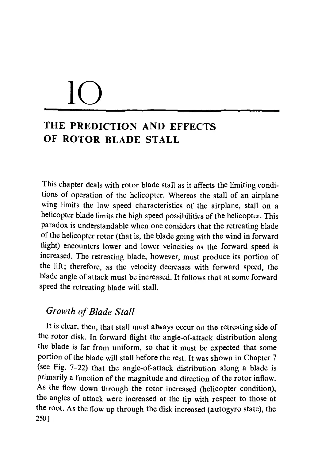
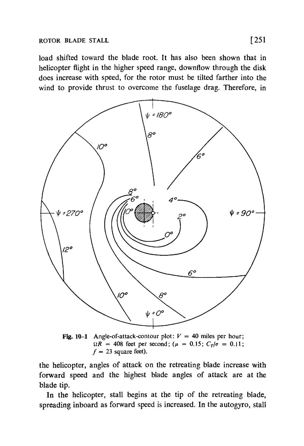
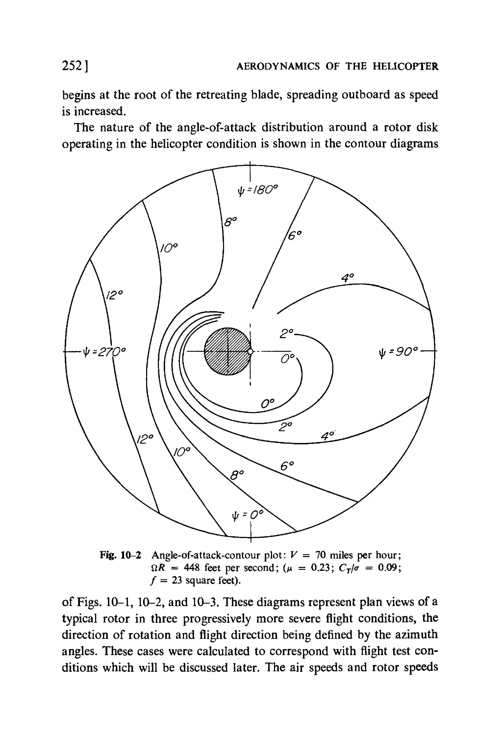
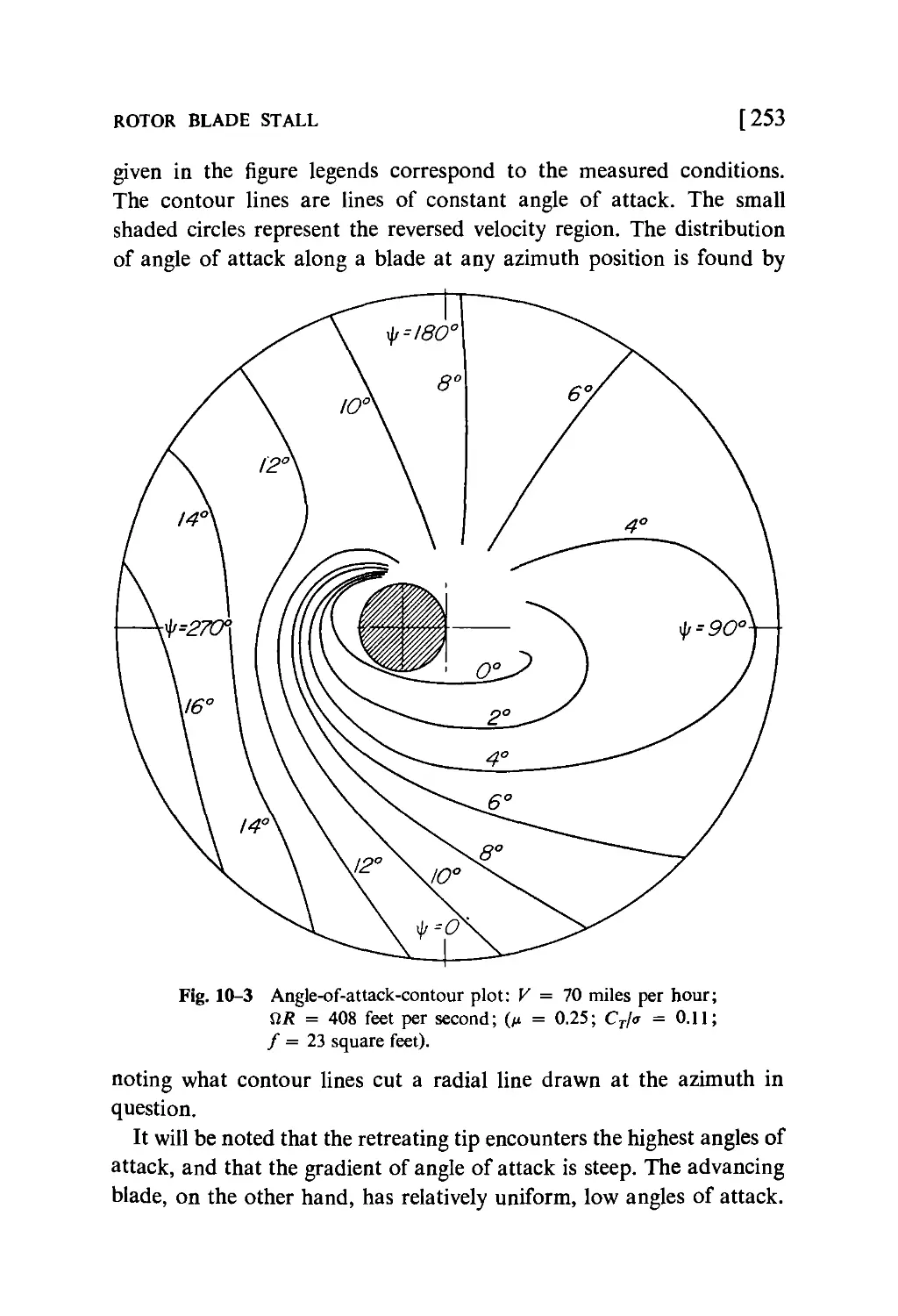








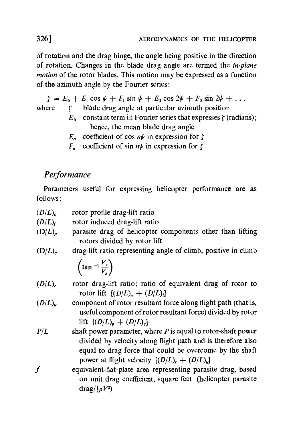

Похожие


Текст
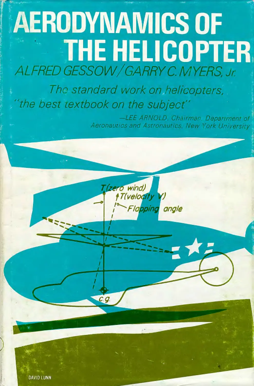
                    AERODYNAMICS OF THE
HELICOPTER
ALFRED GESSOW
GARRY C. MYERS, JR.
FREDERICK UNGAR PUBLISHING CO.
NEW YORK

Dedicated to Morris and Emma Gessow
Eighth Printing, 1985
Copyright 1952 by Alfred Gessow
and the estate of Garry C. Myers, Jr.
Republished 1967 by arrangement with Alfred Gessow
and the estate of Garry C. Myers, Jr.
Printed in the United States of America
ISBN 0-8044-4275-4
Library of Congress Catalog Card Number: 67-26126

PREFACE
TO THE THIRD PRINTING
Since the first printing of Aerodynamics of the Helicopter in 1951,
much has happened to the helicopter to justify the faith of the early
enthusiasts who predicted a great future for the ungainly, noisy,
vibrating aircraft which could barely lift their own weight on a hot
day. The helicopter has fulfilled amply those expectations by proving
its worth in a multitude of commercial and military tasks. It is
especially gratifying that even in military operations, the helicopter
has served primarily in a constructive and lifesaving capacity.
The impressive list of accomplishments achieved by the modern
helicopter is obviously the result of marked improvement over the
early models produced during the period when the text for this book
was written. Why, then, republish the book in its original edition?
To put the question in another way, why was it not fully revised?
Actually, the new printing was produced in response to numerous
requests from engineers, professors, and students who were not able
to obtain copies of the earlier printings. Obviously then, the basic
treatment in the text of the various facets of helicopter aerodynamics
is fundamental and just as valid for today's helicopters as it was for
the earliest versions. The text was not revised for this reason and
for fear of tampering with what experience has shown to be a successful
format. Although much new material could have been added to make
the book more complete, it might have been at the expense of simplicity

PREFACE TO THE THIRD PRINTING
of treatment. With a knowledge of the existing material, the student is
well prepared to understand the current technical periodical literature
which truly represents the forefront of knowledge in any technical field.
The new printing should prove useful also to the many engineers
who are concerned with the design, development, and testing of the
score of different VTOL configurations which have arisen during
the past fifteen or so years. In spite of the great advances in
aeronautical technology, particularly in power plants, which have taken
place during that time, it is safe to say that a VTOL aircraft must
incorporate a low or moderate disk loading rotor in the low speed
end of its flight range in order to justify its dual-role complexity.
In short, helicopter characteristics are required for successful VTOL
operation, and helicopter principles are the basis of a good VTOL
design.
I deeply regret that the untimely death of Garry C. Myers, Jr.,
prevented him from taking part in the many exciting helicopter
developments that have taken place and are yet to come. He made the
most of the years that he had, and the helicopter community, as well
as his family and friends, have benefited from them.
Alfred Gessow
Washington, D. C.
May, 1967

PREFACE
Aerodynamics of rotating-wing aircraft, as the subject stands today, is
the result of more than twenty years' work by many distinguished
investigators such as Glauert, Lock, and Wheatley. While technical
knowledge in many aspects of helicopter engineering is limited,
aerodynamic theory has been reasonably well established over the years by
tunnel and flight tests and has proved useful in the design and
development of present-day helicopters.
Because the solutions of many problems connected with the design
of helicopters—in areas of performance, vibration, stability, and stress
—demand a clear understanding of fundamental aerodynamic
principles, the authors felt that a significant contribution to the field could
be made by presenting clearly and logically the aerodynamics of the
helicopter as developed to date.
This book was written as a text for senior and graduate engineering
students and engineers in the helicopter industry who are interested in
obtaining a more thorough understanding of the rudiments of helicopter
aerodynamics.
The greater part of the authors' training and experience in helicopters
has been gained in the Flight Research Division of the Langley
Aeronautical Laboratory of the National Advisory Committee for
Aeronautics. The vast background of experimental and theoretical rotor
work (comprising over seventy published papers) done by the NACA

PREFACE
during the past fifteen years, served as a sound basis for the aerodynamic
material developed in the book.
In presenting the material the authors have constantly endeavored
to give physical concepts for the phenomena associated with rotating
wings. Theory is developed in its most elemental form, refinements
being added after students become familiar with the rudimentary
material. Lengthy mathematical formulas have been avoided except
where they are of fundamental significance. The aim has been to
develop basic expressions to an extent where they are generally
applicable and may be readily modified by the student to apply to specific
design problems.
A word of explanation may be in order concerning the arrangement
of material. In order that the aerodynamic theory would have greater
significance to students who are unfamiliar with practical aspects of
the helicopter, a chapter devoted to its mechanism and its general
characteristics precedes the aerodynamic treatment. Readers are then
introduced to aerodynamic theory through an analysis of hovering
flight. In hovering, the underlying principles may be mastered without
encountering the added complications that are present in forward flight
analyses—complications arising from the variation in velocity around
the disk. Similarly, the phenomenon of autorotation is first presented
for the vertical flight condition.
To provide an understanding of the phenomena associated with
forward flight, a thorough discussion of the physical concepts of flapping
and feathering is presented. Basic force and moment equations which
are then developed for the rotor in forward flight lead into a simple
and logical method of performance prediction. Though extremely easy
to use, this method is believed to be the most refined yet published
and is shown to predict helicopter performance accurately. The theory
is also shown to apply equally to autorotation and to powered level
flight, the former being considered simply as the special case of zero
shaft power. In all cases, theory is substantiated by sound experimental
evidence.
The effects on performance of the various design parameters, such
as disk loading, rotor solidity, and blade twist, are discussed in order
to provide the student with an understanding of the aerodynamic side

PREFACE
of design compromises. A thorough discussion is also given of the
limiting effects of blade stall and compressibility on high-speed flight.
Means are shown by which designers can postpone these limits and
achieve high forward speeds. Finally, the physical aspects of helicopter
stability and vibration are covered in detail in separate chapters to
give students an understanding of the parameters that influence flying
qualities of the helicopter, and of periodic forces and moments that
excite vibrations in rotating-wing aircraft. Numerous figures and
diagrams are given to illustrate the text.
A complete list of all NACA publications relating to rotating-wing
aircraft is given in Appendix IIA. These papers, when used as
references in the text, are referred to by Roman numerals followed by a
number (e.g. reference IV-3). A representative list of other than NACA
helicopter papers is contained in Appendix IIB. These papers are
referred to in the text by a number alone (e.g. reference 24).
The authors wish to express their admiration and indebtedness to
Mr. F. B. Gustafson, head of helicopter flight research at the Langley
Laboratory, who, as supervisor, freely and patiently shared his
understanding of engineering principles and extensive knowledge of rotating-
wing aircraft. Their thanks are due also to Mr. T. E. McCorkle for his
patience and efforts in illustrating the text.
Alfred Gessow
Garry C. Myers, Jr.
Hampton, Virginia

CONTENTS
1 The Development of Rotating-Wing Aircraft 1
2 An Introduction to the Helicopter 16
3 An Introduction to Hovering Theory 46
4 Hovering and Vertical-Flight Performance Analyses 66
5 Factors Affecting Hovering and Vertical-Flight Performance 89
6 Autorotation in Vertical Descent 117
7 Physical Concepts of Blade Motion and Rotor Control 138
8 The Aerodynamics of Forward Flight 180
9 Forward-Flight Performance 217
10 The Prediction and Effects of Rotor Blade Stall 250
11 An Introduction to Helicopter Stability 268
12 An Introduction to Helicopter Vibration Problems 307
Appendix I 321
Appendix IIA 327
Appendix IIB 337
Index 341

1
THE DEVELOPMENT OF
ROTATING-WING AIRCRAFT
The story of the helicopter is the story of the life works of men
throughout the last five centuries. Early experimenters were seeking in
the helicopter a means by which man might achieve flight. At the
beginning of the twentieth century, however, before any successful
rotating-wing aircraft was devised, man achieved flight in fixed wing,
or "conventional" aircraft. Engineering effort concentrated on
developing the fixed-wing aircraft until today the airplane has been developed
to the point where it is one of the world's most important means of
transportation.
Notwithstanding the development of the conventional airplane, men
have been aware that they had still to achieve complete mastery of the
air; namely, the ability to stay aloft without maintaining forward
speed and to ascend and land vertically in restricted areas. Development
of the helicopter continued to this end.
Three fundamental problems plagued experimenters: (1) keeping
structural weight and engine weight down to the point where the
machine could lift itself and some useful load; (2) counteracting rotor
torque; and (3) controlling the machine in flight. The structural and
engine-weight problems were responsible for the slow progress in early
experiments. In recent years the torque and control problems
predominated, resulting in a number of configurations of rotors and
infinite variations of basic types.
About 1926 a Spaniard, Juan de la Cierva, produced a successful
[1

2 ] AERODYNAMICS OF THE HELICOPTER
rotating-wing machine which employed a propeller for forward motion,
as in an airplane, and a freely rotating rotor for lift. This aircraft he
called the autogyro. While the autogyro was still not a direct-lift
machine it required only small forward speeds to maintain its lift and
could take off and land in extremely short distances. Autogyro
development continued in Europe and in America until by 1936 the art had
reached a state of considerable advancement. The economic
depression of that period, however, together with the overpublicity of the
machine in its early stages of development, brought progress almost to
a standstill.
Paralleling autogyro development, progress was being made toward
a successful helicopter. By 1937 Focke in Germany demonstrated a
successful side-by-side, two-rotor machine, and in 1941 Sikorsky
introduced the VS-300, a single lifting rotor machine with a vertical
tail rotor for torque counteraction. Sikorsky's success gave tremendous
impetus to helicopter development in this country and, in the few
years that followed, at least forty serious and independent developments
sprang up. It is interesting to note that for the most part the helicopter
was developed independently from the autogyro, and many phases of
the rotating-wing art which were quite familiar to autogyro engineers
were completely relearned in helicopter development. Indeed,
autogyros still compete with helicopters in regard to rotating-wing aircraft
speed records, and it is only recently that helicopters have been built
which surpass the autogyros of the nineteen thirties in their ratio of
useful load to total weight.
Chronological Development of the Helicopter
In order to present a comprehensive picture of helicopter
development, the experiments of some of the pioneers in the field are listed
below. The list is by no means complete, for it is intended only to point
out general trends in development.
'B.C. It is known that before the days of the Roman empire the
Chinese constructed "Chinese Tops." The top consisted of a propeller
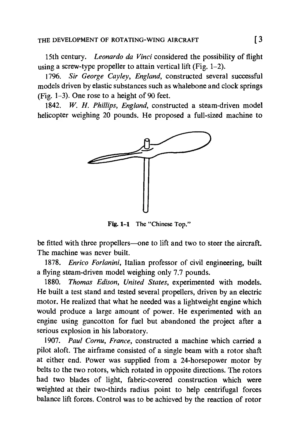
on a stick which was spun between the hands (Fig. 1-1). The "Chinese
Top" probably represented the world's first helicopter.

THE DEVELOPMENT OF ROTATING-WING AIRCRAFT [ 3
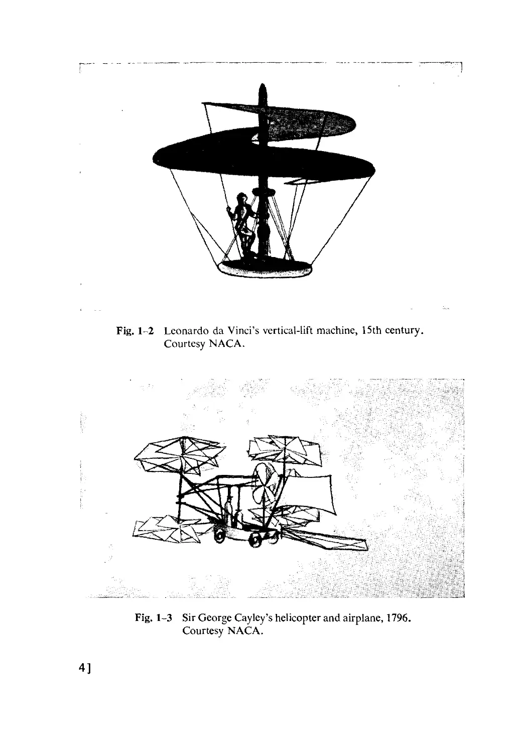
15th century. Leonardo da Vinci considered the possibility of flight
using a screw-type propeller to attain vertical lift (Fig. 1-2).
1796. Sir George Cayley, England, constructed several successful
models driven by elastic substances such as whalebone and clock springs
(Fig. 1-3). One rose to a height of 90 feet.
1842. W. H. Phillips, England, constructed a steam-driven model
helicopter weighing 20 pounds. He proposed a full-sized machine to
Fig. 1-1 The "Chinese Top."
be fitted with three propellers—one to lift and two to steer the aircraft.
The machine was never built.
1878. Enrico Forlanini, Italian professor of civil engineering, built
a flying steam-driven model weighing only 7.7 pounds.
1880. Thomas Edison, United States, experimented with models.
He built a test stand and tested several propellers, driven by an electric
motor. He realized that what he needed was a lightweight engine which
would produce a large amount of power. He experimented with an
engine using guncotton for fuel but abandoned the project after a
serious explosion in his laboratory.
1907. Paul Cornu, France, constructed a machine which carried a
pilot aloft. The airframe consisted of a single beam with a rotor shaft
at either end. Power was supplied from a 24-horsepower motor by
belts to the two rotors, which rotated in opposite directions. The rotors
had two blades of light, fabric-covered construction which were
weighted at their two-thirds radius point to help centrifugal forces
balance lift forces. Control was to be achieved by the reaction of rotor

Fig. 1-2 Leonardo da Vinci's vertical-lift machine, 15th century.
Courtesy NACA.
* *. 1
Fig. 1-3 Sir George Cayley's helicopter and airplane, 1796.
Courtesy NACA.
4]

THE DEVELOPMENT OF ROTATING-WING AIRCRAFT
[5
downwash on airfoils suspended below the rotor. The machine never
flew untethered.
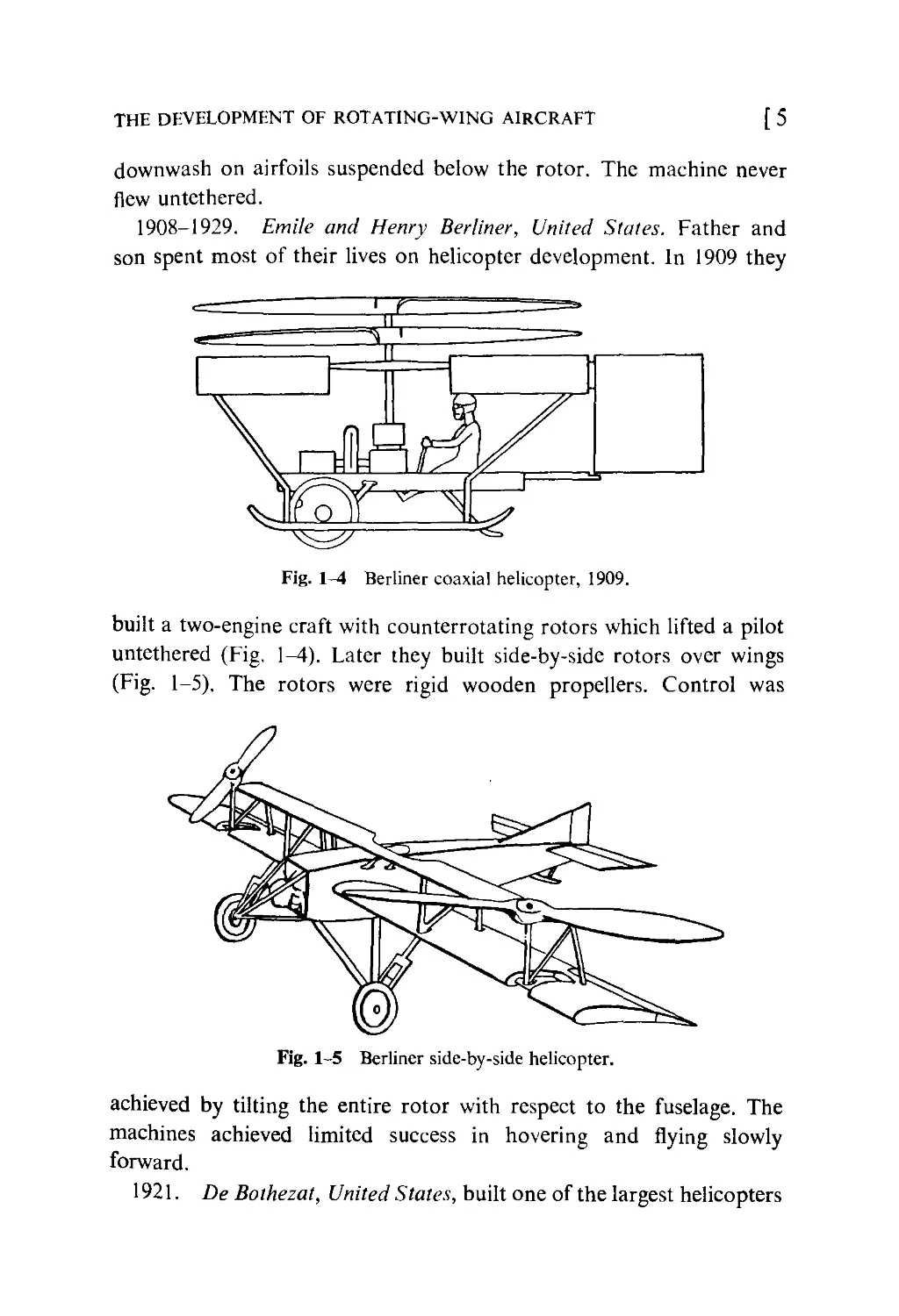
1908-1929. Emile and Henry Berliner, United States. Father and
son spent most of their lives on helicopter development. In 1909 they
Fig. 1-4 Berliner coaxial helicopter, 1909.
built a two-engine craft with counterrotating rotors which lifted a pilot
untethered (Fig. 1-4). Later they built side-by-side rotors over wings
(Fig. 1-5). The rotors were rigid wooden propellers. Control was
Fig. 1-5 Berliner side-by-side helicopter.
achieved by tilting the entire rotor with respect to the fuselage. The
machines achieved limited success in hovering and flying slowly
forward.
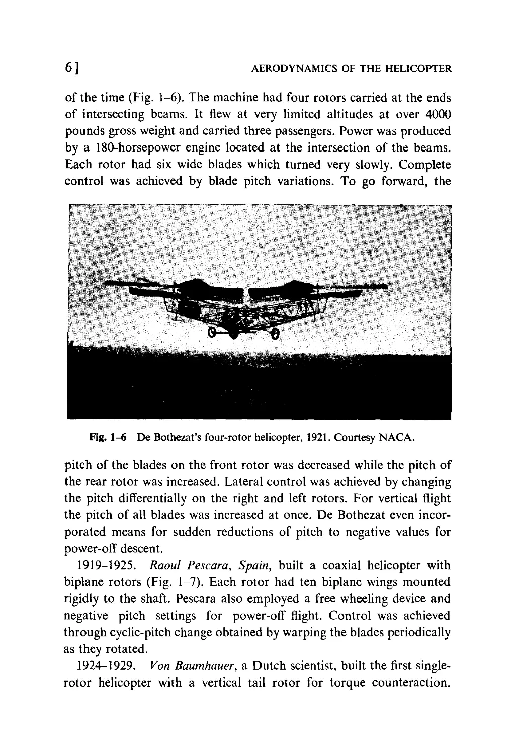
1921. De Bothezat, United States, built one of the largest helicopters

6 ] AERODYNAMICS OF THE HELICOPTER
of the time (Fig. 1-6). The machine had four rotors carried at the ends
of intersecting beams. It flew at very limited altitudes at over 4000
pounds gross weight and carried three passengers. Power was produced
by a 180-horsepower engine located at the intersection of the beams.
Each rotor had six wide blades which turned very slowly. Complete
control was achieved by blade pitch variations. To go forward, the
Fig. 1-6 De Bothezat's four-rotor helicopter, 1921. Courtesy NACA.
pitch of the blades on the front rotor was decreased while the pitch of
the rear rotor was increased. Lateral control was achieved by changing
the pitch differentially on the right and left rotors. For vertical flight
the pitch of all blades was increased at once. De Bothezat even
incorporated means for sudden reductions of pitch to negative values for
power-off descent.
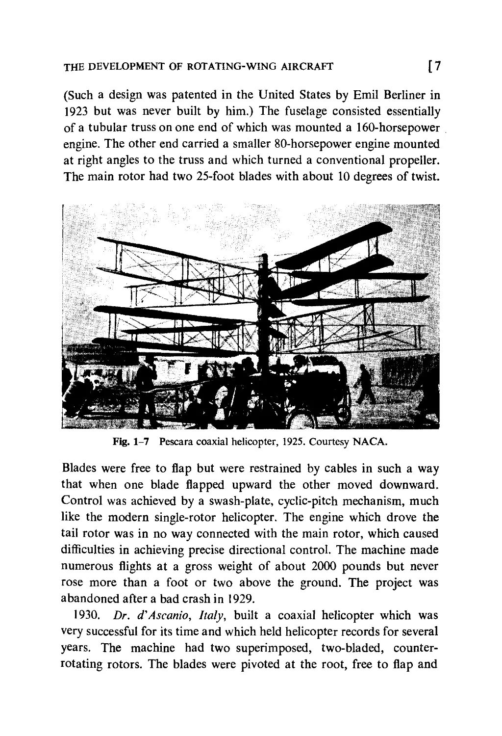
1919-1925. Raoul Pescara, Spain, built a coaxial helicopter with
biplane rotors (Fig. 1-7). Each rotor had ten biplane wings mounted
rigidly to the shaft. Pescara also employed a free wheeling device and
negative pitch settings for power-off flight. Control was achieved
through cyclic-pitch change obtained by warping the blades periodically
as they rotated.
1924-1929. Von Baumhauer, a Dutch scientist, built the first single-
rotor helicopter with a vertical tail rotor for torque counteraction.

THE DEVELOPMENT OF ROTATING-WING AIRCRAFT
[7
(Such a design was patented in the United States by Emil Berliner in
1923 but was never built by him.) The fuselage consisted essentially
of a tubular truss on one end of which was mounted a 160-horsepower
engine. The other end carried a smaller 80-horsepower engine mounted
at right angles to the truss and which turned a conventional propeller.
The main rotor had two 25-foot blades with about 10 degrees of twist.
Fig. 1-7 Pescara coaxial helicopter, 1925. Courtesy NACA.
Blades were free to flap but were restrained by cables in such a way
that when one blade flapped upward the other moved downward.
Control was achieved by a swash-plate, cyclic-pitch mechanism, much
like the modern single-rotor helicopter. The engine which drove the
tail rotor was in no way connected with the main rotor, which caused
difficulties in achieving precise directional control. The machine made
numerous flights at a gross weight of about 2000 pounds but never
rose more than a foot or two above the ground. The project was
abandoned after a bad crash in 1929.
1930. Dr. cTAscanio, Italy, built a coaxial helicopter which was
very successful for its time and which held helicopter records for several
years. The machine had two superimposed, two-bladed, counter-
rotating rotors. The blades were pivoted at the root, free to flap and

8]
AERODYNAMICS OF THE HELICOPTER
change pitch. Control was achieved by servo-tabs on the blades which
were deflected periodically by a system of cables and pulleys. The
tabs cyclically changed the pitch of the entire blade. For vertical flight,
the tabs moved together so as to increase or decrease the pitch of all
blades. The machine flew 3000 feet in five minutes, remained aloft for
almost nine minutes, and achieved an altitude of 54 feet.
1930. M. B. Bleeker, United States, solved the torque problem by
delivering power to propellers mounted on each blade. Power was
supplied through an intricate system of gearing from an engine mounted
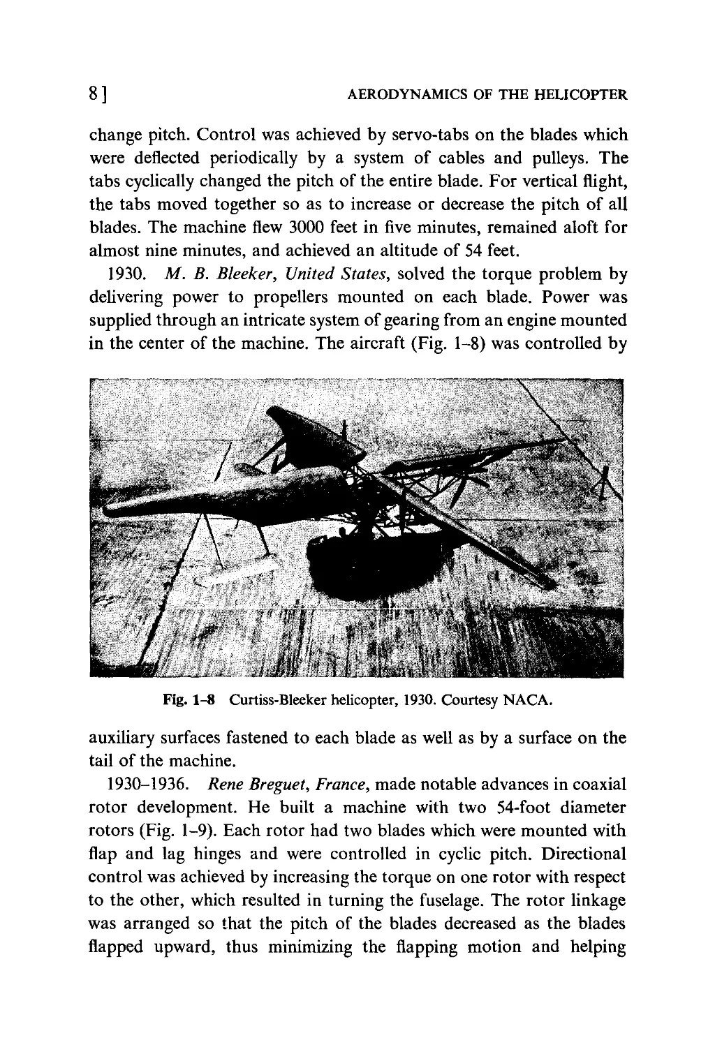
in the center of the machine. The aircraft (Fig. 1-8) was controlled by
H
Fig. 1-8 Curtiss-Bleeker helicopter, 1930. Courtesy NACA.
auxiliary surfaces fastened to each blade as well as by a surface on the
tail of the machine.
1930-1936. Rene Breguet, France, made notable advances in coaxial
rotor development. He built a machine with two 54-foot diameter
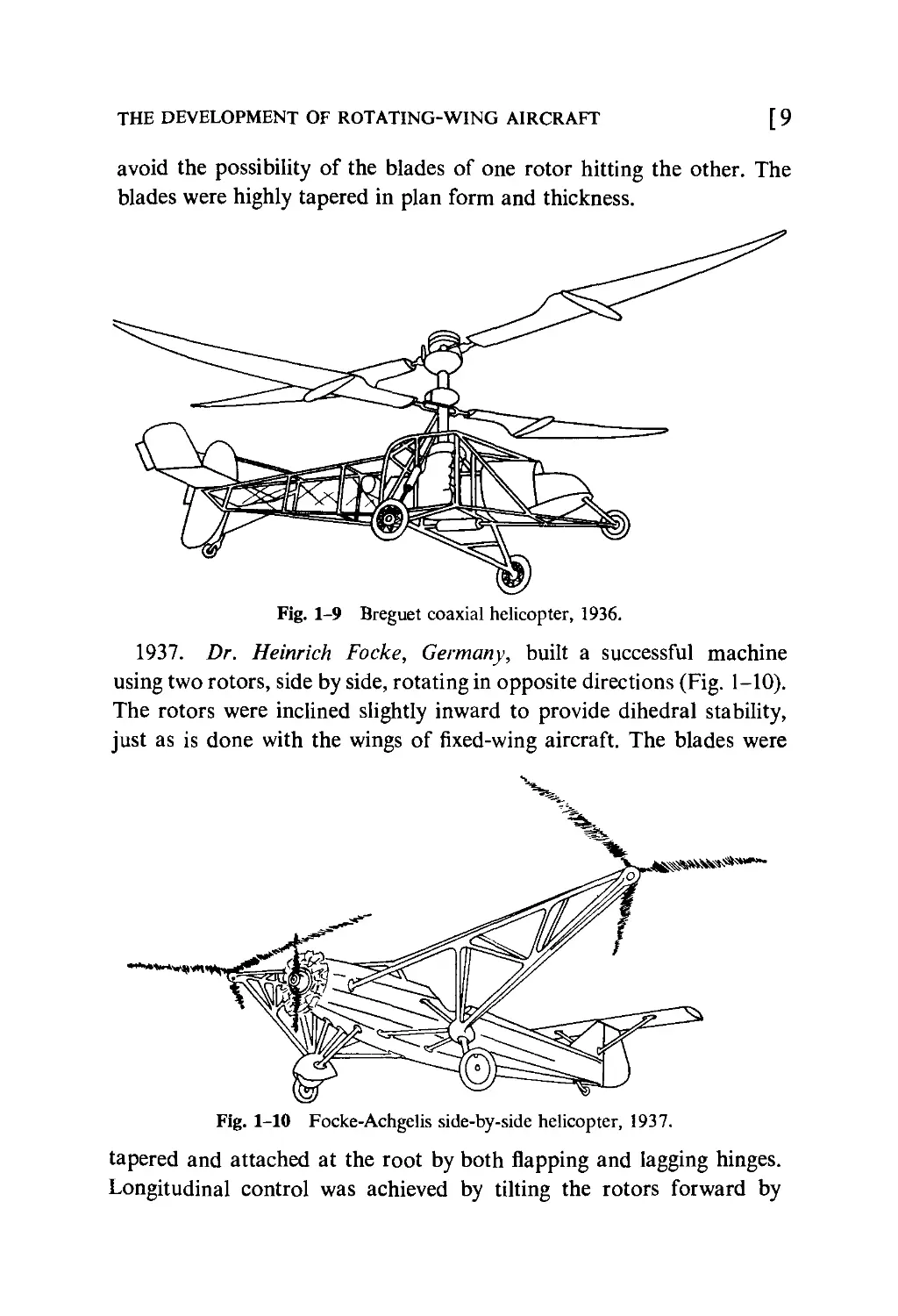
rotors (Fig. 1-9). Each rotor had two blades which were mounted with
flap and lag hinges and were controlled in cyclic pitch. Directional
control was achieved by increasing the torque on one rotor with respect
to the other, which resulted in turning the fuselage. The rotor linkage
was arranged so that the pitch of the blades decreased as the blades
flapped upward, thus minimizing the flapping motion and helping

THE DEVELOPMENT OF ROTATING-WING AIRCRAFT [ 9
avoid the possibility of the blades of one rotor hitting the other. The
blades were highly tapered in plan form and thickness.
Fig. 1-9 Breguet coaxial helicopter, 1936.
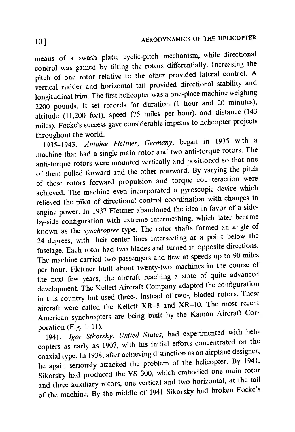
1937. Dr. Heinrich Focke, Germany, built a successful machine
using two rotors, side by side, rotating in opposite directions (Fig. 1-10).
The rotors were inclined slightly inward to provide dihedral stability,
just as is done with the wings of fixed-wing aircraft. The blades were
Fig. 1-10 Focke-Achgelis side-by-side helicopter, 1937.
tapered and attached at the root by both flapping and lagging hinges.
Longitudinal control was achieved by tilting the rotors forward by

10] AERODYNAMICS OF THE HELICOPTER
means of a swash plate, cyclic-pitch mechanism, while directional
control was gained by tilting the rotors differentially. Increasing the
pitch of one rotor relative to the other provided lateral control. A
vertical rudder and horizontal tail provided directional stability and
longitudinal trim. The first helicopter was a one-place machine weighing
2200 pounds. It set records for duration (1 hour and 20 minutes),
altitude (11,200 feet), speed (75 miles per hour), and distance (143
miles). Focke's success gave considerable impetus to helicopter projects
throughout the world.
1935-1943. Antoine Flettner, Germany, began in 1935 with a
machine that had a single main rotor and two anti-torque rotors. The
anti-torque rotors were mounted vertically and positioned so that one
of them pulled forward and the other rearward. By varying the pitch
of these rotors forward propulsion and torque counteraction were
achieved. The machine even incorporated a gyroscopic device which
relieved the pilot of directional control coordination with changes in
engine power. In 1937 Flettner abandoned the idea in favor of a side-
by-side configuration with extreme intermeshing, which later became
known as the synchropter type. The rotor shafts formed an angle of
24 degrees, with their center lines intersecting at a point below the
fuselage. Each rotor had two blades and turned in opposite directions.
The machine carried two passengers and flew at speeds up to 90 miles
per hour. Flettner built about twenty-two machines in the course of
the next few years, the aircraft reaching a state of quite advanced
development. The Kellett Aircraft Company adapted the configuration
in this country but used three-, instead of two-, bladed rotors. These
aircraft were called the Kellett XR-8 and XR-10. The most recent
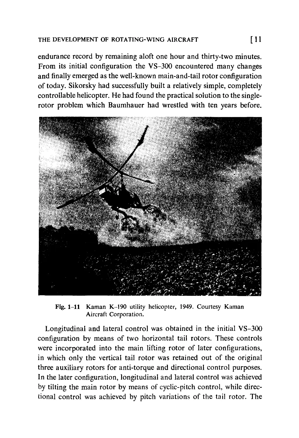
American synchropters are being built by the Kaman Aircraft
Corporation (Fig. 1-11).
1941. Igor Sikorsky, United States, had experimented with
helicopters as early as 1907, with his initial efforts concentrated on the
coaxial type. In 1938, after achieving distinction as an airplane designer,
he again seriously attacked the problem of the helicopter. By 1941,
Sikorsky had produced the VS-300, which embodied one main rotor
and three auxiliary rotors, one vertical and two horizontal, at the tail
of the machine. By the middle of 1941 Sikorsky had broken Focke's

THE DEVELOPMENT OF ROTATING-WING AIRCRAFT
[11
endurance record by remaining aloft one hour and thirty-two minutes.
From its initial configuration the VS-300 encountered many changes
and finally emerged as the well-known main-and-tail rotor configuration
of today. Sikorsky had successfully built a relatively simple, completely
controllable helicopter. He had found the practical solution to the single-
rotor problem which Baumhauer had wrestled with ten years before.
Fig. 1-11 Kaman K-190 utility helicopter, 1949. Courtesy Kaman
Aircraft Corporation.
Longitudinal and lateral control was obtained in the initial VS-300
configuration by means of two horizontal tail rotors. These controls
were incorporated into the main lifting rotor of later configurations,
in which only the vertical tail rotor was retained out of the original
three auxiliary rotors for anti-torque and directional control purposes.
In the later configuration, longitudinal and lateral control was achieved
by tilting the main rotor by means of cyclic-pitch control, while
directional control was achieved by pitch variations of the tail rotor. The

12]
AERODYNAMICS OF THE HELICOPTER
tail rotor was driven by shafting from the main rotor transmission,
so that in case of power failure the main rotor continued to turn the
tail rotor so as to maintain directional control.
The pilot's controls consisted of a pitch stick at his side which he
raised up and down for vertical flight, a control stick in front of him
which he pushed in the direction he wished to go, and rudder pedals
which he operated with his feet for directional control. The pitch stick
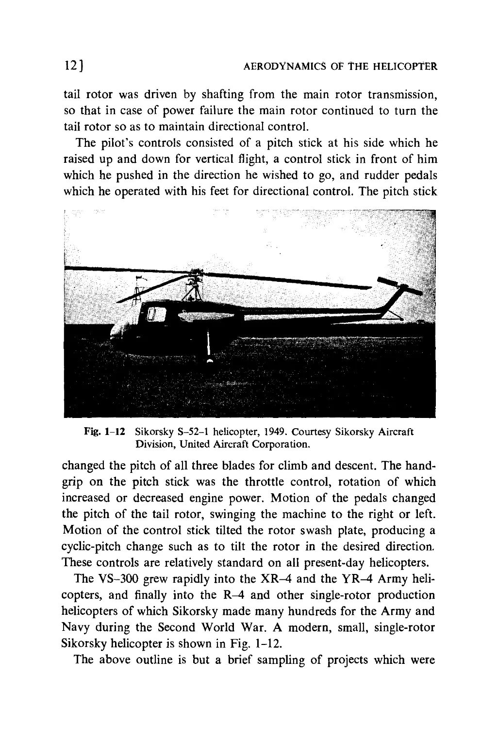
Fig. 1-12 Sikorsky S-52-1 helicopter, 1949. Courtesy Sikorsky Aircraft
Division, United Aircraft Corporation.
changed the pitch of all three blades for climb and descent. The
handgrip on the pitch stick was the throttle control, rotation of which
increased or decreased engine power. Motion of the pedals changed
the pitch of the tail rotor, swinging the machine to the right or left.
Motion of the control stick tilted the rotor swash plate, producing a
cyclic-pitch change such as to tilt the rotor in the desired direction.
These controls are relatively standard on all present-day helicopters.
The VS-300 grew rapidly into the XR-4 and the YR-4 Army
helicopters, and finally into the R—4 and other single-rotor production
helicopters of which Sikorsky made many hundreds for the Army and
Navy during the Second World War. A modern, small, single-rotor
Sikorsky helicopter is shown in Fig. 1-12.
The above outline is but a brief sampling of projects which were

THE DEVELOPMENT OF ROTATING-WING AIRCRAFT [ 13
significant in helicopter development and no attempt has been made
to discuss the details of the many present-day helicopters. In reviewing
the history of the art one is impressed by the large number of
completely separate approaches to the problem. It would appear that
progress was made more in proportion to technological developments
of the time than to the results of experimenters who built on one
another's work. Almost every configuration of rotors imaginable, and
many which are almost unimaginable, have been experimented with.
Autogyro Development
One phase of the history of the rotating-wing not dealt with in the
preceding outline is the development of the autogyro. While it does
not have all the properties of the helicopter, the autogyro involves
basically the same problems of rotor design as the helicopter. Autogyro
development, which began about 1920 and which reached considerable
advancement by 1935, had a great deal to do with the advent of the
successful helicopter.
The story of the development of the autogyro is primarily the story
of Juan de la Cierva. Cierva was particularly interested in making a
flying machine which could land and ascend without high forward
speed and which could not stall and drop to earth if the pilot reduced
speed excessively. To Cierva, stalling was a tremendous limitation to
the airplane, and rather than improve the stalling characteristics of
airplanes he chose to devise an inherently different type of lifting surface.
With his own funds and with a grant from the Spanish Government
he ran wind-tunnel experiments on model rotors and established many
basic facts of rotor behavior. He found that a rotor tilted slightly
back in a wind could produce a sizable lift even at a very low speed.
He further discovered that best results were obtained when the blades
of his "windmills" were set at low positive angles.
Cierva flew his first autogyro in 1923. The rotor was mounted above
an airplane fuselage and acted simply as a wing, rotating in the wind
and supporting the machine. An engine and propeller pulled the
machine through the air as in a normal airplane. Control was achieved
by conventional airplane surfaces which tilted the machine and changed

14]
AERODYNAMICS OF THE HELICOPTER
the direction of rotor lift. Cierva built three machines before he
achieved success. His third machine incorporated freely hinged blades
which Cierva invented as a means of equalizing the lift on the two
sides of his rotor in forward flight. Although the principle of flapping
blades had actually been suggested by Renard, a Frenchman, in 1904,
Cierva rediscovered and first applied the principle.
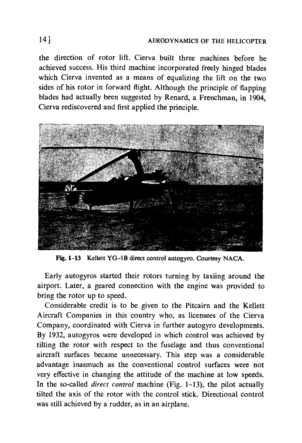
Fig. 1-13 Kellett YG-1B direct control autogyro. Courtesy NACA
Early autogyros started their rotors turning by taxiing around the
airport. Later, a geared connection with the engine was provided to
bring the rotor up to speed.
Considerable credit is to be given to the Pitcairn and the Kellett
Aircraft Companies in this country who, as licensees of the Cierva
Company, coordinated with Cierva in further autogyro developments.
By 1932, autogyros were developed in which control was achieved by
tilting the rotor with respect to the fuselage and thus conventional
aircraft surfaces became unnecessary. This step was a considerable
advantage inasmuch as the conventional control surfaces were not
very effective in changing the attitude of the machine at low speeds.
In the so-called direct control machine (Fig. 1-13), the pilot actually
tilted the axis of the rotor with the control stick. Directional control
was still achieved by a rudder, as in an airplane.

THE DEVELOPMENT OF ROTATING-WING AIRCRAFT [ 15
Raoul Hafner in England advanced the art further by introducing
cyclic-pitch control as a means of effectively tilting the rotor without
encountering the undesirable forces which were transmitted through
the rotor hinges in the direct control machine. Another interesting
version of the autorotating rotor was introduced in the United States
by E. Burke Wilford, who built a four-bladed gyroplane whose rotor
differed basically from other rotors in that it was nonarticulated; that
is, bending stresses in the spars were not relieved by hinges. Balance
and control were achieved by feathering the blades substantially about
their span axis.
The final phase of autogyro development was the introduction of
the "jump take-off." This involved the overspeeding of the rotor on
the ground with the blades set at zero pitch and the subsequent use
of this stored energy to lift the machine into the air by a sudden increase
in pitch. With jump take-off the autogyro closely rivaled the helicopter
in flight characteristics. It was still unable, however, to approach a
landing spot and back away if the spot appeared unsuitable.

2
AN INTRODUCTION
TO THE HELICOPTER
Later chapters of this book will deal primarily with the behavior of
the helicopter rotor in various conditions of flight. The fact that the
rotor has a fuselage, source of power, and means of control will be
taken for granted, and very little attention will be given to the details
of mechanical design. The purpose of the present chapter is to give
the reader a picture of the helicopter as a whole—its geometrical
configurations, its means of control, its general design features, its
performance characteristics, and its flying qualities. This will, it is
hoped, provide a background and permit a clearer understanding of
the following chapters.
Helicopter Configurations
Helicopter configurations may be classified into five main types and
several subclasses. Each type has its unique characteristics, advantages,
and disadvantages. These are discussed below.
the single rotor. In terms of the number of machines in operation
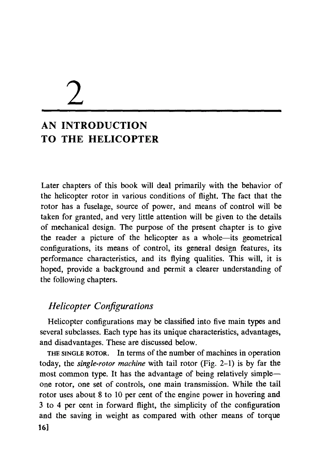
today, the single-rotor machine with tail rotor (Fig. 2-1) is by far the
most common type. It has the advantage of being relatively simple—
one rotor, one set of controls, one main transmission. While the tail
rotor uses about 8 to 10 per cent of the engine power in hovering and
3 to 4 per cent in forward flight, the simplicity of the configuration
and the saving in weight as compared with other means of torque
16]

AN INTRODUCTION TO THE HELICOPTER
[17
counteraction probably compensate for this loss. One disadvantage is
the danger of the vertical tail rotor to ground personnel, the whirling
blades being behind the pilot and thus not under his precise control.
The gyrodyne, a type of helicopter in which the torque counteracting
rotor points forward, has the advantage of using the anti-torque rotor
instead of the main rotor to pull the machine through the air. This
results in more efficient operation of the main rotor in forward flight
Fig. 2-1 Bell H13-B single-rotor helicopter. Courtesy NACA.
since it avoids the tilting forward of the rotor and the accompanying
radial dissymmetry in blade angle of attack. On the other hand, the
gyrodyne torque rotor must be mounted on a relatively short arm
in order to avoid excessive parasite drag, and the engine power
required to counteract torque at the shorter moment arm is accordingly
higher.
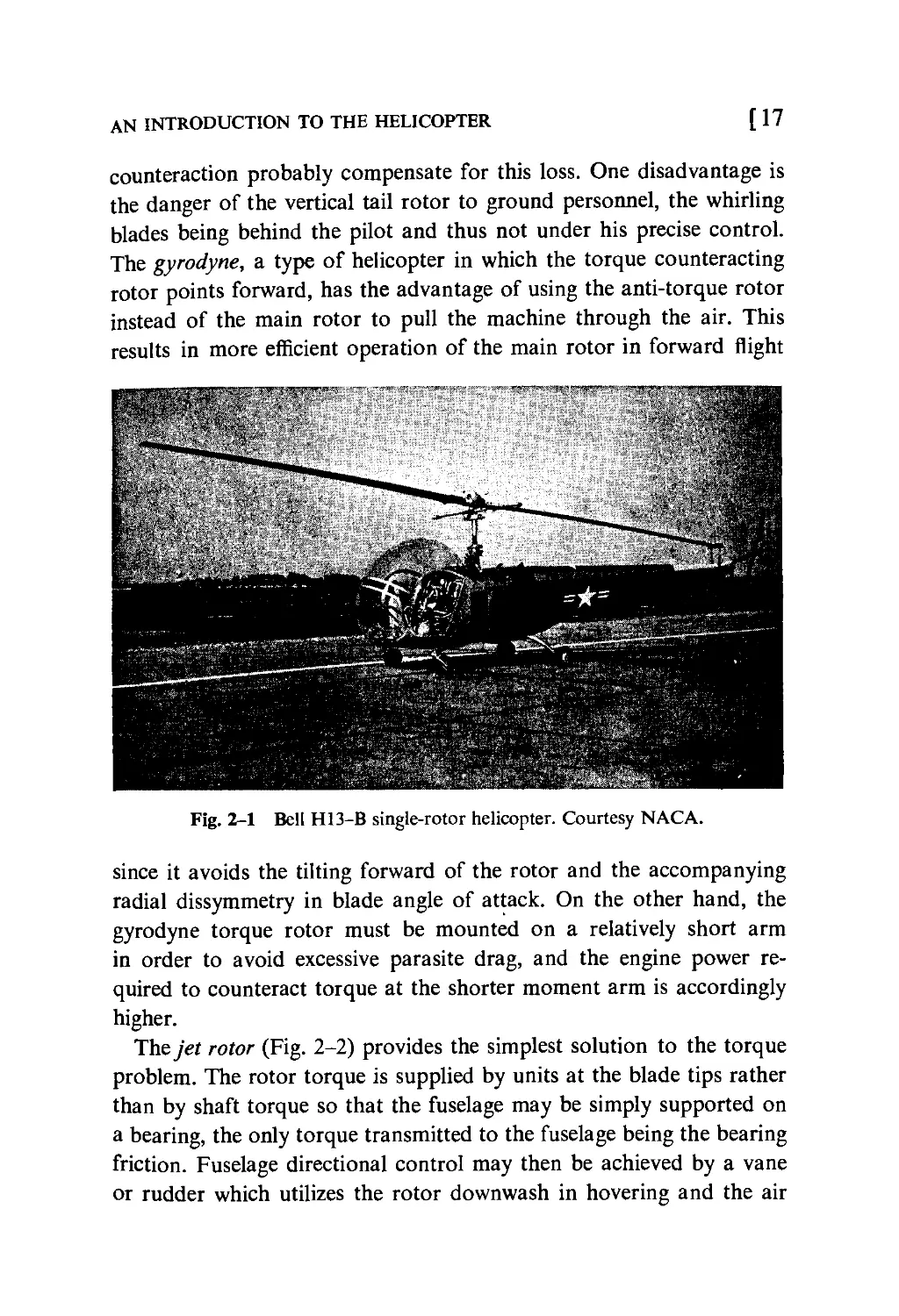
The jet rotor (Fig. 2-2) provides the simplest solution to the torque
problem. The rotor torque is supplied by units at the blade tips rather
than by shaft torque so that the fuselage may be simply supported on
a bearing, the only torque transmitted to the fuselage being the bearing
friction. Fuselage directional control may then be achieved by a vane
or rudder which utilizes the rotor downwash in hovering and the air

18]
AERODYNAMICS OF THE HELICOPTER
stream in forward flight. Jet thrust may be provided by tip units, as
in the ram jet rotor, or by an engine-driven blower from which air is
ducted to rearward-pointing nozzles at the blade tips. The jet rotor
has the advantage of simplicity and small storage space and the
disadvantage of high specific fuel consumption as compared with a
conventional machine. Development will depend primarily on jet engine
development. Ultimately, the jet helicopter may very well prove to be
the most practical configuration.
Fig. 2-2 McDonnell "Little Henry" ram jet helicopter. Courtesy
McDonnell Aircraft Corporation.
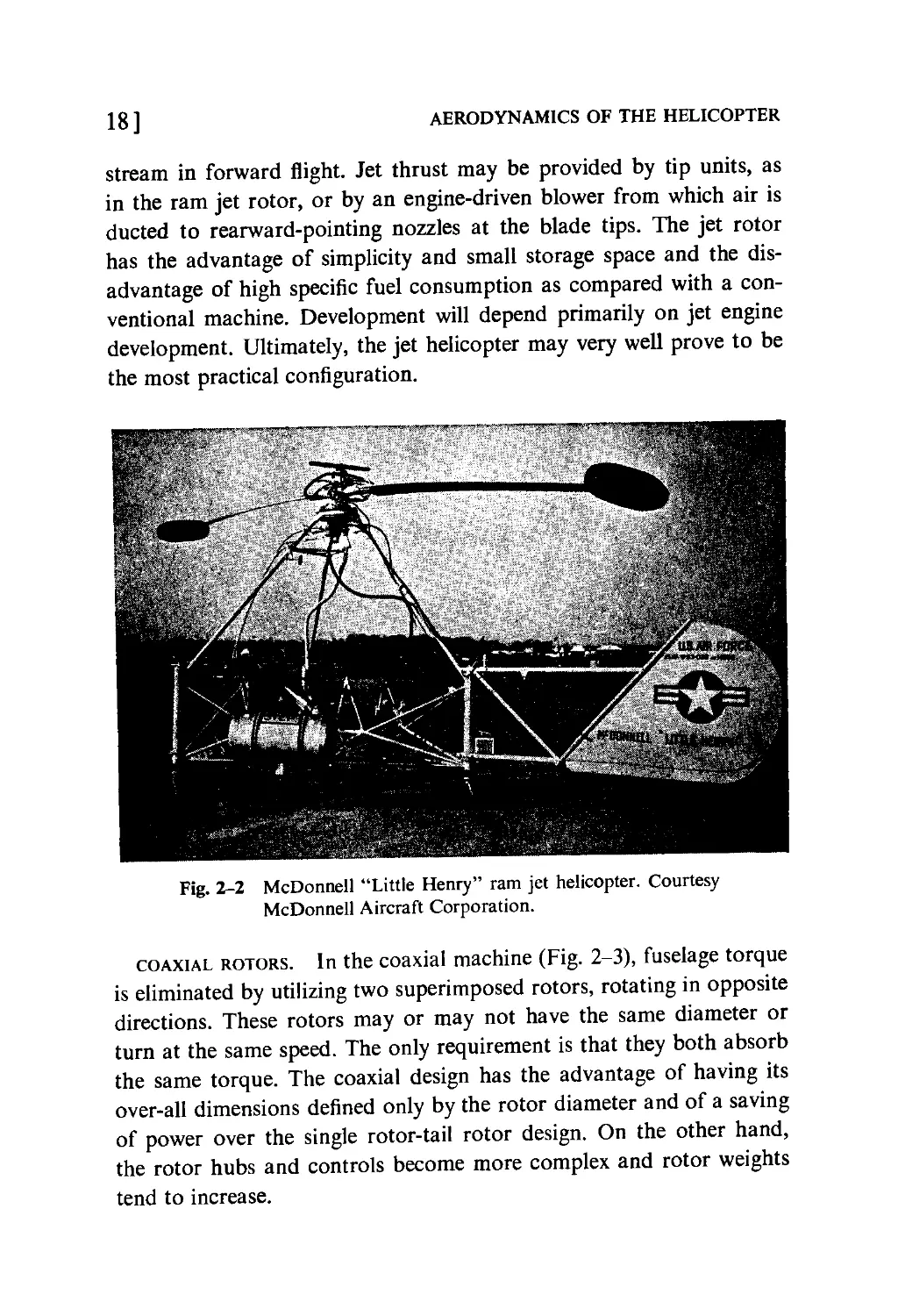
coaxial rotors. In the coaxial machine (Fig. 2-3), fuselage torque
is eliminated by utilizing two superimposed rotors, rotating in opposite
directions. These rotors may or may not have the same diameter or
turn at the same speed. The only requirement is that they both absorb
the same torque. The coaxial design has the advantage of having its
over-all dimensions defined only by the rotor diameter and of a saving
of power over the single rotor-tail rotor design. On the other hand,
the rotor hubs and controls become more complex and rotor weights
tend to increase.

AN INTRODUCTION TO THE HELICOPTER
[19
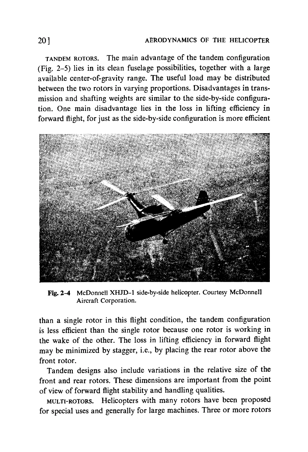
side-by-side rotors. The basic advantage of the side-by-side
configuration (Fig. 2-4) is that the laterally displaced rotors effect a
reduction in power required to produce lift in forward flight, similar to the
aspect ratio effect on an airplane wing. This advantage becomes
important in large multi-engine helicopters where standards require that
level flight be possible with one engine dead, since the reduction in
power necessary to maintain level flight in the side-by-side ship permits
bigger loads to be carried. The configuration has the disadvantage of
Fig. 2-3 Bendix experimental coaxial helicopter. Courtesy NACA.
having either high fuselage parasite drag or high structural weight, for
as the supporting pylons become thin and aerodynamically clean they
become heavy. The supporting pylons, however, may act as lifting
surfaces and unload the rotors in forward flight, effecting a sizable
gain in efficiency at high speed. As compared with the single-rotor
machine, the side-by-side configuration has the disadvantage of
requiring relatively complex gearing and shafting. Its over-all dimensions
are greater than the single-rotor machine, this depending, of course,
on the degree of overlap. The synchropter (Fig. 1-11), in which rotors
are intermeshed to the point of approaching the single rotor, sacrifices
some lifting efficiency gains for compactness and transmission
simplifications.

20]
AERODYNAMICS OF THE HELICOPTER
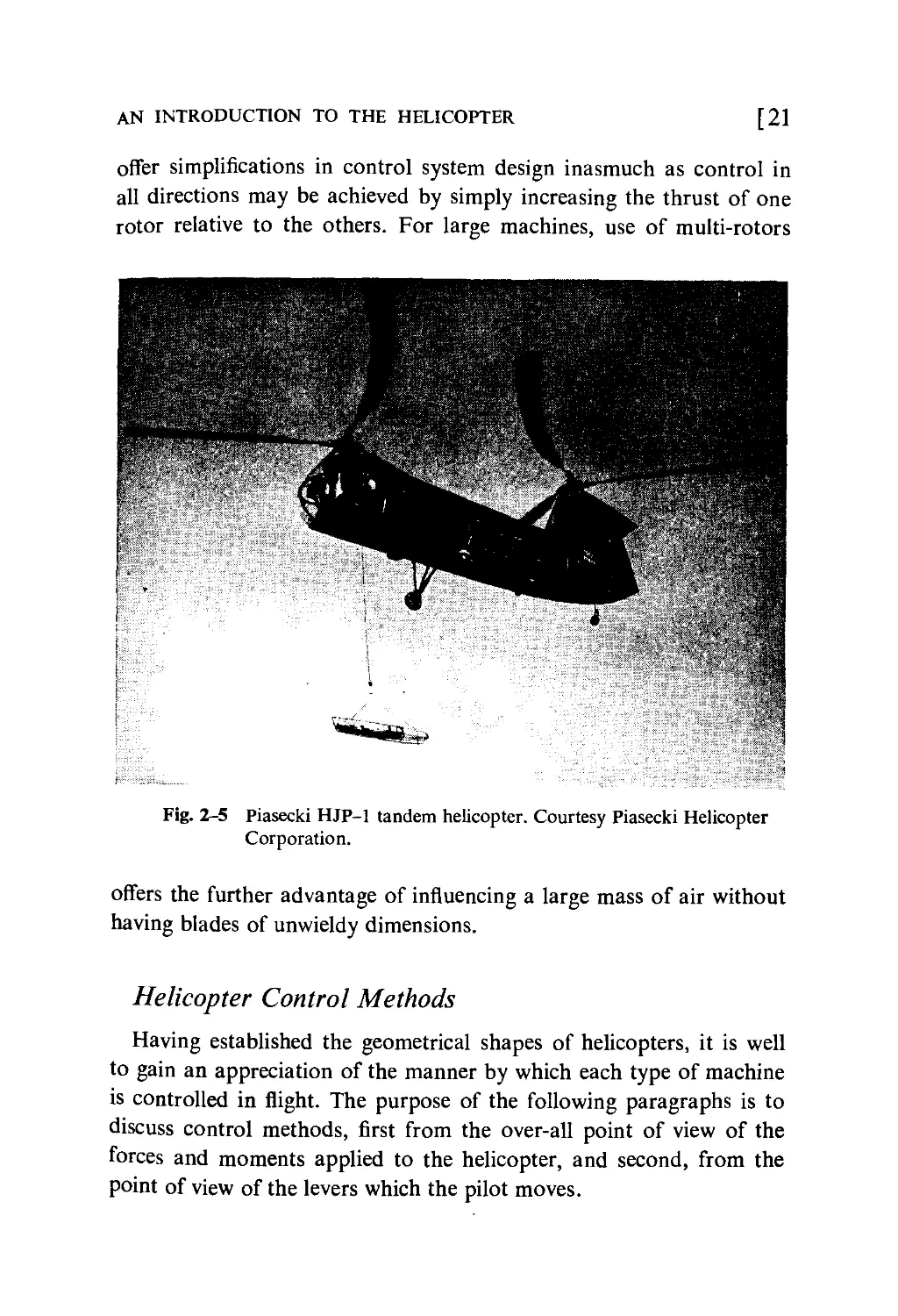
tandem rotors. The main advantage of the tandem configuration
(Fig. 2-5) lies in its clean fuselage possibilities, together with a large
available center-of-gravity range. The useful load may be distributed
between the two rotors in varying proportions. Disadvantages in
transmission and shafting weights are similar to the side-by-side
configuration. One main disadvantage lies in the loss in lifting efficiency in
forward flight, for just as the side-by-side configuration is more efficient
t".--
Fig. 2-4 McDonnell XHJD-1 side-by-side helicopter. Courtesy McDonnell
Aircraft Corporation.
than a single rotor in this flight condition, the tandem configuration
is less efficient than the single rotor because one rotor is working in
the wake of the other. The loss in lifting efficiency in forward flight
may be minimized by stagger, i.e., by placing the rear rotor above the
front rotor.
Tandem designs also include variations in the relative size of the
front and rear rotors. These dimensions are important from the point
of view of forward flight stability and handling qualities.
multi-rotors. Helicopters with many rotors have been proposed
for special uses and generally for large machines. Three or more rotors

AN INTRODUCTION TO THE HELICOPTER
[21
offer simplifications in control system design inasmuch as control in
all directions may be achieved by simply increasing the thrust of one
rotor relative to the others. For large machines, use of multi-rotors
Fig. 2-5 Piasecki HJP-1 tandem helicopter. Courtesy Piasecki Helicopter
Corporation.
offers the further advantage of influencing a large mass of air without
having blades of unwieldy dimensions.
Helicopter Control Methods
Having established the geometrical shapes of helicopters, it is well
to gain an appreciation of the manner by which each type of machine
is controlled in flight. The purpose of the following paragraphs is to
discuss control methods, first from the over-all point of view of the
forces and moments applied to the helicopter, and second, from the
point of view of the levers which the pilot moves.

22]
AERODYNAMICS OF THE HELICOPTER
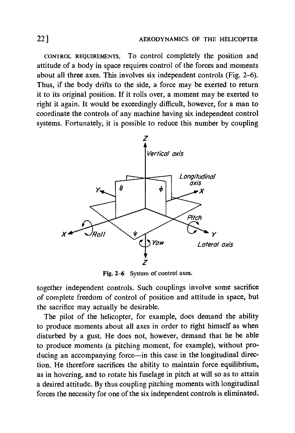
control requirements. To control completely the position and
attitude of a body in space requires control of the forces and moments
about all three axes. This involves six independent controls (Fig. 2-6).
Thus, if the body drifts to the side, a force may be exerted to return
it to its original position. If it rolls over, a moment may be exerted to
right it again. It would be exceedingly difficult, however, for a man to
coordinate the controls of any machine having six independent control
systems. Fortunately, it is possible to reduce this number by coupling
Vertical axis
Longitudinal
axis
X
Y
Lateral axis
Fig. 2-6 System of control axes.
together independent controls. Such couplings involve some sacrifice
of complete freedom of control of position and attitude in space, but
the sacrifice may actually be desirable.
The pilot of the helicopter, for example, does demand the ability
to produce moments about all axes in order to right himself as when
disturbed by a gust. He does not, however, demand that he be able
to produce moments (a pitching moment, for example), without
producing an accompanying force—in this case in the longitudinal
direction. He therefore sacrifices the ability to maintain force equilibrium,
as in hovering, and to rotate his fuselage in pitch at will so as to attain
a desired attitude. By thus coupling pitching moments with longitudinal
forces the necessity for one of the six independent controls is eliminated.

AN INTRODUCTION TO THE HELICOPTER
[23
Actually, four independent controls are adequate for the helicopter.
These are discussed and illustrated below.
(1) Vertical control. This is necessary to fix the position of the
helicopter in the vertical direction. It is achieved by increasing or decreasing
the pitch of the rotor so as to increase or decrease the thrust.
(c)
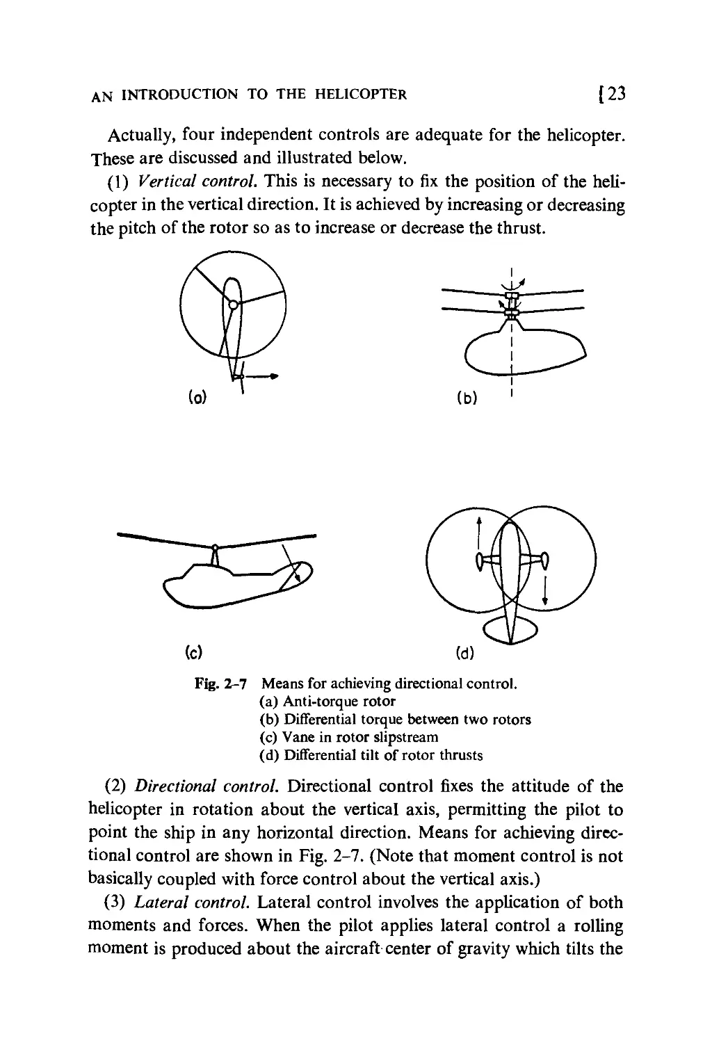
Fig. 2-7 Means for achieving directional control.
(a) Anti-torque rotor
(b) Differential torque between two rotors
(c) Vane in rotor slipstream
(d) Differential tilt of rotor thrusts
(2) Directional control. Directional control fixes the attitude of the
helicopter in rotation about the vertical axis, permitting the pilot to
point the ship in any horizontal direction. Means for achieving
directional control are shown in Fig. 2-7. (Note that moment control is not
basically coupled with force control about the vertical axis.)
(3) Lateral control. Lateral control involves the application of both
moments and forces. When the pilot applies lateral control a rolling
moment is produced about the aircraft center of gravity which tilts the

24] AERODYNAMICS OF THE HELICOPTER
helicopter. As a consequence of the tilt, a component of the rotor
thrust vector acts in the direction of tilt. The application of lateral
control has therefore resulted in a tilt and sideward motion of the
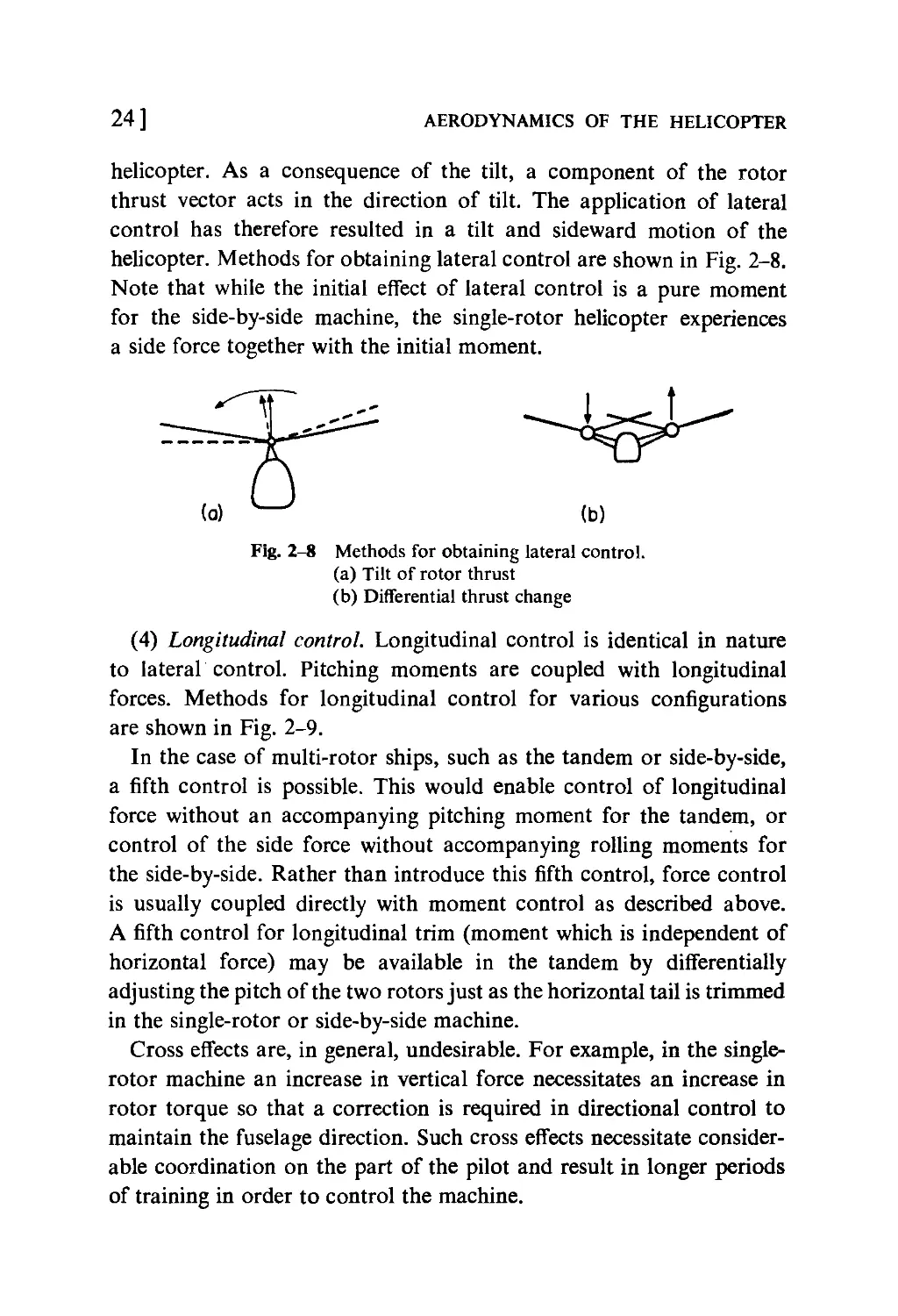
helicopter. Methods for obtaining lateral control are shown in Fig. 2-8.
Note that while the initial effect of lateral control is a pure moment
for the side-by-side machine, the single-rotor helicopter experiences
a side force together with the initial moment.
t
(b)
Fig. 2-8 Methods for obtaining lateral control.
(a) Tilt of rotor thrust
(b) Differential thrust change
(4) Longitudinal control. Longitudinal control is identical in nature
to lateral control. Pitching moments are coupled with longitudinal
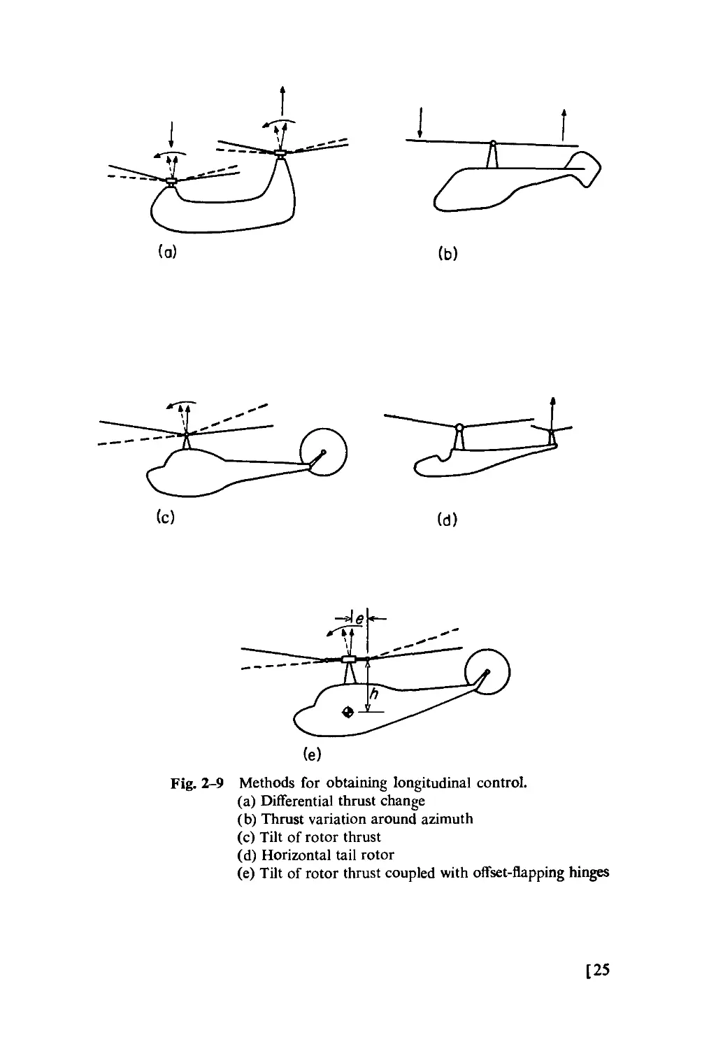
forces. Methods for longitudinal control for various configurations
are shown in Fig. 2-9.
In the case of multi-rotor ships, such as the tandem or side-by-side,
a fifth control is possible. This would enable control of longitudinal
force without an accompanying pitching moment for the tandem, or
control of the side force without accompanying rolling moments for
the side-by-side. Rather than introduce this fifth control, force control
is usually coupled directly with moment control as described above.
A fifth control for longitudinal trim (moment which is independent of
horizontal force) may be available in the tandem by differentially
adjusting the pitch of the two rotors just as the horizontal tail is trimmed
in the single-rotor or side-by-side machine.
Cross effects are, in general, undesirable. For example, in the single-
rotor machine an increase in vertical force necessitates an increase in
rotor torque so that a correction is required in directional control to
maintain the fuselage direction. Such cross effects necessitate
considerable coordination on the part of the pilot and result in longer periods
of training in order to control the machine.

(b)
(c)
(d)
Fig. 2-9 Methods for obtaining longitudinal control.
(a) Differential thrust change
(b) Thrust variation around azimuth
(c) Tilt of rotor thrust
(d) Horizontal tail rotor
(e) Tilt of rotor thrust coupled with offset-flapping hinges
[25

26] AERODYNAMICS OF THE HELICOPTEk
the pilot's controls. In order to produce the forces and moments
necessary to control the machine the pilot is supplied with levers
which he moves with his hands and feet. The conventional system of
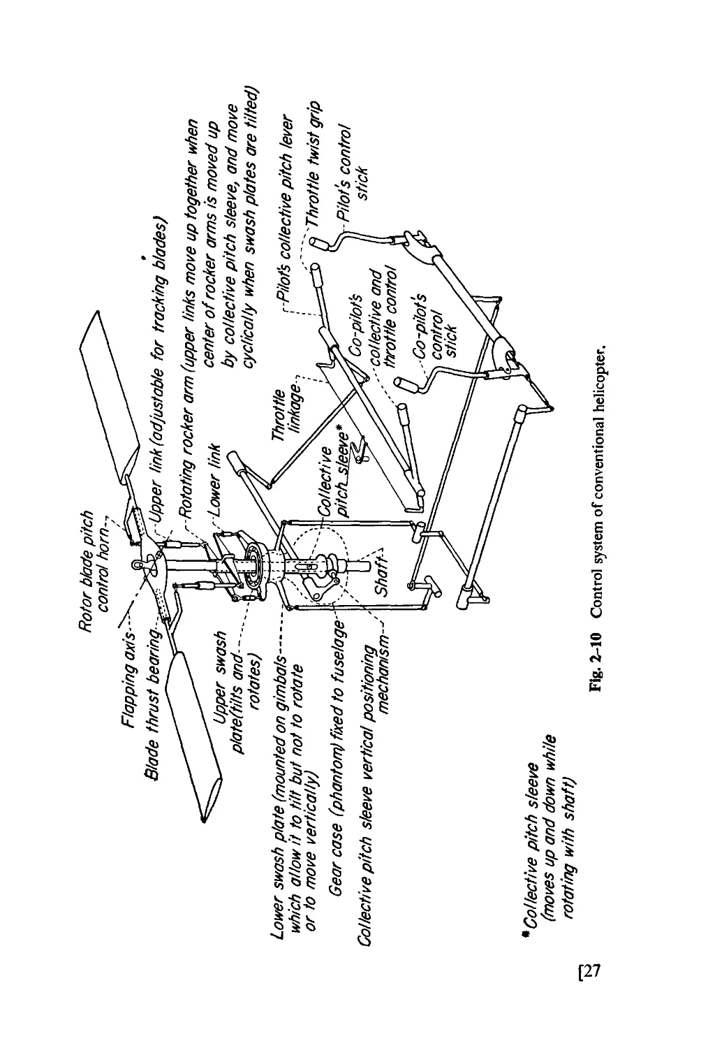
levers is described below and illustrated in Fig. 2-10.
The control stick is located in front of the pilot. It is comparable to
the stick of an airplane and is used for longitudinal and lateral control.
In the helicopter the pilot pushes the stick in the direction he wishes
to go—forward, sideward, or backward.
Pedals, as in an airplane, are used for directional control. To point
the ship toward the right the pilot pushes the right pedal; to the left,
the left pedal.
The pitch lever is operated by the pilot's other hand and is used to
control the pitch of the rotor for up and down flight and for
adjustments as required in forward flight. If the control system is a direct
mechanical linkage, the pitch stick is usually located at the pilot's
side and is moved in an up and down direction. If the pitch is
controlled electrically or hydraulically, the lever may be a small pointer
located within convenient reach, although in that instance a full-sized
emergency lever would also be provided in case of power-control
failure.
The throttle is usually located near or on the pitch stick. In the case
of the mechanical control system, throttle adjustments are accomplished
by twisting a grip located at the top of the pitch stick. In the case of
the powered (electrical or hydraulic) control, the throttle may be
located parallel to the pitch lever so that the two may be moved
together with one hand. In either case, linkages which produce the
necessary throttle change with a given pitch change are usually provided,
so as to automatically keep the rotor speed approximately constant.
In fact, a constant speed governor may be provided which relieves the
pilot of either the pitch or throttle control. In the first case, the governor
adjusts rotor pitch to absorb the engine power and to maintain a
constant rotational speed. In the second case, the governor adjusts the
throttle so as to supply the proper power for a given pitch setting,
again so as to maintain constant rotor speed.
Devices are sometimes employed which automatically decrease the
rotor pitch so as to maintain a certain minimum rotor speed in order

a
c
o
I
I
[27

28]
AERODYNAMICS OF THE HELICOPTER
to assure autorotation in case of power failure and in case the pilot
fails to lower the pitch immediately.
Rotor Types
There are three fundamental types of lifting rotors:
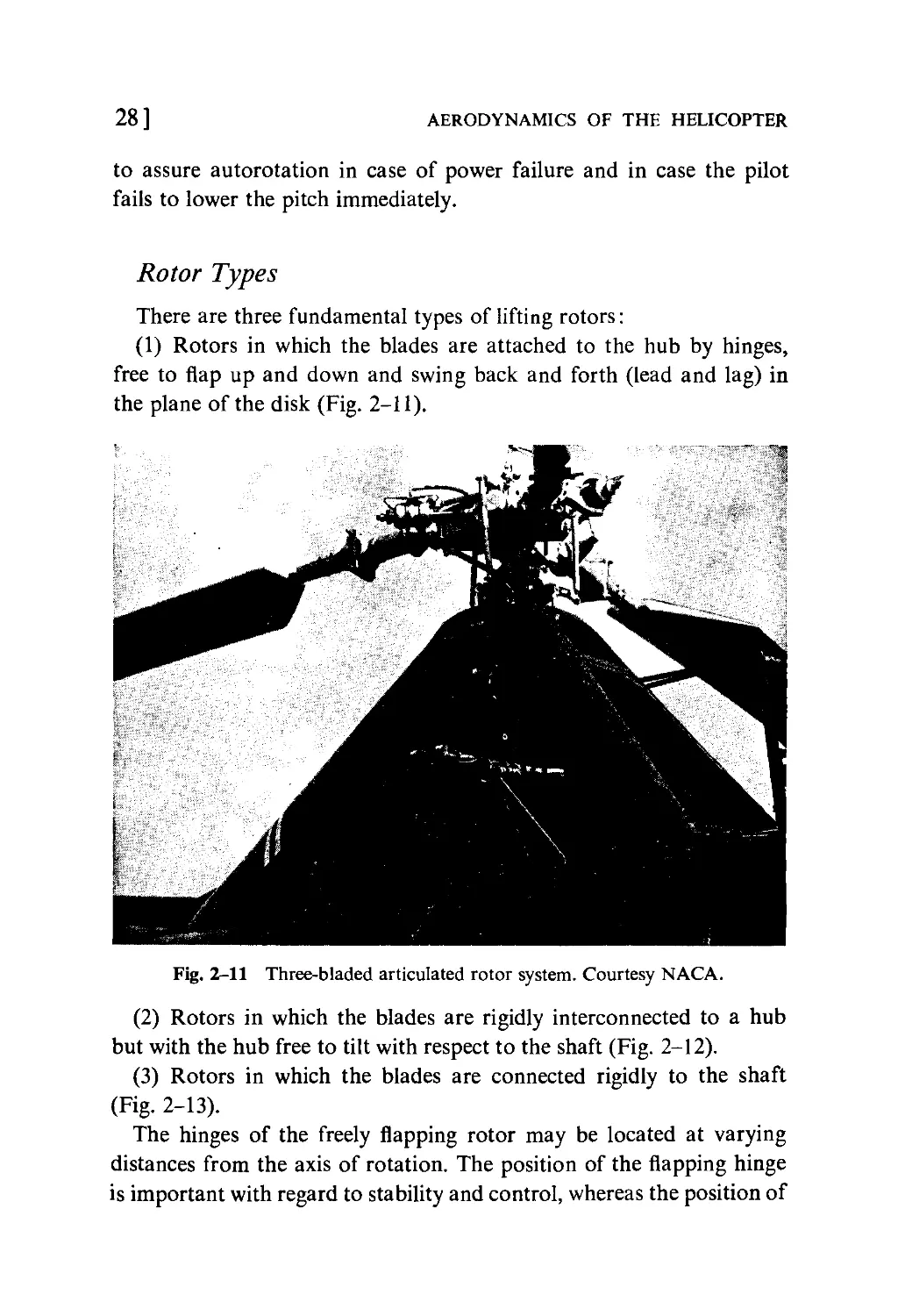
(1) Rotors in which the blades are attached to the hub by hinges,
free to flap up and down and swing back and forth (lead and lag) in
the plane of the disk (Fig. 2-11).
Fig. 2-11 Three-bladed articulated rotor system. Courtesy NACA.
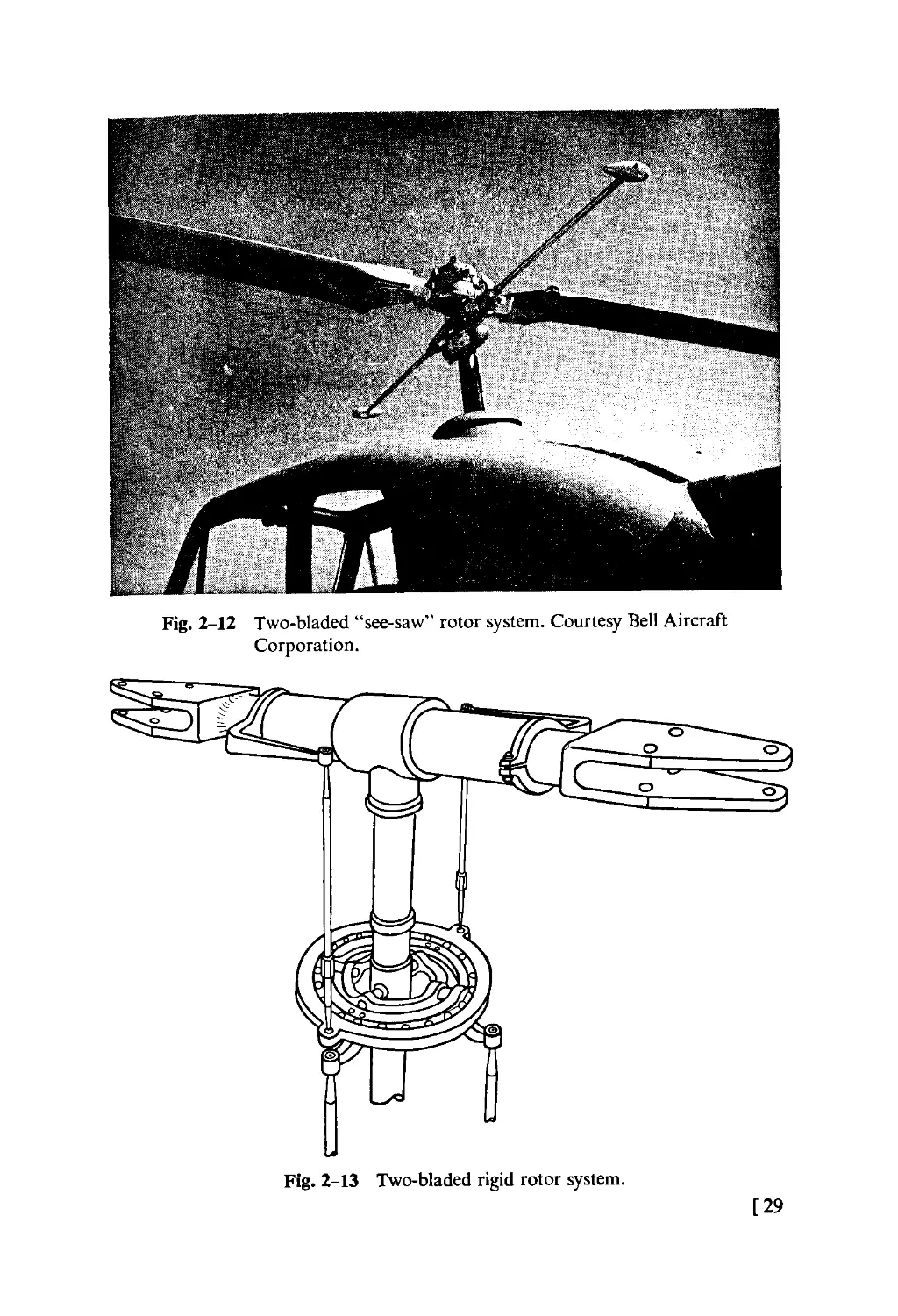
(2) Rotors in which the blades are rigidly interconnected to a hub
but with the hub free to tilt with respect to the shaft (Fig. 2-12).
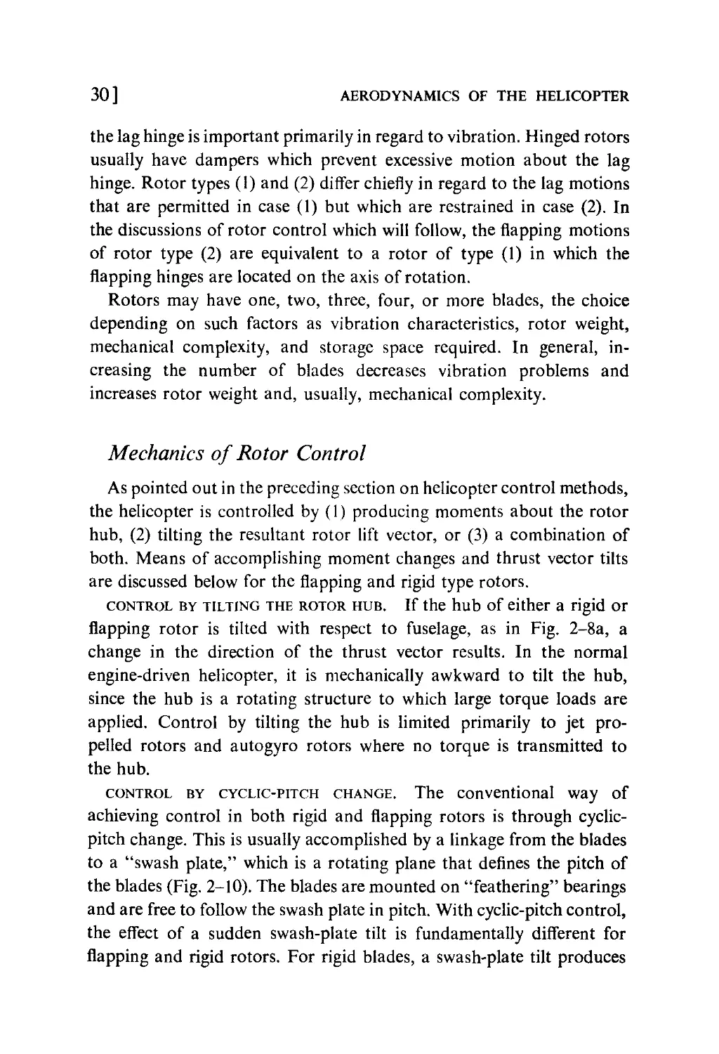
(3) Rotors in which the blades are connected rigidly to the shaft
(Fig. 2-13).
The hinges of the freely flapping rotor may be located at varying
distances from the axis of rotation. The position of the flapping hinge
is important with regard to stability and control, whereas the position of

r
Wl I <w l^^HshK^^^H^^^^^b
Fig. 2-12 Two-bladed "see-saw" rotor system. Courtesy Bell Aircraft
Corporation.
Fig. 2-13 Two-bladed rigid rotor system.
[29

30] AERODYNAMICS OF THE HELICOPTER
the lag hinge is important primarily in regard to vibration. Hinged rotors
usually have dampers which prevent excessive motion about the lag
hinge. Rotor types (1) and (2) differ chiefly in regard to the lag motions
that are permitted in case (1) but which are restrained in case (2). In
the discussions of rotor control which will follow, the flapping motions
of rotor type (2) are equivalent to a rotor of type (1) in which the
flapping hinges are located on the axis of rotation.
Rotors may have one, two, three, four, or more blades, the choice
depending on such factors as vibration characteristics, rotor weight,
mechanical complexity, and storage space required. In general,
increasing the number of blades decreases vibration problems and
increases rotor weight and, usually, mechanical complexity.
Mechanics of Rotor Control
As pointed out in the preceding section on helicopter control methods,
the helicopter is controlled by (1) producing moments about the rotor
hub, (2) tilting the resultant rotor lift vector, or (3) a combination of
both. Means of accomplishing moment changes and thrust vector tilts
are discussed below for the flapping and rigid type rotors.
control by tilting the rotor hub. If the hub of either a rigid or
flapping rotor is tilted with respect to fuselage, as in Fig. 2-8a, a
change in the direction of the thrust vector results. In the normal
engine-driven helicopter, it is mechanically awkward to tilt the hub,
since the hub is a rotating structure to which large torque loads are
applied. Control by tilting the hub is limited primarily to jet
propelled rotors and autogyro rotors where no torque is transmitted to
the hub.
control by cyclic-pitch change. The conventional way of
achieving control in both rigid and flapping rotors is through cyclic-
pitch change. This is usually accomplished by a linkage from the blades
to a "swash plate," which is a rotating plane that defines the pitch of
the blades (Fig. 2-10). The blades are mounted on "feathering" bearings
and are free to follow the swash plate in pitch. With cyclic-pitch control,
the effect of a sudden swash-plate tilt is fundamentally different for
flapping and rigid rotors. For rigid blades, a swash-plate tilt produces

AN INTRODUCTION TO THE HELICOPTER [31
a moment about the rotor hub in the direction of the swash-plate tilt,
owing to the difference in lift on the feathered blades (Fig. 2-14).
For flapping blades with hinges on the axis of rotation, a swash-plate
tilt results in a tilt of the rotor vector. Because the blades are freely
Fig. 2-14 Moment produced by thrust vector offset.
hinged, no moments may be transmitted, and the swash-plate tilt has
the same effect as a corresponding shaft tilt (Fig. 2-9c). When the
flapping hinges are moved outboard, the tilt of the rotor caused by a
swash-plate tilt results in a moment about the hub as well as a thrust
vector tilt. This moment is caused by the blade mass forces acting on
the hub.
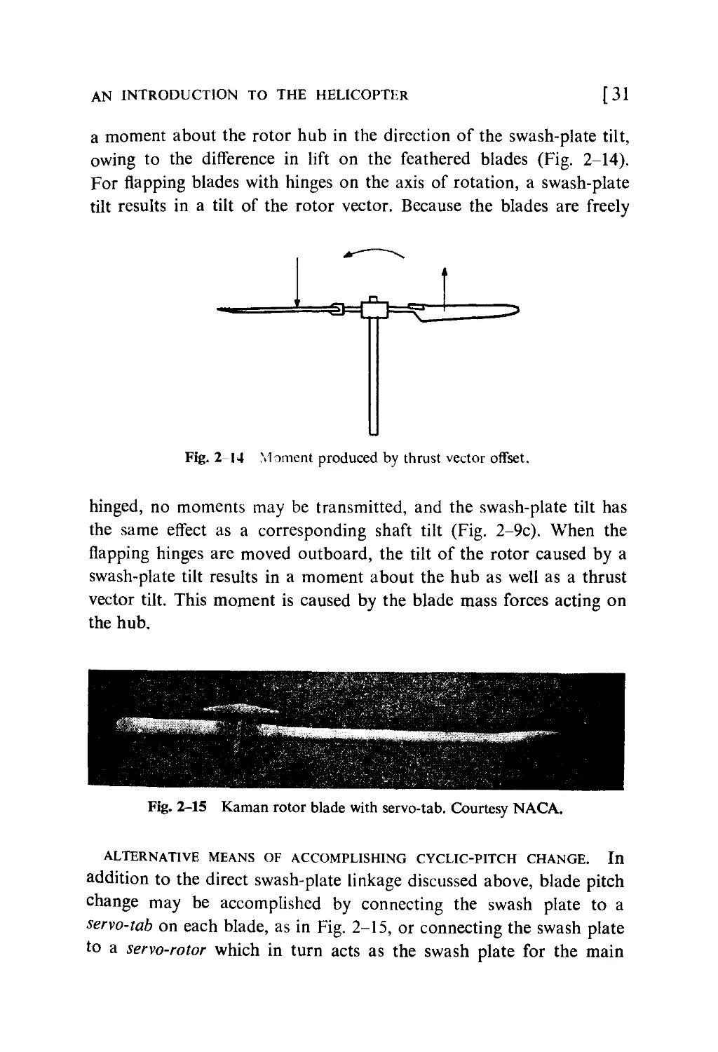
Fig. 2-15 Kaman rotor blade with servo-tab. Courtesy NACA.
ALTERNATIVE MEANS OF ACCOMPLISHING CYCLIC-PITCH CHANGE. In
addition to the direct swash-plate linkage discussed above, blade pitch
change may be accomplished by connecting the swash plate to a
servo-tab on each blade, as in Fig. 2-15, or connecting the swash plate
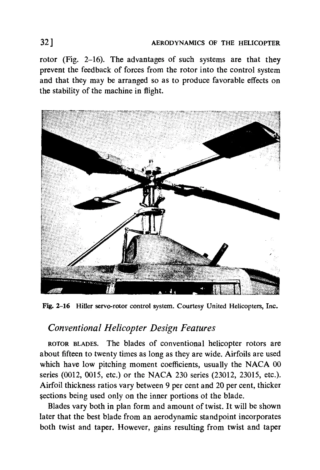
to a servo-rotor which in turn acts as the swash plate for the main

32]
AERODYNAMICS OF THE HELICOPTER
rotor (Fig. 2-16). The advantages of such systems are that they
prevent the feedback of forces from the rotor into the control system
and that they may be arranged so as to produce favorable effects on
the stability of the machine in flight.
Fig. 2-16 Hiller servo-rotor control system. Courtesy United Helicopters, Inc.
Conventional Helicopter Design Features
rotor blades. The blades of conventional helicopter rotors are
about fifteen to twenty times as long as they are wide. Airfoils are used
which have low pitching moment coefficients, usually the NACA 00
series (0012, 0015, etc.) or the NACA 230 series (23012, 23015, etc.).
Airfoil thickness ratios vary between 9 per cent and 20 per cent, thicker
sections being used only on the inner portions of the blade.
Blades vary both in plan form and amount of twist. It will be shown
later that the best blade from an aerodynamic standpoint incorporates
both twist and taper. However, gains resulting from twist and taper

AN INTRODUCTION TO THE HELICOPTER
[33
are oftentimes relatively small (depending on the type of helicopter
and the task it is primarily designed for), and oftentimes factors such
as cost of production win out and blades of simple rectangular plan
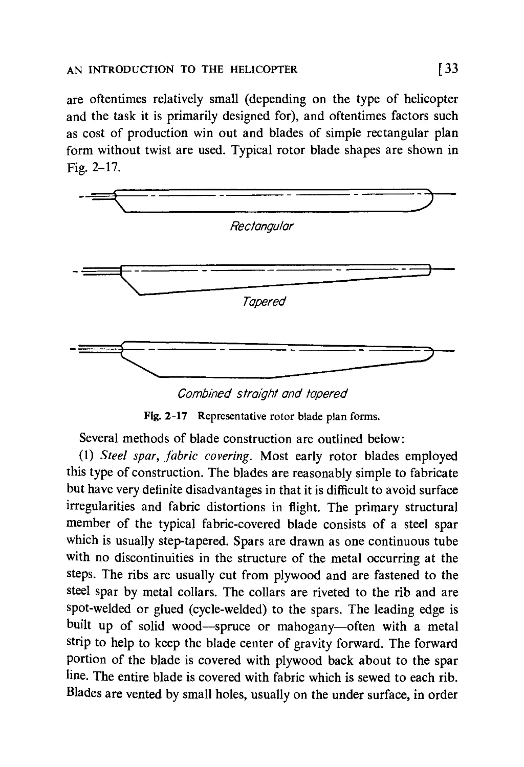
form without twist are used. Typical rotor blade shapes are shown in
Fig. 2-17.
Rectangular
Tapered
Combined straight and tapered
Fig. 2-17 Representative rotor blade plan forms.
Several methods of blade construction are outlined below:
(1) Steel spar, fabric covering. Most early rotor blades employed
this type of construction. The blades are reasonably simple to fabricate
but have very definite disadvantages in that it is difficult to avoid surface
irregularities and fabric distortions in flight. The primary structural
member of the typical fabric-covered blade consists of a steel spar
which is usually step-tapered. Spars are drawn as one continuous tube
with no discontinuities in the structure of the metal occurring at the
steps. The ribs are usually cut from plywood and are fastened to the
steel spar by metal collars. The collars are riveted to the rib and are
spot-welded or glued (cycle-welded) to the spars. The leading edge is
built up of solid wood—spruce or mahogany—often with a metal
strip to help to keep the blade center of gravity forward. The forward
portion of the blade is covered with plywood back about to the spar
line. The entire blade is covered with fabric which is sewed to each rib.
Blades are vented by small holes, usually on the under surface, in order

34] AERODYNAMICS OF THE HELICOPTER
to relieve the internal pressure created by the centrifugal pumping
action of the blade.
(2) Plywood-covered blades. Most of the objectionable features of
the fabric-covered blade can be overcome by using the same basic
structure and covering the entire blade with thin plywood. Some of the
objections to plywood-covered blades are that they require careful
handwork, do not lend themselves to quantity production, and are
not weatherproof.
(3) All-wood blades are used frequently. They are usually built up
from laminations of several woods, heavier woods being used in the
forward portion and light woods such as balsa being used in the
rearward portion. All-wood blades are relatively simple to fabricate,
especially if built with rectangular plan form and constant thickness.
Surfaces can be obtained which are aerodynamically clean and true
to contour. One disadvantage of the all-wood blade is that it is relatively
heavy and, along with fabric and plywood blades, is subject to moisture
and deterioration.
(4) Metal blades are being developed at the present time by most
manufacturers. Blades are either built up from pieces of sheet stock or
utilize extrusions together with sheet metal. Probably the simplest blade
yet fabricated involves an extruded D-spar which forms the leading
edge and a V-shaped sheet metal trailing edge joined to the D-spar
by flush rivets. Entire blade sections have been extruded successfully.
Extrusions lend themselves well to quantity production. It is probably
safe to say that all-metal blades will eventually become standard for
helicopter rotors.
rotor hubs. The hub is a main structural member of the rotor and
is usually forged from steel or dural. Designs differ according to the
hinge offsets and number of blades employed. Usually the forging
houses needle-bearing hinges on which the blades flap.
rotor control linkages. The rotor control mechanism usually
consists of a swash plate, connecting links, and blades which rotate
in their sockets (free to feather). The swash plate consists of a central
nonrotating disk and an outer ring which rotates with the rotor (Fig.
2-10). These parts are connected by thin-race ball or roller bearings.
The inner portion of the swash plate is universally mounted and

AN INTRODUCTION TO THE HELICOPTER [35
connected to a linkage which allows it to move up and down and tilt
in any direction. Blades are connected to the swash plate by links so
that the pitch of the blade is determined by the plane of the swash
plate. Care is usually taken to proportion the linkage so that in its
normal operating attitude the blade will not change pitch as it flaps
or lags. Furthermore, linkages are arranged to minimize these couplings
of pitch with flap or lag in all positions of the blade. Changes of pitch
with flapping, if moderate, have some desirable effects and are often
purposely incorporated. Large changes of pitch with lag angle, however,
are undesirable and are usually avoided as much as possible.
the control system. A typical direct-linkage control system for a
single-rotor helicopter may be understood by again referring to Fig.
2-10. It is seen that the control stick is connected so as to tilt the swash
plate in the direction in which the stick is moved. The pitch stick raises
and lowers the pitch sleeve while retaining any tilt imposed by the
control stick. The mechanical advantage between control stick and
blade is usually such that 1 inch of stick motion results in 1 to 2 degrees
of cyclic-pitch change.
In multi-rotor configurations, control systems are necessarily
modified. In the side-by-side machine the swash plate may be free to tilt only
in a fore and aft direction. In this case, lateral control is achieved by
raising one swash plate and lowering the other, thus tilting the ship
and producing sideward motion. Lateral control may also involve a
swash-plate tilt which is coupled with the collective pitch change so
as to tilt the thrust vector laterally as well as roll the machine. The same
remarks apply to tandem machines in regard to longitudinal control.
fuselage design. Several factors which influence fuselage design
are listed below:
(1) A streamlined shape for low parasite-drag and moment
coefficients.
(2) Good visibility for the pilot.
(3) Area for disposable load located as nearly under the rotor as
possible to avoid center of gravity shifts.
(4) Easy accessibility to engines and transmissions.
(5) Accommodation of a tail rotor and/or stabilizing surfaces at a
reasonable moment arm.

36] AERODYNAMICS OF THE HELICOPTER
In order to increase the range of center of gravity travel for a given
control tilt and in order to improve the control of the machine, it is
desirable to keep the center of gravity as far below the rotor center as
possible.
landing gear. Landing gears of both the three-wheel and four-
wheel types are used. Landing gear design is comparable to normal
airplane design except that the stroke available in the shock absorber
of the helicopter is usually considerably longer to provide softer action
in landings and provide damping for "ground resonance." Alternate
gear arrangements, which permit operation from all possible types of
terrain, are sometimes supplied by the manufacturer. Thus notation
gear which is suitable for water, land, and marsh operation is available,
as well as skid gear for high forward-speed landings on rough, plowed
ground as well as on improved surfaces, and ski gear for soft snow and
rough ice. In all cases, it is important that the landing angle, as
determined by tail wheel or tail skid position, be sufficient to permit high
pitch-up attitudes of the fuselage for flare-outs in autorotation landings.
transmission systems. Transmission systems usually involve gear
ratios between engine and rotor of the order of 10:1. Planetary gear
trains are most efficient from a weight point of view but are expensive
and often noisy. Bevel gears, along with a single-stage-planetary-gear
train, are frequently used. The drive system is also supplied with a
clutch which is engaged either manually by the pilot or centrifugally
when a certain engine speed is reached. In addition to the clutch, a
free-wheeling unit or overriding clutch is incorporated so that the
engine may drive the rotor, but the rotor cannot drive the engine in
case of power failure. In a single-rotor machine, the tail rotor is geared
directly to the main rotor so that in case of engine failure, the main
rotor turns the tail rotor.
Flight Characteristics of the Helicopter
An appreciation of the flight characteristics of the helicopter involves
an understanding of its performance characteristics, its vibration
characteristics, and its stability and control characteristics. The
following paragraphs deal with these topics in a qualitative manner.

AN INTRODUCTION TO THE HELICOPTER [37
performance characteristics. Power must be supplied to the
rotor of the hovering helicopter for two reasons:
(1) Power is required to produce lift. This is referred to as induced
power.
(2) Power is required to drag the blades through the air. This is
called profile-drag power.
The helicopter rotor produces thrust to support the helicopter in
air by imparting momentum to a mass of air. The rotor imparts a
downward velocity to a large mass of air and, in so doing, realizes an
upward thrust. It is clear that power must be expended to produce this
jet of air. The power is, in fact, proportional to the downwash velocity
for a given weight of helicopter. The downwash velocity, in turn,
depends upon the amount of air to which velocity is imparted in
producing the rotor thrust. A large diameter rotor, then, can lift a
weight with much less induced loss than a small diameter rotor.
Profile-drag power arises entirely from the fact that air is a viscous
fluid and that when a body is pulled through this fluid frictional forces
are exerted on the body.
For the normal helicopter in hovering, induced losses account for
about 60 per cent to 70 per cent of the total rotor power required;
profile-drag losses account for about 30 per cent to 40 per cent. The
engine must supply sufficient power for the rotor and, in the case of
a single-rotor machine, for the tail rotor in order that the helicopter
may hover. If more power is applied to the rotor than is required
to overcome the induced and profile losses, then the helicopter
will climb.
In forward flight power must be supplied to drag the fuselage through
the air as well as to overcome the induced and profile-drag losses. The
power required to drag the fuselage through the air increases as the
cube of the forward speed and becomes large at higher speeds. In one
of the early production helicopters, for example, one-half of the
available engine power was used in overcoming fuselage drag at
80 miles per hour.
While parasite-drag power increases rapidly with airspeed, the power
required to produce lift—the induced power—decreases with increasing
speed. As the rotor moves forward, it encounters a larger mass of air

38]
AERODYNAMICS OF THE HELICOPTER
per second. To produce its thrust it therefore needs to impart less
velocity to each mass of air and the energy imparted to the air is
thereby reduced.
The profile-drag power increases slightly as forward speed is
increased, the increase becoming very rapid at high forward speeds.
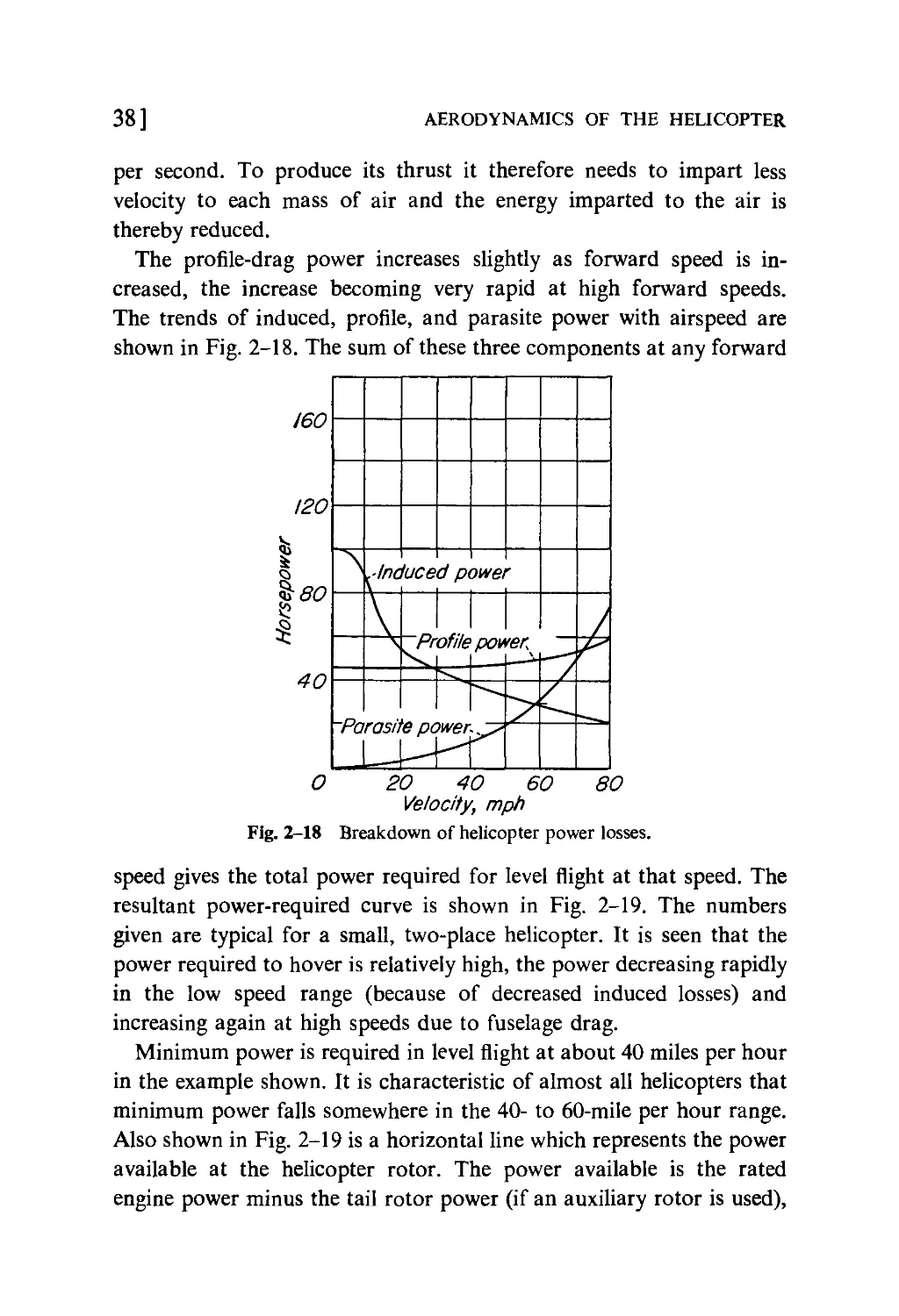
The trends of induced, profile, and parasite power with airspeed are
shown in Fig. 2-18. The sum of these three components at any forward
160
120
!
40
\
-Pa
.■Induced powe\
\
rash
L=J
Pr
ofile
>wer
M
r
'er\
>
■—
0 20 40 60 80
Velocity, mph
Fig. 2-18 Breakdown of helicopter power losses.
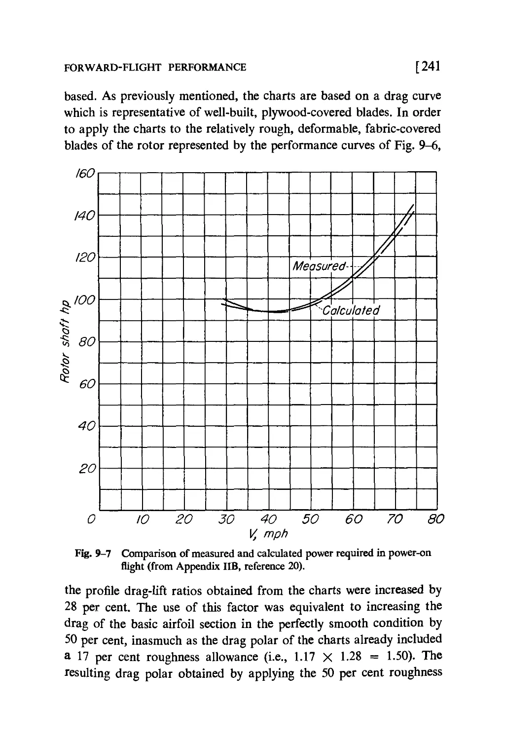
speed gives the total power required for level flight at that speed. The
resultant power-required curve is shown in Fig. 2-19. The numbers
given are typical for a small, two-place helicopter. It is seen that the
power required to hover is relatively high, the power decreasing rapidly
in the low speed range (because of decreased induced losses) and
increasing again at high speeds due to fuselage drag.
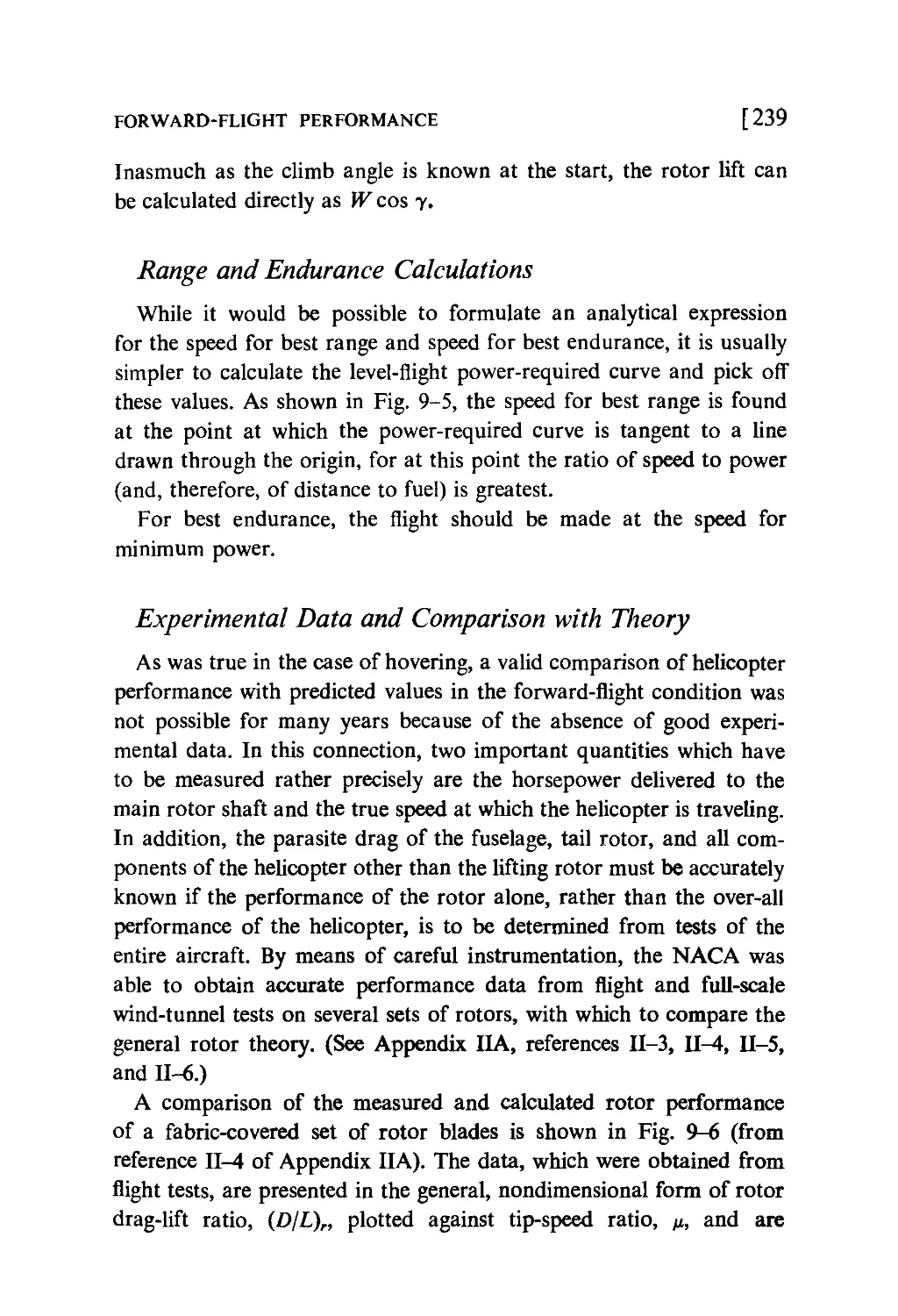
Minimum power is required in level flight at about 40 miles per hour
in the example shown. It is characteristic of almost all helicopters that
minimum power falls somewhere in the 40- to 60-mile per hour range.
Also shown in Fig. 2-19 is a horizontal line which represents the power
available at the helicopter rotor. The power available is the rated
engine power minus the tail rotor power (if an auxiliary rotor is used),

AN INTRODUCTION TO THE HELICOPTER
[39
as well as the frictional losses in the transmission, and losses from
powering a blower to cool the engine.
It is clear that the performance capabilities of a helicopter are
determined by the level of the power-available curve with respect to the
power-required curve. If, for example, the power available is just equal
to the power required to hover, as in curve (a) of Fig. 2-19, the
performance of the machine is marginal. It is only barely able to hover
160
120
I
%80
40
0 20 40 60 80
Velocity, mph
Fig. 2-19 Power-available and power-required curves.
and unable to climb vertically. A slight overload would increase the
induced power required and the machine would be unable to hover.
Actually, a helicopter is able to hover very near the ground even
when it has insufficient power to hover away from the ground. This
is because of a phenomenon known as ground effect. The ground stops
the rotor downwash, or induced velocity, thus decreasing the induced
power required.
It will also be noted that because of the reduction of power required
with forward speed, an overloaded helicopter may take off in a wind
or by making a run on the ground to attain a small forward speed.
While the machine can fly forward in this overloaded condition, it
cannot hover. The marginal hovering performance of many present-day
-N
(b) Psium
-(a)
\
\
(gt
*r availo
iod pert
blc
')
Power available
(marginal)
Pow
er rt
—"
>quii
■ed-
/
/
X
/

40] AERODYNAMICS OF THE HELICOPTER
helicopters has resulted in the loss of several machines in the hands of
inexperienced pilots. When flying close to the ground there is a tendency
to fly by ground speed rather than according to the airspeed indicator.
If winds are involved, a "downwind turn" may result in zero airspeed,
so that the machine will settle to the ground. Again, the helicopter may
be hovering in a wind above some obstacle, such as a row of trees.
When the helicopter drops below the trees, where the wind is decreased,
it is unable to hover and settles to the ground.
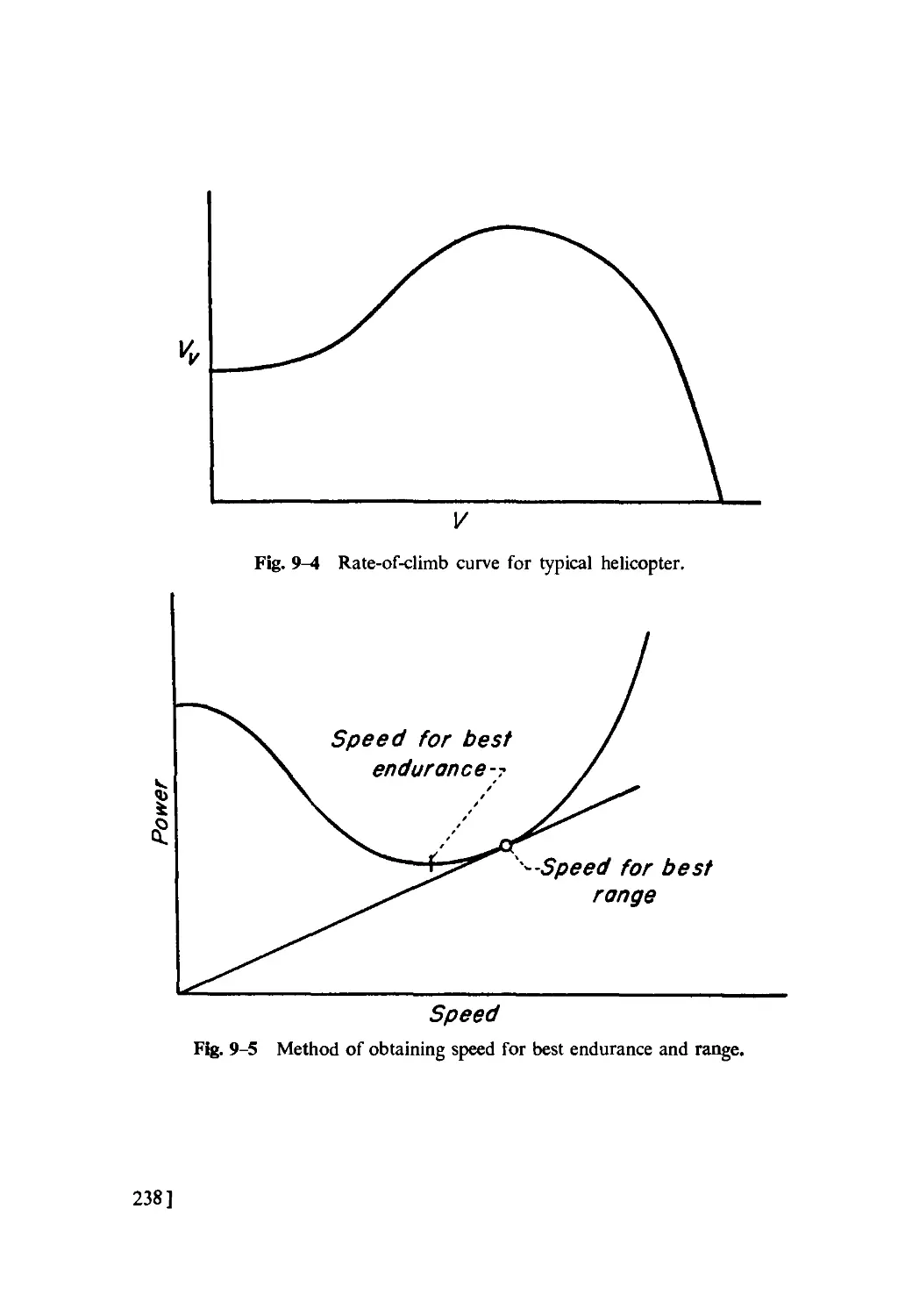
It is clear from Fig. 2-19 that best climb with the helicopter will
occur at about the speed for minimum power in level flight, for here
the greatest excess power available for climb exists.
Top speed in level flight is determined by the point where the power-
required curve and power-available curves cross. It will be noted that
the slope of the power-required curve is very steep at high speed,
because fuselage-drag power is increasing at a rapid rate. Thus, it is
very difficult to increase the top speed of the machine appreciably by
increase in power, inasmuch as very large increases in power are
required to make significant gains in top speed. On a percentage basis,
reductions in fuselage drag by "cleaning up" the fuselage are far more
effective in increasing top speed than increases in power.
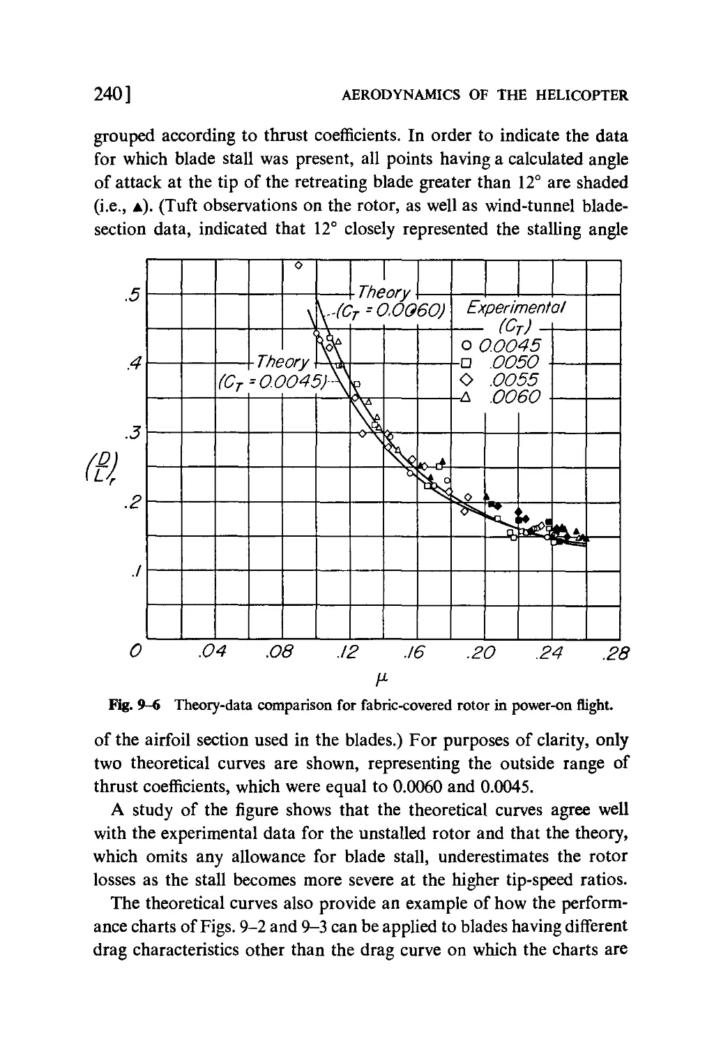
At high forward speeds blade stall is encountered over a portion of
the rotor disk. Stall causes vibration of the helicopter and controls
and a considerable increase in profile-drag power. Blade stall is due
to the difference in velocity encountered by the advancing and retreating
blades in forward flight. As a lifting rotor moves forward, the advancing
blades encounter progressively higher velocities and the retreating
blades progressively lower velocities. In order to maintain its lift, the
retreating blade must operate at progressively higher angles of attack
as forward speed increases. It follows that at some forward speed the
angles of attack on the retreating side will reach the stall.
While the dissymmetry can be reduced by turning the rotor faster,
thus permitting a higher forward speed for a given amount of stall,
this method soon leads to excessively high velocities over the advancing
blade and accompanying power losses and roughness due to
compressibility effects. The fundamental limits to the high speed of the
helicopter are therefore blade stall and blade Mach number. It will

AN INTRODUCTION TO THE HELICOPTER [41
always be difficult to build helicopters which can reach speeds very
much greater than about 200 miles per hour.
In case of power failure, the helicopter is able to glide, its rotors
continuing to whirl in autorotation as does the rotor of the autogyro.
In vertical descent the rotor is about as effective as a parachute of the
same diameter in allowing the machine to descend slowly. At its best
gliding speed the rotor lets the helicopter down at about one-half the
vertical autorotative rate of descent, or about 15 to 20 feet per second.
As the helicopter approaches the ground the pilot may pull back on
his stick and "flare out," trading his energy of forward motion for
additional lifting power. In this manner, he is able to settle slowly to
the ground with very little forward speed. He may also take advantage
of the energy in the rotor and increase the blade pitch, producing
additional thrust while decelerating the rotor.
control forces. Stick forces in the helicopter are quite important
in regard to the pilot's impressions of the machine. Pilots tend to fly
aircraft by the "force feel" of the stick rather than by stick
displacements. Without accurate reference points it is extremely difficult to
judge the number of inches which a stick has been displaced. Most
pilots like a moderate force gradient always resisting a motion of the
stick. For steady flight, desirable stick force characteristics require
that the pilot push with moderate but increasing force to move the
stick forward and pull with increasing force to move the stick aft.
When released, the stick should return to a neutral position.
In maneuvers, the forces which feed back into the pilot's stick have
considerable influence on his impressions of the stability of the machine.
If in a maneuver forces are created which tend to move the pilot's hand
in a direction to aggravate the maneuver, the pilot experiences difficulty
in properly controlling the machine.
While stick forces are quite important in regard to flying qualities,
they are difficult to control in the helicopter. Stick forces in the
helicopter do not arise from straightforward sources as in an airplane.
In an airplane a motion of the control stick deflects a hinged control
surface. Because of the deflection of the hinged surface a moment is
created which is transmitted to the pilot's stick. In the simple cyclic-
pitch control rotor, on the other hand, a motion of the stick changes

42] AERODYNAMICS OF THE HELICOPTER
the pitch of the blades as they rotate. In the helicopter, all stick forces
must therefore arise from pitching moments on the blades themselves.
When airfoil sections are chosen and mounted so as to have no pitching
moments at any pitch angle, then there should be no stick forces for
the pilot to overcome.
Actually, pitching moments exist on rotor blades because of several
secondary effects such as airfoil imperfections, blade-bending
distortions, chordwise mass balance, etc. Stick forces are caused from
these secondary effects rather than from straightforward moments as
in the airplane.
Control forces consist of both oscillating forces and steady forces.
Oscillating forces may occur at frequencies of 1/rev. and even multiples
of the number of blades. Oscillating forces with a frequency of 1/rev.
are entirely chargeable to differences in pitching moments between the
rotor blades. For example, if only one blade of a three-bladed rotor
experiences a pitching moment, this one blade exerts a steady force
on the swash plate as it rotates. This rotating force is transmitted to
the control stick. Because the pilot's hand is not a rigid support, the
control stick yields under the rotating force and describes a small circle.
Helicopters are often characterized by a small 1/rev. stick shake.
Higher frequency oscillations in the control stick can arise at integral
multiples of the number of rotor blades. A three-bladed rotor may,
therefore, experience a 3/rev., 6/rev., 9/rev., etc., oscillation in the
controls. These higher frequency oscillations arise from periodic
changes in the pitching moment of each blade. The periodic changes, in
turn, arise from periodic air force changes in a rotor in forward flight
or from periodic blade deflections. For example, a three-bladed rotor
with equal pitching moments on all three blades will produce a 3/rev.
motion of the control stick in forward flight because of the change in
velocity on the advancing and retreating blades. As the blade comes
forward and experiences higher velocities, its pitching moment is
increased, and since this happens three times for each rotor revolution,
a 3/rev. shake of the control stick results.
Oscillating forces in the control system can be prevented from
annoying the pilot by the use of irreversible controls or by making the effective
mass of the pilot's stick large enough to absorb the oscillating force.

AN INTRODUCTION TO THE HELICOPTER [43
One convenient means of accomplishing the latter is by the use of an
inertia damper which may consist of a weight on a high-pitch screw,
the weight being forced to rotate when axial force is applied to the
screw. The inertia damper is simply a means of producing a large,
effective mass without heavy weights.
Steady forces on the control stick come entirely from 1/rev. variations
in blade-pitching moments. These again may arise from periodic air
forces, periodic blade deflections, or both.
Sometimes tabs are used on blades intentionally to produce pitching
moments. In forward flight these pitching moments then vary
periodically as the velocity over the blade varies, becoming large on the
advancing blade and small on the retreating blade. A steady stick force
results.
Usually stick forces are relatively small in small rotors (20 to 30 feet
in diameter). As diameters increase, however, stick forces increase
rapidly. It is, therefore, very difficult to use directly connected controls
in large rotors since extreme care must be taken in blade construction
to avoid the small secondary effects which produce the annoying control
forces. Servo controls, which relieve the pilot from these feedback
forces, seem to be necessary for very large helicopters.
vibration characteristics. As in the case of control oscillations,
the helicopter itself is subject to vibrating forces from the rotor. If it
is assumed that the force input from each rotor blade is identical, then
the only frequencies at which oscillations occur are again even multiples
of the number of rotor blades. Vibrating forces may be in a vertical,
fore and aft, or sideward direction. The reduction of the input forces
from the rotor blade is primarily a question of blade design, involving
the proper distribution of masses and air forces along the span. The
effect of the input forces on the vibration characteristics of the machine
depends considerably upon the natural frequencies of the fuselage
structure. If the fuselage structure has any mode of vibration, such as
vertical bending, fuselage torsion, etc., in resonance with an exciting
frequency, vibrations may become quite disagreeable. One of the main
problems in minimizing vibrations in the helicopter lies in avoiding
natural exciting frequencies. This is difficult since exciting frequencies
cover a wide range (3/rev., 6/rev., 9/rev., etc.).

44] AERODYNAMICS OF THE HELICOPTER
ground resonance. The helicopter is a very complex dynamic
system, involving masses and springs in several degrees of freedom.
Sometimes couplings occur between blade lag motion in the rotating
system and sideward or fore and aft motion of the shaft. If insufficient
damping is present in the system, a self-excited vibration may result,
the ship shaking back and forth with increasing amplitude and the
blades moving back and forth in the plane of rotation, out of pattern.
This phenomenon is commonly known as ground resonance because
the most frequent place of occurrence of the vibration is on the ground
where the machine is supported on its relatively soft tires, giving a
low natural frequency of the machine in sideward motion. Ground
resonance, if it begins, often results in complete destruction of the
machine within a few seconds. Several helicopters and autogyros have
been destroyed by these self-excited vibrations.
stability characteristics. Hovering in the conventional
helicopter requires considerable practice on the part of the pilot, although
most of the problems tend to disappear with experience. The novice
pilot must learn to put up with high control sensitivity in roll, or, in
other words, the high rate of roll per inch of stick displacement.
Helicopters with conventional control systems are subject to high
control sensitivity which, according to reference VI-7 (Appendix IIA),
can lead to overcontrolling, and in turn, to a short-period, pilot-induced
lateral oscillation. High control sensitivity is apparently due to low
rotor damping, which for the helicopter is a fraction of that for airplanes
(reference VI-7, Appendix IIA). This problem is therefore minimized
with large diameter rotors, which have greater damping than small
rotors.
The normal helicopter in hovering is somewhat sluggish in response
to a sudden control deflection. This sluggishness is not due to a lag
in the response of the rotor to an applied control motion, for the rotor
follows almost instantaneously a motion of the stick, but rather to the
fact that velocity changes or displacement of the helicopter in space
do not follow the inclination of the thrust vector immediately because
of the mass of the helicopter. During training the student pilot
overcomes his first impressions of lag by learning to control the helicopter's
accelerations.

AN INTRODUCTION TO THE HELICOPTER [45
If disturbed from hovering equilibrium with control stick fixed, the
helicopter will describe a slow, translational oscillation and move back
and forth with slowly increasing amplitude. The conventional
helicopter is thus dynamically unstable in hovering. The instability is
easily controllable, however, and is not considered a serious handicap
in the machine inasmuch as the period of the oscillation is long enough
to allow for the pilot's reaction time in perceiving and correcting the
motion. There are several means of stabilizing the helicopter in hovering,
all of which utilize gyroscopic forces.
In forward flight, the normal helicopter may exhibit some undesirable
tendencies in the longitudinal control. Helicopters have a tendency to
"zoom" at low forward speeds following take-off, pitching upward
abruptly, and sometimes requiring full forward stick motion to regain
control of the machine. At normal cruising speed the conventional
helicopter is usually dynamically unstable in pitch, but only mildly so,
with a long enough period to allow the pilot to recognize the disturbance
and correct it. This instability is primarily due to low rotor damping
and to the fact that the conventional helicopter rotor is statically
unstable with angle of attack, the instability becoming greater as the
forward speed is increased. Because of this increase of angle-of-attack
instability with forward speed, the attentiveness required of the pilot
to correct for a disturbance increases rapidly as the helicopter's top
speed is reached, in that at those speeds the disturbance builds up so
rapidly that corrective control must be applied in a few seconds. The
elimination of this pitching instability is considered to be of primary
importance in achieving satisfactory flying qualities. Many
experimental helicopters, and several production machines, already
incorporate devices which either increase the damping in pitch or add
positive static stability with angle of attack.
Most helicopters on the market today have definite instabilities in
some regimes of flight and by airplane standards have very poor flying
qualities. The stability and control characteristics of the helicopter
represent a major present-day development problem, but because they
are receiving considerable attention from manufacturers and
government research agencies, it may be stated with confidence that a rapid
improvement of helicopter flying qualities will not be long forthcoming

AN INTRODUCTION
TO HOVERING THEORY
It is best to start the study of rotor theory with hovering and vertical
flight, inasmuch as there is no dissymmetry of velocities across the
rotor disk in those flight conditions. In other words, contrary to forward
flight, the same conditions exist at a blade element operating at a given
radial distance, irrespective of its azimuth position.
The hovering theory presented in the following chapters is based on
the combination of the momentum theory, originated by W. J. M.
Rankine and developed by R. B. Froude, and the blade-element theory.
Identical equations may be derived by means of the vortex theory, but
it is believed that the combination of the momentum and blade-element
theories has greater physical significance and can be more easily
grasped.
Momentum Considerations
development of thrust. The momentum theory stems from
Newton's second law of motion, F = ma, and is developed on the
basis that the axial velocity u of the fluid through the airscrew disk
is generally higher than the speed V with which the airscrew is advancing
through the air. The increase in velocity of the air from its initial value
V to its value at the airscrew disk, which arises from the production
of thrust, is called the induced or downwash velocity, and is denoted by
v. The thrust developed by the airscrew is then equal to the mass of
46]

AN INTRODUCTION TO HOVERING THEORY
[47
air passing through the disk in unit time, multiplied by the total increase
in velocity caused by the action of the airscrew.
In hovering or vertical climb, the action of the air influenced by a
helicopter rotor is as shown in Fig. 3-1. Because of the increase in
velocity of the air mass by the rotor, there is a gradual contraction of
the slipstream as it approaches the rotor, the maximum contraction or
U-K+V
Fig. 3-1 Flow in vertical climb.
speedup of the air being accomplished within one rotor-diameter
behind the disk.
assumptions of THEORY. The simple momentum theory assumes
the following:
(1) The rotor is composed of an infinite number of blades and
may therefore be considered as an "actuator disk," uniformly
accelerating the air through the disk with no loss of thrust at the
blade tips.
(2) The power required to produce the thrust is represented only by
the axial kinetic energy imparted to the air composing the slipstream.
A frictionless fluid is assumed so that there is no blade friction or

48]
AERODYNAMICS OF THE HELICOPTER
profile-drag losses. Rotational energy imparted to the slipstream is
ignored.1
(3) The disk is infinitely thin so that no discontinuities in velocity
occur on the two sides of the disk.
induced velocity relationships. Consider an airscrew (Fig. 3-2a)
advancing to the left so that the velocity of the free stream relative to
v+aV
V+bV
(a)
Atmospheric pressure-^
(b)
r-Pressure of slipstream
Fig. 3-2 Airscrew in forward flight.
(a) Airstream velocities
(b) Pressure distribution
it is V. Let aVbs the increase in velocity at the disk and bVthe increase
in velocity over free air at an infinitely large distance downstream.
Under the stated assumptions, the work done in unit time by the
thrust of the airscrew on the air must be equal to the increase of the
l Slipstream rotation, caused by the reaction of the torque on the rotor, is considered
in the general momentum theory developed by A. Betz. The theory is completely described
by H. Glauert in reference 18 (Appendix IIB).

AN INTRODUCTION TO HOVERING THEORY [49
kinetic energy of the slipstream in unit time. The relationship may be
expressed as follows:
T{V + aV) = A K.E. (1)
If A is the area of the disk and p the mass density of air in slugs per
cubic foot, the thrust developed by the airscrew can be expressed as
the change of the axial momentum of air in unit time.
T = [pA(V + aV)]bV (2)
The increase of the kinetic energy of the air effected by the airscrew
is equal to one-half of the mass of air passing through the disk multiplied
by the difference in the squares of the velocities infinitely in front of
and behind the disk.
A K.E. = ipA(V + aV)[{V + bVf - V2] (3)
Substituting the expressions for T and A K.E. into equation (1)
[PAV(l + a)bV][V{\ + a)] = \pAV\\ + a)(b> + 2b)
and solving for b in terms of a
b = 2a (4)
Equation (4) states that the induced velocity at the airscrew disk
is one-half of the total increase in velocity imparted to the air column.
It might be mentioned that the static pressure of the slipstream at
distances infinitely in front of and back of the airscrew disk is equal
to the free stream static pressure. As shown in Fig. 3-2b, there is a
falling pressure gradient all along the slipstream, except at the airscrew
disk at which place energy is added to the air.
induced velocity in hovering. The relationship expressed by
equation (4) may be used to obtain the velocity induced by a rotoi
in the hovering state. For this condition, V = 0 and the increase in
velocity at the rotor disk aV is equal to the total velocity through the
disk, or the induced velocity v. Then, from equation (4), the increase
in velocity downstream from the disk, bV, is equal to 2v. If R is the
rotor radius, the thrust T of the hovering rotor may be written from
equation (2) as
T = (PtR2v)2v (5)
Solving for v

50] AERODYNAMICS OF THE HELICOPTER
Inasmuch as the major power loss in hovering is the induced loss,
represented by Tv, it follows that the disk loading T/tR2 should be
kept as low as possible for efficient hovering performance.
It is important to realize that the assumption of uniform inflow by
the momentum theory results in a minimum induced power loss for a
given thrust.1 The mathematical proof of this concept involves setting
up the integrals of the thrust and kinetic energy loss produced by an
annulus of the disk and then, by the calculus of variations, showing
that if the thrust integral is kept constant, the energy integral will be
a minimum when the induced velocity is constant over the disk. This
conclusion can also be arrived at as follows. The thrust of a hovering
rotor is produced by imparting momentum to the air, which depends
on the first power of the induced velocity. The induced or kinetic
energy losses depend upon the square of the velocity. For a given thrust
the kinetic energy losses will be a minimum when the induced velocity
distribution over the disk is equal at every point to the mean velocity,
for only in this condition are velocity peaks, and thus large losses,
avoided.
ideal and actual losses. The analysis made by the simple
momentum theory was idealized, because it neglected profile-drag losses,
nonuniformity of induced flow (including the energy losses incurred
by the spilling of air about the blade tips, commonly called tip losses),
and slipstream rotational losses. Thus, an actual rotor would require
more power to hover with a given load than an "ideal" rotor (i.e.,
a rotor having zero profile drag and uniform inflow), and therefore
would be less efficient.
The order of magnitude of the rotor losses not considered by the
simple momentum theory, expressed as a percentage of the total
power required, is as follows:
Profile-drag losses 30 per cent
Nonuniform inflow 6 per cent
Slipstream rotation 0.2 per cent
Tip losses 3 per cent
1 This is true only when rotational and profile-drag losses are ignored. Rotational energy
losses arise from the rotational velocity imparted to the slipstream by the production of
rotor torque.

AN INTRODUCTION TO HOVERING THEORY [51
In actual practice, values of thrust as high as 83 per cent of the thrust
produced by an ideal rotor have been measured on full-scale rotors.
Rotor Figure of Merit
In estimating the effectiveness of a lifting rotor in the hovering
condition, it is not possible to apply the propeller criterion of efficiency,
namely
_ useful power _ TV
' ~ total power ~ P
because a standard is needed to judge the effectiveness of a rotor in
producing thrust when its velocity of translation is zero. In the hovering
condition, for example, power P is expended in producing thrust T,
while the translational speed of the rotor V is zero, thus making r\ = 0.
Obviously the lifting rotor needs some other standard of efficiency
whereby its lifting ability may be judged.
A very reasonable way to estimate the efficiency of a lifting rotor
is to compare the actual power required to produce a given thrust
with the minimum possible power required to produce that thrust.
The minimum possible power required to produce a given thrust is
obtained with an ideal rotor, inasmuch as such a rotor has minimum
induced power (constant inflow), zero profile-drag power, and zero
rotational and tip losses.
Consequently the criterion of rotor hovering efficiency may be
defined as
_ minimum possible power required to hover _ Tv „.
~~ actual power required to hover P
where Mis called the rotor figure of merit. If equation (6) is substituted
into equation (7), then the general expression for rotor figure of merit is
Thus, the larger the figure of merit for a given rotor, the smaller the
power required to produce a given thrust, or the larger the thrust per
unit horsepower.

52] AERODYNAMICS OF THE HELICOPTER
ideal figure of merit. Inasmuch as the ideal rotor was defined as a
rotor producing thrust with the minimum amount of power, it follows
that the figure of merit of an ideal rotor, or the ideal figure of merit
Mi should equal unity.
Although the figure of merit of an ideal rotor is simply equal to
unity, the maximum figure of merit of a rotor having zero profile
drag but with non-uniform inflow distribution is not a unique number,
in that it varies with thrust coefficient and cannot easily be obtained
as an analytical expression. (As will be explained later, uniform inflow
can only be obtained with blades having ideal twist; untwisted blades
(i.e., blades having no spanwise variation in blade angle) result in a
nonlinear inflow distribution.) Over most of the operating range of
thrust coefficients, however, the maximum figure of merit of untwisted
blades can be considered approximately equal to 0.94 if no profile-drag
losses are present.
By means of the ideal figure of merit, the upper limit to the hovering
performance of any helicopter at various altitudes can be quickly
estimated, if the engine power and the rotor diameter are known. The
use of the ideal figure of merit enables one to discount the claims of
many overenthusiastic rotor designers by showing that the combination
of thrust and power claimed for their rotor is more optimistic than
could be realized with an ideal rotor and therefore never could be
attained in practice.
Example: It is required to compute the maximum thrust that could be
produced by a 40-foot diameter rotor to which is transmitted 170 horsepower,
assuming sea-level operation. Also compute the disk and power loadings of
such a rotor.
From equation (8)
T / T
1 = 0.707 i '
or
T
1 = 0.707
;\oc
170 X 550 \ 0.002378 X tt X (20)2
and
T = 3740 pounds

AN INTRODUCTION TO HOVERING THEORY [53
also
W 3740
disk loading = —^ = — ,,n,2 = 2.98 pounds per square foot
W 3740
power loading = -=- = -p=^- = 22.0 pounds per horsepower
The ideal figure of merit may be used to obtain a simple relation
between disk loading and power loading that is useful for quickly
finding the maximum possible performance of a given rotor design.
It was seen in equation (8) that
1 T
M = —_
In terms of disk loading, D.L., and power loading, P.L.,
(9)
p
Assuming sea-level conditions, the above equation reduces to
P.L. = 38M—-— (10)
This relation is shown graphically in Fig. 3-3 for the ideal figure of
merit, M = 1, along with curves for M = 0.75 and M = 0.50. The
curve for M = 1 is by definition the upper limit for any rotor, since
it represents a rotor with zero profile drag and with uniform induced
flow. The curve for M = 0.75 may be considered typical of good
rotors; the curve for M = 0.50 represents poor rotors. Figure 3-3 is
useful in making preliminary estimates of helicopter hovering performance.
nondimensional figure of merit. As defined by equation (8), the
figure of merit is not expressed in terms of nondimensional quantities.
It can be written, however, in a completely nondimensional and more
compact form. Before proceeding to do so, it is necessary to introduce
nondimensional coefficients for thrust, torque, and power. These
coefficients, which are similar to propeller coefficients and are based
on rotor disk area, are defined by means of the following expressions:
q = cQTR2P(nRyx[ (ii)

54]
AERODYNAMICS OF THE HELICOPTER
It should be noted that CQ = CP because
Q ..0 P
CQ =
,x?-
= CP
ttR2p(QR)2R
The coefficients effect the simplification of performance equations
and, once determined for a particular rotor for a certain operating
60
I
20 i—
i\\
l\
; \
r i i i 11 11 I
"l i ■ I 1 I M l
\
\.-M
V
N
M'0.5
,i n h 111
= 1 (Ideal
-—
O(poor r
rotor)
otor)J
II M 1 1 1 1 1
-^ .
1 1 1 1 1 1 1 1 1
O.75(goc
"—-^^
it ni i in
id rotor)
—_
■ ■
■ 11111111
— —
———«=
iniin M
0 / 2 3 4
Disk loading, Ibs/sq ft
Fig. 3-3 Rotor power-loading versus disk-loading curves.
condition, enable the performance of similar rotors to be quickly
calculated. The usefulness of these coefficients will become apparent
as they are applied throughout the book.
After substituting the coefficients defined by equation (11) into
equation (8), the figure of merit becomes
„, 1 CTTR2P(nR)
M = —^ ——
ICrTrR2,
irR2p
cy/2
V2 C
= 0.707
(12)

AN INTRODUCTION TO HOVERING THEORY
Blade-Element Considerations
[55
The primary limitation of the momentum theory is that it provides
no information as to how the rotor blades should be designed so as
to produce a given thrust. Also, profile-drag losses are ignored. The
blade-element theory provides means for removing these limitations.
The blade-element theory, which was first put in practical form by
Drzewiecki, is based on the assumption that each element of a propeller
or rotor can be considered as an airfoil segment that follows a helical
dL
Flight velocity
Fig. 3-4 Airplane wing element.
path. Lift and drag are then calculated from the resultant velocity
acting on the airfoil, each element being considered independent of the
adjoining elements. The thrust and torque of the propeller or rotor
are obtained by integrating the individual contribution of each element
along the radius.
In order to obtain the resultant velocity at a blade element, the total
flow through the disk must be known. For a rotor in the climb
condition, the flow through the disk is composed of the climb velocity,
P"v, plus the induced velocity, v. The inclusion of the induced velocity
enables two-dimensional flow characteristics to be assumed. This
practice is similar to that of wing theory, in which lift and drag are
determined from the effective angle of attack ae, which is equal to
the geometrical angle, a, minus an induced or downwash angle t.
Thus, referring to Fig. 3-4, ae = a — e, where e = w/V. The differential

56]
AERODYNAMICS OF THE HELICOPTER
lift and drag act perpendicular and parallel to the resultant velocity
y r-
In a similar manner, velocities and the forces acting on a blade
element of a rotor in the climb condition are shown in Fig. 3-5. The
angle </> is the inflow angle of attack and contains the induced velocity
v as well as the climb velocity Vy. The blade pitch angle d is measured
from the line of no lift of the airfoil section to the plane of the rotor
Fig. 3-5 Rotor blade element.
disk. The two-dimensional blade angle of attack is therefore seen to
be the difference between the blade pitch and inflow angles.
The calculation of the effect of profile drag on the power required
by a hovering rotor by means of the blade-element theory will illustrate
the effectiveness of this powerful analytical tool.
Effect of Profile Drag on Figure of Merit
The effect of blade profile-drag losses on the efficiency of a hovering
rotor can be estimated by developing an equation for the power (i.e.,
CG) term in the expression for figure of merit given by equation (12).
> Note that the definitions of the symbols used in Fig. 3-4 apply only to this paragraph.

AN INTRODUCTION TO HOVERING THEORY [57
expression for thrust. From simple blade-element theory, the
expression for the differential lift dL on b rotor blade elements operating
at a distance r from the axis of rotation and rotating with an angular
velocity fi may be written as
dL = cffic dr)(yVR>) (13)
For purposes of simplification, advantage may be taken of the fact
that the flow through the disk is small compared with the tangential
velocity, so that the following can be assumed:
sin (j> = </>
cos <t> = 1 (14)
VR = Qr
The blade-element lift coefficient may be expressed as follows:
c, = aar
= a(d - <*>) (15)
where a is the slope of the curve of section lift coefficient against angle
of attack.
With the aid of equations (14) and (15) the differential lift or thrust
expression becomes:
dT= dL = bip(Qr)2a(d - <f)c dr (16)
For simplicity of integration, it will be assumed that the pitch angle
of a blade element will vary with its radial position r in the following
manner
e = e, ^ (17)
where 6, is the pitch angle at the blade tip. It will be shown in the
following chapter that the pitch distribution given by equation (17)
results in a uniform inflow distribution along the blade span. Such a
ideal twist results in the following variation of inflow angle <t> with r
4> = 4>,~ (18)
where <j>t is the inflow angle at the blade tip.

58] AERODYNAMICS OF THE HELICOPTER
After substituting equations (17) and (18), equation (16) becomes
dT = b~ pWa y (0, - <t>,)c dr (19)
Integrating equation (19) over the blade radius, assuming the blade
chord c constant, the thrust of the rotor is
r = |Pn2ay(0, ~4>,)c (20)
Equating this equation to the expression for thrust as given by equation
(11), an expression for the rotor thrust coefficient is obtained.
T = b ^ pfi2a ^ (6, - <t>,)c = CTTR2p(aR)2
Cr=f^(0, -<*>,) (21)
The term solidity will now be introduced. The solidity, <r, of a rotor
having rectangular blades' may be defined as the ratio of the total
blade area to the rotor disk area. Thus
bcR be „
a ~ 7* = -7R (22)
Substituting a = bc/wR into equation (21), the expression for CT
becomes
CT = -Aa{6, -<*>,) (23)
Equation (23) expresses the thrust of an ideally twisted, constant-chord
blade.
expression for torque. By referring again to Fig. 3-5, it can be
seen that the drag of the blade element is composed of two parts:
(1) the profile drag and (2) the induced drag, which consists of the
components of lift in the plane of rotation arising from the tilt of the
lift vector caused by the inflow velocity.
Inasmuch as the torque about the axis of rotation resulting from
the drag on the element is dD times r, then
dQ = by(Slryc(cdo + <t>c,)r dr (24)
1 The calculation of the solidity of a rotor having blades of any plan form will be
considered in a later section of this chapter.

AN INTRODUCTION TO HOVERING THEORY [59
Before this equation can be integrated, the variation of cdo with r must
be known, which in turn requires a knowledge of the variation of
a, with r. (The variation of 4>ct is known because ideal twist was
assumed.)
The expression for the blade-section angle of attack for an ideally
twisted blade is
a, = ~ (6, -4»)=\ (9, - <t><) (25)
Because the angle of attack of the element varies with the spanwise
position of the element, the profile-drag coefficient will do likewise,
unless the blade section characteristics are such that the variation of
cdo with ar is relatively small over the operating range of the blade.
The assumption of a constant profile-drag coefficient is satisfactory
in many cases, provided that its limitations are understood. For
example, the drag coefficient increases rapidly with increasing angles
of attack above the stall. If this fact is overlooked, the use of the
constant drag coefficient will result in highly optimistic rotor
performance for conditions in which blade stall is present.
For the present case, assume that cdo = 8, where 8 is an average
blade profile-drag coefficient. Substituting the following relations
{0 #)
into equation (24), the differential expression for torque becomes
dQ = b I PQ*r3c |"« + 0, y2{6, - <j>,)a 1 dr (27)
Upon integrating over the blade, the torque equation is
Q = £ pQWc f| + aitf, - fc)l (28)
Equating the above to the expression involving the torque coefficient
as given by equation (11), and substituting a = (bc)/(irR), equation
(28) becomes
CQ =^f|+ a<j>,(d, - *,)! (29)

60] AERODYNAMICS OF THE HELICOPTER
Substituting equation (23) into (29), and rearranging terms
CQ = ^ + <t>,CT (30)
In order to use equation (30) easily, it is necessary to replace <j>, by
parameters that are known or easily determined. This is done as follows:
From equation (6)
/ T jCf7ri\-pyiii\)- j«-r
\2pirR2 \
and, by definition
Combining equation (31) and (32)
<t>, = yj^ (33)
Substituting equation (33) into (30), the torque equation becomes
C° = %2+°4 (34)
M as a function of CT and 5. Equation (34) expresses the
hovering performance of an ideally twisted constant-chord blade of solidity
a and average profile-drag coefficient S. The first part of the equation
represents the induced loss, while the second part expresses the profile-
drag loss.
If equation (34) is substituted into the formula for rotor figure of
merit, an expression is obtained that will help bring about an
understanding of the factors to be considered in the design of a rotor for
the hovering condition. This expression is
M = 0.707 ^
C 3'2
= 0.707 —-p- (35)
Ct'2 , at
If S = 0 (zero profile drag), equation (35) yields the same result that
was previously found, namely that M = 1. In addition, it can be

AN INTRODUCTION TO HOVERING THEORY
[61
seen again that M is independent of rotor operating conditions such
as disk loading or tip speed.
The variation of M with CT for typical values of <r and 8 is shown
in Fig. 3-6. The shape of the curve may be explained as follows. If
the rotor is operating at a small thrust coefficient it can be seen from
equation (35) that M would be small, too, inasmuch as the profile-drag
term in the denominator is fixed and large compared to the numerator.
I
8
4
/
/
/
/
/
Idee
7/ figure
of met
*—■—
. ■
, ■
8-C
<T=C
X0I2
W40
■^ —
.002 .004 .006 .008
Coefficient of thrust, Cr
Fig. 3-6 Figure of merit versus thrust coefficient.
.010
As CT increases, however, the relative importance of the 5 term
decreases, thus allowing M to increase. This continues until at a large
enough CT, the profile-drag term is so small compared to the induced
terms that any increase in CT results in an extremely small increase
in M.
In other words, if the rotor is producing little thrust, or if the rotor
tip speed is very high, both factors resulting in a low CT, the profile
drag will be comparatively high for the thrust produced because the
blade elements have drag even when their lift is zero. Thus the rotor
is not operating very efficiently, for it is absorbing power and producing
little thrust. As the thrust of the rotor increases from zero,
however, its figure of merit increases, for the rate of increase of thrust

62] AERODYNAMICS OF THE HELICOPTER
is greater than the increase in power required to produce thrust.
At very high thrust values, the rate of change of figure of merit with
CT is not as rapid, for the induced losses become a larger percentage
of the total loss. If 5 is fixed, equation (35) shows that M will
asymptotically approach 1 as CT is increased. For an actual design, however,
large increases in CT would result in stalling of the blade sections, which
in turn would result in a large increase in profile drag and a falling
off of thrust, both of which would contribute to a large decrease in M.
Effect of Rotor Tip Speed and Solidity on Figure of Merit
Ideally the most efficient hovering rotor would be one of infinite
diameter and zero rotational speed. The profile-drag losses of such a
rotor would of course be zero, and the induced losses would likewise
be zero, for the rotor would accelerate an infinite mass of air an
infinitesimal amount (v —> 0) to produce thrust. Practical
considerations, of course, such as structural and blade weight and size limitations,
keep the rotor diameter down to reasonable dimensions. It is well to
remember, however, that the larger the diameter for a given thrust,
the smaller is the induced loss.
OPTIMUM COMBINATIONS OF TIP SPEED AND SOLIDITY. Once the
diameter or disk loading has been determined, thus fixing the induced
losses, the next step is to fix the optimum combination (for the hovering
condition) of solidity and rotor tip speed for minimum profile-drag
losses. The choice of these two parameters is dependent upon two
considerations that are somewhat interrelated, (1) the rotor should
operate at the mean lift coefficient closest to the stalling angle of the
blade section, and (2) the rotor should operate at the lowest feasible
tip speed. The use of a low tip speed is equivalent to having the greatest
possible solidity, or in this case, the greatest blade chord, inasmuch
as the rotor diameter has already been fixed.
Both of the above considerations are based on the fact that rotor
thrust varies as the tip speed squared, whereas profile power varies
as the cube of the tip speed. For a given thrust, the cube law results
in the smallest amount of profile-drag power loss at the smallest tip
speed. It follows immediately, therefore, that since the thrust depends

AN INTRODUCTION TO HOVERING THEORY
[63
on the mean lift coefficient CL at which the rotor operates as well as
the blade area and the rotor tip speed, the thrust should be produced
by a high mean lift coefficient and a low tip speed (and hence a high
solidity).
effect of tip speed. The effect of rotor tip speed on the hovering
performance of a helicopter of fixed weight and rotor solidity is shown
for a typical case in Fig. 3-7 (from reference 1-7, Appendix IIA).
6000 2401 1 1 1 1 1 1 1 \2400
4000 %I6O
2000 ■& 80
Hovering power
(W2700 lbs)
Rate of climb
(200 hp, W=2700 lbs)-'-
1600 ■
800
o o
300 370 440 SIO 580
Tip speed, fps
Fig. 3-7 Effect of rotor tip speed on hovering and vertical climb performance.
A reduction in tip speed from 600 feet per second to 400 feet per second
results in a 50-horsepower (26 per cent) decrease in power required
to produce a fixed thrust, or an 800-pound (25 per cent) increase of
thrust for a constant power input. These changes are more significant
when useful load is considered; for example, although an increase in
take-off thrust of 800 pounds is a 25 per cent increase in total thrust,
it represents approximately a 100 per cent increase in useful load for
the helicopter considered. These gains are also shown in Fig. 3-7 in
terms of increased vertical climb performance. Thus, for a fixed power
and helicopter gross weight, a reduction in tip speed from 600 feet per
second to 400 feet per second results in changing the rate at which the
helicopter can climb vertically from 200 feet per minute to
approximately 1150 feet per minute.

64] AERODYNAMICS OF THE HELICOPTER
relationship between CL, CT, and er. The rotor soUdity a, mean
lift coefficient CL, and tip speed SIR are not independent of each other,
but are related by a simple equation. In the hovering condition, the
gross weight of the helicopter W is equal to the rotor thrust and rotor
lift. Therefore,
- fR
W = C, I bipftlrYc dr =
Jo
= CT7rR2p(QR)2
and
Ct = 6 —r (36)
Note therefore that the ratio of thrust coefficient and solidity should
be considered as well as the independent magnitudes of the two
quantities. The relative importance of the lift coefficient and solidity in
rotor performance may be seen in Fig. 3-8 in which the rotor figure
of merit is plotted against the rotor mean lift coefficient as represented
by CT/<r. The figure shows that if a rotor is operating at low mean
lift coefficients, because of poor design or because of necessarily high
tip speeds (such as are necessary for a ram or pressure jet-driven rotor,
for example), then an increase in CT/a by a reduction in solidity would
result in a net gain in figure of merit because of the steepness of the
figure of merit curves in that region. At high values of CT/<r, however,
a net gain in performance can only be obtained (at a fixed value of CT),
by an increase in solidity, because of the relative flatness of the curves
in that region.
It might be remarked that the comparative hovering performance of
various rotors may be shown to advantage on such a plot of M against
CT/a, for by comparing the rotors at the same mean lift coefficient,
the factor of possible differences in operating conditions is removed,
and the rotors can be judged by their physical design alone. Note that
although plotting against CTja provides a comparision at equal mean
lift coefficients, it does not altogether eliminate the primary effects of
solidity, for the lower solidity rotor must operate at a higher tip speed
to provide the same thrust at the same value of CT\a. This increased
tip speed acts to increase the profile-drag power losses, and thus results
in a lower figure of merit, as can be seen from Fig. 3-8.

AN INTRODUCTION TO HOVERING THEORY
[65
Practical considerations, of course, place a lower limit on rotor
speed. One of the most important is safety in case of sudden power
failure, for the more kinetic energy in the blades, the greater is the
time margin possessed by the pilot to lower his pitch to a value that
1.2
1.0
.8
I
.6
.4
.2
O
1
//
/
/
//
/
(J-
/
/
/
Ide
O.Oi
<04
al fig
ure c
,—-
f me
—— ■*
—
——■
, ■
.——■
_ i ■
■O.OI
— —
2
04
08
.20 .24
.28
12 .16
CT/cr
Fig. 3-8 Figure of merit versus thrust coefficient solidity ratio.
will permit autorotation. Large coning angles and the poor
psychological effects of slowly revolving blades also tend to fix a lower limit
on rotor speeds.
It should be emphasized that this section concerns the hovering
rotor and does not constitute design criteria for rotors which must
also operate in conditions of high forward speed. It will be shown in
later chapters that requirements for efficient and smooth operation
at high speeds conflict with hovering design requirements so that a
design compromise must be reached.

4
HOVERING AND VERTICAL-FLIGHT
PERFORMANCE ANALYSES
The precise estimation of helicopter performance in hovenng and
vertical flight depends on an accurate determination of the thrust
produced and the power required by the rotor in those conditions.
In turn, the thrust and the power required by a rotor depend to a
significant degree on the physical design of the rotor blades (i.e., taper,
twist, and blade surface condition). It can be readily imagined that
it might be a laborious task to determine precisely the various sources
of rotor power loss and to include the effects of different design
parameters on these losses. Depending on the accuracy desired, various
assumptions may be introduced into the calculations that will permit
more rapid estimates of rotor characteristics. An example of such an
assumption can be found in the previous chapter, where the section
profile-drag coefficient was assumed not to vary with the radial position
of the section in calculating the gross effects of profile drag on figure
of merit.
In this chapter a general method will be developed for accurately
computing rotor performance which will involve a minimum of
assumptions. The results of this analysis will be compared with experimental
data on full-scale rotors in order to prove the validity of the theory.
A method will then be developed whereby the performance of different
rotors may be quickly estimated for preliminary design and evaluation
purposes.
The value of the induced velocity at each spanwise blade station
66]

HOVERING AND VERTICAL FLIGHT [67
must be known before it is possible to calculate the angle of attack
and the thrust and torque contributed by each blade element. The
calculation of the induced velocity will thus be considered first.
General Equation for Induced Velocity
The momentum and blade-element theories may be combined to
derive a general expression for the velocity induced at any point on a
helicopter rotor that is hovering or climbing vertically.
Fig. 4-1 Annulus of rotor disk.
From equation (16) of Chapter 3, the differential thrust produced by
b blade elements, as given by simple blade-element theory, is
dT = b$p(Vr)2a(d-<l>)c dr (1)
An expression for the differential thrust can also be obtained from
momentum considerations. Consider an annular ring of an airscrew
disk, of thickness dr and of radius r (Fig. 4-1). Thrust produced by
this ring is equal to the mass of air passing through it per unit time,
multiplied by the change in velocity of the mass. In equation form
dT = (2wr dr pu) 2v
= A-wpuvr dr (2)

68] AERODYNAMICS OF THE HELICOPTER
The two thrust expressions can be equated as follows:
b ^ pn2r2a (e - £\ c dr = Airpuvr dr (3)
Substituting u = Vv + v and expanding,
4ttv2 + UvV, + | Qac\ v - ^ cOVa (o - £\ = 0 (4)
Solving the above quadratic for v gives
(5)
The solidity of a rotor was defined in equation (22) of the preceding
chapter as
be . .
a=^R (6)
The solidity of a blade element at radius x, or the local solidity, may
be conveniently defined in the same manner as the rotor solidity by
substituting the local chord at radius x into equation (6). With this
definition, the local solidity <rx of a blade element would then equal
the rotor solidity if the blades were rectangular in plan form, but would
differ from it for blades of varying chord.
Putting x = r/R and the expression for local solidity into equation
(5), the general expression for the induced velocity at a blade element
becomes
The identical expression for v -nay be derived by means of the
vortex theory. Such a derivation can be found in reference 1-15
(Appendix IIA).
Once the induced velocity is known, the inflow angle at a blade
element can be found by means of the following expression (see
Fig. 3-5):

HOVERING AND VERTICAL FLIGHT [69
It can be seen that equation (7) is completely general in regard to
blade plan form and pitch distribution, for it enables the calculation
of the inflow velocity or angle produced by a blade element operating
at a radial distance x and having any chord c and pitch angle 0. The
application of the equation to the calculation of the hovering and
vertical-climb performance of a rotor of any plan form, twist, and
airfoil section will be demonstrated later in the chapter.
. . R
SIR Sir
Section at blade tip Section inboard
Fig. 4-2 Element diagrams illustrating ideal twist.
Referring to equation (7), it is seen that the induced velocity v can
be made constant across the disk by allowing the pitch angle 0 to
vary inversely with x, so that
0 = 0,— = — (9)
' r x
where 0, is the blade-tip pitch angle. In terms of the blade-tip pitch
and inflow angle, the angle of attack becomes
a, = .|_^ =1(0,-0,) (10)
The pitch-angle distribution given by equation (9) was defined in
Chapter 3 as the ideal twist, because it yields the minimum induced
loss for a given thrust. Such a twist appears to be logical, because the
reduced tangential velocity near the inboard end of the blade increases
the inflow angle of attack inversely with the radius so that the pitch
angle must be likewise increased in order to maintain a positive angle
of attack; this point is illustrated in Fig. 4-2. Strictly speaking, the

70] AERODYNAMICS OF THE HELICOPTER
assumption of uniform inflow distribution (ideal twist) demands a
different twist distribution for each thrust coefficient or rate of climb
because a higher CT or Vv calls for a larger blade-tip angle because
of the greater inflow. Inasmuch as the root angle is 90 degrees in both
cases, the distribution of pitch angle along the blade must then vary.
An experimental check of the theoretical induced velocity equation
in hovering was obtained by British flight tests of a full-scale helicopter
(reference 13, Appendix IIB). The shape of the slipstream beneath the
hovering helicopter was first determined by observations of smoke
filaments introduced above the rotor, as shown in the upper part of
Fig. 4-3. The velocity of the slipstream was then measured at two
different heights below the rotor (as shown by the dotted lines in the
figure), and the results extrapolated to yield values of induced velocities
at the plane of the rotor. The experimental data (assuming no tip
losses) is shown in the lower part of Fig. 4-3, together with theoretical
values of v calculated by means of equation (7). Excellent agreement
between the theory and the data is shown, thus indicating the validity
of the combined blade-element-momentum theory.
General Performance Equations in Hovering
It is not always feasible to obtain explicit analytic expressions for
the characteristics of rotors having arbitrary plan forms and airfoil
sections in terms of a nonuniform inflow distribution. In such cases,
use must be made of numerical integration methods for performance
calculations similar to those used in standard propeller analyses. The
general method for carrying out such calculations will now be discussed.
The thrust per unit of blade span may be expressed in coefficient
form as
dCT a ,
The rotor torque is composed of the induced and profile-drag
contributions. The induced part, or the torque caused by the components
of the lift vectors in the plane of rotation, is written as
dC a „,,■.
(12)
sr

.2 .4 .6 .8
Fraction of radius of rotor disc, (r/R)
30
ci.
f
1
20
10
0
Theoretical^
,// 'Experimental
.2 .4 .6 .8
Fraction of blade radius, (r/R)
1.0
Fig. 4-3 Rotor inflow measurements in flight (from Appendix IIB,
reference 13).
[71

72] AERODYNAMICS OF THE HELICOPTER
and the profile-drag contribution is
1hT - T c**
The three unknowns in the above equations (namely, ax, <f>, and ar)
can be determined from the known geometric and aerodynamic
properties of the blade by means of the following relationships:
•■ -
ar = 0 -<f, (16)
[Equation (15) is obtained from equations (7) and (8) by setting Vv = 0.]
The applications of equations (11) through (16) to the calculation
of the performance of different blade designs may be facilitated by
the use of charts and nomograms. For example, equation (15) may
be plotted in a form which would yield a value for </> when the chart
is entered with particular values of the variables ax, 6, and x. The
blade-section angle of attack, ar, is then found from equation (16).
The value of dCT/dx is determined from a second chart for the
particular values of ar, <rx, and x. The differential dCQijdx is obtained
from a third chart, using the previously determined 4> and ar. The
section profile-drag coefficient is then read from the drag curve for
the particular airfoil section at the calculated angle of attack ar and
inserted into a fourth chart from which dCQojdx is obtained.
The process is repeated for a number of stations along the blade
(ten stations is a satisfactory number) and the values of dCT/dx,
dCQi/dx, and dCQJdx are then plotted against x. The areas beneath
these curves yield values for CT, CQi, and CQg, the sum of the last
two terms being equal to CQ. If the complete hovering performance
is desired for a rotor over a large range of thrust coefficients, the
process must be repeated for a number of pitch angles 8.
Tip Losses
The procedure just described is particularly useful in obtaining
comparative estimates of the performance of various rotors. (An

HOVERING AND VERTICAL FLIGHT [73
example of the application of the procedure to rotors differing in blade
twist and plan-form taper will be found in the following chapter.)
When the analysis is used to calculate the "absolute" performance
of a rotor, however, a factor should be included in the calculations
to take into account the reduction in thrust near the blade tips resulting
from the use of a finite number of blades. These thrust losses, or "tip
losses," are caused by the "spilling" of air around the blade tip.
In order to produce lift there is of necessity a difference of pressure
between the upper and lower surfaces of the blade. Air at the blade
tip thus tends to flow from bottom to top, destroying the pressure
difference, and thus the lift in the tip region. The extent of tip losses
depends on the load per foot carried by the blade. The thrust coefficient
and the number of blades are therefore important variables in
determining tip loss, in that the thrust coefficient defines the total loading,
and the number of blades defines the loading per blade. Tip losses
increase as CT increases and decrease as the number of blades increase.
Inasmuch as the loss is dependent on the load per foot of blade it is
essentially independent of the particular combination of blade chord
(solidity) and angle of attack which make up this load. The tip-loss
factor is therefore essentially independent of solidity.
An approximate solution to the problem of calculating tip losses
was published in 1927 by Prandtl and Betz and is contained in reference
18 (see Appendix IIB). Their analysis is considered a good
approximation for lightly loaded rotors and yields, when further approximated,
a simple and physically understandable result; namely,
b
where B is tip-loss factor; blade elements outboard of radius BR
are assumed to have profile drag but no lift
CT is rotor thrust coefficient
b is number of blades per rotor
Thus it is seen that the tip loss varies as the square root of the thrust
coefficient and inversely as the number of blades. Tip losses are zero
for zero loading or for an infinite number of blades. Equation (17)
is plotted in Fig. 4-4 for rotors of two, three, and four blades.

74]
AERODYNAMICS OF THE HELICOPTER
A more rigorous solution to the problem of three-dimensional flow
around a propeller blade was published by S. Goldstein in 1929
(reference 17 of Appendix IIB), and applied to propeller data by Lock
during the following year (reference 11 of Appendix IIB). The results
of the Goldstein theory can be applied to helicopter rotors if greater
accuracy in performance calculations is desired. (See reference 12 of
1.00
.98
.96
B
■—■«.
——.
----
.
~ .
—■—
4
3
blad
NH
blad
—.
blad
?s
^-—
es
~-—
es
.94
.92
'900 .002 .004 .006 .008 .010 .012 .014
Fig. 4-4 Blade tip-loss factors.
Appendix IIB for an example.) It is felt, however, that the comparatively
light disk loadings of conventional rotors (which are of the order of
4 per cent that of propellers), permit the ordinary vortex (or the
combined blade-element momentum) theory to be used for most rotor
calculations if some simple allowance is made for tip losses.
One such allowance which has been widely used and which yields
satisfactory results in performance calculations is to assume that a tip
length equal to one-half the tip chord develops no thrust [or that
B = 1 — (tip chord/27?)]. For blades of conventional plan form and
design, this assumption results in a tip-loss factor B equal to about

HOVERING AND VERTICAL FLIGHT [75
0.97. This figure was substantiated by the previously mentioned flight
tests of reference 13 (Appendix IIB) which reported the fact that tip
losses reduce the effective radius by approximately 3 to 4 per cent.
The manner in which tip losses are taken into account will be shown
subsequently in the chapter.
Experimental Data
For many years, reliable experimental data on the performance of
helicopters have been extremely limited. Although a fair amount of
wind-tunnel data on model rotors were available, the small scale at
which these tests were conducted and the lack of knowledge of wind-
tunnel wall corrections for rotors cast considerable doubt upon the
results. In general, experience has indicated that even comparative
performance tests on small-scale models should be avoided. The results
of such tests are of value only in conjunction with careful theoretical
analysis, and any significant conclusions would have to be checked
by full-scale tests before they could be universally accepted. Also, the
usual ranges of tolerance in the construction of small models, as regards
surface roughness and distortion of contour, usually introduce
significant errors in profile-drag and lift-slope values.
It should be realized that these comments do not necessarily cover
all types of small-scale rotor testing. Stability tests on dynamic models,
for example, are of interest with regard to the effects of large changes
in the various parameters affecting the stability of the helicopter.
Model tests are also valuable in vibration studies and the investigation
of different control type arrangements and various rotor configurations.
The effect of wind-tunnel wall constrictions and the presence of a
ground should, however, be studied in all types of test work to see
if any such effects are present.
An example of careful analysis of the results of small-scale static
thrust tests on model rotors was the investigation made by Montgomery
Knight and reported in reference 1-15 of Appendix IIA. Knight
investigated the rotor parameters that are functions of scale and
concluded that the primary ones are the slope of the lift curve and the
profile-drag curve. He then used his test results as a basis for deriving

76] AERODYNAMICS OF THE HELICOPTER
full-scale values for these parameters. It was found that up to the stall
region a value of lift curve slope equal to 5.75 would closely represent
the symmetrical airfoil sections used in conventional rotors.1 Assuming
a parabolic profile-drag curve of the form c^ = S + ear2, the median
full-scale value of e was found to be equal to 0.3 and it was shown
that 5 varied from 0.006 for large rotors with thin blade profiles, to
0.012 for small rotors with thick profiles, and that 5 = 0.010
represented the full-scale median.
Although Knight's results provided a rapid and fairly accurate
method of estimating and checking rotor hovering performance, the
theory could not be considered verified until full-scale flight data were
obtained with precise instrumentation and with careful experimental
techniques. Such data were obtained by flight tests reported in
references 1-4 and I—10 of Appendix IIA.
The tests were conducted with two sets of main rotor blades, each
set differing from the other in solidity, surface condition, amount of
twist, and airfoil section. The experimentally determined performance
of the two rotors is shown in Fig. 4-5, together with theoretical
performance curves computed by the graphical integration method
(obtained from reference 1-5 of Appendix IIA). The calculations assumed
a tip-loss factor of B = 0.97. Profile-drag coefficients of the "rough"
fabric-covered set of blades, in accordance with the results of wind-
tunnel tests on sections of the actual blade, were increased over the
"semi-smooth" blade values by a factor of 1.28. The other set of blades,
which were of lower solidity, were of smooth plywood construction,
and the "semi-smooth" polar with no roughness correction factor
was assumed. It may be seen from the figure that the discrepancy
between theory and experiment is only a few per cent and that the
theory is well within engineering-design accuracy. It was thus shown
that the over-all predictions of the theory may be used with confidence
for engineering design and analysis.
In addition to providing a check on hovering theory, the test results
of reference 1-4 of Appendix IIA indicated the important effects of
1 Most NACA work is based on a value of lift curve slope equal to 5.73 for
convenience of calculation, for then the lift coefficient equals 0.1 of the angle of attack in
degrees.

HOVERING AND VERTICAL FLIGHT
[77
rotor solidity and blade-surface condition on hovering performance.
The comparative performance of the two rotors tested is shown in
Fig. 4-6 in terms of rotor figure of merit. It can be seen that the plywood
covered rotor was about 15 per cent more efficient than the fabric-
covered rotor. This difference corresponds to an increase in thrust at a
fixed power of about 330 pounds for a 2700-pound machine.
.00060
Flight data
(Fabric covered rotor)
(Plywood covered rotor,' .
'---Ideal rotor
(Uniform inflow, zero profile loss)
.008
Fig. 4-5 Flight check of hovering theory.
Theory indicates that approximately one-half of this performance
difference may be accounted for by the difference in solidities of the
two rotors. A reduction in solidity is advantageous when the tip speed
is fixed and the blade sections are operating at an angle of attack below
the optimum (Cr/<r too low). Thus, in the present case, the 0.042
solidity rotor operated at mean blade angles of attack closer to the
optimum than did the 0.060 solidity rotor with a consequent saving
in profile-drag power.
Aside from the few per cent savings in induced power brought about
by blade twist, most of the remaining performance gains may be
attributed to the smoother, more rigid surfaces of the plywood-covered

78]
AERODYNAMICS OF THE HELICOPTER
blades of the lower solidity rotor, as compared with the fabric-covered
surfaces of the 0.060 solidity rotor blades. The importance of smooth,
rigid-surfaced rotor blades was also demonstrated by flight tests in
the power-on and power-off forward flight conditions.
M
1.0
.8
.6
.4
.2
Fab
Ide
ric covered bla
I a -0.060
0
° 1wi
al ro
des
~-^
tor
„---
Plyw
-—■
ood (
£
v—
lover
= O.C
1° tw
—
9d bl
142 -
ist-.
*—'
ides
O
.02
.04
.06
.08
.10
.12
.14
Fig. 4-6 Comparative hovering performance measurements (from
Appendix IIA, reference 1-4).
Performance of Ideally Twisted, Constant-Chord Blades
One of the few types of rotor-blade designs for which explicit thrust
and torque expressions can be obtained is blades having ideal twist
(i.e., uniform inflow) and rectangular plan form. Although present-day
rotors are not constructed with nonuniform twist, the performance of
such a rotor is very useful as an easily computed base from which to
judge practical rotor designs.
Thrust and torque equations have already been developed in
the previous chapter for a hovering rotor having ideally twisted,

HOVERING AND VERTICAL FLIGHT [79
constant-chord blades. The profile-drag torque was calculated for that
rotor with the assumption that each element of the blade operated
at a constant drag coefficient regardless of the section angle of attack.
Although this assumption is correct enough for certain calculations if
the limitations arising from it are understood, the use of a constant
drag coefficient can result in optimistic performance predictions,
especially when the rotor is operating at angles of attack in the vicinity
of the stall. In this section, the restriction of a constant profile-drag
coefficient is removed by employing an analytical expression to
represent the actual variation of the drag coefficient with blade-section angle
of attack up to the stalling angle. The equations are also made more
general by including vertical climb in addition to hovering and by
taking tip losses into account.
expression for thrust. The differential thrust expression for a
rotor having b blades is
dT = bipQ2r2c,c dr (18)
For the case of ideal twist,
c, = a(6 - *) = a *L (8, - <*>,) (19)
Substituting equation (19) into equation (18) and replacing r by xR,
the total expression for thrust becomes
T = I byn2R'ax(d, - <t>,)c dx (20)
The upper limit of the integral is taken to be x = B instead of x = 1.0
in order to take into account the loss of thrust at the rotor tip.
Upon integrating equation (20), the following is obtained:
T = b = pa2R'a(6, - 4>,)c ^>
^ ^ Jo
,1 ,„ ^ B2
= b = pQ27?3a(0, — 4>,)c y (21)
Equating equation (21) to
T = CtttR2p(UR)2
and letting a = bcjirR, the generalized thrust expression becomes
<£ = ™(6,-4A (22)

80]
AERODYNAMICS OF THE HELICOPTER
EXPRESSION FOR INDUCED AND CLIMB TORQUE. The total power
expended by the rotor in the vertical-climb condition is used in
producing thrust (represented by the induced loss), in overcoming the
profile drag of the blades and in raising the helicopter at a fixed vertical
velocity. (Inasmuch as the fuselage parasite drag is usually small in
climb, it will be ignored.)
The power employed in causing the helicopter to climb is absorbed
by the rotor in a manner similar to the action of induced torque (i.e.,
Fig. 4-7 Effect of climb on inclination of lift vector.
torque resulting from a component of the lift vector in the plane of
rotation). Figure 4-7 illustrates how the lift vector of a blade element
in climb is inclined further from the plane of rotation than it is in
hovering, because of the climb velocity. The increased component of
lift in the plane of rotation in climb results in an increase in rotor
torque. Figure 4-7 also shows that a higher pitch angle is required in
the climb condition in order to obtain the same angle of attack (and
the same thrust) as in hovering.
Inasmuch as the induced and climb torques are produced in the
same manner, a combined expression for both may be written as
follows:
CB 1 R R
Q, + Scitab = b - P(Qrya — ($, - <t>,) — <f,rc dr (23)
Jo z r r

HOVERING AND VERTICAL FLIGHT [81
Placing x = r/R, equation (23) becomes
Qt + gciimb = f byWR'axtf, - 0,)tf>,c dx (24)
Jo
The upper limit to the above integral was taken as x = B as was
done in the expression for thrust, inasmuch as both Qt and Qtmt are
dependent upon the generation of thrust. Integrating equation (24),
Qt + Qciimb = j- bpWR'aid, - tfftfi (25)
Also
Q, + Gain* = {.Co, + Cacmb)irR2p(nR)2R (26)
Equating expressions (25) and (26) and substituting the solidity term,
the following nondimensional expression for the induced and climb
torque is obtained:
Cat + CQcllmb = |-2<Ta(0, - 4$4>, (27)
expression for profile-drag torque. The remaining source of
energy loss (namely, that caused by profile drag) will now be considered.
This loss will, of course, depend on the type of drag curve assumed for
the airfoil section employed. As previously discussed, many treatments
of hovering theory assume that the blade sections operate at an average
drag coefficient, 5. Inasmuch as the section angle of attack varies
inversely along the span for an ideally twisted blade, and because the
drag coefficient for conventional airfoils varies with angle of attack,
it is obviously more correct to try to use the actual drag coefficient
corresponding to the calculated angle of attack.
Knight (reference 1-15 of Appendix IIA) first expressed the relation
between the drag coefficient and angle of attack by a parabolic
expression of the form Cdo = Crfomin + «*»-2- Sissingh (reference 11-21 of
Appendix IIA) then used an analytical expression for Cdo involving
three terms, of the form
Cd0 = So + d,ar + 82ar2 (28)
In reference H-18 of Appendix IIA, Bailey made a study of the
drag coefficients of conventional airfoils and derived a method by
which the constants in equation (28) could be determined for a
particular airfoil section. The following equation was presented in that

82]
AERODYNAMICS OF THE HELICOPTER
report as representative of the drag characteristics of "good" practical-
construction blades of conventional airfoil section:
cdo = 0.0087 - 0.0216ar + 0.400a,2 (29)
The corresponding profile-drag curve is shown in Fig. 4-8 together
with experimental data obtained in the Langley two-dimensional
.040
.032
\
\jOI6
1
1
.008
^"
cd =O.O(
987-C
Fabric covered blade witi
- solid leading edge;
Reynolds number 1.72 xl
■
102/6ar+0.400ari
o6 y
/
//
yy
/
/
i/
s^*~ ]
^-Plywood covered blade;
Reyr
was nt
jmDer 178 x 1
u
o
16
4 8 12
Section angle of attack, ar, deg
Fig. 4-8 Analytical and measured profile-drag curves (from Appendix IIA,
reference 11-16).
low-turbulence pressure tunnel on practical-construction, rotor-blade
specimens having NACA 0012 airfoil section.
The profile-drag torque may be written as
-i:
dx
(30)
Because profile-drag forces are present in the region of unsteady flow
at the blade tip, the expression is integrated along the entire length of
the blade.

HOVERING AND VERTICAL FLIGHT [83
With the substitution of equation (28), equation (30) becomes
Qo = % QWc f *3 L + ij- (0, - «,) + if (0, - *,)21 <& (31)
z jo L x x J
Integrating, Co is found to be
Qo=\ rnWc ft + y (ft ~ *<) + i| (ft - «()21 (32)
Equating (32) to Qo = CqottR2p(Q.R)2R and substituting for <r, the
profile-drag torque coefficient is
C««» = ? [^ + k: ^' -*.)+•£ (ft " *r)2l (33)
final performance equation. The total torque absorbed by the
rotor is represented by the sum of equations (27) and (33).
Cq = \ [f a(9' ~ *'}*' + T + Ti6' ~ ^ + T(9' ~ *')2] (34)
In order for equation (34) to be directly applicable to performance
calculations, 0, and <t>, have to be replaced by CT, so that CQ will be
in terms of known parameters. If equations (7), (8), and (22) are solved
simultaneously, then
2Cr , 1 V,
\
1 52 ' 2QR
T~2C7 4 ^ 1 V, \ <35>
When equations (35) are substituted into equation (34), then the total
torque coefficient is expressed by
c -lc l(v'\2
The first two terms in equation (36) represent induced and climb power,
while the remaining three terms represent profile-drag power.
By means of equation (36), the vertical-climb performance of a

84] AERODYNAMICS OF THE HELICOPTER
rotor may be calculated for any particular solidity, tip-loss factor B,
and operating at any thrust coefficient under the assumption of uniform
inflow. Hovering performance is obtained by setting Vv = 0 in the
equation.
Although hovering and vertical climb have been discussed, all
remarks and formulas apply to small rates (i.e., between 0 and
approximately 400 feet per minute) of vertical descent as well, if — Vy is
substituted for Vv. However, when the velocity of descent becomes of
the same order of magnitude as the induced velocity v, the momentum
theory no longer applies and another approach is indicated. The
vertical descent condition as a whole will be considered in Chapter 6.
Rapid Performance Estimation
The performance of an ideally twisted, constant-chord rotor as
developed in the preceding section may be used as a convenient baseline
from which to estimate roughly and rapidly the characteristics of any
rotor in the hovering condition. The procedure consists of calculating
the performance of the basic rotor by means of equation (36) and then
modifying the result to account for the actual twist, taper, and surface
condition of the rotor considered. This procedure is summarized below
together with a table of corrections for various values of twist and
plan-form taper which were taken from the analysis developed in
reference II—5 of Appendix IIA. (These corrections are discussed in
detail in the following chapter.)
BASIC EQUATIONS. ,
where
q _ T t = rotor thrust, pounds
ttR2p(SIR)2 p _ ajr density, slugs/cubic
foot
Q Power Q = rotor torque, foot-pounds
Cq = TrR2p(ilR)2R = TR2p(QRy QR = rotor tip speed, feet/second
,.... be R = rotor radius, feet
<j — solidity = —-
irJ< b = number of blades m rotor
c = blade chord

HOVERING AND VERTICAL FLIGHT
[85
PROCEDURE
(1) For given weight, air density, radius, and tip-speed, calculate CT
and a.
(2) Find tip-loss factor B from Fig. 4-4 or as 1 — (tip chord/2i?);
calculate CT/<rB2.
(3) Find CQo from Fig. 4-9. Use this value without adjustment for
smooth, well-contoured blades, such as plywood or metal blades of
14
12
in
■
/
o
.02
.04
.06
.08
.10
.12
Fig. 4-9 Profile-drag torque of a rotor with ideally twisted, rectangular blades.
good construction. For blades having rough surfaces or inaccurate
profile, increase CQo by about 30 per cent.
(4) Calculate CQi as Cr3/V\/25 •
(5) CQ — CQo + CQi; calculate power from CQ.
corrections for plan form and twist. Per cent power to be
added to blades having taper, and linear or no twist is as follows:
(Note dependence on CTja values.)
Taper ratio
1:1
1:1
1:1
3:1
3:1
3:1
Twist, degrees
0
-8
-12
0
-8
-12
CT\<s = 0.067
5}
3
H
3}
0
0
CT\a = 0.100
7}
3i
H
3
-i
-i

86] AERODYNAMICS OF THE HELICOPTER
(Preceding chart gives per cent power to be added at fixed thrust. To
find per cent thrust reduction at fixed power, multiply chart values by
0.8 for CTl<r = 0.067 and by 0.4 for CT\a = 0.100.)
Equivalent Chords and Weighted Solidity
In connection with developing nondimensional expressions for rotor
thrust and torque by means of the blade element theory, it was
convenient to group together several terms to form a nondimensional
parameter called solidity. The local solidity of a blade element <rx,
which appeared in the differential expressions for thrust and torque, was
defined as ax = bcjizR, where c is the blade-element chord at radius
x. After the thrust and torque expressions are integrated, it is
convenient to have an over-all solidity value to represent the blade as a whole.
For rectangular blades, the over-all or rotor solidity a would be equal
to the local solidity ax, for in that case both definitions of solidity are
computed with a single value of chord that does not vary with radius.
Rotor solidity was also defined as the ratio of total blade area to rotor
disk area, in that, for a rotor having b rectangular blades of chord
c and radius R, the definition results in <r = bcR/xR2 = bc/7rR.
If, however, the blade plan form is other than rectangular, the single,
average chord which would yield the thrust and torque of the actual
plan form must be determined. This chord is called the equivalent
chord, ce, and may be defined as the chord of a rectangular blade
which would yield the same thrust and torque as the actual blade
plan form.
One way of determining c would be to equate the expressions for
the thrust and torque of a tapered blade to that for a rectangular
blade and so find the relation between the chords of the two blades.
Unfortunately, however, the value of a as determined from the thrust
and torque expressions differ. On a thrust basis, the outer portions
of a blade are more important than the inner portion because the lift
on an element depends on the square of its radial distance from the
axis of rotation. The outboard elements, however, are still more
effective with respect to torque, inasmuch as the torque on an element
depends on the cube of its radial distance.

HOVERING AND VERTICAL FLIGHT [87
Consequently, the equivalent chord may be defined as follows:
On a thrust basis
X =» 1
cx2dx
fx
/
J X
fx = 1
x2dx
' X = 0
On a torque basis
fx =■ 1
(37)
c< = T7T-;— (38>
/ * x1 dx
J x = 0
In order to be fully correct, each rotor of tapered plan form would
have two solidities, equation (37) being used when thrust is calculated
x-0
Fig. 4-10 Plan form of blade with partial, linear taper.
and equation (38) used for torque calculations. As this is cumbersome,
however, and because the taper of conventional rotors is small enough
so that the difference involved in using either definition is also small,
one definition is usually used. Inasmuch as most helicopters are
compared on a weight basis (which is relatively constant for a machine)
rather than on power, the NACA and most agencies use a solidity
involving an equivalent chord determined from thrust considerations.
In comparing rotors, it is important to be consistent.
For a linearly tapered blade, equation (37) results in the chord at
the 0.75 radius as being typical, compared to the chord at the 0.80
station resulting from the use of equation (38). Thus, on a thrust basis
the equivalent chord of a linearly tapered blade is simply the chord
at the 0.75 radius. If a rotor blade is, however, of odd shape or has
large cutouts, the equivalent chord may be found by graphical
integration. This is done by plotting the product of the chord and the

88] AERODYNAMICS OF THE HELICOPTER
square of the radial distance from the center of rotation (expressed
in nondimensional form) against the distance, integrating the area
beneath the curve, and multiplying the result by 3.0. (The factor of
3.0 arises from the integration of the denominator in equation (37),
and is therefore perfectly general.)
Many current rotor designs have the partial taper plan form shown
in Fig. 4-10 and it is, therefore, convenient to have an analytical
expression for the equivalent chord of such a blade. Referring to the
figure, it is seen that between x = 0 and x = a,
c = c0 (39)
and between x = a and x = 1,
c = ( j^tj ) (x - 1) + c, (40)
On a thrust basis, therefore,
['ex2 dx [aCox2 dx+ f1 [(y-irj) (* ~ 0 + C>1
f
Jo
(41)
x2dx
Integrating and substituting the limits in equation (41), the equivalent
chord of a partially tapered blade is
he, (42)
If c0 = ct (rectangular plan form), equation (42) reduces to
ce = c,
For a straight linear taper (a = 0),
ce = Co - l(c0 - c,) (43)
which further checks equation (42), inasmuch as it is already known
from previous considerations that the 0.75 radius chord is typical for
linear taper.

5
FACTORS AFFECTING HOVERING
AND VERTICAL-FLIGHT PERFORMANCE
Several rather unrelated but important items that influence the hovering
and vertical-flight performance of rotors are discussed in this chapter.
Included are such factors as the detail design of the blades themselves,
as well as the influence of such operating conditions as climb and
hovering near the ground and at high altitudes.
Effects of Blade Twist and Taper
Methods whereby improved vertical-flight performance may be
achieved without sacrifices in payload are of interest, particularly to
designers of large, slow-moving, load-carrying helicopters. The
helicopter can be made to carry a greater pay load or to climb at a greater
speed either by improved structural design (which is dependent upon
metallurgical advances and knowledge of the loads imposed on the
helicopter rotor and fuselage), or by a reduction in the aerodynamic
losses sustained by the rotor. As previously discussed, both the induced
and profile-drag losses can be minimized in the hovering condition by
operating with the largest diameter and slowest turning rotor
compatible with structural criteria and operating considerations.
Additional improvement can be sought by the choice of the proper
blade geometry, i.e., selection of the blade plan form and pitch
distribution that would yield the maximum thrust for a given power input
to the rotor. Improvements of this nature appear to be effective, for
[89

90] AERODYNAMICS OF THE HELICOPTER
with the current ratio of pay load to gross weight, the percentage
increase in pay load is approximately four times the percentage increase
in thrust. In addition, the use of a more efficient pitch distribution
might not entail additional production costs, for once the blade jigs
are set up, it is just as easy (with most designs) to produce a blade
having 8 degrees of linear twist, for example, as it is to produce a
perfectly untwisted blade.
That part of the total induced loss arising from a nonuniformity of
inflow may be minimized by twisting the blade so that its root end
has higher pitch angles than the tip (washout), or by tapering the
blade so that the root chord is greater than the tip chord. Over the
major part of the operating range of thrust coefficients, the same
expedients of twist and taper are beneficial with respect to the reduction
of profile-drag losses. The reason for this fact is that profile-drag losses
are dependent on the cube of the velocity, whereas thrust varies as the
square of the velocity, thus making it advantageous for thrust to be
produced by the low velocity inboard sections, while maintaining low
angles of attack on the outboard section.
twist effects. The manner in which twist affects the inflow
distribution and the blade loading (as represented by the section angles of
attack) of an untapered blade operating at a representative CT = 0.0056
and <j — 0.060 is shown in Fig. 5-1.1 The induced velocities and section
angles of attack shown in the figure are plotted against the square of
the radius in order to put proper emphasis on each blade element,
inasmuch as the thrust of the element is dependent on the square of
the velocity at the element. The figure indicates that the application of
increasing amounts of linear twist approaches the effects produced
by ideal twist, in that both the induced velocity and the blade loading
are increased near the inboard end of the blade. Although the effects
of twist are such that the maximum section angle of attack occurring
on the blade is increased, the effects of blade stall are minimized
because the radial distance of the maximum angle of attack is
decreased.
1 The calculations discussed in this section were made by the strip-analysis method
explained in the preceding chapter. This section is a condensation of reference 1-5, in
Appendix IIA, from which Figs. 5-1 through 5-6 were taken.

FACTORS AFFECTING HOVERING AND VERTICAL FLIGHT
[91
The reduction in induced and profile-drag losses that may be realized
with a more uniform inflow distribution as obtained by linear twist
may be seen from Fig. 5-2, in which both induced and profile-torque
coefficients are plotted over a range of thrust coefficients for untapered
.10
.08
.06
v_
.04
.02
0
10
8
6
or, deg
4
2
/
T
(a)
•
———
\-Idealtwist
Blade twist \
t r\a
/
z
/
1
/
I
(b)
-(£.
O°,
~- .-.
„——1
— —
^ —
—-—
Id
Blade
=^
-=!=:
' tw
t-J
* —
ist
■
— —
— —
—
.2
.3
.4
.5
.6
7
.8
.9 1.0
Fig. 5-1 Induced velocity and angle-of-attack distributions in hovering.
blades having varying amounts of twist (and 0.060 solidity). The figure
indicates that twist is beneficial in reducing rotor losses over the range
of thrust coefficients above the conventional minimum (i.e., above
CT ^ 0.0030), although the net change in profile-drag losses appears
insignificant. As might be expected, twist is detrimental at thrust
coefficients near zero, inasmuch as losses are incurred in producing
negative thrust over the outer part of the blades. Consequently, the

.008
.007
.006
.005
.004
.003
.002
.001
1
Id
/
/
Blade
-12?
?a/-4
\
J
I
I
/
twist
,8°
0°
-Coo
/
/
J
K
A
w
/
Blade
-12°
IdeaL
A
////
y//
twist
/■o°
0 .0001 .0002 .0003 .0004 .0005
CQi> COo
Fig. 5-2 Effect of blade twist on induced and profile-drag losses.
92]

FACTORS AFFECTING HOVERING AND VERTICAL FLIGHT
[93
optimum amount of linear twist would decrease with lower operating
mean-lift coefficients.
Figure 5-2 suggests that a linear twist of — 12 degrees realizes most
of the reduction of induced loss made possible by ideal twist, while
yielding almost identical profile-drag losses over the normal operating
range. It appears probable that a few degrees more twist would produce
slightly better results, but that amounts of twist very much above 12
degrees would result in decreasing gains. Highly twisted blades might
also be detrimental in other flight conditions.
.008
.006
.004
.002
1
/
/
Uniform inflow,
zero profile draq-
*
y
*
/
/
ft
h
I
Blade
9Ol ,
twist
12°
**$>
-0°
-8°
O .00016 .00032 .00048
Co
Fig. 5-3 Effect of blade twist on rotor-hovering performance.
The effects of twist illustrated thus far explain the comparative
performance of the twisted, untapered 0.060 solidity rotors shown in
Fig. 5-3.' The curves are compared in the figures with the performance
of an ideal rotor having minimum induced loss (uniform inflow) and
zero profile drag in order to determine the extent to which the ideal
rotor can be approached by practical designs. The significant results
from the figure are summarized in the following table which gives the
percentage increase in thrust resulting from blade twist at fixed power.
1 The blade airfoil section characteristics for the rotors discussed herein make use of
the drag polar given by equation (29) of Chapter 4, and c, = 5.73a, (where a,, is in radians).

94]
AERODYNAMICS OF THE HELICOPTER
The CQ values were chosen to correspond to Cr's of 0.0040 and 0.0060
for the untwisted blade (CT/<r = 0.066 and 0.10).
Blade Twist
(Degrees)
0
-8
- 12
Ideal
Blade Taper
(Ratio of Root Chord to Tip
Chord
1
1
1
1
Increase in Thrust from
Untapered Blade
(Per Cent)
CQ = 0.00026
2
3
5
Ca = 0.00044
3
4
5
taper effects. The changes in rotor performance brought about
by blade taper are similar to the changes effected by twist in that the
larger chord at the inner portion of the blade causes a more uniform
inflow distribution. The separate beneficial effects of taper on the
induced and profile-drag losses of untwisted blades are shown in
Fig. 5-4, and the over-all effects in Fig. 5-5. The conclusions to be
drawn from these figures are summarized in the following table:
Blade Twist
(Degrees)
0
0
Blade Taper
(Ratio of Root Chord to Tip
Chord)
1
3
Increase in Thrust from
Untapered Blade
(Per Cent)
CQ = 0.00026
2
CQ = 0.00044
3
A several per cent increase in hovering performance may not justify
the additional production costs of tapering the blades used on small
helicopters, especially when the benefits of twist can be had at no
additional production cost. Even small efficiency gains are significant
with large helicopters, however, and the tapering of large diameter
blades appears highly desirable for structural reasons.

.008
007
.006
.005
.004
.003
.002
.001
1
1
t
I
I
'
I
/
/
/
/
/
//
//
//
%
Root
chord
Tip chord
/
y
Jv
/
"7,
'/
/
9
0 .0001 .0002 .0003 .0004 .0005
CQi> CQ0
Fig. 5-4 Effect of blade taper on induced and profile-drag losses.
195

96]
AERODYNAMICS OF THE HELICOPTER
.008
.006
.004
.002
/
1
/
/
L
/
/
/
Jniform inflow
7ero profile d
4
/
/
t
s
<
rag..
IS
Root chord
Tip chord
yS
3-
*•*
'"A
1
.00016
Co
.00032
.00048
Fig. 5-5 Effect of blade taper on rotor-hovering performance.
combined twist and taper. Design considerations make it
interesting to determine whether the full performance gains resulting from
twist or taper are realized when both are present. The performance of
blades having both twist and taper was calculated and the comparison
summarized in the following table:
Blade Twist
(Degrees)
0
- 8
- 12
0
- 8 and - 12
0
0
- 12
- 8 and - 12
Blade Taper
(Ratio of Root Chord to Tip
Chord)
Effect of Twist; Without Taper
I
1
1
Effect of Twist; With Taper
3
3
Effect of Taper; Without Twist
1
3
Effect of Taper; With Twist
1
3
Thrust Increase (Per Cent)
CQ = 0.00026
2
3
3
2
1
CQ = 0.00044
3
4
2
3
1

FACTORS AFFECTING HOVERING AND VERTICAL FLIGHT
[97
The increase in thrust obtained with various combinations of blade
twist and taper as compared with the thrust of an untwisted rectangular
blade is shown in the following table:
Blade Twist
(Degrees)
0
- 8
- 12
Ideal
Blade Taper
(Ratio of Root Chord to Tip
Chord)
1
3
3
Optimum
Increase in Thrust from
Untwisted Untapered Blade
(Per Cent)
CQ = 0.00026
5
5
7
CQ = 0.00044
5
5
7
Note that a linearly twisted and tapered blade appears to produce only
2 per cent less thrust at the solidity considered than the optimum rotor,
which very nearly represents the maximum increase in performance to
be expected from twist and taper. (The optimum rotor is discussed in
detail in the following section.)
solidity effects. In order to determine the extent to which the
benefits of twist and taper can be obtained with lower solidity rotors
than the 0.060 solidity treated, a similar analysis, covering equal amounts
of twist and taper as well as the same thrust coefficient range, was
made for a rotor having a solidity equal to 0.042. A comparison of
these figures with the equivalent figures for the 0.060 solidity rotor
shows that, in general, the same results were obtained with both
rotors.
partial taper. In conventionally tapered rotor blades, the taper
usually extends from the tip to approximately one-half of the radius,
the remainder or inboard portion being rectangular in plan form. In
order to determine whether the use of partial, rather than full, taper
resulted in a loss of hovering efficiency, the performance of a blade
tapered over its outer half and having a ratio of root-to-tip chord of
3 to 1 (the root chord being calculated by assuming the leading and
trailing edges of tapered portion are extended to the root) was
calculated and compared with the performance of a fully tapered blade

98]
AERODYNAMICS OF THE HELICOPTER
having the same taper ratio and solidity. Little difference was found
to exist between the two rotors. This conclusion is further
substantiated by an inspection of Fig. 5-6, which shows that the inflow
distribution (and consequently the power losses) of both the partially
and fully tapered rotors operating at the same thrust coefficient
is similar.
08
.06
.02
0
/
1
■ ■ —
Full taper
Partial taper
■ —
.1 .2 .3 .4 .5 .6 .7 .8
10
Fig. 5-6 Effect of partial, instead of full, taper on rotor inflow distribution.
It should be noted that tip losses have been neglected in all of the
preceding calculations. This omission is justifiable in a comparative
study, because it was found upon investigation that the effects of
changes in plan form and twist were not influenced significantly by
tip losses.
twist in forward flight. In connection with the use of twist in
blade design, it will be subsequently shown in Chapters 9 and 10 that
negative twist has been found to improve the efficiency of the rotor
in forward flight as well as in hovering and may be expected to delay
blade stalling at high forward speeds, and adverse compressibility
effects at high tip speeds and high mean-lift coefficients. Blade stalling
is delayed when twist is employed because twist unloads the tips by
reducing the tip angles of attack. Compressibility losses are minimized
for the same reason, in that the critical Mach number of the blade
section is increased at reduced lift coefficients. Blade twist has been
found experimentally to have little effect on the autorotative performance
of rotors in forward flight and in vertical descent.

FACTORS AFFECTING HOVERING AND VERTICAL FLIGHT [99
Optimum Hovering Rotor
The effects of various combinations of blade twist and plan form
taper on hovering performance have just been discussed. The question
then arises as to what the maximum benefits are that can be obtained
by twist and taper, or in other words, what is the "optimum" rotor
design?
With respect to induced losses, the most efficient rotor blade has
been shown to be one that is twisted ideally. It is reasonable to assume
that profile-drag losses will be a minimum when each blade element is
operating at its most efficient angle of attack (i.e., the angle at which
Ci\cd is a maximum if tip speed is fixed, or the angle at which c?'2/cd
is a maximum if the disk loading is fixed). The problem, therefore, is
to determine the twist and taper of a blade that will produce uniform
downwash and each element of which is working at its optimum lift
coefficient.
The optimum rotor for hovering is then defined as one that has
uniform inflow over the disk and which has all its sections operating
at constant angle of attack. Such a rotor is truly optimum only when
rotational (i.e., angular momentum) and profile-drag losses are ignored
in determining the criterion for minimum induced losses, namely,
uniform inflow. It is expected, however, that the optimum rotor as
defined approaches very closely the true optimum for the usual
helicopter disk loadings. The performance of such a rotor may be rather
easily and explicitly calculated.
thrust. In hovering the blade-element pitch is
6 = a, + </> = a, + ^ (1)
Thus the pitch distribution for the optimum rotor is composed of two
parts; a constant part ar, and a variable part <f>, which varies inversely
as the radius for a constant inflow v.
The differential thrust on a blade element is
dT = $p(Qr)2aarc dr (2)
In order to maintain a, independent of r, the chord must be adjusted
so that uniform downwash can be obtained. This latter condition

100] AERODYNAMICS OF THE HELICOPTER
exists when dT varies linearly with r; that is, when the thrust varies
linearly from zero at the blade root to a maximum at the tip. (Such a
loading is associated with uniform downwash inasmuch as momentum
theory shows that the mass of air influenced by a blade element depends
on the radial position of the element.)
Equation (2) shows that dT can be made a linear function of r by
making c the following function of r
c = c,T (3)
Substituting equation (3) into equation (2) gives
dT = \PWraarctR dr (4)
Integrating equation (4) and multiplying the resulting expression
by the number of blades to give the total thrust produced by the rotor
\ (5)
Expressed in nondimensional form, equation (5) reduces to
= ? c, (6)
where ,
induced torque. The induced torque may be expressed as
, = f ^pQ
Jo
Q, = f ^pQVtyc dr (8)
J
With the appropriate substitution for c and <f>, equation (8) becomes
after integration
e (JW)
jy (9)
In coefficient form, equation (9) reduces to
Co, = J c, JL (10)

FACTORS AFFECTING HOVERING AND VERTICAL FLIGHT [101
From momentum considerations,
or
Substituting equations (6) and (11) into equation (10), the expression
for CQi finally becomes
if (.2)
profile-drag torque. In a similar way the profile-drag torque
may be expressed as
Qo= f \bP{SlryCdocr dr
Jo
= ibp(QRyR2ctc^ (13)
or, in nondimensional form, as
CQo = \7fito (14)
performance equation. Adding equations (12) and (14), the
performance of the optimum rotor (i.e., a rotor with twist and taper
to give constant inflow and constant angle of attack along the span)
is represented by
^t\ (15)
In order to compare the optimum rotor with other rotors on the
basis of the same solidity, it is necessary to determine the conventional
weighted solidity of such a rotor. The equivalent chord of the optimum
rotor as calculated from its definition and equation (3) is
Ce = f C,
so that
<r = f a,
Thus, in terms of weighted solidity, equation (15) becomes
C = + l°c

102]
AERODYNAMICS OF THE HELICOPTER
design of optimum rotor. The procedure for designing an
optimum rotor for a particular operating CT after the blade diameter has
been decided upon would be as follows:
(1) For the airfoil section chosen, determine the angle of attack so
that the profile drag is a minimum.
Q
(2) Calculate <r, for the design CT as a, = 4 —.
ci
(3) The proper twist and taper would then be
and
c = c, — I where c, = a, —r-
The performance of the optimum rotor, as compared with the ideal
rotor and with an untwisted, untapered rotor is given in Fig. 5-7.
008
006
CT
004
.002
O
/
1
/
A
/
A
7
//
//
y
s
y
y
/,
Idealrot'dr-^
y
y\
y
y
y
y
y
>
y
y
Optimum rotor-.-*.
y
'^
y
y
^*
y
Untwisted, untapered rotor
.00016
00032
00048
Cn
Fig. 5-7 Comparative performance of limiting rotor designs.
Effect of Climb on Induced-Power Loss
From previous considerations, it should be clear that the induced
velocity produced by a rotor in the climb condition is less than that

FACTORS AFFECTING HOVERING AND VERTICAL FLIGHT [ 103
in hovering, inasmuch as the rotor handles a greater mass of air
(because of the climb velocity) and consequently needs to accelerate
the mass less to produce the same thrust. For similar reasons, a
helicopter descending at a velocity less than the induced velocity at the
rotor (i.e., at small rates of descent) suffers a greater induced loss than
in hovering, because the descent velocity subtracts from the total flow
through the rotor disk. At very large rates of descent, the induced
velocity is again less than in hovering. Although the momentum theory
does not cover the intermediate range of descent velocities (which is
an operating condition treated in detail in Chapter 6), the change in
the induced velocity in going from hovering to climb may be estimated
from simple momentum considerations.
equation for induced velocity in climb. Inasmuch as gross
changes are sought, it can be assumed that the downwash is uniform
across the disk. Let vh = induced velocity in hovering and vv = induced
velocity in climb. From equation (31), Chapter 3,
v, = QR ^ (17)
Inasmuch as the total thrust is the same in both hovering and climb,
the differential expressions for thrust obtained from momentum theory
in the two conditions can be equated.
dT = 2tit dr P2vh2 = 2irr dr p(vv + Vf)2vr
From which
= Vvvv
Solving for v.
— V -4- V V 2 -t- 4v,.2
vy = ' + 2 y + * (18)
Substituting equation (17) into the above, the following expression is
obtained for the induced velocity in climb
EXPERIMENTAL CHECK OF INDUCED VELOCITY IN CLIMB. The validity
of equation (19) will be checked by calculating the ratio of the power
required by a helicopter climbing vertically at 450 feet per minute to

106] AERODYNAMICS OF THE HELICOPTER
in the induced or profile-drag power losses resulting from the climb
velocity, while the curve PvIPh indicates the actual power required.
Figure 5-8 shows that the value of (Ph + WVv)/Ph at the rate of
climb under consideration is 1.26, while the actual power required is
represented by the value of 1.14, indicating a saving of y^ r-^
= 46 per cent. In general, the figure shows that the increase in power
actually required for climb is approximately half the rate of change
of potential energy of the aircraft, indicating a corresponding increase
in lifting efficiency in climb. A similar comparison for rates of descent
up to 450 feet per minute shows that the decrease in shaft power
required is roughly half the rate of change of potential energy, indicating
a corresponding decrease in lifting efficiency. These results may be
summarized by the following handy rule for approximately determining
small rates of climb and descent:
T, ,- , ,. , /excess power \
Vv (feet/second) = 21 y . . I
\gross weight/
ir te w • *\ ~^cm ^ excess horsepower
Vv (feet/minute) = 2(550) 60 r~-—
vK ' ' v ' gross weight
Ground Effect
The effect of the "ground cushion" on the landing characteristics
of fixed-wing airplanes is generally well known. In addition to its
beneficial effect, the increased lift afforded by the presence of the
ground often makes landing quite a problem with lightly loaded,
high performance gliders, inasmuch as the pilot of the sailplane finds
it difficult to lose sufficient airspeed so that he can land on a picked
spot on the field. In general, ground effect on the helicopter rotor is
beneficial for it enables overloaded helicopters to take off and hover
by taking advantage of the lower power required for a given thrust
by flying within the presence of the ground. Ground effect is also
useful in checking the rate of descent of the helicopter in the flare-out
near the ground, especially during power-off landings.
theoretical treatment. The ground influences the performance
of a helicopter rotor through its restraint of the rotor downwash. As

FACTORS AFFECTING HOVERING AND VERTICAL FLIGHT
[107
the helicopter approaches the ground, the induced velocity required
to produce a given thrust is reduced, with a resultant decrease in
induced power. Alternately, if a fixed amount of power is transmitted
to the shaft, ground effect will produce an equivalent increase in thrust.
Z
Rotor (
Ground
Plane
Image {
__jd} —
Pi"
-v-
N
']
—— — •"■ ~j"
-r
A
7
Fig. 5-9 Image vortex system for rotor within ground effect.
Ground effect was investigated mathematically in reference 1-13 of
Appendix IIA (from which Figs. 5-9 through 5-12 were adapted) by
replacing the rotor by a cylindrical vortex and the ground by an image
vortex cylinder (Fig. 5-9). It can be seen from the figure that the
boundary condition of zero vertical velocity at the ground is satisfied,

108]
AERODYNAMICS OF THE HELICOPTER
for the direction of the circulation along the blades of the two vortex
systems is such as to make the induced velocities act in opposite
directions. The velocities, being equal in magnitude, thus cancel each
other at the ground.
It was assumed in the analysis that the blades were twisted in such
a manner as to keep the circulation constant along the radius and
independent of the distance above the ground. The induced velocity
1.00
.80
.60
.40
.20
O'
Z/R^co
3/2
1
l/2_
1/4
•
.
— —
"
. *
—
__-—-
^——■
—-—■
i
-
, — —
.—-"
,--—
y
=——-
/
.20
.80 _y_ 1.00
T
Fig. 5-10 Effect of rotor height on inflow distribution.
.40 .60
X
at the rotor disk, which is attributable to the influence of the two vortex
systems, was solved for by potential theory and an expression was
obtained that represents with a fair degree of accuracy the induced
velocity along the blade for various distances above the ground. These
curves are given in Fig. 5-10.
The results of the analysis of the ground effect on power may be
summarized in a single plot representing the ratio of the power required
in ground effect to that required in free air against height above the
ground for the condition of constant thrust coefficient. The power ratio
can be obtained in the following manner.

FACTORS AFFECTING HOVERING AND VERTICAL FLIGHT [ 109
The total torque absorbed by the rotor is composed of a part required
to overcome profile drag and an induced torque. From equation (36),
Chapter 4, it can be seen that the profile-drag torque of a rotor hovering
in free air (i.e., at an infinite distance above the ground plane) and
having ideally twisted blades, is made up of terms that do not vary with
thrust coefficient, <x50/8, and those that do
, [~| ^ ^f + -^f (~^\ 1.
For hovering in free air, the induced torque as given by the same
equation is {Ct / ty(By/T). If that part of the total torque coefficient
which varies with thrust is denoted by ACQ, then its value in free air is
For purposes of plotting, it is convenient to express ACQ as a
percentage of its free-air value, ACQa>. The ratio may be symbolized by A,
where
A = £&- (23)
ACQ<o
Figure 5-11 gives the variation of A with zjR for a range of values
of CT/<r2. (The parameter CT/a2 is used instead of CT in order to
make the plot independent of solidity.)
The use of Fig. 5-11 in calculating the power required by a rotor
when hovering within ground effect can be illustrated by the following
example.
Example: Determine the power required by a rotor having ideally twisted
blades when hovering at a height of 15 feet above the ground. The following
data are given:
R = 20 feet CT = 0.0060
(j = 0.060 fl = 25 radians/second
a = 5.73 p = 0.002378 slugs/cubic foot
Cdo = 0.0087 - 0.0216ar + 0.400a/
(i.e., 50 = 0.0087, hx = - 0.0216, and S2 = 0.400)
Inserting the above data into equation (22) gives ACQa = O.OOO355.
Then entering Fig. 5-11 at CT/a2 = 1.67 and z/R = 0.75, A is
determined as 0.72. Using equation (23)
ACQ = 0.72 X 0.000355 = 0.000256

110]
AERODYNAMICS OF THE HELICOPTER
The total torque coefficient may then be calculated as
Cq = ACq + -TjT2-
= 0.000256 + 0.000065
= 0.000321
(24)
550
= 215 horsepower
and
1.0
.8
.6
A
.2
Z/R
Fig. 5-11 Effect of rotor height on hovering power required.
The performance of a rotor having blades of any twist and taper in
the region of ground effect may be approximated by using appropriate
expressions for ACQa and for the constant part of the profile drag.
experimental check. A check of the ground effect theory (also
presented in reference 1-13 of Appendix IIA) was obtained from 5-foot
diameter model tests employing untwisted blades. Samples of a
comparison of the results of the tests with those of the mathematical
analysis are given in Fig. 5-12. The rotor performance in free-stream
operation (z/R = oo) is also given in the figure in order to illustrate
the magnitude of the ground effect. Figure 5-12 indicates that the
¥
/
1.5-
4
cT
2.5
w,
"I ,
= 3.5-,

2.5
2.0
1.5
1.0
.5
0
3.5
3.0
2.5
2.0
1.5
1.0
.5
f
//
f%
•"V
/<
s
>
A
+
■ x
o
__ ^_> •—
V''
_ /
r
— /
<**
? ^/^
? bladi
'alcula
VR = c
*-*
y>
ed rotor, u-
ed rotor a -
3d rotor a -
ted Z/R=l.i
X)
y
**-
+
■*
00424
■ 0.0636
-_ 0.0849
Calculated Z/R = 1.0
+
+
i
(a)
(b)
.5 1.0 1.5 2.0 2.5 3.0 3.5 4.0 4.5
Fig. 5-12 Theory-data comparison of rotor performance within ground effect.
(a)Z/R = 1.5
(_b)Z/R=l.O
[HI

112]
AERODYNAMICS OF THE HELICOPTER
agreement between the experimental and the analytical values of the
torque coefficient is quite good for values of Z/R equal to 1.5 and 1.0.
At smaller distances above the ground, however, the agreement was
not as good as shown in the figure inasmuch as the rotor blades began
2.5
2.0
1.5
1.0
.20-
z = height of rotor above ground
T - rotor thrust within ground effect
£= rotor thrust in free air
t05
.25-
0.4
0.8
1.2
D
Fig. 5-13 Empirical curves showing effect of rotor height on rotor thrust
produced at constant power.
to stall at the larger pitch angles because of the sharp reduction in
induced velocity.
empirical treatment. An empirical means for calculating the
effect of the ground on rotor hovering performance is presented in
reference 14, (Appendix IIB). The paper (from which Figs. 5-13 and
5-14 were taken) contains an analysis of the results of about twenty-five

FACTORS AFFECTING HOVERING AND VERTICAL FLIGHT
[113
different model tests (including the data of reference 1-13 of Appendix
IIA), the models having different blade shapes and numbers of blades,
different blade twists and pitch settings, and operating at various rotor
speeds. A summary of the results of the tests is given in Fig. 5-13, in
which the ratio of rotor thrust in ground effect to that in free air is
plotted against rotor height above the ground, expressed in terms of
1.4
1.2
in
\
d
o N^
o ^
0
1
C
3 Flight re
- Curve pi
'suits
'edicted fr
om fig. 5
-13
.2
.6
.8
z/D
Fig. 5-14 Experimental check of ground-effect curves of Fig. 5-13.
the rotor diameter, for different values of free-air thrust coefficient-
solidity ratios.
Figure 5-13 may be used to determine the increase in thrust obtained
at constant power within ground effect for a rotor operating at various
distances above the ground and at various values of free-air thrust
and thrust coefficient-solidity ratio. For example, the figure shows
that if a rotor operates at a height above the ground equal to about
one-fourth of its rotor diameter, at a value of free-air Cr\a
corresponding to 0.10, it can hover with approximately 25 per cent greater load
than it could lift in free air.
The curves of Fig. 5-13 were checked by means of flight tests in a

114] AERODYNAMICS OF THE HELICOPTER
typical single-rotor helicopter. The results of the tests, shown in Fig.
5-14, indicate good agreement with the predicted values of T/Ta as
obtained from Fig. 5-13.
Effect of Engine Supercharging
Helicopter pilots too often have been embarrassed by the marginal
performance of their machines when trying to impress a gallery of
on-lookers by attempting vertical take-off during a hot summer
afternoon. An important reason for the occasional refusal of a helicopter
with marginal power to leave the ground during such times is the
sharp decrease in engine power with increased intake-air temperature
or decreased intake-manifold pressure. In the search for improved
helicopter performance, some designers have overlooked engine
supercharging as a solution for part of their troubles.
As a step in determining the applicability of superchargers to
helicopters, a theoretical study was made in reference 1-11 of Appendix
IIA (from which the discussion and figures contained in this section
were adapted) of the increases in take-off thrust that could be made
possible at different times of the year in various parts of the country
by incorporation of a small amount of supercharging in a typical
helicopter. A typical unsupercharged helicopter engine was selected
and its performance calculated at full throttle operation at altitudes
ranging from 0 to 6000 feet. The engine was assumed to produce
200 indicated horsepower at standard sea-level conditions under
continuous operation at 2100 revolutions per minute.
The engine was then assumed to be fitted with a single-stage, single-
speed, gear-driven supercharger designed for a pressure ratio sufficient
to give 230 indicated horsepower at 2100 revolutions per minute at
2600-feet altitude at full throttle and standard atmospheric conditions.
The 15 per cent increase in the maximum permissible indicated
horsepower was chosen because temporary increases in indicated mean
effective pressure permitted for military take-off operation ranged
from 10 to 20 per cent for a number of supercharged engines. The
performance of the supercharged engine, calculated over the same
temperature and pressure range as was done for the engine without

6000
Standard air. -7
Brake
horsepower-,-
203 BHP
(part throttle)
-40
40
Temperature,
Fig. 5-15 Engine altitude performance.
(a) Without supercharger
(b) With supercharger
120
[115

116]
AERODYNAMICS OF THE HELICOPTER
supercharger, is plotted in Fig. 5-15, together with values of engine
brake horsepower for the unsupercharged engine.
Rotor thrust was calculated for values of power corresponding to
both the supercharged and unsupercharged conditions over the range
of altitudes and temperatures, on the assumption that 80 per cent of
6000
Increase in thrust, lbs—
1
^2000
-40
0
80
40
Temperature, °F
Fig. 5-16 Increase in static rotor thrust due to engine supercharging.
120
the engine brake horsepower was delivered to the rotor. The increase
in static thrust resulting from the increased brake horsepower of the
supercharged engine is shown in Fig. 5-16. The figure reveals that
the probable weight of the supercharger, which might be conservatively
estimated to weigh 50 pounds, is small compared to the take-off thrust
increases made possible by supercharging, particularly when operating
from airports located above sea-level, or at summer temperatures.
Installation of the supercharger, for example, would give a resultant
increase in useful load of 400 — 50 = 350 pounds (or about 70 per cent
of its original useful load) when operating from an airport located at
1000-foot altitude at 75° F.

6
AUTOROTATION IN
VERTICAL DESCENT
Autorotation may be defined as the condition of flight where the lifting
rotor is driven in rotation by air forces, with no power being supplied
through the rotor shaft. Inasmuch as by definition no power is expended
through the rotor shaft, it is clear that the power required to produce
thrust (induced power) and the power required to drag the blades
through the air (profile-drag power) must be supplied from some
external source. The autogyro supplies power through a propeller at the
front of the fuselage, pulling the rotor through the air. The autogyro
or helicopter in the power-off condition glides in autorotation and the
rotor is pulled through the air by the force of gravity.
That a rotor will autorotate in descent is not at all surprising when
one considers the rotor as a windmill. Every boy has whittled out a
propeller and watched it spin in the wind. Closer observation would
have shown that the spinning propeller offered resistance to the wind
and that the higher the wind velocity the greater that resistance, or
drag, became. For the power-off helicopter, this phenomenon may
be interpreted to mean that as the machine descends, the rotor spins
in the wind and that equilibrium is reached when the resistance of the
rotor is equal to the weight of the helicopter. The question for a given
rotor is not "Will it autorotate?" for any rotor will autorotate if the
pitch is low enough. Rather the question is "What will be its minimum
rate of descent in steady autorotation?" The surprising fact about
autorotating rotors is not that they spin in the wind but rather that
[117

118] AERODYNAMICS OF THE HELICOPTER
they are capable of producing such high resistance; that is, capable of
supporting the helicopter in descent at such low rates of descent. Indeed,
a rotor in vertical autorotation is as effective in producing resistance
as a parachute of the same diameter.
The Energy Balance in Autorotation
Before considering the mechanism by which a rotor blade element
achieves autorotative equilibrium, it is well to establish one further
concept of the autorotating rotor. It has already been pointed out
that the power to overcome blade profile drag and to produce lift
must be supplied in power-off flight by the force of gravity pulling
the rotor at a rate of descent.
Analytically, then (neglecting parasite drag)
WVV = Wv + profile-drag power
where W = weight of the helicopter
Vv = rate of descent
v = mean effective induced velocity
Once the weight of a given helicopter is fixed, the induced loss is
determined. For normal rotors in autorotation, profile power
represents 25 per cent to 50 per cent of the total rotor losses. The rate of
descent thus depends heavily on the profile power. It should be quite
clear, then, that the blades must be as smooth as possible and of good
airfoil section in order to achieve low rates of descent. Thus, in order
for the rotor as a whole to produce the required thrust at the lowest
rate of descent, the blades should have as little profile drag as possible.
Forces on the Blade Element in Autorotation
Consider the forces acting on an element of a windmilling rotor,
as in Fig. 6-1. The velocity at the blade element is made up of two
components, as in hovering; the rotational speed Sir and the inflow
velocity u. The section lift force is perpendicular to the relative wind
and therefore a component of the lift vector exists that tends to
accelerate the element in the direction of rotation, while at the same time
the profile drag tends to decelerate the rotor. As drawn in Fig. 6-1

AUTOROTATION IN VERTICAL DESCENT
[119
a net force exists in the plane of rotation which tends to accelerate the
blade element.
Figure 6-1 is drawn with the blade at a negative pitch angle, as one
would normally think of a windmilling rotor. It may be seen, however,
that no fundamental reason exists to prevent autorotation at positive
Direction of rotation
■
Sir
H
\
V
Direction
of wind
Fig. 6-1 Forces acting on a windmilling blade element.
pitch angles, as long as the ratio of lift to drag is high enough to permit
equilibrium. It will be shown that optimum autorotative performance
is obtained at moderate positive angles.
It is well to point out the distinction -between the terms autorotation
and windmilling. As generally accepted, these terms differ only in degree.
Windmilling implies blade settings which produce a maximum of torque,
regardless of the thrust produced. Autorotation implies blade settings
that produce maximum axial resistance to the wind at zero torque.
Moderate positive angles are best for autorotation; negative angles

120]
AERODYNAMICS OF THE HELICOPTER
are best for producing torque. Any windmilling rotor does produce re-
sistance, however, and in this respect windmilling may be considered
as defining an operating condition during which the rotor is primarily
a torque-producing device rather than a thrust-producing device.
A normal autorotating blade element is shown in Fig. 6-2. The
element is in autorotative equilibrium because no accelerating or
Fig. 6-2 Blade element in autorotation.
decelerating in-plane forces exist. Using nomenclature familiar from
the hovering analyses, the following important geometrical relationships
can be established:
The inflow angle, <t>, is
(1)
u
Or
where cdo and ct are the blade-element drag and lift coefficients. Thus,
in autorotative equilibrium,
cdo = c& (2)
The blade angle of attack, a, is
a, = 6 + 4> (3)

AUTOROTATION IN VERTICAL DESCENT
[121
Autorotation Diagram
A convenient diagram for studying the mechanism of autorotation
and determining the autorotative characteristics of a particular airfoil
section is given in Fig. 6-3. (This diagram and its explanation first
appeared in British R & M No. 1108, 1926.) The figure consists of the
airfoil section characteristics, c^/ci, plotted against the blade section
angle of attack, ar, both quantities being drawn to the same scale,
Autorotative
equilibrium^
Accelerating
conditions
Decelerating
conditions
-e-
-</>■
ccr (radians)
Fig. 6-3 Autorotation diagram for investigating equilibrium conditions at
a blade element.
such as radians or degrees. [The vertical scale may be considered as an
angle whose tangent is cdojct (i.e., tan-1 c^/q).]
The diagram is applied to a particular section by first marking off
the pitch angle of the section from the origin of the plot along the ar
axis, and then by constructing a 45-degree line from the pitch angle
as shown in Fig. 6-3. A perpendicular dropped from any point on
this line to the horizontal axis will then define the blade-element inflow
angle <f> on the horizontal axis, inasmuch as the inflow angle may
be obtained by subtracting the pitch angle from the blade section
angle of attack [equation (3)]. Also, because of the equality of

122] AERODYNAMICS OF THE HELICOPTER
the two legs of the right triangle, the vertical leg is also equal
to<j>.
It may now be seen that the condition of operation as represented
by point (a) in Fig. 6-3 is one in which <f> > c^q. For this condition,
the resultant force on the airfoil is displaced from the axis of rotation
in such a manner as to cause the blade element to accelerate, with a
consequent increase in Qr. (See Fig. 6-2.) As Qr increases, <f> decreases.
The element continues to accelerate until its rotational speed has
increased to the point where the element is operating at condition (b).
Autorotative equilibrium is established at (b), because <j> = c^/cj at
that condition.
The following important facts may now be established:
(1) For a given pitch angle, 6, the intersection of the 45-degree line
with:
(a) Any point above the curve [such as point (a)] represents an
accelerating condition wherein the resultant vector falls ahead of the
rotor axis.
(b) Any point of the curve [such as point (b)] represents autorotative
equilibrium wherein the resultant vector falls along the rotor axis.
(c) Any point below the curve [such as point (c)] represents a
decelerating condition wherein the resultant vector falls behind the
rotor axis.
(2) The highest possible value of the pitch angle at which autorota-
tion may exist is such that the 45-degree line is tangent to the curve,
as at point (d).
It is important to note that autorotation is a stable phenomenon as
long as the pitch angle is less than the maximum as denned by point (d).
Any disturbance which slows down the rotor increases ^fand accelerates
the rotor to autorotative equilibrium. Similarly, if a disturbance causes
the rotor to speed up, <j> is decreased, thereby tilting the resultant vector
rearward and decelerating the rotor to equilibrium.
The autorotation diagram also demonstrates some important
concepts concerning variations of rotational speed with blade pitch. If
changes in the inflow velocity u are neglected, then <t> varies inversely
with Or. On the diagram, then, the highest rotational speed corresponds
to the lowest <f>. The pitch for maximum rotor speed is therefore the

AUTOROTATION IN VERTICAL DESCENT [ 123
pitch defined by the intersection of a 45-degree line through the
minimum of the cdjci curve and the horizontal axis. Operating at higher
pitches means operating at lower rotational speeds. As the pitch is
increased, the rotational speed will decrease more and more rapidly
until the highest possible pitch for autorotation is reached [point (d)].
This point represents a discontinuity. Physically, any slight increase
in pitch would result in the rotor stopping, and then turning in the
opposite direction, which of course would be catastrophic in practice
with rotor blades which depend on centrifugal forces for flapping
equilibrium.
Changes in rotational speed with blade pitch may be summarized
by saying that as the pitch is decreased from the maximum value of
autorotation, the rotational speed increases until the minimum c^/c,
is reached, then decreases again as the pitch is decreased further until
finally, at — 90 degrees, the rotational speed becomes zero.
The principal value of the autorotation diagram lies in helping to
visualize autorotative relationships. It must be remembered however
that the diagram applies only to a single blade element inasmuch as
each element of a rotor blade in a given flight condition operates at
different velocities and angles of attack. Some elements may encounter
accelerating forces while others may encounter decelerating forces. It
is therefore necessary to integrate forces on the elements along the
blade in order to determine the behavior of the blade as a whole.
Most Efficient Angle of Attack for Autorotation
The aim in the design of an autorotating rotor is to obtain a minimum
rate of descent at a given helicopter gross weight and horizontal
velocity. While the autorotation diagram clarifies the mechanism of
autorotation it deals only with the resultant rotor inflow, and therefore
not with the rate of descent itself. The relationships employed in the
diagram are therefore inadequate to determine the angle of attack
for minimum rate of descent.
The optimum operating angle of attack may be determined from
energy considerations. It has already been pointed out that the rate
of descent of a given rotor is influenced by the profile-drag power.

124]
AERODYNAMICS OF THE HELICOPTER
The optimum blade angle of attack is therefore determined as the
angle for minimum profile-drag power. The profile-drag power of a
blade element may be expressed as
rf(profile-drag power) = Jc^Or)^ dr(Qr) (4)
For a given element, then,
profile-drag power ~ cdo(0/-)3
Also
dT = c;iP(fiA-)2c dr (5)
For a given thrust, then,
1
Therefore
(Or)
profile power
Vc,
Cdo
(6)
It is apparent from the preceding relationships that for a minimum
profile-drag power loss, and therefore for a minimum rotor sinking
08
04
\
\
8
16
20
24
12
ar, deg.
Fig. 6-4 Section characteristics of a practical-construction NACA 23012 airfoil.
speed, the cdjc,/z ratio of each blade element should be as low as
possible. This conclusion may be tempered somewhat by an
examination of Fig. 6-4, in which the cdjc^ ratio of an NACA 23012 airfoil
section of practical construction is plotted against angle of attack ar.
The figure shows that for good efficiency the operating angle of attack

AUTOROTATION IN VERTICAL DESCENT
[125
could be anywhere in a reasonably high range below the stall angle,
inasmuch as the optimum part of the curve is very flat.
Statement of the Performance Problem
The aim of the performance analysis for the hovering condition was
to find relationships between the power required to hover and the
major variables—thrust, rotational speed, pitch, solidity, and profile
Fig. 6-5 Slipstream of an airscrew as derived from momentum considerations.
drag. The problem in vertical autorotative descent is to find
relationships between these same variables and the rate of descent. As in
hovering, three fundamental physical relationships are available:
(1) The blade element thrust equation
(2) The blade element torque equation
(3) The momentum equation
The first two of these equations express the thrust and torque of an
element in terms of the inflow velocity, and the third relates the thrust
of the rotor as a whole to the inflow. These three relations are sufficient
to define completely the operating conditions of the rotor. The blade-
element thrust and torque expressions are general and are free of
qualifying assumptions. The simple momentum equation, however,
requires a definite physical condition for the airflow. Specifically, the
momentum equation assumes that a definite slipstream exists with
respect to the rotor and that air moves in the same direction far ahead
and far behind the rotor, as shown in Fig. 6-5. Inasmuch as the airflow
direction is downward in hovering and vertical climb and upward in
rapid vertical descent, it is clear that there must be intermediate states
where no definite slipstream exists. In view of these facts it is well to
examine the nature of the flow through the rotor in vertical flight and
to determine the conditions under which the momentum equation
involves irrational assumptions.

126] AERODYNAMICS OF THE HELICOPTER
Flow States of the Rotor
Three basic flow states exist for the rotor in vertical flight; the
normal working state, the vortex-ring state, and the windmill-brake
state. (The various flow states were first described in detail in reference
9, Appendix IIB.) These flow states will now be discussed from the
point of view of an observer moving with the rotor. Climb, from this
point of view, is seen as air moving toward the rotor from above, while
descent is seen from the rotor as air moving up toward the rotor from
below.
the normal working state. The normal working state may be
defined as the state wherein air approaches the rotor in the same
direction as the induced velocity. Flow patterns in this state are shown in
Fig. 6-6a. The flow is downward through the disk and the flow at the
disk is always equal to or greater than the induced velocity. The normal
working state includes conditions from infinite rate of climb to hovering.
the vortex-ring state. As soon as the rotor starts to descend
from hovering, a definite slipstream—extending from far above to far
below the rotor—ceases to exist. The flow pattern is as shown at the
left of Fig. 6-6b. The resultant flow through the disk is still downward,
because of the large induced velocity, but the flow far above the rotor
is upward. The limits of the vortex-ring state are hovering and the
condition where the rate of descent is equal to twice the average induced
velocity at the rotor. This limiting condition is shown at the right of
Fig. 6-6b. The vortex-ring state is characterized by the absence of a
definite slipstream and large recirculating flows.
the windmill-brake state. At large rates of descent, the flow
again becomes smooth, and as shown in Fig. 6-6c, a definite slipstream
exists. The flow is up through the rotor in this condition, and its velocity
decreases as it approaches and passes through the rotor as a result of
the induced velocity which opposes the direction of motion of the
main flow. The slipstream thus expands above the rotor. For low rates
of descent near the limiting conditions of the windmill-brake state,
the expansion of the slipstream is very large and considerable recircu-
lation and turbulence exist, as shown at the left of Fig. 6-6c. Inasmuch

U>v
(down)
V(down)
1
\T
V+v
Climb
Normal
working
state
(a)
V=0
U=v
(down)
Hovering
V(up)
Vortex
ring
state
(b)
U=0
V(up)
Windmill
brake
state
(c)
V(up)
Fig. 6-6 Flow states of an airscrew.
V(up)
im

128] AERODYNAMICS OF THE HELICOPTER
as the momentum theory was predicated on the existence of a definite
slipstream, it follows that the theory is a rational concept only in the
normal working state and in the windmill-brake state. It would thus
appear that proof would be needed of the validity of the concept at the
limit of these states, or in the important condition of hovering.
Performance Calculation in Vertical Descent
As explained in the previous chapters, enough experimental data
have been obtained to date to establish definitely the fact that the
simple momentum relation does yield reasonable and astonishingly
accurate results. Experimental data indicate that momentum theory
even predicts performance at small rates of descent with good accuracy.
It is quite understandable that people have questioned the use of the
momentum equation in predicting helicopter performance. The good
agreement which has been found between theory and experiment may
therefore be regarded as a fortunate occurrence wherein very simple
concepts give reasonable over-all answers to a problem which in reality
involves a very complex flow state. The momentum theory should not,
however, be regarded as a completely rational concept.
Returning to the condition of vertical autorotation, tests show that
the rate of descent of normal rotors is such as to locate vertical
autorotation in the vortex-ring flow state. The momentum equation is
therefore utterly unable to provide a rational relation between thrust
and local inflow velocity and therefore an insufficient number of
physical relations are available to define the condition. While some
attempts have been made to define analytically the nature of the flow
in the vortex-ring state and thus define the inflow velocities at each
blade element, these treatments are quite elaborate, and it is not
considered worth while to present them here. It is, however, interesting
to estimate the "mean" induced velocity in the vortex-ring state; that
is, the velocity which would yield the given thrust and rate of descent
if the inflow were uniform. A logical background for such a study is
the momentum equation itself.
In the normal working state the momentum equation is written as
T = *R*p(y + Vy)2v (7)

AUTOROTATION IN VERTICAL DESCENT [129
where both the induced velocity v, and the rate of climb Vv are positive
when directed downward with respect to the rotor. In the windmill-
brake state equation (7) becomes
T = 2ttR2p(- Vv - v)v (8)
It is convenient to make the velocity terms nondimensional. The
following definitions are therefore introduced:
y
Nondimensional induced velocity, v = ——zrrr (9)
2
— V
Nondimensional rate of climb, V, = — " (10)
For a fixed weight, diameter, and air density, v is proportional to v,
and Vv is proportional to Vv. The nondimensional velocities permit a
single plot to represent all possible values of disk loading and density.
In terms of v and Vv equation (7) becomes
or
V, = i - v (11)
v
for the normal working state, and
1 = _ V(y + V)
or
V, = - - - v (12)
v
for the windmill-brake state.
These relations are plotted in Fig. 6-7. As previously discussed, the
momentum equation loses significance when a definite slipstream does
not exist. For the normal working state this limit occurs when the
induced velocity in vertical descent becomes greater than the hovering
induced velocity, or when v > 1. In the windmill-brake state no
slipstream exists if v > — ^Fy or again when v > 1. The regions of the
momentum equation which have no physical significance are
represented by broken lines in Fig. 6-7.

130]
AERODYNAMICS OF THE HELICOPTER
Using Fig. 6-7 as a background, it is now possible to formulate a
method for determining the mean effective induced velocity in the
vortex-ring state from flight measurements and of predicting the
performance of any rotor in partial-power and power-off descent.
3.0
2.5
2.0
V
1.5
1.0
0.5
\
Wine
\
\
\
\
\
\
\
1mill
\
\
\
\
\
\
\
\
V
J
\
\
\
\
\
\
\
\
Voi
\
\
rtex
\
s
.Hovering
\
A
work
lormc
ing s
-4
-3
-2
-I
O
Fig. 6-7 Theoretical induced-velocity parameter. (Dashed lines indicate
;egion wherein momentum concepts do not apply.)
It is necessary to deduce, rather than exactly determine, the mean
effective induced velocity from flight measurements, inasmuch as it is
almost impossible to measure the induced velocity directly.
The mean effective induced velocity is denned by the following
equation which states that the power at the shaft is the sum of the
climb, induced, and profile-drag powers.
Shaft power = TV, + Tv + ^
(13)

AUTOROTATION IN VERTICAL DESCENT
[131
where 5 is the mean blade section drag coefficient, or the drag coefficient
of the airfoil at the mean blade angle of attack, which is given as the
angle at which the lift coefficient is c/mean = (6Cr)/<r.
Equation (13) may be rewritten in terms of the following nondimen-
sional quantities: CT, CQ, Vy, and P. It then becomes
(14)
It is apparent from equations (13) and (14) that with measured
quantities for shaft power, gross weight, rotor speed, rate of descent,
3.0
2.0
1.0
0
\
\
\
\
\
\
*s
1mill
\
\
\
\
\
\
\
\
J
—brake state--=
i i
\
\
/
ii
181
1:
1!
Von
From
ock
\\
\
'ex
NACA MR No. L5D09a
< Rough blades
o Smooth twisted blades
c
%
«— ring state —»
3 Smooth untwisted blades
i
:
N
ormn
^^
1
working state
-4
-3
-2
-I
0
Fig. 6-8 Empirical curves of v versus Vv in vortex-ring state.
and blade-drag coefficient, the mean effective induced velocity can be
determined. Furthermore, once a curve of effective induced velocity
against rate of descent is established in the vortex-ring state it may be
used to predict the rates of descent of rotors of different solidity and
profile-drag characteristics. Little reliable data, however, are presently

132] AERODYNAMICS OF THE HELICOPTER
available with which to determine the relationship in the vortex-ring
state.
Vertical-flight data are difficult to obtain, for small deviations from
a vertical-flight path may cause sizable reductions in the rate of descent.
Some data are available from NACA tests (reference 1-3 of Appendix
IIA) in which instrumentation was provided to give the pilot a means
of holding a vertical-flight path and to record the exact angle of descent.
Data from these flight tests have been reduced as previously described
and are presented in Fig. 6-8. These data represent conditions of flight
where the angle of descent was less than 5 degrees from the vertical.
While the data are limited, they are believed to represent the best
available measurements. Also included in Fig. 6-8 is a similar curve
established by early British model tests by Lock, Bateman, and
Townend (reference 9 of Appendix IIB).
For purposes of calculating the partial-power descent performance
of a rotor it is more convenient to replot the variables of Fig. 6-8 in
terms of ? + Vv against Fv. Such a plot is given in Fig. 6-9. The rate
of descent of a rotor may be determined by first calculating (v + Vv)
from the given values of CT, CQ, and 8 from equation (14) and then
reading the corresponding value of Vv from Fig. 6-9. The actual rate
of descent VY, may then be calculated from Fv for the known values
of thrust, disk area, and air density.
The solution to the vertical-descent problem just discussed is
admittedly a rough approach. It is believed, however, that the method has
a rational basis and may be expected to give useful estimates of rotor
performance in partial-power descent. The boldest assumption involved
in the method is that a mean drag coefficient is representative of the
over-all profile-drag condition. In the vortex-ring state wherein the
inflow varies along the radius from high positive to high negative
values it is clear that large variations in angle of attack exist. The
assumption of constant profile-drag coefficient is quite satisfactory,
however, in regard to comparisons of total profile-drag power for
different rotors with conventional airfoil sections, for it is
approximately true that blades of varying roughness have proportionate profile
drags throughout the most significant angle-of-attack range. The
assumption is questionable in that it may underestimate the profile

Ib
8
0
-.8
1.6
.——■
1
/
1
/
/
/
-8 O
.8
1.6
Fig. 6-9 Empirical curve for calculating vertical-descent velocities.
[133

134] AERODYNAMICS OF THE HELICOPTER
losses and thus may not properly proportion the profile and induced-
power losses. For normal rotors, which are very similar in regard to
profile-drag characteristics and blade loading, the constant mean
blade-drag coefficient should not involve large inaccuracies.
The Rotor Drag Coefficient in Vertical Descent
The preceding section discussed means of determining the
performance of rotors in partial-power descents in the vortex-ring state. The
method includes, of course, the case of power-off vertical autorotation.
For the special case of vertical autorotation, however, it is interesting
and instructive to use a more direct approach and consider the rotor
simply as a disk producing resistance, ignoring the mechanism by
which the resistance is produced. The over-all resistance of the rotor
may be expressed in terms of a rotor-drag coefficient as
_ thrust
D* ~ \pVyHK> U5J
where CDr is the rotor-drag coefficient.
For a circular flat plate the value of CDr has been found to be about
1.28 and for a parachute or anemometer cup shape about 1.4.
Considering Newton's law, F — ma, it would appear that if all the air in
the path of the disk could be brought to the velocity of the disk (Fig.
6-10) then T = pirRW2 and CDr would then have a value of 2.0. It
would seem, then, that unless the rotor can influence more air than is
encountered in its disk area, 2.0 is a limiting value for CDr.
It is interesting to interpret flight test data in terms of parachutal
drag coefficient. In Fig. 6-11 full-scale flight test results reported in
reference 1-3 of Appendix IIA are plotted in terms of the rotor-drag
coefficient as a function of the blade-loading parameter, CTja. A study
of the figure indicates that values of about 1.2 may be expected for
rotors at normal pitch angles and which have good profile-drag
characteristics.
Also shown in Fig. 6-11 are theoretical curves of CDr plotted against
CT/<r for two different solidity values. It may be seen that the theory
overestimates the rotor-drag coefficient by about 15 per cent, which
means that the helicopter rate of descent (which varies inversely as

AUTOROTATION IN VERTICAL DESCENT
[135
the square root of Cdr) is underestimated only by about half that
amount. Thus vertical rates of autorotative descent may be predicted
with satisfactory accuracy by theoretical methods.
effect of pitch. The parameter CT\a is a measure of the blade-
pitch angle, because the rotational speed of a rotor will vary in
autorotative descent as the pitch angle is changed. The data presented in
V
Boundary of air
influenced by disk
Fig. 6-10 Flow picture for calculating drag of disk by Newton's law.
Fig. 6—11 were obtained at several values of rotational speed in the
range of normal helicopter operating rotor speeds. It may be concluded
from a study of the data that:
(1) The rotational speed of a helicopter rotor in vertical descent can
be kept in the range of normal operating values.
(2) Within the scatter of the data, the rate of descent does not vary
with pitch—rotor speed combinations in the normal working range
of rotor speeds. (This conclusion is substantiated by the theoretical

1.6
1.4
1.2
1.0
.8
1
Theory-^
/
/
f
/
■"
o
a
o
0
0
0
0
o t
a 1
JntwL
rwiste
>ted,
d bio
Mode
des
a
.■10
■ 04
.04
.08
.12
.16
.20
.24
Fig. 6-11 Experimental vertical-autorotative-descent data and a
comparison with theory.
136]

AUTOROTATION IN VERTICAL DESCENT [137
curves shown in Fig. 6-11, in that the curves are relatively flat over
the normal operating range.)
effect of twist. As noted in Fig. 6-11, the data include
measurements for both twisted and untwisted plywood-covered blades of
identical plan form. It should be noted that within the accuracy of the
measurements, the twisted blades (low angles at the tip for good
hovering and forward-flight performance) gave the same rate of descent
as untwisted blades. It appears, therefore, that "helicopter" twist is
not detrimental to vertical-autorotative performance as has often
been suspected from considerations of high inboard angles of attack.

7
PHYSICAL CONCEPTS OF
BLADE MOTION AND ROTOR CONTROL
Before developing quantitative expressions for the forces and moments
acting on a lifting rotor moving edgewise through the air, it is well to
gain a physical understanding of the rotor in forward flight. As shown
in Fig. 7-1, the advancing blades of the rotor encounter higher
velocities than the retreating blades as the rotor moves forward. Considering
first a rigid propeller, it is seen that a sizable rolling moment would be
present in forward flight as a result of the inequality in lift
produced on the advancing and retreating blades. While it is possible to
utilize two side-by-side rigid propellers rotating in opposite directions
to cancel the rolling moments, high alternating blade loads are
involved.
Two standard means are available to overcome the dissymmetry
of lift in forward flight:
(1) The blades may be hinged at their roots so that no moments can
be transmitted through the hub. Control is then achieved by tilting
the hub axis until the resultant rotor vector points in the desired
direction.
(2) The blades may be rigidly attached to the shaft but cyclically
feathered, decreasing the pitch on the advancing (high velocity) side
and increasing the pitch on the retreating (low velocity) side so as to
equalize the lift around the disk.
It will be shown that the two systems are fundamentally equivalent,
differing only in the axis of reference. Historically, the first successful
138]

BLADE MOTION AND ROTOR CONTROL
[139
rotating-wing aircraft was of the flapping type. Consequently, rotor
theory was developed for the hinged system. Because no sacrifice in
generality is involved and because the assumption of a hinged-blade
system is in accordance with the bulk of the literature on rotors, the
ft t t f t t
Fig. 7-1 Velocity distribution on advancing and retreating blades of a
rotor in forward flight.
forward-flight theory developed in later chapters and most of the
physical discussions of this chapter will deal with the pure flapping
rotor.
Equilibrium of Hinged Blades
With blades free to flap, it is clear that the rolling-moment problem
is solved, for no moments (other than blade-pitching moments) can
be transmitted to the hub. The blades will move in such a manner as
to seek equilibrium; that is, in such a way as to make the summation
of the moments about the flapping hinge zero. It was found that the

140]
AERODYNAMICS OF THE HELICOPTER
introduction of flapping hinges usually necessitated hinging the blade
in the dragging or in-plane direction (for reasons which will be
discussed later). The normal flapping blade is thus effectively mounted
to the hub on a universal joint—free to flap, lead, or lag but always
fixed in pitch. As an initial step toward the physical picture of rotor
blade behavior it is well to consider the manner in which the blades
reach equilibrium under the forces imposed. Consider first the simple
Flapping
hinge
Axis of
rotation
Fig. 7-2
case of a rotor in hovering flight with blades hinged in the manner
shown in Fig. 7-2.
equilibrium about the flapping hinge. The forces acting on the
blade in the flapping direction in steady hovering flight are air (lift)
forces, centrifugal forces, and blade weight. These forces produce
moments about the flapping hinge, and the summation of these moments
must be zero. Blade weight is a small factor relative to the centrifugal
and lift forces and for the present purpose it shall be considered
negligible.
To establish the nature of flapping equilibrium in hovering, consider
the simple case of a blade having uniform mass distribution. The

BLADE MOTION AND ROTOR CONTROL
[141
(1)
centrifugal force distribution may be derived as follows. Referring to
Fig. 7-3, the elemental centrifugal force is given by
d(C.F.) = (m dr)Q2r cos 0
where m = mass per unit length of blade
Q, = the rotational speed
r = the radius of the element
/3 = the blade napping angle
Axis of rotation
■mdr
dCF
Fig. 7-3
The component of the centrifugal force perpendicular to the blade
is given by
d(C.F.) sin /3 = m dr QV/3 (2)
(inasmuch as /S is always a small angle). The centrifugal force
distribution perpendicular to the blade thus varies linearly with the radius
for a uniform mass blade, as shown in Fig. 7-4.
Fig. 7-4 Centrifugal force distribution perpendicular to blade.
The moment exerted by the centrifugal forces about the flapping
hinge is then
C.F. moment = \R(MQ,2Rff) = i(CF)i?/3 (3)
where M = mR, the blade mass

142] AERODYNAMICS OF THE HELICOPTER
The lift force distribution along the blade in hovering depends on
the particular blade plan form and twist. As extremes, consider the
untwisted constant-chord blade and the ideally twisted constant-chord
blade. For the untwisted blade the inflow varies approximately linearly
with the radius whereas for an ideally twisted blade the inflow is
Untwisted blade-.
Ideally
twisted
blade
Fig. 7-5 Lift distributions along blade.
constant along the radius. The lift per foot of span for a blade of any
twist is always given by
W = Cl I "V2C (4)
For an ideally twisted constant-chord blade,
c, = u,a = a (e, — - ^ j (4a)
Inasmuch as lift is proportional to c,r2, as can be seen from equation
(4), it follows that from the preceding expression for ct
Lift = constant X r
The lift of an ideally twisted blade thus varies with the radius, whereas
for an untwisted blade ar may be considered roughly constant, and
thus the lift of an untwisted blade varies as the radius squared. (See
Fig. 7-5.)
The moment of the lift about the flapping hinge is then
Lift moment =^X lift (for "ideal" twist) (5)
and
Lift moment = |/? X lift (for no twist and no taper) (6)

BLADE MOTION AND ROTOR CONTROL
[143
The coning angle /3 is determined by equating the lift and centrifugal
force moments so that
. blade lift .. ., „ . , ,, , .
p = —^-p— (for an ideally twisted blade)
(7)
I blade lift
(for an untwisted, constant-chord blade) (8)
The above expressions for /3 are only approximate. Tip losses, for
example, have been neglected. The important point to remember is
Fig. 7-6 Geometry of blade about lag hinge.
that the coning angle varies with the rotor thrust and inversely with
centrifugal force; that is, with the square of the rotor speed. The coning
angle in hovering is, therefore, essentially proportional to the thrust
coefficient CT.
equilibrium about the drag hinge. The hovering equilibrium
about the drag hinge is also determined by equating the vertical hinge
moments to zero. The geometry of the lagging blade is shown in Fig.
7-6. The lag angle f is denned as the angle between the blade and a
line passing through the lag hinge and the axis of rotation. The angle f
is considered positive in the lagging direction. The component of
centrifugal force perpendicular to the blade, tending to rotate the blade
toward zero lag, is given as
where
f = lag angle
i = angle between no lag position and line of action of
centrifugal force

144] AERODYNAMICS OF THE HELICOPTER
From the geometry of Fig. 7-6,
ir = f(r - e)
or
Thus
:.F.) = mflV
-(-5
(9)
The centrifugal force component per foot, d(C.F.)/dr, is therefore
constant along the span. The component of centrifugal force
perpendicular to the blade in the in-plane direction is therefore also constant
along the span.
The moment of the centrifugal force about the lag hinge is given as
C.F. moment =
c.r (10)
where R^g = distance from axis of rotation to blade e.g.
The aerodynamic forces acting on the blade in the plane of rotation
include both induced drag and blade profile drag. For a rough physical
picture, the spanwise aerodynamic force distribution may be considered
proportional to the spanwise lift distribution. Denoting the resultant
of these forces as F, and the point of application as Rdf, then the
aerodynamic moment about the lag hinge is = FRif. Equating the
aerodynamic and centrifugal force moments,
or
F =* MQiX^et/lUt. (11)
The resultant in-plane aerodynamic force F may be expressed in
terms of known quantities by equating the shear forces at the lag hinge.
Resolving forces perpendicular to the no-lag axis, it is seen from Fig.
7-7 that
Torque/e = F cos f + Mn2Rct sin f
(12)

BLADE MOTION AND ROTOR CONTROL [145
Substituting in equation (11)
Torque/e = ^
Or . torque
Equation (13) indicates that for a given rotor, the mean drag angle
is essentially a function of torque/fi2. Because the radial position of
Shaft torque
r.--'
- 4
• / Lag-
'Axis hinge
of
rotation
.Centrifugal
;' moment
lVrog
moment
Drag force
C.F sin £
Fig. 7-7 Force and moment equilibrium at lag hinge.
the resultant aerodynamic force is very large with respect to e (R^s. is
of the order of 0.7/?), the drag angle should be relatively insensitive
to changes in J?df.. For example, when R^s. = 0.7/?, a variation in
Rdf. of ± 30 per cent in equation (13) produces a change in f of only
± 2 per cent.
At a given altitude the torque coefficient Ce is also proportional
to torque/fi2, and therefore the lag angle (at fixed altitude) is
proportional to the torque coefficient, CQ.
Control of the Hinged Rotor in Hovering
To gain a physical understanding of the behavior of a flapping
rotor, it is convenient to consider the action of a simple model rotor.
Imagine a small rotor with freely-hinged blades (as shown in Fig. 7-2)

146]
AERODYNAMICS OF THE HELICOPTER
set at some positive pitch angle. If the shaft is held vertically (Fig. 7-8)
and the model started, the blades will cone upward about the shaft axis.
Because no wind is involved, the model represents a hovering rotor.
The tip-path plane is perpendicular to the shaft, and the resultant
Fig. 7-8 Fig. 7-9
vector lies along this shaft. If the rotor had been started up with its
shaft horizontal as in Fig. 7-9, thrust would have been produced and
the blades would again cone up about the shaft axis. It follows, then,
that anywhere the shaft, or control axis, is pointed, there the thrust
vector will point. Consider a rapid maneuver—such as a sudden change
in the control-axis position in space—as in Fig. 7-10. Because no
..^Control axis
I
Fig. 7-10
moments can be transmitted from hub to blade, the blades cannot be
forced into new positions (and conversely, no gyroscopic forces can
be thrown back into the hub). Consider then, the mechanism by which
the blades again align themselves to rotate about the control axis.

BLADE MOTION AND ROTOR CONTROL
[147
Suppose the model is held with its control axis vertical, as indicated
by the broken lines of Fig. 7-11. Then suppose that the control axis is
suddenly rotated forward in the plane of the paper to the position
shown by the solid lines in Fig. 7-11. Note that the motion changed
the pitch angle of the blade perpendicular to the plane of the paper,
and the blade, which intended to rotate on in the direction shown by
the dashed line now finds itself operating at a higher angle of attack.
Because of the increased lift the blade moves, or "flaps," upward.
Stop Start
Fig. 7-11 Change in blade angle of attack due to shaft tilt.
Similarly, the blade on the opposite side finds itself with a decreased
angle of attack, and it moves downward. This process continues until
the plane of the blades is again perpendicular to the control axis, at
which position no cyclic-pitch changes occur. Thus, although by tilting
the axis it was physically impossible to force the hinged blades to align
themselves with the control axis, the tilt produced a cyclic change in
the blade angle of attack such that the air forces brought the blades
into proper alignment.
It is evident that there will be some delay between a rapid control
angle change and the realignment of the rotor disk. With conventional
blade mass characteristics, this lag is extremely small and its effect
cannot be detected by the pilot as far as response of the rotor disk to
applied control is concerned.
Up to this point only the hovering rotor has been considered. It
has been seen that in hovering the thrust vector always lies along the

148] AERODYNAMICS OF THE HELICOPTER
control axis. Consider now the model moving edgewise through the
air. For convenience, imagine the model held in the jet of a wind tunnel,
its shaft, or control axis, held vertically as in Fig. 7-12.
Considering the air-flow conditions under which the model is
operating, it is not hard to believe that the blade motion (the flapping of
the blade) will be influenced by the horizontal air flow. The following
paragraphs will attempt to explain blade motion physically and will
point out the factors that influence this motion. It will be shown that
Fig. 7-12 Rotor model in wind tunnel.
the effect of the horizontal velocity on the rotor is to "blow" the cone
back; that is, to tilt it rearward and a little to one side.
Blade Flapping Motion
FLAPPING AS REPRESENTED BY A FOURIER SERIES. In Studying flapping
motion in forward flight, it is convenient to express the variation of
the flapping angle 0 with azimuth angle \p in terms of simple sinusoidal
motions about the longitudinal and lateral axes. The axis of reference
in this study is the control axis, which by definition is the axis about
which there is no cyclic-pitch change, or the axis about which the blade
pitch is constant. (The control axis is thus similar to the shaft of the
simple model flapping rotor.) The flapping motion is written as a sum
of simple harmonic motions as follows:
j3 = a0 — a, cos $ — bx sin \[/ — a2 cos 24/ — b2 sin 2\p — . . . (14)
In equation (14) /3 is the angle between the control axis and the blade,
and yf/ is the azimuth angle as measured from the downwind position
in the direction of rotation (Fig. 7-13). Because the Fourier coefficients
in equation (14) find such extensive use in rotor theory it is important

BLADE MOTION AND ROTOR CONTROL
[149
to understand their physical significance. Accordingly, an interpretation
of each coefficient is given below.
^=270°
Fig. 7-13 Azimuth angle measurement.
GEOMETRICAL INTERPRETATION OF THE FOURIER COEFFICIENTS
a0 The coefficient a0 represents that part of the flapping angle which
is independent of the blade azimuth angle, ^. In hovering,
A motion represented by /S = a0 is shown in Fig. 7-14.
Looking left Looking forward
Fig. 7-14 Hovering case wherein /3 = flo.
The coefficient a, represents the amplitude of a pure cosine
motion. If the motion represented by /S = — a, cos $ is plotted
as fi against $, the motion is as shown in Fig. 7-15. The figure
shows that /3 is a maximum at ^ = 180 degrees, or at the
upwind position, and is a minimum at \p = 0 degrees, or at

150]
AERODYNAMICS OF THE HELICOPTER
the downwind position. When viewed from the side and rear,
a rotor executing a periodic blade motion represented by
0 = — a, cos \j/ would appear as in Fig. 7-16.
T
1
= -O,COS
90
180
270
360
Fig. 7-15 Graphical representation of first harmonic cosine blade motion.
ft - -O, COS ty
Looking right Looking forward
Fig. 7-16 Rotor executing first harmonic cosine blade motion.
The coefficient bx represents the amplitude of a pure sine motion.
If the blade motion represented by /S = — bt sin $ is plotted
against $, the result is as shown in Fig. 7-17. Thus, flapping
is zero at the fore and aft positions, is a maximum at ip = 270
degrees, and a minimum at ^ = 90 degrees. A rotor executing

0—t>
f
sin ty
90
180
270
360
Fig. 7-17 Graphical representation of first harmonic sine blade motion.
-b, sin
§_'_
Looking left Looking forward
Fig. 7-18 Rotor executing first harmonic sine blade motion.
* ~02 COS
O
90
180
270
360
Fig. 7-19 Graphical representation of second harmonic cosine blade motion.
[151

152]
AERODYNAMICS OF THE HELICOPTER
a periodic blade motion represented by /3 = — Z>, sin \j/ would
appear as in Fig. 7-18.
The signs (+ or —) with which the terms are established when
defining the series are, of course, arbitrary. Negative signs are used
because they result in plus values for the a, and b, coefficients in normal
forward flight.
Fig. 7-20 Rotor executing second harmonic cosine blade motion.
a2 The coefficients a2, b2, and so on represent the amplitudes of
the higher harmonics. The motion /3 = — a2 cos 2\f/ is plotted
against ^ in Fig. 7-19. It is seen that the flapping is a maximum
at ^ = 90 degrees and ^ = 270 degrees, and a minimum at
^ = 0 degrees and ^ = 180 degrees, and is zero at ^ = 45
degrees, 135 degrees, 225 degrees, and 315 degrees. On the
model rotor, the motion /S = — a2 cos lip would appear as in
Fig. 7-20.
PHYSICAL EXPLANATION OF THE EXISTENCE OF THE COMPONENT MOTIONS.
Any periodic blade motion may be expressed as a superposition of the

BLADE MOTION AND ROTOR CONTROL [153
motions previously described. The accuracy with which the series
describes the motions depends entirely on how many terms are
considered—-an infinite number of terms exactly describes any arbitrary
motion. Actually, only a few terms are necessary to represent blade
flapping motions to a high degree of accuracy. The a0, a, and 6, terms
usually represent the actual flapping motion to within 1 degree and
inclusion of the second and third harmonics (a2, b2, as, 2>3) increases
the accuracy to well within 0.1 degree. The magnitude of a typical
(Thrust outboard) (Thrust inboard)
T
High coning angle Low coning angle
Fig. 7-21 Effect of thrust distribution on coning angle.
flapping motion in forward flight is given by the following example.
[These figures were measured in flight on a small, single-rotor helicopter
at 70 miles per hour (reference III—4, Appendix IIA).]
Coning angle a0 = 8.7 degrees
Backward tilt o, =6.1 degrees
Tilt to right bx = 3.9 degrees
In-plane weaving a2 = 0.5 degree
b2 = — 0.1 degree
Having defined the terms in which the flapping motion may be
expressed, the physical reason for the existence of each coefficient will
now be pointed out.
The coning angle, a0. The existence of a0 has been discussed earlier
under blade equilibrium conditions in the hovering case. There it was
seen that a0 depended upon the magnitudes of the two primary moments
about the flapping hinge—the thrust moment and the centrifugal
moment. It was also pointed out that if the thrust distribution along
the blade changed, thus changing the radial position of the resultant
force, coning was affected. (See Fig. 7-21.)

154]
AERODYNAMICS OF THE HELICOPTER
The inflow velocity through the rotor has a significant effect on the
spanwise thrust distribution. Referring to Fig. 7-22, it can be seen that
the loading on the blade shifts toward the tips with increased inflow
through the disk. A given inflow velocity is much more effective in
reducing the angle of attack near the center of the disk, where the
tangential velocity is small.
Large inflow
Fig. 7-22 Effect of a change of inflow through the disk on coning angle.
The inflow through the disk varies essentially as the power-required
curve. In hovering, where induced flow is large, the inflow through the
disk is considerable; the mean velocity is of the order of 25 feet per
second for normal disk loadings, whereas velocities near the tip are
as high as 35 feet.n£r_secoiuL.As..the-rotor moves forward and
encounters a larger mass of air, the induced flow, and thus the total rotor
inflow, decreases rapidly. At higher speeds, however, the rotor must
tilt forward in order to provide forward thrust to drag along the fuselage.
Thus a component of the forward speed acts through the tilted disk
and the inflow increases. The following statements summarize the inflow
and coning angle changes for a given rotor:

BLADE MOTION AND ROTOR CONTROL
[155
Flight Condition
Hovering
Minimum power
High speed
Inflow
Large (induced)
Small (small
induced, small
parasite)
Large (parasite)
Load
Toward tips
More inboard
Coning
Larger (9 degrees)
Smaller (8 degrees)
Larger (9 degrees)
Toward tips
The backward tilt, a,. As the simplest approach to a,, consider the
rotor in forward flight, assuming that no inertia forces exist on the blades
r 180° No added
velocity
^ = 270°-
Max. decrease
in velocity over
blade
Max. increased
velocity over
blade due to
forward speed
No added velocity
due to forward speed
Fig. 7-23 Effect of forward speed on velocity distribution.
to retard their flapping motion when a force is applied. As shown in
Fig. 7-23, a blade in the downwind position encounters no added
velocity due to forward speed. As the blade moves forward, however,
Sir
''Flapping velocity due
to upward motion of
blade
Fig. 7-24 Effect of blade flapping on element angle of attack.
the velocity and thus the lift are increased. As the blade experiences
this first increased force it immediately moves upward. In flapping
upward, the direction of the relative wind changes so as to decrease
the angle of attack and thus the lift (Fig. 7-24). With no inertia forces

156]
AERODYNAMICS OF THE HELICOPTER
the blade must at all times be in equilibrium; that is, no unbalanced
forces may exist. The flapping velocity must therefore be of such a
magnitude as to decrease the angle of attack enough so that the lift
will remain constant. It follows then that the maximum upward flapping
velocity occurs at \p = 90° where it is needed most. Following the blade
around, then, the flapping velocity would be zero at ^ = 0°, maximum
upward at \p = 90°, zero at f = 180°, maximum downward at ^ = 270°
and again zero at rp = 360°. The rotor is therefore high in front and
low in back, a + a^ kind of motion.
Forcing
function
' Spring
'ith constant K)
\Mass, M
\Damping, C
Fig. 7-25 Mechanical analogy to a flapping blade.
It was assumed in the preceding discussion that the blade had no
inertia. To examine the effects of blade mass and of air damping on
the a{ motion, it is necessary to consider the blade as a dynamic system.
The flapping blade is mechanically equivalent to a system with 1 degree
of freedom with some damping and which is forced to vibrate by a
sinusoidally varying applied force. The equivalent simple system is
shown in Fig. 7-25. The mass is analogous to the flapping blade and
the spring restoring forces to the centrifugal forces; the forced vibration
is supplied by the air force, and the damping is air damping
(proportional to the flapping velocity).
For such a system, the force-displacement phase is related to the
frequency of the forced vibration as shown in Fig. 7-26. In the figure,
wn is the natural frequency of the system, &> is the frequency of the
forced vibration, and <f> is the phase angle between the maximum applied

BLADE MOTION AND ROTOR CONTROL
[157
force and the maximum displacement (that is, the angle by which the
force leads the displacement). The ratio CjCc is the ratio of actual
damping to critical damping, critical damping being defined as the
amount of damping just sufficient to let the displaced mass return to
equilibrium without overshooting.
180
150
120
I
■82
90
60
30
c/c
/
:--0
/
V/
i
/
c/cc
.125
2/
4
A
_-
.
"
'
— —
,
w
Fig. 7-26 Relation between force-displacement phase and frequency for
system with various amounts of damping.
It is seen from the figure then, that the displacement-force phase
angle at any value of a>/a)n is a function of the amount of
damping, except when the force is applied at the natural frequency of the
system. When the exciting force is applied at the natural frequency,
the phase angle is 90° and is independent of the amount of damping.

158] AERODYNAMICS OF THE HELICOPTER
The natural frequency of a hinged blade is expressed by the general
equation for rotational oscillations,
«„ = yl-j radians/second (15)
or
i Ik
<»■> = w- \\-r cycles/second (16)
where K = spring constant, foot-pounds per foot
/ = moment of inertia, slug-feet2
Considering the simple napping rotor with the flapping hinge on the
axis of rotation (Fig. 7-2), it may be seen that the centrifugal restoring
moment on the blade is given by
f*
C.F. moment = / Q2r20m dr
Jo
R3
= mWP y
= MQ^j- (17)
Thus, K, the spring constant, is given as
Restoring moment = Kfi
where
j (18)
Also, / = MR2/3, so that the natural frequency of a hinged blade is
/ IS
«„ = yj-j = '\/Q2 = 0 radians/second (19)
Thus for a blade with the flapping hinge on the rotor axis, the
natural frequency equals the rotational frequency. (This simple result
is modified slightly if the napping hinge does not lie on the axis of
rotation and if hinge angularities exist so that a blade pitch change
accompanies a flapping motion.) When the flapping hinge is at a
distance h from the axis of rotation, the natural frequency is given as
(i9a)

BLADE MOTION AND ROTOR CONTROL [159
Because the exciting air force also has a frequency of 1 per revolution,
then co/o)n = 1 and the force-displacement phase is 90 degrees and is
independent of the amount of damping present. Also, the ratio K/I
has been shown to be independent of the blade mass for a uniform
mass distribution and can be shown independent for any mass
distribution, so that for the simple rotor neither blade mass nor damping
affect the 90° phase shift between force and displacement. Thus, the
results of the initial approach to a, (assuming no inertia forces and
(a)
Fig. 7-27 (a) With coning
(b) Without coning
no damping) are unchanged in the real case, and on the basis of the
forces and effects considered, maximum flapping will occur at \p = 180°
and minimum flapping at \p = 0°.
The sideward tilt, bt. The sideward tilting of the cone, bu may be
viewed as arising from coning, a0. For the coned rotor in Fig. 7-27a,
it may be seen that there is a difference in angle of attack of the blades
at the front and rear of the rotor because of the forward speed. Note
that with no coning (Fig. 7-27b), the effect of the forward velocity is
identical in the fore and aft positions, but that for the coned rotor a
periodic air force is produced because of the forward velocity, V.
As shown in Fig. 7-28, this force is a maximum at ^ = 180°, the
front of the rotor, and is a minimum at ^ = 0°, the rear of the rotor.

160]
AERODYNAMICS OF THE HELICOPTER
Sir
Element at ^- 0°
V sin ft
Vsin B
Element at ^ =
Fig. 7-28 Effect of rotor coning on blade section angles of attack
is ■"that the

BLADE MOTION AND ROTOR CONTROL [161
are still quite large, the air is bent downward as it crosses the disk, so
that the inflow is greater at the rear of the disk. The angle-of-attack
differences at the front and rear of the disk that are a result of coning
are thus accentuated by inflow variations and bt is increased. Indeed,
the nonuniform inflow may be thought of as an effective coning angle
insofar as its effect on bx motion is concerned. The asymmetry of
the inflow increases from zero in hovering to a maximum at some low
forward speed, then decreases steadily as speed increases. At high
speeds the inflow is again almost uniform inasmuch as the bulk of the
inflow is due to the flight velocity acting through the tilted disk.
The higher harmonics. The higher harmonics, a2, b2, a3, bit etc., may
be viewed as a weaving of the blade in and out of the surface of the
cone formed by the first harmonic motions of the blades. The physical
cause of their existence cannot be shown as simply as with ao, au and
by, but it should suffice to point out the presence of forces which can
produce higher harmonic motions. The most obvious source is in the
asymmetrical flow pattern of the rotor. On the retreating side of the
disk there is a region of reversed velocity which is not present on the
advancing side. Simple, symmetrical first harmonic force variations
cannot be expected from such a situation and a source of higher
harmonic motion is evident.
Another source for higher harmonic flapping lies in the very forces
which have been shown to produce ax and bt. It was explained that
the blade was forced to flap to relieve the forces produced by periodic
changes in velocity. To keep constant lift on the blade, however, the
product of angle of attack and velocity squared must be constant. In
order to keep constant lift, the blade would then have to have a flapping
velocity proportional not to sin $ but to sin2 \j/. Thus the blade moving
in a first harmonic pattern still has forces acting on it and these forces
result in higher harmonic motions of the blade. Higher harmonic blade
motions are of little importance in problems of rotor control and rotor
performance but are extremely important in problems of rotor
vibration and blade stress.
THE EFFECTS OF BLADE MASS ON FLAPPING MOTION. The COning
angle, a0, is directly affected by blade mass because the centrifugal
forces are increased with respect to the lift forces when blade mass is

162] AERODYNAMICS OF THE HELICOPTER
increased. The fore and aft flapping, alt has been shown to be inde»
pendent of blade mass, for the exciting forces act on a system in
resonance, which by definition is a system in which the mass forces
are in equilibrium with the spring forces, and in which external forces
are in equilibrium with the damping forces.
The sideward flapping, bl3 also involves a system in resonance and
in this respect is independent of blade mass. The exciting forces for
the Z>, motion, however, have been shown proportional to the coning
angle, a0, which is proportional to blade mass. The amplitude of any
oscillation of a system with damping and in resonance is, of course,
proportional to the magnitude of the excitation. Therefore, as blade
mass increases to infinity, the coning angle decreases to zero, and 6,
decreases to zero inasmuch as the exciting forces decrease to zero.
The higher harmonic motions do not involve a system in resonance,
but rather a forced vibration well above resonance, wherein the exciting
force is opposed almost entirely by the mass forces. The amplitudes of
motion which the higher harmonic air forces produce are therefore
inversely proportional to blade mass and go to zero as blade mass
becomes infinite.
A rotor with very heavy blades thus performs a nearly pure a,
flapping motion; the coning angle, sideward tilt, and higher harmonic
flapping become greater as blades become lighter.
Rotor Control in Forward Flight
The preceding paragraphs have dealt with the behavior of a rotor
when its control axis, or axis of no cyclic-pitch change, is held fixed
and the velocity over the rotor increased (as for the model in the wind
tunnel). It has been shown that the plane of the tips tilts backwards
and to one side (by the amount of a, and bt) with respect to the control
axis. It has also been stated that the resultant thrust of a rotor is
approximately perpendicular to the plane of the tips.
Control of the helicopter in any flight condition involves the proper
orientation of the rotor thrust vector, and therefore of the tip-path
plane, in space. In the preceding discussion of hovering control it was
shown that the tip-path plane is perpendicular to the control axis and

BLADE MOTION AND ROTOR CONTROL
[163
remains so as the control axis assumes different positions in space.
Control in forward flight is obtained in a similar manner, except that
a given increment in control-axis tilt does not correspond to exactly
the same increment of tip-path plane tilt. For example, Fig. 7-29 shows
the rate of change of a, flapping with the angle of tilt of the control
axis a for a typical rotor. It is seen that as the control axis is tilted
forward, the rearward tilt of the tip-path plane with respect to the
control-axis plane decreases. The tip-path plane tilts forward faster
10°--
5° ■
-Axis pointing forward
Control
axis
Axis
pointing aft
-10
10
-5 0 5
Control angle, <r
Fig. 7-29 Variation of longitudinal tip-path plane tilt with control axis tilt.
than the control axis is tilted forward, and tilts rearward faster than
the control axis is tilted rearward. This effect constitutes an instability
of the rotor with angle of attack and is very important in stability
considerations. (See Chapter 11.) In regard to static control, however,
the important point to establish is that the only difference between
control in hovering and in forward flight is one of degree, control
being somewhat more sensitive as forward speed increases.
Having shown that the location of the control axis in space is the
fundamental problem of helicopter control, there remains only the
mechanical problem of how best to achieve the desired control-axis tilt.
On autogyros of the so-called direct control type, the control axis was
located in space by physically tilting the rotor shaft and hub to the
desired position with respect to the fuselage. With the helicopter,
where power is transmitted through the shaft, it becomes mechanically

164]
AERODYNAMICS OF THE HELICOPTER
awkward to obtain control by shaft tilt. To solve the control axis
problem in the helicopter, two means have come into common use:
(1) The rotor hub may be tilted with respect to the shaft, as in
Fig. 7-30. This method divorces the shaft from the control axis because
the hub axis then becomes the control axis—or the axis of no feathering.
Fig. 7-30
Control
axis
Shaft
axis
Control by tilting hub with respect to shaft.
(2) The hub may remain fixed to the shaft and a means provided for
cyclically varying the blade pitch with respect to the hub. Such a system
is shown in Fig. 7-31. The system consists of blades attached to the
hub which are free to flap and free to change their pitch angles. The
blade is held in pitch through a linkage connecting it to the swash plate.
If simple feathering control is defined as a swash-plate system with a
1 : 1 linkage ratio, then the pitch of the blade is always constant with
respect to the plane of the swash plate. The feathering system provides
a convenient means of moving the control axis.
It is well to point out at this time the basic equalities of the flapping

BLADE MOTION AND ROTOR CONTROL
[165
and feathering blade. Consider a rotor in forward flight as in Fig. 7-32.
The rotor shown is a simple flapping rotor. The control axis is vertical
and the tip-path plane tilts rearward by an amount a,. (The rotor under
Fig. 7-31 Control by cyclic pitch.
consideration is one with infinitely heavy blades so that only a, motion
exists.) An observer riding on the control axis and rotating with the
blades observes that the blades flap up and down each revolution but
that they are fixed in pitch. At the same time an observer who sits
'Axis of no
flapping
Plane of tips
Control axis
(Axis of no
feathering)
Fig. 7-32 Flapping rotor in forward flight.
in the plane of the tips, rotating with the blades, observes that the
blades do not flap at all but do change their pitch—high, then low-
once each revolution. The pitch is low on the advancing side of the
rotor and high on the retreating side.

166]
AERODYNAMICS OF THE HELICOPTER
Examining Fig. 7-33, it is seen that the amount of blade feathering
with respect to the plane of the tips is equal in degrees to the amount
of blade flapping with respect to the control axis. Fore and aft (a,)
flapping with respect to the control axis is therefore equal to lateral
(2?,) feathering with respect to the axis perpendicular to the plane of
With respect to
control axis
A = Flapping full down
B = Flapping zero
C = Flapping full up
0=Flapping zero
With respect to
tip-path plane
Feathering zero
Feathering max. down
Feathering zero
Feathering max. up
Fig. 7-33 Blade positions with respect to control axis and tip-path plane.
the tips. The control axis is the axis of no feathering; the axis
perpendicular to the plane of the tips is the axis of no flapping (except
for higher harmonics).
The normal helicopter appears to be quite complicated in its blade
motion because both flapping and feathering motions exist with respect
to the physical, powered shaft. If, however, the feathering is thought
of as simply a means of tilting the control axis through a given angle,
then the system is reduced to one in which only pure flapping exists
with respect to this control axis.

BLADE MOTION AND ROTOR CONTROL
[167
It is desirable to derive geometrical relations that can be used to
transfer the axis of reference to the axis of no feathering (control axis)
from the axis of no flapping (tip-path plane axis), or from an inter-
Tip path plane
Fig. 7-34 Flapping—feathering relationships.
mediate shaft axis. If the blade motion with respect to the control
axis is given by
P = a0 — a{ cos ^ — bx sin \f/ — a2 cos 2$ — b2 sin 2^ ... (20)
and the feathering motion with respect to the plane of the tips is
given by
0 = Ao — Ax cos \(/ — Bx sin \f/ — A2 cos 2^ — B2 sin 2^ ... (20a)

168]
AERODYNAMICS OF THE HELICOPTER
and if flapping and feathering motions with respect to the shaft are
denoted by the subscript s, then from Fig. 7-34,
a = «,-*„ (21)
AB = Ao, (22)
aB = a% (23)
«. = au + Bu (24)
bt = ft,, - ^ (25)
where a represents the angle of attack of the perpendicular to the
(26)
(27)
a2 = c,
etc
One final concept is important in regard to understanding helicopter
control. For a given helicopter—that is, for a given weight and parasite
Resultant
vector fixed
in space foray
given machine at
a given speed
'Plane of
tips fixed
Fig. 7-35 Quantities that are fixed in space for a helicopter in a
given flight condition.
drag, moving at a given speed—the resultant rotor vector is fixed in
space (Fig. 7-35). Because the resultant vector is essentially
perpendicular to the plane of the tips, the plane of the tips is also fixed in
space. It will be proven later, when equations for forward flight are
developed, that for a given condition of operation—a given thrust,
velocity, parasite drag, and a given rotor turning at a given angular
velocity—the flapping motion of the rotor is completely determined.
The control axis is thus fixed with respect to the plane of the tips. In

BLADE MOTION AND ROTOR CONTROL
[169
a given condition, then, the three items which are fundamentally
oriented in space are the resultant vector, the plane of the tips, and
the control axis. The identities presented in equations (21) through (27)
show that a given control axis inclination may be achieved with various
combinations of shaft angle and feathering control. Assuming that
the fuselage angle has no effect on their pitching moment, lift, or
Shaft
axis
Fig. 7-36 Helicopter in a given flight condition with different combinations
of shaft angle and feathering control.
parasite drag, the three helicopters shown in Fig. 7-36 are in identical
flight conditions as far as the rotor is concerned.
Actually, fuselage attitude and control position at a given speed may
change from day to day, because of differences in fuselage center-of-
gravity position. The important point to remember is that fuselage
attitude and control position combinations have no effect on the
attitude of the rotor in space, except insofar as they may secondarily
affect the magnitude and direction of the resultant force (through
changes in fuselage moments, lift, or parasite drag). No gains in rotor
performance can therefore be expected from different combinations
of fuselage attitude and control position (i.e., different combinations of
flapping and feathering).

170] AERODYNAMICS OF THE HELICOPTER
Blade Motion in the Plane of the Disk
source of in-plane blade motion. Periodic blade motion in the
plane of the disk arises from two sources: periodically varying air
forces in the plane of the disk and periodically varying mass forces.
In forward flight it is not surprising that the blade should encounter
varying air forces as it rotates. In view of the variations in velocity and
angle of attack that are encountered it would indeed be odd if variations
in in-plane force did not occur. These forces—or better, moments—
about the lag hinge, cause the blade to swing periodically as it rotates.
There are also mass forces which cause motion of the blade in the
plane of rotation. These mass forces are present whenever the plane
of the tips is tilted with respect to the axis of rotation. To gain a
physical understanding of the nature of the mass forces, consider a
rotor with flapping hinges and cyclic-pitch control in hovering.
Consider further that this hovering rotor has its shaft tilted, its control axis
being kept vertical by applying swash-plate control so as to level the
swash plate (Fig. 7-37). With respect to the shaft axis which rotates
at constant velocity, the blades flap up and down by an amount als.
(Flapping with respect to the control axis is zero in hovering flight.)
From Fig. 7-37 it will be seen that the center of gravity of the forward
blade is nearer to the axis of rotation (the shaft axis) than the rearward
blade. In order to maintain its angular momentum the forward blade
must accordingly move faster than normal and the rearward blade
must move slower than normal. Thus, an observer viewing the rotor
from the powered shaft would see that the blades move back and forth
as they rotate.
On the other hand, an observer viewing the rotor from above,
standing on, and rotating with, the control axis is utterly unaware
that anything unusual is occurring. From his point of view there is
no flapping, no cyclic-pitch change, no cause of any sort for the blades
to move in the plane of rotation. It is not odd, then, that he finds that
there is no in-plane motion with respect to the plane of the tips.
Apparently, then, the existence of this in-plane motion depends on the
axis of reference used. With respect to the shaft axis, the blades move
toward and away from each other as they rotate, while with respect
to the tip-path plane axis no in-plane motion occurs.

BLADE MOTION AND ROTOR CONTROL
[171
It is a worth while exercise to reconcile these two points of view by
determining the forces and resulting motions with respect to one axis
system and showing that the results are compatible with motions found
for a second axis system.
Swash plate
Powered shaft
Control
axis.
Fig. 7-37 Hovering helicopter illustrating the source of in-plane blade motion.
Consider, first, motion with respect to the shaft axis. For this case
then, the flapping motion with respect to the shaft axis is given by
)8J = a0 - a,s cos ^ (28)
In this case, the blades experience two periodic torques about the shaft
axis.
(1) A periodically varying torque exists because of the component
of lift force which acts in the plane perpendicular to the shaft. This
is given as
Lift torque component in plane
perpendicular to shaft =^ Tbra.iau sin ^
Th = thrust per blade
ra, = radius of resultant lift force on blade
au = fore and aft flapping with respect to shaft
(A positive torque is taken as one increasing the lag angle.)
(29)
where

172] AERODYNAMICS OF THE HELICOPTER
(2) A periodic "mass force" torque exists because of the fact that
the blades move toward and away from the axis of rotation, periodically
changing their moment of inertia. In the absence of external torques,
a system must have constant angular momentum, 712; then as /
increases, Q must decrease, causing a periodic change in angular
velocity. These forces caused by masses moving radially in a rotating
plane are termed Coriolus forces in mathematics. They are so
fundamental in rotor dynamics that a clear understanding of their occurrence
is considered necessary.
coriolus forces. Consider a point mass moving radially outward
at constant velocity on a rotating plane (Fig. 7-38). A man getting off
Fig. 7-38 Origin of Coriolus forces.
a moving merry-go-round is a practical analogy. It is clear that as the
point moves radially outward its tangential velocity is increasing.
Because any mass resists changes in velocity, according to Newton's
law, the mass resists the tangential acceleration to the left by exerting
a force to the right on the rotating plane. The tangential acceleration
of the mass due to its increasing tangential velocity is given by
d(Qr)/dt = ttdr/dt = fiF^i
A second less obvious source of tangential acceleration caused by
the radially moving mass lies in the swinging of its radial velocity
vector in space. Because the plane is rotating, the radial velocity vector
is continually changing its direction in space. Acceleration is the rate
of change of velocity per unit time, and therefore the swinging of the
velocity vector must represent an acceleration. The mass is again being

BLADE MOTION AND ROTOR CONTROL [173
accelerated to the left and resists by pushing on the plane to the right.
The tangential acceleration arising from the swinging of the velocity
vector is given as
(Vector length) X dO/dt
where dd is the angle of swing of the vector in time dt. But dd/dt = fi,
so that the acceleration is given by i2Fradiai- Thus, the resultant
acceleration of the mass point moving radially in the rotating plane is 2fiKra<jial
and because the force exerted on a mass is given by F = ma, the
Coriolus force is given as
= 2mKradtal0 (30)
To summarize the above:
(1) Whenever a mass moves radially in a rotating plane it
experiences a tangential force which is proportional to the rotational
velocity and the radial velocity of the mass. This force is given
as /coriolus = 2wFradiali2.
(2) The direction of the force exerted by the mass on its surroundings
is opposite to the direction of rotation when the mass is moving outward
and in the direction of rotation when the mass is moving radially
inward.
The Coriolus torque acting on the hovering rotor of Fig. 7-37 can
now be evaluated. With respect to the rotor shaft, a blade element
moves outward with a velocity
= - rpj. (31)
Because ffs = a0 — au cos \p and jS, = a,s Q sin \l/, the radial velocity
of the blade is given by
= - rQ (a^u sin * - -^ sin 2+\ (32)
If als2 is neglected as small compared to a^als, then the Coriolus torque
is given as
f"
= - / 2/-2fl2c0alj sin yj/m dr
Jo
ofl, fl2sin ^ (33)

174] AERODYNAMICS OF THE HELICOPTER
Remembering that for a uniform mass blade,
aa = 3raJJJM(aRy (34)
where raf. = radius of resultant air force
The Coriolus torque then becomes
Torquec^ = - 2T^,au sin t (35)
The Coriolus torque, therefore, depends on the thrust loading and the
ah flapping but is independent of blade mass.
equation of motion for blade in lag. Expressions have now
been developed for the exciting forces acting on a blade in the in-plane
direction in hovering with respect to the shaft axis. In order to find
what motion results from these applied forces, the mass and spring
characteristics of the system must be known, whence the forces may
be equated to the motion by F = ma.
The spring restoring torque on the blade is given as
C.F. torque = ^ efl2f (36)
The equation of motion of the blades in lag is formed by equating all
torques to the angular acceleration according to the equation, F = ma,
or because this case involves angular motions, to T = /f. Thus,
Talr ^Coriolus ^spring = *J W')
This equation states that the torques acting on the system in the positive
direction are equal to the blade moment of inertia multiplied by the
acceleration in the positive direction. Substituting in the expressions
for the torques,
7>..,au sin + - 2Tbrif.als sin * - MeQ> ~ f = # (38)
The signs may be checked physically as follows. The air force torque,
as seen in Fig. 7-37, tends to increase the lag angle for + a, motion
on the advancing side of the disk where sin ^ is positive. As the blade
moves from the rear to the front of the disk, the blade center of gravity
moves toward the axis of rotation for + a, motion. According to the
previous discussion of Coriolus forces, a mass moving toward the
axis of rotation results in a torque applied by the mass on the rest
of the blade in the direction of rotation. Because the equation expresses

BLADE MOTION AND ROTOR CONTROL [175
the torques acting opposite to the direction of rotation, or in the
positive direction, the Coriolus term bears a negative sign. The spring
torque always resists the motion, and so exerts a force in a negative
direction.
Combining and rearranging terms,
It + Men* y f = - V.Aflu sin * (39)
It will be noted that damping has been neglected in establishing the
equation of motion. Damping actually arises from two sources: (1) air
damping resulting from the increased drag of the blade as it moves
forward in its motion, and (2) damping at the blade root, imposed by
physical dampers. Unless large friction dampers are employed at the
blade roots, damping has small effect on the blade motion and can
be neglected.
The solution to an equation of motion such as equation (39) is
determined by assuming a solution of the form f = f „ sin u>t, where
f 0 is the amplitude of the forced motion. Thus,
- 7u,2f„ + l| eQ^0 = - T^au (40)
and _
efi2 - 7w2
For a uniform mass blade, / = MR2/3. Substituting this expression
for I, and equation (34) for a0,
2
f o = j—^ (42)
3 ~~R
This result has a definite physical significance. For the limiting case
of zero lag-hinge distance, the blade motion is given by
f = f 0 sin ^ = ana,, sin t (43)
It may be seen from Fig. 7-39 that from purely geometrical
considerations the in-plane motion about the shaft is given by f = a^ sin yp
when the blades move at constant velocity with respect to the plane

176]
AERODYNAMICS OF THE HELICOPTER
of the tips. Thus, for a rotor with blades hinged at the center of rotation,
the Coriolus forces cause the blades to move always at constant velocity
*?-v£o (a)
(b)
= BCxat (c)
s
Fig. 7-39 Geometrical concept of in-plane motion.
with respect to the tip-path plane. As the lag hinge is moved outward,
the blade motion in the plane of the tips is given as
f tpp = a<flls
2 R
(44)
It is important to note that while blade flapping motion is essentially
a resonant phenomenon, lagging motion has a natural frequency well

BLADE MOTION AND ROTOR CONTROL
[177
below the rotational speed for normal lag-hinge offsets. The natural
frequency of the lagging motion, wherein spring forces are always in
equilibrium with mass forces, is found by setting the forcing torque
in equation (40) to zero and solving for the frequency. Thus, for
uniform mass distribution
, , MR
and
(45)
A nonuniform mass distribution has small effect on this result. A
blade which is twice as heavy per unit length at the root as at the tip
.0
.6
.2
/
/
/
/
o
.1
.3
A
R
Fig. 7-40 Variation of blade natural lagging frequency with lag-hinge
offset.
differs in natural frequency from a blade with uniform mass by less
than 5 per cent. (See Appendix IIB, reference 27.) For normal lag-
hinge distances, the natural frequency of the blade in lag is about
one-third to one-fourth of the rotational speed. The variation of blade
natural frequency with lag-hinge distance for a uniform mass blade
is shown in Fig. 7-40.

178] AERODYNAMICS OF THE HELICOPTER
lag motion in forward flight. In the preceding discussion it
has been pointed out that for hovering flight the in-plane motion
depends entirely upon the flapping motion of the blades with respect
to the shaft. If no flapping exists, no in-plane motion exists. In forward
flight, however, an additional exciting torque is applied to the system
as a result of the periodic variations in blade drag. This excitation
and the resulting blade motion depend on the condition of flight but
are independent of the particular combination of shaft flapping and
feathering that is used to locate the control axis. The flapping relative
to the shaft may be positive or negative, depending on the fuselage
center-of-gravity position and the tail setting. Because the resultant
in-plane motion is the sum of the motion caused by periodic air forces
and the motion caused by Coriolus torques, the resultant motion may
vary in amplitude and phase by changes of the Coriolus motion through
shaft-position changes. Indeed, it is possible to avoid first harmonic
in-plane motion in forward flight by locating the constant-speed shaft
in the proper position—that position for which the Coriolus torques
exactly compensate the air force torques.
It should be kept in mind that in all practical cases the periodic
in-plane blade motion is quite small—of the order of £ to 2 degrees.
Variations of the mean lag angle from one flight condition to another,
however, may be much larger. From the full-power condition to the
autorotation condition the lag angle may vary from 10 degrees to
— 1 degree.
higher harmonic in-plane motion. In-plane motion, like flapping
motion, contains higher harmonics as well as first harmonics. While
these are usually small compared to the first harmonic motion (and
accordingly were ignored in the discussions of the nature of the in-plane
motion) they are important as sources of vibration. The mechanism
by which higher harmonic motions produce rotor vibrations will be
discussed in Chapter 12. The following paragraphs intend only to
point out the physical reasons for these motions.
Second harmonic motions exist in the hovering case in proportion
to the als flapping that is present. This may be understood physically
by considering that the als motion results in the blade moving toward
and away from the axis of rotation twice each revolution (Fig. 7-41).

BLADE MOTION AND ROTOR CONTROL
[179
The first harmonic motion has been shown in equation (43) to be
proportional to the product aoals. From equation (32) it is seen that
if a0 is zero, then only second harmonic in-plane motion exists, its
amplitude being given by ia,s2. Second harmonic motions also arise
in forward flight in response to second harmonic air force inputs.
I
Unconed\
rotor
Axis of
rotation-
M
Fig. 7-41 Source of second harmonic in-plane motion in hovering.
Fourth harmonic motion can be shown to depend on second harmonic
flapping as far as Coriolus inputs are concerned and on fourth harmonic
air force variations. Higher harmonic in-plane motions are important
with respect to fatigue stresses and rotor vibrations. They are, however,
small enough to be safely neglected as far as their effects on the velocities
and air forces encountered by the blade are concerned.

8
THE AERODYNAMICS
OF FORWARD FLIGHT
The basis of all the commonly used aerodynamic treatments of a rotor
in forward flight is the original analysis of Glauert (Appendix IIB,
references 2, 3, and 5), who undertook the work to investigate the
validity of Cierva's claims for his autogyro, which was then being
built and tested in England. Glauert's work contained a great many
simplifying assumptions which had to be adopted because of the
mathematical complexity of the equations of forward flight. In its most
general form, the analysis of the rotor in forward flight is extremely
complex because of the number of degrees of blade freedom involved
and the variations of velocities and forces over all parts of the disk.
As time went on, and as the autogyro and helicopter received further
study, certain of the simplifications contained in Glauert's work were
investigated and replaced by more advanced treatments. Lock, Sissingh,
and Wheatley, among others, were responsible for many basic advances
in rotor theory. Still others (Bailey in particular) have simplified much
of the previous work and put it in a form which could be used for
practical engineering calculations without the adoption of new
assumptions.
As a first step in the understanding of forward-flight rotor theory,
the discussion will not start with the oversimplified Glauert theory,
nor will it go to the other extreme and develop the latest work with
all its refinements and ramifications. Instead, equations will be
developed for some of the forces and torques acting on the rotor on the
180]

THE AERODYNAMICS OF FORWARD FLIGHT
[181
basis of certain simplifying assumptions which were found to be quite
valid. Detailed mathematics will be avoided wherever possible inasmuch
as an understanding of the problem is the objective. A certain amount
of mathematical formulas which, though not difficult, are sometimes
lengthy, cannot be avoided, however. Each assumption will be pointed
out as it is reached, and its significance will be discussed. After
developing the fundamental theory, refinements to it will be examined and
discussed.
Definition of Reference Axes
The first step in an analysis of a rotor in forward flight is to define
clearly the axes of reference; that is, the axes to which all blade motions
r-Tip path plane
Control axis
'((axis of no feathering)
Rotor shaft axis
\Tip path plane axis
(axis of no flapping)
Perpendicular to flight path
Fig. 8-1 Helicopter reference axes.
and air flow directions will be referenced. Various authors of basic
rotor theory have used different systems of reference axes, and in
order to avoid confusion in using the expressions in the literature, it
is extremely important to understand clearly what axes are being
employed.
Figure 8-1 shows the significant axes of a helicopter. These are:
(1) The control axis or the axis of no feathering. The control axis
is the physical axis of a pure flapping rotor—a rotor with blades fixed
in pitch but free to flap. (See Chapter 7.)
(2) The tip-path-plane axis or axis of no flapping. As pointed out in

182] AERODYNAMICS OF THE HELICOPTER
Chapter 7, the blades change pitch periodically but do not flap with
respect to the plane-of-the-tips axis. The control axis is the axis of
no feathering, whereas the tip-path-plane axis is the axis of no flapping.
The amount of feathering about the tip-path-plane axis is equal to
the amount of flapping with respect to the control axis.
(3) The shaft axis. As shown in Chapter 7, the shaft axis of a
conventional helicopter coincides with neither the control axis nor the
tip-path-plane axis. The normal helicopter has blades which are free
to flap with respect to the shaft and which in addition may be cyclically
feathered with respect to the shaft. In flight, the shaft axis is located
in space in accordance with the weight and moment characteristics
of the fuselage. The fuselage behaves as a pendulum hung in a wind
tunnel, swinging backward until the drag moment equals the weight
moment. The control axis is properly located in flight by tilting the
swash plate with respect to the shaft, thus pointing the control axis
in the desired direction.
The problem of the rotor in steady forward flight is the problem of
denning the magnitude and direction of air flow encountered by each
blade element, in order that the forces acting on the blade element and
finally on the whole blade may be determined. The question is, then,
which of the systems of axes shall be used in such a study. If the control
axis is used, the pitch of the blade element is fixed as it rotates in
azimuth, but the angle at which the blade meets the air is dependent
upon the velocity with which the blade element flaps up and down.
If the tip-path-plane axis is used, the blade element encounters no
angle-of-attack changes because of flapping velocity (except for
harmonics higher than the first) but does experience a periodic change in
pitch angle. If the shaft axis is used, the blade element experiences both
flapping velocities and cyclic pitch changes. Note that the choice of
reference axes in no way affects the validity of the analysis. They are
all geometrically compatible.
For most purposes, using the shaft axis as a reference axis leads to
unnecessary complications, since both flapping and feathering must
be considered. It is then more convenient to use either the control axis
or the tip-path-plane axis as the reference axis. All analyses
presented in this book will be referenced to the control axis—the axis of no

THE AERODYNAMICS OF FORWARD FLIGHT
[183
feathering. This choice is convenient because it is in agreement with
the bulk of NACA rotating-wing publications.
Having established the axis of reference, the components that are
chosen to resolve the resultant rotor force may be defined. It will be
shown in the following pages and has been demonstrated by experiment
that the resultant rotor vector remains approximately perpendicular
to the plane of the tips even in forward flight. More accurately, for
normal rotors, the resultant force is generally inclined slightly aft of
the tip-path plane, usually less than a degree. The control axis tilts
.Tip path plane
Control axis
.Tip path plane
'H force
Control axis
Fig. &~2 Components of resultant rotor force.
backward (i.e. away from the direction of flight) from the axis of the
tip-path plane in normal helicopter flight, the tilt increasing with
forward speed. The angle is always small—less than 5 degrees for
current helicopters. The components of rotor force with respect to
the control axis are shown in Fig. 8-2. Thrust is taken as the component
along the control axis; the H force is defined as the rearward-pointing
component perpendicular to the control axis, and the Y force as the
sideward-pointing component. Because the angle between the resultant
rotor force and thrust is small, the magnitude of the thrust is taken
as the magnitude of the resultant rotor force.
Sign Convention for Rotor Angle of Attack
The thrust vector of a helicopter rotor is inclined forward in order
to secure a component of thrust to overcome the drag of the helicopter.

184]
AERODYNAMICS OF THE HELICOPTER
Consequently, there is a downflow through the tip-path plane because
of the component of forward flight velocity parallel to the control axis.
On the other hand, the tip-path plane of the autogyro rotor is inclined
backward from the flight-path velocity because it is being dragged
by the autogyro and an upflow is required to produce autorotative
forces.
It is convenient to have one set of equations that applies for both
the power-on and power-off (autorotative) conditions of flight. Rotor
expressions will be developed on the basis of autogyro convention
Control
(b)
Fig. 8-3 Orientation of a and T in autorotation and in powered flight.
(a) Autorotation
(b) Power-on flight
because the most useful of existing theories were developed in that
manner. The rotor angle of attack a, which is denned as the angle
between the projection in the plane of symmetry of the control axis
and a line perpendicular to the flight path, is positive when the axis
is pointing rearward. For the power-off or autorotative condition,
a is usually positive, whereas negative angles usually exist in the power-
on or helicopter condition. (See Fig. 8-3.)
From the previous work in hovering, it is known that in order to
develop expressions for rotor thrust and torque, the resultant velocity
and angle of attack at each blade element must be known. Means for
obtaining these items must therefore be considered before setting up
force and torque expressions.

THE AERODYNAMICS OF FORWARD FLIGHT
[185
Rotor Induced Velocity
The total flow through the plane perpendicular to the control axis
is composed of the component of forward-flight velocity V sin a, and
the induced velocity v. It is convenient to express the flow through the
plane in the form of a dimensionless parameter as follows:
x =
Control axis]
Fig. 8-4 Determination of resultant velocity V at rotor.
In a similar manner, the component of forward-flight velocity in
the plane perpendicular to the control axis (V cos a) is expressed in the
form of a tip-speed ratio as:
V cos a ,-,
On the basis of momentum theory, the induced velocity in hovering
was found from the expression
T = (7ri?2pv)2v
where v, the induced velocity, comprises the total flow through the
rotor in the static flight condition. In the same way, the induced velocity
in forward flight may be found from the expression
T = (tR*pV')2v
or
V =
where V is the resultant velocity at the rotor. From Fig. 8-4, it can

186] AERODYNAMICS OF THE HELICOPTER
be seen that V is the vector sum of the translational and induced
velocities. Then
V = [(F sin a - v)2 + (F cos a)2]1 (4)
When equations (1) and (2) are substituted into (4),
V = QR(\2 + M2)* (5)
Expressing T = Cj^^piftR)2 and substituting it and equation (5)
into equation (3), equation (3) becomes
If V = 0, equation (6) reduces to
which is the identical expression previously derived for the hovering
condition when the induced velocity was considered uniform across
the disk. In forward flight, the assumption of uniform inflow is more
justified, inasmuch as the major part of the inflow is due to V sin a,
which is, of course, uniformly distributed across the disk.
It can be shown that the induced velocity as expressed by equation
(3) is equivalent to the induced velocity generated by a wing with
assumed elliptical lift distribution (which results in uniform downwash).
An expression for the rotor angle of attack can be derived by means
of equations (1), (2), and (6). Solving equations (1) and (2) for the
sine and cosine of a.
\QR + v
sin a = ^—
COS a = —p—
Substituting equation (6) into the above and dividing one expression
by the other gives
tan a = - + *^\m (7)
Or, considering a a small angle,

THE AERODYNAMICS OF FORWARD FLIGHT
[187
Blade Element Angle of Attack
Once the induced velocity has been calculated, the next step in the
analysis is to determine the other velocities that contribute to the
Line of
Fig. 8-5 Blade element in forward flight.
Direction
of
rotation.
Flight
direction
V-Vcosoc sinty
-Vcos cc
-Vcosoc costy
Fig. 8-6 Velocity components in plane perpendicular to control axis.
resultant velocity at the rotor blade elements. All of the contributing
velocities are shown in Figs. 8-5, 8-6, and 8-7, referenced both to the
plane perpendicular to the control axis and to the control axis for a
rotor blade located at an azimuth angle ^ from its downwind position.

188]
AERODYNAMICS OF THE HELICOPTER
In addition to the induced flow, the three velocity sources are forward
flight, blade rotation, and blade flapping.
The velocity picture at a blade element in forward flight, as shown
in Fig. 8-5, is similar to that in hovering. The velocity vector UP
represents the component of the resultant velocity along the control
axis, whereas UT represents the component of the resultant that is
perpendicular to it. Referring to Figs. 8-5, 8-6, and 8-7, the following
Control
axis
^Vsin oc-v
Direction of
positive flapping
V cos oc cos
Fig. 8-7 Velocity components in plane of flapping.
expressions for the velocity components at a blade element may be
written:
UT — fir + V cos a sin ^ ^
Up = (V sin a — v) cos 0 — r —■ — V cos a cos <p sin /3 I
The radial component of velocity is ignored, inasmuch as it does not
significantly affect the lift or drag of the blade element.
Inasmuch as 0 is small (of the order of 10°), it is assumed that
cos fi = 1
sin /3 = /S
Using this assumption and substituting equations (1) and (2) into
equation (9), equation (9) becomes
UT = fir + p®R sin ^ )
(10)
UP = KIR - r ^ -
cos
Referring to Fig. 8-5, and noting that <t> is small,
ar = e + 4> = e + ^
U
(11)

THE AERODYNAMICS OF FORWARD FLIGHT [ 189
Now that expressions for the angle of attack and resultant velocity
at each blade element have been derived, expressions for the forces
and torques acting on the rotor can be found by averaging the force
or torque on each element around the disk, integrating these values
along the blade, and finally multiplying by b, the number of blades. It
should be noted, however, that equations expressing the flapping
motion and the flapping velocity must be derived in terms of known
parameters before all the rotor force and torque expressions can be
properly evaluated. An expression for rotor thrust must first be found
in order to derive the flapping constants.
Expression for Thrust
From the simple blade-element theory, the differential lift on a blade
element of one blade can be written as
dL = ipU2c, c dr (12)
where U is the resultant velocity at the blade element, feet per second.
The lift coefficient ct of the blade element is assumed to be proportional
to the angle of attack, an assumption that is valid for lift coefficients
below the stall. Then,
c, = aa, = a (() + ^ (13)
Inasmuch as <j> is small,
£:■%
Substituting equations (13) and (14) into equation (12), the differential
thrust is
dT = ipa(dUT2 + UpUt)c dr (15)
The total thrust produced by a rotor of b blades is then found by
integrating the differential thrust around the azimuth and then along
the blade span. This integration is expressed mathematically as follows:
„ b f2' [* dT ,

190]
AERODYNAMICS OF THE HELICOPTER
The integration of equation (16) can be simplified if the following
integrations are used:
1 f2*
=- / sin \f/ d\f> = 0
=- / cos \b dii = 0
2tt '
1 f'. 2
5T" / Sin
2* Jo
7T- I COS^
^- / sin ^ cos \j/ dyf/ = 0
2* Jo
sin2 ^ cos2 yp dty = ^
(17)
Using equations (10) and (17), the average expressions for UT2 and
£/p(7r around the azimuth become
UT* = (Qr)2 +
- Qr (r ^
(18)
It will be demonstrated shortly [equation (23)] that the average value
of df3/dt around the azimuth is equal to zero, so that
UtUp
Equation (16) then becomes
T = f*b i pa |~0fl2 (r* + £^
(19)
c dr
6r, in coefficient form,
(20)
(21)

THE AERODYNAMICS OF FORWARD FLIGHT [191
It should be noted that equation (21) is an expression for the thrust
of an untwisted, untapered rotor, inasmuch as no variation of pitch
angle or chord with radius was assumed before integrating.
Calculation of Flapping Coefficients
The flapping motion of the blade is repeated identically with each
revolution and therefore can be expressed as a Fourier series in which
the independent variable is \f>, the azimuth angle of the blade from its
downwind position. The Fourier series expresses the acute angle 0
between the blade-span axis and the plane perpendicular to the control
axis as a function of ^, the form being
0 = a0 — a, cos \p — bt sin ^ — a2 cos 2\p — b2 sin 2^ — a3 cos 3^ ... (22)
All harmonics above the second have been found experimentally to
be small. For purposes of simplification in this development, only first
harmonic flapping will be considered.
Flapping velocities and accelerations can now be computed by
differentiating equation (22), remembering that d\f//dt = 0 = constant.
P = f5? = G(a, sin ^ - bt cos <p) )
> (23)
d2B I K '
0 = w = fi2(fli cos * + bi sin w)
Expressions for the blade flapping coefficients are derived from the
fact that the resultant moment of all the forces acting on the blade
about the flapping hinge is equal to zero. These forces are the blade
thrust, weight, centrifugal, and inertia (resulting from blade flapping)
forces, and are shown acting on a blade in Fig. 8-8. Taking moments
about the flapping hinge.
MT - Mw - Met - Mm = 0 (24)
where MT, Mw, MCP, and Af, are the moments about the flapping
hinge caused by the thrust, blade weight, centrifugal, and inertia
forces, respectively. The sign of the inertia terms is negative because
the inertia load acts downward when there is positive (upward) angular
acceleration.

192]
AERODYNAMICS OF THE HELICOPTER
The weight, centrifugal force, and inertia moments can be expressed
by the following equations:
r* R2
w = I mgr dr = mg -=■
f
f
= I
Jo
dr = m$22/3 ^~
(25)
(26)
- (27)
As can be inferred from a consideration of the reference axes
discussed at the beginning of the chapter, if the expressions for the bending
Control axis
Fig. 8-8 Forces acting on a blade element.
moment caused by centrifugal and inertia forces in flapping are
combined, the resultant moment has a value which is independent of the
azimuth angle \f/. A proof of this follows.
Adding equations (26) and (27),
MC
d2p\
~dt2)
(28)
Upon substitution of equations (22) and (23), equation (28) becomes
MCT + Mi = -^5— [O2(ao — «i cos \p — b, sin f)
, cos yf/ -f
sin
(28a)
Because m was considered uniform, the moment of inertia /, of one
blade about the flapping hinge is simply mR3/3. Therefore,
MCF + M, = /,a^0 (29)

THE AERODYNAMICS OF FORWARD FLIGHT [193
It can now be seen from equations (24) and (29) that the thrust
moment MT is independent of the azimuth angle ^ inasmuch as
Mw + MCF + Mj does not vary with tp. This result is true only
when first harmonic flapping motion is considered.
Substituting equation (29) into equation (24) and solving for a0,
IQ2 ^
The thrust moment can be derived as follows. The thrust moment
at any azimuth position is
Jo r dr '
Substituting equation (15) into the above, and dealing with but one
blade,
MT= I ipac(6UT2 + UPUT)r dr (31)
Jo
Substituting for UT and UP from equation (10),
MT = $pacQ2 ['[(Or* + iOflPr + \Rr2) +
Jo
sin ^2fiRr2e + n\R2r - a/3 + in2R2rad +
cos iir'bi - nRr2a0 + in2R2rbt)]dr (32)
It has already been shown that with the assumptions adopted, MT
is independent of \f/. The value of MT can therefore be obtained by
integrating only the first part of equation (32) (the part that is
independent of sin \f/ and cos \p). It follows also that the coefficients of each
harmonic term in equation (32) must be identically equal to zero.
Therefore,
i^] (33)
The coning angle a0 may then be found by substituting equations (25)
and (33) into equation (30). The flapping coefficients a, and bt are
found by equating the coefficients of cos \p and sin \[/ equal to zero in
equation (32). The expression for a0 becomes
a. -—j^ (34)

194] AERODYNAMICS OF THE HELICOPTER
Let
7 = ^ (35)
where 7 is a nondimensional coefficient that represents the mass
constant of the blade and expresses the relationship between the air
forces and mass forces acting on the blade. This coefficient is often
referred to as the Lock number. The Lock number, or mass factor,
is a very important parameter in rotor behavior. It will occur frequently
in blade motion and rotor stability analyses. An infinitely heavy blade
has a Lock number of zero; normal blades have values ranging from
8 to 15.
Substituting equation (35) into (34),
]-& <36)
and setting the coefficients of the cosine and sine terms in equation (32)
to zero,
1
>
07)
1 3(1+^)
The second term in the expression for a0 represents the blade weight
and is usually ignored as being small compared with the first term.
Note that the coning angle is proportional to the Lock number, that
a, is independent of the Lock number, and that b, is proportional to
the coning angle (and hence also to the Lock number). The physical
reasons for these relationships were pointed out in Chapter 7.
Expression for Torque
The torque dQ on a blade element (see Fig. 8-5) is
dQ = r(dD cos <j> - dL sin <£) (38)
Assume that the blade section profile-drag coefficient is constant along
the blade and is equal to a mean value S. Then,
dQ = yu/bcr dr - ipUT24>cfir dr (39)

THE AERODYNAMICS OF FORWARD FLIGHT [ 195
Qo, the profile-drag torque, is then
Go = Yr f [T \ PU^cr d* dr C40)
Substituting the average value of UT2 from equation (18) into the
above, the profile-drag torque is
Qo = ipbcSW / (r3 + y*R*r)dr = frbcbWR\± + ^ (41)
Jo
The induced torque Qt is found by setting up the double integral of
the second term of equation (39) as follows:
b f f2" 1
which, after substituting equation (13) becomes
g, =--/wc !" [2\dUFUTr +
2t 2 Jo Jo
Upon substituting the average values for UPUT and UP2 over the disk,
equation (42) becomes
f"
+ m2-^2'' (iflo2 + lai2 + i^i2) ~ fiR^aJy^ dr (43)
Integrating the above and combining it with equation (41), the total
torque expression is
or
Co = y[^ (1 + M2) " 3 X0 - I X2 - I (a,2 + *,2)
" 5 m2 ("T"+1a'2 +1 *'2) ~ 1MXfll + 5 MfloZ>1] (45)

196] AERODYNAMICS OF THE HELICOPTER
Rotor Drag—H Force
The component of the resultant rotor force in the plane perpendicular
to the control axis (the H force) is composed of the components of
the lift and profile-drag forces in that plane. The force is positive when
(dL costf + dD sintfj
Fig. 8-9 Aerodynamic force components in plane of flapping.
it opposes the translational motion of the aircraft. The elemental
expression for H may be obtained by reference to Figs. 8-5, 8-9, and 8-10.
Direction
of
rotation
Flight
direction
sin $(dD sin <f> + dL cos
-dD cos$-dL sin $
Fig. 8-10 Aerodynamic force components in plane perpendicular to control axis.
The projections of dL and dD acting in a plane perpendicular to the
blade-span axis and taken parallel and perpendicular to the control
axis are (see Fig. 8-5)
dL cos <j> + dD sin <t> (46)
and
dD cos <t> — dL sin 4> (46a)

THE AERODYNAMICS OF FORWARD FLIGHT [ 197
and the components of these projections lying in the plane
perpendicular to the control axis are (see Fig. 8-9)
{dL cos <t> + dD sin <t>) sin £ (47)
and
dD cos <t> — dL sin </> (47a)
(Note that the latter expression is already in the desired plane.)
Taking components parallel to the velocity of translation of the
projections as given by equations (47) and (47a) in the plane
perpendicular to the control axis (see Fig. 8-10), the elemental H may be
written as
dH = (dD cos <t> — dL sin <t>) sin \p — {dL cos <j> + dD sin 4>) sin fi cos ^
(48)
Using the assumption that <£ and ff are small angles, equation (48)
becomes
dH = dD sin ^ - dL(fi cos ^ + <j> sin }) (49)
The profile-drag part of H is
Integrating around the disk, equation (50) reduces to
Ho = ipbcS^2R [ r dr
Jo
which, when integrated spanwise, becomes
Ho = | bcB&W (51)
The "induced" component of rotor drag is
cos i> + <(> sin +) dp dr
2ir Jo Jo *■
, + UP2) sin $\ d* dr (52)
Substituting the series expression for /3 and integrating around the
azimuth, //, becomes
Ht = ipabdi21 [6(y\R2 - r2at) - fX/^a,
Jo
af + V2aA - frRraS] dr (53)

198] AERODYNAMICS OF THE HELICOPTER
Integrating equation (53) spanwise, and combining it with equation
(51) by means of equation (49), the total H force is found to be
H = ±
*„&,+ „<,/] (54)
Defining CH = ^~^r (55)
// in coefficient form is
- i aA + i Ma02] (56)
Equations for the lateral force Y may be derived in a manner similar
to the H derivation. The development can be made from the following
elemental expression for Y (see Fig. 8-10).
= -f f-
2*Jo Jo
cos <£ - dL(fi sin ^ - </> cos ^)rf^ dr (57)
Review of Assumptions
Rotor equations similar to those developed in the preceding sections
can be applied to helicopter performance, stress, stability, and vibration
analyses. In order to apply the equations intelligently for a particular
analysis, however, the assumptions on which the equations are based
must be thoroughly understood, inasmuch as an assumption that is
valid for one type of investigation may lead to erroneous results in
a different application. The uniform inflow assumption in forward
flight, for example, is good in certain types of performance calculations
but is not precise enough for most vibration analyses. In the same
manner, the use of a tip-loss factor B may be sufficiently accurate for
performance calculations but not for blade stress analysis.

THE AERODYNAMICS OF FORWARD FLIGHT [ 199
It is therefore well to review at this time the assumptions on which
the preceding analysis is based. If the use of an assumption is
understood, the designer or research worker can decide for himself if a
particular analysis is refined enough for his purpose.
The assumptions used are as follows:
(1) The blades are untwisted and untapered.
(2) The radial component of the resultant air velocity at each blade
element may be neglected. (Radial flow may be expected to increase
only slightly the total profile drag of the rotor and to have but little
effect on the rotor thrust.)
(3) The induced velocity through the rotor disk is constant. (This
assumption has been found reasonable for the calculated performance
of a rotor operating at tip-speed ratios greater than about 0.10, but
it does result in an error in computing the blade motion, particularly
in £,. In addition, certain types of vibration phenomena experienced
by a helicopter in the transition region between hovering and forward
flight (between zero and approximately 30 miles per hour) can be
explained when the dissymmetry of inflow in this condition is calculated
and used in the analysis.)
(4) The flapping angle /3 and the inflow angle of attack <t> are small
enough so that cos /3 and cos <f> = 1, sin /3 = /3, and sin <t> = <t>- (The
assumption that <j> is a small angle is satisfactory for most ranges of
helicopter operation, but it may lead to significant errors in flight
conditions where the inflow is large, such as in very steep rates of climb
or descent, or if the rotor is used as a propeller as in some types of
convertible aircraft.)
(5) In the Fourier expansion for the flapping angle, second and
higher harmonics are negligible. (While this assumption is satisfactory
for approximate rotor performance calculations and for estimates of
rotor stability, higher harmonic motions, particularly the second and
third harmonics, are a primary source of vibration and stress.)
(6) The effect of the reversed-flow region is negligible. (Reversed
flow occurs at the inboard part of the retreating blades where the
forward flight velocity is greater than the local rotational velocity,
thus causing a flow over the blade section from the trailing to the
leading edges. This region increases with tip-speed ratio.)

200] AERODYNAMICS OF THE HELICOPTER
(7) The blades continue into the center of rotation and the flapping
hinge is located on the axis of rotation. (Flapping-hinge offsets may
be neglected safely in performance estimates but must be taken into
account in stability and control analyses.)
(8) The profile-drag coefficient and lift-curve slope are assumed
constant. (This ignores the fact that blade section angles of attack,
and hence the profile-drag coefficient, vary over the rotor disk even
when stall is not encountered. A more serious limitation is that
blade stall is not taken into account. At high tip-speed ratios, when
large parts of the retreating blades may be stalled, the blade profile
drag increases rapidly while the lift falls off instead of rising further.
The assumption will then result in very optimistic performance
predictions.)
(9) The blades are infinitely rigid in all directions; i.e., the effect
of torsional deflections and blade-bending deflections on the velocity
and angle-of-attack distributions are neglected. (For normal blades,
the effects of deformations on blade motion and rotor performance
are small, but in vibration analyses and control-force studies deflections
become important. Torsional deflections caused by displaced chordwise
center-of-gravity positions are also quite important in stability
calculations.)
(10) Tip losses are ignored. (This assumption results in somewhat
optimistic predictions of rotor induced losses.)
Refined Treatments
The development of the basic rotor equations, as was presented
herein, was repeated by many authors, each of whom extended the
theory by removing one or more of the assumptions listed above. The
contributions of two such authors will now be reviewed, inasmuch as
their work is representative of refined treatments and is used as standard
reference material. In the first paper, NACA Rep. 487 (reference 11-35,
Appendix IIA), Wheatley extended the analyses of Glauert and Lock
by removing some of the assumptions on which their studies were
based. In the second paper, NACA Rep. 716 (reference II—18, Appendix

THE AERODYNAMICS OF FORWARD FLIGHT [201
IIA), Bailey further refined the theory and put it into a form that made
it convenient for engineering calculations.
NACA Rep. 487
The following refinements were included in the theory of NACA
Rep. 487 by Wheatley; a few were considered by Glauert in a
preliminary fashion in some of his early papers.
(1) The limitation of the analysis to blades of constant pitch was
removed so that any linear pitch variation could be introduced. This
was done by setting 6 = 0O + 6i(r/R) into the elemental expression
for blade lift and drag, where 6{ represents the difference between the
root and tip pitch angles.
(2) A method of allowing approximately for tip losses in calculating
thrust was introduced. The following expression for the tip loss factor
B was suggested:
B-l-jk (58)
where c, is the blade tip chord. Sissingh, in reference 11-21 (Appendix
IIA) suggests:
B = 1 - JL^L (59)
Most analyses assume a value for the tip-loss factor B = 0.97. This
factor is introduced into the equations by integrating the thrust and
induced torque expressions from r = 0 to r = 0.97R. The profile-drag
torque expression is integrated out to the blade tip inasmuch as drag
exists even when there is a loss of thrust.
(3) The second harmonic terms in the blade flapping equation were
retained, as well as all powers of n up to and including the fourth.
(4) An approximate method of evaluating the influence of the
reversed flow over the retreating blade was developed. This was done
by integrating the rotor force and torque expressions in several parts.
For example, the general thrust expression is
b f2" fBR 1

202 ] AERODYNAMICS OF THE HELICOPTER
Assuming that the lift-curve slope at 180-degree angle of attack is
equal to that at 0 degrees and that linear twist is used, then
BR 1
-nRsin* i
b f2r fB
f d+
nRsin* i / - \
^() (60)
From the aforementioned equation, it can be seen that the usual
integration was performed over the "advancing" part of the disk (from
yp = 0° to 180°) and that the "retreating" part of the disk (from $
= 180° to 360°) was integrated in two parts—one covering the reversed-
velocity region which contributes negative lift in power-on flight, and
the other the rest of the blade which acts in the normal manner.
(5) Another variation introduced by Wheatley was an energy method
of evaluating the drag of the rotor. Instead of calculating an H force,
Wheatley equated the sum of the energy dissipated in the generation
of thrust and the losses arising from blade drag to the total energy
loss of the rotor per second, DV, where D is the equivalent rotor drag.
Thus
b f2* fR 1
DV= vT + ~ d* i i*bUT dr
lw Jo Jo L
— pR sin 4> 1
i pcSUT3 dr (61)
With the aid of equation (6) and assuming that L = T cos a, the
following expression for the rotor drag-lift ratio was obtained:
jCT
( }
Thus the power expended in moving the rotor through the air at a
given airspeed may be obtained by multiplying the {PJL\ for that
airspeed by LV.
(6) The effect of a varying induced flow on the rotor characteristics

THE AERODYNAMICS OF FORWARD FLIGHT [203
was also studied because if the rotor behaves as a wing, it is reasonable
to expect an increase in the magnitude of the induced velocity in passing
from the leading to the trailing edges of the disk. Limited experimental
data, as well as theoretical investigations, confirm this viewpoint.
Wheatley studied the simplest case of a varying induced velocity;
namely, one in which the induced velocity varied linearly with distance
downstream from the leading edge, the average value over the disk
being the same as obtained from uniform inflow considerations. Thus
the assumption was made that there is superimposed upon the average
induced velocity v an additional velocity v, expressed as
v, = Kv -^ cos ^ (63)
K.
where K is the ratio between v, and v when r = R and cos f = 1.
When an arbitrary value of K = 0.5 was used, it was found that fair
agreement with experimental blade-motion data was obtained, but that
the type of induced velocity assumed had only a secondary effect on
the net rotor forces. Coleman, in reference 11-14 (Appendix IIA),
analytically determined values of K which are useful for calculating
rotor blade-flapping motion and in explaining certain vibration
phenomena that occur in the transition between hovering and forward
flight.
NACA Rep. 716
Although Wheatley's analysis clarified and extended rotor theory
beyond previous limits, the form in which the expressions were given
was unsatisfactory for practical engineering calculations. Bailey found
that considerable simplification could be effected if all expressions
were reduced to three basic parameters that completely define the
operating condition of any rotor; namely, the inflow velocity ratio, X,
the blade pitch, 0, and the tip-speed ratio, p. Therefore, in NACA
Rep. 716 (see Appendix IIA, reference 11-18) the theoretical expressions
for thrust coefficient, flapping coefficients, torque coefficients, and the
profile drag-lift ratio were reduced to simple functions of the inflow
factor X, the blade pitch angles, 0O and 0,, and the tip-speed ratio, n.

204] AERODYNAMICS OF THE HELICOPTER
The coefficients of the X and d terms were expressed as functions of
the tip-speed ratio ^, the mass constant 7, and the tip-loss factor B.
Values of these coefficients, computed for 7 = 15 and B = 0.97, were
then tabulated for a series of specified values of yu. Because the
departures of 7 from 15 and B from 0.97 that are to be expected in modern
rotor designs have a negligible effect on the values of these coefficients,
the tabulated values may be used for calculating the aerodynamic
characteristics of any conventional rotor. The coefficients involved in
the formulas for some rotor characteristics, such as the coning angle
a0, the lateral flapping angle bu and the higher harmonic flapping terms,
are essentially proportional to 7. For these expressions, the results can
be ratioed to account for the actual mass constant of the blade in
question.
In addition, the analysis of Wheatley was extended by approximating
the relation between the section profile-drag coefficient c^, and the
angle of attack an of a blade element by the same power series used
in the hovering analysis of Chapter 4, namely,
A convenient method was also developed in the report for assigning
appropriate values to the coefficients 50) 5^ and S2 for conventional
airfoil sections at any Reynold's number.
The expressions for the flapping, thrust, torque, and profile drag-lift
ratio coefficients are summarized below, together with the tables which
provide numerical coefficients of the X and d terms. The numerical
coefficients which depend on n, B, and 7 were evaluated from lengthy
expressions which are presented in full in the appendix of reference
11-18 (Appendix IIA).
flapping coefficients. The expressions for the coefficients of the
constant term (coning angle) and of the first harmonic flapping terms
are as follows:
^ \ (64)
(65)
(66)

s
Q
Z
o
©
z £
G d
c
I"
0.15
©
©
©
a.
fa.
O
15417
12847
09759
5353
2448
09492
:s:
5266
1786
09056
p O On
>^ *— OO
*-* ^h q
000
^ On OO
(N (N »n
c-l m r-»
£ = §
odd
*- 00 no
CN ~h NO
— « o
© © ©
rg vo so
(N © S
10—00
do©
^H VO 00
fS © «^1
«O ^h 00
o d o
Equation
a\ <n <r>
(N © ^h
O * ©
01
2172
8813
901
so 00 ^o
© do
00 -<t ct\
<^i »r» o\
iri p-; >n
©do
-" "J °
Tt ir> ■*
© ©O
— 00 ^~
<N — S
© © ©
m \o -h
— <^ ©
cs rv; fs
© © ©
377
002
§
If
•o1
fO ^ ^
r- ts r-
fN m O\
© © ©
^ On 00
fN © ©
O\ 00 NO
© © q
do ©
© >r> «
(N w-> NO
<s on <s
00 NO m
© © ©
do©
490
8!
qoS
odd
y—1 so >n
On fS so
^- On r-
odd
■t -H ©
sis
odd
04151
03148
02426
CN SO 00
(N <S On
ss©
© © o
© © ©
©
1
©
1
©
1
«o
©
I
ON
3
d
I
©
1
86
v~) (S -m
588 S
© do ©
[205

I
Q
Z
<
z
O
\3
I
.s
'a.
o
II
5401
306
o
i—*
2575
o
00
r-
00
095
'—'
m
q
9652
o
d
^^
839
©
d
M — ©
566
o 5 8
— © ©
©
00
V£> 00
©
>o *O vi
S v^ ■«4'
odd
-^ 00 O"\
* n N
odd
m oo O
rj 2 -
odd
a1
.5
5 ^
o
1
d
I
o
1
o
I
d
I
o
I
©
I
o
I
o
1
©
©
I
o
1
o
I
907
-0
© ©
J l_
O\ ©
^! **!
© d
I I
©
_J_
o
00
O
I
d d
_J l_
s a
(N —
© ©
J l_
m
© O
I I
o o
I I
©
d
I
© ©
© d
206J

THE AERODYNAMICS OF FORWARD FLIGHT
[207
It will be noted that the subscripts of the symbols (/,,,), (/1>2), etc.,
used in the equations were chosen to indicate the table and the line
in that table where the appropriate numerical values are to be found.
Thus the (/,J coefficients are listed in Table 8-1. This procedure is
used subsequently throughout.
The second harmonic flapping terms are given below. The coefficients
of X, 0O and 0i in tne following equations are not independent of y but
are independent of /*. Values of these coefficients for specified values
of y are given in Table 8-2.
02
M2
(67)
(68)
THRUST COEFFICIENT.
oil
1 = (/M)X
(69)
Numerical values of the coefficients of X, d0, and 0, in equation (69)
are listed.in Table 8-3.
TABLE 8 — 3
NUMERICAL VALUES OF THE COEFFICIENTS
IN EQUATION (69) FOR 2CTl<ra
(y =15; B = 0.97)
Line
1
2
3
Coeff.
of
X
Do
ft
0.4704
0.3042
0.2213
0.05
0.4711
0.3054
0.2219
0.10
0.4730
0.3090
0.2237
0.15
0.4762
0.3148
0.2267
0.20
0.4807
0.3229
0.2310
0.25
0.4868
0.3333
0.2366
0.30
0.4944
0.3460
0.2437
0.35
0.5038
0.3612
0.2523
0.40
0.5152
0.3790
0.2627
0.45
0.5286
0.3996
0.2749
0.50
0.5445
0.4231
0.2892
control axis angle of attack. After the thrust coefficient CT
has been determined, the control axis angle of attack a, which is
the angle between the plane perpendicular to the control axis and the
flight path, can be obtained from the previously derived equation (7);
namely,
tan a = - + , , 2^\ni (70)

208]
AERODYNAMICS OF THE HELICOPTER
accelerating torque. In the previous sections, it was found
convenient to divide the aerodynamic torque into two parts: one
dependent on the components of the lift vectors of the blade elements
parallel to the plane perpendicular to the control axis, and the other
dependent on the components of the profile-drag vectors parallel to
the same plane. In the case of the autogyro, the torque arising from
the inclination of the lift vectors tends to accelerate the rotor and was
therefore designated the accelerating torque. This designation will be
retained even though, in the case of the helicopter, the inclination of
the elemental lift vectors usually tend to decelerate the rotor. The
expression for the accelerating torque coefficient is:
era
(/4.3)X0,
+ (O0,* (71)
Numerical values of the coefficients of X, 0O, and 0, in equation (71)
are listed in Table 8-4.
TABLE 8 — 4
NUMERICAL VALUES OF THE COEFFICIENTS
IN EQUATION (71) FOR 2CQJaa
(T = 15; B = 0.97)
Line
1
2
3
4
5
6
Coeff.
of
A*
X0o
Aft
8o>
Soft
ft!
0.4704
0.3042
0.2213
0
0
0
0.05
0.4739
0.3112
0.22S4
0.0023
0.0033
0.0012
0.10
0.4844
0.3324
0.2419
0.0093
0.0136
0.0050
0.15
0.5018
0.3685
0.2681
0.0216
0.0316
0.0115
0.20
0.5265
0.4205
0.3059
0.0399
0.0584
O.O2I3
0.25
0.5585
0.4900
0.3562
0.0656
0.0958
0.0350
0.30
0.5982
0.5787
0.4205
0.1000
0.1460
0.0533
0.35
0.6457
0.6891
0.5003
0.1450
0.2116
0.0772
0.40
0.7016
0.8238
0.5975
0.2029
0.2959
0.1079
0.45
0.7662
0.9859
0.7144
0.2762
0.4026
0.1467
0.50
0.8399
1.1789
0.8536
0.3676
0.5357
0.1951
It might be noted that the accelerating torque of a rotor with linearly
twisted blades is, for practical purposes, equivalent to that of a rotor
with untwisted blades if the pitch of the blade elements at 75 per cent
of the effective radius BR is identical in the two rotors. Considerable
time can therefore be saved in calculating the accelerating torque with
linearly twisted blades by first determining the blade pitch at 0.75 BR

OS —'
CN O\
00 P CN
F= B 5
d -: ©
o3
CN
Pi
g
OO CN
cn cn
© ©
d «
d
* S £
*•* in
O\ o
© r- ©
>n cn so
— 00 ©
in r- m
d d d
OS 00 so
— so r~
^- r~ so
•* so cn
odd
s ^ 5
CN CN si
odd
d
in cvj
d ©
Z II
00 a «,
a
©■
S 2
CN CN
in cs
d d
E
Ph
0
pq
O
<
U
CN
d
CN
d
d
CN
o\
s
CN
d
so t-
in m
m ©
cn cs
© ©
r--
d
CN
©
o
d
CN
©
8 K
d d
vo
O
O **© «o
rn oo e*)
so — r-
CN TJ- ^
CN
d
CN
d
8
d
SO
in
8
CN)
d
CN
O
U
*o *o «o
00 OS ©
[209

5?
d
m oo
**■ r-
■* 00
d ©
O d
m
©
9.
d
o
rn
d
O »-i 00
5 S P
2 S
d
d
00
d
CS
d
d
00
d
©
d
r
d
en
©
©
CO
en
©
2
- 2
CS u-1
d d
s
fn
2 2
O o
cs cs
d d
d
d d d d d d d d
o
d
oo ^ r**
TJ- CS —
mm©
en cs cs
odd
m —
vo cs
OO ^H
rs
d
S §
q
o
o
II
a.
cs
d
8
cs
d
S 2
© d
©
in
©
cs
d
8
u
t
o -2.
f a"
to'dMa'o^a'O'OKs
-^ <N co
210]

THE AERODYNAMICS OF FORWARD FLIGHT
[211
and then calculating the torque of a rotor with untwisted blades having
this pitch.
decelerating torque. The expression for the decelerating torque
coefficient attributable to profile drag is
?C
+ 82[O5.5)X2 + ('5,6)X0O
+ i t \d 2 _1_ t* \Q O _I_ (* \O 21 /TT\
V's.sF'o i \l5,9f°<Pi r v'saoj"! J \'^)
Numerical values of the coefficients in the terms of equation (72) are
given in Table 8-5.
profile drag-lift ratio. The rotor profile drag-lift ratio is
expressed as
2CT
aa
(r)0 = ^
+ (ks)002 + ('6,9)000, + (^,0)0,2] (73)
Numerical values of the t coefficients in equation (73) are given in
Table 8-6.
In addition, to Table 8-6, the following formula [derived from
equation (69)] and Table 8-7 are helpful in evaluating (D/L),, from
equation (73).
2Cr ,4
aa
+ ('7.2)00 +
(74)
TABLE 8 — 7
NUMERICAL VALUES OF THE COEFFICIENTS
IN EQUATION (74) FOR p ^
<ra
Line
1
2
3
Coeff.
of
X
ft
ft
M = 0
0
0
0
0.05
0.02355
0.01527
0.01110
(y
0.10
0.04700
0.03089
0.02237
= 15
0.15
0.07141
0.04720
0.03399
; B = 0.97)
0.20
0.09609
0.06450
0.04615
0.25
0.12152
0.08308
0.05901
0.30
0.14789
0.10322
0.07275
0.35
0.17538
0.12515
0.08755
0.40
0.20418
0.14911
0.10358
0.45
0.23448
0.17530
0.12103
0.50
0.26648
0.20390
0.14006

212] AERODYNAMICS OF THE HELICOPTER
summary remarks. It should be emphasized that although the
numerical coefficients listed in the preceding tables were computed
with 7 = 15, negligible errors will result for any other value of y
between 0 and 25, except, of course, for the expressions for a0, bt, a2,
and b2. Also, it should be remembered that the analysis is strictly valid
only for constant-chord blades having linear or no twist.
The equations and tables presented above are a convenient means
of rapidly and accurately calculating the blade motion, control-axis
angle of attack, thrust and power characteristics of a rotor in forward
flight. The application of all the equations and the problems of
calculating rotor characteristics is known as the "performance problem"
and is fully discussed in the next chapter. The details of using the
equations and tables, however, will be illustrated by the following
problem (from reference 11-18 of Appendix IIA).
problem. Calculate the performance characteristics of a rotor
operating in the autorotative state at a tip-speed ratio of 0.35 and at a
pitch angle of 4°, and having untwisted (0, = 0) blades that can be
represented by the following profile drag equation:
c«, = 0.0087 - 0.0216a, + 0.400a,2
solution. Inasmuch as the rotor condition is completely
represented by ju, 0O, 0,, and X, of which 0O, 0,, and n are already known,
the first step is to calculate X. The magnitude of X is determined by
the resultant torque on the rotor and can, therefore, be calculated by
means of the torque equations (71) and (72). In the present example,
the resultant torque is zero, for the rotor is in the autorotative condition.
Hence,
2Caa
At n = 0.35, from equations (71) and (72) and Tables 8-4 and 8-5,
the following relationship exists:
a(0.646X2 + O.689X0O + 0.500X0, + O.1450O2 + 0.212000, + O.O770,2)
= O.28O5O + 5,(O.333X + O.28O0O + 0.2200,) + S2(0.694X2
+ l.O92X0o + O.8O70,X + O.4430O2 + 0.676000, + O.2680,2)
Substitution of the appropriate values of 80» 8,, 82, 0O, 0,, and a into
the preceding equation gives a quadratic equation with X as the unknown

THE AERODYNAMICS OF FORWARD FLIGHT [213
variable. Solution of this quadratic gives two values of X. The smaller
(algebraic) value corresponds to operation at a negative angle of attack
and can be ignored. The larger value, which corresponds to operation
at a positive angle of attack, is X = — 0.0050.
With X, 60, and 6l known, the flapping angles can be calculated by
means of Tables 8-1 and 8-2. Thus
a0 = 15[(O.1536)(- 0.0050) + (0.1244)(0.0698)] - -—
= 0.1187 -Mw
7,0*
Using a typical value of -j^ — 0.006, the first harmonic flapping
coefficients are computed to be
a0 = 0.1127 radians
a, = (0.777)(- 0.0050) + (1.041)(0.0698)
= 0.0687 radians
bi = 15[(0.0721)(- 0.0050) + (0.0591)(0.0698)] - (0.452)(0.006)
= 0.0536 radians
In a similar manner, the second harmonic flapping coefficients are
found to be
a2 = 0.0082 radians
b2 = - 0.0033 radians
It will be noted that a value of y = 15 was used for this example in
applying Table 8-2 to the calculations.
The thrust coefficient is obtained from equation (69) and Table 8-3.
2CT
= (0.504)(- 0.0050) + (0.361)(0.0698)
aa
= 0.0227
The profile drag-lift ratio of the rotor is obtained by using equation
(73), Table 8-6, and the known value of n(2CTl<ra) as obtained from
Table 8-7. (The values of n{2CTjad) in Table 8-7 are consistent with
assumptions regarding omission of powers of n greater than n*. Values

214] AERODYNAMICS OF THE HELICOPTER
differ slightly from those obtained by taking n X (2CT/<ra) from
Table 8-3.)
(>■
[(0.1753)(- 0.0050) + (0.1252)(0.0698)]
[(0.353),- 0.0050)
+ (0.286)(0.0698)] + I :j^fj [(0.627)(- 0.0050)2
+ (0.930)(- 0.0050)(0.0698) + (0.378)(0.0698)2]
which gives
/ r>\
= 0.0711
In order to find the complete rotor drag-lift ratio ( -=■) , the induced
contribution must be determined. From equation (62), it can be seen
that
^FW* (75)
Now obtaining 2CT/<ra from equation (69) and Table 8-3, and
taking <r = 0.060, CT is calculated as
CT = 0.0227 X y~'■—
and = 00039°
0.0039
Hence,
2(0.35)[(0.35)2 + (- 0.
= 0.0159
= 0.0870
Limits of Validity of Theory
Another contribution to rotor theory contained in NACA Rep. 716
was the presentation of a convenient means of estimating the limiting

THE AERODYNAMICS OF FORWARD FLIGHT [215
conditions of operation for an autorotating rotor beyond which the
theory is invalid because of blade stall. The method, which was later
extended to include power-on flight, will be included in the discussion
of stall limits in Chapter 10. It is considered desirable, however, to
make the following remarks at this time.
The series used to approximate the profile-drag coefficient of the
blade elements begins to underestimate seriously the drag coefficient
at angles of attack near and beyond the stall. It is impossible, moreover,
to limit the application of the theory to flight conditions in which the
stall angle is never exceeded by any blade element. For moderate values
of thrust and tip-speed ratio, however, these high values of the angle
of attack are either confined to parts of the rotor disk in which the
square of the velocity of the air relative to the blade element is quite
low or to very small areas. Under such conditions the total contribution
of these blade elements to the rotor thrust, torque, and flapping is very
small, and the error in their estimation is negligible.
As the thrust coefficient or tip-speed ratio of the rotor is increased,
the high angle-of-attack region spreads and the accuracy of the theory
is correspondingly reduced. For the power-on flight condition, high
angles of attack first appear near the tip of the retreating blades,
whereas high angles first appear near the root end of the retreating
blades when the rotor is autorotating. The difference in the two power
conditions is due to the fact that the resultant flow is down through
the rotor disk in power-on flight and up in autorotative flight.
Satisfactory limits to the use of the theory and approximately to the
practical operating condition of the rotor in powered flight are the
conditions at which the tip of the retreating blade reaches its stalling
angle of attack. For the autorotative case, limits to the theory would
consist of the conditions at which the velocity of the blade elements
of the stalled inboard sections reached high enough values so that the
contributions of these elements to the total thrust and torque of the
rotor become significant.
Once a condition of operation is reached where significant stall is
imminent, further increases in speed or blade loading result in a very
rapid spreading of the stall over the rotor disk. Because of the very
high profile-drag losses associated with rotor stall, optimum rotor

216] AERODYNAMICS OF THE HELICOPTER
performance is reached at the flight condition at which tip stall first
occurs. Accordingly, it may be stated that the conditions for thrust
coefficient and tip-speed ratio for optimum performance are only
slightly different from the limits of accuracy of the theory. The
conditions for optimum performance will be discussed in detail in
Chapter 10.

9
FORWARD-FLIGHT PERFORMANCE
The problem of computing helicopter performance in forward flight
is complicated by the many variables involved, and by the length and
complication of the equations that define the rotor characteristics.
For these reasons, any "exact" performance method (i.e., a method
that uses the most refined theory available, or the minimum number
of approximations) necessarily involves the use of tables and charts
in order to facilitate the work. The performance charts may be based
upon a method that utilizes the fact that (1) a power balance exists
for a helicopter in steady flight (i.e., the power expended at the main
rotor shaft must equal the sum of all the power losses expended by
the rotor and the fuselage), or (2) the resultant force on the helicopter
in steady flight must be equal to zero. Both methods should yield the
same performance if they are both calculated from the same group
of rotor equations. Method (1) is known as an energy method, although
the name has also been applied to simplified methods that employ
approximations to the rotor losses; whereas method (2) might be called
a balance of force method.
The energy method of performance calculation that will be described
in this chapter was developed and used extensively by the NACA.
The method is among the most accurate available and involves less
time than many so-called "rapid" or "simplified" methods of
performance calculations which yield only approximate results.
[217

218] AERODYNAMICS OF THE HELICOPTER
Basic Performance Equation
Helicopter performance analyses, like those applied to the airplane,
are based essentially on curves of power required against airspeed for
various flight conditions. In order to obtain curves of this type, it is
necessary to consider the various sources of power expended by a
helicopter in steady flight. These power-absorbing elements are:
(1) Rotor
(a) Induced power loss
(b) Blade profile-drag loss
(2) Parasite drag of the fuselage, rotor hub, and tail rotor (if any)
(3) The power necessary to change the potential energy of the
helicopter at a given rate of speed in the climb or glide condition.
The total power required is equal to the sum of all these items.
These power expenditures may be expressed by the following
relationship
HPtoal = HP0 + HP, + HP, + HPC (1)
Each individual power loss may be expressed as the energy dissipated
per second by an equivalent drag force moving at the translational
velocity of the aircraft. Thus, if P represents the total equivalent drag
force (not power) and DB, D,, Dp, and Dc the equivalent drag forces
corresponding to each of the sources of power expenditure, then
D0V = HPB
DtV = HP,
(2)
DCV = HPC
PV =HPum
If equation (2) is substituted into equation (1), then
P = Do + D, + D, + Dc (3)
Equation (3) may be made nondimensional by dividing through by
the rotor lift L. Thus,

FORWARD-FLIGHT PERFORMANCE [219
The first two terms of the right side of equation (4) are sometimes
combined by the relation
(5)
wherein (D/L)r is termed the rotor drag-lift ratio.
The symbol PjL represents the total rotor-shaft power input and
is analogous to the drag-lift ratio of an airplane. It is proportional to
the drag that would absorb the same power at the velocity along the
flight path as the power being supplied through the rotor shaft. Thus,
P/L may be defined as:
P _ shaft power _ QQ ,„
T VL VL W
In a similar manner, (£>/L)0, (D/L)h (D/L)p, and (D/L),. represent
the power required to overcome the rotor profile drag, the rotor induced
drag, the parasite drag of the helicopter without the rotor, and the
climb power. Thus, in order to compute the power required by a
helicopter to fly along a flight path at a given speed, it is only necessary
to compute the individual drag-lift ratios in equation (4), add them
to find PjL, and then determine the shaft power required from equation
(6). The next step, therefore, will be to evaluate each power-absorbing
item as expressed by its drag-lift ratio.
Calculation of Drag-Lift Ratios
induced drag-lift ratio. In equation (75) of the preceding
chapter, the induced drag-lift ratio was written as
With the assumption that L = T cos a, equation (7) becomes
fn\ = £± r m l m
KL)t 4 |_cos3aGu2 + X2)*J v '
At tip-speed ratios above 0.10 (approximately), the bracketed
expression in equation (8) may be considered equal to unity, thereby
allowing the induced drag-lift ratio to be calculated from the rotor lift

220] AERODYNAMICS OF THE HELICOPTER
coefficient alone. The reasoning behind the limitation in the use of
the simpler expression may be understood from the following.
Consider the rotor of a helicopter as a fixed airplane wing. Then, if
it is assumed that the downwash at the rotor is distributed uniformly
across the rotor span, according to simple wing theory the amount of
air influenced by the rotor per second may be considered equal to a
circle of radius R multiplied by the velocity of flight. The lift or thrust
developed by the rotor is then, from momentum considerations
L = jrR2pK(2v) (9)
(Note that equation (9) is equal to equation (3) of Chapter 8 if it is
assumed that the rotor angle of attack a in Fig. 8-4 is zero and that
the contribution of the induced flow v to the total flow through the
rotor is negligible.)
Inasmuch as the induced drag £>, is equal to the component of the
lift force on the velocity V, it follows that
-L - (i), - t <■<»
Combining equations (9) and (10),
or
The induced drag-lift ratio can be simply calculated, therefore, as
CJ4 at all speeds except near hovering or at large rotor angles of
attack. At large angles or at very low speeds (between zero and
approximately 30 miles per hour) wherein the induced velocity is large
compared with the forward-flight speed, (D/L)j should be calculated from
equation (7) or (8).
parasite drag-lift ratio. The parasite drag force of the fuselage,
rotor hub, and all of the nonlifting components of the helicopter may
be expressed as
DP = CDp\pVHR* (12)
where CDp is the parasite drag coefficient. It is usually more convenient
to combine the drag coefficient and the area term in equation (12)

FORWARD-FLIGHT PERFORMANCE
[221
into a single parameter called the equivalent flat-plate drag area. If
such a parameter is denoted by the symbol /, then
D, =nPV* (13)
Dividing equation (13) by rotor lift, the parasite drag-lift ratio is
obtained as
D
_ 1 /
L ~ CL*R*
(14)
Fig. 9-1 Helicopter in climb.
climb drag-lift ratio. Consider a helicopter climbing at an angle
7 as in Fig. 9-1. If the vertical rate of climb of the helicopter is Vv,
then the power that must be supplied by the engine to the rotor to
maintain this rate of climb is equal to WVy. The equivalent drag force
that would absorb this power at the helicopter climb speed V can
therefore be implicitly expressed as
DCV = WV,
or
(15)
Replacing Why L/cos y, and Vy/V by sin y, equation (15) becomes
= tanT (16)

222] AERODYNAMICS OF THE HELICOPTER
For small angles of climb, the climb drag-lift ratio may be simply
taken as equal to the rate of climb divided by the velocity along the
flight path, so that for most calculations
We V
(17)
When the helicopter is descending, gravity reduces the amount of
power required from the engine to maintain flight and, therefore,
(Z)/L)c is negative in glides.
profile drag-lift ratio. So far it has been seen that three out
of the four parameters required to determine the power required by
the rotor in equation (4) can be quickly calculated from simple
expressions that consider the rotor only as a lifting surface. The
calculation of the rotor profile drag, on the other hand, is usually the most
involved item if it is done accurately, inasmuch as details relating to
the rotor operation, such as blade-pitch angles and rotor inflow, must
first be known.
The rotor profile drag-lift ratio, as given by equation (73) of
Chapter 8 is
+ -^ [0«)x2 + (/M)X0O + (r«)xfl,
+ (U0o2 + (UW. + (feio)0|*l (18)
wherein the profile drag of the rotor-blade elements is expressed by the
following equation:
c* = 5o + «.«, + V,2 (19)
For a given machine, flying at a known speed and altitude, all of the
quantities in equation (18) are known except X and 6. In order to
determine X and d, use is made of the thrust and torque equations
developed in the preceding chapter. It can be seen from equations (69),
(71), and (72) of that chapter that CT and CQ are functions of X, 0,
and y., or expressed symbolically
Cr=/(X,0,M)
cQ = F(x, e, M)
In order to solve the above for X and 6, n, CT and CQ must be known.

FORWARD-FLIGHT PERFORMANCE [223
Although n and CT are known quantities, CQ, which represents the
total torque or power absorbed at the rotor shaft, is not known until
the profile-drag contribution is determined. Thus, in order to calculate
{DjL)o, various values of CQ must be assumed until an assumed torque
value is equal to the sum of the individual contributions to the total
torque. This procedure may be summarized as follows:
(1) Assume a value of CQ and solve for X and 9 from the thrust
and torque equations.
(2) Using the values of X and 6 calculated from step (1), calculate
(D/L)o from equation (18).
(3) Calculate P/L by means of equation (4).
(4) Convert P/L to Q and thence to CQ by means of equation (6)
and the definition of CQ.
(5) Compare the assumed value of CQ with that calculated from
step (4). If a difference exists, repeat steps (1) through (4) until the
assumed value of CQ is equal to the calculated value.
It should be understood that the necessity for a trial-and-error process
is not the result of using one particular method of calculation but must
be carried on, in one form or another, with any method. In calculating
(D/L)o, however, laborious computations and the use of lengthy
equations can be eliminated through the use of charts presented in
reference 11-16 (Appendix IIA), which will now be discussed.
Profile Drag-Lift Ratio Charts
method of calculation. The charts shown in Figs. 9-2 and 9-3
give rotor profile drag-lift ratios for a helicopter rotor operating in
forward flight and having hinged, rectangular, untwisted blades.
Charts are given for a range of power input (i.e., various P/L values)
covering glides, level flight, and moderate rates of climb. Each chart
of Fig. 9-2 (from reference 11-16 of Appendix IIA) expresses the
relation between the lift and the profile-drag characteristics of the rotor
for various combinations of pitch angle, tip-speed ratio, and solidity
for a particular value of shaft power input as represented by the
parameter P/L. The charts of Fig. 9-2 are extended to n = 0.10 in
Fig. 9-3, which gives curves of (D/L)o for all P/L values at p. = 0.10.

.28
.26
.24
.22
.20
.18
'-.16
S
$ .14
.08
.06
.04
.02
a(ur*0.4)(270V
'0.4)(270°)=
ii' i I i ill i
'40
2i>
ililililililililililiiilili
A
QL
P=
0.15
\
UUiiU
±&
.2 .4 .6 .8 1.0 20 4.0 6.0 8.010.0 15.0
Lift coefficient-solidity ratio, CL/a
Fig. 9-2 Performance charts for computation of profile drag-lift ratios,
(a) P/L = 0
224]

.28
.26
.24
.22
.20
~I8
t
.«
1
!■"
I
.12
' 10
.08
.06
.04
.02
4
v
a0.O)(k.
(b), ,1, ,
•A
\\
V
V
7o°r>
|
\
{40*
\
v
V
\
\
V
"■(lOJlBTO') =
i ill i
nil
—
V
v
\
\
\
\
\
16°.—
win
Illll
\
\
\
ulii
"
0
\
\
\
s,
■^.
ill
\
\
i
7
\ \
_\—..=:!;
^ .--
S ' ^ if, '
ill 11 i i a liiiui
Illl
1
\
/j='0I5
\
\
\
.,\W
/ r
:.... i
\ y
1 L J 1 J 1 1 1 11 1 ill 1
\
l.ll
I"
\
y
ft
Hil
V
A
III
s
sS
ill
'
li
5° 10-
/
i i
.4 .6 .8 1.0 20 4.0 6O 8.010.0 15.0
Lift coefficient-solidity ratio, CL/a
(b) P/L = 0.1
[225

.26
.24
.22
.20
\*
S
*
.10
.08
.06
.04
.02
0
\V
\ \\
\ \
.5o\ \
\ V
V \
V
\
K
\ N
\
\4C
w
\
\\
v\
V
\
aflcwro°r
a(I.O)
!£i 111 i
'270V
I ll' '
s
\
\
V
\
s\
N
\
\
\
A
V
lir->
III,
5
\;
\
\
\
\\
/\
mi
\
V
\
,il,i
-^.
JO
\
\
\
>
\
\
\
\
v
ill
""1"
\ 25 \
\ S
\ \ll
^ s
ililiihlilililililililili
6=2°'
l\
,1-/0/*
\
~) i
\
\ ...^
i ii i ii 1111 iLl
\
\
xT
, il, <
nil
o
s
A
14
ill
f
">
o
10° 12
.2
Lift coefficient-solidity ratio, CL/o~
(c) PjL = 0.2
226]

.4 .6 8 1.0 2O 4.0 6.0 8.0 10.0 15.0
Lift coefficient-solidity ratio, Cf_/a
(d) P/L = 0.3
[227

n\^< ill I I I ill ■ll.liil..liil.ilii[ililiiliililiilll.lilllilllilllilllllil<lilililllllilllllllllllllilllllHllil 1__L
./ .2 .4 .6 .3 10 20 4.0 6.0 8.010.0 ISO
Lift coefficient-solidity ratio, •
(e) P/L = 0.4
228]

.02
.2
.4 .6 .8 1.0 20
Litt coefficient-solidity ratio, Ci_/ff
(f) P\L = 0.5
4.0 6.O 8.010.0 15.0
[229

56
.52
Kb
.44
.40
X
% .28
.16
.12
.08
.04
\
\
.4
\
6
\
2
0.
\
1
q
\
> \ ^
Sv
0-
\\
\
\
\
>
9
s,
\
~t
u=
>«.
O.i
'O
—
-I
■&......
'5 6 7 8 9 10 15 20 30
Lift coefficient-solidity ratio, C/_/a
Fig. 9-3 Drag-lift ratio chart for M = 0.10
40 50
230]

FORWARD-FLIGHT PERFORMANCE [231
The profile drag-lift ratio charts were constructed by using the
following relationships as well as the equations and tables given in the
preceding chapter.
From equation (6) and assuming that L = IT cos a:
Also, assuming that cos a = 1,
W = CL\pV2vR2 = CTTrR2P(SlR)2
or
-T
(21)
The calculations were made by fixing a value of PjL for each chart,
and then varying CJ<r for a range of ju's. For each value of CJa and
n, corresponding values of 2CTjaa and 2C0/er were calculated from
equations (20) and (21). With thrust, torque, and tip-speed ratio known,
the pitch angle 0 and the inflow ratio X were then determined. With
the three fundamental variables, X, 0, and ix known, the profile drag-lift
ratio corresponding to the fixed conditions was then calculated by
means of equation (18). Because a knowledge of the pitch angle is
useful, the values of 0 that were determined in the course of the
calculations were cross-plotted on the charts.
range of application. Inasmuch as the charts are based on the
theory of reference 11—18 (Appendix IIA), they are subject to the same
limitations arising from the assumptions used in developing that theory.
The range of usefulness of the charts as limited by the most pertinent
assumptions will now be pointed out.
The sample rotor for which the charts were constructed has a blade
mass factor 7 = 15, but the charts are considered applicable to rotors
having values of y ranging from 0 to 25. This range includes any
conventional rotor.
Although the charts were derived for rotors having rectangular
blades, rotor performance as predicted by the charts agreed very well
with data obtained from flight tests of blades having as much as
3 : 1 taper ratio, provided that the rotor solidity was calculated with an
equivalent weighted chord as described in Chapter 4.

232] AERODYNAMICS OF THE HELICOPTER
Although the rotor theory derived in reference 11-18 (Appendix
IIA) was set up to include blades having any amount of linear twist,
the charts of Fig. 9-2 and Fig. 9-3 were constructed for blades having
zero twist. Strictly speaking, therefore, different sets of charts should
be constructed for different amounts of blade twist. The charts may
be used for blades of conventional twist, however, by remembering
that, in general, blades having — 8° twist may be considered to have
of the order of 5 per cent less profile drag than untwisted blades on
the basis of calculations made with the same basic theory.
The same three-term drag curve used in the hovering analysis of
Chapter 4, namely,
Cio = 0.0087 - 0.0216a, + 0.400a,2 (22)
was used in preparing the charts. This drag curve may be considered
as representative of practical construction blades of conventional
airfoil section having fairly accurate leading-edge profiles and rigid
surfaces. The charts may be applied, however, to rough or poorly built
blades of conventional section merely by multiplying the profile drag-
lift ratio obtained from the charts by a constant "roughness" factor
equal to the ratio of the average of the ordinates of the drag curve of
the actual blade to the average of the ordinates of the drag curve used
in the charts. If the two drag curves do not have similar shapes, the
determination of this factor should take into account the relative
importance of different angles of attack; a basis for doing this is
provided later in the discussion of "weighting curves." The use of the
"roughness" factor will be illustrated in a later section of this chapter.
It should be realized that the drag polar on which the charts are
based becomes invalid at angles of attack above the stall and that the
theory would become correspondingly optimistic for conditions of
operation at which stall is present. Lines representing the limits beyond
which the theory becomes increasingly optimistic (because it neglects
stall) are therefore placed on the drag-lift ratio charts. The lines are
drawn for conditions at which the calculated tip angle of attack of the
retreating blade is 12° and 16°. The two values are given on the
supposition that the stall angles of conventional sections lie somewhere
between 12° and 16°. In addition to pointing out the conditions beyond

FORWARD-FLIGHT PERFORMANCE [233
which the theory is optimistic, it will be shown in the next chapter
that the limit lines also serve to indicate the regions of optimum
performance. (The reason for choosing the angle of attack of the
retreating blade as an indication of blade stall, as well as the effects
of blade stall on power required and helicopter top speed, are also
discussed in the following chapter.)
sample calculations. In order to illustrate the manner in which
the charts may be used to estimate the power required by a helicopter
under a given set of conditions, the following example (from reference
II—16 of Appendix IIA) is included:
Assume a helicopter with the following characteristics to be operating
in level flight at sea level at a forward speed of 80 feet per second, and
at a tip-speed ratio of 0.20:
Disk loading, pounds/square foot 2.50
Gross weight, pounds
Blade plan form
Blade twist
Solidity
Parasite-drag area, square feet
3140
Rectangular
None
0.07
15.0
From these values, CL = 0.329 and CJa = 4.70. In order to obtain
a first approximation to (D/L)o, PjL is assumed to be 0.2. Figure 9-2c
then gives a value of 0.086 for (D/L)o at the intersection of the curve
for n = 0.2 with the line for CJa = 4.70. The value of (D/L),, assumed
equal to Q,/4, is computed to be 0.082. The parasite drag-lift ratio is
calculated as
X 0.002378 X 15 X 8~02 .„,,
= 0.036
3140
Because level flight is being considered, (DjL)c is zero, and the value
of P/L from equation (3) is
-£- = 0.086 + 0.082 + 0.036 + 0
= 0.204
As a second approximation, the value of (D/L)o may be obtained
by interpolation between the charts for P/L = 0.20 and for PjL = 0.30.

234] AERODYNAMICS OF THE HELICOPTER
The value so obtained is, within the limits of accuracy in reading the
charts, equal to the original value of 0.086, and no further
approximation is necessary. (After some experience has been gained with the
method, it will be found that even the second approximation can
frequently be omitted, and that in making the first approximation it
will often be sufficiently accurate to use the chart having the nearest
PjL value, rather than interpolating between charts.)
The total rotor-shaft power required for the specified condition may
now be calculated as
0.204 X 3140 X 80 „ . ,
r?7j = 93.2 horsepower
The power absorbed by the tail rotor may also be calculated by
means of the charts. Before proceeding with the calculations it should
be understood that the power absorbed by the tail rotor depends on
the fixed relation of its control axis to the flight path. If the control
axis is fixed backwards from the flight path, there will be an "upflow"
through the tail rotor disk, corresponding to an autorotative condition,
and little or no power is expended at the tail rotor shaft. The force
necessary to drag the tail rotor through the air, however, must be
supplied by the main rotor, which overcomes the tail rotor drag as a
parasite-drag force. As the tail rotor control axis is inclined forward,
it absorbs more and more power through its own shaft, acting as a
helicopter rotor by pulling itself through the air. At the same time, the
main rotor expends less power in pulling the tail rotor along. Thus,
there is a division of power between the main and the tail rotors,
depending on the inclination of the tail rotor control axis.
Proceeding with the calculations, assume that the tail rotor is traveling
at ;u = 0.2, has rectangular, nontwisted blades of solidity equal to
0.10 and radius equal to 4 feet. Let its control axis be set at zero degrees
and be situated at a distance of 25 feet from the main rotor shaft.
The angular velocity of the main rotor is then
""* =7£ = -ofbo" = 20 radians/second
Also
80
fi" = v a = ^ radians/second
\).Z X 4

FORWARD-FLIGHT PERFORMANCE [235
The thrust of the tail rotor is therefore
T hpw X 550 93.2 X 550
T" " Q, X 25 ft = 20X25 = 102*7 P°Unds
Then
r 102/7
x X 42 X 0.002378 X (100 X 4)2 ~
The inflow velocity ratio may be calculated from equation (8) of
Chapter 8, which, for low values of X, becomes
« = - + ft (23)
Setting a equal to zero and solving for X,
Substituting this value of X into equation (69) of the preceding
chapter yields a blade pitch angle 6 of 4.47°. Then, using the relation
given by equation (21),
Cl_ 2Cr_ 2 X 0.00536 _
a a»2 0.10X0.004
The value of P/L corresponding to the specified combination of values
p, 6, and CL/<r is found by interpolation between the P/L = 0.10
and P/L = 0.20 charts to be 0.138.
Then
P TV
hp,, = -j- X -ffq = 2.1 horsepower
Inasmuch as the tail rotor may also be producing a drag, the total
power charged to torque counteraction (distributed between the main
and tail rotors) should be calculated from the sum of the values of
(D/L)o and (D/L), rather than from P/L. The value of (D/L)o at
P/L = 0.138 is found by interpolation between the charts to be 0.120.
Also,
The total (D/L),, is 0.187, corresponding to 2.8 horsepower.

236] AERODYNAMICS OF THE HELICOPTER
The difference between the two values of power (2.8 and 2.1) results
from the drag on the tail rotor and hence must be supplied through the
main rotor shaft as an additional parasite drag. The revised value of
the main rotor-shaft power is then 93.2 + 0.7 = 93.9 horsepower.
EFFECTS OF OPERATING CONDITION ON PROFILE DRAG. It is necessary
from a design point of view to be able to predict the conditions of
operation at which the rotor will perform most efficiently. For a
helicopter of given disk loading and parasite drag, both the induced and
parasite losses are fixed at a particular speed. Rotor profile-drag losses,
however, which form a significant part of the total rotor losses in
forward flight, are dependent on variables that are more directly under
the designer's control. These variables include blade-pitch angles,
rotor thrust or lift coefficient, and rotor solidity. The effects of these
quantities can be readily seen by an inspection of the charts of
Fig. 9-2.
An inspection of the charts reveals that minimum profile drag-lift
ratios are obtained at any tip-speed ratio at the highest pitch angles,
or at the highest values of rotor mean lift coefficients (as represented
by CJa) permitted by the high section angles of attack encountered
on the retreating side of the rotor disk. In other words, optimum
performance is obtained at a given tip-speed ratio by operating as close
to the stall limit lines as possible. This conclusion applies to all flight
conditions, for it will be remembered that most efficient hovering
performance is also obtained when the rotor is operating at section
angles of attack close to the stall. (The consequences of operating at
conditions beyond the stall will be shown in the next chapter.) The
charts also show that the optimum tip-speed ratio for helicopters of
conventional design is approximately 0.25.
Climb Performance Calculations
The problem of computing climb performance can be handled quite
simply by means of the performance charts. In relation to climb, the
solution to either one of two alternate problems is required.
(1) Compute the rate of climb at a given airspeed for a given available
power.

FORWARD-FLIGHT PERFORMANCE [237
(2) Compute the power required to climb at a given rate of climb
and at a given airspeed.
The information may be desired for various gross weights, altitudes,
rotor speeds, etc.
The procedure for calculating the rate of climb (or descent) for a
given available power would be as follows:
(1) Calculate P/L from the available power and given gross weight
(assuming that W = L).
(2) Calculate CL/<r, (D/L)h and (D/L)p from the given weight,
airspeed, altitude, and rotor dimensions.
(3) Using the calculated values of P/L, CL/a, and the given value
of n, determine (D/L)o from the performance charts.
(4) Calculate (D/L)c from the general performance equation
[equation (4)].
(5) Solve for the rate of climb by means of equation (17).
If the angle of climb y is very large, the above process may be repeated
with L = W cos 7 instead of the assumption that L = W. Step (1)
may be omitted for the power-off condition, for then P/L = 0.
The procedure as applied to the sample helicopter discussed in the
preceding section would be as follows if 140 horsepower were assumed
available:
P 140 X 550
(1)
(1) T = 80 X 3140 =
(2) CJ<r = 4.70; (D/L), = 0.082; (D/L)p = 0.036
(3) Using the P/L = 0.30 chart (Fig. 9-2d), the intersection of
CJff = 4.70 and n = 0.20 yields a value of (D/L)o = 0.089
(4) (D/L)e = 0.306 - 0.089 - 0.082 - 0.036 = 0.099
(5) Vv = 0.099 X 80 fps = 7.9 fps = 475 feet per minute
Inasmuch as the climb angle y is small (i.e., about 6°), the calculations
need not be repeated with a new value of L.
A plot of rate of climb against airspeed for a typical helicopter is
given in Fig. 9-4.
The power required to climb at a given rate at a particular airspeed
can be solved in a manner similar to finding the level-flight power of
a sample helicopter, except that a known value of (D/L)c is inserted
into the general performance equation before P/L is calculated.

Fig. 9-4 Rate-of-climb curve for typical helicopter.
Speed for best
endurance-?
^-Speed for best
range
Speed
Fig. 9-5 Method of obtaining speed for best endurance and range.
238]

FORWARD-FLIGHT PERFORMANCE [239
Inasmuch as the climb angle is known at the start, the rotor lift can
be calculated directly as W cos 7.
Range and Endurance Calculations
While it would be possible to formulate an analytical expression
for the speed for best range and speed for best endurance, it is usually
simpler to calculate the level-flight power-required curve and pick off
these values. As shown in Fig. 9-5, the speed for best range is found
at the point at which the power-required curve is tangent to a line
drawn through the origin, for at this point the ratio of speed to power
(and, therefore, of distance to fuel) is greatest.
For best endurance, the flight should be made at the speed for
minimum power.
Experimental Data and Comparison with Theory
As was true in the case of hovering, a valid comparison of helicopter
performance with predicted values in the forward-flight condition was
not possible for many years because of the absence of good
experimental data. In this connection, two important quantities which have
to be measured rather precisely are the horsepower delivered to the
main rotor shaft and the true speed at which the helicopter is traveling.
In addition, the parasite drag of the fuselage, tail rotor, and all
components of the helicopter other than the lifting rotor must be accurately
known if the performance of the rotor alone, rather than the over-all
performance of the helicopter, is to be determined from tests of the
entire aircraft. By means of careful instrumentation, the NACA was
able to obtain accurate performance data from flight and full-scale
wind-tunnel tests on several sets of rotors, with which to compare the
general rotor theory. (See Appendix IIA, references II—3, II-4, H-5,
and II-6.)
A comparison of the measured and calculated rotor performance
of a fabric-covered set of rotor blades is shown in Fig. 9-6 (from
reference II-4 of Appendix IIA). The data, which were obtained from
flight tests, are presented in the general, nondimensional form of rotor
drag-lift ratio, (D/L)r, plotted against tip-speed ratio, p, and are

240]
AERODYNAMICS OF THE HELICOPTER
grouped according to thrust coefficients. In order to indicate the data
for which blade stall was present, all points having a calculated angle
of attack at the tip of the retreating blade greater than 12° are shaded
(i.e., a). (Tuft observations on the rotor, as well as wind-tunnel blade-
section data, indicated that 12° closely represented the stalling angle
5
.4
3
2
.1
(CT
Thr-
0
\
u
:0.0045)-\
1
- Thsofy
V -0.0060)
K-A-
1
Ex
o C
-a
o
-A
peril
(C
1.00
.00
.00
OP
vent
r)
45
50 ■
55
fiP
♦ ^i
1^*.
0
.04 .08
.20
.24 .28
.12 .16
Fig. 9-6 Theory-data comparison for fabric-covered rotor in power-on flight.
of the airfoil section used in the blades.) For purposes of clarity, only
two theoretical curves are shown, representing the outside range of
thrust coefficients, which were equal to 0.0060 and 0.0045.
A study of the figure shows that the theoretical curves agree well
with the experimental data for the unstalled rotor and that the theory,
which omits any allowance for blade stall, underestimates the rotor
losses as the stall becomes more severe at the higher tip-speed ratios.
The theoretical curves also provide an example of how the
performance charts of Figs. 9-2 and 9-3 can be applied to blades having different
drag characteristics other than the drag curve on which the charts are

FORWARD-FLIGHT PERFORMANCE
[241
based. As previously mentioned, the charts are based on a drag curve
which is representative of well-built, plywood-covered blades. In order
to apply the charts to the relatively rough, deformable, fabric-covered
blades of the rotor represented by the performance curves of Fig. 9-6,
160
140
120
Me
asured-
1
>
'Calculated
"§ 80
k
* 60
40
20
0 10 20 30 40 50 60 70 80
V, mph
Fig. 9-7 Comparison of measured and calculated power required in power-on
flight (from Appendix IIB, reference 20).
the profile drag-lift ratios obtained from the charts were increased by
28 per cent. The use of this factor was equivalent to increasing the
drag of the basic airfoil section in the perfectly smooth condition by
50 per cent, inasmuch as the drag polar of the charts already included
a 17 per cent roughness allowance (i.e., 1.17 X 1.28 = 1.50). The
resulting drag polar obtained by applying the 50 per cent roughness

242]
AERODYNAMICS OF THE HELICOPTER
allowance checked with wind-tunnel measurements of practical
construction, fabric-covered blade specimens.
The nondimensional theory-data comparison of Fig. 9-6 is shown
in the form of the familiar plot of rotor-shaft power against velocity
in Fig. 9-7, which was calculated to yield the performance of a
helicopter at standard sea-level conditions having a mean gross weight
of 2560 pounds and an equivalent parasite flat-plate area/ =15 square
.4
.3
m*
0
o
A
V
%
Theory-
-o (
D
-O
A
A
c
o.oc
.00
.06
.00
♦
■ •
■
142-
W6
150-
154
t
.04
.08
.12
.16 .20 .24 .28
Fig. 9-8 Theory-data comparison for plywood-covered rotor in power-on flight.
feet. The figure shows an agreement of about 98 per cent of the shaft
power required.
An application of the performance charts to a rotor having similar
drag characteristics to the drag curve used in the charts is shown in
Fig. 9-8 (from reference II-4 of Appendix IIA). The figure compares
the nondimensional performance of a relatively smooth, plywood-
covered set of rotor blades having —8° twist, as measured in flight,
with a single theoretical curve representative of the average thrust
coefficient at which the data were taken. Good agreement between the
theory and the unstalled (unshaded) points is indicated. When
individual, theoretical drag-lift ratios were calculated at the thrust coefficient
corresponding to each of the data points, instead of comparing the
data with a single curve computed for an average thrust coefficient,

FORWARD-FLIGHT PERFORMANCE
[243
agreement within 1 to 2 per cent was shown for the unstalled flight
conditions. (See Fig. 10-6.)
A check of the theory in autorotative flight is given in Figs. 9-9
and 9-10 (from reference II-4, Appendix IIA), which compare
predicted and flight-measured rotor drag-lift ratios for the fabric and
.4
.3
(ft*
.1
0
\
\
D N
0
D
N
U
•o
D
•o
A
Theory (rough blades)-'
CT
0.0045-
.0050
0055-
0060
.
D
.04 .08 .12 .16 .20 .24 .28
Fig. 9-9 Theory-data comparison for fabric-covered rotor in autorotation.
.3
(ft-*
.1
Theory (av Cr
= 0.0049)-^
CT
-o 0.0046-
O .0050
O .04 .08 .12 .16 .20 .24 .28
Fig. 9-10 Theory-data comparison for plywood-covered rotor in autorotation.

244] AERODYNAMICS OF THE HELICOPTER
plywood-covered rotors in power-off flight. It can be seen that the
theoretical performance curves, computed with the aid of the P/L = 0
chart, serve as a good fairing for the data obtained with both rotors.
In general, it may be said that the comparison between theoretical
analyses and reliable flight data indicate that rotor theory may be used
with confidence for predicting the steady-flight characteristics of single-
rotor helicopters. The good agreement between theory and experiment
establishes the fact that, in calculating average rotor forces, static,
two-dimensional airfoil characteristics can be applied to the dynamic
conditions encountered in the rotor.
Effects of Airfoil Characteristics on Performance
The effects of airfoil-section characteristics on rotor profile-drag
losses can be considered as occurring in two ways:
(1) By variations in the profile-drag characteristics of the same airfoil
profile, as might exist between rotor blades that were built with different
amounts of blade production tolerance, or through deterioration of
blade surfaces with age and use.
(2) By use of different blade profiles.
The importance of smooth, nondeformable blade surfaces in reducing
the power required by the rotor in all flight conditions has been amply
demonstrated by many theoretical and experimental investigations.
It is sufficient to point out that full-scale wind-tunnel and flight tests
have indicated that blades having rough, deformable surfaces, such
as encountered with poorly built, fabric-covered blades having a
number of ribs insufficient to prevent blade surface distortion, require
as much as 10 per cent more power to support a fixed weight in hovering
than do identical blades having accurate leading-edge contours and
smooth, rigid surfaces. Approximately the same percentage increase
in power is required for the rough blades in level flight at the speed for
minimum power. Also, about a 10 per cent increase in the minimum
autorotative rate of descent due to roughness was indicated by a
helicopter tested with two sets of blades. (See references 1-8, 1-12, and
II-4 of Appendix IIA for a detailed discussion of the effects of surface
roughness.)

FORWARD-FLIGHT PERFORMANCE [245
Theoretical investigations also have indicated that significant savings
in profile-drag power may be realized by the use of airfoil sections
designed especially for rotors as distinguished from wings or propellers.
Although most rotor blades at the present time are composed of
conventional wing sections, attention is being given to the development
of special airfoil sections. In addition to a high stall angle and a high
critical Mach number, the desirable aerodynamic characteristics of
airfoil sections suitable for use as rotor-blade sections are:
(1) Nearly zero pitching moment
(2) Low drag throughout the range of low and moderate lifts
(3) Moderate drag at high lifts
Most of the NACA low-drag airfoils that have been developed for
use in wings and control surfaces have too high a pitching-moment
coefficient to warrant consideration for use with current helicopter
designs. (High pitching-moment coefficients lead to undesirable periodic
stick forces, to vibrations, and to undesirable control-position gradients,
all brought about by periodic blade twist.) Although this objection
is removed with the low-drag symmetrical sections, these sections are
not applicable because half of the low drag "bucket," or, in other words,
half of the limited range of lift coefficients in which the drag reductions
are achieved is below zero lift whereas the faster moving portions of
the helicopter blade are nearly always operating at positive lift
coefficients.
In order to place the low drag "bucket" in a useful range of lift
coefficients and still retain zero or almost zero moment coefficients,
a number of special airfoils have been derived by the NACA (references
IV-2, IV-4, and IV-7 of Appendix IIA). A comparison of two such
airfoils with the conventional and commonly used NACA 23012 section
is given in Fig. 9-11. It can be seen that the two H (helicopter) sections
have lower drag over the lower range of lift coefficients, but that they
show an earlier and more violent drag rise at the higher angles than
the 23012 profile. The 8-#-12 section, which was derived later than
the 3-/7-13.5 section, is seen to have better drag characteristics at the
higher angles than the 3-//-13.5.
The section characteristics shown in Fig. 9-11 indicate that if rotor
operation could be restricted to relatively low lift coefficients, the

246]
AERODYNAMICS OF THE HELICOPTER
8-//-12 section would be superior to the 23012. However, a plot of
cdo against ar does not supply sufficient information to reach a
conclusion in this regard in forward flight, inasmuch as the section angle
of attack normally varies from low values on the advancing side to high
values on the retreating side of the disk for the same flight conditions,
.028
.024
.020
.0/6
■€ .012
.008
.004
0
X
—■—
NACA
2
*>y
y
NACA
-—■—
\
. -
—
rn
23
012
8-H-I2
—^
-. —
———
-^
•
—*
-
•—•
\
1
1
I
h
1
/
I
1
/
y
1
■ i
I
i
I
i
! '
/
/
/
/
Reynolds
number
-- - P 6 x I06
7 n y tne\
2.6 xlO6
.2 .4 .6 .8 1.0
Section lift coefficient.
1.2
1.4
1.6
Fig. 9-11 Aerodynamic characteristics of conventional and helicopter
airfoil sections.
and because a given increment in drag coefficient has a smaller effect
on the power absorbed at the low velocity retreating parts of the disk
than at the high velocity advancing side. This idea is illustrated in
Fig. 9-12 (from reference 1-12 of Appendix IIA), which shows the
angle-of-attack distribution and the distribution of power loss per unit
value of profile-drag coefficient for a typical rotor in cruising flight.
In order to permit more rapid quantitative judgment of such factors,
the data may be combined for the two sets of contours into a single

FORWARD-FLIGHT PERFORMANCE
[247
curve showing the relative importance of different parts of the curve of
airfoil-section profile-drag coefficient against section angle of attack.
Power loss
(ft-lb/sec/sq ft/O.OIcdo)
Direction
of
flight
Angle of attack
(deg)
Direction
of
rofation
Fig. 9-12 Power loss and angle-of-attack contours: (V = 55 miles per hour;
ii =0.2; WjS = 2.5 pounds per square foot).
o
4
2
(\\
]
{
\
—~..
"~—
_— -
r
O 2 4 6 8 10
Section angle of attack, ar, deg
Fig. 9-13 Weighting curve for rotor of Fig. 9-12.
12
Such a curve, called a weighting curve (developed and given in reference
1-12 of Appendix IIA), is shown in Fig. 9-13 for the rotor of Fig. 9-12.
The ordinates of the curve represent the power consumed in overcoming

248]
AERODYNAMICS OF THE HELICOPTER
the profile drag of all the blade elements operating at a particular angle
of attack for a unit value of cdo. The total profile drag power absorbed
by the rotor may be calculated simply by multiplying the ordinates of
the weighting curve by the ordinates of the curve of cdo against angle of
attack for the airfoil section and then obtaining the area under the
resulting curve.
An inspection of Fig. 9-13 shows that for the case under
consideration the greatest losses occur over the low angle-of-attack range, but
that significant losses also exist at angles of attack up to 12°. It is
apparent that an airfoil section that has no large drag increase before
12° should be used if large power losses are to be avoided. The NACA
3-W-13.5 would therefore not be appropriate for this condition. It is
thus seen that the weighting curve is a convenient means for evaluating
different airfoil profiles.
The effects of disk loading and tip-speed ratio as determined by
TABLE 9—1
COMPARISON OF ROTOR-BLADE PROFILE-DRAG LOSS OF THE
NACA 3-77-13.5, 8-/7-12, AND 23012 AIRFOIL SECTIONS FOR
VARIOUS FLIGHT CONDITIONS OF A SAMPLE HELICOPTER
(FROM REFERENCES 1-12 AND IV-4 OF APPENDIX IIA)
(R = 20 ft, QR = 400 fps, a = 0.07, / = 15)
1
2
3
4
5
6
7
5
8
Operating Conditions
WIS-= 1.55
3.33
5.42
y. = 0
0.2
0.3
W/S = 1.9
2.5
3.1
n = 0
0
0
W/S = 2.5
2.5
2.5
n = 0.2
0.2
0.2
Rotor-Blade Profile-Drag
Loss, HP
NACA
3-//-13.5
Smooth
16.0
14.5
204.6
14.2
23.2
54.5
18.2
23.2
54.3
NACA
S-H-12
Smooth
14.4
18.5
56.8
16.3
21.2
36.7
17.5
21.2
28.6
NACA
23012
Smooth
20.1
24.1
42.6
21.7
25.7
31.0
23.5
25.7
29.2
Remarks
Effect of loading
(hovering flight)
Effect of tip-speed
ratio
Effect of loading
(forward flight)

FORWARD-FLIGHT PERFORMANCE [249
weighting curves are illustrated in Table 9-1 for three airfoil profiles.
The table shows that for the low loading conditions and all but the high
tip-speed ratio condition, the two H profiles have about the same losses,
and that they are more efficient by as much as 30 per cent than the
23012 profile. For the high loading and the high tip-speed ratio
conditions when stall is present, the 3—/f—13.5 section is the worst because of
its early stall characteristics, whereas the 8-//-12 and the 23012 profiles
have similar power losses.
It may be concluded, therefore, that the 8-7/-12 section shows
promise of being superior to the conventional sections from an
aerodynamic standpoint. Full-scale tests of practical construction blades
incorporating the NACA 8-W-12 section are needed, however, to
determine the true worth of the airfoil under actual operating conditions.

1O
THE PREDICTION AND EFFECTS
OF ROTOR BLADE STALL
This chapter deals with rotor blade stall as it affects the limiting
conditions of operation of the helicopter. Whereas the stall of an airplane
wing limits the low speed characteristics of the airplane, stall on a
helicopter blade limits the high speed possibilities of the helicopter. This
paradox is understandable when one considers that the retreating blade
of the helicopter rotor (that is, the blade going with the wind in forward
flight) encounters lower and lower velocities as the forward speed is
increased. The retreating blade, however, must produce its portion of
the lift; therefore, as the velocity decreases with forward speed, the
blade angle of attack must be increased. It follows that at some forward
speed the retreating blade will stall.
Growth of Blade Stall
It is clear, then, that stall must always occur on the retreating side of
the rotor disk. In forward flight the angle-of-attack distribution along
the blade is far from uniform, so that it must be expected that some
portion of the blade will stall before the rest. It was shown in Chapter 7
(see Fig. 7-22) that the angle-of-attack distribution along a blade is
primarily a function of the magnitude and direction of the rotor inflow.
As the flow down through the rotor increased (helicopter condition),
the angles of attack were increased at the tip with respect to those at
the root. As the flow up through the disk increased (autogyro state), the
250]

ROTOR BLADE STALL
[251
load shifted toward the blade root. It has also been shown that in
helicopter flight in the higher speed range, downflow through the disk
does increase with speed, for the rotor must be tilted farther into the
wind to provide thrust to overcome the fuselage drag. Therefore, in
Fig. 10-1 Angle-of-attack-contour plot: V = 40 miles per hour;
0/? = 408 feet per second; (m = 0.15; CT\a = 0.11;
/ = 23 square feet).
the helicopter, angles of attack on the retreating blade increase with
forward speed and the highest blade angles of attack are at the
blade tip.
In the helicopter, stall begins at the tip of the retreating blade,
spreading inboard as forward speed is increased. In the autogyro, stall

252]
AERODYNAMICS OF THE HELICOPTER
begins at the root of the retreating blade, spreading outboard as speed
is increased.
The nature of the angle-of-attack distribution around a rotor disk
operating in the helicopter condition is shown in the contour diagrams
Fig. 10-2 Angle-of-attack-contour plot: V = 70 miles per hour;
QR = 448 feet per second; (m = 0.23; CT\<r = 0.09;
/ = 23 square feet).
of Figs. 10-1, 10-2, and 10-3. These diagrams represent plan views of a
typical rotor in three progressively more severe flight conditions, the
direction of rotation and flight direction being denned by the azimuth
angles. These cases were calculated to correspond with flight test
conditions which will be discussed later. The air speeds and rotor speeds

ROTOR BLADE STALL
[253
given in the figure legends correspond to the measured conditions.
The contour lines are lines of constant angle of attack. The small
shaded circles represent the reversed velocity region. The distribution
of angle of attack along a blade at any azimuth position is found by
Fig. 10-3 Angle-of-attack-contour plot: V = 70 miles per hour;
QR = 408 feet per second; (m = 0.25; C>/<r = 0.11;
/ = 23 square feet).
noting what contour lines cut a radial line drawn at the azimuth in
question.
It will be noted that the retreating tip encounters the highest angles of
attack, and that the gradient of angle of attack is steep. The advancing
blade, on the other hand, has relatively uniform, low angles of attack.

254] AERODYNAMICS OF THE HELICOPTER
Note that the rate of change of angle of attack with azimuth at the blade
tip is relatively smooth and sinusoidal in nature, while farther inboard
—say at the 0.4 radius—the rate of change of angle of attack is very
rapid on the retreating side. Comparing the three figures, it is seen that
the angle of attack at the retreating tip increases from something over
12 degrees in Fig. 10-1 to over 16 degrees in Fig. 10-3. The area of the
rotor operating in the stalled condition depends, of course, on the
blade-section stall angle. If in Fig. 10-3, the blade stall angle were
12 degrees, then the entire area to the left of the 12-degree contour
would be stalled.
Comparison between Calculated Stall Regions and
Measured Stall Area
The extent to which theory can predict stall may be seen in Fig. 10-4
which compares the theoretically stalled areas (assuming a stall angle of
12 degrees) of Figs. 10-1, 10-2, and 10-3 with stalled areas as measured
in flight (reference II—9, Appendix IIA).
Stall was measured in flight by analyzing pictures taken from a hub-
mounted camera of the action of wool tufts attached to a rotor blade at
different spanwise stations. An angle of attack of 12 degrees was chosen
in the theoretical comparison because wind-tunnel measurements on a
section of the blade indicated this as the stall angle.
It will be noted that the flight condition and point of occurrence of
stall are properly predicted (Fig. 10-4a), and that the rate of growth of
the stalled region is calculated with reasonable accuracy. Figures 10-1
to 10-3 show that the gradient of angle of attack near the retreating tip
is small so that discrepancies in boundaries noted do not reflect large
differences in angle of attack. (By the same reasoning the contours make
it clear that small reductions in the stalling angle of a blade can result
in large increases in stalled area.)
Pilot reactions to the flight conditions represented in Fig. 10-4 are
quite interesting. The condition shown in Fig. 10-4c (where a large
amount of stall is present) represented the most extreme condition that
the pilot was able to maintain long enough to take a record. For this
helicopter, therefore, the condition with this large stalled area (extending

ROTOR BLADE STALL
[255
about one-quarter of the rotor circumference) appeared to represent the
limiting condition of operation.
In the condition of moderate stall, the pilot, although uncomfortable,
was able to control the helicopter satisfactorily and take records. No
effects that would be associated with stall were noted in the first
marginal stall case. It would seem then that although the effects of a
Direction
of
flight
Theoretical
boundary
11 Experimental
stalled area
Fig. 1(M Comparison between theoretical and experimental stalled areas.
(a) V = 40 miles per hour, SIR = 408 feet per second
(b) V = 70 miles per hour, SIR - 448 feet per second
(c) V - 70 miles per hour, SIR = 408 feet per second
small amount of stall are tolerable, operation with large amounts of
stall is prohibitive.
The theory-data comparison of Fig. 10-4 has shown that stall was
observed and predicted to begin at the retreating blade tip. The
calculated angle of attack at this point is therefore an important criterion of
rotor condition of operation. By expressing stall in terms of a single
parameter in this way, it is possible to illustrate graphically the effect on
stall of the variables defining the condition of operation.

256]
AERODYNAMICS OF THE HELICOPTER
Factors That Affect Blade Stall
The factors that affect blade stall may be conveniently summarized
and examined on the charts of Fig. 10-5 (reference II—9, Appendix
IIA). The angle of attack at the retreating tip of the blade depends
upon three variables. It depends first upon the tip-speed ratio n\ that
is, the ratio of forward speed to rotational speed. It also depends
upon the ratio of the thrust coefficient to the solidity CTj<r (which
L(a)
Autorotation-
Fig. 10-5 Theoretical stalling-angle plots.
(a)M =0.15
(b) m = 0.25
(c) y. = 0.35
is a measure of the mean blade lift coefficient), for as the angles of
attack all around the disk increase the angle of the retreating tip also
increases. Finally, the angle of attack at the retreating tip depends
upon the ratio of parasite drag to lift; that is, the degree to which
the thrust vector must tilt forward to overcome the drag of the fuselage.
If a propeller is installed on the fuselage, it is possible in effect to
reduce the parasite drag which the rotor must overcome. In fact, with
increased propeller power, negative values of parasite drag can be
produced. Then, although for positive values of parasite drag the rotor
is dragging the fuselage, for negative values the propeller and fuselage
are dragging the rotor. The limiting condition is that of the autogyro,
for which no power is applied to the rotor. Thus, increasing the

ROTOR BLADE STALL [257
ratio of parasite drag to lift (Fig. 10-5) is equivalent to applying more
and more power to the rotor. Values of the ratio of parasite drag to lift
for present-day helicopters at cruising speeds are of the order of 0.1.
It should be realized that climbing at a given rate of speed will affect
the tip angle in a manner similar to the effects of increased parasite
drag-lift ratio, inasmuch as both parameters tend to increase the rotor
inflow and consequently the angles of attack. Therefore, the ordinates
of the plots of Fig. 10-5 may be considered as {D/L)p -f (D/L)c instead
of parasite drag/lift [or (D/L)p] alone.
Once the tip-speed ratio pi is fixed, the angle of attack at the retreating
tip is determined for combinations of the ratio of parasite drag to lift
and mean blade lift coefficient. The line labeled a<i.ox27o°) = 12° in
Fig. 10-5 represents combinations of these quantities for which the
calculated angle of attack at the retreating tip (at \p = 270°) is 12°.
Similarly, the line labeled a(i.ox27o°) = 16° represents, for a fixed value
of ix, combinations of parasite-drag and mean lift coefficient for which
the retreating tip angle of attack is 16°. Because the stall begins inboard
in the autorotation or near-autorotation conditions, the type of inboard
limit utilized in reference 11-18 of Appendix IIA and briefly discussed in
Chapter 8 has been used for conditions where this limit is more stringent
than the tip angle-of-attack limitations. The condition represented by
the short lines crossing the curves labeled "autorotation" in Fig. 10-5
is one wherein the blade angle of attack shown has been reached at
270 degrees azimuth at a radius such that the tangential velocity is
equal to four-tenths the rotational tip speed. The 12-degree and
16-degree lines represent the range of angle of attack in which
conventional blade airfoils would be expected to stall and have been included
in NACA theoretical papers as probable limiting conditions of the
validity of the theory (see Fig. 9-2).
Definition of Limiting Conditions of Operation
It is of interest to spot the flight test data points of Figs. 10-1, 10-2,
and 10-3 on the theoretical plots of Fig. 10-5. The condition for which
extreme stall was observed in flight (Fig. 10-4c) was at a forward speed
of 70 miles per hour and a rotor speed of 205 revolutions per minute,

258] AERODYNAMICS OF THE HELICOPTER
which corresponds to a tip-speed ratio n of approximately 0.25. This
condition applies therefore to the plot of Fig. 10-5b, and the values of
the ratio of parasite drag to lift and CT/a locate the point as shown.
Because this point represents the extreme amount of tip stall
operationally tolerable, it would appear that, for this rotor, the 16° tip angle-of-
attack line may be taken as the limit of practical conditions of operation.
If in a similar manner the point at which stall was just beginning to
occur is plotted (for a forward speed of 40 miles per hour and a rotor
rotational speed of 205 revolutions per minute, giving a tip-speed ratio
of approximately 0.15 and locating the point on the plot of Fig. 10-5a),
it is found that the coordinate values are such as to place the point on
the 12-degree angle-of-attack line. This result indicates again the
agreement with theory shown earlier for this marginal stall case. It will
be noted that, for the helicopter tested, the operational limit occurred
when the calculated angle of attack at the tip of the retreating blade
exceeded the stalling angle of the airfoil section by approximately
4 degrees.
The 12-degree and 16-degree angle-of-attack lines may be considered
boundaries of three regions, the first representing conditions for which
no stall will be encountered, the second (hatched region in Fig. 10-5)
representing conditions for which a moderate amount of stall is present,
and third (cross-hatched region in Fig. 10-5) representing conditions for
which stall is so severe as to prohibit operation.
If, for example, an attempt were made to fly this helicopter at
100 miles per hour, and hence at a tip-speed ratio of approximately
0.35 and still use the low rotor speed used in the first two cases, the
operating condition would be far beyond the 16-degree angle-of-attack
line that represents the maximum tolerable amount of stall. This point
is shown in Fig. 10-5c.
Power Losses Due to Blade Stall
It is important to determine the power losses (and therefore rotor
efficiency losses) resulting from blade stall in order to know the extent
to which rotor efficiency is reduced before the operating limitations due
to vibration and loss of control are reached. In order to determine the

ROTOR BLADE STALL
[259
effect of stall on power required, profile-power losses as measured on a
typical helicopter have been compared with calculated losses under the
assumption of no blade stall in reference II—7 of Appendix IIA. This
comparison is given in Fig. 10-6.
Performance data obtained with the blades used in these tests indicate
that the parabolic blade-section drag polar discussed in previous
chapters represents the blade profile-drag characteristics in unstalled
2.0
1.6
1.2
.8
0
a <s>
Lt.
0
flight
O
O
A
A
dlimb
<<>
A
I
a?
/^
3
_/
0
i9(94C /o .0044
0045 to .0049
0050 to .0054
.CC55 /o .<
6
12
14 16
18
8 10
a(l.0)(270°}
Fig. 10-6 Effect of rotor stall on power required.
conditions with good accuracy. The parameter which is used to indicate
the stall losses in Fig. 10-6 is the calculated angle of attack at the
retreating blade tip. For each data point the ratio of the measured
profile power to the theoretical profile power (each expressed as a drag-
lift ratio) is plotted against the calculated angle of attack at the retreating
tip. Data for different thrust coefficients and different flight conditions
are included.
It will be noted from Fig. 10-6 that measurements and calculations of
profile losses are in good agreement (the ratio of actual to calculated
power is approximately 1.0) up to the point where the calculated angle
of attack at the retreating tip is approximately 12 degrees. For conditions
in which the calculated angle of attack at the retreating tip was greater
than 12 degrees, measured profile losses were progressively greater than

260]
AERODYNAMICS OF THE HELICOPTER
predicted values which did not account for the increase in blade drag
with stall. For conditions in which the calculated angle of attack at the
retreating tip was 16 degrees, the measured profile losses were
approximately double the predicted values.
These measurements show that power losses due to blade stall begin
as stall is first encountered, and that profile losses are approximately
doubled by the time the calculated angle of attack at the retreating tip
.20
.16
.12
)
%a
04
o
No
\
Adjusted for blade stalling-
allowance
> made
for blade
y
/
_I
stalling-'
4
12 14 16 18
6 8/0
a(l.0)(270')>
Fig. 10-7 Theoretical profile-drag losses adjusted for rotor stall.
exceeds the stall angle by about 4 degrees. The limiting flight conditions,
from a vibration and control standpoint, therefore correspond to
conditions of excessive power losses due to stall. For conventional
helicopters, this extreme stall condition may result in a 20 per cent to
30 per cent increase in horsepower required.
Figure 10-7 (from reference II-7 of Appendix IIA) shows how the
theoretical variation of a rotor drag-lift ratio with tip angle of attack
for a tip-speed ratio p. of 0.25 would be modified by an allowance for
stalling losses based on Fig. 10-6. The choice of p = 0.25 is pertinent
because theory shows it to be nearly optimum as regards profile drag-
lift ratio. The losses due to stall (dashed line in Fig. 10-7) are seen to
outweigh greatly the gains otherwise anticipated from use of higher
blade-section angles of attack. Further, since the optimum profile

ROTOR BLADE STALL [261
drag-lift ratio is shown to occur approximately as stall sets in, the lines of
constant tip angle of attack, which were put on the theoretical drag-lift
ratio charts of Fig. 9-2 as limiting the application of the theory, are
seen to be applicable as lines of optimum performance as well.
Means for Delaying Blade Stall in Helicopter Design
While blade stall always imposes a barrier to high speed and high
altitude operation of the helicopter, several means are available to
extend the range of operating conditions free of stall. Some involve
compromises in rotor efficiency in low-speed flight conditions; some
involve only care on the part of the designer and, perhaps, compromises
in cost of production. The important factors are discussed below.
improvement in section stall characteristics. Very significant
gains are available if the stalling characteristics of present-day rotor
blades are improved. Two means are available for increasing the
stalling angle: (1) irregularities in the section that bring on premature
stall should be avoided and (2) airfoil profiles having higher stalling
angles may be used insofar as is possible without producing drag
increases at low angles and without producing large pitching moments.
Then, too, the successful application of various high lift devices that
would substantially increase the section stall angle without prohibitive
drag increases in the high-velocity, low-angle-of-attack regions of the
disk would offer large possibilities for increasing the top speed of
helicopters.
reduction in fuselage drag. A second method of avoiding stall
from which only benefits accrue is cleaning up the fuselage, inasmuch
as a reduction in parasite drag reduces the forward vector tilt, the inflow,
and thus the angles of attack on the outer portion of the blade. (See
discussion of Fig. 10-5.)
reduction in blade loading. Reductions in the design mean lift
coefficient CT/<x is a powerful means of avoiding blade stall (see Fig.
10-5) but this, unfortunately, usually involves losses in rotor efficiency
in hovering and low-speed flight as already discussed. If a gear shift is
used to provide lower blade loadings at high speed while retaining the
efficient high loadings at low speed, its practicability becomes a question

262]
AERODYNAMICS OF THE HELICOPTER
of weighing initial cost and increased empty weight against its
advantages. Probably a more practical solution to the variable rotor speed
problem is to use part of the weight which would be used in the two-
speed transmission installation to "beef up" the engine bearings in order
to allow engine operation at higher rotor speeds. The result would be
an engine with a considerable range of rotational speeds, allowing the
pilot to operate at lower pitch angles and higher speeds in high-speed or
20
16
I
8.
s
= 0°
y
s
s
,=-8
o
o
20
80
40 60
V, mph
Fig. 10-8 Effect of blade twist on helicopter top speed.
100
high-altitude flight. This method has the significant advantage of using
the increased weight to increase the reliability of the machine in normal
operation as compared to decreasing the reliability by adding additional
wearing parts to the system as does the two-speed transmission.
Another means of varying blade loading with flight condition which
is extremely effective for high-speed flight involves a fixed lifting surface
which unloads the rotor as forward speed is increased. Speeds in excess
of 200 miles per hour should be possible with rotor combinations
involving a fixed wing which unloads the rotor at high speed.
blade twist. Theory indicates, and flight measurements have
shown, that blade twist is effective in delaying stall. Twisting the blade
so as to lower the pitch at the tip with respect to the root pitch tends to

ROTOR BLADE STALL
[263
distribute the lift more evenly along the blade and therefore avoids the
high angle-of-attack region at the tip. Although the lower tip angles are
obtained at the expense of somewhat higher angles inboard, the highest
angles would still occur at the blade tip for normal amounts of twist
(in the neighborhood of — 8°).
The degree to which twist would be expected to delay the occurrence
of high tip angles is illustrated in Fig. 10-8 for a typical two-place
120
I
\80
I
\40
O
Adjusted for blade stalling-._
■-9,=- 8
No allowance made for blade stalling--*
20
80
40 60
V, mph
Fig. 10-9 Effect of blade twist on power required.
100
helicopter at typical operating conditions. The figure (from reference
11-10 of Appendix IIA) shows that, at the same airspeed, the calculated
tip angles of attack of the blades having —8° twist are about 2.5° less
than those of the untwisted blades over the speed range shown.
The effects of twist on rotor stall were experimentally determined by
flight testing two sets of rotors that were identical except for the fact
that one set had untwisted blades, whereas the other set had —8° twist
(reference II—3, Appendix IIA). The results of the tests, showing the
effectiveness of twist in extending the speed range of the helicopter by
delaying blade stall and in reducing the profile-drag power losses due to
stall, are illustrated in Fig. 10-9. The figure gives the variation of profile-
drag power with speed for the test helicopter at a typical operating

264] AERODYNAMICS OF THE HELICOPTER
condition. The solid-line curves in the figure represent the calculated
profile-drag power with no allowance for stall, whereas the dash-line
curves represent the theoretical power plus an experimental correction
for blade stall. These experimental corrections were determined
separately for the two rotors.
The results shown in Fig. 10-9 indicate that stall losses began at a
speed 7 miles per hour (about 10 per cent) higher with the twisted blades
than with the untwisted blades. The figure also shows that, once stall
had developed on both rotors, the twisted blades required
approximately 15 horsepower less to operate at the same speed than did
the untwisted blades, the decrease in additional profile-drag power
due to blade stall amounting to approximately 40 per cent of the
average profile-drag power absorbed by the rotors in the unstalled
conditions.
In addition to pointing out the benefits of blade twist in the stalled
condition, it may be seen from Fig. 10-9 that theory predicts that twist
results in a slight increase in rotor efficiency in the unstalled condition
as well.
Method of Calculating Angle of Attack at Retreating Tip
General equations are given in reference 11-18 Appendix IIA which
define the angle of attack at any point on the blade at ^ = 270 degrees
in terms of the variables X, 6, /*, and 0! (the amount of linear blade
twist). Calculations according to these equations have been included
as the "limit lines" on the NACA profile-drag charts (Fig. 9-2), which
show the combinations of the variables P/L, CL\a, and y. for which
angles of 12 and 16 degrees are encountered at the retreating tip for
rectangular, untwisted blades. These, in turn, have been presented in a
form more convenient for engineering calculations in Figs. 10-10a and
10-10b. Figure 10-10a gives combinations of the variables CV/er, P/L,
and n which result in 12-degree angle of attack at the retreating tip.
Figure 10-lOb defines the 16-degree angle-of-attack conditions.
In calculating the speed at which stall is encountered for a given
helicopter the following procedure is suggested:
(1) For the helicopter in question—for a given rotor diameter,

ROTOR BLADE STALL
[265
solidity, weight, altitude, and tip speed—calculate CT/<r and the
n — P/L values (taken from the calculated power-required curve) for
several forward speeds.
.18
.16
.14
5 .10
.04
.02
(a)
^ \
k \ \
V
^>
\\
\^
s\
\
N
r\
1
9r-o
*0.0)
N
X
v
7
12°
X
X
x[
X
P/L
.10
.20
30
40
50
.05
.10
.35
.40
.15 .20 .25 .30
Tip speed ratio, fj.
Fig. 10-10 Charts for determining tip angle of attack of retreating blade.
(a) "(1.0X270°) = 12°
(2) Determine Cr/<r for 12 degrees for each combination of p. and
P/L from Fig. 10-10a (for three n values, for example).
(3) Graphically interpolate to find the fi value corresponding to
12 degrees at the design CT/<r value.

266]
AERODYNAMICS OF THE HELICOPTER
(4) Repeat above for 16 degrees using Fig. 10-10b. Conditions for
intermediate angles may be determined with reasonable accuracy by
linear interpolation between the 12-degree and 16-degree states.
.18
.16
.14
f»
.08
I .06
I
.04
.02
(t>)
\
\\
\\
\
\\
\x
\
\\
\
V
\
6
=0°
1 1
\
V
\
\
\
\
\
\
\
\
\
\
\
\
\
\
\
\
\
s
P/L
.10
.20
.30
.40
.50
.05 .10 .15 .20 .25
Tip speed ratio, p.
(b) "(1.0X270°) = 16°
.30
.35
.40
Method of Taking into Account Stall Losses in
Performance Calculations
Using the experimentally determined fact that the actual profile
power is about twice the calculated value when the calculated tip angle

ROTOR BLADE STALL [267
of attack exceeds the stall angle by 4 degrees, the following procedure
allows estimation of power losses for a given helicopter.
(1) From the level flight power-required curve, determine the velocity
at which tip angles of 12 and 16 degrees occur, according to the method
previously outlined. (This method is especially applicable when the
power-required curve is available from measurements. If the curve is
being calculated by means of Fig. 9-2, it may be convenient to read off
the stall angles from the performance charts at the same time. Also, the
stall angle depends, of course, on the blade section and blade
construction used. The flight tests previously reported indicate, however, that
for blades of normal construction these values are reasonable.)
(2) Add an increment of power at the speed where the tip angle of
16 degrees was encountered equal to the calculated profile power of
that point without stall.
(3) Fair a curve between the ar = 12° point and ar = 16° point so
as to maintain a uniform rate of divergence from the original curve.
(4) Recalculate the ar = 16° condition for the new power-required
curve.
This condition will now occur at a somewhat lower speed because
of the increased P/L value of the new curve. For this new point, the stall
power increment may be recalculated as above and applied to the
original curve. This recalculation provides some refinement in that in
the theory-data comparison of reference II—7 (Appendix IIA), the
calculations were based on the measured power-required curve which
included the stall effects.
For high-speed and high-altitude performance calculations, where
significant amounts of stall may be encountered, the above power
corrections appreciably influence performance and should not be
neglected.

11
AN INTRODUCTION
TO HELICOPTER STABILITY1
The aim of stability and control theory is to enable an aircraft to be
designed with satisfactory flying qualities. The flying, or handling,
qualities of an aircraft have been defined as the stability and control
characteristics that have an important bearing on the safety of flight
and on the pilot's impressions of the ease of flying and maneuvering an
aircraft. An introductory survey of helicopter stability would therefore
most profitably concern itself with those factors that directly affect
helicopter flying qualities.
NACA flight-test experience with various makes and types of
helicopters (published in references VI-3 and VI-6 of Appendix HA)
has indicated that there are certain primary stability and control
requirements which must be satisfied before the helicopter can be said
to have satisfactory handling qualities. These requirements may, in
some cases, depend solely on the mechanical design of the helicopter,
control-friction limits being an example. In most other cases, the
requirements are primarily aerodynamic in nature and depend on the
response of the rotor and fuselage to control motions or atmospheric
disturbances. It is the object of the present chapter to explain the sources
of the most important of those aerodynamic stability and control
characteristics that are known to affect helicopter flying qualities.
The subject will be introduced by a discussion of the means of heli-
i The material in this chapter first appeared in references VI-4 (Appendix HA) and 22
(Appendix HB).
268]

HELICOPTER STABILITY [269
copter control and of rotor damping caused by a pitching or rolling
velocity; these two factors determining a very important handling
characteristic—control sensitivity. Two additional important stability
characteristics that will be discussed are static stability with speed and
static stability with angle of attack, the latter being objectionably
deficient in many present-day helicopters. The need for considering
both these aspects of static stability will be brought out.
The dynamic stability of the helicopter in both hovering and forward
flight will also be considered in this chapter. It will be shown that the
dynamic behavior of the helicopter is to a large extent determined by
the stability parameters previously mentioned.
Because the mathematical theory of helicopter stability is a complex
subject to the non-specialist in stability theory, and because many of its
conclusions have not yet been soundly established, it is considered
desirable to separate the fundamental ideas of helicopter stability from the
complicated mathematics surrounding them and to explain the fundamentals
in a rather general fashion and in physical terms. One means of
accomplishing this is to correlate the stability concepts of the helicopter with
those of the more familiar and thus more easily understood airplane.
Only the single-rotor helicopter with fully articulated blades and a
conventional control system is considered in this chapter as it is the
fundamental configuration.
Symbols
The following list contains symbols that are used in this chapter and
which are not defined, or are defined differently, in Appendix I. The
sign conventions following the symbols are also pertinent to the
stability discussion.
W gross weight of helicopter or airplane, pounds
L airplane or helicopter lift, pounds
V true airspeed of helicopter or airplane along flight path, feet per
second
b airplane wing span, feet
S rotor disk area or airplane wing area, square feet
CL airplane or helicopter lift coefficient L\\pV%S

270] AERODYNAMICS OF THE HELICOPTER
w angular velocity of helicopter (pitching or rolling), radians per
second
5 angular displacement of rotor cone due to angular velocity of
helicopter, radians
e angular displacement of rotor cone due to a control
displacement or fuselage angle-of-attack change, radians
P period of oscillation, seconds
g acceleration due to gravity, feet per second per second
M pitching moment, foot-pounds
Ma damping in pitch or roll (rate of change of pitching or rolling
moment with pitching or rolling velocity), foot-pounds per
radian per second
My stability with speed (rate of change of moment with translational
velocity), foot-pounds per foot per second
Ma static stability with angle of attack (rate of change of moment
with angle of attack) foot-pounds per radian
Ta rate of change of thrust with angle of attack, pounds per radian
Cm pitching-moment coefficient M/^pV2SR for helicopter;
M/ipV2Sc for airplane, where c is mean aerodynamic chord
a helicopter or airplane fuselage angle of attack, degrees
/ distance between rotor thrust vector and helicopter center of
gravity in trimmed flight, feet
e offset of flapping hinges from the rotor center of rotation, feet
h height of rotor hub above helicopter center of gravity, feet
Helicopter nose-up moments, angular displacements, and angular
velocities are assumed to be positive. For lateral motions from hovering,
moments, angular displacements, and angular velocities which tend to
raise the advancing side of the fuselage are positive. Changes in
translational velocities in the direction of increasing velocity, as well as
upward forces, are also positive.
Stability Definitions
The following stability definitions are given for terms used herein:
Trim. An aircraft is trimmed in steady flight when the resultant force
and moment on the aircraft are equal to zero.

HELICOPTER STABILITY
[271
Aircraft stability. Stability is concerned with the behavior of an
aircraft after it is disturbed slightly from the trimmed condition.
Static stability. An aircraft is statically stable if there is an initial
tendency for it to return to its trim condition after an angular
displacement or after a change in translational velocity from that condition; it is
unstable if it tends to diverge from trim after being displaced. An
aircraft is neutrally stable if it tends to remain in the condition to which
it has been displaced.
Fig. 11-1 Stable and unstable oscillations.
(a) Stable
(b) Unstable
Dynamic stability. The dynamic stability of an aircraft deals with the
oscillation of the aircraft about its trim position following a disturbance
from trim. Figure 11-1 illustrates a typical variation of amplitude of
two oscillations with time. The period of these oscillations, which is
denned as the time required for the oscillation to go through one cycle,
is shown in this figure. If the envelope of the oscillation (dash line)
decreases in magnitude with time, the oscillation is dynamically stable;
if it increases with time, the oscillation is dynamically unstable. The
time to double or half the amplitude of the oscillation is defined as the
time necessary for the amplitude of the envelope to double or half. This
quantity is a measure of the degree of stability or instability of the
oscillation in that a small time to half the amplitude indicates a
rapidly convergent or highly stable oscillation; whereas a small time to
double amplitude indicates a rapidly divergent or highly unstable
oscillation.

272] AERODYNAMICS OF THE HELICOPTER
Rotor Characteristics
In order to best understand the discussion in the succeeding sections,
it is worth while to review certain characteristics of rotor behavior, some
of which were discussed from a different viewpoint in previous chapters.
These characteristics follow.
Rotor Control
The means for controlling the conventional helicopter can be
visualized by considering a system such as that shown in Fig. ll-2a
composed of a shaft rotating counterclockwise (as viewed from above)
and to which are attached two blades which are free to flap about a
chordwise axis perpendicular to the shaft.
If the shaft is suddenly tilted to the position shown in Fig. 1 l-2b,
the blades will realign themselves perpendicular to the shaft only if
forces normal to the tip-path plane are produced as a result of the shaft
tilt to force the blades to follow. Inasmuch as the blades are hinged, no
mechanical forces can be transmitted. If the rotor were located in a
vacuum, no aerodynamic forces would be produced and, hence, the
tip-path plane would remain in its original position. Examination of the
schematic, detailed views of the rotor hub in Figs. 11-2c and 11—2d
shows that this condition of no tip-path plane tilt is mechanically
possible. Under actual operating conditions, however, the tip-path
plane will follow after a short interval of time because of the air forces
that are produced as a result of the shaft tilt.
As can be seen in Fig. 1 l-2b, the tilt of the shaft causes the angle of
attack of the blades to change cyclically. Thus, the blade moving to the
left has an increased lift and moves up to a maximum positive
displacement one-quarter revolution after the position of maximum lift. The
blade moving to the right has a decreased lift and moves down to a
maximum negative displacement one-quarter revolution after the
position of maximum negative lift. Therefore, a short time later, the plane
of rotation is again perpendicular to the rotor shaft as shown in Fig.
ll-2e. Thus, although by tilting the shaft it was impossible to force
physically the hinged blades to align themselves with the shaft, the tilt

HELICOPTER STABILITY
[273
produced a cyclic change in blade angle of attack such that the air
forces brought the blades into proper alignment. (See also discussion
in Chapter 7.)
Rotor shaft"
Plane of
shaft tilt-
Angle
of
attack--,
Angle >/
of / i
attack/, !
'--Plane of
rotation
-Direction
of.
rotation
Original shaft
-position
Tilt of rotor
shaft
(b)
(a)
9o^\^x'p'onfe'''>9O'>:
New-iH \ shaft tilt
shaft ' ' '
position Iri .- ...
lc' shaft position
(d)
Fig. 11-2 The effect of a rotor shaft tilt on the plane of rotation.
This idea can be applied directly to a helicopter in that, if the rotor
shaft is tilted, the rotor will quickly realign itself with respect to the
shaft. A movement of the control stick of a conventional helicopter is
equivalent to tilting the shaft with respect to the fuselage. The resulting
tilt of the rotor with respect to the fuselage will produce a moment about
the helicopter center of gravity because the rotor thrust, which acts

274]
AERODYNAMICS OF THE HELICOPTER
approximately perpendicular to the tip-path plane, is displaced from the
center of gravity. (In this discussion, rotor thrust is assumed to act
perpendicular to the tip-path plane. This assumption is sufficient for a
qualitative understanding of helicopter stability and control although it
may lead to serious quantitative errors in certain flight conditions.) An
additional source of moment is provided by the rotor tilt if the hub has
Original trim configuration
Configuration after control displacement
Mass
forces^
Fig. 11-3 Aerodynamic and mass moments about helicopter center of gravity.
flapping hinges which are offset from the rotor shaft. This moment is
caused by the centrifugal force on the blades.
The two sources of moment are illustrated in Fig. 11-3, which shows
that the moment about the helicopter center of gravity produced by a
unit stick displacement (which may be denned as the control power) is
increased by an increase in the vertical distance between the rotor hub
and the helicopter center of gravity, or by an increase in the flapping-
hinge offset. Although the vertical height of the center of gravity is not
usually a design variable, control power may be adjusted to a consider-

HELICOPTER STABILITY [275
'able extent in the design stage through the use of offset flapping hinges.
An increase in control power through the use of offset flapping hinges
is desirable in order to maintain adequate control during maneuvers in
which rotor thrust is reduced, inasmuch as this source of moment is
independent of rotor thrust. Offset flapping hinges also permit an
increase in the allowable center-of-gravity range of the single-rotor
helicopter. (The moment caused by a shift in center of gravity must be
compensated for by a control moment in order to maintain the
helicopter in trim. Inasmuch as the amount of control displacement is
limited for mechanical reasons, an increase in the amount of control
power is the feasible way to allow for a greater center-of-gravity travel.)
Damping in Pitch (or Roll)
The foregoing discussion points out that because of blade inertia,
some delay exists between a rapid shaft tilt and the realignment of the
rotor with the shaft. Thus, if the shaft continues to tilt, the tip-path
plane will continue to lag behind the rotor shaft and in so doing supplies
the aerodynamic moment necessary to overcome continuously the
flapping inertia of the rotor during steady pitching or rolling.
If the aerodynamic and inertia flapping moments are equated, the
following result for the angular displacement of the rotor plane with
respect to the shaft per unit tilting velocity of the shaft is obtained for
the hovering case:1
The dimensions of the quantities of either side of equation (1) will be
noted to be the units of time. The quantity I6/7O can be interpreted
physically as follows: if the rotor shaft is tilting at any constant angular
velocity, the thrust vector reaches a given attitude in space I6/7O
seconds after the rotor shaft has reached that attitude.
If a helicopter is tilted at an angular velocity u>, as shown in Fig. 11-4,
the ensuing lag of the rotor plane displaces the thrust vector and thus
produces a moment about the center of gravity. If offset hinges are
present, there is an additional moment caused by the tilt, as explained
1 A derivation of equation (1) may be found in reference 28 (Appendix IIB). The effect
of tip-speed ratio, which is of second order, may be easily derived.

276]
AERODYNAMICS OF THE HELICOPTER
in the section titled "Rotor Control". Moments attributable to tilting
velocity are known as damping in pitch or damping in roll, depending
upon the axis about which the tilting occurs and can be expressed
mathematically as AM/Aco or Ma. Because this moment is opposite to
the tilting velocity for the conventional rotor with the assumption that
the thrust is perpendicular to the tip-path plane, Mw is stabilizing and,
according to the convention, negative in sign.
Fig. 11-4 Damping moment arising from pitching velocity.
As indicated in equation (1), the amount of rotor tilt for a given
angular velocity is inversely proportional to the rotor speed and to the
blade mass factor y (and, hence, directly proportional to blade moment
of inertia). It follows, therefore, that small helicopters, which operate
at high rotor speed in order to maintain reasonable tip speeds, will tend
to have less rotor damping than large helicopters. The value of blade
mass factor y is reduced to a considerable extent for helicopters powered
by blade tip-jet units. Tip-jet powered helicopters would therefore be
expected to have considerably more rotor damping than conventionally
powered helicopters. In addition, y may vary appreciably because of
differences in blade construction, although this effect is less marked than
the effect of adding tip units.

HELICOPTER STABILITY [277
In addition to the effects of rotor speed and y, rotor damping may be
increased by the use of devices that act upon the control system in such
a manner as to increase the displacement of the rotor from its trim
position due to a given rate of roll or pitch. An example of such a device
is a rate gyro that would apply opposite control by an amount
proportional to the rolling or pitching velocity of the helicopter. Increased
effective damping is achieved by the Bell Stabilizer Bar (Fig. 2-12) and
the Hiller Control Rotor (Fig. 2-16), both of which act on the same
principle as the rate gyro.
Thus far, design factors and devices that affect rotor damping by
affecting the amount of rotor tilt for a given pitching or rolling velocity
have been discussed. Rotor damping may also be varied by changing the
moment caused by a given rotor displacement. The damping moment
produced by a given rotor displacement will depend upon the rotor
height and the amount of offset of the flapping hinges.
Control Sensitivity
The combination of control power and damping in roll (or pitch)
together determine an important flying-qualities characteristic. This
characteristic is called control sensitivity and may be defined as the
maximum rate of roll (or pitch) achieved by a unit displacement of the
controls. Control sensitivity may be defined in three alternate ways as
follows:
control power
~ rotor damping
control moment
_ x , .,. . stick displacement
Control sensitivity { = -3 :— -
damping moment
angular velocity
angular velocity
stick displacement
Physically, the manner in which control power and damping
determine control sensitivity may be understood from the following
argument. If the control stick is displaced (laterally, for example) and held,

278] AERODYNAMICS OF THE HELICOPTER
the helicopter will initially accelerate angularly at a constant rate that
is inversely proportional to the moment of inertia of the helicopter
about its longitudinal axis. [This result follows from Newton's law
M = I(doildt).] As the angular velocity builds up, the opposing damping-
in-roll moment increases in proportion until an angular velocity is
reached at which the damping moment is equal to the control moment.
The helicopter is therefore stabilized at that angular velocity, because
the resultant moment on the helicopter is zero. It is thus apparent that
if the rotor damping is large with respect to the control power, then the
maximum rate of roll reached by the helicopter by a given stick
displacement would be small, inasmuch as a sufficiently large damping moment
would be produced at a small rolling velocity to balance the control
moment. Alternately, it is clear that if rotor damping is small with
respect to the control power, then the maximum angular velocity
attained by a given stick displacement would be large.
Helicopters with conventional control systems are subject to high
control sensitivity. In fact, according to reference VI-6 (Appendix IIA),
the maximum rate of roll achieved by a small, two-place helicopter may
be as great as those of some modern fighter airplanes at the speeds for
their maximum rates of roll. This is true not because of high control
power, but rather because of low damping, which, for the helicopter, is
a fraction of that for airplanes. This same reference goes on to state that
high control sensitivity can lead to overcontrolling, which in turn
results in a short-period, pilot-induced lateral oscillation.
It is worth while to point out which of the physical characteristics of
the helicopter can be varied so as to reduce excessive control sensitivity.
The height of the rotor and the offset of the flapping hinges do not affect
control sensitivity because they change control power and rotor
damping in proportion. Design factors and devices which increase rotor
damping without affecting control power result in reduced control
sensitivity. Thus, large helicopters operating at low rotor speed,
helicopters with tip-jet units, and helicopters with devices such as the
Bell Stabilizer Bar and the Hiller Control Rotor will have more desirable
values of control sensitivity.
Although rotor height and flapping-hinge offset do not affect control
sensitivity, the ratio of these values to the fuselage moment of inertia

HELICOPTER STABILITY
[279
will determine to a large extent the time necessary to reach the maximum
angular velocity.
Rotor Static Stability with Speed and with Angle of Attack
Inasmuch as an aircraft can be displaced in pitch (angle-of-attack
change) or by a change in forward speed, two aspects of static stability
exist because of the two sets of forces and moments produced by these
two changes.
rotor stability with speed. Consider a rotor mounted on a
helicopter which is subjected to a translational velocity. The effect of
T(zero wind)
fTt'velocity V)
^Flapping angle
Fig. 11-5 Source of moment due to speed change.
this translational velocity is to tilt the tip-path plane in a direction away
from the velocity of translation as shown in Fig. 11-5. This tilting of the
rotor plane is a result of blade flapping. The rotor plane will tilt farther
backwards (that is, flapping will increase) with increasing translational
speeds, inasmuch as the velocity of the advancing blades becomes
increasingly greater than the velocity of the retreating blades. Figure
11-5 indicates that this tilt of the rotor plane due to translational
velocity will produce a moment about the helicopter center of gravity.
The moment will be nose-up with increasing speed and nose-down with
decreasing speed. The variation of moments due to changes in
translational velocity is a measure of stability with speed, which can be
expressed mathematically as AM/AV or Mv. Inasmuch as nose-up

280]
AERODYNAMICS OF THE HELICOPTER
moments are considered positive, My is always positive for the
conventional helicopter rotor.
ROTOR STABILITY WITH ANGLE OF ATTACK. As Was shown in Fig.
11-2, a change in attitude of the hovering helicopter (which is prevented
from translating) results in an equal tilt of the rotor plane with the result
that no rotor moment or change in thrust occurs. Thus, the hovering
helicopter has neutral stability with attitude change. In forward flight,
however, a change in longitudinal attitude (fuselage angle of attack)
- Original trim configuration
Configuration after tilt
(a)
t--C Rotor shaft
Fig. 11-6 Source of moment due to angle change.
(a) Side view of helicopter
(b) Typical blade element
will produce a rotor moment and a thrust change. This moment, which
is due to a change in fuselage angle of attack at constant velocity, arises
from the change in flapping (tilt of the rotor plane relative to the
fuselage) and can be understood by an examination of Fig. 11-6.
Consider a nose-up change in fuselage angle of attack a from the trim
value as shown in Fig. ll-6a. The changes in relative velocities and
angle of attack of a typical blade element, which result from this change
in fuselage angle, are shown in Fig. 11—6b where UP, UT, and a,
represent trimmed values. The change in blade-section angle of attack
Aar is equal to AUP/UT (for the usual assumption of small angles
included in helicopter analyses), and the change in lift at this section,

HELICOPTER STABILITY
[281
which is proportional to AarUT2, is therefore proportional to AUrUT.
Inasmuch as AUP is constant over the rotor disk (the component of
flight velocity through the disk is constant over the disk), the change in
lift due to the change in fuselage angle of attack is greater on the
advancing blade where UT is highest. This unequal increase in lift between the
advancing and retreating blades is compensated for by increased
flapping or a backward tilt of the rotor cone with respect to the fuselage.
At the same time, the increased lift at all sections results in an increase
Trim
Fuselage angle, nose up-
Fig. 11-7 Moment contributed by rotor about center of gravity as a function of
fuselage angle of attack.
in the magnitude of the rotor thrust.
Figure 1 l-6a shows that this tilt of the thrust vector with respect to
the fuselage, which results from the nose-up change in fuselage angle,
produces a nose-up moment about the fuselage center of gravity which
is accentuated by the increased magnitude of the rotor thrust. If a nose-
down change in fuselage angle had been considered, the result would
have been a forward tilt of the rotor cone relative to the fuselage and a
reduction in thrust. Inasmuch as a change in angle results in a change
in magnitude as well as a tilt of the thrust vector, doubling a nose-up
change in angle more than doubles the nose-up moment. Conversely,
doubling a nose-down change in angle results in less than a doubled
nose-down moment but nevertheless a nose-down moment.
The preceding discussion shows that the variation of moment about
the center of gravity with angle of attack at constant speed for the

282] AERODYNAMICS OF THE HELICOPTER
helicopter rotor would be as shown in Fig. 11-7. This figure shows that
the rotor is unstable with fuselage angle of attack and that a given
change in angle of attack from trim produces a greater moment change
in the nose-up direction than in the nose-down direction. The figure also
shows that the instability with angle of attack becomes greater with
larger nose-up angle-of-attack changes and smaller with larger nose-
down angle-of-attack changes.
The variation of moment due to changes in fuselage angle is a measure
of static stability with angle of attack which may be expressed
mathematically as AM/Aa. or Ma. For the statically unstable helicopter rotor,
Ma is, according to the sign convention, always positive in sign. The
variation in thrust with angle change is expressed mathematically as
AT/Aa or Ta. For the conventional helicopter rotor, Ta is positive.
Stability in Hovering Flight
Static Stability
The definition of static stability provides that5 with respect to angular
displacements, the helicopter possesses neutral static stability while
hovering, in that if it is displaced in roll or pitch and prevented from
translational motion, no moments will arise to tend to restore it to its
original position. The concept can be understood by remembering that
the resultant rotor thrust always passes through the helicopter center of
gravity irrespective of the angular position of the helicopter.
It might be pointed out that the conventional fixed-wing airplane in
forward flight is also neutrally stable in roll in that no restoring or
upsetting moments are produced when the airplane is displaced in roll.
Although no restoring moments will be produced by the angular
displacement of the airplane, this displacement will result in a lateral
velocity due to the unbalanced lateral component of lift force. Once the
airplane is moving laterally, the dihedral of the wings, combined with
the sideslip velocity, produces a moment tending to reduce its lateral
velocity by tilting the airplane in a direction opposite to its initial tilt.
This effect can be seen in Fig. 11-8. Thus, an airplane with sufficient
wing dihedral is statically stable with regard to changes in lateral
velocity.

HELICOPTER STABILITY
[283
A similar situation exists for the hovering helicopter. An angular
displacement of the helicopter, while directly producing no restoring
moment, will result in a translational velocity due to the unbalanced
horizontal component of the thrust force. As a result of the velocity, a
moment is produced which tilts the helicopter so that the horizontal
component of the thrust vector acts to reduce the translational speed to
Fig. 11-8 Lateral motion of a fixed-wing airplane.
its initial zero value. Thus, because of its positive rotor stability with
speed, the helicopter is statically stable with regard to changes in
translational velocity. The moment produced by a translational velocity
should be noted to be analogous to the moment produced by wing
dihedral and sideslip velocity for the fixed-wing airplane in forward
flight.
Dynamic Stability in Hovering
The dynamic behavior of the hovering helicopter when upset in roll
or pitch can best be explained by first examining the elements that
influence the behavior of the fixed-wing airplane in forward flight when
upset in roll, inasmuch as the behavior of both aircraft in these
conditions is similar in many respects.
analogy with the airplane. In order to study the dynamic
behavior of the airplane, a more detailed discussion of its behavior when
displaced in roll is desirable. Consider again the airplane displaced in
roll to the right as in Fig. 11—8a. A resultant force to the right that

284] AERODYNAMICS OF THE HELICOPTER
causes the airplane to sideslip to the right can be observed. Once the
airplane is moving laterally, the dihedral of the wings combined with
the sideslip velocity produces a moment tending to restore the airplane
to a level attitude as in Fig. 11—8b. If the airplane is assumed to be
restrained from yawing about its vertical axis so that no other effects
are present, this moment will succeed in leveling the airplane. When the
airplane reaches a level attitude, however, it still has a lateral velocity
that causes it to continue to roll. The horizontal component of wing lift,
now acting to the left, causes the airplane to lose its lateral velocity and
to end up in the condition shown in Fig. 11—8c, wherein the airplane
has zero lateral velocity but is displaced in roll to the left. The resultant
force to the left causes a movement to the left, and the cycle of events is
repeated in the form of an oscillation. If the amplitude of the oscillation
increases with time, the airplane is by definition dynamically unstable;
if the motion decreases in amplitude with time, it is considered
dynamically stable.
During the oscillation, the airplane has an angular velocity about its
longitudinal axis. At the instant when the airplane is in the position
shown in Fig. 11—8b, for example, it is rolling to the left. The result of
the rolling velocity is to reduce the angle of attack of the right wing.
(See Fig. 11-9.) Similarly, the angle of attack of the left wing is increased.
Thus a clockwise moment is produced that tends to oppose the
counterclockwise angular velocity of the airplane. The initial angular
displacement of an airplane thus results in an oscillation during which the
airplane is acted upon by two opposing moments: the first, a moment
produced by the sideslip velocity; and the second, a damping moment
produced by the angular velocity of the airplane.
HELICOPTER MOTION FOLLOWING A DISTURBANCE. The motion follow-
ing an initial angular displacement of a helicopter, as well as the
moments acting on it during the oscillation, is analogous to the motion
(and moments) just described. Just as for the airplane, it is desirable in
the study of the dynamic behavior of the hovering helicopter to discuss
the motion of the helicopter following an angular displacement in
greater detail than was done in the section entitled "Static Stability."
If the hovering helicopter is displaced in roll to the right (Fig. 1 l-10a),
the resultant force to the right will cause the helicopter to move to the

HELICOPTER STABILITY
[285
configuration shown in Fig. 11—10b. The helicopter, in moving from the
position of Fig. 1 l-10a to that of Fig. 1 l-10b, is subjected to a
counterclockwise moment because of its stability with speed. This moment rolls
the helicopter until it reaches the configuration shown in Fig. 11—10c.
b
Right wing
(a)
(b)
Fig. 11-9 Airplane damping due to roll.
(a) Rear view
(b) Side view of right wing
A horizontal force now tends to slow down the helicopter, so that it
returns to zero horizontal velocity in the position of Fig. ll-10d.
Because a horizontal force to the left is now present, the helicopter starts
to move to the left. By proceeding in the manner described for the first
half of the cycle, the helicopter reaches the position shown in Fig.
ll-10a, at which time one cycle of the oscillation will have been
completed, and the process repeats.
Just as is true of the fixed-wing airplane in a lateral oscillation, the
helicopter has an angular velocity about its own axis during the

286]
AERODYNAMICS OF THE HELICOPTER
oscillation which also results in a moment due to damping in roll. This
moment has an important effect on the oscillation. Examine the position
of the helicopter shown in Fig. 11-10c. At this instant the helicopter has
a counterclockwise angular velocity which causes a small clockwise tilt
(c) (d)
Fig. 11-10 Oscillation of a helicopter following an angular displacement in
hovering (damping neglected).
of the rotor cone from that shown with damping neglected. The actual
configuration of the rotor, with damping considered, is as shown in
Fig. 11-11. As can be seen from this figure, the angular velocity of the
helicopter causes the rotor cone to lag behind the position it would have
if no damping were present.
Thus far the separate effects resulting from an angular displacement
in attitude of the helicopter have been examined. It has been seen that
the result of the displacement is an oscillation, and it will now be shown
that stability with speed and damping in pitch (or roll) are most

HELICOPTER STABILITY [287
important in influencing the period of the oscillation. (The factors that
influence the divergence or convergence of the oscillation are indicated
subsequently herein.)
In order to examine the combined effects of stability with speed and
damping in roll, the motion following an angular displacement of a
hovering helicopter is examined in successive steps. For the sake of
clarity, stability with speed and damping in roll are assumed to act
Without damping
With damping
Fig. 11-11 Position of rotor cone with and without damping for helicopter of
Fig. ll-10c.
successively, although their effects actually occur simultaneously. Each
of the following cycles of events should, therefore, be considered as
occurring over a very short interval of time. Also, the moment of inertia
of the fuselage is assumed to be negligible for the immediate discussion.
Consider a hovering helicopter displaced in roll (or in pitch) to an
attitude shown in Fig. 11—12a. Although no moment is produced about
the center of gravity of the helicopter, a resulting force occurs to the
right which will cause a velocity to the right, and the helicopter is
displaced to the configuration of Fig. 11—12b. In this configuration, the
thrust vector has been inclined to the left and produces a
counterclockwise moment about the center of gravity as a result of stability with
speed. Inasmuch as the fuselage moment of inertia was assumed to be
negligible, this moment in turn quickly produces a counterclockwise
angular velocity so that in a short interval of time, the helicopter is in
the configuration of Fig. 11-12c. Because of damping in roll, the
counterclockwise angular velocity has permitted the fuselage to
overtake the rotor cone, so that, after a negligible interval of time, the rotor

Fig. 11-12 Lateral oscillation of a helicopter following an angular displacement
in hovering (damping included).
288]

HELICOPTER STABILITY [289
tilt originally produced by the speed stability is neutralized. Inasmuch
as a horizontal component of force to the right still exists, the helicopter
continues to accelerate in that direction and the process is repeated;
that is, the additional translational velocity causes an additional thrust
vector tilt to the left which produces a counterclockwise moment and an
increase in angular velocity. Because of the damping in roll, this
increased angular velocity permits the fuselage to align itself with the
thrust vector so that again, after a negligible time interval, the additional
tilt produced by the speed stability is neutralized.
Because each cycle has thus far rotated the helicopter toward a level
attitude, the helicopter soon attains a horizontal attitude as shown in
Fig. 1 l-12d. The previous cycles of events continue to occur in the same
way except that from now on the thrust vector is tilted to the left, and
the velocity of the helicopter is thus reduced until it reaches the position
of Fig. 11—12e where it has zero angular and translational velocity.
This position corresponds to that of Fig. 11—12a. Because a horizontal
component to the left is still present, the helicopter starts to move left,
the process represented by Figs. 11—12a to 11—12e is repeated, and the
helicopter continues to oscillate back and forth. The time required for
the helicopter to move from the position shown in Fig. 1 l-12a to that of
Fig. 11—12e is one-half the period of the oscillation.
In reference 28 (Appendix IIB), a formula is derived for the period of
the oscillation of a hovering helicopter having zero fuselage moment of
inertia, which can be written as
._ / T7~
(2)
The formula for damping in roll, Ma, is approximately — Th(8/o)). The
speed stability Mv can be approximately calculated from an equation
that represents the variation of longitudinal flapping with translational
velocity.
From the preceding discussion, the effect of stability with speed and
damping in pitch on the period can be physically interpreted. Consider
the helicopter moving from the position shown in Fig. 11-12a to that
shown in Fig. 11—12b. The larger the speed stability, the greater the
thrust vector tilt in Fig. 11-12b. A larger angular velocity results and,

290] AERODYNAMICS OF THE HELICOPTER
therefore, the position of Fig. 11-12c is reached more quickly. An
increase in speed stability thus reduces the period of the oscillation.
Equation (2) gives the same result inasmuch as the speed stability term
appears in the denominator. The effect of speed stability on period
appears to explain the experimentally observed difference noted in
reference IV-6 (Appendix IIA) between the period of the pitching and
the rolling oscillation for the conventional single-rotor helicopter. If
the tail rotor shaft, for example, is mounted above the center of gravity,
the tail rotor will add to the helicopter's speed stability during lateral
motion, and thus the period will be decreased. This effect arises from the
change in tail rotor thrust due to the change in inflow that occurs while
the tail rotor is experiencing a lateral velocity.
The effect of damping in roll can be seen by comparing Figs. 11—12b
and 11—12c. The larger the damping in roll, the smaller the angular
velocity necessary to neutralize the thrust vector tilt that was produced
by the speed stability in Fig. 11—12b. Slower changes in attitude result
and thus the position of Fig. 11—12c is reached later than if less
damping were present. An increase in damping in roll thus increases
the period of the oscillation. Equation (2) gives the same result inasmuch
as the damping-in-roll term appears in the numerator.
According to the mathematics of reference 28 (Appendix IIB), the
presence of a finite fuselage moment of inertia results in a higher period
of the oscillation than that given by equation (2). The general effects,
however, of speed stability and damping in roll are believed to be valid
also for the case of finite moment of inertia.
Although a physical representation of the effect of the various
parameters on the convergence or divergence of the hovering oscillation
is difficult, their effects have been investigated theoretically. In reference
23 (Appendix IIB), it was concluded that the dynamic instability of the
conventional helicopter in hovering flight can be reduced by decreasing
the moment of inertia of the helicopter fuselage, by increasing the
moment of inertia of the rotor blades about their flapping hinges (which
increases the damping in pitch), by increasing the vertical height of the
rotor above the center of gravity of the helicopter, and by offsetting the
flapping hinges from the center of the rotor.

HELICOPTER STABILITY [291
Usually, most of these factors are fixed by other design considerations
and therefore cannot be easily varied. Inasmuch as single-rotor
helicopters with conventional control systems have shown themselves to be
dynamically unstable, means for improving the dynamic stability
characteristics of helicopters by the addition of special devices which
act upon the control system have been discussed in several papers,
among which are references 25 and 26 (Appendix IIB).
Longitudinal Stability in Forward Flight
Static Stability
As was done in the study of stability of the helicopter in the hovering
condition, some airplane stability concepts are useful in the
interpretation of the physical parameters affecting helicopter static stability in
forward flight.
analogy with the airplane. Inasmuch as an airplane can be
displaced from trim in pitch (angle-of-attack change) or by a change in
forward speed, in general two aspects of static stability exist because
of the two sets of forces and moments produced by these two changes.
If an airplane is flying in a trimmed position and the angle of attack
is increased while its speed is kept constant, the airplane is statically
stable with respect to angle of attack if the resulting aerodynamic
moment is a nose-down moment. (Airplane static stability with angle of
attack is dependent upon center-of-gravity position, inasmuch as
variations in center-of-gravity position affect the moment arm of the
lift forces on the wing and tail.)
Consider now the static stability of an airplane with changes in speed
but with angle of attack kept constant. If power and Mach number
effects are neglected, which is justified for the present discussion, a
variation in speed from trim speed while the angle of attack and flight
path are kept constant (as could be done in a wind tunnel) produces no
aerodynamic moment about the center of gravity. In other words, the
airplane is neutrally statically stable with speed at constant angle of
attack and flight path angle because no change is obtained in lift or
moment coefficients with speed. A given speed change from trim merely

292]
AERODYNAMICS OF THE HELICOPTER
changes all of the aerodynamic forces and moments acting on the
airplane in the same proportion, and the airplane is thereby maintained
in trim.
With these concepts in mind, the static stability of a given airplane
with fixed center-of-gravity location can be expressed by the plots of
moment coefficient against angle of attack and speed of Fig. 11-13, data
o
(a)
Elevator
settings
Airplane angle
\ of
s attack
,-Curve for trim angle of attack
•' at any elevator setting
Airplane flight velocity ■
Curves for specific
combinations of angles
of attack and elevator
setting
(b)
Fig. 11-13 Basic static stability curves of airplane in gliding flight.
(a) Cm against a
(b) Cm against V
for which can be obtained from wind-tunnel tests. Because the moment
coefficient at constant angle of attack and control deflection is
independent of speed as shown in Fig. 11-13b, the single static-stability curve
of Fig. 11-14, which does not depend on speed, can be obtained from
Fig. 11—13a alone. Figure 11-14 was obtained from Fig. ll-13a by
picking off the elevator settings and their corresponding trim angles of
attack, the trim angles of attack being readily converted to lift
coefficients. This type of plot is the conventional way of representing the
static stability of an airplane because it can be easily obtained from

HELICOPTER STABILITY
[293
flight tests of an airplane trimmed in steady level flight (that is, L = W,
CM = 0). A positive slope to the curve of Fig. 11-14 means that the
airplane is stable stick fixed, in that a forward movement of the control
stick (or down elevator) is required for trim at a decreased airplane
angle of attack (or CL).
f
Fig. 11-14 Static stability of airplane as measured in gliding flight.
It should be emphasized that the single curve in Fig. 11-14 completely
defines the static stability of an airplane (at fixed center-of-gravity
position) only because the static stability of an airplane with speed at
constant angle of attack and flight path angle is neutral. When the effect
of propeller operation is considered, however, a single curve such as that
given in Fig. 11-14 is no longer sufficient as the airplane is no longer
neutrally stable with speed at constant angle of attack. Because the
helicopter has positive and not neutra.1 static stability with speed, it is
therefore apparent that, like the airplane in the power-on condition, a
single curve does not suffice.
static stability of the helicopter. The static stability of the
helicopter in forward flight depends upon the moments produced on
the helicopter by a change in speed from trim during flight at a constant
angle of attack, as well as moments produced by a change in angle of
attack from trim at constant speed. The moment contributed by the
rotor as a result of either of these changes has already been discussed in
the section entitled "Rotor Characteristics."
For the actual helicopter, the fuselage and stabilizing surfaces (if any)

294] AERODYNAMICS OF THE HELICOPTER
will also contribute aerodynamic moments which vary when either the
speed or angle of attack is changed. These moments are brought about
in three different ways:
(1) Effect of a variation of moment coefficient with angle of attack.
The conventional helicopter fuselage has an unstable variation of
moment with angle of attack which adds to the rotor angle-of-attack
instability. A fixed tail surface would contribute a stabilizing variation
of moment with angle of attack.
(2) Effect of a constant moment coefficient during steady flight on
stability with speed. The conventional helicopter fuselage has a nose-
down moment coefficient during steady flight. Thus, if the speed of the
helicopter is varied from trim at constant angle of attack, the resulting
variation in moment arising from the change in dynamic pressure is
destabilizing. If stabilizing surfaces contribute a nose-up moment in
steady flight by carrying a down load, the resulting variation of moment
with speed will be stabilizing.
(3) Effect on stability with angle of attack of a thrust-axis offset from
the helicopter center of gravity. The thrust axis is offset from the
helicopter center of gravity during steady flight in order to compensate
for an aerodynamic pitching moment acting on the fuselage or stabilizing
surfaces, or if the helicopter has offset flapping hinges and the center of
gravity is not on the rotor shaft. The conventional helicopter fuselage
has a nose-down moment in steady flight which is compensated for by
the thrust vector being offset ahead of the helicopter center of gravity.
This offset results in the rotor contributing an additional unstable
moment variation with angle-of-attack change as can be understood by
examining Fig. 11-15.
An increase in the fuselage angle of attack results in a nose-up rotor
moment greater (by an amount equal to the product of the thrust
increment and the initial center-of-gravity offset) than the moment
produced by the rotor with no center-of-gravity offset. Thus, nose-down
fuselage moments, which require the thrust axis to be offset forward of
the center of gravity, add to the angle-of-attack instability of the rotor.
If stabilizing surfaces contribute a nose-up moment in steady flight by
carrying a down load, the resulting offset between the thrust vector and

HELICOPTER STABILITY
[295
the helicopter center of gravity counteracts the rotor instability with
angle of attack or, if the offset is great enough, will even make the
helicopter in effect statically stable with angle of attack.
r+Ar
v
r+Ar
Fig. 11-15 Effect of center-of-gravity offset on pitching moment arising from
fuselage angle-of-attack change.
(a) No center-of-gravity offset
(b) Center-of-gravity offset aft of thrust vector
Offset flapping hinges can make a similar contribution to rotor static
stability with angle of attack. For example, if the center of gravity is
forward of the rotor shaft, then, because of the offset hinges, the center
of gravity will also be forward of the thrust vector. Hence, as for the
case of a down load on a tail surface, the rotor instability with angle of
attack is counteracted.

296]
AERODYNAMICS OF THE HELICOPTER
The two types of forward-flight static stability can be represented by
the moment-coefficient curves of Figs. 1 l-16a and 11—16b which can be
obtained from wind-tunnel tests. Figure 11-16a shows the variation of
moment coefficient about the helicopter center'of gravity with fuselage
angle of attack at various speeds. Figure 11-16b shows the variation of
moment coefficient with speed for each of the trim angles of attack
shown in Fig. 11—16a. (Figures 11-16 to 11-19 are presented to show
general trends but the shapes of the curves are arbitrary.)
Increasing
(a)
^Fuselage/ang
Increasing
Eofward'spe
Fig. 11-16 Basic static stability curves for typical tailless helicopter.
(a) Cm against a
(b) Cm against V
In Fig. 11-16a, a separate curve is required for each speed; whereas
the static stability of the airplane requires only the single curve shown
in Fig. 11—13a. The reason for these separate curves arises from the
moments produced by a change in speed from a trim point as can be
seen in Fig. 11—16b; thus, the trim point and curve of Fig. 11—16a are
shifted.
The amount of static stability or instability of the helicopter is
quantitatively defined by the curves of Fig. 11-17, which represent the
slopes of the curves of Fig. 11-16 at the trim conditions. Specifically, the
curve of Fig. 11-17a was obtained by picking off values of airspeed and
ACjAa at Cm = 0 from the curves of Fig. 11—16a. Similarly, the
curve of Fig. 11—17b was obtained from the curves of Fig. 11—16b.
Although methods of obtaining curves similar to those of Fig. 11-17
from flight tests have not yet been fully explored, one technique of
measuring the static stability of a helicopter in flight, which is used by
the NACA, might be mentioned briefly. The method consists of measur-

HELICOPTER STABILITY
[297
ing the variation of stick position with thrust coefficient while
maintaining constant tip-speed ratio and pitch-lever position. Inasmuch as an
increase in thrust coefficient obtained in this manner is accompanied by
an increase in fuselage angle of attack, an aft motion of the stick with
increasing thrust coefficient indicates stability with angle of attack.
Forward speed -
Forward speed-
(a) (b)
Fig. 11-17 Slopes of curves of Fig. 11-16 at Cm = 0.
(a) Stability with angle of attack
(b) Stability with speed
The curves of Fig. 11-17 represent a typical tailless helicopter (one
with no horizontal tail surface) in power-on flight in that it is unstable
with angle of attack and stable with speed. According to reference VI-6
(Appendix HA), this instability with angle of attack is a principal stability
deficiency of the conventional tailless helicopter in forward flight.
It should be emphasized that the curves of Figs. 11-16 and 11-17
represent the characteristics of a helicopter having given center-of-
gravity and stick positions, gross weight, rotor speed, and collective
pitch, and flying at a given altitude. The effect of variations in gross
weight, rotor speed, and altitude can be accounted for by plotting the
stability data in nondimensional form. One possible method of plotting
is shown in Figs. 11-18 and 11-19.
In order to account for a change in stick position, the contribution of
the fuselage and tail surfaces (if any) to the total value of Cm must be
known. The effect of a center-of-gravity change with fixed stick position
can be effectively accounted for by correcting each value of Cm in
Fig. 11-18 by an amount equal to CL(Al/R). For the special case of
no-moment contribution by the fuselage or tail surface, a center-of-
gravity change at a given flight condition results in a change in fuselage
attitude which is compensated for by a change in stick position, and

298]
AERODYNAMICS OF THE HELICOPTER
the stability of the aircraft is unaffected.1 If, however, either the fuselage
or a fixed tail surface do contribute moments that change with angle of
attack, or if the helicopter has offset flapping hinges, a center-of-
gravity change will, by tilting the fuselage, change the fuselage moments
Increasing
Increasing
(b)
Fig. 11-18 Basic nondimensional static-stability curves for typical tailless
helicopter.
(a) Cm against CT
(b) Cm against n
and thus change the horizontal distance between the thrust vector and
the center of gravity in trimmed flight. As discussed previously, this
change in center-of-gravity offset during trimmed flight does affect the
stability of the helicopter.
In order to take account of variations in collective pitch, curves
similar to those in Figs. 11-18 and 11-19 would be needed for
several pitch values. In the practical case, it might be more advantageous
to plot these curves for constant power instead of constant collective
pitch.
Curves similar to those in Fig. 11-18 not only take account of
variations in the trim value of rotor speed but also variations in rotor speed
which will normally occur during changes in fuselage angle of attack or
forward speed. This variation in rotor speed affects the static stability
> 1 For a given flight condition, the attitude of the rotor plane in space is fixed. Thus, in
order to maintain a given flight condition when the center of gravity is shifted and a tilt
of the fuselage and rotor plane results, the control stick must be moved to a position such
that the rotor plane returns to its initial attitude. (See discussion in Chapter 7.)

HELICOPTER STABILITY
[299
of the helicopter. For example, the autorotating rotor has different
stability characteristics than the powered rotor. The primary reason for
this difference is the fact that the rotor speed of the autorotating rotor
is not controlled by the engine but is free to vary with changes in
(a) (b)
Fig. 11-19 Slopes of curves of Fig. 18 at Cm = 0.
(a) Stability with angle of attack.
(b) Stability with speed
forward speed or angle of attack. Reference 24 (Appendix IIB) states
that the effect of these variations in rotor speed is to make the
autorotating rotor neutrally stable with changes in speed at constant angle
of attack and positively stable with changes in angle of attack at constant
speed. Thus, the power-speed characteristics of the helicopter engine
affect the stability of the helicopter.
Dynamic Stability in Forward Flight
Many of the factors that influence the dynamic stability of the
helicopter in forward flight can be understood from the information already
presented about the dynamic behavior of the helicopter in hovering. If
the helicopter is assumed to have neutral static stability with respect to
changes in angle of attack (as it has in hovering oscillations as a result
of near-zero airspeeds), then the period of the longitudinal oscillation
in forward flight is primarily influenced by the same quantities as the
hovering oscillation; namely, static stability with speed and damping in
pitch. This contention is borne out by an examination of the
approximate equation in reference 24 (Appendix IIB) for the period of the
longitudinal oscillation of a helicopter in forward flight. This equation,
which may be written as follows, neglects, among other things, the

300] AERODYNAMICS OF THE HELICOPTER
moment of inertia of the helicopter (moment of inertia is expected to
increase the period):
Myg
If Ma is assumed equal to zero, this formula reduces exactly to the
formula for the period in hovering [equation (2)].
helicopter motion following a disturbance. The importance of
speed stability and damping in pitch can be shown physically by means
of the following discussion. (The description of the oscillation which
follows is only approximate, as secondary effects are ignored.) Consider
a longitudinal oscillation of a helicopter having neutral stability with
angle of attack. Assume the helicopter to be flying at a trimmed
condition in level flight, at which time a disturbance causes it to nose
down and start to descend as shown in Fig. 1 l-20a. The component of
weight along the flight path will accelerate the helicopter and increase
its speed until the helicopter reaches the position shown in Fig. 1 l-20b.
Because of speed stability, this increased velocity produces a backward
tilt of the rotor plane and a nose-up moment, which in turn causes a
nose-up angular acceleration.
The angular acceleration leads to an angular velocity of such
magnitude that the damping in pitch allows the fuselage to overtake the rotor
thrust; thus the vector tilt due to static stability with speed is neutralized.
As long as there is a component of weight along the flight path, the
helicopter speed will continue to increase and the preceding steps will
be repeated. The continually increasing angular velocity of the
helicopter during these steps results in a continuously increasing fuselage
angle of attack. In turn, the thrust will continuously increase until it
levels off the glide path and the helicopter reaches the position shown
in Fig. ll-20c.
In this position, the helicopter has approximately maximum forward
speed, maximum nose-up angular velocity, and maximum fuselage angle
of attack. Inasmuch as the thrust at this point is greater than the
helicopter weight (because the angle of attack is greater than the trim
value), the helicopter will start to climb. The component of weight along
the flight path now opposes the forward motion and the helicopter

4=
Of)
8
'So
§
301

302] AERODYNAMICS OF THE HELICOPTER
begins to slow down, and the backward tilt caused by speed stability is
reduced. The resulting tilt of the rotor plane is forward, inasmuch as the
forward tilt due to damping in pitch is now greater than the rearward
tilt due to speed stability. The nose-down moment in turn reduces the
nose-up angular velocity of the helicopter to a value such that the
damping in pitch again neutralizes the remaining backward tilt of the
rotor plane from trim position which was brought about by speed
stability, and the helicopter is in the position shown in Fig. 1 l-20d.
The component of weight continues to slow down the helicopter and
the preceding steps are repeated until the helicopter reaches the position
of Fig. 1 l-20e where its velocity and angle of attack are equal to the
trim values and it has zero angular velocity. Because the helicopter is
now climbing, it will continue to decelerate and the cycle of events
depicted by Figs. 1 l-20a to 1 l-20e will be repeated except that all
changes will be in the opposite direction. Thus, as shown in Fig.ll—20f,
the helicopter will have approximately minimum forward speed,
maximum nose-down angular velocity and minimum fuselage angle of
attack. When the helicopter reaches the position of Fig. 1 l-20g, it is in
the same flight condition as Fig. 1 l-20a, and the cycle of events depicted
in Figs. 1 l-20a to 1 l-20e is repeated.
EFFECT OF STATIC STABILITY WITH SPEED AND DAMPING IN PITCH ON
period of oscillation. An increase in speed stability will cause a
larger nose-up moment for the increase in speed shown in Fig. 1 l-20b.
This moment will cause larger nose-up angular velocities than hitherto
attained and the position shown in Fig. 1 l-20c will be reached sooner.
Thus, an increase in speed stability reduces the period. Equation (3)
gives the same result inasmuch as Mv appears in the denominator. The
larger the magnitude of the damping in pitch, the smaller the angular
velocity produced by the nose-up moment of Fig. ll-20b which is
required to neutralize the speed stability. A longer time is thus necessary
to reach the angle of attack required to level oft" the helicopter in the
position shown in Fig. 1 l-20c. Thus, an increase in damping in pitch
increases the period. Equation (3) gives the same result in that Ma has
been assumed to be equal to zero, and — Mu is a positive quantity in
the numerator.

HELICOPTER STABILITY [303
EFFECT OF ANGLE-OF-ATTACK STATIC STABILITY ON PERIOD OF
OSCILLATION. Equation (3) shows that the effect of static stability with angle
of attack Ma is to add to, or subtract from, the effect of damping in
pitch Ma. If a helicopter is statically unstable with angle of attack, Ma
is positive and inasmuch as Ta is positive, the term (fVV/g) (MJTa) is
positive. Thus, the magnitude of the numerator and, consequently, the
period, is reduced. Inasmuch as moments due to changes in angle of
attack and angular velocity vary during the oscillation, they must be
approximately in phase in order that they may be added algebraically.
Figures 11—20c and 11—20f show that a and co reach peak values
simultaneously.
Physically, the effect of angle-of-attack stability M„ on the damping
in pitch and thus on the period can be seen from a study of Fig. 1 l-20c.
When the helicopter is in this position, its nose-up angular velocity,
which is a maximum, produces a maximum nose-down moment due to
damping in pitch. At the same time, the angle of attack, which is also
a maximum, results in a maximum nose-up moment in that the
helicopter was assumed to be statically unstable with angle of attack. Thus,
the effect of static instability with angle of attack is to reduce the effect
of damping in pitch and, consequently, the period of the oscillation. It
follows that, if a stabilizing device such as a tail surface is installed on a
helicopter to make it statically stable with angle of attack, the period of
the oscillation will be increased.
INFLUENCE OF WVjg AND Ta ON PERIOD OF OSCILLATION. As pre-
viously discussed, Ma, if stable, adds to, or if unstable, subtracts from
the effect of Mu. The relative contributions of these two quantities
depend upon the relative magnitudes of the angle-of-attack change and
the pitching velocity. The effects of WV\g and Ta are present because
they determine the magnitude of the angle-of-attack change for a given
pitching velocity. These two terms affect the maximum change in angle
of attack for a given maximum pitching velocity as follows: at any point
in the oscillation, the thrust force will differ from the weight of the
helicopter by an amount equal to the centrifugal force produced by the
curved flight path. A change in angle of attack is necessary to produce
this change in thrust. If the change in thrust with angle of attack Ta is

304] AERODYNAMICS OF THE HELICOPTER
increased, a given increase in thrust can be obtained by a smaller change
in angle of attack. Thus, the larger the value of Ta, the smaller the effect
of Ma. This conclusion is substantiated by equation (3) inasmuch as
Ma is divided by Ta. The magnitude of the centrifugal force acting on the
helicopter per unit of pitching velocity depends upon WVjg. Therefore,
the larger the value of this quantity, the greater the required change in
thrust, the greater the change in angle of attack during the oscillation,
and the greater the effect of Ma. Equation (3) gives the same result,
inasmuch as Ma is multiplied by WV/g.
EFFECT OF STABILITY PARAMETERS ON DIVERGENCE OF OSCILLATION. An
example of the influence of the stability parameters that were previously
discussed on helicopter handling qualities is their effect on the rate of
divergence of an oscillation in forward flight. In practice, the rate of
divergence may have an important effect on handling qualities,
particularly if the divergence is so great that only a fraction of one cycle can be
tolerated. (See Appendix IIA, reference VI-6.) According to an
approximate analysis (reference 24 of Appendix IIB), a helicopter that is
statically unstable with angle of attack will also be dynamically unstable,
but a large amount of damping in pitch or a sacrifice in speed stability
will reduce the influence of a given amount of static instability. Thus, it
appears desirable to incorporate in the helicopter some means of
producing stability with angle of attack or a large amount of damping
in pitch. The approximate theory of reference 24 also indicates that the
effect of fuselage moment of inertia is to increase the dynamic instability;
that is, the moment of inertia of the fuselage causes the oscillation to
diverge more rapidly.
Summary Remarks
The discussion of single-rotor helicopters with conventional control
systems that has been given in this chapter may be summarized by the
following paragraphs:
(1) Rotor control is obtained by tilting the thrust vector with respect
to the center of gravity. If offset hinges are present, this tilt produces an
additional moment due to mass forces in the blades. Control power,
which is the control moment obtained per unit stick displacement, is

HELICOPTER STABILITY [305
affected by the height of the rotor above the center of gravity and the
amount of offset of the napping hinges.
(2) Rotor damping arises from a tilt of the thrust vector with respect
to the center of gravity caused by blade inertia during pitching or rolling
of the helicopter. The amount of damping moment for a given angular
velocity is increased by an increase in rotor height, flapping-hinge offset,
and blade moment of inertia, and by a reduction in rotor speed. It can
also be increased by special devices such as the rate-gyro component of
an autopilot, the Bell gyro-bar, and the Hiller control rotor, all of which
apply control proportional to the pitching or rolling velocity.
(3) Control sensitivity, which is an important handling characteristic,
is denned as the maximum rate of roll per unit stick deflection. It
depends upon the ratio of control power to rotor damping. Control
sensitivity is not affected by rotor height or use of offset flapping hinges
inasmuch as those factors vary control power and rotor damping in
proportion. Excessive control sensitivity can be reduced by varying
those factors that increase rotor damping without increasing control
power.
(4) For the helicopter, two aspects of static stability must be
considered; namely, stability with speed and stability with angle of attack.
Unlike the airplane, the helicopter has a moment variation with speed
at constant angle of attack. This moment variation is stable in that an
increase in speed results in a nose-up moment. The helicopter rotor is
unstable with angle of attack at constant speed in that a nose-up change
in angle of attack results in a nose-up moment. The instability with
nose-up changes is greater than that with nose-down changes. Also, the
instability with large nose-up changes is greater than the instability with
small nose-up changes. In addition, most fuselages are also unstable
and thus most conventional helicopters are unstable with angle of
attack, which is a major flying-quality deficiency. The presence of
instability with angle of attack will not show up in a plot of stick
position against speed. Thus, measurements of stick position against
angle of attack at constant speed must also be made for a complete
evaluation of the static stability of the helicopter.
(5) The static stability of the helicopter in forward flight is unaffected
by a center-of-gravity shift if no moments are contributed by components

306] AERODYNAMICS OF THE HELICOPTER
other than the rotor. If there are other moment contributions, as for
example, from a fixed-tail surface, the static stability is affected.
(6) When disturbed from a hovering condition, the resulting motion
of a helicopter is an oscillation, the period of which depends primarily
upon two factors; namely, moments due to changes in speed (stability
with speed) and moments due to the angular velocity of the helicopter
(damping in pitch or roll).
(7) If neutral angle-of-attack stability is assumed and if fuselage
inertia effects are neglected, then the motion of a helicopter following a
disturbance in forward flight is an oscillation, the period of which
depends, as in the hovering condition, mainly upon stability with speed
and damping in pitch. The presence of static instability of the helicopter
with angle of attack causes the oscillation to decrease in period.
(8) According to an approximate theory, dynamic instability in
forward flight can be reduced by the addition of positive static stability
with angle of attack, by increasing the damping in pitch, or by a sacrifice
in speed stability.
Means are being sought for the improvement of helicopter handling
qualities by the use of devices which alter the magnitude of one or more
of the pertinent stability factors. For example, several devices already
in use either increase the damping in pitch or add positive static stability
with angle of attack.

12
AN INTRODUCTION TO
HELICOPTER VIBRATION PROBLEMS
The present chapter is intended to give the reader a physical
understanding of helicopter vibration problems. The aim is to show what
forces the rotor and helicopter as a whole may encounter and the
nature of the response of the rotor and helicopter to these forces. No
quantitative analyses are included.
Kinds of Vibrations
Vibrations may be divided into two types, ordinary and self-excited.
Ordinary vibrations are those in which a system of springs, dampers,
and masses is forced to vibrate by some alternating external force. The
amplitude of the vibration per unit applied force may vary widely,
depending on the proportions of the system and the frequency of the
applied force. Ordinary vibrations will be discussed in detail in this
chapter.
Self-excited vibrations are those requiring no external alternating
force for sustention. When self-excited vibrations occur, the system is
in an unstable state and any small disturbance will cause an oscillation
of increasing amplitude. Examples of self-excited vibrations on the
helicopter include "ground resonance" in which blade lag motion is
coupled with a translational oscillation of the rotor hub, and blade
flutter which involves the coupling of blade flexing and twisting with
[307

308] AERODYNAMICS OF THE HELICOPTER
air forces. Self-excited vibrations will not be further discussed in this
chapter, other than the following brief mention.
Essentially, "ground resonance" is a self-excited mechanical vibration
that involves a coupling between the motion of the rotor blades about
their lag hinges and the motion of the helicopter as a whole on its
landing gear. When the frequencies of the two motions approach each
other a violent shaking of the aircraft occurs which, if undamped, would
result in its complete destruction. (In the past, "ground resonance" has
been responsible for the destrucfion of several autogyros and
helicopters.) This phenomenon was theoretically investigated by the NACA
and other agencies and means were suggested for avoiding "ground
resonance." (See Appendix IIA, references V-5, V-10, V-ll, and
Appendix IIB, reference 30.) In order to make the theory easy to use, it
was put in the form of simple charts which predicted the range of rotor
speeds in which the instability occurred and the amount of damping
necessary to avoid dangerous frequencies.
Another example of a self-excited vibration problem peculiar to
helicopters is sometimes encountered in the operation of two-bladed
rotors. The phenomenon has been called blade weaving because of the
appearance of the wavy path traced by the blade tips and is an
aerodynamic instability or type of flutter. This problem was investigated
theoretically in reference V-6 (Appendix IIA). The general result of the
study was that a see-saw rotor with a coning angle is more unstable than
an airplane wing with corresponding parameters. The additional
destabilizing effect is associated with the difference in blade moments of
inertia about the flapping axis and the axis of rotation. The difference in
moments of inertia may be viewed as representing chordwise against
"flapwise" (i.e., flapping plane) mass distribution. With a large built-in
coning angle, the blade mass is distributed above and below the
feathering axis; mass forces are such as to tend to move the blade masses
farther from the centerline of rotation by lying down and therefore an
unstable spring constant exists. Individually flapping blades, on the
other hand, are subjected to a stable spring constant (unless bent to a
severe S curve by the radial-load distribution), because the mass is
distributed more chordwise than vertically.
With certain combinations of coning angles and blade design para-

AN INTRODUCTION TO HELICOPTER VIBRATION PROBLEMS [309
meters, flutter can occur even when the chordwise center of mass of the
blades is well ahead of the 25 per cent chord point. Proposed remedies
for the flutter include decreasing the coning angle of the blades, designing
the blades so that their mass is confined to the plane of rotation,
increasing the control-system stiffness and forward position of the
center of mass, and adding mechanical damping to the rotor system.
Sources of Energy for Ordinary Vibrations
The energy sources supplying alternating forces to the helicopter are
threefold: air forces acting on the rotors, engine vibrations, and air
forces acting on the fuselage and nonrotating parts of the machine. Of
these, the first two are of most consequence. While engine vibrations
are important with regard to pilot comfort and structural fatigue, their
nature and means of isolation are not within the scope of the present
discussion. The following paragraphs will therefore consider only
vibrations caused by forces applied to the rotor.
Exciting Forces Applied to Rotor Blades
Alternating air forces acting on the rotor blade are almost entirely
due to the periodic variations encountered in forward flight. Hovering
is essentially a steady condition, and periodic air forces which do arise
are due to secondary effects, such as the impulse felt by blades passing
near booms or other structural members.
Because most rotor-force variations are periodic, repeating their cycle
of events faithfully each revolution, all steady alternating inputs must
be even multiples of the rotor speed. Thus, 1/rev., 2/rev., 3/rev., 4/rev.,
etc., inputs occur. Alternating forces of the orders mentioned above all
occur in forward flight due to the variations in velocity and angle of
attack encountered by the rotating blade. For example, the velocity of
a blade element at any azimuth angle \f/ is closely given as
UT = Qr + V sin ty
Inasmuch as the applied forces vary with the square of the velocity,
terms involving sin2 ^ occur. From trigonometry, sin2 \j/ may be expressed

310] AERODYNAMICS OF THE HELICOPTER
as 1/2 — 1/2 cos 2^ so that velocity variations alone involve first and
second harmonic force variations. When the simultaneous angle-of-
attack changes are taken into account, still higher periodic forces are
found.
In general, the amplitude of the applied air force in a given condition
decreases as the order increases. Second harmonic variations are quite
important, especially in the low-speed range where the induced flow
over the disk varies considerably from front to rear. Third and fourth
harmonic inputs are also important.
Periodic air forces are applied in both the thrust and torque (i.e.,
flapping and inplane) directions.
Response of the Nonflexible Hinged Blade
to Periodic Forces
It has been shown in Chapter 7 that the natural frequency of the rotor
blade is approximately 1 per revolution in the flapping direction and
1/3 to 1/4 per revolution in the lagging direction for conventional rotors.
Therefore the air force inputs at 2/, 3/, and 4/rev. are considerably
above the natural frequency of the blade. These forces accordingly
produce amplitudes which depend primarily on the inertia of the blade,
the motions of the blade being nearly 180° out of phase with the applied
force. Higher harmonic motions of the blade as a whole, while small,
are important insofar as they cause forces to be transmitted to the rest
of the helicopter.
Periodic Blade Flexing
Rotor blades are not rigid but flex in both the flapping and in-plane
directions in several modes. In fact, the normal rotor blade behaves
more nearly like a rope than like a rigid rod. The blade may bend in any
of its natural modes, as shown in Fig. 12-1. The frequency at which
these bending modes occur depends on the mass distribution and
stiffness characteristics of the blade as well as on the speed of rotation of the
blade. (Because centrifugal force has a stiffening effect on the system,
the natural frequency of each mode increases as rotational speed is

AN INTRODUCTION TO HELICOPTER VIBRATION PROBLEMS
[311
increased.) It has been found that for blades of conventional mass and
stiffness distribution, the first natural mode of flapwise bending occurs
at a frequency between two and three times the rotor speed.
Fig. 12-1 Natural blade bending modes.
In forward flight, the spanwise distributions of lift and torque vary
periodically, the load shifting toward the tip on the retreating blade.
Typical load distributions are shown in Fig. 12-2. These variations in
load excite the blade flexing modes and the blade responds with an
Retreating blade
Fig. 12-2 Typical blade-load distributions.
amplitude of motion depending on how near the excitation frequency
is to the blade natural frequency. When excitations occur at the natural
frequency, these forces are only opposed by damping forces, because
by definition the spring and mass forces in the blade are in equilibrium.
Thus the forces, when applied near resonance, produce amplitudes much

312] AERODYNAMICS OF THE HELICOPTER
greater than would be expected if the forces were applied statically to
the blade. This dynamic amplification is important in conventional
rotor blades because the exciting forces at 2/rev. and 3/rev. are near
enough to the natural bending frequency to cause large amplifications.
The 2/rev. and 3/rev. fiexings of the blade are important, not only
because of the input forces they may transmit to the rotor hub, but also
because of the high alternating blade stresses and accompanying
possibilities of fatigue failure.
Conventional blades are stiffer in the in-plane direction th^n in the
flapping direction and the natural bending frequencies are
correspondingly higher. The first bending frequency is often about four times the
rotational speed. Considerable amplification of 4/rev.-inputs may,
therefore, occur.
Forces Transmitted to the Rotor Hub
The preceding paragraphs have considered the rotor blades as the
vibrating system. It is also of interest to regard the rotor as the source of
alternating forces applied to the helicopter structure. Flapping or in-
plane motions, or blade flexing in either plane cause periodic forces to be
applied to the hub in the vertical and horizontal plane. Also, variations
in blade-pitching moment are transmitted through the control system.
It is therefore important to determine the manner in which the periodic
input forces from the rotor blades combine to produce a resultant force
acting on the rotor hub.
The fundamental rule governing the force inputs to the rotor hub is
that for alternating forces which are identical on each rotor blade, the
only alternating forces and moments which the blades may transmit to
the rotor hub are those which are integral multiples of the number of
blades. Thus, the hub of a three-bladed rotor receives only 3/rev.,
6/rev., 9/rev., etc., force inputs. The following paragraphs, while not a
rigorous mathematical proof of the above theorem, are intended to show
physically why it is so.
vertical force inputs. Vertical force inputs are simplest to
understand. Suppose that each blade of a two-bladed rotor transmits a 2/rev.
vertical force at the flapping hinge given as F = Fo cos 2 i (Fig. 12-3).
Each blade then exerts its maximum upward force on the hub at

AN INTRODUCTION TO HELICOPTER VIBRATION PROBLEMS [313
\}/ = 0 and \p = 180°. Because the two blades are 180° apart, they exert
their upward force at exactly the same instant, and thus the inputs add
to make an alternating force on the hub of amplitude 2F0. A 2/rev.
force on a two-bladed rotor is therefore directly transmitted. Consider,
however, the resultant hub force due to a 1/rev. force acting at the blade
J I I I
O 90 180 270 360
f, degrees
Fig. 12-3 Two-per-revolution vertical-force input of a two-bladed rotor.
hinge, F = Fo cos ^ (Fig. 12-4). Then when the blade at $ = 0° has
its maximum up load, the blade at \f> = 180° has its maximum down load
and the net vertical force on the hub is 0. Similarly, the blade forces
cancel each other at all other azimuth positions. By similar reasoning
it will be found that for a two-bladed rotor, blade inputs at 1/rev.,
3/rev., 5/rev., etc. cancel while integral multiples of the number of
blades, 2/rev., 4/rev., 6/rev., etc., add. The same rules apply to a rotor
with any number of blades, the integral multiples being additive and all
other frequencies canceling out.
torsional inputs. Alternating forces applied by the blades to the
hub in the in-plane direction may produce alternating torsional moments
about the rotor shaft. Rules governing these moments are exactly the
same as for vertical inputs. Only harmonics which are integral multiples
of the number of blades can produce shaft moments.
■in-plane forces. Alternating forces in the longitudinal or lateral
direction may be transmitted to the shaft by alternating forces acting
about the lag hinge in the in-plane direction. Consider the general case

314]
AERODYNAMICS OF THE HELICOPTER
where a tangential force at the lag hinge is given by Fo sin wf/, where
n is any integer. (Thus, a first, second, third, etc., harmonic variation is
.-■Blade No. I
90
270
360
180
ty, degrees
Fig. 12-4 One-per-revolution vertical-force input of a two-bladed rotor.
Fig. 12-5 Amplitude of a two-per-revolution tangential lag-hinge force.
considered.) At any instant, the component of F acting in, say, the
longitudinal direction is
-fiong. comp. = ^o sin np sin 4>
Reference to trigonometric tables will show that the product of two
sine (or two cosine or sine X cosine) terms is the sum of sine or cosine
terms of frequency n + 1 and n — 1. Thus, a tangential force transmitted
by the rotating blade to the hub at a frequency of n per revolution

AN INTRODUCTION TO HELICOPTER VIBRATION PROBLEMS [315
produces longitudinal or lateral forces at the hub of frequencies n + 1
and n - 1. As was found for vertical inputs, only frequencies which are
integral multiples of the number of blades are additive and result in a
force at the hub; all other frequencies cancel out. Thus, a three-bladed
I
I
_L
90
270
360
180
•ty, degrees
Fig. 12-6 Lateral component of force of Fig. 12-5.
rotor can experience only 3/rev., 6/rev., 9/rev., etc., inputs, but note that
in the case of in-plane forces these longitudinal or lateral inputs at, say,
3/rev. are due to in-plane blade forces at 2/rev. or 4/rev. frequency.
An example may help to clarify the above discussion. Consider a
tangential force acting at the lag hinge of 2/rev. frequency. Suppose, for
example, that the force is given by Fo sin 2+. This force is shown in

316] AERODYNAMICS OF THE HELICOPTER
Fig. 12-5 at different azimuth positions. The force has a maximum
positive value Fo at \f/ — 45° and 225° (positive direction is taken in the
direction of rotation); it has zero amplitude at \j/ = 0, 90, 180, and 270°,
and it has a maximum negative amplitude at \p = 135° and 315°. The
component of this varying and rotating force acting in the lateral
direction is as shown in the upper curve of Fig. 12-6, which is easily
shown to be the curve formed by the superposition of the two curves,
(shown in the lower part of Fig. 12-6), one of frequency sin ^ and one
of frequency sin 3 \p. If a rotor has three blades, each of which are
contributing the above inputs, the 1/rev. part would cancel and only the
3/rev. force would be transmitted to the hub. Thus, a 2/rev. force at a
lag hinge produces a 3/rev. force at the hub of a three-bladed rotor.
An additional fact concerning in-plane force inputs is that the
amplitude transmitted by each blade in the longitudinal or lateral direction is
one-half the amplitude in the rotating plane. Thus, the forces at the lag
hinge of amplitude Fo become for a three-bladed rotor a longitudinal
force of amplitude 3 X (Fol?)-
Blade Pitching Moments—Stick Forces
Periodically varying pitching moments about the blade feathering
axis produce stick forces in the same manner as periodic in-plane forces
at the lag hinge produce longitudinal or lateral forces at the hub. For a
rotor with n blades, periodic stick forces of frequencies n/rev., 2n/rev.,
3«/rev., etc., may occur due to blade pitching moments which vary
with frequencies (n -f l)/rev., (n — l)/rev., (2« + l)/rev., (2« — l)/rev.,
etc.
This rule may also be extended to include steady forces, because
0 X n/rev. (i.e., steady stick forces) are produced by O X n + 1/rev. or
1/rev. blade-pitching moments. Thus for any number of blades 1/rev.
pitching moments produce steady stick forces.
The above statements assume, of course, that the control system is
completely reversible; that is, that a pitching motion of the blade will
cause a movement of the stick. In a conventional rotor-control system,
oscillating stick forces are due entirely to blade-pitching moments
(having both mass and aerodynamic origins). Steady forces may be due

AN INTRODUCTION TO HELICOPTER VIBRATION PROBLEMS [317
to 1/rev. blade pitching moments or to some external source such as a
spring on the control stick.
As an example of forces due to blade pitching moments, consider a
three-bladed rotor in which each blade is subjected to periodic moments
of 1/rev., 2/rev., 3/rev., 4/rev., and 5/rev. According to the rules stated
above, and assuming a reversible control system, stick forces would be
produced as follows:
ON THREE-BLADED ROTOR
Blade Pitching Moment Stick Forces Produced
1/rev. Steady—direction depending on phase of input
2/rev. 3/rev. shake
3/rev. None in control stick—swashplate encounters
3/rev. vertical force (felt in pitch control)
4/rev. 3/rev. shake
5/rev. 6/rev. shake
The amplitude of the moment transmitted per blade, as was found
for in-plane forces, is always one-half the amplitude of the moment in
the rotating system.
The rules discussed in the preceding paragraphs are summarized in
Tables 12-1 and 12-2 for rotors of two, three, and four blades.
Response of the Helicopter to Forces Applied at the
Rotor Hub
The amplitudes of motion which are caused by a given force amplitude
applied at the rotor hub depend on the spring and mass characteristics
of the helicopter. In general, the amplitude of motion of a solid mass
equal to the mass of the helicopter would be small under the applied
forces. For example, a 3000-pound mass responds to a 300-pound force
applied at 6 cycles per second (approximately 3/rev.) with an amplitude
of about 0.01 inch. If, however, the several masses and "springs"
which make up the structure have a natural frequency near the exciting
frequency, considerable amplification may occur and uncomfortable
vibration may result. In designing the structure, care must, therefore,
be taken to see that natural frequencies do not occur in the operating
range of rotor speeds or multiples of the speed.

318]
AERODYNAMICS OF THE HELICOPTER
TABLE 12-1
VERTICAL FORCE TRANSMITTED BY BLADES TO HUB OR
SHAFT TORQUE TRANSMITTED BY BLADES TO HUB
Vertical Force at Flap Hinge
Due to One Blade or Torque
at Hub Due to One Blade
F= Fo
F = Fo sin <//
F = Fo cos 0
F = Fo sin 20
F = Fo cos 2*
F = Fo sin 30
F = Fo cos 30
F = Fo sin 40
F = Fo cos 40
F = Fo sin 5*
/" = Fe cos 50
F = Fo sin 6^
Two
Blades
F.
0
0
2F0 sin 20
2F0 cos 2^
0
0
2Fosin A<P
1FO cos 4f
0
0
2FO sin &4>
Three
Blades
F.
0
0
0
0
3Fa sin 3^
3F0 cos 30
0
0
0
0
3FO sin 60
Four
Blades
Fo
0
0
0
0
0
0
4FO sin 40
4F0 cos 40
0
0
0

< S
So
n
z"
I /-*
o
«zfi
p§y
Egp<
BlhQ
o u <
cm q Pi
H pq <
I 00
<N UJ
- u
U
Q
3
pq
pq Q
Is
£ 5
<S
p^S
P Z
pq o u
q z h
I
1*5 [Tl
Z H
<
ptj
3
O
fti
l
n
S3
■o
o
s
o
lin
Hu
:k
O C3
_ O
Si
Jt3
inal
x>
sag
J ft,
§1
ft.g
2-g
7| •§
ongitu
rce a
j£
orc
or
C '3
O M
2-g
u 3
&* «| S -S
c So?
u§ a".
ok
fN
rN o
.9 S
U5 CJ
kk
II II
k k
o.S
I fN
rPr
■S--S.
fN (N
C ^
k k
II II
kk
8 .5
kT
fN
fN ■*
tfl W5 _ L
o o .S .S
k k
I
.9 o
kk
.9 8
kk
kk
8 ""
l!
k k
S 8
B u
k°k°
II ii
kk
i
CL,
3
i
'a.
II
m 'B
o
fN CU
x: S
2 w>
2|
c
2 >
*1S
s
2!
"2 2
ii
II
11
I-1
.9 8
xT-3
*j cd
2-
Si
"5-3
' 9>
o "
ft, .3
a
[319

APPENDIX I
SYMBOLS1
The following list of symbols, which is subdivided for ready reference
under appropriate headings, contains nomenclature that is used
throughout this book. The symbols given, which are the ones most generally
used in studies of helicopter aerodynamics, are those which have been
adopted as standard by the NACA Subcommittee on Helicopters. The
Subcommittee contains representatives of the NACA, the Civil
Aeronautics Administration, the armed services, the helicopter industry, and
educational institutions.
Physical Quantities
The symbols representing the physical characteristics of the helicopter
and of the medium in which it operates are as follows:
W gross weight of helicopter, pounds
b number of blades per rotor
R blade radius, feet
r radial distance to blade element, feet
x ratio of blade-element radius to rotor-blade radius (r/R)
c blade-section chord, feet
/ cr2dr
ce equivalent blade chord (on thrust basis), feet ^
/ r*dr
Jo
a rotor solidity (bcJirR)
6 blade-section pitch angle; angle between line of zero lift of blade
1 The list of symbols presented herein was taken from reference VIII-2 (Appendix IIA).
[321

322] AERODYNAMICS OF THE HELICOPTER
section and plane perpendicular to axis of no feathering,
radians. (See section "Air Flow Relative to Rotor" for
definition of axis of no feathering.)
60 blade-pitch angle at hub, radians
0, difference between hub and tip pitch angles; positive when tip
angle is larger, radians
e distance from drag hinge (vertical pin) to axis of rotation, feet
m mass of blade per foot of radius, slugs per foot
11 mass moment of inertia of blade about flapping hinge, slug-feet2
7 mass constant of rotor blades; expresses ratio of air forces to
mass forces {cepaR*IQ. (See section "Blade-Element
Aerodynamic Characteristics" for definition of a.)
p mass density of air, slugs per cubic foot
Air-Flow Parameters
air flow relative to rotor. Before the symbols associated with
air flow relative to the rotor are listed, it is advisable to point out that
the axis that is used as a reference for the system is the "control axis,"
or the "axis of no feathering." This axis has been defined in Chapter 7
as the axis about which there is no first harmonic feathering or cyclic-
pitch variation. The plane perpendicular to this axis has been termed the
"rotor disk" in many papers on rotating-wing aircraft.
The symbols for the velocities, velocity parameters, and angles that
are used in defining the air flow relative to the rotor follow:
V true airspeed of helicopter along flight path, feet per second
Vh horizontal component of true airspeed of helicopter, feet per
second
Vv vertical component of true airspeed of helicopter, feet per second
12 rotor angular velocity, radians per second
a rotor angle of attack; angle between axis of no feathering and
plane perpendicular to flight path, positive when axis is
pointing rearward, radians
v induced inflow velocity at rotor (always positive), feet per
second
n tip-speed ratio (F cos aj

APPENDIX I [ 323
X inflow ratio [(Fsina —
V resultant velocity at rotor; vector sum of translational and
induced velocities, feet per second
^ blade azimuth angle measured from downwind position in
direction of rotation, radians
air flow relative to blade element. The symbols for the velocities
and angles defining the air flow relative to the rotor-blade elements are
listed as follows:
UT component at blade element oT resultant velocity perpendicular
to blade-span axis and to axis of no feathering, feet per
second
Up component at blade element of resultant velocity perpendicular
both to blade-span axis and U?, feet per second
UR component at blade element of resultant velocity parallel to
blade-span axis and perpendicular to UT, feet per second
U resultant velocity perpendicular to blade-span axis at blade
element, feet per second
<p inflow angle at blade element in plane perpendicular to blade-
span axis, radians (tan-1 -~)
a, blade-element angle of attack, measured from line of zero lift,
radians (0 + <j>)
°Kx)w blade-element angle of attack at any radial position and at any
blade azimuth angle, degrees; for example a(i.0)(270°) is blade-
element angle of attack at tip of retreating blade at 270 degrees
azimuth position
Aerodynamic Characteristics
BLADE-ELEMENT AERODYNAMIC CHARACTERISTICS. The Symbols for
the two-dimensional aerodynamic characteristics of the airfoil sections
comprising the rotor-blade elements are listed as follows:
ct section lift coefficient
cdo section profile-drag coefficient

324] AERODYNAMICS OF THE HELICOPTER
50, Si, 52 coeflBcients in power series expressing cdo as a function of a,
icdo = 50 + «,«, + 52ar2)
a slope of curve of section lift coefficient against section angle
of attack (radian measure)
rotor aerodynamic characteristics. The symbols for the
quantities that define the aerodynamic characteristics of the rotor are listed as
follows:
L lift, pounds
D drag, pounds
T rotor thrust, pounds
Y lateral force, pounds
Q rotor-shaft torque, pound-feet
P rotor-shaft power, pound-feet per second
V rolling moment, pound-feet
M pitching moment, pound-feet
N yawing moment, pound-feet
CL lift coefficient
CD drag coefficient
CT thrust coefficient (pjy
/ Y \
Cr lateral-force coefficient I , V1 R2 \
CQ rotor-shaft torque coefficient ( 2 , ,2,1
/ p \
Cp rotor-shaft power coefficient ( (qd\i ]
Ct rolling-moment coefficient I, y2 mn]
Cm pitching-moment coefficient ( . y2 R1R J

APPENDIX I [ 325
/ N \
Cn yawing-moment coefficient ( , - rs I
\ipy ttK k/
lade elements o
e profile drag but
M rotor figure of merit f 0.707 -~-2 J
B tip-loss factor; blade elements outboard of radius BR are
assumed to have profile drag but no lift
Rotor-Blade Motion
flapping motion. Blade flapping motion may be described as the
variation with azimuth angle of the blade flapping angle, the flapping
angle being denned as the angle between the blade-span axis and the
plane perpendicular to the axis of no feathering. This motion may be
expressed as a function of the azimuth angle by the Fourier series:
13 = a0 — a, cos ^ — b^ sin \f> — a2 cos 2if/ — b2 sin 2\f/ — . . .
where /3 blade flapping angle at particular azimuth position
a0 constant term in Fourier series that expresses /? (radians);
hence, the rotor coning angle
an coefficient of cos wp in expression for /3
bn coefficient of sin rnp in expression for /?
feathering motion. Feathering motion may be described as the
variation with azimuth angle of the blade pitch angle at a representative
radius, usually taken at 0.75 radius. This motion may be expressed as a
function of the azimuth angle by the Fourier series:
9 = Ao — Al cos ^ — 2?[ sin yp — A2 cos 2$ — B2 sin 2\p — . . .
where 6 blade pitch angle at particular azimuth position
Ao constant term in Fourier series that expresses d (radians);
hence, the mean blade pitch angle at the representative
radius
An coefficient of cos nty in expression for $
Bn coefficient of sin nty in expression for 0
in-plane motion. The blade drag angle is defined as the angle
between the blade-span axis and the line drawn through the rotor center

326] AERODYNAMICS OF THE HELICOPTER
of rotation and the drag hinge, the angle being positive in the direction
of rotation. Changes in the blade drag angle are termed the in-plane
motion of the rotor blades. This motion may be expressed as a function
of the azimuth angle by the Fourier series:
f = Eo + El cos 4> + F, sin 4/ + E2 cos 24/ + F2 sin 24/ + . . .
where f blade drag angle at particular azimuth position
Eo constant term in Fourier series that expresses f (radians);
hence, the mean blade drag angle
En coefficient of cos rnj/ in expression for f
Fn coefficient of sin n4> in expression for f
Performance
Parameters useful for expressing helicopter performance are as
follows:
(D/L)o rotor profile drag-lift ratio
(DjL)i rotor induced drag-lift ratio
(D/L)p parasite drag of helicopter components other than lifting
rotors divided by rotor lift
(D/L)c drag-lift ratio representing angle of climb, positive in climb
(D/L)r rotor drag-lift ratio; ratio of equivalent drag of rotor to
rotor lift [(D/L)o + (£>/£),]
(D/L)u component of rotor resultant force along flight path (that is,
useful component of rotor resultant force) divided by rotor
lift [(D/L)p + (D/L)c]
P/L shaft power parameter, where P is equal to rotor-shaft power
divided by velocity along flight path and is therefore also
equal to drag force that could be overcome by the shaft
power at flight velocity [(D/L)r + (D/L)u]
f equivalent-flat-plate area representing parasite drag, based
on unit drag coefficient, square feet (helicopter parasite

APPENDIX IIA
BIBLIOGRAPHY OF NACA PAPERS
ON ROTATING WING AIRCRAFT1
A key to the abbreviations for NACA papers is given as follows:
Rep Technical Report
TN Technical Note
TM Technical Memorandum
MR Memorandum Report
ARR Advance Restricted Report
ACR Advance Confidential Report
RM Research Memorandum
RB Restricted Bulletin
CB Confidential Bulletin
Papers that are of limited availability are indicated in the following
Bibliography by use of one, two, or three asterisks with the following
significance:
* Copies may be obtained on loan by writing to the NACA or
photostats may be purchased directly from the Library of
Congress.
** Copies available for reference in the Washington Office
library of the NACA or photostats may be purchased
directly from the Library of Congress.
**" Copies available for reference in the Washington Office
library of the NACA.
1 This list was brought up to date from the papers listed in reference VIII—1,
Appendix IIA).
[327

328] AERODYNAMICS OF THE HELICOPTER
All other papers may be obtained by writing directly to the NACA.
I. Aerodynamics of Hovering and Vertical Flight
1. Nikolsky, A. A. and Seckel, Edward, "An Analysis of the Transition of a
Helicopter from Hovering to Steady Autorotational Vertical Descent,"
NACA TN1907, 1949.
2. Nikolsky, A. A. and Seckel, Edward, "An Analytical Study of the Steady
Vertical Descent in Autorotation of Single-Rotor Helicopters," NACA
TN 1906, 1949.
3. Gessow, Alfred, "Flight Investigation of Effects of Rotor Blade Twist on
Helicopter Performance in the High-Speed and Vertical-Autorotative-
Descent Conditions," NACA TN 1666, 1948.
4. Gustafson, F. B. and Gessow, Alfred, "Analysis of Flight Performance
Measurements on a Twisted, Plywood-Covered Helicopter Rotor in
Various Flight Conditions," NACA TN 1595, 1948.
5. Gessow, Alfred, "Effect of Rotor Blade Twist and Plan-Form Taper on
Helicopter Hovering Performance," NACA TN 1542, 1947.
6. Lipson, Stanley, "Static Thrust Investigation of Full-Scale PV-2
Helicopter Rotors Having NACA 0012.6 and 23012.6 Airfoil Sections,"
NACA MR L6D24, 1946.
7. Gustafson, F. B. and Gessow, Alfred, "Effect of Rotor-Tip Speed on
Helicopter Hovering Performance and Maximum Forward Speed,"
NACA ARR L6A16, 1946.
8. Dingeldein, Richard C. and Schaefer, Raymond F., "Static-Thrust Tests
of Six Rotor-Blade Designs on a Helicopter in the Langley Full-Scale
Tunnel," NACA ARR L:F25b, 1945.
***9. Gustafson, F. B., "A Summary of the Effects of Blade Twist on
Helicopter Performance—TED No. NACA 1301," NACA MR L5H24, Army
Air Forces and Bur. Aero., 1945.
10. Gustafson, F. B. and Gessow, Alfred, "Flight Tests on the Sikorsky
HNS-1 (Army YR-4B) Helicopter. II—Hovering and Vertical-Flight
Performance with the Original and an Alternate Set of Main-Rotor
Blades, Including a Comparison with Hovering Performance Theory,"
NACA MR L5D09a, 1945.
11'. Bailey, F. J., Jr. and Voglewede, T. J., "An Estimate of the Effect of
Engine Supercharging on the Take-Off Thrust of a Typical Helicopter at
Different Altitudes and Temperatures," NACA MR L5C12b, 1945.
12. Gustafson, F. B., "Effect on Helicopter Performance of Modifications in

APPENDIX IIA [329
Profile-Drag Characteristics of Rotor-Blade Airfoil Sections," NACA
ACR L4H05, 1944.
13. Knight, Montgomery and Hefner, Ralph A., "Analysis of Ground Effect
on the Lifting Airscrew," NACA TN835, 1941.
*14. Betz, A., "The Ground Effect on Lifting Propellers," NACA TM 836,
1937.
*15. Knight, Montgomery and Hefner, Ralph A., "Static Thrust Analysis of
The Lifting Airscrew," NACA TN 626, 1937.
16. Wheatley, John B. and Bioletti, Carlton, "Analysis and Model Tests of
Autogyro Jump Take-Off," NACA TN 582, 1936.
*17. Wheatley, John B., "An Aerodynamic Analysis of the Autogyro Rotor
with a Comparison between Calculated and Experimental Results,"
NACA Rep. 487, 1934.
**18. Toussaint, A., "Drag or Negative Traction of Geared-Down
Supporting Propellers in the Downward Vertical Glide of a Helicopter," NACA
TN21, 1920.
II. Aerodynamics of Forward Flight
1. Gessow, Alfred, "An Analysis of the Autorotative Performance of a
Helicopter Powered by Rotor-Tip Jet Units," NACA TN 2154, 1950.
2. Carpenter, Paul J., "The Effect of Wind Velocity on Performance of
Helicopter Rotors as Investigated with the Langley Helicopter Apparatus,"
NACA TN 1698, 1948.
3. Gessow, Alfred, "Flight Investigation of Effects of Rotor Blade Twist on
Helicopter Performance in High-Speed and Vertical-Autorotative-
Descent Conditions," NACA TN 1666, 1948.
4. Gustafson, F. B. and Gessow, Alfred, "Analysis of Flight-Performance
Measurements on a Twisted, Plywood-Covered Helicopter Rotor in
Various Flight Conditions," NACA TN 1595, 1948.
5. Dingeldein, Richard C. and Schaefer, Raymond F., "Full-Scale
Investigation of the Aerodynamic Characteristics of a Typical Single-Rotor
Helicopter in Forward Flight," NACA TN 1289, 1947.
6. Gessow, Alfred and Myers, Garry C, Jr., "Flight Tests of a Helicopter in
Autorotation, Including a Comparison with Theory," NACA TN 1267,
1947.
7. Gustafson, F. B. and Gessow, Alfred, "Effect of Blade Stalling on the
Efficiency of a Helicopter Rotor as Measured in Flight," NACA TN 1250,
1947.

330] AERODYNAMICS OF THE HELICOPTER
8. Talkin, Herbert W., "Charts Showing Relations among Primary
Aerodynamic Variables for Helicopter-Performance Estimation," NACA TN
1192, 1947.
9. Gustafson, F. B. and Myers, G. C, Jr., "Stalling of Helicopter Blades,"
NACA TN 1083, 1946.
10. Gustafson, F. B. and Gessow, Alfred, "Effect of Rotor-Tip Speed on
Helicopter Hovering Performance and Maximum Forward Speed,"
NACA ARR L6A16, 1946.
***11. Gustafson, F. B., "A Summary of the Effects of Blade Twist on
Helicopter Performance—TED No. NACA 1301," NACA MR L5H24,
Army Air Forces and Bur. Aero., 1945.
12. Talkin, Herbert W., "Charts for Helicopter-Performance Estimation,"
NACA ACR L5E04, 1945.
13. Migotsky, Eugene, "Full-Scale-Tunnel Performance Tests of the PV-2
Helicopter Rotor," NACA MR L5C29a, 1945.
14. Coleman, Robert P., Feingold, Arnold M., and Stempin, Carl W.,
"Evaluation of the Induced-Velocity Field of an Idealized Helicopter
Rotor," NACA ARR L5E10, 1945.
15. Gustafson, F. B., "Flight Tests of the Sikorsky HNS-1 (Army YR-4B)
Helicopter. I—Experimental Data on Level-Flight Performance with
Original Rotor Blades," NACA MR L5C10, 1945.
16. Bailey, F. J., Jr. and Gustafson, F. B., "Charts for Estimation of the
Characteristics of a Helicopter Rotor in Forward Flight. I—Profile Drag-
Lift Ratio for Untwisted Rectangular Blades," NACA ACR L4H07,1944.
17. Gustafson, F. B., "Effect on Helicopter Performance of Modifications in
Profile-Drag Characteristics of Rotor-Blade Airfoil Sections," NACA
ACR L4H05, 1944.
18. Bailey, F. J., Jr., "A Simplified Theoretical Method of Determining the
Characteristics of a Lifting Rotor in Forward Flight," NACA Rep. 716,
1941.
19. Sissingh, G., "Contribution to the Aerodynamics of Rotating-Wing
Aircraft," Part II, NACA TM 990, 1941.
*20. Pfluger, A., "Aerodynamics of Rotating-Wing Aircraft with Blade Pitch
Control," NACA TM 929, 1940.
♦21. Sissingh, G., "Contribution to the Aerodynamics of Rotating-Wing
Aircraft," NACA TM921, 1939.
22. Hohenemser, K., "Performance of Rotating-Wing Aircraft," NACA TM
871, 1938-

APPENDIX IIA [331
23. Bailey, F. J., Jr., "A Study of the Torque Equilibrium of an Autogiro
Rotor," NACA Rep. 623, 1938.
*24. Breguet, Louis, "The Gyroplane-Its Principles and Its Possibilities,"
NACA TM816, 1937.
***25. Wheatley, John B. and Clay, William C, "Full-Scale Wind-Tunnel
and Flight Tests of a YG-1 Autogiro," NACA MR, Army Air Corps,
August 26, 1937.
26. Wheatley, John B., "An Analytical and Experimental Study of the Effect
of Periodic Blade Twist on the Thrust, Torque, and Flapping Motion of
an Autogiro Rotor," NACA Rep. 591, 1937.
27. Wheatley, John B. and Bioletti, C, "Wind-Tunnel Tests of 10-Foot-
Diameter Autogiro Rotors," NACA Rep. 552, 1936.
***28. Wheatley, John B., "Control-Force and General Performance Tests
of Kellett YG-1 Autogiro," NACA MR, Army Air Corps, March 27,
1936.
29. Wheatley, John B. and Bioletti, Carlton, "Wind-Tunnel Tests of a
10-Foot-Diameter Gyroplane Rotor," NACA Rep. 536, 1935.
30. Wheatley, John B and Windier, Ray, "Wind-Tunnel Tests of a Cyclogiro
Rotor," NACA TN 528, 1935.
31. Wheatley, John B., "The Influence of Wing Setting on the Wing Load
and Rotor Speed of a PCA-2 Autogiro as Determined in Flight," NACA
Rep. 523, 1935.
**32. Schrenk, Martin, "Aerodynamic Principles of the Direct Lifting
Propeller," NACA TM 733, 1934.
*33. Wheatley, John B., "The Aerodynamic Analysis of the Gyroplane
Rotating-Wing System," NACA TN 492, 1934.
34. Wheatley, John B. and Hood, Manley, J., "Full-Scale Wind-Tunnel Tests
of a PCA-2 Autogiro Rotor," NACA Rep. 515, 1935.
*35. Wheatley, John B., "An Aerodynamic Analysis of the Autogiro Rotor
with a Comparison between Calculated and Experimental Results,"
NACA Rep. 487, 1934.
*36. Strandgren, C. B., "The Theory of the Strandgren Cyclogiro," NACA
TM 727, 1933.
*37. Wheatley, John B., "Simplified Aerodynamic Analysis of the Cyclogiro
Rotating-Wing System," NACA TN 467, 1933.
*38. Wheatley, John B., "Wing Pressure Distributions and Rotor-Blade
Motion of an Autogiro as Determined in Flight," NACA Rep. 475, 1933.
39. Wheatley, John B., "Lift and Drag Characteristics and Gliding
Performance of an Autogiro as Determined in Flight," NACA Rep. 434, 1932.

332] AERODYNAMICS OF THE HELICOPTER
**40. Munk, Max M., "Model Tests on the Economy and Effectiveness of
Helicopter Propellers," NACA TN 221, 1925.
III. Rotor Blade Motion and Stall Studies
1. Gessow, Alfred, "Flight Investigation of Effects of Rotor Blade Twist on
Helicopter Performance in the High-Speed and Vertical-Autorotative-
Descent Conditions," NACA TN 1666, 1948.
2. Gustafson, F. B. and Gessow, Alfred, "Analysis of Flight-Performance
Measurements on a Twisted, Plywood-Covered Helicopter Rotor in
Various Flight Conditions," NACA TN 1595, 1948.
3. Migotsky, Eugene, "Full-Scale Investigation of the Blade Motion of the
PV-2 Helicopter Rotor," NACA TN 1521, 1948.
4. Myers, Garry C, Jr., "Flight Measurements of Helicopter Blade Motion
with a Comparison between Theoretical and Experimental Results,"
NACA TN 1266, 1947.
5. Gustafson, F. B. and Gessow, Alfred, "Effect of Blade Stalling on the
Efficiency of a Helicopter Rotor as Measured in Flight," NACA TN
1250, 1947.
6. Gustafson, F. B. and Myers, G. C, Jr., "Stalling of Helicopter Blades,"
NACA TN 1083, 1946.
7. Dingeldein, Richard C. and Schaefer, Raymond F., "High-Speed
Photographs of a YR-4B Production Rotor Blade for Simulated Flight
Conditions in the Langley Full-Scale Tunnel," NACA MR L5C12c,
1945.
***8. Gustafson, F. B., "Observations in Flight of the Region of Stalled
Flow over the Blades of the Kellett YG-1B Tapered-Blade Autogiro
Rotor," NACA MR, Army Air Corps, September 17, 1940.
***9. Bailey, F. J., Jr. and Boothby, W. B., "Photographic Observations of
Blade Motion of the YG-1B Autogiro Equipped with Tapered Rotor
Blades," NACA MR, Army Air Corps, May 9, 1940.
10. Bailey, F. J., Jr. and Gustafson, F. B., "Observations in Flight of the
Region of Stalled Flow Over the Blades of an Autogiro Rotor," NACA
TN 741, 1939.
***11. Wheatley, John B. and Bailey, F. J., "Flight Tests of Blade Motions
and Center-of-Pressure Location on Kellett YG-1 Autogiro," NACA MR,
July 7, 1937.
12. Wheatley, John B., "An Analysis of the Factors that Determine the
Periodic Twist of an Autogiro Rotor Blade, with a Comparison of
Predicted and Measured Results," NACA Rep. 600, 1937.

APPENDIX HA [333
13. Wheatley, John B., "An Analytical and Experimental Study of the Effect
of Periodic Blade Twist on the Thrust, Torque and Flapping Motion of
an Autogiro Rotor," NACA Rep. 591, 1937.
14. Wheatley, John B., "A Study of Autogiro Rotor-Blade Oscillations in the
Plane of the Rotor Disk," NACA TN 581, 1936.
***15. Wheatley, John B., "Blade Motion and Bouncing Tests of KEM
Autogiro," NACA MR, June 13, 1935.
IV. Airfoils
1. SchaefTer, Raymond F. and Smith, Hamilton A., "Aerodynamic
Characteristics of the NACA 8-77-12 Airfoil Section at Six Reynolds Numbers
from 1.8 X 10⁶ to 11.0 X 10⁶," NACA TN 1998, 1949.
2. Schaeffer, Raymond F., Loftin, Laurence K., Jr., and Horton, Elmer A.,
"Two-Dimensional Investigation of Five Related NACA Airfoil Sections
Designed for Rotating-Wing Aircraft," NACA TN 1922, 1949.
3. Gustafson, F. B., "The Application of Airfoil Studies to Helicopter
Rotor Design," NACA TN 1812, 1949.
4. Stivers, Louis S., Jr. and Rice, Fred J., Jr., "Aerodynamic Characteristics
of Four NACA Airfoil Sections Designed for Helicopter Rotor Blades,"
NACA RB L5K02, 1946.
5. Kemp, W. B., "Wind-Tunnel Tests of a Portion of a PV-2 Helicopter
Rotor Blade," NACA MR L5C29b, Bur. Aero., 1945.
6. Tetervin, Neal, "Airfoil Section Data from Tests of 10 Practical
Construction Sections of Helicopter Rotor Blades Submitted by the Sikorsky
Aircraft Division, United Aircraft Corporation," NACA MR,
September 6, 1944.
7. Tetervin, Neal, "Tests in the NACA Two-Dimensional Low-Turbulence
Tunnel of Airfoil Sections Designed to Have Small Pitching Moments and
High Lift-Drag Ratios," NACA CB 3113, 1943.
V. Vibration
1. Morduchow, Morris, "A Theoretical Analysis of Elastic Vibrations of
Fixed-Ended and Hinged Helicopter Blades in Hovering and Vertical
Flight," NACA TN 1999, 1950.
2. Morduchow, Morris, "On Internal Damping of Rotating Beams," NACA
TN 1996, 1949.
3. Carpenter, Paul J. and Peitzer, Herbert E., "Response of a Helicopter
Rotor to Oscillatory Pitch and Throttle Movements," NACA TN 1888,
1949.

334] AERODYNAMICS OF THE HELICOPTER
4. Reissner, H. and Morduchow, M., "A Theoretical Study of the Dynamic
Properties of Helicopter Blade Systems," NACA TN1430, 1948.
5. Coleman, Robert P. and Feingold, Arnold M., "Theory of Ground
Vibrations of a Two-Blade Helicopter Rotor on Anisotropic Flexible
Supports," NACA TN 1184, 1947.
6. Coleman, Robert P. and Stempin, Carl W., "A Preliminary Theoretical
Study of Aerodynamic Instability of a Two-Blade Helicopter Rotor,"
NACA RM L6H23, 1946.
7. Coleman, Robert P., "A Preliminary Theoretical Study of Helicopter-
Blade Flutter Involving Dependence upon Coning Angle and Pitch
Setting," NACA MR L6G12, 1946.
8. Kelley, Bartram, "Response of Helicopter Rotors to Periodic Forces,"
NACA ARR 5A09, 1945.
9. Coleman, Robert P., Feingold, A. M., and Stempin, C. W., "Evaluation
of the Induced-Velocity Field of an Idealized Helicopter Rotor," NACA
ARR L5E10, 1945.
10. Feingold, Arnold, M., "Theory of Mechanical Oscillations of Rotors
with Two Hinged Blades," NACA ARR 3113, 1943.
11. Coleman, Robert P., "Theory of Self-Excited Mechanical Oscillations of
Hinged Rotor Blades," NACA ARR 3G29, 1943.
***12. Bailey, F. J., Jr. and Gustafson, F. B., "Flight Measurements of Stick
Vibration of the YG-1B Autogiro Equipped with Tapered Rotor Blades,"
NACA MR, Army Air Corps, February 28, 1940.
13. Bailey, F. J., Jr., "Flight Investigation of Control-Stick Vibration of the
YG-1B Autogiro," NACA TN 764, 1940.
VI. Stability
1. Amer, Kenneth B., "Theory of Helicopter Damping in Pitch or Roll and
a Comparison with Flight Measurements," NACA TN 2136, 1950.
2. Carpenter, Paul J. and Paulnock, Russell S., "Hovering and Low-Speed
Performance and Control Characteristics of an Aerodynamic Servo-
controlled Helicopter Rotor System as Determined on the Langley
Helicopter Tower," NACA TN 2086, 1950.
3. Gustafson, F. B., Amer, Kenneth B., Haig, C. R., and Reeder, John P.,
"Longitudinal Flying Qualities of Several Single-Rotor Helicopters in
Forward Flight," NACA TN 1983, 1949.
4. Gessow, Alfred and Amer, Kenneth B., "An Introduction to the Physical
Aspects of Helicopter Stability," NACA TN 1982, 1949.
5. Reeder, John P. and Haig, Chester, "Some Tests of the Longitudinal

APPENDIX IIA [335
Stability and Control of an H-13B Helicopter in Forward Flight,"
NACA RM L9E25a, 1949.
6. Reeder, John P. and Gustafson, F. B., "Notes on the Flying Qualities of
Helicopters," NACA TN1799, 1949.
7. Gustafson, F. B. and Reeder, J. P., "Helicopter Stability," NACA RM
L7K04, 1948.
8. Myers, Garry C, Jr., "Flight Measurements of Helicopter Blade Motion
with a Comparison between Theoretical and Experimental Results,"
NACA TN 1266, 1947.
***9. Bailey, F. J., Jr., "A Flight Determination of the Moments of the
YG-1B Tapered Blade Rotor about the Hub Trunnions," NACA MR,
Army Air Corps, November 15, 1939.
10. Hohenemser, K., "Dynamic Stability of a Helicopter with Hinged Rotor
Blades," NACA TM 907, 1939.
*11. Schrenk, M., "Static Longitudinal Stability and Longitudinal Control
of Autogiro Rotors," NACA TM 879, 1938.
***12. Wheatley, John B., "Control-Force and General Performance Tests
of Kellett YG-1 Autogiro," NACA MR, Army Air Corps, March 27,
1936.
***13. Wheatley, John B., "Control-Force Measurements in Flight of the
Pitcairn YG-2 Autogiro," NACA MR, Army Air Corps, February 26,
1936.
**14. Crocco, G. Arturo, "Inherent Stability of Helicopters," NACA TM
234, 1923.
**15. Bateman, H., "Stability of the Parachute and Helicopter," NACA Rep.
80, 1920.
VII. Landings and Loads
1. de Guillenschmidt, P., "Calculation of the Bending Stresses in Helicopter
Rotor Blades," NACA TM 1312, 1951.
2. Duberg, John E. and Luecker, Arthur R., "Comparisons of Methods of
Computing Bending Moments in Helicopter Rotor Blades in the Plane of
Flapping," NACA ARR L5E23, 1945.
***3. Gilruth, R. R., "Results of Landing Tests of Kellett YG-1 Autogiro,"
(ACR 35-278) NACA MR, Army Air Corps and Bur. Air Commerce,
November 15, 1937.
4. Peck, William C, "Landing Characteristics of an Autogiro," NACA TN
508, 1934.

336] AERODYNAMICS OF THE HELICOPTER
VIII. General
1. Gessow, Alfred, "Bibliography of NACA Papers on Rotating-Wing
Aircraft, July 1948." NACA RM L7J30, 1948.
2. Gessow, Alfred, "Standard Symbols for Helicopters," NACA TN 1604,
1948.
*3. Focke, H., "The Focke Helicopter," NACA TM 858, 1938.
*4. Kiissner, Hans Georg, "Helicopter Problems," NACA TM 827, 1937.
**5. Seiferth, R., "Testing a Windmill Airplane ('Autogiro')," NACA TM
394, 1927.
**6. Klemin, Alexander, "An Introduction to the Helicopter," NACA TM
340, 1925.
**7. Moreno-Caracciolo, M., "The 'Autogiro'," NACA TM 218, 1923.
**8. Oemichen, Etienne, "My Experiments with Helicopters," NACA TM
199, 1923.
**9. Balaban, Karl, "Evolution of the Helicopter," NACA TM 196, 1923.
**10. Warner, Edward P., "The Prospects of the Helicopter," NACA TM
107, 1922.
**11. Von Karman, Theodor, "Recent European Developments in
Helicopters," NACA TN47, 1921. (Prepared by NACA Paris Office.)
**12. Lame, M., "Abstracts from the French Technical Press. Study of the
Resistance Offered by Propellers Rotating in an Airstream," NACA TM
21, 1921.
**13. Anon., "The Oemichen Peugeot Helicopter," NACA TM 13, 1921.
(Translated by NACA Paris Office.)
**14. Warner, Edward P., "The Problem of the Helicopter," NACA TN 4,
1920.

APPENDIX IIB
REPRESENTATIVE REFERENCE MATERIAL
FROM SOURCES OTHER THAN NACA
The rotating-wing aircraft papers represented by the following list of
titles is a sample of the large amount of material available for additional
reference.
A key to abbreviations used in this appendix is as follows:
Br. ARC R & M British Aeronautical Research Committee
Reports and Memoranda
Jour. Aero. Sci. Journal of the Aeronautical Sciences
Br. RAE British Royal Aircraft Establishment
(TN or Rep.) (Technical Note or Report)
AFEE Airborne Forces Experimental Establishment
(British)
Royal Soc. Proc. British Royal Society Proceedings (British)
Proc. Third Annual Forum, Proceedings Third Annual Forum, American
Amer. Helic. Soc. Helicopter Society
Aero. Eng. Rev. Aeronautical Engineering Review
Jour. Royal Aero. Soc. Journal Royal Aeronautical Society (British)
1. Klemin, Alexander, "Principles of Rotating-Wing Aircraft," Journal of
the Franklin Institute, Vol. 227, Nos. 2 and 3, 1939.
2. Glauert, H., "A General Theory of the Autogiro," Br. ARC R & M
No. 1111, 1926.
3. Glauert, H., "Lift and Torque of an Autogiro on the Ground," Br. ARC
R&MNo.lUl, 1927.
4. Lock, C. N. H., "Further Development of Autogiro Theory," Br. ARC
R&MNo. 1127, 1927.
337]

338] AERODYNAMICS OF THE HELICOPTER
5. Glauert, H. and Lock, C. N. H., "A Summary of the Experimental and
Theoretical Investigations of the Characteristics of an Autogiro," Br.
ARC R&MNo. 1162, 1928.
6. Lock, C. N. H. and Townend, H., "Wind Tunnel Experiments on a Model
Autogiro at Small Angles of Incidence," Br. ARC R & M No. 1154,1928.
7. Beaven, J. A. and Lock, C. N. H., "The Effect of Blade Twist on the
Characteristics of the C.30 Autogiro," Br. ARC R & M No. 1727, 1936.
8. Hufton, P. A., Woodward Nutt, A. E., Bigg, F. J., and Beavan, J. A.,
"General Investigation into the Characteristics of a C.30 Autogiro,"
Br. ARC R&MNo. 1859, 1939.
9. Lock, C. N. H., Bateman, H., and Townend, H., "An Extension of the
Vortex Theory of Airscrews with Applications to Airscrews of Small
Pitch and Including Experimental Results," Br. ARC R & M No. 1014,
1925.
10. Glauert, H., "On the Vertical Ascent of a'Helicopter," Br. ARC R&M
No. 1132, 1927.
11. Lock, C. N. H., "The Application of Goldstein's Theory to the Practical
Design of Airscrews," Br. ARC R&MNo. 1377, 1931.
12. Kaman, C. H., "Aerodynamic Considerations of Rotors in Hovering and
Vertical Climb Conditions," Jour. Aero. Sci., Vol. 10, No. 7, July 1943,
pp. 201-208.
13. Brotherhood, P., "An Investigation in Flight of the Induced Velocity
Distribution Under a Helicopter Rotor When Hovering," Br. ARC RAE
Rep. No. Aero. 2212, June 1947.
14. Zbrozek, J., "Ground Effect on the Lifting Rotor," Br. ARC RAE TN
No. Aero. 1903, July 1947.
15. Fitzwilliams, O. L. L. and Mather, H. A., "The Vertical Landing of a
Helicopter When the Kinetic Energy of the Rotors is Used as a
Temporary Source of Power," AFEE No. Res. 23, 1947.
16. Squire, H. B., "The Flight of a Helicopter," Br. ARC R & M No. 1730,
1935.
17. Goldstein, S., "On the Vortex Theory of Screw Propellers," Royal Soc.
Proc. (A) 123, 440. 1929.
18. Glauert, H., "Airplane Propellers," Vol. IV, Div. L of "Aerodynamic
Theory," W. F. Durand, ed., Julius Springer, Berlin, 1935.
19. Stewart, William, "Flight Testing of Helicopters," Jour. Royal Aero. Soc,
Vol. 52, No. 449, May 1948.
20. Gessow, Alfred, "A Comparison of Rotor Theory with Experimental

APPENDIX IIB [339
Data Obtained from NACA Flight Tests of a Helicopter in Various Flight
Conditions," Proc. Third Annual Forum, Amer. Helic. Soc, Phila., Pa.,
1947.
21. Zbrozek, J. K., "Stability and Control of Single Rotor Helicopter with
Hinged Blades," Aircraft Engineering, Vol. 21, No. 240, February 1949.
22. Gessow, Alfred and Amer, Kenneth B., "An Explanation of Some
Important Stability Parameters That Influence Helicopter Flying
Qualities," Aero. Eng. Rev., August 1950, Vol. 9, No. 8, pp. 28-35.
23. Sissingh, G., "Contributions to the Dynamic Stability of Rotary-Wing
Aircraft with Articulated Blades," Translation No. F-TS-690-RE, Air
Materiel Command, August 1946.
24. Hohenemser, K., "Longitudinal Stability of the Helicopter in Forward
Flight," Translation No. F-TS-688-RE, Air Materiel Command,
August 2, 1946.
25. Miller, R. H., "Helicopter Control and Stability in Hovering Flight,"
Jour. Aero. ScL, Vol. 15, No. 8, August 1948, pp. 453^t72.
26. Stuart, J., Ill, "The Helicopter Control Rotor," Aero. Eng. Rev., August,
1948, Vol. 7, No. 8, pp. 33-37.
27. Prewitt, R. H. and Wagner, R. A., "Frequency and Vibration Problems
of Rotors," Jour. Aero. ScL, Vol. 7, No. 10, August 1940, pp. 444-450.
28. Hohenemser, K,, "Stability in Hovering of the Helicopter with Central
Rotor Location," Translation No. F-TS-687-RE, Air Materiel Command,
August 1, 1946.
29. Seibel, C, "Periodic Aerodynamic Forces on Rotors in Forward Flight,"
Jour. Aero. ScL, Vol. 11, No. 10, October 1944, pp. 339-342.
30. Deutsch, M. L., "Ground Vibrations of Helicopters," Jour. Aero. ScL,
Vol. 13, No. 5, May 1946, pp. 223-228.
31. Prewitt, R. H., "The Design of Rotor Blades," Jour. Aero. ScL, Vol. 9,
No. 7, May 1942, pp. 255-260.
32. Johnson, W. C. and Mayne, R., "Stress Analysis of Rotor Blades by a
Tabular Dynamic Method," Goodyear Aircraft Corporation Report
R-107-4, 1946.
33. Flax, Alexander H., "The Bending of Rotor Blades," Jour. Aero. ScL,
Vol. 14, No. 1, January 1947, pp. 42-50.
34. Yuan, Shao Wen, "Bending of Rotor Blades in the Plane of Rotation,"
Jour. Aero. ScL, Vol. 14, No. 5, May 1947, pp. 285-293.
35. Owen, J. B. B., "The Stressing of Gyroplane Blades in Steady Flight,"
R&MNo. 1875, 1939.

340] AERODYNAMICS OF THE HELICOPTER
36. Owen, J. B. B., "The Stressing of Gyroplane Blades in Accelerated
Flight," R&M No. 1878, 1939.
37. Miller, R. H., "Jet Propulsion Applied to Helicopter Rotors," Jour. Aero.
ScL, Vol. 13, No. 12, December 1946, pp. 639-645.
38. Kurkjian, H., "Test Instrumentation Problems of the Helicopter," Proc.
Third Annual Forum, Amer. Helic. Soc, Phila., Pa., 1947.
39. Francis, Devon, "The Story of the Helicopter," Coward-McCann, Inc.,
New York, 1946.
40. Hafner, Raoul, "Rotor Systems and Control Problems in the Helicopter,"
Paper read before Royal Aero. Soc, September 1947.

INDEX
actuator disk, 47
airfoil characteristics, effect of on rotor
performance, 244
airfoils, special helicopter, 245
angle of attack, blade section, 56, 187
calculation of tip, 264
most efficient for autorotation, 123
rotor, 184
aQ, equation for calculating, 204
physical explanation of, 149, 153
a,, equation for calculating, 194, 204
physical explanation of, 149, 155
autogyro development, 2, 13
autorotation, phenomenon of, 41, 117
diagram, 121
energy balance in, 118
autorotation, vertical
experimental data in, 131, 136
flow states in, 126
optimum blade angle of attack in, 123
performance calculations for, 128
rotor drag coefficient in, 134
stability of, 122
axes, reference, 167, 181
axis, control, 22, 146
-of no feathering, 181
-of no flapping, 181
shaft, 182
"balance of force" performance method,
217
bu equation for calculating, 194, 204
physical explanation of, 150, 159
bibliography, NACA, 327
other sources, 337
blade, bending modes, 311
construction, 33
-element theory, 55
flapping motion, 148, 325
flexing, periodic, 310
lag angle in hovering, 145
load distributions, 311
mass, effect on flapping, 155, 161
motion in plane of disk, 170, 178, 325
pitching moments on, 316
stall (see stall)
taper, effect on performance, 89
twist, effect on performance, 89, 98, 137,
262
charts, forward-flight performance, 223
tip angle of attack, 265
chord, equivalent, 86
climb drag-lift ratio, 221
effect on induced losses, 102
performance calculations, 236
coaxial rotors, 18
configurations, helicopter, 16
coning angle, a0, 153
equilibrium of forces, 141
control axis, 146, 181
cyclic-pitch, 30, 164
direct, 14, 30, 163
forces, 41
in forward flight, 162
in hovering, 145
mechanics of, 30
methods, 21
power, 274
requirements, 22
sensitivity, 44, 277
system diagram, 27
controls, pilot's, 26
Coriolus forces, 172
damping, rotor, 275
direct control, 164
disk loading, 50, 53
downwash velocity, 46
drag-lift ratios, calculation of, 219
dynamic stability, definition of, 271
in forward flight, 299
in hovering, 283
endurance calculations, 239
energy balance in autorotation, 118
"energy" performance method, 217
engine supercharging, 114
equivalent chords, 86
experimental data
drag-lift ratios in forward flight, 239
forward-flight autorotation, 243
[341

342]
INDEX
experimental data {continued)
forward-flight power required, 241
ground effect, 111, 113
growth of blade stall, 255
hovering performance, 75
induced velocity in climb, 103
induced velocity in hovering, 70
power losses due to blade stall, 259
vertical autorotation, 134
feathering control, 30, 164
motion, Fourier series representation of,
325
figure of merit, definition of, 51
effect of profile drag on, 56
effect of rotor tip speed and solidity on,
62
ideal, 52
flapping-feathering equivalence, 166
flapping and feathering, reconciling
equations, 168
flapping hinges, 140
offset, 274, 295
flapping motion, calculation of, 191
effects of blade mass on, 155, 161
expressions for, 204
Fourier series representation of, 148, 325
higher harmonics of, 161
natural frequency of, 158
flight characteristics of helicopters, 36
flutter, blade, 308
forces, control, 41
Coriolus, 172
transmitted to hub, 312
forward flight, aerodynamics of, 180
performance, 217
theory-data comparisons, 239
Fourier series representation of flapping
motion, 148, 325
of feathering motion, 325
of in-plane motion, 325
fuselage design, 35
parasite drag, 37
Goldstein propeller theory, 74
ground effect, 39, 106
experimental data on, 111, 113
theoretical treatment, 107
ground resonance, 44, 308
gyrodyne, 17
H force, calculation of, 196
definition of, 183
helicopter configurations, 16
design features, 32
development of, 2
general flight characteristics, 36
higher harmonics in flapping, physical
explanation, 152, 161
hinges, flapping, 138
lag, 143
offset, 275
hovering, actuator disk theory, 48
blade-element theory, 55
experimental data in, 70, 75, 77
figure of merit, 51
general equations for blade element in,
70
induced velocity in, 49, 68
momentum considerations, 46
optimum rotor for, 99
performance, factors affecting, 89
performance, rapid estimate of, 84
ideal figure of merit, 52
rotor, 52
twist, 57
induced drag-lift ratio, calculation of, 219
induced power, 37
effect of climb on, 105
induced velocity, 46
effect of climb on, 103
experimental check of, 70, 103
formulas for, 49, 68, 103, 185
inertia damper, 43
in-plane blade motion, 170
effect of lag hinge distance on, 177
equation of motion for, 174
expression for, 175
Fourier series representation of, 325
geometrical concept of, 176
higher harmonics of, 178
in forward flight, 178
in-plane forces, 313
jet rotors, 17
effect on control sensitivity, 278
lag hinges, 140
lag motion (see in-plane blade motion)
landing gear, 36
lift coefficient, mean rotor, 64
dissymmetry, means of overcoming, 138
limits, forward-flight theory, 214
low-drag airfoils, application to rotors, 246
mean rotor lift coefficient, 64
momentum considerations, 46
assumptions in theory, 47
multi-rotor configurations, 18, 35
NACA Rep. 487, 201
Rep. 716, 203
natural modes of blade flexing, 311
offset hinges, effect of
on blade natural frequency, 158
on helicopter stability, 275

INDEX
[343
optimum blade angle of attack in autorota-
tion, 123
rotor for hovering, 99
parasite drag-lift ratio, calculation of, 220
performance calculations
climb, 236
effects of airfoil characteristics on, 244
endurance, 239
forward flight, 217
hovering and vertical flight, 66
parameters for, 326
range, 239
sample of in forward flight, 233
tail rotor losses in forward flight, 234
vertical autorotation, 128
period of oscillation of helicopter, 289, 299,
302
periodic blade flexing, 310
plan form, conventional, 33
partial taper, 88, 97
power available, 39
effect of engine supercharging on, 114
power coefficient, definition of, 53
power, induced, 37
effect of climb on, 105
power loading, 53
power losses due to stall, 258
power required, 39
effect of ground on, 106
profile drag-lift ratio, charts for
determining, 223
method of calculation of, 222
profile-drag power, 37, 247
polar, expression for, 81
range calculations, 239
reference axes, 167, 181
reports, 327, 337
response of hinged blades to periodic
forces, 310
rotor angle of attack, 183, 186
blade types, 32
coefficients, definition of, 53, 134
control concepts, 145, 162
flow states, vertical flight, 126
ideal, 52
optimum hovering, 99
solidity, 58
stall, 40 (see stall)
types, 28
rotor lift-drag ratios, experimental data on,
240, 242
calculation of, 219
self-excited vibrations, 307
servo-tab, 31
-rotor, 31
side-by-side rotors, 19
single rotor, 16
solidity, rotor, 58
weighted, 86
stability characteristics of helicopters, 44
definitions, 270
dynamic, 283, 299
physical explanation of, 268
static, 282, 293
with angle of attack, 280
with speed, 279
stall, experimental data on, 254
factors that affect, 256
growth of, 250
means for delaying, 261
power losses due to, 258
static stability, definition of, 271
in forward flight, 291
in hovering, 282
stick forces, sources of, 316
supercharging, effect on performance, 114
swash plate, 30, 165
symbols, 269, 321
synchropter, 19
tail rotor, power losses in forward flight, 234
tandem rotors, 20
taper, conventional, 33
effects of, 94
partial, 97
tip losses, 50, 72, 201
thrust coefficient, definition of, 53
thrust expressions, in forward flight, 189,
202, 207
in hovering and vertical climb, 49, 70,
79, 100
torque coefficient, definition of, 53
torque expressions, in forward flight, 194,
208
in hovering and vertical climb, 60, 70, 83,
101
in vertical descent, 131
twist, effects of, in forward flight, 98, 262
in hovering, 89
in vertical autorotation, 137
twist, ideal, 57
vertical climb, induced velocity in, 103
performance, 83
vertical descent, autorotation in, 117
rotor flow states in, 126
vibration characteristics, general, 43
vibrations, kinds of, 307
sources of energy for, 309
vortex ring state, 126
weaving, blade, 308
weighting curves, 247
windmill brake state, 126
windmilling, 119