STEWART N. ETHIER
THOMAS G. KURTZ
MARKOV PROCESSES
CHARACTERIZATION AND CONVERGENCE
WILEY SERIES IN PROBABILITY
AND MATHEMATICAL STATISTICS
Markov Processes
Markov Processes
Characterization and Convergence
STEWART N. ETHIER
THOMAS G. KURTZ
® WILEY-
INTERSCIENCE
A JOHN WILEY & SONS, INC., PUBLICATION
Copyright © 1986,2005 by John Wiley & Sons, Inc. All rights reserved.
Published by John Wiley & Sons, Inc., Hoboken, New Jersey.
Published simultaneously in Canada.
No part of this publication may be reproduced, stored in a retrieval system or transmitted
in any form or by any means, electronic, mechanical, photocopying, recording, scanning
or otherwise, except as permitted under Sections 107 or 108 of the 1976 United States
Copyright Act, without either the prior written permission of the Publisher, or
authorization through payment of the appropriate per-copy fee to the Copyright
Clearance Center, 222 Rosewood Drive, Danvers, MA 01923, (978) 750-8400, fax
(978) 750-4470. Requests to the Publisher for permission should be addressed to the
Permissions Department, John Wiley & Sons, Inc., Ill River Street, Hoboken, NJ 07030,
(201) 748-6011, fax (201) 748-6008.
Limit of Liability/Disclaimer of Warranty: While the publisher and author have used their best
efforts in preparing this book, they make no representations or warranties with respect to the
accuracy or completeness of the contents of this book and specifically disclaim any implied
warranties of merchantability or fitness for a particular purpose. No warranty may be created or
extended by sales representatives or written sales materials. The advice and strategies contained
herein may not be suitable for your situation. You should consult with a professional where
appropriate. Neither the publisher nor author shall be liable for any loss of profit or any other
commercial damages, including but not limited to special, incidental, consequential, or other
damages.
For general information on our other products and services or for technical support, please contact
our Customer Care Department within the U.S. at (800) 762-2974, outside the U.S. at (317) 572-
3993 or fax (317)572-4002.
Wiley also publishes its books in a variety of electronic formats. Some content that appears in print
may not be available in electronic format. For information about Wiley products, visit our web site at
www.wiley.com.
Library of Congress Cataloging-in-Publication is available.
ISBN-13 978-0-471-76986-6
ISBN-I0 0-47I-76986-X
Printed in the United States of America.
10 987654321
PREFACE
The original aim of this book was a discussion of weak approximation results
for Markov processes. The scope has widened with the recognition that each
technique for verifying weak convergence is closely tied to a method of charac-
terizing the limiting process. The result is a book with perhaps more pages
devoted to characterization than to convergence.
The Introduction illustrates the three main techniques for proving con-
vergence theorems applied to a single problem. The first technique is based on
operator semigroup convergence theorems. Convergence of generators (in an
appropriate sense) implies convergence of the corresponding semigroups,
which in turn implies convergence of the Markov processes. Trotter's original
work in this area was motivated in part by diffusion approximations. The
second technique, which is more probabilistic in nature, is based on the mar-
tingale characterization of Markov processes as developed by Stroock and
Varadhan. Here again one must verify convergence of generators, but weak
compactness arguments and the martingale characterization of the limit are
used to complete the proof. The third technique depends on the representation
of the processes as solutions of stochastic equations, and is more in the spirit
of classical analysis. If the equations “converge,” then (one hopes) the solu-
tions converge.
Although the book is intended primarily as a reference, problems are
included in the hope that it will also be useful as a text in a graduate course on
stochastic processes. Such a course might include basic material on stochastic
processes and martingales (Chapter 2, Sections 1-6), an introduction to weak
convergence (Chapter 3, Sections 1-9, omitting some of the more technical
results and proofs), a development of Markov processes and martingale prob-
lems (Chapter 4, Sections 1-4 and 8), and the martingale central limit theorem
(Chapter 7, Section 1). A selection of applications to particular processes could
complete the course.
vi PREFACE
As an aid to the instructor of such a course, we include a flowchart for all
proofs in the book. Thus, if one’s goal is to cover a particular section, the chart
indicates which of the earlier results can be skipped with impunity. (It also
reveals that the course outline suggested above is not entirely self-contained.)
Results contained in standard probability texts such as Billingsley (1979) or
Breiman (1968) are assumed and used without reference, as are results from
measure theory and elementary functional analysis. Our standard reference
here is Rudin (1974). Beyond this, our intent has been to make the book
self-contained (an exception being Chapter 8). At points where this has not
seemed feasible, we have included complete references, frequently discussing
the needed material in appendixes.
Many people contributed toward the completion of this project. Cristina
Costantini, Eimear Goggin, S. J. Sheu, and Richard Stockbridge read large
portions of the manuscript and helped to eliminate a number of errors.
Carolyn Birr, Dee Frana, Diane Reppert, and Marci Kurtz typed the manu-
script. The National Science Foundation and the University of Wisconsin,
through a Romnes Fellowship, provided support for much of the research in
the book.
We are particularly grateful to our editor, Beatrice Shube, for her patience
and constant encouragement. Finally, we must acknowledge our teachers,
colleagues, and friends at Wisconsin and Michigan State, who have provided
the stimulating environment in which ideas germinate and flourish. They con-
tributed to this work in many uncredited ways. We hope they approve of the
result.
Stewart N. Ethier
Thomas G. Kurtz
Salt Lake City, Utah
Madison, Wisconsin
August 1985
CONTENTS
Introduction	1
1 Operator Semigroups	6
1	Definitions and Basic Properties, 6
2	The Hille-Yosida Theorem, 10
3	Cores, 16
4	Multivalued Operators, 20
5	Semigroups on Function Spaces, 22
6	Approximation Theorems, 28
7	Perturbation Theorems, 37
8	Problems, 42
9	Notes, 47
2 Stochastic Processes and Martingales	49
I Stochastic Processes, 49
2	Martingales, 55
3	Local Martingales, 64
4	The Projection Theorem, 71
5	The Doob-Meyer Decomposition, 74
6	Square Integrable Martingales, 78
7	Semigroups of Conditioned Shifts, 80
8	Martingales Indexed by Directed Sets, 84
9	Problems, 89
10	Notes, 93
vii
Vlii CONTENTS
3 Convergence of Probability Measures	95
1	The Prohorov Metric, 96
2	Prohorov’s Theorem, 103
3	Weak Convergence, 107
4	Separating and Convergence Determining Sets, 111
5	The Space D£[0, oo), 116
6	The Compact Sets of D£[0, oo), 122
7	Convergence in Distribution in Dc[0, oo), 127
8	Criteria for Relative Compactness in D£[0, oo), 132
9	Further Criteria for Relative Compactness
in D£[0, oo), 141
10	Convergence to a Process in C£[0, oo), 147
11	Problems, 150
12	Notes, 154
4 Generators and Markov Processes	155
1	Markov Processes and Transition Functions, 156
2	Markov Jump Processes and Feller Processes, 162
3	The Martingale Problem: Generalities and Sample
Path Properties, 173
4	The Martingale Problem: Uniqueness, the Markov
Property, and Duality, 182
5	The Martingale Problem: Existence, 196
6	The Martingale Problem: Localization, 216
7	The Martingale Problem: Generalizations, 221
8	Convergence Theorems, 225
9	Stationary Distributions, 238
10	Perturbation Results, 253
11	Problems, 261
12	Notes, 273
5 Stochastic Integral Equations	275
1	Brownian Motion, 275
2	Stochastic Integrals, 279
3	Stochastic Integral Equations, 290
4	Problems, 302
5	Notes, 305
6	Random Time Changes	306
1	One-Parameter Random Time Changes, 306
2	Multiparameter Random Time Changes, 311
3	Convergence, 321
CONTINTS tx
4	Markov Processes in Zd, 329
5	Diffusion Processes, 328
6	Problems, 332
7	Notes, 335
7 Invariance Principles and Diffusion Approximations	337
1	The Martingale Central Limit Theorem, 338
2	Measures of Mixing, 345
3	Central Limit Theorems for Stationary Sequences, 350
4	Diffusion Approximations, 354
5	Strong Approximation Theorems, 356
6	Problems, 360
7	Notes, 364
8	Examples of Generators	365
1	Nondegenerate Diffusions, 366
2	Degenerate Diffusions, 371
3	Other Processes, 376
4	Problems, 382
5	Notes, 385
9 Branching Processes	386
1	Galton-Watson Processes, 386
2	Two-Type Markov Branching Processes, 392
3	Branching Processes in Random Environments, 396
4	Branching Markov Processes, 400
5	Problems, 407
6	Notes, 409
10 Genetic Models	410
1	The Wright-Fisher Model, 411
2	Applications of the Diffusion Approximation, 415
3	Genotypic-Frequency Models, 426
4	Infinitely-Many-Allele Models, 435
5	Problems, 448
6	Notes, 451
11 Density Dependent Population Processes
1 Examples, 452
2 Law of Large Numbers and Central Limit Theorem, 455
452
X
CONTENTS
3
4
5
6
Diffusion Approximations, 459
Hitting Distributions, 464
Problems, 466
Notes, 467
12 Random Evolutions
468
1	Introduction, 468
2	Driving Process in a Compact State Space, 472
3	Driving Process in a Noncompact State Space, 479
4	Non-Markovian Driving Process, 483
5	Problems, 491
6	Notes, 491
Appendixes	492
1	Convergence of Expectations, 492
2	Uniform Integrability, 493
3	Bounded Pointwise Convergence, 495
4	Monotone Class Theorems, 496
5	Gronwall’s Inequality, 498
6	The Whitney Extension Theorem, 499
7	Approximation by Polynomials, 500
8	Bimeasures and Transition Functions, 502
9	Tulcea’s Theorem, 504
10	Measurable Selections and Measurability of Inverses, 506
11	Analytic Sets, 506
References	508
Index	521
Flowchart
529
Markov Processes Characterization and Convergence
Edited by STEWART N. ETHIER and THOMAS G. KURTZ
Copyright © 1986,2005 by John Wiley & Sons, Inc
INTRODUCTION
The development of any stochastic model involves the identification of proper-
ties and parameters that, one hopes, uniquely characterize a stochastic process.
Questions concerning continuous dependence on parameters and robustness
under perturbation arise naturally out of any such characterization. In fact the
model may well be derived by some sort of limiting or approximation argu-
ment. The interplay between characterization and approximation or con-
vergence problems for Markov processes is the central theme of this book.
Operator semigroups, martingale problems, and stochastic equations provide
approaches to the characterization of Markov processes, and to each of these
approaches correspond methods for proving convergence results.
The processes of interest to us here always have values in a complete,
separable metric space E, and almost always have sample paths in Z)E[0, oo),
the space of right continuous £-valued functions on [0, oo) having left limits.
We give DE[0, oo) the Skorohod topology (Chapter 3), under which it also
becomes a complete, separable metric space. The type of convergence we
are usually concerned with is convergence in distribution; that is, for a
sequence of processes {.¥„} we are interested in conditions under which
lim,<nI E[/(X,)J = E[/M] for every/ё C(D£[0, co)). (For a metric space S,
C(S) denotes the space of bounded continuous functions on S. Convergence in
distribution is denoted by X„ =» X.) As an introduction to the methods pre-
sented in this book we consider a simple but (we hope) illuminating example.
For each n I, define
(I)	x„(*) = I + 3x(x — - J, n„(x) = 3x + xlx — -||x — -
\ и/	\	n/\ n
1
2 INTRODUCTION
and let Y„ be a birth-and-death process in Z+ with transition probabilities
satisfying
(2)	P{ Y„(t + A) = j + 1 | Y„(t) . j} = nd}-)h + o(h)
\Л/
and
(3)	P{Y„(t + h)=J-II Y„(t) =j} = W'fyh + o(h)
as A-*0+. In this process, known as the Schldgl model, Y„(t) represents the
number of molecules at time t of a substance Я in a volume n undergoing the
chemical reactions
i	з
(4)	Ro	R2 + 2R ЗЯ,
з	i
with the indicated rates. (See Chapter 11, Section 1.)
We rescale and renormalize letting
(5)	X,(t) = n,/4(n"1 Y„(nll2t) - 1), r 2> 0.
The problem is to show that X„ converges in distribution to a Markov process
X to be characterized below.
The first method we consider is based on a semigroup characterization of
X. Let E„ — {nI/4(n“*y — 1): у e Z+), and note that
(6)	T,(t)/(x) . E[/(X,(t)) | X,(0) « x]
defines a semigroup {7^(0} on B(Ee) with generator of the form
(7)	G„f(x) = п3/2Ц1 + n - ll*x){f(x + n ~ 3'4) - /(x)}
+ и3/2^(1 + n"1/4x){/(x - л"3'4) -f(x)}.
(See Chapter 1.) Letting A(x) s 1 + 3x2, /i(x) = 3x + x3, and
(8)	G/(x) = 4/"(x) - x3/'(x),
a Taylor expansion shows that
(9)	G„ f(x) = G/(x) + n3/2{ A.( 1 + n - "4x) - A( 1 + и " 1/4x)}{f(x + и ~ 3'4) -f{x)}
+ "3/2{a.(1 + и“,/4х) - /41 + n~lt*x)]{f(x - n~314) -/(x)}
+ 4.(1 + и~,/4х) Г (1 - u){f(x + un-3/4) -f{x)} du
Jo
+ ;41 + n"*'4x) J (1 - u){/’(x - un~3/4)-f"(x)} du
+ {(A + PXI + n'll4x) - (Л + pXDJirW,
INTUOtHJCnON
3
for all/е C2(R) with/' g Cc(R) and all x g E„. Consequently, for such/
(10)	lim sup | G„f(x) - Gf(x) | = 0.
я -»co jt • EH
Now by Theorem 1.1 of Chapter 8,
(11)	A s {(/ G/):/gC[ —oo, oo] n C2(R), G/g C[-oo, oo]}
is the generator of a Feller semigroup {T(t)} on C[ —oo, oo]. By Theorem 2.7
of Chapter 4 and Theorem 1.1 of Chapter 8, there exists a diffusion process X
corresponding to {T(t)}, that is, a strong Markov process X with continuous
sample paths such that
(12)	E[/(X(0) I &?] = T(t - s)/(X(s))
for all/g C[ — oo, oo] and t 2: s 2: 0. (J*-* = c(X(u):u <, s).)
To prove that X„=>X (assuming convergence of initial distributions), it
suffices by Corollary 8.7 of Chapter 4 to show that (10) holds for all/in a core
D for the generator A, that is, for all /in a subspace D of 0(A) such that A is
the closure of the restriction of A to D. We claim that
(13)	D = {/+ g:f g g C2(R),/' g Cc(R), (x2g)' g Cc(R)}
is a core, and that (10) holds for all/g D. To see that D is a core, first check
that
(14)	&(A) = {/g C[- oo, oo] n C2(R):/" g C(R), x3/' g C[-oo, oo]}.
Then let h g C2(R) satisfy Z(-i.n h <, Z(-j. л and put hm(x) = h(x/m). Given
/ g &(A), choose g g D with (x2g)' g Cc(R) and x\f - g)' g d(R) and define
(IS)	ЛД) =/(0) - (КО) + Г (/- g)'(y)hm(y) dy.
Jo
Then fm + g g D for each m,fm + g-*f and G(/m + g)->Gf.
The second method is based on the characterization of X as the solution of
a martingale problem. Observe that
(16)	/(ЗД- Гоя/(ВД^
Jo
is an {^/"J-martingale for each /g B(E„) with compact support. Conse-
quently, if some subsequence {XnJ converges in distribution to X, then, by the
continuous mapping theorem (Corollary 1.9 of Chapter 3) and Problem 7 of
Chapter 7,
(17)	/(X(t)) - Г G/(X(s)) ds
Jo
4 INTRODUCTION
is an {J^/j-martingale for each f g C3(6l), or in other words, X is a solution of
the martingale problem for {(/, G/):/g C3(R)}. But by Theorem 2.3 of
Chapter 8, this property characterizes the distribution on DH[0, oo) of X.
Therefore, Corollary 8.16 of Chapter 4 gives XH => X (assuming convergence of
initial distributions), provided we can show that
(18)	lim iiin sup | XJt) | > «I = 0, T > 0.
а“*<ю	tOstsT	J
Let <p(x) ж e* + e~x, and check that there exist constants C,.« > 0 such that
G„</> £ С„'в<р on [-a, a] for each n £ 1 and a > 0, and lim,-®	CBi, <
oo. Letting t,ie = inf {t 0: | Jfjt) | £ «}, we have
(19)	e~c,.,T jnf ф(у)р] sup |X,(t)|^a>
(.OstsT	J
£ £[exp {- Ce> «(г.,. A T)}^(X.(te.. A T))J
<. Е[ф(Х.(0))]
by Lemma 3.2 of Chapter 4 and the optional sampling theorem. An additional
(mild) assumption on the initial distributions therefore guarantees (18).
Actually we can avoid having to verify (18) by observing that the uniform
convergence of G„ f to Gf for f e Cc2(R) and the uniqueness for the limiting
martingale problem imply (again by Corollary 8.16 of Chapter 4) that X„ => X
in DR4[0, oo) where R4 denotes the one-point compactification of R. Con-
vergence in DR[0, oo) then follows from the fact that X„ and X have sample
paths in DR[0, oo).
Both of the approaches considered so far have involved characterizations in
terms of generators. We now consider methods based on stochastic equations.
First, by Theorems 3.7 and 3.10 of Chapter 5, we can characterize X as the
unique solution of the stochastic integral equation
(20)	X(t) = X(0) + 2^/2 W(t) - f X(s)3 ds,
Jo
where PF is a standard, one-dimensional, Brownian motion. (In the present
example, the term	corresponds to the stochastic integral term.) A
convergence theory can be developed using this characterization of X, but we
do not do so here. The interested reader is referred to Kushner (1974).
The final approach we discuss is based on a characterization of X involving
random time changes. We observe first that Y„ satisfies
(21)	X,(t)= Г„(0) +/vX [' A.(n-‘y.(s))dsV Ndn j 1 ВД) ds),
\ Jo	/	\ Jo	/
INTRODUCTION
5
where W+ and AL are independent, standard (parameter I), Poisson processes.
Consequently, X„ satisfies
(22)	X,(t) = X„(0) + n~314 fl + (n3'2 f' A,(l + n * ,/4X„(s)) ds)
— n~3/4R _(n312 p„(l + n l/4X,(s))ds^
+ и3/4 Г(ЛЯ-Д,Х1 +n-,z4X,(s))ds,
Jo
where ft+(u) = N+(u) - и and ft (u) = /V(u) — и are independent, centered,
standard, Poisson processes. Now it is easy to see that
(23)	(n 3/4ft+(n3/2 ),n314 ft Jn3/2 )) =»(H\, HL),
where W+ and ИС are independent, standard, one-dimensional Brownian
motions. Consequently, if some subsequence {Xn } converges in distribution to
X, one might expect that
(24)	X(t) = X(0) + H\(4t) + HC(4t) - |' X(s)3 ds.
Jo
(In this simple example, (20) and (24) are equivalent, but they will not be so in
general.) Clearly, (24) characterizes X, and using the estimate (18) we conclude
X„ =► X (assuming convergence of initial distributions) from Theorem 5.4 of
Chapter 6.
For a further discussion of the Schldgl model and related models see
Schldgl (1972) and Malek-Mansour et al. (1981). The martingale proof of
convergence is from Costantini and Nappo (1982), and the time change proof
is from Kurtz (1981c).
Chapters 4-7 contain the main characterization and convergence results
(with the emphasis in Chapters 5 and 7 on diffusion processes). Chapters 1-3
contain preliminary material on operator semigroups, martingales, and weak
convergence, and Chapters 8-12 are concerned with applications.
Markov Processes Characterization and Convergence
Edited by STEWART N. ETHIER and THOMAS G. KURTZ
Copyright © 1986,2005 by John Wiley & Sons, Inc
OPERATOR SEMIGROUPS
Operator semigroups provide a primary tool in the study of Markov pro-
cesses. In this chapter we develop the basic background for their study and the
existence and approximation results that are used later as the basis for exis-
tence and approximation theorems for Markov processes. Section 1 gives the
basic definitions, and Section 2 the Hille-Yosida theorem, which characterizes
the operators that are generators of semigroups. Section 3 concerns the
problem of verifying the hypotheses of this theorem, and Sections 4 and 5 are
devoted to generalizations of the concept of the generator. Sections 6 and 7
present the approximation and perturbation results.
Throughout the chapter, L denotes a real Banach space with norm || • ||.
1. DEFINITIONS AND BASIC PROPERTIES
A one-parameter family {T(t):t^0} of bounded linear operators on a
Banach space L is called a semigroup if T(0) = / and T(s + t) = T(s)T(t) for all
s, t 0. A semigroup {T(t)} on L is said to be strongly continuous if lim,_o T(t)f
= /for every/g L; it is said to be a contraction semigroup if || T(t)|| <; 1 for all
t £ 0.
Given a bounded linear operator В on L, define
(1.1)	*'*= Z r^°-
1. DEFINITIONS ANO BASIC PBOFEBTIES
7
A simple calculation gives = e*ee'e for all s, t 0, and hence {e,e} is a
semigroup, which can easily be seen to be strongly continuous. Furthermore
we have
(1.2)	||e"|| <, f ^t*||B*|l <• L	= «*"•". t^O.
k-0 K!	k-o *1
An inequality of this type holds in general for strongly continuous semi-
groups.
1.1 Proposition Let {T(t)} be a strongly continuous semigroup on L. Then
there exist constants M I and a) 2: 0 such that
(1.3)	ЦПОЯ	t£0.
Proof. Note first that there exist constants M 1 and t0 > 0 such that
II T(t) || <, M for 0 £ t <, t0. For if not, we could find a sequence {t,} of positive
numbers tending to zero such that || T(t,)|| —» oo, but then the uniform
boundedness principle would imply that sup,|| T(t,)/|| = oo for some f 6 L,
contradicting the assumption of strong continuity. Now let co = t01 log M.
Given t 2 0, write t = kt0 + s, where к is a nonnegative integer and 0 s <
t0; then
(1.4)	|| T(t)|| = || T(s)T(t0)‘ II £ MMk <, MM'1" = Meal.	□
1.2 Corollary Let {T(t)} be a strongly continuous semigroup on L. Then, for
each f 6	a continuous function from [0, oo) into L.
Proof. Let f e L. By Proposition 1.1, if t ;> 0 and h ;> 0, then
(1.5)	|| T(t + h)f- = || T(t)[T(/i)/-/] ||
^Ме“'ИТ(Л)/-/||,
and if 0 <; h <, t, then
(1.6)	|| T(t - h)f -	= || T(t - h)tT(h)f-/] ||
1.3 Remark Let {T(t)} be a strongly continuous semigroup on L such that
(1.3) holds, and put S(t) =	for each t 0. Then {$(!)} is a strongly
continuous semigroup on L such that
(1.7)
||S(t)||^M, t^o.
8 OPERATOR SEMIGROUPS
In particular, if M = 1, then {S(t)} is a strongly continuous contraction semi-
group on L.
Let {$(0} be a strongly continuous semigroup on L such that (1.7) holds,
and define the norm ||| - ||| on L by
(1.8)	lll/lll =sup IIWII-
<40
Then Ц/H £ lll/IH £ M|/Я for each fsL,so the new norm is equivalent to
the original norm; also, with respect to ||| - |||, {S(t)} is a strongly continuous
contraction semigroup on L.
Most of the results in the subsequent sections of this chapter are stated in
terms of strongly continuous contraction semigroups. Using these reductions,
however, many of them can be reformulated in terms of noncontraction semi-
groups.	О
A (possibly unbounded) linear operator A on L is a linear mapping whose
domain 2(A) is a subspace of L and whose range 2(A) lies in L. The graph of
A is given by
(1.9)	ST(A) = {(f, Af):fe 3(A)} c L x L.
Note that L x L is itself a Banach space with componentwise addition and
scalar multiplication and norm ||(/, g)|| = ||/|| + ||^||. A is said to be closed if
&(A) is a closed subspace of L x L.
The (infinitesimal) generator of a semigroup {T(t)} on L is the linear oper-
ator A defined by
(110)	Af= lim ; {T(t)/-/}•
<-o *
The domain 3(A) of A is the subspace of all/б L for which this limit exists.
Before indicating some of the properties of generators, we briefly discuss the
calculus of Banach space-valued functions.
Let A be a closed interval in (— oo, oo), and denote by CJA) the space of
continuous functions u: Д-» L. Let C[(A) be the space of continuously differ-
entiable functions м: A -»L.
If A is the finite interval [a, />], и: Д-» L is said to be (Riemann) integrable
over A if 11т,_0 £k =, u(sk)(tk - tk-i) exists, where a = t0 £ s, £	< • • • £
t„_ ( s s„ £ t„ = b and <5 = max (tk - tk_ t); the limit is denoted by JA m(i) dt or
Ji м(г)dt. If A = [a, oo), m: A—► L is said to be integrable over A if u|(a>A| is
integrable over [a, h] for each b £ a and limj^ JJ u(t) dt exists; again, the
limit is denoted by JA м(г) dt or J® u(t) dt.
We leave the proof of the following lemma to the reader (Problem 3).
1. DEFINITIONS AND BASIC PROPEBTIES
9
1.4	Lemma (a) If и 6 CJA) and fA||u(t)|| dt < oo, then и is integrable over
A and
(III)
u(t) dt
£ II «(Oil dt.
Js
In particular, if A is the finite interval [a, b], then every function in CJA) is
integrable over A.
(b)	Let В be a closed linear operator on L. Suppose that u 6 CJA),
u(0 e for all t e A, Bu e CJA), and both и and Bu are integrable over
A. Then fa m(0 dt e &(B) and
(1.12)	В u(t)dt = Bu(t) dt.
Ja Ja
(c)	If и 6 Cj [a, b], then
(113)
f” d
I — u(t) dt = м(Ь) - «(a).
J. <"
1.5	Proposition Let {T(t)} be a strongly continuous semigroup on L with
generator A.
(a)	If/6 L and t 0, then f'o T(s)f ds e ®(Л) and
(1.14)	T[t)f-f= A f T(s)fds.
Jo
(b)	If/e @(Л) and t 0. then T(t)f 6 S>(A) and
(115)	~ T(t)f= AT(t)f= T(t)Af
at
(c)	If/e Э(Л) and t > 0, then
(1.16)	T(t)/-/= J ‘ AT(s)fds = f T(s)Afds.
JO	Jo
Proof, (a) Observe that
(1.17)	; [T(A) - /] Г T(s)/ d.s = if [ T(s + h)f - HO/] ds
h	Jo	b Jo
="T{s)fds	~	Jo
I	Р + *	I	f*
=	-	T(s)fds--	\ T(s)fds
A	J,	b	Jo
for all h > 0, and as h -♦ 0 the right side of (1.17) converges to T[t)f - f.
10 OPERATOR SEMIGROUPS
(b) Since
(1.18)	1 [T(t + h)f-T(t)f] =	T(t)A„f
n
for all h > 0, where Ah = h ~ *[T(h) - /], it follows that T(t)f e 2(A)
and (d/dt)+T(t)f = AT(t)f= T(t)Af. Thus, it suffices to check that
(d/dt)~ T(t)f = T(tH/(assuming t > 0). But this follows from the identity
(1.19)	[ T(t - h)f - T(t)/] - T(t)Af
— fl
- T(t ~ h)tA„ - Л]/ + [T(t - Л) - Т(г)]Л/,
valid for 0 < h <, t.
(c) This is a consequence of (b) and Lemma 1.4(c).	□
1.6 Corollary If A is the generator of a strongly continuous semigroup
{T(t)} on L, then 2(A) is dense in L and A is closed.
Proof. Since lim,_0+f1 fo T(s)fds—f for every f g L, Proposition 1.5(a)
implies that 2(A) is dense in L. To show that A is closed, let {/„} c 2(A)
satisfy /„ -»/ and Af„ —► g. Then T(t)f„ —f„ = J'o T(s)Af„ ds for each t > 0, so,
letting n—► oo, we find that T(t)f—f = Jo T(s)g ds. Dividing by t and letting
t -> 0, we conclude that f e 2(A) and Af=g.	О
2.	THE HILIE-YOSIDA THEOREM
Let Л be a closed linear operator on L. If, for some real A, 1 — A (s 11 — A) is
one-to-one, 2(1 — A) = L, and (A — A)~l is a bounded linear operator on L,
then 1 is said to belong to the resolvent set p(A) of Л, and RA = (Л — Л)"1 is
called the resolvent (at A) of A.
2.1	Proposition Let {T(t)} be a strongly continuous contraction semigroup
on L with generator A. Then (0, oo) c p(A) and
(2.1)	(A- A)~lg = ["e J'T(t)gdt
Jo
for all g g L and 1 > 0.
Proof. Let 1 > 0 be arbitrary. Define on L by Uig = jo e~l,T(t)g dt.
Since
(2.2)	HU.gll <. Г e-“\\T(t)gU dt^T'M
Jo
2. THE HIUE-YOSIDA THEOREM
11
for each g 6 L, 1Л is a bounded linear operator on L. Now given g g L,
(2.3)	1 [T(A) - IlU.g - If" e-*[T(t + h)g - T(t)g] dt
h	n Jo
J* _ 1 f “	Г*
= —Г—	e~l'T(t)g dt - — e~uT(t)gdt
ft Jo	“Jo
for every h > 0, so, letting h-*0,.we find that ихде^(А) and А1Цд =
Wtg - g, that is,
(2.4)	(2- A)Uлд = g, g 6 L.
In addition, if g 6 0(A), then (using Lemma 1.4(b))
(2.5)	Ад = Г e “T(t)Ag dt = | A(e hT(t)g) dt
Jo	Jo
= A f* е иТ(1)д dt = AUig,
Jo
so
(2.6)	C/2 - A)g = g, де ©(Л).
By (2.6), 2 - A is one-to-one, and by (2.4), Л(2 - A) = L. Also, (2 — Л)”1 «
Ux by (2.4) and (2.6), so 2 6 р(Л). Since 2 > 0 was arbitrary, the proof is
complete.	□
Let Л be a closed linear operator on L. Since (2 — ЛХр — A) =
(p - ЛХ2 - Л) for all 2, p 6 р(Л), we have (p - Л) '(2 - Л) 1 = (2 - Л) 1
(p — Л) *, and a simple calculation gives the resolvent identity
(2.7)	RA R„ = R„ Rx = (2 - p)" ‘(R, - R J,	2, p g р(Л).
If 2 g р(Л) and 12 - p| < || RJ then
(2.8)	f(2-prRr'
» = 0
defines a bounded linear operator that is in fact (p - Л)~1. In particular, this
implies that р(Л) is open in R.
A linear operator A on L is said to be dissipative if || 2/ — Л/Ц 2: 2||/|| for
every f g ©(Л) and 2 > 0.
2.2	Lemma Let Л be a dissipative linear operator on L and let 2 > 0. Then
A is closed if and only if d?(2 — Л) is closed.
Proof. Suppose A is closed. If {/„} с ®(Л) and (2 — Л)/я—»h, then the dissi-
pativity of A implies that {/„} is Cauchy. Thus, there exists f g L such that
12 OPERATOR SEMIGROUPS
/,-»/ and hence Af„—»Af — h. Since A is closed,/6 2(A) and h = (A — A)f. It
follows that 2(A — A) is closed.
Suppose 2(A — A) is closed. If {/„} <= 2(A),/„-* f, and Af„—» g, then (A — A)f„
Af— g, which equals (A — A)f0 for some/0 6 2(A). By the dissipativity of A,
/.—»/<>> and hence f=foe 2(A) and Af =• g. Thus, A is closed.	О
2.3	Lemma Let A be a dissipative closed linear operator on L, and put
р+(Л) = p(A) n (0, oo). If p+(A) is nonempty, then p+(A) = (0, oo).
Proof. It suffices to show that р+(Л) is both open and closed in (0, oo). Since
p(A) is necessarily open in R, p+(A) is open in (0, oo). Suppose that {A„} c.
p+(A) and A„ -♦ A > 0. Given g g L, let g„ = (A - ЛХА, — A)~ lg for each n, and
note that, because A is dissipative,
lA — A I
(2.9)	lim || a, - 0|| = lim || (A - AM - ЛГ'вИ <. lim	—д! ц0ц = о.
Я -* 00	я “♦ оо	я “* 00 ^я
Непсе 2(А — A) is dense in L, but because A is closed and dissipative,
0t(A — A) is closed by Lemma 2.2, and therefore 2(A — A) — L. Using the
dissipativity of A once again, we conclude that A — Л is one-to-one and
||(A — Л)"11| <, A"'. It follows that A e р+(Л), so р+(Л) is closed in (0, oo), as
required.	□
2.4 Lemma Let Л be a dissipative closed linear operator on L, and suppose
that 2(A) is dense in L and (0, oo) <= p(A). Then the Yosida approximation Лд
of Л, defined for each A > 0 by Лд = АЛ(А — Л)"1, has the following proper-
ties:
(a)	For each A > 0, Лд is a bounded linear operator on L and {е'Ля} is a
strongly continuous contraction semigroup on L.
(b)	Лд Л„ = Л„ Лд for all A, p > 0.
(c)	Axf^ After every f g 2(A).
Proof. For each A > 0, let Rx = (A — A)~‘ and note that || Rx || <, A~ '. Since
(A — Л)Яд = I on L and RX(A — A) = I on 2(A), it follows that
(2.10)	Лд = А2Кд - Al on L, A > 0,
and
(2.11)	Лд-АЛдЛ on 2(A), A > 0.
By (2.10), we find that, for each A > 0, Лд is bounded and
(2.12)	11^11 = е-'л||еи1Яя||	<; 1
2. THE HILLE-YOSIDA THEOREM
13
for all t 0, proving (a). Conclusion (b) is a consequence of (2.10) and (2.7). As
for (c), we claim first that
(2.13)
lim ARkf=f, feL.
Л -* CO
Noting that ||АКд/—/|| = ||КАЛ/|| <; 2-,|| Л/||-»0 as А-» oo for each
fe 0(A), (2.13) follows from the facts that ©(Л) is dense in L and
(|2RA —/(( <,2 for all A > 0. Finally, (c) is a consequence of (2.11) and
(2.13).	□
2.5	Lemma If В and C are bounded linear operators on L such that
ВС = CB and f| e** || 5 I and || e'c || £ 1 for all t > 0, then
(2.14)

for every f g L and t 0.
Proof. The result follows from the identity
(2.15)
f d	C1
е'У-е'с/=	— [e*?-*]/*» e'B(B C)e{' S>cfds
Jo *s	Jo
e,ee<'~,)C(B - Qfds.
(Note that the last equality uses the commutivity of В and C.)	□
We are now ready to prove the Hille-Yosida theorem.
2.6	Theorem A linear operator A on L is the generator of a strongly contin-
uous contraction semigroup on L if and only if;
(а)	Й»(Л) is dense in L.
(b)	A is dissipative.
(c)	0t(A - Л) = L for some A > 0.
Proof. The necessity of the conditions (a)-(c) follows from Corollary 1.6 and
Proposition 2.1. We therefore turn to the proof of sufficiency.
By (b), (c), and Lemma 2.2, A is closed and p(A) n (0, oo) is nonempty, so
by Lemma 2.3, (0, oo) c p(A). Using the notation of Lemma 2.4, we define for
each A > 0 the strongly continuous contraction semigroup {Tx(t)} on L by
7}(t) = e,Ai. By Lemmas 2.4(b) and 2.5,
(2.16)	II TMf -	|l <; t IIA J- AJ\\
14
OPERATOR SEMIGROUPS
for all / g L, t 0, and Л, ц > 0. Thus, by Lemina 2.4(c), lim^..^ 7}(t)/exists
for all t 0, uniformly on bounded intervals, for all f g 2(A), hence for every
f g 2(A) = L. Denoting the limit by T(t)/and using the identity
(2.17)	T(s + t)f - T(s)T(t)f = [T(s + t) — TA(s + t)]/
+ 7I(s)[7I(t) - T(t)]/+ [ВД - T(s)]T(t)f
we conclude that {T(t)} is a strongly continuous contraction semigroup on L.
It remains only to show that A is the generator of {T(t)}. By Proposition
1.5(c),
(2.18)	7I(t)/-/- Г WAJds
Jo
for all/g L, t 0, and A > 0. For each/g 2(A) and t 0, the identity
(2.19)	Tx(s)Aj- T(s)Af= T^AJ- Af) + [TA(s) - T(s)] Л/,
together with Lemma 2.4(c), implies that T^AJ"—» T(s)Af as 2—»oo, uni-
formly in 0 <; s <; t. Consequently, (2.18) yields
(2.20)	T(t)f-f= Г T(s)Af ds
Jo
for all / 6 2(A) and t £ 0. From this we find that the generator В of {T(t)) is
an extension of A. But, for each A > 0, A — В is one-to-one by the necessity of
(b), and 2(A — A) = L since A g p(A). We conclude that В = A, completing the
proof.	□
The above proof and Proposition 2.9 below yield the following result as a
by-product.
2.7 Proposition Let {T(t)J be a strongly continuous contraction semigroup
on L with generator A, and let Ak be the Yosida approximation of A (defined
in Lemma 2.4). Then
(2.21)	||eM/- T(t)/|| <, t|| A J- Л/Ц, /g 2(A), t 2> 0, 2 > 0,
so	, for each /g L, Нтд_00е'Лл/ = T(t)f for all t 0, uniformly on bounded
intervals.
2.	8 Corollary Let {T(t)} be a strongly continuous contraction semigroup on
L with generator A. For M c L, let
(2.22)	Aw = {2 > 0: 2(2 — Л)"1: M —»M}.
If either (a) M is a closed convex subset of L and AM is unbounded, or (b) M is
a closed subspace of L and AM is nonempty, then
(2.23)	T(t): M — M, t 2> 0.
2. THE HIUE-YOSIDA THEOREM
15
Proof. If 2, p > 0 and 11 - p/A | < 1, then (cf. (2.8))
(2.24)	М(д-Л)-'= f у fl -jYu(A- Л)'•]-*'.
Consequently, if M is a closed convex subset of L, then A g AM implies
(0, A] c AM, and if M is a closed subspace of L, then A g Am implies (0, 22) c
AM. Therefore, under either (a) or (b), we have AM = (0, 00). Finally, by (2.10),
(2.25)	exp {tAj = exp {-t2} exp {гЛ[Л(Л - A)~ ’]}
я ® 0 «*
for all t 0 and 2 > 0, so the conclusion follows from Proposition 2.7.	□
2.9	Proposition Let (T(t)} and {$(?)} be strongly continuous contraction
semigroups on L with generators A and B, respectively. If A = B, then
T(t) = S(t) for all t 2: 0.
Proof. This result is a consequence of the next proposition.	□
2.10	Proposition Let A be a dissipative linear operator on L. Suppose that
u: [0, 00)-» L is continuous, u(t) g ®(/t) for all t > 0, Au: (0, 00)-» L is contin-
uous, and
(2.26)	u(t) = u(e) -I- J 4u(s) ds,
for all t > e > 0. Then || u(r) || 5 || и(0) || for all t 0.
Proof. Let 0 < e = t0 < *i <    < t„ — t. Then
(2.27)
II НО II = II Ис) II + t [II ИО II - l|M(G-1)113
1» 1
= ll«(e)ll + i [IMOII - IMO - (G - t<-iMHOII]
i = I
+ f [ II M(t<) - (t< - t, _ , MU(O II - II u(t() - (HO - uft, _ ,)) II ]
1 = 1
£ l|u(£)|| + £
i» 1
ll«(O- (G -1(-, MHO II -
C1*
— I Лм(з) ds
Jtit
II «(в) II + E I II 4u(r() - Лф)Н ds,
i* 1 Jtf- t
16 OPERATOR SEMIGROUPS
where the first inequality is due to the dissipativity of A. The result follows
from the continuity of Au and u by first letting max(r, — t<_|)—>0 and then
letting c-»0.	□
In many applications, an alternative form of the Hille-Yosida theorem is
more useful. To state it, we need two definitions and a lemma.
A linear operator A on L is said to be closable if it has a closed linear
extension. If A is closable, then the closure A of A is the minimal closed linear
extension of A; more specifically, it is the closed linear operator В whose
graph is the closure (in L x L) of the graph of A.
2.11 Lemma Let A be a dissipative linear operator on L with 2(A) dense in
L. Then A is closable and ^t(2 — A) = ^t(2 — A) for every A > 0.
Proof. For the first assertion, it suffices to show that if {/„} c 2(A), f, -»0,
and Af„ —»g 6 £, then g « 0. Choose {grm} <= 2(A) such that gm -»g. By the
dissipativity of A,
(2.28) || (2 - A)g„ - Ag || = lim || (2 - A)(g„ + 2/.) ||
H-*0D
lim 2||0„ + AfJ =2||gm||
W-* 00
for every 2 > 0 and each m. Dividing by 2 and letting 2—►oo, we find that
II 9m ~ 9II II 9m II for each m- Letting m-> oo, we conclude that g = 0.
Let 2 > 0. The inclusion &(A — А) э 3t(2 — A) is obvious, so to prove
equality, we need only show that 2(A — A) is closed. But this is an immediate
consequence of Lemma 2.2.	□
2.12 Theorem A linear operator A on L is closable and its closure A is the
generator of a strongly continuous contraction semigroup on L if and only if:
(a)	2(A) is dense in L.
(b)	A is dissipative.
(c)	2(A — A) is dense in L for some 2 > 0.
Proof. By Lemma 2.11, A satisfies (a)-(c) above if and only if A is closable and
A satisfies (aHc) of Theorem 2.6.	□
3. CORES
In this section we introduce a concept that is of considerable importance in
Sections 6 and 7.
3. COKES
17
Let A be a closed linear operator on L. A subspace D of 0(A) is said to be a
core for A if the closure of the restriction of A to D is equal to A (i.e., if
Л|о = A).
3.1	Proposition Let A be the generator of a strongly continuous contraction
semigroup on L. Then a subspace D of 0(A) is a core for A if and only if D is
dense in L and 0(). — Л|о) is dense in L for some A > 0.
3.2	Remark A subspace of L is dense in L if and only if it is weakly dense
(Rudin (1973), Theorem 3.12).	□
Proof. The sufficiency follows from Theorem 2.12 and from the observation
that, if A and В generate strongly continuous contraction semigroups on L
and if A is an extension of B, then A — B. The necessity depends on Lemma
2.11.	□
3.3	Proposition Let A be the generator of a strongly continuous contraction
semigroup {T(t)} on L. Let Da and D be dense subspaces of L with Da c D c
0(A). (Usually, Da = D.) If T(t): Da ~* D for all t 0, then D is a core for A.
Proof. Given f 6 Do and 2 > 0,
(3.1)	f e-^^feD
" k~o \nj
for и = 1,2....By the strong continuity of {T(t)} and Proposition 2.1,
(3.2)	lim (4 - Л)А = lim - f e'	- A)f
= o \n/
= Ге Л'Т(ГХА- A)f dt
Jo
= (Я- Л)'(2- A)f-f.
so Я 2 - A |0) => Da. This suffices by Proposition 3.1 since Do is dense in L. □
Given a dissipative linear operator A with 0(A) dense in L, one often wants
to show that A generates a strongly continuous contraction semigroup on L.
By Theorem 2.12, a necessary and sufficient condition is that .4?(2 - A) be
dense in L for some 2 > 0. We can view this problem as one of characterizing
a core (namely, 0(A)) for the generator of a strongly continuous contraction
semigroup, except that, unlike the situation in Propositions 3.1 and 3.3, the
generator is not provided in advance. Thus, the remainder of this section is
primarily concerned with verifying the range condition (condition (c)) of
Theorem 2.12.
Observe that the following result generalizes Proposition 3.3.
18
OPERATOR SEMIGROUPS
3.4 Proposition Let A be a dissipative linear operator on L, and Do a sub-
space of 2(A) that is dense in L. Suppose that, for each f e Do> there exists a
continuous function uf: [0, oo)-» L such that uf(0)=f uf(t) 6 2(A) for all
t > 0, Auf. (0, oo)-» L is continuous, and
(3.3)	Uf(t) — uz(e) = J Auf(s)ds
for all t > e > 0. Then A is closable, the closure of A generates a strongly
continuous contraction semigroup {T(t)} on L, and T(t)f = uf(t) for all f 6 Do
and t 0.
Proof. By Lemma 2.11, A is closable. Fix f e Do and denote u^ by u. Let
t0 > e > 0, and note that JJ° e ~ 'u(t) dt e 2(A) and
(3.4)	A | e~'u(t) dt = | e~‘Au(t)dt.
Jt	Jt
Consequently,
(3.5)	Г e~'u(t) dt = (e~‘— e~'°)u(e) + | e~* f Au(s) ds dt
Jc	Jc
J^o
(e~a — e~'°)Au(s) ds
c
J'•(°
e“'«(t) dt + e~‘u(e) — e~'°u(t0).
s
Since ||u(/)|| <; ll/ll for all t ^0 by Proposition 2.10, we can let e-»0 and
l0—» oo in (3.5) to obtain Jq e~'u(t) dt e 2(A) and
(3.6)	(1-Л)| е’*м(/)Л=/
Jo
We conclude that 2( 1 — A) о Do, which by Theorem 2.6 proves that A gener-
ates a strongly continuous contraction semigroup {T(z)} on L. Novi for each
/6D0,
(3.7)	T(t)f- T(e)f = £ AT(s)fds
for all t > e > 0. Subtracting (3.3) from this and applying Proposition 2.10
once again, we obtain the second conclusion of the proposition.	□
The next result shows that a sufficient condition for A to generate is that A
be triangulizable. Of course, this is a very restrictive assumption, but it is
occasionally satisfied.
3. CORES
19
3.5	Proposition Let A be a dissipative linear operator on L, and suppose
that L(, L2, L3,. . . is a sequence of finite-dimensional subspaces of 2(A) such
that (L, is dense in L. If A: L,-» L, for n = 1, 2, . . then A is closable
and the closure of A generates a strongly continuous contraction semigroup
on L.
Proof. For и = 1, 2......(A — A)(L„) =» L, for all A not belonging to the set of
eigenvalues of hence for all but at most finitely many A > 0. Conse-
quently, (A — i ^«) = i f°r a4 but at most countably many A > 0
and in particular for some A > 0. Thus, the conditions of Theorem 2.12 are
satisfied.	□
We turn next to a generalization of Proposition 3.3 in a different direction.
The idea is to try to approximate A sufficiently well by a sequence of gener-
ators for which the conditions of Proposition 3.3 are satisfied. Before stating
the result we record the following simple but frequently useful lemma.
3.6	Lemma Let At, A2, . . . and A be linear operators on L, Do a subspace
of L, and A > 0. Suppose that, for each g 6 Do, there exists f„ e 2(A„)r^(A)
for и = I, 2, . . . such that g„ к (A — A„)f„-*g as oo and
(3.8)	lim ||(Л, — Л)/,|| =0.
Then 0f(A — Л) => Do.
Proof. Given geDo, choose {/,} and {g,} as in the statement of the
lemma, and observe that lim,^aj||(A — A)f„ — 9, II = 0 by (3.8). It follows that
lim,|| (A — A)f, — g || = 0, giving the desired result.	□
3.7 Proposition Let Л be a linear operator on L and Do and Dt dense
subspaces of L satisfying Do c <&(A) cDtcL Let ||| • ||| be a norm on Dt.
For n = 1,2,.. ..suppose that Л, generates a strongly continuous contraction
semigroup {T,(t)} on L and 2(A) с £2(Л,). Suppose further that there exist
co 0 and a sequence {e,} <= (0, oo) tending to zero such that, for n = 1,2,...,
(3.9)	НМ,-Л)/|| <; £,|||Л||,	fe2(A),
(3.10)	T/t): Dt-* DIII T,(t)|0, III e"',	t2>0,
and
(3.11)	T„(t)- Do >&(A),
Then A is closable and the closure of A generates a strongly continuous
contraction semigroup on L.
20 OPERATOR SEMIGROUPS
Proof. Observe first that ^(Л) is dense in L and, by (3.9) and the dissipativity
of each A„, A is dissipative. It therefore suffices to verify condition (c) of
Theorem 2.12.
Fix 2 > a). Given g 6 Do, let
(3.12)	e~^Te(-}g e 2(A)
for each m, n 2 1 (cf. (3.1)). Then, for и = 1, 2,..., (Д — Л,)/„,-♦
fo	— A„)g dt = g as m-*co, so there exists a sequence (mJ of
positive integers such that (A — A„)f„'„-*g as n—» oo. Moreover,
(3.13)	IIM.-Л)Л.,.|| ^e.lll/^,.111
m»a
<.£ятя‘ £ e',I*/M"e"*''w,|||0|||
—* 0 as n -» oo
by (3.9) and (3.10), so Lemma 3.6 gives the desired conclusion.	□
3.8 Corollary Let A be a linear operator on L with 2(A) dense in L, and let
HI HI be a norm on 2(A) with respect to which 2(A) is a Banach space.
For n = 1, 2....... let T„ be a linear || • ||-contraction on L such that
T„: 2(A)-* 2(A), and define A„ = п(Тя — 1). Suppose there exist w 2 0 and a
sequence {£„} c (0, oo) tending to zero such that, for n = 1, 2,. . ., (3.9) holds
and
(3.14)	ll|T,|eM)||| <. I +"
n
Then A is closable and the closure of A generates a strongly continuous
contraction semigroup on L.
Proof. We apply Proposition 3.7 with Do =	= 2(A). For и = I, 2.....
expfMj: 2(A)—* 2(A) and
(3.15) |||exp {Mj |в(Л)||| exp { —nt) exp {nt||| Тя|в)Л)|||} £ exp {cm}
for all t 2 0, so the hypotheses of the proposition are satisfied.	□
4. MULTIVALUED OPERATORS
Recall that if A is a linear operator on L, then the graph &(A) of A is a
subspace of L x L such that (0, g) 6 &(A) implies g = 0. More generally, we
regard an arbitrary subset A of L x L as a multivalued operator on L with
domain 2(A) = {/: (f, g) 6 A for some g} and range 2(A) = {g: (/, g)eA for
some f}. A c L x L is said to be linear if A is a subspace of L x L. If A is
linear, then A is said to be single-valued if (0, g) e A implies g = 0; in this case,
4. MULTIVALUED OPHtATOXS
21
A is a graph of a linear operator on L, also denoted by A, so we write Af = g if
(fg)eA. If A c L x L is linear, then A is said to be dissipative if
II if — p|| 2: ЛЦ/II for all (/, g) 6 A and A > 0; the closure A of A is of course
just the closure in L x L of the subspace A. Finally, we define
A - A = {(/, Af - g): (f, g) e A} for each A > 0.
Observe that a (single-valued) linear operator A is closable if and only if the
closure of A (in the above sense) is single-valued. Consequently, the term
“dosable” is no longer needed.
We begin by noting that the generator of a strongly continuous contraction
semigroup is a maximal dissipative (multivalued) linear operator.
4.1 Proposition Let A be the generator of a strongly continuous contraction
semigroup on L. Let Be L x L be linear and dissipative, and suppose that
A с B. Then A = B.
Proof. Let (/, g)e В and A > 0. Then (/, Af — g) g A — B. Since A g р(Л),
there exists h g ®(Л) such that Ah - Ah = Af — g. Hence (h, Af - g) g
A — A с A - B. By linearity, (/ - h, 0) g A — B, so by dissipativity, f = h.
Hence g — Ah, so (/, g) 6 A.	□
We turn next to an extension of Lemma 2.11.
4.2 Lemma Let A c L x L be linear and dissipative. Then
(4.1)	A0 = ((fg)e А.де2(А)}
is single-valued and 2(A — A) = Я(А — Л) for every A > 0.
Proof. Given (0, g) g Ло, we must show that g = 0. By the definition of Ao,
there exists a sequence {(g„,h„)}cA such that g„--+g. For each n,
(g,, h„ + Ag) g A by the linearity of A, so || Ag„ - h„ — Ад || A || g„ || for every
A > 0 by the dissipativity of A. Dividing by A and letting A~* oo, we find that
II0. — 0II II 9n II for each n. Letting и -» oo, we conclude that g = 0.
The proof of the second assertion is similar to that of the second assertion
of Lemma 2.11.	□
The main result of this section is the following version of the Hille-Yosida
theorem.
4.3 Theorem Let A <= L x L be linear and dissipative, and define Ao by
(4.1), Then Ao is the generator of a strongly continuous contraction semigroup
on 2(A) if and only if 2(A — A) => £2(Л) for some A > 0.
Proof. Ao is single-valued by Lemma 4.2 and is clearly dissipative, so by the
Hille-Yosida theorem (Theorem 2.6), Ao generates a strongly continuous
contraction semigroup on 2(A) if and only if 2(A0) is dense in 2(A) and
2(A — Ло) = 2(A) for some A > 0. The latter condition is clearly equivalent to
22
OPERATOR SEMIGROUPS
2(Л — Л) o 2(A) for some A > 0, which by Lemma 4.2 is equivalent to
2(Л — A) о &(A) for some A > 0. Thus, to complete the proof, it suffices to
show that 2(A0) is dense in 2(A) assuming that Л(А — Ло) = 2(A) for some
A > 0.	_____ _________________________________
By Lemma 2.3, Й?(А — Ло) = 2(A) for every A > 0, so 2(Л — A) =
2(Л — A) о 2(A) for every A > 0. By the dissipativity of Л, we may regard
(A — Л)'1 as a (single-valued) bounded linear operator on 2(Л — A) of norm
at most A ~1 for each A > 0. Given (f g) 6 A and A > 0, A/ — g g &(Л — A) and
f g 2(A) c 2(A) с 2(Л — A), so де 2(Л — A), and therefore || A(A — Л)- —f ||
= ||(A — Л)" ‘g|| <, A“11| ||. Since 2(A) is dense in 2(A), it follows that
(4.2)	lim Л(Л-A)	fe 2(A).
A-*ao
(Note that this does not follow from (2.13).) But clearly, (А —Л)-1;
2(Л - A0)—*2(A0), that is, (A - Л)~ l: 2(A)-* 2(A0), for all A > 0. In view
of (4.2), this completes the proof.	□
Multivalued operators arise naturally in several ways. For example, the
following concept is crucial in Sections 6 and 7.
For n = 1, 2.....let L,, in addition to L, be a Banach space with norm
also denoted by ||  ||, and let n„: L-* L, be a bounded linear transformation.
Assume that sup, || it, || < oo. If A,c£, x L„ is linear for each n £ 1, the
extended limit of the sequence {Л„} is defined by
(4.3)	ex-lim A„ = {(f, g) e L x L: there exists (f,, g„) g Л, for each
Я-* 00
и £ 1 such that ||f, ~ njl -* 0 and || g„ - n,g ||-»0).
We leave it to the reader to show that ex-lim.^^A, is necessarily closed in
L x L (Problem 11).
To see that ex-lim,-.*, Л, need not be single-valued even if each Л, is, let
L, = L, я, = 1, and Л, = В + nC for each n £ 1, where В and C are bounded
linear operators on L. If f belongs to Ж(С), the null space of C, and he L,
then A,(f + (l/n)h)—* Bf + Ch, so
(4.4)	{(/, Bf + Ch): f g Ж(С), heL}c ex-lim Л„.
«-♦00
Another situation in which multivalued operators arise is described in the
next section.
5. SEMIGROUPS ON FUNCTION SPACES
In this section we want to extend the notion of the generator of a semigroup,
but to do so we need to be able to integrate functions u: [0, oo)-» L that are
5. SEMIGROUPS ON FUNCTION SPACES
23
not continuous and to which the Riemann integral of Section 1 does not
apply. For our purposes, the most efficient way to get around this difficulty is
to restrict the class of Banach spaces L under consideration. We therefore
assume in this section that L is a “function space” that arises in the following
way.
Let (M, be a measurable space, let Г be a collection of positive mea-
sures on J(, and let У be the vector space of Ж-measurable functions f such
that
(5.1)	ll/ll = sup f |/| du < oo.
к«Г J
Note that ||  || is a seminorm on & but need not be a norm. Let
Ж = {/g У: ll/ll = 0} and let L be the quotient space У/Ж, that is, L is the
space of equivalence classes of functions in where/~ g if ||/~ g|| =0. As
is typically the case in discussions of Zf-spaces, we do not distinguish between
a function in & and its equivalence class in L unless necessary.
L is a Banach space, the completeness following as for Zf-spaces. In fact, if v
is a <7-finite measure on Ж, I <. q < oo, p~ 1 + q* 1 = 1, and
(5.2)
Г =	0: fi « v,
where || • ||, is the norm on ZJ(v), then L = Zf(v). Of course, if Г is the set of
probability measures on then L = B(M, Ж), the space of bounded Л-
measurable functions on M with the sup norm.
Let (S, v) be a ff-finite measure space, let /: S x M -♦ R be У x Л-
measurable, and let g: S-* [0, oo) be У-measurable. If ||/(s,  )|| < g(s) for all
s g S and J g(s)v(ds) < oo, then
(5.3)
sup
J J/(s, x)v(ds) fi(dx)
< sup I |/(s, x)|/r(dx)v(ds)
< I g(s)v(ds) < oo,
and we can define J f(s,  )v(ds) g L to be the equivalence class of functions in
У equivalent to h, where
5 4	h . = H/(s. x)v(ds), f |/(s, x)| v(ds) < oo,
'	*	( 0,	otherwise.
With the above in mind, we say that u: S-» L is measurable if there exists
an У x Ж-measurable function v such that ф, ) g u(s) for each s g S. We
define a semigroup {T(t)} on L to be measurable if T( -)/ is measurable as a
function on ([0, oo), Л[0, oo)) for each f g L. We define the full generator A of
a measurable contraction semigroup {T(r)} on L by
24
OPERATOR SEMIGROUPS
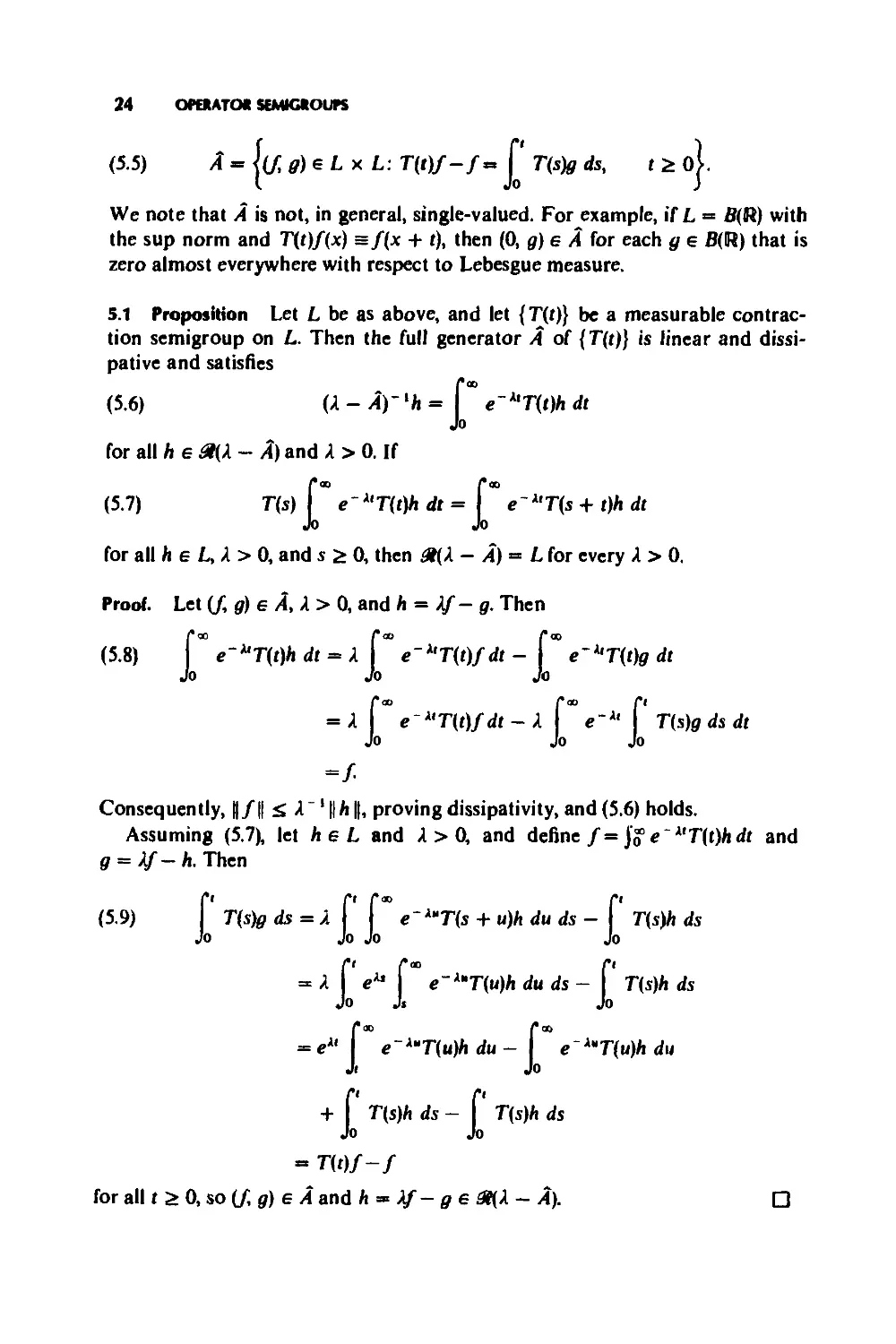
(5.5)
A - <C4 9} 6 L x L. T(t)f-f~
(.	Jo
T(s)g ds,
1210
We note that A is not, in general, single-valued. For example, if L = B(R) with
the sup norm and T(t)/(x) = f(x + t), then (0, g) e A for each g g B(R) that is
zero almost everywhere with respect to Lebesgue measure.
5.1 Proposition Let L be as above, and let {T(t)} be a measurable contrac-
tion semigroup on L. Then the full generator A of {T(t)j is linear and dissi-
pative and satisfies
(5.6)	(A - A)~ lh = Г°° e-*T(t)h dt
Jo
for all h e 9ЦА — Л) and A > 0. If
(5.7)	T(s) Г e~*'T(t}h dt = | e'A'T(s + t)h dt
Jo	Jo
for all h e L, A > 0, and s 0, then 0t(A — A) = L for every A > 0.
Proof. Let (f, g) e A, A > 0, and h = Af — g. Then
(5.8)	f e ^'T(t)h dt = A | e'x,T(t)fdt - | * e^'T(t)g dt
Jo	Jo	Jo
= A I e uT{t)fdt - A I eh Г T(s)g ds dt
Jo	Jo Jo
=f
Consequently, ||/|| £ A" 1ЦЛ||, provingdissipativity, and(5.6) holds.
Assuming (5.7), let heL and A > 0, and define f= jo e ~uT(t)hdt and
g = Af — h. Then
(5.9)	f T(s)g ds = A | | e“A“T(s + u)h du ds — | T(s)h ds
Jo	Jo Jo	Jo
= A I eu I e"A"T(u)/i du ds - Г T(s)h ds
Jo Ji	Jo
=	| e~iuT(u)h du — | e ^T(u)h du
Ji	Jo
+ I T(s)h ds — I T(s)h ds
Jo	Jo
- T(t)f-f
for all t 0, so (f g) e A and h » Af - g e 9ЦА — A).	□
5. SEMIGROUPS ON FUNCTION SPACES
25
The following proposition, which is analogous to Proposition 1.5(a), gives a
useful description of some elements of A.
5.2 Proposition Let L and {T(t)} be as in Theorem 5.1, let h e L and u £ 0,
and suppose that
(5.Ю)
T(t) I T(s)h ds =1 T(t + s)h ds
for all t 0. Then
(5.11)
Proof. Put/ = J* T(s)h ds. Then
(5.12)
I T(t + s)h ds - Г T(s)h ds
Jo	Jo
- j " T(s)h ds - I ‘ T(s)h ds
T(s)(T(u}h - h) ds
for all t 0.
□
In the present context, given a dissipative closed linear operator A c L x L,
it may be possible to find measurable functions u:fO, oo)-*L and
»: [0, oo)-» L such that (u(t), u(0) e A for every t > 0 and
(5.13)
HO = м(0) + I Hs) ds, t 0.
One would expect и to be continuous, and since A is closed and linear, it is
reasonable to expect that

(5.14)
u(s) ds, ИО - «(0) I e A
for all t > 0. With these considerations in mind, we have the following multi-
valued extension of Proposition 2.10. Note that this result is in fact valid for
arbitrary L.
26
OPERATOR SEMIGROUPS
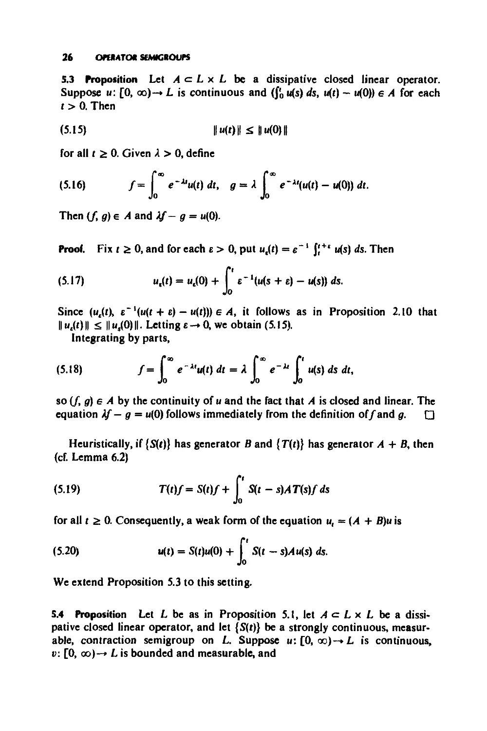
5.3	Proposition Let A c L x L be a dissipative closed linear operator.
Suppose u: [0, oo)-* L is continuous and (f'o u(s) ds, u(t} — u(0)) e A for each
t > 0. Then
(5.15)
II«(Oil £ II«(0)11
for all t 0. Given A > 0, define
(5.16)
e'^uft) dt, g = A I e~A'(u(t) — u(0)) dt.
Io	Jo
Then (f g) e A and Af-g = u(0).
Proof. Fix t £ 0, and for each £ > 0, put u,(t) = e~1 f{+t u(s) ds. Then
(5.17)	u,(t) = ut(0) + j £~*(u(s + e) — u(s)) ds.
Jo
Since (u£(t), l(u(t + 0 — «(0)) 6 A, it follows as in Proposition 2.10 that
II «JO II II «,(0) II • Letting £ -»0, we obtain (5.15).
Integrating by parts,
(5.18)	f= f е'л,и(г) dt = Я J e~u | u(s) ds dt,
Jo	Jo Jo
s° (/. в) 6 A by the continuity of и and the fact that A is dosed and linear. The
equation Af — g = u(0) follows immediately from the definition off and g. □
Heuristically, if {S(t)} has generator В and {T(t)} has generator A + B, then
(cf. Lemma 6.2)
(5.19)	T(t)f = S(t)f + f S(t - 0Л T(s)/ ds
Jo
for all t 2: 0. Consequently, a weak form of the equation u, = (A + B)u is
(5.20)	u(t) = S(t)u(0) 4- j S(t — s)4u(s) ds.
Jo
We extend Proposition 5.3 to this setting.
5.4	Proposition Let L be as in Proposition 5.1, let A c L x L be a dissi-
pative closed linear operator, and let {S(r)} be a strongly continuous, measur*
able, contraction semigroup on L. Suppose u: [0, oo)-»L is continuous,
v: [0, oo)—> L is bounded and measurable, and
5. SEMIGROUPS ON FUNCTION SPACES
(5.21)
u(0 = S(t)u(O) +1 S(t — s)Hs) ds
for all t ;> 0. If
(5.22)
u(s) ds, I HO ds 1 6 A
Io Jo /
for every t > 0, and
(5.23)
S(q + г)ф) ds = S(q) S(r)v(s) ds
for all q, r, t 0, then (5.15) holds for all t 0.
5.5 Remark The above result holds in an arbitrary Banach space under the
assumption that v is strongly measurable, that is, v can be uniformly approx-
imated by measurable simple functions.
Proof. Assume first that u:[0, oo)-»L is continuously differentiable,
v. [0, oo)-* L is continuous, and (u(t), HO) 6 A for all t 0. Let 0 = t0 < t, <
   < t„ = t. Then, as in the proof of Proposition 2.10,
(5.24)
II ИОН = IIИ0)|| + £ [II ИО II - llM(rf_ ,)|0
= IIu(0)|| + Z IIИМИ - ИО - (S(t, - G-.)- ЛИ0-.)
S(t, — s)Hs) ds
£ IIИ0)II + £ [ПИОН - IIИО - (S(t,	— /)ИО - (О - .МОП]
+ X (s0< - О-.) - /ХИО - И*.-.)) -
(S(tt - s)v(s) - HO) ds
£ ИИО)|| + £ [IIИО11 - Ц2ИО-(0-0-.МОН + 115(1,-1,.,)ИОII]
[(5(1, - t,.,) - f)u'(s) - S(t, - s)H0 + HO] ds
<; II u(0) H +	||(S(s" - s') - f)u'(s) - S(s" - s)Hs) + Hs")ll ds,

28 OPfRATOR SEMIGROUPS
where s' = t(_ , and s" = t( for t(_1 s < t,. Since the integrand on the right is
bounded and tends to zero as max (t( — t(_,)-»0, we obtain (5.15) in this case.
In the general case, fix t £ 0, and for each e > 0, put
(5.25)	u,(t) = e"1 J u(s) ds, vs(t) = e"1 J u(s) ds.
Then
(5.26)	ut(t) = e~1 | u(t + s) ds
Jo
J's	p p+ar
S(t + s)u(0) ds + c~1 I I S(t + s — r)v(r) dr ds
о	Jo Jo
«= e~ lS(t) f S(s)u(0) ds + €~1 | J S(/ + s - r)v{r) dr ds
Jo	Jo Jo
+ c"1 f j S(t — r)v(r + s) dr ds
Jo Jo
= S(0|	1 I S(s)u(0) ds + c“1 ( ( S(s — r)v(r) dr ds I
L Jo	Jo Jo	J
+ I S(t - r)vs(r) dr.
Jo
By the special case already treated,
(5.27)	||w,(t)|| £ ~1 J S(sM°) ds + e~1 J J S(s - r)v(r) dr ds
and letting e—»0, we obtain (5.15) in general.
6. APPROXIMATION THEOREMS
In this section, we adopt the following conventions. For n = 1, 2,..., L„, in
addition to L, is a Banach space (with norm also denoted by || • ||) and n„ :
L—t L„ is a bounded linear transformation. We assume that sup, || n„ || < oo.
We write/,-»/iff, 6 L, for each n £ l,f 6 L, and lim,-.^ II/, - n„ /Ц = 0.
6.1	Theorem For n - 1, 2.....let {TJt)} and {T(t)} be strongly continuous
contraction semigroups on L„ and L with generators A„ and A. Let D be a
core for A. Then the following are equivalent:
(a)	For each f 6 L, TK(t)nef~» T(t)f for all t 0, uniformly on bounded
intervals.
6. APPROXIMATION THEOREMS
29
(b)	For each f e L, T„(t)nn f-* T(t)f for all t 0.
(c)	For each f e D, there exists f„ e ©(Л„) for each n к I such that
/„-»/and A„f„-<- Affi.e., {(/ Afy.fe D} c ex-lim^A).
The proof of this result depends on the following two lemmas, the first of
which generalizes Lemma 2.5.
6.2	Lemma Fix a positive integer n. Let {S„(t)} and {S(t)} be strongly contin-
uous contraction semigroups on L„ and L with generators B„ and B. Let
f e @(B) and assume that n„S(s)f e @(B„) for all s 0 and that BnnnS(- )f.
[0, oo)-» L„ is continuous. Then, for each t £ 0,
(6.1)	f-n„ S(t)f =| S„(t - sX B„ n„ - n„ B)S(s)f ds,
Jo
and therefore
(6.2)	I ||(B.n„-n„B)WII ds.
Jo
Proof. It suffices to note that the integrand in (6.1) is ~(d/ds)S„(t - s)n„S(s)f
for 0 <; s < t.	□
6.3 Lemma Suppose that the hypotheses of Theorem 6.1 are satisfied
together with condition (c) of that theorem. For n = I, 2,... and A > 0, let A*
and A* be the Yosida approximations of A„ and A (cf. Lemma 2.4). Then
A*n„f-> Alf for every f e L and A > 0.
Proof. Fix A > 0. Let f e D and g = (A — A)f. By assumption, there exists
f„ e &(А„) for each n I such that /„-♦/ and A„f„~> Af, and therefore (A — A„)f„
-» g. Now observe that
(6.3)	\\А*пяд-п,,А*д\\
= || [Л2(Л - A) - * - Л К g - n„Ц2(Л - A) - 1 - Л/]<? ||
= Л2||(Л - А„)~‘л„д - л„(А - А)~‘дП
Л21|(Л - Anyln„g -/JI + Л2||/Л - п„(А - Л)-'д|1
А\\п„д - (Л - А)ЛН + Л2||/л - VII
for every и ;> I. Consequently, || А*п„д - п„ А*д\\ -»0 for all д е 0H.A — Л|о).
But 0ЦА - Л |D) is dense in L and the linear transformations А*п„ — я„Л2,
n = 1,2,..., are uniformly bounded, so the conclusion of the lemma follows.
□
Proof of Theorem 6.1. (a => b) Immediate.
30 OPERATOR SEMIGROUPS
(b=>c) Let A > 0,/e &(A), and g = (A — A)f so that f = ^е~иТ(1}д
dt. For each n^ I, put /, = j® e~x,TK(t)nKg dt e &(A„}. By (b) and the
dominated convergence theorem, fn —>f so since (А — Ая)/я x it„g—>g = (A
— A)f we also have A^-tAf.
(c => a) For n = I, 2,... and A > 0, let {П0} and {Тл(г)} be the strong-
ly continuous contraction semigroups on L, and L generated by the Yosida
approximations A* and A*. Given f e D, choose {/„} as in (c). Then
(6.4)	T/t)n„ f-n„ T(t)f = T.(tXn. /-/.) + [T.(t)f, - WJ
+ ГМ/. - n„f) + [П0«./~ «. ПО/]
+ «.СП»)/- П0Л
for every n ;> I and t к 0. Fix t0 0. By Proposition 2.7 and Lemma 6.3,
(6.5)	sup || W„ - ПО/.II bm t01| A. f, - A*f,||
O’St Sto	л-»<ю
<; liin t0{ || A. f„ - n„Af\\ + || n.(Af- Лл/)||
+ Ця.ЛУ- Ляля/|| + || Л>я/-/я)||}
^К»0||Л/- Л УII,
where К = sup, || п„ ||. Using Lemmas 6.2, 6.3, and the dominated con-
vergence theorem, we obtain
(6.6)	liin sup ||H0«./-«.И0/11
.-.oo Oststo
J*<0
|| (Л*ля — пя Лл)Тл(х)/|| ds = 0.
0
Applying (6.5), (6.6), and Proposition 2.7 to (6.4), we find that
(6.7)	iiS sup ||Тя(0«./-л.П0/11 <12Ке0||ЛУ- Л/ll.
«-•oo O’St <sto
Since A was arbitrary. Lemma 2.4(c) shows that the left side of (6.7) is zero.
But this is valid for all/ e D, and since D is dense in L, it holds for all/e L.
О
There is a discrete-parameter analogue of Theorem 6.1, the proof of which
depends on the following lemma.
6.4 Lemma Let В be a linear contraction on L. Then
(6-8)	IIB"/-	711 £ х/л||В/-/||
for all/б L and n = 0, I.
6. APPROXIMATION THEOREMS
31
Proof. Fix/б L and n 0. For к = 0, 1,...,
(6.9)	II В"/— B*/|| 5 ||BI*’"/-/||
= I
j=o
S|fc- n| ЦВ/-/Ц.
Therefore
= e“" f (B"/-B*/)£|
f |* - л| ЦВ/-/Ц
*-o	k!
£ (fc-n)2—}> ЦВ/-/Ц
= УЙВ/-/Ц.
(Note that the last equality follows from the fact that a Poisson random
variable with parameter n has mean n and variance n.)	□
6.5 Theorem For n = 1,2..........let T„ be a linear contraction on L„, let £„ be
a positive number, and put A„ = е~'(Т„ - I). Assume that Ктя_ввя = 0. Let
{T(t)} be a strongly continuous contraction semigroup on L with generator A,
and let D be a core for A. Then the following are equivalent:
(a) For each/6 L,	T(t)f for all t £ 0, uniformly on bounded
intervals.
<b) For each f e L, Т}!мпя T(t)f for all t 2> 0.
(c) For each f e D, there exists f„ e L„ for each n к I such that f,->f
and Ля/я — A/(i.e., {(/ Afy.fe D] c ex-lim^ A„).
Proof. (a=»b) Immediate.
(b => c) Let A > 0, f e ^(A), and g = (A — A)f, so that f — Jo e uTfl)g
dt. For each n £ I, put
(6.H)	A = e. f e ^Tknnng.
k«0
32 OPERATOR SEMIGROUPS
By (b) and the dominated convergence theorem,/,—»/ and a simple calcu-
lation shows that
(6.12)	(2 - Л,)/, = я, g + Ле. n„ g
+	“ 1+*“") f е'^'Т^П'д
*-o
for every n 1, so (2 - Ля)/я -*g = {X — A)f. It follows that A„ f, -»Af.
(c => a) Given f e D, choose {/,} as in (c). Then
(6.13) T^nJ-n,T(t)f
+ exp
Л, f(/« -«/) + CXP
- exp <£,
nJ-neT(t)f
for every n 1 and t 0. Fix t0 0. By Lemma 6.4,
(6.14)
lim sup
 -•oo Osisio
1*4, - exp
and by Theorem 6.1,
(6.15) lim sup
 -.00 Oststo
Consequently,
(6.16)
lim sup || T^nJ - n„ - 0.
 -.00 Oststo
But this is valid for all f e D, and since D is dense in L, it holds for all f e L
□
6.6	Corollary Let	be a family of linear contractions on
L with F(0) = I, and let {T(t)} be a strongly continuous contraction
semigroup on L with generator A. Let D be a core for A. If lim£_0
£_ l[F(fi)/—f] = Affor every f 6 D, then, for each f 6 L, V(t/nyf~* T(t)ffor all
t 0, uniformly on bounded intervals.
Proof. It suffices to show that if {t„} is a sequence of positive numbers such
that t,—»t 0, then Vftjriff-» T(t)f for every f 6 L. But this is an immediate
consequence of Theorem 6.5 with T„ = Vftjn) and £, = tjn for each n ;> 1. □
6. AmtOXIMATION THEO*EMS
33
6.7	Corollary Let {T(t)), {S(t)}, and {1/(0} be strongly continuous contrac-
tion semigroups on L with generators A, B, and C, respectively. Let D be a
core for A, and assume that D <= ©(B) n ©(C) and that A * В + C on D.
Then, for each f e L,
(6.П)	lim [s(^(0p- W
for all t 0, uniformly on bounded intervals. Alternatively, if {e„} is a
sequence of positive numbers tending to zero, then, for each f e L,
(6-18)	lim [5(е31/(еЛ,л’У = T(t)f
я —• oo
for all t 0, uniformly on bounded intervals.
Proof. The first result follows easily from Corollary 6.6 with F(t) = S(t)l/(t)
for all t 0. The second follows directly from Theorem 6.5.	□
6.8	Corollary Let {T(r)} be a strongly continuous contraction semigroup on
L with generator A. Then, for each feL, (f — Щп)А)~я/-> T(t)f for all t 0,
uniformly on bounded intervals. Alternatively, if {£„} is a sequence of positive
numbers tending to zero, then, for each feL,(l — £„ Л)“,,/*"У-> T(t)f for all
t 0, uniformly on bounded intervals.
Proof. The first result is a consequence of Corollary 6.6. Simply take
V(t) = (/ — M)~* for each t 0, and note that if £ > 0 and A = £“*, then
(6.19)	= A2(A — A)~lf — Af=AJ,
where Ал is the Yosida approximation of A (cf. Lemma 2.4). The second result
follows from (6.19) and Theorem 6.5.	□
We would now like to generalize Theorem 6.1 in two ways. First, we would
like to be able to use some extension A„ of the generator A, in verifying the
conditions for convergence. That is, given (/, g) e A, it may be possible to find
(/< 0«) 6 for each n 1 such that/„-»/and g„—»g when it is not possible
(or at least more difficult) to find g„) g A„ for each n 1. Second, we
would like to consider notions of convergence other than norm convergence.
For example, convergence of bounded sequences of functions pointwise or
uniformly on compact sets may be more appropriate than uniform con-
vergence for some applications. An analogous generalization of Theorem 6.5 is
also given.
34 OPERATOR SEMIGROUPS
Let LIM denote a notion of convergence of certain sequences f, e L„,
n= 1, 2,..., to elements f g L satisfying the following conditions:
(6.20)	LIM f, «f and LIM g„ = g imply
LIM (о/, + pg„) ~ Pg for all a, p g R.
(6.21)	LIM/*,‘* =/**• for each fc^l and
lim sup ||/<*‘ -/J| V ||/““ -/|| =0 imply LIM /, =/
k-*® я2 1 ,
(6.22)	There exists К > 0 such that for each / g L, there is a
sequence /, g L, with Ц/, || К ||/||, » 1,2 .,., satisfying
LIM/,=/
If A„ <= L„ x L„ is linear for each n 1, then, by analogy with (4.3), we define
(6.23)	ex-LIM A„ = {(/ g) g L x L: there exists (/,, g„) g A„
for each n 2: 1 such that LIM/, = /and LIM g„ = g}.
6.9 Theorem For n = 1, 2,..., let A„ c L, x L, and A c L x L be linear
and dissipative with — A„) = L, and — A) = L for some (hence all)
A > 0, and let {T,(t)} and {T(t)} be the corresponding strongly continuous
contraction semigroups on ^(Л,) and <&(A). Let LIM satisfy (6.2OH6.22)
together with
(6.24)	LIM /, = 0 implies LIM (Л - Л,)~ 7. = 0 for all A > 0.
(a)	If A c ex-LIM A„, then, for each (/, g) g A, there exists (/,, g„) g A„
for each n 1 such that sup, Ц/, || < oo, sup, || дя || < oo, LIM /, = / LIM g„
= g, and LIM T,(t)/, = T(t)/for all t Z 0.
(b)	If in addition extends to a contraction semigroup (also
denoted by { Zi(r)}) on L, for each n 1, and if
(6.25)	LIM /, « 0 implies LIM T,(r)/, « 0 for all t £ 0,
then, for each/g &(A), LIM/, = /implies LIM Tn(t)f„ = T(t)/for all t 0.
6.10 Remark Under the hypotheses of the theorem, ex-LIM A„ is closed
in L x L (Problem 16). Consequently, the conclusion of (a) is valid for all
(/ g) g A.	О
Proof. By renorming L„, n = 1, 2,..., if necessary, we can assume К = 1 in
(6.22).
Let & denote the Banach space (fLii^») x with norm given by
II({/.}. nil = sup.a JII/. || V ll/ll, and let
(6.26)	- {({/.}>/) 6 LIM/. =/}.
6. APPROXIMATION THEOREMS
35
Conditions (6.20) and (6.21) imply that <s a closed subspace of if, and
Condition (6.22) (with К = 1) implies that, for each feL, there is an element
({/.},/) with || ({/.},/) II = ||/||.
Let
(6.27)	= {[({/.},/), ({».}• 0)] e X x 2>: (/., g,) e A. for each
n 1 and (/, g) 6 A}.
Then j/ is linear and dissipative, and — j/) = for all A > 0. The corre-
sponding strongly continuous semigroup {^"(t)} on £2(j/) is given by
(6.28)	^OX{/J J) = ({TJM,}, T(t)f\.
We would like to show that
(6.29)	^(t): n 0(j/) — tfo n 0(j/j.	t2>0.
To do so, we need the following observation. If (/, 0) e A, A > 0, h = Af — g,
({/1Я}, Л) e and
(6.30)	(4, 0.) = ((A - A„)' ‘Л., Af. - Л.)
for each n 1, then
(6.31)	[({/.},/), ({0.}, 0)] 6 (^0 x ^0) n J/.
To prove this, since A c ex-LIM A„, choose (/., 0.) 6 Л. for each n 1 such
that LIM /. =f and LIM 0. = g. Then LIM (h. - (А/, — &,)) = 0, so by (6.24),
LIM (A - Л.Г 4 -/. = 0. It follows that LIM/. = LIM (A - Л.)' */i. =
LIM /. = f and LIM 0. = LIM (Af. - /1.) = Af - Л = g. Also, sup. Ц/. || <
A’1 sup. ||h.|| < 00 and sup. || 0.11 <, 2 sup. ||h. || < co. Consequently, [({/.},/),
({0.}, 0)] belongs to 5^0 x , and it clearly also belongs to j/.
Given ({h.}, h) 6 and A > 0, there exists (/, g) 6 A such that Af- g = h.
Define (/.,0.)еЛ. for each n^l by (6.30). Then (A — .i/) ‘({Л.}, h) =
({/.}./) 6^0 by (6.31), so
(6.32)	(A - j/) ‘:	A > 0.
By Corollary 2.8, this proves (6.29).
To prove (a), let (/, g) 6 A, A > 0, and h = Af - g. By (6.22), there exists
({h.}, h) e with || ({/>.}, h) || = || h ||. Define (/., 0.) 6 Л. for each n 1 by
(6.30). By (6.31), (6.29), and (6.28), ({T.(t)/.},	for all t 2>0, so the
conclusion of (a) is satisfied.
As for (b), observe that, by (a) together with (6.25), LIM/. =/g @(Л)
implies LIM T.(t)/. = T(t)/for all t ;> 0. Let f e ©(Л) and choose {J4*1} «= ®(Л)
such that ||/<м —/II s; 2~* for each к 1. Put f*01 = 0, and by (6.22), choose
36 OPERATOR SEMIGROUPS
({ui*‘},/<*‘ g such that || («*»},/<*» -/**““) II - И/*** -/**'“Il for
each к 1. Fix t 0. Then
(6.33)	LIM £ u'« */<“,	LIM T.(t) £ <*' - W"'
i	i
for each к 1. Since
(6.34)
00
£ «4°
*+l
||/**‘~/|| £ 2~*,
<;3-2-*,
and
(6.35)
r„(t) £ u«‘
4+1
£3-2-*,
|| W“- T(t)/|| ;S2‘,
for each n 2: 1 and к 1, (6.21) implies that
(6.36)	LIM £ ui° = f, LIM T„(t) £ ui° - T(t)/,
i	i
so the conclusion of (b) follows from (6.25).
6.11 Theorem For n = 1, 2,..., let T„ be a linear contraction on L„, let
£, > 0, and put Л, - £," l(T„ - I). Assume that lim,,-,,,, £, = 0. Let A c L x L
be linear and dissipative with — Л) = L for some (hence all) A > 0, and let
{T(t)} be the corresponding strongly continuous contraction semigroup on
&(A). Let LIM satisfy (6.20H6.22), (6.24), and
(6.37)	lim И/.||=0 implies LIM/, = 0.
(a)	If A c ex-LIM A„, then, for each (/, g) e A, there exists /, e L.
for each n^l such that sup, Ц/, || < oo, sup,||A,/,|| < oo, LIM/, =/
LIM AJ„ - g, and LIM T1."*-’/. « T(t)/for all t 0.
(b)	If in addition
(6.38)	LIM/, = 0 implies LIM T’"**/, = 0 for all t 2> 0,
then for each/6 3(A), LIM /, «= /implies LIM = T(t)/for all t 0.
Proof. Let (/, g) g A. By Theorem 6.9, there exists/, g L, for each n 1 such
that sup,Ц/, || < oo, sup,|| Л^/, || < oo, LIM /, =/, LIM Ajn = g, and
LIM = T(t]fiot al) t 0. Since
(6.39)
lim
Я-» 00
Ы'-Ш
Л,>/, — exp {еЛ,}/,
7. PERTURBATION THEOREMS
37
for all t 0, we deduce from (6.37) that
(6.40)
LIM exp
K£Hz-=tw'
t 2t0.
The conclusion of (a) therefore follows from (6.14) and (6.37).
The proof of (b) is completely analogous to that of Theorem 6.9 (b).	□
7. PERTURBATION THEOREMS
One of the main results of this section concerns the approximation of semi-
groups with generators of the form A + B, where A and В themselves generate
semigroups. (By definition, 2(A + B) — 2(A) n £2(B).) First, however, we give
some sufficient conditions for A + В to generate a semigroup.
7.1 Theorem Let A be a linear operator on L such that A is single-valued
and generates a strongly continuous contraction semigroup on L. Let В be a
dissipative linear operator on L such that £2(B) => 2(A). (In particular, В is
single-valued by Lemma 4.2.) If
(7.1)	IIB/H <, a|| ЛГИ +	/6 0(A),
where 0^a< 1 and fl 0, then A + В is single-valued and generates a
strongly continuous contraction semigroup on L. Moreover, A + В = A + B.
Proof. Let у 2: 0 be arbitrary. Clearly, 0(Л + yB) = 0(Л) is dense in L. In
addition, Л + yB is dissipative. To see this, let Л. be the Yosida approx-
imation of A for each ц > 0, so that Лм = цМц — Л)"1 — /]. If/e 2(A) and
A > 0, then
(7.2)	|| Af — (Л + уB)/|| = lim || Л/- (A, + уB)/||
д-»оо
= lim ||(A + n)f- yBf— ц2(ц - A)~ l/||
Ц-* oo
2: lim {||(A + v)f- yB/|| - || ц2(ц - А) 1/||}
ц-* оо
2: lim {(Л + д) 11/Ц -д 11/11}
Ц-* 00
= Л11/11
by Lemma 2.4(c) and the dissipativity of yB.
38 OPERATOR SEMIGROUPS
If/6 2(A), then there exists {/J c. 2(A) such that f,-* f and Af,-* Af. By
(7.1), {Bfn} is Cauchy, so f g 2(B) and Bf,-* Bf. Hence 2(A) <= 2(B) and (7.1)
extends to
(73)	|| Bf || <, a|| Л/Ц + P\\f II, fe 2(A).
In addition, if/c 2(A) and if {/„} is as above, then
(7.4) (A + yB)f = lim Af + у lim Bf, = lim (A + yB)f = (A + yB)f,
M	it	it
implying that A + yB is a dissipative extension of A + yB.
Let
(7.5) Г = {y 0: 2(A — A — yB) «= L for some (hence all) Л > 0}.
To complete the proof, it suffices by Theorem 2.6 and Proposition 4.1 to show
that 1 g Г. Noting that 0 g Г by assumption, it is enough to show that
(7.6)
у G Г n [0, 1)
implies
У. У +
1 — ay4)
2a )
<= Г.
To prove (7.6), let у g Г n [0, 1), 0 <; £ < (2a) *(1 — ay), and A > 0. If
0 G 2(A), then/= (A - A - yB)~lg satisfies
(7.7)	HBfll S «НАД + РИД <; а||(Я + yfi)/|| + ау || В/Ц + Л/И
by (7.3), that is,
(7.8)	||Bf || <; a(l - ay)'11|(A + yfi)/|| + Д1 - ay)’* ||/||,
and consequently,
(7.9)	||B(A-4-yfi)-*0|| ^[2a(l -ay)’1 +/I(1 -ay)-‘A-‘]ll0ll.
Thus, for A sufficiently large, ||eB(A — A — B)~l || < 1, which implies that
I — eB(A — A — yB)~l is invertible. We conclude that
(7.10)	2(A - A - (y + £)B) = 2((A - A - (y + e)B)(A -A-yB)~l)
= 0t(l - eB(A- A -yB)~l)
» L
for such A, so у + e g Г, implying (7.6) and completing the proof.	□
7.2 Corollary If A generates a strongly continuous contraction semigroup
on L and В is a bounded linear operator on L, then A + В generates a
strongly continuous semigroup {T(r)} on L such that
(7.11)	||T(t)|| £ el|B|",	/2:0.
Proof. Apply Theorem 7.1 with В — || В || I in place of B.
□
7. PERTURBATION THEOREMS
39
Before turning to limit theorems, we state the following lemma, the proof of
which is left to the reader (Problem 18). For an operator A, let
Ж(Л) = {/g ®(Л): Af = 0} denote the null space of A.
7.3 Lemma Let В generate a strongly continuous contraction semigroup
{5(0} on L, and assume that
(7.12)	lim Л j el,S(t)f dt = Pf exists for all f g L.
Д-0+ Jo
Then the following conclusions hold :
(a)	P is a linear contraction on L and P1 = P.
(b)	S(t)P = PS(t) = P for all t % 0.
(c)	3?(P) = Ж(В).
(d)	Ж(Р) = «(В).
7.4 Remark If in the lemma
(7.13)	B = y~‘(Q — l),
where Q is a linear contraction on L and у > 0, then a simple calculation
shows that (7.12) is equivalent to
(7.14)	lim (1 - p) £ PkQkfs?f exists for all f g L.	□
/>-1-	k-0
7.5 Remark If in the lemma lim,-.^ S(t)f exists for every feL, then (7.12)
holds and
(7.15)	Pf= lim S(t)f f e L.
If В is as in Remark 7.4 and if lim*^eC*/ exists for every feL, then (7.14)
holds (in fact, so does (7.15)) and
(7.16)	Pf~ lim Qkf feL.
00
The proofs of these assertions are elementary.	□
For the following result, recall the notation introduced in the first para-
graph of Section 6, as well as the notion of the extended limit of a sequence of
operators(Section 4).
7.6 Theorem Let A c L x L be linear, and let В generate a strongly contin-
uous contraction semigroup {£(()} on L satisfying (7.12). Let D be a subspace
40 OPERATOR SEMIGROUPS
of 2(A) and D' a core for B. For n = 1, 2,..., let A„ be a linear operator on L,
and let > 0. Suppose that Нт,_ж a, = oo and that
(7.17)	{(/, g) e A:fe D} <= ex-lim A„,
f|-*OO
(7.18)	{(h, Bh): he D'} <= ex-lim «~1АЯ.
я-*оо
Define C = {(/, Pg): (f,g)eA,fe D} and assume that {(/, g) e C: g e 0} is
single-valued and generates a strongly continuous contraction semigroup
{T(t)} on 0.
(a)	If A„ is the generator of a strongly continuous contraction semi-
group {T,(0} on L„ for each n 1, then, for each f e 0, T/tjnJ"-» T(t)f(or
all t 0, uniformly on bounded intervals.
(b)	If A„ «= e~l(T„ — I) for each n 1, where T„ is a linear contraction
on L, and e„ > 0, and if lim,_(X,£, = 0, then, for each fe 0, T^MnKf~* T(t)f
for all t ;> 0, uniformly on bounded intervals.
Proof. Theorems 6.1 and 6.5 are applicable, provided we can show that
(7.19)	{(f, g) e C: g e 0} <= (ex-lim A„) n (0 x 0).
\ H-*0D	/
Since ex-lim,A„ is closed, it suffices to show that С c ex-lim,A„. Given
(f, g) e A with f s D, choose /, g 2(A„) for each n £ 1 such that /,-»/ and
Л,/,-» g. Given h e D', choose h, e 2(A„) for each n 1 such that h,-+ h and
a,"1Л,h,-» Bh. Then f„ + a~lh„-tf and A„(fn + a/'/i,)-» g + Bh. Conse-
quently,
(7.20)	{(f, g + Bh): (f g) e A, f g D, h e D'} <= ex-lim Л,.
я-»ао
But since ex-lim,Л, is closed and since, by Lemma 7.3(d),
(7.21)	Pg — g e Л(Р) ~Я(В) = ЭД0.)
for all g g L, we conclude that
(7.22)	{(Z Pg): (J. g) e A, fe D) <= ex-lim Л.,
n-»oo
completing the proof.	□
We conclude this section with two corollaries. The first one extends the
conclusions of Theorem 7.6, and the other describes an important special case
of the theorem.
7.7 Corollary Assume the hypotheses of Theorem 7.6(a) and suppose that
(7.15) holds. If Л g Ж(Р) and if {t,} c [0, oo) satisfies lim,-.00t„a, = oo,
7. PERTURBATION THEOREMS
41
then Tj(t,)n,h-*0. Consequently, for each feP~'(D) and 3 g (0,1),
T,(t)n,f-^ T(t)Pf, uniformly in 6 £ t £ 6~ *.
Assume the hypotheses of Theorem 7.6(b), and suppose that either
(i) lim,^ T! a, £, = 0 and (7.15) holds, or (ii) lim,-.e a,e, = у > 0 and (7.16)
holds (where Q is as in (7.13)). If h g Ж(Р) and if {k„} c {0,1,...} satisfies
Нтя^ж = oo, then 7^"n,h-»0. Consequently, for each f g Pl(D) and
d g (0, 1), Tt'-’irJ- T(t)Pf, uniformly in 6 < t <; 6" *.
Proof. We give the proof assuming the hypotheses of Theorem 7.6(a), the
other case being similar. Let h g Ж(Р), let {t„} be as above, and let £ > 0.
Choose s 0 such that || S(s)h || e/2K, where К = sup,2 (|| n„ ||, and let s„ =
s A t„ a, for each n 1. Then
(7.23)	|| 7^)01| 5
T.( — }n.h — n,S(s)h
\a«/
+ ||n.S(s)A|| <.e
for all n sufficiently large by (7.18) and Theorem 6.1. If f g L, then
f— Pf g Ж(Р), so T,(t,)n,(/ — Pf)-*0 whenever {t,} c [0, oo) satisfies lim,-.^
t, = t # 0. If /gP_|(6), this, together with the conclusion of the theorem
applied to Pf, completes the proof.	□
7.8 Corollary Let П,Л, and В be linear operators on L such that В generates
a strongly continuous contraction semigroup (S(t)} on L satisfying (7.12).
Assume that 0(П)	0(A) r> 0(B) is a core for B. For each a sufficiently large,
suppose that an extension of П + aA + a2B generates a strongly continuous
contraction semigroup {7^(0} on L. Let D be a subspace of
(7.24)	{/g ЯП) n 0(A) n Ж(В):
there exists h g 0(П) n 0(A) n 0(B) with Bh = — Af},
and define
(7.25)	C = {(f, РП/ + PAh):fe D, h e 0(П) 0(A) 0(B), Bh=-Af}.
Then C is dissipative, and if {(f g) e C: g g D}, which is therefore single-
valued, generates a strongly continuous contraction semigroup {T(t)} on 5,
then, for each f g D, lim,-.aj T„(t)f = T(t)ffor all t ;> 0, uniformly on bounded
intervals.
Proof. Let {a,} be a sequence of (sufficiently large) positive numbers such that
lim,-.*, a, = oo, and apply Theorem 7.6(a) with L, = L, = 1, A replaced by
(7.26)	{(f, nf + Ah): feD, he 0(D) n 0(A) n 0(B), Bh	- Af},
A„ equal to the generator of {7^,(0}, « replaced by a*, and
D' = 0(D) n 0(A) n g>(B). Since Л,(/+ a; lh) - П/+ Ah + a; ‘ПЛ when-
ever f g D, h g 0(П)	0(A)	0(B), Bh = — Af, and и ;> 1, and since lim,-.^
42
OPERATOR SEMIGROUPS
a~2A„h = Bh for all h e D', we find that (7.17) and (7.18) hold, so the theorem
is applicable. The dissipativity of C follows from the dissipativity of ex-lim.-.^
Л..	□
7.9 Remark (a) Observe that in Corollary 7.8 it is necessary that PAf = 0
for all/e D by Lemma 7.3(d).
(b) Let f 6 2(A) satisfy PAf =0. To actually solve the equation
Bh = — Л/for h, suppose that
(7.27)	| IKSfO-P^)) dt<oo, geL.
Jo
Then h = lima_o+M - B)~lAf = fo (S(0 - P)Af dt belongs to 2(B) (since
В is closed) and satisfies Bh= — Af. Of course, the requirement that h
belong to 2(Tl) n 2(A) must also be satisfied.
(c)	When applying Corollary 7.8, it is not necessary to determine C
explicitly. Instead, suppose a linear operator Co on D can be found such
that Co generates a strongly continuous contraction semigroup on 6 and
Co с C. Then {(/ g) 6 C: g 6 6} = Co by Proposition 4.1.
(d)	See Problem 20 for a generalization and Problem 22 for a closely
related result.	□
8.	PROBLEMS
1.	Define {7(0} on £(R) by T(t)f(x) = f(x + t). Show that {7(0} is a strong-
ly continuous contraction semigroup on L, and determine its generator A.
(In particular, this requires that 2(A) be characterized.)
2.	Define {7(0} on C(R) by
1	( (v —x?)
(8.1)	T(t)f(x) = -== f(y) exp j	> dy
I 2t J
for each t > 0 and 7(0) = 1. Show that {7(0} is a strongly continuous
contraction semigroup on L, and determine its generator A.
3.	Prove Lemma 1.4.
4.	Let {7(0} be a strongly continuous contraction semigroup on L with
generator A, and let f g 2(A2).
(a)	Prove that
(8.2)	7(0/=/+ ГЛ/+ f'(t - s)T(s)A2fds, t 0.
Jo
8. PROBLEMS
43
(b)	Show that || Af\\2 <. 4ЦЛ7И ||/||.
5.	Let A generate a strongly continuous semigroup on L. Show that ,
2(A") is dense in L.
6.	Show directly that the linear operator A = \d2jdx2 on L satisfies condi-
tions (aHc) of Theorem 2.6 when 2(A) and L are as follows:
(a)	2(A) = {fe C2[0, 1 ] • а,Л0 - (- В'ДЛО = 0, i = 0, 1}.
L = C[0, 1], a0) До» ai> Pi 0» “о + До > 0» «i + Pi > 0
(b)	2(A)= {/6 e2[0, oo): ao/"(0) - ДоД0) = 0}
L = C[0, oo), a0, До 2: 0, a0 + До > 0.
(c)	2(A) = C2(R), L = C(R).
Hint: Look for solutions of kf — \f” — g of the form /(x) =
exp{ — y/2kx}h(x).
7.	Show that C®(R) is a core for the generators of the semigroups of Prob-
lems 1 and 2.
8.	In this problem, every statement involving k, /, or n is assumed to hold
for all к, I, n 1.
Let Lt c L2 c L3 c   • be a sequence of closed subspaces of L. Let
Uk, Mk, and MJ” be bounded linear operators on L. Assume that Uk and
Ml” map L„ into L„, and that for some цк > 0, || Ml”|| цк and
(8	.3)	lim || Ml"1 - Mk || = 0.
oo
Suppose that the restriction of A„ = £}ж (to L„ is dissipative and
that there exist nonnegative constants ak, (= alk), Дк|, and у such that
(8.	4)	|| Uk U,f- U, UJ\\ акЛII IVII + IITVII). /в L,
(8-5)	£ Hj fXjt <. У,
J» 1
(8.	6)	||l/kM|” - M}”Uk|| <; Pkl,
and
(8.	7)	£ HjPji^yHi-
J-i
Define A =£*«i M}Uj on
(8.	8)	2(A) = If e Q Lm: £ M>|| l/j/|| < ool.
I m-l /’1	J
If 2(A) is dense in L, show that A is single-valued and generates a
strongly continuous contraction semigroup on L.
44
operator SEMIGROUPS
Hint: Fix A > 3y and apply Lemma 3.6. Show first that for g e &(A) and
/.“M- AJ-'g,
(8.	9)	a-y)||I/J.|| <; ||Uk0|| + £ (Aj + ^a^lll/j/.H.
Denoting by ц the positive measure on the set of positive integers that
gives mass nk to k, observe that the formula
(8.10)
E (Au + ^akj)Fj
defines a positive bounded linear operator on 1}(ц) of norm at most 2y.
9.	As an application of Corollary 3.8, prove the following result, which
yields the conclusion of Theorem 7.1 under a different set of hypotheses.
Let A and В generate strongly continuous contraction semigroups
{T(0} and {$(0} on L. Let D be a dense subspace of L and ||| • ||| a norm
on D with respect to which D is a Banach space. Assume that |||/|||	||/II
for all f g D. Suppose there exists	such that
(8.11)	ЦЛУ11 £И1ЛИ, /eD;
(8.12)	Dc&fB2); ||В2/Кд|||/|||, feD-,
(8.13)	T(t):D—D, S(0: D—D, t 2> 0;
(8.14)	III Tit) HI Sc*', III S(0 III i e*', t^O.
Then the closure of the restriction of A + В to D is single*valued and
generates a strongly continuous contraction semigroup on L.
We remark that only one of the two conditions (8.11) and (8.12) is
really needed. See Ethier (1976).
10.	Define the bounded linear operator В on L s C([0, 1] x [0, 1]) by
B/(x, y) = fo/(x, z) dz, and define A c L x L by
(8.15)	A - {(f, if„ + h):fe C2([0, 1] x [0, 1]) n £(B),
ЛМ-/ДуМ for all yefO, 1],
h 6 Ж(В)}.
Show that A satisfies the conditions of Theorem 4.3.
11.	Show that ex-lim,_e A,, defined by (4.3), is closed in L x L.
12.	Does the dissipativity of A„ for each n s 1 imply the dissipativity of
ex-lim,-.e A,?
13.	In Theorem 6.1 (and Theorem 6.5), show that (aHc) are equivalent to the
following:
в. PROBLEMS
45
(d) There exists A>0 such that (A — A„) ‘я„0—»(Л-Л) 'g for all
geL.
14.	Let L, {L„}, and {я,} be as in Section 6. For each n 1, let {be a
contraction semigroup on L„, or, for each n > 1, let {7^(0} be defined in
terms of a linear contraction Тя on L. and a number e„ > 0 by T„(t) =
j-pm for a|| f о- jn the latter case assume that lim,^ e„ = 0. Let {T(t)}
be a contraction semigroup on L, let f,geL, and suppose that lim,.^
T(t)f= g and
(8.16)	lim sup ||	яяТ(г)/|| = 0
Я-»00 Ost£tQ
for every t0 > 0- Show that
(8.17)	lim sup || T„(t)nJ - я. T(t)/|| = 0
я-»чо 12O
if and only if
(8.18)	lim sup || Т,(Г)я, g - я, T(t)g || = 0.
n-»oo t i 0
15.	Using the results of Problem 2 and Theorem 6.5, prove the central limit
theorem. That is, if Xt, X2,... are independent, identically distributed,
real-valued random variables with mean 0 and variance 1, show that
и |/2 converges in distribution to a standard normal random
variable as и-» oo. (Define TJ"(x) = E[f(x + и“1/2Л'1)] and e„ = и-1.)
16.	Under the hypotheses of Theorem 6.9, show that ex-LIM A„ is closed in
L x L.
17.	Show that (6.21) implies (6.37) under the following (very reasonable) addi-
tional assumption.
(8.19)	If f„ g L„ for each n 1 and if, for some n0> !,/„ = 0
foralln^n0, then LIM/„ = 0.
18.	Prove Lemma 7.3 and the remarks following it.
19.	Under the assumptions of Corollary 6.7, prove (6.18) using Theorem 7.6.
Hint : For each n ;> 1, define the contraction operator T„ on L x L by
20.	Corollary 7.8 has been called a second-order limit theorem. Prove the
following kth-order limit theorem as an application of Theorem 7.6.
Let Ao, At,..., Ak be linear operators on L such that Ak generates a
strongly continuous contraction semigroup {5(0} on L satisfying (7.12).
Assume that 2 s	is a core for Ak. For each a sufficiently
46
OPERATOR SEMIGROUPS
large, suppose that an extension of	generates a strongly contin-
uous contraction semigroup {7^(t)} on L. Let D be a subspace of
(8.21)	^/o 6 0: there exist  • . ,ff-2 6 2 with
£	for m = 0,. . . , к - 1I,
J“0	J
and define
f/	*'*	\	)
(8.22)	С = Л, £ PAifi\fo 6 D,j\,. . . ,f*_1 as above к
(A	>=o	/	J
Then C is dissipative and if {(/, g) e C: g e 6), which is therefore single-
valued, generates a strongly continuous contraction semigroup {T(t)J on
D, then, for each/e D, lim,-.^	= T(t)f for all t 0, uniformly on
bounded intervals.
21.	Prove the following generalization of Theorem 7.6.
Let M be a closed subspace of L, let A c L x L be linear, and let B,
and B2 generate strongly continuous contraction semigroups {SJt)} and
{S2(t)} on M and L, respectively, satisfying
(8.23)	lim A j	dt = Ptf exists for all f e M,
Л-0 + Jo
(8.24)	lim A | e~2,S2(t)f dt = P2f exists for all f e L.
a-o+ Jo
Assume that 3t(P2) <= M. Let D be a subspace of &(A), Dt a core for Blt
and D2 a core for B2. For n = 1, 2,..., let A, be a linear operator on L„
and let a,, fl, > 0. Suppose that lim,^^ a, = oo, lim.-.^ P„ = oo, and
(8.25)	{(/, g) g A:fe D} c ex-lim A„
(8.26)	{(Л, Bjh): h e DJ <= ex-lim <*.lA„,
л-»оо
(8.27)	{(к, B2 к): к е D2} <= ex-lim Р,1АЯ.
л —со
Define С = {(/, PiP2g): (f, д) g A,fe D} and assume that {(/, g) g C: g g
D} generates a strongly continuous contraction semigroup {T(t)} on D.
Then conclusions (a) and (b) of Theorem 7.6 hold.
22.	Prove the following modification of Corollary 7.8.
Let П, A, and В be linear operators on L such that В generates a
strongly continuous contraction semigroup {S(t)} on L satisfying (7.12).
Assume that &(П) D(A) n ®(B) is a core for B. For each a sufficiently
large, suppose that an extension of П + aA + a2B generates a strongly
9. NOTES
47
continuous contraction semigroup {T/t)} on L. Let D be a subspace of
©(П)	&(A) n Ж(В) with ЩР) c 6, and define C = {(/, PAf)'. f 6 D}.
Then C is dissipative. Suppose that C generates a strongly continuous
contraction semigroup {U(t)} on 6, and that
(8.28)	lim A | e~dt = Pof exists for every f g 6.
Д-0+ Jo
Let Do be a subspace of {f e D: there exists h 6 ®(П) n &>(A) n ©(B)
with Bh = — Af}, and define
(8.29)	Co « {(/, Po Mlf+ Po PAhy.fe Do,
h g ©(П) n ©(Л) n ©(B), Bh = - Af}.
Then Co is dissipative, and if {(/ g) g Co: g g Do} generates a strongly
continuous contraction semigroup {T(t)} on Do, then, for each feD^,
lim,-.*, Tft)f = T(t)ffor all t 0, uniformly on bounded intervals.
23.	Let A generate a strongly continuous semigroup {T(t)} on L, let
B(t):L-*L, t2:0, be bounded linear operators such that (B(t)} is
strongly continuous in t 2: 0 (i.e., t—> B(t)f is continuous for eachf g L).
(a) Show that for each feL there exists a unique u: [0, L
satisfying
(8.30) u(t) = T(t)f+ I T(t - s)B(s)u(s) ds.
Jo
(b) Show that if B(t)g is continuously differentiable in t for each g g L,
and f g &(A), then the solution of (8.30) satisfies
(8.31)	~ u(t) ~ Au(t) + B(t)u(t).
Ct
9. NOTES
Among the best general references on operator semigroups are Hille and
Phillips (1957), Dynkin (1965), Davies (1980), Yosida (1980), and Pazy (1983).
Theorem 2.6 is due to Hille (1948) and Yosida (1948).
To the best of our knowledge, Proposition 3.3 first appeared in a paper of
Watanabe (1968).
Theorem 4.3 is the linear version of a theorem of Crandall and Liggett
(1971). The concept of the extended limit is due to Sova (1967) and Kurtz
(1969).
Sufficient conditions for the convergence of semigroups in terms of con-
vergence of their generators were first obtained by Neveu (1958), Skorohod
(1958), and Trotter (1958). The necessary and sufficient conditions of Theorems
48
OPERATOR SEMIGROUPS
6.1 and 6.5 were found by Sova (1967) and Kurtz (1969). The proof given here
follows Goldstein (1976). Hasegawa (1964) and Kato (1966) found necessary
and sufficient conditions of a different sort. Lemma 6.4 and Corollary 6.6 are
due to Chernoff (1968). Corollary 6.7 is known as the Trotter (1959) product
formula. Corollary 6.8 can be found in Hille (1948). Theorems 6.9 and 6.11
were proved by Kurtz (1970a).
Theorem 7.1 was obtained by Kato (1966) assuming a < | and in general by
Gustafson (1966). Lemma 7.3 appears in Hille (1948). Theorem 7.6 is due to
Ethier and Nagylaki (1980) and Corollary 7.7 to Kurtz (1977). Corollary 7.8
was proved by Kurtz (1973) and Kertz (1974); related results are given in
Davies (1980).
Problem 4(b) is due to Kailman and Rota (1970), Problem 8 to Liggett
(1972), Problem 9 to Kurtz (see Ethier (1976)), Problem 13 to Kato (1966), and
Problem 14 to Norman (1977). Problem 20 is closely related to a theorem of
Kertz (1978).
Markov Processes Characterization and Convergence
Edited by STEWART N. ETHIER and THOMAS G. KURTZ
Copyright © 1986,2005 by John Wiley & Sons, Inc
2 STOCHASTIC PROCESSES
AND MARTINGALES
This chapter consists primarily of background material that is needed later.
Section 1 defines various concepts in the theory of stochastic processes, in
particular the notion of a stopping time. Section 2 gives a basic introduction
to martingale theory including the optional sampling theorem, and local mar-
tingales are discussed in Section 3, in particular the existence of the quadratic
variation or square bracket process. Section 4 contains additional technical
material on processes and conditional expectations, including a Fubini
theorem. The Doob-Meyer decomposition theorem for submartingales is
given in Section 5, and some of the special properties of square integrable
martingales are noted in Section 6. The semigroup of conditioned shifts on the
space of progressive processes is discussed in Section 7. The optional sampling
theorem for martingales indexed by a metric lattice is given in Section 8.
1.	STOCHASTIC PROCESSES
A stochastic process X (or simply a process) with index set J and state space
(E, (a measurable space) defined on a probability space (Q, Ф, P) is a
function defined on J x Я with values in E such that for each t 6 J,
X(t, •): Q-> E is an £-valued random variable, that is, {to: X(t, <o) g Г} g &
for every Г g 3t. We assume throughout that £ is a metric space with metric r
49
50 STOCHASTIC PROCESSES AND MARTINGALES
and that Si is the Borel a-algebra ЖЕ). As is usually done, we write X(t) and
X(t, •) interchangeably.
In this chapter, with the exception of Section 8, we take У = [0, oo). We are
primarily interested in viewing X as a “random” function of time. Conse-
quently, it is natural to put further restrictions on X. We say that X is
measurable if X: [0, oo) x fl-* E is У[0, oo) x Ж -measurable. We say that X
is (almost surely) continuous (right continuous, left continuous) if for (almost)
every to g fl, X( - , ш) is continuous (right continuous, left continuous). Note
that the statements “X is measurable” and “X is continuous” are not parallel
in that "X is measurable” is stronger than the statement that X(-, co) is
measurable for each to g fl. The function X(-, co) is called the sample path of
the process at ш.
A collection {&,} = {У,, t g [0, oo)} of <r-algebras of sets in У is a fil-
tration if У, с У,+1 for i, s g [0, oo). Intuitively У, corresponds to the infor-
mation known to an observer at time t. In particular, for a process X we
define {У*} by У* = <r(X(s): s t); that is, У* is the information obtained
by observing X up to time t.
We occasionally need additional structure on {У,}. We say {У,} is right
continuous if for each 15:0, У, = У,+ = П£>оУ(+£- Note the filtration
(У,+ } is always right continuous (Problem 7). We say {У,} is complete if
(fl, У, P) is complete and {A g У: P(A) = 0} <= Уо.
A process X is adapted to a filtration {У,} (or simply {y,}-adapted) if X(t)
is У,-measurable for each t £ 0. Since У, is increasing in t, X is {yj-adapted
if and only if У * с У, for each t 0.
A process X is {Ф ^-progressive (or simply progressive if {У,} = {У,*}) if
for each t 5 0 the restriction of X to [0, t] x fl is У[0, t] x У,-measurable.
Note that if X is {y,}-progressive, then X is {y,}-adapted and measurable,
but the converse is not necessarily the case (see Section 4 however). However,
every right (left) continuous {У,}-adapted process is {У,}-progressive
(Problem 1).
There are a variety of notions of equivalence between two stochastic pro-
cesses. For 0 t, < t2 <    < tm, let ......(wi be the probability measure on
У(Е) x ••• x Si(E) induced by the mapping (X(t,),..., X(tm))-* E", that is,
P,.....JO = P{(X(tl),.... X(tJ) g Г}, Г g Si(E) x • • • x У(Е). The prob-
ability measures {p„ 1, 0$ tj < ••• < t„} are called the finite-
dimensional distributions of X. If X and Y are stochastic processes with the
same finite-dimensional distributions, then we say У is a version of X (and X is
a version of Y). Note that X and Y need not be defined on the same probabil-
ity space. If X and Y are defined on the same probability space and for each
t 5 0, P{X(t) = У(г)} = 1, then we say Y is a modification of X. (We are
implicitly assuming that (X(t), У(г)) is an E x E-valued random variable,
which is always the case if E is separable.) If У is a modification of X, then
clearly У is a version of X. Finally if there exists N g У such that P(N) 0
and X(•, <o) = У(•, <o) for all w N, then we say X and У are indistinguish-
able. If X and У are indistinguishable, then clearly У is a modification of X.
1. STOCHASTIC PROCESSES
51
A random variable t with values in [0, oo] is an {&,}-stopping time if
{t t} e for every t 2 0. (Note that we allow t = oo.) If т < oo a.s., we say
т is finite a.s. If т T < oo for some constant T, we say т is bounded. In some
sense a stopping time is a random time that is recognizable by an observer
whose information at time t is
If t is an {^,}-stopping time, then for s< (, {t s} ec(t < (} =
U„{t S t - l/и} 6 and = =	If т is discrete
(i.e., if there exists a countable set D <= [0, oo] such that |t e Dj =fl), then т is
an {J^j-stopping time if and only if {t = t} g Ф t for each t e D n [0, oo).
1Л lemma A [0, oo]-valued random variable т is an {^,+ }-stopping time if
and only if {t < t} g .F, for every t 2 0.
Proof. If {t < t} g for every t 0, then {t < t + n~ '} g for n m
and {t S t] = P)„{t < t + и'1} g	= .F,+. The necessity was
observed above.	□
1.2	Proposition Let т,,т2, ... be {^J-stopping times and let c g [0, oo).
Then the following hold.
(a)	Tt + c and т, Л c are {.F,}-stopping times.
(b)	sup„ тп is an {^J-stopping time.
(c)	minks„ тк is an {^J-stopping time for each n 2: 1.
(d)	If {.F,} is right continuous, then inf„T„, limB_^ t., and lim,^w t„
are {.Fj-stopping times.
Proof. We prove (b) and (d) and leave (a) and (c) to the reader. Note that
{sup„t, t} = S t} g J5-, so (b) follows. Similarly {inf, т„<г} =
U"{t" < t} 6 so if {&,} is right continuous, then inf,t, is a stopping time
by Lemma 1.1. Since lim^TT, = sup„infBJtmt, and	= inf^sup, t„,
(d) follows.	□
By Proposition Ufa) every stopping time т can be approximated by a
sequence of bounded stopping times, that is, limn_ai т Л n = t. This fact is very
useful in proving theorems about stopping times. A second equally useful
approximation is the approximation of arbitrary stopping times by a nonin-
creasing sequence of discrete stopping times.
1.3	Proposition For и = 1, 2,..., let 0 = tj < 1" < • • • and limk^„ = oo,
and suppose that sup*(t; +, — tj) = 0. Let т be an {.F,+{-stopping time
and define
(LI)
if т = oo.
if iJST	k^.0
52 STOCHASTIC PROCESSES ANO MARTINGALES
Then x„ is an {.F,}-stopping time and lim.^^x, = x. If in addition {tj} c
{t£+*}, then x, t,+1.
Proof. Let y,(t) = maX {t*: t" t}. Then
(1.2)	{t. <; t} = {t, £ y.(t)} = {t < y.(t)} g frM c J5",.
The rest is clear.	О
Recall the intuitive description of ft as the information known to an
observer at time t. For an {-stopping time x, the a-algebra f( should have
the same intuitive meaning. For technical reasons .F, is defined by
(1.3)	» {A g ft A r> {x t} g f, for all t^O}.
Similarly, ft+ is defined by replacing f, by fl+. See Problem 6 for some
motivation as to why the definition is reasonable. Given an E-valued process
X, define -Y(oo) s x0 for some fixed x0 e E.
1.4 Proposition Let x and a be {.F,{-stopping times, let у be a nonnegative
J^-measurable random variable, and let X be an {.^{{-progressive £-valued
process. Define X' and Y by X‘(t) = X(t Л t) and Y(t) = X(t + t), and define
9, = ft*, and Jf, = ft+l, t 2? 0. (Recall that тЛг and x + t are stopping
times.) Then the following hold:
(a)	ft is a <T-algebra.
(b)	x and т Л a are .^-measurable.
(c)	If т £ a, then ft c f*.
(d)	X(t) is ^,-measurable.
(e)	{9t} is a filtration and X' is both {^{-progressive and
{f, {-progressive.
(f)	{Jt",} is a filtration and Y is {jf,{-progressive.
(g)	т + у is an {f,}-stopping time.
Proof, (a) Clearly 0 and О are in fx, since ft is a a-algebra and {t £ t} e
ft. If A n (t £ r| e ft, then A‘ n {t £ r{ « {x £ t} - A n {x £ t) g f,,
and hence A e ft implies Ac g ft. Similarly n {x<t} g/,,
к =1,2,..., implies (|J4Ak) n {x t} = n {t £ t}) g and
hence ft is closed under countable unions.
(b)	For each c 0 and t 0,
(1.4)	(хЛа^с) n (x^ (} = {хЛ<т ^cA(} n {x^ t}
= ({x £ cAt} u {it ScA(J) o {x t} G ft.
Hence {xAa c} e and x Л a is -measurable, as is x (take a = x).
1. STOCHASTIC HIOCESSES
53
(c)	If A 6 then A n {<r i} = Л n {t ^ () л {в t} e for all
t 0. Hence A g f,.
(d)	Fix t > 0. By (b), t A t is Ф,-measurable. Consequently the mapping
<o-~» (t(<o)A t, co) is a measurable mapping of (П, J5-,) into (CO, r] x Q,
3?[0, r] x .F,) and since X is {J^,}-progressive, (s, «>)-♦ X(s, w) is a measur-
able mapping of ([0, t] x Q, 3?[0, t] x .F,) into (E, &(£)). Since X(t A t) is
the composition of these two mappings, it is .F,-measurable. Finally, for
Г g #(£), {Х(т) g Г) n {t t) = {X(tA()g Г} n {t $ () g .F, and hence
{X(t) g Г} G^t.
(e)	By (a) and (c), {SF,} is a filtration, and since 9, c by (с), X' is
{.F,}-progressive if it is {9,}-progressive. To see that X' is {9,}-progressive,
we begin by showing that if s t and H g 3?[0, t] x .F,, then
(1.5)	H n ([0, (] x {тЛг J;s))g .«[0, t] x = .«[0, t] x «Г,.
To verify this, note that the collection Jf, , of H g #[0, t] x .F,
satisfying (1.5) is a «т-algebra. Since A g f, implies 4 n {rAt^s)e JIA„
it follows that if В g 3?[0, t] and A e then
(1.6)	(B x Л) n ([0, t]x (rAt^ s})
= В x (Л n {тЛг s}) g 3?[0, t] x «?,,
so В x A g Jf,,. But the collection of В x A of this form generates
.«[0, t] x .F,.
Finally, for Г g 3t(E) and t 0,
(1.7)	{(.s, <o) g [0, t] x Q: X(t(w)As, w) g Г}
= {(s, <o): X(t(oj) As, w)g Г, t(<o) A t	s £ ()
u {(s, <o): X(s, w) g Г, s < т(<о)Л t}
= ({(s,w):t(w)A( ssst} ^([0, t] x {Х(тЛг)сГ}))
«kl
(s, <a): X(s, <o)g Г, s < ->
nJ
f fc	)\
n <(s, <o): - т(<о)Лг> ) g &[0, t] x
I	J /
since
(1.8)	{(s, e)):t(w)A(^s^(}
л । i/R 1 Pc . fc + 1)\	_
= n.U4 * xr^tA(<---------------> I g #[0, t] X 9,,
\LM J (n n )/
and since the last set on the right in (1.7) is in &[0, t] x 9t by (1.5).
(f) Again {Jf,} is a filtration by (a) and (c). Fix t 2? 0. By part (e) the
mapping (s, oj) > X((t(<o) + r)As, <o) from ([0, oo] x Й, #[0, oo] x
54 STOCHASTIC PROCESSES AND MARTINGALES
into (£, 3?(E)) is measurable, as is the mapping (и, ш)~» (т(ш) + и, ш) from
([О, t] х Q, &[0, t] x &t+l) into ([0, oo] x Q, 3?[0, oo] x The
mapping (u, w)-> X(t(w) + u, a>) from ([0, t] x Q, &[0, t] x &t+l) into
(£, #(£)) is a composition of the first two mappings so it too is measurable.
Since Jf, = ft+l, Y is {Jf’j-progressive.
<g> Let yn = [ny]/n. Note that {t + y„ < t} n {y„ = k/n} =
{t £ t - k/n} n {уя = k/n} g since {у, = k/n} g Consequently,
{t + y,^t}eF(. Since т + у = supM(r + y„), part (g) follows by Proposi-
tion 1.2(b).	□
Let X be an £-valued process and let Г g Я(Е}. The first entrance time into
Г is defined by
(1.9)	т,(Г) = inf {г:Х(г)бГ}
(where inf 0 = oo), and for a [0, oo]-valued random variable a, the first
entrance time into Г after a is defined by
(1.10)	т.(Г, a) = inf {t <r:X(t) g Г}.
For each ш e Q and 0 s t, let Fx(s, t, ш) с E be the closure of
{X(u, a>): s £ и £ i}. The first contact lime with Г is defined by
(1.11)	Tr(F) = inf{t:Fjr(0, t) n Г # 0}
and the first contact time with Г after a by
(1.12)	тг(Г, a) = inf {t a: Fjr(a, t) n Г # 0}.
The first exit time from Г (after a) is the first entrance time of Г* (after a).
Although intuitively the above times are “recognizable” to our observer, they
are not in general stopping times (or even random variables). We do, however,
have the following result, which is sufficient for our purposes.
1.5 Proposition Suppose that X is a right continuous, {.Fj-adapted, £-
valued process and that a is an {.Fj-stopping time.
(a)	If Г is closed and X has left limits at each t > 0 or if Г is compact,
then тс(Г, a) is an {J^j-stopping time.
(b)	If Г is open, then т.(Г, a) is an {^,+}-stopping time.
Proof. Using the right continuity of X, if Г is open,
(1.13)	{t/Г, <7) < t} = U {X(S) G Г} n {<7 < 5} G
>«O r> (0. t)
implying part (b). For n = 1, 2,... let Г„ = {x: r(x, Г) < l/и}. Then, under the
conditions of part (а), тс(Г, a) = lim,,^ тя(Гя, a), and
(1.14)	{тс(Г,<т)^г} »({а5г}п{Х(Г)6Г})^Пл{т.(Гл>а)<г}6^,.	□
2. MARTINGALES
55
Under slightly more restrictive hypotheses on a much more general
result than Proposition 1.5 holds. We do not need this generality, so we simply
state the result without proof.
1.6 Theorem Let {^,{ be complete and right continuous, and let X be an
E-valued {^^-progressive process. Then for each Г g 0ЦЕ), т,(Г) is an
{.F,}-st opping time.
Proof. See, for example, Elliott (1982), page 50.
2. MARTINGALES
A real-valued process X with E[| X(r)|] < oo for all t 0 and adapted to a
hitration {.F,} is an {&^-martingale if
(2.1)	E[X(t + s)|^,] = X(t),	t.s^O,
is an {&,}-submartingale if
(2.2)	E[X(t + s)!^,] 2> X(t),	t, s 2> 0,
and is an {&t}-supermartingale if the inequality in (2.2) is reversed. Note that
X is a supermartingale if - X is a submartingale, and that X is a martingale if
both X and —X are submartingales. Consequently, results proved for sub-
martingales immediately give analogous results for martingales and super-
martingales. If {P\} = {.F*} we simply say X is a martingale (submartingale,
supermartingale).
Jensen’s inequality gives the following.
2.1 Proposition (a) Suppose X is an {Ф,{-martingale, <p is convex, and
E[|<PW0)l] < oo for all t > 0. Then <p ° X is an {^J-submartingale.
(b) Suppose X is an {.F,{-submartingale, <p is convex and nonde-
creasing, and E[|<p(X(t))|] < for all 15:0. Then <p ° X is an
{&, {-submartingale.
Proof. By Jensen’s inequality, for t, s 0,
(2.3)	E[v(X(t + s))|^,] 5 <p(E[X(t + s)| J^,]) 5 <p(X(t)).
Note that for part (a) the last inequality is in fact equality, and in part (b) the
last inequality follows from the assumption that <p is nondecreasing. □
2.2 Lemma Let and t2 be {&,{-stopping times assuming values in
{tj, t2,..., tm{ c [0, oo). If X is an {-submartingale, then
(2.4)	E[*(r2)I^J 2>Х(г,Лт2).
56 STOCHASTIC NtOCESSES AND MAUTINGA1ES
Proof. Assume t, < t2 < • • • < t„  We must show that for every A 6
(2.5)	Г X(x2)dPz Г X(t2/\tl)dP.
JA	JA
Since A = (J7= ((Л n {т( = tj), it is sufficient to show that
(2.6)	I X(t2)J/j>I X(r2Ar1)dP= I
Jno|4=(.)	jAnfn»»))
but since Л n {tj »t(}e J*,., (2.5) holds if
(2.7)	Е[Х(т2)|>„] >„Х(т2Лг,).
Finally, observe that
(2.8)	E[X(T2At4+1)|^,J
= E[X(t*+l)xtu>ul + X(t2A
= Е[Х((ь +1)).^ tiJXitjiti,) + X(t2 A t*)X|nsui
^O*)Zfta>ti,i + X(t2 A t|,)X|t2 S(j)
= X(T2AtJ.
Starting with к = nt — 1 and observing that t2 = r2Atm, (2.8) may be iterated
to give (2.7).	□
The following is a simple application of Lemma 2.2. Let x + = x V 0.
2.3 Lemma Let X be a submartingale, T > 0, and F <= [0, T] be finite.
Then for each x > 0,
(2.9)	pjmax X(t) ;>	x'lE[X+(T)]
lief	J
and
(2.10)	pjmin X(t) 5 -Л < X" '(E[X+(T)] - E[X(0)]).
lief	J
Proof. Let т = min {t g F: X(t) к x} and set т( = тЛ T and т2 = T in (2.4).
Then
(2.11)	E[X(T)] й Е[Х(тЛТ)] = Е[Х(т)х11<я>|] + E[X(T)ztt»*t],
and hence
(2.12)	Е[Х(Т)х„<ж1] £ EEX(T)z|t<a;|] £ xP{r < oc} = xpfmax X(r) £ xl,
l ref	J
which implies (2.9). The proof of (2.10) is similar.	□
2. martingales
57
2.4 Corollary Let X be a submartingale and let F a [0, ao) be countable.
Then for each x > 0 and T > 0,
(2.13)	P< sup X(0>x}<x 'E[X+(T)]
1(€Ггл(0.Г|	J
and
(2.14)	pf	inf X(t) £ -xl -S x l(£[X + (T)] - E[*(0)]).
Proof. Let F, <= F2 c •   be finite and F = (JF„. Then, for 0 < у < x,
(2.15)
P< sup X(z) >	< lim P< max X(e) й у? < y~ lE[X + (T)].
G«Fn|0. T|	J n-a> GeF, r>[0. 11	J
Letting у -»x we obtain (2.13), and (2.14) follows similarly.	□
Let X be a real-valued process, and let F c [0, oo) be finite. For a < h
define T| = min {t g F: X(t) < a}, and for к = 1,2,... define a* = min {t > t*:
t g F, X(e) ;> b} and T* +1 = min {t > ak : t e F, X(t) a}. Define
(2.16)	U(a, b, F) = max {k: ak < oo}.
The quantity U(a, b, F) is called the number of upcrossings of the interval (a, b)
by X restricted to F.
2.5	Lemma Let X be a submartingale. If T > 0 and F с [0, T] is finite,
then
(2.17)
ВД. b. n s «Ml
b - a
Proof.
(2.18)
Since ак Л T < t*+ ( A 7', Lemma 2.2 implies
O«SE £ (ЖнАТ)-Х(в.ЛТ))
Lfc= i
~U(at b. F)
= E £ (X(tktlAT)- X(<rkAT))
_ k= 1
= E
U(at b. F}
E (Х(<цЛТ)- X(rfcAT))
k*2
+ itif)HA T) - (X(atf\T) - a) - a
< E[ - (ft - a)U(a, b, F) + X(tvia_ n,, Л 7 ) - a]
5 E[ — (ft - a)U(a, b, F) + (X(T) - a) + ].
which gives (2.17).
□
58 STOCHASTIC PROCESSES ANO MARTINGALES
2.6	Corollary Let X be a submartingale. Let T > 0, let F be a countable
subset of [0, T], and let F( c F2 <= • • • be finite subsets with F = (JF„.
Define U(a, b, F) = lim,JX U(a, b, F„). Then U(a, b, F) depends only on F (not
the particular sequence {F„}) and
(2.19)
b — a
Proof. The existence of the limit defining U(a, b, F) as well as the indepen-
dence of U(a, b, F) from the choice of {F„} follows from the fact that G с H
implies U(a, b, G) <; U(a, b, H). Consequently (2.19) follows from (2.17) and the
monotone convergence theorem.	□
One implication of the upcrossing inequality (2.19) is that submartingales
have modifications with “nice” sample paths. To see this we need the follow-
ing lemmas.
2.7	Lemma Let (E, r) be a metric space and let x: [0, oo)—»E. Suppose
x(t +) = lim,_,+ x(.v) exists for all t > 0 and x(t-) s lim,^,_ x(s) exists for all
t > 0. Then there exists a countable set Г such that for t g (0, oo) - Г,
x(t-) = x(t) = x(t + ).
Let Г„ = {t: r(x(t-), x(t))Vr(x(t-), x(t +))Vr(x(t), x(t+ )) > n ‘'}. Then
Г„ n [0, T] is finite for each T > 0.
Proof. Since we may take Г = |J„ Г,, it is enough to verify the last statement.
If Г. ci [0, T] had a limit point t then either x(t-) or x(t +) would fail to
exist. Consequently Г„ n [0, T] must be finite.	□
2.8	Lemma Let (E, r) be a metric space, let F be a dense subset of [0, oo),
and let x: F-* E. If for each t s 0
(2.20)	y(i) = lim x(s)
з-ч +
seF
exists, then у is right continuous. If for each t > 0
(2.21)	>*“(/)= lim x(s)
«-•i -
s « F
exists, then y~ is left continuous (on (0, oo)). If for each t > 0 both (2.20) and
(2.21) exist, then y~(t) = y(t-) for all t > 0.
2. MARTINGALES
59
Proof. Suppose (2.20) exists for all t S 0. Given t0 > 0 and £ > 0, there exists
a 8 > 0 such that r(y(to), -Ф)) e for all s 6 F n (t0, t0 + <5), and hence
(2.22)	r(y(t0), y(s)) = lim r(y(t0), x(u)) £ f.
Ы -»s +
U € F
for all s 6 (t0, to + <5) and the right continuity of у follows. The proof of the
other parts is similar.	□
Let F be a countable dense subset of [0, oo). For a submartingale X,
Corollary 2.4 implies P{sup,€f ,,(o. n-V(0 < oo} = I and P{inf,sFn(O.ri-W0 >
-oo} = I	for each 7 > 0, and Corollary	2.6 gives
P{U(a, b, F n	[0, T]) < oo}	= I for all	a < b and	T > 0. Let
(2.23)	fl0 = П H SUP X(t)<oo>n] inf X(t)>- oo >
irl \(l«Fo|0.«l	J (<eFo)0.BJ	J
n Q {U(a, b, F n [0, n]) < oo} j.
a < b	/
a. b « О
Then P(fl0) = I. Forco6fl0,
(2.24)	Y(t, co) = lim X(s, co)
»eF
exists for all t > 0, and
(2.25)	Y (t, co)= lim X(s, co)
S -*t -
n F
exists for all t > 0; furthermore, T( , co) is right continuous and has left limits
with T(t —, co) = Y (t, co) for all t > 0 (Problem 9). Define Y(t, co) = 0 for all
co t fl0 and i > 0.
2.9 Proposition Let A" be a submartingale, and let Y be defined by (2.24).
Then Г s {t: P{ Y(t) # Y(t -)} > 0} is countable, P{X(t) = T(t)} = I for t f. Г,
and
_	( T(t), t 6 ГО, co) - Г,
'2 261	 Uk • 6 Г.
defines a modification of X almost all of whose sample paths have right and
left limits at all t к 0 and are right continuous at all t $ Г.
Proof. For real-valued random variables q and 4 (defined on (fl, , P)) define
(2.27)	y(ij, (;) = inf {e > 0: P{|q - £| > e} < e}.
60 STOCHASTIC PROCESSES AND MARTINGALES
Then у is a metric corresponding to convergence in probability (Problem 8).
Since Y has right and left limits in this metric at all t 0, Lemma 2.7 implies
Г is countable.
Let a 6 R. Then XV a is a submartingale by Proposition 2.1 so for any
T > 0,
(2.28)	a £ X(t)Va E[X(T) Va|^*],	0 <; t < T,
and since {E[X(T)Va|&*]' 0 £ t £ T} is uniformly integrable (Problem 10),
it follows that {X(t)V«: 0 <; t <; T} is uniformly integrable. Therefore
(2.29)	X(t)Va^ lim E[X(s)Va|Jf*]« E[Y(t)Va|^*], t 2 0.
s«O
Furthermore if t £ Г, then
(2.30)	E[£[r(t)Va|^,*] -X(t)Va] <, lim E[ V(t) V a - X(s) V a] = 0,
s-*t -
scQ
and hence, since V(t) = F(t-) a.s. and Y(t-) is ^-measurable,
(2.31)	X(r) V a = E[ Y(t) У a |	= Y(t) У a a.s.
Since a is arbitrary, P{X(t) = У(|)} = I for t ф Г.
To see that almost all sample paths of X have right and left limits at all
t 0 and are right continuous at all t £ Г, replace F in the construction of Y
by FuL Note that this replaces Qo by flocfJo, but that for weft0,
Y( , w) and ^( •, w) do not change. Since for ш g ft0
(2.32)	Y(t, a>) = lim V(s, <o) = lim X(s, <o), t 0,
seFu Г
it follows that
(2.33)	Y(t, ш) = lim Jt(s, <o), t Й: 0,
S — t +
which gives both the existence of right limits and the right continuity of
£( - , ш) at t £ Г. The existence of left limits follows similarly.	□
2.10 Corollary Let Z be a random variable with E[|Z|] < oo. Then for any
filtration {&,} and t 0, E[Z|^J—» E[Z|^, + ] in li as s—► t + .
Proof. Let X(t) = E[Z|J»J, t £ 0. Then X is a martingale and by Proposi-
tion 2.9 we may assume X has right limits a.s. at each t 2? 0. Since {X(t)} is
uniformly integrable, X(t + ) s lim,_,+ X(s) exists a.s. and in Ll for all t Й: 0.
2. MARTINGALES
61
We need only check that X(t + ) = £[Z|.F, + ]. Clearly X(t + ) is
4-measurable and for A e .?,+ ,
(2.34)	I X(t + )dP = lim | X(s)dP = I Z dP.
J a	s-< + J a	Ja
hence X(t + ) = £[Z|.^, + ],	□
2.11	Corollary If {.^,} is a right continuous filtration and X is an
j.F,}-martingale, then X has a right continuous modification.
2.12	Remark It follows from the construction of Y in (2.24) that almost all
sample paths of a right continuous submartingale have left limits at all t > 0.
□
Proof. With reference to (2.24) and Corollary 2.10, for t < T,
(2.35)	У(/) = lim X(s)= lim E[X(7’)|
J "• t +	S — t
s « F	s « F
= E[X(T)^,,] = Е[Х(Т)).Г,] = X(t) a.s.,
so У is the desired modification.	□
Essentially, Proposition 2.9 says that we may assume every submartingale
has well-behaved sample paths, that is, if all that is prescribed about a sub-
martingale is its finite-dimensional distributions, then we may as well assume
that the sample paths have the properties given in the proposition, in fact, in
virtually all cases of interest, Г = 0, so we can assume right continuity at all
t > 0. We do just that in the remainder of this section. Extension of the results
to the somewhat more general case is usually straightforward.
Our next result is the optional sampling theorem.
2.13 Theorem Let X be a right continuous {J^l-submartingalc, and let tt
and t2 be {.^,(-stopping times. Then for each T > 0,
(2.36)	E[X(x2 Л T)|^„] > X(x, Л т2 Л T).
If, in addition, t2 is finite a.s„ E[|X(t2)|] < oo,and
(2.37)	lim £[|X(7’)|Z(tl>ri] = 0,
1
then
(2.38)	E[X(r2)|.^tl] ;> X(r, Лг2).
2.14 Remark Note that if X is a martingale (X and - X are submartingales),
then equality holds in (2.36) and (2.38). Note also that any right continuous
{J5",}-submartingale is an {.^1+ (-submartingale, and hence corresponding
inequalities hold for {.^,4 (-stopping times.	□
62 STOCHASTIC PROCESSES AND MARTINGALES
Proof. For i = I, 2, let tJ” = oo if t( = oo and let tf"' = (к + I)/2" if fc/2" <;
т,- < (k + l)/2". Then by Proposition 1.3, tJ-*’ is an {jFJ-stopping time, and by
Lemma 2.2, for each a g R and T > 0,
(2.39)	E[X(т'2"' Л T) V a | Jf,...] £ Х(т<Г' Л т‘2"’ Л T) V a.
Since a Jf,,„by Proposition 1.4(c), (2.39) implies
(2.40)	E[X(t2"*A T)Va|&„] 2: £[Х(т’Г'Лt'2"‘A T)Va|^„].
Since Lemma 2.2 implies
(2.41)	a £ X(t'2"'A T)Va <, E[X(T) Va|^,r],
{W"’AT)Va} is uniformly integrable as is {Xft’f'A t’2* A T)Va} (Problem
10). Letting n~* oo, the right continuity of X and the uniform integrability of
the sequences gives
(2.42)	E[X(T2AT)Va|^tl] £ E[X(t( At2 A T)Va|
= Х(т( Л t2 A T)Va.
Letting a-* — oo gives (2.36), and under the additional hypotheses, letting
T -» oo gives (2.38).	□
The following is an application of the optional sampling theorem.
2.15 Proposition Let X be a right continuous nonnegative
{^,}-supermartingale, and let tf(0) be the first contact time with 0. Then
X(t) = 0 for all t 2: tc(0) with probability one.
Proof. For и =1,2..... let т„ = те([0, и ')), the first entrance time into
[0, H“l). (By Proposition 1.5, r„ is an {^, + }-stopping time.) Then tJO) =
lim„,a тя. If t„ < oo, then Х(тя) < n~Consequently, for every t > 0,
(2.43)	Е[Х(0|^,я+]5Х(гЛтл),
and hence
(2-44)
Taking expectations and letting и-» oo, we have
(2.45)	E[X(f)Z|tr(Ols(|] = 0.
The proposition follows by the nonnegativity and right continuity.	□
Next we extend Lemma 2.3.
2. MARTINGALES
63
2.16 Proposition (a) Let X be a right continuous submartingale. Then for
each x > 0 and T > 0,
(2.46)
P<sup X(t)2> 4 < xlE[X+(T)]
and
(2.47) P< inf X(t) < ~x > < x '(E[X +(T)] - E[X(0)]).
Its r	J
(b) Let X be a nonnegative right continuous submartingale. Then for
a > 1 and T > 0,
(2.48)
E sup X(t)‘
jst
/ a \
s —г
\a — IJ
Proof. Corollary 2.4 implies (2.46) and (2.47), but we need to extend (2.46) in
order to obtain (2.48). Under the assumptions of part (b) let x > 0, and define
т ~ inf {/: X(t) > x}. Then t is an {.Ф, + ( stopping time by Proposition 1.5(b),
and the right continuity of X implies X(t) x if t < oo. Consequently for
T >0,
(2.49)	(sup X(t) >x>c(t<T(c jsup X(t) x>,
lisr	J	VS?	J
and the three events have equal probability for all but countably many x > 0.
By Theorem 2.13,
(2.50)	ВДтЛП]5£(ЖЙ.
and hence
(2.51)	xP{t <T}< E[X(r)x,tsri] < E[X(T)Z,tsri].
Let <p be absolutely continuous on bounded intervals of [0, oo) with </>' > 0
and </>(0) = 0. Define Z = sup,sr X(t). Then for ft > 0,
J'P
<p'(x)P{Z > x} dx
0
C0
< I <p'(x)x 1Е[^(Т)/|ггд1] dx
= E[X(T^(ZA/))]
where = jb <p'(x)x 1 dx.
64 STOCHASTIC PROCESSES ANO MARTINGALES
If <p(x) = x“ for some a > 1, then
(2.53)	£[(Z A /?)«]	£ W HZ Л РГ ~l]
a “ i
£ -2- £[X(T)a],/a£[(Z A/?)*]<* ~
Ot “ 1
and hence
(2.54)	£[(Z A /?)*],/a 5 ~ £[X(T)a]l'a.
a — 1
Letting Д-» oo gives (2.48).	□
2.17 Corollary Let X be a right continuous martingale. Then for x > 0 and
T>0,
(2.55)	Pjsup |X(t)| 2> xl £ x ’'£[|X(T)|],
us r	J
and for a > 1 and T > 0,
Г	*1	( a \a
(2.56)	£ sup |X(t)|a <. -------------- £[|X(T)|a],
LtsT	J	\a ~ 1/
Proof. Since |X| is a submartingale by Proposition 2.1, (2.55) and (2.56)
follow directly from (2.46) and (2.48).	□
3. LOCAL MARTINGALES
A real-valued process X is an {^,1-local martingale if there exist
{.F,}-stopping times £ t2 • • • with t„—> oo a.s. such that X'’ = X(- Лт„)
is an {.Fj-martingale. Local submartingales and local supermartingales are
defined similarly. Of course a martingale is a local martingale. In studying
stochastic integrals (Chapter 5) and random time changes (Chapter 6), one is
led naturally to local martingales that are not martingales.
11	Proposition If X is a right continuous {.F,}-local martingale and т is an
{.^-stopping time, then Хг = X( • Л t) is an {^,}-local martingale.
Proof. There exist {^J-stopping times т( t2	• such that t„ -> co a.s.
and Хг" is an {J^J-martingale. But then X’( • A t„) = X'"( • A t) is an
{.F,}-mart in gale, and hence X’ is an {.FJ-local martingale.	□
3. LOCAL MARTINGALES
65
In the next result the stochastic integral is just a Stieltjes integral and
consequently needs no special definition. As before, when we say a process V
is continuous and locally of bounded variation, we mean that for all ш g Л,
И ш) is Continuous and of bounded variation on bounded intervals.
3.	2 Proposition Suppose X is a right continuous {J^J-local martingale, and
V is real-valued, continuous, locally of bounded variation, and {.^"J-adapted.
Then
(3.1)	M(t) = Г K(5) dX(s) = HOX(t) - HO)X(O) - f X(s) <Лф)
Jo	Jo
is an {^,}-local martingale.
Proof. The last equality in (3.1) is just integration by parts. There exist
{.^-stopping times r( r2 < • •  such that t„-+ oo a.s. and X’’ is an
{^j-martingale. Without loss of generality we may assume t„ <;
tc(( — oo, — и] u [n, oo)), the first contact time of (— oo, — и] u [n, oo) by X. (If
not, replace r„ by the minimum of the two stopping times.) Let R be the total
variation process
(3.2)
R(t)-sup Y |Hsi + 1)- m)l,
1=0
where the supremum is over partitions of [0, t], 0 = s0 < s, < • • • < sm = t.
For n = 1,2,... let y„ = inf {t: R(t) к и}. Since R is continuous, y„ is the first
contact time of [n, oo) and is an {^{-stopping time by Proposition 1.5. The
continuity of R also implies y„~* oo a.s.
Let ая = уяЛтя. Then a„-+oo a.s. and we claim М(Л<т„) is an
{.F,}-martingale. To verify this we must show
(3.3)
Им) dX(u)
P'-(u) dXe"(u)
for all t, s 0.
Let t = m0 < u( < • • < u„ = t + s. Then
(3.4)
E E Р’-(м»ХХ”(Мй+ ,) - №-(uk)) ^,1 = 0,
L*-o	J
since Xе" is an {&,}-martingale and Р'"(м*) is ^„-measurable. Letting
maxk|uk+| - uJ-»0, the sum in (3.4) converges to the second integral in (3.3)
66 STOCHASTIC PROCESSES AND MARTINGALES
a.s. However, to obtain (3.3), we must show that the convergence is in [}.
Observe
(3.5)
k*0
= Ve”(t + s)Xe-(t + s) -
-£* *Чм*+1ХИ’^+1)- r«-(MJ)
*«0
£ | V‘”(t + s)X'-(t + s) - И^О)Хв-(О) |
+ "z l*e-(M* + l)||P"-(Mt + |)- r-(Mt)|
4-0
< I V°’(t + s)X°-(t + s) - И°-(0)№-(0)| 4- (и VI Xa’(t + s)| )R(a„).
The right side is in Ll, so the desired convergence follows by the dominated
convergence theorem.	□
3.3 Corollary Let X and Y be real-valued, right continuous, {J*,j-adapted
processes. Suppose that for each t, inf,s, X(s) > 0. Then
(3.6)
M,(t)sX(t)- Y(s)ds
Jo
is an {^,}-local martingale if and only if
(3.7)
M 2(t) = X(t) exp
f' r(s) Д
is an {.FJ-local martingale.
Proof. Suppose Mi is an {.FJ-local martingale. Then by Proposition 3.2,
(3.8)
Г'	f	f’	T(u)	)
exP) vHd“f dMi^
Io	I	Jo	J
J’*	f	f1	F(u)	)
«Р -
0	I	Jo	-V(w)	J
J*'	f f’ T(u) 1
e*p]- ^duH(s)ds
0	( Jo J
»X(t)expf- Г2£Ъм1-Х(0)
( Jo Л{и) )
3. LOCAL MARTINGALES
67
is an {.FJ-local martingale. Conversely, if M2 is an {.FJ-local martingale,
then
(3.9)
f explf "S
Io (Jo J
= X(t) - X(0) - | F(s) ds
Jo
is an {.^J-local martingale.
□
We close this section with a result concerning the quadratic variation of the
sample paths of a local martingale. By an “increasing” process, we mean a
process whose sample paths are nondecreasing.
3.4 Pro	position Let X be a right continuous {.Fj-local martingale. Then
there exists a right continuous increasing process, denoted by [X], such
that for each t 0 and each sequence of partitions {u{"*} of [0, t] with
max Jul"! (
(3.10)
SWul'IJ- W))2-PCN0
as n -» oo. If, in addition, X is a martingale and E[X(t)2] < oo for all t 0,
then the convergence in (3.10) is in L*.
Proof. Convergence in probability is metrizable (Problem 8); consequently we
want to show that {£»(-Y(u{"{ J — X(u{"*))2} is a Cauchy sequence. If this were
not the case, then there would exist e > 0 and {nJ and {mJ such that n(-» oo,
m,~* oo, and
(3.11) P
ZW*',) - x(ul"-'))2 - £ (Х(иГД) - W))2
к	к
£	£ e
for all i.
Since any pair of partitions of [0, t] has a common refinement, that is, there
exists {nJ such that {ul"0} c {nJ and {и!1"'*} c {nJ, the following lemma con-
tradicts (3.11) and hence proves that the left side of (3.10) converges in prob-
ability.
3.5 Lem	ma Let X be a right continuous {&J-local martingale. Fix T > 0.
For n = 1,2.....let {u{"*} and {u{"*} be partitions of [0, T] with {«{"•} c {u{"'}
and maxju’f! ( — и*"1)-» 0. Then
(3.12)	£ (X(i><"',) - X«'))2 - £ (Wl.) - Ж"’))2 + o.
k	k
68 STOCHASTIC MOCESSES AND MARTINGALES
Proof. Without loss of generality we can assume X is a martingale (otherwise
consider the stopped process Хг"), and X(0)«=0. Fix M > 0, and let
т = inf {s: |X(s)| S M or |X(s-)|	M}. Note that P{t £ t} £ £[|X(t)|]/M by
Corollary 2.17.
Let {u*} and {vj be partitions of [0, t], and suppose {vt} c {«*}. Let wk =
max (vt: vt <, u*}, and define qk s X’(u*) - X'(uk- ,)and
(3.13)	Z = £(X’(t,) ~	i))2 - £(X'(Ui) - X’(uk_ J)2
= 5X
where & = 2(X'(u4) - X^uj.OXXXml-i) - Xtyvj-0). Note that either = 0
or |£*| <, 4M|X,(ui) — X^Uj.JI and that E [<Jt +11	= 0. Consequently,
(3.14)	Z„ = f
*-1
is a discrete-parameter martingale.
Let
6c2,	|x|£4M2,
(315)	Ф(Х) “ (8M2|x| - 16M4,	|jc| > 4M2.
Let a be an {.FJ-stopping time with values in {u*} and let 0 be
^".-measurable with values in {uk} and 0 a. Let ke and kfi satisfy a = u*, and
0 = ukf and let К = max {k: uk < t}. Then
(3.16)	EMXV» | J - ф(Х’(а))
= 2 Wh + X’(u*_ ,)) - p(X'(Mi_.)) -	J)I#,1
where the last inequality follows from the convexity of <p and the fact that for
к <, К, |Х*(ий)| <. M.
Using the fact that (Zm} is a discrete-parameter martingale,
(3.17)
£[<P(Z)] » Z+ Zk.,) - <p(Zk..) - ik<p'(Zk-.)]
_Jo
'4fc fy
<p"(z + Zk^i) dz dy
Io
£ 2£|^J J <p"(z) dz dyj
3. LOCAL MARTINGALES
69

= 4E
+ 4еГ£
^(X'S^-X'fw^.))2
Fix £ > 0. Let at = min {ий: |Х'(мк) - X'(f()l 2: c{ u {ui+1} and /J( = +
Note that if v, = wk_, uk _, < and a(>r(+l, then (Г(«к.,)
- Л"(^к J)2 £ £2- Consequently, by (3.16) and (3.17),
(3.18)
E[<p(Z)] < 4E
+ 4£2еГ £ %2
L*= i
+ E Е[х,„<и,+ 1|16М2(ф(Х'(Д<)) - <Р(*'(а<)))1
i
Fix I, and let L = min {F. £{=0Z|a,^.ti = N}. Let у = at if L < oo and
у = T otherwise. Then у is an {^,{-stopping time, and hence by (3.18) and the
convexity of <p,
(3.19)
E[<p(Z)] < 4E
+ 4£2E[<p(X'(T))]
+ 16М2Е[Ф(Х’(Т)) - р(Х'(у))]
+ 16M2E £ zta<„HllWW) - <p(X'(*,))) •
List
Given £, c* > 0, let D = {s e [0, T]: | JV(.s) — X(s—)| > e/2{. Then there
exists a positive random variable d such that sg D and ss t s$ + J imply
|X(t) - X(s)| <, e', and 0 s < t £ T, t - s ^6, and |X(t) — X(s)| 2: e imply
(s, t] n D / 0. Let |D| denote the cardinality of D. On {max (ui+ ( - t>() 5 <5{,
(3.20)	£ Zt„ < Vlt „MX W) - <?(*’(«<)))
ISL
5 (|D|A N)SM2e‘.
Let S(T) be the collection of {J^,{-stopping times a with a <,T. Since
(3.21)
<p(X'(a)) 5 Е[<р(Х'(Г))|^я]
for all a g S(T), {<jo(X'(«))' « S(T){ is uniformly integrable. Consequently, the
right side of (3.19) can be made arbitrarily small by taking e small, N large (so
that P{N < |D|{ is small), г small, and max(vl + 1 — u() small. Note that if
N > |D| and max(t>( + 1 - u() < then у = T.
70 STOCHASTIC PROCESSES ANO MARTINGALES
Thus, if Z’"* is defined for {u*"*} and {«!"*} as in (3.13), the estimate in (3.19)
implies
(3.22)	lim E[<p(Z'"')] - 0,
n~*oo
which, since M is arbitrary, implies (3.12).	□
Proof of Proposition 3.4—continued. Assume X is a martingale and
£[X(T)2] < oo. Let be a partition of [0, T], and let X' be as in the proof
of Lemma 3.5. Then
(3.23) £[|£(X(ua + 1) - X(u»))2 - £№♦.) -
£ E[(X(T) - Х(ТЛт))2] + £[|(X(uK + 1) - X(r)XX(t) - X(uK))IZ„<Г|],
where К = max {k: uk < t}. Since for M ;> 1, <p defined by (3.15) satisfies
|x| e + <p(x)/e for every e > 0, the estimates in the proof of Lemma 3.5 imply
{^(X'(ul"ij) ~ X'^l"*))2} is a Cauchy sequence in L* (note that we need
£[X(T)2] < oo in order that this sequence be in L1). Consequently, since the
right side of (3.23) can be made small by taking M large and max(uk + 1 - u*)
small, it follows that {£(X(i4"1i) — X(i4"'))2} is a Cauchy sequence in Ll.
Convergence of the left side of (3.10) determines [X](t) a.s. for each l 2:0.
We must show that [X] has a right continuous modification. Since {Zm} given
by (3.14) is a discrete-parameter martingale. Proposition 2.16 gives
(3.24)
P<sup |Zm| >
ф(е)
Consequently, for I n-» oo and T > 0,
(3.25) sup
Ls2«T
*2'-«
i
2'
o,
and it follows that we can define [X] on the dyadic rationale so that it is
nondecreasing and satisfies
(3.26)
sup
»S2«T
7-ЛУ
. 2' ))
The right continuity of [X] on the dyadic rationale follows from the right
continuity of X. For arbitrary t it 0, define
(3.27)
[X](r)
lim [X](^^_±l
 -•«J	\
Clearly this definition makes [X] right continuous. We must verify that (3.10)
is satisfied.
4. THE PROJECTION THEOREM
71
Let {mJ} = {i/2": 0 <, i <, [2"t]} и {t}. Then
(3.28)
E (X(mJ + 1)-X(mJ))2 -[X](0
and (3.10) follows.
3.6 Proposition Let X be a continuous {.F,}-local martingale. Then [X] can
be taken to be continuous.
Proof. Let [X] be as in Proposition 3.4. Almost sure continuity of [X]
restricted to the dyadic rationals follows from (3.26) and the continuity of X.
Since [X] is nondecreasing, it must therefore be almost surely continuous. □
4. THE PROJECTION THEOREM
Recall that an E-valued process X is {&\}-progressive if the restriction of X to
[0, t] x Q is 3?[0, t] x .F,-measurable for each t 0, that is, if
(4.1)	{(s, a>): X(s, <o) 6 Г} n ([0, t] x П) g .«[0, t] x
for each t 0 and Г g 3t(E). Alternatively, we define the <r-algebra of
-progressive sets iK by
(4.2) ПГ = {Л 6 .«[0, oo) x f- A n ([0, t] x П) g .«[0, t] x
for all t 0}.
(The proof that ПГ is a «т-algebra is the same as for in Proposition 1.4.)
Then (4.1) is just the requirement that X is а ПГ-measurable function on
[0, oo) x O.
The «г-algebra of (^^-optional sets О is the «т-algebra of subsets of
[0, oo) x О generated by the real-valued, right continuous {.F,{-adapted pro-
cesses. An E-valued process X is {.!?,}-optional if it is an ^-measurable func-
tion on [0, oo) x IJ. Since every right continuous {&,{-adapted process
is {^,}-progressive, (P с ПГ, and every {.F, {-optional process is
{J4 5-,}-progressive.
72 STOCHASTIC PROCESSES AND MARTINGALES
Throughout the remainder of this section we fix {&,} and simply say
adapted, optional, progressive, and so on to mean {.F,}-adapted, and so on. In
addition we assume that {&,} is complete.
4,1 Lemma Every martingale has an optional modification.
Proof. By Proposition 2.9, every martingale has a modification X whose
sample paths have right and left limits at every t e [0, oo) and are right contin-
uous at every t except possibly for t in a countable, deterministic set Г. We
show that X is optional. Since we are assuming {.F,} is complete, X is
adapted. First define
(4.3)	yjt) =	\ - <. t < —,
\ и / n n
(set X( — l/n) = X(0)), and note that lim,-,^K„(t) = Y(t) = X(t —). Since У„ is
adapted and right continuous, У is optional.
Fix e > 0. Define t0 = 0 and, for и = 0, 1,2,...,
(4.4)	t. + l = inf{s>t.:|X(s)-X(s-)|>£ or |X(s+) - X(s-)l > e
or )X(s + ) — X(s)\ > e}.
Since X(s + ) = X(s) except for sg Г,
(4.5)	{t, < t} - U П U П W) - ад| > e + Л 6
I m (H.hl 1-1 I
where {s(, tj ranges over all sets of the form 0 s( < t( < s2 < t2 < • • • <
s„< t„< t, |t( — sj < 1/m, and tt, st g Г u Q. Define
(4.6)	zem(t) = £ X|r«, r« +1/т)(0Х(|Л(г,)-Л(г,-)|>«)(-^('гя) ~ Х(хя — ))
«-1
~ S X|t«<(|X(t«.t« + i/«R)(0Z(|X(t,i-хи.-Ц>t)(-^(T») —-^(^» —))
 “ 1
+ Xu*(<)-*(«-n>«)(•ЭДО ~ %(t~))
Since X has right and left limits at each t e [0, oo), lim.^^x, = oo, and hence
Z*m is right continuous and has left limits. By (4.5), {t„ < s} g for s <; t, and
an examination of the right side of (4.6) shows that Z‘m(t) is J*,-measurable.
Therefore Zcm is optional. Finally observe that | У(г) + lim,,-.^ Z‘m(t) — X(t)|
£, and since e is arbitrary, X is optional.	□
4Л Theorem Let X be a nonnegative real-valued, measurable process. Then
there exists a [0, oo]-valued optional process У such that
(4.7)
£[X(x)|^J = У(т)
4. THE PROfECTION THEOREM
73
for all stopping times t with P{t < oo} = 1. (Note that we allow both sides of
(4.7) to be infinite.)
4.3 Remark Y is called the optional projection of X. This theorem implies a
partial converse to the observation that an optional process is progressive.
Every real-valued, progressive process has an optional modification. The
optional process Y is unique in the sense that, if У and Y2 are optional
processes satisfying (4.7), then У( and У2 are indistinguishable. (See Dellacherie
and Meyer (1982), page 103.)	□
Proof. Let A g Ф and В e Я[0,<х>), and let Z be an optional process
satisfying E[%A | ^,] = Z(t). Z exists, since E[%A | is a martingale. The
optional sampling theorem implies E[%A |	= Z(t). Consequently, xB(t)Z(t)
is optional, and
(4.8)	Е[Хв(г)Хл I = Xa(t)Z(t).
Therefore the collection M of bounded nonnegative measurable processes X
for which there exists an optional У satisfying (4.7) contains processes of the
form XbXa, В g .«[0, oo), A g Ф. Since M is closed under nondecreasing limits,
and AT,, X2 g M, Xt X2 implies X t — X2 g M, the Dynkin class theorem
implies M contains all indicators of sets in Я[0, co) x and hence all
bounded nonnegative measurable processes. The general case is proved by
approximating X by X Л n, n = 1, 2,... .	□
4.4 Corollary Let X be a nonnegative real-valued, measurable process. Then
there exists У: [0, oo) x [0, oo) x IJ—» [0, oo], measurable with respect to
3P[0, oo) x 0, such that
(4.9)	£[X(t+ s)|^t] = Y(s, t)
for all a.s. finite stopping times t and all s 0.
Proof. Replace /j(t) by xe(t + s) in the proof above.	□
4.5	Corollary Let X: E x [0, oo) x IJ—> [0, oo) be &(E) x 3?[0, oo) x &-
measurable. Then there exists У: E x [0, oo) x [0, oo], measurable with
respect to &(E) x 0, such that
(4.Ю)	E[X(x, t)|^,] = Y(x, t)
for all a.s. finite stopping times т and all x e E.
Proof. Replace xB(t) by %g(x, t), В e 0ЦЕ) x #[0, oo), in the proof of
Theorem 4.2.	□
The argument used in the proof of Theorem 4.2 also gives us a Fubini
theorem for conditional expectations.
74 STOCHASTIC PROCESSES ANO MARTINGA1ES
4.6	Proposition Let X: £ x fl-> R be ^(£) x ^-measurable. and let ц be a
а-finite measure on 2(E). Suppose f £[|Х(х)|]/г(<Ьс) < oo. Then for every a-
algebra 2 cP, there exists Y: E x Q—» R such that Y is 2(E) x 2-
measurable, Y(x) = £[X(x)| 2] for all x g £, f | T(x)|p(dx) < oo a.s., and
(4.11)
Y(x)^dx) = £ X(xMdx)
4.7	Remark With this proposition in mind, we do not hesitate to write
(4.12)
J £[X(x)|@Mdx) = £ | X(x)fi(dx) 2 .	□
Proof. First assume ц is finite, verify the result for X «ХвХл, Be^(E),
A g P, and then apply the Dynkin class theorem. The a-finite case follows by
writing ц as a sum of finite measures.	□
5. THE DOOB-MEYER DECOMPOSITION
Let S denote the collection of all {P,}-stopping times. A right continuous
{.FJ-submartingale is of class DL if for each T > 0, {Х(тЛ T): t g S} is uni-
formly integrable. If X is an {.F,}-martingale or if X is bounded below, then X
is of class DL (Problem 10).
A process A is increasing if Л(*. cd) is nondecreasing for all wgO. Every
right continuous nondecreasing function a on [0, oo) with a(0) = 0 determines
a Borel measure on [0, oo) by ^[0, t] = o(t). We define
(5-1)	f'/(s)da(s)= f f[s)^ds)
Jo	J(0, <1
when the integral on the right exists. Note that this is not a Stieltjes integral if
/and a have common discontinuities.
5.1	Theorem Let {P,} be complete and right continuous, and let X be a
right continuous {.FJ-submartingale of class DL. Then there exists a unique
(up to indistinguishability) right continuous {J^J-adapted increasing process
A with Л(0) » 0 and the following properties:
(a)	M = X — A is an {^,}-martingale.
5. THE DOOR-MEYER DECOMPOSITION
75
(b)	For every nonnegative right continuous {^,}-martingale У and
every t 0 and t g S,
(5-2)
Y(s—)dA(s)
Y(s) dA(s)
= Е[У(гЛг)Л(еЛт)].
5.2	Remark (a) We allow the possibility that all three terms in (5.2) are
infinite. If (5.2) holds for all bounded nonnegative right continuous
{.FJ-martingales У, then it holds for all nonnegative {^J-martjngales,
since on every bounded interval [0, T] a nonnegative martingale У is the
limit of an increasing sequence {X,} of bounded nonnegative martingales
(e.g., take У„ to be a right continuous modification of У°(г) = Е[У(Т)Л
и|^.]).
(b)	If A is continuous, then the first equality in (5.2) is immediate. The
second equality always holds, since (assuming У is bounded) by the right
continuity of У
(53)
y(s) dA(s)
= lim E Л “• 0D	E Х(,л,й(»-||/(,|УиЛт + n ')(л(и ) л( n
= lim E Л “• 0D	
= Е[У(гЛт)Л(гЛг)].
The third equality in (5.3) follows from the fact that У is a martingale.
(c)	Property (b) is usually replaced by the requirement that A be pre-
dictable, but we do not need this concept elsewhere and hence do not
introduce it here. See Dellacherie and Meyer (1982), page 194, or Elliot
(1982), Theorem 8.15.	□
Proof. For each e > 0, let X, be the optional projection of e 1 f‘o X( • + s)ds,
(5.4)
X,(t) = E в"* X(t + s)ds
L Jo
Then Xc is a submartingale and
(5.5)
lim E[|A-,(t) - X(t)|] = 0,	t2>0.
«-o
76 STOCHASTIC PROCESSES ANO MARTINGAUS
Let У, be the optional projection of £ '(X( • + e) — X( •)), and define
(5.6)	AM = £ Y,(s) ds.
Since X is a submartingale,
(5.7)	K( r) = s -1 E[X(t + e) - X(t) | .F,] 2: 0,
and hence A, is an increasing process. Furthermore
(5.8)	M, = X, - A,
is a martingale, since for t, и 0 and
(5.9)	| (M,(f + w) - MM> dP
JB
= | |	1 | X(t + и + s) ds — e~ 1 | X(t + s) ds
JB \ Jo	Jo
Г*	\
- J	£ - l(X(s + £) - X(s)) ds J dP = 0.
We next observe that {Л,(г): 0 < e	1} is uniformly integrable for each
t 0. To see this, let == inf {s: Л4(е) 2). Then
(5.10)	E[AM - * А Л,(Г)] = E[AM ~ AM A 0]
= E[X,(t) - X^tJAt)]
= E[X(C<.)(X.(0- X^At))]
= s ‘1 f* £[X(ti < ,j(*(t + s) - X(t\ A t + s))] ds.
Since <t}	'E[A,(t)J £d~lE[X(t + e) - X(0)], the uniform integra-
bility of {X(t A(t + 1)): t g $} implies the right side of (5.10) goes to zero as
Л-юо uniformly in 0 < e £ 1. Consequently {Л,(г): 0 < e £ 1} is uniformly
integrable (Appendix 2). For each t 0, this uniform integrability implies the
existence of a sequence {e,} with £,-»0, and a random variable A(t) on (Q,
such that
(5.11)	lim Е[А,Мхй] = £[Л(0хв],
Ц-* 00
for every В e f (Appendix 2). By a diagonalization argument we may assume
the same sequence {e„} works for all t e Q n [0, oo).
Let 0 < s < t, s, t e Q, and В = {Л(г) < Л(е)}. Then
(5.12)	E[(A(t) - Л(£))Хв] = lim E[(Ajt) - Л_(5))/в] 0,
Я-* 00
5. THE DOOV-MEVER DECOMPOSITION
77
so Л(з) S Л(г) a.s. For s, t 0, s, t 6 Q, and Be?,,
(5.13)
E[(X(t + з) - Aft + s) - X(t) + Л(г))/в]
= lim E[(M Jr + s) - MJt))Ze] = 0,
Л -• 00
and defining M(t) = X(t) — Aft) for t 6 Q n [0, oo), we have
E[Mft + з)|^,] = M(t) for all s, t 6 Q n [0, oo). By the right continuity of
{&,} and Corollary 2.11, M extends to a right continuous {&,{-martingale,
and it follows that A has a right continuous increasing modification.
To see that (5.2) holds, let У be a bounded right continuous
{-martingale. Then for t 0,
(5.14) E[Y(t)A(t)] = lim E[ У(г)Ле,(г)]
lim
_Jo
У(з —) <L4,B(s)
lim
_Jo
У(з - )e *1 Е[Х(з + е„) - Х(з) | Я,] ds
£
£
У(з — ‘И(з + ея) - Л(з)) ds
= lim E	У(5-)ея lX(,.1+,„|(w) ds dAfu)
n-*ao |_Jo J®
Yfu—) dAfu) ,
and the same argument works with t replaced by t A t.
Finally, to obtain the uniqueness, suppose Л( and Л2 are processes with the
desired properties. Then At — Л2 is a martingale, and by Problem 15, if У is a
bounded, right continuous martingale,
(5.15)
ЕСПОЛ.Ю] = £
У(з —) <М,(з)
У(з —)</Л2(з)
= £[У(г)Л2(г)].
Let В — {Л Jr) > Л2(0{ and У(з) = E[zel^J (by Corollary 2.11, У can be
taken to be right continuous). Then (5.15) implies
(5.16)	£[(Л|(0-Л2(г)Ы-0.
Similarly take В = {Л2(г) > Л ,(t)} and it follows that A,(t) = Л2(г) a.s. for each
t 0. The fact that At and Л2 are indistinguishable follows from the right
continuity.	□
78 STOCHASTIC PROCESSES ANO MAHTINGAUS
5.3 Corollary If, in addition to the assumptions of Theorem 5.1, X is contin-
uous, then A can be taken to be continuous.
Proof. Let A be as in Theorem 5.1. Let a > 0 and t = inf{t: X(t) — Л(г) £
[ — a, a]}, and define У = A(- At) — X(- At) + a. Since X is continuous,
У 0, and hence by (5.2),
(5.17)
y(s-)<L4(s) =
y(s) <M(s)
For 0 s t, У(з—) £ a, and hence (5.17) is finite, and
(5.18)
(У(з)- y(s-))<M(s)
(Л(з) - Л(з-)) <M(s)
t2>0.
Since a is arbitrary, it follows that A is almost surely continuous.
5.4 Corollary Let X be a right continuous, {^J-local submartingale. Then
there exists a right continuous, {^J-adapted, increasing process A satisfying
Property (b) of Theorem 5.1 such that M г X — A is an -local martin-
gale.
Proof. Let tt £ t2 £ - • - be stopping times such that t„—» oo and X'" is a
submartingale, and let y„ = inf {t: jf(t) £ —n}. Then is a submartingale
of class DL, since for any {.^-stopping time t,
(5.19)	Х,<л,’-(Т)Л(-п)^Х,-л,’-(ТЛх)^ E[X,-A»-(T)|Je’J.
Let A„ be the increasing process for X* АЛ given by Theorem 5.1. Then A ==
Нт.^Л..	□
6.	SQUARE INTEGRABLE MARTINGALES
Fix a filtration {.F,}, and assume {.F,} is complete and right continuous. In
this section all martingales, local martingales, and so on are {.FJ-martingales,
{^J-local martingales, and so on.
A martingale M is square integrable if £[|M(t)|2] < oo for all t 0. A right
continuous process M is a local square integrable martingale if there exist
stopping times t( £ ta £ • • • such that t.—»oo a.s. and for each n 1, M’’ в
M( - At.) is a square integrable martingale. Let Л denote the collection of
right continuous, square integrable martingales, and let ^|0C denote the collec-
tion of right continuous local square integrable martingales. We also need to
6. SQUARE INTEGRABLE MARTINGALES
79
define Jtc, the collection of continuous square integrable martingales, and
Л' loc, the collection of continuous local martingales. (Note that a continuous
local martingale is necessarily a local square integrable martingale.)
Each of these collections is a linear space. Let t be a stopping time. If
M g , Jtc,	|OC), then clearly M’ = M( • Л t) g J( , J(c,
6.1 Pro	position If M 6	then M2 — [M] is a martingale (local
martingale).
Proof. Let M g Л. Since for t, s 0 and t = u0<ux <   • < um = t + s,
(6.1) E[M2(t + s) - M2(t)|	= E[(M(t + s) - M(t))21 ^,2
= £ £ (M(uk+X)-M(uk))2
_»=o
the result follows by Proposition 3.4. The extension to local martingales is
immediate.
If M g ^(^,oc), then M2 satisfies the conditions of Theorem 5.1 (Corollary
5.4). Let <M> be the increasing process given by the theorem (corollary) with
X = M2. Then M2 — <M> is a martingale (local martingale). If Me
<A(-A.ioJ. then by Proposition 3.6, [M] is continuous, and Proposition 6.1
implies [M] has the properties required for A in Theorem 5.1 (Corollary 5.4).
Consequently, by uniqueness, [M] = <M> (up to indistinguishability).
For M, N g ^#,oc we define
(62)
[M, N] = $([M + N, M + N] - [M, M] - [N, N])
and
(6.3)	<M, N> =	+ N, M + N> - <M, M> - <N, N>).
Of course, [M, N] is the cross variation of M and N, that is (cf. (3.10)),
(6.4)	[M, N](t) = lim £ (M(i4-|,) - M(m1-»)XN(m1-1 ,) - W))
in probability. Note that [M, M] [M] and <M,	= <M>. The following
proposition indicates the interest in these quantities.
6.2 Proposition If M, N e Л (^#|OC), then MN — [M, N] and
MN — <M, N> are martingales (local martingales).
80 STOCHASTIC PROCESSES AND MART1NGAUS
Proof. Observe that
(6.5)	MN - [M, N] = K(M + N)2 -[M + N, M + N]
- (M2 - [M]) - (№ - [N])),
and similarly for MN — (M, N).	□
If <M, N) = 0, then M and N are said to be orthogonal. Note that
<M, N> =0 implies MN and [M, N] are martingales (local martingales).
7.	SEMIGROUPS OF CONDITIONED SHIFTS
Let {&,} be a complete filtration. Again all martingales, stopping times,
and so on are {^J-martingales, {.F,{-stopping times, and so on. Let
<£ be the space of progressive (i.e., {^,}-progressive) processes Y such that
sup, E[| У(г)|] < oo. Defining
(7.1)	|| Y || = sup E[| Y(t)|]
t
and уГ = {У s ^’: || У || = 0}, then (the quotient space) is a Banach
space with norm || * || satisfying the conditions of Chapter 1, Section 5, that is,
(7.1) is of the form (5.1) of Chapter 1 (Г = {3, x P: t e [0, oo)}). Since there is
little chance of confusion, we do not distinguish between & and ^f/Ж.
We define a semigroup of operators {^"(s)} on У by
(7.2)	f~(s)Y(t)= £[У(г + s)|^,].
By Corollary 4.4, we can assume (s, t, co)-» ^~(s)Y(t, co) is #[0, oo) x 6?-
measurable. The semigroup property follows by
(7.3)	^(M)^(s)y(t) = £[E[ Y(t + u + s) | t J | &,]
= E[Y(t + и + s)| .F,]
= ZF(« + s)y(C).
Since
(7.4)	sup £[|^(5)У(0|] £ sup £[| У(г)|],
t	t
{^(s)} is a measurable contraction semigroup on SP.
Integrals of the form W = ^f(u)^~(u)Z du are well defined for Borel mea-
surable / with f* |/(u) | du < oo and Z 6 JS? by (5.4) of Chapter 1,
гм	11
(7.5)	W(t) = E /(u)Z(t + u)du,
7. SEMIGROUPS OF CONDITIONED SHIFTS
81
and
(7.6)
»	II Cb
du к |/(u)| ||^(u)Z|| du
<> IIZII Г|Лм)Нм.
Define
(7.7)	.s? = <(У, Z)6 x <£-. У(0- Z(s) ds
I	Jo
is a martingale
Since (У, Z) g if and only if
(7.8)
.f(s)Y = Y +	^(u)Z du,
Jo
s 0,
si is the full generator for {^*(s)| as defined in Chapter 1, Section 5. Note that
the “harmonic functions”, that is, the solutions of siY = 0, are the martin-
gales in 3?.
7.1 Theorem The operator si defined in (7.7) is a dissipative linear operator
with Л(). -.<?) = for all A > 0 and resolvent
(7.9)	(A - si)1W' = e^(s)W ds.
Jo
The largest dosed subspace of JSf on which {^"(s)} is strongly continuous
is the closure of @(si), and for each Y e and s 0,
/	s
(7.10)	f~(s)Y = lim ( / - - .s/ Y.
„-oo \	n	/
Proof. (Cf. the proof of Proposition 5.1 of Chapter 1.) Suppose (У, Z)g si.
Then
(7.11)
e ^(s)(AY - Z)(t) ds
Io
e - Л1Е[Л T(t + s) - Z(t + s) I ,] ds
Io
е Л1Е ЛУ(Г) + Л I Z(t + u) du - Z(t + s) ds
10 L Jo	J
= У(0 + E
LJo
e“A
Z(t + u) du ds t
Io
- E e A’Z(t + s) ds = Y(t).
Ю
82 STOCHASTIC PROCESSES ANO MARTINGALES
The last equality follows by interchanging the order of integration in the
second term. This identity implies (7.9), which since is a contraction,
implies si is dissipative.
To see that - j/) = 2, let IV g Y = [g e~ ^(sjW ds, and
Z = А У — ИЛ An interchange in the order of integration gives the identity
(7.12)	^(r)Y = Г * Ле~и | f(r + u)W du ds
Jo	Jo
= I Ае~Л1 I ^~(u)W duds,
Jo	Jr
and we have
(7.13)	j ^(u)Z du = j Ае-Л’ j fT(s + u)IV du ds — | tf'fujW du
Jo	Jo Jo	Jo
= Гле1’ | ^(u)Wduds- | .7~(u)W du.
Jo J>	Jo
Subtracting (7.13) from (7.12) gives
(7.14)	.^(г)У-| .f(u)Zdu=l 2е"л’ .F(u)W du ds
Jo	Jr Jr
- I ke I ^(u)Wduds + I ^(u)W du
Jo Jj	Jo
= | e^.f(u)W du - | (1 - e-^(u)W du
Jr	Jo
+ I ^(u)W du = Y,
Jo
which verifies (7.8) and implies (У, Z) g si.
If We ^0, then A e'^fsjWds e 0(j/) and lim^ Af? e~^(s)Wds
= W (the limit being the strong limit in the Banach space -Sf). If (У, Z) g si,
then
(7.15)
||^(s)r- Y || = sup E
E[Z(t + u)l^,] du
< s sup E[|Z(z)|]
lo
-s||Z||,
and hence ^(.t/) c Therefore is the closure of ^(j/). Corollary 6.8 of
Chapter 1 gives (7.10).	□
7. SEMIGROUPS OF CONDITIONED SHIFTS
83
The following lemma may be useful in showing that a process is in £0(.s/).
7.2	Lemma Let Y, Z,, Z2 6 if and suppose that Y is right continuous and
that	a.s. for all t. If Y(t) - f'o Zt(s)ds is a submartingale, and
V(z) - jo Z2(s) ds is a supermartingale, then there exists Z e satisfying
Z,(t) < Z(t) < Z2(t) a.s. for all t > 0, such that Y(t) - fo Z(s)ds is a martingale.
7.3	Remark The assumption that Y is right continuous is for convenience
only. There always exists a modification of Y that has right limits (since
Y(t) - foZ2(s)ds is a supermartingale). The lemma as stated then implies the
existence of Z (adapted to	for which Y(t + ) — f'0Z(s)ds is an
{^, + }-martingale. Since E[Y(t + )l ^,] - У(0 and E[f,+“Z(s)ds|^,] =
E[f;+ “ E[Z(s) | ds | J, Y(t) - f о E[Z(s) |	ds is an {^,}-martingale. □
Proof. Without loss of generality we may assume Z( = 0. Then У is a sub-
martingale, and since YVO and (f'o Z2(s) ds — Y(t))V0 are submartingales of
class DL, Y and f'o Z2(s)ds - Y(t) are also (note that | Y(t)| £ Y(t) VO
+ (f'o Z2(s)ds — Y(t)) VO). Consequently, by Theorem 5.1, there exist right con-
tinuous increasing processes At and A2 with Property (b) of Theorem 5.1 such
that Y — At and Y(t) - f'0Z2(s)ds + Л2(г) are martingales. Since Y + A2 is a
submartingale of class DL, and У + Л2-(Л(+Л2) and Y(t) + Л2(е)
— fo Z2(s)ds are martingales, the uniqueness in Theorem 5.1 implies that with
probability one,
(7.16)	Л,(Г) + Л2(0= | Z2(s) ds, t^O.
Jo
Since A2 is increasing,
(7.17)	Л,(е + u) - Л,(г) J Z2(s)ds, t, u2>0,
so Л। is absolutely continuous with derivative Z, where 0 £ Z £ Z2.	□
7.4 Corollary If Y g &, Y is right continuous, and there exists a constant M
such that
(7.18)	|E[Y(t + s)- Y(t)|.F,]| £ Ms, t,s^O,
then there exists Ze# with |Z| M a.s. such that Y(t) - fo Z(s)ds is a
martingale.
Proof. Take Zt(r) = - M and Z2(t) = M in Lemma 7.2.	□
7.5	Proposition Let Y e JS? and let { be the optional projection of
fo Y(- + s)ds and q the optional projection of Y(- + b) - Y, that is, £(t) =
E[fo r(' + s)ds I -^3 and nW = £[ + b) - Y(t)l^,]. Then (£,»/) 6 ,s?.
84 STOCHASTIC PROCESSES ANO MARTINGATES
Proof. This is just Proposition 5.2 of Chapter 1.
7.6	Proposition Let £ 6 St. If {s 1 £[<J(t + s) — £(t) | ^,]: s > 0, t 0} is uni-
formly integrable and
(7.19)	s''E[4(t+ 5)-4(г)|^,]Л ^(t) as s->0+, a.e. t,
then (<f, ff) 6 jZ
Proof. Let £,(t) = e "1 £[f‘o 4(t + s) ds | 3^,] and »/,(t) = e ~1 £[£ (t + s)
- £(t)| ^,]. Then (4t,>?,) g j? and as £-» 0, £«(()—* i(t)and
(7.20)	f ti,(s) ds -* j t](s) ds
in L1 for each t £ 0.
We close this section with some observations about the relationship
between the semigroup of conditioned shifts and the semigroup associated
with a Markov process.
For an adapted process X with values in a metric space (£, r), let Л be the
subspace of St of processes of the form {f(X(t), t)}, where f g B(£ x [0, oo)),
and let Ло be the subspace of processes of the form {/(X(t))}, f g B(E). Then
X is a Markov process if and only if <?~(s): Л-* Л for all s 0, and it is
natural to call X temporally homogeneous if ^*(s): Лй-* Ло for all s 0.
Suppose X is a Markov process corresponding to a transition function
P(s, x, Г), define the semigroup {T(t)} on B(£) by
(7.21)
T(s)f(x)= \f(y)P(s,x,dy),
and let j/ denote its full generator. Then for Y =f° X g Лй,
(7.22)
.T(s)Y - T(s)f> X, s2>0,
and for (f, h) g A, (J ° X, h ° X) g j?.
8. MARTINGALES INDEXED BY DIRECTED SETS
In Chapter 6, we need a generalization of the optional sampling theorem to
martingales indexed by directed sets. We give this generalization here because
of its close relationship to the other material in this chapter.
8. MARTINGALES INDEXED RY DIRECTED SETS
85
A set J is partially ordered if some pairs (u, u) g J x J are ordered by a
relation denoted и < и (or и > м) that has the following properties:
(8.1)
For all и g У,
и < и.
(8.2)
If и <, v and и м,
then и = v.
(8.3)
If и < v and u <; w,
then и <; w.
A partially ordered set ./ (together with a metric p on У) is a metric lattice if
(J, p) is a metric space, if for u, d 6 ./ there exist unique elements и A v g У
and uVr e > such that
(8.4)
{w e J: w <, u} n [we J: w < u} — {we./: w < и At>|
and
(8.5)
{w g У: w u} n {w 6 w c} = {w g У: w и Vг},
and if (u, t>) и Au and (и, и)—» и V v are continuous mappings of,/ x У onto
У. We write min {u(,...,un} for u(A- -Aum, and max {u(,..., um} for
u( V • • • V um. We assume throughout this section that У is a metric lattice.
For u, t> g J with и £ v, the set [u, t>] = {w g J: и <, w < u} is called
an interval. Note that [u, t>] is a closed subset of У. A subset F <= J is
separable from above if there exists a sequence {a„} <z F such that w =
lim,^^ min {a, : w < a(1 i n] for all w g F. We call the sequence {«„} a
separating sequence. Note that F can be separable without being separable
from above. Define = {v g J: v £ u}.
Let (ft, У, P) be a probability space. As in the case У = [0, oo), a collection
{У„} = {У„, и g У} of sub-ff-algebras of У is a filtration if и £ v implies
У„ с У„, and an У-valued random variable т is a stopping lime if {t u} g
У„ for all и g У. For a stopping time r,
(8.6) У, = {A g У: A n {t < u} g У„ for all и g У}.
A filtration {У,} is complete if (ft, У, P) is complete and У„ zo
{A g У: Р(Л) = 0} for all и g У.
Let Гв = {t>: infKSBp(v, w) < n~'}. We say that (У,) is right continuous if
(8.7)
Л Г*
See Problem 20 for an alternative definition of right continuity.
8.1 Proposition Let t(, t2,... be {У„}-stopping times. Then the following
hold :
(a)	max*SBTlk is an {Ув|-stopping time.
(b)	Suppose {УИ} is right continuous and complete. If т is an У-valued
random variable and т = lim,,x t„ a s., then т is an {yj-stopping time.
86 STOCHASTIC PROCESSES ANO MAHTINGAtES
Proof, (a) As in the case У = [0, oo), (max,
(b) By the right continuity,
(8.8)	в = A U A {T* «
and hence
(8.9)
В л (t = lim t„ >) 6 У „. □
8.2	Proposition Suppose т is an {^„}-stopping time and a e J. Define
(8.10)
a
on {t ।
otherwise.
Then t* is an {^„{-stopping time.
8.3	Remark Note that t“ is not in general equal to т A a, which need not be a
stopping time.	□
Proof. If и = а, {т* £ u} « fl 6 If и < a, but u # a, then {t* u} =
(t < u} g У„. In general, {t* $«) = {t*^ uAaje У„ла c &»•	□
8.4	Proposition Suppose т is an {J»u}-stopping time, a 6 J with r S a, and
Je is separable from above. Let {aj be a separating sequence for with
a, = a, and define
(8.11)	t„ = min {а,: т at, i g n}, n 1.
Then t„ is a stopping time for each n^l, a =	and
>*тя^жгя = т.
Proof. Let F„ be the finite collection of possible values of t„ . For и e F„,
(8.12)	{t„ = u} = {т S u} r> А {т^г}се^и,
исХ.пУ,
t»#M
and in general
(8.13)	{r,S«}= IJ {г„ = 1>}бУ„.
The rest follows from the definition of a separating sequence.	□
Let X be an £-valued process indexed by J. Then X is {&^-adapted if
X(u) is .^„-measurable for each и e J, and X is (y„}-progressive if for each
и 6 J, the restriction of X to x fl is У(У„) x ^„-measurable. As in the
8. MARTINGALES INDEXED BY DIRECTED SETS
87
case .f = [0, oo), if У„ is separable from above for each u 6 >, and X is right
continuous (i.e., lim„_„X(u Vo, <u) = X(u, a>) for all ue/ and ш e fl) and
{&„}-adapted, then X is {У„}-progressive.
8.5	Proposition Let r and a be {yj-stopping times with т < a, and let X be
{&„}-progressive. Then the following hold:
(a)	У, is a a-algebra.
(b)	У, сУ„.
(c)	If У„ is separable from above for each и e J, then т and X(t) are
У,-measurable.
Proof. The proofs for parts (a) and (b) are the same as for the corresponding
results in Proposition 1.4. Fix a 6 J. We first want to show that t“ is
^„-measurable. Let {«„} be a separating sequence for Ja with a, = a, and
define t* = min {a(: t" <; a(, i n}. Then (8.12) implies t“ is ^„-measurable.
Since lim,.,, t„" = t", t" is ^„-measurable, and Л'(т') is ^„-measurable by the
argument in the proof of Proposition 1.4(d). Finally, {t e Г) л {t £ a} =
{т* e Г} n {t a} for all a g У and Г e У(У), so {t g Г} g J, and т is
У,-measurable. The same argument implies that X(t) is -measurable. □
8.6	Proposition Suppose {Уи} is a right continuous filtration indexed by У.
For each t 0, let t(t) be an (yj-stopping time such that s <, t implies
t(s) S т(г) and r(t) is a right continuous function of t. Let , — У t(,(, and let g
be an {Jfj-stopping time. Then is an {y„}-stopping time.
Proof. First assume q is discrete. Then
(8.14)
{Ф0 u} = U ({»/ = rj n {т(г() <; u}).
Since [ij = tj g У,(м, {4 = tj r> {t(i() u} g У„. For general q approximate
4 by a decreasing sequence of discrete stopping times (cf. Proposition 1.3) and
apply Proposition 8.1(b).
A real-valued process X indexed by У is an {&„}-martingale if
E[| X(u)|] < oo for all и g У, X is {y„}-adapted, and
(8.15)
E[X(t>)|yj-X(M)
for all u, t> g У with u < u.
8.7	Theorem Let У be a metric lattice and suppose each interval in У is
separable from above. Let X be a right continuous (yj-martingale, and let tj
88 STOCHASTIC PROCESSES AND MARTINGALES
and t2 be {^„}-stopping times with t, £ t2. Suppose there exist {u„}, {um} c
> such that
(8.16)	lim P{uM т( < т2 < иж} = 1
m-» oo
and
(8.17)	lim E[|X(t>JlxhJSM,] =0,
m-* oo
and that £[|X(t2)|] < oo. Then
(8.18)	£[X(T2)|^t|] = X(t,).
Proof. Fix m 1 and for i = 1,2 define
(8.19)	°"
otherwise.
Let {a„} be separating for [u„, with a, = um, and define = min {a*:
Tim S ak, к £ n}. Note r"m assumes finitely many values, and t"„ S t"m. Fix n,
and let Г be the set of values assumed by and r2m. For a g Г with a # um,
(t"„ = a} = {t, S a} r> = a}, and hence A n {t“„ = a} = A n {t, a}
n {T*« = «} 6 ^„.Consequently for a g Г with a # um,
(8.20)	f	X(t-2 J dP
Ja n (q. - )
= f £ WO
«Мл (»;. = •) fie г
= £ f	X(v„)dP
fieTjAry
-	f	X(pm) dP
jAn {>;.-«)
-	I	X(a) dP.
♦M n (t’b » e)
Since r"m = um implies r2m = um, (8.20) is immediate for a = um, and summing
over a e Г, (8.20) implies
(8.21)	f X(t"2J dP = f Ж J dP.
JA	JA
Letting n~* oo and then m~* oo gives
(8.22)	f X(t2) dP = f X(T,)dP,
JA	JA
which implies (8.18).
□
9. PROBLEMS
89
9. PROBLEMS
1.	Show that if X is right (left) continuous and {&,{-adapted, then X is
{.F,{-progressive.
Hint: Fix t>0 and approximate X on [0,t] x fl by X„ given by
X/s, w) = X(tA(([ns] + l)/n), w).
2.	(a) Suppose X is £-valued and {.F, {-progressive, and f e B(E). Show
that f X is {./,{-progressive and У(г) = f'o/Ws)) ds is
{.F,}-adapted.
(b) Suppose X is £-valued, measurable, and {./.{-adapted, and f g B(£).
Show that f ° X is {./.{-adapted and that У(г) = f'of(X(s)) ds has an
{&,{-adapted modification.
3.	Let У be a version of X. Suppose X is right continuous. Show that there
is a modification of У that is right continuous.
4.	Let (£, r) be a complete, separable metric space.
(a)	Let fj, (J2,... be £-valued random variables defined on (fl, ./, P).
Let A = {«r. lim fjw) exists}. Show that Ле/, and that for x g £,
is a random variable (i.e., is У -measurable).
(b)	Let X be an £-valued process that is right continuous in probability,
that is, for each e > 0 and t 0,
(9.2)
lim P{r(X(t), X(s)) > e{ = 0.
Show that X has a modification that is progressive.
Hint: Show that for each n there exists a countable collection of
disjoint intervals [t., s") such that [0, «) = UfC sj)and
(9.3)	РИЖ), X(s)) > 2 "} < 2 ”,	t," < s < sj.
5.	Suppose X is a modification of У, and X and У are right continuous.
Show that X and У are indistinguishable.
6.	Let X be a stochastic process, and let т be a discrete {.F*{-stopping time.
Show that
(9.4)
./* = а(Х(гАт):Г ^0).
7.	Let {./.} be a filtration. Show that {./. +} is right continuous.
8.	Let (fl, Ф, P) be a probability space. Let S be the collection of equiva-
lence classes of real-valued random variables where two random vari-
90 STOCHASTIC PROCESSES AND MARTINGALES
ables are equivalent if they are almost surely equal. Let у be defined
by (2.27). Show that у is a metric on S corresponding to convergence in
probability.
9.	(a) Let {x„} satisfy sup„x„ < oo and infBx, > — oo, and assume that for
each a < b either {n:	b{ or {n: x, <; a} is finite. Show that
lim,_aox, exists.
(b) Verify the existence of the limits in (2.24) and (2.25) and show that
Y ~(t, w) = V(t -, co) for all t > 0 and co 6 Qo.
10.	(a) Suppose X is a real-valued integrable random variable on (Ц .F, P).
Let Г be the collection of sub-a-algebras of Ф. Show that
{£[X |	2 6 Г} is uniformly integrable.
(b)	Let X be a right continuous {&t{-martingale and let S be the collec-
tion of {J5',{-stopping times. Show that for each T > 0,
{Х(ТЛт): т g S{ is uniformly integrable.
(c)	Let X be a right continuous, nonnegative {.F,{-submartingale. Show
that for each T > 0, {X(T Л t): t gS) is uniformly integrable.
11.	(a) Let X be a right continuous {.F,{-submartingale and т a finite
{&,{-stopping time. Suppose that for each t > 0, £[supJS, |У(т + s)
— X(t)|] < oo. Show that V(t) s X(t + t) — X(t) is an
{.F,+,{-submartingale.
(b) Let X be a right continuous {.F,{-submartingale and t1 and t2 be
finite {.F,{-stopping times. Suppose т, S t2 and £[sup1|A'((r1 + s)
Л т2) - X(t,)|] < oo. Show that £[X(t2) -	2> 0.
12.	Let X be a submartingale. Show that sup,£[|X(t)|] < oo if and only if
sup, E[X+(t)] < oo.
13.	Let and f be independent random variables with P{tj = 1} ~
P{q = - 1{ = i and E[|^|] = oo. Define
(9.5)
and
(9.6)
X(t) =
to
(<r(£, »z).
0 t < 1,
t2> 1,
0 t < 1,
1.
Show that X is an {.F,{-local martingale, but that X is not an {^7{-local
martingale.
14.	Let E be a separable Banach space with norm || * and let X be an
E-valued random variable defined on (Q, .F, P).
9. PROBLEMS
91
(a)	Show that for every e > 0 there exist {xj с E and {В]} c with
BJ r> B' « 0 for i # j, such that
(9-7)	X'-'Ex'tr
satisfies || X — Xt || <; e.
(b)	Suppose E[ || X || ] < oo. Define
(9.8)	E[Xt|®] =£i,P(B'm
and show that
(9.9)	||E[X„|0] - Е[Х„|^]||
<;E[||X„-XJ| |Я^е. +62
so that one can define
(9.10)	E[X | S>] = lim E[X, | 3].
«-o
(c)	Extend Theorem 4.2 and Corollary 4.5 to bounded, measurable, E-
valued processes.
15.	Let Ai and A2 be right continuous increasing processes with ЛД0) =
Л 2(0) = 0 and Е[Л,(Г)] < oo, i = 1, 2, t > 0. Suppose that Л1 - Л2 is an
{.F,}-martingale and that Y is bounded, right continuous, has left limits
at each t > 0, and is -adapted. Show that
(9.11)	Г У(а-)<Г(Л,(а)-Ла(а))
Jo
= f r(s-)<M,(s)- Г У(з-)<М2(з)
Jo	Jo
is an {.Fj-martingale. (The integrals are defined as in (5.1).)
Hint'. Let
(9.12)	ri(t) = £,J' y(s)«fc
and apply Proposition 3.2 to
(9.13)	f r.(s)dU,(s)- Л2(5)).
Jo
16.	Let У be a unit Poisson process, and define M(t) = V(t) — t. Show that M
is a martingale and compute [M] and <M>.
92 STOCHASTIC PROCESSES AND MARTINGALES
17.	Let W be standard Brownian motion. Use the law of large numbers to
compute [И']. (Recall [И'] = <W'> since W is continuous.)
18.	Let be the space of real-valued {У,{-progressive processes X
satisfying Jj £[|X(t)|2] dt < oo. Note that S’2 is a Hilbert space with
inner product
(9.14)	(X, У) = £°£[Х(0У(г)]Л
and norm || X || = ^/(X, X). Let Л be a bounded linear operator on &2.
Then Л*, the adjoint of Л, is the unique bounded linear operator
satisfying (AX, У) = (X, A*Y) for all X, Y 6 <f2. Fix s 0 and let U(s)
be the bounded linear operator defined by
(9.15)	l/(s)X(t) =	"S)’
(0,	t < s.
What is l/*(s)? (Remember that l/*(s)X must be {У,}-progressive.)
19.	Let M2,... ,Mm be independent martingales. Let У = [0, oo)" and
define
(9.16)	M(u) = J} A^u/), u e J.
!« 1
(a)	Show that M is a martingale indexed by J.
(b)	Let » a(M(v): и S u), and let т(г), t 0, be {y,{-stopping times
satisfying t(s) £ t(t) for s £ t. Suppose that for each t there exists
c, g J such that т(г) S c, a.s. Let X((t) = Af/x/t)). Show that Xj......
Xm are orthogonal {y,(„}-martingales. More generally, show that
for any / g {1,..., w}, П. s i X( is an {У,(,^-martingale.
20.	Let У be a metric lattice. Show that a filtration {/„ и e У} is right
continuous if and only if for every u, {u,{ с У with и £ u„, n = 1, 2,...,
and u = lim..-.^ u„, we have
21.	(a) Suppose Af is a local martingale and sup,s,|Af(s)| e L1 for each
t > 0. Show that M is a martingale.
(b) Suppose M is a positive local martingale. Show that M is a super-
martingale.
22.	Let X and Y be measurable and {#, {-adapted. Suppose
£[| X(t) | J'o | F(s) | ds] < oo and £[J'O |X(s)F(s)| ds] < oo for every l 2» 0,
and that X is а {У,{-martingale. Show that X(l) Jo Y(s)ds — J‘o X(s)Y(s) ds
is a martingale. (Cf. Proposition 3.2 but note we are not assuming X is
right continuous.)
1». NOTES
93
23.	Let X be a real-valued {^J-adapted process, with E[| X(t)|] < oo for
every t 2 0. Show that X is a {^J-martingale if and only if
Е[Л(т)] = E[X(0)] for every {£,}-stopping time т assuming only finitely
many values.
24.	Let MM„ be right continuous ("5F,}-martingales, and suppose that,
for each / <= {I.......П<е/Ч is also a {3f(}-martingale. Let Tj,...,Tn
be {£,}-stopping times, and suppose E[f|"=1 sup«stJ^X0l] < <»• Show
that M(t) s ["]?., МДгЛ t() is a {^J-martingale.
Hint : Use Problem 23 and induction on n.
25.	Let X be a real-valued stochastic process, and {&,} a filtration. (X is not
necessarily {.^[-adapted.) Suppose E(X(t) | ^,] 0 for each t. Show that
E[X(t)|	0 for each finite, discrete {^,}-stopping time t.
26.	Let (M, Л, ц) be a probability space, and let Л x с Лг c  be an
increasing sequence of discrete a-algebras, that is, for n = 1,2,..., Jtn —
fffAj, i = 1, 2,...) where the A" are disjoint, and М = ^(Л". Let
X e L'(n), and define
(9.17)	Х.-ЕМЛ’Г* f Xdux,.
(a)	Show that {%„} is an {^#„}-martingale.
(b)	Suppose Л = \/я	- Show that Нт„^ж X„ = X /«-a.s. and in L'(/i).
27.	Let {X(t): t 6 У} be a stochastic process. Show that
(9.18)	<r(X(s): s 6 •/) = IJ <r(X(s): sei)
IcJ
where the union is over all countable subsets of J.
28.	Let т and a be {^"J-stopping times. Show that	and
29.	Let X be a right continuous, E-valued process adapted to a filtration
Let/ g C(E) and g, h e B(E), and suppose that
(9.19)	M/t) sf(X(t)) —/(X(0)) - f' 0(X(s)) ds
Jo
and
(9.20)	/(X(t))2 —/(X(0))2 - [' ft(X(s)) ds
Jo
94 STOCHASTIC PROCESSES AND MARDNGALES
are {^,)-martingales. Show that
(9.21)	M/t)2 - f' (/i(X(.s)) - 2f(X(s))g(X(s))) ds
Jo
is an {^"J-martingale.
10. NOTES
Most of the material in Section 1 is from Doob (1953) and Dynkin (1961), and
has been developed and refined by the Strasbourg school. For the most recent
presentation see Dellacherie and Meyer (1978, 1982). Section 2 is almost
entirely from Doob (1953).
The notion of a local martingale is due to ltd and Watanabe (1965). Propo-
sition 3.2 is of course a special case of much more general results on stochastic
integrals. See Dellacherie and Meyer (1982) and Chapter 5. Proposition 3.4 is
due to Doleans-Dade (1969). The projection theorem is due to Meyer (1968).
Theorem 5.1 is also due to Meyer. See Meyer (1966), page 122.
The semigroup of conditioned shifts appeared first in work of Rishel (1970).
His approach is illustrated by Problem 18. The presentation in Section 7 is
essentially that of Kurtz (1975). Chow (1960) gave one version of an optional
sampling theorem for martingales indexed by directed sets. Section 8 follows
Kurtz (1980b).
Problem 4(b) is essentially Theorem II.2.6 of Doob (1953). See Dellacherie
and Meyer (1978), page 99, for a more refined version.
Markov Processes Characterization and Convergence
Edited by STEWART N. ETHIER and THOMAS G. KURTZ
Copyright © 1986,2005 by John Wiley & Sons, Inc
3 CONVERGENCE OF
PROBABILITY MEASURES
In this chapter we study convergence of sequences of probability measures
defined on the Borel subsets of a metric space (S, d) and in particular of
Ds[0, oo), the space of right continuous functions from [0, oo) into a metric
space (E, r) having left limits. Our starting point in Section 1 is the Prohorov
metric p on 0(S), the set of Borel probability measures on S, and in Section 2
we give Prohorov’s characterization of the compact subsets of 0(S). In Section
3 we define weak convergence of a sequence in ^(S) and consider its relation-
ship to convergence in the Prohorov metric (they are equivalent if S is
separable). Section 4 concerns the concepts of separating and convergence
determining classes of bounded continuous functions on S.
Sections 5 and 6 are devoted to a study of the space De[0, oo) with the
Skorohod topology and Section 7 to weak convergence of sequences in
£*(D£[0, oo)). In Section 8 we give necessary and sufficient conditions in terms
of conditional expectations of r*(Xa(t + u), X„(t)) Л 1 (conditioning on for
a family of processes (Xa) to be relatively compact (that is, for the family of
distributions on Dc[0, oo) to be relatively compact). Criteria for relative com-
pactness that are particularly useful in the study of Markov processes are
given in Section 9. Finally, Section 10 contains necessary and sufficient condi-
tions for a limiting process to have sample paths in CE[0, oo).
95
96 CONVERGENCE Of PROBABILITY MEASURES
1.	THE PROHOROV METRIC
Throughout Sections 1-4, (S,d) is a metric space (d denoting the metric), &($)
is the a-algebra of Borel subsets of S, and &(S) is the family of Borel probabil-
ity measures on S. We topologize &(S) with the Prohorov metric
(1.1)	p(P, 0 = inf{£>O:f>(F)^C(F£) + E for all F e V],
where V is the collection of closed subsets of S and
(1.2)	F = |x6 S: inf d(x, y) < el
l >« f	J
To see that p is a metric, we need the following lemma.
1.1 Lemma Let P, Q e &(S) and a, 0 > 0. If
(1.3)	P(F) < 0F*) + P
for all F eV, then
(14)	Q(F) < P(F') + 0
for all F eV.
Proof. Given F, g V, let F2 = S - F\, and note that F2 e V and F, c S — F*2.
Consequently, by (1.3) with F = F2,
(1.5)	Р(П) = 1 - P(F2) 2 1 - G(F5) - 0 2> e(F.) - p,
implying (1.4) with F = Fj.	□
It follows immediately from Lemma 1.1 that p(P, Q) = p(Q, P) for all
P, Q g &(S). Also, if p(P, Q) = 0, then P(F) == Q(F) for all F 6 V and hence for
all F 6 Л($); therefore, p(P, Q) = 0 if and only if P = 0 Finally, if
P, Q, R 6 &(S), p(P, Q) < 8, and p(Q, R) < e, then
(1.6)	P(F) Q(Fa) + <5 <; QfF3) + <5
<; Я((Р)‘) + 8 + £ £ R(F*+*) + 8 + e
for all F eV, so p(P, R) £8 + e, proving the triangle inequality.
The following theorem provides a probabilistic interpretation of the Proho-
rov metric when S is separable.
1.2 Theorem Let (S, d) be separable, and let P,	Q e	&*(S). Define J((P,	Q)	to
be the set of all p e &(S x S) with marginals P	and	Q	(i.e.,	p(A x	S)	= P(A)
and p(S x A) = Q(A) for all A e &(S)). Then
(1.7)	p(P, Q) « inf inf {e > 0: д{(х, у):	d(x,	у)	s}	e}.
0)
1. THE PROHOROV METRIC
97
Proof. If for some £ > 0 and p e Л(Р, Q) we have
(1.8)	д{(х, у): d(x, у) e} <. e,
then
(1.9)	P(f) = M(fxS)
£ p((F x S) n {(x, y): d(x, y) < e}) 4- e
< p(S x F*) + £ = Q(F‘) + e
for all F eV, so p(P, Q) is less than or equal to the right side of (1.7).
The reverse inequality is an immediate consequence of the following lemma.
□
1.3 Lemma Let S be separable. Let P, Q e &(S), p(P, Q) < £, and <5 > 0.
Suppose that Elt... ,EN e d#(S) are disjoint with diameters less than 8 and
that P(E0) where Eo = S — Uf.iEp Then there exist constants c,,...,
cN g [0,1] and independent random variables X, Y0,...,YN (S- valued) and f
([0, 1]-valued) on some probability space (П, f, v) such that X has distribu-
tion P, f is uniformly distributed on [0, 1],
| к on {X 6 E(, £ 2>C(}, i=l.........N,
(1.10)	У = 1	"
Yo on {X e Eo} и IJ {XeE(,t<Cl}
'	i-1
has distribution Qt
(1.11)	{d(X, У)><5 + £} c {XeE0} u < maxiP(E() > 0|l,
I	JJ
and
(1.12)	v{d(X, Y) <5 + e} <. <5 + £.
The proof of this lemma depends on another lemma.
1.4 Lemma Let p be a finite positive Borel measure on S, and let p( 0 and
A( e &(S) for i = 1,..., n. Suppose that
(1.13)	£ pi £ pi (J At) for all Ic{l„..,n}.
if I	\iel /
Then there exist positive Borel measures	on S such that АДЛ,) =
АД5) = pi for i = 1,..., и and £?=, A((^) м(Л) for all A e &(S).
Proof. Note first that it involves no loss of generality to assume that each
Pi > 0-
We proceed by induction on n. For и = 1, define A, on 6?(S) by ЛДЛ) =
98
CONVERGENCE OF ItOIAlILITY MEASURES
PiP(A r> Aij/ftlAi). Then ЛДЛ,) =» At(S) — plt and since p, £ p(AJ by (1.13),
we have ЛДЛ) p(A r> A,) £ д(Л) for all A g #(S). Suppose now that the
lemma holds with n replaced by m for m = l,...,n — 1 and that p, pit and
At (1 £ i £ n) satisfy (1.13). Define ij on .^(S) by r;(A) = p(A n A„)/p(A„), and
let e0 be the largest e such that
(1.14)
£ Pt £(p- £tj)\ |J л,1 for all I с {l,...,n - 1).
i* i	\iti /
Case 1. e0 s p,. Let « p„q and put p =» p - A,. Since p„ p(A„) by
(1.13), p' is a positive Borel measure on S, so by (1.14) (with e = p„) and the
induction hypothesis, there exist positive Borel measures	on 5
such that Л((Л() = A((S) = p, for i = 1,..., n - 1 and £?= / А,(Л) м'(Л) for all
A g &(S). Also, A,(A„) ® A„(S) = p„, so Alt..., have the required properties.
Case 2. e0 < p„. Put p' = p — £0 r;, and note that p is a positive Borel
measure on S. By the definition of e0, there exists Zo g	1}
(nonempty) such that
(115)	X Pi Д'( U Ai) for all /c/0
iti	\iti /
with equality holding for I = /0. By the induction hypothesis, there exist
positive Borel measures Л,- on S, i g 70> such that Л/Л() = ЛД5) = p( for each
i g 70 and У,,, /o ЛДЛ) p'(A) for all A g &(S). Let p, = pt for i = 1,..., n - 1
and pl, = p,,-£o- put Bo = Ul«io4i- define p" on .«(S) by р"(Л) = р'(Л)
— p(A n fl0), and let /, = {I,..., n) — f0. Then, for all I c
(1.16)	E Pi + p(B0) = £ p'(
if l	iflulc
P\ U )
\iUulo /
“ m'( (J Ai) + p'(B0) - pl (J At n Bo )
Kief /	\ie/	/
= n"[ (J Л() + p'(B0).
Xi fl /
Here, equality in the first line holds because equality in (1.15) holds for / — f0 >
while the inequality in the second line follows from (1.14) if n ф I and from
(1.13) if n e /; more specifically, if n g I, then
(1*7) E	U Л/- «ожД'( U л<)-
ialxjlo	\i • I w /о /	\ie/cj/o ✓
1. THE PROHOROV METRIC
99
By (1.16),
(118)	X p'( p"( (J A() for all Ic/„
iti	\iti /
so by the induction hypothesis, there exist positive Borel measures A', on S,
ielit such that АХЛ,) = AXS) = p'( for each is J, and y,(tltA'J(A) д"(Л) for all
A 6 «(S). Finally, let A( = A't for ielt — {n} and A„ = A'„ 4- eon. Then АХЛ() =
AXS) = pi for each i 6 hence for i = 1,.... n, and
(1.19) I АХЛ) = Y ЛИ) + £ АХЛ)
= X Л,(Л a Bo) + X ад + бо'М
ic Io	itli
S p'(A a Bo) + p"(A) + £0»/(Л)
= д'(Л) 4- £0 »»H)
= М(Л)
for all A e &(S), so A(,..., A„ again have the required properties.	□
1.5 Corollary Let p be a finite positive Borel measure on S, and let p, £ 0
and A( e «(S) for i = 1,.... n. Let e > 0, and suppose that
(1.20)	£ pt £ pl (J Л() 4- £ for all fc{l,...,n}.
i • t	\t 6 I /
Then there exist positive Borel measures A,.........A„ on S such that А,(Л() =
А/S) S ft for i - 1,..., и, , АДХ) £ t p( - £, and ( А/Л) д(Л) for
all A 6 «(S).
Proof. Let S' = S xj {A}, where A is an isolated point not belonging to S.
Extend p to a Borel measure on S' by defining д({А}) = e. Letting A\ =
A( vj {A} for i = 1,.... n, we have
(1-21)	X Pt д( U A'() for all (c{l................n}.
itl	Xiel /
By Lemma 1.4, there exist positive Borel measures Ai,...,A^ on S' such that
А;(Л;) = AJ(S') = p( for i = 1....и and АХЛ) £ д(Л) for all A g «(S'). Let
A( be the restriction of AJ to «(S) for i = l,...,n. Then А,(Л() = АХЛ()
АХЛ[) = р/ and AXS — At) = AXS' — Л[) = 0 for i = 1,..., n. Also,
(1.22)	f AXS) = f [p( - AX{A})] 2» £ A ~ M({A}) = f A - e
iж I	i * 1	(* 1	(* 1
and , АХЛ) =	, АХЛ) <; д(Л) for all A g «(S).	□
100
CONVERGENCE OF PRORARIUTY MEASURES
Proof of Lemma 1.3 Let P, Q, e, S, and Eo,..., EN be as in the statement of the
lemma. Let p( = P(Et) and At = E* for i = 1,..., N. Then
(1.23)	I p,^PШ Et]^Q(U Л +e for all /c0..........*}.
iel Kiel /	V»/	/
so by Corollary 1.5, there exist positive Borel measures .on S such
that АДЛ() = 2Д$) £ p( for i — 1,.... N,
N	N
(1.24)	£AXS)££a-s,
and , АДЛ) <, Q(A) for all A e &(S). Define c„ ..., cN g [0,1] by
c( = (p( — k^S))/pt, where 0/0 = 0, and note that (1 — ct)P(E{) = А/S) for
i = 1, ..., N and P(E0) +	, c( P(£() « 1 -	, A,(S). Consequently, there
exist Qo,..., Qn g £?(S) such that
(1.25)	~	= X/B), i = 1.....N,
and
(N	\	N
P(E0)+ £ CiP(E,) -6(B)- X A((B)
i» 1	/	ie 1
for all В g 0(S).
Let X, Уо,..., yN, and f be independent random variables on some prob-
ability space (Ц .F, v) with X, Y0,...,YN having distributions P, Q0, --,Qn
and f uniformly distributed on [0,1]. We can assume that Ylt...,YN take
values in Alt..., AN, respectively. Defining Y by (1.10), we have by (1.25) and
(1.26),
(1.27)	v{ Y g B} - £ e((BXI " с()ЛЕ<)
1
+ Q0(B)(/>(£0) + £ сЛЕ<))
\	i«l	/
for all Bg6?(S). Noting that {X 6 Et, { с,} с {X g £(, Y g Л(} c
{d(X, У) < <5 + e} for i = 1,..., N, we have
N
(1.28)	{d(X, У) 2> <5 + s} с {X g £0} и (J {X g £(, < c,}
i-1
(	N	1
C {X G £0} u < V C(>
I	(* I J
с {X g £0} U If < max ГP(Et} > oil,
I	JJ
1. THE ItOHOROV METRIC
101
where the third containment follows from p( - 2<(S) < e for i = 1,..., N (see
(1.24)). Finally, by the first containment in (1.28) and by (1.24),
N
(1.29)	v{d(X, У) 2> <5 + e} <; P(E0) + £ c( Р(Е()
(= 1
N
= P(Eo) + E (Л - AXS))
i-i
£ <5 + e.	□
1.6	Corollary Let (S, d) be separable. Suppose that X„, n = 1, 2,..., and X
are S-valued random variables defined on the same probability space with
distributions P„, n = 1,2.....and P, respectively. If d(X„, X)» 0 in probabil-
ity as n -» oo, then lim^^/X^. P)-0.
Proof. For n = 1, 2,..., let p„ be the joint distribution of X„ and X. Then
lim^^o, p„{(x, y): d(x, у) e} = 0 for every e > 0, so the result follows from
Theorem 1.2.	□
The next result shows that the metric space (#•($), p) is complete and sepa-
rable whenever (S, d) is. We note that while separability is a topological pro-
perty, completeness is a property of the metric.
1.7	Theorem If S is separable, then ^*(S) is separable. If in addition (S, d) is
complete, then (^(S), p) is complete.
Proof. Let {x,} be a countable dense subset of S, and let denote the
element of #•(£) with unit mass at x g S. We leave it to the reader to show that
the probability measures of the form , a( dx. with N finite, a( rational, and
1 ai = 1> comprise a dense subset of #•($) (Problem 3).
To prove completeness it is enough to consider sequences {P„} c. &(S) with
p(P„_ lt P„) < 2 " for each и 2. For n = 2, 3,..., choose E’"1,..., Eft* e £f(S)
disjoint with diameters less than 2" and with P„ _ JE’o"') $2‘", where Eft* = S
— (JI*-1 Е’Л By Lemma 1.3, there exists a probability space (Q, J5-, v) on
which are defined S-valued random variables У#*,..., Yft*, n = 2, 3,..., [0,1]-
valued random variables {•"*, n = 2, 3,..., and an S-valued random variable
Xi with distribution Plt all of which are independent, such that if the con-
stants eft*....cftl g [0, 1 ], и = 2, 3... are	appropriately chosen, then the
random variable
| on {У„_ j g Eft*, cj"'}, i = 1...................N„,
(1.30)	X„=J
П” on {Ул1 g E<0"'} u IJ {X.., g Eft*, ?-• < c}"'}
’	i=l
102 CONVERGENCE OF PRORABIUTY MEASURES
has distribution P„ and
(1.31)	X.) 2 2""+*} <; 2-"+‘,
successively for и = 2, 3,.... By the Borel-Cantelli lemma,
(1-32)	v| £	X„) < oo? = 1,
ln-J	J
so by the completeness of (S, d), lim,_a)XB s X exists a.s. Letting P be the
distribution of X, Corollary 1.6 implies that lim.-ePfP,, P) = 0.	□
As a further application  of Lemma 1.3, we derive the so-called Skorohod
representation.
1.8 Theorem Let (S,d) be separable. Suppose P„, и = 1, 2,..., and P in
satisfy lim,_a)p(PB, P) = 0. Then there exists a probability space
(Q, v) on which are defined S-valued random variables X„, n = 1, 2,...,
and X with distributions P„, n — 1, 2,..., and P, respectively, such that
lim,-.^ X, = X a.s.
Proof. For к = 1, 2,..., choose E**1,.... E$ g &(S) disjoint with diameters
less than 2~k and with PfEft*) s 2~k, where Eff1 = S — U<**i^**> an<* assume
(without loss of generality) that £k = minls(sNlP(£’/')> 0. Define the
sequence {k„} by
(1.33)	k„ «= max {1} u 2: 1: p(P„, P) <
and apply Lemma 1.3 with Q = P„, e = E^Jk, if k„ > 1 and e = p(P„, P) + 1/n
if k„ = 1, 3 = 2~k\ Et = E^"', and N = for n — 1,2,.... We conclude that
there exists a probability space (fl, v) on which are defined S-valued
random variables У#*,..., УЭД , и == 1, 2,.... a random variable f uniformly
distributed on [0,1], and an S-valued random variable X with distribution P,
all of which are independent, such that if the constants c’f',... , cj,"* g [0,1],
n = 1, 2,..., are appropriately chosen, then the random variable
| У}"> on {X g E)w, £ 2 i = l..................N*.,
(1.34)	X" = j yo» on {x g £*□*"’} u (J {X g £)4 £ < c)"'}
has distribution P„ and
(1.35)	p(X., X)2 2 ^ + ^J
с {X g о <	if кя > 1
( К-1
2. PROHOROV'S THEOREM
103
for и = 1,2....If K„ = minmS!B k„ > 1, then
(	E 1\
$ f v(Xe E’o*'} + v(<J < —I
i2'““ + F.’
and since lim,^ K„ = oo, we have lim,-,,, X„ *= X a.s.	□
We conclude this section by proving the continuous mapping theorem.
1.9 Corollary Let (S, d) -and (S', d') be separable metric spaces, and let
h: S—» S' be Borel measurable. Suppose that P„, n = 1, 2,..., and P in ^(S)
satisfy Нтя_00р(Ря, P) = 0, and define Q„, n = 1,2,..., and Q in ^(S') by
(1.37)	Q„ = Pnh l, Q = Ph'.
(By definition, Ph *(fl) = P{s e S: h(s) g B}.) Let C* be the set of points of S at
which h is continuous. If P(C*) = 1, then lim^^p'((?,,, Q) = 0, where p is the
Prohorov metric on &(S').
Proof. By Theorem 1.8, there exists a probability space (Q, Ф, v) on which are
defined S-valued random variables X„, n = 1,2,..., and X with distributions
P„, и = 1, 2....... and	P, respectively, such that lim,,TX„ = X a.s. Since
v{X g Cb} = 1, we have lim„-.oo h(X„) = h(X) a.s., and by Corollary 1.6, this
implies that lim„ - „ p'(Q„, Q) = 0.	□
2. PROHOROV'S THEOREM
We are primarily interested in the convergence of sequences of Borel probabil-
ity measures on the metric space (S, d). A common approach for verifying the
convergence of a sequence {xn} in a metric space is to first show that {x„} is
contained in some compact set and then to show that every convergent sub-
sequence of {x„} must converge to the same element x. This then implies that
limn_a,x. — x. We use this argument repeatedly in what follows, and, conse-
quently, a characterization of the compact subsets of 0(S) is crucial. This
characterization is given by the theorem of Prohorov that relates compactness
to the notion of tightness.
A probability measure P g t?(S) is said to be tight if for each e > 0 there
exists a compact set К cz S such that P(K.) > 1 — c. A family of probability
measures Л c &(S) is tight if for each s > 0 there exists a compact set К c S
104 CONVERGENCE OF PRORABIUTV MEASURES
such that
(2.1)	inf P(K) ;> I - e.
rut
2.1 Lemma If (S, d) is complete and separable, then each P e &(S) is tight.
Proof. Let {xk} be dense in S, and let P e &(S). Given e > 0, choose positive
integers Nlt N2,... such that
,2-2’
for n = 1, 2,.... Let К be the closure of Р)„г1 U*“i */«)• Then К is
totally bounded and hence compact, and
(	2.3)	P(K) > 1 - f £ - 1 - e.	□
2	.2 Theorem Let (S, d) be complete and separable, and let Л c 0(S). Then
the following are equivalent:
(а)	Л is tight.
(b)	For each e > 0, there exists a compact set К c S such that
(2.4)	inf P(K*) 2> 1 - e,
where K* is as in (1.2).
(с)	Л is relatively compact.
Proof, (a => b) Immediate.
(b=>c) Since the closure of Л is complete by Theorem 1.7, it is suffi-
cient to show that Л is totally bounded. That is, given 6 > 0, we must
construct a finite set Ж c ^(S) such that c {Q: p(P, Q) < d for some
Pe.#}.
Let 0 < e < <5/2 and choose a compact set К c S such that (2.4) holds.
By the compactness of K, there exists a finite set {xlt..., x„} с К such that
K* c. (J"_1 Pt > where В,- = B(x(, 2e). Fix x0 e S and m 2: и/е, and let Ж be
the collection of probability measures of the form
<2-5)
1	= 0 \m/
where 0 kt £ m and JjLo kt « m.
Given Q g uf, let kt = [mgfEJ] for I - l,...,n, where E( = B(
2. PROHOROV'S THEOREM
105
- (Jj~} Вj, and let k0 = m - £"= j kt. Then, defining P by (2.5), we have
(2.6)
Q(F) < q( (J E,) + e
\fn£|*0	/
, r- [»«C(E<)] . n .
2	- ---------+ — +
£ P(F2*) + 2e
for all closed sets F c S, so p(P, Q) £ 2c < 6.
(c=>a) Let £ > 0. Since Л is totally bounded, there exists for n = 1,
2,... a finite subset Жя c Л such that Л c {Q-. p(P, Q) < e/2" +1 for some
P e Lemma 2.1 implies that for n = 1,2,... we can choose a compact
set K,cS such that P(Kn) 1 — e/2" + i for all P e Ж„. Given Q g Jt, it
follows that for и = 1,2,... there exists Pn g ^Кя such that
(	2.7)	2(K;'J” ’) 2> P„(K„) - e/2"+ •	1 - e/2".
Letting К be the closure of Qn2iKJ/2"+l, we conclude that К is compact
and
(2.8)
® F
ew^i-i -=i-e.
□
2	.3 Corollary Let (S, d) be arbitrary, and let Jt a. &(S). If Л is tight, then
Л is relatively compact.
Proof. For each m 1 there exists a compact set Km c S such that
(2.9)
inf P(Km);> 1
and we can assume that K, cK2c - -. For every P g Л and m 1, define
P0"1 g 0(S) by Р*М|(Л) = P(A r> Km)/P(Km), and note that P(ml may be regard-
ed as belonging to Since compact metric spaces are complete and
separable, Л1т> = {P*"*: P g Л} is relatively compact in ^(Km) for each m 1
by Theorem 2.2.
106 CONVERGENCE OF PROBABILITY MEASURES
We also have
(2.10)	P(A) < P(A n Km) + - < Р'"'(Л) + -,
m	tn
(2.11)	^A) £	+.!/”> VU) + ~, m'> m,
P(Km)	m
(2.12)	P(A) > P(Km)I*”\A) 2> (1 - - )Р("*(Л),
\ Ю/
(2.13)	I**\A) *	2> (1 - -)р‘""(Л). m' > tn,
Р(КЖ.) \ mJ
for all P 6 Л, A 6 #(S), and tn 1. By (2.10),
(2.14)	p(P, P’"")£-
m
for all Pg./ and 1. Given Л,, Alt...e&(S) disjoint, (2.13) and (2.11)
imply that
(2.15)	I|P<"'U)-P'",U)I
i
< У (P^A,) - (1 - - )Р<"'(Л() + - Р<""(Л()>)
i \	\ m/	m	/
sp<"'(u л,)-р<"(и л() + ^
\ । / \ । / w
2	2	4
<-+-=-
m	m tn
for every P g Л and m' > m 1.
Let {PJ с Л. By the relative compactness of in there exists
(through a diagonalization argument) a subsequence {Pnt} c {Pn} and
2<m) G j»(KM) such that
(2.16)	lim p(Pi7‘, e("') = 0
k-*oo
for every m2: 1. It follows that
(2.17)	Ql”\F) = lim lim" P<"»(F)
«-*0 fc-* oo
for all closed sets F c S and tn 2: 1, and therefore the inequalities (2.11) and
(2.13)	are preserved for the Q*"1 for all closed sets A a. S, hence for all A g
(using the regularity of the Q*""). Consequently, we have (2.15) for the fi*"1, so
(2.18)	С(Л) s lim е(""(Л)
1И-»«
1 WEAK CONVERGENCE
107
exists for every A e &(S) and defines a probability measure Q e ^(S) (the
countable additivity following from (2.15)). But
(2.19)	p(Pn, Q) < p(Pnt, P™) + p(Pt”\ Qtm') + p(Qtm\ Q)
1	2
< - + p(Pl”>, Qtm>) + -,
m	m
for each к and m 1, implying that lim*-.^ p(P„„, Q) = 0.	□
We conclude this section with a result concerning countably infinite
product spaces.
2.4 Proposition Let (Sk,dk), к = 1, 2,..., be metric spaces, and define the
metric space (S, d) by letting S = i and d(x> У) = £“= i 2 ~k(dk(xk, ук) Л
1) for all x, у g S. Let {PJ c &(S) (where a ranges over some index set), and
for к = 1,2,... and each a, define Pa e 0(Sk) to be the kth marginal distribu-
tion of P„ (i.e., Pj = Pank\ where the projection nk:S-*Sk is given by
nk(x) = xk). Then {P„} is tight if and only if {Pj} is tight for к = 1,2.
Proof. Suppose that {Pj} is tight for к = 1, 2.....and let e > 0. For к = 1,
2,..., choose a compact set Kk c S* such that inf„ Pj(K*) 1 - e/2*. Then
К = i Kk = A*°= i nk '(K*) is compact in S, and
(2.20)	P.(K) 2> 1 - f (1 - PJ(KJ) 1 - e
k = 1
for all a. Consequently, {Pe} is tight.
The converse follows by observing that for each compact set К c S, nk(K) is
compact in Sk and
(2.21)	inf Pj(aJK)) 2> inf Pa(K)
a	a
for к = 1,2,... .	□
3. WEAK CONVERGENCE
Let C(5) be the space of real-valued bounded continuous functions on the
metric space (S, d) with norm ||/|| — supxtS|/(x)|. A sequence {P„} c 5P(S) is
said to converge weakly to P e &(S) if
(3.1)	lim f/dP„ = [fdP, feC(S).
i»-*ao J	J
The distribution of an S-valued random variable X, denoted by PX'1, is the
element of &(S) given by PX’(B) = P{X e B}. A sequence {%„} of S-valued
108 CONVERGENCE OF PROBABILITY MEASURES
random variables is said to converge in distribution to the S-valued random
variable X if {PX~‘} converges weakly to PX~l, or equivalently, if
(3.2)	lim £(/(*„)] - £(/(*)], fe C(S).
л’•co
Weak convergence is denoted by P,*P and convergence in distribution by
X„ => X. When it is useful to emphasize which metric space is involved, we
write “ P„ => P on S” or “X„ =» X in S”.
If S' is a second metric space and f: S—»S' is continuous, we note that then
X„ =>X in S implies/(Хя) =>f(X) in S' since g 6 C(S') implies g af e C(S). For
example, if S = C[0, 1] and S' = R, then ffx) = supOs,sl x(t) is continuous, so
X, =>X in C[0,1] implies supOs(s 1 Xlt(r)=>supOs,sl X(t) in R. Recall that, if
S = R, then (3.2) is equivalent to
(3.3)	lim P{X„ <. x} = P{X £ x}
л-»со
for all x at which the right side of (3.3) is continuous.
We now show that weak convergence is equivalent to convergence in_the
Prohorov metric. The boundary of a subset Л c S is given by dA = A Ac (A
and Ac denote the closure and complement of A, respectively). A is said to be a
P-continuity set if A e &(S) and P(dA) = 0.
3.1 Theorem Let (S, d) be arbitrary, and let {P„} c ^(S) and P g ^(S). Of
the following conditions, (b) through (f) are equivalent and are implied by (a).
If S is separable, then all six conditions are equivalent:
(а)	Нтя^вр(Ря, P) = 0.
(b)	p=>p.
(с)	lim,,-.,* j/dPn = j/dP for all uniformly continuous/g C(S).
(d)	Нтя_00 P„(F)	P(F) for all closed sets F a S.
(e)	lim,_„ P„(G)	P(G) for all open sets G aS.
(f)	Нтя^ж РЯ(Л) = P(A) for all P-continuity sets A c S.
Proof, (a => b) For each n, let e„ = p(Pa, P) + 1/n. Given / g C(S) with/2:0,
(3.4)	ff dP„ = f" ' " P„{f t} dt <. f “'" P({/2 t}-)dt + s,| JU
J Jo	Jo
for every n, so
(3.5)
lim f dP„ S lim I P({f 2 t}‘-}dt
л~*ао J	л-*со JO
3. WEAK CONVERGENCE
109
Consequently,
lim (H/Ц + f)dP„£ (H/Ц + f)dP,
(3.6)
f (IIZII ~f)dP„<, [(IIZII —f)dP
Л-* ® J	J
for all/ e C(S), and this implies (3.1).
(b => c) Immediate.
(c => d) Let F c S be dosed. For each e > 0, define f, e C(S) by
(3.7)	/e(x) = (l-^-^V0,
where d(x, F) = infytf d(x, y). Then/is uniformly continuous, so
(3.8)	hin P„(F) < lim ff, dP„ = | /, dP,
for each e > 0, and therefore
(3.9)	lim P„(F) £ lim | f, dP = P(F).
л-• co	<-»0 J
(d => e) For every open set G c 5,
(3.10)	lim P„(G) = 1 - lim P„(G‘) ;> 1 - P(G‘) = P(G).
n-*oo	n-»ao
(e=>f) Let A be a P-continuity set in S, and let A° denote its interior
(A° = A — dA). Then
(3.11)	lim P„(A) £ lim P„(A) = 1 - lim P„(AC] £ 1 - P(A'} = Р(Л)
я-* go	л-* co	л-»оо
and
(3.12)	lim P„(A) ;> lim Р„(Л°) ;> P(A°) = Р(Л).
Л -*CO	«-• 00
(f =» b) Let /g C(S) with /^0. Then 3{f^ t} c {/= t}, so {/£ t} is a
P-continuity set for all but at most countably many t 0. Therefore,
r	rn/ii
(3.13)	lim /dP„=lim P„{f^.t}dt
J	Л “♦ 00 Jo
и / ll	c
P{f^t}dt= \fdp
I	J
for all nonnegative f g C(S), which dearly implies (3.1).
110
CONVERGENCE OF PRORABIUTY MEASURES
(e =»a, assuming separability) Let £ > 0 be arbitrary, and let Eit E2,...
g &(S) be a partition of S with diameterfEJ < e/2 for i = 1,2.....Let N be
the smallest positive integer n such that	> Et) > 1 — e/2, and let 9 be
the (finite) collection of open sets of the form ((JieZ E()'/2, where
I a {1......N}. Since 9 is finite, there exists n0 such that P(G) S P„(G) + e/2
for all G g 9 and n n0. Given F e V, let
(3.14)	Fo = |J{E(: 1 £i<N, Et r\ F*0}.
Then F^2 g 9 and
(3.15)	P(F) < P(F^2) + e/2
£ P„(F%2) + £ < P.(F‘) + £
for all n n0. Hence p(P„, P) S e for each и n0.	□
3.2 Corollary Let P„, n = 1,2,..., and P belong to ^fS), and let S' e &(S).
For n = 1, 2.....suppose that P„(S') — P(S') — 1, and let P'„ and P' be the
restrictions of P„ and P to #(S') (of course, S' has the relative topology). Then
P„ => P on S if and only if P^ =» P' on S'.
Proof. If G' is open in S', then G' = G n S' for some open set G c S. There-
fore, if P„ => P on S,
(3.16)	lim P„(G') = lim P„(G) P(G) = P'(G'),
л-*оо	л-»оо
soF„ => P' on S' by Theorem 3.1. The converse is proved similarly.	О
3.3	Corollary Let (S, d) be arbitrary, and let (X„, Ул), n = 1,2......and X be
(S x S)- and S-valued random variables. If X„=>X and d(X„, JQ-»O in prob-
ability, then X, =» X.
3.4	Remark If S is separable, then #(S x S) я d?(S) x #(S), and hence
(X, У) is an (S x S)-valued random variable whenever X and Y are S-valued
random variables defined on the same probability space. This observation has
already been used implicitly in Section 1, and we use it again (without
mention) in later sections of this chapter.	□
Proof. If/б C(S) is uniformly continuous, then
(3.17)	lim Е[/(ХЛ)-/(УЛ)] = О.
Consequently,
(3.18)	lim E£/(K)] = lim Е(/(ХЛ)] = E(/(Jf)],
«-»oo	л -»co
and Theorem 3.1 is again applicable.	□
4. SEfARATING AND CONVERGENCE DETERMINING SETS
111
4.	SEPARATING AND CONVERGENCE DETERMINING SETS
Let (S, d) be a metric space. A sequence {/„} c BIS) is said to converge
boundedly and pointwise to f e B(S) if sup, ||/„ || < oo (where || • || denotes the
sup norm) and limn^aj/n(x) = f(x) for every x g S; we denote this by
(4.1)	bp-lim/,=/
л-*ао
A set M c B(S) is called bp-closed if whenever {/„} с M, f g B(S), and (4.1)
holds, we have f g M. The bp-closure of M c B(S) is the smallest bp-closed
subset of B(S) that contains M. Finally, if the bp-closure of M a B(S) is equal
to B(S), we say that M is bp-dense in B(S). We remark that if M is bp-dense in
B(S) and /g B(S), there need not exist a sequence {/,} c M such that (4.1)
holds.
4.1 Lemma If M c BIS) is a subspace, then the bp-closure of M is also a
subspace.
Proof. Let H be the bp-closure of M. For each f e H, define
(4.2)	Hf = {g g H: af + bg g H for all a, b g R},
and note that is bp-closed because H is. If/G M, then Hf => M, so Hf =
H. If/g H, then f g Ht for every g g M, hence g g Hr for every g g M, and
therefore Hf — H.	□
4.2 Proposition Let (S, d) be arbitrary. Then C(S) is bp-dense in B(S). If S is
separable, then there exists a sequence {/„} of nonnegative functions in C(S)
such that span {/„} is bp-dense in B(S).
Proof. Let H be the bp-closure of C(S). H is closed under monotone con-
vergence of uniformly bounded sequences, H is a subspace of B(S) by Lemma
4.1, and xc g H for every open set G a S. By the Dynkin class theorem for
functions (Theorem 4.3 of the Appendixes), H = B(S).
If S is separable, let {xj be dense in S. For every open set G aS that is a
finite intersection of B(x(, 1/k), i, к 1, choose a sequence {/,} of nonnegative
functions in C(S) such that Ьр-Нтя^ж/Л = zG. The Dynkin class theorem for
functions now applies to span {/,: n, G as above}.	□
For future reference, we extend two of the definitions given at the beginning
of this section. A set Ma B(S) x B(S) is called bp-closed if whenever
{(/я. 4Я)} c M, (f, g) g B(S) x B(S), bp-lim,^„/, =f and bp-lim„^T! gn = g, we
have (f, g) e M. The bp-closure of M a B(S) x B(S) is the smallest bp-closed
subset of B(S) x B(S) that contains M.
112 CONVERGENCE OF FROBARIUTY MEASURES
A set Af c C(S) is called separating if whenever P, Q g &(S) and
(4.3)	JfdP^fdQ, feM,
we have P = Q. Also, M is called convergence determining if whenever {P„} c
&(S), P g &(S), and
(4.4)	lim |/dPa= /dP, feM,
я-»® J	J
we have P„ *=► P.
Given P, Q G ^(S), the set of all f g B(S) such that J f dP = f f dQ is
bp-closed. Consequently, Proposition 4.2 implies that £(S) is itself separating.
It follows that if M a C(S) is convergence determining, then M is separating.
The converse is false in general, as Problem 8 indicates. However, if S is
compact, then tP(S) is compact by Theorem 2.2, and the following lemma
implies that the two concepts are equivalent.
4.3	Lemma Let {Pa} c <?(S) be relatively compact, let P e 0(S), and let
Af c C(S) be separating. If (4.4) holds, then P„ => P.
Proof. If Q is the weak limit of a convergent subsequence of {Pj, then (4.4)
implies (4.3), so Q == P. It follows that P, => P.	□
4.4	Proposition Let (S, d) be separable. The space of functions f e C(S) that
are uniformly continuous and have bounded support is convergence determin-
ing. If S is also locally compact, then Ct(S), the space off e C(S) with compact
support, is convergence determining.
Proof. Let {xj be dense in S, and define ftJ e C(S) for i, J = 1,2,... by
(4.5)	/(/x) = 2(l->,yV0.
Given an open set G c S, define g„ g M for m = I, 2,... by gm(x) = (£/(/х)) Л
1, where the sum extends over those i, j such that B(xlf l/j) a G (and
Bfxlt i/j) is compact if S is locally compact). If (4.4) holds, then
(4.6)	Hm P.(G) lim f g„ dP, = f g„ dP
л -»®	л-»® J	J
for m = 1, 2,..., so by letting m-»oo, we conclude that condition (e) of
Theorem 3.1 holds.	□
Recall that a collection of functions Af c C(S) is said to separate points if
for every x, у g S with x # у there exists h g Af such that h(x) # h(y). In
4. SEPARATING AND CONVERGENCE DETERMINING SETS
113
addition, M is said to strongly separate points if for every x e S and д > 0
there exists a finite set {/ib..., hk} с M such that
(4.7)	inf max |/i/у) —/i((x)| > 0.
1 Sis*
Clearly, if M strongly separates points, then M separates points.
4.5 Theorem Let (S, d) be complete and separable, and let M a C(S) be an
algebra.
(a)	If M separates points, then M is separating.
(b)	If M strongly separates points, then M is convergence determining.
Proof, (a) Let P, Q e &(S), and suppose that (4.3) holds. Then
J h dP = f h dQ for all h in the algebra H = {/+ a:fe M, a 6 R), hence
for all h in the closure (with respect to || -1|) of H. Let g e C(S) and e > 0 be
arbitrary. By Lemma 2.1, there exists a compact set К c S such that
P(K) 1 - e and Q(K) 1 - £. By the Stone-Weierstrass theorem, there
exists a sequence {g,} с H such that supielc|g,(x) - 0(x)|-»O as n oo.
Now observe that
(4.8)
ge " dP-
ge'*dP
'к
g„e^dP
IK
две~**’ dP
Is
Ik
g.e^dP
Is
ge^dQ

for each n, and the fourth term on the right is zero since g^e ’*"1 belongs to
the closure of H. The second and sixth terms tend to zero as n—> oo, so the
left side of (4.8) is bounded by 4y%/£, where у = sup,iOte'2. Letting e-* 0,
114 CONVERGENCE OF MOBARIUTY MEASURES
it follows that $gdP = f gdQ. Since g e C(S) was arbitrary and C(S) is
separating, we conclude that P = Q.
(b) Let {P,} c &(S) and P e &(S), and suppose that (4.4) holds. By
Lemma 4.3 and part (a), it suffices to show that {P„} is relatively compact.
Let	6 M. Then
(4.9)	lim f g о (/,.....fk) dP. = f g . (A......f) dP
«-•oo J	J
for all polynomials g in к variables by (4.4) and the assumption that M is an
algebra. Since fit... ,fk are bounded, (4.9) holds for all g g £(R‘). We con-
clude that
(4.10)	P,(A..АГ * - ДЛ.........A)' *. A..........A e M.
Let К aS be compact, and let 6 > 0. For each x g S, choose
{hi,hfM} с M satisfying
(4.11)	c(x) = inf max |h*(y) - Л,х(х)| > 0,
IsIsKxI
and let Gx = {yeS: maxls/slk(X)|h*(y) - /i*(x)| < c(x)}. Then К a.
(JX<K Gx с K*, so, since К is compact, there exist x,.....xm e К such that
К <= U" 1 Gx, <= K*- Define gt....gme C(S) by
(4.12)	gi*)= max |/i^x) - h/VJI,
ls(Sk(X,|
and observe that (4.10) implies that
(4.13)	P„(gi..........gm)~l =>Л01,-..0тГ<
It follows that
(4.14)	lim Pn(K*) 2> firn p/ (J GXI)
«“*00	«-»00 \l=l /
= lim pJx g S: min [jt,(x) - £(*,)] < 0>
«-•oo I 1	J
P< x g S: min [g,(x) - £(x,)] < 0 >
(	ISlSm	J
= p( U Gx.)
\i* I	/
2i P(K),
where the middle inequality depends on (4.13) and Theorem 3.1. Applying
Lemma 2.1 to P and to finitely many terms in the sequence {P„}, we
conclude that there exists a compact set К c S such that inf, РЯ(К*{
1 - 8. By Theorem 2.2, {Ря} is relatively compact.	□
4. SEPARATING AND CONVERGENCE DETERMINING SETS
115
We turn next to a result concerning countably infinite product spaces. Let
(Sk, dk), к = 1, 2,..., be metric spaces, and define S =	and d(x, y) =
y*)A 1) for all x, у e S. Then (S, d) is separable if the S* are
separable and complete if the (Sk, dk) are complete. If the S* are separable,
then «(S) = n**i ад-
4.6 Proposition Let (Sk, dk), к = 1, 2,..., and (S, d) be as above. Suppose
Мк c C(SJ and let
(4.15)	M = {f(x)= П fM.n> \,fkeMku {1} for fc=l............nJ.
к- 1
(a)	If the are separable and the Mk are separating, then M is separat-
ing.
(b)	If the (Sk,dk) are complete and separable and the Mk are con-
vergence determining, then M is convergence determining.
Proof, (a) Suppose that P, Q 6 lP(S) and
(4.16)	Jft(x i) • • fn(x,)P(dx) = J/|(X|) • • /,,K)e(dx)
whenever n 1 and fke Mk u {1} for к = 1,..., и. Given n 2 and fk e
Mk {1} for к = 2,..., и, put
(4.17)	n(dx) = f2(x2)  • fk(x.)P(dx), v(dx) =f2(x2) • • f,(x,)Q{dx),
and let and vl be the first marginals of д and v on &(St). Since M, is
separating (with respect to Borel probability measures), it is separating with
respect to finite signed Borel measures as well. Therefore ц' — v* and hence
(4.18) j	' • f/xJlW = j хЛ1(х()/2(х2) •' • f„(x„)Q(dx)
whenever At e 6?(S(), n 2, and fk g Mk u {1} for к = 2,..., n. Proceeding
inductively, we conclude that
(4.19) jx4f(*i)' ’ ‘ uWW = JZa,Ui)' 11 XA.(x,,)Qtdx)
whenever n > 1 and Ak g 3t(Sk) for fc = 1, ..., n. It follows that P = Q
on । &(Sk) = &(S) and thus that M is separating.
(b) Let {P„} c 0(S) and P e &(S), and suppose that (4.4) holds. Then,
for к = 1, 2,..., lim,4Ti f f dPkn = jf dP* for all f e Mk, where and P*
denote the fcth marginals of P„ and P, and hence P£ =» P*. In particular, this
implies that {P£} is relatively compact for к = 1, 2......and hence, by
116 CONVERGENCE Of PROBABIUTY MEASURES
Theorem 2.2 and Proposition 2.4, {PJ is relatively compact. By Lemma
4.3, P„ => P, so Л/ is convergence determining.	□
We conclude this section by generalizing the concept of separating set. A set
M c B(S) is called separating if whenever P, Q 6 &(S) and (4.3) holds, we have
P = Q. More generally, if Л <= &(S), a set M c M(S) (the space of real-valued
Borel functions on S) is called separating on Л if
(4.20)	J|/| dP < oo, feM,Pe Л,
and if whenever P, Qe Jt and (4.3) holds, we have P= Q. For example, the
set of monomials on R (i.e., 1, x, x2, x3,...) is separating on
(	____। / f ®	\ i/"	)
(4.21) Jf = <Pe^W. lim -I |x|"P(dx)) <oof
(	я — ао H \J-ao	J J
(Feller (1971), p. 514).
5. THE SPACE D£|0, oo)
Throughout the remaining sections of this chapter, (£, r) denotes a metric
space, and q denotes the metric r A 1.
Most stochastic processes arising in applications have the property that
they have right and left limits at each time point for almost every sample path.
It has become conventional to assume that sample paths are actually right
continuous when this can be done (as it usually can) without altering
the finite-dimensional distributions. Consequently, the space D£[0, oo) of
right continuous functions x: [0, oo)->£ with left limits (i.e., for each
t^O, x(s) = x(t) and lim,_,_ x(s) s x(t —) exists; by convention,
lim,_0_ x(s) = x(0—) = x(0))is of considerable importance.
We begin by observing that functions in D£[0, oo) are better behaved than
might initially be suspected.
5.1 Lemma If x e D£[0, oo), then x has at most countably many points of
discontinuity.
Proof. For n = 1, 2,..., let = {t > 0: r(x(t), x(t —)) > 1/n}, and observe
that A„ has no limit points in [0, oo) since lim,_,+ x(s) and lim,_,_ x(s) exist for
all t 0. Consequently, each A„ is countable. But the set of all discontinuities
of x is 1 Л„, and hence it too is countable.	□
The results on convergence of probability measures in Sections 1-4 are best
suited for complete separable metric spaces. With this in mind we now define a
metric on Z)£[0, oo) under which it is a separable metric space if £ is separable,
5. THE SPACE 0,10, «>)	117
and is complete if (E, r) is complete. Let A' be the collection of (strictly)
increasing functions A mapping [0, oo) onto [0, oo) (in particular, Л(0) = 0,
lim,..^ A(r) = oo, and A is continuous). Let Л be the set of Lipschitz continuous
functions A 6 A' such that
(5.1)	y(A) = ess sup | log A'(01
no
, W - A(t)
= sup log------------- < 00.
I>UO	s — t
For x, у g DB[0, oo), define
y(A)V	e“J(x, y, A, u) du ,
Jo	J
where
(5.3)	d{x, y, A, u) = sup q(x(t A u), y(A(t)A u)).
<40
It follows that, given {x,}, {y„} c D£[0, oo), lim,-.^ d(x„, y„) = 0 if and only
if there exists {Ая} с Л such that lim,-.^ y(A„) = 0 and
(5.4)	lim m{u g [0, u0]: d(x„, y„, A„, u) s} = 0
Я-* 00
for every e > 0 and u0 > 0, where m is Lebesgue measure; moreover, since
(5.5)	ess sup | A'(t) - 11 £ 1 - e ~< y(A)
<40
for every IgA,
(5.6)	lim y(AJ = 0
Я-* 00
implies that
(5.7)	lim sup |Ля(г)-г| = О
 ~® 0SIS T
for all T > 0.
Let x, у g De[0, oo), and observe that
(5.8)	sup q(x(tAu), y(A(t)Au)) = sup g(x(A-I(t)Au), y(tAu))
<40	<40
for all A g A and и £ 0, and therefore d(x, y, A, u) = d(y, x, A'l, u). Together
with the fact that y(A) = y(A_|) for every A g A, this implies that
d(x, y) = d(y, x). If d(x, y) = 0, then, by (5.4) and (5.7), x(t) = y(t) for every
118 CONVERGENCE OF MOBARIUTY MEASURES
continuity point t of y, and hence x = у by Lemma 5.1 and the right contin-
uity of x and y. Thus, to show that d is a metric, we need only verify the
triangle inequality. Let x, y, z e DB[0, ao), Аь A2 e A, and и 0. Then
(5.9)	sup q[x(t A u), z(A2(A,(t)) A u))
<40
sup q(x(tAu), y(A,(t)Au))
 40
+ sup 4MAJ0AUX z(A2(Aj(t))Au))
<40
= sup q(x(tAu), y(At(t)Au))
<40
+ sup q(y(t A u), z(A 2(t) A u)),
<40
that is, d(x, z, A2 <> A,, u) £ d{x, y, At, u) + d(y, z, A2, и). But since A2 ° A, g A
and
(5.Ю)	y(A2 о A.) £ tfA,) + y(A2),
we obtain d(x, z) <; d(x, y) + d(y, z).
The topology induced on D£[0, oo) by the metric d is called the Skorohod
topology.
5.2 Pro	position Let {xj c DE[0, oo) and x 6 D£[0, oo). Then lim„_as
d(x„, x) = 0 if and only if there exists {AJ с A such that (5.6) holds and
(5.11)	lim d(xn, x, Ая, и) = 0 for all continuity points и of x.
я-» CO
In particular, lim1I_a)d(xB, x) = 0 implies that lim,^^ x„(u) = lim,_a)xB(u-)
- x(u) for all continuity points и of x.
Proof. The sufficiency follows from Lemma 5.1. Conversely, suppose that
lim.-.^ d(x„, x) = 0, and let и be a continuity point of x. Recalling (5.4), there
exist {AJ c A and {ия) c (u, oo) such that (5.6) holds and
(5.12)	lim sup q(x„{t Л u„), x(A,(r) A w,)) = 0.
H-*0D t^O
Now
(5.13)	sup q(x„{t A u), x(A„(t) A u))
<40
£ sup 9(xB(t A u), x(A,(t A u) A u„))
<40
+ sup д(х(А„(г Л и) A u„), x(A„(r) Л u))
<40
5. THE ST ACE DJ*. ao) 119
£ sup д(хя(гЛия), x(A„(t)Au„))
OS»S«
+	sup	q(x(s), x(u))
«SisU«l»«
V	sup	q(x(A„(u) A u„), x(s))
for each n, where the second half of the second inequality follows by consider-
ing separately the cases t £ и and t > u. Thus, limn_nd(xa, x, A„, u) = 0 by
(5.12), (5.7), and the continuity of x at u.	□
5.3	Proposition Let {x„} c DB[0, oo) and x e DB[0, oo). Then the following
are equivalent:
(a)	lim,^^ d{x„, x) = 0.
(b)	There exists {A„} с Л such that (5.6) holds and
(5.14)	lim sup r(x„(t), *CMO)) * 0
я~<ю OUST
for all T > 0.
(c)	For each T > 0, there exists {AJ c A' (possibly depending on T)
such that (5.7) and (5.14) hold.
5.4	Remark In conditions (b) and (c) of Proposition 5.3, (5.14) can be
replaced by
(5.14')	lim sup rfx,U„(t)), x(t)) = 0.
я-оо OStsT
Denoting the resulting conditions by (b') and (c'), this is easily established by
checking that (b) is equivalent to (b') and (c) is equivalent to (c').	□
Proof. (a=»b) Assuming (a) holds, there exist {A„} cA and {u„} c (0, oo)
such that (5.6) holds, u„-* oo, and d(x„,x, A„, u„)-» 0;in particular,
(5.15)	lim sup r(x„(t A u„), x(A„(t) A u„)) = 0.
Ц-» 00 Ц0
Given T > 0, note that u„ TVA„(T) for all n sufficiently large, so (5.15)
implies (5.14).
(b =» a) Let {A„} с A satisfy the conditions of (b). Then
(5.16)	lim sup q(x„(t Л u), x(A„(t) A u)) = 0
я-оо tiO
for every continuity point и of x by (5.13) with u„ > A„(u)Vu for each n.
Hence (a) holds.
(b => c) Immediate.
120 coNvaceNce of гаомииту measures
(с=>Ь) Let N be a positive integer, and choose {Ля} с Л' satisfying the
conditions of (c) with T ® N, such that for each n, A?(t) ** A*(N) + t - N
for all t > N. Define t* = 0 and, for к = 1,2,...,
(5.17)	t* = inf |t > т?_ i: r(x(t), х(т^_ J) > ~
if г*_,<оо, t* = oo if t*-! ® oo. Observe that the sequence {t*'} is
(strictly) increasing (as long as its terms remain finite) by the right contin-
uity of x and has no finite limit points since x has left limits. For each n, let
= (Ая)*‘(т*) for к = 0, 1,..., where (A*)-1(oo) = oo, and define ц" g A
by
(5.18)	я?(0 = + (t- ulM. - <J-'(tr+1 -
t 6 [м*.я> Mt'+i.J a [0. лп. * = 0, 1.......
дя(0 = UnW + t - N, t > N,
where, by convention, oo ~1 oo == 1. With this convention,
(5.19)	y(p?) = max I log (m^. я - и£ «,)"'(<.,-t£)|
W,< N
and
(5.20)	sup r(x.(t), x(^(t)))
OstSN
£ sup r(x„(t), x(A*(t))) + sup r(x(tf{t)), x{rf{t)))
OstsN	OstSN
2
<, sup r(xn{t), x(A?(t))) + —
osis»	л
for all n. Since 11тя_а)м*>я = т* for к —0, 1,..., (5.18) implies that
Нтя_00у(^я) » 0, which, together with (5.20) and (5.14) with T = N,
implies that we can select 1 < и, < и2 < • • • such that y(/t*) <; i/N and
supOslswr(xM х(дя(0)) <. 3/N for all n nN. For 1 <, n < nt, let e A be
arbitrary. For nN £ n < nN+l, where N 1, let Z, = //я . Then {/„} c A
satisfies the conditions of (b).	□
5.5 Corollary For x, у e DB[0, oo), define
(5.21)	d'{x, y) = inf Г e"“ sup £q(x{tl\u), y(A(t)Au))
At A" JO IkO
V(|A(t)Au - tAu|Al)] du.
The d' is a metric on DB[0, oo) that is equivalent to d. (However, the metric
space (D£[0, oo), d’) is not complete.)
S. ПК SPACE 0,10, oo >
121
Proof. The proof that d' is a metric is essentially the same as that for d. The
equivalence of d and d' follows from the equivalence of (a) and (c) in Proposi-
tion 5.3. We leave the verification of the parenthetical remark to the reader. □
5.6 Theorem If E is separable, then D£[0, oo) is separable. If (E, r) is com-
plete, then (D£[0, oo), d) is complete.
Proof. Let {a,} be a countable dense subset of E and let Г be the collection of
functions of the form
(5.22)	XO-I*-	‘-1......"•
where 0 = t0 < t, < • • • < t„ are rationals, i,,..., i„ are positive integers, and
и 1. We leave to the reader the proof that Г is dense in D£[0, oo) (Problem
14).
To prove completeness, it is enough to show that every Cauchy sequence
has a convergent subsequence. If {xn} c DB[0, oo) is Cauchy, then there exist
I <,	< N2 <    such that m, n Nt implies
(5.23)	d(x„, x„) £ 2~k~ le~k.
For к = 1, 2,.... let у* = and, by (5.23), select uk > к and 2, e A such that
(5.24)	WVd(y*,y*+..4,u*)s2-‘;
then, recalling (5.5),
(5*25)	цк — lim 2,° * * * ° 2^ + j ° 2,
Я -» 00
exists uniformly on bounded intervals, is Lipschitz continuous, satisfies
(5.26)	?(№)£ £ y(2,)^2-*+l,
i =Л
and hence belongs to A. Since
(5.27)	sup q{yk{nk l(t)A u*), y* + ,(д»’Л(0A u*)
>го
= sup q(yk(nk ‘(t) A uj, y, + ,(2k(^ ‘(t)) A uj)
<40
= sup q(yk(t Л u*), y* + ,(2t(r) Л u*))
<40
for к = 1,2,... by (5.24), it follows from the completeness of (E, r) that zk = yk
° цк 1 converges uniformly on bounded intervals to a function y: [0, oo)-> E.
122 CONVERGENCE Of NtOBARlUTY MEASURES
But each zk e DB[0, oo), so у must also belong to D£[0, oo). Since lim*.,,,,
y(/if *) = Oand
(5.28)	lim sup г(ук(цк '(0), y(t)) = 0
*-oo 0s<ST
for all T > 0, we conclude that limJk_00d(yt, у) =» 0 by Proposition 5.3 (see
Remark 5.4).	□
6.	THE COMPACT SETS OF D,|0, co)
Again let (£, r) denote a metric space. In order to apply Prohorov’s theorem
to ^(D£[0, oo)), we must have a characterization of the compact subsets of
D£[0, oo). With this in mind we first give conditions under which a collection
of step functions is compact. Given a step function x e D£[0, oo), define
s0(x) = 0 and, for к = 1, 2,...,
(6.1)	s*(x) = inf {t > s*_ j(x): x(t) # x(t-)}
if s*_ j(jc) < oo, s*(x) = oo ifs^.Jx) = oo.
6.1 Lemma Let Г с E be compact, let 6 > 0, and define Л(Г, <5) to be the set
of step functions x e D£[0, oo) such that x(t) e Г for all t 0 and s*(x)
— s*_1(x)> 6 for each к 1 for which s*_1(x)< oo. Then the closure of
Л(Г, <5) is compact.
Proof. It is enough to show that every sequence in Л(Г, <5) has a convergent
subsequence. Given {x„} <= Л(Г, <5), there exists by a diagonalization argument
a subsequence {ym} of {x„} such that, for к » 0, 1,..., either (a) s*(ym) < oo for
each m, lim^.,,» s*(ym)» t* exists (possibly oo), and limM_a)yB1(s*(yM)) = a*
exists, or (b) st(ym) = oo for each m. Since st(yM) — s*-i(y,J > 6 for each к 1
and m for which Si-i(ym) < oo, it follows easily that {y„} converges to the
function у e D£[0, oo) defined by y(t) = a*, tk £ t < tk+1, к = 0, 1,....	□
The conditions for compactness are stated in terms of the following
modulus of continuity. For x e DB[0, oo), 6 > 0, and T > 0, define
(6.2)	w'(x, <5, T) — inf max sup r(x(s), x(t)),
IM i i.
where {tj ranges over all partitions of the form 0 » z0 </,<•••< г„_1 <
T £ t„ with т1п1а.(а.я(г( — tf_,) > 6 and n 1. Note that w'(x, 5, T) is nonde-
creasing in S and in T, and that
(6.3)	w'(x, 6, T) <; w'(y, <5, T) + 2 sup r(x(s), y(s)).
osi<r+i
*. THE COMPACT SETS Of DJfi, 00)	123
6.2 Lem	ma (a) For each x e DB[0, oo) and T > 0, w'(x, 5, T) is right con-
tinuous in 6 and
(6.4)	lim w'(x, 6, T) = 0.
i-0
(b) If {хя) c De[0, oo), x e DB[0, oo), and lim...^<Цх„, x) = 0, then
(6.5)	lim w'(xB, <5, T) <; w'(x» й, T + e)
«-♦oo
for every 6 > О, T > 0, and e > 0.
(c) For each 6 > 0 and T > 0, w'(x, <5, T) is Borel measurable in x.
Proof, (a) The right continuity follows from the fact that any partition that
is admissible in the definition of w'(x, S, T) is admissible for some 8 > 6.
To obtain (6.4), let N I and define {t*J as in (5.17). If 0 < <5 < min {t* + 1
- t* :t* < T), then w'(x, 6, T) £ 2/N.
(b) Let {хя) c DB[0, oo), x 6 DB[0, oo), <5 > 0, and T > 0. If
limB_00d(xB, x) ® 0, then by Proposition 5.3, there exists {Яя} <= Л' such
that (5.7) and (5.14) hold with T replaced by T + 8 For each n, let y„(t) «
х(-Цг)) for all t 0 and <5„ = supOslsr[^(t + <5) - <l„(t)]. Then, using (6.3)
and part (a),
(6.6)	lim w'(x„, <5, T) = lim w'(yB, 8 T)
я-*ао	«-»oo
<; lim w'(x, <5„, Л./Т))
«-*00
<; lim w'(x, <5„ V 6, T + s)
«-•00
= w'(x, 6, T + £)
for all s > 0.
(c) By part (b) and the monotonicity of w'(x, 8 T) in T, w'(x, 8 T + )
ss lim,^0+ w'(x, 6, T + e) is upper semicontinuous, hence Borel measurable,
in x. Therefore it suffices to observe that w'(x, <5, T) - lim,_0 + w'(x, <5,
(T - e) +) for every x e DE[0, oo).	□
6.3 Theorem Let (£, r) be complete. Then the closure of A c Ds[0, oo) is
compact if and only if the following two conditions hold:
(a)	For every rational t 0, there exists a compact set Г, <= £ such that
x(t) e Г, for all x e A.
(b)	For each T > 0,
(6.7)	lim sup w'(x, <5, T) = 0.
i-0 »«л
124 CONVERGENCE OF PRORARIUTY MEASURES
6.4 Remark In Theorem 6.3 it is actually necessary that for each T > 0 there
exist a compact set Гг <= £ such that x(t) e Гг for 0 £ t £ T and all x e A.
See Problem 16.	□
Proof. Suppose that A satisfies (a) and (b), and let I I. Choose <5( e (0,1)
such that
(6.8)	sup w'(x, I) £ |
and m( 2 such that 1/m, < 6t. Define Г4'1« (J’Vo11"" Г(/Я1, and, using the nota-
tion of Lemma 6.1, let At = •df!’’01,
Given x e A, there is a partition 0 = t0 < tt <•••<!„_,</ t„ <
I + 1 < t„+1 = oo with min13USB(tf — tf_j) > <5f such that
2
(6.9)	max sup r(x(s), x(t)) £
1 S<S"	•
Define x' e At by x'(t) = x(([mft] + O/m,) for t( <, t < tf+1, i = 0, Then
supos;<lr(x'(t), x(t)) £ 2/1, so
(6.10)	d(x', x) £ Г e~“ sup [rfx'(t Au), x(tЛи))A 1] du
Jo ISO
£ 2/1 + e~‘ < 3/1.
It follows that A <= A,11. Now / was arbitrary, so since At is compact for each
I 2: 1 by Lemma 6.1, and since A c Ql4, A,3", A is totally bounded and hence
has compact closure.
Conversely, suppose that A has compact closure. We leave the proof of (a)
to the reader (Problem 16). To see that (b) holds, suppose there exist tj > 0,
T > 0, and {хя} c A such that w'(*„, 1/n, T) £ tf for all n. Since A has
compact closure, we may assume that limB^(X,d(xB, x) = 0 for some
x e D£[0, oo). But then Lemma 6.2(b) implies that
(6.11)	f) <, lim w'(x„, 3, T) <, w'(x, S, T + 1)
«-•oo
for all 6 > 0. Letting 3-» 0, the right side of (6.11) tends to zero by Lemma
6.2(a), and this results in a contradiction.	□
We conclude this section with a further characterization of convergence of
sequences in De[0, oo). (This result would have been included in Section 5 were
it not for the fact that we need Lemma 6.2 in the proof.) We note that
(Cc[0, oo), dv) is a metric space, where
(6.12)	dv(x, y) = | e“ sup (r(x(t), y(0)A 1] du.
Jo 0slS«
6 THE COMPACT SETS OF O,|0, oo) 125
Moreover, if {x,} c CE[0, oo) and x e CE[0, oo), then lim,-.®du(x,, x) = 0 if
and only if whenever {t,} c [0, oo), t 0, and lim,-.® t„ = t, we have lim,-.®
r(x,(t,), x(t)) = 0. The following proposition gives an analogue of this result for
(DE[0, oo), d).
6.5 Proposition Let (E, r) be arbitrary, and let {^} <= De[0, oo) and x e
De[0, oo). Then lim,-.®d(x,, x) = 0 if and only if whenever {t,} c [0, oo),
t 2: 0, and lim,-.® t„ = t, the following conditions hold:
(a)	lim, _ ® rfc,(U> x(t)) Л rfx„(t„), x(t -)) = 0.
(b)	If lim,^® r(x,(t,), x(t)) = 0, s, > t„ for each n, and s, = t, then
lim„^tr r(x„(s„), x(t)) = 0.
(c)	If lim,_® r(x,(t,), x(t-)) = 0, 0 £ sn £ t„ for each n,	and
lim,_® s„ = t, then lim,-.® r(x,(s,), x(t -)) = 0.
Proof. Suppose lim,-.®d(x,, x) = 0, and let {t,J c [0, oo), t 0, and
lim,..®!, = t. Choose T > 0 such that {t,J с [0, T] and t <, T. By Proposi-
tion 5.3, there exists {Л,} <= Л' such that (5.7) and (5.14) hold. Therefore, since
(6.13)	r(x,(t,), x(t)) A r(x,(t,), x(t -))
£ sup r(x,(u), x(^,(u)))
OSIST
+ r(xU,(t,)), x(t))Ar(x(;,(t,)), x(t-))
for each n, and since lim,_® Л,(г,) = t, (a) holds. If, in addition, t, <, s, £ T for
each n and lim,^® s, = t, then
(6.14)	r(x,(s,), x(t)) < sup r(x,(u), x(;,(u)))
Os«s г
+ H*U,(s,)), x(0)
and
(6.15)	r(x(;,(t,)), x(t)) £ sup r(x(;,(u)), x,(u))
0s«sT
+ Hx,(t,), x(t))
for each n. If also lim,^® r(x,(t,), x(t)) = 0, then lim,^®r(xU,(t,)), x(t)) = 0 by
(6.15), so since Л,($,) Л,(г,) for each n and lim,-.®^,(s,) = t, it follows that
lim,_® r(x(^,(s,)), x(t)) » 0. Thus, (b) follows from (6.14), and the proof of (c) is
similar.
We turn to the proof of the sufficiency of (aHc). Fix T > 0 and for each n
define
(6.16)	e, = 2 inf {e > 0: Г(г, n, e) # 0 for 0 £ t <, T},
126
CONVERGENCE Of PRORABIUTV MEASURES
where
(6.17)	Г(г, n, e) » {s e (t - e, t + e) n [0, oo): rfx„(s), x(t)) < e,
r(x,(s-), X(t-)) < £}.
We claim that lim,_a)£, = 0. Suppose not. Then there exist s > 0, a sequence
{«*} of positive integers, and a sequence c [0, T] such that Г(г*, nk, e)
= 0 for all k. By choosing a subsequence if necessary, we can assume that
lim*..,*, tk = t exists and that tk < t for all k, tk > t for all k, or tk = t for all
k. In the first case, lim*^ x(rt) = limJk_a,x(tjk-) = x(t-), and in the second
case, lim*_a,x(t*) == lim*_a)x(t*-) = x(t). Since (a) implies that lim,^a,x,(s) =
lim,,^ x„(s —) ® x(s) for all continuity points s of x, there exist (by
Lemma 5.1 and Proposition 5.2) sequences {a,} and {b„} of continuity
points of x such that a„ < t < b„ for each n and a,-* t and b„—»t sufficiently
slowly that	x,(an) = lim,,^^ xn(a„ —) = lim„^w х(ая) = x(t -)	and
x,(b,) = lim„_ „ x„(b„ -) = lim,^^ x(b,) - x(t). If tk< t (respectively,
tk > t) for all k, then aw (respectively, bHI) belongs to Г(г*, nk, e) for all к
sufficiently large, a contradiction. It remains to consider the case tk = t for all
k. If x(r) = x(t —), then t e Г(г, nk, e) for all к sufficiently large by condition (a).
Therefore we suppose that r(x(t), x(r—)) » 6 > 0. By the choice of (a„} and
{/»„} and by condition (a), there exists n0 1 such that for all n n0,
(6.18)	r(xj(aj, x(t -)) Vr(x„(b„), x(t)) <
(6.19)	sup r(x„(s), x(t))Ar(x,(s), x(t-)) < —
»,SISb.	*
and a„, b„ g (t — e, t + e). Let n £ n0 and define
f	<5 Л e]
(6.20)	s„ = infjs > a„: r(xjs), x(t)) < —у?.
By (6.18), a„ < s„ £ b„, and therefore s„ e (t - e, t + в), r(xB(sB), x(t)) £ (<5 A c)/2,
and rfx„(s„-), x(t)) S (<5 A e)/2. The latter inequality, together with (6.19),
implies that r(x„(s„—), x(t—)) <(<5Ae)/2. We conclude that s„ e Г(г, n, e) for all
n n0,and this contradiction establishes the claim that lim,-„ e„ = 0.
For each n, we construct 2„ e A' as follows. Choose a partition 0 = tj <
*"<••< C.-i < T £ C, with minlsfa.m,(t" - t’-J > Зея such that
(6.21)	max sup r(x(s), x(t)) w'(x, Зея, T) + £,,
ISiSm.	,.ф
and put m* « max {i 0: t" <, T) (mJ is m„ — 1 or mJ. Define 2„(0) « 0 and
2„(t") = inf T(tf, n, e„) for / *= 1,... ,mj, interpolate linearly on [0, £.], and let
2,(0 =	+ 2,(t^.)for all t > t*.. Then Л, e A'and sup,20|2„(t) - t| £eh.
We claim that lim,,-.,,, supOa!,sr"r(-’cJ2,(t)X x(t)) - 0 and hence lim,_a)d(x,,
x) = 0 by Proposition 5.3 (see Remark 5.4). To verify the claim, it is enough
7. CONVERGENCE IN DISTRIBUTION IN OJO, oo)
127
to show that if {t„J <= [0, T], 0£t<,T, and	= then
Нтя-.„г(хя(Ая(гя)), x(t„)) = 0. If x(t) = x(t —), the result follows from condition
(a) since lim,-.^ Ая(гя) = t. Therefore, let us suppose that x(t) Then, for
each n sufficiently large, t = t", for some i„ €	m*} by (6.21) and Lemma
6.2(a). To complete the proof, it suffices to consider two cases, {t„} c ft, T]
and {t„J <= [0, t). In the first case, A„(t„) A„(t) — Ля(г"ш) and r(x„(A„(t£)), x(t)) e„
for each n sufficiently large, so lim„.,(X,r(x1,(A„(t„)), x(t)) = 0 by condition (b),
and the desired result follows. In the second case, A„(tJ < A„(t) =• A„(t"J and
either г(хя(А„(г£)-), x(t-))<£„ or г(хя(А„(г£)), х(г-))^ея (depending on
whether the infimum in the definition of is attained or not) for each n
sufficiently large. Consequently, for such n, there exists s„ with < s„ £
Л/tl) such that r(x,(sB), x(t—))£e„, and therefore lim,^^ г(хя(А,(гя)),
x(t —)) = 0 by condition (c), from which the desired result follows. This com-
pletes the proof.	□
7. CONVERGENCE IN DISTRIBUTION IN Da[0, oo)
As in the previous two sections, (£, r) denotes a metric space. Let denote
the Borel a-algebra of DE[0, oo). We are interested in weak convergence of
elements of ^(De[0, ex»)) and naturally it is important to know more about
SfE. The following result states that is just the o-algebra generated by the
coordinate random variables.
7.1	Proposition For each t 0, define я,: DB[0, oo)—» E by я,(х) = x(t). Then
(7.1)	SfE => У Ё s <т(я, : 0 <; t < oo) = a(n,: t e D),
where D is any dense subset of [0, oo). If £ is separable, then &"E.
Proof. For each e > 0, t 2: 0, and f e C(E),
(7.2)
/f(x) = - f /(n,(x))Js
8 J,
defines a continuous function f* on De[0, oo). Since lim,_0/J(x) = /(я,(х)) for
every x e OE[0, oo), we find that f ° я, is Borel measurable for every f e C(E)
and hence for every f e B(E). Consequently,
(7.3)	я," ‘(Г) = {x e De[0, oo) : хг(я,(х)) = 1} e УЕ
for all Г e B(£), and hence ^E -=> &'E. For each t 2: 0, there exists {t„} <= D r>
[t, oo) such that lim„_00t„ = t. Therefore, я, = lim,^^ я,, is a(n,: s e D)-
measurable, and hence we have (7.1).
128 CONVERGENCE Of PRORARIUTV MEASURES
Assume now that £ is separable. Let n 1, let 0 = t0 < t1 < • • • < t„ <
t.-n = 00> and for a0, в|,a„ € E define >Xa0, a(,..., a„) e Ds[0, oo)by
(7.4)	«Xa0,a!,..., a,X0 = af, tf£t<t<+1, i = 0, l,...,n.
Since
(7.5)	dO/(a0, a,,..., a„), r?(«o, a'j,..., <4)) <, max r(af, aj),
0 3£i S"
q is a continuous function from £"*’ into D£[0, oo). Since each nt is
y'E-measurable and £ is separable, we have that for fixed z e DE[0, 00)>
d(z, q ° (я,0, n,t,.... л,J) is an .^-measurable function from DE[0, oo) into R.
Finally, for m = 1, 2,..., let q„ be defined as was q with t{ = i/m, i == 0, 1,...,
n = m1. Then
(7.6)	lim d(z, qjin,o(x), .... л,ж1(х))) - d(z, x)
m-*oo
for every x e D£[0, oo) (see Problem 12), so d(z, x) is y£-measurable in x for
fixed z e De[0, oo). In particular, every open ball B(z, e) » {x e DE[0, oo):
d(z, x) < e} belongs to tfE, so since £ (and, by Theorem 5.6, DE[0, oo)) is
separable, УБ contains all open sets in D£[0, oo) and hence contains УЕ. □
A £>e[0, oo)-valued random variable is a stochastic process with sample
paths in De[0, oo), although the converse need not be true if £ is not separable.
Let {Xa} (where a ranges over some index set) be a family of stochastic
processes with sample paths in DE[0, ao) (if E is not separable, assume the Xa
are De[0> oo)-valued random variables), and let {PaJ <= &(DE[0, oo)) be the
family of associated probability distributions (i.e., Pa(B) = P{X„ e B} for all
В g УЕ). We say that {XJ is relatively compact if {Pa} is (i.e., if the closure of
{Pa} in ^*(De[0, oo)) is compact). Theorem 6.3 gives, through an application of
Prohorov’s theorem, criteria for {Xa} to be relatively compact.
7.2	Theorem Let (£, r) be complete and separable, and let {Xa} be a family
of processes with sample paths in DE[0, oo). Then {Xa} is relatively compact if
and only if the following two conditions hold:
(a)	For every q > 0 and rational t 0, there exists a compact set
Г, , с E such that
(7.7)	infP{Xe(t)er’.,}2> 1 -q.
а
(b)	For every q > 0 and T > 0, there exists S > 0 such that
(7.8)
sup P{w'(Xa, <5, T)^q} <, q.
7. CONVERGENCE IN DtSTRIRUTION IN OJO, oo)
129
7.3	Remark In fact, if {Xa} is relatively compact, then the stronger compact
containment condition holds; that is, for every ц > 0 and T > 0 there is a
compact set Г, г <= E such that
(7.9)	inf P{X«(t)6 Г,.г for O^t < T} £ 1□
Proof. If {Xa} is relatively compact, then Theorems 5.6, 2.2, and 6.3 imme-
diately yield (a) and (b); in fact, Г’., can be replaced by Г, , in (7.7).
Conversely, let e > 0, let T be a positive integer such that e~T < e/2,
and choose 6 > 0 such that (7.8) holds with q = e/4. Let m > l/<5, put
Г = Urlo Г,2-<-м/т> a,,d observe that
(7.10)	inf P{X,(i/m) 6 Г*'4, i = 0, 1.....mT}	1 - .
Using the notation of Lemma 6.1, let A = Л(Г, <5). By the lemma, A has
compact closure.
Given x g Z>£[0, oo) with w'(x, 6, T) < e/4 and x(i/m) 6 Г‘/4 for
i = 0,1, ..., mT, choose 0 = t0 < tt < •  • < t„., < T £ t„ such that
min, s,s,,(t, -t,_,) > <5 and
£
(7.11)	max sup rfx(s), x(0) < 7.
1 S<S" J. I • (<«- 1.4)	4
and select {у,} с Г such that r(x(i/m), y,) < e/4 for i = 0, 1..............mT. Defining
x‘ e A by
(7.12)
tt- 1 5 t < tt, i = 1,.... n - 1,
we have supOs, <Tr(.x(t), x'(0) < e/2 and hence d(x, x') < e/2 + e T < e, imply-
ing that x g A*. Consequently, infaP{Xa eX'J^l-e, so the relative com-
pactness of (Xa) follows from Theorems 5.6 and 2.2.	□
7.4 Corollary Let (£, r) be complete and separable, and let {Xn} be a
sequence of processes with sample paths in DE[0, 00). Then {Xn} is relatively
compact if and only if the following two conditions hold:
(a) For every q > 0 and rational t 0, there exists a compact set
Г, ,cE such that
(7.13)	lim Р{Ха(г)бГ’.,}2:1 - 4.
n-»oo
(b) For every ц > 0 and T > 0, there exists 6 > 0 such that
(7.14)	ЖР{и/(Хв,<5, Т)^и}
130 CONVERGENCE Of FRORARIUTY MEASURES
Proof. Fix q > 0, rational t 0, and T > 0. For each n 1, there exist
by Lemmas 2.1 and 6.2(a) a compact set Г„ с E and S„ > 0 such that
P{XJt) 6 Г’} 1 - ti and P{w'(Xa,^, Т)Щ}	By (7.13) and (7.14k
there exist a compact set Го с E, So > 0, and a positive integer n0 such that
(7.15)
and
(7.16)
inf P{Xa(r) 6 rj} 2> । “ 1
sup P{w'(X„, So, T)21 f)} £ If.
ft 2*0
We can replace n0 in (7.15) and (7.16) by 1 if we replace Го by Г = (J™-о* Г„
and <50 by <5 = Д;»жV <5,, so the result follows from Theorem 7.2.	□
7.5 Lemma Let (£, r) be arbitrary, let Г, с Г2 c • • • be a nondecreasing
sequence of compact subsets of E, and define
(7.17)	S = {xe D£[0,oo): x(t) e Г, for 0<; t s n, n = 1, 2,...}.
Let {X,} be a family of processes with sample paths in S. Then {Xa} is
relatively compact if condition (b) of Theorem 7.2 holds.
Proof. The proof is similar to that of Theorem 7.2 Let e > 0, let T be a
positive integer such that e~T < e/2, choose S > 0 such that (7.8) holds with
ij = e/2, and let A = Л(Гг, <5). Given x e S with w'(x, S, T) < e/2, it is easy to
construct x'eAnS with d(x, x') < e, and hence x e (A S)‘. Consequently,
infaP{Xa e (Л r> S)‘}	1 — £, so the relative compactness of {Xa} follows
from Lemma 6.1 and Theorem 2.2. Here we are using the fact that (S, d) is
complete and separable (Problem 15).	□
7.6 Theorem Let (£, r) be arbitrary, and let {Xa} be a family of processes
with sample paths in DE[0, oo). If the compact containment condition (Remark
7.3) and condition (b) of Theorem 7.2 hold, then the Xa have modifications Xa
that are DE[0, oo)-valued random variables and {^a} is relatively compact.
Proof. By the compact containment condition there exist compact sets Г„ c
£, n = 1, 2, .... such that infa P{Xa(r) e Г„ for 0 t n) 1 - n"‘. Let
£0 = (Ja Г„. Note that £0 is separable and P{Xa(t) e £0} = 1 so Xa has a
modification with sample paths in Dfo[0, oo). Consequently, we may as well
assume £ is separable. Given rj > 0, we can assume without loss of generality
that {Г,2 is a nondecreasing sequence of compact subsets of £. Define
(7.18)	S, = {x e DE[0, oo): x(t) e Г,2-,.а for 0 <, t £ n, n - 1, 2,...},
7. CONVERGENCE IN DISTRIBUTION IN PJO, oo)
131
and note that infaP{Xa e S,}	1 - 4. By Lemma 7.4, the family {PJ} c
defined by
(7.19)	P’(B) = P{X, eB\Xae S„},
is relatively compact. The proof proceeds analogously to that of Corollary 2.3.
We leave the details to the reader.	□
7.7 Lemma If X is a process with sample paths in DE[0,00), then the com-
plement in [0, ao) of
(7.20)	D(X) = {t^O: P{X(t) = X(t-)} = 1}
is at most countable.
Proof. Let e > 0, d > 0, and T > 0. If the set
(7.21)	{0 <. t <. T: P{r(X(t), X(t-)) 2> s} 2> <5}
contains a sequence {t„} of distinct points, then
(7.22)	P{r(X(ta), X(t„ —)) e infinitely often} 2: <5 > 0,
contradicting the fact that, for each x g D^O, 00), r(x(t), x(t —)) e for at most
finitely many t e [0, Т]. Hence the set in (7.21) is finite, and therefore
(7.23)	{t;>0:P{r(X(t), X(t-))2>s} >0}
is at most countable. The conclusion follows by letting e —» 0.	□
7.8 Theorem Let E be separable and let X„, n = 1, 2, ..., and X be pro-
cesses with sample paths in DE[0,00).
(a)	If X, =* X, then
(7.24)	(XJtJ,..., ХМ) => (Х(ЕД .... X(rt))
for every finite set {t,,.... t*} c D(X). Moreover, for each finite set {t„ ...,
t*} c [0. 00), there exist sequences {t"} c [t„ 00), ...» {t"} c [t*, oo) con-
verging to г,,..., tk, respectively, such that (X„(t"),..., Xa(t"))«*(X(tj), ...,
X(tJ).
(b)	If {Xe} is relatively compact and there exists a dense set D c [0,oo)
such that (7.24) holds for every finite set {t,,..., Г*} c D, then X„«*• X.
Proof, (a) Suppose that X„=»X. By Theorem 1.8, there exists a probability
space on which are defined processes Y„, n 1, 2,.... and Y with sample
paths in D£[0,00) and with the same distributions as X„, n = 1, 2,.... and
X, such that lim.^^dfT,, 7) = 0 a.s. If t e D(X)« D(Y), then, using the
132
CONVERGENCE OF FRORARIUTY MEASURES
notation of Proposition 7.1, n, is continuous a.s. with respect to the dis-
tribution of Y, so lim.-.^ X,(t) = Y(t) a.s. by Corollary 1.9, and the first
conclusion follows. We leave it to the reader to show that the second
conclusion is a consequence of the first, together with Lemma 7.7.
(b) It suffices to show that every convergent (in distribution) sub-
sequence of {Xa} converges in distribution to X. Relabeling if necessary,
suppose that Xa =» Y. We must show that X and Y have the same distribu-
tion. Let {t,, ..., t*} c D(Y) and ...,fke C(E), and choose sequences
{t"J c D [tj, oo),. ., {t"J c D n [(t,oo) converging to t1,..., tk, respec-
tively, and n1 < n2 < n3 < • • • such that
(7.25)
Then
(7.26)
bT fl Я*0Г))1 - *Г fl
Li-i J Li»i
for each m 1. All three terms on the right tend to zero as m-» oo, the first
by the right continuity of X, the second by (7.25), and the third by the facts
that ХЯя => Y and {t„..., tj c D(Y). Consequently,
(7.27)
fl Д*(Г<))1 - 4 П ЛЖ»
L<« i	J	Lj= i
for all {tt, ..., t*} c [0, oo) (by Lemma 7.7 and right continuity) and all
fi, ...,fkeC{E). By Proposition 7.1 and the Dynkin class theorem
(Appendix 4), we conclude that X and Y have the same distribution. □
fl. CRITERIA FOR RELATIVE COMPACTNESS IN Ds(0, oo)
Let (£, r) denote a metric space and q » гЛ 1. We now consider a systematic
way of selecting the partition in the definition of w'(x, д, T). Given e > 0 and
x e DE[0, oo), define t0 = °o = 0 and, for к = 1,2,...,
8. CRITERIA FOR RELATIVE COMPACTNESS IN D,|0, oo)
133
(8.1)
I	E
t* = inf j t > t* _,: r(x(t), x(t* - J) > -
if tk_1 < oo, t* = oo if t*_1 = oo,
(8.2)
I	£
ak = sup j t <, rk: r\x(t), x(t*)) V rfxft -), x(tj) £ ~
if t* < oo, and trk = oo if t* = oo. Given 6 > 0 and T > 0, observe that
w'(x, <5, T) < e/2 implies min {tk +, - <rk: tk < T} > <5, for if тк +, — ak <, 6 and
tk< T for some к 0, then any interval [a, b) containing tk with b — a > 6
must also contain ak or tk+l (or both) in its interior and hence must satisfy
sup,.ыr(x(s), x(t)) 2: fi/2; in this case, w'(x, 6, T) > e/2.
Letting
(8.3)

for к = 0, 1...we have lim*^ sk =* oo. Observe that, for each к 2: 0,
(8.4)	a* £ s* £ t* £ <r*+1 £s*+1 £t*+1>
and
z8 «	.	. T* + t* + , ak + t* tk +,	- ak
(8.5)	sk +,	- s*	£-----------------—	----------
if sk < oo, where the middle inequality in (8.4) follows from the fact that
r(x(t*), x(t* + 1))^e/2 if t* +1 < oo. We conclude from (8.5) that min {t* +1 — ak:
tk < T + 6/2} > 6 implies
(8.6)	min {sk+1 — sk: sk < T} >
for if not, there would exist к 0 with sk < T, tk^ T + 6/2, and sk +, — sk <,
6/2, a contradiction by (8.4). Finally, (8.6) implies w'(x, 6/2, T) <; e.
Let us now regard , <rk, and sk, к = 0, 1,..., as functions from DE[0, oo)
into [0, oo]. Assuming that E is separable (recall Remark 3.4), their
yE*measurability follows easily from the identities
(8.7)
{t* < u} = {Tfc-4 < oo} n (J Цфс(Г), x(t*_j))>^ n {t >tk_1})
and
(8.8)	{a* £ u} = {t* == oo} u ({tk < oo} n Qr(x(u-), x(rj) >
u П f ( U o Qr(*(O. *(**)) > | {t <. T*})J)’
134
CONVERGENCE OF PRORABIUTY MEASURES
valid for 0 < и < oo and к 1, 2,... . We summarize the implications of the
two preceding paragraphs for our purposes in the following lemma.
8.1 Lemma Let (£, r) be separable, and let {X„} be a family of processes
with sample paths in DE[0, oo). Let t*‘*, o*‘J, and s*1*, к = 0, 1,.... be defined
for given £ > 0 and Xa as in (8.1)—(8.3). Then the following are equivalent:
(8.9)	lim inf P{w'(X,, <5, T) < £} = 1,
i-0 a
(8.10)	lim inf P{min {sj/r -	< T} 2> <5} = 1,
*-0 a
(8.11)	lim inf PfminfTJvS - ff*''.’	<T}2ti}«l,
i-0 a
£ > 0, T > 0.
£ > 0, T > 0.
£ > 0, T > 0.
Proof. See the discussion above.	□
8.2.	Lemma For each a, let 0 = sj < Sj < sj < •  • be a sequence of random
variables with lim*-.^ s* = ao, define A* = s*+1 — s* for к = 0, 1,..., let T > 0,
and put K,(T) “ max 0; s*<T}. Define F: [0, oo)-» [0,1] byF(t)«
supasupti.o P{A* < t, s* < T}. Then
(8.12)	F(3) <, sup P< min A* < <5 > £ LF(3) + eT | Le~uF(t) dt
a (os*sK.(T) J	Jo
for all 3 > 0 and L = 1,2,.... Consequently,
(8.13)	lim sup P< min A£<<5>=>0
a-0 a (o sksK.(T)	J
if and only if F(0+) = 0.
Proof. The first inequality in (8.12) is immediate. As for the second,
(8.14)	P-f min A*« < <sU P{&1 <3,sl<T} + P{Ka(T) > L}
(.OslsKatn J *«0
<	, LF(3) + ег£^Х(кнпа£>ехр(-
<	. LF(3) + ет П* {E[x!i;<r) exp (—LA*)]}1/1
**0
<	, LF(6) + eT I °° Le'uF(t) dt.
8. CRITERIA FOR ROATIVE COMPACTNESS IN DJO. oo) 135
Finally, observe that F(0+) = 0 implies that the right side of (8.12) approaches
zeroes 5-»0and then L-» oo.	□
8	.3 Proposition Under the assumptions of Lemma 8.1, (8.9) is equivalent to
(8.15)	lim sup sup P{t*\‘, — af'* < 8, т*‘* < T} = 0, e > 0, T > 0.
4->0	« *20
Proof. The result follows from Lemmas 8.1 and 8.2 together with the
inequalities
(8.16)
£	t* * < T + <5}
£ F{s*7’i “	< 6. s»'* < T + <5}.
О
The following lemma gives us a means of estimating the probabilities in
(8.15). Let S{T) denote the collection of all {.Ff+J-stopping times bounded
by T.
8.4 Lemm	a Let (£, r) be separable, let X be a process with sample paths in
De[0, oo), and fix T > 0 and /? > 0. Then, for each 8 > 0, 2 > 0, and т g S(T),
(8.17)	pj sup <?(A"(t + u), X(t)) > 2, sup q(X(t), X(t - v)) > 2>
£ l~2f[at + 2aj(af + 4<ф]С(<5)
and
(8.18)	P< sup q(X(u), X(0))>2>
t.0s«S*	J
<, 2 ~2f{af(af + 4a2t)C(8) + a, E[q’{X(8), X(0))]},
where
(8.19)
C(<5) = sup sup £| sup </(X(t + u), X(t))<7*(X(t), X(t - v)) I
t«3(T + 28) 0$«s28 Losi>$3*At	J
and a, » 2IMI’'° (and hence (c +	<, а^с* + df) for all c, d 0).
136 CONVERGENCE Of FRORARIUTV MEASURES
8.5 Remark (a) In (8.19), suptcS(r+2M can be replaced by supteSo(r+24),
where S0(T + 26) is the collection of all discrete {^,z}-stopping times
bounded by T + 26. This follows from the fact that for each т e S(T + 26)
there exists a sequence {т„} c So(T + 26) such that t„ r for each n and
lim,,-.,,,!,, = t; we also need the observation that for fixed xeDE[0, oo),
x(t - v)) is right continuous in t (0 £ t < oo).
(b) If we take Л = e/2 e (0,1] and т = т* Л T (recall (8.1)) in Lemma 8.4,
where к 1, then the left side of (8.17) bounds
(8.20)	P{rt+1 - t* £ <5, t* - a* < <5, т* < T},
which for each к 1 bounds 2 — ak < 6, т* < Г, т, > 0}. The left side
of (8.18) bounds P{tt £ 6}, and hence the sum of the right sides of (8.17)
and (8.18) bounds P{rt+, — ak < 6, т* < T} for each к 0.	О
Proof. Given a {^^J-stopping time t, let M,(6) be the collection of
-measurable random variables V satisfying 0 <; V <, 6. We claim that
(8.21)	sup sup £| sup ^д(Х(т + l/), Х(т))^(Х(т), X(t - v)) I
uS(Tti)	Losus24At	J
<. (af + 4a})C(6).
To see this, observe that for each т e S(T + <5) and U e Mx(6),
(8.22)	<j'(X(t + С/), *(t))
J’2«
+ 0), X(t)) + <J*(X(T + 0), Х(т + I/))] de
<.a>s +0)< x(t)) de
Г2»	"I
+ J q'[X(x 4-17 + 0), X(t + U)) d0J,
and hence
(8.23)	sup q'(X(t + U), X(t)M*(X(t), X(t - v))
0st»s24At
/*24
<. afi 6 - ‘	sup <j*(X(t + 0), WWt), X(t - v)) dO
Ja 0£t>s24At
Г2А
+ af 6~' sup <Л*(т + и + в), Х(т + U))
JO 0 stis 2* At
x </(X(t + U), X(t - v)) de
+ aj 6- ‘ f2iqfi(X(T + U + 0), X(t + UMX(t + U), X(t)) dO
Jo
8. CRITERIA FOR RELATIVE COMPACTNESS IN DJO, oo)
137
J'2i
sup ^(X(t + 0), Х(тМХ(т), X(t - v)) de
Г2»
+ laid-' sup qf(X(x + U + 0), Х(т + I/))
Jo OSusJJaO + U)
X </(X(t + I/), X(t + U - t>)) dO;
also, t + U e S(T + 20), so (8.21) follows from (8.23).
Given 0 < »/ < A and т e S(T), define
(8.24)	Д = inf {t > 0: <?(X(t + t), X(t)) > A — q},
and observe that
(8.25)	q"(X(t + Д A 0),	Х(т - v))
<. afq'(X(r + 0), Х(ф’(Х(т), X(r - r))
+ af<flX(t + 0), X(t + AA0)^(X(t + ДЛ0), X(t))
+ ai qf(X(t + 0), X(t + Д A 0))/(X(t + Д A 0), X(t - v))
for O^v^0At. Since т + Д Л0 g S(T + 0), 0-ЛЛ0 6 M,uu(0), and
Д A 0 + v <, 20, (8.21) and (8.25) imply that
(8.26)	El sup ^*(Х(т + ДЛ0), Х(т))</(Х(т). *(t - t>))
LOStlS^At
<, [a, + 2ai(af + 4a|)]C(0).
But the left side of (8.17) is bounded by (A - fi)~>A~fi times the left side of
(8.26), so (8.17) follows by letting rj -» 0.
Now define Д as in (8.24) with t = 0. Then
(8.27)	q2f(X(& A 0), X(0)) £ a,fa*(X(0), Х(Д A 0))</(Х(Л A 0), X(0))
+ <j'(X(0), X(O))<j'(X(aA0), X(0))J
<. afqW), X(AA0))q<’(X(aA0), X(0)) + a,qW), X(0)),
so (8.18) follows as above.	□
8.6 Theorem Let (E, r) be complete and separable, and let {X„} be a family
of processes with sample paths in D£[0, oo). Suppose that condition (a) of
Theorem 7.2 holds. Then the following are equivalent:
(a)	{Xa} is relatively compact.
138 CONVERGENCE OF PRORABIUIY MEASURES
(b)	For each T > 0, there exist ft > 0 and a family {y^5): 0 < 3 < 1, all
a) of nonnegative random variables satisfying
(8.28)	£[«*(X«(t + u), X.(t)) |	Xjt - »)) <. E[ya(3) |
for 0 <; t <; T,0£u :£ 3, and 0 <, v £ 3 A t, where Ф* = F**; >n addition,
(8.29)	lim sup E[y«(<5)] . 0
4-0 •
and
(8.30)	lim sup £[«*(Jf«(JX ЗД)] - 0.
4-0 a
(c) For each T > 0, there exists Д > 0 such that the quantities
(8.31)	C«(<5) =
sup sup e| sup qfi(X,(t + u), ХДОМШ X«(t - v)) 1,
гсЭДП 0£ы£А LOSuS^At	J
defined for 0 < 3 < I and all a, satisfy
(8.32)	lim sup С„(й)« 0;
4-0 a
in addition (8.30) holds. (Here S^(T) is the collection of all discrete
{.F*}-stopping times bounded by T.)
8.7 Remark (a) If, as will typically be the case,
(8.33)	£[fl*(XJt + u), WI £ £W<5) IFJ]
in place of (8.28), then E[qf(X„(3), X,(0))] g Е[уД5)] and we need only
verify (8.29) in condition (b).
(b) For sequences {X,}, one can replace sup, in (8.29), (8.30), and (8.32)
by lim,^^ as was done in Corollary 7.4.	□
Proof, (a =» b) In view of Theorem 7.2, this follows from the facts that
(8.34)	q(X,(t + u), X'(t))q(XJit), X,(t - v})
< q(X„(t + u), XM)/\q(X/t), X/t - v))
S W'(X„ 23, T + <5)Л 1
for 0 <; t T, 0 u <; <5, and 0 v 3 A t, and
(8.35)	qiX„(3), X«(0)) <; w‘(Xt, <5, T) A 1.
(b=»cl Observe that t in (8.28) may be replaced by т e So(T) (Problem
25 of Chapter 2), and that we may replace the right side of (8.28) by its
8. CRITERIA FOR RELATIVE COMPACTNESS IN DJfi, oo)
139
supremum over ue[(UAt]nQ and hence over v e [0, <5Лт]. Conse-
quently, (8.29) implies (8.32).
(c => a) This follows from Lemma 8.4, Remark 8.5, Proposition 8.3, and
Theorem 7.2.	□
The following result gives sufficient conditions for the existence of
{ya(<5): 0 < <5 < 1, all a} with the properties required by condition (b) of
Theorem 8.6.
8.8 Theorem Let (£, r) be separable, and let {Xa} be a family of processes
with sample paths in DE[0, oo). Fix T > 0 and suppose there exist p > 0,
C > 0, and 0 > 1 such that for all a
(8.36)	£[«*(X«(t + h), X«(t)) Л qftX/t), X«(t - h))] <. Ch9,
O£t£T+l,O£h£t,
which is implied by
(8.37)	E[q9ll(Xe(t + h), XJ,t))q9ll(Xe(t), X,(t - h))] <. Ch9,
0£t£ T + 1, O^hgt.
Then there exists a family {y,(5): 0 < 3 < 1, all a} of nonnegative random
variables for which (8.29) holds, and
(8.38)	qf(X,{t + u), X/t))q9(Xa(t), X,(t - v)) <. y«(<5)
for 0 <; t <; T, 0 <, и <; 6, and 0 £ v <, 3 Л t.
8.9 Remark (a) The inequality (8.28) follows by taking conditional expecta-
tions on both sides of (8.38).
(b) Let e > 0, C > 0, в > 1, and 0 < h £ t, and suppose that
(8.39)	P{rfX«(t + h), X«(t)) 2> Л, r(Xe(t), X,(t - h)) £ A) £ A ’Ch9
for all A > 0. Then, letting ft = 1 + e,
(8.40)	E[q’(X,(t + h), X«(t)) Л /(ХД X«(t - h))]
= Г PtfXj! + h), X.(t)) £ x, qf(X„(t), X,(t - />)) 2> x) dx
Jo
x~,lfCh9 dx « pch9.	□
о
Proof. We prove the theorem in the case P > 1; the proof for 0 < P <, 1 is
similar and in fact simpler since qf is a metric (satisfies the triangle inequality)
in this case. In the calculations that follow we drop the subscript a. Define
140 CONVERGENCE OF PRORARIUTY MEASURES
(8.41)
4. = Z q'(X((k + 1)2—), X(fc2-"))A^(X(fc2-"), X((k - 1)2'"))
lS*S2«<r+l)-l
for m = 0, 1,..., and fix a nonnegative integer n. We claim that for integers
m n and J, klt k2, and k3 satisfying
(8.42)	0 £j'2 — £ fc,2'" < k22~m < k32" <. (J + 2)2'" <. T + 1,
we have
(8.43)	<j(X(k32’"), X(ka2'"))A«(X(ka2-"), X(k12'"))£ 2 f q'"-
(If 0 < fl £ 1, replace q by qf and by гц in (8.43).)
We prove the claim by induction. For m = n, (8.43) is immediate since (8.42)
implies that k, = j, k2 «j + 1, and k3 = j + 2, and
(8.44)	q(X((j + 2)2'"), X((j + 1)2-))/\q(X((J + 1)2-), X02-)) <. r/*".
Suppose (8.43) holds for some m2: n and 0£j2"" £ k^"""1 < ka2-"-1 <
k32-"-1 £ 0 + 2)2—£ T + 1. For i=l, 2, 3, let et = q(X(k'i2”'),
Х(к(2~"_1)), where if kt is even, к'{ = kJ2, and if kt is odd, k’t = (kt ± l)/2 as
determined by
(8.45)
e, = q(X((k, + 1)2—-*x X(kj2---*))MX(k(2--*X X((ki - 1)2-"-*)).
Note that q = 0 if kt is even and <,	, otherwise, so the triangle inequality
implies that
(8.46)	q(X(k3 2'"“ *), X(k2 2'"-*)) A q(X(k2 2'"'*), Xf/c,2'" *))
£ [e3 + q(X(k'3 2-"), X(ka 2“")) + sa]
A[e2 + <?(X(fc'a2-"), Ж2'")) + £1]
£ 2^, + <?(X(fc-32-"), жг-ил^жг--"), xffc-,2-")).
By the definition of kJ, we still have 0 £ j2~* £ k\2~m £ k'2 2~m £ k3 2~" £
0 + 2)2"" £ T + 1, and hence the induction step is verified.
If 0 £ t, < t2 < t3 £ T + j and tit t2, and r3 are dyadic rational with
t3 — tt £ 2"" for some иг 1, then there exist j, m, klt k2, and k3 satisfying
(8.42) and t( = kf 2-". Consequently,
(8.47)	<?(X(t3), X(t2))Aq(X(t2), X(t,)) £ 2 £ rf" s <p,.
i яя
By right continuity, (8.47) holds for all 0 £ t, < t2 < t3 < T + j with
t3 - t, £ 2"". If <5 j, let y(<5) = 1; if 0 < <5 < {, let n3 be the largest integer n
«. FURTHER CRITERIA FOR RELATIVE COMPACTNESS IN D(1Q, oo) 141
satisfying 2d < 2'", and define y(<5) = <p„4. Since ab <, aAb for all a, b g [0,1],
we conclude that (8.38) holds. Also,
(8.48)	£[y(<5)] = 2 f £[%*'*]$ 2 f Eh,]1'’
1i=*
^2 f [21(T + l)C2_,e]I/<’,
so lima^0 £[у(й)] = 0(and the limit is uniform in a).	□
8.10 Corollary Let (£, r) be complete and separable, and let X be a process
with values in E that is right continuous in probability. Suppose that for each
T > 0, there exist /? > 0, C > 0, and в > I such that
(8.49)	£[«*(X(t + h2), X(t))Aq’(X(t), X(t - h,))] <, C(ht Vh2)«
whenever 0 <, t — ht <, t <, t + h2 <, T. Then X has a version with sample
paths in D£[0, ao).
Proof. Define the sequence of processes {X„} with sample paths in D£[0, oo)
by -V,(e) = X(([nt] + l)/n). It suffices to show that {X,} is relatively compact,
for by Theorem 7.8 and the assumed right continuity in probability of X, the
limit in distribution of any convergent subsequence of {X,} has the same
finite-dimensional distributions as X.
Given r) > 0 and t 2: 0, choose by Lemma 2.1 a compact set Г, , с E such
that P(X(t) 6 rj ,} 2: 1 — i/. Then (7.13) holds by Theorem 3.1 and the fact
that X„(t)^X(t) in £. Consequently, it suffices to verify condition (b) of
Theorem 8.6, and for this we apply Theorem 8.8. By (8.49) with T replaced by
T + 2, there exist ft > 0, C > 0, and в > 1 such that for each n
(8.50)	Elq'(X„(t + h), XB(t))A <?'(X,,(t), X„(t - h))]
~ !>* ~ A)] v fr* * W ~
v, I	V	' m'1 I 9
\ n	nJ
0 £ t £ T + 1, O^h^t.
But the left side of (8.50) is zero if 2h \/n and is bounded by
C(h + n" *)e 3eCh* if 2Л > l/и. Thus, Theorem 8.8 implies that (8.29) holds,
and the verification of (8.30) is immediate.	□
9.	FURTHER CRITERIA FOR RELATIVE COMPACTNESS IN D£|0, ao)
We now consider criteria for relative compactness that are particularly useful
in approximating by Markov processes. These criteria are based on the follow-
ing simple result. As usual, (E, r) denotes a metric space.
142 CONVERGENCE OF PRORARIUTY MEASURES
9.1 Theorem Let (£, r) be complete and separable, and let {Xa] be a family
of processes with sample paths in D£[0, oo). Suppose that the compact con-
tainment condition holds. That is, for every q > 0 and T > 0 there exists a
compact set Г, r <= £ for which
(9.1)	inf P{X«(t) 6 Г, T for 0 S t <, T} £ 1 - q.
a
Let H be a dense subset of C(E) in the topology of uniform convergence on
compact sets. Then {XJ is relatively compact if and only if {/□ Xa} is rela-
tively compact (as a family of processes with sample paths in DR[0, oo)) for
each f e H.
Proof. Given f e C(E), the mapping x-*f ° x from DE[0, oo) into DR[0, oo) is
continuous (Problem 13). Consequently, convergence in distribution of a
sequence of processes {X,} with sample paths in De[0, oo) implies convergence
in distribution of {/ ° and hence relative compactness of {X,} implies
relative compactness of {/° Xa}.
Conversely, suppose that {/□ Xa} is relatively compact for every fe H. It
then follows from (9.1), (6.3), and Theorem 7.2 that {f°Xa] is relatively
compact for every f e C(E) and in particular that {?(-,z) ° X,} is relatively
compact for each z e E, where q = rA I. Let q > 0 and T > 0. By the com-
pactness of Г,г, there exists for each e >0 a finite set {z,,...,zN} с Г, r
such that min, sfsNg(x, zf) < e for all x e Г, r. If у e Г, r, then, for some
i 6 {1,..., N}, q(y, 2/) < e and hence
(9.2)	q(x, y) < | q(xt zt) - q( y, zt) | + 2e
for all x e E. Consequently, for 0 <, t <, 7", 0 S и 3, and 0 <, v <, 6 A t,
(9.3)	q(X/t + u), X/t))q(X/t), Xa(t - v))
N
<. V I <?(*,(' + u).	- q(Xa(t), z^l Iq(Xa(t), zt) - q(XJ(t - v), z,)|
<-i
+ 4(e + £2) + Z(jr.d) 4 r,. T for tome se|0, T)|
N
£ V w'(q(-,2t)° Xa,26, T + <5)A1
i-1
+ 4(E + £2) +	г,. T forranu a«{0. П1

where 0 < 6 < 1. Note that N depends on rj, T, and e.
9. FURTHER CRITERIA FOR RELATIVE COMPACTNESS IN D,|0, oo) 143
Since limi_osupeE[H’,(q(-, z) ° Xa, 2<5, T + <5)Л I] = 0 for each z 6 £ by
Theorem 7.2, we may select q and c depending on 6 in such a way that
lima j0 sup, £[y,(<5)] = 0. Finally, (9.2) implies that
(9.4)	q(Xtf), X/0)) <. V |«(Xe(<5), z<) - <?(X,(0), z<) | + 2s + ztJr.(oM r„ r>
i= 1
for all <5 > 0, so lima^o sup, £'[<?(A",(<5), A",(0))] = 0 by Theorem 8.6. Thus, the
relative compactness of {X,} follows from Theorem 8.6.	□
9.2 Corollary Let (£, r) be complete and separable, and let {X,} be a
sequence of processes with sample paths in DE[0, oo). Let M c C(E) strongly
separate points. Suppose there exists a process X with sample paths in
DE[0, oo) such that for each finite set {jh,..., gr*} с M,
(9.5)	(jh.gk) ° X, => (gi....gk) ° X in Dm[0, co).
Then X, => X.
Proof. Let H be the smallest algebra containing M и {1}, that is, the algebra
of functions of the form	. .fm, where / 2» 1, m 1, and at e R and
/оеМи{1) for 1=1,...,/ and j = l,...,m. By the Stone-Weierstrass
theorem, H is dense in C(E) in the topology of uniform convergence on
compact sets. Note that (9.5) holds for every finite set ,..., #*} «= H. Thus,
by Theorem 9.1, to prove the relative compactness of {X,} we need only verify
(9.1).
Let Г с E be compact, and let 6 > 0. For each x e E, choose {fif,....
й£(х)} с H satisfying
(9.6)	e(x) s inf max |Л?(у) - fiftx)| > 0,
and let Ux = {у e E: maxls/sMx) (fifty) — fiftx)| < efx)}. Then Гс
U*«r^xc Г4, so, since Г is compact, there exist xlt ...,х,еГ such that
Г <= U">i c a- D«[0. 00)-» 0«[°. °o) by <r(xX0 " supOsiS,x(s)
and observe that a is continuous (by Proposition 5.3). For each n, let
(9.7)	ВД= min {g^X/t)) - efx,)}, t * 0,
Is/sN
where gfac) = maxls/sM„,|fift(x) - Af%x()|, and put Z, = o(V,). It follows from
(9.5) and the continuity of a that Z, =» Z, where Z is defined in terms of X as
Z, is in terms of X„. Therefore Z,(T) => Z(T) for all T e D(Z), and for such T
(9.8)	lim P{X/t) e Г* for 0 <, t <, T}
Я-* eo
£ lim P{Z„(T)<0}
n-*oo
£ P{Z(T) < 0}
2> P{X(t) 6 Г for 0 £ t £ T}
144 CONVERGENCE Of PROBAHUIY MEASURES
by Theorem 3.1, where the last inequality uses the fact that
(9.9)	sup min {gjx) - e(xt)} < 0.
*«r msN
Let ц > 0, let T > 0 be as above, let m 1, and choose a compact set
Г01,с£ such that
(9.10)	Р{Х(г)бГ0>т for 0£t£ T} £ 1 —
this is possible by Theorem 5.6, Lemma 2.1, and Remark 6.4. By (9.8), there
exists nm 1 such that
(9.11)	inf />{X„(r) 6 rfc, for 0 <, t <. T] I - r?2"
»2»«
Finally, for n = I,.... nm - 1, choose a compact set Г,. m <= E such that
(9.12)	P{Xa(t) 6 Г** for 0 <, t <, T} I - r/2".
Letting Гт » (JZ-o* Гя>ж, we have
(9.13)	inf P{X.(t) e Г*'" for 0 <, t <. T} 2> 1 - ^2"",
<12 1
so if we define Г,. r to be the closure of	then Г,г is compact
(being complete and totally bounded) and
(9.14)	inf P{X„(t) e Г,. T for 0 £ t £ T} 2> 1 -
«2 1
Finally, we note that
(9.15)	(0iA«i..лЛв*) ° Хв»*(в1Лв1,...,лЛв*) о X
for all glt....gk e H and eb..., ak e R. This, together with the fact that H is
dense in C(E) in the topology of uniform convergence on compact sets, allows
one to conclude that the finite-dimensional distributions converge. The details
are left to the reader.	□
9.3 Corollary Let E be locally compact and separable, and let E4 be its
one-point compactification. If {X„) is a sequence of processes with sample
paths in De[0, oo) and if {f ° X,} is relatively compact for every f e t(E) (the
space of continuous functions on E vanishing at infinity), then {A,} is rela-
tively compact considered as a sequence of processes with sample paths in
De*[0, oo). If, in addition, (XJh),...,	... ,X(t*)) for all finite
subsets {tj,..., t*} of some dense set D <= [0, oo), where X has sample paths in
De[0, oo), then X„ => X in DE[0, oo).
9. FURTHER CRITERIA FOR RELATIVE COMPACTNESS IN 0,10, oo) 145
Proof. If f e С(ЕЛ), then /(•) — /(Д) restricted to E belongs to C(E). Conse-
quently, {/ ° X,} is relatively compact for every f e С(ЕЛ), and the relative
compactness of {-¥,} in DE4[0, oo) follows from Theorem 9.1. Under the addi-
tional assumptions, X in DEa[0, oo) by Theorem 7.7, and hence X„ =>X
in DE[0, oo) by Corollary 3.2.	□
We now consider the problem of verifying the relative compactness of
{/ ° Xa}, where f e C(E) is fixed. First, however, recall the notation and termi-
nology of Section 7 of Chapter 2. For each a, let X„ be a process with sample
paths in De[0, oo) defined on a probability space (Q„, Pa) and adapted to a
filtration {&*} Let be the Banach space of real-valued {.F*}-progressive
processes with norm || Y|| = supl20 E[| F(t)|] < oo. Let
(9.16)	= |(F, Z) e x : F(t) - | Z(s) ds is an {.F’}-martingale
(.	Jo
and note that completeness of {&*} is not needed here.
9.4 Theorem Let (E, r) be arbitrary, and let {%„} be a family of processes as
above. Let C„ be a subalgebra of C(E) (e.g., the space of bounded, uniformly
continuous functions with bounded support), and let D be the collection pf
f g C(E) such that for every e > 0 and T > 0 there exist (Y„, Z„) e with
(9.17)
sup E sup
a L»a|O. Tin О
I K(0 -/(Xa(t))l < S
and
(9.18)	sup E[||Za||p r] < oo for some pe(l, oo].
(ИМ,. т = [folMOI* ^]1/₽ 'f P<o>; 11^1®.т = ess supOs,sr|fi(t)|.) If Ca is
contained in the closure of D (in the sup norm), then {/ ° X„} is relatively
compact for each	more generally, ((/,,...,/*) ° X„} is relatively
compact in DR»[0, oo) for all/i,/2, .. ,/* e Ca, 1 к oo.
9.5 Remark (a) Taking p = 1 in condition (9.18) is not sufficient. For
example, let n ;> 1 and consider the two-state (E = {0,1}) Markov process
X„ with infinitesimal matrix
(9.19)
n —n
146 CONVHtGINCE OF PROBARIUTY MEASURES
and P{X,(O) — 0} = 1. Given a function / on {0,1}, put Y„ ° X„ and
Z„ «(Л„/) о X„, so that (Y,, ZJ g stn and
(9.20)	Е[|Л,/(Х«(0)|]
= n|/(0) -/(1)|P(X„(t) = 1} + |/(1) -/(0)|P{Xa(t) = 0}
- 1/(1) -/(0)1(1 + (» - IX» + 1)' l(l - e-<-+1>*))
£ 2|/(1) -/(0)|,
for all t £ 0. However, observe that the finite-dimensional distributions of
X„ converge to those of a process that is identically zero, but {X,} does not
converge in distribution.
(b) For sequences {X.}, one can replace supa in (9.17) and (9.18)
by lim,	О
Proof. Since D is actually closed, we may assume that Ca<= D. Let / e Ct,
£ > 0, and T > 0. Then /2 g Ca and there exist (Ya, Za), (Ya, Za) g j/, such
that
(9.21)	sup E	sup •	L«(O.T+1)A		J/(>UO)- K(t)l 9	J	< e.
(9.22)	sup E a	sup _l • (0. T + 1) n Q	|/2(Xa(0) - rjt)|	< E.
(9.23)	sup £[|Z,||,.r+1] < a		oo for some p g (1, oo],	
(9.24)	sup E[||z;np.,r+l] <		oo for some p' g	(1,00].
Let 0 < d < 1. For each t e [0, T] n Q and u g [0, <5] n Q,
(9.25) E[(f(XJ(t + u)) - /(Xa(r)))21
- £[/2(Xa(t + u)) -/2(Xa(t))|^?]
- 2f(Xa(t))E[f(X'(t + u)) -/(Xa(t))l^?]
S2E
to.
1/2(вд - r;(s)i
+ 411/11E
Li«to.
|/(Xa(s)) - Ya(s)|
+ El sup I |Z;(s)| dsi.F,a
LosrsT Jr	I
+ 2Ц/ЦЕ sup IZt(s)l ds.
Losrs T Jr	I J
1ft CONVERGENCE TO A PROCESS IN CJfi, 00)	147
Let 1/p + \/q = 1 and 1/p' + \/q' = 1, and note that £+*|ft(s)| ds
8l'*|| h ||p T+! for 0 r T. Therefore, if we define
(9.26)	ya(<5) = 2 sup |/2(Xa(s)) - r;(s)|
 •(0. T+ 1| г. О
+ 4Ц/Ц sup |/(X.(s)) - Fa(s)|
>e(0. T+l|nQ
+ <5l/’'liz;n,..r+1+ 2||/||<51'«||Za||,ir+1,
then
(9.27)	+ u)) -/(Xa(t)))21 ^?] <; £[ya(<5) | &П-
Note that this holds for all 0 <, t <. T and 0 и £ 8 (not just for rational t
and u) by the right continuity of Xa. Since
(9.28) sup £[ya(<5)] <; (2 + 4||/||)e
a
+ 8™ sup £[||Z;||,..r+1] + гн/П1'* sup £[||Za||,.r+1],
a	•
we may select e depending on 8 in such a way that (8.29) holds. Therefore,
{/°	is relatively compact by Theorem 8.6 (see Remark 8.7(a)).
Let 1 к < oo. Given />,...,/* g Ca, define y£(£) as in (9.26) and set
7«(<*) = D-iTiO*)- Then
(9.29)
4 i W + «)) -Л(Ха(0))2
L/-i

for 0 t T and 0 u 8, and the y^(<5) can be selected so that (8.29) holds.
Finally, relative compactness for к = oo follows from relative compactness for
all к < oo. (See Problem 23.)	□
10.	CONVERGENCE TO A PROCESS IN CE|0, oo)
Let (£, r) be a metric space, and let CE[0, oo) be the space of continuous
functions x: [0, oo)-* £. For x 6 DE[0, oo), define
(10.1)	J(x) = Г e~"[J(x, u)A I] du,
Jo
where
(10.2)	J(x, u) = sup r(x(t), x(t -)).
OStSM
Since the mapping x~*J(x, •) from DE[0, oo) into D(0. „,[0, oo) is continuous
(by Proposition 5.3), it follows that J is continuous on DE[0, oo). For each
x g DB[0, oo), J(x, •) is nondecreasing, so J(x) = 0 if and only if x e CE[0, oo).
148 CONVaCfNCf Of PROBABILITY MEASURES
10.1 Lemma Suppose {x.} <= DE[0, oo), x e DE[0, oo), and lim,-ed(x., x) =
0. Then
(10.3)	lim sup r(x„(t), x(t)) J(x, u)
n-*oo Osism
for all u £ 0.
Proof. By Proposition 5.3, there exists {Я,,} <= Л such that lima_a0
supos.s» WO - t| “ 0 and lim.^e>supOslSBr(x.(t). х(ДДг))) = 0 for all u £ 0.
Therefore
(10.4)	lim sup r(x,(t), x(t))
n-*QO OsiSM
lim sup r(x,(t), x(;.(t)))
 -«oo 0 SIS»
+ lim sup r(x(^(t)), x(t))
n-»oo OausH
S j(x, u)
for all и 0.	□
Let C(De[0, oo), dv) be the space of bounded, real-valued functions on
De[0, oo) that are continuous with respect to the metric
(10.5)	d^x, y) = | e‘" sup [r(x(r), y(0) A 1] du,
Jo Osts»
that is, continuous in the topology of uniform convergence on compact subsets
of [0, oo). Since d S dv, we have ^E в ^(DE[0, oo), d) c &(De[0, oo), dv).
10.2 Theorem Let X„, n = 1, 2,..., and X be processes with sample paths
in DE[0, oo), and suppose that X„ =» X. Then (a) X is a.s. continuous if and
only if J(X,)=>0, and (b) if X is a.s. continuous, then f(X„)=^f(X) for every
.^-measurable f e C(DE[0, oo), dv).
Proof. Part (a) follows from the continuity of J on DE[0, oo).
By Lemma 10.1, if {x„} <= DE[0, oo), x 6 CE[0, oo), and lim,-.00d(xB, x) = 0,
then lim,_.todu(xB, x) — 0. Letting f c R be closed and f be as in the state-
ment of the theorem,/~*(F) is d^-closed. Denoting its d-closure by f~ *(F), it
follows that/~‘(F) n CE[0, oo) = f~ l(F) n Cf[0, oo). Therefore, if P, => P on
(De[0, oo), d) and P(CE[0, oo)) = 1,
(10.6)	lm7 PJ~ \F) <, ImT PjT^F)) <! PCT^F))
Я-»00	Я~*00
- PCr^iF) П CE[0, oo)) - P(f- ‘(F) П CE[0, oo)) - Pf~ \F)
by Theorem 3.1, so we conclude that P»f~1 =* Pf~ *. This implies (b).	□
10. CONVERGENCE TO A PROCESS IN CJfi, oo) 149
The next result provides a useful criterion for a process with sample paths
in DE[0, oo) to have sample paths in CE[0, oo). It can also be used in conjunc-
tion with Corollary 8.10.
10.3 Proposition Let (£, r) be separable, and let X be a process with sample
paths in DE[0, oo). Suppose that for each T > 0, there exist /? > 0, C > 0, and
в > 1 such that
(10.7)	C(t - sf
whenever 0 < s t T, where q = г Л 1. Then almost all sample paths of X
belong to CE[0, oo).
Proof. Let T be a positive integer and observe that
2*T
(10.8)	£ ^(X(t), X(t-))^ Jim £ ^(X(fc2-"),X((fc-1)2-")).
0<fST	R-»Q0 k° 1
By Fatou’s lemma and (10.7), the right side of (10.8) has zero expectation, and
hence the left side is zero a.s.	□
10.4 Pro	position For n = 1, 2,..., let {Y„(k), к = 0, 1,...} be a discrete-
parameter Revalued process, let a, > 0, and define
(Ю.9)	X,(t) = K([«.d)
and
(10.10)	Z,(t) = y,([a, t]) + (a. t - [a, t]X K([a, t] + I) - УДа. t]))
for all t 0. Note that X„ has sample paths in Dw[0, oo) and Z„ has sample
paths in CR<[0, oo). If lim,^ a„ = oo and X is a process with sample paths in
CR4[0, oo), then X„ => X if and only if Z„ => X.
Proof. We apply Corollary 3.3. It suffices to show that, if either X„ => X or
Z„=>X, then d(X„, Z„)~*0 in probability. (The two uses of the letter d here
should cause no confusion.) For n = 1,2,...,
(10.11)	d(X.. Z„)<; Г e-“ sup (|X.(t)-X.(t-)|A l)du
Jo 0s<S»+«._|
ea”’J(X,),
and
(10.12)	J(X,)S I e'“ sup sup (|ZR(t) - Z,(s)| Л 1) du
Jo	OSfSNt-lAISJ<f
150 CONVERGENCE Of PROBABILITY MEASURES
provided a~* ^£. But the function Js: D(p[0, oo)—»[0,1], defined for each
e > 0 by
(10.13)	J,(x)« | e~* sup sup (|x(t) - x(s)|A 1) du
JO OstsM
is continuous and satisfies lim<_0 Jt(x) = J(x) for all x e oo). Conse-
quently, if Z, => X, then (10.12) and Theorem 3.1 imply that
(10.14)	lim P{J(X„) £ <5} <; lim lim P{J,(Z.) 2> <5}
ц-*оо	l~»0 Я “*00
<; lim P{JS(X) 2> <5} = 0
»-o
for all 6 > 0, so we conclude that J(X„}-t0 in probability. The same conclu-
sion follows from Theorem 10.2 if X„=>X. In either case, (10.11) implies that
d(X,, Z,)—»0 in probability, as required for Corollary 3.3.	□
11. PROBLEMS
1.	Let (S, d) be complete and separable, and let P,Qe d*(S). Show that there
exists p g J((P, Q) (see Theorem 1.2) such that
(11.1)	p(P, (2) = inf {e > 0: /i{(x, y): d(x, y) 2= e} S e}.
2.	Define ЦZ||>t - sup,|/(x)| V sup,*,lf(x) ~/(y)l/d(x, y) for each /e C(S).
Given P,Qe ^(S), let
(11.2)	IIP-fill = sup [fdP-(fdQ,
IIZIIm-1 J J
and show that p2(P, Q) £ || P - g||	3p(P, Q).
Hint: Recall that jfdP = j^ftP{f^t}dt if /> 0, and note that
J|(e - d( •, F)) V0 Dm. S 1 for 0 < e < I.
3.	Show that &(S) is separable whenever S is.
4.	Suppose {P,} <= ^(R), P g 5*(R), and P, => P. Define
(11.3)	G,(x) = inf {y e R: P,((-oo, y]) x}
and
(11.4)	G(x) = inf { у e R: P((-oo, y]) x}
for 0 < x < 1, and let <f be uniformly distributed on (0, I). Show that
Ge({) has distribution P„ for each n, G«) has distribution P, and
lim^00G.(«) = G(«)a.s.
и. mo»LfMS
151
5.	Let (S, d) and (S', d') be separable. Let X„, n = 1, 2,..., and X be
S-valued random variables with X„ =» X. Suppose there exist Borel mea-
surable mappings hk, к = 1,2,..., and h from S into S' such that:
(a)	For к = 1, 2,..., hk is continuous a.s. with respect to the distribution
of X.
(b)	hk -» h as к -» oo a.s. with respect to the distribution of X.
(c)	lim*..ж lim,P{d'(hk(X h(X,)) > e} = 0 for every e > 0.
( Show that h(X„) => h(X). (Note that this generalizes Corollary 1.9.)
6.	Let X„, n=l, 2,..., and X be real-valued random variables with
finite second moments defined on a common probability space
(IJ, P). Suppose that {X,} converges weakly to X in L2(P) (i.e.,
lim.-.ao Z] = E[XZ], Z e L2(P)), and {X„} converges in distribution
to some real-valued random variable У. Give necessary and sufficient
conditions for X and У to have the same distribution.
7.	Let X and У be S-valued random variables defined on a probability
space (Q, Ф, P), and let £ be a sub-a-algebra of Ф. Suppose that
M c C(S) is separating and
(11.5)	E[/(X)I^]=/(F)
for every f e M. Show that X = У a.s.
8.	Let M = {/g C(R):/has period N for some positive integer N}. Show
that M is separating but not convergence determining.
9.	Let M c C(S) and suppose that for every open set G c S there exists a
sequence {/,} <= M with 0 <,f, £ %G for each n such that bp-lim,^„/, =
Xa. Show that M is convergence determining.
10.	Show that the collection of all twice continuously Frechet differentiable
functions with bounded support on a separable Hilbert space is con-
vergence determining.
11.	Let S be locally compact and separable. Show that M c C(S) is con-
vergence determining if and only if M is dense in C(S) in the supremum
norm.
12.	Let x g DE[0, oo), and for each n 1, define x„ g De[0, oo) by x,(t) »
x(([Mt]/n)An). Show that lim.^dfx,, x) = 0.
13.	Let E and F be metric spaces, and let/: Е-» F be continuous. Show that
the mapping x-»/° x from DE[0, oo) into Dr[0, oo) is continuous.
14.	Show that DE[0, oo) is separable whenever E is.
152 CONVERGENCE OF PROBABILITY MEASURES
15.	Let (E, r) be arbitrary, let rt с Г2 <=    be a nondecreasing sequence of
compact subsets of E, and define
(11.6)	S = {xe DE[0, x): x(t) e Г, for 0 < t < n, n = 1, 2,..
Show that (S, d) is complete and separable, where d is defined by (5.2).
16.	Let (E, r) be complete. Show that if A is compact in DE[0, oo), then for
each T > 0 there exists a compact set Гт <= E such that x(t) e Гт for
0 <; t £ T and all x e A.
17.	Prove the following variation of Proposition 6.5.
Let {x„} <= De[0, oo) and x e DE[0, oo). Then lim,_a)d(xB, x) = 0 if and
only if whenever t,>s„ ^0 for each n, t^O, lini s=t, and
lim,t„ = t, we have
(11.7)	lim [r(x„(t„), x(t)) V rfxn(s„), x(t))] A r(xK(s„), x(t -)) = 0
Я-* QO
and
(11.8)	lim r(x,(t„), x(t)) A [r(x.(t„), x(t -)) V r(x,(s„), x(t -))] = 0.
n-»oo
18.	Let (E, r) be complete and separable. Let {XJ be a family of processes
with sample paths in DE[0, oo). Suppose that for every £ > 0 and T > 0
there exists a family {X',r} of processes with sample paths in DE[0, oo)
(with X‘-T and X„ defined on the same probability space) such that
(11.9)	sup pj sup r(X‘t' r(t), X/t)) £> < e
a LOStST	J
and {X*' r} is relatively compact. Show that {Xa} is relatively compact.
19.	Let (E, r) be complete and separable. Show that if {X,} is relatively
compact in DE[0, OO), then the compact containment condition holds.
20.	Let {N„} be a family of right continuous counting processes (i.e.,
Na(0) = 0, N/t) — NJt — ) = 0 or 1 for all t > 0). For к = 0, 1,..., let
tJ s» inf {t 0: N„(t) 2 k} and AJ = tj —	i (if < oo). Use Lemma
8.2 to give necessary and sufficient conditions for the relative com-
pactness of {N„}.
21.	Let (E, r) be complete and separable, and let {Xa} be a family of processes
with sample paths in Z>E[0, oo). Show that {X,} is relatively compact if
and only if for every e > 0 there exists a family {X*j of pure jump
processes (with X' and Xa defined on the same probability space)
such that sup„ sup,20r(XJ(t), Xa(t)) < e a.s., (X*(t)} is relatively compact
for each rational t 2 0, and {AZ‘} is relatively compact, where /V‘(t)
is the number of jumps of X* in (0, t].
11. PROBLEMS
153
22.	(a) Give an example in which {X„} and {V„} are relatively compact in
Dr[0, oo), but {(X„, K„)} is not relatively compact in DR1[0, oo).
(b)	Show that if {%„}, {K„}, and {X„ + K,} are relatively compact in
Z)R[0, oo), then {(X„, K„)} is relatively compact in Z>R1[0, oo).
(c)	More generally, if 2 s r < oo, show that {(X„‘, X„,..., X'„)} is rela-
tively compact in Z)R,[0, oo) if and only if {Xj} and {X* + X'}
(к, I = 1,.... r) are relatively compact in Z)R[0, oo).
23.	Show that {(X*, X„,...)} is relatively compact in Z)R«,[0, oo) (where
has the product topology) if and only if {(X„‘,..., X„)} is relatively
compact in Z)R,[0, oo) for r = 1,2,....
24.	Let (E, r) be complete and separable, and let {X„} be a sequence of
processes with sample paths in DE[0, oo). Let M be a subspace of C(E)
that strongly separates points. Show that if the finite-dimensional dis-
tributions of X„ converge to those of a process X with sample paths in
Z)E[0, oo), and if {g ° X„} is relatively compact in DR[0, oo) for every
g g M, then X„ => X.
25.	Let (E, r) be separable, and consider the metric space (CE[0, oo ), dv),
where dv is defined by (10.5). Let Я denote its Borel a-algebra.
(a)	For each t > 0, define я,: CE[0, oo) ► E by n,(x) = x(t). Show that
Л = а(я,: 0 t < oo).
(b)	Show that dv determines the same topology on CE[0, oo) as d (the
latter defined by (5.2)).
(c)	Show that CE[0, oo) is a closed subset of L>E[0, oo), hence it belongs
to .ZE, and therefore .# <= .ZE.
(d)	Suppose that {₽„} c ^(DE[0, oo)), P g ^(De[0, oo)), and P„(CE[0,
co)) = P(CE[0, oo)) = 1 for each n. Define {(Ц <= .3*(CE[0, oo)) and
Q e ^(CE[0, oo)) by Q„ = and Q = Р|я. Show that P„ =>P on
Z)E[0, oo) if and only if Q„ => Q on CE[0, oo).
26.	Show that each of the following functions /й: Z)R[0, oo)-> Z)R[0, oo) is
continuous:
/1(хХ#) = sup x(s),
= inf *(4
(11.10)
ZjUXO = X(s) ds,
Jo
A(*XO = sup (x(s) - x(s-)).
J«f
27.	Let <= be closed under finite intersections and suppose each open
154
CONVERGENCE OF PROBABILITY MEASURES
set in S is a countable union of sets in j/. Suppose P, P„ e &(S), n = 1,
2,..., and Нт,_ж PW(A) = P(A) for every A e jd. Show that P„ =» P.
28.	Let (S, d) be complete and separable and let sd a 0d(S). Suppose for each
closed set F and open set U with F c U, there exists A e sd such that
FcAcU. Show that if {PJ c &(S) is relatively compact and
lim,-.» РДЛ) exists for each A g sd, then there exists P e &(S) such that
P„=>P.
12. NOTES
The standard reference on the topic of convergence of probability measures is
Billingsley’s (1968) book of that title, where additional historical remarks can
be found.
As originally defined, the Prohorov (1956) metric was a symmetrized
version of the present p. Strassen (1965) noticed that p is already symmetric
and obtained Theorem 1.2. Lemma 1.3 is essentially due to Dudley (1968).
Lemma 1.4 is a modification of the marriage lemma of Hall (1935), and is a
special case of a result of Artstein (1983). Prohorov (1956) obtained Theorem
1.7. The Skorohod (1956) representation theorem (Theorem 1.8) originally
required that (S, d) be complete; Dudley (1968) removed this assumption. For
a recent somewhat stronger result see Blackwell and Dubins (1983). The con-
tinuous mapping theorem (Corollary 1.9) can be attributed to Mann and Wald
(1943) and Chernoff (1956).
Theorem 2.2 is of course due to Prohorov (1956).
Theorem 3.1 (without (a)) is known as the Portmanteau theorem and goes
back to Alexandroff (1940-1943); the equivalence of (a) is due to Prohorov
(1956) assuming completeness and to Dudley (1968) in general. Corollary 3.3 is
called Slutsky’s theorem.
The topology on DB[0, oo) is Stone’s (1963) analogue of Skorohod’s (1956)
J ( topology. Metrizability was first shown by Prohorov (1956). The metric d is
analogous to Billingsley’s (1968) d0 on D[0,1]. Theorem 5.6 is essentially due
to Kolmogorov (1956).
With a different modulus of continuity, Theorem 6.3 was proved by Proho-
rov (1956); in its present form, it is due to Billingsley (1968).
Similar remarks apply to Theorem 7.2.
Condition (b) of Theorem 8.6 for relative compactness is due to Kurtz
(1975), as are the results preceding it in Section 8; Aldous (1978) is responsible
for condition (c). See also Jacod, Memin, and Metivier (1983) Theorem 8.8 is
due to Chendov (1956).
The results of Section 9 are based on Kurtz (1975).
Proposition 10.4 was proved by Sato (1977).
Problem 5 is due to Lindvall (1974) and can be derived as a consequence of
Theorem 4.2 of Billingsley (1968).
Markov Processes Characterization and Convergence
Edited by STEWART N. ETHIER and THOMAS G. KURTZ
Copyright © 1986,2005 by John Wiley & Sons, Inc
4
GENERATORS AND
MARKOV PROCESSES
In this chapter we study Markov processes from the standpoint of the gener-
ators of their corresponding semigroups. In Section 1 we give the basic defini-
tions of a Markov process, its transition function, and its corresponding
semigroup, show that a transition function and initial distribution uniquely
determine a Markov process, and verify the important martingale relationship
between a Markov process and its generator. Section 2 is devoted to the study
of Feller processes and the properties of their sample paths, and Sections 3
through 7 to the martingale problem as a means of characterizing the Markov
process corresponding to a given generator. In Section 8 we exploit the char-
acterization of a Markov process by its generator (either through the determi-
nation of its semigroup or as the unique solution of a martingale problem) to
give general conditions for the weak convergence of a sequence of processes to
a Markov process. Stationary distributions are the subject of Section 9. Some
conditions under which sums of generators characterize Markov processes are
given in Section 10.
Throughout this chapter E is a metric space, M(E) is the collection of all
real-valued, Borel measurable functions on E, B(E) e M(E) is the Banach
space of bounded functions with ||/|| = supxcE|/(x)|, and C(E)<= B(E) is the
subspace of bounded continuous functions.
155
156
GENERATORS ANO MARKOV PROCESSES
1.	MARKOV PROCESSES AND TRANSITION FUNCTIONS
Let {X(t), t 0} be a stochastic process defined on a probability space
(Ц 3F, P) with values in E, and let = a(X(s): s < t). Then X is a Markov
process if
(1.1)	P{X(t + s) 6 Г|^} = P{X(t + s) g Г|X(t)}
for all s, t 0 and Г e £(E). If {5f,} is a filtration with <=«?,, t ;> 0, then X
is a Markov process with respect to {9,} if (1.1) holds with replaced by 5F,.
(Of course if X is a Markov process with respect to {9,}, then it is a Markov
process.) Note that (1.1) implies
(1.2)	E[f(X(t + s))|	- E[f(X(t + s))| X(t)]
for all s, t > Oand f g B(£).
A function P(t, x, Г) defined on [0, oo) x E x &(E) is a time homogeneous
transition function if
(1.3)	P(t, x, •) g 0(E),	(i, x) g [0, oo) x £,
(1.4)	P(0, x, •) = (unit mass at x), x g E,
(1.5)	P( •, •, Г) g B([0, oo) x £), Г g .«(£),
and
(1.6)	P(t + s, x, Г) = J P(s, y, r)P(t, x, dy), s, t 2» 0, x g £, Г g .«(£).
A transition function P(t, x, Г) is a transition function for a time-
homogeneous Markov process X if
(1.7)	P{X(t + s) g Г | &*} = P(s, X(t\ Г)
for all s, t 0 and Г g #(E), or equivalently, if
(1.8)	£[/(X(t + s))|^*] » j/(y)P(s, X(t), dy)
for all s, t	0 and f g B(£).
To see that (1.6), called the Chapman-Kolmogorov property, is a reasonable
assumption given (1.7), observe that (1.7) implies
(1.9)	P(t + s, X(u), Г) = P{X(u + t + s) g Г | &*}
= £[P{X(u + t + s) g Г|^в\,} |.FJ]
= £[P(s, X(u + t), Г)|^Л
= J P(s, у, r)P(t, X(u), dy)
for all s, t, и 0 and Г g &(E).
1. MARKOV PROCESSES AND TRANSITION FUNCTIONS
157
The probability measure vg^(E) given by v(F) = P{X(0) g Г} is called the
initial distribution of X.
A transition function for X and the initial distribution determine the finite-
dimensional distributions of X by
(1.10)	P{X(0) g r0, X(t() g Г,,..., X(t„) g rj
=	P(t„-t„-i, yn_it rjPIt,.-,
Jfo Jr„ - i
   P(tp>’o,dyi)v(dyo)-
In particular we have the following theorem.
1.1	Theorem Let P(t, x, Г) satisfy (1.3H1.6) and let v g .4*(E). If for each
t 0 the probability measure f Pit, x,  )v(dx) is tight (which will be the case if
(E, r) is complete and separable by Lemma 2.1 of Chapter 3), then there exists
a Markov process X in E whose finite-dimensional distributions are uniquely
determined by (1.10).
Proof. For 1 <= [0, oo), let E' denote the product space П,(, E, where for each
s, Es = E, and let denote the collection of probability measures defined on
the product ff-algebra П,е/Л(Е3). For sei, let X(s) denote the coordinate
random variable. Note that П,, ,38(ES) = a(X(s): sei).
Let {s(, i = 0, 1, 2,...} <= [0, oo) satisfy # s} for i # j and 50 = 0, and fix
x0 g E. For n > 1, let t( < t2 <  • • < t„ be the increasing rearrangement of
5,,..., s„. Then it follows from Tulcea’s theorem (Appendix 9) that there exists
P„ g ^(1.| such that P„(X(0) g Го, X(t() g Г(,..., X(t„) g Гл} equals the right
side of (1.10) and P„{X(s() = x0} = 1 for i > n. Tulcea’s theorem gives a
measure Q„ on E|J|......Fix x0 e E and define P„ = Q„ x <5(xo xo । on
E' = E”‘.....x	. i seqUence {pj js tight by Proposition 2.4
of Chapter 3, and any limit point will satisfy (1.10) for	«= {s,}.
Consequently {P„} converges weakly to P'1'1 g
By Problem 27 of Chapter 2 for В g 38(E)10- °0’ there exists a countable
subset {s,} <= [0, oo) such that В g a(X(s(): i = 1, 2,...), that is, there exists
6 g Л(Е)М such that В = {(X(s,), X(s2),...) g 6}. Define P(B) s PM(6). We
leave it to the reader to verify the consistency of this definition and to show
that X, defined on (E10- °0’, 38(E)10- °0’, P), is Markov.	□
Let Px denote the measure on 38(E)10,given by Theorem 1.1 with v = <5X,
and let X be the corresponding coordinate process, that is, X(t, ш) = <o(t). It
follows from (1.5) and (1.10) that P„(B) is a Borel measurable function of
X for B={X(0)gFo...........Ж)бГл}, 0<t(<t2<	<»л, го,
Г„ g Л(Е). In fact this is true for all В g 38(E)10, ®’.
158 GENERATORS AND MARKOV PROCESSES
1.2	Proposition Let Px be as above. Then PfB) is a Borel measurable func-
tion of x for each В e 4f(E)(0- ®*.
Proof. The collection of В for which PJB) is a Borel measurable function is a
Dynkin class containing all sets of the form {X(0) g Го......X(t„) e Г„) g
#(E)f0’ and hence all В e ЖЕ)*0, (See Appendix 4.)	□
Let {У(и), и == 0, 1, 2,...} be a discrete-parameter process defined on
(Q, ff, P) with values in E, and let = of У(А): к £ и). Then Y is a Markov
chain if
(1.11)	P{Y(n + m)e Г|^} = P{ Y(n + m) g Г | У(и)}
for all m, n 0 and Г g ЖЕ). A function p(x, Г) defined on E x ЖЕ) is a
transition function if
(112)	ц(х, )еЖЕ), xeE,
and
(113)	р(-,Г)еВ(Е), Ге ЖЕ)-
A transition function д(х, Г) is a transition function for a time-homogeneous
Markov chain Y if
(1.14)	Р{У(и+1)сГ|/;)=>|1ШГ), n 2:0, Ге ЖЕ).
Note that
(1.15)	Р{У(и + т)6 Г|^} = |. .. J/Xy..-»» ГМУ--3. <<№-1)
•  р(У(и), 4л).
As before, the probability measure v g ^*(E) given by v(T) = P{ У(0) g Г) is
called the initial distribution for Y. The analogues of Theorem 1.1 and Propo-
sition 1.2 are left to the reader.
Let {X(t), t 0}, defined on (О, .F, P), be an E-valued Markov process with
respect to a filtration {&,} such that X is {^,}-progressive. Suppose P(t, x, Г) is
a transition function for X, and let t be a {3f,}-stopping time with т < oo a.s.
Then X is strong Markov at т if
(1.16)	P{X(t + t) g Г| £,} - P(t, X(t), Г)
for all t к 0 and Г g ЖЕ), or equivalently, if
(1.17)	E[f(X(t + t)) |	- J7(y)P(t, X(t), dy)
for all t 2 0 and f e B(E). X is a strong Markov process with respect to {&,} if
X is strong Markov at т for all {Sf,}-stopping times т with т < oo a.s.
1. MARKOV PROCESSES AND TRANSITION FUNCTIONS
159
1.3 Proposition Let X be £-valued, {^.{-progressive, and {У,{-Markov, and
let P(t, x, Г) be a transition function for X. Let r be a discrete {«f,{-stopping
time with t < oo a.s. Then X is strong Markov at r.
Proof. Let t,, t2,... be the values assumed by r, and let/g B(E). If В 6 4St,
then В n {t = t({ 6 and hence for t 0,
(1.18)	/(X(t + 0) dP = /(X(tf + t))dP
Jfln(r = t,|	Jfln ft = t(|
X(tl), dy) dP
f(y)P(t, X(i), dy) dP.
Summing over i we obtain
(119)
[ /(X(t + t)) dP = f f/(y)P(t, X(t), dy) dP
'в	Jb J
for all В 6 which implies (1.17).
□
1.4 Remark Recall (Proposition 1.3 of Chapter 2) that every stopping time is
the limit of a decreasing sequence of discrete stopping times. This fact can
frequently be exploited to extend Proposition 1.3 to more-general stopping
times. See, for example, Theorem 2.7 below.
1.5 Proposition Let X be £-valued, {^{-progressive, and {?f,{-Markov, and
let P(t, x, Г) be a transition function for X. Let t be a {£,{-stopping time,
suppose X is strong Markov at т + t for all t 0, and let В g #(£)10- Then
(1 20)
Р{Х(т+ )GB|^{ = PX(t,(B).
Proof. First consider В of the form
(121)
{x g fi*0- ®’: x(t() g £,,( = 1,..., n{
where 0 t, <; t2 <; • • • S t„, Г1( Г2,..., Г, g #(£). Proceeding by induction
on n, for B = {xg El°- x(t() g Г({ we have
(1.22) P{X(i + •) G B|<F,{ = P(X(t + t() g = P(tl( Х(т), Г()
by (1.16), but this is just (1.20). Suppose now that (1.20) holds for all В of the
160 GENERATORS AND MARKOV PROCESSES
form (1.21) for some fixed n. Then
(1.23) E П + tj) V,
П ~ ‘,-i< y,-i< dy,)  Pf^, X(t), dyt)
for 0 £ t( £ t2 S • • • £ t, and f g B(£). Let В be of the form (1.21) with n + 1
in place of n. Then
(1.24)	P{B|«T,} = £ П XnWt + G))
= £ £[Xr.+1Wr + t.+i))l*t+J П Xr№ + tj)
£ P(t,
- t„ Х(т + tj Г,+ 1) П Хг,(*(т + t.))
P(t' + i ~ t.> У«> Г, + 1)хГд(у,) f] хГ1(у()
x P(t, -	dy,) • • • P(tt, X(x), dyt)
P(t.+i - K. r,+1)
x P(t, - t,-i, y,.i, dyj -  • P(t1( X(t), dyj
= Px(t>(P)-
Therefore (1.20) holds for all В of the form (1.21). The proposition now follows
by the Dynkin class theorem.	□
Ordinarily, formulas for transition functions cannot be obtained, the most
notable exception being that of one-dimensional Brownian motion given by
(1.25)
P(L x, Г) = f -A= exp I - (У у-I dy.
Jr dint I 2t j
Consequently, directly defining a transition function is usually not a useful
method of specifying a Markov process. In this chapter and in Chapters 5 and
6, we consider other methods of specifying processes. In particular, in this
chapter we exploit the fact that
(1.26)
T(t)f(x)s \f(y)P(t,x,dy)
1. MARKOV PROCESSES AND TRANSITION FUNCTIONS
161
defines a measurable contraction semigroup on B(E) (by the Chapman
Kolmogorov property (1.6)).
Let {T(t)} be a semigroup on a closed subspace L c B(E). With reference to
(1.8), we say that an E-valued Markov process X corresponds to {T(t)} if
(1.27)	E[f(X(t + s))| ?,*] = T(s)/(X(t))
for all s, t	0 and f e L. Of course if {T(t)} is given by a transition function as
in (1.26), then (1.27) is just (1.8).
1.6 Proposition Let E be separable. Let X be an E-valued Markov process
with initial distribution v corresponding to a semigroup {T(t)} on a closed
subspace L c B(E). If L is separating, then {T(t)} and v determine the finite-
dimensional distributions of X.
Proof. For f 6 L and t 0, we have
(1.28)	|/(y)P{X(t) e dy} = E[/(X(t))]
= E[E[/(X(t))| jrj]]
= E[T(t)/(X(0))] = j T(t)f(x)v(dx).
Since L is separating, v,(D = P{X(t) e Г} is determined. Similarly iff e L and
g 6 B(E), then for 0 t ( < t2,
(1.29)	E[f(X(t,))0(X(t2))] = E[/(X(tl))T(t2 - GMXft,))]
= | f(x)T(t2 - t t)g(x)v,t(dx)
and the joint distribution of X(t() and X(t2) is determined (cf. Proposition 4.6
of Chapter 3). Proceeding in this manner, the proposition can be proved by
induction.	□
Since the finite-dimensional distributions of a Markov process are deter-
mined by a corresponding semigroup {T(t)}, they are in turn determined by its
full generator A or by a sufficiently large set A c A. One of the best
approaches for determining when a set is “sufficiently large" is through the
martingale problem of Stroock and Varadhan, which is based on the observa-
tion in the following proposition.
162 GENERATORS AND MARKOV PROCESSES
1.7 Proposition Let X be an E-valued, progressive Markov process with
transition function P(t, x, Г) and let {T(t)} and A be as above. If (f, g) g A
then
(L30)
M(t) =/(X(t)) - 3(X(s)) ds
Jo
is an {J^'J-martingale.
Proof. For each t, и 0
(1.31)	£[M(t + u)|^*]
= J f(y)P(u> *(0. dy)
-	J J g(y)P(s - t, X(t), dy) ds
-	I g(X(s))ds
Jo
= T(u)f(X(t)) - f"r(s)g(X(t)) ds
Jo
-	I ffWs)) ds
Jo
=f(X(t))- g(X(s)) ds = M(t).
Jo
о
We study the basic properties of the martingale problem in Sections 3-7.
2. MARKOV JUMP PROCESSES AND FELLER PROCESSES
The simplest Markov process to describe is a Markov jump process with a
bounded generator. Let ц(х, Г) be a transition function on £ x Я[Е) and let
A g B(E) be nonnegative. Then
(21)
Л/(х) = X(x) (f(y) -f(x))tdx, dy)
defines a bounded linear operator A on S(£), and A is the generator for a
Markov process in £ that can be constructed as follows.
2. MARKOV JUMP PROCESSES AND FEUER PROCESSES
163
Let {Y(k), к = 0, 1, • • •} be a Markov chain in E with initial distribution v
and transition function /i(x, Г). That is, P{ У(0) 6 Г} = и(Г) and
(2.2)	P{Y(k + 1) 6 Г| У(0), • • •, У(к)} = р(У(к), Г)
for all Г 6 Я(Е) and к = 0, I, .... Let Ao, A(,... be independent and exponen-
tially distributed with parameter I (and independent of У()). Then
	| У(0),	„	• До °-Г<2(У(0))’
(2.3)	X(t) =	
	K(fc),	У	У — Л2(У(/))"	Д2(У0))
defines a Markov process X in E with initial distribution v and generator A.
(Note that we allow 2(x) = 0, taking Д/0 — oo.)
To see this, we make use of an even simpler representation. Let Л =
sup,eE2(x), and to avoid trivialities, assume that 2 > 0. Define the transition
function n'(x, Г) on E x &(E) by
(2.4)	ц'(х, Г) = (1 - М<ЦГ) + ц(х, Г),
\ Л J	л
and note that (2.1) can be rewritten as
(2.5)	Af(x) = 2 j (f(y) - f(x))n'(x, dy).
Let { Y'(k), к = 0, 1,...} be a Markov chain in E with initial distribution v and
transition function fi(x, Г), and let V be an independent Poisson process with
parameter 2. Define
(2.6)	X'(t) = Y'(V(t)),	f>0.
We leave it to the reader to show that X and X' have the same finite-
dimensional distributions (Problem 4).
Observe that
(2.7)	Pf(x) = | f(y)/Y(x, dy)
defines a linear contraction P on B(E) and that, by (2.5), A — 2(P - I). Conse-
quently, the semigroup {T(t)} generated by A is given by
(2.8)	Г(()= f
Let f g B(E). By the Markov property of У' (cf. (1.15)),
(2.9)	E[/( Y'(k + /)) I У'(0)...У'(0]	= P‘/( Y\l))
164 GENERATORS AND MARKOV PROCESSES
for к, I = 0,1,..., and we claim that
(2.10)	E[f(Y'(k + И(г)))|^,] - Pkf(X'(t))
for к = 0, 1,... and t 0, where
(2.11)	^, = .F,k V.F*.
To see this, let A e and В e Then
(2.12)	|	f(Y'(k + V(t)))dP
Ja n в n (ио-о
= f f(Y'(k + l))dP
jAnln (f(t)-I)
= Р(Л А {И(г) = /}) |/(r(fc + D)dP
Ja
— P(A n {И(г) = /}) fp*/(F(/))dP
Jb
- I	p*jm)) dp.
jAnln (k(t)-l)
Since {Л n В n {F(r) = /}: Л e В e 1 = 0, 1,2,...} is closed under
finite intersections and generates by the Dynkin class theorem (Appendix
4) we have
(213)	f /(Y'(k + Hr))) dP = f P*/(X'(t)) dP
Ja	Ja
for all A g and (2.10) follows. Finally, since V has independent increments,
(2.14)	E[/(X'(t + s))I^J
= £[/(F(F(t + s) - F(t) + F(t)))|^,]
=	E[f(Y'(k + F(t)))|^J
= f e~^P^f(X'(t))
k-0	*’•
= T(s)f(X'(t))
for all s, t 0. Hence X' is a Markov process in £ with initial distribution v
corresponding to the semigroup {T(t)} generated by A.
We now assume £ is locally compact and consider Markov processes with
semigroups that are strongly continuous on the Banach space C(E) of contin-
uous functions vanishing at infinity with nonn || f || « supx< B | f(x) |. Note
2. MARKOV JUMP PROCESSES AND FELLER PROCESSES
165
that C(£) — C(E) if E is compact. Let Д i E be the point at infinity if E is
noncompact and an isolated point if E is compact, and put £4 = £ u {Д}; in
the noncompact case, £4 is the one-point compactification of £. We note that
if £ is also separable, then £4 is metrizable. (See, for example, pages 201 and
202 of Cohn (1980).)
A semigroup {T(t)} on <?(£) is said to be positive if T(t) is a positive
operator for each t 0. (A positive operator is one that maps nonnegative
functions to nonnegative functions.)
An operator A on <?(£) is said to satisfy the positive maximum principle if
whenever f g 2(A), x0 g £, and supX6 E/(x) = f(x0) 0, we have Af(x0) <, 0.
2.1 Lemma Let E be locally compact. A linear operator A on C(E) satisfying
the positive maximum principle is dissipative.
Proof. Let f g 2(A) and Л > 0. There exists x0 g £ such that | f(x0) | = || /Ц.
Suppose f(x0) 2? 0 (otherwise replace /by -/). Since supieE/(x) = f(x0) £ 0,
Af(x0) <, 0 and hence
(2.15)	|| Л/ - Af || £ A/(x0) - A/(x0) £ A/(x0) = A || f ||.	□
We restate the Hille-Yosida theorem in the present context.
2.2 Theorem Let £ be locally compact. The closure A of a linear operator A
on <?(£) is single-valued and generates a strongly continuous, positive, contrac-
tion semigroup {T(t)} on <?(£) if and only if:
(a) 2(A) is dense in C(E).
(Ы A satisfies the positive maximum principle.
(c) 2(A — A) is dense in C(E) for some A. > 0.
Proof. The necessity of (a) and (c) follows from Theorem 2.12 of Chapter 1. As
for (b), if/G 2(A), x0 g £, and supie E/(x) =/(x0) £ 0, then
(2.16)	T(t)f(x0) <, T(t)(f+)(x0) <, || / + || =/(x0)
for each t > 0, so Af (x0) £ 0.
Conversely, suppose A satisfies (aHc). Since (b) implies A is dissipative by
Lemma 2.1, A is single-valued and generates a strongly continuous contrac-
tion semigroup {T(t)} by Theorem 2.12 of Chapter I. To complete the proof,
we must show that {T(t)} is positive.
166
GENERATORS AND MARKOV PROCESSES
Let f 6 &(A) and Л > 0, and suppose that infx,£/(x) < 0. Choose {/,} c
<&(A) such that (A — Л)/„—»(A — A)f, and let x„ e E and x0 e E be points at
which fH and f, respectively, take on their minimum values. Then
(2.17)	inf,.£(A - A)f(x) lim(A - Л)/а(хя)
я-»®
£ limA/^xJ
Я-» ®
= Л/(х0)
<0,
where the second inequality is due to the fact that infxcE/n(x) = /„(x„) £ 0 for n
sufficiently large. We conclude that if/e &(A) and 1 > 0, then (A — A}f 2: 0
implies/^ 0, so the positivity of {T(t)} is a consequence of Corollary 2.8 of
Chapter 1.	□
An operator A c B(E) x B(E) (possibly multivalued) is said to be conserva-
tive if (1,0) is in the bp-closure of A. For example, if (1,0) is in the full
generator of a measurable contraction semigroup {T(t)}, then T(t)l = 1 for all
t 20, and conversely. For semigroups given by transition functions, this
property is just the fact that P(t, x, E) «= 1.
A strongly continuous, positive, contraction semigroup on €(Ej whose gen-
erator is conservative is called a Feller semigroup. Our aim in this section is to
show (assuming in addition that £ is separable) that every Feller semigroup on
C(£) corresponds to a Markov process with sample paths in De[0, oo). First,
however, we require several preliminary results, including our first con-
vergence theorem.
2.3 Lemma Let £ be locally compact and separable and let {T(t)| be a
strongly continuous, positive, contraction semigroup on C(E). Define the oper-
ator T4(t) on C(£4) for each t ;> 0 by
(2.18)	T*(t)f=/(A) + ТШ - /(A)).
(We do not distinguish notationally between functions on Ел and their
restrictions to £.) Then {T^O} is a Feller semigroup on C(£4).
Proof. It is easy to verify that {TA(t)} is a strongly continuous semigroup on
C(£4). Fix t ;> 0. To show that T4(t) is a positive operator, we must show that
if a 6 Й, f e €(E), and at +/2 0, then a + T(t)/0. By the positivity of
T(t), T(tX/+)^0 and	2:0. Hence - WAf ), and so
(T(t)/) £ T(t)(/~). Since T(t) is a contraction, || T(tX/")ll S Ilf K«.
Therefore (T(t)/)~ a, so a + T(t)/2: 0.
Next, the positivity of T\t) gives | T4(t)/|	T*(t) || f || » || f || for all
f e С(ЕЛ), so || T4(t) II = L Finally, the generator Л4 of clearly contains
(1.0).	□
2. MARKOV JUMP PROCESSES AND FEUER PROCESSES
167
2.4 Proposition Let E be locally compact and separable. Let {T(t)J be a
strongly continuous, positive, contraction semigroup on C(E), and define the
semigroup {T*(t)} on C(E4) as in Lemma 2.3. Let X be a Markov process
corresponding to {T^O} with sample paths in BF4[0, oo), and let
t = inf{t 2: 0 : X(t) = Д or X(t -) = Д}. Then
(2.19)	P{t < oo, X(t + s) = Д for all s 2 0} = P{t <
Let A be the generator of {T(t)} and suppose further that A is conservative. If
P{X(0) e E} = 1, then P{X e DE[0, oo)} = 1.
Proof. Recalling that E4 is metrizable, there exists g e С(ЕЛ) with g > 0 on E
and #(Д) = 0. Put/= fo е~“Тл(и)д du, and note that f > 0 on E and/(Д) = 0.
By the Markov property of X,
(2.20)	E[e '/(X(t))|	= е'П - s)/(X(s))
= e' J e uT\u)g(X(s)) du
5 e"’/(X(s)),	0^s < t,
so e~'f(X(t)) is a nonnegative {J5^}-supermartingale. Therefore, (2.19) is a
consequence of Proposition 2.15 of Chapter 2. It also follows that
P{X(t) = Д} = P{t <, t} for all t 2: 0.
Let Л4 denote the generator of {T4(t)}. The assumption that A is conserva-
tive (which refers to the bp-closure of A in B(E) x B(E)) implies that (x£, 0) is
in the bp-closure of Ал (considering Ал as a subspace of B(E4) x B(E4)). Since
the collection of (f g) e B(E&) x B(E4) satisfying
(2.21)	E[/(X(t))] = E[/(X(0))] + еГ b(X(s)) dsl
LJo J
is bp-closed and contains Л4, for all t s 0 we have
(2.22)	P{t > t} = P{X(t) 6 E} = P{X(0) 6 E},
and if P{X(0) 6 E} = 1, we conclude that P{X e DE[0, oo)} = P{t » oo} = 1.
□
A converse to the second assertion of Proposition 2.4 is provided by Corol-
lary 2.8.
2.5 Theorem Let E be locally compact and separable. For и = 1, 2,... let
{T„(t)} be a Feller semigroup on <?(E), and suppose X„ is a Markov process
corresponding to {T/t)} with sample paths in DE[0, oo). Suppose that {T(t)} is
a Feller semigroup on <?(E) and that for each f e C(E),
(2.23)	lim T/t) f = T(t)f, t^O.
168 GENERATORS AND MARKOV PROCESSES
If {Хя(0)} has limiting distribution v e 0(E), then there is a Markov process X
corresponding to {T(t)} with initial distribution v and sample paths in
Z)£[0, oo), and X„ =» X.
Proof. For each n 2: 1, let A„ be the generator of {7^(t)}. By Theorem 6.1 of
Chapter 1, (2.23) implies that for eachf e 0(A), there exist/„ e 0(A„) such that
/я->f and A„f„-*Af. Sincef,(X„(t)) — jo A„f„(X„(s)) ds is an {.F*"}-martingale
for each «2 1, and since 0(A) is dense in C(E), Chapter 3’s Corollary 9.3 and
Theorem 9.4 imply that (Хя) is relatively compact in Z)£4[0, oo).
We next prove the convergence of the finite-dimensional distributions of
{Хя}. For each n 1, let {T£(t)} and {T*(t)} be the semigroups on С(ЕЛ)
defined in terms of {7^,(0} and {T(t)} as in Lemma 2.3. Then, for each f 6 C(£4)
and t 0,
(2.24)	lim £[/(Хя(г))] = lim £[7*(0/(ЭД]
я-»оо	Л“*00
= | T\t)f(x)v(dx)
by the Markov property, the strong convergence of {Тя(0}, the continuity of
T“(t)f and the convergence in distribution of {X^O)}. Proceeding by induc-
tion, let m be a positive integer, and suppose that
(2.25)	lim Ef.fl(X,(tl)) • • • A,(X„(tJ)]
я-» ao
exists for all.....f„ e C(E4) and 0 £ tt < • • • < t„. Then
(2.26)	lim WM) •  • /m(XB(tm))/„+,(Xn(t„+,))]
я-»ао
= lim EC/JXJt.))	- tJ/^ДХ^))]
= lim ELftXJt»))  fJXH(te,))T\tm+l -
Я-» co
exists for all...,/m+1 e C(E4) and 0 t, < • • • < tm+1.
It follows that every convergent subsequence of {Хя} has the same limit, so
there exists a process X with initial distribution v and with sample paths in
Dfd[0, oo) such that X„ => X. By (2.26), X is a Markov process corresponding
to {T4(t)}, so by Proposition 2.4, X can be assumed to have sample paths in
De[0, oo). Finally, Corollary 9.3 of Chapter 3 implies X„ => X in D£[0, oo). □
2.6 Theorem Let £ be locally compact and separable. For и = 1, 2, ... let
pjx, Г) be a transition function on E x ^8(£)such that T„, defined by
(2.27)
Тя/(х) = /б-KU dy),
2. MARKOV JUMP PROCESSES AND FEUER PROCESSES
169
satisfies T„ : C(E)-> C(E). Suppose that {T(t)} is a Feller semigroup on <?(E).
Let > 0 satisfy lim,,, = 0 and suppose that for every f e f(E),
(2.28)	lim T(t)f t 0.
Л-» 00
For each n£ 1, let {YJfc), к = 0, 1, 2, . . .} be a Markov chain in E with
transition function д„(х, Г), and suppose {Y„(0)} has limiting distribution
v e З’(Е). Define X„ by YJt) s K([t/«J). Then there is a Markov process X
corresponding to {7X0} with initial distribution v and sample paths in
De[0, oo), and X„ =» X.
Proof. Following the proof of Theorem 2.5, use Theorem 6.5 of Chapter 1 in
place of Theorem 6.1.	□
2.7 Theorem Let E be locally compact and separable, and let {T(t)} be a
Feller semigroup on <?(E). Then for each v e 5*(E), there exists a Markov
process X corresponding to {7X0} with initial distribution v and sample paths
in De[0, oo). Moreover, X is strong Markov with respect to the filtration
= a>0*7+..
Proof. Let и be a positive integer, and let
(2.29)	A„ = A(I — n *Л) ' = n[(f - и-'Л)-' - /]
be the Yosida approximation of Л. Note that since (f - и_,Л) 1 is a positive
contraction on C(E), there exists for each x e E a positive Borel measure
ц„(х, Г) on E such that
(2.30)	(/ - и ' Л) 'f(x) = J Ду)цК(х, dy)
for all f e <?(E). It follows that pj-, Г) is Borel measurable for each Г e 49(E).
For each (/ g) e Л, (2.30) implies
(2 31)	f(x) = J (f(y) - n ‘<?(y))/t„(x, dy), x e E.
Since the collection of (f, g) e 0(E) x B(E) satisfying (2.31) is bp-closed, it
includes (1,0) and hence pjx, E) = 1 for each x e E, implying that p„(x, Г) is a
transition function on E x .49(E). Therefore, by the discussion at the beginning
of this section, the semigroup {T„{t)} on C(E) with generator A„ corresponds to
a jump Markov process X„ with initial distribution v and with sample paths in
DE[0, oo).
Now letting n > oo, Proposition 2.7 of Chapter 1 implies that for each
f e C(E) and t s 0, lim„>tr 7X0/= T(t)/ so the existence of X follows from
Theorem 2.5.
170 GENERATORS AND MARKOV PROCESSES
Let t be a discrete {3f,}-stopping time with т < oo a.s. concentrated on {t,,
t2, ...}. Let A e 9,, s > 0, and f e C(E). Then Лп{: = tj e .F*+I for every
£ > 0, so
(2.32)	Г f(X(z + $)) dP = | fiX(t, + s)) dP
Jxn(teh)
= I T(s - E)f(X(t, + £)) dP
for 0 < £ 5 s and i = I, 2, ... . Since {7X0} is strongly continuous, T(s)f is
continuous on E, and X has right continuous sample paths, we can take e = 0
in (2.32). This gives
(2.33)	E[/(X(t + s))| 9,2 = T(s)/(X(t))
for discrete r.
If r is an arbitrary {#,}-stopping time, with т < oo a.s., it is the limit of a
decreasing sequence {тя} of discrete stopping times (Proposition 1.3 of Chapter
2), so (2.33) follows from the continuity of T(s)f on E and the right continuity
of the sample paths of X. (Replace т by t„ in (2.33), condition on 9,, and then
let n—»oo.)	□
2.8 Corollary Let £ be locally compact and separable. Let A be a linear
operator on C(E) satisfying (a)-(c) of Theorem 2.2, and let {7(0} be the strong-
ly continuous, positive, contraction semigroup on C(E) generated by A. Then
there exists for each x e E a Markov process Xx corresponding to {7(0} with
initial distribution and with sample paths in Df[0, oo) if and only if A is
conservative.
Proof. The sufficiency follows from Theorem 2.7. As for necessity, let (s„} c
3?(/ — A) satisfy Ьр-Нтя^ждя = I, and define {/„} c 2(A) by/„ = (/ — A)~lg„.
Then
(2.34)	lim fjx) = lim £| | e '^(Xx(z)) dt 1 = 1
л-» co	я-» ос LJo	J
for all x e E, so Ьр-Птя^х/я = 1 and Ьр-Нтя_ж Af„ = bp-lim,-.^
(Л ~ 0.) = 0.	□
We next give criteria for the continuity of the sample paths of the process
obtained in Theorem 2.7. Since we know the process has sample paths in
De[0, oo), to show the sample paths are continuous it is enough to show that
they have no jumps.
2. MARKOV JUMP PROCESSES AND FEUER PROCESSES
171
2.9 Prop	osition Let (E, r) be locally compact and separable, and let {T(t)} be
a Feller semigroup on <?(E). Let P(t, x, Г) be the transition function for {T(t)}
and suppose for each x e E and e > 0,
(2.35)
lim t 1 P(t, x, B(x, ef) = 0.
t-0
Then the process X given by Theorem 2.7 satisfies e CE[0, oo)} = 1.
2.10	Remark Suppose A is the generator of a Feller semigroup {T(t)} on
C(E) with transition function P(t, x, Г), and that for each x e E and e > 0
there exists f e 2(A) with f(x) = )) f ||, sup>t Bu f(y) s M < || f)), and
Af(x) = 0. Then (2.35) holds. To see this, note that
(2.36)	(ll/ll - M)P(t, x, B(x, e)') ^f(x) - Ex[f(X(tm
= - f T(s)Af(x) ds.
Jo
Divide by t and let t 0 to obtain (2.35).
□
Proof. Note that for each x e E and t 0,
(2.37)	Пт P(t, y, B(y, ef) < ITS p(t, у, b(x, ~) j 5 p(t, x, b(x
For each 6 > 0 there is a t(x, <5) <; <5 such that for t = t(x, <5) the right side of
(2.37) is less than <5f(x, <5). Consequently, there is a neighborhood U, of x such
that у e U„ implies
(2.38)	P(t(x, <5), y, B(y, ef) 5 2<5t(x, <5).
Since any compact subset of E can be covered by finitely many such Ux, we
can define a Borel measurable function s(y, <5) S <5 such that
(2.39)	P(s(y, <5), y, Bfy, Cf) 2<5s(y, <5),
and for each compact К с E
(2.40)	inf s(y, <5) > 0.
> в к
Define r0 = 0 and
(2.41)	tt + l ~тк + .ч(Х(тк), <5).
Note that limk_0DTk = oo since {X(s): s^(} has compact closure for each
t^O.
Let
(2-42)	Nt(n) = £
* = o
172
GENERATORS AND MARKOV PROCESSES
and observe that
(2.43) Mt(n) - N/n) - I* P(s(X(t*), <5), Х(тД £(Х(т*), e)‘)
*-o
is a martingale. Let К с E be compact, let T > 0, and define
(2.44) у = yj = min {n: N/n) » 1, т„ > Г, or X(t„)£K}.
Then by the optional sampling theorem
(2.45)
W] = E £ PWX(t*), <5), Х(тД В(Х(т*), tf)
L*-o
£ 2<5s(X(t*X <5)
.1 = 0
<; £[2<5ту] £ 2<5(T + <5).
Finally, observe that lim4_0 N/yJ = 1 on the set where X has a jump of size
larger than £ before T and before leaving K. Consequently, with probability
one, no such jump occurs. Since e, T, and К are arbitrary, we have the desired
result.	□
We close this section with two theorems generalizing Theorems 2.5 and 2.6.
Much more general results are given in Section 8, but these results can
be obtained here using essentially the same argument as in the proof of
Theorem 2.5.
2.11 Theorem Let £, £,, Elt ... be metric spaces with £ locally compact
and separable. For и = 1, 2 let »;,:£,-♦£ be measurable, let {7^(0} be a
semigroup on £(£,) given by a transition function, and suppose Y„ is a
Markov process in £, corresponding to {7^(0} such that X„ = о Уя has
sample paths in DE[0, oo). Define n„: £(£)-» B(E„) by n„f=f ° r)„ (cf. Section
6 of Chapter 1). Suppose that {T(t)} is a Feller semigroup on C(E) and that for
each /6 C(E) and t 0, T.(t)n./- T(t)f (i.e.. ||	n„ T(t)f || - 0). If
{-V.(O)} has limiting distribution v 6 ^*(£), then there is a Markov process X
corresponding to {T(t)J with initial distribution v and sample paths in
DE[0, °o), and Хя => X.
Proof. Note that
(2.46)	£[/(%.(t + 0) I = Т„{5)пя /(F.(t))
« я.Т(5)/(У.(1))
= T(s)/(X,(t)).
With this observation the proof is essentially the same as for Theorem 2.5. □
3. THE MARTINGALE PRORIEM. GENERALITIES AND SAMPLE PATH PROPERTIES 173
Finally, we give a similar extension of Theorem 2.6.
2.12 Theorem Let E, Е„ Ег, ... be metric spaces with E locally compact
and separable. For n = 1, 2, .... let r)„ : E„-> E be measurable, let p„(x, Г) be a
transition function on E„ x 3?(E„), and suppose {Уж(к), к = 0, I, 2,...} is a
Markov chain in E„ corresponding to p„(x, Г). Let f.„ > 0 satisfy lim,,..,,. = 0.
Define XJt) = »/,(K([t/e J)),
(2.47)	T„f(x) = | f(y)B„(x, dy), f e B(£,),
and nK: B{E) > B{Ej by n„f-f ° Suppose that {T(t)[ is a Feller semi-
group on C(E) and that for each fe C)E) and t > 0,	T(t)f If
{•¥„(0)} has limiting distribution v e ^(E), then there is a Markov process X
corresponding to {T(t)} with initial distribution v and sample paths in
De[0, oo), and X„ => X.
3.	THE MARTINGALE PROBLEM: GENERALITIES AND
SAMPLE PATH PROPERTIES
In Proposition 1.7 we observed that, if У is a Markov process with full
generator A, then
(3.1)	fWt)) - Г3(ВД ds
Jo
is a martingale for all (/, g) e A. In the next several sections we develop the
idea of Stroock and Varadhan of using this martingale property as a means of
characterizing the Markov process associated with a given generator A. As
elsewhere in this chapter, E (or more specifically (E, r)) denotes a metric space.
Occasionally we want to allow A to be a multivalued operator (cf. Chapter 1,
Section 4), and hence think of A as a subset (not necessarily linear) of
B(E) x B(E). By a solution of the martingale problem for A we mean a measur-
able stochastic process X with values in E defined on some probability space
(fl, Ф, P) such that for each (/, g) e A, (3.1) is a martingale with respect to the
filtration
(3.2)	в V d h(X(u)) du: s<t, he B(E)\
\Jo	/
Note that if X is progressive, in particular if X is right continuous, then
*.F* = In general, every event in differs from an event in by an
event of probability zero. See Problem 2 of Chapter 2.
If {£,} is a filtration with 'A, => for all t 2:0, and (3.1) is a
{#,[-martingale for all (/, g) e A, we say У is a solution cf the martingale
174 GENERATORS AND MARKOV PROCESSES
problem for A with respect to {&,}. When an initial distribution p e 0(E) is
specified, we say that a solution X of the martingale problem for A is a
solution of the martingale problem for (A, p) if PX(O)~1 = p.
Usually X has sample paths in DE[0, oo). It is convenient to call a probabil-
ity measure P e 0(De[O, oo)) a solution of the martingale problem for A (or for
(A, p)) if the coordinate process defined on (DE[0, oo), , P) by
(3.3)	X(t, ш) s w(0, ш 6 Df[0, oo), t 0,
is a solution of the martingale problem for A (or for (A, p)) as defined above.
Note that a measurable process X is a solution of the martingale problem
for A if and only if
(3.4)
= Ef/(X(t,+ 1)) П Л*(Ж))
0 - £| (f(X(t^,)) -/(X(t.)) - ['"‘ffWs)) fl ht(X(tt))
ji.	/ * -1
- E f(X(t„)) П h*(X(tt))l
14	J
- f'"+,£Lx(s)) П Wt*))l ds
whenever 0 t, < t2 < • • • < te+ „ (/, g) e A, and h,..h„e B(£) (or equiva-
lently C(E)). Consequently the statement that a (measurable) process is a solu-
tion of a martingale problem is a statement about its finite-dimensional
distributions. In particular, any measurable modification of a solution of the
martingale problem for A is also a solution.
Let As denote the linear span of A. Then any solution of the martingale
problem for A is a solution for As. Note also that, if /(•'•с A{2>, then any
solution of the martingale problem for Л<2) is also a solution for Л<1), but not
necessarily conversely. Finally, observe that the set of pairs (/, g) for which
(3.1) is a {9(}-martingale is bp-closed. Consequently, any solution of the mar-
tingale problem for A is a solution for the bp-closure of /4s.(See Appendix 3.)
3.1	Proposition Let Л<п and A<2> be subsets of B(E) x B(E). If the bp-
closures of (A”’)s and (Л<2,)5 are equal, then X is a solution of the martingale
problem for Л<п if and only if it is a solution for Л’2*.
Proof. This is immediate from the discussion above.
The following lemma gives two useful equivalences to (3.1) being a martin-
gale.
3.2	Lemma Let X be a measurable process, => and let f,ge B(E).
Then for fixed A e R, (3.1) is a ($?,}-mart ingale if and only if
(3.5)	e ~ uf(X(t)) + fe ~ b(Z/(X(s)) - g(X(s))) ds
3. THE MARTINGALE PRORIEM. GENERALITIES AND SAMPLE PATH PROPERTIES 175
is a {£,}-martingale. If infx/(x) > 0, then (3.1) is a {£,}-martingale if and only
if
(3.6)
/(X(t)) exp
(	f' g(X(s))	)
1	Jo f№	J
is a {^J-martingale.
Proof. If (3.1) is a {£,}-martingale, then by Proposition 3.2 of Chapter 2 (see
Problem 22 of the same chapter),
(3.7)	[/(%(<))- f'g(X(s))dsle*'
L Jo J
+ p(X(s)) - р(Х(м)) ds
= e~ №('))+ Г e'^(X(s))ds
Jo
- f 0(X(s)) ds e "*• - | f g(X(u)) du Ле"** ds
Jo	Jo Jo
= e "№(»)) + Г	- з(Х(5))] ds
Jo
is a {^J-martingale. (The last equality follows by Fubini’s theorem.) If
infx/(x) > 0 and (3.1) is a {9,}-martingale, then
(3.8)	[/(*(»)) -	Г 3(X(s)) dsl exp f- Г
L	Jo J I Jo J
+	Г Г/(ад - f g(X(u))	7“^	expf	-	Г dMl ds
Jo L Jo J	I Jo f(X(u)) J
I Jo J (^U)) J
- [ ds exp | - f dsl
Jo	I Jo f(л(5)) J
+ Г МВД) exp f dul ds
Jo	I Jo f(X(u)) J
_£Px<„»
=f(X(t)) exp
Г g№))
Io /(^M)
ds
f g(X(u))
L zwu))
ds
176 GENERATORS AND MARKOV PROCESSES
is a {&,}-martingale. The converses follow by similar calculations
(Problem 14).	□
The above lemma gives the following equivalent formulations of the mar-
tingale problem.
3.3 Proposition Let A be a linear subset of B(E) x B(£) containing (I, 0) and
define
(3.9)	Л + = {(/, g) e Л: infx/(x) > 0}.
Let X be a measurable £-valued process and let <St -=> Then the following
are equivalent:
(a)	X is a solution of the martingale problem for A with respect to {&,}.
(b)	X is a solution of the martingale problem for Л* with respect to
{*.}•
(c)	For each (/, g) e A, (3.5) is a {Sf(}-martingale.
(d)	For each (/, g) e A +, (3.6) is a {Sf,}-martingale.
Proof. Since (Л+)з = A, (a) and (b) are equivalent. The other equivalences
follow by Lemma 3.2.	□
For right continuous X, the fact that (3.5) is a martingale whenever (3.1) is,
is a special case of the following lemma.
3.4 Lemma Let X be a measurable stochastic process on (Q, P) with
values in £. Let u, v: [0, oo) x £ x JJ-> R be bounded and
#[0, oo) x 3i(E) x ^-measurable, and let w: [0, oo) x [0, oo) x £ x R
be bounded and #[0, oo) x dffO, oo) x 3t(E) x ^-measurable. Assume that
u(t, x, ш) is continuous in x for fixed t and ш, that u(t, X(t)) is adapted to a
filtration {9J, and that v(t, -V(t)) and w(t, t, X(t)) are {SfJ-progressive. Suppose
further that the conditions in either (a) or (b) hold:
(a) For every t2 > G i> 0,
(3.10)
£[«(t2, X(t2)) - u(t„ X(t2))l#„] -	X(t2)) ds <f,
and
(З.И)
£[u(G, X(t2)) - «(tt, X(t,))| <f, J = t, ВД ds
3. THE MARTINGALE PRORIEM. GENERALITIES AND SAMPLE PATH PROPERTIES
177
Moreover, X is right continuous and
(3.12)	lim £[ | Mt - h t, X(t)) - Mt, t, X(t)) I ] = 0, t > 0.
(b) For every t2 > tt 0,
(3.13)	£[u(t2, X(t2)) - u(t2, X(t,))!#„] = E
Mt2, s, X(s)) ds
9.
and
E
(3.14)
EJXlj.Xd.N-uG,, A4*i))l^,J =
u(s, X(t ।)) ds
К
Moreover, X is left continuous and
(3.15)	lim £[ | Mt + b t, X(t)) - Mt, t, X(t)) I ] = 0, t к 0.
Л-0 +
Under the above assumptions,
(3.16)
u(t, X(t)) - {ф, X(s)) + Ms, s, X(s))} ds
Jo
is a {£,}-martingale,
Proof. Fix t2 > t| S: 0. For any partition r, = s0 < s, < s2 < • • • < s,
we have
(3.17)	£[u(t2, X(t2))- u(tbX(r,))!», J
= E
{d(s, X(s")) + Ms'. s, X(s))} ds
under the assumptions in (a), and
(3.18)	£[u(t2, X(t2)) - u(t„ X(ti))l<f„]
= £
{d(s, X(s')) + Ms", s, X(s))J ds

under the assumptions in (b), where s' — sk and s" — s* M for s* < s
Letting max | sk + , — st | -♦ 0, we obtain
s* + |.
(3.19)	£[u(t2,X(t2))-H(rl,X(il))|^„]
£^J {u(s, X(s)) + Ms, s, X(s))} ds
□

178 GENERATORS AND MARKOV PROCESSES
Clearly, only dissipative operators arise as generators of Markov processes.
One consequence of Lemma 3.2 is that we must still restrict our attention to
dissipative operators in order to have solutions of the martingale problem.
3.5 Proposition Let A be a linear subset of B(£) x B(E). If there exists a
solution Xx of the martingale problem for (A, 6X) for each x e E, then A is
dissipative.
Proof. Given (/, g) 6 A and 2 > 0, (3.5) is a martingale and hence
(3.20)	fix) = e[ f V дШ(ад) - 9(Xx(s))) dsl x 6 £.
LJo	J
Therefore
(3.21)	|/(x)|£ [V-1’ || 2/-g || ds £ 2~‘ || 2/-g ||
Jo
and 2 U/Ц ^ || 2/-||.	□
As stated above, we usually are interested in solutions with sample paths in
Z)E[0, oo). The following theorem demonstrates that in most cases this is not a
restriction.
3.6 Theorem Let E be separable. Let A c C(E) x B(E) and suppose that
2(A) is separating and contains a countable subset that separates points. Let
X be a solution of the martingale problem for A and assume that for every
c > 0 and T > 0, there exists a compact set K, rsuch that
(3.22)	P{X(t) e T for all t e [0, T] n Q} > 1 - e.
Then there is a modification of X with sample paths in DE[0, oo).
Proof. Let X be defined on (Q,	P). By assumption, there exists a sequence
{(/, 0<)} c •d such that (/} separates points in £. By Proposition 2.9 of
Chapter 2, there exists ft' c ft with P(O') = I such that
(3.23)	fKX(t)) - | 0,(X(s)) ds
Jo
has limits through the rationals from above and below for all t ;> 0, all i, and
all ш 6 O'. By (3.22) there exists £1" <= П' with P(Q") = I such that {X(t, <o):
/ 6 [0, T] n Q} has compact closure for all T>0 and ш eO“. Suppose
ш e fl". Then for each t > 0 there exist s, e Q such that s„ > t, lim,-.^ s„ = t,
and Jim,_ X(s„, <o) exists, and hence
(3.24)	/(lim,^ X(s,, a>)) = lim /(X(s, «)),
t-u +
3. THE MARTINGALE ИЮНЕМ: GENERALITIES ANO SAMPLE PATH PROPERTIES 179
where the limit on the right exists since ш 6 fl'. Since {/J separates points we
have
(3.25)	lim X(s) e Y(t)
scQ
exists for all t 0 and <o e fl". Similarly
(3.26)	lim X(s) s Y (t)
s~*t -
seO
exists for all t > 0 and ш g fl", so Y has sample paths in DE[0, oo) by Lemma
2.8 of Chapter 2.
Since X is a solution of the martingale problem, if follows that
(3.27)	E[/(Y(t))|	= lim £[/(X(s)) | ^*] =/(X(t))
s~*t +
seO
for every f e &(A) and t 0. Since is separating, P{Y(t) — JV(r)} = I for
all t ;> 0. (See Problem 7 of Chapter 3.)	□
3.7 Corollary Let E be locally compact and separable. Let A c C(E) x B(E)
and suppose that 2{A) is dense in CiE) in the norm topology. Then any
solution of the martingale problem for A has a modification with sample paths
in Оел[0, oo) where Ел is the one-point compactification of E.
Proof. Let A' <= С(£л) x В(£л) be given by
(3.28)	A' = {(f,	= д(Д) = 0, (/|e, 0|e) g A} u {(I, 0)}
and A" = (/!')$. Then any solution of the martingale problem for A considered
as a process with values in E4 is a solution of the martingale problem for A".
Since A" satisfies the conditions of Theorem 3.6, the corollary follows. □
In the light of condition (3.22) and in particular Corollary 3.7, it is some-
times useful to first prove the existence of a modification with sample paths in
D«[0, oo) (where £ is some compactification of £) and then to prove that the
modification actually has sample paths in DE[0, oo). With this in mind we
prove the following theorem.
3.8 Theorem Let (Ё, r) be a metric space and let A <= B(£) x B(£). Let
£ <= £ be open, and suppose that X is a solution of the martingale problem
for A with sample paths in D£[0, oo). Suppose (yc, 0) is in the bp-closure of
A n (C(£) x B(£)). If P{X(0) g £} = I, then P{X e DE[0, oo)} = 1.
180
GENERATORS AND MARKOV PROCESSES
Proof. For m = 1, 2, ..., define the {.F*+ {-stopping time
(3.29)	tm « inf |t: inf,,e-er(y, X(t)) < Д,
Then t, s Tj S and limm_aoX(rmA0 s V(r) exists. Note that T(0 is in
Ё — E if and only if lim^^^ тя = t I. For (/, g) e A n (C(£) x В(Ё)),
(3.30)
Z(A'(r)) -	g(X(s)) ds
Jo
is a right continuous {^’*}-martingale, and hence the optional sampling
theorem implies that for each t 0,
(3.31)
W.At))]-£[/(X(0))] + £
g(X(s))ds .
'o
Letting m—> oo, we have
(3.32)	E[f( V(t))] = E[/(X(0))] + E^£ *‘S(X(s)) dsj,
and this holds for all (/, g) in the bp-closure of A n (С(Ё) x B(£)). Taking
(/> ff) = (Zr> 0), we have
(3.33)	P{t > t} = P{ Y(t) e E} = 1, t 2> 0.
Consequently, with probability 1, X has no limit points in Ё — E on any
bounded time interval and therefore has almost all sample paths in DE[0, oo).
□
3.9 Proposition Let Ё, A, and X be as above. Let E <= Ё be open. Suppose
there exists {(/„, #„)} c A n (С(Ё) x В(Ё)) such that
(3.34)	bp-lim fn - /в,
«-•oo
(3.35)	inf inf g„(x) > -co
П X
and converges pointwise to zero. If P{X(0) g E} = 1, then P{X e
D£[0, oo)} = 1.
Proof. Substituting (/„, g„) in (3.32) and letting n-» oo, Fatou’s lemma gives
(3.36)	P{ T(t) g E} 2> P(X(0) g E} - 1.
3.10 Proposition Let Ё, A. and X be as above. Let Elt Elt ... be open
subsets of Ё and lei E = Ek. Suppose (zE,0) *s *n the bp-closure of
A n (С(Ё) x B(£)). If P{X(0) g E} = 1, then P{X g De[0, oo)} = 1.
3. THE MARTINGALE PROBLEM: GENERALITIES AND SAMPLE PATH PROPERTIES 181
Proof. Let t* be defined as in (3.29) with E replaced by Ek. Then the analogue
of (3.32) gives
(3.37)	P{limm^aiX(r*Ar)6Elk}^P{limm,aDX(r*Ar)GE} = 1.
Therefore almost all sample paths of X are in DE,[0, oo) for every k, and hence
in £>E[0, oo).	□
3.11	Remark In the application of Theorem 3.8 and Propositions 3.9 and
3.10, E might be locally compact and Ё — Ел, or E = Fk, where the F* are
locally compact, Ё = Fk, and Ek = PJis* x П*>*	О
We close this section by showing, under the conditions of Theorem 3.6, that
any solution of the martingale problem for A with sample paths in DE[0, oo) is
quasi-left continuous, that is, for every nondecreasing sequence of stopping
times r„ with lim,-.^ r„ = т < oo a.s., we have lim„_„ Х(т„) = X(r)a.s.
3.12	Theorem Let E be separable. Let Л c C(£) x B(£) and suppose &>(A) is
separating. Let X be a solution of the martingale problem for A with respect
to having sample paths in D£[0, oo). Let £ t2 £   • be a sequence of
{?f,}-stopping times and let т = lim„^ TJ t„. Then
(3.38)	p| lim Х(т„) = Х(т), t < oo > = P(t < oo}.
In particular, P{X(t) = X(t —)} = 1 for each t > 0.
Proof. Clearly the limit in (3.38) exists. For (/, g) e A and t 0,
(3.39)	lim f(X(T„ A t)) - lim E f(X(T At))-	</(X(s)) ds
Л -» 00	Л -* OD L	Jtw A f	J
= £[/(X(rA0)|VStJ,
П
and (3.38) follows. (See Problem 7 of Chapter 3.)	□
3.13	Corollary Let (E, r) be separable, and let A and X satisfy the conditions
of Theorem 3.12. Let F с E be closed and define t = inf {t: X(t) e F or
X(t-) e F} and a — inf {t: X(t) e F}. (Note that a need not be measurable.)
Then т = a a.s.
Proof. Note that {r = a} — {t < oo, X(r) e F} u {r =• oo}. Note that by the
right continuity of the martingales, X is a solution of the martingale problem
for A with respect to {.F*+}. Let U„ = {y: inf, t F rfx, y) < l/и}, and define
182
GENERATORS ANO MARKOV PROCESSES
t„ = inf {t: Jf(t) g U„}. Then t„ is an {-stopping time, r, r2 • •  and
lim,-.® r„ == t. Since X(r,)s 0„,Theorem 3.12 implies
(3.40)
Pit < oo, X(t) = lim X(t„) g F > — P{t < oo}.
(.	л-*оо	J
□
4. THE MARTINGALE PROBLEM: UNIQUENESS, THE MARKOV
PROPERTY, AND DUALITY
As was observed above, the statement that a measurable process X is a solu-
tion of the martingale problem Гог (Л, p) is a statement about the finite-
dimensional distributions of X. Consequently, we say that uniqueness holds for
solutions of the martingale problem for (A, p) if any two solutions have the
same finite-dimensional distributions. If there exists a solution of the martin-
gale problem for (A, p) and uniqueness holds, we say that the martingale
problem for (A, p) is well-posed. If this is true for all p g ^(£), then the martin-
gale problem for A is said to be well-posed. (Typically, if the martingale
problem for (А, 3X) is well-posed for each хе E, then the martingale problem
for (A, p) is well-posed for each p e 0(E). See Problems 49 and 50.) We say
that the martingale problem for (A, p) is well-posed in DE[0, oo) (Cf[0, oo)) if
there is a unique solution P g 0(De[O, oo)) (P e 0(Ce[O, oo))). Note that a
martingale problem may be well-posed in DE[0, oo) without being well-posed,
that is, uniqueness may hold under the restriction that the solution have
sample paths in DE[0, oo) but not in general. See Problem 21. However,
Theorem 3.6 shows that this difficulty is rare. The following theorem says
essentially that a Markov process is the unique solution of the martingale
problem for its generator.
4.1 Theorem Let E be separable, and let A c= B(E) x B(E) be linear and
dissipative. Suppose there exists A’ <= A, A' linear, such that — A') =
Si(A') = L for some 2 > 0, and L is separating. Let p e 0(E) and suppose X is
a solution of the martingale problem for (A, p). Then X is a Markov process
corresponding to the semigroup on L generated by the closure of A', and
uniqueness holds for the martingale problem for (A, p).
Proof. Without loss of generality we can assume A' is closed (it is single-
valued by Lemma 4.2 of Chapter 1) and hence, by Theorem 2.6 of Chapter 1, it
generates a strongly continuous contraction semigroup {T(t)} on L. In parti-
cular, by Corollary 6.8 of Chapter 1,
(4.1)	T(t)/ = lim (I - и-'Л')'1"'!/;	/6	0.
*-» ao
4. THE MARTINGALE PROBLEM: UNIQUENESS, THE MARKOV PROPERTY, AND DUALITY
183
We want to show that
(4.2)
£[/(X(t + u))|	= T(u)f(X(t))
for all f 6 L, which implies the Markov property, and the uniqueness follows
by Proposition 1.6.
If {f g) e A' and A > 0, then (3.5) in Lemma 3.2 is a martingale and hence
(4-3)
/(*(0) =
;,(W(' + $))-<XX(t + s)))ds
which gives
(4.4)	(I - n-'4T'h(X(t)) = E и
e~n‘h(X(t + s)) ds
’o
= еЦ e’h(X(t
for all he L. Iterating (4.4) gives
+ n ’$)) ds
(4.5)	(I — nl A')kh(X(t))
= E
_Jo
exp {—(s, + s2 + • • • + s*)}
'o
x h(X(t + n '($! + s2 + • • • + s*))) dst  dsk
= E
_Jo
Suppose h g 0(A'). Then
Г(к)' *?- ‘e ~sh(X(t + и ~ 4)) ds Г* .
(4.6)	(/-и-'ЛГ^Ш
= Ewxtt + M))i
pl/л	"I
- >e » A’h(X(t + v)) dv ds Pf .
The second term on the right is bounded by
(4.7)	M'hll
Jo
c
--u r(M)-|s'",| le~,ds
fl
= II A'h || E
t«ul
«'* Z A* - w

184 GENERATORS AND MARKOV PROCESSES
where the Лк are independent and exponentially distributed with mean I.
Consequently (4.7) goes to zero as n —» oo, and we have by (4.1)
(4.8)	T(u)h(X(t)) = lim (I - n '1Л') _|"“»Л(Х(г))
= E[h(X(t + u))|^*].
Since &(A') = L, (4.2) holds for all f g L.	□
Under the conditions of Theorem 4.1, every solution of the martingale
problem for A is Markovian. We now show that uniqueness of the solution of
the martingale problem always implies the Markov property.
4.2 Theorem Let E be separable, and let A c B(£) x B(£). Suppose that for
each p e &(E) any two solutions X, Y of the martingale problem for (A, p)
have the same one-dimensional distributions, that is, for each t > 0,
(4.9)	P{X(t) g Г) - P{ T(t) 6 Г), Ге Л(£).
Then the following hold.
(a)	Any solution of the martingale problem for A with respect to a
filtration {&,} is a Markov process with respect to {&(}, and any two
solutions of the martingale problem for (A, fi) have the same finite-
dimensional distributions (i.e., (4.9) implies uniqueness).
(b)	If A c C(£) x B(£), X is a solution of the martingale problem for A
with respect to a filtration {5f,}, and X has sample paths in De[0, oo), then
for each a.s. finite {Sf,}-stopping time t,
(4.10)	E[/(X(t + t))|5fj = £[/(Х(т + t))|X(r)]
for all f g B(E) and t 2: 0.
(c) If, in addition to the conditions of part (b), for each x e E there
exists a solution Px g ^(De[0, oo)) of the martingale problem for (А, йх)
such that PX(B) is a Borel measurable function of x for each В e (cf.
Theorem 4.6), then, defining T(t)/(x) =• f f(w(t))Px(dM),
(4.11)	££/(X(t + t))l = T(t)/(X(t))
for all f g B(£), t S 0, and a.s. finite {5f,)-stopping times т (i.e., X is strong
Markov).
Proof. Let X, defined on (£1, .F, P), be a solution of the martingale problem
for A with respect to a filtration {&t}, fix r i 0, and let F e if, satisfy P(F) > 0.
For В g У define
(4.12)	P,(B) = £~
4. THE MARTINGALE PROBLEM: UNIQUENESS, THE MARKOV PROPERTY, AND DUALITY
185
and
(4.13)
P2(B)=
and set У() = X(r + •). Note that
(4.14) Р,{У(О)е Г} = Р2{У(0) g Г} = P{X(r) e Г| F}.
With (3.4) in mind we set
(4.15)
»/(П = /(Y(t„ +,)) - /(У О - g( V(s)) ds П M Y(tk))
where 0 5 G < t2 < • • • < t„ < t„ + n (/, g) e A, and hk e B(E). Since
E[^(r + -))|5Tr]=0,

and similarly for Et[q( У)]. Consequently, У is a solution of the martingale
problem for A on (ft, .F, P() and (ft, J5-, P2). By (4.9), £|[/(У(0» =
£2[/(У(г))] for each f e B(£) and t 0, and hence
(4.17)	£[Zf E[f(X(r + г)) I *,]] = E[Xf E[/(X(r + t)) | X(r)]].
Since F 6 is arbitrary, (4.17) implies
(4.18)
E[/(*(r + 0)1^] = EEJW + 0)1 ^(H],
which is the Markov property.
Uniqueness is proved in much the same way. Let X and Y be solutions of
the martingale problem for (A, fi) defined on (ft, .F7, P) and (Г, <3, Q) respec-
tively. We want to show
(4.19)
П /лж»! = И П /лад)]
L*=i J L*=i J
for all choices of tk e [0, oo) and fk e B(E) (cf. Proposition 4.6 of Chapter 3). It
is sufficient to consider only/i > 0. For m = 1, (4.19) holds by (4.9). Proceeding
by induction, assume (4.19) holds for all m < n, and fix 0 5 t( < t2 <   < t„
and/i,g B(E),fk > 0. Define
(4.20)
an> _	Г!*-» /ДО]
£[H:=i /ладя ’
Ве^,
(4.21)
£°[z, п;-./аад)]
ад-./лад» ’
В е
186
GENEMTCMS AND MAMOV ItOCISSES
and set <?(t) = X(t„ + t) and P(t) = Y(t„ 4-1). By the argument used above, X
on (ft, Ф, P) and r on (Г, 9, Q) are solutions of the martingale problem for A.
Furthermore, by (4.19) with m » n,
(4.22)
E'[/(-?(0))]
£ЧПг-1А(Х('*))]
_Е°[/(У0,))Пг-1Л(У(аз
EQ[Ib'-i жо]
= Efl[/(P(O))], fe B(E),
so X and P have the same initial distributions. Consequently, (4.9) applies and
(4.23)	E'[/(*(t))] = £°[/( P(O)J. t 2 0, f e B(E).
As in (4.22), this implies
(4.24) Ejf(X(t, + г)) П /ЛЖ))I - EQ Л Y(t. + t)) П Л Ht*))
L	»-i J L	ы
and, setting t,+1 =t, + t, we have (4.19) form = n + 1.
For part (b), assume that A <= C(E) x B(E) and that X has sample paths in
De[0, oo). Then (3.1) is a right continuous martingale with bounded
increments for all (/, g) e A and the optional sampling theorem (see Problem
11 of Chapter 2) implies
(4.26)
(4.25)	E[r/(X(t+))Ш = 0,
so (4.10) follows in the same way as (4.18).
Similarly for part (c), if F e 9t and P(F) > 0, then
P,W~ KF)
and
<4.27)
define solutions of the martingale problem with the same initial distribution
and (4.11) follows as before.	□
Since it is possible to have uniqueness among solutions of a martingale
problem with sample paths in De[0, oo) without having uniqueness among
solutions that are only required to be measurable, it is useful to introduce the
terminology Dfi[0, oo) martingale problem and CE[0, oo) martingale problem to
indicate when we are requiring the designated sample path behavior.
4.3 Cor	ollary Let E be separable, and let A <= B(E) x B(E). Suppose that for
each p e &(E), any two solutions X, У of the martingale problem for (A, p)
4.	THE MARTINGAIE PROBLEM: UNIQUENESS, THE MARKOV PROPERTY, AND DUALITY 187
with sample paths in De[0,co) (respectively, CE[0, oo)) satisfy (4.9) for each
t > 0. Then for each fi g 0(E), any two solutions of the martingale problem for
(А, ц) with sample paths in De[0, oo )(Q[0, oo)) have the same distribution on
De[0, oo)(Ce[0, oo)).
Proof. Note that X and P defined in the proof of Theorem 4.2 have sample
paths in De[0, oo) (CE[0, oo)) if X and Y do. Consequently, the proof that X
and ¥ have the same finite-dimensional distributions is the same as before.
Since £ is separable, by Proposition 7.1 of Chapter 3, the finite-dimensional
distributions of X and Y determine their distributions on DE[0, oo)(CE[0, oo)).
□
4.4 Cor	ollary Let £ be separable, and let A c B(E) x B(E) be linear and
dissipative. Suppose that for some (hence all) A > 0, 0(2. - A) о 0(A), and that
there exists M c B(E) such that M is separating and M c 0(2 - A) for every
A > 0. Then for each ц g 0(E) any two solutions of the martingale problem for
(Л, ц) with sample paths in DE[0, oo) have the same distribution on DE[0, oo).
4.5 Rem	ark Note that the significance of this result, in contrast with
Theorem 4.I* is that we do not require 0(A) to be separating. See Problem 22
for an example in which 0(A) is not separating.	□
Proof. If X and Y are solutions of the martingale problem for (A, ft) with
sample paths in DE[0, oo), and if h g M, then by (4.3),
(4.28)	£ j e ~k,h(X(t)) dt = | (A - A)" 'h du
LJo	j J
= еЦ е~А*Л(У(0)
for every A > 0. Since M is separating, the identity
(4.29)	| %А'£[Л(Х(0)] dt = | е-д'£[Л(¥(г))] dt
Jo	Jo
holds for all h g B(E) (think of jo е А,£[Ь(Х(г))] dt = J h dvi X). By the
uniqueness of the Laplace transform, for almost every t 0,
(4.30)	E[h(X(t))J = £[A(¥(t))],
and if h is continuous, the right continuity of X and Y imply (4.30) holds for
all t 0. This in turn implies (4.9) and the uniqueness follows from Corollary
4.3.	□
The following theorem shows that the measurability condition in Theorem
4.2(c) typically holds.
188
GENERATORS AND MARKOV PROCESSES
4.6 Theorem Let (£, r) be complete and separable, and kt A <= C(E) x B(E).
Suppose there exists a countable subset Aoc A such that A is contained in the
bp-closure of Ao (for example, suppose A <= L x L where L is a separable
subspace of £(£)). Suppose that the DE[0, oo) martingale problem for A is
well-posed. Then, denoting the solution for (А, йя) by Px, P/B) is Borel mea-
surable in x for each В e Sf£.
Proof. By Theorems 5.6 and 1.7 of Chapter 3, (^(DE[0, oo)), p), where p is the
Prohorov metric, is complete and separable. By the separability of £ and
Proposition 4.2 of Chapter 3, there is a countable set M c C(£) such that M is
bp-dense in B(E).
Let H be the collection of functions on DE[0, oo)of the form
(4.31)	n - (f(X(t.+l)) -/(X(t,)) - f'"^(X(s)) ds) П
X	Jt.	/ k-1
where X is the coordinate process, (f,g)eA0, hi,..., h,eM, 0 t2 <
t2 < • • • < гя+1, and t* s Q. Note that since Ao and M are countable, H is
countable, and since f and the hk are continuous, P e &(De[0, ao)) is a solution
of the martingale problem for A if and only if
(4.32)	dP = 0, ff g H.
Let Jt A c ^(De[0, oo)) be the collection of all such solutions. Then Jt A =
А» • h{J°: J 7 dP = 0}, an<l л >s a Borel set since H is countable and
{P: f tf dP = 0} is a Borel set. (Note that if у 6 C(D£[0, ao)), then F/P) = f g
dP is continuous, hence Borel measurable, and the collection of >/ e
B(DE[0, ao)) for which F, is Borel measurable is bp-closed.)
Let G:P(Dr[0, oo))— 0(E) be given by G(P) = PX(0)~l. Note that G is
continuous. The fact that the martingale problem for A is well-posed implies
that the restriction of G to JtA is one-to-one and onto. But a one-to-one Borel
measurable mapping of a Borel subset of a complete, separable metric space
onto a Borel subset of a complete, separable metric space has a Borel measur-
able inverse (see Appendix 10), that is, letting Ря denote the solution of the
martingale problem for (A, p), the mapping of ^(E) into d*(DE[0, oo)) given by
/4—P„ is Borel measurable and it follows that the mapping of £ into
^•(De[0, oo)) given by x— Px = Pix is also Borel measurable.	□
Theorem 4.2 is the basic tool for proving uniqueness for solutions of a
martingale problem. The problem, of course, is to verify (4.9). One approach to
doing this which, despite its strange, ad hoc appearance, has found widespread
applicability involves the notion of duality.
Let (£j, r,) and (£2, r2) be separable metric spaces. Let At c BfEJ x BfEj),
A2 <= B(E2) x B(£2), fe M(Ei x £2), a g M(Ej), fl g M(E2), pt e 0(Et), and
p2 e &(E2). Then the martingale problems for (Ли Pi) and (Л2, /42) are dual
4. THE MARTINGAIE ГК OB LEM: UNIQUENESS, THE MARKOV PROPERTY, AND DUALITY 189
with respect to (f а, /?) if for each solution X of the martingale problem
for (Л,, and each solution Y for (A2,fi2), fola(X(s))|ds < oo a.s.,
f'o I Pi r(s))l ds < oo a.s.,
(4.33)
(4.34)
>j exp
fix, Y(t)) exp
{jo
a(X(s)) ds
H2(dy) < co,
Ho
P(Y(s)) ds
t(dx) < oo.
and
(4-35)
| £^/(X(t), >j exp
a(X(s)) ds
fh(dy)
£ fix, Y(t)) exp < P(Y(s))ds
L	IJo
Piidx)
for every t > 0. Note that if X and Y are defined on the same sample space
and are independent, then (4.35) can be written
(4.36)
£ f(X(t), Y(O))expf *(X(s))ds
(Jo
= £ /(X(0), Y(t)) exp
4.7	Proposition Let (£,, r() be complete and separable and let £2 be separ-
able. Let At <= B(Et) x B(E|), A2 <= B(£2) x B(£2), f g MiEt x £2), and P g
M(£2). Let J( <=. ^(£() contain PXit)1 for all solutions X of the martingale
problem for A ( with PX(0)~1 having compact support, and all t > 0. Suppose
that (Л(, ц) and (Л2, <5,) are dual with respect to if, О, /?) (i.e., a = 0 in (4.35))
for every fie^E,) with compact support and every yeE2, and that
{/(, У): У 6 E2} is separating on J(. If for every у g E2 there exists a solution
of the martingale problem for (Л2, then for each g ^(E,) uniqueness
holds for the martingale problem for (Л(, ц).
4.8	Remark (a) The restriction to ц with compact support in the hypothe-
ses is important since we are not assuming boundedness for f and p. Com-
pleteness is needed only so that arbitrary ц g ^(EJ can be approximated
by ц with compact support.
(b) The proposition transforms the uniqueness problem for At into an
existence problem for Л2. Existence problems, of course, are typically
simpler to handle.	□
190
GENERATORS ANO MARKOV PROCESSES
Proof. Let Yt be a solution of the martingale problem for (A2, 3,). If ц e
^•(£i) has compact support and X and X are solutions of the martingale
problem for (A (, ц), then
(4.37)	£[/(X(t), у)] = I £ fix, Уу(г» exp
Mdx)
= £[/(*(t), y)].
Since {/(, у): У & i* separating on Л, (4.9) holds for X and X,
Now let ц e &(Et) be arbitrary. If X and X are solutions of the martingale
problem for (Л,, fi) and К is compact with ^K) > 0, then X conditioned on
{X(0) g K} and X conditioned on {£(0) g K} are solutions of the martingale
problem for (Л|, g(' n Consequently,
(4.38)	P{X(t) g Г)X(0) g K} - P{X(t) g Г|Я(0) g К), Г g Л(Е1).
Since К is arbitrary and ц is tight, (4.9) follows, and Theorem 4.2 gives the
uniqueness.	□
The next step is to give conditions under which (4.35) holds. For the
moment proceeding heuristically, suppose X and У are independent £,- and
£2-valued processes, g, h g A/(£, x E2),
(4.39)	f(X(t), у) - Г ff(X(s), y) ds
Jo
is an {J*-,^-martingale for every у g E2, and
(4.40)	f(x, Y(t)) - Г'hix, Y(s)) ds
Jo
is an {J’T’J-martingale for every x g £r Then
(4.41)	у fiF/Ws), Yit - s)) exp (f a(X(u)) du + f Д(У(и)) </u)l
ds L	tjo	Jo	JJ
= £^(X(s), Yit - s)) - h(X(s), У(г - s)) + (a(X(s))
-PiYit - s)))/(X(s), Yit - s)))
x exp < j a(X(u)) du + | ДУ(и)) du> ,
IJo	Jo	J J
which is zero if
(4.42)	g(x, y) + aix)fix, y) = h(x, y) + fliy)fix, y).
(Compare this calculation with (2.15) of Chapter 1.) Integrating gives (4.36).
4. THE MARTINCALE PROBLEM: UNIQUENESS, THE MARKOV PROPERTY, AND DUALITY
191
4.9	Example To see that there is some possibility of the above working,
suppose Et = (-oo, oo), E2 = {0, 1, 2, ...}, At/(x) «= f"(x) - xf'(x), and
A2f(y) = У(У ~ W(y — 2) —fly))- Of course Ax corresponds to an Omstein-
Uhlenbeck process and A2 to a jump process that jumps down by two until it
absorbs in 0 or 1. Let f(x, y) — x*. Let X be a solution of the martingale
problem for ЛР Then
(4.43)
W)y - (My - DW2 - yW) ds
is a martingale provided the appropriate expectations exist; they will if the
distribution of X(O) has compact support. Let g(x, y) = My — • )x* 2 — yx”
and a(x) = 0. Then g(x, y) = A2f(x, y) + (y2 - 2y)x\ and we have (4.42) if we
set fl(y) = y2 — 2y. Then, assuming the calculation in (4.41) is justified (and it is
in this case), we have
(4.44)
E[X(t)’',°'] = E X(0)h'' exp < (У2(и) - 2У(и)) ЖЛ ,
and the moments of X(t) are determined. In general, of course, this is noi
enough to determine the distribution of X(t). However, in this case, (4.44) can
be used to estimate the growth rate of the moments and the distribution is in
fact determined. (See (4.21) of Chapter 3.)
Note that (4.44) suggests another use for duality. If У(0) = у is odd, then У
absorbs at 1 and
(4.45) lim E[X(t)>] = lim E X(0)’,<" exp { (У2(и) - 2У(и)) du
= 0,
since the integrand in the exponent is — 1 after absorption. Note that in order
to justify this limit one needs to check that
E exp < I (У2(и) - 2 У(и)) du > I < oo,
where r( = inf {t: У(г) = 1}. Similarly, if У(0) — у is even, then У absorbs at 0
and setting r0 = inf {t; У(г) = 0},
(4.46)
lim E[X(tH = E exp {	(У2(u) - 2У(и)) du
This identity can be used to determine the moments of the limiting distribu-
tion (which is Gaussian). See Problem 23.
The next lemma gives the first step in justifying the calculation in (4.41).
192
GENERATORS AND MARKOV HIOCESSES
4.10 Lemma Suppose f(s, t) on [0, oo) x [0, oo) is absolutely continuous in s
for each fixed t and absolutely continuous in t for each fixed s, and, setting
(fi.fi) s Vf, suppose
(4.47)	Г f |/(s, t)\dsdt<ao i=l, 2, T > 0.
Jo Jo
Then for almost every t 2: 0,
(4.48)
f(t, 0) -/(0, t) = (ft(s, t - s) -f2(s, t - s)) ds.
Jo
Proof.
(4.49)
•r fl
(/i(s. t ~ s) -fi(s, t - s)) ds dt
Jo Jo
fT fl	fT fl
fi(t — s, s) ds dt —	f2(s, t ~ s) ds dt
lo Jo	Jo Jo
T	fT fT
flit - s, s) dt ds - I I f2(s, t - s) dt ds
fT	fT
= I (f(T-s, s) ~/(0, s)) ds -	(f is, T - s) -f(s, 0)) ds
>	Jo
\f(s. 0) -/(0, s)) ds.
Differentiating with respect to T gives the desired result.
The following theorem gives conditions under which the calculation in
(4.41) is valid.
4.11 Theorem Let X and У be independent measurable processes in £, and
E2, respectively. Let f,g,he M(E2 x E2), a e M(Et), and fl e M(E2). Suppose
that for each T > 0 there exist an integrable random variable Гт and a con-
stant CT such that
(4.50)	sup (| a(X(r)) | + 1) | /(X(s), У(1)) | £ Гт,
r. >.i$T
sup (I Д(У(г))| + 1)1 f(X(s), У(1))| S Гг,
r. «. t s г
sup (| a(X(r))| + l)|0(X(s), F(t))| S Гг,
r. MST
sup (| /КУ(Г))| + 1)1 hiXis), y(t))| Гг,
r,«. < s г
4. THE MARTINCALE PROBLEM: UNIQUENESS, THE MARKOV PROPERTY, AND DUALITY
193
and
(4.51)
|a(X(u))|du + I P(Y(u)))du £ CT.
Io	Jo
Suppose that
/WO, У) - <?W0, У) ds
Jo
is an {*Jr*)-martingale for each y, and
(4.52)
fix, У(г)) - h(x, У(х)) ds
Jo
is an -martingale for each x. (The integrals in (4.52) and (4.53) are
assumed to exist.) Then for almost every t s 0,
(4.53)
(4.54)
E У(0)) exp < a(X(U)) du
(Jo
{flWO, У(Г - s)) - h(X(s), Y(t - s))
io
+ (a(X(s)) - 0(Y(t - s)))/(X(s), У(г - s))}
/?(У(и))Ли!> ds .
Io	J J
4.12 Remark Note that (4.54) can frequently be extended to more-general a
and 0 by approximating by bounded a and fi.	□
x exp
Proof. Since (4.52) is a martingale and У is independent of X, for h S 0,
(4.55)
1а(Х(м)) du> exp < P(Y(u)) du
о	J (Jo
- E /(X(s), У(г)) exp
exp
x exp
= E f(X(s + h), Y(t))
dr exp P(Y(u)) du
= E
+ E
/?(У(и)) du
194 GENERATORS ANO MARKOV PROCESSES
£ f(X(r), Y(t))a(X(r)) exp < a(X(u)) du > exp < P(Y(u)) du > I dr
L	(Jo J (Jo J J
g(X(v), Y(t)) dv a(X(r))
x exp
du> exp
g(X(r), У(0) exp jj а(Х(и)) duj exp
dr
q g(X(r), Y(t).
| o(X(u)) du
— exp < I ot(X(u)) du
(Jo
We use (4.50) and (4.51) to ensure the integrability of the random variables
above.
Note that for t, s + h T, the absolute values of the second and fourth
terms are bounded by
(4.56)

Set
(4.57) F(s, t) - E^/(X(s), V(t)) exp
fl(Y(u)) du} .
For 0 = s0 < S] < • • • < sm « s, write
(4.58)
F(s, t) - F(0, t) = X (F(st, t) - Ffs,.!, t)).
Letting max( (st — s,_	0, (4.55) and the fact that (4.56) is O(h2) imply
(4.59) F(s, t) - F(0, t)
E (f(X(r), K(t))a(X(r)) + 0(X(r), V(t)))
x exp
0(Y(u))du
Io
A similar identity holds for F(s, t) — F(s, 0) and (4.54) follows from
Lemma 4.10.	□
4. THE MARTINGALE PROBLEM: UNIQUENESS, THE MARKOV PROPERTY, AND DUALITY 195
4.13 Corollary If, in addition to the conditions of Theorem 4.11,
g(x, y) + a(x)/(x, y) = h(x, y) + (l(y)f(x, y), then for all t 0,
(4.60)
a(X(u)) du
E /(X(0), У(г)) exp { 0(У(и»	.
L	(Jo	) J
Proof. By (4.54), (4.60) holds for almost every t and extends to all t since
F(t, 0) and F(0, t) are continuous (see (4.55)).	□
The estimates in (4.50) may be difficult to obtain, and it may be simpler to
work first with the processes stopped at exit times from certain sets and then
to take limits through expanding sequences of sets to obtain the desired result.
4.14 Corollary Let {&,} and {9,} be independent filtrations. Let X
{?, (-progressive and let т be an {^,(-stopping time. Let У
{^(-progressive and let a be a {#,(-stopping time. Suppose that (4.50) and
(4.51) hold with X and У replaced by X(- A ?) and У(- A<r) and that
ST?
(4.6f)
is an -martingale for each y, and
(4.62)
fix, У(гЛа))- I A(x, Y(s)) ds
Jo
is a {^(-martingale for each x. (The integrals in (4.61) and (4.62) are assumed
to exist.) Then for almost every t 0,
(4.63) е£/(Х(гЛт), У(0)) exp a(X(u)) du
-E /(X(0), У(гЛ<т))ехр
fl(yM)du
Io
A7(sJ, yj ds
E (x(,st|0Ws), y((t-s)Aa))-Z(,_,Se|A(X(sAt), У(Г - s))
Io L
+ (x(,Sfla(X(s)) - x(,_,sr| P(Y(t - s)))/(X(s Л т), У((г - s)Ao)))
Я «At	f«-•!««	}-]
a(X(u)) du +	Р(У(и)) ds.
Ю
>0
1% GENERATORS ANO MARKOV PROCESSES
Proof. Note that (4.61), for example, can be rewritten
(4.64)	f (X(t A t), y) - | Xi,s ti ff(X(s), y) ds.
Jo
The proof of (4.63) is then essentially the same as the proof of (4.54).	□
4.15 Corollary Under the conditions of Corollary 4.14, if
g(x, y) + a(x)/(x, y) s h(x, y) + fl(y)f(x, y), then for all t £ 0,
(4.65)	Ep (X(t Л г), Y(0)) exp * ‘«(X(u)) dujj
-	Ep(X(0), У(гЛа)) exp *'p(Y(u)) du|j
-	Jppus'i " Zt.-.s.|X«(*(sAt), У(« - s)A<r))
+ a(X(s A r))f (X(s A t), Y((t - s) A a)))
( Г»Л«	Г(<-«)Лв	)~|
x exp IJ	a(X(u)) du + I fl(Y(u)) du|J ds.
4.16 Remark As t, a-» oo in (4.65), the integrand on the right goes to zero.
The difficulty in practice is to justify the interchange of limits and expectations.
□
5. THE MARTINGALE PROBLEM: EXISTENCE
In this section we are concerned with the existence of solutions of a martingale
problem, in particular with the existence of solutions that are Markov or
strong Markov. As a part of this discussion, we also examine the structure of
the set ЛA of all solutions of the Z)£[0, oo) martingale problem for a given A,
considered as a subset of &(De[0, oo)). One of the simplest ways of obtaining
solutions is as weak limits of solutions of approximating martingale problems,
as indicated by the following lemma.
5.1 Lemma Let A tz C(E) x C(E) and let A„ <= B(E) x B(E), n == 1, 2,....
Suppose that for each (/, g) e A, there exist (/,, g,) g A„ such that
(5.1)	lim || f, -f || « 0, lim || g„ - g || - 0.
и-»оо	я-»оо
If for each n, X„ is a solution of the martingale problem for A„ with sample
paths in De[0, oo), and if X„ =» X, then X is a solution of the martingale
problem for A.
5. THE MART1NGAIE MtOiLEM; EXISTENCE
197
5.2 Remark Suppose that (E, r) is complete and separable and that 2(A)
contains an algebra that separates points and vanishes nowhere (and hence is
dense in C(E) in the topology of uniform convergence on compact sets). Then
{XJ is relatively compact if (5.1) holds for each (/, g)e A and if for every
e, T > 0, there exists a compact Kt т с E such that
(5.2)	inf P{XM(t)G Kt T for 0<H £ T} £-1-s.
See Theorems 9.1 and 9.4 of Chapter 3.
Proof. Let 0 s t, <, t < s, t,, t, s g £>(X) = {u: P{X(u) = X(u -)} = !}, and
h, g C(E), i = 1,..., k. Then for (/, g) g A and (/,,«„) e 4,satisfying (5.1),
(5.3)	e|7/(X(s)) -/(X(t)) - I 0(X(u))du) П W)
L\	/<=1
= lim EH A(X,(s))-/.(XJOl - f ЛШ«)) du) П MW)
M -* ЕЮ L \	Jt	/ i » I
By Lemma 7.7 of Chapter 3 and the right continuity of X, the equality holds
for all 0 < t, £ t < s, and hence X is a solution of the martingale problem
for A.	□
We now give conditions under which we can approximate A as in
Lemma 5.1.
5.3 Lemma Let E be compact and let A be a dissipative linear operator on
C(E) such that ®(Л) is dense in C(E) and (1,0)gA Then there exists a
sequence {T„} of positive contraction operators on B(E) given by transition
functions such that
(5.4)	lim n(TM - /)/= Af fe 2(A).
Л 00
Proof. Note that
(5.5)	A/sn(n-Л) '/(х)
defines a bounded linear functional on J?(n — Л) for each n ;> I and x e E.
Since A1 = 1 and | Af | <, || f ||, for/ ;> 0,
(5.6)	ll/ll-A/=A( H/Ц-/)<; Ц/H.
and hence А/0. Consequently, A is a positive linear functional on 2(n - Л)
with || A || = I. By the Hahn-Banach theorem A extends to a positive linear
198 GENERATORS AND MARKOV PROCESSES
functional of norm 1 on all of C(E) and hence by the Riesz representation
theorem there exists a measure ц g 0(E) (not necessarily unique) such that
(5.7)	Л/= J / d/4 for all fe0(n-A).
Consequently, the set
(5.8)	M^g^E):^- Л) '/(х) = fdp for all fe 0(n - A)
is nonempty for each n 1 and x e E.
If limi_00xi = x and g M*t, then by the compactness of 0(E) (Theorem
2.2 of Chapter 3), there exists a subsequence of {/^} that converges in the
Prohorov metric to a measure e 0(E). Since for all f e 0(n — A),
(5.9)	f fdnx = lim f fd^ = lim n(n - A)~lf(xk) = n(n - A)~'f(x),
J	k-»oo J	k-» oo
e M" and the conditions of the measurable selection theorem (Appendix
10) hold for the mapping x-» M*. Consequently, there exist ц* g M* such that
the mapping x-* ц* is a measurable function from E into 0(E). It follows that
ц„(х, Г) s /4(Г) is a transition function, and hence
(5.Ю)	Tef(x) = ^f(y)p/x,dy)
is a positive contraction operator on B(E).
It remains to verify (5.4). For f g 0(A),
(5.H)	T„/=T„(/-^4f) + ~THAf
\ n j n
and hence
(5.12)	lim T„f-f
Since 0(A) is dense in C(E) it follows that (5.12) holds for all f e C(E). There-
fore for/g 0(A),
(5.13)	lim п(Тя — l)f = lim T„Af = Af,
я-*оо	я-*оо
since Af g C(E).	□
If E is locally compact and separable, then we can apply Lemma 5.1 to
obtain existence of solutions of the martingale problem for a large class of
operators.
5. THE MARTINGALE It О Bl EM . EXISTENCE
199
5.4 Theorem Let E be locally compact and separable, and let A be a linear
operator on C(E). Suppose is dense in €(E) and A satisfies the positive
maximum principle (i.e., conditions (a) and (b) of Theorem 2.2 are satisfied).
Define the linear operator Ал on C(£4) by
(5.14)	(Л4/)|Е = Л((/-/(Д))|Е),	Л4/(Д) = О,
for all f 6 C(E4) such that (/-/(Д))|Е 6 &(A). Then for each v 6 S(EA), there
exists a solution of the martingale problem for (Л4, v) with sample paths in
«).
5.5 Remark If Ал satisfies the conditions of Theorem 3.8 (with Ё = £4) and
v(£) = 1, then the above solution of the martingale problem for (Л4, v) will
have sample paths in Z)E[0, oo). In particular, this will be the case if £ is
compact and (1, 0) g A.	□
Proof. Note that ®(ЛА) = C(£4) and that f(x0) - sup,, f(y) 'г. 0 implies /(x0)
—/(Д) = suP>/(у) —/(Д) 2: 0 so Л4/(х0) = Л(/-/(Д)Ххо)^0. (If x0 = Д
then Л4/(х0) = 0 by definition.) Since Л41 = ЛО = 0, Л4 satisfies the condi-
tions of Lemma 5.3 and there exists a sequence of transition functions дп(х, Г)
on £4 x й?(£4) such that
(5.15)	A^=nl(/(y) ”f(	dy)' В{Е&)’
satisfies
(5.16)	lim A„f= A*f for all fe ®(Л4).
For every ve ^*(£4) the martingale problem for (Л„, v) has a solution (a
Markov jump process) and hence by Lemma 5.1 and Remark 5.2 there exists a
solution of the martingale problem for (Л, v).	□
We now consider the question of the existence of a Markov process that
solves a given martingale problem.
Throughout the remainder of this section, X denotes the coordinate process
on De[0, co), S' a collection of nonnegative, bounded, Borel measurable func-
tions on De[0, oo) containing all nonnegative constants, and
(5.17)	Jf, = Jf*V<r({r^s}:s^t, tG^).
Note that all r g S' are {^(}-stopping times.
Let Г c ^*(De[0, oo)) and for each v g S(E) let Г, = {P g Г: PX(0)~ 1 = v}.
Assume Г, # 0 for each v and for f g B(£) define
(5.18)
У(Г,./) =
supE^£>y-(X(t))dr
200
GENERATORS AND MARKOV PROCESSES
The following lemma gives an important relationship between у and the mar-
tingale problem.
5.6 Lemm	a Suppose f,ge B(Ej and
(5.19)
/wo)-
Jo
is an {.FJ-martingale for all Ре Г,. Then
(5.20)	y(r„/-ff)
= e '(/WO) - g(X(t))) dt
-Jo
for all P g Г„.
Proof. This is immediate from Lemma 3.2.
We are interested in the following possible conditions on Г and S'.
5.7 Cond	itions
C,: For P g Г, т g S', p = PX(t)~l, and Р'еГ/1, there exists
S(D£[0, oo) x [0, ao)) with marginal Q 6 Г such that
(5.21) E^Xt(X(- Л rj). tl)xc(X(tl + ))]
= f S'CZeW- A T), т) I X(t) = x]E' [ZcW)) I X(0) = XWx)
for all BeSc x #[0, oo) and C e S’g, where (X, у) denotes the coordinate
random variable on De[0, oo) x [0, oo). (Note there can be at most one
such £.)
C2: For P g Г, т g S', and H 0 ^.-measurable with 0 < Ep[ff] < oo,
the measure Q g &(Dk[0, ao)) defined by
(5.22)
Q(C) =
E'[HXc(X(t + ))]
EP[H]
is in Г.
C3: Г is convex.
C4: For each h g C(E) such that h 0, there is a и g B(E) such that
у(Г,, h) = f u dv for all v g S(E).
Cs: Г, is compact for all v g S(E).
We also use a stronger version of C3 and a condition that is implied by C2 •
CJ: For v, Д,, ц2 g S(E) such that v — ад> + (1 - a)/t2 (or some a g (0, 1)
and for P g Г,, there exist Q, g ГМ1 and Q2 g ГМ1 such that P = aQt
+ (1 ~a)Q2.
5. ПК MARTINCAU НИЖЕМ: EXISTENCE
201
Cg: (J,« г Г, is compact for all compact И c
5.8 Lemma Condition C2 implies C2.
Proof. Let ht = dHildv and h2 = d/i2/dv, and note that ah, + (1 - a)h2 = 1.
Then setting Ht = ЛДХ(О)), i = 1,2,
(5.23)
- E'lH.ZcW]
is in r„(,and P = aQt + (1 - a)g2.	□
Condition C'j is important because of its relationship to C4. To see this we
make use of the following lemma.
5.9 Lemma Let E be separable. Let <p. ^*(E) »[0, c] for some c > 0.
Suppose satisfies
(5.24)	ф(ад( + (1 - а)д2) = аф(Д|) + (1 - aWi)
for a g (0, 1) and д,, д2 g ^*(E) and that <p is upper semicontinuous in the
sense that v„ ve ^*(E), v„ =» v implies
(5.25)	' Tim <p(v„) £ <p(v).
M 00
Then there exists и e Й(Е) such that
(5.26)	<p(v) = J и dv, v g ‘P(E).
Proof. By (5.25), u(x) = <р(<\) is upper semicontinuous and hence measurable
({x: u(x) < a} is open). Let E", i = 1, 2, ..., be disjoint with diameter less than
l/и and E = (Ji let x" g E" satisfy u(x?) sup,et. и(х) - l/и. Fix v and
define u„ g B(E) by
(5.27)	u„(x) = £ u(x")xe;(x)
i
and v„ g ^(E) by
(5.28)	v, = £ v(E;)<5<.
i
Then Ьр-lim,^^ u„ = и and v„ =» v. Consequently,
(5.29)	u dv = lim u, dv = lim u dv„ = lim <ptv„) <, <p(v).
202 GENERATORS ANO MARKOV PROCESSES
To obtain the inequality in the other direction (and hence (5.26)) let
д'(В) = v(B r\ Ef)/v(E") when v(E?) > 0 and v„(x) = £ 4>(h1)Xe^x). Note that
lim.-.a, v„(x) <; u(x) by (5.25), and hence
(5-30)	<p(v) = £ pW)v(E;) = I v. dv
i	J
= lim I v, dv £ liin u, dv <, I u dv.
я-*ао J	J я**оо	J
(Note v, <, с.)	О
5.10 Lemma Let (£, r) be complete and separable. Suppose conditions C2
and C3 hold. Then for h e B(E) with h 0,
(5.31)	у(ГМ1 +<, _ а)Я1, h) = ау(ГД1, />) + (!- а)у(Гм, h)
for all a e (0, 1) and jun ц2 6 ^(E). If, in addition, C's holds, then C4 holds.
Proof. Condition C2 implies the right side of (5.31) is greater than or equal to
the left while C3 implies the reverse inequality. If С3 holds, then for v„,
v g ^*(E), v, =» v, we have Г, u (J, Г,, compact. Consequently, every sequence
P„ e Г,а has a subsequence that converges weakly to some P e Г,. Since, for
h e C(E), 'KX(O) dt is continuous on D£[0, oo), it follows that
(5.32)	ImT у(Г,а, h) 5 y(rv, h).
Я-* 00
C4 now follows by Lemma 5.9.	О
Let Ao be the collection of all pairs (f g} e B(E) x B(E) for which (5.19) is
an {F,}- martingale for all P g Г. Our goal is to produce, under conditions
С(-С3, an extension A of Ao satisfying the conditions of Theorem 4.1 such
that for each v g .^(E), there exists in Г, a solution (necessarily unique) of the
martingale problem for (A, v). The solution will then be a Markov process by
Theorem 4.2. Of course typically one begins with an operator Ao and seeks a
set of solutions Г rather than the reverse. Therefore, to motivate our consider-
ation of Ct-Cs we first prove the following theorem.
5.11	Theorem Let (E, r) be complete and separable.
(a)	Let A c B(E) x B(£), let Г — Л A (recall that Л A is the collection of
all solutions of the DB[0, ao) martingale problem for Л), and let S be the
collection of nonnegative constants. Suppose Г„ # 0 for all v g S(E). Then
C(—C3 hold.
(b)	Let A c C(E) x C(E), and let Г — ЛА and S' == {t: {t < t} g F*
for all t 0, т bounded}. Suppose &(A) contains an algebra that separates
points and vanishes nowhere, and suppose for each compact К с E, e > 0,
5. THE MARTINGALE PROM.EM: EXISTENCE
203
and T > 0 there exists a compact K'cE such that
(5.33)	P{X(t) g K' for all t < T, X(0) 6 K}
2> (1 - £)P{X(0) g K} for all P g Г.
Then Ct-Cs and Cs hold.
(c)	In addition to the assumptions of part (b), suppose the De[0, oo)
martingale problem for A is well-posed. Then the solutions are Markov
processes corresponding to a semigroup that maps C(£)into C(£).
5.12	Remark Part (b) is the result of primary interest. Before proving the
theorem we give a lemma that may be useful in verifying condition (5.33). Of
course if £ is compact, (5.33) is immediate, and if £ is locally compact with
A c C(£) x <?(E), one can replace £ by its one-point compactification £4 and
consider the corresponding martingale problem in De»[0, 00).	□
5.13	Lemma Let (£, r) be complete, and let A c C(E) x B(E). Suppose for
each compact К c £ and i, > 0 there exists a sequence of compact K„ <= £,
К c Ke, and (/,, g„) g A such that for F, = {z: infxaK(i rfx, z) <; q},
(5.34)	/>.,, « inf /„(у) - sup Ш > 0,
(5.35)	lim Д; i sup д^(у) = 0,
л -»co ya
and
(5.36)	" inf/Jy)) = 0.
я-»оо	у • К
Then for each compact К с E, e > 0, and T > 0, there exists a compact
K'cE such that
(5.37)	P{X(t) g K' for all t < T, X(0) g K} > (1 - c)P{X(0) g K),
for all P g Jt A.
5.14 Example Let £ = R' and A = {(/, Gf): f g C“(R')} where
(5-38)	Gf=l-lial)d,SJf+Ybl Stf
2 i. j	।
and the a,7 and bt are measurable functions satisfying |a(/x)| <, Mil + |x|2)
and | b/x) | <; M( 1 4-1 x |) for some M > 0. For compact
К c B(0, k) = {z g R*: | z| < k} and q > 0, let K„ = k + n) and let f„ g
Q'(R') satisfy
f„(x) = 1 + log (1 + (к + и + q)3) - log (1 + | x |2)
for | x | <, k + n + if and 0 <, f/x) £ 1 for | x | > к + n + q. The calculations
are left to the reader.	□
204 GENERATORS ANO MARKOV PROCESSES
Proof. Given T > 0, a compact К с. E, and > 0, let F„ be as hypothesized,
and define t„ = 0 if X(0) ф К and t„ = inf {t: X(t) ф F„} otherwise. Then for
(5.39)
тад A T))] = Er
^(X(s))ds,
Io	J
and hence
(5.40)
Д._,Р{0<т.^Т}
2 ЕВД0)) -A(X(r.)))Z|0<t.sri]
= Er -Г Tg,(X(s))ds
- Jo
+ EF[(f/X(T)) -A(X(0)))Z(t.>ri]
s TP(X(0) g K} sup g'(y)
r«r.
+ (II All - infA(y))P{X(0)6K},
>.K
which gives
(5.41)	P{X(t) 6 F„ for all t <, T, X(0) 6 K}
= P{X(0) 6 K] - P{0 < t„ £ T}
2> PRO) g K} 1 - IT sup g,(y) + ||AII - inf А(У)1 )•
From (5.41), (5.35), and (5.36), it follows that for each m > 0 there exists a
compact £„,<=£ such that
(5.42)	P{X(t)eR"m for all t^T, X(0)gK)
2; P{X(0) g K}(1 - £2’").
Hence taking K' to be the closure of f)w КЦ", we have (5.37).	О
In order to be able to verify Ct we need the following technical lemmas.
5.15 Lemma Let (E, r), (Si, pj, and (S2, p2) be complete, separable metric
spaces, let P, g .^(SJ and P, g &(S2) and suppose that Xi'.S^E and
X2; S2—♦ E are Borel measurable and that p g 0(E) satisfies p = P( X^1 =
5. THE MARTINGALE TRO Bl EM. EXISTENCE
205
P2X2"1. Let {B7} c ^(L)> m = 1, 2,be a sequence of countable partitions
of E with {B”+1} a refinement of {B"} and limm^x sup( diameter (B^) = 0.
Define P" g &*(S t x S2) by
_ EF> ’"’’[XcXir (X2)]
(5.43)	P"(C) = ------------------------- д(В")	~
for C g 6?(S( x S2). Then {P"} converges weakly to a probability measure
P g x S2) satisfying
(5.44)	P(A, x A2) = j Е','[хЛ| | X, = xJE'lz^ IX2 = x]M(dx)
for AiG&(St) and Л2 g #(S2). In particular Р(Л ( x S2) = РДЛ J and
P(Si x A2) = P2(A2). More generally, if Zk g B(Sk), к = 1, 2, then
(5.45)	EP[Z, Z2] = j EP>[Z, | Xt = №[Z21X2 = x]M(dx).
Proof. For к = 1, 2, let Ak g Jf(S*). Note that Ep‘[z4(11 Xk = x] is the unique
(/z-a.s.) ^(E)-measurable function satisfying
(5.46)	f E'lzx. | Xk = x]M(dx) = Ep'[XAk Zb(X»)]
Jt
for all В g 3t(E).
By the martingale convergence theorem (Problem 26 of Chapter 2),
(5.47)
^«> <	m(»7)
= Е'ЧхлJ = *]
/х-a.s. and in L2(/i). Consequently,
(5.48)	lim Р"(Л( x Л2) = Р(Л, x Л2)
m oo
(Р(Л । x Л2) given by (5.44)), and since at most one P g ^(St x S2) can satisfy
(5.44), it suffices to show that {P"J is tight (cf. Lemma 4.3 of Chapter 3). Let
e > 0, and let Kt and K2 be compact subsets of S, and S2 such that Рк(Кк)
1 - £2. Then, since P*(K*) = f £[/*, | Хк = х]д(</х),
(5.49)	p{x: EEzkJX* = x] 1 - e} e
and
(5.50)	P(K, x K2)^(l — e)2(1 -2e).
Tightness for {P"J now follows easily from (5.48).	□
206 GENERATORS ANO MARKOV PROCESSES
5.16 Lemma Let (E, r) be complete and separable, and let A c B(E) x 0(E).
Suppose for each v g &(E) there exists a solution of the martingale problem
for (A, v) with sample paths in Z)E[0, oo). Let Z be a process with sample paths
in De[0, oo) and let т be a [0, ao]-valued random variable. Suppose, for
(/, g) e A, that
(5.51)
/(Z(t Ат))— I g(Z(s))ds
Jo
is a martingale with respect to = a(Z(s At), sAt: s £ t). If t is discrete or if
&(A) <= C(E), then there exists a solution Y of the martingale problem for A
with sample paths in PE[0, oo) and a [0, oo]-valued random variable q such
that (У(* A q), q) has the same distribution as (Z(* Л t), t).
Proof. Let P( e &(De[0, oo) x [0, oo]) denote the distribution of (Z, t) and
ц 6 ^(E) the distribution of Z(r)(fix x0 e E and set Z(t) = x0 on {t = oo}). Let
P2 e £*(DE[0, oo)) be a solution of the martingale problem for (А, ц). By
Lemma 5.15 there exists Q g ^(De[0, oo) x [0, oo] x DE[0, oo)) such that, for
ВеУсх #[0, oo] and C g
(5.52) Q(B x Q = J E'-'tbPf, q)|X(q) = x]Ep^X)|X(0) = x^dx)
= | E[Xb(Z, t)| Z(t) - x]E'J[Zc(X)|X(0) = x]p(dx)
where (X, q) denotes the coordinate random variable on DE[0, oo) x [0, oo].
Let (X|, q, X2) denote the coordinate random variable on fl = Ds[0, oo)
x [0, oo] x De[0, oo) and define
(5.53)
V(t) =
X,(r)
X2(t - q)
for t < q
for t q-
Note that on (Й, ^(Q), Q), У(- Ar?) - X,(- Ar?) has the same distribution as
Z(- At). It remains to show that Y is a solution of the martingale problem
for A.
With reference to (3.4), let (/, a) g A, hk g C(E), t| < t2 < t3 < • • • < t,+ 1
and define
(5.54) R = (/(У(1,+,)) -/(У(г.)) - g( Y(s)) ds П M
5. ПК MARTINGALE PROBLEM: EXISTENCE
207
We must show Ea[R] = 0. Note that
(5.55)
К=(/(У(е. + 1Ле;))-/(У(глЛ|/))- p'A’g(y(S))ds) ft W»))
\	Jt, Л 4	/ * « I
/(ж +1 V»/)) - /(У(Г. v»;)) - j ' ' "g( Y(s)) ds ) П M Y^))
Jt* V if	/ к = I
= R, + R;.
Since R( is zero unless t„ < if, we have
(5.56)
E0[R,] = EQ|^/(Y(t.+
л >f	/ * = I
= E'-’lpMt,, ♦, A»/))	A»/))
-	Г’*,А^тл) ПМЖЛ1»))
Jt, Л 4	/ * = I
= E ^/(Z(t.+, At))-/(Z(r„At))
-	Г"* ‘Л 3(2(5» Js) П hk(Z(tk Л t))1
Jtft At	/ k “ I	J
= 0.
It remains to show that EQ[R2] = 0. Suppose first that ®(Л) c C(E). Define
(5.57)
and
IM
Ой = I m
I 00
for i; < oo
for if = oo
(5.58)	R?= /(X2(t.+ lViZm-iZm))
-/(X2(t.Vifm - ifj) - f'‘t'V’"0(X2(s - i/J) ds
Jt» V ff"t
X П Л*(Х2(ГЙ - nJ) п ЫХМ
•* Ъ Чт	<* < Itm
208
GENERATORS AND MARKOV PROCESSES
By the right continuity of X2 and the continuity off, as m—» oo A" converges
a.s. to R2. Noting that R2 = 0 unless < r„+,, we have
(5.59)	EQ[«TJ = £
1<янл+1
X
Km.h
m//	\ \ mm
EFi / Xt,
/	/	/\\	\	/	/	/'
(Hx(s--))ds) П
b, V l/я \	\	®//	/ M l/m	\	\	W,
X(0) = X
x EFt Хе.-!/.) П M*(M) ХМ = x L(dx)
L <*<*/>	J
= 0,
since P2 is a solution of the martingale problem for (А, ц). Letting m—> oo, we
see that EQ[P2] = 0.
If ®(Л) Ф C(E} but is discrete, then EQ[R2] = 0 by the same argument as
in (5.59).	□
Proof of Theorem 5.11 (a). (C|) Let Ре Г, t e У, p = PX(t)~ *, and P1 e Гя.
In the construction of Q in the proof of Lemma 5.16 take Pt(B) =
P((X, t) g B} for В 6 У’е x 3?[0, oo] and P2 = P'. Then the desired $ is
the distribution of (Y, if) defined by (5.53) on (fl, 3f(fl), Q). Note that
Lemma 5.16 applies under either the conditions of part (a) or of part (b).
(C2) Let P g Г, tef, and H 0 and -measurable with
0 < EP[H] < oo. Define Q by (5.22). Then for (/, g) e A, hk e B(E), and
t, < t2 < • •• < t,+ 1,
(5.60)
EQ f(X(t„+,)) -/(X(Q) -	0(X(s)) ds
[Wo
*» i
Ef /(Х(т + гя+
,)) -/(Х(т + Q) - j g(X(s)) ds ) П MX(x + tk))H
___________________Js+h___________/-*°!_____________.
E'CH]
= 0,
since H is .F,-measurable and P g . (Under the assumptions of part (b),
the continuity off allows the application of the optional sampling theorem.)
(C3) The set of P 6 ^fZ>E[O, oo)) for which (3.4) holds is clearly convex.
Proof of Theorem 5.11 (b). To complete the proof of part (b) we need only
verify Cs (which implies Cs), since C4 will then follow from Lemma 5.10.
S. THE MARTINGALE PROBLEM: EXISTENCE
209
(C5) Let Ис #(£) be compact. Then for 0 < e < I and T > 0, by
Theorem 2.2 of Chapter 3, there exist compact К <= E such that
v(K) S 1 — e/2 for all v 6 V and (by (5.33)) compact Kt T <= E such that
(5.61)	P{X(t)eK, r for all t < T}
> P{X(t) 6 K£. T for all t < T, X(0) 6 К}
/	g\	/	lj\*
2:1 I - j ) P{X(0) 6 K} 2: ( I - - 1 2: I - e
for all P g (J,, у Г,. The following lemma completes the proof of Cs and
hence of part (b).
5.17 Lemma Let (E, r) be complete and separable. For e, T > 0, let К, T c
E be compact and define K* r = {x e De[0, oo): x(t) e Kc T for all t < T}. If
A <= C(E) x B(E) and contains an algebra that separates points and van-
ishes nowhere, then
(5.62)	{РбЛ/Р(К,’г)2 1-£ for all e, T > 0}
is relatively compact. If, in addition, A <= C(E) x C(E), then (5.62) is compact.
Proof. The relative compactness follows from Theorems 9.1 and 9.4 of
Chapter 3. If A c C(E) x C(E), then compactness follows from Lemma 5.1
with A„ = Л for all n. Note that K* r is closed, and hence P„=* P implies
P(K£* r) >	P„(K*T)	□
Proof of Theorem 5.11 (c). Let Px denote the solution of the DE[0, oo) martin-
gale problem for (А, 3X). By C's and uniqueness, Px is weakly continuous as
a function of x, and hence by Theorem 4.2 the solutions are Markov and
correspond to a semigroup {T(t)}. By Theorem 3.12, Px{X(t) = X(t —)} - 1
for all t and the weak continuity of Px implies T(t): C(E) C(E).	□
We now give a partial converse to Lemma 5.6, which demonstrates the
importance of condition C4.
5.18 Lemma Let Г c .3*(Z)e[0, oo)) and ST satisfy C2. Suppose u, he B(E)
and
(5.63)	y(rv, h) = | и(х) dv = ЕЧ f e'/i(X(t)) dt
J	LJo	J
for all P g Г, and v g ^(E). Then for each P g Г,
(5.64)	u(X(t)) - j '(u(X(s)) - h(X(s))) ds
Jo
is an {.F,(-martingale.
210
GENERATORS AND MARKOV PROCESSES
Proof. Let P 6 Г, t 0, В 6 S, with P(B) > 0, and v(C) - P{X(t) 6 C| B} for
all C g &(E). Then with Q given by (5.22) for H » %t,
(5.65)
e* j* |V%¥(u)) du dP
dP
= P(B)E° jj e‘h(X(s))ds
= Р(В)у(Г„ h)
= P(B) u(x) dv « u(X(t)) dP.
Hence
(5.66)
= e“‘u(X(t)) + e '/i(X(s)) ds.
Jo
Since (5.66) is clearly a martingale, the lemma follows from Lemma 3.2.
□
5.19 Theorem Let (E, r) be complete and separable. Let S' be a collection of
nonnegative, bounded Borel measurable functions on DE[0, oo) containing all
nonnegative constants, and let {.FJ be given by (5.17). Let Г c^(DE[0, oo))
and suppose Г, Ф 0 for all v g iP(E). Let Ao be the set of (f, g) e B(E) x B(E)
such that
(5.67)	f{X{t)) - | ff(X(5)) ds
Jo
is an {^,}-martingale for all P g Г. Assuming C,-Cs,the following hold:
(a)	There exists a linear dissipative operator A => Ao such that
3(1 - A) = B(E) (hence by Lemma 2.3 of Chapter 1,	- A) = B(E) for
all A > 0) and 2(A} is bp-dense in B(E).
(b)	Either Г, is a singleton for all v or there exists more than one such
extension of Ao-
(c)	For each v g 3(E) there exists P, gT,, which is the unique (hence
Markovian) solution of the martingale problem for (A, v), and if Pt is the
unique solution for (A, then Px is a measurable function of x and
Pv = JPxv(dx).
5. THE MARTINGALE PROM.EM: EXISTENCE
211
(d)	Every solution P of the martingale problem for A satisfies
(5.68)
P{X(t+ )gC|^,} =PX(t,(C)
for all C g and t e У.
Proof. Let/|,/2, ... g C(E) be nonnegative and suppose the span of {/*} is
bp-dense in B(E) (such a sequence always exists by Proposition 4.2 of Chapter
3). Let Г10' = Г and Г,0' = Г,. Define
(5.69)	ri*+" = <Pg Г<“: EF
Io	J
for all v g ^(E) and set Г*** =	Г***. Since Г*,01 is nonempty and compact and
Р-» Ep[fo e~'ft(X(t)) dt] is a continuous function from J*(Db[O, oo)) to R, it
follows that Г4,11 is nonempty and compact and similarly that Г(„к> is nonempty
and compact for each k. The key to our proof is the following induction
lemma.
5.20 Lemma Fix к 0, and let Г,м be as above. If Г**’ and S' satisfy C,-Cs,
then r,k + " and S' satisfy C,-C5. (We denote these conditions by Cj** and
C’k +11 as they apply to Г*** and F*‘ +1 *.)
Proof. Let ц g S(E) and Pg Г^ + ". For В g 31(E) with 0 < /i(B) < 1, C{2}
implies
(5.70)
ХП^О-Е' Ze(X(0))
efk+l(X(t))dt
+ EF z»(X(0))
e 'fk + i(X(t)) dt
< ?(B)y(r™fk+l) +	,).
where /i,(Q = fi(B n C)/p(B) and ц2(С) = ц(Вс n €)/№) for all C g 3t(E),
and the inequality holds term by term. But C*/', C*3' and Lemma 5.10 imply
equality holds in (5.70), so by Cj1 there exists a uk t, g B(E) such that
(5.71)
EF Za(X(0))	e-% + 1(X(t))dr =	M*+1(xMdx).
L Jo	J jb
Hence
(5.72)
e~'fk*i(X(t)) dt
X(0) = x = uk + |(x) p-a.s.
We now verify C**+ '’-Cf +
212 GENERATORS ANO MARKOV PROCESSES
«?**") For P g П‘+“ <= ПЧ » 6 Г, я « PX(t)’', and F g rj,*+" c
r{J*, there exists $ with marginal Q g Г**’ such that (5.21) holds. We must
show ger*,‘+l1. Let y*(dx) = (Е,’[е'",|Х(т) «= x]/EF[e'])y(dx). Then,
using (5.21), (5.72), and C4‘',

(5.73) £Q
е-‘/*+1(Х(0)Л
Io
e-%41(X(t))A
_Jo
+ E° e "
e-‘A+1(X(»; + t))A
Io
= EF
e-/* + 1(X(t))dt
_Jo
+ £fkW = Jc]E''
e-'/M+1(X(t))dt X(O) = x ,ddx)
_Jo
= £'	е-‘Л+|(Х(Г))Л + £'[e-T u* + 1(x)/4*(dx)
LJo	J	J
EF
е"/й + 1(Х(0)Л +£'Te‘W«U+1).
Io
By Cj*1 there exists P" e Г^.1 such that
(5.74)
ИГ1ЧА+1) = &
°°e~'fk+t(X(t)) dt
= EF
e-'f^midt
-Jo
+ E^e'^E
e-%+1(X(t))dt
-Jo
5 EF
-Jo
+ fiTe-W, /»+.)
е-‘Л+1(Х(г)) dt
= E°
e-f^mdt .
-Jo
Hence equality must hold in (5.74), so Q g Г***1*.
(C,J**,,1 Let Pg Пм*1) and т g ST, and let be as above. Then for
В g with 0 < P(B) < 1, С?» and the fact that equality holds in (5.74)
imply
5. THE MARTINGALE PROBLEM: EXISTENCE
213
(5.75)

= ЕИ e-fk + lWt))dt
= Xee ' I e-% + IWt + t))dt
L Jo
+ Er Xe.« '
e 'Zfc + 1(Ar(T + 0) dr
Ю
<	i) + £Ъже-']у(Г'*',Л + 1),
where /if(O = £r[Zee 'z< WT))]/£,Tze«’ '] and ц*2(С) = Ег[_/Я, e '
Хс(Х(т))]/Е,’[хвг e '] for all C g Л(Е). As before С*/*, and Lemma 5.10
imply equality in (5.75), and since the inequality is term by term we must
have
(5.76)
Er xee ' e /*+l(X(r + /)) dt
L Jo
= EFlxte '] uk+l(x)rf(dx)
= ЕЪве Ч + 1(Х(т))],
which implies
(5.77)
at)
e~%+I(X(T + t))
f, I = мй+|(X(t)).
Now let H 0 be &,-measurable with 0 < Er[H] < oo. Then Q, given
by (5.22), is in Г*’, and setting v = QX(0)~ *, (5.77) implies
(5.78)
EQ
e 'A+l(X(t))dt
Io
EF H I e y* + 1(X(T + t))dt
E'CH]
ЕЩН(ВД]
E^H]
u* + l(x)v(dx) = у(Г‘*',Л+|),
and Q g Г<* + ".
(C3*+ *•) C*/* and C'3M imply, by Lemma 5.10,
(5.79)	ИГЙ’1+(1_.,„,А + 1)-ау(Г<«,А + 1) + (1 - «M^’./hi)
214 GENERATORS AND MARKOV PROCESSES
for /4), fi2 6 ^*(E) and 0< a < 1, which in turn implies the convexity of
Г<*+|>.
(C4**1*) Let m* + i be as above. By Cjf*, for he C(E) with h 0 and
e > 0, there exists vt e B(E) such that
(5.80)	у(Г<*', fk +, + Eh) = j vt dv, v 6 J*(E).
We claim that for each x e E
(5.81)	v s lim e-,(i>£(x) - u*+1(x)) = у(Г£+", h)
«-o
and
(5.82)
J t> dv = ^Г1**1*, h).
First observe
(5.83)
v 6 ^(E),
and in particular t>, uk+l and
(5.84)
lim e_'(f,W ~ u* + i(*)) У(П*+". A)-
x-0
For each e > 0, let P, e Г**’ satisfy
vc dv « EF‘
e-*(A+i(X(0) + £h(X(t))) dt .
_Jo	J
Clearly limt_0 f vt dv = ЯПЧЛ+ iX and by the continuity of
fo ^Vk + iWOldt, all limit points of {P,} as e-»0 are in Г^". Con-
sequently,
(5.86)
(5.85)
lim I e-i(i>, - u*+i) dv
«-o J
<; lim E'*	e^'h{X(t)) dt
«-o LJo
5 у(Г<‘ + ", /I).
In particular,
(5.87)
lim £ '(i>£(x) - u*+1(x)) 5 ХП*+". *)•
«-•о
Therefore (5.81) holds and since 0 e**(i>, — u* + l) ||h||, (5.82) follows by
the dominated convergence theorem.
(Cg** °) This was verified above.	□
5. ПК MARTINGALE PROBLEM: EXISTENCE
215
e^fWtyydt
’0
Proof of Theorem 5.19 continued. Let Г’®* = Q* Г**' and for each к 0 let
uk + ( be as above. Then, by Lemma 5.18, for each к 0,
(5.88)	ин1(ВД - f(ut + ,(JV(s)) - fk + ,(X(s))) ds
Jo
is an |.F,}-martingale for all P e Г***1*, hence for all Pg Г*00*. Note that
rt”0’ / 0 for all v 6 t?(E) since T** +11 <= r*v**, Г1** 0 for all k, and Г*,*’ is
compact. Let A be the collection of (/, <?) g 0(E) x 0(E) such that (5.67) is an
{J^J-martingale for all P g Г<ао1. Then A => Ao and since (t*k +1, t*k +1 -/*+1) e
A for к = 1, 2,...,	- Л) contains the linear span of {/J and hence equals
B(E). By Proposition 3.5, A is dissipative, hence by Lemma 2.3 of Chapter 1
- A) = B(E) for all Л > 0. Lemma 3.2 implies
(5.89)	U-Xr'/W»^
for every P g Г*”’. Therefore if/6 C(E), then
(5.90)	bp-lim 2(2 - A)~lf=f
and it follows that &(A) is bp-dense in 0(E), which gives part (a).
Since A satisfies the conditions of Theorem 4.1, the martingale problem for
(Л, v), v g (P(E), has at most one solution, and Г*/1 # 0 implies it has exactly
one solution.
If T„ is not a singleton for some v g 'P(E), then there exist P, P' g T„ and
к > 0 such that
(5.91)	E'T f V'/»(X(t)) dtl / EF Г f % *A(X(t)) dt
LJo	J LJo
(Otherwise Г„ = Г**’ for all к and Г„ = Г*,”0’.) Therefore replacing fk by ||/J|
- fk for all к in the above procedure would produce a different sequence
(5.92)	ПГ " = (pg Г*»: E'T fV '(11.4 +1II ~Л+ i(*(t))) dt
I	LJo
= у(ПЧ IIA+. II -/»+,)}
Let k0 be the smallest к for which there exist v0 and P, P' g Г,о such that
(5.91) holds. Then Г*** / Г***, in fact Г*,** n По = 0» f°r^ > *o- Consequently
ПТ* П?’ and the extension of Ло corresponding to II/ill — /* differs from A.
Let Px denote the unique probability measure in ri”*. The semigroup {T(t)}
corresponding to A (defined on @(A)) can be represented by
(593)
T(t)f(x) = E'l/WtB].
216 GENERATORS ANO MARKOV PROCESSES
Since T(t): 0(A)-* 0(A) and 0(A) is bp-dense in B(E), {T(t)} can be extended
to a semigroup on all of B(E) satisfying (5.93). Consequently,
(5.94)	P(t, x, Г) = Е'ЧЫВД]
is a transition function, and by Proposition 1.2 P/B) is a Borel measurable
function of x for all В = if E. For each v e 0(E),
(5.95)	P, s
is a solution of the martingale problem for (A, v) and hence is the unique
element of Г*,00*. This completes the proof of part (c).
Since Г*** satisfies C2 for all к, Г*®* satisfies C2. For P e Г1®1, tef, and
Be 0, with P(B) > 0,uniqueness implies
(5.96)	- = [ P,(CWx)
where p(D) = Ep[xaXiJ(X(t))]/P(B) for all D e 0(E). Since В is arbitrary in 0,,
(5.68) follows.	О
6. THE MARTINGALE PROBLEM: LOCALIZATION
Let A <= B(E) x B(E), let U be an open subset of £, and let X be a process with
initial distribution v e 0(E) and sample paths in Z)£[0, oo). Define the
{^*}-stopping time
(6.1)	т = inf {t ^0: X(t)i U or X(t-)$U}.
Then X is a solution of the stopped martingale problem for (A, v, U) if
X( ) - X(-At) a.s. and
(6.2)	JU(t)) - J ‘ g(X(5)) ds
Jo
is an {.^(-martingale for all (/, g) e A. (Note that the stopped martingale
problem requires sample paths in Z)£[0, oo).)
6.1	Theorem Let (£, r) be complete and separable, and let A <= C(E) x B(E).
If tne Z)£[0, oo) martingale problem for A is well-posed, then for each v e 0(E)
and open U <= £ there exists a unique solution of the stopped martingale
problem for (A, v, U).
Proof. Let X be the solution of the D£[0, oo) martingale problem for (A, v),
define т by (6.1), and define X(-) = Х(-Лт). Then X is a solution of the
6. THE MARTINGALE PROBLEM: LOCALIZATION
217
stopped martingale problem for (A, v, I/) by the optional sampling theorem
(Theorem 2.13 of Chapter 2).
For uniqueness, fix v and U and let X be a solution of the stopped martin-
gale problem for (A, v, U). By Lemma 5.16 there exists a solution Y of the
D£[0, oo) martingale problem for (Л, v) and a nonnegative random variable q
such that X (= Х(Лт)) has the same distribution as У( • Л»/). Note that in this
case the q constructed in the proof of Lemma 5.16 is inf {t 0: У(г) t U or
У(г-) < I/}, and since the distribution of Y is uniquely determined, it follows
that the distribution of У( • Л q) (and hence of X) is uniquely determined. □
Our primary interest in this section is in possible converses for the above
theorem. That is, we are interested in conditions under which existence and,
more importantly, uniqueness of solutions of the stopped martingale problem
imply existence and uniqueness for the (unstopped) Z)£[0, ao) martingale
problem. Recall that uniqueness for the Z)£[0, ao) martingale problem is typi-
cally equivalent to the general uniqueness question (cf. Theorem 3.6) but not
necessarily (Problem 21).
6.2	Theorem Let £ be separable, and let A <= C(E) x B(E). Suppose that for
each v e &(E) there exists a solution of the Z)£[0, ao) martingale problem for
(Л, v). If there exist open subsets Uk, к = 1,2,..., with £ = (JfL j Uk such that
for each v g ^(£) and к = 1, 2, ... the solution of the stopped martingale
problem for (Л, v, Uk) is unique, then for each v e &(E) the solution of the
D£[0, oo) martingale problem for (Л, v) is unique.
Proof. Let , V2 <    be a sequence of open subsets of £ such that for each i
there exists a к with Ц = Uk and that for each к there exist infinitely many i
with V{ = Uk. Fix v g ^*(£), and let X be a solution of the martingale problem
for (Л, v). Let т0 = 0 and for i 1
(6.3)	Tj = inf {t^.,: X(t)f or X(t-F(}.
We note that lim(^^ t( = ao. (See Problem 27.) For f e C(E) and Л > 0,
(6.4)	£ГГ"е-адО)л]
LJo	J
= ££ Г e~"/(X(t))dtl
<=i LJn-i	J
= £ fife[ e '/(X(t, . , + t))dtl
i = I L	Jo	J
where on {rf ( < co}
(6.5)	rj< = - T,= inf {t Si 0: X(r, , + t) £ V( or X((rf_ , + t)~) t Ц}.
218
GENERATORS AND MARKOV PROCESSES
For i 1 such that P{rf_, < 00} > 0, define
(6.6)
'	E[e~^‘x^l<xl]
for В e ЖЕ}, and
(6.7)	P,(C) =	rr<k«7_ly л
forCe
Let У( be the coordinate process on (De[0, 00), Sf£, P(). Then is a solu-
tion of the stopped martingale problem for(4, р{, Ц), and hence, given p{, its
distribution Pf is uniquely determined. Set
(6.8)	yf = inf{t: У/t)^ Ц or t Ц).
Then for i 1 with P(rf < 00} > 0
(6t9) M(+1(fl).
«<
£r,[e~Ay,Xlw<00lXs(W]«<-i
= »
«(
where
(6.10)	a( = Е[е~л%(<«>|] = £[«’~A',,z|[|1<3C|e~A'7(^<ao|]
= П E^[e-^Xln<«,]•
к- I
Consequently, P,, Pz determine ju(+(, which in turn determines P<+1.
Since pt = v, it follows that the P( are the same for all solutions of the
martingale problem for (A, v) with sample paths in D£[0, oo). But the right
side of (6.4) can be written
(6.11)	£ Ep‘ [£e~ Wi(0) af- 1
so that (6.4) is the same for all solutions of the D£[0, oo) martingale problem
for (A, v), and since 4 is arbitrary, the uniqueness of the Laplace transform
implies £[/(X(t))] *s the same for all solutions. (Note E[/(2f(0)J ls right
continuous as a function of t.) Since f e C(E) is arbitrary, the one-dimensional
distributions are determined and uniqueness follows by Corollary 4.3.	□
Note that the proof of Theorem 6.2 uses the uniqueness of the solution of
the stopped martingale problem for (A, p, Uk) for every choice of p. The next
result does not require this.
6. THE MARTINGALE PROBLEM: LOCALIZATION
219
6.3 Theorem Let (£, r) be complete and separable, and let A <= C(E) x B(E).
Let Ut cz	be open subsets of E. Fix v e &(E), and suppose that for
each к there exists a unique solution Xk of the stopped martingale problem for
(Л, v, Uk) with sample paths in D£[0, oo). Setting
(6.12)	t£ = inf {t: X»(t) t Uk or XJi-Xl/*},
suppose that for each t > 0,
(6.13)	lim Р{тк <, t} = 0.
k-* oo
Then there exists a unique solution of the Z)£[0, oo) martingale problem for
(Л, v).
Proof. Let
(6.14)	r*M = inf {t; Xm(t) t Uk or Xm(t-)*Uk}.
For к < m, X„( • Л t^) is a solution of the stopped martingale problem for
(Л, v, Uk) and hence has the same distribution as Xk. It follows from (6.13)
that there exists a process X^ such that Xk=>Xx. (In particular, for the
metric on DE[0, oo) given by (5.2) of Chapter 3, the Prohorov distance between
the distributions of Xk and Xm is less than E[e"'*"].) In fact, for any bounded
measurable function G on Z)£[0, oo) and any T > 0,
(6.15)	| E[G(XJ Л T))] - £[G(X J A T))]| <; 2||G||Р{гк <. T}.
Let ft, be defined as in (6.14). Since the distribution of X„( A t*) does not
depend onm^k, it follows that the distribution of XT( At‘T) is the same as
that of Xk. Hence
(6.16)	f{X Jr Л <,)) - f ’ g(X Js)) ds
Jo
is an {.Fl*”°}-martingale for each k. Since lim^Tl tt = oo a.s. (P{tt t} =
P{tk < t}), we see that Xx is a solution ot the martingale problem for (Л, v)
with sample paths in D£[0, oo). If X is a solution of the Z)£[0, oo) martingale
problem for (Л, v) and
(6.17)	y£ = inf {t:X(t)t Uk or X(t-)^Uk},
then X( Ayk) has the same distribution as Xk, and hence X has the same
distribution as Xx.	□
6.4 Corollary Let (£, r) be complete and separable. Let Ak, к = 1, 2, ....
Л <= C(E) x B(£) and suppose there exist open subsets I/, c U2 c   with
(Jk Uk = £ such that
(618)	{(/, Xc.ff)- (/. ff) e Л*} = {(/, Xvtg): (f, g) g Л}.
220
GENERATORS AND MARKOV PROCESSES
(In the single-valued case this is just 0(Ak) = ^(Л) and Akf\Vk - Af 1^ for all
f e 0(A).) If for each k, the D£[0, oo) martingale problem for Ak is well-posed,
and if for each v e 0(E), the sequence of solutions {-Vk} of the DE[0, oo)
martingale problems for (Л*, v), к = 1, 2, .... is relatively compact, then the
D£[0, oo) martingale problem for A is well-posed.
Proof. Any solution of the stopped martingale problem for (A, v, Uk) is a
solution for the stopped martingale problem for (Л*, v, Uk) and hence is
unique by Theorem 6.1. Set t* = inf {t: X*(t) ф Uk or Xk(t —) ф l/J.-Then
^k = Xt( •At*) is the solution of the stopped martingale problem and (6.13)
follows from the relative compactness of {-V*}. Theorem 6.3 then gives the
desired result.	□
The following lemma is useful in obtaining the monotone sequence {Uk} in
Theorem 6.3.
6.5 Lemma Let £ be locally compact and separable, and let U,, U2 be open
subsets of £ with compact closure. Let A <= C(E) x B(£), and suppose £2(Л)
separates points. If for each v e 0(E) and к = I, 2, there exists a solution of
the stopped martingale problem for (Л, v, Uk), then for each v e 0(E) there
exists a solution of the stopped martingale problem for (Л, v, Ut u U2).
Proof. Let f* = Ut for к odd and Vk = U2 for к even, and fix x0 e E. Lemma
5.15 can be used to construct a process X and stopping times tt such that
to = 0> t( is given by (6.3), and X(t) = X^t — т(), t( <; t < t( + ,, where Xt is a
solution of the stopped martingale problem for (Л, ц(, V(), ц0 = v, and /^(Г) —
Р(Х(т() 6 Г, t( < oo) + <5Л0(Г)Р{т, = oo}. Let тв = lim,^ t( and note that
(6.19)	f(X(t A tJ) - Г '*g(X(s)) ds
Jo
is an {.^(-martingale for every (/, g) e A. Either т„ = oo, т( = тв < oo for
i > i0 (some i0) or Tf < тв < oo for all i Z 0.
In the second case т(+1 = t( implies X(t() £ V( and hence Х(тв) ф Ut и U2.
In the third case, the fact that (6.19) is a martingale implies lim,_lei_ f(X(t))
exists for f e 0(A), and the compactness of t7, u TT2 and the fact that 0(A)
is separating imply lim,^,^-X(t) exists. But either X(t() or X(x( — Iff Ц, and
hence lim,_,e_ A'(t) £ Ut u V2. Consequently, т = inf (t: X(t) Ut и U2 or
X(t-) t Ut u l/j} 5 and X(-At) is a solution of the stopped martingale
problem for (A, v, L’t kj U2).	□
6.6 Theorem Let £ be compact, A c C(E) x B(£), and suppose that 0(A)
separates points. Suppose that for each x e E there exists an open set U <= E
with xe U such that for each v e 0(E) there exists a solution of the stopped
7. THE MARTINGALE PROBLEM: GENERALIZATIONS
221
martingale problem for (A, v, U). Then for each v e 0(E) there exists a solu-
tion of the De[0, oo) martingale problem for (A, v).
Proof. This is an immediate consequence of Lemma 6.5.	□
7. THE MARTINGALE PROBLEM: GENERALIZATIONS
A. The Time-dependent Martingale Problem
It is natural to consider processes whose parameters vary in time. With this in
mind let A c B(E) x B(E x [0, oo)). Then a measurable E-valued process X is
a solution of the martingale problem for A if, for each (/ g) e A,
(7.1)	/(X(t)) - j g(X(s), s) ds
Jo
is an {♦J5'*}- martingale. As before, X is a solution of the martingale problem
for A with respect to {?>,}, where => */*, if (7.1) is a {&(}-martingale for
each (X g) e A. Most of the basic results concerning martingale problems can
be extended to the time-dependent case by considering the space-time process
X°(t) = (X(t), t).
7.1 Theorem Let A c B(E) x B(E x [0, oo)) and define A0 c B(E x [0, oo))
x B(E x [0, oo)) by
(7.2)	A0 = {(/y, gy + fy'): (f,g)eA,ye Cc'[0, oo)}.
Then X is a solution of the martingale problem for A with respect to {£,} if
and only if the space-time process X° is a solution of the martingale problem
for A0 with respect to
Proof. If X is a solution of the martingale problem for A with respect to {9J,
then for (f g) e A and у e Cc'[0, oo),
(7.3)	XWOMO - f (<j(-V(s), sMs) + /(X(s))y'(s)) ds
Jo
is a {SfJ-martingale by the argument used to prove Lemma 3.4. The converse
follows by considering у s 1 on [0, T], T > 0.	□
Suppose (7.1) can be written
(7.4)	/(X(t)) - I A(s)/(X(s)) ds
Jo
222
GENERATORS AND MARKOV PROCESSES
where {Aft): t s 0} is a family of bounded operators. In this case in consider-
ing the space-time process the boundedness of the operators is lost. Fortu-
nately, the bounded case is easy to treat directly. Consider generators of the
form
(7.5)
A(t)/(x) = Л(Г, x) (/(у)	x, dy)
where Л e M([0, oo) x £) is nonnegative and bounded in x for each fixed t,
(dt, x, •) g <3*(£) for every (t, x) g [0, oo) x £, and p( , •, Г) g B([0, oo) x £)
for every Г g #(£). We can obtain a (time inhomogeneous) transition function
for a Markov process as a solution of the equation
(7.6)
P(s, t, x, Г) = <5Х(Г) +
A(u, x) (P(u, t, у, Г)
— P(u, t, x, Г))д(и, x, dy) du.
7.2 Lemma Suppose there exists a measurable function у on [0, oo) such
that Я(г, x) yfr) for all t and x and that for each T > 0
(7.7)
т
y(t) dt < 00.
Then (7.6) has a unique solution.
Proof. We first obtain uniqueness. Suppose P and ? are solutions of (7.6) and
set
(7.8)	M(s, t) = sup sup | P(u, t, x, Г) — P(u, t, x, Г) |.
x, Г isxst
Since M is nonincreasing in s, it is measurable in s and
(7.9)	M(s, t) J y(u)2M(u, t) du.
A slight modification of Gronwall’s inequality (Appendix 5) implies
M(s, t) = 0.
Existence is obtained by iteration. To see that the solution is a transition
function it is simplest to first transform the equation to
(7.10)	P(s, t, x, Г) = <5Х(Г) exp { - £л(и, x) du|
+ J 2(u, x) exp | — J A(r, x) J P(u, t, у, Г)/4и, x, dy) du.
7. THE MARTINGALE PROBLEM. GENERALIZATIONS
223
(To see that (7.10) is equivalent to (7.6), differentiate both sides with respect to
s.) Fix t and set P°(s, t, x, Г) — <5Х(Г) and
(7.11)	PKV1 (s, t, x, Г) = <5X(Г) exp | — J A(u, x) du|
+ J A(u, x) exp | - J A(r, x) J P"(u, t, у, f)/4u, x, dy) du.
Note that for each n, P"(s, t, x, •) g ^(E), and for each Г g 3t(E), P"(Г)
is a Borel measurable function. Let
M,(s, t) = sup sup | P" + '(u, t, x, Г) - P"(u, t, x, Г) |.
x. Г
Then
(7.12)	M„(s, t) £ sup I A(u, x) exp | - | Л(г, x) dr>A/„_ Ju, t) du
x Js	(. Js	)
<, ^у(и)Мя_|(и, 0 du.
Consequently,
(7.13)	f M*(s, t) £ M0(s, t) + | y(u) f M*(u, t) du
k = 0	Л	k=0
£2+| y(u) Y. 0
Js k»0
and by Gronwall's inequality,
(7.14)	£ M*(s, t) <2 exp 11 y(u) du >.
* = 0	I Ji	J
From (7.14) we conclude that {P"(s, t, x, Г)} is a Cauchy sequence whose limit
must satisfy (7.6).	□
7.3 Theorem Let A and /4 be as above, and define
(7.15) A = {(Z A(-, •) (/(y) -/(-)M-, •, dy)):/G B(E)
If A satisfies the conditions of Lemma 7.2, then the martingale problem for A is
well-posed.
Proof. The proof is left as Problem 29.
□
224
GENERATORS AND MARKOV PROCESSES
B.	The Local-Martingale Problem
If we relax the condition that the functions in A be bounded, the natural
requirement to place on X is that
(7.16)	f(X(t)) - I ff(X(s)) ds
Jo
be a local martingale. (In particular if we drop the boundedness assumption,
(7.16) need not be in L1.) Consequently, for A c M(E) x M(E) we say that a
measurable £-valued process X is a solution of the local-martingale problem
for A if for each (/, &) e A
(7.17)	| |0(X(s))|ds<oo a.s.
Jo
and (7.16) is an {*^*}-local martingale. For example, let
(7.18)	A = {(/,if”):/6C2(R)}.
Then the unique solution of the local-martingale problem for (Л, v), v g ^*(R),
is just Brownian motion with mean zero, variance parameter 1, and initial
distribution v. ltd’s formula (Theorem 2.9 of Chapter 5) ensures that (7.16) is a
local martingale.
Let A , c B(E) x B(E). Let Д be nonnegative and measurable (but not neces-
sarily bounded) and set
(7.19)	A2~{(f,flg)t(f,g)eAt}.
If У is a solution of the martingale problem for A, and т satisfies
rwo I
------------ds “ t,
Io ш
(7.20)
t £0,
then X = К(т(-)) is a solution of the local-martingale problem for A2. (See
Chapter 6.)
Many of the results in the previous sections extend easily to local-
martingale problems.
C.	The Martingale Problem Corresponding to a Given Semigroup
Let {T(t)} be a semigroup of operators defined on a closed subspace L <= B(E).
Then X is a solution of the martingale problem for {T(t)} if, for each и > 0
and f 6 L,
(7.21)	T(u - t)/(X(t))
is a martingale on the time interval [0, u] with respect to (&*} Of course if L
is separating, then X is a Markov process corresponding to {T(t)}.
8. CONVERGENCE THEOREMS
225
8. CONVERGENCE THEOREMS
In Theorem 2.5 we related the weak convergence of a sequence of Feller
processes to the convergence of the corresponding semigroups. In this section
we give conditions for more general sequences of processes to converge to
Markov processes and allow the limiting Markov process to be determined
either by its semigroup or as a solution of a martingale problem.
If a sequence of processes {Хл} approximates a Markov process, it is rea-
sonable to expect the processes to be approximately Markovian in some sense.
One way of expressing this would be to require
(8.1)	lim £[ | £[/(Хл(г + s)) | •F*"] - T(s)f(X„(t)) | ] = 0
П -*00
where {T(s)} is the semigroup corresponding to the limiting process. The
following lemma shows that a condition weaker than (8.1) is in fact sufficient.
8.1 Lemma Let (E, r) be complete and separable. Let {Хл} be a sequence of
processes with values in £, and let {T(t)} be a semigroup on a closed subspace
L c C(£). Let M c C(E) be separating, and suppose either L is separating and
{Хл(г)} is relatively compact for each t 0, or L is convergence determining. If
X is a Markov process corresponding to {T(t)}, X„(0) =» X(0), and
(8.2)
lim Ep/PUt + s)) - T(s)/(X„(t))) П
Ц-» oo L.	Iя I
= 0
for all к 0,0 S G < tj < • • • <	<, t < t + s,f e L, and gt,..., gk 6 M, then
the finite-dimensional distributions of X„ converge weakly to those of X.
Proof. Let f e L and t > 0. Then, since X„(0) => X(0) and T(t)f is continuous,
(8.2) implies
(8.3)	lim £[/(X„(t))] = lim £[Т(г)/(Хл(0))]
n -» co	л -• co
= £[T(t)/(X(0))] = E[/(X(t))],
and hence X„(t) => X(t), using Lemma 4.3 of Chapter 3 under the first condi-
tions on L. Fix m > 0 and suppose (X„(r,),..., Xn(tm)) => (XftJ, .... X(tm)) for
all 0 S t| < t2 < • • • < t„. Then (8.2) again implies
(8.4) lim £|/(Хл(гт + 1))П0ХХ.(г())1
л — co L	Iе!	I
= lim E|T(tmM - ги)/(Х.(гт))П0((Хл(г())1
= еГT(tm+I - Q/(X(Q)fi <А(*(О)1
L	i J
= е[/(Х(Гл,+ 1))П91(Х(Г1))1
L	i* I J
226 GENERATORS AND MARKOV PROCESSES
for all 0 < t, < t2 < • • • < tm+ i,f g L, and g2 gme M. Since relative com-
pactness of {X„(t)}, t 0, implies relative compactness of {(XJtj), ...,
X„(tm + 1)}, we may apply Lemma 4.3 and Proposition 4.6, both from Chapter
3, to conclude (Xjft,) X/tm +,)) => (X(t,) X(tm+,)).	О
The convergence in (8.1) (or (8.2)) can be viewed as a type of semigroup
convergence (cf. Chapter 2, Section 7). For n = 1, 2,... let {3f"} be a complete
filtration, and let be the space of real-valued {^-progressive processes
satisfying
(8.5)
sup E[|<J(t)|] < oo
tsr
for each T > 0. Let з/, be the collection of pairs (<£, <p) 6 x such that
(8.6)
£U) - <p(s) ds
Jo
is a {^"J-martingale. Note that if X, is a {#,"}-progressive solution of the
martingale problem for A„ c B(£) x £(£) with respect to {«Pf), then (/ ° X„,
g ° X.) g for each (/, g) e A„.
8.2	Theorem Let (£, r) be complete and separable. Let A c C(E) x C(£) be
linear, and suppose the closure of A generates a strongly continuous contrac-
tion semigroup {T(t)| on L = @(Л). Suppose X„, n = 1, 2, ..., is a
{^-progressive E-valued process, X is a Markov process corresponding to
{T(t)}, and X„(0)=»X(0). Let M a. C(E) be separating and suppose either L is
separating and {ХД0} is relatively compact for each t 0, or L is convergence
determining. Then the following are equivalent:
(a)	The finite-dimensional distributions of X„ converge weakly to those
of X.
(b)	For each (/, g) e A,
(8.7)
lim fiff/(X.(t + s)) -/(X.(t)) - P’tXXJu)) du") П ^XJtJ)I - 0
 -•«о L\	Jt	J	J
for all к 0, 0 t2 < t2 < •   < tk t < t + s, and h,,..., hk g M.
8. CONVERGENCE THEOREMS
227
(c)	For each (/, g) g A and T > 0, there exist (<J„, <p„) g such that
(8.8)	sup sup E[|£„(s)l] < oo, n is г
(8.9)	sup sup E[ 1 <p„(s)| ] < oo,
	я is T
(8.10)	lim E	к(о-лад»пмад))]-а L	i* i	J
Л —00	
and	
(8.11)	lim E Л —00	(ФЛ(Г)-0(ХЛ(О))ПМВД) =o, <= 1
for all к 0, 0 < t ( < t2 < • •  < tk £ t £ T, and h (,..., hk g M.
8.3	Remark (a) Note that (8.10) and (8.11) are implied by
(8.12)	lim E[|£„(t) -/(X„(t))l] = lim E[|Фл(г) - 0(X„(t))l] = 0.
Л-» 00	л — on
If this stronger condition holds, then (8.1) will hold.
(b)	Frequently a good choice for (£„, <p„) will be
(8.13)
^0-®,’*	E[/(X„(t + s))|^"]dS
Jo
and
(8.14)	<p„(t) = < *Е[/(ХЛ(Г + e„)) -/(ХЛ(Е))1
for some positive sequence {ел} tending to zero. See Proposition 7.5 of
Chapter 2.
(c)	Conditions (8.9) and (8.11) can be relaxed. In fact it is sufficient to
have
(8.15)
lim
Л CD
Е|(фл(Г + s) - 0(X„(t + s))) П />ХХЛ(Г;))
L	i=i.
ds = 0
for all к 0, 0 t( < t2 < • • • < tk S t S T, and ht........hk g M. See (8.23)
below.
(d)	For the implication (c => a) we may drop the assumption that
&(A) <= C(E) provided feL and h g M imply/• h g L and
(8.16)	lim E[/(X„(0))J = E[/(X(0))], fe L.
л -»oo
Note that (8.16) may be stronger than convergence in distribution since f
need not be continuous.	□
Proof, (a => b) This is immediate.
228
GENERATORS ANO MARKOV PROCESSES
(b =» c) Let (/, g) 6 Л, and define and <p„ by
(8.17)
£.(0 =	e-’£[/(X.(t + s)) - g(X,(t + s))| ST,"] ds
and
(8.18)	ф,(г) « {,(t) - f(Xjit)) + g(X„(t)).
Then (£„, ф„) g j?, by Theorem 7.1 of Chapter 2. Clearly (8.8) and (8.9)
hold, and since £„ — / ° X„ == <p„ — g о X„> it is enough to verify (8.10).
Integrating by parts gives
(8.19)	£,(t) = f “e-’£[/(X.(t + s)) - g(X„(t + s))| ST,"] ds
e-ElffXJt + s))|«r,-J ds
'o
T ds
=f(X,(t)) +	e’£ /(X.(t + s))
Jo L
-/(*,(0) - g(X„(t + u)) du ф ds
Jo
and (8.10) follows from (8.7) and the dominated convergence theorem.
(c =>a) Let (f, g) e A, and let <p„) be defined by (8.17) and (8.18). We
claim that {(£„, <p„)} satisfies (8.8)-(8.11) with T replaced by oo. As above, it
is enough to consider (8.10). Let T > 0 and let (£,, ф„) 6 satisfy (8.8)-
(8.11) for all к 0, 0 £ t, < • • • < t* t T,and A,,..., hk e Af.Then
(8.20)	e-*<f.(t) + [>“(£(«) - ф») du
Jo
is a {$f"}-martingale (by the same argument as used in the proof of Lemma
3.2), and for 0 t £ T,
(8.21) £,(t) = e-<r-''£K‘.(T)|5f,"] + j^-<’-''£[£,(3) - tf,(s)ds.
Let к 0, 0 t, < • • • < tk £ t £ T, and h„ ..., hk g M. Then
(8.22)
fifo) -fiX/t))) П
L	/*1
= ЕГ(^(0-е.(0)Пмад)
L
+ £ Г(-f.(0 -/(^.(0)) П *<(*.(0)1
8. CONVERGENCE THEOREMS
229
The first term on the right of (8.22) can be written, by (8.21), as
(8.23) E
Г00 *
e
T~t
’E[/(X„(t + 5)) - g(Xn(t + s))|ff,"] dsflMW)
i=l
- ЕГе-(Г-*(E[£(T)|ST,"] -/(ХЛ(Т)))П MW)
L	.
-eL-'7 У(У((Т))П/1,(^(1))
L	i=i.
+ E
Г e-’(E[/(X„(t + s)) - g(Xn(t + s))|^]
- E[<f„(t + s) - <p„(t + 5)Ю ЛП MW)
1= 1
As и » oo the second term on the right of (8.22) goes to zero by (8.10), as do
the second and fourth terms in (8.23). (Note that the conditioning may be
dropped, and the dominated convergence theorem justifies the interchange
of limits and integration in the fourth term. Observe that (8.15) can be used
here in place of (8.9) and (8.11).) Consequently,
Г	*
(8.24) IhS E (^-/(WlflMW)
,r~"(||/-9ll + Н/11)П ИМ-
t= i
Since T is arbitrary the limit is in fact zero.
Let be the Banach space of real-valued {^-progressive processes f
with norm ||£|| = sup, E[|£(t)|]. Define n,: L> by n, f(t) =/(X.(t)),
and for g J?®, n = 1, 2,..., and/g L, define LIM £„ = /if sup„ ||<J„|| < oo
and
(8.25)
lim E l«Ut) - a,/(t)) П MW)1 = 0
л-*ao L	<' I	J
for all к 0, 0 £ t ( < • • • < tk £ t, and h ..hk e M.
Let {^"„(s)} denote the semigroup of conditioned shifts on Sf*. Clearly
LIM = 0 implies LIM ,(s)<J, = 0 for all s 2: 0, and LIM satisfies the
conditions of Theorem 6.9 of Chapter 1. For each (/ g) g A, we have shown
there exist (<JB, <p„) g such that LIM and LIM <p„ = g. Conse-
quently, Theorem 6.9 of Chapter 1 implies
(8.26)
LIM ^.(sK/= T(s)f
230
GENERATORS AND MARKOV PROCESSES
for all feL and s s 0. But (8.26) is just (8.2), and hence Lemma 8.1
implies (a).	□
8.4 Corollary Suppose in Theorem 8.2 that X„ = r)„ ° Y„ and {9*} = {^7"},
where Y„ is a progressive Markov process in a metric space E„ corresponding
to a measurable contraction semigroup {7^(t)J with full generator A„, and
уя: E„-+E is Borel measurable. Then (a), (b), and (c) are equivalent to the
following:
(d) For each (/, g) e A and T > 0, there exist (/,, g„) e A„ such
that {(£., </>„)} = {(/. ° У., g„ ° К)} satisfies (8.8Н8.11) for all к £ 0,
0 t( < • • • < tk £ t £ T, and hi...hke M.
Proof. (d=»c) It only needs to be observed that (f„, g„) e A„ implies
(/.“ Y„,g,a YJe Д.
(c =>d) By the Markov property, (£„, <p„) defined by (8.17) and (8.18) is
of the form (f, ° Y„,g„ ° /,) for some (f„, g„) e A„, and (d) follows by (8.24).
□
8.5 Corollary Suppose in Theorem 8.2 that X„ «= дя( K,([a, • ])) and =
where {Y„(k), к = 0, 1, 2,...} is a Markov chain in a metric space E„
with transition function ц„(х. Г), ц„: E„-* E is Borel measurable, and a„-» oo
as n—» oo. Define T„: £(£,)—> £(£,) by
(8.27)	T„f(x) = j/(y)p.(x,dy),
and let A„ = a„(T„ - I). Then (a), (b), and (c) are.equivalent to the following:
(e) For each (/, g) e A and T > 0, there exist /„ e B(£„) such that for
g„ = Л/л, {({., ф.)} = {(/,(K([a. ])), 0.(K(K ])))} satisfies (8.8Н8.П) for
all к 0, 0 £ ti < • • • < tk £ t £ T, and ht.....h* e M.
Proof, (e => c)
by
(8.28)
In this case (<J,, <p„) ф Consequently, we define (<f., ф.) e
^,(0 - «.	£[/.(	+ s)])) 19ГД ds
Jo
=Л(К([«.Л)) +	WVB)
\ ot„ /
8. CONVERGENCE THEOREMS
231
and
(8.29)	ф„(0 = a„ E[/.( Ki([«„ t] + 1)) -Л( К([ал r])) I
= 0Я(К([«Я«])) = Ф„(0
(see Proposition 7.5 of Chapter 2) and note that Е[|£„(0 — <f„(r)|]
Е[|фл(01]/«„.
(b=>e) Define n„: B(E) -♦ В(ЕЛ) by n„f=f For(/ g) e A, set
(8.30)	f„ = (1 + a.)- f (гг“Тт!м/- g)
k = o \1 + «„/
and note that
(8.31)	g„ = A„f, = f„ + n„g - n„f
For t = k/a„ (k e Z + ), (8.30) gives
(8.32)
/JK(KG))
,	| ( a.
= E (1 + a„) la„	——
L	Jo \1 + “>
+ s))) - g(Xn(t + s))) ds <T,
— El (1 + a„) a„ I II -
L	Jo \\l + «>
(«>«1
I — e
x (/(X„(t + s)) - g(X/t + s))) ds
+ (1 + «.)' 4 e ’E[/(X„(t + s)) - g(X„(t + s))| ds.
Jo
Since lim„_a, (a,/(l + «n))1*"’1 = e-1 uniformly in s 0, the result now
follows as in the proof of (b => c).	□
8.6 Corollary Suppose in Theorem 8.2 that the X„ and X have sample paths
in BE[0, oo), and there is an algebra Ca c L that separates points. Suppose
either that the compact containment condition (7.9) of Chapter 3 holds for
{Xn} or that Ca strongly separates points. If {(£„, <p„)} in condition (c) can be
selected so that
(8.33)	lim E sup |{„(t)-/(XB(t))| = 0
n on JiQn(0. Г|	I
and
(8.34)	sup E[||<p„||„. r] < oo for some p e (1, oo],
then Xn =*► X.
232 GENERATORS AND MARKOV PROCESSES
Proof. This follows from Theorems 9.4, 9.1, 7.8 and Corollary 9.2, all of
Chapter 3. Note that D in that chapter’s Theorem 9.4 contains &(A).	□
8.7 Corollary Suppose in Theorem 8.2 that the X, and X have sample paths
in De[0, oo), and that there is an algebra С, c L that separates points.
Suppose either that the compact containment condition ((7.9) of Chapter 3)
holds for {X,} or that Ct strongly separates points. If X„ has the form in
Corollary 8.4 and я„ /=/° »;„, then either of the following conditions implies
X. =>X.
(f) For each (/, g) e A and T > 0, there exist (/., g„) e A„ and G. c E„
such that {Y„(t) e G., 0 t £ T) are events satisfying
(8.35)	lim P{ F.(t) e G., 0 £ t T} - 1,
Ц—• CO
sup. IIZ.II < oo, and
(8.36)	lim sup | n, f(y) - /,(y) | = lim sup | я. g(y) - g„(y) | » 0.
яу • Ge	я-»® у • Ge
(g) For each f e L and T > 0, there exist G. c E„ such that (8.35) holds
and
(8.37)	lim sup | T.(f)s. f(y) - n„ | = 0,	0 £ t £ T.
Я-» ao у c Ge
8.8 Remark (a) If G. = £., then (8.35) is immediate and (f) and (g) are
equivalent by Theorem 6.1 of Chapter 1.
(b) If the Y„ are continuous and the G. are compact, then the assump-
tion that sup. HZ.II < 00 can be dropped. In general it is needed. For
example, with £. = E = {0, 1, 2,...} let
(8.38)	Л. f(k) « и -	-/(О))-
(Clearly, if X. has generator Л. with X.(0) = 0, then X. => X where X в 0.)
Let
(8.39)	Л/(к) = <50*(/(1)-/(0)).
Set G. = {0, 1,2......n- IJand
(8.40)	f„(k) - f(k) + <5rt n(/( 1) - /(0)).
Then
(8.41)	A. /.(k) = <WZ( 1) - /(0) + n “ ‘(/(") - /(0))),
and hence
(8.42)	lim sup |/.(k) -/(k)| = lim sup | A„f,(k) - Л/(к)| « 0
n 00 ft я Ge	Я -* ® ft • Ge
8. CONVERGENCE THEOREMS
233
suggesting (but not implying!) that X„ => Я, where R has generator A. Of
course sup, ||/я|| =oo.	□
Proof. Assume (g) holds. For (/, g) e A, let
(8.43)	/„=| e~'Tn(t}nn(f~ g)dt, g, = fn ~ nn(f - g).
Jo
Then (/„, g„) e A„ and
(8.44)	| n„ f(y) - f„(y) | = | n„ g(y) - g„(y) |
= |“e 'T„(tK(/- g*y) dt - Ге'Ч T(t/f- g*y) dt
Jo	Jo
£ £e-'| T„(tK(/- яМу) - n„ TWf- gXy) | dt
+ 2e-r||/-0||.
Using (8.37), the dominated convergence theorem, and the arbitrariness of T, a
sequence G„ can be constructed satisfying (8.35) (for each T > 0) and (8.36).
Consequently (g) implies (f).
To see that (f) implies X„ => X, fix (/, g) e A and T > 0. Assuming
(/„, 9„) e A„ and G„ c E„ are as in (f), define
(8.45)	тл = inf It > 0: | |рл(ВД)|2 ds z t(||p||2 + 1)1.
(Jo	j
Note that (8.35) and (8.36) imply Нт„^^ Р{т„ < T} = 0. Set
(8.46)	£„(t) = /„( F„(t Л тл)),	<p„(t) = gn( Y„(t))x^, „.
Then and <p„ satisfy (8.33) and (8.34) with p = 2 as well as (8.8), (8.10), and
(8.15).	□
8.9 Corollary Suppose in Theorem 8.2 that the X„ and X have sample paths
in Dc[0, oo) and that there is an algebra С, c L that separates points. Suppose
either that the compact containment condition ((7.9) of Chapter 3) holds for
{Xn| or that C„ strongly separates points. If X„ has the form in Corollary 8.5
and nnf = f'=tin, then either of the following conditions implies X„ => X\
(h) For each (/, g) e A and T > 0, there exist /„ e B{E„) and G„ с E„
such that {У„([а„ t]) e G„, 0 <, t <, 7 } are events satisfying
(8.47)	lim P{ K(K t]) e G„, 0 £ t * T} = 1,
n -• 0D
234 GENERATORS AND MARKOV PROCESSES
sup, IIX.II < oo. and
(8.48)	lim sup |я, f(y)-f„(y) I = lim sup | л„ g(y) - A„ f„(y) | = 0.
ftG»	Я-*00 у f Gr
(i)	For each f e L and T > 0, there exist G, с E„ such that (8.47) holds
and
(8.49)	lim sup | T^n„ f(y) - n„ T(t)f(y) | = 0,	0 £ t £ T.
n — ao ysGE
Proof. The proof is essentially the same as that of Corollary 8.7 using (8.30) in
place of (8.43), and (8.28) (appropriately stopped) in place of (8.45).	□
We now give an analogue of Theorem 8.2 in which the assumption that the
closure of A generates a strongly continuous semigroup is relaxed to the
assumption of uniqueness of solutions of the martingale problem. We must
now, however, assume a priori that the sequence {X,} is relatively compact.
Note that {£"} and are as in Theorem 8.2.
8.10 Theorem Let (£, r) be complete and separable. Let A <= C(E) x C(£)
and v e ^(£), and suppose that the DE[0, oo) martingale problem for (A, v) has
at most one solution. Suppose X„, n = 1, 2.....is a {^"{-adapted process with
sample paths in Z)E[0, oo), (X,} is relatively compact, PX„(0}~1 => v, and M c
C(E) is separating. Then the following are equivalent:
(a') There exists a solution X of the Z)E[0, oo) martingale problem for
(4, v), and Хя =» X.
(b') There exists a countable set Г <= [0, oo) such that for each
(/, g) e A
(8.50)
lim f/(X.(t + s)) -/(X.(t)) - Г+>0(ВД) du\ П WW)] = 0
L\	Jt	/ <-i J
for all к 2: 0, 0 r( < t2 < • • • < tt £ t < t + s with tt, t, t + s ф Г, and
,..., e M.
8. CONVERGENCE THEOREMS
235
(c‘) There exists a countable set Г <= [0, oo) such that for each
(f, g) e A and T > 0, there exist (<J„, <p„) e such that
(8.51)
(8.52)
(8.53)
and
(8.54)
sup sup E[ | {„(s) | ] < oo,
n tsT
sup sup £[ | (p„(s) | ] < oo,
 1ST
lim E |o) - /(Х„(П)) П М*Л))1 - 0,
л-»оо Ц	i=l	J
lim £
= 0
(<P.(0
i= 1
for all к > 0, 0 5 t| < t2 < • • • < tM < t T with t(, t $ Г, and h,, ....
hj, e M.
8.11 Remark As in Theorem 8.2, (8.52) and (8.54) can be replaced
by (8.15).	□
Proof. (a'=>b') Take Г « [0, oo) - D(X).	(D(X) = {t 0: P{X(t) =
X(t-)} = 1}.) By Theorem 7.8 of Chapter 3, (X„(t,).X„(tJ) ==>(X(r,),...,
X(tJ) for all Unite sets {t(, t2,.... t»} c D(X), and this implies (8.50).
(b' =»c') The proof is essentially the same as in Theorem 8.2.
(c'=>a') Let Y be a limit point of {X„}. Let (/, g) e A and T > 0,
and let {({,, <p„)} satisfy the assertions of condition (c'). Let к 0,
O^tl<,,,<t»^t<t + s^T with tt, t, t + s e D(K) and ht, .... kk e
M. Since
(8.55)	£ [^„(t + s) - at) ~ £ к(м) du) Д M*-(«*))J = 0.
it follows that
(8.56)
lim £ f(X„(t + s)) -/(X„(t)) - jXX„(u)) du f[	= 0,
and hence
к
(8.57)	E /(У(г + s))	-	g(Y(u)) du fl MW = 0.
L\	/ <= i
By the right continuity of У, (8.55) holds for all 0 £ t( < • • • < t4 £ t <
t + s, and hence У is a solution of the martingale problem for (A, v). There-
fore (a') follows by the assumption of uniqueness.	□
236
GENERATORS AND MARKOV PROCESSES
We state analogues of Corollaries 8.4-8.7 and 8.9. Their proofs are similar
and are omitted.
8.12	Corollary Suppose in Theorem 8.10 that X„ = г)я ° Y„ and {5f"} —
{F,*’"}, where A is a progressive Markov process in a metric space E„ corre-
sponding to a measurable contraction semigroup {7^(t)} with full generator
A„, and tf„: E„-> E is Borel measurable. Then condition (f) of Corollary 8.7
implies (a'), and (a'), (b’J, and (c') are equivalent to the following:
(d'l There exists a countable set Г c [0, oo) such that for every
(/, g) e A and T > 0, there exist (f„,g„)eA„ such that {(<?„, <pj} =
{(/. ° К. в.0 A)} satisfies (8.51H8.54) for all к £ 0, 0 <, t, < • • • < <,
t <, T with tf, t ф Г, and Л,.\ e M.
8.13	Corollary Suppose in Theorem 8.10 that Хя = r)„ ° KO. J) an(^
{5f"} “ where {Y„(k), к = 0, 1,...} is a Markov chain in a metric space
E„ with transition function ц„(х, Г), t]„; Ея-> E is Borel measurable,
and a„-+oo as n-* oo. Define T„: B(E„)—> B(E„) by (8.27) and let A„ **
a„(T„ — I). Then condition (h) of Cdrollary 8.9 implies (a'), and (a'), (b'), and (c')
are equivalent to the following:
(e') There exists a countable set Г c [0, oo) such that for every
(/, g) e A and T > 0, there exist f„ e В(ЕЯ) such that for g„ = A„f„, {(£„,
Ф.)} = {(A(K([“» ]))<	])))} satisfies (8.51H8.54) for all к 0, 0 <,
(,<••<	with t(, t £ Г, and ht..hke M. (Note that we are
not claiming (£„, <p„) e .я/,.)
8.14	Remark In the following three corollaries we do not assume a priori
that {X,} is relatively compact. We do assume the compact containment
condition. The assumption that Ся strongly separates points used in the analo-
gous corollaries to Theorem 8.2 does not suffice.	□
8.15	Corollary Let (E, r) be complete and separable and let (X„} be a
sequence of processes with sample paths in Dc[0, oo). Suppose PX,(0)-1 => v e
0(E) and the compact containment condition ((7.9) of Chapter 3) holds.
Suppose A <= C(E) x C(E), the closure of the linear span of 3(A) contains an
algebra that separates points, and the Dc[0, oo) martingale problem for (A, v)
has at most one solution. If {(<*,, </>„)} in condition (c') of Theorem 8.10 can be
selected so that (8.33) and (8.34) hold, then (a') holds.
8.16	Corollary Instead of assuming in Corollary 8.12 that {X,} is relatively
compact, suppose that {X,} satisfies the compact containment condition ((7.9)
of Chapter 3) and the closure of the linear span of @(Л) contains an algebra
that separates points. Then condition (f) of Corollary 8.7 implies condition (a')
of Theorem 8.10.
8. CONVERGENCE THEOREMS
237
8.17	Corollary Instead of assuming in Corollary 8.13 that {Xn} is relatively
compact, suppose that {.¥„} satisfies the compact containment condition ((7.9)
of Chapter 3) and that the closure of the linear span of &>{A) contains an
algebra that separates points. Then condition (h) of Corollary 8.9 implies
condition (a') of Theorem 8.10.
The following proposition may be useful in verifying (8.7) or (8.50) and as a
result gives an alternative convergence criterion.
8.18	Proposition Let X„, A, and {&”} be as in Theorem 8.2. Let (f g) e A.
For n—1, 2, ..., let 0 = tJ < t" < •• • be an increasing sequence of
{£"}-stopping times with rj < oo a.s. and lim»-.^ tJ — oo a.s. Define
(8.58)	T„+(t) = min {rj:	> (},
(8.59)	t'(0 = max {tJ:	< t},
and
(8.60)	w„(o = f (E[/(x,(r; + j) -яад))| £?.]
k»o
-^ад))Е[т;+, -r;i^.])Ztr.s„.
if
(8.61)	lim ЕЕ1/(Хл(гл+(е)))-/(Хл(0)|]
n -» OO
= lim £[<(t) - tn (/)] = 0, t > 0,
Л-* co
(8.62)	lim E[ 10(X„(t„ (t))) - <XX„(t)) | ] = 0, a.c. t > 0,
Л-* 0D
and
(8.63)	lim E[|H„(t)|] = 0, t > 0,
n -* oo
then
(8.64) lim E
Ц-*0О
E f(XAt + S)) -/(X„(0) -	fl(X„(u)) du V”
= 0
for all s, t 0, which in turn implies, by (8.19),
(8.65)	lim Е[Кл(0-/(Хл(е))|]
Я -* oo
= lim £[|ф„(0-3(Хл(0)|] = 0,	t>0,
л -• oo
where and <p„ are given by (8.17) and (8.18).
238 GENERATORS AND MARKOV PROCESSES
Proof. For any {5f,"}-stopping time т and any Z such that £[ | Z | ] < oo,
(8.66)	£[£[Z|^]|^]X(t>0
= ECZIWlXw =
Consequently,
(8.67)
еГ/(Х,(г + s)) — f(X„(t}} - Г* flPUu» du - (H„(t + s) - H,(t))
= E f(X„(t + s)) -f(X„(t)) -	g(X„(u)) du
-E Е[(/(Х,(т; + 1)) -/(ХДг»))х„<f.s, +5)|ед
+ E Е[0(ХДгг)Кт! +, - t;)x(, , f. s, +,) I ед
= E[f(X,(t + s)) -fiX^it + s))) | ед
- E[/(X.(O) -/(х.(г.+(0))|ед
-еГГ <7(X,(u)) du - Г д[Хя(хя (u))) du
LJ<	J<«>
= W-
By (8.61), (8.62), and the dominated convergence theorem, /„(t) converges to
zero in L1. The quantity in (8.64) is bounded by E(\H„(t + s)|) + £(|WB(t)|)
+ £( | IJt) |) and the limit follows by (8.63).	□
9.	STATIONARY DISTRIBUTIONS
Let A c B(E) x B(£) and suppose the martingale problem for A is well-posed.
Then p e ^*(£) is a stationary distribution for A if every solution X of the
martingale problem for (A, p) is a stationary process, that is, if P[X(t + sj e
Г,, X(t + s2) 6 Г2, ..., X(t + st) 6 Г») is independent of t к 0 for all к к 1,
0 s, < • •• < sk, and Tj,..., Г* 6 #(£).
The following lemma shows that to check that p is a stationary distribution
it is sufficient to consider only the one-dimensional distributions.
9.1	Lemma Let A <= B(£) x B(E) and suppose the martingale problem for A
is well-posed. Let p e ^(E) and let X be a solution of the martingale problem
for (A, p). Then p is a stationary distribution for A if and only if X(t) has
distribution p for all t ;> 0.
9. STATIONARY DISTRIBUTIONS
239
Proof. The necessity is immediate. For sufficiency observe that X, = X(t + )
is a solution of the martingale problem for (А, ц), and hence, by uniqueness,
has the same finite-dimensional distributions as X.	□
9.2	Proposition Suppose A generates a strongly continuous contraction
semigroup {T(t)} on a closed subspace L a B(E), L is separating , and the
martingale problem for A is well-posed. If D is a core for A and ц e ^(E), then
the following are equivalent:
(a)	p is a stationary distribution for A.
(b)	f T(t)f dp = du, feL,t^ 0.
(c)	f Afdp = 0, fe D.
Proof. (a=>b) If X is a solution of the martingale problem for (А, ц), then
by (4.2) and (a),
(9.1)	E[T(t)f(X(0))} = E[/(X(t))J = E[/(X(0))], fe L, t > 0,
which is (b).
(b => a) Let X be a solution of the martingale problem for (А, ц). By
(4.2) and (b),
(9.2)	E[/(X(t))J = £[T(t)/(X(0))] = E[/(X(0))], Je L, t > 0
Since L is separating, X(t) has distribution ц for each t 0, and (a) follows
by Lemma 9.1.
(b => c) This is immediate from the definition of A.
(c => b) Since A is the closure of A restricted to D, we may as well take
D = 2(A). Then, by (c),
(9.3)	f(T(t)/-/) du = 11 AT(s)f ds du
J	J Jo
= jo / AT(S^dti ds = °’
for each f e 2(A) and t ;> 0. Since 2(A) is dense in L, (b) follows. □
If {T(t)} is a semigroup on B(E) given by a transition function and condi-
tion (b) of Proposition 9.2 holds (with L = B(E)), we say that ц is a stationary
distribution for {T(t)}.
An immediate question is that of the existence of a stationary distribution.
Compactness of the state space is usually sufficient for existence. This observa-
tion is a special case of the following theorem.
240 GENERATORS AND MARKOV PROCESSES
9.3	Theorem Suppose A generates a strongly continuous contraction semi-
group {7X0} on a closed subspace L c C(E), L is separating, and the martin-
gale problem for A is well-posed. Let X be a solution of the martingale
problem for A, and for some sequence г,-» oo, define {//,} c 0(E) by
(9.4)
M„(D = t;1 P{X(s) e Г} ds, Г e 0(E).
Jo
If ц is the weak limit of a subsequence of {^B}, then ц is a stationary distribu-
tion for A.
9.4	Remark The theorem avoids the question of existence of a weak limit
point for {д„}. Of course, if E is compact, then {д„} is relatively compact by
Theorem 2.2 of Chapter 3, and existence follows.	О
Proof. Since the sequence {t„} was arbitrary, we may as well assume ц„=*ц.
For f e L and t ;> 0, T(t)f e L c C(E), so
(9.5)	f T(t)f du = lim f T(t)fdn„
J	fi-*oo J
=	lim t'1 p£[W(j»] ds
fl-*oo Jo
=	lim t~* f f T(t + s)fdv ds
fi-*oo	Jo J
=	lim r„~' I T(s)f dv ds
fl** 00	Jt J
p
T(s)fdv ds
o J
-	lim t;1 f'*£[/(X(s))] ds
ж-* eo Jo
°
where v = PX(0)-1, and hence ц is a stationary distribution for A by Proposi-
tion 9.2.	□
We now turn to the problem of verifying the relative compactness of {/<„} in
Theorem 9.3. Probably the most useful general approach involves the con-
struction of what is called a Lyapunov function. The following lemmas
provide one approach to the construction. For diffusion processes, ltd’s
formula (Theorem 2.9 of Chapter 5) provides a more direct approach. See also
Problem 35.
9. STATIONARY DISTRIBUTIONS
241
9.5 Lemma Let A c B(E) x B(E) and let <p, ф e M(E). Suppose there exist
{(/», 0»)} c A and a constant К such that
(9.6)	0 <,fk < <p, к = 1, 2,...,
(9.7)	lim fk(x) = <p(x), хе E, к -»ao
(9.8) and	gk<.K, к = 1,2,....
(9.9)	lim gk(x) = ф(х), x e E. 4-» ao
If X is a solution of the martingale problem for A with Е[ф(Х(0))] < oo,
then
(9.Ю)	Ф(Х(Г)) - |V(X(s)) ds Jo
is an {*^*}-supermartingale.
9.6 Remark Note that we only require that the gk be bounded above. □
Proof. Since
(9.И)
£[ A(X(t))] = E[A(X(0))] + E
!h(X(s)) ds <	+ Kt,
_Jo	J
it follows that
(9.12)	£[<p(X(t))] = lim E[/»(X(t))] 5 E[<p(X(0))] + Kt
and
(9.13)	lim E[ | ф(Х(г)) - A(X(t)) I ] = 0.
k — ao
Since gk is bounded above uniformly in k, Fatou's lemma implies
(9.14) lim E
gk(X(u)) du 5 £	Ф(Х(и}} du *&*
Putting (9.13) and (9.14) together we have
(9.15)
0 = lim E
к-* ao
A(X(t + s)) -A(X(t)) -
t + 1
gk(X(u)) du
> E <p(X(t + s)) - <p(X(t)) -	ф(Х(и)) du
and it follows that (9.10) is a supermartingale.
□
242 GENERATORS ANO MARKOV PROCESSES
9.7 Lemma Let £ be locally compact and separable but not compact, and
let £4 = £ и {A} be its one-point compactification. Let <р,фе M(E) and let X
be a measurable £-valued process. Suppose
(9.16)	Ф(Х(0) - Г V(X(s)) ds
Jo
is a supermartingale, <p 2 0, ф <, C for some constant C, and Нтх_д ф(х) =
— oo. Then {ju,: t 2: 1} <= ^(£), defined by
(9.17)
Л(Г)-Г‘ Р{Х(5)6Г}Л,
Jo
is relatively compact.
Proof. Given m 2 1, select Km compact so that
(9.18)
sup ф(х) <, - m.
Then, for each t к 1,
(9.19)	0 <. E[<p(X(t))] <. £[<p(X(0))] + £
Ф№) ds
-Jo
<. EMX(0W + C£ XxJX(s)) ds
LJo
— mE
Zk. (X(s))ds
= £[ф(Х(0))] + (C + m) P{X(s) e KJ ds - mt,
Jo
and therefore
(9.20)	TT- “	f' Г W e К J Л
с + m c + m	jo
» M,(KJ.
Consequently, the relative compactness follows by Prohorov’s theorem
(Theorem 2.2 of Chapter 3).	□
9.8 Corollary Let £ be locally compact and separable. Let A <= B(E) x B(£)
and <р,фе M(E), Suppose that <p 0, that ф <, C for some constant C and
Нтя_д ф(х) = - oo, and that for every solution X of the martingale problem
«. STATIONARY DISTRIBUTIONS
243
for A satisfying £[<p(A"(0))] < oo, (9,16) is a supermartingale. If X is a station-
ary solution of the martingale problem for A and ц = PX(0)', then
(9.21)	^Km)	I.
C 4- tn
where Km — {x: ф(х) ;> — m}.
Proof. Let a > 0 satisfy Р{ф(Х(0)) a} > 0, and let К be a solution of the
martingale problem for A with P{Y e B} = P{X e В | <p(X(0)) < a} (cf. (4.12)).
By (9.20)
(9.22)	Р{ф(Х(0)) a} lim t -* | P{ Y(s) e Km} ds Р{ф(Х(0)) a}
c + m	jo
= lim t-1 | P{-V(s) e Km, ф(Х(0)) a} ds
t* oo Jo
< M(KJ.
Since a is arbitrary, (9.21) follows.	□
If X is a Markov process corresponding to a semigroup T(t): C(E)~*
C(E), then we can relax the conditions on the Lyapunov function <p and still
show existence of a stationary distribution even though we do not get relative
compactness for {//,: t 2: 1}.
9.9 Theorem Let E be locally compact and separable. Let {T(t)} be a semi-
group on B(E) given by a transition function P(t, x, Г) such that
T(t); C(E)-*C(E) for all t ;> 0, and let X be a measurable Markov process
corresponding to {T(t)}. Let <p, ф e M(E), <p ;> 0, ф £ C for some constant C,
and 1|'тх_д ф(х) < 0, and suppose (9.16) is a supermartingale. Then there is a
stationary distribution for {T(t)}.
Proof. Select e > 0 and К compact so that supI#x ф(х)	— e. Then, as in the
proof of Lemma 9.7,
e	1
(9-23)	MK) >	Е[ф(Х(0))],
C + £ C + £
for all t 1, where nt is given by (9.17). By Theorem 2.2 of Chapter 3, {^,} is
relatively compact in 5*(£4). Let v e &(ЕЛ) be a weak limit point of {/ij as
t-» co, and let ve be its restriction to £. It follows as in (9.5) that for non-
negative f e C(E),
(9.24) \fdvE = \fdv = lim Г T(t)fdnt, | T(t)fdvE.
244
GENERATORS AND MARKOV PROCESSES
Note that if T(t)f e C(E), then we haye equality in (9.24), By (9.23), v^E) > 0
so ц s v^v^E) e f?(E) and
(9.25)	;> j T(t)fdii
for all nonnegative f e €(E) and t 0. By the Dynkin class theorem (Appendix
4), (9.25) holds for all nonnegative f e B(£), in particular for indicators, so
(9.25)	д(Г) 2> J P(t, x, rfr(dx),
for all Г 6 &(E) and t 0. But both sides of (9.26) are probability measures, so
we must in fact have equality in (9.26) and hence in (9.25).	□
The results in Section 8 give conditions under which a sequence of pro-
cesses converge in some sense tp^a limiting process. If {XB} is a sequence of
stationary processes and X„=>X or, more generally, the finite-dimensional
distributions of X„ converge weakly to those of X, then X is stationary. Given
this observation, if {Ля} is a sequence of generators determining Markov
processes (i.e., the martingale problem for A„ is well-posed) and if, for each n,
ц„ is a stationary distribution for An, then, under the hypotheses of one of the
convergence theorems of Section 8, one would expect that the sequence {дл}
would converge weakly to a stationary distribution for the limiting generator
A. This need not be the case in general, but the following theorem is frequently
applicable.
9.10 Theorem Let (£, r) be complete and separable. Let {7^(t)}, {T(t)} be
contraction semigroups corresponding to Markov processes in E, and suppose
that for each n, p, e S?(E) is a stationary distribution for {7^(0}. Let L <= C(E]
be separating and T(t): L-» L for all t 0. Suppose that for each f e L and
compact KcE,
(9.27)	lim sup | TH(t)f(x) - T(t)f(x) | = 0, t Z 0.
«”•00 JC • Jt
Then every weak limit point of {д,} is a stationary distribution for {T(t)}.
9.11 Remark Note that if x,-tx implies Tn(t)j\x„)-+ T(t)f(x) for all t ;>0,
then (9.27) holds.	□
9. STATIONARY DISTRIBUTIONS
245
Proof. For simplicity, assume ц„ => ц. Then for each f e L, t ;> 0, and compact
К с E,
(9.28)
5 lim
T(t)fdn- T(t)fdn,
+ lim
(T(t)f- dfi,
+ lim
f^nn - \fdn
5 lim 2||/||M„(K').
But by Prohorov’s theorem (Theorem 2.2 of Chapter 3), for every e > 0 there
is a compact KcE such that ц/К') < e for all n. Consequently, the left side of
(9.28) is zero.	□
Theorem 9.10 can be generalized considerably.
9.12 Theorem Let (E„, r„), и = 1, 2, ..., and (E, r) be complete, separable
metric spaces, let A„ с В(ЕЛ) x B(E„) and A c B(£) x fl(E), and suppose that
the martingale problems for the A„ and A are well-posed. For v„ e ^*(£„)
(respectively, v e &(E)), let X'„" (respectively, X”) denote a solution of the mar-
tingale problem for (A„, v„) (respectively, (A, v)). Let q„: En + E be Borel mea-
surable, and suppose that for each choice of v„ g £•(£„), n = 1, 2, ..., and any
subsequence of {v,»;"1} that converges weakly to ve#(E), the finite-
dimensional distributions of the corresponding subsequence of {»,„ ° Хя"} con-
verge weakly to those of X”. If for n = 1, 2,..., ц„ is a stationary distribution
for A„, then any weak limit point of {n„q~ *} is a stationary distribution for A.
Proof. If a subsequence of	converges weakly to ц, then the finite
dimensional distributions of the corresponding subsequence of {ffn ° X*"} con-
verge weakly to those of X”. But ° X*’ is a stationary process so Xм must
also be stationary.	□
The convergence of the finite-dimensional distributions required in the
above theorem can be proved using the results of Section 8. The hidden
difficulty is that there is no guarantee that {цяч„"*} has any convergent sub-
sequences; thus, we need conditions under which {/4Я1/Я‘) is relatively
compact. Corollary 9.8 suggests one set of conditions.
246 GENERATORS ANO MARKOV PROCESSES
9.13 Lemma Let E„, E, A„, A, and rjn be as in Theorem 9.12, and in addition
assume that E is locally compact. Let , ф„ e M(EJ and ф e M(E). Suppose
that <pn ;> 0, ф„ <, ф ° q„, ф £ C for some constant C, that Нтх_д ф(х)» - oo,
and that for every solution X„ of the martingale problem for A„ with
< oo,
(9.29)
<Рп(хм) -	ds
Jo
is a supermartingale. For n =* 1, 2, ..., let цп be a stationary distribution for
An. Then, for each m, n 1,
(9.30)
m T C
where Km = {x: ф(х) - mJ, and hence ~1} is relatively compact.
Proof. Let X„ be a solution of the martingale problem for A„ with
£[<p,(X.(0))J < 00. Then, as in (9.19),
(9.31)
0 <. £[<р.(Хл(0))] + £
<. £[<p.(X.(0))] + £ H Ж - X„(s)) ds
LJo
£ £[<p.(X„(0))] + C£ X'Jm, о X„(s)) ds
LJo
X.(s)) ds
and the estimate follows by the same argument used in the proof of
Corollary 9.8.	□
Analogues of Theorem 9.12 and Lemma 9.13 hold for sequences of discrete-
parameter processes. See Problems 46 and 47.
We give one additional theorem that, while it is not stated in terms of
convergence of stationary distributions, typically implies this.
9.14 Theorem Let {n - 1, 2, ..., and {T(t)J be strongly continuous
semigroups on a closed subspace L <= C(£) corresponding to transition func-
tions P„(t, x, Г), n = 1, 2,..., and P(t, x, Г). Suppose for each compact KtcE
and e > 0 there exists a compact K2 <= E such that
(9.32)	inf inf inf P„(t, x, K2) 2? 1 - s.
x • Ki n t
9. STATIONARY DISTRIBUTIONS
247
Suppose that for each f e L, t0 > 0, and compact К с E,
(9.33)	lim sup sup |	\ = 0,
«-•□o x 6 К t<Jo
and suppose that there exists an operator n: L > L such that for each f e L
and compact К с. E,
(9.34)	lim sup | T(t)/(x) - n/'(x)| = 0
x • К
and
(9.35)	lim sup sup | Tn(t)nf(x) - n/(x)| = 0.
xtK Ojgt< ao
Then for each f e L and compact К с. E,
(9.36)	lim sup sup | Tn(t)f(x) - T(t)/(x)| = 0.
«-•oo xi К 0 St < oo
9.15 Remark Note that frequently nf(x) is a constant independent of x, that
is, nf(x) = f/ du where ц is the unique stationary distribution for {T(t)}. This
result can be generalized in various ways, for example, to discrete time or to
semigroups on different spaces. The proofs are straightforward.	□
Proof. For t > t0,
(9.37)	T„(t)f- T(t)f
= тпи - tmf-
+ 7„(t - toXT(to)/- nf)
+	- t0)nf- nf
+ nf- T(t)f
Each term on the right can be made small uniformly on compact sets by first
taking t0 sufficiently large and then letting n-> oo. The details are left to the
reader.	□
We now reconsider condition (c) of Proposition 9.2. Note that D is required
to be a core for the generator of the semigroup. Consequently, if one only
knows that the martingale problem for A is well-posed and not that the
closure of A generates a semigroup, then Proposition 9.2 is not applicable. To
see that this is more than a technical difficulty, see Problem 40. The next
theorem gives conditions under which condition (c) of Proposition 9.2 implies
ц is a stationary distribution without requiring that A (or the closure of A)
generate a semigroup.
We need the following lemma.
248
GENERATORS AND MARKOV PROCESSES
9.16 Lemma Let A c C(E) x C(E). Suppose for each v • 9(E) that the mar-
tingale problem for (A, v) has a solution with sample paths in De[0, oo).
Suppose that <p is continuously differentiable and convex on Gc R", that
-	A (/1 > •••./«)•• E~*G, and that (<?(/;	...,/„), h) e
A. Then
(9.38)
h £ V(p(ft ,f2....../J • (g}, g2......gm).
Proof. Let x e E and let X be a solution of the martingale problem for
(A, 6X). Then by convexity,
E
(9.39)
£*PW) ds = £[<?(/) (X(t)), ... ,Л,(Х(0))] - <р(А(х),
> V?(/i(x), ...,/Л*)) • £[(/((X(t)) -ft(x),
/«,(*))
fM -/m(x))]
= V«P(/1W>
/Jx)) • E
g\(X(s)) ds,...
ffJX(s)) ds I ,
for all t > 0. Dividing by t and letting (-+0 gives (9.38).
□
9.17 Theorem Let £ be locally compact and separable, and let A be a linear
operator on C(E) satisfying the positive maximum principle such that 9(A) is
an algebra and dense in C(E). If ц e 9(E) satisfies
(9.40)	|л/Лм = 0> f e 9(A),
then there exists a stationary solution of the martingale problem for (А, ц).
Proof. Without loss of generality we may assume E is compact and (1, 0) e A.
If not, construct Ал as in Theorem 5.4 and extend ft to 9(ЕЛ) by setting
/4({Д}) = 0. Then Ал and ц satisfy the hypotheses of the theorem. If X is a
stationary solution of the martingale problem for (Лл, /4), then
P{X(t) g £} = ц(Е) = 1, and hence X has a modification taking values in £,
which is then a stationary solution of the martingale problem for (А, p).
Existence of a solution of the martingale problem for (A, ц) is assured by
Theorem 5.4, but there is no guarantee that the solution constructed there will
be stationary. For n = 1, 2,..., let
(9.41)	Л. = {(/, и[(/ - n-‘Л)-'/-/]):/6 9(1 - и-'Л)}.
For f e 9(A) and f„ = (I - n~1 A)f, we see that ||/M-/||-*0 and
||ЛЯ/В — Af\\ -♦ 0 (in fact A„ f„ = Af). It follows from Theorem 9.1 of Chapter
3 that if X„ is a solution of the martingale problem for A„, n = 1,2, 3,..., with
sample paths in Z)E[0, oo), then {XB} is relatively compact.
By Lemma 5.1, any limit point of {Xn} is a solution of the martingale
problem for A. Consequently, to complete the proof of the theorem it suffices
9. STATIONARY DISTRIBUTIONS
249
to construct, for each n > 1, a stationary solution of the D£[0, oo) martingale
problem for (Л„, ц). Note that for f e 9(AH), f = (I - n ' A)g for some
g e 3(A) and
(9.42)	J 4, f dp = J Ag du = 0.
The key step of the proof is the construction of a measure v e .^(E x E) such
that
(9.43)	v(T x E) = v(E x Г) = ^(Г), Г e .«(E),
and
(9.44)	Jh(x)g(y)v(dx x dy) = Jh(x}{I - n~lA) lg(x)n(dx)
for all h e C(E) and g e 3t(l - n ~ 1 A). Let M <= C(E x E) be the linear space of
functions of the form
(9.45)	F(x, y) — Y hMg{y) + f(y)
i = I
for ht, ..., hm, f e C(E), and gi,..., gm e — n 1 A), and define a linear
functional A on M by
(9.46)	AF = Г Г f h((yXf - n lA)~ l0,(y) +/(>’)L(^)-
J L<= i	J
Since Л1 = 1, the Hahn-Banach theorem and the Riesz representation theo-
rem give the existence of a measure v e ^(E x E) such that AF = f F dv for all
FeM (and hence (9.43) and (9.44)) if we show that |AF| < ||F||. This
inequality also implies that if F ;> 0, then ||F|| — AF =
A(||F|| - FK IHIFII - F|| 5 ||F||, so AF S 0.
Let ,/2, ...,fm e @(A), let a* = || fk - n'1ДДЦ, and let <p be a polynomial
on R" that is convex on [ - a(, a(] x [ - a2, a2] x • • x [ - am, am]. Since
&(A) is an algebra, <p(f, ,...,f„)e 0(A), and by Lemma 9.16,
(9.47)	A<p(/\	fm) > V<p(fi.....fm) (Afi......Afm).
Consequently,
(9.48)	<p((f -n 'A)j\.....
£ Ф(/.......Л,)	~ -V<p(fi....fm)-(Af.......Afm)
fl
>	fm) - - A<p(fi, ...,/„),
n
250 GENERATORS ANO MARKOV PROCESSES
and hence
(9.49)	j <p((f - и“ ’Л)/]n”1 A)f„) dp * j.,/J d/4,
or equivalently
(9.50)	J<p(gt,..., gm)dn <?((/ - аГ'Л)1^,..., (/ - n~1 A)~ 'gj dfi
for gt, g„ e 0t(I — n~1Л). Since all convex functions on R" can be approx-
imated uniformly on any compact set К <= R" by a polynomial that is convex
on K, (9.50) holds for all <p convex on R".
Let F be given by (9.45), and define <p: R"-+ R by
(9.51)	<p(u) = sup £ ht(x)ui.
x i- 1
Note that <p is convex. Then
(9.52)	AF = [ f /i,(y)f/-- л) gfyWy)+ f/(y)/4(dy)
J i -1	\ n /	J
£ J<P((i ~ ^'Ar'gt, ...»(/ - п~1А)~1дя) dp + ffdp
£ |p(0i»•••.
E h,<x)gi(y) + f(y)I d/4
i-1	J
£ l|F||.
Similarly —AF = A( —F)£ || — F|| = ||F||, and the existence of the desired v
follows.
There exists a transition function q(x, Г) such that
(9.53)
v(A x B)= I q(x, B)n(dx), A, Be Л(Е),
(see Appendix 8), and hence
(9.54)
iflx, B)n(dx) = v(E x В) = ц(В),
В 6 <8(E).
9. STATIONARY DISTRIRUTIONS
251
Let У(0), У(1), У (2), ... be a Markov chain with transition function rj and
initial distribution ц. By (9.54), {У(к)} is stationary. Since (9.44) holds for all
h 6 C(E) and g 6	— и~ 1Л), it follows that
(9.55)
J ff(y)n(x, dy) = (l ~ n~'A)~ lg(x) /i-a.s.
for all g e &t(I — n 1 A). Therefore
(9.56)
9(Yk)- £* n 40(X)
i = 0
is a martingale with respect to {.?*}. Let И be a Poisson process with par-
ameter n and define X = У(И ))• Then
(9.57)	g(X(t))- |\<XX(s))ds
Jo
is an {J’T'J-martingale for each g e &t(I — и'Л) (cf. (2.6)). We leave it to the
reader (Problem 41) to show that X is stationary.	□
Proposition 9.2 and Theorem 9.17 are special cases of more-general results.
Let A <= B(E) x B(E). If X is a solution of the martingale problem for A and v(
is the distribution of X(t), then {v,} satisfies
(9.58)	V, / + v0 f+ f V,g ds, (f g) e A,
Jo
where v, f = f f dv,. Of course (9.40) is a special case of (9.58) with v, = д for all
t > 0. We are interested in conditions under which, given v0, (9.58) determines
v( for all t ;> 0. The first result gives a generalization of Proposition 9.2 (c =» a).
9.18 Proposition Suppose .#(2 — A) is separating for each 2 > 0. If {v,} and
{Mr) satisfy (9.58k are weakly right continuous, and v0 = g0, then v, = ц, for all
t^O.
Proof. By (9.58), for (/, g) 6 A,
(959)
2 I e uv,f dt = v0 f + 2 I e v„g ds dt
Jo	Jo Jo
= v0/ + 2 I I e~u dt vsg ds
Jo Ji
e " A*v, g ds.
Io
252 GENERATORS AND MARKOV PROCESSES
Consequently,
(9 60)	Г е~\(У~ g) dt = vof (f, g) 6 A.
Jo
Since &(Л — A) is separating, (9.60) implies that v0 uniquely determines the
measure Jo e~*'v, dt. Since this holds for each A > 0 and {v(} is weakly right
continuous, the uniqueness of the Laplace transform implies v0 determines v(,
ti>0.	□
We next consider the generalization of Theorem 9.17
9.19 Proposition Let E be locally compact and separable, and let A be a
linear operator on C(E) satisfying the positive maximum principle such that
2(A) is an algebra and dense in 6(E). Suppose the martingale problem for A is
well-posed. If {v,} <= 2(E) and {/4,} c ^(E) satisfy (9.58) and v0 = /V then
v, = /4, for all t ;> 0.
Proof. Since 2(A) is dense in 6(E), weak continuity of {v,} and {/*,} follows
from (9.58). We reduce the proof to the case considered in Theorem 9.17. As
in the proof of Theorem 9.17, without loss of generality we can assume that
E is compact. Let E0 = E x { —1, 1}. Fix A > 0. For ft 6 2(A) and
B({ -1, 1}), let f=/,/2 and define
(9.61)	Bf (x, n) = fi(n)Af, W + A^/j( - n) ^fdv0~ f (x/2(n)^.
By Theorem 10.3 of the next section, if the martingale problem for A is
well-posed, then the martingale problem for В is well-posed. There the new
component is a counting process, but essentially the same proof will give
uniqueness here.
Define
(9.62)	Д = ( A | Л) x <5| + <5_ ।
\ Jo /	\2	2
Then Ц satisfies f Bf du = 0 for all f e 2(B), and, since the linear extension of
В satisfies the conditions of Theorem 9.17, ц is a stationary distribution for B.
We claim there is only one stationary distribution for B. To see this, we
observe that any solution of the £>e0[0> °°) martingale problem for В is a
strong Markov process (Theorem 4.2 and Corollary 4.3). Let {»j,} be the one-
dimensional distributions for the solution of the £>eo[0, oo) martingale problem
for (B, v0 x <5(). Let (Z, N) be any solution of the 2>eo[0, oo) martingale
problem for B, and define t0 = inf {t > 0:N(t) = — 1} and т = inf {t > t0:
N(t) == 1}. Then
(9.63)	P{(Z(t), N(t)) 6 Г} - P{(Z(t), N(t)) 6 Г, t < t} + E[n.-,(F)x(tsI)].
10. PERTURBATION RESULTS
253
Consequently
(9.64)	lim t '	P{(Z(s), N(s)) e Г} ds = lim Г 1 Ер/, ,(I)Zi,5J ds
I -• ® JO	r oc Jo
= lim t 1 I i/,(f) ds,
I -• oo Jo
and uniqueness of the stationary distribution follows.
If Д is defined by (9.62) with {v,} replaced by {p,}, it is a stationary distribu-
tion for В and uniqueness gives
(9.65)
e S, dt = e *'ц, dl.
Io	Jo
Since A > 0 is arbitrary and {v,} and {p,} are weakly continuous, it follows
that v, = ц, for all t ;> 0.	□
10.	PERTURBATION RESULTS
Suppose that Xt is a solution of the martingale problem for Л, <= B(E()
x and that X2 is a solution of the martingale problem for A2 <= B(E2)
x B(Ej). If Xt and X2 are independent, then (Xt, X2) is a solution of the
martingale problem for A <= B(Et x E2) x B(E, x E2) given by
(lO.l)	A =(ft f2, fft /2 +ft02);	A,,(f2,02)e	A2}.
If uniqueness holds for At and A2, and if (I, 0) e At, i = I, 2, then we also
have uniqueness for A.
10.1 Theorem Let (E,,r,), (E2,r2) be complete, separable metric spaces.
For i = 1, 2, let At <= B[Et) x B(E(), (1, 0)g Л,, and suppose that uniqueness
holds for the martingale problem for At. Then uniqueness holds for the mar-
tingale problem for A given by (10.1). In particular, if X = (X,, X2) is a
solution of the martingale problem for A and X,(0) and X2(0) are indepen-
dent, then Xi and X2 are independent.
Proof. Note that X = (X,, X2) is a solution of the martingale problem for A
if and only if it is a solution for
(10.2)	A = {((/, + II/, II + lX/2 + ||/2|| + 1),
0i(f2 + ll/ill + 1) + (/, + II/,11 + Dffj): (/. 0d e At, i = 1, 2},
so we may as well assume/ S 1 for all (/, ^,) 6 Л,, i = 1,2.
254
GENERATORS ANO MARKOV PROCESSES
For each v g ^*(£J for which a solution Y of the martingale problem for
(Ai, v) exists, define iy,(v, t, Г) = P{ F(t) g Г}, Г g #(£(). By uniqueness, is
well-defined.
By Lemma 3.2 and by Problem 23 of Chapter 2, У is a solution of the
martingale problem for Л, if and only if for every bounded, discrete
{♦J^j-stopping time t,
(Ю.З)
E /(У(т))ехр

for all (f, g)e А/.
Let X = (-Y|, X2) be a solution of the martingale problem for A with respect
to {<ЗГ,} defined on (П, &, P). For Г2 g МЫ with P{X2(0) g Г2} > 0, define
(10.4)	Q(B) =	fiG
E[Xn(*2(0))J
Then X ( on (Q, Ф, Q) is a solution of the martingale problem for A (, and
hence
(Ю.5)	E[Zr,(*i(0)Zr,PG(0))] = »П(*гп П)Р{Х2(0) g Г2}
where vr2(r() = P{X,(0) g Г, |X2(0) g Г2}.
For (ft, gt) e Alti = 1, 2, define
(10.6)	MM = fAXM) exp |	ds J.
Note Mt, M2, and MtM2 are {5f,}-martingales. If t( and t2 are bounded,
discrete {9,}-stopping times, then
(10.7)	£[M|(t|)M2(t2)] =
= EEMjTjArJMjfTjAT,)]
= £[M,(0)M2(0)].
Fix t2 and (f2, g2) 6 A2, and for M2 as above, define
(10.8)	g(B) =
C-L”2(T2)j
For (/, g) g A, and any discrete {Sf,}-stopping time t, (10.7) implies
(Ю.9)
Г/(^i(t)) exp |
L	I Jo / И it5// J J
£[/(Xt(0))M2(0)]
E[M2(t2)]
_ £[/(Xt(0))M2(r2)]
£[M2(t2)]
- £в[/(Х,(0))].
10. PfUTUMATlON RESULTS
255
Consequently Xt on (Q, J5", ()) is a solution of the martingale problem for A (,
and uniqueness implies that ^{Xjt) 6 Г(} = rj,(v, t, Г() where v(T) =
E[ZlU. (0))/2(X 2(0))]/E[/2(X2(0))].
Note that v does not depend on t2, so
(10.10)
f	f'2 о (X (si) ) 1
£ XrW'VfiWifb» exp - “Ц-g ds J
I Jo J1\A i\sf) J J
= ^(v, t, Г,)Е[/2(Х2(0))]
= E[Xr.(* JOAP^O))].
Next, defining
(10.11)
Q(B) =
E[Zr,(* ('))*»]
Be Jf,
(10.10) implies ф(Х2(г) e Г2} = rj2(v2, L ГД where
(10.12)
,	£lzr,(*i(0)zr,(*2(Q))]
V1( J	E[Xr.(*.('))]
П|(уп,г, Г,)Р{Х2(0)бГ2)
P{X((t)6 Г,}
Г2 6 <Я(Ег).
Consequently,
(10.13) P{Xt(t) e Г., X2(t) 6 Г2} = rj2(v2, t, Г2)Р{Х,(t)e Г,}.
Since by uniqueness the distribution of X Jt) is determined by the distribution
of X JO), v2 is uniquely determined by the distribution of (X JO), X2(0)). Conse-
quently, the right side of (10.13) is uniquely determined by the distribution of
(X JO), X2(0)). The theorem now follows by Theorem 4.2.	□
Let A e B(E) be nonnegative and let g(x, Г) be a transition function on
E x Я(Е). Define В on B(E) by
(10.14)
B/(x) = A(x) (Ду) -f(x))g(x, dy).
Let A <= B(E) x B(E) be linear and dissipative. If for some A > 0, B(E) is the
bp-closure of dt(A — Л), then B(E) is the bp-closure of .^?(A — (A + B)) where
A + В = {(/, g + Bf): (f g) e Л}. Consequently, Theorem 4.1 and Corollary
4.4 give uniqueness results for A + B. Also see Problem 3.
We now want to give existence and uniqueness results without assuming the
range condition.
256 GENERATORS ANO MARKOV PROCESSES
10.2 Proposition Let (E, r) be complete and separable, let A c B(E) x B(E),
and let В be given as in (10.14). Suppose that for every v e 0(E) there exists a
solution of the D£[0, oo) martingale problem for (A, v). Then for every
v 6 &(E) there exists a solution of the P£[0, oo) martingale problem for
(A + B, v).
Proof. By the construction in (2.4) we may assume A is constant.
Let О = n*°-i	00) x С®, oo)). Let (Xk, Ak) denote the coordinate
random variables. Define x <sfXlt Д/. I £ k) and = a(Xt, At: I ;> k). By
an argument similar to the proof of Lemma 5.15, there is a probability dis-
tribution on О such that for each k, Xk is a solution of the martingale problem
for A, Дк is independent of a(Xl,Xk, Д(,..., Ak_|) and exponentially
distributed with parameter A, and for A । g SP* and A2 g ',
(10.15)	P(At n A2) = E j P(A2 |Xt+ ,(0) - xMX*(A*), dx)xAl j.
Define t0 = 0, t* = £*_ ( A(, and N(t) = к for t* £ t < т*+,. Note that N is a
Poisson process with parameter <1. Define
(10.16)	X(t) = Xk+I(t -г*),	т*<;г<т*+1,
and .F, = / * V	We claim that X is a solution of the martingale problem
for A + В with respect to {F,}. First note that for (/, g) e A,
(10.17)
f(Xk + (((t V т*)Л। - t*)) —f(Xk+ ДО)) - Г g(Xk+ ,(s - t*)) ds
Ju
is an {F,}-martingale. This follows from the fact that
(10.18)	E (/(Xt+1((rm+1VT*)AT* + 1 -T*))-/(X*+1((tmVT*)AT*+1 -T*))
J'Gmf 1 v 4) A 1	\
g(Xk+t(s - t*)) ds J
(Uvu)Att+l	/
X П W+1 V t* - r*)) 19k V a(Ak +,) 1 = 0,
i-i	J
which in turn follows from (10.15) and the fact that Д£+1 is independent of
Xk+ ,. (See Appendix 4.)
Consequently, summing (10.17) over k,
ft	N(l)
(10.19)	f(X(t)) -/(X(0)) - <?(X(s)) ds - £ (f(Xk+ ,(0)) -/(ХЙ(Д*)))
Jo	*-1
10. PfMTUOBATION RESULTS
257
is an {J^j-martingale, as are
Nw ft	\
(10.20)	X /(Xa + 1(0)) - /(Ям(A'JAJ, dy))
and
(10.21)	£ j(f(y) -f(X(s-))MX(s-), dy) d(N(s) - as).
Adding (10.20) and (10.21) to (10.19) gives
(10.22)	/(X(t)) - /(X(0)) - Г\g(X(s)) + B/(X(s))) ds,
Jo
which is therefore an {^J-martingale.	□
10.3 Theorem Let A <= C(E) x B(E), suppose &(A) is separating, and let В
be given by (10.14). Suppose the De[0, oo) martingale problem for A is well-
posed, let Px e ^(Dt[0, oo)) denote the distribution of the solution for (A, 6 J,
and suppose x-» Px is a Borel measurable function from E into .^(Dt[0, oo))
(cf. Theorem 4.6). Then the D£kI+[0, oo) martingale problem for Cc
B(E x Z + ) x B(E x Z + ), defined by
(10.23)	С = gh + 2( •) j (f(y)h( • + 1)
-f( W )M . dy)j: (J, g) e A, h e B(Z +)|,
is well-posed.
10.4 Remark Note that if (X, N) is a solution of the martingale problem for
C, then X is a solution of the martingale problem for A + B. The component
N simply counts the “new” jumps.	□
Proof. If the martingale problem for A is well-posed, then by Theorem 10.1
the martingale problem for Ao = {(Jh, gh): (f g) e A, h e B(Z + )} is well-posed
(for the second component, N(t) = N(0)). For f e BiE x Z + ) define
(10.24)	Bof(x, k) = A(x) J (f(y, к + I) fix, к))ц(х, dy).
Then C = Ao 4- Bo, and the existence of solutions follows by Proposition 10.2.
For f e B(E) define
(10.25)
T(t)f(x) = ЕЧ/ШО)],
258 GENERATORS AND MARKOV PROCESSES
and note that {7X0} >s the semigroup corresponding to the solutions
of the martingale problem for A. Let (Y, N) be a solution of the
oo) martingale problem for C.
Note that
(10.26)	Z(W(0. „юн exp < A( F(s)) ds !>
(Jo	J
is a nonnegative mean one martingale, and let Q g ^(De[0, oo)) be determined
by
(10.27)	GWhHTt	X(tJ6rm}
•MIO) exP
for 0 <, tj < t2 < • • • < t„, Г,.. Гт g #(£). (Here X is the coordinate
process.) Since (У, N) is a solution of the martingale problem for C, it follows
by Lemma 3.4 that
(10.28)	/(У(0)х(Ж(,,.#(ОЙ exp ] f 'ж F(s)) ds I
(Jo J
- f	exp j I ДУ00) ds
Jo	(Jo	J
is an {^/"'{-martingale for (/, g) g A. Since (10.26) and (10.28) are martin-
gales,
(10.29)	£0 /(X(t.+,)) -/(X(t.)) - tXX(s)) ds [J Wh))
= E У(ГЖ +.)) -f( Yttf) - gtYts)) ds f]
x Z(wu.+i)-w(0() exp
= 0
for ti < t2 < • • • < t„ + l, tf ff) e A, and hk e B(E)y and it follows that Q is a
solution of the martingale problem for A. In particular,
(10.30)
£[Т(г)/(У(0))] = £ /(У(г))ехр
^(y(s)) Л f Z(W(t)-N(0)| )•
'о	J	J
More generally, for t 2: s,
(10.31)	£[T(t - s)/(r(s))] = еГ/(У(0) exp | f'z(r(u)) <ftJz(M.»-WW>
To complete the proof we need the following two lemmas.
10. PERTURBATION RESULTS
259
10.5 Lemma For/б B(£)and t ;> 0,
(10.32)	£| |/(У(0)ехр < f 2(У(и)) du> Ziw^wi.i) <*W)
LJo	(Jo J	J
= elf T(t - s)/(y(s)) dN(s) 1.
LJo	J
Proof. Proceeding as above, for 0 a < b assume £[N(fe) — N(a)] > 0, and
let Q be determined by
(10.33)	e{X(t,)6 Г,,.., X(tm)6 Гт}
£
ШпМ’ + Q)e*P i Л(У(и)) du	dN(s)
i = i IJ»J.
£[N(b) - N(a)]
Then Q is a solution of the martingale problem for A with initial distribution
given by
(10.34)
£
v(D = -
\ans)) dN(s)
£[N(b) - N(a)]
Consequently,
f(Y(s + 0) exp
+ti = wii)i dN(s)
(10.35)	£
T(t)f dv E[N(b) - N(a)]
= еГ Гт(Г)/(У(5)) dN(s)l.
(Note that if E[N(b) — N(a)] = 0, then (10.35) is immediate.)
Since T(u)/(x) is right continuous in u for each x 6 £ and f 6 C(£), we have,
for 0 = t0 < • •  < t„ + 1 = t,
(10.36)
T(t - s)f(Y(s)) dN(s)
lim	f E|f"‘ T(t-td/(y(s))dN(5)
ma* (0+ i	LJtf
lim	X£ r + /(y(s + t-tj)
ma* (tf+ r ~	i = O L Jtt
x exp
А(У(и)) du> Z(W(« + t-tl) = wi«n dN(s)
» £
f(Y(t)) exp А(У(и)) du> Zwo-umi dN(s) .
_Jo	)	J
□
260 GENERATORS AND MARKOV PROCESSES
10.6 Lemm	a For h 6 B(E) and t 2: 0,
D*t	1 Г f' f
h(Y(s)) dN(s) = £	Л(У(з)) h(y)n(Y(s), dy) ds
0	J LJo J
Proof. For (/, g) 6 A,
(10.38)	/№|ВД.Ч - £	j(/(Z)Zini.)+i -M
-/(F(s))Z(N(,)-*^P(y(s). <*F)) ds
is a right continuous martingale. Consequently, if rt = inf {t: N(t) = k],
(10.39)	£[/(y(T*))z(uSI)J - E Г ГЛ' M f./W	d4
Summing over к gives (10.37) with h=f. For general h, the result follows from
the fact that &(A) is separating.	□
Proof of Theorem 10.3 continued. From (10.30) and Lemmas 10.5 and 10.6,
(10.40)	£[/( F(t))] - £[T(t)/( У(0))]
£ /(F(0) ।
lim
min («i+ i
A(F(u)) du> Z(N(t)-N(Sj+1))
- exp j ;(F(u)) Mzinio-nm
LJ«i J
= £	f(Y(t)) exp < ДУ(и)) du>ZiN«)-Ni.)) dN(s)
LJo	(J*	J
- £ /(У(Е)М(У(5)) exp Л(У(и)) dukwo-Nwt ds
LJo	IJ« J
= E
T(t - s)J(y)fdY(s), dy) ds
- E
E[BT(t - s)f(Y(s))l ds.
Io
11. PROBLEMS
261
that is,
(10.41)	Е[/(Г(0)] = Е[Т(0/(У(0))]
+ £e[BT(i - 5)/(Г(5))] ds
for every f e B(E). Iterating this identity gives
(10.42)	Е[/(У(0)] = Е[Т(Г)ДУ(О))]
+ Ге[Т(5)ВТ(г-5)/(У(0))]<й
Jo
+ f| E[BT(s - u)BT(t - 5)/(Г(м))] du ds,
JO Jo
and we see that by repeated iteration the left side is uniquely determined in
terms of Y(0), {T(t)}, and B. Consequently, uniqueness for the martingale
problem follows by Theorem 4.2.	□
11. PROBLEMS
1.	(a) Show that to verify (I. I) it is enough to show that
(11.1) P{X(u)e Г|Х(ГЖ), Ж J,..., X(tl)} = P{X(u)g r|X(t)}
for every finite collection 0 < it < t2 <   • < t„ — t < u.
(b) Show that the process constructed in the proof of Theorem 1.1 is
Markov.
2.	Let X be a progressive Markov process corresponding to a measurable
contraction semigroup {T(t)} on B(E) with full generator A. Let Д,, A2>
... be independent random variables with P{A* > t} = e ', t 2: 0, and let
V be an independent Poisson process with parameter I. Show that
X(n"1	Д*) is a Markov process whose full generator is A„ =
Л(/ - n ~1 A)'', the Yosida approximation of A.
3.	Suppose {T(t)} is a semigroup on B(E) given by a transition function and
has full generator A. Let
(11.2)	Bf(x) = 2(x) | (/(y)	dy)
where 2 g B(E) is nonnegative and ц(х, Г) is a transition function. Show
that A + В is the full generator of a semigroup on B(E) given by a
transition function.
262 GENERATORS AND MARKOV PROCESSES
4.	Show that X defined by (2.3) has the same finite*dimensional distribu*
tions as X' defined by (2.6).
5.	Dropping the assumption that 2 is bounded in (2.3), show
that X(t) is defined for all 12:0 with probability 1 if and only
if /’{ET-o WH*)) == oo} = 1. In particular, show that
Л{ЕГ-о a*/W)) = oo} 0“°0}) - 0.
6.	Show that X given by (2.3) is strong Markov.
7.	Let X be a Markov process corresponding to a semigroup {Г(г)} on B(E).
Let И bean independent Poisson process with parameter 1. Show that
X( lz(nt)/n) is a Markov process. What is its generator?
8.	Let £ = {0, 1, 2, ...}. Let qtJ ;> 0, i $ j, and let qi{ = -q„ < oo.
Suppose for each i there exists a Markov process X1 with sample paths in
D£[0, oo) such that X'(0) = i and
(11.3)	lim e~*(P{X'(t + e) =j|X'(t)} - ZU)(X'(0))
t-«0 +
-4xw JeE.t^O.
(a)	Show that X' is the unique such process.
(b)	For i g £ and и = 1, 2...let X‘„ be a Markov process with sample
paths in De[0, oo) satisfying X'(O) = i and
(11.4)	lim a-*(P{Xl(t + C) =j|Xi(0} - ZU1(X1(O))
= 4Й<км. je£, tsO.
Show that X, =» X1 for all i 6 £ if and only if
(H.5)	i|m 4*"* = • i,jeE
n-»oo
(cf. Problem 31).
9.	Prove Theorem 2.6.
10.	Let , f2, ... be independent, identically distributed random variables
with mean zero and variance one. Let
। t«J
(H.6)	X.(t) = -^X<*-
x/и *”1
Show that X„=*X where X is standard Brownian motion. (Apply
Theorem 6.5 of Chapter 1 and Theorem 2.6 of this chapter, using the fact
that C“(R) is a core for the generator for X.)
11. PROBLEMS
263
11.	Let У be a Poisson process with parameter A and define
(11.7)	Xx(t) = nl(Y(n2t)-An2t).
Use Theorem 6.1 of Chapter I and Theorem 2.5 of this chapter to show
that {X„} converges in distribution and identify the limit.
12.	Let E = R and Af(x) = a(x)f''{x) + b{x)f‘(x) for f 6 C®(R), where a and b
are locally bounded Borel functions satisfying 0 S a(x) $K(I + |x|2) and
xb(x) <; K(l + |x|2) for some К > 0. Show that A is conservative. Extend
this result to higher dimensions.
13.	Let E = R and Af(x) = x2(sin2 x)f'(x) and Bf=f for f e C^fR).
(a)	Show that A, B, and A + В satisfy the conditions of Theorem 2.2.
(b)	Show that A and В are conservative but A + В is not.
14.	Complete the proof of Lemma 3.2.
15.	Let E be locally compact and separable with one-point compactification
Ел. Suppose that A e M(E) is nonnegative and bounded on compact sets,
and that ц(х. Г) is a transition function on E x #(E). Define X as in (2.3),
setting X(t) = Д for t ;> У”дП Д*/Л( T(fc)), and let
0	x = Д
Л(х) J (/(y) ~f(x))n(x, dy)	хе E
for each f g B(E4) such that
(11.9)	sup A(x) J |/(y) -/(x)|^(x, dy) < oo.
x • E J
(a)	Show that X is a solution of the martingale problem for A.
(b)	Suppose B(E4) is the bp-closure of the collection off satisfying (11.9).
Show that X is the unique solution of the martingale problem for
(A, v), where v is the initial distribution for Y, if and only if
о 1/Л(Г(к))=оо} = 1.
(c)	Let E = R*. Suppose sup, Л(х)д(х, Г) < oo for every compact
Г c R*. and
(11.10)	A(x) J|y - х|д(х, dy) £ K(1 + |x|), x e R',
for some constant K. Use Theorem 3.8 to show that X has sample
paths in De[0, oo), and show that X is the unique solution of the
martingale problem for (Л, v).
(11.8) Af(x) =
264 GENERATORS AND MARKOV PROCESSES
16. (Discrete-time martingale problem)
(a) Let д(х, Г) be a transition function on £ x #(£) and let X(n), n = 0,
I, 2, ... be a sequence of £-valued random variables. Define
A:	B(E) by
(11.11)	Afix) = pWx, dy) - fix),
and suppose
(11.12)	/(X(n))-"f AfiXik))
* = 0
is an {.^*}-martingale for each f g B(E). Show that X is a Markov
chain with transition function nix, Г).
(b) Let X(n), n = 0, 1,2....be a sequence of Z-valued random variables
such that for each n к 0, |Х(и + I) — X(n)| = I. Let g: Z-+ [- I, I]
and suppose that
X(n) - ’Xff(X(k))
k»0
is an {^*}-martingale. Show that X is a Markov chain and calcu-
late its transition probabilities in terms of g.
17.	Suppose that (£, r) is complete and separable, and that P(t, x, Г) is a
transition function satisfying
(11.13)	lim sup P|~, x, B(x, e/) — 0
я-*® X \И	/
for each e > 0.
(a)	Show that each Markov process X corresponding to Pit, x, Г) has a
version with sample paths in DE[0, oo). (Apply Theorem 8.6 of
Chapter 3.)
(b)	Suppose
-, x, B(x, e)‘) »» 0
и	/
for each £ > 0. Show that the version obtained in (a) has sample
paths a.s. in CE[0, oo) (cf. Proposition 2.9.).
18.	Let E be compact, and let A be a linear operator on C(£) with &iA) dense
in C(£). Suppose there exist transition functions /z„(x, Г) such that for
each/ e ®(Л)
(11.15)	Afix) = lim n J ifiy) -fix))n„ix, dy)
(11.14) lim sup nP
«-•co x
11. PROBLEMS
265
uniformly in x and that
(11.16)	lim sup n ц„(х, B(x, ef) = 0
n-»ao X
for each e > 0. Show that for every v g ^(E) there exists a solution of the
martingale problem for (A, v) with continuous sample paths.
19.	Let (E, r) be separable, A c B(E) x B(E), f g g M(E x E), and suppose
that for each у g E, (/(•, y), g(-, y)) g A. If for each e > 0 and compact
К с E, inf {/(x, y) — Ду, у): x, у g K, r(x, y) e} > 0 and if for each
x g E, limy_x g(x, y) = g(x, x) = 0, then every solution of the martingale
problem for A with sample paths in BE[0, oo) has almost all sample paths
in CE[0, oo) (cf. Proposition 2.9 and Remark 2.10).
20.	For i = 1, 2,.... let Et be locally compact and separable, and let Л( be the
generator of a Feller semigroup on d(E,). Let E =	( Et. For each i,
let fit g B(E) be nonnegative. For g(x) = /ДхД n I, /, g ®(Л,),
define
(11.17)	Ag(x) = £ AM ( П 4 fM-
Show that every solution of the martingale problem for A has a modifi-
cation with sample paths in £>t[0, oo).
21.	Let E be the set of finite nonnegative integer-valued measures on
{0, 1, 2, ...} with the weak topology (which in this case is equivalent to
the discrete topology). For f e B(E) with compact support, define
(11.18)	Л/(а) = j k2(/(a + <*»-!-<*») -Z(«))a(dk).
(a)	Interpret a solution of the martingale problem for A in terms of
particles moving in {0, 1, 2,...}.
(b)	Show that for each v g ^(E), the BE[0, oo) martingale problem for
(A, v) has a unique solution, but that uniqueness is lost if the
requirement on the sample paths is dropped.
22.	Let E = [0, I] and A = {(/, -f'Yfe C\E},f(Q) =/(!)}.
(a)	Show that A satisfies the conditions of Corollary 4.4.
(b)	Show that the martingale problem for (Л, <51/2) has more than one
solution if the requirement that the sample paths be in BE[0, oo) is
dropped.
23.	Use (4.44) to compute the moments for the limit distribution for X.
Hint: Write the integral as a sum over the intervals on which Y is
constant.
266 GENERATORS AND MARKOV PROCESSES
24.	Let £, = [0, I] and At = {(_/! x(l - x)f" + (a - bx)f')-. fe C2^)},
where 0 < a < b. Use duality to show uniqueness for the martingale
problem and to show that, if X is a solution, then X(t) converges in
distribution as t-* oo with a limiting distribution that does not depend
on X(0).
Hint: Let E2 = {0, 1, 2,...} and/(x, y) = x*.
25.	Let £, = E2 = [0, oo), At = {(/, #")• /g £2(£,). /"(0) = 0}, and A2 -
{(/. if”)’- fe £2(£J. /'(0) = 0}, that is, let A, correspond to absorbing
Brownian motion and A2 to reflecting Brownian motion.
(a)	Let ge C2( — oo, oo) satisfy s(z) = — g( —z). Show that the martin-
gale problems for At and A2 are dual with respect to (/, 0, 0) where
f(x, y)~g(x + y) + g(x- y).
(b)	Use	the result in part (a) to	show that
P{X(t)	> у | X(0) = x}	= P{ F(t) < x |	У(0) =	у}, where	X is	absorb-
ing Brownian motion and Y is reflecting Brownian motion.
26.	Let £ = [0, 1], A = {(/, i/")= /e C2(£),/'(0) =/'(!) =/"(0) =/"(0 = 0),
and let Г c .<?*(De[0, oo)) be Лл, the collection of solutions of the martin-
gale problem for A.
(a)	Show that Г satisfies the conditions of Theorem 5.19.
(b)	Find a sequence {/*}, as in the proof of Theorem 5.19, for which
Г*®1 =	, where
A, = {U C2(£),/"(0) =/"(!) = 0}.
(c)	Find a sequence {/*} for which Г*®1 ® where
A2 = {(/. £T):/g C2(£),/'(0) =/'(!) = 0}.
27.	Let Uk, к = 1,2.....be open with £ = (J® j Uk. Given x 6 De[0, 00).
= inf {u ;> t: x(u) t Uk or x(u-)^l/a}. Show that there exists a
sequence of positive integers kt, k2, ... and a sequence 0 = t, < t2 < • • •
such that ll+i = for each i 2: 1 and lim,-^ t, = oo. In particular every
bounded interval [0, T] is contained in a finite union [t(, S*',).
Hint: Select k~(t) so that x(t —) 6 and k+(t) so that x(t) 6
and note that there is an open interval I, with t e I, such that {x(s-),
x(s): seljc u
28.	Let (E*. rk), к = 0, I, 2..be complete, separable metric spaces. Let
E = (Jk Ek (think of the Ek as distinct even if they are all the same), and
define r{x, у) = rk(x, у) if x, у e Ek for some k, and rfx. У) = I otherwise.
(Then (£, r) is complete and separable.) For к » 0, I, 2,.... suppose that
Ak c C(Ek) x C(£t), that the closure of Ak generates a strongly contin-
uous contraction semigroup on Lk к &(Ak), that Lk is separating, and
that for each v e &(Ek) there exists a solution of the martingale problem
11. PROBLEMS
267
for (Лк, v) with sample paths in DE,[0, oo). Let A c C(E) x C(E) be given
by
(11.19)	A = f ХьЛ, f X* A/*): " * 0.Л 6
(\»=O	»«O	/	J
(a)	Show that the closure of A generates a strongly continuous contrac-
tion semigroup on L s &(A).
(b)	Show that the martingale problem for A is well-posed.
(c)	Let A g C(E), A > 0, and supxfEt A(x) < oo for each k. Let ц(х, Г) be
a transition function on E x JJ(E) and define
(11.20)	Bf(x) = A(x) j (f(y) -f(x))n(x, dy)
for f e C(E). Suppose В c C(E) x C(E).
Let
(11.21)	= sup A(x)p(x, E()
x« Е»
and suppose for some a, b 0,
(11.22)	£/4^а + Ыс, fc^O.
I>*
Show that for each v g ^(E) there exists a unique solution of the
local-martingale problem for (Л + B, v) with sample paths in
De[0, oo).
Remark. The primary examples of the type described above are popu-
lation models. Let S be the space in which the particles live. Then Ek = S‘
corresponds to a population of к particles, Ak describes the motion of the
к particles in S, and A and ц describe the reproduction.
29.	Let A be given by (7.15), let A satisfy the conditions of Lemma 7.2, and
define
(11.23)	U(s, t)f(x) = j/(y)P(S, t, x, dy),
where P is the solution of (7.6).
(a) Let X be a solution of the martingale problem for A. Show that
(11.24)	U(s, t)f(X(s)),	0<;s<;t
is a martingale.
(b) Show that the martingale problem for A is well-posed.
268 GENERATORS AND MARKOV PROCESSES
30. Let <!, <2, ... be a stationary process with E[£l+11, <J2....,&] = 0.
Suppose = o1 and lim,-.^ л-1 £*el £* = a1 a.s. Apply Theorem
8.2 to show that {Л"я} given by
j t"»l
(1125)	X„(t)----
Vй *•»
converges in distribution.
Hint: Verify relative compactness by estimating E[(-Y„(t + u)
— X„(t))21 and applying Theorem 8.6 of Chapter 3.
31. (a) Let (E, r) be complete and separable. Let {Т.(0}, л = 1, 2, .... and
{T(t)} be semigroups corresponding to Markov processes with state
space E. Suppose that T(t); L c C(E)~* L, where L is convergence
determining, and that for each f e L and compact К с E,
(11.26)	lim sup | Тя(г)/(х) - T(t)/(x) |, t Z 0.
я-»® x« К
Suppose that for each л, X„ is a Markov process corresponding to
{7^(t)}, X is a Markov process corresponding to {T(t)}, and Хя(0)=»
X(0). Show that the Unite-dimensional distributions of Хл converge
weakly to those of X.
(b)	Let E = {0, 1,2,...}. Forf e B(E), define
10	k	=	0
Л/(к)-Шл)-/(к)	к *	0, л
|л(/(0)-/(л))	к =	л,
_ (	0	к = 0
Af{} ~	1/(0) -/(*)	к +	о.
Show that Tj(t) = е'л" and T(t)  ёА satisfy (11.26).
(c)	Fix к > 0. For each л 1, let X„ be a Markov process correspond-
ing to A„ defined in (b) with Хя(0) = к. Show that the finite-
dimensional distributions of X„ converge weakly but that X„ does
not converge in distribution in Dc[0, oo).
32.	Let E be locally compact and separable, and let {T(t)} and {S(t)J be
Feller semigroups on C(E) with generators A and B, respectively. Let
{Y„(kj, к = 0, 1,...} be the Markov chain satisfying
£[/(n(2k + 1))| Уя(2к)] - Т0)/(П(2к))
and
£[/(K.(2k))l Уя(2к - 1)] -	f(Y„(2k - 1)),
11. PROBLEMS
269
and set X„(t) = X,([nt]). Suppose that &(A) n is dense in C(£).
Show that {X„} is relatively compact in BE4[0, co) (E4 is the one-point
compactification of E), and that any limit point of {X„} is a solution of
the martingale problem for Л4 + В4 (Л4 and B4 as in Theorem 5.4).
33.	Consider a sequence of single server queueing processes. For the nth
process, the customer arrivals form a Poisson process with intensity A„,
and the service time is exponentially distributed with parameter ц„ (only
one customer is served at a time).
(a)	Let Y„ be the number of customers waiting to be served. What is the
generator corresponding to Y„?
(b)	Let X„(t) = n 1/2 y„(nt). What is the generator for X„?
(c)	Show that if {X„(0)} converges in distribution, lim,,t A„ = A, and
lim,^^ n(A„ - ц„) = a, then {X„} converges in distribution. What is
the limit?
(d)	What is the result analogous to (c) for two servers serving a single
queue?
(e)	What if there are two servers serving separate queues and new
arrivals join the shortest queue?
Hint: Make a change of variable. Consider the sum of the two
queue lengths and the difference.
34.	(a) Let <*2,... be independent, identically distributed real random
variables. For x0, a e R, let Уя(0) = x0 and
(11.27)	Y„(k+ l) = (l +л 'а)ВД + л ,/2<* + 1,	k=0, 1,....
Forf e C2(R), calculate
(11.28)	lim л£[/( У„(к +!))-/(У„(к)) | У„(к) = х],
Я-* 00
and use this calculation to show that X„, given by X„(t) = Уя([лг]),
converges in distribution.
(b) Generalize (a) to d dimensions.
35.	Let E be locally compact and separable, let Л: E -> [0, co) be measurable
and bounded on compact subsets of E, and let p(x, Г) be a transition
function on E x Л(Е). For f e Cc(E), define
(11.29)	Af(x) = A(x) J (f(y)	dy).
(a)	Let v e ^(E), and suppose that the local-martingale problem for
(Л, v) has a solution X with sample paths in BE[0, oo) (i.e., does not
reach infinity in finite time). Show that the solution is unique.
270
GENERATORS AND MARKOV PROCESSES
(b)	Suppose that <p and J | <p(y) | p( •, dy) are bounded on compact sets.
Suppose that X is a solution of the local-martingale problem for
(Л, v) with sample paths in DB[0, oo). Show that
(11.30)	<p(X(t)) — A(*(s)) My) - <p(X(s))MX(s), dy) ds
Jo .
is a local martingale.
(c) In addition to the assumptions in (b), suppose that <p 2: 0 and that
there exists a constant К such that
(11.31)
Л(х) (ф(Л') - <p(x))fd.x, dy) £ К
for all x. Show that (11.30) is a supermartingale and that
(11.32)	<p(X(t))-Kt
is a supermartingale.
36.	Let A <= C(E) x C(E). Suppose that the martingale problem for A is well-
posed, that every solution has a modification with sample paths in
D£[0, oo), and that there exists xoe E such that every solution (with
sample paths in D£[0, oo)) satisfies т г inf {i: X(t) = x0} < oo a.s. Show
that there is at most one stationary distribution for A.
37.	Let £ = R, a,beC2(E), a > 0, and A = {(/, af" + bf')-. feC?(E)}.
Suppose there exists g e C2(E), g 0, satisfying
(1133)
d Г d
у («fl) ~bg = 0
dx dx
and g dx = 1. Show that if the martingale problem for A is well-
posed, then g is the density for the unique stationary distribution for A.
38.	Let E = R and A = {(//" + x4/'): f e C®(£)}. Show that there exists a
stationary solution of the martingale problem for A and describe the
behavior of this process.
39.	Let E = [0, 1], a, be C(E), a > 0, and A = {(/ af" + bf): fe C^E),
f’(0) ~/'(1) = 0}- F>n£l the stationary distribution for A.
40.	Let E = [0, 1], and A = {(/, j/"): /е C2(£), Д0) =/'(l) = 0, and
/'(i) = /'($)}• Show the following:
(a) ^=C(£).
(b)	— A) ft C(E) for some (hence all) 2 > 0.
(c)	The martingale problem for A is well-posed.
11. PROBLEMS
271
(d)	р(Г) = Зт(Г n [|, $]) (where m is Lebesgue measure) satisfies
(11.34)	|i/”dp = 0,	fe^(A),
but ц is not a stationary distribution for A.
41.	Show that X defined in the proof of Theorem 9.17 is stationary.
42.	Let (E, r) be complete and separable. If X is a stationary E-valued
process, then the ergodic theorem (see, e.g., Lamperti (1977), page 102)
ensures that for h e B(E),
(11.35)	litnC* Г A(X(s)) ds
I -♦ oo J0
exists a.s.
(a)	Let v g ^(E). Show that if (11.35) equals J h dv for all h e C(E), then
this equality holds for all h e B(E).
(b)	Let P(t, x, Г) be a transition function such that for some v g ^(E)
(11.36)	lim e" * Г | h(y)P(s, x, dy) ds = f h dv, x g E, h e C(E).
t~*ao Jo J	J
Show that there is at most one such v.
(c) Let v and P(t, x, Г) be as in (b). Let X be a measurable Markov
process corresponding to P(t, x, Г) with initial distribution v (hence
X is stationary). Suppose that (11.35) equals J h dv for all h g 0(E).
Show that X is ergodic. (See Lamperti (1977), page 95.)
43.	Let (E, r) be complete and separable. Suppose P(t, x, Г) is a transition
function with a unique stationary distribution v e P(E). Show that if X is
a measurable Markov process corresponding to P(t, x, Г) with initial
distribution v, then X is ergodic.
44.	For n = 1, 2.....let X„ be a solution of the martingale problem for
= Ш" + nb(n-)/'):/e C?(R)}, where h is continuous and in Li, and
let a = b(x) dx. Let X be a solution of the martingale problem for A
with
S>(A) = {f e Cc(R): f and f" exist and are continuous except
at zero,/'(0 + ) = e”f'(0-), and/"(0 + ) = /”(0-)},
and Л/is the continuous extension off".
(a)	Show that uniqueness holds for the martingale problem for A.
(b)	Show that if X„(0) => X(0), then X„ => X.
Hint: For /g tfr(A), let f„ satisfy /"(x) + nb(nx)f'K(x) - Af{x), and
apply the results of Section 8.
272 GENERATORS AND MARKOV PROCESSES
(c)	What happens if b+(x) dx ® oo and b~(x) dx < co?
45.	Let (E, r) be complete and separable and let A c C(E) x B(E). Suppose
2(A) is separating. Let X be a solution of the Dc[0, oo) martingale
problem for A, let Г e 2(E), and suppose g(x) » 0 for every x e Г and
(f, g) e A. For t £0, define y, » inf {« > t: J“ Xp(X(s)) ds > 0}. Show that
X(uAy,) = X(t) a.s. for all и > t, and that with probability one, X is
constant on any interval [t, u] for which ynMs)) ds = 0-
46.	Let E be separable. For n = 1, 2, .... let {Уя(к), к = 0, 1, 2, ...} be an
E-valued discrete-time stationary process, let ea>0, and assume 8„-»0.
Define X„(t) = X,([t/eJ), and suppose X„ => X. Show that X is stationary.
47.	Let E be locally compact and separable but not compact, and let
E4 = E и {Д} be the one-point compactification. Let v(x, Г) be a tran-
sition function on E x 2(E), and let <p, ф e M(E). Suppose that <p £ 0,
that ф <; C for some constant C and limx_A ф(х) = — oo, and that for
every Markov chain {У(к), к — 0, 1, 2,...} with transition function v(x, Г)
satisfying Е[ф(У(0))] < oo,
(1137)	<p(Y(k))- У ф(У(1))
i-o
is a supermartingale. Suppose Y is stationary. Show that
P{Y(0)e
c + m
where Km = {x: ф(х) — m}.
48.	For i = 1, 2, let Et be a locally compact (but not compact) separable
metric space and let E4 = E( и (Aj be its one-point compactification.
Let X be a measurable Et-valued process, let Y be a measurable
E2-valued process, and let <p g M(E^) and ф e M(Et x E2). For t > 0,
define
(11.38)	/л,(Г,) P{X(s) e Г,} ds, Г, e 2(Et),
1 Jo
and
(11.39)	v,(F2) = - ГP{X(s) g Г2) ds, Г2 g 2(E2).
t Jo
Suppose that
(11.40)	0(X(t)) - f'ф(Х(5), Y(s)) ds
Jo
12. NOTES
273
is a supermartingale, <p 0, ф £ C for some constant C, and that for
each compact K2 c E2, lim„4| supx,Kj ф(х, у) = -oo. Show that if
{v,: t 1} is relatively compact in 0(E2), then {p,: t 1} is relatively
compact in ^(E(). (See Chapter 12.)
49. (a) Let E be compact and A c C(E) x C(E) with &(A) dense in C(E).
Suppose the martingale problem for (Л, dx) is well-posed for each
x g E. Show that the martingale problem for A is well-posed (i.e., the
martingale problem for (Л, p) is well-posed for each ц e £*(E)).
(b) Extend the result in (a) to E and A satisfying the conditions of
Theorem 5.11(b).
50. Let E( = E2 = [0, I], and set E = E, x E2. Let
A, = {(f, hJIhYh 6 C(E2),/| g C2(E|),/'|(0) =
(1141)	Л(0) =Л(1) =Л'(1) = 0},
A2 = {(/i ХМ,Л Х(.|): а е Е2./, g С2(Е.),Л(0) =
/’id) = 0},
and А = At и А2. Show that the martingale problem for (Л, <5(I ,() is
well-posed for each (x, у) e E but that the martingale problem for (Л, p)
has more than one solution if ц is absolutely continuous (cf. Problem 26).
12. NOTES
The basic reference for the material in Sections I and 2 is Dynkin (1965).
Theorem 2.5 originally appeared in Mackevicius (1974) and Kurtz (1975).
Levy (1948) (see Doob (1953)) characterized standard Brownian motion as
the unique continuous process W such that W(t) and W(t)2 - t are martin-
gales. Watanabe (1964) characterized the unit Poisson process as the unique
counting process N such that N(t) - t is a martingale. The systematic develop-
ment of the martingale problem began with Stroock and Varadhan (1969) (see
Stroock and Varadhan (1979)) for diffusion processes and was extended to
other classes of processes in Stroock and Varadhan (1971), Stroock (1975),
Anderson (1976), Holley and Stroock (1976, 1978).
The primary significance of Corollary 4.4 is its applicability to Ray pro-
cesses. See Williams (1979) for a discussion of this class of processes. Theorem
4.6 is essentially Exercise 6.7.4 of Stroock and Varadhan (1979).
The notion of duality given by (4.36) was developed first in the context of
infinite particle systems by Vasershtein (1969), Vasershtein and Leontovitch
(1970), Spitzer (1970), Holley and Liggett (1975), Harris (1976), Liggett (1977),
Holley and Stroock (1979). It has also found application to birth and death
processes (Siegmund (1976)), to diffusion processes, particularly those arising
274
GENERATORS ANO MARKOV PROCESSES
in genetics (Holley, Stroock, and Williams (1977), Shiga (1980, 1981), Cox and
Rosier (1982)) (see Problem 25), and to measure-valued processes (Dawson and
Kurtz (1982), Ethier and Kurtz (1986)).
Lemma 5.3 is due to Roth (1976). Theorem 5.19 is a refinement of a result of
Krylov (1973). The presentation here is in part motivated by an unpublished
approach of Gray and Griffeath (1977b). See also the presentation in Stroock
and Varadhan (1979).
The use of semigroup approximation theorems to prove convergence to
Markov processes began with Trotter (1958) and Skorohod (1958), although
work on diffusion approximations by Khintchine (1933) is very much in this
spirit. These techniques were refined in Kurtz (1969, 1975). Use of the martin-
gale problem to prove limit theorems began with the work of Stroock and
Varadhan (1969) and was developed further in Morkvenas (1974), Papanicol-
aou, Stroock, and Varadhan (1977), Kushner (1980), and Rebolledo (1979) (cf.
Theorem 4.1 of Chapter 7). Proposition 8.18 abstracts an approach of Helland
(1981). The recent book of Kushner (1984) gives another development of the
convergence theory with many applications.
The results on existence of stationary distributions are due to Khasminskii
(1960, 1980), Wonham (1966), Benes (1968), and Zakai (1969). Similar con-
vergence results can be found in Blankenship and Papanicolaou (1978), Cos-
tantini, Gerardi, and Nappo (1982), and Kushner (1982). Theorem 9.14 is due
to Norman (1977). Theorem 9.17 is due to Echeverria (1982) and has been
extended by Weiss (1981).
Problem 25 is from Cox and Rosier (1982). Problem 40 gives an example of
a well-posed martingale problem with a compact state space for which the
closure of A is not a generator. The first such example was given by Gray and
Griffeath (1977a). Problem 44 is due to Rosenkrantz (1975).
Markov Processes Characterization and Convergence
Edited by STEWART N. ETHIER and THOMAS G. KURTZ
Copyright © 1986,2005 by John Wiley & Sons, Inc
5 STOCHASTIC INTEGRAL
EQUATIONS
The emphasis in this chapter is on existence and uniqueness of solutions of
stochastic integral equations, and the relationship to existence and uniqueness
of solutions of the corresponding martingale problems. These results comprise
Section 3. Section I introduces «/-dimensional Brownian motion, while Section
2 defines stochastic integrals with respect to continuous, local martingales and
includes ltd’s formula.
1. BROWNIAN MOTION
Let , £2,... be a sequence of independent, identically distributed, Revalued
random variables with mean vector 0 and covariance matrix /a, the d x d
identity matrix. Think of the process
। i"»i
(ii)	^(0 = -7=Z«*.	'^o,
as specifying for fixed n ;> I the position at time t of a particle subjected to
independent, identically distributed, random displacements of order \/^/n at
times l/n, 2/n, 3/n, .... Now let n—»oo. In view of the (multivariate) central
limit theorem, the existence of a limiting process (specified in terms of its
finite-dimensional distributions) is clear. If such a process also has continuous
sample paths, it is called a «/-dimensional Brownian motion.
275
276 STOCHASTIC INTEGRAL EQUATIONS
More precisely, a process W = {W'(t), t 0} with values in R4 is said to be
a (standard) d-dimensional {&,}-Brownian motion if:
(a)	IT(O) = 0 a.s.
(b)	W is adapted to the filtration {^,}, and is independent of
erfU'fu) - W'(t): u t) for each t 0.
(с)	W(t) - W(s) is N(0, (t — s)f4) (i.e., normal with mean vector 0 and
covariance matrix (t - s)/4) for every t > s 0.
(d)	W has sample paths in С^[0, oo).
When {&,} = in the above definition, W is said to be a (standard)
d-dimensional Brownian motion.
Note that if W is a d-dimensional {^,}-Brownian motion defined on a
probability space (Я,	P), then W is a d-dimensional {^,}-Brownian motion
on (Я,	P), where and & denote the P-completions of &, and J*, and P
denotes its own extension to (If 57 is a sub-ff-algebra of Ф, the P-
completion of 57 is defined to be the smallest o-algebra containing
57 и {Л с Д: A c N for some N e & with P(N) = 0}.)
The existence of a d-dimensional Brownian motion can be proved in a
number of ways. The approach taken here, while perhaps not as efficient as
others, provides an application of the results of Chapter 4, Section 2.
We begin by constructing the Feller semigroup {T(t)} on (?(R4) correspond-
ing to W. The interpretation above suggests that {T(t)} should satisfy
| (Ml
T(t)f(x)= lim E /(x + -7= £
for all f e C(R4), x e R4, and t £ 0. By the central limit theorem, (1.2) is equiva-
lent to
(13)
T(t)f(x) = E[/(x + y?Z)J,
where Z is N(0, I J. We take (1.3) as our definition of the semigroup {T(r)} on
e(R4).
1.1 Proposition Equation (1.3) defines a Feller semigroup {T(t)} on <?(R4). Its
generator A is an extension of
(1.4)
(1.4)	{(/, i^f):fe C2(R4)},
where Д4 ss 1 d2. Moreover, C“(R4) is a core for A.
1. BROWNIAN MOTION
277
Proof. For each t 0, T(t): £(RW)-» £(RW) by the dominated convergence
theorem, so T(t) is a positive linear contraction on C(RW). Let Z' be an inde-
pendent copy of Z. Then, by Fubini’s theorem,
(1.5)	T(s)T(t)/(x) = E[T(t)/(x + 77Z)J
= E{f(x + y/sZ + y/tZ'))
= E[f(x + y/s + tZ)]
= T(s + t)f(x)
for all f e £(№*), x e R4, and s, t 0. Since T(0) = /, this implies that {T(t)} is
a semigroup. Observe that each f e C(R<') is uniformly continuous (with respect
to the Euclidean metric), and let w(f, d) denote its modulus of continuity,
defined for <5 > 0 by
(1.6)	w(f, f>) = sup {| f(y) -/(x)|-. X, у e R/ |y - x| <5}.
Then \\T(t)f -/Ц < E[w(f, y/tZ)] for all t > 0, so by the dominated con-
vergence theorem, {T(t)} is strongly continuous.
To show that the generator A of {T(t)} extends (1.4), fix f e C2(R^). By
Taylor’s theorem,
(1.7)	T(t)/(x) -/(x) = E[/(x + y?Z) -/(x)]
= еГ£ Jiz, d;f(x) + | £ tZ(Zy Л djf(x)
+ f (1 - u) £ «Z(zy{a, s}f(x + Uy/tz) - a, ay/(x)} du |
Jo i.J=l	J
= t{|Aa/(x) + E(t, X)},
for all x g Rw and t 0, where
(1.8)	|r.(t, x)| < f (1 - u) £ {E[Zf]E[Zjw(^ V’ uJtZ)2]}112 du
Jo
<;| i {E[zyMMj/< vAz)1]}*'1.
We conclude that/ g &>(A) and Af = |Да /
Observe next that (1.3) can be rewritten as
(1.9)	T(t)/(x) = Г f(y^2ntYil'1 exp { - | у - x |2/2t} dy,
Ju*
provided t > 0. It follows easily that
278 STOCHASTIC INTEGRAL EQUATIONS
(1.10)	T(t): C(R4)-» ^“(R4), t > o,
where С?ж(й') =	^R4)- By Proposition 3.3 of Chapter 1, (?®(RW) is a
core for A. Now choose h e Cf(R') such that x(x.|X|S1| £ h £ Z(X.-i*ls2i» anc*
define [h„} <= C“(R*) by h,(x) = h(x/n). Given fe C®(RW), observe that fh„->f
and A(fh„) = (Af)h„ +fAh„ + V/- Vh,-» Af uniformly as n-»oo, implying
that C®^) is a core for A. Finally, since bp-lim,^ (h,, Ah„) = (1, 0), A is
conservative.	□
The main result of this section proves the existence of a d-dimensional
Brownian motion and describes several of its properties.
1.2 Theorem A d-dimensional Brownian motion exists. Let W be a d-
dimensional {-Brownian motion. Then the following hold:
(a)	W is a strong Markov process with respect to {J^,} and corre-
sponds to the semigroup {T(t)} of Proposition 1.1.
(b)	Writing W = (Wit WJ, each W, is a continuous, square-
integrable, {J^,}-martingale, and <W}, Wj), = StJt for i,j = 1,.... d and all
t>0.
(c)	With {Л"я} defined as in the first paragraph of this section, Xn=>W
in DaJf), oo) as n—> oo.
Proof. By Proposition 1.1 of this chapter and Theorem 2.7 of Chapter 4, there
exists a probability space (Ц JF, P) on which is defined a process
W = {IF(t), t 2: 0} with И'(О) = 0 a.s. and sample paths in £>я-[0, oo) satisfying
part (a) of the theorem with {= {^,ж}. In fact, we may assume that W has
sample paths in C^fO, oo) by Proposition 2.9 of Chapter 4. For t > s 2 0 and
f e d(Rw), the Markov property and (1.3) give
(1. 11)	E[f(W(t) - z) | &?] = E[f(^/r~sZ + x - z)] |x .	.
Consequently, since W'(s) is ^'•'-measurable,
(1.12)	E[/(IF(t) - IF(s))| &"] = E[f(jT^Z)].
It follows that 3F* is independent of <r(IF(u) - IF(s): и 2 s) and that
IF(t) - ИИ(ж) is N(0, (t - s)Id) for all t > s 2: 0. In particular, IF is a d-
dimensional Brownian motion.
Let IF be a d-dimensional {J^J-Brownian motion where {need not be
{.^T*'}. To prove part (a), let r be an {J^J-stopping time concentrated on {G,
2. STOCHASTIC INTEGRALS
279
t2, ...} c [0, oo). Let A e s > 0, and f e £(RW). Then A n {t = t(} 6 &,t,
so
(1.13)	Г f(W(r + s))dP
Ja n it • n)
= f	+ s)) - ^(t,) + ИЧО)| <F„] dP
J A n |t“(i)
= f	EEnVsZ + xni^^dP
J a о (t = ni
= Г	T(s)f(W(t,)) dP.
J A n (t = r(|
The verification of (a) is completed as in the proof of Theorem 2.7 of
Chapter 4.
Applying the Markov property (with respect to {^,}), we have
(1.14)	£[/( fV(r)) | JFj = Е[/(л + yr^Z)] I, . rw
for all f e £(RW) and t > s 0, hence for all f e C(RW) with polynomial growth.
Taking/(x) = x( and then f(x) = xtxj, we conclude that W( is a continuous,
square-integrable, {&,}-martingale, and
(1.15)	E[ W/t) WJt) |	= Ий«)»Х«) + № -	t>s^0,
for i, J = 1,..., d. This implies (b).
Part (c) follows from Theorems 6.5 of Chapter 1 and 2.6 of Chapter 4,
provided we can show that, for every f e C®(RW),
(1.16)	+ ~F «,)-/(*)]-1Д./(х)
as n -» oo, uniformly in x e R*. Observe, however, that this follows imme-
diately from (1.7) and (1.8) if we replace t and Z by l/л and .	□
2. STOCHASTIC INTEGRALS
Let (Я, Ф, P) be a complete probability space with a filtration {&,} such that
Po contains all P-null sets of &. Throughout this section, {^,} implicitly
prefixes each of the following terms: martingale, progressive, adapted, stop-
ping time, local martingale, and Brownian motion.
Let be the space of continuous, square-integrable martingales M with
M(0) = 0 a.s. Given M e , denote its increasing process (see Chapter 2,
280 STOCHASTIC INTEGRAL EQUATIONS
Section 6) by <Af>, and let L2(<Af>) be the space of all real-valued, progressive
processes X such that
(2.1)

In this section we define the stochastic integral
(2.2)	[ X dM
Jo
for each X e l3((M)) as an element of itself. Actually, (2.2) is uniquely
determined only up to indistinguishability. As in the case with conditional
expectations and increasing processes, this indeterminacy is inherent. There-
fore we adopt the convention of suppressing the otherwise pervasive phrase
“ almost surely ” whenever it is needed only because of this indeterminacy.
Since the sample paths of M are typically of unbounded variation on every
nondegenerate interval, we cannot in general define (2.2) in a pathwise sense.
However, if the sample paths of X are of bounded variation on bounded
intervals, then we can define (2.2) pathwise as a Stieltjes integral, and inte-
grating by parts gives
(2.3)	ГX dM = X(t)M(t) - | M dX, t 2 0.
Jo	Jo
In particular, when X belongs to the space S of real-valued, bounded, adapted,
right-continuous step functions, that is, when X is a real-valued, bounded
process for which there exist 0 = t0 < t, < t2 < • • • with t„-» oo such that
(2.4)	2«0= f *(t()Z|,,.Htl>(0, t^O,
(-0
and X(t() is .^-measurable for each i 0, we have
(2.5)	Гх dM = £ X(t(XM(tj+l)-M(t())+ X(tM1>XM(t) - M(t^)
Jo	<го
ll+lSt
for all t 2 0, where m(t) = max {i 2 0: t, <; t}. Observe that (2.5) is linear in X
and in M.
2.1 Lemma If Af € Лс and X g S, then (2.5) defines a process fo X dM e
J(t and
(2.6)	11 X dM) - I X1 d<M), t ;> 0.
\Jo / r Jo
If, in addition, N e J(t and У g S, then
(2.7)
ХУ 2V>, t 2: 0.
2. STOCHASTIC 1NTEGXAIS
281
Proof. Clearly, (2.5) is continuous and adapted, and it is square-integrable
because X is bounded and M e . Fix t ;> s ;> 0. We can assume that the
partition 0 = t0 < t| < •  • associated with X as in (2.4) is also associated with
Y and that s and t belong to it. Letting
(2.8)	f'x dM = Г X dM - | X dM,
Ji Jo Jo
we have
(2.9)
ВДЛ/(1(+1)- M(l,))
= £	+1) -	= о
i
and
(2.10)
D't	p	p
X dM I У dN - ХУ d(M, N)
0	Jo	Jo
X dM УЛ/V- I XYd(M,
Io Jo Jo	JI.
XY d(M, N)IP,
X X	,) - M(t()XN(t>+,) -
- X X(t,)Y(t^M,	- <M, N\)
i
= 0,
where sums over i range over {i 0: t( > s, t(+1 st}, and similarly for sums
over j. The final equality in (2.10) follows by conditioning the (i,j)th term in
the first sum on and the ith term in the second sum on (as in (2.9)).
This gives (2.7) and, as a special case, (2.6).	□
To define (2.2) more generally, we need the following approximation result.
2.2 Lemma If M e and X G L?(<Af>), then there exists a sequence
{Хя} c S such that
(2.11)
lim E| р(Хя-Х)2 d(M)I = 0,
я-*оо LJo	J
t > 0.
Proof. By the dominated convergence theorem, (2.11) holds with
(2.12)	X„(t) = X(t)Z( Я.Я|(Х(О),
which for each и is bounded and progressive.

282 STOCHASTIC INTEGRAL EQUATIONS
Thus we can assume that X is bounded. We claim that (2.11) then holds by
the dominated convergence theorem with
(2.13) X.(t) = {<M>,-<M>,_e-,A. + Г X(u) d(<M>„ + u),
Jt - Я ’ * A t
which for each n is bounded, adapted, and continuous. Here we use the fact
that if h g B[0, oo) and ц is a positive Borel measure on [0, oo) without atoms
such that 0 < p((s, d) < °o whenever 0 £ s < t < oo, then
(2.14)	lim /j((l - eA t, t])~ ’j h dp = h(t) p-a.e.
t-*0 +	J«~«Af
Of course, this is well known when p is Lebesgue measure, in which case e is
allowed to depend on t. In the general case, it suffices to write the left side of
(2.14) as
|	h(F~,(u))du,
F« - « л «)
where F(t) s p((0, t]), and to apply the Lebesgue case.
Thus, we can assume that X is bounded and continuous. It then follows
that (2.11) holds with
(2.16)	X/t) = x(^Y
which for each и belongs to S.	□
The following result defines the stochastic integral (2.2) for each M g
and X g L2«M>).
2.3 Theorem Let M g and X g L2«M>). Then there exists a unique (up
to indistinguishability) process fo X dM e such that whenever {X,} c S
satisfies
(2.17)	X	- %)1	2 < °°’
we have
(2.18)
sup
os«ST
I X, dM - I X dM
Io	Jo
-0,	T>0,
a.s. and in i?(P) as n—» oo. Moreover, (2.6) holds, and
(2.19)	£[(f0 X = £[f *2
If, in addition, N e Jtc and Y e then
2. STOCHASTIC INTEGRALS
283
(2.20)
Г’	f Г*	P	11/2
|УУ||<7<М, N>| ] У2 rf<M>	У2 rf<N>>
10	I Jo	Jo	J
for all t > 0, and (2.7) holds.
Proof. Choose {Хя} <= S satisfying (2.17); such a sequence exists by Lemma
2.2. Then, for each 7 > 0,
(2.21)
EH sup
L « 0 srs T
dM - dM
Jo
- x„) dM
= 2 £ |еЦГ(Хя+ , - Хя)2 d<M) |1/2 < oo
by Proposition 2.16 of Chapter 2 and by Lemma 2.1 of this Chapter. In
particular, the sum inside the expectation on the left side of (2.21) is finite a.s.
for every T > 0, implying that there exists /I e / with P(A) = 0 such that, for
every cue Я, {%At Jq X„ dM} converges uniformly on bounded time intervals
as n—» oo. By Lemma 2.1, the limiting process, which we denote by Jo X dM,
is continuous, square-integrable, and adapted. (Note that A e & й by the
assumption on {&,} made at the beginning of this section.) Clearly, (2.18)
holds a.s.
Moreover,
2
(2.22)
El sup
LosrsT
I X„dM-
lo
X dM
Io
= E lim
sup
0SIST
dM - dM
Io	Jo
lim E
<.
sup
.0 SIS T
(X„ - Xm) dM
I X„dM- I dM
Io	Jo
2T
= lim 4E
(X„-Xjd<M>
-Jo
2
2
(X„ - X}2 d(M)
284 STOCHASTIC INTEGRAL EQUATIONS
for each T > 0 and each n, so (2.18) holds in l3(P). If {Хя} c S a>so satisfies
(2.7) (with X„ replaced by X'„), then
(2.23)
El sup
LosrsT
dM - %; dM
Io	Jo
<4£
- X')2 d<M>
for each T > 0 and each n. Together with (2.22) this implies the uniqueness (up
to indistinguishability) of Jo X dM.
To show that Jo X dM belongs to JKC and satisfies (2.7), it is enough to
check that
(2.24a)
and
(2.24b)
whenever t^s ^0, where we use the notation (2.8). But these follow imme-
diately from the fact that they hold with X replaced by X„ and the fact that
(2.18) holds in L2(P).
Suppose, in addition, that N e and Y e L2«/V>), fix t 0, and let
Г 6 <0, t]. Since <M + a/V> = <Af> + 2a<M, N> + a2<N>,
(2.25) Zr d<M> + 2a Zr d<M, N> + a2 Zr d<N> i> 0,	0 < s < 1,
for all a g R, and hence
(2.26)
Zr d(M, N>
Я,	p	) 1/2
Xrd<M> Zr <*<*>> ,
From (2.26) and the Schwarz inequality, we readily obtain (2.20) in the case in
which X and Y are simple functions (that is, linear combinations of indicator
functions). A standard approximation procedure then gives (2.20) in general.
To complete the proof, we must check that
(2.27)
XY d<M, N)
1-0
E
E
0 £ s I.
2. STOCHASTIC INTEGRALS
285
for all t s 0. Let {У^,} c 5 be chosen by analogy with (2.17). Then by (2.10),
(2.27) holds with X and Y replaced by X„ and Уя. Applying (2.18) (in L2(P)) and
its analogue for Y as well as (2.20) with XY replaced by (Хя — X)^, and by
_Y(y„ - У) (which sum to X„ Y„ - XY\ we obtain the desired result by passing
to the limit.	□
Before considering further generalizations, we state two simple lemmas. For
the first one, given M g and a stopping time r, define M' and <Л/ >’ by
(2.28)	M'(t)= M(tAr), <M>;= <M>,At, t^O,
and observe that M' e J(c and
(2.29)	<M'> = <Af>'.
2.4 Lemma If M e , X g Z?«1W», and r is a stopping time, then
(2.30)	[ X dM' = Г X dM, t Z 0.
Jo Jo
Proof. Fix t 0. Observe first that
(2.31)	j = £ | X2 = еЦ X1 d(M>
by Theorem 2.3 and (2.29). Second,
(2.32)	e[(£ \ dM^ J = Л X2 d<M)
also by Theorem 2.3. Finally,
(2.33)	E
X dM
= E X2 d(,M\ M)
LJo
= E X2 d<,M) ,
LJo J
where the first equality is obtained by conditioning on ^,лт< the second
depends on (2.7), and the third follows from the fact that <ЛГ, Л/>,л,=
<Л/),л,. We conclude that
(2.34)

which suffices for the proof.
□
286 STOCHASTIC INnCML EQUATIONS
2.5 Lemma If M e Ле, X is progressive, Y 6 L2«M>), and XY 6 L2«A/>),
then X c- L2«fi Y dM)) and
(2.35)
Proof. See Problem 11.
The integrability assumptions of the preceding results can be removed by
extending the definition of the stochastic integral (2.2). Let toc be the space
of continuous local martingales M with A/(0) = 0 a.s. Given M e lac,
denote its increasing process (see Chapter 2, Section 6) by <M), and let
L2J<M» be the space of all real-valued progressive processes X such that
(2.36)
X1 d<M) < ao a.s., t к 0.
If т is a stopping time, define M' and (M)' by (2.28), and observe that
M' g Лс (<M. and (2.29) holds.
2.6 Theorem Let M G ^CiUk and X e L2k«1W>). Then there exists a unique
(up to indistinguishability) process fo X dM e Лс< such that whenever т is a
stopping time satisfying M' e Jtc and X e L2«A/*>), we have
(2.37)
r	Pt
X dM == X dM', t z 0.
(The right side of (2.37) is defined in Theorem 2.3.) Moreover, (2.6) holds. If, in
addition, N g Лс1ос and Y g	then (2.20) and (2,7) hold.
Proof. Given	and X g L2ee«M», there exist stopping times
with r„-*oo such that for each «2:1, ЛГ" g Jte and
ffr X1 d(M) £ n, implying
(2.38)	E^£x2d<M'">J = E^£A'"x2d<M>J^n,	12> 0,
and hence X g L2«A/'*>). By Lemma 2.4,
(2.39)	j ”x dM'* = ГX dM'**'- = Г Л "x dM'\ t 2> 0,
Jo	Jo	Jo
for all m, n 2: 1, and existence and uniqueness of foX dM follow. The conclu-
sions (2.6), (2.20), and (2.7) follow easily from Theorem 2.3 and (2.37).	□
We need the analogues of Lemmas 2.4 and 2.5. The extended lemmas are
immediate consequences of the earlier ones and (2.37).
2. STOCHASTIC INTEGRALS
287
2.7	Lemma If M e X e ^((M)}, and т is a stopping time, then
(2.30) holds.
2.8	Lemma If M e lM, X is progressive, reL/„«M)), and XY e
UM then X e L?ef«fo Y <W»and (2.35) holds.
The next result is known as Ito’s formula.
2.9	Theorem For i = 1, let Ц be a real-valued, continuous, adapted
process of bounded variation on bounded intervals with Ц(0) = 0, let
Mt e JKcjec, and suppose that Xt is a real-valued process such that X/O) is
^o-measurable and
(2.40)	X/0 = ХД0) + W) + MM, t Z 0.
Put X = (Xt,..., Xd) and let f e C’-2([0, oo) x №*), that is,/, and fXiIJ
exist and belong to C([0, oo) x RJ) for i, j = 1...., d. Then
(2.41)	f(t, X(t)) -/(0, X(0))
= f f(s, X(s)) ds+ X I 7x(0. *(’)) d K(S)
Jo	I » I Jo
+ I I Zjs. *(*)) dMM
(-1 Jo
+ i i lf^X(S))d<Mt,Mj>„ tzo.
z (. j«i Jo
2.10 Remark ltd’s formula (2.41) is often written in the easy-to-remember
form
(2.42)	df(t, X(t)) =fM X(t)) dt+ £ fXi(t, X(t)) dXM
(-1
+ ; i f„4t,X(t))dXMdXM.
2 (.уч
where dXM = dVM + dMM and dXM dX/t) is evaluated using the
“multiplication table”
	dVM	dMM
(2.43)	dVM	0	0
dMM	0	
Proof. Denoting by | FJ(t) the total variation of Ц on [0, t], let
(2.44)	тя = inf < t 2: 0: max (| X/0) | + | Ц | (t) + | M.(t) |) n
268 STOCHASTIC INTEGRAL EQUATIONS
for each л, and note that ► oo. Thus it suffices to verify (2.41) with t
replaced by (Лт„ for each л. But this is equivalent (by Lemma 2.7) to proving
(2.41) with Xt, Vt, and M( replaced by X*’, FJ", and M*f for each л. We
conclude therefore that it involves no loss of generality to assume that
|Ц|((), MJf), and are uniformly bounded in t 0, шеО, and
i= 1,..., d.
With this assumption, we can require that f have compact support. Fix
t 0, and let 0 = t0 < t( < • • • < tm = t be a partition of [0, t]. For the
remainder of the proof, we use the notation that for a given process Y (real- or
Revalued), Д* У = Y(tk + l) — Y(tk) for fc = 0,..., m - 1. By Taylor’s theorem,
(2.45)	f(t, X(t)) -/(0, X(0))
= E* {/(<»♦ i, X(tk+ ,)) X(tk+,))}
k = 0
+ “e ш»*. ад+1»-ж.ад»}
k=0
» E* Г‘^7(и, ад.)Ми
k = 0 Ju
+ i
1 k-0
+ E E £») &»Xt AkXj,
2 (.J-l k-0
where K»-X(t»)|jS|X(t»+I)-X(t»)|.
The proof now consists of showing that, as the mesh of the partition tends
to zero, the right side of (2.45) converges in probability to the right side of
(2.41).
Convergence of the sum of the first two terms in (2.45) to the sum of the
first three terms in (2.41) is straightforward (see Problem 12).
Note that by Proposition 3.4 of Chapter 2 and the continuity and bounded
variation of the Yt,
(2.46)	lim XAkXtAtXj
mat(n+ i-rO-0 к
= lim £ Д* Mt Д* Mj
m» (.a + iк
= <M(, Mj),
in probability, and that
(2 47)	lim max |	, X(tJ) | = 0.
mek(r*+;к
Observing that 2 AkXt hkXj = (ДкХ( + Д*Х, )2 - (ДкХ()2 - (ЛкХ/ (i.e.,
Д*Х( Д*Ху is a linear combination of po»itive quantities), the convergence of
2. STOCHASTIC INTEGRALS
289
the last term in (2.45) to the last term in (2.41) is a consequence of the
following lemma.	□
2.11	Lemma Let /be continuous, and let F be nonnegative, nondecreasing,
and right continuous on [0, oo). For n = I, 2, ..., let 0 = tg < t" < tj < • • •,
with tj—» oo. Suppose for each t > 0 that тах(1<<( (tj+ > - (£)-> 0 as n-* oo,
and suppose that f„ and a„ satisfy ая 0,
(2.48)	lim max |/,(tj)-/(t|[)| = 0, t £ 0,
Л -* <X) 1*1 £ r
and
(2.49)	lim £ ujtl) = F(t)
я -> ao tC S t
for each t at which F is continuous. Then
(2.50)
lim Z AUIMt!) = dF(s)
я -* 00 и" S Г	Jo
for each t at which F is continuous.
Proof. Clearly
(2.51)	lim £ /„(ЧМЧ) - £ ЛЧМф = 0.
Я-»оо Ltt’Sr	J
Suppose t is a continuity point of F and F(t) > 0. Let and ц be the probabil-
ity measures on [0, t] given by
Z a-('I)
(2.52)	я,[0, s] =	, OjSsjSt,
Z a-(rZ>
and /т[0, s] = F(s)/F(t), 0 s s t. Then ця => ц, and hence
(2.53)
lim Z /('!Мя('")
R “* on Г*" £ t
= Fit)
290 STOCHASTIC INTEGRAL EQUATIONS
We conclude this section by applying ltd’s formula to give an important
characterization of Brownian motion, which is essentially the converse of
Theorem 1.2(b).
2.12 Theorem Suppose that ,..., Xd e satisfy <X(, ХД = SfJt for
i, j' = 1,..., d and all t 0. Then X = (X,,..., XJ is a «/-dimensional Brown-
ian motion.
Proof. Let 0 e R* be arbitrary, and define/: [0, oo) x RJ-» C by
(2.54)	/(t, x) = exp {i0 • x + ||0|2t},
where t = у/— 1. By Theorem 2.9, {f(t, X(t)), 12: 0} is a complex-valued, con-
tinuous, local martingale, bounded on bounded time intervals, so
(2.55)	£[/(», X(t)) | jrj = /(s>
for all t s 0, that is,
(2.56)	£[exp {10 • (X(t) - X(s))} | .Fj - exp {-fl *1*0 “ <
Consequently, X is a d-dimensional Brownian motion.	□
3. STOCHASTIC INTEGRAL EQUATIONS
Let O'. [0, oo) x R2-* RJ® R4 (the space of real, dxd matrices) and
b: [0, oo) x RJ—»R* be locally bounded (i.e., bounded on each compact set)
and Borel measurable. In this section we consider the stochastic integral equa-
tion
(3.1)	X(t) = X(0) + | a(s, X(s)) dW(s) + | b(s, X(s)) ds, t 0,
Jo	Jo
where W is a d-dimensional Brownian motion independent of X(0) and
fo a(s, X(s)) dW(s) denotes the Revalued process whose ith component is
given by
(3.2)	£ [ ВД dW/s).
j»i Jo
Observe that (3.2) is well-defined (and is a continuous, local martingale) if X is
a continuous, Revalued, {J^J-adapted process, where S’, = .S* V a(X(0)). In
the classical approach of ltd, W and X(0) are given, and one seeks such a
solution X. For our purposes, however, it is convenient to regard W as part of
the solution and to allow {J1-,} to be an arbitrary filtration with respect to
which W is a d-dimensional Brownian motion.
3. STOCHASTIC INTEGRAL EQUATIONS
291
Let p e 0*(RW). We say that (О, P, {J*-,}, W, X) is a solution of the
stochastic integral equation corresponding to (a, b, p) (respectively, (<;, b)) if:
(a)	(Q, JF, P) is a probability space with a filtration {&,}, and W and X
are Revalued processes on (Q, P, P).
(b)	W is a d-dimensional {J^J-Brownian motion.
(с)	X is -adapted, where denotes the P-completion of SFt, that
is, the smallest <r-algebra containing и {Л c Q: A c N for some N e SF
with P(N) = 0}.
(d)	PX(0)~1 = p and X has sample paths in СЯ4[0, oo) (respectively, X
has sample paths in С№[0, oo)).
(e)	(3.1) holds a.s.
The definition of the stochastic integral is as in Theorem 2.6, the roles of
(Q, JF, P) and {JF,} being played by (П, P) and {&,}. Because it is defined
only up to indistinguishability, we continue our convention of suppressing
the phrase “almost surely” whenever it is needed only because of this
indeterminacy.
There are two types of uniqueness of solutions of (3.1) that are considered:
Pathwise uniqueness is said to hold for solutions of the stochastic integral
equation corresponding to (<r, b, p) if, whenever (Q, JF, p, {.F,}, W, A") and
(Q, JF, P, {JF,}, W, X') are solutions (with the same probability space, fil-
tration, and Brownian motion), P{X(0) = A"(0)} = 1 implies P{X(t) = Л"(г)
for all t 2:0} = 1.
Distribution uniqueness is said to hold for solutions of the stochastic integral
equation corresponding to (<r, b, pj if, whenever (Q, JF, P, {&,}, W, X) and
(Q', JF', P', {.F}}, W, X') are solutions (not necessarily with the same prob-
ability space), we have PX ~1 = P'(X') ‘1 (as elements of .^’(C^fO, oo))).
Let
(3.3)	A = {(f,GfYfeC?№)},
where
(3.4)	G =	£ atft, x) dt dj + £ bjt, x) dt
z i. j” i	(-1
and
(3.5)	a = aaT.
Observe that if (Q, .F, P, {JF,}, W, X) is a solution of the stochastic integral
equation corresponding to (<r, b, p), then, by It6’s formula (Theorem 2.9),
292 STOCHASTIC INTEGRAL EQUATIONS
(3.6)
- pG/(s, X(s)) ds =/(X(0)) + £ f/JX^j, X(s)) dW<(s)
Jo	G J “ 1 Jo
for all t 2i 0 and f e C?(Ra), so X is a solution of the CR<[0, oo) martingale
problem for (Л, ц) with respect to {^J.
In what sense is the converse of this result true? We consider first the
nondegenerate case.
3.1 Proposition Let a: [0, oo) x R4 —* R4® R4 and b: [0, oo) x R4-» R4 be
locally bounded and Borel measurable, and let ц e ^(R4). Suppose oft, x) is
nonsingular for each (t, x) e [0, oo) x R4 and o~1 is locally bounded. Define A
by (3.3H3.5). If X is a solution of the C^fO, oo) martingale problem for (Л, ц)
with respect to a filtration {J5’,} on a probability space (Q, SF, P), then there
exists a d-dimensional {J^J-Brownian motion W such that(Q, P, {&,}, W,
X) is a solution of the stochastic integral equation corresponding to (<r, b, ц).
Proof. Since
(3.7)
/(X(t)) —/(X(0)) - Gf(s, X(s)) ds
Jo
belongs to Лс for every f e C™(Ra), it follows easily that (3.7) belongs to ЛсЛк
for every f e C®(R4). In particular,
(3.8)
M,(t) s ХМ - XJO) - b,(s, X(s)) ds
Jo
belongs to Лс1ос and, by (3.6) and Theorem 2.6(see(2.7)),
(3.9)
<Mt, Mj), = I a(/s, X(s)) ds, t 2:0.
Jo
We claim that
(З.Ю)
defines a d-dimensional
2.12 since
lV(f) = ff“‘(s, X(s))dM(s)
Jo
{J^J-Brownian motion. This follows from Theorem
(ff- ‘Ms, X(s)) dMt(s), (a' ^s, X(s)) dMfis)
>	Jo	j
= L [(®"‘)<*а*1((®Г)"‘)и](5, X(s)) ds
It. r - I Jo
= <5|J t, t et 0,
3. STOCHASTIC INTEGRAL EQUATIONS
293
where the second equality depends on Theorem 2.6. Consequently, by Lemma
2.8,
(3.12)	f a(s, X(s)) rfll'(s) = j dM(t) = X(t) - X(0) - | 'b(s, X(s)) ds
Jo	Jo	Jo
for all t > 0, which is to say that (3.1) holds.	□
We turn to the general case, in which a may be singular. Here the conclu-
sion of Proposition 3.1 need not hold because X may not have enough ran-
domness in terms of which to construct a Brownian motion. However, by
suitably enlarging the probability space, we can obtain a solution of (3.1).
It will be convenient to separate out a preliminary result concerning
matrix-valued functions.
3.2 Lemma Let a: [0, oo) x Ra-» R* ® R1* be Borel measurable, and put
a = aaT. Then there exist Borel measurable functions p, tj:
[0, oo) x Rw-> Rw ® R4 such that
(3.13)	рарт + щт = 1л,
(3.14)	at] = 0,
(3.15)	(fw - ар)а(1л - ap)T = 0.
Proof. Suppose first that a is a constant function. Since a e S4 (the set of real,
symmetric, nonnegative-definite, dxd matrices), there exists a real, orthog-
onal matrix U (i.e., UUT = UTU = /J and a diagonal matrix A with non-
negative entries such that a = UTAU. Moreover, a has a unique S^-valued
square root al/2, and al/2 = UTAl/2U. Let Г be a diagonal matrix with diago-
nal entries I or 0 depending on whether the corresponding entry of A is
positive or 0, and let A( be diagonal with Л( Л = Г. Then, since aaT = UTAU,
we have (A}/2t/<7XA}/2t/<7)T = Г. By the Gram-Schmidt orthogonalization
procedure, we can therefore construct a real, orthogonal matrix V such that
A|/2l/o = ГИ, and hence Г1/<т = A,/2K It follows that и<т = Л,/2И, from
which we conclude a = ai,2UTV. It is now easily checked that (3.13)-(3.15)
hold with p = VTA\I2U and t] = VT(I< - DU.
To complete the proof, it suffices to show that the measurable selection
theorem (Appendix 10) is applicable to the multivalued function taking
a g Rw ® Rw to the set of pairs ((/, И) as above. The details of this step are left
to the reader.	□
3.3 Theorem Let a: [0, oo) x R^R^OR* and b: [0, oo) x Rw-> Rw be
locally bounded and Borel measurable, and let p e ^(Rw). Define A by (3.3)-
(3.5), and suppose X is a solution of the C№[0, oo) martingale problem for
(Л, p) with respect to a filtration {.F,} on a probability space (Q, .‘У, P). Let
W' be a d-dimensional {^.'{-Brownian motion on a probability space (O', Ф',
294 STOCHASTIC INTECtAL EQUATIONS
P') and define ft = Q x fl', & = & x ф', P » P x /*',	x and
X(t, co, at') ** X(t, ai). Then there exists a d-dimensional {^,}-Brownian
motion W such that (ft,	P, Й', £) is a solution of the stochastic
integral equation corresponding to (a, b, p).
Proof. Define M by (3.8), A?(t, a), af) = M(t, a>), and J₽'(t, a), af) = W'(t, a)').
Using the notation of Lemma 3.2, we claim that
(3.16)	lT(t) = j 'p(s, X(s)) dJii(s) + j tfs, JP(s)) dtf”(s)
Jo	Jo
defines a d-dimensional {J^j-Brownian motion. Again, this is a consequence
of Theorem 2.12 since
(3.17)	<%,%>.= £ ( f pft(s, X(s)) d&k(s), f p^s, X(s)) dM/s)}
It. 1“ I \Jo	Jo	/ I
+ X ( f ^(s)) ^k(5)> f -^0)) dW%s)\
W p
- X (PftduPpX5-^(s)) ds
k,M Jo
4 fZ
+ X 0М*»ЧлХ4Д(4))Л
к, 1 Jo
= f (papT + Wr)(J(s, ^(s)) ds
Jo
= 50t,	t2:0,
where the first equality uses the fact that	= 0 for k, I = 1,.... d, the
second depends on Theorem 2.6, and the fourth on (3.13). By Lemma 2.8,
(3.14), and (3.15),
(3.18)	fo(s, X(s)) dt^(s) = I (apXs> X(s)) djH(s)
Jo	Jo
+ f (ffifXs, ^(s)) dl₽'(s)
Jo
= f \ap\s, X(s)) dM(s)
Jo
= Й0 - £(/w - ffpXs. *(S)) dlti(s)
= A?(t)
= JP(t) - ^(0) - | b(s, JP(s)) ds, t £ 0,
Jo
3. STOCHASTIC INTEGRAL EQUATIONS
295
where the next-to-last equality is a consequence of (3.15) and
(3.19)
I £ f (Ci - aP)i/s< £(s)) dti/s)\
\j-1 Jo	/1
w P
= E I	X(S)) ds
k. i « 1 Jo
= 0,
and the desired result follows.
□
3.4 Cor	ollary Let a: [0, oo) x Rw—►	and b: [0, oo) x	be
locally bounded and Borel measurable, and let fi e ^(Rw). Define A by (3.3>—
(3.5). Then there exists a solution of the stochastic integral equation corre-
sponding to (a, b, ft) if and only if there exists a solution of the Сда[0, oo)
martingale problem for (Л, ft). Moreover, distribution uniqueness holds for
solutions of the stochastic integral equation corresponding to (<r, b, fi) if and
only if uniqueness holds for solutions of the C№[0, oo) martingale problem for
(A fi).
3.5 Pro	position Suppose, in addition to the hypotheses of Corollary 3.4, that
there exists a constant К such that
(3.20)	|a(t, x)| £ K(1 + |x|2), x • Mt, x) £ K(1 + |x|2),	t£0,xeR2.
Then every solution of the martingale problem for (Л, fi) has a modification
with sample paths in CR<[0, oo). Consequently, the phrase “ CRJ[0, oo) martin-
gale problem” in the conclusions of Corollary 3.4 can be replaced by the
phrase “martingale problem.”
Proof. Let X be a solution of the martingale problem for (Л, fi). By Theorem
7.1 of Chapter 4, X°(t) = (t, X(t)) is a solution of the martingale problem for
4°, where
(3.21)	Л0 = {(yf, yGf + yfy.fe C“(R'), у e Cc'[0, oo)}.
By Corollary 3.7 of Chapter 4, X° has a modification У0 with sample paths in
O«0. OO) X oo). Letting
(3.22)	(Л0)4 = {(/, g) e C(([0, oo) x R')4) x B(([0, oo) x Rw)4);
(/. 0)l(o,,)	6 A °,	/(Д) = $(Д) = 0},
it follows that У0 is a solution of the martingale problem for (Л0)4. Choose
e C®[0, oo) with X|O. q < <p < X(o. ij and ф'<0. Then the sequence
296 STOCHASTIC INTfCHAL EQUATIONS
{(A. »«)} = M0)4 given by f,(t, x) = ф(1/л)ф( |x p/и2), A(A) = 0, and
Л = (Л0)У. satisfies bp-lim^^ /„ =	pointwise, and
sup, ||0"|| < oo. By Proposition 3.9 of Chapter 4, У0 has almost all sample
paths in 19(o.	°°)» and therefore, by Problem 19 of Chapter 4, in
C(0 аЯкИ'[0, oo). Define q: [0, oo) x RJ-> Rw by i/(t, y) = y. Then q о У0 is a
solution of the martingale problem for (Л, ц) with almost all sample paths in
CR<[0, oo), and the first conclusion follows.
The second conclusion is an immediate consequence of this.	□
3.6 Theorem Let a: [0, oo) x R** —♦ Rw® R* and b: [0, oo) x R1*—♦ Rw be
locally bounded and Borel measurable, and let ц e ^(Rw). Then pathwise
uniqueness of solutions of the stochastic integral equation corresponding to
(<r, b, д) implies distribution uniqueness.
Proof. Let (Q, P, P, {&,}, W, X) and (O',	P', {&',}, W', X') be two
solutions. We apply Lemma 5.15 of Chapter 4 with E = CR1([0, oo) x R4,
S, = S2 = C^[0, oo) x C^[0, oo), P, - P(W, XY *, Рг = P'(W', X')~ *, and
Х^ш,, o>2) = X2(o>l, o>2) s (co,, o>2(0)). Letting i = PW~ * = P'(W')“‘, we
have P(W, X(0))*’ =* P'(W‘, X'(Q))~ 1 = i x д. We conclude that there
exists a probability space (ft, &, P) on which are defined C№[0, oo)-
valued random variables W, X, and X' satisfying £)"* = P(W, X)‘l,
АЙ>, Х'У * = P'(W, Х'Г *, and P{X(0) = JF'(O)} == 1. Moreover, for all f, g e
B(C да[0, oo) x CR,[0, oo)),
(3.23)	E'[/(^, X)g(W, X')]
Er[f(W, X)I(W, X(0)) = (fl, x)]Er[g(W', X')l(W', X’(0))
= (fl, x)]A(dfl)/4dx).
Let 0 s, £ • • • £ sk s £ t, tk and ftJ e B(E) for i = 1, .... к and
j = 0,1, 2, 3. Then
(3-24)
П - ^(s)}fa(^fi2(X(sM^))
П fMh) ~ P(s))Er\ П	(W, X(0)) - (fl, x)
• Er fl f3(X'(Sl)) (W1, X'(0)) - (fl, x)
3. STOCHASTIC INTEGRAL EQUATIONS
297
П	~ PWMP)
EP П /н(»Ъ))/п(*(Ъ)) (И', X(0)) = (p, x)
• S'f П /|з№)) (И''. X'(0)) = (p, x)L(rf0M^)
where the second equality depends on the fact that the two conditional expec-
tations on its left side are functions only of (/?(* As), x). It follows that № is a
d-dimensional {.^J-Brownian motion, where
(3.25)
= tf^fs), X(s), X'(s): 0<s <(),
and hence (ft, P, {^,}, X) and (ft, P, X') are solutions of
the stochastic integral equation corresponding to (<r, b, ц). By pathwise
uniqueness, /5{^(t) = X'(t) for all t ;> 0} = 1, so PX1 = PX * = P(X')~‘ =
P'(X’)~'. Thus distribution uniqueness holds.	□
The next result gives sufficient conditions for pathwise uniqueness of solu-
tions of (3.1).
3.7 Theorem Let a: [0, oo) x R1* —♦ Rw® Rw and b: [0, oo) x R1*—» Rw be
locally bounded and Borel measurable. Let U c Rw be open, let T > 0, and
suppose that there exists a constant К such that
(3.26) Ia(t, x) - a(t, y)| V |b(t, x) - 6(t, y)| £ K\x - у|,
0 < t <. T, x, у g U.
Given two solutions (П, P, {^,}, W, X) and (Q, P, {.F,}, W, У) of the
stochastic integral equation corresponding to (<r, b), let
(3.27)	т = inf {t 2: 0: X(t) t U or K(t) i U}.
Then P{X(0) = K(0)} = 1 implies P{X(t Л t) = K(t A t) for 0 <> t £ T} = 1.
298
STOCHASTIC INTEGRAL EQUATIONS
Proof. For 0 t £ T,
(3.28)
E[|X(tAr)- У(|At)|2]
2
£ 2E
(ofs, X(s)) - <r(s, У(х))) dIV(s)
о
2
+ 2E
<; 2E
2 ds
+ 2t£	| b(s, X(s)) - b(s, Y(s)) |2 ds
LJo
< 2№(1 + t)E
|X(s) - T(s)|2 ds
£
|X(sAt) - y(sAt
and hence the desired result follows from Gronwall’s inequality.
In particular, if a(t, x) and b(t, x) are locally Lipschitz continuous in x,
uniformly in t in bounded intervals (i.e., for every bounded open set U c
and T > 0, (3.26) holds for some K\ then we have pathwise uniqueness. This
condition suffices for many applications. However, in some cases, a = aaT is a
smooth function but a is not. In general this causes serious difficulties, but not
when d = 1.
3.8 The	orem In the case d == 1, Theorem 3.7 is valid with (3.26) replaced by
(3.29)	Mt, x) - a(t, y)|2V |h(t, x) - b(t, y)M K|x - y|,
0 £ I £ T, x, у e U.
3.9 Remark If a 2: 0, (3.29) is implied by
(3.30)	|<r2(t, x) - <r2(t, y)| V |b(t, x) - Mt, y)| K|x - y|,
0 <; t <; T, x, у e U.	□
Э. STOCHASTIC INTEGRAL EQUATIONS
299
Proof. For each e > 0, define <p, e C2(R) by ф,(“) “ (u2 + e),/2 and ф, e C(R)
by ФМ = 6|u|/(u2 + c)3/2. For 0 £ t T, we have, by ltd’s formula,
(3.31)	£[<p,(X(t A t) — Y(t At))]
= Ф,(0) + E
{</>',(X(s) - y(s)Xb(s, X(s)) - b(s, Y(s)))
-JO
+	- Y(s)Xa(S, ад - Ф, У(х)))2} dsj
<; <p.(0) + E| I '{K|X(s) - y(s)| + ±Кф'(Х(1) - y(s))} ds 1.
LJo	J
Noting that ф,(и) £ supy.R |y|/(y2 + 1)3/2 for al) и g R and e > 0, we let e-*0
and conclude from the dominated convergence theorem that
(3.32)	E[ I X(t Л t) - Y(t A t) | ] <; KE Г | ’ | X(s) - У(х) | ds
LJo
<. К E[|X(sAt) - У(хЛт)|] ds
Jo
for 0 < t < T, and the result again follows from Gronwall’s inequality. □
We turn finally to the question of existence of solutions of (3.1). We take
two approaches. The first is based on Corollary 3.4 and results in Chapter 4.
The second is the classical iteration method.
3.10 Theorem Let a: [0, oo) x R*-+ R* ® RJ and b: [0, oo) x RJ —» RJ be
continuous and satisfy
(3.33)	|<r(t, x)|2 <. K(1 + |x|2), x  b(t,x) <Z K(1 +|x|2),
t 2: 0, x g R4,
for some constant K, and let ц g d*(R'). Then there exists a solution of the
stochastic integral equation corresponding to (a, b, ц).
Proof. It suffices by Corollary 3.4 and Proposition 3.5 to prove the existence
of a solution of the martingale problem for (4, д), where A is defined by
(3.3H3.5). By Theorem 7.1 of Chapter 4 it suffices to prove the existence of a
solution of the martingale problem for (4°, So x д), where 4° is defined by
(3.21). Noting that 4° c £([0, oo) x RJ) x £([0, oo) x R4) and 4° satisfies the
positive maximum principle, Theorem 5.4 of Chapter 4 guarantees a solution
of the D((0	oo) martingale problem for ((4°)A, <50 x д), where (4°)A is
defined by (3.22). Arguing as in the proof of Proposition 3.5, we complete the
proof using Proposition 3.9 and Problem 19, both of Chapter 4.	□
300 STOCHASTIC INTEGRAL EQUATIONS
3.11 Theorem Let a: [0, oo) x RJ —♦ ® and b: [0, oo) x RJ-*R* be
locally bounded and Borel measurable. Suppose that for each T > 0 and л 2: 1
there exist constants К T and KT „ such that
(3.34)	|<r(t, x)|2 Kr(l + |x|2), xbtt.xjzKjll + |x|2),
0 £ t £ Г, X e
and
(3.35)	| <r(t, x) - o(t, y)| V |6(t, x) - 6(t, y)| <; Kr.Jx - y|,
0 £ t £ T, |x| V I у I £ II.
Given a d-dimensional Brownian motion W and an independent Revalued
random variable { ona probability space (Q, P) such that E[ | {|2] < oo,
there exists a process X with X(0) = { a.s. such that (Q, J5", P, {JF,}, W, X) is a
solution of the stochastic integral equation corresponding to (<r, b), where
Proof. We first give the proof in the case that (3.34) and (3.35) are replaced by
(3.36)	|o(t, x)| V|b(t. x)|<;Kr,	0<u<;T, xefi'
and
(3.37)	|o(t, x) - <r(t, y)| V |b(t, x) - b(t, y)| £ Kr|x - y|,
0 £ t £ T, x, у g R<
Let A'o(t) a <J. Having defined Xo.Xk, let
(3.38)
Xk + I(t) a < + Ф, X*(s)) dW(s) + b(s, Xt(s)) ds,
Jo	Jo
and note that E[!Xt, ((t)|2] < °o for each t 0 by (3.36). For к = 0, 1,.... let
Фк(0 B £[|X*+ ((t) - Xk(t)|2]. Given T > 0, (3.37) implies that
(3.39)
0k(t) S 2K]( 1 + Г) i(s) ds,
Jo
0 £ t £ T.
Since 0o(t) £ 2K|(1 + T)t for 0 £ t T by (3.36), we have by induction that,
for к = 0, 1...
(3.40)
0»(O £
[2K|(1 + Г)]^‘г> + |
(к + 1)!
0 t £ T.
3. STOCHASTIC INTEGRAL EQUATIONS
301
It follows that
(3.41)	£ sup |XktI(0 - Xk(t)|2
LOsrsT
2
£ 2E sup
LOsrsT
(<r(s, Xk(s)) - crfs, Xk ,(«))) t/H/fs)
Io
2
+ 2E sup
LOsrsT
(Ms, Xk(s)) — b(s, Xkl(s)))ds
Io
2
£ 8E
Xk _ ,(s))) dW(s)
+ 2 ТЕ I b(s, Xk(s)) - b(s, Xk ,(s))|2 ds
LJo
<. 2X^4 + 7)	E [ | Xk(s) - Xk _ ,(s) I2] ds
Jo
2K2(4 + T)[2K2(1 + 7)3*7'
*	(к + 1)!

and therefore
(3.42)	£ /4 sup |Xk+I(t)-Xk(t)|s2-‘U f 4‘Ck(T) <oo.
»-0 (OsrsT	J »=0
By the Borel-Cantelli lemma, supOs(:sr |Хк+((г) - Xk(t)| < 2 * for all
к 2 к(ы) for almost all ш. Now 7 was arbitrary, so there exists A g S’ with
Р(Л) = 0 such that, for every ш e Ц [%A, Xk} converges uniformly on bounded
time intervals. Letting X be the limiting process, we conclude from (3.42) that
X(0) = a.s. and (Q, SF, P, {^,}, W, X) is a solution of the stochastic integral
equation corresponding to (<r, b).
We now want to obtain the conclusion of the theorem under the original
hypotheses ((3.34) and (3.35) instead of (3.36) and (3.37)). For each n 2: I, define
p„: [0, oo) x R--* [0, oo) x RJ by p„(t, x) = (t, (1 Л(л/|х|))х), and let a„ =
a<>p, and k, = b " p,. By the first part of the proof there exists a solution
(Q, P, {^,}, W, X„) of the stochastic integral equation corresponding to
(a„,b„). Letting тя - inf {t 2 0: |Хя(г)| 2: л}, Theorem 3.7 guarantees that
X„(t) = Xm(t) whenever O^tSr.At,, and m, n 2: 1. Thus, we can define
X(t) = Хя(г) for 0 £ t £ t„, n 2 1.
To complete the proof, it suffices to show that t.-> oo a.s. By ltd’s formula
and (3.34),
(3.43)	EClog (1 + I X„(t A t„)|2)3
is bounded above in л for fixed t 20. The same is therefore true of
log (1 + л2)Р{тя £ t}, so Р{тя	for each t 2t. 0. Since t( £ t2- • •, the
desired conclusion follows.	□
302 STOCHASTIC INTEGHAL EQUATIONS
4. PROBLEMS
1.	Let И' be a {/-dimensional (J^J-Brownian motion, and let t be an
{^J-stopping time with т < oo a.s. Show that И'*/ ) s 1¥(т + •) - И'(т)
(= 0 if т = oo) is a {/-dimensional Brownian motion, and that is
independent of for each i 0.
2.	Let W be a {/-dimensional {J^J-Brownian motion. Show that
(41)	ХД0 = exp • *V(r) -
is an {^,}-martingale. For d - 1, a > 0, and fi > 0, show that F{supOsJS,
(H'(s) - as/2) > 0} <; e’4
3,	Let W be a one-dimensional Brownian motion. Evaluate the stochastic
integral Jo IF2 dW directly from its definition (Theorem 2.3). Check your
result using Ito’s formula.
4.	Let M e v4<c 1<K and X, У, X t, X2,    e Lic«A/>). Suppose that | X„ |
Y for each и 2i 1 and X„(t)-* X(t) a.s. for each t 0. Show that for every
T >0,
(4.2)
sup
osrsT
\ X„dM - i X dM
Io	Jo
r
->0.
5.	Let IF be a {/-dimensional {^,}-Brownian motion (with {&,} a complete
filtration), and let <r: [0, oo) x Q—»® R2 be {J^j-progressive and
satisfy aaT — . Show that J₽= Jo ofs) d№(s) is a {/-dimensional
{^,}-Brownian motion.
6.	Show that the spherical coordinates
p = | B| = (Bf + B2 + B2)*/2,
(4.3)	<p = cos - * (B3/p) = colatitude,
0 “ tan -1 (B2/B|) = longitude
of a three-dimensional Brownian motion В = (В,, B2, B3) evolve accord-
ing to the stochastic differential equations
dp - dWt + p l dt,
(4.4)	dtp = p~ * dW2 + jp-2 cot <p dt,
d0 “ p -1 esc <p dW3
4. HtOUEMS
303
with a new three-dimensional Brownian motion И' = (H^, W2, W3):
Wt = I p-l(Bt dBt + B2 dB2 + B3 dB3),
Jo
(4.5)	W2 = j p2(csc <p)B3(Bt dBt + B2 dB2) - | sin <p dB2,
Jo	Jo
И3 - | p'1 (esc dB2 - B2 dBt).
Jo
7.	Let a: [0, oo) x RJ —» RJ ® RJ and b: [0, oo) x RJ—» R* be locally
bounded and Borel measurable and suppose that (Q, Sf P, {&,}, W, X)
is a solution of the stochastic integral equation corresponding to (<r, b).
Let c: [0. oo) x RJ-> R be bounded and Borel measurable. Show that if
fe Cc'-2([0, oo) x R'), then
(4.6)	E| f(t, X(t)) exp < Г c(s, X(s)) ds> 1
L	IJo J J
= E[/(0, X(0))J + e| f (Gf+ cf/s, X(s)) exp | [ c(r, X(r)) dr I dsl
LJo	(Jo	J J
for all t 2: 0, where G is defined by (3.4) and (3.5).
8.	Let Ф: RJ -»R- be a C2-diffeomorphism (that is, Ф is one-to-one, onto,
and twice continuously differentiable, as is its inverse Ф"*). Let
a:	—» RJ ® RJ and b: R* -» R* be locally bounded and Borel measur-
able, and suppose the stochastic integral equation corresponding to (<r, b)
has a solution (Q, .^г, P, {^,}, И', X). Observe that then there exist a:
R-—»R-®R- and 6: RJ—»RJ locally bounded and Borel measurable
such that (Q, J'", P, {^,}, И', Ф ° X) is a solution of the stochastic inte-
gral equation corresponding to (&, 6). Define G in terms of a and b and 6
in terms of в and 6 as in (3.4) and (3.5). Show that Gf = [(?(/ ° Ф~ *)] ° Ф
for all f e C'iW1). Thus the relationship between a stochastic integral
equation and its associated differential operator is invariant under diffeo-
morphism.
9.	Let a: RJ—» Sj and b: RJ~> RJ be locally bounded and Borel measurable,
and define A and G by (3.3) and (3.4). Let ф e C2(RJ) and suppose that for
each л 2: 1 there exists a constant K„ 0 such that
(4.7)	max {Уф • аУф, Сф}х1я.|И.^>о.|яИв| <; K„<p.
Show that if X is a solution of the CR<[0, oo) martingale problem for A,
then Р{ф(Х(0)) £ 0} = 1 implies Р{ф(Х(г)) £ 0 for all t z 0} = 1.
Hint: Show that Gronwall’s inequality applies to Е[ф+(Х(гЛтя))],
where тя = inf {t 2: 0: |X(t)| 2r n), by approximating ф+ by a sequence of
the form {Ля » <p).
304 STOCHASTIC INTEGRAL EQUATIONS
10.	Define Jo <4®. -^(®)) ^^(s) for ст: [0, oo) x R*—♦	® R" (the space of real
d x m matrices) locally bounded and Borel measurable with W and X as
before by defining ст: [0, oo) x	RJv" in terms of ст in the
obvious way. Check to see which of the results of Section 3 extend to
nonsquare ст.
11.	(a) Let M G Jtt and X e L2«Af>), and let s 0 and Z be a bounded
JF^measurable random variable. Show that
(4.8)	J'zX dM - Z j^X dM, t > s.
(b) Prove Lemma 2.5.
Hint: First consider X e S.
12.	Let M e |„ and let X be continuous and adapted. Show that for
O = to<t( <"<tm = t,
(4.9)	l x dM ~ lim £X(t*)(A/(t*+1)~ M(t*).
Jo	mix О» я -	k
13.	Let W be a one-dimensional Brownian motion, and let X(t) - Wft) + t.
Find a function <p such that ф(Х(0) is a martingale. (Use Ito's formula.)
Let т = inf {t: X(t) = -a or b}. Use <p(X(t)) to find P{X(t) ® b}. What is
£M?
14.	Let X be a solution in R of
X(t) = x + Г bX(s) ds + Г ctX(s) dW(s)
Jo	Jo
and let Y = X2.
(a)	Use Ito's formula to find the stochastic integral equation satisfied by
У.
(b)	Use the equation in (a) to find E[№].
(c)	Extend the above argument to find E[X*], к = 1, 2, 3.
15.	Let W be a one-dimensional Brownian motion.
(a)	Let X -(X i, X 2) satisfy
X j(t) — X| + I X2(s) ds
Jo
X2(t) = x2 - | X,(s) ds + f cX,(s) dW(s).
Jo	Jo
Define w,(t) - E[X2(t)], m2(t) - Е[Х(г)У(0]. and m3(t) - Е[У2(г)].
Find a system of three linear differential equations satisfied by mt,
S. NOTES
305
m2, and m3. Show that the expected “total energy”
(E[X2(t) + K2(t)]) is asymptotic to ke1' for some A > 0 and к > 0.
(b)	Let X =(%!, X2) satisfy
Jf,(O-Jf,(O)+ l\(s) dH'(s)
Jo
ад = ад) - Гад dH'(s).
Jo
Show that X2(t) + X22(t) = (X?(0) + Xj(0)) e'.
16.	Let W be a one-dimensional Brownian motion.
(a)	For x 0, let X(t, x) = x + Jo AX(s, x) ds + Jo ^/X(s, x) dIV(s) and
tx = inf {t: X(t, x) = 0}. Calculate P{tx < oo} as a function of A.
(b)	For x > 0, let X(t, x) = x — jo AX(.s, x) ds + Jo X(s, x) dfV(.s) with
A > 0, and let tx be defined as above. Show that P{tx < oo} =0, but
that Pjlim,..,,, X(t, x) = 0} = 1.
(c)	For x > 0, let X(t, x) = x + Jo x)) dW'(s), and let tx be defined
as above. Give conditions on a that imply E[tx] < oo.
(d)	For x > 0, let X(t, x) = x + Jo A ds + Jo y/X(s, x) dW'(s), and let tx
be defined as above. For what values of A > 0 is P{tx < oo} > 0?
For these values, show that P{tx < oo} = I, but that E[tx] = oo.
5. NOTES
There are many general references on stochastic integration and stochastic
integral equations. These include McKean (1969), Gihman and Skorohod
(1972), Friedman (1975), Ikeda and Watanabe (1981), Elliot (1982), Mdtivier
(1982), and Chung and Williams (1983). Our treatment is heavily influenced by
Priouret (1974).
Stochastic integrals with respect to square integrable martingales go back
to Doob (1953), page 437, and were developed by Courrege (1963) and Kunita
and Watanabe (1967). The extension to local martingales is due to Meyer
(1967) and Doleans-Dade and Meyer (1970). ltd’s formula goes back, of
course, to Ito (1951).
Theorem 3.3 is due to Stroock and Varadhan (1972), Theorems 3.6 and 3.8
to Yamada and Watanabe (1971), and Theorem 3.10 to Skorohod (1965).
Theorems 3.7 and 3.11 are the classical uniqueness and existence theorems of
Ito (1951).
Problems 6 and 8 were borrowed from McKean (1969) and Friedman
(1975), respectively.
Markov Processes Characterization and Convergence
Edited by STEWART N, ETHIER and THOMAS G. KURTZ
Copyright © 1986,2005 by John Wiley & Sons, Inc
6
RANDOM TIME CHANGES
In this chapter we continue the study of stochastic equations that determine
Markov processes. These equations involve random time changes of other
Markov processes and frequently reduce stochastic problems to problems in
analysis. Section 1 considers random time changes of a single process. The
multiparameter analogue is developed in Section 2. Section 3 gives con-
vergence results based on the random time changes. Sections 4 and 5 give time
change equations for large classes of Markov chains and diffusion processes.
1. ONE-PARAMETER RANDOM TIME CHANGES
Let У be a process with sample paths in ao), and let /? be a nonnegative
Borel measurable function on E. Suppose that ft ° Y is a.s. bounded on
bounded time intervals. We are interested in solutions of
(1.1)
Z(t) - У P(Z(s)) ds).
\Jo J
Observe that if Z is a solution and we set
(1-2)
т(г) - P(Z(s)) ds = /?(У(т(х))) ds,
Jo	Jo
306
1. ONE-PARAMETER RANDOM TIME CHANCES
307
then (see Problem 11)
(13)
.. f’ p(Z(s))	f'"»	1
t Z hm	ds “ ,im n/ v/' du
«-0+ Jo ^(^(S))V E t-0+ Jo W^(m))Ve
J't(l)	I
—-— du,
о PdW)
and equality holds if and only if the Lebesgue measure of {s t: P(Z[s)) - 0}
is zero. Conversely if
(1.4)
p(O j
I ---------du
Io P(Y(u))
has a solution for all t (of necessity unique), then t(t) is locally absolutely
continuous (in fact locally Lipschitz) with
(1.5)
f(t) =	a.e. t.
(differentiate both sides of (1.4)), and hence Z(t) = У(т(г)) is a solution of (1.1).
More generally, let
(1.6)
,nf P fo
du = oo
and suppose Jo (1/0(У(и))) du = oo. If t t( and /?(У(г)) - 0 when t < oo, let
t(t) satisfy (1.4) for
(1.7)
' * fo P(Y(u)) dU - ‘°
and
(1.8)
t(t) = t, t > t0
Then Z(t) = y(t(t)) is a solution of (1.1).
1.1 Theorem Let У, p, and t( be as above. Define
(1.9)	t0 = inf {s: P(Y(s)) = 0}
and
(LIO)	t2 = lim inf {s: P(Y(s)) < e}.
«-o +
(a)	If т0 = t( and /?(У(г0)) = 0 when t0 < oo, then (I.I) has a unique
solution Z(t).
308
RANDOM TIME CHANCES
(b)	Suppose fl is continuous. If t0 « tt = t2 , then there is a unique
locally absolutely continuous function y(t) satisfying
(1.11) ДШЛ#ГШ)
< y'(0 S p( Y(y(t))) VP(Y~(y(t))), a.e. t,
where У~(и) = lim„_l(_ У(р), и > 0, and У~(0)= У(0), and Z(t) = У(у(г))>
that is, c(t) = y(t).
1.2 Remark Note that т0, t(, and t2 may be infinite.
Proof. Existence follows from the construction in (1.7) and (1.8). By (1.3), any
solution, Z(t), with r(t) defined by (1.2), must satisfy i(t)St|. If r(t) < t0, then
P(Z(s)) Ф 0 for all s £ t, and (1.4) uniquely determines r(t). If t( = t0, t(i) is
uniquely determined for all t.
If y(t) satisfies (1.11), then as above
(1.12)
t> li Г A(Hy(s)))V/?(r~(y(s))) 
+ Jo />(W)))V/I(y-(y(s)))Ve
fwo |
Jo P(Y(u))VP(Y~(u))dU
1
1 " -1 " dUt
0 P(Y(u))
since У(и) = y~(u) for almost every u, and y(t) £ tj. Since t2 = т(, /?(У(ы)) A
P(Y~(u)j 0 for и < tj, and hence for y(t) < ,
(1.13)
Г /?(Иу(5)))Л/?(У-(у(5)))	1
Jo 0(У(у(5)))Л0(у-(у(5))) 5SJ0 p(Y(u))
and (1.12) and (1.13) imply Z(y(t)) is the unique solution of (1.1).
We now relate solutions of (1.1) to solutions of a martingale problem.
1.3 Theorem Let A cz C(E) x B(E) and suppose У is a solution of the
OE[0, oo) martingale problem for A.
If the conditions of Theorem 1.1(a) hold for almost every sample path, then
the solution of (1.1) is a solution of the martingale problem for
PA r, (B(E) x B(E)), where
(1.14)
PA = {(/, pg): (f g) e Л}.
1. ONE-PARAMETER RANDOM TIME CHANCES
309
Proof. Note that {t(s) < t} = {fo (1/0(У(и))) du > s} u {t( t} g , so t(s)
is an {.?7+}-stopping time. For (/, g) e A
(1.15)	|0(r(S))ds
Jo
is an -martingale, hence the optional sampling theorem implies
pll)
(1.16)	/(F(T(t)))-	0(F(s))ds
Jo
= /(Z(t)) - |'/)(Z(s))fl(Z(s)) ds
Jo
is an {^7(,) + }-martingale.	□
We have the following converse to Theorem 1.3.
1.4 Theorem Let (E, r) be complete and separable, and let A c C(E) x B(E).
Suppose &(A) is separating, the D£[0, oo) martingale problem for A is well-
posed, and ft g M(E), p 0, is such that PA c 6(E) x B(E). If Z is a solution
of the D£[0, oo) martingale problem for PA, then there is a version of Z
satisfying (1.1) for a process Y that is a solution of the martingale problem for
A.
Proof. First suppose
(1.17)	t(oo) = I P(Z(s)) ds = oo a.s.
Jo
and define
(1.18)	Х0 = 'пНм: I PiZ(s)) ds > t >.
i Jo	J
Then T(t) s Z(y(t)) is a solution of the martingale problem for A, that is, for
(/» 0) e A,
ГгЧ)	p
(1.19)	/(Z(y(t))) -	p(Z(s))g[Z{s» ds = /(Y(t)) - g( У(и)) du
Jo	Jo
is a martingale by the optional sampling theorem. (See Problem 12 for the
equality in (1.19).) Let y+(t) = lim,^,+ y(s). We claim that Z is constant on the
interval [y(t), y+(t)J (see Problem 45 of Chapter 4), and since y(t(t)) t 5
У + (т(О),
(1 -20)	Z(t) = Z(y(t(t))) = У ( | 'p{Z(s)) ds).
\Jo	/
If t(oo) < oo, then У(г) = Z(y(t)) for t <, t(oo) and У must be extended past
t(oo) (on an enlarged sample space using Lemma 5.16 of Chapter 4)	□
310 RANDOM TIME CHANCES
1.5 Theorem Suppose Y is as above, fl is continuous, {X,} is a sequence of
processes with sample paths in Dg[0, oo) such that Y„ =* У, and {/!,} is a
sequence of nonnegative, Borel measurable functions on E such that
(l.2l)	lim sup |Д,(х)- Дх)| = 0
x-oo x«K
for every compact K. Let h„ > 0 and h„ • 0. Suppose Z, Z„, and Bi
satisfy
(1.22)	Z(t)= y( f'p(Z(s)) ds\,
\Jo /
(I-23)	гя(1)= K(f'/lJZ.(s))dsY
\Jo	/
and
aWA.1*.	\
длед dS]
for all t 0. If r0 = t, = t2 a.s., then Z, => Z and И' => Z.
1.6 Remark If Y is quasi-left continuous (see Theorem 3.12 of Chapter 4), in
particular if У is a Feller process, then t0 = t2 a.s. Observe that, for £ > 0,
?*’ = inf {s: /?(У(х)) £ e} £ t0, and by quasi-left continuity, У(т2) =
limt_0 УСт’1’) on the set {t2 < oo}. Consequently, on {t2 < oo},
limt^o ДУ(т,Е’)) =* Д(У(Ъ)) “ 0 as., and hence t2 » t0. Of course if infx p(x) >
0, then r0 = Ti = Ъ = °°-
Proof. By Theorem 1.8 of Chapter 3 we can, without loss of generality,
assume Уя and У are defined on the same sample space (Я, J5’, P) and that
lim,^^ d(Y„, У) = 0 a.s. Fix ш g Я for which lim,^^ d(Y„, У) = 0 and t0 w
Ti = • We first assume fl s supx, is finite. Then
(L25)	w'(Z,, 3, T) S W(Y„, аД, ТД),
(1.26)	w'(fK, 3, T) <; w'(y„, (<5 + Ш ТД),
(127)	{Z,(s): s <i T} c {X,(u): и <; ТД},
and
(1 -28)	{W'(s): ^T}c{ Y„(u): и <; Tp}.
Since {y,} is convergent in De[0, oo), it follows that {Z,} and {B},} are rela-
tively compact in De[0, oo). We show that any convergent subsequence of {ZH}
(or {IF,}) converges to Z, and hence lim.-.^ d(Z„, Z) = 0 (and lim,-.^ d(Bi,
2. MULTIPARAMETER RANDOM TIME CHANCES
311
Z) = 0). If d(Z„t, 2.) = 0, then
(1.29)
lim f P^Z^s)) ds = | Pl2{s)) ds = y(r)
k-<n Jo	Jo
and
(130)
y'(t) = P(2(t)) = lim p(yj f'/J^Zjs)) ds
k~*<x) \ \Jo
for almost every t. The right side is either P(Y(y(t))) or P(Y (y(t))). Therefore
y(t) satisfies (1.11) and hence 2 = Z. Similarly, if lim*^ d(W„t, i?) = 0, then
Jp
/UWk(s)) ds = P(2(s))ds
o	Jo
and the proof follows as for {Z„}.
Now dropping the assumption that the p„ are bounded, let ZM, Z“, and
W, be as above, but with p and p„ replaced by M Л p and M Лря, M > 0.
Since we are not assuming the solution of (1.23) is unique, take Z* = Z„(0"(t))
where
(132)
(P„(ZH(s))\
As above, fix ш e Q such that lim,^^ d(Y„, У) = 0 and t0 = tj = t2. Then
lim,-,^ d(Z“, ZM) = 0, and lim,^^ d(PV^, ZM) = 0. Fix t > 0, and let M >
supJS, A(Z(s)). Note that ZM(s) = Z(s) for s £ t. We claim that for n sufficiently
large, M > supJS, /?„(Z“(.s)) and hence Z“(s) = Z„(s) for s < t. (Similarly for
W'“.) To see this, suppose not. Then there exist 0 < s, </ (which we can
assume satisfy s„-»s0) such that lim,^^ )?H(Z“(sH)) £ M. But {Z„M(s„)} is rela-
tively compact with limit points in {ZM(s0-), ZM(s0)} = {Z(s0-), Z(s0)}. Con-
sequently,
(133) fim p„(Z^s„)) = Пт p(Zr(s„)) < 0(Z(so -)) V /Д Z(.s0)) < M.
n~* 00	Я-* 00
Recall that if ZM(s) = Z(s) for s < t, then d(ZM, Z) e '. Since t is arbi-
trary, it follows that d(Z„, Z)-> 0.	□
2.	MULTIPARAMETER RANDOM TIME CHANGES
We now consider a system of random time changes analogous to (1.1). For
к = 1, 2,..., let (Et, rt) be a complete, separable metric space, and let Yk be a
process with sample paths in DEJ0, oo) defined on a complete probability
312 RANDOM TIME CHANCES
space (Cl, P). Let /J*:	E(-» [0, oo) be nonnegative Borel measurable
functions. We are interested in solutions of the system
(2.1)	Zt(t)= Yk(jjUZ(S)) ds),
where Z = (Zt, Z2,.). (Similarly we set Y »(У,, Y2,...).)
We begin with the following technical lemma.
2.1 Lemma If for almost every co e Cl a solution Z of (2.1) exists and is
unique, then Z is a stochastic process.
Proof. Let S = П/ °°) and define y: S x S —»S by
(2.2)	yk(y, 2) = у/ f pk(z(s)) ds\.
\Jo /
Then yk is Borel measurable and hence
(23)	Г «= {(у, 2): 2 = y(y, 2)}
is a Borel measurable subset of S x S, as is
(2.4)	Гм_* - {(y, 2): 2 = y(y, 2), 2*(t) g B}
for В e &(Ek). Therefore яГм>> = {у: (у, 2) g ГМ(>} is an analytic subset of S
and
(2.5)	{Zk(t)eB}~{Yenrk.,'B}e&
by the completeness of (fl, Ф, P). (See Appendix 11.)	□
In the one-dimensional case we noted that r(t) was a stopping time with
respect to ^,r+, at least in the case r0 = Ti»Д(^(то)) = Ofor t0 < °°-
To determine the analogue of this observation in the multiparameter case
we define
(2.6)	= <r(rk(s*); s* u*), и g [0, oo]®,
and
(2.7)
Я
where c / is the collection of all sets of probability zero, and u’"’ is
defined by t4"' = u* + 1/л, к £ n, and i4"‘ = oo, к > n. A random variable т =
(Т|, t2, ...) with values in [0, oo)® is an {.FJ-stopping time if {r £ u} s
{t| £ u( , t2 £ u2 ,...} g for all u g [0, oo)®. (See Chapter 2, Section 8, for
details concerning multiparameter stopping times.)
2. MULTIPARAMETER RANDOM TIME CHANCES
313
2.2 Theorem (a) For u g [0, oo]°°, t > 0, let Hu , be the set of ы e Q such
that there exists z g S s D£,[0, oo) satisfying
(2.8)
zk(r) = n( 0*(z(s)) ds, Ы
\Jo
r^t, к = I, 2, ....
and
(2.9)
к = I, 2,... .
Then H„ , g .
(b) Suppose a solution of (2.1) exists and is unique in the sense that for
each t > 0 and almost every to g Ц if z* and z2 satisfy (2.8), then
z'(r) = z2(r), r t. Then for all t 0, t(t) = (r ,(t), t2(t),...), with
t»(0 =
(2.Ю)
/»*(Z(s)) ds,
Io
is an {-stopping time.
Proof, (a) Proceeding as in the proof of Lemma 2.1, let Г„ , c S x S be the
set of (y, z) such that z*(r) = yfc(f о flk(z(s)) ds), r £ t, and (2.9) is satisfied.
Then
//,., = {К e лГ, ,) G.^B.
(b) By the uniqueness assumption P({t(r) u} А H„ ,) = 0, and hence
by the completeness of , {r(t) u} g .	□
2.3	Remark If we drop the assumption of uniqueness, then there will in
general (even in the one-dimensional case) be solutions for which t(r) is not an
{.^J-stopping time. See Problem 1.	□
Given У = (Tj, У2, ...) on (О, .^г, P), we say (2.1) has a weak solution if
there exists a probability space (ft, ₽) on which are defined stochastic
processes P = (P(, P2,...) and 2 = (j?,, 22, ...) such that P is a version of У
and
(2.П)
Л(0 = P*f |\(2(s)) Д
\Jo	/
P-a.s.
2.4	Proposition If (2.1) has a weak solution, then for almost every ш g Q
(2.1) has a solution.
314
RANDOM TIME CHANCES
Proof. As in the proof of Lemma 2.1, let S = П* Ол[0, °°) an<* let Г c S x S
be given by (2.3). Let ? be as above, and let лГ = {у: (у, z) еГ). Then
(2.12)
Р{У e лГ) =?{PG лГ) = 1,
that is, (2.1) has a solution for almost every ше Sk
□
2.5	Remark In general it may not be possible to define a version of 2 on
(fl, SF, PY For example, let fl consist of a single point, let y(z) = t, and let
P(z) = y/z. Let <J, defined on (Л,	P), be uniformly distributed on [0, 1] and
define
(2.13)
t <i,
Then for P(t) = t,
(2.14)
but a version of 2 cannot be defined on (Ц P).
□
The condition that r(t) is in some sense a stopping time plays an important
role as we examine the relationship between random time changes and corre-
sponding martingale problems. With this in mind, we say that a stochastic
process Z defined on (Я, P) and satisfying (2.1) is a nonanticipating solution
of (2.1) if there exists a filtration {?>,} indexed by и e [0, oo)® such that с
c JF (JFM given by (2.7)),
(2.15) P{(K,(M| + •), У2(и2 + -X ...)6 B|«.}
= Р{(У,(М| + -X У2(и2 + •),...)€ B|^J
for all Borel subsets В of OtJO, oo), and if ?(t), given by (2.10), is a
{SfJ-stopping time for each t 0.
We have three notions of solution, and hence three different notions of
uniqueness. We say that strong uniqueness holds if for almost every ш e Sk (2.1)
has at most one solution; we say that weak uniqueness holds if any two weak
solutions have the same finite-dimensional distributions; and we say that we
have weak uniqueness for nonanticipating solutions if any two weak, non-
anticipating solutions have the same finite-dimensional distributions.
We turn now to the analogue of Theorem 1.3. Let Yk, к *= 1, 2, ..., be
independent Markov processes corresponding to semigroups {7i(z)}. Suppose
{71(0} is strongly continuous on a closed subspace Lk cz C(Ek), and let Ak be
the (strong) generator for {Tk(t)}. We assume that Lk is separating, contains the
constants, and is an algebra, and that the Db[0, oo) martingale problem for A
is well-posed. By analogy with the one-dimensional case, a solution of (2.1)
should be a solution of the martingale problem for
2. MUITIPARAMETEI RANDOM TIME CHANGES
315
(2.16)
/‘«{(п/ь E П /)
(Af.» Jet	/
/ с {I, 2, ...}, I finite, ft e &(At)
2.6 Lemma Let У(, У2,... be independent Markov processes (as above)
defined on (fl, JF, P). Then a stochastic process Z satisfying (2.1) is a non-
anticipating solution if and only if for every t s 0, r(t) is a {9w}-stopping time
for some {&„} satisfying
(2.17)
П А(К(М» + цЗ)
П Tk(vk)fk(Yk(uk))
kel
for all finite / с {I, 2,e L,, and uk,vk 0, or, setting Hk fk - Ak fk/fk,
(2.18)
E П /*(>*(“* + »*)) exp
Hk A(K(x)) ds
= П «
к e I
for all finite /<={1,2,...}, fke&)+(Ak), and	(&+(Ak) =
{/e®(^):inf„Ea/(x)>0}.)
Proof. The equivalence of (2.17) and (2.15) follows from the Markov property
and the independence of the У*. The equivalence of (2.18) and (2.15) follows
from the uniqueness for the martingale problem for Ak and the independence
of the У*. If does not contain then	still satisfies (2.17) and
(2.18). In particular, can be replaced by where is obtained from as
.Ф „ is obtained from  See (2.7).	□
2.7 Lemma Let Tt, У2.... be independent Markov processes (as above). A
stochastic process Z satisfying (2.1) is a nonanticipating solution if and only if
(2.19)
for all
and hj
(2.20)
E П № + »*)) П вДЫ П M min <“/ "
_*/	l	J \ lei
= E fl TMfk(Yk(uk)) fl 01*(Ш*)) П M min (u> ~ *iOj))vOJ
Lkei	i	j \l«i	/J
Uk, vk 2: 0, 0 s,j £ uk, tj 0, finite /<={1,2, ...},/* e Lk, glk e C(Ek),
e <?[0, oo), or
E ПАШм*+ «>*)) exp
Xa(W) dsl fl fMW)
m	) t
x П M min (“«- txg)>v0)
i \lel	/J
= E fl /*(!«“*)) П 9Ms,k)) fl M min ~
L*»l	(	i \tel
316 RANDOM TIME CHANCES
for all и*, vk 0, 0 Suk, tj 0, finite / с {1, 2, ...},/* g ©+(Лк), д1к e
C(Ek), and hj e C[0, oo).
Proof. The necessity of (2.19) and (2.20) is immediate from Lemma 2.6. Define
(2.21)	= ofTA): h <,ик,ке /)Va[ min(uk - Tj(t))V0: t £ Ol.
Then (2.19) implies
(2.22)
q П + «’*»
Lk«/
«?./] - П MW
J kel
Fix I. If Г => I, then, by taking fk s 1 for к e Г - I, we can replace , in
(2.22) by i-. If uk - oo for к $ I, then, for /' => I, min*«(ut - тк(Г)) V 0 =
minke/ (M* ~ T»(0)V0, and hence with /'3 Л is increasing in Г. For u
satisfying u* - oo, к ф I, we define
(2.23)
9?- VCr.
1=1
and we note that we can replace 9° t in (2.22) by 9°. For arbitrary и define
(2	.24)	9, = П 9?M
where wi"* = «* + l/л for к £ n, uk = oo for к > л. If I cz {1, 2,..., n}, we have
(2	.25) E [Д Л (У‘	+ ~ + r‘)) |	“ П НМЛ ((“* + ;)) •
The right continuity of У*, the continuity offk and Tk(vk)fk, and the fact that
9°M is decreasing in л imply (2.17). A similar argument shows that (2.20)
implies (2.18). Finally {z(t) £ u) = f), {mint</ (up - r*(t)) > 0} e 9„. □
2.	8 Theorem Let У*, к = 1, 2, ..., be independent Markov processes (as
above). Let рк, к « 1, 2, ... be nonnegative bounded Borel functions on E в
f]i £j, and let A be given by (2.16).
(a)	If Z is a nonanticipating solution of (2.1), then Z is a solution of the
martingale problem for A.
(b)	If Z is a solution of the De[0, oo) martingale problem for A, then
there is a version of Z that is a (weak) nonanticipating solution of (2.1).
2.	9 Remark (a) If inf, pk(z) > 0, к = 1, 2, ..., in (b), then Z itself is a non-
anticipating solution of (2.1).
(b) The hypothesis that sup, pk(z) < oo is used to ensure that A cz C(E)
x B(£). There are two approaches toward eliminating this hypothesis. One
1. MULTPARAMETER RANDOM TIME CHANCES
317
would be to restrict the domain of A so that A <= C(E) x B(E). (See Prob-
lems 2, 3.) The other would be to develop the notion of a “local-martingale
problem.” (See Chapter 4, Section 7, and Proposition 2.Ю.)
Proof, (a) Let / с {I, 2, ...} be finite. For kef, let/* e &(Ak), infxeb/*(x)
>0, and set Hkfk = Akfk/fk. Define/= П* e ,/*, g = 0k Ak fk
Им ।-in fj’ and
(2.26)
M(u) = П АШ«*)) exp f“4 A(K(5)) ds
H f	I Jo
By (2.17), for fixed u, Kf^v*) = У»(м» + «*), к = I, 2, ..., are Markov pro-
cesses corresponding to Ak and are conditionally independent given
Therefore
(2.27) E[M(u + tOI^J
- П	+ L’k)|cxp
kc i L
+ Vk
Hkfk(Yk(s))ds
= П /*(>*(«*)) exp
к € I
HMW
= M(u),
and hence M(u) is a {SfJ-martingale.
By assumption, r(t) is a {^„{-stopping time and the optional sampling
theorem (Theorem 8.7 of Chapter 2) implies M(r(t)) is a ^t(()-martingale. But
(2.28)
- П A(Zk(t)) exp < — fik(Z(s))Hkfk(Zk(s)) ds
к € i	(Jo
and
(2.29)
f(Z(t)) - g(Z(s)) ds
Jo
is a martingale by Lemma 3.2 of Chapter 4.
(Ы The basic idea of the proof is to let
(2.30)
and define
(2.31)
y*(u) — inf < t: flktZ(s)) ds > и
(. Jo
У*(М) = Z»(y»(M)).
Note that then, as in the one-dimensional case, the fact that &(Ak) is
separating implies Z satisfies (2.1).
318 RANDOM TIME CHANGES
Two difficulties arise. First, yt(u) need not be defined for all и 0, and
second, even if is defined for all и 0, it is not immediately clear that the
% are independent. Note that for each t > 0 and (/, g) e Ak,
(2.32)	M(u) ~f(Zt(yk(u) A t)) - Г....'pk(Z(s))g(Zk(S)) ds
Jo
= /(П(м Л t Jr))) - fЛ '‘"’«rt K(s)) ds
Jo
is an {^^„J-martingale. By Lemma 5.16 of Chapter 4, there exists a solu-
tion %., of the martingale problem for Ak and a nonnegative random
variable ^(t) such that У*( - A rk(f)) has the same distribution as ,( A qjt)).
Letting t-* oo, rfk(t)) converges in distribution in O£1[0, oo) x [0, oo]
(at least through a sequence of t’s) to (Pl ai, qk(ao)) and УД- А тДоо)) has the
same distribution as K, »(  A c/k(oo)). In particular,
(2.33)	Zk(ao) s lim Zt(t) = lim Ц(иЛтДоо))
и-»оо
exists on {tj(oo) < oo}. Fix yk g Ek and set Zk(ao) = y* on {т*(оо) = oo}.
Let O' = ft x {], Dgt[0, oo) and define
(2.34)	Q(C * B, x B2 x B3 x • •)
= f П P&M dP
JC к
for Ce? and Bk g й?(Оь[0, oo)), where is the distribution of the
Markov process with generator Ak starting from y. Then Q extends to a
measure on S x f]k ^(De„[0, oo)).
Defining Z on Q' by Z(t, (co, co2, co2,...)) s Z(t, co), we see that Z on (Q',
S' x [ ]k #(Db[0, oo)), Q) is a version of Z on (Q,	P). Let Wk denote the
coordinate process in D£J0, oo), that is,
(2.35)	*К(г, (co, coj, co2, co3,...)) = cot( C).
Set
(2.36)
T»(0 “ Pk(Z(s)) ds,
Jo
allowing t = oo, and define
t < T*(oo),
t 2: T*(oo).
(2.37)
‘() W - tjoo)),
We must show that there is a family of о-algebras {&„} such that r(t) is a
{Sf„}-stopping time and the К satisfy (2.17).
2. MUIT1PARAMETER RANDOM TIME CHANGES
319
Let fk e &(Ak), fk > 0. Let фк(хк, t), (d/dt)$k(xk, t) g C(Ek x [0, oo)) with
> 0, and suppose qk(xk, t) satisfies
(2.38)	qk(xk, t) - qk(xk, t) - фк(хк, t)qk(xk, t),
ot
and qk(xk, 0) = fk(xk). For и e [0, oo)®1 define
<2.39, mx.. o -1’;”*;
Uk(xkl	t > uk,
and set Khk = (O/dt)hk/hk. Setting
(2.40) Mk(t) - hk(Zk(t), tk(t)) exp |	|' pk(Z(s))tKhk(Zk(s), rk(s))
I Jo
+ Hk hk(Zk(s), Tj(s))] ds
Lemmas 3.2 and 3.4 of Chapter 4 imply that
(2.41)
П
is a martingale for any finite /<={1,2,...}, with respect to {•/r,z}. Defining
7*(w) by (2.30) for и < tj(oo) and setting y*(u) - oo for и 2: тк(ао), Problem 24
of Chapter 2 implies
£ П ЫМ
(2.42)
- П W*(y,(u))
J kef
for и v, where y,(u) — /\ktt yk(uk). In particular, from the definition of hk
and<?».
(2.43)
Г	f f"‘A <»<«>>
£ П K(Yk(vk Л Tj(oo)), vk Л Tj(oo)) exp j - I Hk fk(Yk(s)) ds
l J4t A <»(«>)
Г /*и»л <»(«>)
x exp < — I	К(Д м* Л Tfc(oo) - 5) ds
I Jo
y/(M>
- £ П MYk(uk A тДоо)), и* Л tj(oo))
x exp < —
( Jo
Фь(Гк(5), uk A T*(oo) - s) ds>
320
RANDOM TIME CHANCES
Observing that
(2.44) E
f f
Пexp { - Hkfk(Yk(s))ds
_k«I	(. Jvk
x exp < — I фк(Ук(з), uk - s) ds
I Jo
= E П ШЛ »* л ехР j “
Гил»(®)
Hkfk(Yk(s))ds
)ыц А г*<оо>
Г р*Чклта(«ю>
х ехр < — фк(Ук(з), ик Л тк(оо) — s) ds
( Jo
we see that we can drop the “ Л тк(оо)” on both sides of (2.43).
Let Ф<Дхк) e satisfy 0 < <plk £ 1, and let 0 £sik £ ut. Let p 0 be
continuously differentiable with compact support in (0, oo) and
jo p(s) ds - 1. Replace фк in (2.38) by
(2.45)
Фь'(хк, t) = - £	“ t “ slk)n)<pu(xk).
Since Lk is an algebra, B„(t)/в фк\ц - )f defines a bounded linear operator
on Lk, and the differentiability of p ensures the existence of qk (see Problem
23 of Chapter 1). Letting n-> oo in (2.43) gives
[1 lW	1
П fAYk(vk)) exp j - Hk A(yk(s)) ds - £ Фа(Ук($|к))>
к  I	(.Лк	<	)
z
7f<«0
= E П exp j -£	.
Setting
(2.47)
- a(Yk(sk): sk £ uJV Q
k
we note that (2.46) implies (2.18) and that
(2.48)
{t(t) £ u} = M yk(uk) t e f| с .
(к	J к
Part (b) now follows by Lemma 2.6.
□
The following proposition is useful in reducing the study of (2.1) with
unbounded pk to the bounded case.
3. CONVERGENCE
321
2.10 Proposition Let a be measurable, and suppose inf, a(z) > 0. Let Z be an
E-valued stochastic process, let q satisfy
a(Z(s)) ds - t,
о
lim,-.^ q(t) = oo a.s., and define
(2.50)
Z*(t) = Z(q(t)).
Then Z is a nonanticipating solution of (2.1) if and only if Z* is a non-
anticipating solution of
(2.51)
ds
Proof. If Z satisfies (2.1), a simple change of variable verifies that Z* satisfies
(2.51). Assume Z is a nonanticipating solution, and let {$>,} be the family of
ff-algebras in Lemma 2.6. Since the r(t) form an increasing family of
{$?„}-stopping times, and for each s, q(s) is a {$ft(I)}-stopping time, Proposition
8.6 of Chapter 2 gives that t*(s) » t(»t(s)) is a {^.{-stopping time. Consequently,
by Lemma 2.6, Z* is a nonanticipating solution of (2.51).
The converse is proved similarly.	□
3. CONVERGENCE
We now consider criteria for convergence of a sequence of processes Z,n>
satisfying
(3.1)
Z'^t) = y<"»( f P(kXZ,n\s)) ds), к - I, 2, ...
\Jo	/
where У£я> is a process with sample paths in DEJ0, oo). We continue to assume
that the (Ek, rt) are complete and separable. Relative compactness for
sequences of this form is frequently quite simple.
3.1 Proposition Let Z,n> satisfy (3.1). If {У1"*} is relatively compact in
DeJ0, oo) and Д*  sup, sup, /?l"‘(z) < oo, then {Zln)} is relatively compact in
Mo. oo), and hence if {is relatively compact in [J* DE,[0, oo) and
sup, sup, PtXz) < oo for each k, then {Z’"*} is relatively compact in
П* °0)-
Proof. The proposition follows immediately from the fact that
(3.2)	W'(Z1"', 6, T) < w'( nt A 6, Л T)
322 RANDOM TIME CHANCES
and
(3.3)	{ZhO g К for all t £ T} => {Г£"Чг) g К for all t £ fl'F}.
(Recall that we are assuming the (Ek, rk) are complete and separable.) □
We would prefer, of course, to have relative compactness in D£[0, oo) where
Е = П*£м but relative compactness of {У'"*} in D£[0, oo) and the
boundedness of the fl? do not necessarily imply the relative compactness of
{Z,B>} in D£[0, oo). We do note the following.
3.2	Proposition Let {Z,B>} be a sequence of processes with sample paths in
De[0, оо), E = fj* Ek. If Z|B> => Z in J"}* D£a[0, oo) and if no two components
of Z have simultaneous jumps (i.e., if P{Zk(t) Z*(t—) and Z^t) Z£t—) for
some t 0} = 0 for all к I), then ZM =* Z in D£[0, oo).
Proof. The result follows from Proposition 6.5 of Chapter 3. Details are left
to the reader (Problem 5).	□
We next give the analogue of Theorem 1.5.
3.3	Theorem Suppose that for к = 1, 2, ..., Yk, defined on (Q, J5’, P), has
sample paths in D£a[0, oo), fl is nonnegative, bounded, and continuous on
E » Et, and either У* *s continuous or fl(z) > 0 for all z g E. Suppose that
for almost every ш g Ц
(3.4)	Zk(t)= y*(f\(Z(s))ds)
\Jo	/
has a unique solution. Let {У’"*} satisfy У,в> =* У in J"}* D£a[0, oo), and for
к = 1, 2.....let fl? be nonnegative Borel measurable functions satisfying
sup„ sup,«K fl?(z) < oo and
(3.5)	lim sup(^)-A(z)l = 0
я-*oo иК
for each compact К <= E. Suppose that Z1"* satisfies
(3.6)	Zl">(t) - У?» ( j'ft"'(Z'"\s)) ds)
\Jo	/
and that И'1"1 satisfies
G’lr/M*.	\
0„(W',B,(s))ds),
0	/
where h„ > 0 and lim, Л,«0. Then Z1"1 =>Z and WM=&Z in
FL »b[0, oo).
3. CONVERGENCE
323
Proof. The proof is essentially the same as for Theorem 1.3, so we only give a
sketch. We may assume У’"* = У a.s. The estimates in (3.2) and (3.3)
imply that if {У’"1^)} is convergent in fj* Da[0, oo) for some ы e fl, then
{Z*"*(<u)} and { W"*(oj)} are relatively compact in [j* DEa[0, oo). The continuity
and positivity of flk imply that any limit point Z(<u) of {Z'"*(<o)} or {W’"*^)}
must satisfy
(3.8)	2k(<«, 0 « co, | Рк(2(ш, s)) ds).
(If Ук is not continuous, then the positivity of pk implies Ук(со, fo pk(2(w, s)) ds)
= У/(со, f'o Pk(2(io, s)) ds) for almost every t 0. See Problem 6.) Since
the solution of (3.4) is almost surely unique, it follows that lim,,^ Z’"* = Z
and lim„^, = Z in f|k DeJ0, oo) a.s.	□
The proof of Theorem 3.3 is typical of proofs of weak convergence: com-
pactness is verified, it is shown that any possible limit must possess certain
properties, and finally it is shown (or in this case assumed) that those proper-
ties uniquely determine the possible limit. The uniqueness used above was
strong uniqueness. Unfortunately, there are many situations in which weak
uniqueness for nonanticipating solutions is known but not strong uniqueness.
Consequently we turn now to convergence criteria in which the limiting
process is characterized as the unique weak, nonanticipating solution.
We want to cover not only sequences of the form (3.6) and (3.7) but also
solutions of equations of the form
(3.9)
Z<">(t) « y<">( p^\ZM(s), £'"’(s)) ds
\Jo
where is a rapidly fluctuating process that “averages” p^ in the sense that
(3.10)
Г'p™(ZM(s), <'"’(5)) ds - I pk(ZM(s)) ds
lo	Jo
The following theorem provides conditions for convergence that apply to all
three of these situations.
3.4 Theorem Let У”0, n = 1, 2..........have values in DE(1[0, 00), let {$ИГ*}
be a hitration indexed by [0, oo)”° satisfying SFjf* э	s» и», к = 1, 2,
...), and let t'"»(r), t 2:0, be a nondecreasing (componentwise) family of
{Sf’,"*}-stopping times that is right continuous in t. Define
(З.П)	Zi">(t) = HVW
Suppose for к — 1, 2,... that {7^(t)} is a strongly continuous semigroup on
Lk с C(Ek) corresponding to a Markov process Ук, and Lk is convergence
determining, that Рк : E-* [0, 00) is continuous, and that either Pk > 0 or Yk is
continuous.
324
RANDOM TIME CHANCES
Assume
(3.12)
forfke Lk, finite I c {1,2,,..}, and u, t> g [0, oo)“, and assume
(3.13)
rl">(t) - 0k(Z<”\s)) ds
Jo
F
->0
for each к « 1,2,... and t £ 0.
(a)	If (У’"*, ZM) =>(Y,Z) in [J* OeXO. oo) x []* co), then Z is a
nonanticipating solution of (2.1).
(b)	Suppose that for each e, T > 0 and к = 1, 2, ... there exists a
compact К* T c Ek such that
(3.14)	inf P{Zl">(t) g K‘ r for all t Z T} 1 - s.
If У'"*=> Y in DEi[0, oo), and (2.1) has a weakly unique nonanticipating
solution Z, then Z*"*=> Z in [J* DEa[0, oo).
3.5 Remark (a) Note that (3.12) implies that the finite-dimensional dis-
tributions of У’"* converge and that the Ук are conditionally independent
given У(0). See Remark 8.3(a) of Chapter 4 for conditions implying (3.12).
(b) If the У1"* are Markov processes satisfying
(3.15)	E П Л(П"Ч + vk)) = fl
_к в I	J к • /
then (3.12) is implied by
(3.16)	lim E[ | m)ft( У<"»(и)) - Tk(t)fk( yf’fu)) | ] - 0
Я “*00
for all t, и к 0 and к-1,2,3,....	□
Proof, (a) If (У’"*, Z^^IY, Z), then (3.13) and the continuity of the ftk
imply (У'"», Z'"», т'"*)=>(У, Z, t) in П*	00) x П* D&№ °0)
X [»(0. oo)[0> oo)]”, where rt is as usual
(3.17)	Mr) = f'^(Z(s)) ds.
Jo
It follows that Zt(t) = Yk(rk(t)) or Yk (tk(i)). We need Zk(t) » УДгДО). К 3* 's
continuous, then (2.1) is satisfied; or if fik > 0, then the fact that tt is
3. CONVERGENCE
325
(strictly) increasing and Zk(t) and Ук(тк(0) are right continuous implies (2.1)
is satisfied.
To see that Z is nonanticipating, note that with the parameters as in
(2.19)
E
(3.18)
П A(y*(“k + ’ *)) П 0<*(М%)1
_k e I	<
• f] h/min (u( - rXtj))VO
j \i«i
- lim E П JUMfc + M) ГI toOTK))
я-*оо l_k U
П hJ
J
min (u( - t}"V/))V0
it i
= lim E E П + «4» П ЫП"Ю)
я-* co	_k e I	Ji
П S min (“I - tHG))VO
j \iti
= lim E fl Tk(vk)fk(Yt\uk)) П П"Ю)
я —ao Lk e f	<
ns min («I - tHtj)) vol
i \iti	/J
= fifn Tk(vk)fk(Yk(uk)) П 0«(Ш»))
Lk<>	<
П SI min (u( - t((tj))VO
j \ it i
Observe that the r( are continuous and that Р{Ук(О = Kk(t —)} = I (cf.
Theorem 3.12 of Chapter 4) for all t. Consequently all the finite-dimensional
distributions of (У00, t'"*) converge to those of (У, r). By Lemma 2.7, Z is a
nonanticipating solution of (2.1).
(b) By part (a), it is enough to show that {(У’"*, Z'"*)} is relatively
compact, since any convergent subsequence must converge to the unique
nonanticipating solution of (2.1). By Proposition 2.4 of Chapter 3, it is
enough to verify the relative compactness of {ZJ"*}. Let
(3.19)
УГ(О =	ds.
Jo
326
RANDOM TIME CHANCES
The monotonicity of yj"* and tj"* and (3.14) imply the convergence in (3.13)
is uniform in t on bounded intervals. For <5, T > 0, let
(3.20)	T) = sup (т1">(1 + <5) - 4">(0) + sup ) - <»(t-)).
ist	tsr
Note that by the uniformity in t in (3.13) and (3.14), as n—»oo and 6—»0,
^">(<5, Т)Л0. Finally
(3.21)	w'(zr\ 3, T) <; w*( Fl"»,	П t1"*(T))
(see Problem 7), and hence for e > 0 the relative compactness of {У1"*}
implies
(3.22)	lim lim P{w'(Z^, <5, T) > s}
4-*0 я-*oo
£ lim Пт PfwW, T), t1">(T)) > e}
4-*0 я“*oo
= 0
and the relative compactness of {ZJ"*} follows.	□
3.6 Corollary Let Yt, У2, ... be independent Markov processes (as above),
let ftk : E-* [0, oo) be continuous and bounded, and assume either pk > 0 or Yk
is continuous. Then (2.1) has a weak, nonanticipating solution.
Proof. Let У<я> = У and И',я> satisfy (3.7) with h„ = l/л. Then {W'f*} is rela-
tively compact by essentially the same estimates as in the proof of Proposition
3.1. Any limit point of {И',я>} is a nonanticipating solution of (2.1).	□
4. MARKOV PROCESSES IN Z'
Let E be the one-point compactification of the d-dimensional integer lattice Zw,
that is, E - ~L* u {Д}. Let flt: Z^—»[0, oo), / g Zw, /Ш) < 00 f°r eac^
к g Zw, and for f vanishing off a finite subset of Zw, set
(4.1)
Л/(х) =
X Л(хХ/(х + I) -/(x)),
i
0,
xgZ',
x — Д.
Let У(, I g Zw, be independent Poisson processes, let X(0) be nonrandom, and
suppose X satisfies
(4.2)
X(t) = X(0) +
t <t00,
X/y.JJftWsHds
4. MARKOV PROCESSES IN Z‘ 327
and
(4.3)	X(t) = A, ikir.
where = inf {t: X(t —) - A}.
4.1 Theorem (a) Given X(0), the solution of (4.2) and (4.3) is unique.
(b)	X is a solution of the local-martingale problem for A. (Cf. Chapter
4, Section 7. Note, we have not assumed Л/is bounded for each/g 0(A). If
this is true, then X is a solution of the martingale problem for Л.)
(c)	If JP is a solution of the local-martingale problem for A with sample
paths in D£[0, oo) satisfying X(t) = A for t > тда (te as above), then there is
a version X of X satisfying (4.2) and (4.3).
Proof, (a) Let X0(t) = X(0) and set
(4.4)	JG(0 = X(0) + £ IY, ( f'pAXk _ ।(s)) ds)
i \Jo	/
Then if т* is the kth jump time of Xk, X*(t) = Xk _ ((t) for t < tk. Therefore
(4.5)	X(t) — lim X*(t), t < lim r*,
к •* оо	к -* co
exists and X satisfies (4.2). We leave the proof of uniqueness and the fact
that lim»,.,,,	= тж to the reader.
(b) Let a(x) = I + PM and
J* 4(0
a(X(s)) ds = t
0
(cf. Proposition 2.10). Then X°(t) = X(q(t)) is a solution of
(4.7)	X°(t) = X(0) + X I Y, ((m)) ds),
where p° s pt/a. Note p? < I. If X° is a solution of the martingale
problem for A° (defined as in (4.1) using the /?°), then by inverting the time
change, we have that X is a solution of the local-martingale problem for A.
For z g (Z + )*\ let
,	Д?(х(0) + £/Л	£|/|z(<oo,
(4.8)	/№) = V 7 )
I 0,	£|/|z( = oo,
and set
(4.9)	Z,(t) = y;( f’pms)) ds) = y;( f'p}(Z(s)) ds).
\Jo	/ \Jo	/
328 RANDOM TIME CHANCES
Since Z is the unique solution of (4.9), it is nonanticipating by Theorem 2.2.
Consequently, by Theorem 2.8(a), Z is a solution of the martingale problem
for
В - l(n /«• L А'Ш- + -А) П Д finite,/, g B(Z+)l.
Ive/ *	/	J
The bp-closure of В contains (/	+ «»)—/)) where / is any
bounded function depending only on the coordinates with indices in I (I
finite). Consequently,
(4.10)	/|Z(O)+ E/Z/o)- f’ £/№))(7(z(0)+ ^IZfcj + k}
X	It I / JO kt I	\	\	it I	/
-/( Z(0) + £ /Z/s)}} ds
\ hi П
is a martingale for any finite I and any/ g &(A°). Letting I increase to all of
Z.d, we see that X° is a solution of the martingale problem for A°.
(c) As before let
(4.11)	I a(£(s)) ds =» t.
Then £°(t) s £(ij(r)) is a solution of the martingale problem for A0. But A0
is bounded so the solution is unique for each £(0). Consequently, if X(0) =
J?(0), then by part (b), X° must be a version of X° and X must be a version
of J?.	□
5. DIFFUSION PROCESSES
Let E = Rw u {A} be the one-point compactification of Rw. For к = 1, 2, ....
let /?*: Rw-»[0, oo) be measurable, ak e Rw, and suppose that for each compact
К <= Rw, supx<K Jjk0., | |2/?fc(x) < oo. Thinking of the a* as column vectors,
define
(5.1)
G(x) = ((G,/x))) - f a^a^W-
к « I
Let F: R1*-» Rw be measurable and bounded on compact sets. For /g C®(R-),
extend /to E by setting/(A) = 0, and define
P-ZJ А] (X) = < L (> j	t
I o,
X s* Д.
5. DIFFUSION PROCESSES
329
Let WJ, i = 1, 2, .... be independent standard Brownian motions, let X(O) be
nonrandom, and suppose X satisfies
(5.3) X(t) = X(0) + f a( W,( I’flWs)) ds ) + f F(X(s)) ds, t <	,
(=1 \Jo	/ Jo
and
(5.4)	X(t) = A, t>^,
where гж = inf {t: X(t-) = A}. The solution of (5.3) and (5.4) is not in general
unique, so we again employ the notion of a nonanticipating solution. In this
context X is nonanticipating if for each t 0, W\ = H^rXl) + •) - И^т/г)),
i - 1, 2,.... are independent standard Brownian motions that are independent
of.F*.
5	.1 Theorem If X is a nonanticipating solution of (5.3) and (5.4), then X is a
solution of the martingale problem for A.
5	.2 Remark (a) Note that uniqueness for the martingale problem for A
implies uniqueness of nonanticipating solutions of (5.3) and (5.4).
(b) A converse for Theorem 5.1 can be obtained from Theorem 5.3
below and Theorem 3.3 of Chapter 5.	□
Proof. The proof is essentially the same as for Theorem 4.1(b).	□
To simplify the statement of the next result, we assume tT = oo in (5.3) and
(5.4).
5	.3 Theorem (a) If X is a nonanticipating solution of (5.3) for all t < oo
(i.e., r, = oo), then there is a version of X satisfying the stochastic integral
equation
(	5.5) K(t) - T(0) + f а, |'у/1((У(5)) c/B,(s) + f F( K(s)) ds.
(= I Jo	Jo
(b) If У is a solution of (5.5) for all t < oo, then there is a version of Y
that is a nonanticipating solution of (5.3).
Proof, (a) Since X is a solution of the martingale problem for A, (a) follows
from Theorem 3.3 of Chapter 5.
(b) Let ty, i = I, 2, .... be independent standard Brownian motions,
independent of the Bt and Y. (It may be necessary to enlarge the sample
space to obtain the ty. See the proof of Theorem 3.3 in Chapter 5.)
330
RANDOM TIME CHANCES
Let
(	5.6)	r<(()= | P{Y(s))ds,
Jo
and let
(	5.7)	y/u) = inf <t: Г ds > u>, и £ t,(oo).
I Jo	J
Define
1	«’И
fy(u - t/oo)) + И'/тДоо)), т/оо) < U < 00.
Since y,(u) is a stopping time, Wt is a martingale by the optional sampling
theorem, as is lV?(u) - u. Consequently, Wt is a standard Brownian motion
(Theorem 2.11 of Chapter 5). The independence of the Wt and the stopping
properties of the t, follow by much the same argument as in the proof of
the independence of the К in Theorem 2.8(b). Finally, since J’o y/PtY(s)
dBjs) is constant on any interval on which Pt(Y(s)) is zero, it follows that Y
is a solution of (5.3).	□
The representations in Section 4 and in the present section combine to give
a natural approach to diffusion approximations.
5.4 The	orem. Let $"*: Rw—» [0, oo), a( g Rw, i = 1,2,..., satisfy
(5.9)	sup sup £ (1 V | a( |2)^"‘(x) < oo
л x « К i
for each compact К c Rw, and let > 0 satisfy lim...^	= oo. Let У^, i = 1,
2,..., be independent unit Poisson processes and suppose X„ satisfies
(5.10)	хя(о = хя(0) + z Д,- ''Ч у; (ля f тад) *) •
Define И?» = < ,/2( u) - ля u) and
(5.11)	F,(x)= ^2£а,/Г(">(х).
I
Let pt: Rw-» [0, oo), i = 1, 2, ..., let F: Rw-» Rw be continuous, and suppose
for each compact К <= Rw that
(5.12)	lim sup |/?("*(x) - Д/х)| - 0, i = 1, 2,....
я-*оо л « К
(5.13)	lim sup | F„(x) - F(x)| = 0,
я-* oo к t К
5. DIFFUSION PROCESSES
331
and
(5.14)
lim lim sup £ la(l2^"(x) = 0-
m-*ao h-*oo
Suppose that (5.3) and (5.4) have a unique nonanticipating solution and that
Хя(0)-» X(0). Let t* = inf {t: |ХЯ(0| £ a or |X„(t-)| £ a} and t, =
inf {E: | X(t)| 2: a}. Then for all but countably many a 2; 0,
(5.15)
WAt>X(-At,)
If lim, -a, r« = oo, then X„ => X.
5.5 Remark More-general results of this type can be obtained as corollaries
to Theorem 3.4.
Proof. Note that
(5.16)	X Jt) - XJO) + £ а, W* ( [’ДНХ Js)) ds) + I FJX„(*)) ds.
i \Jo	/ Jo
It follows from (5J 2), (5.13), (5.14), the relative compactness of {W'!"*}, and
(5.16), that {JfJ- At;)} is relatively compact (cf. Proposition 3.1). Furthermore,
if for a0 > 0 and some subsequence {nJ, 2f„,(-Ar^)=> Yeo, then setting =
inf {t: | KJt) | > a or | Yeo(t -) | £ a}, (X„,( • A tj), tj) => (Уяо(  A	in
DHJ0, oo) x [0, oo] for all a < a0 such that
(5.17)	P<lim i/b =	= I.
Note that the monotonicity of tj„ implies (5.17) holds for all but countably
many a.
Since a0 is arbitrary, we can select the subsequence so that {(%„/ Л тя‘), t£‘)}
converges in distribution for all but countably many a, and the limit has the
form (/( Ai/J, i]e) for a fixed process Y with sample paths in De[0, oo) (tje as
before). (We may assume that y(t) = Д implies K(s) = Д for all s > t.) By the
continuous mapping theorem (Corollary 1.9 of Chapter 3), Y satisfies
(5.18)	У( t Л ъ) - У(0) + £ а, И; (T Л ">(( У(л)) ds ) + f' ’>( У(0) ds.
Here (5.14) allows the interchange of summation and limits. It follows as in the
proof of Theorem 3.4 that У is a nonanticipating solution of (5.3) and (5.4) and
hence У has the same distribution as X. The uniqueness of the possible limit
point gives (5.15) for all a such that lim»^e rjb = a.s. The final statement of
the theorem is left to the reader.	□
332
RANDOM TIME CHANCES
Equations of the form of (5.10) ordinarily arise after renormalization of
space and time. For example, suppose
(5.19)	U„(t) =	+ '£lYl(f’/^(ед	,
i \Jo	/
and set X„(t) = n~1/2 (J „(nt). Then X„ satisfies
(5.20)	X„(t) - X.(0) + £ IW?'( f'fl/f\n*l2XJis)) ds) + f FJX„(s)) ds,
1 \Jo	/ Jo
where ^"’(u) = n~ ll2(Y^nu) — nu) and
(5.21)	F„(x) = n1/2
6. PROBLEMS
1.	Let IF be standard Brownian motion.
(a)	Show that for 0 < a < 1,
(6-‘* 1|4»гл<“ “• ,г0'
and for a 1,
(6'2 ** as- ,>0-
(b)	Show that for a 1 the solution of
(6.3) X(t) = X(0) + W (£ | X(sj |‘ ds j
(c)
is unique, but it is not unique ifO < a < 1.
Let 0 < a < 1 and y0 = sup {t < 100: !V(t) = 0}. Let r(t) satisfy
/«<»> j	po |
‘4 iHWT^
p° 1 J
‘*1 |HWds'
Show that X(t) = W(T(t)) satisfies (6.3), but that it is not a solution of
the martingale problem for A =« {(/, Цх|*/''):/е C®(R)}.
M J” iwr‘'s"’
*(0 = Уо.
2. Let У] and Y2 be independent standard Brownian motions. Let ftf and fi2
be nonnegative, measurable functions on R2 satisfying Д/х, у) £
6. PROBLEMS
333
К(1 + x1 + j»2). Show that the random time change problem
(6.5)	ZXt) - r^p((Z(5))
is equivalent to the martingale problem for A given by
(6.6)	A = {(/, fl, fxx + fl2 f„): fe C2(R2)},
that is, any nonanticipating solution of (6.5) is a solution of the martin-
gale problem for A, and any solution of the martingale problem for A has
a version that is a weak, nonanticipating solution of (6.5).
3.	State and prove a result analogous to that in Problem 2 in which У( and
Y2 are Poisson processes.
4.	Let Y be Brownian motion,
,6” !’!>!:
and
,6« «Hi IS
Show that
(6.9)	Z(t)~ y( f fl,(7(5)) ds)
\Jo	/
has no solution but that
(6.Ю)	Z(t)=rQk(Z(s))^
does. In the second case, what is the (strong) generator corresponding to
Z?
5.	Prove Proposition 3.2.
6.	For Kj(t) = [t] and y2(t) = t, let (Z’f*, Z*2 *) satisfy
ZVV) - Г. (To - "'Vd- Z?’(s))V0
(6.П) y® ______________________________________ 7
Zflt) “Hl (^r>(s) + У(1 - Z'2">(s))V0) <fc),
\Jo	/
334
RANDOM TIME CHANCES
and let (Zt, Z2) satisfy
ZJt) = У, ( [Vd - Z2(s))V0 ds),
(612)	/п	7
Z2(0 = hl I (Z,(s) + 7(1 - Z2(s))V0) ds).
\Jo	/
hat lim^QO(Z<->,Z<2"W(Zl,Z2).
7.	Let r(t) be nonnegative, nondecreasing, and right continuous. Let у g
De[0, oo) and z = y(r(-)). Define
(6.13)	r/(5, T) = sup (т(г + <5) - t(0) + sup (r(t) - r(t-)),
1ST	(ST
and y(t) = inf {u: t(u) t}. Show that if 0 £ t, < t2 and t2 — t, > tj(6, T),
then y(t2) -- y(t,) > <5, and that
(6.14)	w'(z, <5, T) <; w'(y,	T), t(T)).
8.	Suppose in (4.2) that £ |/| ft^x) £ A + B|x|. Show that гж = oo.
9.	Let W and Y be independent, W a standard Brownian motion and У a
unit Poisson process. Show that
(6.15)	Z„(t) = w( j (2 + (- l)r<"*>) ds)
\Jo	/
and
(6.16)	2,(0 = x/2 + (-l)r<-‘»dW'(s)
Jo
have the same distribution, that {Z„} converges a.s., but {2„} does not
converge a.s.
10.	Let E = {(x, у): x, у 0, x + у £ 1}. For f e CX(E), define Af =
x(l — x)/xx — 2xyfXf + y(l — y)fn- Show that if X is a solution of the
martingale problem for A, then X satisfies (5.3) with a( = 0, i 4.
11.	Let f and g be locally absolutely continuous on R.
(a)	Show that if h is bounded and Borel measurable, then
rt	r««»
(6.17)	h(g(z))g'(z) dz = I h(u) du, a, b e R,
with the usual convention that f(z) dz = — fj /(z) dz if b < a.
Hint: Check (6.9) first for continuous h by showing both sides are
locally absolutely continuous as functions of b and differentiating.
Then apply a monotone class argument (see Appendix 4).
7. NOTES
335
(b)	Show that if A e #(R) has Lebesgue measure zero, then
(6.18)	J	dz = 0.
In particular, for each a, m({g'(z) =£ 0} n {g(z) = a}) = 0.
(c)	Show that if g is nondecreasing, then f ° g is locally absolutely con-
tinuous.
(d)	Define
1O.	u i I7'(fl(z))fl'(z) on {z-/'(0(z)) and a'(z) exist},
(6.19) h(z) = <
(0	otherwise.
(Note that m(R — {z: f'(g(z)) and g'(z) exist} и {z: g'(z) = 0}) - 0.)
Show that f ° g is locally absolutely continuous if and only if h is
locally L*, and that under those conditions
(6.	20)	у /(g(z)) = h(z) a.e.
dz
(e)	Let f(t) = x/Td and g(t) = t2 cos2 (1/t). Show that f and g are locally
absolutely continuous, but/ ° g is not.
Hint: Show that/□ g does not have bounded variation.
12.	Let P be a nonnegative Borel measurable function on [0, oo) that is
locally I). Define y(0 = inf {u: jo P(s) ds > r}.
(a)	Show that у is right continuous.
(b)	Show that
(6.21)	f P(s) ds - f
Ja	JO
for all 0 < a < b.
(c)	Show that if g is Borel measurable and Pg is locally Li, then
J*y«)	p
P(s)g(s) ds = g(y(u)) du.
о	Jo
7. NOTES
Volkonski (1958) introduced the one-parameter random time change for
Markov processes. See also Lamperti (1967b). Helland (1978) gave results
similar to Theorem 1.5 with applications to branching processes (see Chapter
9, Section 1).
336 RANDOM TIME CHANGES
The multiparameter time changes were introduced by Helms (1974) and
developed in Kurtz (1980a). Holley and Stroock (1976) use a slightly different
approach.
Applications of multiparameter time changes to convergence theorems are
given in Kurtz (1978a, 1981c, 1982). See Chapters 9 and 11.
Any diffusion with a uniformly elliptic generator with bounded coefficients
can be obtained as a nonanticipating solution of an equation of the form of
(5.3) with only finitely many nonzero at. See Kurtz (1980a).
Markov Processes Characterization and Convergence
Edited by STEWART N. ETHIER and THOMAS G. KURTZ
Copyright © 1986,2005 by John Wiley & Sons, Inc
7 INVARIANCE PRINCIPLES AND
DIFFUSION APPROXIMATIONS
Let f2, ... be independent, identically distributed random variables with
mean zero and variance one. Define
i"»i
(o.i)	I J R
*=t
A simple application of Theorem 2.6 of Chapter 4 and Theorem 6.5 of Chapter
1 gives Donsker’s (1951) invariance principle, Theorem 1.2(c) of Chapter 5,
that is, that Хя => W where W is standard Brownian motion. One noteworthy
property of X„ is that it is a martingale. In Section 1 we show that the
invariance principle can be extended to very general sequences of martingales.
Another direction in which the invariance principle has been extended is to
processes satisfying mixing conditions, that is, some form of asymptotic inde-
pendence. A large number of such conditions have been introduced. We con-
sider some of these in Section 2 and give examples of related invariance
principles in Section 3.
Section 4 is devoted to an extension of the results of Section I allowing the
limiting process to be an arbitrary diffusion process.
Section 5 contains recent refinements of the invariance principle due to
Komlos, Major, and Tusnady (1975, 1976) who showed how to construct X„
and W on the same sample space in such a way that
(0.2)	sup, s T IXM - W(t) | = 0	.
\ y/n /
337
338 INVARIANCE HtINCVUS AND DIFFUSION APPROXIMAHONS
1.	THE MARTINGALE CENTRAL LIMIT THEOREM
In this section we give the extension of Donsker’s invariance principle to
sequences of martingales in Rw. The convergence results are based on the
following martingale characterization of processes with independent
increments.
1.1	Theorem Let C = be a continuous, symmetric, d x d matrix-
valued function, defined on [0, oo), satisfying C(0) = 0 and
(l.l)	«6R*. t > s Z 0.
Then there exists a unique (in distribution) process X with sample paths in
СЯ4[0, oo) such that X(, ii» I, 2....d, and XtXj — cfJ, i, j = 1, 2...d, are
(local) martingales with respect to {&?}. The process X has independent
Gaussian increments.
Proof. As in the proof of Theorem 2.12 of Chapter 5, if X is such a process,
then for 0 g
(1.2)	f(t, X) = exp {iO  X(t) + |0 • C(t)0}
is a martingale, and hence
(1.3)	£[exp {iff • (X(t) - X(s))} |^J = exp {• (C(t) -
which implies X has independent Gaussian increments and determines the
finite-dimensional distributions of X.
To obtain such an X set
(1-4)	XO-EqXO-
(-1
Note that (1.1) implies
(1-5)	| q/t) - cjs) | <, q/t) - c(/s) + Cj/t) - 9/5)
y(t) - y(s)
(take = 1,	” ±1, and & = 0 otherwise), and hence c{j is of bounded
variation and cti can be written as
(1.6)	c(/t) - j dt/s) dy(s),
Jo
1. THE MARTINGALE CENTRAL LIMIT THEOREM
339
where D(s) = ((dtJ(s))) is nonnegative definite. Let Dl,2(s) denote the symmetric
nonnegative-definite square root of D(s), let W be d-dimensional standard
Brownian motion, and set
(1.7)
Then
(18)
is the desired process.
Af(t) = *V(y(0).
X(() =
D dM
Io
1.2	Theorem Let C be as in Theorem LI. Suppose that X is a measurable
process and that, for each 9 e Rw and f e C®(R),
(I-9)	f(9 • X(0) - f'tf"(9 • X(s)) dce(s)
Jo
is an -martingale, where
(LIO)	c/t) = 9 • C(t)9.
Then X has independent Gaussian increments with mean zero and
(i.ii)	адох(Ог] = oo.
1.3 Remark Note that it is crucial that (1.9) be a martingale with respect to
{.F*} and not just with respect to {.'F* *} = <r{0  X(s): s < t}. See Problem 2.
□
Proof. The collection of f for which (1.9) is an {^*}-martingale is closed
under bp-convergence. Consequently,
(112)	exp {i9  X(t)} + Г i exp {19 • X(s)} dc/s)
Jo
is an {.F’J-martingale, and hence, by Ito’s formula, Theorem 2.9 of Chapter 5,
(113)	exp {i9 • X(t) + ^0}
is an	-martingale. The theorem follows as in the proof of Theorem 1.1. □
1.4 Theorem For n = 1, 2, .... let be a filtration and let M, be an
{F,"}-local martingale with sample paths in D№[0, oo) and M„(0) = 0. Let
Л„ = ((Л*/)) be symmetric d x d matrix-valued processes such that A'J has
sample paths in DR[0, oo) and Ля(г) — Ля(з) is nonnegative definite for
t > s 0. Assume one of the following conditions holds:
340 INVARIANCE PRINCIPLES AND DIFFUSION APPROXIMATIONS
(a) For each T > 0,
(1.14)	lim E sup |	- Л/я(1-)| | = 0
Я-* oo Ll £ T	J
and
(1.15)	Л«-[М1,МД.
(b) For each T > 0 and i, J = 1, 2,..., d,
(1.16)	lim E sup - Л&-)1 = 0,
r-oo Lrsr	J
(1.17)	lim E sup | Af„(t) — Afj(t-)|2 I = 0,
я~»оо List	_l
and for i,j » 1, 2,.... d,
(1.18)	- /Iftt)
is an -local martingale.
Suppose that C satisfies the conditions of Theorem 1.1 and that, for each
t 0 and i, j = 1,2......d,
(1.19)	<'(t)->c(J(t)
in probability. Then M, => X, where X is the process with independent Gauss-
ian increments given by Theorem 1.1.
1.5 Remark In the discrete*time case, let {{2: к = 1, 2,...} be a collection of
Revalued random variables and define
(wi
(1.20)	Me(t)-£«
1=1
for some ая-* oo. In condition (a)
(1.21)
*-1
(considering the ft as column vectors), and for condition (b) one can take
fcwl
(1.22)	Ля(0«
*« 1
where = o(ft: I £ k). Of course M, is a martingale if £[ft | J = 0. □
Proof. Without loss of generality, we may assume the M„ are martingales. If
not, there exist stopping times тя with P{t„ < n} £ n~ * such that M„(-A t„) is
a martingale and Ля(-Л?я) satisfies the conditions of the theorem with M„
1. THE MARTINGALE CENTRAL LIMIT THEOREM
341
replaced by Af„(- A t„). Similarly, under condition (b) we may assume the pro-
cesses in (1.18) are martingales.
(a) Assume condition (a). Let
(1.23)	= inf {t: Л“(0 > <?(l(0 + 1 for some i e {1, 2, ..., d}}.
Since (1.19) implies oo in probability, the convergence of M„ is equiva-
lent to the convergence of Л?я = M„(  A i/„).
Fix в e R* and define
(1.24)	K(r) = 0 • M„(t),
(1.25)	ЛЙО = I H«(t)O(0p
i. J
and
(1.26)
Let fe <7>(R),
- Then
Q(0 = £
0 < t =	< t, <  < tm = ( + s, and = V„0k+!>
(1.27)
Ь[/(К(« + 5))-/(Гя(0)|.^]
= E
1
L* = o
(/(K,(t* + 1)) -f(YjM) -fVtttM
Let
(1.28)	у = max {k: tk < n»A(j + s)}
and
(1.29)	C = max |k: tk < q„h(t + s), £tfsd£ cjt +	+ 2d|0|2}•
I	<=o	J
Note that by the definition of , у = ( for max (tfc +1 - tk) sufficiently small.
Then by (1.27),
(130)
E[f(K(t + s)) -/(K(t))l^,"]
= 4 !(/(%*<» -лум) -/тм
L* = 4
+ £ГЕ(/(Шо))-/(%))
_* = o
-/'(K(»*))<* - V"(K(t*))<*2)
+	E1V"(K(g))^
342 INVARIANCE PRINCIPLES ANO DIFFUSION APPROXIMATIONS
Setting Д У„(и) ® Уя(и) — Уя(и -), and letting max (lt+1 - tk)-* 0,
(1.31) Е[/(Уя(г + s)) -/(Уя(0)1
E fW + s)A^)) -/(Уя((| + s) A »,„-))
-/'(Уя((1 + s) A ij„- ))ДУя((1 + s) Л Пя)
+ Е
Е (fW) —f(Y/u—))
_1<В<(Г + 1)Л».
- /'(Уя(и - ))Д УЯ(М) - У”(Y„(u - )ХД У»)1)
+ Е
tit. <l+l|A*,|
ПК(«-)) dA»(u)
Note that the second term on the right is bounded by
(132)
(by the definition of tf„), and hence
(1.33)	|Е[/(УЯ(» + 5))-/(Уя(0)|^,"]|
^CfE\ sup |ДУя(и)| 1 +</Е(с<Х» + «)+ I)»/
+ >i!!((t + s)лi/„-)- ,4*(глр|я—)	,
where Cs depends only on ||/'||, ||/"||, and |/*|. In particular (1.33) can be
extended to all f (including unbounded /) whose first three derivatives are
bounded.
Let ф be convex with <p(0) = 0, lim^® <p(x) = oo, and <p', <p", and tp"'
bounded. Then
1. THE MARTINGALE CENTRAL LIMIT THEOREM
343
(134)
P<sup | r.(t)| >	<
list	J
TO»]
Ф(Ю
< C, £| sup | AK(u)| ( 1 + d ЫТ) + 1)0?
L«sr X <
+ d Y (cMT) + 1)0? I <p(K).
<	Ji
Furthermore, for 3 > 0,0 < t <, T, and 0 S u £ i,
(1.35)	E[(/(K(t + «)) -/(K(t)))21&?]
= E[/2(K(t + u)) -/2(Уя(0)1^."]
- 2/(Уя(0)Е[/(Уя(» + «)) -/(K(O)I^]
< E[y^)l Ш
where
(1.36)	y„(<5) = (Cr + 211/ЦСрГ sup | ЛУЯ(5)|(| + d ЫТ + 3) + 1)0? )
L«sr+* X i	J
+ sup (/t*((t + а) Л ця -) - A%t Л Пя - ))1.
1ST	J
By (1.14) and (1.19),
(1.37)	lim lim E[y„(<5)] = lim(C/2 + 2||/||CZ) sup (ce(t + <5) - <?«(())
ч~*ао	3~»G	t£T
= o,
so for each f e C“(R‘,)1 {/(Уя)} is relatively compact by Theorem 8.6 of
Chapter 3. Consequently, since we have (1.34), the relative compactness of
{X,} = {0 • M„l follows by Theorem 9.1 of Chapter 3. Since 0 is arbitrary,
{Л?„} must be relatively compact (cf. Problem 22 of Chapter 3).
The continuity of <?«(() and (1.19) imply
(1 38) f if "(y(u -)) dA J(M) - f'+ V W)) dct(u)	0
J(l. (I + I) A If.)	Jl
in probability uniformly for у in compact subsets of DR[0, oo). Consequent-
ly the relative compactness of {У„} implies
(1.39) E
if"(K(u -)) dA вя(и) - if"( Уя(и)) dcM
1(1. (I + J) A If.)	Jl
»0.
344 INVARIANCE PRINCIPLES ANO DIFFUSION APPROXIMATIONS
The first two terms on the right of (1.32) go to zero in L1 and it follows
easily (cf. the proof of Theorem 8.10 in Chapter 4 and Problem 7 in this
chapter) that if X is a limit point of {$„}, then (1.9) is an {^'}-martingale.
Since this uniquely characterizes X, the convergence of {M,] follows.
(b) The proof is similar to that of part (a). With and M, defined as in
(1.23), we have
(1.40)	£ c(((t) + 1 + sup (/t'„'(s) - A“(s-)),
and the third term on the right goes to zero in L* by (1.16).
Setting = A'„J(t A r/„), note that
and to apply Theorem 8.6 of Chapter 3, fix T > 0 and define
(1.42)	y„(<5) = sup £ (J“(t + 5) - J«(r)).
1ST 1 = 1
Since
(1.43)	y„(<5) £ £ fc(i(T + £) + ! + sup (Л«(з) - >l"(s-))
l-l\	isr+l
and since (1.16) implies the right side of (1.43) is convergent in Ll, we
conclude that
(1.44)	lim lim E[y„(<5)] = lim sup £ (q/t + <5) - c(((t)) = 0.
1-0 я—oo	1-0 1ST <*1
Let X be any limit point of {Л?я}. By (1.11), X is continuous. Since for
each T > 0, sup„ E[|AJH(T)|2] < oo, (1ЙЯ(Т)} is uniformly integrable, and
hence X must be a martingale (see Problem 7). Since XtXj - ctJ is the limit
in distribution of a subsequence {1ЙЯ,	- Яя{}, we can conclude that it is
also a martingale if we show that	- Я^(Т)} is uniformly
integrable for each T. Since (1.40) and (1.16) imply that {^(T)} is uni-
formly integrable (recall | Я!/(Т)| $M"(T) + it is enough to con-
sider	and since | J0^T)l»t(T)| £ КЙ* (T)1 + <(T)J), it
is enough to consider {AJJ/T)1}. Since A)'t(T)2 =>ХДТ) , {Л?^(Т)2} is uni-
formly integrable if (and only if) Е[А?^(Т)2] -♦ Е[ХДТ)2], that is, if
(1-45)
Let
(1.46)
ECW1] = c(l(T).
tj = inf {t: M'(t)2 > a}
2. MEASURES OF MIXING
345
and
(1.47)	t* = inf {t: X/t)2 > a}.
Since
(1.48)	Й^ТЛт;)1 £ 2(a + sup | M'(s) - лЭД$-)12).
\ 1ST	/
{Л?'(Т AtJ)} is uniformly integrable by (1.17). For all but countably many a
and T, (t*4, AJ^(TAtJIi))=»(t*, X'(TAt’)) and, excluding the countably
many a and T,
(1.49)	E[XXTAt’)2] = lim £[М'4(ТЛ t^)2]
fc -• 00
= lim £[Я«(ТЛгу]
k-* <30
= E[c(XTAt*)J.
Letting a-* oo we have (1.45), and it follows that X(X} - ctj are martin-
gales for i, j = 1, .... d, and that X is the unique process characterized in
Theorem 1.1. Therefore M„ =* X.	□
2. MEASURES OF MIXING
Measures of mixing are measures of the degree of independence of two a-
algebras. Let (Q, .F, P) be a probability space, and let 9 and X be sub-<r-
algebras of Ф. Two kinds of measures of mixing are commonly used. The
measure of uniform mixing is given by
(2.1)	^|jT)=sup sup |В(Л|В) - В(Л)|
В» JT
F(B)>0
= sup IIжл |jf) - PM)L,
All
where ||  ||p denotes the norm for Zf(Q, &, P). The proof of equality of the two
expressions is left as a problem. The measure of strong mixing is given by
(2.2)	a(£, .*) = sup sup | P(AB) - P(A)P(B)\
Alt BtJT
= 1 sup Е[\Р(АЦГ)- P(A)I1
« 1 sup E[|F(B|$F)-F(B)|]
Be JT
= 1 sup 11ЛЛ1.Л- ЖЛ)||,.
346
INVARIANCE PR1NCIP1ES AND DIFFUSION APPROXIMATIONS
Again the equality of the four expressions is left as a problem.
A comparison of the right sides of (2.1) and (2.2) suggests the following
general definition. For 1 £ p oo set
(2.3)	ip^\ Jf) = sup ||P(/I | Jf) - Р(Л)||,.
Ле»
Note that <p = <px and a =	.
Let Et and E2 be separable metric spaces. Let X be E(-valued and <3-
measurable, and let У be £r valued and jf’-measurable. The primary applica-
tion of measures of mixing is to estimate differences such as
(2.4)	E[0(*. У)] - J ^(x, y)^(dx)^)
where p2 and p* are the distributions of X and У. Of course if X and У are
independent then (2.4) is zero. We need the following lemma.
2.1 Lemma Let pY and p2 be measures on and let ||^( - ji2|| denote the
total variation of pt - p2. Let r, s e [1, oo], r~* + s-' = 1. Then for g in
L’(0.Mi + Pi),
(2.5)
Proof. Let ft be the Radon-Nikodym derivative of pt with respect to pt + p2.
Then
(2.6) Ц/U, - jUj|| = sup (pt(A) - p2(A)) + sup (p2(A) - /лМ))
Ле»	Ле»
= J 1/1 ~fll <KPl + Pl),
and
(2.7)
J ff(ft ~fi) d<Pi + Pi)
гр	Т,/*ГГ	“l'/r
d IsH/i-fi\d(pt +Я2) l/i -fi\d(pt + ^)
2.2 Proposition Let 1 r, s, p, q oo, r 1 + s" * = 1, p 1 + q"1 «= 1. Then
for real-valued У, Z with У in L?(Q, JT, P) and Z in £'(Q, Sf, P),
(2.8)	| Е[7У] - E[Z]E[Y] | <; 2«л I Jf)||Z|v|| УЦ,.
2. MEASURES OF MIXING
347
2.3 Remark Note that for q > 2 we may select s = q/p so that (2.8) becomes
(2.9)	|E[Zy] — E[Z]E[y]|^4^-^|jr)||Z||,||y||,.	□
Proof. First assume К 2:0. For Л g define /лМ) = Е[хл К] and д2(Л) =
Р(Л)Е[У]. Then
(2.10)	||Я| - д2|| £ 2 sup | Я1(Л) - д2(Л)|
= 2 sup |E[(E[xJJf] - Р(Л»У]|
л •»
<2 sup \\P(A\JP) — РМ)||,||У||,
А • »
= 2^ЦГ)||У||,.
By Lemma 2.1,
(2.11)	I E[ZY] — E[Z]E[Y]j = j Z dpt - j Z dp2
^2'>/($>|jr)||y|li/r(E[|Z|’y] + £[| г|’]£[У])*'’
^2Ф^иГ)||7||1/(||У||,,
since both £[|Z|*y] and £[|гр]£[У] are bounded by £[| УЦ,.
For general У, apply (2.11) to У+ and Y~ and add to obtain (2.8). Note
that IIУ +1|, + IIУ "||, < 21| У ||, for all q, and for q < 2 this can be improved to
П+11,+ ||У-||,^2’-,|1У|1,.	□
2.4 Corollary Let 1 <, r, s £ oo, r“* + s" * = 1. Then for real-valued Z in
L*(Q, <4, P),
(2.12)	E[\E[Z\.^] - E[Z]f] < 8Ф;/Г(^ 1^)11^11,.
Proof. Let У( be the indicator of the event {£[Z|	- E[Z] 0} and Y2 =
1 - y(. Then
(2.13)	E[lE[Zl.^]-E[Z]l]
= E[E[Z\J?]Y, - E[Z]Yt] - E[E[ZI JY]Y2 - E[Z]Y2]
= E[ZY,] - E[Z]E[Yt] + | E[ZY2] - E[Z]E[Y2] |
and (2.12) follows from (2.8).	□
2.5 Corollary Let I £ u, в, ws oo, и"1 +p‘‘ + w 1  1. Then for real-
valued У, Z with У in /Л(О, JT, P) and Z in L"(Q, 9, P),
(2.14)	|Е[7У] - E[Z]E[y]| <; 2“л2 + Wtff, Jr)||Z||„||У||ж.
348 INVARIANCE PtlNCIPtES AND DIFFUSION APPROXIMATIONS
Proof. By the symmetry of a in SF and JT, it is enough to consider the case
w £ v. Let q = w, p « q/(q - 1), 5 = v/p, and r ® s/(s - 1). Note that since
t>~ * + w"' « p~* + q l £ 1 we must have t> p and hence s 1, and that
и = pr.
By (2.8),
(2.15)	|E[Zy] - E[Z]E[Y]\^ 2*л1ф^|Ж)ИЛ.ПИш.
Finally note that
(2.16)	JT) = sup E[| P(A IJT) - P(A)
Ле»
is a decreasing function of p. Replacing p by 1 in (2.15) and by 2a gives
(2-14).	□
In the uniform mixing case (p = oo) much stronger results are possible.
Note that for each A e У
(2.17)	a.s.
where	is, of course, a constant. We relax this requirement by
assuming the existence of an -measurable random variable Ф such that
(2.18)	|PM|JT) - Р(Л)| £ Ф a.s.
for each A (See Problem 9.) To see why this generalization is potentially
useful, consider a Markov process X with values in a complete, separable
metric space, transition function P(t, x, Г), and initial distribution v. Let
# =	= o(X(u): и t + s) and / = ^, = ofX(u); и £ t). By the Markov
property, for A g .F,+* there is a function hA such that E|jlJ^i+J =
Лл(Х,+1). Therefore for A
(2.19)	I P(A I &,) - Р(Л) I
= I hA(y)P(s, X„ dy) - || hA(y)P(t + s, x, dy)v(dx)
* W)
where
(2.20)	0,.,(z) - sup P(s, z, Г) — I P(t + s, x, r)v(dx) .
r	J
For examples, see Problem 10.
2. MEASURES OF MIXING
349
2.6 Proposition Let 1 < s oo and r * + s“* = 1. Suppose that Ф is JT-
measurable and satisfies (2.18). Then for real-valued Z in L’(Q,	P),
(2.21)	|£[Z| Jf] - £[Z]| <; 2,/гФ'/г(£[| Z|’| JT] + £[|Z|*]),A,
(2.22)	||E[Z| JT] - E[Z]||, < 2 max (ЦФ'^Н,, ||Ф,/г|1я||И|и,
and for 1 < p £ oo,
(2.23)	|| £[Z | JT] - E[Z] ||, < 21|Ф|Ц/ГII E[ IZ |’ | ]||"’.
Proof. Fix В e Jt with P(B) > 0, and take р((Л) = P(A | B) and p2(A) = FC4),
4 el Then noting that ||p( - p2|| < 2P(B)~ * fB Ф dP, Lemma 2.1 gives
(2.24)	P(B)' Г£[Z| •*] dP- E[Z]
Ju
D'	T/r /	f	\>/«
Ф</Р IP(B)-' E[|Z|2|.*’]dP+E[|Z|’]) .
я	J \	Ja	/
For a, fl > Q, let В = {£[Z| Jf] - £[Z] > 2lra/?, Ф < ar,
£[|Z|’| JT] + E[|Z|*] S P’}. If P(B) > 0, then (2.24) is violated. Consequent-
ly, P(B) — 0 for all choices of a and p, which implies
(2.25)	E[Z| - E[Z] < 21/гФ'/г(£[| Z|*| JT] + E[|Z|’])''’.
A similar argument gives the estimate for E[Z] - E[Z| JP’]. Finally (2.21) and
the Holder inequality give (2.22) and (2.23).	□
2.7 Corollary Let l<s^oo and r"* + s~* = 1. Suppose that Ф is JT-
measurable and satisfies (2.18). Then for real-valued У, Z, with Y in
Lr(fi, JT, P) and Z in L’(^.	P),
(2.26)	| £[ZK] - £[Z]E[K] | <; 2 max (||Ф*"г||,, ||Ф*/r||,||Z||,)|| Y||r
and
(2.27)	|£[ZK] - £[Z]£[K]| < 21| УФ,"||Г ||Z||,.
In particular
(2.28)	| £[Zy] - £[Z]E[y] | S 2<^l Jr)||Z||,|| У||r.
Proof. Use (2.21) to estimate £[(£[Z| JT] - E[Z])Y] and apply the Holder
inequality.	□
2.8 Coro	llary Let l<s^oo and r’* +s * = 1. Suppose that Ф is Jf-
measurable and satisfies (2.18). Let Et and E2 be separable. Let X be
measurable and Et-valued, let У be Jt-measurable and E2-valued, and let px
350 INVARIANCE PRINCIPLES AND DIFFUSION APPROXIMATIONS
and fiY denote the distributions of X and Y. Then for ф in £?(£, x E2, &(Et
x Ях x Яг) such that ф(Х, У) is in 11(11, <^> F),
(2.29)
EW(X, П] -
<. 2(Е[Ф])'/Г max
IlKX nil.,
I Ф(х, у) \'nx(dx)nY(dy)
Proof. Since we can always approximate ф by ф„ = п/\(фУ(-л)), we may as
well assume that ф is bounded, and since the collection of bounded ф
satisfying (2.28) is bp-closed, we may as well assume that ф is continuous (see
Appendix 4). Finally, if ф is bounded and continuous, we can obtain (2.28) for
arbitrary Y by approximating by discrete Y (recall E2 is separable), so we may
as well assume that Y is discrete.
There exists a &(E2) x jf-measurable function tp(y, w) such that
Е[ф(Х, у) | jf] = <p(y, •) for each у and £[^(X, У)| JF] = <р(У(), •). (See
Appendix 4.) By (2.21)
(2.30)
ф(У, ) - y)nx(dx)
< 2|/гФ'" E[H(X, y)|*|Jf] + H(x, y)|*^dx)
and hence, since Y is discrete,
(2.31)
EW(X, y)|JF] - ф(х, Y^x(dx)
/	f	\'/«
£ 2'/'ф'Н E[|ф(Х, У)|‘| Jf] + H(x, У)|*дх(</х)	.
Taking expectations in (2.31) and applying the Holder inequality gives (2.29). □
3. CENTRAL LIMIT THEOREMS FOR STATIONARY SEQUENCES
In this section we apply the martingale central limit theorem of Section 1 to
extend the invariance principle to stationary sequences of random variables.
Let {Ук, к c Z} be R-valued and stationary, and define Ф K = a(Yk‘. к £ л) and
JT" = a(Yk: k^ n). For m 0, let
(3.1)	Ф» = Ф^"*"|^я).
The stationarity of {%} implies that the right side of (3.1) is independent of л.
(See Problem 12.)
3. CENTRAL LIMIT THEOREMS FOR STATIONARY SEQUENCES 351
We are interested in
1 I«wl
(3.2)	ад = -7= z к
Vй *'
3.1 Theorem Let {Ук, к e Z} be stationary with Е[Ук] = 0, and for some
<5 > 0 suppose E[| Ук|2+Л] < oo. Let p — (2 + <5)/(l + <5) and suppose
(3.3)	£ [<Р„(т)]л/" +Л) < oo-
m
Then the series
(3.4)	<;2 = £[У}] + 2 £ Е[У, Ук]
k-2
is convergent and X„ => X, where X is Brownian motion with mean zero and
variance parameter a2.
3.2 Remark (a) The assumption that {Ук} is indexed by all к e Z is a con-
venience. Any stationary sequence indexed by к = I, 2, ... has a version
that is part of a stationary sequence indexed by Z. Specifically, given {Xk,
к > 1}, if {Xk} is stationary, then
(3.5)	Р{У;+, e Г,, У/ + 2 g Г2, ..., К|(.еГ.)
= P{X, бГ„Х2еГ2,...Д.еГ.}, I e Z, m = I, 2,..., Гк g .«(R),
determines a consistent family of finite-dimensional distributions.
(b) By (2.16), for p = (2 + <5)/(l + Й),
(3.6)	£ [<p»r'+d) < £
m	m
Proof. By Corollary 2.4,
(3.7)	E[|E[r.+J*vll] ^8<р'|'+^2 + »||Уя + в.111+.
£8Фу+'>''2*>0П|112+л
^8ф*"+»||У1|)2+л.
Consequently the sum on the right of
(3.8)	M(D= £ K+ £ Е[У/ + Я|^(]
k=I m=1
is convergent, and M is a martingale.
The convergence of the series in (3.4) follows from (2.9), which gives
(3.9)
е[у( yj <;4<р£'"+л,(к - 1)11 у,||2+л||ук||2+л.
352 INVARIANCE PRINCIPLES AND DIFFUSION APPROXIMATIONS
Note that
(3.10) M(l) - M(l — I) = Yt + f Е[У,£ Е[У,_,	,]
Wl* 1	Wl* 1
= E E[y/+j^j-
м-0	м-0
is a stationary sequence. The sequence
(З.П)	G„ = f	f ЕСК,.,!/,.,]
converges in L2 (check that it is Cauchy), so
(3.12)
E[(M(l) - M(l - I))2] = lim E[GjJ]
N-oo
= lim
N-oo
£[C?o£[ii+"ijf'3)2] " £[С?о£Сч+"|^*’,зУ])
= lim
W-oo
£[у(+м|^аУ])
/	N
= lim ( Е[У,2] + 2 £ Е[У, Yu J - E[E[YUM.t |^,]2]
N-oo \	m-1
N
- 2 £ E[E[y,+w
m= 1

We have used the stationarity here and the fact that
(3.13)	|E[E[K+iv+1l^,]E[^+B|^,]]l
-|Е[Г1>м>1Е[1{+и|^Д]|
< 4<pJ'"*‘>(N + 1)11 y;+N+,||2+4|| У,+ж||2 .
The fact that (N + 1 )ф£/п +d>(N + 1)-» 0 as N-* oo follows from (3.3) and the
monotonicity of фр(т). Since {Ук} is mixing, it is ergodic (see, e.g., Lamperti
(1977), page 96), and the ergodic theorem gives
(3.14)
I («1
lim - £ (M(l) - M(l - I))2 = <r2r a.s.
Я-00 n I- 1
Define M„(t) = n~l/2M([nt]). Then (3.14) gives (1.19).
3. CENTRAL LIMIT THEOREMS FOR STATIONARY SEQUENCES 353
To obtain (1.14), the stationary of {M(f) — M(l ~ I)} implies that for each
e > 0,
(3.15)	E sup |4,(t) - 4,0-)l I
jsr	J
= f pjsup 14(0- 40-)l >
<; e + j [nT]P{ 14(1) - 4(0)| > v''nx} dx,
Se + T€-'E[|4(l)-4(0)|2xt|M(1>
By Theorem 1.4(a), 4„ =* X.
Finally note that sup,sr |ХЯ(0 - 40)1*0 in probability by the same
type of estimate used in (3.15), so X„ => X.	□
Now let Ф„(т) be a random variable satisfying
(316)	|РМ|^Я)-Р(Л)|<;Фя(т) a.s.
for each 4 e Without loss of generality we can assume that for each m,
{Фя(т)} is stationary and Фя(т) < 1 a.s.
3.3 Theorem Let {У*, к g Z} be stationary with E[yj = 0. Let I < s oo
and Г* + f* « I. Suppose E[ | Yk f “ ’] < oo,
(3.17)	f ||Ф‘»УЛ, < oo,
m = 1
and
(3.18)	f ||Ф&»||, < oo.
1
Then the series in (3.4) converges, and X„ => X, where X is Brownian motion
with mean zero and variance parameter a2.
3.4 Remark If
(3.19)	£ Ф®г("») < oo,
then (3.17) and (3.18) hold.	□
Proof. The proof is essentially the same as for Theorem 3.1 using (2.22) to
estimate the left side of (3.7) and (2.26) to estimate the left sides of (3.9) and
(3.13).	□
354
INVARIANCE PRINCIPLES AND DIFFUSION APPROXIMATIONS
4.	DIFFUSION APPROXIMATIONS
We now give conditions analogous to those of Theorem 1.4 for the con-
vergence to general diffusion processes.
4.1	Theorem Let a = ((a,j)) be a continuous, symmetric, nonnegative defi-
nite, d x d matrix-valued function on RJ and let b: RJ-+ RJ be continuous. Let
A = {(/, G/ = j £ at} d, 8jj + X b, C“(R')},
and suppose that the CR<[0, oo) martingale problem for A is well-posed.
For n = 1,2.......let X„ and B„ be processes with sample paths in D№[0, oo),
and let A„ = ((A1/)) be a symmetric d x d matrix-valued process such that A\*
has sample paths in DR[0, oo) and Л,(0 - Л„(з) is nonnegative definite for
r > 5 0. Set ^" = ofJQs), B„(s), As t).
Let t' = inf {t: |Х„(01 > ror |XH(t-)| r),and suppose that
(4.1)	M„ = X„-B„
and
(4.2)	A/J - A1',	i, j = 1, 2, ..., d,
are {J^'j-local martingales, and that for each r > 0, T > 0, and i,j = 1,..., d,
(4.3)	lim E R-* 00	1	sup IJQO-XJt-)!2 -is тле.	= o,
(4.4)	lim E Я-* 00	sup 14,(0- B„(f-)|21 J	= 0,
(4.5)	lim E	sup Ml'fO- <J(t-)|	= 0,
я-* oo L.1 S TЛг^
(4.6)	sup B‘K(t) - | b/XJs)) ds -► 0,
ISTAril	Jo	|
and
(4.7)
sup
i $ тле.
A‘^t) - a^X/s)) ds
Jo
-0.
Suppose that PX„(0)~l =>vg ^(R4). Then {%,} converges in distribution to
the solution of the martingale problem for (A, v).
Proof. I«et
(4.8)
tf„ = inf <t: A"(t) > tsupa(/x) + 1 for some i>,
4. DIFFUSION APPROXIMATIONS
355
and set Йя = M„( • A Л тя). Relative compactness of {М'я} follows as in the
proof of Theorem 1.4(b), which in turn implies relative compactness for
{X/-A тгя)} since {ВД Лт')} is relatively compact by (4.6). Fix r0 > 0 and let
{%„(• A тя0)} be a convergent subsequence with limit Xго. For all but count-
ably many r < r0>
(ХЯ4( Ла т>(Г»(Лт'), т').
where тг = inf {t: | Xro(t)| r} (i.e., for all r < r0 such that P{lim,
1)
Again as in the proof of Theorem 1.4(b),
(4.9)
M'°(t A tr) = Xro(t A tr) -	b(X'°(s))ds
Jo
and
(4.10)
MJ°(t A rr)A/'°(t A tr) —	a(/Jf°(s)) ds
Jo
are martingales, and by ltd’s formula, Theorem 2.9 of Chapter 5,
(4.H)
f(X'°(t A t')) - Gf(X'%s))ds
jo
is a martingale for each f e C®(Rd). Uniqueness for the martingale problem for
(Л, v) implies uniqueness for the stopped martingale problem for (Л, v,
{x: |x| < r}). Consequently, if X is a solution of the martingale problem for
(Л, v), then X,( AT')=>X( ATr) for all r such that P{lim,^r r' = tr} = 1 (here
tr = inf {t:|X(t)|^r}). But rr » oo as r —» oo (since X has sample paths in
C„.[0, oo)), so X„ => X.	□
4.2	Corollary Let a, b, and A be as in Theorem 4.1, and suppose the martin-
gale problem for (Л, v) has a unique solution for each v g ^(Rj). Let ця(х, Г),
n = 1,2......be a transition function on RJ, and set
(4.12)
b„(x) = n I (y - x)n„(x, dy)
Jly - x|S 1
and
(4.13)
a„(x) = n
xR}' - х)тц„(х, dy).
(4.15)
Suppose for each r > 0 and e > 0,
(4.14)	sup | a„(x) - a(x) | -»0,
)x| Sr
sup 16я(х) -/>(x)| »0,
|x| Sr
356 INVAJUANCE HUNCHES AND DIFFUSION APPROXIMATIONS
and
(4.16)	supn^(x, {y:|y-x|£e})-»0.
|x|Sr
Let У, be a Markov chain with transition function ц„(х, Г) and define X„(t) =
XXfnt]). If РУЯ(О)'1 =»v, then {%„} converges in distribution to the solution of
the martingale problem for (Л, v).
Proof. Let f, be as in the proof of Theorem 4.1, and let y„ =
inf {t: | XJt) - X„(t — )| > 1}. Then (4.16) implies P{y„ < t' Л T} 0 for
each r > 0 and T > 0. Therefore (see Problem 13), we may as well assume
{r !y-x| > 1}) = 0. Let
(4.17)	B,(t)=l	b„(X„(s))ds
Jo
and
J •("<]/"
(а.(ВД) - п~*Ья(Хя(5))Ья(Хя(5))) ds,
о
and (4.3H4.7) follow easily.	□
5.	STRONG APPROXIMATION THEOREMS
In this section we present, without proof, strong approximation theorems of
Komlds, Major, and Tusnady for sums of independent identically distributed
random variables. We obtain as a corollary a result on the approximation of
the Poisson process by Brownian motion. To understand the significance of a
strong approximation theorem, it may be useful to recall Theorem 1.2 of
Chapter 3. This theorem can be restated to say that if ц, v e (P(S) and
р(ц, v) < e, then there exist a probability space (£1, Ф, P) and random vari-
ables X and Y defined on (fl, P, P), X with distribution ц, Y with distribution
v, such that P{d(X, У) e} z.
5.1 Theorem Let ц 6 ^(R) satisfy f е“хд(</х) < oo for | a | a0, some a0 > 0.
Then there exist a sequence of independent identically distributed random
variables {{k} with distribution ц, a Brownian motion W with m =
EfW^l)] = and a1 s var (IV(1)) « var ((t) (defined on the same sample
space), and positive constants С, K, and A depending only on ц, such that
(5.1)	p] max | Sk - И'(к)! > C log л + x> < Ke~*x
(iSkSR	J
for each л 1 and x > 0, where Sk =	1 (i •
5. STRONG APPROXIMATION THEOREMS
357
Proof. See Komlos, Major, and Tusn&dy (1975, 1976).
□
5.2 Corollary Let {{k} and IV be as in Theorem 5.1. Set XJt) =
n'1/2 Elf, - ERkJ) and H<, (t) = n ' ,/2(W(nt) - E[IV(nt)]). (Note that ^(t)
is a Brownian motion with mean zero and var (И^(г)) = t var (£().) Then there
exist positive constants С, K, y, and A, depending only on p, such that for
T 1, n 1, and x > 0,
(5.2)
P < sup | XJt) - H'XOI > Cn 1/2 log n + x> < КГе '
List	J
It follows that there exists a p > 0 such that for n 2, p(PX„ *, PW, *) <
Pn 1/2 log n, where p is the Prohorov metric on ^*(DR[0, oo)).
Proof. Let C|, K|, and A( be the С, K, and A guaranteed by Theorem 5.1 and
set C = 2C(. Then defining iT'ft) = fV(t) — t, the left side of (5.2) is bounded by
(5.3) Pl sup |Sk - W)| > C, log [лТ] - Ci log T +
+ Pl sup sup I W(k. + s) - l^(fc)j > Cl log л +
(kS"T 0<jS 1
The second term in (5.3) is bounded by
(5-4)
nTPl sup | pT(s)| > Ci log л +
and for any a > 0,
(5-5)
Pl sup | PP(s)| > z \ <, 2e,l/2)ata2e "
(osisi	J
(see Problem 17). Selecting a > A( so that aC( > 1, (5.2) is bounded by
(5.6) K, exp J-;/-C, log T+ 2	+ K*TexP 2
£ KT* exp { -А^/лх},
for у = (A, C,)V 1, A = A|/2, and К = Kt + Кг.
358 INVARIANCE PRINCIPLES AND DIFFUSION APPROXIMATIONS
For ak > 0, к = 1,2...with £k = 1, Л > 0 to be determined, and n%2,
(5.7)	P{d(X„, И0 > An ~1/2 log л}
£ pl Г e~' sup l-Yjs) — W£s)| dt > An~m log л>
IJo	tit	J
£ £ pf | e~' sup |Xjs) — W'(s)! dt > akAn~l/1 log л|
к Uk-1 til	J
jg J] pf sup | JQs) - W'(s)! > ек-,акЛп- 1/2 log л>
к llik	J
£ £ Kky exp {- A(ek~*ak A — C) log л)
к
л-* £ Kky exp { — Л(ек-1ак A - С - Л-*) log 2},
к
provided e* ' *ак Л - C - A-1 > 0 and the sum is finite. Note the ak and A can
be selected so these conditions are satisfied. Finally, select ft it A so that
fin ~1/2 log л bounds the right side for all л s 2.	□
5.3 Corollary Let ft e ^(R) be infinitely divisible and J e^nldxj < <x> for
I а I «о. some a0 > 0. Then there exists a process X with stationary indepen-
dent increments, X(l) with distribution ц, a Brownian motion W with the
same mean and variance as X, and positive constants С, K, and A depending
only on ц such that for T 1 and x > 0,
(5.8)	plsup |X(t) - W'(t)| > C log T + xz £ Ke~ix.
i»sr	J
5.4 Remark Note that if we replace x by x + у log T, then (5.8) becomes
(5.9)	P<sup |X(t) - И'(г)| > (C + y) log T + x> КГ',де’Ч
GsT	J
□
Proof. Let {£k} and IF be as in Theorem 5.1. (Note that the С, K, and A of the
corollary differ from those of the theorem.) Let {A"*} be independent processes
with stationary independent increments with the distribution of ATk(l) being p.
Since the distribution on R" of {Xk( 1)} is the same as the distribution of {{k},
by Lemma 5.15 of Chapter 4 we may assume {A\}, {£k}, and W are defined on
the same sample space and that Xk(l) = <Jk. Finally define
к- 1
(5.10)	X(t) - £	+ Xk(t - к + 1), к - 1 jg t < k,
i = 1
S. STRONG APPROXIMATION THEOREMS
359
and note that the left side of (5.8) is bounded by
(5.11)	P<max|Sk — W)l > 3 *C log [T] + 3 *x>
LksT	J
+ P < max sup | ^k(s) | > 3 "1C log T + 3 *x >
(. ksт »< i	J
+ P<max sup |	+ k) — Й^(к)| > 3 lC log T + 3" *x
IksT isl
where J₽(t) = И'(г) - E[W^t)] and JP(t) = X(t) - E[X(t)J. The result follows
from (5.1) and Problem 17.	□
5.5 Coro	llary Let X and W be as in Corollary 5.3. Then
(5.12)
T 108(2 7.)
a.s.
Proof. Take у = 1 in (5.9). Then
(5.13)
Pt sup
|X(Q- fV(t)|
log (2 V t)
> (C + 1)2 log 2 +
v „ f - w'coi	(C +1)|°82'’ д. x 1
-2 L1P. bg (2"-‘ Vt) log 2-- * + log 2J
<. £ P< sup | X(t) - W'(t)! > (C + 1) log 2" + X
• “2 Gil"
< K(1 - 2-Y'e"Ax.
The construction in Corollary 5.5 is best possible in the following sense.
5.6 Theo	rem Suppose X is a process with stationary independent
increments, sample paths in DR[0, oo), and X(O) = 0 a.s„ W is a Brownian
motion, and
(5.14)
lim
I -* 00
|Af(t) - H<(t)|
log(2Vt)
a.s.
Then X is a Brownian motion with the same mean and variance as W.
Proof. See Bdrtfai (1966).
□
360 INVARIANCE FRINOHES ANO DIFFUSION APPROXIMATIONS
6. PROBLEMS
1.	(a) Let N be a counting process (i.e., N is right continuous and constant
except for jumps of + 1) with N(0)= 0. Suppose that C is a contin-
uous nondecreasing function with C(0) = 0 and that N(t) - C(t) is a
martingale. Show that W has independent Poisson distributed
increments, and that the distribution of N is uniquely determined.
(b) Let {Wj be a sequence of counting processes, with N,(0) = 0, and let
A„, n = 1, 2,..., be a process with nondecreasing sample paths such
that sup, (A„(t) - A„(t - H 1 and N„ — A„ is a martingale. Let C be
a continuous nondecreasing function with C(0) = 0, and suppose for
each t^O that Л„(г)-»C(t). Show that N,=>N where N is the
process characterized in part (a).
Remark. In regard to the condition sup, (Ля(г) - Ля(г - )) £ 1, con-
sider the following example. Let Ylt Y2, and A be independent pro-
cesses, У, and Y2 Poisson with parameter one and A nondecreasing.
Let N„(t) = Yi(/l(0) and Ля(г) = пУ2(Л(|)/л). Then N* - A„ is a mar-
tingale and A„(t)—> 0 in probability.
2.	Let W2 and W2 be independent standard Brownian motions and define
Show that for each в e R1, в • X(t) is Brownian motion with variance
16 |2t and hence
(6.2)
f(Q-	Ц0|2Г(0- X(s))ds
is a martingale with respect to 'x = а(в • X(s\. s £ t) (cf. Theorem 1.2),
but that (6.2) is not (in general) an {^'j-martingale.
3.	Let N be a Poisson process with parameter 1, and define P(t) = (- l)N,r*.
For n = 1, 2,.... let
(63)
%„(!) = n-‘	1Ш.
Show that
(6.4)
M(t) = P(t) + 2 F(s) ds
6. PROBLEMS
361
is a martingale and use this fact to show Хя => W where W is standard
Brownian motion.
4.	Develop and prove the analogue of the result in Problem 3 in which V is
an Ornstein-Uhlenbeck process, that is, И is a diffusion in R with gener-
ator Af — \af" — bxf, a, b > 0,f e C®(R).
5.	Let <J|, , ... be independent and identically distributed with > 0 a.s.,
EKJ = Я > 0< and var (<£*) = a1 < oo. Let N(t) = max {k:	।	< t},
and define
(6.5)	Хя(0 = n',/2(/V(nO—Y
\ Я/
(a)	Show that
NIO + 1
(6.6)	M(t)= £ f»-(W) + D/i
»=i
is a martingale.
(b)	Apply Theorem 1.4 to show that X„=>X, where X is a Brownian
motion with mean zero and variance parameter a1/pi.
6.	Let E be the unit sphere in R3. Let ^(x, Г) be a transition function on
E x Я(Е) s< ‘sfying
(6.7)	J yp(x, dy} = px, x e E,
for some p g (- 1, 1).
Define Tf(x) = f f (y)p(x, dy). Suppose there exists v g #(E) such that
(6.8)	lim n1 £ T"/(x) = Ifdv
Я-* oo к = 1	J
for each x g E and f e C(E). Let {Y(k), к = 0, 1, 2,...} be a Markov chain
with transition function p(x, Г) and define
I («I
(6.9)	W-yZK.
y/П i
Show that
(6.10)	M„(t) - X„(t) + p(l - p)-' Y(„,^
is a martingale, and use Theorem 1.4 to prove ХЯ=>Х where X is a
three-dimensional Brownian motion with mean zero and covariance
(6.11)	C(() - l	((J* yt уj v(dy)^.
362
INVARIANCE PRINCIPLES AND DIFFUSION APPROXIMATIONS
sup
. i
7.	For л = 1, 2,let X„ be a process with sample paths in Z)E[0, oo), and
let Мя be a process with sample paths in DR[0, oo). Suppose that M„ is an
{JF^’J-martingale, and that (X,, Мя) =* (X, M). Show that if M is
{Pf}-adapted and for each t 0 {Af,(t)} is uniformly integrable, then M
is an {J^j-martingale.
8.	Verify the identities in (2.1) and (2.2).
9.	Let Г be a collection of nonnegative random variables, and suppose there
is a random variable q such that for each { 6 Г, { $ i| a.s. Show that
there is a minimal such q, that is, show that there is a random variable q0
such that for each i e Г, £ £ q0 a.s. and there exist e Г, I * 1, 2,....
such that q0 — suPi •
Hint: First assume E[q] < oo and consider
(6.12)	sup £
({!(= Г
10.	(a) Let E = {1, 2,.... </}. Let {У(к), к = 0, 1, 2, ...} be a Markov chain
in E with transition matrix /, = ((pIJ)), that is, Р{У(к + 1)=_/
| Y(k) — i} «ptj. Suppose P is irreducible and aperiodic, that
is, P* has all elements positive for к sufficiently large. Let Ря =
а{У(к): к £ л} and ^" = а{У(к): к 2: л}, and define <р(т) =
sup, <рао(Ря + "{Ря). Show that lim,,-.*, log ф(т) = a < 0
exists, and characterize a in terms of P.
(b)	Let X be an Ornstein-LJhlenbeck process with generator Af = \af"
— bxf', a, b > 0. Suppose PX(0)~ 1 = v is the stationary distribution
for X. Compute = ^0<, given by (2.20).
(c)	Let X be a reflecting Brownian motion on [0, 1] with generator
Af = jtf1/". Suppose PX(0)'1 = m (Lebesgue measure) and compute
, = Фо,, given by (2.20).
11.	For л = I, 2,.... let {ft, к - 1, 2,...} be a stationary sequence of random
variables with P{ft = 1} = p„ and P{ft = 0} ш 1 - p„. Let РЦ =
<r(ft.- i^k), ^ = o(ft: i^k), and define 0j(m) = supk <?,(£;+J JFJ).
p
Suppose пря—»A > 0 and maxk^H P{ft+l =	»0 as л—» oo, and
define
("»1
(6.13)
к « 1
Give conditions on ф£(т) that imply N„ * N, where N is a Poisson
process with parameter Я.
12.	Let {yk,keZ} be stationary and define P°.« ст(Ук: 1 к £ л) and
P* = а(Ук: к л). Show that for each m, <р^Ря+я,1Ря) is a nonde-
creasing function of л and <pp(m) = lim,,* фД^"*'"|^?), where фДт) is
given by (3.1).
6. PROBLEMS
363
13.	For n = I, 2, let ря(х, Г) and уя(х, Г) be transition functions on
Rd x #(Rd). Suppose p„(x, Г r> B(x, 1)) = v„(x, Г r> B(x, 1)), x g Rd,
Г g #(RW), and lirn,^ supx np„(x, B(x, If) = 0. Show that for each
v g ^(Rd) there exist Markov chains {Yn(k), к = 0, 1, 2, ...} and {Z„(k),
к = 0, 1, 2, ...} with РУя(0)_* = РУя(0)"' = v, such that Y„ corresponds
to p„(x, Г) and Z„ corresponds to v„(x, Г), and for each К > 0,
lim,^,, P{ Y„(k) f Z„(k) for some к <, nK} =0.
14.	For л = I, 2, ... let У„ be a Markov chain in E„ - {k/n: к = 0, !,...,«}
with transition function given by
(6.14)
р|Уя(к + 1)=£
K(k) - x
XJ(l - X)" A
Apply Corollary 4.2 to obtain a diffusion approximation for У„([nt]) (cf.
Chapter 10).
15.	Let E = {0, I, 2, ...}, and let Z„ be a continuous-time branching process
with generator
(6.15)	Af (к) = Лк X Pi(f(k + I - 1) - f(k}}
for f g Cc(E), where pt 0, I = 0, 1, 2,..., Л > 0, and	( p( = 1. Define
X„(t) = Z„(nt)/n, and assume W,(0) * => v g ^([0, oo)). Suppose
^Г=о Ipi - 1 and £“ 0 I2Pi < oo. Apply Theorem 4.1 to obtain a diffusion
approximation for X„ (cf. Chapter 9).
16.	Let Nt and N2 be independent Poisson processes and let F,G e C*(R).
Apply Theorem 4.1 to obtain a diffusion approximation for X„ satisfying
(6.16)	*„(0 = (- l)*'<-%F(Jf,(t)) + (- If’^nG^t))
(cf. Chapter 12).
Hint: Find the analogue of the martingale defined in (6.4).
17.	Let X be a process with stationary independent increments satisfying
E[X(t)] - 0 for t 0, and suppose there exists a0 > 0 such that
e*,a> = E[e*Jf,h] <oo for |a| £ a0. Show that exp {aX(t) - t$(a)} is а
martingale for each a, I a I £ a0, and that for 0 < a a0
(6.17) P<sup |X(s)| x> < [exp {t<k(a)J + exp {t^( — a)}] exp { — ax}.
364
INVAMANCE PRINCIPLES AND DIFFUSION APPROXIMATIONS
7. NOTES
The invariance principle for independent random variables was given by
Donsker (1951). For discrete time, the fact that the conditions of Theorem
1.4(b) with A„ given by (1.22) imply asymptotic normality was observed by
Levy (see Doob (1953), page 383) and developed by Dvoretzky (1972). Brown
(1971) gave the corresponding invariance principle. McLeish (1974) gave the
discrete-time version of Theorem 1.4(a). Various authors have extended and
refined these results, for example Rootzen (1977, 1980) and Gansler and
Hausler (1979). Rebolledo (1980) extended the results to continuous time. The
version we have presented is not quite the most general. See also Hall and
Heyde (1980) and the survey article by Helland (1982).
Uniform mixing was introduced by Ibragimov (1959) and strong mixing by
Rosenblatt (1956). For p = r = 1, (2.8) is due to Volkonskii and Rozanov
(1959), and (2.14) is due to Davydov (1968). For Ф » Jf), (2.26) appears
in Ibragimov (1962). A variety of other mixing conditions are discussed in
Withers (1981) and Peligrad (1982).
A vast literature exists on central limit theorems and invariance principles
under mixing conditions. See Hall and Heyde (1980), Chapter 5, for a recent
survey and Ibragimov and Linnik (1971). Central limit theorems under the
hypotheses of Theorems 3.1 and 3.3 (assuming (3.19)) were given by Ibragimov
(1962). Weak convergence assuming (3.19) was established by Billingsley
(1968). The proof given here is due to Heyde (1974).
Theorem 4.1, in the form given here, is due to Rebolledo (1979). Corollary
4.2 is due to Stroock and Varadhan (1969). See Stroock and Varadhan (1979),
page 266. Skorohod (1965), Borovkov (1970), and Kushner (1974) give other
approaches to diffusion approximations.
Theorem 5.1 is due to Kornlds, Major, and Tusnidy (1975, 1976). See also
Major (1976) and Csorgo and Revdsz (1981). Theorem 5.6 is due to Bartfai
(1966).
The characterization of the Poisson process given in Problem 1(a) is due to
Watanabe (1964). Various authors have given results along the lines of
Problem 1(b), Brown (1978), Kabanov, Lipster, and Shiryaev (1980), Grigel-
ionis and Mikulevi&ios (1981), and Kurtz (1982).
The example in Problem 2 is due to Hardin (1985).
There is also a vast literature on central limit theorems and related invari-
ance principles for Markov processes (Problems 3, 4, and 6). The martingale
approach to these results has been taken by Maigret (1978), Bhattacharya
(1982), and Kurtz (1981b).
Markov Processes Characterization and Convergence
Edited by STEWART N. ETHIER and THOMAS G. KURTZ
Copyright © 1986,2005 by John Wiley & Sons, Inc
8
EXAMPLES OF GENERATORS
The purpose of this chapter is to list conditions under which certain linear
operators, corresponding (at least intuitively) to specific Markov processes,
generate Feller semigroups or have the property that the associated martingale
problem is well-posed. In contrast to other chapters, here we reference other
sources wherever possible.
Section 1 contains results for nondegenerate diffusions. These include clas-
sical, one-dimensional diffusions with local boundary conditions, diffusions in
bounded regions with absorption or oblique reflection at the boundary, diffu-
sions in RJ with Holder continuous coefficients, and diffusions in RJ with
continuous, time-dependent coefficients.
Section 2 concerns degenerate diffusions. Results are given for one-
dimensional diffusions with smooth coefficients and with Lipschitz continuous,
time-dependent coefficients, diffusions in RJ with smooth diffusion matrix and
with diffusion matrix having a Lipschitz continuous, time-dependent square
root, and a class of diffusions in a subset of R' occurring in population
genetics.
In Section 3, other processes are considered. Results are included for jump
processes with unbounded generators, processes with Levy generators includ-
ing independent-increment processes, and two classes of infinite particle
systems, namely, spin-flip systems and exclusion processes.
365
366 EXAMTIES Of GENERATORS
1. NONDEGENERATE DIFFUSIONS
We begin with the one-dimensional case, where one can explicitly characterize
the generator of the semigroup. Given - oo <, r0 < r, oo, let I be the closed
interval in R with endpoints r0 and r,, Г its interior, and T its closure in
[-00, oo]. In other words,
(I.I) I = Do, rj n R, r=(r0,»’i),	^=[r0,rl].
We identify C(J) with the space of/б C(f°) for which limx_r. f(x) exists and is
finite for i = 0, 1. Suppose a, b e С(Г) and a > 0 on Г. Then there is at least
one restriction of
(1.2)

acting on {fe C(T) n C2(/°): Gfe С(Г)} that generates a Feller semigroup
on C(7).
To specify the appropriate restrictions, we need to introduce Feller’s
boundary classification. Fix r e(r0, rt) and define В, m, p e С(Г) by
(13)	B(x) = j 2o(y)-‘b(y)dy.
(1.4)	p(x) = J e -B(3lt dy, m(x) = J 2a(y) ’ dy,
so that
(1.5)	G = ja(x)e ’	(eB<J°	.
dx \ dx) dm(x) \dp(x))
Define u and v on I by
(1.6)	u(x) = I m dp, u(x) = I P dm.
Then, for i = 0, 1, the boundary rt is said to be
(17)
regular	if	ufrj < 00	and	v(rt) < 00,
exit	if	u(rj < 00	and	и(г() = oo,
entrance	if	u(rt) = 00	and	vfr() < 00,
natural	if	u(rf) = oo	and	iXrf) = oo.
Regular and exit boundaries are said to be accessible; entrance and natural
boundaries are termed inaccessible. See Problem 1 for some motivation for this
terminology.
1 nondecenerate diffusions
367
Let
(1.8)	® = {fe C(T) n С2(Г): Gfe C(T)},
and for i = 0, 1, define
(1.9)	= ®, r( inaccessible,
(1.10)	= </g lim Gf(x) = ok r( exit,
I	x-*n	J
and
(1.11)	= Ife 2: qt lim G/(x) = (- !)'(! - qt) lim eB,x/'(x)|,
I	x-»n	J
r( regular,
where qt e [0, 1] and В is given by (1.3).
1.1	Theorem Given — oo <. r0 < r, oo, define /, Г, and I by
(I.I). Suppose a, b e C(T) with a > 0 on Г, and define G, and by
(1.2) and (L8H111), where qt e [0, I] is fixed if rf is regular, i - 0, I. Then
{(/ Gf): f e r\ &,} generates a Feller semigroup on C(l).
Proof. See Mandi (1968) (except for the exit case).	□
1.2	Corollary Suppose, in addition to the hypotheses of Theorem 1.1,
that infinite boundaries of / are natural. Then {(/, Gf): f e €(/) r> r> ®|t
Gf e <?(/)} generates a Feller semigroup on C(l).
Proof. See Problem I.	□
1.3	Remark We note a simple, sufficient (but not necessary) condition for
the extra hypothesis in Corollary 1.2. If there exists a constant К such that
(1.12)	a(x)<; K(1+x2), |6(x)|<; K(1+|x|), x g Г,
then infinite boundaries of 7 are natural. The proof is left to the reader
(Problem 2).	□
For some applications, it is useful to find a core (such as for the
generator in Corollary 1.2. In Section 2 we do this under certain assumptions
on the coefficients a and b.
We turn next to the case of a bounded, connected, open set Q c Rrf, where
d ^2. Before stating any results, we need to introduce a certain amount of
notation and terminology.
368
EXAMPLES OF GENERATORS
Let 0 < p 1. A function f e C(Q) is said to satisfy a Holder condition with
exponent p and Holder constant M if
(1.13)	sup p-*1]sup f(y) — inf /(y)> = Af,
where the supremum is over 0 < p £ p0 (p0 fixed), x 6 R', and components V
of Q n B(x, p). We denote M by | f |„.
For m = 0, 1......we define
(1.14)	C",*‘(fi) = {/6 £"(0): \D*f |„ < oo whenever |a|»m},
where C°(Q) = £(Q), a 6 (Z +)J, D* « d*‘ • • • and |a| « a, + ••• + .
Observe that functions in C°* need not have continuous extensions to Q,
as such extensions might have to be multivalued on XL
Regarding elements of R' as column vectors, a mapping of R' onto RJ of
the form у = U(x — x0), where x0 е Xi and U is an orthogonal matrix
(UUT = /J, is said to be a local Cartesian coordinate system with origin at x0 if
the outer normal to Xi at x0 is mapped onto the nonnegative y^ axis. For
m = 1, 2,..., we say that dQ is of class €’"•* if there exists p > 0 such that for
every x0 e 5Q, Xi n B(x0, p) is a connected surface that, in terms of the
local Cartesian coordinate system (y t........у J with origin at x0, is of
the form yd = «(y, У^-Д where v g С^б), D being the projection of
dQ n B(x0, p) (in the local Cartesian coordinate system) onto yd = 0.
Assuming is of class a function <p: 8Q—»R is said to belong to
C,l‘(dQ) if, for every x0 g 5Q, ф as a function of (y,.......yj-i) belongs to
€"• "(D), where the notation is as above. Note that if Xi is of class €"• * and if
0 £ к £ m, then each function in С*,я(й) has a (unique) continuous extension
to fi, and its restriction to 5Q belongs to C** *(5Q).
We consider
(1.15)	G = | f ajx) dtdj+i b/x) dt,
treating separately the cases of absorption and oblique reflection at the bound-
ary. St denotes the space of d x d nonnegative-definite matrices.
1.4 Theorem Let d 2 and 0 < p £ 1, and let Q cz be bounded, con-
nected, and open with 8Q of class C2,M. Suppose a: Q—»b: Q—» RJ, a(J,
bt g Cb“(Q) for i,j = 1.....d, and
(1.16)	inf inf в • а(х)в > 0.
x d n |«| -1
Then, with G defined by (1.15), the closure of
(1.17)	A s {(/ Gf):fe Gf~ 0 on Л1)
is single-valued and generates a Feller semigroup on C(£i).
1 NONDECENERATE DIFFUSIONS
369
Proof. We apply Theorem 2.2 of Chapter 4. Clearly, A satisfies the positive
maximum principle. If A > 0 and g e C2 '*(£l), then, by Theorem 3.13 of
Ladyzhenskaya and Ural’tseva (1968), the equation }f-Gf=g has a
solution f e C2,*‘(il) with f = k~lg on dQ. It follows that Gf = 0 on an, so
f e 0(A), proving that &t(A — A) => C2-*(il) for every Л > 0.
To show that 0(A) is dense in C(£l), let f g C2-"(ft). For each Л > 0, choose
йд g 0(A) such that (Л - Л)йд = )f- Gf. Then, as A— oo,
(1.18)	II/- йд|| = sup \f(x)-h3(x)\ = sup r'|G/(x)|-0,
x dЯП	x e ЯП
where the first equality is due to the weak maximum principle for elliptic
operators (Friedman (1975), Theorem 6.2.2).	□
1.5 Theorem Suppose, in addition to the hypotheses of Theorem 1.4, that
c: an — R\ ct G Cl l,(SQ) for i = 1...d, and
(1.19)	inf c(x) • n(x) > 0,
x e СП
where n(x) denotes the outward unit normal to an at x. Then, with G defined
by (1.15), the closure of
(1.20)	A s {(/, Gf): fe С2и((1), c  Vf« 0 on an}
is single-valued and generates a Feller semigroup on C(il).
Proof. Again, we apply Theorem 2.2 of Chapter 4. Because c(x)  n(x) / 0 for
all x g дП, A satisfies the positive maximum principle. (If/g 0(A) has a posi-
tive maximum at x e SQ, then V/(x) = 0.) By Theorem 3.3.2 of Ladyzhenskaya
and Ural’tseva (1968), there exists Я > 0 such that for every g e C2"(H) the
equation Л/- Gf = g has a solution/g С2-*(П) with c V/=0 on an. Thus
- a) = c2"(D).
It remains to show that 0(A) is dense in C(O), or equivalently (by Remark
3.2 of Chapter 1), that the bp-closure of 0(A) contains С(П). By Stroock and
Varadhan (1971) there exists for each x e £1 a solution Xx of the Cn[0, co)
martingale problem for (4, <5X). Consequently, for each/g C(£i),
(1.21)	f(x) = bp-lim n Fe "'E[/(Xx(t))] dt.
Я-* oo Jo
Since the right side of (1.21) belongs to the bp-closure of 0(A), the proof is
complete.	□
Let us now consider the case in which П = R'.
370
EXAMPLES OF CENUATORS
1.6 Theorem Let a: »Sj and b: RJ—» R* be bounded, 0 < ц £ I, and
К > 0, and suppose that
(1.22)	|a(x) - a(y)| + |b(x) - h(y)| <; K|x - y|* x, у e R-
and
(1.23)	inf inf 0 • a(x)0 > 0.
х.Я' |в|- 1
Then, with G defined by (1.15), the closure of {(f, Gf);f e C“(RJ)} is single-
valued and generates a Feller semigroup on 0(R').
Proof. According to Theorem 5.11 of Dynkin (1965), there exists a strongly
continuous, positive, contraction semigroup {7(0} on (?(RJ) whose generator
A extends G (and therefore G |cl(Rd)). It suffices to show that A is conser-
vative and that C“(R*) is a core for A.
Given f e C(R*) and t > 0, the estimate in part 2° of the proof of Theorem
5.11 of Dynkin (1965), with (0.41) and (0.42) in place of (0.40), implies that
dtT(t)f and 5t T(t)/exist and belong to £(RJ). Thus, T(t): C2(R-)-» C2(R-)
for all t 0, so £2(RJ) is a core for A by Proposition 3.3 of Chapter 1. Let
h e C^R*) satisfy Xb(o. n h /Л01 and approximate/ g C2(Rj) by {/h,} c
C2(Rd), where h„(x) = h(x/n), to show that C2(RJ) is a core for A. Similarly,
using the sequence {(h„, Gh,)}, we find that A is conservative. Finally, choose
Ф g C“(R<') with ф 2: 0 and f <p(x) dx = 1, and approximate /g C2(Rj) by
{/* фя} <= C®(R*), where <p„(x) = л<|ф(пх), to show that C“(RJ) is a core for A.
(Note that f * has compact support because both/and <p„ do.)	□
If one is satisfied with uniqueness of solutions of the martingale problem,
the assumptions of Theorem 1,6 can be weakened considerably. Moreover,
time-dependent coefficients are permitted. Consider therefore
(1-24)	G = | f aift,x)5(8j+ f b^t,x)d(,
1.7 Theorem Let a; [0, oo) x S, and b; [0, oo) x RJ—► RJ be locally
bounded and Borel measurable. Suppose that, for every x g RJ and t0 > 0,
(1.25)	inf inf 0 • o(t, x)0 > 0
Osisio |в| = 1
and
(1.26)	lim sup |o(t, y) - a(t, x)| « 0.
f-x О£Г$ГО
Suppose further that there exists a constant К such that
(1.27)	|a(t, x)|£ K(1 + |x|2), I20,xgRj,
2. DEGENERATE DIFFUSIONS
371
and
(1.28)	x • b(t, K(1 + |x|2),	1^0,хеГ
Then, with G defined by (1.24), the martingale problem for {(/ Gfy.fe
C“(RJ)} is well-posed.
Proof. Recalling Proposition 3.5 of Chapter 5, the result follows from
Theorem Ю.2.2 of Stroock and Varadhan (1979) and the discussion following
their Corollary 10.1.2.	□
2. DEGENERATE DIFFUSIONS
Again we treat the one-dimensional case separately. We begin by obtaining
sufficient conditions for C“(7) to be a core for the generator in Corollary 1.2.
2.1 Theorem Given -co < r0 < r( £ oo, define 1 and Г by (1.1). Suppose
a e C2(/), a > 0, a" is bounded, k: / -» R is Lipschitz continuous (that is,
suPx.^/.x*, I My) - Мх)1/1X - у I < oo), and
(2.1)	fl(r() = 0 £ (-l)‘6(r() if |r(| < oo, i-0, 1.
Then with G defined by (1.2), the closure of {(/ Gf): f e Cf(l)} is single-valued
and generates a Feller semigroup {T(t)} on <?(/). If a > 0 on 7°, then {7(0}
coincides with the semigroup defined in terms of a and b by Corollary 1.2
(with <7( = 0 if r( is regular, i = 0, 1).
The proof depends on a lemma, which involves the function space £”y(7),
defined for m = 0, 1,... and у 0 by
(2.2)	£?,(/) = {/e C"(7). «,,/“» g C(l), к = 0,.... m},
where <py(x) = (1 + x2)yl1. Note that Cj(7) = Cm(l).
2.2 Lemma Assume, in addition to the hypotheses of Theorem 2.1, that
b g C2(7) and b" is bounded. Then there exists a (unique) strongly continuous,
positive, contraction semigroup {7(0} on C(l) whose generator A is an exten-
sion of {(/, G/): f g C(l) r> C2(7), Gf g £(/)}; moreover:
(a)	7(0- £_,(/)—» £-,(/) for all t Z 0, m = 1, 2, and у ;> 0.
(b)	||(7(0/)'й < exp (life'llОЙ/'II for all/G £*(/)and t > 0.
Proof. This is a special case of a result of Ethier (1978).	□
Proof of Theorem 2.1. Ci2(f) <= £(/) n C2(7) n A ~ ’<?(/), so under the addi-
tional assumptions of Lemma 2.2, dl2(7) >s & core for A by Proposition 3.3 of
372
EXAMPLES OF GENERATORS
Chapter 1. To obtain this conclusion without the additional assumptions,
choose {Ья} c C2(7) such that each b„ satisfies the conditions of Lemma 2.2,
lim.^a, ||ЬЯ - 61| = 0, and sup, ||b,|| s M < oo. This can be done via convolu-
tions. For each n, let {T„(t)} be associated with a and b„ as in Lemma 2.2. We
apply Proposition 3.7 of Chapter 1 with Do « 2(A) = C1_1(l), Dt « 0l(7),
#1/11 = il/il + il/'ll> ш- M, and e, - ||b„ - 6Ц, concluding that C1^!) is a
core for A under the assumptions of the theorem. The remainder of the proof
that C*(7) is a core for A (and the proof that A is conservative) is analogous to
that of Theorem 1.6. For the proof of the second conclusion of the theorem,
see Ethier (1978).	□
Of course, one can get uniqueness of solutions of the martingale problem
under conditions that are much weaker than those of Theorem 2.1. One of the
assumptions in Theorem 2.1 that is often too restrictive in applications is the
requirement (when b e Cl(l)) that b' be bounded, because, in the context of
Theorem 1.1, infinite boundaries are often entrance. We permit time-
dependent coefficients and so we consider
(2.3)	G = ja(t, x) vt + b(t, x) .
dx	dx
2.3 Theorem Given - oo £ r0 < rt oo, define I by (1.1), and let a and b be
real-valued, locally bounded, and Borel measurable on [0, oo) x I with a 0.
Suppose that, for each л 1 and t0 > 0, a and b are Lipschitz continuous in
| x | £ n, uniformly in 0 £ t £ t0. Suppose further that there exists a constant
К such that (1.27) and (1.28) hold with R' replaced by I, and
(2.4)	o(t, r,) «0$ (- l)‘b(t, rt) if |rt| < oo t 0, i = 0, 1.
Then, with G defined by (2.3), the martingale problem for {(f, Gf): f e Cf(I)}
is well-posed.
Proof. Existence of solutions follows from Theorem 3.10 of Chapter 5,
together with (2.4). (Extend a to be zero outside of 1 and b by setting b(t, x) *=
b(t, r0), x < r0, and b(t, x) = b(t, r(), x > rt.) Uniqueness is a consequence of
Theorem 3.8, Proposition 3.5, and Corollary 3.4, all from Chapter 5.	□
Unfortunately, the extent to which Theorem 2.1 can be generalized to d
dimensions is unknown. However, results can be obtained in a few special
cases.
2.4	Proposition Let a: R*—» R* ® R* and b: R*—»R* satisfy <ru, b( e C2(R*)
for i, j = 1..d, and put a = aaT. Then, with G defined by (1.15), the closure
of {(f, Gf):f g C“(RJ)} is single-valued and generates a Feller semigroup on
C(R').
2. DEGENERATE DIFFUSIONS
373
Proof. A proof has been outlined by Roth (1977). The details are left to the
reader (Problem 4).	□
The following result generalizes Proposition 2.4.
2.5	Theorem Let a: Rd-»Sj satisfy atJ e C2(Rd) with dk dlaij bounded for
................. d, and let b:Ra-»Ra be Lipschitz continuous (i.e.,
sup*.- bOOI/l* - yl < oo)- Then, with G defined by (1.15), the
closure of {(/, Gfy fe C^fR*1)} is single-valued and generates a Feller semi-
group on C'fR4).
Proof. We simply outline the proof, leaving it to the reader to fill in a number
of details. First, some additional notation is needed. For у 0 define
<py: R4 -»(0, oo) by <py(x) = (1 + | x |2)T/2 and
(2.5)	e.,(R-) = {fe C(Rd): <pyfe £(R')}.
For m = 1,2,... and у 0 define
(2.6)	C^R") = {fe Cm(ndy <pyD°fe С(^л) if |a| <. m}.
A useful norm on C".,(Ra) is given by
(2.7)
)1/2
Z (D*/)2
Sl«| Sw J
II —
Finally, we define
(2.8)	<?°_y"([0, 7] x R") = {/e C° "([0, T] x R-): iPrD’f
e C([0, T] x Ra) if |a|^m}.
Suppose, in addition to the hypotheses of the theorem, that b, e C2(Ra) and
dkb(, dk d,b( are bounded for i, k, I = 1.......d. Then there exist sequences
о’"’: Ra-+Ra® Ra and bw: Ra-»Ra with the following properties, where
a’"’ = <7<">(<7<"|)г:	b'*' e C®(Rd), a}"’ atJ and bj"’-» bt uniformly on compact
sets, and а}"’/ф2, Ь}"’/ф(, dk dk bj"’, dk 5(bJ"’ are uniformly bounded, i,j, k,
1=1,...,d.
Fix n for now. Letting G„ be defined in terms of a*"1 and b’"’ as in (1.15), one
can show as in Problem 5(b) that the closure of {(f, G„f): f e C7‘(Ra)} is
single-valued and generates a Feller semigroup {T>(t)} on OR4). (This also
follows from Proposition 2.4.) Moreover, a slight extension of this argument
shows that for each m 1, T„(ty.: Сж(1йа) -* C^R4) for all f^O and {T„(t)}
restricted to C"(R4) is strongly continuous in the norm || -1| (recall (2.7)). A
simple argument involving Gronwall's inequality implies that for each у > 0,
there exists . > 0, such that 7^(t)«p._r <. exp (2„yt)«^.y for all i > 0. Using
the fact that C3(R4) n C. 4R-) c 3(R4) for у sufficiently large, we conclude
that if/e C®(R4), t > 0, and u„(s, x) = T„(t - s)/(x), then u„ e C° /([0, t] x R4)
n <?°-4([0, t] x R4) and dujSs + G„u„ = 0.
374
EXAMPLES OF GENERATORS
We can therefore apply Oleinik’s (1966) a priori estimate (or actually a
simple extension of it to C?r(R')) to conclude that there exists a> ;> 0, depend-
ing (continuously) only on the uniform bounds on	5*
and dk d/b’"*, such that
(2.9)	SH/kw
for all fe C®(R*), all n, and all t 0. (The proof is essentially as in Stroock
and Varadhan (1979), Theorem 3.2.4.) It follows that for each л and t £0,
T„(t): (?23(I!V)-» <?23(й') and (2.9) holds for all/c C2_ 3(R'). Since
(2.10)
||(G. - G)/|l | £
2 (.j-i
Дд ~ atj
03
11Фз 3( djf\\
03
1103
4
i = l
£ £я11/11с X»
for all /g£13(Rj) and all n, where Пт,_Л £я =* 0, the stated conclusion
follows from Proposition 3.7 of Chapter 1 with Do — and 0(A) —
Di = Cl з(И‘|), at least under the additional hypotheses noted in the second
paragraph of the proof. But these are removed just as in the proof of Theorem
2.1, the analogue of Lemma 2.2 following as in (2.9) from Oleinik’s result. □
To get uniqueness of solutions of the martingale problem in general, we
need to assume that a has a Lipschitz continuous square root.
2.6	Theorem Let a: [0, oo) x R*1-» RJ® RJ and b: [0, oo) x RJ~* RJ satisfy
the conditions of Theorem 3.10 of Chapter 5, and put a = aaT. Then, with G
defined by (1.24), the martingale problem for {(f,Gf):fe C”(RJ)} is well-
posed.
Proof. The result is a consequence of Theorems 3.10 and 3.6, Proposition 3.5,
and Corollary 3.4, all from Chapter 5.	□
2.7	Remark Typically, it is a, rather than a, that is given, and with this in
mind we give sufficient conditions for a*/2, the S^-valued square root of a, to
be Lipschitz continuous. Let a: [0, oo) x RJ-»Sj be Borel measurable, and
assume either of the following conditions:
(a)	There exist C > 0 and 6 > 0 such that
(2.11)	|a(t, y) - aft, x)| £ Cjy - x|, t S 0, x, у e R-,
and
(2.12)	inf inf в  aft, x)0 > 6.
(i.x)«10.	|8| = 1
2. DEGENERATE DIFFUSIONS
375
(b)	a(/t, -) e C2(Rd) for i, j = 1, .d and all t 0, and there exists
1 > 0 such that
(2.13)	sup max sup|0-(d*aX{>x)0|£^
(I. *>•(<>. oo)x Rd ISlSrf |в|=1
Then a1/2 is Borel measurable and
(2.14)	|a'/2(t, y)-a'/2(t, x)|^K|j'-x|, t ;> 0, x, у e Rd,
where К = C/(2Sil2) if (a) holds and К = </(2Л)'/2 if (b) holds. See Section
5.2 of Stroock and Varadhan (1979).	□
We conclude this section by considering a special class of generators, which
arise in population genetics (see Chapter 10).
2.8 Theorem Let
(2.15)	Kd = L[0, l]d:f x,^l
(. 1
define a:	Sd by a(/x) = xtf(l — xy), and let b: Kd -» Rd be Lipschitz con-
tinuous and satisfy
bj(x) 0	if	x e Kd	and	xt = 0, i = 1, ..., d,
(2.16)	d	d
£ b,\x) <; 0	if	x g Kd	and	£ x( =	1.
(=i
Then, with G defined by (1.15), the closure of {(Д Gf): f e C2(Kd)} is single-
valued and generates a Feller semigroup on C(Kd). Moreover, the space of
polynomials on Kd is a core for the generator.
The proof is quite similar to that of Theorem 2.1. It depends on the follow-
ing lemma from Ethier (1976).
2.9 Lemma Assume, in addition to the hypotheses of Theorem 2.8, that
ht,.... bd g C4(Kd). Then the first conclusion of the theorem holds, as do the
following two assertions:
(a)	T(t): C4KJ -» Cm(Kd) for all t 2 0 and m = 1, 2.
(b)	||а(Т(0Л	1 1Э<Л for all/eC‘(Kd) and t > 0,
where
(2.17)	A = max £ 11^6,11.
IS'Sd J= 1
376
EXAMPLES OF GENERATORS
Proof of Theorem 2.8. Choose b’"*: Kt—»for n = 1, 2, ... satisfying the
conditions of Lemma 2.9 such that lib”0 — b|| = Oand
(2.18)
sup max £ ||5jb}"*|| < oo.
I I j* I
The latter two conditions follow using convolutions. To get (2.16), it may be
necessary to add «„(I - (d + ljx() to the b["*(x) thus obtained, where ея-> 0+.
The first conclusion now follows from Proposition 3.7 of Chapter 1 in the
same way that Theorem 2.1 did. The second conclusion is a consequence of
the fact that the space of polynomials on Kt is dense in C2(Kt) with respect to
the norm
(2.19)
lll/lllca^ = I IWII
l«lsi
(see Appendix 7).
3. OTHER PROCESSES
We begin by considering jump Markov processes in a locally compact, separ-
able metric space E, the generators for which have the form
(3.1)	Af(x) = Л(х) J(f(y) -/(x)Mx, dy),
where A e 0bc(E) is nonnegative and ц(х, Г) is a transition function on
E x Я(Е). We assume, among other things, that A and the mapping x-> ц(х, •)
are continuous on E. Thus, if E is compact, then A is a bounded linear
operator on C(E) and generates a Feller semigroup on C(E). We can therefore
assume without further loss of generality that E is noncompact. The case in
which E = {0, 1,...} is treated separately as a corollary.
3.1 Theorem Let E be a locally compact, noncompact, separable metric
space and let Ел = E u {A} be its one-point compactification. Let A e C(E) be
nonnegative and let ц(х, Г) be a transition function on E x #(E) such that the
mapping х-*ц(х, •) of E into 0(E) is continuous. Let у and ij be positive
functions in C(E) such that 1/y and 1/rj belong to C(E)and
(3.2)
3. OTHER PROCESSES
377
(3.3)	lim A(x)^(x, K) = 0 for every compact x-A		К с E,
(3.4)	sup A(x) x • E	•	f У(х) ~ Иу) , . , _ |	^(х^у)=С2<	OO,
(3.5)	sup A(x) x«£	J	Г ф) - ri(x) . . . „	oo.
Then, with A defined by (3.1), the closure of {(/ Af):fe C(E), yfeC(E),
Af c <?(E)} is single-valued and generates a Feller semigroup on C(E). More-
over, C/Е) is a core for this generator.
Proof. Consider A as a linear operator on C(E) with domain 2(A) =
{f g C(E): yf g C(E)} c C(E). To see that A: 2(A) » C(E), let f e 2(A) and
observe that Af e C(E) and
(3-6)
I 4f(x)| <; A(x) | f — я(х, dy) + -Ц lly/ll
LJ Az/	A-*/J
£ |<\+Ах) + c J lly/ll
(. yW J
^(C2||l/y|| + 2C,)||y/||, xgE,
by (3.2) and (3.4). Using the idea of Lemma 2.1 of Chapter 4, we also find that
A is dissipative. 
We claim that .4f(a - Л) 2(A) for all a sufficiently large. Given n > 1,
define A„ on C(E) as in (3.1) but with A(x) replaced by >.(x)An. By (3.3),
A„: CfE)-* C(E), and hence A„ is a bounded linear operator on C(E)
satisfying the positive maximum principle. It therefore generates a strongly
continuous, positive, contraction semigroup {7^(t)} on C(E). By (3.4), there
exists wSiO not depending on n such that уЛ„(1/у) £ a>, so
* "’W)^
(3.7)
- = I e “’ВД( A„ - - - ) ds <; 0
У Jo \ У 7 J
for all t 2: 0. Let/e 2(A). By (3.7), T„(t)f e S»M)and
(3.8)
IlyWII < уТя(0^ ||у/II ^“'lly/ll
378 EXAMPLES OF GENERATORS
for all t 0. Hence, if a > w, then (a — AJ" lf e 2(A) and
(3.9)	h(a- Ля)-У|| (a-to)'*117/II.
so
(3.10)	||(Л-ЛХа-Ля)-,/||
i^ll
c. / a \
by (3.2). Since f and n were arbitrary, we conclude from Lemma 3.6 of Chapter
1 that Л(Л - Л) => 2(A).
Thus, by Theorem 4.3 of Chapter 1,
(3.11)
Ло = {(f ff) e A: g e C(E)}
is single-valued and generates a strongly continuous, positive, contraction
semigroup {T(t)} on C(E). Clearly, if/G 2(A0), then 40/is given by the right
side of (3.1) and A„f—♦ 40/as n-> oo. It follows from Theorem 6.1 of Chapter
1 that T„(t)f + T(t)f for all feC(E) and t 0. In particular, by (3.7),
T(t)(l/y) S e“’(l/y) for all t 0, so T(t): 2(A)—> 2(A) for every t 0. We con-
clude from Proposition 3.3 of Chapter 1 that 2(A0) n 2(A) is a core for Ao,
that is, the closure of {(/, Af): f g C(E), yf e C(E), Af e <?(E)} generates {T(t)}.
Let f e 2(A0) n 2(A) and choose {ft,} <= Ct(E) such that Xt*. e: > i>i
ft, 1 for each n, and observe that {/ft,} <= Cc(E), fh„-*f uniformly, and
Л(/й,)-*Л/ boundedly (by (3.7)) and pointwise. Recalling Remark 3.2 of
Chapter 1, this implies that Ct(E) is a core for Ao 
It remains to show that Ло is conservative. Fix x g E, and let X be a
Markov process corresponding to {TA(t)} (see Lemma 2.3 of Chapter 4) with
sample paths in DE4[0, oo) and initial distribution 3„. Extend rf from E to EA
by setting rj(&) = oo. Let л 1 and define
(3.12)	r, - inf {t Й 0: ,i(X(t)) > n}.
Then, approximating tj monotonically from below by functions in Cr(E), we
find that
(3.13)
E[rtX(tAt,))] - г?(х) + E
4r/(X(s)) ds
^П(х)+ C3E|J°
£ rf(x) + C3 tn,
4(X(s)) ds
3. OTHER PROCESSES
379
for all t 0 by (3.5), so E[r,(X(t Л тя))] is bounded in t on bounded intervals.
By the first inequality in (3.13),
(3.14)	q(X(t Л г.))] <; ц(х) + C3 I EMX(s Л г.))] ds,
Jo
and thus
(3.15)	nHr, <; (} <; E[»rtX(t A t„))] <;
for all t > 0 by Gronwall’s inequality. It follows that lim,,,, тя = oo a.s. and
hence X has almost all sample paths in D£[0, oo). By Corollary 2.8 of Chapter
4, we conclude that Ло is conservative.	□
3.2 Corollary Let E = {0, I, ...} and
(3.16)	4f(.)=
Jao
where the matrix (qij)itJi0 has nonnegative ofT-diagonal entries and row sums
equal to zero. Assume also
(3.17)	sup oo,
/>0 » + 1
(3.18)	lim qu = 0, j 0,
(-* 00
(3.19)	sup £	< oo,
(3 20)	sup L(j- Oq,j < oo-
Then the closure of {(/, Af): f e Cc(E)} is single-valued and generates a Feller
semigroup on C(E).
Proof. Apply Theorem 3.1 with A(i)//(i, {;'}) = qit for i f j, n(i, {i}) = 0, and
y(i) = »KO = i+I-	□
We next state a uniqueness result for processes in R*1 with Levy generators,
that is, generators of the form
(3.21) Gf(x) -1 f u./t, x) 8,	8}f(x)	+	£	b^t, x) 8, f(x)
f	I	у  Vf(x)\
+	I f(x	+ y) ~f<*)	-	\ - J, \i ) /4L dy).
Jr'	\	1 + IУI /
3.3 Theorem Let a: [0, oo) x RJ- + S, be bounded, continuous, and positive-
definite-valued, b: [0, oo) x	bounded and Borel measurable, and
380
EXAMPLES OF GENERATORS
ц: [0, oo) x	such that Jr |y|2(l + |y|2)”*p(t, x; dy) is bounded
and continuous in (t, x) for every Г e &(R'). Then, with G defined by (3.21),
the martingale problem for {(f, Gf):fe C®(RJ)} is well-posed.
Proof. By Corollary 3.7 and Theorem 3.8, both from Chapter 4, every
solution of the martingale problem has a modification with sample paths in
D№[0, oo). The result therefore follows from Stroock (1975).	□
When a, b, and p in (3.22) are independent of (t, x), A becomes
(3.22)	G/(x) = | £ atj 8, 8jf(x) + £ bt 8,f(x)
2 t.j-i	i-i
+ f (лх + у)-/(х)-^-^\^у).
X	1 + IУI /
Every stochastically continuous process in R' with homogeneous, independent
increments has a generator of this form, where a e S4, b e RJ, ц e ^df(RJ), and
|y|2(l + |y|2)- 'n(dy) < oo (see Gihman and Skorohod (1969), Theorem
VI.3.3). In this case we can strengthen the conclusion of Theorem 3.3.
3.4 Theorem Let a e , be R', and ц e ^(R2), and assume that
fn* ly|2(l + Ы2)-,яИу) < °°> Then, with G defined by (3.22), the closure of
{(/, Gf):f e C2(R')} is single-valued and generates a Feller semigroup on
C(RJ). Moreover, C®(RJ) is a core for this generator.
Proof. If a is positive definite, then by Theorem 3.3, the martingale problem
for {(f Gf):f e C®(R-)} is well-posed. For each x g Rj, denote by Xx a solu-
tion with initial distribution <5X, and note that since (Gf)* « G(f*) for ail
f e C“(RJ), wheref*(y) = f(x + y), we have
(3.23)	Е[Жх(г))1 = E{f(x + y0(t))J
for all f e B(E) and t 0. It follows that we can define a strongly continuous,
positive, contraction semigroup {T(r)} on C(R2) by letting T(t)f(x) be given by
(3.23). Denoting the generator of (T(t)} by A, we have {(f, Gf): fe C®(RW)} <=
A, hence {(f Gf):fe C2(R')} c a. Moreover, by (3.23), T(t): ^(R')- <?®(R')
for all t 0, so 0“(RJ) is a core for A by Proposition 3.3 of Chapter 1.
Let h e C“(RJ) satisfy zB(0. ц h £ zB(Ot2|, and approximate f e £°°(RJ) by
{fh„} a. C“(RJ), where h„(x) « h(x/n), to show that C“(R*) is a core for A. (To
check that bp-lim,^^ 4(//i„) = Af it suffices to split the integral in (3.22) into
two parts, |y| £ 1 and |y| > 1.) Similarly, using {(h„, Л/iJ}, we find that A is
conservative. The case in which a is only nonnegative definite can be handled
by approximating a by a + el, e > 0.	□
3. OTHER PROCESSES
381
We conclude this section with two results from the area of infinite particle
systems. The first concerns spin-flip systems and the second exclusion pro-
cesses. For further background on these processes, see Liggett (1977, 1985).
3.5 Theorem Let S be a countable set, and give { — I, 1} the discrete topol-
ogy and E s {— 1, 1}S the product topology. For each i g S, define the differ-
ence operator A( on C(E) by A(/(r/) = Дм) -ДпЬ where ((i?)7 = (1 - 2<50)ty for
all j g S. For each i g S, let ct g C(E) be nonnegative, and assume that
(3.24)	sup Hqll < oo, sup £ ||AjfJI < oo.
icS	itS JtS
Then, with
(3.25)	Л=£сХ8)Ап
its
the closure of {(/, Af): f g C(E),	||A(/|| < oo} is single-valued and gener-
ates a Feller semigroup on C(E). Moreover, the space of (continuous) functions
on E depending on only finitely many coordinates is a core for this generator.
Proof. The first assertion is essentially a special case of a more general result
of Liggett (1972). The second is left to the reader (Problem 8).	□
3.6 Theorem Let S be a countable set, and give {0, 1} the discrete topology
and E = {0, 1}S the product topology. For each i,J g S, define the difference
operator Ao on C(E) by Ao/(^) =f(i}ri) -f(rj), where
p*. kfij
(3.26)	Gj»l)* = pj. k = i
k=J.
For each i, j g S, let cti g C(E) be nonnegative and ytj be a nonnegative
number, and assume that cti = 0, c!} s , ci} < yi}, and — y}l for all i, j g S,
(3.27)	sup £ yi} < oo,
ieS JeS
and
(3.28)	£ sup |c(J(^) - c(JMI £ Kyu, i,j g S,
k«S ireE
where (fc = 6ki + (1 - 2<5kf)^ for all I e S and К is a constant. Then, with
(3.29)	A = X
l.JtS
the closure of {(/, Af):fe C(E), Li.jes Ум1|А0/|| < 00} is single-valued and
generates a Feller semigroup on C(E). Moreover, the space of (continuous)
functions on E depending on only finitely many coordinates is a core for this
generator.
382
EXAMPLES OF GENERATORS
Proof. The references given for the preceding theorem apply here.	□
4. PROBLEMS
1.	For each x g I = [r0, r(], let Px e oo))	be	the distribution of the
diffusion process in T with initial	distribution	&x	corresponding to	the
semigroup of Theorem 1.1. Let X be the coordinate process on C/[0, oo),
and define t, = inf {t 2: 0: X(t) = y}	for у el.
(a)	Show that rt is accessible if and only if there	exist x e Г and t	> 0
such that
(4.1)	inf Px{x> £ t} > 0.
(b)	Suppose r( is inaccessible. Show that r( is entrance if and only if there
exist у g Г and t > 0 such that
(4.2)	inf Px{tj, £ t} > 0.
*«<>. ri>
(c)	Prove Corollary 1.2.
2.	Suppose, in addition to the hypotheses of Theorem 1.1, that there exists a
constant К such that (1.12) holds. Show that infinite boundaries of / are
natural.
3.	Use Proposition 3.4 of Chapter 1 to establish Theorem 2.1 in the special
case in which 1 = [0, oo) and
(4.3)	a(x) = ax, b(x) = bx, x e 1,
where 0 < a < oo and — oo < b < oo. (The resulting diffusion occurs in
Chapter 9.)
Hint: Look for solutions of the form u(t, x) = e ~л,Ох.
4.	Assume the hypotheses of Proposition 2.4, and for each t 2: 0 define the
linear contraction S(t) on (?(RJ) by
(4.4)	S(t)/(x) = E[/(x + ^a(x)Z + tb(x))],
where Z is N(0,1 J. ({5(0} is not necessarily a semigroup.) Given t 2 0 and
a partition n - (0 = t0 tj f„ = 0 of [0, t], define /Дп) =
maxl3:(3.R(t(-t(_i)and
(4.5)	S, = S(t,-t._|) - S(t|-t0),
4. PROBLEMS
383
and note that S„: C2(R') (?2(RJ). Define the norm ||| • ||| on (?2(RJ) by
(4.6)
III/III =
4	) 1/2
£(<W)2 + Z (Std}f)2\
1=1	1 SIS/S4	J
Prove Proposition 2.4 by verifying each of the following assertions:
(a)	There exists К > 0 such that
(4.7)	||S(t)S(s)/ — S(t + s)f || <; Ksji Hl/lll
for all/ g C2(RJ) and s, t e [0, 1].
(b)	There exists К > 0 such that
(4.8)	III 5(0/III ^(1 + Kt) 1Ц/HI
for all / e £2(R*) and 0 <, t 1.
(c)	By parts (a) and (b), there exists К > 0 such that
(4.9)	US,,/- S„2/|| Kt^nOVH^) lll/HI
for all/ e (?2(RJ), 0 < t £ 1, and partitions n(, n2 of [0, t],
(d)	Choose <p g C“(Rj) with </>2 0 and J</>(x)dx=l, and define
{</>„} c C/(RW) by </>„(*) = nJ</>(nx). Then there exists К > 0 such that
(4.10)	||S(tX/ ♦ </>„) - (3(0/) ♦ </>„11 <;
n
for all/ g C2(RJ), 0 <. t 1, and n.
(e)	By parts (b)-(d), for each / g С(йа) and t 2 0,
(4.И)	T(0/= lim S(-)7
я jo \^/
exists and defines a Feller semigroup {T(t)} on £(й4) whose generator
is the closure of {(/, Gf): f g C”(Rj)}, where G is given by (1.15).
5.	(a) Use Corollary 3.8 of Chapter 1 to prove the following result.
Let E be a closed convex set in Rw with nonempty interior, let
a:	and b: Е-» RJ be bounded and continuous, and for every
x g E let £(x) be an Revalued random variable with mean vector 0
and covariance matrix a(x). Suppose that E[ |£(x)|3] is bounded in x
and that, for some t0 > 0,
(4.12)	x + y/ti(x) + tb(x) e E a.s.
whenever x g E and 0 t t0. Suppose further that, for 0 t t0.
the equation
384
EXAMPLES OF GENERATORS
(4.13)	S(t)/(x) - E[/(x + ^(x) + tb(x))]
defines a linear contraction S(t) on C(E) that maps C3(E) into €3(E),
and that there exists К > 0 and a norm |||  ||| on C3(E) with respect to
which it is a Banach space such that
(4.14)	ll|S(t)/||| £(1 + Kt) HI/1»
for all / g C3(E) and 0 t <. t0. Then, with G defined by (1.15), the
closure of {(/, Gf): f e С“(Е)} is single*valued and generates a Feller
semigroup on C(E).
(b)	Use part (a) to prove Proposition 2.4 under the additional assump*
tion that atj, bt e C3(RJ) for i, j = 1,..., d.
(c)	Use part (a) to prove Theorem 2.8 under the additional assumption
that b,...........b<e C3(K<).
(d)	Use part (a) to prove Theorem 2.1 under the additional assumptions
that — oo < r0 < rt < oo, a, b e C3(7), and a =	, where a( e
C3(/), n/rj =» 0, and a( > 0 on Г for i ® 0, 1, and <То/(<го + <t() is
nondecreasing on Г and extends to an element of C3(I).
6.	Fix integers r, s 2 and index the coordinates of elements of * by
(4.15)	J = {(i, j): i - 1...  j	- 1....s, (/, J) (r, s)}.
Fix у 0 and, using the notation (2.15), define G: C2(K„_ ,)--> C(K„-i)
by
(4.16)	G = |	£	- xH) - у £ (xtJ- xt.x.j) d(J,
where x(. =	x0, x.} = x(J, and x„ = 1 -	л«, xo- n foUows
from Theorem 2.8 that the closure of {(/ Gf): fe С2(КГ1_()} is single-
valued and generates a Feller semigroup on C(K„_ (). Use Proposition 3.5
of Chapter 1 to give a direct proof of this result.
Hint: Make the change of variables
(4.17)	P( = x(., 4j = x.Jt Dlj = xlj-xl.x.j,
where i = 1,..., r — 1 and j • 1,..., s — 1, and define
(4.18)	degree П Р?'П Ч? П П
\i« 1	1	<• 1	1
r-1	>-|	f il l
= L ki + L h +2 L E mu •
i-i j-i	j-i
Let L„ be the space of polynomials of “degree ” less than or equal to n.
5. NOTES
385
7.	Let S be a countable set, give [0, l]s the product topology, and define
(4.19)	К = <jx g [0, If: £ x, < ll.
(	leS J
Suppose the matrix (q^), jtS has nonnegative off-diagonal entries and row
sums equal to zero, and
(4.20)	sup £ |<7.j | < oo.
JtS ItS
Show that, with
(4.21)	G =	- Xj) dt dj + £ ( £ qtixA 5(,
2 I.JtS	ItS \JeS /
the closure of {(/ Gf): f e C(K),f depends on only finitely many coordi-
nates and is twice continuously differentiable} is single-valued and gener-
ates a Feller semigroup on C(K).
8.	Use Problem 8 of Chapter 1 to prove Theorems 3.5 and 3.6.
5. NOTES
Theorem 1.1 is a very special case of Feller’s (1952) theory of one-dimensional
diffusions. (Our treatment follows Mandi (1968).) Theorems 1.4, 1.5, and 1.6
are based, respectively, on partial differential equation results of Schauder
(1934), Fiorenza (1959), and Il’in, Kalashnikov, and Oleinik (1962). The first
two of these results are presented in Ladyzhenskaya and Ural’tseva (1968) and
the latter in Dynkin (1965). Theorem 1.7 is due to Stroock and Varadhan
(1979).
Essentially Theorem 2.1 appears in Ethier (1978). Theorem 2.3 is due pri-
marily to Yamada and Watanabe (1971). Roth (1977) is responsible for Propo-
sition 2.4, while Theorem 2.5 is based on Oleinik (1966). Remark 2.7 is due to
Freidlin (1968) and Phillips and Sarason (1968). Theorem 2.8 is a slight
improvement of a result of Ethier (1976).
Theorem 3.3 was obtained by Stroock (1975), and Theorems 3.5 and 3.6 by
Liggett (1972).
Problem 4 is Roth’s (1977) proof. Problem 5(c) generalizes Norman (1971)
and Problem 5(d) is due to Norman (1972). Problem 6 can be traced to Littler
(1972) and Serant and Villard (1972). Problem 7 is due to Ethier (1981).
Markov Processes Characterization and Convergence
Edited by STEWART N. ETHIER and THOMAS G. KURTZ
Copyright © 1986,2005 by John Wiley & Sons, Inc
9
BRANCHING PROCESSES
Because of their independence properties, branching processes provide a rich
source of weak convergence results. Here we give four examples. Section 1
considers the classical Galton-Watson process and the Feller diffusion
approximation. Section 2 gives an analogous result for two-type branching
models, and Section 3 does the same for a branching process in random
environments. In Section 4 conditions are given for a sequence of branching
Markov processes to converge to a measure-valued process.
1. GALTON-WATSON PROCESSES
In this section we consider approximations for the Galton-Watson branching
process, which can be described as follows: Let independent, nonnegative
integer-valued random variables Zo, ft, к, n = I, 2, .... be given, and assume
the ££ are identically distributed. Define Z,, Z2,... recursively by
di)	z.-s'ft.
к- I
Then Z„ gives the number of particles in the nth generation of a population in
which individual particles reproduce independently and in the same manner.
The distribution of £ is called the offspring distribution, and that of Zo the
386
1. GALTON-WATSON PROCESSES
387
initial distribution. We are interested in approximations of this process when
Zo is large. The first such approximations are given by the law of large
numbers and the central limit theorem.
1.1 Theorem Let Z„, Ц be as above and assume = m < oo. Then
Z
(1.2)	lim y1 = m" a.s.
Zo-»oo ^0
In addition let var (ft) = £[((t — m)2] = a2 < oo. Then as Zo -♦ oo the joint
distributions of
(1.3)	W; = Zo l ,2(Z„ - m"Z0)
converge to those of
(1.4)	И? = £ т" ,,+ |>2Ц
/= i
where the Vt are independent normal random variables with Е[Ц] = 0 and
var (Ц) = a2.
1.2 Remark Note that
(1.5)	Wf =mW™ j + m'" n/2K.	□
Proof. The limit in (1.2) is obtained by induction. The law of large numbers
gives
(1.6)	lim = lim Zo * £	- m as.,
Zo~* <jo 0 Zo~*ao k=l
and assuming limZ(l^w Z„ _,/Z0 = m" * a.s.,
Z	/Z \	z"'
(1.7)	lim -= = z;j| £ «= m" a.s.
Zo-oo ^0	X ^0 /	k«l
Rewriting W* as
(1.8)	W„ = ZOI2(Z„-m"Z0)
= Z0-'/2f (m-
i
" /z \*'2	z'->
= Z m"’,( ад2Е(^-тХ
we see from (1.8) that it is enough to show the random variables
(1.9)	U, = ZfJfX'dl - m)
k- t
388
RANCHING PROCESSES
converge in distribution to independent 7V(0, <r2) random variables. Let =
a(Z0,	1 I £ n, 1 к < oo). Then as in the usual proof of the central limit
theorem
(1.10)	lim £[exp |	1]
Zo-»ao
= lim £{[exp	— «)}]*'*' = exp {-j<r202}	a.s.,
Zi- i -oo
where the expectation on the right is with respect to {. Therefore
(1.11)	lim E f] exp {10, U,} = П exP {- j®20?}
Zq-»oo Jr I	J /= 1
and the convergence in distribution follows from the convergence of the char*
acteristic functions.	□
Of more interest is the Feller diffusion approximation.
1.3 Theorem Let E[^J = 1 (the critical case) and let var (ЭД = a1 < oo. Let
Zf* be a sequence of Galton-Watson processes defined as in (1.1), and suppose
Z{J"*/m converges in distribution. Then W* defined by
Z’"*
(112)
m
converges in distribution in D|0 „,[0, oo) to a diffusion with generator
(1*13)	Af(x) = |a2x/"(x), f e C“([0, oo)).
Proof. By Theorem 2.1 of Chapter 8, C“([0, oo)) is a core for A. Note that
Zf/rn is a Markov chain with values in £„ = {//m: 1 = 0, 1,2,...}, and define
(114)
T„/(x) = £
(MX \ 
«* i £*)
!• 1 /.
where the are independent and distributed as the Д. By Theorem 6.5 of
Chapter 1 and Corollary 8.9 of Chapter 4, it is sufficient to show
(1.15) lim sup MU(x) -/(x)) - ^2x/"(x)| - 0, fe C“([0, ao)).
m -• oo x a Em
For x g £„,define
(1.16)	e„(x) = m(T„/(x) -/(x)) - kV"(x)
= «£[/("•* &) -/(*)]-” ‘’Л rw
= Stxfl - р)(г(х +	-/«(X)) duj,
1. CAITON-WATSON PROCESSES
389
where S„ = n 1,2	(& — 1). Suppose the support of f is contained in
[О, с]. Since
/7	i mx
(117) x + v - Smi = x + и - £ (£* - 1) > x(l - d),
V m	m k-l
the integrand on the right of (1.16) is zero if d 1 - с/х. Consequently,
(118)
Sixx(l - d) f" x +t>
Io	\	\
dv
£	SL*(1 -f)2|IZ"lt dv
Jo v(l -с/х)
= x||/"||((c/x)A 1)2S2X.
To show that supx ejx) = 0, it is enough to show lim„ , ем(хя) = 0
for every convergent sequence xM, where we allow 1»тя^л xm - <x>. Since
E[S2X] = a2 for all nt, x, inequality (1.18) implies ея(хя) = 0 if either
xm = 0 or xM — oo. Therefore we need only consider the case
xm-»x, for 0 < x < oo. Replacing x by xm in (1.18), V, where V is
N(0, a2), and hence the left side of (1.18) converges in probability to zero and
the right side converges in distribution to x||/"||((c/x) Л 1)2И2. Since
(1.19)	lim еГхЛГ||((-^)л1У$£х 1= £Гх||Г||((-)л1Уи
 -» I	\ \	/	/ I I \\'^/	/
the dominated convergence theorem implies lim,, ^. £m(xm) = 0.
Let be a sequence of nonnegative integer-valued, independent, identically
distributed random variables. Given Zo, independent of the , define
(1.20)	S(l) = Z0 + £({»- 1)
k = I
and for и > 0,
(1.21)	Z^sff’z/).
Let
(1.22)	Y^^Z,.
(>o
Since
r.	Z.-t
(1.23)	Z„Z„,=	£ tfk- D= £ <r.-1+k-Zn l,
к - Ь - t + 1	к ’ I
390 MANCHING PROCESSES
we see that Z„ is a Galton-Watson branching process (i.e., the joint distribu*
tion of the Zn defined by (1.21) is the same as in (1.1) for the same offspring
and initial distributions). We use the representation in (1.21) and Theorem 1.5
of Chapter 6 to give a generalization of Theorem 1.3.
Let be a sequence of branching processes represented as in (1.21) with
offspring distributions that may depend on m. Let cm > 0 be a sequence of
constants with lim,^^ = oo and define
(1 24)	V„(u) = с'1 ('"f “k" - 1) + гй
\ к» I	/
and
(1.25)	W'M(t) = C;lZ,':>).
Then
W„(s) ds = У„ P(W„(s))ds ,
0	/ \Jo	/
where fl(x) = x V 0.
1.4 Theorem Suppose (for simplicity) that У„(0) is a constant, that
l*mm-oo Kn(0) = У(0) > 0, and that {K,(l)J converges in distribution. Then
Уи => У where У is a process with independent increments, and Wm =* W in
Z>(o. oo) where W satisfies
(1.27)	W(t) - У ( I Д W(s)) ds)
for t <тх = linVj. inf {s: W(s) > n} and W(t) = oo for t .
1.5 Remark If W(t) < oo for all t 0 a.s., then Wm =» W in D(0 „,[0, oo). □
Proof. For simplicity we treat only the case where a « supm E[| У^,(1)|] < ao,
which in particular implies EfW'.ft)] ^(Oje^and hence ц = oo.
Let ^(t) = X,(t) - Ум(0). Since {K,(I)J converges in distribution and
Ут(0)~» У(0), {1)} converges in distribution, and we have
(1.28)	lim E[exp {i0X„(m~	= lim E[exp {itLYJl)}]
m -»oo	m-* oo
= №)
It follows that
(1.29)	lim E[exp {i0Xm(t)}] = lim £[exp {if)Xjm~ 'c;1)}]1'*-'1
m-»oo	m-»oo
=
The independence of the implies the finite-dimensional distributions of
1. CALTON-WATSON PROCESSES
391
Xm converge to those of the process X having independent increments and
satisfying £[?'•*”*] = ^(0)’. To see that the sequence {-¥„} is relatively
compact, define = <r(XJs): s < f) and note that the independence implies
(1.30)	E[|Xm(t + u)-X„(t)| Л l ЦГГ0
< Е[|Хя(и)| A 1] VE
Л 1
\ Ш/
and the relative compactness follows from Theorem 8.6 of Chapter 3.
Under the assumption that supm E[| Km(l)|] < oo, the theorem follows
from Theorem 1.5 of Chapter 6 if we verify that t0 - t( a.s. (defined as in (1.6)
and (1.9), both of Chapter 6).
Note that Хя(г) — Xm(t —)	— c~l and it follows from Theorem 10.2 of
Chapter 3 that M(t) = inf,s, -Y(s) is continuous (see Problem 26 of Chapter 3).
Consequently X(t0) = 0 if t0 < oo, and by the strong Markov property the
following lemma implies t0 = t( a s. and completes the proof.	□
1.6 Lemma Let X be a right continuous process with stationary, indepen-
dent increments (in particular, the distribution of X(t + u) - X(t) does not
depend on u) and let X(0) = 0. Suppose inf, s, X(s) is continuous. Then
(l.3l)
P< (OVX(t))-' dt = oo> = I
(Jo	J
for all e > 0.
Proof. The process X may be written as a sum X = X t + X 2 where Xt and
X2 are independent, X2 is a compound Poisson process, and X, has finite
expectation. Then (1.31) is equivalent to
(1.32)	p] r(OVJf1(t))-* dt = oo J = I
(Jo ,	J
for all £ > 0, which in turn is equivalent to showing
(1.33)	r(t)=inf<s: J (0 VXjiu))- 1 du t > = 0 a.s.
I Jo	J
for all t 0. Let Z(t) = Xt(t(t)). Then (cf. (1.4) of Chapter 6)
(1.34)	r(t) — Г 0VZ(s)ds= ('z(s)ds
Jo	Jo
392
•RANCHING PROCESSES
since Z is nonnegative by the continuity of inf1S, X(s). Let c == EfA’Jl)]. Since
t(t) is a stopping time and XJt) - ct is a martingale, we have
(1.35)	£[T(t)] = | £[Z(s)] ds - | ЕСХ.ШЙ ds
Jo	Jo
= | c£[t(s)] ds,
Jo
and it follows that £[t(t)] = 0. Hence we have (1.33).
□
2. TWO-TYPE MARKOV BRANCHING PROCESSES
We alter the model considered in Section 1 in two ways. First, we assume that
there are two types of particles (designated type 1 and type 2) with each
particle capable, at death, of producing particles not only of its type but of the
other type as well. Second, we assume each particle lives a random length of
time that has an exponential distribution with parameter A(, i ® 1, 2, depend-
ing on the type of the particle. Let p‘u be the probability that at death a
particle of type i produces к offspring of type 1 and / offspring of type 2.
The generator for the two-type process then has the form
(2.1) Bf(zt, z2) = A,z( £	- 1 + k, z2 + /) -f(2i, z2))
k,;
+ *2*2 E	+ к, Z2 - 1 + /) -/(z( , Z2)).
к, I
Let (yt, y2) have joint distribution and let (^t, t^2) have joint distribution
Pm. Assume that < oo and £[i/*?] < oo, i = 1, 2. Let mtJ = £[уД and
m2j = We assume mtJ > 0 for all i,j; that is, there is positive probability
of offspring of each type regardless of the type of the parent. We also assume
that the process is critical; in other words the matrix
(2.2)
м = (т"
ml2
m22.
has largest eigenvalue 1. This implies that the matrix
(2.3)
/%(mn - 1)
A2(m22 - 1),
has eigenvalues 0 and - q for some rj > 0. Let (v,, v2)r denote the eigenvector
corresponding to 0 and p2)T the eigenvector corresponding to -q. We
can take v(, v2 > 0 and and p2 will have opposite signs.
2. TWO-TYPE MARKOV BRANCHING PROCESSES
393
Let (z(, z2) be fixed. We consider a sequence of processes {(ИУ0, Z’2"*)} with
generator В and (Z’f^O), Z'2"*(0)) = ([nz(], [nz2]). Define
V V|Z'|">(nt) + v2Z'2">(nt)
(2.4)	X„(t) =---------------------
n
and
v(t'_ ^^\nt) + ft2Znnt)
П
Then Xn and Уяеп” are martingales (Problem 8). Since for t > 0, e”4'-* oo as
n-» oo, the fact that Y„enl" is a martingale suggests that У„(()»0 and, conse-
quently, that Z^ntyn «-Д1Д2	so that Z^intj/n % ц2
(vj ц2 - v2 Я1) and Z(2\nt)/n ® /2, X„(t)/(v2д*, - v( ц2). This is indeed the case,
so the limiting behavior of {Xn} gives the limiting behavior of (Z^\nt)/n,
Z(!\nt)/n) for t > 0.
We describe the limiting behavior of {У„} in terms of
(2.6)	^(1)= Уя(г)+ f^yn(s)d.s,
Jo
which is also a martingale.
Define
^1 = vj?! - 1) + V2y2,	£2 = Я1(У1 - I) + Я2У2.
(2.7)
01 = *1 Ф1 + V2(^2 - 1),	02 = /<2 ^1 + /'2(^2 - 0
Let =	and a?} = Е[ф,<pj, and note that EftiJ = E[0(] = 0,
E[£2] = -Wi^i'.and Е[ф2]= -tjn2i2l.
2.1 Theorem (a) The sequence {(Xn, И')} converges in distribution to a
diffusion process (X, W) with generator
(2.8)	Af(x, w) = | (at , fxx(x, w) + 2at2 fxw(x, w) + a22 fww(x, w))
where аи = (Л( ц2 a}j - k2 nt a?)/(v1 ц2 - щ v2).
(b) For T > 0, sup, s т I Уя(г) — Уя(0)е | converges to zero in probabil-
ity, and hence for 0 < tt < t2, J}j ntjY„(s) ds converges in distribution to
W(t2) - W(t,).
<c> For T > 0,
sup,s T I Z\”\nt)/n - (я2 x„(t) - V2 y„(0)e -"")/(v, ц2 - v2ti,)|
converges to zero in probability.
394 MANCHING PROCESSES
Proof. It is not difficult to show that C“([0, oo) x ( — oo, oo)) is a core for A
(see Problem 3). With reference to Corollary 8.6 of Chapter 4, let f e
C“([0, oo) x (- oo, oo)) and set
(2.9)
7.(0 =/(ХД IK(r)).
To find g„ so that g„) e we calculate Ьт,_0 e’’E[ZO + £) -Z(OI^?]
and obtain
(2.Ю)
§„(1) = л^ Z?(nt)Et
f(x„(t) + - , WJr) + - £2) -f(X,(t), WJr))
\ n	П /
+ лЛ2 Z^(nt)E^ f(xH(t) + -<pl, w;(t) + - ф2) — f(X„(t), ад
\	n	П j
+ лг,Уя(г)/„(Хя(г), ад,
where E{ and E„ only involve the and <pt. Recalling that £[£,] =
E[0i] = O, ERs]- -ЧЯ1АГ*, E[«P2] =	’» and K>(0 -
(p( Z^nt) + (i2 Z1" *(лг))/л, we see that if we expand /in a Taylor series about
(X„(t), И'(г)), then the terms involving/, have zero coefficients and the terms
involving/, cancel. Hence we have
(2.11)	§я(г) = Л|2-'л-'2Плг)[а;1/„(Хя(г), ВД
+ 2a}2 /хДХя(г), Щ(г)) + ah	^(t))]
+ h 2 - ‘л - lZn«f)[a?i W/t))
+ 2a?2 /xw(X,(t), ад + a222 /ww(2(R(t), ад]
+ о(л'ад
= Af(x„(t\ ад + удг^хдг), ад + О(л-'Х.(0),
where h is smooth and does not depend on л. The last step follows by repla-
cing n~'Z\K>(nt) by (M2XH(t)~ v( yR(t))/(Vl я2 - v2^i) and n“lZ'2"»(nt) by
(Pi X„(t) - v( y„(t))/(v2 Я1 ~ V| Hi) and collecting terms. The error is
О(л_,Хя(г)) since n“,Z,">(nt) and n-’Z^nt) are bounded by a constant times
Finally, setting
(2.12)
/„(0 ад + л-^-'уя(г)й(хя(г), ад,
2. TWO-TYPE MARKOV MANCHING PROCESSES
395
and calculating g„ so that (/„, g„) e .s?„, we obtain
(2.13) 0я(О = §я(О + ^-'А|2'"»(лг)
x Ed
№ + Ъ,, ИДО + Ь2
n	n
- Уя(г)Л(Хя(г), ВД

x E.
хя(0 + - Ф., идо + - ф2
Л	л
- Уя(г)й(Хя(г), TO
+ Уя2(г)/ЦХДО, ИДО)
= §я(0 - л -«гуЧиОя, Й(ХЯ(О, то
- л - ,Z,2>(nt)p2 h(X.(t), W„(t)) + О(л - *ХЯ(1))
= Л/(ХЯ(О, ТО + ООГ %(0, л - 'Хя(1)).
Since Х„ is a martingale and
(2.14)
ВД(0] = *2(0) + Е
+ d2n 'Z^nsJE.h’iJH*
S Хя(0) + (Л, V,-' + d2 v2 ') E[X„(s)] ds
Jo
= X2(0) + t(d1vr* +d2v2')X„(0),
we have
(2.15)
sup *я(г)
.1ST
S 4E[X2(T)] < 00.
E
Consequently,
(2.16)
lim E sup | /(Хя(г), TO -A(01 = 0
and
396
BRANCHING PROCESSES
(2.17)
lim E sup | Af(X„(t), W„(г)) - Л(0 I = 0,
я-*оо Ll£ T
so part (a) follows by Corollary 8.6 of Chapter 4. Observe that (2.6) can be
inverted to give
(2.18)	УЯ(Г) - e--'Уя(0) = nqe-’4^(0 - ВД) ds
+ в-*(ед - ад).
Let U„(s) = sup,sr | WH(t + s) - ед |. Then for t £ T,
(2.19)
| Уя(г) - е-"-'Уя(0)| <. nfle~^UH(s) ds +
Part (b) follows from the fact that (/„=* I/ (l/(s) = sup,sr | W(t + s) - IV(r)|)
and lim,-.;, U(s) = 0. Part (c) follows from part (b) and the definitions of X„
and Уя.
3. BRANCHING PROCESSES IN RANDOM ENVIRONMENTS
We now consider continuous-time processes in which the splitting intensities
are themselves stochastic processes. Let X be the population size and Ak,
к ;> 0, be nonnegative stochastic processes. We want
(3.1) P{X(t + At) = X(t) - 1 + к | Jf,} «= E Ak(s)X(s) ds + o(At),
that is (essentially), we want Ak(t) At to be the probability that a given particle
dies and is replaced by к particles. The simplest way to construct such a
process is to take independent standard Poisson processes Yk, independent of
the Ak, and solve
(3.2)
X(t) - X(0) + £ (к - 1)Ук( Ak(s)X(s) ds
We assume that £ к f'o Ak(s) ds < oo a.s. for all t > 0 to assure that a solution
of (3.2) exists for all time. In fact, we take (3.2) to define X rather than (3.1). We
leave the verification that (3.1) holds for X satisfying (3.2) as a problem
(Problem 4).
3. BRANCHING PROCESSES IN RANDOM ENVIRONMENTS
397
By analogy with the results of Sections 1 and 2, we consider a sequence of
processes X„ with corresponding intensity processes A],"1 and define Z„(t) =
X„(nt)/n. Assuming Xn(0) = n and defining Л„(г) = £k°°,o (k - 1 )Aln,(t), we get
(3.3)	Z„(t) = 1 + f (k - l)n ' Y,(n2 I'aI-MZ^) ds
к«o	X Jo
= 1 + f (к - 1)л'Рк(л2 ГлПл^ад ds
+ I nH„(n.s)Z„(s) ds
Jo
= U„(t) + f n/tn(ns)Z„(s) ds.
Jo
Set
(3.4)	Bn(t) = f nA „(ns) ds.
Jo
Then
(3.5)	Zj(0e’B"w = 1+|	dU„(s).
Jo
Note that U„ is (at least) a local martingale. However, since B„ is continuous
and U„ has bounded variation, no special definition of the stochastic integral
is needed.
3.1 The	orem Let D„(t) — f’o (k — I )2Aj,"’(n.s) ds. Suppose that (B„, D„)
=> (B, D) and that there exist a„ satisfying a„/n --» 0 and
(3.6)
lim I £ (к - I )2 Ak"'(ns) ds = 0 a.s.
for all t > 0. Then Z„ converges in distribution to the unique solution of
(3-7)
Z(t) = eB,°
’2B,’»Z(s) dD(s)
where W is standard Brownian motion independent of В and D.
Proof. We begin by verifying the uniqueness of the solution of (3.7). Let y(t)
satisfy
(3.8)
-w
dD(s) - t
398
RANCHING PROCESSES
for t < Г = fo e B,1> dD(s). Then
(3.9)
[/ /*я»>
1 + W e~ 2B(,>Z(s) dD(s)
\Jo
= e**№ 1 + W
It follows that Z(t) = eB,o2(J’o e~B,1> dD(s)), where 2 is the unique solution of
(З.Ю)
2(u)= 1 + w( 2(s)ds
\Jo
Note that 2 is the diffusion arising in Theorem 1.3, with a2 = 1. See Theorem
1.1 of Chapter 6. By Corollary 1.9 of Chapter 3, we may assume for all t > 0,
(3.11)	lim sup | B„(s) - B(s)| = 0	a.s.,
я-»оо
lim sup |DH(s) - D(s)| » 0	a.s.,
я-»оо s$r
lim f £ (k - l)2AJ(ns) ds — 0 a.s.
я-*оо Jo *>«
Since the A* are independent of the Yk, it is enough to prove the theorem
under the assumption that the A? are deterministic and satisfy (3.11). This
amounts to conditioning on the A?. With this assumption we have that
(3.12)	E[Z„(e)] - eB-(’>
and VK =	e“B*,J* dt/,(s) is a square integrable martingale with
(3.13)	< к, K>, = fe~2B,wZH(s) dD„(s).
Jo
Fix T > 0. Let т„(г) satisfy
e-2BMZH(s) dD„(s) =• t
о
for t < Г„ = fo e ~ 2B’”,Z,(s) dD„(s), let Wo be a Brownian motion independent
of all the other processes (we can always enlarge the sample space to obtain
Wo), and define
(3 15)	r<r->
U.I3)	иуп Ш-Г.Н ИЯ(П Гя<;г<оо.
Then Щ is a square integrable martingale with < W„, И'), = t, and
(3.16)	2я(г)е-в«'’» = 1 + W'^£e-2B«'1»ZR(s) dDn(s)j, t £ T.
3. BRANCHING PROCESSES IN RANDOM ENVIRONMENTS
399
Since <W„, И'), = t for all n, to show that W„ => W using Theorem 1.4(b) of
Chapter 7 we need only verify
(3.17)
lim E sup | H'(s) — H'(s-)!2
= 0
for all t > 0. Setting b„ = sup0S(S T | B„(t)|, we have
(3.18)	в|\ир|ВД-W'(s-)!2
= e| sup | K(s) - |Z(S-)|21
LosssT	J
t(k - П2 / Гт
L ------2—К I"2 Af"*(ns)ZH(s) ds )
k>«n n \ Jo	/J
J'T
£ (k - l)2Aln,(ns)E[Zn(s)] ds
0 fc >a„
J*T
У (к - l)2A|r*(«s) ds.
о к
The right side goes to zero by (3.11) and the hypotheses on ая. Since
Z„(t)e " B"”> is a martingale,
(3.19)	Pfsup Z„(t)ee""1 > z> 5 z"‘,
Usr	J
and relative compactness for {Z„} (restricted to [0, T]) follows easily from
(3.16) and the relative compactness for {И^}. If a subsequence {Z„J converges
in distribution to Z, then a subsequence of
««i, f’o exp {- 2BJs)}ZRa(5) dD^s))}
converges in distribution to (IV, f'o exp { -2B(s)}Z(s) dD(s)), and (3.16) and the
continuous mapping theorem (Corollary 1.9 of Chapter 3) imply
(3.20)	Z(t) = eB,° p + W QV 2B,1,Z(s) dD(s)}]
for t £ T. The theorem now follows from the uniqueness of the solution of
(3.20) and the fact that T is arbitrary.	□
3.2 Example Let <J(t) be a standard Poisson process. Let Aq(i) = 1, A"(t) = 1
+ n ’ ,/2( - 1H"’, and A; = 0 for к * 0, 2. This gives
(3.21)
»„(')= n*'2(- I)*1"5' ds
Jo
400
BRANCHING PROCESSES
and
(3.22)
ад» (2 + n ,/2( -1 )«"’>) ds.
Jo
Then (B„, D„)=*(B, D) where В is a standard Brownian motion and D(t) » 2t.
(See Problem 3 of Chapter 7). The limit Z then satisfies
(3.23)
Z(t) = eB,° 1 + W 2e-2B,1,Z(s) ds .
L \Jo	/_
Note that В and M( ) = W(Jq 2e~ 2B,,>Z(s) ds) are martingales with <B>, = t,
<B,M>, = 0, and <M>, =	2e-2B,1,Z(s)ds. For fe C2(R) define
g(x, y) - /(e'(l + y)). Then by Ito’s formula,
(3.24)	/(Z(t)) = g(B(t), M(t))
=/(!)+ flx(B(s), M(s)) dB(s)
Jo
+ f’fl,(B(s), M(s)) dM(s)
Jo
+ |(iSxx(BW, M(s)) + e~2a'^Z(s)g>y(B(s), M(s)) ds
Jo
=/(l) + M(t)
+ f*(|Z(s)/'(Z(s)) + (Z(s) + |Z(s)2)/"(Z(s))) ds,
Jo
and we see that Z is a solution of the martingale problem for A with Af(z) «
W(z) + (z + 122)/''(2).	□
4.	BRANCHING MARKOV PROCESSES
We begin with an example of the type of process we are considering. Take the
number of particles {N(t), t i> 0} in a collection to be a continuous-time
Markov branching process; that is, each particle lives an exponentially distrib-
uted lifetime with some parameter a and at death is replaced by a random
number of offspring, where the lifetimes and numbers of offspring are indepen-
dent random variables. Note that N has generator (on an appropriate domain)
(4.1)	Af(k) = X akpt(f(k - 1 + /) - f(k))
t
where Pl is the probability that a particle has I offspring.
In addition, we assume each particle has a location in R' and moves as a
Brownian motion with generator |A, and the motions are taken to be indepen-
4. BRANCHING MARKOV PROCESSES
401
dent and independent of the lifetimes and numbers of offspring. We also
assume that the offspring are initially given their parent’s location at the time
of birth. The state space for the process can be described as
(4.2)	E = {(k, x(, x2.....xk): к = 0, 1, 2...xt e R'};
that is, к is the number of particles and the xt are the locations. However, we
modify this description later.
Of course it may not be immediately clear that such a process exists or that
the above conditions uniquely determine the behavior of the process. Conse-
quently, in order to make the above description precise, we specify the gener-
ator for the process on functions of the form f(k, xt, x2,..., xj  FI*=> i <Xx/)
where g e ^(A) and ||g|| < 1. If the particles were moving without branching,
then the generator would be
(4.3)	fl X П 0 6 ^(ДХ Hflll < 1
i	2 /= i	<*/	/
If there were branching but not motion, then the generator would be
(4.4)	л2 = Я n g(xi)> £ “tow*/)) - fl(x>)) П g<xi)\ Hell < •
i\<=i pi	i*>	/
where <p(z) =	0 Ptg'< that is, <p is the generating function of the offspring
distribution. The assumption that the motion and branching are independent
suggests that the desired generator is A, + A2.
More generally we consider processes in which the particles are located in a
separable, locally compact, metric space Eo, move as Feller processes with
generator B, die with a location dependent intensity a e C(E0) (that is, a
particle located at x at time t dies before time t + At with probability
a(x) At + o(At)), and in which the offspring distribution is location dependent
(that is, a particle that dies at x produces I offspring with probability p/x)). We
assume that pt e C(E0) and define
(4.5)	<p(z) = ptz', |z|S 1.
/
Note that for fixed z, <p(z) e C(E0). We also assume lpt e C(E0), that is, the
mean number of offspring is finite and depends continuously on the location
of the parent. We denote (d/dz)<p(z) by <p'(z). In particular <?'(!) = fp,.
The order of the x( in the state (k, x,, x2,.... xj is not really important
and causes some notational difficulty. Consequently, we take for the state
space, not (4.2), but the space of measures
{k
£<5X|:k=0, 1,2........x( g Eo
i-1
where denotes the measure with mass one at x. Of course E is a subset of
the space ^(Eo) of finite, positive, Borel measures on Eo. We topologize
402
BRANCHING PROCESSES
^4f(E0) (and hence E) with the weak topology. In other words, lim,^^  p if
and only if
(4.7)	lim j f <1ц„ = If dp
я-*оо J	J
for every f e C(E0). The weak topology is metrizable by a natural extension of
the Prohorov metric (Problem 6). Note that in E, convergence in the weak
topology just means the number and locations of the particles converge.
Let C*(E0) = {fe C(E0): inf f> 0}. Define
(4.8)	<0, p> - J fl dp, ge C(E0), peE,
and note that for p -	( <5I( and g e C*(E0),
(4.9)
i = 1
Extend В to the span of the constants and the original domain, by defining
Bl = 0, so that the martingale problem for {(/, Bf):f e S)(B) n C*(E0)} is still
well-posed. With reference to (4.3) and (4.4), the generator for the process will
be
(4.10)	A =	e<‘°* *>	+	~	:
A e ЭД n C*(E0), Hell < 1|.
Let {S(t)J denote the semigroup generated by B. By Lemma 3.4 of Chapter
4, if X is a solution of the martingale problem for A, then for g satisfying the
conditions in (4.10)
(4.11)	exp «log S(T - t)g, X(t)>) - | exp «log S(T - s)g, X(s»}
Jo
/*(<p(S(T - s)fl) - S(t - s)fl) v, A
x (-----------, -^(s)) “s
\ S(T - s)g	7
is a martingale for 0 £ t £ T. Note that
(4.12)	exp «log S(T - t)g, p>} = exp «log S(T - t)g, p>}
) BS(T - t)g \
X\ SiT-tjg'y-
4. BRANCHING MARKOV PROCESSES
403
4.1 Lemma Let X be a solution of the martingale problem for (Л, 6„). Then
setting | X(t)| = <l, X(t)> (i.e., | X | is the total population size),
(4.13)	Е[|Х(01]^1я1ехр{Ц|а(ф'(1)- 1)||},
and
(4.14)	pjsup | X(t)| exp {-t||a(<p'(l) - 1)||) > xl < —.
I r	J *
Proof. Let Л > 0 be a constant. Take g = e л. Then
(4.15)	MA(t) = e - д|*,°| - I e ~ д|*,,,|<а(ф(е'д) - e д)ед, X(s)> ds
Jo
is a martingale, and hence
(4.16)	Е[е -Д,*<'>|] = е"Д|я| + | Е[е-д|*,1,|<а(ф(е д) - e д)ед, X(s)>] ds,
Jo
so
(4.17)	E[e~Д|*,0М|X(t)|] < E[1 - е-д1*<'>1]
= 1 - е*д|м1 + Г£[е д|,|1||<а(1 - едф(ед)), X(s)>] ds
Jo
< 1 - е^д|д| + Г*Е[е'д|*”,|<а(ф'(1) - <д(е Д))Л, X(s)>] ds
Jo
1 _ e Л|я| + f||а(ф(,)" ^е"л»иЕ[е’ Л|*,’"АI *<s)l 1ds-
By Gronwall’s inequality
(4.18)	E[exp { — Л | X(t)|} | X(t)| ]
< A‘(l - exp {-Л|я1}) exp {t||a(<p'(l) - <p(e л))||}-
Letting Л—» 0 gives (4.13).
Let
(4.19)	M(t) - lim A’ ‘(1 - Мд(0) = |X(t)| - Г<а(Ф'(1) - 1), X(s)> ds.
д-о	Jo
From (4.13) it follows that the convergence in (4.19) is in l! and hence M is a
martingale and
(4.20)	|X(t)| exp {-г||а(ф'(1) - 1)11}
is a supermartingale. Consequently (4.14) follows from Proposition 2.16 of
Chapter 2.	□
404 MANCHING PROCESSES
4.2 Theorem Let B, a, and p be as above, and let A be given by (4.10). Then
for v 6 0(E) the martingale problem for (Л, v) has a unique solution.
Proof. Existence is considered in Problem 7. To obtain uniqueness, we apply
Theorem 4.2 of Chapter 4. Let X be a solution of the martingale problem for
(Л, v) and define
(4.21)	u(t, fl) = E[exp «log g, X(t)>}].
Note that u(t, ) is a bounded continuous function on E'— {g e C*(E0):
Hell < 1}. For H g C(E') define
(4.22)	ГН(д) « lim £-'(H(e~“g + (1 - e~“Mfl)) - H(g))
<-♦0 +
if the limit exists uniformly in g. Observe that Г is dissipative, since ГН »
lime_0 + E~'(Qt - l)H where Qt is a contraction. We claim that u(t, •) g ®(Г)
and
(4.23)	Tu(i, fl) = E^exp «log g, X(t)>}	, X(t)^J.
To see this write
(4.24)	£~ \u(t, (e-«fl + (1 - e-“Mfl))) - u(t, fl))
C(
E
Io
= £
exp «log (e““fl + (1 - e-"Mfl)), X(t)>}
x
<x(<p(fl) - fl)
A + (e“ - 1 Mfl)*
ds.
The expression inside the expectation on the right of (4.24) is dominated by
(4.25)	llaMfl) - fl)|| |X(t)| £ 2||a|| |X(t)|,
so by (4.13) and the dominated convergence theorem it is enough to show
(4.26)
exp «log (e'"fl + (1 - e-“)fl>(fl)), p>}
/a(0(fl) “ fl) \
- exp «log fl, p>} (-------------, p )
\ St	!
converges to zero as s—»0 uniformly in g for each де £. To check that this
convergence holds, calculate the derivative of (4.26) and show that it is
bounded. Finally, define
(4.27)
0(t)H(g). H(S(t)g)
4. BRANCHING MARKOV PROCESSES
405
and note that {У(0} is a contraction semigroup on C(E'). The fact that (4.11) is
a martingale gives (for T - t)
(4.28)	u(t, g) - E[exp {<log S(t)g, X(0)>}] + | Tu(s. S(t - s)g) ds
Jo
“ ^(l)u0(g) + f У(1 - s)Tu(s, fl) ds.
Jo
By Proposition 5.4 of Chapter 1 there is at most one solution of this equation,
so E[exp {<log fl, X(t)>}] is uniquely determined. Since the linear space gener-
ated by functions of the form exp {<log g, ц)} for g e C+(E0) is an algebra
that separates points in ^#(E0), it follows that the distribution of X(t) is deter-
mined, and since v was arbitrary, the solution of the martingale problem for
(Л, v) is unique by Theorem 4.2 of Chapter 4.	□
We now consider a sequence of branching Markov processes X„, л = 1, 2,
3,..., with death intensities a„, and offspring generating functions <p„, in which
the particles move as Feller processes in Eo with generators B„, extended as
before. We define
(4.29)	Z„ = n %.
Note that the state space for Z„ is
(4.30)	E„ = L e ц = л' ‘ f <5Х,, x, e Eol,
I	i = i	J
and that Z„ is a solution of the martingale problem for
(431)
4, = IfexP {<" log S’ Я». exp {<л log fl, я>} /wB"g t
l\	\	9
g g 0(B„), inf fl > 0, IlflH < 1
Define
(4.32)	F„(h) = лая(1 _ Фя( 1 _ и - ‘h) - л ~ lh)
for h g C+(E0), ||h|| < л. If li e 3(B,) n C+(E0) and ||/i|| < л, then setting
A = 1 - n lh we have
(4.33)	I exp {<л log (1 - л lh), ц>}, exp {<л log (1 - л ‘h), ц>}
x
1-л‘/1 ,Я//
6 Ая.
406 BRANCHING PROCESSES
For simplicity, we assume £0 is compact (otherwise replace £0 by its one-point
compactification).
4.3 Theorem Let £0 be compact. Let В be the generator for a Feller semi-
group extended as before, and let F(): C*(£o)-> C(£o). Suppose
(4.34)	ex-lim B„ = B,
H-*00
(435)	sup ||ая(Ф;(1) - Dll < oo,
Я
and for each к > 0,
(436)	lim sup HFJh) - F(h)|| - 0.
я-♦co Ji«C*(£q)
II * II S *
If {Z„(0)) has limiting distribution v e 9(JK(E0)), then Z„»>Z where Z is the
unique solution of the martingale problem for (A, v) with
(437)
A = {exp {- <h, я», exp {- <h, я>}< - Bh - F(h), /i>: h e 9(B) n C+(£o)}.
4.4 Remark From Taylor’s formula it follows that
(438)	F„(h) = «я(ф'я(1) - l)h - n‘ 4 I (1 - v)tf( 1 - n lhv) dv h2,
Jo
so typically F(h) — ah - bh2, where
(439)	a = lim «„(<jpL(l) “ О
Я-» 00
and
(4.40)	b = lim £ <pZ( 1).
In particular, if ая = n and <p„(z) e | + |z2, then F(h) = - jh2. Since the inte-
gral expression multiplying h2 in (438) is decreasing in h, (435) and the exis-
tence of the limit in (436) imply there exist positive constants Ck, к = 1, 2, 3,
such that
(4.41)	-(Clh + C1h2)^F(h)^C3h.	□
Proof. We apply Corollary 8.16 of Chapter 4. For h e 9(B) r> C*(£o), there
exist h„ g 9(B„) r> C*(£o) such that Нтя_л h„ “ h and Птя_ж B„h„ = Bh.
5. PROBLEMS
407
For n sufficiently large, ||hj < n and h, | inf h = r > 0. Consequently,
taking g = (1 — n~'h„) in A„,
(4.42)	sup |exp {<n log (1 ~n-,h„), ц>} - exp { — <h, я>} I
< sup exp {-£<1, р>}<1, я>11" ,og (• - я'Ч) - M
S£~‘ll« log (1 - n ‘hn)-h||
and
(4.43)	sup exp {< л log (1 - л Л), я>} (	Д
и • e.	\	1 _" ""	/
-«<*•'*><-Bh-F(h),^>
< sup exp {-£<1, я>}< 1, Я>
И«Е.
-ВЛ-FA)
1 - л *ЬЯ
+ Bh + F(h)
+ ||-Bh-F(/i)||||n log (1 - n-'h„) - h||
Therefore, condition (f) of Corollary 8.7 in Chapter 4 is satisfied with G„ = E„.
The compact containment condition follows from (4.14), and it remains
only to verify uniqueness for the martingale problem. Uniqueness can be
obtained by the same argument used in the proof of Theorem 4.2, in this case
defining
(4.44)
TH(h) = lim £‘‘(W((h + £F(h))V0) - H(h)).
t-o +
The estimates in (4.41) ensure that the limit
(4.45) ГЕ[ехр {-<h, X(t)>}]
= lim £ ‘E[exp {-<(h + eF(h))V0, X(t)>) - exp {-<h, X(t)>}]
exists uniformly in h.
5. PROBLEMS
1.	State and prove an analogue of Theorem 1.3 for a Galton-Watson process
in independent random environments. That is, let rj2,  be indepen-
dent and uniform on [0, I]. Suppose the {J are conditionally independent
given / = i = I, 2,...) and F{ft = /|^} = FA)- Define Z„ as in (I.I).
408
BRANCHING PROCESSES
Consider a sequence of such processes {Z1"'1} determined by {P}"°} and
Z<M,(0), and give conditions under which Z,m>([rn-])/rn converges in dis-
tribution.
2.	Let {X„} be as in Section 2. Represent (Z*"', Zj”) using multiple random
time changes (see Chapter 6), and use the representation to prove the
convergence of {Л"я}.
3.	Show that D “ C®([0, oo) x (— oo, oo)) is a core for A given by (2.8).
Hint: Begin by looking for solutions of u,»Au of the form
e-a<Ox sin (b(t)x + cy) and e~*”)x cos (b(t)x + cy). Show that the bounded
pointwise closure of A (D contains (/, Af) for f**e~ax sin (bx + cy) and
f = e ~ax cos (bx + cy), and the bp-closure of Л(Л — Л|о) contains
e~*x sin (bx + cy) and e~*x cos (bx + cy), and hence all of £([0, oo) x
(- oo, oo)). See Chapter 1, Section 3.
4.	In (3.2), assume J] к f*0 Ak(s) ds < oo a.s. for all t > 0.
(a) Show that the solution of (3.2) exists for all time.
(b) Show that the solution of (3.2) satisfies (3.1).
5.	(a) In (3.23) suppose В is a Brownian motion with generator jqf" + bf.
Show that Z is a Markov process and find its generator.
(b) In (3.23) suppose В is a diffusion process with generator $a2(x)f"
+ m(x)f. Show that (Z, B) is a Markov process and find its gener-
ator.
6.	Let JK(E0) be the space of finite, positive Borel measures on a metric space
Eo. Let 1я1=М(Е0) and define p(p, v) = р(д/| p|, v/| v|) + 11	- | v| |
where p is the Prohorov metric. Show that p is a metric on JK(E0) giving
the weak topology and that (^(Eo), p) is complete and separable if (Eo, r)
is.
7.	Let B, a, and <p be as in (4.10), and let s > 0. Let B, s B(I — eB)~ 1 be the
Yosida approximation of В and let | p | — p(E0), that is, the total number of
particles. Set
g e C(E0), in( g > 0, ||S|| < 1|.
(a)	Show that At extends to an operator of the form of (2.1) in Chapter 4
and hence for each p e E, the martingale problem for (Л,, 3M) has a
unique solution. Describe the behavior of this process.
(b)	Let p e E and let X, be a solution of the martingale problem for
(Л,, <5Я) with sample paths in D£[0, oo). Show that {Xt, 0 < £ < 1} is
relatively compact and that any limit in distribution of a sequence
«. NOTES
409
{%,„}, 8„—»0, is a solution of the martingale problem for (Л, <$„), A
given by (4.10).
8.	For X„ and Y„ defined by (2.4) and (2.5) show that X„ and Y„eH4' are
martingales.
6. NOTES
For a general introduction to branching processes see Athreya and Ney (1972).
The diffusion approximation for the Galton-Watson process was formulated
by Feller (1951) and proved by Jifina (1969) and Lindvall (1972). These results
have been extended to the age-dependent case by Jagers (1971). Theorem 1.4 is
due to Grimvall (1974). The approach taken here is from Helland (1978). Work
of Lamperti (1967a) is closely related.
Theorem 2.1 is from Kurtz (1978b) and has been extended by Joffe and
Metivier (1984). Keiding (1975) formulated a diffusion approximation for a
Galton-Watson process in a random environment that was made rigorous by
Helland (1981). The Galton-Watson analogue of Theorem 3.1 is in Kurtz
(1978b). See also Barbour (1976).
Branching Markov processes were extensively studied by Ikeda, Nagasawa,
and Watanabe (1968, 1969). The measure diffusion approximation was given
by Watanabe (1968) and Dawson (1975). Also see Wang (1982b). The limiting
measure-valued process has been studied by Dawson (1975, 1977, 1979),
Dawson and Hochberg (1979), and Wang (1982b).
Markov Processes Characterization and Convergence
Edited by STEWART N. ETHIER and THOMAS G. KURTZ
Copyright © 1986,2005 by John Wiley & Sons, Inc
10
GENETIC MODELS
Diffusion processes have been used to approximate discrete stochastic models
in population genetics for over fifty years. In this chapter we describe several
such models and show how the results of earlier chapters can be used to justify
these approximations mathematically.
In Section 1 we give a fairly careful formulation of the so-called Wright-
Fisher model, defining the necessary terminology from genetics; we then
obtain a diffusion process as a limit in distribution. Specializing to the case of
two alleles in Section 2, we give three applications of this diffusion approx-
imation, involving stationary distributions, mean absorption times, and
absorption probabilities. Section 3 is concerned with more complicated genetic
models, in which the gene-frequency process may be non-Markovian. Never-
theless limiting diffusions are obtained as an application of Theorem 7.6 of
Chapter 1. Finally, in Section 4, we consider the infinitely-many-neutral-alleles
model with uniform mutation, and we characterize the stationary distribution
of the limiting (measure-valued) diffusion process. We conclude with a deriva-
tion of Ewens* sampling formula.
410
1. THE WRIGHT-FISHER MODEL
411
1. THE WRIGHT-FISHER MODEL
We begin by introducing a certain amount of terminology from population
genetics.
Every organism is initially, at the time of conception, just a single cell. It is
this cell, called a zygote (and others formed subsequently that have the same
genetic makeup), that contains all relevant genetic information about an indi-
vidual and influences that of its offspring. Thus, when discussing the genetic
composition of a population, it is understood that by the genetic properties of
an individual member of the population one simply means the genetic proper-
ties of the zygote from which the individual developed.
Within each cell are a certain fixed number of chromosomes, threadlike
objects that govern the inheritable characteristics of an organism. Arranged in
linear order at certain positions, or loci, on the chromosomes, are genes, the
fundamental units of heredity. At each locus there are several alternative types
of genes that can occur; the various alternatives are called alleles.
We restrict our attention to diploid organisms, those for which the chromo-
somes occur in homologous pairs, two chromosomes being homologous if they
have the same locus structure. An individual's genetic makeup with respect to
a particular locus, as indicated by the unordered pair of alleles situated there
(one on each chromosome), is referred to as its genotype. Thus, if there are r
alleles, At, ..., A,, at a given locus, then there are r(r + l)/2 possible geno-
types, A/Aj, I <i<j<r,
We also limit our discussion to monoecious populations, those in which
each individual can act as either a male or a female parent. While many
populations (e.g„ plants) are in fact monoecious, this is mainly a simplifying
assumption. Several of the problems at the end of the chapter deal with
models for dioecious populations, those in which individuals can act only as
male or as female parents.
To describe the Wright-Fisher model, we first propose a related model. Let
At, ..., A, be the various alleles at a particular locus in a population of N
adults. We assume, in effect, that generations are nonoverlapping. Let be
the (relative) frequency of AtAj genotypes just prior to reproduction,
I < iis j < r. Then
(ID	Pi-F« + { EPy + J Ер,
is the frequency of the allele Af, I < i < r.
For our purposes, the reproductive process can be roughly described as
follows. Each individual has a large number of germ cells, cells of the same
genotype (neglecting mutation) as that of the zygote. These germ cells split
into gametes, cells containing one chromosome from each homologous pair in
the original cell, thus half the usual number. We assume that the gametes are
produced without fertility differences, that is, that all genotypes have equal
412 GENETIC MODELS
probabilities of transmitting gametes in this way. The gametes then fuse at
random, forming the zygotes of the next generation. We suppose that the
number of such zygotes is (effectively) infinite, and so the genotypic frequencies
among zygotes are (2 - <5(j)p(pj, where <50 is the Kronecker delta. These are
the so-called Hardy-Weinberg proportions.
Typically, certain individuals have a better chance than others of survival to
reproductive age. Letting w(j denote the viability of AtAj individuals, that is,
the relative likelihood that an AtAj zygote will survive to maturity, we find
that, after taking into account this viability selection, the genotypic frequencies
become
1 Xjksl (2 ~ ^ki)wkiPkPi
and the allelic frequencies have the form
оз)	,
L*.i ^taPkPt
where wJt s= wtJ for 1	i < j' r. The population size remains infinite.
We next consider the possibility of mutations. Letting utJ denote the prob-
ability that an At gene mutates to an Aj gene (u« s 0), and assuming that the
two genes carried by an individual mutate independently, we find that the
genotypic frequencies after mutation are given by
(1.4)	P.7 -(1 -“•* +
*si
where
(15)	“<* = (1 - L «Х + Иц,
\ к /
the latter denoting the probability that an A( gene in a zygote appears as Aj in
a gamete. The corresponding allelic frequencies have the form
(1.6)	pt* = £ uf.pt,
k
as shown by the calculation
(1.7)	₽r-£i(i+^)P<*A*A<v/
j
= IE E (“*<“«* +
2 J »SI
- J £(«ft + иЦ)Р{,
2 kSl
= - £(МЙ + «Ml + ^м)Р*л1,ку|
2 к, I
1. THE WRICHT-FISHER MODEL
413
+ mp?a<.*u
к. I
- Z “ftp*-
к
Again, the population size remains infinite.
Finally, we provide for chance fluctuations in genotypic frequencies, known
as random genetic drift, by reducing the population to its original size N
through random sampling. The genotypic frequencies P'(J in the next gener-
ation just prior to reproduction have the joint distribution specified by
(1.8)	(P;y)(sj ~ N - ‘ multinomial (N, (P?f)isJ).
This is simply a concise notation for the statement that (NP'ii)lii has a multi-
nomial distribution with sample size N and mean vector (/V/>**)<5j- terms
of probability generating functions,
["I /	\ N
П СГЛ = £ Pft*Co 
 J \lsj /
We summarize our description of the model in the following diagram:
reproduction	selection	mutation	regulation
adult -----—►	zygote-----------• adult-——► adult--------» adult
N, P,j, p(	oo, (2	- 5(,)p,p„ p,	oo, P?j,P? *>,PtW	N,p-tl,p\
Observe that (1.8), (1.4), (1.5), (1.2), and (1.1) define the transition function of
a homogeneous Markov chain, in that the distribution of (Ptj)>sj is completely
specified in terms of (Ptj)t<j- We have more to say about this chain in Section
3. For now we simply note that if the frequencies P(** are in Hardy-Weinberg
form, that is, if
(1.Ю)	Pft* “ (2 - W*P**
for all i <, j, then
н.п) еГп / rih< */p']
L < J L<sj J
= (l(2 - Ш*р?*ьъУ
by (1.9), implying that
(1.12)	(p;...p3 ~ (2/V) 1 multinomial (2N, (pf*.....p**)).
414 GENETIC MODELS
One can check that (1.10) holds (for all in the absence of selection (i.e.,
wtJ =» 1 for all i S J) and, more generally, when viabilities are multiplicative
(i.e., there exist i>(,..., u, such that wu = vt Vj for all i j), but not in general.
Nevertheless, whether or not (1.10) necessarily holds, (1.12), (1.6), (1.5), and
(1.3) define the transition function of a homogeneous Markov chain, in that
the distribution of (p\, ..., p/J is completely specified in terms of (pt, ...,
(Note that p, “I-	p(.) This chain, which may or may not be
related to the previously described chain by (1.1), is known as the Wright-
Fisher model. Although its underlying biological assumptions are somewhat
obscure, the Wright-Fisher model is probably the best-known discrete sto-
chastic model in population genetics. Nevertheless, because of the complicated
nature of its transition function, it is impractical to study this Markov chain
directly. Instead, it is typically approximated by a diffusion process. Before
indicating in the next section the usefulness of such an approach, we formulate
the diffusion approximation precisely.
Put Z + = {0, 1,...} and
(1.13)	KN = |(2N)- *a:,a g (Z+y *, j’a, S 2n\.
Given constants p{J 0 (with pu = 0) and a(J (= aJt) real for i, j = 1,..., r, let
{ZN(k), к at 0, 1,...} be a homogeneous Markov chain in KN whose transition
function, starting at (pt,..., p,-i) g KN, is specified by (1.12), (1.6), (1.5), (1.3),
and
(1.14)	uy = [(2N)-%]Ar-‘,	w«-[l +(2N)-%]V|,
and let TN be the associated transition operator on C(KN), that is,
(1.15)	TNf(Pl..........Р,-,)«£[/(/>!.......Pi-,)].
Let
(1.16)	K = |p = (Pi.......p,_J g [0, I]'-1:
(.	(-1 J
and form the differential operator
1 r-l	Й1	Й
(1.17)	G = - E	ЕьХр)т“.
optdpj	dpt
where
(118)	a,/p) - p^tJ - pj
and
(1.19)	- £pyp(+ £pjiPj + pl Y.auPj~ Z °MPkPi\
J=1	J-l	\J-1	k.l-l	/
2. AFFUCATIONS OF THE DIFFUSION APPROXIMATION
415
Let {T(t)} be the Feller semigroup on C(K) generated by the closure of
A = {(/, Gf)-. f e C2 *(K)} (see Theorem 2.8 of Chapter 8), and let X be a diffu-
sion process in К with generator A (i.e., a Markov process with sample paths
in CK[0, oo) corresponding to {T(t)}).
Finally, let XN be the process with sample paths in DK[0, oo) defined by
(1.20)	XN(t) - Z"([2/Vt]).
1.1 Theorem. Under the above conditions,
(1.21)	lim sup sup \ТЩр)- Т(гЩр)1 =0
N-oo Osisro ц Kn
for every f e C(K) and t0 0. Consequently, if XN(0) => X(0) in K, then
XN => X in DK[0, oo).
Proof. To prove (1.21), it suffices by Theorem 6.5 of Chapter 1 to show that
(1.22)	lim sup \2N(Tn - I)f(p) - <3/001 = 0
N~*aa pc Kn
for all f e C2(K). By direct calculation,
(1.23)	2NEW ~ P<1 - b{p) + O(N ~'),
(1.24)	2N cov (p\, p'j) - atfp) + O(N~'),
(1.25)	2NE[(p'( — P<)4] = 0(/V'),
and hence
(1.26)	2/VE[(pl - pfip'j - Pjn - a,fp) + O(N~l),
(1.27)	2/VP{|P;-P(| >£} ==0(ЛГ'),
as N—» oo, uniformly in p e KN, for i, J = 1, ..., r — 1 and e > 0. We leave to
the reader the proof that (1.23), (1.26), and (1.27) imply (1.22) (Problem 1).
The second assertion of the theorem is a consequence of (1.21) and Corol-
lary 8.9 of Chapter 4.	□
2. APPLICATIONS OF THE DIFFUSION APPROXIMATION
In this section we describe three applications of Theorem 1.1. We obtain
diffusion approximations of stationary distributions, mean absorption times,
and absorption probabilities of the one-locus, two-allele Wright-Fisher model.
Moreover, we justify these approximations mathematically by proving appro-
priate limit theorems.
416
GENETIC MODELS
Let {ZN(k}, к = 0,1,...} be a homogeneous Markov chain in
(2.1)
Km-	..2N
whose transition function, starting at p e KN, is specified by (1.12), (1.6), (1.5),
(1.3), and (1.14) in the special case r = 2. Concerning the parameters pl2, p2l,
<tu, tfl2, and <r22 in (1.14), we assume that <r12 =0 and relabel the remaining
parameters as p|t p2, fflt and <r2 to reduce the number of subscripts. (Since all
viabilities can be multiplied by a constant without affecting (1.3), it involves no
real loss of generality to take w12 = 1, i.e., <r12 = O.)Then ZN satisfies
(2.2)
p|zN(k + 1) = ^-
I	ZN
ZN(k) = pj = j(p**y(l - p**)2N-y,
where
(2.3)
(2.4)
p** = (1 - Ml)p* + u2(l - p*),
WiP2 + P(1 - p)
wtP2 + 2p(l - p) + w2(l - p)2’
and
(2.5) M( = [(2N)- ‘p(] Aj, wt = [1 + (2N)- l<| V|, i = 1, 2.
Recalling the other notation that is needed, TN is the transition operator on
C(KN) defined by (1.15),
(2.6)	К = [0, 1],
and XN is the process with sample paths in DK[0, oo) defined by (1.20). Finally,
(T(t)} is the strongly continuous semigroup on C(K) generated by the closure
of A s {(/, Gf):fe C2(K)}, where
, д2 d
<2.’)	0.1а(р)_ + ад_,
(2.8)
and
o(p) = p(l - p),
(2.9)	6(p) = -pip + p2(l - p) + p(l - p)[tf iP - tf2(l - p)].
and X is a diffusion process in К with generator A. Clearly, the conclusions of
Theorem 1.1 are valid in this special case.
As a first application, we consider the problem of approximating stationary
distributions. Note that, if pt, p2 > 0, then 0 < p** < 1 for all p g Kn, so Zn is
an irreducible, finite Markov chain. Hence it has a unique stationary distribu-
tion vN e (Of course, we may also regard vN as an element of 0*(K).)
Because vN cannot be effectively evaluated, we approximate it by the station-
ary distribution of X.
2. APPLICATIONS OF THE DIFFUSION APPROXIMATION
417
2.1 Lemma Let p2 > 0. Then X has one and only one stationary dis-
tribution v g Moreover, v is absolutely continuous with respect to
Lebesgue measure on K, and its density h0 is the unique C2(0, 1) solution of
the equation
(2.10)	Mo)" - (bh0)' = 0
with fo h0(p) dp - 1. Consequently, there is a constant fi > 0 such that
(2.11)	h0(p) = /?p2',,"*(l -p)2"'"' exp {<т(р2 + ct2(1 -p)2}
forO < p < 1.
Proof. We first prove existence. Define h0 by (2.11), where fi is such that
fo Ыр) “ 1. and define v g by v(dp) = h0(p) dp. Since (ahoX0 + ) =
(ah0Xl -) = Oand (2.10) holds, integration by parts yields
(2.12)	Г Gf dv = 0, fe C2(K).
Jk
It follows that Af dv = 0 for all f g &(A), and hence
(2.13)	Г T(t)f dv = f f dv, fe C(K\ t 2; 0.
Jk Jk
Thus, v is a stationary distribution for X. (See Chapter 4, Section 9.)
Turning to uniqueness, let v g &(K) be a stationary distribution for X, and
define
(2.14)	c(p)= | b(q)v(dq).
Ло. я
Since (2.13) holds, so does (2.12). In particular, cf 1) = 0 (take /(p) = p). so
(2.15)	0 = £}af" dv -	'Г(р) dpjv(dq)
= f W" dv - I 7 "(P)[ f b(?)M)l dp
Л	Jo LJio. pi J
- f /"(р)Йа(р)М) - 4p) dp]
Jk
for every f e C2(K). Therefore,
(2.16)
Hp)v(dp) = c(p) dp
418 GENETIC MODELS
as Borel measures on K. Since a > 0 on (0, Ц we, have v(dp)« dp on (О, IX so
by (2.14), c is continuous on [0, 1). By (2.16), v(dp}/dp has a continuous version
h0 on (0, 1), and |ah0 = c there. Thus, by (2.14),
(2.17)	Mp)Mp) = c(0) + Г %)h0(?) dq
Jo
for 0 < p < 1. It follows that h0 e C2(0, 1) and (2.10) holds, so since h0 is
Lebesgue integrable, it is easily verified that h0 has the form (2.11) for some
constant fl. To verify that P is such that jo h0(p) dp — 1, and to complete the
proof that v is uniquely determined, it suffices to show that v({0}) “ v({ 1}) = 0.
By (2.11), (ah0XO + ) = 0, so by (2.17), c(0) = 0. Since b(0) = p2 > 0, we have
v({0}) = 0 by (2.14). Similarly, c(l -) = 0, so v({l}) = 0, completing the proof.
□
We now show that vN, the stationary distribution of ZN, can be approx-
imated by v, the stationary distribution of X.
2.2 Theorem. Let pit p2 > 0- Then vN => v on K.
Proof We could essentially quote Theorem 9.10 of Chapter 4, but instead we
give a self-contained proof. By Prohorov’s theorem, (vNj is relatively compact
in iP(K), so every subsequence of {vN} has a further subsequence {vN.} that
converges weakly to some limit v e &(K). Consequently, for all f e C(K) and
t^0,
(2.18)	|Л0М = lim T(t]fdvN.
JU	JKn
- lim f TWdvN.
Jkh-
= lim	f dvN.
N’-»od Jkn*
so v is a stationary distribution for X. (This gives, incidentally, an alternative
proof of the existence of a stationary distribution for X.) By Lemma 2.1, v = v.
Hence the original sequence converges weakly to v.	□
2.3 Remark If « a2 = 0, then the stationary distribution of Theorem 2.2
belongs to the beta family. In particular, its mean is p2/(Pi + p2\ which also
happens to be the stable equilibrium of the corresponding deterministic model
/>=-PiP + pa(l-p).	□
2. APPLICATIONS OF THE DIFFUSION APPROXIMATION
419
If = 0 (respectively, if ц2 - 0), then 1 (respectively, 0) is an absorbing
state for the Markov chain ZN, so interest centers on the time until absorption
and (if nt = ц2 — 0) the probability of ultimate absorption at 1. Of the three
cases, = ц2 = 0,	= 0 < ц2. and Я1 > 0 ~ Яг < will suffice (by symmetry)
to treat the first two. Let
(2.19)
F = {0, 1} if /Л = Яг = 0,
F={1) if Я1“0, Яг>°-
Then F is the set of absorbing states of ZN (and hence X*), and it is easily seen
(by uniqueness, e.g.) that F is also the set of absorbing states of the diffusion X.
Define DK[0, oo)-» [0, oo] by
(2.20)	<(x) = inf {t 2; 0: x(t) g F or x(t -) g F}
where inf 0 = oo. Then < is Borel measurable, so we can define
(2.21)	tN = C(XN), t = «%).
In order to study the mean absorption time E[tw] and (if Я1 = Яг = 0) the
absorption probability P[XN(tN)= 1}, we regard E[t] and P{X(t) = 1} as
approximations, the latter two quantities being quite easy to evaluate. The
following theorem is used to provide a justification for these approximations.
2.4	Theorem Let = 0, ц2 2: 0. If XN(0) => X(0) in K, then (XN, tN) =>(%, t)
in DK[0, °°) x oo], and the sequence {tN} is uniformly integrable.
We postpone the proof to the end of this section.
2.5	Remark It follows from Theorem 2.4 that, for each N 1, tN and т have
finite expectations, hence they are a.s. finite, and therefore XN(tN) and X(r) are
defined a.s. and equal to 0 or 1 a s. These facts are needed in the corollaries
that follow. It is also worth noting that the first assertion of Theorem 2.4 is not
a consequence of Corollary 1.9 of Chapter 3 because the function x>-*(x, f(x))
on DK[0, oo) is discontinuous at every x g Dk[0, oo) for which <(x) < oo, hence
discontinuous a.s. with respect to the distribution of X.	□
2.6	Corollary Let = 0, ц2 2: 0. If XN(0)	X(0), then
(2.22)
lim E[t„] = E[t],
N — ao
Proof. By Theorem 2.4, tn=>t, so (2.22) follows from the uniform integra-
bility of {tN}.	□
420
GENETIC MODELS
2.7 Corollary Let pl = p2 “ 0- И XN(Q) =» X(0), then
(2.23)	lim P{Xn(tn) - 1} - P{X(t) - 1}.
(2.23)
Proof. Define DK[0, oo) x [0, co]--> К by <*(x, t) « x(t) for 0 £ t < oo and
f(x, oo) - f, say. Then { is continuous at each point of Сж[0, oo) x [0, oo),
hence continuous a.s. with respect to the distribution of (X, t). By Theorem 2.4
of this chapter and Corollary 1.9 of Chapter 3, Xn(tn) =» X(t), so (2.23) follows
from Remark 2.5.
To evaluate the right sides of equations (2.22) and (2.23), we introduce the
notation Pp{ } and £,[•], where the subscript p denotes the starting point of
the process involved in the probability or expectation.
2.8 Proposition Suppose first that = p2 e 0- Let f0 be the unique C2(K)
solution of the differential equation Gf0 = 0 with boundary conditions/o(0) =
0,/o(l) “ I- Then Pp{X(t) = 1} == /0(p) for all p e K. Consequently,
(2.24)
where Afa) = a2q2 + o-2(l - q)2.
Now suppose that p2 = 0, p2 2 0. Let g0 be the unique C(K) r> C2(K — F)
solution of the differential equation Gg0 = — 1 with boundary conditions
(2.25)
00(0) = 0o(D = 0,	if p2 - 0,
0o(O + ) finite, 0o(l) “ 0, if p2 > 0.
Then Ep[t] =• g0(p) for all p e K. Consequently, if p2 = 0, then
.....	2eA,,) . .
(2.26) Ep[t] = e-*«>	—•— drdq
Jo J< “ П
J*1	fl/2 2*A(r>
e A<”	wi—7\drd<i'
о Л 0
and, if p2 > 0, then
(2.27)
ЕДт] -	q~2l,1e-2^	2r2*1-,(l - r)"‘eA(,> dr dq.
Proof. For each f e C2(K), p e K, and t 2: 0, the optional sampling theorem
implies that
(2.28)
E„[f(X(t Л 0)] =/(p) + E J	G/(X(s)) ds .
2. APPLICATIONS OF THE DIFFUSION APPROXIMATION
421
Replacing/by f0 and letting t-> oo, we get P,{.¥(r) = 1} =/0(p) for all p e K.
Here we are using Remark 2.5.
Given h e C(K), let g be the unique C(K) n C2(K - F) solution of the
differential equation Gg = -h with boundary conditions analogous to (2.25).
Then g = Bh, where
fp fi/2
(2.29) Bh(p)= e""*»	—-----Mr) dr dq
Jo Jf Hi П
J'i	fi/2 2eA,r’
e	----- Mr) dr dq
0 Jf Ц1 - r)
if p2 = °. and
J* *	f*
q 2ие-ы 2r2*J ,(l - Г) *eA,r,h(r) dr dq
p	Jo
if p2 > 0- Consequently, Bh e C2(K) if h e C*(K) and h = 0 on F. Thus, we
choose {h„} c Cl(K) with h„ 0 and h„s I — Xr- Replacing/by g„ = Bh„ in
(2.28), and noting that bp-lim gn = g0, we obtain
(2.31)	A t))J - g0(p) - E,[t A t]
for all p g К and t 0. Letting t -» oo gives Ex[t] « 0o(p)by (2.25).
We leave it to the reader to verify (2.24), (2.26), and (2.27).	□
2.9 Remark As simple special cases of Proposition 2.8, one can check that
Ip,	<7 = 0,
(2.32)	P,{X(t)=l}= 1-e-2"
if p( = p2 = 0 and °। = — o2 = <7, and
(2.33)	E,[r] = -2[p log p + (1 - p) log (1 - p)]
if pi = p2 = <71 = <r2 = 0. To get some idea of the effect that selection can
have, observe that, when p = j, the right side of (2.32) becomes 1/(1 + e ”),
and in view of (2.5), | a | may differ significantly from zero. When interpreting
(2.33) (or, more generally, (2.26) or (2.27)), one must keep in mind that, because
of (1.20), time is measured in units of 2N generations.	□
In order to prove Theorem 2.4, we need the following lemma.
2.10 Lemma Let p, = 0, p2 2: 0, and define the function g0 as in Proposition
2.8. Then there exist positive integers, к and No, depending only on p2, <7(,
and <r2, such that
(2.34)	Ep[tw] < K0o(P). p e KN, N No.
422 GENETIC MODELS
Proof. Define the operator GN on C(KN) by
(235)	GNf(p) = 2N{E,[/(Z"(1))] -Др)}.
For 0 S e < j, let
(2.36)
iz/a Л8» 1 ~ £) if Pa = 0
UM - «) if Pa > 0,
and put Ц^е) » KN n V(e). (Note that F(0) — К — F.) The first step in the
proof is to show that
(2.37)	lim lim sup GNg0(p) £ -1.
ж-*оо N“*oo p « Km(ih/2N)
A fourth-order Taylor expansion yields
(2.38) G„ g0(p) = 2n|Д	E,[(ZN(1) - р)Ж(Р)
+	E,[jz"(l) - p)4 £(1 - t)3g£>(p + t(Z"(l) - p)) dt
for all p e 1^(0) and N 1. (We note that the integral under the fourth expec-
tation exists, as does the expectation itself.) Expanding each of the moments
about p**, which we temporarily denote by y, we obtain
(2.39)
GNg0(P) - 2N(y - p)g'0(p) +	- + (У - P)2 Lo(p)
2 [_ 2/V	J
2N[rtl -,XI -M Wl -rtr-r> .
+ T L <W + 2N + (' " P* J»’
2N ГV[l_-y^ У(1 - УХ1 - 6y + 6y2)
+	6 [ (2N)2	+	(2N)3
, 4y(l - yXl - 2yXy - p) , 6y(l - yXy - р)д ,
+	(2N)3	+ 2N +
(У - P)2 j
x (1 - t)3 sup |0?‘(p + t(g - p))| dt
Jo	Ош l
for all p e KN(0) and N 1, where 10Ni p | S 1. Now one can easily check that
(2.40)	2N(p** - p) - b(pXl + O(N~')) + O(p2(l - p)2N~ ')
and
(2.41)	p**(l - p**) = a(pXl + O(N’*)) + O(Pa(l - p)2N~l)
2. APPUCATIONS OF THE DIFFUSION APPROXIMATION
423
as N-» oo, uniformly in p e KN. Also, by direct calculation, there exist con-
stants M|,...,	, depending only on рг, о,,and <r2,such that
(2.42)
10o(p)l < log
1 + Pl I
(P + PiXl - P)J
1Л)1 м
1 + Pi
(P + PiXl ~ P)
Ifc —
1
for all p e И(0) and к = 2, 3,4. Finally, we note that
(2.43)	min tp 4--<4 - P)4-nJU ~ P-.<(4-.Pfl a (l _ „ (p + PjXLlP)
oi«s1	1 + Pl	1 + Pl
since the minimum occurs at q = 0 or q » 1, and therefore
(2.44)	I* (1 - t)3 sup 10})4|(p + t(q - p))\dt <	-----
Jo os,si	L(P + PiXl-p)J
for all p e F(0). By (2.39H2.42) and (2.44), we have
(2.45)	Gn 0o(p) 3 №.p)g"0(p) + b(p)g'0(p)
L * + Pi J
+a'4W('’7‘m'~'T + <w’i
L 1 + Pi J
as IV-» 00, uniformly in p e FN(0), which implies (2.37) since Gg0 = - 1.
Next, we show that
(2.46)
limGw0o{ 1	<0,	m=l,2......
w-oo \	2А/
Fix m 2i 1, and let pN - (1 - m/2/V) VO. Since g% is bounded on (0, j) if p2 > 0>
there exists a constant Mo, depending only on pj,®,, and a2,such that
(2.47)
0o(p) -	; - — + 2(<r,p - <r2(l - p))Lo(p)
P(* - P) L P	J
S -j—+ Mo log Г —-------------1
1 - p L(p + PiXi - p)j
424
GENETIC MODELS
for all p e F(0). Consequently, a second-order Taylor expansion yields
(2.48)	Gn g0(pN) - 2NEPm[Zn( 1) - pMpN)
+ 2NEph (ZN(1) — pN)J (l-tkOTdt
L	Jo
S 2N£,JZ"(1) - PN]g'M
+ 2NM0E,m\(Zn(1)-Pn)2	(1 -t)
L	Jo
х1О8(<гг^ъ)л
- 4NEJ (ZN(1) - pN)2 (1 - «XI " П‘' dt
L	Jo	J
for each N 2: 1, where Y — pN + t(ZN( 1) - pN). Using (2.42) and (2.43), the first
two terms on the right side of (2.48) are O(N~* log N) as N-* oo, so (2.46) is
equivalent to
(2.49)
lim NE J (ZN( 1) - pN)2	(1 - tXl - IT' dt > 0.
N-oo	L	Jo	J
Denoting p** by pj* when p ® pN, the expectation in (2.49) can be expressed
as
2N / J	\ 2 fl	/	/ J	\ \ ~ *
2-50	i?o\2N~2jv/ Jo ~ l\2N + \2N ~ 2n))	1
; J(i -
and since 1 - pjj* = tn/2N + O(N~2), an application of Fatou’s lemma shows
that the left side of (2.49) is at least as large as
(2.51)	£(/-m)2 f (1 - t)[m +t(/-m)]-'
i«o Jo
which of course is positive; here we have used the familiar Poisson approx-
imation of the binomial distribution. This proves (2.46), and, by symmetry,
(2.52)	Итблвобг-т) <0. m « 1, 2.............
N-oo
if p2 = 0- Combining (2.37), (2.46), and (if p2 = 0) (2.52), we conclude that there
exist к and No such that
(2.53)	Gn 0o(p) <; - 1,	p e WO), N Z No •
2. APPLICATIONS OF THE DIFFUSION APPROXIMATION
425
Finally, to complete the proof of the lemma, we note that
(2.54)	|eo(Z"(n)) - G„ g0(Z"(m)), n = 0, 1...,}
is a martingale, so by the optional sampling theorem and (2,53),
(2.55)	E,[0o(*"(t„At))] = 0o(p) + E^—
< 0o(p) “ ± Л t]
for all p e F„(0), t ® 0, 1/2N, 2/2N,.... and N 2i No, and this implies (2.34). □
Proof of Theorem 2.4. For 0 < £ < j, define DK[0, oo)-» [0, oo] by
(2.56)	<‘(x) = inf {t 2i 0; x(t) ф И(е) or x(t-) t F(c)}
where F(e) is given by (2.36). (Note that C° = C; see (2.20).) Then £'(*)-» C(x)
and e —»0 for every x g Ck[0, oo), hence a.s. with respect to the distribution of
X. In addition, we leave it to the reader to show that is continuous a.s. with
respect to the distribution of X for 0 < £ < {(Problem 3).
We apply the result of Problem 5 of Chapter 3 with S = DK[0, oo), S' =
DK[0, oo) x [0, oo], h(x) ® (x, <(x)), ht(x) = (x, £“(*)), where 0 < ck < j and
£j-»0 as k-> oo. To conclude that h(XN)=> h(X), that is, (XN, tN)=>(X, t), we
need only show that
(2.57)	lim lim Р{р(С(Хы), <(%")) > 5} = 0
4-0 N-00
for every 8 > 0, where p(t, f) = |tan“ * t - tan * t' |. By the strong Markov
property, the inequality |tan * t - tan"* (t + s)| < s for s, t 0, and Lemma
2.10, we have
(2.58)	P{p(C(XN), ЦХ”)) > <5}
£[Xk<x(	{t* > <5}]
sup E„[t„]
ptKitry H«F
ST'k sup g0(p)
peKryt'hr
for all 8 > 0, N £ Nit and 0 < e < j, where tj, = C(XN). Since g0 = 0 on F,
(2.57) follows from (2.58).
Finally, we claim that the uniform integrability of {tN} is also a conse-
quence of Lemma 2.10, Let g0, к, and No be as in that lemma. Then
(2.59)	sup > t} s t ' sup E„[t„] £ Г'к sup g0(p)
p*Kn	pfKn	p« К
426 GENETIC MODELS
for all N £ No and t > 0, so there exist t0 > 0 and q < 1 such that
(2.60)	sup sup P,{tN > t0} < fi.
NilP«K«
Letting = {t»> > m/2N}, we conclude from the strong Markov property
that, if n [2JVt0], then
(2.61)	P/E2+.) =	S 4p№
for each m 0, p e KN,and N 1. Consequently, for arbitrary I > 1,
OO (t + lM / j \>	(	j )
(2.62)	E,[W]«L L	= А
k-0 7-kn + l \z/v/	{, 2/vJ
<.
k-0
«о X <k + 1	<00
k-0
for all p e KN and N 1, where n = [2Nt0], Since the bound in (2.62) is
uniform in p and N, the uniform integrability of {tn} follows, and the proof is
complete.	□
3. GENOTYPIC-FREQUENCY MODELS
There are several one-locus genetic models in which the successive values
(from generation to generation, typically) of the vector (Pq)(Sj of genotypic
frequencies form a Markov chain, but the successive values of the vector (plt
.... p,-i) of allelic frequencies do not; nevertheless, the genotypic frequencies
rapidly converge to Hardy-Weinberg proportions, while, at a slower rate, the
allelic frequencies converge to a diffusion process. Thus, in this section, we
formulate a limit theorem for diffusion approximations of Markov chains with
two “time scales,’’ and we apply it to two models. Further applications are
mentioned in the problems.
Let К and H be compact, convex subsets of R" and R", respectively, having
nonempty interiors, and assume that 0 g H. We begin with two lemmas
involving first-order differential and difference equations, in which the zero
solution is globally asymptotically stable.
3.1 Lemma Let с: К x R"-» R" be of class C2 and such that the solution
T(t, x, y) of the differential equation
(3.1)
У(Г, x, у) - c(x, У(г, x, у)),	У(0, x, y) - y,
dt
3. CENOTVHC-HtEQUENCY MODELS
427
exists for all (t, x, у) e [0, oo) x К x H and satisfies
(3.2)	lim sup | K(t, x, y)| = 0.
I-»oo (x. y) • К * H
Then there exists a compact set E, with К x НсЕс К x R", such that
(x, у) e E implies (x, K(t, x, у)) e E for all t £ 0, and the formula
(3.3)	S(t)h(x, y) - h(x, Y(t, x, y))
defines a strongly continuous semigroup {S(t)} on C(E) (with sup norm). The
generator В of {S(t)j has C2(E) в {/|£: f e C2(R" x R")j as a core, and
(3.4)	Bh(x, у) - X c^x' У) У) on К x H, he C2(E).
(=i oy(
Finally,
(3,5)	lim sup | S(t)h(x, y) ~ h(x, 0) | = 0, h e C(E).
I-» oo (x. y) 6 £
Proof. Let E - {(x, K(t, x, y)): (t, x, y) e [0, oo) x К x Я}, By (3.2), E is
bounded, and E is easily seen to be closed. If (x, у) e E, then у = y(s, x, y0) for
some s 0 and y0 g H. Hence (x, K(t, x, y)) - (x, y(t + s, x, y0)) g E for all
t 0, and
(3.6)	lim sup | y(t, x, y)| lim sup sup | y(t + s, x, y0)| = 0
f-*oo (x. y)«£	t-* oo «fe 0 (x, yo)« К и H
by (3.2). It is straightforward to check that {S(t)J is a strongly continuous
semigroup on C(E). By the mean value theorem, C2(E) c &(B) and (3.4) holds.
Since S(t): C2(E)~* C2(E) for all t 0, C2(E) is a core for B. Finally, (3.5) is a
consequence of (3.6).	□
3.2	Remark If c(x, у) = <p(x)y for all (x, y) g К x R", where <p: К -♦ R" ® R"
is of class C\ and if for each x g К all eigenvalues of cp(x) have negative real
parts, then c satisfies the hypotheses of Lemma 3.1. In this case, y(t, x, y) =
^}y	□
3.3	Lemma Given <5^ > 0, let с: К x be continuous, such that the
solution K(k, x, y) of the difference equation
(3.7)	{Y(k + 1, x, у) - K(k, x, y)} = c(x, Y(k, x, у)),	У(0, x, y) - y,
which exists for all (k, x, y) g Z + x К x H, satisfies
(3.8)	lim sup | Y(k, x, y)| = 0.
k —oo (x.y|.K«H
Then there exists a compact set E, with К x H с Ес К x R", such that
(x, y) g E implies (x, Y(k, x, y)) g E for k = 0,1,..., and the formula
(3.9)	S(()k(x, y) = E[h(x, У( m x, y))],
428 GENETIC MODELS
where Г is a Poisson process with parameter £"*, defines a strongly contin-
uous semigroup {S(r)} on C(E). The generator В of {S(t)} is the bounded linear
operator
(З.Ю)	b = V(G-/),
where Q is defined on C(£) by Qh(x, y) » h(x, у + c(x, у)). Finally,
(3.11)	lim sup | Qkh(x, y) - /i(x, 0) | = 0, h e C(E).
k — oo (x. fjt E
Proof. Let E = {(x, Y(k, x, y)): (k, x, y) g Z + x К x Н]. The details of the
proof are left to the reader.	□
3.4	Remark If c(x, у) = ф(х)у for all (x, y) g К x R", where <p: К R" ® R"
is continuous, and if for each x g К all eigenvalues of <p(x) belong to
{C g C: |C + й“* | < <5“*}, then c satisfies the hypotheses of Lemma 3.3. In
this case, Y(k, x, у) e (I +	<p(x))ky.	□
The preceding lemmas allow us to state the following theorem. Recall the
assumptions on К and H in the second paragraph of this section.
3.5	Theorem For N = 1, 2, .... let {ZN(k), к = 0, 1,...} be a Markov chain
in a metric space EN with a transition function p^z, Г), and denote
J /(zjp^z, dz') by E,[/(ZN(1))]. Suppose both <bN: EN-> К and	H
are Borel measurable, define XN(k) ~ ФК(гК(к)) and YN(k) = 4'>(ZN(k)) for
each к 0, and let eN > 0 and 6N > 0. Assume that limN_a, 6N = e [0, oo)
and limw^Q0 en/6n = 0. Let each of the functions a: KxR"-»R"®R",
b: К x R"-» R", and с: К x R"-» R" be continuous, and suppose that, for i,
j = 1,.... mand / = 1,.... n,
(3.12)	e; '/WO) - x,] « Ь/x, y) + o(l),
(3.13)	*/даГ(1) - x^l) - x,)] = atfx, y) + o(l),
(3.14)	^*Е,[(УГ(1)-х()4]“0(1).
(3.15)	6; lE,mi) - yj = с/х, y) + o(l),
(3.16)	a;*E,[(r"(l) - E,[W)])2] - 0(1).
as N-» oo, uniformly in z g En, where x = <bN(z)and у = Ч\(г). Let
(П’>
and assume that the closure of {(/ Gf): f e C2(K)} is single-valued and gener-
ates a Feller semigroup {l/(t)} on C(K) corresponding to a diffusion process X
in K. Suppose further that c satisfies the hypotheses of Lemma 3.1 if <5*, = 0
and of Lemma 3.3 if <5„ > 0. Then the following conclusions hold:
3. CENOTVMC-FREQUENCV MODELS 429
(a)	If X"(0) => X(0) in K, then X"([ /e„]) => X in DK[0, oo).
(b)	If {tN} c [0, oo) satisfies limw^Q0 tN = oo, then X*([tw/5w]) => 0 in H.
3.6 Remark (a) Observe that (3.12H3.14) are analogous to (1.23), (1.26),
and (1.25), except that the right sides of (3.12) and (3.13) depend on y. But
because of (3.15), (3.16), and the conditions on c, it is clear (at least
intuitively) that conclusion (b) holds, and hence that TN([t/£wJ) => 0 for each
t > 0. Thus, in the “slow” time scale (i.e., t/eN), the YN process is
“approximately” zero, and therefore the limiting generator has the form
(3.17).
(b) We note that (3.14) implies
(3.18)	е;'Р,{|ХГ(1)-х(|>у} =0(1), у > о,
for i = 1, ..., m. (Here and below, we omit the phrase, “as N-> oo, uni-
formly in z g En, where x = 4>w(z) and у = TN(z).") In fact the latter condi-
tion suffices in the proof.	□
Proof. Let E be as in Lemma 3.1 if 6^ = 0 and as in Lemma 3.3 if <5^ > 0,
and apply Theorem 7.6(b) of Chapter 1 with LN = B(E„) (with sup norm),
L = C(E), and nN: L-* LN defined by nNf(z) — f(x, y), where x = d»N(z) and
у — T^z). Define the linear operator A on L by
। m	q2	m	g
(3.19)	A = - £ a^x, y) —— + £ b,(x, y) —,	®(A) = C*(E),
2(.y=i oxt oxj (=1 ox(
and let В be the generator of the semigroup {S(t)J on L defined in Lemma 3.1
if = 0 and in Lemma 3.3 if > 0. Define P on L by Ph(x, y) = h(x, 0), and
let D = @(A) r> 0t(P) and D' = C2(E). By the lemmas, D' is a core for B, and
(7.15) of Chapter 1 holds if 8^ = 0, while (7.16) of that chapter holds (where Q
is as in Lemma 3.3) if 8^ > 0. Let - en l(TN - /), where TN is defined on LN
by TNf(z) = E,[/(Z"(1))], and let aN = 8n/en.
Given f g D,
(3.20)	A„ nN f(z) = £n- ' E,[/(X"( 1X у) - /(x, у)]
= Е^'£1[ХГ(1)-х(]/х,(х,у)
/= 1
+ | f *Е,[(ХГ(1) - x,XX"(l) - x7)]/X|X/x, у)
+ £ en *Е,Г(Xf( 1) - X<xx;(l) - xy)
L
• £(1 - u}{L4x +	~ *>• P) -/«.«/*. Р»
= Af(x, y) + o(l),
430 GENETIC MODaS
where the first equality uses the fact that f e &t(P), the second uses the convex-
ity of K, and the third depends on (3.12), (3.13), and (3.18). (To show that the
remainder term in the Taylor expansion is o(l), integrate separately over
|XN(1) - x| £ у and | XN(1) - x| > y, using the Schwarz inequality, (3.13), and
(3.18).) This implies (7.17) of Chapter 1.
Given h e D',
(3.21)	6;'ед*"(1), K*(D) - h(x, E,[Y”(1)])]
= f <5;'Е,[ХГ(1)-х1]Мх,У)
f-1
+1	'£JW(i) - x(X*7(i) -	2. zN(i))]
+ f i ^ '£,[(*!*(!) - x(XY/N(l) - E.[Y},(l)]>f*(*«w. 2. z"(l))l
ci j-1
+ | t ^,Е,[(К<*(1)-Е,[КГ(1И)
2 f.y-l
X (r/( 1) - £,[r7(l)]H*(fcw, 2, ZN( 1))]
where
(3.22)	nN(g, z, Z"(l))
~ f'(1 - u)ff(x + u(*N(l) - x), Е,[И1)] + ИЛ1) - E,[YN(1)])) du.
Jo
(Here the convexity of H and of К x H is used.) But the right side of (3.21) is
o(l) by the Schwarz inequality, (3.12), (3.13), and (3.16). Consequently,
(3.23)	*An nN h(2) = 5;' {h(x, EJYN( 1)]) - h(x, y)} + o(l)
= Bh(x, y) + o(l)
by (3.15) and either (3.4) or (3.10). This implies (7.18) of Chapter 1.
Finally, define p:K-»E by p(x)«=(x, 0), and observe that
G(/° p) = (PAf) о p for all feD. Since the closure of {(/, Gf):f e C2(K)} is
single-valued and generates a Feller semigroup {1/(0} on C(K), the Feller
semigroup {T(t)} on 15 = 0t(P) satisfying
(3.24)	U(t)(f о p) - [T(0/] op, feD.t^O,
is generated by the closure of PH|D. Theorem 7.6(b) of Chapter 1, together
with Corollary 8.9 of Chapter 4, yields conclusion (a) of the theorem, and
Corollary 7.7 of Chapter 1 (with h(x, У) = |У I) yields conclusion (b).	□
3. CENOTWfC-EREQUENCV MODELS 431
3.7 Remark (a) Since en = 0, (3.12) implies that (3.13) is equivalent
to
(3.25)	e; '/даГ(1) - Е,[*Г(1)]Х*7(1) - £,[*;<I)])] = ah(x, у) + 0(1)
for i, j = 1,.... m and that (3.14) is equivalent to
(3.26)	e;'£,[(*"(1) - £T[^(1)])4] = o(l)
for i = 1, ..., m. It is often more convenient to verify (3.25) and (3.26). We
note also that, if limN^00 &N = 0, then (3.15) implies that (3.16) is equivalent
to
(3.27)	^*Е,[(ГГ'(1)-У1)2] = о(1)
for I = 1,.... n.
(b) It is sometimes possible to avoid explicit calculation of (3.16) by
using the following inequalities. Let t and tj be real random variables with
means £ and ij such that | | < M a.s. and | rj | < M a.s. Then
(3.28)	var (£ + if) < 2(var £ + var p)
and
(3.29)	var ({,) < £[(^ - ft)2]
< 2£[(£ - <f)2n2l + 2?£[(p - i))2]
< 2M2(var £ + var p).	□
In the remainder of this section we consider two genetic models in detail,
showing that Theorem 3.5 is applicable to both of them. Although the models
differ substantially, they have several features in common, and it may be
worthwhile pointing these out explicitly beforehand.
Adopting the convention that coordinates of elements of R,(,+ 0/2 are to be
indexed by {(f, j): 1 gi <J < r}, the state space EN of the underlying Markov
chain ZN in both cases is the space of genotypic frequencies
(3.30)	En = V G(Z + r,,+ '»/2, £vy = N>.
I	isj J
In applying Theorem 3.5, the transformations £-»Rr_| and VN:
EN~> R,,,+ 0/2 are given by
(3-31)	<MP0W = (Pi.........P,-()
and
(3-32)	^(Р<А^) = (еокр
where p( is the allelic frequency (1.1) and Qy is the Hardy-Weinberg deviation
(3.33)	Qtj = Py — (2 — SyjPtPj.
432
GENETIC MODELS
Observe that Ф^(ЕМ) <= К, where К is defined by (1.16). As we see, in both of
our examples, the functions a: К x	й'-1 ® R,_* and
b: К x +	R'~* are such that a(J(p, 0) and bfa>, 0) are given by the
right sides of (1.18) and (1.19). Consequently, the condition on G in Theorem
3.5 is satisfied. In addition, the function с: К x R,|,+ l>'2-> Rr0’+,,/2 is seen to
trivially satisfy the conditions of either Remark 3.2 or Remark 3.4. (Hence H
can be taken to be an arbitrary compact, convex set containing
Thus, to apply Theorem 3.5, it suffices in each case to specify the transition
function, starting at (Py)1Sj e EN, of the Markov chain ZN, and to verify the
five moment conditions (3.12H3.16) for appropriately chosen sequences {en}
and {aN}.
Before proceeding, we introduce a useful computational device, which
already appeared in (1.7) without explicit mention. Given (dfj)fij e R,(,+ l,/2, we
define
(3.34)	dtJ = Kl + 6tJ) dUJ^Jt ij - 1,.... r.
We apply this symmetrization to PtJ, Pfi, Pfi*, P'(j, Q(j, Q'IJt and so on. The
point is that (1.1) can be expressed more concisely as p{ = Рц- For later
reference, we isolate the following simple identity. With (d(>)(s>as above,
(3.35)	EWW +
kJ
— H + 3«3jk(l — ^<j^ki)](l + ip)
к, I
= &tj X ^(k +	W “ 1. .... r.
к
3.8 Example We consider first the multinomial-sampling model described in
Section 1. The transition function of ZN, starting at (Py)(SJ g En, is specified
by (1.8), (1.4), (1.5), (1.2), (1.1), and (1.14).
Since £[PJj] = P(**, we have
(3.36)	2NE[p't - pj = 2N(pf* - p() - b,(p) + O(N-'),
where b: K—►R'*' is given by (1.19). (Throughout, all О and о terms are
uniform in the genotypic frequencies.) The relation cov (PJk, Pj() =
/V'P(*k*(Mk<- FJ!*) implies
(3.37)	cov (Л;*, P1,,) = N~ V<5„^kXl + i/iM* - ЗД,
and therefore, by (3.35),
(3.38)	2N cov (p;, p'j) = £ 2N cov (Pft.
kJ
= W* + Л7 - 2РГРГ
= р?*(<5у-рГ) + /’5*-рГрГ-
3. CENOTYMC-FREQUENCV MODELS 433
This shows, incidentally, that (1.10) is not only sufficient for (1.12) but necess-
ary as well. Now observe that p(** = p( + O(N"') by (3.36) and
(3.39)	Pf = 1	- ЫРьР. + O(N ')
2 kSl
= piPj + O(N~ *),
so
(3.40)	2N cov (p;, p'j) = ptfu - p}) + O(N ').
Next, we note that
(3.41)	£[(2^ - QJ = PJ* - (2 - <5(>)[cov (pj, p}) + p,**p**] - Qu
= -Q.j + O(N-')
by (3.39) and (3.40).
Finally,
(3.42)	2 NEW, ~ ЯМ)4] 2 Nr3 £ £[(/*, - E[Z^])4]
J=i
= O(Nl)
since Py ~ N~‘ binomial (N, E[Py]) for each i <,j, and the fourth central
moment of N~1 binomial (N, p) is O(N~2), uniformly in p. Also,
(3.43)	var (Qy) £ 2 var (P„) + 2(2 - &tJ)2 var (pjp^)
< O(N ') + 4(2 - <5y)2(var (pi) + var (p)))
— O(N ')
by (3.28) and (3.29). This completes the verification of conditions (3.12H3.16)
of Theorem 3.5 (see Remark 3.7(a)) with sN = (2N)~1 and 6N = 1.
We note that the limits as N -♦ oo of the right sides of (3.36) and (3.40)
depend only on pH ..., pr_(. (For this reason, Theorem 3.5 could easily be
avoided here.) However, this is not typical, as other examples suggest. □
3.9 Example The next genetic model we consider is a generalization of a
model due to Moran. Its key feature is that, in contrast to the multinomial-
sampling model of Example 3.8, generations are overlapping. A single step of
the Markov chain here corresponds to the death of an individual and its
replacement by the birth of another.
Suppose the genotype A,Aj produces gametes with fertility w'J* and has
mortality rate w|2>. If (Py)<sj e EN is the initial vector of genotypic frequencies,
then the probability that an A,Aj individual dies is
(3.44)
, __!Г&_
434
GENETIC MODELS
The frequency of At in gametes before mutation reads
(3.45)
Pl МА/
where wj** = w|p for I £ i <j £ r. With mutation rates utJ (where utl = 0), this
becomes
(3.46)	pt* = ( 1 - X utJ }pt + X иJtpt
\ j / j
after mutation, so the probability that an AtAj individual is born has the form
(3.47)	pu = (2 —
Consequently, the joint distribution of genotypic frequencies P'tJ after a
birth-death event is specified as follows. For each (к, I) ± (m, n) (with
1 S к S I £ r, 1 £ m £ n £ r),
lPtJ+N~l if (i,j) = (m,n)
(3.48)	p;,=	if (i,j)-(fc, 0
(Ptj otherwise
with probability yuP^, and P'tJ = P,7 for all i £ j with probability £kst yupu.
If we further require that
(3.49)	utj = (/V~'pyjAr"1, wj)» = (1 + Ar-'tf)}>)V|, к « 1, 2,
where ptj ;> 0 (with plt = 0) and <Ty'( = aft) is real for i, j = 1, ..., r, then the
transition function of ZN, starting at (P(J) e EN, is specified by (3.44)-(3.49).
To evaluate the appropriate moments, observe that
(3.50)	Etfj - Py] = N *' [ - у./1 - p(J) + (1 - yy)/Iy] = N l(P,j - y(J)
and
(3.51)	E[(P;k - PlkXPj, - P„)] = N * 2[ -(Уй Pfl + У fl Pu.) +	+ Р«Л
Noting that ytJ = w^Py/^ Ч?Лк( and Ду = p?*p**, where wff a wjj» for
1 £ i < j! £ r, and letting y( = Уу«we have
(3.52)	№E[p; - pj = № J] Е[Лу - Лу]
j
- y0)
j
“ N(pt* - yj
= -L PtjPt + L рар, + L ауЛу
j j j
-P^uPh + OIN-1),
fc. I
4. INEINITELY-MANY-AU.ELE MODELS
435
where atj = <r}J* - aft * is the difference between the scaled fertility and mortal-
ity, and
(3.53)	N2£[(P1 - P,Xp' - Pj)J = N2 L - IWj, - /»,)]
k. t
= £ [ ~ (Ул	+ у# Д»)
+ 1(^0 ^(I^JkXl + ^(ХУ(к + Дл)]
= -(y(p** + ър<**) + К<Му< + p**) + + Др]
= —2-PiPj +	+ PtJ + P(Pj) + O(N ')
= P^J- Pj) + ^j + O(N l),
where the third equality uses (3.35).
We also have
(3.54)	NE[Q;7 - Q(J] = NE[P'tj - PJ + 0(N ')
= /?M-yv + O(N')
= ~QIJ + 0(Ni),
so since | P'tj - PtJ\ <, N~1 with probability one, the conditions (3.12H3.16) of
Theorem 3.5 are satisfied with eN = /V-2 and 6N = Nl (recall (3.27)). Thus,
the theorem is applicable to this model as well.	□
4.	INFINITELY-MANY-ALLELE MODELS
In the absence of selection, the Wright-Fisher model (defined by (1.12), (1.6)
with pf = pk, and (1.5)) can be described as follows. Each of the 2N genes in
generation к + 1 selects a “parent” gene at random (with replacement) from
generation k. If the “parent” gene is of allelic type Л(, then its “offspring”
gene is of allelic type A} with probability uj.
In this section we consider a generalization of this model, as well as its
diffusion limit. Let E be a compact metric space. E is the space of “types.” For
each positive integer M, let Рм(х, Г) be a transition function on E x Jf(E), and
define a Markov chain {YM(k), к - 0, 1, ...} in EM = E x •  • x E (M factors)
as follows, where Y^(k) represents the type of the ith individual in generation
k. Each of the M individuals in generation к + 1 selects a parent at random
(with replacement) from generation k. If the parent is pf type x, then its
offspring’s type belongs to Г with probability Рм(х, Г). In particular,
(4.1)	Ef П Ж£(к + 1)) Y“(k) = (X|, .... xM)I
Li* I	J
- n
436
GENETIC MODELS
if/i,...,A 6 {1,M} are distinct and /,,e B(E), since the components
of YM(k + 1) are conditionally independent given YM(k).
Observe that the process
(4.2)	XM(t)= %, ^у^ггам»])»	*5 0,
has sample paths in O#(E)[0, oo). Our first result gives conditions under which
there exists a Markov process X with sample paths in 0^)£)[O, oo) such that
XM=>X.
Suppose that В is a linear operator on C(E), and let
(4.3)	= L = f] </, •>:/ ^ l./i........./.6 ЭД) c C(<?{E)\
l (-1	J
where </, p) denotes dp for/6 0(E) and ц e ^(E). Given <p = fji- i</i» ‘>
e S), define
(4.4)	G<p(p) = | Z(aZ^>-</bP><//.P>) П </-.я>
Z >*J	ичм*(. j
+ i <Bf„ П <//.
and let
(4.5)	A - {(ф, G<p)t ф 6 &}.
4.1 Theorem Suppose that the linear operator В on C(E) is dissipative, &(B)
is dense in C(E), and the closure of В (which is single-valued) contains (1, 0).
Then, for each v e £%^(E)), there exists a solution of the D?(EJ[O, oo) martin-
gale problem for (Л, v). If the closure of В generates a Feller semigroup on
C(E), then the martingale problem for A is well-posed.
For M = 1, 2.......define Xм in terms of Рм(х, Г) as in (4.2), and define QM
and 0M on 0(E) by
(4.6)	QM f(x) = f /(y)PM(x, dy), BM = M(QM - I).
If the closure of 0 generates a Feller semigroup on C(E), if
(4.7)	0<=ex-lim0M,
M-tn
and if X is a solution of the Dy(£)[0, oo) martingale problem for A, then
X**(0)=> X(0) in .'P(E) implies Xм => X in D,(£)[0, oo).
4. INHN1TELY-M ANY-ALLELE MODELS
437
Proof. Under the first set of hypotheses on B, Lemma 5.3 of Chapter 4
implies the existence of a sequence of transition functions Рм(х, Г) on
E x &(E) such that the operators BM, defined by (4.6), satisfy limM^, BMf =
Bf for all f 6 ®(B). In particular, (4.7) holds.
Hence it suffices to prove existence of solutions of the martingale problem
for A assuming that 3>(B) is dense in C(E) and (4.7) holds. Let <p —
G choose f*........................f^eB(E) such that /“ */< and
BMf“+Bft for i=l...........fc, and put <pM = П? = ></(**, '>• Given ц =
M ~1	! <5XJ, where (x!.xM) g Em, we have
(4.8) E
<Pm( X
XM(0) = ц
Mt k
- м~' Д <e"z“ <>
M I
+ M “ ———— £ <c«/Г/?. я> П я>
(М — К + I)!	и:я*(.т
+ О(Л<-2),
where the factor М\ЦМ — к)! is the number of ways of selecting;lt ...,A so
that they are all distinct, and M \/(M - k + 1)! is the number of ways of
selecting	so that j( = j„ (I, m fixed) but they are otherwise distinct.
Hence
(4.9)	ME\ <pd X“[ ±)) - Фм(я) *M(0) = J
Л/l k /	\	/	X
- "  (MTlji( ПОГ. />)<»«/!“. я>( П <См/Г. я>)
x i I	M> П <e«/.".C>- П </."•!>}
i*m (.	it: я * Cm	J
+ O(Ml)
= G<p(n) + o(l),
438
GENETIC MODELS
and the convergence is uniform in ц of the form ц ®= M~' Yj-t &*j> where
(Xi,., xM) e EM. Here we are using the fact that, since is dense in C(E),
Quf +f for every f e C(E). As in Remark 5.2 of Chapter 4, it follows from
Theorems 9.1 and 9.4, both of Chapter 3, that {Xм} is relatively compact. As
in Lemma 5.1 of Chapter 4 we conclude that for each v e ^(^*(E)), there exists
a solution of the martingale problem for (A, v).
Fix v g &(&(E)). To complete the proof, it will suffice by Corollary 8.17 of
Chapter 4 to show that the martingale problem for (Л, v) has a unique solu-
tion, assuming that В generates a Feller semigroup {£(()} on C(E). Let X be a
solution of the martingale problem for (A, v). By Corollary 3.7 of Chapter 4, X
has a modification X* with sample paths in oo). Letflt
Then
а к	к
(4.10)	- П <S(u - M, = - L <SS(u - t)f„ П <S(u -	I»
for 0	t < и and all g 0(E), so by Lemma 3.4 of Chapter 4,
(4.11)	n<S(u -tAutf, X*(tAu)>
<« 1
- Г I E KS(“ - <»S(u - s)fm, y*(s)> - <S(u -	X*(s)>
Jo 2 l*m
•<S(u - S)f„, У*(5)>} П <S(“ -	**(*)> ds
я: n#G *
is a martingale in t for each и 0. Hence
(4.12) еГ П <f„ X(u» 1 = f П nYv(dn)
L<-i J J («1
+ | f E s[<S(u - s]f,S(u - s)f„, *(s)>
2 Jo It* L
X П <S(u-s)A,X(s)>lds
я:	nt	_J
- Q) <«(“ -	*(*»] ds.
Moreover, (4.12) holds for all/i,... ,ft e C(E) since 2(B) is dense in C(E).
Let Y be another solution of the martingale problem for (Л, v), and put
(4.13)
A(u) = sup
/1..............A »C(E). ||/(|| s 1
Ид
<z,^(u)>- n<Z. iwll-
(«1	JI
4. INFINITELY-MANY-AILELE MODELS
439
Then, since (4.12) holds with X replaced by У,
(4.14)
ft(u) < k(k - 1)1 pk(s) ds,
Jo
и £ 0.
We conclude that pk(u) = 0 for all к I and и 0, and hence that X and Y
have the same one-dimensional distributions. Uniqueness then follows from
Theorem 4.2 of Chapter 4.	□
The process X of Theorem 4.1 is therefore characterized by its type space E
and the linear operator В on C(E). Let E„ E2,... and E be compact metric
spaces. For n = 1, 2, .... let	E„—* E be continuous, and define n.:
C(E)-»C(E.) by n,f = f^ti„	&(E„)-* 0(E) by f(,n = n4,1, and n„:
C(?(E)) - С(йИ( E.)) by ft. f=f о fi,.
4.2 Proposition Let Blt B2,... and В be linear operators on C(E(), C(E2), ...
and C(E), respectively, satisfying the conditions in the first sentence of
Theorem 4.1. Define Л,, A2,... and A in terms of E(, E2,... and E and
B,, B2,... and В as in (4.3)-(4.5). For n = 1, 2,..., let X, be a solution of the
°°) martingale problem for A,. If the closure of В generates a Feller
semigroup on C(E), if
(4.15)
В c ex-lim B. (with respect to {n.}),
л~*ао
and if X is a solution of the D,(E)[0, oo) martingale problem for A, then
i)„(X„(0)) => У(0) in 0>(E) implies f), » X, => X in DW)[0, oo).
Proof. By (4.15),
(4.16)
A cz ex-lim A, (with respect to {ft.}),
я-« oo
so the result follows from Corollary 8.16 of Chapter 4.
□
We give two examples of Proposition 4.2. In both, E. is a subset of E, г/, is
an inclusion map, and hence >j. can be regarded as an inclusion map (that is,
elements of ^(E„) can be regarded as belonging to ^(E)). With this under-
standing, we can suppress the notation tj, and >j..
440
GENETIC MODELS
4.3 Example For л = 1, 2, ... let E„ = {к/^/л: к e Z} и {Д} (the one-point
compactification), define B„ to be the bounded linear operator on C(E„) given
by
(4.17)	+
\v/n/ i2 X Jn /	2 X v/n
к
n
and В„ДД) • 0, where a1 0, and let Хл be a solution of the В,(Ея)[0, oo)
martingale problem for A„ (defined as in (4.3)-(4.5)). Xx is known as the
Ohta-Kimura model.
Let E = R и {Д} (the one-point compactification), define В to be the linear
operator on C(E) given by
(4.18)	Bf(x) = ta2m
and ВДД) = 0, where 0(B) - {f e C(E): (/—ДД))|Я e C*(R)}, and let X be a
solution of the B^(E)[0, oo) martingale problem for A (defined by (4.3H4.5)). X
is known as the Fleming-Viot model.
By Proposition 1.1 of Chapter 5 and Proposition 4.2 of this chapter,
XJfi)^X(Q) in ^(E) implies X„*»X in B,(E)[0, oo). (Recall that we are
regarding ^(E,) as a subset of ^(E).) The use of one-point compactifications
here is only so that Theorem 4.1 and Proposition 4.2 will apply. It is easy to
see that, for example, P{A"(0XR) = I} = I implies P{A"(tXR) = 1 for all
t>0} = l.	□
4.4 Example For л = 2, 3,..., let E„ *= {1/л, 2/л.......1}, define В, to be the
bounded linear operator on C(E„) given by
where 0 > 0, and let X„ be a solution of the martingale problem for A„
(defined as in (4.3H4.5)). Observe that X,(t) = УГ-i pXM/r, where (Pi(t), ....
pr_ Jt)) is the diffusion process of Section I with Po = 0/2 for i = 1..........
r, (i j) independent of i and J, and = 0 for i,j » 1..........r. Thus, X, could
be called the neutral r-allele model with uniform mutation. (The term
“ neutral ” refers to the lack of selection.)
Let E = [0, 1], define В to be the bounded linear operator on C[0, 1] given
by
(4.20) ВДх) - # f \f(y) - Дх)) dy - A> - Дх)),
Jo
where Л denotes Lebesgue measure on [0, 1], and let X be a solution of the
n[0, oo) martingale problem for A (defined by (4.3H4.5)). We call X the
infinitely-many-neutral-alleles model with uniform mutation.
4. 1NFIN1TELY-MANY-ALLELE MODELS
441
By Proposition 4.2, X,(0)=>X(0) in P[0, I] implies	in
D,(0. ij[0, oo). (Again, we are regarding &(E„) as a subset of J*[0, I].) Of
course, with E = [0, I] and
(4.21)
(0 \	0
ZM /	ZM
м^е,
in Theorem 4.1, we have X**(0)=>X(0) in ^[0, 1] implies XM=>X in
D,(o n[0, oo). Thus, X can be thought of as either a limit in distribution of
certain (n — l)-dimensional diffusions as n-* oo, or as a limit in distribution of
a certain sequence of infinite-dimensional Markov chains.	□
The remainder of this section is devoted to a more detailed examination of
the infinitely-many-neutral-alleles model with uniform mutation.
4.5 Theorem Given v e ^(^[0, 1]), let X be as in Example 4.4 with initial
distribution v. (In other words, X is the process of Theorem 4.1 with
E = [0, 1], with В defined on C[0, 1] by Bf = |б«/, A> -/), where 0 > 0 and
Л is Lebesgue measure on [0, 1], and with initial distribution v.) Then almost
all sample paths of X belong to C#(0 n[0, oo), and
(4.22)	P{X(t) e &.[0, 1] for all t > 0} = 1,
where &a[0, 1] denotes the set of purely atomic Borel probability measures on
[0, 1].
Proof. Using the notation of Example 4.4, let X„ have initial distribution
v„ g 0(0(E„)), where the sequence {vj is chosen so that v„=> v on ^[0, 1].
Then X„=>X in D#(0. ц[0, oo), and since C^(0.1([0, oo) is a closed subset of
D,(0. i j[0, oo), we have
(4.23)	1 = lim Р{Х„ g C^io. J0> oo)} P{X g C^[OJ0, oo)}
я-»оо
by Theorem 3.1 of Chapter 3.
The proof of the second assertion is more complicated. Observe first that
for f g C[0, 1],
(4.24)	Mf(t) = <J, X(t)> - <J, X(0)> - | 1 ««/, Л> - </, X(s)>) ds
Jo *
is a continuous, square-integrable martingale, and (see Problem 29 of Chapter
2) its increasing process has the form
(4.25)	<MJ, = f«/2, X(.s)> - </, X(s)>2) ds.
Jo
442
GENETIC MODELS
Consequently, if у 2i 2 and f,ge C[0, 1] with f, g 0, ltd’s formula (Theorem
2.9 of Chapter 5) implies that
(4.26) Mfr) = <f, X(t»’ - а Х(0)У
ГМ<Л W " </. X(s»2Xf, xw1
Jo (Az/
+ ~	2> - </, ^)»</, *W' J ds
is a continuous, square-integrable martingale, and
(4.27)	<M}, Af}>, = y2 </,	'«fg, *(s)>
- </, X(s)X(h X(s»)(g, X(s)>’-' ds.
(Note that <•, •> is used in two different ways here.) Let us define <p„ y:
^[0, I] -♦ [0, oo) for each у > 0 and л « 1,2,... by
IIV //I 21V
+ ... + J I 1 _ _
It follows that, for each у 2 and n = 1, 2,
(4.29)
+ £	- V^Xis))
+ ^2~Xr-i -?..rX*(s))ps
is a continuous, square-integrable martingale with increasing process
(430)
I». V) = У2 (<P„.2, -i “ <pi.rKX(s)) ds;
in fact, this holds for each у > 1 as can be seen by approximating the function
xy by the C2[0, oo) function (x + е)у. Defining <py: 0[O, 1]-» [0, oo] for each
у > 0 by
(4.31)
= fLosxsi /4{x})’’, if y¥= 1.
(1,	if y-1,
4. INHNITHY-MANY-ALLEU MODELS
443
we have bp-lirn,^ фя<г = <p, for each y^ 1, while <p„ yz^r as «Zoo for
0 < у < I. We conclude that, for each у > 1,
(4.32) Z/t) = <р,Ш - <p,(X(0))
-Ш)’’--[(0+2’Надл
is a continuous, square-integrable martingale with increasing process
(4.33)	//t) = у2 | (<p2y _ । - <pJXX(s)) ds;
Jo
here we are using Hm,^^ £[Z,.(f)2] = lim, _^£[/,y(()] = £[/.(()] and the
monotone convergence theorem to show that, when 1 < у < 2,
(4.34)
oo,
t 0.
Letting </>! +(я) = bp-lim. ^i +	« £0SJ[S we have
(4.35)
0 = lim £[ZT(t) - Z2(t)] = E 11(1 -	+XX(s)) ds
У-2 +	LJO
for all t 0, so P{X(t) g ^„[0, 1] for almost every t > 0} = 1. To remove the
word “ almost,” observe that
(4.36)	lim £[Z,(t)2] - lim £[/,(t)]
»-l+	y-l+
= E\ f'<p1+(l -<p1+XX(s))dsl = 0
LJo	J
for each t 2i 0 by (4.33) and (4.35). Fix t0 > 0. By Doob’s martingale inequality,
sup05r sro | Zy(t) | —♦ 0 in probability as y-> 1 + , so there exists a sequence
У,-* 1 + such that sup0s,5t01Zy„(r)| —»0a.s. Letting
(4.37)	ф) = (Hi $	_ JXfs)) ds,
we obtain from (4.32) and (4.35) that, almost surely,
(4.38)	<pj +(X(t)) - <p( +(X(0)) - 4(t) + jfft - 0,	0^t
Since is nondecreasing in t, we conclude that P{X(t) g .^,[0, I] for all
t > 0} = 1, as required.	□
4.6 Theorem The measure-valued diffusions X„, n = 2, 3...........and X defined
as in Example 4.4, have unique stationary distributions Д„, n = 2, 3....and Д,
respectively. In fact, Д, is the distribution of£"=l &61п, where (<*"...ft) has
a symmetric Dirichlet distribution with parameter 0/(n - 1) (defined below).
444
GENETIC MODELS
Moreover, there exist random variables ^2	0 with j = 1
such that
(439)
(5*i.......
as л—» oo for each к 1, where «J",denote the descending order
statistics of	Finally, ft is the distribution of 1 <£(£„,, where и,,
u2,... is a sequence of independent, uniformly distributed random variables
on [0, I], independent of £2,....
Proof. Fix n 2i 2. Let E, = {l/л, 2/л, ..., 1} and define	e C(E„) by
ffj/n) — <50. Let (£",..., <*;) have a symmetric Dirichlet distribution with par-
ameter £„ s 0/(л - 1), that is, ({",.... &_,) is a К-valued random variable
(recall (1.16) with r = л) with Lebesgue density Г(лея)Г(£я)'"(Р| • • • pj*"1. and
<2=1- Х’ч' Let v. g 0(0(Е„)) be the distribution of	To
show that v„ is a stationary distribution for X„, it suffices by Theorem 9.17 of
Chapter 4 to show that
(4.40)
G. П </ьЯ>"‘
'#(£.(	\(-l	/
for all integers m)t..., m„ 2i 0, where G„ is as in (4.4) with B„ given by (4.19).
(Actually, this can be proved without the aid of Theorem 9.17 of Chapter 4 by
checking that the span of the functions within parentheses in (4.40) forms a
core.)
But with | m | = m1 + • • • + m,, the left side of (4.40) becomes
(4.41)
f R t «fifj • P> " </<, pX/j.	" iq) П </,. яГ*'*
J#(£.) (2 <J-I	1-1
+1	_ Ar ^т‘ П </..
2 \Л - I Л - I	/	1-1	J
= А Ё <?(*« -	П	«УГ-*-**
_2<.j-i	i-i
+1 o i (A - A	п «ггА
1 Л • / iя I	I
= еГ| - 1 + иП
-i|m|(|m| - 1 +л£,)П(еТ'1
4. INHNITELY-MANY-ALLELE MODELS
445
and this is zero because
(4.42)
£[(W
I(™i + £„)•• Г(т„ + e,)
Г(|т| + л£я)
and Г(и) = (и - 1)Г(и — 1) if и > 1. As for uniqueness, suppose is a station-
ary distribution for X„, and note that the left side of (4.41) with v„ replaced by
is zero. Inducting on the degree of П’-i	(namely, |m|), we find
that f П"=1 </(, p>'"'p,(dp) *s uniquely determined for all ..., m„ 0.
Hence ря is uniquely determined.
By Theorem 9.3 of Chapter 4, X has a stationary distribution p. Noting
that
(4.43)	f g( П </ь /oWp) « 0
J \(“i	/
for all к I and j\......fke C[0, 1], we obtain the uniqueness of p as above,
except here we induct on k. It follows from Theorem 9.12 of Chapter 4 that
Дя=>Доп 0»[O, 1].
Theorem 4.5 immediately implies that p(^„[0, 1]) = I. We leave it to the
reader to check that therefore there exist random variables ( >	;> • • •;> 0
with Jjii = I and uo u2,... with distinct values in [0, I] such that p is the
distribution of	The assertion that (4.39) holds says simply that the
joint ^„-distribution of the sizes of the к largest atoms converges to the joint
p-distribution. Unfortunately, this cannot be deduced merely from the fact
that ря =>p on ^[0, 1]. However, by giving a stronger topology to .^[O, 1], we
can obtain the desired conclusion.
We define the metric p* on ^[0, I] as follows: given p, v e .^[0, 1], let F„,
F, be the corresponding (right-continuous) cumulative distribution functions,
and put
(4.44)	p*(p, v) = rfF'.FJ,
where dO|Oi n denotes a metric that induces the Skorohod topology on D[0, 1]
(see Billingsley (1968)). The separability of (^[0, I], p*) follows as does the
separability of D[0, 1]. We note that £"=1 £"<5)/я, n - 2, 3....and ।
are (^[0, 1], p*)-valued random variables, so we regard their distributions p„,
n « 2, 3....and p as belonging to I], p*). We claim that
(4.45)	ря => p on (i?[0, I], p*).
Letting
(4.46)	F„(t) = £ ft, F(t) - £	0 < r < 1,
Ч» s r	vi s r
we see from the definition of p* that it suffices to show that F„ =» F in D[0, 1].
We verify this using Theorem 15.6 of Billingsley (1968), which is the analogue
for D[0, 1] of Theorem 8.8 of Chapter 3.
446 GENETIC MODELS
Let C « (Jt“ |{t g [0, 1]: P{u( = t} > 0}. Then C is at most countable, and
for q.......tk g [0, 1] - C, the function p-*(p([0, tj),p([0, tj)) is p-a.s.
continuous on (^[0, 1], p) (p being the Prohorov metric), so
(4.47)	(FJr.)....F.(tk))=>(F(t1)......F(rfc))
by Corollary 1.9 of Chapter 3. In particular, if t e [0, 1] - C, then
(4.48)	E[F(t)] - lim E[F.(t)]
»-* 00
= lim E[ft + • • • + ф,]
»-* oo
.. [nt]
= lim = t,
«
so E[F(t) - F(t - )] = 0, and hence C= 0. It follows that (4.47) holds for all
t1....tj g [0, 1]. Finally, let 0 £ tk £ t £ t2 £ 1. Then for n = 1,2.....
(4.49)	£[(F.(t) -	- F.(t))2]
= F[(^"m, j + > + ••• + 5"1,,))2(5"1,,) +1 + • • • + <J"WI))2]
= e[(z;)2(z;)2],
where (Z", Z2) is a К-valued random variable (recall (1.16) with r = 3) with
Lebesgue density Г(а„ + P„ + У,){Г(а,)Г(Д,)Г(у,)}“’p^'M" M" 1 anc* («..
Д. У.) = ((["'] - ["'iJk.. (["'11 “ [и']к.. (Я - [tHii + [ntj])£,)• Hence (4.49)
becomes
/4	«.(«< + Ж + >)	< (D»] ~ [««ЗУ C"t2] ~ ["О
(а, + P, + у.) • • • (а, + Р„ + у, + 3) \ л )\ п
£ (G - G)2-
We conclude that F„ => F in D[0, 1], and hence (4.45) holds.
Let us say that x g D[0, 1] has a jump of size <5 > 0 at a location t g [0, 1]
if |x(t) -x(!-)|“<5. For each x g D[0, 1] and i £ 1, we define s/x) and l/x)
to be the size and location of the ith largest jump of x. If s/x) = s(+1(x), we
adopt the convention that l/x) < 1/+1(х) (that is, ties are labeled from left to
right). If x has only к jumps, we define s/x) = l/x) = 0 for each i > k. We leave
it to the reader to check that s,, s2, ... and lt, l2,... are Borel measurable on
D[0, 1]. Suppose {x„} c D[0, 1], x g D[0, 1], and ,/x,, x)-»0. Then
(4.51)	(s^x.)....sk(xj)-+ (sjx),.... S(k(x))
and, if S|(x) > s2(x) > • • •, then
(4.52)..............(sjx,)........sk(x„), IJx,),.... 4(x,))-> (s।(x).sk(x), lt(x),.... Ik(x)).
It follows from the definition of p* that
(4.53)	(sJF,)..............Si(FJ)
4. !NHN1TELY-MANV-ALL£L£ MODELS
447
is a p*-continuous function of ц e £?[0, 1], where F* is as in (4.44). Now since
the ^.-distribution of (4.53) is the distribution of (<fn.5fk)) for each л k,
and since the Д-distribution of (4.53) is the distribution of (£,, ..., £k), we
obtain (4.39) from (4.45).
We leave it as a problem to show that
(4.54)	Ptf, >t2 >•••}- I
(Problem 12). It follows that
(4.55)	(s,(F„)...s^F,),	.....W)
is a p-a.s. p*-continuous function of p e &[0, 1]. Now the ^.-distribution of
(4.55) is the distribution of
(4.56)	••••	M"« •••’ M!)
for each n > k, where (ли".....nuj) is independent of ({"..О and takes on
each of the permutations of (I, 2,..., л) with probability I/л!. By Corollary 1.9
of Chapter 3, (4.56) converges in distribution as л -* oo to the Д-distribution of
(4.55), that is, to the distribution of....(;k, u,. .... uk). This allows us to
conclude that u(, u2, ... is a sequence of independent, uniformly distributed
random variables on [0, I], independent of t,2.......................... □
We close this section with a derivation of Ewens’ sampling formula. Given
a positive integer r, a vector fl — (flt.Дг) belonging to the finite set
(4.57)	rr-fae(Z + r: £ ja, = rl,
and v e ^(^.[0, 1]), let P(/?, v) denote the probability that in a random sample
of size r from a population whose “type” frequencies are random and distrib-
uted according to v, flj “types ” are represented j times (j = I, ..., r).
4.7 Theorem Let p be as in Theorem 4.6, let r I, and let /I e Г,. Then
<4.58»
Proof. Observe that for each v g ^(^.[0, 1]),
(4.59)	P(P, v) = I P(p, fyvfdp)
and
(4.60)	P(/?. i ) = £ -	s1(F.r•s2(F.r’ • • •,
448 GENETIC MODELS
where the sum ranges over all sequences (m,, m2,...) of nonnegative integers
for which । m{ = r and P} is the cardinality of {i 1: mt —j} (j1.....r).
Denote (4.60) by (p^p). Then <pf is lower semicontinuous with respect to p*
and
(4-61)	£ ф.(р) - (S|(F3 + Si(F„) + •••)'» 1,
.«r,
implying that <pf « 1 -	is also upper semicontinuous with respect
to p*, hence p*-continuous. We conclude that
(4-62)	lim I <pf dp„ « I <pf dp.
n-*oo J	J
The proof is completed by showing that the left side of (4.62) equals the
right side of (4.58). That is,
(W) f%	• • • #.
j ntj! m2: •
-	(Ti>»-i2>:~ri)* 1 £[,<"' ,iy~1
-	fl
J= 1 vJ
SS A J у HMi +£,)••• Г(т„ + ея) Г(ие,)
Д (jlf' L Г(г + n£,)	Г(£.)"
/	' _J_\ и!Г(£,)'-^Г(1 +£,Г • • • Г(г + £„/' Г(И£.)
" V-1 0-/7 Р,1   ZPjV Г(г 4- И£я) Г(£.)«
_ п......j—
where the sums are as in (4.60); here we are using Г(ея) = Г( 1 + е„)/ея .	□
5. PROBLEMS
1.	Show that (1.23), (1.26), and (1.27) imply (1.22).
2.	Let X be the diffusion process in К of Section 1 in the special case in
which pq = yj > 0 for i, j « 1............r. Show that the measure p e ^(K),
defined by
(5.1)	p(dp) « Ppi1' 1 •• •	1 exp I £ a(jPlpj] dPl -- dpr l
\<U-i	/
5. PROBLEMS
449
for some constant ft > 0, is a stationary distribution for X. (This gener-
alizes parts of Theorems 2.1 and 4.6.)
3.	Let X be as in Theorem 2.4. Show that C. defined by (2.56), is continuous
a.s. with respect to the distribution of X for 0 < e < j.
4.	Let X be the diffusion process in К of Section I in the special case in
which Ц(, = у > 0 for i - 1.......r — 1, p(j = 0 otherwise, and at} - 0 for i,
j = l..... r. Let т = inf {t 2: 0: min|S(Sr_|X;(t) = 0}. If p e К and
P{X(0) = p} = 1, show that, for i = 1, .... r — 1,
(5.2)	P{X{r) = 0} = 1 - J	£ (Pi + Pj)'1
E (pi + pj + Pk)~‘ +	+ (—i)r ,(i - p,) '
11
5.	Put / = {1..r),	and let X be the diffusion process in E = [0, 1]' with
generator A  {(/, Gf): fe C2(E)}, where
(5.3)	G = | £ Kt *P|(1 - pt) Sf + £ I apt 1 - pt) + £ PijPjf St,
2 tel	itl (.	Jel J
jt i'is the infinitesimal matrix of an irreducible jump Markov process
in I with stationary distribution (к()(е/, and a is real. (Specifically, ptJ 2: 0
for i £ J, there does not exist a nonempty proper subset J of I with
p(J = 0 for all i e J and j t J, Kt> 0 for each i e I, 1 Kj - 1, and
i K<PtJ “ o f°r each J e i-}
(a)	Formulate a geographically structured Wright-Fisher model of
which X is the diffusion limit, proving an appropriate limit theorem
(cf. Problem 7).
(b)	Let т = inf {t 0: X(t) = (0,..., 0) or X(t) = (1......I)}.	Show that
< oo, regardless of what the initial distribution of X may be.
(c)	If p e E and P{X(0) = p} = 1, show that
P{X(t) = (!,...,
(5.4)
1 - exp { - 2aZiti KiPi}
I — exp {— 2<r}
6.	Construct a sequence of diffusion processes XN in [0, I], and a diffusion
X in [0, 1] with the following properties: 0 and 1 are absorbing bound-
aries for XN and X, and XN => X in D(0 (1[0, oo); but, defining < by (2.20)
with F = {0, 1} and and t by (2.21), xN fails to converge in distribution
to T.
7.	Apply Theorem 3.5 to Nagylaki’s (1980) geographically structured
Wright-Fisher model. In fact, this is already done in the given reference,
450
GENETIC MODELS
so the problem consists merely of verifying the analysis appearing there
and checking the technical conditions.
8.	Apply Theorem 3.5 to the dioecious multinomial-sampling model
described by Watterson (1964).
Hint: Rather than numbering the genotypes arbitrarily, it simplifies
matters to let P}** be the frequency of AtAj (i £ j) in sex s(s “ 1. 2). This
suggests, incidentally, that the general case of r alleles is no more difficult
than the special case r - 2. Finally, we remark that the assumption that
mutation rates and selection intensities are equal in the two sexes is
unnecessarily restrictive.
9.	Apply Theorem 3.5 to the dioecious overlapping-generation model
described by Watterson (1964).
10.	Karlin and Levikson (1974) state some results concerning diffusion limits
of genetic models with random selection intensities. Prove these results.
Hint: As a first step, one must specify the discrete models precisely.
11.	Let X| (respectively, X) be the Ohta-Kimura model (respectively, the
Fleming-Viot model) of Example 4.3, regarded as taking values in ^(Z)
(respectively, d*(R)). Show that Jf, (respectively, X) has no stationary
distribution.
12.	Let	' be as in Theorem 4.6. Show that Р{^ >{,>•••} 1.
13.	Let <fl	be as in Theorem 4.6. Consider an inhomogeneous
Poisson process on (0, oo) with rate function p(x) ® Ox~le~\ In particu-
lar, the number of points in the interval (a, b) is Poisson distributed with
parameter p(x) dx. Because j“ p(x) dx < ao (= oo) if a > 0 (» 0), the
points of the Poisson process can be labeled as i/j > i/a > • • •. Moreover,
i bas expectation jo xp(x) dx •= 0, and is therefore finite a.s. Show
that ({p £2,...) has the same distribution as
(55)	(-Л1..Л
14.	Let X be the stationary infinitely-many-neutral-alleles model with
uniform mutation (see Theorem 4.6), with its time-parameter set extended
to (- oo, oo).
(a)	Show that {Jf(t), -oo < t < oo} and {Jf(-t), - oo < t < oo} induce
the same distribution on C,(0.)((- oo, oo). (Because of this, X is said
to be reversible.)
(b)	Using (a), show that the probability that the most frequent allele (or
“type”) at time 0, say, is oldest equals the probability that the most
frequent allele at time 0 will survive the longest.
6. NOTES
451
(c)	Show that the second probability in (b) is just where is as
in Theorem 4.6. (See Watterson and Guess (1977) for an evaluation
of this expectation.)
6. NOTES
The best general reference on mathematical population genetics is Ewens
(I979). Also useful is Kingman (1980).
The genetic model described in Section I is a variation of a model of
Moran (1958c) due to Ethier and Nagylaki (1980). The Wright-Fisher model
was formulated implicitly by Fisher (1922) and explicitly by Wright (1931).
Various versions of Theorem 1.1 have been obtained by various authors.
Trotter (1958) treated the neutral diallelic case, Norman (1972) the general
diallelic case, Littler (1972) the neutral multi-allelic case, and Sato (1976) the
general multi-allelic case.
The proof of Lemma 2.1 follows Norman (1975b). Theorem 2.4 is essentially
from Ethier (1979), but a special case had earlier been obtained by Guess
(1973). Corollary 2.7 is due to Norman (1972).
Section 3 comes from Ethier and Nagylaki (1980). Earlier work on diffusion
approximations of non-Markovian models includes that of Watterson (1962)
and Norman (1975a). Example 3.8, as noted above, is similar to a model of
Moran (1958c). Example 3.9 is essentially due to Moran (1958a, b).
Theorem 4.1 is due to Kurtz (1981a). The characterization of X had earlier
been obtained in certain cases by Fleming and Viot (1979). The processes of
Example 4.3 are those of Ohta and Kimura (1973) and Fleming and Viot
(1979). Example 4.4 was motivated by Watterson (1976), but the model goes
back to Kimura and Crow (1964). Theorem 4.5 is analogous to a result of
Ethier and Kurtz (1981). The main conclusion of Theorem 4.6, namely (4.39), is
due to Kingman (1975). Finally, Theorem 4.7 is Ewens’ (1972) sampling
formula; our proof is based on Watterson (1976) and Kingman (1977).
Problem 2 is essentially Wright’s (1949) formula. The reader is referred to
Shiga (1981) for uniqueness. Problem 4 comes from Littler and Good (1978).
See Nagylaki (1982) for Problem 5(aXc). Problem 11 (for XJ is due to Shiga
(1982), who obtains much more general results. Problem 13 is a theorem of
Kingman (1975), while Problem 14 is adapted from Watterson and Guess
(1977).
Markov Processes Characterization and Convergence
Edited by STEWART N. ETHIER and THOMAS G. KURTZ
Copyright © 1986,2005 by John Wiley & Sons, Inc
11
DENSITY DEPENDENT
POPULATION PROCESSES
By a population process we mean a stochastic model for a system involving a
number of similar particles. We use the term “particles” broadly to include
molecules in a chemical reaction model and infected individuals in an epi-
demic model. The branching and genetic models of the previous two chapters
are examples of what we have in mind.
In this chapter we consider certain one-parameter families of processes that
arise in a variety of applications. Section 1 gives examples that motivate the
general formulation. Section 2 gives the basic law of large numbers and central
limit theorem and Section 3 examines the corresponding diffusion approx-
imation. Asymptotics for hitting distributions are considered in Section 4.
1. EXAMPLES
We are interested in certain families of jump Markov processes depending on
a parameter that has different interpretations in different contexts, for
example, total population size, area, or volume. We always denote this par-
ameter by n. To motivate and identify the structure of these particular families,
we give some examples:
452
1. EXAMPLES
453
A. Logistic Growth
In this context we interpret л as the area of a region occupied by a certain
population. If the population size is k, then the population density is k/n. For
simplicity we assume births and deaths occur singly. The intensities for births
and deaths should be approximately proportional to the population size. We
assume, however, that crowding affects the birth and death rates, which there-
fore depend on the population density. Hence the intensities can be written
(ID
If we take A(x) = a and p(x) = h + ex, we have a stochastic model analogous
to the deterministic logistic model given by
(1.2)
к = (a - b)X - еХг.
В. Epidemics
Here we interpret л as the total population size, which remains constant. In
the population at any given time there are a number of individuals i that are
susceptible to a particular disease and a number of individuals j who have the
disease and can pass it on. A susceptible individual encounters diseased indi-
viduals at a rate proportional to the fraction of the total population that is
diseased. Consequently, the intensity for a new infection is
(1.3)	~
Л Л Л
We assume diseased individuals recover and become immune independently of
each other, which leads to the assumption
(1.4)
п“М/ = »»Я^-
The analogous deterministic model in this case is
(1.5)
=	цХг.
454
DENSITY DEPENDENT POPULATION PROCESSES
C. Chemical Reactions
We now interpret n as the volume of a chemical system containing d chemical
reactants Rl,R2,...,Ri undergoing r chemical reactions
(1.6) bjjRj + b2jR2 + “ ‘ +	+ CjjRj + • • • + CjjRj,
J = 1, 2, ...,r,
that is, for example, when the jth reaction occurs in the forward direction,
molecules of reactant R,, b2J molecules of reactant R2, and so on, react to
form ctJ molecules of R|, c2j molecules of R2, and so on. Let bj = (btJ, b2J,
..., bjy), Cj “ (clp c2J,..., Cjj), and define
(1.7) \bj\ — btJ + b2J + b2J + • •  + biJt xbj = fj x*4
(-1
The stochastic analogue of the “ law of mass action ” suggests that the inten-
sity for the occurrence of the forward reaction should be
where к » (kt, k2,.... fcj) are the numbers of molecules of the reactants. The
intensity for the reverse reaction is
(1.9)

If we take as the state the numbers of molecules of the reactants, then the
transition intensities become
(1.10) tfu- Z	(?)+ Z «-,е',+ЧП (kt
cj-bj-i	\°Ч/ bj-cj-i	(-1 XHj,
and the analogous deterministic model is
(I.11)	- Z ((co - b^x*‘ + (bu - сУ)ДАе>)
J-l
where
j -________*1____
J

□
2. LAW OF URGE NUMBERS AND CENTRAL LIMIT THEOREM 455
In the first two examples the transition intensities are of the form
(1.12)
= npt
In the last example, (1.12) is the correct form if ctj and btJ only assume the
values 0 and I, while in general we have
(1.13)
— n
We consider families with transition intensities of the form (1.12) and
observe that the results usually carry over to the more general form with little
additional effort.
To be precise, we assume we are given a collection of nonnegative functions
p(, / g Z-, defined on a subset E cz RJ. Setting
(1.14)
E, = En {л~*к: к e Z4},
we require that x e E„ and Д/х) > 0 imply x + n~ *1 e E„. By a density depen-
dent family corresponding to the pt we mean a sequence {X„} of jump Markov
processes such that X„ has state space E„ and transition intensities
(1.15)
= и/U-ж/*). x, yeE„.
2.	LAW OF LARGE NUMBERS AND CENTRAL LIMIT THEOREM
By Theorem 4.1 of Chapter 6 we see that the Markov process with inten-
sities - np^k/n), satisfies, for t less than the first infinity of jumps,
(2.1)
n P‘\ и )Л ’
Jo \ и / /
where the Yt are independent standard Poisson processes.
Setting
(2.2)
F(x) = £ IpM
and X„ = n~ , we have
(2.3)	X„( t) = X„(0) + £ In -‘ p/n f ^Xjs)) ds) + f ’ F(Xn(s)) ds
t \ Jo	/Jo
456 DENSITY DEPENDENT POPULATION PROCESSES
where %u) = У/u) - u is the Poisson process centered at its expectation. The
state space for X„ is E„ given by (1.14), and the form of the generator for X„ is
(2.4)	A, /(x) = X nPM(f(x + n 'l/) - /(x))
- Z "A(xX/(x + "~l0 ~JM -n-'l- Vf(x))
+ F(x) • V/(x),	x g E„.
Observing that
(2.5)	lim sup |л~*Р((ли)| = 0	a.s., t> 0,
N-*O> NSV
we have the following theorem.
2.1 Theorem Suppose that for each compact К <=. E,
(2.6)	X HI SUP PM < oo
i *tK
and there exists MK > 0 such that
(2.7)	|F(x)-F(y)|^MK|x-y|, x,yeK.
Suppose X„ satisfies (2.3), lim,^^ X„(0) = x0, and X satisfies
(2.8)	*(t) = x0 + £f(X(s)) ds, t 0.
Then for every t 0,
(2.9)	lim sup | X„(s) — Jf(s)| = 0 a.s.
Il-*oo isr
2.2 Remark Implicitly we are assuming global existence for X = F(X),
X(0) =* x0. Of course (2.7) guarantees uniqueness.	□
Proof. Since for fixed t 0 the validity of (2.9) depends only on the values of
the in some small neighborhood of {X(s): s £ t}, we may as well assume
that s supx,£ Д/x) satisfies
(2.10)	LUlA<oo
and that there exists a fixed M > 0 such that
(2.11)	I F(x) - F(y)| £ M |x - y|, x, yeE.
2. LAW OF LARGE NUMBERS AND CENTRAL LIMIT THEOREM
457
Then
(2.12)	«„(<) = sup X„(u) - X„(0) - £f(X„(s)) ds
<. £ HI"-1 sup I P|(n0(U)|
< E i/in-’(K(n/V) + nfat),
(
where the last inequality is term by term. Note that the process on the right is
a process with independent increments, and the law of large numbers implies
(2.13)	lim £ |/|n-*(>X«A0 4- «Л0
Fl 00 i
= р|/|0>
= £ lim HI"‘,(W<O + "ftO.
i Ft -• ao
that is, we can interchange the limit and the summation. But the term by term
inequality in (2.12) implies we can interchange the limit and summation for the
middle expression as well, and we conclude from (2.5) that
(2.14)	lim £„(t) = 0 a.s.
Ft ao
Now (2.11) implies
(2.15)	| X„(0 - *(01 I *,(0) - x01 + £„(t) + f' M | X„(s) - X(.s) | ds,
Jo
and hence by Gronwall’s inequality (Appendix 5),
(2.16)	| X„(t) - X(t) | £ (| X„(O) - x01 + £.(t))eM’
and (2.9) follows.
□
Set И'|">(и) = л 1/2 %ли). The fact that И'}"’ => Wt, standard Brownian
motion, immediately suggests a central limit theorem for the deviation of X„
from X. Let Ип(0 = ^/nfX^t) - X(t)). Then
(2.17)	K(t) = ОД + £ MXn(s)) ds I +	(F(X„(s)) - F(X(s))) ds.
t \Jo	/ Jo
458 DENSITY DEPENDENT POPULATION PROCESSES
Observing that X„ = X + n~i,2V„, (2.17) suggests the following limiting equa-
tion:
(2.18)	K(t) = И(0) +£W,( ГДАВД ds) + | 'sF(X(s))V(s) ds
1 \Jo / Jo
= И(0) + U(t) + I 3F(X(s))V(s) ds,
Jo
where dF(x) = ((5jF/x))).
Let Ф be the solution of the matrix equation
(2.19)	-7-Ф(г, s) = 5Т(Х(г))Ф(г, s),	<P(s, s) = I.
ot
Then
(2.20)	F(t) = Ф(г, 0)И(0) + ГФ(г, s) dU(s)
Jo
- Ф(г, 0)Г(0) + U(t) + |Ф(г, s) dF(X(s))U(s) ds
Jo
= Ф(г, ОХИ(О) + U(t)) + | Ф(г, s) 5F(X(s)XC/(s) - U(t)) ds.
Jo
Since U is Gaussian (in fact, a time-inhomogeneous Brownian motion), V is
Gaussian with mean Ф(г, 0)F(0) (we assume F(0) is nonrandom) and covari-
ance matrix
(2,21)	cov (F(t), F(r)) = j Ф(г, s)G(X(s))[<i>(r, s)]r ds,
Jo
where
(2.22)	G(x) = £ ir^x).
(
2.3 Theorem Suppose for each compact К с E,
(2.23)	£ |/|2 sup fax) < 00,
I xtK
and that the Bt and dF are continuous. Suppose X„ satisfies (2.3), X satisfies
(2.8), V„ = у/п(Хя - X), and lim^^ ИДО) = И(0) (И(0) constant). Then V„ => V
where V is the solution of (2.18).
Proof. Comparing (2.17) to (2.18), set
(2.24)	ГЛ(г) = £ /ИГ ( f’WX.(s)) ds
( \Jo
3. DIFFUSION APPROXIMATIONS
459
and
(2.25)	£„(t) = |	- F(X(s)) - n 1/2 3F(X(s))Vj(s)) ds.
Jo
Theorem 2.1 implies supJS, |еДя)| —♦ 0 a.s. and (/„ => U in D№[0, oo). But, as
in (2.20),
(2.26)	K(r) = Ф(г, 0)K(0) + U„(t) + ея(г) + Гф(е, s) dF(X(sMU„(s) + ys)) ds,
Jo
and V„ => V by the continuous mapping theorem, Corollary 1.9 of Chapter З.П
3. DIFFUSION APPROXIMATIONS
The basic implication of Theorem 2.3 is that X„ can be approximated (in
distribution) by 2„ = X + n 1/2 К An alternative approximation is the
“diffusion approximation" Z„, whose generator is obtained heuristically by
expanding/in (2.4) in a Taylor series and dropping terms beyond the second
order. This gives
(3.1)	B„ f(x) = ^ £ Gt/x) 5, 8J f(x) + £ FM 8, f(x).
i. J	i
The statement that 2, approximates X„ is, of course, justified by the central
limit theorem. No similar limit theorem can justify the statement that Z„
approximates X„, since the Z„ are not expressible in terms of any sort of
limiting process. To overcome this problem we use the coupling theorem of
Komlos, Major and Tusnady, Corollary 5.5 of Chapter 7, to obtain a direct
comparison between X„ and Z„.
Suppose the are continuous and the solution of the martingale problem
for (B„, £j,(o)) is unique. Then it follows from Theorem 5.1 of Chapter 6 that
the solution can be obtained as a solution of
(3.2)	Z„(t) = X„(0) + £ In ' * Wt (n Гд^)) ds') + ['F(Z„(s)) ds
I \ Jo	/Jo
where the Wt are independent standard Brownian motions. By Corollary 5.5
and Remark 5.4 both of Chapter 7, we can assume the existence of centered
Poisson processes such that
(3.3)	sup
I ~ H«t) |
log (2 V t)
460
DENSITY DEPENDENT POPULATION PROCESSES
and for /?, у > 0 there exist Л, К, C > 0 such that
(3.4)
P<sup | Рдг) - Hflt)| > C log л + x> £ Kn~ye~ix.
Gsp»	J
Since the Wt are independent, we can take the P( to be independent as well. Let
X„ satisfy (2.3) using the fj constructed from the Wt. Then X„ and Z„ are
defined on the same sample space and we can consider the difference | Хя(г)
- Z„(t) |. (Note that the pair (X„, Z„) is not a Markov process even though
each component is.)
3.1 Theorem Let X, X„, and Z„ be as above, and assume Хя(0) =
X(0). Fix с, T > 0, and set N, = {y g E: inf,sr |Z(t) - y| e}. Let =
supx. Nt /2/x) < oo and suppose Д, = 0 except for finitely many /. Suppose
M > 0 satisfies
(3.5)	Ifl/x) - ft(y)l £ M|x - y|,	x, yeN„
and
(3.6)	|F(x) - F(y)| £ M|x - y|,	x, yeN,.
Let t„ = inf {t: X„(t) £ N, or Z/t) / Nt}. (Note Р{тя > T}— 1.) Then for
n 2 there is a random variable Гя and positive constants Ar, Cr, and KT
depending on T, on M, and on the Д, but not on л, such that
(3.7)
and
(3-8)
sup |Z„(t)-Z„(t)|<;
iSTAt,	"
Р{Г* > CT + x} £ KTn~2
exp { -Лгх1/2 - /Г" I.
I log «J
Proof. Again we can assume Д = sup<(£ Д/х) < oo and (3.5) and (3.6) are
satisfied for all x, у g E. Under these hypotheses we can drop the тя in (3.7).
By (3.4) there exist constants С/, K' independent of n and nonnegative
random variables L} „ such that
(3.9)	sup | P/О - I С* H n + Q. я
isifiT
and
(3.10)
P{L(* я > x} K} n 2e~ix.
3. DIFFUSION APPROXIMATIONS
461
Define
(3.Il)	A| „(z) = sup sup | Wi(u + r) - W,(u)|.
z log я
Let k„ = [лД| T/z log л] + I. Then
(3.12)	A(„(z) < 3 sup sup | WJ(kz log n + v) - WJ(kz log л)|,
к < kn v £ z log n
and hence for z, c, x 2i 0
(3.13)	P{A(, „(z) £ z1/2(c log n + x)}
^k„P<3 sup | WJ(t))| s z1,2(c log n + x)
L U £ Z log Я
5 2k„ P{ | HJ(l)| 2: Jk log n + x)(log n) *'2}
. f (c2 log n + 2cx + x2/log n)
<; ak, exp --------------------------------
where a = supxi0 ex2/2P{ | И«I) | 2x), Since A( n(z) is monotone in z,
(3.14)	Alns sup (z + I) l,2Al n(z)
OSlSH/IlT
sup m"1/2A|H(m)
1 s m £ nfiiT + 1
for integer m. Therefore
(3.15)	P{A| „ > c log л + x}
. x ~ . f (c2 log и + 2cx + x2/log n))
<; (1 + Л0, T)ak, exp { - -------5---------------L-5-П
t	I о	J
Since k, = O(n) there exist constants C2 and K2, independent of л, such that
(3.16)	> C2 log л + x} K2n~2 exp
Setting L2 „ = (A| „ - C2 log л) V 0, we have
(3.17)	P{L2h > x} K2n 2 exp
Taking the difference between (2.3) and (3.2) (recall only finitely many are
nonzero),
x2 )
_ j	л_____(
X 18 log nJ’
x2 1
18 log nJ’
462 DENSITY DEPENDENT POPULATION PROCESSES
(3.18)	|ад - zjit)\
£ «*' £ |/l 4 « ds - /J/ад) ds
1 I \ Jo	/	\ Jo	,
+ n-‘ £ HI Wi л дхад) ds - W, Ini /?XZ.(s)) ds
i \ Jo	/	\ Jo
+ I F(X.(s))- F(Z.(s))|ds
Jo
£ л-1 £ I/КС/ log и + L/t.)

(Ш) - M^s))) ds
Io
- Z„(s)\ ds.
Io
Let y„(t) = n|X,(t) - Z„(t) | /log n. Then
(3.19)	yjr) <.	111 (cf +
/ fl \l/2	/
+ 1 + M I 7.(5) Л I £|/|IC2 +
\ Jo /	1	\
log nJ
and setting y. = sup(S T y.(t) we have
(3.20)
+ (Xf + ipW I Ulfc?+
\MT /	i \ log И/
The inequality у a + y,/2b implies у £ 2a + b2. Hence there is a constant CT
such that
(3.2!) ?.s+ 2г"£|/|(C; +	+ MT.|-(?|(|(C? +
2еыт
*Сг + н^?|/|£''- +
МТе2мт
(log л)2
= CT + L, = Г.г.
Since the sums in (3.21) are finite, (3.10) and (3.17) imply there exist constants
KT, ir > 0 such that
(3.22)	P{L„ > x) <; KTn~2 exp |-Arxl/2 -
and (3.8) follows.
□
3. DIFFUSION APPROXIMATIONS
463
We now have two approximations for X„, namely Z„ and 2„. The question
arises as to which is “best.” The answer is that, at least asymptotically, for
bounded time intervals they are essentially equivalent. In order to make this
precise, we consider Z„ and 2„ as solutions of stochastic integral equations:
(3.23) ZJt) = Z„(0) + n~1/2 £ fw/2(ZR(s)) rfWft.s) + | F(Z„(s)) ds
i Jo	Jo
and
(3.24) /„(t) = X(0) + n 112 £	/2(X(s)) rfWfc)
t Jo
+ (F(X(s)) + aF(X(s)X2R(s) - X(s))) ds.
Jo
3.2 Theorem In addition to the assumptions of Theorem 3.1, suppose that
the fl}'2 are continuously differentiable and that F is twice continuously differ-
entiable in N,. Let Z„ and 2„ satisfy (3.23) and (3.24). Let n(Xn(0) — X(0))-> 0.
Then
(3.25)
sup |n(ZH(t) - 2n(t)) - P(t)|-»O,
1ST
where Psatisfies
(3.26) P(t) = £ / I Vft'/2(X(s)) • K(s) dHI(s) + f'<?F(X(s))P(s) ds
t Jo	Jo
+ ^^d^iXis^V^ds
Jo l.j
and V satisfies
(3.27)
Ht) = U|	dWAs) + dF(*(s))|/(s) ds.
I Jo	Jo
3.3 Remark The assumption that > 0 for only finitely many I can be
replaced by
£|/|2Д<оо and £ |/|2 sup |Vpll,2(x)|2 < oo.	□
Proof. Let U* = ^/n(ZH - X). A simple argument gives
(3.28)
E sup | UM - F(r) |2
List
-•♦a
464
DENSITY DEPENDENT POPULATION PROCESSES
We have
(3.29)	(r) s n(Z.(r) - 2,(t))
+ | 'dF(X(s))^(s) ds
Jo
>(>(F(ZJs)) - F(X(s))) - n~1/2 dF(X(s))U/s)) ds.
*0
By hypothesis n(X„(0) - X(0))-»0. The second term on the right converges to
the first term on the right of (3.26) by (3.28) of this chapter and (2.19) of
Chapter 5. The limit in (3.28) also implies the last term in (3.29) converges to
the last term in (3.26), and the theorem follows.	□
By the construction in Theorem 3.1, for each T > 0, there is a constant
CT > 0 such that
(3.30)
lim P (sup |X.(r) - Z.(t)| > — ---"7 = 0.
UsT	" J
whereas by Theorem 3.2, for any sequence a.-» oo,
(3.31)
limP sup|Z.(r)-Z.(r)|>;4-0.
n-a> (isT	"J
Since Bartfai’s theorem, Theorem 5.6 of Chapter 7, implies that (3.30) is best
possible, at least in some cases, we see that asymptotically the two approx-
imations are essentially the same.
4.	HITTING DISTRIBUTIONS
The time and location of the first exit of a process from a region are frequently
of interest. The results of Section 2 give the asymptotic behavior for these
quantities as well. We characterize the region of interest as the set on which a
given function <p is positive.
4.1 The	orem Let <p be continuously differentiable on R< Let X. and X
satisfy (2.3) and (2.8), respectively, with <p(X(0)) > 0, and suppose the condi-
tions of Theorem 2.3 hold. Let
(4.1)	t. = inf {t: ?(X.(t)) 0}
4. HITTING DISTRIBUTIONS
465
and
(4.2)	r = inf {t: <p(X(t)) < 0}.
Suppose r «	c oo and
(43) Then	V<p(X(t)) • F(X(t)) < 0.
(4.4)	Ci	i	Уф(Х(т)) • Hr) V”(T"	X)=* VV(X(T)) • F(X(r))
and
<«>	Tx XF№)|-
4.2 Rem	ark One example of interest is the number of susceptibles remaining
in the population when the last infective is removed in the epidemic model
described in Section 1. This situation is not covered directly by the theorem.
(In particular, r = oo). However see Problem 5.	□
Proof. Note that
(4.6)	£ <P(X(O) = V<p(X(0) • F(X(t))
ot
so that (4.3) implies <p(X(r - £)) > 0 and tp(X(t + £)) < 0 for 0 < f. < r.
Since X„—>X a.s. uniformly on bounded time intervals, it follows that
тя-> t a.s. Since ф(Хя(тя)) < 0 and <p(X„(r„ -)) > 0,
(4.7)	| ^MW) | Z | УйФ(Хя(гя)) - <р(Хя(гя -))) |
= |V<p(ej (l/(tJ- Ия(гя-))|
for some 0„ on the line between Хя(тя) and X„(r„ —), and since => V and V is
continuous, the right side of (4.7) converges in distribution to zero. By the
continuity of X, </>(Л'(т)) = 0 and
(4.8)	vA(<p(X(T)) - v»(X(t„)))
= у/п(<р(Хя(т„)) - ф(*(тя))) - у/п<р(Х„(тя))
= ^(<р(Х(тя) + п l/4(U) ~ Ф(*(гя») - J~n<p(Xя(тя»
=> V^X(t)) • И(г).
But the left side of (4.8) is asymptotic to
(4.9)	- V<p(X(r)) • F(X(r))^(tn - r),
and (4.4) follows.
466
DENSITY DEPENDENT POPULATION PROCESSES
Finally
(4.Ю)
7«(Уя(тя) - ВД
= W,) + у/п(Х(гя) - *(T))
* Уф(*(т)) • F(*(t)) W
□
5.	PROBLEMS
1.	Let X„ be the logistic growth model described in Section 1.
(a)	Compute the parameters of the limiting Gaussian process V given by
Theorem 2.3.
(b)	Let Z„ and 2„ be the approximations of Хя discussed in Section 3.
Assuming Z„(0) *= 2„(0) £ 0, show that Z„ eventually absorbs at zero,
but that 2„ is asymptotically stationary (and nondegenerate).
2.	Consider the chemical reaction model for Rt + R2t=±Rj with parameters
given by (1.10).
(a)	Compute the parameters of the limiting Gaussian process V given by
Theorem 2.3.
(b)	Let Jf(O) be the fixed point of the limiting deterministic model (so
X(t) = X(0) for all t 0). Then V„ is a Markov process with station-
ary transition probabilities. Apply Theorem 9.14 of Chapter 4 to
show that the stationary distribution for V„ converges to the station-
ary distribution for V.
3.	Use the fact that, under the assumptions of Theorem 2.1,
(5.1)	X„(t) - Хя(0) - f F(X,(s)) ds
Jo
is a local martingale and Gronwall’s inequality to estimate F{supis, |X„(s)
- X(s)| £ e}.
4.	Under the hypotheses of Theorems 3.1 and 3.2, show that for any bounded
U c with smooth boundary,
(5.2)	| P{ V„(t) e U} - P{ V(t) g U} | = О ().
\ v n /
5.	Let X„ = (S„, /„) be the epidemic model described in Section 1 and let
X = (S, I) denote the limiting deterministic model (S for susceptible, / for
infectious). Let r„ = inf {t: /„(t) = 0}.
6. NOTES
467
(a)	Show that if 7(0) > 0, then 7(t) > 0 for all t > 0, but that lim,-.^
7(t) = 0 and S(oo) = lim,_S(t) exists.
(b)	Show that if у/п(Хя(0) - X(0)) converges, then у/п(5я(тя) - S(oo))
converges in distribution.
Hint: Let satisfy
/*»»(»>	/*oo
(5.3)	7H(s) ds = r, t < 7Js) ds,
Jo	Jo
and show that X„(?„( )) extends to a process satisfying the conditions
of Theorem 4.1 with <p(xlt x2) = x2.
6.	NOTES
Most of the material in this chapter is from Kurtz (1970b, 1971, 1978a).
Norman (1974) gives closely related results including conditions under which
the convergence of Pn(t) to P(t) is uniform for all t (see Problem 2). Barbour
(1974, 1980) studies the same class of processes giving rates of convergence for
the distributions of certain functionals of V„ in the first paper and for the
stationary distributions in the second. Berry-Esseen type results have been
given by Allain (1976) and Alm (1978). Analogous results for models with age
dependence have been given by Wang (1977).
Darden and Kurtz (1985) study the situation in which the limiting deter-
ministic model has a stable fixed point, extending the uniformity results of
Norman and obtaining asymptotic exponentiality for the distribution of the
exit time from a neighborhood of the stable fixed point.
Markov Processes Characterization and Convergence
Edited by STEWART N. ETHIER and THOMAS G. KURTZ
Copyright © 1986,2005 by John Wiley & Sons, Inc
12
RANDOM EVOLUTIONS
The aim in this chapter is to study the asymptotic behavior of certain random
evolutions as a small parameter tends to zero. We do not attempt to achieve
the greatest generality, but only enough to be able to treat a variety of exam-
ples. Section I introduces the basic ideas and terminology in terms of perhaps
the simplest example. Sections 2 and 3 consider the case in which the under-
lying process (or driving process) is Markovian and ergodic, while Section 4
requires it to be stationary and uniform mixing.
1. INTRODUCTION
One of the simplest examples of a random evolution can be described as
follows. Let N be a Poisson process with parameter Л, and fix a > 0. Given
(x, y) g R x {-1, 1}, define the pair of processes (У, У) by
(1.1)	X(t) = x + а Г K(s) ds, Y(t) = (- 1 )N<r,y.
Jo
X(t) and аУ(0 represent the position and velocity at time t of a particle
moving in one dimension at constant speed a, but subject to reversals of
direction at the jump times of N, given initial position x and velocity ay.
468
1. INTRODUCTION
469
Let us first observe that (X, У) is a Markov process in R x {-1, ||, For if
we define for each t 2 0 the linear operator T(t) on C(R x {- 1, 1}) by
(12)
T(t)f(x, y) = £[/(*(0, F(t))],
where (X, У) is given by (1.1), then the Markov property of Y implies that
(13)
E[f(X(t), У(г)) |^J = T(t - s)f(X(s), Y(s))
for all f e С(П x {— 1, 1}), (x,y)e R x {-1, 1|, and t > s 20. It follows
easily that {T(t)} is a Feller semigroup on d(R x {-1, 1}) and (X, У) is a
Markov process in R x {— 1, 1} corresponding to {T(t)}.
Clearly, however, X itself is non-Markovian. Nevertheless, while У visits
ye {-1, 1}, X evolves according to the Feller semigroup {Tx(t)} on C(R)
defined by
(14)
=f(x + aty).
Consequently, letting r(, r2, ... denote the jump times of У, the evolution of
X over the time interval [s, t] is described by the operator-valued random
variable
(1.5)	^(s, t) = 7r(0)((Ti Vs)At - s)THt|l((t2 Vs)At - (r, Vs)At) ••
in the sense that
(1.6)	£[/(%(t), y(t)) I V = Л5, 0{f( . Г(г))И*(«))
for all f g C(R x {— 1, 1}). The family {•/($, t), t 2 s 2 0} satisfies
(1.7)
#~(s, t)^~(t, u) = ,T(s, u), s <, t u,
and is therefore called a random evolution. Because Y “controls” the develop-
ment of X, we occasionally refer to У as the driving process and to X as the
driven process. Observe that (13) and (1.6) specify the relationship between
{T(t)} and {^"(t)}. (Of course, in the special case of (1.1), the left side of (1.6)
can be replaced by f(X(t), F(t)) because .f7* c J'",1'. In general, however, X
need not evolve deterministically while У visits y.)
To determine the generator of the semigroup {T(t)}, let
f e C,0(R x {— 1, 1}) and t2 > t, 2; 0. Then
(1.8)	f(X(t2), Yft^-ffXftJ, У(«2))= xY(s)fx(X(s), Y(t2))ds
and
(1.9) E[/(X(t|), У(12)) -/(%(»,), y(tI))l^',’’1]
= E
4f(X(tt), -Y(s))-f(X(tt), Y(s))} ds ,
470 RANDOM EVOLUTIONS
so by Lemma 3.4 of Chapter 4,
(110)
Y(t)) - Af(X(s), Y(s)) ds
Jo
is an {.F,^-martingale, where
(1-11)	Af(x, у) = ay/x(x, у) + A{/(x, -у) -/(x, у)}.
Identifying (?(R x {- 1, 1}) with C(R) x (?(R), we can rewrite A as
(1.12)
dx
0
0
d
dx
-1
1
1
-1
with 3(A) = d?*(R) x £*(R). Since 3?(4) <= C(R) x £(R), it follows from the
martingale property and the strong continuity of {T(t)} that the generator of
{T(t)} extends A. But by Problem 1 and Corollary 7.2, both of Chapter I, A
generates a strongly continuous semigroup on <?(R) x £(R). We conclude from
Proposition 4.1 of Chapter 1 that A is precisely the generator of {T(t)J.
This has an interesting consequence. Let/e 02(R) and define
(1.13)
\h(t, x)/ \fj
for all (t, x) g [0, oo) x R. Then g and h belong to (?2([0, oo) x R) and satisfy
the system of partial differential equations
(1.14)
0, = адж - Л(0 - h),
h, = -ahx + Л(0 - h).
Letting u = j(0 + h) and v = j(g - h), we have
u, = avx,
(115)
t>, = aux — 2 Av.
Hence u„ = au,x = auxx — 2Adx = auxx — (2A/a)u,, or
a2 a
(116)	M’°* 2Л Mxx ~ 2Л M"
This is a hyperbolic equation known as the telegrapher's equation. Random
evolutions can be used to represent the solutions of certain of these equations
probabilistically, though that is not our concern here.
1. INTRODUCTION
471
In the context of the present example, we are interested instead in the
asymptotic distribution of X as a -» oo and Я -► oo with a2 — A. Let 0 < в < 1
and observe that with a = 1/e and ). = 1/e2, (1.16) becomes
(1.17)
i 6
= i",x - 2
This suggests that as e - ► 0, we should have X => x + W in Ся[0, oo), where W
is a standard one-dimensional Brownian motion. To make this precise, let N
be a Poisson process with parameter 1. Given (x, y) e R x {-1, 1}, define
(Xе, n for 0 < в < 1 by
I p
(1.18)	%‘(0 = x + - T'(s)ds, T'(t) = (-l)w,'/lJ’y.
e Jo
By the Markov property of Ye,
E	E	1 f’
(1.19)	M‘(t) = - Ye(t) - - у + - T'(s) ds
2	2	в Jo
= X‘(t) -x + F- Ye(t) -€-y
is a zero-mean {J**'}-martingale, and Me(t)2 - t is also an -martingale.
It follows immediately from the martingale central limit theorem (Theorem 1.4
of Chapter 7) that Me => W in DR[0, oo), hence by (1.19) and Problem 25 of
Chapter 3, that Xе => x + W in Ся[0, oo).
There is an alternative proof of this result that generalizes much more
readily. Let f g C2(R), and define f, g C* °(R x { - 1, 1}) for 0 < в < I by
(1-20)	ft(x, y) =/(x) + E-yf(x).
Then, defining At by (LI 1) with a = l/в and Я = l/s2, we have
(1.21) A, ft(x, y) = - yf'(x) + ±у2Г(х) - - yf'(-x) =
В	R
for all (x, y) g R x {— 1, 1}. The desired conclusion now follows from Proposi-
tion 1.1 of Chapter 5 and Corollary 8.7 of Chapter 4.
It is the purpose of this chapter to obtain limit theorems of the above type
under a variety of assumptions. More specifically, given F, G: Ra x Ra, a
process Y with sample paths in D£[0, oo), and x g Rd, we consider the solution
X1, where 0 < r < 1, of the differential equation
£x‘(t) = r(x'(r),
(1.22)
*(?))ЧФ'"1’
with initial condition X'(0) = x. Of course, F and G must satisfy certain
smoothness and growth assumptions in order for Xе to be well defined. In
472
RANDOM EVOLUTIONS
Section 2, we consider the case in which £ is a compact metric space and the
driving process Y is Markovian and ergodic. (This clearly generalizes (1.18).)
In Section 3, we allow £ to be a locally compact, separable metric space. In
Section 4, we again require that £ be compact but allow У to be stationary
and uniform mixing instead of Markovian.
2.	DRIVING PROCESS IN A COMPACT STATE SPACE
The argument following (1.20) provided the motivation for Corollary 7.8 of
Chapter 1. We include essentially a restatement of that result in a form that is
suitable for application to random evolutions with driving process in a
compact state space.
First, however, we need to generalize the Riemann integral of Chapter 1,
Section 1.
2.1 Lemma Let £ be a metric space, let L be a separable Banach space, and
let ц g £»*(£). If/; £-♦ L is Borel measurable and
(2.1)	j ll/(y)llp(^) < oo,
then there exists a sequence {/„} of Borel measurable simple functions from £
into L such that
(2.2)	lim f |AW-/(y)W^-0.
я -*oo J
The separability assumption on L is unnecessary if £ is e-compact and / is
continuous.
Proof. If L is separable, let {g„} be dense in L; if £ is e-compact and / is
continuous, then /(£) is tf-compact, hence separable, so let {#„} be dense in
/(£). For m, n = 1, 2, ... define ЛЯ1И = {g e L: ||g -	< 1/m} - (Jfc=! Лк.«.
and
(23)	KdW-
Then, letting B„. „ = (Jj. ( " '(4k. J, we have
(2.4)	f ||h._ „(у) -/(У)||^У) £ - J + [ ll/WIM^)
J	m	J».._
2. DRIVING PROCESS IN A COMPACT STATE SPACE
473
for m, n = 1,2,..., and hence
(2.5)	lim Din | ||hH.„(y)-/(y)||^(d>) = 0.
m-*oo я-»ос J
We conclude that there exists {m„} such that (2.2) holds with /„ = Ля. .	□
Let E, L, and p be as in Lemma 2.1, and let f : E* L be a Borel measurable
simple function, that is,
(2.6)	f(y) = £ Хи*(У)0к >
k = 1
where ,..., Вл e <Я(Е) are disjoint, gt,..., gn e L, and n £ 1. Then we define
(2.7)	Г fdp = £ я(Вк)0к-
J	k= 1
More generally, suppose f: E-* L is Borel measurable and (2.1) holds. Let {/„}
be as in Lemma 2.1. Then we define the (Bochner) integral of f with respect to p
by
(2.8)	I f dp = lim | f„ dp.
It is easily checked that this limit exists and is independent of the choice of the
approximating sequence {/„}.
In particular, if E is compact, L is arbitrary, and p e &(E), then f f dp exists
for all /belonging to CJE), the space of continuous functions from E into L.
We note that Ct(E) is a Banach space with norm |||/||| = supy,E ||/(y)||.
2.2 Proposition Let E be a compact metric space, L a Banach space,
P(t, у, Г) a transition function on [0, oo) x E x sB(E), and p g t?(E) Assume
that the formula
(2.9)	S(t)g(y) = j g(z)P(t, y, dz)
defines a Feller semigroup {S(t)| on C(E) satisfying
(2.10)	lim A j e hS(t)g dt = i д dp
д-о+ Jo	J
for all д e C(E), and let Bo denote its generator. Observe that (2.9) also defines
a strongly continuous contraction semigroup {S(t)} on C((E), and let В denote
its generator.
Let D be a dense subspace of L, and for each у e E, let Пх and Ay be linear
operators on L with domains containing D such that the functions уП,/
474 RANDOM EVOLUTIONS
and y—> Avf belong to CJE) for each f e D. Define linear operators П and A
on Cl(E) with
(2.11)	0(П) = {fe CL(E):f(y) e ^(П„) for every у e E,
and у-» П„(/(у)) belongs to CL(E)}
and
(2.12)	S>(4) = {fe CL(E):f(y) e S>(Ar) for every у e E
and y-> Afftyfy belongs to CL(E)}
by (П/ХУ) = П,(/(у)) and (4/ХУ) - Л„(/(у)). Let 0 be a subspace of CL(E)
such that
(2.13)	S)0 = ^g^)fl.gl,...,gHeS)(B0),fl,...,fl,eD,n^ 1}
с с &(П) n &(A) r>
and assume that, for 0 < £ < 1, an extension of
{(/, П/+ e~ lAf+ e 2Bf): f e 2} generates a strongly continuous contraction
semigroup {7Д0} on CL(E).
Suppose there is a linear operator И on CL(E) such that Af e ^(И) and
к'Л/g Q> for all f e D and BVg = —g for all g e ^(И). (Here and below, we
identify elements of L with constant functions in Ct(E).) Put
(2.14)
C - Я /, (П/+ ЛН/ХуМ) =/e
Then C is dissipative, and if C, which is single-valued, generates a strongly
continuous contraction semigroup {T(t)} on L, then, for each f e L,
lim^o W = T(t)f for all t 0, uniformly on bounded intervals.
2.3 Rema	rk Suppose that (2.10) can be strengthened to
(2.15)
S(t)g - I g dp dt < oo, g e Cl(E).
By the uniform boundedness principle, there exists a constant M such that
(2.16)
S(t)g - g dp I dt <. M Ш, g e CL(E),
and hence for each у e E there exists a finite signed Borel measure v(y, •) such
that
(2.17)
p(z)v(y, dz), g e CL(E),
2. DRIVING PROCESS IN A COMPACT STATE SPACE
475
where the right side is defined using (2.8). If f (H/Xz)v( , dz) e for all f e D,
then, by Remark 7.9(b) of Chapter 1, V: {Af:fe D} -» is given by
(2.18)	(^ХУ) = |fl(z)v(y,dz).	□
Proof. We claim first that
(2.19)	(f 0((-)Z,: gt.g„ e C(E),ft, ... ,f„ e L, n * ll
= i	)
is dense in Ct(E). To see this, let г. > 0 and choose yt, уя e E such that
E = (J7=! B(yt, c). Let ffff„e C(E) be a partition of unity, that is, for
i = 1,..., n, 0( > 0, supp 0( a B(yf, c), and £"=1 g, = 1 (Rudin (1974), Theorem
2.13). Given fe CL(E), let/ =	, 0,()/(y,). Then/, belongs to (2.19) and
(2.20)	III/ -/III <; sup {H/(X) -/(y)||: r(x, y) < «},
where r is the metric for E. But the right side of (2.20) tends to zero as s -»0, so
the claim is proved. Since S^(B0) is dense in C(E) and D is dense in L, we also
have &0 dense in CJE).
It follows that {$(<)} is strongly continuous on CJE), (2.10) holds for all
/g Ct(E), and (2.16) implies (2.17). Note also that S(t): ^0—»^0, so @0 is a
core for В by Proposition 3.3 of Chapter 1.
We apply Corollary 7.8 of Chapter 1 (see Remark 7.9(c) in that chapter)
with the roles of П and A played by the restrictions of П and A to <2.	□
2.4 Theorem Let E be a compact metric space, let F, G e CRXRd x E), and
suppose that for each n 1 there exists a constant M„ for which
(2.21)	|F(x, y) - F(x, y) | < M„\x - x'|,	| x | V | x | <. n, у e E,
that Gj, ..., Gj g C10(Rd x E), and that
|F(x,y)| V|G(x,y)|
(2.22)	sup ----------———j---------< oo.
Let {$(/)} be a Feller semigroup on C(E), let p e ^(E), and assume that
(2.23)	lim A f e irS(()0 dt = I g dp, g e C(E).
д-о+ Jo	J
Let Bo denote the generator of {S(t)J.
Suppose that J G(x, y)p(dy) = 0 for all x e Rd and that there exists for each
у g E a finite, signed, Borel measure v(y, •) on E such that the function
H: R" x E - defined by
(2.24)	H(x, y) = | G(x, z)v(y, dz),
476
RANDOM EVOLUTIONS
satisfies, for i = 1, d, Ht e C*-°(RJ x E), H^x, •) g 0(Bo) for each x e R4,
and В0[НДх, -)](y) = -G,(x, y) for all (x, y) e R4 x E. Fix g &(E), and let
У be a Markov process corresponding to {S(t)} with sample paths in Z>£[0, oo)
and initial distribution ц0. Fix x0 e R4, and define X* for 0 < £ < 1 to be the
solution of the differential equation
(2.25)
£ x\t) = f (wt), y fVH + - cfm y(±
dt	\	\£ /) e \ \e
with initial condition X'(0) = x0. Put
(2.26)	C =	| £ atJ S, djf + £ b( d,f\.f€ C2(R4)l,
l\ 2 i.j = i	i-i /	J
where
(2.27)	a,/x) = j G,(x, y)Hj(x, y^dy) + j G/x, у)Щх, y)p(dy)
and
(2.28)	b/x) = J F((x, y)p(dy) + J G(x, y) • VxH^x, y)fj(dy).
Then C is dissipative. Assume that C generates a Feller semigroup (T(t)} on
C(R4), and let X be a Markov process corresponding to {T(t)} with sample
paths in Ся<[0, oo) and initial distribution <5X0. Then X‘=>X in C^fO, oo) as
s-0.
2.5 Rema	rk Suppose that (2.23) can be strengthened to
(2.29)
sup
IO (x. JI IW « £
S(O[0(*> )](y) - 9(x, 2)fdd2)
dt < oo,
g g <?(R4 x £).
Then u(y, dz) is as in (2.17) with L = (?(R4).
Proof. We identify СЛИ^(Е) with £(R4 x E) and apply Proposition 2.2 with
L « C(R4), D = Cc2(R4), fl, = F(-, у) • V, A, - G(-, y) • V, ®(ПУ) = ^(Ay) =
Cc‘(R'), and
(2.30)	® = {/g С/°(R' x E):/(x, •) g ^(fl0) for all x g R',
and (x, y)-> B0[f(x, • )](y) belongs to (?(RJ x E)}.
Clearly, St с Р(П) n 0(A). We claim that 0 c 0(B). To see this, let
(2.31)	6 = {(/ g) g <?(R' x E) x £(R' x E):
f(x, •) g 0(BO) for all x g RJ,
and g(x, y) = B0[f(x, • )](y) for all (x, y) g R' x E},
2. DRIVING PROCESS IN A COMPACT STATE SPACE
477
and observe that 6 is a dissipative linear extension of the generator В of {$(()}
on C(RJ x E), and hence б = В by Proposition 4.1 of Chapter 1.
Next, fix ee(O, I), and define the contraction semigroup {7Д/)} on
x E) by
(2.32)
Tt(t)/(x, y) = E
where У is a Markov process corresponding to {S(t)J with sample paths in
De[0, oo) and initial distribution <5,, and X1 satisfies the differential equation
(2.25) with initial condition X'(0) = x. The semigroup property follows from
the identity
(2.33) E/(X'(t), y(-2
\ \C
9
Y
s/t1
= E
= Tt(t-
valid for all t > s 0 and f e B(W x E) by the Markov property of Y and the
fact that X'(s + •) solves the differential equation (2.25) with (Л"(0), У( /£2))
replaced by (X‘(s), X((s + - )/c2)). We leave it to the reader to check that Tr(tj:
C(Wd x E)—» C(RJ x E) for all t 0. Using (2.22) we conclude that Tt(t): £(R*'
x E)-* C(RJ x E) for every t 0. Let f e & and r2 > r, £ 0.Then
(2.34) f X£(G
ds
and
(2.35)
q f *‘(g), Y

«!
'T >l/«!
so by Lemma 3.4 of Chapter 4,
(2.36)	/(m	Г(п/+1и/+£4 B/Yx'W. г(л))л
478 RANDOM EVOLUTIONS
is a martingale. It follows that {T(t)} is strongly continuous on hence on
£(R' x E). We conclude therefore that the generator of {7J(r)} extends
{(/, П/+£~ *4/+£'2B/):/g S^}.
We define V on ^(И) = {Af.f e C2(RJ)} by (Vg)(x, y) = J g(x, z)v(y, dz) and
note that И:	& “nd
(2.37)	(BM/Xx, у) = В0[Я(х, •) • W)](y)
= - G(x, y) • V/(x) = - Af(x, y)
for allf e C2(RJ) and (x, y)e R* x E. It is immediate that C, defined by (2.14),
has the form (2.26H2.28). Under the assumptions of the theorem, we infer
from Proposition 2.2 that, for each f e <?(RJ), T,(t)f—» T(t)f as e—>0 for all
t 0, uniformly on bounded intervals. By (2.33), (2f*(), У(/е2)) is a Markov
process corresponding to {7J(t)} with sample paths in B№x£[0, oo) and initial
distribution <5X0 x p0 and therefore, by Corollary 8.7 of Chapter 4 and
Problem 25 of Chapter 3, X1 => X in CR-[0, oo) as £-* 0.	□
2.6 Example Let E be finite, and define
(2.38)	Bog(i)= £ qiig(j),
j«£
where Q = (q^jee is an irreducible, infinitesimal matrix (i.e., q(i 0 for all
i A 9ij = 0 f°r all * G and there does not exist a nonempty, proper
subset J of E such that q^ = 0 for all i g J and J ф J). Let ц = (p()(,£ denote
the unique stationary distribution. It is well known that
(2.39)	lim B(t,i, {;}) = p;, i, JgE,
Г“» OO
and (2.23) follows from this. By the existence of generalized inverses (Rao
(1973), p. 25) and Lemma 7.3(d) of Chapter 1, there exists a real matrix v =
(vij)i.ieE such that Qva = — z for all real column vectors A = (Л()(<£ for which
A  ц = 0. It follows that the function H of Theorem 2.4 is given by
(2.40)	H(x, f)= £ vuG(x, J).
J«£
Alternatively, using the fact that the convergence in (2.39) is exponentially fast
(Doob(1953), Theorem VI. 1.1), Remark 2.5 gives (2.40) with
(2.41)	v0 = f"(P(t, i, {j}) - it,) dt.
Jo
This generalizes the example of Section 1.	□
2.7 Example Let E == [0, 1], and define
(2.42)	Bo = {(fl, jfl"): g g C2[0, 1], 0(O) - g'(l) = 0}.
3. DRIVING PROCESS IN A NONCOMPACT STATE SPACE 479
We claim that the Feller semigroup {S(t)} on C[0, 1] generated by Ba (see
Problem 6(a) in Chapter 1) satisfies
lim sup S(t)0(y) -	0(z) dz = 0,
Io
This follows from the fact that {S(t)} has the form
(2.43)
Г-00 OSJS I
s G C[0,1].
(2.44)
S(t)0(y) = g(z)p(t, y, z) dz,
Jo
where
(2.45) pit, y, z)= £ pit, y,2n + z) + £ p(t, y, 2n - z)
л » - ao	я » - ®
and pit, y, z) = (2nt) 1/2 exp {-(z - y)2/2t}, together with the crude inequal-
ity
(2.46)
sup p(t, y, z) -
Osisl
inf pit, y, z) <
Os«s I
2
valid for 0 < у < I and t > 0. In particular, p is Lebesgue measure on [0, 1].
The function H of Theorem 2.4 can be defined by
(2.47)
Hix, y) = -2
UG(x, w) dw dz.
Note that H((x, •) g t^(B0) for each x e Ra and i = 1, ...,d since
Gix, w) dw = 0 for all x e JV by assumption.	□
3.	DRIVING PROCESS IN A NONCOMPACT STATE SPACE
Let Y be an Ornstein-Uhlenbeck process, that is, a diffusion process in R with
generator
(3.1)	Bo = {(0. 5*0): 0 g C(R) n C2(R), 5*0 g C(R)},
where #0(y) = 0"(y) - y0'(y). The analogue of (1.18) is
(3.2)	X'(t) = x + - I ’ H«) ds, Y'it} = Y (
e Jo	/
and one might ask whether the analogous conclusion holds. Even if Theorem
2.4 could be extended to the case of E locally compact (with C(E) replaced by
(?(E)), it would still be inadequate for at least three reasons. First, (2.22) is not
satisfied. Second, convergence in (2.23) cannot be uniform if the right side is
nonzero. Third, with G(x, y) = y, we have Hix, y) = y, which is not even
bounded in у e R, much less an element of ®(B0). This last problem causes the
480
RANDOM EVOLUTIONS
most difficulty. We may be able to find an operator V that formally satisfies
Bo Vg = -g (e.g., if Bo is given by a differential operator Sf, we may be able to
solve = -g for a large class of g), but Vg £ &(B0) for the functions g in
which we are interested.
There are several ways to proceed. One is to prove an analogue of Proposi-
tion 2.2 with the role of CJE) played by the space of (equivalence classes of)
Borel measurable functions f : E-> L with ||/( )Ц g D(p), where p is the sta-
tionary distribution of Y. However, this approach seems to require that Y
have initial distribution p.
Instead, we apply Corollary 8.7 (or 8.16) of Chapter 4, which was formu-
lated with problems such as this in mind. The basic idea in the theorem is to
“cut off’ unbounded Vg by multiplying by a function ф, e Cc(E\ with </>, = 1
on a large compact set, selected so that ф, Vg g 3>(B0) and В0(ф, Vg) is
approximately —g. We show, in the case of (3.2), that X* => x + y/2W in
Cr[0, oo)ass->0 + .
3.1 Theorem Let E be a locally compact, separable metric space, let F, G g
Cr/Rj x E), and suppose that Ft,.... Ft g C,,o(R* x E), that Gt,.... Gj g
C2,0(R* x E), and that
(3.3)	sup MXlfe!2!<00
1+1*1
for every compact set К с E. Let {3(0} be a Feller semigroup on C(E) with
generator Bo and let p e ^*(E). Let p: £-»(0, oo) satisfy \/p g C(E), let ф e
C2[0, oo) satisfy y(0. X|o, 2]< fix 0 < 0 < 1, and define ф, e Ct(E) and
К, с E by
(3.4)	ф,(у) = ф(ер(у)) and К, = {у g E: e*p(y) £ 1}.
Assume that ф, e <&(B0) f°r eaC^ 6 (0, I) and
(3.5)	sup | Boфг(у)| = o(82) as 8-»0.
Define
(3.6)	Л = ]g g C(RJ x E): | sup |g(x, y)|p(dy) < oo for I = 1, 2, ...>,
(.	J |x|$/	J
and let V be a linear operator on Л with &(V) <= {g g Л'. J g(x, y)p(dy) = 0
for all x g RJ} such that if g g &(V), then (FgX*. •)^X*) e &(B0) for every
x g R' and 0 < 8 < 1 and
(3.7)	sup |В0[(ИдХх, )ф.( )](у) + д(х,у)| = о(1) as 8-0
for I = 1, 2, .... Assume that f g C(Rj) and g g Q(V) imply fg g &(V) and
ИЛ)=/Ид.
3. DRIVING PROCESS IN A NONCOMPACT STATE SPACE
481
The following assumptions and definitions are made for i, j, к = 1, d.
Suppose G( g ^(F) and the left side of (3.7) with о = G( is o(c) as e-» 0 for
/=1,2.....Assume W( = KG, g C2-°(R' x E) and F„ G(HP G( ЙН/Эх, g Jt
Suppose а1} and bt, defined by (2.27) and (2.28), belong to C*(RJ). Suppose
G( Hj + GjHi- atl g 0(F). F, + G •	- b( g ®(F), atj = V(Gt If + G} fft
- atJ) g C, 0(R' x E), and 6, = F(F, + G Vx Ht - h,) e C'- °(R2 x E).
Assume that H(, F(Hj, F( dH/cbc,, G(aJ(1, G( дай/дх(, G(6j, G( 56/<?x(, when
multiplied by the function (x, y)-» x(U n( | x ()/p(y), are bounded on Rd x E for
/ = I, 2, ... . Assume further that ау, ftf, Ftajk, F( dajk/dxt, Fth^ F, dSj/dx^
when multiplied by the function (x, y)-»Xio./|( Iх I I/pW2, are bounded on
R'xEfor/=l,2........
Fix ц0 g ^(E), and let У be a Markov process corresponding to {S(t)J with
sample paths in DE[0, oo) and initial distribution ц0. Assume that
(3.8)	lim p|y (4) eK, for 0£Г£т1=1
c-o i Xе /	J
for each T > 0. Fix x0 g R2 and define Xе for 0 < e < I to be the solution of
the differential equation (2.25) with initial condition Xe(0) = x0. Put
(3.9)	C =	a>i8>8if+ ffc<^/VeCc3(RJ)l.
(A 2 l.M 1	1*1	/	J
Then C is dissipative. Assume that C, which is single-valued, generates a Feller
semigroup {T(t)} on C(RJ), and let X be a Markov process corresponding to
{T(t)J with sample paths in C„4[0, oo) and initial distribution <5X0. Then
=> X in CHJ[0, oo) as e --»0.
3.2 Remark Instead of assuming an ergodicity condition such as (2.29),
which would be rather difficult to exploit here (and may be rather difficult to
verify), we assume the existence of a linear operator V such that (essentially)
В0У=—7.	□
Proof. For each e g (0, I), exactly the same argument as used in the proof of
Theorem 2.4 shows that {(Xf(t), У((/е2)), t 0} is a progressive Markov
process in R' x E corresponding to a measurable contraction semigroup with
full generator that extends {(/, Atf): f e &}, where
(3.10)	0 = {fe Ct,,0(R* x E): /(x, ) g 0(Bo) for all x g R'}
and
(3.11)	4t/(x, y) = {F(x, у) + в *G(x, y)} • Vx/(x, y) + e 2B0[/(x, )](y).
(Note that if/e S), the function (x, y) -* B0[/(x, )](y) is automatically jointly
measurable.) Let (/, g)e C and define
(3.12)	ht = V(G Vf) = H Vf
482 RANDOM EVOLUTIONS
and
(3.13)	h2 = HF- Vf + G • Vxh, -fl)
= 1 S 5< 8jf + Ui 8if
2 i. J« I	(-1
For each e e (0, 1), define ft g & by
(3.14)	f,(x, y) = (f(x) + ehi(x, y) + E2h2(x, у))ф,(у\
and observe that
(3.15)	4,/е(х,у) = е-7(х)В0ф,(у)
+ E- *{G(x, y) • V/(^_(y) + B0[h|(x, -)ф.( )](У)}
+ {F(x, y) • V/(x) + G(x, y) • Vxh,(x, у)}ф.(у)
+ BMx, -)фе( )](у)
+ e{F(x, y) • Vxhi(x, y) + G(x, y) • Vxh2(x, у)}ф,(у)
+ e2F(x, y) • Vxh2(x, у)ф,(у)
for all (x, y) g Rd x E. By (3.5) and the other assumptions,
(3.16)	sup sup |/«(x, y)| < oo,
0<«<l (x, ncR'xf
(3.17)	lim sup |/,(x, y)-/(x)| = 0,
«-*0	JN»K,
(3.18)	lim sup | At f,(x, y) - g(x) | = 0.
t-0 (x. ДО» K,
In view of (3.8), the result follows from Corollary 8.7 of Chapter 4.	□
3.3 Example Let E = R and define Bo by (3.1), where 9g(y) = fl"(y) - yfl'(y).
It is quite easy to show that the Feller semigroup {S(r)J on (?(R) generated by
Bo has a unique stationary distribution ц, that ц is N(0, 1), the standard
normal distribution, and that
(3.19)	bp-lim - | S(s)g ds - j fl(z)^(dz) =0, fl g C(R).
I-»® 11 Jo	J	I
However, these results are not explicitly needed.
For each n 1, define фя: R-> (0, oo) by фя(у) = (1 + y2)"/2,
(3.20)	= -|fl g C(Rd x R): sup	< oo for /=1,2, ...),
I	IxISty.R ФАУ)	J
and Л।	. Define V on
(3.21)	®(F) = L g Г fl(x, y)?’^2 dy = 0 for all x g R-}
- 00
4. NON-MARKOVIAN DRIVING PROCESS
483
by
(3.22)	Vg(x, у) = I ' e*1*1 g(x, w)e>"w!'2 dw dz,
Jo Jt
and note that V: ®(И) n —»Лл for each n 1. Also, if
g g 0(F) n C' W x R) and |Vxfl| e	then Vg g C'^R" x R) and, for
i = 1, ..., d, f)g/Sx( e &>(V) and d(Vg)/dxf = F(^/<?x().
Fix m 1 and let p = ф3м and 0 = j. Observe that V satisfies the required
conditions (in fact (3.7) is zero). Assume, in addition to the assumptions on F
and G in the first sentence of the theorem, that Gf e 0(V) n Лт and F(,
3F(/3xj, G(, dGt/8xjt 82Gl/8xj 5xk g Лт for i, j, к = 1, ..., d. If C satisfies the
condition of the theorem, the only condition that remains to be verified is (3.8).
For this it suffices to show that
(/ s \ 2\ JlH/2
1 + УI -3 I I =0 a.s., t £ 0.
\£ / /
For the latter it is enough to show that for each ). > 0 there exists a random
variable у such that
(3.24)	P{ | У(г)| £ ч + ? for all t £ 0} = I.
To verify (3.24), we need only show that lim,_a, |У(г)|/г2 = О a.s. for every
2 > 0, which follows from the representation
(3.25)	У(0 = e  ' У(0) + e'’ H'k2' - 1),
where W is a standard one-dimensional Brownian motion, and the law of the
iterated logarithm for W.	□
4.	NON-MARKOVIAN DRIVING PROCESS
We again consider the limit in distribution as к» 0+ of the solution X' of the
differential equation
(4.1)
4 X‘(t) = Fl X'(t), У(4 11 + ~ GlX'it),
dt	\ \e / / c \
driven by У(/е2), where У is a process in a compact state space. However,
instead of assuming that У is Markovian and ergodic as in Section 2, we
require that У be stationary and uniform mixing.
484 RANDOM EVOLUTIONS
4.1 Theorem Let £ be a compact metric space, let F, G: RJ x E—»RJ, and
suppose that F,,..., e C1’ °(R*' x E), Gt, ..., Gj g C2, °(Rj x £), and
....	. IF(x, y)| V |G(x, >>)|
(4.2)	sup -----------——-----------< oo.
(x.y)<R'x£	* + I-* I
Let У be a stationary process with sample paths in De[0, oo), and for each
t 2r 0, let and &' denote the completions of the o-algebras and
<r{ K(s): s 2: tj, respectively. Assume that the filtration {is right continuous,
and that
(4.3)	<p(u) e sup sup | P(B | A) - P(B) |
reo Atf,.*•*>*•
satisfies
J* 00
utp(u) du < co.
о
Suppose that
(4.5)	£[G(x, У(0))] =0, x g R<
Fix x0 g R', and define X' for 0 < £ < 1 to be the solution of the differential
equation (4.1) with initial condition X'(0) - x0. Put
(4.6)	C =	| £ atj d( 8J+ £ b, a, A/g C.W)),
(A 2 (.j-i	(“i	/	J
where
(4.7)	a(j(x) = f°°E[GXx, У(0))С/х, У(г))] dt + fA[G/x, У(0))С/х, У(г))] dt
Jo	Jo
and
(4.8)	b,(x) = £[Ff(x, У(0))] + .["ад*, У(0)) • VxG/x, У(г))] dt.
Then C is dissipative. Assume that C, which is single-valued, generates a Feller
semigroup {T(t)} on C(RJ), and let X be a Markov process corresponding to
{T(t)} with sample paths in CR4[0, oo) and initial distribution <5Xo. Then
X‘ => X in Сц^[0, oo) as £-♦ 0.
Proof. Let t, и 2 0 and let X be essentially bounded and “-measurable.
Then by Proposition 2.6 of Chapter 7 (r = 1, p «= oo),
4. NON-MARKOVIAN DRIVING PROCESS
485
(4.9)	III-F,] - E[X]IL ^2V(u)||XU,
where <p(u) is defined by (4.3). For example, conditioning on Fo and using
(4.5), we find that
(4.10)	| E[G{x, Y(0))Gt(x, Y(t))] | <; sup | G/x, y) 12<p(t) sup | G/x, y) |
»	X
for all x e R\ t 0, and i,j = I, ..., d. The same inequality holds when G(
and/or Gj are replaced by any of their first- or second-order partial x-
derivatives, and therefore the coefficients (4.7) and (4.8) are continuously differ-
entiable on R-.
We also observe that the diffusion matrix (at/x)) is nonnegative definite for
each x e R*. For if x, f g R*1 and T > 0,
7£ Г
(4.11)
G(x, Y(t)) dt
'o
- E [G((x, Y(s))G/x, Y(t))
1 Jo Jo
+ G/x, Y(s))G((x, Y(t))] ds dt
-	E[G((x, Y(()))G/x, Y(t - s))
' Jo Jo
+ G/x, Y(0))G((x, Y(t - s))J ds dt
to
E Gt(x, Y(0)) G/x, Y(s)) ds
Jo
+ E G/x, Y(0)) G((x, Y(s)) ds
Jo
dt.
As T oo, (4.11), which is nonnegative, converges to
(4.12)	£ i,<Jja(/x).
i.J = i
Thus, C satisfies the positive maximum principle, hence C is dissipative
(Lemma 2.1 of Chapter 4) and C is single-valued (Lemma 4.2 of Chapter I).
The growth condition (4.2) guarantees the global existence of the solution
X‘ of (4.1). Denote by {.F‘} the filtration given by	and let .s/‘ be
the full generator of the associated semigroup of conditioned shifts (Chapter 2,
Section 7). By Theorem 8.2 of Chapter 4, the finite-dimensional distributions
486
RANDOM EVOLUTIONS
of X' will converge weakly to those of X if for each (/, g) e C, we can find
(/', e‘) e for every e e (0, 1) such that
(4.13)	sup sup E[ | /‘(t) | ] < oo, T > 0, « »sr
(4.14)	sup sup E[| g’(t) | ] < oo, T > 0, i rsT
(4.15)	limE[|/‘(t)-/(X'(t))|] = 0,	t£0, t-0
and
(4.16)	Нт£[|0‘(О-0(ЛО)1] = О, t^0. g-0
By Corollary 8.6 of Chapter 4 and Problem 25 of Chapter 3, we have X* => X
in C„[0, oo) as conditions	e—>0 if (4.14) and (4.15) can be replaced by the stronger
(4.17)	sup E ess sup |fl‘(t)l 1 < oo, T > 0, c L 1ST	J
and
(4.18) lim E sup | /‘(t) -/(X‘(t)) | = 0, T > 0.
c->0 Lr«Qr>|0. T]	J
Fix (/. в) e C, and let e g (0, 1) be arbitrary. We let
(4.19)	/‘(0 =/(X‘(t)) + E(i\(t) + e2/?2(t),
where the correction terms e ^(^‘) are chosen by analogy with (3.12)
and (3.13). Let us first consider . We define f\; x [0, oo) x Q-* R by
(4.20)	f\(x, t, w) = G(x,	ojh • V/(x).
Clearly,/' is 5?(RJ) x 5?[0, oo) x JF-measurable and is C2 in x for fixed (t, a»).
In fact, there is a constant such that f\(x, t, co) = 0 for all | x | 2: k,, t 2 0,
and w g Q, and
(4.21)	!!/',(•, t, <U)||C2 £ sup ||G(-, y) • Vf(-)||ca s у < oo
у
4. NON-MARKOVIAN DRIVING PROCESS
487
for all t^O and w e Cl, where s £|«| s J|D*/II- By Corollary 4.5 of
Chapter 2 there exists g\: R1* x [0, oo) x [0, oo) x П -» R, ^(RJ) x #[0, oo)
x C-measurable, C2 in x for fixed (s, t, a»), such that
(4.22)	g\(x, s, t, ш) = EJ[/‘i(x, » + s, )](w)
for all x e Rd and s, t 0, where E' denotes conditional expectation given
here and below. Moreover, g\ may be chosen so that gt(x, s, t, <i>) = 0 for all
I x| , s, t > 0, and ш e Cl, and
(4.23)	h‘1(-, ’, t>(U)||CJ<2y0^
for all s, t 0 and w g Q. The latter can be deduced from (4.5), (4.9), and
(4.21). We now define h\: R*1 x [0, oo) x Cl -♦ R by
(4.24)	h\(x, t, w) = e ~2 f g\(x, s, t, w) ds.
Jo
Clearly, h\ is d?(RJ) x ^-measurable and is Cf in x for fixed (t, <u). In fact,
/i‘i(x, l, w) — 0 for all | x |	, t £ 0, and w g Q, and
(4.25)	||h‘i(-, t, w)||C2 < 2y J <p(s)ds
Jo
for all t > 0 and ш g Cl. Finally, we define : [0, oo) x QR by
(4.26)	H\(t, w) = h\(X'(t, а»), I, a»).
It follows that /i'i is optional (hence progressive).
To show that e we apply Lemma 3.4 of Chapter 4. Fix r2 > tt
0. Clearly,
(4.27)
f'2	d
= V,M(mt2) • T X*(s)ds
Jf I
• ГЖ^(ХЪ), t2)ds.
For each x g Rj and s 0, we have
(4.28)	s, t2, • )](«>) =	t2 + s, •)]](«)
= Ef,[/‘i(*. t2 + s, •)](«)
= g\(x, s + t2- tlt tlt <o),
468 RANDOM EVOLUTIONS
and therefore
(4.29)	£;,[/•!(X-(G), r2) - h‘J(X«(tl), tl)]

1). 5> tj) ds -	S, t() ds
-Jo	J Jo
= £
s + t2 - t,, t,) ds -	!), s, tj) ds
Jo
-e 2	s, ti)ds
Jo
-£'2E,*,
/‘(•^‘(h). 5) ds .
Finally, we must verify condition (3.15) of Chapter 5, which amounts to
showing that, for each t ~г. 0,
(4.30)	lim E[ | Vx h\(X‘(t), t + <5) - Vx h\(X‘(t), 01 ] - 0.
э-*о +
(We can ignore the factor F + e~lG because Vxh\(x, t, co) has compact
support in x, uniformly in (t, co).) Using the bound (4.23), the dominated
convergence theorem reduces the problem to one of showing that, for each s,
t£0,
(4.31)	lim £[| Vxrf(m s. t + Й, ) - Vxfl«1(*’,(0. s, t, )|] = 0
*-o +
or
(4.32)	lim £[| £?+<[Vx t + 6 + s)] - £,*[?! /I(X«(t), t + s)] | ] = 0.
<>-o +
But (4.32) follows easily from the right continuity of У and the right continuity
of the filtration {^J}. We conclude from Lemma 3.4 of Chapter 4 that
(4.33)	(fi(t), {F(x, y) + £- *G(x, y)} • Vxh\(x, t) - £‘2G(x, y) • V/(x)) g j/*,
where x — X‘(t) and у = У(г/е2).
We turn now to the definition of A'2(0- We define/2: HV x [0, oo) x Q-» R
by
• V/(x) + G(x, Yl 4, co
\ \e
• Vx h\(x, t, co) - g(x).
Observe that f2 is #(RJ) x (^-measurable and is C,1 in x for fixed (t, co). In fact,
there is a constant k2 such that f2(x, t, co) « 0 for all |x| Й: k2, t 0, and
co ell, and
(4.34) f2(x, t, co) = f(x, Y ш
4. NON-MARKOVIAN DRIVING PROCESS
489
(4.35) ИЛО, t, <u)||e, <; sup ||F(-, y) • V/(x)||c.
r
+ sup IIG(•, y) • Vxh\(-, t, w)||c, + llflllc,
>. Г. Ш
s q < oo
by (4.25). We now define g\, h2, and Л‘2 by analogy with g\, h\ , and Л,. The
only thing that needs to be checked is the analogue of (4.23), which is that, for
appropriate constants c,, c2 > 0,
(4.36)
for all s, t 0 and o> e Q. Observe that the right side of (4.36) is Lebesgue
integrable on [0, oo) by (4.4).
To justify (4.36), fix x e and s, t 0. Then
(4.37)
0‘2(x, s, t) - E'[f'2(x, t + s)]
by the definition of C. Consequently, a similar equation holds for
Vxg2(x, s,t, •) with each integrand replaced by its x-gradient. By (4.9),
(4.38)
E,‘
2<p( 4) sup |F(x, y) • V/(x)|.
\e / •,
Since Vx h\(x, t + s) = e 2 J” s', t + s) ds\ we need to consider
(4.39)
490 RANDOM EVOLUTIONS
for fixed s' £ 0. By (4.9), this is bounded by
(4.40)	2<p (4) sup | G(x, y) • Vx{G(x, z) • V/(x)} |.
\® / j,«
Moreover, conditioning on &!+, and applying (4.9) and (4.5), each of the two
expectations in (4.39) is bounded a.s. by
(4.41)	sup | G(x, y)12<p(4) sup | Vx{G(x, y) • V/(x)} |.
у	\e / У
Thus, (4.39) is bounded by c3 ^((s V s'J/e2) for an appropriate constant c3.
Similar bounds hold when all integrands are replaced by their x-gradients, and
thus (4.36) can be assumed to hold. It follows from (4.36) that
(4.42)	||h2(•, t, w)||Ci £ Ct f <p(s) ds + 2c2 | s<p(s) ds
Jo	Jo
for all t 0 and w e O.
The argument used to show that 4*( e now applies, almost word-for-
word, to show that
(4.43)	(Л*2(г), {F(x, y) + s' *G(x, y)} • Vxfi2(x, t)
- e-2{F(x, y) • V/(x) + G(x, y) • Vxh\(x, t) - #(x)}) g .s/1,
where x = X‘(t) and у = У(г/е2). The only point that should be made is that, in
proving the analogue of (4.32), Vx t + 6 + s) no longer converges
pointwise in w, but only in L‘. However, this suffices.
Clearly,
(4.44)	(/(x), {F(x, y) + c* *G(x, y)} • V/(x)) g
where x = X‘(0 anc* У « У(г/«2). Recalling (4.19), we obtain from (4.44), (4.33),
and (4.43) that
(4.45)	(/‘(t), g(x) + cF(x, y) • Vxfi‘(x, t) + eG(x, y) • Vxfi‘2(x, t)
+ £2F(x, y) • Vxfi‘2(x, г)) g
where x = X‘(t) and у = У(г/е2). By (4.25) and (4.42), together with the fact
that Vxhi(x, t, w) and Vxfi2(x, t, w) have compact support in x, uniformly in
(t, a»), we see that (4.13)—(4.18) are satisfied, and hence the proof is complete. □
6. NOTES
491
5. PROBLEMS
1.	Formulate and prove a discrete-parameter analogue of Theorem 2.4. (Both
X and У are discrete-parameter processes, and the differential equation
(2.25) is a difference equation.)
2.	Give a simpler proof that X‘ => x + JlW in (3.2) by using the represent-
ation
t £ 0,
where W is a one-dimensional Brownian motion.
3.	Generalize Example 3.3 to the case in which У(1) s UZ(t), where
(5.2)	dZ(t) = S dW(t) + NZ(t) dt
and U, S, and N are (constant) d x d matrices with the eigenvalues of N
having negative real parts, and W is a d-dimensional Brownian motion.
4.	Extend Theorem 4.1 to noncompact E. The extension should include the
case in which У is a stationary Gaussian process.
6.	NOTES
Random evolutions, introduced by Griego and Hersh (1969), are surveyed by
Hersh (1974) and Pinsky (1974).
The derivation of the telegrapher’s equation in Section I is due to Goldstein
(1951) and Kac(1956).
The results of Section 2 were motivated by work of Pinsky (1968), Griego
and Hersh (1971), Hersh and Papanicolaou(1972), and Kurtz (1973).
Theorem 4.1 is due essentially to Kushner (1979) (see also Kushner (1984)),
though the problem had earlier been treated by Stratonovich (1963, 1967),
Khas’minskii (1966), Papanicolaou and Varadhan (1973), and Papanicolaou
and Kohler (1974).
Markov Processes Characterization and Convergence
Edited by STEWART N. ETHIER and THOMAS G. KURTZ
Copyright © 1986,2005 by John Wiley & Sons, Inc
APPENDIXES
1.	CONVERGENCE OF EXPECTATIONS
Recall that X„ -* >X implies X/>X implies X„ => X, so the following results,
which are stated in terms of convergence in distribution, apply to the other
types of convergence as well.
1.1 Proposition (Fatou's Lemma) Let 0, n = 1,2...........and Хл => X. Then
(i.i)	lim ад,] ;> ад].
й“»00
Proof. For M > 0
(1.2)	lim ад J £ lim ад„ Л M] = £[* A Af ],
я-»оо	я-^оо
where the equality holds by definition. Letting Af —» oo we have (1.1).	□
1.2 Theorem (Dominated Convergence Theorem) Suppose
IXJjSK, n = 1, 2.................. X„~X,	К=>У
and lim^^ ад] - £[У]. Then
(1.3)	lim ад,] = ад].
492
2. UNIFORM 1NTFCRABILITY
493
Proof. It is not necessarily the case that (X„, У„) =>(.¥, У). However, by Pro-
position 2.4 of Chapter 3, every subsequence of {(-¥„, У„)} has a further sub-
sequence such that УЯ1)=>(^, P), where Я and X have the same
distribution, as do P and У. Consequently, УЯ4 + X„t => P + X and УП4
- X.L => P - X, so by Fatou’s lemma,
(1.4)	lim (Е[УЯ4] +	£ E[ У] + £[X]
fc -• CD
and
(1.5)	lim (E[yj - E[XJ) £ £[У] - Е[Х].
к -• CD
Therefore lim^ = E[X], and (1.3) follows.
2.	UNIFORM INTEGRABILITY
A collection of real-valued random variables {X,} is uniformly integrable if
sup, E[ | X,| ] < oo, and for every e > 0 there exists a 8 > 0 such that for every
a, P(A,) < 8 implies | E[X, Xa.J I < «•
2.1 Proposition The following are equivalent:
(a)	{%,} is uniformly integrable.
(b)	lim^„ sup, Е[х(|ж.| > w, IX, | ] =0.
(c)	lim,_ sup, E[|X,|-NA|X.|]=0.
Proof. Since P{ | X, | > N} £ N~ 'E[| X,| ], it is immediate that (a) implies
(b). More precisely,
NP{|X,|>/V} =SE[x(|X,|>N)|X,|],
and since
(2.1)	E[ | X, | - N A | X, | ] = ECx.ix.i > n>( IX. | - /V)]
= BTXiur.i => MI *.l] - W{l *.l > N},
(b) implies (c). Finally note that if P(/4,) N2, then
(2.2)	E[n.|X,|]s;E[|X.| - NA|X.|] + NP(AJ
<; E[|X,| - NA |X.|] + N-',
and (c) implies (a).	□
494 APPENDIXES
2.2 Proposition A collection of real-valued random variables {X.} is uni-
formly integrable if and only if there exists an increasing convex function <p on
[0, oo) such that lim.^^ ф(х)/х = oo and sup. E[<p(IX,l)] < oo.
Proof. We can assume <p(0) = 0. Then <p(x)/x is increasing and
(23)
£ry I.Y n< ,^»(|X.|)]
Therefore sufficiency follows from Proposition 2.1(b).
By (b) there exists an increasing sequence {NJ such that
(2.4)	sup £ к£[х(|х.|>^)1 X. | ] < oo.
a I = 1
Assume No = 0 and define <p(0) - 0 and
(2.5)	<p'(x) - (fc -	Nk^x<Nk,t.	□
\ Nk+i - NkJ
2.3 Proposition If X„ => X and {X.} is uniformly integrable, then
lim.-.., £[X.] « £[XJ Conversely, if the X„ are integrable, X,^X, and
lim^.^ E[| X.|] = E[|X|], then {A".} is uniformly integrable.
Proof. If {A".} is uniformly integrable, the first term on the right of
(2.6)	E[|X„|] = E[|Jf.| - NA|X.|] + £[NA|X.|]
can be made small uniformly in n. Consequently lim.4Q0 E[|X.|] = E[|X|],
and hence lim.^^ E[X.] = E[X] by Theorem 1.2.
Conversely, since
(2.7)	lim £[|X.| - NA|X.|] = E[|X|] - £[NA|X|]
Л-* 00
and the right side of (2.7) can be made arbitrarily small by taking N large, (b)
of Proposition 2.1 follows.	□
2.4 Proposition Let {X.} be a uniformly integrable sequence of random vari-
ables defined on (Q,	P). Then there exists a subsequence {X.J and a
random variable X such that
(2.8)	lim E[X.,Z] » E[XZ]
00
for every bounded random variable Z defined on (Q, Ф, P).
2.5 Remark The converse also holds. See Dunford and Schwartz (1957),
page 294.	□
3. BOUNDED POINTWISE CONVERGENCE
495
Proof. Since we can consider {X„VO} and {JfHA0} separately, we may as
well assume X„ 0. Let з/ be the algebra generated by {{.¥„< a}: n = 1, 2,
.a c Q}. Note that is countable so there exists a subsequence {ХЯД such
that
(2.9)	^(A) s: lim E[.Y„tz J
к -• ao
exists for every A e s9. Let # be the collection of sets A e Ф for which the
limit in (2.9) exists. Then з/ с If A, В e <9 and A с B, then В — A e 9. The
uniform integrability implies that, if {A*} <= 9 and At c A 2 c •••, then {J* Ak
g 9. (P(|J»	~ Лм) can be made arbitrarily small by choosing m large.)
Therefore the Dynkin class theorem (Appendix 4) implies 9 => <r(.</).
Clearly ц is finitely additive on <r(.t/), and the uniform integrability implies
ц is countably additive.
Clearly ц « P on so there exists a <r(.c/)-measurable random variable
X such that ;<(A) = Л e a(x9).
By (2.9),
(2.10)	lim E[X„4 Z] = E[XZ]
к -* oo
for all simple <r(3/)-measurable random variables and the uniform integrability
allows the extension of that conclusion to all bounded, <r(.</)-measurable
random variables. Finally, for any bounded random variable Z,
(2.11)	lim E[XMZ] = lim E[Z | о(з/)]]
к -• «л	к-* oo
— E[ X E[Z | a(,c/)]) = E[XZ],	□
3.	BOUNDED POINTWISE CONVERGENCE
Let E be a metric space and let V(E) denote the space of finite signed Borel
measures on E with total variation norm
(3.1)	||v|| = sup (| v(A)| + | v(E - A)|).
Л • ЖЕ)
A sequence {/„} c B(E) converges in the weak* topology to f (denoted by
w*-lim„^r. f„ = f) if lim,^^ J /„ dv = J f dv for each v e FfE). A sequence
{/„} converges boundedly and pointwise tof (denoted by bp-lim,^^ f„ = f) if
sup„||/„|| < oo and lim,^ /я(х) =/(x) for each x e E.
3.1	Proposition Let/„, n — I, 2,..., and f belong to B(E). w*-lim„_и /„ =/if
and only if bp-lim, ., f„ =f.
3.2	Remark This result holds only for sequences, not for nets.	□
496
APPENDIXES
Proof. If w*-lim„_00 f„ = f, then sup, | J f„ dv) < oo for each v e V(E) and the
uniform boundedness theorem (see e.g., Rudin (1974), page 104) implies
sup, Ш < oo. Of course, taking v = 3X implies lim,-,» f„(x) — f(x).
The converse follows by the dominated convergence theorem.	□
Let H c B(E). The bp-closure of H is the smallest subset Й of 0(E) contain-
ing H such that {/„} <= Й and bp-lim,^^ f„=f imply /ей. Note the bp-
closure of H is not necessarily the same as the weak* closure. For example, let
E “ [0. 1] an£l W ® {nX(»/"’.(»+о/"’»' 0 к < л2, л = 1, 2, ...}. Then H is bp-
closed, but it is not closed in the weak* topology.
4.	MONOTONE CLASS THEOREMS
Let Q be a set. A collection Л of subsets of О is a monotone class if
(Ml)	{Л,} с Л and Л|С=Л2с--- imply оАяеЛ
and
(М2)	(АЯ}<=Л and AtsA2^""" imply n A„ e Л.
К collection & of subsets of О is a Dynkin class if
(DI)	Qg0,
(D2)	A, В g and A <= В imply В - A e 2,
(D3)	{A„}<=& and A|<=A2<=--- imply u A„ e S).
4.1	Theorem (Monotone Class Theorem) If sd is an algebra and Л is a
monotone class with sd <= Л, then <r(sd) с Л.
Proof. Let M(sd) be the smallest monotone class containing sd. We want to
show M(sd) = <t(j/). Clearly it will be sufficient to show that M(sd) is a a-
algebra.
First note that {A g M(sd): A‘ g M(sd)} is a monotone class that contains
sd and hence M(sd), that is, A e M(sd) implies Ac e M(sd). Next note that for
A g sd, {В: A u В g M(A)} is a monotone class containing sd and hence
M(sd), that is, A g sd and В g M(sd) imply A u В g M(sd). Finally, by this
last observation, if A g M(sd) then (0: A u В g M(sd)} is a monotone class
containing sd and hence M(sd), that is, M(sd) is closed under finite unions.
Since M(sd) is closed under finite unions, by (Ml) it is closed under countable
unions, and hence is a a-algebra.	□
4. MONOTONE CLASS THEOREMS
497
4.2	Theorem (Dynkin Class Theorem) Let .Z be a collection of subsets of fl
such that А, В e У implies A r> В e if. If 2 is a Dynkin class with if c Q,
then a(.f) c <&.
Proof. Let В(У) be the smallest Dynkin class that contains У. It is sufficient
to show that D(f) is a a-algebra. This will follow from (03) if we show 0(У) is
closed under finite unions.
If A, В g if, then Ac, 8е, and Ac u 8е = Q - A n В are in D(£f). Conse-
quently 4' и ? - /4' = 4 n 4' и В =11	4 n A‘ n 8е — A‘ и
В — В, and 4uB = fl-4'nB< are in D(if).
For A g if, {В: А и В e is a Dynkin class containing if, and hence
A g if and В g В(У) imply А и В e D(if). Consequently, for A e D(.f),
{В: A u В g DC'/)} is a Dynkin class containing if, and hence 4, Be D(./)
implies 4 и В e D(./).	□
4.3	Theorem Let H be a linear space of bounded functions on Q that con-
tains constants, and let У be a collection of subsets of Q such that A, В e if
implies A n В e if. Suppose iA g H for all A e if, and {f„} с H, j\ <.f2 5
• • , and sup„ fn<,c for some constant c imply f s bp-lim,^ x H. Then H
contains all bounded <r(.'/)-measurable functions.
Proof. Note that {Л: g H} is a Dynkin class containing if and hence
<r(if). Since H is linear, H contains all simple a(./)-measurable functions. Since
any bounded a(./)-measurable function is the pointwise limit of an increasing
sequence of simple functions, the theorem follows.	□
4.4	Corollary Let H be a linear space of bounded functions on Q containing
constants that is closed under uniform convergence and under bounded point-
wise convergence of nondecreasing sequences (as in Theorem 4.3). Suppose
Ho с H is closed under multiplication (/, g g Ho implies fg g ffQ). Then H
contains all bounded a(H0)-measurable functions.
Proof. Let F g C(R). Then on any bounded interval. F is the uniform limit of
polynomials, and hence f g Ho implies F(f) g H. In particular. f, =
[1 A(/- a) VO]1'" is in H. Note that<f2 <  • • 5 Land hence
(4.1)	X(r>ai = lim f, g H.
Я ao
Similarly, for ,... ,fm g Ho ,
(42)	.../„><>„) eH
and, since a(H0) = a({{/( > a,, ...,/M > am}: f g Ho, a, g R}), the corollary
follows.	□
We give an additional application of Theorem 4.3.
498 APPENDIXES
4.5 Proposition Let Et and E2 be separable metric spaces. Let X be an
£i-valued random variable defined on (Я,	P), and let Jt” be a sub-ff-
algebra of JF. Then for each ф e B(Et x E2) there is a bounded &(E2)
x -measurable function <p such that
(4	.3)	Е[ф(Х, Y) | Jf](a>) = ф(У», m),
for every jf -measurable, £2-valued random variable Y. If X is independent of
JT, then ф does not depend on w. Specifically,
(4	.4)	<p(y, w) = <p(y) - Е[ф(Х, у)].
Proof. If ф(х, у) = g(x)/i(y), then <p{y, •) = h(y)£[g(X)| Jt'3]. Let Я be the col-
lection of ф e B(Et x E2) for which the conclusion of the proposition is valid,
and let / = {Л x B: A e В e #(E2)}. Since yA xB(x, y) = yA(x)y^y), the
proposition follows by Theorem 4.3.	□
5.	GRONWALL'S inequality
5.1 Theorem Let ц be a Borel measure on [0, oo), let e 0, and let f be a
Borel measurable function that is bounded on bounded intervals and satisfies
(5.1)	0 <; fit) <; £ + | /(s)p(ds), t 2 0.
J|O. 0
Then
(5.2)	f(t) <; ее*101 ", t 0.
In particular, if M > 0 and
(5.3)	0 <; fit) ^e + M Г fis) ds, t 0,
Jo
then
(5.4)	fit) <. EeM', t £ 0.
Proof. Iterating (5.1) gives
(5.5)	/(t)^e + «f Г •• f p(ds*) • • nidst)
k-l JlO.oJlO.li) J(O, i»-i)
^ £ + £ X ~ (p[0, £))*
= £e<it0-".	□
6 THE WHITNEY EXTENSION THEOREM
499
6.	THE WHITNEY EXTENSION THEOREM
For x g R*1 and a g Zt, let x* = ["]£= i XJ‘> l«l = ak’ and «! = П?= i “k-
Similarly, if Dk denotes differentiation in the к th variable,
(6.1)	D’f = П D?f
k= I
and iff is r times continuously differentiable on a convex, open set in R', then
by Taylor’s theorem
(6.2)	D*f(y) =	£	^D'^fMy-x)’
Wsr-I«l I1-
+ £	" f (I - «)' |m| ’[0* + <У(х + u(y - x))
|0|=r-|«| P- Jo
— D*+*f(x)] du (y -xf.
6.1 Theorem Let E c Rd be closed. Suppose a collection of functions
{f,: a g Zt, I a I < r} satisfies f„: E * R for each a,
(6.3)	f,(y)= £ ^f'^x)(y- X)' + R,(x,y)
I0IS' - l«l P-
for all x, у e E, and for each compact set К c Rd,
(6.4)	lim sup |	•’ x, у e E n К, | x - у | < 6 > = 0.
л-о (.I x — у I	J
Then there exists f e C(Rd) such that f |£ =f0.
6.2	Remark Essentially the theorem states that a function f0 that is r times
continuously differentiable on E can be extended to a function that is r times
continuously differentiable on Rd.	□
Proof. The theorem is due to Whitney (1934). For a more recent exposition
see Abraham and Robbin (1967), Appendix A.	• □
6.3	Corollary Let E be convex, and suppose E is the closure of its interior
E°. Suppose f0 is r times continuously differentiable on E° and that the deriv-
atives D*f0 are uniformly continuous on E°. Then there exists f e C(Rd) such
that/ le. =f0.
Proof. Let R„(x, y) be the remainder (second) term on the right of (6.2). There
exists a constant C such that for x, у e E°,
(6.5)	| R«(x, y)| s C|x - y|r~wH»(|x - y|),
500
APPENDIXES
where
(6.6)
w(<5) = max sup 11У/(у) — D*f(x)l.
|«|-r x.y.E*
By continuity (6.5) extends to all x, у e E. Since lim4^0 w(<5) = 0, the corollary
follows.	□
7.	APPROXIMATION BY POLYNOMIALS
In a variety of contexts it is useful to approximate a function f e C(RJ) by
polynomials in such a way that not only/but all of its derivatives of order less
than or equal to r are approximated uniformly on compact sets. To obtain
such approximations, one need only construct a sequence of polynomials {p„}
that are approximate delta functions in the sense that for every /e Cc(RJ),
(7.1)
f(y)P„(x - y) dy ~f(x),
and the convergence is uniform for x in compact sets. Such a sequence can be
constructed in a variety of ways. A simple example is
(7-2)	pjz) = n* f 1 - n' *2.
\ л /
To see that this sequence has the desired property, first note that
For x in a fixed compact set and л sufficiently large
(7.4) f f(y)p„(x - y) dy
Jr'
= I* f(x — -	л'*2 du.
JnISr’ \ n /	\ n /
The second equality follows from the fact that/has compact support, and (7.1)
follows by the dominated convergence theorem.
7. APPROXIMATION BY POLYNOMIALS
501
7.1 Proposition Let f e C(RJ). Then for each compact set К and £ > 0, there
exists a polynomial p such that for every | a | r,
(7.5)
sup | D*f(x) — D*p(x)| < e.
x e К
Proof. Without loss of generality we can assume f has compact support.
(Replace/by C  /, where £ g C“(IRj) and С = I on K.} Take
(7.6)
P„(x) = f(y)p„(x - y) dy = f(x - y)p„(y) dy
and note
(7.7)
D*p„(x) = Df(x - y)p„(y) dy = D*f(y)pn(x - у) dy.
J»
For л sufficiently large, p„ will have the desired properties.
As an application of the previous result we have the following.
7.2 Proposition Let <p be convex on Then for each compact, convex set
К and £ > 0, there exists a polynomial p such that p is convex on К and
(7.8)
sup | <p(x) - p(x) | < e.
xa К
Proof. Let p e be nonnegative and
(7.9)
P(y) dy =
'r*
Then for n sufficiently large,
(7.10)	<Pt(x)= ip(y)n'p(n(x - >•)) dy
Jr*
is infinitely differentiable, convex, and satisfies
(7.П)	sup |<p(x) - <p,(x)| < p
x« К	J
For 3 sufficiently small, <p2(x) s <Pt(x) + 31 x |2 satisfies
(7.12)
sup | <p(x) - <p2(x) | <. —.
x« К	J
502
APPENDIXES
Recall that a function ф e C2(RJ) is convex on К if and only if the Hessian
matrix цр^ф)) is nonnegative definite. Note that ((D(Dj<p2)) *s positive defi-
nite. In particular
(7.13)
By Proposition 7.1 there exists a polynomial p such that
(7.14)	sup |ф2(х)-р(х)|^^,
and Dt Djp approximates DiDJ<p2 closely enough so that
(7.15)	£ zlzJDlDjp(x) £	xeK.
Consequently, p is convex on K, and (7.12) and (7.14) imply p satisfies (7.8). □
8.	BIMEASURES AND TRANSITION FUNCTIONS
Let (M, Jt) be a measurable space and (E, r) a complete, separable metric
space. A function v0(X, B) defined for A e Jt and В 6 #(E) is a bimeasure if for
each A e Jt, v0(/t, •) is a measure on 5R(E) and for each В g .#(E), v0(-, B) is a
measure on Jt.
8.1 The	orem Let v0 be a bimeasure on Jt x 3&(E) such that 0 < v0(M, E) <
oo, and define p = v0(-, E). Then there exists ц; M x #(E)-> [0, oo) such that
for each x e M, rj(x, •) is a measure on .#(E), for each В g J(E), y(-, В) is
^-measurable, and
(8.1)
v0(/l, B) = rfx, B)p(dx), A e Jt, В e 9t(E).
Ja
Furthermore,
(8.2)
idx, У)ч(х, dy)p(dx)
defines a measure on the product ff-algebra Jt x Jf(E) satisfying v(X x B) =
v0(A, B) for all A g Л, В e J(E).
8.2 Rem	ark The first part of the theorem is essentially just the existence of a
regular conditional distribution. The observation that a bimeasure (as defined
by Kingman (1967)) determines a measure on the product o-algebra is due to
Morando (1969), page 224.
В. BIMEASURES AND TRANSITION FUNCTIONS
503
Proof. Without loss of generality, we can assume v0(M, E) = 1 (otherwise
replace v0(/t, B) by v0(4, B)/v0(M, £)). Let {x(} be a countable dense subset of
E, and let Bt, B2,... be an ordering of {Bfjq.k"’): i = 1, 2..к = 1,2,...}.
For each В e ЗЦЕ), v0(-, B)« ц, so there exists B), .^-measurable,
such that
(8.3)	v0(/t, B) = rj0(x, B)p{dx), Ae Л.
Ja
We can always assume tj0(x, B) < 1, and for fixed В, C, with В <= C, we can
assume rjQ(x, В) £ r/0(x, C) for all x. Therefore we may define rj0(x, E) = 1,
select tf0(x, Bt) satisfying (8.3) (with В = B(), and define r/0(x, Bf)= 1 -
ff0(x, Bt), which satisfies (8.3) with B = Bf. For any sequence Ct, C2, ...
where C, is B, or Bf, working recursively we can select ij0(x, Ct n C2 n • • • n
Ck n Bk+t) satisfying (8.3) with В = Ct r> C2 n • • • n Ck n Bk + t and
rj0(x, Ct n C2 n • • • n Ck n Bk +1) £ q0(x' Ct n C2 n • • • n Ck), and define
tf0(x, Ct n C2 n • • • n Ck n Bf +1) = rf0(x, C, n C2 n • • • n Ck)
- fi0(x, Ct n C2 n ••• n Ck n Bk + 1),
which satisfies (8.3) with В = Ct C2 n • • • n Ck n Bf+ 1. For В g & „ =
ff(Bt.....B„), define г?0(х, В) = £ цй{х, Ct n C2 n •  • n C„) where the sum is
over {Ct n C2 n  • • n C„: Ct is Bt or Bf, Ct n C2 n • • • n Ся с B}. Then
tf0(x, B) satisfies (8.3) and t]0(x, •) is finitely additive on (J„
Let Гя = {Ct n C2 n n C,: C| is B, or Bf}, and for СеГ, such that
C 0, let zc e C. Define ^„(x, •) g .^(E) by
(8.4)	iMx, В) = £ й,с(В)„0(х, C).
C«r.
Note that for Bg J,, fi„(x, В) = ^0(x, B). For m = I, 2, ... let Km be compact
and satisfy v0(Af, Km) £ 1 — 2~". For each nt, there exists Nm such that for
n Nm there is a В e K satisfying Km с В c K^m. Hence
(8.5)	f inf tjH(x, K^nldx) j tj0(x, B)/j(dx) > v0(M, Km) 1 - 2 ".
J »г*.	J
Therefore
(8.6)	inf *1r(x'	< I —	£ m2"",
I «2N«	J
and hence by Borel-Cantelli
(8.7)	G = <x: lim fi„(x, 1 — m"1 for all but finitely many
(.	Я~»00	J
satisfies n(G) = 1. It follows that for each x g G, {»/я(х, •)} is relatively compact.
Since lim,^^ »;я(х, В) = q0(x. В) for every В e (J„ SFn, for x e G there exists
504
APPENDIXES
ff(x, •) such that r/,(x, )=>^(x, •). (See Problem 27 in Chapter 3.) By Theorem
3.1 of Chapter 3
(8.8)	lim I q,,(x, B)fj(dx) ж I rfa, B}fi(dx}
n***qo Ja	Ja
for all В e £B(E) such that
(8.9)	j r/(x, dB)p(dx) = 0.
JA
Since for В e |J,
(8.10)	lim I ч/х, B)(4dx) » v0(H, B),
«“•« Ja
it follows from Problem 27 of Chapter 3 that (8.1) holds.	□
9.	TULCEA'S THEOREM
9.1 Theorem Let (Clk, ^k), к =» 1, 2,.... be measurable spaces, Cl = xfl2
x • • • and / «/j x /j x •••. Let ?! be a probability measure on & k,
and for к = 2, 3, ... let Pk: Qj x • • • x Ок_, x [0, 1] be such that for
each (o>j.....o>k_ t) e Q, x • • • x Qk_(, Pk(a)i...o>k_ ।, •) is a probability
measure on &k, and for each Ae&k, Pk( , A) is x •••
x ^k_ j-measurable. Then there is a probability measure Pon#' such that
for A e & k x • • • x Уk,
(9.1) P(A хПк+1 xQk + 2 x - )

<Dk-t, da>k) ••• Pi(da)t).
Proof. The collection of sets
л/ = {Л x flk+1 xOk+1 x •••: A e x x ,Fk, к = 1, 2,...}
is an algebra. Clearly P defined by (9.1) is finitely additive on л/. To apply the
Caratheodory extension theorem to extend P to a measure on <t(j/) =* 0, we
must show that P is countably additive on л/. (See Billingsley (1979), Theorem
3.1.)
To verify countable additivity it is enough to show that {0.} c sd, Bi =>
B2=> ••• and lim,..^ P(BJ > 0 imply Q, B„ 0. Let B„ = A„ x £lk.+i
10. MEASURABLE SELECTIONS AND MEASURABILITY OF INVERSES 505
x + 2 X " for e x x B, => B2 => • • •, and P(B„) >
0. (We can assume кя~» oo.) For n = 1, 2,... and к < k„, define
(9-2) fk.№t......"4)= I •• Хл.("Л.............«U
jQt 11 Jftk»
x Pk'(a)t, ..., wk._ (, dwj • • • Pk + I(wt.wk, dwk + l),
and for к £ кя,/к.я(«1....«к)	=	......"J- Note that
(93) /к, я(«...... o>k) = J A +я(о>,..<Dk + ,)Pk + Jed!, ..., o>k, da>k +1)
and
(9.4)	P(B„) = jA.^JPJ^)-
Furthermore note that A.„ ^А.я + i so fl* = bp-lim,^^ A.* exists, and by the
monotone convergence theorem,
(9.5)	lim P(B„) = j gt(wt)Pt(dwt)
H-*oo	J
and
(9.6)............gk(wt.......wk) = J flk + Jw,.wk + t)Pk + t(wt.wk, do>k +,).
Iflim„_, P(B„) > 0, there must be ait с П, such that 0t(d>t) > 0 and by induc-
tion a sequence ait, ai2,... such that gk(w,,.... wk) > 0, к = 1,2,.... Finally,
since
(9 7)	fljw,.....wk.) <fk" „(Л(.....mJ
= Xa№i.......
(d)t,<62,...) e B, for every n, and hence (w,, w2,..,) 6 Q, B,.	□
10.	MEASURABLE SELECTIONS AND MEASURABILITY OF INVERSES
Let (Af, Jf) be a measurable space and (S, p) a complete, separable metric
space. Suppose for each x g M, Гх c S. A measurable selection of {Гх} is an
Л-measurable function f . M -> S such that f(x) e Гх for every x e M.
10.1	Theorem Suppose for each x g M, Гх is a closed subset of S and that
for every open set 1/cS, {x g M: Гх n U 0} g J(. Then there exist A:
M-+S, n = l,2,..., such that A is .^-measurable, A(x) g Гх for every x e M,
and Гх is the closure of {ft(x),f2(x),...}.
506
APPENDIXES
10.2	Remark Regarding х-»Гх as a set-valued function, if {x g M: Гх n
U Ф 0} e Л for every open U, the function is said to be weakly measurable.
The function is measurable if “open” can be replaced by “closed” The
theorem not only gives the existence of a measurable selection, but also shows
that any closed-set-valued, weakly measurable function has the representation
(known as the Castaing representation) Гх = closure {/i(x),/2(x),...) for some
countable collection of ^-measurable functions.	□
Proof. See Himmelberg (1975), Theorem 5.6. Earlier versions of the result are
in Castaing (1967) and Kuratowski and Ryll-Nardzewski (1965).	□
10.3	Corollary Suppose (M, Л) » (E, #(E)) for a metric space E. If y„ g ГХа,
n = I, 2....and lim.-.^, x„ = x imply that {y,} has a limit point in Гх, then
there is a measurable selection of {Гх}.
10.4	Remark The assumptions of the corollary imply that for К <= E
compact, (Jx, к Гх is compact.	□
Proof. Note that for a closed set F, {x: Гх n F 0} is closed, hence mea-
surable. If U is open, then U — (Jx F„ for some sequence of closed sets {Fx},
and hence {x: Гх n U = 0} = (J„ {x: Гх n F„ = 0} is measurable. □
For a review of results on measurable selections, see Wagner (1977).
One source of set-valued functions is the inverse mapping of a given func-
tion <p: Et-» E2, that is, for x g E2 take Гх » <p~ *(x) = {y g E1: ф(у) = x). If
Ф is one-to-one, then the existence of a measurable selection is precisely the
measurability of the inverse function. The following theorem of Kuratowski
gives conditions for this measurability.
10.5	Theorem Let (St,pt) and (S3,p2) be complete, separable metric
spaces. Let Et g ^(S,), and let <p: Et-»S2 be Borel measurable and one-to-
one. Then E2 e <p(Ei) = {<p(x): x g E,} is a Borel subset of S2 and <p~l is a
Borel measurable function from E2 onto E,.
Proof. See Theorem 3.9 and Corollary 3.3 of Chapter I of Parthasarathy
(1967).	□
11.	ANALYTIC SETS
Let N denote the set of positive integers and = N“. We give N the discrete
topology and JT the corresponding product topology. Let (S, p) be a com-
plete, separable metric space. A subset A <= S is analytic if there exists a contin-
uous function <p mapping Ж onto A.
11. ANALYTIC SETS
507
11.1	Proposition Every Borel subset of a complete, separable metric space is
analytic.
Proof. See Theorem 2.5 of Parthasarathy (1967).	□
Analytic sets arise most naturally as images of Borel sets.
11.2	Proposition Let (S(, p() and (S2,p2) be complete, separable metric
spaces and let <p:St—>S2 be Borel measurable. If A e then
tp(A) = {(p(x): x e 4} is an analytic subset of S2.
Proof. See Theorem 3.4 of Parthasarathy (1967).	□
11.3	Theorem Let (S, p) be a complete, separable metric space and let
(fl, P) be a complete probability space. If Y is an S-valued random variable
defined on (fl, P) and A is an analytic subset of S, then {Y e A} g &.
Proof. See Dellacherie and Meyer (1978), page 58. The definition of analytic
set used there is more general than that given above. The role of the paved set
(F, in the definition in Dellacherie and Meyer (page 41) is taken by
(S, ^(S)), and the auxiliary compact space E is (IM4)°°, where N4 is the one-
point compactification of N. Let В <= E x S be given by
В = {(x, ф(х)): x g N®}, where <p is continuous on N® Then for {zj dense in
s, В = J, cl{x g N": IXjl <m,j = 1,..., n, <p(x) g B(z„ n~')} x B(z„
n-1), where cl denotes the closure in (M4)°°. Consequently В e (Jf(E)
x (Jf(E) is the class of compact subsets of E) and A is the projection
onto S of B, so A is ^(S)-analytic in the terminology of Dellacherie and
Meyer.	□
Markov Processes Characterization and Convergence
Edited by STEWART N. ETHIER and THOMAS G. KURTZ
Copyright © 1986,2005 by John Wiley & Sons, Inc
REFERENCES
Abraham, Ralph and Robbin, Joel (1967). Transversal Mappings and Flows. Benjamin, New York.
Aldous, David (1978). Slopping limes and lightness. Ann. Probab. 6,335-340.
Alexandroff, A. D. (1940-1943). Additive set functions in abstract spaces. Mat. Sb. 8, 307-348; 9,
563-628; t3, 169-238.
Allain, Marie-France (1976). filude de la vilesse de convergence d’une suite de processus de
Markov de saut pur. C. R. Acad. Sci. Paris 282, 1015-1018.
Alm, Sven Erick (1978). On the rate of convergence in diffusion approximation of jump Markov
processes. Technical Report, Department of Mathematics, Uppsala University, Sweden.
Anderson, Robert F. (1976). Diffusion with second order boundary conditions, J, ll. Indiana Univ.
Math. J. 25,367-395,403-441.
Arlslein, Zvi (1983). Distributions of random seis and random selections. Israel J. Math. 46,
313-324.
Aihreya, Krishna B. and Ney, Peter E. (1972). Branching Processes. Springer-Verlag, Berlin.
Barbour, Andrew D. (1974). On a functional central limit theorem for Markov population pro-
cesses. Adv. Appl. Probab. 6, 21-39.
Barbour, Andrew D. (1976). Second order limit theorems for the Markov branching process in
random environments. Stochastic Process. Appl. 4,33-40.
Barbour, Andrew D. (1980). Equilibrium distributions for Markov population processes. Adv.
Appl. Probab. 12, 591-614.
BArtfai, PAI (1966). Die Beslimmung des zu einem wiederkehrenden Prozess gehorenden Verleil-
ungsfunkiion aus den mit Fehlern behaften Daten eiher Einziger Relation. Stud. Sci. Math.
Hung. 1,161-168.
508
REFERENCES
509
BeneA, VAclav Edvard (1968). Finite regular invariant measures Гог Feller processes. J. Appl.
Probab. 5,203-209.
Bhattacharya. Rabi N. (1982). On lhe functional central limit theorem and the law of the iterated
logarithm for Markov processes. Z. Wahrsch. verw. Gebiete60. 185-201.
Billingsley, Patrick (1968). Convergence of Probability Measures. Wiley, New York.
Billingsley, Patrick (1979). Probability and Measure. Wiley, New York.
Blackwell, David and Dubins, Lester E. (1983). An extension of Skorohod's almost sure represent-
ation theorem. Proc. Amer. Math. Sac. 89, 691-692.
Blankenship, Gilmer L. and Papanicolaou, George C. (1978). Stability and control of stochastic
systems with wide band noise disturbances I. SIAM J. Appl. Math. 34.437-476.
Borovkov, A. A. (1970). Theorems on lhe convergence to Markov diffusion processes. Z. Wahrsch.
verw. Gebiete 16,47-76.
Breiman, Leo (1968). Probability. Addison-Wesley, Reading, Mass.
Brown, Bruce M. (1971). Martingale central limit theorems. Ann. Math. Statist. 42. 59-66.
Brown. Timothy C. (1978). A marlingale approach lo the Poisson convergence of simple point
processes. Ann. Probab. 6,615-628.
Castaing, Charles (1967). Sur les mulli-applicalions mesurables. Rev. Francaise Inf. Rech. Opera. I,
91-126.
Cheniov, N. N. (1956). Weak convergence of stochastic processes whose trajectories have no
discontinuities of lhe second kind and the heuristic approach lo lhe Kolmogorov-Smirnov
tests. Theory Probab. Appl. I, 140-149.
ChernofT, Herman (1956). Large sample theory: parametric case. Ann. Math. Statist. 27, 1-22.
Chernoff, Paul R. (1968). Note on product formulas for operator semigroups. J. Funct. Anal. 2,
238-242.
Chow, Yuah Shih (i960). Martingales in a «-finite measure space indexed by directed sets. Trans.
Amer. Math. Soc. 97, 254-285.
Chung, Kai Lai and Williams, Ruth J. (1983). Introduction to Stochastic Integration. Birkhauser,
Boston.
Cohn, Donald L. (1980). Measure Theory. Birkhauser, Boston.
Costantini, Cristina, Gerardi, Anna and Nappo, Giovanna (1982). On lhe convergence of
sequences of stationary jump Markov processes. Statist. Probab. Lett. 1, 155-160.
Costantini, Cristina and Nappo, Giovanna (1982). Some results on weak convergence of jump
Markov processes and their stability properties. Systems Control Lett. 2, 175- 183.
Courrege, Philippe (1963). Integrates stochastiques el martingales de саггё integrable. Siminaire
Brelot-Choquet-Deny, 7th year.
Cox, E. Theodore, and Rosier, Uwe (1982). A duality relation for entrance and exit laws for
Markov processes. Stochastic Process. Appl. 16, 141-151.
Crandall, Michael G. and Liggett, Thomas M. (1971). Generation of semi-groups of nonlinear
transformations on general Banach spaces. Amer. J. Math. 93, 265-298.
Csdrgo, Miklos and RAvisz, PAI (1981). Strong Approximations in Probability and Statistics. Aca-
demic, New York.
Darden, Thomas and Kurtz, Thomas G. (1986). Nearly deterministic Markov processes near a
stable point. To appear.
Davies, Edward Brian (1980). One-Parameter Semigroups. Academic, London.
Davydov, Yu. A. (1968). Convergence of distributions generated by stationary stochastic processes.
Theory Probab. Appl. 13,691-696.
Dawson, Donald A. (1975). Stochastic evolution equations and related measure processes. J.
Mnltivar. Anal. 5, 1-52.
510
RHSENCES
Dawson, Donald A. (1977). The critical measure diffusion process. Z. Wahrsch. verw. Gebiete 40,
125-145.
Dawson, Donald A. (1979). Stochastic measure diffusion processes. Canad. Math. Bull. 22, 129-
138.
Dawson, Donald A. and Hochberg, Kenneth J. (1979). The carrying dimension of a measure
diffusion process. Am. Probab. 7,693-703.
Dawson, Donald A. and Kurtz, Thomas G. (1982). Applications of duality to measure-valued
processes. Advances in Filtering and Optimal Stochastic Control. Leet. Notes Cont. Iqf. Sci. 42,
Springer-Veriag, Berlin, pp. 177-191.
Dellacherie, Claude and Meyer, Paul-Andri (1978). Probabilities and Potential. North-Holland,
Amsterdam.
Dellacherie, Claude and Meyer, Paul-Andri (1982). Probabilities and Potential B. North-Holland,
Amsterdam.
Doleans-Dade, Catherine (1969). Variation quadratique des martinpies continues 4 droite. Am.
Math. Statist. 40,284-289.
Doleans-Dade, Catherine and Meyer, Paul-Andri (1970). Intigrales stochastiques par rapport aux
martingales locales. Seminaire de Probabilities IV, Leet. Notes Math., 124, Springer-Veriag,
Berlin.
Donsker, Monroe D. (1951). An invariance principle for certain probability limit theorems. Mem.
Amer. Math. Soc. 6.
Doob, Joseph L. (1953). Stochastic Processes. Wiley, New York.
Dudley, Richard M. (1968). Distances of probability measures and random variables. Ann. Math.
Statist. 39, 1563-1571
Dunford, Nelson and Schwartz, Jacob T. (1957). Linear Operators Part I; General Theory. Wiley-
Interscience, New York.
Dvoretzky, Aryeh (1972). Asymptotic normality for sums of dependent random variables. Proc.
Sixth Berkeley Symp. Math. Statist. Prob. 2, University of California Press, pp. 513-535.
Dynkin, E. B. (1961). Theory of Markov Processes. Prentice-Hall, Englewood Cliffs, N.J.
Dynkin, E. B. (1965). Markov Processes 1,11. Springer-Veriag, Berlin.
Echeverria, Pedro E. (1982). A criterion for invariant measures of Markov processes. Z. Wahrsch.
verw. Gebiete Ы, 1-16
Elliot, Robert J. (1982). Stochastic Calculus and Applications. Springer-Veriag, New York.
Ethier, Slewart N. (1976). A class of degenerate diffusion processes occurring in population
genetics. Conun. Pure Appl. Math. 29,483-493.
Ethier, Stewart N. (1978). Differentiability preserving properties of Markov semigroups associated
with one-dimensional diffusions. Z. Wahrsch. verw. Gebiete 45,225-238.
Ethier, Stewart N. (1979). Limit theorems for absorption times of genetic models. Ann. Probab. 7,
622-738.
Ethier, Stewart N. (1981). A class of inflnite-dimensional diffusions occurring in population
genetics. Indiana Univ. Math. J. 30, 925-935.
Ethier, Stewart N. and Kurtz, Thomas G. (1981). The infinitely-many-neutral-alleles diffusion
model. Adv. Appl. Probab. 13,429-452.
Ethier, Stewart N. and Kurtz, Thomas G. (1986). The inflnitely-many-alleles model with selection
as a measure-valued diffusion. To appear.
Ethier, Stewart N. and Nagylaki, Thomas (1980). Diffusion approximation of Markov chains with
two lime scales and applications lo population genetics. Adv. Appl. Probab. IX 14-49.
Ewens, Warren J. (1972). The sampling theory of selectively neutral alleles. Theor. Pop. Biol. 3,
87-112.
Ewens, Warren J. (1979). Mathematical Population Genetics. Springer-Veriag, Berlin.
RBBUNCES
511
Feller, William (1951). Diffusion processes in genetics. Proc. Second Berkeley Symp. Math. Statist.
Prob., University of California Press, Berkeley, pp. 227-246.
Feller, William (1952). The parabolic differential equations and the associated semi-groups of
transformations. Ann. Math. 55,468-519.
Feller, William (1953). On the generation of unbounded semi-groups of bounded linear operators.
Ann. Math. 58, 166-174.
Feller, William (1971). An Introduction to Probability Theory and Its Applications II, 2nd ed.,
Wiley, New York.
Fiorenza, Renato (1959). Sui problemi di derivata obliqua per le equarioni elliniche. Ric. Mat. 8,
83-1Ю.
Fisher, R. A. (1922). On the dominance ratio. Proc. Roy. Soc. Edin. 42, 321-431.
Fleming, Wendall H. and Viol, Michel (1979). Some measure-valued Markov processes in popu-
lation genetics theory. Indiana Univ. Math. J. 28,817-843.
Freidlin, M. I. (1968). On the factorization of non-negative definite matrices. Theory Probab. Appi.
13, 354-356.
Friedman, Avner (1975). Stochastic Differential Equations I. Academic, New York.
GMnsler, Peter and HMusler, Erich (1979). Remarks on the functional central limit theorem for
martingales. Z. Wahrsch. verw. Gebiete 50, 237-243.
Gihman, I. I. and Skorohod, A. V. (1969). Introduction to the Theory of Random Processes. W. B.
Saunders Co., Philadelphia.
Gihman, I. I. and Skorohod, A. V. (1972). Stochastic Differential Equations. Springer-Verlag,
Berlin.
Gihman, 1.1, and Skorohod, A. V. (1974). The Theory of Stochastic Processes I. Springer-Verlag,
Berlin.
Goldstein, Jerome A. (1976). Semigroup-theoretic proofs of the central limit theorem and other
theorems of analysis. Semigroup Forum 12,189-206.
Goldstein, Sydney (1951). On diffusion by discontinuous movements, and on the telegraph equa-
tion. Quart. J. Meeh. Appi. Math. 4, 129-156.
Gray, Lawrence and Griffeath, David (1977a). On the uniqueness and nonuniqueness of proximity
processes. Ann. Probab. 5,678-692.
Gray, Lawrence and Griffeath, David (1977b). Unpublished manuscript.
Griego, Richard J. and Hersh, Reuben (1969). Random evolutions, Markov chains, and systems of
partial differential equations. Proc. Nat. Acad. Sci. USA 62, 305-308.
Griego, Richard J. and Hersh, Reuben (1971). Theory of random evolutions with applications to
partial differential equations. Trans. Amer. Math. Soc. 156,405-418.
Grigelionis, Bronius and MikuleviCius, R. (1981). On the weak convergence of random point
processes. Lithuanian Math. Trans. 21,49-55.
Grimvall, Anders (1974). On the convergence of sequences of branching processes. Ann. Probab. 2,
1027-1045.
Guess, Harry A. (1973). On the weak convergence of Wright-Fisher models. Stochastic Process.
Appi. 1, 287-306.
Gustafson, Karl (1966). A perturbation lemma. Bull. Amer. Math. Soc. 72, 334-338.
Hall, P. (1935). On representatives of subsets. J. London Math. Soc. 10, 26-30.
Hall, Peter and Heyde, С. C. (1980). Martingale Limit Theory and Its Applications. Academic, New
York.
Hardin, Clyde (1985). A spurious Brownian motion. Proc. Amer. Math. Soc. 93, 350.
Harris, Theodore E. (1976). On a class of set-valued Markov processes. Ann. Probab. 4, 175-194.
512
REFERENCES
Hasegawa, Minoru (1964). A note on the convergence of semi-groups of operators. Proc. Japan
Acad. 40, 262-266.
Helland, Inge S. (1978). Continuity of a class of random time transformations. Stochastic Process.
Appl. 7, 79-99.
Helland, Inge S. (1981). Minimal conditions for weak convergence to a diffusion process on the
line. Ann. Prabab. 9,429-452.
Helland, Inge S. (1982). Central limit theorems for martingales with discrete or continuous time.
Scand. J. Statist. 9, 79-94.
Helms, Lester L. (1974). Ergodic properties of several interacting Poisson particles. Adv. Math. 12,
32-57.
Hersh, Reuben (1974). Random evolutions: a survey of results and problems. Коску Mt. J. Math.
4,443-477.
Hersh, Reuben and Papanicolaou, George C. (1972). Non-commuting random evolutions, and an
operator-valued Feynman-Kac formula. Comm. Pure Appl. Math. 25, 337-367.
Heyde, С. C. (1974). On the central limit theorem for stationary processes. Z. Wahrsch. verw.
Gebiete 30,315-320.
Hille, Einar (1948). Functional Analysis and Semi-groups, Am. Math. Soc. Colloq. Publ. 31, New
York.
Hille, Einar and Phillips, Ralph (1957). Functional Analysis and Semi-groups, rev. ed„ Amer. Math.
Soc. Colloq. Publ. 31, Providence, R.I.
Himmelberg, C J. (1975). Measurable relations. Fund. Math. R7,53-72.
Holley, Richard A. and Liggett, Thomas M. (1975). Ergodic theorems for weakly interacting
systems and the voter model. Ann. Prabab. 3,643-663.
Holley, Richard A. and Stroock, Daniel W. (1976). A martinpie approach to infinite systems of
interacting processes. Ann. Probab. 4, 195-228.
Holley, Richard A. and Stroock, Daniel W. (1978). Generalised Ornstein-Uhlenbeck processes
and infinite particle branching Brownian motions. Publ. RIMS, Kyoto Univ. 14, 741-788.
Holley, Richard A. and Stroock, Daniel W. (1979). Dual processes and their applications to
infinite interacting systems. Adv. Math. 32,149-174.
Holley, Richard A., Stroock, Daniel W., and Williams, David (1977). Applications of dual pro-
cesses to diffusion theory. Proc. Symp. Pure Math, 31, AMS, Providence, R.I., pp. 23-36.
Ibragimov, I. A. (1959). Some limit theorems for strict-sense stationary stochastic processes. Dokl
Akad. Nauk SSSR, 125,711-714.
Ibragimov, I. A. (1962). Some limit theorems for stationary processes. Theory Probab. Appl. 2,
349-382.
Ibragimov, I. A. and Linnik, Yu. V. (1971). Independent and Stationary Sequences of Random
Variables, Wolters-Noordhoff, Groningen.
Ikeda, Nobuyuki, Nagasawa, Masao, and Watanabe, Shinzo (1968, 1969). Branching Markov
processes I, II, III. J. Math. Kyoto 8, 233-278,365-4Ю; 9,95-160.
Ikeda, Nobuyuki and Watanabe, Shinzo (1981). Stochastic Differential Equations and Diffusion
Processes, North Holland, Amsterdam.
Il'in, A. M., Kalashnikov, A. S., and Oleinik, O. A. (1962). Linear equations of the second order of
parabolic type. Russ. Math, Surveys 17,1-143.
ltd, Kiyosi (1951). On stochastic differential equations. Mem. Amer. Math. Soc. 4.
ltd, Kiyosi and Watanabe, Shinzo (1965). Transformations of Markov processes by multiplicative
functionals. Ann. Inst. Fourier 15, 15-30.
Jacod, Jean, Mdmin, Jean, and Mitivier, Michel (1983). On tightness and stopping times. Stochas-
tic Process. Appl. 14,109—146.
REFERENCES
513
Jagers, Peter (1971). Diffusion approximations of branching processes. Ann. Math. Statist. 42,
2074-2078.
Jitina, Miloslav (1969). On Feller's branching diffusion processes. Cosopts Pist. Mat. 94. 84-90.
Jofle, Anatole and Metivier, Michel (1984). Weak convergence of sequences of semimartingales
with applications to multitype branching processes. Tech. Rep., University de Montreal.
Kabanov, Yu. M., Lipster, R. Sh., and Shiryaev, A. N. (1980). Some limit theorems for simple
point processes (a martingale approach). Stochastics 3, 203-216.
Kac, Mark (1956). Some stochastic problems in physics and mathematics. Magnolia Petroleum
Co. Colloq. Leet. 2.
Kac, Mark (1974). A stochastic model related to the telegrapher's equation. Rocky Mt. J. Math., 4,
497-509.
Kallman, Robert R. and Rota, Gian-Carlo (1970). On the inequality ||/'||2 S 4||/||  ||/"||.
Inequalities, Vol. II, Oved Shisha, Ed. Academic, New York, pp. 187-192.
Karlin, Samuel and Levikson, Benny (1974). Temporal fluctuations in selection intensities: Case of
small population size. Theor. Pop. Biol. 6, 383-4(2.
Kato, Tosio (1966). Perturbation Theory for Linear Operators. Springer- Yerlag, New York.
Keiding, Niels (1975). Extinction and exponential growth in random environments. Theor. Pop.
Biol. 8,49-63.
Kertz, Robert P. (1974). Perturbed semigroup limit theorems with applications to discontinuous
random evolutions. Trans. Amer. Math. Soc. 199, 29-53.
Kertz, Robert P. (1978). Limit theorems for semigroups with perturbed generators, with applica-
tions to multiscaled random evolutions. J. Funct. Anal. 27, 215-233.
Khas’minskii, R. Z. (i960). Ergodic properties of recurrent diffusion processes and stabilization of
the solution of the Cauchy problem for parabolic equations. Theory Probab. Appi. S, 179-196.
Khas'minskii, R. Z. (1966). A limit theorem for the solutions of differential equations with random
right-hand sides. Theory Probab. Appi. II, 390-406.
Khas'minskii, R. Z. (1980). Stochastic Stability of Differential Equations. Sijthoff and Nordhoff.
Khintchine, A. (1933). Asymptotische Gesetze der Wahrscheinlichkeitsrechnung. Springer-Yerlag,
Berlin.
Kimura. Motoo and Crow, James F. (1964). The number of alleles that can be maintained in a
finite population. Genetics 49, 725-738.
Kingman, J. F. C. (1967). Completely random measures. Pacific J. Math. 21. 59 78.
Kingman, J. F. C. (1975). Random discrete distributions. J. R. Statist. Soc. В 37, I 22.
Kingman, J. F. C. (1977). The population structure associated with the Ewens sampling formula.
Theor. Pop. Biol. II, 274-283.
Kingman, J. F. C. (1980). Mathematics of Genetic Diversity. CBMS-NSF Regional Conf. Series in
Appi. Math., 34. SIAM, Philadelphia.
Kolmogorov. A. N. (1956). On Skorohod convergence. Theory Probab. Appi. I, 213- 222.
Komlos, Jinos, Major, Peter, and Tusnady, Gabor (1975, 1976). An approximation of partial
sums of independent RV's and the sample DF I, ll. Z. Wahrsch. verw. Gebiete 32, 11 l-l31;
34, 33-58.
Krylov, N. V. (1973). The selection of a Markov process from a system of processes and the
construction of quasi-diffusion processes. Math. USSR Izvestia 7, 691-709.
Kunita, Hiroshi and Watanabe, Shinzo (1967). On square integrable martingales. Nagoya Math. J.
30. 209-245.
Kuratowski, K. and Ryll-Nardzewski, C. (1965). A general theorem on selectors. Bull. Acad. Polon,
Sci. Ser. Sci. Math. Astronom. Phys. 13, 397-403.
514
HEHRENCB
Kunz, Thomas G. (1969). Extensions of Trotter’s operator semigroup approximation theorems. J.
Funct. Anal. 3, 354-375.
Kurtz, Thomas G. (1970a). A general theorem on the convergence of operator semigroups. Trans.
Amer. Math. Soc. 148, 23-32.
Kurtz, Thomas G, (1970b). Solutions of ordinary differential equations as limits of pure jump
Markov processes. J. Appl. Probab. 7,49-58.
Kurtz, Thomas G. (1971). Limit theorems for sequences of jump Markov processes approximating
ordinary differential processes. J. Appl. Probab. 8,344-356.
Kurtz, Thomas G. (1973). A limit theorem for perturbed operator semigroups with applications to
random evolutions. J. Funct. Anal. 12, 55-67.
Kurtz, Thomas G. (1975). Semigroups of conditioned shifts and approximation of Markov pro-
cesses. Ann. Probab. 3, 618-642.
Kurtz, Thomas G. (1977). Applications of an abstract perturbation theorem to ordinary differen-
tia*. equations. Houston J. Math. 3,67-82.
Kurtz, Thomas G. (1978a). Strong approximation theorems for density dependent Markov chains.
Stochastic Process. Appl. 6, 223-240.
Kurtz, Thomas G. (1978b). Diffusion approximations for branching processes. Branching Pro-
cesses, Adv. Prob. 5, Anatole Joffe and Peter Ney, Eds., Marcel Dekker, New York, pp.
262-292.
Kurtz, Thomas G. (1980a). Representation of Markov processes as multiparameter time changes.
Ann. Probab. 8,682-715.
Kurtz, Thomas G. (1980b). The optional sampling theorem for martingales indexed by directed
sets. Ann. Probab. 8, 675-681.
Kurtz, Thomas G. (1981 a). Approximation of Population Processes. CBMS-NSF Regional Corf.
Series in Appl. Math. 36, SIAM, Philadelphia.
Kurtz, Thomas G. (198 lb). The central limit theorem for Markov chains. Ann. Probab. 9,557-560.
Kurtz, Thomas G. ((981c). Approximation of discontinuous processes by continuous processes.
Stochastic Nonlinear Systems, L. Arnold and R. Lefever, Eds. Springer-Veriag, Berlin, pp.
22-35.
Kurtz, Thomas G. (1982). Representation and approximation of counting processes. Advances in
Filtering and Optimal Stochastic Control, Leet. Notes Cont. Inf. Sci. 42, W. H. Fleming and
L. Ci. Gorostiza, Eds., Springer-Veriag, Berlin.
Kushner, Harold J. ((974). On the weak convergence of interpolated Markov chains to a diffusion.
Ann. Probab. 2,40-50.
Kushner, Harold J. (1979). Jump-diffusion approximation for ordinary differential equations with
wide-band random right hand sides. SIAM J. Control Optim. 17, 729-744.
Kushner, Harold J. (1980). A martingale method for the convergence of a sequence of processes to
a jump-diffusion process on the line. Z. Wahrsch. verw. Gebiete 53,207-219.
Kushner, Haro/d J. (1982). Asymptotic distributions of solutions of ordinary differential equations
with wide band noise inputs; approximate invariant measures. Stochastics 6, 259-277.
Kushner, Harold J. (1984). Approximation and Weak Convergence Methods for Random Processes.
MIT Press, Cambridge, Massachusetts.
Ladyzhenskaya, O. A. and Ural’tseva, N. N. (1968). Linear and Quasilinear Elliptic Partial Differ-
ential Equations. Academic, New York.
Lam peril, John (1967a). The limit of a sequence of branching processes. Z. Wahrsch. verw. Gebiete
7,271-288.
Lamperti, John (1967b). On random time substitutions and the Feller property. Markov Processes
and Potential Theory, Joshua Chover, Ed., Wiley, New York, pp. 87-101.
Lamperti, John (1977). Stochastic Processes. Springer-Veriag, New York.
REFERENCES
515
Livy, Paul (1948). Processus Stochastique et Mouvement Brownien. Gauthier-Villars, Paris.
Liggett, Thomas M. (1972). Existence theorems for infinite particle systems. Trans. Amer. Math.
Soc. 165,471-481.
Liggett, Thomas M. (1977). The stochastic evolution of infinite systems of interacting particles.
Leet. Notes Math. 598,187-248. Springer-Verlag, New York.
Liggett, Thomas M. (1985). Interacting Particle Systems. Springer-Verlag, New York.
Lindvall, Torgny (1972). Convergence of critical Galton-Watson branching processes. J. Appl.
Probab. 9,445-450.
Lindvall, Torgny (1974). Limit theorems for some functionals of certain Galton-Watson branch-
ing processes. Adv. Appl. Probab. 6, 309-321.
Littler, Raymond A. (1972). Multidimensional stochastic models in genetics. Ph.D thesis, Monash
Univ.
Littler, Raymond A. and Good, A. J. (1978). Ages, extinction times, and first passage probabilities
for a multiallele diffusion model with irreversible mutation. Theor. Pop. Biol. 13, 214-225.
Mackeviiius, V. (|974). On the question of the weak convergence of random processes in the space
D[0, oo). Lithuanian Math. Trans. 14,620-623.
Maigret, Nelly (1978). Thiorime de limite centrale functionnel pour une chaine de Markov
recurrente au sens de Harris et positive. Ann. Inst. Henri Poincare 14,425-440.
Major, Peter (1976). The approximation of partial sums of independent RV's. Z. Wahrsch. verw.
GebieteSS, 213-220.
Malek-Mansour, M., Van Den Broeck, C., Nicolis, G., and Turner, J. W. (1981). Asymptotic
properties of Markovian master equations. Ann. Phys. 131, 283-313.
Mann, Henry B. and Wald, Abraham (1943). On stochastic limit and order relations. Ann. Math.
Statist. 14, 217-226.
Mandi, Petr (1968). Analytical Treatment of One-Dimensional Markov Processes. Springer-Verlag,
Berlin.
McKean, Henry P., Jr. (1969). Stochastic Integrals. Academic, New York.
McLeish, D. L. (1974). Dependent central limit theorems and invariance principles. Ann. Probab.
2,608-619.
Mitivier, Michel (1982). Semimartingales: A Course on Stochastic Processes. Walter de Gruyter,
Berlin.
Meyer, Paul-Andri (1966). Probability and Potentials. Blaisdell, Waltham, Mass.
Meyer, Paul-Andri (1967). Intigrales stochastiques I, II, III, IV. Seminaire de Probabilites I. Leet.
Notes Math. 39, 72-162.
Meyer, Paul-Andri (1968). Guide detaille de la theorie generate des processus. Seminaire de
Probabilites II. Leet. Notes Math. 51, 140-165.
Mirando, Carlo (1970). Partial Differential Equations of Elliptic Type. Springer-Verlag, Berlin.
Moran, P. A. P. (1958a). A general theory of the distribution of gene frequencies I. Overlapping
generations. Proc. Roy. Soc. London В 149, 102 -111.
Moran, P. A. P. (|958b). A general theory of the distribution of gene frequencies. II. Non-
overlapping generations. Proc. Roy. Soc. London В 149, 113-116.
Moran, P. A. P. (1958c). Random processes in genetics. Proc. Camb. Phil. Soc. 54,60-71.
Morando, Philippe (1969). Mesures aleatoires. Seminaire de Probabilites III, Leet. Notes Math. R8,
190-229. Springer-Verlag, Berlin.
Morkvenas, R. (1974), Convergence of Markov chains to solution of martingale problem. Lith-
uanian Math. Trans. 14,460-466.
Nagylaki, Thomas (1980). The strong-migration limit in geographically structured populations. J.
Math. Bid. 9,101-114.
516
RffEHNCES
Nagylaki, Thomas (I982). Geographical invariance in population genetics. J. Theor. Biol. 99,
159-172.
Neveu, J. (1958). Thtorie des semi-groups de Markov, l/niu. California Publ. Statist. 2, 3I9-394.
Norman, M. Frank (I97l). Slow learning with small drift in two-absorbing-barrier models. J.
Math. Psych, ft, I-2I.
Norman, M. Frank (I972). Markov Processes and Learning Models. Academic, New York.
Norman, M. Frank (1974). A central limit theorem for Markov processes that move by small
steps. Ann. Probab. 2, 1065-1074.
Norman, M. Frank (1975a). Diffusion approximation of non-Markovian processes. Ann. Probab.
3, 358-364.
Norman, M. Frank (1975b). Limit theorems for stationary distributions. Adv. Appi. Probab. 7,
561-575.
Norman, M. Frank (1977). Ergodicity of diffusion and temporal uniformity of diffusion approx-
imation. J. Appi. Probab. 14, 399-404.
Ohta, Tomoko and Kimura, Motoo (1969). Linkage disequilibrium due to random genetic drift.
Genet. Res. Camb. 13,47-55.
Ohta, Tomoko and Kimura, Motoo (1973). A model of mutation appropriate to estimate the
number of electrophoretically detectable alleles in a finite population. Genet. Res. Camb. 22,
201-204.
Oleinik, Olga A. (1966). Alcuni risultati suite equazioni lineari e quasi lineari ellitico-paraboliche a
derivate parziali del second ordine. Atti Accad. Nat. Lincei Rend. Cl. Sci. Fis. Mat. Natur. (в)
40, 775-784.
Papanicolaou, George C. and Kohler, W. (1974). Asymptotic theory of mixing stochastic ordinary
differential equations. Comm. Pure Appi. Math. 27, 641-668.
Papanicolaou, George C, Stroock, Daniel W., and Varadhan, S. R. S. (1977). Martingale
approach to some limit theorems. Conference on Statistical Mechanics, Dynamical Systems,
and Turbulence, Duke University, M. Reed, Ed., Duke Univ. Math. Series 3.
Papanicolaou, George C. and Varadhan, S. R. S. (1973). A limit theorem with strong mixing in
Banach space and two applications to stochastic differential equations. Comm. Pure Appi.
Math. 26,497-524.
Parthasarathy, K. R. (1967). Probability Measures on Metric Spaces. Academic, New York.
Pazy, Amnon (1983). Semigroups of Linear Operators and Applications to Partial Differential Equa-
tions. Springer-Verlag, New York.
Peligrad, Magda (1982). Invariance principles for mixing sequences of random variables. Ann.
Probab. 10,968-981.
Phillips, Ralph S. and Sarason, Leonard (1968). Elliptic-parabolic equations of the second order.
J. Math. Meeh. 17,891-917.
Pinsky, Mark A. (1968). Differential equations with a small parameter and the central limit
theorem for functions defined on a finite Markov chain. Z. Wahrsch. verw. Gebiete 9,101-111.
Pinsky, Mark A. (1974). Multiplicative operator functionals and their asymptotic properties.
Advances in Probability 3, Dekker, New York.
Priouret, P. (1974). Processus de diffusion et equations differentielles stochastiques. Leet. Notes
Math. 390. Springer-Verlag, Berlin.
Prohorov, Yu. V. (1956). Convergence of random processes and limit theorems in probability
theory. Theory Probab. Appi. 1, 157-214.
Rao, C. Radhakrishna (1973). Linear Statistical Inference and Its Applications, 2nd ed. Wiley, New
York.
Rebolledo, Rolando (1979). La rnithod des martingales appliquie 4 I’itude de la convergence en
loi de processus. Bull. Soc. Math. France Mem., 62.
REFERENCES
517
Rebolledo, Rolando (1980). Central limit theorems for local martingales. Z. Wahrsch. verw.
Gebiete 51, 269-286
Rishel, Raymond (1970). Necessary and sufficient dynamic programming conditions for contin-
uous time stochastic control. SIAM J. Control 8, 559—571.
Rootrtn, Holger (1977). On the functional central limit theorem for maningales. Z. Wahrsch. verw.
Gebiete 3», 199-210.
Rootrtn, Holger (1980). On the functional central limit theorem for martingales !!. Z. Wahrsch.
verw. Gebiete 51, 79-93.
Rosenblatt, Murray (1956). A central limit theorem and a strong mixing condition. Proc. Nat.
Acad. Sci. U.S.A. 42.43-47.
Rosenkrantz, Walter A. (1974). Convergent family of diffusion processes whose diffusion coeffi-
cients diverge. Bull. Amer. Math. Soc. 80,973 976.
Rosenkrantz, Walter A. (1975). Limit theorems for solutions to a class of stochastic differential
equations. Indiana Univ. Math. J. 24,613-625.
Rosenkrantz, Walter A. and Dorea, С. C. Y. (1980). Limit theorems for Markov processes via a
variant of the Trotter-Kato theorem. J. Appl. Probab. 17, 704-715.
Roth, Jean-Pierre (1976). Operateurs dissipatifs et semigroups dans les espaces de fonctions con-
tinues. Ann. Inst. Fourier, Grenoble 26, 1-97.
Roth, Jean-Pierre (1977). Operateurs elliptiques comme ginirateurs infiniUsimaux de semi-
groupes de Feller. C. R. Acad. Sci. Paris 284, 755-757.
Rudin, Walter (1973). Functional Analysis. McGraw-Hill, New York.
Rudin, Walter (1974). Real and Complex Analysis, 2nd Ed. McGraw-Hill, New York.
Sato, Ken-iti (1976). Diffusion processes and a class of Markov chains related to population
genetics. Osaka J. Math. 13,631-659.
Sato, Ken-iti (1977). A note on convergence of probability measures on C and D. Ann. Sci.
Kanazawa Univ. 14, 1-5.
Schauder, J. (1934). Uber lineare elliptische Differentialgleichungen zweiter Ordnung. Math. Z. 38,
257-282.
Schldgl, F. (1972). Chemical reaction models for non-equilibrium phase transitions. Z. Physik 253,
147-161.
Serant, Daniel and Villard, Michel (1972). Linearization of crossing-over and mutation in a finite
random-mating population. Theor. Pop. Biol. 3, 249-257.
Shiga, Tokuzo (1980). An interacting system in population genetics. J. Math. Kyoto Univ. 20,
213-242.
Shiga, Tokuzo (1981). Diffusion processes in population genetics. J. Math. Kyoto Univ. 21, 133-
151.
Shiga, Tokuzo (1982), Wandering phenomena in infinite allelic diffusion models. Adv. Appl.
Probab. 14,457-483.
Siegmund, David (1976). The equivalence of absorbing and reflecting barrier problems for stochas-
tically monotone Markov processes. Ann. Probab. 4,914-924.
Skorohod, A. V. (1956). Limit theorems for stochastic processes. Theory Probab. Appl. 1, 261-290.
Skorohod, A. V. (1958). Limit theorems for Markov processes. Theory Probab. Appl. 3, 202-246.
Skorohod, A. V. (1965). Studies in the Theory of Random Processes. Addison-Wesley, Reading,
Mass.
Sova, Miroslav (1967). Convergence d'opirations liniaires non bornies. Rev. Roumaine Math.
Pures Appliq. 12, 373-389.
Spitzer, Frank (1970). Interaction of Markov processes. Adv. Math. 5, 246 290.
518
80OENCES
Stone, Charles (1963). Weak convergence of stochastic processes defined on a semi-inflnite time
interval. Proc. Amer. Math. Soc. 14,694-696.
Stratonovich, R. L. (1963, 1967). Topice in the Theory of Random Noise /, 11. Gordon and Breach,
New York.
Strassen, Volker (1965). The existence of probability measures with given marginals. Ann. Math.
Statist. 36,423-439.
Stroock, Daniel W. (1975). Diffusion processes associated with Levy generators. Z. Wahrsch. verw.
Gebiete 32. 209-244.
Stroock, Daniel W. and Varadhan, S. R. S. (1969). Diffusion processes with continuous coefficients
I, II. Comm. Pure Appl. Math. 22,345-400,479-530.
Stroock, Daniel W. and Varadhan, S. R. S. (1971). Diffusion processes with boundary conditions.
Comm. Pure Appl. Math. 24, 147-225.
Stroock, Daniel W. and Varadhan, S. R. S. (1972). On the support of diffusion processes with
applications to the strong maximum principle. Proc. Sixth Berkeley Symp. Math. Statist. Prob.
3,333-359.
Stroock, Daniel W. and Varadhan, S. R. S. (1979). Multidimensional Diffusion Processes. Springer-
Verlag, Berlin.
Trotter, Hale F. (1958). Approximation of semi-groups of operators. Pacific J. Math. 8,887-919.
Trotter, Hale F. (1959). On the product of semi-groups of operators. Proc. Amer. Math. Soc. 10,
545-551.
Vasershtein, L. N. (1969). Markov processes over denumerable products of spaces describing large
systems of automata. Probl. Peredacht hform. 5(3), 64-73.
Vasershtein, L. N. and Leontovich, A. M. (1970). Invariant measures of certain Markov operators
describing a homogeneous random medium. Probl. Peredachi Inform. 6(1), 71-80.
Volkonskii, V. A. (1958). Random substitution of time in strong Markov processes. Theory
Probab. Appl. 3,310-326.
Volkonskii, V. A. and Rozanov, Yu. A. (1959). Some limit theorems for random functions I.
Theory Probab. Appl. 4, 178-197.
Wagner, Daniel H. (1977). Survey of measurable selection theorems. SIAM J. Control Optim. 15,
859-903.
Wang, Frank J. S. (1977). A central limit theorem for age and density dependent population
processes. Stochastic Process. Appl. 5, 173-193.
Wang, Frank J. S. (1982a). Probabilities of extinction of multiplicative measure diffusion processes
with absorbing boundary. Indiana Univ. Math. J. 31,97-107.
Wang, Frank J. S. (1982b). Diffusion approximations of age-and-position dependent branching
processes. Stochastic Process. Appl. 13, 59-74.
Watanabe, Shinzo (1964). Additive functionals of Markov processes and Livy systems. Japanese J.
Math. 34, 53-70.
Watanabe, Shinzo (1968). A limit theorem of branching processes and continuous state branching
processes. J. Math. Kyoto Univ. 8,141-167.
Watanabe, Shinzo (1971). On stochastic differential equations for multi-dimensional diffusion
processes with boundary conditions. J. Math. Kyoto Univ. 11,169-180.
Watterson, G. A. (1962). Some theoretical aspects of diffusion theory in population genetics. Ann.
Math. Statist. 33,939-957.
Watterson, G. A. (1964). The application of diffusion theory to two population genetic models of
Moran. J. Appl. Probab. 1,233-246.
Watterson, G. A. (1970). On the equivalence of random mating and random union of gametes in
finite, monoecious populations. Theor. Pop. Biol. 1,233-250.
REFERENCES
519
Watterson, G. A. (1976). The stationary distribution oT the infinitely-many neutral alleles diffusion
model. J. Appl. Probab. 13,639-651.
Watterson, G. A. and Guess, Harry A. (1977). Is the most frequent allele the oldest? Theor. Pop.
Biol. 11, 141-160.
Weiss, Alan (1981). Invariant measures of diffusions in bounded domains. Ph.D. dissertation. New
York University.
Whitney, Hassler (1934). Analytic extensions of differentiable functions defined on closed sets.
Trans. Amer. Malh. Soc. 36, 369-387.
Williams, David (1979). Diffusions, Markov Processes, and Martingales. Wiley, New York.
Withers, C. S. (1981). Central limit theorems for dependent variables. I. Z. Wahrsch. verw. Gebiete
57, 509-534.
Wonham, W. M. (1966). Lyapunov criteria for weak stochastic stability. J. Differential Equations 2,
195-207.
Wright, Sewall (1931). Evolution in Mendelian populations. Genetics 16,97-159.
Wright, Sewall (1949). Adaptation and selection. Genetics, Paleontology, and Evolution, G. L.
Jepson, E. Mayr, and G. G. Simpson, Eds. Princeton University Press, Princeton, pp. 365-
389.
Yamada, Toshio and Watanabe, Shinzo (1971). On the uniqueness of solutions of stochastic
differential equations. J. Math. Kyoto Univ. 11, 155-167.
Yosida, Kosaku (1948). On the differentiability and the representation of one-parameter semi-
groups of linear operators. J. Math. Soc. Japan 1,15-21.
Yosida, Kosaku (1980). Functional Analysis, 6th ed. Springer-Veriag, Berlin.
Zakai, Moshe (1969). A Lyapunov criterion for the existence of stationary probability distribu-
tions for systems perturbed by noise. SIAM J. Control 7, 390-397.
Markov Processes Characterization and Convergence
Edited by STEWART N. ETHIER and THOMAS G. KURTZ
Copyright © 1986,2005 by John Wiley & Sons, Inc
INDEX
Note: * indicates definition
A, 23*
// , 145*
Abraham, 499
Absorption probabilities, convergence, 420
Absorption time, convergence in distribution,
419
Adapted:
to directed filtration, 86*
stochastic process, 50*
Aldous, 154
Alexandroff, 154
Allain, 467
Alm, 467
Analytic sets, 506
Anderson, 273
Artstein, 154
Athreya, 409
6(E), 155*
♦I, 96*
Barbour, 409, 467
Birtfii. 359, 364, 464
Benef. 274
Bhattacharya, 364
Billingsley, 154, 364, 445, 504
Bimeasure, 502
Blackwell, 154
Blankenship, 274
Bochner integral, 473*
Borovkov, 364
Boundary classification, one-dimensional
diffusion, 366, 382
Boundary of set, 108*
Bounded generator, 162. 222
Bounded pointwise convergence. III*, 495
bp-closure. III*. 496*
bp-convergence, 111 *
bp-dense. 111 *
bp-lim, 495*
Branching Markov process. 400
generator. 402
Branching process:
Galion-Watson, 386*
in random environments, 396
two-type Markov, 392
Brown, 364
Brownian motion, 276*. 302, 359
martingale characterization, 290. 338
strong approximation. 356
368
Castaiog, 506
C(E), 164*
C(E), 155»
Cf(0, martingale problem. 186*
Chapman-Kolmogorov property, 156*
Chemical reaction model, 2. 454. 466
ChenCov, 154
Chemoff. 48, 154
Chemoff inequality, 30
Chemoff product formula. 32
Chow. 94
Chung, 305
Closed linear operator, 8*
Closure of linear operator. 16*
521
522
INDEX
Compact containment condition, 129*
for Schlogl model, 4
sufficient conditions, 203
Compact sets;
in Dt(0, ®), 123
in.*4(S), 104
Conservative operator, 166*
Contact time, 54*
Continuous mapping theorem, 103
generalization, 151
Convergence determining set, 112*
conditions for, 151
counterexample, 151
on product space, 115
Convergence in distribution, 108*
for branching Markov processes, 406
via convergence of generators, 2, 388, 393,
406, 415, 428, 436, 475, 480, 484
in Df|0, x). 127, 131, 143, 144
for Feller processes, 167
for Markov chains, 2, 3, 168, 173, 230, 233,
236
for Markov processes, 172, 230, 232, 236
for measure-valued genetic model, 439
to process in Ct|0, »), 148
using random time change equation, 3, 310,
322, 323, 390, 397, 458
Convergence in probability, metric for, 60*,
90
Core, 17*
conditions for, 17, 19
examples, 3, 43, 365
of generator, 17*
for Laplacian, 276
Costantini, 5, 274
Courtage, 305
Cox, 274
Crandall, 47
Crow, 451
Csdrgd, 364
De|0, x), 116*
Borel sets in, 127
compact sets in, 122
completeness, 121
modulus of continuity, 122*, 134
separability, 121
Darden, 467
Davies, 47, 48
Davydov, 364
Dawson, 274, 409
Dellacherie, 73, 75. 93, 94, 507
Dt[0, x) martingale problem, 186*
uniqueness, 187
Density dependent family, 455*
diffusion approximation, 460
Gaussian approximation, 458
law of large numbers, 456
Diffusion approximation:
density dependent family, 460
examples, I, 360, 361
Galton-Watson process, 388
genotypic-frequency model, 426
for Markov chain, 355, 428
martingale problem, 354
random evolution, 475, 480, 484
random time change equation, 330
strong approximation, 460
for Wright-Fisher model, 363, 415
Diffusion process:
absorbing boundary, 368
boundary classification, 366, 382
degenerate, 371
generator, 366
one-dimensional, 367
in R‘, 370
random time change equation, 328
reflecting boundary, 369
stochastic integral equation for, 290
Discontinuities of functions in Dt(0, x):
convergence of, 147
countability of, 116
Discrete stopping time:
approximation by, 86
strong Markov property, 159
Dissipativity:
of linear operator, 11 *
martingale problem, 178
of multivalued linear operator, 21
positive maximum principle, 165*
Distribution:
convergence in, 108*
of random variable, 107*
Doleans-Dade, 94, 305
Dominated convergence theorem, 492
Donsker, 364
Doob, 93, 94, 273, 305, 364, 478
Doob inequality, 63, 64
Doob-Meyer decomposition, 74*
Driving process, 469
Duality, 188», 266
Dubins, 154
Dudley, 154
Dunford, 494
Dvoretzky, 364
Dynkin, 47, 93, 273, 370, 385
Dynkin class, 496*
Dynkin class theorem, 497
INDEX
523
E4, 165*
Echeverria, 274
Elliot, 75, 305
Entrance time, 54*
Epidemic model, 453, 466
Equivalence of stochastic processes, 50*
Ergodic theorem, 352
Ethier, 44, 48, 274, 371, 372, 375, 385, 451
Ewens. 451
Ewens sampling formula, 447
Exit time, 54*
convergence in distribution, 419, 464
ex-LIM, 34*
ex-lim, 22*
Extended limit, 22*
generalized, 34
фг(''| >). 346
50*
Fatou's lemma, 492
Feller, 116, 385, 409
Feller process:
continuity of sample paths, 171
convergence in distribution, 167
version in DJO, »), 169
Feller semigroup, 166*
for Brownian motion, 276
Filtration, 50*
complete, 50*
directed index set, 85
Markov with respect to, 156
right continuous, 50*
Finite-dimensional distributions
convergence, 225, 226
determined by semigroup, 161
for Markov process, 157
of stochastic process, 50*
Fiorenza. 385
Fisher, 451
Fleming, 451
Fleming-Viot model, 440, 450
martingale problem, 436
Forward equation, uniqueness, 251, 252
Freidlin, 385
Friedman, 305, 369
Full generator, 23*, 261
related martingales, 162
Galton-Watson branching process, 386
Ginsler. 364
Generator:
absorbing diffusion, 368
bounded. 162, 222
bounded perturbation, 256. 257, 261
branching Markov process, 402
core of, 17*
d-dimensional diffusion, 370, 372, 373, 374,
375
degenerate diffusion. 371. 372, 373, 374, 375.
408
examples, 3. 43, 365
extended limit, 22*, 34
full, 23*
Hille-Yosida theorem. 13
independent increments process, 380
infinite particle system, 381
jump Markov process. 376
Levy process, 379
nondegenerate diffusion, 366, 370
one-dimensional diffusion, 366, 371
perturbation, 37, 44
properties, 9
reflecting diffusion, 369
resolvent of, 10*
of semigroup. 8*
uniqueness of semigroup, 15
Yosida approximation of, 12*
Genotypic-frequency model, 426
Gerardi, 274
Gihman, 305, 380
Goldstein, 48, 491
Good, 451
Gray, 274
Griego, 491
Griffeath, 274
Grigelionis, 364
Grimvall, 409
Gronwall's inequality, 498
Guess, 451
Gustafson, 48
Hall, (54 , 364
Hardin, 364
Hardy-Weinberg proportions, 412*
deviation from, 431
Harris, 273
Hasagawa. 48
Hausler, 364
Helland, 274, 335, 364, 409
Helms, 336
Hersh, 491
Heyde, 364
Hille, 47, 48
Hille-Yosida theorem, 13, 16
for multivalued generators, 21
for positive semigroups on £, 165
Himmelberg, 506
Hitting distribution, convergence, 420, 464
524
INDfX
Hochberg, 409
Holley, 273, 274, 336
Ibragimov, 364
Ikeda, 305, 409
ll’in, 385
Increasing process, 74*
Independent increments process, generator, 380
Indistinguishability of stochastic processes, 50*
Infinitely-many-allele mode], 435
convergence in distribution, 436
infinite particle system, generator, 381
Infinitesimal generator (see generator)
Initial distribution, 157*
Integral, Banach space-valued, 8, 473
Integration by parts, 65
Invariance principle, 278
for stationary sequence, 350
strong, 356
Inverse function, measurability of, 506
ltd. 93 , 305
ltd's formula, 287
Jacod, 154
lagers, 409
Jensen’s inequality, 55
Jifina, 409
Joffe, 409
Jump Markov process:
construction, 162, 263
examples, 452
generator, 376
random time change equation, 326, 455
Kabanov, 364
Kac, 491
Kalashnikov, 385
Kailman, 48
Karlin, 450
Kato. 48
Keiding, 409
Kertz, 48
Khas’minskii, 274, 491
Khintchine, 274
Kimura, 451
Kingman, 45], 502
Kohler, 491
Kolmogorov, 154
Komtos, 356, 364, 459
Ktylov, 274
Krylov's theorem, 210
Kunita, 305
Kuratowski, 506
Kurtz, 5, 47, 48, 94, 154, 273, 274, 336, 364,
409, 451, 467, 491
Kushner, 4, 274, 364, 491
Ladyzhenskaya, 369, 385
Lamperti, 335 , 352, 409
Leontovitch, 273
Levikson, 450
L6vy, 273, 364
L6vy process, generator, 379
Liggett. 47, 48, 273, 381. 385
Lindvall, 154, 409
Linear operator, 8*
closable, 16*
closed, 8*
closure of,* 16*
dissipative, 11*
graph of, 8*
multivalued, 20
single-valued, 20
Linnik, 364
Lipster, 364
Littler, 385, 451
L’«M», 280
Local martingale, 64*
example, 90
see also Martingale
Local-martingale problem, 223*
Logistic growth model, 453, 466
Lyapunov function, 240
McKean, 305
MackeviCius, 273
McLeish, 364
Maigret, 364
Major, 356, 364, 459
Malek-Mansour, 5
Mandi, 367, 385
Mann, 154
Markov chain, 158*
diffusion approximation, 355, 428
Markov process, 156*
convergence in distribution, 172, 230, 232.
236
corresponding semigroup. 161
sample paths in Ct(0, %), 264, 265
sample paths in DJ0, x), 264
Marriage lemma, 97
Martingale, 55*
central limit theorem, 339, 471
characterization using stopping times, 93
class DL, 74*
continuous, 79
convergence in distribution, 362
INDEX
52S
cross variation, 79
directed index set, 87*
Doob inequality, 63, 64
local, 64
multiparatneter, 317
optional sampling theorem, 61, 88, 92, 93
orthogonal, 80*
( ) process, 79*, 280, 282
quadratic variation, 67*. 71
relative compactness, 343
right continuity of, 6]
sample paths of. 59, 61
square integrable, 78*. 279
upcrossing inequality for, 57
Martingale problem, 173*
bounded perturbation, 256, 257
branching Markov process, 404
Ct|0, «>), 186*
collection of solutions, 202
continuation of solutions, 206
convergence in distribution, 234
DJ0, x), 186*
diffusion approximation. 354
discrete time, 263
for distributions, 174*
equivalent formulations, 176
existence, 199, 219, 220
existence of Markovian solution, 210
independent components, 253
local, 223*
localization, 216
Markov property, 184
measure-valued process, 436
for processes, 173*
for random time change, 308
sample path properties, 178
sample paths in CF[0, x), 295
slopped, 216*
Schldgl model, 3
time-dependent, 221*
uniqueness, 182*, 184, 187, 217, 219
well-posed, 182*
Matrix square root, 374
M(E), 155*
Measurability of P,, 158, 188, 210
Measurable selection, 505
Measurable semigroup, 23*
Measurable stochastic process, 50*
Measure-vsiued process, 40], 436
Mlmin, 154
Metivier, 154, 305, 409
Metric lattice. 85*
separable from above, 85
Meyer. 73, 75, 93, 94. 305, 507
Mikulevifius, 364
Mixing, 345, 362
Modification:
progressive, 89
of stochastic process, 50*
Modulus of continuity, 277*
in Df|0, x), J22*, 134, 310, 321, 334
Monotone class, 496*
Monotone class theorem, 496
for (Unctions, 497
Moran, 451
Moran model, 433
Morando, 502
Morkvenas. 274
Multiparametcr random time change, see
Random time change equation
Multiparatneter stopping lime, 312
Multivalued operator, 20*
domain and range of, 20*
Nagasawa, 409
Nagylaki, 48, 449, 451
Nappo, 5, 274
Neveu, 47
Ney, 409
Norman, 48, 274, 385, 451, 467
Offspring distribution, 386
Ohta, 451
Ohta-Kimura model, 440, 450
Oleinik, 374, 385
Optional:
modification. 72
process, 71*
sets, 71*
Optional projection, 73*
in Banach space, 91
Optional projection theorem, 72
Optional sampling theorem, 61,92, 93
directed index set, 88
multiparameier, 317
Omstein-Uhlenbeck process, 191
Papanicolaou, 274, 49]
Parthasarathy, 506, 507
Pazy, 47
P-continuity sei, 108*
ЛЕ), 96
Peligrad. 364
Perturbation by bounded operator, 38
Perturbation of generator, 37, 44
Phillips, 47, 385
Picard iteration, 299
Pinsky, 491
526
INDEX
Poisson process, martingale characterization, 360
Portmanteau theorem, 108
Positive maximum principle, 165*
Positive operator, 165*
Positive semigroup, 165*
Predictable process, 75
Priouret, 305
Process, see Stochastic process
Product space;
separating and convergence determining sets
in, 115
tightness in, |07
Progressive modification, 89
Progressive sets, 71*
with directed index set, 86
Progressive stochastic process, 50*
Prohorov, 154
Prohorov metric, 96, 357, 408
completeness of, 101
separability of, 101
Prohorov theorem, 104
Quadratic variation of local martingale, 67
Quasi-left continuity, 181
Random evolution. 469*
diffusion approximation, 475, 480, 484
Random time change, multiparameter, 311
Random time change equation, 306*
convergence in distribution, 310, 322, 323,
390, 397. 458
corresponding martingale problem, 308, 309,
316
corresponding stochastic integral equation, 329
diffusion approximation, 330
for diffusion process, 328
for jump Markov process, 326, 455
multiparameter, 312*
nonanticipating solution, 314, 315
nonuniqueness, 332
relative compactness, 321
for SchlOgl model, 3
strong uniqueness, 314
uniqueness, 307
weak solution, 313
weak uniqueness, 314
Rao, 478
Rebolledo, 274 , 364
Relative compactness:
in DJ0. “), 197, 343
In.^DJO, »)), 128, 137, 139, 142, 152
Resolvent identity, 11
Resolvent for semigroup, 10*
Resolvent set, 10*
Reversibility, 450*
R6v6sz, 364
Rishel, 94
Robbin, 499
Rootzdn, 364
Rosenblatt, 364
Rosenkrantz, 274
Rbsler, 274
Rota, 48
Roth, 274, 373, 385
Rozanov, 364
Rudin, 496
Ryll-Nardzewski, 506
Sample paths:
continuity of, 171
for Feller process, 167
for solution of martingale problem, 178
of stochastic process, 50*
Sarason, 385
Sato, 154, 451
Schauder, 385
Schldgl, 5
Schldgl model, 2
Schwartz, 494
Semigroup, 6*
approximation theorem, 28, 31, 34, 36, 39,
45, 46
with bounded generator, 7
of conditioned shifts, 80*, 92, 226, 229, 485
contraction, 6*
convergence, 225, 388
convergence of resolvents, 44
corresponding to a Markov process, 161
ergodic properties, 39
Feller, 166*
generator of, 8*
Hille-Yosida theorem, 13
for jump Markov process, 163
limit of perturbed, 41, 45, 473
measurable, 23*. 80
perturbation, 37
positive, 165*
strongly continuous, 6*
unique determination, 15
Separable from above, 85*
Separating set (of functions), 112*
on product space, 115
on subset of./YS). 116
Separation (of points), 112*
Serant, 385
Set-valued functions, measurability, 506
Shiga, 274, 451
Shiryaev, 364
INDEX
527
Siegmund, 273
Single-valued operator, 20*
Skorohod, 47, 154, 274, 305, 364. 380
Skorohod representation, 102
in R, 150
Skorohod topology:
compact sets in. 122
completeness, 121
metric Гог, 117*, 120*
separability, 121
Slutsky, 154
Slutsky theorem, 110
Sova. 47, 48
Space-time process, 221, 295
Spitzer, 273
Stationary distribution, 238*, 239
characterization, 248
convergence, 244, 245, 418
existence, 240, 243
Гог genetic diffusion, 417, 448
infinitely-many-allele model, 443
relative compactness, 246
uniqueness, 270
Stationary process, 238*
Stationary sequence:
invariance principle Гог, 350
Poisson approximation, 362
Stieltjes integral, 280
Stochastic integral:
iterated, 286, 287
with respect to local martingale, 286*
with respect to martingale, 282*
Гог simple fiinctions, 280
Stochastic integral equation, 290
corresponding martingale problem. 292, 293
corresponding random time change equation,
329
existence, 299, 300
pathwise uniqueness, 291, 296, 297, 298
uniqueness in distribution, 291, 295, 296
Stochastic process, 49*
adapted, 50*
(right, left) continuous, 50*
equivalence of, 50*
finite-dimensional distributions, 50*
increasing, 74*
index set of, 49*
indistinguishability, 50*
measurable, 50*
modification of, 50*
progressive, 50*
sample paths of, 50*
state space of, 49*
version of, 50*
Stone, 154
Stopped martingale problem, 216*
Stopped process, X’, 64, 68, 285
Stopping time, 51*
approximation by discrete, 51, 86
bounded, 51*
closure properties of collection, 51
contact time, 54*
corresponding <r-algebra. 52*. 89
directed index set, 85
discrete, 51*
entrance time, 54*
exit time, 54*
finite, 51*
truncation of, 51, 86
Strassen, 154
Stratonovich, 491
Strong approximation, 356, 460
Strong Markov process, 158*
Strong Markov property, 158*
for Brownian motion, 278
Strong mixing, 345*
Strong separation (of points), 113*, 143
Stroock, 273, 274, 305, 336, 364, 369, 371,
374, 375, 380, 385
Submartingale, 55*
of class DL, 74*
Supermartingale, 55*
nonnegative, 62
Telegrapher’s equation, 470
Tightness, 103*
Time homogeneity, 156*
Total variation norm, 495*
Transition function:
continuous time, 156*
discrete time, 158*
existence, 502
Trotter, 47, 48. 274, 451
Trotter product formula, 33
alternative proof, 45
Tulcea’s theorem, 504
Tusnidy, 356, 364, 459
Uniform integrability, 493*
of class DL submartingale, 74
of conditional expectations, 90
of submartingales, 60, 90
weak compactness, 76
Uniform mixing, 345*, 348, 484
Uniqueness:
for forward equation, 251, 252
for martingale problem, 182
for random time change equation, 307, 314
528 INDEX
Uniqueness (Continued)
for stochastic integral equation, 291, 295. 296,
297, 298
for u' « Au, 18, 26
Upcrossing inequality, 57
UraFtseva. 369, 385
Varadhan, 273, 274. 305, 364, 369, 371, 374,
375, 385, 491
Vasershtein. 273
Version of stochastic process, 50*
Villard, 385
Viot, 451
Volkonski, 335, 364
Wagner, 506
Wald, 154
Wang, 409, 467
Watanabe, 47, 93, 273, 305, 364, 385, 409
Watterson, 450, 451
Weak convergence, 107*. See also Convergence
in distribution
Weak topology, metric for, 96, 150*
Weiss, 274
Whitney, 499
Whitney extension theorem, 499
Williams. 273, 274, 305
Withers, 364
Wonham, 274
Wright, 451
Wright-Fisher model, 414
X’, 64*
Yamada, 305, 385
Yosida, 47
Yosida approximation of generator, 12*, 261
Zakai, 274
Markov Processes Characterization and Convergence
Edited by STEWART N. ETHIER and THOMAS G. KURTZ
Copyright © 1986,2005 by John Wiley & Sons, Inc
FLOWCHART
This table indicates the relationships between theorems, corollaries, and so on. For
example, the entry C2.8 P2.1 P2.7 T6.9 T4.2.2 under Chapter 1 means that Corollary
2.8 of Chapter 1 requires Propositions 2.1 and 2.7 of that chapter for its proof and is used in
the proofs of Theorem 6.9 of Chapter 1 and Theorem 2.2 of Chapter 4.
Chapter 1
P1.1 C1.2 P1.5b C1.6 C1.2 P1.1 R1.3 L1.4a Prob.3 L1.4b Prob.3 P2.1 P3.4
L1.4c Prob.3 P1.5c L2.5 P5.4 L6.2 P1.5a C1.6 P1.5b Pl.1 P2.1 РЗ.З P3.7
T10.4.1 P1.5C L1.4c C1.6 T2.6 P2.7 P3.4 L6.2 T6.11 R4.2.10 P4.9.2 TB.3.1 C1.6
P1.1 P1.5ac P2.1 T2.6 P2.7 P4.9.2 T10.4.1 P2.1 L1.4b L1.5b C1.6 T2.6 P2.7 C2.B
P3.3 P3.7 P4.1 T6.1 L6.3 T6.5 T6.9 T7.1 R7.9b T2.7.1 C4.2.B L2.2 L2.3 T2.6 L2.11
L2.3 L2.2 T2.6 T4.3 T6.9 T6.11 T4.5.19a L2.4a T2.6 P2.7 T6.1 L2.4b T2.6 P2.7
L2.4C T2.6 P2.7 T6.1 C6.B 17.1 L2.5 L1.4c T2.6 P2.7 T2.6 P1.5c C1.6 P2.1
L2.2 L2.3 L2.4abc L2.5 T2.12 P3.4 T4.3 T7.1 T4.4.1 P2.7 P1.5c C1.6 P2.1 L2.4abc
L2.5 P2.9 C2.8 T6.1 T4.2.7 C2.8 P2.1 P2.7 T6.9 T4.2.2 P2.9 P2.10 P2.7 P2.10
P2.9 P3.4 L2.11 L2.2 T2.12 P3.1 P3.4 T2.12 T2.6 L2.11 P3.1 P3.5 P3.7 T4.2.2
P3.1 L2.11 T2.12 РЗ.З T6.1 L6.3 T6.5 R3.2 T8.1.5 TB.3.1 P3.3 P1.5b P2.1 P3.1
P5.1.1 ТВ. 1.6 T8.2.1 TB.3.1 TB.3.4 L10.3.1 P12.2.2 P3.4 L1.4b P1.5c T2.6 P2.10
L2.11 P3.5 T2.12 L3.6 P3.7 TB.3.1	P3.7 P1.5b P2.1 T2.12 L3.6 C3.B TB.2.1
TB.2.5 T8.2.8 C3.8 P3.7 P4.1 P2.1 T7.1 R7.9c T12.2.4 L4.2 T4.3 T4.4.1 T12.4.1
T4.3 L2.3 T2.6 L4.2 TB.3.1 P5.1 C4.B.7 C4.B.16 P5.2 P2.7.5 P5.3 P5.4
L1.4c T9.4.3 R5.5 T6.1 P2.1 L2.4ac P2.7 P3.1 L6.2 L6.3 T6.5 T7.6a C7.7a T4.2.5
T4.2.11 R4.8.8a TB.3.1 L6.2 P1.4c P1.5c T6.1 L6.3 P2.1 P3.1 T6.1 L6.4 T6.5
T6.11 T6.5 P2.1 P3.1 L6.4 T6.1 C6.6 C6.7 C6.8 T7.6b C7.7b T4.2.6 T4.2.12 T5.1.2C
T9.1.3 T10.1.1 C6.6 T6.5 C6.7 C6.B C6.7 T6.5 C6.6 C6.8 L2.4c T6.5 C6.6 T2.7.1
T4.4.1 P4.9.2 T4.9.3 T6.9 P2.1 L2.3 C2.8 T6.11 T4.8.2 R6.10 Prob.16 T6.11
P1.5C L2.3 L6.4 T6.9 T7.1 P2.1 L2.4c T2.6 P4.1 C7.2 C7.2 T7.1 L7.3a Prob.18
C7.7ab L7.3b Prob.18 L7.3c Prob.18 L7.3d Prob.18 T7.6ab R7.9a E12.2.6 R7.4
T10.3.5ab R7.5 T10.3.5ab T7.6a T6.1 L7.3d C7.7a C7.B T7.6b T6.5 L7.3d
C7.7b T10.3.5ab C7.7a T6.1 L7.3a T7.6a C7.7b T6.5 L7.3a T7.6b T10.3.5b C7.8
T7.6a P12.2.2 R7.9a L7.3d R7.9b P2.1 R12.2.3 R7.9c P4.1 P12.2.2 R7.9d
529
530
FLOWCHART
Chapter 2
L1.1 P1.2d P1.5b L4.1 P1.2a P1.2b P1.4g P1.2c P1.2d L1.1 P1.3 T2.13
R3.8.5a R4.1.4 T4.2.7 T5.1.2a P1.4a P1.4b Pl.4def P2.15 T4.2 C4.4 C4.5
Pt.4c P1.4ef L2.2 T2.13 P3.2 L4.1 P1.4d P1.4b L2.2 T2.13 P3.2 L4.1 R4.3 P4.1.S
T4.3.12 T4.4.2bc LS.2.4 Р1.4» P1.4bc P1.4f P1.4f P1.4bce P1.4fl P1.2b L3.8.4
P1.5a P3.2 P3.4 L3.5 P3.6 TS.1 T4.6.1 T4.6.2 T4.6.3 C4.6.4 L4.6.5 L4.10.6 T5.2.9
T5.3.7 TS.3.11 PI.5b L1.1 P2.1S P2.16b CS.3 CS.4 T4.3.8 C4.3.13 T7.1.4ab T7.4.1
T8.3.1 T1.6 P2.1a C2.17 P3.4 L3.5 P3.6 P6.2 T7.1.4a T9.2.1a P2.1b P2.9 T2.13
L7.2 L2.2 P1.4cd L2.3 L2.5 T2.13 L2.3 L2.2 C2.4 C2.4 L2.3 P2.9 C2.11 R2.12
P2.16a L2.5 L2.2 C2.6 C2.6 L2.5 P2.9 C2.11 R2.12 L2.7 P2.9 L2.8 P2.9
T4.3.6 P2.9 P2.1b C2.4 C2.6 L2.7 L2.8 Prob.8 Prob.9 Prob.10a C2.10 L4.1 R7.3
T4.3.6 C2.10 P2.9 Prob. 10a C2.11 R2.14 T12.4.1 C2.11 C2.4 C2.6 C2.10 Prob.9
75. / R5.2a R2.12 C2.4 C2.6 Prob.9 P3.4 L3.5 P3.6 T5.1 L4.6.5 T2.13 P1.3
P1.4cd P2.1b L2.2 Prob. 10a R2.14 P2.13 P2.16b P3.1 P3.2 P3.4 L3.5 P3.6 T4.2 C4.4
C4.5 T5.1 R5.2b CS.4 P4.2.9 T4.3.8 P4.39 P4.310 T4.3.12 C4.4.14 T4.5.11b L4.5.13
T4.6.1 T4.6.2 T4.6.3 C4.6.4 L4.6.5 T4.10.1 L4.10.6 L5.2.4 T5.3.7 T6.1.3 T6.1.4
T6.2.8b T6.5.3b T7.1.4ab T7.4.1 T8.3.1 L9.1.6 P10.2.8 L10.2.10 R2.14 C2.10 T2.13
P2.15 T4.3.8 P4.3.9 P4.3.10 C4.3.13 L4.5.13 T6.1.3 T6.1.4 T6.2.8b T6.5.3b T7.1.4ab
T7.4.1 T8.3.1 P2.15 P1.4b P1.5b T2.13 R2.14 P4.2.4 P2.18a C2.4 C2.17 P34
P3.6 T7.1.4a T9.3.1 L9.4.1 Р2.16Ь P1.5b T2.13 C2.17 T5.2.3 T5.3.11 T9.2.1a
C2.17 P2.1a P2.16ab P3.4 L3.5 P3.6 T10.4.5 P3.1 T2.13 P3.2 P1.4cd P1.5a
T2.13 C3.3 L4.3.2 C3.3 P3.2 P3.4 P1.5a P2.1a R2.12 T2.13 P2.16a C2.17 L3.5
Prob.8 Prob.10a P6.1 TS.2.9 T7.1.4a L3.5 P1.5a P2.1a R2.12 T2.13 C2.17 Prob.Wa
P3.4 P3.8 P1.5a P2.1a R2.12 T2.13 P2.16a C2.17 Prob.Wa L4.1 L1.1 P1.4cd
P2.9 T4.2 C4.4 C4.5 T4.2 P1.4b T2.13 L4.1 TA.4.2 P7.5 R4.3 P1.4d C4.4 P1.4b
T2.13 L4.1 TA.4.2 C4.5 P1.4b T2.13 L4.1 TA.4.2 T12.4.1 P4.6 TA.4.3 R4.7 R4.7
P4.6 T7.1 T4.8.2 R4.8.3b C4.8.4 C4.8.5 C4.8.12 C4.8.13 T5.1 P1.5a C2.11 R2.12
T2.13 Prob.15 PA.2.1 PA.2.4 C5.3 CS.4 P6.2 L7.2 TS.2.3 L5.2.4 R5.2a C2.11
R5.2b T2.13 R5.2c C5.3 P1.5b TS.1 C5.4 T2.13 T5.1 P5.2 TS.2.9 P6.1 P3.4
P6.2 TS.2.9 P6.2 P2.1a T5.1 C5.4 P8.1 Prob.10c T5.2.3 LS.2.4 T7.1 P1.2.1 C1.6.8
R4.7 P7.6 T4.8.2 R4.8.3a T4.8.10 L7.2 P2.1b T5.1 Prob.Wb C7.4 R7.3 P2.9
C7.4 L7.2 P7.5 P1.5.2 T4.2 P7.6 R4.8.3b P7.6 T7.1 P7.5 P8.1a P8.1b P8.6
P8.2 P8.Sc R8.3	P8.4 T8.7	P8.5a	P8.5b	P8.5c P8.2	P8.6 P8.1b
P6.2.10 T8.7 P8.4 T6.2.8a
Chapter 3
L1.1 T1.2 L1.3 C1.6 L1.3 C1.5 T/.2 T1.7 T1.8 L1.4 C1.5 C1.5 L1.4 L1.3
C1.6 T1.2 T1.7 C1.9 T1.7 L1.3 C1.6 Prob.3 T2.2 T4.4.6 T4.6.3 T1.8 L1.3 C1.9
T7.8a T6.1.5 T6.3.3 C1.9 C1.6 T1.8 T4.5b T6.3.4a T6.5.4 T7.4.1 T9.2.1b T9.3.1
C10.2.6 C10.2.7 T10.4.6 T11.2.3 TA. 1.2 L2.1 T2.2 T4.5ab C7.4 C8.10 C9.2 T4.1.1
P4.4.7 TA.B.1 T2.2 T1.7 L2.1 C2.3 T4.5b P4.6b T7.2 R7.3 L7.5 L4.5.3 T4.S.11b
L4.S.1S R4.9.4 T4.9.9 T4.9.10 T10.2.2 TA.1.2 TA.8.1 C2.3 T2.2 L4.9.13 P2.4
P4.6b T4.1.1 T3.3.4b TA.1.2 T3.1 C3.2 C3.3 P4.4 T4.5b C8.10 C9.2 T10.2b P10.4
T4.5.11C L4.5.17 T10.4.5 TA.8.1 C3.2 T3.1 C9.3 R9.1.5 C3.3
FLOWCHART
531
ТЭ.1 P10.4 T7.3.1 T7.3.3 T7.4.1 Т11.2.3 R3.4 L8.1 L4.1 P4.2 P4.2 L4.1 TA.4.3
T4.5a T4.4.6 T4.5.19a С7.2.В L4.3 T4.5b P4.6b L4.B.1 P4.4 T3.1 T4.5a L2.1
P4.2 T4.5b T4.5b С1.9 L2.1 Т2.2 Т3.1 L4.3 Т4.5а Р4.6а Р4.1.6 Т4.4.2а С4.4.3
L4.B.1 P4.6b Т2.2 Р2.4 L4.3 L5.1 Р5.2 Р6.5 Р7.1 TB.1.1b Р5.2 L5.1 Р6.5 Р7.1
Т7.8а Т4.5.11с Р6.3 С5.5 Т5.6 L6.2b Р6.5 С9.2 L10.1 L4.5.10 Т4.5.19а RS.4 75.6
Р6.5 С5.5 Р5.3 Т5.6 Р5.3 R5.4 Prob. 14 Р7.1 Т7.2 R7.3 Т7.Ва С9.2 Т4.4.6 Т4.6.3
L6.1 Т6.3 Т7.2 L7.5 L6.2a L6.2b Т6.3 Р6.5 С7.4 L6.2b P5.3 L6.2a L6.2c T6.3
L6.2c L6.2b T6.3 L6.1 L6.2ab Prob. 16 T7.2 T6.3.3 R6.4 Prob. 16 R7.3 C9.2
P6.5 L5.1 P5.2 P5.3 R5.4 L6.2a Рб.3.2 P7.1 L5.1 P5.2 T5.6 T7.8b C4.4.3 ТТЛ
T2.2 T5.6 L6.1 T6.3 C7.4 T8.6 T9.1 R7.3 T2.2 T5.6 R6.4 C7.4 L2.1 L6.2a T7.2
T6.1.5 P6.3.1 T6.3.4b C6.3.6 T6.5.4 79.3.1 L7.5 T2.2 L6.1 Prob.15 77.6 T7.6 L7.5
L7.7 T7.8ab L4.5.1 T4.8.10 T7.8a T1.8 P5.2 T5.6 L7.7 77.6b C8.10 C9.2 L4.S.1
T4.8.10 T7.8b P7.1 L7.7 T7.8a TA.4.2 C9.3 C4.B.6 C4.8.15 L8.1 R3.4 P8.3 L8.2
PB.3 P8.3 L8.1 L8.2 76.6 L8.4 P2.1.4g R6.5b 76.6 R8.5a P2.1.3 R8.5b L84
76.6 T8.6 Prob.2.25 T7.2 P8.3 L8.4 R8.5b RB.7a CB.10 T9.1 T9.4 T7.1.4ab T7.4.1
T9.1.4 R8.7a T8.6 T9.4 R8.7b	T8.8 CB.10 R8.9a	R8.9b	C8.10 L2.1
T3.1 T7.8a T8.6 T8.8 T9.1 T7.2 T8.6 Prob.13 C9.2 C9.3 R4.S.2 L4.S.17 C4.8.6
C4.8.15 T4.9.17 T7.14a T10.4.1 C9.2 L2.1 T3.1 P5.3 T5.6 R6.4 T7.8a T9.1 C4.6.6
C9.3 C3.2 T7.8b T9.1 T4.2.5 T4.2.6 T4.2.11 T4.2.12 T9.4 T8.6 R8.7a Prob.23
T4.2.5 T4.2.6 T4.2.11 T4.2.12 R4.5.2 L4.5.17 C4.8.6 C4.8.15 T4.9.17 T10.4.1 R9.5a
R9.5b L10.1 P5.3 710.2b T10.2a P10.4 T7.1.4b T9.1.4 T11.4.1 T10.2b T3.1
L10.1 P10.3 P10.4 T3.1 C3.3 T10.2a
Chapter 4
T1.1 Prob.2.27 L3.2.1 P3.2.4 TA.9.1 P1.2 TA.4.2 P1.5 T5.19C P1.3 T2.7 R1.4
P2.1.3	P1.5 P2.1.4d P1.2 TA.4.2 P1.6 P3.4.6a 74.1 P1.7 P10.2.8 L2.1 722
712	.4.1 T2.2 C1.2.8 T1.2.12 L2.1 76.1.4 76.1.5 T8.3.1 L2.3 P2.4 T2.5 T2.6 T2.11
T2.12 T8.3.1 P2.4 P2.2.15 L2.3 72.5 72.6 72.11 72.12 T2.5 T1.6.1 C3 9.3 T3.9.4
L2.3 P2.4 72.7 T11.2.3 T2.6 T1.6.5 C3.9.3 T3.9.4 L2.3 P2.4 T5.1.2c T2.7 P1.2.7
P2.1.3 P1.3 T2.5 C2.8 P2.9 T5.1.2 T8.3.1 T10.1.1 T12.2.4 T12.3.1 T12.4.1 C2.8
P1.2.1 T2.7 TB.3.1 P2.9 T2.2.13 T2.7 75.1.2 T10.2.4 T12.2.4 T12.3.1 T12.4.1
R2.10 P1.1.SC T2.11 T1.6.1 C3.9.3 T3.9.4 L2.3 P2.4 T2.12 T1.6.5 C3.9.3 T3.9.4
L2.3 P2.4 P3.1 T4.1 L3.2 P2.3.2 Prob.2.22 Prob.14 P3.3 P3.5 T4.1 C4.4 L5.6
L5.18 Т5.19а P9.2 T9.3 T10.1 L6.2.6 T6.2.8ab L9.4.1 P3.3 L3.2	L3.4 T10.3
L6.2.8b T9.4.3 T10.4.1 T12.2.4 T12.3.1 T12.4.1 P3.5 L3.2 Т5.19а T3.6 L2.2.8
P2.2.9 Prob.3.7 C3.7 C3.7 T3.6 PS.3.5 TB.3.3 T10.4.1 T3.8 P2.1.5b T2.2.13
R2.2.14 R5.5 TB.3.3 P3.9 P2.1.5b T2.2.13 R2.2.14 PS.3.5 P5.3.10 P3.10 P2.1.5b
T2.2.13 R2.2.14 R3.11	T3.12 P2.1.4d T2.2.13 Prob.3.7 C3.13 T5.11c R6.1.6
T6.3.4a C3.13 P2.1.5b R2.2.14 T3.12 T4.1 T1.2.6 L1.4.2 C1.6.8 P1.6 P3.1 L3.2
75.19c T4.2a P3.4.6a P4.7 T10.1 T10.3 T9.4.3 T10.4.1 T4.2b P2.1.4d Prob.2.11b
T4.2c P2.1.4d Prob.2.11b 75.11c P9.19 T9.14 C4.3 P3.4.6a РЗ.7.1 C4.4 76.2 P9.19
C4.4 L3.2 C4.3 R4.5 Prob.22 T4.6 ТЗ.1.7 РЗ.4.2 T3.5.6 TA. 10.5 P4.7 L3.2.1
T4.2a R4.8a	R4.8b E4.9 Prob.23 L4.10 R4.12 T4.11 C4.13 R4.12 L4.10
C4.13 T4.11 C4.14 T2.2.13 C4.15 C4.15 C4.14 R4.16 L5.1 L3.7.7 T3.7.8a
75.4 L5.17 T9.17 R5.2 T3.9.1 ТЗ.9.4 T5.4 L5.3 T3.2.2 TA.10.1 75.4 T10.4.1 T5.4
L5.1 R5.2
532
FLOWCHART
L5.3 75.3.10 R5.5 T3.8 L5.6 L3.2 L5.8 L5.9 L5.10 L5.10 P3.5.3 L5.9 75.11b
T5.11a L5.16 75.11b T5.11b T2.2.13 T3.2.2 L5.10 Т5.11а L5.17 Т5.11с Т5.11С
Т3.3.1 РЗ.5.2 Т3.12 Т4.2с T5.11b R5.12 L5.13 Т2.2.13 R2.2.14 Е5.14 L5.15
Prob.2.26 ТЗ.2.2 L5.16 75.3.6 С7.5.3 L5.16 L5.15 Т5.11а 76.1 L6.5 76.1.4 Т6.2.8Ь
L5.17 Т3.3.1 ТЗ.9.1 ТЗ.9.4 L5.1 75.11b L5.18 L3.2 75.19а Т5.19а L1.2.3 РЗ.4.2
P3.S.3 L3.2 Р3.5 L5.18 L5.20	T5.19b Т5.19С Т4.1 Р1.2 T5.19d L5.20 L5.20
Р3.5.3 L5.10 T5.19ad Т6.1 Р2.1.5а T2J.13 L5.16 С6.4 77.4.1 Т6.2 Р2.1.5а
Т2.2.13 С4.3 Prob.27	Т6.3 Р2.1.5а Т2.2.13 ТЗ.1.7 ТЗ.5.6 С6.4 С6.4 Р2.1.5а
Т2.2.13 Т6.1 Т6.3 L6.5 Р2.1.5а R2.2.12 Т2.2.13 L5.16 76.6 Т8.6 L6.5 Т7.1
Р5.3.5 Т5.3.10 L7.2 Т7.3 Prob.29 L8.1 L3.4.3 Р3.4.6а 78.2 Я6.3.5а Т8.2 Т1.6.9
R2.4.7 Т2.7.1 L8.1 С8.4 С8.5 СВ.6 R8.3a Т2.7.1 R8.3b R2.4.7 Р2.7.5 R8.3C
С8.7 С8.9 R8.3d С8.4 R2.4.7 Т8.2 C8.S R2.4.7 Т8.2 С8.6 Т3.7.8Ь ТЗ.9.1
СЗ.9.2 ТЗ.9.4 Т8.2 С8.7 СВ.9 Т9.2.1а Т12.4.1 С8.7 Р1.5.1 R8.3c С8.6 Т12.2.4
712.3.1 R8.8a Т1.6.1 R8.8b С8.9 R8.3c C8.8 79.1.3 T10.1.1 Т10.3.5a T8.10
T2.7.1 L3.7.7 T3.7.8a C8.12 CB.13 C8.15 R8.11 C8.16 C8.17 C8.12 R2.4.7 T8.10
C8.13 R2.4.7 T8.10 R8.14 C8.15 T3.7.8b ТЗ.9.1 ТЗ.9.4 Т8.10 С8.16 CB.17
С8.16 Р1.5.1 R8.11 C8.1S 79.4.3 Р10.4.2 С8.17 R8.11 С8.15 ТЮ.4.1 Р8.18
L9.1 Р9.2 Р9.2 Р 1.1.5с С1.1.6 С1.6.8 L3.2 L9.1 79.3 L10.2.1 Т9.3 С 1.6.8 L3.2
Р9.2 710.4.6 R9.4 ТЗ.2.2 L9.5	R9.6	L9.7 ТЗ.2.2 С9.8 Т9.9 ТЗ.2.2
Т9.10 ТЗ.2.2 R9.11	Т9.12 710.4.6 L9.13 С3.2.3 Т9.14 R9.15	L9.16
79.1	7 Т9.17 ТЗ.9.1 ТЗ.9.4 L5.1 L9.16 Prob.41 ТА.8.1 Р9.19 Т10.4.6 Р9.18
Р9.19 Т4.2с С4.3 Т9.17 Т10.3 Т10.1 Т2.2.13 Prob.2.23 L3.2 L4.2a Т10.3 Р10.2
РА.4.5 710.3 Т10.3 L3.4 Т4.2а Т10.1 Р10.2 L10.5 L10.6 Р9.19 R10.4 L10.S
Т10.3 L10.6 Р2.1.5а Т2.2.13 710.3
Chapter 5
Р1.1 Р1.3.3 71.2 71.2с 79.3.1 Е10.4.3 Т11.2.3 Т1.2 Т4.2.7 Р4.2.9 Р1.1 Р3.1
79.3.1 Т1.2а Р2.1.3 T1.2bc 711.2.3 Т1.2Ь Т1.2а С3.4 73.7 ТЗ.В 73.11 Е9.3.2
Т1.2с Т1.6.5 Т4.2.6 Р1.1 Т1.2а L2.1 Т2.3 L2.2 Т2.3 Т2.3 P2.2.16b Т2.5.1
Р2.6.2 L2.1 L2.2. L2.4 72.6 Т3.11 L2.4 P2.1.4d Т2.2.13 Т2.5.1 Р2.6.2 Т2.3 72.6
L2.7 L2.5 Prob.11 L2.8 Т2.6 Т2.3 L2.4 L2.7 L2.B 72.9 Т3.1 73.3 73.7 77.1.1
L2.7 L2.4 Т2.6 72.9 L2.8 L2.5 Т2.6 Р3.1 73.3 Т2.9 Р2.1.5а Р2.3.4 С2.5.4 Р2.6.1
Т2.6 L2.7 L2.11 Prob.12 Т2.12 Р3.1 С3.4 73.8 77.1.1 77.1.2 77.4.1 Е9.3.2 Т10.4.5
R2.10 L2.11 72.9 Т2.12 Т2.9 Р3.1 73.3 76.5.3b Р3.1 T1.2b Т2.6 L2.8 Т2.9
Т2.12 L3.2 ТА.10.1 73.3 ТЗ.З Т2.8 L2.8 Т2.12 L3.2 С3.4 76.5.3а С3.4 Т1.2Ь
Т2.9 ТЗ.З 73.10 78.2.3 78.2.6 Р3.5 С4.3.7 Р4.3.9 Т4.7.1 Prob.4.19 73.10 7В.1.7
78.2.3 78.2.6 Т3.6 L4.5.15 78.2.6 Т3.7 Р2.1.5а Р2.2.13 T1.2b Т2.6 ТА.5.1 73.11
Т3.8 T1.2b Т2.9 ТА.5.1 78.2.3 R3.9 Т3.10 Р4.3.9 Т4.5.4 Т4.7.1 Prob.4.19 С3.4
Р3.5 78.2.3 78.2.6 Т3.11 Р2.1.5а P2.2.16b T1.2b Т2.3 Т3.7 711.3.2
Chapter 6
Т1.1а 71.1b T1.1b L3.S.1 Т1.1а 71.5 R1.2 Т1.3 Т2.2.13 R2.2.14 79.3.1 Т1.4
Т2.2.13 R2.2.14 L4.5.18 Prob.4.45 Prob.12 Т1.5 ТЗ.1.8 СЗ.7.4 Т1.1.Ь 79.1.4 R1.C
Т4.3.12 L2.1 ТА. 11.3 Т2.2а ТА.11.3 12.2Ь T2.2b Т2.2а 74.1b 75.1 R2.3 Prob.1
Р2.4 ТА.11.3 R2.5 L2.6 L4.3.2 L2.7 72.8ab Р2.10 L2.7 L2.6 73.4а 75.4
Т2.8а Т2.8.7 L4.3.2 L2.6 74.1b 75.1 T2.8b Prob. 1.23 Т2.2.13 R2.2.14 Prob.2.24
L4.3.2 L4.3.4 L4.5.16 Prob.4.45 L2.6 R2.9a R2.9b P2.10
FLOWCHART
533
P2.8.6 L2.6 Т4.1Ь T5.1 P3.1 СЗ.7.4	Р3.2 РЗ.6.5 Prob.5 ТЗ.З ТЗ.1.8 Т3.6.3
Т3.4а СЗ.1.9 Т4.3.12 L2.7 T3.4b С3.6 T3.4b РЗ.2.4 СЗ.7.4 Т3.4а Prob.7 R3.5a
L4.8.1	R3.5b С3.6 СЗ.7.4 Т3.4а Т4.1а T4.1b T2.2b Т2.8а Р2.10 Т4.1с
Т4.1с T4.1b Т11.2.1 Т5.1 T2.2b Т2.8а Р2.10 R5.2a Т5.3а Т11.3.1 R5.2a Т5.1
R5.2b Т5.3а Т5.3.3 Т5.1 T5.3b Т2.2.13 R2.2.14 Т5.2.12 Т5.4 СЗ.1.9 СЗ.7.4
L2.7 R5.5
Chapter 7
Т1.1 Т5.2.6 Т5.2.9 T1.4b Т1.2 Т5.2.9 Т1.4а R1.3 Prob.2 Т1.4а Р2.1.5Ь Р2.2.1а
Т2.2.13 R2.2.14 Р2.2.16а Р2.3.4 ТЗ.8.6 ТЗ.9.1 Prob.3.22c Т1.2 Prob.7 Т3.1 ТЗ.З
T1.4b P2.1.5b Т2.2.13 R2.2.14 ТЗ.8.6 Т3.10.2а Т1.1 Prob.7 РА.2.2 РА.2.3 Т9.3.1
R1.5	L2.1	Р2.2	Р2.6 Р2.2 L2.1 R2.3 С2.4 С2.5 R2.3 Р2.2	Т3.1	С2.4 Р2.2
Т3.1	С2.5	Р2.2	Р2.6	L2.1 С2.7 С2.В ТЗ.З Т12.4.1 С2.7 Р2.6	ТЗ.З	С2.8 РЗ.4.2
Р2.6 РА.4.5 Т3.1 СЗ.З.З Т1.4а R2.3 С2.4 R3.2a R3.2b ТЗ.З СЗ.З.З Т1.4а
Р2.6	С2.7	R3.4	Т4.1	P2.1.5b Т2.2.13 R2.2.14 СЗ.1.9 ТЗ.З.З ТЗ.8.6	Т4.6.1 Т5.2.9
04.2	С4.2	Т4.1 Prob.13 Т5.1 С5.2 С5.3 С5.2 Т5.1 Prob.17	С5.3	L4.5.15 Т5.1
Prob.17 R5.4 CS.5 Т11.3.1 С5.5 R5.4 Т11.3.1 Т5.6
Chapter 8
Т1.1 Е12.3.3 С1.2 Prob.1 R1.3 Prob.2 Т1.4 Т4.2.2 Т1.5 R1.3.2 Т4.2.2 Т1.6
Р1.3.3 Т1.7 Р5.3.5 Т2.1 Р1.3.3 Р1.3.7 L2.2 Т9.1.3 L2.2 Т2.1 Т2.3 С5.3.4
Р5.3.5 Т5.3.8 Т5.3.10 Р2.4 Prob.4 T2.5 T2.5 P1.3.7 P2.4 TA.5.1 T2.6 C5.3.4
PS.3.S T5.3.6 T5.3.10 R2.7 T2.8 P1.3.7 L2.9 PA.7.1 T10.1.1 L10.2.1 T10.3.5ab
L2.9 T2.B T3.1 P1.1.5C R1.3.2 P1.3.3 L1.3.6 T1.4.3 T1.6.1 P2.1.5b T2.2.13 R2.2.14
T4.2.2 L4.2.3 T4.2.7 C4.2.8 TA.5.1 C3.2 C3.2 T3.1 T3.3 C4.3.7 C4.3.8 T3.4 T3.4
P1.3.3 ТЗ.З T3.5 Prob.8 T3.6 Prob.8
Chapter 9
T1.1 PA.4.5 R1.2 T1.3 T1.6.5 C4.8.9 T8.2.1 TA.1.2 T1.4 T3.8.6 T3.10.2a
Prob.3.26 T4.4.2C T6.1.5 L1.6 R1.5 C3.3.2 L1.6 T2.2.13 T1.4 T2.1a P2.2.1a
P2.2.16b C4.8.6 Prob.3 T2.1b T2.1b C3.1.9 T2.1a T2.1c T2.1c T2.1b T3.1
T2.2.16a СЗ.1.9 СЗ.7.4 P5.1.1 T5.1.2 T6.1.3 T7.1.4b E3.2 E3.2 T5.1.2b T5.2.9
Prob.7.3 T3.1 L4.1 P2.2.16a L4.3.2 TA.5.1 T4.3 T4.2 P1.5.4 L4.3.4 T4.4.2a L4.1
Prob.7 T4.3 P1.5.4 L4.3.4 T4.4.2a C4.8.16 L4.1 R4.4
Chapter 10
T1.1 T1.6.5 T4.2.7 C4.8.9 T8.2.8 Prob.1 T2.2 L2.1 P4.9.2 T8.2.8 T2.2 R2.3 T2.2
ТЗ.2.2 T1.1 L2.1 R2.3 L2.1 T2.4 Prob.3.5 P4.2.9 L2.10 Prob.3 РА.2.2 C2.6 C2.7
R2.5 РА.2.3 C2.7 P2.B C2.6 СЗ.1.9 T2.4 РА.2.3 C2.7 СЗ.1.9 T2.4 R2.5 P2.8
T2.2.13 P4.1.7 R2.5 R2.9 R2.9 P2.8 L2.10 T2.2.13 T2.4 L3.1 P1.3.3 T3.5ab
R3.2 L3.3 TS.Sab R3.4 T3.5a R1.7.4 R1.7.5 T1.7.6b C4.8.9 T8.2.8 L3.1 L3.3
R3.6a ЕЗ.В E3.9 T3.5b R1.7.4 R1.7.5 T1.7.6b C1.7.7b T8.2.8 L3.1 L3.3 R3.6a
R3.6a T3.5ab R3.6b R3.7a ЕЗ.В E3.9 R3.7b E3.8 T3.5a R3.7a E3.9 T3.5a
R3.7a T4.1 PI .1.5b C1.1.6 ТЗ.9.1 T3.9.4 L4.3.4 C4.3.7 T4.4.2a L4.5.3 C4.8.17
TA.5.1 P4.2 E4.4 P4.2 C4.8.16 T4.1 E4.3 E4.4 T4.5 E4.3 P5.1.1 P4.2 E4.4 T4.1
P4.2 T4.5 T4.6 T4.5 C2.2.17 Prob.2.29 T3.3.1 T5.2 9 P4.2 E4.4
534
FLOWCHART
T4.6 T4.6 СЗ.1.9 Т4.9.3 Т4.9.12 Т4.9.17 Е4.4 Т4.5 Prob. 12 Т4.7 Т4.7 Т4.6
Chapter 11
T2.1 T6.4.1C TA.5.1. 72.3 T4.1 R2.2 T2.3 СЗ.1.9 СЗ.З.З T4.2.5 PS.1.1 T5.1.2a
T2.1 T4.1 T3.1 T6.S.1 R7.5.4 C7.S.5 TA.S.1 T3.2 TS.3.11 R3.3 T4.1 T3.10.2a
T2.1 T2.3 R4.2 Prob.5
Chaptar 12
L2.1 P2.2 P1.3.3 C1.7.8 R1.7.9C R2.3 72.4 R2.3 R1.7.9b P2.2 R2.S T2.4 Pl.4.1
Prob.3.25 T4.2.7 P4.2.9 L4.3.4 C4.8.7 P2.2 E2.6 E2.7 R2.5 R2.3 E2.6 E2.6
L1,7.3d T2.4 R2.S E2.7 РгоЫ.ба T2.4 T3.1 Prob.3.2S T4.2.7 P4.2.9 L4.3.4 C4.8.7
E3.3 R3.2 E3.3 T8.1.1 T3.1 T4.1 L1.4.2 C2.2.10 C2.4.5 Prob.3.25 L4.2.1 T4.2.7
P4.2.9 L.4.3.4 C4.8.6 P7.2.6
Appendixes
P1.1 T1.2 T1.2 СЗ.1.9 ТЗ.2.2 РЗ.2.4 P1.1 T9.1.3 P2.3 P2.1 T2.5.1 P2.2 P2.3
P2.2 P2.1 T7.1.4b T10.2.4 P2.3 T1.2 P2.1 T7.1.4b R10.2.5 C10.2.6 P2.4 T4.2
T2.5.1 R2.5 P3.1 P3.2 T4.1 T4.2 T2.4.2 C2.4.4 C2.4.5 T3.7.Bb P4.1.2 P4.1.5
P2.4 T4.3 T4.3 T4.2 P2.4.6 РЗ.4.2 C4.4 P4.S C4.4 T4.3 P4.5 T4.3 P4.10.2
C7.2.B T9.1.1 T5.1 T5.3.7 T5.3.B T8.2.5 TB.3.1 L9.4.1 T10.4.1 T11.2.1 T11.3.1
T6.1 C6.3 R6.2 C6.3 T6.1 P7.1 78.2.8 P7.2 P7.2 P7.1 T8.1 L3.2.1 T3.2.2
T3.3.1 Prob.3.27 T4.9.17 R8.2 T9.1 T4.1.1 T10.1 L4.S.3 L5.3.2 C10.3 R10.2
C10.3 T10.1 R10.4 T10.5 74.4.8 P11.1 P11.2 T11.3 L6.2.1 T6.2.2a P6.2.4
Markov Processes Characterization and Convergence
Edited by STEWART N. ETHIER and THOMAS G. KURTZ
Copyright © 1986,2005 by John Wiley & Sons, Inc
WILEY SERIES IN PROBABILITY AND STATISTICS
ESTABLISHED BY WALTER A. SHEWHART AND SAMUEL S. WlLKS
Editors'. David J. Balding, Noel A. C. Cressie, Nicholas I. Fisher,
Iain M. Johnstone, J B. Kadane, Geert Molenberghs. Louise M. Ryan,
David W. Scott, Adrian F. M. Smith, Jozef L. Teugels
Editors Emeriti: Vic Barnett, J. Stuart Hunter, David G. Kendall
The Hailey Series in Probability and Statistics is well established and authoritative. It covers
many topics of current research interest in both pure and applied statistics and probability
theory. Written by leading statisticians and institutions, the titles span both state-of-the-art
developments in the field and classical methods.
Reflecting the wide range of current research in statistics, the series encompasses applied,
methodological and theoretical statistics, ranging from applications and new techniques
made possible by advances in computerized practice to rigorous treatment of theoretical
approaches.
This series provides essential and invaluable reading for all statisticians, whether in aca-
demia, industry, government, or research.
t ABRAHAM and LEDOLTER • Statistical Methods for Forecasting
AGRESTI • Analysis of Ordinal Categorical Data
AGRESTI • An Introduction to Categorical Data Analysis
AGRESTI • Categorical Data Analysis, Second Edition
ALTMAN, GILL, and MCDONALD • Numerical Issues in Statistical Computing for the
Social Scientist
AMARATUNGA and CABRERA Exploration and Analysis of DNA Microarray anil
Protein Array Data
ANDEL • Mathematics of Chance
ANDERSON • An Introduction to Multivariate Statistical Analysis, Third Edition
*	ANDERSON • The Statistical Analysis of Time Series
ANDERSON, AUQUIER, HAUCK, OAKES, VANDAELE, and WEISBERG
Statistical Methods for Comparative Studies
ANDERSON and LOYNES • The Teaching of Practical Statistics
ARMITAGE and DAVID (editors) • Advances in Biometry
ARNOLD, BALAKRISHNAN, and NAGARAJA • Records
*	ARTHANARI and DODGE • Mathematical Programming in Statistics
*	BAILEY • The Elements of Stochastic Processes with Applications to the Natural
Sciences
BALAKRISHNAN and KOUTRAS • Runs and Scans with Applications
BARNETT • Comparative Statistical Inference, Third Edition
BARNETT and LEWIS • Outliers in Statistical Data, Third Edition
BARTOSZYNSKI and NIEWIADOMSKA-BUGAJ • Probability and Statistical Inference
BASILEVSKY • Statistical Factor Analysis and Related Methods: Theory and
Applications
BASU and RIGDON • Statistical Methods for the Reliability of Repairable Systems
BATES and WATTS • Nonlinear Regression Analysis and Its Applications
BECHHOFER, SANTNER, and GOLDSMAN • Design and Analysis of Experiments for
Statistical Selection, Screening, and Multiple Comparisons
BELSLEY • Conditioning Diagnostics. Collinearity and Weak Data in Regression
•Now available in a lower priced paperback edition in the Wiley Classics Library.
1'Now available in a lower priced paperback edition in the Wiley- Interscience Paperback Scries.
t BELSLEY, KUH, and WELSCH • Regression Diagnostics: Identifying Influential
Data and Sources of Collinearity
BENDAT and PIERSOL • Random Data: Analysis and Measurement Procedures,
Third Edition
BERRY, CHALONER, and GEWEKE • Bayesian Analysis in Statistics and
Econometrics: Essays in Honor of Arnold Zellner
BERNARDO and SMITH • Bayesian Theory
BHAT and MILLER • Elements of Applied Stochastic Processes, Third Edition
BHATTACHARYA and WAYMIRE • Stochastic Processes with Applications
t BIEMER, GROVES, LYBERG, MATHIOWETZ, and SUDMAN • Measurement Errors
in Surveys
BILLINGSLEY • Convergence of Probability Measures, Second Edition
BILLINGSLEY • Probability and Measure, Third Edition
BIRKES and DODGE • Alternative Methods of Regression
BLISCHKE AND MURTHY (editors) • Case Studies in Reliability and Maintenance
BLISCHKE AND MURTHY • Reliability. Modeling, Prediction, and Optimization
BLOOMFIELD • Fourier Analysis of Time Series: An Introduction, Second Edition
BOLLEN • Structural Equations with Latent Variables
BOROVKOV • Ergodicity and Stability of Stochastic Processes
BOULEAU • Numerical Methods for Stochastic Processes
BOX • Bayesian Inference in Statistical Analysis
BOX • R. A. Fisher, the Life of a Scientist
BOX and DRAPER • Empirical Model-Building and Response Surfaces
♦	BOX and DRAPER • Evolutionary Operation: A Statistical Method for Process
Improvement
BOX, HUNTER, and HUNTER • Statistics for Experimenters: Design, Innovation,
and Discovery, Second Editon
BOX and LUCENO • Statistical Control by Monitoring and Feedback Adjustment
BRANDIMARTE • Numerical Methods in Finance: A MATLAB-Based Introduction
BROWN and HOLLANDER • Statistics: A Biomedical Introduction
BRUNNER, DOMHOF, and LANGER • Nonparametric Analysis of Longitudinal Data in
Factorial Experiments
BUCKLEW • Large Deviation Techniques in Decision, Simulation, and Estimation
CAIROLI and DALANG • Sequential Stochastic Optimization
CASTILLO, HADI, BALAKRISHNAN, and SARABIA • Extreme Value and Related
Models with Applications in Engineering and Science
CHAN • Time Scries: Applications to Finance
CHARALAMBIDES • Combinatorial Methods in Discrete Distributions
CHATTERJEE and HADI • Sensitivity Analysis in Linear Regression
CHATTERJEE and PRICE • Regression Analysis by Example, Third Edition
CHERNICK  Bootstrap Methods: A Practitioner’s Guide
CHERNICK and FRIIS • Introductory Biostatistics for the Health Sciences
CHILES and DELFINER • Geostatistics: Modeling Spatial Uncertainty
CHOW and LIU • Design and Analysis of Clinical Trials: Concepts and Methodologies,
Second Edition
CLARKE and DISNEY • Probability and Random Processes: A First Course with
Applications, Second Edition
*	COCHRAN and COX • Experimental Designs, Second Edition
CONGDON • Applied Bayesian Modelling
CONGDON • Bayesian Statistical Modelling
CONOVER • Practical Nonparametric Statistics, Third Edition
COOK • Regression Graphics
COOK and WEISBERG • Applied Regression Including Computing and Graphics
•Now available in a lower priced paperback edition in the Wiley Classics Library.
Now available in a lower priced paperback edition in the Wiley-lnterscience Paperback Series.
COOK and WEISBERG • An Introduction to Regression Graphics
CORNELL • Experiments with Mixtures, Designs, Models, and the Analysis of Mixture
Data, Third Edition
COVER and THOMAS • Elements of Information Theory
COX • A Handbook of Introductory Statistical Methods
♦	COX • Planning of Experiments
CRESSIE • Statistics for Spatial Data, Revised Edition
CSORGO and HORVATH • Limit Theorems in Change Point Analysis
DANIEL • Applications of Statistics to Industrial Experimentation
DANIEL • Biostatistics: A Foundation for Analysis in the Health Sciences, Eighth Edition
*	DANIEL • Fitting Equations to Data: Computer Analysis of Multifactor Data,
Second Edition
DASU and JOHNSON • Exploratory Data Mining and Data Cleaning
DAVID and NAGARAJA • Order Statistics, Third Edition
♦	DEGROOT, FIENBERG, and KADANE • Statistics and the Law
DEL CASTILLO • Statistical Process Adjustment for Quality Control
DeMARIS • Regression with Social Data: Modeling Continuous and Limited Response
Variables
DEMIDENKO • Mixed Models: Theory and Applications
DENISON, HOLMES, MALLICK and SMITH • Bayesian Methods for Nonlinear
Classification and Regression
DETTE and STUDDEN • The Theory of Canonical Moments with Applications in
Statistics, Probability, and Analysis
DEY and MUKERJEE • Fractional Factorial Plans
DILLON and GOLDSTEIN • Multivariate Analysis: Methods and Applications
DODGE • Alternative Methods of Regression
*	DODGE and ROMIG • Sampling Inspection Fables, Second Edition
*	DOOB • Stochastic Processes
DOWDY, WEARDEN, and CHILKO • Statistics for Research, Third Edition
DRAPER and SMITH • Applied Regression Analysis, Third Edition
DRYDEN and MARDIA • Statistical Shape Analysis
DUDEWICZ and MISHRA • Modern Mathematical Statistics
DUNN and CLARK • Basic Statistics: A Primer for the Biomedical Sciences,
Third Edition
DUPUIS and ELLIS • A Weak Convergence Approach to the Theory of Large Deviations
*	ELANDT-JOHNSON and JOHNSON • Survival Models and Data Analysis
ENDERS • Applied Econometric Time Series
t ETHIER and KURTZ • Markov Processes: Characterization and Convergence
EVANS, HASTINGS, and PEACOCK • Statistical Distributions, Third Edition
FELLER ' An Introduction to Probability Theory and Its Applications, Volume I,
Third Edition. Revised; Volume II, Second Edition
FISHER and VAN BELLE  Biostatistics: A Methodology for the Health Sciences
FITZMAURICE, LAIRD, and WARE • Applied Longitudinal Analysis
*	FLEISS  The Design and Analysis of Clinical Experiments
FLEISS • Statistical Methods for Rates and Proportions, Third Edition
t FLEMING and HARRINGTON • Counting Processes and Survival Analysis
FULLER • Introduction to Statistical Time Scries, Second Edition
FULLER  Measurement Error Models
GALLANT • Nonlinear Statistical Models
GEISSER • Modes of Parametric Statistical Inference
GEWEKE • Contemporary Bayesian Econometrics and Statistics
GHOSH, MUKHOPADHYAY, and SEN • Sequential Estimation
•Now available in a lower priced paperback edition in the Wiley Classics Library.
Tnow available in a lower priced paperback edition in the Wiley lnterscience Paperback Series.
GIESBRECHT and GUMPERTZ • Planning, Construction, and Statistical Analysis of
Comparative Experiments
GIFI • Nonlinear Multivariate Analysis
GIVENS and HOETING • Computational Statistics
GLASSERMAN and YAO • Monotone Structure in Discrete-Event Systems
GNANADESIKAN • Methods for Statistical Data Analysis of Multivariate Observations,
Second Edition
GOLDSTEIN and LEWIS • Assessment: Problems, Development, and Statistical Issues
GREENWOOD and NIKULIN • A Guide to Chi-Squared Testing
GROSS and HARRIS • Fundamentals of Queueing Theory, Third Edition
t GROVES • Survey Errors and Survey Costs
*	HAHN and SHAPIRO • Statistical Models in Engineering
HAHN and MEEKER • Statistical Intervals: A Guide for Practitioners
HALD • A History of Probability and Statistics and their Applications Before 1750
HALD • A History of Mathematical Statistics from 1750 to 1930
t HAMPEL • Robust Statistics: The Approach Based on Influence Functions
HANNAN and DEISTLER • The Statistical Theory of Linear Systems
HEIBERGER • Computation for the Analysis of Designed Experiments
HEDAYAT and SINHA • Design and Inference in Finite Population Sampling
HELLER • MACSYMA for Statisticians
HINKELMANN and KEMPTHORNE • Design and Analysis of Experiments, Volume I :
Introduction to Experimental Design
HINKELMANN and KEMPTHORNE • Design and Analysis of Experiments, Volume 2:
Advanced Experimental Design
HOAGLIN, MOSTELLER, and TUKEY • Exploratory Approach to Analysis
of Variance
HOAGLIN, MOSTELLER, and TUKEY • Exploring Data Tables, Trends and Shapes
*	HOAGLIN, MOSTELLER, and TUKEY • Understanding Robust and Exploratory
Data Analysis
HOCHBERG and TAMHANE • Multiple Comparison Procedures
HOCKING • Methods and Applications of Linear Models: Regression and the Analysis
of Variance, Second Edition
HOEL • Introduction to Mathematical Statistics, Fifth Edition
HOGG and KLUGMAN • Loss Distributions
HOLLANDER and WOLFE • Nonparametric Statistical Methods, Second Edition
HOSMER and LEMESHOW • Applied Logistic Regression, Second Edition
HOSMER and LEMESHOW • Applied Survival Analysis: Regression Modeling of
Time to Event Data
t HUBER • Robust Statistics
HUBERTY • Applied Discriminant Analysis
HUNT and KENNEDY • Financial Derivatives in Theory and Practice
HUSKOVA, BERAN, and DUPAC • Collected Works of Jaroslav Hajek—
with Commentary
HUZURBAZAR • Flowgraph Models for Multistate Time-to-Event Data
IMAN and CONOVER • A Modern Approach to Statistics
t JACKSON • A User’s Guide to Principle Components
JOHN • Statistical Methods in Engineering and Quality Assurance
JOHNSON • Multivariate Statistical Simulation
JOHNSON and BALAKRISHNAN • Advances in the Theory and Practice of Statistics: A
Volume in Honor of Samuel Kotz
JOHNSON and BHATTACHARYYA • Statistics: Principles and Methods, Fifth Edition
JOHNSON and KOTZ • Distributions in Statistics
•Now available in a lower priced paperback edition in the Wiley Classics Library.
1’Now available in a lower priced paperback edition in the Wiley-Interscience Paperback Series.
JOHNSON and KOTZ (editors) • Leading Personalities in Statistical Sciences: From the
। Seventeenth Century to the Present
JOHNSON, KOTZ, and BALAKRISHNAN • Continuous Univariate Distributions,
Volume I, Second Edition
JOHNSON, KOTZ, and BALAKRISHNAN  Continuous Univariate Distributions,
Volume 2, Second Edition
JOHNSON, KOTZ, and BALAKRISHNAN • Discrete Multivariate Distributions
JOHNSON, KOTZ, and KEMP • Univariate Discrete Distributions, Second Edition
JUDGE, GRIFFITHS, HILL, LtlTKEPOHL, and LEE The Theory and Practice of
Econometrics, Second Edition
JURECKOVA and SEN • Robust Statistical Procedures: Aymptotics and Interrelations
JUREK and MASON • Operator-Limit Distributions in Probability Theory
KADANE  Bayesian Methods and Ethics in a Clinical Trial Design
KADANE AND SCHUM • A Probabilistic Analysis of the Sacco and Vanzetti Evidence
KALBFLEISCH and PRENTICE • The Statistical Analysis of Failure Time Data, Second
Edition
KASS and VOS • Geometrical Foundations of Asymptotic Inference
t KAUFMAN and ROUSSEEUW  Finding Groups in Data: An Introduction to Cluster
Analysis
KEDEM and FOKIANOS • Regression Models for Time Series Analysis
KENDALL, BARDEN, CARNE, and LE • Shape and Shape Theory
KHURI  Advanced Calculus with Applications in Statistics, Second Edition
KHURI, MATHEW, and SINHA • Statistical Tests for Mixed Linear Models
* KISH  Statistical Design for Research
KLEIBER and KOTZ • Statistical Size Distributions in Economics and Actuarial Sciences
KLUGMAN, PANJER, and WILLMOT • Loss Models: From Data to Decisions,
Second Edition
KLUGMAN, PANJER, and WILLMOT • Solutions Manual to Accompany Loss Models:
From Data to Decisions, Second Edition
KOTZ, BALAKRISHNAN, and JOHNSON • Continuous Multivariate Distributions,
Volume I, Second Edition
KOTZ and JOHNSON (editors) • Encyclopedia of Statistical Sciences: Volumes I to 9
with Index
KOTZ and JOHNSON (editors) • Encyclopedia of Statistical Sciences: Supplement
Volume
KOTZ, READ, and BANKS (editors) • Encyclopedia of Statistical Sciences: Update
Volume I
KOTZ, READ, and BANKS (editors) • Encyclopedia of Statistical Sciences: Update
Volume 2
KOVALENKO, KUZNETZOV, and PEGG • Mathematical Theory of Reliability of
Time-Dependent Systems with Practical Applications
LACHIN  Biostatistical Methods: The Assessment of Relative Risks
LAD • Operational Subjective Statistical Methods: A Mathematical, Philosophical, and
Historical Introduction
LAMPERTI • Probability: A Survey of the Mathematical Theory, Second Edition
LANGE, RYAN, BILLARD, BRILLINGER, CONQUEST, and GREENHOUSE 
Case Studies in Biometry
LARSON  Introduction to Probability Theory and Statistical Inference, Third Edition
LAWLESS • Statistical Models and Methods for Lifetime Data, Second Edition
LAWSON  Statistical Methods in Spatial Epidemiology
LE • Applied Categorical Data Analysis
LE • Applied Survival Analysis
LEE and WANG  Statistical Methods for Survival Data Analysis, Third Edition
♦Now available in a lower priced paperback edition in the Wiley Classics Library.
Tnow available in a lower priced paperback edition in the Wiley lntcrscience Paperback Series.
LePAGE and BILLARD • Exploring the Limits of Bootstrap
LEYLAND and GOLDSTEIN (editors) • Multilevel Modelling of Health Statistics
LIAO • Statistical Group Comparison
LINDVALL • Lectures on the Coupling Method
LINHART and ZUCCHINI • Model Selection
LITTLE and RUBIN • Statistical Analysis with Missing Data, Second Edition
LLOYD • The Statistical Analysis of Categorical Data
LOWEN andTEICH • Fractal-Based Point Processes
MAGNUS and NEUDECKER • Matrix Differential Calculus with Applications in
Statistics and Econometrics, Revised Edition
MALLER and ZHOU • Survival Analysis with Long Term Survivors
MALLOWS • Design, Data, and Analysis by Some Friends of Cuthbert Daniel
MANN, SCHAFER, and SINGPURWALLA • Methods for Statistical Analysis of
Reliability and Life Data
MANTON, WOODBURY, and TOLLEY Statistical Applications Using Fuzzy Sets
MARCHETTE • Random Graphs for Statistical Pattern Recognition
MARDIA and JUPP • Directional Statistics
MASON, GUNST, and HESS Statistical Design and Analysis of Experiments with
Applications to Engineering and Science, Second Edition
McCULLOCH and SEARLE • Generalized, Linear, and Mixed Models
McFADDEN  Management of Data in Clinical Trials
*	McLACHLAN • Discriminant Analysis and Statistical Pattern Recognition
McLACHLAN, DO, and AMBROISE • Analyzing Microarray Gene Expression Data
McLACHLAN and KRISHNAN • The EM Algorithm and Extensions
McLACHLAN and PEEL Finite Mixture Models
McNEIL • Epidemiological Research Methods
MEEKER and ESCOBAR • Statistical Methods for Reliability Data
MEERSCHAERT and SCHEFFLER Limit Distributions for Sums of Independent
Random Vectors: Heavy Tails in Theory and Practice
MICKEY, DUNN, and CLARK • Applied Statistics: Analysis of Variance and
Regression, Third Edition
*	MILLER • Survival Analysis, Second Edition
MONTGOMERY, PECK, and VINING Introduction to Linear Regression Analysis,
Third Edition
MORGENTHALER and TUKEY Configural Polysampling: A Route to Practical
Robustness
MUIRHEAD • Aspects of Multivariate Statistical Theory
MULLER and STOY AN • Comparison Methods for Stochastic Models and Risks
MURRAY  X-STAT 2.0 Statistical Experimentation, Design Data Analysis, and
Nonlinear Optimization
MURTHY, XIE, and JIANG Weibull Models
MYERS and MONTGOMERY • Response Surface Methodology: Process and Product
Optimization Using Designed Experiments, Second Edition
MYERS, MONTGOMERY, and VINING • Generalized Linear Models. With
Applications in Engineering and the Sciences
t NELSON  Accelerated Testing, Statistical Models, Test Plans, and Data Analyses
t NELSON  Applied Life Data Analysis
NEWMAN  Biostatistical Methods in Epidemiology
OCHI  Applied Probability and Stochastic Processes in Engineering and Physical
Sciences
OKABE, BOOTS, SUGIHARA, and CHIU • Spatial Tesselations: Concepts and
Applications of Voronoi Diagrams, Second Edition
OLIVER and SMITH • Influence Diagrams, Belief Nets and Decision Analysis
PALTA • Quantitative Methods in Population Health: Extensions of Ordinary Regressions
•Now available in a lower priced paperback edition in the Wiley Classics Library.
tNow available in a lowerpriced paperback edition in the Wiley-Interscience Paperback Series.
PANKRATZ • Forecasting with Dynamic Regression Models
PANKRATZ  Forecasting with Univariate Box-Jenkins Models: Concepts and Cases
*	PARZEN • Modern Probability Theory and Its Applications
PENA, TIAO, and TSAY • A Course in Time Series Analysis
PIANTADOSI  Clinical Trials: A Mcthodologic Perspective
PORT  Theoretical Probability for Applications
POURAHMADI  Foundations of Time Series Analysis and Prediction Theory
PRESS  Bayesian Statistics: Principles, Models, and Applications
PRESS  Subjective and Objective Bayesian Statistics, Second Edition
PRESS and TANUR • The Subjectivity of Scientists and the Bayesian Approach
PUKELSHEIM  Optimal Experimental Design
PURI, VILAPLANA, and WERTZ New Perspectives in Theoretical and Applied
Statistics
t PUTERMAN  Markov Decision Processes: Discrete Stochastic Dynamic Programming
QIU  Image Processing and Jump Regression Analysis
*	RAO  Linear Statistical Inference and Its Applications, Second Edition
RAUSAND and H0YLAND • System Reliability Theory: Models, Statistical Methods,
and Applications, Second Edition
RENCHER • Linear Models in Statistics
RENCHER • Methods of Multivariate Analysis, Second Edition
RENCHER  Multivariate Statistical Inference with Applications
*	RIPLEY • Spatial Statistics
RIPLEY • Stochastic Simulation
ROBINSON  Practical Strategies for Experimenting
ROHATGI and SALEH 1 An Introduction to Probability and Statistics, Second Edition
ROLSKI, SCHMIDLI, SCHMIDT, and TEUGELS  Stochastic Processes for Insurance
and Finance
ROSENBERGER and LACHIN • Randomization in Clinical Trials: Theory and Practice
ROSS  Introduction to Probability and Statistics for Engineers and Scientists
t ROUSSEEUW and LEROY • Robust Regression and Outlier Detection
*	RUBIN  Multiple Imputation for Nonresponse in Surveys
RUBINSTEIN  Simulation and the Monte Carlo Method
RUBINSTEIN and MELAMED • Modem Simulation and Modeling
RYAN  Modern Regression Methods
RYAN  Statistical Methods for Quality Improvement, Second Edition
SALTELLI, CHAN, and SCOTT (editors) • Sensitivity Analysis
*	SCHEFFE  The Analysis of Variance
SCI IIMEK  Smoothing and Regression: Approaches, Computation, and Application
SCHOTT  Matrix Analysis for Statistics, Second Edition
SCHOUTENS  Levy Processes in Finance: Pricing Financial Derivatives
SCHUSS  Theory and Applications of Stochastic Differential Equations
SCOTT  Multivariate Density Estimation: Theory, Practice, and Visualization
*	SEARLE Linear Models
SEARLE Linear Models for Unbalanced Data
SEARLE  Matrix Algebra Useful for Statistics
SEARLE, CASELLA, and McCULLOCH • Variance Components
SEARLE and WILLETT  Matrix Algebra for Applied Economics
SEBER and LEE • Linear Regression Analysts, Second Edition
t SEBER • Multivariate Observations
t SEBER and WILD • Nonlinear Regression
SENNOTT • Stochastic Dynamic Programming and the Control of Queueing Systems
*	SERFLING ' Approximation t heorems of Mathematical Statistics
SHAFER and VOVK • Probability and Finance: It s Only a Game!
♦Now available in a lower priced paperback edition in the Wiley Classics Library.
Inow available in a lower priced paperback edition in the Wiley Intersciencc Paperback Series.
SILVAPULLE and SEN • Constrained Statistical Inference: Inequality, Order, and Shape
Restrictions
SMALL and McLEISH • Hilbert Space Methods in Probability and Statistical Inference
SRIVASTAVA • Methods of Multivariate Statistics
STAPLETON • Linear Statistical Models
STAUDTE and SHEATHER • Robust Estimation and Testing
STOYAN, KENDALL, and MECKE • Stochastic Geometry and Ils Applications, Second
Edition
STOYAN and STOYAN • Fractals, Random Shapes and Point Fields: Methods of
Geometrical Statistics
STY AN  The Collected Papers of T. W. Anderson: 1943-1985
SUTTON, ABRAMS, JONES, SHELDON, and SONG Methods for Meta-Analysis in
Medical Research
TANAKA • Time Series Analysis: Nonstationary and Noninvertible Distribution Theory
THOMPSON • Empirical Model Building
THOMPSON  Sampling, Second Edition
THOMPSON • Simulation: A Modeler’s Approach
THOMPSON and SEBER  Adaptive Sampling
THOMPSON, WILLIAMS, and FINDLAY • Models for Investors in Real World Markets
TIAO, BISGAARD, HILL, PENA, and STIGLER (editors) Box on Quality and
Discovery: with Design, Control, and Robustness
TIERNEY • LISP-STAT: An Object-Oriented Environment for Statistical Computing
and Dynamic Graphics
TSAY ' Analysis of Financial Time Series
UPTON and FINGLETON • Spatial Data Analysis by Example, Volume II:
Categorical and Directional Data
VAN BELLE Statistical Rules of Thumb
VAN BELLE, FISHER, HEAGERTY, and LUMLEY • Biostatistics: A Methodology for
the Health Sciences, Second Edition
VESTRUP  The Theory of Measures and Integration
VIDAKOVIC Statistical Modeling by Wavelets
VINOD and REAGLE • Preparing for the Worst: Incorporating Downside Risk in Stock
Market Investments
WALLER and GOTWAY • Applied Spatial Statistics for Public Health Data
WEERAHANDI  Generalized Inference in Repeated Measures: Exact Methods in
MANOVA and Mixed Models
WEISBERG  Applied Linear Regression, Third Edition
WELSH  Aspects of Statistical Inference
WESTFALL and YOUNG 1 Resampling-Based Multiple Testing: Examples and
Methods for p-Value Adjustment
WHITTAKER • Graphical Models in Applied Multivariate Statistics
WINKER  Optimization Heuristics in Economics: Applications of Threshold Accepting
WONNACOTT and WONNACOTT • Econometrics, Second Edition
WOODING • Planning Pharmaceutical Clinical Trials: Basic Statistical Principles
WOODWORTH • Biostatistics: A Bayesian Introduction
WOOLSON and CLARKE • Statistical Methods for the Analysis of Biomedical Data,
Second Edition
WU and HAMADA • Experiments: Planning, Analysis, and Parameter Design
Optimization
YANG • The Construction Theory of Denumerable Markov Processes
*	ZELLNER  An Introduction to Bayesian Inference in Econometrics
ZHOU, OBUCHOWSKI, and McCLISH  Statistical Methods in Diagnostic Medicine
•Now available in a lower priced paperback edition in the Wiley Classics Library.
1Now available in a lower priced paperback edition in the Wiley-lnterscience Paperback Series.