/


Текст
Time Series
Applications to Finance
Ngai Hang Chan
WWW
WILEY SERIES IN
PROBABILITY AND STATISTICS
Time Series
WILEY SERIES IN PROBABILITY AND STATISTICS
Established by WALTER A. SHEWHART and SAMUEL S. WILKS
Editors: David J. Balding, Peter Bloomfield, Noel A. C. Cressie,
Nicholas I. Fisher, Iain M. Johnstone, J. B. Kadane, Louise M. Ryan,
David W. Scott, Adrian F. M. Smith, Jozef L. Teugels;
Editors Emeriti: Vic Barnett, J. Stuart Hunter, David G. Kendall
A complete list of the titles in this series appears at the end of this volume.
Time Series
Applications to Finance
Ngai Hang Chan
Chinese University of Hong Kong
^WILEYHNTERSCIENCE
A JOHN WILEY & SONS, INC., PUBLICATION
This book is printed on acid-free paper. @
Copyright © 2002 by John Wiley & Sons, Inc. All rights reserved.
Published simultaneously in Canada.
No part of this publication may be reproduced, stored in a retrieval system or transmitted
in any form or by any means, electronic, mechanical, photocopying, recording, scanning or
otherwise, except as permitted under Sections 107 or 108 of the 1976 United States
Copyright Act, without either the prior written permission of the Publisher, or
authorization through payment of the appropriate per-copy fee to the Copyright
Clearance Center, 222 Rosewood Drive, Danvers, MA 01923, (978) 750-8400, fax (978)
750-4744. Requests to the Publisher for permission should be addressed to the
Permissions Department, John Wiley & Sons, Inc., 605 Third Avenue, New York, NY
10158-0012, (212) 850-6011, fax (212) 850-6008. E-Mail: PERMREQ@WILEY.COM.
For ordering and customer service, call 1-800-CALL-WILEY.
Library of Congress Cataloging-in-Publication Data
Chan, Ngai Hang.
Time series : applications to finance / Ngai Hang Chan.
p. cm. — (Wiley series in probability and statistics. Financial engineering section)
“A Wiley-Interscience publication.”
Includes bibliographical references and index.
ISBN 0-471-41117-5 (cloth : alk. paper)
1. Time-series analysis. 2. Econometrics. 3. Risk management. I. Title.
II. Series.
HA30.3 .C47 2002
332'.01'5195—dc21 2001026955
Printed in the United States of America
10 987654321
To Pat and our children, Calvin and Dennis
This page intentionally left blank
Contents
Preface
xi
1 Introduction 1
.1.1 Basic Description 1
1.2 Simple Descriptive Techniques 5
1.2.1 Trends 5
1.2.2 Seasonal Cycles 8
1.3 Transformations 9
1.4 Example 9
1.5 Conclusions 13
1.6 Exercises 13
2 Probability Models 15
2.1 Introduction 15
2.2 Stochastic Processes 15
2.3 Examples 17
2-4 Sample Correlation Function 18
2.5 Exercises 20
3 Autoregressive Moving Average Models 23
3.1 Introduction 23
3.2 Moving Average Models 23
3.3 Autoregressive Models 25 vii
viii CONTENTS
3.3.1 Duality between Causality and Stationarity 26 3.3.2 Asymptotic Stationarity 28 3.3.3 Causality Theorem 28 3.3.4 Covariance Structure of AR Models 29 3-4 ARMA Models 32 3.5 ARIMA Models 33 3.6 Seasonal ARIMA 35 3.7 Exercises 36
4 Estimation in the Time Domain 39 4.1 Introduction 39 4-2 Moment Estimators 39 4-3 Autoregressive Models 40 4-4 Moving Average Models 4% 4.5 ARMA Models 43 4.6 Maximum Likelihood Estimates 44 4-7 Partial ACF 47 4-8 Order Selections 49 4-9 Residual Analysis 53 4-10 Model Building 53 4.11 Exercises 54
5 Examples in Splus 59 5.1 Introduction 59 5.2 Example 1 59 5.3 Example 2 62 5.4 Exercises 68
6 Forecasting 69 6.1 Introduction 69 6.2 Simple Forecasts 70 6.3 Box and Jenkins Approach 71 6.4 Treasury Bill Example 73 6.5 Recursions 77 6.6 Exercises 77
7 Spectral Analysis 79 7.1 Introduction 79 7.2 Spectral Representation Theorems 79 7.3 Periodogram 83 7-4 Smoothing of Periodogram 85 7.5 Conclusions 89 7.6 Exercises 89
CONTENTS ix
8 Nonstationarity 93
8.1 Introduction 93
8.2 Nonstationarity in Variance 93
8.3 Nonstationarity in Mean: Random Walk
with Drift 94
8.4 Unit Root Test 96
8.5 Simulations 98
8.6 Exercises 99
9 Heteroskedasticity 101
9.1 Introduction 101
9.2 ARCH 102
9.3 GARCH 105
9-4 Estimation and Testing for ARCH 107
9.5 Example of Foreign Exchange Rates 109
9.6 Exercises 116
10 Multivariate Time Series 117
10.1 Introduction 117
10.2 Estimation of p and Г 121
10.3 Multivariate ARMA Processes 121
10.3.1 Causality and Invertibility 122
10.3.2 Identifiability 123
10-4 Vector AR Models 124
10.5 Example of Inferences for VAR 127
10.6 Exercises 135
11 State Space Models 137
11.1 Introduction 137
11.2 State Space Representation 137
11.3 Kalman Recursions IfO
11.4 Stochastic Volatility Models 142
11.5 Example of Kalman Filtering of Term Structure 144
11.6 Exercises 150
12 Multivariate GARCH 153
12.1 Introduction 153
12.2 General Model 154
12.2.1 Diagonal Form 155
12.2.2 Alternative Matrix Form 156
12.3 Quadratic Form 156
12.3.1 Single-Factor GARCH(1,1) 156
12.3.2 Constant-Correlation Model 157
X
CONTENTS
12.4 Example of Foreign Exchange Rates 157
12.4.1 The Data 158
12-4-2 Multivariate GARCH in Splus 158
12.4-3 Prediction 166
I2.4.4 Predicting Portfolio Conditional
Standard Deviations 167
12.4.5 В EK К Model 168
12-4-6 Vector-Diagonal Models 169
12.4.7 ARMA in Conditional Mean 170
12.5 Conclusions 171
12.6 Exercises 171
13 Cointegrations and Common Trends 173
13.1 Introduction 173
13.2 Definitions and Examples 174
13.3 Error Correction Form 177
13-4 Granger’s Representation Theorem 179
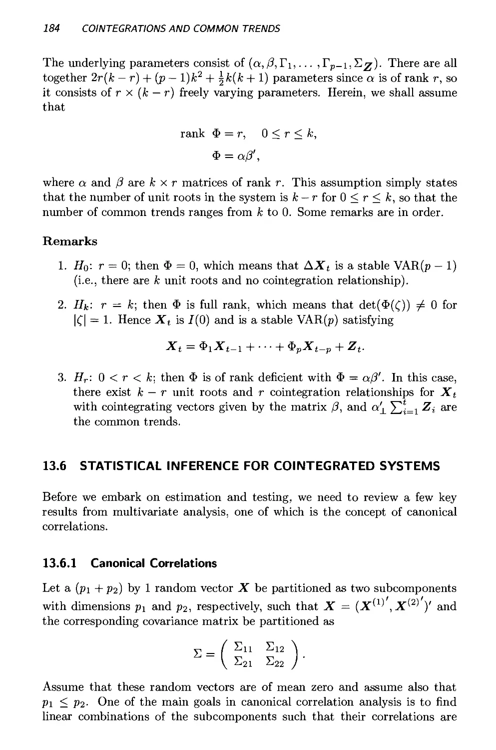
13.5 Structure of Cointegrated Systems 183
13.6 Statistical Inference for Cointegrated Systems 184
13.6.1 Canonical Correlations 184
13.6.2 Inference and Testing 186
13.7 Example of Spot Index and Futures 188
13.8 Conclusions 193
13.9 Exercis es 193
References 195
Index 201
This textbook evolved in conjunction with teaching a course in time series
analysis at Carnegie Mellon University and the Chinese University of Hong
Kong. For the past several years, I have been involved in developing and
teaching the financial time series analysis course for the Masters of Science in
Computational Finance Program at Carnegie Mellon University. There are
two unique features of this program that differ from those of a traditional
statistics curriculum.
First, students in the program have diversified backgrounds. Many of them
have worked in the finance world in the past, and some have had extensive
trading experiences. On the other hand, a substantial number of these stu-
dents have already completed their Ph.D. degrees in theoretical disciplines
such as pure mathematics or theoretical physics. The common denominator
between these two groups of students is that they all want to analyze data
the way a statistician does.
Second, the course is designed to be fast paced and concise. Only six weeks
of three-hour lectures are devoted to covering the first nine chapters of the
text. After completing the course, students are expected to have acquired a
working knowledge of modern time series techniques.
Given these features, offering a full-blown theoretical treatment would be
neither appropriate nor feasible. On the other hand, offering cookbook-style
instruction would never fulfill the intellectual curiosity of these students. They
want to attain an intellectual level beyond that required for routine analysis
of time series data. Ultimately, these students have to acquire the knack of
xi
xii PREFACE
knowing the conceptual underpinnings of time series modeling in order to get
a better understanding of the ever-changing dynamics of the financial world.
Consequently, finding an appropriate text which meets these requirements
becomes a very challenging task.
As a result, a set of lecture notes that balances theory and applications,
particularly within the financial domain, has been developed. The current text
is the consequence of several iterations of these lecture notes. In developing
the book a number of features have been emphasized.
• The first seven chapters cover the standard topics in statistical time
series, but at a much higher and more succinct level. Technical details
are left to the references, but important ideas are explained in a con-
ceptual manner. By introducing time series in this way, both students
with a strong theoretical background and those with strong practical
motivations get excited about the subject early on.
• Many recent developments in nonstandard time series techniques, such
as univariate and multivariate GARCH, state space modeling, cointegra-
tions, and common trends, are discussed and illustrated with real finance
examples in the last six chapters. Although many of these recent de-
velopments have found applications in financial econometrics, they are
less well understood among practitioners of finance. It is hoped that
the gap between academic development and practical demands can be
narrowed through a study of these chapters.
• Throughout the book I have tried to incorporate examples from finance
as much as possible. This is done starting in Chapter 1, where an equity-
style timing model is used to illustrate the price one may have to pay
if the time correlation component is overlooked. The same approach
extends to later chapters, where a Kalman filter technique is used to
estimate parameters of a fixed-income term-structure model. By giving
these examples, the relevance of time series in financial applications can
be firmly anchored.
• To the extent possible, almost all of the examples are illustrated through
Splus programs, with detailed analyses and explanations of the Splus
commands. Readers will be able to reproduce the analyses by replicating
some of the empirical works and testing alternative models so as to
facilitate an understanding of the subject. All data and computer codes
used in the book are maintained in the Statlib Web site at Carnegie
Mellon University and the Web page at the Chinese University of Hong
Kong at
http://www.st a.cuhk.edu.hk/dat al/st af f/nhchan/tsbook.html.
Several versions of these lecture notes have been used in a time series
course given at Carnegie Mellon University and the Chinese University of
PREFACE xiii
Hong Kong. I am gratefule for many suggestions, comments, and questions
from both students and colleagues at these two institutions. In particular,
I am indebted to John Lehoczky for asking me to develop the program, to
Jay Kadane for suggesting that I write this book, and to Pantelis Vlachos,
who taught part of this course with me during the spring of 2000. Many of
the computer programs and examples in Chapters 9 to 13 are contributions
by Pantelis. During the writing I have also benefited greatly from consulting
activities with Twin Capital Management, in particular Geoffrey Gerber and
Pasquale Rocco, for many illuminating ideas from the financial world. I hope
this book serves as a modest example of a fruitful interaction between the
academic and professional communities. I would also like to thank Ms. Heidi
Sestrich for her help in producing the figures in Latex, and to Steve Quigley,
Heather Haselkorn, and Rosalyn Farkas, all from Wiley, for their patience
and professional assistance in guiding the preparation and production of this
book. Financial support from the Research Grant Council of Hong Kong and
the National Security Agency throughout this project is gratefully acknowl-
edged. Last, but not least, I would like to thank my wife, Pat Chao, whose
contributions to this book went far beyond the call of duty as a part-time
proofreader, and to my family, for their understanding and encouragement of
my ceaseless transitions between Hong Kong and Pittsburgh during the past
five years. Any remaining errors are, of course, my sole responsibility.
Ngai Hang Chan
Shatin, Hong Kong
March 2001
This page intentionally left blank
1
Introduction
1.1 BASIC DESCRIPTION
The study of time series is concerned with time correlation structures. It has
diverse applications ranging from oceanography to finance. The celebrated
CAPM model and the stochastic volatility model are examples of financial
models that contain a time series component. When we think of a time series,
we usually think of a collection of values {Xt : t = 1,... ,n} in which the
subscript t indicates the time at which the datum Xt is observed. Although
intuitively clear, a number of nonstandard features of Xt can be elaborated.
Unequally spaced data (missing values). For example, if the series is about
daily returns of a security, values are not available during nontrading days
such as holidays.
Continuous-time series. In many physical phenomena, the underlying quan-
tity of interest is governed by a continuously evolving mechanism and the data
observed should be modeled by a continuous time series A(t). In finance, we
can think of tick-by-tick data as a close approximation to the continuous evo-
lution of the market.
Aggregation. The series observed may represent an accumulation of under-
lying quantities over a period of time. For example, daily returns can be
thought of as the aggregation of tick-by-tick returns within the same day.
Replicated series. The data may represent repeated measurements of the
same quantity across different subjects. For example, we might monitor the
1
2 INTRODUCTION
total weekly spending of each of a number of customers of a supermarket chain
over time.
Multiple time series. Instead of being a one-dimensional scalar, Xt can be
a vector with each component representing an individual time series. For
example, the returns of a portfolio that consist of p equities can be expressed
as Xt = (Хц,... , Xpt)', where each Xit, i = 1,... ,p, represents the returns
of each equity in the portfolio. In this case, we will be interested not only in the
serial correlation structures within each equity but also the cross-correlation
structures among different equities.
Nonlinearity, nonstationarity, and heterogeneity. Many of the time series en-
countered in practice may behave nonlinearly. Sometimes transformation may
help, but we often have to build elaborate models to account for such non-
standard features. For example, the asymmetric behavior of stock returns
motivates the study of GARCH models.
Although these features are important, in this book we deal primarily with
standard scalar time series. Only after a thorough understanding of the tech-
niques and difficulties involved in analyzing a regularly spaced scalar time
series will we be able to tackle some of the nonstandard features.
In classical statistics, we usually assume the X's to be independent. In
a time series context, the X’s are usually serially correlated, and one of the
objectives in time series analysis is to make use of this serial correlation struc-
ture to help us build better models. The following example illustrates this
point in a confidence interval context.
Example 1.1 Let Xt be generated by the following model:
Xt = p + at 0at i, at ~ N(0,1) i.i.d.
Clearly, E(Xt) = p and varXt = 1 + 62. Thus,
cov(Xt,Xt_fe) = E(Xt - p)(Xt-k - p)
E(at 0at-i)(at-fc $at—k i)
-6*,
1 + 02,
0,
|fc| = 1,
к = 0,
otherwise.
Let X = (52”=1 Xt)/n. By means of the formula
П \ n Q n t— 1
- E Xt = Evar(Xt) + E Ecov(Xt’
t=l / t=l t=lj=l
BASIC DESCRIPTION 3
Table 1.1 Lengths of Confidence Intervals for n = 50
0 L(0)
-1 -0.5 0 0.5 1 L(-l) = (4-^),/2 = 2 1.34 1 0.45 0.14
it is easily seen that
Oy — var X
= -^n(l + 02) - -~{n - 1)0
n2 n2
= - (1 + 02 - 20 + —
n \ n 7
1
n
(1-0)=+^
n
Therefore, X ~ N(u, cr^-). Hence, an
{CT) for is
approximate 95% confidence interval
— 9 _ 2
X ± 2<Ц_ = X ± —
л Vn
9Д11/2
(1 - 0)2 + -
n
If 0 = 0, this CI becomes
coinciding with the independent identically distributed {i.i.d.) case. The dif-
ference in the Cis between 0 = 0 and 0^0 can be expressed as
L(«) =
1/2
n
Table 1.1 gives numerical values of the differences for n = 50. For example,
if 0 = 1 and if we were to use a CI of zero for 0, the wrongly constructed CI
would be much longer than it is supposed to be. The time correlation structure
given by the model helps to produce better inference in this situation. □
Example 1.2 As a second example, we consider the equity-style timing model
discussed in Kao and Shumaker (1999). In this article the authors try to ex-
plain the spread between value and growth stocks using several fundamental
quantities. Among them, the most interesting variable is the eamings-yield
gap reported in Figure 4 of their paper. This variable explains almost 30%
4 INTRODUCTION
Scatterplot of Style SpreadsjS^ubspgjenj^S-iy.oip^i^j/alue Return • Growth Return)
E
199307 -
199307" _ 19830
196706 199904 % *106310
198301 •
1МЭС»*
• 196711
,198212e Tee101
J мою
196405
ф 198406
196106
,199411 •
, , 199903
198206
188107
1МВ0Э
fteeot
196501 «
189104 ф
90306 • 196607
' .1966^’®“’»
f 199907 •t’JSX
1M004
i£eoe
* 19660»
'98207
** 196006 197906
197904 ф
197902 e 197907 •
197903 ф
197910
^Uto
199509 ’“®°®
199007 .”»»1O
-2
2
0
Earnings-Yield Gap
Fig. 1.1 Equity-style timing.
of the variation of the spread between value and growth and suggests that the
earnings yield, gap might be a highly informative regressor. Further descrip-
tion of this data set is given in their article. We repeat this particular analysis,
but taking into account the time order of the observations. The data between
January 79 to June 97 are stored in the file eygap. dat on the Web page for
this book, which can be found at
http://www.sta.cuhk.edu.hk/datal/staff/nhchan/tsbook.html
For the time being, we restrict our attention to reproducing Figure 4 of Kao
and Shumaker (1999). The plot and SpluS commands are as follows:
>eyield<-read.table("eygap.dat",header=T)
>plot(eyield[,2],eyield[,3],xlab="Earnings-Yield Gap",
+ ylab="Return Differential")
>title("Scatterplot of Style Spreads (Subsequent
+ 12-month Value Return - Growth Return)
+ against Earnings-Yield Gap, Jan 79- Jun 97",cex=0.6)
>identify(eyield[,2],eyield[,3],eyield[,l],cex=0.5)
As illustrated in Figure 1.1, the scattergram can be separated into two
clouds, those belonging to the first two years of data and those belonging to
subsequent years. When time is taken into account, it seems that finding
an R2 = 0.3 depends crucially on the data cloud between 79 and 80 at the
lower right-hand corner of Figure 1.1. Accordingly, the finding of such a high
SIMPLE DESCRIPTIVE TECHNIQUES 5
explanatory power from the eamings-yield gap seems to be spurious. This
example demonstrates that important information may be missing when the
time dimension is not taken properly into account. □
1.2 SIMPLE DESCRIPTIVE TECHNIQUES
In general, a time series can be decomposed into a macroscopic component
and a microscopic component. The macroscopic component can usually be
described through a trend or seasonality, whereas the microscopic component
may require more sophisticated methods to describe it. In this section we deal
with the macroscopic component through some simple descriptive techniques
and defer the study of the microscopic component to later chapters. Consider
in general that the time series {Xt} is decomposed into a time trend part Tt,
a seasonal part St, and a microscopic part given by the noise Nt- Formally,
Xt = Tt + St + Nt
= Pt + Nt-
(1-1)
1.2.1 Trends
Suppose that the seasonal part is absent and we have only a simple time trend
structure, so that Tt can be expressed as a parametric function of t, Tt = a+/3t,
for example. Then Tt can be identified through several simple devices.
Least squares method. We can use the least squares (LS) procedure to es-
timate Tt easily [i.e., find a and 3 such that — Tt)2 is minimized].
Although this method is convenient, there are several drawbacks.
1. We need to assume a fixed trend for the entire span of the data set,
which may not be true in general. In reality, the form of the trend may
also be changing over time and we may need an adaptive method to
accommodate this change. An immediate example is the daily price of
a given stock. For a fixed time span, the prices can be modeled pretty
satisfactorily through a linear trend. But everyone knows that the fixed
trend will give disastrous predictions in the long run.
2. For the LS method to be effective, we can only deal with a simple
restricted form of Tt.
Filtering. In addition to using the LS method, we can filter or smooth the
series to estimate the trend, that is, use a smoother or a moving average filter,
such as
s
Yt = Sm(At) = ^2 arXt+r-
r~—q
6 INTRODUCTION
We can represent the relationship between the output Yt and the input Xt as
Xt | filter | Sm(Xt) = Yt.
The weights {<zr} of the filters are usually assumed to be symmetric and
normalized (i.e., ar = a_r and ^2 a,. = 1). An obvious example is the simple
moving average filter given by
The length of this filter is determined by the number q. When q = 1 we have
a simple three-point moving average. The weights do not have to be the same
at each point, however. An early example of unequal weights is given by the
Spencer 15-point filter, introduced by an English actuary, Spencer, in 1904.
The idea is to use the 15-point filter to approximate the filter that passes
through a cubic trend. Specifically, define the weights {<zr} as
CL^ — CL—y
ar = 0, | r |> 7,
(a0, ai,... ,a7) = ^(74, 67, 46, 21, 3, -5, -6, -3).
It can easily be shown that Spencer 15-point filter does not distort a cubic
trend; that is, for Tt = at3 + bt2 + ct + d,
7 7
Sm(Xt) = 57 52 arNt+r
y= — 7 r=—7
7
— 5
r—— 7
= Tt.
In general, it can be shown that a linear filter with weights {<zr} passes a
polynomial of degree к in t, ^i=0Citl, without distortion if and only if the
weights {<zr} satisfy two conditions, as described next.
Proposition 1.1 Tt = ^2rar7j+r, for all kth-degree polynomials Tt = co +
ci t + • • + Cktk if and only if
52 r^ar = 0) for j = 1) , к.
SIMPLE DESCRIPTIVE TECHNIQUES 7
The reader is asked to provide a proof of this result in the exercises. Using
this result, it is straightforward to verify that Spencer 15-point filter passes a
cubic polynomial without distortion. For the time being, let us illustrate the
main idea on how a filter works by means of the simple case of a linear trend
where Xt = Tt + Nt, Tt = a + (3t. Consider applying a (2g + l)-point moving
average filter (smoother) to Xt :
1 1
Yt = Sm(Xt) = —- £ Xt+r
y r=—q
= У? [a + /3(t + r)] + Nt+r
“r -L
r=—q
= a + /3t
if „ *, У'1 „ Nt+r = 0. In other words, if we use Yt to estimate the trend,
2g+l £-jr=—q ь ‘ ч v ч
it does a pretty good job. We use the notation Yt = Sm(A”t) = Tt and
Res(A’t) = Xt—Tt = Xt — Sm(A’t) = Nt. In this case we have what is known
as a low-pass filter [i.e., a filter that passes through the low-frequency part
(the smooth part) and filters out the high-frequency part, Nt]. In contrast,
we can construct a high-pass filter that filters out the trend. One drawback
of a low-pass filter is that we can only use the middle section of the data. If
end-points are needed, we have to modify the filter accordingly. For example,
consider the filter
Sm(Xt) = £a(l-ay'Xt_>,
j=o
where 0 < a < 1. Known as the exponential smoothing technique, this plays a
crucial role in many empirical studies. Experience suggests that a is chosen
between 0.1 and 0.3. Finding the best filter for a specific trend was once an
important topic in time series. Tables of weights were constructed for different
kinds of lower-order trends. Further discussion of this point can be found in
Kendall and Ord (1990).
Differencing. The preceding methods aim at estimating the trend by a
smoother Tt- In many practical applications, the trend may be known in ad-
vance, so it is of less importance to estimate it. Instead, we might be interested
in removing its effect and concentrate on analyzing the microscopic compo-
nent. In this case it will be more desirable to eliminate or annihilate the effect
of a trend. We can do this by looking at the residuals Res(A’t) = Xt — Sm(A’t).
A more convenient method, however, will be to eliminate the trend from the
series directly. The simplest method is differencing. Let В be the backshift
operator such that BXt = Xt-i. Define
NXt = (1 B)Xt = xt- xt^,
^Xt = (l-Byxt, J = 1,2,... .
8 INTRODUCTION
If Xt = Tt + Nt, with Tt = Y^j=oajti > then NXt = j\aj + XT Nt and Tt is
eliminated. Therefore, differencing is a form of high-pass filter that filters out
the low-frequency signal, the trend Tt, and passes through the high-frequency
part, Nt- In principle, we can eliminate any polynomial trend by differencing
the series enough times. But this method suffers one drawback in practice.
Each time we difference the series, we lose one data point. Consequently, it
is not advisable to difference the data too often.
Local curve fitting. If the trend turns out to be more complicated, local
curve smoothing techniques beyond a simple moving average may be required
to obtain good estimates. Some commonly used methods are spline curve
fitting and nonparametric regression. Interested readers can find a lucid dis-
cussion about spline smoothing in Diggle (1990).
1.2.2 Seasonal Cycles
When the seasonal component St is present in equation (1.1), the methods of
Section 1.2.1 have to be modified to accommodate this seasonality. Broadly
speaking, the seasonal component can be either additive or multiplicative,
according to the following formulations:
_ ( Tt + St + Nt, additive case,
* [ TtStNt, multiplicative case.
Again, depending on the goal, we can either estimate the seasonal part by
some kind of seasonal smoother or eliminate it from the data by a seasonal
differencing operation. Assume that the seasonal part has a period of d (i.e.,
St+d = St, = o)-
(A) Moving average method. We first estimate the trend part by a moving
average filter running over a complete cycle so that the effect of the
seasonality is averaged out. Depending on whether d is odd or even, we
perform one of the following two steps:
1. If d = 2g, let Tt = (^Xt-q + Xt_9+i + • • + At+q-i + |Aj+9)
for t = q + 1,... ,n — q.
2. If d = 2q + 1, let Tt = 1 52r=-9 Xt+r for t = q + 1,... , n - q.
After estimating Tt, filter it out from the data and estimate the seasonal
part from the residual Xt — Tt. Several methods are available to attain
this last step, the most common being the moving average method.
Interested readers are referred to Brockwell and Davis (1991) for further
discussions and illustrations of this method. We illustrate this method
by means of an example in Section 1.4.
(B) Seasonal differencing. On the other hand, we can apply seasonal dif-
ferencing to eliminate the seasonal effect. Consider the dth differencing
EXAMPLE 9
Fig. 1.2 Time series plots.
of the data Xt — Xt-d- This differencing eliminates the effect of St in
equation (1.1). Again, we have to be cautious about differencing the
data seasonably since we will lose data points.
1.3 TRANSFORMATIONS
If the data exhibit an increase in variance over time, we may need to transform
the data before analyzing them. The Box-Cox transformations can be applied
here. Experience suggests, however, that log is the most commonly found
transformation. Other types of transformations are more problematic, which
can lead to serious difficulties in terms of interpretations and forecasting.
1.4 EXAMPLE
In this section we illustrate the idea of using descriptive techniques to analyze
a time series. Figure 1.2 shows a time series plot of the quarterly operating
revenues of Washington Water Power Company, 1980-1986, an electric and
natural gas utility serving eastern Washington and northern Idaho. We start
by plotting the data. Several conclusions can be drawn by inspecting the plot.
• As can be seen, there is a slight increasing trend. This appears to drop
around 1985-1986.
• There is an annual (12-month) cycle that is pretty clear. Revenues are
almost always lowest in the third quarter (July-September) and highest
10 INTRODUCTION
_ Washington Water Power Co
Operating Revenues: 1980-1986
1980 1981 1982 1983 1984 1985 1986
Fig. 1.3 Annual box plots.
in the first quarter (January-March). Perhaps in this part of the country
there is not much demand (and hence not much revenue) for electrical
power in the summer (for air conditioning, say), but winters are cold
and there is a lot of demand (and revenue) for natural gas and electric
heat at that time.
• Figure 1.3 shows box plots for each year’s operating revenues. The
medians seem to rise from year to year and then fall back after the third
year. The interquartile range (IQR) gets larger as the median grows and
gets smaller as the median falls back; the range does the same. Most of
the box plots are symmetric or very slightly positively skewed. There
are no outliers.
• In Figure 1.3 we can draw a smooth curve connecting the medians of
each year’s quarterly operating revenues. We have already described
the longer cycle about the medians; this pattern repeats once over the
seven-year period graphed. This longer-term cycle is quite difficult to
see in the original time series plot.
Assume that the data set has been stored in the file named washpower. dat.
The Splus program that generates this analysis is listed as follows. Readers
are encouraged to work through these commands to get acquainted with the
Splus program. Further explanations of these commands can be found in the
books of Krause and Olson (1997) and Venables and Ripley (1999).
>wash_rts(scan(‘‘washpower.dat’’),start=1980,freq=4)
>wash.ma_filter(wash,c(l/3,1/3,1/3))
>leg.names_c(’Data’,’Smoothed Data’)
EXAMPLE
11
>t s.plot(wash,wash.ma,lty=c(1,2),
+ main=’Washington Water Power Co
Continue string: Operating Revenues: 1980-1986’,
+ ylab=’Thousands of Dollars’,xlab=’Year’)
>legend(locator(1),leg.names,lty=c(1,2))
>wash.mat _matrix(wash,nrow=4)
>boxplot(as.data.frame(wash.mat),names=as.character(seq(1980,
+ 1986)), boxcol=-l,medcol=l,main=’Washington Water Power Co
Continue string: Operating Revenues: 1980-1986’,
+ ylab=’Thousands of Dollars’)
To assess the seasonality, we perform the following steps in the moving
average method.
1. Estimate the trend through one complete cycle of the series with n =
28, d = 4, and q = 2 to form Xt — ft : t = 3,... , 26. The Tt is denoted
by washsea.ma in the program.
2. Compute the averages of the deviations {Xt — Tt} over the entire span of
the data. Then estimate the seasonal part Si : i = 1,... , 4 by computing
the demeaned values of these averages. Finally, for i = 1,... ,4 let
Si+4j — St : j = 1,... ,6. The estimated seasonal component Si is
denoted by wash.sea in the program, and the deseasonalized part of
the data Xt — St is denoted by wash. nosea.
3. The third step involves reestimating the trend from the deseasonalized
data wash.nosea. This is accomplished by applying a filter or any
convenient method to reestimate the trend by Tt, which is denoted by
wash.ma2 in the program.
4. Finally, check the residual Xt — Tt — St, which is denoted by wash.res
in the program, to detect further structures. The Splus code follows.
> washsea.ma_filter(wash,c(l/8,rep(l/4,3),1/8))
> wash.sea_c(0,0,0,0)
> ford in 1:2){
+ for(j in 1:6) {
+ wash.sea[i]_wash.sea[i]+
+ (wash[i+4*j][[1]]-washsea.ma[i+4*j][[1]])
+ }
+ }
> ford in 3:4){
+ for (j in 1:6){
+ wash.sea[i]_wash.sea[i]+
+ (wash[i+4*(j-l)][[1]]-washsea.ma[i+4*(j-l)][[1]])
+ }
+ }
12 INTRODUCTION
Time
Fig. 1.4 Moving average method of seasonal decomposition.
> wash.sea_(wash.sea-mean(wash.sea))/6
> wash.seal_rep(wash.sea,7)
> wash.nosea_wash-wash.sea
> wash,ma2_filter(wash.nosea,c(1/8,rep(1/4,3),1/8))
> wash.res_wash-wash.ma2-wash,sea
> write(wash.seal, file=’out.dat’)
> wash.seatime_rts(scan(’out.dat’),start=1980,freq=4)
7, This step converts a non-time series object into a time
7. series object.
> ts.plot(wash,wash.nosea,wash.seatime)
Figure 1.4 gives the time series plot, which contains the data, the desea-
sonalized data, and the seasonal part. If needed, we can also plot the residual
wash. res to detect further structures. But it is pretty clear that most of the
structures in this example have been identified.
Note that Splus also has its own seasonal decomposition function stl.
Details of this can be found with the help command. To execute it, use
> wash.stl_stl(wash,’periodic’)
> dwash_diff(wash,4)
> ts.plot(wash,wash.stl$sea,wash.stl$rem,dwash)
Figure 1.5 gives the plot of the data, the deseasonal part, and the seasonal
part. Comparing Figures 1.4 and 1.5 indicates that these two methods ac-
complish the same task of seasonal adjustments. As a final illustration we can
difference the data with four lags to eliminate the seasonal effect. The plot of
this differenced series is also drawn in Figure 1.5.
EXERCISES
13
Fig. 1.5 Splus stl seasonal decomposition.
1.5 CONCLUSIONS
In this chapter we studied several descriptive methods to identify the macro-
scopic component (trend and seasonality) of a time series. Most of the time,
these components can be identified and interpreted easily and there is no
reason to fit unnecessarily complicated models to them. From now on we
will assume that this preliminary data analysis step has been completed and
we focus on analyzing the residual part Nt for microscopic structures. To
accomplish this goal, we need to build more sophisticated models.
1.6 EXERCISES
1. (a) Show that a linear filter {a./} passes an arbitrary polynomial of
degree к without distortion, that is,
mt =
з
for all /cth-degree polynomials mt = Co + citH-----\-Cktk if and only
if
' = 1, and jrdj = 0 for r = 1,..., k.
3 3
(b) Show that the Spencer 15-point moving average filter does not
distort a cubic trend.
2. If mt = 52fc=ocfe^fc’^ = 0, ±1,..., show that Amt is a polynomial of
degree (p — 1) in t and hence Ap+1mt = 0.
14 INTRODUCTION
3. In Splus, get hold of the yearly airline passenger data set by assigning
it to an object. You can use the command
x_rts(scan(’airline.dat’),freq=12,start=1949)
The data are now stored in the object x, which forms the time series
{Yt}. This data set consists of monthly totals (in thousands) of interna-
tional airline passengers from January 1949 to December 1960 [details
can be found in Brockwell and Davis (1991)]. It is stored under the file
airline.dat on the Web page for this book.
(a) Do a time series plot of this data set. Are there any obvious trends?
(b) Is it necessary to transform the data? If a transformation is needed,
what would you suggest?
(c) Do a yearly running median for this data set. Sketch the box plots
for each year to detect any other trends.
(d) Find a trend estimate by using a moving average filter. Plot this
trend.
(e) Estimate the seasonal component Sk, if any.
(f) Consider the deseasonalized data dt = Xt — St,t = 1, Rees-
timate a trend from {dt} by applying a moving average filter to
{dt}; call it mt, say.
(g) Plot the residuals rt = Xt — iht — St- Does it look like a white noise
sequence? If not, can you make any suggestions?
Probability Models
2.1 INTRODUCTION
In the next three chapters, we discuss some theoretical aspects of time series
modeling. To gain a better understanding of the microscopic component {M},
basic probability theories of stochastic processes have to be introduced. This
is done in the present chapter, and Chapters 3 and 4 deal with commonly
used ARIMA models and their basic properties. In Chapter 5, two examples
illustrating ideas of these chapters are given in detail with Splus commands.
Readers who want to become acquainted immediately with series model fitting
with Splus may want to review some of these examples at this point.
Although one may argue that it is sufficient for a practitioner to analyze a
time series without worrying about the technical details, we feel that balanced
learning between theory and practice would be much more beneficial. Since
time series analysis is a very fast moving field, topics of importance today
may become passe in a few years. Thus, it is vital for us to acquire some basic
understanding of the theoretical underpinnings of the subject so that when
new ideas emerge, we can continue learning on our own.
2.2 STOCHASTIC PROCESSES
Definition 2.1 A collection of random variables {A”(t) : t G 71} is called a
stochastic process.
15
16 PROBABILITY MODELS
In general, {X(t) : 0 < t < oc} and {Xt : t — 1,2,... , n} are used to define
a continuous-time and a discrete-time stochastic process, respectively. Recall
that all the X’s are defined on a given probability space (Q,F, F). Thus,
Xt = Xt(w) : П —> R for a fixed t.
On the other hand, for a given ш G Q, Xt(aj) can be considered as a function
of t and as such, this function is called a sample function, a realization, or a
sample path of the stochastic process. For a different w, it will correspond to a
different sample path. The collection of all sample paths is called an ensemble.
All the time series plots we have seen are based on a single sample path.
Accordingly, time series analysis is concerned with finding the probability
model that generates the time series observed.
To describe the underlying probability model, we can consider the joint
distribution of the process; that is, for any given set of times (ti,... ,tn),
consider the joint distribution of (Xt,,... , Xtn), called the finite-dimensional
distribution.
Definition 2.2 Let T be the set of all vectors {t = (ti,... ,tnfi G Tn :
ti < • - < tn, n = 1,2,...}. Then the (finite-dimensional) distribution
functions of the stochastic process {Xt,t G T} are the functions G
T} defined for t = (ti,... , tn)' by
Ft(x) = P(Xtl <x-t,... ,Xt„ <xn), x = (x1,... ,xn)' G Rn.
Theorem 2.1 (Kolmogorov’s Consistency Theorem) The probability distri-
butionfunctions {Ff(-),t G T] are the distribution functions of some stochas-
tic process if and only if for any n G {1,2,... }, t = (ti,... , tn)' G T and
1 <i < n,
lim Ft(x) = Ft{i}(x(i)), (2.1)
Xi~»oo v ’
where t(j) and x(i) are the (n — 1)-component vectors obtained by deleting the
ith components of t and x, respectively.
This theorem ensures the existence of a stochastic process through spec-
ification of the collection of all finite-dimensional distributions. Condition
(2.1) ensures a consistency which requires that each finite-dimensional distri-
bution should have marginal distributions that coincide with the lower finite-
dimensional distribution functions specified.
Definition 2.3 {Xt} is said to be strictlystationary if for all n, for all
(ti,... ,tn), and for all r,
(Xt„... ,Xtn) = (Xtx+r,... ,Xtn+T),
where = denotes equality in distribution.
EXAMPLES
17
Intuitively, stationarity means that the process attains a certain type of
statistical equilibrium and the distribution of the process does not change
much. It is a very restrictive condition and is often difficult to verify. We
next introduce the idea of covariance and a weaker form of stationarity for a
stochastic process.
Definition 2.4 Let {Xt : t G T} be a stochastic process such that var(Aj) <
oo for all t & T. Then the autocovariance function 7x(-,-) of {W} is
defined by
yx(r, s) = cov(Xr, Xs) = E(Xr - EXr)(Xs - EXS), r,seT.
Definition 2.5 {At } is said to be weakly stationary (second-order sta-
tionary, wide-sense stationary) if
(i) E(Xt) = p for all t.
(ii) cov (Xt, Xt+r) = у(т) for all t and for all t.
Unless otherwise stated, we assume that all moments, E\Xt |fc, exist whenever
they appear. A couple of consequences can be deduced immediately from
these definitions.
1. Take т = 0, cov(Xt, Xt) = 7(0) for all t. The means and variances of a
stationary process always remain constant.
2. Strict stationarity implies weak stationarity. The converse is not true
in general except in the case of a normal distribution.
Definition 2.6 Let {W} be a stationary process. Then
(i) 'у(т') = cov(Xj, Xt+T) is called the autocovariance function.
(ii) р(т) = 7(t)/7(0) is called the autocorrelation function.
For stationary processes, we expect that both 7Q and p(-) taper off to zero
fairly rapidly. This is an indication of what is known as the short-memory
behavior of the series.
2.3 EXAMPLES
1. Xt are i.i.d. random variables. Then
P(t) =
1,
0,
т = 0,
otherwise.
Whenever a time series has this correlation structure, it is known as a
white noise sequence and the whiteness will become apparent when we
study the spectrum of this process.
18 PROBABILITY MODELS
2. Let У be a random variable such that var Y = <r2. Let Yi = Y2 = • • • =
Yt = • = Y. Then
p(r) = 1 for all t.
Hence the process is stationary. However, this process differs substan-
tially from {X/} in example 1. For {Xt}, knowing its value at one time
t has nothing to do with the other values. For {У/}, knowing Fi gives
the values of all the other Y^s. Furthermore,
— (Xj + • • • + Xn) —» EXi = p by the law of large numbers.
n
But (У + • • • + Уп)/п = У. There is as much randomness in the nth
sample average as there is in the first observation for the process {Ft}-
To prevent situations like this, we introduce the following definition.
Definition 2.7 If the sample average formed from a sample path of a
process converges to the underlying parameter of the process, the process
is called ergordic.
For ergordic processes, we do not need to observe separate indepen-
dent replications of the entire process in order to estimate its mean value
or other moments. One sufficiently long sample path would enable us
to estimate the underlying moments. In this book, all the time series
studied are assumed to be ergodic.
3. Let Xt = AcosOt + ВsmOt, A,В ~ (0,<r2) i.i.d. Since EXt = 0, it
follows that
cov(Xt+/l,Xt) = E(Xt+hXt)
= E(AcosO(t + h) + В sin#(t + /i))(Acos#t + Bsinflt)
= <r2 cos 8h.
Hence the process is stationary.
2.4 SAMPLE CORRELATION FUNCTION
In practice, 7(7-) and p(r) are unknown and they have to be estimated from
the data. This leads to the following definition.
Definition 2.8 Let {Xj} be a given time series and X be its sample mean.
Then
(i) Ck = — X)(Xt+fc — X)/n is known as the sample auto-
covariance function of Xt.
(ii) rk = Ck/Co is called the sample autocorrelation function (ACF).
SAMPLE CORRELATION FUNCTION 19
The plot rfc versus к is known as a correlogram. By definition, ro = 1.
Intuitively, Ck approximates ~;(k) and Гк approximates p(k'). Of course, such
approximations rely on the ergordicity of the process. Let us inspect the ACF
of the following examples. In the exercise, readers are asked to match the
sample ACF with the generating time series.
1. For a random series (e.g., Yt’s are i.i.d.), it can be shown that for each
fixed k, as the sample size n tends to infinity,
rk ~ AN(0,1/n);
that is, the random variables y/n Гк converge in distribution to a stan-
dard normal random variable as n —» oo.
Remark. A statistic Tn is said to be AN(/zn. c2) (asymptotic normally
distributed with mean pn and variance <r2) if \Tn— pn)/an converges in
distribution to a standard normal random variable as the sample size n
tends to infinity. For example, let Xi,... ,Xn be i.i.d. random variables
with E'(A’1) = p, and var(Ai) = c2 > 0. Let Xn = (^2"=1 X^/n and
rp ___ — P
П ” ’
Then by the central limit theorem, Tn converges in distribution to a
standard normal random variable as n —> oo [i.e., Xn is said to have an
AN(p, <r2/n)]. In this case, pn = p and <r2 = <r2/n.
2. Yt = Y, rk = 1.
3. A stationary series often exhibits short-term correlation (or short-memory
behavior), a large value of pi followed by a few smaller correlations which
subsequently get smaller and smaller.
4. In an alternating series, alternates between positive and negative
values. A typical example of such a series is an AR(1) model with a
negative coefficient, Yt = + Zt, where ф is a positive parameter
and Zt are i.i.d. random variables.
5. If seasonality exists in the series, it will be reflected in the ACF. In
particular, if Xt = a cos ta>, it can be shown that Гк = cos ka>.
6. In the nonstationary series case, Гк does not taper off for large values of
k. This is an indication of nonstationarity and may be caused by many
factors.
Notice that the examples above suggest that we can “identify” a time series
through inspection of its ACF. Although this sounds promising, it is not a
procedure that is always free of error. When we calculate the ACF of any
given series with a fixed sample size n, we cannot put too much confidence in
20 PROBABILITY MODELS
the values of for large k’s, since fewer pairs of (Xt,Xt~k) will be available
for computing rfe when к is large. One rule of thumb is not to evaluate
for к > n/3. Some authors even argue that only r^’s for к = O(logn) should
be computed. In any case, precautions must be taken. Furthermore, if there
is a trend in the data, Xt = Tt + Nt, then Xt becomes nonstationary (check
this with the definition) and the idea of inspecting the ACF of Xt becomes
questionable. It is therefore important to detrend the data before interpreting
their ACF.
2.5 EXERCISES
1. Given a seasonal series of monthly observations {X<}, assume that the
seasonal factors {£)} are constants so that St = St-y2 for all t and
assume that {Zt} is a white noise sequence.
(a) With a global linear trend and additive seasonality, we have Xt =
a + pt + St + Zf Show that the operator Д12 = 1 — B12 acting on
Xt reduces the series to stationarity.
Fig. 2.1 Correlograms for Exercise 3.
EXERCISES 21
(b) With a global linear trend and multiplicative seasonality, we have
Xt = {a + (3f)St + Zt. Does the operator Д12 reduce Xt to station-
arity? If not, find a differencing operator that does.
2. If {Xt = Acosta; : t = 1,... , n} where A is a fixed constant and ш is a
constant in (0,7г), show that —» cosA'a; as n —> 00. Hint You need
to use the double-angle and summation formulas for a trigonometric
function.
3. Let Zt ~ N(0,1) i.i.d. Match each of the following time series with its
corresponding correlogram in Figure 2.1.
(a) Xt = Zt.
(b) Xt = -O.SXt-r + Zt.
(c) Xt = sin(7r/3) t + Zt.
(d) Xt = Zt — 0.37^.
This page intentionally left blank
Autoregressive Moving
Average Models
3.1 INTRODUCTION
Several commonly used probabilistic models for time series analysis are intro-
duced in this chapter. It is assumed that the series being studied have already
been detrended by means of the methods introduced in previous chapters.
Roughly speaking, there are three kinds of models: the moving average model
(MA), the autoregressive model (AR), and the autoregressive moving average
model (ARMA). They are used to describe stationary time series. In addition,
since certain kinds of nonstationarity can be handled by means of differencing,
we also study the class of autoregressive integrated moving average models
(ARIMAs).
3.2 MOVING AVERAGE MODELS
Let {Z<} be a sequence of independent identically distributed random vari-
ables with mean zero and variance <r2, denoted by Zt ~ i.i.d.(0,<r2). If we
require {Zt} only to be uncorrelated, not necessarily independent, then {Zt}
is sometimes known as a white noise sequence, denoted by Zt ~ WN(0, <r2).
Intuitively, this means that the sequence {Zt} is random with no system-
atic structures. Throughout this book we use {Zt} to represent a white
noise sequence in the loose sense; that is, {Zt} ~ WN(0,<r2) can mean ei-
ther {Zt} ~ i.i.d.(0, cr2) or that {Zt} are uncorrelated random variables with
mean zero and variance cr2. By forming a weighted average of Zt, we end up
23
24 AUTOREGRESSIVE MOVING AVERAGE MODELS
with a moving average (MA) time series model as follows:
Yt — Zf + O[Zt- [ + • • • + OqZt-q, Zt ~ WN(0, <r2).
(3-1)
This is called a moving average model of order q, YlA(q'). It has many attrac-
tive features, including simple mean and autocovariance structures.
Proposition 3.1 Let {У} be the MA(q) model given in (3.1). Then:
(i) EYt = 0.
(ii) var Yt = (1 + 4-----h 02)<r2.
(Hi)
0, | к |> q,
СГ2 £ 0»0»+|fc|, |&|<Ф
1=0
cov(yt,yt+fc) =
Proof
cov(yt,y<+fc) = E(y<y<+fc)
= E(Zt + • • • + OgZt-q)(Zt+k + ’ ’ ' + OqZt+k-q)
q-|fc|
= с2 £ 0,0i-|.|k|, where 0q = 1. □
i=0
Observe that
p(fc) =
g-|fc| q
1=0 1=0
1,
0,
| к |< q, к 0,
к = 0,
otherwise.
Hence, for an MA(q) model, its ACF vanishes after lag q. It is clearly a
stationary model. In fact, it can be shown that an MA(?) model is strictly
stationary.
Example 3.1 Consider an MA(1) model Yt = Zt — O^Zt-i. Its correlation
function satisfies
{1, к = 0,
-0!/(l+02), | A: |=1,
0, otherwise.
Consider another MA(1) model:
Zt = Zt — —Zt_i;
VI
AUTOREGRESSIVE MODELS 25
then
Px(k) = py(k)- 1=1
Both {Xt} and {Y)} have the same covariance function. Which one is
preferable, {Xt} or {У)} ? To answer this question, express {Zt} backward in
terms of the data. For the data set {yt}, the residual {Zt} can be written as
Zt = Yt + O^Zt-i = Yt + + #iZt-2)
= Yt + OiYt-i + OlYt-г + • • • . (3.2)
For the data set {Xt}, the residual {Zt} can be written as
Zt = Xt + —Zt~i = • • • = Xt + —Xt-i + -2%t-2 + • • . (3-3)
V] VI
If |#i| < 1, equation (3.2) converges and equation (3.3) diverges. When we
want to interpret the residuals Zt, it is more desirable to deal with a convergent
expression, and consequently, expression (3.2) is preferable. In this case, the
MA(1) model {Yt} is said to be invertible.
In general, let {У;} be an MA(qt) model given by Yt = e(B)Zt, where
0(B) = 1 + OtB H-----h 0qBq with BZt = Zt-i. The condition for {У;} to be
invertible is given by the following theorem.
Theorem 3.1 An MA(q) model {У(} is invertible if the roots of the equation
0(B) = 0 all lie outside the unit circle.
Proof. The MA(1) case illustrates the idea. □
Remark. If a constant mean p is added such that Yt = p + 0(B)Zt, then
EYt = p but the autocovariance function remains unchanged.
3.3 AUTOREGRESSIVE MODELS
Another category of models that is commonly used is the class of autore-
gressive (AR) models. An AR model has the intuitive appeal that it closely
resembles the traditional regression model. When we replace the predictor in
the classical regression model by the past (lagged) values of the time series,
we have an AR model. It is therefore reasonable to expect that most of the
statistical results derived for classical regression can be generalized to the AR
case with few modifications. This is indeed the case, and it is for this reason
that AR models have become one of the most used linear time series mod-
els. Formally, an AR(p) model {У(} can be written as ffBfYt = Zt, where
Ф(В) = (1 — ф1В — • • — фрВр), BYt = Yt-i, so that
Yt = ф1У1-± + • • + fpYt_p + Zt-
26 AUTOREGRESSIVE MOVING AVERAGE MODELS
Formally, we have the following definitions.
Definition 3.1 {Y(} is said to be an AR(p) process if.
(i) {Yt} is stationarity.
(ii) {Yt} satisfies <p(B)Yt = Zt for all t.
Definition 3.2 {Yt} is said to be an AR(p) process with mean p if {Yt —
p} is an AR(p) process.
3.3.1 Duality between Causality and Stationarity*
There seems to be confusion among different books regarding the notion of
stationarity and causality for AR (ARMA in general) models. We clarify this
ambiguity in this section.
Main Question: Is it true that an AR(p) always exists?
To answer this question, consider the simple AR(1) case where
Yt = + Zt, Zt ~ WN(0,<r2). (3.4)
Iterating this equation, Yt = Zt + фZt-^ + • • • + фк+^^к-\- This leads to
the following question.
Question 1. Can we find a stationary process that satisfies equation (3.4)?
First, if such a process {Y(} did exist, what would it look like?
• Since {Yt} satisfies (3.4), it must have the following form:
к
Yt = 52^Zt_! + ^+1Yt_fc_1.
i=0
• Assume for the time being that \ф\ < 1. Since {Y} is stationary, EYf =
constant for all t. In particular, denote ||Yt112 = EYf: we have
к
|| Yt - ^^Zt-JI2 = ф2к+2 IlYt-t-! ||2 = 0 as fc —> oo.
j=o
Hence, Yt = *n T2. For this newly defined process Yt =
we have the following properties:
* Throughout this book, an asterisk indicates a technical section that may be browsed
casually without interrupting the flow of ideas.
AUTOREGRESSIVE MODELS 27
(i) Yt satisfies (3.4) for all t.
(ii) EYt = 0, var Yt = <т2/(1 - ф2).
(iii)
cov (Yt, Yt+k) = cov I У7 у? (plZt+k-i
\j=0 1=0
= cr2 ^2 <A2j+fc = ffV/(i - Ф2\
j=0
Therefore, the newly defined {T/} is stationary and the answer to Question 1
is that there exists a stationary AR(1) process {Yt} that satisfies (3.4).
Question 2. How about the assumption that |</>| > 1?
This assumption is immaterial, since it is not needed once we have estab-
lished the correct form of {Yt}- Although when |</>| > 1, the process {Tt} is no
longer convergent, we can rewrite (3.4) as follows. Since Y)+i = </>Yf + Zt+i,
dividing both sides by ф, we have
Yt = ^Yt+i - ^t+i- (3.5)
Ф Ф
Replacing t by t+1 in (3.5), we arrive at Tt-i-i = (4}+2 —Zt+2)/^- Substituting
this expression into (3.5) and iterating forward on t, we have
Ф Ф
- + 1f1y
~ ~Tt+1 + ф \ф^+2 ~ ф^+2)
_ _ 1 1
Therefore, Yt = — Ф~^Zt+j, is the stationary solution of (3.4). This
process, {Zt}, is, however, unnatural since it depends on future values of
{4}}, which are unobservable. We have to impose a further condition.
Causal Condition: A useful AR process should depend only on its history
[i.e., {Zk : к — —oo,... , t}], not on future values. Formally, if there exists a
sequence of constants {V’t} with £2°°0 \ipi\ < 00 such that Yt = ^iLo&Zt-i,
the process {4}} is said to be causal (stationary in other books).
Question 3. Would the causal condition be too restrictive?
^pZt+2 --+ -^Tt+fe+1.
28 AUTOREGRESSIVE MOVING AVERAGE MODELS
Let {Yt} be the stationary solution of the noncausal AR(1) Yt = $Yt-\ +
Zt, |</>| > 1. We know that Yt = Zt+j is a stationary solution to
(3.4), albeit noncausal. However, it can be shown that {Yt} also satisfies
Yt = ^Vt-! + Zt, Zt~(0,a2)
for a newly defined noise {Zt} ~ i.i.d.(0, <r2) (see Exercise 1). Consequently,
without loss of generality, we can simply consider causal processes! For the
AR(1) case, the causal expression is Yt = Zt-j.
3.3.2 Asymptotic Stationarity
There is another subtlety about the AR(1) process. Suppose that the process
does not go back to the remote past but starts from an initial value Yo. Then
Yt = Zt + <^Zt-\ + <^2Zt-2 + •• + </>* 1 Z\ + <^Yq.
If Yo is a random variable that is independent of the sequence {Zt} such that
EYq 0, then EYt = (ffEYr In this case, the process {У}} is not even
stationary. To circumvent this problem, assume that Yo is independent of the
sequence {Zt} with EYq = 0. Consider the variance of Yt:
var Yt = <r2 fl + ф2 + • + d2fz l)^ + ф2* var Yo
= ^M)+021varl.
1 — Ф2
<T2 .
—► --— as t —> oo, \ф
Even with EYq = 0, the process {Yt} is nonstationary since its variance is
changing over time. It is only stationary when t is large (i.e., it is stationary in
an asymptotic sense). With fixed initial values, the AR model is not stationary
in the rigorous sense; it is only asymptotically stationary. It is for this reason
that when an AR model is simulated, we have to discard the initial chunk of
the data so that the effect of Yq is negligible.
3.3.3 Causality Theorem
Recall that a process is said to be causal if it can be expressed as present and
past values of the noise process, {Zt, Zt-i, Zt-2,... }. Formally, we have the
following definition:
Definition 3.3 A process {Yt} is said to be causal if there exists a sequence
of constants {Vb’}’s such that Yt = ^jZt-j with IV’jl < oo.
For an AR(p) model </>(B)Yt = Zt, we write
OO
Y=<P~4B)Zt=4’(B)Zt = Y'VlZt_l, (3-6)
2=0
AUTOREGRESSIVE MODELS 29
where t[)0 = 1. Under what conditions would this expression be well defined
[i.e., would the AR(p) model be causal]? The answer to this question is given
by the following theorem.
Theorem 3.2 An AR(p) process is causal if the roots of the characteristic
polynomial ф(г) = 1 — фг — --фргр are all lying outside the unit circle [i.e.,
{z : ф(г) =0} C {z : |z| > 1}].
Proof. Let the roots of </>(z) be £1?... ,(p. Note that some of them may be
equal. By the assumption given, we can arrange their magnitudes in increasing
order so that 1 < |Ci| < • • < |CP|. Write |<д| = 1 + e for some e > 0. For z
such that \z\ < 1 + e, ф(г) yf 0. Consequently, there is a power series expansion
for ф(г')-1 for \z\ < 1 + e; that is,
1 oo
= (3-7)
is a convergent series for |z| < 1 + e. Now choose 0 < 6 < e and substitute
z = 1 + 6 into equation (3.7). Then
oo
«ьй)=§Л(1 + 4),<”'
Therefore, there exists a constant M > 0 so that for all i,
1^(1 +<5)
that is, for all i, \ipi\ < М(1 + <5)-\ Hence, \фг\ < oo. As a result, the process 1 OQ Yt = ——-Zt = y^iZ Ф(в) is well defined and hence causal. 3.3.4 Covariance Structure of AR Models Given a causal AR(p) model, we have q(fc) = E(YtYt+k) = E {Z^iZt-i) \i=Q / oo = E V’iV’t+i i=0 t—i □ / oo \ 1 ) \z=o / (3-8)
30 AUTOREGRESSIVE MOVING AVERAGE MODELS
Example 3.2 For an AR(1) model Yt = (f>Yt-\ + Zt, we have ipi = фг, so
that q(fc) = ст2фк/(1 — ф2) and p(k) = фк. □
Although we can use equation(3.8) to find the covariance function of a given
AR(p) model, it requires solving 0’s in terms of ф'ъ and it is often difficult
to find an explicit formula. We can finesse this difficulty by the following
observation. Let {Yt} be a given stationary and causal AR(p) model. Multiply
Yt throughout by Yt-k:
YtYt-k = + • • + 0pYtpYt. к + ZtYt-k-
Taking expectations yields
q(fc) = <^i7(fc — 1) 4---h фр^(к - p).
Dividing this equation by 7(0), we get
p(fc) = ф1р(к — !) + •• + фрр(к — p) for all к.
We arrive at a set of difference equations, the Yule-Walker equations, whose
general solutions are given by
p(fc) = AiTr“|fe| H---h Ap7T“|fc|,
where {77} are the solutions of the corresponding characteristic equation of
the AR(p) process,
1 — 0izp-1 — • • • — фргр = 0.
Example 3.3 Let {Yj} be an AR(2)model such that Yt = 01^-1 + Ф2Yt-2 +
Zt- The characteristic equation is 1 — ф^г — фъ^2 = 0 with solutions
Ъ = (-<^i ± \Ai +4<M ’ « = 1, 2.
202 \ v /
According to Theorem 3.2, the condition |тгг| >1, i = 1,2, guarantees that
{Yt} be causal. This condition can be shown to be equivalent to the following
three inequalities’.
Ф1 + Ф2 < 1,
01-02>-l, (3.9)
|02| < 1-
To see why this is the case, let the AR(2) process be causal so that the
characteristic polynomial 0(z) = 1 — ф^г — фъ^2 has roots outside the unit
circle. In particular, none of the roots of 0(z) = 0 lies between [—1,1] on the
real line. Since 0(z) is a polynomial, it is continuous. By the intermediate
value theorem, 0(1) and 0(—1) must have the same sign. Otherwise, there
AUTOREGRESSIVE MODELS 31
exists a root of ф(г) = 0 between [—1,1]. Furthermore, ф(0) has the same sign
as ф(1) and ф(—1). Now, ф(0) = 1 > 0, so ^>(1) > 0 and </>(—1) > 0. Hence,
</>(1) = 1 - Ф1 - Ф2 > 0;
that is,
Ф2 + Ф1 < 1-
Also,
'Ф(— 1) = 1 + ф1 — Ф2 > 0;
that is,
Ф2 — Ф1 < 1-
To show that \ф2\ < 1, let a and (3 be the roots of ф(г) = 0 so that |a| > 1
and |/3| > 1 due to causality. According to the roots of a quadratic polynomial,
we have
a/3 = -i,
Ф2
l^| = UTtfi
|ap|
1
“ ЫЙ
< 1,
showing that causality for an AR(2) model is equivalent to (3.9).
Given фх and ф%, we can solve for 7Ti and 7Г2. Furthermore, if the two
roots are real and distinct, we can obtain a general solution of p(k) by means
of solving a second-order difference equation. Details of this can be found
in Brockwell and Davis (1991). The main feature is that the solution p(F)
consists of a mixture of damped exponentials. In Figure 3.1, plots of the ACF
for an AR(2) model for different values of ф^ and Ф2 are displayed. Notice
that when the roots are real (in quadrants 1 and 2), the ACF of an AR(2)
model behaves like an AR(1) model. It is either exponentially decreasing, as
in quadrant 1, or alternating, as in quadrant 2. On the other hand, when the
roots are complex conjugate pairs, the ACF behaves like a damped sine wave,
as in quadrants 3 and 4. In this case, the AR(2) model displays what is known
as pseudoperiodic behavior. □
To summarize, relationships between causality and invertibility of an AR
model ^(B)Yf = Zt and an MA model Yt = 0(B)Zt can be represented as
follows:
Zt V’(B) = ^(B)“1 -^Yf,
Yt tt(B) = 0(B)-1 -+Zt.
Causal
Invertible
32 AUTOREGRESSIVE MOVING AVERAGE MODELS
Fig. 3.1 ACF of an AR(2) model.
3.4 ARMA MODELS
Although both the MA and AR models have their own appeal, we may have
to use a relatively long AR or long MA model to capture the complex struc-
ture of a time series. This may become undesirable since we usually want
to fit a parsimonious model; a model with relatively few unknown parame-
ters. To achieve this goal, we can combine the AR and MA parts to form an
autoregressive moving average (ARMA) model.
Definition 3.4 {¥)} is said to be an ARMA(p, q) process if.
(i) {Yj} is stationary.
(ii) For all t, where Zt ~ WN(0, a2).
Definition 3.5 {У)} is called an ARMA(p, q) with mean p if {Yt — p} is
an ARMA(p, q).
Given the discussions about causality and invertibility, it is prudent to
assume that any given ARMA model is causal and invertible. Specifically, let
<№)Yt = e(B)Zt,
with
0(B) = 1 - фгВ-------фрВР,
0(B) = 1 - 0iB-------09B9,
ARIMA MODELS 33
where ф(В) and 0(B) have no common roots, with ф(В) being causal [i.e.,
ф(В) satisfies Theorem 3.2] and 0(B) being invertible [i.e., 0(B) satisfies The-
orem 3.1]. Under these assumptions, {1^} is said to be a causal and invertible
ARMA(p, q) model. In this case,
-+Yt,
Zt = (~-Yt = Tr(B)Yt ;Yt 0(B) v 7 - 9(B) ^zt
Example 3.4 Let Yt — = Zt — 0Zt-i be an ARMA(1,1) model with
ф — 0.5 and 0 = 0.3. Then
ф(В) = (l-0.3B)</>-1(B)
= (1 - 0.3B)(l + 0.5B + (0.5)2B2 + • •)
= 1 + 0.2B + 0.1B2 + 0.05B3 + • •
Hence, = 0.2 x (0.5)'1. i = 1, 2,... , ф0 = 1. Also, tt, = 0.2 x (0.3)'1, i =
1,2,... , ttq = 1 • Therefore,
OO OO
p(k) = ^2^k+i/
i—0 i=0
~ (0.5)fc. □
The usefulness of ARMA models lies in their parsimonious representation.
As in the AR and MA cases, properties of ARMA models can usually be char-
acterized by their autocorrelation functions. To this end, a lucid discussion of
the various properties of the ACF of simple ARMA models can be found on
page 84 of Box, Jenkins, and Reinsei (1994). Further, since the ACF remains
unchanged when the process contains a constant mean, adding a constant
mean to the expression of an ARMA model would not alter any covariance
structure. As a result, discussions of the ACF properties of an ARMA model
usually apply to models with zero means.
3.5 ARIMA MODELS
Since we usually process a time series before analyzing it (detrending, for
example), it is natural to consider a generalization of ARMA models, the
ARIMA model. Let Wt = (1 — B)dYt and suppose that Wt is an ARMA(p, q),
<t>(B)Wt = 0(B)Zt. Then ф(В)(1 - B)dYt = 0(B)Zt. The process {TJ is said
to be an ARIMA(p, d, q), autoregressive integrated moving average model.
34 AUTOREGRESSIVE MOVING AVERAGE MODELS
Usually, d is a small integer (< 3). It is prudent to think of differencing as a
kind of data transformation.
Example 3. 5 Let Yt = a + fit + Nt, so that (1 — B)Yt = fi + Zt, where
Zt = Nt — Nt-i- Thus, (1 — B)Yt satisfies an MA(1) model, although a non-
invertible one. Further, the original process {Ft} is an ARIMA(O,1,1) model,
and as such, it is noncausal since it has a unit root. □
Example 3. 6 Consider an ARIMA(0,l,0), a random walk model:
Yt = Yt-i + Zt.
If Yq = 0, then Yt = Zt, which implies that var Yt = to3. Thus, in
addition to being noncausal, this process is also nonstationary, as its variance
changes with time. □
As another illustration of ARIMA model, let Pt denote the price of a stock
at the end of day t. Define the return on this stock as n = (Pt — Pt-i)/Pt-i- A
simple Taylor’s expansion of the log function leads to the following equation:
rt =
Pt ~ Pt-i
Pt-i
= log
Л-Л-Л
Pt-1 J
1 pt
-loeJT7
= log Ft - log Pt_ 1.
Therefore, if we let Yt = log Ft, and if we believe that the return on the stock
follows a white noise process (i.e., we model n = Zt), the derivation above
shows that the log of the stock price follows an ARIMA(0,l,0), random walk
model. It is because of this that many economists attempt to model the return
on an equity (stock, bond, exchange rate etc.) as a random walk model.
In practice, to model possibly nonstationary time series data, we may apply
the following steps:
1. Look at the ACF to determine if the data are stationary.
2. If not, process the data, probably by means of differencing.
3. After differencing, fit an ARMA(p, q) model to the differenced data.
Recall that in an ARIMA(p, d, q) model, the process {F}} satisfies the equa-
tion ф(В)(1 — B)dYt = 0(B)Zt. It is called integrated because of the fact that
{F)} can be recovered by summing (integrating). To see this, consider the
following example.
SEASONAL ARIMA 35
Example 3. 7 Let {Yt} be an ARIMA(1,1,1) model that follows
(1 — </>B)(l — B)Yt = Zt-OZt^.
Then Wt = (1 — B)Y( = Yt — Yt-i. Therefore,
= ^Yk ~ Yk~^ =Yt~Y0=Yt if Yo = 0.
t=i k=i
Hence, Yt is recovered from Wt by summing, hence integrated. The differenced
process {Wt} satisfies an ARMA(1,1) model. □
3.6 SEASONAL ARIMA
Suppose that {Yt} exhibits a seasonal trend, in the sense that Yt ~ Yt-S ~
Yt-2s • • Then Yt not only depends on Yt-i, Yt-2, , but also Yt_s, Yt-2si
To model this, consider
#В)ФР(В5)(1 - B)d(l - Bs)DYt = 0(B)&Q(Bs)Zt, (3.10)
where
ф(В) = 1-ф1В--------фрВр,
0(B) = 1-01B--------0qBq,
$P(BS) = 1 - Ф1В5-------3>pBsP,
Qq(Bs) = 1 - 01BS-------QqBsQ.
Such {Yt} is usually denoted by SARIMA(p, d, q) x (P,D,Q)S. Of course, we
could expand the right-hand side of (3.10) and express {Yt} in terms of a
higher-order ARMA model (see the following example). But we prefer the
SARIMA format, due to its natural interpretation.
Example 3.8 Let us consider the structure of an SARIMA(1,0,0) x (0,1,1) 12
time series {Yt}, which is expressed as
(1 - </>B)(l - B12)Yt = Zt - 0Zt_12, (1 - В12 - фВ + <^B13)Yt = Zt - 0Zt_12,
so that
Yt = Yt_12 + Ф (Y^ - Yt_13) + Zt - 0Zt^2- (3-11)
Notice that Yt depends on Yt-12, Yt-i, Yt-iz as we// as Zt-i2- If {Yt} repre-
sents monthly observations over a number of years, we can tabulate the data
36 AUTOREGRESSIVE MOVING AVERAGE MODELS
using two-way ANOVA as follows:
January 1994 Yi 1995 У13 1996 У25
December У12 +24 v36
For example, У26 = /(V25, У14, У13) + ••• • In this case there is an ARMA
structure for successive months in the same year and an ARMA structure for
the same month in different years. Note also that according to (3.11), Yt also
follows an ARMA(13,12) model, with many of the intermediate AR and MA
coefficients being restricted to zeros. Since there is a natural interpretation
for an SARIMA model, we prefer a SARIMA parameterization over a long
ARMA parameterization whenever a seasonal model is considered. □
3.7 EXERCISES
1. Determine which of the following processes are causal and/or invertible:
(a) Yt + 0.2Уг_! - 0.48У(_2 = Zt.
(b) Yt + 1.9Yt-i + 0.88dt-2 = Zt + Q.2Zt-\ + 0.7Zt_2.
(c) Yt + 0.6Yt_2 = Zt + 1.2Zf_i.
(d) Yt + 1.8Yt-i + 0.81Yt_2 = Zt.
(e) Yt + 1.6Y)_ 1 = Zt — 0.4Zt_i + 0.04Zt_2.
2. Let {Yt : t = 0, ±1,...} be the stationary solution of the noncausal
AR(1) equation
Yt = <l>Yt_1+Zt, |</>|>1, {Zt} ~ WN(0,a2).
Show that {У/} also satisfies the causal AR(1) equation
Yt =f>-1Yt-i+Wt, {WJ~WN(0,<t2)
for a suitably chosen white noise process {И/}. Determine a2.
3. Show that for an MA(2) process with moving average polynomial 6{z) =
1 — 0iz — O2Z2 to be invertible, the parameters (0i,02) must lie in the
triangular region determined by the intersection of the three regions
02+01 < 1>
02 - 0i < 1,
|02| < I-
EXERCISES 37
4. Let Yt be an ARMA(p, q) plus noise time series defined by
Yt = Xt+Wt,
where {Wt} ~ WN(0, <r2 ), {A/} is the ARMA(p. q) time series satisfying
</>(B)Xt = e(B)Zt, {Zt} ~ WN(0, a2),
and E(WsZt) = 0 for all s and t.
(a) Show that {At} is stationary and find its autocovariance function
in terms of <r2 and the ACF of {A/}.
(b) Show that the process Ut = (^{B^Yt is r-correlated, where r =
max(p, q), and hence it is an MA(r) process. Conclude that {¥)}
is an ARMA (p,r) process.
5. Consider the time series Yt = A sin ivt+Zt, where A is a random variable
with mean zero and variance 1, is a fixed constant between (0, тг), and
Zt ~ WN(0,<72), which is uncorrelated with the random variable A.
Determine if {У/} is weakly stationary.
6. Suppose that Yt = (—YfZ, where Z is a fixed random variable. Give
necessary and sufficient condition(s) on Z so that {У<} will be weakly
stationary.
7. Let Yt = Zt - 0Zf_i, Zt ~ WN(0,<r2).
(a) Calculate the correlation function p(fc) of Yt.
(b) Suppose that p(l) = 0.4. What value(s) of 0 will give rise to such
a value of p(l)? Which one would you prefer? Give a one-line
explanation.
(c) Instead of an MA(1) model, suppose that Yt satisfies an infinite
MA expression as follows:
Yt = Zt + C(Zt-1 + Zt_2 + ••), (3.12)
where C is a fixed constant. Show that Yt is nonstationary.
(d) If {У;} in equation (3.12) is differenced (i.e., Xt = Yt — Yt-i), show
that Xt is a stationary MA(1) model.
(e) Find the autocorrelation function of {Af}.
8. Consider the time series
Yt — 0.4Y)-i + 0.45Y)-2 + Zt + Zt-t + 0.25Zj_2,
where Zt ~ WN(0,<r2).
38 AUTOREGRESSIVE MOVING AVERAGE MODELS
(a) Express this equation in terms of the backshift operator B; that
is, write it as an equation in B, and determine the order (p, d, q)
of this model.
(b) Can you simplify this equation? What is the order after simplifi-
cation?
(c) Determine if this model is causal and/or invertible.
(d) If the model is causal, find the general form of the coefficients V’j’s
so that Yt =
(e) If the model is invertible, find the general form of the coefficients
ttj’s so that Zt =
Estimation in the
Time Domain
4.1 INTRODUCTION
Let {Yt} be an ARIMA(p, d, q) model that has the form
</>(B)(l - B)d(Yt 9(B)Zt, Zt ~ WN(0, <r1 2).
The unknown parameters in this model are (/z, </>i,... , фр,6\,... , <т2)' and
the unknown orders (p, d, q). We shall discuss the estimation of these param-
eters from a time-domain perspective. Since the orders of the model, (p, d, q),
can be determined (at least roughly) by means of inspecting the sample ACF,
let us suppose that the orders (p, d, q) are known for the time being. As in
traditional regressions, several statistical procedures are available to estimate
these parameters. The first one is the classical method of moments.
4.2 MOMENT ESTIMATORS
The simplest type of estimators are the moment estimates. If EYt = (J,. we
simply estimate ц by Y = (1/ri) Yt and proceed to analyze the demeaned
series Xt — Yt — Y. For the covariance and correlation functions, we may use
the same idea to estimate 7(fc) by
1 n — k
Ck=-^Yt-Y)(Yt+k-Y).
n t—'
t=l
39
40 ESTIMATION IN THE TIME DOMAIN
Similarly, we can estimate p(fc) by
One desirable property of is that it can be shown that when Yt ~ WN(0,1),
~ AN(0,1/n). Therefore, a 95% CI of pk is given by ±2/v/n. However,
this method becomes unreliable when the lag, k, is big. A rule of thumb is to
estimate p(k) by for к < n/3 or for к no bigger than O(log(n)). Because of
the ergodicity assumption, moment estimators are very useful in estimating
the mean or the autocovariance structure. Estimations of the specific AR or
MA parameters are different, however.
4.3 AUTOREGRESSIVE MODELS
Given the strong resemblance between an AR(p) model and a regression
model, it is not surprising to anticipate that estimation of an AR(p) model is
straightforward. Consider an AR(p) process
Yt — faYt-i + • • • + <frpYt-p + Zt.
(4-1)
This equation bears a strong resemblance to traditional regression models.
Rewriting this equation in the familiar regression expression,
/ Yt-i \
Yt — (Ф1,- , Фр) I • I + Zt = Y't_^ + Zt,
\ Yt-P /
where ф = {ф\,... ,фр)г and Yt-i = (Yt-i,--- ,Yt_pY. The least squares
estimate (LSE) of ф is given by
(n \ 1 / n
t=l / \t=l
Standard regression analysis can be applied here with slight modifications.
Furthermore, if Zt ~ N(0, <r2) i.i.d., then ф is also the maximum likelihood
estimate (MLE). In the simple case that p = 1, Yt = </>Yt-i + Zt, we have
^^YtYt^/ZLiYt2-,.
Further, Zt = Yt — Y't_^ is the fitted residual and almost all techniques
concerning residual analysis from classical regression can be carried over. Fi-
nally, standard asymptotic results such as consistency and asymptotic nor-
mality are available.
Theorem 4.1
Ъ(.ф-ф)-+ Ш^г;1),
AUTOREGRESSIVE MODELS 41
where —► denotes convergence in distribution of the corresponding random
variables as the sample size n —► oo and
/ 7(0) 7(1) • • 7(p - 1) \ • 7(P - 2)
* 7(0)
к * * 7(0) )
Example 4.1 For an AR(1) model, we have -fn (ф —
with
N(0, <t2/7(0)),
7(0) = var Yt = ф2 var Yt_i + <r2
= <^27(0) + <r2.
Thus, 7(0) = сг2/(1 — ф2) [i.e., ф ~ AN(</>,(1 — d2)/n)].
□
From the preceding theorem, usual inference such as constructing approxi-
mated confidence intervals or testings for ф can be conducted. Alternatively,
we can evaluate the Yule-Walker (Y-W) equation via multiplying equation
(4.1) by Yt-k and taking expectations,
q(fc) = </>17(Л;-1)Ч-----\-фР1(к-р),
р(к) = ф!р(к-Т)-\--------\-фрр(к — р), к = 1,...,р.
In matrix notation, these equations become
/ P(O) P(l) ••• p(p-l) \ z
p(l) p(0) p(p-2) /
\p(p-l) p(0)
Hence, the Yule-Walker estimates are the ф such that
/ 1 ri
ф = R~1r = I n 1
\ rp-i '''
rp-i
Гр-2
1
Again, asymptotic properties of the Y-W estimates can be found. When
the sample size n is big and the order p is moderate, computational cost
can be enormous for inverting the matrix R. In practice, it would be much
more desirable to solve these quantities in real time (i.e., in a recursive on-
line manner). The Durbin-Levinson (D-L) algorithm offers such a recursive
scheme. We would not pursue the details of this algorithm, but refer the
interested reader to the discussion given in Brockwell and Davis (1991). In
42 ESTIMATION IN THE TIME DOMAIN
any case, most of the computer routines, including those of SPLUS programs,
use this algorithm to estimate the parameters. Roughly speaking, we can
classify the estimation steps as follows:
1. Use the Durbin-Levinson algorithm to evaluate the Yule-Walker esti-
mates.
2. Use the Yule-Walker estimates as initial values to calculate the maxi-
mum likelihood estimates (MLE) of the parameters. Details of the MLE
are given in Section 4.6.
3. To estimate the standard error in the AR equation, use the estimator
1 n
O’2 — — ~ ФМ-1 + • • + ipYt-p-
11 t=i
4.4 MOVING AVERAGE MODELS
Contrary to the AR model, estimation for an MA model is much more tricky.
To illustrate this point, consider the simple MA(1) model Yt = Zt — 0Zt_i.
Suppose that we intend to use a moment estimator for 0. Then
-0
P1 ~ 1+02
and
-0
ri =-----
1+02
Thus,
- -i ±
2n
This estimator is nonlinear in nature. Such a nonlinearity phenomenon is
even more prominent for an MA(q) model. In general, it will be very difficult
to express the 0/s of an MA(q) model as functions of r/s analytically.
Alternatively, if | 0 |< 1, then
Zt = Yt + 0Zt-i — Yt + OYt-t + fPYt-2 + • • .
Let = 52"=1 Z%. We can find the 0 such that >f?(0) is minimized, where
Zt = Zt(&} implicitly. Note that even in this simple MA(1) case, S{&} cannot
be minimized analytically. In particular, for given Yi,... , Yn and 0, and
conditional on Zq = 0, set
= У1,
Z2 = Y2+0Z1^Y2 + 0Y1,
Zn = Yn+0Zn_i,
ARMA MODELS
43
and compute S*(0) = J2"=1 Z'f for the given в, where we use S'* to denote that
this quantity is evaluated conditional on the initial value Zq — 0. In general,
we can perform a grid search over (—1,1) to find the minimum of S*(0) by
means of a numerical method, the Gauss-Newton method, say. This is also
known as the conditional least squares (CLS) method. Specifically, consider
+ (4.2)
from an initial point 0*. Note that this equation is linear in 0, thus J2"=1 Z^O) =
S*(0) can be minimized analytically to get a new 0Q). Substitute #(!) for 0*
into (4.2) again and iterate this process until it converges. Note that the
quantities
dzt(<n dZt-^e*-) dza(o)
~~d0-=e do...........- + ~1T = Q
can be evaluated recursively.
For a general MA(q) model, a multivariate Gauss-Newton procedure can
be used to minimize S*(0) via Zt = Yt + &iZt-i + ••• + OqZt-q such that
Zq = = • • = Zi-g = 0, where в = (01;... ,0q)'.
4.5 ARMA MODELS
Having seen the intricacies in estimating an MA model, we now discuss the
estimation of an ARMA model by means of a simple ARMA(1,1) model.
Example 4.2 Let Yt — (j)Yt-i = Zt — 0Zt-\. Conditional on Zq = 0 = Yo,
find (ф, в) that minimizes
n
t=i
where
Zt = Yt — fiYt-x + 0Zt-\. □
For a general ARMA(p, q), we perform a similar procedure to find the esti-
mates by solving a numerical minimization problem. Let Zt — Yt — ф\Yt-1 —
-----0pYt_p + 0iZt-i-|----\-0qZt-q. Compute Zt = Zt(<fi 0), t=p+l,... ,n
and find the parameters (ф, 9) that minimize
3^ф,0)= £ Zt2^,0fi
t=p+i
For an invertible MA or ARMA model, the initial values of Yq = ^-i =
Yi-p = • • = Zo = • = Z^q = 0 have little effect on the final parameter
estimates when the sample size is large.
44
ESTIMATION IN THE TIME DOMAIN
4.6 MAXIMUM LIKELIHOOD ESTIMATES
Previous discussions focussed mainly on least squares procedure, that is, find-
ing an estimate that minimizes some forms of the sum of mean square errors,
££?(<£, 0). Another commonly used statistical procedure in this situation
is the method of maximum likelihood (ML). In general, the likelihood pro-
cedure looks for the parameter value that corresponds most closely with the
data observed. To illustrate the likelihood principle, consider the following
recapturing example adopted from Feller (1968).
Example 4.3 (Estimation of Population Size) Suppose that a fund man-
ager wants to launch a financial product in a new region. He wants to know
the demand for the product and thus is interested in knowing the population
size in this region. The manager decides to conduct a survey and interviews
1000 clients at random in the first round. During the interview, each of these
clients is issued an identification code. After several months, the manager
interviews another round of 1000 clients at random, and it is found that 100
clients in the second round were interviewed in the first round. What conclu-
sion can be drawn concerning the size of the population in this region? To
answer this question, define the following:
n = unknown population size
rii = number of people interviewed in the first round
r = number of people interviewed in the second round
к = number of people in the second round who were
identified in the first round
qk(n') = probability that the second round interview contains exactly
к people who were identified in the first round
Using the hypergeometric distribution, it is seen that
qk(n) =
In this example, we have щ = r = 1000 and к = 100. Ifn = 1900, substituting
these numbers into the expression above, we get
9ioo(n) =
(1000!)2
(100'1900!)
With a population size of 1900, it is virtually impossible that the same 100
people interviewed in the first round would be interviewed again during the
second round. For any given particular set of rii, r, and k, we may want to
MAXIMUM LIKELIHOOD ESTIMATES 45
find the value of n that maximizes the probability qn(k) since for such an n,
our observed data would have the greatest probability. This is the key idea of
the likelihood principle, and the value h is called the maximum likelihood
estimate. In other words, for a given set of data, the value h is among all
possible values of n which is most consistent with the given set of data in terms
of maximizing the likelihood. To compute the maximum likelihood, consider
the ratio
qk(n) = (n - m)(n - r)
%(n-l) (n - П1 - r + k)n'
It can easily be seen that
qk(n) Г > 1, if nk < n^r,
qk(n - 1) [ < 1, if nk > nir.
This means that when n increases, the sequence qk (n) first increases and then
decreases. It reaches its maximum when n is the largest integer before the
number n^r/k. Thus, h ~ пуг/к. In this example, the maximum likelihood
estimate of the population size h = 10, 000. □
Recall that if Xi,... , Xn are i.i.d. random variables with a common prob-
ability density function f(x,f)fi the likelihood equation is defined as
n
L(®,0) = I]/(^,0). (4.3)
i=l
The maximum likelihood estimate 0, of 0 is obtained by finding the value of
0 that maximizes (4.3). In other words, we would like to find the value of
the unknown parameter that maximizes the likelihood (probability) that it
happens for a given set of observations aq,... , xn. Notice that this is a very
general procedure and the i.i.d. assumption can be relaxed. For a time series
problem, this idea can still be applied and we shall illustrate this idea through
an example.
Consider an AR(1) model Yt = </>Yt-i + Zt, Zt ~ N(0, <r2), i.i.d. The joint
probability density function (pdf) of (Z2,... , Zn) is given by
/ 1 \ ("-!)/2 / 1 n \
f(Z2,... ,Zn) = — J expf
where Y2 = <fiY\ + Z2,... ,Yn = <fYn_i + Zn. By means of the transformation
of variables method and the fact that the determinant of the Jacobian of this
transformation is 1, the joint pdf of Y2,... , Yn conditional on Yi is given by
/ x \(n—1)/2
/(Y2, • • • , Yn I Yi) = ( -—- I exp
\ Z7T(7z /
^g(y,
46 ESTIMATION IN THE TIME DOMAIN
Recall that Yj ~ N (0,<r2 */(l — <^>2)) if Zq,Z_j, Z~2, • • • are i.i.d. N(0,<r2).
Since
/ 1 \М2 Г, "J
Ж1) = eXP ~ ’
\27T(7Z / |_2(7Z
the likelihood function is given by
L(^) = /(Y1,... ,УП)
= /(У2,... ,Уп|У1)ЛУ1)
n
^2(yt-^yt_1)2 + (i-^2)y12
_t=2
<^2exp —^S^)
2(7 z
where 8(ф) = ^2"=1(У — 0У i)2 + (1 — <^)2У2. Therefore, the log-likelihood
function becomes
A(<^,<t2) = logL(<£)
= 5 log27r - logo-2 + i log(l - ф2) - (4-4)
ILL icr
For a given ф, the log-likelihood function A can be maximized with respect
to a2 by setting dX/dfj2 = 0. Solving this equation leads to d2 = 8(ф)/п.
Further, since
5(^) = 5Д^) + (1-^2)У12,
where 8*(ф) = ^2"=2(У—<^У-1)2, f°r moderate to large n, the second term in
this expression is negligible with respect to S'*(0) and S'(0) = 8х(ф). Hence for
a large sample size n. the value of ф that minimizes 8(ф) and 8*(ф) are similar,
and minimizing the unconditional sum of squares 8(ф) over ф is tantamount
to minimizing the conditional sum of squares 8*(ф).
Similarly, when maximizing the full log-likelihood A, the dominating factor
is 8(ф) for large n since | log(l — ф2) does not involve n, except in the case
when the minimizer occurs at ф near 1. This is another reason why precautions
need to be taken when dealing with a nonstationary or nearly nonstationary
AR(1) model (i.e., when ф = 1).
As a compromise between CLS and MLE, we find the estimator such that
8(ф) is minimized. This is known as the unconditional LSE. Starting with
the most precise method and continuing in decreasing order of precision, we
can summarize the various methods of estimating an AR(1) model as follows:
1. Exact likelihood method. Find ф such that Х(ф) is maximized. This is
usually nonlinear and requires numerical routines.
2. Unconditional least squares. Find ф such that 8(ф) is minimized. Again,
nonlinearity dictates the use of numerical routines.
PARTIAL ACF 47
3. Conditional least squares. Find ф such that 5'*(0) is minimized. This is
the simplest case since ф can be solved analytically.
Notice that all three procedures are asymptotically equivalent. In general,
for an ARMA(p, g) model, we can use any one of these methods in a similar
manner. To find the unconditional least squares, we need to find ф such
that 8(ф) is minimized. As in the case of CLS, the explicit form for such an
estimator is usually complicated for a general ARMA model.
Finally, similar to Theorem 4.1, there is also a central limit theorem for the
MLE ф of an ARMA(p, q) model. We refer readers to Brockwell and Davis
(1991) for a general statement about this result.
4.7 PARTIAL ACF
Recall that we can identify the order of an MA model by inspecting its
ACF. We now introduce a similar device to identify the order of an AR
model. For any given к > 1, let a collection of a stationary time series,
{Yt_k,Yt-k+i, ,Ft-i, Yt} be given. Consider predicting Yt linearly based
on {У4_^+1,... Denote this predictor by Yt. In a mathematical con-
text, this means projecting Yt linearly onto the space spanned by the random
variables {yt_fc+i,... , see, for example, Brockwell and Davis (1991)
for further discussions using the Hilbert space formualtion. In other words,
~ Then
Yt = 8tYt-\ + • • • + Bk \Yt k w
and
Zt=Yt- /diYt-i — • • • — /3k~iYt-k+i-
Allowing time to travel backward, consider “predicting” Yt-k linearly based
on {yt_fc+1,... ,yt-i}; we have
Yt-k — 8iYt-k+i + • + 0k-iYt-i
and
Zt-k = Yt-k ~ 0iYt-k+i — — /3k-iYt-i.
The reason that the coefficients of these two predictions end up being identical
is a consequence of the stationarity of the time series. Since these coefficients
can be determined through the projection equation, which in turn depends
on the covariance structure of the time series, it can be shown that under the
stationarity assumption, the coefficients of these two predictions are exactly
the same.
Now, consider the correlation coefficient between these two sets of residuals,
Zt and Zt-k- This is defined as the partial autocorrelation coefficient (PACF)
of order к. It captures the relationship between Yt and Yt-k that is not
48 ESTIMATION IN THE TIME DOMAIN
explained by the predictors Yt-k+i, • Yt-i (i.e., after regressing Yt and Yt^
on the intermediate observations У-t+i,... , У-i). The PACF is usually
denoted by either a(k) or фьь- Note that фьь — corr (Zt_fc,Zt) with фи =
p(l). Formally, we define
Definition 4.1 The PACF of a stationary time series is defined as
Ф11 = p(l),
Фкк СОГГ (Yfc-i-i /?s-p|y2(... jYfc-i-i, Yj ^sp{V2, --— 2,
where PbP{y2,... ,Yk}Y denotes the projection of the random variable Y onto the
closed linear subspace spanned by the random variables {Y2,... , Y^}.
Example 4.4 Consider the simple case where we only have {У, Y2, У }. Then
Y=P1Y2 and Yi = pfY2.
Therefore,
Ф22 = corr (Уз - Р1У2, У - Р1У2)
= соу(У3-р1У2,У1-р1У2)
[var (У3 - Р1У2) var (У - Р1У)]1/2'
Now,
cov (Уз - р1У2, У - Р1У2) = 72 - Р171 - Pi7i + Р?7о
= 7о(Р2 - 2р{ + Pi)
= 7о(Р2 - р?)
and
var (У3 - Р1У2) = var У3 - 2pi cov (У3, У2) + pj var У2
= 7о(1 - 2pi7! + pf)
= 7о(1 - Pi).
Substituting these back to (4.5), we obtain
As a consequence, for an AR(1) model, pk = фк, Ф22 — 0. □
In general, for an AR(p) model, it can easily be seen that for n > p,
Yn — ф1Уп-1 + • • • + фрУп-р- On the other hand, У = h(Y2,... , У,-1) for
some function h. Thus, cov (Zn, Zfi) — cov (Yn — Yn, У — У) = cov (Zn, У —
ORDER SELECTIONS 49
h(Y2,... , Yn-j)). Since {Yt} is an AR(p) process, the random variable Yj —
h(Y2,... , Yn_j) can be written as <?(Zj, Z2,... , Zn_i) for some function g. As
Zn is uncorrelated with Zj,... , Z„_. j, it is uncorrelated with g(Zj,... , Zn),
and consequently,
cov (Zn,Z!) = COV (Zn, Y1 - h(Y2,... , Yn-i))
= cov (Z„,g(Z1,... ,Z„))
= 0.
Hence, we have the following result.
Theorem 4.2 For an AR(p), — 0 for к > p.
In practice, we replace the p’s by r’s to calculate the sample PACF фкк-
Equivalently, it can be shown that from the Yule-Walker equations, ф^, j =
1,... ,k; к = 1,2,... . can be obtained by solving the equations
p(0) p(l) ••• p(k — 1) \ / \ / p(l)
P(l) P(0) p(k-2) j =
P(°) / \ фкк / \ p(k)
Therefore, the PACF can be obtained by solving for the last coefficient in
the Yule-Walker equation. In particular, the sample PACF is obtained by
replacing the p(k)'s by the 7>’s in the Yule-Walker equation. The proof of
this fact can be found in Brockwell and Davis (1991). Similar to the situation
of the sample ACF there is also a central limit theorem for the PACF фкк-
Theorem 4.3 For an AR(p) model, y/n фкк ~ AN(0,1) for к > p.
As a result, we can use the sample PACF, фкк, to identify the order of an
AR model in the same way that we use the sample ACF, rk, to identify the
order of an MA model. It should be noted, however, that there is no clear
pattern for the sample PACF of an MA model.
4.8 ORDER SELECTIONS*
Although we can use the ACF and the PACF to determine the tentative orders
p and q, it seems more desirable to have a systematic order selection criterion
for a general ARMA model. There are two commonly used methods, the FPE
(final prediction error) and the AIC (Akaike’s information criterion). Both
methods are best illustrated through an AR model.
‘Throughout this book, an asterisk indicates a technical section that may be browsed
casually without interrupting the flow of ideas.
50 ESTIMATION IN THE TIME DOMAIN
To consider the FPE, suppose that we are given a realization X = (Xi,... ,
Xn) of an AR(p) model (p < n). Let Y = (Yi,... , Yn) be an independent
realization of the same process. Let ,фр be the MLE based on X.
Consider the one-step-ahead predictor of Yn+i using these </>’s, that is,
y„+i &iYn T * * * T (j>pYn-p.
Then the MSE becomes
MSE = E(Yn+1 -Y;ill)2
= E(Yn+1 ~hYn---------ФрУп-р)2
— ^(Уг+1 Ф1^п ’ ’ ’ ФрУп-р
-(Ф1-Ф1)УП--------(.фр-фр^п-р)2
^2 + Е((ф- ф)'(Хп+1^п+1^ = АФ ~ </>)) , (4-6)
where ф = (ф^,... , фр)' and ф = (фг,... , фр)'.
Because X and Y are independent, the second term in equation (4.6) can
be written as the product of the expected values, so that
MSE = a2 + Е((ф - ф)'Гр(ф - ф)),
with Гр — EfYiYj)?Recall that п1//2(ф — ф) ~ AN(0, <т2Грx). Using this
fact, we have
Hence,
2
MSE = a2 + = a2 fl + -V
n X П/
Further, if a2 is the MLE for <r2, then nd2/ст2 ~ x«-p- Replacing er2 by
па21(n — p) in the expression above, we have
FPE = a2 . (4.7)
\n —p J
Therefore, we would like to find a p such that the FPE is minimized.
Note that the right-hand side of (4.7) consists of two quantities: ст2 and
(n +p)/(n — p). We can interpret this equation as follows: When p increases,
a2 decreases but the quantity (n+p)/(ri — p) increases. Thus, minimizing the
FPE criterion aims at striking a compromise between these two quantities,
and the term (n +p)/(n — p) plays the role of a penalty term when the model
complexity p is increased.
A second commonly used criterion is Akaike’s information criterion (AIC),
based on the Kullback-Leibler information index. Roughly speaking, this
ORDER SELECTIONS 51
index quantifies a metric between two competing models. The key idea is to
define an index and to select a model that minimizes this index.
Given an ARMA(p. q) with realization {Xj,... ,Xn), let /3 — and
a2 be MLEs based on {Xx,... , Xn}. Further, assume the X’s to be normally
distributed and let {Yi,... ,Yn} be an independent realization of the same
process. Consider the likelihood (log-likelihood) function
/ , \ n/2
ад<,2) = (2Ы exp
1
----------------’
—2 logL(/3,<r2) = nlog27r +nlogcr2 + Sx(j3)/a2,
-2 log Lx(/3, d2) = n log 2?r + n log ст2 + Sx(j3)/a2
= n log 2tt + n log <72 + n.
Hence,
—21ogLy(/3,<72) = nlog2TT + nloga2 + Syify/a2
= -21ogLl:(/3,fi2) + Syify/a2 - n.
Taking expectations yields
E(-2 log Ly(j3, <t2)) - E(-2 log Lx(0, a2)) + E(Sy(0)/a2) - n
— E(Kullback-Leibler index).
To evaluate this expectation, we make use of the following facts. Their
proofs can be found in Brockwell and Davis (1991).
1.
S,w S,w + 0 - +1(3 --РУ
Therefore,
E(Sy&}) = ESV(J3) + a2E((0 - - /3))
as
^^ANflln1!/) and
X C'/Jj Oft j
Since
E y = a2, we have y a2.
\ n J n
Further, since /3 — has covariance matrix V, E((j3 — /Зуу-^/З — /3)) =
p + q. Combining all these facts, we have
Е($у(/ЗУ) ~ (T2(n+p + q).
52 ESTIMATION IN THE TIME DOMAIN
2. Since n о2 = 5Ж(/3) ~ <r2x2n_p_Q, which is independent of Д
E \ | (because X is independent of У)
\ I E\a2)
_ <j2(n+p + q')
<7 2 (n — p — q) jn ’
E ( ] - n = n[(n + p + g)/(n - p - g) - 1]
\ a )
= 2n(p + q)/(n-p-q).
3. Therefore, the K-L index can be approximated by
-2 log (Да2) + 2(p + Q)n = AICC
n — p — q
[i.e., E(AICC(/3)) S E(K-L index)].
Formally, we have the following definition for Akaike’s information criterion
corrected (AICC) and Akaike’s information criterion (AIC).
Definition 4.2
AICC(/3) = -21о8Аж f/3, + 2(p + g-+1)™ (4.8)
\ n J n — p — q — 2
AIC(/3) - —21ogLx +2(p + g + l). (4.9)
To use these criteria, fit models with orders p and q such that either AICC
or AIC is minimized. Since we never know the true order for sure, in using
AIC we should not choose a model based on the minimal value of AIC solely.
Within a class of competing models, a minimum value of p ± C may still be
legitimate when other factors, such as parsimony and whiteness of residuals,
are taken into consideration.
Another commonly used order selection criterion is the Bayesian informa-
tion criterion (BIC). It attempts to correct the overfitting nature of the AIC.
For a given ARMA(p, q) series {W }, it is defined as follows.
Definition 4.3
BIC(/3) = (n — p — q) log [nd2/(n — p — </)] + n(l + log х/2тг)
+ (P + (?) log
(^2Xi -na2)/(p + t?)
_ 1=1
(4.10)
where a2 is the maximum likelihood estimate of the white noise sequence.
MODEL BUILDING 53
4.9 RESIDUAL ANALYSIS
After a model has been fitted, the next step to check the model is to perform
a residual analysis. Specifically, let the residuals be denoted by Zt =Yt — Yt.
Then perform the following steps:
1. Make a time series plot of Zt.
2. Plot the ACF of Zt.
3. Under the null hypothesis that Zt ~ WN(0,1), it can be shown that
the rj (of Zt) ~ N(0,1/n). As a rule of thumb, one can use ±2/y/n
to determine if the observed rj is significantly different from zero. But
remember that only short lags of rj are meaningful.
4. Instead of looking at the rj’s individually, consider the sum
h
Q = n{n + 2)^f2z{j)/{n-j), (4.11)
1=1
where rz(j) is the sample correlation of Zt at lag j. This is known as
Portmanteau statistics. It pools together the information of r/s for
several lags. To use Portmanteau statistics, we need the following result
regarding its asymptotic distribution when the Zt are white noise.
Theorem 4.4 Let {Zt} ~ WN(0,1) and Q be the Portmanteau statistic
defined in (4.11). Then Q —► X(„_p_Q) as n oo.
(i) In practice, h is chosen between 15 and 30.
(ii) This procedure needs large n, say n > 100.
(iii) The power of this statistic can be poor.
4.10 MODEL BUILDING
Model building can be classified into three stages:
1. Model specification (choosing ARIMA)
2. Model identification (estimation)
3. Model checking (diagnostic)
Corresponding to each of these stages, we have the following procedures.
1. ARIMA, trend + seasonality, and so on.
54 ESTIMATION IN THE TIME DOMAIN
2. LSE, CLSE, MLE, and so on.
3. Residual analysis, Portmanteau statistics, and so on.
After step 3, remodel the data and return to step 1. This recursion may
have to be repeated several times successively before a satisfactory model is
attained.
4.11 EXERCISES
1. Consider the conditional least squares procedure for an MA(1) model
with ZQ = 0,
Yt = Zt-0Zt^. (4.12)
(a) For a given initial value в0, express the conditional sum of squares
= 52 %t (#) in terms of Y.
(b) Perform a Gauss-Newton search to find the value of в that min-
imizes Using equation (4.2), demonstrate how you would
proceed to solve for 0j analytically in the first iteration. To solve
this, you may assume that the values of dZt(ff)/dO are known for
the time being.
(c) Using the defining equation (4.12) of the MA(1) model, show how
to compute the derivatives of dZt(0)/df) recursively.
(d) Once you obtained , you can repeat the steps above to get a new
#2 in the same manner and repeat the procedure until it converges.
This is the spirit of the Gauss-Newton search.
2. Consider an AR(1) model
Yt = фУ^ + Zt, Zt ~ N(0,<r2),i.i.d.
(a) Verify that the log-likelihood function Х(ф, a2) is given by equation
(4-4).
(b) Derive that the maximum likelihood estimates of ф and a2 are
given by
a2 = 3(ф)/п,
where
n
3(ф) = - 3Yt^ )2 + (1 - ф2^2,
t=2
and ф is the value of ф that minimizes the function
= — log(n—18(ФУ) - тГ1 log(l - ф2).
EXERCISES 55
3. For an AR(1) process the sample autocorrelation /5(1) is
AN(<^>, (1 — ф2)/п). Show that y/n (p(l) - <^>)/(l — p2(l))1//2 is AN(0,1).
If a sample of size 100 from an AR(1) process gives /5(1) = 0.638, con-
struct a 95% confidence interval for ф. Are the data consistent with the
hypothesis that ф = 0.7?
4. Consider the AR(2) process {У} satisfying
Yt - $Yt-i - ф2У^2 = Zt,
where {Zt} ~ WN(0,<r2).
(a) For what value of ф is this a causal process?
(b) The following sample moments were computed after observing
У1,... ,У2оо:
7(0) = 6.06, p(l) = 0.687, p(2) = 0.610.
Find estimates of ф and a2 by solving the Yule-Walker equations.
If you find more than one solution, choose the one that is causal.
5. Let {У} be an ARMA(1,1) time series satisfying
У = </>У-1 + Zt — 0Zt-i,
where {Zt} ~ WN(0,<r2).
(a) Solve for q(0) and q(l) in terms of ф and в.
(b) It is given that the MLE
(M of f “П
V о J \ o J
satisfies the following theorem:
where
x _ 1-ф0 { (1 - ф2)(1 - ф&) -(1 - 02)(1 - ф2) \
(Ф - о)2 V -(i - 02)(i - Ф2) (i - 02)(i - Ф&) ) '
Instead of an ARMA(1,1) model, assume that the data are actually
generated from an AR(1) model У — <5У-1 + Zt. It is known in
this case that the MLE ф ~ AN(<^>, (<r2/n)(l — ф2)). Explain what
happens to the standard error of the MLE ф if we overfit the AR(1)
model by the ARMA(1,1) model.
56 ESTIMATION IN THE TIME DOMAIN
6. Consider an MA(1) model satistfying
Yt = Zt-0Zt^,
where {Zt} ~ WN(0,1). It is given that the ACF of {У} is given by
7(0) = (1 + 02), 7(1) = —в, y{k) = 0 for |/c| > 1.
Suppose that we have three data points У,Уг, and У3.
(a) Find the coefficient b so that the estimator У3 — bY2 of У3 minimizes
E(Y3 - У3)2 = E(Y3 - &У2)2.
(b) Similarly, with the value of b given in part (a), let У = bY2 be an
estimator of У. Evaluate
cov(y y,y -У).
(c) Hence, deduce that the partial ACF at lag 2 for {У} is given by
О2
^22 1 + 02 + 04
Series A
0 100 200 300 400 500
Series В
0 100 200 300 400 500
20 40 60 60 100
Series : r1
Series: r1
Fig. 4.1 Exercise 7.
EXERCISES 57
(d) Show that for the MA(1) model {У4},
_ 0fc(l-02)
^kk~ 1 _ 02(fc+l) fOT k ~ 2'
7. Let {Zt} be i.i.d. N(0,l) random variables. We generate three time series
according to models (a), (b), and (c) as follows:
(a) Yt = 0.85Yt^+Zt-0.7Zt^.
(b) Yt = Zt+0.7 Zt^.
(c) Yt = 1.5У4-1 - 0.75У4-2 + Zt.
In Figure 4.1, the first plot in the first column is the time series plot of
the series (a), the second plot in the first column is the time series plot
of the series (b), and the third plot in the first column is the time series
plot of the series (c). The second and third columns of Figure 4.1 are
the ACF and PACF of either series (a), (b), or (c). Note that within
the same row, the second and thrid columns of Figure 4.1 are the ACF
and PACF of the same series. Match series rl- r3 with series (a)-(c).
Explain your answer briefly.
This page intentionally left blank
Examples in Splus
5.1 INTRODUCTION
Ideas from previous chapters are illustrated through two examples in this
chapter. These examples are analyzed in detail using Splus programs. Some
of the subtle points of Splus programs are also demonstrated in these exam-
ples.
5.2 EXAMPLE 1
This is an example of the yield of short-term government securities for 21
years for a country in Europe in a period in the 1950s and 1960s. The data
are stored in the file yields.dat on the Web page for this book. Several
observations can be made about this series.
>yield.ts_scan(’yields.dat’)
>ts.plot(yield.ts)
>acf(yield.ts)
>acf(yield.ts,30,type=’partial’)
There is an upward trend in the data, but there is not much seasonality. From
Figure 5.1 we see that the data are clearly nonstationary. This phenomenon
is quite common for financial series. Therefore, we should first difference the
data as Wt = (1 — B)Ft. The plot of the differenced data and its corresponding
ACF and PACF are given in Figure 5.2.
59
60 EXAMPLES IN Splus
O 50 100 150 200 250
Time
Series : yield.ts
0.8 1.0
O 5 10 15 20 25 30
Lag
Fig. 5.1 Time series and ACF for the yield data.
>w_diff(yield.ts)
>ts.plot(w)
>acf(w)
>acf(w,30,type=’partial’)
Since there is a lag-one correlation in the ACF from Figure 5.2 that is different
from zero, we may attempt an ARIMA(O,1,1) model for the original data, that
is, fit an MA(1) for Wt as
(l-B)Yt = Zt-0Zt-1. (5.1)
>w.l_arima.mle(w,model=list(order=c(0,0,1)))
>w.l$model$ma
[1] -0.4295783
>arima.diag(w.1)
This is also equivalent to fitting an ARIMA(O,1,1) to the demeaned series
Yt — E(Yt). One could have executed the command
w.2_arima.mle(yield.ts-mean(yield.ts),model=list(order=c(0,1,1)))
and obtain the same result. Note that Splus reverses the sign of 0 and gives
an estimate 0 = —0.43. Therefore, the fitted equation becomes (1 — B)Yt =
Zt + 0.43Zt-i. The last panel of Figure 5.2 gives the diagnostic plot of the
fitted residuals. A simple ARIMA(O,1,1) model works reasonably well. This
EXAMPLE 1
61
Series : w
Fig. 5.2 Time series and ACF for the differenced yield data.
ARIMA Model Diagnostics: w - mean
Plot of Standardized Residuals
is a typical example for financial data, as most of them fit quite well with the
random walk hypothesis (recall the discussion following Example 3.6). We
can also perform simple forecasts with (5.1):
Уп+i — + Zn+1 + 0.43Zn.
(5-2)
Since Zn+i is unknown, we let Zn+1 as E(Zn+i) = 0, so that
Уп+i = Yn + 0.43Zn.
To complete the computation of Уп+1 from this equation, we need to specify
Zn. This can be computed recursively as follows. Let the series {У1,. . , Уп}
be given and let Eq = Zq = 0. Then according to (5.2),
Zi = Yi — Eq — 0.43Zq = Ei,
Z2 = Y2-Y1- 0.43Z!,
Z3 = Y3 - У2 - 0.43Z2,
Zn — Yn — Yn—i — 0.43Zn—i.
62 EXAMPLES IN Splus
Jan. 73 Jan, 75 Jan, 77
Tim© in months
Series : accdeaths
Series : accdeaths
Fig. 5.3 Time series plots, ACF, and PACF of accdeaths.
After obtaining Zn in this manner, we can subsitute this value into (5.2) to
obtain Уп+1-
5.3 EXAMPLE 2
This is an example concerning the number of accidental deaths on U.S. high-
ways between 1973 and 1978. The data are stored in the file accdeaths.dat
on the Web page for this book. Here is an illustration of the Splus commands
that can be used to analyze this series:
>accdeaths_scan(’accdeaths.dat’)
>ts.plot(accdeaths)
>acf (accdeaths,30)
>acf(accdeaths,30,type=’partial’)
By inspecting the ACF in Figure 5.3, a clear seasonal pattern is detected
at lags 12, 24, 36, and so on. This is kind of intuitive, due to the high
traffic during summer months. Note that we have a choice here; we can either
do a seasonal smoothing as discussed in Chapter 1, or perform a seasonal
differencing to account for the yearly effect. We choose the latter approach
and perform a seasonal differencing at 12 lags for the data.
>dacc <- diff(accdeaths,12)
>ts.plot(dace)
>acf(dace)
>acf(dace,30,type=’partial’)
EXAMPLE 2 63
ARIMA Model Diagnostics: ddacc - mean(ddacc)
Plot of Standardized Residuals
Jan, 74 Jan, 75 Jan, 76 Jan, 77 Jan. 78 Jan, 79
Time in monihs
P-value for Goodness of Fit Statistic
Fig. 5.4 Time series, ACF, and PACF of differenced data.
By inspecting the ACF of dace in Figure 5.4, significant correlations up to
lag 6 are detected. This leads to further differencing.
>ddacc <- diff(dacc)
>ts.plot (ddacc)
>acf(ddacc)
>acf(ddacc,30,type=’partial ’)
Significant values of the ACF are detected at lags 1 and 12 in Figure 5.5
for ddacc, indicating a possible MA(1) x MA(12) model. Now entertain a
SARIMA model with this preliminary information. We begin by fitting a
SARIMA(0,0,1) x (0,0,1)12 model to the demeaned series.
>ddacc.l <- arima.mle (ddacc-mean (ddacc), model = list
+(list(order = c (0, 0, 1)), list(order = c(0, 0, 1),
+ period =12)))
>ddacc.l $model[[l]]$ ma
> 0.4884 (This is the MA parameter for the MA(1) part)
> ddacc.1 $model[[2]]$ ma
> 0.5853 (This is the MA(12) parameter for the MA(12) part)
>ddacc.l$aic
> 852.73
64
EXAMPLES IN Splus
Jan. 74 Jan. 76 Jan, 78
Time in months
Series : ddacc
Series : ddacc
0.0 0.5 1.0 1.5 2.0 2.5
Lag
Fig. 5.5 Time series, ACF, and PACF of twice differenced data.
Essentially, what we have done is
Wt = (1 - B)(l - B12)Xt,
Vt = Wt - W, W= 28.8,
Vt = (1-0B)(1-0B12)Z(,
Wt = 28.83 + (1 - 0.488B)(l - 0.5853B12)Z(.
In other words, the model attempted so far is
(1 - B)(l -- B12)X( = 28.83 + (1 - 0.488B)(l - 0.5853B12)Z(,
with an AIC value 852.73. If we want to get the standardized residuals,
ACF plots, and p-values of Portmanteau statistics for various lags, use the
command
>arima.diag(ddacc.1)
to generate Figure 5.6. Alternatively, try to fit an MA(13) to Wt — W, and
we should expect a large number of coefficients to be zeros. To do this, we
proceed as follows:
>ddacc.2 <- arima.mle(ddacc-mean(ddacc),model=list
+(order=c(0,0,13)))
>ddacc.2$model$ma
This command gives the estimated values of all 13 MA parameters:
EXAMPLE 2
65
ARIMA Model Diagnostics: ddacc - mean(ddacc)
P-value for Goodness of Fit Statistic
Fig. 5.6 Diagnostics and Portmanteau statistics for ddacc. 1.
0.5 -0.025 0.067 0.085 -0.13 0.19
0.16 0.012 -0.11 -0.03 -0.09 0.611
-0.4
>a <- ddacc.2$model$ma/(2*sqrt(diag(ddacc.2$var.coef)))
The object a consists of the two-standard-deviation ratios 0j/2&J for j =
1,... ,13. Hence, if a particular entry of a is bigger than 1 in magnitude,
it would indicate that the particular coefficient is significantly different from
zero. The values of a are given as follows:
2.17 -0.11 0.30 0.38 -0.56 0.83
0.73 0.05 -0.50 -0.12 -0.43 2.73
-1.65
Here, we observe 0i,0i2,0i3, and possibly 0q to be significantly different from
zero. Refit the data by specifying , di2, $13 to be the only nonzero values.
>ddacc.3 <- arima.mle(ddacc-mean(ddacc),model=list
+ (order=c(0,0,13),ma.opt=c(T,F,F,F,F,F,F,F,F,F,F,T,T)))
66
EXAMPLES IN Splus
ARIMA Model Diagnostics: ddacc - mean(ddacc)
Plot of Standardized Residuals
Jan, 74 Jan, 75 Jan, 76 Jan, 77 Jan, 78 Jan, 79
Time in months
P-value for Goodness of Fit Statistic
Fig. 5.7 Diagnostics and Portmanteau statistics for ddacc.3.
>ddacc.3$model$ma
>arima.diag(ddacc.3)
The estimated values are = 0.46, = 0.63, #13 = —0.22, with q = 3.
The AIC value is AIC = 854.47 = —21ogL(<72) + 2(p + g + l), where p = 0 and
q = 13. Therefore, —21ogL(<72) = 854.47 — 28, which implies that the correct
AIC should be equal to 854.47 — 28 + 8 = 834.47 since there are only three
independent parameters and the correct q = 3. The p-values of Portmanteau
statistics for this particular model seem to be quite poor (see Figure 5.7). As
a further attempt, we try a model by including a possible nonzero
>ddacc.4 <- arima.mle(ddacc-mean(ddacc),model=list(order=
+c(0,0,13), ma.opt=C(T,F,F,F,F,T,F,F,F,F,F,T,T)))
>ddacc.4$model$ma
> 0.60 ... 0.41 ... 0.67, -0.47
> AIC = 869.85
This time, q = 4 instead of 3, giving a revised AIC value as 869.85 — 18 =
851.85. The diagnostic statistics in Figure 5.8 becomes more reasonable this
time. The overall model is then
(1-B)(1 -B12)Xt = 28.83 + (l —0.608B —0.411B6 —0.677B12 + 0.473B13)Zt.
EXAMPLE 2 67
ARIMA Model Diagnostics: ddacc - mean(ddacc)
Fig. 5.8 Diagnostics and Portmanteau statistics for ddacc.4.
To perform a forecast, one can use Splus with the preceding fitted model as
follows:
>ddacc.fore <- arima.forecast(ddacc-mean(ddacc),
+ n=6,model=ddacc.4$model)
>ddacc.fore$mean <- ddacc.fore$mean + mean(ddacc)
>67.771946 218.134433 -163.567978 9.058976 108.256377 62.774339
The preceding command forecasts the mean values of the series Wt + W
for t = 73,... , 78. However, since we are interested in the values of Xt, we
have to undifference the forecasted values Wt to get the values of Xt back.
Thus, for t = 73,... , 78,
Xt = Wt + Xt-i + Xt-12 — X-13-
This gives the forecasted values listed in Table 5.1.
Table 5.1 Forecasted and Actual Values of Xt,t = 73,... ,78
t 73 74 75 76 77 78
Forecasted values Xt 8348 7622 8357 8767 9798 10,180
Observed values Xt 7798 7406 8363 8460 9217 9316
68 EXAMPLES IN Splus
5.4 EXERCISES
1. Reload the airline sales data in Exercise 3 of Chapter 1, which are listed
on the Web page for this book under the file airline.dat.
(a) Perform a time series analysis on the airline data set.
(b) Forecast the next 12 values from the end of the data set with cor-
responding 95% forecasting intervals. You should also plot out the
graph of the forecasts.
2. Perform a time series analysis on the weekly exchange rate between
the U.S. dollar and the pound sterling for the years 1980-1988. This
data set can be found on the Web page for this book under the file
exchange.dat. Use the examples presented in this chapter as outlines
to conduct your analysis.
Forecasting
6.1 INTRODUCTION
Having observed a time series {Yi,... , Yn}, we are usually interested in fore-
casting a future value Yn+h- It will be useful to distinguish between two
types of forecast, the ex post and ex ante forecasts. The ex post forecasts
observations when the “future” observations are known for certain during the
forecasting period. It is used as a means to check against known data so
that the forecasting model can be evaluated. On the other hand, the ex ante
forecasts observations beyond the present, and in this case, the future obser-
vations are not available for checking. Suppose that we observe {Yi,... , Yn};
we may use {Yi,... , Ур} (T < n) to estimate a model and use the estimated
model to forecast Ir+i, • > Yn- These are ex post forecasts since we can use
them to compare against the observed Yp+i,... , Yn. The estimation period
in this case is T. On the other hand, when we forecast Y^+i, • • • , Yn+h for
h > 0, we are doing ex ante forecasts. After fitting a model, we estimate a
future value Yn+h at time n by Yn(/i) based on the fitted model, while the
actual value of Yn+h is unknown. The forecast is h steps ahead; h is known
as the lead time or horizon. In practice, there are different ways to perform
forecasts and we discuss several of these methods in the following sections.
We begin by introducing three important quantities. The first is the forecast
function Yn(h). which is also denoted by Y(n, 7г), Yn+h or Yff+h. Formally, it
69
70 FORECASTING
is defined as
Yn+h = E(Yn+h\Yn,...)
— Psp{Yn,...}Yn+h
~ PnYn+h
= Yn+h- (6-1)
Note that this is the conditional mean of Yn+h given the history. It can be
shown that this is the best estimator in terms of the mean square error (see
Exercise 1). The second quantity is the corresponding forecast error, which is
defined as
en(h) = Yn+h-Y£+h, (6.2)
while the third is the variance of this error given by
P^+h = E\{Yn+h-Y^\Yn,...]. (6.3)
Again, this variance is simply the conditional variance of the forecast error
based on the history of the data.
6.2 SIMPLE FORECASTS
If the underlying time series has a simple trend such as those discussed in
Chapter 1, Yn can be forecasted by means of simple extrapolation. This is
most useful when long-term forecasting is desired, where it is unlikely to be
worthwhile to fit a complicated model. Specifically, consider Yn = mn + Xn,
the signal plus noise model. Suppose mn is constant, so that the series is
stationary. Then
Yn+h = PnYn+h — Yhn+h = mn, (6-4)
where the last quantity, mn, can be estimated by exponential smoothing.
To conduct exponential smoothing, recall from Chapter 1 that the estimated
trend at time n is expressed as a convex combination of the current observation
and the previous estimate as
mt+i = aYt+1 + (1 - a)Tt+i
= aKt+i + (1 - a)mt+1
= aYt+1 + (1 - a)mt [using (6.4)], t = l,...,n,
with mi = У1. By iterating this recursion, it can be seen easily that the
current estimated value mn is simply a weighted average of the data:
t-2
mt = 5?a(l - a)jYt_j + (1 - а)*-1У1.
j=o
BOX AND JENKINS APPROACH
71
When the trend is not constant, one simple generalization of the forecast
function is
— an 4“ bnh,
where an and bn designate the level and the slope of the trend function at
time n. A simple generalization of the exponential smoothing, known as the
Holt- Winters algorithm, can be derived to account for such a situation. To
illustrate this idea, first forecast the level an+i by exponentially smoothing
the current value and the last forecasted value as
at+i = aYt+i + (1 — a)Y)+i
= aYt+i + (1 - a)(«t + bt) for t — 2,... , n.
For the slope, first consider
Y^+2 = -PnKi+2 = an + 6„2.
On the other hand, when Yn + i is available, we can compute
^n+2 = ^n+l^n+2 = Яп+1 + &n+l-
Since both Y™+2 and У,"Д* are estimating the same future value Yn+2, it is
reasonable to expect them to be close. By equating these two quantities, we
see that bn+i ~ an — an+i +2bn. This idea motivates writing dt+i as a convex
combination of at+1 — at and bt as
bt+i = /3(at+i - at) + (1 - /3)St for t = 2,... , n.
By combining the recursions for the estimated levels and slopes and fixing the
initial conditions = Y^ and &2 = K2 ~ Yi, &n and bn can be computed so
that forecast of Y™+/t can be obtained. Similar to exponential smoothing, the
values a and /3 are chosen such that the sum of squares of the prediction error
ei minimized. In practice, a and (3 are found to be lying between 0.1
and 0.3. Further generalization of the Holt and Winters method for seasonal
trends can be found in Kendall and Ord (1990).
6.3 BOX AND JENKINS APPROACH
This procedure amounts to fitting an ARIMA model and using it for forecast-
ing purposes. It is discussed in detail in Abraham and Ledolter (1983). Let
Yt follow a causal and invertible ARMA(p. q) model <i)(B)Yt = 6(B)Zt. Then
Y) = V’o = 1- Consider the following conditional expectations:
адуп,...) = |
72 FORECASTING
The last equation follows from the fact that Yn = so that
E(Zg\Yn,...) = E(Zs\Zn,...). Furthermore, since the forecast function sat-
isfies
Yffih = E(Yn+h\Yn, ...) = ^^E(Zn+h^Yn,...) = Y^Zn+h-i,
i=0 i=h
it follows that the forecast error becomes
h--i
enW = Yn+h — Yn+h ~ ' ^i^n+h—i-
i=0
In particular, the forecast error variance is given by
h—1
P^+h = E(en(hf\Yn,...) = az2 E ^2-
i=0
Therefore, as long as the forecast errors (innovations) are normally distributed,
a (1 — a) probability interval for the forecast values can be constructed as
where za denotes the ath percentile of a standard normal random variable.
Example 6.1 Suppose that the following SARIMA(1,0, 0) x (0,1,1)12 has
been fitted to a data set:
Yn = Кг—12 + ф(Хп-1 — Кг-1з) + Zn — OZn-xi- (6-5)
Since E(Zn+i\Yn,...) = 0, we have
Yff+1 = E(Yn+1\Yn,Yn-i,...)
= K-n + Ф(Хп — Ki-12) — QZn-11-
Therefore,
Yff+2 = E(Yn+2\Yn,Yn-i,...)
= E(F)i_io + ф(¥п+1 — Yn_и) + Zn+2 — 0Zn-io|K>: •)
= у^10 + Жп+1-К-11)-^п_10. (6.6)
This procedure can be continued recursively. For example, ifYn+i is avail-
able, by virtue of (6.6),
Y^1 = Yn-W + Ж+1 - Кг-ll) - ^n-10
= Кг-ю + <+1 - yn_n) - VZn-io - + Фуп+1
= Yff+2 + ф(Yn+1-Yff+1)
= y”+2 + <^Zn+1. □
TREASURY BILL EXAMPLE
73
О 10O 200 300 400
Series : ttbill
Lag
Fig. 6.1 Time series plots, ACF of T-bills, and log(T-bills).
For a general ARMA(p, q) model, similar equations can be used to calcu-
late the values of the forecast. Again, approximations for the values of Zn
appearing in the forecasts are computed recursively for n = p+ l,p + 2,... by
solving for Zn in the ARMA equation and by making the assumptions that
Zn = 0 for n < p.
6.4 TREASURY BILL EXAMPLE
Consider the series that consists of the monthly interest rate on three-month
government Treasury bills from the beginning of 1950 through June 1988. The
Web site at the Federal Reserve Bank at St. Louis,
http;//www.stls.frb.org/fred/data/business.html
contains many interesting long-term bond yield data. This data set is stored
under the file ustbill.dat on the Web page for this book. The time series
plot, the ACF, and the log-transformed series are given in Figure 6.1.
It is clear from the plots that the data are nonstationary in both mean and
variance. As a first attempt, consider the difference in the logs of the data;
call this series “dintbill” and designate it as Xt. From Figure 6.2, both ACF
and PACF show that there are strong correlations at lags 1, 6, and perhaps 17.
Since the lag 17 correlation is only marginally significant, which may be caused
by a number of factors (nonstationary variance, for example), we start with
an AR(6) model, then an MA(6) model, and finally, an ARMA(6,6) model
for dintbill. In terms of the diagnostics and the AIC values, both ARMA(6,6)
74 FORECASTING
О TOO 200 300 400
Series : dintbill
Fig. 6.2 Time series plots, ACF, and PACF of Xt.
and MA(6) compare less favorably than the AR(6). The diagnostic plots of
the residuals of the fitted AR(6) model are given in Figure 6.3.
Consequently, we choose the AR(6) model as the fitted model and attempt
to forecast the future values based on it. In summary, the fitted model is
= zt,
where Yt = Wt — W, Wt = (1 — B)Xt, Xt = log(tbill) at month t, and
ф(В) = 1 + 0.45B - 0.2B2 + 0.09B3 + 0.04B4 - 0.01B5 - 0.21B6. The Splus
program for this analysis follows.
> tsplot(ttbill)
> acf(ttbill)
> tsplot(log(ttbill))
> acf(log(ttbill))
> dlntbill_diff(log(ttbill))
> tsplot(dintbill)
> acf(dintbill)
> acf(dintbill,30,'partial')
> d3_arima.mle(dintbill-mean(dintbill),model=list
+ (order=c(6,0,0)))
> d3$model$ar
[1] 0.44676167 -0.19584331 0.09226429 0.04264963 -0.01214136
-0.20785506
> d3$aic
[1] -1027.108
> arima.diag(d3)
TREASURY BILL EXAMPLE 75
ARIMA Model Diagnostics: dintbill - mean(dlntbill)
Plot of Standardized Residuals
j. Jiii Jii. L illill.l Li ii Uli iIiI1.Il J.>. A.... л .Л .Il likiiJ.k.Jl II LI&IjIII 1. J .11 1 Ifal .JLialM IkJI i.t 1 Ji»,.. 1 । । bi.
*ТГ'фппрпГтт| 4lwT " * "'ITT ТГ1 c11* ”
0 100 200 300 400
P-value for Goodness of Fit Statistic
Fig. 6.3 Diagnostic plots of the fitted residuals from the AR(6) model.
> d3fore_arima.forecast(dintbill-mean(dintbill),n=6,
+ model=d3$model)
> d3fore
$mean:
[1] 0.017246377 -0.015810111 -0.023524633 0.005293435
0.022376072
[6] 0.003773632
> d33_exp(d3fore$mean + mean(dintbill))
> tfore_c(0,0,0,0,0,0)
> tfore[l]_ttbill[456]*d33[l]
> for (i in 2:6){
+ tfore[i]_tfore[i-1]*d33[i]}
> tfore
[1] 5.892155 5.821250 5.707001 5.758577 5.910733 5.955093
> tsplot(ttbill[457:462],tfore)
> leg.names_c(’Actual’,’Forecast’)
> legendQocator(1) ,leg.names,lty=c( 1,2))
The forecasted and observed values for the first six months of 1988 are
given in Table 6.1. Note that the Splus program accomplishes the following
steps:
76 FORECASTING
Fig. 6.4 Plots of actual and forecasted values.
1. Fit an AR(6) to the series Wt — W and forecast the next six values from
this model as Yt+h = Wt+h — W. Therefore, Wt+h — Yt+h. + W for
h = 1,... ,6.
2. Recover Xt from Wt as Xt+h = Wt+fl + Xt+h_i = Yt+h + W + Xt+h-i
3. Recover Tbillt+h — e*,+h = exp(Yt+h + W + Xt+fl-i).
As can be seen from Figure 6.4, the model forecasts the first three months
in 1988 reasonably well. However, when interest rates started hiking in April
1988, the fitted model did not have enough predictability to pick up this sharp
rise. This is one of the shortcomings of using an ARIMA model to forecast
a volatile financial series. Nevertheless, the overall trend of the forecasted
values still follows the series observed. We have only modeled the data set by
means of its own internal dynamics without taking account of any exogeneous
information in this example. There are other ways to model fixed-income
assets, commonly known as term-structure models, which have been studied
extensively in the finance literature. Further details can be found in Chapter
10 of Campbell, Lo, and MacKinlay (1997).
Table 6.1 Forecasted and Actual Rates of T-Bills in 1988
t Jan. Feb. Mar. Apr. May June
Forecasted rates 5.89 5.82 5.71 5.76 5.91 5.96
Observed rates 5.81 5.66 5.70 5.91 6.26 6.46
EXERCISES 77
6.5 RECURSIONS*
Suppose that a zero mean stationary time series {Yi,... , Yn} is given. In
this section we mention two commonly used algorithms for calculating the
prediction of Yn+i- Let {Yi,... , Yn} be a zero mean stationary time series.
The first algorithm makes use of the Durbin-Levinson recursion and expresses
the one-step-ahead prediction of Yn+i as the data, so that
n
Yn+1 = Yn"+1 = PnYn+1 = ^^Уп+1_л (6.7)
J=i
where the coefficients are determined via the Durbin-Levinson recursion,
and the last coefficient, фпп, is the PACF of the series. Note that this ex-
pression is to write the predictor in terms of a linear combination of the data
The second algorithm expresses Yn+i as a linear combination of the one-
step-ahead prediction error (innovation) Yj — Yj, j = 1,... , n, as
n
K+I = '^'Onj(Yn+i-j —Yn+i-j), (6.8)
j=o
where the coefficients 0nj can be computed recursively by means of the in-
novation algorithm. This algorithm is particularly useful when we have an
ARMA(p, q) model so that 6nj are functions of the underlying parameters
ф, 0. It is used to establish an on-line recursion to evaluate the likelihood
function for an ARMA(p, q) model. Further discussions about these methods
can be found in Chapter 5 of Brockwell and Davis (1991).
6.6 EXERCISES
1. Suppose we wish to find a prediction function g(X') that minimizes
MSE = E[(Y -g(X')2],
where X and Y are jointly distributed random variables with a joint
density f(x,y). Show that the MSE is minimized by the choice
g(X) = E(Y\X).
2. Let Xt be an ARMA(1,1) model
(i-</>B)(xt-p) = zt-ezt_1.
* Throughout this book, an asterisk indicates a technical section that may be browsed
casually without interrupting the flow of ideas.
78 FORECASTING
(a) Derive a formula for forecast function X™+h in terms of (</>, 0) and
zt.
(b) What would X™+h tend to as h tends to oo? Can you interpret
this limit?
(c) Find the formula for var[et(/i)]. Again, interpret this formula as h
tends to oo.
3. Write a Splus program to perform a Holt-Winters prediction of the
accidental deaths series (ignoring the seasonal component) discussed in
Section 5.3 for t = 73,... ,78. Compare your results with those given
in Table 5.1 and comment on the differences.
4. Without a logarithm, fit an ARIMA model to the original monthly Trea-
sury rates in Section 6.4 and compare your forecasted values with the
model given in the example.
5. Let {Y(} be a stationary time series with mean /z. Show that
PjTp{l,Yi,... ,K,}Ki+/i = (J- + Ps-p{Xi,... ,X„}^n+h,
where Xt =Yt — /z.
Spectral Analysis
7.1 INTRODUCTION
Although spectral analysis has many important applications in physical sci-
ences and engineering, its applications in the field of finance are still limited.
Nevertheless, given its historical background and applications in other disci-
plines, a basic understanding about its nature will be fruitful. In this chapter
we discuss briefly the idea of spectral analysis in time series. Further de-
tails about spectral analysis can be found in the books by Bloomfield (2000),
Koopmans (1995), and Priestley (1981).
7.2 SPECTRAL REPRESENTATION THEOREMS
Most time series exhibit some periodic patterns that can roughly be repre-
sented by a sum of harmonics. To understand this type of approximation, we
introduce a few terms. The first one specifies the rate at which a series oscil-
lates in terms of cycles, where a cycle is defined as a sine or cosine wave defined
over a time interval of extent 2тг. The oscillation rate w is the frequency, which
is defined as cycles per unit time. Sometimes, it is more convenient to define
frequency as radians per unit time A [1 radian = 1/(2тг) of a cycle] and we
have the relation
A = 2ttw.
Finally, the period 7q of an oscillating series is defined as the length of time
required for one full cycle and can be expressed as the reciprocal of the
79
80 SPECTRAL ANALYSIS
frequency,
To - 1/X.
As an example, let -B(Aj) be a sequence of independent random variables
defined over a given sequence of frequencies —тг < Ai < • • < An < тг in
radians per unit time. Consider the process defined by
n
Yt — sin(27rwjZ + </>)
J=1
= ^B^) sm(Xjt + ф)
J=i
- £А(А,)е^,
1=1
where the last approximation follows from Euler’s identity of complex num-
bers. The quantities A(Aj), j = 1,... ,n, are random amplitudes that are as-
sumed to be independent random variables with E(A(Xj)) — 0, var (A(Aj)) =
<Tj,j = 1,... , n, and ф is a fixed phase shift among these harmonics. Such a
process {У(} is stationary. To check this, first observe that EYt = 0. Further,
if we denote Yt as the complex conjugate of Yt, the covariance function of Yt
is given by
7(fc) = EYt+kYt
= E I A(AJe’(t+fe)A^ A(A;)e_itA' |
\j=i z=i /
=
Hence, the process {У(} is stationary.
Define a function E(A) = JT.A for — тг < A < тг. Then F is a non-
decreasing function and we can express as a Riemann-Stieltjes integral
of F as
7(Jfc) = f eikX dF(X). (7.1)
J —7Г
In particular, Е(тг) = = var Yt- F *s caHccl the spectral distribution
function of {У}. Furthermore, if F is absolutely continuous, the function
/(A) = dF\X')/dX is known as the spectral density function of the {У}. More
generally, it can be shown that equation (7.1) holds for a wide class of sta-
tionary processes. The next three theorems, usually known as spectral repre-
sentation theorems, are technical in nature. Since they are used primarily in
SPECTRAL REPRESENTATION THEOREMS 81
deriving theoretical properties, we shall just state these theorems without pur-
suing the details. Interested readers may find further discussions in Priestley
(1981).
The first theorem states that the covariance function of a stationary process
is related to the spectral distribution function through a Fourier transform.
This is sometimes known as the spectral representation theorem of the auto-
covariance function.
Theorem 7. 1 7(-) is the ACF of a stationary process {Y(} iff
7(fc) = Г егкХ dF(X),
J —7Г
where F is a right continuous, nondecreasing function on [—тг, тг] with F(—тг) =
0. Further, if F is such that F(7) = /(A) dX, then /() is called the spectral
density function of {У}.
The second theorem relates the process {Y(} itself to another stationary
process {Z(A)} defined over the spectral domain. It is sometimes known as
the spectral representation theorem of the process.
Theorem 7. 2 Every zero mean stationary process {Y(} can be written as
Yt= I eitx dZ(X),
J —7Г
where {Z(A)} is a stationary process of independent increments.
The third theorem relates the spectral density function to the autocovari-
ance function.
Theorem 7. 3 An absolutely summable 7(-) is the ACF of a stationary pro-
cess {Y(} iff it is even and the function f is defined as
1 00
fW = E y(k)e-ikX > 0
Z7T
k= — oo
for all X G [—тг, тг], in which case f is called the spectrum or spectral density
ofy(-).
Remark. It is easy to see that such an f satisfies the following properties:
1. f is even [i.e., /(A) = /(-A)].
2- 7(fc) = fZeikXf(X) dX = £wcos(fcA)/(A) dX.
82 SPECTRAL ANALYSIS
Example 7. 1 Let Yt = + Zt, |</>| < 1, an AR(1) process. Recall that
= p(fc)/7(0), where p(k) = фк and 7(0) = <т2/(1 ~ф2)- Now consider the
function
1 00
fW = E ^k)eikX.
Z7T , ‘
In particular,
1 1
K=—OO
1
2тг
-| -| _ 12
— —-------------r------5- > 0 for all А e (-7Г, тг].
2тг 1 — 2</>cos A + </>2 ~ J к , J
According to Theorem 7.3, y(k) is the autocovariance function of a stationary
process {At}, which is the given AR(1) process. □
The graphs of f for different values of ф in this example are given in Figure
7.1.
„ Series; arl.sim „ Series; ar2sim
Smoothed Periodogram Smoothed Periodogram
0.0 0.1 0.2 0.3 0.4 0.5 0.0 0.1 0.2 0.3 0.4 0.5
frequency
bandwidth= 0.0175594,95% C.l. is (-2.95496,4.50582 )dB
frequency
bandwidth= 0.0175594,95% C.l. is (-2.95496,4.50582 )dB
Fig. 7.1 Spectrum for an AR(1) model with different ф.
PERIODOGRAM 83
For a general ARMA(p, q) process, its spectral density function is given by
О
/(л) = ь
0(e~iX)
</>(е-гА)
In particular, for the AR(1) case we have
f(x} = <y2 1
A ’ 2тг |</>(e-iA)|2 ’
where
|</>(е-гА)|2 = (1 — </>егА)(1 — фе~гХ) = 1 — 2</>cosA + ф2,
agreeing with Example 7.1. Since any “nice” function can be approximated
by a rational function, the result above implies that for any given stationary
process with a “nice” spectrum, it can be approximated by an ARMA process
through spectral consideration. This is one of the reasons why an ARMA
model is useful.
Example 7. 2 As a second example, let {У(} ~ WN(0,<r2). Recall that p(fc) =
0 for к f 0 and
2
= VAe(-7r,7r].
Z7T
In other words, the spectrum f is flat for all frequencies, hence the term white
noise. □
7.3 PERIODOGRAM
In practice, since p(k) and 7(fc) are unknown, we must resort to estimation
and construct
1 00
A") = E
Z7T ,
K= — OO
However, evaluating f is difficult. Instead, consider the following function:
Definition 7.1
/(W) = 1
71
t=l
(7-2)
known as the periodogram.
Note that the periodogram is just a truncated expression of f, as shown in
the following result.
84 SPECTRAL ANALYSIS
Theorem 7.4 Let ujj = 2тг)/n be a nonzero frequency. Then
1^) = ^e~ik^.
|fe|<n
Proof. According to Definition 7.1,
fL '
t-1 t=l
Recall the fact that eltui = = 0 if ал,- 0. Hence,
/Ь) = 1 ££(yt - m)(ye - т)ё^-^
n t=i e=i
= 52 у(к)е~гЫТ □
I fc| <n
To speed up the calculation of /(w), we usually employ the fast Fourier
transform algorithm. Again, details on this method can be found in Priestley
(1981). Since the spectrum is estimated by /(w), one immediately questions:
Why would a periodogram be good? What property would 1(ш) possess for
a periodic series? Since a periodogram at a given Fourier frequency is the
Fourier coefficient for the expansion of the data vector У = (У1;... ,УП) in
terms of an orthonormal basis at that particular frequency, we expect the
periodogram to have a strong contribution (level is high) when the data have
a periodic component that is in sync with the given Fourier frequency. Specif-
ically, consider the following example.
Example 7.3 Let Yt = a costd; в G (0, тг) be fixed and a, a random variable
such that E(a) = 0,var(a) = 1. For a fixed ш G [—тг, тг], consider
52 c°s = 5Za c°s c°s
= 52 | tcos ^ (^+w) + c°s i(^—^)] •
Hence,
\^v 4 J O(n) H 0 = ш,
> Yt cos tea = < ._ л ,
1 [ 0(1) if 0 / uj.
Equivalently,
г<,л - I if 6 = □
/H-fo(l) if0/u. °
In other words, for a given stationary series, use /(w) to estimate the
periodicity of the series. If the series is periodic, its periodogram attains a
SMOOTHING OF PERIODOGRAM 85
bandwldth= 0.363242 , ( -2.68553,3.90889 )dB
Fig. 7.2 Spectrum of the accidental death data set.
large value at ш — в and a small value otherwise. The periodogram of Example
5.2 reveals this feature in Figure 7.2.
>spectrum (accdeaths, spans=c(5,7))
This periodogram 7(w) has a peak at | cycle. With a series of length
n = 72, this translates to a period of 12. The scale of the periodogram
in Splus is decibel, which is 101og10/(w). The command spans=c(5,7) is
an input parameter from the user for smoothing the periodogram. One can
adjust the shape of the periodogram by tuning this parameter. Details of this
function can be found by typing help (spectrum).
7.4 SMOOTHING OF PERIODOGRAM*
Since = n '| ’tul;,|2, /п(шу)/2тг would be an estimate of
We now extend the definition of In to the entire interval of [—тг, тг].
Definition 7.2 For any a> G [—тг, тг], the periodogram is defined as
7n(w)
if a>k — тг/п < w < Wfe + тг/п and 0 < a> < тг,
if w G [—тг, 0).
(klfe )
’Throughout this book, an asterisk indicates a technical section that may be browsed
casually without interrupting the flow of ideas.
86 SPECTRAL ANALYSIS
This definition shows that In is an even function that coincides with the
original definition of periodogram at the nonnegative Fourier frequencies. For
u> G [0,7f], let g(n, w) be the multiple of 2тг/гг that is closest to w, and let
g(n, a?) = g(n, — u) for —тг < ш < 0. Then Definition 7.2 can be written as
7n(w) = In(g(n,ш)) for all w G [—тг,7г]. (7.3)
Asymptotic properties of In can be deduced and they can be found in Brock-
well and Davis (1991). Since In is defined through some kind of interpolation,
its graph would be spiky. For a better interpretation, we may want to smooth
it. For example, consider the moving average version
Er E +
|fc|<m
This would be a smoothed estimate of since it pools in the m nearby
frequencies of Wj. In general, we consider a smoothed version of In as
/(ч)=ш = 52 wn(k)in^j+k),
|fc|<m„
where {wi„ } is a sequence of positive integers and {Wn(-)} is a sequence of
weight functions such that:
1. mn = o(n).
2. Wn(k) = Wn(-k), Wn(k) > 0.
3- E|fc|<m„ Wn(k) = 1 and E|fc|<mn W%(k) 0.
Similar to the earlier discussion, in general, we can define a discrete spectral
average estimator for any <jj G [—tt, tt] by
/M = /(5(n,u;)) (7.4)
= x*- Wn(fc)7„(g(n,u) + 2/стг/п), (7.5)
Z7T z'
|k|<mn.
where g(n, w) is the multiple of 2?r/n that is closest to w. Here the sequence
{m„} is known as the bandwidth (bin width) and the functions Wn are weight
functions.
Under certain regularity conditions for a stationary linear process Fj =
Ejlo can shown that the smoothed estimate f has the following
asymptotic properties:
1.
lim = /(w).
n—>00
SMOOTHING OF PERIODOGRAM 87
2.
( \ . f 2/2M
lim E WnC?) cov(/H, /(A)) = /М)
\|j|<m„ ) (_ 0
IV = A = 0 or 7Г,
0 < <jj = A < тг,
w ф A.
This result indicates that there is a compromise between bias and variance
of the spectral estimator. When mn is large, the term —> 0, which
implies that the variance of f is small. The periodogram is smooth, but the
bias may be large since /М depends on values of /n(M at frequencies distant
from и. On the other hand, if mn is small, the estimator will have a narrow
frequency band and will give an estimator with small bias but with possibly
large variance.
Alternatively, we can also define the lag window estimators as
AM = E w(h/r)y(h)e~ihM,
Z7V *—'
|/i|<r
where w(x) is an even, piecewise continuous function of x satisfying
1. w(0) = 1.
2. |w(j:)| < 1 for all x.
3. w(x) — 0 for |j:| > 1.
The function w is called the lag window and Д, is called the lag window
spectral density estimator. By taking the special case that w(x) = 1 and
r = n, we have = (1/2тг)7пМ) for all nonzero Fourier frequencies Wj.
Although the discrete spectral average estimator and the lag window esti-
mator have different expressions, they can be linked by means of a spectral
window, defined as
№'M = E ^h/r)e~^.
|/i|<r
It can be shown that
AM ~ Л E
Z7T ' n
ld<[n/2]
Consequently, it is a discrete spectral average estimator with weighting func-
tions
2tt
wn(j) = — wm)-
It can further be shown that the lag window estimators have desirable asymp-
totic properties under certain regularity conditions; in particular:
88
SPECTRAL ANALYSIS
1.
lim £(Д(ш)) = f(w).
n—»oe
2.
-var(/L(w)) ->
r
2/2(u?) j21w2(x) dx
/2M w2(a:) dx
if <jj = 0 or 7Г,
if 0 < cj < тг.
We shall now present a couple of examples for spectral windows.
Example 7.4 (Rectangular Window) The rectangular window has the
form
/ \ fl tf\x\ < 1,
w(a:) = < n ,!
0 otherwise.
The corresponding spectral window is given by the Dirichlet kernel
W(w) = (27г)-1
sin(r +
sin(u?/2)
In this case, the asymptotic variance is (2r/n)f2 (a?).
□
Example 7.5 (Bartlett Triangular Window) The Bartlett (triangular)
window has the form
, . f 1 — |:r| if !ar| < 1,
W X ( 0 otherwise.
The corresponding spectral window is the Fejer kernel,
. . ,sin2(ru
= (гтгг)-1—^-
Sin (CJ
The asymptotic variance in this case becomes (2r/3ri)f2(uf). □
Comparing these two examples, we see that the Bartlett window has a
smaller asymptotic variance than the rectangular window. Other examples
abound, including the Daniell window, Blackman-Tukey window, Parzen win-
dow, and so on. Each is an improvement on its predecessor in terms of asymp-
totic variance. Details can be found in Priestley (1981).
Finally, confidence bands for spectral estimators can be constructed by us-
ing the fact that is approximately distributed as a chi-squared
distribution with v degrees of freedom, where v = 2/[^2|fc|<m^ W2(A:)] is
known as the equivalent degrees of freedom of the estimator. Consequently,
for 0 < u>j < 7Г, an approximate 95% confidence interval is given by
' Xo.975 Xo.025 '
EXERCISES 89
7.5 CONCLUSIONS
Although spectral analysis is useful, it has limitations. First, spectral analysis
deals with estimating the spectral density function, which lies in an infinite-
dimensional function space from a time series of finite length. This is an
example of the nonparametric density estimation problem. As such, we would
not expect spectral estimation to deliver the same amount of accuracy as for
a finite-dimensional parametric model: an ARMA, for example.
Second, it is important to realize that when inferences are drawn from the
periodogram, we should pay more attention to its overall qualitative behavior
rather than to microscopic details. After all, it is the general shape of the
spectrum that matters most, uncovering periodicity, for example. In this
context, applications of spectral analysis to econometric time series will be
less useful than applications to physical sciences. Since the periodicity of most
econometric time series, such as business cycles or quarterly effects, can easily
be identified, spectral analysis in these areas will be of only marginal value.
Uncovering unexpected periodicity in other areas would be more informative.
Third, prediction in the spectral domain has not been discussed in this
chapter. This was once an active research area, and interested readers can
find more discussion of this topic in Hannan (1970).
7.6 EXERCISES
1. Show that
dX = <[
if к = h,
otherwise.
2. Let f be the spectral density function of a stationary process {A( } with
absolutely summable autocovariance function q(-) defined by
1 oo
fW = T~ E -7Г < A < 7Г.
Z7T , —*
п— — ос
(a) Show that f is even [i.e., /(A) = /(—A)].
(b) Consider the function
fnW = ~E
2im
Show that fn(X) = (1/2тггг) 52|Л|<п(тг — |/i|)e and that
fn(X) tends to /(A) as n tends to infinity.
(c) Deduce from part (b) that /(A) > 0.
90 SPECTRAL ANALYSIS
(d) Show that
7(fc) = f eikXf(X) dX = f cos(fcA)/(A) dX.
J —TT J — 7Г
3. (a) Let {At} and {У/} be two stationary processes with spectral density
functions fxW and fY(A), respectively. Show that the process
Vt = At + Yt is also stationary with spectral density function
fvW = fxW + fyW.
(b) Let Vt = Xt + Yt, where {At} satisfies
At = aAt_i + Wt,
with |aj < 1 and {I}} and {Ж} are independent white noise pro-
cesses with zero mean and common variance a2. Find the spectral
density function of {Ft}.
4. Compute and sketch the spectral density function of the process {At}
defined by
At -0.99A(_3 + At, Zt ~WN(0,1).
(a) Does the spectral density suggest that the sample path of {At} will
exhibit oscillatory behavior? If so, what is the approximate period
of the oscillation?
(b) Simulate a realization of {Ai,... , Ago} and plot the realization.
Does the plot support the previous conclusion? Also plot its peri-
odogram.
(c) Compute the spectral density function of the process
Ft = -(Af-i + At + A’t+i).
«5
Compare the numerical values of the spectral densities of {At}
and {Ft} at frequency ui = 2тг/3. What effect would you expect
the filter to have on the oscillations of {At}?
(d) Apply the three-point moving average filter to the simulated real-
ization. Plot the filtered series and the periodogram of the filtered
series. Comment on your result.
5. Consider an AR(2) model
Yt = -^iFt-i + <t>2Yt-2 + Zt, Zt ~ WN(0,<t2).
(a) Derive an expression for the spectral density function of {Ft}.
EXERCISES 91
(b) Simulate a series of length 500 with ф1 = 0.4 and ф2 = —0.7 by
using Zt ~ N(0,1), i.i.d. Is such a series causal? Plot its peri-
odogram and comment on its shape. Can you detect some period-
icity? Why?
6. Let {Xt} be the process defined by
Xt = Л cos(-7rt/3) + В sin(-7rt/3) + Yt,
where Yt = Zt + 2.5Zf_i, Zt ~ WN(0, ст2), A and В are uncorrelated
random variables with mean zero and variance v2, and Zt is uncorrelated
with A and В for each t. Find the autocovariance function and the
spectral distribution function of {Xt}.
7. Perform a spectral analysis on the Treasury bill data set discussed in
Chapter 6. State all conclusions from your analysis and compare them
with what you found earlier in a time-domain analysis.
This page intentionally left blank
Nonstationarity
8.1 INTRODUCTION
Different kinds of nonstationarity are often encountered in practice. Roughly
speaking, a nonstationary time series may exhibit a systematic change in
mean, variance, or both. We have developed some intuitive ideas regarding
dealing with nonstationary time series. For instance, by inspecting the ACF,
we may render a series to stationarity by differencing. Since the definition
of nonstationarity varies, we focus our discussion on a special form of non-
stationarity that occurs most often in econometrics and financial time series
(i.e., nonstationarity in the mean level of the series). Before doing that, we
start with a brief discussion of the transformation of nonstationary time se-
ries with nonconstant variances. In the next chapter we study the notion of
heteroskedasticity more systematically.
8.2 NONSTATIONARITY IN VARIANCE
Consider the situation where the mean level of the series is varied determin-
istically, but the variance of the series is varying according to the mean level.
Such a series can be expressed as
It = l^t + Zt,
where is a nonstochastic mean level but the variance of {У/} has the form
var (Yt) = var (Zt) = /i2(/xt)<r2 for some function h. Such an expression
93
94 NONSTATIONARITY
has the effect that the variance of {Tt} is proportional to its mean level Mt-
To account for such a phenomenon, we want to find a transformation g on
{It} such the variance of g(Yt) is constant (i.e., to find a variance-stabilizing
transformation). This can be accomplished by using a Taylor’s approximation.
Specifically, since
s(Tt) = g(nt) + (Yt ~ Ht)g'(nt),
we have
var (g(Yt)) = [g'(/it)]2 var (Yt) = [д' (Mt)]2h2(^t)a2.
By specifying the variance of g(Yt) to be a fixed positive constant c (i.e.,
setting the right-hand side of this equation to a constant c), we obtain the
relationship g'(/it) = l//i(Mt).
As an example, if h(/M) = Ht, then g'(nt) = 1//it, which implies that
g(l-Lt) = log (Mt), resulting in the usual logarithmic transformation. On the
other hand, if h(/it) = (Mt)1/2, g'(nt) = (Mt)-1/2, and this implies that
<?(Mt) = 2мУ2, resulting in the square-root transformation. In general, the
Box-Cox transformation, yx = (yx — 1)/A if A 0 and yx = log(y) if A = 0,
can be used as an appropriate variance-stabilizing transformation. More de-
tails about the Box-Cox transformation can be found in Chapter 6 of Weisberg
(1985).
8.3 NONSTATIONARITY IN MEAN: RANDOM WALK WITH DRIFT
When nonstationarity in the mean level is presented, the situation can be
more complicated than nonstationarity in variance. Consider a linear trend
plus a noise model
Yt = /Зо + /3it + Zt.
Differencing leads to
AYt = ^ + AZt.
Although this model is stationary, it is no longer invertible. Another way to
represent a change in mean level is to consider the following two models:
Yt = /Зо + (3\t + vt (TS),
It = /31 + It-i + vt (DS),
where the {t’t}’s are usually correlated but stationary. Both (TS) and (DS)
give rise to a time series that increases in the mean level over time, but a
fundamental difference exists between them. For the first model, a stationary
process {vt} results after detrending, while for the second model, a stationary
process {vt} results after differencing. If we were to difference the first model,
the resulting process becomes
Alt = Л + Avt,
NONSTATIONARITY IN MEAN: RANDOM WALK WITH DRIFT 95
so that a noninvertible process {Дг>4} results. This is undesirable. The real
question becomes how we can differentiate between these two models. This
is one of the challenging problems for econometricians, and one way to re-
solve this is to build a model that encompasses both situations. Specifically,
consider the model
Yt = 0o + 0it + vt,
where
vt = aq i + Zt, Zt ~ N(0, <t2), i.i.d.
Simple algebra shows that
Yt = 0o + 010 + avt-i + Zt
= 0o + 0it + a(Vt-i — 0o ~ 0i(t ~ 1)) + Zt
= A)(l — a) + 0i(t — a(t — 1)) + aYt-i + Zt
= /3o(l a) + 0iOc + — a) + alj-i + Zt
'= 7o + 71 + alt-1 + Zt,
where the symbol := means “defined as.” In this case, 70 = 0o(1 — a) + 0ia
and 71 = /3i(l — a). Note that:
1. If a = 1,70 = 0i, 7i = 0 and Yt = /31 + It-i + Zt, we end up with model
(DS), a differenced stationary series.
2. If a < 1, Yt — 70 + 7if + aYt-i + Zt, we end up with model (TS), a
trend stationary series.
Also observe that the trend stationary {Tj} satisfies
Yt = 70 + 7i< + alt-i + Zt,
so that
(1 — B)Yt = 70 + 7it + (a — l)lt-i + Zt-
We can test for the coefficient a = 1. If a = 1, recall that 70 = 0i and 71 = 0,
so that we have a differenced stationary series
(1 - B)Yt = 0i+ Zt. (8.1)
On the other hand, if a < 1, we have a trend stationary series
(1 - B)Yt = 70 +7it + (a - 1)У)_! + Zt. (8.2)
To perform this test, we have to inspect the regression coefficient (a — 1) of
Yt-i in equation (8.2) to test if it is equal to zero. Under the null hypothesis
H : a = 1, (8.2) reduces to (8.1).
96 NONSTATIONARITY
Looking at it differently, if we rewrite (8.2) as
Yt = 7o +71* + a^t-i + Zt, (8.3)
then under H : a = 1 (recall that 70 = /31 and 71 =0), (8.3) becomes
Yt = /3i + It-i + Zt- (8-4)
Consequently, the problem of testing for the regression coefficient H : a—1 = 0
in (8.2) can be reformulated as the problem of testing for H : a = 1 in (8.3),
which in turn is reformulated to testing for H : a = 1 in the following problem:
Yt = /3i + aYt-\ + Zt.
This problem turns out to be related to the unit root statistic, discussed in
the next section.
8.4 UNIT ROOT TEST
The previous discussion leads us to consider the following testing problem.
Consider testing for the AR coefficient H : a = 1 in the model
Yt — /3i + aYt-i + Zt.
(8-5)
To illustrate the key idea, let us assume further that /31 = 0 in equation (8.5).
Then {У( } follows a random walk model under H. and statistical tests for this
kind of model are collectively known in the time series and econometric liter-
ature as random walk or unit root tests. Consider the least squares estimate
d for a in (8.5). It is of the form
ELirt2-i ’
In particular,
/ - _ -I\ _ (l/n) Et=i Yt-iZt . .
( (WEE1^2-1 ( }
To study the properties of the test statistic in equation (8.6), we need to
consider the asymptotic behavior of the numerator and denominator. For
the denominator, we rely on the simple form of the functional central limit
theorem (invariance principle):
Theorem 8.1 Let Z^,... ,Zn be a sequence of i.i.d. random variables
with mean zero and variance 1. Let t G [0,1] be given and let
Yn(t) = (1/y/n) ЕЙ Zt, where [nt] denotes the integer part of the number
nt. Then Yn(t) IV(t) as n tends to 00, where IV(t) is a standard Brownian
motion defined on [0,1].
UNIT ROOT TEST 97
A proof of this theorem can be found in Billingsley (1999). In Section
8.5 we discuss how to use a discretized version of this theorem to simulate
the sample path of Brownian motion. In terms of (8.6), observe that under
H : a = 1, Yt = Zt. Therefore, direct application of Theorem 8.1
immediately yields (l/y/n)Y(t') W(t). Accordingly, the denominator in
(8.6) can be shown to converge to
1 n n / V \ 2 1
_Lv^y2 = Yi Yt~1 1 £
t-1 n
f W2(t) dt.
Analyzing the numerator in (8.6) is more tricky. Consider the following
derivation. Under H : a = 1,
Yt — Yt-i + Zt,
Ut2 =yt2_1 + 2yt_1Zt + Zt2. (8.7)
Summing both sides of (8.7) from 1 to n and simplifying yields
'£Yt-iZt = ±(Yi-'£zi\. (8.8)
t=l \ t=l /
Clearly, Yfjn —> W2(l) and (1/?г)52"=1 Zf —> 1 almost surely. Substituting
these facts into (8.8), we obtain
W(t) dW(tf
where the last step follows from Ito’s rule; see, for example, Cksendal (1998).
In summary, we have derived the following theorem.
Theorem 8.2 Let Yt follow (8.5) with fit = 0. Then under H : a = 1,
- !)
/о W(t) dW(t)
fo^(t) dt
(8-9)
The result above is usually known as the unit root test statistic or Dickey-
Fuller statistic. Its numerical percentiles have been tabulated by various peo-
ple and can be found in the books of Fuller (1996) and Tanaka (1996). When
the assumption that /31 = 0 is removed, the argument above can be used with
slight modification, and the resulting statistic will be slightly different from
(8.9). Details of these extensions can be found in Tanaka (1996).
98 NONSTATIONARITY
8.5 SIMULATIONS
As the asymptotic distributions related to unit root tests are mostly non-
standard, one has to resort to simulations in empirical studies. To this end,
Theorem 9.1 serves as the building block, and one can simulate functionals of
Brownian motions as follows.
Consider a discretized version of Theorem 8.1:
W'Xtfc+i) = W(tk) + el..'/At, (8.10)
where tk+i — tk = At, and к = 0,... ,N with to = 0. In this equation,
etk ~ N(0,1) are i.i.d. random variables. Further, assume that IV(to) = 0.
Except for the factor At, this equation is the familiar random walk model.
Note that from this model, we get for j < k,
fc-i
W(tk)- =
i=j
There are several consequences:
1. As the right-hand side is a sum of normal random variables, IV(tfc) —
W(tj) is also normally distributed.
2. By taking expectations we have
E(W(tk) - = 0,
/fc-i \2
var (W(tk) - W(tjY) = E I y^c^x/At j = (k - j) At = tk - tj.
\i=j /
3. For ti < t2 < t3 < t4,
W(t4) —W(t3) is uncorrelated with W(t2) — W(ti).
Equation (8.10) provides a way to simulate a standard Brownian motion
(Wiener process). To see how, consider a partition of [0,1] into n subintervals
each with length 1 /n. For each number t in [0,1], let [nt] denote the greatest
integer part of it. For example, if n = 10 and t = |, then [nt] = [^] = 3.
Now define a stochastic process in [0,1] as follows. For each t in [0,1], define
1 [nt]
= (8-n)
v t=l
where 6i are i.i.d. standard normal random variables. Clearly,
—1 H" £[nt] i—5
EXERCISES 99
which is a special form of (8.10) with At = 1/n. Furthermore, we know that
at t = 1,
1 ”
-S’lnt] = Sn = -y=
v i=l
has a standard normal distribution. Also by the central limit theorem, we
know that Sn tends to a standard normal random variable in distribution
even if the c, are only i.i.d. but not necessarily normally distributed. The
idea is that by taking the limit as n tends to oo, the process S[nt] would tend
to a Wiener process in distribution. Consequently, to simulate a sample path
of a Wiener process, all we need to do is to iterate equation (8.11).
In other words, by taking limit as At tends to zero, we get a Wiener process
(Brownian motion):
dW(t) = e(t)Vdt,
where c(t) are uncorrelated standard normal random variables. We can in-
terpret this equation as a continuous-time approximation of the random walk
model (8.10). Of course, the validity of this approximation relies on Theo-
rem 8.1.
8.6 EXERCISES
1. Using equation (8.11), simulate three sample paths of a standard Brow-
nian motion for n = 100,500, and 1000 and plot out these paths with
the Splus program.
2. Download from the Internet the daily stock prices of any company you
like.
(a) Plot out the daily prices. Can you detect any trend?
(b) Construct the returns series from these prices and plot the histor-
gram of the returns series. Does it look like a normal curve?
(c) Construct the log returns series from these prices and plot the
histogram of the log returns series. Does it look like a normal
curve?
(d) Use Exercise 1 in conjunction with Theorem 8.2 to simulate the
limiting distribution of the unit root statistics.
(e) Perform a unit root test on the hypothesis that the log returns
series of the company follows a random walk model.
This page intentionally left blank
Heteroskedasticity
9.1 INTRODUCTION
Similar to linear regression analysis, many time series exhibit a heteroskedastic
(nonconstant variance) structure. In a linear regression model, if the response
variable Y has a nonconstant variance structure such as
0 \
Y = X(3 + e, where var (e) = <r2
/
0
0
w2
\ o
Wn J
then instead of using the ordinary least squares procedure, we use a gener-
alized least squares (GLS) method to account for the heterogeneity of e. In
time series it is often observed that variations of the time series are quite small
for a number of successive periods of time, then much larger for a while, then
smaller again for apparently no reason. It would be desirable if these changes
in variation (volatility) could be incorporated into the model.
A case in point is an asset price series. If a time series of an asset price
on a log scale (e.g., stock or bond prices, exchange rates in log scale, etc.)
is differenced, the differenced series looks like white noise. In other words, if
{I}} denotes the series of the log of the price of an underlying asset at period
t, we usually end up with an ARIMA(0,l,0) model for {It},
ДУ) = Xt = et, where q ~ N(0,l), i.i.d.
(9-1)
101
102 HETEROSKEDASTICITY
This equation simply states that the returns of the underlying asset Xt =
Yt — yt_i behave like a Gaussian white noise sequence, which is consistent with
the celebrated random walk hypothesis. Although this seems reasonable as
a first-order approximation, further analysis reveals other kinds of structures
that cannot be explained adequately by equation (9.1). Typical signatures of
these features, usually known as stylized-facts are:
1. {At} is heavy-tailed, much more so than the Gaussian white noise.
2. Although not much structure is revealed in the correlation function of
{At}, the series {A2} is highly correlated. Sometimes, these correlations
are always nonnegative.
3. The changes in {At} tend to be clustered. Large changes in {A4} tend
to be followed by large changes, and small changes in {At} tend to be
followed by small changes.
The last point deserves some attention. The pursuit for understanding
changes in the variance or volatility {ft} is important for financial markets;
investors require higher expected returns as a compensation for holding riskier
assets. Further, a time series with variance changing over time definitely has
implications for the validity and efficiency of statistical inference about the
parameters. For example, the celebrated Black-Scholes formula used in option
pricing requires knowledge of the volatility process {07 }
It is partly for these reasons that time series models with heteroskedas-
tic errors were developed. In this chapter we discuss the popular ARCH
and GARCH models briefly. There are other alternatives that can be used
to capture the heteroskedastic effects: for example, the stochastic volatility
model. A nice review of some recent developments in this field can be found
in Shephard (1996). There is also a GARCH module available in the Splus
program.
9.2 ARCH
One of the earliest time series models for heteroskedasticity is the ARCH
model. In its simplest form, an ARCH model expresses the return series Xt
as
At = utet,
where it is usually assumed that et ~ N(0,1), i.i.d. and <jt satisfies
p
(Tt = a0 + 57 aiXt-i- (9.2)
i=l
ARCH 103
Let T-j-i = Xt_2, • • •) denote the sigma field generated by pass in-
formation until time t — 1. Then
Е(Х=К1М(*Ж1)
= <72Е(б2|Л-1)
This identity implies that the conditional variance of Xt evolves according to
previous values of X? like an AR(p) model: hence the name pth-order au-
toregressive conditional heteroskedastic, ARCH(p), model. Clearly, conditions
need to be imposed on the coefficients in order to have a well-defined process
for equation (9.2). For example, to ensure that <т2 > 0 and Xt is well defined,
one sufficient condition is
а,- > 0 for i = 0,... ,p,
and
cii + • • • + CUp < 1.
We do not pursue proof of this statement here. Interested readers can find
related discussions in standard references on ARCH [see, e.g., Campbell, Lo,
and MacKinlay (1997) or Gourieroux (1997)]. Instead, let us consider the
following ARCH(l) example.
Example 9.1 Let Xt = cqc; with <r2 = qq + aiX?_1. Substituting this recur-
sion repeatedly, we have
At — et
= e2(ao + ai-X-2^)
= Q(>62 + aiAt2_ie2
= а0с2 +aie2(<Tt2_16t2_1)
= «об2 + + aiX2_2)
n
Ei 2 2 I ~n+l 2 2 2 \r2 rn
alet '' ’ d” Qq 6t 6t_ • • • 6t_nAt_n_^. □
1=0
If «i < 1, the last term of the expression above tends to zero as n tends to
infinity, and in this case,
oo
X? = ' et-j- (9.3)
J=o
In particular, EX? = ao/(l — q J. The following conclusions can be deduced
from this example.
104 HETEROSKEDASTICITY
1. It follows from equation (9.3) that Xt is causal although nonlinear [i.e.,
it is a nonlinear function of (et, et_i,...)].
2.
E(Xt) = Е(ад|Л-1)) = Е(Е(<74е4|Л-1)) = о.
3. var (Xt) = E(X?) = a0/(l - ai).
4. For h > 0,
E(Xt+hXt) = E(E(Xt+hXt\Et+h-i))
= E(XtE(at+het+h\^t+h-i))
= 0.
5. ад2|Л-1) = a2 = Q0 + aiXt2_!.
Alternatively, we can express the ARCH(l) model as
у 2 __ 2 । y2 _2
xt = <Tt + xt - at
= a0 + оцХ^ + (T^(e2 - 1)
= ao + a^Xt_t + Vt-
Formally, we can think of an ARCH(l) as an AR(1) for the process {X2}
driven by a new noise {ft}. By assuming that 0 < on < 1 and the process to
be stationary, what can we say about the covariance structure of an ARCH(l)?
To answer this question, we have to evaluate the covariance function of X2.
To this end, consider
E(at) =E(ao + aiX2_1)2
= q2 + 2aqq2/(1 - ai) + «?{var X2., + ^(X2.!)]2}- (9.4)
Recall that X2 = «о + сцХ?^ +vt, so that
var (X2) = var (ut)/(l - a2) (9.5)
var (vt) = var (<т2(с2 - 1))
= Е(<74)Е(е2-1)2
= 2Е(<74). (9.6)
Substituting equations (9.5) and (9.6) into (9.4), we obtain
E(rf) = «о + 2agai/(l - aj + 2E(<rt4)a2/(l - a?) + afao/t1 “ ai)2-
Simplifying this expression, we have
GARCH 105
If 1 > a2 > the left-hand side of (9.7) is negative while its right-hand side
is positive, leading to a contradiction! Therefore, for the process to be well
defined [i.e., E(a?) exists], a? < |. In this case we can deduce the following
observations:
1. For simplicity, suppose that EX? = ao/(l — ai) = 1. Then
EX? = E(a?e?) = 3E(a?)
= 3 Г ao 1 1 ~ Q i
(1 — on)2 1 — 3a2
_ 4 / 1 - a? \
> 3 since a? < -
Therefore, the heavy-tailed phenomenon is reflected in this model.
2. Due to the AR(1) structure of {A2}, it is clear that
corr (X?, X?_s) = a* > 0.
This reveals the nonnegative nature of the ACF of X?.
3. The ARCH(l) equation a? = a(J + partially captures the phe-
nomenon that large changes in return would be followed by large changes
in variance (volatility).
9.3 GARCH
Similar to the extension from an AR model to an ARMA model, one can
extend the notion of an ARCH model to a generalized ARCH, (GARCH)
model. Specifically, a GARCH model can be expressed in the form
At — et ~ N(0,1),
p 9
<jf2 = a0 + 57 + 57 (9-8)
i=l j=l
Conditions on a’s and /J’s need to be imposed for equation (9.8) to be well
defined. Since finding exact conditions for a general GARCH(p, q) model can
be tricky, one has to resort to case-by-case study. A glimpse of the technical
aspects of this problem can be found in the article by Nelson (1990). One of
the main reasons to consider the GARCH extension is that by allowing past
volatilities to affect the present volatility in (9.8), a more parsimonious model
may result. We shall not pursue the GARCH model in its full generality, but
instead, let us consider the following illustrative GARCH(1,1) model.
106 HETEROSKEDASTICITY
Example 9.2 Let Xt be a GARCH(1,1) model so that
= ao + + ftWt-r
Since of. : is unobservable, one way is to estimate it from the initial stretch of
the data, say the first 50 points. This procedure is often unsatisfactory, and a
better approach is to reparametrize it and to think of it as an ARMA process.
Specifically, consider
Xf=a^ + (Xf-a^
— ao + aiXt_r + + X? — erf
= ao + («1 + ~ Pi — CTt-i) + ~ at
= «о + («1 + P^Xf-! + Vt — (3iVt-l,
where Vt = Xf — c2 = c2 (e2 — 1). With this expression, the process {A2} can
be viewed as an ARMA(1,1) process driven by the noise vt. □
This fact is true in general. One can deduce easily that
Theorem 9.1 If Xt is a GARCH(p. q) process, then X^ is an ARMA(m,p)
process in terms of Vt = аЦе^ — 1), where m = max{p. q} with a, = 0, i > q
and (3j = 0, j > p.
Remarks
1. When a GARCH(1,1) model is entertained in practice, it is often found
that o-i + /31 = 1. When Oi + /31 = 1, the underlying process Xt is
no longer stationary and it leads to the name integrated GARCH(1,1)
[IGARCH(1,1)] model. One of the interpretations of the IGARCH(1,1)
model is that the volatility is persistent. To see this point clearly, con-
sider
E(&t+i = E(ao + aiXf + /fie2 l-T't-i)
= O(; + (Oi + (31)<Tt — ao + Cj .
= ВД ^t+2 |Л)|Л-1)
= E(ao + (Tt+i | Ft-1)
= 2oq + n't.
In general, by repeating the preceding argument, we have
E^t+j\Et-1) = ja0 + a?- (9-9)
Notice that we have conditioned on Ft-i instead of Ft since at+1 is
measurable with respect to the smaller sigma field Ft so that
l-^t) — CTt+i
ESTIMATION AND TESTING FOR ARCH 107
Therefore, we would like to look at the genuine one-step-ahead predic-
tion E((T^+11Et-1)• According to equation (9.9), today’s volatility affects
the forecast of tomorrow’s volatility, and this effect keeps perpetuating
into the infinite future. Hence, any shock to Xf or cr2 will be carried
forward (i.e., persist). Although the IGARCH(1,1) model bears a strong
resemblance to the random walk model, precautions need to be taken
for such an analogy; see Nelson (1990) for details.
2. In equation (9.8), only the squares or magnitudes of Xt-t and <?t-j affect
the current volatility cr2. This is often unrealistic since the market reacts
differently to bad news than to good news. There is a certain amount
of asymmetry that cannot be explained by (9.8).
3. Owing to the considerations above, there are many generalizations of
the GARCH model to capture some of these phenomena. There are
t-GARCH, e-GARCH, and n-GARCH models, just to name a few. We
shall not discuss any of these here, but the basic concept is to extend
the notion of conditional heterogeneity to capture other observed phe-
nomena.
4. The Gaussian assumption of q is not crucial. One may relax it to allow
for more heavy-tailed distributions, such as a /-distribution. Splus does
allow one to entertain some of these generalizations. Of course, having
the Gaussian assumption facilitates the estimation process.
9.4 ESTIMATION AND TESTING FOR ARCH
According to the definition of ARCH, it is clear that Xt\Et-i ~ N(0, cr2) with
conditional probability density function
/(^|Л-1) = (27Ttrt2) 1/2 exp
where cr2 = a0 + 52i=i ai-^t-i- By iterating this conditional argument, we
obtain
f(xn,. . . , |ж0) = /(^nl^n-i, • • • ,xo) • • • /(xz^i'Xojftx^Xo),
n
\ogf(xn, . . . , Ж1 |ж0) = ^log/fol^t-i)
n -j 1 n 2
=-^log27r + ^2--log<72-(9.10)
t=l t=l 1
Therefore, substituting cr2(ao, oq,... , ap) = ao + агХ2,- into the equa-
tion above for different values of (ao,... , ap), the MLEs can be obtained
108 HETEROSKEDASTICITY
by maximizing the log-likelihood function above numerically. If it turns out
that the is not normal, one can still use this method to obtain the pseudo
(quasi) maximum likelihood estimate (PMLE or QMLE). Details can be found
in Gourieroux (1997).
Note that this method can also be applied to the GARCH model. Recall
that in the linear time series context, it is usually more tricky to estimate an
ARMA model than a pure AR model, due to the presence of the MA part.
In the estimation of a GARCH model, similar difficulties are encountered. To
illustrate the idea, consider the simple GARCH(1,1) example where
at = ao + (9-11)
Rewriting the equation above in terms of the volatility cr1 2 yields
c2 = (1 — /3i5) Чо-о + aiX2_1)
= (1 + /315 + /3252 + • • • )(ao + oi Ar(2_. J.
Therefore, the volatility cr2 depends on all the past values of X2. To evaluate
cr2 from this equation, we truncate the values of Xt = 0 for t < 0 and cr2 =
0 for t < 0. Then cr2 is approximated by d2 for t = 1, 2,... recursively as
&t = ao + + ftl&t-li
where Xt = 0 for t < 0, Xt = Xt for t > 0, and d2 = 0 for t < 0. By iterating
this equation, we get
d2 = a0,
df — ao + a i A^i + /31 d2
= «о + o^X2 + /3iO!o,
Substituting this expression for d2 for various values of 0 = (ao,«i,/3i) into
the likelihood function (9.10) and maximizing it, we can find the MLE nu-
merically. In general, the same idea applies to a GARCH(p, q) model.
Finally, another popular approach to estimation is the generalized method
of moments or the efficient method of moments, details of which can be found
in Shephard (1996).
As far as testing is concerned, there are many methods. In what follows,
we discuss three simple approaches.
1. Time series test. Since an ARCH(p) implies that {X2} follows an
AR(p), one can use the Box-Jenkins approach to study the correlation
structure of X2 to identify the AR properties.
EXAMPLE OF FOREIGN EXCHANGE RATES 109
2. Portmanteau tests for residuals. Let the Portmanteau statistic be de-
fined as
h
Q = n(n + 2) - i),
7 = 1
where r(J) denotes the ACF of the fitted residual of X2. If the model
is specified correctly, then for large sample sizes,
Q Xh-m,
where m is the number of independent parameters used in the model
and denotes convergence in distribution as the sample size n —> oo.
3. Lagrange multiplier test.
Theorem 9.2 Assuming that Xt is an ARCH(p) model, regress X2
with respect to Х2_ъ... , X2_p and form the fitted regression equation
p
Х2 = а0 + ^а{Х2_г. (9.12)
г = 1
Let R2 denote the coefficient of determination from (9.12). Then under
the null hypothesis H: ou = • • = ap = 0 (i.e., no heterogeneity),
nR2 x2P-
Note that Theorem 9.2 is stated in terms of nR2, which can be shown to
be asymptotically equivalent to the Lagrange multiplier test statistic. Again,
details of this equivalence can be found in Gourieroux (1997). Although this
is a widely used statistics, it has been documented that it has relatively low
power. Thus we should use it with caution. When the underlying conditional
structure is misspecified, rejecting the null hypothesis may not necessarily
mean that the GARCH effect exists.
9.5 EXAMPLE OF FOREIGN EXCHANGE RATES
In this example, the weekly exchange rates of the U.S. dollar and British
pound sterling between the years 1980 and 1988 analyzed earlier are studied
again. The data are stored in the file exchange. dat on the Web site for this
book. Let ex.s denote the Splus object that contains the data set. We
perform a time series analysis on ex.s as follows. First, the histogram of the
data is plotted and it is compared with the normal density. As usual, we start
by differencing the data.
110 HETEROSKEDASTICITY
Fig. 9.1 Histograms of the differenced exchange rates.
>dex_diff(ex.s)
>hist(dex, prob=T, col=0)
>library(MASS)
>c(ucv(dex,O),bcv(dex,O))
[1] 0.0038 0.032
(This command gives an estimate for the size of the window
used in constructing a kernel density.)
>lines(density(dex,width=0.03),lty=3)
(This command draws a kernel estimate of the histogram of
the data with a bin width of 0.03)
>x_seq(-0.1,0.1,0.01)
>lines(x,dnorm(x,mean (dex),sqrt(var(dex))),lty=l)
(This command draws a normal density with mean and variance
being the mean and variance of the data, i.e., treating the data
as normally distributed.)
> leg.names_c("Kernel Density", "Normal Density")
> legendQocator(l) , leg.names, lty=c(3,D)
(These last two commands produce the legends for the graphs.)
If we look at Figure 9.1, the heavy-tailed phenomenon, particularly the
right-hand tail, is clear. Next, an exploratory time series analysis is performed
to compare the structures of the ACF of the data, the differenced data, and
the squares of the differenced data.
>par(mfrow=c(3,2))
>tsplot(ex.s)
>acf(ex.s)
>tsplot(dex)
EXAMPLE OF FOREIGN EXCHANGE RATES 111
0 100 200 300 400
Series: ex.s
0 100 200 300 400
Series: dex
0 100 200 300 400
Fig. 9.2 Time series plots and ACFs for Xt and Xf.
>acf(dex)
>tsplot(dex*dex)
>acf(dex*dex)
Inspection of Figure 9.2 confirms the possibility of an ARCH/GARCH
structure. To test for this possibility, we use the Lagrange multiplier (LM)
test. To this end, regress X? with respect to X^_r, X^_2, X^_3, X^_4. Lag 4
is chosen because analysis with further lags does not reveal extra information.
>xl_lag(dex)
>xl_c(0,xl [1:468])
>x2_lag(xl)
>x2_c(0,x2[1:468])
>x3_lag(x2)
>x3_c(0,x3[1:468])
>x4_lag(x3)
>x4_c(0,x4 [1:468])
>zl_xl*xl
>z2_x2*x2
112 HETEROSKEDASTICITY
>z3_x3*x3
>z4_x4*x4
>lm.I_lm(dex*dex"zl+z2+z3+z4)
>summary(lm.1)
Call: lm(formula = dex * dex " zl + z2 + z3 + z4)
Residuals:
Min IQ Median 3Q Max
-0.002848 -0.0006073 -0.0004331 0.0001337 0.0187
Coefficients:
Value Std. Error t value PrOItl)
(Intercept) 0.0005 0.0001 5.4863 0.0000
zl 0.0469 0.0461 1.0171 0.3096
z2 0.0333 0.0457 0.7275 0.4673
z3 0.1379 0.0458 3.0130 0.0027
z4 0.1099 0.0461 2.3813 0.0177
Residual standard error: 0.00151 on 464 degrees of freedom
Multiple R-Squared: 0.04026
F-statistic: 4.866 on 4 and 464 degrees of freedom, the
p-value is 0.0007485
Correlation of Coefficients:
(Intercept) zl z2 z3
zl -0.2837
z2 -0.3088 -0.0634
z3 -0.3065 -0.0387 -0.0682
z4 -0.2807 -0.1450 -0.0389 -0.0655
> t_470*0.04026
> l-pchisq(t,4)
[1] 0.0008140926
The p-value of the LM test is 8 x 10“4, and consequently, the presence of
heterogeneity is confirmed. The last step is to fit a GARCH model to the
data.
>module(garch)
>dex.mod_garch(dex~-1,"garch(1,1))
> summary(dex.mod)
Call: garch(formula.mean = dex " -1, formula.var = ~ garch(l.l))
Mean Equation: dex " -1
EXAMPLE OF FOREIGN EXCHANGE RATES 113
Conditional Variance Equation: ~ garchd, 1)
Conditional Distribution: gaussian
Estimated Coefficients:
Value Std.Error t value Pr(>|tI)
A 3.157e-05 1.374e-05 2.298 0.0110107
ARCH(l) 6.659e-02 2.045e-02 3.256 0.0006068
GARCH(l) 8.915e-01 3.363e-02 26.511 0.0000000
AIC(3) = -2064.388
BIC(3) = -2051.936
>plot(dex.mod)
From this fit, we arrive at the model
cr2 = 3.2 x 1СГ5 + О.вЭст?-! + О.Об?^2-!-
Figure 9.3 displays the plot of the fitted model, which consists of the ACF of
the squares of the data, the conditional standard deviations, the ACF of the
residuals of the fitted model, the normal probability (Q-Q norm) plot of the
residuals, and so on. There are other options from the Splus program; readers
can experiment with them. From the Q-Q norm plot, heavy-tailed effects still
exist in the residual. Further, di + Д = 1; a possible IGARCH(1,1) model is
considered. We can do this by executing the following commands:
>new.mod_revise(dex.mod)
Make a selection (or 0 to exit):
1: edit: C
2: edit: CO
3: edit: arch
4: edit: garch
Selection: 3
A data window such as Figure 9.4 comes up at this point. For example, if
you want to change the oq value in UNIX, highlight it at the top row and hit
the delete key. Type in the new value you want, 0.069, and hit the return key
for this example. This will change the arch.value from the original display
into 0.069. If you would like to use this as a starting value and estimate it
from the model again, leave the default value under arch, which as 1. If you
114 HETEROSKEDASTICITY
0 too 200 300 <wo
Senes with 2 Coixfrtional SO Superimposed
ACF cl squaed OMetvenons
0 100 200 300 400
Condriicflil Standard Deviations
Fig. 9.3 Plots of dex.mod.
Residuals
would like to fix it, change this value to 0. In this example, we leave it as 1.
Click on the commit and quit icons to commit the change.
Suppose now that we would like to set »o ~ 0. Choose 2 from the edit
menu. Another data menu like Figure 9.5 comes up. Change the value to 0
and the which level to 0 to fix it. Click on the commit and quit icons again.
The model has now been revised. Now fit the revised model with garch.
Fig. 9.4 Data editor.
EXAMPLE OF FOREIGN EXCHANGE RATES 115
S-PLUS Data Editr
|Oiut C aut Beetore |йюгС
J3 15723519340J925e-0S
Fig. 9.5 Data editor.
Cross Correlation Residuals
Fig. 9.6 Plots of dexl.mod.
116 HETEROSKEDASTICITY
>dexl.mod_garch(series=dex,model=new.mod)
>plot(dexl.mod)
Essentially, we arrive at the revised model:
cr2 = 0.069X2_! + О.ЭЗст^р
This is an IGARCH(1,1) with plots given in Figure 9.6. This seems to provide
a better fit than the GARCH(1,1) alone in the sense that the Q-Q norm
plot has a less heavy-tailed effect. The improvement seems to be marginal,
however.
There are other kinds of options that one can try with the Splus program.
For example, one can simulate the fitted model, change the distribution of
the error term to nonnormal, predict future at, and so on. We shall not
pursue these details; interested readers can explore these options with the
help command or consult the Splus GARCH manual.
9.6 EXERCISES
1. Let Xt be an ARCH(l) process
cr2 = a0 +
(a) Show that
=
Op 1 + ai
1 — 1 — ’
(b) Deduce that
ад4) = з
1 — a? \
1 - 3o2 J ’
2. Show that for an IGARCH(1,1) model, for j > 0,
E(pt+S\Et-1) = 3<*o + cr2.
3. Let Xt be a GARCH(2,3) model,
2 3
0-2 = «0 + 52 + 52
i=l j=l
Show that X? can be written as an ARMA(3,2) model in terms of the
process = Cf (c2 — 1)- Identify the parameters of the ARMA process
in terms of the parameters of the given GARCH(2,3) model.
4. Perform a GARCH analysis on the U.S. Treasury bill data set discussed
in Chapter 6.
10
Multivariate Time Series
10.1 INTRODUCTION
Often, time series arising in practice are best considered as components of
some vector-valued (multivariate) time series {Xt} having not only serial
dependence within each component series {At,}, but also interdependence
between different components {AA} and {Ay}, i j. Much of the theory
of univariate time series extends in a natural way to the multivariate case;
however, two important problems arise.
1. Curse of dimensionality. As the number of components in {Xt} in-
creases, the number of parameters increases. As an example, for a mul-
tivariate time series consisting of a portfolio of 10 equities, even a simple
vector AR(1) model may need up to 100 freely varying parameters; the
curse of dimensionality comes into effect.
2. Identifiability. Contrary to the univariate case, it is not true that an
arbitrary vector ARMA model can be identified uniquely. We shall see
an example of this later.
In this chapter we aim to provide a brief summary of multiple time series
which leads to the development of vector autoregressive and moving average
(VARMA) models. We do not attempt to provide a comprehensive account of
the details of multiple time series; interested readers are referred to Liitkepohl
(1993) and Brockwell and Davis (1991).
First introduce a few basic notions. A k-variate time series is a stochastic
process consisting of fc-dimensional random vectors (Ati, Xt2,... ob-
117
118 MULTIVARIATE TIME SERIES
served at times t (usually, t = 1,2,...). The component series {Хг,} could
be studied independently as univariate time series, each characterized, from
a second-order point of view, by its own mean and autocovariance function.
Such an approach, however, fails to take into account the possible dependence
between the two component series, and such cross-dependence may be of great
importance for predicting future values of the component series.
Consider the series of random vectors, Xt = (Хц, • • • , Xtk)' and define the
mean vector
= E(Xt) = (E(Xtl),... , E(Xtk))'
and covariance matrices
/ 7n(t + h,Z) ••• 7ifc(t + /i,t)
T(t + h,t) = cov(Xt+/l, Xt) = I ' :
\ 7fei(* + M) ••• ^kk(t + h,t)
where 7i7(i + h,t) = cov(Xt+hti, Xt<j). In matrix notation,
T(t + h, t) = E(Xt+h — nt+h)(Xt — nt)'.
The series {Xt} is said to be stationary if the moments and T(t + h, t) are
both independent of t, in which case we use the notation
Д = E(Xt)
and
T(/i) = cov(Xt+h,Xt).
The diagonal elements of the matrix above are the autocovariance functions of
the univariate series {A^}, while the off-diagonal elements are the covariances
between and Ay, i j. Notice that 7,7(h) = Tji(—h). Correspond-
ingly, the autocorrelation matrix is defined as
(Pn(h) ••• Pifc(h)
••• pkk(h)
Pij(h) = 7v(/t)(7«(0)7jj(0))^1/2.
Example 10.1 Consider the bivariate time series
Xti = Zt,
At2 = Zt + 0.75Zt_10, Zt ~WN(0,1).
Then p = 0 and
г(°) = 4(7 ,Д‘ )(Zt,Zt + 0.75Zt_10)l = ( J .2 Y
\Zt + (J.75Z;. _ Ю/ J \ 1 1 + (U. io) }
INTRODUCTION
119
Similarly,
tv ml - ( 0 °’75 A j ivim _ ( 0 0
Г(- 10) 0 0.75 J and Г(10) 0.75 0.75
Further,
fff_in1= ( 0 0.6 \ ( 1 0.8 \
10) 0 0.48 J ’ R^ у 0.8 1 J ’
and
Я(10) = Q 6 Q 48 )
Theorem 10.1 The following results hold:
1. Ifh) = Г(-Л)'.
2. |7uWI < [7ii(0)7j>(0)]1/2.
3.
52 ^Г(г-»а7- >0,
i,j=l
for n = 1, 2,... and ai,a2, ,an E Rk.
Proof
1. By assuming that /z = 0,
Г(Л) = E(Xt+hX't)
= E(XtX't+hy
= E(Xt_hX'ty by stationarity
= Г(-Л)'.
2. Follows from \ptj(h)\ < 1.
3. Follows from
2
fa'(X3-M) >0.
j=i /
This is also known as the positive semidefinite property of Г(-).
The simplest multivariate time series is a white noise.
□
□
120 MULTIVARIATE TIME SERIES
Definition 10.1 {Zt} ~ WN(0,E) if and only if {Zt} is stationary with
/z = 0 and
= J S if Л = 0,
' ' {0 otherwise.
Definition 10.2 {Zt} ~ i.i.d.(0, S) if {Zt} are independent identically dis-
tributed with pt, = 0 and covariance matrix S.
Definition 10.3 {Xt} is a linear process if it can be expressed as
Xt= J CjZt-j for {Zt} ~WN(0,E),
J=-oo
where {Cy} is a sequence of к x к matrices whose entries are absolutely
summable, that is,
|Cj(i, l)\ < oo for i, I — 1,2,... , k.
j=-oo
Clearly, for a linear process Xt, E(Xf) = 0 and
Г(Л)= J Cj+hSC', Л = 0,±1,±2,....
j=-oo
An MA(oo) representation is the case where Cj = 0 for j < 0,
oo
xt = У CjZt_7-.
7=0
An AR(oo) representation is such that
OO
X( + y^XH = Z(.
7=1
Finally, for a spectral representation, if |7y(/i)| < 00 f°r every i, j = 1, 2,
then
1 00
fW = E e~iXhT(fi), -тг < А < тг,
h= — OG
and Г can be expressed in terms of
Г(Л) = P eiXhf(X) dX.
Note that both Г(А) and /(A) are к x к matrices in this case.
MULTIVARIATE ARMA PROCESSES 121
10.2 ESTIMATION OF p, AND Г
A natural estimator of the mean vector /z in terms of the observations X1; X%,
... , Xn, is the vector of sample means
For r(/j) we use
г(л) = <
for 0 < h < n — 1,
fw
for — n + 1 < h < 0.
The correlation pijffi) between Xt+h,i and is estimated by
Pij(h) = 7у(Л)(7гг(0)7^-(0))“1/2,
where fvi[h) is the (z,J)th element of f (h). If i = j, ргз reduces to the sample
autocorrelation function of the ith series.
10.3 MULTIVARIATE ARMA PROCESSES
As in the univariate case, we can define an extremely useful class of multivari-
ate stationary processes {Xt} by requiring that {Xt} should satisfy a set of
linear difference equations with constant coefficients. The multivariate white
noise {Zt} constitutes the fundamental building block for constructing vector
ARMA processes.
Definition 10.4 {Xt} is an ARMA(p, q) process if {Xt} is stationary and
if for every t,
Xt — Ф1Х4~1 — • • • — ФрХ(.р = Zt + @iZt-i + • • • +
where {Zt} ~ WN(0,E). [{Xt} is an ARMA(p,q) process with mean pi if
{Xt — pi} is an ARMA(p,q) process ].
Equivalently, we can write this as
Ф(В)Х4 = e(B}Zt, {Zt}~ WN(0,E),
where Ф(г) = Ik — Ф1-2 — • • • — &pzp and ®(z) = Ik + ®iz + • • • + @qzq are
matrix-valued polynomials. Note that each component of the matrices Ф(г)
and ®(z) is a polynomial in z with real coefficients and degree less than p, q,
respectively.
122 MULTIVARIATE TIME SERIES
Example 10.2 Setting p = 1 and q = 0 gives the defining equation
Xt = Ф1Х4_1 + Zt
of a multivariate AR(1) series {Xt}- By using a similar argument in the
univariate case, we can express Xt as
OO
xt = ^{zt4
;=o
if all the eigenvalues of Ф1 are less than 1 in absolute value, that is,
det(/ — гФ1) / 0 for all z E C such that |z| < 1.
In this case we have an MA(oo) representation with Cj = Ф{. □
10.3.1 Causality and Invertibility
Definition 10.5 (Causality) An ARMA(p, q) process &(B)Xt = ®(B)Zt
is said to be causal if there exist matrices {Фу} with absolutely summable
components such that
Xt = 'bjZt-j for all t.
j=i
Causality is equivalent to the condition
det^(z)) / 0 for all z E C such that |z| < 1.
The matrices Фу are found recursively from the equations
Фу = + £ ^k^jk, J = 0,1,,
k=i
where we define @0 = Ik, ®j = 0 for j > q, Фу = 0 for j > p and Фу = 0 for
j < 0.
Definition 10.6 (Invertibility) An ARMA(p, q) process Ф(В)Х4 = ®(B)Zt
is said to be invertible if there exist matrices {Пу} with absolutely summable
components such that
Zt = У HyXt_y for all t.
y=o
Invertibility is equivalent to the condition
det(@(z)) / 0 for all z E C such that |z| < 1.
MULTIVARIATE ARMA PROCESSES 123
The matrices П7 are found recursively from the equations
Пу = -Фу - ^2 ©fclly-fe, j = 0, 1, ... ,
k=l
where we define Фо = — Ik, Фу = 0 for j > p, ®j = 0 for j > q, and Пу = 0
for j < 0.
10.3.2 Identifiability
For the multivariate AR(1) process in Example 10.2 with
0
, ( 0 0.5
*= 0
we get
3=0
SO Фу = Ф7.
Xt2
0 0.5
0
_ / 0.5X( _ 1.2 + Zft
\ Zn
= Zt + *&iZt-i
( ZtY
\Zn
Zti)
Zn)
0 0.5
0
Zt-T.,1.
0 ) \Zt-Y,2
0
[i.e., {Xt} has an alternative representation as an MA(1) process]. As a con-
clusion, the data can be represented as either a VARMA(l,0) or a VARMA(0,l)
model.
More generally, consider a VARMA(1,1) model of the form
Xt — ^Xf-i + Zt + ®Zt~i,
о I and ® = ( 0
(0 a + m
(/ — ФВ)”1 = (/ + ФВ), so that the MA representation of Xt is
Xt = (1-ФВ)-1(/ + @В)Я4
= (/ + ФВ)(/ + @В)Я4
~Zt+{ 0
™ j . It can easily be seen that
о )Zt^-
For any given value of m, the given VARMA(1,1) model leads to the preceding
MA(1) representation. In other words, this MA(1) equation corresponds to
124 MULTIVARIATE TIME SERIES
an infinite number of VARMA(1,1) models with Ф = j and
© = q о™ ) ’ Moreover, each of these VARMA(1,1) models is always
causal and invertible. Consequently, it is not always true that we can identify
a VARMA model uniquely from a given MA(oo) representation.
Further restrictions need to be imposed, and details on these issues are be-
yond the scope of this chapter. Interested readers may find further discussion
in Liitkepohl (1993). From now on we shall assume that a convenient form of
a VARMA model has been established and we shall proceed with our analysis
based on this form.
10.4 VECTOR AR MODELS
Consider a vector AR (or VAR) time series model
-Vp = V + ФА( , + . . . + ФрА|--р + Zt,
with Zt ~ WN(0,S). Note that v = (iq,... ,Rk)' a fixed vector of intercept
terms allowing for the possibility of a nonzero mean E(Xt)- First consider a
VAR(l),
= V + Ф:%, : + Zt.
If this generation mechanism starts at time t = 1, we get
X i = i/ + Ф1Х0 +
X2 = 1/ + Ф1.Х1 + Z2 = v + Ф1(г/ + Ф1Х0 + ^i) +
= (F/c + Ф1)1^ + фЗ-Xfi +
t-i
Xt = (1к + Ф1 + • • + Ф4Г> + Ф^о +
1=0
Continuing with this process into the remote pass, we may write the VAR(l)
process as
OO
Х4 = М + £ф^,
i=0
where the mean vector of Xt, E(Xt) = fj. = и + Ф11/ + Ф^1/ + • • • if Ф1 has
all of its eigenvalues less than 1 in absolute value.
Since the condition on the eigenvalues of the matrix Ф1 is of importance,
we call a VAR(l) process stable if
det(Ffc - гФ1) / 0 for |z| < 1.
VECTOR AR MODELS 125
Note that this is equivalent to the statement that the eigenvalues of Ф1 are
less than 1 in modulus since the eigenvalues of Ф1 are defined to be the values
A satisfying the equation det^x — Aik) = 0- For a general VAR(p) process,
we can extend the previous discussion by writing any general VAR(p) in a
VAR(l) form. Specifically, we can write
and
Фр_1 Фр \
0 0
0 0
Ik 0 /
where Xt, v, and Zt are of dimensions кр x 1 and Ф is kp x kp. Then the
original VAR(p) model,
Xt — v + Ф1АС; i + • • • + ФрА(_р + Zt,
can be expressed as
+ - Z(.
Following the foregoing discussion, Xt will be stable if
det(/fcp — гФ) 0 for |z| < 1.
In this case, the mean vector becomes
M = E(Xt) = (IkP - Ф)
126 MULTIVARIATE TIME SERIES
and the autocovariances are
г(ьн£<Г^(Фг)',
г—0
--- ~ /
where = E(ZtZt). Using the к x kp matrix
J = 0,... ,0),
the process Xt can be obtained by setting Xt = JXt- Since {_X"t} is a
well-defined stochastic process, so is {X(}. Its mean vector is E(Xt) = J[L,
which is constant for all t, and its autocovariances rx(h) = are
also times invariant.
Further, one can show that
det(Ffcp - гФ) = det(Ffc - Ф12-----Фр2р),
which is called the reverse characteristic polynomial of the VAR(p) process.
Hence, the VAR(p) process is stable if its reverse characteristic polynomial
has no roots on the complex unit circle. Formally, a VAR(p) process {A'/} is
said to be stable if
det(Ffc — Ф12 — — ФР2Р) / 0 for \z\ < 1.
This condition is also called the stability condition and it is easy to check for
a VAR model. Consider, for example, the two-dimensional VAR(2) process
Xt = v +
0.5
0.4
O.i A / 0
0.5 ) ‘-1 + 0.25
° ) xt_2 + zt.
Its reverse characteristic polynomial is
Г/ i 0 \ / 0.5 0.1 A _ / 0 0 A 2
det 0 1 J у 0.4 0.5 )Z ^ 0.25 0 )Z
= 1 - z + 0.21z2 - 0.025z3.
The roots for this polynomial are
z-t = 1.3, z2 = 3.55 + 4.26z, and z% = 3.55 — 4.26i.
You can find the roots using the Splus command
> polyroot(c(l,-1,0.21,-0.025))
[1] 1.299957+9.233933e-15i 3.550022+4.262346e+00i
[3] 3.550022-4.262346e+00i
Note that the modulus of z2 and 23 is |z2| = |zg| = \/3.552 + 4.262 = 5.545.
Thus the process satisfies the stability condition since all roots are outside the
unit circle. A common feature of stable VAR processes (when you plot them
with, say, tsplot in Splus) is that they fluctuate around constant means,
and their variability does not change as they wander along.
EXAMPLE OF INFERENCES FOR VAR 127
10.5 EXAMPLE OF INFERENCES FOR VAR
Most of the inferences on estimation and testing for VAR models are similar
to those of the univariate case, although notations for writing down the esti-
mator can become notoriously complicated. Again, we shall not discuss these
details but mention that most of the estimation methods are still likelihood
based. As in the univariate case, computations of likelihood procedures can be
very tricky when MA parts are incorporated, and this problem becomes more
severe for VARMA models. Notice that at the writing of this book, Splus
only supports VAR models. Although this is somewhat limited, it should be
pointed out that VAR models work quite well in many of the financial and
econometric applications. Consequently, the rest of this section is devoted to
an example to illustrate the VAR features of Splus.
Consider a three-dimensional system consisting of quarterly seasonally ad-
justed German fixed investments disposable income, and consumption expen-
ditures in billions of deutsche marks. The data are from 1960 to 1982 but we
will only use data up to 1978 for the analysis. This data set can be found in
Liitkepohl (1993) and is also stored on the Web page for this book under the
file name weg.dat. The actual data file consists of five columns. The first
column contains the year, the second the quarter, and columns 3 through 5
contain the actual data.
We first read the data in Splus using the read.table command, and let
Splus know that we are dealing with time series data using the rts command
as follows:
> weg_read.table(’weg.dat’,row.names=NULL)
> weg
> weg
VI V2 V3 V4 V5
1 1960 1 180 451 415
2 1960 2 179 465 421
3 1960 3 185 485 434
4 1960 4 192 493 448
5 1961 1 211 509 459
6 1961 2 202 520 458
75 1978 3 675 2121 1831
76 1978 4 700 2132 1842
77 1979 1 692 2199 1890
78 1979 2 759 2253 1958
79 1979 3 782 2276 1948
80 1979 4 816 2318 1994
81 1980 1 844 2369 2061
82 1980 2 830 2423 2056
128 MULTIVARIATE TIME SERIES
83 1980 3 853 2457 2102
84 1980 4 852 2470 2121
85 1981 1 833 2521 2145
86 1981 2 860 2545 2164
87 1981 3 870 2580 2206
88 1981 4 830 2620 2225
89 1982 1 801 2639 2235
90 1982 2 824 2618 2237
91 1982 3 831 2628 2250
92 1982 4 830 2651 2271
> WEG_weg[l:76,]
> invest_rts(WEG$V3,start=c(1960,l),freq=4)
> income_rts(WEG$V4,start=c(1960,l),freq=4)
> consum_rts(WEG$V5,start=c(1960,l),freq=4)
> invest
1 2 3 4
1960 180 179 185 192
1961 211 202 207 214
1962 231 229 234 237
1963 206 250 259 263
1964 264 280 282 292
1965 286 302 304 307
1966 317 314 306 304
1967 292 275 273 301
1968 280 289 303 322
1969 315 339 364 371
1970 375 432 453 460
1971 475 496 494 498
1972 526 519 516 531
1973 573 551 538 532
1974 558 524 525 519
1975 526 510 519 538
1976 549 570 559 584
1977 611 597 603 619
1978 635 658 675 700
start deltat frequency
1960 0.25 4
We plot the series in Figure 10.1 and their autocorrelations in Figure 10.2.
Notice that in Figure 10.2, the diagonal elements are the ACFs of the uni-
variate series of each component, and the superdiagonal plots are the cross
ACFs between the components. For the subdiagonal plots, observe that the
lags are negative. These are the plots of which according to part
1 of Theorem 10.1 equal Rji(h). This provides a way to get hold of Rji(h).
EXAMPLE OF INFERENCES FOR VAR 129
500 1000 1500 2000
Fig. 10.1 German investment, income, and consumption data.
For example, the (2,1) entry of Figure 10.2 represents 7?1г(—h) — T?2i(^)-
Therefore, R21 (13) = T?i2(-13) = 0.058.
> weg.ts_t s.union(invest,income,consum)
> tsplot(weg.ts)
> legend(1960,2000,legend=c("income","consumption",
+ "investment"),lty=l:3)
> acf(weg.ts)
The original data have a trend and are thus considered nonstationary. The
trend is removed by taking first differences of logarithms:
> dlinvl_diff(log(invest))
> dlincl_diff(log(income))
> dlconl_diff(log(consum))
> par(mfrow=c(3,1))
> tsplot(dlinvl);title("investment")
> tsplot(dlincl);title("income")
> tsplot(dlconl);title("consumption")
> dweg.ts_ts.union(dlinvl,dlincl,dlconl)
> acf(dweg.ts)
130 MULTIVARIATE TIME SERIES
invest and income
income and invest
Fig. 10.2 Sample ACF of German data.
The time series plots of the first differences as well as the sample autocor-
relation functions are shown in Figures 10.3 and 10.4, respectively.
We fit a VAR model using the ar function, which uses the AIC criterion
to select the order.
> weg.ar_ar(dweg.ts)
> weg.ar$aic
[1] 12.536499 7.375732 0.000000 12.605591 17.017822
[6] 30.794067 35.391541 50.271301 54.909058 66.699646
[11] 71.657837 80.051147 92.501953 93.377502
> weg.ar$order
[1] 2
> weg.ar$ar[1,,]
[,1] [>2] [,3]
[1,] -0.309421629 0.1552022 0.8746032
[2,] 0.041505784 -0.1069321 0.2424691
[3,] -0.003082463 0.2385896 -0.2722486
EXAMPLE OF INFERENCES FOR VAR 131
investment
I960 1965 1970 1975
income
Fig. 10.3 First differences of logarithms of German investment, income, and consump-
tion.
> weg.ar$ar[2,,]
[,1] [,2] [,3]
[1,] -0.15150616 0.14152186 0.83874440
[2,] 0.04778249 0.03499804 -0.02906964
[3,] 0.03408687 0.35225770 -0.03116566
> weg.ar$var.pred
[,1] [,2] [,3]
[1,] 2.156003e-03 7.242693e-05 1.267914e-04
[2,] 7.242693e-05 1.486544e-04 6.316167e-05
[3,] 1.267914e-04 6.316167e-05 9.070559e-05
This means that the parameter estimates are
/ -0.309 0.155 0.875 \ / -0.152 0.142 0.839 \
Ф1 = 0.042 -0.107 0.242 , Ф2 = 0.048 0.035 -0.030 ,
\ -0.003 0.239 -0.272 / \ 0.034 0.352 -0.031 /
132 MULTIVARIATE TIME SERIES
dlinvl and dinci
Fig. 10.4 Sample ACF of the differenced data.
and
/ 2.156003e-03
= 7.242693 e-05
\ 1.267914e-04
7.242693 e-05
1.486544 e-04
6.316167e-05
1.2679146-04
6.316167 e-05
9.070559e-05
The residuals can be seen in Figure 10.5.
> tsplot(weg.ar$resid)
> legend(1975,-.10,legend=c("income","consumption","investment"),
+ lty=l:3)
Finally, using the fitted model for the data from 1960 to 1978, we can
attempt to predict the next eight quarters using the function pred. ar, which
is presented in the Splus help window for ar. Figure 10.6 shows the predicted
values (solid) and the actual values (dotted lines).
# function to predict using an ar model:
# ahead gives the number of predictions to make
pred.ar <- function(series, ar.est, ahead = 1)
EXAMPLE OF INFERENCES FOR VAR 133
-0.15 -0,10 -0.05 0.0 0.05 0..10
Fig. 10.5 Time series plot of residuals.
{
order <- ar.est$order
series <- as.matrix(series)
pred.out <- array(NA, dim = c(order + ahead,
ncol(series)),dimnames = list(NULL,
dimnames(series) [ [2]]))
mean.ser <- apply(series, 2, mean)
ser.cent <- sweep(series, 2, mean.ser)
pred.out[seq(order), ] <- ser.cent[rev(nrow(
series) - seq(order) + 1), ]
for(i in (order + 1):nrow(pred.out)) {
pred.out [i, ] <- apply(aperm(ar.est$ar,
c(l, 3, 2)) * as.vector(pred.out
[i - seq(order), ]), 3, sum)
}
sweep(pred.out[ - seq(order), , drop = F], 2,
mean.ser, "+")
}
134 MULTIVARIATE TIME SERIES
0 10 20 30 40 50 60 70 80
> weg.pred_pred.ar(dweg.t s,weg.ar,ahead=8)
> weg.pred
dlinvl dlincl dlconl
[1,] -0.008301602 0.02043956 0.02162485
[2,] 0.011163449 0.02080164 0.01499163
[3,] 0.021437457 0.01790787 0.02019181
[4,] 0.013896021 0.02104020 0.01905175
[5,] 0.018114067 0.02035429 0.01930151
[6,] 0.017550547 0.02044569 0.01993871
[7,] 0.017769750 0.02073731 0.01968315
[8,] 0.018156437 0.02061101 0.01981476
EXERCISES 135
10.6 EXERCISES
1. Consider the German economy example discussed in Section 10.5.
(a) Fit a univariate time series to each component in this data set.
(b) Combine the three fits that you obtained from part (a) and form
a three-dimensional multivariate time series by stacking them to-
gether. How do you compare this model with the VAR(2) used in
Section 10.5?
(c) Perform a forecast based on your combined series and compare
your result with those given in Section 10.5.
2. (a) For any matrix Ф such that Ф2 = 0, show that (I — ФВ)-1 =
(I + ФВ), where В is the backshift operator.
(b) Establish the reverse characteristic polynomial result for the case
к = 2 and p = 2; that is, for a VAR(2) model (/2 — Ф1В —
Ф2В2)Х( = Zt, show that
det(/2 — Ф12 — Фг-г2) = det(T4 — гФ),
where
3. In the United States of Wonderland, the growth rates for income (GNP)
and money demand (М2) and an interest rate (IR) are related in the
following VAR(2) model:
/ GNPt \ / 2 \ / 0.7 0.1 0 \ / GNPt-t \
M2t j = 1 + 0 0.4 0.1 M2<_i
\ IRt ) \ 0 / \ 0.9 0 0.8 / \ IRt-! /
/ -0.2 0 0 \ / GNPt-2 \ / Zu \
4- I 0 0.1 0.1 1 I Л/2^_2 j A I Z2t j ,
\ 0 0 0 J \ IRt-2 / \ Z-M J
where
/ 0.26 0.03 0 \ /0.5 0.1 0 \
= 0.03 0.09 0 = PP', P= 0 0.3 0 .
\ 0 0 0.81 / \ 0 0 0.9 )
(a) Show that the process Xt = (GNPt, M2t, IRt)' is stable.
(b) Determine the mean vector of Xt-
(c) Write the process of Xt in the Xt, VAR(l) form.
This page intentionally left blank
____11
State Space Models
11.1 INTRODUCTION
State space representations of time series have had a long history. They have
found applications in diverse disciplines. Under a state space setting, an ex-
tremely rich class of time series, including and going well beyond the linear
models considered in this book, can be formulated as special cases of the gen-
eral state space model defined below. Early accounts of state space models and
the associated Kalman filter recursions can be found in control engineering
literature [see, e.g., Kailath (1980) or Hannan and Deistler (1988)]. A recent
account of time series analysis that emphasizes the state space methodology
is given in Shumway and Stoffer (2000). Other references for state space
frameworks in the econometric literature are Harvey (1993) and Aoki (1990).
A very general Bayesian state space framework under the context of the dy-
namic linear model is given in West and Harrison (1997).
11.2 STATE SPACE REPRESENTATION
A state space model of a given time series (possibly multivariate) {Yt : t =
1,2,...} consists of two equations: the observation equation and the state
equation. The observation equation relates the observed data {Yt} to the
underlying states {Xt : t = 1,2,...} (most likely unobservable or latent)
that govern the system via
Yt = GtXt + Wt, (11.1)
137
138 STATE SPACE MODELS
where {W(} ~ WN(O,J?t) represents the observation errors and Gt is a se-
quence of matrices. The state equation describes the evolution of the states
via
Xt+1 = FtXt + V t, (11.2)
where {F/} is a sequence of matrices and {Vt} ~ WN(O, Qt) denotes the errors
incurred in describing the states. It is usually assumed that the observation er-
rors and the state errors are uncorrelated [i.e., E(WsVt) = 0 for all s and t].
To complete the specification, the initial value of X j is assumed to be uncor-
related with all the errors {Vt} and {Wt}.
Definition 11.1 A time series {Vt} has a state space representation if there
exists a state space model for {V(} as specified in equations (11.1) and (11.2).
Remarks
1. The uncorrelatedness assumption between the errors can be relaxed.
Further, one can include a control term HtUt in the state equation (11.2)
to account for exogenous information. In an ARMA context, such an
inclusion is usually known as an ARMAX model.
2. In many applications, the observation and system matrices {F(}, {Gt};
{Ft}, {Qt} are independent of time, resulting in a time-invariant system.
We deal only with time-invariant systems in this book.
3. By iterating the state equation, it can easily be seen that
Xt = A(X!,Vi,... ,Vt_i),
Yt =gt(X1,V1,... ,Vt_!,Wt),
for some functions ft and gt. In particular, we can derive
E(VtX's) = 0, E(VtY's) = 0, 1 < s < t,
E(WtX's) =0, 1 < s < t, and E(WtY's} = 0, 1 < s < t.
The usefulness of a state space representation is that it is highly flexible
and can be used to represent a large number of time series models. As given,
neither {Xt} or {Vt} is necessarily stationary. Whenever a simple state space
representation can be found, we can study the behavior of the states {Xt}
from the observations {Vt} via the observation equation (11.1). Notice that
the states and the observations do not have to be completely unrelated. Past
observations can be components in a state. To illustrate this point, consider
an AR(p) model.
Example 11.1 Let {Yt} be a causal AR(p) model <p(B)Yt = Zt. To express
it in a state space representation, define Xt = (Vt-p+i, Yt-p+2,... ,Yt)' and
STATE SPACE REPRESENTATION 139
Zt+Y — (0,... , 0, Zi , -] ')'. Then
/ 0 1 0 ••• 0 \
00 1 ••• 0
Xt+Y = Xt + Zt+Y
0 0 0 1
фр фр—1 Фр-2 • )
:= FXt+ZM,
Yt = ($,-• ,0,l)Xt.
These equations have the required forms of (11.1) and (11.2). In this case,
Wt = 0 and Vt = Zt+i. The causality condition is equivalent to the condition
that the state equation is stable (i.e., the eigenvalues of the state matrix F all
lie inside the unit disk). □
As a second example, let us consider the structural model, which permits
random variation in the trend process. Recall that in Chapter 1, we decom-
posed a time series into Yt = Mt + Wt, where Mt represents the trend.
Example 11.2 Consider the random walk plus noise model represented by
Yt = Mt + Wt,Wt ~ WN(0, <72 ),
Mt+1 = Mt + Vt, Vt ~ WN(0, <7?),
with the initial value My = wiy fixed.
Notice that this model is already written in a state space representation.
The trend component is unobservable and follows a random walk model, while
the observation is expressed in a signal plus noise equation. This is sometimes
known as a local level or random walk plus noise model. The signal-to-noise
ratio is defined as
SNR =
which is an important factor in determining the features of the model. The
larger this factor is, the more information can be gathered about the signal Mt
On the other hand, when <7^ is zero, Mt is constant and the model reduces to
a trivial constant mean model. If we extend the trend equation to incorporate
a linear trend, we have
Mt = Mt-i + Bt~i + Vt-i,
Bt = Bt-1 + Ut-i, Ut ~WN(0,<j2),
where Mt represents a local linear trend with slope Bt-i at time t — 1. To
write this equation in a state space form, define Xt = (Mt,Bt)'. Then
Xt+1 = ( 0 1 )X/ + Vu
140 STATE SPACE MODELS
where Vt = (Vt,Ut)'. This constitutes the state equation. For the observation
equation, we have
Yt = (l,O)Xt + Wt,
where we assume {Xi,Ui,Vi,Wi,U2,V2,W2,...} to be an uncorrelated se-
quence of random variables. In this model,
F=(1 } Y G = (1,O), Q = f °2 YandR = cr2w. □
These two examples demonstrate the versatility of the state space formu-
lation. In general, we can write an ARIMA(p, d, q) model or any randomly
varying trend plus noise component models in state space forms, although
finding one that is convenient to work with could be a tricky exercise.
11.3 KALMAN RECURSIONS
The fundamental problems associated with a state space model can be collec-
tively classified into one of the following three categories, which are concerned
with estimating the state vector Xt in terms of the observations Yi, Y 2, • • •
and an initial value Yo- Estimation of Xt in terms of
1. Yq, ... , Yt-i defines a Kalman prediction problem.
2. Yo,... , Yt defines a Kalman filtering problem.
3. Yo,... ,Y n(n > t) defines a Kalman smoothing problem.
Each of these problems can be solved by using an appropriate set of Kalman
recursions. Usually, Yo is chosen to be equal to the vector (1,... ,1/. Define
Pt(Xt) = P(Xi\Y0,... ,Yt) = Ps-p{YQ,...,Yt}X^ г = 1,... ,v as the best
linear predictor of Xi in terms of Yo,... , Yt- Further, introduce the notation
Pt(X) = (Pt(X1),... ,Pt(Xjy,
Xt = Pt-i(Xt), the one-step-ahead prediction,
at = E[(xt-Xt)(Xt-XtY],
where £lt denotes the one-step-ahead prediction error covariance matrix.
Theorem 11 .1 (Kalman Prediction) For a given state space model, the
one-step-ahead predictors and their error covariance matrices are determined
uniquely by the initial conditions
Xt =P(X1|Y0), Qi =E[(X1-Xi)(Xi -Xi)'],
and the recursions for t = 1,2,... :
Xt+1 = FtXt + Qt^Yt - GtXt),
KALMAN RECURSIONS 141
where
&t = GtTLtG't + ©t = FSltG't,
and denotes the generalized inverse of the matrix &t-
Theorem 11 .2 (Kalman Filtering) The filtered estimates X(|( = Pt(Xt)
and their error covariance matrices fi(|t = А[(Х/. — — АГф)'] are
determined by the relations
Pt(Xt) = Pt^Xt + SltG'^tYt - GtXt)
and
fit|t = fit — fitGjA( 1GrtQ(.
Theorem 11 .3 (Kalman Smoothing) The smoothed estimates Xt]n =
Pn(Xt) and the error covariance matrices Qf|n = _Е[(Х( — Xt\n)(Xt — X(|„)']
are determined for fixed t by the following recursions, which can be solved suc-
cessively for n = t,t + 1,... :
Pn(Xt) = P„_i(Xt) + Clt,nG'ntf(Yn - GnXnfi
fit,n+l = fit,n[Pn — ©nAn1Gn]/1
£lt\n = Ot|n_l —
where £lt,n = -Е[(-Х\ — Xt)(Xn — Xn)'j with initial conditions Pt-i(Xt) =
Xt and Slt,t — fit|t-i = fit being determined from the Kalman prediction
recursions.
Proofs of these theorems can be found in Brockwell and Davis (1991).
Although tedious, these results provide the necessary algorithms to compute
prediction in an on-line manner, and they have been programmed in many
packages, including Splus. Furthermore, by combining these algorithms with
Gaussian likelihood, we can compute the MLE very efficiently. Consider the
problem of finding the parameter в that maximizes the likelihood function for
given Y!,... , Yn. Let the conditional density of Yt given (Yt~i,... , Уц)
be ft(Yt\Yt-i,... ,Уо). The likelihood function of Y i,... , Yn conditional
on Yо can be written as
Wb- ,Уп) = ПА(У(|^(-1,... ,Ух).
t=i
Assuming all the errors to be jointly Gaussian and letting It = У t — Pt-iYt =
Y t — GXt as the one-st ep-ahead prediction error with covariance matrix Д ( =
the conditional density can be written as
ft(Yt\Yt^,... ,yj = (27r)-’"/2(det Д()-т/2 exp .
142 STATE SPA CE MODELS
Therefore, the likelihood function of the observations Y i,... , Yn is given by
,Yn) = (27r)-n-/2
-1/2
exp
In particular, when w = 1 (i.e., the series is univariate), we have
£(0,У!,... ,Yn) = (27r)-"/2
-1/2
exp
where Yj = Pj-i(Yj) denotes the one-step-ahead prediction of Yj with Y) = 0
and Vj = E(Yj+1 — ij+i)2 denotes the variance of the one-step-ahead pre-
diction (innovation) error. Using Kalman filtering, both Yj and Vj can be
updated recursively. This algorithm has been used in Splus to evaluate the
MLE for an ARMA model.
In general, given the observations, an initial value Kq, and a starting value
во, the likelihood function can be maximized numerically from the preceding
equation with the aid of the Kalman recursions. Furthermore, once the MLE
is found, we can compute forecasts based on the state space representation
and mean square errors by means of Kalman predictions.
11.4 STOCHASTIC VOLATILITY MODELS
One of the applications of a state space representation in finance is in modeling
heteroskedasticity. In addition to GARCH models, stochastic volatility mod-
els offer a useful alternative for describing volatility clustering. It is not our
intention to provide a comprehensive account of the developments of stochas-
tic volatility models here; interested readers may find detailed discussions
about various aspects of stochastic volatility models in Ghysels, Harvey, and
Renault (1996) and Taylor (1994). Rather, our aim here is to introduce the
stochastic volatility model through the state space representation.
In stochastic volatility models, the instantaneous variance of the series
observed is modeled as a nonobservable or latent process. Let {ж( } denote
the returns on an equity. A basic setup of a stochastic volatility model takes
the form
Xt = CTtCt,
<Tt = exp(vt/2),
(П-3)
where {£/ } is usually assumed to be a sequence of independent standard nor-
mal random variables, and the log volatility sequence {c(} satisfies an ARMA
relation
</>(R)vt = в(В)гц.
(U-4)
STOCHASTIC VOLATILITY MODELS 143
Here, {r)t} is a Gaussian white noise sequence with variance r, </>(•) and &()
are polynomials of order p, q, respectively, with all their roots outside the
unit circle and with no common root, and В is the backshift operator Bxt =
xt-i- Conceptually, this represents an extension with respect to GARCH
models, since the evolution of the volatility is not determined completely by
the past observations. It also includes a stochastic component and allows for
a more flexible mechanism. Unfortunately, since {cq} is not observable, the
method of quasi maximum likelihood cannot be directly applicable. By letting
yt = logic2, ut = logZ2, and taking the log and squaring equation (11.3), we
have
yt = vt+ut, (11.5)
= 0(В)ту. (11.6)
In this expression, the log volatility sequence satisfies a linear state space
model with state equation (11.6) and observation equation (11.5), while the
original process {crt} follows a nonlinear state space model. To complicate
matters further, the observation error ut = log£2 in (11.5) is non-Gaussian.
Consequently, direct applications of the Kalman filter method for linear Gaus-
sian state space models seem unrealistic. Several estimation procedures have
been developed for SV models to circumvent some of these difficulties. Melino
and Turnbull (1990) use a generalized method of moments (GMM), which
is straightforward to implement but not efficient. Harvey, Ruiz, and Shep-
hard (1994) propose a quasi maximum likelihood approach based on ap-
proximating the observation error {u(} by a mixture of Gaussian random
variables which renders (11.5) and (11.6) into a linear Gaussian state space
setup. A Bayesian approach is taken by Jacquier, Polson, and Rossi (1994).
Kim, Shephard, and Chib (1998) suggest a simulation-based exact maxi-
mum likelihood estimator, and Sandmann and Koopman (1998) propose a
Monte Carlo maximum likelihood procedure. Although each of these meth-
ods is reported to work well under certain conditions, it is difficult to assess
their overall performances across different data sets. Alternatively, the SV
model can be considered as a discrete-time realization of a continuous-time
process.
In summary, although stochastic volatility models have natural links to
state space representations, they are nonlinear and non-Gaussian state space
forms. As such, it takes more work to estimate and test for an SV model.
Further developments about estimating SV models and long-memory effects
can be found in Chan and Petris (2000). From a pure modeling perspective,
an SV model seems to be more flexible, but the lack of available softwares
for SV models also makes it less readily applicable in practice. Empirical
evidence shows that both GARCH and SV models perform similarly, and it
is not clear that one form can be uniformly better than the other. Perhaps it
is for this reason that GARCH models have been receiving considerably more
attention at the user’s end.
144 STATE SPACE MODELS
11.5 EXAMPLE OF KALMAN FILTERING OF TERM STRUCTURE
In this example we illustrate how to use Kalman filters in estimating the
simple Vasicek term-structure model discussed in Babbs and Nowman (1999).
In the basic framework, consider the instantaneous spot rate r(t) described
by
j
r(t) = ju(t) - ^Xj(t),
J=i
dXj(t) = dt + <TjdWj(t).
For a fixed j, the discretized version of the second equation can be written as
Xk = f 1 — — ) Afc-i + r)k
\ n J
~ e + rjk-,
where % ~ N(0, V2). In this setting, Xi,... , Xj represents the current effects
of J streams of economic “news” whose impact is described by the state
equation. Here, we simplify the case where Wj denotes independent Brownian
motions, although this assumption can be relaxed to incorporate correlations
among different components as studied in Babbs and Nowman. From now on,
we further restrict our attention to a one-factor model, J = 1, with constant
parameters [i.e., ju(t) = p-,<Tj = <r,£j = £, and Wj = W]. If we denote the
market price of risk associated with W as в, the resulting pricing formula for
B(M, t), the price of a unit nominal pure discount bond maturing at time
M, is given in equation (5) of Babbs and Nowman. Using the fact that the
theoretical interest rate
R(M, t) = —— logB(t + t, t),
where т = M — t denotes the residual term to maturity, and equations (5),
(14), and (15) of Babbs and Nowman, we can write
7?(M,t) = A0(r)-A1(r)X(t),
where
A0(t) = 7?(oo) - w(r),
А1(т) = Я(Ст),
Я(оо) = (j. + dv ~ v2/2,
w(t) = Я(£т) (dv - y) + ^Я(2£т)и2,
Я(а:) =
1 - e~x
X
(П-7)
(П-8)
EXAMPLE OF KALMAN FILTERING OF TERM STRUCTURE 145
When we discretized the equation for r(t) and X(t), a state space formula-
tion resulted, with the following observation and system equations. For each
г = 1,... ,7V,
Rlk = Aq(t^) -di (Тг)-Х\; H“ 6 jfc,
xk = +T)k,
where ~ N(0,ct2(V>)) and T)k ~ N(0, V2(V>)) denote the observation and
system noise, respectively. In this setting, the unknown parameters are de-
scribed collectively by a hyperparameter = (м> С s° that the variances
of both of the observation and system errors are functions of ip. Also, note
that the state X is unobservable and that the only observable component
is the interest rate Rik, where к = 1,... ,n denotes the time of the obser-
vations and i = 1,... ,N denotes the dimension of the observation vector
Rk = (Rik, • • • , RnlY• This framework provides a good candidate for making
use of the Kalman filter algorithm to estimate the parameters ip = (jj,, в, £, ст)'.
Specifically, consider the following spot rates example (see
http://economics.sbs.ohio-state.edu/jhm/ts/mcckwon/mccull.htm
for a detailed description of the data). The data are spot interest rates for
eight maturities for each month from August 1985 to February 1991 (so that
n = 67 months in total). These are basically points on the zero-coupon yield
curve. The eight maturities chosen are for three and six months; one, two,
three, five, seven, and ten years; and N = 8. The data are stored in the file
zeros. dat on the Web page for this book. In this example, n = 67 and N =
8, with Rik denoting the three-month rates for к = 1,... ,67, 7?2t denoting
the six-month rates for к = 1,... ,67, ..., and R%k denoting the ten-year
rates for к = 1,... , 67. Writing it in a vector form, the observation equation
becomes
Rk = d(ip) + Z(ip)Xk + efc,
where d(ip) = (A0(n),... , A0(t8))' and Z(ip) = (Ai(ti), ... , A^rs))' are 8 x
1 vectors with Ao and Ai defined in equations (11.7) and (11.8), respectively,
and Ti,... ,7g denote the residual terms to each maturity. In this equation it
is assumed that ek ~ N(0, S(V’))- The state equation is the same as before:
Xk = e-^-t^Xk^1+Tlk,
where T)k ~ N(0, V2 (?/)). With this setting, we can now estimate and predict
the interest rates by means of the Kalman filter recursion. The main idea lies
in writing down the log-likelihood function of all the R’s via the Kalman equa-
tion in a recursive manner and optimize this likelihood function numerically.
Before doing that, we present some basic data summaries in Table 11.1.
To get a feeling about the data we can import them into Splus as follows:
> zeros_read.table(’zeros.dat’,row.names=NULL,header=T)
146 STATE SPACE MODELS
Table 11.1 Summary Statistics
r(t) Mean Stand. Dev.
3-month 6.93597 1.0570630
6-month 7.102134 0.9762329
1-year 7.385955 0.9251570
2-year 7.723090 0.8190899
3-year 7.914313 0.7738133
5-year 8.146104 0.7417155
7-year 8.330224 0.7380349
10-year 8.484090 0.7152038
By using the following commands, we obtain a figure of the yield curve for
February 91:
> maturity_c(0.25,0.5,1,2,3,5,7,10)
> plot(maturity,zeros$Feb91,type=’b’,xlab="maturity(years)",
+ ylab="rate",axes=F)
> axis(1,at=maturity,labels=as.character(maturity))
> axis(2)
> box(bty = "1")
Unfortunately, Splus cannot do much more for us in terms of using the
Kalman filter, so we have to use some other package. There are available
Kalman filter routines in MatLab as well as IMSL, which is a collection of
numerical and statistical libraries written in Fortran, and it can be called
from both Fortran and C. In particular, the KALMN routine performs the stan-
dard Kalman filter, and it can be used in conjunction with the UMINF routine
to obtain maximum likelihood estimates using a quasi-Newton optimization
method. It is stored in the file imsl2. f on the Web page for this book.
The Fortran code follows:
c MAIN PROGRAM, CALLS THE SUBROUTINES UMINF AND FUNC
c**************************************************************
program kalman
integer nobs, nparam
parameter (nobs=67,nparam=4)
c
integer iparam(7)
real func,fscale,fvalue,rparam(7),param(nparam),xguess
& (nparam),xscale(nparam),ydata(8,67),r(8,8),covv(8,8)
common ydata.r.covv
external func.uminf,hfun,wfun,rfun
EXAMPLE OF KALMAN FILTERING OF TERM STRUCTURE 147
Q**************************************************************
c IMPORT THE DATA AS WELL AS THEIR SAMPLE VARIANCE COVARIANCE
c MATRIX
open(5,f ile=’zeros.dat’)
read(5,*) ((ydata(i,j),j=l,67),i=l,8)
open(50,file=’varcovar’)
read(50,*) ((r(i,j),j=l,8),i=l,8)
c**************************************************************
c STARTING VALUES FOR THE LIKELIHOOD MAXIMIZATION AS WELL AS
c PARAMETERS NEEDED IN UMINF
c**************************************************************
data xguess/7.0,70.0,15.0,2.0/,xscale/l.0,1.0,1.0,1.0/,
& fscale/1.0/
c
iparam(l)=0
call uminf(func,nparam,xguess,xscale,f scale,iparam,
& rparam,param,fvalue)
c**************************************************************
c STANDARD OUTPUT
c**************************************************************
write(*,*) ’ ’
write(*,*) >* * * Final estimates for Psi * * *>
write(*,*) ’mu = ’,param(l)
write(*,*) 'theta = ’,param(2)
write(*,*) ’ksi = ’,param(3)
write(*,*) ’sigma = ’,param(4)
write(*,*) ’ ’
write(*,*) ’* * * optimization notes * * * ’
write(*,*) ’the number of iterations is ’, iparam(3)
write(*,*) ’and the number of function evaluations is ’,
& iparam(4)
do 30 i = 1,8
write(*,*) ’prediction standard errors = ’, sqrt(covv
& (i,i))
30 continue
end
c**************************************************************
c SUBROUTINE FUNC USED BY UMINF
c CALLS KALMN
c**************************************************************
subroutine func (nparam,param,ff)
integer nparam
148 STATE SPACE MODELS
real param(nparam), ff
c
integer Idcovb,Idcovv,Idq,Idr,Idt,Idz,nb,nobs,ny
parameter (nb=2,nobs=67,ny=8,ldcovb=2,ldcovv=8,ldq=2,
& ldr=8,ldt=2,ldz=8)
c
integer i,iq,it,n
real alog,alndet,b(nb),covb(ldcovb,nb), cow (Idcovv, ny),
& q(ldq,nb),ss,t(ldt,nb),tol,v(ny),y(ny),ydata(ny,
& nobs),r(ldr,ny),z(ldz,nb),tau(ny),ksi(ny),phi
common ydata,r,covv
intrinsic alog
external amach,kalmn,hfun,rfun,wfun
c
data tau/3.0,6.0,12.0,24.0,36.0,60.0,84.0,120.0/
c
tol=100.0*amach(4)
do 5 i = 1,ny
ksi(i) = param(3)*tau(i)
z(i,l) = rfun(param,4) - wfun(param,4,tau(i))
z(i,2) = -1.0*hfun(ksi(i))
5 continue
c
covb(l,l) =0.0
covb(l,2) =0.0
covb(2,l) = 0.0
covb(2,2) = 1.0
c
do 6 i =l,nb
do 7 j=l,nb
q(i,j) = covb(i,j)
7 continue
6 continue
c
b(l) = 1.0
b(2) = 0.0
n=0
ss=0
alndet=0
iq=0
it=0
c
phi = exp(-l.0*param(3)/nobs)
t(l,l) = 1.0
EXAMPLE OF KALMAN FILTERING OF TERM STRUCTURE 149
t(l,2) = 0.0
t(2,l) = 0.0
t(2,2) = phi
do 10 i = l.nobs
y(l) = ydata(l,i)
y(2) = ydata(2,i)
y(3) = ydata(3,i)
у(4) = ydata(4,i)
у(5) = ydata(5,i)
у(6) = ydata(6,i)
у(7) = ydata(7,i)
y(8) = ydata(8,i)
call kalmn(ny,у,nb,z,Idz,r,Idr,it,t >Idt,iq,q,Idq,tol,
& b, covb, Idcovb, n, s s, alndet, v, cow, Idco w)
10 continue
ff=n*alog(ss/n) + alndet
return
end
c UTILITY FUNCTIONS
real function hfun(x)
real x
c
hfun = (1 - exp(-x))/x
return
end
c
c
real function rfun(x,n)
integer n
real x(n)
c
rfun = x(l) + x(2)*(x(4)/x(3)) -0.5*((x(4)**2)/(x(3)**2))
return
end
c
c
real function wfun(x,n,tau)
integer n
real x(n),tau
external hfun
150 STATE SPACE MODELS
real ksit,ksit2
ksit = x(3)*tau
ksit2 = 2.0*ksit
wfun = hfun(ksit)*(x(2)*(x(4)/x(3)) - ((x(4)**2)/(x(3)**2
& ))) + 0.5*hfun(ksit2)*((x(4)**2)/(x(3)**2))
return
end
The output is given below:
* * * Final estimates for Psi * * *
mu = 5.05167
theta = 65.71723
ksi = 44.0575
sigma = 2.03501
* * * optimization notes * * *
the number of iterations is 11
and the number of function evaluations is 30
prediction standard errors = 1.0571
prediction standard errors = .9762429
prediction standard errors = .9251597
prediction standard errors = .8190907
prediction standard errors = .7738137
prediction standard errors = .7417156
prediction standard errors = .7380349
prediction standard errors = .7152039
The estimated values of /x = 5.05167, 0 = 65.7172, and a = 2.03501 are
very close to the results that Babbs and Nowman report (/x = 5.94, в = 64.83,
and a = 1.32). Our estimated value for £ = 44.0575, however, is somewhat
different from the value reported there (£ = 19.1). There could be many
reasons for this discrepancy. First, the data sets are different since we do not
use any swaption data in our example. Second, the time periods of the two
different data sets are also different. Nevertheless, we see that the Kalman
filter provides an efficient algorithm to estimate the parameters of a term-
structure model.
11.6 EXERCISES
1. Consider the simple linear regression model
yt = ztb + wt, wt ~ N(0.<72), t = 1,2,... .
(a) Express this regression model in a state space form. Notice that
the predictor Zt is known. Identify all the necessary coefficient
matrices and errors in your state space form.
EXERCISES 151
(b) Let bn denote the least squares estimate of the regerssion coefficient
b evaluated at time n. By means of direct computation, show that
bn — bn—i Xn(yn znbn-i)
for an appropriately defined Kalman gain matrix Kn and identify
Kn.
(c) Compare your result with the Kalman filter recursions and identify
and Qr) .
(d) Show that
var (bn) = (1 - Knzn) var (6n-i).
Again, compare your formula with the Kalman filter recursions.
2. Consider the local trend model
Yt = Mt + Wt, Wt~WN(0,cr2),
Mt+1 =Mt + Vt, Vt ~ WN(0, a2).
(a) Show that Yt can be written as an ARIMA(O,1,1) model
Yt = yt_! +Zt + OZ^
for an appropriately chosen noise sequence Zt, where Zt ~ WN(0, cr2).
(b) Determine 0 and cr2 in terms of cr2. and cr2.
(c) By letting cr2. = 8 and cr2 = 20, simulate a series of Yt according
to this local trend model.
(d) Perform a time series analysis on the simulated Yt. What conclu-
sions can you deduce?
3. Let Yt be an ARMA(p, q) model with p = 1 and q = 2 defined by
(1 - = (1 - - 02B2)Zt, Zt ~ WN(0,<r2).
(a) By letting r = max{p, q + 1} = 3, </>j. = 0 for j > 1, 0j = 0 for
j > 2, and #o = l, show that Xt can be written in a state space form
with the state vector defined by Xt = (Xt-2, Xt-i, Xt)', where Xt
satisfies the AR(1) model Xt = фуХЬ-у + Zt. Consider a state
space system with observation equation
Yt = (-02,-0M'Xt (U.9)
and state equation
/ ° 1 0 \ / 0 \
-Xt+i = i 0 0 1 I Xt + I 0 I Zt+1-
\ Фз Фъ Ф1 / \ 1 /
152 STATE SPACE MODELS
Identify the system matrices F,G,R, and Q. Show that the Yt
defined by equation (11.9) follows the ARMA(1,2) model given;
that is, show that Yt actually satisfies
(1 - = (1 - 0rB - 02B2)Zt.
(b) Alternatively, let m = max{p, <?} = 2, = 0 for j > 1, and let Xt
be a two-dimensional state vector that satisfies the state equation
xt+1 = ( ° 1 ) Xt + HZt,
\ Ф1 Ф1 J
where H = (^1,1^2)', "Ф1, and ф2 are the coefficients of z and z2 in
the expansion of (1 — Oiz — #2Z2)/(1 — Ф1т). Let
Yt = (l,0)Xt + Zt.
(c) Solve for H in terms of ф±, 0lt and 02 explicitly.
(d) Identify the system matrices F and G and deduce that F2 — фур =
0.
(e) By writing
Xt+i = FXt + HZt,
Yt = GXt + Zt, (11.10)
show that the Yt defined in this way actually follows an ARMA(2,1)
model; that is, deduce that the Yt defined in equation (11.10) sat-
isfies
(1 - ф^В^ = (1 - O.B - 02B2)Zt.
This is known as the canonical observable representation of an
ARMA process.
(f) Which of the two state space formulations in parts (a) and (b)
would you prefer? Comment briefly.
12
Multivariate GARCH
12.1 INTRODUCTION
Based on the discussions about multivariate ARMA models, it becomes very
natural to consider modeling the volatility process in a higher-dimensional
situation. So far, we have only considered the volatility of single asset returns
and have tried to model the volatility process in terms of a univariate GARCH
model or a univariate stochastic volatility model. Recall that for a univariate
GARCH, the underlying equation is governed by
Xt = atet, 6t~WN(0,l),
where = E(X^ l-Ft-i) denotes the conditional variance that satisfies the
equation
« p
°t = «о + Y^t-i +
i=l J=1
In general, we may want to consider a portfolio that consists a vector
of asset returns whose conditional covariance matrix evolves through time.
Suppose that after filtering this multivariate series through ARMA mod-
els, we arrive at a portfolio that consists of к assets of return innovations
i = 1,... ,k. Stacking these innovations into a vector Xt. we de-
fine (Ju^t = var(XM|.Ft_i) and = cov(Xi>t,Xj^Ft-i)- In this case,
St = denotes the conditional variance-covariance matrix of all the
returns. The simplest generalization of the univariate GARCH (1,1) model
153
154 MULTIVARIATE GARCH
relates the conditional variance-covariance matrix St to XtX't as follows:
Xt = ^t/2Zt,
^(XtX'tl^t-i) = St.
One main difficulty encountered in this equation lies in finding a suitable
system that describes the dynamics St parsimoniously. Without imposing
further simplifications, it is easily seen that the model will become unmanage-
able rather quickly. Furthermore, the multiple GARCH equation also needs
to satisfy the positive definiteness of St. To illustrate the key ideas and to
avoid unnecessarily cumbersome notation, unless otherwise specified, we shall
restrict our attention to a multivariate GARCH(1,1) model with к = 3 for the
remainder of this chapter.
12.2 GENERAL MODEL
To begin, we introduce the vech operator as follows. Given any square matrix
A, vech A stacks elements on and below the main diagonal of A as follows:
(«11 Я12 Я13
«21 «22 a23
«31 «32 a33
an
«21
«31
«22
«32
\ a33 /
In general, if A is an m x m matrix, vech(A) is an m(m + 1)/2-dimensional
vector. The vech operator is usually applied to symmetric matrices in order
to separate elements only. With this notation, we can model St as follows:
vech(St) = ш + Ф vech(St-i) + A vech(Xt-i^t-i)- (12.1)
Note that Xt, Zt, and w are all 3 x 1 vectors, w is a 6 x 1 vector, and Ф and
A are 6x6 square matrices. The total number of parameters in this model is
2r^+i)i2 ^+i)=i08_
2 2
Even for moderate k, it is clear that this model can become very complicated.
Certain restrictions need to be imposed on (12.1) to reduce the number of
parameters and to ensure that St is positive definite.
GENERAL MODEL 155
Example 12.1 To get an idea as to how the dynamics of volatilities are de-
scribed by (12.1), consider the special case where w = 0 and Ф = 0:
f CT114 \ An A12 • A15 Ai6 \ Xi’t-iXi’t-i
021,t A21 A22 • • • A25 A26 Х24-1Х14-1
vech(St) = 0224 O314 = A31 A41 A32 • • • A42 • • A3 5 A45 Азе A46 7 7 7 7
O324 A51 A52 • • • A55 Азе Хз,/_ 1X24-1
\ &33,t j Agi Аб2 • Аб5 Аве J \ X34-1X34-1
PVTien equating the elements on the two sides of the preceding equation, we see
that each volatility is related to past squares of returns in a rather complicated
manner. For example, writing out the first equation gives
fii,t — AnXj* t_i + Ai2^2,t-i^i,t-i + A13X24-1
+ А14А'з1(-1 Xij-i + A 15X34-1X2,4-1 + AieXf t_j.
Even under the simplifying assumptions that Hi depends only on Xt, but not
w or St-i (i.e., ш = 0 and Ф = 0), this equation is far from being simple. □
12.2.1 Diagonal Form
The first simple model of (12.1) is the case when Ф and Л are both diagonal
matrices. In this case the (i,j)th element of St is
^ij,t — T Xtft — iXj t— 1. (12.2)
For this model, each element of St follows a univariate GARCH(1,1) model
driven by the corresponding elements of the cross-product matrix Xt-iX't_1
and the element This model has three parameters for each element of
St and thus has 3fc(fc + l)/2 = 18 parameters for the entire model.
Example 12.2 Continuing with Example 12.1, where ш = 0 and Ф = 0,
the matrix Л = diag(Ai,... , Ae). In this case, the elements aij in (12.2) are
related to the diagonal elements through the equation (Ai, Аг, A3, A4, A5, Ав) =
(«и, «21,«22, «31, «32, «33) •
In Splus, this model is known as the vector-diagonal model. Specifically,
let a three-dimensional vector a = (0,1,02,03)'. Then an equivalent vectorize
version becomes
vech(St) = diag(vech(aaT)) vech(Xt-iXf_1).
Note that this is a special case of the diagonal form with Л = diag(vech(aaT)). □
156 MULTIVARIATE GARCH
12.2.2 Alternative Matrix Form
Instead of vectorizing S(, we may want to model it directly in a matrix form.
There appears to be no unique way of doing this. In Splus it uses the form
« p
St = ш + At ® Bi ® Sj-i, (12.3)
г=1 г=1
where the symbol ® stands for the Hadamard product (element-by-element
multiplication). All quantities in equation (12.3) are к x к matrices (fc is the
dimension of the observed vector) except for Xt, which is а к x 1 column
vector. The matrices w, Ai, and Bi must be symmetric.
For the GARCH(1,1) case, equation (12.3) reduces to
E; = ш + A ® (Xt-iXT_i) + В <8>
Consider again the simple example where ш = В = 0. In the diagonal form
(12.2), this equation becomes
^t=A®(Xt_1xl_1),
where A is symmetric and vech(A) = A = diag(Ai,... , Ae). In the particular
case that A = (aaT), where a = (а^аг^з)', the diagonal form studied in
(12.2) becomes
St = (aaT)® (Xt-iXf.J.
12.3 QUADRATIC FORM
A model termed the BEKK model by Engle and Kroner (1995) works with
quadratic forms rather than individual elements of Sj. In this case we write
St = CC + B'^t-iB + A'Xt-tX't^A, (12.4)
where C is a lower triangular matrix with kfk + l)/2 parameters, and В and
A are к x к square matrices with k2 parameters, giving rise to a total of
2fc2 + k(k + l)/2 = (5fc2 + fc)/2 = 24 parameters. Weak restrictions on В and
A guarantee that E( is always positive definite. Again, Splus allows for this
specification, known as the BEKK model. In this case, the matrices A and В
do not necessarily have to be symmetric.
12.3.1 Single-Factor GARCH(l.l)
A special case of the quadratic form or BEKK model is known as the single-
factor model. In this case we try to model the volatilities among the assets in
terms of one single source (a factor). Specifically, we write
St = C’C + AA'^w'St.jw + «(w'Xt-i)2), (12.5)
EXAMPLE OF FOREIGN EXCHANGE RATES 157
where A and w are fc-dimensional vectors and a and /3 are scalars. C is again
a lower triangular matrix with k(k + l)/2 parameters. Usually, we assume
that w = (wi,... , Wk)' such that Wi = 1 (i.e., we think of w as weights).
Let Xpt = w'Xt and <rpp,t — w'Stw. Then the (i,j)th element of St can
be written as
&ij,t — Cij T ^iXj/3(Tpptt— i + XiXjOXp ,
where Cij is the (i.j)th element of the matrix C'C. Consider the expression
app,t = w'^t-iw — w'C'Cw + w/AA/w(/3w'S(_iW + a(w' X t-i)2)
= (CwY^Cw) + (А'и’)2(/3<7Рр.(_1 + аХ£ы).
We deduce that
&ij,t — + AjAjtJpp^,
&pp,t = IFpp + @&pp,t— 1 + j ,
where Xt = Xi/(X'w)2, a = (X'w)2a, /3 = (A'w)2/3, with wtj, and wpp defined
appropriately. In this setting, the covariance of any two assets (returns) move
through time only with the variance of the portfolio, OpPlt, and this variance
follows a univariate GARCH(1,1). It can easily be seen that this is a special
case of the BEKK model where the matrices in the quadratic form A =
y/oc wX' and В = yffi wX'. It has (fc2 + 5k + 2)/2 = 13 parameters. Since this
is a special case of the BEKK model, Splus can be used to fit this model.
12.3.2 Constant-Correlation Model
In this model, each return variance follows a GARCH(1,1) model and the
covariance between any two returns is given by a constant correlation times
the conditional standard deviation. Specifically, we write
Wii T ftii&iip—l T LUi,
&ij,t = Pi/ •
This model has a total of к a’s, к f3’s, and k(k + l)/2 p's giving a total of
k(k + 5)/2 = 12 parameters. In Splus this model is given by the command
ccc.g(p,q). We illustrate these arrays of models with Splus in the next
section.
12.4 EXAMPLE OF FOREIGN EXCHANGE RATES
In this example we study the foreign exchange rates used in Diebold and
Nerlove (1989). Although Diebold and Nerlove use a single-factor ARCH
model, we do not follow their approach completely. Instead, we use the data
as a vehicle to illustrate the various features of Splus in fitting a multivariate
GARCH model.
158 MULTIVARIATE GARCH
12.4.1 The Data
We study seven major dollar spot rates; the Canadian dollar, deutsche mark,
British pound, Japanese yen, French franc, Italian lira, and Swiss franc. The
data are from the first week of July 1973 to the second week of August 1985
and represent seasonally unadjusted interbank closing spot prices on Wednes-
days, taken from the International Monetary Markets Yearbook. They are
available on the Web page for this book under the file forex.dat. We read
the data in Splus using the read.table command, and convert them into
regular time series as follows:
> forex_read.table(’forex.dat’,row.names=NULL,header=T)
> forex2_rts(forex[,2:8],start=c(1973,29),freq=52)
12.4.2 Multivariate GARCH in SPLUS
Following the foregoing discussion, we restrict our attention to three compo-
nents, к = 3. We deal with the deutsche mark (DM), the British pound (BP),
and the Japanese yen (YEN) only, denoted by St = (Sit, S2t, Sat)'. Their
time series plots are shown in Figure 12.1.
A visual inspection indicates nonstationarity in each of the series, so we
proceed by taking differenced natural logs [i.e., Xt = (I — B) log St], which al-
low convenient interpretation by means of the approximate percentage change.
The time series plots of Xt are given in Figure 12.2.
> dlmpy_diff(log(mpy))
> tsplot(dlmpy)
> legend(100,0.06,legend=names(as.data.frame(dlmpy)),lty=l:3)
After taking this nonstationarity into account, we can use the function
mgarch to fit multivariate GARCH models. One of the most general models
handled is the diagonal-vec form discussed in Section 3.2.2. In our case where
p — q = 1, the conditional variance matrix is given by
St = ш + Ai <8> (JCt-i-^t-i) + B± ® St-i, (12.6)
where the symbol ® stands for the Hadamard product (element-by-element
multiplication). All quantities in equation (12.6) are 3x3 matrices except for
Xt, which is a 3 x 1 column vector. The matrices w, A±, and B± must be
symmetric. Notice that this form models the conditional covariance matrix
in an element-by-element manner. The command
series.mod_mgarch(series~-l, ~dvec(l,1))
will fit the model shown in equation (12.6) for p = 1 and q = 1. This model
is also referred to as the order (1,1) diagonal-vec model.
EXAMPLE OF FOREIGN EXCHANGE RATES 159
1974
1976
1976
1960
JAPAN
1962
Fig. 12.1 Time series plots of the raw data.
1966
Example 12.3 We use the function mgarch to fit the order (1,1) diagonal-
vec model:
> mpy.mod.dvec_mgarch(dlmpy ~-l, ~dvec(l,l))
To see a brief display of the model and the estimated coefficient values, type
> mpy.mod.dvec
Call: mgarch(formula.mean = dlmpy~-l, formula.var=~dvec(l,1))
Mean Equation: dlmpy ~ -1
Conditional Variance Equation: ~ dvec(l,l)
160 MULTIVARIATE GARCH
Fig. 12.2 Differenced logarithms of the series.
Coefficients:
Ad, 1)
A(2, 1)
A(3, 1)
A(2, 2)
A(3, 2)
A(3, 3)
ARCHd; 1, 1)
ARCH(1; 2, 1)
ARCHd; 3, 1)
ARCHd; 2, 2)
ARCHd; 3, 2)
ARCHd; 3, 3)
GARCHd; 1, 1)
GARCH(1; 2, 1)
GARCHd; 3, 1)
GARCHd; 2, 2)
GARCHd; 3, 2)
GARCHd; 3, 3)
1.199e-05
-4.955e-06
1.066e-05
2.207e-06
-1.724e-06
1.235e-06
1.070e-01
1.090e-01
1.032e-01
6.910e-02
7.747e-02
5.348e-02
8.211e-01
8.344e-01
8.385e-01
9.000e-01
8.748e-01
9.393e-01
EXAMPLE OF FOREIGN EXCHANGE RATES 161
From the output above, the estimated coefficients in equation (12.6) are
/ 1.199 e-05
a> = I —4.955e-06
\ 1.066 e-05
—4.955e-06
2.207e-06
—1.724 e-06
1.066e-05
— 1.724e-06
1.235 e-06
/ 8.211e-01
Bi = 8.344e-01
\ 8.385e-01
8.344e-01 8.385e-01
9.000e-01 8.748e-01
8.748e-01 9.393e-01
and
1.070e-01
1.090e-01
1.032e-01
1.090e-01
6.9106-02
7.747e-02
1.032e-01
7.747e-02
5.348e-02
The function summary provides not only the information above, but also
standard inference results about the parameter estimates and test statistics :
> summary(mpy.mod.dvec)
Call: mgarch(formula.mean=dlmpy~-l, formula.var=~dvec(1,1))
Mean Equation: dlmpy ~ -1
Conditional Variance Equation: ~ dvec(l,l)
Conditional Distribution: gaussian
Estimated Coefficients:
Value Std.Error t value PrOItl)
A(l, 1) 1.199e-05 2.660e-06 4.507 3.915e-06
A(2, 1) -4.955e-06 1.438e-06 -3.446 3.036e-04
A(3, 1) 1.066e-05 2.155e-06 4.946 4.878e-07
A(2, 2) 2.207e-06 7.930e-07 2.784 2.769e-03
A(3, 2) -1.724e-06 7.750e-07 -2.224 1.324e-02
A(3, 3) 1.235e-06 4.002e-07 3.086 1.060e-03
ARCHd; 1, 1) 1.070e-01 1.463e-02 7.312 4.030e-13
ARCHd; 2, 1) 1.090e-01 1.454e-02 7.496 1.126e-13
ARCHd; 3, 1) 1.032e-01 1.908e-02 5.407 4.564e-08
ARCHd; 2, 2) 6.910e-02 1.161e-02 5.949 2.239e-09
ARCHd; 3, 2) 7.747e-02 1.304e-02 5.941 2.351e-09
ARCHd; 3, 3) 5.348e-02 6.215e-03 8.604 0.000e+00
162 MULTIVARIATE GARCH
GARCH(1; 1, 1)
GARCH(1; 2, 1)
GARCH(1; 3, 1)
GARCH(1; 2, 2)
GARCH(1; 3, 2)
GARCHd; 3, 3)
8.211e-01
8.344e-01
8.385e-01
9.000e-01
8.748e-01
9.393e-01
2.308e-02
1.983e-02
2.614e-02
1.599e-02
2.274e-02
5.588e-03
35.569
42.084
32.074
56.271
38.472
168.100
0.000e+00
0.000e+00
0.000e+00
0.000e+00
0.000e+00
0.000e+00
AIC(18) = -11804.52
BIC(18) = -11724.44
Normality Test:
Jarque-Bera P-value Shapiro-Wilk P-value
GERMANY 14.76 0.0006226 0.9869 0.6746
UK 1203.23 0.0000000 0.9521 0.0000
JAPAN 876.58 0.0000000 0.9560 0.0000
Ljung-Box test for standardized residuals:
Statistic P-value Chi-square d.f.
GERMANY 25.34 0.01331 12
UK 17.27 0.13965 12
JAPAN 17.71 0.12482 12
Ljung-Box test for squared standardized residuals:
Statistic P-value Chi-square d.f.
GERMANY 8.433 0.7505 12
UK 1.433 0.9999 12
JAPAN 4.835 0.9633 12
Lagrange multiplier test:
Lag 1 Lag 2 Lag 3 Lag 4 Lag 5
GERMANY 1.15796 1.224393 -0.48768 -0.5168 -0.6364
UK -0.24630 -0.031264 0.06862 -0.3687 -0.3745
JAPAN 0.08048 -0.006353 -0.08270 -0.1131 -0.4491
Lag 6 Lag 7 Lag 8
GERMANY 1.5077 -0.98599 -0.205
UK -0.5422 -0.08647 -0.102
JAPAN -0.5800 0.30541 1.154
EXAMPLE OF FOREIGN EXCHANGE RATES 163
Lag 9 Lag 10 Lag 11 Lag 12 C
GERMANY 0.4657 0.4067 1.1327 -0.1457 0.66144
UK 0.1230 -0.1714 0.8290 -0.0212 0.09538
JAPAN -0.4607 -0.3207 -0.8834 0.1006 1.15361
TR~2 P-value F-stat P-value
GERMANY 9.112 0.6933 0.8407 0.7094
UK 1.440 0.9999 0.1312 1.0000
JAPAN 4.556 0.9712 0.4173 0.9935
To make visual assessment of the goodness of fit of the model mpy. mod. dvec,
we can use the plot function
> plot(mpy.mod.dvec)
Make a plot selection (or 0 to exit):
1: plot: All
2: plot: Observations and ACFs
3: plot: ACFs of Cross-product of Observations
4: plot: ACF of the Squared Norm of the Observations
5: plot: Residuals and Conditional SDs
6: plot: Standardized Residuals and ACFs
7: plot: ACFs of Cross-product of Std Residuals
8: plot: ACF of the Squared Norm of the Std Residuals
9: plot: QQ-plots of the Standardized Residuals
□
Visual comparisons between the behavior of the multivariate time series and
the behavior of the multivariate standardized residuals for the fitted model pro-
vide excellent guidance in assessing the fit of the model. Note here that while
in the univariate case the standardized residuals are simply the model residu-
als divided by the conditional standard deviation, the standardized residuals
for a multivariate GARCH are obtained by the whitening matrix transforma-
tion:
For a well-fitted multivariate GARCH model, this transformation produces
standardized residual vectors that have an approximately diagonal conditional
covariance matrix.
We can make a comparison plot as follows. Select menu choices 2 and 6 to
obtain the plots in Figures 12.3 and 12.4. The fitted model has resulted in
somewhat smaller ACF values for the standardized residuals relative to the
series observed.
164 MULTIVARIATE GARCH
Fig. 12.3 Selecting menu choice 2: observations and ACFs.
Make menu selections 3 and 7 to get the ACFs of the cross-product plots
shown in Figures 12.5 and 12.6. By the ACFs of cross-products, we mean the
ACFs of all pairwise products of two or more multivariate time series. For our
tri-variate series we get the following: The upper-left-hand plot is the ACF
of the squared values of the DM series; the lower-right-hand plot is the ACF
of the squared values of the YEN series and the lower-left-hand plot is the
ACF of the product of the DM and YEN series. Figure 12.5 for the series
observed reveals significant autocorrelation in all six plots, indicating a need
for GARCH modeling.
Figure 12.6 for the standardized residuals series shows that most but not all
of the autocorrelation structure has been removed by the fitted diagonal-vec
GARCH model. We may wish to try and refine the trivariate GARCH model
in order to remove the small number of remaining significant correlations in
the ACFs of the standardized residuals.
When we have more than two series to model, it may be inconvenient to
plot and compare the ACFs of all cross-products. Splus addresses this issue
by providing plots for the ACFs of the Euclidean norm of the residuals and
the standardized residuals, where the Euclidean norm is the square root of
EXAMPLE OF FOREIGN EXCHANGE RATES 165
Fig. 12.4 Selecting menu choice 6: standardized residuals and ACFs.
the sum of squares of the elements of a vector. If the ACF of the norm of
the multivariate series exhibits significant correlation, multivariate GARCH
modeling may be called for. If the ACF of the norm of the standardized
residuals for the fitted model exhibits little correlation, the GARCH model fit
is probably pretty good. Menu selections 4 and 8 result in these ACF plots.
We can also get paired plots of the residuals and their conditional standard
deviations by making menu selection 5. Finally, by making menu selection 9,
we can look at the normal Q-Q plots of the standardized residuals, which are
shown in Figure 12.7.
The object mpy.mod.dvec has several components which can be extracted.
Using residuals or sigma.t will return matrices with each column corre-
sponding to one of the time series in the multivariate set. For example,
residuals(mpy.mod.dvec)
is a 632 x 3 matrix with the first column corresponding to the DM series
of length 632, the second column corresponding to the BP series, and the
third to the YEN series. We can extract the standardized residuals using the
standardize»? option in the call of the function residuals.
166 MULTIVARIATE GARCH
Fig. 12.5 Selecting menu choice 3: ACFs of cross-product observations.
We get Figures 12.8 and 12.9 using the commands
> pairs(dlmpy)
> pairs (residuals (mpy. mod. dvec, standardized))
As we can see in Figure 12.8, the data sets for the original series are highly
correlated, with a few outliers in evidence. In Figure 12.9 we see that the
bulk of the standardized bivariate residuals have a nearly circular scatter
plot, which means that the standardization has resulted in the bulk of the
residuals being uncorrelated. The few outliers seen in Figure 12.8 remain in
Figure 12.9 but with different orientations.
12.4.3 Prediction
Once we fit a multivariate GARCH model, we can use the predict func-
tion, with the fitted model object as an argument, to create an object of the
EXAMPLE OF FOREIGN EXCHANGE RATES 167
Fig. 12.6 Selecting menu choice 7: ACFs of cross-product of standardized residuals.
class mgarch.predict. This predictions object has the following components:
series.pred, the predicted values of the series; sigma.pred, the predicted
values of the conditional standard deviations; and R.pred, the predicted val-
ues of the conditional correlation matrix. After creating the mgarch.predict
object, we can use the plot function to get plots of these predicted series.
12.4.4 Predicting Portfolio Conditional Standard Deviations
If we have a portfolio with weights w = (wi,... , w^), where d represents many
financial time series returns, with the weights summing to 1, we can predict
the conditional standard deviations of the portfolio у using arguments optional
for the plot function. In our example, if the weights are w = (0.25,0.50,0.25),
we can use the following:
> mpy.mod.dve c.pred_predict(mpy.mod.dve c,20)
> plot(mpy.mod.dvec.pred,portfolio=T,weights=c(0.25,0.5,0.25))
168 MULTIVARIATE GARCH
JAPAN GERMANY
Quantiles of Standard Normal
Quantiles of Standard Normal
Quantiles of Standard Normal
Fig. 12.7 Selecting menu choice 9: Q-Q plots of the standardized residuals.
12.4.5 BEKK Model
The quadratic model, also known as the BEKK model, can be fitted in Splus
using ~bekk(p,q) as the second argument to mgarch. For example:
> mpy.mod.bekk_mgarch(dlmpy "-1, ~bekk(l,1),trace=F)
The BEKK(1,1) model has the following conditional covariance matrix
structure:
Et = AAT +
(12-7)
Because of the presence of a paired transposed matrix factor for each of the
dxd matrices A, Ai, and Вi, symmetry and nonnegative-definiteness of the
conditional covariance matrix Sf are assured.
For our example, we have
/ 1.890e-03 1.105e-04 3.330e-03 \
A = 1.105e-04 —1.469e-03 1.296e-04 ,
\ 3.330e-03 1.296e-04 6.779e-07 /
EXAMPLE OF FOREIGN EXCHANGE RATES 169
Fig. 12.8 Bivariate scatter plot of the original series.
/ 9.187e-01
Ai = -9.526e-04
\ 4.472e-02
—3.632e-02 6.526e-02
8.925e-01 3.776e-02
—1.398e-02 9.339e-01
and
/ 3.510e-01 —1.005e-04 -9.379e-02 \
Bi = —8.426e-03 3.195e-01 -5.906e-02 .
\ — 1.034e-01 1.873e-02 3.035e-01 /
12.4.6 Vector-Diagonal Models
In vector-diagonal models we assume that Ф and A in equation (12.6) are
diagonal matrices. In this case we have
— AAr + <8> (Xt-i® ^t-i- (12.8)
For this model, each element of follows a univariate GARCH model driven
by the corresponding element of the cross-product matrix This
model is obtained by making the matrices A and Ф diagonal.
The diagonal form, seen in (12.8), can also be fitted in Splus using the
~dvec.vec.vec(p,q) argument. For example
170 MULTIVARIATE GARCH
Fig. 12.9 Bivariate scatter plot of the standardized residuals.
> mpy.mod.vec_mgarch(dlmpy ~-l, ~dvec.vec.vec(l,l),trace=F)
leads us to the estimates
and
' 2.606 e-03 —1.673 e-03 2.860 e-03
A= [ —1.673e-03 2.860e-03 7.679 e-04 —5.629 e-05 -5.629 e-05 8.097e-04
ai = ( 9.320e-01 > 9.152e-01 9.698e-01 ) j ,
bi - f 2.9916-01 \ 3.195e-01 i 2.292e-01 \
12.4.7 ARMA in Conditional Mean
If there is a mean structure, we fit the following general model with a vector
ARMA structure:
r 3
Vt = c + $tyt-i + + xt.
(12.9)
EXERCISES
171
For example, we fit a diagonal ARMA(1,1) with a dvec (1,1) model for the
residuals by using the command
> mpy.mod.arma_mgarch(dlmpy ~ arma(l,l), ~dvec(l,l), trace=F)
In our example we get
/ —7.867e-05 \
c = —3.914e-04 ,
\ —1.489e-04 )
Ф1 = diag{4.452e-01,5.824e-01,6.590e-01},
©i = diag{—3.532e-01, -4.830e-01, -5.998e-01},
/ 8.365e-01
Ai = 8.335e-01
\ 8.309e-01
8.335e-01
9.1416-01
8.7916-01
8.309e-01
8.7916-01
9.402e-01
and
/ 9.904e-02 1.088e-01
Bi = 1.088e-01 6.0856-02
\ 1.072e-01 7.395e-02
1.072e-01
7.395e-02
5.342e-02
12.5 CONCLUSIONS
In this chapter we have considered an array of multivariate GARCH models.
Due to the high-dimensional nature of the problem, it becomes inevitable
that many of the models used in fitting multivariate GARCH series possess a
rather complicated form. It is hoped that by following the examples given in
this chapter, readers can acquire the essentials of fitting some commonly used
multivariate GARCH models. It should also be pointed out that at the time
of writing of this book, there are very few software products that support
multivariate GARCH models. The only two commonly used platforms are
Splus and SAS. It is a rule rather than an exception that users must develop
their own software support for fitting multivariate GARCH series.
12.6 EXERCISES
1. Consider the foreign exchange rate example analyzed in Diebold and
Nerlove (1989) and Section 12.4.1 of this chapter. Download this data
set from the Web page for this book.
(a) Perform a univariate GARCH analysis on all seven countries as
done in the paper. You might also want to fit an AR structure
on the conditional mean as well. Comment on your analysis with
respect to the findings given in Diebold and Nerlove.
172 MULTIVARIATE GARCH
(b) Perform a multivariate GARCH analysis on the following four coun-
tries: U.K., Germany, Canada, and Japan. You might want to fit
a number of models, such as the BEKK or the diagonal model.
Comment on your analysis.
(c) In particular, utilize a constant correlation model for these four
countries. Comment on your results with the findings of the single-
factor model given in Diebold and Nerlove.
2. Finding a reasonable theoretical assignment for this chapter is almost
impossible. For cultural enrichment and entertainment, with the obvi-
ous modifications, one might want to consider the following celebrated
assignment from Lang (1965). Take any article or book on GARCH
models and prove all the theorems without looking at the proofs given
in that article or book!
13
Cointegrations and
Common Trends
13.1 INTRODUCTION
Cointegration deals with the common behavior of a multivariate time series.
It often happens in practice that each component of a multivariate time series
may be nonstationary, but certain linear combinations of these components
are stationary. Cointegration studies the effects of these combinations and
the relationships among the components.
A large number of texts have been written on cointegration since the pub-
lication of the seminal paper by Engle and Granger (1987). For example, the
book by Johansen (1995) provides one of the most complete coverages of the
statistical theory of cointegrated time series. A succinct survey of some of
the results presented in this book is given in the review article by Johansen
(1996). Other references about statistical inference for cointegrated systems
include Stock and Watson (1988), Phillips (1991), Park (1992), Reinsei and
Ahn (1992), and Chan and Tsay (1996).
On the econometric front, several monographs and special collections of
papers have also been devoted to this subject; see, for example, Banerjee,
Dolado, Galbraith, and Hendry (1993), Engle and Granger (1991), Maddala
and Kim (1998), and special issues of Oxford Bulletin of Economics and Statis-
tics (1990, 1992) and Journal of Policy Modeling (1993).
173
174
COINTEGRATIONS AND COMMON TRENDS
13.2 DEFINITIONS AND EXAMPLES
The notion of cointegration is usually discussed along with such topics as
nonstationarity, unit roots, and common trends. Two excellent surveying
articles on trends and cointegration are those of Stock (1994) and Watson
(1994). Given the large number of papers written on this subject, it seems
prudent to limit our focus to a few fundamental concepts. We follow the
approach used in Johansen (1996) and exemplify a couple of examples in that
article to illustrate the idea. By adopting such an approach, this chapter aims
at providing a useful tutorial in cointegration.
From a statistical perspective, the idea of cointegration stems from the
notion of transformations. When the underlying data exhibit certain nonsta-
tionary behavior, one usually introduces transformation to render the data
to stationarity. For example, the Box-Cox power transformation is often ap-
plied when nonconstant mean or variance behaviors are detected. In a time
series context, Box and Tiao (1977) discuss the idea of applying canonical cor-
relation transformations on a multivariate time series to identify stationary
components.
In economics, it is often the case that although individual components of a
multivariate time series Xt = (Xti,... , Xtk)' appear to be nonstationary, the
overall behavior of Xt may be modeled by a stationary process after a suitable
transformation is applied to Xt. Thus, the idea of cointegration deals with
the common behavior of a multiple time series. It stems from the fact that
certain linear transformations of Xt may be stationary. Engle and Granger
(1987) formulate the idea of cointegration and present statistical procedures
to test for cointegration for a multiple time series.
To begin, first note that nonstationarity arises when a stationary process
is aggregated. For example, consider the process Xt = Zt, where Z, is
an uncorrelated sequence of random variables with mean zero and variance
a2, usually known as a white noise sequence and denoted as Zt ~ WN(0, cr2).
Then Xt has variance ter2, so that Xt is nonstationary. In this case, Xt is an
example of an integrated order 1, /(1) process and it is the cumulated sum of
Zt that gives rise to the nonstationarity. Specifically, we define the notion of
integration for a multivariate time series Xt as follows:
Definition 13.1 The process Xt = 'biZt-i is said to be integrated
of order zero, 7(0), if^2iL0'&i 0.
To understand why the last condition is necessary in this definition, con-
sider a simple univariate (A = 1) AR(1) case.
Example 13.1 Let Xt = pXt-i + Zt, with \p\ < 1 and Zt ~ WN(0,1).
Clearly, Xt = рг Zt-i and = 1/(1 — p) 0. According to the
definition, Xt is 7(0). Now consider
DEFINITIONS AND EXAMPLES 175
t t t
XXi = XPXi-i +Ez-
i=l i=l i=l
Rearranging terms, we have
(l-p)^Xt = £zi-p(Xt-X0),
1=1 i=l
that is,
t t Г oo
^x^i-p)-1^-^ ^PXZ^-Z-O
i=l i=l _i=O
This equation shows that it is the condition О Ф = (1 — p) 1 that
guarantees the cumulated process Xi to be nonstationary. On the other
hand, the differenced process Yt = XXt = Xt — Xt-i is clearly stationary, but
it is not necessarily 1(0). To see this fact, consider
Yt = Xt- Xt-i
OO oo
i=O i=O
oo
i=O
with if0 = 1,^4 = рг(1 — 1/p), * = 1,2,.... Direct calculation shows that
^2'Фг = Q. According to the definition, although the process {Vt} is stationary,
it is not I(0). □
Having defined the notion of 1(0), we can now define the notion of /(1) as
follows.
Definition 13.2 A k-dimensional {Xt} is said to be integrated of order
1,/(1), ifXXt^(I-B)Xt = Xt-Xt_1 is 1(0).
Herein, we define BXt = Xt-i- The difference between /(0) and /(1) is
demonstrated by the random walk model.
Example 13.2
xxt = xt-xt_1 = zt,
with {Zt} being an 1(0) process so that {Xt} becomes an /(1) process. Note
that in this case, Xt — Xq + ^2^=1
176
COINTEGRATIONS AND COMMON TRENDS
In fact, any process {Xt} of the form
Xt = C^Zfc +
fc=l fc=o
is also an /(1) process provided that (7^0. To check this, consider
XX t = Xt- Xt_x
= c Zk + £ CfcZt-fc - c Zk - CfcZt-1-fc
fc=l k=0 fc=l k=0
= CZt + CkZt-k — Zt_i_k
fc=0
= (C + Co)Zt + ^(Ck - Ck_fi)Zt_k,
fc=l
which is 1(0) provided that C + Cq + ^2^=1(<7*; — Cfc-i) / 0 (i.e., C / 0).
To understand the real effect of cointegration on a multivariate time series,
consider the following three-dimensional example.
Example 13.3 Let
Xa = Zu + Zt2,
1 v—
Zu + Zts,
2 i=l
Xl3 = Zt3,
where (Ztl. Zt2, Z^f ~ WN(0,13) and I3 denotes the identity matrix of order
3.
Clearly, Xt = (Xti, Xt2, Xts)' is nonstationary since the first two compo-
nents consist of the common term Z^, called the common trend or the
common nonstationary component of Xt. On the other hand,
XXt = (I- B)Xt
= Xt- Xt_!
Zti + Zt2 — ^t-1,2, + ^t2 ~~ Zifi ~ Zt-it3
ERROR CORRECTION FORM
177
is stationary. It can easily be checked that AXt is 1(0), hence Xt is 1(1).
Furthermore,
t t
-Wi — 2Xt2 = Zu + Zt2 — Za — 2Zt3
i—1
= Zt2 — 2^t3:
which is stationary as it is expressed as a finite sum of two uncorrelated
white noise sequences. Although Xt is nonstationary, for fi'Xf, where [3 =
(1, — 2,0)' is stationary, we say that Xt is cointegrated with cointegrating vec-
tor j3 = (1, —2,0)'. The part Zu is called a common stochastic trend
of the process Xt. In this example, stationarity is attained by either differ-
encing or by taking linear combinations. О
As an application of this example, suppose that Xti represents the whole-
sale price index for a specific country, Xt2 represents a trade-weighted foreign
price index, and Xt3 represents the exchange rates between these two coun-
tries, all measured in logarithmic scales. Preceding equations indicate that
the two indices are driven by the same stochastic common trend ^.=1 Zu.
The equation
Хц — 2Xt2 — Xt3 = Zt2 — SZt3
represents a stationary equilibrium relationship between the two indices and
the exchange rate with (1, —2, —1)' being an cointegrating vector. This is an
example of purchasing power parity; further details can be found in Johansen
(1996).
With this example as the background, we can now define cointegration
precisely.
Definition 13.3 Let {Xt} be an 1(1) process. If there exists (3^0 such that
/3'Xt is stationary by a suitable choice of (3'Xq, then Xt is called cointe-
grated and /3 is called the cointegrating vector. The number of linearly
independent cointegrating vectors is called the cointegrating rank, and
the space spanned by the cointegrating vectors is called the cointegrating
space.
Remark. Let Xt be /(1) and let A be a matrix of full rank. Then AXt
is also /(1). Further if (3 is the cointegrating vector, then (A-1)'/3 is the
corresponding cointegrating vector of AXt. Consequently, the notion of /(1)
is invariant under any nonsingular linear transformation.
13.3 ERROR CORRECTION FORM
To carry out inference for cointegrated series, Engle and Granger (1987) make
use of the idea of error correction form for a multivariate time series. Again,
this concept is best understood through an example.
178
COINTEGRATIONS AND COMMON TRENDS
Example 13.4 Consider the bivariate process
= —ai(-Xt-i,i — 2Xt_i,2) + Zti,
XXt2 = Zt2,
where
Zt = (Ztl,Zt2)’ ~WN(O,/2).
Several interpretations can be deduced from this example.
1. Change in Xti is related to a disequilibrium error — 2Xt_i 2 by
the adjustment coefficient <*i.
2. XX t is 1(0), so that Xt is 1(1). To establish this, consider
XXn \
xxt2 I
XXt =
—«1^2(1 — <*i)’(^t-j-i,i — 2Zt-i
i—0
Zt2
—«1 2«i \ / Zt_u
О 0 у у Zt-12
/ 1 0 \
о i Д zt2
/ —<*i(l — <*i) 2<*i(l — <*i) \ / Zt-2,1 \
\ 0 0 у у Zt-2,2 у
which implies that 0. So XX t is 1(0) and Xt is 1(1).
3. Xt\ — 2Xt2 is an AR(1) process. To check this, observe that
Xtl — At-ij = —<*i(Xt-i,i — 2Xt-ii2) + Zti,
Xf2 — Xt-1,2 = Zt2-
Therefore,
Xti — 2Xt2 = (1 — <*i)At-ij — (1 — ai)2Xt-i,2 + Zti — 2Zi2
= (1 — <*i) (Xt -1, i — 2Xt -1,2) + Ztt — 2Zt2.
Consequently,
Xu — 2Xt2 = 5^(1 — — 2Zt-i,2)
i=O
- 52(1 - ^(Zt-i,! - 2Zt-t>2) + (1 - <*i)‘(Xoi - 2X02)
= ^(l-a1y(Zt-i,1-2Zt-i,2)
г=0
GRANGER'S REPRESENTATION THEOREM 179
when the initial values Xoi — 2Xo2 are expressed in terms of past values
of Z’s. In particular,
t
Xt2 = Zi2 + X02
i— 1
oo
Xa = 2Xt2 + У2(1 - ai)‘(Zt-,,i - 2Zt_it2)
i=O
t oo
= 2^2 Z-i2 + — <*1)'(Zt-i,l ~ 2Zt-i,2^ + 2%02-
i=l г=0
Hence, Xti — 2Xt2 is an 1(0) stationary AR(1) process.
4- Accordingly, (1,— 2)' is the cointegrating vector, as Xti — 2Xt2 is sta-
tionary and 1(0) and Zi2 is the command trend.
5. The idea of error correction can be interpreted as follows. Let Xti rep-
resent the price of a commodity in a particular market and Xt2 is the
corresponding price of the same commodity in a different market. Sup-
pose that the equilibrium position between the two variables is given by
Xti = yXt2 and change in Xti is given by its deviation from this equi-
librium in period t — 1 :
XXti = ai(Xt-iti — yXt-i^) + Za.
Similarly, if we apply the same interpretation to Xt2, we have
XXt2 — affXt-i,! — -yXt-ifi) + Zt2.
If Xa and Xt2 are 1(1), then according to the definition, AXti and
XXt2 are 1(0). Further, since Zti and Zt2 are assumed to be stationary
and 1(0), this implies that
ai(Xt-i,i — yXt-ifi) = XXti — Zti
must be stationary (i.e., Xt is cointegrated). О
13.4 GRANGER’S REPRESENTATION THEOREM
The ideas of Example 13.4 can be summarized succinctly by the celebrated
Granger’s representation theorem. Consider a fc-dimensional vector autore-
gressive (VAR(p)] model Xt which satisfies the equation
Xt = $iXt-i+---+<I>PXt-P + Zt, (13.1)
180 COINTEGRATIONS AND COMMON TRENDS
where {Zt} ~ WN(O,/*,), a fc-dimensional white noise process. It is well
known [see, e.g., page 11 of Liitkepohl (1993)] that a sufficient condition for
Xt to be stationary is that the solutions of the characteristic polynomial of
(13.1) lie outside the unit circle (no unit roots allowed), that is,
det(/ - Ф1С - • • — Фр(р) 0, for all |(| < 1.
Now, define Ф(£) = I — Ф1£ — ••• — Фр£р, Ф = —Ф(1), and Г =
-с/Ф(С)М |c=i +Ф. Then,
Ф = -Ф(1) = Ф1 Ч----1- Фр -
г
dC
+ Ф
С=1
= Ф1 + 2Ф2С |<=1 + • • • +рФрСр-1 |<=1 +Ф
= Ф1 + 2Ф2 + • • + рфр + Ф1 + + Фр - I
= 2Ф1 + ЗФ2 + • • • + (р + 1)Фр - I.
With these definitions, we first state a well-known condition under which
a stationary VAR(p) process is 1(0).
Theorem 13.1 IfXt is a stationary VAR(p) process such that det^(£)) / 0
for all |C| < 1, then Xt can be given an initial distribution such that it becomes
1(0) if and only if Ф is full rank. In this case, there is no unit root for Xt
(stationary) and
OO
Xt = ^4!iZt_i,
i=0
where Ф(£) = = (Ф(£))-1 converges for |£| < l + <5 for some <5 > 0.
Since Ф = Ф1 + • • • + Фр — I, the full rank condition of Ф in this theorem
holds if and only if detФ = det^(l)) / 0. In other words, the full rank
condition of Ф simply means that det^(£)) / 0 for ( = 1. When this matrix
is of reduced rank, we have a cointegrated system.
Definition 13.4 Let a be any к x r matrix of rank r (r < k). Define a± to
be а к x (к — r) matrix which is full rank such that а'а± = 0.
Now assume that the following condition holds for Xt:
det^(£)) =£ 0 for all |£| < 1
(i.e., the process Xt is nonstationary since it can have unit roots). Under this
assumption, we have Granger’s representation theorem.
Theorem 13.2 (Granger’s Representation Theorem) Let Xt be a
VAR(p) process and let det^(£)) 7^ 0 for all |C| < 1 (i.e., unit roots are
GRANGER'S REPRESENTATION THEOREM 181
allowed so that the process Xt can be nonstationary). Then Xt is /(1) if and
only if
Ф = a/3',
where a and [3 are к x r matrices which are of full rank r (r < k), and
a'± Г/Al is of full rank.
In this case, &Xt and /3'Xt can be given initial distributions so that they
become 1(0). Furthermore, under these circumstances, Xt can be expressed
as
xt = ^zi + M>(B)zt
z=l
and
p-i
^Xt = a(3'Xt_1+^ri ^Xt-i+Zt, (13.2)
г—1
where
Гг = —(Фг+i + • • • + Фр), i = 1,... ,p — 1.
Note that (13.2) in this theorem is the error correction form expressed in
terms of ДХ(. Again, this theorem can best be understood in terms of a
specific VAR(2) example.
Example 13.5 LetXt = Ф1Х/.-1+Ф2А’/. 2 + -Z). By differencing, we have
Xt — Xt--i = —(I — Ф1)-Х"г-1 + Ф2-Х/-2 + Zt,
AXt = —(I — Ф1)Х t~l + (I — Ф1)^Г{_2 — (I — Ф1 — Ф2)-Х\_ 2 + Zt
= -(I - Ф1)(Хг-1 - Xt-2) - (I - Ф1 - Ф2)Х1-2 + Zt
= — (I — Ф1) ДА;-; + Ф.Х^_2 + Zt
= Ф^Г{_2 — (I — Ф1) Д-ХД.-1 + Zt
= Ф^Г{_1 — Ф(^Г{_1 — Xt-2) ~ (I ~ Ф1) + Zt
= ФХ(-1 + (Ф1 — I — Ф) AXi-i + Zt
= ФХ(_! + Г1 ДХ,-! + Zt,
where Г1 = —Ф2. Note that this last expression is exactly the error correction
form. Under cointegration, we have Ф = aff and
&Xt = -affXt-i + Г! ДХг-i + Zt.
Therefore, the cointegrating vectors are a{3' and the common trend is
182
COINTEGRATIONS AND COMMON TRENDS
We now use a second example to illustrate the reduced rank structure for
a VAR model.
Example 13.6
ДА( - ( о 1 ) %t-i + Zt = AXt_x + Zt.
In other words,
Xt = (I + A)Xt_i + Zt = Ф1Хг_1 + Zt,
where
I T , . /1 — au 2qi
ф‘ = / + л= 0 1
Observe that
Ф(О=/-Ф1<
= /-(/ + A)C
( 1 - С + -2«1< \
\ 0 i-C )
/ «1 — 2a 1 \ . / l oq 2aq \
0 0 / 0 1 )
with
Ф = Ф(1)={^ J"1
and
detWO) = (1-C)(1 + «1C-C).
This characteristic polynomial has roots / = 1 and £ = (1 — ai)'1 if ai 1.
Therefore, for 0 < ai < 1, detФ(O = 0 for / = 1 and £ = 1/(1 — oq), and
as a result, detФ(C) = 0 for | £ |> 1. Clearly, Ф has reduced rank (= 1) and
Ф = aft', where a = (aq,0)z,/3 = (1, — 2)', a± = (0,1)', and f3± = (2,1)'.
Hence,
«1Ж = (0,1)(2Ф! - /)Q =1.
By letting XQ = 0, the condition of Granger’s representation theorem is sat-
isfied and Xt is therefore /(1). In this case,
STRUCTURE OF COINTEGRATED SYSTEMS 183
where
Xti
Xt2
0
0
ex?
i=0
(1 - «1
0
Фг =
-2(1 -«J*
0
i = 0,1,...
that is,
Xt = zi + £ Фг^-г-
2 = 1 2=0
Note that the quantity a±.' Zt of this equation constitutes the common
trend. Substituting the definition of = (0,1)' into this expression, the
common trend equals to ^i2- Furthermore,
AXt=( Q1 ^^Xt^ + Zt
= (“J ) (l,-2)Xt-i +zt
= + Zt.
In this case, the cointegrating vector is [3 = (1, —2)' and Г, - 0 in Granger’s
representation theorem. О
13.5 STRUCTURE OF COINTEGRATED SYSTEMS
Expressing a cointegrated system in the error correction form yields
p-i
XX t = ФХМ + ^2П AXt_! + Zt,
i=l
Zt ~N(O,SZ).
184
COINTEGRATIONS AND COMMON TRENDS
The underlying parameters consist of (a, (3, Ti,... , Гр_1, S^). There are all
together 2r(k — r) + (p — 1)A:2 + ^k(k + 1) parameters since a is of rank r, so
it consists of r x (k — r) freely varying parameters. Herein, we shall assume
that
rank Ф = r, 0 < r < k,
Ф = a/3',
where a and (3 are к x r matrices of rank r. This assumption simply states
that the number of unit roots in the system is к — r for 0 < r < k, so that the
number of common trends ranges from к to 0. Some remarks are in order.
Remarks
1. Hq: r = 0; then Ф = 0, which means that &Xt is a stable VAR(p — 1)
(i.e., there are к unit roots and no cointegration relationship).
2. Hk'. r = k\ then Ф is full rank, which means that det^(£)) / 0 for
|C| = 1. Hence Xt is 1(0) and is a stable VAR(p) satisfying
Xt = Ф1 Ti-i + • • + ФРХ4_Р + Zf
3. Hr: 0 < r < k; then Ф is of rank deficient with Ф = a(3'. In this case,
there exist к — r unit roots and r cointegration relationships for Xt
with cointegrating vectors given by the matrix /3, and a2
the common trends.
13.6 STATISTICAL INFERENCE FOR COINTEGRATED SYSTEMS
Before we embark on estimation and testing, we need to review a few key
results from multivariate analysis, one of which is the concept of canonical
correlations.
13.6.1 Canonical Correlations
Let a (pi +P2) by 1 random vector X be partitioned as two subcomponents
with dimensions pi and P2, respectively, such that X = (X® , X® )' and
the corresponding covariance matrix be partitioned as
Sn S12
S21 S22
Assume that these random vectors are of mean zero and assume also that
Pi < P2- One of the main goals in canonical correlation analysis is to find
linear combinations of the subcomponents such that their correlations are
STATISTICAL INFERENCE FOR COINTEGRATED SYSTEMS 185
biggest. In summary, the following algorithm can be used; for details, see
Anderson (1984).
1. Find U = a'X^ and V — -y'X^ such that corr((7, V) is maximized
subject to the condition that EU2 = EV2 = 1. Suppose that such
linear combinations are found and let them be a1-1-1 and Let U\ =
X(1) and Vj = yA-1 X'2’ and denote the correlation between Ui
and Vi by Ai.
2. Find a second set of linear combinations of X1-1-1 and X!'2>, U2 and
V2, say, with EUf = EVf = 1 such that among all possible linear
combinations which are uncorrelated with Ui and Vi from step 1, U2
and V2 have the largest correlation, and denote this correlation, by A2.
3. Continuing with this procedure, at the rth step, we have the following
linear combinations U\ — Vj = X^2\ ... , Ur = аУ^Х^1),
Vr = y<r> X^ with corresponding correlations Ai > A2 > • • • > Ar, and
EU? = EV2 = 1, i = 1,... , r.
Definition 13.5 These r pairs Ur and Vr are known as the rth canonical
variates, where Ur = and Vr = 'x<2), each with unit vari-
ance and uncorrelated with the first r — 1 pairs of canonical variates. The
correlation Xr is called the rth canonical correlation.
Theorem 13.3 The quantities A2,... , A2t satisfy
I Si2S221S2i — A2S11 1=0, (13.3)
and the vectors ... , a^P1^ satisfy
(Е^Е^Ег! — А2Ец)а = 0. (13-4)
In other words, <Уг) and are the eigenvector and eigenvalues of the matrix
^12^22^21 — Sn. We can give the following interpretations for canonical
correlations and variates.
1. X2 can be thought of as a measure of the relative effect of V = y'X^
on predicting U = a'X^ (i.e., ft'X’1-1 is the linear combination of X^1)
that can be predicted best by a linear combination of X!2> given by
yx(2)).
2. In the one-dimensional case, assume that U and V have mean zero and
variance 1 with correlation p. Suppose that we want to predict U by a
multiple of V, bV, say. Then the mean square error of this prediction is
E(U - bV)2 = 1 - 2bp + b2 = (1 - p2) + (b - p)2.
186
COINTEGRATIONS AND COMMON TRENDS
This error is minimized by taking b = p with mean square error (1 — p2).
Thus the greater the effect of p2, the more effective V is in predicting
U.
3. In practice, we need to replace the unknown covariance matrix S by its
estimate S and then solve the sample canonical variates a and sample
canonical correlation A2. These can also be shown to be the maximum
likelihood estimates if X is assumed to be normally distributed. Details
can be found in Anderson (1984).
13.6.2 Inference and Testing
Recall that from Granger’s representation theorem, given that Xt is /(1), the
error correction form is
p-i
AX( = ФХ(_1 + Гг ДХ(_, + Zt,
i=l
where Ф — a fl' is of rank r(r < fc), with a and /3 being к x r matrices.
Let Zt ~ N(0, S^), so that Xt becomes a Gaussian time series. We now
show how to construct estimators and tests for cointegrated systems by the
following steps. Let the length of the underlying series be T.
1. Regress AXt on AXt-i, г = 1,... ,p — 1 and form the residuals Rot-
2. Regress Xt-i on AXt-i, i = 1, • • - ,p — 1 and form the residuals Ri(.
3. Calculate the sums
1 T
&ij = /p RitRjft = 1-
t=l
Theorem 13.4 Under the hypothesis Hr: Ф = a fl' with гапк(Ф) = r, the
maximum likelihood estimate for (3 is given by
fl = (hi,... ,vfl),
where each Ъг is а к x 1 vector obtained by solving the following eigenvalues
and eigenvectors problem:
| ASu - S'io^S'oi 1= 0
for
1 > Al > • • • > Xr > 0,
with
(XiSn — SwS0Q Soi)Vi = 0.
STATISTICAL INFERENCE FOR COINTEGRATED SYSTEMS 187
In this case, the maximum likelihood function becomes
<x | Soo I Щ=1(1 - AO,
and an estimator of a is given by a = Soij3.
Note that by the definition of canonical correlation, A; represents the
squared canonical correlation between ДХ( and Xt_i after adjusting for the
effects of j,... , ДХ(_р. Again, the following remarks can be given to
Theorem 13.4.
Remarks
1. If r = О, ДА; is /(0), but X(-i is /(1), so that we expect that 7LXt
and Xt-i are uncorrelated. A proof of this fact can be found in Chan
and Wei (1988). This result means that all Aj should be very small.
2. If r = k, AXt and X(-i are both I(0). In this case we expect significant
relationships among them. As a result, the estimates of (3 are coming
from those that correlate most with the stationary process ДХ( after
adjusting for the effects of ДХ(_1;... ,ДХ(_р.
3. For r in between, we choose /3 by taking the most correlated components
in the canonical correlation sense.
Turning to testing for the hypothesis of Hr (i.e., there are at most r coin-
tegrating relationships), consider the likelihood ratio statistic as follows:
к
Qr = -21nQ(Rr | Hk) = -T Ml - A;)-
z=r+l
We reject Hr in favor of Hr+i if Q, is too big. The interpretation for con-
structing such a statistic can be argued as follows. When Hr is true, there
are supposed to be r cointegrating relationships which should be captured
by Ai,... , Ar. As a consequence, Aj for i = r + 1,... , к should then be
relatively small. If on the contrary they are observed to be too big for any
given series, Qr becomes huge and there is strong evidence of rejecting Hr
in favor of Hr+i. With this interpretation, the next step is how to compare
Qr with known distributions. In a standard multivariate context, we expect
to compare Qr with some form of a chi-squared distribution. Unfortunately,
due to the nonstationarity of Xt, standard asymptotic is no longer available.
Instead, we need to consider the following theorem.
Theorem 13.5 Let Xt be a VAR(p) with r cointegrating relations. Then
Qr = -21og(Q(Rr|Rfc))
к
= -T log(l - Аг)
i=r + l
188 COINTEGRATIONS AND COMMON TRENDS
where
g = trace
with B(s) being the (k — r)-dimensional standard Brownian motion.
Notice that the limiting distribution depends only on the number к — r,
which is the number of common trends in the underlying series Xt- Tabu-
lations of special cases of £ can be found in a number of places, including
Banerjee, Dolado, Calbraith, and Hendry (1993), Johansen (1995), Tanaka
(1996), Maddala and Kim (1998), and Liitkepohl (1993). Other examples
and applications of cointegrations can be found in Chapter 19 of Hamilton
(1994).
13.7 EXAMPLE OF SPOT INDEX AND FUTURES
Our data set consists of 1861 daily observations of the spot index and the
futures price of the Nikkei Stock Average 225 (NSA), covering the period
from January 1989 through August 1996. This data set is analyzed in Lien
and Tse (1999) and is stored under the file dh.dat on the Web page for this
book. It can be read in Splus using
> dh.dat_read.table(’dh.dat’,row.names=NULL,header=T)
We will convert the data from daily to monthly (93 months altogether), since
the Splus program that we introduce runs out of memory very fast with big
data sets. For that reason we do
> spotmonth_numeric(93)
> futmonth_numeric(93)
> for(i in 0:93){
spotmonth[i+1]_mean(dh.dat$SPOT[dh.dat$INDEX==i])
futmonth[i+1]_mean(dh.dat$FUTURES[dh.dat$INDEX==i])
J
and two vectors with monthly data are created, spotmonth and futmonth.
We convert them into regular time series and plot them, with the resulting
plot shown in Figure 13.1.
> spotmonth-rts(spotmonth,start=c(1989,1),freq=12)
> futmonth_rts(futmonth,start=c(1989,1),freq=12)
> spot fut_t s.union(spotmonth,futmonth)
> tsplot(spotfut)
> legend(1994,35000,legend=c("Spot Index","Futures Price"),
EXAMPLE OF SPOT INDEX AND FUTURES 189
Fig. 13.1 Nikkei stock average, 1989/1 through 1996/8.
+ lty=l:2)
> title(’Time series plot of original monthly data’)
Observe in Figure 13.1 how close the two series are, suggesting a possible
cointegration. Besides the data, we can also download the source code that
will be used to determine the cointegration factor on the Web page for this
book under the file coin. q. The source code can be loaded into Splus using
the command
> source(’coin.q’)
The vector series will be modeled by a VAR model, whose order will be
determined by the AIC criterion using the function coin.order, which is
included in the coin.q package.
> coin.order(spotfut,1,15)
[[1U :
[1] 0
$order:
[1] 0 1 2 3 4 5 6 7 8 9 10 11 12 13 14 15
190 COINTEGRATIONS AND COMMON TRENDS
$AIC: [,1] $HQ: [,1]
[1,] 30.03754 [1,] 30.03754
[2,] 23.83575 [2,] 23.87973
[3,] 23.79718 [3,] 23.88569
[4,] 23.41154 [4,] 23.54512
[5,] 23.30038 [5,] 23.47960
[6,] 23.31654 [6,] 23.54195
[7,] 23.25862 [7,] 23.53082
[8,] 23.30175 [8,] 23.62132
[9,] 23.24694 [9,] 23.61448
[10,] 23.33625 [10,] 23.75237
[11,] 23.43114 [11,] 23.89645
[12,] 23.44845 [12,] 23.96360
[13,] 23.35808 [13,] 23.92370
[14,] 23.19575 [14,] 23.81248
[15,] 22.94025 [15,] 23.60876
$SC:
[,1]
[1,] 30.03754
[2,] 23.94467
[3,] 24.01647
[4,] 23.74264
[5,] 23.74479
[6,] 23.87578
[7,] 23.93426
[8,] 24.09537
[9,] 24.16019
[10,] 24.37079
[11,] 24.58867
[12,] 24.73073
[13,] 24.76690
[14,] 24.73292
[15,] 24.60767
The function coin, order accepts the cointegration rank and the maximum
order of the VAR model as arguments. Notice that in our example the min-
imum AIC is attained at lag 15. Then use the coinec.ml to get the value
of the likelihood ratio statistic as well as the estimate for (3. For testing the
hypothesis Ho: r = ro = 0, try
> spotfut.co0_coinec.ml(spotfut,0,15)
EXAMPLE OF SPOT INDEX AND FUTURES 191
that is, we create an Splus object spotfut.coO using coinec.ml with argu-
ments the bivariate series, ro, and the VAR order. This command produces
a number of outputs, as follows:
> names(spotfut.coO)
[1] II II "M" "order" "dY" "YI" "dX"
[7] "R0" "Sil" "Rl" "SOO" "S10" "SOI"
[13] "G" "D" "eigM" "eig" "C" "H"
[19] "residuals" "Zu" "Qr" "ar" пу<<
"tratio"
We are mostly interested in the objects С, H, and Qr, which are /3, a, and Q,
respectively. Those values are
> spotfut.coO$Qr
[1] 27.38487
> spotfut.coO$H
[, 1]
[1,] -408.4281
[2,] -420.6450
> spotfut.coO$C
[,U [,2]
[1,] 0.01097465 -0.01093322
While for Hq'- r = ro = 1 (i.e., for one unit root), we have
> spotfut.col_coinec.ml(spotfut,1,15)
> spotfut.col$Qr
[1] 0.7501444
> spotfut.col$H
[,13
[1,] -408.4281
[2,] -420.6450
> spotfut.col$C
[,13 [,2]
[1,] 0.01097465 -0.01093322
Hence, the LR statistic for testing r = 0 (i.e., 2 unit roots) is Qr =
27.38487, while the LR statistic for testing r = 1 (i.e., 1 unit root) is Qr =
0.7501444. Using the tabulated values of the Qr statistic from Johansen and
Juselius (1990), we select a model with one unit root. The VAR coefficients
for the model can be retrieved by using
192 COINTEGRATIONS AND COMMON TRENDS
> spotfut.col$ar
[,1] [,2] [,3] [,4] [,5] [,6]
[,7]
[1,] -4.803346 5.514735 1.898729 -1.669563 4.579344 -4.413753
[1,] 8.778863
[2,] -5.501376 6.211529 2.124517 -1.915902 3.701566 -3.517150
[2,] 9.211856
[,8] [,9] [,10] [,11] [,12] [,13]
[,14]
[1,] -8.672473 3.077767 -3.145176 -8.335677 7.885471 -5.432223
[1,] 5.400558
[2,] -9.103786 3.199721 -3.249017 -8.312419 7.847850 -5.463355
[2,] 5.428096
[,15] [,16] [,17] [,18] [,19] [,20]
[,21]
[1,] -3.109619 3.313804 3.685125 -3.565751 3.726477 -3.641071
[1,] 0.5527697
[2,] -3.493974 3.679815 3.556284 -3.427241 4.110664 -4.023150
[2,] 0.5064034
[,22] [,23] [,24] [,25] [,26] [,27]
[,28]
[1,] -0.5870155 0.5422025 -0.7212085 -1.612225 1.409778 3.228336
[1,] -3.174341
[2,] -0.5183685 1.0584595 -1.2518207 -1.949711 1.750407 3.396192
[2,] -3.357184
[,29] [,30]
[1,] -1.294167 1.600571
[2,] -1.528398 1.846917
which gives the final estimated model for the bivariate series:
AX( = + [\AXt_t + - • • + Г15ДХ(-15 + Zt,
where
__дне 4281 \
J, (3 = (0.01097465, -0.01093322),
—420.6450/ v '
/ -4.803346 5.514735 \
11 -5.501376 6.211529
-1.294167 1.600571 \
-1.528398 1.846917 ) '
The series Wt = 0.0110A\( H—О.ОПОХг;. forms a cointegrating linear com-
bination that should be stationary, and this series is plotted in Figure 13.2.
Relative to the original two series, the series Wt certainly looks more station-
ary.
> tran.sf_as.vector(spotfut.col$C‘/,*%t (spotfut))
> tran.sf_rts(tran.sf,start=c(1989,1),freq=12)
> tsplot(tran.sf)
EXERCISES
193
1990
1992
1996
Time
Fig. 13.2 Transformed series Wt = О.ОПОХп H—O.OllOJG;.
13.8 CONCLUSIONS
As indicated in the introduction, cointegration has been an actively pursued
area of research, particularly among econometricians. Owing to its simple
idea, it is reasonable to expect that the concept of cointegration will be gaining
its significance in other areas of social sciences. Recently, the concept of
cointegration has found applications in many areas in finance. For example,
Hiraki, Shiraishi, and Takezawa (1996) use cointegration and common trends
to explain the term structure of offshore interest rates, and more recently, Lee,
Myers, and Swaminathan (1999) used the idea of cointegration to determine
the intrinsic value of the Dow Jones industrial index. Another area that is
under rigorous development is combining long-memory phenomena together
with cointegration, called the fractional cointegration; see, for example, Lien
and Tse (1999). Owing to space limitation, we are unable to provide more
descriptions about these developments. We hope this survey offers a focused
and practical introduction to cointegration.
13.9 EXERCISES
1. Let Xti = 52*=1 Zu and Xt2 = Z(2, where {Z,i} and {Zi2} are two
independent sequences of i.i.d. random variables.
194 COINTEGRATIONS AND COMMON TRENDS
(a) Show that Xt2 is 1(0).
(b) Show that Xti is 1(1).
(c) Show that Xt — Xtl + Xt2 is 1(1).
2. If Xt is /(di) and Yt is /(</2) with di / </2, show that Xt + Yt is 1(d),
where d = max{d1; c^}-
3. In Example 13.3, show that the vector (0,0,1) is also a cointegrating
vector.
4. Consider the equations
~ ^t-1,2) + Ztl,
XXt2 = -(Xf-ip — Xi-ip) + Zt2,
where {Ztl} and {Z(2} are two independent sequences of i.i.d. random
variables.
(a) Solve these equations for Xti and Xt2 in terms of Z(i and Z(2-
(b) Find an equation for Xti — Xt2 and another equation for Xtl +2Xt2,
(c) Show by direct calculations that Xtl — Xt2 is stationary, but the
processes Хц and Xt2 are nonstationary.
(d) What happens if | is replaced by --
References
1. Abraham, В., and Ledolter, J. (1983). Statistical Methods for Forecasting.
Wiley, New York.
2. Anderson, T. W. (1984). An Introduction to Multivariate Statistical
Analysis, 2nd ed. Wiley, New York.
3. Aoki, M. (1990). State Space Modeling of Time Series, 2nd ed.
Springer-Verlag, New York.
4. Babbs, S. H., and Nowman, К. B. (1999). Kalman filtering of generalized
Vasicek term structure models. Journal of Financial and Quantitative
Analysis 34, 115-130.
5. Banerjee, A., Dolado, J. J., Galbraith, J. W., and Hendry, D. F. (1993).
Cointegration, Error Correction, and the Econometric Analysis of
Nonstationary Data. Oxford University Press, Oxford.
6. Billingsley, P. (1999). Convergence of Probability Measures, 2nd ed.
Wiley, New York.
7. Bloomfield, P. (2000). Fourier Analysis of Time Series: An Introduction,
2nd ed. Wiley, New York.
8. Box, G. E. P., and Tiao, G. C. (1977). A canonical analysis of multiple
time series. Biometrika 64, 355-365.
195
196 REFERENCES
9. Box, G. E. P., Jenkins, G. M., and Reinsei, G. C. (1994). Time Series
Analysis: Forecasting and Control, 3rd ed. Prentice Hall, Upper Saddle
River, N.J.
10. Brockwell, P. J., and Davis, R. A. (1991). Time Series: Theory and
Methods, 2nd ed. Springer-Verlag, New York.
11. Brockwell, P. J., and Davis, R. A. (1996). Introduction to Time Series
and Forecasting. Springer-Verlag, New York.
12. Campbell, J. Y., Lo, A. W., and MacKinlay, A. C. (1997). The
Econometrics of Financial Markets. Princeton University Press,
Princeton, N.J.
13. Chan, N. H., and Petris, G. (2000). Recent developments in
heteroskedastic financial series, in Chan, W. S., Li, W. K., and Tong,
H. (eds.), Statistics and Fincance: An Interface. Imperial College Press,
London, pp. 169-184.
14. Chan, N. H., and Tsay, R. S. (1996). On the use of canonical correlation
analysis in testing common trends, in Lee, J. C., Johnson, W. O., and
Zellner, A. (eds.), Modelling and Prediction: Honoring S. Geisser.
Springer-Verlag, New York, pp. 364-377.
15. Chan, N. H., and Wei, C. Z. (1988). Limiting distributions of least squares
estimates of unstable autoregressive processes. Annals of Statistics 16,
367-401.
16. Chatfield, C. (1996). The Analysis of Time Series, 5th ed. Chapman &
Hall, New York.
17. Diebold, F.
X., and Nerlove, M. (1989). The dynamics of exchange rate volatility:
a multivariate latent factor. Journal of Applied Econometrics 4, 1-21.
18. Diggle, P. J. (1990). Time Series: A Biostatistical Introduction.
Clarendon Press, Oxford.
19. Engle, R. F., and Granger, C. W. J. (1987). Cointegration and error
correction: representation, estimation, and testing. Econometrica 55,
251-276.
20. Engle, R. F., and Granger, C. W. J. (1991). Long-Run Economic
Relations: Readings and Cointegration. Oxford University Press, Oxford.
21. Engle, R. F., and Kroner, K. (1995). Multivariate simultaneous
generalized ARCH. Econometric Theory 11, 122-150.
22. Feller, W. (1968). An Introduction to Probability Theory and Its
Applications, 3rd ed. Wiley, New York.
REFERENCES
197
23. Fuller, W. A. (1996). Introduction to Statistical Time Series, 2nd ed.
Wiley, New York.
24. Ghysels, E., Harvey, A. C., and Renault, E. (1996). Stochastic volatility.
In Maddala, G. S., and Rao, C. R. (eds.), Handbook of Statistics, Vol. 14.
Elsevier Science, Amsterdam, The Netherlands.
25. Gourieroux, C. (1997). ARCH Models and Financial Applications.
Springer-Verlag, New York.
26. Hamilton, J. D. (1994). Time Series Analysis. Princeton University Press,
Princeton, N.J.
27. Hannan, E. J. (1970). Multiple Time Series. Wiley, New York.
28. Hannan, E. J., and Deistler, M. (1988). The Statistical Theory of Linear
Systems. Wiley, New York.
29. Harvey, A. C. (1993). Time Series Models, 2nd ed. Prentice Hall, Upper
Saddle River, N.J.
30. Harvey, A., Ruiz, E., and Shephard, N. (1994). Multivariate stochastic
variance models. Review of Economic Studies 61, 247-264.
31. Hiraki, T., Shiraishi, N., and Takezawa, N. (1996). Cointegration,
common factors, and term-structure of yen offshore interest rates. Journal
of Fixed Income, December, 69-75.
32. Jacquier, E., Polson, N., and Rossi, P. (1994). Bayesian analysis of
stochastic volatility models. Journal of Business and Economic Statistics
12, 371-389.
33. Johansen, S. (1995). Likelihood-Based Inference in Cointegrated Vector
Autoregressive Models. Oxford University Press, Oxford.
34. Johansen, S. (1996). Likelihood-based inference for cointegration of
some nonstationary time series. In Cox, D. R., Hinkley, D. V., and
Barndorff-Nielsen, О. E. (eds.), Time Series Models: In Econometrics,
Finance and Other Fields. Chapman & Hall, New York.
35. Johansen, S., and Juselius, K. (1990). Maximum likelihood estimation and
inference on cointegration: with applications to the demand for money.
Oxford Bulletin of Economics and Statistics 52, 169-210.
36. Kailath, T. (1980). Linear Systems. Prentice Hall, Upper Saddle River,
N.J.
37. Kao, D. L., and Shumaker, R. D. (1999). Equity style timing. Financial
Analysts Journal, February, 37-48.
198 REFERENCES
38. Kendall, M., and Ord, J. K. (1990). Time Series, 3rd ed. Oxford
University Press, New York.
39. Kim, S., Shephard, N., and Chib, S. (1998). Stochastic volatility:
likelihood inference and comparison with ARCH models. Review of
Economic Studies 65, 361-393.
40. Koopmans, L. H. (1995). The Spectral Analysis of Time Series. Academic
Press, San Diego, Calif.
41. Krause, A., and Olson, M. (1997). The Basics of S and S-Plus.
Springer-Verlag, New York.
42. Lang, S. (1965). Algebra. Addison-Wesley, Reading, Mass, p.105.
43. Lee, С. M. C., Myers, J., and Swaminathan, B. (1999). What is the
intrinsic value of the Dow? Journal of Finance 54, 1693-1741.
44. Lien, D., and Tse, Y. K. (1999). Forecasting the Nikkei spot index with
fractional cointegration. Journal of Forecasting 18, 259-273.
45. Liitkepohl, H. (1993). Introduction to Multiple Time Series Analysis, 2nd
ed. Springer-Verlag, New York.
46. Maddala, G. S., and Kim, I. M. (1998). Unit Roots, Cointegration, and
Structural Change. Cambridge University Press, Cambridge.
47. Melino, A., and Turnbull, S. (1990). Pricing foreign currency options with
stochastic volatility. Journal of Econometrics 45, 239-265.
48. Nelson, D. B. (1990). Stationarity and persistence in the GARCH(1,1)
model. Econometric Theory 6, 318-334.
49. Oksendal, B. (1998). Stochastic Differential Equations: An Introduction
with Applications, 5th ed. Springer-Verlag, New York.
50. Park, J. Y. (1992). Canonical cointegrating regressions. Econometrica
60,119-143.
51. Phillips, P. С. B. (1991). Optimal inference in cointegrated systems.
Econometrica 59, 283-306.
52. Priestley, M. B. (1981). Spectral Analysis and Time Series. Academic
Press, San Diego, Calif.
53. Reinsei, G. C., and Ahn, S. K. (1992). Vector AR models with unit
roots and reduced rank structure: estimation, likelihood ratio test, and
forecasting. Journal of Time Series Analysis 13, 353-375.
REFERENCES 199
54. Sandmann, G., and Koopman, S. J. (1998). Estimation of stochastic
volatility models via Monte Carlo maximum likelihood. Journal of
Econometrics 87, 271-301.
55. Shephard, N. (1996). Statistical aspects of ARCH and stochastic
volatility. In Cox, D. R., Hinkley, D. V., and Barndorff-Nielsen, О. E.
(eds.), Time Series Models: In Econometrics, Finance and Other Fields.
Chapman & Hall, New York.
56. Shumway, R. H., and Stoffer, D. (2000). Time Series Analysis and Its
Applications. Springer-Verlag, New York.
57. Stock, J. H. (1994). Unit roots, structural breaks and trends. In Engle,
R. F., and McFadden, D. L. (eds.), Handbook of Econometrics, Vol. IV.
Elsevier, Amsterdam, The Netherlands.
58. Stock, J. H., and Watson, M. W. (1988). Testing for common trends.
Journal of the American Statistical Association 83, 1097-1107.
59. Tanaka, K. (1996). Time Series Analysis: Nonstationary and
Noninvertible Distribution Theory. Wiley, New York.
60. Taylor, S. J. (1994). Modeling stochastic volatility: a review and
comparative study. Mathematics of Finance 4, 183-204.
61. Venables, W. N., and Ripley, B. D. (1999). Modem Applied Statistics with
S-Plus, 3rd ed. Springer-Verlag, New York.
62. Watson, M. W. (1994). Vector autoregressions and cointegration. In
Engle, R. F., and McFadden, D. L. (eds.), Handbook of Econometrics,
Vol. IV. Elsevier, Amsterdam, The Netherlands.
63. Weisberg, S. (1985). Applied Linear Regression, 2nd ed. Wiley, New York.
64. West, M., and Harrison, J. (1997). Bayesian Forecasting and Dynamic
Models, 2nd ed. Springer-Verlag, New York.
This page intentionally left blank
Index
Additive, 8
Alternating, 19
ARMAX, 138
Asymptotic normally distributed, 19
Asymptotically stationary, 28
Autocorrelation function, 17
sample autocorrelation function, 18
Autocovariance function, 17
sample autocovariance function, 18
Autoregressive integrated moving average
model, 33
ARIMA, 33
Autoregressive moving average model, 32
AR model, 25
AR(2), 30
ARMA, 32
SARIMA, 35
Backshift operator, 7
Bandwidth, 86
Bartlett (triangular) window, 88
BEKK model, 156
Bivariate time series, 118
Box-Cox transformation, 94
Canonical correlation, 185
Canonical observable representation,
152
Causal, 27, 28
condition, 139
Characteristic polynomial, 29
reverse, 126
Circular scatter plot, 166
Cointegrated, 177
cointegrating rank, 177
cointegrating space, 177
cointegrating vector, 177
Common stochastic trend, 177
Conditional least squares, 43, 47
mean, 70
variance, 70
Constant correlation, 157
Correlogram, 19
Curse of dimensionality, 117
Cycle, 79
Damped sine wave, 31
Decibel, 85
Diagnostic plot, 60
diagnostic statistics, 66
Dickey—Fuller statistic, 97
Differencing, 7
Dirichlet kernel, 88
Durbin-Levinson, 41
Ensemble, 16
Equity-style timing, 3
Equivalent degrees of freedom, 88
Ergordic, 18
Error correction form, 177
Exact likelihood method, 46
Exponential smoothing, 70
Exponential smoothing technique,
7
201
202 INDEX
Filter, 5
high-pass, 7
low-pass, 7
moving average, 5
Spencer, 6
Finite-dimensional distribution, 16
Fitted residuals, 60
Forecasts, 69
ex ante, 69
ex post, 69
forecast error, 70
Fourier frequency, 84
FPE (final prediction error), 49
Frequency, 79
Functional central limit theorem, 96
Gauss-Newton method, 43
Granger’s representation theorem, 180
Hadamard product, 156
Heavy-tailed, 102
Heterogeneity, 101
Heteroskedastic, 101
ARCH, 103
autoregressive conditional
heteroskedastic, 103
GARCH, 105
IGRACH, 106
mgarch, 159
mgarch.predict, 167
multivariate GARCH, 154
Holt-Winters, 71
Horizon, 69
Identifiability, 117
Information index, 50
Akaike’s information criterion (AIC),
52
Bayesian information criterion (BIC),
52
Kullback-Leibler information
index, 50
Integrated of order 1, 175
1(1), 174
Integrated of order zero, 174
1(0), 175
Invariance principle, 96
Invertible, 25
Ito’s rule, 97
Kalman, 140
filtering, 140
prediction, 140
smoothing, 140
Kolmogorov’s Consistency Theorem,
16
Lag window, 87
Lag window spectral density estimator,
87
Lagrange multiplier test, 109
Latent, 142
Lead time, 69
Least squares, 5
Likelihood ratio statistic, 187
Logarithmic transformation, 94
Macroscopic, 5
Maximum likelihood, 44
Maximum likelihood estimate, 45
Microscopic, 5
Moment estimates, 39
Moving average method, 8
Moving average model, 24
MA(1), 24
Multiplicative, 8
Multivariate, 117
Non-Gaussian, 143
Nonlinear, 143
Nonstationary time series, 93
Observation equation, 137
Partial autocorrelation coefficient
(PACF), 47
Period, 79
Periodogram, 83
Persistent, 106
PMLE, 108
Portmanteau statistics, 53
p-values of Portmanteau statistics, 64
Portmanteau tests for residuals, 109
Positive semidefinite property, 119
Projection equation, 47
Pseudoperiodic behavior, 31
Purchasing power parity, 177
QMLE, 108
Random walk model, 34, 96
Random walk plus noise, 139
Realization, 16
Rectangular window, 88
Return, 34
Sample function, 16
Sample path, 16
Seasonal component, 8
Seasonal differencing, 8
Seasonal part, 5
Short-memory behavior, 17
Signal plus noise model, 70
INDEX 203
Signal-to-noise ratio, 139
Simulations, 98
Single-factor model, 156
Smoother, 5
Spectral analysis, 79
spectral density function, 80
spectral distribution function, 80
spectral representation theorems, 80
Spline, 8
SPLUS, 4
Square-root transformation, 94
Stable, 124, 139
Standard Brownian motion, 96
Standardized residuals, 64
State equation, 137
State space model, 137
Stationarity, 17
Stationary, 16
differenced stationary, 95
second-order stationary, 17
strictly stationary, 16
trend stationary, 95
weakly stationary, 17
wide-sense stationary, 17
Stochastic process, 15
Stochastic volatility models, 142
Structural model, 139
Stylized-facts, 102
Subdiagonal plots, 128
Superdiagonal plots, 128
Term-structure models, 76
Vasicek term-structure, 144
Three-point moving average, 6
Time-domain, 39
Time-invariant systems, 138
Trend, 5
time trend, 5
trend stationary, 95
Two-way ANOVA, 36
Unconditional least squares, 46
Unit root tests, 96
VAR, 124
Variance-stabilizing transformation, 94
VARMA, 117
Vech, 154
Vector-diagonal, 155
Vector-valued, 117
Volatility, 101
Web page for this book, 4
Weights, 6
White noise, 83
White noise sequence, 17
Whitening matrix transformation, 163
Wiener process, 98
Yule-Walker, 30
estimates, 41
WILEY SERIES IN PROBABILITY AND STATISTICS
ESTABLISHED BY WALTER A. SHEWHART AND SAMUEL S. W1LKS
Editors
David J. Balding, Peter Bloomfield, Noel A. C. Cressie, Nicholas I. Fisher,
Iain M. Johnstone, J. B. Kadane, Louise M. Ryan, David W. Scott,
Adrian F. M. Smith, Jozef L. Teugels
Editors Emeriti: Vic Barnett, J. Stuart Hunter, David G. Kendall
The Wiley Series in Probability and Statistics is well established and authoritative. It covers
many topics of current research interest in both pure and applied statistics and probability
theory. Written by leading statisticians and institutions, the titles span both state-of-the-art
developments in the field and classical methods.
Reflecting the wide range of current research in statistics, the series encompasses applied,
methodological and theoretical statistics, ranging from applications and new techniques
made possible by advances in computerized practice to rigorous treatment of theoretical
approaches.
This series provides essential and invaluable reading for all statisticians, whether in aca-
demia, industry, government, or research.
ABRAHAM and LEDOLTER • Statistical Methods for Forecasting
AGRESTI • Analysis of Ordinal Categorical Data
AGRESTI An Introduction to Categorical Data Analysis
AGRESTI Categorical Data Analysis
ANDEL • Mathematics of Chance
ANDERSON • An Introduction to Multivariate Statistical Analysis, Second Edition
* ANDERSON • The Statistical Analysis of Time Series
ANDERSON, AUQUIER, HAUCK, OAKES, VANDAELE, and WEISBERG •
Statistical Methods for Comparative Studies
ANDERSON and LOYNES • The Teaching of Practical Statistics
ARMITAGE and DAVID (editors) • Advances in Biometry
ARNOLD, BALAKRISHNAN, and NAGARAJA Records
* ARTHANAR1 and DODGE • Mathematical Programming in Statistics
* BAILEY The Elements of Stochastic Processes with Applications to the Natural
Sciences
BALAKRISHNAN and KOUTRAS • Runs and Scans with Applications
BARNETT Comparative Statistical Inference, Third Edition
BARNETT and LEWIS Outliers in Statistical Data, Third Edition
BARTOSZYNSKI and NIEWIADOMSKA-BUGAJ Probability and Statistical Inference
BASILEVSKY • Statistical Factor Analysis and Related Methods: Theory and
Applications
BASU and RIGDON • Statistical Methods for the Reliability of Repairable Systems
BATES and WATTS • Nonlinear Regression Analysis and Its Applications
BECHHOFER, SANTNER, and GOLDSMAN • Design and Analysis of Experiments for
Statistical Selection, Screening, and Multiple Comparisons
BELSLEY • Conditioning Diagnostics: Collinearity and Weak Data in Regression
BELSLEY, KUH, and WELSCH • Regression Diagnostics: Identifying Influential
Data and Sources of Collinearity
BENDAT and PIERSOL Random Data: Analysis and Measurement Procedures,
Third Edition
*Now available in a lower priced paperback edition in the Wiley Classics Library.
BERRY, CHALONER, and GEWEKE • Bayesian Analysis in Statistics and
Econometrics: Essays in Honor of Arnold Zellner
BERNARDO and SMITH • Bayesian Theory
BHAT • Elements of Applied Stochastic Processes, Second Edition
BHATTACHARYA and JOHNSON Statistical Concepts and Methods
BHATTACHARYA and WAYMIRE • Stochastic Processes with Applications
BILLINGSLEY • Convergence of Probability Measures, Second Edition
BILLINGSLEY • Probability and Measure, Third Edition
BIRKES and DODGE Alternative Methods of Regression
BLISCHKE AND MURTHY • Reliability: Modeling, Prediction, and Optimization
BLOOMFIELD Fourier Analysis of Time Series: An Introduction, Second Edition
BOLLEN • Structural Equations with Latent Variables
BOROVKOV • Ergodicity and Stability of Stochastic Processes
BOULEAU Numerical Methods for Stochastic Processes
BOX • Bayesian Inference in Statistical Analysis
BOX R. A. Fisher, the Life of a Scientist
BOX and DRAPER • Empirical Model-Building and Response Surfaces
♦BOX and DRAPER • Evolutionary Operation: A Statistical Method for Process
Improvement
BOX, HUNTER, and HUNTER • Statistics for Experimenters: An Introduction to
Design, Data Analysis, and Model Building
BOX and LUCENO Statistical Control by Monitoring and Feedback Adjustment
BRANDIMARTE Numerical Methods in Finance: A MATLAB-Based Introduction
BROWN and HOLLANDER • Statistics: A Biomedical Introduction
BRUNNER, DOMHOF, and LANGER • Nonparametric Analysis of Longitudinal Data in
Factorial Experiments
BUCKLEW • Large Deviation Techniques in Decision, Simulation, and Estimation
CAIROLI and DALANG • Sequential Stochastic Optimization
CHAN • Time Series: Applications to Finance
CHATTERJEE and HADI • Sensitivity Analysis in Linear Regression
CHATTERJEE and PRICE Regression Analysis by Example, Third Edition
CHERNICK • Bootstrap Methods: A Practitioner’s Guide
CHILES and DELFINER • Geostatistics: Modeling Spatial Uncertainty
CHOW and LIU • Design and Analysis of Clinical Trials: Concepts and Methodologies
CLARKE and DISNEY • Probability and Random Processes: A First Course with
Applications, Second Edition
* COCHRAN and COX Experimental Designs, Second Edition
CONGDON • Bayesian Statistical Modelling
CONOVER • Practical Nonparametric Statistics, Second Edition
COOK • Regression Graphics
COOK and WEISBERG • Applied Regression Including Computing and Graphics
COOK and WEISBERG • An Introduction to Regression Graphics
CORNELL • Experiments with Mixtures, Designs, Models, and the Analysis of Mixture
Data, Third Edition
COVER and THOMAS • Elements of Information Theory
COX • A Handbook of Introductory Statistical Methods
*COX • Planning of Experiments
CRESSIE • Statistics for Spatial Data, Revised Edition
CSORGO and HORVATH • Limit Theorems in Change Point Analysis
DANIEL • Applications of Statistics to Industrial Experimentation
DANIEL • Biostatistics: A Foundation for Analysis in the Health Sciences, Sixth Edition
♦DANIEL Fitting Equations to Data: Computer Analysis of Multifactor Data,
Second Edition
♦Now available in a lower priced paperback edition in the Wiley Classics Library.
DAVID • Order Statistics, Second Edition
*DEGROOT, FIENBERG, and KADANE • Statistics and the Law
DEL CASTILLO • Statistical Process Adjustment for Quality Control
DETTE and STUDDEN • The Theory of Canonical Moments with Applications in
Statistics, Probability, and Analysis
DEY and MUKERJEE • Fractional Factorial Plans
DILLON and GOLDSTEIN • Multivariate Analysis: Methods and Applications
DODGE • Alternative Methods of Regression
*DODGE and ROMIG • Sampling Inspection Tables, Second Edition
*DOOB • Stochastic Processes
DOWDY and WEARDEN • Statistics for Research, Second Edition
DRAPER and SMITH • Applied Regression Analysis, Third Edition
DRYDEN and MARDIA • Statistical Shape Analysis
DUDEWICZ and MISHRA • Modem Mathematical Statistics
DUNN and CLARK • Applied Statistics: Analysis of Variance and Regression, Second
Edition
DUNN and CLARK • Basic Statistics: A Primer for the Biomedical Sciences,
Third Edition
DUPUIS and ELLIS • A Weak Convergence Approach to the Theory of Large Deviations
*ELANDT-JOHNSON and JOHNSON • Survival Models and Data Analysis
ETHIER and KURTZ • Markov Processes: Characterization and Convergence
EVANS, HASTINGS, and PEACOCK • Statistical Distributions, Third Edition
FELLER • An Introduction to Probability Theory and Its Applications, Volume I,
Third Edition, Revised; Volume II, Second Edition
FISHER and VAN BELLE • Biostatistics: A Methodology for the Health Sciences
*FLEISS • The Design and Analysis of Clinical Experiments
FLEISS • Statistical Methods for Rates and Proportions, Second Edition
FLEMING and HARRINGTON • Counting Processes and Survival Analysis
FULLER • Introduction to Statistical Time Series, Second Edition
FULLER • Measurement Error Models
GALLANT • Nonlinear Statistical Models
GHOSH, MUKHOPADHYAY, and SEN • Sequential Estimation
GIFI • Nonlinear Multivariate Analysis
GLASSERMAN and YAO • Monotone Structure in Discrete-Event Systems
GNANADESIKAN • Methods for Statistical Data Analysis of Multivariate Observations,
Second Edition
GOLDSTEIN and LEWIS • Assessment: Problems, Development, and Statistical Issues
GREENWOOD and NIKULIN • A Guide to Chi-Squared Testing
GROSS and HARRIS • Fundamentals of Queueing Theory, Third Edition
*HAHN • Statistical Models in Engineering
HAHN and MEEKER • Statistical Intervals: A Guide for Practitioners
HALD • A History of Probability and Statistics and their Applications Before 1750
HALD • A History of Mathematical Statistics from 1750 to 1930
HAMPEL • Robust Statistics: The Approach Based on Influence Functions
HANNAN and DEISTLER • The Statistical Theory of Linear Systems
HEIBERGER • Computation for the Analysis of Designed Experiments
HEDAYAT and SINHA • Design and Inference in Finite Population Sampling
HELLER • MACSYMA for Statisticians
HINKELMAN and KEMPTHORNE: • Design and Analysis of Experiments, Volume 1:
Introduction to Experimental Design
HOAGLIN, MOSTELLER, and TUKEY • Exploratory Approach to Analysis
of Variance
HOAGLIN, MOSTELLER, and TUKEY • Exploring Data Tables, Trends and Shapes
Now available in a lower priced paperback edition in the Wiley Classics Library.
*HOAGL1N, MOSTELLER, and TUKEY • Understanding Robust and Exploratory
Data Analysis
HOCHBERG and TAMHANE • Multiple Comparison Procedures
HOCKING • Methods and Applications of Linear Models: Regression and the Analysis
of Variables
HOEL • Introduction to Mathematical Statistics, Fifth Edition
HOGG and KLUGMAN • Loss Distributions
HOLLANDER and WOLFE • Nonparametric Statistical Methods, Second Edition
HOSMER and LEMESHOW • Applied Logistic Regression, Second Edition
HOSMER and LEMESHOW • Applied Survival Analysis: Regression Modeling of
Time to Event Data
HOYLAND and RAUSAND • System Reliability Theory: Models and Statistical Methods
HUBER • Robust Statistics
HUBERTY • Applied Discriminant Analysis
HUNT and KENNEDY • Financial Derivatives in Theory and Practice
HUSKOVA, BERAN, and DUPAC • Collected Works of Jaroslav Hajek—
with Commentary
IMAN and CONOVER • A Modem Approach to Statistics
JACKSON • A User’s Guide to Principle Components
JOHN • Statistical Methods in Engineering and Quality Assurance
JOHNSON • Multivariate Statistical Simulation
JOHNSON and BALAKRISHNAN • Advances in the Theory and Practice of Statistics: A
Volume in Honor of Samuel Kotz
JUDGE, GRIFFITHS, HILL, LUTKEPOHL, and LEE • The Theory and Practice of
Econometrics, Second Edition
JOHNSON and KOTZ • Distributions in Statistics
JOHNSON and KOTZ (editors) • Leading Personalities in Statistical Sciences: From the
Seventeenth Century to the Present
JOHNSON, KOTZ, and BALAKRISHNAN • Continuous Univariate Distributions,
Volume 1, Second Edition
JOHNSON, KOTZ, and BALAKRISHNAN • Continuous Univariate Distributions,
Volume 2, Second Edition
JOHNSON, KOTZ, and BALAKRISHNAN • Discrete Multivariate Distributions
JOHNSON, KOTZ, and KEMP • Univariate Discrete Distributions, Second Edition
JURECKOVA and SEN • Robust Statistical Procedures: Aymptotics and Interrelations
JUREK and MASON • Operator-Limit Distributions in Probability Theory
KADANE • Bayesian Methods and Ethics in a Clinical Trial Design
KADANE AND SCHUM • A Probabilistic Analysis of the Sacco and Vanzetti Evidence
KALBFLEISCH and PRENTICE • The Statistical Analysis of Failure Time Data
KASS and VOS • Geometrical Foundations of Asymptotic Inference
KAUFMAN and ROUSSEEUW • Finding Groups in Data: An Introduction to Cluster
Analysis
KENDALL, BARDEN, CARNE, and LE • Shape and Shape Theory
KHURI • Advanced Calculus with Applications in Statistics
KHURI, MATHEW, and SINHA • Statistical Tests for Mixed Linear Models
KLUGMAN, PANJER, and WILLMOT • Loss Models: From Data to Decisions
KLUGMAN, PANJER, and WILLMOT • Solutions Manual to Accompany Loss Models:
From Data to Decisions
KOTZ, BALAKRISHNAN, and JOHNSON • Continuous Multivariate Distributions,
Volume 1, Second Edition
KOTZ and JOHNSON (editors) • Encyclopedia of Statistical Sciences: Volumes 1 to 9
with Index
KOTZ and JOHNSON (editors) • Encyclopedia of Statistical Sciences: Supplement
Volume
*Now available in a lower priced paperback edition in the Wiley Classics Library.
KOTZ, READ, and BANKS (editors) • Encyclopedia of Statistical Sciences: Update
Volume 1
KOTZ, READ, and BANKS (editors) • Encyclopedia of Statistical Sciences: Update
Volume 2
KOVALENKO, KUZNETZOV, and PEGG • Mathematical Theory of Reliability of
Time-Dependent Systems with Practical Applications
LACHIN • Biostatistical Methods: The Assessment of Relative Risks
LAD • Operational Subjective Statistical Methods: A Mathematical, Philosophical, and
Historical Introduction
LAMPERTI • Probability: A Survey of the Mathematical Theory, Second Edition
LANGE, RYAN, BILLARD, BRILLINGER, CONQUEST, and GREENHOUSE •
Case Studies in Biometry
LARSON • Introduction to Probability Theory and Statistical Inference, Third Edition
LAWLESS • Statistical Models and Methods for Lifetime Data
LAWSON • Statistical Methods in Spatial Epidemiology
LE • Applied Categorical Data Analysis
LE • Applied Survival Analysis
LEE • Statistical Methods for Survival Data Analysis, Second Edition
LePAGE and BILLARD • Exploring the Limits of Bootstrap
LEYLAND and GOLDSTEIN (editors) • Multilevel Modelling of Health Statistics
LIAO • Statistical Group Comparison
LINDVALL • Lectures on the Coupling Method
LINHART and ZUCCHINI • Model Selection
LITTLE and RUBIN • Statistical Analysis with Missing Data
LLOYD • The Statistical Analysis of Categorical Data
MAGNUS and NEUDECKER • Matrix Differential Calculus with Applications in
Statistics and Econometrics, Revised Edition
MALLER and ZHOU • Survival Analysis with Long Term Survivors
MALLOWS • Design, Data, and Analysis by Some Friends of Cuthbert Daniel
MANN, SCHAFER, and SINGPURWALLA • Methods for Statistical Analysis of
Reliability and Life Data
MANTON, WOODBURY, and TOLLEY • Statistical Applications Using Fuzzy Sets
MARDIA and JUPP • Directional Statistics
MASON, GUNST, and HESS • Statistical Design and Analysis of Experiments with
Applications to Engineering and Science
McCULLOCH and SEARLE • Generalized, Linear, and Mixed Models
McFADDEN • Management of Data in Clinical Trials
McLACHLAN • Discriminant Analysis and Statistical Pattern Recognition
McLACHLAN and KRISHNAN • The EM Algorithm and Extensions
McLACHLAN and PEEL • Finite Mixture Models
McNEIL • Epidemiological Research Methods
MEEKER and ESCOBAR • Statistical Methods for Reliability Data
MEERSCHAERT and SCHEFFLER • Limit Distributions for Sums of Independent
Random Vectors: Heavy Tails in Theory and Practice
*MILLER • Survival Analysis, Second Edition
MONTGOMERY, PECK, and VINING • Introduction to Linear Regression Analysis,
Third Edition
MORGENTHALER and TUKEY • Configural Polysampling: A Route to Practical
Robustness
MUIRHEAD • Aspects of Multivariate Statistical Theory
MURRAY • X-STAT 2.0 Statistical Experimentation, Design Data Analysis, and
Nonlinear Optimization
MYERS and MONTGOMERY • Response Surface Methodology: Process and Product
Optimization Using Designed Experiments, Second Edition
Now available in a lower priced paperback edition in the Wiley Classics Library.
MYERS, MONTGOMERY, and VINING • Generalized Linear Models. With
Applications in Engineering and the Sciences
NELSON • Accelerated Testing, Statistical Models, Test Plans, and Data Analyses
NELSON • Applied Life Data Analysis
NEWMAN • Biostatistical Methods in Epidemiology
OCHI • Applied Probability and Stochastic Processes in Engineering and Physical
Sciences
OKABE, BOOTS, SUGIHARA, and CHIU • Spatial Tesselations: Concepts and
Applications of Voronoi Diagrams, Second Edition
OLIVER and SMITH • Influence Diagrams, Belief Nets and Decision Analysis
PANKRATZ • Forecasting with Dynamic Regression Models
PANKRATZ • Forecasting with Univariate Box-Jenkins Models: Concepts and Cases
*PARZEN • Modem Probability Theory and Its Applications
PENA, TIAO, and TSAY • A Course in Time Series Analysis
P1ANTADOSI • Clinical Trials: A Methodologic Perspective
PORT • Theoretical Probability for Applications
POURAHMADI • Foundations of Time Series Analysis and Prediction Theory
PRESS • Bayesian Statistics: Principles, Models, and Applications
PRESS and TANUR • The Subjectivity of Scientists and the Bayesian Approach
PUKELSHEIM • Optimal Experimental Design
PURI, VILAPLANA, and WERTZ • New Perspectives in Theoretical and Applied
Statistics
PUTERMAN • Markov Decision Processes: Discrete Stochastic Dynamic Programming
*RAO • Linear Statistical Inference and Its Applications, Second Edition
RENCHER • Linear Models in Statistics
RENCHER • Methods of Multivariate Analysis, Second Edition
RENCHER • Multivariate Statistical Inference with Applications
RIPLEY • Spatial Statistics
RIPLEY • Stochastic Simulation
ROBINSON • Practical Strategies for Experimenting
ROHATGI and SALEH • An Introduction to Probability and Statistics, Second Edition
ROLSK1, SCHMIDLI, SCHMIDT, and TEUGELS • Stochastic Processes for Insurance
and Finance
ROSS • Introduction to Probability and Statistics for Engineers and Scientists
ROUSSEEUW and LEROY • Robust Regression and Outlier Detection
RUBIN • Multiple Imputation for Nonresponse in Surveys
RUBINSTEIN • Simulation and the Monte Carlo Method
RUBINSTEIN and MELAMED • Modem Simulation and Modeling
RYAN • Modem Regression Methods
RYAN • Statistical Methods for Quality Improvement, Second Edition
SALTELL1, CHAN, and SCOTT (editors) • Sensitivity Analysis
*SCHEFFE • The Analysis of Variance
SCHIMEK • Smoothing and Regression: Approaches, Computation, and Application
SCHOTT • Matrix Analysis for Statistics
SCHUSS • Theory and Applications of Stochastic Differential Equations
SCOTT • Multivariate Density Estimation: Theory, Practice, and Visualization
*SEARLE • Linear Models
SEARLE • Linear Models for Unbalanced Data
SEARLE • Matrix Algebra Useful for Statistics
SEARLE, CASELLA, and McCULLOCH • Variance Components
SEARLE and WILLETT Matrix Algebra for Applied Economics
SEBER • Linear Regression Analysis
SEBER • Multivariate Observations
SEBER and WILD • Nonlinear Regression
SENNOTT • Stochastic Dynamic Programming and the Control of Queueing Systems
*Now available in a lower priced paperback edition in the Wiley Classics Library.
*SERFLING • Approximation Theorems of Mathematical Statistics
SHAFER and VOVK • Probability and Finance: It’s Only a Game!
SMALL and McLEISH • Hilbert Space Methods in Probability and Statistical Inference
STAPLETON • Linear Statistical Models
STAUDTE and SHEATHER • Robust Estimation and Testing
STOYAN, KENDALL, and MECKE • Stochastic Geometry and Its Applications, Second
Edition
STOYAN and STOY AN • Fractals, Random Shapes and Point Fields: Methods of
Geometrical Statistics
STYAN • The Collected Papers of T. W. Anderson: 1943-1985
SUTTON, ABRAMS, JONES, SHELDON, and SONG • Methods for Meta-Analysis in
Medical Research
TANAKA • Time Series Analysis: Nonstationary and Noninvertible Distribution Theory
THOMPSON • Empirical Model Building
THOMPSON • Sampling, Second Edition
THOMPSON • Simulation: A Modeler’s Approach
THOMPSON and SEBER • Adaptive Sampling
TIAO, BISGAARD, HILL, PENA, and STIGLER (editors) • Box on Quality and
Discovery: with Design, Control, and Robustness
TIERNEY • LISP-STAT: An Object-Oriented Environment for Statistical Computing
and Dynamic Graphics
TSAY • Analysis of Financial Time Series
UPTON and FINGLETON • Spatial Data Analysis by Example, Volume II:
Categorical and Directional Data
VAN BELLE • Statistical Rules of Thumb
VIDAKOVIC • Statistical Modeling by Wavelets
WEISBERG • Applied Linear Regression, Second Edition
WELSH • Aspects of Statistical Inference
WESTFALL and YOUNG • Resampling-Based Multiple Testing: Examples and
Methods for p-Value Adjustment
WHITTAKER • Graphical Models in Applied Multivariate Statistics
WINKER • Optimization Heuristics in Economics: Applications of Threshold Accepting
WONNACOTT and WONNACOTT • Econometrics, Second Edition
WOODING • Planning Pharmaceutical Clinical Trials: Basic Statistical Principles
WOOLSON and CLARKE • Statistical Methods for the Analysis of Biomedical Data,
Second Edition
WU and HAMADA • Experiments: Planning, Analysis, and Parameter Design
Optimization
YANG • The Construction Theory of Denumerable Markov Processes
*ZELLNER • An Introduction to Bayesian Inference in Econometrics
ZHOU, OBUCHOWSKI, and McCLISH • Statistical Methods in Diagnostic Medicine
*Now available in a lower priced paperback edition in the Wiley Classics Library.