PRACTICAL SPECTROSCOPY SERIES VOLUME 27
SECOND DERIVATIVES
v.\..60s & 70s Genuine S100 bills
.008
,-fl Bogus $100 bills
' " *~ B Ink recipes)
-.009 *
Near-IR Wavelengths
Handbook of
Near-Infrared Analysis
Second Edition, Revised and Expanded
edited by
Donald A. Burns
Emil W. Ciurczak

Handbook of
Near-Infrared Analysis
Second Edition, Revised and Expanded
MARCEL
H
edited by
Donald A. Burns
NIR Resources
Los Alamos, New Mexico
Emil W. Ciurczak
Purdue Pharma LP
Ardsley, New York
Marcel Dekker, Inc. New York · Basel

ISBN: 0-8247-0534-3
This book is printed on acid-free paper.
Headquarters
Marcel Dekker, Inc.
270 Madison Avenue, New York, NY 10016
tel: 212-696-9000; fax: 212-685-4540
Eastern Hemisphere Distribution
Marcel Dekker AG
Hutgasse 4, Postfach 812, CH-4001 Basel, Switzerland
tel: 41-61-261-8482; fax: 41-61-261-8896
World Wide Web
http: / / www.dekker.com
The publisher offers discounts on this book when ordered in bulk quantities. For
more information, write to Special Sales/Professional Marketing at the head-
headquarters address above.
Copyright Cv) 2001 by Marcel Dekker, Inc. All Rights Reserved
Neither this book nor any part may be reproduced or transmitted in any form or by
any means, electronic or mechanical, including photocopying, microfilming, and
recording, or by any information storage and retrieval system, without permission
in writing from the publisher.
Current printing (last digit):
10 987654321
PRINTED IN THE UNITED STATES OF AMERICA

Handbook of
Near-Infrared Analysis

TOMAS B. HIRSCHFELD
1939-1986
To the memory of Tomas B. Hirschfeld, who contributed so much to the
field of spectroscopy in general and to near-infrared spectroscopy in
particular. His unbelievable depth of knowledge, his unselfish giving,
and his seemingly endless energy will remain a goal and an inspiration
to all who had the good fortune to know him. Tomas, we miss you greatly.

Foreword
To Tomas'friends—
I cannot tell you how much dedicating this book to my son's memory means
to me and would have meant to him.
Born with a kind and loving heart, he suffered very much from early
childhood up to maturity because there were no special institutions for
gifted children in Uruguay. He had to make his way through school as
a loner. Always years younger than his classmates, but outshining them all,
he was unable to get onto friendly terms with them.
Maturity found him starved for friendship, but when he came to the
United States, all of a sudden, he found friends everywhere. It drew him
to meetings and conferences where he was sure to meet them all, and he
warmed himself in the friendship of so many colleagues.
The ever recurring words in eulogies, in the wording of awards, and in
conversations I had with many of you on occasion of the Eastern Analytical
Symposium and The Pittsburgh Conference were "genius" and "friend,"
and you all stressed what a wonderful friend Tomas had been and how much
he had given to all of you.
I want to express here how much you have given to him, how he bathed
himself in your friendship, and how much happiness he found in it. And
now, this ultimate gesture to dedicate this book to him is a sign of true
and everlasting friendship.
Friedrich von Schiller, the German poet, with words made famous the
whole world over by Beethoven's "Choral Symphony," expresses:
Wem der groose Wurf gelungen,
eines Fruendes Freund zu sein,
wer ein Iwides Weib errungen,
mische seinen Jubel ein.
which can be translated as:
Who the biggest prize has gained.

vi Foreword
such as a friend's friend to be,
who a gentle wife obtained,
come and jubilate with me.
Tomas loved these lines which express so well why his short life had been
such a happy one. I would like to thank you for the part you have played
in it.
Ruth Nordon de Hirschfeld
From Tomas Hirschfeld's wife—
I would like to join my mother-in-law in thanking all of you who are behind
this dedication. It means a lot to us to know that his work will not be
forgotten, and that the love he gave to his friends and colleagues is
reciprocated.
Judith Hirschfeld

Preface
Near-infrared (NIR) spectroscopy is a technique whose time has arrived.
And for good reason: it is unusually fast compared to other analytical
techniques (often taking less than 30 seconds), it is nondestructive, and
as often as not no sample preparation is required. It is also remarkably
versatile. If samples contain such bonds as C-H, N-H, or O-H, and if
the concentration of the analyte exceeds about 0.1% of the total
composition, then it is very likely to yield acceptable answers—even in
the hands of relatively untrained personnel.
The price to be paid, however, is the preliminary work, typical of any
chemometric method. The instrument/computer system must be "taught"
what is important in the sample. While this task may be time-consuming,
it is not difficult. Today's sophisticated software offers the user such choices
of data treatments as multiple linear regression (MLR), partial least squares
(PLS), principal components regression (PCR), factor analysis (FA), neural
networks (NN), and Fourier transform (FT), among others. The trade-off is
a good one: even after several hours (or days) of calibration, the multiple
advantages of analysis by NIR far outweigh the time required for method
development.
This book is divided into four parts. Following the Introduction and
Background, there is a general section on Instrumentation and Calibration.
This is followed by Methods Development, and the depth of NIR's utility
is covered by a broad (if not comprehensive) section on Applications.
The second edition of Handbook of Near-Infrared Analysis was
written for practicing chemists and spectroscopists in analytical, polymer,
forage, baking, dairy products, petrochemicals, beverages, pharmaceutical,
and textile chemistry who are responsible for methods development or
routine analyses in which speed, accuracy, and cost are vital factors.
Several chapters have been updated (theory, instrumentation,
calibration, sample preparation, agricultural products, wool, and textiles),
and there are several new chapters (on history, FT/NIR, aspects,
calibration transfer, biomedical applications, plastics, and counterfeiting).

viii Preface
All this should enable you to assess the potential of NIR for solving
problems in your own field (and it could even lead to your becoming a hero
within your organization). You will discover the relative merits of on-line,
in-line, and at-line analyses for process control. You will see how
interferences can be removed spectrally rather than physically, and how
to extract "hidden" information via derivatives, indicator variables, and
other data treatments.
Thanks are due many people in our lives: Linda Burns, who put up
with the disappearance of all flat surfaces in our house for those weeks when
piles of papers were everywhere, awaiting some semblance of organization
into a book; the publisher, whose prodding was minimal and whose patience
was long; the special people in Emil's life: Alyssa, Alex, Adam, and Alissa;
and Button (the Wonder Dog); and the many contributors, both original
and new. We hope that this general book will be useful to those already
using NIR as well as to those just entering the field and having to make
important decisions regarding instrumentation, software, and personnel.
Suggestions for improving the next edition are most welcome.
Donald A. Burns
Emit W. Ciurczak

Contents
Foreword Ruth Nordon de Hirschfeld and Judith Hirschfeld ?
Preface vii
Contributors x"i
Part I. Introduction and Background
1. Historical Development 1
Peter H. Hindle
2. Principles of Near-Infrared Spectroscopy 7
Emil W. Ciurczak
3. Theory of Diffuse Reflection in the NIR Region 19
Jill M. Olinger, Peter R. Griffiths, and Thorsten Burger
Part II. Instrumentation and Calibration
4. Commercial NIR Instrumentation 53
Jerome J. Workman, Jr. and Donald A. Burns
5. Fourier Transform Spectrophotometers in the Near-Infrared 71
William J. McCarthy and Gabor John Kemeny
6. NIR Spectroscopy Calibration Basics 91
Jerome J. Workman, Jr.
7. Data Analysis: Multilinear Regression and Principal
Component Analysis 129
Howard Mark
8. Data Analysis: Calibration of NIR Instruments by PLS
Regression 185
Hans-Rene Bjorsvik and Harald Martens

x Contents
9. Aspects of Multivariate Calibration Applied to
Near-Infrared Spectroscopy 209
Marc Kenneth Boysworth and Karl S. Booksh
10. Transfer of Multivariate Calibration Models Based on
Near-Infrared Spectroscopy 241
Eric Bouveresse and Bruce Campbell
11. Analysis Using Fourier Transforms 261
W. Fred McCiure
Part III. Methods Development
12. Sampling, Sample Preparation, and Sample Selection 307
Phil Williams
13. Indicator Variables: How They May Save Time and
Money in NIR Analysis 351
Donald A. Burns
14. Qualitative Discriminant Analysis 363
Howard Mark
15. Spectral Reconstruction 401
William R. Hruschka
Part IV. Applications
16. Application of NIR Spectroscopy to Agricultural Products 419
John S. Shenk, Jerome J. Workman, Jr., and
Mark O. Westerhaus
17. NIR Analysis of Baked Products 475
B. G. Osborne
18. NIR Analysis of Dairy Products 499
Rob Frankhuizen
19. Application for NIR Analysis of Beverages 535
Lana R. Kington and Tom M. Jones
20. NIR Analysis of Wool 543
Michael J. Hammersley and Patricia E. Townsend

Contents *¦
21. FT/IR versus NIR: A Study with Lignocellulose 563
Donald A. Burns and Tor P. Schultz
22. NIR Analysis of Textiles 573
Subhas Ghosh and James Rodgers
23. Near-Infrared Spectroscopy in Pharmaceutical Applications 609
Emil W. Ciurczak and James Drennen
24. Biomedical Applications of Near-Infrared Spectroscopy 633
Emil W. Ciurczak
25. NIR Analysis of Petrochemicals 647
Bruce Buchanan
26. NIR Analysis of Polymers 659
Cynthia Kradjel
27. Plastics Analysis at Two National Laboratories 703
Part A: Resin Identification Using Near-Infrared
Spectroscopy and Neural Networks
M. Kathleen Alam, Suzanne Stanton, and Gregory A. Hebner
Part B: Characterization of Plastic and Rubber Waste in a
Hot Glove Box
Donald A. Burns
28. Process Analysis 729
Gabor John Kemeny
29. Detection of Counterfeit Currency and Turquoise 783
Donald A. Burns
Index SO 3

This Page Intentionally Left Blank

Contributors
?. Kathleen Alam Sandia National Laboratories, Albuquerque, New
Mexico
Hans-Rene Bjersvik University of Bergen, Bergen, Norway
Karl S. Booksh Arizona State University, Tempe, Arizona
Eric Bouveresse Vrije Universiteit Brussels, Brussels, Belgium
Marc Kenneth Boysworth Arizona State University, Tempe, Arizona
Bruce Buchanan S2I LLC, Shenandoah, Virginia
Thorsten Burger University of Wurzburg, Wurzburg, Germany
Donald A. Burns NIR Resources, Los Alamos, New Mexico
Bruce Campbell Airt Consulting, Douglasville, Georgia
Emil W. Ciurczak Purdue Pharma LP, Ardsley, New York
James Drennen Duquesne University, Pittsburgh, Pennsylvania
Rob Frankhuizen State Institute for Quality Control of Agricultural
Products (RIKILT-DLO), Wageningen, The Netherlands
Subhas Ghosh Institute of Textile Technology, Charlottesville, Virginia
Peter R. Griffiths University of Idaho, Moscow, Idaho
xiii

xiv Contributors
Michael J. Hammersley* Wool Research Organisation of New
Zealand, Inc., Christ church, New Zealand
Gregory A. Hebner Sandia National Laboratories, Albuquerque, New
Mexico
Peter H. Hindle Peverel Design Ltd., Essex, England
William R. Hruschka Agricultural Research Service, U.S. Department
of Agriculture, Beltsville, Maryland
Tom M. Jones SmithKline Beecham Pharmaceuticals, King of Prussia,
Pennsylvania
Gabor John Kemeny KEMTEK Analytical, Inc., Albuquerque, New
Mexico
Lana R. Kington Bristol-Myers Squibb, Mead Johnson Nutritional
Group, Zeeland, Michigan
Cynthia Kradjel Integrated Technical Solutions, Inc., Port Chester,
New York
Howard Mark Mark Electronics, Suffern, New York
Harald Martens Norwegian University of Science and Technology,
Trondheim, Norway
William J. McCarthy Thermo Nicolet, Madison, Wisconsin
W. Fred McClure North Carolina State University, Raleigh, North
Carolina
Jill M. Olinger Eli Lilly and Co., Indianapolis, Indiana
B. G. Osborne BRI Australia Ltd., North Ryde, Australia
James Rodgers Solutia, Inc., Gonzalez, Florida
1 Retired

Contributors xv
Tor P. Schultz Mississippi State University, Mississippi State,
Mississippi
John S. Shenk The Pennsylvania State University, University Park,
Pennsylvania
Suzanne Stanton Sandia National Laboratories, Albuquerque, New
Mexico
Patricia E. Townsend* Wool Research Organisation of New Zealand,
Inc., Christ church, New Zealand
Mark O. Westerhaus The Pennsylvania State University, University
Park, Pennsylvania
Phil Williams Canadian Grain Commission, Winnipeg, Manitoba,
Canada
Jerome J. Workman, Jr. Kimberly-Clark Corp., Neenah, Wisconsin
* Retired

This Page Intentionally Left Blank

1
Historical Development
Peter H. Hindle
Peverel Design Ltd., Essex, England
I. THE DISCOVERY OF NEAR-INFRARED RADIATION
The interaction of light with matter has captured the interest of man over the
last two millennia. As early as A.D. 130, Ptolemaeus tabulated the refraction
of light for a range of transparent materials and in 1305, Von Freiburg simu-
simulated the structure of the rainbow by using water-filled glass spheres.
By the mid-eighteenth century, through the work of great scientists
such as Snell, Huygens, Newton, Bradley, and Priestly, the laws of reflection
and refraction of light had been formulated. Both the wave and corpuscular
nature of light had been proposed along with measurement of its velocity
and adherence to the inverse square law. For the student of the infrared,
it is Herschel's discovery of near-infrared radiation (NIR) that is probably
of the greatest significance.
Sir William Herschel was a successful musician turned astronomer.
Without doubt, he was one of the finest observational astronomers of
all time. In 1800, he wrote two papers (I) detailing his study of the heating
effect in the spectrum of solar radiation. He used a large glass prism to dis-
disperse the sunlight onto three thermometers with carbon-blackened bulbs.
Toward the red end of the spectrum, the heating effect became apparent.
However, just beyond the red, where there was no visible light, the tempera-
temperature appeared at its greatest.
Herschel referred to this newly discovered phenomenon as "radiant
heat" and the "thermometrical spectrum". Erroneously, he considered this
form of energy as being different from light. Whilst his conclusions may
appear surprising to us, we must remember that there was no concept

2 Hindle
of an electromagnetic spectrum, let alone that visible light formed only a
small part of it. It was left to Ampere, in 1835, employing the newly invented
thermocouple, to demonstrate that NIR had the same optical characteristics
as visible light and conclude that they were the same phenomenon. Ampere's
contribution, often overlooked, is important because it introduces, for the
first time, the concept of the extended spectrum.
However, Herschel clearly attached great importance to the analysis
of light. In a letter to Professor Patrick Wilson, B) he concludes:
"... And we cannot too minutely enter into an analysis of light, which is
the most subtle of all active principles that are concerned with the mech-
mechanism of the operation of nature."
By the beginning of the twentieth century, the nature of the electro-
electromagnetic spectrum was much better understood. James Clerk Maxwell
had formulated his four equations determining the propagation of light
and the work of Kirchoff, Stefan, and Wien were neatly capped by Max
Plank's radiation law in 1900.
Observationally, little progress had been made. Fraunhofer had used a
newly produced diffraction grating to resolve the sodium "D" lines in a
Bunsen-burner flame as early as 1823 and Kirchoff had visually recorded
the atomic spectra of many elements by the 1860s. Sadly, lack of suitable
detection equipment impeded real progress outside the visible part of
the spectrum.
II. THE FIRST INFRARED SPECTRA
An important step was taken in the early 1880s. It was noted that the photo-
photographic plate, invented in 1829 by Niepce and Daguerre, had some NIR
sensitivity. This enabled Abney and Festing C) to record the spectra of
organic liquids in the range 1-1.2 ??? in 1881. This work was of great
significance, not only did it represent the first serious NIR measurements
but also the first interpretations, because Abney and Festing recognized
both atomic grouping and the importance of the hydrogen bond in the
NIR spectrum.
Stimulated by the work of Abney and Festing, W. W. Coblentz D)
constructed a spectrometer using a rock-salt prism and a sensitive
thermopile connected to a mirror galvanometer. This instrument was highly
susceptible to both vibration and thermal disturbances. After each step in
the rotation of the prism, corresponding to each spectral element to be
measured, Coblentz had to retire to another room in order to allow the
instrument to settle. Each pair of readings (with and without the sample

Historical Development 3
in the beam) was made with the aid of a telescope to observe the galva-
galvanometer deflection. It took Coblentz a whole day to obtain a single
spectrum. Around 1905 he produced a series of papers and ultimately
recorded the spectra of several hundred compounds in the 1-15 ??\ wave-
wavelength region.
Coblentz discovered that no two compounds had the same spectrum,
even when they had the same complement of elements (for example the
isomers propanl-ol and propan2-ol). Each compound had a unique "finger-
"fingerprint." However, Coblentz noticed certain patterns in the spectra, for
example all compounds with -OH groups, be they alcohols or phenols,
absorb in the 2.7 ??? region of the spectrum. In this way, many molecular
groups were characterized. He also speculated in the existence of harmon-
harmonically related series. Essentially, Coblentz gave chemists a new tool, spectro-
scopy, where they could obtain some structural information about
compounds.
It is interesting to note that contemporaries of Coblentz were working
on exciting, new, instrumental designs, which, years later, were to become
the mainstay of present-day spectrometry. Rowland developed large, ruled
diffraction gratings and concave gratings, in particular, in the 1880s. In
1891, A. A. Michelson E) published a paper describing the two-beam
interferometer.
III. A STEADY EVOLUTION
During the first half of the twentieth century many workers extended the
spectral database of organic compounds and assigned spectral features
to functional groups. While infrared spectroscopy had moved away from
being a scientific curiosity it was used very little; suitable spectrometers
did not exist and few chemists had access to what instruments there were.
Over half a century was to pass between Coblentz's original work and
the routine use of spectroscopy as a tool, indeed, two-thirds of a century
would pass before routine NIR measurement made its debut.
Possibly, the first quantitative NIR measurement was the determi-
determination of atmospheric moisture at the Mount Wilson observatory by F.
E. Fowle in 1912 F) followed, in 1938, by Ellis and Bath G) who determined
water in gelatin. In the early 1940s, Barchewitz (8) analyzed fuels and Barr
and Harp (9) published the spectra of some vegetable oils. In the late 1940s
Harry Willis, working at ICI, used a prewar spectrometer to characterize
polymers and later employed NIR for the measurement of the thickness
of polymer films.

4 Hindle
The state of the art by the mid-1950s is summarized by Wilbur Kaye
A0), in 1960 by R. E. Goddu A1) and in 1968 by K. Whetsel A2). It is
interesting to note that up to 1970, only about 50 papers had been written
on work concerning NIR.
In the 1930s, lead sulphide (PbS) was being studied as a compound
semiconductor and the advent of the Second World War stimulated its
development as an infrared detector for heat-sensing purposes. In the 1950s,
PbS became available for commercial applications as a very sensitive detec-
detector for the 1-2.5??? wavelength region. The NIR region, at last, had a good
detector.
Research into near-infrared spectra A-2.5 ???) as opposed to the
mid-infrared (mid-IR) (roughly 2-15/im) had a slow start. Many
spectroscopists considered the region too confusing with many weak and
overlapping peaks of numerous overtone and combination bands (making
assignments difficult). Compared with the mid-IR absorption features were
very weak (by two or three orders of magnitude) and because of the overall
complexity, baselines were hard to define. However, two aspects of NIR
technology were initially overlooked. Firstly, the PbS detector was very
sensitive and because tungsten filament lamps (particularly quartz halogen)
were a good source of NIR radiation, diffuse reflection measurements were
possible. Secondly, relatively low-cost instruments could be manufactured
because detectors, light sources, and, importantly, optics made from glass
were inexpensive.
IV. THE DIGITAL REVOLUTION
Modern near-infrared technology relies heavily on the computer (and the
microprocessor in particular), not only for its ability to control and acquire
data from the instrument, but to facilitate calibration and data analysis.
The foundations of data analysis were laid down in the 1930s. Work on
the diffuse scattering of light in both transmission and reflection, by
Kubelka and Munk A3) in 1931, opened the door to NIR measurements
on solids. In 1933, Hotelling A4) wrote a classic paper on principal com-
components analysis (PCA) and Mahalanobis formulated a mathematical
approach for representing data clustering and separation in
multidimensional space.
In 1938, Alan Turing created the first programmable computer,
employing vacuum tubes and relays. By the 1950s, the first commercial com-
computer, UNIVAC, was available. By the mid-1950s, FORTRAN, the first
structured, scientific language had been developed by Backus at IBM.
The first personal computer (PC) was probably the Altair in 1975, followed

Historical Development 5
in 1977 by the Commodore PET, the same year that saw Bill Gates and Paul
Allen found Microsoft. IBM joined the fray with their first PC in 1981 and
their designs set the format for compatibility. PC sales of around 300,000
in 1981 rocketed to 3 million in the next year. The PC soon became the
driving force behind NIR instrumentation.
Starting in the 1950s there was a growing demand for fast, quantitative
determinations of moisture, protein, and oil. Kari Norris, already working
for the USDA, was charged with solving the problem for wheat. He took
the then bold step of choosing NIR, working with primitive means by
today's standards. In 1968, Ben-Gera and Norris published their initial
work on applying multiple linear regression (MLR) to the problem of cali-
calibration relating to agricultural products. The early 1970s saw the birth
of what was to become the laboratory instrument sector of NIR with
the emergence of names like Dickey-John, Technicon, and Neotec all in
the United States.
At the same time, and quite separately, online process instruments
emerged. In Germany, Pier Instrument produced a two-filter sensor with
tube-based electronics. In 1970, Infrared Engineering (in the U.K.) and
Anacon (U.S.) both employing integrated circuit-based (IC) electronics
entered the marketplace. A few years later Moisture Systems Corporation
(U.S.) entered the field. Online instrumentation is now used for both con-
continuous measurement and process control over a wide range of applications
including chemicals, pharmaceuticals, tobacco, food, drinks, and
Web-based products A5, 16).
During the 1980s, the microprocessor was integrated into the designs
of most instruments. Much more sophisticated data acquisition and
manipulation was now possible. The scope of data treatment display
and interpretation was enhanced to include MLR, partial least squares,
PCA, and cluster analysis. Third-party software suppliers have emerged
offering a wide choice of data treatments, feeling the user from the con-
constraints of instrument suppliers. Subsequent chapters of this book are
devoted in detail to these issues.
NIR technology has evolved rapidly since 1970 and has now gained
wide acceptance. In many sectors, it is now the measurement of choice.
Its history is far richer than can be presented within the scope of this chapter
and so some references for further reading have been included A7-32).
REFERENCES
1. W. Herschel, Philos. Trans. R. Soc. 90 255-283, A800).
2. W. Herschel, William Herschel Chronicles, vol. 1, William Herschel Museum,
Bath, U.K.

6 Hindle
3. W. Abney and E. R. Festing. Phil. Trans. R. Soc., 172 887-918 A881).
4. W. W. Coblentz, Investigations of Infrared Spectra Part 1. Publication No. 35,
Carnegie Institute of Washington A905).
5. A. A. Michelson, Phil. Mag., 31 256 A891).
6. F. E. Fowle, Astophys. J., 35 149-162 A912).
7. J. Ellis and J. Bath, J. Chem. Phys., 6 723 A938).
8. P. Barchewitz, J. Chem. Phys.. 45 40 A943).
9. I. Barr and W. Harp, Phys. Rev., 63 457 A943).
10. W. Kaye, Spectrochim. Ada. 6, 257 A954); ibid., 7 181 A955).
11. R. E. Goddu, Adv. Anal. Chem. Inst.. 1 347 A960).
12. ?. ?. Whetsel et al.. Anal. Chem.. 30 1598 A958).
13. P. Kubelka and E. Munk, Zeits. Tech. Physik.. 12 593 A931).
14. H. Hotelling, J. Ed. Psych.. 24 417-441, 489-520 A933).
15. I. Ben-Gera and ?. ?. Norris, J. Feed Sci., 64 33 A968).
16. I. B. Benson, Meas. and Control. 22B) 45-99 A989).
17. P. H. Hindle, Paper Technology and Industry. (Sept. 1984).
18. L. A. Butler, Cereal Foods World. 28 238 A983).
19. M. S. Day and R. B. Feam, Lab. Practice. 31 328 A982).
20. G. Birth, J. Food Sci., 44 949 A979).
21. S. Borman. Anal Chem.. 56 934 A984).
22. D. E. Honigs, Anal. Instrument. 14 1 A985).
23. ?. ?. Norris, Cereal Foods World. 31 578 A986).
24. D. L. Wetzel, Anal. Chem., 55 1165 A983).
25. K. B. Whetsel, Appl. Speetrose. Rev.. 2 1 A968).
26. K. Boer. Trends Anal. Chem., 3 9 A984).
27. A. Polessello and R. Giangiacomo, CRC Crit. Rev., 18 203 A983).
28. C. Stauffer, Cereal Foods World. 29 577 A984).
29. L. G. Weyer, Appl. Spectro.ic. Rev.. 21 1 A985).
30. R. Moens, Cereal Foods World. 25 518. A980).
31. E. Stark et al., Appl Speetrose. Rev.. 22 335 A986).
32. J. Workman, J. Near Infrared Speetrose. 1 221-245 A993).

2
Principles of Near-infrared
Spectroscopy
Emil W. Ciurczak
Purdue Pharma LP, Ardsley, New York
I. INTRODUCTION
While it is not truly necessary to have a firm theoretical understanding
of near-infrared spectroscopy (NIRS) for an analyst to use the
technique, we believe that a grasp of the theory is de rigueur for
developing meaningful analytical methods. The methodology of NIRS
contains some theoretical considerations not often addressed in more
common spectroscopic applications. Hydrogen bonding shifts dominate
the spectrum while interactions and nonlinearities (over large ranges)
show nearly total disregard for the tenants of Beer's law. The devel-
development of applications is quite different from the better-known
ultraviolet/visible (UV/Vis) and infrared (IR) applications, with a
nearly total dependence on statistics and chemometrics to develop
methods.
Throughout the text, we will allude to some consequence of these
theoretical considerations or mechanical differences. It would behoove
the serious worker to become, not only familiar with the theoretical and
instrumental aspects of this text, but with several of the recommended
readings after each chapter.
With that said, we would like to assure any worker in the field that a
fair number of applications may be generated with only a cursory knowl-
knowledge of theory. We believe that we have included enough rules of thumb
to allow methods similar to those described herein to be developed with
confidence.

8 Ciurczak
The book is broken down into specific topics and the development
chemist/pharmacist/engineer could pick and choose among topics. We rec-
recommend that the reader might be able to utilize information from chapters,
that, at first glance, might seem to have nothing to do with his or her current
problem. The chemistry does not change with application, however, and
there is no such thing as gratuitous knowledge.
A. Early History
In 1800, the English astronomer William Herschel was working on a seem-
seemingly trivial astronomical question: which color in the visible spectrum
delivered heat from the sun? He used a glass prism to produce a spectrum
while a thermometer, its bulb wrapped in black paper, was used to measure
the temperature changes within each color. Slight increases were noted
throughout the spectrum, but they were nothing when compared with
"pure" sunlight, in other words, all the colors combined. Going out for
a meal, he left the thermometer on the table just outside the spectrum ...
next to the red band.
When he returned, the temperature had risen dramatically. He
postulated an invisible band of light beyond the red, or in Latin, infra red!
Since his prism was glass, and glass absorbs mid-range IR radiation, the
band was truly near-infrared (NIR) (or very short wavelength IR!) This
work was duly reported A) and essentially forgotten.
Some work was done in the NIR region of the spectrum in the later
portion of the nineteenth century, namely by Abney and Festing B) in 1881.
They measured the NIR spectrum photographically from 700 to 1200 nm.
Some workers made NIR photographs throughout the early part of this
century, however few practical uses were found for the technique. In 1881,
Alexander G. Bell C) used the NIR to heat a sample inside of an evacuated
cell. Along with the sample was a sensitive microphone that he used to detect
heating/expansion of the sample as it was exposed to various wavelengths of
(NIR) light. This was the earliest beginnings of photo-acoustic spec-
troscopy.
Around 1900, W. W. Coblentz used a salt prism to build a primitive
infrared spectrometer D,5). It consisted of a galvanometer attached to a
thermocouple to detect the IR radiation at any particular wavelength.
Coblentz would move the prism a small increment, leave the room (allowing
it to reequilibrate), and read the galvanometer with a small telescope.
Readings would be taken for the blank and the sample. The spectrum would
take an entire day to produce and, as a consequence, little work was done in
the field for some time.

Principles of Near-infrared Spectroscopy 9
B. Early Instrumentation
The Second World War produced the seeds for mid-range IR instruments.
Synthetic rubber produced to replace supplies lost due to the German naval
presence needed to be analyzed. Industrial IR instruments were first devel-
developed for this purpose. Postwar research showed that the mid-range region
of the spectrum was more suited to structural elucidation instead of quan-
quantitative work.
With the explosion of organic synthesis, IR spectrometers became
common in almost every laboratory for identification of pure materials
and structure elucidation. With the appearance of commercial UV/Vis
instruments in the 1950s to complement the mid-range IRs, little was done
with near-IR.
The early UV/Vis instruments, however, came with the NIR region as
an "add-on." Using such instrumentation, Karl Norris of the U.S. Depart-
Department of Agriculture (Beltsville, MD) began a series of ground-breaking
experiments using NIR for food applications. With a number of coauthors
F-11), he investigated such topics as blood in eggs, ripeness of melons, pro-
protein and moisture in wheat, and "hardness" of wheat.
It is no coincidence, then, that several companies specializing in NIR
equipment should spring up in nearby communities of Maryland over
the years A2). In fairness, Dickey-John produced the first commercial
NIR filter instrument and Technicon (now Bran + Leubbe) the first com-
commercial scanning (grating) instrument. Available instruments are covered
later in the text. However, before looking at the hardware, it is necessary
to understand the theory.
II. THEORY
A. Classical versus Quantum Models
Vibrational spectroscopy is based on the concept that atom-to-atom bonds
within molecules vibrate with frequencies that may be described by the laws
of physics and are, therefore, subject to calculation. When these molecular
vibrators absorb light of a particular frequency, they are excited to a higher
energy level. At room temperature, most molecules are at their rest or zero
energy levels. That is, they are vibrating at the least energetic state allowed
by quantum mechanics A3). The lowest or fundamental frequencies of
any two atoms connected by a chemical bond may be roughly calculated
by assuming that the band energies arise from the vibration of a diatomic
harmonic oscillator, and obey Hooke's Law, in other words,
? = 1/2? (k/?I'2 A)

10 Ciurczak
where ? = the vibrational frequency
k = the classical force constant
? = the reduced mass of the two atoms
This works well for the fundamental vibrational frequency of
simple diatomic molecules, and is not too far from the average value
of a two-atom stretch within a polyatomic molecule. However, this
approximation only gives the average or center frequency of the
diatomic bond. In addition, one might expect that, since the reduced
masses of, for example CH, OH, and NH are 0.85, 0.89, and 0.87
respectively (these constitute the major absorption bands in the NIR
spectrum), the "ideal" frequencies of all these pairs would be quite
similar.
In real molecules, the electron withdrawing or donating properties of
neighboring atoms and groups greatly influence the bond strength and
length, and, thus, the frequency of the X-H bonds. While an average wave-
wavelength value is of little use in structural determination or chemical analyses,
these species' specific differences are what give rise to a substance's
spectrum. The "k" values (bond strengths) vary greatly and create energy
differences that can both be calculated and utilized for spectral
interpretation.
B. Fundamental Frequencies
Unlike the classical spring model for molecular vibrations, there is not a
continuum of energy levels. Instead, there are discrete energy levels
described by quantum theory. The time-independent Schroedinger equation
B)
is solved using the vibrational Hamiltonian for a diatomic molecule.
Somewhat complicated values for the ground state (n = 0) and suc-
succeeding excited states are obtained upon solving the equation. A simplified
version of these levels may be written for the energy levels of diatomic
molecules,
Ev = (v+l/2)h/27r(kAu)l/2 (v = 0.l,2...) C)
where the Hooke's Law terms may still be seen. Rewritten, using the quan-
quantum term hv, the equation reduces to
Ev = (v+l/2)hv (v = 0,1,2...) D)

Principles of Near-infrared Spectroscopy 11
In the case of polyatomic molecules, the energy levels become quite
numerous. To a first approximation, one can treat such a molecule as a
series of diatomic, independent, harmonic oscillators. The equation for this
case can be generalized as
3N-6
E(vi, v2, v3,...) = ]T(v,- + l/2)hv E)
(vi,v2,V3 = 0, 1,2 )
In any case where the transition of an energy state is from 0 to 1 in any
one of the vibrational states (vi, v2, vj,...) the transition is considered a
fundamental and is allowed by selection rules. Where the transition is from
the ground state to Vj = 2, 3,..., and all others are zero, it is known as
an overtone. Transitions from the ground state to a state for which
Vi = 1 and vj = 1 simultaneously are known as combination bands. Other
combinations, such as v; = 1, Vj = 1, Vk = 1, or ?; = 2, Vj = 1, etc., are also
possible. In the purest sense, overtones and combinations are not allowed,
but do appear as weak bands due to anharmonicity or Fermi resonance.
C. Anharmonicity and Overtones
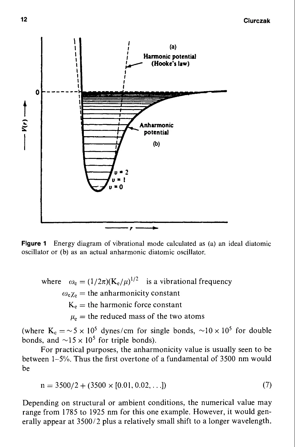
In practice, the so-called ideal harmonic oscillator has limits. A graphic
demonstration may be seen using the "weight-from-the-ceiling" model.
As the weight approaches the point at which the spring is attached to
the ceiling, real compression forces are fighting against the bulk of the spring
(often neglected in simple calculations). As the spring stretches, it eventually
reaches a point where it loses its shape and fails to return to its original coil.
This so-called "ideal" case is shown in Figure la. When the extreme limits
are ignored, the barriers at either end of the cycle are approached in a
smooth and orderly fashion.
Likewise, in molecules, the respective electron clouds of the two bound
atoms, as well as the charges on the nuclei, limit the approach of the nuclei
during the compression step, creating an energy barrier. At the extension
of the stretch, the bond eventually breaks when the vibrational energy level
reaches the dissociation energy. Figure lb demonstrates this effect. The bar-
barrier for decreasing distances increases at a rapid rate, while the barrier at the
far end of the stretch slowly approaches zero.
As can be seen from the graphic representation, the energy levels in the
anharmonic oscillator are not equal. The levels are slightly closer as the
energy increases. This phenomenon can be seen in the equation
Ev = (v + l/2)hwe - (v + l/2Jft>e*e + higher terms F)

12
Ciurczak
\ I
I
\\
\\
\\
i|
i|
pi
1=
J—
?
1
tz
tz
tz
tz
\=
V-
\
.
1
1
1
1
1
1
1
1
f—:>
f/
1 /
//
/
/
7u-2
—Vo» 1
¦^/ ? mO
(a)
Harmonic potential
—- (Hooke's law)
?
Anharmonic
potential
(b)
Figure 1 Energy diagram of vibrational mode calculated as (a) an ideal diatomic
oscillator or (b) as an actual anharmonic diatomic oscillator.
where ?? = A/2?)(??/?I/2 is a vibrational frequency
???? = tne anharmonicity constant
Ke — the harmonic force constant
/ie = the reduced mass of the two atoms
(where Ke =~5 ? ??5 dynes/cm for single bonds, ~10 ? 105 for double
bonds, and ~15 ? ??5 for triple bonds).
For practical purposes, the anharmonicity value is usually seen to be
between 1-5%. Thus the first overtone of a fundamental of 3500 nm would
be
? - 3500/2 + C500 ? [0.01, 0.02,...])
G)
Depending on structural or ambient conditions, the numerical value may
range from 1785 to 1925 nm for this one example. However, it would gen-
generally appear at 3500/2 plus a relatively small shift to a longer wavelength.

Principles of Near-infrared Spectroscopy 13
The majority of overtone peaks seen in a NIR spectrum arise from the
X-H stretching modes (O-H, C-H, S-H, and N-H) because of energy con-
considerations. Also, as quantum mechanically forbidden transitions, the over-
overtones are routinely between 10 and 1000 times weaker than the fundamental
bands. Thus a band arising from bending or rotating atoms (having weaker
energies than vibrational modes) would have to be in its third or fourth
overtone to be seen in the NIR region of the spectrum.
For example, a fundamental carbonyl stretching vibration at
1750 cm or 5714 nm would have a first overtone at approximately
3000 nm, a weaker second overtone at 2100 nm, and a third, very weak
overtone at 1650 nm. The fourth overtone, at about 1370 nm would be
so weak as to be analytically useless. (These values are based on a 5%
anharmonicity constant.)
D. Combination Bands
Another prominent feature of the NIR spectrum is the large number of com-
combination bands. In addition to the ability of a band to be produced at twice
or three times the frequency of the fundamental, there is a tendency for
two or more vibrations to combine (through addition or subtraction of
the energies) to give a single band.
A simple system containing combination bands is the gas SO2 A4).
From the simple theory of allowed bands
# bands = 3N-6 (8)
there should be three absorption bands. These are the symmetric stretch
(found at 1151 cm"), the asymmetric stretch (found at 1361 cm), and
the O-S-0 bend (found at 519 cm).
The three bands mentioned are the allowed bands according to Group
Theory. However, while these are all the bands predicted by basic Group
Theory, bands also appear at 606, 1871, 2305, and 2499 cm. As was dis-
discussed earlier, for the molecule to acquire energy to be promoted from
the ground state to a second level (first overtone) or higher is impossible
for a harmonic oscillator. For the anharmonic oscillator, however, a first
overtone of twice the frequency of the symmetric stretch is possible. This
band occurs at 2305 cm, with the 3 cm difference from an exact doub-
doubling of the frequency accounted for by the anharmonicity.
This still leaves three bands to be explained. If the possibility exists
that two bands may combine as va — Vb or va + Vb to create a new band,
then the remaining three bands are easy to assign arithmetically. The total
bands for SO2 can be assigned as seen in Table 1.

14 Ciurczak
Table 1 Band Assignments for the
Infrared Spectrum of Sulfur Dioxide
(Ref. 14)
? (cm ')
519
606
1151
1361
1871
2305
2499
Assignment
V] — V2
V\
Vi
2i'i
V\ + Vj
In like manner, any unknown absorption band can, in theory, be
deduced from first principles. When the bands in guestion are C-H, N-H,
and OH D000-2500 cm), the overtones and combinations make up most
of the NIR spectrum.
The vibrational secular equation, as normally shown, deals with the
fundamental vibrational modes. For a polyatomic molecule, there are 3N-6
energy levels for which only a single vibrational quantum number is one
when the rest are zero. These are the fundamental series, where the elevation
from the ground state to one of these levels is known as a fundamental. The
usual secular equation ignores overtones and combinations, neglecting their
effect on any fundamental.
There are, however, occasions where an overtone or combination band
interacts strongly with a fundamental. Often this happens when two
excitations give states of the same symmetry. This situation is called Fermi
resonance A5) and is a special example of configuration interaction. This
phenomenon may occur for electronic transitions as well as vibrational
modes.
We may assume the frequencies of three fundamentals, rij, rij, and nk,
to be related as follows:
vi + Vj = vk
where the symmetry of the doubly excited state

Principles of Near-infrared Spectroscopy 15
is the same as the singly excited state
(ID
This is the case where the direct product representation for the ith and
jth normal modes is or contains the irreducible representation for which the
kth normal mode forms a basis. These excited states, having the same
symmetry, interact in a manner that may be described by the secular
equation as
Vj)-V Wy.k
y.k vk - ?
A2)
The roots, ?, are then the actual frequencies with the magnitude of the inter-
interactions given by the equation:
dT A3)
where the interactional operator W has a nonzero value because the
vibrations are anharmonic. Since it is totally symmetric, the two states,
??} and ?/fk, must belong to the same representation for the integral to have
a finite value.
One consequence of these equations is that one of the roots of the
secular equation will be greater than either (vj + Vj) or i»k, while the other
is less than either mode. The closer the two vibrations exist initially, the
greater their eventual distance in the spectrum. Another result is a "sharing"
of intensity between the two bands. While normally a combination band is
weaker than the fundamental, in Fermi resonance the two intensities
become somewhat normalized.
An example of a molecule displaying Fermi resonance is carbon
dioxide. The O-C-O bending mode is seen at 667 cm in the IR. The
overtone (in the Raman) is expected near 1330 cm. However, the sym-
symmetric C-O stretching mode has approximately the same frequency. The
result is that the observed spectrum contains two strong lines at 1388
and 1286 cm instead of one strong and one weak line at 1340 and
1330 cm"', respectively.
While readily apparent in the better resolved mid-range IR, this effect
is somewhat difficult to observe in the NIR region, often hidden under
the broad, overlapping peaks associated with this region.
Three texts exist that are entirely devoted to the theory and application
of NIRS A6-18). These may be used to supplement the information in this
chapter.

16 Ciurczak
III. DATA TREATMENT
The most common data treatment for NIR spectra is multiple linear
regression (MLR). Since the earliest work was performed on agricultural
products, absolute standards were not available. Clearly, calibration
materials were not able to be produced artificially. As a consequence, pri-
primary methodology for calibrations tended to be wet chemical methods such
as Karl Fischer, azeotropic distillation, or loss on drying for water
determinations and Kjeldahl distillations for nitrogen (protein
determinations). Since the accuracy of an NIR method depends upon
the accuracy of its calibration technique, early methods were not as good
as GC, LC, or precise titrometric techniques.
In cases where a single wavelength cannot give a satisfactory equation
as per Beer's law, a MLR may be used. In MLR, the response of the
spectrum with relation to the change in solute concentration is accounted
for at several wavelengths. The need for this transformation may be due
to peak shifting caused by hydrogen bonding, refractive index shifts, or sev-
several other physical parameters. The MLR equation, may be expressed as
Cunk = KA)A" + KB)A2 + ... + K(n)An + K@) A4)
where Cunk = concentration of solute
K(x) = reciprocal of extinction coefficient at wavelength ?
Ax = absorbance at wavelength ?
K@) = intercept of calibration curve
Traditionally, analysts place the weighed standards or "known"
values from a reference method on the X-axis, or abscissa. The values
derived from the analysis are then placed on the ordinate, or Y-axis A9).
It is assumed that the balance or reference method used generates precisely
"known" data, superior to the resultant data. These are usually referred
to as independent (X) and dependent (Y) variables.
The precision of an NIR method is often that its orders of magnitude
are more precise than a chemical reaction or separation-based method.
In pedagogically correct data-handling theory (borrowed from
statisticians), the better known (less erroneous) values are placed on the
abscissa while the data with a higher uncertainty are placed on the ordinate.
In spectrometric methods, certainly in the case of NIRS, the "resultant"
absorbance values are often more accurate than the so-called referee
method. In such cases, the spectral values are properly placed on the X-axis
and the referee values on the Y-axis.

Principles of Near-infrared Spectroscopy 17
This is the reason for the structure of the MLR equation (Eq. 9). In the
common equation for a straight line,
Y = mx + b A5)
y = dependent variable
m = slope of the line
? = independent variable
b = y-intercept
For the MLR equation, the concentration of the analyte is designated as the
"Y" of the equation. While the absorbance is the "measured" value in the
system, it is nonetheless the more precise measurement and is treated
accordingly.
In cases where synthetic standards can be manufactured, as in HPLC
eluates, the spectral data and the reference data are nearly as accurate
and precise. Using four or five place analytical balances and class A volu-
volumetric glassware, precise reference solutions may be made from serial
dilutions. The MLR equation is still used in its classic form, however.
Since the absorbance values are known to at least four significant
figures, any nonlinearity must be due to physical and/or chemical interac-
interactions within the system being measured. Especially in the case of preparative
level solutions, where the solvent is often the lessor of the two components at
the highest solute concentration, dimers, trimers, and higher-order com-
complexes might be expected from complex organic molecules with multiple
polar groups. In such cases, more than one wavelength can and must be
used to obtain linear analytical results.
More involved algorithms are now in common use for the determi-
determination of analytes in complex matrices. Matrix algebra, as well as fast,
high-powered computers, make light work of the most complex
calculations. These will be discussed in greater detail later in the text.
REFERENCES
1. W. Hershel, Phil. Trans. Royal Soc, 90, 225 A800).
2. W. Abney and E. R. Festing, Phil. Trans. Royal Soc, 92, 887 A881).
3. A. G. Bell, Philosophical Magazine, 11, 510 A881).
4. W. W. Coblentz, Astrophys. J., 20, 1 A904).
5. W. W. Coblentz, "Investigation of Infrared Spectra," Part 1, Carnegie
Institution, Washington, DC, 1905.
6. I. Ben-Gera and K. H. Norris, Isr. J. Agr. Res., 18, 125 A968).
7. I. Ben-Gera and ?. ?. Norris, J. Food Sci., 33, 64 A968).

18 Ciurczak
8. ?. ?. Norris, R. F. Barnes, J. E. Moore, and J. S. Shenk, J. Anim. Sci.. 43, 889
A976).
9. W. L. Butler and ?. ?. Norris, Arch. Biochem. Biophys., 87, 31 A960).
10. D. R. Massie and K. H. Norris, Trans. Amer. Soc. Agricul. Eng., 8, 598 A965).
11. K. H. Norris and W. L. Butler, IRE Trans, on Biomed. Elec, 8, 153 A961).
12. Pacific Scientific, now NIRSystems, Silver Spring; TRABOR and Katrina,
Hagerstown; Brimrose, Baltimore; LT Industries, Gaithersberg; and Infrared
Fiber Systems, Silver Spring.
13. J. D. Ingle, Jr. and S. R. Crouch, Spectrochemical Analysis, Prentice-Hall,
Englewood Cliffs, NJ, 1988.
14. R. S. Drago, Physical Methods in Chemistry, W. B. Saunders Co., Philadelphia,
Chapter 6, 1977.
15. F. A. Cotton, Chemical Applications of Group Theory, 3rd Ed., John Wiley &
Sons, New York, 1990.
16. B. G. Osborne and T. Fearn Near-Infrared Spectroscopy in Food Analysis, John
Wiley & Sons, Inc., New York, 1986.
17. P. Williams and ?. ?. Norris, Near-Infrared Technology in the Agricultural and
Food Industries, Amer. Assoc. of Cereal Chemists, St. Paul, MN, 1987.
18. D. A. Burns and E. W. Ciurczak, Handbook of Near-Infrared Analysis, Marcel
Dekker, Inc., New York, 1992.
19. N. R. Draper and A. Smith, Applied Regression Analysis, John Wiley and Sons,
New York, 1981.

3
Theory of Diffuse Reflection in the NIR
Region
Jill M. Olinger
Ell Lilly and Co., Indianapolis, Indiana
Peter R. Griffiths
University of Idaho, Moscow, Idaho
Thorsten Burger
University of Wiirzburg, Wiirzburg, Germany
I. INTRODUCTION
The use of near-infrared (NIR) diffuse reflection for the quantitative analy-
analysis of many products and commodities is now becoming widely accepted.
For many of the algorithms developed to achieve multicomponent
determinations from the diffuse reflection spectra of powdered samples,
a linear dependence of band intensity on analyte concentration is not absol-
absolutely mandatory for an analytical result to be obtained. Nonetheless, it is
probably true to say that all of these algorithms yield the most accurate
estimates of concentration when the intensity of each spectral feature is
linearly proportional to the analyte concentration. These algorithms usually
incorporate band intensities as log 1/R', where R' is the reflectance of the
sample relative to that of a nonabsorbing standard, such as a ceramic disk.
The use of log 1 /R' as the preferred ordinate is contrary to what most physi-
physical scientists would consider appropriate for a diffuse reflection
measurement. Thus an understanding of the theories of diffuse reflection
and the validity of the assumptions for each theory should be helpful in
understanding the strengths and limitations of NIR diffuse reflection and,
19

20
Olinger et al.
perhaps, will help to explain why accurate analyses may be made after band
intensities are expressed as log 1/R'. The theory of Kubelka and Munk is
presented in some detail in this chapter along with a summary of the discrete
ordinate approximation of the radiation transfer equation and the diffusion
approximation. Together with some of the earlier work on light scattering,
an understanding of the importance of the assumptions in arriving at
the final solutions that are experimentally valid can be achieved. The last
part of this chapter contains a discussion of some recent work that has been
done in the NIR on the radiation penetration depth in powder layers and on
the effects of absorption by the matrix on adherence to Kubelka-Munk
(K-M) theory.
II. LAMBERT COSINE LAW
The phenomenon of diffuse reflection is easily observed in everyday life.
Consider for example the intensity of radiation reflected from a completely
matte surface. The reflected (or remitted) radiation is everywhere of the
same intensity no matter what the angle of observation or what the angle
of incidence. It was the same observation that led Lambert A) to be the
first to attempt a mathematical description of diffuse reflection. He pro-
proposed that the remitted radiation flux /,-, in an area f cm2, and solid angle
? steradians (sr), is proportional to the cosine of the angle of incidence
? and the angle of observation 3 (Figure 1), in other words:
CS0
dco
cos ? cos 9 = ? cos ?
A)
light
source
observer
Figure 1 Schematic representation showing variables used in the Lambert cosine law.

Theory of Diffuse Reflection 21
where 5? is the irradiation intensity in W/cm2 for normal incidence, ? is the
radiation density or surface brightness in W cm" sr~', and the constant C
is the fraction of the incident radiation flux that is remitted. C is generally
less than I since some radiation is always absorbed.
Equation 1 is known as the Lambert cosine law and, according to
Kortum B), can be derived from the second law of thermodynamics,
although Wendlandt and Hecht C) disagree. According to Kortum, it is
rigorously valid only for a black-body radiator acting as an ideal diffuse
reflector (i.e., the angular distribution of the reflected or remitted radiation
is independent of the angle of incidence). It is, however, contradictory
to call a black-body radiator an ideal diffuse reflector because all incident
radiation is absorbed by a black-body and none is absorbed by an ideal
diffuse reflector. An ideal diffuse reflector has never been found in practice
and therefore deviations (large and small) always occur from the Lambert
cosine law. Various workers, including Pokrowski D-6), Wright G), and
Woronkoff and Pokrowski (8), have reported the results of experimental
investigations that were designed to prove or disprove the Lambert cosine
law. They found that, in general, the law holds true only when both the
angle of incidence ? and the angle of observation ·9 are small.
III. MIE SCATTERING
One of the more accepted general theories of the scattering of light was
developed at the turn of the century by Mie (9). As Mie scattering relates
primarily to the scattering of radiation by isolated particles, only a very
brief introduction will be given here, although Kortum B) has presented
•a somewhat less abbreviated description. The reader is referred to Refs.
10-12 for a comprehensive survey, not only of Mie theory but also the
theories of Rayleigh, Gans, Born, and others. Mie developed equations
to describe the angular distribution of both the intensity and the
polarization of scattered radiation for a plane wave scattered once (single
scattering) by a particle, that can be both dielectric and absorbing. In Mie's
description, the particle was spherical, with no limitation on its size. He
showed that the angular distribution of scattered radiation for single
scattering is not isotropic. The basic equation that was developed by
Mie is:
where /»s, is the scattered intensity at a distance R from the center of the
sphere; Io is the intensity of the incident radiation; and / is the wavelength

22 Olinger et al.
of the incident radiation. ix and i2 are functions of the angle of the scattered
radiation, the spherical harmonics or their derivatives with respect to the
cosine of the angle of scattered radiation, the refractive index of both
the sphere and its surrounding medium, and the ratio of the particle
circumference to wavelength. The ratio of the refractive index of the sphere
to its surrounding medium is designated m, and the ratio of the particle
circumference to wavelength is designated p. Equation 2 applies only to
the case of a dielectric nonabsorbing particle and unpolarized incident
radiation. If the particle is absorbing, the complex refractive index must
be used in the determination of i\ and i2.
Mie theory, although general for spherical particles of any size, is valid
only for single scattering and therefore applicable only to chemical systems
in which particles are well separated. For example, scattering by the gases
of the atmosphere (the molecules of which are well separated) is a special
case of Mie theory, in other words, the case where the particle is much
smaller than the wavelength of incident radiation. The theory of scattering
by particles of this type was developed and explored by Rayleigh A2-14).
On the other hand, most applications of NIR reflection analysis involve
samples for which it is expected that multiple scattering will take place
within the sample. The investigations of Theissing A5) took Mie theory
one step further by assuming multiple scattering from particles that
nonetheless are still assumed to be sufficiently well separated that inter-
interference and phase differences between the scattered radiation from the
particles are negligible. Scattering order was defined as the number of times
a photon is scattered. Theissing found that with an increase in the order of
scatter, the forward scattering predicted by Mie theory decreases and
the angular distribution of scattered radiation tends to be isotropic. He also
found that the larger the ratio of particle circumference to wavelength, the
greater must be the order of scatter to produce an isotropic distribution.
For example, if/? is 0.6 and m is 1.25, twofold scattering is required for
an isotropic distribution of the reflected radiation. But if ? = 5 and
m = 1.25, a scattering order of 8 is required for isotropic reflection of
radiation.
In the NIR, particle diameters are typically fairly large, on the order of
100 ???, and so/?, the ratio of the particle circumference to wavelength, will
be large; thus the order of scattering must also be large in order to have an
isotropic distribution of the scattered radiation. It is expected, however,
that for a sufficiently large number of particles and a sufficiently thick
sample (the bounds necessary to define what is sufficient being unknown),
multiple scattering does occur for most samples of the type used for
NIR reflection analysis so that an isotropic distribution of the diffusely
reflected radiation should at least be approached. This means that for both

Theory of Diffuse Reflection 23
already established applications of NIR reflection analysis and potential
applications being considered, a theory for multiple scattering within a
densely packed medium is required to describe quantitatively the change
in reflectance with a change in concentration.
For most samples of the type for which NIR reflection analysis may be
possible, the scattering density is large, the ratio of particle circumference to
wavelength is much greater than 1, and the particles are so densely packed
that phase relations and interferences between scattered beams do exist.
Thus for samples of this type no general quantitative solution to the problem
of multiple scattering has been found. Therefore, the scientist must resort to
the use of phenomenological theories.
IV. RADIATION TRANSFER TREATMENTS
Most theories that have been developed to describe the diffuse reflection of
radiation evolved from a general radiation transfer equation. In simple
terms, a radiation transfer equation can be written:
-dl = ??? ds C)
An equation such as this describes the change in intensity, dl, of a beam of
radiation of a given wavelength in a sample whose density is ? and for which
the pathlength is ds. ? corresponds to the attenuation coefficient for the total
radiation loss whether that loss is due to scattering or absorption. The gen-
general form of the radiation transfer equation that is used in the derivation
of most phenomenological theories considers only plane-parallel layers
of particles within the sample and can be written:
where ? is the cosine of the angle ?? with respect to the inward surface
normal; ?' is the cosine of the angle .9 with respect to the outward surface
normal; dx is the optical thickness and is equal to ?? dx where dx is the
distance between the boundaries of one plane-parallel layer; / is the intensity
of the beam of radiation striking the layer; ?0 = ?/(? + ?) is the albedo for
single scattering, with the scattering and absorption coefficients ? and a,
respectively. The scattering phase function ??(?,?') denotes the probability
for scattering from direction ?' into ?. If every element scatters isotropically,
??(?, ?') = 1 and is independent of the angle between the incident radiation
and the scattered radiation. Chandrasekhar has published extensively on
radiation transfer A6). Other authors who have contributed to the literature
on this topic more recently are Truelove A7) and Incropera et al. A8).

24 Olinger et al.
The phenomenological theories that have been developed can be con-
considered either continuum theories or discontinuum theories. Continuum
theories consider the absorption and scattering coefficients as properties
of the irradiated layer. Discontinuum theories consider a layer as being
made up of a series of partial layers whose thicknesses are dictated by
the size of the scattering and absorbing particles. Optical constants can then
be found from the scattering and absorption of these particles B). In the first
part of this chapter we will only consider a sample as a continuum. Detailed
discussions of discontinuum theory are given by Kortiim B) who, along with
Wendlandt and Hecht C), presented a statistical solution to the radiation
transfer equation. More recent work by Dahm and Dahm A9) is
summarized later in Section VIII of this chapter.
V. SCHUSTER'S THEORY
In 1905, Schuster B0) made the first attempt to find a simplified solution of
the radiation transfer equation. He made the simplifying assumption of
using two oppositely directed radiation fluxes, / and J. Radiation traveling
in a forward direction through a sample (forward with respect to the direc-
direction of the incident radiation) is designated as /. Radiation traveling in
the opposite direction is labeled as J. With this simplification, Schuster
derived the following two differential equations:
^- = (k + s)I-sJ E)
??
% + s)J-sI F)
?/?
where
k = — G)
? + ?
and
s = -?- (8)
? + ?
? is the true absorption coefficient of single scattering and ? is the scattering
coefficient for single scattering. The abbreviation s used by Schuster is ident-
identical to the albedo co0 for single scattering. It is relevant to discuss a
coefficient of single scattering for a continuum model in that these
coefficients relate to the reflectance measured as if the particles in the model
were "exploded" apart so that only single scattering could occur.

Theory of Diffuse Reflection 25
If the boundary conditions are set as:
I = I0 at ? = 0
/ = /(t) ->· 0; J — 0 at ? = ? for ? ->· oo.
the differential equations 5 and 6 can be solved to give the reflectance at
"infinite depth," in other words, the depth which a sample must be in order
to have no further change in the measured diffuse reflectance:
_j{T=0)_\-(k/(k + 2s)Y
°°~ h ~1+(*/(*+ 2*)I'2
This equation can be rewritten as:
(l-???J k 2a
A0)
Equation 10 gives the reflectance behavior for isotropic scattering
when two oppositely directed radiation fluxes are assumed in the direction
of the surface normal. As summarized below, Kubelka and Munk B1)
derived an expression similar to Schuster's solution, the primary difference
being in the definition of the two constants k and s. While Schuster defines
these constants in terms of the absorption and scattering coefficients for
single scattering, Kubelka and Munk simply define k and s in their equations
as the absorption and scattering coefficients for the densely packed sample
as a whole.
VI. KUBELKA-MUNK THEORY
Kubelka and Munk made several assumptions in their derivation of a
simplified solution to the radiation transfer equation. A tabulation of
the variables that are used in their derivation and that are discussed in
the assumptions is found in Table 1. Figure 2 shows a schematic represen-
representation of the type of system for which Kubelka and Munk derived their
solution. The assumptions are listed as follows:
1. The radiation flux (/ and J) travels in two opposite directions.
2. The sample is illuminated with monochromatic radiation of inten-
intensity 70.
3. The distribution of scattered radiation is isotropic so that all reg-
regular (specular) reflection is ignored.
4. The particles in the sample layer (defined as the region between
? — 0 and ? = d are randomly distributed.

26 Olinger et al.
5. The particles are very much smaller than the thickness of the
sample layer d.
6. The sample layer is subject only to diffuse irradiation.
7. Particles are much larger than the wavelength of irradiation (so
that the scattering coefficient will be independent of wavelength),
although if only one wavelength is to be used then this assumption
is not relevant.
8. The breadth of the macroscopic sample surface (in the vr plane) is
great compared to the depth (d) of the sample and the diameter of
the beam of incident radiation (to discriminate against edge
effects).
9. The scattering particles are distributed homogeneously through-
throughout the entire sample.
Table 1 Variables Used in the Development of Kubclka and Munk's Simplified
Solution to the Radiation Transfer Equation
d sample layer thickness
+ .y downward direction through the sample
— .y upward direction through the sample
.v = 0 illuminated surface
.v = d unilluminated surface
/ radiant flux in +x direction
J radiant flux in —x direction
/o incident flux
? angle at which a particular ray traverses through t/.?
dx an infinitesimal layer
dx/cos ? pathlength of a particular ray traversing rf.Y
??? average pathlength of radiation passing through dx in the +.y direction
3.\73 cos ? angular distribution of is intensity in the +.? direction
d$j average pathlength of radiation passing through dx in the —x direction
? fraction of radiation absorbed per unit pathlength in the sample
? fraction of radiation scattered per unit pathlength in the sample
(Note, neither ? or ? are exactly the same as the corresponding parameters defined by Schuster.)
Either an exponential or hyperbolic solution may be developed,
although only the exponential derivation will be shown here. A detailed
description of the hyperbolic solution can be found in Ref. 2.
We will first describe how Kubelka and Munk arrived at the two fun-
fundamental differential equations that, once solved, give the simplified sol-
solution similar to the one in Eq. 10. Because it is feasible that the angle

Theory of Diffuse Reflection
27
illuminated
surface
? - 0
/ ?
dx
Figure 2 Schematic representation of a sample for which the Kubelka-Munk
equation was derived. Consider the cube as a sample throughout which the particles
(only shown in a portion of the sample) are randomly distributed.
through dx, ,9, that the radiation might follow could be between 0 and 90°,
the average pathlength for radiation passing through dx in the + ? direction
can be found by the following integral:
??, = dx I (9///9.9)(c/,9/ cos ,9) = udx
Jo
(?)
If no absorption or scattering occurred, the illumination of the layer
dx could be described by:
Id ?? = Iu dx
A2)
Since, however, absorption and scattering do occur, the decrease in intensity
of the illumination of dx can be shown by including a combination of

28 Olinger et al.
absorption and scattering coefficients:
(? + ?)???, = (e, + a)Iudx
= ???? dx + alu dx
The term elu dx represents that component of the radiation that is absorbed
while the term alu dx represents that component of the radiation that is
scattered. Radiation traveling in the —x direction (the / flux) also has a
corresponding average pathlength through dx:
/•?/2
dt,j = dx / (9///9S)/(i/9/ cos ,9) = ? dx A4)
Jo
Again, if no absorption or scattering were to take place for radiation
traveling in this direction, then the illumination of the layer dx in the
-x direction would be described by:
Jdt, = Jvdx A5)
The corresponding equation can be written for the absorption and
scattering that occurs for the / radiation flux:
A6)
= ?/? dx + aJv dx
Similarly to Eq. 13, the term cJv dx corresponds to that part of the radiation
that is absorbed while the term ?/? dx corresponds to that part of the
radiation that is scattered. It is necessary to know, however, the actual
change dl or dJ in the radiation fluxes, / and / that were incident on
the layer dx, respectively, after the radiation has traversed a distance
dx. Not only does the absorption and scattering of the forward radiation
flux affect /, but the component of the scattered / radiation flux will also
affect / and therefore dl. The same correlation can be made for / and there-
therefore for dJ. It must therefore be true that:
—dl = —ml dx - aul dx + avJ dx A7)
dJ= -e.vJ dx -avjdx + auldx A8)
The signs in the preceding equations are indicative of the fact that as ?
increases / must decrease and / must increase.
If the sample is an ideal diffuser, then the angular distribution of the
radiation flux through a plane layer dx in a given direction is:
A9)
9//9,9 = / sin 2,9 = 2/ sin,9 cos 9 B0)

Theory of Diffuse Reflection 29
These expressions can then be substituted into Eqs. 11 and 14 describing
the average pathlength of radiation through dx to solve for this quantity.
Doing so we find that ??? = u = 2. Likewise, dc,j = ? = 2. If we now sub-
substitute for u and ? in the differential equations 17 and 18 we obtain:
-dl = -2eIdx-2aIdx + 2aJdx B1)
dJ = -2?/ dx - 2aJ dx + 2?? dx B2)
Using Kortum's notation B), the absorption coefficient of the material
k is equal to t and the scattering coefficient of the material s is equal to ?. We
can then designate ? = 2k and 5 = 2s to obtain the two fundamental sim-
simultaneous differential equations from which a simplified solution to the gen-
general radiation transfer equation can be found:
-dl = -KI dx -SIdx + SJ dx B3)
dJ = -KJ dx - SJ dx + SI dx B4)
It should be noted here that Kubelka and Munk define scattering
differently than does Mie. Mie defines scattering as any change in the direc-
direction of travel of a beam of radiation due to interaction with a particle.
Kubelka and Munk defined scattered radiation as only that component
of the radiation that is backward reflected into the hemisphere bounded
by the plane of the sample's surface.
It should also be noted that the previous differential equations will still
hold true even if collimated radiation at an angle of 60° to the surface nor-
normal is used instead of diffuse irradiation because for an incident angle
of 60°:
= dx/cosF0°) = 1/0.5 = 2 = u = ? B5)
The differential equations can be simplified by setting
S + K , ?
and J/I = r. The simplified form of Eqs. 21 and 22 then becomes:
-dI/Sdx=-aI + J B7)
dJ/S dx = -aJ + I B8)
Dividing the first equation by / and the second equation by J and then
adding the two equations, it is found that:
dr/Sdx = r2 -2ar + I B9)

30 Olinger et al.
Using the principle of separation of variables to solve differential equations
we obtain:
I(r - 2ar + I)~l dr = SI clx C0)
Since the integration must be done over the entire thickness of the sample,
the boundaries are:
.? = d: (J/I)x=d = Rg = reflectance of the background C1)
? = 0: (J/I)x=0 = R = reflectance of the sample C2)
Equation 30 can be integrated using partial fractions where the first step in
the fractionation is:
dr 1
-dr C3)
(/•2 - 2ar + 1) (/· + Bar - lI/2)(/· - Bar -
The solution of Eq. 30 can then be found to be:
/2)
(RK- a - (a2 - l)l/2)(R - a + (a2 - 1I/2)
Because it is assumed that the layer is of infinite depth, in other words,
d = oo and Rs = 0, Eq. 34 is reduced to
(-a - (a2 - IY/2)(RX -a + (a2 - 1I/2) = 0 C5)
that can be solved for the reflectance R^:
R
a + (a2 - 1I/2 = 1+K/S + ((K/SJ + 2K/S)]/2
( }
Rearranging Eq. 36 in terms of the ratio K/S we obtain an equation that is
similar to the one first derived by Schuster:
The function A - ?00J/2?0? is known as the K-M function and is
usually given the symbol/(/?oo). Thus it is seen that the reflectance, which
is measurable, is a function only of the ratio of two constants, ? and 5,
and not of their absolute values. For quantitative analysis, Eq. 37 can
be used to determine the concentration c of an absorbing analyte, as shown
in Eq. 38:
(l-Rxf ? (????)??·
2RX S S
where a is the (base 10) absorptivity.
C8)

Theory of Diffuse Reflection 31
Other scientists in the field B2-26) derived expressions similar to those
of Schuster B0) and Kubelka and Munk B1). Earlier theories developed by
Gurevic B7) and Judd B8,29) were shown by Kubelka C0) to be special
cases of the K-M theory, while Ingle C1) showed that the formulas derived
by Smith C2), Amy C3), and Bruce C4) can be derived from the equations
of Kubelka and Munk.
Because the simplified solution obtained by Kubelka and Munk is a
two-constant equation and therefore experimentally testable, and because
so many other workers' derivations are derivable from Kubelka and ? unk's
work, their solution is the most widely accepted, tested, and used. Other
workers have derived solutions to the radiation transfer equation that
are more complicated than these two-constant formulas. For example, a
third constant has been added to account for different fractions of forward
and back scattering C5). Ryde C6,37) included four constants since a dif-
difference in the scattering between incident light and internally diffused light
is assumed, while Duntley C8) developed a model with eight constants,
as a difference between both the absorption and scattering coefficients
due to incident and internally diffused radiation was assumed. However,
none of these theories is readily applicable in practice, and therefore the
treatment of Kubelka and Munk is most often applied.
Another two-constant approach, based on a discrete ordinate approxi-
approximation of the radiation transfer equation A6,39) was recently applied to
describe the diffuse reflectance in the NIR D0,41). In this approach, the
integral in Eq. 4 is approximated by a weighted sum over discrete directions
(i.e., representing the diffuse radiation field inside the sample by radiation
fluxes in distinct directions):
??{?. ?')?(?, ?')??' = ? ?;??(?,, ?^?(?, /(,), C9)
;=-?
where the directions ?) are chosen to be zeros of Jacobi polynomials
/>;,lI)B/i/-l) = 0 D0)
with the corresponding coefficients cij given by C9):
1
Introducing Eq. 39 into Eq. 4 leads to a system of differential equations:
'''CU(^ = ~/(?·??) + ?? ajP°^· ^O(?· '</) D2)
- j=-N

32 Olinger et al.
For the case of 3 radiation fluxes (j = -1, 0, + 1) the directions and
coefficients are given by:
?_? = -2/3 ?0 = 0 ?+? = +2/3 D3)
?-? = 3/4 ?0 = 1/2 ?+? = 3/4 D4)
and the system of three differential equations can be solved analytically to
obtain the diffuse reflectance and transmittance as a function of the optical
thickness ? and the albedo ?0 D2). With a given sample thickness d and
the relations ? = (<x + a)d and ?0 = ?/(?+?), the diffuse reflectance and
transmittance can also be described as a function of the scattering coefficient
? and the absorption coefficient ? (here, the coefficients are denned accord-
according to the Mie theory).
In the case of a diffusely illuminated, isotropically scattering, and
optically thick sample (Kubelka and Munk's assumptions), the three -flux
approximation yields the following relation between the ratio ?/? and
the diffuse reflectance Roo D0):
8 2??? 8 5
D5)
The factor 3/8 in Eq. 45 is identical to the result of Mudgett and Richards
D3), who related the ratio of the Kubelka-Munk absorption to scattering
coefficient to the corresponding ratio of the Mie coefficients.
To obtain solutions for the in common spectrometers usually present
boundary condition of (almost) directional sample illumination, the inten-
intensity /(?, ?) in Eq. 4 is separated into the reduced incident intensity 7,/,>(?,
?) and a diffuse intensity /<?//(?, ?):
/(?, ?) = Idir{T, ?) + Idiff{x, ?) D6)
where /,/,>(?, ?) is given by:
?<??,(?,?)=^?-??(?-1) D7)
with the directional impinging flux Fo. Substituting Eqs. 46 and 47 into the
radiation transfer equation (Eq. 4) and taking advantage of the <5-function
in the presentation of Ijir leads to the radiation transfer equation as a func-
function of only the diffuse intensity Uiff plus a source function
%(?, Woe-* D8)
4?
that accounts for the attenuated incident radiation. A more detailed dis-
discussion and analytical expressions of the diffuse reflectance and transmit-
transmittance as a function of ? and ?0 can be found in the publication by

Theory of Diffuse Reflection 33
Kuhn et al. D2). In the case of a directionally illuminated, isotropically
scattering, and optically thick sample, the three-flux approximation yields:
a = (l-^_6-_ D9)
? 2/??? 5(Rx+4)
or its inverse
a 6\ / or
4- + - +2 4-?-
? 5/ \ ?- u/ EQ)
2a 6
? 5
A totally different approach to investigate the radiation transfer is the
diffusion approximation, which is often used in biomedical applications
[e.g., D4,45)]. The propagation of the photons in a sufficiently thick sample,
with a scattering coefficient that is much larger than the absorption
coefficient, can be described by a diffusion process (analogous to Fick's
law of mass diffusion). Similar to Eqs. 36 and 50, the diffuse reflectance
of an optically thick sample R^ can be expressed as a function of the ratio
?/?, which for directional sample illumination yield D6):
Roo= 2 -T72 E1)
? j y ?** ?j
The different radiative transfer models to describe the diffuse reflec-
reflectance of an optically thick sample are compared with each other in Figure
3. The diffusion approximation (Eq. 51), the three-flux approximation (Eq.
50) and the data according to a numerical solution of the radiative transfer
equation by Giovanelli D7) are calculated for directional sample
illumination. The data according to the K-M theory (Eq. 36) is obtained
for diffuse sample illumination. Thus, the differences between the K-M
theory and the other models are due to the different illumination conditions
as well as due to differences in the definition ???/S and ? /?. As can be seen
in Figure 3, the three-flux approximation is in very good agreement to the
calculations of Giovanelli, whereas the diffusion approximation exhibits
increasing deviations for larger ?/?-ratios (corresponding to smaller
albedos). For ?/? = 1 or ? = 0.5, the relative deviations are in the order
of 7%.
It should be mentioned that in all the models presented specular reflec-
reflection at the air-sample boundary is neglected; thus these models are only
valid for loose powders and have to be used with care for other samples.

34
Olinger et al.
cc
ID
?
Jj 0.1
"?3
0.01
Kubelka-Munk theory
diffusion approximation
3-flux approximation
+ Giovanelli
0.001
0.01
0.1
a/a and K/S
10
Figure 3 Diffuse reflectance R^ of an isotropically, optically thick sample according
to the three-flux approximation, the diffusion approximation, Giovanelli, and the K-M
theory.
VII. EFFECT OF ANISOTROPIC SCATTERING
Although the K-M treatment is most often applied to diffuse reflection
spectra of dilute dispersions of absorbing materials in a nonabsorbing
powdered matrix, it is usually found that plots oif{Rx) versus the concen-
concentration of the absorbing component c deviate from linearity at quite low
concentrations for measurements taken in the mid-infrared (IR) or
ultraviolet-visible (UV/Vis) region of the spectrum where the absorptivities
of absorption bands may be quite high. For NIR spectra, band
absorptivities are usually significantly weaker, so that linear plots of
f(Rot) versus c often may be obtained even at fairly high concentrations
when the absorptivity of the matrix is zero. On the other hand, if the matrix
has even a weak absorption or if the analyte has strong absorption bands,
diffuse reflection spectra of binary mixtures are no longer adequately
described by K-M theory. This behavior was originally thought to be caused
by the simple two-flux model shown in Figure 2 breaking down.
One of the assumptions listed at the start of the earlier discussion of
K-M theory is that the medium scatters isotropically. Chandrasekhar A6)

Theory of Diffuse Reflection 35
gave an exact solution of the radiation transfer equation for an isotropically
scattering medium, in other words, a medium for which the scattering phase
function p(cos 0) = 1, where 0 is the angle of scattering (from a direction
given by ?' = cos 9' and ?' into a direction given by ? and ?).
Especially for particles larger than the wavelength, pronounced
forward scattering occurs and the shape of the scattering phase function
is very complex. It can be expressed as a series of Legendre polynomials D8):
?(?\ ?' -> ?, ?) = p(cos 0) = ? "'«^«(cos 0) E2)
Using the expansion of P,,(cos 0) with respect to ?, ?' and the azimuthal
angles ?, ?' D9) and integrating Eq. 52 over the azimuthal angles yields:
?') E3)
n=0
where the subscript ?' indicates that the phase function has been integrated
with respect to ? and ?'.
Taking the second term of the expansion into account yields the linear
anisotropic scattering phase function:
p(cosO) = 1 +H'icos0. E4)
where ?? is related to the anisotropy factor
J4n
g= / p@)cos6dQ E5)
through ?? = 3g D8). Chandrasekhar has also described exact solutions to
the radiation transfer equation in this case, but the solution is far too
complex to be applicable to the quantitative analysis of powdered mixtures.
The solution has been put into a more tractable form by several
workers, including Pitts E0) who developed an approximate solution
and Giovanelli D7) who put Pitts's solution into a more useful form (now
most commonly known as the Pitts-Giovanelli formula), which gives the
reflectance as a function of the direction cosine of the angle of incidence
?? as:
-g
?'/2
E6)
2(?)'/2 + 3-,
where
? = C - ??#)A - ?0) E7)
If the components of a binary mixture are designated 1 and 2, and the rela-

36 Olinger et al.
tive weight of those components W = W2/ W\, so that the concentration of
component 2 is W/(W+ 1), the albedo of single scatter may be expressed
as:
\+P\W
Wo = /nT7w E8)
where P\ — ?\/?2, Pi — («? + ?\)/?\, and .P3 = (?2 + ??)/?\. Equation 58
may be expressed in terms of the weights, absorption coefficients, and
scattering coefficients of the individual components as:
C + ^)^
W° (a,
Thus the Pitts-Giovanelli equation requires four empirical parameters,
P\, P2, Pi, andg fora complete characterization of the diffuse reflectance of
a binary mixture. Although spectra can befit over a wide concentration
range to Eq. 56 by a suitable selection of the values of these parameters,
obtaining good estimates of these parameters a priori is difficult or
impossible. Thus the Pitts-Giovanelli treatment is never used in practice
to obtain linear plots of a function of the measured reflectance at a wave-
wavelength corresponding to an absorption band of the analyte against con-
concentration, even for a binary mixture of an absorbing analyte in a
nonabsorbing matrix. This treatment has been shown by Hecht to describe
the diffuse reflectance of visible radiation by a model system consisting
of soluble absorbers in a liquid medium containing nonabsorbing scattering
particles E1,52). In a related study (again in the visible region of the
spectrum), Hecht E3) showed that the Pitts-Giovanelli formula is a good
approximation to the equation for radiation transfer even for large values
of the anisotropy factor g. He suggested that this result indicates that
the breakdown of the K-M theory is not so much due to the failure of
the two-flux approximation as to the neglect of anisotropy of scatter.
The scaling concept is an approach to take anisotropic scattering into
account, even if the scattering phase function and thus the anisotropy factor
g is not explicitly known. Here, the unknown phase function is
approximated by the sum of an isotropic part and a ()-peak in forward
direction:
p(cos0) = (l-g) + 2g<5(l-cos0) F0)
representing an isotropic radiation field and the forward scattered radiation,
where g is weighting the two parts. Then, McKellar and Box E4) have
shown that the radiation transfer equation for anisotropic scattering can
be reduced to the case of isotropic scattering (Eq. 4 with ?(?,?') = 1), if
the scattering coefficient ? is scaled to yield the effective scattering coefficient

Theory of Diffuse Reflection 37
?* = ?A —g). The corresponding effective albedo ?^ and the effective
optical thickness t* are then given by:
-g)
co*= , .. _ and ?* = ?A-???) F1)
that leads to the new radiation transfer equation:
? \ '?> = -/(?*, ?) + 1/2?* / /(?*, ?')?? F2)
This is a significant simplification since the anisotropy factor g, which
is usually unknown, has been eliminated from the radiation transfer
equation and is implicitly included in the effective coefficients. Applying this
concept to the previously presented relations between the diffuse reflectance
of an optically thick sample and the ratio of its absorption to its scattering
coefficient only requires to replace the scattering coefficient by the effective
scattering coefficient ?* to implicitly take anisotropic scattering into
account.
Another scattering phase function that should be mentioned because it
is often used in astrophysics and biomedical applications is the
Henyey-Greenstein phase function E5-57):
The expansion coefficients are given by irn = (In + \)g". This expansion can
be implemented in Monte-Carlo simulations of the radiative transfer or in
the discrete ordinate approximation of the radiation transfer equation.
In the latter case, the summation of the expansion is only carried out from
? = 0 to ? = 2N— 1, where ? is the number of fluxes per hemisphere A6).
Thus, to obtain a reasonable approximation of the scattering phase
function, the previously presented three-flux approximation (N = 1) is
not sufficient to explicitly model anisotropic scattering. The three-flux
approximation is therefore usually applied in combination with the scaling
concept D0-42).
VIII. DISCONTINUUM THEORIES OF DIFFUSE REFLECTION
The mathematics of most of the theories described require the assumptions
that samples are homogeneous and that particles are infinitesimally small,
so that there is no significant loss in a single particle caused by absorption
or scattering. Such theories are called continuum theories. In many real

38 Olinger et al.
samples, individual particles absorb or scatter a significant fraction of the
incident radiation. In this case, the K-M theory becomes an approximation.
Theories in which the phenomena occurring at individual particles have
been called discontinuum theories. Dahm and Dahm A9) have developed
a discontinuum theoretical treatment based on the original work of Benford
E8). It is assumed that each layer of material is bounded by two parallel
infinite planes. Of the radiation entering the /th layer, the total forward flux,
in other words, the fraction leaving the layer in the same direction, is th and
the total backward flux is /¦,-, and the fraction absorbed is a,·. The total
forward flux includes both transmission and forward scatter and the total
backward flux includes both external and internal reflection and
backscatter.
Benford's equations allow the total forward and backward flux and the
total absorption to be calculated in terms from the properties of an indi-
individual layer. The overall properties for a material composed of two layers
are given by:
''+/ = ??~^7~\; ''I+I = *¦' + ? '?m ; ai+j = l ~ 't+J ~r>+' F4)
U r") U '
If t,, r,, and a, represent the known properties of a sample that contains
a number /'of identical layers, each of which is described by t\, r\, and a\, the
properties of a sample containing /' such layers is given by Benford as:
''+· = 71 ?; '¦'+> = '"' + 71 ?'- fl'+i = 1 - '1+1 - '?+?
A-/·,·/·!) A "
F5)
Dahm and Dahm considered what happens when the thickness of the sample
is doubled or halved, and computed the total backward flux, Rx for an
infinitely thick sample by an iterative solution of the latter set of equations.
They showed that if the sample consists of an infinite number of layers,
each with a forward flux of t,, a backward flux off,, and absorption of a,,
f(Roo) = ~B-ai-2rl) F6)
The K-M equation was derived for a matrix of infinitesimally small
particles. Because the numerator of the K-M function is the absorption
coefficient,/(/?oo) varies linearly with the concentration of each component
of the sample. However, it is known that the K-M equation is only an
approximation. The Dahm equation (Eq. 66) may be expected to give a
more exact solution for diffuse reflectance in the case of particles of finite
size.

Theory of Diffuse Reflection 39
IX. EXPERIMENTAL CONSIDERATIONS
If diffuse reflectance spectrometry is to be used for quality-control purposes
it is essential to know the actual investigated sample volume, which is equiv-
equivalent to the radiation penetration depth or the effective sample size m. In a
recent publication by Berntsson et al. E9), the effective sample size of phar-
pharmaceutical powders was investigated by the previously presented three-flux
approximation and an empirical method. In this publication, the effective
sample size meff is defined as the mass per area of the sample at which
its diffuse reflectance has reached 98% of the diffuse reflectance of a cor-
corresponding optically thick sample.
To obtain meff with the use of the three-flux approximation (in the
following it's called the ERT method), the scattering and absorption
coefficients of the investigated powder are obtained from diffuse reflection
and transmission measurements on optically thin samples [for a detailed
discussion see D0, 60)]. Then, at each wavelength, the diffuse reflectance
as a function of the scattering and absorption coefficients is calculated
for a gradually increasing sample thickness and compared to the diffuse
reflectance of an infinitely thick sample. The sample thickness for which
the 98% limit is reached corresponds to the effective sample size meff.
This method is compared to a totally independent procedure, where
diffuse reflection spectra are collected at several controlled powder
thicknesses [in the following called variable layer thickness (VLT) method].
The diffuse reflectance of the powder layers increases with increasing sample
thickness until the reflectance of an optically thick sample (R^) is reached.
For each measured wavelength, an exponential function is fitted to the
experimental data (log 1IR presentation of the measured reflectance versus
sample thickness). Using the 98% limit, the effective sample size meff
can be obtained from the exponential fit [see F1) for a detailed discussion
of the VLT method].
Figure 4 presents the effective sample size of a microcrystalline
cellulose powder (MCC, particle size range 65-300 ???) in the NIR region.
Using the tapped density of 0.30 g/cm3, the effective mass per area is tran-
transformed into an effective penetration depth in mm, shown on the right axis.
The wavelength dependence of the effective sample size, which is inversely
correlated to the absorption coefficient, and the good correspondence of
the two methods can clearly be seen. The upper limit for the VLT method
was 1400 nm for the MCC sample because the curve fitting becomes
unstable if the effective sample mass per area is below the smallest powder
mass per area used in the measurements. However, both methods are suit-
suitable for the determination of the actual probed sample volume of a diffuse
reflection measurement.

40
Olinger et al.
0.75
C\J
0.60
0.45
?.
I 0.30
?> 0.15
/ ?
\
VLT method
ERT method
2.5
- 2.0
?
?
?.
?
1.5?
?
1.0 ?
?
?.
?>
0.5
500
1000 1500
2000
2500
wavelength / nm
to
?>
Figure 4 Effective sample size and penetration depth of microcrystalline cellulose
powder according to the ERT and the VLT method.
Another important point in practical NIR measurements is that a rela-
relative reflectance, /?ro, rather than an absolute diffuse reflectance, R^, is
usually measured. The relative reflectance is equal to the ratio 7s/7r, where
Is is the intensity of radiation reflected from the sample and 7R is the inten-
intensity of radiation reflected from a reference material. (In the case of NIR
reflectance spectrometry this material is usually a ceramic disk.) Strictly
speaking, the K-M equation as well as the other presented models require
that an absolute reflectance, denned as the ratio h/I0, be measured, where
7S is denned as above and 70 is the intensity of the incident radiation.
The measurement of absolute reflectance can only be made directly through
the use of an integrating sphere, and even then some care is required. An
absolute reflectance can be derived from relative reflectances although
the derivation requires several experimental measurements B).
Kortum B,62) showed that the use of relative reflectances in the visible
region can cause deviations from K-M theory if the analyte is surrounded by
an absorbing matrix. This effect was shown by measuring the reflectance of
Cr2O3 in an absorbing matrix relative both to the pure diluent and to a
highly reflective standard (MgO). When the diluent was used as the
reference, a plot of /(O versus concentration of Cr2O3 was nonlinear.

Theory of Diffuse Reflection 41
When MgO was used as the reference, a similar plot yielded a straight line
with a positive intercept. Kortum states that a straight line with a zero
intercept can only be obtained when/(/?TO/4) is plotted versus c, where:
where ??,,? is the absolute reflectance of the analyte {A), RxA+M is the
reflectance of the analyte + matrix relative to the reflectance of the matrix
(?/), ? is the absolute reflectance of a nonabsorbing standard, and RxM
is the reflectance of the matrix relative to the reflectance of the nonabsorbing
standard. For most NIR reflection analyses of cereal products, it is imposs-
impossible to measure either the value R^ M or flTOi/4+A/ due to the complexity
of the sample. Therefore this type of correction for the absorption of
the matrix should only be viable for samples that are relatively simple,
for example, binary and ternary mixtures. Even for simple samples use
of Eq. 64 may not be productive because treatment of this type does
not linearize plots of/(/?TO) versus c for powdered mixtures measured
by mid-IR diffuse reflectance spectrometry F3).
It is generally accepted that the K-M equation, like Beer's law, is a
limiting equation and should only apply for weakly absorbing bands, in
other words, when the product of absorptivity and concentration is low.
For organic materials, absorptions in the NIR are due to vibrational over-
overtones and combination bands. The absorptivities of these bands are much
weaker than the absorptivities of the corresponding fundamental vibrations.
Thus most organic analytes can be considered to be weakly absorbing in the
NIR even without dilution. As noted previously, however, for most NIR
analyses, the analyte (such as protein or lipid molecules in a cereal) is usually
not isolated from other components, but is surrounded by a matrix that is
not only complex but that also often absorbs the incident radiation at least
as strongly as the analyte at the analytical wavelengths. In a cereal product
analysis the matrix would largely consist of carbohydrate molecules. It
would therefore be expected that unless the proper referencing method
is used, absorption by the matrix surrounding the analyte may cause
deviations from the K-M equation.
IX. EFFECT OF THE ABSORPTION OF THE MATRIX
In light of the differences between the quantitative behavior of diffuse reflec-
reflection spectra in the visible and mid-IR regions, the effect of absorbing
matrices on NIR reflection spectra was investigated by Olinger and Griffiths
F4). Up to three components—carbazole, NaCl, and graphite—were mixed

42 Olinger et al.
during the preparation of each sample. Carbazole was intended to represent
a typical organic analyte because it contains both C-H and N-H bonds.
NaCl and graphite represent nonabsorbing and absorbing components
of the matrix, respectively. Carbazole, NaCl, and graphite were each ground
and sieved separately into particle size ranges of 18-53 ??? and 75-125 ???.
Samples used to model the behavior in a nonabsorbing matrix consisted
of binary mixtures of carbazole and NaCl. Samples used to model the effects
of an absorbing matrix consisted of carbazole dispersed in NaCl with either
1 wt% or 5 wt% of graphite added.
Reflectance spectra were calculated by ratioing the spectrum of the
sample against a spectrum of the diluent that contained with the same
weight percent graphite. If the sample contained x% carbazole, y% graphite,
and z% NaCl, the reference was prepared with (x+z)% NaCl and y%
graphite. [For all samples consisting of carbazole in an absorbing matrix
it was true that {y/(y + z)}100 = 1 or 5 wt% as appropriate.] In this way,
the reference should have the same reflectance as the matrix surrounding
the analyte. Samples prepared in this way are referred to as being ratioed
against a weight-corrected reference.
Corrections for baseline variations due to packing differences and
possible particle-size variations were performed by subtracting the value
in a region of minimal absorption by the carbazole analyte from the value
corresponding to the band of interest. When a sloping baseline was
encountered, an equivalent correction was performed after linear inter-
interpolation between two wavelengths at which absorption by the analyte
was minimal.
For particles with diameters between 18 and 53 ???, a sample of 1 wt%
graphite reflects about 65% of the incident radiation relative to the reflection
of NaCl of the same particle size. Absorption by the added graphite
increased markedly with particle size. For samples of the same composition
containing particles with diameters ranging between 75 and 125 ???, the
reflectance dropped to about 30%. The high absorptivity of graphite is suf-
sufficiently great that any photon entering the smallest graphite particle used
in this study is completely absorbed.
Plots of /{R'oo) and log l/R'^ versus the concentration of carbazole
(particle size 18-53 ???) are shown for three matrices—pure NaCl, 1 wt%
graphite in NaCl, and 5 wt% graphite in NaCl (Figures 5 and 6). Converting
the measured reflectance of carbazole to the K-M functions yields a fairly
linear plot when the carbazole analyte was dispersed in the nonabsorbing
matrix (NaCl) (Figure 5a). Conversely, log l/?'^ values provided a more
linear plot over a major portion of the concentration range studied when
the analyte was dispersed in a matrix containing 1 wt% graphite (cf. Figures
5b and 6b). When the matrix contained 5 wt% graphite, neither/(/^J nor

Theory of Diffuse Reflection
43
0.2 -
20
40 60
Wt% Carbazole
80
Figure 5 /(?'^) versus concentration for carbazole dispersed in (a) NaCl; (b) 1 wt%
graphite/NaCl; (c) 5 wt% graphite/NaCl using the weight-corrected referencing
method. Particle size for all components of each sample is 18-53 ???.
log l/.R'co yielded linear plots, although the plots of log l/R'^ versus con-
concentration of carbazole were more linear than the corresponding /(R^) plots
(Figures 5c and 6c).
The behavior shown in Figures 5 and 6 is surprising in two respects.
First, even though graphite has a high absorptivity, the concentrations
are low enough that contributions to the signal from front surface reflection
should be negligible, which should favor adherence to the K-M function. (At
high concentration, the reflectance of graphite plateaus at approximately
10% reflectance because of front surface reflection.) The second anomaly
is that the absorption of radiation on the addition of graphite to carbazole
is not additive. If the absorption of radiation by graphite and carbazole
were additive, /(R'^) of background-corrected analyte bands for carbazole
surrounded by an absorbing matrix should vary linearly with concentration
even though the concentration of graphite decreases as the concentration of
carbazole increases.
All reflectance spectra in this study as described previously were
obtained using a weight-corrected reference, in other words, to calculate

44
Olinger et al.
61
Jit· ?' *"^ "
? <:
s ?
? ?
? t
v ?
?
4 ·
2-
20
40 60
Wl% Carbazole
80
100
Figure 6 log \/R'^ and average number of carbazole particle diameters interrogated
versus concentration of carbazole dispersed in (a) NaCl; (b) 1 wt% graphite/NaCl;
(c) 5 wt% graphite/NaCl using the weight-corrected referencing method. Particle size
for all components of each sample is 18-53 ???.
R'^ the single-beam spectrum of the sample was ratioed against that of a
matrix in which the percent graphite had been adjusted to match the actual
weight percentage of graphite in the sample. In practice, however, most
NIR reflectance spectra are collected by simply ratioing the sample to a
nonabsorbing reference, typically a ceramic disk. The values of /(/?Oo)
and log l/R'^ are relatively insensitive to the nature of the reference, pro-
provided that /(/JO,,) and log ?/?'^ are calculated after baseline correction
of the reflectance (?'^) spectrum. For log 1/ R'^ spectra, baseline correction
can be performed with equal validity on the R'x or log 1 / R'x spectrum. On
the other hand /(R'^,) is strongly dependent on the reflectance of the ref-
reference material if baseline correction is performed after conversion to
the K-M function.
Although most samples for which NIR reflection analysis is used are
too complex for the direct application of Eq. 64, the system described
by Olinger and Griffiths F4) was simple enough to derive absolute
/(R'ac) values. For carbazole dispersed in 1 and 5 wt% graphite in NaCl,
plots of the absolute value offiR'^) derived using Eq. 64 against carbazole

Theory of Diffuse Reflection 45
concentration (assuming ? for NaCl = 0.96) gave much better linearity than
the corresponding plots oifiR'^) versus concentration as shown in Figure
5b and 5c especially at the lower concentrations, but did not completely
linearize these plots.
NIR reflection analyses of cereal products are often performed using
particles with an average diameter of 100 ??\ F5), whereas the results
reported previously are for somewhat smaller particles. When the corre-
corresponding measurements were made on carbazole samples for which the
particles were in the size range 75-125 ???, the linear range of each plot
decreased. These results led us to consider the probable interaction of
the incident radiation with the sample in diffuse reflection spectrometry.
It is obviously impossible to describe how each photon interacts with a
diffusely reflecting powder due to the number of reflections, refractions,
and diffractions that may occur in a sample containing irregularly shaped
particles. Nevertheless, it is possible to conceptualize certain events and
their effects on the measured reflectance.
When a weakly absorbing analyte (such as carbazole in the NIR) is
completely surrounded by a nonabsorbing matrix (such as NaCl), the prob-
probability of radiation interacting with an analyte particle is great, since Fresnel
reflection is generally low and the radiation should pass through the matrix.
The reflectance of each NaCl particle can vary from about 4% for normal
incidence to 100% at grazing incidence F6). After transmission through
any particle (analyte or matrix), the radiation has a certain probability
of being scattered back out of the sample to the detector with no further
absorption by the analyte. The larger the particles, the greater is this
probability. Because radiation incident on a nonabsorbing particle has a
higher probability of being transmitted than being reflected according to
the Fresnel equations, the probability of radiation being transmitted
through several analyte particles is quite high especially if the particle diam-
diameter is small. The K-M equation was derived for such a sample (weakly
absorbing analyte in a densely packed medium allowing multiple reflections
and scatterings within the sample). As can be seen from Figure 5a, the K-M
equation is followed quite well for carbazole dispersed in a nonabsorbing
matrix.
The effect of adding particles capable of strongly absorbing radiation
at the same wavelength as the analyte can change this behavior. In this case,
when radiation enters the sample and encounters one of the highly absorb-
absorbing particles, the most probable event is that the radiation will be absorbed
and hence not detected. Radiation that has passed into the sample and
has interacted with at least one analyte particle is less likely to be scattered
out of the sample and reach the detector if it has the chance to be absorbed
subsequently by a highly absorbing particle. Thus the average number

46 Olinger et al.
of reflections occurring within the sample decreases. This decrease is appar-
apparently enough that the K-M theory, which assumes both random distribution
of particles within that part of the sample interrogated by the incident
radiation and multiple scattering in the sample B), should no longer provide
a quantitative description of band intensities relative to concentration.
The behavior described previously was explained by a change in the
depth below the macroscopic plane of the sample at which the intensity
of the incident beam is reduced by a certain fraction. This penetration depth
is inversely dependent on the concentration of graphite. Thus the incident
beam has a much smaller probability of interacting with an analyte particle
when the graphite concentration is high; in this case the intensity of the
analyte bands in the DR spectrum is correspondingly weakened. Adherence
to the behavior predicted by the K-M equation [as manifested by the
linearity of plots of /(R'^) versus concentration shown in Figure 5b and
5c] is therefore likewise reduced.
An estimate of the effective penetration depth of the beam in a diffuse
reflection measurement can be made from the measured values of log 1 / R^.
Let us assume an average particle diameter d of 33 ??? for the 18- to 53-???
particles and 100 ??? for the 75- to 125-//m particles. The absorptivity
of carbazole at 1672 nm is 15cm; thus the absorbance of single 33
and 100-//m-thick particles is 0.05 and 0.15, respectively. By dividing the
baseline corrected values of log \/R'x by the absorbance per particle,
the effective number of carbazole particles through which the radiation
reaching the detector has passed, N, can be calculated. This number is
shown as the right-hand ordinate of Figure 6, which shows that for the
18- to 53-//m particles of carbazole, the beam does not interrogate the equiv-
equivalent of more than six analyte particles. For the larger particles this number
is reduced to about 2.3. For both the small and large particles, ? is reduced
even further if the matrix contains an absorbing component (graphite).
The average number of carbazole and NaCl particle diameters
through which those photons reaching the detector have passed, ? can
be estimated to a first approximation at Nx/(x + z), where .v is the percent-
percentage of carbazole and ? is the percentage of NaCl, remembering that inter-
interaction of a photon with graphite leads to total absorption. Plots of ?
versus carbazole concentration are shown in Figures 7 and 8 for the small
and large particles, respectively.
For samples where the analyte is present at low concentration in a
nonabsorbing matrix, ? is as large as 60 for the smaller particles (Figure
7a) and 20 for the larger particles (Figure 8a). The upper bound of the
penetration depth is given by 0.5Nd, which in both cases is about 1 mm.
Because of the effect of scattering, it is unlikely that the true penetration
depth is much more than about one-third of this value, in other words,

Theory of Diffuse Reflection
47
20 40 60
Vfl% Carbazole
80
100
Figure 7 ? versus concentration of carbazole for 18- to 53-//m particles dispersed in
(a) NaCl: (b) 1 wt% graphite/NaCl; (c) 5 wt% graphite/NaCl.
300 ??\. For the MCC powder with comparable particle sizes, penetration
depths between 300 and 800 ??? have been obtained in this wavelength range
(Figure 4). Thus for the smaller particles, the beam penetrates no more than
about 10 particle diameters below the macroscopic surface of the sample,
while for the larger particles the penetration depth is reduced to only three
or four particle diameters (however, the absolute penetration depth in
mm can still be larger for the larger particles). In the former case, this depth
is apparently large enough that the assumptions made in the derivation of
the K-M equation are fulfilled, so that a plot oif(R'x) versus c is linear
for smaller particles in the absence of graphite (Figure 3a). If the penetration
depth is only three or four particle diameters, however, at least two of these
assumptions, namely, that the particles are very much smaller than the
thickness of the sample layer and that the sample is subject to diffuse
illumination, are of questionable validity. The increased curvature of the
plot offiR'^) versus c for large particles in comparison to the corresponding
plot for small particles lends credence to this conclusion.
For samples prepared with 1 wt% graphite ? is surprisingly constant,
having a value of approximately 10 for the 18- to 53-/im particles and 3
for the 75- to 125-/im particles, see Figures 7b and 8b, respectively. This

48
Olinger et al.
^_
0
L.
Ill
13 A11
c
J5
c
XI
111
"s
0
L.
L.
Ill
!=
ers
C
s
¦5
~o
«
c
20 .
18 .
16 .
14 .
12 .
10 .
8 .
6 .
4
2 .
0
1
?
\
\
\
\
V
?
\
vs. ?
? A
20
40 60
Wl% Carbazole
80
100
Figure 8 ? versus concentration of carbazole for 75- to 125-//m particles dispersed in
(a) NaCl; (b) 1 wt%graphite/NaCl; (c) 5 wt% graphite/NaCl.
result implies that the beam penetrates little more than one particle diameter
into the sample, so that it is very unlikely that all the assumptions in the
derivation of the K-M equation are fulfilled. This result also helps to explain
why plots of log l/?'^ versus c are more linear than plots ??/XR'^) versus c
for samples prepared with 1 wt% graphite. Since the beam penetrates to
the same depth for all analyte concentrations, the absorption should depend
primarily on the number density of the analyte particles in the top layer and
less on the scattering coefficient. In this case, log \/R'^ should be directly
proportional to the analyte concentration provided that baseline correction
is performed adequately.
For samples prepared in a matrix of 5 wt% graphite/NaCl, ? actually
increases slightly with the carbazole concentration (as the graphite concen-
concentration decreases). In this case, the effective penetration depth increases with
carbazole concentration and plots of log 1 / R'^ versus c would be expected to
be concave, and indeed this behavior is observed in practice (Figures 7c and
8c). NIR diffuse reflection analyses are commonly applied to the determi-
determination of components in an absorbing matrix. The results of the study
described previously suggests the reasons why plots of log 11 R'x versus anal-

Theory of Diffuse Reflection 49
yte concentration are more linear in practice than the corresponding plots
using the K-M treatment.
In summary, therefore, although detailed investigations of the theory
of diffuse reflection spectrometry by many workers have been carried
out since the turn of the century, only rarely are the treatments resulting
from these studies useful for quantitative and qualitative analysis, and a
simple conversion of reflectance values to log 1 / R'^ appears to be effective
for many powdered samples being analyzed by NIR reflection spectrometry.
But to obtain a better understanding of the effect occuring in reflection
spectrometry, investigations with more sophisticated radiative transfer
models like the discrete ordinate approximation or the diffusion approxi-
approximation are necessary.
REFERENCES
1. J. H. Lambert, Photometria she de mensura et grodibus luminis colorum et
umbrae, Augustae Vindelicorum, 1760.
2. G. Kortiim, Reflectance Spectroscopy, Springer-Verlag, New York, 1969.
3. W. W. Wendlandt and H. G. Hecht, Reflectance Spectroscopy, (P. J. Elving and
I. M. Kolthoff, eds.), Interscience, New York, 1966.
4. G. I. Pokrowski, Z. Physik, 30: 66 A924).
5. G. I. Pokrowski, Z. Physik, 35: 35 A926).
6. G. I. Pokrowski, ? Physik, 36: All A926).
7. H. Wright, Ann. Physik, 1: 17 A900).
8. G. P. Woronkoffand G. J. Pokrowski, ? Physik, 20: 358 A924).
9. G. Mie, Ann. Physik, 25: 377 A908).
10. H. C. Van de Hulst, Light Scattering by Small Particles, John Wiley and Sons,
New York, 1957.
11. G. Oster, Chem. Rev., 43: 319 A947).
12. M. Kerker, The Scattering of Light and Other Electromagnetic Radiation,
(Ernest M. Loebl, ed.), Academic Press, New York, 1969, pp. 27-31.
13. J. W. Rayleigh, Phil. Mag., 12: 81 A881).
14. J. W. Rayleigh, Phil. Mag., 47: 375 A899).
15. ?. ?. Theissing, J. Opt. Soc. Am., 40: 232 A950).
16. S. Chandrasekhar, Radiative Transfer, Clarendon Press, Oxford, 1950
(reprinted by Dover Publications, 1960).
17. J. S. Truelove, J. Quant. Spectrosc. Radiat. Transfer, 39: 27-31 A988).
18. E. P. Incropera, T. D. Craig, and H. G. Houf, J. Quant. Spectrosc. Radiat.
Transfer, 31: 139-147 A984).
19. D. J. Dahm and K. D. Dahm, J. Near Infrared Spectrosc, 7: 47-53 A999).
20. A. Schuster, Astrophys. J, 21: 1 A905).
21. P. Kubelka and F. Munk, ? Tech. Physik, 12: 593 A931).
22. ?. ?. Melamed, J. Appl. Phys., 34: 560 A963).

50 Olinger et al.
23. Z. Bodo, Ada Phys. Hung., 1: 135 A951).
24. J. Broser, Ann. Physik, 5: 401 A950).
25. E. O. Hulbert. J. Opt. Soc. Am., 33: 42 A943).
26. H. E. I. Neugebauer, Z. Tech. Physik., 18: 137 A937).
27. M. Gurevic, Physik. Z, 31: 753 A930).
28. D. B. Judd, J. Res. Natl. Bur. Sid., 12: 354 A934).
29. D. B. Judd, J. Res. Natl. Bur. Sid., 13: 281 A934).
30. P. Kubelka, J. Opt. Soc. Am., 38: 448 A948).
31. G. W. Ingle, ASTM Bull., 116: 32 A942).
32. T. Smith, Trans. Opt. Soc. London, 33: 150 A931).
33. L. Amy, Rev. Optique, 16: 81 A937).
34. H. D. Bruce, Tech. Pap. 306, Natl. Bur. Std, 1926.
35. L. Silberstein, Phil. Mag., 4: 1291 A927).
36. J. W. Ryde, Proc. Roy. Soc. (London), A90: 219 A931).
37. J. W. Ryde, J. Soc. Glass Technol., 16: 408 A932).
38. S. Q. Duntley, J. Opt. Soc. Am., 32: 61 A942).
39. M. G. Kaganer, Opt. Spectrosc, 26: 240-242 A969).
40. T. Burger, J. Kuhn, R. Caps, and J. Fricke, Appl. Spectrosc, 51: 309-317
A997).
41. T. Burger, H. J. Ploss, J. Kuhn, S. Ebel, and J. Fricke, Appl. Spectrosc, 51:
1323-1329 A997).
42. J. Kuhn, S. Korder, M. C. Arduini-Schuster, R. Caps, and J. Fricke, Rev. Sci.
Instrum., 64: 2523-2530 A993).
43. P. S. Mudgett and L. W. Richards, Appl. Opt., 10: 1485-1502 A971).
44. A. Kienle, M. S. Patterson, N. Dognitz, R. Bays, G. WagnPres, and H. van den
Bergh, Appl. Opt., 37: 779-791 A998).
45. H. Wabnitz and H. Rinneberg, Appl. Opt., 36: 64-74 A997).
46. M. S. Patterson, E. Schwartz, and B. C. Wilson, Proc. SPIE, 1065: 115-122
A989).
47. R. G. Giovanelli, Opt. Acta, 2: 153 A955).
48. H. C. van de Hulst, Multiple Light Scattering, vol. 2, Academic Press, New
York, 1980.
49. E. Jahnke, F. Emde, and F. Losch, Tables of Higher Functions, McGraw-Hill,
New York, 1960.
50. E. Pitts, Proc. Phys. Soc, London, sect. B, 67: 105 A954).
51. H. G. Hecht, Anal. Chem., 48: 1775-1779 A976).
52. H. G. Hecht, Appl. Spectrosc, 34: 157-160 A980).
53. H. G. Hecht. Appl. Spectrosc, 30: 610-614 A976).
54. B. McKellar and M. A. Box, J. Atmos. Sci., 38: 1063-1068 A981).
55. L. G. Henyey and J. L. Greenstein, Astrophys. J., 93: 70-83 A941).
56. T. J. Farrell, M. S. Patterson, and M. Essenpreis, Appl. Opt., 37: 1958-1972
A998).
57. S. A. Prahl, M. J. C. van Gemert, and A. J. Welch, Appl. Opt., 32: 559-568
A993).
58. F. Benford, J. Opt. Soc. Am., 36: 524-554 A946).

Theory of Diffuse Reflection 51
59. O. Berntsson, T. Burger, S. Folestad, L.-G. Danielsson, J. Kuhn, and J. Fricke,
Anal. Chem., 71: 617-623 A999).
60. T. Burger, P. Keym, J. Kuhn, and J. Fricke. J. Near Infrared Spectrosc, 6: 33
A998).
61. O. Berntsson, L.-G. Danielsson, and S. Folestad, Anal. Cliim. Acta, 364:
243-250 A998).
62. G. Kortum, Naturwissen, 47: 600-609 A966).
63. P. J. Brimmer and P. R. Griffiths, unpublished results, 1986.
64. J. M. Olinger and P. R. Griffiths, Anal. Chem., 60: 2427-2435 A988).
65. D. L. Wetzel, Anal; Chem., 55: 1165A-1176A A983).
66. N. J. Harrick, Internal Reflection Spectroscopy, John Wiley and Sons, New
York, 1967, p. 59.

This Page Intentionally Left Blank

Commercial NIR Instrumentation
Jerome J. Workman, Jr.
Kimberly-Clark Corp., Neenah, Wisconsin
Donald A. Burns
NIR Resources, Los Alamos, New Mexico
I. INTRODUCTION
Prior to World War II, the near-infrared (NIR) region was not considered to
be particularly useful for organic compositional spectroscopy. The expla-
explanation for this line of reasoning seemed obvious. The NIR region consisted
only of overtone and combination bands of fundamental molecular
vibrations. It was also obvious that all these combination and overtone
bands occur in a relatively narrow region G50-3000 nm) as compared
to the fundamental bands occurring at 2800-50,000 nm. Thus it was
observed that NIR bands are severely overlapped, difficult to resolve, and,
once resolved, difficult to interpret. If the same information is obtained with
better resolution in the infrared (IR) region, then why would any chemist be
interested in the difficulties inherent with NIR spectroscopy?
The difficulties in using the NIR region for qualitative much less quan-
quantitative analysis seemed enormous. If samples were not dried prior to NIR
analysis, the changes in hydrogen bonding due to the effects of sample
temperature, ionic strength, and analyte concentration would complicate
the interpretation of over-lapping NIR spectral bands. Changes in hydrogen
bonding bring about real and apparent band shifts as well as flattening or
broadening of band shapes. The overtone and combination molecular
absorptions found within the NIR region inherently have significantly lower
intensity as compared to the fundamental IR absorptions. Thus the changes
53

54 Workman and Burns
in absorbance in the NIR region would be quite small with respect to
changes in concentration. The relatively small extinction coefficients due
to combination and overtone NIR bands would place severe restrictions
on the allowable noise levels and stability for any NIR instrument in order
to be useful for quantitative work.
With the expansion of technology and manufacturing capabilities in
the early 1940s, the use of spectrophotometry gained a greater respect from
chemical analysts. Commercial instrument manufacturers responded by
offering a wide range of research quality instruments that could scan make
analog photometric measurements in the ultraviolet (UV) A90-350 nm),
visible C50-750 nm), NIR G50-2500 nm), and classical mid- and far-IR
regions. The late 1940s and early 1950s brought about the proliferation
of research papers describing the use of IR instruments for synthetic chemi-
chemical and natural product identification. For the reasons described previously,
the NIR region was considered less suitable for this type of work than the
mid- and far-IR regions.
In the late 1960s, work led by Karl Norris, considered by many to be
the "father" of NIR, demonstrated the potential value of this region for
quantitative work by making measurements of agricultural products.
The U.S. Department of Agriculture, the then-employer of Mr. Norris,
made a decision to provide research facilities for continued work in rapid
measurement of agricultural products by using NIR. The only commercially
available NIR instruments at that time were those developed to optimize
measurements in the UV and visible regions, with the NIR capability only
as an added feature. These instruments were noisy by modern standards
and would not make adequate measurements without modifications.
Whetsel A) had characterized the essential features of seven manufacturers,
all claiming to have commercially available instrumentation suitable for
high-quality NIR measurements. These seven instrument companies
included Beckman, Cary (now Varian), Coleman, Perkin-Elmer, Shimadzu,
Unicam, and Zeiss.
Norris decided that because none of the commercially available instru-
instruments was designed specifically for making NIR measurements, he and
coworkers would design a system. The practical use of such an instrument
involved the application of correlation algorithms to account for the
interferences in natural product spectra. The broad absorption bands for
ground wheat and soybean spectra were extremely complex. Following this
basic work, the Illinois Department of Agriculture solicited bids for
Norris-designed instruments to measure protein, oil, and moisture in
soybeans.
The first commercial unit was produced by Dickey-John. This instru-
instrument incorporated a tungsten-halogen source, six research grade inter-

Commercial NIR Instrumentation 55
ference filters, and uncooled lead sulfide detectors at 0-45° geometry. The
samples measured on such an instrument had dry matters above 85%
and were ground to pass a 1 mm screen prior to packing in a
quartz-windowed sample cup. The unit was demonstrated at the 1971
Illinois Start Fair. Following the introduction of this first instrument.
Neotec designed and built a rotating filter grain quality analyzer. Both
the Dickey-John and Neotec instruments were dedicated systems with
analog circuitry; neither instrument was generally considered user-friendly.
In the mid-1970s. Technicon Instruments entered the arena by asking
Dickey-John to manufacture the InfraAlzer instrument line for them.
The first Technicon/Dickey-John instrument was named the Infralyzer
2.5 and included the features of "dust-proof sealed optics and internal tem-
temperature control. These features improved the ruggedness and long-term
wavelength stability of the instrument. Technicon also utilized the
integrating sphere to give both reference reading and signal integration
for each measurements. Neotec countered with improvements in their
own systems. The competition was initially very intense to win a large order
for instrumentation from the Federal Grain Inspection Service (FGIS). The
FGIS had adopted NIR initially as an approved method of analysis. The
result of the competition was orders for all three companies. It was noted
that the ultimate performance of the initial instruments was roughly
equivalent. For a detailed discussion on the history of NIR instrumentation,
refer to Ref. 2.
II. INSTRUMENTATION DESIGN
Instruments can be categorized in several ways to specified in Table 1.
Instrument manufacturers will point out the advantages of their own instru-
instrument brands, but the consumer must be as objective as possible when mak-
making a purchasing decision. All instrument engineering designs either are
optimized for a specific type of sample presentation geometry, or the design
becomes a compromise system expected to solve a multiplicity of measure-
measurement problems. In the research phase an instrument with broad capabilities
is generally the instrument of choice. Once an application has been clearly
defined, an instrument optimized for the specific sample presentation
geometry and sample type would give the most reliable results. A list of
the criteria most often used to compare instrumentation is shown in
Table 2.
Figure 1 shows the two most prevalent basic instrument designs com-
common in modern NIR analysis. The simple differences can be quite dramatic
when making spectroscopic measurements. For example, reflectance

56 Workman and Burns
Table 1 Distinguishing Characteristics of NIR Instrumentation (Hardware Only)
1.0 Optical Configurations
A. Interference filters (wedge, discrete)
B. Moving diffraction grating(s) (holographic, stigmatic)
C. Prism(s)
D. Near-infrared emitting diodes (NIR-EDs)
E. Interferometers (Michelson, etc.)
F. Acoustooptical tunable filters (AOTF)
G. Fixed grating (Hadamard mask exit slit with fixed grating)
H. Diode array detector (fixed grating)
2.0 Scan Rates
A. Slow F0-90 sec, or longer, for full range)
B. Medium A0-60 sec for full range)
C. Fast @.1-10 sec for full range)
3.0 Source Type
A. Infrared (Globar, Nernst glower, Nichrome wire, tunable laser)
B. Near-infrared (tungsten-halogen monofilament, NIR-ED)
4.0 Detector Type
A. Infrared thermal type (thermocouples, thermisters, pneumatic devices)
B. Infrared photon detectors (semiconductors such as InAs, InSb. PbS, and
PbSe)
C. Near-infrared photon detectors (semiconductors such as lnGaAs, PbS,
and InAs)
5.0 Sample Averaging Technique (to average sample presentation effects)
A. Spinning or rotating cup
B. Stepwise averaging of long-path cell
C. Integrating sphere
6.0 Dustproofing (for use in environments with fine dust)
A. Sealed optical chamber
B. Outer cabinet with O-ring seal
C. Positive air pressure within instrument chamber
7.0 Waterproofing (for use in humid environments)
A. Internal drying feature (such as dry air or desiccant)
B. Sealed optics and electronics
C. Dry air positive air flow
8.0 Vibration-Tolerant
A. Low-mass moving parts
B. No moving parts
9.0 Optimized Instrument Design for:
A. Noncontact reflectance (telescoping optics)
B. Near-infrared transmittance (NIT)
C. Near-infrared reflectance (NIR)
D. Reflectance and/or transmittance (NIR/NIT)

Commercial NIR Instrumentation 57
Table 2 Basic Instrument Specifications Used for Instrument Comparisons
Wavelength Range: The total useful wavelength range for the specified instrument.
The useful range is limited by the specific lamp source used, the optical design,
and the detector(s).
Bandwidth; For grating instruments, this characteristic is formally defined as the
convolution of the dispersion of the grating and the slit functions for both the
entrance and exit slits. This term is not equivalent to resolution but determines
the resolution of an instrument. Bandwidth is sometimes equated to slit width
or bandpass. The bandwidth or bandpass can be defined as the full width at half
maximum (FWHM) of the bandshape of monochromatic radiation passing
through a monochromator. With high-quality optics, the smaller the bandwidth,
the higher the resolution.
Wavelength Accuracy: Wavelength accuracy for any spectrometer is defined as the
difference between the measured wavelength of a wavelength standard and the
nominal wavelength reported for that wavelength standard. Standard reference
materials (SRMs) are available from the National Institute for Standards and
Technology (NIST) for wavelength accuracy measurements.
Photometric Accuracy: Photometric accuracy is the difference between the nominal
absolute photometric value in transmittance, reflectance, or absorbance of a stan-
standard reference material and the actual photometric measurement obtained using a
specified instrument under test. SRMs for photometric accuracy measurements
are also available from NIST. Photometric accuracy measurements are made un-
under prespecified sample presentation geometries.
Photometric Noise: This is the actual root mean square deviation for sample scans
for a specified wavelength range and for a specified absorbance level.
Photometric Range; This is the photometric range of an instrument from the highest
useful absorbance that can be reproduced to the lowest detectable absorbance.
This specification is also termed dynamic range.
Baseline Flatness: Every spectrophotometer will exhibit a change in the flatness of its
baseline measurement. The degree of flatness in transmittance, reflectance, or ab-
absorbance is equal to the difference between the minimum and maximum values
for a baseline reference scan. Baseline flatness is more precisely defined as the
maximum difference in photometric values of a regression line drawn through
all the data points of a baseline reference scan. A different term, baseline drift,
refers to the change in photometric value of a spectrometer's baselines at a specific
wavelength with respect to time.
Stray Light; Stray light, sometimes termed stray radiant energy, is the major cause of
nonlinearity for most instruments. It is defined as the sum total of any energy or
light other than the wavelength of interest that reaches the sample and detector.
Scan Speed{s): Slow, medium, and fast scan speeds are usually defined in the most
advanced UV-Vis-NIR spectrophotometers. In systems dedicated for NIR work,
the scan speed may not be adjustable, due to the requirement for extremely
low noise for NIR quantitative measurements.

58
Workman and Burns
Table 2 (continued)
Digital Smoothing: The analog signal received from the detector(s) is often processed
differently between instrument manufacturers. Some instruments may smooth the
data prior to exporting; different algorithms may be used to perform this smooth-
smoothing. Other manufacturers may export raw data only.
Data Interval: This is the interval that data can be reported in or captured. The
smaller the interval, the greater the information available for processing, decon-
volution, etc.
Scan Modes: Many instruments allow the user to switch from transmittance to re-
reflectance.
Optics: The optical component quality determines the overall quality of measure-
measurements made on an instrument. Poor-quality optics result in high stray light, small
dynamic range, higher noise, poor photometric accuracy and reproducibility, poor
wavelength accuracy and reproducibility, etc.
measurements penetrate only 1-4 mm of the front surface of ground
samples. This small penetration of energy into a sample brings about greater
variation when measuring nonhomogeneous samples than transmittance
techniques.
?
source monochromator sample detector
Near-Infrared Transmittance (NIT)
source
monochromator
D
sample
D
detectors
Near-Infrared Reflectance (NIR)
Figure 1 Basic instrument configurations.

Commercial NIR Instrumentation 59
In transmittance measurements the entire pathlength of a sample is
integrated into the spectral measurement, thereby reducing errors due to
nonhomogeneity of samples. Transmittance techniques are most useful
for measuring large particles. For fine particles, the front surface scatter
brings about a loss of energy transmitted through a sample with the net
effect being a decrease in the signal-to-noise of the instrument. In
transmittance, higher frequency energy is most commonly used due to
its greater depth of penetration into the sample. The higher frequency
energy (800-1400 nm) is more susceptible to front surface scattering than
lower frequency energy. Transmittance measurements must therefore be
optimized, taking into consideration the relationships between the fre-
frequency used for measurement, front surface scatter, and the pathlength
of the sample. In transmittance measurements, particle size can be small
enough to begin to scatter most of the energy striking the sample. If the
particle size is sufficiently small, the instrument will not transmit enough
energy through the sample for the detectors to record a signal. To
compensate, the ideal research instrument would have both transmittance
and reflectance capabilities. Other chapters in this book discuss the advan-
advantages of the various presentation geometries with respect to specific
applications.
Figure 2 is a diagram of an instrument detector system used for diffuse
reflectance. This geometry provides for monochromatic light to illuminate
the sample at a 0° angle (normal incidence) to the sample. The collection
detectors for the reflected light are at 45°. Two or four detectors at a
45° angle can be used. Generally only lead sulphide (PbS) detectors are used
for measurements in the 1100- to 2500-nm region, whereas PbS
"sandwiched" with silicon photodiodes are most often used for
visible-near-infrared work (typically 400-2600 nm).
The signal from the detectors is added into a low-noise, high-gain
amplifier and then converted from analog to digital. The digital signal is
exported from the instrument to an onboard or external microcomputer
for data processing, calibration, and storage. The computer records a signal
representing the actual wave-length used for measurement with the raw
reflectance or transmittance digital data. This function is repeated for both
the sample and the reference. The spectrum, then, is the difference between
the raw reflectance measurement of the sample and the raw reflectance
measurement of the reference material. Raw reflectance is converted to
absorbance using the function Absorbance = -logA0)* Reflectance, com-
commonly referred to as log 1 / R. Raw transmittance is converted to absorbance
using the expression log \/T.
Another sample presentation geometry quite common in NIR
spectroscopic measurements is the integrating sphere (Figure 3). The use

60
Workman and Burns
MONOCHROMATIC
LIGHT
PHOTO CELL
SAMPLE
PHOTO CELL
WINDOW
SAMPLE HOLDER
Figure 2 Diffuse reflectance using a 0-45 sample presentation geometry. (Reprinted
with permission from Karl Norris. From K. Norris, Reflectance Spectroscopy in Mod-
Modern Methods of Food Analysis, AVI, Westport. CT, 1984.)
SAMPLE BEAM
REFERENCE BEAM
DETECTOR
INTEGRATING
SPHERE
DETECTOR
SAMPLE
Figure 3 Diffuse reflectance using an integrating sphere sample presentation
geometry.

Commercial NIR Instrumentation 61
of integrating spheres dates back to the first commercial photometers. The
greatest advantage of the integrating sphere in the early days is that a detec-
detector placed at an exit port of the sphere was not susceptible to energy
fluctuations from the incident beam because of deflection (scattering),
refraction, or diffraction of light when working in the transmittance mode.
So-called "sweet spots" on photomultiplier tubes and early semiconductor
and photodiode detectors made it impossible to get reproducible measure-
measurements using detectors without the benefit of an integrating sphere. As detec-
detector technology improves, the advantages of the integrating spheres for
energy collection are not as critical. The use of a sphere provides for internal
photometric referencing, producing a sort of pseudo-double-beam
instrument. Single-beam instruments must be set up to measure a reference
material before or after the sample scans are taken. This requires some slight
inconvenience on the part of the user. Whether the sampling geometry user
spheres or 0-45, there is no clear-cut advantage of one type of sample pres-
presentation system over the other. The main difference is that the 0-45
geometry lends itself better to a transmittance measurement than the
integrating sphere systems (Figure I).
The first Neotec filter-type NIR spectrophotometers utilized a tilting
filter concept (Figure 4a). This concept utilized wedge interference filters
that transmitted energy at varying wavelengths and bandpasses dependent
on the incident angle of the light passing through the interference filter
wedge. This concept was refined into the spinning filter systems (Figure 4b).
The basic principle remained the same, but now the filters were mounted in
an encoder wheel for greater positioning accuracy (wavelength rep-
roducibility) and greater reliability.
Another type of filter system consisted of the interference filter instru-
instrument (Figure 5). This instrument type uses prespecified research grade dis-
discrete interference filters. The filters are mounted in a turret and rotated
slowly to different positions during measurement scanning. These instru-
instruments are rugged but sometimes lack all of the information necessary
for optimizing calibrations. If the selection of interference filters is not cor-
correct for the specific application where the instrument is required, successful
calibrations are not possible. Systems currently exist configured with any-
anywhere from 6 to 44 discrete wavelength interference filters.
Dedicated dispersive (grating-type) scanning NIR instruments have
been available since 1978. These instruments varied in optical design,
yet all systems had the common features of tungsten-halogen source lamps,
single monochromator with a holographic diffraction grating, and uncooled
PbS detectors. The design of a system that became available in 1982 is shown
in Figure 6. This complex instrument was typical of the slower scanning
systems and has a rather complex optical diagram for a single

62
Workman and Burns
rotating tilting
alter wheel
source
quartz
sample window
light blocking
flag
Olter
Interference
Rlters C-7)
Encoder Wheel
Light Beam
Reflection
Detectors
Sample
Transmission Detector
Figure 4 Two types of tilting filter instrument designs.
monochromator instrument. Note the integrating sphere that gives the
enhanced feature of a pseudo-double-beam operation.
The modern designed monochromators are shown in Figures 7 and 8.
These instrument designs differ in that Figure 7 shows a typical
predispersive monochromator-based instrument where the light is dispersed
prior to striking the sample. In Figure 8, the postdispersive design allows the
transmission of more energy into either a single fiberoptic strand or a
fiberoptic bundle. The white light is piped through the fiberoptic where
it strikes the sample, and returns to the dispersive element (grating). After
striking the grating the light is separated into the various wavelengths prior
to striking the detector(s).

o
?
?)
POSITION 1
POSITION 2
MIRROR
LENS
TURRET-MOUNTED FILTERS
LENS
SOURCE
?
55
3
?
3
Figure 5 Typical turret-mounted discrete filter instrument. (Courtesy of Bran and Luebbe Analyzing Technologies, Inc.)
?
CO

64
Workman and Burns
EXIT
SLIT
FOIOING
MIRROR ~
VARIABLE
ENTRANCE -
SlIT
Z-S ^GRAl
TUNGSTEN
SOURCE
ROTATING MIRROR/
OARK/OPEN CHOPPER
OARKBIAOES rol(J|NG
MIRROR , ·,
APERTURE ? ? \ .? ?
SOURCE
SPHERE
CONOENSER
IENS
ENTRANCE LENS
.=»,'- VARIABLE
h ENTRANCE SlIT
SPHERE WINDOW/
LENS
\ EXIT SlIT
EXIT LENS
. FILTER
WHEEL
Figure 6 Optical design of a single monochromator scanning instrument. (Courtesy
of Bran and Luebbe Analyzing Technologies, Inc.)
Figure 7 Diagram of a predispersive, fast-scanning, grating spectrophotometer con-
configured for reflectance or transmittance. (Courtesy of NIRSystems, Inc.)

Commercial NIR Instrumentation
65
s
A
?
?
SOURCE
POWER
ORDER
8ORTER
L
8TD8
TRANSMISSION
?
Figure 8 Diagram of a postdispcrsivc, fast-scanning, grating spectrophotometer
configured for reflectance or transmittance. (Courtesy of NIR Systems. Inc.)
Future designed systems include diode array detector advances C),
NIR-ED sources D), Hadamard mask exit slits E), AOTFs F),
ultrafast-spinning interference filter wheels G), interferometers with no
moving parts (8), and tunable laser sources.
III. COMMERCIAL INSTRUMENTATION
Table 3 highlights the various instrument companies, types of instrument,
and wavelength coverages of the models manufactured. The type desig-
designation indicates whether the instrument is considered by the manufacturer
and the industry to be a dedicated NIR instrument or whether the instru-
instrument is optimized for a different wavelength region. Although many instru-
instruments have capabilities of measuring in the NIR region, only
instruments specifically optimized to the NIR region are useful for serious
quantitative work. Of the dedicated NIR units, several are specifically
designed for the grain or flour industry. Addresses for these companies
can be found in Ref. 9. The wavelength ranges and technologies stated
in the table are based on information found in instrumentation reviews,
such as Refs. 10 and 11, as well as literature provided by the manufacturers.

Table 3 Common Commercial UV-Vis-NIR,
Manufacturer
ABB Bomen, Inc.
Acton Research Corp
Air Instruments & Measurements
Alliance Inst
American Holographic
Analect Instr (Div of Orbital)
Analytical Spectral Devices
Analytichem Corp
Axiom Analytical, Inc.
ASD
Bio-Rad/Digilab
Bomen
Bran + Luebbe
Brimrose
Bruker
Bruins Instruments
Buchi Analytical
Buhler
Butler
Carl Zeiss Jena GMBH
Chemicon Inc.
Comdisco Laboratory & Sci Group
NIR, and MIR-IR
Instrument type
FT-NIR
DA
FT-NIR
DA
FT-NIR
FT-NIR
F
SM
FT-NIR
AOTS
AOTS
FT-NIR
DM
FTIR
FTIR
FTIR
FT-NIR
DM
Instrumentation
Type designation
NIR-MIR-IR
VIS-NIR
VIS-NIR
NIR-MIR-IR
NIR
NIR
NIR
NIR
NIR
NIR-MIR-IR
UV-Vis-NIR
NIR-MIR-IR
NIR-MIR-IR
NIR-MIR-IR
NIR
UV-Vis-NIR
Wavelength range (nm)
714-2632
200-1100
350-2500
750-3000
1445-2348
600-2500
1000-2500
900-1700
1100-2500
750-3000
190-3000
750-22,000
2000-28,000
2000-50,000
750-3000
190-3100
<
3·
0)
0)
3
?
OS
urns

Control Development Inc.
CVI
Dickey-John, Churchill
Dsquared Development, Inc.
DYNA Labs, Inc.
EG&G Princeton Applied Research
Elsag Bailey Applied Automation
EOS Corp.
Equitech
Factory of L.I. (Hungary)
Foss Electric
FOSS/NIRSystems
FOSS/Tecator
Futurex
Galileo Electro-Optics Corp.
General Analysis Corp.
Graseby Specac
Guided Wave (see UOP)
Hitachi Instruments, Inc.
Infrared Engineering Inc.
Infrared Fiber Systems Inc.
International Equipment Trading Ltd.
ISC BioExpress
Jasco
Katrina, Inc.
KES
CCD & PbS array
DA
AOTF
SM
FT-NIR
F
F
SM
SM
SM
SM
SM
LED
DM
Grating
NIR-ED
DA
NIR
NIR
NIR
NIR
NIR
NIR
NIR
NIR
NIR
Vis-NIR
NIR
NIR
NIR-IR
UV-Vis-NIR
1445-3210
800-1700
1000-1700
750-2600
NIT (NP)a
NIT (NP)a
400-1100
1300-2500
? 00-2500
400-2500
NIR (NP);l
200-1100
1000-20,000
187-3200
o
?
3
3
?
?
iat
NIR
IStl
I
0)
o*
3
NIR
NIR
900-1050
NIT (NP)a
??
¦?

OS
Table 3 (continued)
Manufacturer
Instrument type
Type designation
Wavelength range (nm)
Keft
Keft
Labsphere Inc.
L. T. Industries, Inc.
LECO Corp.
Leybold Inficon Inc.
Mattson Instruments, Inc.
MIDAC Corp.
Moisture Systems Corp.
Minarad Spectrum Inc.
NDC Infrared Engineering
Net Radar Inc.
Nicolet Instruments Corp.
NSG Precision Cell, Inc.
Ocean Optics
OKTec
OLIS: On-Line Instrument Systems
Optical Solutions Inc.
Optometrics USA Inc.
Optronic Laboratories, Inc.
Orbital Sciences Corp.
Oriel Instruments
Oxford Analytical Inc.
Prinacon Analyso
Percon GmbH
SM
Filter
FTIR
FTIR
F
F
FTIR
DA
DA
Gratin
DA
F
(NP)a
F
NIR
MIR-IR
MIR-IR
NIR
NIR
MIR-IR
UV-Vis-NIR
400-2400
NIR-IR (NP)
2000-25,000
NIR (NP)a
NIT (NP)a
2500-20,000
200-1100
NIR
NIR
NIR
NIR
800-1100
NIR (NP)a
NIR (NP)a
NIR (NP)a
D)
3
D)
?
c

Perkin-Elmer Corp.
Perten
Polytec PI, Inc.
Process Sensors Corp.
Reedy
Reflex Analytical Corp.
Rosemount Analytical
Scientific Apparatus Exchange
SENTECH Instruments, GmbH
Shimadzu Scientific Instruments
Spectral Instruments, Inc.
Spectr Alliance
Spectrotech, Inc.
Speim Grating
Tecator
Teledyne Brown Eng. Analyt. Inst.
ThIS Analytical
Trebor Industries
UOP Guided Wave
Varian Optical Spectroscopy Instrs.
Visionex Inc.
VTT
Wilks Enterprise, Inc.
Zeltex, Inc.
DM
FTIR
DA
F
F (?)
AOTF
DM
DA
Solid state
NIR-ED
SM
F
SM
DM
UV-Vis-NIR
NIR-IR
UV-Vis-NIR
Vis-NIR
NIR
Vis-NIR
Vis-NIR
UV-Vis-NIR
UV-Vis-NIR
175-3200
750-22,000
190-3200
200-1100
NIR (NP)a
190-2200
185-3152
Commercial 1
MIR 1
nstrumentati
?
DA

70 Workman and Burns
It is essential that the user of NIR instrumentation have the option of
presenting samples to the spectrophotometer in the most reproducible
manner. Other chapters in this book describe sampling devices available
for a multiplicity of applications. Instrument manufacturers are continu-
continuously developing new presentation devices for contact and noncontact
reflectance; online, at-line, and side-stream monitoring; transmittance,
transflectance, interactance, attenuated total reflection, and microsampling.
A good general text on instrumentation is found in Ref. 12.
REFERENCES
1. ?. ?. Whetsel, Appl. Spectrosc. Rev., 2A): 1-67 A968).
2. A. Butler, Cer. Foods World, 28: 238 A983).
3. Promotional information from KES Analysis Inc., New York, NY.
4. Literature from Katrina, Inc., Gaithersburg, MD.
5. Information from D.O.M. Associates. Inc., Manhattan, KS, and NIR Systems,
Inc., Silver Spring, MD.
6. Promotional literature from Bran & Luebbe Analyzing Technologies, Inc.,
Elmsford, NY.
7. Information from Infrared Engineering, Inc., Waltham, MA.
8. Information from Hitachi Instruments, Inc., San Jose, CA (refers to UV-Vis
interferometer).
9. Exhibitor Listing in Final Program, Pittsburgh Conference, Chicago, 1991.
10. E. W. Ciurczak, Spectroscopy, 6D): 12 A991).
11. Instrumentation 1991 Review, Chem. Eng. News, March 18, 20-63 A991).
12. R. D. Braun, Introduction to Instrumental Analysis, McGraw-Hill, New York,
1987.

Fourier Transform Spectrophotometers
in the Near-Infrared
William J. McCarthy
Thermo Nicolet, Madison, Wisconsin
Gabor John Kemeny
KEMTEK Analytical, Inc., Albuquerque, New Mexico
I. INTRODUCTION
Near-infrared (NIR) spectroscopy has an established pedigree. When
Herschel studied NIR energy in 1800, it was the first region of the electro-
electromagnetic spectrum to be discovered (after the visible region). Almost a
hundred years later the Michelson interferometer is often given as the his-
historical beginning of Fourier transform (FT) spectroscopy. Almost a
hundred years ago William Coblentz measured infrared (IR) spectra of
organics. Almost 50 years ago, Karl Norris used NIR to characterize agri-
agricultural products using the new field of chemometrics. Over 25 years ago,
the advent of minicomputers allowed Fourier Transform Infrared (FTIR)
spectroscopy to dominate IR identification, but the chemometrics tech-
techniques were slow to be adopted in FTIR. One reason is that many spectra
are required for chemometrics and a FTIR spectrum has thousands of data
points compared to the hundreds of spectral data points in a dispersive
NIR spectrum. The arrival of increasingly powerful computers has renewed
interest in chemometrics for Fourier Transform spectrometers and allowed
the Fourier Transform Near-Infrared (FT-NIR) spectrophotometer indus-
industry to grow. As of today there are many companies producing FT-NIR
spectrophotometers to exploit the inherent advantages of the NIR region:
Analect/Orbital, Bio-Rad, Bomem, Bran + Luebbe, Bruker, Buehler,
71

72
McCarthy and Kemeny
Diffuse
Reflectance
Module
(Integrating
Sphere)
Transmission
Accessory
Figure 1 Typical FT-NIR analyzer showing common sampling options.
Nicolet, and Perkin-Elmer. The FT-NIR spectrophotometer shown in Fig-
Figure 1 displays many of the common sampling options used in the NIR.
Integrating spheres or other types of diffuse reflectance accessories are
utilized heavily in the NIR. Fiber-optic probes can measure remote samples
in diffuse reflectance or transmission. Transmission accessories or cells are
often temperature controlled or heated.
A. FT-NIR Spectrophotometer Design
An FT-NIR spectrophotometer utilizes an interferometer to modulate the
NIR signal and a computer (typically a PC) to obtain the spectra of
materials. A simplified diagram of an FT-NIR spectrophotometer is
depicted in Figure 2. A detailed description of an FT system has been
described elsewhere A,2).
1. Source
The NIR energy is supplied by the source. FT-NIR spectrophotometers
typically use halogen bulbs with a wattage of 5-50 watts. Because of the

Fourier Transform Spectrophotometers 73
Figure 2 Optical layout of an FT-NIR spectrophotometer.
throughput advantage described in the following text, halogen bulbs are
often derated (i.e., operated with reduced voltage or current) to extend their
lifetime.
2. Interferometer
The energy of the source is collimated and directed into an interferometer
where it is modulated. Each wavelength has a distinctive modulation fre-

74
McCarthy and Kemeny
quency in the range of kHz, which can then be transformed by the computer
into its actual electromagnetic frequency. The simplest form of an interfer-
interferometer consists of two mutually perpendicular plane mirrors, one of which
moves along its axis at a common velocity, and a beamsplitter.
3. Beamsplitter
The beamsplitter partially reflects the NIR energy onto the fixed mirror and
transmits the remaining to the moving mirror. The reflected beams are rec-
ombined at the beamsplitter and directed out. The beamsplitters are layered
coatings placed on a substrate. The single-beam instrument responses shown
in Figure 3 were collected using the same detector, optics, and source so the
differences observed are due to the beamsplitter. FT-NIR spectro-
photometers commonly use three different types of substrates: Quartz,
CaFi, and KBr with varying proprietary coatings.
The resulting interference between the beams depends on the optical
path difference or retardation. When the fixed and moving mirror are
equidistant from the beamsplitter, the retardation is zero. Neglecting losses,
1.0
?
I
a
?
?
?
0.0
Quart:
CaF
11000 10000 9000 8000 7000 6000 5000 «00 3000
cm1
Figure 3 Single-beam curves of FT-NIR spectrophotometer beamsplitters.

Fourier Transform Spectrophotometers 75
all the source energy reaches the detector at this point. The variation in
intensity as the moving mirror is translated contains the spectral infor-
information retrieved by the Fourier transform (FT).
4. Laser
FT-NIR spectrophotometer uses a monochromatic source [typically a
HeNe (helium neon) laser] to control the movement of the mirror, ensure
alignment of the interferometer, and provide wavelength precision. The
detector signal intensity is a cosine function I(t) = FcosDnvat) where a
is the optical frequency of the HeNe A5802.78 cm) and the mirror vel-
velocity ? is measured in cm/s. A typical mirror velocity for a FT-NIR
spectrophotometer is ? = 0.633 cm/s. The HeNe laser frequency is then
modulated at 20 kHz, which puts the lower frequencies in the audio range
where low-noise electronics are available to digitize and transform the
signal. The detector response is measured at every zero-crossing of the HeNe
laser signal.
5. Detector
The NIR signal is delivered to the sample, which selectively absorbs and
reflects or transmits the remainder to the detector. Several different detector
types are available for FT-NIR spectrophotometers with advantages and
disadvantages (see Table 1). Because FT-NIR spectrophotometers typically
scan rapidly, detectors that can respond quickly are used.
6. Optical components
Other optical components are needed to focus, collimate, or redirect the
NIR energy. Redirection is typically accomplished using flat front surface
mirrors. Aluminum is typically used because of its relatively low cost. Gold
can be used and has higher reflectance in the NIR but drops off as it gets
closer to the visible. Focusing or collimating optics are either mirrors or
lenses. Parabolic, ellipsoidal, or aspheric mirrors are used. The mirrors
are often front surfaced, either aluminum or gold. Lenses may also be used
as optical elements and are typically CaFi, quartz, or borosilicate glass.
7. Other optical components
Other optional components may be attenuators that reduce the energy for
highly transmitting samples. Wheels or flippers that contain calibration
or qualification standards have also been placed internally in the FT-NIR
spectrophotometer. Apertures, either adjustable irises or wheels with differ-
different size apertures, have been used to restrict the angle of the optical beam to

76
Table 1 FT-NIR Detectors
McCarthy and Kemeny
Detector
DTGS
PbSe
PbS
InSb
MCT
InGaAs B.6
micron cutoff)
InGaAs A.7
micron cutoff)
Responsivity
Slow
Intermediate
Slow
Fast
Fast
Fast
Fast/
Intermediate
Detectivity
low
Intermediate
Intermediate
Very High
Very High
High
Very High
Note
Flat response but relatively
insensitive and can be damaged
by UV
Extremely nonlinear
Response is inversely
proportional to modulation
frequency
Must be liquid nitrogen cooled
Must be cooled (either liquid
nitrogen or TE cooled
Can also be TE cooled. Other
formulations are available
Gain amplification can require
the detector to be run at a
slower speed
achieve optimal resolution. Some systems have also used fixed apertures to
eliminate variation.
II. FOURIER TRANSFORM INTERFEROMETRY
The principle of interferometry is what distinguishes FT-NIR
spectrophotometers from most other spectroscopic instruments. The inter-
interference between two beams with an optical path difference or retardation
creates the interferogram. A Michelson interferometer, the simplest form
of an interferometer, consists of two mutually perpendicular plane mirrors,
one of which moves along its axis at a common velocity, and a beamsplitter
(Figure 4). The beamsplitter partially reflects the source energy to the fixed
mirror and reflects the remaining energy to the moving mirror. The beams
reflected from the mirror are recombined by the beamsplitter and directed
to the detector. (There are slight reflective losses, which effect the efficiency
of an interferometer, but are neglected for this discussion.)

Fourier Transform Spectrophotometers
77
Fixed Mirror
Source
Beamsplitter
Detector
Moving Mirror
Figure 4 A Michelson (or Twyman-Green) interferometer.
In a Michelson interferometer the optical retardation is equal to twice
the moving mirror displacement. When the fixed and moving mirror is
equidistant, the retardation is zero for all frequencies and the two beams
interfere constructively. Therefore, neglecting losses, all the source energy
reaches the detector at this point. The variation in intensity as the moving
mirror is displaced contains the spectral information that is retrieved by
a FT. The detector signal intensity for a broadband source is
/(/) = r(v)cosD7tvv<). The mirror velocity ? of interferometers is generally
chosen so that the modulation frequency Bvv) is in the audio range.
For example, a typical mirror velocity for a rapid scanning interferometer
is ? = 0.64 cm/s. If the interferometer covers the spectral range of
10,000 cm to 4000 cm, then the modulation frequencies the detector
must respond to lie in the range of 12.8 to 5.1 kHz.
The interferogram of a broadband source is represented by
/(/) = f^r(v)cosDnvvt)dt'. The spectral response F(v) of the interfer-
interferometer can be calculated using the cosine FT pair of the preceding equation:
?(?) = f^

78 McCarthy and Kemeny
A. Advantages of FT-NIR spectrophotometers
In principle, an interferometer-based spectrometer has several basic advan-
advantages over a classical dispersive instrument.
1. Multiplex advantage (Fellgett advantage). In a dispersive instrument,
a wavelength is measured, the grating is moved, and another wavelength is
measured sequentially. If a scan takes time T, and m spatial elements are
examined, the wavelength element is examined for At = 77m. The more
spatial elements (higher resolution), the smaller amount of time that the wave-
wavelength is measured. Therefore in a dispersive instrument, assuming the main
source of noise is the detector, signal-to-noise is reduced by Jm All fre-
frequencies in the spectra are measured simultaneously in an FT-NIR
spectrometer for the entire time T. This is because an interferometer can
modulate at frequencies that are proportional to the wavelength. The time
advantage is even larger, since it is directly proportional to m. A complete
spectrum can be collected very rapidly and many scans can be averaged
in the time taken for a single scan of a dispersive spectrometer.
2. Throughput advantage (Jacquinot advantage). For the same res-
resolution, the energy throughput in an FT-NIR spectrometer can be higher
than in a dispersive spectrometer, where it is restricted by the slits. In com-
combination with the multiplex advantage, this leads to one of the most important
features of a FTIR spectrometer: the ability to achieve the same
signal-to-noise ratio as a dispersive instrument in a much shorter time.
The theoretical etendue or throughput of an optical system is dependent
on the solid angle of the optical path ? and the areas A of the detector
and sources (or ASQS = AjQj). For an FT-NIR spectrophotometer, the solid
angle is limited by the aperture (also known as the J-stop) that gives the des-
desired resolution, ??. The ????? = 2?^- for an interferometer. For a grating
system the max throughput and solid angle is related to a term
that relates to the focal length and the characteristics of the grating (a).
The other important term is the size of the slit that gives the desired
resolution ?^? = 2??)^ where w is related to the slit width. The ratio of
the solid angles gives an expression of the Jacquinot advantage
j = "uMi = _?— , For higher wavenumbers the Jacquinot advantage
becomes greater.
3. Cannes advantage. The intrinsic wavelength scale in an FT-NIR
spectrometer provides wavelength repeatability better than one part in a
million. The wave number scale of an FT-NIR spectrometer is derived from
a HeNe laser that acts as an internal reference for each scan. The wave number
of this laser is known very accurately and is very stable. As a result, the wave
number calibration of interferometers is much more precise. If a calibration
standard such as the ? 1ST standard reference material SRM1920 is used,

Fourier Transform Spectrophotometers 79
the wave number calibration is more accurate and has much better long-term
stability than the calibration of dispersive instruments.
4. Negligible stray light. Because of the way in which the FT-NIR
spectrometer modulates each source wavelength, there is no direct equivalent
of the stray light effects found in dispersive spectrometers.
5. Constant resolution. In dispersive instruments, throughput is
typically optimized by adjusting the slit width during the scan. Thus,
signal-to-noise is constant but resolution varies. Instead, in FT-NIR spectro
photometers the resolution is defined by the J-stop (Jacquinot stop) aperture
size, which does not change during data collection. Increasing the length
of the scan for an interferometer increases resolution. Narrowing the slit width
in a dispersive spectrometer increases resolution, but this is limited by how
narrow a slit can be reliably closed. Because of this, FT-NIR spectro-
spectrophotometers typically have a maximum resolution value much higher than
even research-grade dispersive spectrometers.
6. Continuous spectra. Because there are no grating or filter changes,
there are no discontinuities in the spectrum.
III. REQUIREMENTS OF QUANTITATIVE NIR
MEASUREMENTS
One of the major obvious differences between dispersive and FT-NIR
spectrophotometers is the fact that FT instruments can achieve high optical
resolution without compromising signal-to-noise ratio (Figures 5 and 6). An
inherent advantage of the FT is that the resolution does not directly depend
on mechanical light-limiting devices such as a slit. In a dispersive instrument
each resolution element is a defined sliver of the total available light. The
levels of signal-to-noise on the dispersive instrument detectors are limited
by the light level thus the higher resolution carries the price of worse
signal-to-noise ratio. High optical resolution with high signal-to-noise is
important for quantitative analysis.
The FT instrumentation has the proportional advantage in the
mid-IR, where the whole experiment is almost always light limited. In
the NIR it was argued in the past that there is just so much light that
the advantages of the FT cannot be realized. It is true that the modulated
and collected radiation from a quartz halogen source A0-50 W) can over-
overwhelm NIR detector, heating the detector and causing nonlinearities. In
actual sampling situations however, the light levels are reduced drastically,
a pharmaceutical tablet for example can reduce the light levels by a factor
of a million, so the light-starved detector performs much better in an
FT, due to the multiplex advantage.

80
McCarthy and Kemeny
0.40
0.30
0.10
7800
7000
Figure 5 Comparison of spectra from a dispersive and FT-NIR spectropho to meter.
When evaluating FT-NIR it is important to consider real applications
for the comparisons. It is obvious that much higher resolution can be
achieved using an FT instrument. The higher resolution allows, for example,
the ability to check the wavelength calibration using the vibrational-
rotational water vapor lines C). Water-vapor lines in a real application
could be a source of error if not completely resolved, because of the chang-
changing humidity levels in the laboratory environment. Also, many materials,
have very sharp bands, which would not be resolved at 10-20 nm resolution
of typical dispersive instruments. The better-resolved sharper bands give
better chances for a selective analysis because of the increased peak height
and the more characteristic spectral shape. Figure 7 shows a portion of
the NIR spectrum of talc, where the smaller side lobe is not even resolved
as a shoulder with 32 cirT1 resolution (equivalent to 6 nm at 7200 cirT1).
There are many chemicals, for example liquid hydrocarbons, some pharma-

Fourier Transform Spectrophotometers
81
0.15
0.14
0.13
0.12
0.11
0.10
| 0.09
•S 0.08
o
I 0.07
0.06
0.05
0.04
0.03
0.02
0.01
H2O
5500
5400
5300
5200
cm-1
Figure 6 High-resolution water-vapor lines (first overtone).
ceutical materials, vitamins, and others, where the improved resolution does
improve quantitative results. As is evident from Figure 7b, the improved
resolution also reduces the signal-to-noise ratio. This is a minor peak with
low response collected with one scan (~| second) to show the trade-off
of resolution and signal-to-noise in a FT-NIR spectrophotometer. The
top trace shows the sharpest feature, but it is also the noisiest. In order
to increase resolution, FT-NIR spectrophotometer instruments move the
scanning mirror longer, thus allowing less signal averaging per unit time.
In addition, the higher resolution results in more data points; thus the wave-
wavelength element is better defined. The resolution advantage of FT allows
scanning with the lowest resolution in many real applications thus collecting
the highest signal-to-noise spectrum, while the optical resolution is still far
superior to dispersive instruments.
A vitamin mixture was also prepared to study the effect of resolution
on quantification. The actual concentrations of component were: L-ascorbic
acid (vitamin C) with target value of 250 mg (varied in the calibration set
from 2-55% of total); thiamine (B-l) target 100 mg (varied 9-30% of total);
nicotinamide (niacin) 20 mg target B-6% of total); riboflavin (B-2) 30 mg

82
McCarthy and Kemeny
64 cm1
cm
^/M ? . 16cm'
^J\k- 2
cm
cm"'
cm
2
7400 7350 7300 7250 7200
cm
1
1
«^«^/m>^n*»»^—<*""*??|.
7 \
7150
1
7100 7050
b
7000 6950
^ cjn"i
8 cm1
16 cni
VI rnr1
10750 10700 10650 10600 10550 10500 10450 10400 10350 10300
cm1
Figure 7 NIR spectrum of talc: a) effect of resolution on band shape, b) effect of
resolution on signal-to-noise.
C-7% of total); pyridoxine (B-6) target 5 mg @.2-2.% of total); filler, added
to bring total weight to 500 mg @.5-60% of total); and cellulose and
hydroxypropyl methyl cellulose. The spectra were collected in diffuse reflec-
reflectance mode using an integrating sphere. For most of the components, higher
resolution did not show any improvement in the quantification (as measured
by comparing correlation coefficients). The minor component pyridoxine
did show an improvement (Figure 8). Resolution effects can also help in
transmission experiments. For example, determining an active compared
to a placebo (Figure 9). The multiplex advantage of the FT-NIR

Fourier Transform Spectrophotometers
83
0.95
Figure 8 Correlation coefficient R2 as a function of resolution fora) L-ascorbic acid,
b) thiamine, c) nicotinamide, d) riboflavin, e) pyridoxine.
spectrophotometer can be readily seen in energy-limited experiments such as
transmission tablet analysis. A typical layout for this experiment is seen in
Figure 10.
A typical example of a sample that requires transmission is soft-gel
pharmaceutical formulations. For example, a vitamin ? soft gel gives very
little spectral information in reflection because of the thickness of the gelatin
coating. Transmission through the vitamin shows detailed spectral

84
McCarthy and Kemeny
0.50
0.48
0.46
0.44
8 0.42
| 0.40
(A
< 0.38
0.36
0.34
0.32
0.30
0.28
Placebo
4800
4600 4400
cm
4200
Figure 9 Spectra of an active pharmaceutical formulation compared to a placebo.
information. Comparing this spectrum with the spectra of the oil extracted
from the sample and measured using a fiber-optic dip probe shows the power
of this technique (Figure 11). Studies have also been performed looking at
changes of soft-gel formulation with moisture (Figure 12).
IV. STANDARDS
The key assumption of most chemometric methods is that all of the spectral
data has the same x-axis alignment. Even slight shifts in peak positions
among spectra can create a significant cause of variance that may drastically
reduce the reliability of the method. These issues are particularly important
to the pharmaceutical industry. While the wavelength precision must be
validated on any instrument, the requirement for consistent wavelength
registration across a group of instruments is a major concern for many
NIR analytical methods D,5).
Because NIR is typically a low-resolution technique, the importance
of accurate wavelengths or wavenumbers was not emphasized. The pro-

Fourier Transform Spectrophotometers
85
Detector
Flexible Light Shield
Pharmaceutical Tablet
Optical Window
Near-Infrared
Illumination
Figure 10 Schematic of transmission experiment for tablet analysis.
posed USP method for wavelength accuracy defines three peaks with
tolerances of ±1 nm at 2000, 1600, 1200 nm. This translates to allowable
errors of 5.0, 7.8, and 13.9 cm. A typical FT-NIR spectrophotometer
has a precision of better than 0.01 cm. In Figure 13 a three-week
monitoring of the water-vapor peak at 7299 shows a standard deviation
of 0.0027 cm" @.0005 nm). This precision has required careful evalu-
evaluations of the standards that are used for NIR.

86
McCarthy and Kemeny
Reflection
10000
8000
6000
cm"'
Figure 11 Comparing vitamin ? spectra of reflection, transmission, and extracted oil
from inside the capsule.
Softgel
?
?
V)
"?
?

I
(?
14
12
10
8
NIR vs. Actual
FT = 0.9975
RMSECV=0.210
5 10
% Moisture (Loss on Drying)
15
Figure 12 NlR-derived moisture values compared to actual values.

7299.075
7299.065
7299.055
7299.045
7299.035
7299.025
?
?.
?
-?
?
3"
3
?
•?
?
2.
?
•?
31
?
?
?
?
3
Accuracy Tests
Figure 13 Trend line of position of water-vapor peak.

88
McCarthy and Kemeny
However, even in FT-NIR spectroscopy the actual wavelength accu-
accuracy depends to a small degree on the optical design of the instrument.
The measured wavenumber v' — v{l — \or) where ? is related to the etendue
or aperture. The differences are a linear shift and the observed differences
are typically less than 0.1 cm" deviation C). To correct for the differences,
the spectral features of a known standard are measured and the laser fre-
frequency adjusted to shift the spectrum. In practice, this is rarely done because
the observed differences are small.
Bomem has reported using toluene as test of both wave number and
absorbance repeatability and reduced differences to less than ±0.1% E).
Many FT-NIR spectrophotometers are designed to have internal stan-
standards for calibration procedures. The most common internal standard is a
polystyrene sheet (Figure 14) used in transmission. Polystyrene has also
been used in reflection.
10000
8000
6000
Figure 14 NIR standards.

Fourier Transform Spectrophotometers 89
A sheet of polystyrene was compared to SRM 1921 (the NISTmid-IR
standard) and shown that a thicker sample of polystyrene plastic that has
been validated with the SRM 1921 standard would make an excellent ref-
reference material for verifying wavelength accuracy in a medium resolution
FT-NIR spectrophotometer F). Traceable standards such as the SRM 2035
and SRM 1920x are also used and designed to fit in the sample position.
A. Abscissa
Photometric linearity is an important area as well. Photometric qualification
is based on a set of transmission or reflectance standards with known values.
In transmission, filters with known transmittance values are used. In
reflectance, Labsphere® Spectralon gray standards with reflectance values
from 0.99 to 0.02 are used.
V. CONCLUSIONS
In the last decade, FT-NIR spectrophotometers have made inroads into the
traditional NIR applications areas: particularly the pharmaceutical,
petrochemical, and chemical markets. The advantages of FT provide the
ability to produce accurate, reproducible spectra for identification, and
quantification of difficult samples. This makes FT-NIR an invaluable tool
for quality control and quality assurance applications.
REFERENCES
1. P. R. Griffiths and J. A. de Haseth, Fourier Transform Infrared Spectrometry,
Wiley, New York, 1986.
2. R. J. Bell, Introductory Fourier Transform Spectroscopv, Academic, New York,
1972.
3. S. R. Lowry, J. Hyatt and W. J. McCarthy, Applied Spectroscopv (submitted
for publication).
4. Near-Infrared Spectrophotometry, Phurmacopeial Forum, 24D): 1998.
5. H. Bujis, The Promise of FT-NIR: Universal Calibrations.

This Page Intentionally Left Blank

6
NIR Spectroscopy Calibration Basics
Jerome J. Workman, Jr.
Kimberly-Clark Corp., Neenah, Wisconsin
I. INTRODUCTION
A. Basic Discussion
The purpose of this chapter is to provide a quick reference /overview to
near-infrared (NIR) spectroscopy "calibrationists" on the important
aspects of quantitative or qualitative calibration techniques as illustrated
by the flow chart in Figure 1. The main task of the computer in NIR
spectroscopy, aside from driving the instrument or collecting data, is to
interpret the spectra using a variety of multivariate mathematical
techniques. These techniques are used to produce a mathematical cali-
calibration model. Figure 2 illustrates the various sample sets used for testing
calibration models and the conditions where recalibration is indicated.
The purpose of the calibration model is to relate the concentration of
some analyte found in a sample to the spectral data collected from that
sample.
The task of calibration can be somewhat elementary when dealing with
one- or two-component matrices but becomes quite complex when dealing
with samples of biological origin where only minute changes in absorbance
indicate large concentration changes, and where interfering bands overlap
severely causing interference/interaction with bands representing the com-
components^) of interest. In biological samples of this nature, the detection
limit of even major components can be as high as 0.5-1.0% absolute. In
contrast, the detection limit for water in acetonitrile might be 50 or
100 /ig/L @.005-0.01%). A great deal of NIR mythology surrounds such
differences in performance in the use of the technique depending on the
91

92
Workman
Diverse Population Set
is Collected
Spectra are Measured
for Entire Sel
A Calibralion
Set is Selected
A Validation Sel
is Selected
Wet Chemical Analysis
is Performed for All Samples
A Calibralion Model is Computed
Using Mullivanale Statistics
Validation Testing is Perlormed
for the Calibration Model
Add
Outlier" Samples
to Calibration
Sel
Routine Analysis is Perlormed
YES
Are
Check Samples
Accurately
Analyzed
Check
"Wef
Chemistry
Figure 1 NIRS calibration flow chart.
application. For example, the user analyzing a diverse product such meat
and bone meal may obtain a standard error for calibration of 1.1% absolute
for protein (N * 6.25) using modified partial least squares with sophisticated
sample selection, scatter correction, mathematical modeling, instrument

NIR Spectroscopy Calibration Basics
93
Spectra are Measured
for Calibration Sample Set
Mathematical
Calibration Modeling
Is Completed
Add "Outlier
Samples to Calibration
Set
NO
Does
Calibration
Work on
Validation Set?
Will
Bias and/or
Slope Adjustment
Adequately
Correct
Calibration?
Does
Calibration
Work on
Monitor Sets?
Continue
Routine
Analysis
YES
Figure 2 ? IRS calibration validation and monitoring chart.
standardization, and the like, whereas his or her counterpart in the chemical
division of the company achieves a standard error for calibration of 0.05%
for moisture in toluene using a single-term second derivative data
pretreatment, a simple mixture design for calibration samples, and a

94 Workman
two-wavelength stepwise regression. Now unless the two analysts are
thoroughly trained in NIR technology they will argue about which method
of calibration is best when they are simply involved in different uses of
the analytical method. These are the types of problems that will be addressed
briefly in this chapter.
In the present NIR spectroscopy technique, radiant energy in the 700-
to 2600-nm portion of the spectrum is diffusely reflected or transmitted
from or by a sample and detected using either a silicon photodiode detector
(below 1100 nm) or a photoresist cooled or uncooled lead sulfide detector
(above 850 nm). When light interacts with the sample, the amount of
reflected or transmitted energy received at the detector is dependent on
both the chemical (molecular absorbance) and physical (scattering/
reflective) properties of the sample as well as the optical measurement
geometry. These principles are best understood starting with the Fresnel,
Raleigh, and Mie equations, and continuing with discussions by Schuster,
Kubelka, and Munk. An excellent discussion of these principals can be
found in Ref. 29.
When particle size becomes small and scattering large, reflectance
losses will restrict the use of transmission measurements and decrease
signal-to-noise in diffuse reflectance measurements. When pathlength is
reduced to allow transmission, there is still the problem with sampling error
in nonuniform samples. Reflectance losses still create a significant decrease
in signal that is not related directly to chemical information. In cases where
small particles are involved, and where surfaces are Lambertian (diffuse
reflectors), reflectance measurements provide the greatest bulk chemical
information. Diffuse reflectance measurement geometries tend to exclude
a large portion of the specular component and thus are not affected to a
large extent by surface reflectance/scattering losses. As samples increase
in absolute reflectivity, less bulk information can be measured using either
transmission or diffuse reflectance measurement geometries. As a sample
becomes more like a mirrored surface (highly isotropic), only specular
reflectance using s- or p-polarized light can yield information on surface
properties.
NIR spectroscopy technology involves the multidisciplinary
approaches of the analytical chemist, statistician, and computer pro-
programmer. Knowledge of reflectance and general optical spectroscopy is also
essential in the advanced use of this technology. Cliemometrics is a term
applied to the generic discipline involving computers and mathematics
to derive meaningful chemical information from samples of varying
complexity. It is important for users managing NIR equipment to at least
familiarize themselves with basic concepts from these disciplines.

NIR Spectroscopy Calibration Basics 95
B. Instrumentation: NIR Sensitivity and Detection Limits
When denning instrument performance for a specific NIR spectroscopic
application, the terms detection limit and sensitivity (or signal-to-noise)
can be used. Detection limit can be loosely approximated for any NIR
spectroscopic method as equal to three times the SEC (Standard error
of calibration) for the specified application. The detection limit for a specific
application may also be described as three times the repack error for the
sample spectrum representing the lowest constituent concentration. This
value approximates a 99% confidence that a difference in concentration
between two samples can be correctly determined.
Sensitivity for any NIR method can be evaluated as the slope of the
calibration line for concentration of analyte (y axis), versus change in
optical response (x axis), between samples of varying concentration.
Sensitivity, from a purely instrumental point of view, is expressed as
signal-to-noise or the ratio of peak height for a particular compound versus
peak-to-peak noise at some absorbance (usually zero).
II. THE NIR METHOD: REVIEW OF THE CONCEPTS
A. Relating Absorbance to Concentration
The NIR spectroscopy algorithms used to "interpret" optical data for
absorbing samples may be explained as different approaches to relating
sample absorbance (A) at specific wavelengths to analyte concentrations
via Beer's law. To continue:
A)
where A = absorbance (optical density)
? = molar absorptivity
c = molar concentration of absorber
d = sample pathlength
and thus
A
c =
B)
Md
So the multiregression equation commonly used for calibration is:
? = Bo + Bi(- log Rj) + ? C)

96 Workman
where ? = percent concentration of absorber
Bo = intercept from regression
Bi = regression coefficient
/ = index of the wavelength used and its
corresponding reflectance (Ri)
? = total number of wavelengths used in regression
? = random error
This is actually a form of Beer's law with each ? term containing both
pathlength and molar absorptivity (extinction coefficient) terms. Most
simply, the concentration is related to the optical data as
_, change in concentration
C one. = — : * absorbance + some error
change in absorbance
or Cone. = K* absorbance + some error
Thus, ? the regression coefficient is equal to the change in concentration
divided by the change in absorbance. Therefore if there is a large change
in concentration for the calibration set with a relatively large change in
absorbance, the regression coefficients tend to stay small, indicating a large
sensitivity and signal-to-noise ratio. In contrast, if we have a large concen-
concentration change relative to a small change in absorbance, the regression
coefficients tend to be large and indicate low sensitivity and low
signal-to-noise. This simple model applies whether a univariate
(one-wavelength) or multivariate (many-wavelength) regression is
performed.
If calibrations are performed for the simplest case involving one anal-
yte per wavelength and no instrument error (i.e., no instrument drift with
time, or noise), Eq. 3 could be used with a single term.
Y = B\(-\ogR) D)
By knowing Y, and measuring -log R at each wavelength /', Eq. 4 could be
used to solve for B. However, real-world complications exist, such as instru-
instrument noise, drift, nonlinearity between optical data and analyte concen-
concentration (deviations from Beer's law), scattering, nonlinear dispersion,
error in reference laboratory results, physical property variations in
samples, chemically unstable samples, band overlap, band broadening,
and sampling errors. If ideal conditions are approximated A) noise is
assumed to be stochastic (random) and not unidirectional; B) precautions
are taken to optimize signal-to-noise ratios; C) reference readings at each
wavelength and collected to negate drift considerations; and D) excellent

NIR Spectroscopy Calibration Basics 97
laboratory technique and sample selection protocol are followed, Eq. 3 may
be used to solve for B(o) and B(/). This multilinear regression is a math-
mathematical model relating the absorbance of several samples to their analyte
concentration (as previously determined via primary wet chemical
methods). The regression provides a best-fit linear model for absorbance
versus analyte concentration, and the mathematical model minimizes the
sum of the square residuals (distances) from each data point to the
regression line (termed ? estimate). Note that Beer's law is a rigorously
derived model applying only to transmission spectroscopy.
Beer's law applies where refractive index, scattering specular reflection
at "infinite-finite" numbers of surfaces all obey the Fresnel formulas. A
definite reflectance theory does not exist, as the convolution of an infinite
number of integrals would be required to describe all the combined light
interaction effects at all surfaces under varying conditions. Thus, Beer's
law is often shown to illustrate the properties of NIR spectroscopy for lack
of an ideal model.
So how does one generate a calibration? Let's go back to basics and
observe that (ideally) one can find a suitable wavelength for any given sub-
substance wherein absorption is proportional to concentration (Beer's law).
But as we noted, the real world is often nonideal, and absorbances deviate
from (Beer's law at higher concentrations due most often to nonlinearity
of detection systems, scattering effects (which are wavelength-dependent),
and stray light-caused nonlinearity. Note that spectra of compounds with
absorbance bands more narrow than the instrument resolution can demon-
demonstrate substantial nonlinearities due to the stray light characteristics of
the instrument.
Even when one restricts measurements to lower concentrations
where the relationship between change in absorbance and concentration
is linear, the calibration line seldom passes through the origin.
Accordingly, even for single components, an offset is most often observed.
The use of derivative math pretreatments is often used to reduce the
nonzero bias, yet derivatives do not remove multiplicative error and
nonlinearities. The offset occurs as a compensation to background inter-
interference and scattering. In a practical sense, most of the previous consider-
considerations do not matter accept in an academic sense. This is due to the fact
that the practical tools used in NIR are mostly based on empirical cali-
calibration methods where calibration techniques are well understood. Cali-
Calibration equations using multivariate techniques are used to
compensate for the full variety of common variations found in "noisy"
chemical values and imperfect instrumental measurements. This is why
properly formulated calibration models work extremely well despite
the imperfect world of the analyst.

98 Workman
If a set of samples is analyzed with high precision by some reference
(standard) method so the analyte concentrations are known, they can be
used as a "teaching set" to generate an equation suitable for subsequent
predictions. To be a good teaching set, the samples must evenly span
the concentration range of interest. There is analytical "danger" in
developing calibrations using sample sets with uneven constituent
distributions as the mathematical calibration model will most closely fit
the majority of samples in the calibration set. Therefore, a calibration model
will be weighted to most closely fit samples at, or approximately at, the mean
concentration value. Conversely, an evenly distributed calibration set will
equally weight the calibration model across the entire concentration range.
A properly developed calibration model will perform most accurately
for samples at high and low concentration ranges when the calibration
set is evenly distributed.
Note that the points do not lie in a straight line but are removed from a
line by some distance (called a residual). With a mathematical treatment
known as a linear regression, one can find the "best" straight line through
these real-world points by minimizing the residuals. This line is known
as the calibration line, and its equation can be used to determine the con-
concentration of unknown samples. If we use principal components regression
(PCR) or partial least-squares (PLS), we are regressing the sample scores
rather than the optical data directly. A review of calibration problems
encountered using standard spectroscopic techniques is outlined in the
following paragraphs.
B. Major Error Sources in NIRS
In reflection of radiation at solid matte surfaces, diffuse and specularly
reflected energies are superimposed. The intensity of the diffusely reflected
energy is dependent on the angles of incidence and observation, but also
on the sample packing density, sample crystalline structure, refractive index,
particle size distribution, and absorptive qualities. Thus, an ideal diffusely
reflecting surface can only be approximated in practice, even with the finest
possible grinding of the samples. There are always coherently reflecting sur-
surface regions acting as elementary mirrors whose reflection obeys the Fresnel
formulas. Radiation returning back to the surface of the sample from its
interior can be assumed as largely isotropic and should thus fulfill the
requirements of the Lambert law. The assumption is made that radiant
energy is continuously removed from the incident NIR beam and converted
to thermal vibrational energy of atoms and molecules. The decrease in the
intensity of the diffusely reflected light is dependent on the absorption
coefficient of the sample. The absorption coefficient (K), when taken as

NIR Spectroscopy Calibration Basics 99
the ratio K/S, where 5 is the scattering coefficient, is proportional to the
quantity of absorbing material in the sample.
Utilizing the Kubelka-Munk (K-M) theory we then can relate the
reflectance (R) to the absorption (K) and the scattering coefficient (S) by
the equation:
It may be stated that R, the diffuse reflectance, is a function of the ratio K/S
is proportional to the addition of the absorbing species to the reflecting
sample medium. On these relationships is based the assumption that the
diffuse reflectance of an incident beam of radiation is directly proportional
to the quantity of absorbing species interacting with the incident beam,
and so R depends on analyte concentration.
NIR spectroscopic theory does not have to assume a linear relation-
relationship between the optical data and constituent concentration, as data
transformations or pretreatments are used to linearize the reflectance data.
The most used linear transforms include log MR and Kubelka-Munk as
math pretreatments. Calibration equations can be developed that com-
compensate to some extent for the nonlinear relationship between analyte con-
concentrations and log \IR or Kubelka-Munk-transformed data. PCR,
PLS, and multilinear regression can be used to compensate for the
nonlinearity.
If a matrix absorbs at different wavelengths than the analyte,
Kubelka-Munk can prove to be a useful linearization method for optical
data A). If the matrix absorbs at the same wavelength as the analyte,
log 1/ R will prove to be most useful to relate reflectance to concentration.
Attempts to minimize the effects of scattering and multicoUinearity using
standard normal variate and polynomial baseline correction are described
in Ref. 2. When generating calibration equations using samples of known
composition, the independent variable is represented by the optical readings
(-log R) at specific wavelengths, while the analyte concentration (as deter-
determined by manual laboratory technique) is the dependent variable. The
stepwise multiple regression statistic allows for the selection of calibration
spectral features that correlate (as a group) most closely to analyte concen-
concentration for a particular sample set. Once optimal wavelengths are selected,
the NIR spectroscopy instrument can be calibrated to predict unknown
samples for the quantity of the desired analyte. Thus, regression analysis
is used to develop the relationship (regression calibration equation) between
several spectral features and the chemical analyte (constituent) being
investigated. Note that calibration equations will also contain wavelength

100 Workman
terms to compensate for repack variations and interferences such as sample
moisture content.
Questions often arise as to which mathematical treatments and instru-
instrument types perform optimally for a specific set of data. This is best addressed
by saying that reasonable instrument and equation selection composes only
a small quantity of the variance or error attributable to the NIR analytical
technique for any application. Actually, the greatest error sources in any
calibration are generally reference laboratory error (stochastic error
source), repack error (nonhomogeneity of sample—stochastic error source),
and nonrepresentative sampling in the learning set or calibration set popu-
population (undefined error).
Total variance in analysis = Sum of all variances due to all error
sources.
Recent NIR research of necessity is moving toward an explanation of
the chemistry involved in the various applications. Originally, the tech-
technology was totally empirical and only statistical methods were used to pro-
provide tests of calibration validity. With an increasing knowledge base, the
NIR community is designing experiments in an attempt to reveal more in-
information about this technology for samples with vastly differing chemical
and physical properties. Thus, future users will be able to solve NIR
spectroscopy problems with greater chemical and statistical knowledge a
priori.
The largest contributions to calibration error can be minimized by
reducing the major contributors to variance. These major error sources
are described in Table 1 and in the following text.
1. Population error
Population sampling error can be minimized by collecting extremely com-
comprehensive datasets and then reducing them via subset selection algorithms
(e.g.. Bran and Luebbe PICKS Program, and NIRSystems Subset
algorithm). These techniques allow maximum variation in a calibration
set with minimum laboratory effort C,4).
2. Laboratory error
This source of error can be substantially reduced by performing an in-house
audit for procedures, equipment, and personnel, paying particular attention
to sample presentation, drying biases, and random moisture losses upon
grinding E).

NIR Spectroscopy Calibration Basics
101
Table 1 Calibration Error Sources with Recommended Action for Error
Reduction
Variance source
Recommended solutions
Nonhomogeneity of
sample
Laboratory error
Physical variation in
sample
Chemical variation in
sample with time
Population sampling
error
Non-Beer's law
relationship
(nonlinearity)
Spectroscopy does not
equal manual
chemistry
Instrument noise
• Improve mixing guidelines
• Improve grinding procedures
• Average replicate repacks
• Rotate sample cup
• Measure multiple readings of large sample volume
• Laboratory audit to correct procedural error
• Suggest improvements on analytical procedures
• Retrain analysts on procedures
• Check and recalibrate reagents, equipment, etc.
• Improve sample mixing during sample preparation
• Diffuse light before it strikes the sample using a light
diffusing plate
• Pulverize sample to less than 40-? particle size
• Average multiple repacks
• Rotate sample, or average five sample measurements
• Freeze-dry sample for storage and measurement
• Immediate data collection and analysis following
sample preparation
• Identification of kinetics of chemical change and
avoidance of rapidly changing spectral regions
• Review calibration set selection criteria
• Use sample selection techniques such as SUBSET or
PICKS used for Selecting Calibration Set
• Use smaller concentration ranges for each
calibration
• Use baseline correction such as standard normal
variate or polynomial baseline correction
• Use one or more indicator variables
• Try shorter pathlengths
• Check dynamic range of instrument
• Use different chemical procedures (possibly
spectroscopic)
• Redefine analytical requirements in terms of known
chemistries
• Check instrument performance (i.e., gain, lamp
voltage, warm-up time, etc.)
• Determine signal-to-noise

102
Workman
Table 1 (continued)
Variance source
Recommended solutions
• Check precision with standard sample replicate
measurements
• Replace faulty components
• Use depolarizing elements
• Improve sample presentation methods
• Investigate wide variety of commercially available
sample presentation equipment
• Select and test calibration model carefully
• Calculate new equation
• Select calibrations with lowest noise, wavelength
shift sensitivity, and offset sensitivity
• Identify and transfer actual (not nominal)
wavelengths and corresponding regression
coefficients
• Cumulative normal plots
• CENTER program by ISI
• DISCRIM by Bran and Luebbe
• Triple-check all handscribed data
Integrated circuit
problem
Optical polarization
Sample presentation
extremely variable
Calibration modeling
incorrect
Poor calibration transfer
Outlier samples within
calibration set
Transcription errors
3. Packing error
Packing variation can be accommodated by compression (averaging) mul-
multiple sample aliquots, by generating a calibration equation on the com-
compressed data and then by predicting duplicate packs of unknown
samples F). Spinning or rotating sample cups also can reduce this error.
The concept is to produce as large a population of measurements as possible
noting that the mean of this set of measurements more closely approximates
a less "noisy" measurement value. The combination of these methods can
reduce prediction errors by as much as 70% (relative) for predicted values
as compared to less careful sample collection and presentation.
C. The Meaning of Outliers
Outlier prediction is important during the calibration modeling and
monitoring phases. True spectral outliers are considered to be samples

NIR Spectroscopy Calibration Basics 103
whose spectral characteristics are not represented within a specified sample
set. Outliers are not considered to be part of the group that is designed
to be used as a calibration set. The criterion often given representing outlier
selection is a sample spectrum with a distance of greater than three
Mahalanobis distances from the centroid of the data. Another quick defi-
definition is a sample where the absolute residual value is greater than three
to four standard deviation from the mean residual value G). Standard
multivariate or regression texts more extensively describe these selection
criteria.
In a practical sense, outliers are those samples that have unique char-
character so as to make them recognizably (statistically) different from a des-
designated sample population. Evaluation criteria for selecting outliers are
often subjective; therefore there is a requirement that some expertise in
multivariate methods by employed prior to discarding any samples from
a calibration set.
III. THE CALIBRATION PROCESS
A. Selecting the Calibration Set
The selection or preparation of a set of calibration standards involves
following important considerations. The analyst must prepare samples
that include the complete range of component concentration as evenly
distributed as possible. Random sample selection will cause the math-
mathematical model to most closely fit to the middle concentration samples
while the few samples at extremely high or low concentration levels will
influence the slope and intercept inordinately. Even concentration distri-
distribution will allow the model to minimize the residuals at the extremes
and at the center with relatively equal weighting. Note: In the past,
weighted regression techniques have not received widespread use in NIR;
thus the general case for the most commonly used regression algorithms
is discussed here.
Besides sample distribution, another critical consideration in
selecting/preparing standards is uniform matrix distribution. What is mean
here is that the variance in background composition can bring about sub-
substantial changes in spectra such as band broadening and peak position shifts.
Background characteristics must then be carefully considered when com-
composing the standard calibration set. For example, if the polarity of the selec-
selected samples changes with the concentration of various matrix components
(e.g., pH) and a polarity change brings about band shifts in the spectra,
in order to develop a mathematical model for this application a wide range

104 Workman
of pH differences must be included in the calibration standards. A cali-
calibration model is then developed representing the types of samples that will
be analyzed in the general analysis procedure. Another example often found
with solid samples is the effect of moisture content within a solid or
powdered sample. The presence or absence of water in a sample will, of
course, influence the extent of hydrogen bonding within the sample.
Hydrogen bonding will affect both band position and width. If a mathemat-
mathematical model is developed on standards that include a wide range of the
component of interest but a small range in moisture, the calibration model
will only be useful for samples with a narrow moisture range such as
was represented by the standards. Each calibration problem represents
something slightly different, yet successful calibration can be performed
by paying attention to the finer details.
Other common error sources that are included are technician error in
sample preparation, temperature differences in standards or instrument
while taking data, calibration standard instability, instrument noise and
drift, changes in instrument wavelength setting, nonlinearity, stray light
effects, particle size differences, color differences with concentration, solvent
interaction differences with change in concentration, and the reference
method does not measure the same component as a spectroscopic method.
An example of the last problem would typically be found if measuring
the percent composition of protein in a biological solid or liquid. A thermal
analysis or Kjeldahl procedure might be used as a primary method to pro-
provide reference values to use for calibration. Both thermal analysis and
Kjeldahl procedures produce measurements of total reduced nitrogen con-
content. A NIR spectrum does include information on peptide bonds directly,
but not on reduced nitrogen. In this type of application the spectroscopic
data never will agree perfectly with the spectroscopic data.
When composing a calibration set using volumetric or gravimetric
techniques, there are several important items to consider. Often the
refractive index of liquids changes with concentration. Particularly
problematic are high concentration standards. This problem can be over-
overcome by operating in narrow ranges that approximate linearity, a term
sometimes called range splitting. The actual absorptivity of a mixture is
dependent on the bandpass of an instrument. By leaving the instrument
settings of bandpass, scan speed, and response fixed during analysis, this
problem can be minimized. The narrower the absorption band of the sample
as compared to the bandwidth of the instrument the more deviation from
Beer's law occurs. This is due to the fact that a smaller percentage of
the total energy passing through or into the sample is attenuated by the
absorbing substance. In other words, the narrow absorption band is receiv-
receiving a greater proportion of light that it does not absorb. Broad bands

NIR Spectroscopy Calibration Basics 105
measured with relatively narrow bandpass instruments do not suffer this
problem.
Synthetic samples are generally not considered useful for developing
calibration models due to several of the previously mentioned consid-
considerations. A rule of thumb for synthetic samples dictates that if there is
any spectroscopically observable interaction between the components in
the mixture, it will be impractical to produce a standard calibration set.
If the only option for the analyst is to produce synthetic standard samples,
some rules of mixture design must be followed. In composing standards
it has been an unofficial rule of thumb that 10 or more samples per term
(wavelength or independent variable) should be used in the mathematical
model or equation. Actually, having as many samples as required to rep-
represent variability of the samples to be measured is a technical requirement.
Experimental design can assist the user in composing a calibration set when
the total components or variables within the sample have been estimated.
This can be done using principal component analysis (8) or by surveying
the applications literature for the experience of the previous researchers.
For powdered samples, particle size and moisture (O-H stretch) compose
the first two major components. Mixture design concepts can be useful
in understanding the calibration model concept.
Selecting a sample set for calibration involves the logic and under-
understanding used by pollsters to predict elections. The calibration experiment,
however, involves less confusing variables than election polls and much
greater confidence is placed on these analytical calibrations. For example,
there is generally a substantial a priori knowledge of the chemistry involved
in the analytical samples prior to the calibration. Other variables, such as
temperature, instrumental variations, and the like, are at least understood
in principle. In the election case, war, scandal, economics, or revolutions
create unpredictable results. Yet polling science can be useful in selecting
calibration samples from large, open populations. If a calibration set is
properly selected, the resulting calibration will accurately predict unknown
samples.
Calibration sets must not only uniformly cover an entire constituent
range; they must also be composed of a uniformly distributed set of sample
types. Ideal calibration sets are composed of equal to or greater than 10-15
samples per analytical term. These samples ideally have widely varying com-
composition evenly distributed across the calibration range. The sample set must
also not exhibit intercorrelation between moisture or particle size with one
of the components of interest. An exception to this intercorrelation rule
is allowed in obvious cases such as total solids determination or some such
application where moisture is an indirect measurement of the total solids.
In another well-known case, the hardness of wheat is directly related to

106 Workman
the particle size distribution of ground wheat due to the grinder-wheat
interaction.
The variance of the sample set used to produce NIR spectroscopy cali-
calibration equations determines both robustness and accuracy for a particular
application. A calibration learning set that includes a wide variation of
sample types and a large constituent range will allow a calibration model
where a wider range of materials may be analyzed, but with a resultant loss
in accuracy. If the calibration learning set has a small variance in sample
type and a narrow constituent range, the accuracy for analyzed samples
within the range is increased, but fewer unusual samples can be analyzed
with confidence using this approach. Thus, for quality control procedures,
one may wish to have both calibrations available. The robust calibration
is used to detect "outliers," while the dedicated calibration is used to accu-
accurately measure the constituent values of "normal" samples. Outlier detec-
detection techniques can be used to predict the "uniqueness" of a sample
using the ? statistic, also known as Mahalanobis distance.
B. Determination of Standard Concentrations: Manual Methods
Finding the composition of standard samples is not a problem when using
synthetic mixtures for calibration. Samples that are not synthetic and that
are characterized as complex in nature must be analyzed using an accepted
or authorized chemical procedure prior to calibration. Several error sources
are introduced into the calibration data that are produced by the primary
analytical method. For example, if the analyst were working with a liquid
in order to characterize moisture content using spectroscopy, an oven or
Karl Fischer titrimetric method would be selected to determine the moisture
content in the standard set. Following this procedure, a calibration model
would be developed using the primary method composition and relating
it to the spectroscopic data. For each technique used as a primary method
there are inherent errors in measurement. This error must be considered
when developing the calibration equation model. Random error within
the chemical data must be reduced to the minimum possible level in order
to perform the optimum calibration. Error in the chemical (laboratory data)
cannot be removed mathematically but it can be reduced by using the aver-
average composition as determined by replicate chemical measurements for each
sample.
C. Collecting Optical Data
Collecting optical data using a set of standards involves several noteworthy
points. The analyst must be aware that the instrument varies from day

NIR Spectroscopy Calibration Basics 107
to day, and within a single day. Thus samples measured on one day may not
agree with samples measured on another day. An instrument reading will
vary on the same day with lamp temperature and usage. As the temperature
of the lamp and detector equilibrate, the instrument reaches its maximum
stability. Until there is no temperature gradient in the instrument, it will
drift. The user should be alert to such problems as placing instrumentation
near air conditioner or heating vents, as the instrument may drift depending
on changes in temperature and humidity. Note that humidity also plays an
important role in any infrared (IR) instrument. Measuring standards when
low relative humidity is in the environment will not allow accurate
prediction of samples in high humidity. Changes in spectra may be due
to both sample changes and increased absorption of energy due to moisture
within the instrument.
Data should be collected by random sample selection for both cali-
calibration standards and, if possible, routine samples. Spectroscopic measure-
measurement should be performed under as identical conditions as possible
between calibration conditions and routine operations. Data should not
be collected in order of concentration or the mathematical calibration model
might correlate to changes in an instrument that have no relationship to
changes in the concentration of samples.
For routine measurements of complex samples for which the instru-
instrument will be calibrated for relatively long periods, it is advisable to
measure calibration standards over a several day period and under varying
temperature conditions. In this case the instrumental variation from day to
day will be "ignored" or minimized in the resulting mathematical cali-
calibration model.
For routine, single-component measurements these precautions seem
to be overly rigorous. However, multicomponent problems are inherently
more complex and require the proper management of several variables
in order to develop a suitable calibration. The ultimate goal of calibration
is to calculate a mathematical model of the calibration data that is most
sensitive to changes in concentration of the sample and least sensitive to
nonconcentration-related factors, such as physical, chemical, and
instrumental variables. Every case must be evaluated in terms of the chemi-
chemical and physical data of samples and the information that the analyst wishes
to obtain. For example, specular reflectance of surfaces contains infor-
information for refractive index, surface film thickness, and the bulk optical
properties of a sample. Scattering from particles is wavelength-dependent,
with the high-frequency/high-energy light subject to the most scattering
and the low-frequency/low-energy light subject to the least amount of
scattering; the higher the frequency, the greater the sample penetration.
In highly scattering samples, NIR energy may penetrate only to one or

108 Workman
two particle thicknesses in depth. With highly absorbing samples,
penetration may be up to several millimeters.
When highly crystalline materials are measured, the analyst may use a
ground-glass diffusing element, or Fresnel lens between the source and the
sample. This type of approach can bring about decreased sensitivity of
the calibration to surface packing of the sample. The use of polarized light
in diffuse reflectance of heavily oriented crystals may prove useful. The com-
common method used to decrease sensitivity to scattering samples is to pulverize
and thoroughly mix them, and to rotate the sample cup during
measurement. These considerations can be helpful when making measure-
measurements of highly scattering samples. It should be noted that monochromators
employing diffraction gratings rather than dispersion prisms produce
increased p-polarized light over the s-polarized component. Instruments
using different monochromator types and sampling geometries will ulti-
ultimately produce slightly different reflectance data. Bandpass, response,
and scan speed also affect the actual raw reflectance data and should be
noted when reporting such data in technical reports and scientific journals.
The effects of changing any of these instrument parameters during
calibration and routine analysis can be disastrous. The analyst must estab-
establish the measurement and instrument environment conditions and maintain
these throughout the quantitative calibration and prediction (analyses)
work. The problems associated with differences in the instrument environ-
environment have been studied while using mobile van laboratories. Temperature
variation alone between summer and winter conditions has brought signifi-
significant challenges to accurate and reproducible results C).
D. Developing the Mathematical Model
Mathematical modeling of calibration standards has been addressed exten-
extensively both in this book and in the general literature. It is the intention
of this chapter to point the analyst to several literature sources for detailed
information while highlighting some of the more important principles of
mathematical calibration modeling techniques. It is the best mathematical
model that when applied to photometric data obtained from a sample of
unknown concentration will compute a reliable, accurate, and reproducible
value of percent composition for the component(s) of interest. The ideal
mathematical model will be "blind" to endogenous instrument variation,
temperature effects, background interferences, and the like, and at the same
time be most sensitive to changes in the concentration of the component(s)
of interest.
The operation of NIR spectroscopy instruments involves measure-
measurement of the reflected incident beam from the sample surface at a number

NIR Spectroscopy Calibration Basics 109
of wavelengths and from a standard reflecting surface at the same
wavelengths. Thus, in practice the sample reflectance measurement is a rela-
relative measurement as compared to a nonstandard reflector. The relationship:
intensity of sample reflectance
Reflectance = -. : -z—- ~
intensity of reference reflectance
exists at every wavelength measured. The K-M function, which includes
formalized scattering and absorption terms, is not generally used in
NIR spectroscopy, except for particle size measurements or for highly
scattering solid samples. Logarithmic reflectance terms are most often used
in deriving a calibration equation. The scattering effects of the sample
are somewhat compensated for in the calibration model most often by using
first or second derivative math pretreatments to partially compensate for
baseline offset between samples and to reduce instrument drift effects. Quite
often the most important use of derivatives is to glean additional infor-
information from the spectrum—information that is not resolved using log
l/R only.
The general statistical expression used for NIR spectroscopy
calibrations is a multiple linear regression (MLR) type. In practice, the
regression equation is solved for the best set of coefficients that when com-
combined with the spectral data predict the constituent content for unknown
samples. It is always possible to solve the regression equation for a single
set of calibration samples (closed set), although the purpose of the cali-
calibration is to obtain a general or "universal" equation that allows for accu-
accurate prediction of constituent values in any sample the analyst might
encounter (Figure 2).
Our discussion up to this point has brought forward many of the
important factors of experimental design that must be considered when
formulating the optimum calibration. Proper setup of calibration sets yields
calibrations that are superior in terms of both precision and accuracy. The
"garbage-in, garbage-out" adage applies in NIR spectroscopy. The com-
computer is used simply to perform repetitive calculations faster and more accu-
accurately than are possible with manually computed results. The complexity of
calibration development has not allowed completely automated mathemat-
mathematically modeling in any current software. In any case, the most critical step
in calibration is the proper collection of samples to represent the population
for routine analysis.
Several models have been proposed for automatic calibration. These
include spectral matching of unknown samples to standards that have
already had a calibration developed for them. The procedure would in effect
"select" the proper calibration model for the samples presented. Other pro-
proposed autocalibration methods have included ideas where a product is ident-

110 Workman
Table 2 Description of Independent Variable Terms (Math Pretreatment or D-;ta
Decomposition Techniques)
Name of ind. var. term Equivalence in —Log R terms
-Log R I
First difference "derivative" 2
Second difference "derivative" 3
Higher order differences "derivatives" >4
Difference ratios >4
Fourier coefficients I—full spectrum
Principal components scores I—full spectrum
Factor analysis scores I—full spectrum
Curve-fitting coefficients I—full spectrum
Partial least-squares scores I—full spectrum
ified as to type and then the selection of a calibration equation is based on
the estimated range of the constituent. Thus, a different calibration line
would be used for material A at 10-15% analyte concentration than would
be used for the same material at, say, 15-20% analyte. This technique
has been termed product identification, followed by range splitting or
"bracketing." Other more sophisticated approaches involve using dis-
discriminant analysis to sort samples by spectra or equation type and then
applying the selected equation to the sample data. All of these approaches
are interesting and provide plenty of opportunity for additional work in
the area of calibration techniques, yet the commonly used calibration tech-
techniques include the rigor of experimental design, calibration modeling,
and validation testing. Short-cuts to these methods are experimental,
theoretical, and when attempted by the uninitiated will result in great poten-
potential for failure.
So how does one select proper mathematics to calibrate for the
samples at hand? Table 2 demonstrates the common algorithms for
multivariate calibration. Note that first- through fourth-order functions
are used with either zero or natural y intercepts. The method of least squares
is used to obtain these calibration equations. When a small number of stan-
standards are used or when the relationship between the optical data and con-
concentration is not known, a segment fit can be used. The segment fit
assumes nothing about the data other than the fact that each datum has
the same significance in the calibration and that predicted values are based
only on a series of lines that connect the data points. A segment fit produces
no goodness-of-fit statistics due to the fact that it always forms a "perfect"
fit to the data. It can be useful in single-component rapid analysis or

NIR Spectroscopy Calibration Basics 111
feasibility studies. A complete univariate software package will include
segment fitting as a convenience for analysts performing "quick-and-dirty"
experiments, but this type of calibration is not particularly useful for serious
analyses. Linear calibrations, also referred to as a first-order or univariate
case, are most commonly used for simple calibrations of a single component
with the relationship for concentration versus optical data assumed to fol-
follow Beer's law. Multicomponent methods, also termed multivariate
techniques, are used when a single wavelength will not predict concentration
due to band overlap or when more than one component is to be measured
simultaneously.
Simple multicomponent measurements are sometimes used when the
spectra of two or more chromophores within a mixture are found to be
overlapped across the entire spectral region of interest. When performing
multivariate analysis on such mixtures, the analyst must select wavelengths
where the molar absorptivities for the components are most different. With
complex matrices, it is impossible to know if an ideal set of wavelengths
has been selected for a calibration equation. Often when new instrumental
effects are indicated and when new calibration sets are selected, new
wavelengths are chosen for the same application. It has been somewhat dis-
dissatisfying to be caught in a trap of juggling wavelengths always hoping to
find the best combinations for a particular analytical task. In multilinear
regression, the analyst assumes that adding new or different wavelengths
will provide a calibration equation compensating for noise, interferences,
nonlinearity, background scattering, and other "nasty" deviations from
Beer's law; sometimes this is true and sometimes not A0-15).
PCR has been applied in a variety of calibration techniques with
reported success A6-20). This technique has the obvious benefit of not
requiring wavelength searches. The analyst must decide how many com-
components (or eigenvectors) to use in the calibration equation. PLS is another
multivariate technique that seems to show promise in calibrations where
samples are most complex and where low signal-to-noise relationships exist
between analyte and spectral features. PLS has wide-ranging applications
in a variety of spectroscopic and scientific situations B1-27). PLS also
shows promise in color modeling. Table 2 illustrates the most common
mathematical pretreatments and their equivalence in log 1/R terms. Table
3 gives several arguments for and against the various calibration modeling
techniques.
E. Validating the Mathematical Model
The following tests (Table 4) are used to determine NIR spectroscopy
equation acceptance:

112
Workman
Table 3 Using a Variety of Mathematical Modeling Techniques
Technique
Comments
MLR
-Log/?
Difference math
Difference ratios
FT-N1R
PCA
A: Most robust for all math pretreatments
A: Mathematical properties explored and best understood
A: Spectral interpretation most straightforward
A: Eliminates truncation errors due to additional data
transformation
A: Easiest to use and interpret
A: Proper regression technique will compensate for additive
and multiplicative error
A: Will resolve band overlap
A: Reduction of additive (offset) error
A: Compensates for instrument drift
A; Enhances definition of difficult or "hidden" spectral
information
A: Valuable as a visual research tool for spectroscopists
A1. May show predictive advantage fro spectra with large offset
or difficult-to-resolve data
D: Will show apparent improvement on calibration statistics;
could result in overfit of the calibration data
D: Far more sensitive to instrument noise, thus smoothing
required
D; Constrains the search algorithm and prevents optimal
coefficient selection
D: Complicates spectral interpretation
A; Apparent calibration advantage as determined empirically
A: May find applications in online work where variation in the
baseline may present problems
A: Can be use to "filter" high-frequency noise from spectral
data
A; Allows 95% compression of data for storage
A: Allows convolution and deconvoution for band
identification; No distinct advantage for prediction
A: One solution to the wavelength problem
A: Can be used on fixed-filter instruments to enhance
calibration
A: Allows greater capability in spectral matching (search), pure
component delineation, noise filtering, and discriminant
analysis
D: Difficult to interpret spectrally; Some predictive
improvement in low signal-to-noise analyte problems

NIR Spectroscopy Calibration Basics 113
Table 3 (continued)
Technique Comments
PLS A: Gives weighted PCR calibration (added dimensionality)
A: All the advantages of PCR
A: Can be more robust than MLR
A: Some predictive improvement for difficult constituents with
low signal-to-noise/low detection limits
D: User must be particularly cautious to avoid overfitting of
calibration spectra to include instrumental artifacts
PLS D: In general, it is more difficult to transfer calibrations
between instruments
Factor analysis A more generic term for PCA PLS-type algorithms
(FA)
Curve fitting A technique for identifying individual component bands from
overlapping spectra; useful as a spectral evaluation technique
A = advantage; D = disadvantage.
Table 4 Statistical Tests Common to NIR Methods (Common Symbols)
R1 coefficient of multiple determination
? capital sigma represents summation or sum of all values within parenthesis
? notation for total number of samples used for computation
y, a singular y value for the /th sample. In real cases it represents all the actual y
values for the 1st through Nth data points
y, symbol for the estimated y value given a regression line. Therefore for any given
set of a1 values, for an /th sample there is a corresponding, or estimated value
based on the x, values. It can also be stated as an analytical value derived by
the calibration equation
y mean y values for all samples where y is some function of ? as y = fix)
? number of wavelengths used in an equation
r simple correlation coefficient for a linear regression for any set of data points;
this is equal to the square root of the R1 value
bo bias or j-intercept value for any calibration function fit to x, y data. For bias
corrected standard error calculations the bias is equal to the difference
between the average primary wet chemical analytical values and the NIR-
predicted values
Bj regression coefficient at one wavelength used in a regression equation

114 Workman
I. Standard Methods
1. Coefficient of determination
2. Correlation coefficient
3. F-test statistic (F for regression)
4. Confidence limits for prediction values based on F
5. Partial F or t2 test for a regression coefficient
6. Standard error of estimate (standard error of calibration)
7. Bias-corrected standard error
8. Standard error of cross-validation
9. Standard error of prediction
10. Standard error of laboratory
11. Standard deviation of difference
12. Offset sensitivity (index of systematic variation)
13. Random variation sensitivity (index of random variation)
II. Methods for Testing PCR and PLS Equations
14. Prediction sum of squares (PRESS)
15. Cross-validation
16. Validation plots
Explanations for these statistical tests can be found in standard stat-
statistical texts and instrument manufacturers' instruction manuals. Detailed
description of these methods are beyond the scope of this chapter.
F. Routine Analysis and Modeling
Statistics useful in monitoring the validity of a calibration equation as well
as the fitness of individual samples to calibration include:
1. Lab and NIR means differences
2. Bias control limits
3. Unexplained control limits
4. Lab and NIR standard deviation differences
5. Slope
6. Coefficient of determination (R2)
All of the previously mentioned statistics are useful in determining
both the feasibility of an NIR method as well as calibration equation val-
validity for well-known applications. The statistics allow us to determine
the fitness of a particular calibration; they allow us to select the proper
numbers and locations of wavelength choices using purely statistical
criteria; and they give us some indication of the ability of a particular cali-
calibration to accurately predict analyte concentrations in samples never pre-

NIR Spectroscopy Calibration Basics 115
viously presented to the instrument. The use of bias and slope adjustments to
improve calibration or prediction statistics requires some precautionary
statements. As illustrated in Figure 2, if monitor sample sets are accurately
analyzed, routine analysis is assumed to be validated. If, on the other hand,
a calibration model fails during the validation or monitoring steps, a com-
complete recalibration is the most correct procedure. Bias and/or slope correc-
corrections are used to adjust a calibration model in order to correct
differences in wet laboratory methods/procedures between the calibration
sample set and monitor sample sets. Prediction errors requiring continued
bias and slope corrections indicate drift in laboratory chemistry or instru-
instrument photometric or wavelength instability.
G. Transfer of Calibrations
Technically valid calibrations transfer is not the trivial process that some
would propose. In fact, due to advancing calibration mathematics such
as PCR, PLS, and spectral matching/search algorithms, it becomes even
more critical that transfer technologies be scientifically scrutinized. To date,
the most successful approach for transferring calibrations for use with all
multivariate mathematical modeling techniques is found in a three-pronged
approach.
1. Make instrumentation more alike and more reliable. This requires
that center wavelength, bandpass, response, wavelength accuracy,
and reproducibility be within close tolerances between instru-
instruments where transfer is to be attempted.
2. Relatively small differences between instruments are corrected
vising firmware or computer software to make the instruments
virtually identical.
3. Calibrations to be used for transfer are developed to be insensitive
to temperature and instrument variation to within specified
tolerances.
When these procedures are correctly implemented, calibration transfer
is routine and valid. Of course, all calibrations do not require this rigor, but
these techniques are appropriate as a "universal" procedure.
H. Performing An Actual Feasibility Study
In determining whether or not a particular chemical component can be
measured using NIR spectroscopy, it is helpful to run through a checklist
of important steps:

116 Workman
Table 5 Simple Procedure to Develop a Feasibility Calibration
1. Collect approximately 30-50 samples covering the entire concentration range to
the constituent of interest.
2. The conventional chemical analyses on these samples must be as accurate as
possible. The chemical values used must be the mean results for blind duplicate
analyses using an official chemical procedure.
3. There should be no intercorrelation between major constituents unless this
relationship always exists within this type of material.
4. Eventual variations in particle size, sample presentation, and process conditions
must be represented within the test sample population.
5. The calibration model is tested using cross-validation methods such as SECV
and PRESS (see Table 4).
6. Overall quality of the calibration is tested using the statistical methods found
within Table 4.
7. If wavelength calibrations are used, the selected wavelengths utilized in the
calibration equation should match the vibrational absorbance frequencies
known to correspond to the constituent of interest.
8. A validation sample set should be used to determine approximate SEP value.
1. Determine whether transmission or reflectance is most
appropriate.
2. Develop a sample presentation procedure that is both rapid and
reproducible.
3. Measure spectra for high, medium, and low concentration levels.
4. Measure several spectra for each of the samples, taking different
aliquots for each in order to determine repeatability and estimate
detection limit.
A comparison of these results will allow a preliminary judgment as to
whether more samples should be measured to determine more accurate esti-
estimates for SEP and standard deviation of difference (SDD) (Tables 4 and 5).
V. STATISTICAL TERMS
Sum of squares regression (SSrcgr):
?
SSres = ?jj>,-J>J
1=1

NIR Spectroscopy Calibration Basics
117
Sum of squares for residuals (SSres):
1=1
Mean square for regression (MSregr):
N - 2
J^tot ~ J^res i=l
d.f. for regr. ? + 1
Mean square for residuals (MSres):
?
?? z_jt ? yi)
JJres _ i=J
d.f. for residual ~ N-K-l
Total sum of squares (SStot):
TV
1=1
VI. TEST STATISTICS
Statistics: F-Test Statistic for the Regression
Abbreviations: F, T~
Summation Notation:
T.(yi-hYH.N-K-\)
1=1
\ 1=1
(N-K-l)
/
1 -
1=1
T.iyt-yrH.N-\)
\ '=1
/ J
Computational Formula:
R2(N - ? - 1) = MSregr
MSres
Comments: Also termed ^from regression, or t2. .Fincreases as the equation
begins to model, or fit, more of the variation within the data. With R2 held

118
Workman
constant, the F value increases as the number of samples increases. As the
number of wavelengths used within the regression equation decreases, F
tends to increase. Deleting an unimportant wavelength from an equation
will cause the F for regression to increase.
The F statistic can also be useful in recognizing suspected outliers
within a calibration sample set; if the F value decreases when a sample
is deleted, the sample was not an outlier. This situation is the result of
the sample not affecting the overall fit of the calibration line to the data
while at the same time decreasing the number of samples (TV). Conversely,
if deleting a single sample increases the overall F for regression, the sample
is considered a suspected outlier. F is defined as the mean square for
regression divided by the mean square for residual (see statistical terms
in this table).
Statistic: Coefficient of Multiple Determination
Abbreviations: R? or r2
Summation Notation:
R2=\-
\ '=1
/ ?
V=i
/
Adjusted R2 for proper degrees of freedom; unadjusted R2 (general
notation)
Computational Formula:
_·> . SEC2 i
lgeJ SSjot
Comments: Also termed the R2 statistic, or total explained variation. This
statistic allows us to determine the amount of variation in the data that
is adequately modeled by the calibration equation as a total fraction of 1.0.
Thus R2 = 1.00 indicates the calibration equation models 100% of the vari-
variation within the data. An R2 - 0.50 indicates that 50% of the variation
in the difference between the actual values for the data points and the pre-
predicted or estimated values for these points are explained by the calibration
equation (mathematical model), and 50% is not explained. R2 values
approaching 1.0 are attempted when developing calibration. R2 can be esti-
estimated using a simple method as outlined below.
VEST
1
1 —
en -
>3'-'range

NIR Spectroscopy Calibration Basics
119
where SEL = Standard error (deviation) of the wet laboratory, and
SDrange = standard error (deviation) of the ? values (concentration
values)
Statistic: Confidence Limits for Predicted Values
Abbreviation^): YdzC.L.
Summation Notation:
(Confidence\ j,
\ interval /
1/2
N-K- I
Where F is FB, N-K-l, I -a) from the ^-distribution table.
Computational Formula:
(Confidence
(Confidence^
\ interval /
? (
? ?
?
1/2
Comments: Also termed confidence bands, confidence intervals for a cali-
calibration line, or 95%* confidence limits for a calibration line. We note that
the confidence interval for any statistic is equal to the statistic±Z or the
square root of IF times the standard error of the statistic. In calibration,
the confidence limit allows us to estimate the precision of the analytical
method for samples of differing actual concentrations. Often confidence
limits can be shown as follows.
g
?
LU
tr
a.
ACTUAL CONCENTRATION (x)

120 Workman
This relationship can be calculated for most ?, ? situations where
? =/(*)¦
Statistic: Student's / value (for a regression)
Abbreviation(s): t, *J~F, F[/2
Summation Notation: See coefficient of multiple determination for sum-
summation notation of R2.
Computational Formula:
1I/2_Fi/2_iMSregrI/2
>2 -* \ MSres |
/ test for regression
Comments: This statistic is equivalent to the .F statistic in the determination
of the correlation between A'and Fdata. It can be used to determine whether
there is a true correlation between an NIR value and the primary chemical
analysis for that sample. It is used to test the hypothesis that the correlation
really exists and has not happened only by chance. A large / value (generally
greater than 10) indicates a real (statistically significant) correlation between
A'and Y.
Statistic: Student's / test for the residual or the difference between the NIR
analysis and the primary wet chemical analysis for any sample.
Abbreviations: t, F[/2
Summation Notation: See SEC summation notation.
Computational Formula:
Residual (y, — >',·)
' = ~ SEC = SEC
Comments: This test allows evaluation criteria for assessing the variation
between an NIR value and its primary chemical value. / values of greater
than 2.5 are considered significant and those NIR analyses having such large
/ values may possibly be outliers. Replicate primate wet chemistry should be
performed on such samples. If the wet chemistry is proven correct, the
sample may be a spectral outlier. Most often, high /-test values here indicate
poor laboratory results or a problem with sample presentation, such as
grinding, or packing of the sample cup.
Statistic: Partial F or t2 test for a regression coefficient
Abbreviation: t2
Summation Notation: See statistical terms (page 270).
Computational Formula:
SSres(all variables except 1) - SSres(all variables included)
Partial F =
MSres(all variables)

NIR Spectroscopy Calibration Basics 121
Comments: This test indicates if the addition of a particular wavelength
(independent variable) and its corresponding regression coefficient
(multiplier) add any significant improvement to an equation's ability to
model the data (including the remaining unexplained variation). Small F
or / values indicate that no real improvement is given by adding the wave-
wavelength into the equation.
If several wavelengths (variables) have low / or lvalues (less than 10
or 100, respectively), it may be necessary to delete each of the suspect
wavelengths, singly or in combination, to determine which wavelengths
are the most critical for predicting constituent values. In the case where
an important wavelength is masked by intercorrelation with another
wavelength, a sharp increase in the partial Fwill occur when an unimportant
wavelength is deleted and where there is no longer high intercorrelation
between the variables still within the regression equation.
The / statistic is sometimes referred to as the ratio of the actual
regression coefficient for a particular wavelength to the standard deviation
of that coefficient. The partial F value described is equal to this / value
squared; noting that the / value calculated this way retains the sign of
the coefficient, whereas all F values are positive.
Statistic: Standard error of estimate (SEE), also termed standard error of
calibration (SEC).
Abbreviations: SEE, SEC
Summation Notation:
1/2
SEE = SEC =
Computational Formula:
SEE = SEC = {MSres}
Comments: This statistic is the standard deviation for the residuals due to
differences between actual (primary wet laboratory analytical values)
and the NIR predicted values for samples within the calibration set. It
is an indication of the total residual error due to the particular regression
equation to which it applies. The SEC will decrease with the number of
wavelengths (independent variable terms) used within an equation, indi-
indicating that increasing the number of terms will allow more variation within
the data to be explained, or "fitted." The SEC statistic is a useful estimate
of the theoretical "best" accuracy obtainable for a specified set of
wavelengths used to develop a calibration equation. The SEE is another
term for SEC, both terms designating the square root of the mean square

122 Workman
for residuals. In this calculation, the residual for each sample is equal to the
actual chemical value minus the NIR predicted value for all samples within
the calibration set.
Statistic: The Standard Error of Prediction
Abbreviation(s): SEP
Summation Notation: See statistical terms (page 270)
Computational Formula:
SEP = {MSres}1''2
Comments: The SEP is also termed the standard error of performance, also
known as the standard deviation for the residuals due to differences between
actual (primary wet chemical analytical values) and the NIR predicted
values for samples outside of the calibration set using a specific calibration
equation.
The SEP is calculated as the root mean square differences (RMSD),
also known as a mean square for residuals for ? — 1 degrees of freedom.
It allows for comparison between NIR-observed predicted values and
wet laboratory values. The SEP is generally greater than the SEC but could
be smaller in some cases due to chance alone. When calculating the SEP,
it is critical that the constituent distribution be uniform and the wet chem-
chemistry be very accurate for the validation sample set. If these criteria are
not met for validation sample sets, the calculated SEP may not have validity
as an accurate indicator of overall calibration performance. To summarize,
the SEP is the square root of the mean square for residuals for ? — 1 degrees
of freedom, where the residual equals actual minus predicted for samples
outside the calibration set.
Statistic: Standard Error of Cross-Validation (SECV)
Abbreviation(s): SECV
Summation Notation: See statistical terms (page 270)
Computational Formula:
SECV={MSr,s}l/2
Comments; The calculation of SECV is a method for determining the
"best" number of independent variables to use in building a calibration
equation. The SECV method is based on an iterative (repetitive) algorithm
that selects samples from a sample set population to develop the cali-
calibration equation and then predicts on the remaining unselected samples.
Some procedures for calculating SECV may calibrate using two-thirds
of the samples while predicting on the remaining one-third of the samples.
The SECV is an estimate of the SEP and is calculated as SEP or SECV
as the square root of the mean square of the residuals for ? - 1 degrees
of freedom, where the residual equals the actual minus the predicted value.

NIR Spectroscopy Calibration Basics 123
In most statistical software packages, the SECV is computed for several
different equations, the equation with the lowest SECV being selected
as the best calibration.
This method for testing calibration models is often used for MLR,
PCR, and PLS.
Statistics: The Bias-Corrected Standard Error
Abbreviation(s): SEC(C), SEP(C)
Summation Notation: See statistical terms (page 270).
Computational Formula:
SEC(C) = SEP(C) =
Comments: Bias-corrected standard error measurements allow the
characterization of the variance attributable to random unexplained error.
The bias value is calculated as the mean difference between two columns
of data, most commonly actual minus NIR predicted values.
Statistic: Standard Deviation of Difference (SDD)
Abbreviations: SDD, SEDdupiicates
Summation Notation: See computational formula as follows: .
Computational Formula:
1/2
I -> 1 1/2
SDD* = SEDdupiicates =
?
2N
*where ?, is an individual analytical result (one of several replicate analyses)
y is the average analytical results for all replicate values
? is total number of samples
.vi = first analysis
y<2 = second analysis
Comments: The repack error, sometimes referred to as the SDD or standard
error of differences for replicate measurements (SED replicates), is calcul-
calculated to allow accurate estimation of the variation in an analytical method
due to both sampling and presentation errors. It is a measure of precision
for an analytical method.
Statistic: Offset Sensitivity
Abbreviation^): OS, ISV
Summation Notation: See computation formula as follows.

124 Workman
Computation Formula:
Comments: Also termed systematic variation or index of systematic vari-
variation (ISV); O.S. is equal to the sum of all regression coefficents or
PCR/PLS factors. The larger the value, the greater is the sensitivity to par-
particle size differences between samples or to the isotropic (mirrorlike)
scattering properties of samples. The offset sensitivity is used to compare
two or more equations for their "blindness" to offset variation between
samples. Equations with large offset sensitivities indicate that particle size
variations within a data set may cause wide variations in the analytical
result.
Statistic: Random Variation Sensitivity
Abbreviation(s): RVS = {IRVjj
Summation Notation: See computational formula as follows.
Computational Formula:
?
RVS = (lRV)l/2 =
Comments: This statistic is also termed the index of random variation
(IRV). Random variation sensitivity is calculated as the sum of the
absolute values of all regression coefficients, multipliers, or ? coefficients
(for PLS regression). The larger the value, the greater the sensitivity to
factors such as poor wavelength precision, temperature variations within
samples and instrument, and electronic noise. The higher the value, the
less likely the equation can be transferred successfully to other
instruments.
Statistics: Standard Error of the Laboratory (SEL) for Wet Chemical
Methods
Abbreviation(s): SEL
Summation Notation: See formulas as follows.
Comments: The SEL can be determined by using a single sample analyzed in
replicate by one or more laboratories. The average analytical value for the
replicates on a single sample is determined as:
?
- _ i=l' ' _ V'l +.V2 ? I-.Vh

NIR Spectroscopy Calibration Basics 125
If duplicate analyses are used within a single laboratory, our SEL is given by
SEL =
?
1/2
2N
1/2
where y, = individual laboratory result
y — mean of two lab results (y\ + y'2I1
? = total number of samples (not total number of analyses)
>? — first analysis
)'2 — second analysis
yN = Mh analysis
If multiple replicate analyses are performed (greater than three), we calcu-
calculate SEL as:
SEL =
? ?
y=l ,= 1
1/2
This can apply whether the replicates were performed in a single laboratory
or if a collaborative study was undertaken at multiple laboratories.
Additional techniques for planning collaborative tests can be found in
Ref. 5.
Note: r = number of replicate analyses for each sample.
A. Principal Components Regression and Partial Least Squares
Testing
Statistic: PRESS (Prediction Sum of Squares)
Abbreviation(s): PRESS
Summation Notation: See text as follows.
Comments: PRESS allows the determination of the optimum number of
factors, also termed dimensions, PLS components, eignevectors, principal
components or principal factors. PRESS is computationally intensive
and results in the use of substantial computer time. The procedure would
normally start by using one factor as a model while leaving a single sample
out of the calibration set. After a calibration is developed using the remain-
remaining samples, the algorithm is programmed to predict the one selected sample
and record the difference between the actual versus the predicted values.
When this procedure is iterated (repeated) for the entire sample set, the
sum of squares for the residuals, ??=??'? ->'?J- is reported. The procedure
then adds another factor (now two) and repeats the process. Finally, the

126 Workman
PRESS procedure will stop when the predesignated number of factors is
reached (say 10-20 maximum) and at that time the calibration model with
the least number of factors and the smallest sum of squares for residuals
is selected as the best model for the calibration set used. A plot of PRESS
values (v axis) versus the number of factors (x axis) is often used to deter-
determine the minium PRESS corresponding with the smallest number of factors
in the calibration model. An excellent description of this procedure
(algorithm) is found in Ref. 7, p. 325. Note that PRESS results are often
presented or reported in two columns as number of factors, and sum of
squares for residuals or PRESS values as columns one and two, respectively.
Statistic: Cross-validation
Abbreviation(s); SECV
Summation Notation: See text as follows.
Comments: The cross-validation algorithm is performed identically to
PRESS with the exception that rather than sum of squares for residual
as the reported results, the cross-validation uses the square root of the mean
squares for residuals, using jV - 1 degrees of freedom for each model as:
I 1/2
?(?/-.?,-J
SECV = {MSres}1/2 =
N- 1
Thus a cross-validation report would traditionally include two columns;
column one as number of factors, and column two as the standard error
of cross-validation (SECV).
Statistic: Validation by Prediction Using SEP
Summation Notation: See previous discussion for SEP.
Comments: A final calibration model is often tested by predicting a set of
samples alike in composition to the calibration set. The SEP is then calcul-
calculated and compared to the SEL and SEC as to acceptability of performance.
If errors are not acceptable, recalibration steps should be reviewed.
An excellent discussion on additional procedures in evaluating PLS
modeling is found in Ref. 28, pp. 70-71.
B. AST ? Practice for Multivariate Regression
An official ASTM (American Society for Testing and Materials, 100 Barr
Harbor Dr., West Conshohocken, PA 19428) document, "Standard Prac-
Practices for Infrared, Multivariate, Quantitative Analyses," has been published
C0). This 25 page document was first designated ?1655-94 and later
?1655-97 (revised). The document includes "a guide for the multivariate
calibration of infrared spectrometers used in determining the physical or

NIR Spectroscopy Calibration Basics 127
chemical characteristics of materials." The practice applies to "the Near
Infrared (NIR) spectral region (roughly 780 to 2500 nanometers) through
the Mid Infrared (MIR) spectral region (roughly 4000 to 400 cm)." In
addition, the practice also includes procedures for collecting and treating
data for developing IR calibrations; definitions for terms and calibration
techniques; and criteria for validating the performance of a calibration
model.
While several official chemometric methods of analysis have
published, this practice provides the first official working document for
the application of chemometric multivariate analysis techniques to NIR
and IR spectrometers. Technical discussions are included for selecting
the calibration set; determination of concentrations or properties, or both,
for calibration samples; and the collection of IR (and NIR) spectra. In
addition, the topics of calculating the mathematical model, validating
the mathematical model, and applying the finished model for analysis of
unknowns is described; the technical issues for routine analysis and
monitoring, and calibration transfer are included within the practice.
The mathematics of MLR, PCR, and PLS are delineated; with a discussion
of the estimation of parameter values from spectra also included C0-33).
ACKNOWLEDGMENT
The author is grateful to Academic Press for permission to use sections from
H. Mark and J. Workman, Calibration: Developing the Calibration Model,
and Calibration: Auxiliary Statistics for the Calibration Model, Chaps. 36
and 37, in Statistics in Spectroscopy Academic Press, San Diego, CA., 1991.
REFERENCES
1. J. M. Olinger and P. R. Griffiths, Anal. Chem., 60: 2427 A988).
2. R. J. Barnes, M. S. Dhanoa, and S. J. Lister, Appl. Spectrosc, 43E): 772 A989).
3. D. E. Honigs, G. M. Hieftje, J. L. Mark, and ?. ?. Hirschfeld, Anal. Chem., 57,
2299 A985).
4. J. Shenk, Equation Selection, in Near Infrared Reflectance Spectroscopy
[NIRS): Analysis of Forage Quality, G. C. Marten, F. E. Barton II, and J.
S. Shenk (eds.), USDA Ag. Hdbk. No. 643, National Technical Information
Service, 5285 Port Royal Road, Springfield, VA., pp. 26-27 A986).
5. W. J. Youden, Statistical Manual of the AOAC. AOAC, 1111 N. Nineteenth
St., Suite 210, Arlington, VA 22209.
6. H. Mark and J. Workman, Jr., Anal. Chem., 58: 1454 A986).

128 Workman
7. ?. R. Draper and A. Smith, Applied Regression Analysis. John Wiley and Sons,
New York, 1981, p. 152.
8. I. A. Cowe and J. W. McNicol, Appl. Spectrosc, 39: 257 A985).
9. J. Shenk, personal communication and private industrial reports, 1986.
10. J. Sustek, Anal. Chem., 46: 1676 A974).
11. D. E. Honigs, J. M. Freelin, G. M. Hieftje, and ?. ?. Hierschfeld, Appl.
Spectrosc, 37: 491 A983).
12. M. A. Maris, C. W. Brown, and D. S. Lavery, Anal. Chem., 55: 1694 A983).
13. H. J. Kisner, C. W. Brown, and G. J. Kavarnos, Anal. Chem., 55: 1703 A983).
14. M. Otto and W. Wegscheider, Anal. Chem. 57: 63 A985).
15. S. D. Frans and J. M. Harris, Anal. Chem., 57: 2680 A985).
16. D. Metzler, C. M. Harris, R. L. Reeves, W. H. Lawton, and M. S. Maggio,
Anal. Chem., 49: 864A A977).
17. R. N. Cochran and F. H. Home, Anal. Chem., 49: 846 A977).
18. I. A. Cowe and J. W. McNicol, Appl. Spectrosc, 39: 257 A985).
19. S. Kawata, H. Komeda, K. Sasaki, and S. Minami, Appl. Spectrosc, 39: 610
A985).
20. H. Mark, Anal. Chem., 58: 2814 A986).
21. S. Wold, P. Geladi, K. Esbensen, and J. Ohman, J. Chemometrics, 1: 41 A987).
22. P. Geladi and B. Kowalski, Anal. Chem. Ada., 185: 19 A986).
23. D. Haaland and E. Thomas, Anal. Chem., 60: 1193 A988).
24. D. Haaland and E. Thomas, Anal. Chem., 60: 1202 A988).
25. W. Lindberg, J-A. Persson, and S. Wold, Anal. Chem., 55: 643 A983).
26. I. E. Frank, J. H. Kavilas, and B. R. Kowalski, Anal. Chem., 55: 1800 A983).
27. A. Lorber, L. E. Wangen, and B. R. Kowalski, J. Chemometrics, 1: 19 A987).
28. H. Martens and T. Naes, Multivariate Calibration by Data Compression, in
Near-Infrared Technology in the Agricultural and Food Industries, P. Williams
and K. Norris (eds.). Am. Assoc. of Cereal Chemists, St. Paul, MN, 1987,
pp. 57-87.
29. G. Kortum, Reflectance Spectroscopy, Springer-Verlag, New York, 1969, pp.
103-163.
30. ASTM E1655-97, "Standard Practices for Infrared, Multivariate, Quantitative
Analyses," American Society for Testing and Materials, 100 Barr Harbor Dr.,
West Conshohocken, PA 19428.
31. J. Workman and J. Brown, "A New Standard Practice for Multivariate, Quan-
Quantitative Infrared Analysis, Part 1," Spectroscopy, 11B), 48-51 A996).
32. J. Workman and J. Brown, "A New Standard Practice for Multivariate, Quan-
Quantitative Infrared Analysis, Part 2," Spectroscopy, 11(9), 24-30 A996).
33. J. Workman, "The First ASTM Standard Practice for NIR Multivariate Quan-
Quantitative Analysis," NIRNews, 9A), 5-6 A998).

Data Analysis: Multilinear Regression
and Principal Component Analysis
Howard Mark
Mark Electronics, Suffern, New York
I. PRINCIPLES OF CALIBRATION: THE ERROR-FREE CASE
We will begin by considering a simplified model, one where Beer's law
strictly applies, the constituent of interest (which is the only one in the
sample) has only a single absorption band and is contained in a
nonabsorbing matrix, the concentration of the constituent is known exactly
over a fairly broad range, and the spectrometer we are using has absolutely
no noise, nonlinearity, or any other fault. In such an ideal case the spectrum
would look like that in Figure la.
In this idealized case, the height of the absorbance peak is strictly
proportional to the concentration of the constituent. A plot of these
variables would look like Figure 2. In a case like the one portrayed in Fig-
Figures la and 2, where all the assumptions hold exactly, we can calibrate
our system using only two samples since two points determine the line. Then
the slope and intercept can be easily determined from the usual mathemat-
mathematical formulas, and then we can write the usual formula for Beer's law:
A = eC A)
where ? represents the molar extinction coefficient (we have assumed unity
pathlength in order to simplify the equation) and is thus equal to m, the
slope of the line.
However, in the usual case it is not the absorbance we are interested in,
but rather the concentration of the constituent. We make this explicit by
129

130
Mark
1.0 ¦
?
(a)
0.0 '
1100
WAVELENGTH (nm)
2500
0.5
0.0
1100
(b)
WAVELENGTH (nm)
2500
0.5 ?
0.0 ·
1100
(c)
WAVELENGTH (nm)
2500
Figure 1 Idealized spectra, with no noise, (a) Three different concentrations of a
material with only one absorbance band in a nonabsorbing solvent, (b) Analyte is
similar to a, with an interfering material also present, (c) Bands of both materials
interfere with each other.

Data Analysis: MLR and PCA
131
3 -
2 -
1 -
slope ¦ m - dY « dA
dX dC
CONCENTRATION
Figure 2 In the strict Beer's law case, with no error in either variable, a straight line
can be plotted exactly through all the data, since two points determine the line.
An unknown can then be measured by measuring its absorbance at PI, projecting
the reading to the line at point P2, and projecting the point of intersection to the
concentration axis.
solving Eq. 1 for concentration:
B)
where c ' is the inverse ???. This expression is sometimes called the "inverse
Beer's law" formulation of the situation. We note here that ? is a constant
and thus could be replaced by any symbol representing that constant. We
will find it convenient to use the symbol b. Thus Eq. 2 can be rewritten as:
C = bA C)
where b represents the constant calculated from the inverse of c.
The next simplest case is illustrated in Figure lb. In this case the
absorption band of the constituent that we wish to measure is overlapped
by a band of an interferent. Since the absorption at ?? is due only to con-

132 Mark
stituent 2, we could, if we wished, compute the concentration of this material
as we did previously. The total absorption at ?\, however, is due to the sum
of the contributions of both constituents at that wavelength. If we knew
the absorbance due to constituent 1 only we could use Eq. 3 to calculate
the concentration of constituent 1. We can find the value of this absorbance
by subtracting the absorbance of constituent 2 at wavelength 1:
C, =—(Ai -C2Ei2) D)
where the double (/,./th) subscript on ? represents the extinction coefficient at
A, of constituent j.
However, C2 is unknown. Yet by measuring at /.i we can obtain a
measure of Cy.
An = F.22C2 E)
Substituting Eq. 5 into Eq. 4 we obtain:
Ci= — Au --^-Axt F)
Cn 8nf.22
We have explicitly solved for the concentration of C\ in terms of only
the measured absorbances at ?\ and ?2 and the extinction coefficients of
the two materials at the two measured wavelengths. We note that this is
also an inverse Beer's law formulation, and that at no time do we ever have
to know the concentration of constituent 2 explicitly. Thus we find that
the inverse Beer's law formulation of quantitative spectroscopic analysis
has several distinct advantages over the direct Beer's law formulation:
1. The equations developed provide an explicit solution for the con-
concentration of the unknown analyte in terms solely of the
measurable absorbances.
2. Only the concentrations of the desired analyte need be known. The
values for other constituents of the sample need never be
determined, even during the calibration step, although in order
to develop a good calibration equation there should be variation
in these values. Indeed, in some cases, even the number of other
compounds in the calibration samples may not be known.
3. It is unnecessary to have values for the various extinction
coefficients.
4. In some types of measurements, and diffuse reflectance provides a
prototype example, the effects of extraneous physical phenomena
are super-imposed on the readings. In such cases distinct values
for extinction coefficients cannot be specified, but the inverse

Data Analysis: MLR and PCA 133
Beer's law formulation can account for these phenomena by
implicitly including corrections for the effects in the calibration
coefficients.
When we consider the effect of error in the data we will find that there
is another important, although more subtle, advantage of applying the
inverse Beer's law formulation to quantitative spectroscopic analysis.
The next case is illustrated in Figure lc, where we have two materials
in a sample that absorb at mutually interfering wavelengths. In this case
Beer's law still holds, and we still assume no error of any sort in either
the optical data or the constituent values. Since Beer's law holds, the
spectrum we can measure is, at every wavelength, the sum of the
absorbances of the spectra of the constituents. Thus, at wavelengths ?\
and ??, we can write the Beer's law expression for the corresponding
absorbances:
A\ = ei ? Ci +t:l2C2 Ga)
E22C2 Gb)
In Eqs. 7a and 7b the subscripts on the absorbances (A) represent the
absorbance at the two different wavelengths, the subscripts on the con-
constituents (C) represent the two different constituents, and the i,j subscripts
represent the molar extinction coefficients for the two materials (the j
subscript) at the two different wavelengths (the / subscript).
Is it possible, for the cases of Figures lb and lc, to draw a graph that
looks like Figure 2? Conceptually the answer is yes, although it is extremely
difficult to draw a graph that could actually be used to read values from the
way we could use Figure 2.
Since there are two optical variables and a concentration variable,
there are a total of three variables. This system thus requires a
three-dimensional space for representation. Such a space is representable
on a two-dimensional piece of paper. When more complicated situations
are encountered, higher dimensional spaces become necessary; these can
no longer be represented with two-dimensional diagrams. However, the
mathematical basis for handling these cases is the same as for the two wave-
wavelength (three-dimensional) case; thus this case serves as an ideal intermedi-
intermediate example. Such a graph is shown in Figure 3.
As we see in the figure, three points are sufficient to determine a plane;
this plane is the calibration plane, completely analogous to the calibration
line that we presented for the spectrum of Figure la. Its use is also
analogous: to measure an unknown, the absorbances at the two analytical
wavelengths are measured and the point PI determined. Just as in the
one-wavelength case, PI is projected to the calibration plane, and the point

134
Mark
CALIBRATION
PLANE
Figure 3 When interferences require the use of more than one wavelength, the
graphical approach requires a calibration plane instead of a calibration line.
of intersection (P2) is projected onto the concentration axis, thus providing
the reading.
How can we do this mathematically, in a manner similar to the con-
conversion we made in going to Eq. 3? Well, Eqs. 7a and 7b are two equations
in two unknowns, the unknowns in this case being the concentrations.
We can solve these equations for the two concentrations Cl and C2.
The result is:
C, =
E-n
-G,2
(8a)
-«21
?] ? S22 —
(8b)
Equations 8a and 8b display many characteristics that are important
in understanding what is going on because they represent the prototype
equations for multiwavelength analysis.

Data Analysis: MLR and PCA 135
First of all, we note again that the concentrations of the constituents
are expressed solely in terms of the measurable quantities A\ and A2,
and that they are related to these measurable quantities by factors (i.e.,
the coefficients of the absorbances) that are combinations of constants.
Therefore these factors are themselves constant, and thus Eqs. 8a and
8b can be rewritten:
C, =buAl+bnA2 (9a)
(9b)
Basically, what we have done is to solve the simultaneous Eqs. 7a and
7b for the unknowns, which are the concentrations. In principle we could
do the same thing for any number of wavelengths needed to perform a
spectroscopic analysis. The difficulty with that approach is that the
equations quickly become far too cumbersome to manage. Three is the prac-
practical limit here; this approach is useful mainly for gaining understanding.
To extend our capabilities beyond two or three wavelengths, we take
note of the details of the conversion from Beer's law to inverse Beer's law:
the form of the coefficients of the absorbances in Eqs. 8a and 8b. These
coefficients are the result of applying the process known as matrix inversion
to a 2 ? 2 array of numbers. Matrix operations are beyond the scope of
this chapter, so we will simply note that they are the means of generalizing
these concepts to larger numbers of wavelengths.
One further point merits discussion. In Eqs. 8a and 8b we have solved
Eqs. 7a and 7b for both constituents. This is useful, but not required.
As in the case of Figure lb, if we are interested in the concentration of only
one of the constituents we are not required to solve for the other; the con-
concentration of the second constituent need never be known.
II. CALIBRATION WITH ERROR
Errors in the data to be used for calibration may be classified into three
categories: random error in the reference laboratory values, random error
in the optical data, and systematic error in the relationship between the two.
The proper method of dealing with errors of the data depends on whether
the affected variables are the reference values or the optical data.
Theoretically, if all the necessary extinction coefficients are known,
then error in the data would have no bearing on the generation of a suitable
calibration; Eq. 8 could be created from first principles and used to calculate
the calibration coefficients needed to predict unknown samples via Eq. 9. In
reality, knowledge of all these factors has not yet been achieved, particularly

136 Mark
in the near-infrared (NIR) region of the spectrum. Thus calibrations are
performed empirically; in this situation, the question of error in the data
becomes important.
In fact, it is exceedingly difficult to decide which error sources are
larger: the optical or reference laboratory's. The difficulty comes about
because of the different units in which the two are measured; how is one
to compare error in percent constituent with electronic noise level to see
which is larger?
However, the noise of current NIR instrumentation is so extraordi-
extraordinarily small that it is invariably smaller than almost anything else in the
calibration experiment. That fact might be considered justification for con-
concluding a priori that the reference laboratory results are always the
dominating factor. However, that simplistic conclusion ignores the fact that
the total error of the optical data depends on sample-induced errors as well
as instrumental errors, and these can be much larger than the noise level
of the instrument. Such errors include particle size effects, repack variations,
effects of impurities, and effects due to changing physical characteristics of
the samples (e.g., crystallinity).
The knowledge that in a large number of cases the errors in the optical
data due to the samples are also small has made routine the implicit assump-
assumption that the error in the optical data is always small compared to the ref-
reference laboratory errors, so that the inverse Beer's law formulation is
always used; thus the optical data are always considered the X data and
the reference laboratory values are considered the ? data.
III. CALIBRATION WITH ERROR IN ? ONLY
In the simplest and most studied case there is error in only the ? (the
dependent) variable (i.e., in the reference laboratory values for the con-
constituent). In spectroscopic practice this situation frequently arises when
natural or synthetic products must be analyzed by a reference method in
order to obtain values for the calibration, or training, set of samples. Figure
4a illustrates the danger of using only two points to determine the cali-
calibration line in the presence of error. As calibration line I shows, it is very
unlikely that the points chosen will actually correspond to the proper slope
and intercept of the line that the majority of points follow. If the points
chosen are particularly inopportune, a line such as shown by calibration
line 2 might even be obtained. In a case such as this, the desired calibration
line is one such as illustrated in Figure 4b, where a "best fitting" calibration
line is determined in such a way that all the data are taken into account. In

Data Analysis: MLR and PCA
137
?
?
CO
9
3 -
2 -
1 -
(a)
?
CO
3 -
2 -
1 -
calibration line ->
(b)
CONCENTRATION
Figure 4 (a) When there is error in the data, using only two points to determine the
line can result in a poorly fitting line as these two lines illustrate, (b) By getting a
best fit to all the points, much better results will be obtained.
practice, the best fitting line is determined by the method of least-squares
regression.
The multiwavelength situation corresponding to Figure 4b is illus-
illustrated in Figure 5. Just as the line in Figure 4b was fitted to all the data

138
Mark
CALIBRATION
PLANE
Figure 5 When an error is present in the data, the calibration plane must be fit by
least squares.
for the single wavelength, the plane in Figure 5 is fitted to all the data in the
multiwavelength case, splitting the differences among them.
The standard method of calibration under these conditions is the use of
least-squares regression analysis. Regression is particularly suitable when
the reference values for the analyte are determined by chemical analysis
using a reference method. Regression then becomes the preferred method
for a number of reasons: only the constituents for which calibrations are
desired need be determined by the reference method; since the reference
values usually contain the largest errors, making these the ? variables puts
the errors in the proper place in the data, and, while simple regression
is performed on data with symmetry between the two variables, the data
used for multiple regression do not have the same symmetry under these
circumstances. For example, in Figure 2 the two variables are equivalent
and, as Eqs. 7 and 8 show, can be related by equivalent mathematical
formulas. On the other hand, if reference values for only one or a few con-
constituents are available for the samples, it is not possible to write a set of
equations corresponding to Eq. 7 for the multivariate case; the symmetry
of the two-variable system has been broken.

Data Analysis: MLR and PCA 139
Regression analysis, both simple regression (meaning only one inde-
independent variable) and multiple regression (more than one independent
variable), has been developed over many years, and many of its character-
characteristics are known. In particular, the least-squares method is valid only when
the following four fundamental assumptions hold:
1. There is no error in the independent (X) variables.
2. The error is the dependent variable (Y) is normally distributed.
3. The error in the dependent variable is constant for all values of the
variable.
4. The system of equations is linear in the coefficients (note: not
necessarily in the data; the variables representing the data may
be of polynomial or even transcendental form).
Here we present the derivation of the equations for multiple regression
analysis (the "least-squares" fit of a multivariate equation to data). We note
that the derivation is subject to these four assumptions being valid. Methods
of testing these assumptions and advice on dealing with failure of them to
apply in particular cases are well discussed in the statistical literature.
The reader is strongly urged to become familiar with methods of inspecting
data and to apply them routinely when performing regression calculations.
A more detailed derivation, including the derivation of the auxiliary
statistics for a regression; can be found in Applied Regression Analysis,
by N. Draper and H. Smith (John Wiley and Sons, 2nd ed., 1981), a book
that should be considered required reading for anyone with more than
the most casual interest in regression analysis.
A dataset to be used for calibration via the multiple regression
least-squares method contains data for some number («) of readings, each
reading presumably corresponding to a specimen, and some number (m)
of independent variables, corresponding to the optical data. The dataset
also contains the values for the dependent variable: the analyte values from
the reference laboratory. We begin by defining the error in an analysis
as the difference between the reference laboratory value of the analyte,
which we call Y, and the instrumental value for the constituent, which
we call ? (read "K-hat"):
e=Y-Y A0)
Using X to designate the values of the optical data, we note that, for
any given sample, ? is calculated according to the calibration equation:
? = bo + hXi +b2X2 + ¦ ¦ ¦ + bn,Xm (I I)

140 Mark
and thus the error e is equal to:
e= Y-bo-b{X{ -b2X2 A2)
Equation 12 gives the error for a single reading of a single specimen in
the set of specimens composing the calibration set. The least-squares prin-
principle indicates that we wish to minimize the sum of the squares of the errors
for the whole set. The sum of the squares of the errors is:
- b2X2 b,nXm) A3)
1=1 (=1
where the subscripts on the variables represent the different wavelengths,
and the summations are taken over all the specimens in the set.
In order to minimize the sum of the squares of the errors, we do the
usual mathematical exercise of taking the derivative and setting it equal
to zero. For a given set of data, the error, and the sum squared error, will
vary as the coefficients change, therefore the derivatives are taken with
respect to each coefficient.
bo-biXi -b2X2 J = 0 A4b)
Taking the specified derivatives gives rise to the set of equations:
) = 0 A5a)
X2 ) = 0 A5b)
) = 0 A5c)
The next step is to divide both sides of Eqs. 15 by 2, and simplify by
multiplying out the expressions:
) = 0 A6a)
bxXxX\ -b2XxX2 ) = 0 A6b)
YX2 - b0X2 - bxX2Xx - 62*2*2 ) = 0 A6c)

Data Analysis: MLR and PCA 141
The next step is to separate the summations and rearrange the
equations:
· = ?>' (I7a)
2 + - = ??!' (I7b)
bo ? *2 + bi ????2 + h ? A + ¦ ¦ ¦ = ?^2 ? A7c)
The multipliers of the 6, on the left-hand side of Eqs. 17, as well as the
terms of the right-hand side of Eqs. 17, are all constants that can be cal-
calculated from the measured data. Thus we have arrived at a system of
m +1 equations in m+ 1 unknowns, the unknowns being the /?,, and the
coefficients of the b, being the summations. Solving these equations thus
gives us the values for the b, that minimize the sum-squared errors of
the original set of equations represented by Eq. 13.
It is important to remind ourselves again at this point that the error of
the data indicated in Figures 4B and 5 is only in the ? (dependent) variable.
In the vast majority of cases we deal with in near-infrared analysis (NIRA),
this situation is found to obtain. Regression theory states that the standard
error of estimate, the measure of error in the regression, should be equal
to the error of the dependent variable. Indeed, it is because there is so little
error in the instrumental measurements on NIRA that multiple regression
analysis is an appropriate mathematical tool for calibrating the instruments.
IV. AUXILIARY STATISTICS FROM REGRESSION
In addition to the calibration coefficients, most multiple regression
programs calculate a number of auxiliary statistics, which have the purpose
of helping the operator decide how well the calibration fits the data, and how
well the calibration can be expected to predict future samples. The most
important of these statistics are the standard error of estimate (SEE),
the multiple correlation coefficient (R), the statistic F for regression, and
the Student t values for the regression coefficients.
A. Standard Error of Estimate
The SEE and the multiple correlation coefficient are both ways of
calculating how well the calibration equation fits the data. The key differ-
difference between them is that the SEE has units, while the multiple correlation
coefficient is dimensionless. The units of the SEE are the same as the units
of the dependent variable.

142 Mark
The SEE is calculated according to the equation:
SEE =
\
? rr A8)
(n-m—\) v '
where ? is the reference laboratory value of the analyte, ? is the analyte
value produced by the calibration equation, ? is the number of readings
in the data, and m is the number of independent variables in the calibration
equation. This equation calculates what is sometimes called the RMS error,
corrected for what are known as degrees of freedom. This correction takes
into account the fact that when many variables are used for fitting the data,
the fit to the data can appear to be much better than it actually is. The utility
of this formulation is that it depends on the differences between the
instrumental value for the analyte and the reference laboratory value. In
the absence of instrumental error, the SEE is a measure of the error of
the reference laboratory. It is also an indication of whether the answers
provided by the calibration equation will be sufficiently accurate for the
purposes for which they are being generated.
It is possible for the SEE to indicate that the calibration is less accurate
than the reference laboratory, even in the absence of instrumental error, if
the wavelengths used as the independent variables in the calibration do
not account for all the interferences in the samples or if extraneous physical
phenomena are present.
B. Multiple Correlation Coefficient
The multiple correlation coefficient is, as previously stated, a dimensionless
measure of the degree to which the calibration fits the data. The multiple
correlation coefficient is the same as the ordinary correlation coefficient
between the reference laboratory values and the instrument readings for
the samples in the calibration set. Normally a correlation coefficient can
have values between —1 and +1. In a calibration situation, however, only
positive values can exist. A value of this statistic close to zero indicates that
the calibration is failing to relate the instrument readings to the reference
values. As the correlation coefficient increases, the instrument readings
become better and better indicators of the reference values until, when it
reaches unity, the instrument values and the reference values are identical
in all cases.
Because the multiple correlation coefficient is dimensionless, it is a
useful way of comparing data or results that have different units, and that
are difficult to compare in other ways. On the other hand, the multiple
correlation-coefficient is a number, and just looking at a number doesn't

Data Analysis: MLR and PCA 143
necessarily tell all about a situation. In particular, the value of the multiple
correlation coefficient does not give any indication of how reliable that
number is or how well the calibration equation can be expected to perform
on future samples.
C. F for Regression
Since the multiple correlation coefficient alone does not indicate how
reliable the data are, it is useful to have a statistic that performs that
function. Such an indicator has been developed by statisticians: it is the
F for regression. F is calculated from the expression:
:YJ]/m 09)
J]/(?-'?-\)
Note that the summation in the denominator is the same one that appeared
in the expression for SEE. In terms of giving a number that can be related
to the multiple correlation coefficient, the F for regression can also be shown
to be equal to:
R2 n- m - 1
F = -* B0)
(\-RJ m
From Eq. 20 it is clear that this statistic becomes large when R is close
to 1 (there is a close relationship between the instrumental values and the
reference laboratory values), if « is large (many specimens are used in
the calibration) and m is small (few independent variables are needed
for the calibration, avoiding the possibility of equations that appear good
but are actually overfitting the data).
What do values of F for regression mean in terms of the analytical
performance of the calibration? We have noted previously that the SEE
measures the accuracy of the calibration equation for the calibration
samples. The value of F is an indicator of how well this accuracy can be
expected to hold up when unknown samples, not included in the calibration,
are measured. If the value of F for regression is low, the calibration is not
robust, and the performance on future unknown samples is likely to be
substantially worse than on the calibration samples. If F is large, then
the calibration should have approximately the same accuracy on future
unknown samples as on the calibration samples.
D. Student's f for the Coefficients
The value of t for a given coefficient is equal to the value of the coefficient
divided by the estimate of the standard error of that coefficient obtained

144 Mark
from the regression data. It arises this way: Because the values of the depen-
dependent variable each contain a contribution from the random error in the ref-
reference laboratory, if another set of samples were to be used for the
calibration, a different set of data would be used in the calibration, even
if the data were taken from different aliquots of the same specimens. Then,
when the calculations were performed, slightly different answers would
result. It is possible to estimate from the data itself how much variation
in the coefficients would result from this source. The estimate of the vari-
variation is called the "standard error of the coefficient"; and Student's t is
a coefficient divided by its standard error.
Thus, if Student's t is large, then the potential variation is small, and
vice versa. While there are many possible reasons why t for a particular
coefficient might be small, a large value for t indicates several things:
the corresponding coefficient is relatively unaffected by variations in the
data; the coefficient is well denned and thus likely to maintain its value
if measurement conditions change somewhat, making the calibration
equation robust against small changes in the measurement conditions. A
large value of t also indicates that the corresponding independent variable
is important to the overall predictive capability of the calibration equation.
It is also useful to note that this t is the square root of a statistic known
as the partial F for deletion, another statistic sometimes used to determine
whether a coefficient is a candidate for deletion from a calibration equation.
V. EFFECT OF INTERCORRELATION
Even in the absence of error in the X variables, intercorrelation among them
can occur, with deleterious effects on the calibration. Intercorrelation
among the independent variables (sometimes called multicollinearity) is
often found in data taken using diffuse reflectance techniques, due to what
is commonly referred to as particle size effects, and contributes to the insta-
instability of calibrations performed on such data. When even one of the cali-
calibration wavelengths changes, the calibration coefficients at all
wavelengths change due to the variation in extinction coefficients. In
addition to that source of variation, intercorrelation among the optical data
used as independent variables in a calibration makes the calibration
coefficients sensitive to the values of the dependent variable against which
the instrument is being calibrated.
The source of this sensitivity can be seen in Figure 6, where the con-
condition is displayed diagrammatically. We previously alluded to the necessity
of having the data corresponding to the independent variables spread out
over the plane of the variables; Figure 5 showed such an ideal situation.

Data Analysis: MLR and PCA
145
CORRELATED ABSORBANCE DATA
I
Figure 6 Correlation among the optical data causes the calibration plane to be
unstable. This results in large apparent differences between calibrations resulting from
different data sets.
Figure 6 shows a two-wavelength (three variable) situation where the optical
data at the two wavelengths are shown highly correlated with each other
rather than being spread out uniformly over the entire ?\ /? plane. Thus
the reference laboratory data for the constituent, instead of being spread out
over the calibration plane, is concentrated into a narrow, somewhat
cigar-shaped region of space. The axis of this cigar-shaped region of space
is well defined, but directions orthogonal to it are not. Consequently, when
a calibration plane is calculated, it is very unstable around the axis of
the cigar shape. This is manifested by the fact that when different sets
of data are used to perform a calibration, small differences in the random
errors of the reference laboratory tilt the plane severely, causing vastly dif-
different calibration planes to be calculated. This shows up in the calibrations
as widely differing sets of calibration coefficients. The data analyst, seeing
only the changes in the calibration coefficients, cannot be sure whether these
changes are due to the intercorrelation phenomena described here, real dif-
differences in the samples being used for the calibration, or other artifacts.
Figure 6 shows the situation for a two-wavelength calibration.
Intercorrelation effects can also occur when more than two wavelengths
are being used. Indeed, as more wavelengths are included in the calibration,
this effect is likely to become more common and more severe. In Figure 6,

146 Mark
the degree of intercorrelation can be described mathematically by the simple
correlation coefficient between the data at the two wavelengths. When more
than two wavelengths are included in the calibration, the corresponding
mathematical description is the multiple correlation coefficient among
the data at all the wavelengths involved. Conceptually, this can be generated
by using the data at one of the wavelengths as the dependent variable in a
multiple regression calculation, with the data at all the remaining
wavelengths used as the independent variables. The multiple regression
algorithm applied to such data can produce all the auxiliary statistics
for the regression; of these, only the multiple correlation coefficient is of
interest here. It is that statistic that determines how unstable the calibration
coefficients are. If used, this calculation should be applied to the data at each
of the wavelengths in the calibration; the resulting multiple correlation
coefficient for each wavelength will indicate the degree of instability of
the calibration coefficient corresponding to the data at that wavelength.
VI. WAVELENGTH SELECTION IN THE SINGLE-WAVELENGTH
CASE
At this point it is appropriate to consider the question of wavelength
selection. We start with the noise-free case: What wavelength should we
choose for the analysis? Intuitively, most spectroscopists would select
the peak of the absorbance band in Figure la. If pressed for a reason,
the one given would usually be something related to "best signal-to-noise."
But in the hypothetical, ideal case we are considering, there is no noise.
Hence the signal-to-noise ratio is constant all across the absorbance band,
thus providing no reason to prefer one wavelength over another within this
spectral range.
However, neither does that mean that we can choose a wavelength
completely arbitrarily. When performing the calibration, the value of
the calibration coefficient will depend on the value of ? at the analytical
wavelength, by Eq. 2. Thus the wavelength selected for calibration must
be used for analysis or, since the analyte will have a different extinction
coefficient at a different wavelength, error will be generated by lack of
fit of the equation due to the use of an incorrect value of the calibration
coefficient.
VII. WAVELENGTH SELECTION WITH MULTIPLE
WAVELENGTHS
Even with multiple wavelengths, in the perfect error-free case, wavelength
selection for the purpose of optimizing calibration/prediction performance

Data Analysis: MLR and PCA 147
is again unnecessary and/or impossible. For the illustrative examples, we
have shown the wavelengths used as being located at the absorption maxima
of the constituent bands, but this was a matter of convenience, habit, and
utility. If the data are truly perfectly error-free, then any wavelengths will
permit the generation of a calibration equation that fits the data perfectly;
two points determine the calibration line and three, the plane with no error
regardless of the wavelength used. Thus wavelength selection based on ana-
analytical performance is impossible because that provides no criterion for
choosing one wavelength over another, as long as we remain in the wave-
wavelength regions where the constituents do in fact exhibit absorption. Wave-
Wavelength selection is unnecessary for the same reason, in other words, any
wavelength will do the job equally well.
Different wavelengths will, of course, give rise to different values for
the calibration coefficients, reflecting the different values of the extinction
coefficients at different wavelengths. From Eqs. (8) it is clear that changing
one wavelength will result in a change in the coefficients for all wavelengths,
since the calculation for each calibration coefficient contains a contribution
from each constituent at each wavelength.
In the case shown in Figure lc, with mutually interfering peaks, we
have even lost the justification we previously had for using the spectral
peaks. As Figure lc shows, with mutually interfering peaks a wavelength
corresponding to an absorption peak of one material will inevitably corre-
correspond to the slope of the other material. The change in extinction coefficient
on the slope of the second material will inevitably change all the calibration
coefficients.
VIII. WAVELENGTH SELECTION WITH ERROR IN ? ONLY
The situation here is similar to the completely error-free case discussed
previously. Even with error in the ? variable, if the ^variables are noise-free
and the relationship between the Ts and the ? is linear, there is no criterion
for choosing one wavelength over another as the predictor variable.
The mathematical operation called analysis of variance provides a
mathematical proof that the total variance of the error of a result is the
sum of the variances due to each source of error. Thus, if the errors in
X are in fact zero, then the signal-to-noise ratio is the same at every
wavelength, although the signal is not what we might think it is. This arises
from the fact that the error in reference laboratory values are of course
constant regardless of the wavelengths used for the optical data, and since
(by hypothesis) there is no error contribution from the optical data there
is no change in the signal-to-noise ratio as different wavelengths are used,
and thus there is again no criterion for making a selection.

148
Mark
This is the cause of the notorious propensity NIRA has for selecting
different wavelength sets when performing calibrations on different
datasets, even though these sets contain essentially equivalent data for
the same constituent in the same material: Without a sharply defined
criterion, the computer is essentially "dithering" over a number of different
but equivalent possibilities. However, because of the effects of changes
in e. due to the different wavelength combinations, the changes in wavelength
give rise to calibrations with vastly different sets of coefficients.
IX. WAVELENGTH SELECTION WITH NOISE IN THE OPTICAL
DATA
We have seen that when all the variables are completely noise free there is no
preferred wavelength to use for performing the analysis. For example, Fig-
Figure 7 shows such a spectrum, corresponding to Figure la. It is clear to
the spectroscopist that a wavelength near the peak of the absorbance band
is preferable to a wavelength in the tail because of its much higher
signal-to-noise ratio. But what does this mean exactly? How can we decide
where the noise begins and ends? And, more importantly, what constraints
0.0000
1200.0 1400.0 1800.0 1800.0 2000.0 2200.0 2400.0
WAVELENGTH
Figure 7 Noise in the optical data affects the wavelengths that will be chosen by an
automatic computer search; a priori predictions of which wavelength will be chosen
can be done only on a probabilistic basis.

Data Analysis: MLR and PCA 149
are there on a computer, programmed to pick the "best" wavelength or set
of wavelengths?
To investigate these questions, we must review the nature of noise in a
spectrum. When a spectrum is noisy, the value measured at any wavelength
is the sum of the "true" value plus the contribution of the noise source.
Indeed, mathematicians have shown that under such conditions the only
factor that has any consistency is the probability of finding any given value
of the noise, and that the standard deviations and variances follow
well-defined distributions whose properties have been extensively studied.
The distribution followed by variances is called the ?2 distribution.
The range of values of any statistic that will occur with a known prob-
probability is called the confidence interval for that statistic. In the case of
spectral data contaminated with noise, we need to determine the confidence
interval for the wavelength to be chosen.
Consider Figure 7. At the peak of the spectral absorption band shown,
the spectrum has some signal-to-noise ratio. At the wavelengths near the
spectral peak, the "signal" is essentially constant but, as mentioned, the
noise varies with wavelength. On the tail of the absorption band, the signal
is much smaller than at the peak. Hence, for any given amount of noise,
the signal-to-noise ratio will be smaller in the tail than at the peak. The
wavelength chosen will be the one where the signal-to-noise ratio is the
highest of all the wavelengths within the confines of the absorbance band.
Clearly, when the signal due to the absorbance band falls so low that
its ratio to the smallest value of noise at any one wavelength is less than
the signal-to-noise ratio at the peak, then no wavelength further away from
the peak can be chosen. But the value of noise, and the actual wavelength
at which that smallest noise is found, is random and determined by the
probabilistic characteristics of the ?2 distribution of variances.
Another consideration that must be taken into account is the fact that
the ?2 distribution itself is a function of the number of degrees of freedom in
the data (degrees of freedom is not exactly the same as the number of
readings, but for our current purposes, it is close enough that we will con-
consider them to be the same). The point that needs to be made is that as more
readings are included in the data, the lower confidence limit rises and gets
closer to the most probable value of the distribution. This translates into
the fact that as more readings are collected the confidence interval for wave-
wavelength selection gets tighter around the peak wavelength, although this
happens very slowly.
This procedure, however, does give us the information needed to put
probabilistic limits on the actual wavelengths that will be chosen. For
example, from standard statistical tables we find that for 20 df (degrees
of freedom), 95% of the time the variance will be above 0.542 of the expected

150 Mark
value and 5% of the time below it. The corresponding ratio of standard
deviations is 0.736. Therefore, 95% of the time the wavelength chosen will
fall within the bounds where the absorbance is 0.736 of the peak absorbance.
The distribution of wavelengths chosen, then, will depend on both the
probabilistic distribution of the noise, which depends on the distribution
of y1 (which in turn depends on the number of readings in the dataset),
and on the shape of the absorbance band in question, because that deter-
determines the signal part of signal-to-noise.
A computer, of course, knows nothing of this. In the usual procedure
for calibrating NIR instrumentation, the computer is given a set of reference
laboratory values for a group of specimens and the set of optical data
measured from those same specimens, and told to use some variation of
an algorithm that instructs it to find the "best" (meaning the smallest SEE)
calibration from the available data. The computer then does exactly what
it is told, neither knowing nor caring that its choice of wavelength is, to
a large extent, based on the noise characteristics of the particular dataset
it happens to be working with. This accounts for the notorious propensity
of computerized wavelength searches to come up with different sets of
wavelengths (usually the "wrong" ones) for what are purported to be
the same types of specimens: each one is matched to the particular noise
characteristics of the individual dataset that it happens to be using; the
wavelengths are effectively being chosen at random.
To overcome this problem a different method of wavelength selection
must be used. Two methods that suggest themselves are first, for the
operator to override the computer and select wavelengths himself. Current
research indicates that when the operator forces the computer to use the
same wavelengths on different datasets, the resulting calibrations are
essentially the same (i.e., the computer arrives at the same calibration
coefficients). The second method is to avoid the use of the concept of a best
calibration, since it is a fiction, anyway, and use some other criterion to
select the wavelengths.
X. INCLUDING EXTRANEOUS VARIABLES IN A CALIBRATION
Most of the specialized packages developed for NIR spectroscopic analysis
do make a sharp distinction between the optical data and the constituent
(reference laboratory) results. With some programs (particularly older
ones), optical data may be used only as independent variables, and constitu-
constituent values only as dependent variables in a calibration. During the dis-
discussion of the effects of intercorrelation we discussed the desirability of
using optical data as a dependent variable. We now discuss cases where
it is appropriate to use constituent data among the independent variables.

Data Analysis: MLR and PCA 151
A computer doesn't know, and doesn't care, what the numbers it
handles stand for; a number is a number. Numbers in a set of data that
are used as calibration data for a spectrometer usually represent the optical
data or some transformation thereof. However, there is no reason why
the independent variables used in the calibration need be limited to the
optical data.
There are two types of information that could be included along with
the optical data in a calibration. The first type represents data that
inherently can be represented by meaningful numerical values, usually
numbers that represent real, meaningful physical quantities. Examples of
such physical quantities would be temperature, pressure, (accurately)
known concentration of an interferent, density, etc. Information of that sort
could be included with the optical information as the input to a regression
program, and the results will include a regression coefficient for that variable
along with coefficients for the optical data. The auxiliary statistics will then
be appropriate for the calibration including that variable. If the computer
program in use does not provide explicit provision for including such
information, then the numbers can be put in place of the data corresponding
to one item of optical data. The computer will do its job; it will then be up to
the operator to keep track of the meaning of the particular variable that has
been used that way.
A caveat is in order here: If a calibration is developed using extraneous
information of the sort described, then the corresponding information must
forever after be available for the future samples that are to be analyzed.
Failure to include the extraneous information will degrade the accuracy
of the calibration disastrously.
The second type of extraneous variables found particularly useful in
NIR analysis, called indicator variables, are discussed in a separate chapter.
XI. PRINCIPAL COMPONENTS: INTRODUCTION
Strangely, there seems to be a similarity between principal components and
the weather; to paraphrase the ancient saying: "everyone talks about it,
but nobody seems to know quite what it is." At least, inspection of a number
of sources seems to reveal only the lack of any statement that begins
"Principal components is/are ..." and then continues with a definition that
is complete, concise, clear, consisting of words rather than mathematics,
even though the initial mathematical foundation for what is now called
principal component analysis (PCA) can be traced as far back as 1901 A),
and the development of the concept into its modern form is credited to
Hotelling in 1933 B).

152 Mark
Recent applications to NIRA are found in Refs. 3-7, as well as a
number of papers by Martens concerned mainly with partial least-squares
(PLS) analysis (see also Chapter 8) where principal components are dis-
discussed peripherally, usually for comparison purposes (e.g., Refs. 8 and 15).
Despite the plethora of work using this method of data analysis, the
available definitions found in current literature that come closest to the ideal
are as follows:
"Abstract factor analysis (also called principal component analysis) is a
mathematical technique that can be applied to laboratory data to deter-
determine how many factors, or components, have contributed to an observed
event" C). (Not very complete)
"Principal component analysis is the simplest and most commonly used
bilinear method" (8). (Not complete, and definitely not concise, consider-
considering that bilinear methods required the previous ? pages to describe)
"Principal components are linear combinations of random or statistical
variables which have special properties in terms of variances" (9). (Not
complete, not clear—what are those "special properties?")
"PCA is a data reduction technique which extracts from a large number of
variables, 700 log [/R measurements for example, measured on a given set
of samples, a much smaller number of new variables, ten say, which
account for most of the variability between samples" A0). (Again, not
complete)
"The Principal components of a random vector X arc the elements of an
orthogonal transformation of ?'which have zero correlations" A1). (Also
incomplete)
"The basic idea of principal components analysis is to describe the dis-
dispersion of an array of ? points in /^-dimensional space by introducing
a new set of orthogonal linear coordinates so that the sample variances
of the given points with respect to these derived coordinates are in
decreasing order of magnitude. Thus the first principal component is such
that the projections of the given points onto it have maximum variance
among all possible linear coordinates; the second principal component
has maximum variance subject to being orthogonal to the first, and
so on" A2). (Almost complete, but lacks a bit in the "concise" and "clear"
departments)
"Briefly, the first principal component is (any) vector (commonly taken to
have length 1) such that the perpendicular projections of the points onto
that vector have the largest possible variance" A3).
"Principal components analysis is a mathematically appealing tool for
examining multivariate data" A5). (!)
"Several versions of PCR exist ... but in the version considered here, p\,
..., p,\ are defined as the normalized eigenvectors of XX corresponding
to the A largest eigenvalues" A6).

Data Analysis: MLR and PCA 153
A. Definition and Discussion
That's quite a list, and everybody seems to have a different piece of the
definition. Part of the difficulty is that not everybody is discussing the same
thing; some are discussing principal components while others are talking
about PCA, which consists of methods of obtaining principal components.
The American Society for Testing and Materials recently adopted the
following definition:
"Principal component analysis—a mathematical procedure for resolving
sets of data into orthogonal components whose linear combinations
approximate the original data to any desired degree of accuracy. As suc-
successive components are calculated, each component accounts for the
maximum possible amount of residual variance in the set of data. In
spectroscopy, the data are usually spectra, and the number of components
is smaller than or equal to the number of variables or the number of
spectra, whichever is less" A7). (Much better)
Having investigated what's available, let us now take a stab at putting
all the pieces together and completing the sentence at the beginning of this
section.
Thus, principal components are:
1. the results of applying a mathematical technique
2. that generates eigenvectors
3. corresponding to the largest eigenvalues of a covariance matrix
4. that are orthogonal (uncorrelated)
5. and unique linear combinations of which
6. account for the largest possible amount of variance of the data
7. with the fewest such linear combinations.
Also, while not part of the definition, we will note here an important
property of principal components: Since different principal components
express the variations of the data that are uncorrelated, each component
contains a representation of those variations of the data that are correlated
with each other, across the wavelengths.
Now what does all that mean? Perhaps we can approach an answer to
this question by comparing PCA to another operation that is similar
but more familiar: Fourier analysis.
B. Comparison with Fourier Analysis
Mathematical theory tells us that any given arbitrary function, as long as it
is well behaved (i.e., single-valued, continuous, continuous derivatives, etc.),
can be approximated as closely as desired by adding together other

154 Mark
functions; the more of these other functions we use, the better the approxi-
approximation to the target function. We call the original function, the one to
be approximated or regenerated, the target function. In spectroscopic
applications, all functions of interest—the target function, and any of
the various types of functions used to describe the target function—are
spectra. Some may hesitate at this; it may seem to be stretching the definition
of a spectrum to call the sine and cosine waves of Figure 8b-d spectra.
However, for our purposes, it is convenient to define a spectrum (at least
one relevant to optical spectroscopy) as a list of values, each value being
associated with a wavelength; by this definition, each sine wave in Figure
8 is indeed a spectrum.
It is preferable that the functions we will use to do the approximating
be orthogonal to each other; otherwise it might happen that more than
one of these other functions could account for the same feature in the target
function. It is also standard practice to adjust the magnitude of the approxi-
approximating functions by scaling the function by a factor such that:
Factor =(^^,2)l/2 B1)
The process of making this adjustment is called normalization (not to
be confused with the normalization used with Mahalanobis distances, as
described in Chapter 14) and the factor is called the normalization factor.
For our purposes here, we will divide all such functions into two
classes. One of these classes is the class of functions defined mathematically;
this class includes the trigonometric functions (sines and cosines), Bessel
functions, orthogonal polynomials, etc. When trigonometric functions
are used, the determination of which trigonometric functions to use and
how they should be weighted and combined in order to approximate or
reconstruct a given target function is called Fourier analysis. Chapter 11
contains a full description of the use of Fourier analysis in NIR
spectroscopy, but since we are going to use that technique for comparison,
we present a brief discussion here also.
1. Fourier analysis
As an example of how Fourier analysis works, consider Figure 8a-d. Part a
presents a spectrum of hard red spring wheat; this is the target function
that we will be reconstructing. Parts b-d present the first three lowest fre-
frequency sine and cosine waves. To emphasize the parallelism between
Fourier analysis and principal component analysis, we will introduce some
nomenclature, and call these sine and cosine waves Fourier components,
in analogy to principal components. Thus Figure 8b-d presents the Fourier
components that we will use to approximate the target spectrum. Each

Data Analysis: MLR and PCA
155
(a)
°°00 WAVaENQTH(nm) 2500 00 WAVELENGTH (nm) 2500
(b)
1100 WAVELENGTH (nm)
WAVELENGTH (nm)
(c)
WAVELENGTH (nm)
(d)
1100 WAVELENGTH (nm) 25°° 11°° WAVELENGTH (nm)
(h)
Figure 8 Target spectrum of wheat that will be reconstructed and three components
of each type that will be used in the reconstruction, (a) Spectrum of wheat, (b-d)
First three Fourier components, (e) Spectrum of wheat, (f-h) First three principal
components of wheat.

156 Mark
Fourier component consists of two parts: a real (cosine) portion and an
imaginary (sine) portion. The first Fourier component consist of one-half
cycle each of the sine and cosine portions; the «th Fourier component con-
consists of ? half-cycles of each portion.
Figure 9a shows the real and imaginary parts of the initial portion
(indeed, the first 25 points) of the Fourier transform of the target wheat
spectrum. How are these obtained? There are a number of algorithms that
can be used to obtain the Fourier transform of any given function. While
the algorithm we present here is not normally the one of choice, for
expository purposes the following approach is most useful. Basically each
point of the Fourier transform represents the "amount" of the correspond-
corresponding Fourier component in the target spectrum. Thus, if the Fourier com-
components have been normalized as described in Eq. B1), the first point of
the Fourier transform is computed as:
B2a)
B2b)
where R(l) and /A) represent the real and imaginary parts of the first point
of the Fourier transform T, represents the value of the target spectrum
at the /th wavelength, and C\, and Si, represent values of the cosine and
sine waves comprising the real and imaginary portions of the first Fourier
component at the /th wavelength. Similarly, the nth point of the Fourier
transform is computed as:
R(n) = ?r,C,,,(real) B3a)
7(/7) = ? r,S,,,(imag.) B3b)
Again using the nomenclature of PCA to describe a Fourier transform, the
various points constituting the Fourier transform would be called the
Fourier scores of the target spectrum. This computation is the same as
the one by which principal component scores are obtained from principal
components; hence the analogy of the names follows. The value of the
/th point of the Fourier transform, in other words, the /th Fourier score,
is simultaneously the result of the cross-product between the (normalized)
Fourier component and the target spectrum (that is how the "amount"

Data Analysis: MLR and PCA
157
?. ooo
?.ooo
4.000
3.000
2.000
1.000
0.000
-1.000
-2.000
-3.000
(a)
?.000 10.000 IB.000
WAVELENGTH
20.000
28.000
9.000
10.000 IB.000
NAVEL?????
20.000
2B.0OO
(b)
Figure 9 Transforms of the wheat spectrum, (a) Fourier transform, (b) Principal
component transform.

158 Mark
is determined), and the proper value by which to scale the corresponding
Fourier component to regenerate the target spectrum (that is how the
"amount" is used). Figures 10 and II demonstrate this: from the Fourier
transform presented in Figure 8a, successive approximations to the target
spectrum are made by including successively more Fourier components,
scaled by the corresponding values of the Fourier transform. Each approxi-
approximation is overlayed on the target spectrum for comparison. Figure lOa-c
shows the results of including first one, then two, then three Fourier com-
components (shown in Figure 8b-d) in the reconstruction. Parts a-d of Figure
11 show the results of including 5, 10, 15, and 20 Fourier components. Note
that in each case the fit shown is the best possible fit that can be achieved
with the given number of trigonometric functions. Thus, in Figure 10a,
the fit shown, poor as it is, is the case that can be achieved with a single
sinusoid. [Note that the use of both the sine and the cosine is what creates
the phase shift the produces the fit shown, which is obviously better than
either one would produce alone. Hence the definition of Fourier transforms
in terms of complex numbers, so as to include both real (cosine) and
imaginary (sine) parts.]
For the purpose of further comparisons, part b-d of Figure 12 and
parts a-d of Figure 13 present the differences between the target spectrum
and the various Fourier approximations using the corresponding number
of Fourier components as Figures 10 and 11. These differences represent
the error of the reconstruction; as more components are included in the
reconstruction process the approximation gets better and the total error
decreases.
2. Principal component analysis
In the sense we have used the Fourier components, to construct an approxi-
approximation to the target spectrum, principal components are just like the
Fourier components. This is also demonstrated in Figures 8-13, where cor-
corresponding operations are performed exactly in parallel with those that were
done using the Fourier components.
Thus, in parts d-f of Figure 8 we present the first three principal com-
components of a set of spectra of hard red spring wheat; these correspond
exactly to the first three Fourier components (which, as we remember,
are sine and cosine functions, shown in parts a-c of that same figure) except
that there is no need to represent separately real and imaginary parts of the
principal components. As we are interested in them, principal components
are always real. Consequently each of the principal components presented
in Figure 8 is represented by a single curve, as opposed to the two curves
needed to represent one Fourier component.

Data Analysis: MLR and PCA
159
WAVELENGTH (nm)
0.0
2500 1100
(d)
WAVELENGTH (ran >
2500
09
8
I
§
WAVELENGTH (nm)
0.0
2500 0
(?)
WAVELENGTH (nm)
00
WAVELENGTH (ran)
2500 1100
WAVELENGTH (nm)
Figure 10 Reconstructions of the target wheat spectrum, (a-c) Reconstructions
using one, two. and all three Fourier components, respectively, (d-f) Reconstructions
using one, two. and all three principal components.

160
Mark
1.0
,a) 0 WAVELENGTH (nm) 2500 ^ 1100 WAVELENGTH (nm)
(a)
2500
1.0
(b)
1100 WAVELENGTH (nm)
2500 „ 1100
WAVELENGTH (nm) 2500
UJ
?
?
(c)
WAVELENGTH (nm)
— 0.0 ·—
2500 1100
(9)
WAVELENGTH (nm)
2500
UJ
?
1100 WAVELENGTH (nm) 2500 1100 WAVELENGTH (nm) 2500
Figure 11 Reconstructions of the target wheat spectrum, (a-d) Reconstructions
using 5, 10, 15, and 20 Fourier components, respectively, (e-h) Reconstructions using
5, 10, 15 and 20 principal components.

Data Analysis: MLR and PCA
161
0.8
(a)
1100 WAVELENGTH (nm)
2500 1100 WAVELENGTH (nm) 2500
(b)
1100 WAVELENGTH (nm)
0.6
0.0
WAVELENGTH (nm)
2500
1100 WAVELENGTH (nm) 250° l10° WAVELENGTH (nm) 25°°
<<¦)
1100 WAVELENGTH
(nm)
2500 1100
WAVELENGTH (nm)
2500
Figure 12 (a and e) Target wheat spectrum, (b-d) Differences between the target
spectrum and the approximations using one, two, and three Fourier components,
respectively, (f-h) Differences between the target spectrum and the approximations
using one, two, and three principal components, respectively.

162
Mark
0.5
(a) "°° WAVELENGTH (nm)
0.5
2500 1100
(?)
WAVELENGTH (nm)
(b)
0.5
-0.5
0 WAVELENGTH (nm) 2500 1100 WAVELENGTH (nm)
2500
0.5
-0.5
(c)
0.5
1100 WAVELENGTH (nm) 2500 1100 WAVELENGTH (nm) 25°°
(9)
1100 WAVELENGTH (nm) 2500 (h) 1100 WAVELENGTH (nm) 2500

Data Analysis: MLR and PCA 163
The "amount" of each principal component in any given target
spectrum is determined the same way, and has the same meaning, as the
amount of the various Fourier components in each target spectrum: after
normalizing each principal component using Eq. 21, the cross product
between the normalized principal component and the target spectrum is
computed; in principal component nomenclature, this is called the principal
component "score" for that principal component and the target spectrum.
Computing the score for each principal component results in a series of
numbers corresponding to the target spectrum, just as the cross products
of the Fourier components with the spectrum resulted in the series of
numbers that we called the Fourier transform of the target spectrum. Since
the process of obtaining the principal component scores is identical to
the process used to obtain the Fourier scores, it would seem that what
we have generated by doing this a mathematical construct that we are fully
justified in calling the principal component transform of the target
spectrum, just as earlier we were justified to call the elements of the Fourier
transform the Fourier scores. Having recognized this parallelism between
the two transform methodologies, it is clear that we can do the same things
with the principal component transform as we did with the Fourier trans-
transform. For example, in Figure 8b, we plot the first 25 points of the principal
component transform of the target wheat spectrum, exactly as we plotted
the Fourier transform of that spectrum in Figure 8a.
Similarly, in Figure lOd-f we plot the result of approximating the tar-
target wheat spectrum using only the first, then the first two, then the first three
principal components (shown in Figure 8f-h) and in Figure 1 lf-h we plot
the approximations using 5, 10, 15, and 20 principal components,
respectively. These may be compared with the corresponding
reconstructions using Fourier components shown in the first group of plots
in each figure. Also, the corresponding differences from the target spectrum
are presented in Figures 12d-f and 13f-h, where they may be compared
with the errors of the Fourier reconstruction shown in the first column
of those figures.
Figure 13 (a-d) Differences between the target spectrum and the approximations
using 5, 10, 15, and 20 Fourier components, respectively, (e-h) Differences between
the target spectrum and the approximations using 5, 10, 15, and 20 principal
components, respectively Note that the scale for the differences between the target
spectrum and the reconstruction using principal components causes them to be
expanded 10 times compared to the differences of the target spectrum from the Fourier
components.

164 Mark
When comparing these differences, care must be taken to note the
scales of each part of the figures. All parts of Figure 12, except for the target
spectrum shown in parts a and e, use the same scale: —0.4 to +0.6
absorbance. In Figure 13, however, while the differences of the Fourier
approximations (parts a-d) to the target spectrum is approximately the same
as in Figure 12 (—0.5 to +0.5 absorbance), the scale for the differences from
the principal component approximation (Figure 13e-h) expands the plot by
a factor of 10 (-0.05 to +0.05).
At this point the only thing that seems to be missing that prevents us
from being able to complete the picture of the parallelism between Fourier
transforms (and their corresponding Fourier components) and principal
component transforms (and their corresponding principal components)
is information regarding the origin of the principal components that are
presented in Figure 8.
C. What Makes Principal Components Unique?
To begin to understand the origin of the functions that represent the
principal components, we turn again to the fact mentioned in Section
2B, i.e., that for our current purposes we divide all functions into two
classes. We also remind ourselves that the Fourier components, from which
we generated the Fourier transform, are members of the class of functions
that are defined by analytical mathematical expressions.
Principal components, on the other hand, are members of the other
class of functions, the class of functions which contains all those functions
that are defined empirically and that represent in some sense functions that
are arbitrary in that they are not describable by a priori analytic mathemat-
mathematical expressions. Other such functions also exist. An example which is, per-
perhaps, more familiar, is Gram-Schmidt orthogonalization. This approach
requires the use of "basis functions"; these also fall into the category of
being nonanalytic functions; often the basis functions are spectra of the pure
materials that comprise the specimens to be analyzed, and this approach is
sometimes called "curve fitting" in NIR spectroscopy. What distinguishes
principal components from all the other possible arbitrary functions that
can be used for similar purposes?
For the answer to this question, we go back to the definition of
principal components as presented in Section 2A. We noted there that
principal components were orthogonal and account for the maximum poss-
possible variance of the data.
The next question is, if principal components are orthogonal, what are
they orthogonal to? The answer is: to each other. Principal components are
determined by computing them from the set of data that they then represent,

Data Analysis: MLR and PCA 165
and when principal components are computed, they are all computed in such
a manner that the relation:
J2x,Xj=0 ??? B4)
holds for any pair of principal components in the set. This condition is not
unique; many sets of functions obey the relation expressed by Eq. 24 (e.g.,
the various sine and cosine waves of the Fourier analysis discussed above
all follow this rule), but it is one necessary condition. Essentially, it states
that all principal components computed from a given dataset should be
uncorrelated.
The condition that does uniquely define principal components, and
distinguishes them from all other possible ways of expressing any given
function as the sum of other orthogonal functions, is part 6 of the definition
in Section A: the requirement that each principal component should account
for the maximum possible amount of variance in the set of data from which
it is computed.
This means that if we compute a principal component from a set of
spectra, as Figure 8f is a principal component for wheat, then we can fit
that principal component to each of the spectra in the dataset from which
it was computed. Figure lOd, for example, shows the first principal
component of wheat being fit to a wheat spectrum; all that need be done
is to successively consider each of the spectra in the initial set as the target
spectrum. Then, scaling the principal component properly, it can be
subtracted from each of the spectra in the initial set, just as we subtracted
the first principal component from the target spectrum to produce the dif-
difference spectrum shown in Figure I2f. Having calculated all these residual
spectra ("residual" referring to the difference: it is what "remains" after
the principal component is subtracted) we can then compute the following
quantity:
Residual sum of squares — Y^ Y^ R'j B5)
where the j subscript refers to all the wavelengths in spectrum and the i
subscript refers to all the spectra in the dataset; i.e., the residual sum of
squares (RSS) is the sum of squares of all the residuals in the entire dataset.
Having performed this computation for the principal components, we
could perform the same computation for the residuals obtained from
any other set of functions used to fit the data, e.g., the Fourier component
that is displayed in Figure 8b, with its fit shown in Figure 10A and residual
shown in Figure I2b.

166 Mark
Having computed and compared all these values of RSS we note the
following facts: first, the total sum of squares (TSS), i.e.,
?? ?/(-*?; ~ ^/J where Xtj is the absorbance of the /th spectrum at the
yth wavelength and Xj is the mean absorbance at theyth wavelength) for
any given set of data is constant (since it depends only on the data and
not on any fitting functions); and second, the mathematical/statistical oper-
operation known as analysis of variance (ANOVA) tells us that the TSS is in fact
equal to the sums of squares of each contribution. This means that the sum
of squares not accounted for by the fitting function (or functions) is equal
to the sum of squares of the residuals, i.e., to the error of the approximation.
Thus, since by their definition, principal components account for the maxi-
maximum possible amount of variance (which in this case also holds for the
sum of squares), the ANOVA guarantees that principal components are
also distinguished by the fact that the RSS obtained from using principal
components is smaller than that obtained from any other possible set of fitting
functions, or, in other words, a principal component (specifically, the first
principal component) will fit the data better than any other possible function
can. Furthermore, having fit the spectra with one principal component, the
residual spectra can be used to generate a second principal component which
will be orthogonal to the first, and will give the smallest RSS of all possible
functions that could be used to fit the set of residual spectra resulting from
fitting the first principal component. Thus, in this sense, the principal com-
components fit the target functions better with fewer components than any other
means of trying to fit and reconstruct the target spectra, and will give a
better reconstruction of the target spectra than any other functions will,
using the same number of functions. Thus the first two principal components
will fit the data better than any possible pair of other functions, the first three
principal components will fit better than any possible triplet of other
functions, etc.
As an example, we can compare the fits obtained using the Fourier
components to those obtained using the principal components. Figures
l(M3 are set up so that the left-hand part of each figure is directly com-
comparable to the right-hand part. For example. Figure lib and I If each
use 10 components to reconstruct the target spectrum; the left-hand side
shows the reconstruction using 10 Fourier components while the right-hand
side shows the result of using 10 principal components.
Comparing Figures 10-13, it is clear that in all cases the principal
components give a closer fit to the target spectrum than the Fourier com-
components do, as long as we compare the result of using one set to the result
of using the same number of the other.
Strictly speaking, there is no guarantee that this condition will hold
true for any one single spectrum; Eq. 25 is guaranteed true only for the

Data Analysis: MLR and PCA 167
entire set of data. However, as Figures 10-13 show, in practice Equation 25
often holds true on a spectrum-by-spectrum basis also.
Another word of caution in this regard: this characteristic of principal
components, to approximate the data better than any other mathematical
function that might be used for that purpose, is defined only for the dataset
from which the principal components were computed. It may be expected
that it will also hold true for other data of the same type as that from which
the principal components were created, but that is not guaranteed, and it is
certainly not so for different types of data.
D. Are Principal Components Brought by the Stork?
The foregoing is all well and good, and explains what the important charac-
characteristics of principal components are, but tells us nothing about how they are
generated. Principal components are computed according to the following
algorithm (or one of its variations):
Consider a set of ? spectra, each containing m wavelengths. First, the
m arithmetic means of the data are computed for each wavelength, then
this mean spectrum is subtracted wavelength by wavelength from each
of the spectra in the set. An m ? m array of cross products is created from
each spectrum, after the mean spectrum has been subtracted, such that
the /, yth member of the array is the product of the value of the spectrum
at the jth wavelength times the value of the spectrum at theyth wavelength.
Corresponding terms of the arrays from each spectrum are added together;
the resulting array is called the sum of cross products matrix, for obvious
reasons. Mathematically, this can be expressed as:
A-.prod,,, = Y^X^ - X,)(Xj,k - Xj) B6)
k=\
The principal components are the eigenvectors of the sum of
cross-products matrix; we shall neither prove this result nor discuss how
eigenvectors are obtained. The former requires more advanced mathematics
than is appropriate for our level of discussion; the latter is somewhat farther
removed from NIRA than would warrant discussion here. Both topics are
well-described elsewhere, the former in texts of mathematical statistics
(9) and the latter in texts about numerical analysis (II).
However, viewed as an eigenvalue problem, principal components
have some features of interest. First of all, we note that eigenvectors are
solutions to the equation:
= ?? B7)

168 Mark
where [X] is the sum of cross-products matrix, [V\ is an eigenvector that
satisfies the equality, k is a constant that along with [ V\ satisfies the equality;
and [V\[X\ represents a matrix multiplication.
The eigenvalue (i.e., the constant in Eq. 27) has a useful property: The
value obtained by dividing the eigenvalue associated with a given
eigenvector (principal component) by the sum of all the eigenvalues is
the fraction of the variance that is accounted for by that corresponding
eigenvector. Since each principal component as it is computed accounts
for the maximum possible variance in the data (a corollary of the fact that
the RSS is the smallest possible), the first few principal components account
for the maximum variance due to effects of real physical phenomena on the
spectra. This is so because real phenomena will have systematic effects
on the spectra; the systematic effects will, in general, be larger than the ran-
random effects due to, say, noise. Thus only noise is left for the later
components; furthermore each noise component will have approximately
the same magnitude. Consequently, one way to identify those principal com-
components that represent the noise is to notice at which point the eigenvalues
become nearly constant, as more principal components are computed.
XII. CALIBRATION
It should be noted that computation of the principal components of
spectroscopic data is normally based solely on the optical data; there is
no explicit relationship between the principal components and the compo-
composition of the specimens comprising the set from which the spectra were
measured, the usual interest of practitioners of NIR spectroscopy, on
the other hand, is in methods of performing quantitative analysis using
spectroscopic techniques. To do this, something more is required than just
the extraction of the principal components from the data; there must be
a method of relating the principal components to the constituent for which
a calibration is desired.
Principal components are considered superior as predictor variables
than the optical data that are directly produced by NIR instruments. This
is because, since noise is rejected from the initial principal components pro-
produced, these principal components represent true sources of variation of
the spectra, presumably caused by real physical phenomena; they are some-
sometimes called latent variables as opposed to the direct variables that are actu-
actually measured.
What is a latent variable? A convenient analogy here is reconstructing
the spectrum of a mixture from the spectra of the pure chemical species that
the mixture contains. The spectra of the pure chemicals would be the latent

Data Analysis: MLR and PCA 169
variables of the measured spectrum; they are latent because they are not
directly accessible in the spectrum of the mixture.
Are principal components the spectra of the pure chemicals in the
mixtures representing the samples? While this is possible, in general it does
not happen. Principal components represent whatever independent
phenomena are affecting the spectra of the specimens composing the cali-
calibration set. If one of the constituents in the specimens does in fact vary
completely independently of everything else, and this constituent has a
spectrum of its own, then one of the principal components will indeed rep-
represent the spectrum of that constituent. There are two problems associated
with this, however. First, it is most unusual for any one constituent to vary
in a manner that is exactly independent of any other. There is inevitably
some correlation between the various constituents in a set of specimens;
therefore any principal component will represent the sum of the effects
of these correlated constituents. Second, even if independence is
accomplished (say, by using a statistically designed set of specimens) there
is a dependence in that the sum of all constituents must equal 100%; con-
consequently, the principal component representing that source of independent
variability will look like the difference between the constituent of interest
and all the other constituents in the specimens. The spectrum of the con-
constituent could be extracted from this mathematically, as we will see in
the following text, but the principal component will not in itself look exactly
like the spectrum of the pure constituent.
Figure 14 illustrates the flow of computation needed to perform a
principal component calibration. Starting with a data matrix that consists
of ? spectra of m wavelengths each, plus the set of reference laboratory
values for the constituent of interest in each specimen, the optical data
are separated from the constituent values and the m ? m sum of
cross-products matrix computed as described in Eq. 26.
The principal components are computed from the sum of
cross-products matrix; for mathematical reasons the number of components
may not be greater than the lesser of ? or m, and may be restricted to an even
smaller number, which depends on the data. Thus, the number of principal
components computed may be between 1 and the maximum number allowed
for the given dataset. We will call the number of principal components that
are calculated p. The principal components then form a matrix that contains
? rows and m columns; as Figure 8 shows, each principal component has a
value corresponding to every wavelength in the original spectra.
The next step is to compute the scores for each principal component
with each data spectrum as described by Eq. 23, in other words, to compute
the principal component transform for every spectrum. Thus there are ?
scores computed for each specimen, resulting inannx/i matrix of scores;

170
Mark
DATA
OPTICAL
DATA
(? ? ?)
CROSS"
REFERENCE
LAB VALS
(? ? 1)
:055
PRODUCT
MATRIX
(? ? ?)
?
;gen-
VECTORS
(? ? ?)
Scores
(W ? P)
JOPTICAL
1 DATA
1
CALIBRATION
MATRIX
SCORES REFERENCE
LAB VALS.
(? ? ?) + (? ? 1)
CALIBRATION:
COEFFS. OF
SCORES
A X P)
EIGEN-
EIGENVECTORS
CALIBRATION:
COEFFS. OF
OPTICAL DATA
A ? ?)
Figure 14 Flow of computation in a principal component calibration. Some files are
read multiple times (e.g., the original data) and some are both created and used by the
calibration program (e.g., the principal components themselves, i.e., the eigenvalues).
the set of scores from each specimen is then combined with the reference
laboratory value from that specimen.
It is this set of data that is used to perform the calibration calculations.
Principal component regression calculations are performed exactly the same
way as in a "normal" NIR calibration except the optical data are replaced
by principal component scores.

Data Analysis: MLR and PCA 171
The result is a set of coefficients that multiply the scores, so that
predictions can be carried out using the same formalism as for normal cali-
calibration methods:
C = bo + biSi+b2S2 + --· B8)
except that, again, the variables used are the scores of the principal com-
components included in the calibration rather than the optical data that are
normally used. Except for this difference in the data used as the input
to the multiple regression routine, the calibration is normal in every respect;
therefore it is possible to compute not only the calibration coefficients but
also any and all of the auxiliary statistics that are associated with a
calibration.
To perform prediction using this approach requires retaining not only
the calibration coefficients but also the lists of values representing the
principal components that were used to create the calibration, so that when
unknowns are measured in the future the scores can be calculated. This
is necessary because it is the scores that the calibration coefficients operate
on.
However, this situation can be simplified as follows: Note that, in simi-
similar fashion to Eq. 23, each principal component score is computed from the
optical data according to the values of the corresponding principal
component as follows:
Si = PhXi+P2iX2 + ··· B9)
where Xj is the optical data for the 7th wavelength and/?;,, is the value of the
ith principal component at the;th wavelength. Then, substituting the proper
expression from Eq. 29 for the various S, in Eq. 28, and rearranging, we find
that:
+bi_P2l
+ {b\ ? i2 + b2P22 + biPr. + ¦ · -)Xi C0)
Each item in the parentheses in Eq. 30 is a constant; therefore each
parenthesized expression is a constant and they may be replaced by indi-
individual constants, leading to an equation of the form:
C = bQ + k\X\ +k2X2 + --- C1)
This is now an equation in which the k,, the coefficients, are now
coefficients of the optical data rather than coefficients of the principal
component scores. This has three consequences: A) It is not necessary
to retain the values of the principal components. B) Because they have

172 Mark
the same form as normal calibration constants, these coefficients may be
keyed directly into current NIR spectrometers and used for prediction
in a standalone mode. C) Because there is one of these coefficients corre-
corresponding to every wavelength in the original set of spectra, this calibration
equation fits the definition of a "spectrum" given in Section XI.? of this
chapter. Therefore, it may be plotted as a spectrum or treated in any other
manner that a spectrum can be treated.
For example, Figure 15 shows the spectra corresponding to the
calibrations for protein obtained from the set of wheat data we used for
our illustrative examples. These spectra correspond to the use of one, two,
and three principal components to develop the calibration equation. The
plot of the calibration equation can be examined to determine the charac-
characteristics of the spectra that are important to the prediction process. In Figure
15, for example, we see positive excursions at 2180 nm (corresponding to the
absorbance of the protein amide) and a doublet at 1700 nm (corresponding
to the overtone of C-H stretching); therefore these are important con-
contributors to the protein calibration.
On the other hand, besides some ink, we find negative excursions at
1940 nm (indicating a correction for water) and a 2100 nm (indicating a
correction for starch).
XIII. CHARACTERISTICS
These are several other characteristics of principal components that make
them interesting and useful for several different purposes.
In Section XII we discussed the fact that principal components rep-
represent latent variables and that these are orthogonal and mathematically
independent. We also noted that if a given physical phenomenon was in
fact independent of the other sources of variation of the data, then a single
principal component will represent the spectrum due to that phenomenon.
This consideration is general in that the phenomenon need not be a chemical
constituent. While it is common to think only of chemical constituents in
this regard, the mathematics of the situation are general; it therefore
becomes meaningful to speak of the spectrum of particle size or the spectrum
of temperature in a given product, even though ordinarily we would only
speak of the effect of particle size and of temperature on the spectrum
of the chemical constituents.
It is not necessary that values of the phenomenon of interest be known
in order to obtain its spectrum. We will see in the following text that it is
possible to obtain the spectrum of a pure constituent from the spectra
of mixtures when the values of concentration of the constituent in each

Data Analysis: MLR and PCA
173
O.O-
O.Ola)
¦1.0
1100
WAVELENGTH (nm)
2500
-15.0.1
1100
(b)
WAVELENGTH (nm)
2500
15.0 ?
Figure 15 The calibration equation, after conversion into the form of coefficients of
the optical data, has the characteristics of a spectrum, and may be plotted as such.
The three calibrations shown here are all calibrations of the hard wheat specimens,
of which one is shown in Figure 8. The calibrations differ in whether one, two, or three
principal components were included in the calibration calculations (parts a-c,
respectively).

174 Mark
mixture are available, but this is not necessary if the constituent concen-
concentration (or other phenomenon of interest) is uncorrelated with anything else
in the training set. This being the case, this is a method of obtaining spectra
of the constituents of a material even when the material is not being
analyzed for those constituents.
Another aspect of the question of principal components representing
spectra of independently varying constituents is that they represent the
spectrum of the constituent in its natural state. An example of interest
in this regard is that it is well known that the spectrum of water in natural
products is not the same as the spectrum of pure water due to the effect
of hydrogen bonding, dissolved organic and inorganic materials, etc.
The spectrum of water obtained through a PCA will represent the water
as it exists in the natural product. There is a major difficulty, however,
in ensuring that the water is actually uncorrelated with anything else in
the material. If there is a correlation, then the spectrum of the water will
be contaminated with the spectrum of whatever it is correlated with;
and there is a danger of assigning effects to the water spectrum that are
actually due to the presence of another constituent with which the water
is fortuitously correlated.
XIV. SPECTRAL RECONSTRUCTION
In the previous section we noted that there are two ways in which principal
components can be used to obtain the spectra of the constituents of a
set of data. In that section we discussed one of the approaches, namely,
that if a given constituent is present in the calibration dataset and
uncorrelated with any other phenomenon in the samples, then one of
the principal components will be the spectrum of the constituent. Other
algorithms to extract pure component spectra from those of mixtures in
the absence of composition information have also been investigated A8).
Here we present the other side of the coin: If the constituent of interest
is not completely uncorrelated with the other constituents, but its concen-
concentration is known in the various samples of the training set, then there is
also an algorithm that can recover the spectrum of the constituent.
The approach used is similar to that of Honigs et al. A9), and which is
further discussed in Chapter 15 of this book. The variable in Eq. 4 of Ref. 18
is analogous to the inverse of the coefficients of the Principal Component
calibration, expressed in Eq. 31. This is perhaps most clearly indicated from
dimensional analysis; as pointed out in Ref. 17, the variable Cab has units of
absorbance/concentration, while the units of the coefficients of any quan-
quantitative calibration are concentration/absorbance. It is then straightforward

Data Analysis: MLR and PCA 175
to determine that the reconstructed constituent spectrum may be computed
from the equation:
Rj=@.0\k,)(\-0.0\C) + Xj C2)
where Ar; represents the principal component calibration coefficient from Eq.
31, is the mean constituent value, Xj is the mean value of all the sample
spectra at the /th wavelength, and a factor of 0.01 is required to correct
the equation for the fact that constituent concentrations are normally
expressed in percentages.
The use of this algorithm for spectral reconstruction has most of the
same characteristics as the previous algorithm A9), including the fact that
it works best on data that produce good quantitative calibration results,
that it produces a spectrum representing what the "pure" constituent
spectrum would be like, and that the reconstructed spectrum represents
the constituent as it exists in the product. However, here we must also heed
the warning, as pointed out in Section XIII.B, concerning the distortion
of the spectrum by fortuitous correlations. These are operative using this
method of spectral reconstruction, as with any other.
The current approach, however, has the advantage that rather than
being based on an individual wavelength-by-wavelength reconstruction,
it used the correlated structures inherent in the dataset, and that are found
by the PCA. Furthermore, if a given principal component is found not
to assist the calibration process, then it can be deleted from the special rec-
reconstruction process also; these two facts cause it to provide more accurate
reconstructions.
This is indicated in Figure 16, where the reconstructed spectrum of
wheat protein is presented. Three reconstructions are shown using several
combinations of principal components. It is clear that the reconstruction
is improved with the inclusion of more components.
Another aspect to this method of spectral reconstruction is that it is
not necessary to use principal components to perform the reconstruction.
Any set of functions that can be used to perform a calibration can also
be used in the reconstruction process. In line with the discussion in the early
part of this chapter, Figure 17 illustrates the use of Fourier components to
perform spectral reconstruction. In this case also, use of more components
result in a more accurate reconstruction. However, just as principal com-
components account for most of the variance of the dataset with fewest
components, so also does the reconstruction converge faster with principal
components than with any other type of function. Comparing Figures
16 and 17, it is clear that it requires 25 Fourier components to do only
slightly better than one principal component in recreating the spectrum
of wheat protein.

176
Mark
WAVELENGTH (run)
2500
0.8-1
1100
(b)
WAVELENGTH (nm)
2500
0.8t
hi
?
0.0
iioo
(c)
WAVELENGTH (nm)
2500
Figure 16 Spectral construction of wheat protein, (a) Reconstruction using one
principal component, (b) Reconstruction using two principal components, (c) Rec-
Reconstruction using three principal components.

Data Analysis: MLR and PCA
177
0.8 ?
1400.0 1600.0 1800.0 MOo'.O aSOO.O 8400*.0
WAVELENGTH (nm)
0.8 ?
taoo.o i400.o 1600.? laoo.o aooo.o aaoo.o 24oo.o
(b) WAVELENGTH (nm)
Figure 17 Spectral reconstruction of wheat protein using Fourier components, (a)
Reconstruction using 10 Fourier components, (b) Reconstruction using 25 Fourier
components.

178 Mark
XV. ADVANTAGES
A. Lack of Requirement for Wavelength Selection
One of the main advantages of using the principal component approach to
calibration is that there is no need to perform a wavelength search. One
of the great difficulties in generating NIR calibrations has been the question
of selecting the wavelengths at which to calibrate; in Section IX of this
chapter we saw that the noise of the spectra causes large random changes
in the wavelengths actually picked, whereas in actuality many wavelengths
in the neighborhood of spectral peak are equivalent. This problem is
exacerbated by the fact that some of the important effects superimposed
on NIR spectra have no distinct absorbance bands (there is no absorbance
band for particle size, for example), yet it is clear that some wavelength
must be used in order to make a correction for this phenomenon.
The use of principal component calibrations sidesteps that entire
question; as Figure 15 shows, the same number of wavelengths are used
in the calibration regardless of the number of principal components that
were included in the calculations that gave rise to the calibration.
One desirable consequence of this is that while all the wavelengths are
included in the calibration equation, the difficulties usually encountered
with this situation, such as the calibration coefficients "blowing up" due
to overfitting, do not occur. At least, they do not occur solely on account
of the use of all available wavelengths. It is still possible to overfit a cali-
calibration by including an excess number of principal components in the
calibration, with results equivalent to what is obtained when too many
wavelengths are used. In general, however, it is easier to avoid including
too many principal components because, due to the orthogonality of the
components, the values of the t statistics for the coefficients of the principal
components are directly interpretable as indicating which components
should be retained and which ones deleted from the calibration.
Furthermore, the use of principal components to create calibration
equations automatically gives the proper weighting to each wavelength,
which takes into account the different signal-to-noise ratios at the different
wavelengths. In NIR data the signal-to-noise ratio is particularly difficult
to assess. While the noise levels are very low, they are nonzero and relatively
easy to measure. The signal, on the other hand, is extremely difficult to deter-
determine because the "signal" that is operative is the change in absorbance at
each wavelength due to the changing concentration of each constituent
in the material. Thus, not only does each constituent have its own
signal-to-noise ratio, it is virtually impossible to tell what that is for any
given constituent at any specified wavelength.

Data Analysis: MLR and PCA 179
The avoidance of a need to select wavelengths, however, is replaced by
a corresponding requirement: the need to select the principal components to
include in the calibration. However, it was previously shown that this prob-
problem is much easier to solve. The orthogonality of the principal components
makes the use of the t statistic calculated for each coefficient of the principal
component scores an eminently efficacious method of selection G).
B. Robustness
The orthogonality of the principal components combined with the fact that
collectively they account for the maximum amount of variance in the data
makes the use of principal components an inherently robust method of
calibration. It is well known that since the principal components are
orthogonal, calibrations based on them obviate the problems associated
with calibrations based on the highly correlated optical data.
C. Interpretation of Calibration Equations
In Section XII we noted that the calibration equation is itself a spectrum,
and as such it can be plotted and spectroscopic interpretations made based
on the spectrum of the calibration.
XVI. QUALITATIVE ANALYSIS (SIMCA)
SIMCA is a multivariate technique of analyzing data that has only recently
been implemented NIR analysis. It is fundamentally a combination of
methods that individually have been used for NIR analysis for a consider-
considerable time. The acronym SIMCA stands for 50ft independent modeling
of class analogies.
The basic approach is well described by Sharaf et al. B0). While these
authors point out that the SIMCA approach can be applied to a more gen-
general class of problems than simple classification (i.e., identification),
approaching the method from the point of view of the more limited appli-
application will perhaps clarify the approach.
A PCA is performed on a set of data for which qualitative analysis is
desired. After computing the principal components, the scores are
calculated, just as described in Section XI.B.2.
These principal component scores are now used to perform qualitative
analysis by surrounding each region of multidimensional space containing
the scores corresponding to each group with a surface. While Sharaf et
al. illustrate the process using parallelograms and their higher dimensional

180 Mark
analogs, conceptually the enclosing surface could as well be an ellipse or
ellipsoid, just as was done to describe the space containing the original data
in Chapter 14. Thus, computing Mahalanobis distances based on principal
component scores incorporates the advantages of the principal component
approach to data analysis into the qualitative analysis field also.
Thus, the combination of PCA and discriminant analysis, both of
which are techniques that have already found use in NIRA individually,
could be combined to form still another method of greater power and wider
applicability.
XVII. DATA COMPRESSION
Since the computation of principal components packs the most information
into the fewest numbers, this would seem to be the ideal method of data
compression, far more compact, for example, than the use of Fourier trans-
transforms provides. This is both true and false. While it may be possible to
recreate a spectrum by specifying many fewer principal component scores
than Fourier scores, for example, in the case of the Fourier approach to
data compression the Fourier components that will be used to do the actual
recreation of the spectrum are known mathematical functions.
In the case of principal components, on the other hand, the fact that we
need to specify fewer scores can be greatly overshadowed by the fact that we
also need to carry around the excess baggage of the definition of the
principal components themselves. If only one or a few spectra are to be
recreated, then the definitions of the principal components may completely
overwhelm the smaller number of scores needed. If many spectra are
involved, the savings in storage space due to the smaller number of scores
for each spectrum more than compensates for the overhead of having to
retain the definitions of the principal components.
XVIII. WHAT PRINCIPAL COMPONENTS WON'T DO
Last but not least, we want to make sure that we don't leave misconceptions
in the minds of our readers. It was noted in Section III of this Chapter that
one of the fundamental assumptions of regression analysis is that there
is no error in the independent variables; all the error should be in the depen-
dependent variables. In NIRA, this is usually the case; the reference laboratory
error against which the calibrations are performed are normally the limiting
error source of the calibration process.

Data Analysis: MLR and PCA 181
This being the case, it should be clear that no manipulations of the
independent variables, in other words, the optical data, no matter how
sophisticated, can improve the calibration beyond that limit. Therefore,
while the use of principal components does bring advantages with it to
the calibration process, those advantages will in general not include
obtaining a better calibration.
Now I will back-pedal a bit. In a particular case, it may happen that
principal components will produce a better calibration than .the standard
multiple regression approach: there appears to be a contradiction, but that
is indeed only appearances.
The case here is that the regression may not have been properly
performed. If the principal components can produce a certain result, then
the standard regression approach is also capable of producing an equivalent
result. The difference is not the ultimate capabilities of the data or of the
algorithm. Rather, it is that the degree of difficulty of obtaining the optimum
result and the required skill on the part of the data analyst are both much
higher for the standard regression case; and this is one of the true benefits
of using principal components.
In Section XV,B, we repeated the generally held belief that since
principal components are orthogonal and tend to reject noise in the data,
they are more robust than other methods of analyzing data. It is certainly
true that when a principal component calibration is performed, changing
the number of principal component scores included in the calibration does
not change the regression coefficients of those scores that are included, while
in contrast, it is well known that due to the intercorrelations among the
readings at different wavelengths, calibrations based directly on NIR optical
data are very variable, the coefficients of the data changing considerably as
different wavelengths are included in the calibration.
However, it is a truism that all statistics that are calculated from data
containing a random component themselves have a random component.
Thus, the mean of a given set of data that contains random noise is some
particular value; that value includes the random contribution of the noise.
If another set of data is collected under conditions as nearly identical to
the first as possible, the mean will not be identical to the first because
the contribution due to the random component will not be the same.
There seems to be no reason to believe that principal components are
immune to this phenomenon. Certainly, when real samples are run via
NIRA, there are enough random contributions to the data to go around.
Instrumental (electronic) noise and sample noise (e.g., particle size, repack
effects, nonhomogeneity) should introduce considerable variation in the
data; it would be surprising indeed if these had no effect whatsoever on
the principal components that are computed.

182 Mark
Multivariate methods of data analysis are touted as the mathemat-
mathematical equilavent of "wonder drugs;" they are supposed to cure all ills.
Indeed, they go a long way in that direction. However, the side effects
of their use have not been widely investigated; what preliminary results
exist B1) indicate that the whole story is not yet known; there is con-
considerable variation in the principal components that are computed when
different sets of nominally the same noise are added to the same initial
set of data.
A corollary to the fact that the reference laboratory error dominates
NIR calibration error (a condition that is right and proper, and that con-
conforms to the theoretical basis of regression analysis) is the fact that direct
comparisons of calibration results using different mathematical
transformations of the data are generally invalid. The reason for this is
the fact that the statistic available for the comparison, the sum of squares
due to deviation from the regression (or the corresponding mean square,
which is normally reported as the SEE), is essentially the same in the dif-
different cases because it reflects only the reference laboratory error.
Variations due to changes in any of the other error sources are swamped
out by this one source. Thus, it is not ordinarily possible to tell whether
a given change in the magnitude of error due to one of these other sources
is real or simply an artifact of using a different set of data, with different
noise characteristics, simply by comparing values of the SEE or of the mean
square.
The situation is not hopeless; however, it does require that a more
complicated approach be used. In particular, it is necessary that suitable
data be collected that will allow a direct calculation of the error due to
any particular source. This in turn requires that data should be collected
according to a statistically designed scheme, so that the source of variation
to be studied can be separated from the others. One example of how this
approach can be applied to NIR data to extract the values of several sources
of variation at the same time has appeared in the literature G). Statistical
texts are available that describe a number of other experimental designs
that may be applied. For unusual circumstances it may be necessary to con-
consult a statistician; such a consultation is a good idea anyway, as statistical
methodologies are fraught with pitfalls to trap the unwary and
inexperienced, and an expert guide is invaluable.
There is an additional difficulty in determining which principal com-
components represent systematic (i.e., real) phenomena and which represent
the noise of the measurements. This is important because the number of
principal components that represent real phenomena is the effective rank
of the matrix. Previously, the eigenvalues resulting from the PCA have been
studied with a view to trying to determine which are significant.

Data Analysis: MLR and PCA 183
Another approach has also been presented F). Noise, being random,
will change when subjected to an averaging process. Since principal com-
components representing real phenomena are purely systematic, they will
not change when averaged. Thus, using a statistically designed set of data,
where principal components can be calculated on both averaged and
unaveraged data, will allow a determination of which ones are systematic
and which are random, since only the random ones will change between
the two cases. The coefficients of the principal component scores upon per-
performance of the calibration calculations will allow for an easy way to com-
compare the two cases, component by component.
ACKNOWLEDGMENT
The author gratefully acknowledges permission of Bran and Luebbe
Analyzing Technologies to include copyrighted material originally appear-
appearing in the Principal Components Analysis section of the IDAS-PC manual.
REFERENCES
1. K. Pearson, Phil. Mag. (Ser. 6). 2: 559-572 A901).
2. H. Hotelling, J. Educ. PsychoL, 24: 417-441, 498-520 A933).
3. I. A. Cowe and J. W. McNicol, Appl. Spectrosc, 39B): 257-266 A985).
4. I. A. Cowe, J. W. McNicol, and D. C. Cuthbertson, Analyst, 110: 1227-1232
A985).
5. I. A. Cowe, J. W. McNicol, and D. C. Cuthbertson, Analyst, 110: 1233-1240
A985).
6. H. Mark, ChimicaOGGI. edizione: Teknoscienze Sri. (Sept.): 57-65 A987).
7. H. Mark, Anal. Chem., 58(\3): 2814-2819 A986).
8. H. Martens, S. Wold, and M. Martens, A Layman's Guide to Multivariate
Analysis, in Food Research and Data Analysis (Harald Martens and Helmut
Russwurm, eds.). Applied Science Publishers, New York, 1983, p. 482.
9. T. W. Anderson, An Introduction to Multivariate Statistical Analysis, John
Wiley and Sons, New York, 1958, p. 282.
10. B. G. Osborne and T. Fearn, Near Infrared Spectroscopy in Food Analysis. John
Wiley and Sons, New York, 1986, p. 108.
11. W. J. Kennedy and J. E. Gentle. Statistical Computing, Marcel Dekker, New
York, 1980, p. 566.
12. R. Gnandesikan, Methods for Statistical Data Analysis of Multivariate
Observations. John Wiley and Sons, New York, 1977, p. 8.
13. K. Enslein, A. Ralston, and H. S. Wilf, Statistical Methods for Digital Com-
Computers, John Wiley and Sons, New York, 1977, p. 306.

184 Mark
14. G. P. McCabe, Technometrics, 26B): 137 A984).
15. T. Naes and H. Martens, Commun. Statist.—Simul. Comput., 14C): 545-576
A965).
16. G. L. Durst, Am. Lab., August 1986, p. 116.
17. Standard Definitions of Terms and Symbols Relating to Molecular
Spectroscopy, ASTM Vol. 14.01, Standard E131-90.
18. J. Liu and J. L. Koenig, Anal. Chem., 59B1): 2609-2615 A987).
19. D. Honigs, D. M. Hieftje, and T. Hirschfeld, Appl. Spectrosc, 38C): 317-322
A984).
20. M. A. Sharaf, D. Illman, and B. R. Kowalski, Chemometries (Volume 82 in
Chemical Analysis: A Series of Monographs on Analytical Chemistry and
Its Applications), John Wiley and Sons, New York, 1986, p. 242.
21. H. Mark and J. Workman, The Effect of Principal Component Analysis in
Regard to the Noise Sensitivity of Calibration Equations, Paper #030,
Pittsburgh Conference and Exposition, Atlantic City, N.J., March 9-13, 1987.

8
Data Analysis: Calibration of NIR
Instruments by PLS Regression
Hans-Rene Bjorsvik
University of Bergen, Bergen, Norway
Harald Martens
Norwegian University of Science and Technology, Trondheim, Norway
I. INTRODUCTION
Partial least-squares regression (PLSR) is a multivariate data analytical
technique designed to handle intercorrelated regressors. It is based on
Herman Wold's general PLS principle A), in which complicated,
multivariate systems analysis problems are solved by a sequence of simple
least-squares regressions.
The PLSR method to be presented here is formally defined as a
predictive two-block regression method based on estimated latent variables.
The present orthogonalized multifactor version B) was primarily developed
by Svante Wold. The so-called PLS1 version of this PLSR (one single
analyte) will be described in detail in this chapter. It was first applied suc-
successfully to near-infrared (NIR) data by Martens and Jensen C), and their
algorithmic representation will be used here, although with a more recent
notation.
The purpose of the multivariate calibration here is to predict an ana-
lyte's concentrations y\ in objects i = 1, 2, ... , / from a set of optical
densities jc,* at wavelength channels k = 1, 2, ... ? via a linear predictor
equation shown in Eq. 1:
k=l
185

186 Bjorsvik and Martens
Based on data y = (y,·, / = I, 2, ... I)T and X = (xik, /= I, 2, ...,/; A' = I,
2, ... , K) from a set of / calibration samples (calibration objects), the par-
parameters in the predictor equation are to be estimated statistically. Once
obtained, this predictor equation can be used for converting X data into
y estimates in new future objects.
The PLSR is a bilinear regression method that extracts a small number
of "factors," t,,, a = I, 2, ... , A that are linear combinations of the ? ?
variables, and use these factors as regressors for y. In addition, the X
variables themselves are also modeled by these regression factors. Therefore
outliers with abnormal spectra x, in the calibration set or in future objects
can be detected.
What is special for the PLSR compared to, for example, the more
well-known statistical technique of principal component regression (PCR)
is that the y variable is used actively in determining how the regression
factors t,,, a = I, 2, ... , A are computed from the spectra X, Each PLSR
factor ta is defined so that it describes as much as possible of the covariance
between X and y remaining after the previous a - I factors have been esti-
estimated and subtracted.
To illustrate the PLSR method, we shall examine data from a labora-
laboratory experiment performed by participants in a course in quantitative
chemometrics. The course was held by the authors at 0stfold College of
Engineering, Department of Chemistry and Chemical Engineering, Norway,
Autumn 1987. The purpose of the experiment was to determine ethanol in
mixtures with two similar compounds (methanol and w-propanol) by
fiberoptic NIR spectrophotometry. Mixtures of the three different alcohols
were prepared, where the concentrations were varied between 0 and 100%
of each of the three alcohols. Two different mixture sets were made. One
of them will be used as a calibration set and the other as a test set, in other
words, mixtures where the concentration of the analyte are "unknown."
In the present illustration ethanol is regarded as the analyte to be
calibrated for. The two compounds methanol and n-propanol will be treated
as "unidentified interferents." Hence, only the ethanol concentration data
(y) will be used in the data analysis.
To illustrate how the model building and interpreting of an PLSR cali-
calibration model proceeds, the experiment will be worked through step by step,
and various plots will be used to explain how the data can be analyzed and
interpreted.
II. NOTATION
In this chapter the following notation convention is used: Matrices and
vectors are in boldface letters, for example, X and y; thus uppercase letters

Data Analysis
187
Table 1 Notation Used
Symbol Explanation
k
a
t,,
Pi
*l
X
y
h
\
E,,
f«
RMSEP
PLSR
PCR
SMLR
PLSl
. / = 1, 2, .
,/;/t= 1,2, .
I)
K)
Matrix containing NIR spectra X = (.v,a.
K)
Vector containing ethanol concentration (>',, / = 1, 2, .
Index variable for number of objects (/ = 1, 2 I)
Index variable for number of X variables (k = 1, 2, ...
Index variable for number of factors (a = 1 A)
Score vector for factor a
Loading for factor a
Loading weight for factor a
Mean of X over all objects and for each variable k = 1, 2 ?
Mean of y over all objects
"Intercept"
Vector containing regressors
Residual in X matrix after a factors
Residual in y vector after a factors
Root mean squares of error prediction
Partial least squares regression
Principal component regression
Stepwise multiple linear regression
PLSR with only one >-variable
are used when there is more than one variable, and lowercase letters when
there is only one variable. Scalars are denoted by ordinary letters, for
example, qa.
All vectors are column vectors unless written as a transpose, for
example, x,r. The symbol, for example, y, means the statistically estimated
value of the corresponding variable.
In Table 1 all variables used in this chapter are described.
III. EXPERIMENTAL
A. Equipment and Software Requirements
The NIR absorbance spectra (log 1 / T) of the three alcohols were measured
with a Guided Wave Model 200-40 spectrophotometer, equipped with ger-
germanium detector, 600 L/mm grating, Vis-NIR 6-to-l probe, and a 5-mm
probe tip. The total optical fiber length was about 4 m and the optical
pathlength of the sample was 10 mm. The data acquisition (instrument con-

188 Bjorsvik and Martens
troller) and analysis were done on a Copam AT (IBM AT compatible com-
computer). The calibration analysis was done in an early version B.0) of the
Unscrambler package, (www.camo.com) originally developed by the second
author (described in Unscrambler user manual) D). The final graphics plots
were made in the Grapher program (Golden Software, Inc., Golden,
Colorado), described in the Grapher reference manual E).
More recent information about multivariate calibration may be found
in Ref. 17. An updated introduction on how multivariate NIT calibration
can be seen as part of a general chemometrics/qualimetrics method is given
in Ref. 18.
B. Laboratory Procedure
A calibration set of 15 ethanol/methanol/«-propanol mixtures and a similar
test set of 11 such mixtures were prepared by mixing pure compounds. Their
weight fractions are given in Tables 2 and 3, respectively.
The alcohols that were used in this experiment were of analytical qual-
qualities and are produced by E. Merck (methanol), A/S Vinmonopolet
(ethanol), and E. Merck (/7-propanol).
Table 2 Calibration Set of the Three Alcohols: Methanol, Ethanol, and
/i-Propanol
Sample
No.
1
2
3
4
5
6
7
8
9
10
11
12
13
14
15
Analyte
% ethanol
0.0
0.0
100.0
33.0
24.9
25.3
50.0
0.0
33.4
33.4
0.0
0.0
66.6
66.7
33.0
Interferent
% methanol
0.0
100.0
0.0
33.4
49.8
24.9
25.0
50.1
66.6
0.0
75.0
25.0
33.4
0.0
33.4
Interferent
% n-propanol
100.0
0.0
0.0
33.6
25.3
49.8
25.0
49.9
0.0
66.6
25.0
75.0
0.0
33.3
33.6

Data Analysis
189
Table 3 Prediction Set of the Three Alcohols: Methanol, Ethanol, and n-Propanol
Sample
No.
I
2
3
4
5
6
7
8
9
10
II
Analyte
% ethanol
0.0
100.0
0.0
50.0
0.0
49.9
0.0
0.0
25.0
50.0
25.0
Interferent
% methanol
100.0
0.0
0.0
50.0
50.0
0.0
75.0
25.7
50.0
25.0
25.0
Interferent
% n-propanol
0.0
0.0
100.0
0.0
50.0
50.1
25.0
74.3
25.0
25.0
50.0
For each of the mixtures (in total 26 objects) the NIR absorbance
spectra was recorded between 1100 nm and 1600 nm at every 5 nm, in total
101 A'variables.
Figure 1 shows the NIR absorbance spectra of the three pure alcohols,
the analyte ethanol ? in solid line and the two "unidentified interferents"
methanol (M) and 77-propanol (P) in dashed lines.
2.0 -?
1.5 -
u
u
c
?
-?
k_
?
CO
1.0 -
0.5 -
0.0 ? ? 1 1 1 1 1 1 j 1 1 1 1 1 1 1 j 1 1 r
1100 1200 1300 1400 1500 1600
Wavelength nm
Figure 1 NIR absorbance spectra of ethanol (E) in solid line, methanol (M), and
n-propanol (P) in dashed lines.

190 Bjorsvik and Martens
IV. DATA ANALYSIS METHOD
A. The PLS Regression Method
Partial least squares is a loose term for a family of philosophically and
technically related multivariate modeling methods derived from Herman
Wold's basic concepts of iterative fitting of bilinear models in several blocks
of variables. These concepts arose around 1975 as a practical solution to
concrete data analytical problems in econometrics: When multivariate stat-
statistical modeling tools based on maximum likelihood principle are applied
to real data with many colinear variables and a modest number of
observations, grave identification and convergence problems were often
encountered. These problems were overcome by the more empirical PLSR
approach, based instead on the least-squares principle.
The PLS principle can be applied to a variety of modeling problems.
The most common implementation in econometrics has been one-factor
path modeling of multiblock relationships. These relationships can be esti-
estimated as either formative models or reflective models. We here concentrate
on reflective two-block linear (X, Y) formulations. Measured variables
?, ? = /(latent variables) + residuals in X, Y.
1. Bilinear modeling
PLSR belongs to the class of bilinear regression methods, which again
belongs to a wider class of regressions on estimated latent variables.
The purpose of using PLSR in multivariate calibration is to obtain
good insight and good predictive ability at the same time. The responses
of an NIR instrument at different wavelengths X = (??, ??, x.i, ... , ? ?:)
are usually highly collinear (intercorrelated), especially so for scanning
NIR instruments. A problem therefore arises in ordinary multiple linear
regression (MLR), since MLR assumes each A'variable to have unique in-
information about y. To be useful, an NIR calibration method has to handle
the phenomenon of multicollinearity.
In classical stepwise multiple linear regression (SMLR) the collinearity
is handled by picking out a small subset of individual, distinctly different X
variables from all the available X variables. This reduced subset is used
as regressors for y, leaving the other X variables unused. In analogy, deriva-
derivative and ratioing calibration techniques handle the collinearity by selecting a
small subset of X variables in certain fixed-difference and ratio patterns, to
be used as regressors.
In regression methods employing estimated latent variables we seek to
treat the collinearity in the A'data as a stabilizing advantage rather than as a
problem. This is done by seeking to compress all the NIR information in all

Data Analysis 191
the relevant wavelengths into a small subset of artificial variables, called
latent variables or regression factors ti, t2, t3, ... , tA, Estimates of these
factors ? = (ti, ... , t(/, ... , t^) are used as regressors for y. They are also
used as regressors for X itself, in order to obtain residual spectra, which
are useful as interpretation and diagnostic tools,
The estimated factors are often defined to be orthogonal to one
another in the calibration set, since this simplifies the regression
computations, The model for regressions on estimated latent variables
can be summarized by Eqs. 2-4:
? = ?·(?) B)
? = ?(?) + ? C)
y = ?(?) + f D)
where u(), p(), and q() are mathematical functions to be defined in the
following text, and ? and f are residuals (representing measurement noise,
model errors, etc.).
Notice that Eqs. 2 and 4 can be rewritten and expressed by Eq, 5:
y = </(?·(?)) + f = b(\) + f E)
In the bilinear versions of these methods functions vv(), />(), and b() represent
linear functions. The actual values of these have been estimated statistically,
based on empirical data (x,,y,) for a set of calibration samples i = 1,2,,,.,
/. As the name implies, PLSR employs the principal of least squares in this
estimation. The term partial reflects the fact that the various parameters
are estimated in different partial modeling steps rather than in one major
parameter estimation process,
Before going into the details of PLSR modeling, let us consider some
general aspects of bilinear*modeling applicable to other bilinear methods
as well (e.g., PCR).
Prior to the bilinear modeling the different X variables may be
scaled to similar noise standard deviations, in order to stop high noise
variability in some variables from hiding low, but informative variability
in others,
Normally these scaled X and y variables are centered around their
means x, y prior to the calibration analysis. The main reason is that
centering normally gives better linear approximation of possible nonlinear
structures, Multivariate calibration, after all, concerns how to make good
local approximations to the true but unknown nonlinear X-y relationship
for a certain type of samples measured in a certain way.

192 Bjorsvik and Martens
The bilinear regression models then express the many input variables
X = (??, ?2, ... , xa:) in terms of a few factors ? = (ti, t2, ... , tA), and
these factors are also used for modeling y. This is given in Eqs. 6 and 7:
X = lxr + TPr + EA F)
y = y + Tq + fA G)
Variables ? = tia, i - 1, 2, ... , /; a = 1, 2, ... , A) are called the factor
scores, and define the level or "concentration" (positive or negative) of
factor a in objects i — 1,2,... , /. A score of, for example, tm = 0 represents
a sample i having the average level of factor a. Parameters ? = (p^, k = 1,
2, ... , K; a = 1, 2, ... , A) and q = (qa, a = 1, 2, ... , A) are cor-
correspondingly called the X and y loadings for the factors. They define
how each individual X and y variables are related to each underlying latent
factors tn. For instance, a factor loading qa = 0 represents a factor a with
no relevance for y, while pak = 0 represents an X variable k that is
uncorrelated to factor a. Thus each vector pn is an abstract difference
spectrum with a positive or negative value for each wavelength k = 1, 2,
... , K. Matrices EA and iA in the bilinear model are the X and y residuals
after A factors as shown in Eqs. 8 and 9:
UvTA (8)
f<f=y-y-ti<7i tAqA (9)
The term bilinear model stems from the fact that X (and y) are linear
functions of both scores ? and loadings ? (and q). In the bilinear model
the product sum TPr = tip[" + t2pj+ ··· + t^pj) is intended to span
the different systematic variabilities in the NIR spectra, varying chemical
constituents (e.g., different organic solvents as hydrocarbons, alcohols,
and ketones) and varying physical phenomena (light scattering, temperature
effects, etc.).
In practice, the model parameters have to be estimated from empirical
data. Since the regression is intended for later prediction of y and X, the
factor scores ? are generally defined as functions of X : ? = w(X). The
major difference between calibration methods is how ? is estimated. For
instance, in Fourier regression m>() is defined as a series of trigonometric
functions; in PCR it is estimated as a series of eigenvector spectra for
(X - 1 xr)r(X - lxr), etc. In PLSR w() is defined as a sequence of X versus
y covariances.

Data Analysis 193
2. PLS1 regression
The PLSR estimation of the bilinear model for one y variable (PLS1) can be
expressed in different ways. In the present orthogonalized version the bilin-
bilinear factors a = 1, 2, ... , A are estimated and eliminated one at a time.
For each new factor a the PLSR scores are estimated as a linear com-
combination of the A'residuals after the previous a - 1 factors, given in Eq. 10:
i = E0_,wfl A0)
where the so-called loading weight spectrum Wn = (wa/r-, k = 1, 2, ... , K)T
in PLSR is denned as the normalized covariance matrix between the
centered y variable and the residual variability remaining after the previous
a— 1 factors, Efl_i, as shown in Eq. 11:
?/., = ga(y - iy)TEa-i A1)
There ga is a coefficient chosen so that the sum of squares of wfl = 1.0. These
residuals after the previous a- 1 factors, E,,_i are denned by Eq. 12:
En_, = X - lx - t,pf - - i._ipj_, A2)
The corresponding loadings for each factor, pn and qa, are simply estimated
by univariate linear regression (projection) of the X and y variables on te.
Thus, PLSR consists of extracting a few linear combinations of the many
X variables, to, a = 1, 2, ... , A. These estimated factors ti( are used as
regressor for both X and y. Each X combination tfJ is denned so as to
maximize its covariance with y.
This PLSR model has some nice orthogonality properties: The matrix
of loading weights W = (wfJ> a = 1, 2, ... , A) first of all is orthonormal,
in other words, WrW = I (the identity matrix). In addition, the present
orthogonalized version of PLSR produces orthogonal scores (??? is
diagonal). The price to be paid for the latter is the double set of loadings,
W and P. The loadings ? = (pa, a = 1, 2, ... , A) are not orthogonal like
W. But usually wfl and pu are very similar, so it suffices to study one of them
graphically.
More detail on PLSR is given, for example, in Refs. 6-11 and 15.
PLSR in multivariate calibration is covered in detail in Ref. 9.
3. Calibration and prediction
Multivariate calibration in PLSR consists of estimating the model
parameters, including the optimal number of factors to use in the mode,
A. One factor is estimated at a time, a = 1, 2, ... , A, in terms of its par-
parameters wa, tH, pn, qa, En, and fa, before the next factor is estimated.

194 Bjorsvik and Martens
The final calibration model thus consists of parameters, x, y, A, W, P,
and plus various summary statistics based on T, EA, and iA to be used
for subsequent outlier detection diagnostics. In addition, each calibration
sample is characterized with respect to scores tu and residuals.
All these parameters are useful for interpretation of the calibration
data, detecting outliers in the calibration set, etc. (Some details on how
to determine the optimal number of factors and to assess the quality of
the calibration are given in the following text).
Then, once estimated, this calibration model can be used for prediction
of v, from x, in new objects / = 1,2,... , I. This can be done in two ways: For
every new object / with input data x,, the scores /,„ are obtained by
Ua = eJ.a-\Wa, where e^;_, is expressed by Eq. 13.
fl-l
e,-0_i =x,7'-x-?]/,„,p7". A3)
m=\
and y, is predicted by using Eq. 14.
n-l
h=y + J2t,mqm A4)
m=l
Alternatively, >>,· can equivalently be predicted by Eq. 15.
a:
)'= b0 + ?^?,-kbk A5)
k=\
These estimated regression coefficients b = (bk, k = 1, 2,... , K) are defined
as by Eqs. 16 and 17.
b = W(PrW)q:r A6)
Z,0=p0_XTb A7)
4. Validation and assessment
During calibration it is important to determine the optimal number of PLS
factors to retain in the calibration model; using too few factors can leave
important NIR structure unmodeled, and using too many factors draws
too much measurement noise from the X and y data into the calibration
model. To guard against modeling nonsense, only factors with predictive
ability are accepted in the calibration model. Cross-validation is used here.
The full PLSR calibration modeling was thus repeated 10 times, each time
regarding a new set of about 10% of the calibration objects / = 1, 2,...,
/ as a local, temporary test set. When finished, every calibration object

Data Analysis 195
has been treated as an "unknown" test object. The estimated predictive
errors after a factors were thus obtained in the root mean square error
of prediction (RMSEP). RMSEP is mathematical expressed in Eq. 18:
RMSEP =
?
The optimal number of factors A was determined as the number of factors
after which RMSEP no longer decreased meaningfully.
Graphical inspection of loadings p(;, a = \,2,...,A was also used as
an extra validation; factors that primarily reflect random noise are ignored
in the final model.
The corresponding lack-of-fit standard deviation of each of the X
variables, based on Ea, is defined in Eq. 19.
For the calibration set the degrees of freedom is here defined as
di=(IK-K-AK) = (I- \-A)K. An analogous s(ek) for a test set is
defined with df = I(K-A). More detail is given in Refs. 17-18.
This two-block predictive PLS regression has been found very satis-
satisfactory for multivariate calibration and many other types of practical
multivariate data analysis. This evaluation is based on a composite quality
criterion that includes parsimony, interpretability, and flexibility of the data
model; lack of unwarranted assumptions; wide range of applicability; good
predictive ability in the mean square error sense; computational speed; good
outlier warnings; and an intuitively appealing estimation principle. See, for
example, Refs. 12, 14, 16-18.
The underlying notion in bilinear modeling is that "something causes
the systematic variabilities in the X data." But we may not correctly know
what it is; there may be surprises in the data due to unexpected interferents,
chemical interactions, nonlinear responses, etc. An approximate model of
the subspace spanned by these "phenomena" in X is created. This A'model
is used for stabilizing the calibration modeling. The PLS regression primar-
primarily models the most dominant and most >>-relevant of these X phenomena.
Thus neither the manifest measured variables nor our causal assumptions
about physical "laws" are taken for granted. Instead we tentatively look
for systematic patterns in the data, and if they seem reasonable, we use them
in the final calibration model.
By approximating complicated multivariate input data by a few bilin-
bilinear factors, the user can plot simplified "maps" (in two or three dimensions

196
Bjorsvik and Martens
of the main relevant information in the data). This allows the user—the
person who needs the information and who knows the data and their con-
context—to bring into use background knowledge and intuition in the
interpretation, information that would be far too complex numerical infor-
information in the statistical modeling.
B. The PLS1 Algorithm
In this section, the PLS1 method (PLSR for one >'-variable) will be described
in matrix algebra. The algorithm described here are the way the unscrambler
program package derive a calibrating PLS 1 model for predicting purposes (a
model with only one j-variable). In Figure 2 the algorithm is illustrate
E,
=
X
1 f
I
Figure 2 The PLS1 regression method is shown for modeling one y variable from A: A'
variables in objects / = 1,2 /. The figure shows that the variability not picked up by
the A first bilinear factors remain in the residual matrices ? and f. Each factor t,,
represents a linear combination of the X variables. Each latent variable also has a
loading vector p,,, which show how it related to the individual X variables, and another
loading vector qu that relates it to the y variable.

Data Analysis 197
schematically, where the arrows illustrate the way the data flow appear, and
the boxes illustrates matrices, vectors, and scalar numbers. In Eq. 20, the
factor counter is initialized and set to zero. In Eqs. 21 and 22 the data
matrixes X and y, respectively, are centered. Steps 23-30 are repeated until
the algorithm converges.
a = 0 B0)
Ea = X-lir B1)
fa = y-y B2)
a = a + 1 B3)
B4)
B6)
?? = ?(|_? -ti(pj B8)
I, = fa_, - taqa C0)
V. RESULTS AND DISCUSSION
Figure 1 showed that no single wavelength was selected for the analyte
ethanol; the two interferents also absorb at every wavelength, although
in somewhat different patterns.
The absorbance spectra log(l/7) were shifted to the same average
baseline, based on the range between channels 41 A305 nm) and 45
A325 nm). These wavelength-corrected spectra represent the 101 X

198
Bjorsvik and Martens
variables in the present dataset. The weight percentage of the analyte
ethanol represents the y variable.
The X and ? data for the 15 calibration mixtures were submitted to
PLSR calibration.
A. Residual Statistics
Figure 3 shows how the average estimated predictive error (RMSEP) for the
analyte ethanol (y) is reduced as the PLSl model increases in complexity
(a — 0, 1, 2,...)· From chemical considerations one would expect two
PLS factors to be sufficient in this set, since we have three constituents
and their sum is 100%. The figure shows that most of the ethanol variability
is correctly described by two PLS factors, but a minor third factor also seems
to have predictive validity.
Figure 4 shows how the variability sie^) in the X spectra of the cali-
calibration set is progressively described by the factors.
0.30
0.25 -
0.20 -
D-
LU
?
0.15 -
0.10 -
0.05 -
0.00
1 2 3
Number of factors
Figure 3 Estimated root mean square error of prediction for ethanol ty RMSEP
versus the number of factors, a — 1, 2

0.00 —? ? ? ? ? ? ? ? ? ? ? ? ? ? ?
199
1100
1200
1300 1400
Wavelength nm
1500
1600
Figure 4 Estimated residual standard deviation, Mfik) versus wavelength at X chan-
channels k - 1, 2, ? after a = 0, 1, ..., 3 PLS factors.
B. PLSR Model
Figures 5-9 show the resulting PLSR model for the X spectra in terms of the
average ? ("a = 0") and the loading weights wa and loadings ?? for factors
a = 1, 2, 3. The figure shows that the first three factors seem to model
smooth spectral phenomena, while the remaining factors primarily reflect
noise. The two types of loading spectra are seen to be reasonably similar.
Usually the individual PLS factors cannot be expected to reflect individual
chemical or physical phenomena in the X data, like the spectral contri-
contributions by the analyte alone. For instance, in the present case the
2.0 -i
1 1 1 1 1 1 1 1 1 1 1 1 1
-2.0
1100
1200
1300 1 400
Wavelength nm
1500
Figure 5 Model center ? corresponding to mean of y - 0.311.

Bjorsvik and Martens
-0.5
1100
1200
1300 1400
Wavelength nm
1500
1600
Figure 6 Loading weight w, and loading ??, corresponding to q\ = 0.34 and an
explained sum of squares in X, i[ t\ = 1.195.
0.5 -r
0.3 -
-0.0 -
-0.3 -
-0.5
? 1 1 1 1 1 1 1 1 1 1 1 ? 1 1
1100 1200
1300 1400
Wavelength nm
1500
1600
Figure 7 Loading weight w2 and loading p:, corresponding to */: = 0.986 and an
explained sum of squares in X, t:7 t: = 0.824.
interferents' concentration will have to decrease when the analyte concen-
concentration increases. In general, the PLS factors will reflect combinations of
different chemical and physical phenomena.
To study the actual chemical and physical phenomena affecting the X
data, it can therefore be more informative to study combinations of
PLS factors. Figure 10 shows a two-way plot of the loadings pa for factors
a = 1 and a ~ 2. Each point in this plot represents a certain wavelength.
Figure 11 shows the corresponding score plot for ta. Each point here rep-

201
-0.3-
-0.5
1100
1200
1300 1400
Wavelength nm
1500
1600
Figure 8 Loading weight W3 and loading pj, corresponding to q$ = 0.341 and an
explained sum of squares in X, tf t^ = 0.103.
0.5 ?
0,3 :
0.0 -
0.3-
0.5-
1 1 1 1 1
1—1—1—1—
A
r
? ? ?
a/
0/
1 1 1
1100 1200 1300 1400
Wavelength nm
1500
1600
Figure 9 Loading weight W4 and loading p4, corresponding to q$ = 0.472 and an
explained sum of squares in X tj^ t4 = 0.005.
resents an object in the calibration set. The positions of samples containing
pure analyte and the two pure interferents methanol and «-propanol are
marked in the plot. The scores reveal a triangular shape, corresponding
to the ternary mixture design. But a slight nonlinearity is apparent; this
was reflected in the third PLS factor, which also had predictive ability.
The reason for this nonlinearity is unknown, but it arises primarily for
mixtures of the two alcohols with the largest difference in refractive index
and molecular weight. Similar effects have been observed using the same

202
Bjorsvik and Martens
0.4 -?
-0,5 -0.4 -0.3 -0.2 -0.1 0,0 0.1 0.2 0.3
-0,4
Loading factor
Figure 10 Two-way loading plot for the two first factors in the PLSR model. Abscissa:
loading pi. Ordinate: loading p;. Each point represents a wavelength. Adjacent wave-
wavelength channels have been connected by straight lines; some variables have been
marked explicitly for interpretation purposes.
fiberoptics cuvette in other solvent mixtures like benzene, cyclohexane, and
toluene. Figures 3-9 indicate that the optimal number of PLS factors is
A = 3. Figure 12 summarizes the corresponding PLS predictor in terms
of the estimated regression coefficient b. It shows that the analyte ethanol
is optimally determined as a weighted sum of the X variables with positive
weights in wavelength regions 1130 to 1200, 1230 to 1260, and 1355-1365
and negative weights in regions 1155-1170, 1200-1230, and 1400-1440 nm.
C. Prediction of Analyte in New Objects
The NIR spectra xi for the 11 test objects ; = 1, 2 11 was fitted to the
obtained PLSR model, and the level of the analyte ethanol was predicted.
The results are compared to the known analyte levels in Figure 13. A very
good predictive ability (R = .99, RMSEP = 0.018 was obtained).

203
-0.8
-0.8 -0.6
-0.4 -0.2 0.0
Score factor
Figure 11 Two-way score plot for the first two factors in the PLSR model. Abscissa:
score ti. Ordinate: t:. Each point represents an object. The binary mixtures in the
design have been connected by straight lines. The corners of the triangle gives the
positions of the analyte ethanol and the "unknown" interferents methanol and
n-propanol.
1.2 -?
-1.2
1100
1200
1300 1400
Wavelength nm
1500
1600
Figure 12 Calibration result for three PLS factors, summarized by the estimated
regression coefficients b plotted against wavelength. The corresponding offset
b0 = 2.752.

204
1.0 -?
Bjorsvik and Martens
¦a
o.o
0.3 0.5
Experiment values
0.8
of y
1.0
Figure 13 Predicted versus known concentration of the analyte ethanol, of the II
objects in the test set. Three PLS factors were used in the predictions.
VI. DISCUSSION
How "good" is PLSR? The performance of regression methods in NIR cali-
calibration can be assessed by theoretical considerations and by empirical com-
comparisons on real datasets. The former is cheaper, while the latter may be
more realistic. Both approaches are valuable when assessing PLSR. But
both also have their problems,
The PLS1 regression seeks to optimize two things at the same time,
spanning the main types of NIR variation (compressing X into T) and relat-
relating the chemical data to the NIR data (regressing y on T). Its performance
hence depends on several things: the structure within the NIR data X
and their noise levels, the X — y relationships, and the noise level in>\ There-
Therefore PLSR is more difficult to study theoretically than, for example, the
traditional NIR or mixture models under standard statistical assumptions.
But NIR calibration is always a complex statistical systems analysis;
irrespective of regression method, NIR calibration is usually done
interactively. Background knowledge is used as part of the modeling

Data Analysis 205
method. So theoretical evaluations have to be used with caution for any NIR
calibration method.
On the other hand, the predictive ability of a calibration model is very
difficult to assess empirically. Even the computational methods that we use
are questionable: Do squared errors correspond to the loss function that
the user really wants? And the statistical requirements are important:
How many test samples should be needed to test the predictive ability
to what detail, and how should these test samples be distributed statistically
in the multivariate sense? These are difficult questions for statisticians and
chemists alike. On this basis, how can we assess PLSR as an NIR calibration
method?
From theoretical considerations and from our experience, the
following can be said about the performance of PLSR in NIR calibration:
for high-quality calibration data (low noise and good linearity for X
and y); PLSR will usually give the same prediction ability as many other
multivariate calibration methods. The choice of method is then a matter
of taste and habit.
Compared to PCR, PLSR usually gives more of the relevant modeling
in the first few factors, making the graphical inspection of the model easier.
Compared to, say, SMLR the bilinear PLSR calibration model is
usually easier to understand: The SMLR (and PLSR) regression coefficient
vector b is a contrast between all the different phenomena affecting the
NIR spectra, so it can be very confusing. The bilinear PLSR allows us
to study these NIR phenomena more or less individually, by graphical
inspection of the ^-dimensional model subspace.
If there is particularly grave nonlinearity in the X — y relationships,
and a surplus of X variables is available, then SMLR may sometimes give
slightly better predictive ability than PLSR and other full-spectrum
methods, since the SMLR can simply skip the X variables that display
the gravest nonlinearity for y, while the full-spectrum methods may have
to model them.
On the other hand, if there is appreciable random noise in the NIR
data (X), then full-spectrum methods must be expected to give better
predictive precision than SMLR due to the full-spectrum smoothing effect.
If the chemical data (y) are noisy and the number of calibration
samples low, then PLSR may or may not give an advantage over other
methods. On the one hand, PLSR then overfits more easily than, for
example, PCR, since the noisy >'-variable is used more extensively in PLSR
and in PCR. In that respect PLSR resembles SMLR, where ? is used
for both variable selection and parameter estimation. So the validation
to determine the optimal number of factors is then very important in PLSR.
On the other hand, we have observed that if the X data contain a lot of

206 Bjorsvik and Martens
variability irrelevant for modeling y, then PLSR has a better chance, than,
for example, PCR of extracting just the v-relevant X structures before over-
fitting.
In summary, we have never found a case where PLSR has performed
clearly worse than, say, SMLR or PCR, and we have found many cases
where PLSR performs clearly better (in terms of understandable calibration
models and low predictive errors). Thus we regard PLSR, with proper a
priori weighting of the input variables, proper outlier detection, and con-
conservative validation, to be a relatively safe and informative calibration
method of general applicability.
However, it is essential to regard the design/calibration/interpre-
design/calibration/interpretation/prediction/outlier detection process in NIR analysis as a part of
the general cycle of scientific learning. In this context the choice of cali-
calibration method is primarily a question of what gives the best insight
and the best outlier warnings in practice, not what gives the lowest statistical
mean square error under idealized conditions. This means that the software
implementation is just as important as the regression method itself.
ACKNOWLEDGMENTS
The authors express their gratitude to Randi Marie Hoem of Nerliens
Kemisk Tekniske A. S. Oslo, and Arne Rosdahl (f) of Guided Wave
International, Helsingborg, for making available the NIR
spectrophotometer. The first author gratefully acknowledges Director of
Chemistry R&D Ole Henrik Eriksen at Nycomed AS for the opportunity
to do the research necessary for this chapter.
REFERENCES
1. K. G. Joreskog and H. Wold, Systems Under Indirect Observations,
Causality/Structure/Prediction, Vols. I and II, North-Holland, Amsterdam,
1983.
2. S. Wold. H. Martens, and H. Wold, The multivariate calibration problem in
chemistry solved by PLS method. Proc. Conf. Matrix Pencils (A. Ruhe and
B. Kagstrom, eds.). Lecture Notes in Mathematics, Springer-Verlag,
Heidelberg, March 1982, pp. 286-293.
3. H. Martens and S. A. Jensen, Partial least squares regression: A new two-stage
NIR calibration method. In: Progress in Cereal Chemistry and Technology.
Vol. 5a (J. Holas and J. Kratochvil, eds.), Elsevier, Amsterdam, 1983, pp.
607-647.

Data Analysis 207
4. Umscrambler Users Guide, Version 2.0. Software package for multivariate cali-
calibration and prediction. General version: CAMO A/S, Jarleveien 4, N-7041
Trondheim, Norway; Spectrometry version: Guided Wave Inc., 5200 Golden
Foothill Pkwy, El Dorado Hills, CA 95630, 1987.
5. Grapher Reference Manual version 1.75. Golden Software, Inc., 807 14th
Street, P. O. Box 281, Golden, Colorado 80402, 1988.
6. I. S. Helland Biometrics, 43: 61-70 A987).
7. A. Hoskuldsson, PLS regression methods. J. Chemometrics, 2: 211-228 A988).
8. P. Geladi and B. R. Kowalski, Anal. Chem. Ada, 185: 1-17 A986).
9. H. Martens and T. Nxs, Multivariate Calibration, John Wiley and Sons, New
York.
10. T. Nics, C. Irgens, and H. Martens, Appl. Stat., 195-206 A986).
11. Wold et al. in B. R. Kowalski, (ed.) Chemometrics: Mathematics and Statistics
in Chemistry, D. Reidel, Dordrecht, The Netherlands, 1984.
12. H. Martens and T. Nss, Multivariate calibration by data compression. In
Near-Infrared Technology in the Agricultural and Food Industries, Second
Edition (P. Williams and K. Norris, eds.), American Ass. of Cereal Chemists,
St. Paul, Chapter 4, B001).
13. H. Martens, Multivariate calibration, combing harmonies from an orchestra of
instruments into reliable predictors of chemical composition, Invited paper on
the 46th session of the 1SI, Tokyo, 1988.
14. M. Martens (ed.), Data approximation by PLS methods. Proceedings Symposi-
Symposium, May 1987. Report No. 800 from the Norwegian Computing Center, P. O.
Box 114, N-0314 Oslo 3, Norway.
15. S. Wold, A. Ruhe, H. Wold, and W. J. Dun III. Siam J. Sci. Stat. Comp., 5:
735-743 A984).
16. M. Martens and H. Martens, Partial least squares regression, in Statistical Pro-
Procedures in Food. Research (J. R. Piggott, ed.), Elsevier, London, 1986, pp.
293-359.
17. H. Martens and T. N<es, Multivariate Calibration. J. Wiley & Sons Ltd. A989).
18. H. Martens andM. Martens, Multivariate Analysis of Quality. An Introduction.
J. Wiley & Sons Ltd., B001).

This Page Intentionally Left Blank

Aspects of Multivariate Calibration
Applied to Near-Infrared Spectroscopy
Marc Kenneth Boysworth and Karl S. Booksh
Arizona State University, Tempe, Arizona
I. INTRODUCTION
Chemometrics is often defined as the application of statistics and mathemat-
mathematics to the analysis of chemical data. Without arguing the sufficiency of this
definition, it is safe to say that the application of multivariate statistical
and mathematical spectral analysis methods to near-infrared (NIR) data
provides an intriguing set of advantages absent in univariate analysis of
NIR data. Foremost of these advantages are the abilities to preprocess
NIR spectra for removal of complex background signals, perform
multianalyte calibration and calibration in the presence of multiple chang-
changing chemical signals, and the ability to readily detect the presence of samples
that deviate from the bulk of the calibration set.
This chapter consists of two distinct parts. In the first part, a cursory
overview of chemometric methods, as applicable to analysis of and
quantitation with NIR data is presented. In Section II common methods
for preprocessing NIR spectra are described. Section III discusses
multivariate methods for developing predictive calibration models with
NIR spectra. In Section IV, strategies for sample and model validation
are presented that exploit the multivariate nature of NIR spectra. The per-
performance of the multivariate methods discussed in Sections II through
IV are applied to a set of 80 NIR reflectance data of corn flour for deter-
determination of four physical properties: moisture, oil, protein, and starch.
The second part of this chapter presents a novel method for improving
the precision of multivariate calibration with NIR spectra from scanning
209

210 Boysworth and Booksh
and filter-wheel spectrometers. Optical regression (OR) employs the
regression model to determine the optimal operational parameters for
the scanning monochrometer or filter-wheel that maximizes the analytically
useful signal-to-noise ratio. The theory of OR is presented is Section VI and
the method is applied to mixtures of dense nonaqueous phase liquids.
Naturally, it is impossible for one chapter to cover every aspect of
chemometrics, as applicable to NIR spectral analysis, in sufficient detail.
Instead, a representative sampling of chemometric methods is chosen
and discussed. The goal is to present a range of accepted and commonly
employed methods aimed at multivariate calibration with NIR data. These
methods represent a basic foundation of chemometric analysis from which
other new or more specialized methods evolve. Along with the chemometric
methods of proven utility, a handful of new, promising analysis tools are
interspersed in the discussion. These methods are chosen to be representa-
representative of the cutting edge of NIR analysis. While these newer methods are
currently in the chemical literature, it is still too early to reliably predict
their long-term impact.
II. DATA PREPROCESSING
The successful application of multivariate calibration methods is contin-
contingent upon the degree of uninformative variance in the NIR spectra.
NIR spectra are commonly identified with low-intensity peaks occurring
on the shoulders of more intense background spectra. These baselines
may occur from black-body radiation from hot samples, scattering in
turbid samples, or high concentrations of water in the sample. Con-
Concurrently, uninformative variance may be introduced into a data set by
changes in the operational parameters of the NIR spectrometer. For
example, the alignment of gratings, mirrors, and lamps, or employment
of a different attenuated total reflectance cell could all alter the appearance
of the NIR spectra.
This section describes promising multivariate methods for alleviating
the effects of uninformative baseline variation. Other preprocessing
methods, such as linearizing transformations of the spectra, smoothing
functions. Fourier filters, derivatives, and estimation of a polynomial back-
background are not discussed here. The absence of these popular methods is
not meant as a critique of their efficacy; in many cases derivatives or smooth-
smoothing are the ideal preprocessing methods for an application. However, these
common methods are well documented in monographs dealing with
univariate analyses.

Aspects of Multivariate Calibration 211
A. Mean Centering and Variance Scaling
Two of the most commonly employed methods of preprocessing
multivariate data are mean centering and variance scaling of the spectra.
Taken together, the application of mean centering and variance scaling
is autoscaling.
Mean centering is applied by subtracting the mean spectrum of the
data set from every spectra in the data set. For a data set R(/ ? J) of /
samples each of J discrete digitized wavelengths, the mean centered yth
wavelength of the ;th sample is defined by
In a multivariate sense, this preprocessing method translates the col-
collection of data to the origin of the multivariate space where analysis will
be performed. The practical consequence of mean-centering data is often
a more simple and interpretable regression model. In effect, mean centering
removes the need for an intercept from the regression model. Consequently,
since fewer terms in the regression model may need to be estimated, esti-
estimated analyte concentrations may be more precise following mean
centering of the data. It should be noted that mean centering does not always
yield the most precise calibration model. Each calibration method should be
tested on mean centered and nonmean-centered data.
The effect of mean centering is demonstrated in Figures I and 2 (A and
B). Figure IA presents the raw spectra of the 40 corn flour samples employed
in Section V, while Figure IB presents the mean-centered spectra. Although
the spectra do not appear to be visually interpretable, none of the variance
within the data set has been altered. The major effect of mean centering
is removing the broad sloping background from the data collection. The
effect of mean centering is shown in the cartoons of Figure 2A and Figure
2B. The data cloud in the upper right corner of Figure 2A is translated
to the origin of the J dimensional space. The arrows of Figure 2 present
the direction of greatest variance from the origin. For the nonmean-centered
data, the direction of greatest variance is the mean of the spectra. With
mean-centered data, the direction of greatest variance is now the direction
of greatest variance within the data set. Consequently, more of the infor-
information content of a data set can usually be described with a more simple
model if the data is mean centered.
Variance scaling is applied to theyth wavelength of every spectrum by
division of the standard deviation of the yth wavelength over all spectra
in the calibration set. Thus, by variance scaling, the impact each variable

212
Boysworth and Booksh
o.
1000 1500 2000
Wave length (nm)
-0.0 3
2500 1000
1500 2000
Wavelength (nm)
2500
0.
*
-2
1000
1500 2000
Wavelength (nm)
2500
-4
1000
1500 2000
Wavelength (nm)
2500
Figure 1 Forty corn calibration samples: (A) no pretreatment, (B) mean centered,
(C) variance scaled, and (D) autoscaled.
has in determining the parameters of the calibration model is equalized.
Variance scaling is best employed when the variance of a particular wave-
wavelength has no correlation to the useful information content of that particular
wavelength. Variance-scaled data gives equal weight to all wavelengths,
regardless of whether they represent a vibrational overtone, scattering,
or just baseline noise. Consequently, variance scaling is seldom beneficial
for NIR calibration. However, in instances where the analytically useful
signal is very weak compared to other absorbances, variable scaling can
be essential.
The effect of variance scaling and autoscaling are shown in Figures lC
and ID for the corn flour spectra and in the cartoons of Figure 2. Variance
scaling of the corn flour spectra have little superficial effect seen in Figure
lC. However, a close inspection would show that the spread of data at each
wavelength is much more uniform across the spectra. This is more readily
seen in Figure ID where variance scaling is applied to the mean-centered
spectra. Figure 2C shows that variance scaling transforms the oblong data

Aspects of Multivariate Calibration
213
Wavelength 2
Wavelength 2
Figure 2 Cartoon representation of (A) untreated data, (B) mean-centered data, (C)
variance-scaled data, and (D) autoscaled data. Arrows designate direction of greatest
variance.
cloud into a unit circle. The direction of greatest variance from the origin is
still the mean spectrum. Autoscaling translates the unit circle to the origin
of the data space. The direction of greatest variance is now determined
by the internal variance of the data with each wavelength having equal
weight (regardless of the original magnitude of internal variance).
B. Multiplicative Scatter Correction
Multiplicative scatter correction (MSC) was developed to reduce the effect
of scattered light on diffuse reflection and transmission NIR spectra A,2).
This method has also shown utility as a means of removing varying back-
background spectra with nonscattering origins. Consequently, MSC sometimes
appears as multiplicative signal correction. The basic application of
MSC is presented here. However, a more advanced version of MSC exists
that assumes a unique scattering model for different regions of the spectra
also exists C).
Scattering theory states that scattering should have a multiplicative
effect on reflection (and transmittance) spectra. That is, the observed spectra

214
Boysworth and Booksh
1000
1500 2000
Wa ve length (nm)
2500
1000
1500 2000
W a ve length (nm)
2500
0.2 0 4 0.6
Mean Spectrum
0.
1000 1500 2000 2500
W a ve length (nm )
Figure 3 Forty corn calibration samples: (A) untreated, (B) plot of samples 38 and 28
versus average of 40 samples, (C) MSC applied to 40 calibration samples, and (D)
MSC applied to 40 future samples.
will contain a broad, changing background from differential scattering at
each wavelength. In Figure 3 A it is apparent that the largest source of vari-
variance within the 40 samples is derived from scattering. Assuming a
multiplicative model for the scattering, the scattering profile in a spectrum
can be deduced from a plot of the spectrum of a standard scatterer versus
a given spectrum at each wavelength. An ideal "standard" would have
no NIR absorbance (or transmittance) features; however the mean spectrum
from a collection of similar samples will suffice. Figure 3B presents the plot
of the intensity of each wavelength for the mean of 40 calibration spectra
versus two of the individual calibration spectra. Note that one is scattering
more than the average spectrum and one is scattering less than the average
spectrum.
The plot for each of these two samples lies about a line with a little
variation around the line. The difference between each sample and the best
fit line through each sample in Figure 3B can be interpreted as the chemical

Aspects of Multivariate Calibration 215
signal and the best fit line gives the spectrum of the scattering in the sample.
Consequently, the scattering is determined by regressing each spectrum onto
the mean spectrum, where the scattering at theyth wavelength of a sample
can be modeled by
xj = a + bxj + ?, B)
with a and b being constant for all / wavelengths in the sample. The
scatter-corrected data is determined by the scaled deviations about the
regression
C)
The corrected spectra for the 40 calibration NIR corn flour samples is shown
in Figure 3C. For correction of future samples, the mean of the calibration
set may be employed as the scatter standard. Figure 3D shows the corrected
spectra of 20 corn flour spectra that were not included in the calibration set.
Evident from these figures is that the spectral features are not distorted by
MSC contrasted to scatter correction by calculating the second derivative
of each spectrum.
C. Orthogonal Signal Correction
Orthogonal signal correction (OSC) was recently developed as an alterna-
alternative to MSC for NIR spectra. OSC is fueled by the realization that the
majority of the spectral variance in an NIR data set is of little or no ana-
analytical value. Therefore, variance that is orthogonal to the property of
interest is removed from the data set. Three algorithms have been published.
The original iterative algorithm employs alternating orthogonalization and
regression steps to determine the orthogonal signals D). A second algorithm
iteratively orthogonalizes the data prior to a regression step to determine the
orthogonal instrument signal E). The final algorithm employs an
eigenproblem to directly determine the orthogonal instrumental signal F).
Future spectra are corrected by projecting each future spectra into the
OSC model.
Unlike MSC, OSC requires a degree of optimization to determine the
best scatter-correction protocol for a given application. The ideal number
of orthogonal "factors" to be removed from the data set must be
determined; the more factors eliminated, the greater the reduction of
orthogonal variance. Figure 4A-4D presents the OSC-corrected spectra
of 40 corn flour calibration spectra for determination of moisture. Figure
4A presents OSC with a one-factor correction, Figure 4B presents OSC with
a two-factor correction, and Figures 4C and 4D present OSC with a three-
and four-factor correction, respectively. Two shortcomings of OSC, com-

216
Boysworth and Booksh
0.15
0.05
at
5?
-0.05
-0.02
1000
15 00 2000
Wavelength (nm)
2500
-0.04
1000
1500 2000
Wavelength (nm)
2500
0.04
0.02
at
-0.02
-0.04
0.04
0.02
-0.02
1000
1500 2000
Wavelength (nm)
2500
-0.04
1000
1500 2000
Wavelength (nm)
2500
Figure 4 OSC applied to corn flour spectra: (A) one-factor correction for moisture,
(B) two-factor correction for moisture, (C) three-factor correction for moisture,
and (D) four-factor correction for moisture.
pared to MSC, are evident. First, the corrected spectra do not look like NIR
spectra. This is a consequence of part of the "real" NIR signal being dis-
discarded with part of the background scattering. Therefore, it is difficult
to achieve an intuitive, visual, feel for the sufficiency of the signal correction.
Second, as more orthogonal signal is discarded, the remaining spectral
intensity decreases. This is logical because both the orthogonal scattering
and orthogonal NIR spectra are removed from the data set.
A significant difference between OSC and MSC is highlighted in Fig-
Figure 5. Figure 5A through 5B present the two-factor correction of the same
40 corn flour samples for determination of oil, moisture, protein, and starch,
respectively. On one hand, OSC requires a unique scatter-correction model
to be determined for each analyte in a data set. Also, the success of the
signal correction will be partially dependent on the accuracy of the analyte
to be calibrated (i.e., moisture content). Conversely, only one MSC model
needs to be determined for a range of analytes and the value of the analytes
do not need to be known to determine the correction model. On the other

Aspects of Muitivariate Calibration
0.3
217
0.06
0.04
0.02
0
-0.0 2
1000
1500 2000
Wavelength (nm)
0.04
0.02
-0.02
-0.04
-0.04
2500 1000
0.02
0.0 I
-0.0 I
1500 2000
Wavelength (nm)
2500
1000 1500 2000 2500
Wavelength (nm)
-0.02
1000 1500 2000 2500
Wavelength (nm)
Figure 5 OSC applied to corn flour spectra: (A) two-factor correction for oil, (B)
two-factor correction for moisture, (C) two-factor correction for protein, and (D)
two-factor correction for starch.
hand, OSC calculates a scatter-correction model that is optimized for a par-
particular application. This may, in fact, lead to an improved calibration model
relative to MSC corrected data.
D. Instrument Standardization
MSC and OSC address changes in the spectral backgrounds, or baselines,
that occur from changes in the sample matrix. However, spectral changes
often occur from "drift" in the spectrometer. To mitigate the effects of
spectrometer drift, or to better permit simultaneous analysis of spectra from
different spectrometer, instrument standardization is employed. The goal of
standardization is to develop a transformation function that makes spectra
collected at one point in time appear as if they were collected under the
same instrumental conditions as a previous set of "standard" spectra.
The ideal implementation of instrument standardization would have a

218 Boysworth and Booksh
high-resolution, laboratory spectrometer be the standard instrument;
spectra collected on low-resolution, inexpensive spectrometers would be
standardized to become higher resolution spectra.
One standardization method popular in the literature is piecewise
direct standardization (PDS) G-10). With PDS, a set of transfer samples
are analyzed on both the original instrument and the instrument to which
the calibration model will be transferred. It is best if the transfer samples
are a subset of the calibration set; however, other surrogate samples
may be employed. A separate transfer function is determined for each wave-
wavelength in the spectra by least squares regression using neighboring
wavelengths as the independent variables. That is, a local subset of variables
measured on the second instrument is employed to build a model that pre-
predicts what each measurement would have been if it were measured with
the first instrument. This method accounts for shifts and intensity changes
over a small spectral window. The drawback of PDS is that success of
the standardization is dependent on choice of the transfer samples. The
transfer samples must be identical when measured on each instrument
and the set of samples must span the space of all encountered spectral
changes between the two instruments. Therefore, the choice and number
of transfer samples must be optimized by the analyst.
A more useful method of standardization would not require transfer
samples to be analyzed. A general method based loosely on MSC has also
demonstrated success when there are relatively minor performance differ-
differences between the original and second instruments A1,12). Here a local
selection of wavelengths from each spectrum are regressed against the mean
spectrum to build a transfer function. Consequently, the spectra from the
second instrument are not transformed to look like the spectra from the
first instrument. Instead, spectral from both instruments are transformed
to lie in a common multidimensional space.
III. MULTIVARIATE CALIBRATION
The goal of calibration is to relate the observed spectra, in a predictive
manner, to a property of interest. In the example presented here, NIR
spectra are employed to moisture, oil, protein, and starch in corn flour
samples. Multivariate analysis has three intrinsic capabilities that make
a powerful tool for calibration applications A3). First, complete signal
selectivity is not required for successful implementation of multivariate cali-
calibration methods. With univariate calibration, a NIR signal must be deter-
determined that is unique to the analyte of interest, in other words, protein.

Aspects of Multivariate Calibration 219
Obviously, in a complex sample such as corn flour, finding a unique wave-
wavelength for an analyte is impossible. Second, multivariate analysis allows
for calibration of a multicomponent sample. Not only can a calibration
model be constructed for more than one analyte, but the model can be con-
constructed for the analyte in the presence of multiple spectral interferents.
And finally, multivariate analysis permits powerful diagnostic tools to
aid in assessing the quality and reliability of future spectra. Such diagnostics
do not exist for univariate calibration methods.
There are two paradigms of multivariate calibration. Classical least
squares (CLS) models the instrumental response as a function of analyte
concentration.
R = CST + ? D)
where each row of R is the spectrum of a sample, C is a matrix
(samples ? constituents) of the extrinsic property of interest (often con-
concentration) and S are NIR spectra of each constituent in R. Equation 4
follows a logical Beer's law-type model where the instrument response
is expressed as a function of the constituent's concentration and spectra.
For a set of recorded spectra, R, with known constituent extrinsic
properties, C; S can be estimated by ordinary least squares inversion of C
Sr = C+R E)
Premultiplication of a future recorded spectrum, run, by the (pseudo)inverse
of S affects the estimation of extrinsic properties in the unknown sample,
c,,,, = S+r,,,, F)
Consequently there are advantages and disadvantages associated with CLS.
The primary advantage is that estimates of the true constituent spectra are
derived during calibration. However, CLS requires knowledge of the con-
concentrations of all constituents with a spectral profile in the calibration set.
From a practical standpoint, this may be an unreasonable requirement.
In many cases, in other words, spectroscopic estimation of octane number
or Reed vapor pressure, no "spectrum" of the extrinsic property would
exist.
The alternative to the CLS calibration model is the inverse least
squares (ILS) calibration model. Employing an ILS model alleviates the
need for complete knowledge of the calibration set constitution. With
the ILS model, concentration (or any intrinsic property) is modeled as a
function of instrument response
c = Rb G)

220 Boysworth and Booksh
where the vector b relates the variance in the observed data, R, to c. The
regression vector b is chosen to be correlated to c and contravariate
(orthogonal) to all sources of variance in R that are not correlated to c.
This regression vector is purely a mathematical construct and has no physi-
physical meaning. By employing such soft-modeling calibration based on
correlation, knowledge of only the extrinsic property of interest to be esti-
estimated is required for calibration. Numerous regression methods based
on the ILS model exist. These methods differ only in the nature of the
regression vector or the manner in which the regression vector is calculated.
Common linear ILS calibration methods are discussed in Sections III.A to
III.D.
A. Multiple Linear Regression
For the linear calibration methods, the regression vector, b, is estimated
directly from R and c where
b = R+c (8)
with the overscript ? representing an estimate and the superscript +
representing an arbitrary inverse of a matrix. The linear ILS methods differ
in the determination of R+. With multiple linear regression (MLR) R+
is determined from the normal equations,
R+=(RTR)"'RT (9)
While this is perhaps the most straightforward methods of performing ILS
calibration, MLR suffers from numerous shortcomings. First, collinearity
in R makes determination of the true inverse of (RTR) an ill-condition prob-
problem. Collinearity in R occurs when any column of R can be expressed as
linear combinations of the other columns of R, or when there are more
columns in R than there are rows in R. With NIR spectroscopy, the cor-
correlation of absorbances (or transmissions) of adjacent wavelengths leads
to collinearity in R. Also, there are usually fewer calibration samples avail-
available than there are recorded wavelengths in NIR spectra. Consequently,
MLR often leads to unstable estimates of b. The MLR model will fit
the calibration set well. If the regression vector is unstable, small random
errors in future samples will be magnified. This may result in large
prediction error in future samples.
However, MLR should not be summarily rejected. For applications
with a small number of wavelengths (i.e., data from filter-wheel
spectrometers) MLR is potentially the most applicable ILS method. In some
cases, application of MLR following judicious selection of a wavelength
may outperform other ILS calibration methods.

Aspects of Multivariate Calibration 221
B. Principal Components Regression
One common and robust ILS calibration method is principal components
regression (PCR) A4,15). The first step of PCR is factorization of R with
the principal component analysis (PCA) decomposition where
R = USVT A0)
The orthonormal columns of U define the sample space of R and the
orthonormal columns of V define the wavelength space of R. The columns
of U and V are arranged in decreasing order of variance of R described.
The scale of U and V lies in the diagonal matrix S. Mathematically the
columns of U are the eigenvectors of RTR, the columns of V are the
eigenvectors of RRT and the diagonal elements of S2 are the eigenvalues
of either matrix. Some factors of R (columns of U and V) are related to
systematic chemical information; other factors mostly describe random
instrumental and measurement errors. Under the assumption that the
NIR spectral variations from sample to sample are greater than the
instrumental noise, the first few factors that describe the chemical signal
are deemed significant. The remaining factors are discarded for calibration.
Once significant factors are determined, error reduction is
accomplished by discarding factors that describe random variance. Thus
R^USV =R (II)
where the overscript implies only the significant factors are retained.
Because PCR (and PLS as follows) discards variance from the calibration
(truncated columns of U and V) set prior to regression, these methods
are said to be biased. However, any loss of accuracy is compensated by
an improvement in precision. The net result is a general lessening of
prediction errors compared to employing all of the variance of R in cali-
calibration as with MLR.
The second step in PCR is the estimation of the regression vector b.
Either a subset of the scores, U, or the random-error reduced response
matrix, R, can be related to the dependent variable, c. However, both
options are equivalent. The orthonormal character of the scores and
loadings make estimation of b trivial once R has been factorized by Eq.
10. Because both UrU and VrV are identity matrices,
b = R+c = VS^'tfc A2)
where the inverse of the square diagonal matrix S is the inverse of the
elements along the diagonal. Estimation of c for future samples is

222
Boysworth and Booksh
Table 1 Spectral and Predictive Variance Captured By Successive PCR Factors for
Determination of Oil in Corn Flour Samples. The NIR Reflection Spectra Were
Pretreated by MSC and Mean Centering
Factors
1
2
3
4
5
6
7
8
9
10
11
12
13
14
15
Percent
spectral
variance
88.21
6.57
2.16
0.98
0.76
0.46
0.30
0.25
0.11
0.06
0.03
0.03
0.02
0.01
0.01
Cumulative %
spectral
variance
88.21
94.78
96.94
97.92
98.68
99.14
99.45
99.70
99.81
99.87
99.90
99.93
99.95
99.96
99.97
Percent
predictive
variance
3.53
47.07
0.01
10.26
2.07
8.83
0.33
21.06
0.01
0.67
0.30
0.64
1.10
0.08
0.40
Cumulative %
predictive
variance
3.53
50.60
50.61
60.86
62,93
71.76
72.10
93.15
93.16
93.83
94.14
94.78
95.88
95.97
96.37
accomplished by multiplication of the regression vector with the recorded
instrumental response of the sample in question.
«?» = Tl,b
A3)
Table 1 presents the spectral and concentration variance described for
successively more complex (more factors) PCR calibration models for oil in
corn flour. The data are processed by MSC and mean centering the spectra
and concentrations. Each successive factor describes less spectra variance.
The first factor contains 87% of the total spectral variance about the mean
of the data set while the second and third factors contain 6% and 2%
respectively. The remaining factors describe less than 1% of the spectral
variance each. However, while the first factor does describe most of spectral
information, the first factor only accounts for 3% of variation in oil content.
With the most important factors for predicting oil concentration being the
second D7%), eighth B1%), and fourth A0%) factors, eight factors are
required to describe 90% of the oil concentration variation. Therefore,
factors with a low signal-to-noise ratio have a large effect on the accuracy
of the calibration model.

Aspects of Multivariate Calibration 223
C. Partial Least Squares Regression
Partial least squares regression (PLS) A6-18) has been employed since the
early 1980s and is closely related to PCR and MLR A8). In fact, PLS
can be viewed as a compromise midway between PCR and MLR A9).
In determining the decomposition of R (and consequently removing
unwanted random variance), PCR is not influenced by knowledge of the
estimated property in the calibration set, c. Only the variance in R is
employed to determine the latent variables. Conversely, MLR does not
factor R prior to regression; all variance correlated to c is employed for
estimation. PLS determines each latent variable to simultaneously optimize
variance described in R and correlation with c, p. Technically, PLS latent
variables are not principal components. The PLS factors are rotations of
the PCA PCs for a slightly different optimization criterion.
Mathematically the first PLS factor is determined to maximize
A4)
c' c
Successive PLS factors maximize Eq. 14 under the constrained
orthogonality to prior PLS factors. The PLS factors are determined by
iterative algorithms that are described in most chemometric texts B0-22)
and in references A5,18). In fact, numerous algorithms exist that are
optimized for various sizes of R B3,24).
PLS has two distinct advantages compared to PCR. First, PLS gen-
generally provides a more parsimonious model than PCR. PCR calculates
factors in decreasing order of R-variance described. Consequently, the first
factors calculated, that have the least imbedded errors, are not necessarily
most useful for calibration. On the other hand, the first few PLS factors
are generally most correlated to concentration. As a result, PLS achieves
comparable calibration accuracy with fewer latent factors in the calibration
model. This further results in improved calibration precision because the
first factors are less prone to imbedded errors than are lower variance
factors.
Second, the PLS algorithm is often faster to implement and optimize
for a given application than is the PCR algorithm. PLS calculates the factors
one at a time. Hence, only the latent variables needed for calibration are
determined. PCR, employing the singular value decomposition, calculates
all possible principal components for R prior to regression. For large data
sets that require relatively few factors for calibration, PLS can be signifi-
significantly faster than PCR.
Compared to PCR, PLS leads to more parsimonious calibration
models. Where PCR required eight factors to describe 90% of the oil

224
Boysworth and Booksh
Table 2 Spectral and Predictive Variance Captured By Successive PLS Factors for
Determination of Oil in Corn Flour Samples. The NIR Reflection Spectra Were
Pretreated By MSC and Mean Centering
Factors
1
2
3
4
5
6
7
8
9
10
11
12
13
14
15
Percent
spectra
variance
82.54
12.19
0.84
0.57
1.78
0.78
0.61
0.11
0.22
0.12
0.07
0.05
0.02
0.01
0.02
Cumulative %
spectral
variance
82.54
94.73
95.58
96.15
97.94
98.72
99.33
99.44
99.66
99.78
99.85
99.90
99.92
99.93
99.96
Percent
predictive
variance
13.96
43.35
26.28
9.15
0.84
0.83
0.44
1.65
0.34
0.51
0.42
0.49
0.45
0.41
0.20
Cumulative %
predictive
variance
13.96
57.30
83.58
92.73
93.58
94.40
94.84
96.49
96.83
97.34
97.77
98.25
98.70
99.11
99.31
variation, PLS only requires four factors (Table 2). By determining the
factors such that spectral and predictive variance are simultaneously
maximized, PLS can achieve the 90% predictive level while employing only
94% of the spectral variation. PCR required 99.7% of the spectral variance.
D. Locally Weighted Regression
The global linear models calculated by PCR are PLS are not always the best
strategy for calibration. Global models span the variance of all the samples
in the calibration set. If the data are nonlinear, then the linear PCR and
PLS methods do not efficiently model the data. One option is to employ
nonlinear calibration methods. The second option is to employ linear cali-
calibration methods on small subsets of the data.
The locally weighted regression (LWR) philosophy assumes that the
data can be efficiently modeled over a short span with linear methods.
The first step in LWR is to determine the ? samples that are most similar
with the unknown sample to be analyzed. Similarity can be defined by dis-
distance between samples in the spectral space, B5) by projections into the
principal component space, B6) and by employing estimates of the property

Aspects of Multivariate Calibration 225
of interest B7). Once the ? nearest standards are determined, either PLS or
PCR is employed to calculate the calibration model.
LWR has the advantage of often employing a much simpler, and more
accurate, model for estimation of a particular sample. However, there are
three disadvantages associated with LWR. First, two parameters must
be optimized for LWR (number of local samples and number of factors)
compared to just one parameter (number of factors) for PLS and PCR.
Second, a new calibration model must be determined for every new sample
analyzed. Third, LWR often requires more samples than PCR or PLS in
order to build meaningful, local calibration models.
IV. MODEL SELECTION AND VALIDATION
There are two important validations that may be performed during
multivariate calibration. The first validation is to determine if any of the
samples in the calibration set are outliers. Outliers may be samples with
unique spectral features that do not occur in the bulk of the other samples,
samples with extreme properties that are outside the range of the other
samples, or calibration samples that have been mislabeled. The validation
test is determination and assurance of the optimal preprocessing and
optimal number of factors in the calibration model.
A. Outlier Detection
Two important statistics for identifying outliers in the calibration set are the
sample leverage and the studentized residuals. A plot of leverage versus
studentized residuals makes a powerful tool for identifying outliers and
assigning probable cause. The sample leverage is a measure of the influence,
or weight, each sample has in determining the parameters of the calibration
model. Samples near the center of the calibration set (average samples) will
have a relatively low leverage compared to samples at the extreme edges
of the experimental design and outliers. The sample leverage is determined
by
h, = l/l + uju, A5)
where u, is the row of U associated with the significant factors for the ;th
sample. Consequently the same leverage ranges from 0 for a sample in
the center of an infinitely large calibration set to 1 for an extreme sample
in a small data set.
The studentized residual is an indication of how well the calibration
model estimates the analyte property in each sample. The studentized

226 Boysworth and Booksh
residual is similar to the Student's /-statistic; the estimation error of each
sample is converted to a distance in standard deviations away from zero.
An additional term is often added to the calculation to correct for the weight
each sample has in determining the calibration model. The studentized
residual is increased for samples with a large leverage; this is known as
the studentized leverage corrected residuals.
The studentized leverage corrected residuals are calculated by
''=^7= A6)
where
? =
\
he - cd2
I-N-l
(?)
with ? being the number of factors in the calibration model.
The plot of studentized leverage corrected residuals versus sample
leverage provides insights into the quality of each calibration sample.
Samples with low leverages and low studentized residuals are typical
samples in the calibration set. Samples with large studentized residuals
and small leverages are suspect for concentration errors (mislabeled
samples). Samples with large studentized residuals and large leverages
may have either unique spectra features or concentration errors. Large
sample leverages and small studentized residuals may be caused by spectral
errors or by perfectly good samples that happen to lie at the extremes
of the experimental design. Therefore, these samples should be examined
closely before they are removed from the calibration set.
Example plots of leverage versus studentized residual are presented in
Figure 6A through 6D. The figures were constructed for a five-factor
PLS calibration model with mean-centered, MSC-corrected spectra for
determination of moisture, oil, protein, and starch, respectively. It has
not yet been determined whether a five-factor PLS model is the best model
for calibration. However a five-factor model is close enough to optimal
to determine whether or not samples are obviously bad samples. In all four
plots the majority of the samples have low leverages and low studentized
residuals. The large studentized residuals of sample 39 in Figure 6B and
samples 26 and 6 in Figure 6D draws scrutiny upon these samples. The
recorder oil estimate of sample 39 and protein estimate of sample 36 are
unremarkable. The values lie near the center of the range of analyte values.
It would be impossible to speculate on the source of the prediction errors
without knowledge of how the reference analysis was performed. However,

Aspects of Multivariate Calibration
227
1 2
Studentized Residual
1 2
Studentized Residual
0.5
> 0.3
?
¦a 0.2
?
0
0.4
«8
64
?-
?? §* ? 7*3 t
68
379
2 « fi
(?)
69
1 2
Studentized Residual
1 2
Studentized Residual
Figure 6 Outlier diagnostics for five-factor PLS model for calibration of (A)
moisture, (B) oil, (C) protein, and (D) starch.
the protein concentration of sample 6 is noteworthy. The difference in con-
concentration between sample 6 and the closest protein concentration in the
calibration set accounts for 20% of the spread of protein concentrations.
Therefore, sample 6 could either be the recipient of a large experimental
error or be in a nonlinear concentration regime.
Sample 38, and to a lesser extent sample 28, present high leverages for
all four analyses. However, the studentized residuals for the two samples are
not that large. Since these two samples have high leverages and low residuals
for all four analyses, it is expected that they are more likely to contain
spectral errors than to be extreme concentration values. Interestingly,
samples 38 and 28 are the extreme samples for degree of scattering. As
the greatest and least scattering samples. Samples 38 and 28 were chosen
for Figure 3B. This implies that the MSC might not be perfect for correction
of these spectra. Indeed, a slight dog-leg in Figure 3B for sample 38 suggests
that a piece-wise MSC algorithm might be more appropriate.

228 Boysworth and Booksh
B. Model Selection
Once the preprocessing and sample validation has been performed, the next
tack is the optimization and validation of the calibration model. The goal
here is to choose the most accurate and precise calibration model possible
and to estimate how well it will perform in future samples. If a sufficient
quantity of calibration samples is available, the best method for selecting
and validating a model is to divide the calibration set into three subsets.
One set is employed to construct all of the models to be considered. The
second set is employed to choose the best model in terms of accuracy
and precision. The third set is employed to estimate the performance of
the chosen model on future data. Alternately, the data set can be divided
into to subsets with the optimal calibration model being chosen by cross
validation B8).
There are three statistics often employed for comparing the perform-
performances of multivariate calibration models: root mean squared error of cali-
calibration (RMSEC), root mean squared error of cross validation
(RMSECV), and root mean squared error of prediction (RMSEP). All three
methods are based on the calculated root mean squared error (RMSE)
RMSE=\yj(ci-ciJ/l\ A8)
where RMSEC, RMSECV, and RMSEP differ in the determination of c.
The best estimate of future performance of a calibration model is the
RMSEP. Concentration estimates, c, in the RMSEP are determined by
applying the calibration model to a subset of data that was not employed
in determining the model parameters. The RMSEP may be calculated
for a validation set in order to determine the optimal number of factors
in a model or to a test set in order to test the performance of the optimal
model on future data. If an external subset of data is not available to
optimize the calibration model, the RMSEP can be estimated by the
RMSECV. The concentration estimates of Eq. 18 are determined in CV
by iteratively removing (and replacing) each sample from the data set. When
a sample is removed from the data set, a calibration model is constructed
from the remaining samples. The property of the removed sample is then
estimated by the calibration model. RMSEC is a measure of how well
the calibration model fits the calibration set. This is potentially the least
informative of the three statistics. RMSEC is an extremely optimistic esti-
estimation of the model performance. As more factors are included in the cali-
calibration model, the RMSEC always decreases.

Aspects of Multivariate Calibration
0.4
229
0 5 10
Numbe r of Factors
0.
15
5 10
Number of Factors
15
1
0.8
w 0.6
in
S
ei 0.4
0.2
?
\«
V
0 5 10
Number ofFactors
0 5 10
Number ofFactors
15
Figure 7 Model optimization statistics for PCR calibration of (A) moisture, (B) oil,
(C) protein, and (D) starch. Solid lines indicated RMSEC, dashed line represents
RMSECV, and dotted line represents RMSEP for the validation set.
The performances of the three statistics are evident in Figures 7 and 8.
Figure 7A-D presents the RMSEC, RMSECV, and RMSEP versus number
of factors for PCR calibration of moisture, oil, protein, and starch,
respectively. All spectra were preprocessed by MSC and mean centered.
Figure 8 is identical to Figure 7, except PLS was performed for calibration.
The optimal number of factors estimated by statistical tests applied to
the RMSE, choosing the first minima in the plot, or choosing the global
minimum in the plot B8). In this, and following analysis, the optimal model
will be defined from the first minimum unless later minima yield
"significantly" lower RMSE.
Note that the RMSEC is always decreasing along with the number of
factors. In contrast, the RMSECV and RMSEP occasionally increase when
more factors are included. As more factors are included in the calibration
model, the model begins to fit the random errors imbedded in the spectra
and concentrations. Therefore, the RMSEC will always decrease as more

230
Boysworth and Booksh
0 5 10
Number of Factors
15
5 10
Number ofFactors
15
5 10
Number of Factors
15
5 10
Number of Factors
15
Figure 8 Model optimization statistics for PLS calibration of (A) moisture, (B) oil,
(C) protein, and (D) starch. Solid lines indicated RMSEC, dashed line represents
RMSECV, and dotted line represents RMSEP for the validation set.
factors are added. However, new samples not included in the calibration set
will have a different realization of random errors. Therefore, the calibration
model will not fit these errors to the same degree as the errors in the cali-
calibration set. When extra factors that mostly describe random errors are
included in the calibration model, these factors will not fit the errors in
future samples and the RMSECV and RMSEP may increase.
Also note that the RMSEC usually provides the most optimistic esti-
estimate of model performance. In the limit, if every factor were included
in the calibration model, the RPCEC would be zero. This is due to the ability
of the calibration model to model the random errors in the calibration set;
eventually every source of variation is modeled. However, the random
errors in future samples cannot be precisely modeled. This is evident in
the RMSEP and RMSECV yielding similar RMSE. Therefore, RMSECV
is a better estimate of the future performance of model prediction than
is RMSEC.

Aspects of Multivariate Calibration 231
V. FURTHER ANALYSIS OF CORN FLOUR SPECTRA
Table 3 presents the RMSE for determination of moisture, oil, protein, and
starch with PCR and PLS calibration. The 80 samples data set was divided
into three subjects. Forty samples, selected randomly, were designated
the calibration set. These samples were employed to calculate the RMSEC
and RMSECV. The remaining 40 samples were split into two 20 sample
groups: the validation and test sets. The 4th and 6th columns of Table 3
contain the optimal RMSEP calculated with the validation and test sets,
respectively. The 5th and 7th columns contain the RMSEP for the test
and validation sets as determined by the number of factors recommended
by the other set. For example, for determination of moisture using PCR
(first row). The RMSEP for the validation set recommends 11 factors be
included in the model (column 4). When an 11-factor model is applied
to the test set, a RMSEP of 0.167 is achieved. The eighth column of Table
3 presents the ensemble RMSEP for the validation and test sets as calculated
from the number of factors recommended by cross validation. The
predictive ability of the models is better visualized in Figure 9 where the
true versus estimated properties of the four analytes are plotted for the
calibration, validation, and test sets with PLS calibration. The equivalent
plots for PCR are qualitatively similar. In these plots the estimated concen-
concentration for the calibration set is presented for the number of factors rec-
recommended by cross validation. The estimated concentrations for the test
and validation sets employed the models recommended by the RMSEP
of each set.
Many of the trends discussed in the first four sections are evident in
Table 3. PLS generally yields a more parsimonious calibration model than
does PCR. PLS requires five to eight factors while PCR is recommending
8 to 10 factors. The RMSEC is the most optimistic estimation of model
performance. However, the RMSEC usually recommends approximately
the same number of factors as the RMSECV and the RMSEP (at least
for the test set).
A comment on estimating the proper number of factors is warranted
here. Note that there is usually a spread of recommended model com-
complexities for each analyte. The optimal number of factors chosen depends
on the data set employed to determine the best model. Similarly, there
is a spread of estimated model performances. In some cases, the validation
set presents lower RMSEP than the test set. Reasons for these two obser-
observations can be found in Figure 9. In Figure 9A, it is seen that the moisture
values of the test set (x) do not span the same range as the calibration
(.) or validation (o) sets. Likewise, for oil, the validation set is bunched
in the middle of the range of oil concentrations while the test samples

Table 3 Root Mean Squared Errors for PCR and PLS-based Calibration of Corn Flour Samples. Parenthetical Numbers
Indicate the Number of Factors Employed in the Calibration Model
PCR Moisture
PLS Moisture
PCR Oil
PLS Oil
PCR Protein
PLS Protein
PCR Starch
PLS Starch
RMSEC
0.13 (8)
0.12E)
0.07 F)
0.07 E)
0.12 (8)
0.09 (8)
0.23 (8)
0.25 D)
RMSECVh
0.17 (8)
0.15 (8)
0.09 F)
0.09 D)
0.15 (8)
0.16 D)
0.30 (8)
0.29 F)
PMSEVC
0.17 A1)
0.15 (9)
0.08 A0)
0.06 (9)
0.17 A0)
0.14 (8)
0.33 (9)
0.26 (8)
V>Td
0.17
0.19
0.10
0.10
0.17
0.20
0.36
0.33
RMSETC
0.14(8)
0.13 E)
0.09 E)
0.08 E)
0.14 A0)
0.15E)
0.24 (8)
0.30 F)
T>vf
0.20
0.17
0.08
0.11
0.14
0.15
0.32
0.27
CV > V&Tg
0.17
0.17
0.10
0.09
0.18
0.19
0.35
0.32
(a) Optimal root mean squared error of calibration, (b) Optimal root mean squared error of cross validation calculated from the calibration set. (c) CD
Optimal root mean squared error of prediction calculated from the validation set. (d) Root mean squared error of prediction calculated from ><
the test set with the model optimized from the validation set. (e) Optimal root mean squared error of prediction calculated from the test set. (f) S
Root mean squared error of prediction calculated from the validation set with the model optimized from the test set. (g) Root mean squared error 3,
of prediction calculated from the test and validation sets with the model optimized from cross validation of the calibration set. '
?
oo
?
?
5?

Aspects of Muitivariate Calibration
233
10.5
?
10 11
Estimated Moisture
3.5
Estimated Oil
Estimated ? rote in
63 64 65
? s tim a te d S ta re h
66
Figure 9 Plots of measured versus estimated sample properties for (A) moisture, (B)
oil, (C) protein, and (D) starch. Calibration samples are indicated by (.), test set
samples by (x), and validation set samples by (o).
lie more at the extremes. This means that the different sets give more weight
to different areas of the calibration set. Some regions of the experimental
design might be harder to model than others, or some regions might be more
prone to overfitting (employing random errors for correlation to concen-
concentration variance). Therefore, no single estimate of optimal model complexity
of model performance should be considered an exact value. Each estimate
should have error bounds assigned. However, the proper manner to assign
the error bounds is not known!
VI. OPTICAL REGRESSION
In the first five sections, the muitivariate, NIR spectral preprocessing
methods and determination of calibration models were presented.
Muitivariate regression models were calculated, optimized, and applied

234 Boysworth and Booksh
to digitized spectra of corn flour. Following determination of the
multivariate model, the model will be applied to future spectra for esti-
estimation of the property of interest. With dispersive spectrometers, all
wavelengths of the future spectra are collected simultaneously. The spectra
are digitized, multiplied by the regression vector and the analyte concen-
concentration estimate is achieved (Eq. 13). However, with scanning and
filter-wheel spectrometers, uniform digitization of spectra prior to computer
manipulation is not necessarily the optimal method for applying
multivariate estimation. This section presents an alternative method of
applying a multivariate regression model with scanning and filter-wheel
spectrometers.
OR is designed to optimize the analytical precision of estimation for
multivariate analysis with scanning or filter-wheel spectrometers. That
is, the standard deviation of c in Eq. 13 will be minimized. OR employs
the regression vector as a template for optimal collection of the spectral
images B9). In essence, the magnitude in the regression vector at each wave-
wavelength relays the relative importance of that wavelength for the overall
analysis. Wavelengths associated with small values in the regression vector
contain relatively little analytical information; large regression-vector
values denote analytically significant wavelengths. Consequently, the ana-
analytically important signal-to-noise ratio can be maximized by spending more
time integrating wavelengths with large regression-vector values at the
expense of time devoted to unimportant measurements.
OR can be viewed in two contexts. On one level, it is a method for
dynamic development of optimal experimental designs. Once a measure-
measurement problem is defined—that is, the regression vector is calculated—OR
determines the optimal manner to collect future spectra that maximize
predictive precision under the constraint of constant analysis time. This
can also be inverted to minimize analysis time while maintaining constant
accuracy and precision. Alternately, OR is a step toward an integrated
optical computer. Much of the data analysis is performed on the
detector—alleviating the need of many digitization steps. Consequently,
errors associated with digitization and reading the detector are minimized.
Performing more of the computations on the detector also minimizes
the postcollection, computational time, and requirements.
A. Theory
OR is derived from statistical propagation of error theory. Consider a set of
J wavelengths, r, where the observed errors are independently and
identically distributed along a Gaussian distribution with a mean of zero
and a standard deviation of ?. Given a regression vector, b, the magnitude

Aspects of Multivariate Calibration 235
of the projection r onto b is indicative of a sample quality or quantity, c. This
quantity parameter is hence estimated by Eq. 13 as
j
c = (r + e)rb = ?(?¦+ ej)bj A9)
7=1
where the errors in c are
j
7=1
The expected standard deviation of these errors in prediction are given as,
1/2
) =ff||b||2 B1)
V/=i / \/=i 7
where ||b||2 is the two-norm, or euclidian norm, of b. Equation 21 gives the
standard deviation of prediction for Traditional multivariate regression
where each of the J wavelengths are equivalently recorded—that is, the same
integration time is dedicated to all J measurements. This is digital regression
(DR).
Alternately, the relative integration time for each measurement can be
adjusted, under the constraint of constant total integration time, to be equal
to the relative weight of each measurement in the regression vector. The new
integration times, bf, are determined by the regression vector,
b+ = b(y/||b||,). B2)
where ||b||i is the one-norm, or sum of the absolute values. Equation 22 sets
the time dedicated to integration at each channel to be from 0 to J time units.
Some channels, the most influential ones for regression, will be allocated
more than the 1.0 time units given by normal digitization, and the least
important channels can, in the limit, be eliminated if the regression
coefficient is zero. The standard deviation of estimation for OR is deter-
determined to be
B3)
Comparison of Eq. 23 to Eq. 21 shows the OR will yield more precise
estimations whenever
1/2(T||b||2 B4a)

236
or, equivalently,
Boysworth and Booksh
B4b)
Since, by mathematical proof ./'^llblb/llbll, > 1 and /is 2 or greater by defi-
definition for multivariate analysis, OR is expected to yield lower standard
deviations of estimation than DR.
B. Application
The predictive performance of OR and DR are compared on a collection of
tertiary mixtures of dense nonaqueous liquids. NIR transmittance spectra
are collected with a low-resolution, fiber-optic NIR spectrometer. A quartz
tungsten halogen lamp was used as the light source (Oriel). This light
was focused on an optical fiber with a 0.38 numerical aperture. This fiber
was connected to an Ocean Optics NIR/visible transmission cell. The
transmitted light was collected by a second optical fiber. An acousto-optic
tunable filter (AOTF, Brimrose) was employed for wavelength discrimi-
discrimination and a thermoelectrically cooled InGaAs detector (Oriel) was
employed for signal transduction. The AOTF and InGaAs detector were
controlled by Labview software. A three-level mixture design (Figure
10) was employed to construct tertiary mixtures of dichloromethane,
toluene, and cyclohexane. Spectra were collected from 1105 nm to 1200 nm
with 5-nm resolution. Each wavelength was integrated for 6.25 seconds at
Toluene
Figure 10 Experimental design for comparison of OR and DR. Light gray circles
designate standards, black circles designate unknowns.

Aspects of Multivarlate Calibration
237
sity (mV
c
<u
\~\ ¦¦-··...
\ \
\ * ;
\ * /
/\ * /
/ \ x /
/ \ y
DichlorometharA /\
?5
/ /
/ /
' /
/
/
/
/
/
/
/
?
•4
Toluene
.\ /"
\ /
\ /
\ /
"¦¦·····......
Cyclohexane -—~~
1100 1110 1120 1130 1140 1150 1160 1170 1180 1190 1200
Wavelength (nm)
Figure 11 Recorded NIR transmittance spectra of dicloromethane (solid), toluene
(dashed), and cyclohexane (dotted).
80 Hz for the calibration spectra. Spectra of the pure constituents are pre-
presented in Figure 11.
A comparison of the relative integration times at each wavelength for
OR and DR is shown in Figure 12 for dichloromethane. Plots for toluene
and cyclohexane appear similar. The integration time at each wavelength
for optical regression is proportional to the absolute value of the regression
vector at the specific wavelength with the total integration time scaled
to the total integration time allocated for DR. Consequently, with the
OR scaling, the most analytically important wavelengths will have the best
signal-to-noise.
As predicted by theory, OR returns more precise estimates of analyte
concentration than DR. Figure 13 presents the plot of precision of analysis
for the five unknowns described in Figure 10. Each standard deviation
is calculated from 10 replicated analyses. The accuracies of the two alterna-
alternatives are equal because both methods employ the same regression vector.
The relative precision of estimation varies among the 15 samples based
on location in the experimental design. Samples farthest from the center
of the experimental design are expected to have larger standard deviations
of estimation. Two of the fifteen concentration estimates are less precise
for OR than for DR. This is primarily due to random chance with the small
number of replicate samples analyzed. However, taken as a group, analysis

238
Boysworth and Booksh
Optical Scan Times
Digital Scan Times
1100 1110 1120 1130 1140 1150 1160 1170 1180 1190 1200
am
Figure 12 Integration times for DR (solid) and OR (striped) applied to quantitation
of dichloromethane in a mixtures with toluene and cyclohexane.
Dichloromethane
Toluene
Cyclohexane
0.5 1 1.5 2 2.5 3
Standard Deviation w/ Optical Regression
3.5
Figure 13 Comparison of precision of estimation for OR and DR applied to NIR
transmittance of dichloromethane, toluene, and cyclohexane.

Aspects of Multivariate Calibration 239
by the paired difference test shows that OR is more precise than DR at
greater than the 99% confidence level.
ACKNOWLEDGMENTS
The authors thank Dr. Mike Blackburn of Cargill for the NIR reflectance
data of corn flour. The authors wish also to thank the National Science
Foundation and Center for Process Analytical Chemistry for supporting
the optical regression investigations.
REFERENCES
1. P. Geladi, D. MacDougall, and H. Martens, "Linearization and
Scatter-Correction for Near-Infrared Reflectance Spectra of Meat," Applied
Spectroscopy, 39: 491-500 A985).
2. T. Isaksson and T. Naes, "The Effect of Multiplicative Scatter Correction and
Linearity Improvement on NIR Spectroscopy," Applied Spectroscopv, 42:
1273-1284A988).
3. T. Isaksson and B. Kowalski, "Piece-Wise MSC Applied to Near-Infrared
Diffuse Transmittance Data from Meat Products," Applied Spectroscopy,
47: 702-709 A993).
4. S. Wold, H. Antii, F. Lindgren, and J. Ohman, "Orthogona; Signal Correction
of Near Infrared Spectra," Chemom. Intell. Lab. Sysl., 44 175-185 A998).
5. S. Sjoblom, O. Svensson, M. Josefson, H. Kullberg, and S. Wold, "An Evalu-
Evaluation of Orthogonal Signal Correction Applied to Calibration Transfer of Near
Infrared Spectra," Chemom. Intell. Lab. Syxt. 44: 229-244 A998).
6. T. Fearn, "On Orthogonal Signal Correction," Chemom. Intell. Lab. Sv.st, 50;
52-47 B000).
7. Y. Wang, M. J. Lysaght, and B. R. Kowalski, "Improvement of Multivariate
Calibration through Instrument Standardization," Anal. Chem.. 64: 562-565
A992).
8. C. S. Chen, C. W. Brown, and S. C. Lo, "Calibration Transfer from Sample Cell
to Fiber-Optic Probe," Appl. Spectro.s., 51: 744-748 A997).
9. J. Lin, "Near-IR Calibration Transfer between Different Temperatures," Appl.
Sped., 52: 1591-1605 A998).
10. P. J. Gemperline, J. H. Cho. P. K. Aldridge, and S. S. Sekulic, "Appearance of
discontinuities in spectra transformed by the piecewise direct instrument stan-
standardization procedure," Anal. Chem., 68: 2913-2915 A996).
11. T. B. Blank, S. T. Sum, S. D. Brown, and S. L. Monfre, "Transfer of
Near-Infrared Multivariate Calibrations Without Standards," Anal. Chem.,
68: 2987-2995 A996).

240 Boysworth and Booksh
12. S. T. Sum and S. D. Brown "Standardization of Fiber Optic Probes for Near
Infrared Multivariate Calibrations," Appl. Sped., 752: 869-877 A998).
13. K. S. Booksh and B. R. Kowalski, "Theory of Analytical Chemistry," Anal.
Chem., 66: 782A-791A A994).
14. I. T. Jolliffe, Principal Component Analysis, Springer-Verlag, New York, 1986.
15. J. M. Sutter, J. M. Kalavias, and P. M. Lang, "Which Principal Components to
Utilize for Principal Components Regression," J. Chemom. 6: 217-225 A992).
16. A. Lorber, L. E. Wangen, and B. R. Kowalski, "A Theoretical Foundation for
the PLS Algorithm," J. Chemom., 1: 19-31 A987).
17. P. Geladi and B. R. Kowalski, "PLS Regression: A Tutorial," Anal. Chim.
Ada, 185: 1-17 A986).
18. R. Marbach and ?. ?. Heise, "On the Efficiency of Algorithms for
Multivariate Linear Calibration used in Analytical Spectroscopy," TRAC,
11: 270-275 A992).
19. M. Stone and R. J. Brooks, "Continuum Regression: Cross-validated
Sequentially-constructed Prediction Embracing Ordinary Least Squares,
Partial Least Squares, and Principal Component Regression," J. R. Stat. Soc.
B., 52: 337-369 A990).
20. B. M. Wise and B. R. Kowalski, Process Chemometrics, in Process Analytical
Chemistry, (F. McLennaan and B. R. Kowalski, eds.), Blackie Academic:
London, 1995.
21. D. L. Massart, B. G. M. Vandeginste, S. N. Deming, Y. Michotte, and L.
Kaufman, Chemometrics: A Textbook, Elsevier, Amsterdam, 1988.
22. D. L. Massart, B. G. M. Vandegonste, L. M. C. Buydens, S. DeJong, P. J. Lewi,
and J. Smeyers, Handbook of Chemometrics and Qualimetrics, Elsevier,
Amsterdam, 1997.
23. S. de Jong, "S1MPLS: an Alternative Approach to Partial Least Squares
Regression," Chemom. Intell. Lab. Syst., 18: 251-263 A993).
24. R. Manne, "Analysis of Two PLS Algorithms for Multivariate Calibration,"
Chemom. Intell. Lab. Syst., 2: 187-197 A987).
25. T. Naes, and T. Isaksson, "Locally Weighted Regression of Diffuse Near
Infrared Transmittance Spectroscopy," Appl. Spectros., 46: 34-43 A992).
26. T. Naes, T. Isaksson, and B. R. Kowalski, "Locally Weighted Regression and
Scatter Correction for Near-Infrared Reflectance Data," Anal. Chem., 62:
664-673 A990).
27. Z. Wang, T. Isaksson, and B. R. Kowalski, "New Approach for Distance Meas-
Measurement in Locally Weighted Regression," Anal. Chem., 66: 249-260 A994).
28. E. Malinowski, Factor Analysis in Chemistry, 2nd ed., John Wiley and Sons,
New York, 1991.
29. A. M. C. Prakash, C. M. Stellman, and K. S. Booksh, "Optical Regression: A
Method for Improving Quantitative Precision of Multivariate Prediction with
Single Channel Spectrophotometers," Chemom. Intell. Lab. Syst., 46: 265-274
A999).

10
Transfer of Multivariate Calibration
Models Based on Near-Infrared
Spectroscopy
Eric Bouveresse
Vrije Universiteit Brussels, Brussels, Belgium
Bruce Campbell
Airt Consulting, Douglasville, Georgia
I. INTRODUCTION
A. Near-infrared Spectrophotometry in Analytical Chemistry
In many different fields of analytical chemistry, there is a constant need for
more and more performant analysis methods. To be performant, such
methods should allow an easy, fast and cheap analysis of a wide variety
of products. Therefore, near-infrared (NIR) spectrophotometry has become
one of the most powerful techniques in analytical chemistry A-5), because
of the following advantages:
1. NIR spectrophotometry enables the analysis of a wide variety of
samples, including for instance strongly absorbing samples or
opaque solid materials.
2. NIR wavelengths allow the use of long fiber optics, which is very
convenient for online process analysis.
3. NIR spectrophotometry requires little or no sample preparation
and therefore enables easy and fast data collection. It also
decreases or eliminates errors due to sample preparation.
241

242 Bouveresse and Campbell
4. NIR spectrophotometry is much faster than the majority of the
classical analytical techniques. Indeed, the analysis time ranges
from a few seconds to several minutes B).
5. NIR spectrophotometry is a nondestructive method. This rep-
represents a considerable advantage for applications where the
analyzed samples must not be altered (e.g., biological and medical
applications F), online process monitoring, etc.).
6. NIR spectrophotometry enables the determination of several
properties from a single measurement.
Because of these considerable advantages, NIR spectrophotometry has
become more and more popular in many different industrial fields, such
as the agroalimentary industry E), the pharmaceutical industry G-10),
the chemical industry A1,12), the petroleum industry A3,14), the cosmetic
industry A5), the textile industry A6), etc. Overviews of NIR applications
are available in the literature A-3).
B. Development of NIR Calibration Models
The development of NIR calibration models consists of four steps:
1. The first one is the analysis of the calibration samples by the ref-
reference method to obtain the corresponding reference value of
the studied parameter (e.g., concentration of a particular com-
compound) for each calibration sample.
2. The second one is to obtain the NIR spectrum of each calibration
sample on a NIR instrument.
3. The third one is the determination of the mathematical relation-
relationship between the NIR spectra and the corresponding reference
values of the studied parameter (the y-value).
4. The fourth one is the validation of the calibration with indepen-
independent samples. These validation samples are analyzed by both
NIR and reference techniques to check that both are in acceptable
statistical agreement.
The validated calibration model can then be used to predict values of the
studied parameter for new samples. The process is to scan the new samples
with the NIR instrument and use the calibration to predict the studied par-
parameter. It should be observed that correct predictions could only be
obtained if the NIR spectra of the new samples are within the range of
variables (concentration, sample temperature, sample age, etc.) covered
by the calibration samples. Because extrapolation of the calibration model
outside these ranges almost always leads to erroneous predictions, it is

Transfer of Multivariate Calibration Models 243
usually more convenient to develop calibration models on very large
databases, in order to cover the expected number of sources of variations.
In practice, calibration databases can sometimes involve several hundred,
if not thousands, of calibration samples collected over very long periods
of time. Therefore, the development of such calibration models requires
considerable effort, high costs, and long delays.
C. Situations Yielding Invalid Predictions
Calibration models can yield invalid predictions when changes occur
between the measurements of the calibration samples (referred to as the
calibration step in this chapter) and the measurements of new samples
for prediction (referred to as the prediction step in this chapter). Three main
sources of changes can be distinguished:
The first source is that the instrumental response of a
spectrophotometer can materially change between the calibration and
prediction steps. The instrumental response of a NIR instrument can be
subject to variations due to instrument aging (continuous drift in the
instrumental response) or to an important repair (sudden shift in the
instrumental response). If the instrumental response of the
spectrophotometer changed between the calibration and the prediction step,
incorrect predictions will be obtained.
The second source is in the situation where the calibration is done on
one spectrophotometer, the primary or master one, and is transferred to
a second (the slave, secondary, server, host) spectrophotometer. Without
a proper transfer, erroneous predictions will be obtained. The reason for
this is each NIR spectrophotometer has its own instrumental response,
and this response is different from the one of another instrument, even
if both instruments are identical (same characteristics, same manufacturer,
same model).
The last source arises from variations in the measurement conditions
between both calibration and prediction steps (changes in temperature,
changes of measurement cell. etc.). For instance, physical parameters such
as temperature can have a strong influence on the bond vibrations, and
therefore on the shape of the resulting NIR spectra A7). If the temperature
or temperature range of the predicted samples is not identical to that of
the measured samples in the calibration step, predictions obtained with
the spectra collected in the prediction step will be erroneous.
Since the predictive ability of a calibration model can be seriously
damaged by the previously described sources of changes, it means that a
calibration model developed in well-defined measurement conditions on
an NIR instrument will provide reliable predictions only if new samples

244 Bouveresse and Campbell
are measured using the same measurement conditions and on the same
instrument, the instrumental response of which has to be nearly constant.
In many practical situations, it is very difficult to fulfill all these
requirements. However, since the development of a calibration model is
a long, sometimes tedious, and delicate procedure, NIR users would like
to avoid developing separate calibration models on each instrument. This
implies the measurement of numerous calibration samples on each
instrument. If the instrumental response of the NIR spectrophotometer
fluctuates unacceptably over time, the spectrophotometer must be period-
periodically recalibrated. In this case, at a minimum, calibration samples would
have to be rescanned. If the calibration samples are chemically unstable
samples, which simply cannot be stored over time, this recalibration must
be performed with new calibration samples. Additional work, time, and
efforts are necessary to analyze these new calibration samples by both ref-
reference and NIR methods; the work performed for the analysis of older cali-
calibration samples being no longer useful. Finally, if the measurement
conditions of the new samples have changed, the instrument must be
recalibrated with calibration samples remeasured in the new measurement
conditions, which again implies periodic remeasurement of numerous cali-
calibration samples.
D. How To Deal with Such Situations?
To avoid situations yielding invalid predictions resulting from the problems
outlined previously, different approaches have been proposed:
Standardization methods: In order to correct calibrations that no
longer yield valid predictions, standardization procedures can be used
A8-21). These procedures are based on three main steps. The first step con-
consists of scanning some well-chosen samples (referred to as standardization
samples) in both calibration and prediction steps, in order to estimate
the differences between both calibration and prediction steps. The second
step consists of computing standardization parameters, in order to correct
the estimated differences. The choice of the standardization samples and
the method used to compute the standardization parameters have to be
carefully studied and chosen in order to obtain an optimal standardization.
Finally, the standardization coefficients must be validated with independent
samples measured in both calibration and prediction steps.
Development of robust calibration models: This approach consists of
building calibration models that are not sensitive to the spectral differences
due to the previously mentioned changes. Even if spectral differences occur
between both calibration and prediction steps, the use of such robust cali-
calibration models yields standardized predicted y-values.

Transfer of Multivariate Calibration Models 245
Instrument recalibration: This approach consists of selecting a subset
of calibration samples representative of the original calibration data set.
When the current calibration model does not yield good predictions, this
subset can be remeasured on the instrument, and a new calibration model
is determined with the new spectra of the subset samples.
II. STANDARDIZATION METHODS
A. Principles of Standardization Methods
The three important steps of standardization methods are A) estimation of
the spectral differences between calibration and prediction steps, B)
calculation of standardization parameters able to correct the estimated
differences, and C) validation of the standardization parameters.
B. Selection of Standardization Samples
To estimate the differences between calibration and prediction steps, stan-
standardization samples are measured in both steps. The choice of the standard-
standardization samples is therefore very important, and particular attention must be
paid to this delicate problem. In this section, the different types of standard-
standardization samples are presented and the main criteria for selecting standard-
standardization samples are discussed, namely the stability and representativity
of the standardization samples.
1. Stability and Representativity of the Standardization Samples
Stability: The physical and chemical stability of the standardization samples
is the crucial point for successful standardization. Indeed, if changes occur
in the standardization samples between both calibration and prediction
steps, a part of the spectral differences will be due to these changes, and
it will not be possible to differentiate these differences from the ones between
calibration and prediction steps. The resulting standardization parameters
will therefore correct the instrumental differences but will also incorporate
the differences due to the instability of the standardization samples. Such
standardization parameters will yield erroneous results when used for
predictions in routine practice.
Representativity: Standardization samples should be as representative
as possible of the samples to which the standardization parameters will be
applied. If the standardization samples are not representative, the differ-
differences seen in the use of them will usually not be germane to the intended
use. Thus, erroneous correction factors may be derived; factors that will

246 Bouveresse and Campbell
cause future predictions to be in error. The further the standardization
samples are from representative, the worse the situation.
2. Approaches for Selecting Standardization Samples
Two main approaches can be distinguished; selection of a representative
subset of standardization samples among the calibration samples and
the use of independent standardization samples.
Selection of a representative subset consists of selecting a subset of
representative samples among the numerous calibration samples collected
in the calibration step and measuring the samples from this standardization
subset in the prediction step. The main advantage of the standardization
subset is the high representativity of the standardization samples, provided
a good subset selection method is used. Different subset selection methods
have been proposed in the literature B2,23). A comparative study B4)
showed that the smallest and most representative subset is obtained by
the Kennard and Stone algorithm B3). One important consideration is
to ensure samples in the subset cover the entire range of values.
Selection of independent standardization samples consists of
measuring a set of independent samples on both instruments. These inde-
independent samples are not used for model development. Either samples close
to the physical and chemical structure of the analyzed samples or very dif-
different samples such as generic standards can be used. The main advantage
of this approach is the user does not have to develop special storage con-
conditions that probably still would not ensure having stable standardization
samples.
3. Selection of the Most Suitable Approach
The selection of the most suitable approach consists of making the best
compromise between representativity and stability for a given situation
if both cannot be perfectly met. The use of a representative subset of cali-
calibration samples can yield representative standardization samples, but
the stability of the samples may be a problem (e.g., for food products).
By using independent standardization samples, it is possible to choose
samples stable enough between both calibration and prediction steps,
but these samples are less representative. This compromise can be
summarized by the plot shown in Figure 1. The next part of this chapter
indicates which approach should be chosen in a number of given situations.
When the calibration samples are very stable or can be kept stable over
time (e.g., by protecting samples from the light, temperature effects, loss of
volatile components, and by storing them under inert atmosphere), the
subset selection approach should be used, because it enables one to obtain

Transfer of Multivariate Calibration Models 247
Good
Representativity
Bad
Repres
I Unstable
j calibration
\ samples
SUBSET SELECTION
Stable
calibration
samples
i
Very stable |
calibration
samples )
PURE
CHEMICALS i
PRODUCTS i
( GENERIC 1
! STANDARDS;
Figure
Bad Good
Stability Stability
1. Stability and representativity relationship of the standardization samples.
stable and representative standardization samples. This situation is the ideal
one, because there is no real compromise to be made between stability and
representativity.
During the measurement of the calibration samples, a set of indepen-
independent standardization samples has to be simultaneously measured to check
the stability of the instrumental response. For the standardization of a single
instrument over time, the stability is the most critical point since the same
samples should be used over very long periods of time. In such a case, only
perfectly stable samples can be used as standardization samples. If the
analyzed samples are or can be kept perfectly stable, a representative stan-
standardization subset can be selected among the calibration samples. However,
if they cannot be kept stable over time, it is necessary to select independent
stable standardization samples. These should be as representative of the
samples to be analyzed as possible. The most stable standardization samples
are generic standards such as halons B5-27), polystyrene B8), etc.
However, these samples are usually so different from the analyzed samples,
that the results obtained are usually not satisfactory. Therefore, the use
of these standards should be limited to the monitoring of particular
instrumental parameters over time B9,30). A more suitable way of
obtaining a stable and representative standardization set is to use a set
of mixtures containing well-chosen pure chemicals similar to the analyzed
samples C1). However, even this may lead to error, as slight, unknown

248 Bouveresse and Campbell
amounts of impurities can differ between bottles of the same production lot.
One such example is the presence of particulates in containers used to store
the chemicals.
For the standardization of different instruments, it should be noted
that the stability of the standardization samples is not as critical as for
the standardization of a single instrument over time. When two NIR instru-
instruments must be standardized, the standardization samples need only be
stable between the moment at which they are measured on the master instru-
instrument and the moment at which they are measured on the slave instrument.
This period of time does not exceed a few minutes, if both instruments
are located at the same place, and is not longer than a few days, if both
instruments are far from each other. Therefore, less stable but more rep-
representative standardization samples can be used. For instance, Shenk
and Westerhaus provide a set of 30 standardization cups containing differ-
different agricultural products that are representative of most of the agricultural
samples currently analyzed by NIR spectrophotometry C2,33). These agri-
agricultural samples are probably not perfectly stable over several years, but
because they can be considered as very stable over the space of a few days,
they can therefore be used as standardization samples.
4. Number of Standardization Samples
A sufficiently high number of samples must be included in the standardiz-
standardization set in order to contain enough information concerning the
instrumental differences between both calibration and prediction steps.
Too low of a number of standardization samples will yield an incomplete
standardization. Too high of a number of standardization samples rep-
represents a loss of time. There are no absolute rules to decide how many stan-
standardization samples should be used, but this number is strongly
conditioned by two factors, namely the standardization method used
and the complexity of the spectral differences. The choice of how many stan-
standardization samples often depends on the standardization method and com-
complexity of the spectra.
The number of standardization samples depends on the standardiz-
standardization approach used. For instance, the method proposed by Shenk and
Westerhaus C2,34) is based on a wavelength index correction followed
by a spectral intensity correction. To obtain a performant wavelength index
correction step, the ISI standardization procedure requires 15 to 30 stan-
standardization samples. When the piecewise direct standardization (PDS) is
applied B2,28,35-37), it is recommended to select a subset of calibration
samples. Due to the local correction of the PDS algorithm, the resulting

Transfer of Multivariate Calibration Models 249
number of standardization samples is often smaller than 10, and satisfactory
results were obtained in most of the cases reported B4).
The number of standardization samples also depends on the com-
complexity of the differences between both calibration and prediction steps.
For instance, Shenk and Westerhaus suggested using 30 standardization
samples in order to standardize instruments that require wavelength cor-
corrections C3). However, for NIR instruments that do not need such wave-
wavelength corrections, Shenk and Westerhaus introduced the "single sample
standardization," which consists of measuring a single standardization
sample in both calibration and prediction steps and correcting the spectral
intensities by the offset resulting from the spectral differences of the single
standardization sample C3).
C. Computation of the Standardization Parameters
1. The Different Approaches to Compute Standardization
Parameters
Different approaches have been proposed to compute standardization par-
parameters used to correct the differences between both calibration and
prediction steps. Indeed, standardization parameter can be determined
in order to correct the predicted j-values, the NIR spectra, or the calibration
coefficients.
2. Standardization Methods Based on Correcting Predicted Values
This standardization approach (usually referred to as "the slope/bias
correction") consists of computing predicted y-values for the standardiz-
standardization samples with the calibration model. These transfers are most often
done between instruments using the same dispersion device, in otherwords,
Fourier transform to Fourier transform, or grating to grating. The proce-
procedure is as follows. Predicted j-values are computed with the standardization
spectra collected in both calibration and predicted steps. The predicted
y-values obtained with spectra collected in the calibration step are then
plotted against those obtained with spectra collected in the prediction step,
and a univariate bias or slope/bias correction is applied to these points
by ordinary least squares (OLS). For new spectra collected in the prediction
step, the calibration model computes y-values and the obtained predictions
are corrected by the univariate linear model, yielding standardized pre-
predictions.
The main advantage of this method is that it requires only a simple
univariate correction. This approach is simple, fast, and easy to understand.

250 Bouveresse and Campbell
Therefore, many applications using the slope/bias correction as standard-
standardization method can be found in the literature C8-40).
If several properties must be predicted from a single NIR spectrum,
this method should be applied for each property, in order to correct each
calibration model independently. Moreover, the slope/bias correction
requires the computation of r-values for the standardization samples, which
makes the use of generic standards impossible. Finally, this simple approach
can only be used for instrument standardization when the differences
between calibration and prediction steps are rather simple. When more
complex instrumental differences occur, the predictions cannot be corrected
by a simple univariate correction. To decide whether the slope/bias correc-
correction method can be successfully applied, a procedure based on a statistical
F-test was proposed D1).
3. Standardization Methods Based on Transferring NIR Spectra
This approach consists of transforming the spectra of the new samples col-
collected in the prediction step to be similar to the spectra used for the cali-
calibration step. The calibration model can therefore be applied to these
transformed spectra in order to obtain correct predictions of the studied
properties.
A number of standardization methods based on transferring NIR
spectra were proposed in the literature, namely a patented algorithm pro-
proposed by Shenk and Westerhaus C2-34), the two-block partial least-squares
(PLS) algorithm D2,43), the direct and PDS algorithm B2), standardization
algorithms using the wavelet domain D4), and standardization algorithms
using artificial neural networks D5,46), etc. The aim of this chapter is
not to give a detailed description of all existing standardization algorithms
A8-21), but to present the specificity of the algorithms based on transferring
spectra, their advantages, and their limitations. The aim of this chapter is
also to present a way of selecting the most suitable algorithm for transfer-
transferring NIR spectra. The next questions can be very helpful in deciding which
algorithm is the most suitable.
Type of the spectrophotometers involved? When considering a transfer,
the type of spectrophotometer should be considered. Transfers between the
same model of instrument from the same manufacturer are usually the
easiest. When transfers between different models are attempted, the
difficulty increases. Hardest of all are the ones between instruments that
have different approaches to the dispersion of the radiation, such as between
Fourier transform-base and wavelength dispersion.
Do NIR spectra have the same data resolution?The first essential point
of a standardization problem concerns the type of spectrophotometers

Transfer of Multivariate Calibration Models 251
involved. The majority of the algorithms existing in the field of instrument
standardization are able to deal with instruments providing exactly the same
numbers of data points at the same wavelengths. However, it can happen
that instruments of different types need to be standardized. This is, for
instance, the case when a calibration model developed on an expensive
high-resolution monochromator (e.g., in a central laboratory) has to be
transferred to a cheap filter instrument (e.g., in an industrial process).
Among the standardization algorithms previously mentioned, only two
methods can be applied, namely two-block PLS D3,44) and direct standard-
standardization B2). These two methods first compress the information in a few
principal components (for direct standardization) or in a few latent
variables (for two-block PLS), and then compute a transfer matrix relating
both computed data matrices. The major advantage of these two methods
is that calibration models developed on the monochromator instrument
can directly be transferred to the filter instrument (see Section II.C.4).
However, parameters such as the number of principal components or latent
variables to be used have to be optimized.
Another problem of data resolution is that a number of standardiz-
standardization algorithms can only be applied to spectra made of a regularly sampled
data sequence (monochromators, Fourier-transform instruments, etc.), but
they cannot be used with spectra made only of a few discrete wavelengths
(filter instruments). For instance, the PDS algorithm based on a moving
window of neighboring wavelengths B2) or the standardization in the
wavelet domain requiring a regularly sampled data sequence D2) cannot
be used, if the slave instruments used are filter based.
Are the standardization samples representative of the calibration
samples? The second important point is the nature of the standardization
samples used. For some standardization algorithms, successful standardiz-
standardization results can only be obtained if the representativity of the standard-
standardization samples is satisfactory. This is the case for multivariate
algorithms such as the two-block PLS D3,44), the direct and PDS B2)
or the algorithms based on neural networks D5,46). Therefore, these
algorithms can only be applied when the experimental calibration domain
is well covered by the standardization samples B4).
For these algorithms based on local multivariate corrections, a poor
representativity of the standardization at a few wavelengths can create arti-
artifacts in the transferred spectra. It should be noted that the local but
univariate spectral intensity correction of the Shenk-Westerhaus algorithm
is less sensitive to artifacts. When less representative standardization
samples are used, ones that cover a range much larger than the one covered
by the calibration samples, nonlinearities in the spectral intensities can
appear. To deal with these nonlinearities, the Shenk-Westerhaus algorithm

252 Bouveresse and Campbell
has been modified using locally weighted regression C1). They reported
acceptable results with pure chemicals as standardization samples.
How many standardization samples are available for standardization!
An important point to consider is the number of standardization samples
necessary to estimate the transfer parameters. Some methods based either
on univariate local corrections (Shenk-Westerhaus algorithm) or on
multivariate local correction (PDS, standardization in the wavelet domain,
etc.) can be performed with a reduced number of standardization samples.
However, multivariate methods based on the whole spectral range (direct
standardization, two-block PLS) usually require more standardization
samples to obtain a good and stable estimation of the standardization par-
parameters B1).
How complex are the spectral differences? Another point to be checked
is the complexity of the instrumental differences. The instrumental differ-
differences existing between NIR spectrophotometers can be either very simple
(e.g., global systematic bias in spectral intensities, etc.) or more complex
(e.g., local band broadening, local peak shift, etc.).
If two instruments from the same type and from the same manufac-
manufacturer are used, one can expect that the spectral differences will be easier
to correct, and one will therefore select a simple method able to deal with
such simple differences. In such a case, one would recommend the
Shenk-Westerhaus algorithm (simple, univariate, less sensitive to artifact,
etc). However, if different instruments of different quality and from different
manufacturers are used, or if there are temperature variations between the
calibration and prediction steps, one can expect more complex spectral
differences, and one will apply a more powerful standardization algorithm
able to deal with such changes. For instance, when instrumental differences
between calibration and prediction steps become more complex (e.g., peak
broadening), the univariate corrections used in the Shenk-Westerhaus algo-
algorithm are not able to deal with such differences anymore, and incorrect
results can be obtained. In such a case, the use of local and multivariate
standardization methods should be recommended, such as the PDS method.
Another weakness of the Shenk-Westerhaus algorithm is its linear
character. If the range covered by the standardization samples is small,
spectral intensities can be successfully corrected by univariate linear
regressions. However, when the standardization samples cover a larger
spectral intensity range, nonlinear effects due to samples with large spectral
intensity values can occur.
In all cases, it is highly recommended to perform a visual inspection of
the spectral differences before deciding on the standardization method to be
used. If spectral changes differ substantially from one wavelength range to
another one, local standardization methods such as the PDS or the stan-

Transfer of Multivariate Calibration Models 253
dardization in the wavelet domain is recommended. It should be noted that
the standardization in the wavelet domain should be preferred when the
signal-to-noise level of the slave instrument is much lower than the one
of the master. This is because of the ability of wavelets to decrease or even
eliminate noise from spectral data. Finally, if spectral changes show signifi-
significant nonlinearities, the standardization using neural networks can be
recommended.
4. Standardization Methods Based on Transferring Calibration
Models
This standardization approach consists of transferring the calibration
model from the calibration step to the prediction step. This transferred
model can be applied to new spectra collected in the prediction step in order
to compute reliable predictions. An important remark is that the standard-
standardization parameters used to transfer calibration models are exactly the same
as the ones used to transfer NIR spectra. Some standardization methods
based on transferring spectra yield a set of transfer parameters. For
instance, the two-block PLS algorithm yields a transfer matrix, and each
new spectrum collected in the prediction step is transferred by simply
multiplying it by the transfer matrix. For these standardization methods,
the calibration model can be transferred from the calibration step to the
prediction step using the same transfer matrix. It should be pointed out that
all standardization methods yielding a transfer matrix (direct
standardization, PDS, etc.) could be used in order to transfer the model
from the calibration to the prediction step. For instrument standardization,
the transfer of a calibration model from the master instrument to the slave
instruments enables each slave instrument to compute its own predictions
without systematically transferring the data back to the master instrument.
5. Validation of the Standardization Parameters
To validate the standardization parameters, independent samples should be
measured in the prediction step. Depending on the retained approach, either
the resulting spectra should be transferred, or the transferred calibration
model should be applied to the spectra. Standardized predictions are
obtained and these predictions must be compared either with the reference
values (this implies that the standardization samples have been analyzed
by the reference method), or with the predictions obtained in the calibration
step (this implies that the standardization samples have been measured in
the calibration step). This procedure verifies the standardized predictions
are in good statistical agreement with either the reference method or the
original calibration model.

254 Bouveresse and Campbell
6. Forward Transfer
The forward transfer involves developing a transform process for altering
spectra from the calibration step to the prediction step. The transformed
spectra can then be used to develop a calibration in the prediction step.
This process is much faster than a calibration done using new calibration
standards. The transform process can be done with only a few standards
scanned in both steps, and because this is done over a short time interval,
the stability of standards is usually not a problem.
The forward transfer is particularly interesting in the following
situations:
1. A more performant instrument has been bought to replace an old
one. The whole calibration database should be transferred from
the old to the new instrument, and the calibration model should
be developed with the transformed spectra.
2. The instrumental response of a single NIR instrument has
changed over time. Instead of correcting the collected spectra
of new samples, it is also possible to transfer the whole calibration
database to match the new conditions.
3. Process conditions such as temperature have been modified and
the new samples are not within the calibration domain anymore.
Instead of correcting the collected spectra of new samples for
temperature, it is also possible to transfer the whole calibration
database to account for the spectral changes due to temperature
variations.
III. DEVELOPMENT OF ROBUST CALIBRATION MODELS
This approach consists of building calibration models that are not sensitive
to the spectral differences due to the previously mentioned changes. The
main advantage of robust calibration models is that they can be transferred
without performing any correction. Therefore, no standardization samples
need to be measured in both calibration and prediction steps.
A. Models Robust Against Expected Sources of Variations
An interesting approach yielding robust calibration models was proposed by
De Noord A8). It consists of incorporating in the calibration design all
sources of variation that can be expected. If one wishes to develop a cali-
calibration model robust against temperature variations and differences
between instruments, one will measure calibration samples at different tern-

Transfer of Multivariate Calibration Models 255
peratures and on different instruments. Extracting the information relevant
for modeling from such a calibration set yields a calibration model that
is orthogonal to the included sources of variations. It can therefore be
applied to new samples, whatever the sample temperature and the instru-
instrument used.
This approach is very powerful, and the resulting model is not sensitive
to the sources of variations included in the design. However, the main limi-
limitation of this approach is that it is very difficult to foresee all sources of
variation beforehand A8,47). Erroneous results will be obtained if
unexpected sources of variation appear. In such a case, this new source
of variation has to be included in the calibration database and the cali-
calibration model must be updated. Such an approach can be recommended
only when a calibration model is developed on a limited number of
instruments, otherwise the amount of data to be collected would be too
large.
B. Models Robust Against Simulated Perturbations
This approach consists of selecting wavelengths that are robust against the
spectral differences between the calibration and prediction steps and using
these selected wavelengths to compute calibration coefficients. This
approach was proposed by Mark and Workman D8) to build a calibration
model robust against wavelength shifts between two NIR instruments.
To determine which wavelength is robust, small variations of the
wavelengths are introduced and the resulting changes in the regression
coefficients are studied. The wavelengths for which the wavelength
variations have no effect on the regression coefficients are selected and used
to build robust MLR models. Such an approach was also used by Despagne
et al. D9), where the PLS calibration model the most robust against simu-
simulated perturbations (wavelength shift, linear differences in spectral
intensities, and stray light, etc.) was retained.
This method is very efficient in building models robust against
perturbations that are known in advance and can be simulated. Moreover,
the simulation of the perturbations enables avoiding the measurement of
large data sets under many different conditions. However, the main limi-
limitation of this approach is that the model can be made robust only against
variations that can be simulated. Erroneous results will be obtained if
sources of variation appear that cannot be simulated. In such a case, this
new source of variation has again to be included in the calibration database,
and the model must be updated. Such a calibration model should be rec-
recommended when most of the expected variations can be simulated. This
is the case when one wishes to develop a calibration model robust against

256 Bouveresse and Campbell
fluctuations of the instrumental response over time. This enables the
reduction of the number of situations that need either standardization over
time or model updating.
C. Robust Models Based on Pretreated Spectra
This approach consists of eliminating all sources of variation not related to
the y-values through data preprocessing. The elimination of information
useless for the modeling leads to more robust calibration models. This
approach was applied to build PLS models for the NIR of heavy oil products
D7), and it was demonstrated that using the calibration model based on
spectra after a second derivative mathematical treatment followed by a
multiplicative signal correction was less sensitive to wavelength drifts than
the calibration model based on raw spectra. Other preprocessing techniques,
such as the orthogonal signal correction (OSC) E0,51), can be used to elim-
eliminate all sources of variation not related to the y-values. By using a wavelet
analysis of the NIR spectra E2), the instrument-dependent information
was removed from the y-dependent information. This enabled the develop-
development of a calibration model robust against instrumental differences. Finally,
a more sophisticated way of preprocessing the spectra data is to use
finite-impulse response filters E3), which eliminates the instrument-
dependent information from the spectra.
The main advantage of this approach is that no a priori knowledge is
necessary to develop a robust calibration model. This approach has been
successfully applied to develop calibration models robust against
instrumental fluctuations over time, as well as calibration models robust
against instrumental differences between different spectrophotometers.
However, each preprocessing technique can make the model robust only
against a certain type of variation. For example, the multiplicative signal
correction or the standard normal variate transformation can eliminate
spectral differences due to particle size, but will not be able to correct very
complex differences due to, for example, temperature variations. Therefore,
this approach should be used with particular attention. For the moment, a
number of promising preprocessing techniques have been successfully tested
on a certain number of data sets. The limits of each preprocessing technique
are not well defined. Therefore, one can never be sure that the selected pre-
preprocessing will give acceptable results in all cases.
IV. INSTRUMENT RECALIBRATION
The last way of dealing with invalid predictions consists of selecting a subset
of calibration samples that is representative of the original calibration data

Transfer of Multivariate Calibration Models 257
set. This subset should contain the spectral information relevant for cali-
calibration that is present in the original data set. When the current calibration
model does not yield good predictions (fluctuations of the responses of a
NIR instrument over time, differences between two NIR instruments, etc.),
this subset can be remeasured using the new measurement conditions
and a new calibration model is determined with the new spectra of the subset
samples.
In most of the encountered case studies, this approach is not satisfac-
satisfactory because one would like to avoid the recalibration procedure. However,
there are some cases where this approach can be recommended. Firstly, all
calibration samples should be perfectly stable over time, otherwise the
new calibration model will account for both calibration information and
sample aging. If this model is applied on new samples, erroneous predictions
will be obtained since the new samples will not be properly located in the
calibration domain because of sample aging. Another important point is
the size of the recalibration subset. If the number of samples to be retained
to cover all sources of variation is large, the use of the subset recalibration
will be very time-consuming and the use of a smaller subset for standard-
standardization will be a better alternative. However, if the relevant spectral infor-
information can be easily summarized in a few calibration samples (yielding
a parsimonious and simple model), this approach can be recommended,
since the amount of work for the recalibration will be similar to the one
for instrument standardization.
V. CONCLUSION
Transferring calibration models is important for every application, as all
instruments will eventually fail. If preparations have been made beforehand,
the transfer is facilitated. Without such preparations, the replacement of the
calibration will usually involve as much work as the original calibration.
The types of calibration transfer algorithms differ substantially in their
ease of use and applicability. Choosing the correct one can be difficult.
However, a rule of thumb is that as the spectrophotometers become more
similar, both the transfers are easier and the algorithm simpler. Some
important points have been discussed in order to help users to select the
most suitable approach. As for calibration, the complete transfer step
should be carefully validated.
New algorithms and approaches are constantly being published. The
final approach would be able to transfer calibrations within minutes and
not be dependent on the condition, age, or type of instrument. This is a
formidable task, and probably will not be reached soon, if ever. In the

258 Bouveresse and Campbell
meantime, there will be improvements of a somewhat incremental nature,
improvements that the user of transfers should be aware of in order to
employ the best one.
Recently, the use of robust models has been proposed to obtain cali-
calibration models that are not sensitive to certain types of variations.
Therefore, it enables one to reduce the number of situations where standard-
standardization is necessary. This approach is very interesting, because each stan-
standardization can be a delicate task. Both approaches can be very
powerful and should be complementary. The development of robust models
can strongly reduce the number of situations requiring calibration transfer,
but standardization cannot be avoided in a number of cases where the dif-
differences are either unexpected or too complex.
REFERENCES
1. D. L. Wetzel, Anal. Client., 55: 1165A, A983).
2. W. F. McClure, Anal. Chenu, 66: 43A A994).
3. J. Workman Jr., J. Near Infrared Spectrosc, 1: 221 A993).
4. K. I. Hildrum, T. Isaksson, T. Naes, and A. Tandberg, Near Infra-red
Spectroscopy: Bridging the Gap Between Data Analysis and NIR Applications,
Ellis Horwood, Chichester, 1992.
5. B. G. Osborne, T. Fearn, and P. H. Hindle, Practical NIR Spectroscopy with
Applications in Food and Beverage Analysis, 2nd ed. Longman Scientific
and Technical, Essex, 1993.
6. R. J. Dempsey, D. G. Davis, R. G. Buice Jr., and R. A. Lodder, Appl.
Spectrosc, 50: 18A A996).
7. P. K. Aldridge. R. F. Mushinsky, M. M. Andino, and C. L. Evans, Appl.
Spectrosc, 48: 1272 A994).
8. B. F. MacDonald and K. A. Prebble, J. Pharm. Biomed. Anal., 11: 1077 A993).
9. M. A. Dempster, J. A. Jones, I. R. Last, B. F. MacDonald, and K. A. Prebble, J.
Pharm. Biomed. Anal., 11: 1087 A993).
10. W. Plugge and C. Van der Vlies, J. Pharm. Biomed. Anal., 10: 797 A992).
11. C. Jones and J. A. Brown, Adv. Insturm., 38: 429 A983).
12. U. Eschenauer, O. Henck, M. Huehne, P. Wu, I. Zegber, and H. W. Siesler,
Near-infrared Spectroscopy: Bridging the Gap Between Data Analysis and
NIR Applications, K. I. Hildrum, T. Isaksson, T. Naes, and A. Tandberg, eds.
Ellis Horwood, Chichester, 1992.
13. A. F. Parisi, L. Nogueiras, and H. Prieto, Anal. Chim. Ada, 238: 95 A990).
14. M. S. Zetter and B. A. Politzer, Hydrocarbon Processing, 72: 103 A993).
15. P. Walling and J. Dabney, J. Soc Cosmet. Chem., 39: 191 A988).
16. S. Ghosh, Journal of the Textile Institute, 84: 85 A993).
17. P. C. Williams, ?. ?. Norris, and W. S. Zarowski, Cereal Chemistry, 59: 473
A982).

Transfer of Multivariate Calibration Models 259
18. O. E. De Noord, Chemom. Intell. Lab. Sy.it., 25: 85 A994).
19. T. Dean and T. Isaksson, NIR News, 4B): 8 A993).
20. T. Dean and T. Isaksson, NIR News, 4D): 14 A993),
21. E, Bouveresse and D. L. Massart, Vib. Spec, 11: 3 A996).
22. Y. Wang, D. J. Veltkamp, and B. R. Kowalski, Anal. Chem., 63: 2750 A991).
23. R. W. Kennard and L. A, Stone, Technometrics, 11: 137 A969).
24. E. Bouveresse and D. L. Massart, Chemom. Intell. Lab. Sys., 32: 201 A996).
25. P. Dardenne and R. Biston, Proc. Third International Conference on Near
Infrared Spectroscopy, Biston R. and Bartiaux-Thill N. eds., Agr. Res, Cent.
Publ., Belgium, 1991, p. 655.
26. P. Dardenne, R. Biston, and G. Sinnaeve, Near Infra-red Spectroscopy, K, I,
Hildrum, T. Isaksson, T. Naes, and A. Tandberg, eds., Ellis Horwood,
Chichester, 1992, p. 453.
27. E, Bouveresse, D, L. Massart, and P. Dardenne, Anal. Chim. Ada. 297: 405
A994).
28. Y. Wang and B, R. Kowalski, Appl. Spectrosc, 46: 764 A992).
29. E. Bouveresse, S. C. Rutan, Y, Vander Heyden, W. Penninckx, and D. L.
Massart, Anal. Chim. Ada, 348: 283 A997).
30. E. Bouveresse, C, Casolino, and D. L, Massart, Appl. Spectrosc, 52: 604 A998),
31. E, Bouveresse, D. L. Massart, and P. Dardenne, Anal. Chem., 67: 1381 A995).
32. J, S. Shenk, Proc. Third International Conference on Near Infrared
Spectroscopy, Biston R, and Bartiaux-Thill N., eds,, Agric. Res. Centre Publ.,
Belgium, 1991, p. 649.
33. J. S. Shenk and ?. ?. Westerhaus, NIR News, 4E): 13 A993).
34. J. S. Shenk and M. O. Westerhaus, U, S. Patent No. 4866644, Sept, 12, 1991,
35. Y. Wang, M, J. Lysaght, and B, R. Kowalski, Anal. Chem., 64: 562 A992).
36. Y, Wang and B. R. Kowalski, Anal. Chem., 65: 1301 A993).
37. Z. Wang, T. Dean, B. R. Kowalski, Anal. Chem., 67: 2379 A995).
38. B. G. Osborne and T. Feam, J. Food Technol., 18: 453 A983).
39. J, A, Jones, I, R. Last, B. F, MacDonald, and K. A. Prebble, J. of Pharm
Biomed. Anal., 11: 1227A993).
40. N. B. Buchmann and S. Runfors, J. Near Infrared Spectrosc, 3: 35 A995).
41. E, Bouveresse, C. Hartmann, D. L. Massart, I, R. Last, and K. A. Prebble,
Anal. Chem., 68: 982A996).
42. B. Walczak, E, Bouveresse, and D. L. Massart, Chemom. Intell. Lab. Syst., 36:
41 A997).
43. M. Forina, G. Drava, C. Armanino, R. Boggia, S. Lanteri, R, Leardi, P, Corti,
P. Conti, R. Giangiacomo, C. Galliena, R. Bigoni, I. Quartari, C. Serra, D.
Ferri, O. Leoni, and L. Lazzcri, Chemom. Intell. Lab. Syst., 27: 189 A995).
44. M. Forina, C. Armanino, and R. Giangiacomo, NIRS, in Near Infra-red
Spectroscopy, K, I. Hildrum, T. Isaksson, T. Naes and A, Tandberg, eds., Ellis
Horwood, Chichester, 1992, p. 91.
45. R, Goodacre and D. B, Kell, Anal. Chim. Ada. 348: 511 A997).
46. F. Despagnc, B, Walczak, and D. L. Massart, Appl. Spectrosc, 52: 732 A998),
47. ?. ?. De Noord, Chemom. Intell. Lab. Syst., 23: 65 A994).

260 Bouveresse and Campbell
48. H. Mark and J. Workman, Spectroscopy, 11: 28 A988).
49. F. Despagne and D. L. Massart, Anal. Chem., 69 3391 A997).
50. S. Wold, H. Antti, F. Lindgren, and J. Ohman, Chemom. Intell. Lab. Syst., 44:
175 A998).
51. J. Sjoblom, O. Svensson, M. Josefson, H. Kullberg, and S. Wold, Chemom.
Intell. Lab. Syst., 44: 229 A998).
52. J. Trygg and S. Wold, Chemom. Intell. Lab. Syst., 42: 209 A998).
53. T. B. Blank, S. T. Sum, and S. D. Brown, Anal. Chem., 68: 2987 A996).

11
Analysis Using Fourier Transforms
W. Fred McClure
North Carolina State University, Raleigh, North Carolina
1. INTRODUCTION
Fourier transform infrared (FTIR) techniques are well-established tech-
techniques A,9,14) and have been for a long time. However, the use of Fourier
transforms in the analysis of near-infrared (NIR) spectra had not been tried
until 1981, especially Fourier analysis of NIR spectra obtained from dis-
dispersion instruments. Our A)* excitement over the use of Fourier transforms
in the analysis of NIR data was stimulated by work that was ongoing in the
field of information processing. There had been some very exciting results in
using Fourier transforms in the transmission of voice information. Electri-
Electrical engineers had demonstrated that voice information could be carried
in just a few low-frequency Fourier coefficients. The work produced mag-
magnificent results. First, the voice information or signal was digitized. The
Fourier transform was taken of the signals and the Fourier coefficients were
transmitted down the line. However, only the first few Fourier coefficients
were transmitted and, on the other end, the Fourier transform was taken
again, giving intelligible voice information. Some fidelity, such as the dis-
distinction between male and female voice, was lost but the content of the in-
information was there.
The driving force behind our interest in this area at that time was three
problems encountered working in wavelength space. First there were too
*The author gratefully acknowledges the collaboration of Dr. Abdul Hamid in the early stages of
the development of Fourier analysis of NIR data.
261

262 McClure
many data in a spectrum. At that time we were recording 1700 data points
per spectrum from 900 to 2600 nm. Archiving spectra required a
tremendous amount of magnetic storage and the problems of retrieval were
becoming insurmountable. Second, the data within a spectrum were highly
intercorrelated, a phenomenon referred to as multicollinearity. This meant
there were superfluous data in the spectrum, but there was no sound basis
for discarding any. Third, NIR calibrations based on wavelength data were
rather unstable. That is to say, if new spectra were added to a calibration
set and another multilinear calibration obtained, the wavelengths included
in the new calibrations may not be the original ones. There were no fun-
fundamental principals in place at that time for selecting the most appropriate
wavelengths for calibration equations.
It occurred to us that if sufficient voice information was encoded in the
first few Fourier coefficients to give intelligible information when
"retransformed," we should be able to use this same technique to compress
NIR spectra to a smaller set of numbers. This in turn would result in much
faster and more stable calibrations. We performed our first experiments
in 1978 but, because the results were so unbelievable, we did not publish
the data until much later B,3). We were extremely pleased to discover that
as few as six pairs of Fourier coefficients, just 12 numbers, from log A1R)
spectra could be used to estimate chemistry in pulverized samples of tobacco
without loss of accuracy or precision C). Since that time we have demon-
demonstrated that a number of advantages can be accrued by working in the
Fourier domain (FD) rather than the wavelength domain (WD). In this
chapter we will discuss the advantages of working in Fourier space from
the qualitative (special transformations) and quantitative (chemical
determinations and efficiency) standpoint.
II. FOURIER MATHEMATICS
Any well-behaved periodic function can be represented by a Fourier series of
sine and cosine waves of varying amplitudes and harmonically related
frequencies. This may be illustrated using the square wave function given
in Figure la. Couching the illustration in spectroscopy jargon, let us assume
that the square wave spectrum represents an absorption band with an
absorbance of 1.0 centered at 1300 nm. We know that this spectrum can
be defined mathematically in terms of sine and cosine terms as follows:
/(?) =«o + («? ???? + bx cosou) + (????2?), + b2cos2io?.)
+ ¦·¦ + (cik sin ktok + bk cos kiok)

Fourier Transforms
263
1.100 1.140 1.180 1.220 1.260 1.300 1.340 1.380 1.420 1.460 1.500
WAVELENGTH CuM)
Figure 1. Square-wave spectrum (a) and inverse Fourier transforms using an and bo
(b), a\ and b\ (c), ai and bi (d), ay and by (e), and aa, bo, through a^ and h^ (f).
The first term a0 is the average value of the spectrum (called the mean term,
Figure lb). The weighting factors a,, b, are sometimes referred to as
coefficient pairs. The magnitude of a, and b, determines the amplitudes
of the contributing terms. We will show later that these are really the Fourier
coefficients where / = 1, 2, 3, ... , k is the Fourier index.
For periodic functions the b0 coefficient is always zero. The terms
involving a\ and b\ are the sine and cosine components with one oscillation
in the internal 1200 nm to 1300 nm (Figure lc); the terms involving a2
and 62 are the sine and cosine components with two oscillations in this
interval (Figure Id); the terms involving a3 and 63 are the sine and cosine
components with three oscillations in this interval (Figure le). Hence
the terms involving a, and bj are the sine and cosine components having
, oscillations in this interval. Including enough terms in Eq. 1 (say, 50 pairs)
will produce an excellent facsimile of the square wave (Figure If)· Table 1
gives the coefficients for the square wave transformation; note that
even-numbered coefficients are always zero, a characteristic peculiar to
the square waveform.

264 McClure
Table 1 First 40 Fourier Coefficients of the Square-Wave Spectrum in Figure laa
Fourier
index
«o
«?
A,
hi
en
by
«4
ft,
as
A5
«(.
As
«7
h
«8
As
«9
A9
«10
Aio
Value of
coefficient
400.00
- 254.64
2.00
0.00
0.00
84.87
-1.99
0.00
0.00
-50.90
2.00
0.00
0.00
36.34
-2.00
0.00
0.00
-28.25
2.00
0.00
0.00
Fourier
index
«u
An
«12
A|2
«13
bn
«14
Am
«15
Al5
«16
Ah,
«17
Al7
«18
Al8
«19
Aii
«20
A2o
Value of
coefficient
23.09
-2.00
0.00
0.00
-19.52
2.00
0.00
0.00
16.90
-2.00
0.00
0.00
- 14.89
2.00
0.00
0.00
13.30
-2.00
0.00
0.00
"Note that even-numbered coefficients are all zero, a characteristic of the square waveform.
III. THE FOURIER TRANSFORMATION
A. The Periodicity Requirement
If a square waveform can be adequately represented by a series of sine and
cosine terms, then any NIR spectrum can be represented as a Fourier series
of sine and cosine waves of varying amplitude and harmonically related
frequencies provided the spectrum is periodic and continuous. A typical
NIR spectrum of tobacco seeds is given in Figure 2a. From the standpoint
of periodicity, there exists a discontinuity on the right end of the spectrum
due to the dominant linear trend upward as wavelength increases. That
is, if we lay the same spectrum end-to-end repeatedly, this discontinuity
makes the spectrum aperiodic. When we use multiple linear regression
(MLR) in wavelength space for the purpose of computing the chemical con-
content of a series of samples, this linear trend as well as the discontinuity can be

Fourier Transforms
265
?.???
?.7??
CL
- 8.488
?
?
e.iee
-e.
(a) /
UNTILTED/
(b)
? TILTED
t.tee
i.«e t.eee
WAVELENGTH CuM)
2.15?
2.see
Figure 2. Untilted or original (a) and tilted (b) spectrum of wool. The tilted spectrum
satisfies the periodicity requirement of the Fourier transform.
disregarded. However, it cannot be ignored if a spectrum is to be tran-
transformed to the FD for analysis. One effective method of compensating
for this problem is to adjust or "tilt" the spectrum by replacing /(A;,) by
B)
-/wo
where m is equal to the observed /(A,,) -/WO· If the m value for each
spectrum is stored, then the effect of the adjustment can be removed when
the spectrum is recalculated. Otherwise, the Fourier transformation will
generate artifacts at the beginning and the end of the recalculated spectrum.
The effect of this tilting operation can be seen in Figure 2. Note how Figure
2a slopes upward so that the end points of the spectrum are at two different
levels. Laying this spectrum end-to-end along the wavelength axis leaves
a discontinuity at the beginning of each period. However, one can readily
appreciate that laying Figure 2b, the tilted spectrum, end-to-end repeatedly
will produce a periodic waveform with one period covering the range from
1150 to 2449 nm.

266 McClure
?. Fourier Transforms
IfF(l), FB),... ,F(N— 1), F(N) represents the recorded spectral values at ?
equally spaced wavelengths, denoted by 1, 2, 3, ...,/, and if TV = 2M is
even, then it is well known that the spectrum can be approximated by:
\^ B??\ ^ . BKk)\
F(a) = ao+ 2^akC0S[~Tr) + 2^^'sin [~??? +«A/cosGt/) C)
k=\ \ ^ / k=\ \ N /
for/ = 1,2,... ,N (wavelength index) and k = 1,2,... , ? (Fourier index).
The values of a*· and bk, the Fourier coefficients, are computed easily via the
mixed-radix fast Fourier transform (FFT) developed for efficiently
computing the following definitions:
V=l
for k= 1,2, 3, ...,M= 1
?-
for k = 1,2, 3, ...,M- 1
1 ^
G)
One of the nice features of the Fourier approach is that A- (the number of
Fourier coefficients) can be kept reasonably small and yet provide an excel-
excellent facsimile of the recorded NIR spectrum B). Figure 3 illustrates this
feature. Spectrum a in Figure 3 is an originally recorded spectrum of wool.
Spectrum b is the Fourier-reconstructed spectrum using only the first 50
pairs of coefficients; it has been shifted upward to permit the reader to com-
compare the reconstructed spectrum with the original. Figure 4 is the difference
spectrum obtained by subtracting the original spectrum (a) from the model
spectrum (b); this "noise" spectrum has a standard deviation of 230
microlog A//?) units, giving an r2 of fit for the two spectra of 0.999988.
This implies that most of the spectral information is contained in the first
50 pairs of Fourier coefficients.
The output from the FFT may be stored in the form of a Fourier
spectrum B) much as a wavelength spectrum is stored. The arrays can

Fourier Transforms
?.???
?.750
- e.see
(9
?
267
?.25?
8.888
(a)
ORIGINAL
1 .108
1.450 1.8?0
UAVtLtNGTH CuMJ
2.150
2.588
Figure 3. Original (a) and recomputed spectrum (b) from the first 50 pairs of Fourier
coefficients.
be of the form a0, a\, b\, &2, t>2, ¦¦¦ , ? ?-2, t>M-2- The bo term (where sin
0 = 0) is dropped from the array because it makes little contribution to
the spectral information and can easily be accounted for in other ways.
The coefficient pairs are arranged conveniently in the Fourier spectra in
order of increasing frequency. For example, the Fourier spectrum of the
original spectrum in Figure 3 is shown in Figure 5. Table 2 gives the first
40 Fourier coefficients for this transformation. Since the complete Fourier
spectrum is a mirror image about zero, only the right half need be stored.
This arrangement makes it easy to apply apodization functions to the data
for purposes of smoothing, self-deconvolution, derivatives, etc. It should
be mentioned at this point that the Fourier transform of an vV point
spectrum can have as many as TV points, or Nil a, values and Nllbj values.
Finally, we should also define
E(f) =
(8)
and
(9)

268
McClure
0.100
-0.100
?.???
1.458
i.eee
UAVtLtNGTH CuHi
2.15?
2.500
Figure 4. Difference spectrum obtained by subtracting Figure 3a from Figure 3b.
Note that the standard deviation of the difference is only 230 microabsorbance units.
where ? and T~\ are the Fourier transform and the inverse Fourier
transform, respectively. The word inverse implies direction, not a different
form of the Fourier transform. The Fourier transform of a set of Fourier
coefficients produces the spectrum from which the Fourier coefficients were
derived.
IV. QUALITATIVE SPECTRAL ANALYSIS
A. Convolution Smoothing in Wavelength Space
Smoothing is one of the first operations performed on recorded NIR spectra.
Its purpose is to remove as much noise as possible from spectra without
excessively degrading important information. The three most popular
methods for smoothing spectra in wavelength space are A) moving point
average (MPA), B) polynomial (sometimes referred to as the
Savitzsky-Golay method), and C) Fourier. The first two are performed
in wavelength space; the third is performed using Fourier space. The first
two methods involve "convolution" of two functions in wavelength space.
Fourier smoothing achieves the same objective by a simple multiplication

Fourier Transforms
I .400 ?
269
0.900
FOURIER SPECTRUM
§
? 0.400
?
?
&
2
?
-0.100
-0.600
0.000
0.S00 1.000
FOURIER INDEX / 100
1 .500
2.000
Figure 5. Fourier coefficients are stored in a Fourier spectrum typical of the one
above. Note that most of the information is below the first 100 coefficients or 50 pairs.
Only the right half of the Fourier spectrum is stored. Both the real a, and the imaginary
hi coefficients are stored alternatively in the same spectrum (see Table 1).
of two functions in Fourier space plus the Fourier transforms to and from
Fourier space. So, what is convolution?
1. Convolution
The convolution of two functions /(/.) and g(k + ?) over the interval from
— ? to ? is usually written as
+M
k=-M
Now convolution in and of itself is rather boring, but the tedium goes away
when you realize that you can take Eq. 10 and do something useful with
it, such as smoothing.
2. Moving point average smoothing
Moving point average (MPA) smoothing is an easy way to understand con-
convolution. It is explained here to dismiss the myth put forth by many writers

270
McClure
Table 2 First 40 Fourier Coefficients of the Spectrum of Wool in Figure 5a
Fourier
index
«0
«1
hi

bl
by
«4
ft.
as
«6
?
«7
b7
«S
h
«<)
b,
«in
b\o
Value of
coefficient
131.94
20.57
-17.27
- 59.28
28.27
55.56
-49.84
-6.72
-1.52
27.20
62.18
-21.84
-28.76
-2.27
34.74
6.07
-2.77
4.77
18.08
24.71
-0.53
Fourier
index
«11
An
«12
Al2
«13
ftu
«14
b\4
«15
Al5
«16
bit,
«17
bn
«18
bin
«19
Al9
«20
620
Value of
coefficient
-15.13
-18.54
-9.37
19.57
1.88
1.34
6.15
5.30
4.51
-0.91
-4.07
1.72
2.94
-4.56
-4.27
-2.84
1.11
2.72
1.43
-0.57
"Note that none of the coefficients are zero. This is a characteristic of real NIR spectra.
that convolution is easier calculated than visualized or understood.
Basically, smoothing computes the average of an odd number of sequential
points, replacing the center point with the average value, or
./;¦(/) =
1=1
(?)
where/(.(/) is the calculated center point of the interval,.//(/) equals the /th
value of the spectral data in the interval, and TV is any odd number of
sequential points. The MPA smoothing process usually starts on the left
end of the spectrum (at the shortest wavelength) and moves to the right
one data point at a time until the right end of the spectrum is reached.
Because the center point of the interval is replaced with the average,
(TV— l)/2 points on each end are not included in the smoothed spectrum

Fourier Transforms 271
(a problem obviated by using Fourier transforms). The severity of MPA
smoothing increases as TV increases.
Now here's the interesting part. Note that Eq. 11 is very similar to Eq.
10. The only difference is that Eq. 11 lacks the multiplication of ./(A) by
g(k + k) and the division by N. So let's rewrite Eq. 11 such that
/•(A) =
k=-M
?
A2)
Now/t.(A) is still the calculated center point of the interval, but the interval is
defined from — ? to 4- M. This interval is called the convolution interval.
Also, ? = B? + 1) is the total number of points in the convolution interval,
and is usually an odd number of points. The spectral index A is the point of
reference for the convolution function such that when A = 0 the convolution
function g(k) is positioned so that the - ? point is lined up with the first
point in the spectrum. Each point of g(k) from - ? to ? is multiplied
by the corresponding (aligned) points in the spectrum, and the values
are summed and divided by N. The result replaces the spectral value cor-
corresponding to the aligned center point of the convolution function. Then
A is set to 1, which moves the "boxcar function" to the right one point
and the process in repeated and so on until the boxcar function reaches
the right end of the spectrum. Hence, Eq. 12 requires that g(k + ?.) slide
point by point, similar to a template, along the axis of the spectrum from
A = 0 to (P — N) where ? is the total number of points in the spectrum.
If we require that all values of g(k) be equal to 1 for all values of k form
— ? to + M, g(k) will look like Figure 6b, a boxcar-shaped function with
an amplitude of 1.0 and a width of TV points. Hence, you can see why
MPA smoothing is referred to as boxcar smoothing. The MPA smoothing
process (referring to Figure 6a-c) on any NIR spectrum,/(A) (Figure 6a),
will produce the spectrum in Figure 6c, a spectrum that lacks resolution.
Since we have restricted the values of gik + ?) to 1, Eq. 12 reduces
nicely to Eq. 11 where the process of multiplying /(A) by g(k 4- A) across
the interval - ? to ? is omitted from the notations. Hence, Eq. 12 requires
the computation of the convolution for each value of A from 0 to (P — M),
where ? is the number of points in the spectrum. Note also that ? points
must be dropped from the left end and the right end of the smoothed
spectrum. Another interesting thing about convolution smoothing using
Eq. 12 is that the convolution function may take different forms (triangular,
cosine, etc.) depending on the type of spectral data and the objectives of the
smoothing process D).

272
McClure
i.e
?.?
Figure 6. Illustrations of convolution and FSD: (a) A spectrum consisting of two
overlapping absorption bands whose peaks are clearly resolved, (b) A boxcar con-
convolution function, (c) MPA smoothed form of (a) having resolved peaks, (d) Fourier
transform of (c). (e) Exponential apodization function, exp B?\?\). (f) Apodized
Fourier spectrum accenting the high-frequency coefficients, (g) The self-deconvolved
spectrum showing clearly resolved peaks. Parts a, b, and g are WD representations;
d, e, and f are FD.
Convolution of an instrument slit function with an absorption band
can be illustrated using Figure 7. Let us assume that the function in Figure
7B is the slit function of a scanning spectrometer having a bandpass of 9 nm.
Also, let us assume that the spectrum in Figure 7A is the absorption band of
an analyte, whose full width at half-height (FWHH) is 10 nm, to be scanned
by the spectrometer. The recording process convolves the slit function with

Fourier Transforms
273
WAVCLEMTH CtJO
Figure 7. MPA smoothing: (Al) section of the spectrum in Figure 9a, (A2) smoothed
by a 9-point MPA smooth, (B) a Lorentzian band with a peak height of 0.75 and
FWHH of 10 nm, (C) the MPA convolving function g(\), and (D) convolution of Part
? with B.
the absorption band yielding the spectrum in Figure 7C whose amplitude is
diminished and whose FWHH is broadened. As a general rule, unless
the bandpass of the spectrometer is considerably narrower than the FWHH
of the absorption band, the recorded band will always have a diminished
peak height and a broadened FWHH. We will show later how Fourier
self-deconvolution (FSD) can be used to remove the slit function from
the spectral absorption bands.
3. Polynomial smoothing
Polynomial smoothing involves statistically fitting, by least-squares
techniques, a polynomial of the form:
= a0 + ?\?
?2?2 ?
h an?"
A3)

274 McClure
to an odd number of sequential spectral data points and computing the cen-
center point of the interval from the polynomial D); ? is the degree of the
polynomial. The procedure then requires that one point on the left end
of the interval be dropped and a new point on the right of the interval
be picked up. New regression coefficients arc calculated and the polynomial
is used to compute the second center point. The fitting and calculating pro-
process slides to the right one point at a time until the right end of the spectrum
is reached. Seldom would you use a polynomial of a degree higher than 5
(quintic) for NIR data. Note, although trivial, that no smoothing will
be imposed on the spectral data if the number of points in the interval
is one less than the degree of the polynomial. That is, a polynomial of degree
? will fit ? — 1 points perfectly. Of course, the polynomial method could be
used to recompute all points in the interval, but this is seldom done due
to the uncertainty of fit in the regression for points removed from the center
point of the interval. Therefore, (N — l)/2 points, where TV is an odd number
of points over which the polynomial is fitted, are usually dropped just as in
the case of the MPA smoothing method. Polynomial smoothing, like
MPA smoothing, works on one interval at a time, moving to the right
one point at a time.
4. Fourier smoothing
Fourier smoothing achieves the same objective as MPA and polynomial
methods but without the loss of end points. The process seems rather
circuitous at first, but a closer look at the results makes the process more
appealing. Referring to Figure 8, the spectrum f(l) is transformed to the
FD giving the Fourier spectrum Bl. This spectrum is then multiplied by
an apodization function (a boxcar function is shown in B2). Finally, the
Fourier transform of the truncated Fourier spectrum is computed, yielding
the smoothed spectrum.
The effect of smoothing spectral data can be appreciated by looking at
Figure 9 and Table 3. Figure 9a is a spectrum of wool scanned over the range
1150-2500 nm. One data point at 1800 nm has been changed from a
recorded value of 0.323 to 0.5. \og(\lR) units. This change appears as a
noise spike on the original spectrum in Figure 9a. In the 25-point MPA
smooth spectrum the spike has been diminished significantly, but in the pro-
process the values of the surrounding data points have been drastically elevated
(Figures 7A and 9b). In addition, 12 points on either end of the spectrum
have been dropped as a result of the convolution process. On the other hand,
Fourier smoothing has a much less severe effect on surrounding data and
end points are not dropped from the spectrum.

Fourier Transforms
275
f(x)*g(x)
[A]
WAVELENGTH
DOMAIN
f(x)*g(x)
Figure 8. Convolution smoothing in the WD versus smoothing via the FD. MPA
smoothing involves the convolution of two functions in wavelength space, but only
multiplication of two functions in Fourier space.
The two protein bands B055 and 2077 nm) and the water band
A941 nm) in Figure 9a are marked for reference later. Two things should
be noted from Table 3. First, MPA smoothing degraded the water band
from 0.7168 to 0.7115 as the convolution interval increased from 1 (no
smoothing) to 25 points. At the same time the peak of the water band shifted
from 1941 to 1943 due to a smoothing moment caused by the asymmetry of
the water band. Note this point: If a band is symmetrical there will be
no shift of the peak no matter how large the convolution interval. This
one fact makes it impossible to determine a priori the optimum convolution

276
McClure
1 .888
8.758
- 8.588
G>
?
8.258
a. 888
1.188
8.558
8.458
G>
?
l
8.358
8.258
(b)
1941
ORIGINAL.
MPA C25 PTS3
FOURIER C58 PAIR)
1.398
1.688 1.?78
WAVELENGTH CuM)
2.268
2.558
1.775
1 .785
1.7?5 1.885
WAVELENGTH CuM)
.815
1 .825
Figure 9. Spectra of wool: (a) Original spectrum with a noise spike at 1800 nm, MPA
B5 pts) smoothed spectrum, and Fourier E0 pair) smoothed spectrum, (b) MPA
smoothing of the noise spike, (c) Polynomial smoothing of the noise spike, (d) Fourier
smoothing of the noise spike.

Fourier Transforms
277
0.55?
8.458
?
?
8.35?
8.258
(C)
1.775
8.558
8.458 -
3
8.358 -
8.258
1 .775
1.785
1 .785
1.7?5 1.885
WAVELENGTH CuM)
t . 795 t . 885
WAVELENGTH CuM)
1.815
1 .825
(d)
25
\ __
1
50
1
NONE
J 100
\ 8t5
t .825
Figure 9. Continued.

278
McClure
Table 3 Effect of MPA and Polynomial Smoothing on Position and Peak Value of
Water Band in Wool
mPA
No. points
1
5
9
17
25
smoothing
^-max
1941
1941
1942
1942
1943
\og(\/R)
0.7168
0.7168
0.7158
0.7147
0.7115
Polynomial smoothing1'
No. points
1
5
9
17
25
? ni a \
1941
1941
1941
1941
1941
logd/?)
0.7168
0.7168
0.7168
0.7168
0.7168
'Fourier smoothing gave the same results but without loss of end points.
interval. Consequently, unless you know a lot about the characteristics of
the noise in your spectrometer plus detailed information concerning the
FWHH of the absorption bands, judgments concerning smoothing are
purely empirical.
The effect of boxcar, polynomial, and Fourier smoothing can be seen
by expanding the region around the noise spike at 1800 nm in Figure 9b-d.
Boxcar smoothing (Figure 9b) spreads the effect of the noise spike equally
over the convolution interval. Polynomial smoothing (Figure 9c) spreads
the effect over the region of fit but in the process produces features that
fall below the normal spectrum. Both boxcar and polynomial smoothing
had an effect only within the convolution and region of fit, respectively.
Fourier smoothing (Figure 9d), on the other hand, produces smoothing with
very little effect on the neighboring points. In this case, 39 coefficients pro-
produced the best smoothing without excessively altering neighboring points.
It is only when the number of coefficients approaches 100 that the effect
on neighboring points becomes a problem.
B. Deconvolution via Fourier Space
FSD is the process of removing the effect of the convolution function
g(k + A) (Figure 6b) from the spectrum in Figure 6c. Another way of putting
it is to say FSD allows you to take Figure 6c with its unresolved absorption
bands and get Figure 6a, the original spectrum with its resolved bands.
When you scan a spectrum with your machine, you may end up with a
spectrum that looks very much like Figure 6c. You don't have spectrum
A as a reference point. However, you can see a shoulder on spectrum C
that alerts you to a "hidden" absorber. You would like to know the center

Fourier Transforms 279
wavelength of that absorber. FSD will allow you to make that
determination.
The process is a rather simple and fun to do. First, you take the Fourier
transform of the spectrum c in Figure 6. Then you multiply the resulting
Fourier coefficients D, point by point, by an exponential eli: (Figure 6e)
where ? is the Fourier index over the range from 0 to L. The value of ?
determines the degree of self-deconvolution. The Fourier transform of
the result yields the self-deconvolved spectrum in G with its clearly resolved
peaks.
It is even more fun to look at the effects achieved with FSD of real
spectra as in Figure 10. Figure 10a gives the spectra of ground and
whole-kernel wheat along with their FSD spectra. The FSD spectrum of
kernel wheat has tick marks on absorption bands that correspond to the
tick marks on the negative peaks of the second derivative spectrum of kernel
wheat (Figure 10b). As can be seen, all the bands that appear in the FSD
spectrum also appear in the derivative spectrum. The principal difference
is that the derivative spectrum is in a form not easily related to the original
\og(\/R) spectrum.
How do we know if we have over-deconvolved? Well, we don't.
Neither do we know if our derivative transform produces spurious bands.
Both FSD and the derivatization of recorded data are pretty much an art,
not a science. One just has to try it and develop a feel for its effect on
the data. But here are some guidelines: A) FSD will produce negative lobes
when you over-deconvolve a spectrum. If these lobes go below zero, you
have probably over-deconvolved. B) Look at the narrowest bands. If lobe
production around the narrow bands look as if they should not be there,
then you probably have over-deconvolved. C) Finally, you can compare
deconvolved spectra with derivative spectra. Until you get a feel for
FSD you may want to use this security blanket.
C. Computing Derivatives via Fourier Space
NIR researchers are aware that certain advantages may be achieved with
derivative spectra. Removal of the offset and the dominant linear term from
the spectral data is observed in the computation of derivatives and moving
from \og(\/R) to derivatives was one of the first attempts to correct for
particle-size variations.
There are basically three different approaches to take in computing
derivatives from experimentally acquired discrete data: A) by convolution,
B) by polynomial regression, and C) via the Fourier domain. The first
method, namely MPA convolution, is derived from an expansion of the
Taylor series. The Taylor series expansion of a function ? = F(k) at (?, + ?/)

280
McClure
I.688M
I.7S8
8
e.2se
FSD
I I I
FSD
V^
KERNEL
GROUND
?.see
9.ZS9H
?.see i.?ee
tUVOBWTHMO
2.see
KERNEL
e.see
?.7??
UAVOENCTH (JO
2.188
2.S88
Figure 10. FSD (a) of the NIR spectra of whole-kernel and ground wheat along with
the derivative spectrum of whole kernel wheat (b). Tic marks on the whole-kernel
spectrum in (a) correspond to the tick marks on the negative peaks of the derivative
spectrum in (b). Note the ease with which the deconvolved spectra in (a) compare
with the original spectra.

Fourier Transforms 281
about A, is
where F, is the ordinate corresponding to A, and (A, + ??) is the region of
convergence. The function at (A, — ??) is similarly given by
The first four terms of Eqs. 14 and 15 are added to get an expression for Ft,
yielding
F(A, + ??) + F(A, - ??) = 2F'/ + F,(AAJ A6)
Therefore
pn _ F(X, + ??) - IF, + F,(A, - ??)
Equation 17 is called the first central difference E) approximation of the
second derivative of the function F(A) at A,, and the solution is simply
an algebraic expression. Therefore, the second derivative of the absorbance
(?-?/??' can be approximated by the following expression
d2A _ M(;.,+A;,)} - 2??? + (?,?,-??)}
??~ ???
where ?? is a small wavelength interval, say, 1 or 2 nm. Equation 18 is the
mathematical representation of a simplified form (A — 2B+ C) extensively
referred to in the literature F). As such, both are only an approximation
of the true derivative.
Derivatives are inherently noisy. Choosing to do derivatives with only
three points, as is implied by Eq. 18, will result in noisy data. For example, if
one were to compute the derivative of the noise spike in Figure 9, the results
would be
d2A
—f = (Vl799) - 2(Vmo) + (Vim) A9)
d?u
or
@.3134) -B)@.50) + @.3130) = 1.6264 B0)
a value that is not the derivative at 1800 nm, assuming the noise spike were
not present. In practice, smoothing is incorporated into the derivative
calculation by requiring values of A, B, and C in the simplified equation
to be the computed averages of a segment of points F).

282 McClure
Polynomial smoothing requires that an odd set of points be fitted to a
polynomial and the center point calculated from the polynomial. Likewise,
the derivative spectrum may also be computed from that same polynomial.
For example, Eq. 13 can be used to compute the second derivative of F{/.)
by noting that
F"(?.) = ?, + 2?2? + ¦¦¦+ ??,,?"^ B1)
The procedure is repeated for each group at a time, dropping one point on
the left and picking up one at the right each time. As was the case with
polynomial smoothing, derivative computations with polynomials can be
enhanced by considering it a convolution process and using the convoluting
numbers provided by Savitzky and Golay D).
1. Fourier derivatives
Computation of derivatives of NIR spectra in Fourier space is much more
efficient than the computations in wavelength space. From Eq. 3, letting
? = Ink IN, the first derivative with respect to ? becomes
Kak ??{??) + ? Kbk cos(K.x) - ???, ??(??) B2)
The second derivative becomes the derivative of Eq. 7:
df\x)_ ^ „, _J2nkx
K-ak cos(—j - ? K~hk s,
?/?'2 k=\ \ " / k=x
- ?2?? cosGly) B3)
Derivative spectra in wavelength space may be produced by applying the
inverse Fourier transform (Eq. 9) to Eqs. 22 and 23. Note that the position
of first two terms in Eq. 22 must be switched before doing the inverse
transformation.
Figure 1 la-c gives a comparison of the derivatives from three com-
computational methods: A) MPA a, B) polynomial b, and C) Fourier c.
The MPA smoothing process used a segment size of 21 points, the polyno-
polynomial segment size was 25, and the number of coefficient pairs used in
the Fourier computation was 69. The Fourier derivatives contain the same
number of points as the original spectrum while the convolution techniques
drop points on both ends of the spectrum.
In view of the fact that the derivative spectra are made up of values
computed from K:ak and K:bk, it is interesting to contemplate the meaning
of a derivative given a z value equal to 1.5 or some other fractional value.

Fourier Transforms
283
UJ
(c)
968
UAVELEN6TH <r*>
245?
Figure 11. Comparison of derivatives obtained by MPA (a), polynomial (b), and
Fourier (c) methods. There is very little difference except the Fourier methods give
you all 1300 points while the other two methods drop points from each end of the
spectra.
Such derivatives are easy to compute in the FD, but their effects as well as
their meaning are yet to be determined.
E. Corrects for Particle Size Anomaly
The first term a0 in Eq. 3 is the mean term. Exclusion of the mean term a0
from the inverse Fourier transform makes a correction for linear back-
background effects, the largest of which is particle size. This is illustrated in Fig-
Figure 12 where the curves are offset due to particle size. Figure 12a shows

284
McClure
?.???
?. 760
3 0.580
?.25?
1.900
t.C
?.726
- ?.46?
?. 175
-?.???
(b)
?.9??
2.05?
2.200
WAVELENGTH Cu»)
2.350
2.500
2.050
2.200
WAVELENGTH
2.358
2.580
Figure 12. Relationship of the mean term «n to particle size: (a) Inverse transformed
spectra using coefficients I-99 and (b) inverse transformed spectra using coefficients
2-99 (leaving out the first term); note that the spectra come closer together in (b).

Fourier Transforms 285
four spectra of wool over the range from 1930 to 2450 nm, each sample
having a different fiber diameter from 19.3 to 38.6 ???. Note that as the
fiber diameter becomes smaller the spectra shift downward. Removing
the mean term from the arrays of Fourier coefficients and applying the
inverse Fourier transform gives the results in Figure 12b. The curves come
closer together by virtue of excluding the mean term. A slight multiplicative
difference still remains between the curves in Figure 12b. It is not possible to
remove this difference entirely due to absorption distinctions within each
sample.
Particle-size correction may not work to an advantage. Such correc-
corrections often produce poorer calibrations than without corrections. This is
also true in wavelength space where derivative calibrations (which appear
to correct for particle size) are found to give poorer results than log( 1 / R)
calibrations. So questions arise concerning the advisability of particle-size
corrections. Here again the Fourier approach has an advantage. With
calibrations taking only 1.9 min (for 100 samples), the user is encouraged
to test the calibration both ways, with and without the mean term.
V. QUANTITATIVE SPECTRAL ANALYSIS
A. Estimating Composition with Fourier Coefficients
Selecting the optimum wavelengths for calibration equations from 700 or so
points in the spectra remains a problem. Spectral data are intercorrelated to
a high degree, making it even more difficult to mathematically pick out the
best set wavelengths. This problem is referred to by statisticians as
multicollinearity A5). Even modern multivariate manipulations are not suf-
sufficient in and of themselves to yield the most robust calibration G).
Combing, shown in Table 4, is a rather interesting way to demonstrate
multicollinearity. The table shows the effect of combing on the standard
error of performance (SEP). Starting with 200 spectra with 840 points over
the range 910-2588, we removed equally spaced segments of the data result-
resulting in spectra with 99, 50, 25, 13, 7, and 5 points per spectrum in seven
different datasets. The first spectral data point at 910 was retained in all
sets, and the size of the comb was purely arbitrary. The results were
surprising. Only the constituent nicotine showed a consistent degradation
from an SEP of 0.178% for 840 points per spectrum to 0.292% for only
5 equally spaced points per spectrum. For all the datasets, there was suf-
sufficient information to give a good appraisal of the six constituents in
tobacco. That is, performances of the calibrations with reduced data, even

286 McClure
Table 4 Effect of Combing on Performance (SEP) of NIR Calibrations for Six
Constituents on Tobacco1'
No.
points
840
99
50
25
13
7
5
NIC
0.178
0.190
0.227
0.252
0.267
0.281
0.292
Standard Errors
SUG
0.998
0.947
0.902
0.919
0.858
0.984
1.107
NIT
0.142
0.131
0.133
0.126
0.128
0.145
0.147
of Performance
WSN
0.143
0.132
0.145
0.140
0.140
0.149
0.152
POT
0.169
0.184
0.193
0.117
0.182
0.181
0.272
CAL
0.195
0.171
0.222
0.205
0.246
0.250
0.293
¦'Number of samples for calibration = 100; number of samples for validation = 100
with only 5 points per spectrum, were not drastically different from the
calibrations based on the original dataset with 840 points in each spectrum.
In Table 5 we see that the principal component transformation of the
spectral data does not improve the performance of calibrations A6) for
(DCM) extractables in wool. This table compares forward MLR, and back-
backward MLR, with the branch-and-bounds and principal components
regression (PCR). Interestingly, principal components was no better than
backward MLR, not much better than forward MLR, and not nearly as
good as the branch-and-bounds method of selecting wavelengths for the
MLR algorithm. Although the forward linear regression performed well
for calibration, the validation statistics (SEP) are inferior. Backward
Table 5 Comparison of PCR with MLR of \og(l/R) Data
Model
Forward MLR
Backward MLR
PCR
1st 8
All 19
Branch-and-bounds
Meth = C
Meth = R
Meth = A.R.
r~
.818
.825
.714
.826
.823
.826
.825
SEC
0.071
0.070
0.088
0.071
0.070
0.071
0.070
SEPa
0.125
0.069
0.253
0.119
0.063
0.064
0.064
'Residual grease in wool.

Fourier Transforms 287
Table 6 Comparison of the Fourier Method with the Wavelength Method for
Estimating Sugars in Tobacco
Model
Logd/?)
DRIR
Z>2[log(l/ R)]
FFA-11)
FFB-12)
Terms
6
7
7
12
12
R2
.968
.972
.964
.964
.965
SEC
0.690
0.644
0.734
0.838
0.749
SEP
0.998
0.990
1.047
0.975
0.836
regression compares well with the branch-and-bounds method except for the
additional wavelengths required to achieve comparable values of standard
error calibration (SEC) and SEP. The branch-and-bounds program allows
the choice of/?2, adjusted R2, or Mallow's Cp statistics A7) as the criterion
for selecting the best equation. The NIR team at the Wool Research Organ-
Organization of New Zealand is convinced that PCR has no advantage and that
the branch-and-bounds method is adequate for their work. These findings
raise a real question: What is the best way to get a good, lasting calibration?
It was shown previously that the log( 1IR) spectra of many agricultural
products and food can be reproduced from the first 50 pair of Fourier
coefficients including the mean term B,3). It seems logical to assume that
if these coefficients can be used to reproduce the original spectra with such
accuracy composition measurements could be made with those same
coefficients. We will now demonstrate that calibration equations can be
developed from the first six pairs of coefficients with no loss in accuracy.
Table 6 compares the SEC and SEP using Fourier coefficients with
analyses using WD data. The dataset is based on 200 spectra of pulverized
tobacco—100 for calibration and 100 for testing the calibration. The aver-
average triplicate analyses of the sugars was attached to the spectral data
for both calibration and prediction samples. The results show certain advan-
advantages in using Fourier coefficients for determining sugar levels in tobacco.
First, the calibration process did not have to deal with the problem of
selecting wavelengths; the first 12 or so coefficients were fitted into an
MLR model similar to the procedure followed in the WD. Transformation
to the FD arranges the composition data so that the most important infor-
information is in the first few coefficients. As long as the original spectra do
not have very sharp peaks, as is the case for spectra of agricultural products,
the first coefficients in the Fourier spectrum are the prime candidates for
calibration equations. Second, the calibration procedure took far less time
because the MLR algorithm did not have to search through 840 points.

288 McClure
Table 7 Magnetic Storage Requirements for 200 Spectra with Each Spectrum
Containing 1680 Data Points
Data type Pts/spectrum Bytes stored Space savings (%)
Log(l//?) 1680 1.359,616 0
F099 99 105,216 92
F012 12 28,416 98
We should not that the Fourier equation FFA-11) included the mean
term while the FFB-12) equation excluded it, the latter having the lowest
SEP @.836%) for all three models. The equilibrium moisture content of
tobacco is known to be proportional to sugar level. Moisture content is
known to affect the particle-size distribution during grinding. Therefore,
the improvement noted in Table 6 by leaving out the mean term is likely
due to the particle-size correction achieved by excluding the mean term.
B. Cutting Computer Storage Requirements by 98%
Storing NIR spectral data can very quickly become a critical problem. For
example, storing 200 spectra, each spectrum containing 1680 data points,
on an IBM PS/2 operating under MS DOS will require more than 1.3 MB
of magnetic storage (refer to Table 7). Adequate reproduction of agricul-
agricultural spectra requires the retention of as few as 50 pairs of coefficients
or 99 numbers, giving a savings in storage space of at least 92%. More than
2000 spectra can be archived as Fourier coefficients on a single 3.5 in dis-
diskette. Since only 99 numbers per spectrum would have to be transmitted,
modem transfer of spectra between locations is extremely fast.
If the data are to be used only for computations of chemical com-
composition, magnetic storage requirements may be reduced even further. It
has been demonstrated that fewer than six pairs of Fourier coefficients
are needed to compute certain constituents in an agricultural product B,3).
This results in a 98% savings in magnetic storage and means that the spectra
from more than 9000 samples can be retained on a single 3.5 in. diskette.
The downward trend in the cost of magnetic storage media appears on
the surface to diminish any concerns over data storage. Yet working with
large datasets in the WD clearly demonstrates the need for an alternative
method for archiving NIR data. Frustrations quickly emerge in the process
of trying to determine the appropriate data type (log \/R, derivatives, etc.)
to be used for calibration equations. While removable hard disks and tapes
provide attractive means of storage, the problems associated with

Fourier Transforms 289
cataloging the content of the disks becomes very frustrating. Compressing
of data using Fourier transforms so that they will fit nicely on single
diskettes is an attractive storage alternative.
C. Reducing Calibration Times by 93%
Development of a 10-term calibration from 200 spectra with each spectrum
containing 1680 points takes 10.5 min on an IBM PS/2 model 80 running
at 25 mHz. In Fourier space a 10-term equation can be computed in 45 sec.
This represents a 93% savings of computer time. Although these ben-
benchmarks were obtained on a system with a high-speed disk, it is readily
apparent that the Fourier method would make 3.5-in. diskette systems
tolerable even for large datasets. This brings up the next advantage.
D. Encouraging Calibration Maintenance
Because it takes typically less than 45 sec to compute a calibration equation
in Fourier space, NIR equipment can become an integral part of many more
time-constrained quality control schemes. As new calibration samples
become available the question as to when it would be proper to recalibrate
is less likely to arise. Calibration is performed quickly and attention is
directed to other things.
Table 8 illustrates the extent to which calibration maintenance can be
taken. The table shows what the user must consider in the second year
Table 8 Calibration Maintenance for Neutral Detergent Fiber in Forges: 2nd Year
Performance of NIR Calibration
Line
1
2
3
4
5
6
7
8
Composition
of calib. file
100/2a
100/1
75/1+24/2"
50/1+50/2
25/2
50/2
100/1+25/2
100/1+50/2
Cal.
?
134
150
147
142
34
67
182
215
R2
.927
.930
.923
.912
.968
.938
.916
.899
SEC
1.935
1.806
1.910
2.120
1.407
1.952
1.941
2.183
PRED
?
134
134
100
100
100
134
231
199
SEP
2.799
3.912
2.711
2.410
3.514
2.391
3.175
2.609
"Means 100% new samples from year 2 in the calibration file.
''Means 75% samples from year 1, 25% from year 2.

290 McClure
of a calibration used to estimate the neutral detergent fiber content of
forages. Adjustments for bias are not taken into consideration here. The
second line in the table shows that if the first year calibration is used to
estimate the samples from the second year the standard error may jump
to 3.912%. If he recalibrates (line 1 in Table 8), the SEP is 2.799%. Line
4 indicates that a 50/50 recalibration would be best. Line 5 indicates
the hazard of using too few samples in the calibration; the R2 of calibration
is high but the SEP is poor. The computing time taken to run all eight
calibrations was less than 6 min.
E. Reducing Multicollinearity
Transformation of NIR spectra to the FD reduces multi-collinearity and the
FD data still contain sufficient information to reproduce the spectra with
very little error. Figure 13a-c illustrates the multicollinearity problem in
the WD and compares it with multicollinearity in the FD. Note that the
correlation coefficient for spectral data points separated by 2 nm across
the wavelength range (based on 200 spectra) remains at 1.0 (Figure 13a
across the entire range). Basing the correlation on the points separated
by 10 nm (Figure 13b) we see that the correlation begins the drop only
slightly. For data points separated by 20 nm the correlation drops to a mini-
minimum of .66 at the long-wavelength end of the spectra. However, for Fourier
spectra (Figure 13d) the correlation between adjacent points never exceeds
.66, and the first 12 coefficients never exceed an intercorrelation of .44. Fig-
Figure 13d includes a pairing of the real (sine) and imaginary (cosine)
coefficients. Even if we separate the real and imaginary coefficients (Figure
13e and Q the correlation between any adjacent numbers never exceeds .66.
Note also that the correlation of many adjacent pairs in Figure d, e,
and f are close, if not equal, to zero. The low multicollinearity of data
in the FD could be the basis for the excellent standard errors of prediction
achieved from FD calibration equations with 11 terms.
VI. ARTIFICIAL INTELLIGENCE
A. Spectral Searching, Matching, and Component Identification
Modern NIR instrumentation with the support of high-speed personal com-
computers has the potential for performing artificial intelligence (AI). Spectral
searching and matching (SAM), determination of instrument noise, and
detection of instrument anomalies are among the easily adaptable features
that can be run transparent to the user. Incoming raw materials can be

Fourier Transforms
291
?.??
. 8.99p
II
1l 8.88
111
0 8.77
?
8.68
0 8.55
< ?·«
? ?·33
0!
? ?.2;
?
? ?.??
8.
??? 1.87 1.24 1.41 1.58 1.75 1.92 2.89 2.28 2.43 2.60
WAVELENGTH (???|)
(a)
1.18
. 8.99
II
Ij. 8.88-
111
0 8.77 -
?
8.68
S»·55
u ··»
8.22
0
?
-L
J-
_L
_L
¦?;?? 1.87 1.24 1.41 1.58 1.75 1.92 2.C
(b) WAVELENGTH
2.2? 2.43 2.8
Figure 13. Comparison of multicoUinearity in wavelength versus Fourier space. Note
that the intercorrelation of adjacent numbers in the Fourier spectra is much lower than
that found in the WD.

292
McClure
1.10
. 0.99
L
\l 0.88
111
Q 0.77
?
0.66
O0.SS
0.33
0.22
0
?
0.
(C)
1.10
1.87 1.24 1.41 1.58 1.75 1.82 2.09 2.26 2.43 2.68
WAVELENGTH CUM3
0.
(d)
.0 0.2 8.4 0.6 0.8 1.0 1.2 1.4 1.6 1.8 2.0
FOURIER INDEX / 100
Figure 13. Continued.

Fourier Transforms
293
1.10
?.89
0.88
0.77
?.??
0.S5
0.44
0.33
0.22
0.11
0.
3.0 0.1 0.2 0.3 0.4 0.5 0.6 0.7 0.8 0
FOURIER INDEX / 100
9 1.0
0.1 0.2 0.3 0.4 0.5 0.6 0.7 0.8 0
FOURIER INDEX / 100
9 1.0
Figure 13. Continued.

294 McClure
Table 9 Results from Spectral Searching and Matching of Tobacco Types with a
Reference Base Consisting of Flue-cured, Burley, Maryland, and Dark-fired
Tobaccos
Type
FLU
DRK
MAR
BUR
FO
100
100
93
94
Dl
100
100
92
94
D2
100
100
92
97
PW
99
100
38
84
checked for quality or impurities by comparing spectra from the incoming
material to a set of reference spectra. SAM programs would enable instru-
instruments to advise low-skilled personnel of the product type and of the most
appropriate calibration equations available for the product. In addition,
online monitors can be programmed to alert operators of changes taking
place in the finished product.
Table 9 illustrates the power of searching in the Fourier domain. The
reference database consisted of four spectra of flue-cured, burley, Maryland,
and dark-fired tobaccos. Each spectrum was the average of 50 spectra. Then
50 additional samples, different from the ones that made up the average,
from each type were compared against the database. The correlation
coefficient (sometimes referred to as the cosine vector of the comparison)
of each comparison was the basis of the match. The results in Table 9 give
the percentage of the correct matches for the search. Fourier (FO) showed
a superior performance over the search by first and second derivatives
in the WD.
Work in mid-infrared and other analytical technologies (9-11) would
lead us to believe that spectral searching and matching would be more
efficiently implemented in the FD. Indeed this is true. In view of previous
results B,3) showing that as few as 50 pairs of Fourier coefficients can
be used to approximate spectra with a high degree of accuracy, we have
shown that spectral searching and matching in the FD can be achieved
easier, faster, and without loss of precision and accuracy.
Furthermore, it is likely, based on recent work in the United
Kingdom A2) and in this lab, that components in a mixture can be quickly
identified by matching Fourier vectors rather than wavelength spectra. It
has been demonstrated that as few as 25 pairs of Fourier are sufficient
to make determinations of components in foods. Since only a few numbers
need to be matched for each feed component, the procedure would be very
timely.

Fourier Transforms 295
?. Checking Instrument Noise in Real Time
Noise margins for certain NIR applications may need to be very low in order
to get good performance. If these instruments are operating online, there
needs to be a way to keep track of the noise levels. Analyses via the FD
can be very useful in monitoring the performance of an instrument.
The noise spectrum in Figure 14 was obtained by reconstructing a
spectrum from 100 pairs of Fourier coefficients and subtracting the
reconstructed spectrum from the original. The standard deviation of the
difference in this case is 82.8 ???. The standard deviation spectrum could
serve as a real-time index of the noise. It could be recorded for every scan
taken and a program could be written to alert the operator if the limits were
exceeded.
C. Testing for Instrument Anomalies in Real Time
Mechanical problems in NIR instrumentation can be a real problem,
especially for online instrumentation where environmental noise may defect
our ability to hear audible noise that would normally be detected in a quiet
laboratory. Mechanical noise, causing the lamp filament to vibrate, can
be transferred to the spectrum. Information in the Fourier spectrum is a
good indicator of this type of noise. Because the power spectrum is easily
computed from the following:
PS = 7«? + b\ B4)
a record of the performance of an instrument can be easily maintained. For
agricultural spectra, the magnitude of PS above the Fourier index 200 is
indicative of noise. If mechanical noise is present it will usually show up
in this region. The increased power below index 200 accounts for the major
part of the spectral information.
Figure 15a and b gives the power spectrum of two Comp/Specs.
Both systems were constructed identically. However, on examination
of the power spectra of the two instruments a noise peak at index
757 was discovered for instrument 1, a peak that did not appear in
the power spectrum of instrument 2. The peak at index 757 corresponds
to a noise frequency of 4.8 Hz, a mechanical noise problem in one of the
gears of the instrument.
Furthermore, it can be seen in Figure 15 that the magnitude of the
noise below index 200 is much lower for instrument 1 than it is for instru-
instrument 2. Thus, one would consider instrument 1 to give better results than
instrument 2 by virtue of its low noise.

296
McClure
?. 288
?.???
?.???
1.325
1.75?
UAVELENSTHUim)
Figure 14. Routine noise information obtained using Fourier analysis. The Fourier
derived spectrum was obtained by taking the inverse Fourier transform of the Fourier
spectrum truncated to 100 pairs. Acquisition of this data could be transparent to
the userof NIR instrumentation. The noise spectrum (b) was obtained by subtracting
the original spectrum from the Fourier-reconstructed spectrum (a).

Fourier Transforms
297
e.
.5 1.3 2.1 2.9 3.7 4.S S.3 6.1
INDEX / 100
6.9 7.7 8.5
(a)
.5 1.3 2.1 2.9 3.7 4.S S.3 6.1 6.9 7.7 8.5
Figure 15. Power spectra of two scanning NIR spectrometers: (a) Comp/Spec No. I
at North Carolina State University and (b) Comp/Spec No. 2 at the Oxford Experiment
Station, Oxford, North Carolina.

298
McClure
V. INTERFEROGRAM SPACE
A. Estimating Chemistry from Interferogram Data
That the first 12 Fourier coefficients contain sufficient information to allow
one to determine chemical constituents in many products has turned out
to be a major advantage. Coupled with other research demonstrating that
mid-IR interferograms could be used in searching and matching algorithms,
it was our conviction that the chemical absorption information in the
wavenumber domain spectrum of a sample obtained with an interferometer
would be present in its interferogram. With this in mind, a low-resolution
Fourier transform near-infrared (FT-NIR) spectrometer was designed
and constructed using water-free quart/inconel beam splitter, PbS detector,
and a moving mirror on ball bearings that was motor driven.
Interferograms containing 512 points each were acquired in the diffuse
reflectance mode from 66 samples of tobacco that had been analyzed for
total alkaloids in advance. The samples were also scanned in a dis-
1.688
I .288
8.688
?
?
?
<
O
Ul
-I
u.
ui
?
8.888
'-8.608
-I .288
-I .688
8.818
8.861
1.713
(a)
2.565
INDEX/100
3.417
4.266
5.128
Figure 16. (a) Interferogram of tobacco, (b) Log(l/#) spectrum produced from the
interferograms shown in Figs. 4 and 5. (c) Predicted versus actual total alkaloids
in 33 samples of tobacco.

Fourier Transforms
299
8.588
0.416
8.333
a.
3 8.258
a
Q
8.166
0.383
8.088
1 .118
0.950
0.990 ?.871 0.751 0.631 0.512 0.392
UAVENUMBER CCm 5
8.950 1.342 1.733 2.125 2.517 2.988 3.308
/«\ X TOTAL ALKALOIDS CLA6)

300
McClure
persion-type computerized spectrometer (Comp/Spec) to obtain \og(\/R)
spectra in the WD. The spectra from the 66 samples were split into two
files, one containing the odd-numbered and the other containing the
even-numbered spectra. Calibrations were developed on the odd spectra
and validation was performed on the even spectra.
A typical interferogram of tobacco is shown in Figure 16a. All 512
points of the scan are shown. However, note that the interferogram numbers
beyond 100 points contain very little information. The wavenumber
spectrum obtained by Fourier transforming this interferogram to
wavenumber space an be seen in Figure 16b. The absorption bands of water
at 8333 cm A.2 ???), 6897 cm A.45 ???), and 5155 cm A.94 ???) are
easily observed on the plot.
Performance of the FT-NIR instrument for determining total
alkaloids in tobacco is given in Figure 16c. Four I-numbers within
10 points of the center burst were selected by the multilinear calibration
algorithm for determining total alkaloid composition (see Table 10A).
Table 10 Performance Data for Stepwise Multilinear Calibration for Total
Alkaloids in Tobacco Using Interferograms Compared to Wavenumber and
Wavelength Domain Data
A. Interferogram Data
Point Number
52
48
60
44
B. Wavenumber Data
Wavenumber
11,102
6,773
5,412
10,483
C. Wavelength Data
Wavelength
2202
1476
1670
1508
??
-?.???133
0.000966
- 0.004998
0.004251
??
-0.00541
-0.00859
0.00694
0.00777
??
-22.174
421.317
199.074
-615.089
R2
.920
R2
.857
R2
.928
SEC
0.393
SEC
0.491
SEC
0.369
SEP
0.617
SEP
0.894
SEP
0.414
"The regression coefficients.

Fourier Transforms 301
These results support earlier findings that low-resolution information can
be used to make chemical determinations in chemically complex samples.
The SEC was 0.393% and the SEP was 0.617%. This is acceptable when
compared to WD results (Table IOC, where the SEC was 0.369%> and the
SEP was 0.414%) obtained with the dispersion-based instrument. The
wavenumber results (Table 10B) were slightly poorer (SEC — 0.491
and SEP = 0.894%). Keep in mind that the resolution of the FT-NIR
instrument was greater than 60 cm B5.3 nm at 2.0 ???) while that
of the Comp/Spec was better than 10 nm across the whole spectrum.
B. No-Moving-Parts FT-NIR
Kawata and Minami A4) are doing some fascinating work with
no-moving-parts FT-NIR. Their instrumentation is a combination of FT
interferometry and multichannel (MC) detection and is called MCFT. It
is well suited for measurements in the NIR, the range of which is limited
only by the lack of suitable array detectors to cover the entire range. As
it is, they can acquire spectra from 900 to 2000 ??\. Because their designs
contain no moving parts, their instruments are compact, easy to align, very
durable, and quite rugged.
The potential of interferograms in analytical chemistry will increase in
popularity in the years to come. No-moving-parts FT-NIR instruments will
make this a much needed exploitation.
REFERENCES
1. Abdul Hamid, personal communications.
2. F. G. Giesbrecht, W. F. McClure, and A. Hamid, Appl. Spectrosc, 35B):
210-214A981).
3. W. F. McClure, A. Hamid, F. G. Giesbrecht, and W. W. Weeks, Appl.
Spectrosc, 38C): 322-328 A984).
4. A. Savitzky and M. J. E. Golay, Anal. Chem., 3E(8): 1627-1639 A964).
5. M. Abramowitz and I. A. Stegun (eds.). Handbook of Mathematical Functions,
National Bureau of Standards Applied Mathematics Series 55. U.S. Govern-
Government Printing Office, Washington, D. C, 1964, p. 877.
6. P. C. Williams, Commercial near-infrared reflectance analyzers, Near-Infrared
Technology in Agricultural and Food Industries (P. Williams and K. Norris,
eds.), American Association of Cereal Chemists, St. Paul, Minn., 1987, p. 113.
7. W. F. McClure, S. L. Ranford, and M. J. Hammersley, Analysis of near
infrared data: Extracting information from a black hole. Third International
Conference on Near Infrared Spectroscopy. Brussels, Belgium, June, 1990.
8. W. R. Hruschka and ?. ?. Norris, Appl. Spectrosc, 36C): 261-265 A982).

302 McClure
9. D. A. Hanna. J. C. Marshall, and T. L. Isenhour, Appl. Spectrosc. 52C):
314-317 A976).
10. H. B. Woodruff, G. L. Ritter, S. R. Lowry, andT. L. Isenhour, Appl. Spectrosc,
30B): 213-216 A976).
11. E. W. Small, G. T. Rasmussen. and T. L. Isenhour, Appl. Spectrosc. 55E5):
444^50 A979).
12. A. M. C. Davies, CARNAC: A method of measuring composition by spectral
searching and matching with Fourier vectors. Personal communications, 1990.
13. R. M. Hoy and W. F. McClure, Appl. Spectrosc. 43F): 1102-1104 A989).
14. S. Kawata and S. Minami, Present status of spectroscopic instrumentation in
Japan: Progress and development of MCFT-NIR, in The Proceedings of the
2nd International NIRS Conference (M. lwamoto and S. Kawano, cds.). Korin
Publishing Co., Ltd. Tsukuba. Japan. 1989, pp. 3-10.
15. E. O. Wcsolowsky, Multiple Regression and Analysis of Variance. John Wiley
and Sons. New York. 1976, pp. 49-64.
16. S. L. Ranford. M. J. Hammcrsley, and V. C. Patrick. Raw wool testing using
near-infrared analysis. Proceedings of the 7th International Wool Textile
Research Conference: Vol. II, Tokyo, 1985, pp. 167-176.
17. C. L. Mallows, Technometrics. 15: 661-675 A973).
BIBLIOGRAPHY
Smoothing
Porchet, P., and ?. ?. Gunthard, 1970. Optimum sampling and smoothing con-
conditions for digitally recorded spectra. J. Phys. E: Scientific Instr.. 3: 261-264
[DOC 362],
Stcinicr, J., Y. Trcmonia, and J. Dcltour, 1972. Comments on smoothing and dif-
differentiation of data by simplified least squares. Anal. Chein., 44: 1906-1909
[DOC 54],
Wilson, P. D., and ?. ?. Edwards. 1976. Sampling and smoothing of spectra. Appl.
Spectrosc. Rev., 12: 1-81 [DOC 471],
Kauppinen. J. K.., D. J. Moffatt, ?. ?. Mantsch, and D. G. Cameron. 1982. Smooth-
Smoothing of spectral data in the Fourier domain. Appl. Optics. 27A0): 1866-1872
[DOC 1353],
Nevius, ?. ?., and H. L. Pardue. 1984. Development and preliminary evaluation of
modified Savitzky-Golay smoothing functions. Anal. Client., 56: 2249-2251
[DOC 161].
Aubanel. ?. ?., and ?. ?. Oldham. 1985. Fourier smoothing without the fast Fourier
transform. Byte Mag.. (February): 211-218. [DOC 1385].
Savitzky. ?.. and M. J. E. Golay. 1964. Smoothing and differentiation of data by
simplified least squares procedures. Anal. Client.. 56(8): 1627-1639.
Fourier Transforms
Jenkins. ?. ?., and D. G. Watts. 1969. Spectral Analysis and Its Application.
Holden-Day, San Francisco.

Fourier Transforms 303
Singleton. R. C. 1969. IEEE Trans. Audio Electroacou.it., AU-17B): 93-103.
Rayner. J. N. 1971. An Introduction to Spectral Analysis. Pion LTD, London.
Bell. R. J. 1972. Introductory Fourier Transforms. Academic Press. New York.
Champeney, D. C. 1973. Fourier Transforms and Their Physical Applications. Aca-
Academic Press. New York.
Brigham. ?. ?. 1974. The Fast Fourier Transform. Prentice-Hall. Englewood Cliffs,
" NJ.
Swartz. M.. and Shaw. L. 1975. Signal Processing: Discrete Spectral Analysis,
Detection and Estimation. McGraw-Hill, New York.
Marshall. A. G. (cd.). 1982. Fourier. Hadamard. and Hilbert Transforms in
Chemistry. Plenum Press, New York.
Fourier Transform Infrared Spectroscopy
Griffith, Peter R. 1975. Chemical Infrared Fourier Transform Spectroscopy. John
Wiley and Sons. New York. (p. 506).
Hanna, D. ?.. Marshall. J. C and Isenhour, T. L. 1976. Appl. Spectrosc, 32C):
314-317.
Woodruff. H. B.. Ritter. G. L., Lowry. S. R.. and Isenhour. T. L. 1976. Pattern
recognition methods for the classification of binary infrared spectral data. Appl.
Spectrosc. 30B): 213-216.
Fcrraro. J. R., and Basilc, L. J. A979). Fourier Transform Infrared Spectroscopy.
Academic Press. New York.
Small. E. W.. Rasmussen, G. T., and Isenhour. T. L. 1979. An Infrared search system
based on direct comparison of interferograms. Appl. Spectrosc, 33E): 444-450.
Fourier Analysis of Near-Infrared Spectra
Wcsolowsky, E. O. 1976. Multiple Regression and Analysis of Variance. John Wiley
and Sons, New York, pp. 49-64.
Giesbrecht. F. G.. McClure, W. F., and Hamid. A. 1981. The use of trigonometric
polynomials to approximate visible and near infrared spectra of agricultural
products. Appl. Spectrosc. 35B): 210-214.
McClure. W. F.. Hamid, ?.. Giesbrecht. F. G.. and Weeks. W. W. 1984. Fourier
analysis enhances NIR diffuse reflectance spectroscopy. Appl. Spectrosc., 380):
322-328.
Davies, A. M. C, S. M. Ring, J. Franklin. A. Grant, and W. F. McClure. 1985.
Prospects of process control using Fourier transformed infrared data. Proceed-
Proceedings of the 1985 International Conference on Fourier and Computerized Infrared
Spectroscopy. Ottawa.
McClure, W. F., and A. M. C. Davies. 1985. Fourier analysis of near-infrared data.
Proceedings of the 1985 International Conference on Fourier and Computerized
Infrared Spectroscopv. Ottawa.

304 McClure
McClure, W. F., and A. M. C. Davies. 1987. Fourier self-deconvolution of
near-infrared spectra of chemically complex samples. Proceedings of the 6th
FTS Conference. Vienna (August 24-28).
Davies, A. M. C, and McClure, W. F. 1987. CARNAC: Making chemical
determinations by pattern recognition. Proceedings of the 5th Pacific Scientific
Users Conference. Rockville, Maryland (May 4-6).
Conventional NIR Analysis
Ben-Gera, I. and ?. ?. Norris. 1968. Direct spectrophotometric determination of fat
and moisture in meat products. J. Food Sci., 33: 64-67.
Bittner, D. R., and ?. ?. Norris. 1968. Optical properties of selected fruits vs.
maturity. Trans. Am. Soc. Agric. Eng., 11: 534-537.
Davies, A. M. C, and W. F. McClure. 1985. Near infrared analysis of foods. Anal.
Proc. (England), 22: 321-322.
Devaux, M. F., D. Bertrand, and G. Martin. 1986. Discrimination of bread-baking
quality of wheats according to their variety by near-infrared reflectance
spectroscopy. Cereal Client., 63: 151-154.
Gaines, T. P. andG. A. Mitchell. 1979. Chemical methods for soil and plant analysis.
Univ. Georgia, Coastal Plain Exp. Sta. Agronomy Handbook, No. 1, pp. 65-70.
Hamid, ?., and M. L. McLester, 1977. Personal communications.
Hamid, ?., W. F. McClure, and W. W. Weeks. 1978. Rapid spectrophotometric
analysis of the chemical composition of tobacco. Part 2: Total alkaloids. Beitr.
Tabakforsch., 9: 267-274.
Hamid, ?., W. F. McClure, and ?. ?. Whitaker. 1981. NIR analysis of food
products: Part II. Stepwise linear regression in memory limited environment.
Am. Lab., 13A): 108-121.
Hruschka, W. F.,and ?. ?. Norris. 1982. Least-squares curve fitting of near infrared
spectra predicts protein and moisture content of ground wheat. Appl.
Speetrosc, 56C): 261-265.
McClure, W. F. 1968. Spectral characteristics of tobacco in the near infrared region
from 0.6 to 2.6 microns. Tobacco Sci., 12: 232-235.
McClure, W. F. 1984. History and future prospects for near-infrared analysis. Anal.
Proc. (England), 21: 485-486.
McClure, W. F., and R. E. Williamson. 1982. Rapid spectrophotometric analysis of
the chemical composition of tobacco: Part 3: Polyphenols. Beitr. Tabakforsch.,
11F): 219-227.
McClure, W. F., and A. Hamid. 1980. Rapid NIR measurement of the chemical
composition of foods and food products. Part 1: Hardware, Am. Lab., 12(9):
57-69.
McClure, W. F., ?. ?. Norris, and W. W. Weeks. 1977. Rapid spectrophotometric
analysis of the chemical composition of tobacco. Part 1: Total reducing sugars.
Beitr. Tabakforsch., 9: 13-17.
Norris, K. H., and W. L. Butler. 1961. Techniques for obtaining absorption spectra
on contact biological samples. IRE Trans. Biomed. Electron., 8: 153.

Fourier Transforms 305
Norris, K. H. 1964. Trans. Am. Soc. Agric. Eng., 7 240.
Snook, M. E., and ?. ?. Chortyk. 1982. An improved extraction-HPLC method for
tobacco polyphenols. Tobacco Sci., 26: 25-29.
Williamson, R. E.. J. F. Chaplin, and W. F. McClure. 1986. Near-infrared
spectrophotometry of tobacco leaf for estimating tar yield of smoke. Proceed-
Proceedings of 40th Tobacco Cliem. Res. Conf., Knoxville, Tenn.
Williamson, R. E., and W. F. McClure. 1983. The role of near-infrared
spectrophotometry in tobacco genetic research. Abstracts, 10th Tobacco
Annual Meeting Fed. Anal. Chem. and Spec. Soc, Philadelphia, p. 79.
Williamson, R. E., and W. F. McClure. 1985. Near-infrared spectrophotometry in
tobacco genetic research. Proceedings of 39th Tobacco Chem. Res. Conf,
Montreal, p. 7.
Williamson, R. E., and W. F. McClure. 1986. Rapid spectrophotometric analysis of
the chemical composition of tobacco. Part 4: Total nitrogen. Tobacco Sci.
Williamson, R. E., V. A. Sisson, W. F. McClure. 1986. Estimation of total nitrogen
in tobacco tissue by near-infrared reflectance spectrophotometry. Suppl. to
Plant Phys., 80D): 14.

This Page Intentionally Left Blank

12
Sampling, Sample Preparation, and
Sample Selection
Phil Williams
Canadian Grain Commission, Winnipeg, Manitoba, Canada
I. INTRODUCTION
Near-infrared (NIR) technology offers a rapid method for the analysis of a
wide range of material for a large number of chemical and physicochemical
parameters. Both NIR reflectance and transmittance (NIT) have become
recognized as rapid, accurate, precise, and pollution-free methods of
analysis, and have earned respect among instrumental methods. The main
reasons for the rapid climb to fame of NIR technology are (I) its speed
while maintaining accuracy, B) its freedom from chemicals and therefore
from pollution, and C) simple sample preparation. Modern NIR instru-
instruments are durable, and are capable of excellent accuracy and precision. They
are backed up with comprehensive software and generally reflect a great deal
of inspired input from the instrument company engineers. The main sources
of error in NIR testing lie with the samples, their selection, preparation, and
reference analysis. This chapter is an informal attempt at drawing attention
to the chief trouble areas in these aspects of NIR technology. Provided they
are efficiently accomplished, excellent analysis can be achieved with several
different software systems. If they are not efficiently carried out, consistent
and accurate NIR analysis is not possible, no matter how sophisticated
the software. More recently, improvements in whole-grain instruments have
revolutionized NIT and NIR testing of grains and seeds. This is done mainly
to the removal of the need for grinding samples, and the errors thereby
induced. Sample preparation, however, (including grinding) is essential
307

308 Williams
to reference analysis, and many ground-sample NIR instruments are still in
use.
But why do we need analysis at all? The objective of any chemical or
physicochemical analysis is to determine the potential functional properties
of the material being analyzed. Chemists and technologists in many fields
have striven to develop tests that will enable them to predict end-product
utilization potential of a substance from a knowledge of its chemical com-
composition. The best known example is probably the protein test for wheat,
which assists the cereal chemist in estimating bread and cookie baking
quality. Moisture tests are carried out to determine whether a shipment
of grain is safe to store or whether it should be dried, and also to determine
for how much water is the buyer paying the full grain price. Nutritionists
need information on energy, digestibility, and other parameters. But during
the 30 or so years that have passed since the first introduction, NIR has
transcended the confines of grain technology, has expanded into most fields
of industry and commerce, and has made its presence felt in the areas
of medical diagnosis and environmental science.
To determine functionally and price, primary and secondary
processors and commodity brokers demand the most accurate chemical
and instrumental analyses obtainable. But what of the material tested? This
is almost invariably a sample of the complex conglomeration of flour, grain,
cotton/polyester, cottonseed, silage, milk, coal, or whatever commodity is
to be purchased or used. The integrity of laboratory analysis, whether it
be by NIR or a reference wet chemistry method lies at the mercy of the
sample tested. The "sample tested" is in turn dependent on the sampling
method and its preparation for analysis. This chapter will address these
aspects. Sample selection is also very important. In particular, it affects cali-
calibration of NIR instruments and is discussed later.
II. SAMPLING
About 30 factors affecting the accuracy and precision of NIR analysis are
attributable to sampling, samples, or sample presentation. These are
summarized in Table 1.
Most analysis is carried out on what is purported to be a sample that is
completely representative of the whole. This can be achieved only by A)
continuous sampling of the shipment as it was delivered followed by accu-
accurate subdividing into a manageable amount for testing, or B) repeated ran-
random sampling of the material followed again by accurate subdividing.
But what does our representative sample tell us? Accurate analysis of
the sample will tell us the average or mean result of the test applied to

Sampling, Sample Preparation, and Sample Selection
Table 1 Sample-associated Factors in NIR Analysis
309
Sampling
a.
b.
c.
d.
e.
f.
g-
h.
1.
J·
k.
1.
m.
n.
0.
Type of sampler
Location of sampler
Material to be sampled
Foreign material
Physical nature of material
Size of sample
Flow characteristics
Sample transfer method
Blending
Storage
Identification/documentation
Variability of population
Frequency of sampling
Subsampling
Sample selection (calibration)
a.
b.
c.
d.
e.
f.
Samples
Type of material
Composition
Oil
Moisture
Fiber
Physical texture
Foreign material
Blending
Identification/
documentation
a.
b.
c.
d.
e.
f.
g-
h.
i.
j-
k.
1.
m.
Sample preparation
Type/Model of instrument
Type of test
Intermittent
In-line/online
Sample cell type
Sample cell size
Particle size
Bulk density
Composition
Oil
Moisture
Fiber
Physical nature
Stratification
Static electricity
Cell loading
Cell cleanup
Grinder type
the final sample. It will tell us whether the sample would meet specifications
laid down prior to purchase. It will enable us to predict the likely
functionality of the entire parcel of material represented by the sample
in the process for which it is intended. It will tell us the value of the sample,
and therefore the price. But will it tell us everything we need to know?
Not necessarily. The "truly representative sample" can be dangerously
misleading.
A typical example of the unreliability of the truly representative
sample concerns moisture testing. A continuous sample taken during the
filling of a large bin at a subterminal elevator, wherein the grain is likely
to remain in storage for several months, may indicate that the average
moisture content of the grain in the bin is 12.8%, low enough for safe
storage. In practice, the moisture content of subsamples may range from
less than 10% to over 16%. The pockets of higher moisture grain would
be likely to support the development of fungal infestations so that when
the grain is removed from storage, an extensive degree of mustiness and
spoilage may have occurred, and the functionality and value of the grain
could have fallen significantly. As well, heat may develop in patches where
the moisture content was high, to the extent of damaging the grain.
When a composite sample is taken to represent the entirety, the rel-
relevant tests should be carried out on all subsamples that contribute to

310
Williams
the final representative sample in order to find out what the sample truly
represents. It is important to know the variance within a population, such
as a grain bin or stack of bales or a batch of cans, as well as the mean ana-
analytical results, so the range and standard deviation should be reported
as well as the mean. The mean itself should be reported as a weighted mean
based on the weight of material as well as on the composition represented
by each subsample. This is particularly true of NIR testing, because the
reliability of calibration lies in the natural variance incorporated into
the calibration samples. On the other hand, the simplicity and speed of
a NIR test of the subsamples facilitates testing all subsamples of a sampling
sequence. Using NIR technology, it is possible to report data for each indi-
individual subsample of a composite. NIR/NIT instruments can greatly
improve the integrity of sampling and analysis. If NIR analysis of every
subsample shows a high degree of variability in moisture content, the
bin contents should be turned if the grain is intended for long storage,
to redistribute the moisture and thereby reduce the moisture content of
the high-moisture patches.
A note here about weighted means. If subsamples are to be analyzed
and compiled into a report on the overall composition of the entire
population, it is sometimes necessary to relate each analytical result to
the actual amount of material represented by the subsample. For example,
a cargo of wheat may be subsampled 8 times during the loading. The
samples may represent different amounts of wheat, depending on things
such as the time of day, etc. The overall result should be compiled into
a weighted mean. An example is given:
Report on protein content of the M. V. "Ocean Maru"*
Subsample
1
2
3
4
5
6
7
8
Total weight
Mean protein %
Weighted mean
protein %
Weight in tons**
4326
5651
4894
5904
5012
4655
4310
1255
36,007
Protein
content
13.9
13.2
13.5
13.6
13.7
13.4
13.8
14.5
13.68
13.54
Weight ? protein content
4326 ? 13.9 = 60,131.4
5651 ? 13.2 = 74,593.2
4894 ? 13.5 = 66,069.0
5904 ? 13.2 = 77,932.8
5012 ? 13.7 = 68,664.4
4655 ? 13.4 = 62,377.0
4310 ? 13.8 = 59,478.0
1255 ? 14.5 = 18,197.5
A3.9 + 13.2+ ... 14.3)/8
F0,131.4 + 74,593.2+ ...
18,197.5)/36,687
* Fictitious name; ** weight represented by subsample; MV, marine vessel.

Sampling, Sample Preparation, and Sample Selection 311
In this case the entire cargo was guaranteed to contain wheat at 13.5%.
The weighted mean showed that after loading the first 30,000 tons the mean
protein content was 13.47%, in other words below the guarantee. The
addition of 4310 tons at a higher protein content brought up the level
to exactly 13.50%. The cargo was then "topped up" or "finished" with
high-protein wheat to ensure that the guarantee was met.
The total yield of a single plant may be regarded as a truly represen-
representative sample, because there is no more grain available. Nondestructive tests
such as kernel weight or NIT tests for protein or moisture will tell the tester
the average result for that plant, but again individual seeds will vary in size
and composition, and the variance is still an important factor in the indi-
individuality of the plant. For example, the seeds in pods of one faba bean
genotype may differ from top to bottom of the plant to a much greater
degree than those of another genotype.
In the field of NIR technology, there has been a tendency to think of
samples in terms of grain because grain is what originally focused attention
onto NIR as a rapid and accurate method of analysis, comparable to other
physicochemical methods A). In the early days of NIR testing, more than
95% of all applications dealt with grain or products immediately derived
from grain, such as flour, semolina, or malt. The last half of the "NIR era"
A985-2000) has seen its rapid diversification into many fields in food,
agriculture, plastics Pharmaceuticals, petrochemicals, textiles, wine, dairy
products, forages, mixed feeds, and other areas, including live animals
and people, and the terrain (lakes, rivers, and seas) that makes up the
environment.
A sample can be anything from a few grams of grain or a few milliliters
of beer to a fistful of straw, a sheet of plywood, or a human arm. Liquids
with viscosities ranging from thinner than water to thick slurries; plastic
solids such as plastics themselves or something of the consistency of cheese;
a piece of cloth, soil, wood, or wool; an area of skin; a liter of river water;
or a bagful of cow manure, all of them present individual precepts for either
bringing the material into contact with the NIR instrument or, more
recently, the NIR instrument to the sample. All of these materials pose
the questions of A) how to take the sample, B) how to prepare it in a manner
that is acceptable to the instrument and that will assure reliable results, and
C) how to present it to the instrument.
Sampling methods can be subdivided into three types: A) automatic,
B) manual, and C) no sampling at all as such due to (a) the entire population
being tested or (b) the NIR instrument reading the sample directly as in
online systems or by interactance B). An important aspect of sampling
for NIR work is that practically any application calls for calibration of
the instrument against a reference method. Samples for NIR analysis should

312 Williams
be withdrawn and prepared in exactly the same way as those used for the
reference analyses used for calibration. Exceptions lie in some industrial
applications and in interactance applications. When the material to be
analyzed is too big or too inaccessible to furnish 60-100 samples for cali-
calibration and verification, sample sets may be artificially created by varying
composition of a suitable number of small batches of the material. These
can be used to calibrate NIR equipment, and the accuracy of the subsequent
analysis verified by determination of the functionality of the end product.
Often in such applications, the constituent to be determined is either a
"standout" type of chemical compound or water, and there are generally
fewer interferences than are encountered with agricultural and food
applications.
For most applications, it is essential that the state of all samples be
identical when the results of the reference analysis are used in calibration.
This means that physical parameters such as particle size and shape of
the calibration test, and reference samples should be mutually compatible,
and that the reference results must be relayed to the NIR instrument on
the same "as-is" moisture, oil, or more simply constitutional basis that
the instrument will see. The formula for conversion of the percentage of
a constituent to an as-is moisture basis from data reported on a constant
moisture basis is:
% composition as is =% composition
? [A00 — % moisture as is)
-^ A00 — % moisture constant)]
For example, a series of samples have been submitted for calibration with
protein content (Dumas) values reported on a 12% moisture basis. One
sample has a moisture content of 9.1% as is and a protein content A2%>
moisture basis) of 13.7%. What is the as-is protein content?
% protein as is = 13.70 ? [A00 - 9.1)/A00 - 12)]
= 13.70 x(90.9)/(88)
= 14.15%
This may be complicated in the analysis, for example, of fresh meat, which
may contain up to 80% water, due to the difficulty in determining the water
content. An error of 2% in determination of the moisture can lead to errors
of over 1% in reporting the protein and fat contents. The same criteria apply
to fresh fruits and vegetables, and to materials such as silage or wood pulp,
fresh breads—in fact, to any high-moisture material. This is particularly
important when the reference analysis depends on 1 g or less of finely
divided material. NIR test cells may hold several grams, while whole-grain

Sampling, Sample Preparation, and Sample Selection 313
instruments may test 100 g or more. Moisture can cause lots of problems in
calibration and verification—it may even be the biggest single source of
trouble—but we aren't going to talk about calibration here!
Errors in NIR analysis are frequently credited to the reference analysis
method, whereas the transgression has often occurred before the reference
method is begun. In a Kjeldahl test, the assumption is made that sample
preparation stops before the laboratory; after all, the weigher weighs a pre-
prescribed quantity of the sample sent to the laboratory. But the test is really
determining total nitrogen in the form of ammonia. The actual measure-
measurement is done at the titration bench and only takes a few seconds. Everything
up to there, including digestion and distillation, is sample preparation. The
actual determination of total nitrogen by titration is just as fast as an
NIR test, but the sample preparation takes much longer. This aspect is par-
particularly important in some applications where it is both easier and more
practicable to use NIR than a standard method.
Sometimes NIR instruments can make a measurement of a parameter
that is more meaningful than a reference chemical or physicochemical test.
An example is the testing of wheat for hardness. Hardness affects the
way in which wheat breaks down during grinding, and hard wheats have
a higher mean particle size (MPS) and more coarse particles than softer
wheats. Classical hardness tests depend on sieving or sedimentation. Sieving
is essentially a two-dimensional measurement, while sedimentation methods
mainly depend on a derivation of Stokes' law, which assumes all particles to
be spherical. NIR is a three-dimensional measurement that takes cognizance
of three-dimensional size and shape, and is therefore theoretically a more
comprehensive principle for assigning a hardness index to wheat.
III. SAMPLING AND ERROR
There are four main sources of error associated with the sample. These are
A) the source of the sample, B) the sampling method, C) the sample itself,
including sample preparation, and D) final sample presentation.
A. The Source of the Sample
What does this mean? One concept is that the sample has to represent the
whole population, such as a cargo of grain, a collection of bales of wool,
or the soil of a field. Another concept is that the sample should provide
information on what the operator needs to know. This may be furnished
by taking samples of materials that are, or have been affected by certain
circumstances. This type of sample would include samples drawn from a

314 Williams
material during processing. The analysis would provide information as to
the efficiency of the process, rather than relating to the actual value of
the material being sampled. Another example is the analysis of plant or
animal material, to provide information on fertility, or the impact of a
change in the environment. Animals such as mussels live for several years
at the bottom of lakes and rivers, and respond to changes in their
environment, such as those induced by construction of dams, etc. Analysis
of these over a period can yield valuable information on the progression
of deterioration or recovery of their growing location.
Soil analysis is beset with the further complication that samples have
to be taken from different depths, to reflect movement of nutrients during
the seasons. Precision agriculture is focusing renewed attention to the
selection of methods of sampling fields, in order to improve the efficiency
of fertilizer use. Here the controversy is whether analysis of plant material
is more practicable than soil analysis in provision of the necessary
information. Plant material, such as grain or herbage, is more readily appli-
applicable than soil analysis, as well as being more amenable to analysis by NIR.
It also reflects nutrients that are available to the plant.
B. Sampling Itself
About 14 factors affect the actual sampling process. These include A) identi-
identification of the area or areas in the operation from where the sample or
samples are to be collected, B) collecting or taking of the sample, C)
the nature of the material to be sampled, D) the amount and type of foreign
material present, E) the physical size, shape, and bulk density of the indi-
individual items comprising the population, F) flow characteristics, G) size
of sample required, (8) packaging the sample, (9) transporting the sample,
A0) blending the sample, A1) sample identification, A2) natural variance
within the population that will affect the frequency of subsampling, A3)
subsampling, and A4) storage of the sample.
1. Sampling location
Deciding on the most suitable location at which sampling is to be carried out
is not always a simple process. In a large grain terminal, it is customary to
take the sample during horizontal rather than vertical conveying. Belt
and chain conveyors lend themselves more readily to installation of sam-
sampling devices. In a primary (country) elevator, the sample may be taken
manually at the back of the truck during unload (Fig. 1) or a pneumatic
probe may be installed (Fig. 2).

Sampling, Sample Preparation, and Sample Selection
315
Figure 1 Hand sampling a farm truck at a country elevator.
Figure 2 Pneumatic probe for sampling farm trucks.

316 Williams
The location of the probe, access of the trucks to the unloading ramp,
and transport of the sample have to be taken into consideration. In loading
railcars from primary delivery points, the grain often drops through the
elevator en route to the scale and the leg that elevates the grain into the
discharge spout. The vertical stream of grain can be sampled manually
or automatically. Sampling of railcars or trucks during loading from a pri-
primary (country) elevator can be carried out by manually scooping a sample
periodically from the stream of grain that passes down through the elevator
before entering the car. This system, and sampling from the rear of a farm
truck during unload into an auger are examples of sampling vertical
streams. Sampling fields for standing crops or soil involves a comprehensive
identification of sites within the field to ensure statistically correct coverage.
Soil sampling is further complicated by the need to sample at two or more
depths. In industrial plants, location of sampling has to embrace both
raw materials and finished products, and often intermediate products. Tem-
Temperature and physical state of the sample, accessibility of sampling and
transporting equipment, and environmental conditions at possible sampling
locations are factors affecting the decision as to where to locate the sampling
system. It is often necessary to locate sampling at several stages of pro-
production to determine progress in the development of the product so that
changes in composition of product and raw materials or conditions may
be monitored or implemented. Sampling for environmental work involves
sampling waters of lakes, rivers, streams, and oceans, also the sediments
underlying these bodies of water. Special equipment may be required,
and even specialized staff, such as divers, to take samples of sediments
and living organisms.
2. Collecting the sample
This is related to C) the type of material to be sampled.
3. Grains and similar materials
Foreign material, insects, etc. are usually present in grains and seeds, and
form part of the grading/pricing system. It is essential that any sampling
system results in samples that represent the amounts of these elements pre-
present accurately. Systems that bias the amounts of light or heavy foreign
material, or kill insects, etc. are not acceptable. Automatic sampling is
widely used in the grain and food industries, and because of its continuous
operation provides excellent service to the testing laboratory. There are sev-
several forms of automatic sampling. The diverter-type sampler used in modern
terminal grain elevators provides a comprehensive sample of a truckload, a
railway carload, or a ship, both loading and unloading, and can also be

Sampling, Sample Preparation, and Sample Selection
317
used to provide a running sample of a bin full of grain during the filling or
emptying of the bin. Grain moves horizontally into and out of elevators
and warehouses on conveyors, either belt- or chain-type, either of which
can be sampled with a diverter sampler. The principle of the diverter sampler
is illustrated in Figure 3.
The sampling arms pass through the grain mass periodically, and the
grain is delivered pneumatically directly into the inspection or testing
laboratory. The amount of sample taken is regulated by adjusting the fre-
frequency by which the sampling arms pass through the grain. An essential
adjunct to the diverter sampler is the stream splitter or sample divider
(Fig. 4). Diverter samplers usually deliver a relatively large amount of
sample, too much for testing purposes, so that some of the sample must
be redirected back to the conveyor.
(a)
Figure 3 Diverter sampler, (a) Principles. Probes (L) move through grain stream by
the action of reciprocating arms (S). Grain is moved through flexible tubing (F)
pneumatically to receiving tubing (P) and thence to the inspection/analytical
laboratory, (b) Diverter sampler in situ. C = sampling probes. D = conveying tube
to laboratory. (Courtesy Pioneer Grain Ltd., Vancouver, Canada.)

318
Williams
Continued
The stream splitter must be very accurate, and the sampler arms must
dip to the bottom and reach the sides of the conveyor in order to ensure
even distribution of grain, including foreign material. Flour and other
powdered substances can also be sampled using specialized diverter
samplers. These work using an impeller that receives the free-flowing
materials from conveyor tubing, accesses it to the viewing area of the
NIR equipment, and effects its ejection and return to the main stream,
if necessary, or to a receiver for laboratory verification (Fig. 5). Size of
the sample is regulated by the size of the impeller, and frequency of sampling
by a timing system.
Another type of automatic sampler is the Woodside sampler, which
consists of chains carrying small cups (Fig. 6). The chains pass through
the grain stream, the buckets fill and empty directly into a hopper, from
which the sample can be transported by gravity pneumatically or manually
into the test laboratory. The size of sample delivered by a Woodside sampler
can be regulated by the number and size of the cups. The modern tendency is
to move toward the diverter-type sampler. These are generally more flexible
than the Woodside sampler. For example, peas are very hard and more or
less round, and tend to bounce into and out of the small cups of a Woodside
sampler. Diverter samples are not subject to this source of error.

Sampling, Sample Preparation, and Sample Selection
319
Figure 4 Sample stream splitter. (Courtesy Saskatchewan Wheat Pool, Ltd.,
Vancouver, Canada.)

320
Williams
? -
Figure 5 Flour/grain impeller continuous sampler for NIR analysis. ? = main flour
stream; J = access for flour samples (covered by electronically controlled flap); L,
L' = impellers; ? = light source; ? = collimating lens; ? = sample sensing cell;
Q, Q' = detectors; S = compression system; W = sample egress, controlled
electronically; V = flour sample receptacle (for laboratory verification); X = flour
return to main stream.

Sampling, Sample Preparation, and Sample Selection
321
Figure 6 Woodside sampler.
It is practicable to withdraw too much sample, then subdivide it using
a stream splitter. The subdivision step helps to assure that the sample is
well blended before it is analyzed. Pneumatic transfer over long distances
may cause changes in moisture content due to the amount of air used,
and the constant abrasion of sample against itself and the walls of the con-
conveyer tubing. But NIR technology protects the integrity of the analysis
by affording the means of testing for moisture simultaneously with every-
everything else and enabling analytical data to be reported on a con-
constant-moisture basis. Automatic samplers can be used for any
free-flowing material, including liquids, where the sampling devices can
be simply operated by suction. The sampling method is governed principally
by the nature and bulk of the material to be sampled.
Many variations on the previously mentioned themes have been devel-
developed for use in the grain, food, dairy, animal feed, fermentation,
petrochemical, and other industries, and the efficiency of all of them depends
on the five premises of withdrawal, blending, subdivision (optional and not
always necessary depending on the installation), transfer, and preservation

322 Williams
of the initial condition of the material. The efficiency of the system in pres-
preservation of the sample during the operation should be carefully checked
by manual sampling and transfer prior to full-scale adoption.
There are many instances where analysis of, say, a cargo of grain after
delivery for protein content shows a consistent 0.1-0.3% difference from
the mean of the samples taken continuously during loading. This may
be due to a consistent difference in moisture content between grain
delivered by bucket elevator and belt to a ship, and that of the grain sample
transferred over a fairly long distance pneumatically to a testing
laboratory. The pneumatic conveying may cause a loss of 1% moisture
or more, relative to the more gentle conveying of the main grain stream.
Differences in infestation, or foreign material content can also occur
due to imperfect sampling. Adjustments can be made to fine-tune sample
size and ensure that practically no changes take place during automatic
sampling. The checking should be repeated from time to time, particularly
if operational conditions vary significantly due to weather, workload,
and other factors. Bins at grain terminals can be sampled at any level
by vacuum-operated probes, which can penetrate to depths of up to several
meters, and are useful for sampling bins where grain has been held static
for a long period. The samples can be subdivided after withdrawal, by equi-
equipment such as the Boerner divider.
Manual sampling is gentler than automatic sampling. It is also much
slower, and subject to the error of complacency. In some situations such
as hand sampling from moving conveyors, or streams of grain falling from
appreciable heights by gravity into bins or holds, hand sampling can be
hazardous due to the possibility of injury or dust inhalation. In the grain
industry, hand sampling is carried out mainly on delivery of farm trucks
to an elevator or processing plant and during the loading of railcars or
trucks from a primary elevator. The sampling may consist simply of
diverting grain into a pail by hand. Provided the sampling is carried out
during the entire unloading or loading operation, an excellent sample
can be taken.
In some developing countries that import grains, hand sampling of
belts is fairly widely encountered. The position available to the hand sampler
may result in only part of the conveyor being accessible, and samples can be
very unreliable A) if the sampler has not been thoroughly trained in the
principles and technique of sampling, and B) if there is not clear access
to all parts of the conveyor. Hand samplers may take the form of hollow
probes of various lengths for probing bins (Fig. 7), truckloads, or railcar
loads; sampling cups such as the Ellis cup for sampling belt conveyors
C) and various types of sampling cups with longer handles such as the
Pelican sampler used for sampling streams of grain.

Sampling, Sample Preparation, and Sample Selection
323
Figure 7 Hand probe for sampling railcars or trucks.
Another form of hand sampler is the bag probe, used for probing bag-
bagged commodities. The bag probe is a small metal trough open at one end
with a point at the other. The point is thrust into a bag and grain flows
out down the trough and is collected in a suitable receptacle. Subsamples

324 Williams
obtained from probing several bags can be blended to form a composite
sample, but for the most complete information each individual bag should
be tested at the upper and lower halves of the bag.
4. Forages, fibers, and related materials
Bales, stacks and pits of hay, other forages and silages can be sampled by
metal probes that consist of steel bars of various lengths, the ends of which
carry several barbs. The probe is pushed into the bale or stack, twisted,
and withdrawn. The barbs carry a sample from the inside. Several bales
should be probed or several probes made of a stack or bin at different levels
and locations to make up the final sample. Again it is advisable to analyze
as many subsamples as possible, to determine the variance that exists within
the bulk of material.
Bales of wool and cotton may also be sampled by a probe or core
type of sampler. The Wool Research Organization of New Zealand devel-
developed a very efficient automatic core-type sampler for very dense wool
bales. It also perfected a subsampler to provide samples for direct
NIR analysis for residual grease and moisture. Woven textiles can be
sampled by cutting out a piece of the fabric or, more simply, by taking
a direct reading of the fabric. Care should be taken with direct NIR
reading of woven and other fibrous textiles, because the direction and
orientation of the weave may affect the diffuse reflectance and accuracy
of analysis. Sampling of paper is similar to that of textiles. Breads can
be sampled by slicing and either analyzed directly or after drying and
grinding. Fruits and vegetables are sampled by taking whole fruits or
vegetables. Sample presentation involves subsampling individual items
of the fruit or vegetable.
A word about reporting data for nutritional purposes. When materials
with high moisture content, such as fresh fruits and vegetables, meat, fish, or
cooked items, such as canned peas, or even breads, are to be used in for-
formulation of diets or feeds, the composition may have to be reported on
an as-is basis with respect to moisture content. For example, the protein
content of peas is well known to be about 27-30% on a moisture-free basis.
But nothing or no one eats dry peas—they are much too hard, and they
are cooked before eating. The moisture content of cooked peas is about
67%, so the protein content of the peas as they are actually eaten is reduced
to about 9-10%. This is the contribution that the peas make to the diet,
where the diet or animal feed is to be prepared to contribute a certain
amount of protein, etc. per day.

Sampling, Sample Preparation, and Sample Selection 325
5. Liquids
Sampling of liquids depends on the viscosity and clarity of the liquid. Very
free-flowing liquids such as gasoline, wine, beer, worts, liquors, whey,
and others can best be sampled and analyzed simultaneously using
flow-through cells. This system can also be applied to solutions of
substances, such as extracts. The principles of transflectance D) or direct
transmittance are most widely used. Milk presents a special condition,
because it consists of a suspension of fat globules in an aqueous solution
containing protein, sugar, and other substances. The fat globules are lighter
than water, and are in more or less constant movement. This constitutes an
important source of error in NIR transmittance spectroscopy (NIT),
because the fat globules cause variable diffusion of the light as it passes
through the sample.
Transflectance is not likely to be more successful than transmittance
for analysis of milk by NIR, because the surface presented to the instru-
instrument will be changing in composition, due to the progressive changes
in fat content. Transmittance or reflectance of the sample in a large cell,
with continuous agitation is the recommended method of sample presen-
presentation for NIR analysis of milk, or any other type of liquid sample con-
containing suspended material that is liable to settling at the bottom or
surface of the cell.
As viscosity increases it becomes increasingly difficult to use
flow-through cells, due to the pressures necessary to force the heavier liquids
through the fairly fine tubing used in flow-through cells, and also to diffi-
difficulties of sample-to-sample clean-up. Thicker liquids such as lubricating
oils or cosmetics are best sampled by withdrawing the sample with a scoop
or syringe and analyzing it in a specially designed cell. As liquids become
thicker they approach the slurry consistency. Temperature exerts an import-
important effect on viscosity, and it is important to analyze the sample at the same
viscosity as when the sample was withdrawn. Differences in viscosity may
affect refractive index and, in turn, the diffuse reflectance from or transmit-
transmittance through the sample.
The next degree of viscosity includes extremely viscous materials such
as face creams, some salad dressings, and epoxy and other types of resins.
These can be sampled in the same way as lubricating oils. Opaque types
of slurry are best analyzed by diffuse reflectance. Some industrial slurries
are at elevated temperatures when sampled but solidify on cooling. This
type of slurry can be poured into a cell, a surface "struck" while the sample
is cooling, and the smooth surface of the cooled solid used in NIR analysis.
This type of sampling is used in the cocoa industry. Cocoa butter and choc-
chocolate itself can be sampled from melts in this way.

326 Williams
6. Semisolids
Ordinary butter (the toast type) is another example of a liquid/semisolid,
depending on temperature. Butter is really a slurry of water in fat, differing
from many materials of similar stiff room temperature textures in that
its production is essentially a room temperature operation. Materials of this
type can be sampled with a core-type sampler in the semisolid state or by
methods previously described, in the liquid state. They can also be sampled
by an extrusion system, whereby the sample is "chopped off' from an
extruded stream. It is important that temperature be controlled so that
the cut surface remains level and does not start to flow. Cheese is even more
solid and can be sampled by simply taking a slice. "Processed" cheese is
usually manufactured in the liquid state, and can be sampled and analyzed
as-is, or fed into a sampling cell and allowed to solidify before analysis.
"Crumbly" materials, such as biscuit (cookie) or cake doughs, dough mixes
for pasta or noodle production or compressed (fresh) yeast, can be sampled
manually or by an extrusion system. This includes thick slurries, which will
eventually either solidify or be compressed into solid sheets or blocks.
7. Nonsampling
This method can be applied to NIR analysis of large sheets of material. This
includes some types of plastics, paper, cardboards, and materials such as
certain types of wall board. These materials can also be "sampled" by
"nonsampling." Nonsampling means that the NIR instrument reads or ana-
analyzes the sample by direct application of the detection system to the sample
surface and communication of the signal to the computing system by means
of fiber-optics. The signal is taken by diffuse reflectance from denser
materials or by body transmission from less dense surfaces. Body trans-
transmission or interactance is a technique invented at the U.S.D.A. laboratory
at Beltsville, MD, and recently introduced for the NIR determination of
body fat in human beings B). The sensing unit is applied to the surface
and the signal reaches the detector from around the sensing unit.
Materials such as wood, rubber, solid plastics, and other materials can
also be nonsampled and analyzed directly. NIR analysis of this type is
simplified by the fact that usually only one or two constituents are to be
determined. Also there is a very strong signal at specific wavelengths, rela-
relative to the background, for the constituents to be determined. Conventional
sampling of these materials must be used for reference analyses. Fiber-optics
can now extend the range of offline measurements to several meters, and it is
likely that both fiber-optics and interactance will find many applications in
NIR analysis in industry in the future.

Sampling, Sample Preparation, and Sample Selection 327
8. "Dry" or low moisture crystalline solids
Materials such as tablets of Pharmaceuticals, coals, certain salts, soil, and
similar substances, can be sampled manually or automatically. Soil is almost
invariably sampled manually. At the other extreme, substances such as raw
meat and fish, which have very high moisture contents, are also usually
sampled manually. One reason for this is that the parent materials of sub-
substances such as meat or fish are individual animals.
9. Sampling of very large objects
Objects, such as trees, or aquatic marine plants present the questions of what
part of the plant should be sampled. This may require research to determine
the areas of the object, the composition of which is most closely related to
the functionality (of an object such as a tree), or status (of a lake, river-bed,
etc.). The question of sample preparation of materials such as water
hyacinth also has to be addressed, because these plants are very large. Oper-
Operations such as drying can only be carried out on subsamples, and it is import-
important to determine the areas of the plants that will yield the information
required. Large animals do not present such a problem, since organs, body
tissues, or fluid can provide the information.
No matter what the material or sampling method, the variance
between individual samples or subsamples of the same material should
be established and recorded in order for the sampling technique to truly
represent the composition and end-product utilization potential of the
material being analyzed. This applies to situations as varied as grain
entering a ship or a collection of mussels on a riverbed.
C. Sample Handling
Sample handling includes packaging and transportation. Packaging of a
sample is only a factor if the sample has to be transported an appreciable
distance from source to laboratory, or if storage is necessary. In most cases,
for grain, forages, and a wide range of commodities, plastic bags are very
suitable for interim sample packaging. For liquids, plastic, metal, or glass
containers may be used. If the sample is hot, some precaution should be
taken to prevent implosion of the container during cooling. Many types
of modern plastic containers come with tight-fitting lids, which effectively
protect the contents from moisture interchange. These are inexpensive
and available in square or round forms. Square containers are stackable,
but round containers are easier to clean and are the most practicable. Care
must be taken in stacking samples in square containers, so that the weight
of containers stacked on top of each other doesn't cause breakage.

328 Williams
It is important to check the suitability of plastic containers from sev-
several aspects. For example, the lids can be too tight fitting, so that in opening
the containers damage can be incurred to both the hands and the lids.
(Damage to the lids is the more important, because they may not be
reusable, whereas the hands will heal in a few days!) If samples are to
be stored frozen, care should be taken in selection of plastic containers,
because some plastics become brittle at freezing temperatures, and may
crack during storage, or immediately on removal from storage. Shape
and size of containers should also be evaluated for suitability.
Transporting the sample may be done automatically or manually.
Manual sample transfer simply means carrying the sample to the laboratory
or mailing it. Automatic sample transfer is usually done by means of
pneumatics or by gravity. Both of these methods concern solid samples.
Liquids and slurries can be pumped and, except for thick or "lumpy"
slurries, can be analyzed directly by NIR using flow-through reflectance
or transmittance cells. Pneumatic sample transfer is widely used for grains
and other commodities. It is fast, and pneumatic ducting can be adapted
to a wide variety of situations and distances. A disadvantage is that the
use of high-volume air may result in some moisture loss. This should be
monitored during the initial installation by cross-checking using hand sam-
sampling and sealed containers. Pneumatic transfer is fairly expensive in
operation. Gravity sample transfer is also widely used. Automatic samplers
can deliver into ducting that leads the sample directly into the laboratory.
Hand-sampling systems can employ either type of sample transfer. Trans-
Transport of samples to or from laboratories is often done using special envelopes
or "Zip-lock" bags.
D. Blending, Subsampling and Sample Identification
Before sample preparation the sample should be thoroughly blended. In the
case of grains and powdered substances, liquids, and slurries, this reduces
the possibility of stratification of the material, which can be a serious source
of error. Stratification can occur in liquids due to differences in temperature,
refractive index, composition, density, and other factors. Blending of
forages means ensuring that the correct proportion of leaves to stems is
maintained, and that the sample submitted for sample preparation contains
the correct proportion of plant species present in the sward. Blending of
materials such as forages is best done by hand. Grain can be blended by
hand, or by equipment such as the Boerner or Dean-Gamit sample dividers.
The efficiency of blending should be monitored during the develop-
development of a sample preparation process.

Sampling, Sample Preparation, and Sample Selection 329
Subsampling is usually a necessary preliminary to sample preparation.
This is usually carried out manually for "long" samples of forages, straws,
and silages, and both blending and subsampling may be facilitated by using
a small chaff cutter or similar chopping equipment to reduce the sample
to fairly short pieces A-2 cm in length). Care should be taken to minimize
moisture, sap, and leaf loss. Granular commodities can be subsampled auto-
automatically with stream splitters, or manually with equipment such as a
Boerner or Dean-Gamit divider, which can be used with a wide range of
materials.
Sample identification is an important aspect of sampling. No matter
how efficient the sampling method, all is in vain unless every sample is cor-
correctly identified. About 3% of all major errors in laboratory testing are
attributable to analytical results being associated with the wrong sample.
The durability of markers should be checked, to make sure that the identi-
identification doesn't get rubbed off, or fades between sampling and analysis.
The ideal marker is one that is stable to heat, time, and smudging,
non-water-soluble, but removable with a solvent such as alcohol, to facili-
facilitate reuse of the containers.
IV. SAMPLE PREPARATION
Sample preparation is the actual generation, synthesis, or preparation of
samples for calibration and monitoring. It should be achieved in such a
way that the sample presented for analysis has not been changed from
its original state. Sample preparation without causing changes in moisture
content may not be possible. Precautions should be taken to determine
the moisture content before and after preparation, and the analytical data
reported on the basis of the original moisture content, except in cases where
data have to be reported on a constant moisture basis.
Sample preparation is the second fundamental principle involved in
successful NIR analysis. It includes identification and documentation,
cleaning, drying, subsampling, grinding, and blending. Some of these oper-
operations have already been described. Factors involved in sample preparation
include the nature of the material including physical size, texture, etc., its
composition, amount and type of foreign material present, grinding or other
forms of size reduction, blending, and identification. Cleaning means
removing foreign material that may interfere with analysis and with indus-
industrial processing. It includes removal of weed seeds, broken seeds, pieces
of plant material, pods, stones, metal, soil, etc., from cereals, pulses,
and oilseeds; removal of soil, etc., from forage plants; removal of vegetable
matter from wool, and cotton; filtration of insolubles from liquids; and

330 Williams
other forms of cleaning. A wide range of specialized equipment is available
for cleaning grains and oilseeds E,6). Equipment for cleaning of other
materials is specialized and often custom-made. The presence of large
amounts of foreign material can affect the efficiency of withdrawal of
samples. If it is not removed, foreign material may also affect the accuracy
of analysis, because the composition and texture of the foreign material
may be quite different from the sample.
Drying is necessary in many high-moisture materials such as fresh
corn, silages, and other substances, before grinding and before analysis.
Drying of grains and forages is extensively documented G-9). Care has
to be taken to avoid damage to the physical nature of the material or to
its chemical and physico-chemical makeup and functionality. Fresh corn
is often harvested at well over 30% moisture and must be reduced to
15% or lower before grinding or storage. This can be achieved by forced
air drying, ideally at temperatures of not higher than 40 C. Silages contain
significant quantities of volatile fatty acids and esters that can be lost
on drying, with concomitant changes in chemical makeup. Often the vol-
volatiles need to be determined, and losses on drying can cause serious errors
in analysis. Losses of volatiles can be minimized by methods such as
two-stage air drying, which includes a low-temperature (up to 35 C) stage
(A) to a moisture level low enough to enable grinding A2-15%), at which
stage the volatiles can be determined. Moisture is determined in the partially
dry material by conventional air oven drying at 130"C for 65 min (stage B).
The volatiles are subtracted from the (moisture + volatiles) in the second
stage, and the second-stage moisture used to compute the total moisture
content using the formula:
Moisture % = Moisture A
RIOO-?) ? Bl
L 100 J
The volatiles must then be corrected to the moisture level at which the results
are to be reported or to the original as-is moisture basis.
Alternatively, a known weight of the high-moisture material can be
extracted with 95% ethanol, which will extract volatile fatty acids and most
of the water. The water remaining can be determined by direct drying.
The volatiles can be determined in the alcoholic solution by techniques such
as gas-liquid chromatography (GLC) or high-performance liquid
chromatography (HPLC). Another subsample of the original material
can be oven dried and the total loss in weight corrected by subtracting
the volatiles percent to give the total moisture content. Slurries can be
analyzed directly, then moisture determined by a single- or two-stage
method to enable accurate reporting of analytical data on an as-is or con-
constant moisture basis. Volatiles can also be determined by a combination

Sampling, Sample Preparation, and Sample Selection 331
of oven drying and determination of moisture by Karl Fischer titration(lO).
The volatiles are given by difference between oven and Karl Fischer results.
The same applies to substances such as butter and cheese for which data
on volatiles may be necessary.
Freeze-drying, or high-vacuum drying offers an alternative method of
drying without loss of volatile substances. Freeze-drying is time-consuming,
and expensive, but effective. Methods for drying material without loss of
volatile constituents are painstaking procedures, but one of the objectives
of this chapter is to provide advice as to the methods of sampling and sample
preparation likely to give the most accurate analysis by NIR or standard
methods. When the NIR instrument is calibrated to all constituents includ-
including moisture, think of all the trouble it will save!
V. GRINDERS AND GRINDING
In the early days of NIR analysis, sample preparation usually involved
grinding a sample of grain into meal. Attention has been drawn to the influ-
influence of grinder type and grain type on the granularity of the resultant
whole-meal (II). But even a simple process such as grinding a sample of
grain poses several questions. What type of grinder should be used? Is a
certain type of grinder best suited to a particular commodity? What does
the action of grinding do to a sample in terms of its composition? What
are the main factors affecting the efficiency of a grinder? What are the cri-
criteria of a good grinder?
A. Types of Grinders
There are five main types of grinders. The first is the burr mill, typified by the
Falling Number models KT30 and KT3303; the LabConco Model 900/950
burr mill, the most widely used grinder of its type until recently; the Buhler
Model ML1204 laboratory burr mill; the Buhler/Miag Model 12285 mill;
and the Brabender Schrot mill. All of these mills operate at about
2400-3000 rpm, and have one fixed and one rotating burr. Particle size
is determined by burr shape and by adjusting the distance between the burrs.
Uniformity of particle size and shape when grain is ground using a burr mill
is strongly affected by the moisture content of the material. Burr mills
usually have an open chamber and the meal does not pass through a screen.
A special type of burr mill is the Hobart Model 2040 coffee grinder, whose
vertical tungsten steel burrs are tooled in a manner analogous to grooved
millstones. Burr mills are very durable and very sensitive to grain texture
in terms of the MPS distribution of the resultant meal. They are direct-drive

332 Williams
grinders, operating directly as the same speed as the motor, and as a result
tend to be noisy.
The second class of grinder is the cutting type. Mills with a cutting
action work through a rotating central shaft that carries up to four
"knives," which are really pieces of hardened steel, one end of which
has been ground to form a sharp-edged chisel-type knife. The wall of
the chamber carries two stationary knives. The sample is chopped into fine
particles by the action of the two sets of knives. Cutting action mills usually
operate at about the same rpm as burr mills. They operate with a closed
chamber in that the meal is forced through a screen. Cutting action mills
generally cause less moisture loss than other mills.
The third type of grinder is the hammer mill. Hammer mills consists of
a two- to four-armed beater bar that rotates inside a closed chamber, and the
meal is forced through a screen on its way to the sample receiver. Hammer
mills usually gyrate at about 8500-10,000 rpm. They also tend to be noisy
due to the higher rpm and air displacement. They are extremely robust,
and the hammer or beater bar usually requires no attention for the life
of the grinder. Occasionally screens wear out and the holes of the smaller
screens gradually increase in size under heavy use. This is partly a tempera-
temperature effect. Wear is faster if the screens are continuously hot due to heavy
workload. Most hammer mills have rigid beaters, but some have swinging
beaters.
Impeller mills are the fourth category of grinder. These consist of a
high-speed two-arm impeller whirling at 25,000-30,000 rpm in round or
oval grinding chambers. The cutting arms are made of hardened steel
and the chamber of stainless steel with a plastic cover. A stainless steel liner
will greatly prolong the life of the grinder cover. A special type of impeller
mill is the Udy Cyclone grinder, in which the impeller is an aluminum vac-
vacuum cleaner fan adapted to grind the material by firing it at high speed
A3,000 rpm) against an abrasive surface. Unlike other impeller mills,
the cyclone grinder forces the meal through a screen, while the air flow pass-
passing through a plastic cyclone channels the meal into a receiver jar. Yet
another type of impeller mill is the Waring blender. Commonly used to pre-
prepare milk shakes in the kitchen, it can serve as a very useful grinder for small
samples and also as a blender for emulsifying lumpy slurries. It differs from
the cyclone and small impeller mills in that its speed of rotation is much
slower. The Waring blender is difficult to clean after use with slurries or
oleacious materials.
There are other one-of-a-kind grinders, including the Retsch centrifu-
centrifugal mill, which is the fifth type of grinder. This device carries a turret-shaped
impeller surrounded by a circular screen through which the sample is forced
into a circular sample receiver chamber. The impeller revolves at either

Sampling, Sample Preparation, and Sample Selection
333
Table 2 Main Types of Grinders Available
Grinder type Grinding system
Typical grinder models
Burr
Vertical, indented burrs
Elevated graduated burrs
Horizontal indented cone
Indented discs
Cutting action 4 rotating, 2 stationary blades
6 pairs of blades
Angled blades
Hammer mills Rigid beater cross
Swing-out hammers
Rigid beater
Impeller 2-blade oval chamber
2-blade round chamber
Fan-type impeller with cyclone
Centrifugal Rotating pins
Hobart Models 2040,* 2030*
Falling Number (FN) KT
3303**
Miag 12285B*
Glen Creston S 80
Wiley No. 3
European Brewing Congress
(EBC)
Casella
Christy/Norris 8-in. FN
KT-3100
Glen Creston DFH 48
Labormim Model 1 (Hungary)
Krups 75
Braun KSM-1, Moulinex
Culatti (Heavy-duty)
U-D Cyclone CSM-1, Tecator
CycloTec
Retsch ZM-1
* No longer commercially available, but typical of type.
** Reference to a specific grinder does not constitute an endorsement.
10,000 or 20,000 rpm, depending on the material to be pulverized. The sub-
subject of grinders has been reviewed in connection with grains A2). The main
types of grinder and some examples are given in Table 2.
B. Factors Affecting Grinder Performance
The main factors affecting grinder performance are summarized in Table 3.
Grinder rpm affects MPS, particle size distribution (PSD), particle
shape, rate of throughput, temperature increase during grinding, moisture
loss, and power consumption. MPS is generally inversely related to rpm,
whereas rate of throughput, sample temperature, moisture loss, and power
consumption all increase directly as rpm. In the use of the Udy cyclone
grinder a reduction in rpm from 13,000 to 12,000 will increase MPS by about
5%, mainly by reducing the amount of very fine particles. The rpm of a
motor, and therefore of the grinding element of a grinder is directly related
to power input. Power supplies often vary by + / — 5% during a day
due to peak loads and other factors. The corresponding fluctuations in

334
Williams
Table 3 Factors Affecting Grinder Performance
Factor
Type of grinder affected
RPM
Types and design of burrs
Sample composition (moisture, oil, fiber, etc.
Sample physical texture (hardness)
Size of grinding chamber
Size and design of cutter knives or beaters
Number of cutting edges or beaters
Screen aperture
Type of receiving container
Air flow
Workload
Size of material to be ground, e.g. seeds
Type of material to be ground
All
Burr mills only
All*
All
Cutting-type, hammer
Cutting-type, hammer
Cutting-type, hammer
Hammer, impeller, cutting-type,
centrifugal
Hammer
Hammer. Cyclone. CycloTec
All. especially burr mills
Cyclone. CycloTec
All
* Cyclone and CycloTec not strongly influenced, burr mills strongly affected by moisture or
fiber content, high-speed impeller and centrifugal mills not affected by oil content.
rpm can cause a significant changes in ? PS and PSD. This in turn affects
diffuse reflectance, bulk density, packing characteristics, moisture loss,
and other features of the output of the grinder. This factor becomes more
important with high-rpm grinders. Ideally for the most precise performance,
grinders, as well as NIR instruments, should work through a voltage
regulator. In general, the signal from an NIR or NIT instrument itself
on a single sample) is more consistent than the characteristics of the
powdered materials it is used to analyze.
Types of burrs also influence both ? PS and PSD. Typical of this effect
is the relative performance in terms of particle characteristics of ground
hard red spring wheat when ground in three different types of burr mills,
all with different shapes and sizes of buffs. The Hobart model 2040, the
Buhler model ? LI 204 laboratory grinder, and the LabConco model 900
burr mill gave MPS of 245, 435, and 440 ??\, respectively. The Buhler
and LabConco meals differ in that the LabConco grinder produced a
whole-meal with a much higher proportion of fine particles than the Buhler.
Burr shape also affects durability and throughput. The Hobart 2040 mill
with its vertical millstone-shaped burrs had a significantly faster
throughput, including sample-to-sample cleanup, than the other two.
The more recently introduced Falling Number models KT30 and KT3303

Sampling, Sample Preparation, and Sample Selection 335
are easy to clean and have high throughput, but are as susceptible as the
other burr mills to voltage/rpm fluctuation.
The performances of burr- and cutting-type grinders, and any grinder
with relatively low rpm are more susceptible to fluctuations in sample com-
composition, particularly in moisture and oil content. Burr mills usually give
poor performance when sample moisture content is above 15%. Similarly,
these grinders are not suited to grinding seeds with high oil content.
Soybeans, which have 18-21% oil, can be ground in burr mills, but cleanup
makes the grinding of soybeans very tedious. Grinders with screens are gen-
generally not suitable for grinding seeds with oil content of above 5% without
cleaning of the grinder between samples.
When oil content climbs to 10% or higher, the oil acts as a pasting
agent, the screens rapidly become clogged, and it becomes difficult to grind
high oil content seeds without excessive heat buildup and oil extrusion.
The Retsch centrifugal grinder is less susceptible to this than other grinders
with screens, particularly when grinding canola (rapeseed) or similar
oilseeds, and is the most suitable grinder for all types of oilseed (except palm
kernels). Small-chambered high-revolution impeller mills are also useful
(and much cheaper) for grinding oilseeds. In these mills 20-30 g of seeds
can be reduced to a fine uniform powder by grinding in up to four 15-s
"bursts," with the partially ground grain being moved or stirred inside
the chamber between bursts.
Palm kernels, faba beans, and other large, very hard seeds can be
ground by a two-stage system. One convenient method is to pregrind
the seeds in a hammer mill fitted with a screen with large (8 mm) round
holes. The seeds are ground in a few seconds and emerge as a coarse meal,
which can then be ground in an impeller mill (for high oil content seeds)
or a cyclone or similar grinder. Forages and highly fibrous materials such
as wool or cotton can be ground in mills with a cutting action, such as
the Wiley or Culatti mills. The main effects of the fiber are to increase par-
particle length in proportion to width and to decrease bulk density.
Rice presents another factor in grinder performance. While several
types of grinders can be used to grind rice, paddy (rice with the hull
adhering) is extremely abrasive, and can cause wear of grinder burrs,
beaters, impellers, and screen apertures more quickly than any other grain
(A. B. Blakeney, personal communication, 1998).
What is the ideal grinder? The ideal grinder should be capable of
grinding a wide range of materials, and giving a fine grind, with consistent
PSD with all of them. It should not heat up unduly during grinding many
samples, and should be self-cleaning, or at least easy to clean. It should
be capable of handling a range of sample sizes, for example from 50 g
to 300 g or more, or from 1-20 g for small grinders. It should be durable,

336
Williams
Table 4 Suggested Grinders for Specific Laboratory or NIR Testing
Workload Commodity
Grinder
High Grains, cereals, pulses KT 3303, U-D Cyclone," CycloTec'1
(Foss/Tecator)
Medium Grains, cereals, pulses KT 3100, U-D Cyclone,'1 CycloTec,a
Retsch,
Christy/Norris 8in. Wiley Intermediate,
Glen Mills S 500, others
Medium Oilseeds Retsch, Krups 75, Culatti, Moulinex,
Braun
Medium Forages Christy/Norris 8in., Cyclone,1 Wiley
No. 4
Prereduction Forages, hard seeds Christy/Norris 8in.,h Wiley No. 4
(a) Fitted with I.Omm screen; (b) fitted with 8-l0mm screen; and (c) fitted with forage head.
and not require excessive maintenance in the way of replacing burrs,
impellers, hammers, screens, etc. It should be capable of grinding without
excessive dust or noise, and finally it should be available commercially
at a competitive price. MPS, PSD, and, to a certain extent, particle shape
are all affected by grinder type, rpm, grinder screen size, feed rate, and com-
composition, with particular emphasis on moisture, oil, and fiber contents. Of
the three, moisture content is the most important, and ideally all samples
should be at a reasonably uniform moisture content. There is no grinder
that is ideal for all commodities, but Table 4 indicates some grinders which
are best-suited to grinding certain materials.
Although oil content has a very significant influence on particle
characteristics, it only affects oilseeds, oil-bearing legumes (soybeans
and peanuts), and certain other commodities such as oats, corn, and lupin,
wherein oil content can vary from 3% to 10%. Moisture content affects
the grinding characteristics of all grains including oilseeds. Grinding of
fibrous substances that are high in moisture A5% or higher) results in meals
with a higher proportion of longer (larger) particles, because the interaction
between cellulosic substances and moisture content has the effect of increas-
increasing the proportion and length of longer particles.
To ensure the highest degree of uniformity in particle characteristics,
feed rate to the grinder should be regulated. In general, fast feed rates
D_5 g/s) cause an increase in particle size, while low feed rates @.5-1 g/s)
result in smaller particle size. In wheat, this can amount to as high as 40 ???
in MPS depending on the type of wheat (differences usually greater with
hard wheat types). High throughput grinders such as the Udy Cyclone

Sampling, Sample Preparation, and Sample Selection 337
grinder, the Falling Number KT3100, and the Christy/Norris hammer mill
should be fitted with a feed rate regulator. Excessive feed rates also overload
the grinder, and cause broken driving belts, increased wear of screens and
abrasive liners, and other problems.
VI. BLENDING OF SAMPLES
After grinding, all samples must be thoroughly blended before NIR (or any
other) analysis. This is usually done by mixing in the receptacle, or in
the sample container. Liquids must also be well blended and free from
air bubbles or layers. Layers or strata in liquids are associated with changes
in composition and/or changes in refractive index, both of which can affect
accuracy and precision. This is particularly important when flow-through
cells are being used. The temperature of the cell and the reservoir leading
to the cell must be controlled to prevent variation in density and refractive
index of the liquids. Slurries and other viscous liquids must also be
thoroughly mixed. Ideally liquids should be continuously agitated during
scanning to prevent layering. This is particularly important in the case
of milk, wherein changes in composition and particle (fat globule) distri-
distribution are inevitable.
When substances are sampled in the liquid form and solidify in the
sample cell, no stratification or changes in the sample surface should occur.
If it does, direct reflectance analysis of such materials can give inaccurate
information as to the composition of the material. Slurries of coarse
material in a suspending medium should be "ground" by passing the slurry
through a high-speed impeller to reduce the size of the particles of the coarse
material to improve analytical precision. The simplest case is the direct
analysis of solid materials by application of the NIR sensing unit to the
surface, or by interactance. Sufficient readings should be taken to ensure
adequate precision and representation of the composition, but no blending
is involved.
VII. SAMPLE STORAGE
In most routine analysis situations for quality control, storage of samples is
not a factor because samples are either analyzed almost immediately after
preparation or, in the case of in-line analysis (analysis carried out directly
on the material during and immediately following industrial processing),
the sample arrives, is scanned, and leaves the sensing area, and there is
no need for storage. When sample storage is necessary, it is essential that

338 Williams
the sample presented for analysis be unchanged from that which was taken,
in terms of composition and physical form. Sample storage includes storage
of samples before preparation, and after preparation but before analysis. It
also includes long- and short-term storage. For storage of samples before
preparation, short-term storage usually means up to 2-3 weeks, while
for long-term storage the term can be a year or more. For samples after
preparation including grinding, short-term storage can vary from an hour
or two to overnight, while long-term storage should not be more than a
week.
The most common changes are changes in temperature, moisture con-
content, volatiles such as low molecular weight fatty acids, other simple acids
such as lactic acid, esters and carbonyl compounds, and free fatty acids.
Oxidation can also occur. Temperature is a factor that is often overlooked
in NIR analysis. Samples ground in high-speed impeller-action grinders
can become quite warm during grinding. Materials, such as wheat flour,
often reach temperatures as high as 50°C during processing. This should
be taken into account during the development of calibrations. In-line analy-
analysis may be carried out on the warm (hot?) material, and samples at the full
temperature range should be included in the calibration and validation
exercises. Flour milling, and many other types of processing in which
the products are analyzed in-line, must be considered as a form of sample
preparation, since the milling operation is the last thing that happens to
the sample before analysis.
Changes in moisture content during sample preparation are particu-
particularly dependent on the original moisture content of the sample. The laws
of physics are inviolate and moisture exchange with the surrounding atmos-
atmosphere is inevitable if the moisture content of the sample is not in equilibrium
with the relative humidity of the atmosphere surrounding the sample. In dry
atmospheres, grains and forages can lose moisture until they reach levels as
low as 5-8%. Low moisture content can affect the way in which substances
such as grains reduce on grinding. This, in turn, can affect the particle
characteristics and their diffuse reflectance, and can cause discrepancies
in NIR analysis. Conversely, material can also absorb moisture to the extent
that mold may develop. This can occur in cold storage. Opening the door to
remove or add samples causes warm air to enter the cold storage room. This
warm air will carry more moisture, which will leave the atmosphere in the
cold room, and become absorbed by any samples exposed to the air. Samples
stored in cold storage should be protected by storage in heavy plastic bags,
or in moisture-tight metal or plastic containers.
Material with very high moisture content, in other words, above 15%,
must be refrigerated if storage periods of more than 24 h are anticipated,
to prevent the development of molds or bacterial activity, but ideally it

Sampling, Sample Preparation, and Sample Selection 339
should be analyzed directly after sampling. Silages and fresh grass or leafy
forages should be dried before analysis and the moisture content
determined, with suitable precautions to avoid loss of volatiles so that
the protein content or that of other constituents can be reported accurately.
An error of 1 or 2% in reported moisture content will affect the accuracy of
determination of all other constituents and, as a consequence, moisture
is probably the most important constituent of all materials. Meats and fish,
and fresh vegetables and fruit all have moisture contents of 70% or higher,
and should be analyzed by NIR or reference methods directly after
sampling.
Materials of lower moisture content (up to 15%) should be stored in
metal or plastic containers and sealed or covered with tightly fitting lids
to prevent moisture exchange. Samples should be carefully blended before
storage to facilitate accurate subsampling before analysis. For long-term
storage, ideally all material should be stored under refrigerated conditions.
Materials with high oil content are the most difficult to store because they
are prone to deterioration by moisture loss which, in a closed container,
can stimulate the development of fungi, and also deterioration of the oil.
Deterioration includes oxidative rancidity, increases in free fatty acids
and other factors, and also depends on the composition of the oil. For
example, oats with an oil content of only about 5% are very susceptible
to rancidity. Ground oilseeds undergo changes caused by oxidation and
agglomeration that affect diffuse reflectance. It is advisable to analyze
oilseeds such as rapeseed, soybean, flaxseed, peanuts, etc., as soon as prac-
practicable after grinding.
The amount of material stored can also be a factor in the efficiency of
storage. The amount necessary for complete analysis should be calculated,
then twice the amount stored (in case of possible reanalysis) plus about
10% to allow for spillage. Storage of quantities substantially greater than
needed ties up containers and storage space, which results in extra expense
and may reduce the efficiency of storage. Plant material, such as straws
or grasses, should not be stored in the "long" state, but should be
subsampled, dried, and ground before storage to reduce the size of con-
containers and storage space.
Storage of samples after preparation for analysis should be in con-
containers that facilitate mixing before NIR analysis, or weighing for reference
analysis. The containers should also enable taping to reduce moisture loss.
Two- or four-ounce ointment tins are ideal for sample storage, because they
hold enough of any ground material for NIR analysis, the material can be
easily mixed, and the tins are straight-sided and easy to tape. An array
of tight-lidded plastic containers are also available for this type of storage.
In areas where the relative humidity is naturally high, ground-dried

340 Williams
materials may gain moisture, and these precautions are equally applicable.
Storage of ground samples in plastic containers may cause some difficulties
in analysis due to static electricity, especially in dry climates. Fibrous
materials in particular often become orientated, and stick to spatulas
and the walls of the containers.
VIM. SAMPLE CELLS AND SAMPLE PRESENTATION
This section refers to the actual presentation of the sample to the NIR
instrument. First, a word on sample presentation cells. Most NIR instru-
instruments have some sort of cell by which the sample is presented to the
instrument. As a result of interaction between customers and instrument
manufacturers for specific applications, sample presentation cells occur
in a multitude of shapes and sizes, although most companies retain the same
sample cell for their off-the-shelf NIR models. A successful sample cell
should be easy to fill without stratification, easy to clean, and should provide
a sample layer deep enough to ensure diffuse reflectance from the sample
only, without the possibility of the signal reaching the detector consisting
partly of reflectance from the cell cover.
Very small samples can be analyzed by placing a ceramic (or other)
standard between the sample and the cell cover. In this way, spectra have
been recorded from samples as small as 10 ?\ of liquid and a few milligrams
of solid material. It is possible to emphasize a spectral anomaly (Woods
anomaly) that occurs around 1500 nm if the surface presented to the instru-
instrument is not uniform. This will appear as a band of varying intensity.
The instruments have no sample cell, and the sample is accessed to the
optical system through an impeller. Subsequently, it has been shown that
complications can arise with this method of sample access. For example,
some materials, such as high-moisture grains, may not flow evenly through
the instrument. This has been overcome by some NIT instrument companies
by developing a sample transport system comprising a cell and a system for
accessing the cell to the optics. Cells of different widths provide path lengths
to suit different types of grains. Modern NIT instruments automatically
adjust the path length to suit each commodity.
Loading of sample cells may appear to be the easiest step in NIR
analysis. In practice, it is one of the most critical, in that the bottom of
the layer of sample is what the instrument actually senses. Stratification
during filling the cell can affect accuracy and precision. All the care taken
in sampling and sample preparation is wasted if insufficient attention is paid
to loading the cell. A recent study of replicated NIR analysis of a series of
wheat cargoes showed that cell loading was a bigger source of variance than

Sampling, Sample Preparation, and Sample Selection 341
grinding A3). The cell-loading error can be determined by loading the cell
several times with the same ground sample, and rotating it through 180°.
Readings are then taken without rotating the sample, so that the instrument
is simply rescanning the sample. This tests the instrument error, versus error
induced by cell loading and stratification. The sample must be thoroughly
remixed between loadings.
The only guideline to efficient cell loading is that of care and attention
to ensure even distribution of the sample against the cell window. Use of
several sample cells can speed up analysis of large numbers of samples.
Small differences may occur between quartz or glass cell windows, and
reproducibility of results between cells should be checked. Some glass
windows show an absorber near 2180 nm, which can interfere with
calibrations for protein and other nitrogenous constituents. The thickness
of glass windows is more variable than is that of quartz, which causes
window-to-window variance. If more than one cell is to be used with glass
windows, intercell agreement should be checked before use.
Filling the cell with the same amount is also important. This can be
attained by striking a level sample surface before closing the cell. Overfilling
or underfilling the cell changes the degree of compaction at the surface. This
changes the diffuse reflectance and hence the NIR results. Overfilling can
also cause extrusion of oil, in the case of oilseeds A4), and for very highly
oleaginous samples an open-top cell with no cover may give the best results.
The Percon Inframatic NIR instrument presents a special case in that there
is no cell as such. The degree of compaction of the sample in the Inframatic
sample compartment is important. Undercompaction causes inaccuracies,
while overcompaction may force the sample compartment open.
A. Cell Cleanup
This is yet another factor in accurate and consistent NIR analysis. It is affec-
affected by the composition and degree of fineness of the material to be analyzed,
by the material of which the cell and spatula are made, by the design of the
cell, by the moisture content of the analyte and of the atmosphere, and
by other factors, including the clothes of the operator, which can introduce
static electricity. In general, the higher the bulk density of a grain, the finer
will be its particle size on grinding particularly in an impeller or hammer
mill. Peas, chickpeas, lentils, and beans give meal with the highest bulk den-
density (Table 5), followed by cereals, oilseeds, and forages.
Sample cells are more difficult to free from very dense meals and flours,
and it is usually necessary to wipe the cell cap and glass/quartz cover surface
with soft tissues. NIR analysis of oilseeds unavoidably results in extrusion of
some oil onto the surface of the cell window. Between samples of oilseeds,

342 Williams
Table 5 Bulk Densities of Some Common Powdered Plant
Materials
Commodity
Faba bean (Vicia faba)
Lentil
Wheat flour (hard wheat)
Corn (maize)
Wheat whole-meal (hard)
Soybean hulls
Barley
Undefatted soybean meal
Wheat bran
Oats
Defatted rapeseed meal
Dried alfalfa meal
Barley straw (mature)
Bulk density
(g/cm3)
0.639
0.542
0.514
0.506
0.495
0.489
0.390
0.360
0.349
0.345
0.338
0.240
0.142
butters, or any other high-fat or high-oil material, the window should be
cleaned with alcohol, then water to remove the alcohol, followed by careful
drying, because both alcohol and water have characteristic bands in the
NIR region. Fibrous materials may cause difficulties in cell cleanup due
to static electricity. Cleanup of flow-through cells can be achieved by
washing with a liquid such as water, or (more efficiently) by allowing
the next sample to pass through the cell for several seconds before taking
the next readings. Viscous liquids and slurries are similar to oilseeds in that
they require washing and drying of cells and covers between samples.
B. Static Electricity
Static electricity causes orientation of the powdered sample at the cell cover
surface, which can seriously affect precision. This is most apparent when the
cell window is of quartz rather than glass, and when the moisture content of
the material is very low. Low atmospheric relative humidity and repeated
cleaning of quartz cell windows by rubbing with tissues or brushing also
increase static electricity. Other factors that affect static electricity include
the presence of carpeting made of synthetic materials, plastic spatulas, nylon
brushes, and a high proportion of nylon or other synthetic textile in the
clothing of the operator (including underwear). Storage of ground
materials, particularly fibrous materials in plastic bags, may cause so much

Sampling, Sample Preparation, and Sample Selection 343
static electricity that it is difficult to get the sample out of the bag and into
the cell.
C. Undetected Moisture
Oilseeds and other seeds, the results of which are reported on a
moisture-free basis, are usually dried before analysis by reference methods,
because the moisture interferes with the determination of oil by extraction.
For the most accurate results, the seeds should be dried in a vacuum oven
after grinding, then analyzed. If the seeds are dried whole, then ground
for analysis, the ground material will absorb water rapidly, and may con-
contain 2-4% moisture by the time it is analyzed. This undetected moisture
can induce significant errors to the reporting of reference results for oil
or protein A5). Figure 8 illustrates the difference in the moisture band
at 1930 nm for soybeans dried before and after grinding. The moisture
content of the six samples of dried soybean seed varied up to 3-4% enough
to cause errors of about 2% in protein content. The reason for the absorp-
absorption of water in the presence of very hygroscopic cellulosic fiber in the
oilseed testa-pericarp. If the oilseeds are to be analyzed by NIR there
is no need for drying the samples before analysis. Moisture must then
be determined to enable reporting of the oil, protein, etc., results on a
moisture-free basis.
Agglomeration of ground material after grinding is a source of error in
oilseed analysis by NIR. Agglomeration of particles affects particle
behavior and, consequently, diffuse reflectance (J. Panford, personal com-
communication, 1986). Oil acts as a pasting agent, and the degree and speed
of agglomeration is positively related to the oil content. Samples should
be analyzed by NIR or used in calibration within 1 or 2 days of grinding
to avoid this source of error, and it is important that they be prepared
in the same way and stored for the same time as the samples used in
calibration. The introduction of NIT instruments capable of accurate analy-
analysis of whole oilseeds will likely prove to be very valuable in oilseed analysis,
because NIT eliminates grinding, oil extrusion, moisture, and agglomer-
agglomeration errors.
Fruits and vegetables present a special case. First, they have a very
high moisture content, and second, they vary widely in size and color. They
can be analyzed by transmittance A6) or by reflectance. For analysis by
reflectance, a good technique is to take a slice of the individual fruits or
vegetables, and read the surface directly. It is also possible to pass the
material through a high-speed blender to produce a slurry for presentation
to the NIR instrument. One advantage of the slurry approach is that several
pieces of fruit or vegetable can be blended to reduce sampling error. Meats

344
Williams
7. 43E-3
4. 31E-3 -
?. ???-3 -
-1.94E-3
-5. B7E-3
-?. 19?-3
1746 1783
1821
1858
WAVELENGTH 0*0
Figure 8 Inverted second-derivative N1R spectra of soybeans dried in vacuum oven
at 100 C overnight, (a) Not dried at all; (b) seeds dried, then ground; and (c) seeds
ground, then dried. The water bands in the 1930nm area in spectrum c are significantly
lower than those in spectrum (b).
and fish, which also have high water contents, can be analyzed directly using
a fiber-optics attachment or after mincing in a mincer such as a
sausage-maker, which produces a very finely minced product similar to saus-
sausage meat.
Some types of high moisture samples can be scanned and analyzed
directly in plastic bags. This will effectively preserve the moisture status
of the sample, as well as avoiding loss of volatiles. This technique is par-
particularly applicable to samples of materials with obnoxious odors, such
as manures, or materials that may give off harmful vapors. It is also useful
for quality control analysis of packaged materials, because the materials
can be analyzed without removing them from their package. An empty
plastic bag, or portion of a bag, can be used as reference. The instrument
software will subtract the reference from the sample spectrum, which should
eliminate spurious absorbance bands arising from the plastic.

Sampling, Sample Preparation, and Sample Selection 345
Liquid samples can also be scanned directly in scintillation vials. Some
instruments offer special attachments for this type of presentation, such as
the Rapid Content Analyzer attachment for the Foss/NIRSystems Models
6500 and 5000.
Instrument companies such as Bran + Luebbe, Foss/NIRSystems,
and LT Industries have designed and perfected an extremely diverse array
of sample presentation systems for application with specific materials. This
include in-line systems for continuous monitoring of materials during indus-
industrial processing. These may be used in conjunction with fiber-optics attach-
attachments that carry optical data to spectrophotometers, which can then be
installed in a location where they will not be exposed to the rigorous con-
conditions that may persist at the actual processing site. There are many
examples of installations of custom-designed sample presentation systems
in industry. In the grain industry, whole-grain analyzers have minimized
errors incurred by sample presentation.
IX. SAMPLE SELECTION
In the case of NIR instruments, sample selection is really a factor only in
calibrations and their validation, because the operator has no choice in
the samples presented for routine analysis. Calibration has been a bone
of contention ever since the dawn of the NIR era. The most serious criticism
of NIR technology is that the instruments require separate calibrations for
different commodities for the same constituent, as well as for different con-
constituents of the same commodity. There are two main methods of
calibration. The first calls for accumulation of sufficient samples with ref-
reference analyses to enable generation of calibration and verification files,
followed by selection of samples to fill these files. The second method
involves selection of samples strictly on the basis of spectral characteristics,
followed by reference analysis on only the relatively small number of
samples that display the most comprehensive variance in optical data. These
two methods are referred to respectively as conventional and spectral
methods of sample selection in this chapter.
Conventional methods of sample selection involve identification of all
sources of variance likely to be encountered in future analysis including
sample source (growing location and season) and the range of composition
in constituents or parameters to be tested. The most important factors that
affect the behavior of solid samples are chemical composition, physical
texture, bulk density, processing method, temperature, and color. The first
three factors are mainly responsible for packing characteristics in the sample

346 Williams
cell, which affect the diffuse reflectance from the surface. Color affects the
gross reflectance of light energy from the surface and can introduce biases,
particularly at lower wavelengths.
Chemical composition affects the sample in two ways. First, a com-
composition factor. The amount of water, oil, and fiber present all affect the
way a sample grinds. Generally, the higher the moisture, the coarser the
MPS of the ground material. High moisture can also affect the shape of
particles, which become "flaky" at high moisture levels. Accurate determi-
determination of moisture becomes very critical with very high-moisture
substances, because errors in the moisture test will affect the accuracy of
reporting the results of all other analyses. It can also cause materials to
pack more densely. Oil acts as a pasting agent and has a very important
influence on packing characteristics. Materials with high oil content will
form a densely packed surface with lower diffuse reflectance than low-
oil content substances. The presence of highcellulosic constituents generates
long narrow particles, which pack differently than materials lower in fiber,
such as ground grains.
Second, the presence of high concentrations of constituents, which
absorb in the same area, can cause the selection of wavelengths in alternate
areas for one or more constituents. For example, for highly fibrous oilseeds,
wavelengths selected for the determination of oil may be in the 12- or
1700-nm areas rather than in the "traditional" 2300-nm area.
It is important to select samples with uniform distribution with
respect to the range of constituent or constituents to be determined.
Selection of samples with Gaussian distribution of samples will cause
the results of subsequent analysis to regress toward the mean. This
phenomenon, called the Dunne effect A7), is most pronounced in sample
sets with very large variance and lower coefficients of correlation
between NIR and reference analyses. A minimum of 100 samples should
be used in a calibration. If the range in composition is. for example,
from 9% to 18%, this means that about 10 samples each should be
included in the range 9-10. 10-11, etc., up to 17-18%. Operating man-
manuals provided by the instrument manufacturers give detailed instructions
for sample selection.
The biggest drawback with uniform selection of samples is that it
is usually necessary to analyze a lot of samples in order to identify
sufficient samples with required composition toward the extremes.
Furthermore, it may be necessary to analyze an even greater number
of samples if several constituents are to be determined. In practice, this
can best be achieved by storage of analyzed samples prior to calibration,
and carrying out the calibration when sufficient samples have been
accumulated.

Sampling, Sample Preparation, and Sample Selection 347
A. Spectral Sample Selection
During the past 15 years an alternative method for sample selection, based
on spectral characteristics, has been introduced A8,19). The procedure calls
for recording the spectra, then selecting the samples likely to provide the
best calibration for a given constituent based solely on spectral variance.
The selected samples are then submitted for reference analysis. This method
significantly reduces the number of samples to be analyzed by the reference
methods and, therefore, the expense of the laboratory testing. Drawbacks
to this methods are A) a large number of samples must be assembled
and scanned in order to provide spectra displaying maximum variance.
All sources of variance (composition, growing environment, etc.) must still
be identified, and samples assembled to provide spectral variance from
all sources, B) different sample sets may be necessary for different con-
constituents, C) modern NIR technology has expanded into the determination
of minor constituents such as antinutritional factors in food legumes
and cereals, and spectra often do not differ very much in the wavelength
areas used in determination of these constituents. Use of partial
least-squares (PLS) regression can overcome this hurdle.
A fourth factor is that physical texture has a very significant effect on
particle size and shape, and therefore on spectral characteristics. Variance
in spectra may be caused by differences in particle size, rather than to
chemical composition. As a result, sample sets may be selected with unsat-
unsatisfactory distribution in composition across the anticipated range for the
constituent to be determined. Alternatively, a very small sample set
can be selected, which may not lead to a stable calibration. Modern
methods of spectral selection incorporate principal component analysis
B0), which uses all wavelengths available. This procedure improves
spectral sample selection. Another method of improving the integrity of
spectral sample selection is to derivatize the log 1IR data before selection.
Derivatization reduces variance caused by particle size and, as a result,
differences between spectra are more likely to be due to chemical than
physical differences.
Modern NIR software, such as WINISI offers excellent methods for
spectral sample selection, and is another procedure, which is likely to
become much more widely used in the future. The philosophy is that when
two samples have spectra that are very closely similar there is only a need
for one of them. In this way, Gaussian distribution of calibration samples
and the Dunne effect are largely eliminated, because many samples will
be spectrally similar, and only a relatively small proportion of a population
will be selected. This will also reduce the need for expensive reference
analysis.

348 Williams
Probably the best advice to give to an aspiring NIR user is that, when
data are available sample selection on the basis of chemical or
physicochemical analysis is the safest route to take. Agricultural and food
commodities are very complicated substances, with oil, protein, moisture,
and cellulosic components present in various degrees and in substances with
very big differences in physical texture and functionality. The scope for
interactions is almost infinite. For applications involving simply moisture
or a single chemical constituent in a plastic, textile, pharmaceutical,·or some
other industrial product, spectral selection may be preferable. Finally, for
some industrial applications where the product is simply too big to sample
and the NIR instrument has to be brought to the product (sample) surface,
or for in-line analysis it may be necessary to prepare samples synthetically
by preparing small batches of the product with deliberately varying com-
composition.
V. SUMMARY
Sample selection, sampling, sample preparation, and sample presentation to
the instrument are fundamental to accurate and precise testing by both NIR
and reference methods. This chapter summarizes the steps involved in all
three operations. Of these, sample preparation is arguably the area from
which most errors arise, because it is hard to prepare a sample without
changing it in some small way from its original form—the form in which
it will be used or consumed. Sample preparation includes documentation,
blending, subsampling, removal of unwanted material, grinding, and
reblending after grinding and storage. Sample presentation to the instru-
instrument also ranks high on the list of things to which attention must be paid,
although most of the responsibility for this lies with the engineering of
the instrument. In many cases improvements in the statistics of the effec-
effectiveness of a NIR calibration lie in improvements in one or more of the
factors involved in the sample itself, its preparation, and its presentation
to the instrument.
Particle size, moisture content, and temperature, the three main
factors identified early in the NIR era, are all intrinsic to effective sample
preparation and presentation.
REFERENCES
1. P. C. Williams, K. H. Norris, C. W. Gehrke, and K.. Bernstein, Comparison of
near-infrared methods for measuring protein and moisture in wheat. Cereal
Foods World, 28: 149-152, 1983.

Sampling, Sample Preparation, and Sample Selection 349
2. J. M. Conway, K. H. Norris, and C. E. Bodwell, A new approach for the esti-
estimation of body composition: infrared interactance. Amer. J. Clin. Nutr..
40: 1123-1130, 1984.
3. P. E. Parker, G. R. Bauwin, and H. L. Ryan, Sampling, inspection and grading
of grain, in Storage of Cereal Grains and Their Products, 3rd ed. (C. M.
Christensen, ed.), The American Association of Cereal Chemists, St. Paul,
MN, 1982, p. 10.
4. P. C. Williams, Commercial near-infrared reflectance analyzers, in
Near-infrared Technology in the Agricultural and Food Industries (P. Williams
and K. Norris, eds.). The American Association of Cereal Chemists, St. Paul,
MN, 1987, p. 111.
5. J. F. Lockwood, The Screenroom, in Flour Milling, 4th ed. (J. F. Lockwood.
ed.), The Northern Publishing Co., Ltd., Liverpool, England, 1960, pp.
209-219.
6. L.-A. Appleqvist and B. Loof, Post-harvest handling and storage of rapeseed, in
Rapeseed, Cultivation, Composition, Processing, Utilization (L.-A. Appleqvist
and R. Ohlson, eds.), Elsevier Press, Amsterdam, Holland, 1972, pp. 60-100.
7. R. C. Brook and G. H. Foster, Drying, cleaning and conditioning, in Handbook
of Transportation and Marketing in Agriculture, Vol. II. Field Crops (?. ?.
Finncy, Jr., ed.), CRC Press Inc., Boca Raton, FL, 1981. pp. 63-110.
8. F. W. Bakker-Arkema, R. C. Brook, and L. E. Lerew, Cereal grain drying, in
Advances in Cereal Science and Technology, Vol. II. (Y. Pomeranz, ed.),
The American Association of Cereal Chemists, St. Paul, MN, 1978, pp. 1-90.
9. G. H. Foster, Drying cereal grains, in Storage of Cereal Grains and Their Pro-
Products, 3rd ed., (C. M. Christensen, ed.), The American Association of Cereal
Chemists, St. Paul, MN, 1982, p. 79.
10. G. C. Galletti and R. Piccaglia, Water determination in silages by Karl Fischer
titration. J. Sci. Food Agric, 43: 1-7, 1988.
11. P. C. Williams and ?. ?. Thompson, Influence of wholemeal granularity on the
analysis of HRS wheat for protein and moisture by near-infrared reflectance
spectroscopy (NIR). Cereal Chemistry. 55: 1014-1037, 1978.
12. P. C. Williams, A study of grinders used for sample preparation in laboratory
analysis of grains. Cereal Foods World, 29: 770-775, 1984.
13. W. R. Hruschka. Data analysis: Wavelength selection methods, in
Near-infrared Technology in the Agricultural and Food Industries (P. Williams
and K. Norris, eds.). The American Association of Cereal Chemists, St. Paul,
MN, 1987, p. 41.
14. P. C. Williams, Variables affecting near-infrared spectroscopic analysis, in
Near-infrared Technology in the Agricultural and Food Industries (P. Williams
and K. Norris, eds.), The American Association of Cereal Chemists, St. Paul,
MN, 1987, p. 158.
15. P. C. Williams and ?. ?. Norris, Qualitative applications of near-infrared
reflectance spectroscopy, in Near-infrared Technology in the Agricultural
and Food Industries (P. Williams and K. Norris, eds.). The American Associ-
Association of Cereal Chemists, St. Paul. MN, 1987, p. 241.

350 Williams
16. G. S. Birth, W. C. Turlcy, and S. Kays, Non-destructive determination of
soluble solids in onions. Pacific Scientific, Gardner/Neotec Instruments Div.,
Tech. Paper No. 4036.
17. W. Dunne and J. A. Anderson, A system for segregating Canadian wheat into
sub-grades of guaranteed protein content. Can. J. Plant Sci., 56: 433-450, 1976.
18. D. E. Honigs, G. M. Hieftje, H. L. Mark, and ?. ?. Hirschfeld, Unique sample
selection via near-infrared spectral subtraction. Anal. Clwni., 57: 2299-2303,
1985.
19. H. L. Mark and D. Tunnell, Quantitative near-infrared reflectance analysis
using Mahalanobis distances. Anal. Chem., 57: 1449-1456, 1985.
20. H. Martens and T. Naes, Multivariate calibration by data compression, in
Near-infrared Technology in the Agricultural and Food Industries (P. Williams
and K.. Norris, eds.). The American Association of Cereal Chemists, St. Paul.
MN, 1987, p. 64.

13
Indicator Variables: HowThey May Save
Time and Money in NIR Analysis
Donald A. Burns
NIR Resources, Los Alamos, New Mexico
I. BACKGROUND
In near-infrared spectroscopy (NIRS), as we've seen in earlier chapters, one
teaches the instrument/computer system what to look for in a given type
of sample, then expects the hardware/ software combination to produce valid
answers when it is presented with unknown samples of the same type. But
what kind of answers are we seeking? Usually, they are quantitative answers,
in other words, how much of substance XYZ is present in the sample.
Occasionally we use what is called discriminant analysis to obtain a quali-
qualitative answer, in other words, is this sample A, or B, or C, or none of these?
But there is a third kind of answer that we ought to consider, and it's
based on information (data) that we sometimes have but generally ignore.
The software provided by most instrument manufacturers will accommo-
accommodate this "excess" information, and it behooves us to know that advantages
accrue from using it. Let's take it from the beginning.
From earlier chapters we now know the big role played by
clieniometrics in NIRS. An early (and still popular) type of data treatment
is multiple linear regression (MLR), and one way to express the equation
generated by its program is
% Conc=F(l) ? Abs(H/l)+
FB) ? Abs( Wl) ? +
F(N) ? Abs(H//V)+
F(o)
351

352 Burns
where F(\). ..F(N) are "weighting factors" and Abs(W\)... Abs(WN) are
absorbances at specified wavelengths. F(o) is an offset (bias) and essentially
moves the calibration line up or down.
The same equation can be written this way:
?
% Cone = Y^[F(i) ? Abs( J*7)] + F(o)
What we're going to show in this chapter is how an additional term in this
equation can often produce better answers. The modified equation can
be written this way:
?
% Cone = Yyp(i) ? Abs( J*7)] + F(o) + [GxIV\
i=l
where the last bracketed term is a second offset/bias that will be zero when
the indicator variable (IV) = zero, but will contribute to the value when
IV = 1. As we shall see, IV can only have these two values, 0 or 1. In other
words, we shall merely indicate the presence or absence of a factor rather
than assign a continuum of values to it.
A typical calibration for an NIR method might involve the following:
• Thirty samples whose absorbances have been obtained by scanning
over the wavelength range 1100-2500 nm, and
• Varying levels of some constituent, previously determined by an
acceptable laboratory (reference) method
If this is the maximum amount of information that can be provided,
then the system must work with what it has. But more often than not there
are additional data that could be supplied and are not, because they aren't
deemed to be important at the time. Examples of such additional data might
be:
• Which one of two chemists prepared each sample?
• Which one of three suppliers provided the starting material?
• Which samples were air dried at room temperature, and which ones
were heated to 55° in an oven?
This seemingly unimportant (irrelevant?) information can be included
in the calibration procedure, and it just might lead to our knowing more
about the samples than we thought possible. For instance, does it really
make any difference who prepared the samples? Does the source of the
starting material affect the answer? Does drying temperature have any effect
on the final product? Answers to such questions as these can be obtained
using so-called indicator variables in the calibration procedure. In this

Indicator Variables 353
chapter we'll learn how this is accomplished by following the course of a real
calibration. Because of the proprietary nature of some of the materials, con-
constituent names have been changed and values have been scaled to maintain
confidentiality.
II. THE PROBLEM
An electrically conducting polymer is made with a stabilizer that is present
at levels ranging from 0-45 units. There are six additional differences in
the samples, and each of these parameters can be at either of two levels,
identified as follows: operator, particle size, vendor, solvent, pressure,
and temperature. The questions to be answered are:
1. Can NIRS be used to analyze this polymer for the stabilizer?
2. Are any of the six other parameters important (significant)?
While we generally settle for an answer to #1. we would be well
advised to consider #2 (and perhaps reap such benefits as higher accuracy,
better precision, and/or simpler sample preparation).
III. PROCEDURE
For purposes of illustration we will take 32 samples A6 run in duplicate).
The tracings of the entire set of samples are shown in Figure 1. It is imme-
immediately apparent that A) a spectrum exists, so analysis by NIR is probably
possible, and B) there are no obvious wavelengths where major differences
seem to occur. The full dataset is shown in Table 1, and the columns beyond
the first two require further explanation.
As the term indicator variable might imply, we will "indicate" (with a 1
or a 0) the presence or absence of a given parameter. In the case of two
operators/analysts/technicians, the sample was either handled by one speci-
specified person or it wasn't. Thus, operator A could be represented by a 1 in the
first column, and the alternative operator (B) would then be represented by a
0. Two different particle sizes of some variable would be similarly
represented, for example, the smaller size with a 0 and the larger size with
a 1. We'll address the case of more than two levels/operators/sizes/etc,
later. For an initial understanding, the case of two alternatives is sufficient.
Two search strategies were available: a traditional step-up search, and
the more powerful all-possible-eombinatiom (APC) search. The latter was
selected because of its capability of handling indicator variables. The initial
search was done over the wavelength range 1100-2416 nm and used all

354
Burns
.730
.700
.690
.600
.530
.500
.450
.400
1200
1400
1600 1B00
HAVELEN6TH
2000
2200
2400
(nml
Figure 1 Family of tracings of 16 duplicate polymer samples.
available data. Since the single analyte plus the six possible additional par-
parameters is roughly equivalent to seven constituents, the search required sev-
several hours to produce its first equation. The parameters and statistics are
shown in Table 2.
IV. INTERPRETATION
The F value is > 20, so the equation is reasonable (if not ideal in this
real-world case). This statistic is a measure of our confidence in the
regression, and it generally indicates how well the calibration line will pre-
predict answers. The F value increases as A) we add more samples, B) we elim-
eliminate wavelengths with little or no "predictive power," C) the correlation
coefficient approaches unity, and D) we delete true outliers. The initial cali-
calibration line is reproduced as Figure 2. It reflects the correlation coefficient
of .965, and it suggests the existence of (perhaps) one outlier. Of the three
wavelengths chosen, one A226 nm) is an order of magnitude less important
than the other two. This is apparent by comparing their regression
coefficients. However, the t value (Student's r-test) was sufficiently high
( > 2.5) to warrant keeping this wavelength.

Indicator Variables 355
Table 1 Chemlist of Data File (duplicates not shown). File ID: Polymer
Electrically Conducting
Sample
I
->
3
4
5
6
7
8
9
10
II
12
13
14
15
16
Stabilizer
3
42
24
6
15
9
12
21
0
39
27
45
30
18
33
36
Operator
?
1
0
?
1
1
1
?
?
0
1
1
0
1
0
1
Particle
size
1
0
1
1
0
?
0
1
0
?
1
1
0
1
0
1
Vendor
1
1
0
1
0
1
0
0
1
1
1
?
?
1
0
?
Solvent
1
0
0
0
1
1
?
1
?
1
1
1
0
0
1
0
Pics.
1
1
?
0
?
0
1
1
?
1
0
?
0
1
1
1
Temp.
0
0
1
1
1
1
0
0
?
1
0
?
0
1
1
1
Table 2 Regression for Stabilizer (Range: 0-45)
Wavelength
1226
1660
1758
Intercept
Factor
Operator
Particle size
Vendor
Solvent
Pressure
Temperature
Correlation coefficient = 0.965
SEE = 4.38
F value = 33
Regr. coef.
3.899
- 35.376
31,957
-696
-2.33
1.61
13.7
12.8
0.53
2.74
? Value
5.34
- 7.39
7.62
-1.35
1.04
5.86
6.92
0.31
1.74

356
Burns
0.00 S.00 10.00 15.00 20.00 28.00 30.00 35.00 40.00 48.00
Figure 2 Initial regression of polymer samples including suspected outlier.
An examination of the t values for each of the six factors (parameters)
reveals that vendor and solvent are truly significant. It is also noteworthy
that their contributions could be 13.7 and 12.8 units, respectively, to the
stabilizer (which can be predicted with an error of only 4.38 units). Ignoring
these contributions (about 3 ? the system error) could result in poor pre-
predictions.
V. FURTHER DATA MANIPULATION
On the basis of the above interpretation of this first regression, a second one
was done with two differences: A) The same three wavelengths were
"forced" into the equation (to avoid waiting several more hours for a
new calibration), and B) the outlier (which was flagged in the printout)
was removed from the input data. The consequence of deleting this outlier
is shown in the following table
Full datasct One sample removed
F value
SEE
Corr cocf
33
4.38
.965
42
3.78
.973

Indicator Variables 357
The 27% increase in the .F value confirms that the deleted sample was indeed
an outlier. Likewise, the reduction in the error means the decision to remove
it was a valid one. The correlation coefficient would be expected to rise along
with an improvement in F value.
The next regression was to evaluate the consequence of deleting those
parameters with low / values. Accordingly, operator, particle size, pressure,
and temperature were eliminated (along with the outlier) for the next
equation.
All 6 parameters Only 2 parameters
F value 42 57
SEE 3.78 4.29
Corr coef .973 .959
Clearly, the equation has become more "robust" (F value rose another
36%), even though we've lost a little in the other two statistics. The trade-off
may be a good one and the elimination of four relatively unimportant par-
parameters could be a time saver in sample preparation. We're now fairly sure,
for example, that there is no significant difference between the two
operators, that particle size doesn't seem to influence the ability of the
equation to predict stabilizer level, etc. This knowledge is very likely to
simplify sample handling.
One last regression could serve to fine-tune the procedure by
decreasing the wavelength interval from 14 to 6 nm to see if a better
equation can be generated by this higher resolution data. To a very slight
degree it can be improved, as shown below and in Table 3:
14-nm spacing 6-nm spacing
F value 57 59
SEE 4.29 4.37
Corr coef .959 .959
Wavelength #1 1226 1212
#2 1660 1672
#3 1758 1756
A slight change in wavelengths occurred, along with an improvement in the
F value. The increase in the standard error of estimate (SEE) is a result
of including the sample that had been rejected from the previous calibration.
With this new combination of wavelengths, all samples could be used (there
being no justification to declare one or more to be outliers). This final
equation, then, is significantly better than the first one, as seen by the steady
improvement in "robustness" without serious deterioration of other stat-

358 Burns
Table 3 Regression for Stabilizer (Range: 0-45) Eq. 4
Wavelength
1216
1672
1756
Intercept
Factor
Vendor
Solvent
Correlation coefficient = 0.959
SEE = 4.37
F value = 59
Rcgr. coef.
3.526
-38.001
35.067
-738
14.0
13.3
/ Value
5.45
-7.46
7.66
6.25
7.20
istics from intermediate values. The various values are compiled in the
following table for convenient comparison:
Equation
F value 33 42 57 59
SEE 4.38 3.78 4.29 4.37
Corrcocf .965 973 ,959 ,959
All data I
Outlier remove·
I Fine-tuned
4 of 6 parameters out
Could anything more be done to improve the equation? Possibly, by search-
searching with a still smaller wavelength increment, by using a larger teaching set
of samples, by reinstating one of more of the four deleted parameters
(which, admittedly, have a small contribution), and perhaps by adding
additional wavelengths.
VI. THE SOLUTION
Two questions were posed near the beginning of this chapter, and we now
have enough information to answer both of them. A) NIRS can be used
to analyze the polymer for the stabilizer over the range 0-45 units with

Indicator Variables 359
a SEE of 4.4 units when both vendor and solvent are taken into account. B)
Of the six factors identified, two are significant (i.e., have high / values) and
consequently have contributions well above the "noise" level and should
not be ignored.
VII. WHAT ABOUT MORE THAN TWO LEVELS?
For ? levels of a given parameter we must use N— 1 indicator variables.
Assume, for example, that we have samples of a product manufactured
at four different sites. The four sites can be identified with three indicator
variables, designated IV1, IV2, and IV3 as follows:
Ind var
Site
A
?
C
D
IV1
0
1
0
0
IV2
0
0
1
0
IV3
0
0
0
1
Note that one site is arbitrarily designated as the "reference" site, and all its
indicator variables are given the value zero. For all of the samples at one of
the other sites, IV1 gets the value 1 and all the other indicator variables
get 0. The pattern continues for all sites, with only one " appearing
for any given site. Thus, three indicator variables can accommodate four
groups of samples.
As soon as the analyst is satisfied that a particular indicator variable
is not significant, then it can be dropped from the data input. For
example, in the previous listing of four sites, if IV1 and IV3 were not
statistically significant, then it would be clear that site C (identified with
IV2) is indeed different from the three other sites, and samples from site
C should be so designated such that the special contribution due to
location (whether the influence is positive or negative) can provide the
necessary correction.
Here are two more examples: an antibiotic and a paper product.
A. Antibiotic
A pharmaceutical company produces a certain antibiotic using four differ-
different tanks. From these, 15 liquid samples were drawn and two injections
into a liquid-handling flow cell on an NIR instrument were made, providing

360 Burns
a total of 30 samples (sufficient for this preliminary evaluation). There was
no sample preparation except filtration of the fermentation broth. The data
for these samples are shown in the following table:
lnd var
Tank
A
?
C
D
1
0
1
0
0
2
0
0
1
0
3
0
0
0
1
Age
4-6
5-6
0-4
0-3
?
3
3
5
4
Cone
82-100
77-98
1.5-74
0-51
Tank designations are arbitrary, age is given in days, and concentrations
have been scaled for proprietary reasons. The equation obtained looked
similar to this:
Cone = J2[F(i) ? Abs( WL(i))] + F(o)
;=l
- 17.8 x IVA)
- 30.0 ? IVB)
-45.2 ? IVC)
Here's what the equation tells us: Relative to the arbitrary reference tank A,
tank ? (indicator variable #1) must have 17.8 units subtracted from its
uncorrected concentration. Similarly, values from tanks C and D must
be lowered by 30 and 45 units, respectively. The "error" by ignoring which
tank is the source is appreciable.
Additional interpretation is possible when we have more statistics:
Range:
Std dev
err
Range :
0-100
(range)
3.34
38.6
1
3.34 " '
units (arbitrary)
= 38.6
F=616
6 ? = .997
As a general rule, the "standard deviation of the range" should be at least 10
times greater than the SEE. In this example that requirement is met. Also,
the .F value and the correlation coefficient are sufficiently high to warrant
further investigation of NIR as an analytical method for these samples.
If the coefficient associated with an indicator variable is close to the
system error (the SEE), then that parameter can probably be ignored.
However, if it is more than 2.5 times the SEE, then we do ourselves a favor

Indicator Variables
361
by including it in the equation. Consider the following data where we cal-
calculate this ratio, in other words the contribution as determined by the
indicator variable divided by the SEE [the system "noise"]:
Tank
2
3
4
IV
1
2
3
Coef
17.8
30.0
45.2
t value
8.6
11.6
15.8
Ratio
5.3
9.0
13.5
Ratio =
contribution where "noise" = SEE
noise
= 3.34
The t value alone dictates that the coefficient is significant. The calculated
ratio confirms this by showing us the extent to which the contribution
exceeds the SEE. (Recall from your first course in analytical chemistry that
the limit of sensitivity is typically 1.5-2.0 times the system noise. All we're
saying here is that values that are several times the system noise are worth
keeping.)
B. Paper Product
Fifteen solid samples (two orientations of each) were obtained from two
different machines. It was presumed that the machines were performing
identically, and the main thrust of the evaluation was to determine the
appropriateness of NIR to perform a rapid analysis without any sample
preparation (except cutting and/or folding of the paperlike material). While
the results were gratifying, the additional information obtained by
employing indicator variables was unexpected an provided an explanation
for seemingly erratic analytical results from earlier work. Consider the
following:
Machine
X
?
IV
1
0
?
7
8
Concentration
A
0-100
0-100
?
54-100
54-100
Separate equations were generated for each concentration range, leading to
an overall better calibration. For the 0-100 concentration range, the

362 Burns
equation was
3
Conc(A) = Y^F(i) ? Abs( WL(i)) + F(o) + [12.3 ? IV]
?=1
For Conc(B) the factor in the bracket was 48.6. What all this tells us is
compiled in the following table:
Concentration
Range:
SD (range)
SEE
Ratio
F value
R
A
0-100
35.6
3.2
11.1
531
.996
?
54-100
15.2
1.54
9.9
460
.996
Again, the ratio of SD (range) to SEE is near or above 10, and the other
statistics are satisfactory. The following summary suggests that the differ-
difference between the two machines is worth noting for the ? concentration
range; this may or may not be true for the A range.
Noise Error at top
Range Coef t value ratio of range (%)
A
?
12.3
48.6
2.5
8.0
3
31
.8
.6
12
48
.3
.6
VIM. SUMMARY
Indicator variables can easily be added to a calibration if one has reason to
question the influence of one or more controllable factors on the accuracy
or precision of an analysis. A factor can be designated "absent"' or
"present" with assigned values of 0 or 1, or additional indicator variables
can be used to designate more than two possibilities. The evaluation of
the statistics produced by incorporating indicator variables provides quan-
quantitative evidence of the effect that one or more factors may have on a given
analytical procedure or process. Thus, this can be a route to
• Increased accuracy or precision,
• Simplified sample handling by elimination of irrelevant steps, and
• Revealing previously unknown interactions in a process or
procedure.

14
Qualitative Discriminant Analysis
Howard Mark
Mark Electronics, Suffern, New York
I. INTRODUCTION
All qualitative spectroscopic analysis depends in one way or another on
comparing spectra of the specimens to be identified with spectra of
"knowns" or "standards." In the course of development of the various
spectroscopic methods used for chemical analysis, many methods of making
such comparisons have been devised. A small subset of these methods has
been applied to near-infrared (NIR) analysis. The methods have been
chosen by the various NIR practitioners to match the characteristics of
the NIR spectra to which they are applied.
The methods used all have one characteristic in common: They avail
themselves of the powerful computer hardware invariably associated with
the NIR spectrometers used. They all apply one of several powerful
algorithms that allow accurate identifications to be made by distinguishing
what are often small absorbance differences. The enormous signal-to-noise
ratios that the instruments provide are, of course, indispensable, but even
with this, a computer is needed to separate information that cannot always
even be detected with the unaided analyst's eye. Thus, in the NIR region,
using different analytical methods is equivalent to applying different
algorithms to the data.
Having seen what is the same, let us now consider what is different
between the different algorithms used. One way to distinguish among
363

364 Mark
the algorithms is to separate them by the number of wavelengths that are
included in the matching process.
Reflecting the history of NIR analysis as having been developed from
both monochromator-based and interference filter-based spectrometers,
some algorithms match spectra across the entire spectral region, while
others use relatively few individually selected wavelengths from the
spectrum, with an auxiliary algorithm that optimizes the selection. We will
begin by considering methods that use selected wavelengths.
II. METHODS BASED ON SELECTED WAVELENGTHS: USE OF
NON-EUCLIDEAN DISTANCE MEASURES
The most common method of classifying an unknown material using optical
spectroscopy is to visually examine the spectrum. The chemist inspecting a
spectrum for the purpose of determining the nature of the sample giving
rise to the observed bands normally concentrates his attention on the regions
of the spectrum showing absorbance peaks, and classifies or identifies the
sample by matching the location and strength of absorbance peaks to those
of known substances. It is possible to generalize this procedure by noting
that, if the absorbance is measured with sufficient accuracy, then any wave-
wavelength where there are absorbance differences between the substances to
be distinguished can serve to classify them.
For illustration, we consider the three spectra in Figure 1, which rep-
represent the spectra of hard wheat, soft wheat, and soy meal. Figure 1 (a) shows
the NIR reflectance spectra of these materials over the wavelength region
1100-2500 nm. Figure l(b) shows one section of the same spectra, expanded
so as to emphasize the portion of the spectrum on which we wish to con-
concentrate our attention. Figure l(b) also indicates the approximate high
and low extremes of several readings of each sample. The spread between
the spectra of each material is characteristic of reflectance spectra of
powders. When repacked, different grains of the powder are near the
surface, and the differences in orientation, particle size, etc., of the surface
grains gives rise to differences in reflectance when different packs of the same
material are measured. Thus, in the case of solid powders measured by
reflectance, the generation of discriminating criteria is complicated by
the need to distinguish the different materials in the face of this extraneous
source of variation in the measured spectra.
In this case it is easy, almost trivial, to distinguish these materials by
eye: The presence of high concentrations of starch in wheat causes the
measured absorbance at 2100 nm to always exceed the absorbance at
2180 nm, while the absence of starch in soy meal causes the reverse relation

Qualitative Discriminant Analysis
365
1290.0 1400.0 tSOO.O 1800.0
WAVELENGTH
2000.0 2200.0
2400.0
(a)
0.B000
0.7000
0.6000
0.5000
0.4000
(b)
0.3000 \ ' 1 · 1 ' 1 ' ·——' 1 ' 1 ' 1 ' I—1 1 ' 1
2000.0 2020.0 2040.0 2080.0 20B0.0 2100.0 2120.0 2140.0 2160.0 2180.0 2200.0
MAVELEN6TH
Figure 1 Spectra of hard wheat, soft wheat, and soy meal, (a) Spectra over the full
range of the instrument, 1100-2500 nm. (b) Boxed portion of Part (a), expanded.

366 Mark
to exist in that material. Due to the nature of the different types of wheat, the
kernels of hard and soft wheat grind differently, so that there always exists a
large particle size difference between the ground materials, hard wheat
always having the larger particle size when the normal grinding is carried
out (Udy Cyclotec grinder fitted with a 1-mm screen). This difference in
particle size is converted to a corresponding difference in measured
absorbance value upon measurement of the NIR spectra of the two
materials. As Figure l(b) shows, this difference is larger than the difference
due to repack of either material. Thus the two wheat types can be dis-
distinguished by their overall level; this can be done at any arbitrary
wavelength, or, in particular, it can be done at the same two wavelengths
that, as we have seen, serve to distinguish wheat from soy meal.
So much for our visual observations of the spectra. Following the
earlier development of this topic A,2), we want to generate a method of
converting these visual observations to something that can be fed into a
computer, so that the spectral inspections and classification tasks can be
done automatically. In order to do this we note the following: Each
spectrum is really "only" a plot of the absorbance of the samples at each
wavelength. In the innards of the computer these same spectra are rep-
represented by the numerical values corresponding to the absorbance of the
materials at each wavelength. We have already noted that we can perform
the task of distinguishing these three materials by using only two
wavelengths: 2100 and 2180 nm. Therefore it should be possible to dispense
with all the data except the absorbances of the specimens at those two
wavelengths and still be able to classify the samples.
Table 1 is a partial listing of the data from the wheat and soy meal.
From the data in Table 1 we note that each spectrum has an absorbance
value at the two wavelengths we will use to perform the classification, 2100
and 2180 nm, that conforms to the conditions we noted from the spectra.
Now, every scientist knows what can be done with tabular data such as
those presented in Table 1: we can make a plot. By plotting the absorbance
readings of several samples of each of the three materials at 2100 nm versus
the corresponding readings at 2180 nm, we obtain the results shown in Fig-
Figure 2(a). The three materials are represented by three groups of points.
The groups are well separated; this indicates that the spectra of the various
materials are sufficiently different at these two wavelengths that, as we have
seen in the previous spectral plot, these two wavelengths alone can be used to
characterize the three materials. All we would need to do to analyze
unknowns would be to compare there spectra with those of these three
known materials by plotting the point corresponding to the absorbances
of the unknowns at these same two wavelengths. If the point corresponding
to the unknown fell among those for any of the knowns, we would classify

Qualitative Discriminant Analysis
367
Table 1 Partial Listing of Data Corresponding to Typical Absorbance Readings of
Hard and Soft Wheats and Soy Meal at the Two Wavelengths Used for
Discrimination'1
Hard red spring wheat White club wheat (soft)
2100 nm 2180 nm 2100 nm 2180 nm
Soy meal
2100 nm 2180 nm
0.50482
0.49690
0.48190
0.50106
0.48669
0.50616
0.50186
0.49157
0.51388
0.52275
0.46430
0.45664
0.44505
0.46028
0.44647
0.46568
0.46176
0.44906
0.47172
0.47966
0.42552
0.43536
0.43257
0.43321
0.43180
0.42996
0.41947
0.42050
0.42082
0.42517
0.37907
0.38604
0.38206
0.38555
0.38079
0.38134
0.37417
0.37332
0.37219
0.37823
0.51368
0.52308
0.50879
0.53371
0.50434
0.48316
0.53172
0.46237
0.55124
0.51540
0.54222
0.55082
0.54411
0.56455
0.53654
0.51229
0.56585
0.49642
0.58448
0.54384
' Extracted from the data used to generate Figure 2.
the unknown as being the same as the known material within whose data the
point fell.
Clearly, more substances could be included in this set of materials to be
distinguished as long as all were different at these two wavelengths; in such a
case they would be represented as points in different parts of the plane con-
containing the data.
In general, of course, we could not expect to classify an arbitrarily
large number of different materials using only two wavelengths. Rather,
we would need many wavelengths, corresponding to a large number of
dimensions. For three wavelengths, we could conceivably draw a picture
similar to that in Figure 3. We would require three axes, one for each
wavelength. Each axis would require one dimension to contain it; therefore
a three-wavelength discriminating function requires three dimensions to
represent it. We also require of the data one more characteristic that we
mention for the sake of completeness: the data for each group should have
a multivariate normal distribution. In this case the cigar-shaped regions
of space shown in Figure 3 are the regions containing data points corre-
corresponding to the absorbances at three wavelengths. The absorbance at
any given wavelength determines the position of the point for that specimen
parallel to the corresponding wavelength axis. Data points for similar
materials form clusters in what is now a three-dimensional space—one
dimension for each wavelength used for the identification.

368
Mark
0.9400-
0.9200-
0.9000-
0.4800-
0.4600-
0.4400-
0.4200-
0.40004
0.35
54
V
HARD
WHEAT jp
4
4
4
SOFT
WHEAT
• 1 . 1 . 1 I 1 1
0.4000 0.4500
y*
•
0.9000
A
. ?
*
** SOY
0.9500
(a)
ABSORBANCEAT2180nm
?
? 2100 ?
,NCt A
ASB
0.9600-
0.9400-
0.9200-
0.9000-
0.4800-
0.4600-
0.4400-
0.4200-
0.3S5S
(b)
6.4000 0.4500 0.5000 0.5a6d
ABSORBANCEAT2180nm
Figure 2 Plots of the absorbances of the three materials at the two wavelengths of
interest. Since similar materials have similar relations between the wavelengths, they
tend to cluster together, forming groups in the two-dimensional space. In Part (a)
the means of each group at each wavelength is indicated; where they cross is the
"location" of the group.

Qualitative Discriminant Analysis
369
Figure 3 Ellipsoids are the three- and higher dimensional surfaces that define the
size, shape, and orientation of the data arrays in the corresponding multidimensional
spaces. These surfaces are the equivalents of the ellipses that in Figure 2 do the same
job in two dimensions.
Use of more wavelengths would require correspondingly higher
dimensions. For large numbers of wavelengths, which require cor-
correspondingly large numbers of dimensions, we must abandon the visual
approach and create a mathematical method for locating data in
multidimensional space. Even for three dimensions, while we can draw
schematic diagrams to illustrate the concepts, it is not really practical to
actually try to plot real data and draw conclusions from such a
three-dimensional plot. A computer can handle any number of dimensions
with equal ease; so in all cases beyond an ordinary two-dimensional case,
it is much more convenient to devise such a mathematical method so that
we can discriminate between different materials using as many wavelengths
as necessary to distinguish them. The two- and three-dimensional cases,
however, serve to bridge the gap between our visualization of what happens
and the mathematical representation of it.

370 Mark
We will generate this mathematical description for the
two-dimensional case, thus relating it to the visual description. Consider
Figure 2(a) and note that each group is located in a different part of the
space of interest. We will classify samples by defining the locations of
the various groups in this space, and assign a sample to a group if it is "near"
that group. This is simply a matter of quantifying the visual approach
mentioned previously, where we concluded that we would identify an
unknown if it fell "within" the group boundaries; previously we did not
specify how we would determine if a new data point was within the bound-
boundaries or not.
The problem thus breaks down into two parts: locating the groups, and
defining a criterion for determining whether a sample is near a given group
in the space.
We define the position of a group in multidimensional space as the
point corresponding to the mean value at each measured wavelength. This
is illustrated in Figure 2(a), where the mean at each wavelength for each
group is indicated; the point where the lines join at the center of the
group is the "location" of the group in space. The list of numbers
describing the mean absorbance values of any given material (or the cor-
corresponding group of data points) at the several wavelengths being used
is a mathematical vector called the group mean of that group. The set
of vectors describing all the materials to be distinguished is called the
group mean matrix.
The determination of distance is a bit more complex. Euclidean dis-
distances are not optimum, for the following reason: If we consider the three
groups in Figure 2, we note that each group is somewhat elongated, with
the direction of elongation lying along an approximate 45° line compared
to the axes of the plot. If we consider points ? and ? in Figure 2(a), it
is clear that point ? is likely to be a member of group B, while point
? is not, because point ? lies within the cluster of points that cumulatively
define group ? while point ? does not. This is despite the fact the point
? lies closer to the central location of the group than point ? does.
To overcome this difficulty, we would like to define a distance measure
D in such a way that the equivalent Euclidean distance is large in those
directions in which the group is elongated. A method of accomplishing this
was introduced by Mahalanobis C), and the quantity D, defining the "unit
distance vector" in multidimensional space, is called the Mahalanobis
distance.
The Mahalanobis distance can be described by an ellipse (or ellipsoid,
in more than two dimensions) that circumscribes the data, as shown in
Figure 2(b). A very readable development of the mathematics is presented
by Gnanadesikan D). The distance D, from a point X to the center of a

Qualitative Discriminant Analysis 371
group ,·, is described by the matrix equation:
D2 = (X - Xi)'M(X - X,) A)
where D is the distance, X is the multidimensional vector describing the
location of point x, X-, is the multidimensional vector describing the location
of the group mean of the /th group, (X - X,)' is the transpose of the vector
(X — Xj), and ? is a matrix determining the distance measures of the
multidimensional space involved.
The relationship of this equation to the previous discussion is
apparent: The various sets of X, represent the group means of the different
materials to be distinguished. The distance measures described are defined
by the matrix M. It is convenient to consider the distance from the center
of the group to the circumscribed ellipse as representing 1 SD of the data.
We still need to define the boundary of a group. An initial "ballpark"
value for this criterion was set at three times Mahalanobis distance, but
recent work on the problem has shown that a more accurate value can
be determined by considering the number of wavelengths and the number
of spectra in the training set E). In this work it was shown that the upper
control limit (UCL, i.e., the boundary of the group) should be between 2.18
and 6.24 times Mahalanobis distance for common combinations of the
number of wavelengths and number of spectra in the training set. Table
2 lists the appropriate boundary values for various combinations of the
numbers of wavelength and spectra contributing to each group.
There are three possible scenarios that can occur when unknowns are
read: the data from the unknown sample can fall within the boundaries
of zero, one, or more than one group. If the data from the unknown do
not fall within any group boundaries, then the unknown represents a sample
that was not included in the training set. If the unknown falls within the
boundaries of one group only, then the unknown sample is identified, in
other words, it can be assigned unambiguously to that group. If the unknown
falls within the boundaries of more than one group, there is an ambiguity.
This in indicative of insufficient separation of the different groups, in other
words, the spectra are too similar (at least at the wavelengths chosen) to
classify the samples; we will discuss this case at length further on. However,
in this case we are forewarned of the possibility of misclassification because
the groups involved will have their group means within a distance of less
than twice the boundary size, making the boundaries of the groups overlap.
Gnanadesikan D) describes three variant ways to construct the
circumscribing ellipses, calling them Ml, M2, and M3. These are illustrated
in Figure 4 (for the two-dimensional case). Figure 4(a) illustrates Ml, a unit
matrix. The ellipsoid reduces to a sphere, and the use of Ml reduces the
calculation of distance D to the calculation of Euclidean distances.

372 Mark
Table 2 Values for the UCL to Use for Defining the Boundary of a Group
No.
wavelengths
2
3
5
7
9
10
a
level
.01
.05
.10
.01
.05
.10
.01
.05
.10
.01
.05
.10
.01
.05
.10
.01
.05
.10
25
3.42
2.66
2.30
3.94
3.14
2.76
4.90
4.00
3.57
5.89
4.84
4.35
6.98
5.75
5.18
7.59
6.24
5.63
No. samples
50
3.22
2.55
2.22
3.63
3.96
2.62
4.33
3.63
3.28
4.95
4.21
3.84
5.54
4.76
4.37
5.83
5.03
4.63
in training set
75
3.15
2.52
2.19
3.54
2.90
2.58
4.17
3.52
3.19
4.71
4.04
3.71
5.20
4.51
4.17
5.44
4.74
4.39
100
3.12
2.50
2.18
3.49
2.87
2.56
4.09
3.47
3.15
4.60
3.96
3.64
5.05
4.41
4.08
5.26
4.61
4.28
Source: Reproduced from Ref. 5 with permission.
Matrix M2 uses the inverse of the variance-covariance matrix; the
elements of the variance-covariance matrix are defined by the calculation:
Element VtJk = Y^Xm - */*)(% - A» B)
where V^ represents value of ijth element of the variance-covariance
matrix corresponding to the fcth group, ?7,* represents the value of the data
from the /th specimen of the A:th group at the ith wavelength, and X(k rep-
represents the mean value of the data for the fcth group at the ith wavelength.
The summation is taken over all the samples belonging to a particular
group. Use of M2 implies fitting a separate ellipsoid to the data for each
material to be distinguished. This is demonstrated in Figure 4(d).
Matrix M3 of Gnanadesikan describes the inverse of the matrix
formed by pooling the within-group covariance matrices of all groups. This
is an approach that has been implemented in currently available commercial
instruments. Use of M3 defines a common metric for all groups in the

I
g
(a)
ABS0RBANCEAT2180nm 0 55
ABSORBANCE AT 2180 nm
?
?.
I
?
i
5"
0)
3
>
I
1
?
c
8 0 52
8
l·—
<
ABSORBANCE AT 2180 nm
ABSORBANCE AT 2180 nm
(c)
Figure 4 Variations on the theme—the bounding ellipsoids can be fitted to the data in various ways, (a) Circles: space
is Euclidean, (b) Same ellipse for each data group: defines Mahalanobis distance; all groups are assumed to have same
size, shape, orientation, (c) Ellipses have same shape and orientation; size is fitted to RMS group size, (d) Each ellipse is
fitted individually to the corresponding group, which may each have different sizes, shapes, and orientations.
CO
CO

374 Mark
dataset, indeed for the entire multidimensional space; this is shown in Figure
4(b). The defining equation is similar to Eq. 2, but there are two differences:
First, there is only one inverse variance-covariance matrix that applies to the
entire dataset, and the entire space. For this reason, the same "rubber
ruler", which stretches or shrinks depending on the direction of
measurement, applies to the entire space. Second, the elements of this
matrix, before inversion, are the summations of the corresponding elements
of the individual variance-covariance matrices defined by Eq. 3:
Element Vi} = V T(Xlik - Xik)(XlJk - XJk) C)
k=\ i=
where the summations are now taken over all the ? different groups.
Typical values for a group mean matrix and for a pooled inverse
variance-covariance matrix are illustrated in Table 3, in which the values
have been computed from the wheat and soy data of Figures 1 and 2,
and which is partially listed in Table 1.
The statistical theory of discriminant analysis also defines a linear dis-
discriminant function very similarly to Mahalanobis distance. These functions
have characteristics that are of interest to NIR spectroscopists: The linear
Table 3 Values of the Group Mean Matrix, Inverse Pooled Variance—Covariance
Matrix, and RMS Group Size for the Data of Table la
Group mean
RMS
2100 nm 2180 nm group size
Hard wheat 0.51008 0.46790 1.24557
Soft wheat 0.41894 0.37029 1.32280
Soy meal 0.51898 0.54992 1.70579
Inverse pooled variance—covariance matrix
Elements Elements
corresponding corresponding
to 2100 nm to 2180 nm
Elements 114801.9385 -118775.7229
corresponding
to 2100 nm
Elements -118775.7229 128155.7967
corresponding
to 2180 nm
1 Also illustrated in Figures 1 and 2.

Qualitative Discriminant Analysis 375
discriminant functions are similar in form to regression equations, so that,
in principal, at least, they could be entered into the current types of instru-
instrumentation the same way that standard quantitative calibrations are.
However, the current implementations of the discriminant analysis
approach to qualitative analysis via NIR spectroscopy use Mahalanobis
distances rather than linear discriminant functions because of their other
characteristic: Linear discriminant functions do not permit as
straightforward a means of detecting outliers and samples not in the training
set as Mahalanobis distances do, in addition to other advantages that will be
considered further on.
The main disadvantage of using Mahalanobis distance for actual dis-
discrimination of unknowns (compared to using linear discriminant functions)
is the amount of computation required. As shown in Eq. 1, the calculation of
a Mahalanobis distance requires two matrix multiplications. This is con-
considerably more computation than use of a linear discriminant function
requires, because once the linear discriminant functions have been
determined, classifying unknowns using linear discriminant functions
requires no more computation than a similar regression equation. However,
the continuing decline in the cost of ever-increasing amounts of computer
power makes this consideration almost trivial.
The use of these concepts in practice is straightforward. Data at the
wavelengths available in an instrument are collected for several samples
representing the various materials to be distinguished; these constitute
the training set. The data at each wavelength are averaged separately
for each material, forming the group mean matrix. The pooled covariance
matrix is formed by creating the covariance matrix for each group as
described in Eq. 2, adding the corresponding terms of each individual
covariance matrix, and dividing by ? — m (where ? is the total number
of samples and m is the number of groups). This matrix can now be inverted
by any of several standard methods. The group mean matrix and inverse
pooled covariance matrix in conjunction constitute what can be thought
of as the calibration "equation," even though they do not represent a single
actual equation.
To classify an unknown sample, the Mahalanobis distance D from the
unknown to each of the materials in the training set is calculated from Eq. 1.
The sample is assigned to the group to which it is closest. In the usual case, a
given sample will lie within the boundaries of the group to which it belongs,
and far away from any other group. There are two noteworthy exceptions to
this. The first exception is the case where a given unknown is outside the
boundaries of any group. Assuming that the discrepancy is not due to stat-
statistical variability (which can be overcome by using a boundary correspond-
corresponding to a lower ? level from Table 2) or a change in the measurement

376 Mark
technique, then this is an indication that the unknown sample is of a type not
represented in the calibration teaching set.
The other exception is the case where a given sample is close to more
than one of the calibration samples. This can only occur if the calibration
samples themselves have very similar spectra and thus are close together
in multidimensional space. This can be detected during the calibration.
As discussed previously, groups closer than twice the boundary distance
overlap, potentially causing such mis-classification. This situation can be
detected during calibration, and steps taken (either mathematical, such
as using more and/or different wavelengths; or physical steps, such as dif-
different sample preparation methods).
A. Wavelength Selection
When only a few materials are to be distinguished, the differences between
the spectra can be ascertained visually and the wavelengths to use for
the discrimination selected manually. If some of the spectra are very similar,
or if there are so many different materials involved that visual inspection
becomes confusing, then such an a priori selection would not be possible.
In the absence of a prior knowledge of which wavelengths are suitable
for performing the desired discriminations, a method of selecting the
optimum set of wavelengths is needed.
A method that as been used in the statistical literature has been to
compute the value of
Yf,Xk - X)'M(Xk - X) D)
where Xk is the vector representing the group mean of the kth group, X is the
vector representing the grand mean of all the groups in the dataset, and ?
represents whichever matrix defines the distance metric for the
multidimensional space. The result of this computation is effectively a com-
comparison of the between-group distances to the within-group distances of
each specimen's data from its proper group mean. The variables (i.e.,
the wavelengths or their analogs) are chosen so that the between-group dis-
distances are maximized. This procedure is useful in some of the discrimination
problems that statisticians deal with, but has one major drawback for
spectroscopic analysis: the between-group distances calculated according
to Eq. 4 depend most heavily on those groups that are far away from
the others, in other words, those whose spectra are most different. However,
materials with greatly differing spectra are easy to distinguish, almost
regardless of the wavelengths used. What is needed in a practical discrimi-

Qualitative Discriminant Analysis 377
nation situation is a method of maximizing the distances between groups
that are close together in multidimensional space, in other words, a criterion
that emphasizes the differences between those materials that have similar
spectra.
The statisticians' solution to this problem has been to compute all the
intergroup distances and select the variables that maximize the distance
between the closest pair of groups.
The method of wavelength selection that has been devised for
implementation with the current algorithms in use in NIR is similar to
the second method described above: the distances Ay between all pairs
of groups iandy are computed, then the sum of the inverse squared distance,
in other words, (I/A/J is formed. The groups that are closest together will
contribute most heavily to this sum; thus selecting those wavelengths that
cause this sum to be smallest results in the selection of the wavelengths that
best separate the closest groups, in other words, best distinguish the most
similar spectra. The groups that are far apart (i.e., dissimilar) are no prob-
problem to distinguish among. This approach has an advantage over the simpler
one in that this technique will optimize among all groups that are com-
comparably closely spaced rather than concentrating on only the single closest
pair.
B. Normalization
The use of the M3 matrix, in other words, the inverse pooled covariance
matrix, as the basis of calculating Mahalanobis distances in
multidimensional space implies that all the groups have essentially the same
size, shape, and orientation, so that only one specifying matrix is needed to
describe them all. In NIR analytical technology, as we have seen, the nature
of the reflectance phenomenon is such that the data at all wavelengths have a
tendency to increase or decrease together. As demonstrated in Figure 2, this
shows up as the tendency for the data points to lie along parallel lines. In
three dimensions, the phenomenon would appear as a tendency for the data
of the various groups to occupy parallel "needles" or cigar-shaped regions in
space (shown in Figure 3), and so forth. However, empirically we find that
materials with large values of log(l//?) have larger variations in the data
than samples with small values of log(l//?). This suggests that, while dif-
different groups tend to have the same shape and orientation, they can differ
in size. This could lead to false conclusions when analyzing unknowns, since
pooling the data from large and small groups gives an incorrect estimate of
the sizes of the individual groups. This could then lead to false rejection
of samples that are actually part of a large group, and false assignment

378 Mark
of unknown samples to a small group when in fact the sample lies beyond the
boundary of that group.
To avoid this problem, the Mahalanobis distance can be normalized
according to the sizes of the various groups that are in the training set.
Having calculated M3, we can compute the root mean square (RMS) size
of each group by first calculating the distance Z), of each sample in the train-
training set from the group mean of its assigned group; then, for each group,
calculate:
RMS group size = jf-± E)
Dividing the Mahalanobis distance from a sample to each group mean
by the RMS group size for the corresponding group will normalize the dis-
distances so that more accurate representations of the distance to the various
group means can be calculated, decreasing the possibility of error.
For the wheat and soy data used for the previous illustrations, the
RMS group sizes are also presented in Table 3. Comparison of these
numbers with the plotted groups in Figure 2 will help relate the mathemat-
mathematical concepts to the visual appearance of the data.
Computing normalized distances in this manner provides a result that
is, in a sense, intermediate between the results obtained through use of
the M2 and M3 matrices of Gnanadesikan. Whereas M2 assumes a different
shape, size, and orientation for each group, and M3 assumes the same shape,
size, and orientation for all groups, the use of normalized distances assumes
the same shape and orientation, but different sizes for each group in the
calibration. Figure 4(c) illustrates the relation of normalized distances to
the other multidimensional measures; these relationships are also
summarized in Table 4.
Note that the various matrices defining the distance measures in
multidimensional space are in order of increasing improvement of the fit
of the defining ellipsoid to the data groups, starting from the completely
arbitrary hyperspheres, to fitting to the pooled group shapes, to fitting
the groups sizes, to fitting each group individually. This increasingly
improved fit of the ellipsoids to the data provides added accuracy of
classification, but comes with concomitant side effects, as shown in the vari-
various columns of Table 4. The side effects include a requirement for increas-
increasingly large numbers of calibration samples, and a change in the nature
of the space to becoming non-Euclidean and nonmetric spaces.
Use of the unit matrix, matrix Ml using the nomenclature of
Gnanadesikan, is the only space that is Euclidean. The use of circles (or
spheres, or hyperspheres, depending on the dimensionality) gives such
spaces the characteristic of having the same measuring "yardstick" in

?
Table 4 Comparison of the Various Multidimensional Distance Metrics
s
CO
?
3
0)
3
>
0)
Symbol
Defining matrix
Nature of ellipsoid
Number of samples
required for calibration
Nature of space
Ml Unit matrix
M3 Pooled inverse variance
covariance matrix
Normalized Pooled inverse variance-
M3 covariance matrix, modified
by RMS group size
M2 Individual inverse variance -
covariance matrix
Circles (hyperspheres) implies
al! groups are spherical
Same ellipsoid for all groups;
implies all groups have same
size, shape, orientation
Modified ellipsoid; implies all
groups have same shape and
orientation, different sizes
Ellipsoid fitted to each group;
implies each group has different
size, shape, and orientation
5 per group, to define group
mean
5-10 per group; pooling several
groups provides good estimate
of ellipsoid
10-15 per group or enough to
ensure good measure of one
groups "standard deviation"
25 per group, or enough to
define each group's shape and
orientation
Euclidean metric
(Ay = Dj.)
Non-Euclidean
metric
Non-Euclidean
nonmetric
(A,/A-)
Non-Euclidean,
nonmetric

380 Mark
all directions. In all other cases, the use of an ellipse (or ellipsoid) means that
the yardstick stretches or contracts depending on the orientation. However,
in a given direction, the measure of distance is uniquely specified, and such
spaces are called metric spaces. Use of matrices M2, M3, or normalized
group sizes all imply non-Euclidean spaces.
Use of the unit matrix, Ml, or the pooled inverse var-
variance—covariance matrix, M3, further implies that distances measured
in opposite directions are the same, in other words, Z),y = Dp. This does
not hold true for distances measured in spaces where the group sizes are
normalized, or where the inverse variance—covariance matrices are com-
computed separately for each group. A measurement from group i to group
j uses the distance measurement appropriate for group /, while that from
group j to group / uses the distance measurement appropriate for group
j. Spaces such as these are called nonmetric spaces because there is no unique
specification of the distance measure, even in a given direction, and
Ay ? Djh
The characteristic of a space as being nonmetric does not preclude the
use of such a space for performing classification. When calculating distances
in a nonmetric space, the distance from a sample to a given group is cal-
calculated using the distance measure appropriate to that group; this provides
an unambiguous determination of that distance. Put into different terms,
if we go back to thinking of the multidimensional distances as standard
deviations, this is equivalent to calculating how many standard deviations
away from each group a given sample is. And the fact that each group
has a different standard deviation is of no consequence: We simply measure
from each group in terms of its own standard deviation.
C. Applications
The most obvious and straightforward use of these concepts is the appli-
application to qualitative analysis. Having generated a set of group means
and an inverse pooled variance—covariance matrix for a given set of
materials, it then becomes possible to determine whether unknown materials
can be classified as one or another of the knowns, by calculating the distance
of the unknown to each of the known groups, and assigning it to one group
(or, to use equivalent chemical terminology, to identify it as one of the
knowns by determining that the spectra match) if it falls within the bound-
boundaries of that group.
In discussing the concepts used to set up the multidimensional classi-
classification scheme, we have been using the terminology and nomenclature
of statistics, with occasional references to the equivalent terminology from
chemistry, chemometrics, and /or spectroscopy. It is pertinent at this point

Qualitative Discriminant Analysis 381
to indicate how the previous discussion relates to these more familiar
subjects.
In terms of chemometrics, the concepts presented here fall into the
category of supervised classification methods, because it must be known
beforehand which group each specimen falls into. Unsupervised training
methods also exist, in which samples are grouped based solely on the charac-
characteristics of the data. In order to use the methods presented here, the
additional information, in other words, which samples belong to which
group, must be known beforehand. It is conceivable, however, that that
information could be derived from an unsupervised classification scheme
and then applied to the supervised scheme.
In the nomenclature of chemistry and/or spectroscopy, these methods
fall into the categories of library searching and spectral matching. It must be
recognized, however, that the library may be a rather specialized one, and
the concept of a spectrum comes close to breaking down; absorbances
at only a few disparate wavelengths is only marginally a spectrum, while
the absorbance at only one wavelength may perhaps be considered a
"spectrum" only by courtesy.
1. Detection of samples not included in training set
As was discussed, data from a material not in the training set, which has
different spectral characteristics from any of the included materials, will
fall outside the boundaries of all of the groups. Figure 5 illustrates such
a case, where we have added a synthetic sample represented by artificial
data, that falls outside all the group boundaries. The distances between
unknown sample to each of the known groups are listed in Table 5.
From Table 5 it is clear that the new sample is not part of any group,
indicating that such a sample has not been seen before. A caution is in order
here though. It is possible that the sample is not consistent with the known
data groups due not to its being an unknown material, but because of
an anomalous effect, such as a shift in the operating point of the instrument
or, perhaps, if the sample is a solid, a worn grinder or improper packing of
the sample into the cup. It may also indicate a sample that is contaminated,
rather than one that is completely different from what it is supposed to be.
2. Warnings of misclassification
Table 2 lists the UCLs for Mahalanobis distances, in other words, the dis-
distance from the group mean defining the outer boundary of each group.
If we perform the thought experiment of imagining two groups approaching
each other, the regions of multidimensional space defining the two groups
will be isolated from each other as long as the two group boundaries do

382
Mark
0.5600 ?
0.5400
0.5200 ·
0.5000·
0.4?00
0.4600-
0.4400-
0.4200-
0.4000
1>*
0.3500
1
0.4000
0.4500
2180 ??
0.5000
0.5500
Figure 5 The data point outside any of the defined groups has a large Mahalanobis
distance from all of them, and would be classified as not belonging to any of the groups
in the training set.
not overlap. As the groups get closer and closer, eventually the two bound-
boundaries will touch each other. As shown in Figure 6(a), this conditions occurs
when the distance between the two groups is exactly twice the UCL.
If the two groups get still closer, then the regions of space defined by
the group boundaries overlap. A datum from a sample falling in this region
cannot be assigned unambiguously to either group, because it falls in
the domain of both groups. This situation occurs when the distance between
the two groups is less than twice the UCL, and is illustrated in Figure 6(b).
Table 5 Distance Between the Artificially Introduced Data Shown in
Figure 5, Outside Any of the Known Groups, and Each Group
Group
Mahalanobis distance
Normalized distance
Hard wheat
Soft wheat
Soy meal
14.85
20.32
11.65
11.92
15.36
6.83

Qualitative Discriminant Analysis
383
2'UCU
(a)
REGION OF
UNCERTAINTY
(b)
Figure 6 (a) When two groups are separated by exactly twice the UCL, the group
boundaries touch and are on the verge of overlapping, (b) When the two groups
are closer than twice the UCL, the boundaries overlap; any data falling in the shaded
region cannot be unambiguously assigned to either group.
This condition can be detected by computing intergroup distances for
all pairs of materials during the calibration step. What to do about it is
not as readily discerned. If the groups are "too close," it means that the
spectra of the materials are too nearly similar, at least at the wavelengths
used, to tell the difference between them. If other wavelengths are available
that show larger differences, then these should be included; that will improve

384 Mark
matters. If, on the other hand, there are no other wavelengths available with
larger differences than the ones already in use, then things become more
difficult.
It is almost unheard of in NIR analysis to admit defeat; someone is
always holding out the carrot of a "magic" wavelength set, or a "magic"
data treatment that will resolve all problems. The fact of the matter is that
if the spectra are the same, nothing you do to the data will make them
be different. As we will see in Section IV.A, however, including wavelengths
that do not have discriminatory power will make things worse rather than
better.
Is there any hope at all, then, in such cases? Yes, but it becomes necess-
necessary to turn to other areas of science for the answers. At this point no specific
recommendations are available because the NIR community has not yet
started to include other types of expertise in solving NIR problems. In
general, however, there are some areas that can be pointed to.
Making use of chemical derivatization (as distinguished from math-
mathematical derivatives: dAldk) has been used for many years in distinguishing
chemicals that are outwardly similar. Causing a chemical reaction to occur
that gives rise to very different products from similar starting materials
is an old and hallowed methodology. We generalize this procedure by noting
that finding a way to treat the samples to enhance the differences between
them will work, and more surely than trying a whole bunch of empirical
data treatments. The treatment may be chemical or physical; the nature
of what is needed will depend on the materials.
This, of course, is much more work than simply putting samples into
an instrument or data into a computer. However, in difficult cases, the
instrument and/or the computer may need a little help from the analyst.
This, of course, is the point: such manipulations need only be done in
the difficult cases. If, out of a large set of materials, two or three cannot
be distinguished from each other, then the proper course of action is to
define them as single group; then only if a sample is identified by the classi-
classification algorithm as belonging to that group is it necessary to take further
action, in order to make a final determination as to the identity of the
material.
3. Transfer of calibrations
Having generated a discriminant calibration, it is often useful to be able to
utilize that calibration on several different instruments. Because the differ-
differences between different instruments result from unavoidable manufacturing
variations, the effect on the readings is to cause changes in the value of the
readings taken at any given wavelength. The size and shape of the groups

Qualitative Discriminant Analysis 385
in multidimensional space is due mainly to the differences in reflectivity of
the sample as different repacks, samples of different compositions, etc.,
are measured.
To a first approximation, then, we can separate the effects due to
instrument and sample; instrumental differences affect mainly the group
mean matrix, and within-group sample differences affect mainly the inverse
pooled covariance matrix. Thus, in order to use the Mahalanobis dis-
distance-based discriminant function on a different instrument than the
one it was generated on, it is necessary to change only the group mean
matrix to accommodate the readings from the new instrument.
This adjustment can be performed on fewer samples than were needed
to perform the original calibration. In favorable cases only one sample of
each material is needed. The "favorable case" in this instance is that the
sample of each material gives a reading that is a good approximation to
the mean value of the readings, at each wavelength included in the
calibration. Otherwise, several samples or, in the case of powdered solids,
at least several repacks should be measured in order to obtain a good esti-
estimate of the value of the new group mean vector for each material.
The group mean matrix is then simply replaced with the new values of
the mean absorbance for each material to be distinguished.
4. Applications involving a single group
As described, a major use of the concepts presented in this section is the
identification, or discrimination, of one set of materials from the others.
This implies the existence of two or more materials; presumably each
material will form a distinct grouping of data in multidimensional space.
This presumption will be correct when the spectra of the different materials
differ from each other, and there will be as many groups in space as there
are different materials to be distinguished (with exceptions as described
in Section II.C.2).
On the other hand, it is also possible to perform the calculations that
define the circumscribing ellipses using data that correspond to only one
group; this will result in a group mean vector and an inverse covariance
matrix that define the size, shape, orientation, and position of that single
group. Such a detailed description can also be put to a number of uses.
Application to Quality Control and Wavelength Selection for Discrimination
from a Single Group. One obvious extension of the use of Mahalanobis dis-
distances to classify materials is its application to using NIR to distinguish
"good" (or acceptable) product from "bad" (or defective) product for whatever
criterion this distinction is based on. As long as the bad product has spectral
features that distinguish it from the acceptable product, then qualitative

386 Mark
NIR analysis can be used as a quality control tool. If desired, the different ways
that any given product can become defective can be used to set up the different
data groups, just as if they were actually different materials, because, in fact,
they are.
However, more to the point in this section is the fact that such a com-
complicated scheme is not necessary; it suffices to simply define the
multidimensional boundaries of the good product; then any sample of future
production that falls outside those boundaries is defective (or at least sus-
suspect).
Only one new difficulty appears: how to choose the wavelengths that
will allow this discrimination task to be performed.
The method of selecting wavelengths presented, for the case of dis-
distinguishing among many groups, works satisfactorily for the task for which
it was generated, but less well for other tasks. In order to apply this criterion,
all intergroup distances are considered and maximizing the smallest distance
is used as the criterion for wavelength selection. For quality control
purposes, however, it is not important to distinguish among different classes
of defective product (or, at most, only secondarily so). The important dis-
discrimination is to tell the difference between any defective product and
the good product.
It is therefore necessary to modify the basic discriminant criterion so
as to optimize the calibration technique to perform the quality control
function.
We present the wavelength selection criterion to use for this situation
in the form of some actual data where some defective materials were to
be distinguished from the good material. In this case the defects in the
materials were due to the leaving out of various ingredients that were sup-
supposed to be part of the product, as well as not having the correct amount
of the desired material present.
Table 6 shows the results of an initial wavelength search used to
classify good (called control) material from several different types of
defective material.
All the groups were included in the calibration dataset; and the
wavelengths selected for this discrimination task were 1604, 2010, and
2248 nm. From the first row in Table 6 we see that all the defective materials
are satisfactorily distinguished from the control group except group #4:
missing A, at a Mahalanobis distance of 3.4 from the control group. Thus
it is possible for product without A to be misclassified as being satisfactory,
and vice versa. Thus this combination of wavelengths is unsatisfactory
for the task at hand.
Examining Table 6, we find that the closest pair of groups, the ones
with the most nearly similar spectra, are groups #3 (high) and #6 (missing

Qualitative Discriminant Analysis 387
Table 6 Results from Wavelength Search Using All Groups''
Group
Control
Low
High
Missing
Missing
Missing
Missing
Low
6.5
A
?
C
D
High
9.4
15.5
Miss. A
3.4
9.4
6.5
Miss. ?
16.8
22.3
7.9
14.1
Miss. C
8.5
14.8
1.7
6.1
8.9
Miss. D
9.1
14.1
3.9
6.5
8.5
4.8
Miss. ?
9.9
15.7
9.6
8.8
16.5
8.7
12.7
'l Wavelengths used for discrimination: 1604, 2248, and 2010 nm.
C). While it is this pair of materials that caused the wavelengths to be selec-
selected as they were, the wavelengths we wish to find are those that will dis-
distinguish all materials from the control group.
Examining the first row of Table 6, we see that the missing A group is
by far the most difficult one to distinguish from the control group. Thus,
to attack the problem, what is needed is a method to distinguish these
two materials. In order to find such wavelengths, the sample set was edited
so that only the control and the missing A samples were represented in
the calibration dataset. Performing a wavelength search on these data only,
the wavelengths set—1870, 2024, and 2080 nm—were selected as the ones
to best distinguish the missing A samples from the control samples.
This last triplet of wavelengths was used to perform a discriminant
calibration on the full dataset; the results of this calibration are presented
in Table 7. The discrimination between the control and the missing A groups
is improved, as expected, although still not sufficiently to perform a reliable
analysis.
Table 7 Results from Calibration Using Two Groups to Determine Wavelengths,
But Performing the Calibration Calculations on Whole Dataset:'
Control
Low
High
Missing
Missing
Missing
Missing
Low
5.8
A
?
C
D
High
9.1
14.8
Miss. A
3.9
8.8
6.5
Miss
15.
21.
7.
12.
. ?
4
0
0
7
Miss. C
9.0
14.8
1.9
7.2
7.8
Miss. D
9.2
14.9
1.4
6.4
7.7
2.8
Miss. ?
7.3
12.7
5.5
6.7
12.1
4.4
5.3
? Wavelengths were used: 1870. 2024, and 2080 nm.

388 Mark
Table 8 Results from Calibration Using Same Wavelengths as in Table 7a
Low High Miss. A Miss. ? Miss. C Miss. D Miss. ?
Control
Low
High
Missing A
Missing ?
Missing C
Missing D
12.5
31.8
43.9
22.0
33.0
12.5
81.0
92.6
49.4
59.6
19.8
32.3
14.1
12.2
63.1
27.6
39.7
4.5
9.1
53.8
10.5
21.0
17.8
49.9
42.0
99.2
39.5
45.7
Inverse covariance matrix calculated from the control group only.
Another interesting factor that can be seen in Table 7 is that the
Mahalanobis distance between the high and the missing C samples has also
increased, from 1.7 to 1.9 times Mahalanobis distance. This surprising
development might perhaps cast doubt on the reasoning behind the devel-
development of the original wavelength selection criterion, but notice that the
distance between the high and the missing D samples has dropped to 1.4,
a smaller value than in the calibration used for Table 6. Thus it was this
lack of discrimination that prevented the 1870-, 2024-, 2080-nm set from
being selected initially.
The final calibration was generated by retaining the wavelengths found
to be best for distinguishing all materials from the control group, the ones
used for the results presented in Table 7, but separating the control samples
from all the others and using only the control samples' data to determine the
inverse covariance matrix. This procedure fits the "size" and "shape" par-
parameters optimally to the control group, thus providing the best possible
criterion for distinguishing all other materials from it. Table 8 shows
the results of using this calibration procedure. All materials representing
defective product are now well separated from the control group and
are easily distinguishable from it (rather than from each other, an unnecess-
unnecessary criterion).
Applications to Quantitative Analysis. There are two aspects to this appli-
application of Mahalanobis distance measures. The first is the direct application
of calculating Mahalanobis distances to performing quantitative analysis,
and it is discussed in Section 1 below. The second is the calculation of
Mahalanobis distances as an adjunct to ordinary regression analysis, and vari-
various aspects of this application are discussed in Sections 2 to 4 below.

Qualitative Discriminant Analysis 389
ABSORBANCEAT \
Figure 7 A method of using Mahalanobis distances to perform quantitative analysis.
The large ellipse indicates the region of space occupied by the entire range of the
samples; the small ellipses indicate the regions occupied by small subranges of the
constituent. By calling each subrange a separate group, an unknown sample can
be assigned value for the constituent.
Use of Mahalanobis Distances for Quantitative Analysis. This use of
multidimensional distance measures is not well developed, but enough work
has been done to suggest feasibility G). Ordinarily, we consider a set of data
to be used for quantitative analysis to be one coherent group, as discussed
in Section II.CAa and illustrated in Figure 7.
If the large ellipse in Figure 7 represents the data from the entire set of
specimens, then in this approach we break up this group based on the con-
constituent composition, as shown by the small ellipses in the Figure.
Presumably, we already know that there are spectral differences cor-
corresponding to the different compositions. Thus, by making each subrange
of constituent composition a separate group, classifying a sample as belong-
belonging to one or another group is the same as assigning it a value for the con-
constituent concentration: this is, ipso facto, quantitative analysis.

390 Mark
As do most things, this new approach has both advantages and
disadvantages. One of the potential advantages, for which evidence exists
in the reported work G), is that one group, representing one constituent
concentration, can include several different types of material. Thus, this
approach may be less sensitive to differences in the ranges of types of
material that can be included in one calibration than ordinary regression
is.
There are two obvious disadvantages: the first is that it is necessary to
have samples in each and every subrange of the constituent range, because
each subrange is effectively identified separately. This is a more severe
requirement than the corresponding one for regression, which merely
requires that the range be covered with a good spread of values.
The second disadvantage is that we lose the auxiliary statistics that the
ordinary least-squares regression programs provide, so that it becomes more
difficult to ascertain how well the calibration is performing.
Detection of Outliers in Quantitative Analysis. We have noted in Sec-
Section II that data for Mahalanobis distance calculations should have a
multivariate normal distribution. A coherent set of data for regression analysis
will also meet this criterion. Thus, fitting a boundary to the region of space
occupied by the regression data will allow identification of samples that differ
from the training set samples. As shown in Figure 5, a sample well outside the
boundary of a group will be at a large distance from the group.
One point to note about outliers is that a sample is an outlier if it
doesn't fit in with the rest of the samples, whether or not it is predicted
correctly. A sample outside the UCL of its corresponding group is such
a sample; by measuring the Mahalanobis distance, this case can be identified
as such solely on the basis of the optical data alone.
Selecting Samples for Quantitative Analysis. The samples that are
optimum for quantitative analysis are those that span the ranges of all
variations to which the specimens to be calibrated are subject. In Chapter
7 of this book, the desirability of including samples with all combinations
of high and low values of the constituents was noted. However, inclusion
of the "normal" range of particle sizes, and any other normal variations
of the data; is also desirable, and usually this information is not available.
In the ordinary set of randomly selected specimens that are to be used
for calibrating an NIR instrument, most samples are not at the extremes
of any of the pertinent variables; if the sample set is large enough, the vast
majority of samples will be very close to the group mean, indicating that
they are unexceptional in any way. Because most of these specimens occupy
the same region of multidimensional space, they are therefore redundant, so

Qualitative Discriminant Analysis 391
that the exercise of collecting the reference laboratory results for them is
wasteful of both time and money.
To avoid this waste of time and money, and also to use those samples
that have the largest spread of variations not only in those variables whose
values are known but also in those variables that we may not even know
exist but that have an effect on the spectrum, what is needed is a method
of selecting samples that has certain characteristics. Those characteristics
are as follows: (I) It is based on measurements of the optical data only,
and B) it selects the samples that show the most differences in the spectra.
An algorithm based on Gauss-Jordan reduction has been developed to over-
overcome this problem (8), and here we present an approach based on the
Mahalanobis distance concept.
The basis of this approach is indicated in Figure 8. The data points in
the figure represent the optical data that would be collected from a set
of calibration specimens. Figure 8, as usual, shows the data in two
dimensions; but we must keep in mind that in general the concept applies
to data in many dimensions. The data are spread out, as is usual, in an
ellipsoidal form, representing the multivariate normal distribution of the
data. Fitting a boundary ellipse to the data shows that data points are com-
comparably far away from the center of the data, in other words, from the group
mean, regardless of their direction from the group mean. However, while the
distance from the group mean to a sample's data is determined by the
amount of variation in the data, the direction from the group mean to a
sample's data is determined by the nature of the variation. For example,
we noted that in Figure 2, all the samples appear to lie approximately
on a 45° line. This 45° line represents the spread of the data due to repack
and particle size effects: Because particle size effects cause data at both
wavelengths to increase by nearly the same amount, the effect is to move
the data along the 45° line. The spread perpendicular to the 45° line is caused
by the variations in the spectra caused by the differing compositions of the
specimens measured.
So it is when more than two wavelengths are used: The spread in dif-
different dimensions is caused by wavelength changes due to different physical
phenomena affecting the spectra. Calculating the shape of the bounding
ellipsoid causes all these dimensions to have equal effect in determining
how far away from the group mean a given sample lies.
The sample selection algorithm, then, is simply a matter of selecting
those specimens that are at the outer fringes of the data cloud. The nature
of the process used to determine the shape of the boundary ensures that,
if several samples are selected, they will lie in different directions and there-
therefore represent the different sources of variation. Furthermore, the fact that
they lie in the fringes of the data cloud ensure that they are the samples

392
Mark
EXTREME
SAMPLES
ABSORBANCEAT ?
Figure 8 The data points in different directions are equally far from the group mean
in terms of Mahalanobis distances; selecting samples represented by points at the outer
fringes of the data cloud results in a set of samples with the maximum variability, and
thus optimum for calibration.
that show the maximum amount of variation, as well as the most differences
among the causal phenomena.
An advantage of this approach over the Gauss-Jordan method is that,
in the Gauss-Jordan method, after a few samples have been selected the
residual data represent the noise level and further selections are made
essentially at random. In the approach using Mahalanobis distances,
samples at the fringes of the data remain there no matter how many samples
have already been selected. Furthermore, the selection process can always be
performed in one pass over the data; and there is no uncertainty introduced
into the selection process by changing the first sample selected.

Qualitative Discriminant Analysis 393
Evaluating Sample Preparation Methods. The RMS group size, cal-
calculated is described (Section II.B), is also a useful way to select a method
of preparing samples for NIR quantitative analysis. Previous work F) has
shown that if a material is subjected to several different methods of preparing
it for NIR quantitative analysis, then reading several repacks of each sample
prepared by the various methods being tested provides enough information
in the optical data alone in determine which sample preparation method
is the best. Because the determination will be made solely on the basis of
the optical data, it is not necessary to obtain reference laboratory results.
In order to make this determination, obtain enough of one sample of
the material for which an ordinary quantitative calibration is desired to
provide as many separate repacks as will be needed. Only one sample should
be used in order to avoid confusing the effects of the different sample prep-
preparation methods with sample variability. For the same reason, the sample
must be as homogeneous and well mixed as possible.
Prepare separate aliquots of the sample for NIR analysis using each of
the methods that are under consideration. Read each of the different pre-
preparations with the NIR instrument, using at least 25 repacks of each
preparation. Each set of > 25 repacks, each set corresponding to a different
preparation method, will be considered a different material and should be
labeled as such, in a way that will allow the algorithm to separate the dif-
different preparations into different groups.
The interest here is not in determining whether the algorithm can
identify which samples were prepared by which method, but rather simply
in which method causes the least spread of the data in multidimensional
space as measured by the RMS group size (Eq. 5). The sample preparation
method giving the smallest spread is the one that produces the most homo-
homogeneous sample for presentation to the instrument. Thus comparison of
the RMS group sizes corresponding to the different sample preparation
methods, and selecting the sample preparation method that results in
the smallest RMS group size, will provide the best method for quantitative
analysis.
All interesting sidelight to the work reported in Ref. 6 is the fact that,
for a given material, different methods of preparing the sample may be
better for quantitative analysis of different constituents.
III. METHODS BASED ON USE OF ENTIRE SPECTRUM
For several reasons, performing NIR qualitative analysis based on
Mahalanobis distance calculations does not satisfy all needs. One of the
main difficulties is the fact that, because matrix operations are involved,

394 Mark
it is not practical to perform the necessary calculations on data from more
than a relatively small number of wavelengths.
An approach that uses only a small number of wavelengths is also
unsatisfactory to many chemists and spectroscopists, who are familiar with
comparing spectra visually, and require full spectra, measured at uniformly
spaced intervals, for this purpose. In some cases, such as in the pharma-
pharmaceutical industry, regulatory requirements state that full spectra must be
obtained, and also require that spectroscopic methods of identifying
unknowns, or even confirming the identity of known materials, must use
the full spectrum. In addition, it is necessary to select the wavelengths
to use for the identification/discrimination task, and if the starting data
are extensive, such as when full spectral scans are available, this can become
very time consuming, just as is wavelength selection for quantitative
analysis.
The application to NIR spectroscopy has taken two forms to date:
direct spectral matching and calculating direction cosines.
A. Use of Direction Cosines
This approach to spectral matching was initially developed for use in the U V
region of the spectrum (9) and in the mid-IR A0,13) where its use as a
matching criterion was applied to the interferograms produced by Fourier
Transform (FT) IR spectrometers A1,12) as well as to spectra. Use in
the NIR region quickly followed A4,15).
The value calculated as the criterion for deciding how well an unknown
sample matches a known is the cosine of the angle between the
multidimensional points representing the two spectra. This value has also
been termed the "match index" (MI) A4,15) and it calculated from the
expression:
?
MI = — m F)
\i=I (=1 /
The match index takes values between - 1 and + 1; ordinarily a
sample is identified as belonging to the group for which the match index
is closest to + I-
The match index has an interesting geometric interpretation. Figure 9
shows the wheat-soy data used previously. In the case of the match index,
the quantity calculated is the cosine of the angle between an unknown
sample, shown as a cross, and the point representing the known (library)

Qualitative Discriminant Analysis
395
0.35
3.56-
-
0.40-1
4
4
TO
ORIGIN
1 1 1 | 1 1 1 1 | 1 1 1 1 f 1 1 1 1
0.55
ABSORBANCE AT 2180 nm
0.56-
0.40
? ' ' ?
TO
ORIGIN
I I I
0.35
0.S5
ABSORBANCE AT 2180 nm
Figure 9 In polar coordinates the angle between the unknown and the data can be
used to classify. If the unknown is within the angular bounds of given group, then
it can be assigned to that group.

396 Mark
sample belonging to the known group of data, or, as shown in Figure 9A, the
group mean. If the unknown falls within the bounds representing the given
group as shown in Figure 9B, it is classified as belonging to that group.
Thus, the geometric equivalent of this calculation is essentially a measure-
measurement of multidimensional distance using polar coordinates rather than
Cartesian coordinates.
Another interesting characteristic of Eq. 6 is the fact that, if each
spectrum in corrected by subtracting the mean value, so each sum of squares
becomes the sum of squared differences from the mean [?(? - XJ], then the
match index becomes the correlation coefficient between the two spectra.
B. Use of Direct Spectral Matching
This approach calculates the value of the discrimination criterion:
|>i, - ??? G)
where X\ and X2 represent the unknown and known (library) spectra.
Use of this approach to the discrimination problem is equivalent to
calculating the Euclidean distances between the unknown and each of
the known materials; then the sample is identified as belonging to the group
to which the distance is smallest.
While this approach has the advantages of both being simple and using
the entire spectrum, it is subject to some disadvantages compared to the
Mahalanobis distance approach. First, it does not account for the possibility
of variations in the compositions of the samples, such as occur in the identi-
identification of natural products, or for variations due to physical changes such
as particle size/repack effects. Because of the sensitivity to spectral
variations caused by compositional changes of the samples, this approach
is restricted to the identification of pure chemicals, such as are found in
the pharmaceutical and chemical industries. The sensitivity to spectral
changes caused by physical variations of the samples means that it cannot
be applied directly to the measured spectrum. The spectrum must first
be transformed, by mean subtraction, by calculation of the derivative
(dAldk), or by some other mathematical transformation that removes
the particle size/repack effect from the data.
C. Use of Principal Components
Chapter 7 of this book describes the generation and properties of the math-
mathematical constructs called principal components. Since principal com-

Qualitative Discriminant Analysis 397
ponents are calculated solely from the optical data, they are not restricted,
as some might think, to quantitative analysis, even though historically their
major use in NIR spectroscopy has been for that purpose.
The possibility of using principal components for qualitative analysis
has always existed, and recently this use has been described.
The basic concepts of using principal components in this manner are
similar to the other methods of computerized qualitative analysis that have
already been described in this chapter. After the principal components have
been calculated (as described in Chapter 7) the principal component scores
are also calculated as described. These scores may now be used as the
variables to which any of the described algorithms may be applied.
The principal component scores for each material tend to cluster in
multidimensional space, in a similar fashion to the way the data points
representing individual wavelength measurements cluster. Thus, any of
the methods that are applied to the clusters of data in the "ordinary" quali-
qualitative analysis approaches (Mahalanobis distances, direction cosines, etc.)
may be used. One approach, which has been used only with the principal
component approach to qualitative analysis, has been to demarcate the
groups by a maximum (Euclidean) distance that a data point may lie from
the group along each principal component axis. This is conceptually equiv-
equivalent to enclosing the group in a box with planar (or hyperplanar, as
appropriate) walls; these walls enclose the boundaries of the group.
The advantages of the principal component approach to qualitative
analysis are similar to the advantages of this approach in quantitative ana-
analysis: It avoids the need for wavelength selection, and reduces the sensitivity
of the classification scheme (whichever one is used) to the random noise of
the data.
There is one decision to be made, however, in using this method of
qualitative analysis that is not necessary when quantitative analysis is
performed: selection of the data to be used in the initial computation of
the principal components. There are two possibilities here. One is that
the entire dataset obtained from measurements on all the different materials
(in the library) to be distinguished may be used together to compute the
principal components. Alternatively, the data from each material in the
library may be used separately, and separate (and different) principal com-
components calculated for each different material. This latter procedure has
been used in other spectroscopic regions, and it is known by the acronym
SIMCA. At this time there is no evidence that either approach provides
superior performance; indeed, in most practical cases we would expect that
the spectral differences are great enough for any of the approaches
mentioned to provide essentially perfect identification given any reasonable
set of materials in the library. Marginal cases (where the differences in

398 Mark
approach might make a difference in the results) have not yet arisen to the
point where they have brought themselves to the attention of the scientific
community.
IV. COMPARISON OF METHODS
Despite the intuitive desire to have an entire spectrum available for identi-
identification purposes, it is advantageous to have techniques available that
do not require the entire spectrum in order to classify (identify) a substance.
Instruments using a finite number of fixed filters, common in the NIR
spectral region, cannot use an algorithm based on a complete spectrum.
Even when monochromator-based instruments are used, time can be saved
by measuring only a small number of preselected wavelengths.
In addition to the limitations of the direct spectral matching approach
discussed in Section III.B, there is another, more subtle difficulty that arises
when full spectral scans are used for automatic computerized identification
of unknown materials. This limitation applies to both of the spectral
methods used. To examine the cause of this, let us imagine that we have
collected two spectra of the same material, and let us imagine further that
we have properly corrected for the effect of particle size shifts on the data.
In this case, the two spectra should be essentially identical. However, they
will not be actually identical because of the effect of instrumental noise.
In this case the effect of noise on the data is easily calculated, and the
two spectra will be separated by a multidimensional Euclidean distance
equal to ??, where ? is the noise level of the instrument.
In the case of a full spectral scan, ? is large; therefore the distance
between the spectra will also be relatively large, due solely to the noise
of the instrument.
Now let us consider this effect on the discrimination of two spectra that
are similar but differ by a small amount at only a few wavelengths. In this
case, we would also expect the distance between the spectra to be small,
perhaps comparable to the distance between the two identical spectra. Thus,
in such a case, the instrumental noise from the wavelengths that do not
contribute to the discrimination of the materials blurs the distinction
between similar spectra, making them indistinguishable from identical
spectra. Thus, when trying to distinguish materials with very similar spectra,
we are better off using only those wavelengths that have actual discriminat-
discriminatory power, and leaving out those that do not contribute to the identification
process.
Another advantage of the Mahalanobis distance approach is the fact
that at this time it is much better understood theoretically. This gives rise

Qualitative Discriminant Analysis 399
to two characteristics: first, it allows theoretical bounds to be specified as the
limits for classifying samples and for detecting samples not part of the train-
training set. For both spectral match methods in current use, limiting bounds
must be determined empirically.
The second characteristic derived from a well-developed theoretical
basis is the wide range of applications, other than strict identification, that
have been presented in Section II.C.
A limitation of the use of Mahalanobis distances is encountered when
the samples available do not match the conditions for which the
Mahalanobis distance concept was generated. If the samples do not exhibit
inherent variability within each group, so that a bounding ellipsoid can
be generated, then the data cloud collapses into a point in multidimensional
space, the size of the cloud being reported as almost zero. Future measure-
measurements then report all samples as not having been included in the training
set because instrument noise is sufficient to remove the new sample to a
sufficiently large distance that, when compared to the calculated size of
the groups, is too large to be acceptable. Such a case was recently reported
A6). In that case, the problem was overcome by artificially introducing ran-
random noise onto the data in order to enlarge the group sizes. Another sol-
solution would be to use Euclidean distances; this would also require an
empirical determination of the group boundaries.
Some of the advantages of using full spectra have been discussed in
Section III. Another is the savings in calibration time due to not having
to perform any wavelength searching. However, this time savings is
mitigated during analysis of unknowns because of the longer measurement
time needed.
ACKNOWLEDGMENT
The author gratefully acknowledges permission of Bran and Luebbe
Analyzing Technologies to include copyrighted material originally appear-
appearing in the discriminant analysis section of the IDAS-PC manual.
The author gratefully acknowledges permission of Applied
Spectroscopy to include the copyrighted material in Table 2, originally
appearing in Appl. Spectrosc. 41, G), 1204-1213 A987).
REFERENCES
1. H. L. Mark and D. Tunnell, Anal. Chem., 57: 1449-1456 A985).
2. H. Mark, Anal. Chem.. 58: 379-384 A986).

400 Mark
3. P. C. Mahalanobis, Proc. Natl. Inst. Sci., 2: 49-55 A936).
4. R. Gnandesikan, Methods for Statistical Data Analysis of Multivariate
Observations, John Wiley and Sons, New York, 1977, Chap. 4.
5. R. G. Whitfield, ?. ?. Gerger, and R. L. Sharp, Appl. Spectrosc, 41A):
1204-1213 A987).
6. H. Mark, Anal. Client., 59: 790-795 A987).
7. J. Workman and ?. Mark, paper #121, 14th Annual Meeting of the Federation
of the Analytical Chemistry and Spectroscopy Societies, Detroit, MI, Oct. 1987.
8. D. E. Honigs, G. M. Hieftje, H. Mark, and ?. ?. Hirschfeld, Anal. Chem.,
57A2): 2299-2303 A985).
9. J. A. Reid and E. C. Wong, Appl. Spectroc, 20E): 320-325 A966).
10. K. Tanabe and S. Saeki, Anal. Chem., 47(\): 118-122 A975).
11. J. dc Haseth and L. V. Azarraga, Anal. Chem., 53A4): 2292-2296 A981).
12. L. V. Azarraga, R. R. Williams, and J. A. de Haseth, Appl. Spectrosc, 35E):
466-469, 1981.
13. P. M. Owens and T. L. Isenhour, Anal. Chem., 55(9): 1548-1553 A983).
14. K. M. Ronan, P. J. Cooper, and T. H. Begley, Paper #120, 13th FACSS
Meeting, St. Louis, MO, Sept. 28-Oct 3, 1986.
15. P. J. Cooper, Paper ANYL #111, 193rd National ACS Meeting, Denver CO,
April 5-10, 1987.
16. E. Ciurczak, The Discriminant Analysis of Pure Liquids, presented at the 10th
International NIRA Symposium, Technicon Science Center, Tarrytown,
New York, Sept. 9-10, 1986; abstract available from Bran and Luebbe
Analyzing Technologies/Technicon Industrial Systems, Elmsford, New York.

15
Spectral Reconstruction
William R. Hruschka
Agricultural Research Service, U.S. Department of Agriculture, Beltsville,
Maryland
I. INTRODUCTION
Although spectral reconstruction in the near-infrared (NIR) has usually
meant the statistical estimation of the shape of the in vivo spectrum of
a component of a mixture, we use the term in a broader sense to collect
here a set of tools that enhance the qualitative understanding of spectra
and calibrations. These methods require that "full spectra" be available,
in other words, enough closely spaced wavelengths are measured so that
a spectrum looks like a continuous curve. The methods should work in
any spectral region, but usually require that the measured spectrum be
linearly related to the concentrations of the sample components.
We look first at the correlation plot and the related Honigs
reconstruction. These use regression at each wavelength to give information
about components or correlations. Section III then discusses difference
spectra, which use the difference at each wavelength to give the same kind
of information. The last section shows how mathematically sharpening
the absorption bands in a spectrum helps perception of the underlying
absorbers.
The reader should be warned that these methods do not give definitive
answers, but do help one's understanding, and often guide experimental
design. Also, we will see that some refinement of each method is needed
to bring out its full utility and avoid mistaken interpretations.
The principles will be illustrated by a set of samples described in Ref. I
and Table 1. These are a set of 100 hard red spring wheat samples with a
401

402 Hruschka
Table 1 Composition of 100 Hard Red Spring Wheat Samples
Mean Standard deviation
Water
Protein
Starch
Hardness
11.57
13.94
74.48
96.95
1.33
2.23
2.43
13.82
wide range of protein and moisture. The measured protein and moisture
allows us to estimate the "starch" concentration as 100-%protein-%
moisture, with "starch" remaining in quotation marks because of the
method of estimation. The hardness of these samples has been measured
by NIR, giving an example in which the component of interest is not well
defined and/or has no absorption bands.
For clarity in the plotted spectra, and because this region is available
to most instruments described in this book, the spectra from 1600 nm to
2400 nm are used, although the NIR includes the region 700-3000 nm.
The spectra were measured at 1.6-nm intervals, giving 500 closely spaced
points, and recorded as logio(l/reflectance) [abbreviated log(l//?)]
satisfying the linearity requirement sufficiently for these examples. Figure
1 shows a typical wheat spectrum and the spectra of water, protein, and
starch. Figure 2 shows four wheat spectra from the illustrative set covering
four combinations of high and low protein and moisture. Most of the
spectral differences in this figure are caused by particle size or scatter vari-
variation from sample to sample. If each spectrum is "normalized" (by an offset
and a multiplier) to coincide with the average of the 100 samples at 1680 and
2260 nm, the result in Figure 3 allows the compositional differences to
predominate. This adjustment could be termed spectral reconstruction
because it answers the question, "What would the spectra look like if
the scatter effect were the same for all samples?"
II. CORRELATION PLOTS
The correlation plot (r plot) is the result of single-term regressions, one at
each available wavelength, of composition against log( 1 //?). The corre-
correlation coefficient (/·) is then plotted against wavelength. For example, using
the 100 samples, moisture content is regressed against the log(l //?) value
at 1600 nm, giving r = .7778. Then the moisture is regressed against
log(l//?)at 1601.6 nm, giving r = .7777. The regression is repeated at each

Spectral Reconstruction
403
. 5 -
a.
s.
?
.13
1600
1800 2000 2200
WAVELENGTH <nm)
2400
Figure 1 Spectra of wheat and components.
.6 -
a
a
?
XPROTEIN XMOISTURE
12.6 14.3
17. 4 13. 2
12.7 9.5
17.5 9.7
1600
1800 2000 2200
WAVELENGTH (nu)
2400
Figure 2 Four wheat spectra.

404
Hruschka
ce
u
?
_J
????
181313 2000 221313
WAVELENGTH (nm)
2400
Figure 3 Spectra of Figure 2 normalized to two wavelengths.
1.13
. 4
U.'
Ll
? .2
u
?
U -. 2
-. 6
161313
WATER
PROTEIN
N--_ / \ -starch;
. , ? t. ,, , . . . . ? ^?-: , . . .
1?00 2000 221313
WAVELENGTH <nm>
2400
Figure 4 Correlation plots for wheat components and hardness.

Spectral Reconstruction 405
Table 2 Correlation Between Components of 100 Hard Red Spring Wheat Samples
Water
Protein
Starch
Hardness
Water
-.14 (;·)
-.42
.59
Protein
.02 (r)
-.84
.40
Starch
.17
.71
-.69
Hardness
.35
.16
.48
of the 500 available wavelengths and the r values are plotted as in Figure 4,
which gives the r plots for water, protein, "starch," and hardness.
Although the r plots are more useful in derivative or multiterm
versions, some information can be had from them: The water and hardness
correlations are high at all wavelengths, but the plots have different
character. The water plot peaks at 1935, which is the wavelength of the
dominant water band. The hardness plot has peaks at the protein peaks,
indicating a correlation between hardness and protein. The protein and
starch plots are almost mirror images of each other, indicating an inverse
correlation between these components. These observations are borne out
by the correlations in Table 2.
The Honigs reconstruction (H plot) B) is related to the /· plot as
follows: Each regression (one per wavelength) gives an r and the coefficients
in the regression equation:
% composition = a + b*(\og l/R)
where * denotes multiplication. So for each wavelength, we have not only an
r, but also a (intercept) and b (slope). Each wavelength also has an average
spectral value for the 100 samples. This suggests that the a plot, the b plot,
and the average spectrum might also be of interest. These are shown in Fig-
Figures 5 and 6. The Honigs method estimates the in vivo spectrum of a con-
constituent by adding a multiple of the b plot to the average spectrum. The
results for the four example components are shown in Figure 7. The water
and protein reconstructions show a remarkable similarity to the spectra
of the extracted components shown in Figure 1, as does the "starch"
reconstruction, although the starch concentrations were only estimated.
One must be careful when making statements based on these plots. For
example, the appearance of water in the protein and starch spectra of Figure
1 shows that these pure components had some water in them when their
spectra were measured, whereas the appearance of water in the protein
and starch reconstruction indicates that there is a correlation between pro-
protein and moisture and between starch and moisture in this dataset.

406
Hruschka
. 8
.6 -
.4 -
.2
W 0. 0
o
(? -· 2
-. 4
-. 6
-. 8
WATER.
HARDNESS
PRDTEIN
'STARCH'
/ \
2000 2200
WAVELENGTH <nm)
Figure 5 Slope plots for wheat components and hardness.
2400
. 6
.5
? .2
. 1
0.0
PRDTEIN
'STARCH'
-"*"- — — — '
J_
¦'¦¦¦¦ I I—I—I—U.
1600
1800 2000 2200
WAVELENGTH <nm)
2400
Figure 6 Intercept plots for wheat components and hardness.

Spectral Reconstruction
407
. 8 -
¦-? .7 -
U
tn
?
u
q:
. 6 -
. 5 -
. 4 -
(?
(J
¦-> .3
?
. 2 -
. 1
1600
-
-
: HARDNESS //
I \ WATER
/\ \
(\\o
/.·· / ¦¦
V \ /
i ^^
'STARCH'
PROTEIN ':
1800 2000
WAVELENGTH (™)
2200
2400
Figure 7 Honigs reconstruction of the in vivo spectra of wheat components and
hardness.
Similarly, in the water ? plot, the broad shoulder to the right of the
1940-nm band probably does not indicate some form of bound water,
but only a correlation between water and starch in this dataset. But this
is not the whole story. Recall that the ? plot is a weighted sum of the average
spectrum and the b plot. If the average spectrum and the b plot (or ;· plot)
both have peaks at the starch band, the ? plot must also. It is possible
to select a subset of the samples in which there is a negative correlation
between water and starch, resulting in an ? plot showing less of a starch
band.
Figure 8 shows that the hardness reconstruction is almost the same as
the average spectrum. This is understandable, since the particle size distri-
distribution (which is related to hardness) has a similar effect at all wavelengths;
and although the correlation to hardness is high at all wavelengths, Figure
9 shows that the slope of the regression is low at all wavelengths, resulting
in little contribution to the reconstruction. Conversely, if a reconstructed
spectrum of a component or characteristic is similar to the average
spectrum, one can safely guess that the component is highly correlated
to particle size or scattering.

408
Hruschka
. 6
a:
(J
?
.3
HONIGS
RECONSTRUCTED
HARDNESS
.2
1600
2000 2200
WAVELENGTH <nm)
2400
Figure 8 Average spectra and Honigs reconstructed hardness.
a.
?
0. 0
- DIFFERENCE · 7. 8
I I I ¦ I I I I I
1600
1800 2000 2200
WAVELENGTH <nm)
2400
Figure 9 Difference spectrum between averages of high-water and low-water sample
sets.

Spectral Reconstruction 409
In conclusion, the correlation and related plots are useful, but atten-
attention must be paid to the correlations between the components of the
samples.
III. DIFFERENCE SPECTRA
Subtracting one spectrum from another, wavelength by wavelength, can
give information about component spectra. One must choose the original
spectra carefully, and a weighted difference is more useful. Algebraically,
if S and ? are two spectra, then D = S-a*T is the weighted difference
spectrum. By varying a we can bring out more or less of the desired
character. To create Figure 9, we divided the 100 samples into two
sets—the 50 highest moisture samples and the 50 lowest moisture
samples. We then took the average spectrum of each set and took
the difference between the average of the high-moisture set and the aver-
average of the low-moisture set. Figures 10-12 were made similarly, by
ordering the 100 samples by a component, and the taking the difference
between the average of the high samples and the average of the low
samples within that ordering. Table 3 gives the corresponding averages
of the compositions.
As with the Honigs reconstruction, the similarity of the difference
spectra to the expected spectra is remarkable at first glance. But again,
correlations between components can lead to misinterpretation. In the
water difference spectrum, the shoulder at 2120 nm occurs because
not enough of the starch has been subtracted, not because of some pre-
previously unknown water absorption band. Table 3 shows that the
low-water samples average 75.25% starch, which is lower than the
73.71% starch average of the high-water samples. (The direction of this
difference is to be expected from the negative correlation between water
and starch shown in Table 2.) By subtracting more of the low-water
spectrum from the high-water spectrum, we can eliminate most of
the starch shoulder. Alternatively, as in Figure 13, we can choose
two samples (not averages of samples) with different water levels,
but the same starch/protein ratio. The difference will generally have
more noise than the difference between averages, but in this case the
false starch peak is small.
Some comments about the protein difference spectrum: First, it has
very little water. Second, the small sharp peak at 1870 nm is probably a
water vapor band.
Third, the decline in the spectrum after 2200 nm is probably a com-
combination of the lack of water and subtracting too much starch.

410
Hruschka
.6
.5
. 1
0. 0
¦ ¦ ¦ ?
0.25 + OIFFERENCE · 15
? ? ?.
1600
1800 2000 2200
WAVELENGTH Cnm)
2400
Figure 10 Difference spectrum between averages of high-protein and low-protein
sample sets.
.6
.5 -
. 4 -
C .3
u
?
.2
. 1
0. 0
/ \ /
. 0. 12 + (HIGH - 0. 93»L0W)»9
1600
1?00 2000 2200
WAVELENGTH (nm)
2400
Figure 11 Difference spectrum between averages of high-starch and low-starch
sample sets.

Spectral Reconstruction
.6
411
q:
?
?
. 2
. 1
0. 0
'. LOW HARONESS
. [DIFFERENCE · 9
1600
2000
WAVELENGTH <nm)
2200
2400
Figure 12 Difference spectrum between averages of high-hardness and low-hardness
sample sets.
Table 3 Average Composition of 50 High and 50 Low Samples When
100 Samples Are Ordered by a Component
Ordered by
Water
Protein
Starch
Hardness
Water
12.68
10.47
11.47
11.68
11.13
12.02
12.22
10.93
Protein
13.61
14.28
15.80
12.09
12.40
15.49
14.57
13.32
Starch
73.71
75.25
72.74
76.23
76.47
72.49
73.21
75.75
Hardness
104.54
89.36
101.41
92.49
89.16
104.74
108.18
85.73
IV. SHARPENED SPECTRA
The NIR spectra of agricultural samples have broad overlapping peaks.
There are several methods of mathematically sharpening these peaks so that
they do not overlap C). Each method requires some trade-off between the
amount of sharpening and the creation of artifacts, and usually involves

412
Hruschka
0.0
1600
1?00 2000 2200
WAVELENGTH <nm)
2400
Figure 13 Difference spectrum between two wheat spectra with the same pro-
protein/starch ratio.
some smoothing of the spectra. We use in these examples the finite second
difference (commonly called derivative) method described in Ref. 3, pre-
preceded by a 4.8-nm running mean smooth. In this method the amount of
sharpening is determined by the "gap" parameter. Figure 14 shows the
sharpening of the water spectrum with a wide A2.0-nm) and a narrow
B.4-nm) gap. Similar spectra can be obtained by other methods by adjusting
the- corresponding parameters. The derivative has the peculiarity of
inverting the spectrum, so that the peaks become narrow valleys.
The corresponding sharpenings of the protein and starch spectra are in
Figures 15 and 16. The fact that the different amounts of sharpening give
different numbers of underlying peaks tempts one quickly to the question,
"How many peaks are really there?" This question should be approached
carefully. In some situations, as in the spectra of gasses, the absorbers
are much narrower than the resolution of the spectrophotometer measuring
the spectra. Here we can use sharpening to separate bands that are actually
separate in nature. However, with the kind of spectra shown in this chapter,
the bands are naturally broad. Sharpening here can introduce an artificial
division into subpeaks that has no physical basis, or clever manipulation
of the sharpening parameters can produce evidence for a variety of con-
conflicting hypotheses about the underlying absorbers.

Spectral Reconstruction
413
a:
?
13
(\l
?.
?
. 1 -
0.0
(a)
1600
1800 2000 2200
WAVELENGTH (nm)
2400
L
D
13
(\1
?
. 1 -
0.0
(b)
1600
1800 2000 2200
WAVELENGTH <nm)
2400
Figure 14 Spectrum of water and second derivatives, (a) gap = 2.4 nm; (b)
gap = 12.0 nm.

414
Hruschka
) ¦ ¦ ? ¦ ? ¦ ? ? ? ? ? ? ? ? ? ? ? ?
0. 0
1800
(a)
1800 2000 2200
WAVELENGTH Cnrn)
2400
0.0
1600
(b)
1800 2000
WAVELENGTH Cnm>
2200
2400
Figure 15 Spectrum of protein and second derivatives, (a) gap = 2.4 nm; (b)
gap = 12.0 nm.

Spectral Reconstruction
415
(a)
01
?
L
?
?
?
CM
OH
u
?
(b)
?
.2
1600
1?00 2000
WAVELENGTH <nm>
2200
2400
.3 -
. 2
1600
1?00 2000 2200
WAVELENGTH <nm>
2400
Figure 16 Spectrum of starch and second derivatives, (a) gap = 2.4 nm; (b)
gap = 12.0 nm.

416
Hruschka
a:
?
?
D

CM
PROTEIN MOISTURE
12.8 14.3
17.4 13.2
12.7 0.5
17.5 «L7
1600 1800 2000 2200 2400
Figure 17 Spectra of Figure 2 and second derivatives (gap=2.4 nm).
1.0
OH
D
0.0
?
?
-?
CM
-1.0
1600
1 XPROTEIN XMOISTURE
12- ? 14.3
17.4 13.2
12.7 9.5
17.5 9.7
1800 2000 2200
WAVELENGTH inn)
2400
Figure 18 Second derivatives of spectra of Figure 2 (gap = 12.0 nm).

Spectral Reconstruction
0.0
417
?
?
-1.0
?/
XPBOTEIN
12.6
17.4
12.7
17.5
XMOISTURE
14.3
13.2
0.5
9.7
2100
WAVELENGTH (nm>
2200
Figure 19 Detail of Figure 17.
a. a
01
?
L
?
TJ
c
-1.0
XPROTEIN
12. ?
17.4
12.7
17.5
XMOISTURE
14.3
13.2
9.5
9.7
2200
WAVELENGTH (n«)
Figure 20 Detail of Figure 18.

418 Hruschka
Sharpening is a useful tool with naturally broad-banded samples when
the goal is to develop calibrations or to understand why calibrations work.
We conclude with Figures 17-20 that illustrate how sharpening can accen-
accentuate small differences in the spectra of Figure 2.
REFERENCES
1. W. R. Hruschka and ?. ?. Norris, Appl. Spectrosc, 36: 261 A982).
2. D. E. Honigs, G. M. Hieftje, andT. Hirschfeld, Appl. Spectrosc, 38: 317 A984).
3. W. R. Hruschka, in Near-Infrared Technology in the Agricultural and Food
Industries (P. Williams and K. Norris, eds.), American Association of Cereal
Chemists, St. Paul, MN, 1987, pp. 35-56.

16
Application of NIR Spectroscopy to
Agricultural Products
John S. Shenk
The Pennsylvania State University, University Park, Pennsylvania
Jerome J. Workman, Jr.
Kimberly-Clark Corp., Neenah, Wisconsin
Mark O. Westerhaus
The Pennsylvania State University, University Park, Pennsylvania
I. NIR TECHNOLOGY IN AGRICULTURE: 1968 TO PRESENT
A. Brief History
Agriculture produces the food and fiber needed for human existence. Since
the beginning of recorded history agricultural products have been marketed
and fed on the basis of their volume or weight (i.e., bushels, tons, etc.). In the
past 100 years it became apparent that nutrient content as well as quantity
measurements should be considered in deriving proper animal feeding pro-
programs. During this 100-year period, laboratory methods were developed
and refined to provide nutrient information to the industry; however,
nutritional evaluation of these products was and still is expensive and time
consuming. Near-infrared spectroscopy (NIRS) analysis offered the
promise of rapid low-cost analysis of nutrient composition that could be
applied to the ever-expanding requirement for increased efficiency in the
feeding of livestock.
The acronym NIRA, or near-infrared analysis, is a term that implies
the use of computer algorithms and multivariate data-handling techniques
419

420 Shenk et al.
to provide either qualitative or quantitative analysis of a sample (or
samples). NIRS includes a single spectral measurement and as such is a
more generic definition. For example, an optical engineer involved in
the design of a NIR instrument would be involved with NIRS but not
necessarily NIRA.
First reports of NIRS were described in the literature as early as 1939
A,2). Further work on the potential applications of NIRS to analytical
problems was developed by Kaye in 1951 C-7). Sutherland suggested in
1950 that with few exceptions, hydrogenic (X-H) stretching vibrations were
responsible for all of the absorption bands in the NIR region. Whetsel (8)
compiled a review of NIR literature up to 1969. These findings led to
the development of commercial NIR moisture monitors in the 1960s.
KarlNorris and coworkers in 1968 (9,10) applied NIRS to the analysis
of agricultural products. They recognized the potential of the diffuse reflec-
reflectance measurement in the NIR region for rapid analysis of grains. These
agricultural materials were found to exhibit specific absorption bands in
the NIR region. Norris suggested that NIR instruments be used to measure
protein and moisture in grains and protein, oil, and moisture in soybeans.
The suggested instruments were to contain, at a minimum, the following
wavelengths: 1680, 1940, 2100, 2180, 2230, and 2310 nm.
Papers by Norris et al. in 1976 A1,12) added a new dimension to
NIRS analysis of agricultural products. This work was conducted on a
Cary 14 scanning monochromator and demonstrated that forages could
be analyzed by NIRS for quality constituents, including factors such as
sheep digestion and intake. Because commercial scanning monochromators
were not available, they proposed a new set of wavelengths at 1672, 1700,
1940, 2100, 2180, and 2336 nm for forage materials. This information
could be used to construct simple filter instruments for general feedstuff
analyses.
By 1977, Shenk et al. A3,14), using a custom-designed spectro-
computer system, presented additional evidence that NIRS could provide
rapid and accurate analysis of forage quality. In early 1978 they developed
portable instrumentation for use with a mobile van that could be taken
to the farm and used in hay markets A5,16). Barton and Burdick A7-19),
using a tilting filter instrument, demonstrated that this instrument configur-
configuration was capable of analyzing the major quality constituents in forage
products acceptably. These findings led to the development of the U.S.
Department of Agriculture (USDA) NIRS Forage Network in 1978.
One of the major objectives of this network was to develop and test com-
computer software needed for NIRS research in forages. This network of seven
laboratories presented a summary of their research findings in USDA Agri-
Agriculture Handbook 643 in 1985 B0). The scope of the project was expanded

Application of NIR Spectroscopy to Agricultural Products 421
to include grains, soybeans, and other agricultural products, and a new
supplement to the handbook was published in 1988.
By 1983 commercial companies began to market NIRS instrumen-
instrumentation and software for forage and feed analysis. With the complex absorp-
absorptive matrices of these materials, greater wavelength coverage as
provided by the scanning monochromators, scanning filter instruments
(tilting filters), or fixed filter instruments with more than 10 filters became
a requirement (Shenk and Barnes, 1977). Simple calibrations with a few
filters do not provide acceptable accuracy.
The research prior to 1986 involved instrument and software
development, new applications and constituent calibrations, and feasibility
studies by university forage extension and instrument manufacturers. The
most notable examples of this last point were the extension projects for
NIR vans in Pennsylvania, Minnesota, Wisconsin, and Illinois. More recent
efforts led to improvements in initial instrumentation, development of
improved calibration concepts, standardization of instruments, monitoring
systems, and a better understanding of the fundamental aspects of NIRS.
II. NIR SPECTRA OF AGRICULTURAL PRODUCTS:
THEORETICAL ASPECTS
A. Chemical Bonds and NIR Absorption
The spectral characteristics of agricultural products are very similar to those
of other materials. With the exception of gas phase and high-temperature
applications, NIR @.7-2.7 ???) includes the molecular absorptions of
the overtone @.7-1.8 ???) and combination A.8-2.7 ???) bands. For each
fundamental absorption band there exists a series of overtones with
decreasing intensity depending on the increasing multiple or transition
number (Table I). The various bands can form a myriad of combination
Table 1 Band Intensities for the NIR versus the Mid-IR Region
Band Average Intensity* Relative Intensity (%)
Fundamentals 10,000 100
Binary 100 1
Ternary 10 0.1
Quaternary 1 0.01
Quintary 0.05 0.005
* In cm:/molc.

422
Shenk et al.
bands with band intensities increasing as frequency decreases (longer
wavelengths). NIR band intensities are much weaker than their correspond-
corresponding mid-infrared (mid-IR) fundamentals by a factor of 10-100 (Table 1).
Molecular vibrations exist in the NIR region in the form of X-H,
where X is carbon, nitrogen, or oxygen. X-H functionalities are due to
hydrogenic stretching, bending, or deformation vibrations. Other important
functionalities in the NIR region include the carbonyl carbon-to-oxygen
double-bond stretching vibrations, carbon-to-carbon stretching vibrations,
and metal halides. The higher wavelengths also contain information on
the structural or "skeletal" bending and distortion within a molecule.
Stretching vibrations occur at higher frequencies (shorter wave-
wavelengths) than bending vibrations. Stretching vibrations are either symmetri-
symmetrical or asymmetrical whereas bending vibrations are either out of plane or in
plane. Out-of-plane bending consists of wagging and twisting, and in-plane
bending consists of scissoring and rocking. For any given molecule,
stretching occurs at the highest frequency, followed by scissoring, wagging,
and twisting and rocking (Figure 1). The major bands in the NIR region
are second or third harmonics of fundamental O-H, C-H, and N-H
stretching vibrations found in the mid-IR region. Monochromatic light pro-
produced by an NIR instrument interact with finely ground plant material as
reflection, refraction, absorption, diffraction and transmission (Figure 2).
Loss of energy from the sample can occur due to specular reflection, internal
W///////WA
C) C-0 sireichms
1200-1000 ?»
Fourth overtone
2083~2500nm
D) C—?—? bending (oul-u(-pUne)
6S0- 250 «·'
Beyond range
B) C-O-H btndins (in-pl»nt)
Third overtone
2222~2777nm
A) O-H «reichin»
3700 - 3000 coT'
First overtone 1351~1667nm
Figure 1 Vibrations and absorptions of the alcoholic hydroxyl group.

Application of NIR Spectroscopy to Agricultural Products
423
(a) Specular Reflectance
(b) Diffuse Reflectance
(c) Absorption
(d) Transmittance
(e) Refraction
(f) Scattering
Figure 2 Interaction of NIR radiation with solid particles in a sample.
refraction, complete absorption, and trapping losses due to wide-angle solid
ray reflection. If the sample absorbs none of the incident energy, total reflec-
reflection occurs. Agricultural products selectively absorb NIR radiation that
yields information about the molecular bonds within the material being
measured. Although Beer's law, which is summarized in its simplest form
by the statement that molecular bond concentration is linear with log
1/transmission is assumed valid for all NIR spectroscopy; we note that
in fact there is no definitive theory for diffuse reflectance.
B. NIR Spectra
An NIR absorption band is produced when NIR radiation at a specific fre-
frequency vibrates at the same frequency as a molecular bond in the sample.
The theoretical shape of the absorption band (Figure 3) is Lorentzian in
the frequency (wavenumber) scale. The slit shape of the instrument gives
a smoothing function to the band that approaches a normal distribution,
termed the slit distribution function. The final shape of the band is some-
somewhere between Lorentzian and Gaussian (normal). An absorption peak
(Figure 3) is defined as the highest absorption in a band. Shoulders are
noticeable deviations in the spectral shape that do not have a defined
maximum. NIR data points are usually collected from a sample in log
of inverse reflectance [log(l//?)] form. Resulting spectra contain only a
few definable absorption peaks (Figure 4).
Bands are defined by three parameters—location, height, and
width—and cannot be accurately estimated in \og(\/R) form. Valleys
are created between peaks and have different shapes due to adjacent and
overlapping bands with different heights and widths. The estimate of band

424
Shenk et al.
Figure 3 Simulated absorption bands in Lorentzian, modified Lorentzian, and
Gaussian waveforms.
location is probably the most accurate measurement of these three
parameters.
The estimates of band height and width are difficult to make because of
the overlapping of nearby absorption bands. In overlapping bands, an
increase or decrease of intensity in one of the bands can "appear" as a band
shift or change in location for the remaining overlapped bands. Log(l /R) is
the preferred form of collecting NIR spectra. In this relationship absorption
is assumed linear with concentration. A typical spectrum of an agricultural
product contains 7-10 peaks with numerous shoulders. These peaks are
composites of numerous individual bands that cannot be visibly resolved
in log(l/.R) form. Figure 4 is a typical forage spectrum with an inset
simulating possible underlying peaks in a small portion of the curve.
General features of a spectrum include a multiplicative response to
changes in particle size (Figure 5), confounding of the 1100- to 1400-nm
region with information from the visible region, specular reflectance that
is proportional to absorption and therefore greater at the shorter

Application of NIR Spectroscopy to Agricultural Products
425
0.6000 ?
0 0000
iioo
1300
1500 1700 1900
WAVELENGTH Inm)
2100
2300
2500
Figure 4 Forage spectrum displayed in \og(\/R) form with inset showing simulated
absorption bands.
wavelengths, confounding of the 2300- to 2500-nm region with mid-IR tails
trailing into NIR, and shifting of the baseline caused by differences in
sample holder glass thickness or placement of the sample.
C. Derivatized Spectra
The spectra of agricultural products are often displayed in difference or
derivatized form. One form of expressing derivative math treatments is
D, G, S\, and S2 where D is the derivative number (order), G is the
gap between points used to calculate the difference, and S\ and S2 are
the number of data points used to smooth the data. A first-order derivative
of log(l //?) results in a curve containing peaks and valleys that correspond
to the point of inflection on either side of the \og{\/R) peak (Figure 6).
The simulation figure in the lower right corner of the figure demonstrates
this feature. It is rather difficult to visually interpret first derivative because
band peaks and valleys do not follow the log(l //?) spectral pattern.
The second-order derivative calculation results in a spectral pattern
display of absorption peaks pointing down rather than up. Second deriva-

426
Shenk et al.
o.eooo
L
0
G 0.6000
1
R
?.????
0.2000
0.0000
J
1
«-VISIBLE-*
?
1
PARTICLE SIZE
\
BA
1
t
SELINE
1
I
/_
1 s~'
J
<-MID-IR >
-
? ?
1100.00 1300.00 1500.00 1700.00 1900.00 2100.00 2300.00 2500.00
WAVELENGTH (nm)
Figure 5 General features of a NIR spectrum of an agricultural product.
0.0025 ?
t 0.
D
?
R
I
V-0
A
?
I
V
?
-0
0000
0025
0050
-0 0075
1100
1300
1500 1700 1900
WAVELENGTH (nm)
2100 2300
2500
Figure 6 Forage absorbance spectrum displayed as a first-order derivative with
simulated absorption bands.

Application of NIR Spectroscopy to Agricultural Products
427
tive can be very helpful in spectral interpretation due to the fact that in this
form band intensity and peak location are maintained with those in the
\og(\/R) spectral pattern, and apparent band resolution enhancement takes
place. The gap size and amount of smoothing used to make the
transformation will affect the number of apparent absorption peaks. Using
a small gap size with second derivative math treatment B, 2, 2, 1) will pro-
produce 35-40 peaks in the spectrum of most agricultural products. The major
advantage here is that second derivative generates few if any false peaks
in the negative direction. However, second derivative generates two false
valleys in the positive ordinate scale for every band in a negative direction.
This effect on the spectral pattern can be seen from the simulated example
included with Figure 7.
The third-order derivative is rarely used to interpret spectra. It exhibits
the same qualities as a first-order derivative and is even more difficult to
interpret meaningfully. The fourth-order derivative, on the other hand,
is a very useful math treatment to aid in spectral interpretation. A very
narrow gap D, 4, 3, 1) will generate 60-70 apparent absorption peaks
(Figure 8) pointing up. Peak location becomes clearer in this mode because
0.0030 f
2
?
d 0.0015
0 .0000
-0 0015
-0.0030
"L
1100
1300
1500 1700 1900
WAVELENGTH (nm)
2100
2300
2500
Figure 7 Forage absorbance spectrum displayed as a second-order derivative with
an inset showing simulated absorption bands.

428
Shenk et al.
0.0050 I
4
t
h 0.0025
0.0000
-0 0025
-0 0050
1100
1300
1500
1700 1900
WAVELENGTH (nm)
2100
2300
2500
Figure 8 Forage absorbance spectrum displayed as a fourth-order derivative with an
inset showing simulated absorption bands.
little overlap is experienced. This math treatment emphasizes narrow
absorption bands while broad peaks with 80- to 100-nm widths may be dif-
difficult to see. The fourth derivative can provide interesting new information
but might cause problems with spectral interpretation due to mathematical
artifacts such as false valleys and side lobe bands, as is shown by the simu-
simulated example in Figure 8.
D. Specific Functional Groups Bands in Agricultural Products
As previously stated, absorption bands are produced when NIR radiation at
specific frequencies (wavelengths) resonates at the same frequencies as a
molecular bond in the sample. Molecular bonds are often described as
simple harmonic oscillators. The NIR absorptions are referred to as bands
because even a monochromator does not produce radiant energy at specific
wavelengths but rather as a band that is usually 10-12 nm wide in dedicated
NIR instruments.
The NIR analyst is most interested in the major molecular bonds
found in whole plant material. Figure 9 was developed to give a general

Application of NIR Spectroscopy to Agricultural Products
429
0.3000
L
0
G 0.2250
1
/
R
0.1500
0.0750
0.0000
C-H VIBRATION THROUGHOUT SPECTRUM
OVERTONE REGION
-COMBINATION REGION
1100
1300
1500 1700 1900
WAVELENGTH (nm)
2100
2300
2500
Figure 9 General representation of X-H vibrational information available in agri-
agricultural products.
picture of where the X-H vibrational information can be found. To date,
optimum wavelengths for NIRS analysis have relied on empirical
calibrations to predict quality constituents for agricultural products. The
difficulty in preselecting the best set of wavelengths to use for any particular
analysis is brought about by the broad array of chemical compounds present
in the sample. This results in extensive overlapping and perturbed NIR
absorption bands. The term wavelength becomes less useful in this situation
because although it relates to a specific band location in the spectra, the
band itself is a composite of many bands containing information on more
than one type of molecular vibration. Another difficulty in relating spectra
to specific functionalities is found in the fact that reference methods used
in calibration do not measure vibrational information but rather chemical
or physical properties that do not have simple molecular vibrational
explanations.
Although not complete, data have been compiled on band positions,
ranges, intensities, and types of characterizing locations in agricultural
products using a variety of sources B1-23). Basic information exists in
the literature that indicates the frequencies (wavelengths) of bond

430
Shenk et al.
absorptions occurring for generic functional groups as well as those
functionalities most important to the NIR analyst [24-26] (Table 2).
E. Special Considerations
1. Water and hydrogen bonding
The transflectance spectrum of pure water is apparently rather simple in
log(l /R) form. When transformed into a fourth derivative, it becomes more
complex with a number of apparent major and minor absorption peaks
(Figure 10). It is possible that some of the apparent peaks are false because
of fourth-derivative side lobe artifacts, but it is obvious that neither the
first overtone band at 1450 or the combination band at 1930 can be gen-
generated from a single Gaussian or Lorentzian absorption band. Each of these
broad bands at 1450 and 1930 contains information on more than one
hydrogen-bonded subspecies. It is known that variations in hydrogen-
bonded molecular subspecies can cause band broadening and peak position
shifts. Variations in hydrogen bonding (intra- and intermolecular) result
-0.0500
0.0000 |_
1100
1300
1500 1700 1900
WAVELENGTH (nm)
2100
2300
2500
Figure 10 Spectrum of pure water in transflectance form displayed in Log(\/R) and
fourth-order derivative.

Application of NIR Spectroscopy to Agricultural Products
431
Table 2 Basic Characterizing Wavelengths in the NIR Region'
Wavelength Characteristic
(ran)
2270
2310
2230
2336
2180
2100
1940
1680
Lignin
Oil
Reference
Cellulose
Protein
Carbohydrate
Moisture
Reference
Wavelength Bond Vibration
Structure
1143 C-H second overtone
1160 C = ? stretch 4th overtone
1170 C-H second overtone
1195 C-H second overtone
1215 C-H second overtone
1225 C-H second overtone
1360 C-H combination
1395 C-H combination
1410 O-H first overtone
1415 C-H combination
1417 C-H combination
1420 O-H first overtone
1440 C-H combination
1446 C-H combination
1450 O-H stretch first overtone
1450 C = ? stretch 3rd overtone
1460 Sym N-H stretch 1st overtone
1463 N-H stretch 1st overtone
1471 N-H stretch 1st overtone
1483 N-H stretch 1st overtone
1490 N-H stretch 1st overtone
1490 O-H stretch 1st overtone
1490 Sym N-H stretch 1st overtone
1492 N-H stretch 1st overtone
1500 N-H stretch 1st overtone
1510 N-H stretch 1st overtone
1520 N-H stretch 1st overtone
1530 N-H stretch 1st overtone
Aromatic
C = O
.HC = CH
.CH,
.CH2
.CH
.CH,
.CH:
ROH
Oil
.CH:
Aromatic
ArOH
.CH:
Aromatic
Starch
H2O
C = O
Urea
.CONH;
CONHR
.CONH2
CONHR
Cellulose
Urea
ArNH;
.NH
Protein
Urea
RNH,

432
Shenk et al.
Table 2 (Continued)
Wavelength
1540
1570
1620
1685
1695
1705
1725
1740
1765
1780
1780
1790
1820
1860
1900
1908
1920
1930
1940
1950
1960
1980
1990
2030
2050
2055
2060
2070
2070
2090
2100
2100
2140
Bond Vibration
O-H stretch 1st overtone
N-H stretch 1st overtone
C-H stretch 1st overtone
C-H stretch 1st overtone
C-H stretch 1st overtone
C-H stretch 1st overtone
C-H stretch 1st overtone
S-H stretch 1st overtone
C-H stretch 1st overtone
C-H stretch 1st overtone
C-H stretch/HOH deformation combination
O-H combination
O-H stretch/C-O stretch 2nd
overtone combination
C-Cl stretch 6th overtone
C = ? stretch 2nd overtone
O-H stretch 1st overtone
C = ? stretch 2nd overtone
O-H stretch/HOH deformation combination
O-H bend 2nd overtone
C = ? stretch 2nd overtone
O-H stretch/O-H bend combination
Asym N-H stretch/amide IIh
combination
N-H stretch/N-H bend combination
C = ? stretch 2nd overtone
N-H/Amide IIb or
N-H/Amide IIIb or
combination
Sym N-H stretch/amide Ib combination
N-H bend 2nd overtone or N-H
bend/N-H stretch combination
N-H deformation overtone
O-H combination
O-H combination
O-H bend/C-O stretch combination
Asym C-O-O stretch 3rd overtone
C-H stretch/C = ? stretch combination or sym
C-H deformation
Structure
Starch
CONH
= CH2
Aromatic
.CH,
.CH,
.CH,
-SH
CH2
Cellulose
Cellulose
H:O
Cellulose
C-Cl
-CO2H
P-OH
CONH
Starch
Cellulose
H2O
-CO2R
Starch
CONH2
Urea
Urea
CONH
CONH2
Protein
Protein
Urea
Oil
.OH
Starch
Starch or cellulose
?
Oil
NC = CH

Application of NIR Spectroscopy to Agricultural Products 433
Table 2 (Continued)
Wavelength Bond Vibration
Structure
2170 Asym C-H stretch/C-H deformation HC = CH
combination
2180 N-H bend 2nd overtone Protein
C-H stretch/C = ? stretch combination Protein
C = ? stretch/amide IIIb combination Protein
2200 C-H stretch/C = ? stretch combination -CHO
2270 O-H stretch/C-O stretch combination Cellulose
2280 C-H stretch/CH2 deformation Starch
2300 C-H bend 2nd overtone Protein
2310 C-H bend 2nd overtone Oil
2322 C-H stretch/CH2 deformation combination Starch
2330 C-H stretch/CH2 deformation combination Starch
2335 C-H stretch/C-H deformation Cellulose
2352 CH2 bend 2nd overtone Cellulose
Protein
2380 C-H stretch/C-C stretch combination Oil
2470 C-H combination .CH2
2470 Sym C-N-C stretch first overtone Protein
2488 C-H stretch/C-C stretch combination Cellulose
2500 C-H stretch/C-C and C-O-C stretch Starch
2530 Asym C-N-C stretch 1st overtone Protein
" Original work.
'' Amide I: C = ? stretch. Amide II: N-H in-plane bend; C-N stretch. Amide III: C-N stretch;
N-H in-plane bend.
in changes in the force constants of the X-H bonds. The largest change in the
force constants of the fundamental vibrations occurs for the X-H stretching
vibration. It is known that in the case of O-H vibrations, the apparent band
location is isolinear and changes position linearly with changes in
temperature.
This information has important implications in agricultural products.
The water bands at 1450 and 1930 nm consist of multiple overlapping
bands. The apparent location of these composite bands changes as the
spectra are measured from one sample type to another. This apparent shift
in band position is due to the changes in the relative proportions of the
individual bands making up the composite bands. In addition, the concen-
concentrations of the molecular subspecies in any particular sample are directly
influenced by chemical interactions with other molecular species in the
sample. The largest observable changes in the NIR region are due to changes

434
Shenk et al.
0 0750
0 1400
L
D
G 0 0500
0. 1000
1
0 0250
0 0600
0 0000
0.0200
-0.0250
-0 0200
CORN GRAIN
ORYING CURVE
1100
1300
1500 1700 1900
WAVELENGTH (nm)
2100
2300
2500
Figure 11 Difference spectrum of forage and corn grain samples before and after
drying.
in hydrogen bonding. To demonstrate this relationship, a difference
spectrum was obtained for two agricultural products before and after
drying. Although this difference spectrum is not a perfect representation
of the O-H bonding in the product, it does provide a profile for comparing
changes in O-H band positions and shapes for different materials (Figure
II). Not only do these O-H patterns differ from one agricultural product
to another, but these profiles can be altered easily by changing sample
temperature. As the sample is cooled the individual band at 1900 becomes
reduced and the individual band at 1928 increases. This causes a shift in
the composite 1930 band and is caused by changes in ? bond formation
and/or ? bond breakage. These small changes can have serious effects
on analytical accuracy. This principal is demonstrated in Figures 12 and
13 with a fourth-derivative transformation of a forage and grain sample
differing in only 3°C. The fourth derivative of pure water has been added
to show the general agreement between O-H band location of these indi-
individual bands in pure water and forage and grain.
Hydrogen bonding and chemical equilibrium relating to hydronium
ion concentration can be determined. Increased mass upon hydrogen

Application of NIR Spectroscopy to Agricultural Products
0 00?0
-0.00?0
435
?
PURE WATER
1?90
1910
1930
WAVELENGTH
1950
(nm)
1970
1990
Figure 12 Influence of a 3'C change in room temperature. Hay absorbance spectra
displayed as fourth-order derivatives with a fourth-order derivative transfkctance
spectrum of pure water included for reference.
bonding due to inter- and intramolecular interaction can be determined by
O-H bands shifting to higher wavelengths and by band broadening or
narrowing, and even by apparent band shape and intensity changes. If there
is an increase in non-hydrogen-bonded species within a sample, one might
observe several effects on the spectral pattern, including band position shifts
to lower wavelengths and band narrowing. The hydrogen bonding relating
to sample chemistry must be considered in high-moisture forage samples
and especially in slurry samples containing greater than about 50% water.
These spectra must be carefully monitored in terms of temperature, ionic
strength, and other factors relating to hydrogen-bonded species in solution.
To understand shifts in the frequency of hydrogen-bonding vibrations
we note that hydrogen bond formation results in shifts to lower frequencies
(longer wave-lengths), whereas hydrogen bond breakage results in band
shifts to higher frequencies (shorter wavelengths). At the extremes, shifts
of the magnitude 80-120 cm, corresponding to 21-50 nm, may be
observed. This substantial sensitivity of NIRS to small changes in
stereochemistry and hydrogen bonding are part of the reason that moist

436
Shenk et al.
?.???? ?
4
t
ri ? 0040
D
?
R
I
V 0 0000
A
?
I
V
?
-0.0040
-0 00?0
PURE WATER
• CORN GRAIN B3 C)
\\/— CORN GRAIN B6 C)
1?90
1910
1930 1950
WAVELENGTH (nm)
1970
1990
Figure 13 Influence of a 3 C change in room temperature. Corn grain absorbance
spectra displayed as fourth-order derivatives with a fourth-order derivative
transflectance spectrum of pure water included for reference.
or reactive synthetic or artificial sample mixtures are often not useful to
develop NIR calibrations, particularly if the sample will undergo chemical
changes (hydrogen bonding in particular) within a mixture.
2. Particle size effects in forage materials
Particle size effects are generally multiplicative in nature, as shown in Figure
5. It has been deemed desirable to try to eliminate or reduce particle size
effects using a variety of mathematical approaches. Multiple linear
regression will tend to compensate for multiplicative scatter by "forcing"
the regression intercept toward the mean reference value of the dataset. This
relationship has been demonstrated algebraically B7) and is explained in the
chapter on data analysis. Techniques such as derivatizing the data have also
been used to minimize the effects of particle size, although derivatives only
remove general baseline shifts and cannot correct for multiplicative effects.
More complex means of attacking the particle size question have also
been attempted. These include experiments using mathematical modeling

Application of NIR Spectroscopy to Agricultural Products 437
for simultaneous removal of particle size and water B8), the use of Fourier
deconvolution B9), multiplicative scatter corrections C0), and principal
components elimination C1). Barnes et al. A03) introduced a procedure
termed detrending that uses standard normal variate (SNV) with polyno-
polynomial baseline correction A02). These corrections for particle size may
not always improve accuracy of NIRS analysis for two reasons. First, none
of these procedures does a perfect job of removing particle size effects inde-
independent of absorption information. Second, particle size may be useful in-
information in the calibration even though linear mathematics is used to
derive the analytical equation.
These correction techniques cannot be expected to improve calibration
and prediction data in all cases. The lack of significant improvement in ana-
analytical data using these correction techniques might indicate that the particle
size is a potentially useful variable in predicting sample chemistry. The mean
particle size and distribution can be an indirect measure of plant chemistry
due to the interaction of the various plant structures, such as stems and
leaves, to various drying and grinding regimes.
III. REFERENCE METHODS FOR NIRS ANALYSIS
A. Definition of the Concept
The NIR spectrum contains information about the major X-H chemical
bonds in an agricultural product. The spectrum by definition is dependent
on all the functional groups that absorb NIR radiation, which in turn
are correlated to the major chemical, physical, and or sensory components
of a substance. The spectrum also contains all of the information due to
light interaction with the sample as well as instrumental artifacts, and data
collection and computational errors.
In contrast, the currently accepted laboratory procedures that are used
to calibrate NIR instruments are not well defined chemically and can be very
difficult to relate to spectroscopic data. The problem lies in the fact that the
traditional laboratory procedures are the accepted means for measuring
the quality of agricultural products and have been in use by the agricultural
industry for many decades.
These traditional chemical procedures were developed for one main
purpose, that being to estimate the feeding value of a material for livestock
production. These procedures fit into three general categories: A) proximate
analysis, developed more than 100 years ago to estimate general nutritive
value; B) the Van Soest detergent techniques, developed in the late 1960s
to give a broad analytical system with better nutritional and chemical
definitions; and C) specific analytical procedures designed to measure single

438 Shenk et at.
chemical entities that could be used to better describe the nutritional profile
of a feed substance.
When NIRS became a viable technology in the 1970s, early researchers
were faced with a major dilemma. The agricultural industry was familiar
with current laboratory procedures (i.e., reference methods) because it
had worked with them for many years and had developed feed composition
tables and ration-balancing schemes around these laboratory methods.
The response of the agricultural community to changing technology was
the requirement that any new analytical procedure must be shown capable
of duplicating the analytical results demonstrated by the accepted tra-
traditional methods. The difficulty, then, for those working with NIRS on
a research basis was that traditional methods were difficult to relate to mol-
molecular level chemical and spectroscopic theory. Thus it became a difficult
task to obtain forage quality information from spectroscopic data so that
livestock rations could be balanced. The difficulties in introducing the tech-
technology were compounded by the fact that commercial instruments and soft-
software were not developed to the point that industry could rely on their
performance.
In the 1980s commercial instruments and software were no longer a
limiting factor to the use of NIRS technology. Nevertheless, the basic dif-
differences between the traditional laboratory reference methods and the mol-
molecular vibrational information available from NIR spectral data are still
unresolved.
Two examples will be used to demonstrate this most difficult problem.
The most widely used reference method for measuring moisture in agricul-
agriculture products is oven drying overnight at 100°C or 135°C for 2 h. Careful
examination of the NIR spectra of these apparently dry samples reveals
that moisture is still present in a sample following the 100°C drying method.
Both reference drying methods also remove constituents other than
moisture in samples containing volatile compounds. Assuming the NIR
spectral data are valid, some means of quantifying the differences in the
moisture content found using the drying procedures and the apparent
moisture content of the sample using a spectroscopic method must be found.
Definitions of these relationships are necessary if the agricultural industry is
to be able to utilize NIR data. Studies by Windham et al. C2) show that
NIRS correlates better to the Karl Fisher method of moisture determination
than to ovendrying methods for several types of agricultural products. Thus
it has been suggested that oven-drying methods constitute a procedure for
estimating a "crude" moisture content, whereas a more valid method of
moisture determination is found in the Karl Fisher procedure.
The second example of the difficulty in relating traditional methods to
spectroscopic data involves estimating protein content in agricultural pro-

Application of NIR Spectroscopy to Agricultural Products 439
ducts. The current reference method for estimating protein concentration of
most agricultural products can be denned as nitrogen times a constant to
convert nitrogen to protein. Stated simply, then, crude protein is only a
measure of total nitrogen in a material. As was covered in the section
on theoretical aspects, nitrogen does not have vibrational response in NIR.
By definition, then, the reference method for estimating protein cannot
be measured directly by NIRS. NIRS, however, can measure ?—? mol-
molecular vibrations that are part of the overall protein molecule. It thus should
be theoretically possible to estimate protein content, or at least N-H con-
contents, with NIRS. In this case, as in the example of determining moisture,
the reference method and NIR measure different attributes of the protein
molecule. The strength of the relationship between the reference method
and NIRS depend on the agreement between all available N-H bond in-
information and total N.
The relationship between the total nitrogen content of a sample and
the total protein predicted using the NIR data is most applicable to those
samples containing one major protein in a rather simple matrix. The
prediction of crude protein in spring wheat is an example of this case,
although the simple relationship become complicated when the five major
types of wheat are involved. The N-H information becomes more complex
with the addition of other proteins and matrix constituents, and will result
in higher prediction errors. Using more wavelength in the prediction
equation can compensate to some extent for increased sample complexity
but even this approach has limitations. Increasing the number of term
in an equation brings about an increase in the effects of instrumental vari-
variation such as noise, on the predicted values. In calibration, a mathematical
algorithm is used to fit multivariate spectral data containing X-H infor-
information to a reference method that is measuring only total reduced nitrogen
from amines and amide following Kjeldahl digestion of proteins. Here, then,
is a prime example of the dilemma faced by NIR researchers attempting to
provide the agricultural industry with an estimate of protein that does
not relate well to the current reference method. Predicting animal response
using spectroscopic data of forages and grains might be considered to
be the greatest challenge to researchers in this field. This application is also
considered to be the most valuable potential use of NIRS.
B. Chemical Reference Methods for Agricultural Products
1. Moisture
The measurement of moisture by NIRS might seem to be relatively
uncomplicated due to the high relative intensity or high extinction

440 Shenk et al.
coefficient of the moisture O-H bands. The O-H vibrations of water exhibit
a large absorption in the NIR region and should be easily and accurately
quantifiable. Studies by Windham revealed that the accuracies for water
determinations were not as great as might have been expected. As previously
stated, oven moisture methods are more appropriately termed oven "drying
methods" because volatile materials are known to be lost depending on the
type of sample. The NIRS calibration error will increase as the concen-
concentration of volatile compounds in the sample increases, and as the ratios
of pure water to bound or trapped water vary.
2. Protein
Of the many methods used to measure the total nitrogen in a sample of plant
material, the Kjeldahl nitrogen determination method is by far the best
known and most widely practiced C3,34). The Kjeldahl procedure was first
used in routine agricultural work in 1900 C5). The actual procedure suffers
from several disadvantages, though it has become the reference procedure
by which all other nitrogen determination methods are compared. The
multiple-step procedure is relatively costly, complicated, time consuming,
and hazardous. In an attempt to improve on the disadvantages of the
Kjeldahl procedure, other methods for determining ammoniacal nitrogen
following the traditional digestion and distillation have been employed
C6-38).
As stated earlier, the ratios between total nitrogen and total protein
content is variable for each individual type of agricultural product. A
number of procedures can and possibly should be tried to replace total nitro-
nitrogen determination methods as an estimate of total protein. Most of the
alternative methods, however, are comparatively imprecise and inaccurate.
Possible protein determination procedures might include solubility or
peptidization of protein and resulting opalescence, as has been used to esti-
estimate protein in wheat C9). Amino acid analysis by fluorescent strip
scanning following gel electrophoresis has been a widely used technique
D0). The use of automatic amino acid analyzers following prior separation
by NaDoSO4 (SDS, sodium dodecyl sulfate) gel electrophoresis is receiving
topical usage. Pyrolysis of protein-containing materials with detection of
? 2 gas is also utilized for protein content estimates D1).
Reaction of protein with organic dyes has been utilized to estimate the
protein content of cereal grains. These methods involve disruption of plant
cell walls by ultrasound or homogenization, followed by dye-protein reac-
reaction, filtration, and color measurement D2). None of these techniques
adequately measures the total protein content of whole-plant material,
for the most part, and so the problem of measuring total protein by a ref-

Application of NIR Spectroscopy to Agricultural Products 441
erence method that could be used by NIRS or other spectrophotometric
methods is still unresolved. The Kjeldahl procedure or modifications of
the Kjeldahl method are still the reference method of choice for NIRS cali-
calibration of crude protein.
Table 3 demonstrates the wavelength selection for several protein cali-
calibration equations. Several of the general articles in the bibliography
following this chapter are useful for identification of the various bands
related to protein content. The most important wavelengths for direct meas-
Table 3 Common NIR "Protein" Absorption Wavelengths as Demonstrated by
the Literature
Reference
source
Wetzel [89]
Workman [74]
Shenk [90]
Forage filters
IRSCS
Barton [18]
Original
Revised
IRSCS
Kaye [6]
NH general
NH bands
1 amines
NH Perturbed
Shenk [14]
Coleman [91]
Shenk [92]
Alfalfa protein
(peaks defined)
Montana State
U. [93]
Winch [94]
Legume-grass
1000
? ?
I I
10*50
1025
Second calibration
Burdick [95]
Coelho [96]
1 1 1
1460
15*0
16*80
1680
1680
1500
1778
15*10
1498
17*33
Wavelengths (r>m)
2000 2500 3000
1 1 1 1 1 1
2055 2180
21*39 2190
194*0 21*00 2180 2*336
212*5 2191
21*05 2179 2*334
20*94 2*168 23*30
20*90
2900
2884 2930
19*75
2100 2180
21*00-2200
2058 2168 23*09
17*02 1930 1981 2349
1940
1940
15*01 1577
2100 2180
2100 2180 2230
2100 2*180
21*08 2216
1*166 1622 1726 21*54

442 Shenk et al.
urement of protein by NIR include the carbonyl stretch of the primary
amide at 2060 nm (Maillard effect bound protein observed here); 2168-
to 2180-nm combination band consisting of N-H bend second overtone;
the C-H stretch/C = ? stretch combination; and the C = ? stretch/N-H
in-plane bend/C-N stretch combination bands. The bands at 2050-2060 nm
indicate N-H stretching vibrations of various types and are also useful. Aro-
Aromatic containing amino acids/proteins also exhibit the aromatic C-H
stretch first overtone in the 1640- to 1680-nm region. In certain cases
the N-H stretch first overtone regions are used for protein measurement
in the 1500- to 1530-nm region.
3. Fiber
Animals utilize roughage materials by bacterial action. The bacterial diges-
digestion allows the cellulose and pentosans in feed materials to be converted
to usable organic acids. The chief acid metabolites include acetic, propionic,
and butyric. The volatile fatty acids are absorbed through the ruminal wall
and utilized by the animal for energy. The total cell wall content (or total
fiber) of plants is generally estimated using the neutral detergent fiber assay
D3). The total fiber content of forage material includes cellulose,
hemicellulose, lignocellulose, silica, pectins, insoluble starch, bound cell
wall protein (Maillard reaction), and exogenous contaminants. Plant qual-
quality as defines by total digestibility can be estimated by crude fiber or acid
detergent fiber assay. The acid detergent fiber method actually defined
the total lignocellulose and silica in plant matter. The major portions of
a plant cell as delineated by the Van Soest analysis include cell contents
and cell wall components.
NIR instruments have been calibrated for the major fibrous com-
components with some success D4). The structures of cellulose, pectins, and
lignin are known to some extent (Tables 4 and 5) and thus tentative band
assignments can be made for these structures. The cell wall is mostly com-
composed of polysaccharides such as cellulose. The cellulose of plants consists
of an unbranched polymer of gluco-pyranose (polyglucose) units linked
by carbon (?, 1-4) bonds. The repeating cellulose unit has been termed
cellobiose. Cellulose is one of the most abundant, if not the most abundant,
carbohydrates on earth. Carbohydrates are of course composed of carbon,
hydrogen, and oxygen. Thus we may expect to see many absorption bands
in the NIR region for fibrous materials.
Noncellulose polysaccharides are referred to as hemicelluloses.
Whereas the cellulose gives rise to the various structural microfibrils in
the cell wall, the hemicelluloses surrounding the microfibrils compose
the matrix cell wall component. One may expect to find several

Application of NIR Spectroscopy to Agricultural Products 443
Table 4 Common NIR "Fiber" Absorption Wavelengths as Demonstrated by the
Literature
Reference 1000
source | |
Wetzel [89]
Workman [74]
Shenk [90]
Forge filters
IRSCS
Barton [18]
Original
Revised
IRSCS
Kaye [6]
CH groups
Coleman [91]
Lignin 11*00
Fiber 1
Fiber 2
CHO
carbohydrates
Shenk [92]
Cellulose
Montana State U.
[93]
Winch [94]
Burdick [95]
Coelho [96]
Shenk [15]
Wavelengths (nm)
1500 2000 2500 3000
1 III II III
It ? ? ? ? ? ? ? ? ? ? ? ? ? i
2100 2336^2352
1778 23*48
16*72 17*00 21*00 23*36
14*03 1679 1708 23*74
15*39 1661
15*55 17*02
161*5 17*10
17*00 23*50
13*00
15*00
22*00
23*50
21*60
14*83 19*30 21*02
1778^ 1*818 213*9 23*36
168*0 1940 2*100 2*180 22*30 2*310
22*43 2*308
J5*34 17*02 21*98 2270
13*50 1702 19*02
monosaccharide building blocks in the hemicelluloses including glucose,
galactose, manose, xylose, and arabinose. Work has been performed to
determine the cell wall carbohydrates and starch in alfalfa using NIR D5).
The vascular portions of leaves and stems are encapsulated by a
material called lignin. Late-harvested grasses along with woody plants
are relatively high in lignin. Lignin is defined as a member of a group
of vegetable compounds that are insoluble in 72% sulfuric acid; these com-
compounds contain phenylpropanoid residues as building blocks.

444 Shenk et al.
Table 5 Tentative Band Assignments for Cellulose and Lignin
Type of
Material
Cellulose
Lignin
Test Band Assignment
O-H str. 1st overtone
C-H str 1st overtone
O-H str. and 2nd over C-O str
C-H str. and C-H deform
CH2 sym. str. and = CH2 deform
CHt deform. 2nd overtone
CH str./C-C str. comb.
C-H str. 2nd overtone
O-H str. 1st overtone
C-H str. combination
O-H str. 1st overtone
C-H str. combination
C-H str. 1st overtone
Wavelength
(nm)
1490
1780
1820
2335
2347
2352
2488
1170
1410
1417
1420
1440
1685
Other plant materials such as lipids, simple sugars, hormones,
vitamins, organic acids, and exogenous compounds are observed in the
NIR spectra of fresh plant material. Some of these compounds are lost
or altered following drying. This consideration must be noted when working
with plant material for either research or routine NIR measurements.
4. Minerals
The concentration of inorganic components in forage crops varies according
to crop maturity, temperature, and soil pH and composition. The analyses
of mineral content can reveal soil or management deficiencies as well as
optimum harvest time for proper crop management. Actual mineral analy-
analyses are used to determine the amount of mineral supplementation to be
added to an animal ration for proper nutritional balance. Reference
methods of analysis include inductively coupled argon plasma (ICP), atomic
absorption spectroscopy (AAS), and X-ray fluorescence spectroscopy
(XRF). These techniques are well established for the analysis of mineral
elements in whole-plant material. The exact procedures for sample prep-
preparation and analysis are well documented. Copies of the procedures may
be obtained from instrument manufacturers or are readily found using basic
texts for each analytical technique.
The major inorganic elements required for the proper growth of forage
crop include phosphorus, potassium, sulfur, magnesium, and calcium. The

Application of NIR Spectroscopy to Agricultural Products 445
micro nutrients, or nutrients present in trace amounts, are iron, manganese,
boron, zinc, copper, molybdenum, and chlorine. Sodium and selenium have
most recently received more widespread attention as potential elements
measurable using NIRS.
Minerals exist in the plant as organic complexes, chelates with other
mineral salts, and in ionic forms. Moreover, the percent dry matter com-
composition of forage material is relatively low in mineral concentration.
Because of their low concentrations, the absorptions due to the presence
of minerals are difficult to detect above the changes in signal due to the
repack errors of the repetitive sample presentation (packing methods).
Because the range of mineral composition is low within respective species
groups, and even for widely diverse forage sample population groups, it
is difficult to select the proper calibration equations based on the computed
statistics.
Theoretically, there are no absorption bands for mineral species D6) in
the NIR region. Organic complexes and chelates may be detected using
NIR, but ionic forms and salts have no spectral fingerprint. Theoretically,
salts can be detected in high-moisture samples due to changes in hydrogen
bonding are resultant band shifts.
Specific work to determine mineral content in forages indicates that
NIR analysis could be directly measuring organic acids D6,47), although
there is no special work completed which verifies this hypothesis. On the
other hand, it is quite possible that although there is some signal in the
NIR region that is directly measuring organically bound mineral
components, it is likely that the computed selected calibration wavelengths
are related to the protein, fiber, and specular characteristics of the sample.
Table 6 indicates the estimated versus actual mineral composition of a for-
forage dataset using only protein and fiber (ADF) information predict mineral
composition. More work is required to determine the relationship between
the relatively high organic acid composition of forage crops and the indi-
individual mineral concentrations.
5. In vitro and animal response
Norris et al. A2) described the first prediction of animal response from the
spectra of forage samples. Since that time animal studies have been conduc-
conducted by Wan et al. D8) using esophageal-fistulated sheep and Eckman et al.
D9) using sheep fed diets containing mixtures of forage and concentrates.
Further response work has been documented by Holecheck et al. E0) using
esophageally fistula ted cattle, Shenk et al. E1) using sheep fed a hay diet,
and Abrams et al. E2) using dairy cattle data. In nearly every case the results
of these studies showed that more than one reference method must be used

446 Shenk et al.
Table 6 Comparison of Mineral Predictions fro a Forage Dataset Using A) the
NIR Spectra with a Four-Term — Log 1 / R equation and B) Crude Protein and Acid
Detergent Fiber Only, to Predict Mineral Content (Mixed Species Hay)
Constituent
% ?
% ?
% Ca
% Mg
%P
% ?
% Ca
% Mg
?
25
25
25
25
20
20
20
20
Rli
0.873
0.836
0.939
0.873
0.920
0.640
0.861
0.358
Rh
SEE"
Calibration
0.840
0.546
0.892
0.683
0.031
0.347
0.148
0.031
Prediction
0.910
0.500
0.857
0.308
0.031
0.495
0.171
0.068
SEEh
0.033
0.506
0.185
0.045
0.033
0.558
0.174
0.070
' Using four-term -Log \/R equation.
'' Using CP and ADF to predict mineral content (% mineral = a + b.x + cv where .v is the crude
protein reference value and y is the acid detergent fiber reference value).
to analyze a diet for best prediction of animal response from that diet. NIRS
prediction is best made by using many different wavelengths in a prediction
equation that characterizes those spectral bands most correlated directly
to animal response for any given diet. The results from each of these studies
confirm that given accurate animal response data, the NIRS scanning
instrument can accurately predict the intake and digestion of livestock from
forage measurement data. Abrams et al. E2) showed that NIRS was found
in some cases to be more accurate in predicting animal response than
any of the current reference methods or combinations of these reference
methods. This finding again points out the dilemma in relating traditional
methods to NIRS. The NIR spectroscopic method can be more accurate
in predicting animal response than current reference methods, but it requires
calibration against some primary reference procedure to make the predicted
information useful for interpretation.
6. Conclusion
Three approaches can be outlined to resolve the differences between com-
components measured using a traditional reference method and the X-H infor-
information provided in NIR spectra. First, chemical reference procedures

Application of NIR Spectroscopy to Agricultural Products 447
that relate more closely to the NIRS spectroscopic measurement must be
selected. Second, spectroscopic reference methods such as nuclear magnetic
resonance (NMR) and/or mass spectra E3) should be used to relate directly
to NIRS. Third, animal response data should be directly correlated to NIRS
data. In relating NIR or other spectrophotometric data directly to animal
response, other factors might be incorporated into multi-variate prediction
animal response models. These factors include information on animal
genetics, health data, weather information, and the like.
C. Sample Preparation Methods for NIRS Analyses
1. Sampling
Proper sampling is essential for any chemical technique in order to achieve
an aliquot for analysis that properly represents the composition of the larger
sample of interest. Increased accuracy and precision in the laboratory will
not improve on poor sampling technique, nor will it give more accurate
numbers for estimating actual forage or feed quality. Correct sampling pro-
procedures are included in the following to serve as a guide to good sampling
techniques.
Collect 0.5-kg samples so each forage type to be analyzed. This quan-
quantity is considered to be a minimum sample weight for reliable sample
representation. For various types of hay, a minimum of 10-20 bales or
sample sites within the stacks are sampled. A sampling probe is used to
collect the several core samples. The core samples are combined, mixed
thoroughly, and reduced to 1 L of volume. For ensiled forage materials,
each silo or storage site is sampled separately and samples are collected
from a minimum of three to five feedings when using an animal management
program. Samples must be refrigerated until combined and mixed in a large
container. The combined samples are to be frozen before mailing to a lab-
laboratory or if analysis will be delayed by 24 h or more. Approximately
1 L of sample is subsampled from the combined larger sample. Haylage,
silage, and other high-moisture samples are kept frozen until several hours
prior to analyses.
Grains and concentrates are collected as a series from three to five
feedings or from several A0-15) sampling sites within a storage bin.
The samples are then combined, mixed, and a 1-L quantity is withdrawn
for analysis.
Pasture is sampled at 15 different locations including the areas of best
and worst growth. The material is combined and mixed and subdivided into
a 1-L manageable sample.

448 Shenk et al.
2. Drying
Two basic methods have been utilized for drying forage samples: oven and
microwave. The two methods produce spectra with somewhat different
characteristics and thus it is the preferred procedure to use only one drying
method for any calibration database. The oven-drying procedure producing
the minimum chemical changes in the sample involves a forced air con-
convection oven at 65°C. Samples are left in the oven until they attain approxi-
approximately 95% dry matter (8-12 h).
For microwave drying, a variable-power (not variable intensity)
microwave is recommended. Any of the major name brand systems are
adequate as long as there is a control for the time interval on the microwave
generator. An internal rack may be purchased to accommodate several
paper holders while drying two or more samples simultaneously.
A procedure for microwave drying includes A) thoroughly mixing the
sample; B) weighing enough sample so as to produce approximately
30 g of dried material; C) placing the sample in a microwave-approved con-
container; and D) drying the sample using proper technique as explained in the
following text.
Proper microwave drying technique involves using a power setting,
and specified time interval for drying, dependent on the oven manufacturer
and model number, and the total moisture content within the sample.
The important aspects of microwave drying are as follows: A) To prevent
hot spots caused by the intense energy beam characteristic of some
microwave generators, the sample should be taken out of the oven and
mixed periodically during the drying process. B) Samples with greater than
about 70% dry matter should be mixed every ^ to 1 min (try the shorter
time until mastering the technique). C) Very moist samples, with less than
about 65-70% dry matter, can be left in the microwave for 3-4 min, then
mixed, then dried for additional 30-sec intervals. Mixing facilitates the
drying process and prevents burning of the samples. Samples may be readily
ignited by high internal temperatures as the drying process nears the 90-95%
dry matter range. Overheating will chemically and thus spectrally affect
samples and should thus be avoided.
3. Grinding
Dried samples should be chopped in a commercial grade kitchen-type
blender for 30 s to 1 min; then the sample is ground through any one of
a variety of grinders. The grinders most commonly used in forage work
include the UDY, the Cyclotec, the Wiley, or the Brinkman; all with 0.5-
or 1.0-mm screens. The 1.0-mm screen is most commonly used due to

Application of NIR Spectroscopy to Agricultural Products 449
the combined advantages of reasonable sample throughout and optimum
particle size.
Samples that are to be analyzed in slurry form by transmission or
diffuse reflectance may be pulverized or homogenized using various cell
disrupter devices or high-speed blenders. The solid particulate material
is suspended by vigorous mixing shaking and spectral measurements are
taken immediately.
4. Mixing
Samples that are in a dry form require tumbling or thorough mixing to mini-
minimize the effects of repack error. Repack error is an effect that is demon-
demonstrated for a given sample as the differences between sample spectral
measurements of several aliquots of a sample. If this effect is not minimized,
the correlation between the optical data and the reference chemical infor-
information is drastically reduced and the sensitivity of NIR for any particular
application is reduced. Repack averaging, or compression, and other
methods of reducing these effects have been demonstrated in the literature
E4).
5. Packing
As discussed in the section on light interaction and particle size in this
chapter (Figure 2), it is essential that the NIR user present samples to
the spectrophotometer in the most repetitive or reproducible manner. Table
7 delineates the types of presentation devices currently available by the vari-
various instrument manufacturers for sample presentations. The variety of tech-
techniques available allow several approaches to the forage quality analysis
problem. Diffuse reflectance of dried and ground samples in a closed-cup
device is the most commonly used procedure, whereas transflectance and
transmission have also been used to analyze wet forage samples E5,56).
Experiments using remote fiberoptic probes have been attempted using
the overtone region of the NIR spectrum in forage analyses E7). Reason-
Reasonably priced glass fibers attenuate energy, particularly in the combination
band region A.8-2.7 ??\) due to the relatively high O-H content of the
glass. Further improvements in fiber technology will allow greater uses
for glass and other materials as fiberoptic components for quantitative
as well as qualitative analytical work.
6. Unground samples
The trend in NIRS analysis since the 1990s has been to analyze agri-
agriculture samples unground and even undried. Grains were analyzed

450 Shenk et al.
Table 7 Types of Sample Presentation Devices Available from Commercial NIR
Instrument Manufacturers*
Solid sample cup
Rotating solid sample cup
Liquid cup
Viscous liquid cup
Transmission liquid cell
Disposable sample cup
Transflectance cell
Research transflectance cell
Chemical cell
Thermostatted transflectance liquid cell
Transmission microcell
Remote fiberoptics assemblies
Film holding cell
Long- or short-pathlength flow cells
Semimicrotransmission cells
Low-temperature G7°K) devices
Various coarse sample cells
* These devices are sold with various pathlengths and differing mechanical structure depending
upon manufacturer. Several manufacturers will custom design cells or cell holders for individual
customers.
unground in transmission since the late 1980s. Good reference papers
for early work with forages are by Dardenne et al. and de la Roza
et al., 1995. Samples of these materials are scanned in their natural
form and then dried and ground for reference method analysis. If
the sample is high in moisture, the dry matter determination must
be made from the wet material immediately after it is scanned. The
moisture of a sample can change 0.5% in less than a minute so this
analysis must be done with great care. In addition, the samples are
sometimes not homogenous. Unground corn silage is a good example.
To obtain a good representative sample, it is best to use a large sample
and repack the cup 2 to 3 times to average out sample variation and
chemical composition.
In general it can be said that unground samples of grains will provide
the same accuracy as ground samples. With high-moisture forage materials,
the accuracy is not as good as it is for dried and ground samples.
Nevertheless, if the calibration is done carefully, these prediction models
are useful in routine analysis.

Application of NIR Spectroscopy to Agricultural Products 451
IV. CALIBRATING NIR INSTRUMENTATION
A. Compiling a Sample/Spectral Library
In order to develop an analytical method using NIR spectroscopy, a cali-
calibration set is used. This calibration set allows the user to collect spectra
from a set of samples with widely varying compositions and matrix con-
conditions. These data are collected at several discrete wavelengths where they
are processed using a variety of computerized mathematical modeling
techniques. When the collected or measured spectral information is
regressed against the known concentration values in the calibration set,
a series of weighing (regression) coefficients can be determined. When col-
collected spectral information from unknown samples is multiplied by the
regression coefficients (stored in the computer), an analytical result is
calculated. Both wavelengths and coefficients for the calibration equation
are chosen using multiple linear regression mathematics, irrespective of
the data decomposition technique(s) used prior to the regression. Data
decomposition techniques are mathematical approaches that reduce data
in the full-wavelength spectral domain to those of a reduced dataset or series
of spectra functions. Principal components analysis (PCA), partial least
squares (PLS), derivatives, Fourier space, and even a set of fixed filter
wavelengths are all data decomposition techniques. The specifics of these
techniques are addressed in several areas of this text.
Selecting a forage sample set for proper calibration has been compared
to using pollsters to predict elections: If the sample is large enough and
representative of the entire voting population; it will be accurate E8). Thus
the reference laboratory must collect and analyze in duplicate a sample
population that is representative of the entire population being analyzed.
Calibration sets must not only uniformly cover an entire constituent range,
they must also be composed of a uniformly distributed set of sample types.
Ideal calibration sets are composed of a proper number of samples with
widely varying compositions and constituent values. It was originally
suspected, based on the wheat and oilseed data, that a minimum of 50
samples would be required to derive a calibration equation, across forage
samples of mixed species A5). These calibrations were successful for very
small populations but did not predict large randomly selected populations
adequately. For example, it is now known that to adequately measure con-
constituents across all types of wheat, the screening of hundreds of samples
is needed for a good robust calibration. The calibration samples used must
contain all of the variance expected to be encountered in a "real-world"
analysis situation. The variance of the sample set used to produce NIR cali-
calibration equations determines both the robustness and the accuracy of the
analytical equation.

452 Shenk et al.
B. Repeatability File
A general rule for developing a calibration database is to include all the
sources of variation that you expect to encounter during routine analysis.
Often, two sources of variation are not well represented in the Product
Library file (nomenclature used by NIRSystems). One is variation in
temperature, both of the sample and of the instrument. Temperature affects
OH bonding, causing a shift in the composite absorption peak for water.
This shift is affected by starch content. The other source of variation is
instrument differences that remain after instrument standardization. This
is less important if several standardized instruments were used to scan
samples for the Product Library. Variation sources such as these can be
incorporated into the calibration after the database is developed by creating
a repeatability (REP) file. A REP file contain spectra of one or more sealed
samples scanned under different conditions.
The goal of including a REP file in a calibration is to develop an
equation that gives the same predicted value across all conditions rep-
represented in the scans. The equation is developed to be insensitive to the
REP file's spectral variation. It is important that there be no changes in
the sample scanned under the different conditions. If the sample is allowed
to change in moisture content, for example, the equation will be less
sensitive to moisture changes. A REP file should not be used to make a
calibration less sensitive to repack errors because the variation among
repacks is too similar to the variation among samples to be analyzed.
The REP file concept is a special feature that is only implemented in WinlSI
II (a product by Infrasoft International, LLC).
How is a REP file used in the calibration process? First, the mean of all
spectra obtained from one physical sample is computed. The mean is then
subtracted from each spectrum in the group. This is repeated for each
sample used in the REP file, giving a file of spectral deviations. The spectra
in the Product Library are also centered by subtracting the grand mean from
each individual spectrum. The calibration program then combines the Prod-
Product Library spectral deviations with the REP file spectral deviations. The
calibration program scales the REP file deviations to be appropriate for
the number of Product Library spectra. The centered laboratory reference
values from the Product Library are combined with zeros for the REP file.
A normal least squares calibration has the property that the predicted value
for the average spectrum is the average lab value. A calibration using a REP
file attempts to make the predicted value of the average spectrum plus each
REP file deviation still equal the average lab value. REP file calibrations
are slightly less accurate than their least squares counterparts, but offer

Application of NIR Spectroscopy to Agricultural Products 453
much improved repeatability in situations represented in the REP file. REP
files are highly recommended.
C. Global Calibrations
A global calibration is one designed to analyze all reasonable samples of a
given product. More precisely, a global calibration might have the capa-
capability of being used for 90-95% of all samples of a given product. The first
step in creating a global calibration is to define the domain of samples
to be covered by the calibration A00,101). Specific calibrations based on
a small range of samples will typically perform better than broad-based
calibrations as long as the samples to be analyzed are represented in the
calibration set. However, only a small set of samples can be analyzed by
a specific calibration. The goal in deriving a global calibration is to cover
as broad a range of samples as possible while maintaining acceptable accu-
accuracy E2,60).
Sample selection
Once the analysis domain is defined, samples must be selected to represent
the domain. Random sampling could be used if all samples in the domain
were available at one time. Global calibrations, however, are usually devel-
developed to analyze new samples collected in different locations and in future
harvests or years. The best way to prepare for these future samples is to
use samples collected from many different locations from recent harvests
or years. Several techniques for reducing large forage sample populations
to manageable subsets have been attempted. To date these procedures have
included selection of sample subsets by means of random, stratified, or
nearest centroid clustering techniques F1,62,100,101). Unique sample
selection has been useful as a technique for subset selection. This method
provides a subset including only those samples that are most spectrally
unique and will provide the maximum sample variance in the smallest
number of samples F3).
Two statistics are useful in selecting samples of a global calibration.
The standardized ? statistic (Mahalanobis distance) tells how different a
sample is from the average sample in the calibration set. We will call this
the Global ? (GH). Adding legitimate samples with large GH values to
the calibration set will expand the analysis domain. However, as the domain
is enlarged, the NIR spectrum to sample chemistry relationship may become
nonlinear, resulting in less accurate models based on linear methods. A good
limit for GH is 3.0.

454 Shenk et al.
The second statistic is the Neighborhood ? (??) and is used to con-
control the closeness of neighboring samples within the calibration set. The
NH of a sample is similar to the GH, but instead of being the distance
to the average spectrum, it is the distance to the closest neighboring sample.
The neighborhood of a sample is defined as the space around the sample
where another spectrum would have a distance to the sample less than a
specified limit value. A good limit for NH is 0.60 if scanning from 1100-2498
nm or 0.20 if scanning from 850 to 1050 nm. NH values can be used to
eliminate nearly redundant spectra by letting one sample represent each
neighborhood and eliminating any other spectra in the neighborhood.
Proper use of these statistical tools will provide two benefits: first, the
calibration set will be efficiently structured to cover the entire analysis
domain, and second, the cost of developing the calibration will be reduced
since fewer samples will be required to represent the product.
D. Local Calibration
LOCAL (Patent # 5,798.526) (added references 1&2) was developed to pre-
predict the one at a time analysis of unknown samples using large databases
containing thousands of spectra and reference values. This single sample
prediction concept uses the spectrum of the unknown sample to select simi-
similar samples to make a custom calibration for each constituent to be pre-
predicted. The database is searched for the spectra that correlate most
highly with that of the unknown sample. These samples are used to generate
a series of PLS models, corresponding to a models with 1, 2, 3, ... PLS
factors. At this point, the global calibration program would pick one model
based on the cross validation error. But LOCAL has more information than
the global calibration program. LOCAL knows how well the spectrum of
the unknown sample is fit by each model. Models that explain the spectrum
of the unknown sample better are deemed more trustworthy than models
that explain the spectrum of the unknown sample poorly. LOCAL uses this
information along with information about the size of the regression
coefficients to compute a weighted average of the series of predicted values,
giving higher weight to the models deemed most trustworthy. The GH
and NH values associated with the prediction are based on PLS scores
for each constituent.
In order to provide the highest level of accuracy and analysis speed, the
program was designed to work with two different spectra file types. A) Nor-
Normal spectra data files in reflectance or transmission, and B) reduced (RED)
derivatized files. Speed can also be improved by splitting a Product Library
into subgroups and using a discriminant equation to select the appropriate
subgroup database. There is no one best solution for all files of spectra,

Application of NIR Spectroscopy to Agricultural Products 455
so testing and experimentation are required to find the combination of data
treatments that give the desired accuracy at the fastest speed for a given
database. Once the parameters are optimized, the instrument operation pro-
program can perform these predictions in real-time. LOCAL can improve the
accuracy of prediction over global calibrations by 10% to as much as
30% depending on the spectral diversity of the samples in the Product
Library file.
Samples with spectral features
Global calibration sets must also contain samples with special features.
These samples might be the result of an unusual growing season, differing
harvesting techniques, contamination, or mixture with other products.
Examples of these types of samples include frost-damaged grains,
improperly fermented silages early in the harvest season, grains harvested
in an immature stage of growth, forage samples contaminated with soil,
and mixed feeds derived from unusual combinations of ingredients. Samples
with these features may not appear in the normal sample collection
procedure.
Spectra may also acquire special characteristics during sample
preparation. The best approach is to standardized sample processing
and presentation in the instrument. However, small differences in grinding
procedures, drying methods, and sample handling inevitably will occur.
The calibration set must include samples with these special features. If it
is desirable that a calibration support multiple processing methods, samples
representing all methods must be added to the calibration set.
Special consideration should be given to sample moisture and tem-
temperature as the sample is measured. Unless samples are stored in sealed,
moisture-proof pouches, water and other volatile compounds will
equilibrate to the levels in the surrounding atmosphere. Samples stored
for a long time will tend to equilibrate to a common dry matter value.
Samples whose spectra exhibit low and high water content should
deliberately be added to the calibration set.
Temperature has a major effect on the shape of water bands in agri-
agricultural materials. The underlying cause behind the changes in band shape
is explained by the fact that the apparent water band is actually a composite
of several underlying bands, representing the different forms of water in the
sample. As temperature changes, water in the sample changes from one
form to another (i.e., there are different amounts of hydrogen bonding),
resulting in a different composite band. A recommended temperature for
samples during measurement should be established, and an effort should
be made to deliberately add temperature variability to the scans of cali-

456 Shenk et al.
bration samples. This will allow accurate analyses of samples that deviate
from the recommended temperature.
In general, deliberately adding samples with special characteristics to
broaden the calibration set is beneficial. The advantage of using a cali-
calibration specific to a group of samples is that the analyses are usually more
accurate than analyses from a broad-based calibration. The disadvantage
of using a specific calibration is that many different equations are needed
to analyze all possible samples of a product.
E. Mathematical Transformations of Spectral Data
As discussed in the chapter on data analysis, there are many techniques
that can be used for mathematical modeling of forage calibration data.
The proper use of these techniques, however, requires an in-depth knowl-
knowledge about the statistics relating to repetitive measurements and,
specifically, multivariate statistics. Lack of knowledge in these subject
areas may result in an improper calibration set, modeled with an
empirical-only data-handling technique. Improper interpretation of a cali-
calibration equation is a danger when the user is not aware of the meaning
of various statistical methods. Simply running data through the latest
mathematical algorithm will result in nothing interpretable and is only
pseudoscience.
1. Quantification
Several mathematical and statistical procedures are available to calibrate
NIRS instruments (i.e., quantify the relationship between spectral data
and the reference methods). These methods include Fourier transformation
F4), PCA F5), PLS, modified stepwise least squares regression B0),
all-possible-pairs regression, least-squares curve fitting F6) and others.
Experience in the NIRS Forage Network indicates that least-squares
regression can be used to develop global calibrations with acceptable accu-
accuracy and performance. Colinearity or intercorrelation do not present them-
themselves to be a problem when using the currently available regression
algorithms. For optimal calibrations, the primary requirements include
properly measured spectroscopic data combined with accurate and precise
reference values. Given these two requirements, modern desktop computers
using least-squares algorithms are capable of automatically processing
hundreds of samples, testing and evaluating a number of data
transformation procedures conducting within-file evaluation, and testing
the equation for transferability across instruments.

Application of NIR Spectroscopy to Agricultural Products 457
2. NIRS algorithms
The purpose of the various algorithms for calibration is to optimize a math-
mathematical interpretation (model) of the calibration data that will allow an
accurate prediction of constituent values in unknown samples. The math-
mathematical modeling can be done in a number of ways, but the final test
of any calibration is the accurate prediction of samples not included in
the calibration. The most rigorous test for a calibration equation is to test
its accuracy using a number of sets of known prediction samples and to
verify the resulting errors with statistical hypothesis tests. Some of the tests
most commonly used in agricultural product calibrations are explained
in Section VII.
F. Selecting Calibration Equations
Selecting calibration equations for routine or research analysis requires
familiarity with the NIR forage literature. Of all the applications of
NIR analysis, by far the greatest number of papers to date have been gen-
generated in regard to forage and grain analyses F7-83). As seen in the
references of this chapter, the main theme of the literature has been the
analysis or the development of the feasibility of using different instruments
and math treatments for routine analysis on rather large or potentially open
populations.
Statistical criteria alone may be used to select and validate calibration
equations in NIR spectroscopy. In the ideal case, much is known regarding
the chemistry of the samples to be analyzed. Chemical knowledge allows
the user to determine optimal wavelength selection and gives greater con-
confidence that the NIR method is directly predicting the constituent(s) of
interest. Without chemical knowledge the user must rely on purely statistical
selection criteria and is cautioned against misuse of the computational
power routinely available with modern computers.
The method of calibration equation selection developed by the NIRS
Forage Network follows in an abbreviated form. Note that the terminology
used is that of the Forage Network and it is not consistent with all NIR users
or statisticians. Each term and abbreviation will soon be standardized by
ASTM Task Group on NIR E-13.03.03. For each constituent, the standard
error of calibration (SEC) and coefficient of determination (R2) for each
calibration equation are important criteria for decision making with respect
to equation selection. As wavelength (independent terms) are added to the
equation, SEC will decrease and R2 will increase.
A second step in equation selection is to evaluate the standard error of
analysis (SEA) of each equation using a sample set not included in the

458 Shenk et al.
calibration. The SEA is an indication of the performance of the equation on
the independent samples. For each math treatment the equation SEA will
reach a minimum value as terms are added to the equation. Unlike SEC,
which decreases with each additional term, SEA decreases until overfitting
of the data is evidenced by an increase in the SEA value as terms are added
to the calibration equation. As a guide, the values of SEC and SEA should
be within 20% of each other. Other general guidelines for equation selection
might include the following. A more detailed chapter on calibration is
included elsewhere in this text.
1. The math treatment should have the lowest SEC value and the
fewest number of terms (wavelengths) to prevent overfitting.
2. No wavelength should have a partial F-statistic value of less than
10 for its corresponding regression coefficient to prevent over-
fitting.
3. Regression coefficients should not exceed ±10,000 in order to
minimize problems in equation transfer, due to instrument noise
and other inter-instrument variations.
4. The slope of the regression line relating the NIRS analytical value
of SEA to the primary reference value should be close to 1.
Finally, equation selection is completed using criteria such as those
listed in order to choose the final "best" equation from the group of
individual best equations. Check the wavelengths for the final selected
equation against the literature (such as Tables 2-5). When the best
equation is selected, recalculate a new equation using the same math
treatment and wavelengths as had been used in the best equation. This
final equation is determined using the original calibration sample data
and the prediction or test sample data. This equation is now ready to
enter a system to monitor equation performance with time and sample
changes.
If the equation performs well at first but its accuracy begins to deterio-
deteriorate over time, recalibration is probably indicated. Samples should be
screened with a subset selection technique and a discriminant test (such
as the ? statistic), and selected samples should be analyzed with a primary
reference method. These selected samples are added to the original cali-
calibration set and the equation selection process is repeated.
V. ROUTINE AGRICULTURAL APPLICATION
Routine forage analysis involves the setup of a rugged instrument to per-
perform fast and accurate analyses of any forage types received routinely

Application of NIR Spectroscopy to Agricultural Products 459
at any analytical laboratory. Routine use of NIR spectroscopy is a special-
specialized use of the technology requiring substantial problem solving prior to
implementation. Routine performance characteristics of NIR are signifi-
significantly different from research applications. Routine calibrations are gener-
generally developed for large groups of plant species with diverse growth
stages and thus are expected to include wider variation than research-type
calibrations. Routine calibrations are developed using large closed
populations in an attempt to mathematically model open populations. Work
specifically dealing with the problems of routine analyses are discussed in
great detail in Refs. 67-83.
Global calibrations are presently available for most of the major prod-
products used in formulating diets for livestock. General categories include
forage, grains, mixed feeds, and feed ingredients. SEA for these equations
falls into three categories. In the first category are those product con-
constituents that exhibit a high correlation between the spectral information
and the reference values. Examples include crude protein and moisture
in most grains (84); oil in protein supplements, such as soymeal; and fat
in several types of animal by-products. These product and constituent com-
combinations demonstrate the smallest SEC for any agricultural products in
which NIRS is used.
A second category of materials exhibiting slightly larger SEC
includes crude protein and moisture in forages and mixed feeds, and in some
cases, the fiber and mineral calibrations involving foragelike materials. For
these constituents, NIRS and the reference methods are not measuring
the same functionality (e.g., NIRS measures N-H, not all forms of N).
The higher analysis error in the second category is due to the imperfect
relationship between the two measurements. A third category includes
all other constituent measurements that have some predictive accuracy that
in a specific case are more accurate than average values from a feed com-
composition table.
An example of the latter category is the prediction of crude protein in
fish meal. The standard error of analyzing crude protein in fish meal is large
when compared to prediction of crude protein in wheat (i.e., 1.5% for fish
meal and 0.3% for wheat). This is not a problem of sampling or mathemat-
mathematical method of developing the calibration, but is due to the lack of agreement
between the spectral information in the sample and the reference method.
The alternatives to accepting the current standard error of 1.5% are to
A) use the average value for crude protein from a feed composition table,
B) wait until the sample is analyzed by the reference method, or C) calibrate
to another reference method that better relates to the information in the
spectra. Step 3 also includes educating the industry on the use of this
new analysis.

460 Shenk et al.
VI. CALIBRATION TRANSFER
A. Basic Problem Defined
Calibration development using NIR instrumentation for agricultural prod-
products is an involved and tedious undertaking. Therefore it is advantageous
to be able to transfer calibrations from the original or "master" instrument
to a "slave" or host instrument with minimal loss in performance. This
is no minor problem due to the usual differences among instruments (Table
8). General guidelines for calibration (or spectral) transfer procedures
are described in the following text. As improvements are made in the per-
performance specifications for spectrophotometers, the demand for increased
uniformity among instruments increases. The end user is becoming more
aware of instrument design specifications and expects nearly identical per-
performance from each instrument used.
B. Methods of Transfer
One of the important goals of NIRS analysis has been uniformity of
analysis, in otherwords, a sample should obtain the same analysis value
from all instruments. The first effort by instrument manufacturers was
to accomplish this goal using a slope-and-bias adjustment applied to analy-
analysis values. In 1986 a second method was developed that could be used with
instruments generating spectra (85), in otherwords, monochromator or
tilting filter instruments. This method adjusted the equation wavelengths
and coefficients so that the modified equation could be used on different
instruments without slope-and-bias adjustment to analytical values.
The third method involves a spectral modification technique. The pro-
procedure termed virtual master, is performed by developing a virtual template
of a master filter or monochromator instrument using a standardization set
of samples with widely varying spectral composition. The slave or transfer
instrument is then standardized using the virtual template of the master (87).
This concept involves two methodologies: transformation of the mas-
master monochromator spectra to look like spectra from another instrument
model, and standardization of spectra to look like spectra from the master
instrument of the same model. Transformed spectra are said to come from
a "virtual" instrument because the instrument from which the spectra
appear to come did not produce the spectra. A monochromator can be con-
configured as a virtual tilting or fixed filter instrument. These virtual filter
instruments can be used as master instruments to which actual filter instru-
instruments are standardized. Both methods rely on the spectra of the standard-
standardization samples to characterize the instruments.

Application of NIR Spectroscopy to Agricultural Products
Table 8 Factors Affecting Calibration Transfer and
Instrument Performance
461
Factors
Optics
Wavelength accuracy
Wavelength reproducibility
Photometric energy (accuracy)
Dynamic range
Sphere gain
Specular sensitivity
Focusing lens characteristics
Optical glass composition
Optical F ratio
Stray light effects
Distance of sample to optics
Resolution
Electronics
Detector position
Detector photometric response
Detector linearity
A/D digitization loss
White noise
Response
Temperature stability
Sample
Reflectance stability
Functionality changes with temperature
Specular variability
Nonhomogeneity
Calibration
Wavelength choice
Coefficient choice
Number of terms
Math treatment
Effect
Large
Medium
Small
Large
Medium
Medium
Medium
Small
Medium
Medium
Large
Small
Small
Medium
Small
Small
Small
Small
Medium
Medium
Large
Medium
Medium
Medium
Medium-large
Medium-large
Small
Verification of instrument standardization is found in Table 9. This
table represents the standard error of difference (SED) between the master
monochromator maintained in the United States and three other
monochromators in Europe. Calibration equations for this test were devel-
developed from 221 samples supplied for the European MRS ring test on grass
silage. Agreement between monochromator analysis after standardization

462 Shenk et al.
Table 9 SED between Master Monochromator and Three 6250 European
Monochromators Using the Same Ring Test Calibration for All 221 Samples*
DM
?
DOV
DOC
ASH
CF
IUK
0.98
0.29
4.10
4.01
0.32
0.31
IB
0.87
0.35
6.64
5.39
0.28
0.25
IG
0.69
0.26
5.32
4.43
0.33
0.27
UKB
0.77
0.52
3.59
4.69
0.23
0.19
UKG
0.93
0.35
2.87
1.66
0.19
0.22
BG
0.69
0.34
3.23
4.74
0.23
0.23
* All measurements are in g/kg. 1 = lnfrasoft International; UK = United Kingdom, Ralph
Barnes; ? = Belgium, Dr. R. Bistone; G = Germany, Dr. Christian Paul. DM = dry matter.
? = nitrogen. DOV = digestible organic matter in vitro. DOC = digestible organic matter
in cellulase. ASH = ash. CF = crude fiber.
is almost as good as agreement of blind duplicates in the respective reference
method in a good laboratory.
Comparisons of standardized tilting filter instruments in Belgium are
presented in Tables 10 and 11. Table 11 shows the agreement between four
Pacific Scientific 4250 standardized instruments analyzing soymeal. Table
11 shows the agreement of the same instruments analyzing hay. SED were
all acceptable and similar to those reported in USDA Handbook 643B0)
for calibration equation transfer. The advantage to these methods is that
calibration equations can be shared among all standardized instruments
without modification.
A single Technicon 400 was available for this study; it was used to
generate a virtual 400 from the master monochromator. The SEDs reported
in Table 12 represent the accuracy of transforming a Pacific Scientific
monochromator into a virtual Technicon 400; they do not include the varia-
variability from one Technicon 400 to another.
Table 10 SED between Four Standardized Pacific Scientific 4250
Instruments Using the Same Wheat Analytical Equations*
Instrument # -> 1 2 3 4
Crude protein 0.50 0.40 0.55 0.46
Fiber 3.20 2.25 2.30 3.30
Dry matter 0.70 0.80 0.72 0.88
* All measurements are in g/kg.

Application of NIR Spectroscopy to Agricultural Products 463
Table 11 SED between Four Standardized Pacific Scientific 4250 Instruments
Using the Same Hay Analytical Equations*
Instrument #->
Crude protein
Acid detergent fiber
Neutral detergent fiber
Phosphorus
Calcium
Potassium
Magnesium
Dry matter
1
2.10
6.72
10.50
0.10
0.42
0.82
0.11
1.30
2
1.80
5.99
11.10
0.13
0.52
0.90
0.13
1.10
3
2.22
7.01
9.98
0.15
0.44
0.72
0.15
1.19
4
1.99
6.40
10.65
0.12
0.59
0.95
0.10
1.50
All measurements are m g/kg.
Table 12 SED between the Master Pacific 6250
Monochromator and Standardized Technicon 400
Using the Same Wheat Analytical Equations*
Instrument #—>¦ 1
Crude protein 0.50
Fiber 2.35
Dry matter 0.86
* All measurements are in g/kg.
C. New Methods of Instrument Standardization
Following the development of these methods of standardization, it was
found that a simpler method of standardization could be employed for
the NIRSystems line of instrumentation. Because wavelength alignment
is accomplished with internal polystyrene and didymium filters within
the instrument, no further wavelength adjustments were necessary. The
entire standardization procedure could be simplified to scanning one sealed
sample of the product. The best single sample to accomplish this standard-
standardization is the sample closest to the mean of the Product Library of samples.
By scanning this sealed sample on both master and host instrument, the
standardization could be accomplished by simple subtraction of master
and host spectra. This simple correction is then made before the unknown
sample is predicted in routine analysis.
The standardization procedures were expanded further to instruments
measuring transmission through solid particles between 850 and 1050 nm.
Under these conditions, three adjustments needed to be made: A) wave-

464 Shenk et al.
length alignment needs to be verified, B) pathlength needs to be adjusted,
and C) spectral offset needs to be adjusted. These corrections were success-
successfully made for Infratec instruments using three samples of grain. Because
these samples cannot be sealed, care must be taken to A) choose three
samples with GH values near the center of the Product Library, B) make
sure each sample pours uniformly, and C) make sure the samples are
equilibrated to room moisture. The samples must be scanned in triplicate
and averaged to reduce the effect of repack error with poured samples.
D. Calibration Transfer Goal
The goal of standardization is to have the total error (bias and unexplained
error) among instruments of the same magnitude as the variation of
predicting subsamples from a container of the product. In addition, the
GH and NH outlier tests should have the same sensitivity on the host instru-
instruments as they do on the master instrument. Our experience over the past 20
years with standardization of NIRS instruments, monochromators manu-
manufactured by others, filter instruments, and now the Infractec instrument
has shown that this goal can be achieved using the methods described in
this chapter. They have worked for ground and unground samples, dry
and high moisture samples, solids, liquids and mixtures of the two, filter
and monochromator instruments, and in reflectance and transmission.
Two methods can be used to provide statistical verification of these
results. The first is the SED among predicted values for sealed samples
(or room-equilibrated samples for an Infratec) between the master and host
instrument.
_ SQRT[SUM(mastei-i - hostiJ]
SQRT[n-l]
The second method is applied when more than two instruments are to be
compared. In this case we use the standard error of pooled or average dif-
differences (ASD) among instruments. Some confusion occurs in that the for-
formulas differ by the SQRT of 2.0 when applied to two instruments. The
pooled error formula gives a smaller value.
_ SQRT{SUM[SUM(replicateij - mean;J]}
SQRT[SUM(n-1)]
In the situation where more that two instruments are to be compared, an
analysis of variance can be used to remove sample and instrument differ-
differences and compare bias and unexplained error for the group of standardized
instruments.

Application of NIR Spectroscopy to Agricultural Products 465
E. Summary of Major Points
The transformation to a virtual master and instrument standardization pro-
procedures allows the user of NIR instrumentation to be in control of the ana-
analytical process. Key points to remember are:
1. Transformation and characterization requires an external
IBM-compatible computer having 512K RAM memory, 8087
math coprocessor, chip, and EGA card.
2. The NIRS instrument must be in good working condition
with RMS noise less than 30 ??? (ceramic reference to
ceramic).
3. Every effort should be made to stabilize instrument and
sample temperature as the characterization samples are
scanned.
4. Reference samples to be used for characterization should rep-
represent all products to be analyzed by the instrument. A minimum
of 30 samples is recommended.
5. The transformation of a scanning monochromator to filter
instrument need only be developed once for each instrument
type.
6. Instrument standardization requires scanning the char-
characterization samples with the master monochromator (as a
virtual filter instrument) and the filter instrument to be
standardized.
7. Instruments need only be standardized once unless the instru-
instrument under-goes a major change or repair.
8. The instrument controller program used in routine operation of
the instrument standardizes the spectra for sample analysis
and spectral storage.
9. Calibration databases are maintained only on the master
monochromator and used to develop calibration equations for
filter or other monochro-mator instruments.
10. Equations for any product or constituent can generally be used
among standardized instruments without slope or bias
adjustment.
11. Equations for a product or constituent can be updated at any
time and made available to host instruments even if new math
treatments or wavelengths are selected.
12. Analytical results across instruments are most repeatable when
all instruments of the same model use the same equation.
13. A simple monitoring system can be employed to establish and
maintain confidence in the entire system.

466 Shenk et al.
VII. MONITORING NIRS ANALYSES
A. Standard Error of a Difference
The risk involved in applying broad-based NIRS analytical equations to
future samples has been discussed elsewhere [52,86,87]. Many factors
can cause the analysis error to exceed the limits established in the calibration
process. In order to test for this situation, choose a small set of samples and
compare the NIRS analytical and reference method values. Control limits
for these errors are established from the SEC for each calibration equation.
The monitoring system is primarily based on the concept of
differences. One of the most meaningful statistics used in this monitoring
system is the SED. The following terms are used in the monitoring system
as it is used by the agriculture industry.
RMS = standard error of difference between two scans collected from
the same instrument.
SEC — standard error of calibration or standard error of difference
between the reference method values and NIRS analysis values
in calibration using degrees of freedom = ? —? -1.
SEA, SEP = standard error of analysis, or standard error of
performance, expressed as a difference between NIR analyses
values and reference method values.
SEL = standard error of difference between blind duplicates using the
reference method.
SED = standard error of difference between reference values obtained
from different laboratories,
= standard error of difference between NIRS analysis values
between two standardized NIRS instruments of the same
model,
— standard error of difference between NIRS analysis values
between two standardized NIRS instruments of different
models.
The formulas for these calculations are as follows:
SED =
Bias =
TD2-(TDY/N
SED(C) = J^V ;

Application of NIR Spectroscopy to Agricultural Products 467
As shown by the above formulas, SED can be partitioned into two errors: A)
a systematic difference (bias) between the two sets of analysis values cal-
calculated as the difference between the means of the two sets of values,
and B) SED corrected for bias [SED(C)] or unexplained error, caused
by using an equation not designed specifically for the samples being tested.
The slope of reference values regressed on predicted values usually differs
from 1, and is included in unexplained error.
B. Control Limits
Having defined the errors, two control limits are needed: one to determine
if a meaningful bias is occurring and one to determine if a meaningful
increase in unexplained error is occurring. Details of this procedure are
described in a supplement to USDA Handbook 643 published in 1988;
however, a brief example of the monitoring system is presented in the
following text.
Assuming that A) a difference between the NIRS analytical values and
reference values in either bias or unexplained error is to be detected with
90% confidence, B) at least 100 samples are present in the calibration set,
C) a bias greater than the SEC and an unexplained error greater than
two times the SEC are unacceptable, the following procedure is
recommended:
1. Choose nine samples at random from the group of samples to be
analyzed.
2. Obtain analysis values by both the reference and NIRS methods.
3. Calculate bias control limits: BCL = 0.6 (SEC).
4. Calculate unexplained error control limits: UCL = 1.3 (SEC).
5. Compute the bias and unexplained error of the analytical values in
the test set.
These tests should be made whenever there is some reason to believe
that an equation may not be performing well. At a minimum, at least
one sample out of every 100 should be set aside for reference method analy-
analysis after NIRS analysis. One in 50 would be better. When nine monitoring
samples have been accumulated, they should be analyzed by the reference
method and evaluated using the method described.
If bias or unexplained error control limits are exceed, steps should be
taken to either add these samples to the existing calibration set and
recalibrate, or develop a new calibration for this specific group of samples.
Adjusting the bias only fixes the problem on a temporary basis; another
set of nine samples would probably suggest a different bias correction.
The problem is in the calibration set and can only be corrected there.

468 Shenk et al.
Table 13 Control Limits for Monitoring NIRS Technology
Control Limits Value
Control limits for a properly working instrument RMS < 30
Control limits for a properly standardized SED < 1.3 (factory SED)
instrument
Control limits for a correct set of test samples ? average < 2.0, none > 3.0
Control limits for duplicate reference values from SEL < 1.3 (M SEL)
another laboratory
Control limits for agreement between NIRS SEA < 1.3 (SEC)
analysis values and reference method values
Control limits for agreement of reference method SED < 1.3 (M SEL)
values between two laboratories
Control limits for agreement of NIRS analysis SED < SEC
values between two standardized instruments
of different models
RMS = root mean square noise of the instrument. SEC = standard error of calibration for
each constituent. SEA = standard error of analysis or the difference between analysis values
from the same samples analyzed by NIR and the reference laboratory. SED = standard error
of a difference. Factory SED = standard error of the difference between the same samples
analyzed by the master and slave instrument at different times. ? = standardized ? statistic.
SEL = standard error of the laboratory reference values. (This statistic can be either the dif-
difference between duplicates in one laboratory or the difference between the same samples
analyzed by two different laboratories.) ? SEL = standard error of blind duplicates in the
master reference laboratory.
This simple monitoring system using control limits can be applied to
other areas of the analytical system. These include errors within laboratories
(SEL), errors between laboratories (SED), errors between standardized
instruments of the same model (SED), and errors between instruments
of different models (SED). General guidelines for the monitoring system
are given in Table 13.
C. Action
The action required if any of these control limits are expected depend upon
the specific test performed. If an instrument is not working properly or
is not standardized properly it usually is a problem to be taken care of
by the manufacturer. If a problem exists with the reference methods within
or between laboratories, these problems have to be addressed there. If
the control limits for the analysis have been exceeded and the problem
is not an instrument, standardization, or reference method problem, the
calibration itself may be at fault.

Application of NIR Spectroscopy to Agricultural Products 469
The most obvious problem with the calibration may be that the new
test samples were not processed in the same manner as the calibration
samples. If this is found to be the case, either new samples must be taken
and processed correctly or a new calibration must be performed. Only after
all of these points have been exhausted should the calibration equation itself
be altered. Simple slope and bias adjustment will probably do more harm
than good.
Slope and bias changes can be caused by changes in the reference
method changes in the instrument, changes in sample processing, and
changes in sample temperature. The problem can best be corrected by elim-
eliminating all of these problems. If the problem persists, the only way it
can be corrected is by adding the new test samples to the calibration. This
action will require recalibration.
D. Recalibration
Recalibration is necessary whenever A) the instrument changes, B) samples
are believed to be part of the original calibration population but on analysis
exhibit many large ? values or, C) during monitoring of NIRS analyses
using the primary reference method, the test results continue to fall outside
the control limits.
Samples for recalibration should be selected on the basis of spectral
characteristics. As was stated in Section IV.B, the same program used
to select samples for the calibration can now be used to choose samples
for recalibration. The current calibration file is used as a library and the
new population of samples is divided into similar samples, samples to
be added to the calibration, and outlier samples.
The samples to be added are analyzed by the primary reference method
and the new population of calibration samples resubmitted to the entire
calibration procedure. After the "best" equation for each constituent
has been selected, continue to monitor the analysis of this new equation.
Depending on the spectral variation of the new population to be predicted,
the calibration, monitoring, and recalibration procedure many need to
be repeated a number of times.
REFERENCES
1. W. Gordy and P. C. Martin, J. Chem. Phys., 7: 99 A939).
2. W. Gordy and S. C. Stanford, J. Chem. Phys., 9: 204 A941).
3. W. Kaye, C. Canon, and R. G. Devaney, J. Opt. Sot: Am., 41: 658 A951).
4. W. Kaye and R. G. Devaney, J. Opt. Soc. Am., 42: 567 A952).

470 Shenk et al.
5. W. Kaye and A. Thompson, Hydrogen Bonding and Electrostatic Interaction.
Molecular Symposium, Ohio State Univ., June 1953.
6. W. Kaye, Spectrochim. Ada, 6: 257 A954).
7. W. Kaye. Spectrochim. Ada, I: 181 A955).
8. K. B. Whetzel, Appl. Spectrosc. Rev., 2A): 1 A968).
9. I. Ben-Gcra and ?. ?. Norris, Isr. J. Agr. Res., 18: 125 A968).
10. I. Ben-Gera and K. H. Norris. J. Food Sci., 33: 64 A968).
11. ?. ?. Norris and R. F. Barnes, Infrared Reflectance Analysis of Nutritive
Value of Feedstuffs, in Proc. First Int. Symp. Feed Comp., Utah Agr. Exp.
Sta., Utah State Univ., Logan, 1976, p. 237.
12. K. H. Norris. R. F. Barnes, J. E. Moore, and J. S. Shenk, J Anim. Sci.. 43: 889
A976).
13. J. S. Shenk and M. R. Hoover. Infrared Reflectance Spectro-Computer Design
and Application, in Proc. 7th Technicon Int. Cong., 2. Tarrytown, N.Y., 1976,
p. 122.
14. J. S. Shenk and R. F. Barnes, Current Status of Infrared Reflectance, in Proc.
34th Soutli. Past, and Forage Crop Impr. Conf., Auburn, Alabama, 1977,
pp. 57-62.
15. J. S. Shenk, M. O. Westerhaus, and M. R. Hoover. Infrared Reflectance Analy-
Analysis of Forages, in Proc. Int. Grain and Forage Harr. Conf, Am. Soc. Agr. Eng..
St. Joseph, Mich., 1978, pp. 242-244.
16. J. S. Shenk. M. O. Westerhaus, M. R. Hoover, K. M. Mayberry, and ?. ?.
Goering, Predicting Forage Quality by Infrared Reflectance Spectroscopy,
in Proc. 2nd Int. Green Crop Drying Conf., Univ. of Saskatchewan, 1978,
pp. 292-299.
17. F. E. Barton II and D. Burdick, Analysis of Bermudagrass and Other Forages
by Near-Infrared Reflectance, in Proc. 8th Res. and Ind. Conf., Coastal
Bermudagrass Processors Assoc, Athens, Georgia, 1978, pp. 45-51.
18. F. E. Barton II and D. Burdick, J. Agr. Food Chein., 27 1248 A979).
19. F. E. Barton II and D. Burdick, Prediction of Crude Protein in Dehydrated
Coastal Bermudagrass by NIR Reflectance, in Proc. 10th Res. and Ind. Conf,
Coastal Bermudagrass Processors Assoc, Athens, Georgia, 1980, pp. 103-106.
20. J. S. Shenk, in Near Infrared Reflectance Spectroscopy (NIRS): Analysis of
Forage Quality. G. C. Marten, F. E. Barton II, and J. S. Shenk (cds.), USDA
Agricultural Handbook NO. 643.
21. G. C. Marten, Near Infrared reflectance spectroscopy analysis of rumen
fermentation and cellulase forage digestion. Crop Sci., (in press).
22. D. H. Clark and R. C. Lamb, J. Dairy Sci., 69: Abstr. Suppl.. 136 A986).
23. J. Workman, J Dairy Sci., 69: Abstr. Suppl., 136 A986).
24. B. G. Osborne and T. Fearn, Near Infrared Spectroscopy in Food Analysis,
Wiley, New York, 1986, pp. 35-40.
25. J. R. Dyer, Applications of Absorption Spectroscopy of Organic Compounds,
Prentice-Hall, Englewood Cliffs. N. J., 1965.
26. Bran and Luebbe/Technicon Instruments, Instruction Manual for IDAS:
Theory of NIRA. 1987, pp. Al.9-Al.il.

Application of NIR Spectroscopy to Agricultural Products 471
27. J. Workman. Near-Infrared Spectroscopy: Evaluating the Effects of Known
Spectral Changes on Wavelength Selection and Optimal Mathematical Treat-
Treatment Using Synthetically Generated Data, Eastern Analytical Symp., New
York, 1986, No. 269.
28. J. S. Shenk and M. O. Westerhaus, Software Standardization of NIR
Instrumentation, 14th FACSS, 1987, No. 129.
29. W. F. McClure and R. E. Williamson, Status of Near Infrared Technology in
the Tobacco Industry, in Proc. 40th Tobacco Chemists Research Conf,
Knoxville, TN, 1986, pp. 34-35.
30. H. Martens, Multivariate Calibration by Partial Least Squares (PLS)
Regression, Eastern Analytical Symposium, New York, 1986, No. 85.
31. D. Honigs and C. Miller, Regular and Anomalous Particle Size Effects in Near
Infrared Spectroscopy, Eastern Analytical Symposium, New York, 1987. No.
135.
32. W. R. Windham, J. R. Robertson, and R. G. Leffler, Crop Sci., 4: 777-783
A987).
33. J. Kjeldahl, Z. Anal. Chem., 22: 366: A883).
34. J. Kjeldahl, Medd. Carlsberg Lab., 2: 1 A883).
35. W. O. Whitcomb and E. J. Bell, The Protein Test in Marketing Wheat,
Montana State Coll. Agr. Expt. Sta. Bull, 189 A926).
36. Orion Research, Inc., Applications Bulletin Nos. 16 and 17, Cambridge. Mass..
1978.
37. Association of Official Analytical Chemists (AOAC), Official Methods of
Analysis, 13th ed. Washington, D.C.: 1980.
38. J. Wong, J. Biol. Chem., 55: 431 A923).
39. L. Feinstein and J. R. Hart, Cer. Chem., 36: 191 A959).
40. F. R. Elevitch, S. B. Aronson, T. V. Feichtmeir, and M. L. Enterline. Am. J.
Clin. Pathol, 46: 692A966).
41. H. H. Cheng and J. M. Bremmer, Methods of Soil Analysis, Am. Soc. Agron.,
Madison, Wise, 1965.
42. D. C. Udy, Cer. Chem., 31: 389 A954).
43. H. K. Goering and P. J. Van Soest, Forage Fiber Analyses, USDA Agricultural
Handbook No. 379, 1970.
44. G. C. Marten, G. E. Brink, D. R. Buxton, J. L. Halgerson, and J. S. Hornstein,
Crop. Sci., 24: 1179 A984).
45. K. A. Albrecht, G. C. Marten, J. L. Halgerson, and W. F. Wedin, Crop. Sci.,
27: 586 A987).
46. D. H. Clark, H. F. Mayland, and R. C. Lamb, Agron. J.. 79C): 485 A987).
47. D. Clark, E. E. Cary, and H. F. Mayland, Agron. J., 81: 91-95 A989).
48. R. G. Ward, G. S. Smith, J. D. Wallace, N. S. Urguhart, and J. S. Shenk, J
Anim. Sci., 54, 399-402 A982).
49. D. D. Eckman, J. S. Shenk, P. J. Wangsness, and M. O. Westerhaus, J. Dairy
Sci.. 66: 1983-1987 A983).
50. J. L. Holecheck, J. S. Shenk, M. Vavra, and D. Arthur, J. Anim. Sci., 55:
971-975 A982).

472 Shenk et al.
51. J. S. Shenk, I. Landa, M. R. Hoover, and ?. ?. Westerhaus, Crop Sci., 21:
355-358 A981).
52. S. M. Abrams, J. S. Shenk, M. O. Westerhaus, and F. E. Barton II, J. Dairy
Sci., 70: 806-813 A987).
53. F. E. Barton II, NIRS Workshop, ECOP Invit. Workshop on NIRS; Nov.
13-15, 1985, Madison, Wise.
54. H. Mark and J. Workman, Jr., Ana!. Chem., 58: 1454 A986).
55. T. H. Blosser and J. B. Reeves III, J. Dairy Sci., 69: Abstr. Suppl., 136 A986).
56. T. H. Blosser, High-Moisture Feedstuffs, Including Silage, in G. C. Marten, F.
E. Barton II, and J. S. Shenk (eds.) USD A Agr. Hdbk. No. 643, 1985, pp. 56-57.
57. ?. ?. Norris, USDA Research Center, Beltsville, MD, personal com-
communication, August 12, 1987.
58. Feedstuffs, March 16, 1981, p. 43.
59. D. E. Honigs, G. M. Hieftje, and ?. ?. Hirschfcld, Appl. Spectrosc, 38: 844
A984).
60. W. C. Templeton, Jr., J. S. Shenk, K. H. Norris, G. W. Fissel, G. C. Marten, J.
H. Elgin, Jr., and ?. ?. Westerhaus, Forage Analysis with Near-Infrared
Reflectance, Spectroscopy. Status and Outline of National Research Project,
in Proc. XIVInt. Grassl. Cong., G. J. Allen Smith and Virginia W. Hays (eds.),
Westview Press, Boulder, CO A983).
61. J. Workman, Near Infrared Spectroscopy: A Comparison of Random Versus
Spectrally Selected Calibration Sets for Use in Forage Quality Evaluation,
in Proc. Forage and Grasslands Conf., Athens, Georgia, Am. For. Grass.
Coun., Lexington, KY, pp. 132-136.
62. J. Shenk, Equation Selection, in Near Infrared Reflectance Spectroscopy
(NIRS); Analysis of Forage Quality, G. C. Marten, F. E. Barton II, and J.
S. Shenk (eds.), USDA Agr. Hdbk. No. 643, pp. 26-27.
63. D. E. Honigs, G. M. Hieftje, H. L. Mark, and T. B. Hirschfeld, Anal. Chem.,
57: 2299 A985).
64. W. F. McClurc, H. Aboul, F. G. Glaesbrecht, and W. W. Weeks, Appl.
Spectrosc, 380): 222 A984).
65. D. Bertrand, P. Robert, and V. Tran, Mathematical Treatments of NIR
Spectra of Mixtures, in Proc. 11th I.C.C. Mtg., Vienna, 1985.
66. W. R. Hruschka and ?. ?. Norris, Appl. Spectrosc, 36G,): 261-265 A982).
67. R. A. Isaac, Field Monitoring of Nitrogen in Plant Tissue by NIRA, in Proc.
Int. Symp. on NIRA, Technicon Instr., Tarrytown, N.Y., 1982.
68. R. A. Isaac, Determination of Protein in Vegetative Alfalfa and Small Grains
Using NIRA, in Proc. Int. Symp. on ?7??, Technicon Instr., Tarrytown, N.Y.,
1983.
69. R. A. Isaac and W. Dorsheimer, Am. Lab., April 1982.
70. P. Randall, Use of NIRA in Animal Feed Analysis, in Proc Int. Symp. on
NIRA, Technicon Instrs., Tarrytown, N.Y., 1984.
71. E. V. Valdes, L. G. Young, I. McMillan, and J. E. Winch, Analysis of Hay,
Haylage, and Corn Silage Samples by Near Infrared Reflectance Spectroscopy,
in Proc. Int. Symp. on NIRA, Technicon Instrs., Tarrytown, N.Y., 1984.

Application of NIR Spectroscopy to Agricultural Products 473
72. E. V. Valdes, L. G. Young, I. McMillan, and J. E. Winch, Prediction of Chemi-
Chemical Composition of Hay, Haylage, and Corn Silage Samples by NIRA, in Proc.
Int. Symp. on NIRA, Technical Instrs., Tarrytown, N.Y.
73. E. V. Valdes, L. G. Young, and J. E. Winch, Application of Near Infrared
Reflectance Spectroscopy (NIR) for the Evaluation of Forage Samples, in
Proc. Int. Symp. on NIRA, Technicon Instrs., Tarrytown, N.Y., 1984.
74. J. J. Workman, doctoral dissertation, Columbia Pacific University. University
Michigan films International No. LD-00993, 1984.
75. W. C. Vercauteren, NIRA in Compound Feed Production, in Proc. Int. Symp.
NIRA, Technicon Instrs.. Tarrytown, N.Y., 1984.
76. J. E. Winch, E. Valdes, and L. G. Young, The Use of Fixed Wavelength ?
Infrared Analytical Equipment to Analyze Forages, in Proc. Int. Symp. on
NIRA, Technicon Instrs., Tarrytown, N.Y., 1983.
77. J. Wolsink and H. Vedder, Experience with the InfraAlyzer 500 for Predicting
Digestibility of Forages, in Proc. Int. Symp. on NIRA, Technicon Instrs.,
Tarrytown, N.Y., 1985.
78. Y. Park, M. Anderson, and J. Walters, J. Dairy Sci., 66: 235 A983).
79. G. C. Marten, J. L. Halgerson, and J. H. Cherney, Crop. Sci., 23: 94 A983).
80. G. C. Marten, I. Landa, M. R. Hoover, and ?. ?. Westerhaus, Crop. Sci., 21: 3
A981).
81. J. H. Wolsink and ?. ?. Vedder, Anim. Feed Sci. Technoi, 15: 190 A986).
82. D. Burdick, F. E. Barton II, and B. Nelson, Agron. J., 73: 399 A981).
83. J. M. deRuiter and J. C. Burns, Crop. Sci., 27: 1069 A987).
84. P. C. Williams, Cereal Chem., 52: 561 A975).
85. R. D. Benson, Statistical Process Control Techniques Using Near-Infrared
Reflectance Spectroscopy, in Proc. of the World Conf. on Emerging Techno-
Technologies in the Fand Oils Industry, A. R. Baldwin (ed.), American Oil Chemists
Society, 1986.
86. D. J. Minson, K. L. Butler, N. Grummitt, and D. P. Law, Anim. Feed Sci.
Tech., 22\-2YI A983).
87. J. S. Shenk and ?. ?. Westerhaus, Software Standardization of NIR
Instrumentation, 14th FACSS. 1987, No. 129.
88. H. Mark and J. Workman, Jr., Spectroscopy, 3A1): 28-36 A988).
89. D. L. Wetzel, Anal. Chem., 55A0): 1172A A983).
90. J. S. Shenk, M. O. Westerhaus, and M. R. Hoover, J. Dairy Sci., E2E): 810
A97).
91. S. W. Coleman, F. E. Barton II, and R. D. Meyer, Calibration of a
Near-Infrared Spectrometer for Prediction of Forage Quality, Oklahoma State
University A Exper. Station, June, 1982, pp. 104-105.
92. J. S. Shenk, K. H. Norris, R. F. Barnes, and G. W. Fissel, Forage and Feedstuff
Analysis with Infrared Reflectance Spectro/Computer System, XIII Interne!
Grassl. Cong., Leipzig, May 1977, pp. 1440-1441.
93. P. Meland, Ingman Laboratories, Minneapolis, Minnesota, personal com-
communication, 1980.

474 Shenk et al.
94. J. E. Winch, Crop Sci. Dept., Univ. of Guelph. Ontario. Canada, personal
communication, 1980.
95. D. Burdick. F. E. Barton II, and B. D. Nelson, Rapid Determination of Forage
Quality with a Near Infrared Filter Spectrometer, in Proc. 36th Southern
Pasture a Forage Crop Improvement Con)'., Bcltsville, Maryland (May 1979),
pp. 81-86.
96. M. Coelho and F. G. Hembry, Laboratory Methods of Forage Evaluation. III.
Ne Infrared Reflectance Analysis, in Proc. of the Program and Research Pro-
Progress Reports, Louisiana State University Anim. Sci. Dept.. Baton Rouge.
1982, pp. 195-199.
97. J. S. Shenk and ?. ?. Westerhaus. Standardizing NIRS Instruments, in Proc.
of the Third International NIRS Conference, Brussels, 1990.
98. ?. ?. Westerhaus, Improving Repeatability of NIR Calibrations across
Instruments, in Proc. of the Third International NIRS Conference, Brussels,
1990.
99. J. Workman, Sample Selection Techniques, in Proc. of the Third International
NIRS Conference, Brussels. 1990.
100. J. S. Shenk and M. O. Westerhaus. Population definition, sample selection, and
calibration procedure for near infrared reflectance spectroscopy. Crop. Sci., 31'.
469-474A990).
101. J. S. Shenk and ?. ?. Westerhaus, Population structuring of near-infrared
spectra and modified PLS regression. Crop. Sci., 31: 1548-1555 A990).
102. J. S. Shenk and ?. ?. Westerhaus, New standardization and calibration pro-
procedures for NIRS analytical systems. Crop. Sci., 31: 1694-1696 A990).
103. R. J. Barnes. M. S. Dhanoa, and Susan L. Lister. Appl. Spectrosc.,43: 772-777
A989).
104. T. K. Nadler. S. T. McDaniel. M. O. Westerhaus. and J. S. Shenk. Appl.
Spectrose., 43 A989).
105. ?. ?. Nadler, Identifying Resonances in the Near-Infrared Absorption
Spectrum, masters thesis, Pennsylvania State University. University Park,
1988.
106. H. Mark and J. Workman, Statistics in Spectroscopy, Academic Press, San
Diego. 1991.
107. J. S. Shenk. ?. ?. Westerhaus. and P. Berzaghi. Investigation of a LOCAL
calibration procedure for near infrared instruments. J Near Infrared
Spectroscopy, 5, 223-232 A997).
108. P. Berzaghi. J. S. Shenk. and ?. ?. Westerhaus. LOCAL prediction with near
infrared multi-product databases J. Near Infrared Spectroscopy, 8, 1-9 B000).
109. B. de la Roza. A. Martinez, S. Modrono, and B. Santos, Determination of the
quality of fresh silage by near infrared reflectance spectroscopy, in Near
Infrared Spectroscopy: The future waves. A. M. C. Davies and P. Williams,
(eds.). pp. 537-541 A995).
110. P. Dardenne. R. Agneessens. and G. Sinnaeve. Fresh forage analysis by near
infrared spectroscopy. Near Infrared Spectroscopy: The future waves. A.
M. C. Davies and P. Williams, (eds.). pp. 531-536 A995).

17
NIR Analysis of Baked Products
B. G. Osborne
BRI Australia Ltd, North Ryde, Australia
The application of near-infrared (NIR) reflectance and transmittance to the
analysis of wheat is now well established and is approved both by the
American Association of Cereal Chemists and International Association
for Cereal Science and Technology. The success of the NIR techniques
in the grain trade has aroused a great deal of interest in their application
to a range of foods. This chapter reviews the actual and potential uses
of NIR reflectance in the baking industry for the analysis of ingredients
(especially flour), process intermediates (dough), and final products (bread,
biscuits, flour confectionery, pasta, and breakfast cereals).
I. BAKERY INGREDIENTS
A. Bakers' Flour
The most important ingredient of nearly all baked products is flour, which is
therefore the subject of quality specifications. The analysis of flour is the
major practical in-bakery application of NIR and is common practice in
both the United States and the United Kingdom. The experimental sim-
simplicity of NIR means that the equipment is easily operated by nontechnical
bakery personnel and its capability of generating essentially instantaneous
results allows it to be used prior to unloading bulk flour into the bakery's
silos. Thus, flour shipments may be checked for conformity to specifications
so that unsatisfactory loads may be rejected before they enter the production
system and compromise the quality of the bakery's product line. The baking
475

476
Osborne
quality parameters that have been determined on flour by NIR are protein,
moisture, particle size, ash, color, starch damage, and water absorption.
1. Protein
Protein is arguably the most important single constituent in bakers' flour
and therefore has received the most attention from NIR researchers A-7).
It also affords an excellent example of the development, validation, and
monitoring of NIR calibrations. Protein determination would normally
be carried out on a filter instrument containing either a limited number
(between 6 and 19) of filters at fixed wavelengths or filters that may be tilted
so as to scan over a limited wavelength range. These instruments have been
discussed in Chapter 4. Although tilting filter instruments are no longer
manufactured, their calibration was straightforward because for each
sample only a single piece of optical data was recorded: the ratio of two
first derivatives. These data were fitted by least squares to protein values
determined by the Kjeldahl method.
Calibration of a fixed filter instrument, on the other hand, is made
difficult by the multicoUinearity problem induced by the effect of particle
size on reflectance spectra (Figure 1). MulticoUinearity simply means that
0.52
en
Q
0. 00
1200
1500 1800 2100
WAVELENGTH CNM)
2400
Figure 1 NIR spectra of five flour samples of varying particle size.

NIR Analysis of Baked Products 477
the reflectance data (log \/R or "log values") at the various wavelengths
correlate with each other much more than with protein content of the
samples. This condition violates one of the basic requirements of multiple
regression analysis, the method usually employed for developing
calibrations on log 1IR data, that the independent variables (i.e., log 11R)
be uncorrelated. Fortunately, multiple regression is able to compensate
empirically for the effect of particle size by including reference terms in
the equation. The problem is one of selection of the most appropriate meas-
measurement and reference wavelengths.
The most common method for selecting variables in multiple
regression is the forward stepwise procedure. This begins by selecting
the single variable that correlates best with the reference data, then adds
terms one at a time to minimize the residual sum of squares at each step.
The procedure is terminated when the added term ceases to be statistically
significant. Because this procedure does not allow a term, once selected,
to be removed from the equation, it often performs badly in NIR wavelength
selection because the multicollinearity makes the selection of the first wave-
wavelength haphazard. There are several ways around this problem: A) allow
deletion of wavelengths by iteration, in otherwords, after each addition,
remove wavelengths one at a time and replace with the best available until
each wavelength is replaced by itself; B) begin by selecting wavelengths
two at a time (see page 491); C) study all possible combinations; D)
normalize the data before regression.
With only six possible wavelengths, typical for a fixed filter instrument,
it is possible to calculate the residual sum of squares for all the 26 — 1 = 63
possible combinations of one or more wavelengths. Then, using the residual
sum of squares as a criterion to compare equations involving the same
number of wavelengths, it is possible to identify the best few equations with
two wavelengths, the best few with three, and so on. Because equations with
the fewest terms are the most reliable in performance, one of these is chosen
with the choice between alternatives being made on grounds of
spectroscopic interpretability. This approach was used by Osborne et al.
for the calibration of protein in flour C,5) with a three-term equation
involving log MR at 2180, 2100, and 1680 nm. This can be seen to be a
sensible equation because 2180 nm corresponds to an absorption band
in wheat gluten that lies on the shoulder of a broad starch band with an
absorption maximum at 2100 nm (Figure 2). Therefore, 2180 nm is the pro-
protein measurement wavelength while 2100 nm allows a correction to be made
for the effect of starch at 2180 nm. However, the 2100-nm term is involved in
the calibration also because there is a high negative intercorrelation between
starch and protein that is a characteristic of flour, so that a measurement at a
wavelength characteristic of starch adds constructively to the calibration.

478 Osborne
2100 2180
?
?
1600 1800 2000 2200 2400
WAVELENGTH (NM)
Figure 2 NIR spectra of wheat gluten (a) and wheat starch (b).
Inclusion of such intercorrelations in calibration equations must, however,
be treated with caution because it can result in instability (cf. ash in flour,
page 481). The 1680 nm is a neutral wavelength that has the function of
correcting for the particle size of the sample.
An alternative approach to calibration of a fixed filter instrument
involves normalization of the data prior to regression analysis. With the
increasing practice of interfacing microcomputers to filter instruments, this
has become a practical proposition for the quality control laboratory.
The simplest method would be to divide all the log 1/ R data by that at
a neutral wavelength, say 1680 nm. However, it is more satisfactory to div-
divide by the mean spectrum or to rotate each sample spectrum so that it
is centered around the mean spectrum. The algorithm to accomplish the
latter computation is known as multiplicative scatter correction (MSC)
and proceeds as follows: If yiw donates the log 1/R value of the /th sample
at wavelength ir and y,v the mean of the log 1 / R values for all the calibration
samples at that wavelength, the data for all the wavelengths may be fitted by
least squares:
V/«- = a + byin.

NIR Analysis of Baked Products
0.52
479
u
Q
0. 00
2100
1200 1500 1800
WAVELENGTH (NM>
Figure 3 NIR spectra of the flour samples in Fig. 1 after MSC.
2400
to produce estimates for a and b that are then used to correct the spectrum
by the formula:
?,? - a
? —
Because the multicollinearity has been reduced, although by no means
eliminated (Figure 3), it should be possible to find a calibration equation
by forward stepwise regression. Application of the MSC algorithm to
the calibration data for flour protein discussed previously E7 samples,
tv = 2310, 2230, 2180, 2100, 1940, 1680 nm) gave the following results:
Forward stepwise regression selected 2180 nm then 2100 nm, although
the choice was close (because of the high negative correlation with protein
at 2100 nm). The third wavelength selected was 2230 nm, which was dif-
different from that involved in the only-three-term subset A680 nm), although
it has the same function (see page 489). MSC therefore has the capability to
simplify both calibration development and interpretation.
The accuracy of calibrations for the determination of protein in
straight grade flour when assessed on samples differing from those used
in the calibration is of the order of 0.20% expressed as a standard error
of prediction (SEP) A,3,5). Further, the calibrations have been found to

480 Osborne
be applicable to a wide range of sample types A,3) and be stable over a long
period of time without adjustment C). Because NIR is being used as a prac-
practical tool to check bakery flour specifications B), it is nevertheless likely that
disputes will arise between the supplier and the baker as to the accuracy of
the NIR calibration. The usual course of action in such circumstances would
be to analyze the disputed sample by the reference Kjeldahl method when
almost certainly a discrepancy will be found between this result and the
NIR result. This does not necessarily mean, however, that the calibration
requires adjustment. The reason is to be found by partitioning the variance
defined by the SEP E):
SEP" = S^ + S^m + Se
where Sk is the repeatability of the Kjeldahl method, Snir the repeatability
of the NIR method, and St. a third component that represents the lack
of fit of the calibration model. This third component may be considered
as a random variable for a number of flours but can behave like a systematic
error for a particular flour. Therefore, the question of bias in an NIR cali-
calibration can only sensibly be asked in the context of a population of flours
and can only be tested with a representative sample from that population.
The derivation and validation of an NIR calibration requires a great
deal of time and effort. It is of enormous benefit for the same calibration
to be used in other instruments of the same model so that the entire pro-
procedure does not have to be repeated in each bakery. It is an important pre-
prerequisite, however, that the calibration be universal for all the flour
types to be analyzed in all the bakeries in which it will be used. Transfer
of calibration constants for protein in flour between nine fixed filter instru-
instruments has been demonstrated by Osborne and Fearn F). The instruments
were situated in different laboratories and the Fq value for each was adjusted
using a set of 20 samples. A second set of 20 samples was used to evaluate the
performance of the instruments compared with the Kjeldahl method. The
mean of the NIR results varied from 10.92% to 11.30% while the mean
Kjeldahl result was 11.03%. Analysis of variance gave a reproducibility
of 0.17% for NIR and 0.14% for Kjeldahl. Regular monitoring of both
NIR and Kjeldahl results may be carried out by means of check samples
(8).
2. Moisture
One of the strengths of the NIR technique is its ability to enable the sim-
simultaneous determination of several constituents to be carried out on the
same sample. The determination of moisture was the first application of
NIR in food analysis and is of sufficient importance to warrant a whole

NIR Analysis of Baked Products
481
1940
0. 48
C?.
Q
0.03
2310
1200
1500 1?00
WAVELENGTH CNM)
2100
2400
Figure 4 NIR spectra of a flour sample, before (a) and after (b) oven drying.
chapter in this book. It is sufficient here to mention that the moisture content
of bakers' flour needs to be determined and that this may be accomplished
concurrently with protein A-7). Moisture has a strong absorption band
at 1940 nm that is not overlapped by bands due to other constituents of
flour (Figure 4); therefore calibration is straightforward because only a
single reference wavelength B310 nm) is required (9).
The accuracy of NIR calibrations for moisture SEP is of the order of
0.15% A,3,5), which is better than for protein. Between-laboratory perform-
performance F) is also better with mean values for 20 samples ranging from 13.08%
to 13.28% between nine instruments compared to a mean for oven drying of
13.13%. The reproducibility was 0.16%..
3. Particle size
The mean particle size (MPS) is an important quality parameter for biscuit
(cookie) flours. Because particle size has a pronounced effect on log MR
values, it follows that it can be measured by NIR. Only a single, preferably
neutral, wavelength is required C). The relationship between MPS and
log MR at 2230 nm is distinctly nonlinear C) but over the narrow range

482 Osborne
typical of U.K. biscuit flours a sufficiently linear calibration may be
obtained. A SEP of 3% was achieved over the range 57-74% of flour that
passes a 75-??? sieve (B. G. Osborne, unpublished results).
4. Ash
The conventional test for the purity of flour with respect to bran contami-
contamination in ashing. Ash is defined as the oxidized residue remaining after flour
is incinerated at high temperatures. Because the ash yield of bran (up to 8%)
is considerably higher than that of the endosperm @.3%), the ash yield of
flour is a sensitive index of bran contamination. High ash content of a white
flour adversely affects both its baking performance and the crumb color of
bread baked from it. Therefore, flour specifications usually aim for the mini-
minimum ash yield.
Ash has no characteristic NIR absorption bands but one of the major
components of bran is cellulose, which has a characteristic band at 2336 nm
(Figure 5) although this overlaps with a band due to starch. However, NIR
measurements at this wavelength should be an index of bran content of flour
and therefore correlate highly with ash. Empirical calibrations for ash have
been reported B,4,7) on superficial inspection appear to perform
2336 \ \ 2345
K
?
2000 2100 2200 2300 2400
WAVELENGTH CNM>
Figure 5 NIR spectra of cellulose (a), starch (b), and oil (c).

NIR Analysis of Baked Products 483
satisfactorily. However bran also contains higher amounts than endosperm
of oil and protein and these ash calibrations usually contain wavelengths
characteristic of oil and protein. For a given grist, ash may also be related
to particle size because soft wheats tend to yield flours of higher ash content
than hard wheat. The dangers of these secondary correlations are illustrated
by the results of Boiling and Zwingelberg A0), who reported than when the
grist changed the NIR "ash" followed the protein upward, although the
actual ash was unchanged. Similarly, both Williams et al. A) and Iwamato
et al. A1) reported that ash calibrations employed wavelengths associated
with oil absorptions and particle size and use of these calibrations on inde-
independent samples resulted in serious errors. Williams et al. A) proposed
the incorporation of 2345 nm in ash calibrations on the grounds that it
is less prone to interference from oil. However, Iwamato et al. A1) showed
that the absorption band at 2345 nm disappeared in the spectrum of
defatted flour and concluded that it was not associated with cellulose
but a solvent-extractable substance. Their conclusion is supported by the
spectra of cellulose and oil shown in Figure 5.
It is apparent from the results of considerable research that it is
inappropriate to attempt NIR calibration against ash yield of flour and that
an index such as oil, which has NIR absorption bands, might be employed.
Bertrand et al. A2) proposed using oil as a marker for bran in semolina
without calibration against a reference method. Their measurement wave-
wavelength of 1724 nm was also noted by Iwamato et al. A1) as an oil band
that is related to flour purity.
5. Color
The alternative to ash as an index of flour purity is a color measurement
because the color of the flour is directly related to the crumb color of
the loaf baked from it. At least one NIR instrument contains a filter in
the visible region at E40 nm) and this allows color to be measured at
the same time as protein and moisture B). The reflectance at 540 nm is
calibrated against the AACC Agtron method, which is also a dry color
measurement. However, the color of flour is a complex phenomenon that
includes contributions from the bran content (grade), degree of yellowness
(Agtron), and particle size. In an attempt to measure the bran content inde-
independently of the other factors because it influences loaf volume), Kent-Jones
and Martin designed a color grader that makes a measurement at a similar
wavelength to the Agtron method but on a slurry of flour and water. This
measurement is known as the grade color figure (GCF). Reflectance
measurements made at 540 nm by the NIR instrument are highly correlated
with Hunterlab values for dry flour (/¦ = 0.95), but only poorly correlated

484 Osborne
with GCF. However, if two wavelengths E40 and 1680 nm) are used, the
latter correlation coefficient improves to 0.93 and the equation gives a
SEP of 0.46 GCF unit C).
6, Starch damage and water absorption
The proportion of starch granules mechanically damaged during the milling
process is an important quality factor in modern bread making because the
baker requires a flour whose water absorption does not vary from one batch
to another. Although starch damage is not the only factor that influences
water absorption, it is the one which the miller can control in a given grist
by adjusting the milling conditions. An NIR starch damage calibration
was derived by Osborne and Douglas using a scanning monochromator
A3); then appropriate filters were obtained for this measurement to be
performed on a fixed filter instrument C). The SEP for this calibration
was 3.2 Farrand units, which is large in comparison with the range normally
encountered in bread flours B0-40 Farrand units). A more serious problem
is that the calibration constants are large so that the equation converts
a very small change in instrument response to a much larger change in
measured starch damage. This results in the calibration being very sensitive
to sources of error such as variation in sample temperature. The reason
for this is to be found by applying principal components analysis to the
calibration data in Ref. 13. Principal components analysis identifies the
number of independent sources of variation in the spectral data and their
wavelength dependency. In this example, 99.94% of the variance is
accounted for by the first four principal components (Table 1). The first
is due to particle size and the second and third to moisture; it is the fourth
principal component that has the same wavelength characteristics as the
original calibration but this only represents 0.06% of the variance and
has a poor correlation with starch damage. From the correlations between
starch damage and principal components 1-3 it is apparent that the cali-
calibration was heavily dependent on NIR measurement of particle size and
Table 1 Principal Components Analysis of Starch Damage Calibration Data
Principal % Correlation Coefficient
Component Variance Against Starch Damage Wavelengths (nm)
I
2
3
4
98.65
1.04
0.19
0.06
-0.33
0.41
0.63
0.29
Nonspecific
1940
1940, 2100
1466, 1580, 1940, 2100, 2282

NIR Analysis of Baked Products 485
moisture. A direct NIR calibration for water absorption with a SEP of 1.5%
has been derived E). The wavelengths involved in this calibration corre-
correspond to protein, moisture, and starch damage, the major factors known
to influence water absorption. However, because damaged starch plays a
significant role in the Farrand equation to predict water absorption from
wet chemical data, NIR must measure damaged starch reliably, in addition
to the established measurements of protein and moisture, if it is to measure
water absorption successfully.
B. Baking Quality of Flour
Because bakers are using the NIR technique for flour quality control, it is
appropriate to consider whether NIR can predict the baking quality in terms
of measurable properties of the bread or biscuit. The following is a summary
of some unpublished results obtained by the Flour Milling and Baking
Research Association, Chorleywood, from two experiments designed to
explore this possibility.
Forty-nine commercially milled flours ranging from weak English to
strong Canadian were baked into 400-g loaves in a carefully controlled pro-
procedure involving a constant recipe (with the exception of water absorption)
and constant mixing, proving, molding, and baking conditions. NIR data
on the flours were recorded using a 19-filter instrument, the protein content
of the flours (8.7-14.5%) was determined by the Kjeldahl method (? ? 5.7),
and the volume of the loaves A170-1600 ml) was measured by the method
of seed displacement. Multiple regression analysis was carried out for loaf
volume versus NIR data using all 19 log \/R values; then small subsets
in which the standard deviation was approximately the same as for the full
model were selected. Several possible subsets gave standard errors of cali-
calibration (SEC) in the range 45-50 ml, with protein wavelengths making
the major contribution in each case; the subset 2180, 2100, 1680 nm gave
a SEC of 50 ml. However, Kjeldahl protein figures could be used to predict
loaf volume on the same samples with a SEC of 49 ml. It is clear from these
results that the contribution of NIR to the prediction of loaf volume lies in
its ability to measure protein content; NIR performs neither better nor
worse than Kjeldahl data. Previous work with wheat carried out using a
scanning monochromator A4) gave rise to the same conclusion. It was also
reported A4) that NIR is unable to measure ?-amylase activity. This is illus-
illustrated by the data given in Table 2 in which one of the 49 flours (a strong
Canadian) was progressively supplemented with fungal ?-amylase. This
had the effect of increasing the measured loaf volume but not the loaf vol-
volume predicted by NIR.

486 Osborne
Table 2 Effect of ?-Amylase Activity on Measured and
NIR-Predicted Loaf Volume
Actual Loaf
Volume (ml)
1462
1511
1544
1586
1604
Predicted Loaf
Volume (ml)
1502
1528
1502
1505
1476
a-Amylase
(Farrand Units)
2
12
21
55
102
Over a 5-year period, a total of 75 flour samples were baked into
semisweet and short-sweet biscuits using carefully controlled procedures
and NIR data on the flours were recorded using a scanning monochromator.
Multiple regression of data on four biscuit properties (water level, biscuit
weight, texture, and bulk density) on the NIR data was carried out after
transformation on the second derivative and with a different Fo allowed
for each of the five blocks of data. Plots of correlation coefficient versus
wavelength for each of the parameters closely resembled that for flour pro-
protein and forward stepwise regression selected known protein wavelengths.
It must be concluded on the basis of the available evidence that NIR is
not applicable to the prediction of flour baking quality, is of limited use for
measurement of ash, starch damage, and water absorption, but may be used
on a practical basis for measurement of protein, moisture, particle size, and
color.
C. Wheat Gluten
Gluten is separated from ground wheat and used in the form of a dried
powder as a supplement in bread for two reasons: A) to assist the base flour
to carry the inert bran and sustain higher proof and loaf volumes in breads
made from brown and wholemeal flours than would otherwise be possible;
and B) to replace, wholly or partly, the protein in bread flour normally
derived from high-protein wheat in the grist.
NIR calibrations for protein and moisture in gluten were derived using
29 commercial samples on which protein had been determined by the
Kjeldahl method (? ? 5.7) and moisture by oven-drying at 103°C for 16 h.
NIR data were recorded on a six-filter instrument and the statistics of
the calibration equations selected by studying all the subsets are given
in Table 3. Hence NIR may be used to measure the protein content (%)

NIR Analysis of Baked Products 487
Table 3 Calibration Statistics for NIR Analysis of Gluten
Statistic Protein Moisture
Wavelengths (nm)
Range (%)
Correlation coefficient
SEC (%)
2180, 2100, 2300
62.6-78.2
0.980
0.73
1940, 2100, 2230
6.9-9.5
0.985
0.12
of the base flour (Pp) and the gluten (Pg)- The amount of gluten (WG)
required to raise the protein content of the flour to Ps may be calculated
from these measurements according to the formula:
Although the SEC for PG given in Table 3 is large, it is negligible compared
to Pg - Ps while the error in Pp is quite large relative to Ps - Pf- Therefore,
it is the error of NIR flour protein measurement that dictates the error in
WG.
D. Additive or Nutrient Premixes
Chemical additives used in baking and not already present in flour in the
required quantities are added to the dough in the form of a premix.
NIR has been used in a model experiment by Osborne to determine three
bread improvers (ascorbic acid, L-cysteine, and azodicarbonamide) in
admixture in a starch diluent A5). Although the accuracy of each calibration
was not satisfactory for their determination at the levels encountered in
bakery premixes, the results were sufficient to indicate the potential of
NIR for this type of application. This potential has been realized in the
determination of nicotinamide in nutrient premixes where Osborne A6)
obtained excellent results by NIR compared with high-performance liquid
chromatography. The NIR calibration involved a ratio of second
derivatives at 2138 nm, corresponding to a nicotinamide absorption band,
and 2070 nm as a reference.
E. Packaging Materials
Bakeries make extensive use of laminates for packaging of their products
and it is necessary to use the correct laminate for a particular product.
A rapid method for detecting a faulty or incorrect batch of laminate is there-

488
Osborne
fore highly desirable. In a feasibility study to test the possible application of
NIR to this problem. Davies et al. demonstrated that the absence of one
component in a three-component laminate could be detected using a filter
instrument A7). It is probable that discriminant analysis could be applied
to the classification of packaging materials in the way it has for
Pharmaceuticals A8).
II. DOUGH
Baking processes generally involve the blending of flour with water and
other ingredients to produce a dough or batter, which is then baked in
an oven to form the product. Control of the amounts of ingredients is more
usefully carried out by analyzing the intermediate as this can more easily
by recycled and the wastage of energy in baking as unsatisfactory product
is avoided.
NIR has been used for the compositional analysis of short-sweet
biscuit doughs and dough pieces A9). It is obvious from the spectra in
Figure 6 that the absence of an ingredient could readily be detected from
1.37
?
(b)
0. 24
1200
1500 1800
WAVELENGTH (NM>
2100
2400
Figure 6 NIR spectra of mixtures of sugar/fat (a), sugar/fat/water (b), and
sugar/fat/flour/water (c).

NIR Analysis of Baked Products 489
Table 4 Calibration Statistics for NIR Analysis of Bread Dough
Statistics
Wavelengths (nm)
Range
Correlation coefficient
SEC (%), ? = 51
SEP (%) ? = 37
Protein
2230, 2180, 2100, 2050
5.2-7.5
0.940
0.20
0.29
Fat
2310, 2100
0.3-1.6
0.821
0.25
0.33
the NIR spectrum. Quantitative calibrations were obtained using whole
dough pieces that were sufficiently accurate to screen for gross errors in
water, sucrose, or flour addition, while the calibration for fat allowed
the detection of metering errors at 5% relative to the total amount of flat
in the recipe. Although this work was carried out using a monochromator,
only eight wavelengths in total were required so that the application would
be of practical value using a filter instrument.
A similar experiment has also been carried out with bread dough and
the calibration statistics are given in Table 4. This application was
accomplished with a 19-filter instrument and as for biscuit doughs the
results indicate that NIR could be used to screen for gross errors in ingredi-
ingredient levels.
III. CEREAL FOODS
Bakers analyze their own and competitors' finished products for several
reasons: A) as a check on the levels and quality of ingredients used; B)
to ensure compliance with any statutory compositional requirements, e.g.,
moisture content of bread; and C) to provide data for nutrition labeling.
Few bakeries have chemical laboratories; therefore a technique such as
NIR is required if they are to carry out these analyses themselves and a
number of applications of NIR to the analysis of baked products have been
published (Table 5).
A. Bread
NIR had been employed in the United Kingdom, United States, and South
Africa for the determination of protein, fat, and moisture in sliced bread
B0-23). Satisfactory calibrations were obtained by taking circular
subsamples from each of 5-6 slices and averaging the NIR data, provided
that precautions were taken to prevent moisture loss from the disks during

490 Osborne
Table 5 Summary of Applications of NIR to the Analysis of Baked Products
References
Product
Bread
Biscuits
Cake mixes
Breakfast cereals
Pasta
Snack food
Moisture
20-23
19
—
—
29
—
Protein
20-22
—
—
—
29
—
Fat
20-23
19
25
—
29
—
Starch
24
—
—
—
—
31
Sugars
22
19
25
28
—
—
Fiber
—
—
26-27
—
31
Table 6 Accuracy of NIR Calibrations for Sliced Bread
Calibration
SEC (%)
SEP (%)
Ref.
Protein
Fat
Moisture
Dry matter
0.09
0.24
0.23
0.16
0.13
0.24
0.46
0.67
0.57
0.20
—
0.22
0.18
—
0.20
0.51
0.62
—
20
21
22
20
21
22
20
22
21
analysis. Drying and grinding of the bread did not significantly improve the
accuracy of the NIR analytical method B0,22). The standard errors (Table
6) were remarkably consistent between the different studies and very accept-
acceptable for routine use (coefficients of variation 1-2%). The calibrations also
proved stable across the variability found between bakeries B3) and readily
transferable between bread baked by widely different procedures and flour
B2). Calibrations have also been reported for total sugars in bread slices
B2) with a SEC of 0.34% in the range 0.9-5.6% and starch in air-dried bread
B4) with a SEC of 2.0% in the range 51-65%.
B. Biscuits
The possible use of NIR in the monitoring of automatic metering equipment
used for fat, sucrose, dry flour, and water in short dough biscuit products has
been investigated A9). This study introduced an experimental design to

NIR Analysis of Baked Products 491
minimize intercorrelations between the major variables and a novel wave-
wavelength selection strategy now widely used for monochromators. A standard
recipe was varied to provide as great a range as possible for each of the
four constituents under investigation. To prevent high correlations between
fat and sucrose, the recipe was randomized by varying independently the
amounts of these two ingredients. Then, for each recipe, the amounts of
water and flour were calculated so that the dough produced would be
capable of manipulation on a rotary molder. Biscuits were presented whole
to an NIR scanning monochromator with the writing and docker pin holes
facing the light beam, as would be the case on a production line. The wave-
wavelength selection strategy involved selection of wavelengths two at a time
to find the best pair. Choosing two variables together in this way overcomes
the multicollinearity problem and when a two-term equation is adequate
this procedure should find it. If necessary, further wavelengths may be selec-
selected by forward stepwise regression. NIR calibrations for fat, sucrose, dry
flour, and water in whole biscuits were thus obtained. However, although
the calibration had high correlation coefficients and acceptable precisions
compared with other methods, only that for fat (Figure 7) was capable
of sufficient accuracy for the detection of ingredient metering errors likely
to be encountered in a commercial bakery.
C. Flour Confectionery
The NIR calibrations for doughs, breads, and biscuits described previously
were derived by means of designed experiments carried out under carefully
controlled conditions in pilot bakeries. However, NIR is used under com-
commercial conditions and an example is the analysis of dry cake mixes B5).
A 19-filter instrument was used for this application that was calibrated
in the laboratory, then assessed under quality control conditions in the
bakery. It was desirable to have a single calibration for a range of different
mixes (bread, scone, sponge, shortbread, and shortcrust) and this was
achieved for fat and sucrose. The calibration for fat gave a SEP of 1.7%
in the range 3-26% while that for sucrose gave a SEP of 2.7% in the range
13-41%. Although these SEP figures are much higher than those obtained
between replicate determinations using the corresponding reference
methods (fat by Soxhlet 0.38% and sucrose by high-performance liquid
chromatography 1.04%), they proved acceptable for quality control pur-
purposes in view of the speed with which NIR results could be obtained.
D. Breakfast Cereals
The relationship between NIR measurements and neutral detergent fiber
(AACC method 32-20) values of breakfast cereals was investigated by

492
Osborne
>-
CD
26.0 ?
24. 0 ¦¦
22. 0 ¦
20.0 ¦¦
18.0 ¦¦
16.0
16.0
18.0
20. 0 22. 0
FAT BY NIR X
24.0
26.0
Figure 7 Plot of actual versus NIR fat contents for 32 prediction samples of whole
biscuits.
Baker et al. In a preliminary study B6) a correlation coefficient of 0.985 and
a SEC of 1.36% over the range 0-31.7% was obtained using 213 samples of
various cereals based on wheat, maize, oats, and rice. These results were
achieved by means of a two-term calibration equation in which the NIR
data were treated as first derivative of log 1 / R divided by the first derivative
of log MR at a reference wavelength. Either a monochromator or a
tilting-filter instrument could be used to generate these data treatments.
Further work with a different monochromator instrument B7) resulted
in a very similar equation with SEC of 1.5%; testing this equation on inde-
independent samples gave a SEP of 1.8%. Calibration wavelengths for fiber
A352, 2204, 2448, and 2450 nm) had to be selected so as to avoid inter-
interference caused by the presence of crystalline sucrose in the samples. Because

NIR Analysis of Baked Products 493
of the interference, it became apparent that it might be possible to determine
the total sugar content of breakfast cereals by NIR. In an experiment
designed to test this hypothesis B8), 84 branded cereals, of which the total
sugar content ranged from zero to 54%, were used. These were divided into
calibration and prediction sets of 40 and 44 samples, respectively, and a
calibration equation derived using first-derivative ratios of 1432/1822
and 1692/1782 nm. This equation gave a SEC of 2.7% on the calibration
samples and a SEP of 2.8% on the prediction samples against the reference
gas-liquid chromatography method. The SEP is in very close agreement with
that reported for sucrose in cake mixes B5) and confirms that NIR shows
promise for the determination of sugars in cereal foods.
E. Pasta
The possible application of NIR to the determination of fat, protein,
moisture, and egg contents of ground pasta has been studied by Kaffka
et al. in two carefully controlled experiments B9,30). In the first of these
experiments B9), pasta samples were prepared with 0, 2, 4, or 6 whole eggs
per kg, and fat and protein were determined by chemical analysis. Although
excellent calibrations were achieved, the same wavelengths were involved in
each and it was concluded that the egg, fat, and protein contents were highly
intercorrelated. Although fat and protein may be suitable markers from
which to measure the egg content of pasta, these two constituents should
be determined independently of each other if the application is to be used
successfully. In the second experiment C0), therefore, the pastas were pre-
prepared by adding egg yolk and albumin in varying proportions in an attempt
to randomize the fat and protein levels; the actual correlation between the
levels of these constituents was 0.362 but this was reduced further by incor-
incorporating samples having the same composition but ground to different par-
particle sizes. Single-term calibrations involving ratios of second derivatives
of log 11R data were derived for fat, protein, and moisture with SEC figures
at 0.11, 0.24, and 0.24%, respectively.
F. Miscellaneous Cereal Foods
The applications of NIR to the analysis of baked products discussed so far
were designed for specific classes of samples such as bread or biscuits,
although in some cases B5-28) calibrations have been derived for a range
of individual products of the same class. The use of sample-specific
calibrations in a bakery, however, is highly inconvenient; because a wide
range of products need to be analyzed, many calibrations would be required.
Apart from the problem of exceeding the memory capacity of the simpler

494 Osborne
instruments, this introduces a greater likelihood of systematic error due to
the wrong calibration being employed. NIR researchers are beginning to
realize the possibility and value of more universal calibrations.
Baker C1) used NIR to determine fiber and starch in a wide range of
ground snack foods (potato chips, corn chips, extruded snacks, popcorn,
crackers, and pretzels) with SEP values of 1.4% and 3.5%, respectively.
Ratios of derivatives of log \l R at wavelengths characteristic of the con-
constituent under study and of interferences were used in these calibrations.
Osborne C2) derived a single calibration for the determination of fat in
bread, biscuits, and breakfast cereals. This calibration using log \l R data
of 1720 and 1700 nm after normalization by the MSC algorithm gave a
SEP of 1.10% over a range of fat contents 1.2-27.3%. It was, however,
necessary to freeze-dry the bread and to grind all the samples prior to
NIR analysis. Therefore, although a universal calibration could be
obtained, more sample preparation was required. Furthermore, while
the SEP obtained was better than for cake mixes, it was considerably worse
than for bread (Table 6).
Another approach to universal calibration is to extract the sample and
analyze the extract. Meurens et al. C3) proposed a technique for NIR analy-
analysis of aqueous solutions which is known as dry extract spectroscopy by
infrared reflectance (DESIR). This involves applying a small aliquot of
a:
?
Ll
?
a:
w
a
a
?
u
w
?
2000 2100 2200 2300 2400
WAVELENGTH (NM>
Figure 8 NIR spectra of 0.4-4.0 mg sucrose on glass-fiber paper.

NIR Analysis of Baked Products
495
the solution to glass fiber paper (a diffusely reflecting support), followed by
rapid evaporation of the solvent in a microwave oven and examination
of the paper by NIR. Figure 8 shows the second-derivative spectra derived
from 10 aqueous solutions containing 0.2-2.0% sucrose in 0.2% increments,
which had been evaporated onto glass fiber paper. The calibration obtained
between mg sucrose and second derivative at 2092 nm is shown in Figure 9.
Applying DESIR to cereal samples should minimize problems arising from
interferences due to starch, protein, fat, and fiber. In addition, calibration
may be accomplished by the use of standard solutions instead of
preanalyzed samples, as in Figure 9.
IV. CONCLUSIONS
NIR is widely applicable to the banking industry for the analysis of
ingredients, process intermediates, and final products. A number of success-
5.00 ?
4. 00 · ¦
8 3. 00 +
g
in
2.00 ¦¦
1.00 ¦¦
0.00
0.00
1.00
2. 00 3. 00
SUCROSE BY DESIR (MG)
4.00
5.00
Figure 9 Calibration for sucrose by DESIR.

496 Osborne
ful calibrations have been described in the literature and discussed in this
chapter but many more will be possible now that the strengths and
limitations of NIR technology are becoming better understood. Much
can be learned even from unsuccessful calibration attempts in this respect.
REFERENCES
1. P. C. Williams, B. N. Thompson, D. Wetzel, et al. CerealFds. Wld,26E): 234
A981).
2. V. R. Diachuk, E. Hamilton, N. Savchuk, and S. S. Jackel, Bakers Dig., 55E):
72 A981).
3. B. G. Osborne, S. Douglas, and T. Fearn, J. Fd. Technoi, 17: 355 A982).
4. H. Boiling and H. Zwingelberg, Getreide, Mehl Brot, 36(%): 197 A982).
5. B. G. Osborne, S. Douglas, and T. Fearn, in Progress in Cereal Chemistry and
Technology (J. Holas and J. Kratochvil, eds.), Elsevier, Amsterdam A983); Part
A, pp. 577-581.
6. B. G. Osborne and T. Fearn, J. Fd. Technoi, 18: 453 A983).
7. M. lwamato, C. R. Kwang, T. Suzuki, and J. Uozumi, Nippon Shokuhin Kogyo
Gakkaishi, 31: 50 A984).
8. B. G. Osborne and G. M. Barrett, Milling, 179F): 26 A986).
9. B. G. Osborne, J. Sci. Fd. Agric, 38: 341 A987).
10. H. Boiling and H. Zwingelberg, Getreide, Mehl Brot, 38(\): 3 A984).
11. M. lwamato, N. Kongsree, J. Uozumi, and T. Suzuki, Nippon Shokuhin Kogyo
Gakkaishi, 33: 842 A986).
12. D. Bertrand, P. Robert, M. F. Devaux, and J. Abecassis, in Analytical
Applications of Spectroscopy (C. Creaser and A. M. C. Davies, eds.), Royal
Society of Chemistry, London A988), pp. 450-456.
13. B. G. Osborne and S. Douglas, J. Sci. Fd. Agric, 32: 328 A981).
14. B. G. Osborne, J. Sci. Fd. Agric, 35: 106 A984).
15. B. G. Osborne, J. Sci. Fd. Agric, 34: 1297 A983).
16. B. G. Osborne, Analyst, Lond, 112: 313 A987).
17. A. M. C. Davies, A. Grant, G. M. Gavrel, and R. V. Steeper, Analyst, Lond.,
110: 643 A985).
18. H. L. Mark and D. Tunell, Anal. Chem., 57: 1449 A985).
19. B. G. Osborne, T. Fearn, A. R. Miller, and S. Douglas, J. Sci. Fd. Agric, 35: 99
A984).
20. B. G. Osborne, G. M. Barrett, S. P. Cauvain, and T. Fearn, J. Sci. Fd. Agric,
35: 940 A984).
21. C. A. Groenewald, Supplement to SA Food Review, 59 A984).
22. K. Suzuki, C. E. McDonald, and B. L. D'Appolonia. Cereal Chem., 63D): 320
A986).
23. E. Duvenage, J Sci. Fd. Agric, 37: 384 A986).
24. B. G. Osborne, Anal. Proc, 20: 79 A983)
25. B. G. Osborne, T. Fearn, and P. G. Randall, J. Fd. Technoi., 18: 651 A983).

NIR Analysis of Baked Products 497
26. D. Baker, K. H. Norris, and B. W. Li, in Dietary Fibers, Chemistry and
Nutrition (G. E. Inglett and S. I. Falkenhag, eds.), Academic Press, New York,
1979, pp. 72-78.
27. D. Baker, Cereal Chem., 60C): 217 A983).
28. D. Baker and ?. ?. Norris, Appl. Spectrosc, 39: 618 A985).
29. K. J. Kaffka and F. Kulcsar, Ada aliment., 11A): 47 A982).
30. K. J. Kaffka, K. H. Norris, and M. Rosza-Kiss, Ada aliment., 11B): 199
A982).
31. D. Baker, Cereal Fds. Wld., 30F): 389 A985).
32. B. G. Osborne, in Analytical Applications of Spectroscopy (C. Creaser and A.
M. C. Davies, eds.), Royal Society of Chemistry. London A988), pp. 68-71.
33. M. Meurens, P. Van Den Eynde, and M. Vanbelle, in Proceedings of IV
International NIR Users Conference. Pacific Scientific, Marlow A986).

This Page Intentionally Left Blank

18
NIR Analysis of Dairy Products
Rob Frankhuizen
State Institute for Quality Control of Agricultural Products (RIKILT-DLO),
Wageningen, The Netherlands
I. INTRODUCTION
Economic and legal constraints require strict control of the composition of
dairy products. For example, the level of butterfat, which is the most valu-
valuable ingredient in raw milk, is controlled by law or by customers' specifi-
specifications in a whole range of dairy products. In the Netherlands the
quality payment scheme to farmers, which applies differential payments
depending among others on fat and protein level, forces the industry to test
many thousands of raw milk samples. On the other hand, the worldwide
market is becoming highly competitive and there often is a great surplus
of powder, butter, and cheese, particularly in Europe and New Zealand.
The introduction of milk quotas means farmers will need rations even more
finely tuned to produce the right levels of butterfat, protein, and casein.
The industry also supplies milk-based baby foods and other dietary pro-
products. It is essential that, for nutritive reasons, these products comply with
the claimed composition.
The official reference analytical procedures for moisture, fat, protein,
and lactose all take too long to be satisfactory for controlling a manufac-
manufacturing process. Consequently, there is an urgent need for instruments that
can rapidly determine quality or other important economic parameters
A-3).
Near-infrared reflectance spectroscopy (NIRS) in particular poten-
potentially provides these benefits and has been practiced now for some years
D).
499

500 Frankhuizen
Rapid analysis of milk for fat, protein, and total solids content by
infrared (IR) absorption spectroscopy already has had a significant impact
on the dairy industry E) and is an approved AOAC method F). However,
IR absorption spectroscopy is only suitable for liquid samples; con-
consequently, milk powder, cheese, and other solid products have to be blended
and homogenized by dissolving before analysis G). Reflectance
spectroscopy measures the intensity of light reflected from the surface of
a sample, thereby eliminating the need for this sample preparation. In par-
particular, NIR spectroscopy makes use of this principle. NIR spectra for
casein, butter, and dried milk have been determined by Goulden (8), result-
resulting in the use of several wavelengths to determine sample composition.
The application of NIR to determine the chemical composition of milk
powders has been thoroughly investigated (9-13). Birth and Washam
improved the reproducibility of reflectance measurement on blue cheese
A4). Giangiacomo et al. reported significant correlations between reflec-
reflectance measurements and composition of powdered, freeze-dried blue cheese
A5). Data of Frank and Birth indicate extensive overlapping between NIR
absorption bands of major milk constituents A6).
This is typical for NIR spectra of agricultural products. Absorbance
measurements at three to eight wavelengths are usually necessary to deter-
determine adequately the concentration of a particular constituent. Over the past
few years the State Institute for Quality Control of Agricultural Products
(RIKILT) in the Netherlands investigated the suitability of NIRS for
measuring the composition of some dairy products such as raw milk, butter,
casein and caseinate, milk powders, and cheese. Correlations between major
and some minor constituents analyzed by classical chemical methods, and
NIRS reflectance measurements were determined. For this wavelengths
were computer-selected and unsuitable wavelengths were eliminated, based
on statistical parameters and product or constituent information A7-21).
A. Use of NIRS in the Dairy Industry
NIRS can be used in different areas of the dairy industry. It is possible to
survey applications in three ways:
1. Analysis of the incoming milk in terms of fat, protein, and lactose
for payments to farmers and standardization of the milk in terms
of fat, protein, and solids.
2. Analysis of the (spray)-dried products on fat, moisture, and pro-
protein to get the right composition mixture for special products
and analysis of the raw materials for the production of cream,
cheese, casein, and whey.

NIR Analysis of Dairy Products
501
3. Analysis of the finished products to control the products in
terms of legal regulations and customers' or producers' speci-
specifications.
Governmental or other official laboratories for quality control of dairy
products can use NIRS as a screening method for rapid analysis of the com-
composition of unknown samples. Besides with NIRS it might be possible to
determine quality parameters where in the past no direct correlation with
chemical or physical methods was apparent.
B. Standard Methods
The standard methods of laboratory analysis by wet chemistry vary from
country to country. However, the following methods are generally accepted
as standard methods in the dairy industry B2):
Component
Moisture
Fat
Protein
Lactose
Lactic acid and lactates
Ash
Salt
PH
Method
Toluene
Oven
Karl Fisher
Vacuum
Gerber
Soxhlet extraction
Gravimetric
Rose-Gottlieb
Schmid-Bondzynski-Ratzlaff extraction
Mojonnier
Babcock
Kjeldahl
Dye binding
Photometric
Reductometric
Polarimetric
Titrimetric
Enzymatic
Photometric
Enzymatic
Furnace
Potentiometric
Titrimetric
Gravimetric
Electrometric

502 Frankhuizen
II. CALIBRATION PROCEDURE
NIRS measurements are as good as the calibration. That is why great accu-
accuracy and expense has to be made by calibrating a NIRS instrument. Cali-
Calibration is achieved by taking a set of samples that have been analyzed
by reference methods for parameters of interest. A minimum of 40 cali-
calibration samples normally is required in order to adequately calibrate
the instrument. It is very important that a set of calibration samples rep-
represents the full range of the product being analyzed. For achieving a good
"robust" calibration it is therefore necessary that samples are collected
over a period of time depending upon composition, production process,
production period and production area. Definite minimum and maximum
ranges are difficult to set, however, as a general guideline the range should
not go smaller than 2% and not exceed 20% for major constituents. It is
important to know that most dairy products will change in composition
over a period of time. Milk powder absorbs and dissipates moisture very
readily. Products containing high levels of fat are liable to fat oxidation
over a period of a few months and products containing high levels of
lactose or other carbohydrates may undergo some form of crystallization.
The oxidation and crystallization processes can change the absorbance
characteristics of fat and carbohydrates. Adequate storage will prevent
significant changes in absorbance characteristics, however, it is better
to use fresh samples and analyze the samples with the reference methods
and NIRS at the same time. Accurate and consistent laboratory analysis
is important in order to obtain the best results with the NIR technique.
When sufficient samples with the required range are collected a regression
analysis between the analytical data and the optical density values of
the samples can be carried out and will result in a set of constants (K
values). Each product and constituent has its own set of constants. Stat-
Statistical tests, incorporated in the software of the instrument, enables the
user to choose the proper filter or wavelength combination for his
calibration. Absorbance measurements at 3 to 8 wavelengths are usually
necessary to determine adequately the concentration of a particular con-
constituent. Standard deviation, correlation coefficient and the /-test are
the most important parameters for achieving a good calibration by using
a multiple linear regression program. The ultimate test of any calibration
is to check the validity of results obtained on samples that did not belong
to the calibration set. Assuming a good conformity with the reference
methods the calibration can be used for routine measurements. It is
important that the validity of the calibration is checked frequently.
(Sample selection/handling and data analysis will be discussed in more
detail in Chapter 12).

NIR Analysis of Dairy Products
III. MILK
503
Milk has a NIR absorption spectrum very similar to that of water B3)
(Figure 1). The difference between milk and water is that milk contains
scattering particles in the form of fat globules and protein micelles. A beam
of electromagnetic irradiation traveling through such a light-scattering
medium takes a path longer than the sample thickness B4), with a sub-
subsequent increase in absorption, or intensification of the absorption bands
A0,25). The introduction of light particles can result in erroneous infor-
information due to the wavelength dependence of the extinction B6) and an
untrue, partial collection of the transmitted light B7). These problems
can be overcome by using an integrating sphere to collect the transmitted
light B5).
Another problem is the very broad and intensive absorption bands of
water that overlap the absorption bands of protein and fat in the NIR milk
spectrum for a great part (Figure 1). This overlap makes it difficult to cor-
correlate specific bands to the constituents from which they arise. Besides,
the small variation of protein and fat content in standardized milk may
cause only very slight changes in the NIR spectrum. Therefore, it is necess-
necessary to transform the raw data to first and second derivatives to interpret
and correlate the overlapping absorption bands of protein and fat in the
0.0
1100 1300 1500 1700 1900 2100 2300 2500
Wavelength (nm)
Figure 1 NIR reflectance spectra of milk and water.

504
Frankhuizen
NIR milk spectrum (Figures 2a and 2b). In this way reliable and accurate
results can be obtained.
Milk and its derivatives can be analyzed by NIRS for fat, protein,
lactose, and total solids content using a special drawer unit equipped with
0.3
?
:ive
derivai
?
?
0.2 -
0.1 -
o.o -
-0.1 -
-0.2 -
-0.3 -
-0.4
Water
Milk
(a)
1100 1300 1500 1700 1900 2100 2300 2500
Wavelength (nm)
??
?
0.010
0.005 -
0.000 :
-0.005 -
-0.010
(b)
2200
2250 2300 2350 2400
Wavelength (nm)
Figure 2 (a) Second derivative NIR spectra of milk and water, (b) Second derivative
NIR spectra of milk and water with specific absorption bands of fat at 2304 and
2343 nm, respectively.

NIR Analysis of Dairy Products 505
Table 1 NIRS data (g/100 g) for Raw Cow Milk (Mixed Samples), Measured with
a InfraAlyzer 500 Equipped with a Liquid Sample Cell and Homogenizer, Compared
to Reference Methods
Constituent ? SEP Range Accuracy Required
Fat 50 0.034 4.1-7.5 0.04
Protein 50 0.038 2.1-2.8 0.04
Lactose 50 0.043 3.5-4.1 0.05
? = number of samples; SEP = standard error of prediction; reference method fat; Gerber;
protein: Kjeldahl; lactose: enzymatic.
a liquid cell. It uses the principle of transflectance, which combines the
advantages of transmission and of reflectance. The reflected light measured
in this case originates both from the surface of the liquid and from the rear
of the cell. In the latter case it has passed through the thin film of liquid
contained in the cell. A high-pressure pump and a two-stage
homogenization will homogenize the milk emulsion to particle size well
below a micrometer. The unit also provides for temperature control and
automatic wash from the NIR instrument. For achieving an accurate meas-
measurement it is absolutely necessary that the samples be freshly analyzed after
warming to about 45° in a waterbath and mixing with a mixer at the inlet of
the homogenizer. Study of the suitability of NIRS for the determination of
fat, protein, and lactose of milk (mixed samples of several individual cows)
for payments and standardization purposes shows that the accuracy of
NIRS is acceptable (Table I).
Study of the usefulness of NIRS for the determination of fat, protein,
and lactose of goat's milk shows that the SECs of a test set originating from
30 individual goats (Table 2) is about five to ten times higher than the SECs
of the separate calibration based on mixed samples (Table 3). This is caused
not only by an increased variation in the sample composition but especially
by deviation of the fat and protein composition caused by udder disease
(mastitis) of some goats. However, by addition of the individual samples,
Table 2 NIRS Calibration Data (g/100 g) for Raw Goat's Milk
(Individual Goat Samples) Compared to Reference Methods
Constituent ? SEC Range
Fat 30 0.226 2.8-7.0
Protein 30 0.170 2.8-4.1
Lactose 30 0.281 3.3-5.1

506 Frankhuizen
Table 3 NIRS Calibration Data (g/100 g) for Raw Goat's Milk
(Mixed Samples of Several Individual Goats) Compared to
Reference Methods
Constituent ? SEC Range
Fat 20 0.022 3.0-6.3
Protein 20 0.028 3.0-3.9
Lactose 20 0.058 3.5-4.9
Table 4 NIRS Calibration Data (g/100 g) for Raw Goat's Milk
(Mixed and Individual Samples) Compared to Reference
Methods
Constituent ? SEC Range
Fat 50 0.096 2.8-7.0
Protein 50 0.079 2.8-4.1
Lactose 50 0.133 3.3-5.1
including the deviating samples, to the calibration set and by an increase of
the number of wavelengths, it was possible to calculate a calibration with
more acceptable accuracy (Table 4).
It must be concluded that the measurement of fat, protein, and lactose
of milk by NIRS can be successful. Our experience with cow and goat milk
shows that the main problem is to find a representative sample set, a method
of presenting the sample to the instrument that is exactly reproducible, and a
method to identify unknown samples with an abnormal spectra. Study of
Bertrand et al. B8) illustrates that principal components analysis (PCA)
has the potential to select the most relevant calibration samples
(independent of the chemical composition) and to identify samples with
abnormal spectra as an outlier.
IV. MILK POWDERS
A. General
Milk powder has been found to be one of the most suitable products to be
analyzed using NIRS because of its uniform particle size and shape as well
as its consistent formulation. Because milk powder has a small particle size,
it doesn't require grinding. It is important, however, that the samples be well
mixed and blended. Powder is simply inserted into a sample cup, leveled off,

NIR Analysis of Dairy Products
507
and sealed with a backing plate. For achieving good "robust" calibrations
we collected milk powders from the most important milk powder-producing
EEC countries during a period of 2 years. Depending on composition, pro-
production process, and production period, samples were selected for the
calibrations. The samples were analyzed in duplicate according to the
following methods: Moisture was determined by oven drying B h at 102°C),
protein (total nitrogen ? 6.38) by the Kjeldahl method, and fat by the
Rose-Gottlieb extraction method. Ash content was determined by dry
ashing A h at 500°C) and enzymatic methods were used to measure lactose
and lactate content. The mean value for the skim milk powder content
in calf-feed was calculated by using results from an enzymatic coagulation
of the paracasein determined according to EEC method L296/10 B9).
Reflectance measurements were obtained by using an InfraAlyzer 400 after
the powder had reached room temperature.
All combinations were tested by selected samples representative of the
calibration. During the test period it was not always possible to get a test set
with the same range as the calibration set. Therefore the R values of the test
sets are sometimes smaller than those of the calibration sets.
To ensure that the correct wavelength was chosen, a spectral scan of a
few different milk powders and of its isolated constituents protein, fat, and
lactose was carried out using an InfraAlyzer 500 (Figures 3 and 4). The
1.0
2 0.8
g 0.6
?
I 0.4
b
in
?1
< O.2
0.0
SMP
BMP
1 1___
1100 1300 1500 1700 1900 2100 2300 2500
Wavelength (nm)
Figure 3 Typical NIR reflectance spectra of skim milk powder, buttermilk powder,
and full cream milk powder.

508
Frankhuizen
1.6
1.2
(?
?
8 0.8
@
?
b
in
5 0.4
?
^ ^
L.,-··
-' ¦-.
1 . -1
Laclusy
¦¦¦—-->'
' ,
0.0
1100 1300 1500 1700 1900 2 100 2300 2500
Wavelength (nm)
Figure 4 NIR reflectance spectra of skim milk powder and various isolated con-
constituents (· = selected wavelength).
most useful interference filters for analyzing fat, protein, moisture, and
lactose in milk powders are shown in Figure 4 and given in Table 5.
B. Results and Discussion
1. Protein
High correlations were observed between the protein percentages deter-
determined by the Kjeldahl method and those estimated by the InfraAlyzer
400 (Table 6). The square multiple correlation coefficients of 0.97 to 0.999
with standard errors of calibration (SEC) of 0.18 to 0.34% are acceptable
compared with the standard deviation of the reference method of about
0.15% for milk powders.
Furthermore it is important to realize that the Kjeldahl method deter-
determines the crude instead of the true protein percentage. The crude protein
percentage, however, can differ more or less from the true protein
percentage, depending on the season and resulting in fluctuations in the per-
percentage of nonprotein nitrogen (NPN). Probably NPN differs in the NIR
absorption from the true protein, likely resulting in an increased SEC com-
compared with a calibration against the true protein percentages.

NIR Analysis of Dairy Products 509
Table 5 Absorption Bands of Milk Powder Constituents
Filter No.a
20
16
17
15
14
9
6
4
Absorption Band
(nm)b
1650
1940
1734
1759
2100
2139
2230
2310
Constituents Contributing to Absorption
Water, protein, lactose reference
Water
Protein, fat
Fat, protein
Protein, lactose
Protein, lactose, water reference
Fat, protein, lactose reference
Fat, protein
" Filters of the Technicon InfraAlyzer 400 that correspond to the given wavelength bands.
'' Approximate wavelength.
Concerning the prediction sets (test sets), the results for the SEP and R
values are comparable with those of the calibration sets. It can be concluded
that the calibration are robust and reliable. Calibration procedures resulted
in four to eight filters giving significant information, including filters for
protein absorption at 2139 and 1734 nm.
2. Moisture
Correlation coefficients were calculated between moisture determined by
oven drying and moisture estimated by the InfraAlyzer 400 (R - 0.97, tot.
0.99). Averaged SECs of 0.12% are acceptable (Table 7). The results
obtained for the prediction sets are comparable with those of the calibration
sets. The calibration procedure resulted in three to six filters giving signifi-
significant information including the most significant filter for moisture absorp-
absorption at 1940 nm.
Moisture determined by oven drying, often used for milk powder, is
known to be affected by the relative air humidity, which has a negative influ-
influence on reproducibility. The InfraAlyzer 400 is calibrated with the results of
oven drying, in other words, the accuracy of the NIR is highly limited by the
accuracy of the reference method. The NIR linear relationship is, however,
calculated with a large number of samples spread over a wide range of time.
Under these circumstances the influences of the relative air humidity are
averaged and canceled out. To demonstrate this, 24 tins were filled with
a homogeneous sample of spray-dried skim milk powder and air-tight
sealed. Moisture in these samples was determined in duplicate on several

Table 6 NIR Reflectance Data for Protein (g/100 g) in Some Milk Powders
Product
Skim milk powder
Buttermilk powder
Skim milk powder + buttermilk powder
Denatured milk powder
Milk powder with nonmilk fat
?
159
116
274
92
61
Calibration
R
0.97
0.97
0.98
0.98
1.00
SEC
0.27
0.21
0.34
0.34
0.18
Range
32.9-41.2
28.9-34.6
28.9-41.2
27.1-40.1
17.6-26.0
?
100
50
150
50
50
Prediction
R
0.97
0.97
0.97
0.96
0.98
SEP
0.25
0.21
0.36
0.42
0.25
Range
33.5-40.6
29.2-34.6
29.2^-0.6
28.5-39.7
18.4-25.4
Ul
?
Table 7 NIR Reflectance Data for Moisture (g/100 g) in Some Milk Powders
Calibration
Prediction
Product
Skim milk powder
Buttermilk powder
Skim milk powder + buttermilk powder
Denatured milk powder
Milk powder with nonmilk fat
?
159
116
274
100
64
R
0.97
0.99
0.97
0.97
0.98
SEC
0.12
0.13
0.13
0.11
0.13
Range
2.9-5.8
2.7-6.3
2.9-6.2
2.8-6.3
1.3-4.4
?
100
50
150
50
50
R
0.97
0.99
0.99
0.96
0.96
SEP
0.11
0.10
0.14
0.16
0.14
Range
3.1-5.7
2.7-6.3
2.7-6.3
3.1-6.2
1.5-4.3
i
?
3

NIR Analysis of Dairy Products
3.90
3.85
511
EEC-METHOD
INFRA-ALYZER
?"=>
Figure 5 The relationship of moisture content versus time for two methods in skim
milk powder.
days over a period of 2 months, according to the oven method and by the
InfraAlyzer 400.
Figure 5 gives the relationship of moisture content versus time for the
two methods. The reproducibility of the NIR is obviously better than that
of the oven method, whereas both methods give the same mean values
as expected. Thus the moisture content determined by NIR gives more accu-
accurate results than determination by the oven method.
3. Fat
For fat calibrations of skim milk powder it was impossible to get samples
with enough variation in fat content. Owing to the standardization of this
product the calibration set is not ideal. All calculated correlation coefficients
are above 0.98 with an SEC of 0.09-0.31% (Table 8). The latter 0.31% is
found for a combined calibration of skim milk powder and buttermilk
powder. The standard error is about twice as high than the separate cali-
calibrations, which is caused by an increased variation in the sample com-
composition. On the other hand, samples of milk powder with nonmilk fat
give a wide variation of fat content. The SEC value is 0.30. By making
two calibrations the SEC value decreases to 0.14 on average. The values
of SEP and R obtained for the prediction sets are comparable with those
of the calibration sets.

Table 8 NIR Reflectance Data for Fat (g/100 g) in Some Milk Powders
Product
?
159
116
275
92
62
33
29
Calibration
R
0.98
1.00
0.99
0.99
1.00
1.00
0.99
SEC
0.09
0.15
0.31
0.19
0.30
0.15
0.13
Range
0.8-2.8
3.3-11.2
0.6-11.2
0.6-7.5
26.2-50.4
32.1-41.5
47.4-50.4
?
100
50
150
50
50
25
25
Prediction
R
0.98
0.99
0.97
0.96
0.99
0.99
0.99
SEP
0.10
0.14
0.41
0.24
0.34
0.14
0.14
Range
0.5-1.3
5.3-10.7
0.5-10.7
0.8-6.5
27.2-49.9
32.3-40.9
47.9-49.9
Skim milk powder
Buttermilk powder
Skim milk powder + buttermilk powder
Denatured milk powder
Milk powder with nonmilk fat (overall)
Milk powder with nonmilk fat (lower range)
Milk powder with nonmilk fat (higher range)
Table 9 NIR Reflectance Data for Lactose (g/100 g) in Some Milk Powders
Calibration
Prediction
Product
Skim milk powder
Buttermilk powder
Skim milk powder + buttermilk powder
Denatured milk powder
Milk powder with nonmilk fat
?
159
116
275
92
64
R
0.95
0.99
0.96
0.96
1.00
SEC
0.38
0.35
0.62
0.62
0.34
Range
42.6-51.6
37.0-47.6
36.6-51.6
36.8-49.0
23.4-37.6
?
100
50
150
50
50
R
0.94
0.99
0.95
0.94
0.98
SEP
0.44
0.37
0.83
0.75
0.38
Range
43.6-50.2
37.1-47.3
37.1-50.2
37.5-48.2
24.5-36.1
?
I
n"
3

N1R Analysis of Dairy Products 513
The calibration procedure resulted in five to seven niters giving sig-
significant information, especially the filters for fat absorption at 2310 and
1759 nm.
4. Lactose
SECs of 0.38, 0.35, and 0.34% were calculated for the determination of
lactose in skim milk powder, buttermilk powder, and milk powder with
nonmilk fat (Table 9). These are acceptable in relation to the standard
deviation of the reference method of about 0.25%. The SEC for the com-
combined calibration of skim and buttermilk powder and for denatured milk
powder are too high for accurate analysis. Similar results were observed
for the test set. This is caused by the variation in physical and chemical
composition of the samples and by the few specific NIR bands of lactose
in relation to the overall NIR spectrum. Therefore many filters are needed
for the calibration. About 10 filters gave significant information. Although
each of the filters gave a low correlation coefficient, the combination of
10 filters resulted in an acceptable R value.
5. Lactate
Although there are no special claims for the lactate content in buttermilk
powder, a calibration for this component was still made (Table 10) because
it may give information about A) the original lactose content, B) the ratio
between lactose and protein, or C) the amount of addition of neutralizing
compounds for the lactic acid. The latter influences the ash content.
The lactate content in skim milk powder of about 30-100 mg/100 g is
too small to be determined by NIR. The combination of skim and butter-
buttermilk powder samples in one calibration resulted in an increased accuracy.
For the determination of lactate in buttermilk and denaturated milk
powder, the use of a lot of filters A2 in total) gives significant information.
The need for so many filters is caused by the variation in physical and chemi-
chemical composition of the samples and by the few specific NIR bands of lactate
in relation to the overall NIR spectrum.
6. Ash
In contrast to most organic compounds, most inorganic compounds give no
characteristic reflection signals in the NIR region. The correlation between
the ash content determined by incineration at 500°C and the ash content
predicted by NIRS (Table 11) can only be based on the presence of organic
and/or bound milk salts. Probably the ash content predicted by the
InfraAlyzer is correlated to the total amount of organic compounds and

Table 10 NIR Reflectance Data for Lactate (g/100 g) in Some Milk Powders
Product
Buttermilk
Skim milk
Denatured
powder
powder + buttermilk
milk powder
powder
?
116
275
92
Calibration
R
1.00
0.99
0.99
SEC
0.16
0.23
0.10
Range
0.0-9.0
0.0-9.0
0.1-4.2
?
50
150
50
Prediction
R
0.99
0.96
0.97
SEP
0.21
0.54
0.19
Range
0.1-7.2
0.0-7.2
0.3^.1
Table 11 NIR Reflectance Data for Ash (g/100 g) in Some Milk Powders
Calibration
Prediction
Product
Skim milk powder
Buttermilk powder
Skim milk powder + buttermilk powder
Milk powder with nonmilk fat
Denatured milk powder
?
159
116
275
63
100
R
0.76
0.97
0.85
0.99
0.86
SEC
0.08
0.19
0.23
0.09
0.18
Range
7.7-8.3
6.9-10.0
6.9-10.0
3.9-6.6
6.6-9.5
?
100
50
150
50
50
R
0.73
0.92
0.85
0.96
0.79
SEP
0.11
0.23
0.37
0.15
0.27
Range
7.6-8.2
6.9-9.5
6.9-9.5
4.0-6.4
6.7-9.4
2
3
ZS
(D
3

NIR Analysis of Dairy Products 515
Table 12 NIR Reflectance Data for Skim Milk Powder Content (g/100 g) in Milk
Powder with Nonmilk Fat
Product
Milk powder
with nonmilk
fat
/)
63
Calibration
R SEC
1.00 0.43
Range
50.3-76.8
/)
50
Prediction
R SEP
0.98 0.55
Range
50.2-75.8
water because of the large number of niters G-11) giving significant
information.
For skim milk powder the range in ash content is too small for deter-
determination by NIRS as can be seen from the relatively high SEC and SEP
values and the small correlations coefficients, especially for the prediction
set. For the other products quantitative analysis is possible, however, with
a relative low accuracy.
7. Skim milk powder content
Skim milk powder can be converted to calf feed by adding nonmilk fat.
Because this product is EEC-aided, the determination of the percentage
of skim milk powder in calf feed is prescribed by the EEC B9). Determi-
Determination of the skim milk powder content is done by enzymatic coagulation
of paracasein, a time-consuming method. Moreover, the enzymatic method
lacks accuracy. Therefore work has been done to determine the milk powder
content by NIRS. The results improve if the skim milk powder content is
based on the above-mentioned method together with the results of the pro-
protein, lactose, fat, and ash content. For these reasons the calibration of
the InfraAlyzer 400 is based on these parameters. The results show that
the percentage of skim milk powder in a mixture of milk powder and
nonmilk fat can be determined by NIR quantitatively (Table 12).
C. Repeatability and Reproducibility
Repeatability and reproducibility of the determination of moisture, fat, pro-
protein, ash, and lactose in skim milk powder with the InfraAlyzer 400 were
calculated. For this purpose, 24 subsamples of skim milk powder were
analyzed in duplicate on 24 successive working days with the InfraAlyzer
400 (Table 13) and with the reference methods (Table 14). From Tables
13 and 14 it can be concluded that the repeatability of the InfraAlyzer

516 Frankhuizen
Table 13 Repeatability and Reproducibility (g/100 g) of InfraAlyzer 400 Method
for Skim Milk Powder
Moisture
Fat
Protein
Ash
Lactose
Mean
3.710
0.712
35.705
7.964
48.779
r
0.034
0.037
0.18
0.085
0.39
Rn
0.034
0.042
0.18
0.085
0.49
CVr.
0.3
2.1
0.2
0.4
0.4
r = repeatability = 2.83.s,.
-R,, = reproducibility over the test period within the laboratory = 2.83s/;
CVn:i = coefficient of variation over the test period = s/(i /mean ? 100%
Table 14 Repeatability and Reproducibility (g/100 g) of Reference Method for
Skim Milk Powder
Moisture
Fat
Protein
Ash
Lactose
Mean
3.712
0.718
35.802
7.952
49.021
r
0.068
0.037
0.207
0.029
0.180
R»
0.15
0.042
0.327
0.075
0.478
CVr,
1.4
2.1
0.3
0.4
0.4
400 for the determination of moisture, fat, and protein in milk powder is the
same or better than that of the reference methods, whereas the repro-
reproducibility is the same or better for all components determined by NIR.
V. CASEIN AND CASEINATES
Caseins are produced by precipitating the protein from milk and drying the
precipitate to approximately 8% moisture. Casein is a white crystalline sub-
substance and is manufactured in two forms depending on the process used for
precipitation: acid casein and rennet casein. Caseins come in various mesh
sizes, as well as unground casein. The most common sizes are 30, 60,
80, and 100 mesh. For preparation of sodium or calcium caseinate the casein
is mixed with water, sodium hydroxide, or calcium hydroxide and the
mixture is spray-dried to approximately 4% moisture. The powder produced
is a very fine white powder that is very soluble. Because caseinates have

NIR Analysis of Dairy Products
517
?.?
0.6
rr
?
s °·4
b
@
0.2
0.0
Ca-Cas
acid—Cas
Na-Cas
1100 1300 1500 1700 1900 2100 2300 2500
Wavelength (nm)
Figure 6 NIR reflectance spectra of sodium caseinate spray, calcium caseinate spray,
and acid casein.
small particle sizes its grinding is not required. Also 60-, 80-, and 100-mesh
casein does not require grinding; however, unground casein and 30-mesh
casein require grinding for a short time (about 20 s) in a laboratory grinder.
The different methods to produce caseine and caseinates not only give prod-
products with differences in particle size, shape, and composition, but also with
differences in reflectance characteristics (Figure 6). Therefore it is better
to make different calibrations for each category of product. However,
obtaining a relevant number of samples of one category with a range of
constituents can be a problem because of the tight specifications demanded.
Some analysts therefore manipulate the composition of the calibration
samples. A range for moisture can be obtained by drying out some samples
and exposing other samples to the atmosphere to absorb moisture. Fat
is another parameter that remains constant in casein and caseinates.
However, manipulating the range by blending high- and low-range samples
tends to become unrepresentative of the manufacturing process and there-
therefore will not give accurate results. Another way to obtain samples with
a sufficient range for calibration is to manipulate the process of producing
casein and caseinates—a rather wasteful and expensive operation.
In order to calibrate our NIRS instruments we have collected during a
period of more than a year samples of casein and caseinate originating from

518 Frankhuizen
Table 15 NIR Reflectance Data (g/100 g) Measured with a InfraAlyzer 500 of a
Combined Calibration of Casein and Caseinates
Constituent
Moisture
Protein
Fat
Ash
?
? ? ? ?
? ? ? ?
Calibration
R
0.99
0.95
0.75
0.97
SEC
0.14
0.41
0.10
0.25
Range
3.2-8.9
85.9-92.9
0.52-1.22
0.3-4.9
?
? ? ? ?
? ? ? ?
Prediction
R
0.99
0.93
0.71
0.96
SEP
0.15
0.50
0.11
0.27
Range
3.5-8.7
86.2-92.8
0.6-1.2
0.5-4.7
the most important casein and caseinate producer in the Netherlands.
However, especially for the fat and ash content, it was not possible to
get a calibration set with sufficient variation in range that is necessary
to make a reliable and robust calibration. In order to get more variation
in sample composition we tried to make one "combined" calibration for
both casein and caseinates. In spite of the earlier-mentioned differences
in particle size and reflectance characteristics between casein and caseinates
samples, the results for the calculated parameters were surprisingly good
(Table 15). Emanating from the required accuracy of 0.1% for moisture,
0.05% for fat, 0.3% for protein, and 0.1% for ash, the accuracy of the deter-
determination of the mentioned parameters by NIRS is relative low. However,
the NIRS linear relationship is calculated from the results of a large number
of samples spread over a wide range of composition. By that, the calibration
should be reliable and robust for screening all kinds of casein and caseinates
on composition, which is confirmed by testing the calibration with 100
samples of divergent composition (Table 15).
VI. BUTTER
The composition of butter is regulated by law for parameters such as
moisture and the solids nonfat content. The economics of manufacture
demand that the final products are as near to the target values as possible.
Traditionally, therefore, within the industry a wide range of empirical tests
have been built up to measure these parameters rapidly in order to be able
to correct the production process immediately. Advantage of the NIRS
technique is that the very speed of analysis often enables more tests to
be carried out, thus providing tighter control than otherwise might be
possible. To make a reliable butter calibration for measuring moisture

NIR Analysis of Dairy Products 519
and solids nonfat content, it is important to know that there are a few factors
that can influence the accuracy negatively. The first one is the variation in
composition. It is not easy to obtain a relevant number of samples with
a sufficient range of moisture and solids nonfat content because of the tight
specifications demanded. The second factor is the sample temperature.
We have observed that a difference in temperature of about 5' C affects
the accuracy negatively caused by differences in absorbance level even after
transforming the spectra in second derivative spectra (Figures 7a and 7b).
Therefore, it is absolute necessary to standardize the sample temperature
for NIR analysis. The third important factor is the sample preparation
and the loading of the sample cup. Butter that has a very high milk fat con-
content may undergo structural changes by kneading the sample resulting
in differences in reflectance. Therefore sample preparation and loading
of the sample cup must be standardized. Because hardened butter will
not spread easily into a cup with a quartz window without kneading of
the sample, and because closed cups require more time to clean before
measuring of the next sample, we used an open cup. With a little practice
it is possible to pack butter samples into an open cup using a spatula
and to prepare a surface suitable for determinations of quality or com-
composition.
We have collected 50 samples of hardened butter (sour uncolored)
originating from four different factories, and analyzed the samples in dupli-
duplicate with both the reference methods and NIRs (InfraAlyzer 500). The cali-
calibration is tested by selected samples representative of the calibration set as
far as possible. The calculated SEC of 0.07% for moisture and solids nonfat
content (Table 16) are compared with the standard deviation of the refer-
reference method of about 0.05%. Concerning the prediction set (test set),
the results for the SEP values are comparable with those of the calibration
set. It can be concluded that the calibration is useful for screening butter
samples on moisture and solids nonfat content. The calibration procedure
Table 16 NIR Reflectance Data for Moisture and Solids Nonfat Content (g/100 g)
of Butter
Constituent
Moisture
Solids nonfat
content
n
50
50
Calibration
R SEC
0.96 0.07 15
0.94 0.07 1
Range
.30-16.36
.59-2.41
?
50
50
0
0
Prediction
R SEP
.94 0.08 15
.88 0.09 1
Range
.33-16.33
.63-2.37

520
Frankhuizen
2.0
tr
O)
?
?
?
@
?
(a)
??
?
?)
(b)
0.5 -
o.o
1100 1300 1500 1700 1900 2 100 2300 2500
Wavelength (nm)
0.4
0.2 -
0.0 h
1700
1800
1900
2000
Wavelength (nm)
Figure 7 (a) NIR reflectance spectra for butter obtained by 15 C, 20°C, and 25 C.
(b) Second derivative NIR-spectra of butter obtained by 15 C, 20cC, and 25 C.
for moisture resulted in three filters giving significant information, including
the filter for water at 1940 nm. The procedure for solids nonfat content
selected four filters, including the filter for fat at 1759 nm, for water at
1940 nm, and for protein at 2100 nm.

NIR Analysis of Dairy Products 521
VII. CHEESE
Cheese is one of the most difficult products to analyzed using NIRS because
of the differences in process, physical and chemical composition, and the
high level of moisture and milk fat. Therefore, it is very important to stan-
standardize the sampling and sample preparation in order to get an accurate
and representative measurement. The purpose of our study was to investi-
investigate the feasibility of applying NIRS to measure some major and minor
constituents, as well as the ripening time of the two most important Dutch
cheese types: edam and gouda. To this purpose we collected about 200
samples of cheese of both types from six different producers in the
Netherlands. The samples were prepared for analysis by removing the rind
and ground, using a Hobart mill provided with a cheesehead according
to the Dutch standard. The samples were analyzed in duplicate according
to the following methods. Moisture content, salt content, and pH were
determined according to the Dutch standard. Fat content was measured
by the Schmid-Bondzynski-Ratzlaff extraction method. Total nitrogen con-
content was measured according to the Dutch standard making use of a Kjeltec
automatic system. The protein content was calculated by multiplying total
nitrogen content with the factor 6.38. The soluble ? contents were deter-
determined according to the method of Noomen C0).
A. Sample Preparation
As a general rule temperature differences of the samples will adversely affect
the precision of the results. Products having high milk fat contents may
undergo structural changes resulting in differences in reflectance. For simi-
similar reasons ground cheese should not be exposed to room temperatures
any longer that is strictly necessary and "spreading" movements when filling
the sample cup should be avoided.
The RIKILT procedure for preparing cheese samples for NIR is as
follows:
1. Take samples according to Dutch standard.
2. Prepare the sample according to Dutch standard. (Note: If analy-
analysis is postponed, the prepared sample should be stored in a cool
place, i.e., about 8°C. It should be removed from cold storage
a few hours before commencing the analysis and be allowed to
attain room temperature, i.e., 20±2°C, without any active heating.
In the sample container the sample should be mixed with a
spatula.)

522 Frankhuizen
3. Using a spatula, transfer sample to an open sample cup until it is
amply filled.
4. Using the spatula, compress the (grained) sample to a level just
below the rim of the sample cup. Avoid "spreading"
manipulations.
5. Place the sample cup in the sample drawer of the NIR apparatus
and close the sample drawer.
6. Carry out the measurement.
7. After measuring, remove the sample material and clean the sample
cup.
8. For prediction purposes (composition of unknown samples) make
measurements in triplicate (by repeating steps 3 to 6 inclusive).
9. Average the results obtained and calculate by means of the cali-
calibration graph the percentages of the components. (Note: For
drawing the calibration graph it is usually sufficient to perform
single measurements.)
1. Effect on precision
By taking average absorbance/reflectance values of three measurements, a
reduction of SEC or SEP of about 30% is obtained. Temperature deviations
of 5-10°C between the samples produces an increase of the SEC or SEP of
10-50%, depending on the component to be determined.
2. Alternative sample preparation
In order to reduce the influence of the sample preparation on the accuracy of
the NIRS measurements we investigated an alternative sample preparation
(described in the following text). This alternative procedure offers advan-
advantages over the previously described one because of the complete elimination
of the variability in grain size, the uniform sample thickness (and thus the
uniform height of filling the sample cup), whereas at the same time the
(sub)samples will less readily "perspire." Samples prepared in this manner
will produce a reduction in SEC and SEP of 20-40% as compared to
the SEC and SEP calculated from a similar set of samples prepared by
the other method. Nonetheless we have chosen the sample preparation first
described for the following two reasons:
The sample material is similar to that used for the classical (reference)
method, and
The (sub)samples obtained are considered representative of the entire
cheese.
The alternative sample preparation method is as follows:

NIR Analysis of Dairy Products 523
• Follow the instructions of NEN 3752 up to 4.2.
• With the aid of a slicing apparatus for cheese or meat, cut a
7-mm-thick slice from the sample.
• With the aid of a cork borer, squeeze a small circular piece (of
diameter 27 mm) out of the cheese.
• Place this piece in the center of an open sample cup and make the
measurement.
B. Results: Major Constituents
As expected, high correlation coefficients between the reference, methods
and NIRS were found for moisture, fat, and protein (Table 17). The
SEC between the reference methods and NIRS are relatively low compared
with the required accuracy of 0.2% for moisture, 0.2% for fat, and 0.25%
for protein. Better results can be obtained by splitting up the calibration
set into two, one for each type of cheese. In that case the SEC values decrease
by about 30%. Concerning the results obtained for the prediction sets it can
be concluded that the calibrations are robust and reliable for screening
samples on major constituents. To give optimal results four wavelengths
per constituent were selected.
C. Results: Minor Constituents
Although NIRS is a new and exciting technique, the main potential of the
technique is in the analysis of conventional major constituents such as
moisture, fat, protein, and sugars in all kinds of products. Nevertheless
we also investigated the possibilities of NIRS to determine some minor con-
constituents in cheese. This was done in order to evaluate the accuracy of NIRS
for the analysis of salt and pH for control purposes and to evaluate the
possibility of determining parameters such as the amount of nitrogen
Table 17 NIR Reflectance Data for Moisture, Fat, and Protein (g/100 g) of a
Combined Calibration of Gouda D8 + ) and Edam Cheese D0 + ) Obtained with an
InfraAlyzer 500
Product
Moisture
Fat
Protein
?
125
125
125
Calibration
R
0.993
0.995
0.995
SEC
0.32
0.26
0.37
Range
34.4_46.04
22.89-43.06
23.23-28.45
100
100
100
Prediction
R
0.991
0.992
0.995
SEP
0.35
0.28
0.36
43
23
23
Range
.11-45.98
.01-34.04
.25-28.40

524 Frankhuizen
soluble in water or in trichloroacetic acid (TCA). Preliminary chemical
investigations at our institute show that the last-mentioned parameters give
a rather high correlation with the ripening age of Dutch cheese C1). From
these it seems possible to control cheese on its declared degree of ripeness
in terms of young ripened cheese through measuring the mentioned
parameters.
Results for the calculated parameters salt, pH, sol. N/tot. N, TCA sol.
N/tot. N, and water-soluble primary amines are surprisingly good (Table
18). For salt the second-derivative method gives the best results. This could
be expected because the determination of salt by NIRS is based on the
change in the behavior of the water component in the spectrum.
Bernal and Fowler C2) showed that the addition of electrolytes
changes the spectrum of water in the IR overtone region. Luck C3) showed
that temperature variations caused similar spectral changes and attributed
these changes to variations in the amount of hydrogen bonding. Begley
et al. C4) showed that the best calibration of NIR data to salt content
in meat occurs at a point in the spectrum where the salt-induced changes
in the water spectrum can be mathematically isolated from other spectral
variations by using a scanning NIRS instrument.
The low correlation coefficient of 0.747 for the pH is caused by the
small pH range of about 0.6 pH unit. On the other hand, determination
of pH in cheese by NIRS is the result of many overlapping overtones that
are also very weak. Consequently it seems impossible to make a high pre-
precision calibration for the measurement of pH by NIRS. Mathematical
manipulation of the raw NIR data of the cheese samples shows a high cor-
correlation or intercorrelation between the parameters—water sol. N/tot.
N, TCA sol. N/tot. N, and water-soluble primary amines—and the total
protein content. This is to be expected because during cheese ripening pro-
proteins are broken down to peptides and amino acids, mainly by enzymatic
processes. Because the measurement of protein by NIRS is based on the
absorption of casein molecules as well as a variety of peptides and amino
acids, it is very difficult to resolve the protein absorption bands in a lot
of smaller bands and to correlate these bands to the constituents from which
they arise. The only possibility probably is to use higher order mathematical
data transformations.
D. Determination of Ripening Time
1. General
Dutch regulation for gouda and edam cheese requires a minimum ripening
time of 28 days at a minimum temperature of 12°C before they may be sold.

Table 18 NIR Reflectance Data for Some Minor Constituents of Gouda D8 + ) and Edam Cheese D0 + )*
(I)
?
Constituent
Salt (NaCl)
pH
Water sol. N/tot. ?
TCA sol. N/tot. ?
Water-soluble primary amines (?????/g protein)
?
125
125
125
125
70
Calibration
R
0.937
0.747
0.916
0.905
0.976
SEC
0.15
0.08
2.07
1.34
43.1
Range
1.2-3.3
5.1-5.8
H.l-34.7
8.4-22.8
300-160
?
100
100
100
100
Prediction
R
0.932
0.713
0.892
0.891
SEP
0.16
0.08
2.50
1.51
oduct
Range
1.2-3.3
5.1-5.7
11.1-36.0
8.4-24.3
* Obtained with an infraAlvzer 500.
to

526 Frankhuizen
This is the only legal constraint set for the degree of ripening of these two
types of cheese. For more aged cheese there are no legal rules. Cheese being
sold in retail is classified on the basis of its ripening time as follows: young
(min. 28 days), young-matured (min. 2 months), matured (min. 4 months),
extra matured (min. 7 months), old (min. 10 months), and extra old (min.
1 year). Because ripening conditions for cheese of the same type show little
variation, a relationship between maturity (degree of ripening) and ripening
time or category can be expected. Because the cost price is dependent on the
category (the younger the cheaper), it is of interest to be able to verify the
classification. Preliminary chemical investigations at our institute C1) show
that, from an analytical and economical point of view, an acceptable esti-
estimation of the ripening time of edam and gouda cheese can be made with
a maximum of three independent variables. The three variables chosen
by stepwise linear regression analysis were the TCA sol. ?/tot. ? ratio,
which in all cases gave the highest correlation, the salt content, and the
moisture content. The proteolytic parameter TCA sol. N/tot. ? will
increase with time, but the rate of the proteolytic degradation process will
diminish with decreasing water content and increasing salt content. There-
Therefore the variance in ripening temperature, humidity, enzyme activity, total
composition, etc., influences the relationship between ripening stage and
age negatively. The multiple correlation coefficients of the series were situ-
situated between 0.94 and 0.95. If discriminating between the young and
the young-matured class of both edam and gouda cheese the 95% confidence
level is 12-13 days, and 18 days if discriminating between the
young-matured and matured class.
Next to the above-mentioned chemical investigations we also studied
the suitability of NIRA for the determination of the ripening stage of cheese.
The same samples as for the chemical investigations were used. About 100
cheese samples with different ripening stages were collected from different
producers. The known age of the cheese samples ranged from 25 to 412 days.
2. Results
For the total sample set we found a correlation coefficient of 0.92 with a SEC
of 28 days (Table 19). The reason for this high SEC is the very large range of
25-412 days for the cheese samples. It seems that in this large range the
relationship between ripening stage and age of cheese is not a linear one
(Figure 8). The SEC is much lower when a calibration with a subset of
samples with a range up to 160 days is made. Now a correlation coefficient
of 0.96 is found with a SEC of about 11 days, somewhat higher than
the value of about 8 days found with the chemical method. Furthermore
we have divided the reduced set into two different samples sets because

NIR Analysis of Dairy Products
527
Table 19 NIR Reflectance Data for Determination of the Ripening Time (Days) of
Edam and Gouda Cheese Obtained with an InfraAlyzer 500
Type of Cheese
40%+ 48% fat
40%+ 48% fat
40% fata
48% fat'1
?
100
80
40
40
R
0.92
0.96
0.97
0.97
Calibration
SEC
28
11
7
10
Range
25^12
25-160
25-160
25-160
" Gouda cheese with 40% fat in dry matter.
'' Edam cheese with 48% fat in dry matter.
400
350
300
-? 250 -
?
% 200 -
? 150
100
50
?
50
100
150 200 250
300
350 400
Actual
Figure 8 Relationship between the actual age and the predicted age of two types of
dutch cheese samples (range 25^-12 days).
we used two different cheese types: 40% fat in dry matter and 48% fat in dry
matter. A multiple correlation coefficient of 0.97 is calculated for both types
of cheese with SEC values of 7.2 days (Figure 9) and 10 days, respectively
(Table 19).
It was surprising that the selected wavelengths for the prediction of age
are the same as used for predicting the ratio between TCA sol. ?/tot. N, the
percentage of water, and the percentage of salt. These are exactly the same

528
Frankhuizen
?
?
redict'
?
160
140
120
100
80
60
40
20
20
100
120 140
160
Actual
Figure 9 Relationship between the actual age and the predicted age of cheese
samples with 40% fat (range 25-160 days).
parameters as are found in the chemical method. Because young-matured
cheese is the main product, we tested the combined D0%+ 48%) calibration
for samples in the range of 25-160 days with 20 unknown samples. The
results indicated that this calibration is insufficient for quantitative deter-
determination of the age of young-matured or matured cheese. Because only
the minimum ripening time of a cheese with a significance of 5% ( = 0.05)
is of interest, a one-tail test is required. The 95% reliability interval of
the lower tolerance limit, or rejection limit, for the cheese categories is
1.64 ? residual standard error. For our test set we calculated for a 95%
reliability interval a SEP of about 25 days A.64x15 = 25). As was
mentioned previously, the required analytical and economical accuracy
in this region must be about 14 days. Therefore we must conclude that deter-
determination of the ripening time of cheese with NIRS is insufficient.
VIII. CONCLUSION
The increasing demands of quality control in the dairy industry requires the
development of instruments for rapid determination of quality-defining

NIR Analysis of Dairy Products 529
parameters. NIR reflectance instruments have the potential to provide these
benefits. The main problem of NIRA is to find a representative sample set to
calibrate the NIRA instrument. Sample preparation plays an important
role. Particle size, homogeneity, temperature, and presentation of the
sample have to be standardized.
The precision of NIRA is limited to a great extent by the precision of
the reference methods used for calibration. Therefore, accurate and consist-
consistent laboratory analyses are very important.
Useful regression equations can be generated to determine the major
constituents in milk, milk powder, casein, butter, and cheese. The accuracy
of NIR analysis of major constituents in dairy products is similar to the
accuracy obtained with the well-known reference methods. Repeatability
and reproducibility of NIRA is the same or better than that of the reference
methods.
By using a scanning instrument quantitative determination of par-
parameters such as salt, pH, water sol. ?/tot: N. TCA sol. ?/tot. N, and
water-soluble primary amines is also possible. The accuracy of the deter-
determination of these parameters with NIRS is relative low.
Quantitative determination of the age of cheese with NIRS is only
possible with low accuracy.
REFERENCES
1. G. M. Roberts, Infrared Analysis of Milk Powders and Casein Products. Tech-
Technical paper Pacific Scientific no. 4007, 1977.
2. R. W. V. Weaver, Infrared Reflectance Analysis Applied to the Dairy Industry,
Proc. 8th Technicon Int. NIRA Congress, London, 1978.
3. R. W. V. Weaver, Near Infrared Reflectance Analysis Applied to Dairy Pro-
Products, Proceedings of a Seminar, University of Reading, London. Royal Society
on Chemistry, 1984, pp. 91-102.
4. A. M. C. Davies and A. Grant, Int. J. Food Sci. Technol., 22: 191 A987).
5. T. C. A. McGann, Irish J. Food Sci. Technol., 2: 141 A978).
6. D. A. Biggs, J. Assoc. Off. Anal. Chem., 55: 488 A972).
7. D. A. Biggs, Applications of Infrared Instrumentation in Cheese Analysis, Proc.
1st Biennial Marschall Int. Cheese Conference, Madison, Wisconsin, 1979, pp.
409-414.
8. J. D. S. Goulden, J. Dairy Sci., 24: 242 A957).
9. R. J. Bear, J. F. Frank, and M. Loewenstein, J. Assoc. Off. Anal. Chem., 4: 66
A983).
10. I. Ben-Gera, ?. ?. Norris, Isr. J. Agric. Res., 18: 117 A968).
11. P. Casado, C. Blanco, A. Pozas and L. Matorras, Proc. Int. Dairy Congress,
1978, p. 376.

530 Frankhuizen
12. R. J. Bear and J. F. Frank, Analysis of Nonfat Dry Milk Using Near Infrared
Reflectance Spectroscopy, Proc. 2nd Annual NIRA Symposium, Technicon,
Tarry-town, New York, 1982.
13. C. H. White, G. A. Muck, M. Bulthaus, and P. Rotolo. The Use of IR Reflec-
Reflectance Analyzer for Measurement of Fat and Total Solids of Dairy Products,
Proc. 73rd Annual Meeting of Am. Dairy Science Assoc, 1978.
14. G. S. Birth and C. J. Washam, J. Dairy Set, 60: 57 A977).
15. R. Giangiacomo, D. Torreggiani, J. F. Frank, M. Loewenstein, et al. J. Dairy
Set, 62: 39 A979).
16. F. J. Frank and G. S. Birth, J. Dairy Sci., 65: 1110 A982).
17 R. Frankhuizen, E. A. M. Boers, and H. Oortwijn, Zuivelzicht, 75: 210 A983).
18. R. Frankhuizen, ?. ?. ?. Boers, and H. Oortwijn, Zuivelzicht, 75: 547 A983).
19. R. Frankhuizen, The Use of NIRA for Quality Control of Dairy Products,
Proc. 8th Int. Symposium on Near Infrared Reflectance Analysis, Technicon,
Tarrytown, New York, 1985.
20. R. Frankhuizen and N. G. van der Veen, Neth. Milk Dairy J., 39: 191 A985).
21. R. Frankhuizen, The Use of NIRS for Quality Control of Dairy Products, Proc.
Int. Near Infrared Diffuse Reflectance/Transmittance Spectroscopy Con-
Conference, Budapest, 1986.
22. M. Tuinstra-Lauwaars, E. Hopkin, and S. Boelsma, J. Assoc. Off. Anal. Chem.,
68: 1235 A985).
23. J. D. S. Goulden, J. Dairy Res., 31: 273 A964).
24. H. Meistre, Proc. Cold Spring Harbor Symp. Quant. Biol., Vol. 3, 1935, pp.
191-209.
25. W. L. Butler and ?. ?. Norris, Arch. Biochem. Biophys., 87: 31 A960).
26. P. Latimer, Plant Physioi, 32: 17 A957).
27. ?. ?. Norris, Measuring and Using Transmittance Properties of Plant
Materials, Proceedings Electromagnetic Radiation in Agriculture Conference,
Illuminating Engineering Society, New York, and American Society of Agri-
Agricultural Engineers, St. Joseph, Michigan, 1965, pp. 64-66.
28. D. Bertrand, P. Robert, D. Launay, and M. F. Devaux, Application of Principal
Component Analysis to the Determination of Fat and Protein Content of Milk
by Near Infrared Spectroscopy, Proc. Euro Food Chem. IV, Leon, Norway,
1987. pp. 519-523.
29. EEC regulation nr. 1725/79. Annex III, method L296/10. Quantitative analysis
of skimmed milk powder in feedingstuffs by enzymatic coagulation of casein.
30. A. Noomen, Neth. Milk Dairy J., 31: 163 A977).
31. D. P. Venema, H. Herstel, and H. L. Elenbaas, Neth. Milk Dairy J., 41: 215
A987).
32. J. D. Bernal and J. Fowler, Chem. Phys., 1: 515 A933).
33. W. A. P. Luck, Structure of Water and Aqueous Solutions, Hans Richaz, St.
Augustine, West Germany, Ch. 3, 1974.
34. T. H. Begley, E. Lanza, K. H. Norris, and W. R. Hruschka, J. Agric. Food
Chem., 32: 984 A984).

NIR Analysis of Dairy Products 531
SUGGESTED READINGS
Ahmed, W., and M. Goldstein. Analytical applications of reflectance spectroscopy in
the near infra-red region: A method for quality control of fat in dried milk. Lab.
Pract., 25; 385 A976).
Anon., Applications note on measurement of fat and total solids in milk samples
usingaGQA-31 EL, Pacific Scientific Technical Paper NIR 4000, May 18,1978.
Anon., Infrared milk analysis, Interim official first action, Official Methods of Analy-
Analysis of the Association of Official Analytical Chemists, Ed. Horwits, W. AOAC,
Washington, D. C, 13th edition, 1980, pp. 248-249.
Atherton, H. V., and J. A. Newlander, Chemistry and testing of dairy products. AVI
Publ. Co. Inc. Westport, CT, 4th edition, 1980, pp. 105-111.
Biggs, D. A. Instrumental infrared estimation of fat, protein and lactose in milk:
Collaborative study, J. Assoc. Off. Anal. Chew., 67E): 1015 A978).
Biggs, D. ?., Performance specifications for infrared milk analysis, J. Assoc. Off.
Anal. Client., 62F): 1211 A979).
Biggs, D. ?., Infrared estimation of fat, protein and lactose in milk: Evaluation of
Multispec instrument, J. Assoc. Off. Anal. Chem., 62F): 1202 A979).
Black, R. G., Analysis of raw milk by NIR, Proc. NIR 84: An International Sytn-
posium on Near Infrared Reflectance Spectroscopy, Melbourne, Australia,
1984, pp. 105-114.
Blanco, C, P. Casado, and A. Poza, Application of diffuse reflectance spectroscopy.
It's application to the determination of powder milk composition, Quim. Ind.
(Madrid). 26E): 361-363 A980) (in Spanish).
Brown, R. J., Modern Methods of analysis of milk and milk products: rapid deter-
determination of main components. Milk: The Vital Force: 507 A987).
Collyer, M. J., An evaluation of the Neotec model 102 microcomputer controlled
scanning spectrophotometer, for the measurement of major component in full
cream milk powder. Dissertation submitted to the University of Reading,
Department of Food Science, in partial fulfillment of the degree of Master
in Science in Dairy Science, September 1982.
Diller-Zulauf, ?., and H. R. Egli, Quantitative rapid determination of fat, nitrogen
and dried substances in whey products with the InfraAlyzer, Dtsch. Molk.-Ztg.,
103B4): 820-822 A982) (in German).
Diller-Zulauf, ?., and H. R. Egli, Quantitative Schnellbestimmung von Lactose,
Fett-Stickstoff- und Trockensubstanze an Milch sowie des Milchfettgehaltes
von Rahm mit dem InfraAlyzer 400 Dairy (DR), Alimenta, 5: 107; 6: 148
A985).
Egli, H. R., Standardisation, quality insurance and control of milk products with the
Technicon InfraAlyzer 400 Dairy, NIRA International Symposium, Technicon,
Paris, November 1983.
Egli, H. R. and U. Meyhack, Measurements of the Principal Constituents of Solid
and Liquid Milk Products by Means of Near Infra Red Analysis, Proceedings
of a Seminar, University of Reading England, March 28-30, 1984. London,
Royal Society on Chemistry, 1984.

532 Frankhuizen
Frank, J. F., Moglichkeiten zur Schnellbestimmung der Kasezusammensetzung
durch die Anwendung der Reflektionsspektroskopie, DMZ: Deutsche Molk.
Zeg.. 15: 438 A983).
Gilkison, 1., An evaluation of the Technicon InfraAlyzer 400 Dairy for the analysis
of milk and dairy products, NIRA International Symposium, Technicon, Paris,
November 1983.
Goulden J. D. S., D. J. Manning, Determination of moisture in dairy products by
near-infrared absorption of methanol extracts, J. Dairy Res., 37(\): 107 A970).
Guiader, M., Cheese and Meat Analysis by NIR, International Near Infrared
Diffuse Reflectance/Transmittance Spectroscopy Conference, Budapest,
Hungary, May 1986.
Hammingh, ?., Experience with the Technicon InfraAlyzer 400 R in dried dairy
products, as well as on-line analysis of milkpowders, NIRA International Sym-
Symposium, Technicon, Paris, November 1983.
Haugaard, C, Photometric determination of fat in milk, J. Dairv Sci., 49A0): 1185
A966).
Hirschfeld, T., Sample area optimization in a diffuse reflectance near-infrared
spectrophotometer, Appl. Spectrosc, 39F): A985).
Honigs, D. E., Near Infrared Analysis, Anal Instrument., 14: 1-62 A985).
Honigs, D. E., G. M. Hieftje, and T. Hirschfeld, Number of samples and
wavelengths required for the training set in near-infrared reflectance
spectroscopy, Appl. Spectrosc, 38F): A984).
Kaffka, K. J., and F. Kulsc2r, Attempts to determine egg content in pastry products
using the NIR-technique, Ada Alimentaria, 77A): 47 A982).
Lawrence, R. C. and J. Gilles, The assessment of the potential quality of young
Cheddar cheese, N. Zeal. J. Dairy Sci. Technoi, 75A): A980).
Luchter, K., Interlaboratory milk study with the Technicon InfraAlyzer 400 Dairy,
NIRA International Symposium, Technicon, Paris, November 1983.
McGann, T, C. ?., Control of moisture in skim milk powders by IR reflectance using
the Anocan model 106, Anim. Prod., The Agriculture Institute, 1975.
Mills, B. L., F. R. Van de Voort, Evaluation of CH stretch measurement for esti-
estimation of fat in aqueous fat emulsions using infrared spectroscopy, J. Assoc.
Off'. Anal. Chem., 65F): 1357 A982).
Mitchell, D. J., R. W. Weik and W. Hortritz, Collaborative studies of methods for
butterfat in homogenized and chocolate milk, J. Assoc. Off'. Agric. Chem.,
47: 573 A964).
Sjaunja, L.-O., Studies on milk analysis of individual cow milk samples, thesis,
Swedish University of Agriculture Sciences, 1982.
Roy, R. B., and J. Bahl, Theoretical Basis for the Analysis of Fats and Oils by NIRA,
Presented at the 2nd Annual NIRA Symposium, Technicon Corporation,
Tarrytown, New York, June 1982.
Rudzik, L., and R. Wobbecke, Need for homogenization in infrared measurements
on milk, DZM: Deutsche Molk.-Ztg., 36A1): 298 A982) (in German).

NIR Analysis of Dairy Products 533
Toohey, F. S., Testing of dried milk by NIR, Proc. NIR 84: An International Sym-
Symposium on Near Infrared Reflectance Spectroscopy, Melbourne, Australia,
1984, pp. 114-119.
De Vilder, J., and R. Bassuyt, Practical experiences with an InfraAlyzer 400 in
determining the water, protein and fat content of milk powder,
Milchwissenschaft, 38B): 65 A983).
Whetsel, ?. ?., Near-infrared spectrophotometry, Appl. Spectrosc. Rev., 2A): 1-67
A968).
Wollard, D. C, NIR technologie within the New Zealand dairy Industry: Its
dramatic impact, Proceedings of NIR 84, an international symposium on
near-infrared reflectance spectroscopy, Melbourne, Australia, 1984, pp.
95-105.

This Page Intentionally Left Blank

19
Application for NIR Analysis of
Beverages
Lana R. Kington
Bristol-Myers Squibb, Mead Johnson Nutritional Group, Zeeland, Michigan
Tom M. Jones
SmithKline Beecham Pharmaceuticals, King of Prussia, Pennsylvania
I. INTRODUCTION
Important applications of near-infrared analysis (NIRA) are found in the
beverage and nutritional formula industries. Technologies have been
described for NIR determinations of constituents in alcoholic beverages
such as beer, wines, and distilled spirits; nonalcoholic beverages such as
fruit juices, coffees, teas, and soft drinks; and other products such as infant
and adult nutritional formulas. Some of these applications are described
in this chapter.
A. Sample Preparation
Liquid NIRA differs from NIR applications for ground or powdered
samples in a few key ways. Rather than utilizing true reflectance
measurements, liquid analysis involves transmission or a combination of
transmission and reflectance sometimes referred to as transflectance A).
Another way in which liquid measurement differs from the measurement
of powders involves the introduction of the sample to the instrument. Prep-
Preparation of a liquid sample may involve dilution, suspension, or
homogenization prior to sample introduction. A different type of sample
cell, usually a flow cell of some type, is then required.
535

536 Kington and Jones
B. Liquid Cell Design
Several general factors should be weighed when designing or choosing a
liquid cell. The mode of detection—transmission or transflectance—will
influence the decision. Other factors to consider are the physical character-
characteristics of the sample. A liquid sample could be a slurry, a suspension, a
solution, or an emulsion. An additional consideration is the application
environment in which the sample will be used. Remote applications could
utilize a flow cell in which the sample is injected manually or is processed
via a homogenizer and pumped into the cell automatically. Online
applications would probably require the ability for the sample to flow con-
continuously or alternately fill and empty the cell as needed during process con-
control.
Liquid cell design often takes into account the effect of temperature on
reproducibility of measurements. Temperature effects on NIR protein are
reported to be a factor in differences discovered between Federal Grain
Inspection Service Laboratories in the early 1980s B). Williams et al. in
a 1983 study conclude that an inverse relationship exists between tempera-
temperatures of ground samples and their corresponding apparent protein contents
C). Three suggestions for compensating for the differences are presented.
One method is to select wavelengths that are minimally sensitive to tem-
temperature fluctuations. A second approach is to analyze samples at the same
temperature at which the calibration was developed. The third suggestion
is to develop a temperature compensation factor by use of a correlation
chart. This sensitivity to temperature has also been noted by users of
NIR technology for liquid analysis D). Although the preferred tactic for
addressing this potential problem is to select wavelengths that are not tem-
temperature sensitive, many available liquid cells are designed with mechanisms
to maintain constant temperature.
II. ALCOHOLIC BEVERAGES
NIRA is widely utilized for the analysis of constituents in a variety of
alcoholic beverages. These include beer, wine, and distilled spirits.
Applications range from direct readings for alcohol content to calibrations
for original gravity, a function of alcohol.
A. Beers
NIRA has been applied for determinations of alcohol and other constituents
in beers. Coventry and Hunston have reported calibrations for alcohol in

NIR Analysis of Beverages 537
Table 1 Wavelengths Used in Calibrations to Determine
Composition of Beers
Constituent Wavelength (nm)
Alcohol (ref.) 2230
Alcohol 2310
Water 1445
Sugar 2I00
Source: Ref. 6.
beers using transmission E). The most successful calibration for alcohol in a
variety of light and dark beers utilized a single wavelength, 1672 nm. Stan-
Standard errors of the calibration ranged from 0.2 to 0.3 over a range of 0-11%
alcohol content.
The European brewing industry uses NIRA extensively to monitor the
brewing process. Critical parameters measured by NIRA include alcohol;
original gravity which is a function of alcohol; real extract; apparent extract;
sugars; and total solids. To ensure reproducibility of these measurements,
attention is given maintaining a fixed sample temperature. One method
of achieving this result is circulate water at the desired temperature through
a modified solid sample compartment. A cell for this purpose has been devel-
developed by Technicon Europe. Approximately 20 ml of liquid is injected into
the cell. Equilibration time to achieve the desired temperature is only about
30 s. Some key wavelengths for these types of calibrations described by
Dzwinczyk are presented in Table 1 F).
In a related application, the brewing industry has also extended the
uses for NIRA to include analysis of raw material components. Total nitro-
nitrogen in barley and malt and ?-acids in hops are two such applications G).
B. Wines and Distilled Liquors
In routine use in more than 50 sites in France is the NIR measurement of
alcohol and sugars in wine and distilled liquors G). The concentration
of alcohol in wine was determined by Kaffka and Norris as early as 1976
(8). The accuracy of their calibration is reported as better than 0.1% by
volume at 11-17% alcohol using transmittance as the mode of detection.
Sucrose in wine has also been investigated. An accuracy of 0.2% is achieved
with a calibration for sucrose levels of 0.8-8.8%. The same authors reported
a determination of tartaric acid, another constituent of interest in the
wine-making industry, over a range of 0.5-8.2% with an accuracy of 0.1%.

538 Kington and Jones
III. NONALCOHOLIC BEVERAGES
Constituents present in many nonalcoholic drinks have also been
quantitated with NIRA, for example, moisture and caffeine in coffee G).
Other applications have been developed for constituents in teas, soft drinks,
and fruit juices. Most of these applications are unpublished.
A. Fruit Juices
Calibrations for degrees Brix and acidity in fruit juices have been performed
utilizing transflectance and a 45° Centigrade liquid cell (9). The calibration
parameters are presented in Tables 2-4 with the wavelengths utilized for
each calibration.
Table 2 NIR Calibrations for Brix and Acid Over Entire Range
Wavelengths (cm)
R
SEE
?
F ratio
Brix
(range = 4.4-19%)
1445
1778
1818
2190
0.999
0.200
66
7348
Acid
(range = 0.3-2.26%,)
1828
2010
1576
2150
0.996
0.041
66
1779
Source: Courtesy of L. ? McDermott, Techmcon Industrial Systems, Ref. 9.
Table 3 NIR Calibrations for Brix on Basis of Percent Brix
Wavelengths (nm)
R
SEE
?
F ratio
4-8
1436
1450
1506
0.990
0.161
15
184
Brix Range (%)
9-14.4
1352
1744
2220
0.995
0.146
29
89
14.5-19
1436
2206
2388
0.997
0.127
22
1072
Source: Courtesy of L. P. McDermott, Technicon Industrial Systems. Ref. 9.

NIR Analysis of Beverages 539
Table 4 NIR Calibrations for Acid on Basis of Percent Brix
Wavelengths (nm)
R
SEE
?
F ratio
4-8
2276
1954
2052
0.999
0.023
15
4822
Brix Range (%)
9-14.4
1436
1828
1758
0.990
0.038
29
405
14.5-19
1352
1534
1800
0.960
0.024
22
70
Source: Courtesy of L. P. McDermott, Techmcon Industrial Systems, Ret". 9
Carbohydrate in fruit juices has been determined using NIRA trans-
mittance with a 2.2-nm pathlength cell A0). Such calibrations have worked
best when performed for each type of fruit, and have achieved relative stan-
standard deviations of 0.25% in the range of 9.3-11.3% for orange juice.
B. Glucose in Water Solutions
NIRA calibrations have also been developed for glucose solutions manu-
manufactured for pediatric use D). These solutions typically range from 5 to
10% glucose by volume in water. The simplicity of preparing standard sol-
solutions directly from glucose raw material sources makes this an extremely
rapid, accurate, and reproducible alternative to standard AOAC
methodology.
IV. FORMULA PRODUCTS
Infant formula products and other nutritional formulas directed to the
needs of hospital patients provide a multibillion dollar annual market
for several manufacturers. These liquid formulas are complex suspensions
of nutrients, the levels of which are carefully controlled. Regulation of these
products, especially infant formulas, dictates the need for a complex array of
nutrient analyses. While these preparations may often resemble milk or
dairy products, they are actually quite different, and provide unique ana-
analytical problems. Several of the required tests, however, lend themselves well
to spectroscopic techniques including NIRA.

540 Kington and Jones
A. Historical Background
The use of NIRA for monitoring constituent levels in infant formula prod-
products began in the late 1970s. Protein, fat, content, and total solids
monitoring were the targets of initial efforts in this area A1). The early work
paralleled the development of NIRA for dairy applications. Instrumen-
Instrumentation was relatively simple at this point, utilizing a flow cell in the place
of the powder sample holder. Samples were prewarmed and injected into
the flow cell manually via syringe.
In the early 1980s, significant progress was made to expand the appli-
application of NIRA to other types of formula products. Calibrations for
constituents in several soy-based, milk-based, and glucose/water formu-
formulations were developed A1,12).
These included infant- and hospital-directed products. Concurrently,
instrumentation was greatly improved for dairy and liquid applications A3).
Samples were now preheated, homogenized, and introduced to the instru-
instrumentation through use of an external sample preparation module.
The evolution of formula applications involving NIRA extended to
the process environment in 1986. Calibrations were developed for different
process lines in which the protein, fat, and total solids levels were monitored
at different process stages by laboratory personnel using benchtop equi-
equipment A4). Wavelengths and regression statistics reported for these
calibrations are produced in Tables 5 and 6. The next logical extension
of NIRA development would be to perform this testing using online
techniques.
B. Accuracy and Precision
Utilizing NIRA for formula analysis has proven to be cost-effective and
reliable A4). The use of a careful check sample program ensures the con-
Table 5 Soy Formula Calibration for Major Constituents
Wavelengths (nm)
R2
SEE
?
F ratio
Protein
2100
2180
0.9933
0.0770
31
6316
Fat
1759
2270
2310
2348
0.9989
0.0529
31
19378
Solids
1818
1982
2139
0.9998
0.0751
31
172592
Source: Courtesy of Bristol-Myers Squibb MJNG, Ref. 14.

NIR Analysis of Beverages 541
Table 6 Milk-Base Formula Calibration for Major Constituents
Wavelengths (nm)
R2
SEE
?
F ratio
Protein
I8I8
2100
2139
2180
0.9946
0.535
45
5977
Fat
2270
2310
2336
0.9993
0.0477
45
62364
Solids
1445
2100
1982
2270
0.9995
0.1446
45
59852
Source: Courtesy of Bristol-Myers Squibb MJNG. Ref. 14.
tinued accuracy and reliability of analytical data obtained by the technique
over a long period of time A5). Table 7 provides an indication of the accu-
accuracy and precision typical of formula applications.
A summary of specific liquid formula applications in which NIRA is
used as a primary method of analysis is given in Table 8. As NIRA becomes
more widely used in this industry, the list of applications will continue to
expand.
Table 7
Precision
Relative
?
Typical Accuracy
(% RSD)
accuracy (%)
and Precision of
Total Solids
< 0.5
±1
6
NIRA for Liquid
Fat/Oil
<0.3
±1
6
Formula Analysis
Protein
< 0.5
±3
6
Source: Courtesy of Bristol-Myers Squibb MJNG. Ref. 15.
Table 8 Liquid Formula NIRA Applications
Application Constituents
Whey-casein infant formula Protein, fat, solids
Soy protein infant formula Protein, fat, solids
Glucose/water solution E% and 10%) Glucose
Complete isotonic formula Protein, fat, solids
Complete liquid diet Protein, fat. solids
Source: Courtesy of Bristol-Myers Squibb MJNG.

542 Kington and Jones
V. CONCLUSIONS
The use of NIRA for beverage and infant formula applications is rapidly
increasing. Typically involving high-volume markets with concurrently
large sample volumes in quality control, these product types are ideal can-
candidates for NIR technologies. Investments in instrumentation, calibration
software, and operator training are easily and quickly recoverable. Rela-
Relatively few NIR applications for beverage and formula products have been
published to date, however, due to the highly competitive markets involved.
This situation may well be resolved as the number of applications and par-
participating laboratories continues to increase.
REFERENCES
1. D. A. Burns, NIR Resources, Putnam Valley. New York, personal com-
communication, 1984.
2. Anon., Mill. Bak. News, 20 (APR): 33 A981).
3. P. C. Williams, K. H. Norris, and W. S. Zarowski, Cereal Chem., 59F): 473
A982).
4. N. U. Siddiqui and ?. ?. Jones, Bristol-Myers, Evansville, Indiana,
unpublished study, 1981.
5. A. G. Coventry and M. J. Hunston, Cereal Foods World, 29A1): 715 A984).
6. M. Dzwinczyk, NIRA in the Brewing Industry, Proc. 8th Int. Symposium on
Near Infrared Reflectance Analysis (NIRA), Technicon, Tarrytown, New York,
1985.
7. M. Day, Food Proc, 53: 51 A984).
8. K. J. Kaffka and ?. ?. Norris, Ada Aliment., 5C): 267 A976).
9. L. P. McDermott. Technicon, Tarrytown, New York, personal communication,
1988.
10. B. G. Osborne and T. Fearn, Near Infrared Spectroscopy in Food Analysis, John
Wiley and Sons, New York, 1986, p. 132.
11. N. U. Siddiqui, Bristol-Myers, Evansville, Indiana, personal communication,
1987.
12. ?. ?. Jones, Smith-Kline and French Laboratories, King of Prussia,
Pennsylvania, personal communication, 1987.
13. K. Luchter, InfraAlyzer 400D Evaluation, Proc. 4th Int. Symposium on Near
Infrared Reflectance Analysis, Technicon, Tarrytown, New York, 1983.
14. ?. ?. Jones and L. R. Rademacher, A Strategy for the Use of NIRA in Liquid
Formula Quality Control Applications, Proc. Rocky Mountain Conference,
Denver, Colorado, 1986.
15. L. R. Rademacher, Quantitative Aspects of NIRA: Its Value as a Control Tool,
Proc. 4th Int. Symposium on Near Infrared Reflectance Analysis, Technicon,
Tarrytown, New York, 1983.

20
NIR Analysis of Wool
Michael J. Hammersley* and Patricia E. Townsend*
Wool Research Organisation of New Zealand, Inc., Christchurch, New Zealand
I. INTRODUCTION
Both the wool production and the wool textile-manufacturing industries
offer great scope for the application of near-infrared (NIR) techniques.
The demand for raw (unprocessed) fiber testing is considerable; for com-
commerce as well as to assist sheep-breeding programs. Applications as a quality
control tool during textile manufacture would bring the benefits already
obvious in those industries where NIR is now commonplace.
Even now the field is relatively unexploited. There is one major appli-
application where NIR is routinely currently in use, and providing an appreciable
and appreciated benefit to its users: the analysis of washed wools in New
Zealand, the world's major exporter of such wools. The success of that work
has encouraged other, related applications but, as yet, these operate on a
smaller scale. Most attention has been given to the raw wool area where
perhaps the largest benefits might accrue in the short term but where
the material exhibits its greatest variability—a marked emphasis on sam-
sampling and sample presentation is characteristic of raw wool applications.
Wool as shorn consists of a virtually pure protein fiber carrying two
classes of undesirable contaminant: those produced by the normal metabolic
processes of the sheep and those derived from the environment. The con-
contaminants produced by the sheep are wool wax and suint. Suint is dried
sweat and consists mainly of organic and inorganic salts of potassium. Wool
* Retired.
543

544
Hammersley and Townsend
Blend by
mechanical
action
i
i
Samples from
bales (core-
boring)
Sub-sample
3x 150g
\
s,
r
Wash
Dry
Sub-sample
again
Soxhlet (ethanol, for
residual grease)
Ashing
(residual dirt)
Washing
Yield
Caustic soda
dissolution
(vegetable matter
content)
Wool Base
Measurement
Figure 1 Summary of the wool yield tests.
wax, the waxy secretion produced by the sebaceous glands, is a very complex
material containing high molecular weight esters together with some free
alcohols and acids. Another contaminant that may be present is dung.
The externally derived contaminants are mainly fragments of veg-
vegetation such as seeds, leaves, small twigs, etc., picked up as the sheep grazes.
Mineral matter is also present. It comes from windblown dust or from direct
contact of the fleece with bare ground.
In addition to these contaminants, all wool contains some moisture.
Wool, even though apparently dry, may contain up to some 30% moisture,
a typical figure being about 14%, depending on the relative humidity of
the surrounding air. Suint, present only in unwashed wool, also contains
some moisture owing to its hygroscopic nature.
The wool content of greasy wool may be as low as 40-50% and the cost
of the fiber ensures that there is a great interest for commercial purposes in
measuring the "yield"—one definition of the wool content. In the major
wool-growing and exporting countries of Australia and New Zealand
the annual costs of yield testing account for several million dollars.
The standard method for yield determination is published under the
aegis of the International Wool Textile Organization AWTO) A). A sum-
summary of the procedures is shown in Figure 1; the detailed description runs

NIR Analysis of Wool 545
to 29 A5 pages. The earliest application of NIR to yield testing was reported
by Sabbagh and Larsen B). Using a six-filter instrument (InfraAlyzer 2.5)
they achieved a standard error of calibration (SEC) of 2.8% for wool
base—the yield expressed as clean dry-fiber content. There were no
validation experiments and the reported result refers to the SEC achieved
with 25 wools ranging in wool base from 31% to 53%. In this pioneering
work the problems of sampling and sample presentation were encountered
for the first time. A full account will be found in Sabbagh's thesis C).
These findings provoked a flurry of work in Australia. At the Univer-
University of New South Wales, Scott and Roberts D) started to use NIR to esti-
estimate clean fleece weight (CFW), the product of the greasy (as shorn)
fleece weight and yield. CFW represents the quantity of wool grown since
the previous shearing and it is used for sire (ram) selection. The yield
measure used was the washing yield (see Figure 1), the traditional measure
in this application. By this time the need for validation samples was
recognized and furthermore the use of "mini-coring" methods for
subsampling was evaluated. Mini-coring is analogous to the core-boring
methods normally used to take samples from bales of wool. Core-boring
cutters for bales may be about 20 mm in diameter, and Scott and Roberts'
mini-cores were obtained with a cutter of 2 mm diameter.
Scott and Roberts' published data D) provided no estimates of either
SEC or the standard error of prediction of unknowns (SEP). For CFW cor-
correlations with the reference results of 0.99, 0.99, and 0.96 are reported
for three flocks, each flock having its own calibration equation. The cor-
correlations for CFW were slightly better than those for washing yield itself.
Scott and Roberts D) also rioted that they could estimate mean fiber
diameter (MFD) from NIR data. This important parameter ranges from
about 18 to 45 ??? or so. To a large extent, fiber diameter indicates the
end use and fine wools command higher prices. Because grinding procedures
are inappropriate for wool, the sensitivity of NIR spectra to particle size,
normally seen as unfortunate and undesirable, becomes an exploitable prop-
property and gives an estimate of MFD.
Later work on this aspect reported by Scott et al. E) claimed cor-
correlations of 0.9 against one of the standard methods, the
fiber-diameter-by-airflow method F). Unfortunately these encouraging
results were obtained only with clean fiber; working with greasy fiber
the correlation fell to 0.74. Similar results for wool base estimates were
reported by Larsen and Kinnison G) using a six-filter InfraAlyzer 400 with
samples of commercial lots of wool as well as ram fleece samples, and they
too observed that high correlations with fiber diameter were obtainable.
For fiber diameter estimates correlation coefficients of 0.93 are quoted
for the commercial lots in both the greasy and the washed states while a

546 Hammersley and Townsend
value of 0.94 was obtained with the ram fleeces. However, these statistics
refer only to the calibration set and the technique was not fully validated
and put to use.
It is fair to observe that NIR is not likely to be the method of choice if
MFD is of prime interest. However, a moderately reliable estimate of MFD
may be valuable if it is gained in the course of other measurements, as would
be the case with ram-screening programs.
Degree of medullation is another physical property which, like fiber
diameter, might be expected to be not predictable by NIR. Medullation
is a characteristic seen mainly in the coarser wools; the fiber contains voids
that may be connected so that the fiber forms a tube. It has significance
for some textile products and its presence often needs to be detected
and quantified. Ranford et al. (8) initially investigated the use of NIR
as an alternative to the normal reference method, projection microscopy,
which is very tedious. While the results were encouraging, the precision
achieved was relatively poor owing mainly to the low precision of the ref-
reference results. Later experiments used medullation estimates obtained from
the WRONZ medullameter (9), a device in which the wool substance is
rendered transparent by immersion in a liquid of the same refractive index.
The medulla are thereby made visible and the degree of medullation is
measured photoelectrically. A significant improvement in SEP was pro-
produced by this change and, following some further refinements, medullation
estimates were added in 1990 to the other standard parameters that might
be measured in wool scours A0).
Another approach to cost reduction in yield testing was made by
Slack-Smith et al. A1) at the Australian Wool Testing Authority where
attempts were made to use NIR estimates of residual fatty matter in scoured
(washed) wool as a replacement for the soxhlet extraction procedure of the
standard yield test (Figure 1). A set of 32 scoured wool cores was used
to calibrate Technicon InfraAlyzer and Neotec GQA 31 instruments via
multiple regression techniques. Validation performance on 919
"unknowns" was considered satisfactory in that bias was largely absent
and the between-test-specimen variances for the NIR results were similar
to those obtained from the soxhlet method. Although an attempt was made
to introduce the technique on a large scale, it was found that the calibration
equations were not significantly robust and the method was abandoned.
Connell and his colleagues at the CSIRO Division of Textile Physics
carried out a very wide-ranging investigation in the hope of using NIR
to estimate yield. Their early work was dominated by an emphasis on cali-
calibration methods and very encouraging statistics were produced based on
the calibration sets.
Australian wools may have vegetable matter (VM) contents which are

NIR Analysis of Wool 547
high by New Zealand standards ( > 1%). Connell and Brown A2) observed
that it was useful to supplement NIR data with reflectance measurements
in the visible region because the VM is usually darker than the wool. Using
a six-filter InfraAlyzer together with a Macbeth Corporation Colour
Eye they derived equations that were claimed to give a precision (95%
CI) of ±1.8% for wool base that compares well with the ±1% of the standard
method.
Connell's group continued their researches using spectrophotometers
such as the Neotec 6350 rather than discrete filter instruments and Connell
and Norris A3) claimed that a small improvement in performance could
be obtained by using "non-standard" wavelengths when measuring washed
wool. Support for this view was expressed later by Higgerson et al. A4)
working with greasy wool and citing a reduction of SEC from 2.2—3.0%
to 1.8% by using the nonstandard wavelengths available in the 19-filter
InfraAlyzer 400R.
Similar figures for SEC were also quoted by Connell and Norris A5)
and again by Connell A6) for greasy wool. Only in this latter paper was
the matter of validation seriously considered. Unfortunately, the SEP values
obtained were so poor that the research effort was stopped.
With hindsight it seems likely that at least part of the reason for this
unfortunate outcome lay in the use of inadequate calibration sets.
In New Zealand the group at the Wool Research Organisation of New
Zealand, Inc., (WRONZ) concentrated initially on the properties of scoured
wool. Scouring is basically a wash in an aqueous detergent solution followed
by rinsing and drying; there are accessory processes that may be performed
such as the blending of wool lots, bleaching and/or the application of other
chemical treatments. In contrast to the Australian case most of the New
Zealand wool clip is exported scoured.
The parameters of primary interest are the levels of remaining wool
wax, called residual grease, and the moisture content. For residual grease
the reference method is soxhlet extraction with dichloromethane, which also
removes detergent residues, usually minute. Normal residual grease figures
run from about 0.15% to about 0.6% of the weight of clean, dry wool.
An upper limit of 0.5% is commonly specified so as to avoid problems
in processing the wool.
Moisture content is commonly expressed as a percentage of the weight
of clean dry fiber and called regain. The reference method involves drying to
constant weight at 105±2°C. Typical figures range from about 14% to about
20%>. High regains incur the risk of mildew during storage or shipping.
NIR methods were first introduced to the scouring industry in the form
of 19 filter InfraAlyzers providing measurements of residual grease and
regain. As the hardware evolved so did the methods and measurements

548 Hammersley and Townsend
change. Thus the introduction of the Foss-NIRSystems Model 6500, with a
spectral range from 400 nm to 2500 nm, allowed the introduction of color
measurement. The very recent introduction of a diode array-based
instrument, very fast and "viewing" a relatively large area, has allowed rad-
radical changes to sample handling to the extent that fully automatic
unattended operation is feasible.
In short, the initial InfraAlyzer-based work, on residual grease in
particular, both developed the WRONZ skills and ensured a secure place
in the scouring industry for the technology. Hardware evolution has
allowed expansion of the suite of measurements and a yet closer approach
to the industry ideal—an online, fully automatic operation that measures
everything of interest at very little cost. These developments in New
Zealand represent the longest-lived, most extensive, and most fully evolved
industrial application in the wool industry. This success has given impetus
to similar developments for greasy wool and for partly processed materials.
A description of the scoured wool implementation comprises most of the
remainder of this chapter, with emphasis given to those aspects peculiar
to it.
II. INSTRUMENTATION
Whilst the instrumentation from the established manufacturers almost
invariably performs to specification, it suffers, inevitably perhaps, from
being designed as "general purpose". One chooses the sample holders most
appropriate for one's material and similarly the operational mode, the data
treatment methods etc. To various degrees one fits the material to the
machine rather than the other way around. For the first two generations
of NIR spectrophotometers (InfraAlyzers, Model 6500s) deployed in the
wool industry this was emphatically true. Only with the most recent
developments, a joint effort between KES Analysis Inc. of New York
and WRONZ, has the instrumentation been consciously designed to suit
wool. An outline of the salient characteristics of the three instruments
follows.
InfraAlyzer 400R:
19 filters. 1445-2348 nm
Area of sample seen:
36 cm- (after WRONZ modification)
Time to measure one test specimen:
approximately 5.25 min
Sample handling/presentation:
10 g test specimen obtained from ~ 100 g primary (core-bored)
sample by mini-coring A7). A "wool drawer" and associated

NIR Analysis of Wool 549
sample cup designed by WRONZ allows readings from eight
nonoverlapping areas that increase the total area "seen" and
slows down the instrument markedly. The use of eight readings
is not excessive. The standard deviation of the mean of eight
readings on wool is comparable with but still higher than that
of a single reading on wheat flour, a product with which the
InfraAlyzer has had considerable success.
Parameters measured:
residual grease, regain, medullation (in one installation only)t
Foss-NIRSystems Model 6500:
400-2500 nm with 2 nm resolution
Area oj sample seen:
80 cm2 using a WRONZ cell similar to the Foss-NIRSystems high
fat/moisture cup.
Time to measure one test specimen:
approximately 1.7 min
Sample handling/presen tation:
10 g test specimen obtained from ~100 g primary (core-bored)
sample by hand
Parameters measured:
residual grease, regain, "as-is" color,* base color,* fiber
diameter,t, medullationt
KES/WRONZ NiraSpec:
400—1700 nm with 7.3 nm resolution from 400 nm to 1100 nm
and 10 nm resolution from 1100 nm to 1700 nm
Area of sample seen:
260 cnr
Time to measure one test specimen:
approximately 1 min
Sample handling/presentation:
entire core-bored sample used as test specimen
Parameters measured:
residual grease, regain, "as-is" color,* base color,* fiber diameter,
medullationt
* A description of these wool characteristics follows in Section IV (reference
methods).
t Morphological attribute, NIR estimates are desired.
Thus, the major advantages of the Model 6500 over the InfraAlyzer
lay in the extended spectral range, thereby allowing color measurements,
and in the larger area "seen" by the instrument, which allowed the elim-
elimination of mini-coring and higher throughput. That increase in
throughput became essential; scour productivity has risen steadily and
eventually InfraAlyzers could no longer keep up. Ironically, part of
the reason for the increased productivity lies in the introduction of
NIR technology.
With regard to color measurement, it is fair to observe that the Model

550
Hammersley and Townsend
Figure 2 The evolution of sample size: 10 g mini cored sub-sample for an
InfraAlyzer compared with 100 g complete primary sample for NiraSpec.
6500 was not designed as a colorimetric instrument. The optical geometry
does not comply with specifications of the Commission International de
L'Eclairage (CIE), there is no method of setting the zero of the reflectance
scale, the white standard is not specified, and, in the authors' experience,
it varies appreciably between instruments. Furthermore there is no pro-
provision in the software to calculate color values from the spectral data.
To some extent these objections can be overcome by treating color values
as though they were constituents but this yields a level of performance below
the true capabilities of the instrument. This point is discussed further in the
Calibration Mathematics Section.
The major advantages of the NiraSpec arise from the sheer speed of
measurement together with the size of sample "seen". The latter, in turn,
arises from the provision, to WRONZ, of the spectrophotometric
components, leaving WRONZ to design the sample handling/presentation.
Use of the entire core sample eliminates the labor of subsampling, eliminates
the risk of regain changes induced by sample manipulation, and renders
fully automatic operation possible. A further advantage is that provision
can be made to obtain color values in the conventional way rather than
by correlation (treating color values as constituents).

NIR Analysis of Wool
551
Figure 3 Hand loading a 100 g sample into NiraSpec during industrial use prior to
automation.

552 Hammersley and Townsend
Examples of test specimens are shown in Figure 2 while a prototype
NiraSpec instrument in routine industrial use but prior to automation,
is shown in Figure 3.
III. CALIBRATION SET ASSEMBLY
One well-known constraint on the quality of predictive equations is the need
for a comprehensive coverage of all normal variables within the calibration
set. Fortunately, WRONZ is a research association serving almost the entire
New Zealand wool industry and the collection of samples from all over the
country was not too difficult. Even so, the relative paucity of
high-grease-content wools remained as a constraint on the residual grease
calibration range that is now 0.15-0.8%, although one InfraAlyzer instal-
installation was successfully extended to 1.1%. The problem has become worse
in recent years as the now-extensive use of NIR methods in New Zealand
wool scours means that it is very rare for out-of-spec ( >0.5% residual
grease) wools to be produced. Some wools were deliberately underscoured
at WRONZ in an attempt to remedy the deficiency but this proved
unhelpful.
Deliberate variation of the regain, on the other hand, has been found
very satisfactory, it being only necessary to expose the wool to a dry atmos-
atmosphere over silica gel or a moist atmosphere over water for a few hours at
room temperature. A calibration range of about 8-22% regain appears
to be entirely satisfactory in practice.
One further constraint must be mentioned. Wool-scouring technology
is continually changing in attempts to improve the product and/or increase
efficiency. Changes in detergent type and the use of chemical treatments
such as the mothproofer application during scouring are but two of the
changes whose introduction may render a calibration equation unsatisfac-
unsatisfactory for the new product.
IV. REFERENCE METHODS
Another well-known constraint on the quality of predictive equations is
the quality of the results from the standard methods. The lessons learned
in other industries are no less relevant here and an intensive investigation
of the nature of soxhlet extraction was necessary before it became
possible to produce satisfactory NIR predictions of residual grease
content.
Briefly, the conventional wisdom was that only the number of
syphonings of the soxhlet apparatus was important, the time spent on

NIR Analysis of Wool 553
Table 1
Operator*
Reproducibility of Moisture
Reference
Mean
Content
SD
Measurements
Mean
NIR
SD
A 12.25 0.26 12.52 0.09
? 12.57 0.13 12.48 0.07
C 12.58 0.23 12.48 0.07
Overall 12.465 0.259 12.495 0.075
* All operators used the same material. Each operator made 10 measurements.
the process being considered irrelevant. In fact, when dichloromethane is
used as the solvent the reverse is true and reasonably close control of
the process time is essential. As reported by Hammersley A8), once the pro-
procedure is appropriately controlled it is quite normal to achieve 95% confi-
confidence limits of ±0.03% extractable matter for the mean of two
determinations within one laboratory even when using several operators.
Comparable figures for soxhlet extractions performed prior to the establish-
establishment of the revised method ranged from ±0.14 to ±0.20% extractable
matter—this with a typical level of extractables of 0.3-0.4%!
In contrast, moisture content measurements were straightforward.
The standard method involves drying the sample to constant weight with
a forced draught of air at 105±2°C. Careful operatives are able to obtain
easily the quality of result illustrated by Table 1. It might even be inferred
from Table 1 that the NIR results may be more accurate as well as more
precise than the reference results in that, provided bias is absent, the more
precise result is usually also the more accurate result.
Color measurements are complicated by the industrial use of measure-
measurements made with the wool in two states. "As-is" color refers, not
surprisingly, to measurements without modification to the material other
than bringing it to the standard density for wool color measurements
A60kg/m3).
Base color refers to measurements made after a further, rigorous
cleaning of the wool A9). Base color values are representative of the fiber
alone, contributions to the color from surface impurities having been largely
removed. Base color values are higher than the corresponding "as-is" values
B0). The difference is a valuable measure of the efficiency of the scouring
and supplements the residual grease figure in that respect.
The IWTO reference methods for raw wool colorimetry B1) describe
the precautions necessary when operating the colorimeter as well as the
acceptable preparatory methods. Conventional commercially available

554 Hammersley and Townsend
colorimeters such as the Hunterlab ColorQuest and the ACS-Datacolor
CS-3 are used. Instruments of 45/0 or 0/45 configuration are preferred
but not essential.
"As-is" color measurements are not robust—the color can be altered
very easily by the handling of the wool B0). This characteristic makes it
difficult to measure reproducibly; it also means that the innate value of
the measurement is low. Nevertheless, within any one scouring plant,
the difference between base tristimulus ? and "as-is" tristimulus ? is a valu-
valuable guide to scouring efficiency. This will be particularly so for the
NiraSpec where the sample handling will be eventually automatic and
therefore, presumably, reproducible.
The reference method adopted for "as-is" color measurements is
essentially the same method used for the base color measurements A9)
but without the rigorous cleaning procedures. Ideally no reference method
(wool color measurement) is required for calibration but standard col-
orimetric measurements allow the calculation of "SEP" figures and hence
some reassurance about the data quality.
Fiber diameter is measured by evaluating the resistance to the flow of
air of a small mass of fibers prepared in a standardized way. The procedures
are described by the IWTO B2); it is a long-established technique used
widely and giving little trouble in the majority of cases.
Medullation, when provided, is also based on an indirect method, in
this case via the opacity resulting when the wool is immersed in a liquid
of the same refractive index (9). For both fiber diameter and medullation
the primary reference method is projection microscopy. Such measurements
are very slow, tedious and incompatible with the classic NIR requirements
for large numbers of high-quality measurements. The use of the indirect
methods effectively makes NIR calibration possible. It should be noted,
however, that fiber diameter is best measured in other ways if the measure-
measurement is important and that the demand for medullation measurements is
low. Neither of these morphological characteristics is affected by the
scouring process.
V. CALIBRATION MATHEMATICS
The substantial changes in hardware of the successive generations induced
major modifications to the sample handling /presentation methods, as
already described. There were also changes to the calibration calculation
procedures, initially because of the greater quantity of data.
It should be stressed at this point that the authors' stance with regard
to validation populations is that all of their data should be collected after

NIR Analysis of Wool 555
the calibration set data so as to most closely simulate what happens in
practice. The common procedure of taking, for example, every third sample
as a validation sample is not favored except, perhaps, as a screening exercise
to clean up the calibration set. All of the WRONZ work reported here refers
to such separate, post-calibration, validation sets.
InfraAlyzer 400 data, having a maximum of 19 data points/spectrum,
are restricted in the variety of mathematical manipulations available for the
purpose of generating a predictive equation. Even so, many methods were
tried B3). Eventually, the "branch and bound" technique of Furnival
and Wilson B4) was found both satisfactory in performance and easy to
apply, being part of the BMDP statistical software package B5). With
careful choice of the limiting parameters stable equations were consistently
produced.
Moisture content equations typically used four or five variable (log
\/R) terms; values of SEC and SEP were usually about 0.3 and 0.4
respectively. The use of regain instead of moisture content increases the
standard errors slightly and in practice the instruments are calibrated to
give moisture content, which is then converted to regain in the external
computer.
Predictive equations for residual grease are quite different. In general it
was found desirable to use 12 or even more variable terms. With residual
grease being a minor component it seemed to be necessary to gather more
information from the spectrum than is usual for "easy" variables such
as moisture content.
The wavelengths chosen were selected purely on statistical grounds.
No dire consequences arose from those procedures. The NIRA instruments
ran 168 h/wk throughout the year, bias changes were not needed and
recalibration was rare. The lack of ability to transfer equations was shown
to arise from variations in the filter characteristics between the instruments
B6) rather than from the use of long equations.
One unusual procedure used is the feedback of knowledge about the
population. Williams C3) observed that when a calibration is based on
a Gaussian distribution of samples with respect to concentration, then
the results of the analysis of unknown samples would be regressed toward
the population mean. The phenomenon makes one contribution to the skew
often observed in the data because the high-concentration samples will be
underpredicted and the low concentration samples overpredicted. In
practice skew from this source will be reasonably common for it is very
difficult to attain the ideal rectangular distribution of concentration within
the calibration set. This is certainly the case for the distribution of residual
grease levels in scoured wools.
In the Gaussian situation Williams C3) claims that the NIR result will

556 Hammersley and Townsend
be related to the true result as follows:
? = ? + (? - P)*r
where ? = NIR result
? = population mean
? — manual (reference) result (i.e., "true" result)
;= correlation coefficient between the NIR result and the manual
(reference) result for the calibration set
? is the NIR result arising from a calibration equation obtained in the usual
way but the quantity of interest is M, the normally unknown manual
(reference) result. The equation can be solved for ? as follows:
? = -{~P(r - 1) + N)
r
Now
? — F 4- V^ F \ ( '
is the normal predictive equation for an InfraAlyzer, obtained by the usual
statistical methods. It follows that an improved predictive equation may
be obtained by using the following parameters:
New constant = P\ ) + —
New coefficients = —
r
Table 2 Efficacy of Skew Reduction Using William's Equation
Validation Population
S14
SI4 corrected
S18
SI8 corrected
S32V
S32V corrected
S33V
S33C corrected
No. of Samples
124
124
193
193
93
93
150
150
Slope*
0.219
0.130
0.110
0.007
0.278
0.177
0.199
0.089
CI
±0.076
±0.076
±0.058
±0.062
±0.105
±0.107
±0.120
±0.132
* Slope: gradient of the regression line fitted to a plot of residual vs. reference values.

NIR Analysis of Wool 557
Table 3 SEP Values for Moisture Content
Software
ISI
NSAS
NSAS
NSAS
Table 4
Software
NSAS
NSAS
NSAS
Package
SEP Values
Package
Equation
13 terms
6 terms, 1st derivative
3 terms, 2nd derivative
3 terms, log (\/R)
for Residual Grease
Equation
6 terms, 7 factors (PLS)
9 terms, 1st derivative
9 terms, 2nd derivative
SEP
0.27
0.28
0.27
0.27
SEP
0.081
0.081
0.083
Both the calibration and the "unknown" sample sets must be represen-
representative of the same parent population for this step to be valid but this
restriction is a normal requirement for NIR application anyway.
Examples of the efficacy of the correction are shown in Table 2 where
the slope is the gradient of the line relating the residuals (reference result
minus InfraAlyzer result) to the reference results. In all four cases a signifi-
significant reduction has been produced. In two cases the corrected slope is
not significantly different from zero.
The much greater number of data points A050) obtained from the
Model 6500 makes the use of BMDP inappropriate. All calibration work
for the Model 6500 was carried out using the NSAS package from
Foss-NIRSystems.
Comparisons were made B7) between the algorithms available within
the NSAS package as well as with those provided by ISI-NIRS2 from
Infrasoft International. These comparisons were made on data from cali-
calibration sets of 225 and 193 for residual grease and moisture content
respectively. The corresponding validation set sizes were 123 and 109. It
became clear that no one algorithm was consistently the best (lowest SEP);
more commonly there was little to choose between them. The moisture con-
content data of Table 3 are typical.
Similarly, for residual grease estimates, using "visible band"
D00-1100 nm) data the results in Table 4 were obtained.
Clearly all of the algorithms are approximately equally efficient at
extracting the relevant data from the spectra.

558 Hammersley and Townsend
Table 5 Wavelengths Used for Moisture Content (NSAS)
Equation
Wavelengths
6 terms, 1st derivative
3 terms, 2nd derivative
3 terms, log A/ R)
1460, 1520, 1760, 1940, 2020, 2100
1480, 1520, 1820
1740, 2020, 2180
It can be noted too that no computational procedure is yet known to
the authors that, when applied to wool data, outperforms MLR on\og(\/R)
from an InfraAlyzer 400.
The use of generously sized, carefully selected calibration sets together
with high-grade reference data is mandatory. Elaborate computational pro-
procedures appear to add little.
The spectroscopic interpretations are not always straightforward. For
example, consider the wavelengths selected by the NSAS package for
moisture content as shown in Table 5.
The spectra of one wool at three moisture content levels are shown in
Figure 4. Wavelengths clearly associated with water-related absorption
have been chosen for each of the three-term equations of Table 5 with
the exception of the 1740 nm choice in the log (\R) set. That wavelength
may be regarded as a reference wavelength, a common component of
log A/ R) equations.
The case of the 1st derivative equation is less easy to explain yet it
1100 1300 1500 1700 1900 2100 2300 2500
Wavelength (nm)
Figure 4 The spectra of one wool at three moisture-content levels.

NIR Analysis of Wool 559
performs well. Moreover, such a situation prevails strongly for all residual
grease equations. The spectral changes associated with residual grease levels
are very subtle indeed.
Most, maybe all, workers derive their predictive equations using stat-
statistical approaches. Many, but not all, relate the results to spectroscopy
afterward. Spectroscopy appears never to be used as the basis of selecting
a wavelength in the first place. While this situation is less than fully satis-
satisfactory it can be noted there have been no unfortunate consequences
observed by the authors, despite several years of industrial use of NIR equi-
equipment in several wool-scouring plants.
Calibration for "as-is" color measurements is best done by treating the
instrument as a colorimeter rather than simply treating the color values as
though they were constituents B8). If this is impractical owing to software
or other limitations then the use of transformed data will be helpful because
colorimetric data such as tristimulus values ?, ?, ?, are simply weighted
sums of reflectances.
X = I;.R;X;S;.A/ ? = I;.R;.y,S;.AA ? = ?????&?
Where R;. is the reflectance of the object; S;.A/. the spectral distribution of
the flux irradiating the object; and x;, y;., z;, the CIE color-matching
functions B9).
One useful transformation is to the variables Rx, Rv, and R: using the
following equations.
R- =
78.2| 118.1
?
Too
?
118.1
Rx represents the amber component of ? on a 0-1 scale; Rv and R: are
the corresponding ? and ? functions. It must be noted that the numerical
constants in these equations relate only to Illuminant C data B9).
Calibration can then proceed using log (\/Rx), log A//?,.), and log
(\/R:) as the reference data.
Other transformations that may be considered are those to the
color-descriptive variables L*a*b*.

0.97
0.87
0.89
0.73
1.21
1.19
1.12
0.89
560 Hammersley and Townsend
Table 6 "As-is" Color: SEP Values
Calibration ? ?
NSAS on 7, ?
NSAS on log A/??), log (\/R:)
NSAS on L*. b*
"Colorimetric"
Number of samples: calibration 210, validation 110. Range of values (validation
set): ? 51-68, ? 41-63. Reference measurements: Hunterlab ColorQuest. "Col-
"Colorimetric" calibration: based on actual reflectances after correction B8).
Table 7 Base Color: SEP Values
SEP SE (reference)
Tristimulus X 0.84 0.91
Tristimulus ? 0.86 0.92
Tristimulus ? 1.29 1.28
The SEP data refer to a Foss-NIRSystems Model 6500.
For Illuminant Obased data and the 1931 standard colorimetric observer
with 10 nm summation Xn = 98.041, Y,, = 100, and Z,, = 118.103.
An example of the effects of these transformations is shown in Table 6.
Note that all of the data have been retransformed to tristimulus values
before calculation of the SEP values. All of the quoted NIR data have been
obtained from a Foss-NIRSystems Model 6500.
The direct colorimetric approach favored for "as-is" color measure-
measurements is inappropriate for base color measurements unless the vigorous
cleaning step of the standard method B1) is employed for the NIR test
specimen. Calibration by correlation is employed. Examples of the SEP
values obtained are shown in Table 7 together with the corresponding
SE values for the reference method.
The morphological characteristics, fiber diameter and the degree of
medullation, are sometimes requested. While an estimate of diameter
may be obtained from Vis-NIR spectrophotometers, the data quality is

NIR Analysis of Wool 561
quite inferior to that of the reference method and it is to be regarded as a
guide only.
Conventional correlation approaches are used for each of them.
VI. EXTENSIONS
The success of the WRONZ scoured-wool application has provoked a
reexamination of applications previously discarded. Baxter and Wear C0),
extending work by Nissen-Wooller and Marler C1), successfully argued
for the incorporation of the NIR method as an acceptable alternative to
soxhlet extraction with ethanol in the IWTO yield test method A).
WRONZ has extended its calibration services to cover tops—a partly
processed form of clean wool being essentially scoured wool plus lubricant.
Greasy wool applications are also at an advanced stage of development.
Another step in the evolution of the scoured wool work would be to
certify on the basis of in-scour NIR measurements rather than on soxhlet
extractions at another locality some time later. The statistical argument
is compelling. A commercial scourment may consist of 50 bales and each
bale is sampled and tested by NIR. The certified soxhlet result is based
on a small subsample of the pooled primary samples and so the certificate
for perhaps 20 tons of wool is generated from two or three 10 g soxhlet
test specimens while the scour has generated some 40 or 50 NIR results,
one for each bale. The argument will be even more compelling after the
widespread adoption of NiraSpec instruments generating their data on com-
complete core samples.
While a change from certification by a separate organization to cer-
certification on the basis of in-scour measurements carries obvious risks, it
is clear that there are no technical reasons for not changing.
Materials such as yarns, fabrics and carpets offer many possibilities for
valuable applications of NIR methods. Wool is frequently blended with
other fibers and control of the proportions may be crucial. Enthusiasm
for these needs to be tempered by the knowledge so well expressed by Davies
C2), who has spoken of fully validated methods taking years rather than
months to develop. Even so, the high stability of modern instruments means
that recalibration can be infrequent and hence the rewards appreciable.
REFERENCES
1. IWTO Specifications of Test Methods, 1WTO-19-85 (E), 1985.
2. H. R. Sabbagh and S. A. Larsen, Proc. West. Am. Soc. Anim. Set.. 29: 108
A978).

562 Hammersley and Townsend
3. H. R. Sabbagh, M.Sc. thesis. Univ. Wyoming, 1978.
4. R. F. Scott and ?. ?. Roberts, Wool Tech. Sheep Breed., 26: 27 A978).
5. R. F. Scott, E. M. Roberts, and M. J. Keogh, Anim. Prod. Aunt., 14: 515 A982).
6. IWTO Specifications of Test Methods, IWTO-28-82 (E), 1982.
7. S. A. Larsen and J. L. Kinnison. Text. Res. J., 52: 25 A982).
8. S. L. Ranford, M. J. Hammersley, and V. C. Acker, Wool Tech. Sheep Breed.,
34: 147 A987).
9. J. Lappage and J. Bedford, WRONZ Report No. R107, 1983.
10. S. L. Ranford, M. J. Hammersley, V. C. Acker, and F. L. Glassey, Proc. 8th Int.
Wool Text. Rex. Con/., WRONZ, Christchurch, New Zealand, 1990.
11. T. Slack-Smith, D. Fong, and S. A. S. Douglas, J. Text Inst., 70: 33 A979).
12. J. P. Connell and G. H. Brown, J. Text Inst., 69: 357 A978).
13. J. P. Connell and ?. ?. Norris, Text. Res. J.. 50: 371 A980).
14. G. J. Higgerson, J. W. Marler, and J. P. Connell, /. Text. Inst.. 76: 133 A985).
15. J. P. Connell and ?. ?. Norris, Text. Res. J.. 51: 339 A981).
16. J. P. Connell. Text. Res. J., 53: 651 A983).
17. W. B. van Pelt, M. J. Hammersley, and G. Henderson, WRONZ Commun. No.
76, A982).
18. M. J. Hammersley, Proc. IWTO Tech. Ctee., Brussels, Belgium, Report No. 23
(January 1983).
19. M. J. Hammersley, WRONZ Communication No. Cl 18, A991).
20. P. E. Townsend and M. J. Hammersley, WRONZ Report No. R185, A991).
21. IWTO Specifications of Test Methods, IWTO-56-99, 1999.
22. IWTO Specifications of Test Methods, IWTO-28-93 (E), 1993.
23. S. L. Ranford, M. J. Hammersley, and V. C. Patrick, Proc. Int. Wool Text. Res.
Conf., Tokyo, II. 167-175, A985).
24. G. M. Furnival and R. W. Wilson, Technometrics, 16: 499 A974).
25. W. J. Dixon (ed.). BMDP: Biomedical Computer Programs, Univ. of California
Press, Los Angeles, A977).
26. M. J. Hammersley, S. L. Ranford, and P. E. Townsend, Proc. Int. Wool Text.
Res. Con/. Christchurch. II, 218. A990).
27. M. J. Hammersley, P. E. Townsend, G. F. Grayston, and S. L. Ranford, Text.
Res. J.. 65: 241 A995).
28. M. J. Hammersley and P. E. Townsend. Proc. 6th Intermit. Conf. On NIR
Spectroscopy. Lome, Vic. Australia, 465 A994).
29. CIE—Commission Internationale de L'Eclairage, Colorimetry, 2nd ed. A986).
30. B. P. Baxter and J. Wear. Proc. IWTO Tech. Cttee., Nice, France. (December,
1995).
31. B. F. Nissen-Wooller and J. W. Marler, Proc. IWTO Tech. Cttee. Report no. 14
Puntu del Este, Uruguay (April, 1992).
32. A. M. C. Davies, Eur. Spectrosc. News, 73: 10 A987).
33. P. C. Williams. NIR 84, Proc. Int. Symp. NIRS, Royal Australian Chemical
Institute, Cereal Chemistry Div., Melbourne, 156 A984).

21
FT/IR versus NIR
A Study with Lignocellulose
Donald A. Burns
NIR Resources, Los Alamos, New Mexico
Tor P. Schultz
Mississippi State University, Mississippi State, Mississippi
This study was prompted by a report on the rapid determination of
lignocellulose by diffuse reflectance Fourier transform infrared reflectance
spectroscopy (FT/IR) (I). Although the results of that study were good,
the claims by the promoters of near-infrared (NIR) instrumentation
suggested that the latter might produce equally good results in less time
and with less sample preparation.
Accordingly, samples that had been analyzed in the mid-IR with a
Nicolet 20DX FT/IR instrument were reanalyzed (by DAB) in the NIR
region with a Bran + Luebbe InfraAlyzer. The FT/IR analyses were
performed by two different methods: (I) with a Harrick DRIFT attachment,
and B) via KBr pellet (with and without derivatization of the absorbance
signal). This chapter compares the results obtained from the InfraAlyzer
500 with those produced on the Nicolet 20DX. Although both studies dealt
with three analytes (lignin, cellulose, and hemicellulose) in two woods (pine,
a conifer or softwood, and sweetgum, a hardwood), we limit this report to
lignin only. Readers who require additional details are directed to the ref-
referenced literature.
563

564 Burns and Schultz
I. FT/IR ANALYSES
Figure 1 is a tracing of the absorbance (and its first derivative) of sweetgum
over the range 2000 to 800 wavenumbers E.0 to 12.5 ????). The regression
line obtained from the derivative treatment is shown in Figure 2 together
with the individual data points from the two methods of analysis. The
equations describing the line are as follows:
A: - 9.59 + 4(Abs[,472]/Absti365]) + 3.96(Abs[i602]/Abs[n65])
+ 15.6(Abs[mi]Absti365] R2 = 0.962
B: - 2 + 8.2(Abs[i602]/Abs[i275] + 4.55Abs[i
s]) R2 = 0.968
The individual terms are ratios of absorbances at the wavenumbers specified
within the brackets, and the correlation coefficient is given for each method.
Lignin in pine is a bit better. The regression is shown in Figure 3, and
the corresponding equations are as follows:
A: 14 + 22.3(Abs[i2i2]/Abs[i4i8] + 18.2(Abs[i.-t65]/Abs[i4i8])
R2 = 0.977
B: 27.4 + 42.2(Abs[i2i2]/Absti5i8]) R2 = 0.981
Whereas the determination of lignin in sweetgum required equations with
three terms (+ offset), its determination in pine required fewer terms
for both methods. Despite this, the statistics improved.
II. NIR ANALYSIS
Sample preparation for NIR has been addressed elsewhere and will not be
repeated here. Suffice it to say that an unmeasured sample is poured into
a cup, the excess is smoothed off, the back is attached, the cup is placed
into the drawer, and closing the drawer correctly positions the sample inside
the instrument.
The reader should bear in mind that, since this study was done, several
vendors have introduced FT/NIR instruments. If the initial effort had been
done with one of these instruments, reuslts would have been comparable,
albeit very likely faster.
To see if NIR had a chance of competing with FT/ IR, the initial study
was one of feasibility. From the group of 33 pine samples we removed three
that, from the chemical analysis, represented a high-, medium-, and

FT/IR Versus NIR
565
?
?
?
ID
?
?
?
?
?*.
5
§§
CO ?
?? <?
?
?
?
?
?
8
?
?
(?
SWEETGUM 0:30. KBR PELLET
2000.0 1800.0 1600.0 1400.0 1200.0 1000.0 800.00
WAVE NUMBERS (CM-1)
Figure 1 FT/IR spectrum of a typical sweetgum: absorbance and its first derivative.
FT-IR
PRED.
VALUE
35-1
25-
15 ¦
a. a. METHOD I, R2 =96.2?
¦ ¦ METHOD 2, R2 =96.8?
*/r
?
?
15
25
35
MEASURED SWEETGUM LIGNIN CONTENT, %
Figure 2 Lignin in sweetgum: predicted vs. actual.

566
Burns and Schultz
??-ir
PRED.
VALUE
35
25
15
. . METHOD 1, R2 = 97.7X
¦ ¦ HETHOD 2, R2= 98.11
J
/ k
#l·
15
—i—
25
MEASURED PINE LIGNIN CONTENT, 5!
Figure 3 Lignin in pine: predicted vs. actual.
?
35
l.OOO'
.900
.800
.700
.600
.500
.400
.300
.200
.100
0.000
FEASIBILITY - PINE
1200
1400
1600 1800 2000
HAVafNGTH (nm)
2200
2400
Figure 4 NIR spectra of pine samples containing low, medium, and high levels of
lignin.

FT/IR Versus NIR
567
I.OOOt
CALIBRATION - PINE
1200
1400
1600 1800 2000
KAVELENGTM (n«i)
2200
2400
Figure 5 NIR spectra of 33 pine samples (including outlier).
low-level of lignin. The tracing in Figure 4 revealed that it had structure in
the 1100-2500 nm region, and the visual differences among the three levels
was encouraging. Consequently, the entire group was scanned, producing
the family of tracings in Figure 5. One sample was clearly different from
all the rest. This was confirmed by a statistical analysis that identified it
as an outlier, and it was removed from the set. The resulting regression line
is shown in Figure 6, and its equation is as follows:
2262] - 987Abs[i828] + 639 Abs[2oio]
% lignin =68.4 + 1334
- 1210 Abs[2430]
The correlation coefficient was 0.996 and the F value (a measure of
robustness of the equation) was 2764. See the chapter dealing with statistics
for an appreciation of this relatively high F value. Over the range 8-31%
lignin, the standard error of estimate (SEE) was 0.41.
A second set of pine samples, not used for the calibration, was used as
a confirmation set to test the validity of the equation. Figure 7 shows that the
distribution of data points around its regression line is nearly as good as the
calibration line.

568
Burns and Schultz
30.00'
25.00'
? 20.00
?
15.00
10.00
5.00
CALIB. -
¦ >
LIGNIN
IN
PINE >^
5.00 10.00
15.00 20.00 25.00
ACTUAL
30.00
Figure 6 Lignin in pine: predicted vs. actual (calibration set).
3C.00·
CONFIRMATION -
LIGNIN IN PINE
5.00 10.00 15.00 20.00 25.00 30.00
!.00
Figure 7 Lignin in pine: predicted vs. actual (confirmation set).

FT/IR Versus NIR 569
The analysis for lignin in sweetgum produced similar results, but with
slightly poorer statistics: three wavelengths were required A478, 1492,
and 1898 nm) to produce an equation with a correlation coefficient of 0.98,
an F value of 490, and an SEE of 0.89 over the range 10-30% lignin.
III. COMPARISON
The two instrumental techniques are compared in Table 1 on the basis of
their calibration statistics and the standard error of performance (SEP) with
a confirmation set. NIR would appear to have an edge over FT/IR on all
counts: correlation is better, equations are more robust (higher F values),
and there are lower errors. If one adds to this comparison two time factors,
NIR emerges as a clear winner, as is shown in Table 1.
We have reported B) an extension of this study, which includes
cellulose and hemicellulose in addition to lignin. NIR has less of an advan-
advantage when the matrix is pine and is somewhat inferior to FT/IR when
the matrix is sweetgum.
IV. DISCRIMINATION
Experts in this field could probably look at samples of pine and sweetgum
and tell the difference instantly. But can the instrument tell the difference?
Using a discriminant analysis program based on Mahalanobis distances,
it was determined that three wavelengths are necessary and sufficient to dis-
distinguish the two groups. Figure 8 shows the distribution of all samples used
in this study, plotted at the two most important wavelengths A716 and
1744 nm). The two elongated ellipses neither touch nor overlap, although
the addition of the third wavelength provides even more separation.
Additional details on discriminant analysis are found in the chapter by
Howard Mark.
V. THE FUTURE
Every year analytical instrumentation gets better, and this includes both
FT/IR and NIR hardware. As already mentioned, we now have FT/NIR
instruments to bring the advantages of FT down into the so-called NIR
region. And "near" IR, which used to be defined as covering the range
of 1100-2500 nm, now seems to include that space between the visible
and NIR. It's been dubbed the "far-visible" and the "near-near-IR" for

Table 1 Comparison of NIR and FT/IR for Lignin Analysis
Sample
Pine
Sweetgum
Corr
NIR
0.998
0.986
coef.
FT/IR
(avg)
0.979
0.965
Calibration
NIR
2764
490
F value
FT/IR
(A)
459
194
(B)
1152
230
Eq
0.55
0.57
SEP (Confirmation)
NIR
Full
0.64
1.29
FT/IRa
(A)
2.05
1.79
(B)
1.43
1.23
" = 5 samples/group.
Eq = 8 samples, equivalent to FT/IR set.
Full = about 30 samples.
CD
c
(n
s>
i.
to
|

FT/IR Versus
.29
.29
.28
.28
?
! .27
.27
.26
.26
NIR
DISCRIM.
PINE VS SWEETGUM
***
*¦ +
*- *^
+ + *^
571
.25
*¦
-*
.25
.26
.26 .27
1716NM
.27
.28
28
Figure 8 Pine and sweetgum grouping from discriminant plot.
lack of a more descriptive handle. Add to this the obvious advantages of
fiberoptic probes for remote sensing, and we're destined to see instruments
that give us "instant" answers—both the yes/no qualitative kind, and
the very desirable quantitative variety. Finally, the chemometric data treat-
treatments (which many say got their start in the early NIR instruments, despite
its not being so identified) get better along with the hardware. So it shouldn't
surprise anyone that the chemist of the future may get answers as fast as
Robbie the Robot analyzed the corn squeezings in that 1956 sci-fi movie
"Forbidden Planet."
REFERENCES
1. T. P. Schultz, M. Templeton, and G. D. McGinnis, Anal Chem, 57: 2867 A985).
2. ?. ?. Schultz and D. A. Burns, Tappi Journal, 73: 209 A990).

This Page Intentionally Left Blank

22
NIR Analysis of Textiles
Subhas Ghosh (Author of Natural Fibers Section)
Institute of Textile Technology, Charlottesville, Virginia
James Rodgers (Author of Synthetic Fibers Section)
Solutia, Inc., Gonzalez, Florida
I. INTRODUCTION
Near-infrared spectroscopy (NIRS) has been found to be a useful technique
to characterize raw materials and finished textile products, and NIR
methods and techniques continue to find increasingly diverse and
wide-ranging quantitative and qualitative applications in the textile
industry. Quantitative analyses determine the amount (or quantity) of
the property/species of interest in a substance or material. Qualitative
analyses can be used to either identify a specific specie or substance present
in a material (i.e., coating on a fiber), the type of material itself (i.e., cotton,
nylon, or polyester), or the quality of the material. NIR quantitative and
qualitative methods allow the user to rapidly, accurately, and precisely
monitor key chemical, physical, and morphological properties of textile
fibers, yarns, fabrics, and chemical textile auxiliaries. Chemical properties
are specific chemical species or groups present in the material (i.e., CH,
OH, NH) that result in NIR spectral absorbencies at distinctive
wavelength(s). Physical properties are nonchemical molecular or physical
properties (i.e., turbidity, light scattering) that result in changes or move-
movement in NIR spectral absorbencies. Morphological changes are changes
in the material's molecular structure or fiber's morphology (i.e., hydrogen
bonding, crystalline state, and structure) that result in changes in NIR
spectral absorbencies.
573

574 Ghosh and Rodgers
NIR analyses are useful because a sample may be rapidly, accurately,
and precisely tested without destroying its integrity or sample matrix.
Because textile test specimens are normally in solid form, diffuse reflectance
spectroscopy provides a special advantage by eliminating extensive sample
preparation for testing textile materials. Additional productivity advan-
advantages are simplicity and ease of operation, minimum training requirements,
and multiple property/specie analyses. A high level of accuracy and pre-
precision are achieved through the use of advanced chemometric
software/ modeling, stable instrumental platforms, and flexible instrumental
settings (scan frequency, scan averaging, etc.).
This chapter will be presented in two sections—one for natural fibers
(cotton, wool, blends, etc.) and one for synthetic fibers (nylon, polyester,
blends, etc.). Each section will review many of the more common
NIR analyses, methods, and techniques for textile products. Both labora-
laboratory and at-line/online NIR analyses will be reviewed. In addition, a
more detailed description will be provided in each section for a few
of the more common NIR textile techniques. Even though most textile
readers may have prior knowledge of some of these detailed applications,
it cannot be assumed that all readers are familiar with all of them. Thus,
background and a brief preparatory description of the textile process
and materials prior to each detailed application will be given, as well
as specific references for those who wish to study the subject in greater
detail.
II. NATURAL FIBERS
NIRS has been found to be a useful technique to characterize raw materials
and finished textile products. Because textile test specimens are in solid
form, diffuse reflectance spectroscopy provides a special advantage by elim-
eliminating extensive sample preparation for testing textile materials such as
fiber, yarn, and fabric. NIR analysis is useful because a sample may be
rapidly tested without destroying its integrity.
Perhaps some preparatory description of the textile process and
materials prior to each application will be useful. Even though most textile
readers are expected to have a prior knowledge of some of these
applications, it cannot be assumed that they are familiar with all of them.
Therefore, essential background is provided for each application as well
as some references for those who wish to study the subject in greater detail.
In this part of the chapter, a discussion of the measurement of cotton textile
and synthetic textile properties is presented.

NIR Analysis of Textiles 575
A. Amount of Reducing Sugar from Cotton Surface
Native cotton contains approximately 95% cellulose and some other
materials such as waxes, pectins, protein, organic acids, and sugars.
Stickiness of cotton during processing is often attributed to the high
sugar-content level that is in excess of 0.5%. The problem becomes evident
when deposits are built up on rolls and other parts of the machine. This
situation is further aggravated by unfavorable climatic conditions. Most
common observations show deposits on the cards, draw frames, combers,
and spinning frames. In addition, more frequent roller lapping has been
observed. Well-known causes of stickiness are the white fly (Benesia tabi),
and aphid (Aphis gossypii) secretions commonly referred to as honeydew.
Stickiness of cotton is also attributed to other plant sugars and seed oils
A). Sugars mainly found in cotton include glucose, mannose, fructose,
and pentoses; these are collectively called reducing sugars. The amount
of reducing sugars and other related substances present in cotton is usually
measured by comparing the reducing ability of the hot water extraction
of the cotton to that of a reducing substance such as glucose.
Perkin's A) procedure can be used as a reference method to calibrate
the NIR instrument. In the Perkins method, the aqueous sample extract
of cotton, which mostly contains reducing substances, is reacted with an
excess of potassium ferricyanide in the presence of sodium carbonate.
The potassium ferricyanide oxidizes the reducing materials and in the pro-
process is reduced to potassium ferroeyanide. The amount of potassium
ferroeyanide produced is determined by titrating with standard eerie sulfate
in an acid solution using o-phenanthroline/ferrous sulfate complex (ferroin)
as an indicator. The amount of eerie sulfate consumed is proportional to the
amount of potassium ferroeyanide, which in turn corresponds to the amount
of reducing materials present in original samples. Perkin's method is
calibrated by using known amounts of glucose in standard solution.
Raw cotton contains both simple and complex carbohydrates. Simple
carbohydrates include mono- and disaccharides. Collectively, water-soluble
simple carbohydrates are classified as reducing sugars. Disaccharides are
easily hydrolyzed to monosaccharides. In general, reducing sugars
(monosaccharides) are often unbranched and regarded as straight-chain
polyhydroxyaldehydes (aldoses) or ketones (ketoses); the former have
the carbonyl group on C-l (carbon atom 1) and the later on C-2. The
remaining carbon atoms are hydroxylated. The mid-infrared examinations
of reducing sugars show a broad band with shoulder in the region of
3.2-2.6 yum, which is due to OH groups that are hydrogen-bonded in various
degrees. Because all reducing sugars have similar chemical structures, their
NIR scans are expected to be quite similar, as shown in Figure 1.

576 Ghosh and Rodgers
1.200T
SUCROSE
X
1.000J
aOoj - GLUCOSE
.600
.400J 'j / - ^ -·¦---· ? ^ ^
COTTON
.200
/'¦, '¦ ¦"
,'^^ FRUCTOSE
/
'¦^- GLUCOSE/
FRUCTOSE
:,r\;. ¦.:-./- y
WAVELENGTH (nm)
0.000*
1200 1400 1600 1800 2000 2200' 2400
Figure 1 NIR spectra of cotton, glucose, fructose, sucrose, and a dry mixture of
glucose/fructose.
Figure I was constructed by scanning cotton fiber and various sugars
in powder form on a Technicon InfraAlyzer 500. Samples were scanned
from 1100 to 2500 nm at 4-nm steps. It can be seen by the comparison
of the spectra in Figure I that slight differences do exist, especially in
the C-H combination region. Table I shows the principal bands in NIR
spectra of raw cotton, sucrose, glucose, fructose, and a mixture (dry powder)
of glucose and fructose (molar ratio I : I). Band positions were obtained
from an individual scan of cotton, glucose, fructose, and a mixture of
glucose and fructose.
In Table I there are slight differences in the C-H combination and the
C-H first overtone region of sucrose, glucose, and fructose. The assignment
of absorption bands that are used for the generation of calibration equations
can be made by finding the proper combination of the fundamental
vibrations of functional groups associated with reducing sugars.
The coefficient of determination (R2) was 0.98 with a standard error of
prediction (SEP) of 0.02%. A 2-g cotton fiber in a solid sample cup was used
for scanning. A four-wavelength regression model including 1445, 1722,
1905, and 2230 nm was generated from correlation of reflected log A/R)
data to the sugar values obtained from the titration method (Figure 2).

NIR Analysis of Textiles
577
Table 1 Principal Bands in NIR Spectra of Raw Cotton, Glucose, Fructose, and a
Mixture of Glucose and Fructose*
Cotton
2340
2270
2100
1920
1820
1585
1550
1490
1375
1220
Glucose
2340
2255
2150
2085
1950
1902
1730
1590
1520
1385
1195
Fructose
2370
2250
2080
1945
1740
1580
1450
1380
Glucose/fructose
2370
2260
2100
1940
1740
1580
1520
1380
1195
Wavelength expressed as ?1??? (nm). Molecular ratio 1:1.
0.1 0.2 0.3 0.4 0.5 0.6 0.7
% REDUCING SUGARS, PERKINS' METHOD
0.8
Figure 2 Relationship between the amount of reducing sugars using Perkin's method
and as determined on the InfraAlyzer 500; R2 = 0.98.

578 Ghosh and Rodgers
The absorbance bands occurring at 1445 and 1905 nm are assigned,
respectively, to overcome and combination band of OH group stretching
vibrations B). Usually, the free OH groups show greater absorbance
due to the combination band around 1905 nm, while the hydrogen-bonded
OH group exhibits maximum absorbance at longer wavelengths. In
addition, the combination band is more often utilized for the measurement
of OH groups because its absorptivity is approximately twice as great as
that of the first overtone band.
Giangiacoma et al. D) used the NIR method successfully to analyze
glucose, fructose, and sucrose from dry powdered samples. Reducing sugars
present in aqueous solution were concentrated onto glass fiber by evapor-
evaporation prior to analysis by the NIR instrument E).
Because in aqueous solution there is more water-sugar than
sugar-sugar interaction, Lanza et al. F) were unable to use the NIR method
to measure individual reducing sugars from fruit juices. However, by using
slightly modified NIR methods that included separate calibration equations
for each class of samples, these authors were able to analyze total sugars
from a wide variety of fruit juices and wines.
Because cotton composition and physical characteristics vary widely
from one growth area to another, it is necessary to collect the calibration
sample set from a wide variety of cottons representing different growth
regions. Cotton samples taken directly from the bale can be used for cali-
calibration and analysis. However, samples with a very high level of trash
should be cleaned through a trash analyzer. A comparative measurement
of reducing sugars in cotton by NIR A and Perkins' manual method is shown
in Figure 2.
The combination band at 2230 nm may be attributed to the CH2
stretching and bending vibrations. This band position also corresponds
to the combination band due to CO and OH groups stretching vibrations.
Because the most reducing sugars show absence of a CO group absorption
in the UV region, the combination band at 2230 nm may be entirely
due to CH2 bending and stretching vibrations. The absorbance band at
1722 nm results from the first overtone of CH stretching vibrations. Appar-
Apparently more than one assignment is possible to give the observed band
because of the complex sugar scans in the NIR region.
B. Quantitative Analysis of Polyester/Cotton Blends
It is a common practice in textile manufacturing to blend fibers of two or
more generic types to achieve desired fabric characteristics. For example,
cotton is often blended with polyester terephthalate (PET) fibers to enhance
durability and make the fabric easy to care for. The proportion of each type

NIR Analysis of Textiles 579
Table 2 Principal Bands in NIR Spectra of Cotton and Polyester Terephthalate
1216
1270
1372
1444
1490
1550
1590
1708
Cotton
?,?;?? (nm)
1776
1824
1930
2104
2276
2340
1128
1172
1368
1412
1616
1660
1716
1800
Polyester Terephthalate
Xmax (nm)
1828
1868
1908
1952
2088
2132
2156
2184
2256
2336
2396
of fiber in the total blend must remain constant in the manufacturing
process. Normally, polyester/cotton blend analysis is performed by dissolv-
dissolving cotton in 70% H2SO4 solution. This procedure requires 8 h before the
final result is obtained. Near-infrared reflectance analysis (NIRA) is used
to perform a blend analysis within 2 min in textile laboratories.
Both cotton and polyester (polyethylene terephthalate) fiber show
characteristic bands in the NIR region. Principal bands in NIR spectra
of cotton and polyester are listed in Table 2. Band positions are calculated
from the individual spectra of cotton and PET, as shown in Figure 3.
Usually a regression model consisting of three or four wavelengths can accu-
accurately determine the composition of a blend.
Two methods of blending are employed in the textile industry:
intimate and drawing blend. Intimate blending is performed at the very
beginning of the process in the opening line, and draw blending is done
at an intermediate processing stage in the drawing operation. The sample
presentation differs slightly, depending on the type of blended stock,
because the homogeneity of the blend depends on the method of blending.
Intimate blend samples require two readings with different sample
orientations with respect to the source @° and 90° rotation); an average
of the two readings should be used. Draw blend samples, however, require
four determinations: after two determinations (at 0° and 90°) the speci-
specimen must be turned over and two more readings taken at different
orientations.
A set of samples was analyzed using the NIR and a gravimetric
method to determine the percent polyester in the blend, as shown in Table
3. Because the complex NIR spectra of the polyester/cotton is difficult

Ghosh and Rodgers
129«.9 14»! .? Hit.I 1399.9 2)94.9 2299.9
Figure 3 NIR spectra of polyester (PET) and cotton.
Table 3 Blend Analysis
Percent PET
H2SO4 Dissolution
54.15
57.31
58.48
64.48
68.85
67.64
73.09
74.06
Percent PET
by NIRA
54.11
57.10
58.27
65.25
69.05
66.18
73.53
74.87
to analyze, a spectra reconstruction G) method can be used to generate sep-
separate spectra for polyester and a spectra of cotton for a spectrum of the
polyester/cotton blend sample. An example of the spectral reconstruction
is shown in Figure 4 that can be used to interpret the method.

NIR Analysis of Textiles
581
.500
.300
.100 -
.500 .
.300 .
.100 .
•
COTTON
I ? ?
POLYESTER
1 1 1 1 L.
?
?1
/"¦· 1/
—1 ' 1 ' 1 ' 1 '
1200
1400
1600
1800 2000 2200 2400
Figure 4 Spectral scan of 50/50 polyester/cotton blend (A) and spectral rec-
reconstruction of polyester/cotton blend (B).
C. Degree of Mercerization
In the mercerization process, cotton fabrics are usually treated with 20%
NaOH solution under tension. Its purpose is to enhance the fabric's charac-
characteristics such as dye affinity, dimensional stability, tensile strength, and
lustre (8,9). The process must be controlled to ensure fabric quality.
Dye shade variation is the most common quality problem related to
mercerized fabrics. The conventional method for determining the degree
of mercerization, barium activity number (BAN), is laborious and requires
6 h before a result is obtained, which makes the test unsuitable for process
control. Determining the BAN has been the only accepted method for

582 Ghosh and Rodgers
measuring the degree of mercerization. The BAN of mercerized fabric is
determined by boiling the samples of mercerized and unmercerized fabrics
in a soap and soda ash solution. Both samples are washed until a neutral
pH is obtained. Fabrics are treated with a barium hydroxide solution
for a definite time period. The ratio of the amount of barium hydroxide
absorbed by the mercerized specimen to that absorbed by the unmercerized
specimen is determined by titrating against 0.1 HClj.
NIR spectra of unmercerized and mercerized cotton have been com-
compared by Nikitin A0). It has been stated that mercerization caused band
shifts at specific wavelengths and the weakening of the intermolecular inter-
interaction of the cellulose structure along with an increase in the OH-O spacing.
The band shifts, however, could also be attributed to a structural
rearrangement of the cellulose macromolecules. Untreated native cotton
contains mainly cellulose I structure; however, conversion of cellulose I
to cellulose II occurs when the native cellulose is treated with NaOH.
The conversion is associated with crystal lattice transformation and a
decrease in order due to the imperfection in the cellulose crystallites. Equa-
Equatorial X-ray diffraction trace of the mercerized and unmercerized cotton,
which was prepared using an Ni-filtered Cuk ? radiation, is shown in Figure
5. It is interesting to observe that a shoulder begins to appear at 2? = 20°,
consisting of the A0) line of cellulose II in the mercerized sample. The degree
of conversion of cellulose I to II, owing to the NaOH treatment, is illustrated
in Figure 6. The conversion ratio was calculated from the diffractogram
after correcting for the change in order using a procedure reported by
Gjonnes and Norman A1).
A three-wavelength regression model can be used to determine the
degree of mercerization of cotton fabric. There is an excellent agreement
between the BAN and NIR mercerization index as illustrated in Figure 7.
NIR spectra of native and mercerized cotton are shown in Figure 8.
The hydroxyl group overtone region near 1445 nm shows a more pro-
pronounced band in mercerized cotton and some of the bands have disappeared
because of the NaOH treatment by removing various noncellulasic
materials from the cotton surface. The second-derivative spectra of the
mercerized cotton (Figure 9) show a change in peak ratio in the hydroxyl
overtone region, indicating a conformational change of the OH group.
Moreover, there is a change in absorption at the 1820 nm band as the degree
of mercerization increases.
It is assumed A0) that an alcoholate-type derivative is formed:
Cellulose-OH -+ Ccllulose-ONa
when the cotton fabric is treated with NaOH. After rinsing with weak acid
and neutralizing the original structure, cellulose-OH is retained; however,

NIR Analysis of Textiles
583
10
BRAGG'S ANGLE (??)
Figure 5 Comparison of equatorial scans of cellulose I and forming cellulose II.
the conformation of the macromolecule changes and thus the hydroxyl
groups involved in the hydrogen bonding are affected.
D. Cotton Fiber Maturity
Cotton is by far the most important fiber in the apparel textile industry.
Cotton fiber maturity is an important fiber property that influences end
use properties of raw cotton. Fiber maturity does not indicate the length
of the period of fiber growth. It means that the fiber wall has developed
to an acceptable level of thickening. The cotton fiber initially grows out
from the seed wall with just the primary (outside) wall being formed. Only
after the fiber has grown to almost its full length does the secondary wall
begin to form, starting on the outside wall and growing inward, causing
the fiber to thicken. Immature cotton results when the normal wall
thickening processes are interrupted because of insets, plant disease, and
bad weather. The degree of maturity of cotton fiber must be determined

584
Ghosh and Rodgers
1.2
100
110 120 130
NIR MERCERIZATION INDEX
140
150
Figure 6 Relationship between the cellulose II/I conversion ratio and mercerization
index.
150
140 -
130
120 -
110 -
100 -
90
100
110 120 130 140
BAN, OXFORD COTTON
Figure 7 Relationship between BAN and mercerization index measured by NIRS.

NIR Analysis of Textiles
585
.394
.300-
.206-
.018-
-.076
MERCERIZED
UNMERCERIZED
1100 12?6
1471
1657 1?43
WAVELENGTH (NM)
2029
2214 2400
Figure 8 NIR spectra of native (low) and high mercerized cotton.
u
?
?
UJ
(ABSORBAf
UJ
:vati
LlJ
?
XOND
UJ
en
4
2
1
-
-1
-3
36
.7B-
.21 ¦
.36-
.94
.51
/
/
//
? /
\
\
\J
1350 1379
?
\
\
\
\
\
\\
\\
\
1407
UNMEB8ERIZED
\ ^
\JX MERCER I,ZED
1436 1464
1
1
J
1493
¦
I V
1521 1550
WAVELENGTH (NM)
Figure 9 Second-derivative spectra of high- and low-mercerized cotton.

586 Ghosh and Rodgers
Table 4 Composition of Typical Mature Cotton
Percent
Cellulose 94.0
Protein (? ? 6.25) 1.3
Pectic substances 0.9
Ash 1.2
Wax 0.6
Malic, citric, and other organic acids 0.8
Total sugars 0.5
Pigment Trace
Other 0.9
Source: Ret". 25.
before it is processed in the textile plant because immature cotton produces
an unacceptable product.
A typical chemical composition of native cotton is given in Table 4
A2). The main constituent is cellulose. Some other materials, such as waxes,
pectin, sugars, organic acid, protein, etc., are also present. The relative
amount of pectins and other noncellulosic substances reduce as the cotton
matures A2).
Ward A3) pointed out that crystal growth occurs during the maturity
of cotton fibers. Therefore, better order and greater crystallinity of the
cellulose molecule is expected for the matured fibers.
Usually, two methods are used to determine cotton fiber maturity,
for example, Causticaire and the Shirley Maturity Tester. These
time-consuming methods also confuse fiber fineness with maturity.
Therefore, they provide biased maturity values. A more fundamental
method has been developed by Thibodeaux, USDA, where maturity of
cotton is measured by taking the ratio of the fiber wall area to the area
of a circle of the same perimeter. This is accomplished by using a microscope
and an image analyzer. NIR is a better alternative in determining fiber
maturity because it can be calibrated to measure maturity at different levels
of fiber fineness and is fast in testing as a routine procedure. Two important
criteria must be considered while selecting samples (a "trial set") for
calibration. Characteristics of cotton vary considerably from one growth
area to another and from one generic variety to another. Therefore, a trial
set should contain samples from different growth areas and varieties to
obtain a robust calibration. Moreover, it is necessary to categorize samples
in different groups of fiber fineness to use an appropriate bias for each group.
A sample presentation does not require any special technique. A 2-g sample
can be packed in a standard solid sample cup for presentation.

NIR Analysis of Textiles
587
5.41
? 2.98 ¦
-1.B7 ¦¦
8 -4.30··
-6.73
1100 1286 1471 1657 1843 2029 2214 2400
WAVELENGTH (NM)
Figure 10 Derivative spectra of matured and immature cotton.
In Figure 10, second-derivative spectra of immature and matured
cotton are illustrated. Absorbance change due to a change in maturity
can be observed at various wavelengths. More than one model can be used
to predict fiber maturity. However, a four-wavelength regression model
was developed by correlating absorbance (log 1/ R) values to microscopic
maturity values.
Fiber samples collected from the various textile plants were tested by
the NIR and microscopic methods. The relationship between the two sets
of data is shown in Figure 11, where agreement was excellent with;·2 = 0.97.
NIR cotton maturity tests were performed on four varieties of cotton during
their various stages of growth as illustrated in Table 5. This method of
determining cotton maturity provides a technique for textile manufacturing
to quickly detect cotton samples that could create quality problems in textile
products.
E. Summary
Near-infrared reflectance analysis (NIRA) is a useful technique for
characterizing textile raw materials, fiber, yarns, and fabrics. It is a
nondestructive quantitative analysis that is simple to use and allows rapid

588
Ghosh and Rodgers
0
0.3 0.35 0.4 0.45 0.5 0.55 0.6 0.65
USDA MICROSCOPIC MATURITY
Figure 11 Relationship between the ITT NIR maturity and microscopic maturity by
USDA.
Table 5 Cotton Fiber Growth Period and Maturity
Days after
pink flower
25
30
35
40
45
50
55
r
STVL 213
50.2
63.1
64.0
68.9
69.9
75.5
75.7
0.97
NIR maturity
STVL 825
42.7
59.7
60.9
68.8
75.9
79.2
78.7
0.98
index
DPL 50
47.4
57.7
61.6
69.1
72.0
76.7
77.5
0.99
DES 119
49.5
63.7
66.0
69.4
68.6
75.0
77.5
0.95
testing of the sample. Its ability to measure multiple components of the
sample simultaneously and eliminate extensive sample preparation are
major advantages of NIRA in the characterization of textile materials.
Many innovative mathematical treatments, e.g., discriminant analysis
and spectral reconstruction, have been developed by instrument
manufactures and software companies. These instruments not only aid
in the quantitative analysis of the data but also allow morphological inves-

NIR Analysis of Textiles 589
tigations of fibers and yarns and rapid, qualitative identification of specific
sample sets.
Several NIRA applications were presented on the quantitative
characterization of textile raw materials, fibers, yarns, and fabrics. NIRA
has been used to measure the percent moisture and finish-on-fiber of fibers
and yarns, the amount of reducing sugars and maturity of cotton fibers,
the degree of mercerization of cotton fabrics, the percent polyester in
polyester/cotton blends, and the heat-set temperature of nylon carpet yarns.
In each analysis, excellent agreement has been observed between the stan-
standard laboratory method and NIRA results. Various mathematical treat-
treatments of the data, e.g., derivative math, enable the investigator to
predict the probable type and extent of morphological changes occurring
within the textile samples.
Discriminant analysis has been used to identify and classify similar but
different fibers, polymers, and yarns based on the differences in their proper-
properties and morphology. It has been used to identify and classify different nylon
polymer types (nylon 66 and 6) and heat-setting methods (Suessen and
Superba) by polymer type, heat-setting method, and simultaneously by
polymer type and heat-setting method. Further, discriminant analysis
has been used to identify and classify staple polyester fibers by fiber pro-
producer, by tenacity level, and simultaneously by producer and tenacity level.
As the advances in NIRA methodology and instrumentation continue,
increased use of the technique for textile applications will also continue to
grow. One area of high potential is that of online real-time analysis of textile
samples in a production line. NIRA exemplified the use of sophisticated late
20th-century instruments in an established, relatively conservative industry.
It does so by characterizing textile materials accurately, quickly, with simple
and easy-to-use procedures.
III. PROPERTIES OF SYNTHETIC FIBERS AND YARNS
A. Percent Moisture in Nylon Fibers
The moisture content is synthetic fibers, yarns, and fabrics is a critical vari-
variable that can have significant impact on physical properties, processing
behavior, and manufacturing productivity. For hydrophilic materials, like
nylon, the moisture content in the fiber, yarn, and fabric serves as a comp-
complementary variable to temperature and heating time A4,15). It is known
that temperature and heating time significantly influence the morphology
of the synthetic fiber, which in turn impacts its dyeing and physical pro-
properties. For nylon fibers, it has been shown that an increase in the water

590 Ghosh and Rodgers
content (i.e., increased relative humidity or increased moisture add-on in
processing) of the fiber yields similar results as with an increase in tempera-
temperature or heating time. Hence, it is of critical importance in the
textile-manufacturing process to monitor and control the moisture content
of the nylon material.
There are several methods that can be used to measure the moisture
content of nylon materials. These methods include such well-known tech-
techniques as titration, dielectric capacitance, resistance, heated balance, and
microwave devices to name a few. One of the better known standard
methods for determining the total moisture content of textile fibers and
yarns is the Karl Fischer reagent (KFR) titration method. The KFR method
is the quantative reaction of water with the methanolic KFR solution of I2,
O2, and pyridine (or pyridine substitute) A6). The method consists of
placing the yarn sample in a flask containing the KFR solution and then
back-titrating the system with KFR solution to match a blank's (no yarn)
color. The end point of the titration can be visually observed in the back
titration by the color change from yellow to rust brown, or it can be deter-
determined coulometrically. Although the KFR method is very accurate, it is
time consuming, requires careful laboratory and sampling techniques,
and normally uses odorous chemicals. NIRA can be used to perform
the analysis on nylon yarns in less than 5 mi 11 in a textile laboratory
and avoids the use of odorous chemicals.
Water has very strong absorbance bands in the NIR spectral region
A7,18). An investigation comparing the percent moisture on nylon 66 spun
fiber as measured by NIRA, using the Technicon 400TX InfraAlyzer, to
that measured by the KFR method is shown in Figure 12 B0). The sample
size was 3.5±0.5 g and two packings were made for each sample. The cali-
calibration samples ranged form 0.60% to 10.87% moisture. From the cali-
calibration data, the regression models used in the investigation were a
two-wavelength A722 and 2083 nm) and a three-wavelength A445-, 1905-,
and 1940-nm) model. The SEP were excellent, being 0.5% H2O, for the
three-wavelength model, and 0.3% for the two-filter model. The
three-wavelength model was expected, as the 1445, 1905, and 1940 nm
wavelengths have been previously assigned as OH group stretching
vibrations. The precision and sensitivity of the two-wavelength model were
unexpected. The 1722-nm wavelength has been assigned as the first overtone
of CH stretching vibrations and the 2083-nm wavelength has been assigned
as the C = O/N-H stretch combination. Because neither wavelength cor-
corresponds to an expected OH band assignment, the two-wavelength model
must be responding to a particular change in the nylon 66 yarn rather than
the moisture level alone. Because nylon 66 is a hydrophilic material, it
has a strong attraction for water and is capable of having hydrogen bonding

NIR Analysis of Textiles
591
? 5 -?
?
NIRA(% H20)
Figure 12 Percent moisture on nylon 66 spun yarn by the NIRA and KFR methods,
three-wavelength model. (Redrawn from information in Ref. 20.)
between the water and nylon 66 molecules. Thus, the hydrogen bonding
forces and molecular structure of nylon 66 are somewhat dependent on
the percent moisture content. One possible explanation for the
two-wavelength model is that changes in the percent moisture content of
the fiber results in changes in the crystalline environment of the C-H
and amide species, and it is this change that the NIRA method is detecting.
B. Finish-on-Fiber Measurements
It is a common practice in the manufacturing of synthetic fibers to add a
small amount of lubricating material to the fiber to assist its performance
and runability in downstream textile-manufacturing processes A4,21-23).
The lubricating material is often referred to as "finish". The three primary
functions of the finish are lubrication of the fiber surface, static protection,
and filament cohesion. The thin layer of finish is an interface between
the fiber and other surfaces. The finish acts as a lubricant to reduce frictional
wear and damage when the fiber passes over other contact surfaces, such as

592 Ghosh and Rodgers
guides, rolls, and needles. The finish provides static protection and filament
adhesion to the fiber bundle so as to maintain the fiber bundle integrity
and uniformity, properties that are critical to the success of the downstream
textile manufacturing of the fiber bundle. The two basic methods for finish
application to the fiber surface are the roll and metered finish methods.
The more traditional roll application consists of a rotating roll applicator,
partially submerged in the finish solution, taking the finish solution from
the roll to the fiber surface. This application method is very simple and inex-
inexpensive but normally not uniform in its application of finish. The metered
finish method consists of an accurately regulated flow, or "spray", of finish
through a metering pump directly onto the fiber surface, yielding a more
uniform application of finish.
The amount of finish on the fiber surface, called finish-on-fiber or FOF,
is of critical importance in the textile-manufacturing process. Too little fin-
finish on the fiber will not give the fiber bundle acceptable lubrication, static
protection, and filament cohesion for downstream processing, resulting
in "flaring" and excessive mechanical wear on the fiber bundle that will
cause interruptions, and lost productivity, in downstream processing.
The application of excessive finish to the fiber may cause the fiber bundle
to adhere to contact surfaces, causing interruptions in downstream
processing. In addition, excessive finish application often results in deposits
on contact surfaces that not only affect the downstream process efficiency
but also result in increased costly cleaning of the processing machinery.
Hence, the control and monitoring of the finish level on the synthetic fiber
is critical to maximum productivity and processibility in
textile-manufacturing processes.
There are several methods that can be used to measure the FOF of
synthetic fibers, but the traditional methods for nylon fibers consist of
the extraction of the finish oils from the fiber and the subsequent quanti-
quantitative determination of the amount of finish present on a known weight
of fiber (FOF). The finish oils are extracted with either hot or cold organic
solvents (i.e., CC14) from the fiber. Two methods of determining the
FOF are a gravimetric and an infrared (IR) method. In the gravimetric
method, the solvent is vaporized on a steam table and the finish residue
weighed. The FOF is the weight of the finish residue compared to the initial
sample weight. The gravimetric method is time consuming and may be influ-
influenced by the evaporation of volatile oils present in the finish during the
vaporizing procedure. A more common FOF method consists of measuring
the IR absorption of the various CH species in the extracted finish oils
at 3.3- to 3.5-??? wavelength, and this absorption is compared to a known
standard to obtain the FOF. Although both methods are accurate, they
do require solvent extraction of the finish from the fiber and careful, exten-

NIR Analysis of Textiles 593
Table 6 Finish-on-Fiber Comparison (%)
Item
X
Sx
SEP
95% CI
IR
1.06
0.032
—
0.09
10
NIRA
1.12
0.048
0.04
0.03
10
Source: Adapted from Ref. 20.
sive laboratory and calibration procedures. NIRA methodology can be used
to perform the analysis in less than 5 min without laborious extraction,
laboratory, and calibration procedures.
A set of nylon 66 spun yarn samples were analyzed using the NIRA
method (Technicon 400TX InfraAlyzer) and the IR solvent extraction
method. This example demonstrates a unique capability of the NIRA
technique—the ability to perform nondestructive multiple measurements
on a single sample simultaneously. Here, both percent moisture and
FOF could be measured on the same 3.5-g sample. A four-wavelength
NIRA regression model consisting of 546, 1818, 2230, and 2270 nm was
used in the evaluation. As shown in Table 6, there was good agreement
between the IR extraction and NIRA methods, with a SEP of 0.04% FOF.
The 546-nm wavelength can be attributed to the finish base, the 2230-
and 2270-nm wavelengths are due to overtone and combination CH
stretches from the various CH groups in the finish oils, and the 1818-nm
wavelength is due to a C = O/O—? stretch combination.
C. Heat Set Temperature Measurements
Heat setting, or twist setting, of synthetic yarns is one of the most critical
processes in textile manufacturing. Heat setting is a heat-treating process
where heat is uniformly applied to the yarn under specific conditions of
temperature, yarn tension, moisture, and heating time in order to obtain
satisfactory fabric aesthetics, properties, and quality B4-26). Heat-treating
the yarn is normally performed for stabilization against shrinkage, relax-
relaxation of internal stresses, bulk development, dye fixation, twist setting,
or permanence, and it gives the yarn a thermal and morphological
"memory". Heat has a significant impact on the molecular structure of
synthetic yarns, which in turn influences the yarns' chemical and physical
properties and the morphological response of the yarns to further manu-

594 Ghosh and Rodgers
facturing steps. Type and quality of heat setting can significantly affect the
dye level, dyeing strike rate, dye bath exhaustion, dyeing variability, bulk
appearance, and dye fastness of the yarn and resulting fabric.
Heat-setting consistency and uniformity are of critical importance in
carpet yarn manufacturing. Nonuniform and inconsistent heat setting
can result in streaks in the finished carpet. A streak is a visual pattern
parallel to the tufting direction that is caused by physical, optical, or
dye difference, either within the yarn tuft line or between adjacent yarn tuft
lines. One of the major components of heat setting is the temperature at
which the yarn is heat-set—the heat-set temperature. Several studies in car-
carpet yarn manufacturing have shown that small but significant variations
in the heat-set temperature of the synthetic yarn during heat setting can
result in streaks in the finished carpet B7,28).
Two forms of heat setting are primarily used in carpet yarn man-
manufacturing—the hank process (autoclave) and the continuous processes
B1). The autoclave process is labor-intensive, requires multiple processings
steps, and is subject to heat-setting variations and nonuniformities. The
continuous processes are single-step, require little labor, and are more
attractive from both a technical and an economic standpoint. Because
the early 1970s, an increasing number of the continuous processes have
been introduced. The most common of the continuous processes are
the Suessen and Superba heat-setting systems. The Suessen is a dry
method, while the Superba is a wet method. In the Superba process,
the yarn is heat set with saturated steam; in the Suessen process, the yarn
is heat set with dry heat, in which the small amount of steam present serves
as a conditioning medium and to reduce oxidation and yarn discoloration.
Superba and Suessen heat setting result in yarns with vastly different
morphological and dye properties B8-30). Moisture lowers the glass
transition temperature of the fiber and favors growth of large crystallites.
Dry heat favors initial nucleation of the fiber structure, forming small
crystallites up to a given temperature, where crystal growth is favoured.
The result is that wet heat-set yarns have a more open structure and
increased crystallinity than dry heat-set yarns, which leads to an increased
dyeing rate for the Superba yarns.
For hydrophillic yarns, like nylon 66 and nylon 6, the differences in the
dyeability of the Superba and Suessen heat-set yarns are dramatic. Carpet
yarns heat set by continuous processes are susceptible to streakiness due
in part to A) the large number of settings and controls that can deviate
from standard conditions by operator choice or by normal system
fluctuations; and B) the more uniform yarn produced by these systems poss-
possibly presenting a more perfect background for yarn defects to appear in the
carpets. Thus, proper control and monitoring of the major parameters

NIR Analysis of Textiles
595
of the heat-set process, especially the heat-set temperature, is critical to the
quality of the finished carpet.
Various techniques, such as X-ray diffraction, fiber density, dyeing or
dye rate methods, and thermal methods of analysis, used to estimate the
heat history and heat-set temperature of synthetic yarns are not suitable
for routine quality control/process control because of the time and extensive
sample preparation required to perform the test. Therefore, NIRA meth-
methodology offers a simple, rapid, and accurate technique for measuring the
heat-set temperature of carpet yarns.
Several authors have demonstrated the NIRA method's superior capa-
capabilities in the measurement of nylon carpet yarn heat-set temperature
B0,31,32). The NIR spectrum for nylon, using the Technicon 500C
InfraAlyzer, is shown in Figure 13. Examples using the Technicon 400TX
and 500C InfraAlyzers will be presented for Superba and Suessen heat-set,
undyed (greige) yarns, and for dyed yarns. The sample size was 3.0±0.5 g
Ui
?
<
CO
s
CO
<
1400 1600 1800 2000
WAVELENGTH (nm)
2200
2400
Figure 13 NIRA spectra of heat-set nylon yarn, H00-2500 nm. (Redrawn from in-
information in Ref. 35.)

596 Ghosh and Rodgers
and two packings were made for each sample. The calibration samples
ranged over a very wide E0°) range for both the Superba and the Suessen
models. Although several NIRA prediction models have been proposed
and utilized for the Superba and Suessen heat-set nylon carpet yarns, they
contain two consistent features. First, the 2130-nm wavelength is common
to the published models. Second, the wavelengths used in the prediction
model normally occur in the same NIR spectral region from 2080 to
2310 nm. The prediction models are not necessarily "universal"; rather,
they are explicit models that will predict the heat-set temperature differences
within a given set or type of samples. Sample preparation and presentation,
environmental, instrumental, and manufacturing process differences
between different locations or mills may result in slight differences in the
absolute prediction models for each location or mill. Many of these differ-
differences can be easily corrected with a slight bias change for each location
or mill.
The NIRA prediction models for heat-set temperature of nylon 66 and
6 carpet yarns normally contain three wavelengths, and the most frequently
used published NIRA predict model contains the 2100-, 2130-, and 2270-nm
wavelengths. Studies of the various NIRA spectra obtained from various
Suessen heat-set nylon 66 carpet yarns and comparison of the NIRA spectra
to other polymers with similar functional groups have yielded much infor-
information on probable wavelength assignments and the probable rationale
for the 2130-nm wavelength commonality in the published NIRA prediction
equations C3). The 2130-nm wavelength is due to both the C-H/C = ?
stretch combination and N-H deformation/N-H stretch combination,
the 2100-nm wavelength is due to C = ? stretch combinations, and the
2270-nm wavelength is due to various CH and CH2 stretches, bends,
and deformations. It has been proposed that a consistent "slope" change
is occurring at the 2100- and 2130-nm wavelengths, with increasing absorp-
absorption at 2100 nm and decreasing absorption at 2130 nm with increasing
heat-set temperature. This slope change is most likely the driving force
enabling the NIRA method to measure the heat-set temperature. The
2270-nm wavelength is most likely a reference or baseline band for the
NIRA spectra, as nonsignificant absorption differences were observed with
increasing heat set temperature.
In addition to this spectroscopic approach, the effects of changes in
heat history on the NIRA spectra, and on the prediction models for heat-set
temperature, of nylon carpet yarns have been studied from a
crystallographic approach C4). Various crystalline, thermal, and laser
light-scattering parameters were measured. It has been shown that the
NIRA spectrum and prediction models are responding to changes in the
nylon fiber's crystalline perfection with changing heat-set temperature.

NIR Analysis of Textiles
597
The two components of the crystalline perfection index for nylon 66 are the
hydrogen-bonding plane (dlOO) and the van der Waals plane (dOlO).
The dO 10 spacing, after 190°C, correlates well to increasing heat-set
temperature, while the dlOO spacing exhibits a random pattern. Thus,
the NIRA spectrum and prediction models for heat-set nylon carpet yarns
are responding to change in the C-H stretches in the van der Waal's plane.
1. Heat Set Temperature Prediction
a. Greige Nylon Carpet Yarns. For Superba heat-set carpet yarns,
there is excellent agreement between the Superba actual measured process
heat-set temperature and the NIRA-predicted heat-set temperatures for both
nylon 66 and 6 yarns. Figure 14 is a comparison of a nylon 66 Superba heat-set
yarn lot that was heat set over a wide temperature range, and it demonstrates
the excellent agreement between the NIRA method and the process heat-set
temperature. The multiple coefficient of determination (R2) and SEP were
very good, being 0.99 and 1.8°F, respectively.
275
?
?
1-
X
?-
??
245
235
219
249
299 265
NIRA(°F)
279
2«9
299
Figure 14 Relationship between Superba heat-set temperature and the NIRA
method for nylon 66 greige yarn. (Redrawn from information in Ref. 20.)

598 Ghosh and Rodgers
Table 7 Suessen Heat-Set Temperature of Greige Nylon 66 Yarns
HST range ( C)*
196-211
205-215
190-210
190-210
178-210
176-210
174-210
184-224
180-210
Pooled SEP ( C)
NIRA
1.2
0.6
0.9
1.9
2.6
2.4
3.2
2.4
4.2
2.3
SEP(
All
Thermal
1.4
2.3
1.4
1.4
7.9
4.8
—
1.9
3.8
3.7
¦C)
190-210
NIRA
1.2
0.6
0.9
1.9
0.6
1.6
1.3
1.3
1.1
1.2
C
Thermal
1.4
1.3
1.4
1.4
3.4
2.1
—
1.7
3.4
2.2
* HST = heat set temperature.
A majority of the work to date has been on Suessen heat-set nylon 66
or 6 greige carpet yarns, where the NIRA prediction model measured
the Suessen heat-set temperature of samples that had been Suessen heat
set at different temperatures. Table 7 shows the NIRA method's capabilities
for nine nylon 66 sample sets. The NIRA method did accurately measure the
effective heat-set temperature of these Suessen samples. The NIRA method
and measurement variability were very good and comparable to the thermal
methods of analysis, with an R2 of 0.97 and pooled SEP of 2.3°C over the
entire measurement range. These results are well within the temperature
limits normally required to prevent dye streaks in the finished carpets.
In many cases, it was observed that the NIRA model's and thermal analysis
method's prediction capability decreased below 190°C and above 220°C.
This decrease results in higher-than-normal SEPs for the sample sets that
contain the very low and very high heat set temperatures. However, the
Suessen heat-set temperature of primary interest to the carpet manufacturer
normally lies in the region of 190-210°C. Within this region, the NIRA
method's agreement with the Suessen heat-set temperature was excellent,
with an R2 of 0.97 and a pooled SEP of 1.2°C.
The deviation from linearity in the NIRA model's prediction capa-
capability for nylon 66 yarns below 190°C was investigated with various
crystalline, thermal, and laser light-scattering parameters C4). These
deviations are normally minor and nonsignificant ( < 2°C) down to 180°C,

NIR Analysis of Textiles 599
but they consistently appear. Strong similarities are observed in the plots,
versus Suessen heat-set temperature, of the NIRA measured heat-set
temperature, thermal parameter peak height ratio (the ratio of the peak
heights from the two peaks obtained in a differential scanning calorimeter
scan of heat-set nylon 66 yarns), laser light-scattering intensity, and X-ray
diffraction dOlO spacing. For all of these methods, a definite change in
the morphological response as a function of heat-set temperature is
exhibited in the plots by a marked change in slope at ~190°C. The distinct
crystalline response transition occurring in nylon 66 at ~190°C is the Brill
transition. Thus, the slight deviation in linearity in the NIRA model's
response below heat-set temperatures of 190"C is due primarily to the Brill
transition.
b. Dyed Nylon Carpet Yarns. The difference in dyed versus greige
nylon carpet yarns is that the dyed yarns have undergone the additional
textile-manufacturing processes of tufting, dyeing, and finishing. These
additional processes can impact the yarns' morphological properties, so it
is by no means certain that the greige yarns calibration equations will perform
satisfactorily for the dyed yarns. A comparative study is presented in which
several samples of nylon 66 yarns that had been Suessen heat set at different
temperatures were dyed by several different laboratory and manufacturing
processes. The NIRA method, with only minor modifications to the
three-wavelength prediction equation, did accurately measure the effective
heat-set temperature of the dyed samples. The method and measurement
variability were good. Figure 15 shows this good agreement, on a nylon
66 lot, with an R2 of a 0.96 and a SEP of 2.7°C. As observed with the greige
yarn nylon 66 samples, the model's prediction capability decreased below
190°C and above 220"C. The SEP within the 190-210°C range, the Suessen
temperature region of primary interest to most nylon carpet yarn
manufacturers, was 2.3°C.
2. Process Control Measurements, Nylon Carpet Yarns
In the previously mentioned heat-set temperature examples, the work
centered on "model prediction" evaluations, where the NIRA method
measured the heat-set temperature of nylon 66 and 6 carpet yarns that
had been heat set at different temperatures. The second broad area of
heat-set temperature measurements is "process control" evaluations, in
which the NIRA methodology monitors, on a routine basis, the heat-set
temperature differences on routine heat-set samples. The process control
measurements of heat-set temperature will be illustrated using Suessen
heat-set nylon 66 carpet yarns. Many carpet yarn manufacturers attempt
to control the Suessen heat-set temperature to within ±3°C of target

600
Ghosh and Rodgers
224
21 6
O 208
I
?
?
200
192
IB4
??4 192 200 208 216
NIRA(°C)
2 24
232
Figure 15 Relationship between Suessen heat-set temperature and NIRA method
for dyed nylon 66 yarn. (Redrawn from information in Ref. 20.)
(normally 200°C) using the Suessen system controllers. As mentioned
previously, heat-set temperature values outside of ±5°C from target are
of primary concern for streak propensity B8). Therefore, NIRA method-
methodology can be used as a diagnostic tool to A) monitor and identify
off-temperature Suessen tunnels that have significantly low (or high)
heat-set temperatures (outlier/exception mode) and to B) monitor the effec-
effective Suessen heat-set temperature over time of the Suessen unit
(time-monitoring mode). In both cases, the NIRA methodology is used
to monitor the Suessen unit for off-standard conditions.
A three-wavelength NIRA prediction equation was used to monitor
two large sets of routine process Suessen heat-set samples C5). A total
of 528 samples representing 88 work shifts over a 30-day period were
evaluated. The NIRA method successfully measured by Suessen heat-set
temperature of both lots of routine production, as shown for the second
lot in Table 8. No NIRA values, shift or daily average, were outside the
±5°C "streak limit," indicating excellent process control monitoring.

NIR Analysis of Textiles 601
Table 8 NIRA Measurement of Suessen Heat-Set Temperature, Routine
Production"
Day
I
2
3
4
5
6
7
8
9
10
11
12
13
14
15
16
17
X
Sx
X
Sxph
" Target
11 Sxp =
NIRA,
SI
201
200
197
199
197
201
199
200
202
199
200
200
198
201
203
202
201
200
1.7
1.4
= 200°C for Suessen unit.
pooled Sx, all shifts.
by Shift (°C)
S2
202
199
198
201
201
200
202
201
200
200
201
200
199
200
200
200
198
200
1.1
200
S3
202
201
201
201
199
202
201
202
197
199
199
201
200
201
201
201
201
201
1.3
NIRA, Daily ( C)
S
202
200
199
200
199
201
201
201
200
199
200
200
199
201
201
201
200
Source: Adapted from Ref. 35.
The NIRA method predicted that no Suessen heat-setting streaks should
occur in the finished carpets. The NIRA method also detected the known
slight heat-set temperature differences between the six tunnels in a Suessen
unit. The yarns from both lots were tufted, dyed, and finished into carpets.
As the NIRA method had predicted, no streaks were obtained in the carpets
of both lots.
D. Discriminant Analysis Measurements
Identification of different polymers, their properties, and their
morphological differences normally requires extensive testing and
complicated, time-consuming analysis. The statistical analysis method of

602 Ghosh and Rodgers
discriminant analysis has been combined with NIRA to identify dissimilar
textile products. The discriminant analysis technique and theory have been
previously discussed C6). Most textile fibers, yarns, and fabrics have chemi-
chemical structures that yield complex NIR spectra, and as such these species
normally require three or more wavelengths to classify the material. The
discriminant analysis technique is simple to use, rapid, and does not require
extensive, time-consuming sample preparation and analysis. The dis-
discriminant analysis technique develops calibration identification equations
that can be used to identify samples that are similar to the calibration
samples. The following examples were performed with the Technicon 500C
and 400TX InfraAlyzers.
1. Nylon and Heat-Setting Type Identification
It is well known that different nylon polymer types (nylon 66 and 6) and
different heat-setting methods (Suessen and Superba) will have different
fiber morphology and molecular structure, and these differences can often
result in dye streaks if yarns of different heat setting or nylon polymer type
are mixed. The NIRA method, using the discriminant analysis technique,
has been shown to quickly and accurately identify nylon 66 and 6 yarns
that have been either Suessen of Superba heat set C7). The evaluation con-
consisted of three separate identification sets—nylon polymer type, heat-setting
type, and specific identity. For the nylon polymer type and heat-setting type
identification, the discriminant analysis software was being asked to identify
the standard one variable (polymer type or heat-setting type) based on the
detection of the known morphological differences between nylon 66 and
6 yarns and between Suessen and Superba heat-set yarns. The specific ident-
identity classification presented a much more complex problem to the dis-
discriminant analysis software, for it was being asked to identify a sample
based on two variables—polymer type and heat-setting type. Three- and
four-wavelength calibration equations were obtained for the identification
sets (Table 9). The Mahalanobis differences between the identification sets
were large. The larger the Mahalanobis distances between the groups,
the higher the probability for the discriminant analysis technique to cor-
correctly classify the sample sets. The size of the Mahalanobis distances
between groups indicate that the molecular structure differences measured
by the discriminant analysis technique are greater for the polymer types
than for the heat-setting types. The calibration equations were then
evaluated for predictability using four sample sets of 34 yarns. The 34
unknowns were classified according to polymer type, heat-setting type,
and specific identity (Table 10). The classification of the unknowns was
excellent, with 100% correct identification for all three calibrations.

Table 9 Discriminant Analysis Calibration Equations
x
>
in
?
Calibration Set
Nylon polymer type
Heat-setting type
Specific identity
Wavelengths
(nm)
2472
2486
2500
1884
2094
2122
2500
1506
1534
2472
2500
From
Nylon 66
Suessen
Suessen/nylon
Suessen/nylon
Superba/nylon
Mahalanobis Distances (MD)
To
Nylon 6
Superba
66 Suessen/nylon 6
Superba/nylon 66
Superba/nylon 6
6 Superba/nylon 66
Superba/nylon 6
66 Superba/nylon 6
MD
65.60
6.96
45.44
11.11
37.15
56.28
8.38
47.97
i
s
?
Source: Adapted from Ref. 37.
O)
s

?>
?
Table 10 Identification of Nylon Heat-Set Unknowns
Sample
Set
A
?
C
D
Number
10
10
4
10
Unknowns
Polymer
Type
Nylon 66
Nylon 6
Nylon 66
Nylon 6
Heat-Setting
Type
Suessen
Suessen
Superba
Superba
Polymer
Type
10
10
4
10
Correct Classification
Heat-Setting
Type
10
10
4
10
Specific
Identity
10
10
4
10
Source: Adapted from Ref. 37.
?
?
(?
3P
30
?
a.
IQ
<D

Table 11 Identification of Staple Polyester Tenacity Unknowns
>
?
CD
X
Sample
Set
1
2
3
4
5
6
7
8
Number
5
5
5
5
5
5
5
5
Unknowns
Fiber Producer
DuPont
DuPont
Celanese
Celanese
Eastman
Eastman
Hoeschst
Hoeschst
Tenacity
Level
High
Regular
High
Regular
High
Regular
High
Regular
Fiber
Producer
5
5
5
5
5
5
5
5
Correct Classification
Tenacity
Level
5
5
5
5
5
5
5
5
CD
lit
Simultaneous
5
5
5
5
5
5
5
5
Source: Adapted from Ref. 38.
?
??

606 Ghosh and Rodgers
2. Polyester Fiber by Different Producers
It has been observed that polyester staple fibers that are of different tenacity
(response to tensile stress placed on the fiber) levels and that are produced by
different fiber producers will have different fabric dyeing and manufacturing
production criteria. Both regular and high-tenacity staple polyester fiber
was obtained from four fiber producers C8). The NIRA method, with dis-
discriminant analysis software, successfully identified and classified the staple
polyester samples by producer, by tenacity level, and simultaneously by pro-
producer and tenacity (Table 11). The fiber identification was successful even
when the polyester fiber was blended with cotton in a 50/50 blend. The eight
groups of fibers were dyed. Variations in dye uptake, which would have
resulted in quality problems, were present between the various tenacity
levels and producers. This NIRA method provided a quick and accurate
technique for the identification of the polyester fiber before quality problems
could occur.
REFERENCES
1. ?. ?. Perkins, Textile Industries, 49: March A977).
2. S. Ghosh and R. B. Roy, JTI, 79: 3 A988).
3. B. G. Osborne and T. Fearn Near Infrared Spectroscopy in Food Analysis,
Longman Scientific and Technical, Essex, England, 1986, p. 133.
4. R. Giangiacoma et al., J. Food Set., 46: 531 A981).
5. M. Meurens, Proceedings of 3rd Annual Users Conference for NIR Research,
Pacific Scientific Inc., Silver Springs, Maryland.
6. E. Lanza and B. W. Li, J. Food Sci., 49: 995 A984).
7. D. E. Honigs, G. M. Hieftje and T. Hirschfeld, Appl. Spectrosc, 38C): 317
A984).
8. S. M. Edelstein, Am. Dyes Stuff Ref, 25: 458 A936).
9. E. S. Olson, Wet Processing, Volume I, Preparation of Fibers and Fabrics,
Noyes, Park Ridge, New Jersey, 1983, p. 164.
10. V. 1. Nikitin, Vest». Leingr., 3: 33 A950).
11. J. Gjonnes and N. Norman, ACTA Chem. Scand.. 14C): 683 A960).
12. J. D. Guthrie, C. L. Hoftpanir, M. F. Stansbury and W. A. Reevers, Survey of
the Chemical Composition of Cotton Fibers, Cotton Seed, Peanuts, and Sweet
Potatoes, A Literature Review, United States Department of Agriculture, Agri-
Agricultural Research Administration, Bureau of Agriculture and Industrial
Chemistry, AIC-61 (revised March 1949).
13. K. Ward, Jr., Chemistry and Chemical Technology of Cotton, Interscience, New
York, 1955, p. 15.

NIR Analysis of Textiles 607
14. J. H. Saunders, Polyamides, Fibers, in Encyclopedia of Textiles, Fibers, and
Non-woven Fabrics (M. Grayson, ed.), John Wiley and Sons, New York, 1984,
p. 347.
15. H. W. Starkweather, Transitions and Relaxations in Nylons, in Nylon Plastics
(M. Kohan, ed.), John Wiley and Sons, New York, 1973, p. 307.
16. E. Scholz, Karl Fischer Titratioti, Springer-Verlag, New York, 1984.
17. J. Mitchell, Anal. Chim. Ada., 81: 231 A976).
18. P. Rotolo, Cereal Foods World, 24C): 94 A979).
19. H. Mark, Chemical Assignments of Near Infrared Absorption Bands, Customer
Applications Group, Technicon, Tarrytown, NY.
20. J. Rodgers, Specific Applications of NIRA in the Textile Industry, Proc. 7th
International NIRA Symposium, Technicon Technical Center, Tarrytown,
NY, 1984.
21. H. Billica, Fiber Producer, April: 21 A984).
22. R. Crossfield, Fiber World, March: 21 A984).
23. C. King, Fiber Producer, October. 17 A980).
24. R. H. Bost, et al., Textile World, May: 103 A982).
25. M. J. Denton, Textile Month, June: 57 A983).
26. S. Ghosh and J. Rodgers, Melliand Textilberichte, 67(\): 26 A986).
27. J. Baeder, Operation Techniques on Continuous Heatsetting Machines, Part II:
Early Detection of Process Upsets, Proc. 2nd Symposium on Solving Tufted
Textile Problems, Textile Eng. Dept., Auburn University, Auburn, Alabama,
1981.
28. K. Gosline, An Overview of the Carpet Yarn Twist Setting Process, Proc. Car-
Carpet Manufacturing Technology Conference, Clemson University, Clemson,
South Carolina, 1984.
29. W. T. Hotfeld and M. S. Shepand, Can. Textile J., May: 72 A977).
30. R. W. Miller and M. Gibson, Effects of Process Induced Morphology Changes
on Dyeing of Nylon 6,6 Carpets, AATCCRA91, International Dyeing
Symposium, Atlanta, Georgia, 1983.
31. S. Ghosh and J. Rodgers, Textile Res. J., 55(9): 556 A985).
32. W. Tincher, et al.. Textile Chem. Color., 18B): 25 A986).
33. J. Rodgers and S. Lee, Textile Res. J., 59(9): 513 A989).
34. J. Rodgers and S. Lee, Textile Res. J., 61(9): 531 A991).
35. J. Rodgers, NIRA Potential for the Process Monitoring of
Heatset-Temperature, Proc. 10th International NIRA Symposium, Technicon
Technical Center, Tarrytown, NY, 1986.
36. H. Mark and D. Tunnell, Anal. Chem., 57: 1449 A985).
37. S. Ghosh and J. Rodgers, Melliand Textilberichte, 69E): 361 A988).
38. S. Ghosh, Applicable Textile Process Control Analysis for Monitoring by
NIRA, NIRA Seminar, Charlotte, North Carolina, 1986.

This Page Intentionally Left Blank

23
Near-Infrared Spectroscopy in
Pharmaceutical Applications
Emil W. Ciurczak
Purdue Pharma LP, Ardsley, New York
James Drennen
Duquesne University, Pittsburgh, Pennsylvania
1. INTRODUCTION
Although first reported by Herschel in 1800, the near-infrared (NIR) region
was ignored until the late 1950s. Publications describing pharmaceutical
applications appeared approximately ten years later, with the majority
appearing since 1986. Reviews of NIR spectroscopy were first
published in the early 1990s A,2) and contain references to earlier reviews.
Several texts on NIR are also available C-6). Two, edited by Patonay
and Burns and Ciurczak, contain chapters on pharmaceutical applications.
Ciurczak published a comprehensive review of pharmaceutical applications
G); numerous papers by others, including references 8-11, discuss topics
in Pharmaceuticals.
The conventional NIR region lies between 700 and 2500 nm. NIR
spectra arise from absorption bands resulting from overtones and com-
combinations of fundamental mid-IR (MIR) stretching and bending modes.
They have low molar absorptivities with broad, overlapping peaks. The
low absorptivities are a primary reason for the usefulness of the method
for analysis of intact dosage forms. These absorbances arise from C-H,
OH, and N-H bonds.
609

610 Ciurczak and Drennen
The earliest publications of NIR assays of Pharmaceuticals appeared
in the late 1960's, although these first pharmaceutical applications did
not involve intact dosage forms. Usually, the drug was extracted, then
analyzed. In some cases, solid-state spectra were collected from ground
dosage forms.
In 1966, Sinsheimer and Keuhnelian investigated a number of
pharmacologically active amine salts both in solution and in the solid state
A2). In 1967, Oi and Inaba quantified two drugs: allylisopropylacetureide
(AL) and phenacetin (PH) A3). Samples were dissolved in chloroform
and quantified at 1983 nm for AL and 2019 nm for PH.
Sinsheimer and Poswalk determined water in several matrices A4).
Solid samples were analyzed for hydrous and anhydrous forms of strychnine
sulfate, sodium tartrate, and ammonium oxalate mixed with KCl and
compressed into disks containing 100 mg KCl and 25 mg of drug. The water
band at 1940 nm was seen in the hydrates for some samples.
II. QUALITATIVE ANALYSIS
A. Raw Materials
A landmark paper presented by John Rose in 1982 A5) showed that a large
number of structurally similar penicillin-type drugs could be identified
and determined using NIR techniques developed at his company.
In 1984, Mark introduced the Mahalanobis distance in an algorithm
for discriminant analysis of raw materials. The theory behind the software
was described in a paper by Mark and Tunnell A6) and first applied to
Pharmaceuticals by Ciurczak A7). With the advent of 100% testing of
incoming raw materials, now in practice in Europe, qualitative analysis
of raw materials by NIR became popular quickly.
For qualitative analysis pure materials, pure liquids, or where few
samples exist, the discriminant technique may prove difficult; little variation
exists and a new, perfectly acceptable, sample may be misidentified due to
small differences not seen in the original sample set. Ciurczak A8) suggested
a technique where artificial samples may either be made physically or
electronically. Ciurczak also reported on the use of spectral matching
and principal components evaluation for raw materials testing A9,20) as
well as components of granulations or blending studies B1,22). Recent
reports of possible requirements for in-process blend uniformity testing
may make such qualitative testing valuable for all products manufactured
in the United States.

Pharmaceutical and Medical Applications 611
B. Blending Studies
Because almost all materials used in the phramaceutical industry have NIR
spectra, the use of NIR for assuring blend homogeneity may prove to
be a valuable application. Ciurczak B4-25) reported some of the first work
on this subject. His work involved the use of a fiber probe to collect spectra
from various locations in the mixer. Spectral matching and principal
Component Analysis (PCA) were used to measure how similar the powder
mix in a particular portion of the blender was to a pre-determined "good"
or complete mix. The match Index or PCA scores were plotted versus time
to access the optimal blending time.
Drennen, in his thesis defense first used NIR to study homogeneity
during processing of semisolid dosage forms B6). The translucent state
of the samples was addressed in the paper. Later, he used similar approaches
for the study of powder blend homogeneity.
Kirsch and Drennen covered the state of the art in 1995 B7). This
paper includes several works that were never published, merely presented
at conferences. The historic value of these papers is worth reading this title.
In 1996, Wargo and Drennen used NIR to assess the homogeneity of a
hydrochlorothiazide formulation B8). NIR results were compared to
traditional UV analysis of thieved samples to validate the NIR method.
Single- and multiple-sample bootstrap algorithms and traditional
chi-square analysis of standard deviation were used to determine blend
homogeneities. Qualitative pattern recognition techniques were proven
superior to simple analysis of standard deviation or variance. The authors
pointed out that, regardless of the algorithm that is applied for homogeneity
determinations, statistical criteria must be set for accurate determination of
mixing endpoint.
C. Verification of Supplies for Double-Blinded Clinical Studies
Clinical trials usually involve the use of placebos that are deliberately made
to look like the actual dosage form. Often, various levels of actives are pre-
present, again in dosage forms that appear identical. The most common
approach for identifying the blinded samples has been to "sacrifice" some
of the blister packs to ascertain whether the materials are in the correct
order. Alternatively, tablets or other solid dosage forms may be analyzed
directly through the clear polymer casing of the blister packs in a
noninvasive and nondestructive NIR assay for identification of placebos
and samples with different dosage levels.
In two papers, Ritchie et al. B9,30) described an approach for
performing qualitative NIR analysis of clinical samples with a concern

612 Ciurczak and Drennen
for cGMP's (current Good Manufacturing Practices). Since clinical lots are
often ad hoc formulations, it is difficult to generate a Discriminant equation
prior to the actual clinical trial. Ritchie developed a procedure whereby
equations are quickly generated for any particular study, then
discarded.
Dempster et al. used three sampling configurations to qualify clinical
samples of tablets containing 2, 5, 10 and 20% concentrations of active
agent, plus a matching placebo and a marketed drug used as clinical
comparators C1). The first conjugation required that the tablets be removed
from the blister packs. In the second, tablets were scanned through the
plastic packaging using a reflectance module. With the third arrangement,
tablets were analyzed through the plastic blister packaging with a fiber-optic
probe.
Using the first configuration, all but the 2% tablets were easily
classified; the 2% tablets could not be differentiated from placebo samples.
With the second and third configurations, only 10 and 20% tablets, placebo,
and clinical comparator tablets could be properly classified.
Another application of NIR in the analysis of clinical batches was
published in 1994 by Aldridge et al. C2). A NIRSystems Model 6500
spectrometer with a custom sampling configuration was used for spectral
collection from the blister-packed samples.
D. Active Ingredients within Dosage Forms
From 1982 through 1985, few NIR analyses of dosage forms were published.
Since 1986, there have been many articles. The first was a 1986 paper by
Ciurczak and Maldacker C3), using NIR for tablet formulation blends,
examining the use of spectral subtraction, spectral reconstruction, and dis-
discriminant analysis. Blends were prepared where actives [aspirin (ASA),
butalbital (BUT), and caffeine (CAF)] were omitted from the
formulation or varied over a range from 90 to 110% of label strength.
For spectral subtraction, spectra of true placebos were subtracted,
yielding spectra very close to that of the omitted drug. (Since this was a
dry blend, a "true" placebo was possible. Wet blends give different results
due to H-bonding.)
Identification of constituents by spectral reconstruction was
performed with commercially available software, based on work by Honigs
C4), later expanded upon by Honigs, Heiftje, and Hirschfeld C5). Using
a series of mixtures of known concentrations, the spectrum of the drug
was reconstructed, providing identification of actives in the blend.
The third experiment classified samples by discriminant analysis. In
one series of blends, the CAF, BUT, and ASA concentrations varied

Pharmaceutical and Medical Applications 613
independently between 90% and 110% of the claim on the In another series,
one of the three drugs was excluded from the mixture, while the others were
varied between 90 and 110%. The Mahalanobis distance statistic was used
for classification of formulations. This technique was used for samples
of complete formulations (all three drugs at 100% of label strength),
borderline formulations, and samples lacking one active component.
In 1986, Whitfield et al. C6) used discriminant analysis to ascertain
that a veterinary drug, dosed in chicken feed, was present before conducting
a quantitative analysis. Since a simple MLR equation was used, they felt a
positive identification, confirming the presence of the correct drug
substance, should be run prior to analysis.
A considerable amount of work has been performed by Ciurczak on
counterfeit tablets (unpublished). Using the same algorithms that have been
applied to discriminate between placebos and active products, counterfeit
products may be easily identified. The spectral variability stems from
different raw materials and manufacturing processes, even though the active
may be present at the correct level.
E. Packaging Materials
As indicated in another chapter in this text, polymers have been analyzed by
NIR for some time. In 1985, Shintani-Young and Ciurczak C7) used dis-
discriminant analysis to identify polymeric materials used in packaging: plastic
bottles, blister packaging, and PVC wrap, to name a few. Replacement of
the time-intensive IR, using attenuated total reflectance (ATR) cells,
was considered quite good. Information such as density, cross-linking,
and crystallinity may be measured. NIR testing of polymeric materials
is covered in detail by Kradjel and McDermott in the Handbook of NIR
Analysis C8).
F. Polymorphism
When organic (drug) molecules crystallize from a solvent, the crystal struc-
structure is dependent upon the speed of crystallization, temperature, polarity
of the solvent, concentration of the material, etc. Since the energy of the
crystal affects the (physiological) rate of dissolution and, thus, the potency
and activity of the drug, polymorphism is an important pharmaceutical con-
concern C9). The most common tool to determine crystal form is Differential
Scanning Calorimetry (DSC.) Unfortunately, DSC uses small samples
and may not represent the bulk of the material. X-ray diffraction is another
excellent technique, but quite slow and sometimes difficult to interpret.

614 Ciurczak and Drennen
In 1985, Ciurczak D0) reported using NIR to distinguish between the
polymorphic forms of caffeine. This technique has been applied to
proprietary drug substances, but data are unavailable for public
presentation.
Polymorphism was also reported upon by Gimet and Luong D1) in
1987. They found NIR a useful tool to ascertain whether the processing
of a granulation led to any crystallinity changes of the active material.
It has been noted in the past that physical process such as milling, wet
granulating or compressing of tablets can cause polymorphic changes of
a drug substance.
Aldridge et al. D2) used pattern recognition to differentiate between
the desired and unwanted polymorphs of an active substance. More
importantly, the method was transferred to at least six other instruments
for application.
Polymorphism of drug substances was studied by DeBraekeleer et al.
D3) in 1998. They used PCA, SIMPLISMA, and orthogonal projections
to correct for temperature variation during the monitoring of polymorph
conversion. This is performed in real-time, on-line in a commercial process.
G. Optical Isomers
In a presentation by Ciurczak D4), it was observed that pure d- and /-amino
acids gave identical NIR spectra, while racemic crystals generated quite
different spectra. A paper presented by Ciurczak D5) in 1986 outlines work
later completed by Buchanan et al. D6). In this work, varying
percentages of d and /-valine were mixed physically and scanned by NIR.
The spectra were identical except for particle size induced baseline shifts.
These mixtures were then dissolved and recrystallized as racemic crystals.
These new samples were scanned by NIR; obvious qualitative and
quantitative differences were observed.
Mustillo and Ciurczak D7) presented a paper discussing the spectral
effect of optically active solvents on enantiomers. This information was later
used to screen for polar modifiers in normal phase chromatographic systems
where racemic mixtures were involved D8).
H. Structural Isomers
Structural or geometric isomers may be distinguished by NIR. The
xanthines (caffeine, thobromine, and thophylline) were discriminated in
a paper by Ciurczak and Kradjel D9). In that same presentation, ephedrine,
and pseudoephedrine were shown to have different spectra. The differences
in many of these cases is one methyl group or the exchange of position

Pharmaceutical and Medical Applications 615
of a (-H) with a (-OH) on the same carbon atom. The sensitivity of NIR to
intermolecular bonding makes the technique valuable for detecting such
position exchanges.
III. QUANTITATIVE ANALYSIS
A. Particle Size
It has long been recognized that the spectra of powdered samples are affec-
affected by their particle sizes E0,51). The effect of particle size differences is
usually seen as a sloping baseline in the spectrum, where baseline increases
at longer wavelengths. Many approaches were suggested to circumvent this
problem including physical (screening, grinding) and mathematical (second
derivative, multiplicative scatter correction) corrections. In 1985, Ciurczak
E2,53) presented work showing that there was a linear relationship between
the absorbance at any wavelength and the reciprocal of the particle size. The
calibration for the project was by low-angle laser scattering (LALS).
Ilari et al. E4) used scatter correction in diffusely reflected NIR to
determine the particle sizes of materials. Particle sizes of both organic
and inorganic materials were determined by this technique.
O'Neil et al. E5) measured the cumulative particle size distribution of
microcrystalline cellulose with diffuse reflectance NIR. Both MLR and PCA
were used for the work. The results were consistent with those obtained by
forward-angle laser light scattering.
B. Moisture
Because water provides the greatest extinction coefficient in the NIR for
pharmaceutically relevant materials, it stands to reason that this is one
of the most measured substances by the NIR technique. A recent
application, involves noninvasive measurement of water in freeze-dried
samples. Derksen et al. E6), for instance, used NIR determine water
through the moisture content of samples with varying active content. Kamet
et al. applied NIR to moisture determination of lyophilized pharmaceutical
products E7).
Warren et al. E8) described a technique for determining water in
glycerides. Transmission spectra of propylene glycol and glycerine were
used to calibrate and measure the water content.
Correlation of total, bound, and surface water in raw materials was the
subject of a paper by Torlini and Ciurczak E9). In this paper, NIR was
calibrated by Karl Fischer titration, DSC, and TGA. It was seen that there

616 Ciurczak and Drennen
was a qualitative difference between "surface" and "bound" water that
could be distinguished by NIR, but not by chemical or typical loss on drying
(LOD) techniques. The thermal analysis methods were needed for
calibration.
C. Hardness
One quality control application of near-IR spectroscopy is the
nondestructive determination of tablet hardness. Near-IR prediction of
tablet hardness has been used and investigated by Drennen for a number
of years. In 1991, the first publication of the near-IR technique for this
application appeared B6). Ciurczak and Drennen published similar results
in 1992 F0) and by Drennen and Lodder in 1993 F1). Results of a study
presented at the 1994 annual meeting of the American Association of
Pharmaceutical Scientists were published in a 1995 paper F2). In that
paper, Kirsch and Drennen identified the utility of the technique in the
determination of multiple firm-coated tablet properties, including tablet
hardness. In a review paper regarding the use of near-IR in the analysis
of solid dosage form, Kirsch and Drennen discussed the historical aspects
of near-IR prediction of tablet hardness B7).
Changes in dosage form hardness are seen as sloping spectral baseline
shifts, in which the absorbance increases as hardness increases. This is more
pronounced at longer wavelengths where most samples have a higher
baseline absorbance, and is due to a multiplicative light scattering effect
F3). This is the most obvious spectral change seen with increasing tablet
hardness, although for some samples other spectral changes occur F4).
Multivariate statistical techniques are commonly employed in near-IR
quantitative and qualitative analysis because these approaches have been
proven useful for extracting desired information from near-IR spectra,
which often contain up to 1200 wavelengths of observation per spectrum.
Principal component analysis-principal component regression (PCA/PCR)
is one such multivariate approach. Descriptions of this technique can be
found in multivariate analysis books; an excellent description is provided
in a text by Manley F5). Many scientists hesitate to rely on multivariate
calibration models due to the complexity of the statistics involved. The
quality of a multivariate model is highly dependent upon the factors chosen.
Incorporation of too many factors leads to an over-fit model, which
provides a low calibration error value, but predicts unknown samples
poorly. Too few factors lead to a model that neither adequately fits the
calibration data, nor accurately predicts new samples. Typically, factors
are included or excluded from the calibration model based upon their
statistical significance, but this may not provide the optimum model. While

Pharmaceutical and Medical Applications 617
multivariate approaches provide more flexibility to those developing
such models, this flexibility demands experience on the part of the
analyst.
Simpler approaches employing single or multiple wavelengths of
observation can also be used for calibration development. However, the
dependence of these models upon one or a few wavelengths of observation
may cause them to be unduly influenced by changes in absorbance that
are not directly due to changes in the parameter of interest. In addition,
a deficiency of programs that search for the most highly correlated
wavelengths, for wavelength-based hardness calibrations, is that such
programs routinely select wavelengths at the long-wavelength extreme of
the spectrum, as the magnitude of the spectral baseline offset is greatest
in this region. However, near-IR instrumentation is often noisier at the
higher wavelengths (due to lower sensitivities of the detector materials
and light intensity of the source, depending on the instrument design),
making the selection of these wavelengths for calibration development less
than ideal. Therefore, full spectral methods such as PCA/PCR are often
preferred.
To simplify hardness determination, Kirsch and Drennen F6)
presented a new approach to tablet hardness determination that relies
on simpler, more understandable statistical methods and provides the
essence of the full spectral multivariate methods, but does not depend upon
individual wavelengths of observation. Specifically, the previous hypotheses
regarding the spectroscopic phenomena that permit NIR-based hardness
determinations were examined in greater detail. Additionally, a robust
method employing simple statistics based upon the calculation of a spectral
best-fit was developed to permit NIR tablet hardness prediction across a
range of drug concentrations.
The character of a spectrum, its pattern of peaks and valleys due to the
chemistry of a sample, varies little with changes in tablet hardness.
However, as described above, a significant shift in the spectral baseline
of a tablet occurs with increasing hardness, due to the physical changes
brought about by increasing compacting force. The proposed approach
exploits this baseline shift and involves the determination of a best-fit line
through each spectrum, thereby reducing the spectrum to slope and
intercept values. This provides two advantages. First, the calculation of
the best-fit line through the spectrum characterizes this change in spectral
baseline slope. Second, the entire spectrum can be used, which means that
the absorbance of any one peak or band does not unduly change the slope
of the regression line. Therefore, variations in formulation composition
are averaged across the entire spectrum, and are less likely to affect the slope
of the best-fit line.

618 Ciurczak and Drennen
After the calculation of the best-fit line, each near-IR spectrum has
been reduced to slope and intercept values. Using ordinary least squares,
a calibration can be developed which regresses the slopes and intercepts
of the best-fit lines against the laboratory-determined hardness values of
the respective tablet samples. The prediction of an unknown tablet's
hardness involves the collection of a near-IR spectrum, reduction of that
spectrum to slope and intercept values, and subsequent determination of
the tablet's hardness from the calibration equation. The advantages of this
approach are its de-weighting of individual absorbance peaks and valleys,
its use of simple and understandable statistics, and the lack of a need to
make "judgment calls" concerning the inclusion or exclusion of factors
during calibration development.
Additionally, this robust method employing simple statistics based
upon the calculation of a Spectral Best-Fit was permits near-IR tablet
hardness prediction across a range of drug concentrations.
In 1997, Morisseau and Rhodes F7) published a paper similar to the
work by Drennen and Kirsch wherein they used NIR to determine the
hardness of tablets. Four formulations (two of hydrochlorothiazide (HCTZ)
and two of chlorpheniramine (CTM)) and a placebo were prepared with
hardness levels between 2 and 12 kg. Using MLR and PLS, equations were
generated which allowed good prediction of hardness for all the products.
IV. DETERMINATION OF ACTIVES IN TABLETS AND
CAPSULES
In the earliest NIR assays, tablets and capsules were not analyzed intact.
Before NIR spectral collection, drugs were extracted from the matrix into
solution. The first reported use of NIR for tablets was by Sherken in 1968
F8). In this study, meprobamate in tablet mixtures and commercially avail-
available preparations was assayed. Two wavelengths, corresponding to the sym-
symmetric and asymmetric stretching modes of the primary amine group in the
drug molecule, were used.
Allen used NIR for the quantitative determination of carisoprodol
(CAR), phenacetin (PH), and caffeine (CAF) F9). Twenty tablets were
pulverized and an aliquot dissolved in chloroform. Standard solutions of
CA, PH, and CAF were scanned between 2750 and 3000 nm. CA and
PH were determined at 2820 nm (CA) and 2910 nm (PH), with CAF
determined at 3390 nm. The coefficient of variation (CV) was 1.4% or less.
In 1977, Zappala and Post used NIR for meprobamate (MEP) in
four pharmaceutical preparations: tablets, sustained-release capsules,
suspensions, and injectables G0). The NIR method was an improvement

Pharmaceutical and Medical Applications 619
over that introduced by Sherken; it took advantage of a MEP (primary
amine) combination band at 1958 nm, not subject to the interference the
peak at 2915 nm suffered.
Twenty tablets or capsules were pulverized and an aliquot dissolved in
chloroform. Nine commercial products from four manufacturers were
analyzed. The CV was 0.7% for tablets and 1.3% for capsules A.5% for
the reference method).
In 1990, Corti et al. used an extraction prior to NIR to improve the
detection limit G1). Oral contraceptives were used in the study for
ethinylestradiol (???) and norethisteroiie (NOR), two synthetic hormones.
Qualitative and quantitative analyses were desired. 80 mg tablets @.05 mg
??? and 0.25 mg NOR) were extracted with chloroform and scanned.
In a semi-quantitative method, six wavelengths were used in a
Mahalanobis distance calculation, and it was possible to distinguish the
??? extracts at concentrations below 0.05%. For quantitative analysis,
multiple linear regression (MLR) was employed. The correlations obtained
were ???, r2 = 0.85, and NOR, r2 = 0.86. With low drug concentrations
and a short range of values, the SECs were high.
NIR spectroscopy proved valuable for the analysis of pharmaceutical
powders in a 1981 paper by Becconsall et al. G2). NIR and UV
photoacoustic spectroscopy were used for determination of propranolol
(PR)/magnesium carbonate mixtures. Spectra were collected from 1300
to 2600 nm with carbon black as the reference. An aromatic C-H combi-
combination band at 2200 nm and an overtone band at 1720 nm were used to
quantify PR. In this case, the UV data was nonlinear while the NIR method
provided a linear calibration.
In 1982, Ciurczak and Torlini published on the analysis of solid and
liquid dosage forms G3). They contrasted NIR calibrations for natural
products versus those for pharmaceuticals. Samples prepared in the
laboratory are spectrally different from production samples. Using labora-
laboratory samples for calibration may lead to unsatisfactory results; production
samples for calibration are preferred (see Figure 1).
NIR was compared with HPLC for speed and accuracy. The effect of
milling the samples prior to analysis was also investigated. Two
dosage-form matrices were studied: a caffeine (CAF)+acetaminophen
(APAP) mixture and an APAP mixture. APAP mixtures were analyzed after
milling, and CAF-APAP mixtures were analyzed with and without milling.
Multiple linear regression (MLR) was used for the calibration.
Milling of the CAF+APAP mixture improved the determination of
APAP, but CAF was unchanged. The difference between theoretical and
predicted concentrations was —0.25%, competitive with HPLC. NIR allows
rapid analysis times with no expense for solvent purchase and disposal.

620 Ciurczak and Drennen
15Zei5XJ tS3»1S26 !#*?15«? 1950 1S5« tSfSifGZ 1566 tSTO 1ST* 1STS1KZ 1SS6 1SS0 159» ISM tBZ ???? ???? 161» ???? 16?? 1SZ6 1630 1€3*
iAj a we length
Figure 1 A comparison of second derivative spectra of two commercial lots versus a
laboratory produced lot of sustained-release analgesic tablets.
In 1987, Chasseur assayed cimetidine (CIM) granules G4). Individual
batches of granules were prepared with CIM concentrations ranging
from 70 to 130% of labeled potency. For calibration, first and second
derivative spectra and one or two wavelengths were included in the model.
A two-wavelength model using first derivative spectra gave optimum
results, with an SEP =1.75%. The SEE for the NIR = 2.73% and
UV = 2.97%.
A 1987 paper by Osborne used NIR to determine nicotinamide (NIC)
in vitamin premixes G5). HPLC, the reference method for NIC, required
3 days to analyze 36 samples: the NIR method required only 30 minutes.
Twenty-five mixtures were used for calibration, with concentrations
from zero to 6%. Spectra were collected between 1200 and 2400 nm. Second
derivative spectra were calculated and the calibration obtained the ratio of
the second derivative values at 2138 nm (NIC) and 2070 nm (a spectral
minimum). The SEP for the validation set was 0.56% w/w. HPLC and
NIR gave comparable results.
In a 1988 paper, Lodder and Hieftje used the quantile-BEAST
(bootstrap error-adjusted single-sample technique) G6) to assess powder
blends. In the study, four benzoic acid derivatives and mixtures were
analyzed. The active varied between 0 and 25%. The individual benzoic acid
derivatives were classified into clusters using the nonparametric standard
deviations (SDs), analogous to SDs in parametric statistics. Acetylsalicylic

Pharmaceutical and Medical Applications 621
acid was added to the formulations at concentrations of 1 to 20%. All
uncontaminated samples were correctly identified. Simulated solid dosage
forms containing ratios of the two polymorphs were prepared. They were
scanned from 1100 to 2500 nm. CVs ranged from 0.1 to 0.9%.
NIR was used in 1989 to quantify ketoprofen in gel and powder
matrices for encapsulation G7). Two ranges were used: ±5% of theory
and 3 to 30% active. The SEP was approximately 2%, with no sample having
an error greater than 3.5%.
Corti et al. analyzed ranitidine and water in sample tablets G8).
Production samples, when made under control, contain a narrow range
of values for active concentration. It is then difficult to cull any number
of samples to generate a desired range of sample values in the calibration
set to cover a 20% (90 to 110% of label claim) range, as done for typical
HPLC methods. The result is a diminished correlation coefficient due to
the small range of values in the calibration set.
Actual drug content of the samples was determined by HPLC; water
content was determined by Karl Fischer moisture analysis. For prediction
of the drug content, three NIR calibrations using MLR were developed.
Lab samples provided a SEE and SEP of 8.4% with unknown samples.
The second calibration of production samples provided a SEP = 1% for
production samples and 6.4% for lab samples. A third calibration, using
both production and modified samples, gave SEP's of ~1% for both.
The optimum calibration provided a range of ~5%.
The calibration for water employed production samples as is and
modified with additional moisture (vapor phase addition). Both SEE
and SEP were <0.1%. For production samples over a 1-year period, the
NIR method had the greatest error for moisture with < 1%. As a qualitative
test, it erroneously rejected samples with a moisture content > 2%. The
results showed that, for products with little production variability, a small
number of samples (~10 to 20) are sufficient for an initial equation. This
may be built upon with altar batches containing less or more than the
amounts used for the initial calibration.
Ryan et al. in 1991 G9) reported one study where NIR found to be
unsuitable for its intended application. The purpose was to find a rapid
method for the verification of clinical packaging. Both MIR and NIR were
used to identify two cholesterol-lowering drugs: lovastatin and simvastatin.
Both methods provided detection limits of ~1% (w/w) for ground samples.
NIR was unable to differentiate the two drugs at concentrations below 0.1%.
In 1992, Corti et al. analyzed antibiotic compounds by NIR (80). MLR was
used for the quantification and Mahalanobis distances for qualitative
analysis. Qualitative analysis (using Mahalanobis distances) differentiated
ten antibiotic preparations, including three types of ampicillin and blends

622 Ciurczak and Drennen
of erythromycin powder and granules. The SEE and SEP for each
calibration were < 2%.
A 1993 paper by Blanco et al. addressed concerns of laboratory
manipulation of production samples prior to analysis (81). Two commercial
preparations of ascorbic acid (vitamin C) were analyzed, including one
granular product and one effervescent tablet. No less than five batches were
used.
All samples were ground to a specific mesh size (either 250 or 100
micron). To expand the calibration range, samples were diluted with the
primary filler or overdosed with ascorbic acid. Prior to analysis, three
preprocessing methods were evaluated: multiplicative scatter correction
(MSC), signal scaling, and first derivative. In this study, first derivative
spectra provided the best calibration results.
SMLR calibrations used up to four wavelengths and provided r>0.99
and SEE and SEP < 2.4%. Calibrations were developed using PLS, on full
A100 to 2500 nm) and reduced wavelength A300 to 1800 nm) ranges.
Two or three factors were adequate for the calibrations, giving SEE and
SEP values of < 2%. SMLR was more accurate for the simpler granule
preparation, while PLS was more accurate for the effervescent formulation.
V. ANALYSIS OF INTACT DOSAGE FORMS
The first report of NIR applied to the analysis of intact dosage forms was a
result of the deaths caused by cyanide-laced capsules in the early and
mid-1980's. The FDA analyzed 2 million capsules by a variety of methods.
In 1987, Lodder et al. published a landmark paper in which
intact capsules were analyzed by NIR spectroscopy (82). The quantile-
BEAST bootstrap algorithm was used in the analysis of adulterated and
unadulterated capsules.
Capsule color and positioning of the adulterant in the capsule affected
the NIR measurements. The relative position of the adulterant in the capsule
was predictable by the NIR. Many of the capsules studied had a white and a
colored end. The white ends of the capsules caused more light-scattering and
a lower signal when oriented toward the light source, indicating the signifi-
significance of sample positioning in NIR analysis of intact dosage forms.
A calibration was established for a quantile-BEAST determination of
capsule KCN content. A LOD of 2.6 mg of KCN was established in
acetaminophen capsules with an average mass was 670 mg ( < 0.4% of
the capsule weight).
Another paper by Lodder and Hieftje discussed NIR analysis of intact
tablets (83). Their custom sample cell (82) had been modified, with a smaller

Pharmaceutical and Medical Applications 623
right circular cone at the vertex of the main cone and oriented in the opposite
direction. This insert served to illuminate the side of the tablet oriented away
from the light source.
Commercial aspirin tablets were analyzed at 18 wavelengths using the
modified sample apparatus and two other configurations. PCA was followed
by discriminant analysis with the quantile-BEAST algorithm. Cluster
separation was greatest for the spectra collected with the modified sample
cell and least for tablets that had been powdered and placed in a traditional
sample cup.
Lodder and Hieftje published an article on the quantitative and
qualitative characterization of capsules with low concentrations of
contaminant (84). Using quantile-quantile (QQ) plots, they detected
subpopulations in NIR spectral clusters. These subpopulations were defined
as samples whose distance from the center of the training group were less
than three SDs.
Ten to 13 acetaminophen capsules (repacked to minimize variation)
were used for the training set and an equal number used to validate the
model. Samples were produced by adding aluminum shavings (~208 mg
per capsule) or floor sweepings (~221 ppm per capsule.) The investigators
found that the r's for the plots of the contaminated samples fell below
the confidence level established by the QQ plots of the unadulterated
training and test sets. Detection of trace contaminants was possible with
as few as one or two wavelengths.
That same year, Jensen et al. used NIR in the analysis of amiodarone
tablets (85). The film coating was scraped off and the tablets glued to
an anodized aluminum plate. Six wavelengths were chosen for the
calibration. Tablets ranging from 47 to 63% of the active ingredient were
prepared in increments of 2%. The NIR calibration provided an r2 =0.996
and SEE = 0.45.
Results published by Kirsch and Drennen in 1995 (86) suggest that
valuable information about the tablet core can be obtained through the film
coat, permitting nondestructive analysis of coated dosage forms for
potency, hardness and other parameters. Likewise, the NIR method
provided an accurate measure of coating levels.
An investigation of degradation products was published in 1990 by
Drennen and Lodder (87). The major degradation process in aspirin tablets
is the hydrolysis of aspirin to salicylic acid. One of two accepted U.S.P.
methods must be performed to verify tablet aspirin content. A second
HPLC analysis is performed to verify that salicylic acid levels do not
exceed 0.3%.
Tablets were stored in a hydrator for ~168 hours, with tablets
withdrawn at regular intervals. Samples were weighed and spectra collected

624 Ciurczak and Drennen
prior to HPLC analysis. NIR spectra of the tablets were collected in the 1100
to 2500 nm region, using the double-reflecting sample apparatus described
by Lodder and Hieftje (88). The spectra were processed by PCA, and
the scores analyzed by a bootstrapping pattern recognition algorithm.
The study had three objectives. First, changes in NIR spectra were
correlated to the time aspirin tablets spent in the hydrator. The calibration
had an r = 0.95 and SEE= 18.8 hours. Second, a calibration was developed
for the prediction of salicylic acid content. The HPLC values ranged from
0.36 to 1.66 mg, allowing NIR prediction of the degradant with a SEP
of 144 jig. Third, the mass of water absorbed was determined by NIR. Given
the strong absorbance of water in the NIR region, a correlation between the
spectra and water was expected. The amount of water absorbed was less
than 2.5 mg and was predicted with a SEP of 163 ?g. Thus, small changes
in moisture content can be detected.
Prediction of the dissolution rate is another application of NIR.
Carbamazepine is used for the treatment of epilepsy and consistent
dissolution of the dosage form is critical for therapeutic blood levels of drug.
In 1991 (Zannikos et al.), dissolution profiles of brand name and generic
carbamazepine tablets were compared after storage in high humidity (89).
The calibration was based upon the percentage of drug in solution after
one hour in a U.S.P. type II dissolution apparatus.
Spectra of intact tablets were collected, then dissolution rates
determined. The spectra and dissolution profiles of the generic tablets
changed little during the five days of high-humidity storage, but the spectra
and dissolution profiles of the brand-name tablets changed significantly.
A PCA calibration followed by the bootstrap algorithm was developed
for the brand-name tablets. The calibration correlation coefficient was 0.99,
and the SEP for extent of dissolution after one hour was 6.8%.
Drennen and Lodder published a paper in 1991 comparing the
improved quantile-BEAST to the Mahalanobis distance calculation for
the qualitative analysis of carbamazepine tablets (90). The Mahalanobis
distance calculation assumes that spectral variations associated with
both the calibration and test sets are randomized. In complex
pharmaceutical mixtures this may not be the case. The bootstrap algorithm,
however, is a nonparametric test usable with nearly any spectral data
distribution.
In this study, dissolution profiles of carbamazepine tablets exposed to
high humidity were classified by the Mahalanobis distance calculation
and the bootstrap method using full spectra and PC. This use of full spectra
required access to an IBM-3090 600J supercomputer. In multiple tests, the
bootstrap calculation proved more accurate than the Mahalanobis
calculation. In one experiment, nine tablets with slow dissolution rates were

Pharmaceutical and Medical Applications 625
used as a training set. Twenty-one tablets with a variety of dissolution rates
were used to test the model. The modified bootstrap calculation correctly
identified all tablets with faster dissolution rates than the training set, while
the Mahalanobis calculation incorrectly identified 58% of the tablets with
a higher dissolution rate.
Two book chapters discussing NIR analysis of tablets were published
in 1991. The first was from the Fourth International Conference on NIRS
(91). In it, Stark used a newly developed diode array spectrometer scanning
from 520 to 1800 nm. The instrument was useful for macro- and
micro-specimens. Samples were placed on a glass slide maintained at an
angle to the probe. Spectra were collected from a 1-mg sample of
acetaminophen powder. The sample was divided into 500 mg, 250 mg,
and 125 mg. Diffuse reflectance spectra of intact acetaminophen, ibuprofen,
and antacid tablets were collected.
Monfre and DeThomas published a chapter describing NIR
calibration for QC monitoring of a marketed vasodilator (92). For the
calibration, individual tablets were crushed to a fine powder and scanned.
Second derivative spectra were used to minimize the light scattering and
a bias correction was used to factor the scattering efficiency of tablets versus
powders. With excipient concentrations varying, a drug absorbance
wavelength was ratioed by a matrix absorbance wavelength. These
normalized values were then used for the calibration.
HPLC was used as the reference method: the tablets varied between
96% and 102% of labeled potency. The NIR-determined value was within
0.5 mg of the HPLC value.
In a 1993 review, Drennen and Lodder presented new research on the
prediction of tablet hardness (93). Tablets ranging in hardness from 0.3
to 10.75 kilopons (KP) were scanned and subjected to the destructive
reference test. Increasing tablet hardness caused an upward shift in the
baselines, probably due to a reduction of light scattering. It was assumed
that a harder, smoother tablet surface reduced the light scattering from
the surface, allowing more light to penetrate causing increased absorbance.
Tablets were easily classified according to hardness using a bootstrap
algorithm. Predictions of hardness gave SEE and SEP values ~0.6 KP.
Further studies by Drennen on a variety of tablet dosage forms over a
12-year period have indicated that the standard error for NIR hardness
tablet hardness prediction is probably in the neighborhood of 0.5 kp, at
the level of error for traditional destructive diametral crushing-strength
tests.
In one paper by Kirsch and Drennen F2), three experiments were
performed on coated tablets. In the first experiment, intact theophylline
tablets coated with an ethylcellulose polymer were analyzed by

626 Ciurczak and Drennen
acousto-optic tunable filter (AOTF) spectrometers. Tablets were coated
with increasing levels of ethylcellulose to vary the dissolution profiles. After
spectra were collected, the dissolutions were run on a U.S.P. dissolution type
II apparatus. The time required for 50% of the drug to enter solution used as
the measure of dissolution rate. Principal Component (PC) regression was
used to develop the calibration. This gave a SEE of 2.8 min, a coefficient
of variation (COV) of 0.977, and an SEP of 6.6 min: the time to 50%
dissolution ranged from 48 to 93 min.
The potential of this method to monitor film coating was investigated
in the second experiment. Tablets coated with 2 to 7% ethylcellulose were
used to predict film coat thickness. NIR spectral changes correlated well
with film thickness. Using the first PC, a SEE of 0.0002 inches was obtained,
for coating thicknesses ranging from 0.001 and 0.003 inches. Drennen and
Kirsch have patented a system for controlling coating processes with
NIR spectroscopy.
The third experiment in the paper was the determination of the
hardness of coated tablets. Thirty-eight tablets whose hardness ranged from
6 to 12 KP were analyzed spectroscopically and then by the reference
method. Prediction of hardness with a standard error of 0.6 KP was possible
with multiplicative scatter correction. This research confirmed the results of
hardness studies reported by Drennen and Lodder.
The qualification of tablet characteristics was evaluated in a study of
two algorithms: soft independent modeling of class analogies (SIMCA)
and the quantile-BEAST (94). The study involved tablet hardness, moisture
content, dissolution rate, and degradant concentration.
An evaluation of the performance of these algorithms in predictions
using inside model space and outside model space was conducted. In
principal component regression, principal axes highly correlated with sample
constituents of interest are considered to be inside model space, while axes
typically attributed to spectral noise are termed outside model space.
SIMCA provided highly variable results, while the quantile-BEAST
gave better results overall and more consistent prediction. The best results
were obtained when the quantile-BEAST algorithm used the full spectra,
with no principal axis transformation.
VI. SOME CONSIDERATIONS FOR INTACT DOSAGE FORM
ANALYSIS
Numerous styles and brands of instruments and sample cells have been used
for the analysis of tablets. The authors currently use several brands of
instrumentation for tablet analysis, including filter based, diffraction grating

Pharmaceutical and Medical Applications 627
based, and acoustic-optic tunable filter based instrumentation. Detector
configurations are evolving slowly towards an optimum design, however,
the designs of most manufacturers are suitable for many applications.
Tablets have been successfully analyzed with integrating spheres and with
a standard dual angled detector configuration. Intact tablets are analyzed
in both diffuse reflectance and transmittance modes. A chapter in this text
is dedicated to instrumentation.
The first analyses of individual intact tablets and capsules involved the
use of reflective aluminum sample cells, designed specifically for tablets (83)
or capsules, allowing illumination of all surfaces, and probably collecting
transmitted signal. Illumination of all surfaces enhances sensitivity. The
authors now often use the latest configuration of the cell, the CAPCELL™
(Optical Prototypes, Inc., Mars, PA 16046), for individual intact tablets
and capsules.
Sample positioning is the single largest source of error in NIR analysis
of tablets in diffuse reflectance or transmission measurements. Hardware,
methodology, and mathematics may be used to reduce this error. Tablet
specific sample cells allow consistent positioning of tablets and reduce
this error. The collection of three spectra per tablet, with 120° rotation
between spectra was used by the authors. Using the mean (or median)
spectrum for each tablet significantly reduces the spectral variability.
The median calculation results in less weighting by odd spectra than does
the mean.
Tablet spectra must usually be corrected for baseline shifting prior to
analysis. Many techniques have been attempted, but second derivative
and multiplicative scatter correction (MSC) calculations are most common.
This baseline correction is critical even if an average tablet spectrum is used.
Curved surfaces, debossing, and scoring affect the spectrum of a tablet
as positioning is varied, but the effects of such factors can be reduced by the
methods just discussed. Natural variations in tablet mass and hardness also
affect a tablet's spectrum through baseline shifting. Work by Baxter
involved a method of normalizing weight variations (95).
Baxter concluded that NIR reflectance spectra are "in essence a
picture of active per unit area" and do not allow detection of differences
in tablet weight. Thus, reference assay values should be normalized for
tablet weight, multiplying the HPLC reference value by the
theoretical tablet weight and dividing by the actual tablet weight.
Values predicted from this calibration must then be denormalized by
multiplying the NIR predicted value by the tablet weight, divided by the
theoretical weight. Baxter observed a reduction in residual values from
2.17% to 1.57% for 228 tablets for which active concentrations were
predicted.

628 Ciurczak and Drennen
VI. CONCLUSIONS
Tremendous advances have been made recently in the use of near-IR
spectroscopy for the analysis of pharmaceutical dosage forms. Just fifteen
years ago, near-IR spectroscopy was used in a way that offered relatively
few advantages over other analytical methods for the analysis of dosage
form drug content, requiring extractions with organic solvents prior to
sample analysis. With advances in instrumentation, software, and sample
handling, rapid characterization of intact dosage forms has become a
reality. The pharmaceutical industry is beginning to develop near-IR
methods to monitor many phases of the manufacturing process, from
the arrival of bulk raw material at the loading dock, to the inspection
of tablets for final release.
Myths about the "black box" nature of this method have been
debunked, and as those involved in analytical methods development,
process control, and quality assurance acquire a more thorough
understanding of near-IR spectroscopy and its capabilities, pharmaceutical
applications will become more widespread. Near-IR instruments are
becoming faster, smaller, and less expensive, increasing their potential
for application as process monitors in many phases of the manufacturing
process. Pharmaceutical manufacturers are under increasing pressure to
validate their processes and to provide extensive documentation of ongoing
validation activities. Near-IR has proven to be a rapid and rugged analytical
method capable of continuous on-line process monitoring, making it a
valuable method to couple with ongoing validation activities.
In many ways, NIR spectroscopy is an ideal method for pharma-
pharmaceutical process control, particularly for the analysis of intact dosage forms.
As production costs, including analytical expenses, continue to increase, the
advantages of near-IR spectroscopy will become more attractive. With NIR
spectroscopy, the pharmaceutical industry will move one step closer to
"zero-defect" quality control, making the costs associated with the
method's development well spent.
VII. REFERENCES
1. K. A. Martin, Appl. Spectrosc. Rev., 27, 325-383 A992).
2. J. K. Drennen, E. G. Kraemer, and R. A. Lodder, Crit. Rev. Anal. Chem., 22,
443-475 A991).
3. G. Patonay (ed.) Advances in Near-Infrared Measurements, JAI Press,
Greenwich, CT, 1993.

Pharmaceutical and Medical Applications 629
4. B. G. Osborne and T. Fearn, Near-Infrared Spectroscopy in Food Analysis,
Longman Scientific and Technical, New York, 1986.
5. W. R. Hruschka, "Data Analysis: Wavelength Selection Methods," in
Near-Infrared Technology in the Agricultural and Food Industries, (P. Williams
and K. Norris, eds.), American Association of Cereal Chemists, 1987.
6. D. A. Burns and E. W. Ciurczak, Handbook of Near-Infrared Analysis, Marcel
Dekker, New York, 1992.
7. E. W. Ciurczak, Appl. Spectrosc. Rev., 23, 147-163 A987).
8. P. Corti, E. Dreassi, and S. Lonardi, IL Farmaco, 48, 3-20 A993).
9. M. Josefson, I. Jedvert, S. Johansson, and F. W. Langkilde, Eur. J. Pharm. Sci.,
2, 82-83 A994).
10. W. Plugge and C. Van der Vlies, J. Pharm. Biomed. Anal, 10, 797-803 A992).
11. B. F. MacDonald and K. A. Prebble, J. Pharm. Biomed. Anal., 11, 1077-1085
A993).
12. J. E. Sinsheimer and A. M. Keuhnelian, J. Pharm. Sci., 55, 1240-1244 A966).
13. N. Oi and E. Inaba, Yakugaku Zasshi, 87, 213-215 A967).
14. J. E. Sinsheimer and ?. ?. Poswalk, J. Pharm. Sci., 57, 2006-2010 A968).
15. J. J. Rose, T. Prusik, and J. Mardekian, /. Parenter. Sci. Techno!., 36B), 71
A982).
16. H. L. Mark and D. Tunnell, Anal. Chem., 57G), 1449 A985).
17. E. W. Ciurczak, presented at 7 th Ann. Symp. On ? IRA, Technicon, Tarrytown,
NY, 1984.
18. E. W. Ciurczak, presented at 9th Ann. Symp. On NIRA, Technicon, Tarrytown,
NY, 1986.
19. E. W. Ciurczak, presented at A A PS Nat ? Meeting, Las Vegas, November 1990.
20. E. W. Ciurczak, Pharm. Tech., 15(9), 141 A991).
21. E. W. Ciurczak, presented at Eastern Anal. Symp., Somerset, NY, November,
1990.
22. E. W. Ciurczak, presented at A APS Nat'l Meeting, Las Vegas, November,
1990.
23. In the GMP Drug Report, December, 1999.
24. E. W. Ciurczak, presented at A APS Nat'l Meeting, Las Vegas, November,
1990.
25. E. W. Ciurczak, Pharm. Tech., 15(9), 141 A991).
26. J. K. Drennen, Ph.D. Thesis Dissertation, University of Kentucky, 1991.
27. J. D. Krisch and J. K. Drennen, Appl. Spectrosc. Rev., 30, 139 A995).
28. D. J. Wargo and J. K. Drennen, /. Pharm. and Biomed. Anal., 14A1), 1414
A996).
29. G. E. Ritchie, presented at 9th Internal ? Diffuse Reflectance Conf, Wilson
College, Chambersburg, PA, August 1998.
30. G. E. Ritchie, presented at PittCon, New Orleans, March 2000.
31. M. A. Dempster, J. A. Jones, I. R. Last, B. F. MacDonald, and K. A. Prebble, /.
Pharm. Biomed. Anal., 11, 1087-1092 A993).
32. P. K. Aldridge, R. F. Mushinsky, M. M. Andino, and C. L. Evans, Appl.
Spectrosc, 48, 1272-1276 A994).

630 Ciurczak and Drennen
33. E. W. Ciurczak and T. A. Maldacker, Spectroscopy, 1A), 36-39 A986).
34. D. E. Honigs, Ph.D. dissertation, Indiana University, 1984.
35. D. E. Honigs, G. M. Heiftje, and T. Hirshfeld, Appl. Spectrosc, 38, 317 A984).
36. R. G. Whitfield, Pharm. Manuf, 3D), 31-40 A986).
37. T. Shintani-Young and E. W. Ciurczak, presented at PittCon, New Orleans,
March, 1985.
38. C. Kradjel and L. McDermott, "NIR Analysis of Polymers" in Handbook of
Near-Infrared Analysis, D. A. Burns and E. W. Ciurczak, editors. Marcel
Dekker, New York, 1992.
39. G. Ghielmetti, T. Bruzzese, C. Bianchi, and F. Recusani, J. Pharm. Sci., 65F),
905 A976).
40. E. W. Ciurczak, presented at FACSS, Philadelphia, October, 1985.
41. R. Gimet and T. Luong, J. Pharm. Biomed. Anal., 5, 205-211 A987).
42. P. K. Aldridge, C. L. Evans, H. W. Ward, S. T. Colgan, N. Boyer, and P. J.
Gemperline, Anal. Chem., 68F), 997 A996).
43. K. DeBraekeleer, F. Cuesta Sanchez, P. A. Hailey, D. C. A. Sharp, A. J.
Pettman, and D. L. Massart, J. Pharm. Biomed. Anal., 17, 141 A998).
44. E. W. Ciurczak, presented at FACSS, Philadelphia, 1985.
45. E. W. Ciurczak, presented at 26th Annual Conf. Pharm. Anal., Merrimac,
Wisconsin, 1986.
46. B. R. Buchanan, E. W. Ciurczak, A. Grunke, and D. E. Honigs, Spectroscopy,
3(9), 54A988).
47. D. M. Mustillo and E. W. Ciurczak, presented at Eastern Anal. Symp.,
Somerset, NY, November, 1990.
48. E. W. Ciurczak and T. A. Dickinson, Spectroscopy, 6G), 36 A991).
49. C. Kradjel and E. W. Ciurczak, presented at 1st Pan Amer. Chem. Conf, San
Juan, PR, October, 1985.
50. P. Kubelka, J. Opt. Soc. Am., 38, 448 A948).
51. G. Kortum, Reflectance Spectroscopy: Principles, Methods, Applications,
Springer-Verlag, New York, 1969.
52. E. W. Ciurczak, 1st Pan Amer. Chem. Conf, San Juan, PR, October, 1985.
53. E. W. Ciurczak, R. P. Torlini, and M. P. Demkowitz, Spectroscopy, 1G), 36
A986).
54. J. L. Ilari, H. Martens, and T. Isaksson, Appl. Spectrosc, 45E), 722 A986).
55. A. J. O'Neil, R. D. Jee, and A. C. Moffat, The Analyst, 124, 33-36 A999).
56. M. W. J. Derksen, P. J. M. van de Oetelaar, and F. A. Maris, J. Pharm. and
Biomed. Anal., 17, 473-480 A998).
57. M.S. Kamet, P. P. DeLuca, and R. A. Lodder, Pharm. Res., 6A1), 961 A989).
58. R. J. Warren, J. E. Zarembo, C. W. Chong, and M. J. Robinson, J. Pharm. Sci.,
59A), 29 A970).
59. R. P. Torlini and E. W. Ciurczak, presented at PittCon, Atlantic City, March
1987.
60. E. W. Ciurczak and J. K. Drennen, Spectroscopy, 7F), 12 A992).
61. J. K. Drennen and R. A. Lodder, in Advances in Near-Infrared Measurements,
G. Patonay, Editor, JA1 Press, Greenwich, CT, 1993, pp. 93-112.

Pharmaceutical and Medical Applications 631
62. J. D. Kirsch and J. K. Drennen, J. Pharm. Biomed. Anal, 13, 1273 A995).
63. W. R. Hrushka, in Near-Infrared Technology in the Agricultural and Food
Industries. P. C. Williams and ?. ?. Norris, editors, Amer. Assoc. Cereal
Chem., St. Paul, MR 1987, pp. 35-55.
64. J. D. Kirsch and J. K. Drennen, paper APQ 1177, presented at A A PS National
Meeting, Seattle, WA, October 1996.
65. B. Manlcy, Multivariate Statistics: A Primer, Chapman and Hall, London,
1986.
66. J. D. Kirsch and J. K. Drennen, J. Pharm. and Biomed. Anal, 19, .351 A999).
67. K. M. Morisseau and C. T. Rhodes, Pharm. Res., 14A), 108 A997).
68. S. Sherken, J. Assoe. Offic. Anal. Chem., 51, 616-618 A968).
69. L. Allen, J. Pharm. Sci., 63, 912-916 A974).
70. A. F. Zappala and A. Post, J. Pharm. Sci., 292-293 A977).
71. P. Corti, E. Dreassi, G. Corbini, S. Lonardi, and S. Gravina, Analusis, 18,
112-116 A990).
72. J. K. Bccconsall, J. Percy, and R. F. Reid, Anal. Chem., 53, 2037-2040 A981).
73. E. W. Ciurczak and R. P. Torlini, Spectroscopy, 2C), 41-43 A987).
74. J. C. Chasseur, Chim. Oggi, 6, 21-24 A987).
75. B. G. Osborne, Analyst, 112, 313-315 A987).
76. R. A. Loddcr and G. M. Hieftje, Appl. Spectrosc, 42, 1351-1365 A988).
77. P. Corti, E. Dreassi, C. Murratzu, G. Corbini, L. Ballerini, and S. Gravina,
Pharm. Aeta Heir., 64, 140-145 A989).
78. P. Corti, E. Dreassi, G. Corbini, S. Lonardi, R. Viviani, L. Mosconi, and M.
Bernuzzi, Pharm. Aeta Helw, 65, 28-32 A990).
79. J. A. Ryan, S. V. Compton, M. A. Brooks, and D. A. C. Compton, J. Pharm.
Biomed. Anal, 9, 303-310 A991).
80. P. Corti, L. Savini. E. Dreassi, S. Petriconi, R. Genga, L. Montecchi, and S.
Lonardi, Process Control Qual, 2, 131-142 A992).
81. M. Blanco, J. Coello, H. Iturriaga, S. Maspoch, andC. De La Pezuela, Talanta,
40, 1671-1676 A993).
82. R. A. Lodder, M. Selby, and G. M. Hieftje. Anal. Chem.,59, 1921-1930A987).
8.3. R. A. Lodder and G. M. Hieftje, Appl. Spectrosc, 42, 556-558 A988).
84. R. A. Lodder and G. M. Hieftje, Appl. Spectrosc, 42, 1500-1512 A988).
85. R. Jensen, E. Peuchant, I. Castagne, A. M. Boirac, and G. Roux, Spectrosc. Int.
J..6, 63-72 A988).
86. J. D. Kirsch and J. K. Drennen, J. Pharm. Biomed. Anal. 13, 1273-1281 A995).
87. J. K. Drennen and R. A. Lodder, J. Pharm. Sci., 79, 622-627 A990).
88. P. N. Zannikos, W. I. Li, J. K. Drennen, and R. A. Lodder, Pharm. Res., 8,
974-978 A991).
89. J. K. Drennen and R. A. Lodder, Spectroscopy, 6(8), 34-39 A991).
90. E. Stark, in Making Light Work: Advances in Near Infrared Spectroscopv, I.
Murray and I. A. Cowe (editors), VCH, Weinheim, Germany, 1991. pp. 27-34.
91. S. L. Monfre and F. A. DeThomas, in Near Infra-Red Spectroscopy: Bridging
the Gap Between Data Analysis and NIR Applications, K. I. Hildrum (ed.),
Ellis-Horwood, Chichester, UK, 1992, pp. 435-440.

632 Ciurczak and Drennen
92. J. K. Drennen and R. A. Lodder, in Advances in Near-Infrared Measurements,
G. Patonay (ed.), JAI Press, Greenwich, CT, 1993.
93. J. K. Drennen and R. A. Lodder, Submitted to /. N.I.R.S. for publication.
94. R. A. Lodder, M. Selby, and G. M. Hieftje, Anal. Chem.,59, 1921-1930 A987).
95. M. Baxter, Paper #353, presented at Eastern Analytical Symposium, Somerset,
NJ, 1994.

24
Biomedical Applications of
Near-Infrared Spectroscopy
Emil W. Ciurczak
Purdue Pharma LP, Ardsley, New York
While the various applications in this chapter are listed by topic—blood
chemistry, blood oxygen, and so forth. There may be overlaps or
applications where a single application is difficult to assign.
I. BLOOD GLUCOSE
One of the most publicized and pursued uses of near-infrared (NIR) in the
life sciences is for in situ glucose measurements. A number of patents
for noninvasive blood-glucose devices have been issued. For instance,
the one developed by Ham and Cohen A), patent number 5,553,616, where
the light is passed through the finger. The poster, by Gabriely et al., acquired
spectral data from the thumb and used it to measure clinically relevant
plasma glucose B) scanning from 400 to 1700 nm with a fiber-optic probe.
Modeling of the glucose-blood system has been an ongoing project for
Gary Small (Ohio University) and Mark Arnold (University of Iowa). In
1993 C), they published a paper modeling glucose in a protein-containing
matrix. They found a partial least-squares (PLS) regression gave the best
correlation with a standard error of 0.24 mM.
In 1994, they reported a temperature-insensitive method D) where
temperatures between 32°C and 41°C were investigated. The variations
caused large variations in the spectra from water-band shifts.
Fourier-filtering effectively eliminated these differences [standard error of
estimate (SEE) = 0.14 mM.]
633

634 Ciurczak
Small, Arnold, et al. A996) used physiological levels of glucose
A-20 mM) in the presence of protein and triglycerides E). Multivariate
manipulation algorithms compensated for the variations in the blood as
the glucose level remains unchanged. They also published work on using
quadratic-PLS and digital-filtering techniques to account for
nonglucose-related changes in the spectra F).
Two papers by Arnold et al. A998) G,8), were devoted to the
calculations used in noninvasive blood-glucose measurements. They used
neural networks (NN) and PLS to understand how light is attenuated as
it passes through tissue. They recommended that fat, water, and tissue
be compensated for in any model considered.
David Haaland et al. published a 1992 paper (9) using whole blood for
the model. Scanning from 1500 to 2400 nm, a PLS equation was developed
on glucose-spiked whole blood. The range of 0.17 to 41.3 mM gave an
equation with a SEE= 1.8 mM.
A device by Schrader uses a laser to illuminate the humor of the eye to
measure blood glucose A0), based on a patent by Schrader et al. A1). Glucose
levels in the anterior chamber of the eye were measured with a latency of ~20
minutes. The equations developed had an error of ±30 mg/dL.
NIR through skin and muscle shows the blood-glucose level is similar to
the glucose level in tissues A2). Contradicting this work was a paper by
Stern berg et al. A3). They claimed that tissue contained only 75% of the level
found in the blood. Most readings in NIR are inclusive of blood and tissue.
Arnold et al. built phantoms of water, fat, and muscle tissue reading
the skin of a patient A4). In vivo overtone spectra collected across human
webbing tissue F.7 mm thick) are simulated with water-layer thickness
from 5.0 to 6.4 mm (when combined with fat-layer thickness from 1.4
to 4.2 mm.)
This "phantom" work was continued (Arnold et al.) in a later
publication A5), designed to "warn" the inexperienced user of the pitfalls
of chemometrics. They carefully omitted glucose from their samples that
were randomly assigned glucose values and a PLS regression was
performed. An equation was developed that gave reasonable standard
errors, regression coefficients, etc. However, this equation could not predict
glucose when actual samples were tested.
Maier et al. observed correlated blood glucose with reduced scattering
coefficient of tissue A6). The scattering coefficient was measured with a high
enough precision to detect changes in glucose.
Researchers at the University of Krakow published several math
treatments of the spectra produced by blood through skin and muscle
A7-19). They used NN, however, these algorithms could not be run on
desktop computers a decade ago.

Biomedical Applications of NIRS 635
One technique B0), used a fiber-optic lightpipe through the skin of a
finger. The device used a portion of fiber, stripped of cladding, as an
attenuated total reflectance (ATR) cell. Much of the radiation is lost in
the skin, so white light was used. The monochromator was post-sample,
giving better sensitivity.
Heise et al. B1) published a procedure for measuring blood glucose
through the lip. At 1100 to 1800 nm, using PLS, the mean-square prediction
error (PRESS1/2) was between 45 and 55 mg/dL.
II. BLOOD OXYGEN
One early report of NIR for diagnostic applications came from Jobsis in
1977 B2). He monitored the degree of oxygenation of certain metabolites.
Later, Ozaki et al. B3) examined venal blood to determine the level of
deoxyhemoglobin. Using a miniature integrated-sphere, the back of the
hand was illuminated. The 760-nm band in the spectrum correlated well
with deoxyhemoglobin.
Michael Sowa B4) used NIR imaging to monitor regional and
temporal variations in tissue oxygenation. He studied effects of periods
of restricted blood outflow (venous outflow restriction) and interrupted
blood inflow (ischemia.) Multivariate analyses of image (Fuzzy C-means)
and spectral data time courses were used to identify correlated spectral
and regional domains. The region from 400 to 1100 nm was plotted as a
"topographical" representation of the phenomenon. Peaks and valleys were
apparent where blood became oxygenated and deoxygenated.
Mancini et al. B5) estimated skeletal muscle-oxygenation by using the
differential absorption properties of hemoglobin. Oxygenated and
deoxygenated hemoglobin have identical absorptivities at 800 nm, while
deoxygenated hemoglobin predominates at 760 nm. Venous oxygen
saturation and absorption between 760-800 nm were correlated.
The influence of fat layers on measuring the oxygenation of blood was
examined by Lin et al. in 1998 B6). The phantom experiments showed fat
makes a difference in patient-to-patient measurements. These may be
compensated in any individual patient. Yamamoto addressed the issue
of fat interference with an oximeter that corrected for the influence of
subcutaneous fat B7).
The water effects on hemoglobin concentration in a tissuelike phantom
were studied by Franceschini et al. in 1996 B8). DiMarzio's students B9) at
Northeastern University built a device to measure blood-oxygen in the
brain, particularly for newborns. A NIR beam enters the patient's head
at one point and a second probe is used to collect light at a second point.

636 Ciurczak
?. X. Jiang et al. presented a device to measure cerebral
tissue-oxygenation C0) using fiber optics and shorter wavelengths. A device
to perform diffuse reflectance measurements on the skin was developed by
Marbach and Heise C1). It has an on-axis ellipsoidal collecting mirror with
efficient illumination for small smapling areas of bulky body specimens.
Keiko Miyasaka presented work C2) at a meeting in Toronto. He
introduced what he calls a "Niroscope" for NIR spectroscopy. His work
was performed during pediatric anesthesia and intensive care. He found
Beer's law was not followed rigorously when the signal was passed through
the cranium.
What Miyasaka was measuring was the intercranial chromopher levels
of oxygenated hemoglobin (HbO2), deoxygenated or reduced hemoglobin
(Hb), and cytochrome redox status. Two methods were used: photon
counting and a micro-type pulse laser. Van Huffel et al. from Belgium
monitored the brain to correlating behavioral states of preterm infants
to understand the development of brain-hemodynamics autoregulation
C3,34). The concentrations of HbO2, Hb, and Cytochrome aa.^ (Cytaa-0
were used to monitor the oxygenation level in infant brain blood.
Cooper et al. in 1998 C5) performed another study on the adult brain.
NIR was used to determine the effects of changes in the rate of oxygen
delivery on adult rat-brain chemistry. Absolute levels of oxyhemoglobin,
deoxyhemoglobin, and the redox state of the CuA center in mitochondrial
cytochrome oxidase. A study on human infants was performed by J. S.
Wyatt et al. C6). They used NIR to quantify the cerebral blood volume
in human infant.
Kupriyanov et al. determined intracellular pO2 in cardiac muscle by
the balance between its diffusion from vascular (VS) to intercellular space
(IS) and its uptake by mitochondria C7). Ischemia in the forearm was
studied by Mansfield et al. in 1997 C8). In this study, the workers used
Fuzzy C-means clustering and PCA of time series from the NIR imaging
of (volunteers') forearms. They attempted predictions of blood depletion
and increase without a priori values for calibration.
Wolf et al. in 1996 C9) used NIR and laser Doppler flowmetry (LDF)
to study the effect of systemic nitric oxide synthase (NOS) inhibition on
brain oxygenation. The study, performed on rats, demonstrated no effects
on brain oxygenation during cortical spreading depression (CSD).
Doppler ultrasound was combined with NIR in a study D0) by Liem
et al. They followed the cerebral oxygenation and hemodynamics in preterm
infants treated with repeated doses of indomethacin. In addition to the
normal concentrations of oxyhemoglobin, deoxyhemoglobin, and oxidized
cytochrome aa.^ measured by NIR, transcutaneous pO2 and pCO2, arterial
O2 saturation, and blood pressure were measured as well.

Biomedical Applications of NIRS 637
A piece of equipment, developed to measure oxygen content, was
produced by the Centre for Biomedical Technology in Australia D1).
It consisted of five 1W lasers at wavelengths of 780, 800, 830. 850, and
980 nm and used a photodiode receiver. It used the hemoglobin/
deoxyhemoglobin absorbance differences and measured the SO2 content
of the blood as well.
The physical placement of detectors on the scalp for brain blood
oxygenation was studied by Germon et al. in a 1998 study D2). Detectors
placed 2.7 and 5.5 cm from a NIR emitter were compared for the
determination of Hhb, OiHb, oxidized cytochrome C oxidase, and total
hemoglobin. The signal change/photon pathlength detected at 5.5 cm
was significantly greater for Hhb than for 2.7 cm. The increase in all
chromophores detected at 5.5 cm during scalp hyperemia was significantly
less than at 2.7 cm.
With similar instrumentation, Henson et al. determined the accuracy
of their cerebral oximeter under conditions of isocapnic hypoxia D3).
Using healthy volunteers, dynamic end-tidal forcing was used to produce
step changes in PetO2, resulting in arterial saturation ranging from
~70 to 100% under conditions of controlled normocapnia (resting
PTetO2) or hypercapnia (resting plus 7-10 mmHg.) The ?? concen-
concentrations for each patient under each condition were determined: A) Hoshi
et al. investigated the neuronal activity, oxidative metabolism, and blood
supply during mental tasks D4); B) Okada presented work on impaired
interhemispheric integration in brain oxygenation and hemodynamics
in schizophrenia D5); C) Hoshi looked into the features of hemo-
dynamic and metabolic changes in the human rain during all-night
sleep D6); and D) Hirth et al. studied the clinical application of NIR
in Migraine patients D7). They assessed the transient changes of brain
tissue oxygenation during the aura and headache phases of a migraine
attack.
Surgeons are concerned with brain blood flow to patients undergoing
cardiopulmonary bypass surgery. An intensive study by Chow et al. was
conducted where blood flows were restricted to patients from age 2 w to
over 20 y D8). NIR was used to correlate blood-flow rate with NIR spectra
of the brain. Flows of 0.6, 1.2, and 2.4 L.m2. min~' were used. Their results
showed that flow was related to mean arterial pressure, but did not
correspond to pulsality. Pulse rate is often used as a diagnostic to assure
sufficient blood flow to the brain during surgery.
Totaro et al. published a paper on the factors affecting measurement
of cerebrovascular reactivity when measured by NIR D9). They covered
the relative transparency of the skin, skull, and brain in the 700 to 1100 nm
region and the oxygen-dependent tissue absorption changes of hemoglobin.

638 Ciurczak
The test was based on a three-min baseline, a three-min hypercapnia E%
COt in air), and a two-min recovery period.
Changes in NIR spectra and transcranial Doppler sonography
parameters were significantly correlated with variations of end-tidal CO2
(P < 0.005). Their overall conclusion was that NIR was a viable technique
for evaluation of cerebrovascular reactivity for patients with
cerebrovascular disease.
Exciting work was reported by Hitachi at a meeting in Japan E0). The
research used NIR to detect blood flow changes in the brain to determine
sites of epileptic activity. The location of blood flow increases responded
well with conventional methods such as intercranial electroencephalogram
(EEG) or Single Photon Emission Computed Topography (SPECT) The
technique was able to determine the side of the brain where the episode
was taking place in all the patients on which it was tried.
III. TISSUE
Dreassi et al. published a series of papers on atopy of skin. The first E1),
discusses how NIR penetrates complex structured matrices to at least
0.20 mm. He found NIR to give valuable insight into the stratum corneum.
Using PCA, they decomposed the global structural information into
components such as water and lipid structures. The group also studied
interactions between skin and propylene glycol 400 (PEG 400), isopropyl
myristate (IPM), and hydrogel E2). They examined spectral differences
and differences in response in terms of water and lipid content between
normal and atopic skin after reaction with these reagents.
Using PCA, they were able to distinguish atropic from normal skin
simply from contact with these reagents. Similar results were reported in
a later work from this group E3) (third in a series). Using a series of
perfluorinated polyethers (fomblins) of differing molecular weight and
viscosity, the NIR spectra of normal and atopic skin were assessed.
The interaction between the chemicals and the skin consist of two
stages; it is physically modified and the water is moved and redistributed.
One important assessment made with NIR is the viability of tissue after
trauma E4). Prolonged and severe tissue hypoxia results in tissue necrosis
in pedicled flaps. The group used NIR to identify tissue regions with a
low oxygen supply. It was seen that oxygen delivery to the flap tissue
dropped immediately. As expected, severe trauma that causes severing
of the skin from the main blood flow causes necrosis of the tissue. NIR
may be used as a tool in assessing the success of reattachment of the
traumatized skin.

Biomedical Applications of NIRS 639
Similar work is being performed by Folke Lind of Sweden E5). He
is introducing monitoring equipment to monitor tissue oxygenation
of patients in need of hyperbaric oxygen (HBO) treatment. Since
hypoxia is reversible, NIR is believed to be the most rapid tool in a trauma
situation.
Fingernails were studied by Sowa et al. both in vivo and ex vivo E6).
Mid-IR (MIR) and NIR spectra were taken of viable and clipped human
nails. Depth profiling by MIR was physically performed while performed
nonintrusively by photoacoustic spectroscopy (PAS), NIR-ATR, NIR
diffuse reflectance, and PAS were compared. Assignments were made, such
as N-H stretch-amide II bend combination being centered at 4868 cm-1
in this basic study. They concluded that the lower energy NIR-ATR, for
purposes of their study, gave the best results.
Measurements such as body fat in infants are easily made by NIR E7).
Newborns can be evaluated for body fat due to breast feeding versus
non-breast feeding. This is more accurate than body weight that includes
other tissues and bone.
Another application to pre- and newborns was published by Liu et al.
in 1997 E8). NIR was used as a measure of fetal lung maturity from
the spectra of amniotic fluid. The lecithin/spingomyrlin (L/S) ratio was
determined by thin layer chromatography (TLC) and used to calibrate a
NIR equation using whole amniotic fluid extracted from pregnant women.
About 350 ?? of fluid was required. This was scanned from 400 to 2500 nm.
The correlation between further samples of fluid and TLC results was about
0.91. Of course, a PLS equation was needed due to the complex nature of the
samples.
Tissue temperature was measured by Barlow et al. in 1995 E9).
Absorbance changes in the transmission water spectrum between
700-1600 nm and between 800-2200 nm (reflectance) were found to
correlate with the temperature of the tissue. The SEE = 0.02 to 0.12°C
and SEP = 0.04 to 0.12°C.
Tissue is a highly dispersing medium and various attempts have been
made to mitigate this scattering. Tsai et al. presented a paper concerned
with the absorption properties of soft-tissue constituents F0). They used
the region from 900 to 1340 nm. Shorter NIR wavelengths have lower
scattering coefficients, lower absorptivities, and, consequently, deeper
penetration in tissue. At the same symposium, Schmitt et al. presented a
paper discussing the processing of spectra from turbid biological tissue F1).
Because tissue both scatters and attenuates any light passing through
it, many papers have been published about the measurement approach.
Rava et al. used NIR Raman to generate spectra F2), using a Nd : YAG
laser to penetrate the tissue with sufficient power. They used a

640 Ciurczak
charge-coupled device (CCD) to collect sufficient light for a high
signal-to-noise spectrum.
Anderson-Engels et al. presented a series of papers on time-resolved
transillumination of tissue, specifically with tumor detection in mind
F3-67). In these paper, the group details the physics involved in using a
pico-second diode-laser, a mode-locked argon-ion/dye-laser, or a mode-
locked Ti : sapphire laser to conduct time-resolved spectroscopy on tissue.
In one case, a human (female) breast is compressed to ~35 mm for the test.
Light, in 100 femptosecond (fs) pulses (at 792 nm) (giving a 50 ps apparatus
function), are dispersed to a signal that is more than one ns long. The
dispersion curve obtained contains information about the optical
properties of the tissue. In the case of scattering-dominated attenuation
(scattering coefficient^absorption coefficient) detection of early
transmittal light will be practically insensitive to variations in the
absorption coefficient. The scattering properties determine the amount
of detected early light.
Robert Lodder has been producing excellent results in the assessment
of arterial walls for a decade F8). In this, the location and quantities of
HDL, LDL, and apolipoproteins in living tissue were determined. A
compound parabolic concentrator (CPC) was used to compress the beam
from a transmitting optical fiber onto a small spot on the artery surface.
Light in the 1100 to 2500 nm range was transmitted through the
concentrator onto the exterior arterial wall. The scattered light was detected
att the proximal end of the CPC by lead sulfide detectors, located off axis of
the incident beam. False color maps are then produced wherein the types
and amounts of each type of plaque are determined.
Recently, Lodder's group presented the latest software breakthrough
F9). The procedure predicted plaque at risk of breaking free and causing
potential strokes. The software, named CALDATAS, was the latest
multivariate program developed by Lodder, beginning with two called
BEAST and /or BEST. It is recommended that his Web page be visited
for a full accounting of the work G0,71).
A. Chemistry (in vitro)
Cell culture media was analyzed by McShane and Cote' in 1998
G2). Samples of a three-day fibroblast culture were analyzed by
standard clinical techniques as well as by NIR. Glucose, lactate, and
ammonia were determined after building a model from several lots of cell
culture media. The purpose was to follow the nutrient levels to determine
noninvasively when fermentation was complete. A study by Jeff Hall

Biomedical Applications of NIRS 641
was performed, using NIR to analyze the major components of human
breast milk G3).
Shaw et al. G4) performed analyses of urine samples. They quantified
protein, creatinine, and urea. The SEP (using PLS) for the urea, creatinine,
and protein were 16.6, 0.79, and 0.23 mmol/L, respectively. Further urine
analyses were performed by Jackson et al. in 1977 G5). Urine glucose,
protein, urea, and creatinine concentrations were analyzed using
simple algorithms. Urea was calibrated by correlating the absorbance at
2152 nm. Comparison with standard methods gave linearity with a slope
of ~ 1.00.
As an example of ex vivo determinations, Shaw et al. were able to
correlate the chemistry of Synovial fluid, drawn from patients' knees, with
arthritis diagnosis G6). A model equation was built using PLS. The
prediction of further arthritis sufferers was remarkably good when the
equation was tested.
Schultz et al. used NIR and MIR to examine the structure of
Ribonuclease A (RNase A) G7). In MIR, the thermal unfolding of the
protein was used as a model for the structural changes occurring in water.
In NIR, the N-H combination band (amide bond) at 2055 nm, found in
native RNase A, was shifted to 2050 nm upon thermal unfolding. H-D
exchange experiments were also used to estimate the number of
unexchanged amide protons after exposure to D2O. The conclusion was
that NIR region may be used as a conformation-sensitive monitor of
the thermally induced unfolding of proteins in H2O solutions.
Modeling was performed on polypeptides by Canadian scientists
G8) working on medical diagnostic methodology. In their study,
NIR Photoacoustic (PA) spectroscopy was used to study 19 homo-
polypeptides. The biochemical information was compared with data from
MIR. Specific modes were assigned (e.g., the CH-stretch combination
region.)
Cell bioreactors may be monitored by NIR. Mark Riley et al. reported
on fermentation control G9). The workers used a computer simulation to
generate spectra of mixtures of components found in fermentation mixtures.
This model allowed for reasonable assay values for a simple binary solution
of glucose and glutamine. They then modeled a complex solution containing
varying concentrations of ammonia, glucose, glutamate, glutamine, and
lactate.
Another fermentation study was presented by Hall et al. in 1996 (80).
A simultaneous NIR assay for acetate, ammonia, biomass, and glycerol
was developed for an industrial Escherichia Coli (E. Coli) fermentation
broth. The PLS equation gave standard errors of 0.7 g/L, 1.4 g/ L, 0.7 g/L,
and 7 mmol/L respectively.

642 Ciurczak
?. (Bio) Chemistry (in vivo)
One example of this work was performed by Zhang et al. (81). NIR was
correlated with standard pH measurements to perform in vivo determination
of the myocardial pH during regional ischemia.
Some work was reported on the World Wide Web (82). Researchers
have been working on developing fluorescent probes where markers
covalently bind to biomolecules. The penetrating power of NIR light is
the driving force behind this research.
C. Cancer
PAP smears were screened using NIR spectroscopy at Johns Hopkins Uni-
University (83). Healthy patients, patients with abnormal cells, and patients
with cervical cancer were screened using NIR. Using discriminent analysis
PCA the samples were grouped and used to examine other samples. Malig-
Malignant and healthy tissues were distinctly different, while abnormal tissues
carried spectral features from both sets.
Mammograms are uncomfortable and embarrassing for women. NIR
imaging (84) and an "optical biopsy" (85) may be performed. NIR radiation
has been suggested as an alternative to both x-rays and physical, invasive
biopsies. Breast cancer is one of the leading causes of death and disfigure-
disfigurement in woman, it is best detected early (85).
Magnetic resonance imaging (MRI) is used where x-rays are question-
questionable. Using NIR simultaneously could give a better picture of the mass's
chemistry (86). A time-resolved imager capable of acquiring images simul-
simultaneously was used for this work in the range between 780 and 830 nm.
Work was performed by Ntziachristos et al. (86). In it, they used both
MRI and NIR for precise coregistration of images to examine the potential
and limitations of optical mammography. Using a time-resolved imager,
the group acquired NIR images simultaneous with MR images. The contrast
at 780 and 830 nm was used to study the relative enhancement and kinetics
due to the administration of Infracyanamine R25, a NIR contrast agent.
In 1994, Meurens et al. (87) was able to determine that cryostat sec-
sections of carcinomatous tissue were different spectrally from non-
carcinomatous tissue. Four wavelength regions from 1200 to 2370 nm
were found best for classification.
IV. PHYSICS, PHYSICAL PARAMETERS, MATH, AND
IMAGING
The advancement of the instrumentation and software is sometimes
ignored. A paper presented by Abbot et al. (88) used laser Doppler perfusion

Biomedical Applications of NIRS 643
imaging to follow skin blood flow. The work was done in red and short wave
NIR regions of the spectrum. A multichannel instrument for tissue imaging
was developed at the University of Illinois (Urbana-Champaign) (89). They
developed a frequency-domain instrument for noninvasive, real-time, NIR
optical tomography of tissue in vivo. They also constructed a spatial
map of the optical properties of a strongly scattering medium in a semi-
infinite-geometry sampling configuration.
In an article by Piantadosi et al., algorithms are the topic of discussion
(90). Using a half-dozen research papers as examples, the authors discuss
approaches used in NIR, citing both the hardware and the software.
One paper (91) discussed a technique called fuzzy optimal associative
memory (FOAM), used for background prediction of NIR spectra. This
software yields better background scans for calculation of NIR spectra
of glucose in plasma matrices (from single-beam data.)
Arridge et al. published an article on finite element approach for
modeling photon transport in tissue (92). In this method, called finite
element modeling (FEM), the photon density inside an object and photon
flux at its boundary is introduced into modeling light transport through
tissue. They derive a model for one particular case. The calculation of
the boundary flux is a function of time resulting from a (>-function point
input to a two-dimensional circle (showing as a line source in an infinite
cylinder) with homogeneous scattering and absorption properties.
REFERENCES
1. Patent, F. M. Ham and G. M. Cohen, patent No. 5,553,616 A997).
2. I. Gabriely et al., 59th Scientific Session, American Diabetes Association
Meeting, San Diego, CA, 1999.
3. M. A. Arnold and L. A. Marquardt, Anal. Chem., 65: 3271 A993).
4. M. A. Arnold et al., Appl. Spectrosc, 48{4): 477 A994).
5. M. A. Arnold et al.. Anal. Chem.. 68A): 1124 A996).
6. G. W. Small et al., Appl. Spectrosc. JJD): 402 A999).
7. J. J. Burmeister, M. A. Arnold, and G. W. Small, IEEE Lasers and Electro-
Optics Society. 12: 6 A998).
8. M. R. Riley, M. A. Arnold, and D. W. Murhammer, Appl. Spectrosc, 52A0):
1339 A998).
9. D. M. Haaland et al., Appl. Spectrosc, 4EA0): 1575 A992).
10. W. F. Schrader, "Non-Invasive Anterior Chamber Glucose Monitoring by
Near-Infrared Absorption Spectroscopy, an Alternative to Blood-Glucose
Monitoring in Diabetic Patients?," Proc. 96th DOG Annual Meeting, 1998.
11. Patent, J. Backhaus et al., U.S. patent #5,535,743 (July 16, 1996).
12. U. Fischer et al., Honn. Metab. Res., 26: 515 A994).

644 Ciurczak
13. F. Sternberg et al.. Diabetes Care, 18: 1266 A995).
14. M. A. Arnold et al., Photochem, and Photobiol. 67(\): 50 A998).
15. M. A. Arnold et al., Analyt. Chem., 70: 1773 A998).
16. J. S. Maier et al., Optics Lett.. 79B4): 2026 A994).
17. K. Jagemann et al., Z. Phys. Chem., 191: 179 A995).
18. C. Fischbacher et al., Fresenius J. Anal. Chem., 359: 78 A997).
19. K. Danzer et al-, IEEE LEOS Newsletter, 4A8) A998).
20. H. Shamoon et al., Amer. Diabetes Assn., Paper 426, San Diego, June 1999.
21. ?. ?. Heise et al., Appl. Spectrosc, 47A): 875 A993).
22. F. F. Jobsis, Science, 198: 1264 A977).
23. Y. Ozaki et al., Appl. Spectrosc, 46(\): 180 A992).
24. M. G. Sowa et al., Appl. Spectrosc, 51B): 143 A997).
25. D. M. Mancini et al., J. Appl. Physiol, 77{6): 2740 A994).
26. L. Lin et al., Proc. oj'SPIE, 3257 (Photonics West), Paper 41, San Francisco,
January 1998.
27. K. Yamamoto et al., Proc. of SPIE. 3257 (Photonics West), Paper 17, San
Francisco, January 1998.
28. M. A. Franceschini et al., Optical Society of America, Washington, DC, 1996.
29. K. Feldscher, The Northeastern Voice, www.voice.neu.edu/970123/oxygen.
html, July 12, 1999.
30. Z. X. Jiang et al., Proc. of SPIE, 3257 (Photonics West), Paper 44, San
Francisco, January 1998.
31. R. Marbach and ?. ?. Heise, Appl. Optics, 34D): 610 A995).
32. K. Miyasaka, 96 PICU Conference, Toronto.
33. S. van Huffel et al., Dept. of Pediatrics and Neonatal Medicine, University
Hospital Gasthuisberg, Leuven, Belgium, www.esat.kuleuven.ac.be/sista/
yearreport96 / node6.html.
34. S. Van Huffel et al., eee.esat.kuleuven.ac.be/sista/yearreport/node33.html,
1998,
35. C. E. Cooper et al,, Biochem. J., 332: 627 A998).
36. J. S. Wyatt et al., J. Appl. Physiol.. 68: 1086 A990).
37. V. V. Kupriyanov et al.. J. Mol. Cell. Cardioi, 29: 2431 A997).
38. J. R. Mansfield et al., Computerized Med. Imaging and Graphics. 21E): 299
A997).
39. T. Wolf et al., J. Cereb. Blood Flow Metab., 16: 1100-1107 A996).
40. K. D. Liem et al., European J. Pediat., 153G), 504 A994).
41. H. Nguyen and G. Murphy, Centre for Biomedical Technology, University of
Technology, Sydney, Australia, and P. Cooper et al., CRC for Cardiac
Technology, July 12, 1999, www.eng.uts.edu.au/~htn/research.html.
42. T. J. Germon et al., J. Clin. Monit., 10: 1 A998).
43. L. C. Henson et al.. Anesthesiology, 88(\): 58 A998).
44. Y. Hoshi et al., Neurosci. Lett., 172: 129 A994).
45. F. Okada et al.. Euro. Arch. Pschiatry Clin. Neurosci., 244: 17 A994).
46. Y. Hoshi et al.. Brain Res., 652: 257 "A994).
47. C. Hirth et al., www.ukrv.de/ch/neuro/hirth.html, 1998.

Biomedical Applications of NIRS 645
48. Chow et al., J. Thoracic and Cardiovascular Surgery, 114D): 1123 A997).
49. R. Totaro et al., Clin. Sci., 95: 497 A998).
50. (News Release), http://koigakubo.hitachi.co.jp/research/med/release/br.
html.
51. E. Dreassi et al.. Analyst, 722(8): 767 A997).
52. E. Dreassi et al.. Analyst, 722(8): 771 A997).
53. "Application of Near-Infrared Reflectance Spectroscopy in the Study of Atopy.
Part 3. Interactions Between the Skin and Fomblins", P. Corti et al., Analyst,
722(8): 788 A997).
54. M. F. Stranc et al., Brit. J. Plastic Surg., 51: 210 A998).
55. F. Lind, Department of Surgical Sciences, Karolinska Institute, Stockholm,
Sweden, http://research.kib.ki.se/e-uven/public/K3794.html.
56. M. G. Sowa et al., Vibrational Spectrosc, 10: 49 A995).
57. N. Kasa and K. M. Heinonen, Acta Paediatr., 82: 1 A993).
58. ?. ?. Liu et al., Internat'l J of Gynocol. & Obstet., 57: 161 A997).
59. C. H. Barlow et al., in Optical Tomography, Photon Migration, and
Spectroscopy of Tissue and Model Media, B. Chance and R. R. Alfano, (eds.),
SPIE, 2389: 818 A995).
60. C. Tsai et al., Proc. of SPIE, 3257 (Photonics West), Paper 14, San Francisco,
January 1998.
61. J. M. Schmitt et al., Proc. of SPIE, 3257
62. R. P. Rava et al., Appl. Spectrosc., 46B): 187 A992).
63. S. Anderson-Engels et al., www-lmlc.fysik.lth.se/Prog9395/p43.htm.
64. Medical Optical Tomography: Functional Imaging and Monitoring, R. Berg et
al., (eds.), G. Muller et al., SPIE Institute Series, 11: 397-424, Bellingham,
WA, 1993.
65. O. Jariman et al., Acta Radiologica, 33: 277 A992).
66. R. Berg et al., Appl. Opt., 32: 574 A993).
67. S. Anderson-Engels et al., SPIE, 2081: 137-146, Budapest, Hungary, 1993.
68. R. A. Lodder and L. Cassis, Spectroscopy, 5G): 12 A990).
69. Amer. College Cardiol, 48th Annual Sci. Session, New Orleans, March, 1999.
70. http://kerpuac.pharm.uky.edu/mcpr/news.
71. R. J. Dempsey et al., http://kerouac.pharm.uky.edu.
72. Michael J. McShane and Gerard L. Cote', Appl. Spectrosc, 52(8), 1073 A998).
73. J. Hall, Proc. SPIE, 3257, Photonics West, San Francisco, January 1998.
74. "Quantitation of Protein, Creatinine, and Urea in Urine by Near-Infrared
Spectroscopy," R. Anthony Shaw et al.. Clinical Biochem, 29A): 11 A996).
75. M. Jackson et al.. Biophysical Chemistry, 68: 109 A997).
76. R. A. Shaw et al., Reumatol Int., 15: 159 A995).
77. C. P. Schultz et al., Biospectrosc, 4: S19 A998).
78. J. Wang et al., J. SPIE, 2089: 492 A996).
79. M. R. Riley et al., AIChE 1999 Annual Meeting, Session 280-non-
invasive measurements, http://198.6.4.175/docs/meetapp/programming/
techprogram / abstracts /1731 .html.
80. J. W. Hall et al., Appl. Spectrosc. 50A): 26 A996).

646 Ciurczak
81. S. Zhang, Proc. of SPIE, 3257 (Photonics West), Paper 13, San Francisco,
January 1998.
82. Regensburg University, http://pc3898.uni-regensburg.de/Wolfbeis/et/labels.
html, Institute of Anal. Chem., 1996.
83. Zhengfang Ge et al., Appl. Spec, 49D): 1324 A995).
84. V. Ntziachristos et al., University of Pennsylvania, www.lrsm.upenn.edu/
—vasilis/Concurrent.html.
85. University of Illinois Urbana-Champaign, ScienceDaily, July 13, 1999.
www.sciencedaily.com.
86. V. Ntziachristos et al., www.Irsm.upenn.edu/~vasilis/frresearch.html. Univer-
University of Pennsylvania, 1997.
87. M. Meurens et al., Appl. Spectrosc. 48B): 190 A994).
88. N. C. Abbot et al., J. Investigative Dermatology, 107F): 2235 A996).
89. M. A. Franceschini et al., presented at the 1995 SPIE Conference, on Web
page of the University of Illinois at Urbana-Champaign, www.physics.uiuc.
edu / groups / fluorescence / spie9 5.
90. C. A. Piantadosi et al., Analyt. Biochem., 253: 277 A997).
91. P. B. Harrington and B. W. Wabuyele, Appl. Spectrosc, 50A): 34 A996).
92. S. R. Arridge et al., Med. Phys.. 20B): 299 A993).

25
NIR Analysis of Petrochemicals
Bruce Buchanan
S2I, LLC, Shenandoah, Virginia
From the start to the end of a day, a person uses a large number of
petrochemicals. Products of the petrochemical industry include plastics,
Pharmaceuticals, gasolines, and many more. A large industry exists in
the exploration, refining, and manufacturing of petroleum and its
by-products. As supplies become scarce, performing an analysis at each
process step to enhance efficiency will become increasingly necessary.
Because the near-infrared (NIR) consists of overtones and combination
bands of the fundamental vibration bands, it is rich in information
concerning most organic molecules A-3). When judiciously applied to a
process, NIR analysis can be used to enhance process utility.
Petrochemicals are defined as chemicals that are derivatives of
petroleum D). The very word petroleum is a combination of the Latin roots
for rock {petra) and oil (oleum). Petroleum is defined in Webster's dictionary
as a solution of hydrocarbons occurring in rock strata, which are those
compounds consisting of carbon and hydrogen E). Because petrochemicals
are compounds containing C-H bonds, parameters of hydrocarbons can
be determined with NIR analysis. In the past, the NIR wavelength region
has been used in the determination of the number of-CH3 and -CH2 groups
of various hydrocarbons. This chapter will be limited to the discussion of
compounds that consist of carbon and hydrogen and exist in natural
petroleum. Any exceptions to this definition will be noted.
In the early years of use of the NIR wavelength region, the majority of
the work was in assigning bands. In 1923 and 1924, Ellis assigned the peaks
at 2300, 1700, 1380, 1190, 1030, 900, 830, and 760 nm as the overtones
of the C-H band F,7). These were attributed to the second through eighth
647

648 Buchanan
overtones, respectively, based on the carbon-hydrogen stretching
fundamental occurring at 6900 nm. It was later shown that the 6900-nm
band was a C-H "bending" or deformation vibration (8). The actual
stretching vibration occurs at 3500 nm, which makes the true stretching
overtones around 1750, 1150, 880, and 700 nm (first to fourth). The other
bands seen by Ellis must have been overtones or combination bands of
the bending fundamental vibration. Ellis reported the NIR spectra of 40
organic liquids, of which benzene, toluene, pentane, hexane, heptane,
octane, and />ara-xylene can be classified as petrochemical using our
previous definition. Later authors were concerned mainly with cataloging
spectra of hydrocarbons (9-13). The work by Liddel and Kasper has
thorough interpretations of 36 NIR spectra.
By the late 1930s, the NIR wavelength region was being used for
quantitative analysis. While the mid-IR was popular because the detectors
used made obtaining spectra easy, NIR was considered useful because glass
(or quartz) materials could be used. (This still is a compelling reason to use
NIR analysis.) While the time to obtain a NIR spectra was considerably
longer, because photographic plates had to be used, the instruments were
much easier to design. Also, the NIR spectra of hydrocarbons were
relatively simple compared to that of grains or other natural substances.
This made it possible to obtain analytical results without computer
assistance. Rose reported the use of the NIR to calibrate the structural
groups of 55 hydrocarbons A4). An equation that predicted CFb functional
groups used a peak at 1600 nm for quantitation. This wavelength gave the
greatest sensitivity for the > CH2 functional group, as opposed to 1200,
1190, 1150, or 1140 nm, which were also tested. No explanation was offered
as to why this wavelength should have given the best prediction. The major
problem encountered by Rose consisted of deviations from the actual when
attempting to determine primary, secondary, and tertiary C-H groups.
A later study A5) used a simpler instrument than the one used by Rose
to obtain spectra of hydrocarbons. The response from this instrument
was then used to calibrate the number of C-H groups. The results were
good for paraffins, but there was difficulty in measuring naphthenes. A
correction for the deviation was done using the weight percent naphthene
ring in the compound. A follow-up study calculated > CH groups for higher
molecular weight hydrocarbons A6). All of these studies used simple linear
equations for calibration.
Workers continued to develop calibrations for methyl functional
groups into the 1980s. One particular work A7) obtained the spectra of
50 individual hydrocarbons. Calibrations for carbon-hydrogen groups were
then developed at five different wavelengths. A calibration was developed
for linear hydrocarbons, branched hydrocarbons, those containing

NIR Analysis of Petrochemicals 649
isopropyl functional groups, and branched compounds with isopropyl
functional groups. A subset of the branched group consisted of two groups
branched off the same carbon atom. Equations that predicted reasonably
well were developed for each class of compounds. The relationship was
directly found from Beer's law:
? A)
where a was unit absorptivity, A was absorbance, b was path length (cm),
d was the density of the compound, and Fx was the weight fraction of
the functional group. By plotting y = Albd versus Fx, a straight line
of slope equal to a resulted. We will leave it to the reader to rearrange
Eq. A) in the form of Y = mx + b as an exercise. By establishing the
calibration in this manner. Fx could be predicted using the absorbance
and density of the compound. It should be obvious to the reader that
the authors of this study severely limited their technique. Using this
method required a separate method to measure density. However, another
wavelength that correlated to density might have been chosen, making the
determination of functional groups dependent on the NIR spectra only.
To make this selection requires testing potentially thousands of equations
for an adequate correlation to density, a difficult proposition without
a computer!
The main advance that has sparked the resurgence of the NIR analysis
in industry is the development of fast, high-capacity, and inexpensive
computers. Past workers were limited by the lack of high-capacity,
high-speed computers. Without adequate computers, interpretation of
the NIR spectra and quantitative analysis with NIR spectra is difficult.
The recent advances in computers have allowed analysis to be performed
that would have been inconceivable in the early days of NIR analysis.
Workers can now evaluate thousands of equations to find the optimum
equation versus processing one or two equations that may or may not
be the equation of choice. Another option is to use the entire spectrum.
The capacity and speed of a personal computer allow the modern worker
to use the entire spectrum, taking advantage of all of the information
present.
In many of the works previously discussed in this chapter, the
analytical wavelengths are selected manually. The spectroscopy of the
functional groups are studied in depth and the wavelengths are selected
based on the information gathered. The problem with this approach, which
is discussed in Refs. 14, 15, and 17, is the intermolecular and hydrogen
bonding effects that cause overlap of the peaks. Simple linear models based
on the band assignments often are inadequate in NIR analysis. Using

650 Buchanan
computers to select analytical wavelengths that correlate best with the
parameter of interest allow selection of equations that compensate for
the interactions. By using these statistical methods with the NIR spectra
(use of statistics in chemistry is known as "chemometrics"), the chemistry
of the system need not be fully understood by the analyst. Instead,
wavelengths that correlated to the parameter and correct for background
effects are selected so that the optimum prediction is found. A fast, relatively
inexpensive, and multivariate method (NIR analysis) is used to replace a
slow, expensive, and univariate method (physical tests) A8).
Honigs et al. A8) showed that the NIR wavelength region could be
used to calibrate heats of formation, mean molecular weight, and the
number of methyl groups per molecule. A Digilab FTS-15C Fourier
transform IR instrument was used to obtain the spectra. The instrument
had an Si beam splitter, a PbSe detector cooled to 300 K, and a CaF2
flow-through cell. The instrument had a resolution of 4 cm and boxcar
apodization was used. The calibration set consisted of 42 specimens and
the verification set had 48 specimens. The calibration equations were found
using a row reduction algorithm A9). The reference values were found
by multiplying the weight percent of each constituent by the appropriate
constant and summing the products. The mean molecular weight and heats
of formation were found in the CRC Handbook F0th ed., CRC Press, Boca
Raton).
Equations are found that predict each of the parameters of interest.
The heats of formation are predicted very well (R = 0.993), as are the mean
molecular weight (R = 0.986) and number of methyl groups per molecule
(R = 0.997). While it might be surprising that the physical parameters
can be calibrated to directly, it becomes less surprising when one remembers
that NIR spectra consist of overtones and combinations of C-H bonds.
Also, hydrogen bonding effects are detectable in the NIR region. Because
the chemical constituents contribute in a linear manner to the absorbance
(Beer's law), any physical parameter with a first-order dependence on
concentration on hydrocarbons is potentially monitored with NIR
spectroscopy. Physical properties can be determined, even though the
analyst does not completely understand the physical reasons that particular
wavelengths were selected.
Callis et al. B0) determined octane number using NIR spectroscopy.
Fifty spectral scans were averaged from 660 to 1215 nm. A
three-wavelength calibration equation was found that yielded calibrations
that predicted to 0.3-0.4 octane numbers. The correlation coefficient for
the predictions was 0.95. Much time and expense is saved by using NIR
spectroscopy to replace the current method. The current method for
measuring octane is to use a special engine that burns a pint of gasoline.

NIR Analysis of Petrochemicals 651
Two ASTM methods are routinely used to obtain octane numbers. These are
ASTM 2699-84 for research octane and ASTM 2700-84 for motor octane
numbers. (The octane number reported at the pump is an average of these
two numbers.) Both of these methods are operator-dependent, require
frequent recalibration of equipment, and take 20 min or more per sample.
Moreover, the engine may cost $100,000 or more. The NIR method is
simpler, quicker, and less expensive to use for routine analysis. In addition
to octane number, several other parameters were correlated to, including
vapor pressure, API gravity, Br number, Pb, S, aromatic compounds,
and oleflnic compounds.
Another application of the NIR wavelength region is that of remote
analysis. This has a special attraction in the analysis of hydrocarbons,
because many hydrocarbons are explosive. The weak absorptivities of
the NIR wavelength region, compared to mid-IR region, allow reasonable
pathlengths to be used. Measurements can be made through the pipeline.
Effects of a coating on the cell windows are minimized because the coating
is only a minor fraction of the entire pathlength. Also, by sampling through
the actual streams, sample handling is eliminated. Finally, as a
spectroscopic method, the NIR is nondestructive. These attributes make
NIR analysis ideally suited for process measurements.
Use of optical fibers to make the measurements allows the instrument
to be kept in a clean, vibration-free environment. This makes the engineer-
engineering of the instrument much simpler because one does not need to be as
concerned about making the instrument vibration-resistant or explosion-
proof. Worker exposure to potentially toxic environments is lowered.
Explosive specimens can be measured with a lower probability of the
measurements sparking an explosion. Using optical fibers in an explosive
environment saves considerable expense over encasing the instrument in
an explosion-proof chamber. Because many fibers can be multiplexed from
the source and to the detector, one instrument can be used to monitor many
locations in the plant.
Telecommunications grade optical fibers exist that have spectral
windows in the NIR region. This allows the measurement to be made
remotely, which is an attractive advantage when dealing with flammable
substances. Unfortunately, telecommunications-grade optical fibers contain
several absorptions that limit the useful wavelength range. The hydroxyl
group absorptions occur at 1.38, 1.23, 0.95, and 0.72 ??? B1). These are
relatively strong overtones and combinations of the fundamental
absorptions. The combination of these absorptions are the reason that
the useful analytical range of optical fibers is limited. Figure 1 shows a
spectrum of a 200-??? fused silica fiber with a doped silica cladding.
The spectrum is obtained by taking minus the log of the ratio of the signal

652
Buchanan
-0.2
1100
1300
1500
wovelength (nm)
1700
1900
Figure 1 Spectrum of a 200 ??? core optical fiber with high OH present.
through 50 m of fiber to that obtained through I m. The useful region of this
fiber is marked, as are the hydroxyl peaks.
Even with the limitations of telecommunications-grade optical fibers,
several studies have been done where they are used in the analysis of propane
and methane gas B2-24). An InGaP light-emitting diode (LED) is used in
the analysis of propane. The LED emits at 1.68 ??? with a 0.04-nm spectral
width. Five kilometers of an optical fiber that has a fused silica core is used.
The detection limit is 3160 ppm B.4 Torr). This is well below the explosive
limit of propane A7 Torr). A similar study is done using methane, except
a InGaAsP/InP quanternary LED is used that emits at 1.33 ???. Methane
has a combination band at 1.33 ???. The detection limit is 2000 ppm
A.5 Torr), again well below the explosive limit of 50 ppt C8 Torr).
The last study to be discussed is that of determining methanol in
gasolines B5). Methanol is used as a blending agent because of its relatively
low cost compared to that of gasoline. However, problems with using
methanol include phase separations, fuel injector failure, and dealer
misrepresentation B6). Because of methanol's usefulness as an additive
to gasoline, a method to measure methanol in gasoline in a fast,

NIR Analysis of Petrochemicals 653
nondestructive manner is needed. NIR analysis has been used to determine
ethanol in gasolines with a precision of 3-6% B7). Because of gasoline's
toxicity and volatility, it is desirable that the measurements be made
remotely. Optical fiber transmission measurements were used to obtain
spectra, and then stepwise multiple linear regression (SMLR) was used
to select analytical wavelengths.
All data was collected with a modified Technicon InfraAlyzer 500
NIR instrument. Moveable mirrors were used to divert the light from
the integrating sphere to an aperture at the side of the instrument. An
optical rail was used to position an optical fiber coupler to the side of
the instrument. The light was coupled into approximately 30 m of a 200-???
optical fiber (Spectraguide UR-840-S001-63, 206-??? core, 250-???
cladding, 520-??? polymer support). A 2-mm liquid specimen cell was held
in place using a conventional IR cell mount. Field lenses were used to
collimate the light through the cell and refocus the light back into the
optical fiber. A PbS detector (Hamamatsu P394, Z)*=lxl0ucm
Hz1/2/W) was wired into the Technicon's amplifier board. A 2-mm
fixed-exit slit was used.
All gasoline specimens were obtained at local Seattle retail dealers.
The methanol was spectroscopic grade obtained from Baker Chemical
and used without further purification. The methanol was added to a
determined weight of gasoline and the weight percent calculated. A total
of 39 specimens were synthesized; 29 were made at one time and 10 were
made at a later date.
Scans were made in the 1500- to 1750-nm range in 1-nm increments.
Data were collected for a carbon tetrachloride blank after data for five
specimens had been obtained. This was done because carbon tetrachloride
was no appreciable absorptions in the NIR region. The raw data were
converted to absorbance values, -log(///o), where / is the intensity of
the sample scan (signal minus dark current) and Iq is the intensity of
the carbon tetrachloride reference scan. The SMLR was performed using
a Fortran program written at the University of Washington.
Figure 2 shows three representative spectra of methanol in gasoline
obtained over an optical fiber. The fourth spectrum is a reconstructed
spectrum of methanol B8). The signal-to-noise ratio in these spectra is
roughly 100:1, which is one to two orders of magnitude less than
conventional NIR analysis. Fortunately, multi-variate mathematics can still
extract the desired information in spite of the loss of signal because of the
high hydroxyl background.
A sample set for each study was constructed by making and obtaining
spectra for the 29 specimens at a time different from that of 10 additional
specimens. In one calibration the equation was found using the 29 specimens

654
Buchanan
0.8
0.7 -
0.6 -
0.5 -
0.4
0.3 -
0.2 -
0.1 -
?
-0.1
A- 1.6% ?- 11.1%
C- 19.6% D- recon
1500 1550 1600 1650 1700 1750
Wavelength (nm)
Figure 2 Methanol in gasoline spectra. Spectrum D is a reconstructed spectrum of
methanol.
and that equation was used to predict the 10 specimens, whose spectra were
obtained at a later time. The second equation was found by pooling all the
specimens and randomly selecting 10 to be used as the verification set.
Figure 3 shows the prediction of methanol using four wavelengths from
the first study (Table 1). Figure 4 shows the four-wavelength prediction
using the calibration equation developed from the pooled samples
(Table 2). The problem with using data collected at one time to predict later
specimens is illustrated in Figure 3. The conditions are not the same for the
two sample sets, which causes the first calibration equation to have
predicted values with an offset (Table 1), compared to the second calibration
(Table 2). As Figure 4 shows, adding samples obtained at different times can
be used to develop an equation that is able to correct for the drift of the
instrument. This example is not a worst-case scenario. The specimens in
the first study were predicted with a constant offset as opposed to random
values. This problem helps one to see the importance of using a control
chart to monitor the performance of an calibration. In this situation a
control chart would have shown the offset and the constant term could have
been adjusted accordingly.

NIR Analysis of Petrochemicals 655
Table 1 Calibration Equation for First Study
Three-Wavelength Calibration
Wavelength (nm)
offset
1673
1619
1664
? = 0.9990
F=3979
SEC =0.2463
SEP=1.1813
Four-Wavelength Calibration
Wavelength (nm)
offset
1673
1619
1664
1702
? = 0.9992
F=3833
SEC =0.2174
SEP = 0.6266
b
197.419
-198.847
281.435
-99.245
b
161.189
- 220.729
195.141
-91.340
95.092
SEC: Standard Error of Calibration.
SEP: Standard Error of Prediction.
The calibration that predicts the best is not necessarily the
calibration that has the best fit.* In this case, four wavelengths were used
in the best prediction (Table 2), while the best fit used three wavelengths.
The statistics of the fit would tend to indicate the three-wavelength
calibration over the four-wavelength calibration. However, the
predictive ability of the calibration is the most important aspect, and
that favours the four-wavelength calibration. In choosing a calibration
to use in the process system, all the statistics possible should be used
B9). In this case, it is shown that the SEP would suggest the use of a
calibration that does not have the best fit. The fit statistics (the R, F,
*Fit is defined as how well the model explains the samples in the calibration set, in other words,
those samples used to develop the equation. Prediction is calculating the parameter for a "new"
sample that was not used to develop the equation.

656 Buchanan
Table 2 Calibration Equation for Second
Study
Three-wavelength Calibration
Wavelength (nm)
offset
1668
1624
1667
R = 0.9978
F=1916
SEC = 0.3883
SEP = 0.2951
Four-Wavelength Calibration
Wavelength (nm)
offset
1678
1624
1667
1671
? = 0.9981
F=1562
SEC =0.3726
SEP = 0.2456
b
186.924
¦112.897
271.548
¦168.889
b
186.650
-64.580
272.557
- 185.896
-31.257
and SEC) show that the calibration using three wavelengths is a
significant one; it is just not the most robust one. The statistics also
indicate that the fourwavelength case is significant.
NIR spectroscopy over an optical fiber can be used to measure
petrochemicals. With the advent of small, powerful, and inexpensive
minicomputers, the method has gained an added dimension. The analyst
can now try hundreds of thousands of equations, which allows
corrections for complex interactions. Better yet, analysis can be
performed using the entire spectrum. Thus, all of the information
contained in the spectrum is used. With the advances in optical fiber
technology, NIR spectroscopy can now be used to monitor a process
remotely. This is particularly crucial in petrochemical analysis because
of the volatility of the specimen. We can expect to see a large increase
in the use of NIR analysis in the petrochemical industry.

NIR Analysis of Petrochemicals
657
+¦ 2 wavelengths
Actual weight percent
3 wavelengths
15
4 wavelengths
Figure 3 Prediction of methanol using a calibration set collected during a single
experiment.
3 wavelengths
Actual weight percent
4 wavelengths
Figure 4 Prediction of methanol using a calibration set collected from experiments
over a period of time.

658 Buchanan
REFERENCES
1. L. G. Weyer, Appl. Spectrosc. Rev., 21: 1 A985).
2. W. Kaye, Spectrochim. Acta, 6: 257 A954).
3. ?. ?. Wheeler, Chem. Rev., 59: 629 A959).
4. D. B. Guralnik, ed. Webster's New World Dictionary, World, New York, 1972.
5. The Petroleum Handbook, 6th ed., Elsevier, Amsterdam, 1983.
6. J. W. Ellis, Phys. Rev., 22: 200 A923).
7. J. W. Ellis, Phys. Rev., 23: 48 A924).
8. L. J. Bellamy, Infrared Spectra of Complex Molecules, John Wiley and Sons,
New York, 1958.
9. R. B. Barnes and R. R. Brattain, J. Chem. Phys., 3: 446 A935).
10. U. Lidded and C. Casper, Bur. Stand. J. Res., 11: 599 A933).
11. J. Barnes and W. H. Fulweiler, J. Opt. Soc. Am., 15: 331 A927).
12. R. A. Oetjen, H. M. Randall and W. E. Anderson, Rev. Mod. Phys., 16: 260
A944).
13. R. A. Oetjen and ?. ?. Randall, Rev. Mod. Phys., 16: 265 A944).
14. F. W. Rose, Bur. Stand. J. Res., 20: 129 A938).
15. R. R. Hibbard and A. P. Cleaves, Anal. Chem., 21: 486 A949).
16. A. Evans, R. R. Hibbard, and A. S. Powell, Anal. Chem., 23: 1604 A951).
17. C. Tosi and A. Pinto, Spectrochim. Ada, 28A: 585 A972).
18. D. E. Honigs, T. B. Hirschfeld, and G. M. Hieftje, Anal. Chem., 57: 443 A985).
19. D. E. Honigs, J. M. Freelin, G. M. Hieftje, and ?. ?. Hirschfeld, Appl.
Spectrosc, 37: 491 A983).
20. J. J. Kelley, C. H. Barlow, T. M. Jinguji, and J. B. Callis, Anal. Chem., 61D):
313 A989).
21. J. C. Palais, Fiber Optic Communications, Prentice-Hall, Englewood Cliffs,
New Jersey, 1984.
22. K. Chan, H. Ito, and H. Inaba, Appl. Phys. Lett., 43: 634 A983).
23. K. Chan, H. Ito, and H. Inaba, Appl. Optics. 22: 3802 A983).
24. K. Chan, H. Ito, and H. Inaba, Appl. Phys. Lett., 45: 220 A984).
25. B. R. Buchana and D. E. Honigs, Appl. Spectrosc, 41: 1388 A987).
26. E. V. Anderson, Chem. Eng. News, 62: 9 A984).
27. J. L. Wong and B. Jaselski, Analyst (London), 107: 1282 A982).
28. D. E. Honigs, G. M. Hieftje, and ?. ?. Hirschfeld, Appl. Spectrosc, 38: 317
A984).
29. N. R. Draper and H. Smith, Applied Regression Analysis, John Wiley and Sons,
New York, 1996.

26
NIR Analysis of Polymers
Cynthia Kradjel
Integrated Technical Solutions, Inc., Port Chester, New York
I. INTRODUCTION
Although Leo Baekeland produced the first true synthetic plastic in 1907,
the scientific community as a whole did not accept macromolecular theory
until the late 1920s. Dr. H. Staudinger first proposed the theory of large
molecular weight compounds in 1920. He synthesized many macro-
molecules and then tested viscosity, melting points, and solubility A-4).
A debate raged between Staudinger and other proponents of
macromolecular theory versus proponents of the association theory. The
association theorists rejected the possibility of high molecular weight com-
compounds and did not believe that these atoms were linked by covalent bonds.
Instrumental analysis provided the proof that ended the controversy.
Dr. Herman Mark presented his X-ray crystallography studies in Germany
in 1926, concluding that "cellulose has covalent bonds" E). Detection
of both crystalline and noncrystalline regions in cellulose led to the dis-
discovery that polymers do not have a uniform molecular weight but a range
of molecular weights that can be statistically averaged.
Today polymers scientists rely on many different methods of
instrumental analysis to develop, test, and classify macromolecules.
Infrared (IR) spectroscopy, one of the most important analytical tools
in research as well as in manufacturing, is used to test the quality of
incoming monomers, to control processes, to control quality control and
to confirm quality of intermediates and final products. IR is even used
to troubleshoot processing problems and to analyze the competitor's pro-
products. IR spectroscopy has value in structure elucidation and quantitative
659

660 Kradjel
analysis of polymers. Hausdorff F) and Kagarese and Weinberger G) were
the first to publish collections of IR spectra of polymers.
The near-infrared (NIR) region of the electromagnetic spectrum was
discovered by Sir William Herschel in 1800 (8). However, it was not until
the 1950s that suitable sources and sensitive lead sulfide detectors (9) were
available for NIR instrumentation. In 1954, engineers at DuPont developed
an NIR process analyzer using the newly discovered lead sulfide detector
and an Ebert monochromator for dispersion. The same group developed
a "workhorse" NIR process analyzer using the lead sulfide detectors
and optical interference filters A0).
Early work in the field of NIR analysis was published by Robert F.
Goddu at Hercules Powder Company A1), Wilbur Kaye at Tennessee
Eastman Company A2), and Owen H. Wheeler A3) at the University of
Puerto Rico. These reviews are extensive and include detailed band assign-
assignment of organic functional groups in the NIR region. The authors prepared
the samples by dissolving them in solvents such as CCI4 prior to analysis.
Quantitative analysis was performed using simple peak ratio calculations.
Glatt and Ellis published studies on linear polymers A4). Miller and Willis
did early work on quantitative analysis of synthetic polymers A5).
Elbert Crandall A6) at Kansas State College found the NIR region
valuable for studying polyamic acids as well as step reaction and addition
polymers. Crandall melted the polymers and pressed them between glass
plates to form a transparent film. Most NIR analyses of polymer today
are performed directly on the material without sample pretreatment as a
result of advances in instrument design, sample handling devices, and
the development of computer-generated chemometric data analysis. Soph-
Sophisticated algorithms using factor analysis enable users to "decompose"
the data and determine information about the parameter of interest from
spectra that contain information about the entire matrix as well.
II. COMPARISON OF NEAR-INFRARED VERSUS
MID-INFRARED FOR POLYMER ANALYSIS
The NIR region complements the mid-IR region A7). Siesler A8) published
studies comparing the IR and NIR region. Due to the different types of
absorption bands and their resulting intensities, some polymer applications
are better suited to the NIR region of the spectrum, while other applications
are better suited to the mid-IR region. The bands in the NIR @.8-2.5 um)
are overtones and combinations of the fundamental absorbances found
in the classical mid-IR region. These bands are mainly due to hydrogenic
stretches of C-H, N-H, and O-H bonds. Because organic polymers are

NIR Analysis of Polymers 661
composed primarily of carbon, hydrogen, nitrogen, and oxygen atoms, the
NIR spectra of organic polymers feature sharp, strong absorbance bands
when compared to NIR spectra of natural products.
A. Overtones
Overtones or harmonics are multiples of fundamental mid-IR absorption
bands. The approximate location of the first and second overtone can be
calculated by dividing the frequency of the fundamental by a factor of
two and by a factor of three respectively. (The actual frequency of the har-
harmonics are shifted about several percentage points away from the exact mul-
multiple value due to the anharmonicity constant in Schroedinger's equation.)
The relative intensity of the absorbance band of the first overtone of a
fundamental is approximately one order of magnitude less than the relative
intensity of the fundamental absorption band. The relative intensity of
the absorbance band of the second overtone is approximately two orders
of magnitude less than the relative intensity of the fundamental absorption
band and so on.
The diminished intensity of overtone bands is analytically useful for
spectroscopic applications involving analysis of samples containing strong
mid-IR absorbers; nonhomogeneous samples that require averaging greater
surface area to improve results; and samples containing inorganic fillers.
Samples containing strong mid-IR absorbers, such as aqueous
solutions, can be analyzed directly. Polymer latexes with up to 99% water
content have been analyzed for percent solids and copolymer ratio. The
overtone bands of water are still very strong, but are confined to the region
from 1400 to l500nm leaving the (C-H)n and (N-H)n overtone region
A500-1900 nm) relatively unaffected by the large concentration of water
(Figure I). Sample cells with variable pathlengths can be used to increase
the sensitivity of the organic constituents.
Packing materials, including laminates and other types of multilayered
films, can be analyzed intact because the NIR light goes through all layers.
Absence of any component in a laminate of polypropylene, polyethylene,
and nylon can be detected by NIR A9).
Pellets or molded products can be analyzed "as is" B0). When the
absorption band is off-scale in the primary overtone region A300-1900 nm),
then the secondary overtone region G00-1300 nm) can be utilized.
Reinforced thermoplastics or composites are often nonhomogeneous
and require much averaging to get a representative result. Overtone bands
of nonhydrogenic bonds of inorganic compounds are very weak and do
not absorb appreciably in this region. Therefore, NIR is useful for the
nondestructive determination of organic compounds in the presence of

662
Kradjel
0,2000-·
1200.0 1400.0 1600.0 1BO0.0
«AVELENGTH
2000.0
2200.0
2400.0
Figure 1 Latexes can be analyzed "as is" for copolymer ratio and solids content. In
this scan of a typical latex, the C-H and N-H bands of the polymer can be seen between
1500 and 1900 nm and above 2200 nm. The O-H of water can be seen between 1400
and 1500 nm and 1900 and 2000 nm.
inorganic fillers, such as percent binder and degree of cure in composites
(Figure 2).
Another advantage of the lesser intensity of inorganic bands is the lack
of absorbance of glass, enabling its use in sample devices. Samples can be
pressed between disposable microscope slides and scanned, or scanned
through glass vials. Fiber-optic sampling devices, manufactured from glass,
are widely used in NIR analysis for easy sampling of raw materials or for in
situ measurement of process streams. Note, however, if an application
requires measurement in the region where Si-OH absorbs B100 nm), glass
is not suitable as a sampling device. The glass will retain varying amount
of water, resulting in a variable peak at 2100 nm due to Si-OH absorbance.
B. Combination Bands
Combination bands arise from sums and differences of fundamental
stretching and bending vibrations. The combination bands of molecules
are dependent on molecular symmetry and thus are unique B1). As a result,
absorbance due to sums and differences of molecular motion can be used to
resolve closely absorbing species. For example, consider a sample matrix

NIR Analysis of Polymers
663
0.0600-
1200.0 1400.0 1600.0 1800.0
WAVELENGTH
aooo.o
2200.0
2400.0
Figure 2 Second-derivative scan of a melanine/formaldehyde glass-filled composite.
NIR can be used to analyze for percent binder and degree of cure without having to
destroy the sample.
containing an O-H of an alcohol, an O-H of a carboxylic acid, and an O-H
of water. The overtones of all three O-H bands fall within tens of
nanometers away from each other whereas the combination bands fall
approximately 100 nm apart (Figure 3).
Another example of the uniqueness of combination bands is the res-
resolution of the O-H and N-H bands as seen when monitoring epoxide curing
with NIR spectroscopy. The O-H and N-H fundamental bands often over-
overlap in the mid-IR whereas they are distinguishable in the NIR region.
Further discussion of NIR analysis of epoxy curing reactions is covered
later in this chapter.
C. Intact Sampling
The greatest advantage of NIR spectroscopy is the ease of sample handling.
Reflectance, transmission, or transflectance can be used. Classical
spectroscopy requires physical separation of the constituent of interest from
the matrix, usually by dissolution in a solvent. Conversely, NIR
spectroscopy when combined with chemometric principles does not require
physical separation of the analyte from the matrix. Absorption bands

664
Kradjel
0.100-
0.050·
0.000-
-o.oso-
-0.100
1800.0 1850.0 1900.0 1950.0 2000.0 2050.0 2100.0 21S0.0 2200.0
WAVELENGTH
Figure 3 Second-derivative representation of two polyester resins in the OH com-
combination band region. The O-H bands of water, alcohol, and carboxylic acids are well
resolved between 1900 and 2200 nm.
due to the constituent of interest are "mathematically" separated from the
absorption band of the matrix.
Nondestructive analysis of the sample also makes NIR spectroscopy
unique in that physical and chemical properties can be measured simultane-
simultaneously. Log MR spectra have been correlated to a variety of physical proper-
properties such as particle size B2), viscosity of polymers, degree of dispersion in
paint system B3), and "heat history" of nylon B4), a property related
to the crystalline/amorphous ratio of nylon.
D. Identity and Quality Testing
Advances in factor analysis have lead to the increased usage of qualitative
analysis for polymer analysis. A teaching set of known materials is used
to determine acceptable radii and residual criteria using either library or
cluster modeling techniques B1a). Identification and verification of
unknown substances is then achieved by comparing the radii and residual
criteria of the new material to the criteria established for the reference
materials in the modeling step.

NIR Analysis of Polymers 665
Howell et al. demonstrated the use of NIR for discriminating between
different types of polymer materials B6).
NIR techniques are also used for identity confirmation of fabricated
products such as cap liners that are used in drinking bottles. Eilert B7)
describes a method with ten liner types including polyethylene,
polypropylene, polyester, and a polyethylene /polypropylene blend. Cluster
models were successfully established to identify the material used in
unknown cap liners. This model also included several materials that differed
only in quality or "grade." With the proper teaching set, the NIR qualitative
method can be established to separate between different quality or grades of
material.
NIR qualitative methods have also been applied in blending stages of
polypropylene-powdered polymer blends for rapid discrimination of "in
spec" and "out of spec" material B8). The teaching set used samples that
sere correctly proportioned as well as samples that had either 20% too little
or too much of one the five additives. Concentration targets ranged from
about 2% to about 13% of additive. The model was able to correctly classify
unknowns as either "in spec" or "out of spec."
Identification of plastics waste by NIR has been studied by several
groups. The Fraunhofer Institute has developed a method based on an
analyzer using acousto-optical tunable filter (AOTF) techniques, operating
between 1000 to 1800 nm B9). The identification rate exceeds 10 parts
per second with part sizes of 60 mm and distances between the parts of
50 mm for household waste. A method for recognition of ??, ??, PS,
polyvinylchloride (PVC) and polyethylene terephthalate (PET) materials
in household waste has been developed as well as a method for recognition
of PC, acrylobutadiene-styrene (ABS), PMMA, PUR, and PBT in technical
plastics.
Various methods have been developed to separate plastics from
nonplastics. W. van de Broek et al. combined partial least squares (PLS)
C0) and multiple linear regression (MLR) data analysis C1) with NIR
imaging to achieve the separation. D. Wienke et al. studied the use of
NIR imaging with six-wavelength analysis C2). They used reference and
dark current spectral images to correct the raw spectral images for normal
fluctuations in background due to instrumentation conditions C3).
Additional investigation was conducted using FuzzyARTMAP classifi-
classification models C4,35).
E. Process Analysis
Another major advantage that the NIR region offers over other techniques
is the increased pathlength of anywhere from 0.1 mm to several centimeters.

666 Kradjel
The larger pathlengths reduce clogging and other problems related to par-
ticulate content of viscous materials.
"Processability" of polymers can be analyzed using discriminant
analysis. Discriminant analysis groups samples in multidimensional space
based on the Log 11R data of their NIR spectra C6). Mahalanobis distance,
a multidimensional distance measurement, is used to classify unknowns in
relation to the groups. In a process situation, the analyzer is calibrated with
representative samples of a "rejected" batch, a "borderline" batch, and an
"in-spec" batch. New batches can be analyzed as they are charged and
processing problems can be detected while the problems are still correctable.
These developments are of great interest to manufacturers of thermosetting
resins and other irreversible polymeric processes.
Polymer reaction monitoring has been studied by Siesler et al. C7).
Optical-fiber remote NIR spectroscopy has been used to monitor the com-
composition of methyl methacrylate during the polymerization process, the
copolymer reaction of styrene/maleic anhydride with 6-aminohexanoic
acid, and the structural changes during the formation of polyethylene
terephthalate film.
Several authors describe the use of NIR in severe conditions during
polymer melt formation, including Williams et al. C8), Brimmer et al. C9),
and Lammes D0). Van der Elst describes the implementation of online
Acousto-Optical-Tunable-Scanning (AOTS) technology for control of a
polymerization process in a batch reactor D1). He describes the
de-bottlenecking and estimated reduction in average cycle time by > 10%
achieved by online determination of solvent/monomer ratios. The analyzer,
an InfraPrime, is interlocked with catalyst and monomer inlet valves, with a
response time of less than 15 s. Dual optical fibers are used, one for reference
and one for sample beam, to eliminate optical window fouling problems.
The system operates with minimum requirements of 15 barg/150°C.
III. POLYMER APPLICATIONS OF NEAR-INFRARED
ANALYSIS
A. Polyethylene and Polypropylene
NIR can be used in the feed preparation step to monitor the purity of
incoming materials and to test for water content of raw materials. In
the addition reaction step, the disappearance of the double bonds can be
monitored using NIR. Terminal double bonds have a combination band
at about 2110 nm and a first overtone band at 1620 nm. In the recovery
phase, the residual solvent can be determined by NIR.

NIR Analysis of Polymers 667
NIR is not well suited for analysis of the backbone structure of the
final product. One can measure the ratio of CH3, CH2, and CH bonds D2),
but their specific location on the molecular backbone cannot be readily
determined by this technique.
NIR has been used to distinguish between HDPE, LDPE, PP, PET,
and PS and blends using discriminant analysis. Samples were analyzed
directly in the pellet form using the InfraProver, a Fourier Transform
NIR (FT-NIR) system.
A quantitative method has been developed for ethylene-propylene
copolymers D3-45). Combination bands 2275, 2312, and 2466 nm were
used to determine monomer ratios. Miller et al. determined the composition
of high-density/low-density polyethylene blend films D6).
Methods have been developed to determine melt flow index of
polypropylene beads. Samples were averaged using a rotating cup sample
drawer. The predictability of the calibration was enhanced when the
learning set was split into two subclasses, "low melt flow index," @-1)
and "high melt flow index" ( > 1). Wavelengths selected for low melt flow
index were 1688, 2204, and 2220 nm; r2 was 0.9998, and standard error
of estimate (SEE) was 0.005. The high melt flow index method used
wavelengths 1192, 1692, and 2140 nm with an r2 of 0.9996 and SEE of 0.48
D7).
NIR is used as a quality control tool for quantifying the additives used
in the finishing stage. Quantitative analysis of ultraviolet (UV) stabilizer in
polypropylene by NIR is one such example. The combination bands of
the methylenic stretches in polypropylene occur between 2000 and 2400 nm,
the first overtones occur around 1600 nm, and the second overtones occur
between 1000 and 1200 nm D8) whereas the aromatic CH absorptions
of the UV stabilizer are shifted to shorter wavelengths D9). As these bands
were readily distinguishable, quantification of UV stabilizers containing
aromatic CH absorptions was possible to a detection limit of 100 ppm. Per-
Percent slip is another typical additive measured by NIR in fabricated products
such as polypropylene overcaps for bottles and or polypropylene bottle con-
container parts.
B. Polyvinylchloride
Rigid PVC tiles were scanned to determine percent activator using an
InfraAlyzer 500 Edapt-1 E0). This system transmits the light to the sample
via low-OH bundled fibers. After striking the sample, the light is reflected
into a gold-plated integrating sphere located on the end of the fiber probe.
The activator in the PVC tiles varied from 0.08% to 0.4% and was
measurable to ±0.02%. Wavelengths used were 1268, 2066, 2150, and

668
Kradjel
2220 nm, and the with an r2 of 0.9813. The aromatic C-H stretching of the
activator compound was shifted to shorter wavelengths E1) than the
straight-chain CH stretching of the PVC bands.
Plasticizer and processing aid content are measured in flexible PVC
with this technique. Samples, typically coarse white powder, are poured into
a closed cup with a low-moisture quartz window and a screw-close bottom,
and scanned in reflectance mode. Plasticizer, dioctyl phthalate, ranges from
24.75 to 29.50% and is measurable with an r2 of 0.994 and an SEE of ±0.2%.
The processing aid, expoxidized soybean oil, is determined with an r2 of
0.992 and an SEE of ±0.1%. The important bands were 1650, 1690, and
1700 nm. The wavelength at 1690 nm is an overtone of the aromatic
C-H on the phthalate ring. The absorption band is shifted to a shorter wave-
wavelength than aliphatic C-H bands. The other wavelengths are most likely
used to reference the absorbance of the PVC backbone. This application
is well suited to an online application. The typical powder mix line is shown
in Figure 4.
Resin
Weighing Hoppers
High Speed Mixer
Cooler
To Packaging or Melt Mix Line
Figure 4 Schematic of a typical powder mix line. NIR on-line analyzers can be used
to monitor addition of dry additives.

NIR Analysis of Polymers 669
C. Polyvinyl Alcohol
Polyvinyl alcohol (PVA) has been analyzed for OH number in the solid form
using NIR. The samples were scanned from 1100 to 2500 nm "as is" in a
solid form using NIR. Hydroxyl number ranged from 86 to 89 and the
SEE ±0.2%. Key wavelengths included 1650, 1660, and 2062 nm. The 1650
and 1660 nm wavelengths are used to reference the -CH2 backbone in
the matrix and 2062 nm is an O-H combination band.
PVA films have been analyzed for moisture and additives. The
moisture in PVA film gradually equilibrates with atmospheric conditions
over time. The -OH in moisture hydrogen-bonds with the OH in the
PVA films.
Hydrogen bonding shifts the frequency of the -O-H to longer
wavelengths E2). Bond shifting in the 1400 to 1700 nm and the 1850 to
2150 nm was intense in PVOH film. In addition, the first scan was
dramatically different because both inter- and intrahydrogen bonding were
disrupted by the initial NIR beam energy incident to the sample. The film
was scanned from 1100 to 2500 nm using a transflectance in a cell with
a low-moisture quartz window and a screw-close back with a ceramic back-
backing.
To demonstrate the wavelength shift in this region, an InfraAlyzer 500
was set up to scan continuously for 1 h (Figure 5). Note that the overtone
region for -O-H changes with time and is unstable. This shift is due to
a change in hydrogen bonding. There are areas, however, where the bonds
are more stable with time. Although the overtone O-H region was selected
as being statistically the best wavelength region, this area is not the best
pick from a spectroscopic point of view. The region where the bands do
not shift with time are more reliable for measurement of the moisture con-
content of PVOH.
PVA was analyzed in synthetic pulp containing polypropylene and
cellulose. The 2100-nm band could not be used to measure PVOH in the
presence of cellulose, so a band in the 2350-nm region was used for PVOH
analysis E3). In the textile industry, PVA is used for "sizing" textile
materials as they pass through the plant and is eventually removed in
the "desizing" step. NIR is becoming widely accepted as a quantitative tool
for desize testing E4).
Vinyl acetate/vinylchloride copolymers were analyzed with diffuse
reflectance and photoacoustic technique. The 2150-nm band, assigned as
an ester carbonyl, was used E5). Ethylene/vinyl acetate copolymer was
quantified using an InfraAlyzer 500 and a Rotating Cup Drawer (RSD).
Vinyl acetate was measured between 1.6 to 32.2% with an r: of 0.9999
and an SEE of ±0.16 using wavelengths of 1500, 1548, and 1644 nm E6).

670
Kradjel
0.400
0.300
o.aoo
0.100-
o.ooo-·
-0.100--
-o.aoo-
-0.300-
-0.400-
) | ( ^
1400.0 1450.0 1500.0 1550.0 1600.0 1650.0 1700.0 1750.0 1B00.0
WAVELENGTH
Figure 5 O-H band shift between 1400 and 1500 nm as polyvinyl alcohol is scanned
over a period of 1 h. Calibrations for PVOH should be based on wavelengths that
are more stable with time.
D. Polyvinyl Acetals
Commercial polyvinyl butyrate is manufactured by reacting
polyvinylacetate in alcohol to form a polyvinyl alcohol. An acid catalyst
and butyraldehyde are then added to the polyvinyl alcohol to form polyvinyl
butyrate, a free-flowing powder. The resulting hydroxyl concentration
(expressed as a percent of polyvinyl alcohol) ranges from 17% to 22%.
A quality assurance method was developed for hydroxyl content. To
maximize accuracy and precision, the white powder was milled in a Udy
cyclone grinder, with a 1 -mm screen and then packed into a standard closed
cup. The calibration range of hydroxyl was 17 to 22%, with an SEE of
±0.2%. An r2 of 0.993 was obtained. A five-wavelength calibration using
1734, 1940, 2100, 2208, and 2270 nm was used.
E. Polystyrene
Polystyrene, with a glass transition temperature (Tgi) of about 100°C, is
clear crystalline polymer at temperatures below 100°C, yet an amorphous
and easy to mold thermoplastic at temperatures greater than 100'C.

NIR Analysis of Polymers
671
1.8000-
1.6000-·
1.4000-
uj 1.2000-·
0.8000··
0.6000-
0.4000··
0.2000
1200.0 1400.0 1600.0 1800.0 2000.0 2200.0 2400.0
WAVELENGTH
Figure 6 Four absorbance bands of crystalline polystyrene are used to test the
linearity of wavelength attainment in NIR spectrophotometers.
Crystalline polystyrene has a distinct NIR spectrum and is often used
to calibrate NIR spectrophotometers for a linear wavelength attainment
over a spectral range. Measurements are made at 1143.7, 1680.2, 2167.2,
and 2306.8 nm to test the linearity of the spectrophotometer (Figure 6).
Further tests have been developed to facilitate testing on a daily basis E7).
Quality assurance methods have been developed to detect the concen-
concentration of additives in stabilized polystyrene. One approach is to press
the polymer pellets into a disk using a sample prep device located on most
extruding machines. This disk is then placed on an optical flat and scanned
from 1100 to 2500 nm using transflectance. This reproducible sampling
technique enables detection to 100 ppm of additive and greatly reduces
prediction errors. Another method has been developed to measure ppm
of phenolic antioxidant, ppm zinc stearate, and melt flow index in crystalline
polystyrene and percent of rubber, ppm zinc stearate, and melt flow index in
impact polystyrene. This method measures the polymer pellets whole,
averaging multiple readings of the same sample in a rotating cup sample
drawer E8).
Styrene-acrylic copolymers were analyzed via NIR for styrene content
using the 2100-nm aromatic C-H combination band E9). Spectral charac-
characteristics of these blends are so distinct that no special sample preparation

672 Kradjel
technique is required. NIR has also been applied for the compositional
analysis of styrene-acrylonitrile (SAN), styrene-methyl methacrylate,
styrene/butadienne F0), AS in polyvinylchloride F1), and styrene-acrylic
copolymers.
Rubber-modified polystyrenes, such as ABS polymers, are two-phase
systems in which the elastomer component is dispersed through the rigid
phase. These rubber-modified styrene polymers can be analyzed directly
in the latex (or aqueous emulsion) phase. Although aqueous content can
approach 99%, the overtone and combination bands of the OH of water
fall between 900 and 1000; 1400 and 1500; and 1900 and 2000 nm. The
O-H absorption bands are broad. However, the O-H bands are not present
from 700 to 900; 1500-1900; and 2000-2500 nm. The overtone and com-
combination bands of (C-H)n-related bands are measurable in these regions.
Samples were poured directly onto a 0.3-mm viscous cell. This
pathlength improves the sensitivity in the C-H regions. Copolymer ratio
and percent solids were determined directly on the sample, eliminating
the need to dry down the sample.
Resin content in glass-filled polystyrene materials was analyzed
without sample preparation. Analysis can be performed at line to control
compounding and blending at the molding machine.
F. Acrylic and Methacrylic Polymers
1. Ester-Based
Key analytical parameters in the manufacture of acrylic esters are residual
monomer and residual OH content. Residual OH was analyzed in poly-
methacrylate. A corrosion-resistant cell with temperature equilibration
at 15°C was used to reduce sampling error. Results were analogous for
samples analyzed in transmission and transflectance. The range studied
was 0.5 to 7.5% residual OH. An r2 of 0.992 and an SEE of 0.3 were
obtained.
Composition of methyl acrylate (MA) and methyl methylacrylate
(MMA) comonomer was analyzed in temperature-equilibrated a liquid cell
C0°C). The MA concentration ranged from 10 to 18% and the MMA con-
concentration ranged from 82 to 99%. The MA calibration used the following
wavelengths: 1728, 2312, and 2400 nm; and the MMA calibration used
2192, 2280, and 2400 nm. Combination bands are affected by small mol-
molecular symmetry differences and thus are often used to separate materials
with similar organic functional groups.
Other NIR applications include the measurement of the poly-
polymerization of methyl methacrylate and the residual monomer in acrylic

NIR Analysis of Polymers 673
sheets F2). ABS and acrylate latexes can be tested for composition and
percent solids. Wavelengths used for percent butyl acrylate were strictly
CH4 combination bands whereas those used for percent solids A680, 1710,
2270) represented both C-Hn overtone and combination bands F3). The
butyl acrylate ranged from 0.2 to 22%, with a SEE of ±0.1 and an r2 of
0.98. Solids ranged from 16 to 18% with a SEE of ±0.1 and an r2 of 0.99.
Miller et al. F4) studied polyoctadecylmethacrylate absorbed on alumina
by NIR.
2. Amide-Based
NIR has been used to determine total nitrogen in acrylamide cellulose esters
F5). Nitrogen content can be correlated to "crosslinkability" of these
polymers. Manual results were obtained using the Kjeldahl procedure.
Nitrogen content ranged from 0.3 to 1.3% and SEE of the NIR method
was ±0.02 with an r2 of 0.998. Samples were coarse powders and were
scanned as is in a standard closed cell from 1100 to 2500 nm.
G. Polyamides
A majority of polyamides go into manufacture of textile fibers. Ghosh and
Rodgers used a filter analyzer to determine heat set temperature of nylon
yarn F6). Their work was based on the ratio of crystalline to amorphous
nylon. Combination bands were vital in resolving the spectral characteristics
of crystalline to amorphous nylon rations. Percent moisture in caprolactam
was studied for eventual placement online. The laboratory study measured
moisture in the range of 0.05 to 9% with a standard error of prediction (SEP)
of 0.4 and an r2 of 0.995. Samples were scanned from 800 to 2500 nm at
room temperature with satisfactory results. Improved accuracy and pre-
precision are attainable by use of a temperature correction algorithm.
Additives to thermoplastic nylon were analyzed on a fixed filter
analyzer. The samples were presented as cubes and films with both sample
presentation methods giving similar results. The additive range was 0.25
to 1.25%, with an SEE of ±0.04 and an r2 of 0.99.
H. Cellulose Ester
The degree of substitution (DS) or acetyl value of cellulose acetate is a
measure of the degree of esterification of cellulose. The manual test involves
saponification followed by a back titration. NIR has been used to analyze
acetyl value by measuring the hydroxyl number directly and then calculating
the acetyl value from the OH number results. Mitchell et al. F7) studied

674 Kradjel
acetyl content in cellulose acetate by NIR as early as 1957. De Wit et al.
published their work on routine testing of cellulose esters F8). Plasticizer
content has been analyzed in a cellulose acetate by a fixed filter analyzer.
The plasticizer ranged from 9.8 to 23.1% with an SEE of 0.4% and an
r2 of 0.994. Wavelengths used were 1680, 1722, 2336 nm (related to -C-Hn
stretching) and 1982 (related to the second overtone of C = 0).
An NIR method was developed for the simultaneous determination of
percent polymer and moisture in a wood pulp substrate. Samples are placed
directly on the optical window of the filter analyzer. Results are reported as
follows:
Polymer Moisture
Range. % 0-22 5-6
No. of Samples 20 20
r 0.999 0.996
SEE 0.4 0.5
I. Hydroxyethyl Substitution on Starch
NIR was used to analyze hydroxyethyl substitution on starch. The range
was 1.0 to 2.5% with an SEE of 0.15%. The sample form was a coarse white
powder, and was well suited to the standard closed cup. Table 1 shows the
comparison of manual and NIR values for percent hydroxylethyl substi-
substitution on starch.
J. Alcohols
Analysis of the -O-H functional group band is one of the major applications
of this technology. Manual -O-H determination usually involves a
Table 1 Comparison of Manual and NIRA
Values for Percent Hydroxyl Ethyl
Substitution on Starch
Manual NIRA Difference
1.06 1.09 -0.03
1.72 1.69 0.02
2.17 2.15 0.02

NIR Analysis of Polymers 675
phthalation and back titration, which is time-consuming and requires the
use of noxious chemicals. Hydroxyl number is denned as the mg of
KOH equivalent to the hydroxyl content of 1 g of alcohol. Early work
by Hilton F9) demonstrated the utility of the NIR region for measuring
hydroxyl group absorption bands. LeFevre et al. G0) and Miller G1) used
the -O-H bands near 1400 and 2100 nm to determine the molecular weight
of polyethylene glycols.
Filter-based analyzers have been used for this application due to their
inherent ruggedness and minimal maintenance requirements. No a priori
knowledge on the part of the process operator is required, yet the analyzer
provides accurate and precise results. C. Jones and Brown G2) monitored
hydroxyl number in polyols using a single-filter single reference spectra
photometer. Byron G3) and Turley and Pietrantonio G4) used filter
analyzers for simultaneous hydroxyl number and moisture Ethylene oxide
was also determined. Online systems are also in use for this application
in combination with fiber-optic sampling systems. Grob et al. describe
remote online monitoring of polyol production using NIR G5).
1. Fatty Alcohols (Higher Aliphatic Alcohols)
In the fatty alcohol process, NIR is used for raw-material quality testing
to check residual free fatty acids and moisture content. In the
hydrogenolysis reaction, conversion of the ester or acid to alcohol can
be monitored.
NIR is also used as a quality assurance tool for the final product. A
fatty alcohol calibration for was developed on a fixed filter instrument,
which included the key wavelength 2040 nm. Samples were injected into
a fixed-pathlength liquid transflectance cell with temperature equilibration
set at 45°C. This sampling design provides a high level of accuracy and
precision. The OH number range was 150 to 430. The SEP was ±0.4
OH, with an r2 of 0.99999, and an F value of 99,255.
When an analytical technique is used online, absolute accuracy can
sometimes be "traded-off" for ease of sampling because of the frequency
of measurement. Typical lab technique measure only a few results to rep-
represent an entire batch where an online measurement can generate results
every few seconds. Plotting these results in statistical control charts as
shown in Figure 7 G6) gives a better profile of the product target versus
upper and lower limit. In this case, the temperature equilibration step
was eliminated when the method was transferred online for process con-
control of OH number in fatty alcohol manufacture. As a result, there
was a small increase in the error of the method, but the calibration

676
Kradjel
30
28 -
26
24
22
20
18
16
14
12
10
?
6
4
2
0
- Upper Limit
A A
- Lower Limit
V
1.00 5.00 9.00 13.00 16.00 20.00 24.00
Hours
Figure 7 When using an NIR method for process control, statistical control charting
can be used to set upper and lower control limits. This method clearly shows the dif-
difference between one sample with an unusual result vs. a series of samples that are
trending toward the upper or lower control limit.
performed well enough with respect to the required accuracy and pre-
precision to be implemented. In this case, the benefits of frequent testing
and ease of sampling were a consideration in the calibration development
step.
The temperature sensitivity of fatty alcohols has been investigated.
Samples were injected into a variable transflectance temperature cell.
The temperature on the cell was varied from 37 to 45°C and sample
measurements were taken at 1°C intervals. A linear trend is observed
between temperature and predicted hydroxyl number (Figure 8). Over a
range of approximately 2°C, it appears that the error due to temperature
effects is tolerable.
Temperature can be used as an indicator variable G7) or a temperature
correction algorithm can be used to compensate for temperature variations
greater than 2"C. The same samples were analyzed in transmission, and
the results were analogous.

NIR Analysis of Polymers
677
Figure 8 A linear trend is observed between temperature and predicted hydroxyl
number. Temperature can be included in the calibration as an indicator variable
or via a temperature correction algorithm.
2. Synthetic Alcohols
NIR is used in both process control and quality assurance of synthetic
alcohol manufacture. A calibration was developed on a precision scanning
analyzer using a temperature-controlled liquid cell at 45°C. Samples ranged
from 130-290 OH. The r2 was 0.9998, with an SEE of ±0.8 OH and an F
value of 14,000.
An InfraPrime AOTS system was used to analyze synthetic alcohols as
shown in Figure 9. Ultrasonic waves are used to tune the light energy, result-
resulting in a spectrophotomer with no moving parts and flexible, ultrasfast
scanning. The spectra in the figure were obtained by scanning through a
disposable glass vial. However, fiber-optics sampling systems are most com-
commonly used to collect the spectra.
3. Polyhydric Alcohols
NIR analysis of sorbitol was attempted in aqueous solutions. Problems
arose because mannitol, an isomer of sorbitol, was also present in solution.

678
Kradjel
1200.0 1300.0 1400.0 1S00.0 1800.0 1700.0 1800.0
WAVELEN6TH
Figure 9 Hydroxyl number can be determined online using AOTS technology, which
enables ultrafast scanning with no moving parts.
The two were indistinguishable in aqueous solutions. Mannitol and sorbitol,
however, are crystalline as a final product and were readily distinguished in
the solid form with NIR G8).
4. Esterified Alcohols
A method to determine hydroxyl number of sorbitan esters has been devel-
developed using a scanning NIR analyzer. Hydroxyl number ranged from 7.4
to 329, with an SEE of ±11 and an r2 of 0.0071. The SEE was improved
when the teaching set was divided into subclasses. The ranges of OH number
on the two subclasses were 0 to 50 and 51 to 329.
5. Ethoxylates
NIR has been used to measure the percent of water in ethylene glycol, one of
the raw materials used in the production of polyethoyxlates. Samples were
scanned from 1100 to 2500 nm in a thermostated liquid cell D5°C). An
SEE of ±0.15% and an r2 were obtained over the range 0 to 10% H2O.
The moisture combination band, 1940 nm, was used as well as a (C-H)n
combination band in a two-wavelength calibration.

NIR Analysis of Polymers
679
Molecular weight of polyethylene glycol can be calculated by dividing
the measured hydroxyl number by 34 (Molecular weight = 34/OH#) A
typical calibration ranges from 31-137 OH number with an SEE of ±0.15
and an r2 of 0.998. Samples were run on a filter instrument in a 65°C
thermostated transflectance cell. Table 2 shows lab versus Infra
Alyzer-predicted results for polyethylene glycol molecular weight determi-
determination and OH determination.
Table 2 Lab versus InfraAlyzer Predicted Results for Polyethylene Glycol
Molecular Weight Determination and OH Determination
Lab
316
316
308
308
387
387
201
201
204
204
393
393
195
195
195
400
400
196
196
305
305
313
313
406
406
" SEP
Polyethylene
glycol
? W determination"
InfraAlyzer
307
305
308
308
410
409
202
203
198
198
407
405
192
191
191
408
405
198
197
303
304
316
315
414
414
= 8.520: h SEP = 0
Difference
-9
-11
0
0
23
22
1
2
-6
-6
14
12
-3
-4
-4
8
5
2
1
_2
-1
3
2
8
8
.283.
Lab
10.77
10.77
11.04
11.04
8.78
8.78
16.94
16.94
16.64
16.64
8.65
8.65
17.47
17.47
17.47
8.50
8.50
17.39
17.39
11.13
11.13
10.85
10.85
8.37
8.37
Polyethylene glycol
—OH determination*1
InfraAlyzer Difference
11.06
11.13
11.05
11.04
8.30
8.32
16.86
16.74
17.20
17.20
8.36
8.40
17.67
17.81
17.82
8.34
8.39
17.18
17.26
11.23
11.19
10.77
10.78
8.21
8.22
0.29
0.36
0.01
0.00
-0.48
-0.46
-0.08
-0.20
0.56
0.56
0.29
-0.25
0.20
0.34
0.35
-0.16
-0.11
-0.21
-0.13
0.10
0.06
-0.08
-0.07
-0.16
-0.15

680 Kradjel
A calibration for hydroxyl number and moisture was developed using
43 samples, all PO and EO-PO (heteric and block) diols, triols, and blends
G9).
Samples were analyzed on a filter system using 65°C thermostated
liquid cell. Results are summarized in Tables 3 and 4. SEE can be improved
if calibrations are generated for specific ranges.
Ethylene oxide (EO) was analyzed as a single variable and in combi-
combination with glycerin (EO+GLY) (80). Results are summarized in Table 5.
6. Alkoxy Alcohols
Alkoxylates of various types have been analyzed by NIR, including alcohol
and nonylphenol ethoxylates, polyethylene glycol, polypropylene glycol,
and copolymers of various base materials (81-83).
A polypropylene oxide of triethanoolamine was studied. This product
has a distribution of zero, mono, di, etc. adduct. The OH number obtained
by NIR is an average of the various types of -OH groups with slightly dif-
Table 3 Calibration Results with Wide Ranges of
Hydroxyl Number
Hydroxyl Number Moisture
Range 27-265 mg KOH/g 0.01-0.35%
R2 0.9997 0.9761
SEE/n* 1.24/41 0.02
F 30,119 292
* ? = number of samples in the calibration set.
Source: Data from Ref. 74.
Table 4 Calibration Results
Obtained with a Tighter Range of
Hydroxyl Number
Hydroxyl Number
Range
R2
SEE
F
25.6-111.1
0.9996
0.47
26,000
Source: Data from Ref. 74.

NIR Analysis of Polymers 681
Table 5 Comparison of Ethylene Oxide Analyzed as a Single Variable and in
Combination with Glycerin
Range, %
R2
SD
F
Wavelengths
% EO+GLY
Low GLY
0-73.1
0.9996
0.56
75,400
1680
1790
High GLY
0-73.1
0.9993
0.8
29,600
1680
1790
2250
Low GLY
0-71.6
0.9996
0.59
40,600
1680
1722
2100
2100
'., EO
High GLY
0-71.6
0.9996
0.67
39,500
1680
1722
1818
Source: Data from Ref. 74.
ferent absorptivities at one wavelength. In order to distinguish specific types
of OH groups contributing to the overall OH number, reference data must
be obtained by NMR or HPLC and then correlated to the spectra using
the data analysis programs available with NIR instruments (84).
7. Sulfonated Alcohols
Sulfonated alcohols are used for anionic detergents. Ammonium lauryl
sulfate and sodium lauryl sulfate were analyzed for active, anionic
detergent; solids; moisture; benzoic acid viscosity; and pH (85-87).
8. Method for Analyzing a Wide Variety of Alcohols
When many different types of products are being analyzed, a practical tech-
technique often utilized is to combine qualitative analysis with qualitative
analysis. First, the unknown are classified by qualitative analysis, in
otherwords, discriminant analysis (88,89). Cascade software (90) automati-
automatically classifies a sample using discriminant analysis and steps to the proper
calibration for quantitative determination.
For example, different calibration equations may be developed for
sucrose-based polyols than for amine-based polyols. The instrument can
automatically predict the unknown as belonging to the "amine-based
polyol" class of compounds, then automatically predict the actual hydroxyl
and moisture value. The analysis protocol is determined by both the accu-
accuracy requirements of the analyst and the diversity of materials to be

682 Kradjel
routinely analyzed. This approach is very useful when analysts run a variety
of product types.
K. Polyurethanes
An NIR method was developed to measure moisture in the drying step of a
polyurethane prepolymer process. Decreasing moisture content over time
is apparent in the spectra (91).
A hydroxy-terminated polyurethane, prepared from ethylene glycol
@.5 mol) and 2,4 toluene diisocyanate (TDI) @.3 mol), exhibits an N-H
band at 1470 and 2050 nm. The 2050-nm band undergoes a large increase
upon heat curing (92).
An isocyanate-terminated polyurethane, derived from TDI and
polypropylene glycol with MW = 600, shows N-H bands at 1470 nm
and 2040 nm. The 2040-nm band increases on heat curing (93). NIR
can be used to monitor the ratio of polyol or polyester being reacted with
isocyanate. A substantial reduction in scrap rate occurs when precise ratios
of polyol and isocyanate are known by the molding operator.
Miller et al. analyzed rigid polyurethane foams by NIR spectroscopy
(94). Further studies by Miller et al. included the use of factor analysis
to analyze polyester urethane urea block copolymers, (95,96) and the deter-
determination of physical properties of reaction-injected-molded polyurethane
by NIR-FT-Raman spectroscopy (97).
L. Polyesters
1. Alkyds
Kienel and Henry (98) showed that when phthalic anhydride and glycerol
are heated together, the acid number drops very quickly as the dibasic acid
reacts with primary hydroxyls. Phthalic anhydride then reacts with second-
secondary hydroxyls to form a network structure.
Process control of alkyd manufacture depends on rapid measurement
of acid number and viscosity. Acid number is expressed as the milligrams
of KOH required to neutralize free fatty acid in 1 g of alcohol. Acid number
and viscosity are plotted to determine the proper end point. When the resin
has achieved the desired end point, it is pumped to a thinning tank.
NIR has been used to simultaneously determine acid number and
hydroxyl number of alkyds. The simultaneous analysis of acid and hydroxyl
number allows process operators to determine if the stoichiometry of the
reaction is correct. Alkyds were analyzed at line by grabbing a sample, pour-
pouring it directly into a 0.5 mm viscous cell, and then placing it in a NIR filter

NIR Analysis of Polymers 683
analyzer. The viscous cell consists of a stainless steel base with a stage of a
specified pathlength. Several drops of the sample are placed on the stage,
and a quartz cover glass is placed on the top. Excess sample runs into over-
overflow troughs. The following summarizes the results:
Alkyd Resin
OH #
Acid #
Range
40-180
3-45
SEE
4.1
3.6
?
?"
0.99
0.95
# Samples
34
34
Advances have been made in fiber-optic sampling techniques that overcome
problems with sampling high temperature and high viscosity materials. As a
result, in situ sampling with fiber-optic probe systems is being implemented
for these type of applications.
Crandall et al. (99) reacted phthalic anhydride and ethylene glycol to
show a decrease in the 1910-nm band due to C = O. A similar decrease
in the 1910-nm band due to C = O was observed during the reaction of
phthalic anhydride and glycerol. Viscosity, an important process parameter,
has been quantified in alkyd resins using NIR. Qualitative NIR can also be
used before the reaction begins to determine if the kettle has been "charged"
properly. Discriminant analysis can be used to determine if all of the
reactants are present and if they are present in the correct proportions.
2. Unsaturated Polyesters
Unsaturated polyesters are analyzed by NIR for hydroxyl and acid number
A00). Samples were poured into a 0.5-mm viscous cell (previously
described), cooled to room temperature, and placed in an NIR filter
analyzer. Results of two different unsaturated polyester calibrations are
summarized in the following text:
Polyester
No. 1
OH#
Acid #
No. 2
OH #
Acid #
Range
14-45
1-38
15-70
1-30
SEE
0.5
0.5
0.8
0.6
r
0.999
0.999
0.998
0.997
# Samples
50
50
20
25

684 Kradjel
NIR is also being used to measure the binder and loss on ignition (LOI) of
unsaturated polyester-fiberglass composites.
3. Saturated Aliphatic Polyesters
Hydroxyl number, acid number, and moisture in saturated aliphatic
polyesters can be simultaneously determined using NIR.
4. Aromatic Polyesters
Production of high molecular weight PET for bottles and tire cord
applications can be monitored using NIR. Carboxylic acid end groups
can be generated as a by-product and, because of their acidity, can catalyze
further degradation of the polymer. Thus, acid and hydroxyl number con-
content are critical parameters. NIR has been used to measure acid and
hydroxyl number at various stages of the process. White-powdered samples
were ground in a Krupp mill and poured into a standard cup to improve the
accuracy and precision. Averaging and math treatments can be used to
eliminate the need for grinding. However, one can expect slightly higher
SEEs then those obtained in this study. Results for the simultaneous analy-
analysis of acid and hydroxyl number in PET is summarized in the following
table.
Polyester
Acid #
OH#
Range
2.5-75
52-118
SEE
3.0
3.2
0.99
0.98
# Samples
29
16
Moisture analysis, also measurable by NIR, is another important parameter
because the polyesters are typically dried to less than 200 ppm to prevent
hydrolysis.
NIR has been used to measure percent degradation and viscosity of
polyester terephthalate films. A method has been developed A01) to elim-
eliminate the effect of interference fringes and orientation due to stretching
of the film. A special integrating sphere with PbS detectors at 0 and 90
has been used in combination with sample cup using frosted quartz
windows.
Miller et al. A02) determined the crystallinity and morphology of
fibrous and bulk PET by NIR reflectance spectroscopy. NIR applications
for polyester fiber, such as percent finish, are discussed by Ghosh in the
chapter on textile analysis in this textbook.

NIR Analysis of Polymers 685
M. Epoxy Resins
Epoxy resins contain two or more epoxide rings per molecule. The epoxy
groups react with curing agents in a ring-opening reaction to yield
high-performance thermosetting plastics. The reactivity of epoxy resins
can be expressed as equivalent weight, which is the molecular weight per
reactive group.
Epoxy resins are used for protective coating and in structural
applications. When properly formulated and cured, they have excellent
resistance to moisture and organic solvents, stable electrical characteristics
under various environmental conditions, and an excellent adhesion to most
materials. When reacted with curing agents, epoxies have very low shrink-
shrinkage because no by-products are given off in their curing reaction. Determi-
Determination of the state of cure advancement provides information on the
nature and characteristics of polymerized materials. It is generally deter-
determined by the nature of the hardness, film thickness interdependence, type
of substrate, time, temperature, and the chemical formulation of the system.
The traditional thumb test, scratch and solvent resistance, and hardness
evaluations are subjective in nature and limited in real-life applications.
NIR measurement is objective as it provides a method of measuring the
actual conversion or disappearance of functional groups during the
advancement of curing reactions. The changes in absorbance with time
and temperature provide the actual staged degree of epoxy curing.
Sample handling is a critical variable in the spectroscopic testing of
these matrices. Over the period of the cure, the samples can be converted
from the liquid state to a gel state to the solid state. NIR enables the
resin to be scanned as is without the need to dissolve it in solvents.
Disposable, glass sampling windows can be used. If the sample is
nonhomogeneous, large areas of the sample can be averaged to represent
an average state of cure advancement. In addition, the N-H and O-H
bands can be resolved in the overtone and combination band region,
whereas the fundamental absorbances of these bands are often overlapping
in the mid-IR region.
H. Danneberg A03) analyzed epoxy resins for epoxide equivalent by
NIR. One milliliter of molten resin was pressed between glass plates using
1/16-inch Teflon spacers. After the resin cooled, the glass plates were
removed, leaving epoxy "buttons" that were inserted directly into the
spectrophotometer. Band assignments were made for the terminal epoxy
overtone at 1159 nm and the combination at 2208 nm. These bands are
due to C-H stretching and OH deformation and are shifted away from
other C-H bands due to the electronegativity of the strained oxirane
structure.

686 Kradjel
For epoxy equivalent measurement, Danneburg used an isobestic
point to overcome problems created by hydrogen bonding. Over the period
of the cure, the hydrogen bonding changes dramatically. The OH group
when hydrogen bonding occurs at longer wavelengths than the free OH.
He observed that the increase in the hydroxy peak at 1428 nm stops after
1 h. Then, the OH broadens and a shoulder appears at 1470 nm. Upon
solidification, a different type of ? bending appears to replace the previous
type. He denned an isobestic point as a wavelength that meets the following
three conditions:
• Conversion of one absorbing compound, X, into another one, Y,
in such a way that the concentration of X+Y, expressed in equiv-
equivalents per volume unit, remains constant.
• Absorption bands of X and ? must overlap.
• Beer's law must be obeyed for both compounds at the isobestic
point. The sum of X+Y must be a constant value regardless of
the single absorption values of X and Y.
The use of the isobestic point for OH eliminates the problem of band shifting
due to hydrogen bonding A04).
Goddu and Delker A05) analyzed terminal epoxides with accuracy
and precision of ±2%. Weyer A06) measured the intact epoxide group
of an allyl glycidyl ether grafted to polypropylene with the 2200-nm band.
Samples were presented to the analyzer as 60-mil plaques.
Several epoxy/amine crosslinking reactions were studied by
monitoring the disappearance of reactants and the formation of products
A07). The organic functional groups that change as crosslinking takes place
are:
• Disappearance of the epoxy reactant at 2208 nm
• Disappearance of the NH of the primary amine crosslinking agent
at approximately 1500 and 2000 nm
• Formation of the NH of a secondary amine at approximately
1500 nm
• Eventual disappearance of the secondary amine band at 1500 nm
as the tertiary amine is formed
• Formation of the O-H as the oxirane ring is opened at approxi-
approximately 1400 nm
The epoxy resins used in the study were A) a resin prepared from
bisphenol A and epichlorohydrin (Epon 828) and B) a phenyl glycidyl ether
(PGE) resin. Crosslinking agents were hexamethylenediamine (HMDA)

NIR Analysis of Polymers 687
and ADH. The chemical formulas are shown as follows:
? ?-
Epon828 ?? — CH — CH, — O~ [<~> — C — <O — O~CHj —
— O4-.<~>— C — CH2—CH — CH,
I \ /
CH, ?
PGE
The basic reaction mechanism of the crosslinking reaction is as follows:
RNHj + R'CH —CH— CHj—> R'CH2—CH —CHj— OH —>
NH
R
R1—CHj —CHj—OH
N—CH.
I I
R CH2OH
Reactants combined in 1 :1 and 1 :2 ratios are reacted for various amounts
of time. Table 6 compares the change in the primary NH combination band
at approximately 2000 nm, the primary/secondary NH overtone band at
approximately 1500 nm, and the epoxy combination band at 2208 nm under
the various experimental conditions. The CH combination band due to the
epoxy ring at 2208 nm disappears even under mild curing conditions with
HMD A. The 2208-nm peak is still present in the ADH/PGE system after
0.5 h, but disappears after 1 h. The combination band in the 2028—2040-nm
region is due to the aliphatic primary amine group in the curing agents.
Neither the secondary or tertiary amine exhibits a combination band in this
region. The 2040-nm band in the ADH/PGE 1:2 systems is strong after
0.5 h, but decreases in absorbance after 1 h and even more so after 2 h. This
denotes the decrease in concentration of primary amine as the curing
reaction takes place. In the ADH/PGE; 1:4 system, the 2040-nm band
is of medium intensity after 0.5 h, but disappears after 1 h. The disappear-
disappearance of the band denotes the disappearance of primary amine in the curing
system.

688
Kradjel
Table 6 Comparison of Primary N-H Combination Band at -2000 nm,
Primary/Secondary Overtone Band at —1500 nm, and Epoxy Combination Band at
2208 nm
Reactants
HMDA+EPON
HMDA+PGE
HMDA+PGE
ADH+PGE
ADH+PGE
ADH+PGE
ADH+PGE
ADH+PGE
ADH+PGE
Conditions
l:l/4h
1: 2/0.5 h
l:2/lh
l:2/0.5h
1:2/1h
l:2/2h
1:4/0.5h
1:4/1 h
l:4/2h
Wavelengths
1540
2028
2208
1544
2028
2208
1544
2028
2208
1556
2040
2208
1556
2040
2208
1556
2040
2208
1552
2040
2208
1548
2040
2208
1552
2040
2208
Comments
Strong, sharp
Strong, sharp
Not present
Strong, sharp
Strong, sharp
Not present
Not present
Not present
Not present
Strong, sharp
Strong, sharp
Weak, sharp
Weak, sharp
Weak, sharp
Not present
Strong, sharp
Weak, sharp
Not present
Strong, sharp
Medium, sharp
Weak, sharp
Medium, sharp
Not present
Not present
Medium, sharp
Not present
Not present
The first overtone of the aliphatic NH symmetrical stretch occurs in
the 1500-nm region. Unlike the combination band, both primary and sec-
secondary amines absorb in this region. Interference from the first overtone
of the OH stretching vibrations at 1400 nm is easily avoided with the high
resolution available from NIR instruments.
The HMDA/PGE 1 :2 system has both the overtone and combination
band after 0.5 h, but neither after 1 h. The disappearance of both bands after
1 h, denotes that there is a negligible amount of primary and secondary
amine in the curing system after 1 h. In the ADH/PGE 1 :2 system, the

NIR Analysis of Polymers 689
primary amine absorbance bands steadily decrease upon curing. However,
the band at 1556 decreases after 0.5 h, and then increases after 1 h. The
initial decrease in absorbance is due to the decreasing concentration of pri-
primary amine. The subsequent increase in absorbance is due to the formation
of secondary amines. The same phenomenon is observed in the ADH/PGE
1 :4 system. To further explore the reactions of the amine curing agent
in the epoxy-amine cure, a precision scanning system was set up to scan
continuously. A 1:2 ratio of bisphenyldiglycidyl ether and 2,4,6-tri
(dimethyl) aminoethylphenol (DMP) were mixed together on a glass slide.
A cover slide was pressed on top of the mixture. The sample cell was placed
on a flat ceramic sample holder. The material was scanned from
1100-2500 nm in a continuous mode. The initial reading was measured
at 1.2 min and the final reading at 188.2 min. A calibration was developed
to predict time of reaction.
The calibration results are reported in the following table:
Epoxy/Amine Cure
Range, min 1.2-188.2
SEE 0.82
r2 0.9999
F value 13,833
The data were plotted in a log-log mode. The Log 1IR absorbance at
2080 nm was plotted on the y-axis and the Log 11R absorbance at 1506 nm
was plotted on the x-axis. As the reaction takes place, the absorbance of the
1506 nm band relative to the 2080-nm band increases steadily. It then
reaches an inflection point and begins to decrease relative to the 2080 nm
(Figure 10).
This boomerang-shaped pattern of absorbance may be attributed to an
initial increase in absorbance of the NH overtone band as the primary amine
is converted to a secondary amine and then followed by a decrease in the
absorbance of the NH overtone band as the secondary amine is converted
to a tertiary amine.
A similar boomerang-shaped pattern occurs in the reaction of
bisphenyldiglycidyl ether and N-aminoethylpiperazine (AEP). A 1 : 2 ratio
was mixed and placed in a glass test tube placed between two single fibers.
An AOTS NIR analyzer was used for this experiment. The samples were
scanned from 800-1700 nm. For this experiment, the system was set to scan
at the rate of one complete scan per second.

690 Kradjel
1506NM
Figure 10 Conversion of a primary amine to a secondary amine to a tertiary amine
during an epoxyamine cure. The absorbance at 1506 nm vs. 2080 nm was plotted
for 100 spectra.
The Log 1 / R data at 1542 and 1412 nm was plotted on a log-log chart.
As initial decrease of absorbance of the 1542-nm peak is seen. Then a slight
increase in absorbance occurs. This is followed by a final decrease in
absorbance that levels off after about 5 min (Figure 11) The spectroscopy
of this reaction appears to support the conversion from primary amine
to secondary amine to tertiary amine species over the course of the curing
reaction.
An epoxy/carboxylic acid anhydride A:1) cure was studied in the
same manner. The reaction mechanism begins with a ring-opening step
to generate a half ester. Then, the carbonyl group reacts with epoxy to form
a hydroxydiester. The spectrum obtained by continuously scanning the
reaction show the disappearance of the epoxy band at 2208 nm and the
appearance of the OH group at 1980 nm (Figure 12).
Solids content was determined in epoxy resin using NIR. The sample
was poured into a 0.5-mm viscous cell and analyzed in a filter NIR analyzer.
Samples ranged from 76 to 86%, with an SEE of 0.35% and an r2 of 0.994.
Samples of different colors were combined in one equation using indicator
variables A08).

NIR Analysis of Polymers
691
2.5000
2.3000-
2.2000
2.1000
2.0000
1.9000
1.?000
t
1.7000 1.B000 1.9000 2.0000 2.1000 2.2000 2.3000 2.4000
1412 NM
Figure 11 Conversion of a primary amine to a secondary amine to a tertiary amine
during an epoxyamine cure. The absorbance at 1412 nm vs. 1542 nm was plotted
for 100 spectra. Additional information about the reaction kinetics is available because
the data were obtained using AOTS technology, which enables ultrafast scanning.
0.300
o.aoo -?-
-??. too
0.000 +
-0.100--
-o.aoo--
-0.300
i9oo.o i95o.o aooo.o aoso.o aioo.o aiso.o aaoo.o
WAVELENGTH
Figure 12 Decrease of the C-H of the epoxy group at 2208 nm and the appearance of
the O-H group in the 1900-nm region for an epoxycarboxylic acid cure system.

692 Kradjel
Resin formation is usually broken down to three stages: A, B, and C.
The ?-stage resin is usually a thermoplastic that is insoluble in organic
solvents. This material is typically dumped from a kettle, cooled, and then
ground to a fine powder.
Additives including fillers and colorants are added to the ?-stage resin.
Upon heating and further reaction, a B-stage resin is forced. B-stage resins
are barely soluble in organic solvents but are fusible under heat and
pressure. The final step is the fabrication of B-stage resins into products
or parts during the C stage. C-stage resins are infusible, crosslinked
materials.
It is advantageous to analyze the A- and B-stage resins for key par-
parameters to avoid fabrication of inferior products in the C stage. Simul-
Simultaneous analysis of resin content and flow content in B-stage resins was
achieved using NIR.
Glass/epoxy B-stage resins were analyzed in a standard closed cup.
Resin content refers to the amount of resin in the composite. Flow content
is an estimate of the degree of cure. Results are summarized in the following
table:
Range, %
No. of Samples
SEE
?
?"
Wavelengths
Resin Content
33-42
10
0.8
0.951
1445
1818
1940
Flow Content
9-17
10
1.1
0.919
1818
2139
2180
The sample set was run with an EDAPT-1 probe A09), a referenced
fiber-optic probe with an integrating sphere located at the tip of the fiber
bundles. The SEE and the r2 improved on both percent resin and flow con-
content. Table 7 compares the two methods of sample preparation.
The improvement is attributed to the fact that the sample is directly in
contact with the sphere of the fiber-optic probe whereas in the instrument,
there is a finite gap and an additional sample window between the sample
and the integrating sphere A10). The wavelengths chosen for the equations
generated using the EDAPT-1 probe were 2206, 2346, and 2444 for resin;
and 1394, 1632, and 1870 for flow content.
NIR has been successfully applied to a wide variety of B-stage
composite materials, listed in the subsequent sections of this chapter.

NIR Analysis of Polymers 693
Table 7 Calibration Results with Standard Cell and EDAPT-1
Percent resin
Flow content
Standard
SEE
0.79
1.1
Cell
MCC
0.9511
0.919
EDAPT-1
SEE
0.27
0.17
MCC
0.9933
0.998
The technique can measure large areas of sample and average
nonhomogeneous sample readings. In addition, the EDAPT-1 fiber probe
can be placed directly on the sample, enabling nondestructive analysis.
Resin content and flow content (degree of cure) can be simultaneously
determined.
Epoxy content was analyzed on white and black prepreg sheets using
the EDAPT-1 probe. Each sheet was scanned at two orientations and
averaged. Wavelengths chosen were 1254, 1268, and 2164 nm. The range
of epoxy resin was 30 to 33% with an SEE of 0.2 and an r2 of 0.991.
Two distinct calibrations were required.
N. Phenolic Resins
The amount of hexamethylenetramine in ?-stage phenolic resins was deter-
determined using NIR. The resin material was sampled in a fine powder form,
using the standard closed cup. Spectral characteristics of the methyl and
amine groups of the crosslinking agent are distinct as well as hydroxyl
groups and aromatic CH groups of the phenolic resin.
The range of hexamethylenetramine was 0 to 1% with an SEE of 0.4%
and an r2 of 0.992.
The wavelengths chosen were 1722, 1786, and 1828 nm.
Paper/phenolic and linen /phenolic B-stage resins were analyzed using
a precision scanning NIR analyzer. The results are summarized in the
following table:
Paper/ phenolic
No. of Samples
r-
SEE
Wavelengths
53-56
10
0.903
0.5
1394
1674
1702
1-11
10
0.953
1.0
1840
2040
2336

694 Kradjel
Linen/phenolic
Range
No. of samples
IT-
SEE
Wavelengths
Resin content
57-61
11
0.928
0.4
1114
1394
1422
Flow content
24-35
11
0.909
1.7
2083
2190
2250
O. Silicones
Silicone lubricants are sprayed on textile fibers to facilitate processing. The
application of the lubricant is frequently measured by NIR techniques.
A linear trend was observed between percent finish on nylon and
absorbance. The Si-OH band and the Si-C-H band are shifted relative
to the C-OH band and the C-C-H band due to lesser electronegativity
of Si as compared to the C. Ghosh et a. (Ill) report the measurement
of lubricants on nylon materials.
Silicone resins are frequently used to coat materials to provide desired
characteristics. The measurement of silicone films on paper products has
also been performed. A silicone curing reaction on a paper substrate
was studied using NIR. The degree of cure could be followed by the dis-
disappearance of the Si-OH bands and the appearance of Si-C-H bands.
Discriminant analysis was used to group coating quality for
silicone-coated polyester film. Results are preliminary but do indicate that
NIR can distinguish between "good" and "bad" coating. Wavelengths
chosen were 1722, 1940, and 2272 nm. Mahalanobis distances between
groups are reported in the following table:
1722
1940
2272
Good
8.7
Bad
10.6
2.0
Borderline
15.6
7.8
6
Glass/silicone B-stage resins were analyzed using NIR. Calibration results
are summarized in the following table:

NIR Analysis of Polymers 695
Range, %
No. of Samples
r-
SEE
Wavelengths
Resin Content
30-33
12
0.902
0.4
1680
2250
2336
Flow Content
0.3-2.7
12
0.716
0.5
2180
2250
2336
P. Melanine/ Formaldehyde
Glass/melanine/formaldehyde B-stage resins have been studied using NIR.
Samples were scanned directly with multiple point averaging. The results are
summarized in the following table:
Range, %
No. of Samples
r~
SEE
Wavelengths
Resin Content
35-39
10
0.945
0.4
1445
1790
1982
Flow Content
8-18
10
0.968
0.9
1632
2080
2276
IV. CONCLUSIONS
Rapid, nondestructive analysis of a wide variety of chemical and physical
properties of polymers is achievable using NIR analysis. Raw materials
can be quickly tested for identity and quality conformance. Batch-to-batch,
lot-to-lot, and drum-to-drum consistency can be determined. Spectral
patterns of materials can be archived for future comparison with new
materials.
Quality assurance and quality control of polymeric materials is greatly
facilitated by the ease of sampling, the reproducibility of results, and the
speed of testing.

696 Kradjel
The use of NIR in polymer process applications has grown
tremendously. Results are obtained online in seconds, providing a high
measuring frequency, which makes NIR an ideal technique for statistical
process analysis. Real-time testing also enables detection of malfunction
in time for process corrections to be implemented. Anticipatory process con-
control is especially important for thermosetting materials that, once reacted,
are irreversibly formed.
Clearly, the implementation of NIR in polymer manufacturing pro-
processes results in improved product quality and overall process efficiency.
REFERENCES
1. H. Staudinger, Ber Bunsenges. Phys. Chem., 53: 1073 A920).
2. H. Staudinger and J. Fritschi, Helv. Chim. Ada, 5: 785 A922).
3. H. Staudinger, Ber. Bunsenges. Phys. Chem., 59: 3019 A926).
4. H. Staudinger, K. Frey, and W. Starck, Ber. Bunsenges. Phys. Chem., 66: 1782
A927).
5. G. Allan Stane, Development of Modern Polymer Theory, Chemtech., August
1984, p. 492.
6. ?. ?. Hausdorff, Analysis of Polymers by Infrared Spectroscopy, presented at
the Pittsburgh Conference on Analytical and Applied Spectroscopy,
Pittsburgh, PA, March 1951.
7. R. E. Kagarese and L. A. Weinberger, Infrared Spectra of Plastics and Resins,
U.S. Department of Commerce, OTS Bull. no. PB 111438 A954).
8. W. Hershel, Phil. Trans., 90: 225 A800).
9. E. Stark and K. Luchter, Appl. Spectrosc. Rev., 22D): 335 A986).
10. E. S. Taylor, Spectroscopy, 4A): 10 A989).
11. R. F. Goddu, Near Infrared Spectrophotometry, in Advances in Analytical
Chemistry and Instrumentation, Vol. 1, C. N. Reilly ed., Interscience, pp.
347-424.
12. W. I. Kaye, Spectrochim. Ada, 6: 257-287 A954).
13. ?. ?. Wheeler, Chem. Rev., 59: 629 A959).
14. Glatt and Ellis, "Near Infrared Pleochroism II. The 0.3-2.5 Region of Some
Linear Polymers," J. of Chemical Physics, Vol. 19, No. 4, April 1951.
15. Miller and Willis. "Quantitative Analysis in the 2 ? Region Applied to
Synthetic Polymers," J. Appl. Chem., Sept. 6, 1956, 385-391.
16. E. W. Crandall and A. N. Jaytap, J. Appl. Polym. ScL, 21: 449 A977).
17. D. Griffith, "Mid Infrared and Near Infrared Reflectance Analysis," in Proc.
Second Annual Symposium on Near Infrared Reflectance Analysis, Technicon
Industrial Systems, Tarrytown, NY, 1982.
18. H. Siesler, "Mid and NIR Infrared Spectroscopy of Polymers. Recent Devel-
Developments in Molecular Spectroscopy," Proceedings of the 10th National Con-
Conference on Molecular Spectroscopy, Bulgaria, Aug./Sept. 1988.

NIR Analysis of Polymers 697
19. A. M. C. Davies, A. Grant, G. M. Gavrel, and R. V. Steeper, Analyst, 110: 643
A985).
20. L. G. Weyer, J. Appl. Polym. Sci.. 31: 2417 A986).
21. See Ref. 13
22. E. Ciurczak, Spectroscopy, 1A): A986).
23. J. E. Hall et al., J. Coat. Technol., 60: 756, 49-61 A988).
24. S. Ghosh and J. Rodgers, Textile Res. J., 55(9): A985).
25. Operation Manual for Sesame Software, Bran+Luebbe, 4 Werkstrasse,
Norderstedt, Germany, 1998.
26. H. Howell and J. Davis, "Qualitative Identification of Polymeric Materials
using Near IR Spectroscopy." Am. Chem. Soc. PMSE Division Spring
Meeting, 1991.
27. A. Eilert et al. "Near Infrared Analysis of Polymers," Pittsburgh Conference,
Orlando, FL, March, 1999.
28. See Ref. 27.
29. T. Rohe and H. Kull, Fraunhofer Institute Chemische Technologie, "Plastics
Identification—fast, reliable, flexible," Bulletin, D-76327 Pfinztal
(Berghausen) Germany.
30. W. van den Broek et al., "Plastic Identification by Remote Sensing
Spectroscopic NIR Imaging Using Kernal Partial Least Squares (KPLS),"'
Chemom., Intel!. Lab. Systs., 35B), 187-197 A996).
31. W. van der Broek et al., '^Identification of Plastics among Non-plastics in
Mixed Waste by Remote Sensing Using Near Infra-Red Imaging
Spectroscopy. I. Image Improvement and Analysis by Singular Value
Decomposition," Anal. Chem.. 67B0), 3753-3759 A995).
32. D. Wienke, et al., "Near Infra-red Imaging Spectroscopy (NIRIS) and Image
Rank Analysis for Remote Identification of Plastics in Mixed Waste,"
Presented at ANAKON '95 held in Schiliersee, Germany, 24-26 Apr. 1995;
Fresenius' J. Anal. Chem.. 354A-%), 823-828 A996).
33. D. Wienke, W. ?. ?. ?. van den Broek and L. Buydens, "Identification of
Plastics among Non-plastics in Mixed Waste by Remote Sensing Near
Infrared Imaging Spectroscopy, II. Multivariate Image Rank Analysis for
Rapid Classification," Anal. Chem. 67B0), 3753-3759 A995).
34. R. FeldholT, D. Wienke, K. Cammann, and H. Fuchs, "A Device for On-line
Post-Consumer Package Identification using NIR Spectroscopy Combined
with a Fuzzy ARTMAP Classifier Has Been Demonstrated in An Industrial
Environment," Applied Spectroscopy, 51, 362-368 A997).
35. D. Wienke, et al., "Comparison of an Adaptive Resonance Theory Based on
Neural Network (ART-2a) against other Classifiers for Rapid Sorting of Post
Consumer Plastics by Remote Near Infrared Spectroscopic Sensing Using
an InGaAs Diode Array," Anal. Chim. Ada., 377A-3), 1-16 A995).
36. Operation Manual for Discriminant Analysis Software. Technical Publication
No. DSA-008-01, Bran and Luebbe Analyzing Technologies, Elmsford, NY.
37. H. W. Siesler, "Near Infrared Spectroscopy for Polymer Reaction and Process
Control: Synthesis, Processing and Recyling," NIR News, EA) 3-6 A995).

698 Kradjel
38. William, Stuart, and H. L. McPeters, "NIRS Spectroscopy in Real Time
Analysis of Polymer Melt Processes," Making Light Work. Advances in NIR.
I. Murray and I. C. Cowe, (eds.). Conference on NIR, Aberdeen, Scotland,
1991, 544-553.
39. Brimmer, Monfre, and DeThomas. "Real Time Monitoring of the Production
of Polyurethane," in Making Light Work. Advances in NIR. I. Murray and I.
C. Cowe (eds.) Conference on NIR. Aberdeen, Scotland, 1991, 554-565.
40. Lammes, Van Uum, and Kleijn. "Process Analysis: Properties; of
Polyethylene Terephthalate Measured by NIR Spectroscopy; In Line Analysis
of Polyethylene Terephthalate Melt," Macromol. Chem. Phv., 196: 2029-2034
A995). See Ref. 11.
41. R. H. Van der Elst, "The Implementation of On-Line NIR (AOTS) for Con-
Control of a Polymerization Process in a Batch Reactor." Presentation at
KVIV-BIRA Symposium, Antwerp, 1997.
42. C. Tosi and A. Pinto, "Near Infrared Spectroscopy of Hydrocarbon Func-
Functional Groups," Spectrochimica Ada, 28A: 585-597 A972).
43. C. Tosi, Makromol. Chem., 112: 303 A968).
44. R. M. Bly, R. E. Kiener, and B. A. Fries, Anal. Chem., 38B): 217 A966).
45. T. Takeuchi, S. Tsuge, and Y. Sugimura, Anal. Chem., 41A): 184 A969).
46. C. E. Miller, "Use of Near-Infrared Spectroscopy to Determine the Compo-
Composition of High-Density/Low-Density Polyethylene Blend Film," Applied
Spectroscopy. 47B) 22 A993).
47. See Ref. 27.
48. See Ref. 11.
49. L. Weyer, Appl. Spectrosc. Rev., 2/A &2): 1 A985).
50. Operation Manual for the EDAPT-1. Technical Publication No:
DSM-0007-01. Bran and Luebbe Analyzing Technologies, Elmsford, NY,
1989.
51. See Ref. 49.
52. See Ref. 11.
53. L. Weyer, "The Use of Derivative Nodes in Near Infrared Spectroscopy," in
Analytical Applications of Spectroscopy, C. S. Creaser and A. M. C. Davies,
(eds.j.
54. L. Lamere, "Applications of Near Infrared Reflectance Analysis in Warp
Sizing: Determination of Size Add-On." Copyright 1987 Air Products and
Chemicals, Inc. Presented at the 1990 TQCA meeting.
55. M. Kirkbright, "The Determination of Combined Vinyl Acetate in Polyvinyl
Chloride/Polyvinylacetate Copolymcr by Near Infrared Photo-Acoustic
Spectrometry and Diffuse Reflectance," Analytica Chimica Acta. A982).
56. See Ref. 21b.
57. M. Dzwinczyk and H. Mark, "Method for Daily Check of Wavelength Accu-
Accuracy in Near Infrared Reflectance Spectrophotometers," Spectroscopy, 6:
(June 1986).
58. Sec Ref. 27.

NIR Analysis of Polymers 699
59. A. Giammarise, "Near Infrared Analysis of the Styrene Content of
Copolymers with Aliphatic Acrylates and Methacrylates," Anal Letts., 2C):
117 A969).
60. See Ref. 15.
61. W. H. Greive and D. D. Doepken, "The Determination of Acrylonitrile-
Butadienne-Styrene Terpolymer in Polyvinyl Chloride Compounds with
Infrared or Near Infrared Spectroscopy," Polym. Eng. Ser., 19-23 (January
1968).
62. See Ref. 15.
63. See Ref. 11.
64. C. Miller and T. Yin, "NIR Reflectance Analysis of
Polyoctadecylmethacrylate Absorbed on Alumina," J. Materials Science
Letters, «467-469 A989).
65. R. B. Roy and C. Kadjel, "Application of NIRA Techniques for the Deter-
Determination of Polymer End and Functional Groups," J. Polym. Sci. A: Polym.
Chem., 26: 1733 A988).
66. See Ref. 24.
67. Mitchell. Bockman, Lee, "The Determination of Cellulose Acetate by Near
Infrared Spectroscopy," Anal. Chem. 29D) 499-502, (Apr. 1957).
68. J. S. De Wit and D. Dugger, "Routine Testing of Cellulose Esters by Near
Infrared Spectroscopy," in Process Control and Quality, 1992.
69. C. L. Hilton, Anal. Chem., 31: 1610 A959).
70. R. J. W. Lefevre, G. M. Parkins, and R. Roper "The Spectroscopic Estimation
of Molecular Weights of Polyethylene Glycol Dissolved in Benzene," Aust. J.
Chew., 13: 169 A966).
71. See Ref. 15.
72. C. Jones and J. A. Brown, "Polyether Polyol Monitoring Using Near Infrared
Process Photometers," J. Adv. Inst.. 38A): 429 A983).
73. T. Byron, "Fast OH Number: Determination for Process Control," in Proc.
2nd Annual NIRA Symposium, Technicon, Tarrytown, NY 1982.
74. P. Torley and A. Pietrantonio, "Rapid Hydroxyl Number Determination by
Near Infrared Reflectance Analysis," J. Cell Plastics, 274-277 (July-August
1984).
75. R. L. Grob, D. J. Skakan, K. Dix, and K. Nielsen, "Remote On-line
Monitoring of Polyol Production Using Near Infrared Spectrophotometry,"
Process Control and Quality, 2: 225-235 A992).
76. R. A. Taylor, An Introduction to Statistical Qualitv Control, Koch Label Co.,
1987.
77. D. A. Burns and H. Mark, "Indicator Variables in NIRA: How to Use Them,"
in Proc. 7th Int. Symposium on Near Infrared Reflectance Analysis NIRA,
Technicon, Tarrytown, NY 1985.
78. C. Miller and D. Honigs, Different Crystalline Phases Using Near Infrared
Diffuse, Spectroscopy, 4C): (March/April 1989).
79. See Ref. 74.
80. See Ref. 74.

700 Kradjel
81. W. Campbell, "The Use of Near Infrared Spectroscopy for the Determination
of Hydroxyl Value in Alkoxylates," in Proc. ? IRS Int. Symposium, Technicon
Industrial Systems, Scheveningen, Holland, April 1986.
82. J. M. Chalmers and W. C. Campbell, "The Use of NIRS for the Determination
of Hydroxyl Value in Alkoxylates," in Analytical Applications of
Spectroscopy, C. S. Creaser and A. M. C. Davies, (eds.), 1988.
83. See Ref. 74.
84. P. Grady, Internal communication to Bran and Luebbe Analyzing
Technologies, 1987.
85. P. Walling, Application of NIRA in the Toiletries Industries, in Proc. 10th Int.
Symposium on Near Infrared Reflectance Analysis, Technicon, Tarrytown,
NY, A986).
86. P. Walling and J. M. Dabney, J Soc. Cosmetic Chem.. 37: 445 A986).
87. A. Pietrantonio, Detergents Actives and Moistures, in Proc. 4th Int. Sym-
Symposium on Near Infrared Reflectance Analysis, Technicon, Tarrytown, NY,
A983).
88. H. Mark, Anal. Chem., 57 1449 A985).
89. Operation Manual for Discriminant Analysis Software Technical Publication
No. DSA-0008-01. Bran and Luebbe Analyzing Technologies. Elmsford,
NY, 1989.
90. Operation Manual for Cascade Software. Technical Publication No.
DSA-0025-01. Bran and Luebbe Analyzing Technologies, Elmsford, NY,
1989.
91. See Ref. 27.
92. See Ref. 16.
93. See Ref. 16.
94. C. E. Miller and ?. ?. Eichinger, "Analysis of Rigid Polyurethane Foams by
Near-Infrared Diffuse Reflectance," Applied Spectroscopy, 44E): 887 A990).
95. C. C. Miller, P. G. Edelman, B. D. Ratner, and ?. ?. Eichinger, "NIR Analy-
Analyses of Poly Ether Urethane Urea Block Copolymers Part I: Buck
Composition," Applied Spectroscopy, 44D): 576 A990).
96. C. E. Miller, P. G. Edelman, B. D. Ratner, and ?. ?. Eichinger, "NIR Analy-
Analyses of Poly Ether Urethane Urea Block Copolymers Part II: Phase
Separation," Applied Spectroscopy. 44D): 581 A990).
97. C. E. Miller, D. D. Archibald, M. L. Myrick, and S. M. Angel,
"Determination of Physical Properties of Reaction-Injection-Molded
Polyurethanes by NIR-FT-Raman Spectroscopy," Applied Spectroscopy,
A990).
98. R. H. Kienle and A. G. Hovey, J. Am. Chem. Soc, 52: 3636 A930).
99. See Ref. 16.
100. See Ref. 65.
101. G. S. Taylor, Internal communication to Bran and Luebbe Analyzing
Technologies, Elmsford, NY, A989).

NIR Analysis of Polymers 701
102. C. E. Miller and ?. ?. Eichinger, "Determination of Crystallinity and
Morphology of Fibrous and Bulk Polyethylene Terephtalate by Near-Infrared
Diffuse Reflectance Spectroscopy," Applied Spectroscopy, 44C): 496 A990).
103. H. Danneburgh. SPE Trans., 78-88 (January 1963).
104. See Ref. 103.
105. R. Goddu and D. Delker, Anal. Chem., 30: 2013 A958).
106. See Ref. 20.
107. Kradjel, Cynthia, "Determination of the State of Epoxy Cure Advancement
using NIRA Procedures," in The Pittsburgh Conference on Analytical Chem-
Chemistry and Applied Spectroscopy, New Orleans, LA. Paper number 833, A987).
108. See Ref. 77.
109. Operation Manual for the EDAPT-1 Technical Publication DMS-0007-01.
Bran and Luebbe Analyzing Technologies, Elmsford, NY, A989).
110. G. Kemeny, Internal communication. Bran and Luebbe Analyzing
Technologies, Elmsford, NY, A988).
111. S. Ghosh et al.. International Proceedings Institute of Textile Technology,
Biannual Report. Charlottesville, VA.

This Page Intentionally Left Blank

27
Plastics Analysis at Two National
Laboratories
This chapter consists of two parts, both dealing with the use of near-infrared
(NIR) spectroscopy to identify plastic materials at National Laboratories.
Part A describes work done at Sandia National Laboratory and Part ?
describes work done at Los Alamos National Laboratory.
Part A
Resin Identification Using Near-Infrared Spectroscopy and
Neural Networks
M. Kathleen Alam, Suzanne Stanton, and Gregory A. Hebner
Sandia National Laboratories, Albuquerque, New Mexico
I. INTRODUCTION
In Europe, quotas are in place that will mandate that 15% of the waste
headed to landfills be recovered in recycling programs. While the U.S.
government has yet to implement such a strong policy, some individual
states have begun to require some form of recycling, for instance,
implementing regulations requiring products to contain a certain percentage
of recycled material.
703

704 Alam et al.
Plastic waste recycling is difficult due to the costs associated with it. In
the United States and abroad, recovered plastic wastes have been used to
replace virgin materials A) as filler materials for wood and concrete
composites B-4), and as sources for feedstock recycling and energy recovery
E). While the degree of resin purity required for each end use is different, in
all cases minimal separation of the resins is desired F). The most preferred
route for recycled plastic materials is the replacement of virgin resin in
manufacturing. However, the costs of collecting, sorting, and processing
of polymer waste is more expensive than manufacturing items from virgin
materials G,8). Sorting is a key step in the recovery process, as the quality,
strength, and subsequently, the value of the resulting product increases
the purer the incoming resin stream.
Common methods for sorting waste plastics are hydrocycloning,
which separates the polymer species based on their densities, and
labor-intensive hand sorting, both of which are error prone. Newer
technologies for separating polymers from other materials include
electrostatic separation, and pneumatic table separation (9). For separating
individual polymers, more advanced technologies have been developed for
sorting waste plastics based on spectroscopic measurements. X-ray
fluorescence has been used to separate polyvinyl chloride (PVC) from other
plastics via X-ray fluorescence spectroscopy A0). Several visible, IR,
and Raman methods have been developed to sort waste plastics by color
and resin type A0-19).
A potential resin sorting system must have high throughput. Industry
requires that a minimum of 5 items be sorted per second with a high degree
of accuracy. IR methods have the capability to meet or exceed these
requirements due to the fast spectral acquisition of IR instrumentation,
and the unique absorption patterns of polymer resins. Near infrared
reflectance spectroscopy (NIRS) is especially well suited as a possible resin
sensor, due to the relative ease of sample presentation, and the relative
insensitivity to minor components within the resin matrix (i.e., pigments,
additives). Because the current cost of recycled resin is low and the profit
margins are small, the NIRS sensor must be inexpensive so that the
investment cost can be quickly recuperated. The hostile environment of
most recycling plants (e.g., dirt, water, temperature extremes) necessitates
a rugged system as well. If repairs are required, the system should be
modular to reduce the need for highly trained technicians.
An integral part of a NIRS resin sensor must be a robust classification
method. Univariate classification of NIRS spectra collected from resin is
difficult, if not impossible, due to the overlapping nature of NIR spectral
bands, and the variation in scattering due to the variability in sample
presentation. Multivariate preprocessing and analysis methods are capable

Plastic Analysis at Two National Laboratories 705
of providing the increased precision and accuracy needed. Multivariate
pattern recognition methods such as Mahalanobis distance, K-Nearest
Neighbor (KNN) and Soft Independent Modeling of Class Analogies
(SIMCA) have shown the ability to provide accurate classification of
spectral data B0-25).
Neural network technology has also shown promise for spectral data
analysis B6-28). Originally conceived as models for human learning and
cognition, artificial neural networks (ANNs) have seen wide use in the fields
of speech and image recognition B9), as well as in sound recognition C0),
and process control C1,32). ANNs have the ability to filter noise, as do
many of the multivariate pattern recognition techniques, and they have
the ability to model offsets and slopes in the spectral data. They may also
be configured to check incoming data for deviations, and if needed, update
the model off line.
The combination of NIRS and ANNs is presented here as a potential
sensor for separating waste plastics according to resin type. Laboratory
results indicate good separation of five of the six categories of resins
commonly found in consumer items. Results using a field prototype are also
presented.
II. THEORY
A. Artificial Neural Networks
ANNs are composed of elements called nodes that process a series
of weighted inputs (Figure 1). The input signals, Opi, are weighted by
scalars, Wjj, which are determined iteratively during the training process.
The weighted inputs are summed, then transformed using a linear or
nonlinear transfer function, f(x). A common transfer function is the
sigmoid:
??) = [? + <*-?'?)?? (i)
The value ? in (Eq. 1) refers to the weighted summation of input signals.
The parameter ? refers to the gain, and is usually set by the user. The
gain modifies the shape of the sigmoid curve and serves to increase or
decrease the amount of nonlinearity in the model. Because the results
of this transfer function are limited to values between 0 and 1, outputs
of the individual nodes are subsequently limited to this range as well.
Nodes are grouped together into layers, and a network can have several
layers. A common architecture calls for the network to be fully connected
and feed forward, that is, all nodes on one layer send their output signals

706
Alam et al.
Figure 1 Schematic representation of a neural network node, j. The inputs into node./
are represented by O/h Oih and O/;, where / represents an arbitrary transmitting node
and / is the total number of transmitting nodes. The weights, H7/,, through Wu.
are applied to each input value. Each weight is determined iteratively, as the network
trains. Weighted inputs are summed, then transformed according to the function ./??).
forward to all nodes on the following layer (as an example, see Figure 2).
Given training data, a network alters its weights until the "correct"
answers are achieved. In the present application, a multilayer back-
propagation method is used to adjust the weights. Backpropagation
involves using the errors at each output as factors in adjusting the weights,
thus "back-propagating" the error through the network C3). Weights are
altered until the root mean square (r.m.s.) error of the network is below
a minimum threshold.

Plastic Analysis at Two National Laboratories
707
Input Pattern, ?
Hidden layer 1
Nodes are {l..i..Ij
Hidden layer 2
Nodes are fl.j.J}
[2500
Output Layer
Nodes are {1?..?}
12 3 4 5 6
Figure 2 Schematic representation of a multilayer network. For waste plastic
classification, spectral reflectance values provide inputs (IN) into the network. Two
hidden layers are used, (HIDl and HID2), composed of a variable number of nodes.
The outputs of the network (OUT), indicate the resin from which the spectrum
was collected.

708 Alam et al.
III. EXPERIMENTAL
Household plastic samples were collected from various sources. The resin
type of each item collected was identified by SPI (Society of Plastic
Industries) codes printed on the items. The codes consist of a number, 1-7,
inside a triangle. The numbers refer to the resin type: 1-polyethylene
terephthalate (PET), 2-high density polyethylene (HDPE), 3-polyvinyl
chloride (PVC), 4-low density polyethylene (LDPE), 5-polypropylene (PP),
and 6-polystyrene (PS). Items with code 7, which refers to co-layered
items or other resin materials, were not included in the study. Training
and test sets were developed from the collected samples. The training
set consisted of 80 items, and the test set consisted of 63 items. Coupon
samples, approximately 2" ? 2" in size, were collected from each item.
Adhesives, grime, and other impurities present on the coupons were not
removed. Paper labels were removed, or avoided when coupons were
collected. Various angles, shapes, and colors were purposely chosen for
coupons to mimic the differing attributes of the larger samples.
NIR reflectance spectra were collected using a Laser Precision PCM
4000 Fourier transform near infrared (FT-NIR) spectrometer, equipped
with CaF beamsplitters and a thermoelectrically cooled PbSe detector.
An Axiom diffuse/specular reflectance attachment, set at 15°C, was used
to collect the reflectance spectrum from each sample coupon. Each sample
spectrum was the result of a 5 scan average, collected at 4 cm resolution,
covering the spectral range 1000 to 2500 nm, for a total of 1556 digitized
points. Reflected sample intensities were ratioed to those from a standard
ceramic disk (Coors Ceramic Company, Golden, CO). Log(l/R) values
were calculated and used for analysis. The entire sample spectrum, including
scan averaging, fast Fourier transform (FFT), and the calculation of the
Log(l /R) values, took approximately 10 s. Spectra were collected at various
locations on each sample coupon in the training set, for a total of 494
training spectra. A single spectrum was collected for each test set coupon
for a total of 63 test spectra. The number of spectra collected for each resin
category, in both the training set and test sets is listed in Table 1.
Preprocessing of spectral data was performed using routines written in
MATLAB (The Mathworks, Natick, MA), operating on either a PC-486
or a SUN Workstation.
Artificial neural networks, using multilayer backpropagation
architectures were created using the software package NeuralWorks II
Professional Software Package (NeuralWare, Inc., Pittsburgh, PA), running
on a Sun Workstation. The number of input nodes to the network was
variable. Both single hidden layer and two-layer networks were trained
and tested. Networks with two hidden layers (HID) were found to perform

Plastic Analysis at Two National Laboratories 709
Table 1 Samples and Spectra within Training and Test Sets
Category
PET
HDPE
PVC
LDPE
PP
PS
Totals
Category
PET
HDPE
PVC
LDPE
PP
PS
Totals
Training Set
Number of Spectra
78
79
102
86
73
77
494
Test Set
Number of Spectra
11
10
10
10
13
9
63
Number of Samples
23
19
8
11
9
10
80
Number of Samples
11
10
10
10
13
9
63
optimally. Both six-output and five-output networks were evaluated. For
the six-output network, each output corresponded to one of the six distinct
polymer types, while for the five-output network, HDPE and LDPE resin
were combined into a single category. The learning rate during standard
backpropagation training was set at 0.9, momentum was set at 0.0, and
the gain of the sigmoid transfer function was set at 1.0. The learning rate
and momentum are used in calculating the changes in the weights. The final
convergence criterion was ±0.5% r.m.s. error.
A. Field Instrumentation
The prototype instrument was based upon a spinning circular variable
wavelength filter (CVF) and utilized a low-noise InAs detector. A CVF
is a time-dependent wavelength selector that passes a narrow spectral band.
The spectral region of the band depends on the angular position of the filter.

710 Alam et al.
Light from a tungsten halogen lamp was modulated by a rotating
chopping wheel. Lenses collected and collimated the modulated light,
sending it to the plastic target. Reflected light from the plastic target
was collected and focused through the CVF onto a low-noise IR detector
(cooled InAs photodiode). A motor coupled to the filter shaft rotated
the filter. An encoder attached to the motor indicated the position of
the shaft as a function of time.
The output from the detector was measured using a lock-in amplifier.
The lock-in amplifier amplified frequencies that were within a narrow
frequency band as determined by a reference frequency. In this case the
reference frequency was the frequency of the modulated light from the lamp.
All background noise at frequencies not within the pass band of the lock-in
amplifier was rejected.
An IBM-compatible computer was used to assimilate the data. The
detector output provided the reflected signal as a function of time while
the encoder on the shaft of the CVF provided the filter wavelength as a
function of time. The computer processed the information to give reflectance
as a function of wavelength. A schematic of the device is shown in Figure 3.
IV. RESULTS AND DISCUSSION
A. Spectroscopy
NIR reflectance spectra of the six types of recyclable plastics collected for
this study are shown in Figure 4. Bands seen are primarily those arising
from overtones and combinations of C-H and O-H stretching and bending
vibrations. Combination bands of C-H are found between 2100 and
2500 nm while overtones of aromatic, methyl, and methylene C-H stretches
are found between 1600 and 1800 nm and between 1150 and 1230 nm.
Within a resin category, the location of the spectral bands were
constant. However, offsets, slopes, and the maximum optical density (O.D.)
varied considerably due to the variability in each sample's color, shape,
thickness, and orientation in the spectrometer. Figure 5 shows several
spectra of polystyrene, collected from various samples. Baseline offsets
are present with typical variations on the order of ±0.25 O.D. and a
maximum deviation of 1.7 O.D. for a black-pigmented polystyrene
sample. Sloping offsets are also apparent in several of the spectra. While
preprocessing can eliminate some of the deviations, others must be
incorporated into the model.

Plastic Analysis at Two National Laboratories
Lamp
711
Modulation
reference
Input
Computer
Detector
Lock-In amplifier
or ADC's
Time dependent filter (CVF)
Figure 3 Schematic diagram of CVF-based instrument used for resin identification.
c
D
2
PS
PP
LDPE
PVC
HDPE
PET
IK
-A—
1000
1500 2000
Wavelength, nm
2500
Figure 4 Reflectance spectra collected from post-consumer plastics for the NIR
spectra region 1000-2500 nm A0,000-4000 cm), shown as Log(l/R). Spectra have
been offset for clarity. Each spectrum is the result of a 5 scan average.

712
Alam et al.
0
-0.5
1000
1500 2000
Wavelength,nm
2500
Figure 5 Subset of reflectance spectra collected from PS samples (Log 1 /R). Note the
variation in slope intensity, and baseline offset. The spectrum with a 1.7 O.D. offset is
from a black pigmented PS sample.
B. Artificial Neural Networks
Optimization of the networks is described elsewhere A8). Preprocessing
effects, number of hidden layers, number of nodes within a layer, and types
of transfer functions were evaluated. Every 18th point of the 1556-point
spectrum was used for input data, for a total of 87 points. The optimal
network for the six-output application was determined to be a three-layer
network, consisting of the 87 inputs, 15 nodes on the first hidden layer,
11 nodes on the second hidden layer, and the 6-node output layer
(87-15-11-6 network). The optimal preprocessing method for the input
spectra consisted of subtracting the mean spectral intensity of each sampled
from itself and then dividing the result by the standard deviation of the
spectral intensities in the sample:
B)
where xy is the reflectance value at the /th wavelength of they'th sample, Xj is
the mean of all the reflectance values in they'th sample, and Sj is the standard
deviation of all the reflectance values in the jth sample.
Results for the training and test sets using the described 6-output
network are shown in Tables 2 and 3. Results are shown as the number

Plastic Analysis at Two National Laboratories
Table 2 Neural Network Predicted Value of Training Data
713
Known
Resin
Type
PET
HDPE
PVC
LDPE
PP
PS
PET
78
0
0
0
0
0
HDPE
0
71
0
8
0
0
PS
0
0
102
0
0
0
LDPE
0
3
0
83
0
0
PP
0
0
0
0
73
0
PS
0
0
0
0
77
Table 3 Neural Network Predicted Value of Test Data
Known
Resin
Type
PET
HDPE
PVC
LDPE
PP
PS
PET
11
0
0
0
0
0
HDPE
0
8
0
2
0
0
PS
0
0
10
0
0
0
LDPE
0
2
0
8
0
0
PP
0
0
0
0
13
0
PS
0
0
0
0
9
of samples identified within the resin category. The tables show that using
the 87-15-11-6 network with the normalized data, the only errors noted were
in the distinction of LDPE and HDPE plastics. This is not surprising,
because the molecular structure of LDPE and HDPE is so similar.
Reconstructing the network with 5 outputs (combining LDPE and HDPE),
gave 100% training and test classification.
C. Field Instrumentation
The first prototype developed, described previously, is a high-speed
scanning NIR spectrometer that is capable of producing a reflectance
spectrum from 1300 to 2400 nm in 75 milliseconds. A schematic of the
system is shown in Figure 3. Reflectance spectra obtained using the
prototype device are shown in Figure 6. Figure 6a-f correspond to the
plastic resins PET, HDPE, PVC, LDPE, PP, and PS respectively. Using
the current system, we have demonstrated a spectral acquisition time of

714
Alam et al.
a)
5-0.5
53
1400 1500 1600 1700 1800 1900 2000 2100 2200 2300
Wavelength, nm
b)
1400 1500 1600 1700 1800 1900 2000 2100 2200 2300
Wavelength, nm
C)
1400 1500 1600 1700 1800 1900 2000 2100 2200 2300
Wavelength, nm
Figure 6 Single-beam spectra collected from post-consumer plastics for the NIR
spectral region 1300-2400 nm, shown as Reflectance. Each spectrum was collected
in 75 milliseconds.
75 millisecond or 13.3 spectra per second. The background was not removed
from the data prior to data analysis.
Despite the significant background component contained in the data,
the trained neural network was capable of predicting the six standard resin
types with accuracy greater than 96% without background subtraction.
Again, errors in prediction were those involving LDPE and HDPE. The
background component (predominantly due to the spectral features of
the quartz halogen IR lamp) does not represent a limit to this

Plastic Analysis at Two National Laboratories
715
d)
1400 1500 1600 1700 1800 1900 2000 2100 2200 2300
Wavelength, nm
e)
1400 1500 1600 1700 1800 1900 2000 2100 2200 2300
Wavelength, nm
1400 1500 1600 1700 1800 1900 2000 2100 2200 2300
Wavelength, nm
Figure 6 Continued.
implementation. The spectra produced by the CVF have lower resolution
than the FTIR spectra, yet initial studies indicate that the neural network
is capable of identifying the six standard plastic resins with a very high
degree of accuracy.
Although the 75 millisecond acquisition time is a significant
improvement over laboratory-based collection times, some conveyer speeds
may require a faster collect time. A second prototype, not detailed here,
incorporated acousto optical tunable filter (AOTF) technology that allowed
faster, and more selective data collection.

716 Alam et al.
V. CONCLUSIONS
NIRS combined with neural network technology has shown the ability to
provide a very capable sensor for sorting waste plastics. In both laboratory
and field testing, greater than 95% accuracy was achieved on test sets, with
errors limited to distinguishing between HDPE and LDPE. Relatively
inexpensive implementations of the technology may provide a much-needed
solution for the sorting needs of the recycling industry.
VI. ACKNOWLEDGMENTS
This work was performed at Sandia National Laboratories. Sandia is a
multiprogram laboratory operated by Sandia Corporation, a Lockheed
Martin Company, for the United States Department of Energy under
Contract DE-AC04-94AL85000. Thanks go to Chris Coil, Pat Nelson,
Brigetta Bauer, Jeanne Bando, Kevin Killeen, and Regan Montano for
aiding in data collection and analysis. Work by Tom Hamilton with the
field prototype was most appreciated. Finally, we thank Sandia's
Laboratory Directed Research and Development Program for supporting
this research.
REFERENCES FOR PART A
1. S. Karlsson and A.-C. Albertsson, Recycling of Cheap Packaging Waste Versus
Expensive Engineering Materials, J. Kahovec, (ed.), 38th Microsymposium on
Recycling of Polymers, Prague, Czech Republic, Wiley, VCH A997).
2. C. Zandonella. New Scientist, 162: 26 A999).
3. F. March, Sea Technology, 37: 35 A996).
4. K. Rebeiz, S. Yang, and D. Fowler, ACI Materials Journal, 91: 313 A994).
5. J. Brandrup, Ecological and Economical Aspects of Polymer Recycling, J.
Kahovec, (ed.) 38th Microsymposium on Recycling of Polymers, Prague, Czech
Republic, Wiley, VCH A997).
6. ?. ?. Bikales, Final Report of the 1UPAC Working Party on Recycling of
Polymers, J. Kahovec, (ed.), 38th Microsymposium on Recycling of Polymers,
Prague, Czech Republic (Wiley, VCH, 1997).
7. C. Hadjilambrinos, Environmental Conservation, 24: 298 A996).
8. K. R. Kreisher, et al., Modern Plastics, April: 1 A990).
9. W. Michaeli and K. Breyer, Polymer Recycling—Status and Perspectives, J.
Kahovec, (ed.), 38th Microsymposium on Recycling of Polymers, Prague,
Czech Republic (Wiley, VCH, 1997).
10. J. A. Schut, Plastics Technology, 38: 15 A992).

Plastic Analysis at Two National Laboratories 717
11. C. T. McCourt. et al., "Computer-Controlled System and Method for Sorting
Plastic Items," U.S. Patent 5,150,307, 1992.
12. H.D.Ruhl, Jr., and K. R. Beebe, "Method for Sorting Used Plastic Containers
and the Like," U.S. Patent 5,134,291, 1992.
13. A. Murase and N. Sato, Appl. Spec, 53: 745 A999).
14. D. M. Scott, Measurement Science & Technology, 6: 156 A995).
15. C. E. Tinney, B. Thomson, and E. Johnson, Spectroscopy, 11: 50 A996).
16. K. J. Allen V. and R. G. Rodriguez, Appl. Spec, 53: 672 A999).
17. D. Wienke, et al.. Analytical Chimica Ada, 317: 1 A995).
18. M. K. Alam. S. L. Stanton, and G. A. Hebner, Spectroscopy, 9: 30 A994).
19. J. Florestan, et al., Resources Conservation and Recycling, 10: 67 A994).
20. H. L. Mark and D. Tunnel, Anal. Client., 57: 1449 A985).
21. H. Mark, Anal. Client., 59: 790 A987).
22. B. R. Kowalski and C. F. Bender, Anal. Client., 44: 1405 A972).
23. B. R. Kowalski and C. F. Bender, J. Anter. Client. Soc, 94: 5632 A972).
24. P. J. Gemperline, L. D. Webber, and F. O. Cox, Anal. Client., 61: 138 A989).
25. S. Wold and M. Sjostrom, "SIMCA: A Method for Analysing Chemical Data in
Terms of Similarity and Analogy," in Symposium on Cliemonietrics, Theory and
Application, B. R. Kowalski, (ed.), Washington, DC: American Chemical
Society, 1977, vol. 52, 243.
26. R. Feldhoff, D. Wienke, K. Cammann, and H. Fuchs, Appl. Spec, 51: 362
A997).
27. H. Yang, J. Jegla, and P. Griffiths, Fresenius Journal of Analytical Chemistry,
362: 25 A998).
28. M. E. Munk, M. S. Madison, and E. W. Robb, Journal of Chemical Information
and Computer Sciences, 36: 231 A996).
29. R. P. Lippmann, IEEE ASSP, 4: 4 A987).
30. R. P. Gorman and R. J. Sejnowski, "Sonar Classifier," in DARPA Neural
Network Study, Oct. 1987-Feh. 1988, AFCEA International Press, Fairfax,
VA, 1988, p. 421.
31. R. S. Sutton. "GTE Process Monitor." in DA RPA Neural Network Study, Oct.
1987-Feh. 1988, AFCEA International Press, Fairfax, VA, 1988, p. 411.
32. D. Nguyen and B. Windrow, "The Truck Backer-Upper: An Example of
Self-Learning in Neural Networks," in International Joint Conference on
Neural Networks, IJCNN, IEEE, Washington, DC, 1989, vol. 2, p. 357.
33. J. R. Long, V. G. Gregoriou, and P. J. Gemperline, Anal. Client., 62: 1791
A990).

718 Burns
Part ?
Characterization of Plastic and Rubber Waste in a Hot
Glovebox
Donald A. Burns
NIR Resources, Los Alamos, New Mexico
I. INTRODUCTION
Waste has accumulated ever since studies with radioactive materials were
first undertaken. Typical waste consists of plastic, rubber, glass, and metal
equipment as well as clothing, other cloth, and paper products. At Los
Alamos National Laboratory, for example, about 40,000 drums of waste
contaminated with Pu and Am radionuclides were put into temporary
storage awaiting transfer to a permanent storage facility.
Government regulations required that the contents of these drums be
identified prior to any transfer to another site. (Editors note: that site,
now in use, is the Waste Isolation Pilot Plant (WIPP) near Carlsbad in
southeastern New Mexico.) Accordingly, a project was initiated in which
representative drums were opened in a total containment facility—a special
room where each individual item of waste could be safely analyzed. The
room was essentially a hugh glovebox fitted with several windows and
sealed-in gloves on two of its walls. Inside, a remotely controlled crane could
open a drum and pour its contents onto a movable table so that several
persons could handle each item (i.e., weigh, measure, identify, photograph,
and analyze) prior to returning it to its drum. The diagram in Figure 7
is a top view of the room.
NIRS was chosen as the analytical method of choice for the plastics
and rubber materials because the literature supported the use of this
nondestructive technique when C-H, N-H, or O-H chemical bonds were
involved. Plastics are polymers in which the repeating units vary
considerably. For example, polyethylenes have a repeating unit consisting
of only -CHi- units. If one of the hydrogens is changed to a methyl group
(Me), it becomes PP. If a phenolic group (Ph) is attached, it becomes
PS. Substituting a chlorine atom (Cl) produces PVC whereas substituting
a fluorine atom for each of the four hydrogens produces Teflon. Modifying

Plastic Analysis at Two National Laboratories
719
DRUM
MOVABLE
TABLE
Figure 7 Top view of glovebox room showing remote-controlled table, overhead
crane for dumping contents of barrel onto table, and three of several sets of built-in
gloves.
the carbon backbone to include nitrogen and oxygen creates the
polyurethane family, which can be either ether- or ester-based (i.e.,
-C(OH)-O- or -(C = O)-O-). Some of these structures are shown as follows:
-[CH:-CH:]n- -[CMeH-CFl·],,- -[CPhH-CH2]n- -[CClH-CH2]n- -[NH-CHO]n-
polyethylene polypropylene polystyrene polyvinylchloride polyurethane
This study involved the examination of fifteen 55-gallon drums con-
containing heterogeneous waste (combustibles). One hundred eighty-three
samples were subjected to qualitative analysis by NIRS and over 82% were
positively identified. The rest of Part ? describes the instrumentation
employed, how the analyses were performed, the special sample holder,
and the results/discussion.
II. INSTRUMENTATION
A top-of-the-line scanning monochromator (FOSS/NIRSystems Model
6500 with a remote reflectance probe at the end of a five-foot fiber optic cable)

720
Burns
CLOUEBOX
WIHDOW
HIF.
BROCKET
«-FIBER OP'.n
SENSOR
1 ?
CLOUE ENTRHHCE8
FRONT VIEW
Figure 8 Diagram of major components outside the glovebox.
was used with the vendor's software (NSAS and IQ2). It was mounted on a
bracket above a window outside the large enclosure that would receive
the drums and contain their contents during opening, identification, and
repackaging. Cables connected the monochromator to both the sensor
box containing the detector probe and a computer on a rolling cart
(Figure 8).
To avoid contaminating the instrument, a modification had to be made
to one of the glovebox windows (typically made of safety glass). Because
safety glass is fabricated with a layer of plastic between two pieces of glass,
the sandwiched plastic would create an analytical dilemma. Accordingly,
the modification consisted of removing a 3-inch diameter circle in the
window and replacing it with a similar size/shape piece of quartz, thereby
avoiding the need to look through one piece of plastic while attempting
to identify other plastics. Figure 9 shows how the quartz window simplified
the spectrum of the background.
So information about the sample could be obtained in a noninvasive
manner, a means was needed to hold samples of varying sizes and shapes
in such a position within the glovebox so that the remote reflectance probe
outside the glovebox would always be in the correct alignment. Reference
to Figure 10 will simplify the description that follows. A hollow Teflon
piston about 3" square ? 5" long contained a spring-loaded loop of Teflon
wire, part of which rested on the flat surface of one end (top left). The piston
fit snugly inside a square inner tube whose inside surface was lined with
black felt for a light-tight seal (top right). A sample, up to the size of a
man's fist, was held on the end of the piston by the Teflon wire (center left).
The piston was pulled back until the sample could no longer be seen when

Plastic Analysis at Two National Laboratories
2
721
2.180
1.600
1.260i
.890
420
.000
SAFETY GLASS IN
GLOVEBOX WINDOW
?
1200023500 26000 27000 29080 31000 33000 35000
Figure 9 NIR tracings with and without quartz insert in glovebox window.
looking across the end of the inner tube (center right). This entire assembly
was then inserted into the outer tube, which was attached to the inside
of the glovebox window and was also lined with black felt on its inner
surfaces (bottom left). When the inner tube was inserted as far as it would
go into the outer tube, the sample was positioned close to, but not touching,
the quartz insert in the glovebox window. In this position, the NIR beam
impinged upon the sample and the reflected light was detected by the sensors
in the remote reflectance probe attached to the outside of the glovebox
window (bottom right).
A library of spectra was created by scanning 148 individual samples
representing 16 categories of anticipated plastics and rubber. Scans of
the following materials were taken over the range 1100 to 2500 nm:
HDPE [2]
LDPE [4]
Nylon
PET [1]
Polyurethane
PVC [3]
Plastics
PP[5]
PS [6]
Teflon
Tygon
Polycarbonate
Rubber
Butyl
Latex
Neoprene
Nitrile
Vinyl
The numbers in brackets following some of the plastics are
manufacturers' labels that are printed inside triangles molded into
those plastics that are recyclable.

722
Burns
TEFLON
SIDE VIEW
HANDLE
SIDE VIEW
*· HANDLE
PISTON INNER TUBE
ENDVIEW
STRETCHED
SPRING
QUARTZ
INSERT
ENDVIEW
OUTER TUBE
INNER TUBE
SAMPLE BEHIND
THIS LINE
·- CLOVEBOX WINDOW
OUTER TUBE
SENSORS
GLOVEBOX
WINDOW
REMOTE
PROBE
OUTER TUBE
GLOVEBOX
WINDOW
Figure 10 Special sample holder; see text for details.
The push-button switch on the remote reflectance probe was rewired
into a foot-switch so that the analyst, whose gloved hands were inside
the glovebox manipulating each sample, could initiate a scan most
efficiently. Each scan was displayed in real time on the computer's monitor
in Log 1/7? mode (absorbance versus wavelength). Some samples were
scanned more than once, and absorbances were saved at 2 nm increments
G00 data points) in the computer and on a floppy disk. About 20 plastic
or rubber samples were analyzed each day. If this number seems low, know

Plastic Analysis at Two National Laboratories 723
that for each sample other people were making written records, audio
recordings, and multicamera videotape records for complete documentation
of the procedure.
At the end of each day, all the scans were subjected to qualitative analy-
analysis using the vendor's software. After evaluating various data treatments,
first derivatives were used for all library entries and all predictions. The
resulting printed report contained the date, time of each scan, sample name,
sample identification when compared with the stored library, and
Mahalanobis distance from the library sample. [Editor's note: if the reader
doesn't understand Mahalanobis distances, refer to Chapter 13 in Part II.]
III. RESULTS
A portion of a typical printout is given in the following table:
Plastics and Rubber Characterization
STTP at Los Alamos National Lab
Date of Analysis: 3-27-95
Data points/scan: 700
Scan range: 1100-2500 nm
Method: Distance
Time
16:41
16:48
16:52
17:00
17:02
17:08
17:51
Sample
PVC ?
Nylon
Syringe
Thin Sheet
Small bag
Tape, msk
Identified as
PVC
Nylon
Nylon
Poly Prop
PVC
LDPE
Latex
Distance
2.3
1.2
1.6
1.7
2.1
2.0
16.1
The entry under "Sample" is what the operator predicted when the
scan was initiated. The output under "Identified as" is what the system soft-
software found after comparing the scan with those in the library. "Distance" is
the Mahalanobis distance: if < 3, the identification was considered correct.
For some samples, the distance was > 6 (i.e., ±6 standard deviations from
the center of the cluster in the library) and the identification was considered
incorrect. During the early days of the project, results such as that obtained
at the 17:51 scan (when the sample was thought to be masking tape)

724 Burns
prompted the addition of one or more standards into the library until the
incorrect answer fell into a known category. Latex had not been included
among the standards when the 17:51 sample was scanned. As the library
expanded and the study progressed, the operator's predictions improved.
Sometimes a library can be made more robust by adding to it the
spectra of "unknown" samples that become known by reference to the
literature. A case in point within this study is illustrated in Figure 11. Pylox
gloves, according to the vendor, are made of vinyl rubber, but the analysis
with the original library declared them to be unknown. When the two groups
of spectra were compared, however, it became apparent that the only real
difference was the water associated with the gloves (note the water peak
at 1940 nm in Figure lla). So, when the spectra of the Pylox gloves were
added to the library, the "fingerprint" for vinyl was modified (in the region
of this water peak) to include a larger standard deviation to accommodate
this added water, thereby enabling the software to properly identify the
gloves as vinyl. Clearly, unknowns cannot be indiscriminately added to
a library just so their identification matches the operator's wishes. There
must be evidence that the unknown is in fact the same as that which
was previously is the library.
The following tables shows the ranking of the materials analyzed by
NIR. Note that this does not reflect the ranking of the total content of
all 15 drums. Teflon appeared more often than anything else, and was
eventually recognized without recourse to an actual analysis. The category
"unknown" contains those materials whose spectra could not be found
in the library when the study was terminated. This number was higher before
some members of the group were placed in a category following operator
(manual) scrutiny of their spectra.
Rank
1
3
4
5
6
7
8
9
10
11
12
13
14
Material
Teflon
Unknown
LD PE
PP
PVC
PS
Nylon
Latex
PET
Vinyl
HD PE
Polycarbonate
Tygon
Butyl
Percent
19.1
17.5
16.4
15.8
11.5
5.5
3.3
3.3
2.2
2.2
1.6
0.5
0.5
0.5

Plastic Analysis at Two National Laboratories
w«: ttwrnmrn *****: uhm I pylox gloves]
725
tt»
ilMMt WPI ft* !·!·§» ???? WWI i··
Vinyl Rubber in Library
^mimtM^.—^» illinium» ??? |
Figure 11 Effect of adsorbed moisture on spectra of Pylox gloves.
a

» d» ai
i
T&LON ¦ FIRST DERIVATIVE
??·:
?? nS Si Si ai am
Figure 12 Effect of derivatizing the Log l/R spectra.
M*
??
BUTYL RUBBER ¦ FMST DERIVATIVE
I J
urn om tm im ? »
?,
vm am

Plastic Analysis at Two National Laboratories 727
IV. DISCUSSION
It is typical of most NIR spectra to tilt upward at the high wavelength end of
the spectrum. This baseline "tilt" can be removed by converting the spectra
to one of their derivatives. For example, the family of teflon spectra in Fig-
Figure 12 (top, left) shows an average increase of about half an absorbance
unit over the standard wavelength range 1100 to 2500 nm. This tilt is
no longer observed in the first derivative display in Figure 12 (top, right).
Not surprisingly, it is customary when building a library to make this kind
of conversion.
In addition to flattening the baseline, this technique also removes
much of the offset. Of course, this means that each spectrum of an unknown
must be converted to the same derivative before a search of the library is
made. Second derivatives are frequently used and sometimes are a route
to better matches. In this particular circumstance, first derivatives are
necessary and sufficient.
Another example, this time using a family of spectra with much more
structure than that exhibited by teflon, is butyl rubber. Here, the initial
absorbance is quite high (Figure 12, bottom, left). This fact is "lost" when
any derivative is taken (Figure 12, bottom, right). Should the derivatives
of two different materials be so similar that confusion could arise and
no distinction could be made, then the operator might need to look at
the original (underivatized) spectra to assign an identity.
V. CONCLUSION
NIRS was applied in a nondestructive, noninvasive manner to characterize
plastics and rubber materials in a large glovebox containing radioactive
waste. A modification of the glovebox window, coupled with a special
sample holder, precluded any chance of contaminating the commercial
instrument. One hundred eighty-three samples were qualitatively analyzed
over a period of one month, compared with a library containing 16
categories, and 82.5% were identified.
REFERENCES FOR PART ?
1. D. A. Burns and R. Villarreal, Identification of Plastics in a Hot Glovebox, 35 th
ORNL/DOE Conference on Analytical Chemistry in Energy Technology, Oct.
13, 1994, Gatlinburg, TN.
2. STTP Procedure for Characterizing Plastics and Rubber at WCRFF, Los
Alamos National Laboratory, Publication CST-STP-OPS5-061 /(), February,
1995, Los Alamos, NM.

This Page Intentionally Left Blank

28
Process Analysis
Gabor John Kemeny
KEMTEK Analytical, Inc., Albuquerque, New Mexico
I. INTRODUCTION
In the last 35 years a new principle regarding competitive advantage has
emerged and it is having a profound impact on the way we think of products
and production. In the center of this line of thought are the quality of the
product, the quality of the production process, and the relationship of
the two. According to the "Oth law of quality management," the producer
of highest quality is also likely to be the producer of the least cost product
A). This principle runs in contrast to the formerly generally accepted con-
concepts in economy.
The role of quality is increasingly recognized in continuous chemical
and food production as well as other processes. In continuous processes,
from an analytical chemical approach, the goal in most cases is to keep
the process composition steady at around the optimum physical and chemi-
chemical conditions. Uniform quality is a requirement from many other aspects
too. There are legal obligations that have to be fulfilled by product com-
composition, and in many cases the most economical product is the one closest
to the legal limits. There are requirements for environmental protection,
for production, and for plant safety. All of these require that the compo-
composition of various products be kept stable. This principle was analyzed quite
some time ago B), and the theory of control, the controllers, and the
actuators were developed and became available in parallel with the growth
of the chemical-petrochemical industries. It was realized early that the
"missing link" was the reliable, selective, and sensitive process analyzer.
729

730 Kemeny
Near-infrared (NIR) is one of the techniques that can be used to
nondestructively analyze a product online at the process level. Because
of the advantages of optical analysis, the development of infrared (IR) pro-
process instrumentation goes back to the early 1940s. Figure 1 shows a con-
continuous infrared (CIR) plant stream analyzer from 1943; this has
already been a second-generation analyzer with improved electronics. Since
then the online optical analyzer instrumentation has grown into an estab-
established business sector within process instrumentation C). As a part of this
development of the overall field there is a general trend that the share
of complex multicomponent analytical instruments is increasing (IR
spectrophotometers, mass spectrometers, nuclear magnetic resonance
(NMR) spectrometers, and different chromatographs) D,5). Various
NIR laboratory techniques are also being more and more implemented
in online industrial applications.
In most areas of production the output of the plant has to be
monitored. The simplest monitoring is when random or systematic samples
are pulled and taken "offline" to get the analysis results in a quality control
(QC) laboratory. These results are then fed into a so-called statistical pro-
process control algorithm or software in order to check the consistency of
the plant output.
The next level in the control of the production output is a continuous
auditing function done by an automatic analyzer. A continuous or
semicontinuous auditing of concentrations of the finished products can
alleviate the product liability problems but cannot prevent the large-scale
Figure 1 Infrared plant analyzer from 1943. (Courtesy J. Appl. Spectrosc)

Process Analysis 731
massive production of faulty finished goods. This is the reason why in nearly
all chemical manufacturing processes there is a desire to analyze and moni-
monitor the intermediate products, not only the finished goods, and make process
control decisions based on the results of the analysis. This is in short the
"closing of the loop" on the analyzer F).
There are many publications discussing other general needs for online
analysis. In general it is required to check the quality of raw or starting
materials; for closed-loop process control to increase the efficiency of
the processes; to decrease the manpower requirement; to ensure the safety
and integrity of the chemical processes; to ensure the level of industrial
hygiene; and to monitor the by-product and waste outputs for environmen-
environmental control.
Beyond the off-line analytical instrumentation—which is usually
located in the plant QC laboratory—Callis and his coauthors G) define five
eras of process analytical chemistry.
The first step is to take the instrument physically close to the process
stream. This is called by Callis the at-line era, in which approach the
analyzer is dedicated to the process line. Because it is physically closer
and usually operated by plant personnel, the delay time of the analysis
associated with the off-line instruments is drastically reduced.
The second is the online era in which the instrument is connected to the
process line and either is drawing intermittent samples or is continuously
sampling the process. NIR instruments have been very extensively used
in the QC laboratory as most of the application chapters of this book would
testify. The unmodified instruments are frequently used very close to the
processes. Liquid samples are, for example, drawn from the process streams
and are pumped through modified laboratory liquid cells.
According to the definitions of Ref. 7, in-line usually means chemical
or electrochemical interaction of the sample and the sensor that is in direct
contact with the process stream, typically with the main process stream.
This is an extremely advantageous approach for "difficult" samples because
the sample stream does not have to be diverted, filtered, or treated outside
the process line. In fast, sensitive processes the additional advantage is that
there is no delay typically associated with bypass sampling. Although
NIR analyzers can be configured to fulfill the definitions of the in-line
arrangement, the NIR liquid analyzers usually come closer to definitions
of the fifth, the noninvasive era. Optical analysis done by NIR light does
not destroy the sample and does not interact with the sample to change
its composition; thus in both the liquid and the "noncontact" sample
arrangements (see following chapters), the noninvasiveness criterion is
fulfilled. In solid "contact-type" sampling a grinding step could be intro-
introduced that changes the physical properties of the sample, this arrangement

732 Kemeny
is therefore invasive to the process. The ground portion usually has to be
directed to waste.
Although NIR process analyzers can be classified according to the
above five "eras," it seemed preferable here to classify them according
to their sample presentation techniques.
The general requirements of the process analysis will be discussed
followed by the requirements and actual examples of liquid analysis,
followed by contact-type solid analysis, and noncontact sample
arrangement. The spectroscopic and mathematical principles of NIR online
analysis are similar to the ones discussed in the other chapters of this book.
The emphasis of the discussion will be on the specific instrumental require-
requirements and special sampling requirements that are unique to the process ana-
analytical approach.
II. REQUIREMENTS OF PROCESS ANALYSIS
A. The Analyzer and Its Environment
Process analyzers are integral parts of the process control loop. Therefore,
their parameters have to match the requirements of the control loop of
the particular process.
Large-volume continuous production processes are designed for
24-hour operation. Therefore, the analyzers should also be capable of con-
continuous uninterrupted operation. Well-designed analyzers are reliable
enough to provide analytical results over long periods of time. In case they
should fail the built-in diagnostic routines detect the faulty conditions
before the false result could damage the product through the misguided con-
control system. As soon as the false operation condition is recognized an error
message is generated. This could be a digital message or a simple digital
logic signal connected to the process controller receiving the analyzer con-
concentration output. Faulty conditions occur not only due to hardware failure
but also due to a faulty sampling condition. The latter is more frequent and
could be caused by clogging or bubbles in a liquid cell or by the temporary
lack of sample in solid sampling.
The 24-hour-a-day unattended operation is made possible by automat-
automatic sampling systems and intelligent supervisory diagnostics. The only
planned interruptions in the operation of the analyzer should be the
calibration/recalibration and the maintenance.
High on-stream availability requires that both the analyzer be
protected from the plant/process environment and the process be protected
from the hazards the analyzer may generate.

Process Analysis 733
NIR analyzers do not use potentially explosive diluents, reagents, or
carrier gases, but the light source, which in most instruments is an incan-
incandescent tungsten-halogen lamp, is operated at high temperature. The most
common NIR detectors require up to 200 V dc, which represents electrical
spark hazard if the instrument enclosure is not designed appropriately.
In general, however, optical analyzers pose less danger to the process
environment than the plant environment does to the analyzers. Acidic fumes
cause irreversible damage to various optical elements—mirrors, filters
gratings. Sensitive mechanisms, such as grating drives and filter wheels,
are also in jeopardy of corrosion. In NIR analysis the analytical signal
change of weak absorbers is often below 1 milliabsorbance. The slightest
deposition of foreign materials, delamination, and pitting of the optical
elements could cause a change in the detected signal and result in gradual
change of calibration.
The internal optical/mechanical elements can be protected by proper
mechanical and systems design. The enclosure designs have sound
well-tested practices. To support this there are design and testing guidelines,
standards, testing companies, agencies, and consultants.
Some effects of the environment or the sample itself cause optical
changes exterior to the instrument enclosure. Sample can deposit onto
the optical window of the sample cell, or water can condense onto the optical
window of a noncontact analyzer from vapor phase. Remedies for some of
these types of problems will be discussed under the respective sample types
later.
B. Rate of the Analysis
Optical analysis can be done relatively fast. NIR analysis can be performed
within a few seconds, depending on the magnitude of the analytical signal,
the sample absorbance, and the overall error of the measurement. Simple
analytes like moisture require only two to three wavelengths. On the other
hand, more complex analytes may be best calibrated using up to six
wavelengths. Not only does the scanning at more wavelengths take more
time but the smaller analytical signal associated with the weaker absorption
also requires longer averaging. Speed of analysis is usually not a limiting
factor in the application. However, some high-speed film or web defect
detection would require faster optical arrangements than the ones commer-
commercially available.
The purpose of the analysis is to use the data to control the process.
The processes have characteristic transfer functions that govern the rate
of change due to compositional alterations or due to change in the control
settings. A large drying kiln or a reactor vessel has a large time constant

734
Kemeny
and lag time with which the control change could be detected in the output,
whereas the defects in plastic films and fibers could show up for milliseconds.
The analyzer has to be able to monitor the change in composition as it
occurs without delay and without distortion. If fluctuation occurs with a
frequency off, then according to the Nyquist criteria the sampling rate (rate
of analysis) has to be at least 2f. In practice, an approximately 4f-6f fre-
frequency is recommended for an undistorted characterization of the process
variable. Honigs (8) discussed the timeliness of near-infrared analysis.
Figure 2 illustrates the relationship of a changing process signal and
the frequency of the analysis. If the large swinging of the signal (a) is to
be corrected, the analyzer has to be able to detect the changes on the same
time scale as it occurs.
Analyzing the signal, a large variation is observed. This remains
unnoticed with the point sampling of scheme b. Sampling scheme c provides
enough measurement points to follow the signal's low-frequency variation.
There should be no control action taken at each random local variation
of the signal because the point sampling carries the errors of the local
TIME —>
Figure 2 Relationship of process variable and the sampling rate, (a) Process variable
(concentration), (b) Undersampling. (c) Appropriate sampling rate, (d) Sampling with
signal averaging.

Process Analysis
735
variations also. The ideal analyzer, shown as sampling d, covers the whole
available time, averaging the individual readings to decrease the errors
of the local variations of the process variable, which is in our discussion
the concentration. Averaging a plurality of readings at the same time
decreases the sampling and the instrumental error of the analysis.
The string of analysis output results mathematically from time series
with usually even time spacing. The mathematical treatments developed
for time series analysis can be applied to predict trends, drifts, etc., which
have impact on process control decisions. The analysis results can form
the input data for the so-called statistical process control, developed earlier
for discrete production (9,10). Figure 3 shows one of the basic types of pres-
presentation chart. Statistical process control has an extensive literature (see
Ref. 11).
C. Analyzers in the Process Control System
The process analyzers are not only physically and environmentally integral
parts of the processes, but they have to be part of the same information-
o
»
a.
UCL
Target Value
LCL
TIME >
Figure 3 Presentation of process variable.

736
Kemeny
Central Plant /
Piocess Control
Computer
Control Room Area
Process Area
Concentration
Display
1
Tiend Recorder. |
Remote Display
Process
Analyzer
I
J
Piocess Control
Equipment
Process Stream
Figure 4 Process analyzer in process control.
processing system. The block diagram of Figure 4 indicates the central role
of the result that the analyzer provides. The process controller (PLC),
the analyzer, and the actuators (not shown) form the local loop, which
has to work uninterrupted in a continuous production.
Local and remote concentration displays offer the information to the
operators of the process for an off-line control loop based on human
decisions.
Remote central computers supervise the whole production process,
observe and register the trends, outline data points, compute statistics, etc.
One of the supervisory computer functions is the monitoring of the perform-
performance of the analyzers, in order to organize the timing of the calibration
sessions.
There are several other factors that might influence the operation of
the analyzers that will not be dealt with here (vibration, EMI /RFI shielding,
etc.). These and other details of the features, requirements both technical
and organizational, are compiled in many articles and books A2-15). Rela-
Relatively little has been disclosed about the specifics of the NIR analyzers,

Process Analysis 737
however, because the surge of interest in this technique in online analysis is
quite recent A6,17).
III. ANALYSIS OF LIQUIDS
NIR analysis of liquids has the longest history of all sampling types, simple
two-filter, two-wavelength instruments have been used for decades, mainly
for the analysis of moisture in various liquid matrices. At first glance
the sample presentation of liquids seems to be much simpler than that
of solids and other types of materials, but there are several factors
influencing the precision of the analysis.
A. Optimal Pathlength
In Figure 5a and b the spectra of two arbitrarily chosen liquids are shown in
the 700- to 2600-nm region. The -OH-containing material has much higher
absorbance and broader peaks in the whole spectrum. In both spectra, simi-
similarly to other substances, the higher-order overtones and combination bands
are weaker following an approximately logarithmic scale. Whereas in the
mid-infrared region it is typical to record the mid-infrared spectrum of
an organic material in a film pressed between two mid-infrared transmitting
disks that limit the thickness of the film to a few micrometers, in the
long-wavelength part of the NIR spectrum typical liquid cell pathlengths
range from 0.1 to 0.5 mm. On the short-wavelength side of the spectrum,
however, the absorption bands are so weak that in order to achieve a
few tens of absorbance units the cell pathlength has to be increased to
10-100 mm.
One of the important parameters of liquid analysis is the optimum
selection of the pathlength to achieve the most precise analytical results.
Examining Figure 5 it is obvious that depending on the wavelength range
different optimum pathlengths apply. In classical spectrophotometry A8)
it was known that the optimum sample absorbance is around 0.434. It
is less known that this value is optimum only under several assumptions.
One of the assumptions is that the spectrophotometer noise is detector
noise-limited. In other words, all other factors influencing the noise and
thus the measurement are significantly smaller than the absorbance or
transmittance imprecision due to detector signal fluctuations. The other
assumption is that the material is analyzed by a single-wavelength
determination.
NIR analysis is typically a secondary analytical method, in other
words, it has to be calibrated with several samples of known concentrations.

738
Kemeny
1
1.5
?
so
i
V
I
rb
or
m
m
ce
|
5
?
S
i
5
—
! 1 1 1 1
(a)i-Nr
|
*
1
i
1
=
=
=fcr
|
? 1 11
rRONAPh
=
THAL
5
ENE
1
m
?
1 ' ' ¦ ' ? 1 !
1
s
1
I
1
B+ttt-
?
—'—
?
m
?
—
—?—
—1 "t
?
1
<=F=f=
?
I
I
1
i--l !/I 1 S
sr/' j |-
1: ?'!
?
I
I
?
s
¦
=
=
=
F
1
=
d
=
=
? i ¦ j ¦ j I ' ?""?~!
—r-1
m
?
?
~| 1
~i
35=
I
I
?
—
?—
1
i
1
li
I
= ? =
!i
= =
r
1
1
t
II
= _
1000
1500
Wavelength (ran)
2000
2500
1000
1500
Wavelength (ran)
2000
2500
Figure 5 Transmission spectra of liquids, (a) 1-Nitronaphthalene.
6-Chloro-l-hexanol. (Courtesy of Sadtler Research Laboratories.)
(b)
The optical readings at several wavelengths are combined with the known
concentrations to provide multiple-wavelength absorbance readings. The
optimum pathlength in a multi-wavelength analysis was discussed by
Honigs et al. A9). In a linear multiwave-length calibration the concentration

Process Analysis 739
is determined by
C(%) = Ko + ???? + ... + ?,,?,, A)
where K0-Kn are calibration constants, and Al...An are measured
absorbances at different wavelengths. Expressing the absorbances in
transmittance, we obtain:
C = tf0+ ?*,·(-log ?,) B)
Differentiating Eq. B) and expressing it in natural logarithm:
is obtained. The error of the concentration reading is added from the indi-
individual error terms at each wavelength. There are no cross-error terms
because the optical measurements at each wavelength are statistically
independent. The goal of this analysis is to gain the optimum, in other
words, the minimum, of the relative concentration error. Assuming that
the detector noise ? is constant throughout the analysis wavelength range
and it is the dominant error source, all transmittance errors (dT,) are
assumed to be the same and equal to E. Rewriting the formula in
absorbance:
Ac-_ ? /???· 10^.
c 2.303 ? ??,?, ? '
Some simplified cases can be considered. In the first case all absorbances of
the material are the same. This assumption holds true in several NIR
spectra, being relatively featureless. The minimum concentration errors
occur at the classical optimum absorbance of 0.434 in this boundary case.
In another special case one term is considered much larger than the other
ones, this being the case of one strong absorbance band dominating the
spectrum, the other wavelengths are used as references. Equation D) is
reduced to
Ac ? JO*
c ~ 2.303 A, E)
The optimum value again is 0.434.
When the entire spectrum is used for the calibration, the optimum
pathlength is arrived at if the mean absorption approximates 0.434 rather
than any individual absorbance reading.

740 Kemeny
The last simplified case is that in which several wavelengths are used in
the calibration. Optimization calls for a pathlength where the minimum
absorbance results in equal error to the one introduced by the maximum
absorbance included in the calibration equation. It has to be emphasized
that these conclusions are only valid if the system is detector noise-limited
and not amplification-, analog-to-digital conversion-, or pathlength-limited.
B. Factors Influencing Liquid Analysis
1. Sample Transport Systems
On-stream process analyzers are known to be no better than their sampling
systems. This emphasizes the importance of a well-designed sampling
arrangement because in the practice of the process analysis most of the prob-
problems downtime, and false readings occur due to sampling failures rather
than electronic or instrument malfunction B0,21). A reliable sampling sys-
system is a must in NIR analysis too.
The liquid samples can be actively or passively transported through
the liquid cell. Active transport in this sense means the addition of a pump
in a bypass line, whereas passive transport is driven by pressure difference.
The pressure drop across the sample cell could range from a few mm
Hg to several bars. If the pressure drop required for the sample flow
can be maintained by the pressure difference between two sampling points
in the process, the sample will flow through the cell without external pump.
This could be achieved by inserting a restriction in the flow of the process
material if the overall pressure requirements allow this pressure drop.
The two sides of the orifice will provide the necessary pressure difference
as long as the material is streaming. This is a relatively simple way to achieve
the sample bypass loop to work; but the stream in the main pipe has to be
constant, otherwise the pressure will vary with the rate of material flux
in the main pipe. Some basic sample transport arrangements are shown
in Figure 6.
In some processes, where the reaction kinetics or the possible contami-
contamination of the sample does not allow it to be fed back to the process, the
sample is directed to waste, and consequently the outlet pressure drops
to atmospheric. This may allow a simple single-line sampling transport from
the process if the pressure at that point is above atmospheric. The drawback
of this type of sampling is that an aliquot of the process material is wasted,
and if it poses environmental hazards it has to be recovered or properly
disposed of.
The global pressure in the process could be low, close to atmospheric,
for example, in an open reaction vessel. In this case an external small pump,

Process Analysis
741
Orifice
(b)
Flow
Adjustment
Figure 6 Sample transport systems, (a) In-line pump, (b) Pressure difference
(restriction of flow), (c) Pressure difference (pump).
for example, a peristaltic pump, dedicated to the analyzer could be used
(Figure 6a).
Material will flow through the cell if a pressure difference builds up due
to the restriction in the main stream (Figure 6b). Transport can also be
achieved by placing the sample inlet and outlet points on two sides of a
process pump. The pressure difference is relatively constant while the pump
is in operation (Figure 6c).

742 Kemeny
?? principle, in all of these sampling arrangements the sample could
be continuously flowing or regularly stopped for each measurement.
The continuous flow is simpler and requires less attention. In a stopped
mode the sample is more stable. However, particles could settle during
the static state onto the optical windows. If the application calls for
the stabilization of the temperature of the sample, the increased amount
of material transported through the cell requires more heat transport to
achieve the same controlled temperature range. On the other hand, a slow
continuous material transport can be better stabilized for constant
temperature.
All liquid cells utilizing thin sample pathlength have very limited
material throughout capability. This could cause significant lag time
between the actual process concentration change and the analyzer detecting
it. Reduction of the bypass volume is desirable to minimize the lag time.
Reduction of the dead volume of the sample cell reduces the washout time
and the backmixing of the old sample with the fresh.
No external pipes or pumps are needed if the optical system allows
in-stream operation. In this mode the material is transported as it would
be otherwise at that point of the process, and the analyzing light enters
and exits through windows mounted in the pipe. Another in-line arrange-
arrangement is an "optrode" protruding in the stream from one side of the process
pipe or vessel.
Figure 7 is a diagram of a typical bypass analyzer arrangement. The
process line is sampled by opening the isolation valve. The flow can be main-
maintained through continuous or intermittent flow sampler systems. Between
the isolation valve and the sampling system off-line samples can be drawn
through a valve for laboratory calibration purposes. The sample condition-
conditioning system maintains that all physical parameters of the sample are appro-
appropriate and best for the analyzer. Sample conditioning and other
important factors will be dealt with in the following sections. The analyzer
can operate between its specified pressure limits and yield the best results,
if the pressure is maintained relatively constant. The analyzer has to be
bypassed by a pressure relief and pressure protection line. External cali-
calibration liquids can be introduced into the analyzer through a valve for
in situ calibration. In many processes even a small aliquot of the sample
stream can be very expensive or can be very hazardous if directed to waste.
This is why it is better if a sample recovery system retrieves and returns
the sample to the process at an appropriate location.
An important factor of the sample transport system is the flow rate at
the location of the optical analysis. The best results can be obtained with
a laminar liquid flow. At higher Reynolds numbers the liquid may form
small currents that will result in noise on the analytical signal. Although

Process Analysis
Prooess Line
743
Swnol·
Return
Isolation Valves
X
Sampling
System
Sample
Recovery
System
Sample
Conditioning
System
Sample Bypass
Piess.Piotect.
Calibration
System
ANALYZER
To Waste
Figure 7 Bypass sampling system.
the liquid is a homogeneous matrix, local index of refraction changes could
stem from small temperature variations (Figure 8).
In summary, the parameters of the process and the material determine
which of the following is the desirable sample transport system:
1. Active transport (pump)
2. Passive transport (pressure difference)
3. In-stream analysis (no bypass transport)
Each arrangement has advantages and disadvantages. Therefore the
sampling system has to be tailored to the actual application.

744
Laminar flow
Kemeny
I I
' Optical window
¦¦¦¦^BJJBJBjBJBJBjaJBJI
¦¦¦¦¦¦¦
¦
1
1
¦
1
¦
1
1
¦
1
¦
1
1
¦
1
Turbulent flow
Turbulence
(Local indeH of reflectance
changes)
Figure 8 Laminar and turbulent flow in liquid cell.
2. Pathlength Variation
One of the key parameters of a NIR liquid analyzer is the reproducible
pathlength. This is pivotal in all optical instruments (spectrophotometers),
but the relatively small pathlength—especially above about 1600 nm for
more absorbing liquids (aqueous solutions)—renders this parameter
critical. Furthermore, the pathlength of the cell should not change after
dismantling the cell for cleaning and installing it again in the process. It
should also be insensitive to slight pressure variations. At long wavelengths
where the pathlength is very small, even the smallest dimensional change
represents a large relative pathlength error. As discussed earlier, the
optimum sample absorbance for quantitative analysis is dependent not only
on the absolute absorbance values but also on the other noise sources. The
contribution of the pathlength error in photometric determination is treated
in B2). The concentration error
Ac
c
?/1
Ab
F)

Process Analysis
745
where the AAIA is the relative absorbance error and Ablb is the relative
pathlength error. Substituting the individual error terms does not lead
to an analytically solvable equation. However, numerically calculating
the relative concentration error as a function of absorbance, the optimum
absorbance moves to a larger value. The optimum absorbance as a function
of the log of the pathlength error divided by the photometric error is close to
linear over three orders of magnitude, pushing the original optimum
absorbance value from its original 0.434 to close to 2.0 AU. The l/x type
function for the simplest case with 0.434 as optimum absorbance is seen
in Figure 9 as a function of molar concentration.
3. Effect of Temperature Variations
In most processes the liquid sample has to be conditioned. Conditioning as
shown in Figure 10 includes reduction and control of the pressure. This
is required to protect the analyzer and to maintain a steady optical
pathlength. Other conditioning modules are the temperature controller
and the filter. It is known in the laboratory NIR liquid analysis that the
sample is to be kept at a stable temperature in order to gain precise con-
0.25 0.5
1 mol/1
0.75
Extinction Coefficient (AU*l/mol*cm)
+ 0.1 mol/1
1.75 2 2.25
? 10 mol/1
Figure 9 Optimum pathlength in ideal one-wavelength concentration measurement.

746
Kemeny
Liquid Sample
From Process
Pressure
&Control
Temp.
Control
(Heat Exch.)
Filter
To
Analyzer
Figure 10 Sample pretreatment functions.
centration data. Slight temperature variations are known to change the
hydrogen bonding structure of water in particular, but many change the
spectral characteristics of other materials through changing the hydrogen
bonding or other chemical equilibria. This is the reason why laboratory
NIR liquid analyzers have temperature-controlled liquid cells, ensuring
approximately O.I to 0.2°C temperature stability. The spectrum of water
(Figure lla and b) is drastically changed by varying temperature. The tem-
temperature was varied between 84 and 10°C. The set of curves show strong
changes in the spectrum due to the appearance or disappearance of several
water species. Liquid water in this temperature range has large molecular
clusters, dozens of H2O molecules held together by hydrogen bonds.
The spectral changes are gradual as the average size of these clusters
becomes smaller with the elevation of the temperature. The intensity of
some bands increases at the expense of others resulting in shifts of different
band maxima. Similar changes in the spectrum of water can be observed
not only as a function of temperature but as a function of adsorption cover-
coverage affecting the same hydrogen-bonded cluster formations B3,24).
Needless to say, the strong effect of temperature change in aqueous samples
can easily overwhelm the weak analytical signal in dilute solutions.
Within a few degrees range, where the effect of the temperature change
can be considered linear, the calibration algorithms can somewhat correct
for the changes. The principle of using temperature as an additional variable
in the calibration is used in solid samples (whole-grain analysis) in a com-
commercially available bench-top instrument (Trebor Industries T-90). Outside
a certain range the sample temperature cannot vary without the potential
loss of precision of the chemical analysis even using temperature correction
algorithms.
In the laboratory-type instruments where the material flow is very
small, a few ml/min, or where the flow is stopped before the optical meas-

Process Analysis
1.2000?
1.1000
1.0000' '
gj 0.9000-
0.?000
0.7000··
0.6000
747
1300.0 13S0.0 1400.0 1450.0 1500.0 1550.0 1600.0 1650.0 1700.0
WAVELENGTH
0.6000 -
1?00.0 1900.0 2000.0 2100.0 2200.0 2300.0 2400.0 2300.0
WAVELEN8TH
Figure 11 Spectra of water at different temperatures. 1.10 C: 2, 22 C; 3, 28 C.4, 36 C;
5. 44 C; 6, 57 C, 7. 74 C. 8. 86 C

748 Kemeny
urement starts, there is ample time for the temperature to stabilize close to
the targeted controlled temperature. In process analysis in the online
arrangement the material flow has to be stopped or an efficient heat
exchange applied. In the in-line arrangement where the main process stream
is temperature-controlled, the actual temperature can be measured and this
value can be used to correct the calibration.
The other effect of temperature variation is that it changes the index of
refraction of the liquids, which may change the effective pathlength of the
liquid cell.
Yet another aspect of the temperature in process analysis is that some
samples must be hot in order to flow (plastics, margarine, etc.). In this case
the sample cell has to be designed to avoid cold spots, where the material
could be deposited, and eventually clog the cell. In food processes the depo-
deposition of the material is highly undesirable also for sanitary reasons.
4. Filtering
One of the limitations of optical analysis of industrial samples is that the
measurement is grossly affected by suspended particles and bubbles in
the liquid. An aliquot of the main stream can be continuously filtered before
the analyzer. This is especially required in the long-wavelength range of the
NIR where due to the small pathlength the liquid cell has to contain very
narrow channels of a few tens of a millimeter. Figure 12 shows an outline
of a continuous bypass filter that can be used to treat the incoming sample
stream.
The homogeneously dispensed particles of a few micrometers diameter
cannot be filtered out easily, but if their concentration and particle-size dis-
distribution stays relatively constant, the measurement can still be done,
especially if the pathlength is small.
The effect of suspended solids or other scattering material, like fat
globules, was studied by Birth B5). Figure 13 shows the schematic diagram
of his apparatus where the light is impinging on a sample containing
light-scattering centers. Two detectors are placed on the opposite side of
the illumination, one detector on the optical centerline, the other at a
45° angle. The first detector measures the on-axis transmittance, which
decreases as the scattering reduces the energy collected by the detector.
The other detector measures the light intensity scattered by the particles
in the 45" direction. The concentration of a dye in the presence of a
scattering media, like milk dissolved in water, shows nonlinear concen-
concentration dependence. This nonlinearity can be compensated using
scatter-corrected absorbance values (K1). The diffuse thickness ? can be
determined with the simple apparatus and can be used to correct absorption

Process Analysis
749
Flow
Indicator
To
Analyzer
IN
BYPASS
FILTER
Pressure
Indicator
Bypass
Stream
Figure 12 Bypass filter in analyzer stream.
45
Detectors
45 Deg.
m Nc
Sample
Normal
DIFFUSE
TRANSMITTANCE
\
Light
Figure 13 Schematic of apparatus to study light scattering in diffuse transmitting
material.

750 Kemeny
coefficients.
In a real sampling situation, however, different diffuse thickness values have
to be used for each individual sample set and can only help linearize the
concentration function if the degree of scattering remains constant.
Another disturbing factor in liquid sampling is the appearance of gas
bubbles. It is known that liquids dissolve significant amounts of gases from
the atmosphere. Even more can be dissolved if pressurized, as is usual
in the production of beer or nonalcoholic beverages. The gas is freed to
form bubbles by the increase of temperature or the decrease of pressure.
Both of these could occur in a real sampling situation changing of the
equilibrium. The pressure, for example, has to be dropped for analysis if
the process is operating at a higher pressure than that for which the liquid
cell has been designed. In some food processes, for example, in the pro-
production of beer, the material is cooled and the bubbles will form if the tem-
temperature is elevated even to ambient.
Some thin liquid cells were constructed to reduce the effect of bubbles
by special hydraulic design. One such cell has grooves that trap and direct
the bubbles away from the optical beam (Figure 14).
Usually the small bubbles are the problem, which can form a foam that
changes the optical reading slightly. If a large bubble is trapped in the
Liquid
IN
Bubble free _ ...
optical area Bubbles Grooue
Figure 14 Bubble-free liquid cell.

Process Analysis
751
optical beam, it changes the light intensity enough to be able to recognize
this as an error condition. Random spikes of similar magnitude on the con-
control chart can in many cases be traced back to bubbles trapped and later
washed from the liquid cell.
Small entrained bubbles can be collapsed and separated from the
liquid in bubble separators (gas separators) (Figure 15).
Yet another factor disturbing the optical liquid analysis could be an
incomplete phase separation. Small globules of another liquid phase could
cause subtle optical changes, less than the gas bubbles, because the index
of refraction and the density of liquids are much closer than those of
any gas. Phase separators of various sizes and efficiency are available
and well known in the particular industry where the analyzer is to be
installed.
In-line filters provide adequate solution only if the stream is relatively
free of particles (rust, catalysts, etc.). If the flow of material to be filtered
is larger or if it contains more suspended material, bypass filters (Figure
16) have to be used.
Gas Outlet
Liquid
Gas
Bubbles
Fiber Bed
Liquid Sample
In
Bubblefree
Liquid Outlet
Figure 15 Bubble separator.

752
Kemeny
Filter Element
,\\\\\\\\\\v
\\\\v
Housing
Filtered Liquid
(To Analyzer)
Figure 16 Bypass filter.
Out
Bypass filters of different designs are available. It is advantageous if
the filter cleaning is continuous. Swirling of the liquid in the filter cavity
is used in a commercial filter (Collins Products Co., Livingston, Texas).
Different filters are available to filter out particles routinely down to
1 ???? diameter. In other more complex filters, motor-driven agitation helps
increase the efficiency of the filter. The centrifugal action not only helps
to separate heavier particles but also separates residues of the heavier phase.
This latter feature is helpful to remove the water traces from gasoline-type
streams.
C. Liquid Analyzers
The liquids in different processes are very different not only in their pressure,
temperature, viscosity, and flux, but in their optical properties. As was dis-
discussed earlier, the presentation of the liquid sample to the optical beam
is the most important aspect of the analysis.
Adequate sample pretreatment will reduce the measurement error
stemming from the temperature and pressure variations. In-line filters
can reduce or remove the residual particles that would scatter the light pass-
passing through the liquid.
Before the sample treatment can be decided, the basic optical arrange-
arrangement has to be selected. In some online NIR analyzers the sampling arrange-
arrangement is fixed; in others the sampling probe or cell is selectable. The first

Process Analysis
753
question to be asked is, What type of optical interaction dominates in the
actual sample? Figure 17 shows the three typical cases: fully opaque (a),
moderately opaque (b), and clear liquids (c). In the case of the clear liquids
the transmission is dominant; thus the simple transmission arrangement
works well if the pathlength is adequately selected.
Liquid streams containing particulate matter are the most difficult to
measure precisely. In the extreme case where the light will not go through
the liquid even in a small pathlength, the "classical" NIR reflectance
arrangement can be applied. A window should be mounted on the process
pipe or vessel and the instrument should illuminate the material through
(a)
Sample
(b)
Dominant
Scattering
in Sample
Diffuse reflectance
and
Diffuse
Transmittance
(c)
Dominant
Diffuse Transmitt.
or Transmittance
Figure 17 Liquid sample types containing light-scattering material.

754
Kemeny
the window. The high concentration of scattering centers will ensure that the
so-called infinite thickness is achieved for reflectance. The reflected portion
of the light is enough for the quantitative analysis.
If the amount of scattering is not enough to reflect a large portion of
the illuminating light, or if the concentration of the scattering centers varies,
a special arrangement, the so-called transflectance, provides the best quan-
quantitative results. Figure 18 shows the basic elements of the transflectance cell.
The light first travels through the sample, it is partially absorbed, partially
scattered, and partially unchanged. As the light reaches the far side of
the liquid cell it has changed its original direction; thus a very wide-angle
collection would be needed in a transmission arrangement. However, a
varying portion of the light was reflected back also in a wide angle toward
the illumination side. In the setup shown on the figure, the far side of
the cell is also made reflective, which will direct the light again toward
the illumination side. The collection of a good portion of the light at a wide
angle can be achieved by placing an integrated sphere close to the optical
window. In order to reduce the variance of the optical signal, the reflective
surface is made of diffusely scattering material. Diffuse ceramic, stainless
steel, and diffuse gold-coated reflectors are used in the commercially avail-
available InfraAlyzer Model 600 D/L. The instrument (Figure 19) consists of
an electrooptical module and a 19-inch standard rack mountable controller.
The liquid manifold is attached to the electrooptical module. The liquid
manifold encloses a transflectance cell with external fluid temperature con-
control. Due to the small pathlength @.1-0.5 mm) required in the 1100 to
Optical
Window
IN
Diffuse
, , Gasket/
I O-Ring
OUT
Reflectance Heating/Cooling
BasePlate Element
Figure 18 Transflectance liquid cell.

Process Analysis
755
Figure 19 InfraAlyzer 600 D/L analyzer with liquid manifold. (Courtesy of Bran
and Luebbe Analyzing Technologies, Inc.)
2500-nm region, the liquid flow is small and the pressure cannot be very
high. This multiwavelength instrument has been successfully used in several
food and beverage industries.
The integrated liquid analyzers contain the illumination and detection
optics along with the liquid cell in one unit B6,27), or the sampling point and
the analyzer is connected via a short, large-diameter fiber bundle B8). The
typical integrated liquid analyzer is not mounted into the main process line.
Apart from some special cases, the pathlength is too small to allow an
appreciable amount of liquid to pass through; therefore the main stream
is sampled in a bypass mode. The bypass allows the insertion of different
sample pretreatment devices, conditioning the pressure, temperature, etc.
The bypass also allows the cleaning of the liquid cell without disruption
of the process. The isolation valves on both the sampling and return points
can be closed, and the sample loop drained and cleaned.
Beside these advantages, the bypass mode has obvious disadvantages.
The material in the conditioned bypass line may not be the same as the
main stream. A longer sampling line, the slow transport in the sampling

756
Kemeny
will cause a delay in sensing the rapid change of concentration in the process.
If the process analyzers are located in a common analyzer house in the plant,
the delays can be several minutes, depending on the layout of the plant and
the transport rates.
One other important factor in a production process is the handling of
materials taken out of the process. In most food industries it is not con-
considered good practice to return any sample material once it is removed from
the stream. In these processes the analyzer in a bypass mode will produce
waste, albeit a small amount.
In summary, the main advantage of the integrated liquid analyzers, as
opposed to the fiber optic-based ones, is the relatively higher precision of the
analysis, allowed by the smaller losses in getting the light to the sampling
point and by the better light collection.
D. Fiber Optic-Based Analyzers
The overriding reason for using fiber optics to carry out an analysis remote
from the sampling point is the hazards associated with the processing of
flammable, explosive, toxic, hot, or cold samples (Figure 20). The require-
requirements and regulations do not make it possible in some processes to mount
electronics containing, for example, a hot light source and high voltages.
There are explosion-proof enclosures available, but they are expensive,
heavy, and not practical for the packaging of a complete NIR instrument.
Electro-
Optical
Module
Fiber-Optic Lightguide
Light Return
Hazardous
Area
Liquid
Cell
(Optrode)
Figure 20 Separation of the sample cell and the electrooptical part by a fiber-optic
light guide.

Process Analysis 757
There are ways around the use of heavy explosion-proof enclosure, for
example, the purging of the enclosure with an inert gas, and keeping a con-
constant overpressure inside the cabinet. The satisfactory mounting of the
optical window and maintaining double safety in case the window should
break is still not a straightforward engineering job. These difficulties are
the reasons why the separation of the electronic functions from the process
by fiber optics is gaining more and more popularity.
The science and technology of fiber optics is a very large and active
field. The advances are fueled by the need in communication to transport
light pulses with minimal distortion for longer and longer distances. The
fiber materials and manufacturing practices along with the light sources
and detectors are optimized to fulfil the needs of the usually monochromatic
light transmission. The application of broad-band light transmission has
also developed and, although smaller in volume, special fibers are available
for the whole optical spectrum from ultraviolet to mid-infrared.
For the purposes of NIR analysis two basic fiber configurations are
currently in use. For longer separation distances between the optical
instrument and the sensing point, only single fibers are practical. This
type of fiber is available from many manufacturers, in thousands of feet
length. However, if we start emphasizing the special needs of the precision
optical sensing, the available options become more and more limited. The
other basic type of fiber is a bundle containing many of the individual
fibers thus increasing the light throughput. Fiber bundles are usually made
only in a few meters in length, and are very expensive compared to single
fibers.
Light transmission through a fiber is a very simple procedure. In a
qualitative sense we can say the light that is "pumped" into the fiber
has to arrive at the other end if the material of the fiber is not absorbing
it. In the length that fibers are currently applied in analyzers (up to a
few hundred feet) the absorption is negligible. Figure 21 shows the light
attenuation in typical plastic clad and glass clad fibers. The scale of attenu-
attenuation is dB/km; thus, for example, the worst attenuation A00 dB/km)
in a glass-on-glass fiber around 1400 nm is 1 : 10 in a 100-m fiber. This
of course is only true when the light is already in the fiber.
The largest light losses occur in coupling the light into the fibers. Typi-
Typical single-fiber diameters used for carrying light for quantitative purposes
are usually above 600 ???. Most commercially available fiber optic-based
analyzers use incandescent light sources having coils larger than 1 to 2 mm.
Even with the most careful design the numerical aperture (NA) of the fiber
and the size of the light source limits the energy that can possibly be coupled
into the fiber. Larger diameter fibers are available in single-fiber packages,
but the fibers become increasingly rigid with larger diameter thus losing

758
Kemeny
1000-
100-
10-
dB/kra
Fused Silica Core
Plastic Cladding
Fused Silica Core
Doped Fused Silica Cladding
600
1200 1800
Wavelength [nm]
2400
Figure 21 Attenuation of typical fiber-optic light guides.
the advantages that the fibers can transport the light flexibly into
hard-to-reach sampling points.
Several companies offer turnkey fiber optic-based NIR analyzers:
Bran and Luebbe Analyzing Technologies
Guided Wave
LT Industries
NIRSystems
The various models offered by these companies are common in that the
optical system is mostly grating based. The scan speed, type of fiber, and
optrodes differentiate the systems. NIR Systems has a tilting filter-based
fiberoptic model also.
A typical fiber optic-based analyzer is the InfraAlyzer 600 T/L, shown
in Figure 22. The main housing of the analyzer contains the grating-based
optical system, the controller, and power supplies. The NEMA 4-rated
analyzer housing and the liquid cell is connected with custom-length
flexible-steel armored electrical conduit cable. Inside the cable, protected
from the industrial environment, resides the 600- or 1000-??? diameter
plastic clad silica fiber. The liquid cells are customized for the application,
for temperature, pathlength, and material flux through the liquid cell. A
10-mm liquid cell and three wavelengths calibration was used for the

Process Analysis
759
Figure 22 Controller unit and liquid cell of the infraAlyzer 600T/L (Courtesy of
Bran and Luebbe Analyzing Technologies, Inc.)
monitoring of acetic acid concentration in ternary model mixture (Figure
23).
The fiber optic-based liquid analyzers find applications in most chemi-
chemical or petrochemical processes. The clear liquids are easy applications in the
process because the model mixtures can be used in the calibration of the
instrument in the laboratory before installation. The best wavelengths
for polyols, for example, can be established using general-purpose labora-
laboratory analyzers.
Food samples present more challenge to the liquid cell design, as most
foods (chocolate syrup, cheese, salad dressings, etc.) contain high concen-
concentration of particulates and are therefore opaque. The actual illumination

760
Kemeny
9 -
?.? -
?.6 -
?.4 -
8.2 -
? -
7.8 -
7.6 -
7.4 -
7.2 -
7 -
6.8 -
6.6 -
6.4 -
6.2 -
6 -
11
? 1
13
Time (Hours)
-?—
14
Figure 23 Output of online liquid monitor.
and light collection of the liquid cell makes a large contribution on the best
wavelength selection. Preliminary feasibility can be proven on other
instruments, but the final calibration has to be done using the same optics
that are planned for installation in the process.
It is expected that there will be several improvements in the state of the
art of fiber optic-based liquid analyzers. The improvements will target both
the fiber-optic cable connecting the analyzer with the sampling point and the
analyzer itself.
Improvements are expected also in the optical design of the system
that couples light into the fiber from the illuminating light source or
monochromator. The optimization of the fiber illumination optics has to
be done to achieve the smallest noise and drift in the overall system. This
criterion is met if the most light energy is collected onto the fiber with
the cone angle allowed by the numerical aperture of the fiber. Some
overfilling in cone angle and some overfilling in illuminated area, larger than
the cross-section of the fiber, was postulated by the late Tomas Hirschfeld to
be the best design. The overfilling somewhat reduces the sensitivity of the
optical system to induced variations of the transmitted light intensity
due to a combination of different factors. Vibration, optical tolerances,

Process Analysis 761
and index of refraction changes due to temperature change are some of the
factors that change the intensity and the "color" of the transmitted light.
Another area for improvements in the future is the analyzer itself.
Currently available instruments use rotating or tilting filters and grating
monochromators, all of which are mechanically actuated. The current sys-
systems are limited in speed by the mechanical motion; the useful measurement
time is limited by the dead times spent between positions and by the mech-
mechanical settling times. The factor that can be used to compare different optical
systems is the "duty cycle," defined as the ratio of the time spent measuring
the sample or reference to the total measurement time.
There are some potential new technologies that are inherently faster
because the wavelength is selected electronically. DuPont Instruments
recently launched a silicon diode array spectrophotometer for online
purposes. Diode arrays were used earlier for general-purpose laboratory
UV-visible spectrophotometers and as liquid chromatography detectors
(Hewlett-Packard, Varian, and many other liquid chromatography detector
manufacturers). Although the Si detectors limit the detection wavelength to
below 1100 nm, many analytical problems can be solved because of the
excellent signal-to-noise ratio. The development of the detector array tech-
technology will make it possible to expand the wavelength further into the NIR.
Some of the recently developed detector materials are still very expensive
and /or require liquid nitrogen cooling, but the simplicity, sensitivity,
and ruggedness of the optical system make this approach attractive; thus
new development is expected in this direction.
The other promising technology is the so-called acoustooptical
tunable filters (AOTF). The principle of operation of AOTF has been known
since the late 1960s. As shown in Figure 24, the broad-band light is directed
onto a TeU2 crystal. On one surface of the specially cut crystal an acoustic
transducer is bonded. The acoustic transducer is a piezoelectric material,
in this case LiNbO3 driven by 1 to 4 W of radiofrequency (RF) coupled
into the transducer. The high-frequency C0-200 MHz) acoustic waves
induce index of refraction waves in the acoustooptical material. The waves
travel through the crystal very quickly. Typically within 20 to 30 jisec
the acoustic waves "fill" the crystal, interacting with the broad-band light
traveling through the crystal. The angles of the crystal axis, the relative
angles of the broad-band light, and the acoustic wave are defined in the
crystal design to optimize the light-acoustic wave interaction. The result
of the interaction is the splitting of the broad-band light into three beams.
The center beam is the unaltered white light traveling through the crystal.
The TeC>2 material has virtually no absorption from the visible spectrum
all the way to about 5 ???. The two new beams generated by the acoustically

762
Kemeny
TeO2 Crystal
Monochromatic Light
(Extraordinary Beam)
Nonscattered
Light
Input Optical
Beam
Monochromatic Light
(Ordinary Beam)
Acoustic
Transducer
RF Input
Figure 24 Principle of operation of acoustooptical tunable filters.
excited crystal are monochromatic and orthogonally polarized. These
beams can be used as monochromatic light sources for analytical purposes.
The main advantage of the AOTF optics is that the wavelength is
electronically selected without the delays associated with mechanical
monochromators. The electronic wavelength selection allows a very
high-duty cycle because almost no time is wasted between wavelength
switching. In comparison with "fast-scanning" instruments the advantage
is not only that the scanning rate is orders of magnitude faster but also that
the wavelength access is random. If only four or five selected wavelengths
are required for the concentration equation, the AOTF instrument is able
to select those and is not confined to accessing all wavelengths serially
(fast-grating monochromators) or multiplexed (FT-NIR).
Besides the speed and efficiency of wavelength selection, the
acoustooptical tunable spectrometers (AOTS) are much smaller than
grating monochromators with equal resolution. In a properly engineered
design the long-term wavelength repeatability also surpasses that of the
grating monochromators.
The first practical devices were used in the 1970s for dedicated optical
purposes. The first report on demonstrating the use of a complete com-
computerized spectrophotometer for NIR analytical purposes based on AOTF
was presented in 1986 B9,30). Bran and Luebbe demonstrated an
AOTF-based NIR liquid analyzer in 1990.
Other companies (Westinghouse, Combustion Control Division,
Orrville, Ohio and Infrared Fiber Systems, Silver Springs, Maryland) have
also demonstrated AOTF-based spectrometer systems C1). The acousto-

Process Analysis
0.500
0.400
0.300
763
1200.0 1300.0 1400.0
WAVELENGTH
1500.0
1800. 0
Figure 25 NIR spectrum of chloroform in 10-mm-pathlength liquid cell. The
spectrum was recorded with an InfraAlyzer AOTS.
optic materials, their theory and devices have been available for some time.
The reason for their not being applied in commercial NIR instruments
was that there were many detailed engineering tasks to be solved before
the devices and systems could show true optical performance comparable
to the highest grade research analyzer. In most real industrial applications
optical performance is at least as important as speed of scanning.
The high performance (better than 30 ^<Abs standard deviation among
repeated scans taken less than a second each) of the AOTF-based system of
Bran and Luebbe is achieved by the proprietary dark-field dual-beam optical
module, the special high-speed RF synthesizers, the low-noise high-speed
detector-preamplifier module, and the efficient fiber-optic coupling. Figure
25 shows a typical single-scan spectrum of chloroform. The time spent
to collect any one point in the spectrum was approximately 100
IV. CONTACT ANALYSIS OF SOLIDS
A. Sampling Parameters
In a wide variety of agricultural and food industries as well as in the
chemical and pharmaceutical industries there is a growing need for rapid

764 Kemeny
online analysis of several parameters of particulate materials. In compari-
comparison with process liquids, solid samples, raw materials, intermediate pro-
products, or final products are much more difficult to be handled by
continuous analytical methods. In addition, solid materials, crystalline
powders, pelletized plastics, or animal feed mixtures are typically
inhomogeneous. Moreover, inhomogeneities of the samples are physical,
chemical, or both.
Concentration inhomogeneities can be caused by mixing different
materials of different concentrations. If the inhomogeneities are in a macro-
macroscopic scale comparable with the sample cuvette size or the volume of the
optical cell in which the measurement occurs, the local concentration vari-
variation will affect the measurement. Beyond the concentration variation of
the sample, the optical physical characteristics of the sample also have a
profound effect on the result; therefore, special sampling techniques have
to be developed.
NIR analysis is directed to the determination of bulk properties and
concentrations of the sample. In order to ensure precision of analysis, a
large enough number of particles have to be present in the sample cell.
Hirschfeld C2) discussed the relationship of measurement error as a func-
function of sample area geometry and the average diameter of the particles.
One effect of large particle size in a solid sampling diffuse reflectance cell
is that the light penetration changes, distorting the spectrum. This is a
known phenomenon in the visible-NIR C3,34).
(8)
where AT,, is the transmittance error, d is the particle size, D is the area of
illuminated sample, ? is the light penetration depth expressed in the number
of particle layers in which the intensity (/o) of the incident light diminishes to
/o/e, and ? is the transmittance variance between particles. The stochastic
noise due to particle nonuniformity and the presence of a finite number
of particles in the field is discussed under two different sets of optimization
conditions. One optimization was carried out with the detector size varied;
in the other calculation the detector size was fixed. In both treatments,
the calculations with actual particle size diameters and sample area show
that the sample nonuniformity is a dominant noise source even for appar-
apparently small particles and fairly uniform particulates. The optimum con-
conditions with sample diameters of several hundred micrometers call for
large sample areas. In an example, assuming variable-size detector,
?/=500??? average particle size, three-layer light penetration (« = 3),
and 5% transmittance variance between particles, the optimum sample

Process Analysis 765
diameter is 2.79 cm. The optimum diameter with fixed detector size, on the
other hand, is 6.28 cm.
Ideal contact solid sampling means presenting the solid sample for the
optical analysis close to the optical analyzer contacting the optical window.
However, transporting powdered solids through a sample cell is much more
difficult than liquids. Liquids fill the volume of the cell completely; bubbles,
if any, rise to the top of the cell leaving a continuous fluid medium at
the bottom part of the cell to be measured. Solid powdered materials,
on the other hand, flow only if a certain flow angle is maintained to over-
overcome the cohesion of the particles. This angle is characteristic of the respect-
respective materials. Ultrasonic or other mechanical devices are needed, for
example, to empty storage silos if the cohesion of the particle is larger
due to increased moisture content. Similarly, ultrasonic agitation can be
used to loosen the particles of solids or pressurized air can help-enhance
the transport through pipes and chutes.
The optical concentration analysis is based on the light interacting
with the material of a certain optical density in a defined reproducible
pathlength. In liquids a fixed pathlength is maintained that along with
the relatively constant physical density of the liquid allows uniform
sampling. It is, however, extremely difficult to keep both the density
and the optical pathlength constant in solids. Powdered solids are com-
compressible under normal pressure, unlike liquids. The filling factor is known
to influence the light scattering and light penetration depth considerably.
In an experiment, whole-grain wheat was poured gently into a sample
holder of a Trebor-90 NIR transmission analyzer. This way it occupies
a much larger volume because the individual kernels are randomly
oriented. When agitated by ultrasonic vibration or by a Vortex test-tube
mixer up to 15% settling can be observed C5). This naturally increases
the average material density in the optical path and results in much lower
transmittance readings at all wavelengths. The settling effect was different
for different types of wheat due to the different average shapes and sizes
of the varieties.
In the laboratory NIR analysis the manufacturers have developed a
string of solid sample cuvettes. The filling factor is known to influence
the light scattering and light penetration depth considerably in all solids.
The reproducible material density is targeted to be achieved by rubber
cushion or spring mechanisms. Even by the application of the same force,
reproducible cuvette filling can only be achieved by reproducible
cuvette-loading practices. If the solid cap is filled properly the powder fills
the space behind the optical window. Improper packing can result in air
gaps and crevices in the powder at the optical window. These standardized
conditions have to be ensured by the online sampling devices too.

766 Kemeny
?. Solid (Powder) Analyzers
Contact solid analyzers can be used if the solid materials can be made to
come in contact with the optical window, which is ideally an integral part
of the process analyzer. The sample is analyzed through the optical window.
This has the distinct advantage that the sample plane is at an optimal pos-
position for the measurement, the sample is protected from the ambient light,
and good instrumental precision can be achieved. If the sample material
does not scratch the window material, does not form irreversible deposits
on the window, and can be handled to move in and out of the sample cell,
a measurement precision close to that of the laboratory-type NIR analyzer
can be achieved. The use of hard, abrasion-resistant materials (sapphire,
quartz) for the window is suggested because even the softest benign sample,
such as flour, may contain microscopic very hard particles, which in a con-
continuous long operation could scratch softer glass. The formation of micro-
microscopic scratches causes hard-to-detect drift in the concentration output.
There are several experimental of commercial solid sampling
arrangements. An online version of the PerCon NIR diffuse reflectance
(laboratory) analyzer, the Inframatic 8100 was reported C6). The instru-
instrument was used in the flour industry to measure protein, ash, and moisture
content on a continuous basis C7). In the online measurement six standard
filters B310, 2230, 2180, 2100, 1940, and 1680 nm) were used. The flour
stream in a bypass chute is interrupted, with the flour compacted against
the optical window. The instrument is placed in a bypass chute from the
main flow. Flour remaining after the optical measurement is returned to
the main flow.
A NIR solid sampling system for animal feedstuffs, flour, milk
powder, egg and soya products, cement, and lime is described in British
Patent 2,150,917B. In order to achieve reliable representative sampling
the continuous stream of material is allowed to fall freely and a sample trap,
positioned in the stream on two sides of the optical window, is closed
intermittently. The trapped material is compacted to allow uniform density
for the time of the optical measurement. After the measurement the trap
opens on the bottom and the aliquot material returns to the main stream.
Compaction of the material can be achieved in different sampling systems
pneumatically via a plunger or an Archimedian screw according to British
Patent 2,142,721A (Figure 26).
One of the important applications of NIR analysis is in flour mills
where the flour is fortified with high-protein flours or wheat gluten, both
of which cost much more than the low-protein flour. In an example it
was calculated that in a 10-ton mill 0.25% savings resulting from reduction
of the unnecessary protein (gluten) addition can mean up to about ?180,000

Process Analysis
767
Optical Window
Figure 26 Screw conveyer-type sampling system. (After British Pat. 2,142,721A.)
a year according to 1985 wheat prices C8). NIROS II, manufactured by
Henry Simon Ltd., uses a bypass sample spout from the main flour stream
to present the solid sample to the NIR optical head. Pneumatic sampling
is activated by a built-in electronic controller. The sample is taken between
pneumatically controlled trapdoors and compressed by a pneumatically
controlled piston (Figure 27). Sample removal is enhanced by compressed
air between consecutive measurements to clean the optical window. The
electrooptical part of the NIR process analyzer system is based on the Bran
and Luebbe InfraAlyzer optical head with 19 interference filters. The elec-
electronic components of the instrument functions are contained in a standard
19-in. rackmount. The optics and the sample module can be placed up
to 30 ft from the controller without decreasing the optical performance.
Another approach to sampling is taken by NIR Systems (formerly
Pacific Scientific). The Dynascan powder analyzer, shown in Figure 28,
is based on the tilting interference filter NIR analyzer of the same company.
The special sample presentation module is built onto the standard analyzer.
The sample enters the top section of the cylindrical compartment. A rotating
paddle wheel with four blades divides the cylindrical sample compartment
into four sections. One section is being filled while the previous section

768
Kemeny
Inlet
Trap Door
Piston
Sample IN
Outlet /
Trap Door
I
Optical Window
NIR
ANALYZER
Sample
Sample
OUT
Figure 27 Sampling system to ensure uniform compression of sample.
Sample IN
Instrument
Body
Optical
^ Window
Sample OUT
Paddle Wheel
With Wiper
Figure 28 Paddle wheel-type sampling system.

Process Analysis
769
is being measured. The optical window is in contact with the sample that in
this design is not compacted against the window. After the measurement
the wheel is turned by 90° and next sample is rotated in front of the window.
The previous sample lot is disposed of through the opening on the bottom of
the sample compartment. The Dynascan powder analyzer can take
powdered or granular material at approximately 2 kg/min from a process
stream. It is suggested that it be used for food and dairy products, flour
milling, pharmaceuticals, stock feeds, and petrochemicals. In the so-called
universal powder module each quadrant is about 20 in.3 volume with a
maximum rotation speed of 20/min.
A 14-filter contact analyzer block diagram is shown in Figure 29. No
special sample presentation devices are provided with the Infracont 14c
offered by Focus Engineering (Hungary). It can be used for fast-moving
samples that can be directed to cover the optical window continuously
during the measurement. The instrument contains the 14-filter wheel,
internal referencing, and the microcomputer to calculate and transmit
the concentration data. Ideal mounting of this type of instrument is on
the bottom or the side of an oblique chute with continuously moving sample.
It has been successfully used for protein and moisture analysis of crushed
sunflower seeds, which are very coarse to be sampled in a stopped-flow
mode. Sunflower seed is a very difficult sample to measure even in a lab-
laboratory environment because of its high oil content. Strong grinding
squeezes the oil out, further increasing the inhomogeneity of the material
that also contains optically different hull parts of several millimeters size.
Another contact sampling arrangement was used in the flour mill of
Kansas State University C9,40).
Figure 29 Optical arrangement of a contact solid analyzer (Focus Engineering Gmk,
Hungary), (a) light source; (b) filter wheel; (c) reflectance standard; (d) detectors; (e)
filter wheel housing; (f) signal-processing electronics; (g) power supply; (h) sample;
(i) concentration display; (j) sample selector; (k) concentration selector.

770
Kemeny
Most of this discussion of online solid sampling has dealt with
powdered solids in continuous processes. In many manufacturing processes
the materials are treated in batches. Incoming raw material has to be
inspected for identification or QC purposes. Flexible sampling can be
achieved by connecting the optical analyzer and a probe head by optical
fibers. In order to achieve good signal-to-noise ratio and precise analysis,
relatively short high-quality fiber-optic cables are used. Figure 30 shows
EDAPT-1 manufactured by Bran and Luebbe. EDAPT-1 is an add-on mod-
module to be used with the InfraAlyzer 500 scanning monochromator analyzer.
The probe contains a diffuse gold-coated integrating sphere similar but
much smaller than the one used inside the InfraAlyzers. The unique
dual-fiber sample reference system allows extremely good signal-to-noise
ratios. The flexible probe can be used in industrial processes to analyze
coatings on textiles and other fibers, identifying pharmaceutical raw
materials in containers without removing the material for sampling. The
performance and utility of EDAPT-1 was demonstrated, among other
industrial applications, on epoxy sheets to measure the degree of
crosslinking.
Figure 30 EDAPT-1 dual fiber-optic reflectance probe. (Courtesy of Bran and
Luebbe Analyzing Technologies, Inc.)

Process Analysis 771
V. NONCONTACT ANALYSIS
Analysis in the NIR range is nondestructive; therefore it would be ideal if the
analysis could happen without even coming in contact with the process
sample. As can be seen from an earlier chapter, pulling samples from liquids
or solids is fraught with dangers for the process, requires costly sampling
devices, and, most expensive of all, requires constant maintenance and
supervision.
Noncontact analysis, on the other hand, is performed by an optical
head not touching the sample. However, there is a price to be paid for
the advantages of noncontact sampling. The analyzer, which is a sensitive
device, will be disturbed by several factors of the sampling environment
and process environments.
A. Factors Influencing Noncontact Analysis
The analyzer signal output, which should ideally be the concentration only,
will be a convoluted signal where superimposed on the concentration value
are the
1. Local concentration variations
2. Optical variations
3. Sample-sensor distance variations
4. Sample speed variations
The convoluted signal that is expressing all the changes of the process
sample environment is also affected by the process conditions.
Other factors influencing the noncontact analysis are the
5. External (ambient) light
6. Temperature variation of the sample
7. Ambient temperature changes
8. Mechanical vibrations
9. Power-line fluctuations
10. Dust
11. Corrosive vapors (steam, water vapor)
Figure 31 shows the schematic sampling arrangement whereby the
sample is transported on a conveyer belt. In a real sample even if the overall
concentration is constant, the individual particles of the sample could be of
different concentration. The changes in the concentration alter the individ-
individual optical readings at different wavelengths differently.
The particle size of the sample changes with the source of material or
with the adjustment or wear of the process grinders, mixers, or with chang-

772
Kemeny
NONCONTACT
OPTICAL HEAD
IT7
SAMPLE-TO-SENSOR
DISTANCE V
1N11OMOGENE1T1ES OF THE SAMPLE
* Cuncenlraliun
* Granularity
* Color
CONVEYER KELT
Figure 31 Noncontact optical arrangement.
ing moisture content. All of these will change the optical readings in a
nonlinear fashion. Changing particle size affects the diffuse light scattering
practically at all wavelengths, but not necessarily to the same degree.
The sample-to-sensor distance is also changing in a real manufacturing
environment. The control devices in the overall process are keeping the
temperature, pressure, or other process parameters constant in a closed
loop. One of the process variables commonly controlled to achieve, for
example, the targeted moisture value is the material transport rate. The
material stream can vary in a wide range in an automated process. The
change of material flux affects the cross-section of the solid material trans-
transported and thus the level of the material. If the sensor is over the sample
flow, the increased flux results in a reduced sample-to-sensor distance.
Sample distance variations change the optical readout; thus the manufac-
manufacturers of noncontact analyzers specify the limits within which the concen-
concentration variation is still acceptable. This is usually about ±1-2 in. from
the nominal sample distance. The different noncontact optical designs
are usually optimized to reduce the unwanted effect of the sample distance
variations.

Process Analysis
773
?. Sample Speed Variation
Sample speed variations are known to interact with the multiwavelength
analysis. As was shown previously, the speed of the analysis is critical
in optical process analysis. Optical methods in general are often chosen over
chromatography or wet chemical methods because they provide nearly
instantaneous readings, although in a different time scale optical analysis
is also influenced by the speed with which the sample is moving or changing.
In a slow analysis, like gas or liquid chromatography, the analysis results are
provided in the several minutes to tens of minutes range; therefore the local
concentration variations cannot be followed. This may not be necessary
where either the process is not changing or the control equipment cannot
intervene to correct for the change because of its large delay or time con-
constant. Figure 32 outlines a typical noncontact analyzer with a rotating inter-
interference filter wheel. The light with the respective wavelength is flashed onto
the sample and the reflected signal is detected. As the filter wheel is rotated
NON-CONTACT
OPTICAL HEAD
SAMPLE
CONVEYER 11ELT
Figure 32 Analysis of moving sample with multifilter noncontact optics.

774
Kemeny
a small portion of the sample is examined with the light at single
wavelengths. The next light with the different wavelength is flashed at a
different potion of the sample. The consecutive readings are combined in
an analog or digital fashion to provide the concentration readout. Figure
33 illustrates the principle of this type of consecutive reading. If the values
at the same wavelength or the computed concentrations are different
due to any of these reasons, the values can be averaged to reduce the error
associated with the measurement.
Averaging is known to reduce the error of the overall result by a factor
of N, if ? readings are averaged. If the error associated with the individual
readings is known, the number of required averages can be calculated.
r. =
yfN
(9)
Where ? is the necessary number of independent readings to achieve e error,
? is the standard deviation of the individual readings. This formula is,
however, valid only in ideal cases, where the analyzer is infinitely faster than
the sample changes and thus the consecutive data points can be considered
statistically independent.
Homogeneous samples, films, and webs can move at very rapid speeds
and slow-moving materials may contain inhomogeneities, large particles, or
color changes.
C1?2?3
Sample ^ "^wj>·^
? '·'^ "·¦·>¦¦·.'*'. <?'i";} :;¦:"¦"¦'¦''·.';{» ;;''.?¦""
Illuminated /
Sample Area
«¦
Figure 33 Illumination of the sample with rotating multifilter analyzer.

Process Analysis 775
The theoretical treatment of random signals has a large literature because
the treatment of random signals and noise is at the heart of many physical
and electronic principles, like astrophysics, radar, and other communication
technologies D1).
In NIR analysis the reflectance of the material is measured at different
wavelengths. This measurement on continuously moving samples in statisti-
statistical terms is a sampling of continuous random variables. In the simplest case
the sample is moving and is not homogeneous, but the targeted average
concentration is the same. The detector signals can statistically be con-
considered stationary random processes. Equation (9) is only valid for readings
that are statistically independent. NIR analysis in real time is much more
complicated because of the fine system of correlations between the data
points. There is a measurable finite correlation between the observed values
at different wavelengths on the same or very close sample spots:
A\ — B\ — C\, Ai - B2 - Ci, etc. (Figure 33). Correlation is found between
consecutive readings A\ - Ai — Ai, B\ — B2 — B3, etc., and between the cal-
calculated consecutive concentrations (Y\, Y2, etc.).
In a single-variable case let ? be a stationary random process variable
with a mean m and a finite variance ?.
E(Xn) = ??? A0)
where E(x) is the first moment that is the average of the process variables.
The real stationary value of this process variable is estimated by averages
calculated for shorter time intervals.
1 N
? = ???>< ??
n=\
The statistical average of this sample mean is
1 ?
= mx A2)
The statistical average of the sample mean is equal to the mean value of the
random process variable. This means that averaging the local averages gives
an "unbiased estimator" of the true process variable in a stationary process.
If we allow the number of measurements to increase without limit:
lim ?2(?) = 0 A3)
iV->oo
means that as the number of measurement increases the sample mean con-
converges to the desired mean, called the limit in the mean. The sample mean
becomes a better and better estimator as the number of measurements

776 Kemeny
increases. However, the rate with which this convergence occurs is very
much dependent on the nature of the individual readings. The variance
of the sample mean is
?2(?) =
A4)
n=l n=l
where E(xnxm) is the correlational between the wth and wth data points.
This describes an ideal case, where the consecutive readings are
uncorrelated:
^ A5)
The other extreme case is where the samples are fully correlated:
E(xnxm) = Eix2) A6)
for all m and ? values. If the samples are highly correlated, the variance of
the sample mean approximates the variance of the random variable itself
in the extreme case for any number of samples. The effect of this is that
any number of measurements will not improve the estimation of the desired
mean compared to the single measurement.
In a nonstationary process compositional changes should be detected,
this being the goal of the continuous analysis. The theoretical treatment
of dynamic systems is much more complicated than that of the stationary
one. That is why some effects can be better traced in model experiments.
A sample transport model was built to move samples with different
speeds above which experimental spectroradiometers and optical heads
can be mounted. Figure 34 shows the recorded detector signal at the same
wavelengths obtained using three different sample speeds D2). The sample
was tobacco loosely arranged in multiple layers. The shape of the leaves
was different; the size varied from about 4 to 8 in. The sample tray is circular
of about 6 ft diameter, the measurement was triggered each time at the same
position of the rotating tray. In order to study the dynamic behavior of the
model optical system at different sample speeds, a step function was
superimposed on the concentration profile of the sample by moistening
one leaf and placing on the top of the sample tray. This provided about
a 20% jump in the moisture content, while the other leaves were equilibrated
well in the laboratory atmosphere.
With the increase of sample speed, the peak, representing the optically
and concentration-wise different material, becomes narrower and noisier.
In the real noncontact process analysis a key and most often measured
parameter is moisture. Moisture is usually measured in the simplest case by

Process Analysis
777
I I I I I I I I I I I I I I I I I I I I I I I I I I I I I I I I I I I I I I (! 1 I I I I
DATAP01NTSA00 ma/point)
? 9.09 ??/? + 11.6 ??/? ? 15.? in/?
Figure 34 Measured light intensity reflected from moving tobacco sample.
the difference of the readings (or the log of the ratios) at two different
wavelengths. If the two wavelength readings are delayed relative to each
other (see (Figure 35), the peak occurs with a little time delay relative
to the other wavelength. If the two values are combined—in this case sub-
subtracted—a derivative-type distortion of the true analytical signal is
obtained. It was possible to detect this effect in the previously described
experiment; the increase of the sample speed to 15 in./sec resulted in the
derivative-type distortion (Figure 36). The distortion becomes worse with
longer time delay, and note that the averaging of the concentration does
not remedy the error.
One of the ways to study the dynamic behavior of measuring systems is
Fourier analysis. The Fourier transform of the signal as a function of time
reveals the hidden frequency characteristics D3). The result of the Fourier
transform is obtained in a frequency scale. The frequency can be combined
with the physical speed of the sample and the Fourier transform can be
displayed in a spatial frequency scale (Figure 37). In this experimental
system, under these sampling conditions the chart starts at around 2 in.
The system is unable to resolve anything under a certain dimensional limit.

778
Kemeny
?—
?-
-?
-?-
''¦'¦ ?' ?' ?' I'11
J U
TIME —>
Figure 35 Observed detector signals at two different wavelengths and calculated dif-
difference signal.
?
I
-0.02 4ttt
DATAP01NTSA00 nu/point)
? 15.8 In/.
Figure 36 Effect of sample speed on the observed log ratio signal.

Process Analysis
779
15 -
1* -
13 -
12 -
11 -
10 -
9 -
? -
V -
? -
5 -
4 -
3 -
2 -
1
0
12
IB
20
2B
SPATIAL TRIQUINCY (in)
? 9.09 in/S
Figure 37 Fourier transform of detector signal measured with moving sample.
The actual resolution is not only influenced by the sampling rate and the
sample speed, but by the instrumental time constant as well.
Another factor in the spatial resolution capability of an optical system
is naturally the size of the illuminated area. Depending on the actual design,
this dimension can be optimized based on the required resolution, the
required minimum number of particles in the illuminated area, the
sample-to-sensor distance and its expected variation.
In Figure 37 some characteristic periodicity can also be noted. The
peak around 6 in. is probably due to the periodicity caused by the average
dimension of the individual leaves as they were semirandomly arranged
on the experimental sample holder.
C. Noncontact NIR Analyzers
Noncontact NIR analyzers were known and widely used since the early
1970s. The first use of these analyzers was in measuring moisture content
of samples moving on conveyers. Several two- or three-color interference
filter-based instruments are still manufactured and sold for applications

780 Kemeny
in the inorganic, tobacco, food, chemical, and plastic industries, among
others.
The instruments have some common features. The optical module
illuminates the sample to be measured from about 5-12 inches. NEMA-4
or an equivalent-rated instrument protection is provided for both the optical
and the electronic modules.
There are several thousand NIR moisture sensors installed in different
industries, but due to the competitive and proprietary nature of the pro-
processes there have been very few reports in the literature about the successful
specific applications. From among the reported applications, a Moisture
Register NIR analyzer was used to look at the moisture content of crackers
moving at a speed of 100 ft/min D4). Other examples are paper moving
50 ft/min web speed and the phosphate ore drying process monitoring D5).
A comparative study of different noncontact instruments was reported
to measure cake moisture in wastewater treatment D6).
Although moisture provides a large and broad analytical band at 1.94
and 1.4 ??\ for noncontact analysis, there have been several successful
applications to measure constituents other than moisture. Noncontact
moisture analyzers are offered with optional filter wheels sensitive to other
constituents. Multifilter analyzers were claimed to detect complex, weakly
absorbing constituents, like nicotine in tobacco.
Versions of the original designs are used in webs and films to measure
thickness and composition. A 15-filter plastic film analyzer was reported
D7).
Because of the need to measure more demanding samples, lower con-
concentration levels, less absorbing analytes, and more complex matrices, more
wavelengths are required to gain information about the sample. An online
web analyzer with seven tilting filters and single-beam arrangement was
offered by Pacific Scientific (currently NIR Systems, Inc.) for the measure-
measurement of continuous sheets or webs. The company targets the instrument
for the measurement of moisture, coating thickness, and other factors of
chemical composition. LT Industries' Quantum 1200 also has a fiber-optic
remote noncontact sampling head that allows fast scans of continuous
spectra.
The noncontact arrangement is the most suitable in most processes
with solid materials. The material does not have to be diverted, ground,
and wasted after the measurement. One of the most and more important
consideration for the selection of sampling type for the process analyzer
is how sanitary the sampling point can be designed. In the noncontact
arrangement the food or pharmaceutical material is transported without
any intervention by the analyzer therefore the arrangement meets all
requirements.

Process Analysis 781
REFERENCES
1. M. Tribus, Deming's Definition of Management, MIT Center for Advanced
Engineering Studies, 1987.
2. W. Shewhart, Economic Control of Quality in Manufactured Product, Van
Nostrand, New York, 1931.
3. On Stream Process Analyzer Market, Frost & Sullivan, New York, 1982.
4. V. C. Utterback, Chem. Eng., June 1976, pp. 141-144.
5. J. Jutila, InTech, July 1979, pp. 38^4.
6. S. M. Jacobs and S. M. Mehta, Am. Lab., Dec. 1987, pp. 15-22.
7. J. B. Callis, D. L. Illman, and B. R. Kowalski, Anal. Chem., 59(9): 624A-635A
A987).
8. D. E. Honigs, Am. Lab., Dec. 1987, pp. 49-51.
9. W. E. Deming, Mech. Eng., 66: 173-177 A944).
10. G. Kateman and F. W. Pijpers, Quality Control in Analytical Chemistry, vol.
60, Chem. Anal. Ser, Monogr. P. J. Elving, J. E. Winfordner, and I. M. Kolthoff
(eds.), John Wiley and Sons, New York, 1981.
11. D. M. Himmelblau, Process Analysis by Statistical Methods, John Wiley and
Sons, New York, 1970.
12. K. J. Clevett, Process Analyzer Technology, John Wiley and Sons, New York,
1986.
13. D. J. Huskins, Quality Measuring Instruments in On-line Process Analysis,
Halstead Press, New York, 1982.
14. P. E. Mix, The Design and Application of Process Analyzer Systems,
Wiley-Interscience, New York, 1984.
15. J. R. P. Clark, Anal. Chem. Acta, 190: 1-11 A986).
16. T. Hirschfeld, J. B. Callis, and B. R. Kowalski, Science, 226: 312-318 A984).
17. P. J. Cooper, Cereal Foods World, 28D): 241-245 A983).
18. H. Willard, L. Merritt, J. Dean, and F. Settle, Instrumental Methods of
Analysis, 6th ed., Wadswoth, Belmont, CA, 1981.
19. D. E. Honigs, G. M. Hieftje, and T. Hirschfeld, Appl. Spectroscopy. 39B):
253-256 A985).
20. B. G. Liptak and K. Venczel, Process Measurement, Instrument Engineers'
Hand-book, rev. ed. Chilton, Radnor, PA, 1982.
21. D. C. Cornish, G. Jepson, and M. J. Smurthwaite, Sampling Systems for Pro-
Process Analyzers, Butterworths, London, 1981.
22. T. Hirschfeld, D. Honigs, and G. Hieftje, Appl. Spectrosc, 39C): 430^133
A985).
23. G. J. Kemeny and D. L. Wetzel, Moisture: Study of a Lively Near-Infrared
Diffuse Reflectance Spectrum, Paper 117, FACSS 13th Annual Meeting, Sept.
28-Oct. 3, 1986, St. Louis, MO.
24. G. J. Kemeny and D. L. Wetzel, Differences in the Spectrum of Water, AACC
Annual Meeting, Nov. 1-6, 1987, Nashville, TN.
25. J. Birth, Appl. Spectrosc, 36F): 336 A982).
26. C. Jones and J. E. Reed. Chem. Eng., 85: 111-114 A978).

782 Kemeny
27. C. Jones, InTech, Aug. 1982, pp. 51-54.
28. I. Landa, Advances in On-line NIR Instrumentation, Eastern Analytical Symp.,
Oct. 1986, New York.
29. G. J. Kemeny and D. L. Wetzel, Novel Very High Speed Near-Infrared
Spectrometer System, Paper 175, FACSS 13th Annual Meeting, Sept, 28-Oct.
3, 1986. St Louis, MO.
30. G. J. Kemeny and D. L. Wetzel, Acousto-Optic Tunable Filter Based Analyzer
System, Third International Diffuse Reflectance Conference, Aug. 17-22, 1986,
Chambersburg, PA.
31. E. W. Cziurczak, Spectroscopy, 5A): 10-11 A990).
32. T. Hirschfeld, Appl. Spectrosc, 39F); 1085-1086 A985).
33. W. M. Wendlandt and H. G. Hecht, Reflectance Spectroscopy, Interscience,
New York, 1966, p. 46.
34. G. Kortum, Reflectance Spectroscopy, Springer-Verlag, New York, 1969.
35. G. J. Kemeny and D. L. Wetzel, Unpublished results, Kansas State University,
Manhattan, 1985-1986.
36. N. N., Die Muhle + Mischfuttertechnik, 120: 229 A982).
37. H. Boiling and Z. Zwingelberg, Muhle + Mishfuttertechnik, 119: 550-554
A982).
38. R. Lawson and S. C. W. Hook, FMBRA Bull., AugustD): 143-152 A985).
39. D. L. Wetzel, On-Line Monitoring for the Control of Process, NIRA Symposi-
Symposium, 1984, Tarrytown, NY.
40. D. L. Wetzel, J. A. Levin, and E. S. Posner, Remote On-line Monitoring:
Hardware, Software and Economics, NIRA symposium, 1985, Tarrytown, NY.
41. W. B. Davenport and W. L. Root, Random Signals and Noise, McGraw-Hill,
New York, 1958.
42. G. J. Kemeny. R. Rachlis, H. Mark, and J. Workman, Effect of Sample Motion
in NIR Analysis, Pittsburgh Conference on Analytical Chemistry and Applied
Spectroscopy, Feb. 22-26. 1988, New Orleans.
43. R. W. Ramirez, The FFT Fundamentals and Concepts, Prentice-Hall,
Englewood Cliffs, NJ, 1985.
44. P. J. Mann, Food Eng., July 1977, pp. 130-132.
45. S. Kerry, Control Instrument., 13A): 41^2 A981).
46. C. T. Andersen, R. E. Rice, and R. C. Polta, Evaluation ofNoncontact Moisture
Analyzers, Metropolitan Waste Control Commission. St Paul, MN, 1979-1980.
47. J. A. Sneller. Mod. Plastics, 30; 34-37 A987).

29
Detection of Counterfeit Currency and
Turquoise
Donald A. Burns
NIR Resources, Los Alamos, New Mexico
I. INTRODUCTION
A near-infrared (NIR) spectrum can reveal information that counterfeiters
don't anticipate. As such, it can be used to detect fakes in those materials
where the additional spectral information above the visible region differs
from that in genuine materials. This chapter addresses efforts to thwart
those who would print counterfeit currency or offer colored plastic to
tourists seeking to purchase turquoise jewelry. Some of this work was done
by the author during his tenure as a staff member at Los Alamos National
Laboratory (LANL).
II. CURRENCY
A. Background
When a researcher at LANL described his efforts to embed a microdot
(containing information confirming its legitimacy) in new currency, two
questions arose: "What about existing currency?" and "Could NIR be a
route to the detection of counterfeit currency?" The technique had already
been applied to paper A-5) and a study by Dale and Klatt F) had employed
783

784 Burns
principal component analysis (PCA) to currency, albeit only new and aged
samples.
A request to a local bank for samples of counterfeit currency was
denied, a bank officer pointing out A) the illegality of possessing any,
and B) the requirement that they must immediately turn in to the Secret
Service (SS) whatever they receive. Accordingly, a formal request was made
to the nearest office of the SS, which forwarded it to their Forensic Services
Division in Washington, DC. Two months later, a registered letter arrived
containing ten counterfeit $20 notes, and an analytical plan was formulated.
B. Experimentation
Prior to scanning the bills, two major concerns had to be addressed:
1. What is the best spectral range? Possibilities were 400-2500 (the
entire Vis-NIR), 700-1100 (the near-NIR), or 1100-2500 (the
conventional NIR). The 400-750 range was considered the least
useful, because humans are likely to be able to see whatever
differences occur here.
2. Should the entire bill be scanned, or only selected parts? A full
scan would necessarily include both paper and ink, while an
appropriate mask could limit the observation to areas containing
no ink (to answer the obvious question of whether paper, ink,
or both would be required for discrimination). Also, if the entire
bill was to be scanned, then some sort of sample moving
mechanism would have to be designed and constructed.
Actual scanning was done with a Foss/NIRSystems Model 6500
spectrophotometer with a remote reflectance attachment at the end of a 5-ft
fiber-optic cable. The reflectance module was turned upside down so its
2" ? 2" window faced upward. The window was covered with a piece of
white Teflon containing a rectangular opening 5x12 mm, thus forming
a mask to define the scanned area. A block of white Teflon was used as
backing, in other words, the currency was sandwiched between the two
pieces of Teflon. For the "paper only" study with the $20 bills, the area
visible to the instrument was on the front of the bill near the left side, near
the center (just to the right of the portrait), and/or near the right side. This
positioning avoided having any inked area show through the mask.
Scanning was done over the entire visible/NIR range in 2-nm
increments, but only the NIR portion was used for discrimination. Use
of the vendor's software (IQ2) showed that 100% discrimination between
genuine and counterfeit bills was obtainable on the paper only. However,

Detection of Counterfeit Currency and Turquoise 785
one need not necessarily employ such a sophisticated software package. A
case in point is a spreadsheet approach to divining wavelengths.
C. Identification of Best Wavelengths (Unconventional Approach)
Seven genuine $20 bills were scanned as described previously along with the
ten bogus bills. Three scans of each bill provided 51 spectra. The standard
plot of absorbance (Log 1/R) versus wavelength is shown in Figure 1,
top left. The data treatment consisted of taking the second derivative
and subtracting the mean from each spectrum, thus emphasizing the
differences between the two groups (Figure 1, top right). To further
emphasize these differences and help identify those specific wavelengths
where the greatest differences occur, the scale was expanded (Figure 1,
bottom left). The two largest "loops" are labeled A and B. Absorbances
at each of two wavelengths A454 and 1492 nm) were then recorded for
all 51 spectra.
To show this as a graph with two clusters of points, a Lotus 123
spreadsheet was constructed with three columns: A) absorbances at
1454 nm for all 51 spectra (the X-values), B) absorbances at 1492 nm
for the genuine bills (the Yi values), and C) absorbances at 1492 nm
for the counterfeit bills (the Ya-values). The result was a cluster diagram
(Figure 1, bottom right) wherein the separation is estimated to be about
17 Mahalanobis units. The vendor's discriminant software (IQ2), using
the same spectra but different wavelengths, calculated a better (larger)
Mahalanobis distance (> 40 units). In either case, it is readily apparent that
separation of the two clusters was complete.
When this study was presented at a seminar attended by government
and banking officials, a number of challenges were issued. We'll let these
challenges, and their individual resolutions, tell the rest of the story.
1. Challenge #1
It was postulated that the technique probably wouldn't work on the recently
discovered Supernote—a counterfeit $100 bill that had been missed by
existing detection devices at all twelve federal reserve banks G). Obtaining
samples of these counterfeit $100 bills wasn't easy, but after several
weeks of correspondence, 24 bogus bills became available at the local
SS office.
It was decided to scan through the same mask Ex12 mm) that had
been used with the counterfeit $20 bills and look at an inked area on
the back of the $100 bill. Granted, there are many areas on the bills worthy
of examination, and we did in fact evaluate such inked areas as A) the black

lib:
09
MB
Mr
-un
f
o° ? ?
?
* Jm **** lL ***
Figure 1 S20 bills: top left—Log MR tracings of both genuine and counterfeit bills; top right—second derivatives with mean
subtracted; bottom left—scale expanded to show major "loops;" bottom right—cluster diagram from loops A and B.

Detection of Counterfeit Currency and Turquoise 787
seal on the front, left of center, B) the green seal on the front, right of center,
C) the portrait on the front, and D) the picture of the tower on the back.
After due consideration, we chose to zero in on the tower.
First, tracings in Log 11R mode of the 24 counterfeit bills were made
(Figure 2, top) followed by tracings of 30 genuine $100 bills kindly lent
by a local bank (Figure 2, bottom). The 30 genuine bills consisted of a
random mix without regard to date of issue. The two groups were then
displayed together (Figure 3, top) and major differences emerged in the
lower third of the family of tracings. The greatest difference occurred at
900 nm and this is emphasized in the first derivative tracing (Figure 3,
bottom).
It was incorrectly assumed that the counterfeit $100 bills were a mix of
Supernotes and other bogus bills. But an expansion of the scale of the second
derivative revealed the presence of two groups (Figure 4). Suspecting that
we had been given a mixture of Supernotes and other (non-Supernote)
counterfeit bills, a query to the Washington office revealed that they were
all Supernotes, and that we had identified two different ink recipes used
by the counterfeiters.
2. Challenge #2
Our limited database C0 genuine bills) was regarded as insufficient, and we
were also questioned as to the age of the bills. Another 30 genuine bills
were borrowed from the bank and this time we kept track of the date each
was printed. Included were bills from the 1960s, 1970s, 1980s, and 1990s.
Granted, age made a difference. However, even though some of the oldest
bills had a spectrum similar to the counterfeit bills in the Log 11R mode,
their descending peak in the first derivative mode appeared at a lower
wavelength (recall Figure 2, bottom) and they were easily distinguished
from the counterfeit bills (Figure 5). Moreover, when all 84 bills B4
counterfeit plus two groups each of 30 genuine) were displayed together
(Figure 6), it was apparent that, old or new, the genuine bills could be easily
distinguished from the Supernotes. Bills printed in the 1980s and 1990s were
tightly clustered (Figure 7) while bills printed in the 1960s and 1970s formed
another cluster, well separated from the counterfeit money and reasonably
separated from the more recently printed genuine bills.
Many different approaches exist in the legal printing of currency to
permit detection when inept counterfeiters are unaware of their presence
(8). But it's a cat-and-mouse game of production and deception that
continues indefinitely: as each deterrent is devised, the counterfeiters beat
it. The rest of this section confirms what is well known by government

788
Burns
- 54 Sh*U: 1MAUT
.B21B
-.BUZ
« 7R tM 1» 1MB19M22N2SM
FiU: A:CCHW Speetrw: 38 SMfle: 729A-INTBI
.17621
-.BUZ
« IS 1M 1»
1U6
22M 2SN
Figure 2 $100 bills: top—Log MR tracings of 24 "Supernotes;" bottom—Log MR
tracings of 30 genuine bills A0 each old, new, and intermediate).

Detection of Counterfeit Currency and Turquoise
789
??·: a:CMM Spctrw: 54
.1762'
.vm
.8993
.868B
.8223
-.8162
ltBAIH
788 1B8B 1388 1608 1988 22Bi 2588
File: A:C0HieeU
16MUT
.BIS
788 1888 1388 1688 1988 2208 2588
Figure 3 $100 bills, composite of 24 counterfeit and 30 genuine: top—Log MR
tracings; bottom—first derivatives.

790
Burns
rite: *:0»?» Spctrw: 54 SmpI·: ttMIR
mat
.8882
.M32-
.9867
-J1B1
SECOND
DERIVATIVES
A & ? ARE 2
DIFFERENT INK
RECIPES USED
BY SUPERNOTE
COUNTERFEITERS
792 B23
854
885
915
946
977
Figure 4 $ 100 bills: second derivatives of 24 Supernotes depicting two different ink
recipes.
54 Sn»U: UWHT
GENUINE
\
SUPERNOTES
GENUINE-OLD
-.B152
755
811
866
922
977
1833 UBB
Figure 5 $100 bills; first derivatives of mixture B4 Supernotes plus 30 genuine)
showing effect of age.

Detection of Counterfeit Currency and Turquoise 791
m··. cwiuunium rnsr bbwmnb
«84
.(???
.BB33
.BB66
.BlflB·
-.8134
Figure 6 $100 bills: first derivatives of larger mixture B4 Supernotes plus 60
genuine) showing effect of age.
0.005
0.004 h
z 0.003
?
1 0.002
8
5 0.001
?
-0.001
-0.002
?
?
d 80s & Newer
+ S-Note
? 60S & 70s
Mean
+ +
¦iv^ +
Separation = 45
-0.004 I -0.0021 0 0.002 j 0.004 I 0.006 j 0.008 I
-0.003 -0.001 0.001 0.003 0.005 0.007 0.009
Absorbance at 1067 (nm)
Figure 7 $100 bills: cluster diagram showing excellent separation of Supernotes from
different groups of genuine currency.

%«>ln«: U ta»!* J41t.ll
SPECIAL
ro
99 m B4 Mi
Tilm: C:-J«ItSSSHC Sfactr·: 24 COUmOTlt · 1 SFICIM. ??? SOWCI 12
2M5
au
1522
¦Kl-
Ml·
¦162
m 957 1214
| SPECIAL |
?
? COUNTERFEIT
1471 1729 1986
ym
2243 29
rrao 8MQ for pol.t,
>: * tar»: «Bb
SPECIAL BILLS
COUNTERFEIT
-2 DIFFERENT
INK RECIPES
Figure 8 Comparison of special counterfeit $100 bill with 60 genuine bills and 24 Supernotes: top left-Log \/R tracings; top
right—second derivatives; bottom left—Log \/R tracings; bottom right—second derivatives.
CD

Detection of Counterfeit Currency and Turquoise 793
officials. Confidentiality precludes the naming of sources of additional
counterfeit $100 bills; they are identified only as "source A" and "source
B."
3. Challenge #3
"Source A" tested our algorithm with a special $100 bill that closely
matched the genuine group but was in fact counterfeit (Figure 8, top left).
Although a major difference occurred near the top of the visible region,
it was not apparent, even to the trained eye. The second derivative tracing
in this region, however, (Figure 8, top right) shows how easy it was to
identify. Likewise, this bill had many of the characteristics of the Supernotes
(Figure 8, bottom left) but its second derivative tracing (Figure 8, bottom
right) provided a means of distinguishing it.
4. Challenge #4
Finally, "source B" presented us with 24 counterfeit $100 bills, and on
the first run two were incorrectly identified as genuine. Now it was time
to do some fine-tuning. Figure 9 details the sequence of events that
led to a modification of the algorithm to account for these new found
differences. In the initial Log \/R tracing (Figure 9, top), these superb
counterfeit bills looked much like a typical group of 30 genuine bills,
except for the offset (not very useful in distinguishing them). Even
the first derivative (Figure 9, center) didn't help much, because a couple
of the genuine bills showed a similar peak (albeit smaller) in the area
of greatest difference. But the second derivative (Figure 9, bottom)
clearly separated these excellent counterfeits from the genuine bills,
whether old or not. A difference also occurred in the high end of the
visible region (note peaks A and B), but their proximity was too close
for reliable distinction.
Much more could be (and has been) written on this subject. Suffice it to
say here that NIR is a proven route to the detection of counterfeit currency,
and because of the relatively and unavoidably small database, work should
be ongoing to thwart the efforts of counterfeiters. LANL offered this work
as an R&D 100 Contest entry in 1996 under the title "SuperScan Counterfeit
Currency Detector" but it wasn't among the top 100. Moreover, the FBI
and SS seemed disinterested, saying there is no problem. However, an
invention disclosure was filed and a patent (9) issued.

794
Burns
SSK7M UC W
HI..·
OLD, QENUINE
COUNTERFEIT
li Si S»
Figure 9 Comparison of two excellent counterfeit $100 bills with several genuine
bills: top—Log \/R tracings; center—first derivatives; bottom—second derivatives.

Detection of Counterfeit Currency and Turquoise 795
III. TURQUOISE
A. Background
It all started with a story on the evening TV news. A method was being
described for detecting fake turquoise, because A) jewelry is big business
in the Southwest—Santa Fe, Albuquerque, and Taos in New Mexico,
and B) the tourists ought to be protected from being sold counterfeit
versions of it. The TV screen showed a blue material sold as turquoise,
but suspected of being colored plastic, undergoing a "test" in a crucible
suspended over a torch. If the material turned black, it wasn't turquoise;
if it didn't, then it might have been the genuine material. Shortly after this
broadcast, articles appeared in local newspapers A0,11) calling readers'
attention to the dishonesty of some vendors.
The mention of the word plastic caught the author's attention. It is
well known that NIR has been used successfully for years to identify various
plastics in a totally nondestructive manner. Why, then, not use it to
differentiate plastic turquoise lookalikes from the real McCoy? Accordingly,
samples were solicited from local jewelry stores and jewelry supply houses.
This wasn't any easy task. More than once I was immediately shown
the front door when I asked for samples of fake turquoise. (The nerve
of even suggesting that a jeweler might offer other than the genuine
material!) But one sympathetic dealer and a local consultant/collecter
eventually lent me a few stones.
B. Experimentation
The same instrumentation used in the counterfeit currency study was
used here (Figure 10). The remote reflectance probe of the
FOSS/NIRSystems Model 6500 was turned upside down so samples could
be placed on its 2" ? 2" window, always covered with a black cloth during
scanning.
The first few scans were quite encouraging. Tracings of the three
plastic fakes were significantly different from both natural turquoise and
some treated versions (Figure 11). There are many different treatments used
to embellish turquoise stones: polished, fracture-scaled, enhanced,
stabilized, etc. The Grolier encyclopedia A2) has pointed out that both
now and in the past centuries far more substitute and artificial gemstones
have been in circulation than natural, properly identified stones. And this
surely applies to turquoise. It is quite legal to sell treated turquoise stones
as long as they're not identified as genuine turquoise.

796
Burns
2x2" Window
Remote j
Model
6500
Reflectance
Probe
(upside
down)
Figure 10 Diagram of instrumentation for turquoise analysis.
c-.MWssamui 9 mem log i/i
1.187
.963
NATURAL
TURQUOISE
TREATED
PLASTIC FAKES
1» 13N 1» OH 1SH Z1N 23N 2SN
htmFl forma
.969
Figure 11 Tracings in Log MR mode of first nine samples.

NATURAL t
POLISHED
Detection of Counterfeit Currency and Turquoise 797
Plk: CWIBSMUBG· ? SHCTM O00» «IV WT I MKE
.B3MT
.8191
.8178
.8134
-.9H7
-.8259
ISM 1M1 1?? ifcTfc 1714 17S1 17m 1fl2fi
Figure 12 Second derivative tracings of natural and fake turquoise; one sample was
polished.
Derivative treatments generally identify fakes easily (Figure 12).
These second derivatives reveal distinct peaks for plastic substitutes in a
region where natural turquoise as well as many treated versions are
relatively flat. Employing NIRSystems' IQ2 software, the "Match by
Distance" of 12 samples of natural, treated, and fake stones had average
Mahalanobis distances within each group of 1.26, 1.05, and 0.77,
respectively. On another group of 14 samples, all correctly identified by
distance, these numbers were 1.06, 1.44, and 0.75, respectively. Match
by correlation was always less accurate.
Cluster diagrams generally provide a good visual presentation of
group separations. Figure 13 reveals a separation of 14 Mahalanobis
distances between plastic fakes and natural stones, using wavelengths
identified in a 2-wavelength discriminant analysis program followed by
LOTUS 123 graphics. Figure 14 depicts the best two of a 3-wavelength
discriminant analysis using Technicon's A3) IDAS software. Results are
shown in the following table:

798
Burns
WUOtSESIWtt
Fret Start» F* Jwriiy Study
488
J9B -
3B8
2S8
288
138
188
98
8
-98
•«8
NATURAL
SEP'N = 14
MAHAL DIST
FAKE
/a'·
13/
-388
-288
1??
28?
4??
1968 111
??? ????. VINMBt
Figure 13 Cluster diagram showing excellent separation of natural and fake
turquoise.
Group Name
Mahalanobis Distances from
Fake
Stabilized
Natural
I to 2
1 to 3
2 to 3
19.2
13.4
29.3
Turquoise is regarded as the mineral cuprous aluminum phosphate with the
following formula:
following formula:
CuAlb(PO4L(OH)s ¦ AH2O
(I)
Because the Cu and the Al show no appreciable structure in the NIR region,
it is likely that we're looking at P-O and/or P = O bonds along with the
usual -OH group. But there's a close cousin of turquoise known as variscite
whose formula is
AIPO4-2H2O B)

Detection of Counterfeit Currency and Turquoise
799
?.«?
?.??
8.??3
?.??
? .
-?.8?1
-?.«?
-?.???
????? · ????? «?.
( fra JHN. ikte )
/?
(^,. ' STABILIZED
NATURAL
FAKE
-e.ee
?.??5 ?.?1 ?.?15 ?.?
1128 IK
ami -t-miuMi ost»uizh>
9.K5
6.83
Figure 14 Cluster diagram from best two of 3-wavelength discriminant analysis
showing separation of three classes of samples.
A New Mexico jewelry wholesaler wondered if this material, sometimes sold
as genuine turquoise, could be distinguished from true turquoise. Figure 15
shows that it can usually be distinguished from both natural turquoise
and plastic fakes.
Finally, unlike many materials that can be altered in form to
accommodate an analytical system or procedure, gems are confined to
the realm of nondestructive testing. An article by Armstrong, Wang,
Beesley, and Ribinovitz A4) deals with turquoise and rubies in this
connection. These workers pointed out that the current analytical
challenge is the detection of organic fillers used to alter the appearance
of surface-reaching fissures. These fillers are typically epoxy resins, and
Figure 16 reveals how easy they are to detect. Manufacturers of turquoise
jewelry very often use this kind of treatment to enhance their product.
In this chapter we have attempted to show how NIR can be applied to
the field of counterfeiting. The examples of currency and turquoise
gemstones are intended to whet the appetite of those who see a wide-open
field here and are willing to further explore it.

800
Burns
UG
596
486
3??
266
i
? 1??
?
?
-zee
-386
TUNWUSE STONES
Indian Jtwlmt Supply
. VARISCIT
AVERAGE
.7." FAKE
• ^
NATURAL
¦ifl rCP
? I
OUTLIER ?
-188
? «8
918 Ml
QNATURAL XftKt
208
Figure 15 Cluster diagram resolving the question "Can VARISCITE be distinguished
from natural turquoise and counterfeit stones?".
file: A:
.3588
.2728
.1948
.116»
.8388
Srectr*-: 11 faerie:
PEAKS DUE TO HARDENER
\
PEAK DUE TO SEALER
1188 1271 1443 1614 1786 1957 2129 2388
Figure 16 Easy detection of adulteration of turquoise by epoxy resins for so-called
"fracture-sealed" treatment.

Detection of Counterfeit Currency and Turquoise 801
REFERENCES
1. C. M. Paralusz, ACS National Meeting, Abstr #85, 1987, Denver, CO.
2. F. A. DeThomas, Rocky Mt. Conference, Abstr #206, 1988.
3. C. M. Paralusz, Appl Spectr, 43: 1273 1989.
4. P. J. Brimmer, Pittsburgh Conference, Abstr #1373. 1990, New York.
5. S. Monfre, Rocky Mt. Conference, Abstr #211 1990.
6. M. D. John and ?. ?. Keon, Applied Spectroscopy, 43: 1399 1989.
7. F. Dannen and I. Silverman, The Supernote, The New Yorker, Oct 23, 1995 pp
49-55.
8. R. Lipkin, New Greenbacks, Science News, 149: 58 A996).
9. D. A. Burns, Detection of Counterfeit Currency, Patent Number: 5,757,001,
May 26, 1998.
10. Fake jewelry comes under fire, The Santa Fe New Mexican, Aug. 13, 1998.
11. Retired LA scientist develops device that can easily detect fake turquoise, Los
Alamos Monitor, Sept. 11, 1998.
12. Grolier Electronic Publishing Inc., copyright 1992.
13. Technicon is now Bran + Luebbe.
14. D. W. Armstrong, X. Wang, C. R. Beesley and R. Ribinovitz, Analysis of
fissure-filled turquoise, emeralds, and rubies by near-infrared spectroscopy,
Amer Lab, 31, Oct. 1999, pp. 41-47.
Suggestions for Further Reading
15. ?. ?. Adams, Conspiracy Against the Dollar, Reader's Digest, 69 March,
1995.
16. Z. Pamela, High-tech ink to be added to U.S. bills. Chemical ? Engineering
News, Oct. 9, 1995, pp. 7-8.
17. Checking Currency Paper on the Fly, Lasers ? Op tonics, Dec. 1995, pp. 29-30.
18. The Science of Money, Discover, Oct. 1998.

This Page Intentionally Left Blank

Index
Abney, 2, 8
Absorbance/ concentration
relationship, 95
Accuracy
increased with indicator
variables, 362
photometric and wavelength,
41, 57
Acousto optical tunable filter, 40,
48, 56, 66
Acrylic polymers, 672
Advantage
Connes, 79
Felgett, 78
Jacquinot, 79
multiplex, 78
throughput, 79
Advantages of principal
components analysis,
178
Age of currency, 787
Agricultural products, 4
application of NIR
spectroscopy, 419
Alcoholic beverages, 536
Alcohols, 674
sulfonated, 681
Algorithm, PLS, 196
Algorithms for NIRS, 457
Allen, Paul, 4
Altair computer. 4
Ampere, 2
Anacon, 5
Analysis, 610
of corn flour spectra, 231
of liquids, 727
of petrochemicals, 647
of pharmaceutical
granulations, 610
pelletized dosage forms, 610
of polymers, 649
process, 719
rate of, 723
Analysis using Fourier
transforms, 261
Angle of incidence /observation,
21
Anharmonicity, 11
Anisotropic scattering, 34
Anisotropy factor, 35
ANN (Artificial Neural
Networks), 705
Antibiotic, example with
indicator variables, 359
AOTF (Acoustic Optical Tunable
Filter), 762
AOTF/AOTS, 40, 56
Artificial intelligence, 290
803

804
Index
Artificial neural networks
(ANN), 705
Ash
in flour, 482
in milk powder, 513
At-line era, 731
Auxiliary statistics from
regression, 141
Backus, 4
Baked products, 475
Bakers' flour, 475
Bakery ingredients, 475
Baking quality of flour, 485
Band energies, 9
Bands (combination/
fundamental/OT), 53,37
Bandwidth, 41, 57
Barchewitz, 3
Barr, 3
Bath, 3
Beam (single,double), 44, 61
Beamsplitter, 73
Beer, 536
Beer's Law, 96
Bell, 8
Ben-Gera, 4
Beverages, 535
Bilinear modeling, 190
Biomedical applications, 633
Biscuits, 490
Black-body radiator, 21
Blending of samples, 336
Blood
glucose, 633
oxygen, 635
in eggs, 9
Bonds, chemical, 421
Bradley, 1
Bread, 489
Breakfast cereals, 491
Butter, 518
Calibration, 193
basics, 91
dairy products, 502
development of, 242
equation selection, 457
global, 453
line, 98
local, 454
NIR instruments, 451
PCA, 168
PLS, 185
robust, 254
time, 289
transfer, 115, 384, 460
with error, 135
with indicator variables, 352
with ? error only, 136
wood analysis, 568
wool, mathematics for, 554
wool analysis, 550
Calibration, multivariate, 218
Calibration equations,
interpretation of, 179
Cancer, 642
Carbazole, graphite, NaCl study,
42
Carpet yarns, Greige nylon, 597
Casein and caseinates, 516
Cellulose esters, 673
Cellulose in wood, 563
Cereal foods, 489
Characterization of plastic and
rubber waste, 718
Cheese, 521
Chemical bonds, 421
Chemical reference methods
(agricultural products),
439
Chemometrics, 94, 209
Circular variable wavelength
filter (CVF), 709
Classical least squares, 219

Index
805
Clean fleece weight (CFW), for
wool, 545
Closing the loop, 731
CLS (see Classical Least Squares)
Concentration/absorbance
relationship, 95
Coblentz, 2, 8, 71
Coefficients, Fourier, 285
Color of flour, 483
Combination bands, 12, 37, 53
in polymers, 662
Commercial instruments, 53, 37
Commodore PET computer, 4
Comparison of techniques in
wood analysis, 569
Component identification,
spectral, 290
Computation of standardization
parameters, 249
Computer storage requirement,
288
Computing derivatives in Fourier
space, 279
Confectionery, flour, 491
Confirmation equation, 568
Conifer (pine wood), 563
Connes advantage, 79
Constant resolution, 79
Contact analysis of solids, 763
Continuous auditing of process
streams, 730
Continuous monitoring/
analyzing, 54
Continuum theories, 24
Control limits, 467
Convolution smoothing, 268
Corn flour analysis, 231
Corpuscular nature of light, 1
Correcting predicted values,
249
Correction, scatter,
multiplicative, 213
Correction, signal, orthogonal,
215
Correction for particle size, 283
Correlation
coefficient, multiple, 142
plots, 402
Cosines, direction, 394
Cotton, 573
blends with polyester, analysis
of, 578
fiber maturity, 583
Counterfeit currency and
turquoise, 783
Cuprous aluminum phosphate
(turquoise), 798
Currency
counterfeit, detection of, 783
effect of age, 787
Daguerre, 2
Dairy products, 499
Data
analysis, 129
PLS, 185
compression, 180
preprocessing, 210
Dickey-John, 5
Deconvolution
in Fourier space, 278
of real spectra, 279
Degree of mercerization, 581
Derivatives (in Fourier space),
279
Derivatized spectra, 425
Detection
of counterfeit products, 783
for FT-NIR, 89
lead sulfide, 38, 55
limits, 95
of outliers, 225
Development of calibration
models, 242

806
Index
Diatomic harmonic oscillator, 9
Dickey-John, 9
Difference spectra, 409
Diffraction gratings, 3, 40, 56
Diffuse reflectance, 19,43, 60, 563
Diode, NIR-emitting, array
detector, 40, 56
Direct standardization,
piecewise, 218
Direction cosines, 394
Discontinuum theories, 24
Discriminant analysis, 363
of currency, 775
of textiles, 601
Discrimination
pine vs. sweetgum, 569
of woods, 569
Dispersive, 77
post- and pre-, 47, 64
Distilled liquors, 537
Dough, 488
DRIFT attachment (Harrick),
563
Drying (of samples for
agricultural products),
448
Eggs, blood in, 9
Electricity, static, 342
Ellis, 3
Epoxy resins, 685
Equation
calibration, selecting, 457
lignin in wood, 564
Equation, Schroedinger, 10
Error
calibration, 129
of estimate, standard, 142
laboratory, 100
packing, 102
population, 100
[Error]
in sampling, 313
sources in NIR, 98
in ? only, 136, 147
Error-free case (calibration), 129
Estimate, standard error of, 141
Ethoxylates, 668
Euclidian distance, 370
Extinction coefficients, 37, 54
Extraneous variables, 150
.F statistic for regression, 143
Fast Fourier transforms (FFT),
266
Fat in milk powder, 511
Feasibility study, 115
Federal Grain Inspection Service,
39, 55
Felgett advantage, 78
Fermi resonance, 14
Festing, 2, 8
FGIS, 55, 39
Fiber optics in process analysis,
756
Fiber (in agricultural products),
442
Fiberoptics, 47, 62
Fibers, natural, 574
Fibers and yarns, synthetic, 589
Films, polymer, thickness of, 3
Filter
circular variable wavelength,
709
interference/spinning/tilting,
44, 61
Filtering of suspended particles,
748
Fingerprint, 3
Finish-on-fiber measurements,
591

Index
807
Flour
confectionery, 491
corn, spectra analysis, 231
Flow
laminar, 744
turbulent, 744
Forage (particle size effects), 436
Formaldehyde/melanine, 695
Formula products (beverages),
539
FORTRAN, 4
Forward transfer, 254
FOSS/NIRSystems Model 6500,
719
Fourier
analysis, 154
coefficients, 285
derivatives, 282
smoothing, 274
transforms, 49, 66, 71, 261
spectrophotometers, 71
Fowle, F E, 3
Fraunhofer, 2
Fruit juices, 538
FT (see Fourier, transforms)
FTIR, 49, 66, 71
FTIR vs. NIR, 564
FT-NIR, 71, 301, 564
FT-NIR detectors, 89
Functional groups in agriculture,
428
Fundamantals 53, 37
G ? IV (second bias), 352
Galvanometer, mirror, 2
Gasoline, 650
Gates, 4
Gelatin, water in, 3
Global calibrations, 453
Glovebox, hot (radioactive), 718
Glucose in water solutions, 539
Gluten (wheat), 486
Goddu, 3
Granulations, analysis of, 610
Graphite, carbazole, NaCl study,
42
Grating, holographic, 40, 45, 56,
61
Grinding (of samples for
agricultural product, 448
Grinding/qrinders, 331
Hadamard mask, 40, 47, 56, 65
Hardness of wheat, 9
Hardwood analysis, 563
Harmonic oscillator, diatomic, 9
Harmonically related series, 3
Harp, 3
Harrick DRIFT attachment,
563
HDPE (high density
polyethylene), 708
Heat set temperature
measurements, 593
Hemicellulose, 563
Herschel, 1, 8, 71
Historical development, 1
Holographic grating, 45, 61
Hookels Law, 9
Hotelling, 4
Huygens, 1
Hydrocloning, 704
Hydrogen bonding, 37, 53, 430
IDAS software, 797
Identity and quality testing of
polymers, 664
Indicator variables 351, 352
InfraAlyzer, 53, 55, 58, 759
Infrared engineering, 5
Ink recipes of supernotes, 787

808
Index
Instrument
anomalies and noise, 295
recalibration, 256
standardization, 463
for wool analysis, 548
Integrating sphere, 39, 44, 55, 61
Intelligence, artificial, 290
Interactions revealed by indicator
variables, 362
Intercorrelation, effect on, 144
Interference filters, 38, 55
Interferogram space, 298
Interferometer, 40, 73, 56, 3
Interpretation of calibration
equations, 179
Invalid predictions, 243
In-line analysis, 731
IQ2 software, 720
IWTO (International Wool
Textile Org.), 544
Laser, 73
Lead sulfide, 3
detectors, 38, 55
Least squares
classical, 219
regression, partial, 223
Library, compiling a
sample/spectral, 451
Lignin, 563
Lignocellulose, 563
Linear regression, 98
multiple, 220
Liquid cell design for beverages,
536
Liquors, distilled, 537
Locally weighted regression, 224
Los Alamos National
Laboratory, 783
Low density polyethylene
(LDPE), 708
Jacquinot advantage, 79
Juices, fruit, 538
Kaye, Wilbur, 3
Kirchoff, 2
Kjeldahl method (NIR
alternative), 440
Kubelka and Munk, 4
Kubelka-Munk (K-M) theory,
20, 25, 99
K-nearest neighbor (KNN), 705
Lactate/lactose in milk powder,
513
Lambert cosine Law, 20
Lambertian (diffuse) reflectors,
94
Laminar flow, 744
Mahalanobis, 4
distance, 370, 569
Major constituents in dairy
products, 523
Manufacturers of NIR
instruments, 49, 66
Matching, spectral, 290
Mathematical model, developing,
108
Mathematical transformations,
456
MATLAB software, 708
Maturity of cotton fiber, 583
Maxwell, 2
Mean centerin, 211
Mean fiber diameter (MFD), of
wool, 545
Melanine/formaldehyde, 695
Melons, ripeness, 9
Mercerization, degree of, 581

Index
809
Methacrylic polymers, 672
Methanol in gasoline, 652
Michelson, 3
Michelson interferometer, 71, 56,
40
Mid-IR vs. NIR for polymer
analysis, 660
Mie scattering, 21
Milk, 503
powders, 506
Minerals (in agricultural
products), 444
Minor constituents in dairy
products, 523
Misclassification (discriminant
analysis), 381
Mixing (of samples for
agricultural products),
449
MLR (see Multiple Linear
Regression), 220
Model selection, 228
validation, 225
Models robust against simulated
perturbations, 255
Moisture
in agricultural products, 439
atmospheric, 3
in flour, 480
in milk powder, 509
in nylon fiber, 589
in soybeans, 38, 54
undetected, 343
in wheat, 9
Moisture Systems Corp., 5
Money, saved with indicator
variables, 351
Monitoring granulations, 611
Monitoring of NIR analyses, 466
Monochromators, types of, 40,
56
Mount Wilson observatory, 3
Moving point average (MPA)
smoothing, 269
MRI (magnetic resonance
imaging), 642
Multicollinearity, 144, 285
Multilinear regression, 129
Multiple
correlation coefficient, 142
linear regression, 4, 220
Multiplex advantage, 78
Multiplicative scatter correction
(MSC), 213
Multivariate calibration, 218,209
NaCl, carbazole, graphite study,
42
Natural fibers, 574
Neotec, 5
Neural networks, 703
Newton, 1
Nicolet Model 20DX FT/IR, 563
Niepce, 2
NIR analyzers, noncontact, 779
NIR vs. mid-IR for polymer
analysis, 650
NIT (near-IR transmittance), 307
Noise
instrument, 295
levels, 54, 37
photometric, 41, 57
Non alcoholic beverages, 538
Non contact analysis, 771
Non Euclidean distance
measures, 364
Normalization (discriminant
analysis), 377
Norris, 71, 9, 4
No-moving parts FT-NIR, 301
NSAS software, 720
Number of standardization
samples, 248

810
Index
Nylon, 589
heat-setting type
identification, 602
Nyquist criteria, 724
Octane number, 650
Oil (in soybeans), 38, 54
Oils, vegetable, 3
On-line analysis, 731, 54
Optical regression, 210
Orthogonal signal correction
(OSC), 215
Oscillator, harmonic, 9
Outlier detection, 390, 225, 102
Overtone bands, 37, 53
Overtones, 11
in polymers, 661
Oxygen, blood, 635
Packaging
for baked products, 487
of samples for agricultural
products, 449
Paper product (indicator variale),
361
Parameters, computation of, 249
Partial least squares, 98, 251
algorithm, 196
calibration, 185, 193
data analysis, 185
prediction, 193
regression, 193, 199, 223
residual statistics, 198
validation, 194
Particle size, 42, 59
anomaly correction, 283
circumference, 22
effects, 144
in forage analysis, 436
of flour, 481
Pasta, 493
Pathlength
optimal, 737
in samples, 39, 59
variation, 744
PCA (see Principal components
analysis)
Principal components regression,
221, 98
PDS (Piecewise Direct
Standardization), 218,
251
Pelletization, 616
Periodicity, 264
Perturbations, simulated, 255
PET (polyethylene terphthalate),
708
Petrochemicals, 647
Pharmaceutical, 610
dosage forms, pelletized,
610
granulations, 610
Phenolic resins, 693
Photodiodes (silicon), 44, 61
Photometric (accuracy/noise/
range), 57, 41
Piecewise direct standardization,
218
Pier instrument, 5
Pine, 563
Pitts-Giovanelli formula, 35
Plane-parallel layers (of
particles), 23
Planck, 2
Planck stream analyzer, 54
Plant (industrial) analyzer, 730
Plastics, 703
turquoise fakes, 795
waste characterization, 718
Polyesters, 682
Polymides, 673
fiber, 606

Index
811
Polyester/cotton blends, analysis
of, 578
Polyethylene, 666
Polymer films, thickness of, 3
Polymers, analysis of, 659
Polynomial smoothing, 273
Polypropylene (PP), 666, 708
Polystyrene, 670, 708
Polyurethanes, 682
Polyvinyl acetals, 670
Polyvinyl alcohol, 669
Polyvinyl chloride (PVC), 667,
704
Population error, 100
Postdispersive instrument, 65, 47
Powder (solid) analysis, 766
Precision, increased with
indicator variables, 362
Predicted values, correcting, 249
Predictions
calibration (via PLS), 193
invalid, 243
Predispersive instrument, 47, 64
Preprocessing, data, 210
Pretreated spectra, 256
Priestly, I
Principal components
advantages of, 178
analysis, 4, 129, 158, 396
calibration, 168
characteristics, 172
definition/discussion, 153
introduction to, 151
regression, 221
uniqueness, 158
vs. Fourier analysis, 153
Principles
of calibration, 129
of near-infrared spectroscopy,
7
of standardization methods,
245
Prism, rock-salt, 2
Prisms, 40, 56
Process
analysis, 729
analysis of polymers, 705
control measurements in nylon
yarn, 599
control systems, 735
Propanol, 3
Protein
in agricultural products, 440
analysis, 53
in flour, 476
instrumentation, 53
in milk powder, 508
in soybeans, 38, 54
in wheat, 9
Ptolemaeus, 1
Qualitative
analysis, 179, 268
discriminant analysis, 363
Quality control (discriminant
analysis), 385
Quantile-BEAST, 614
Quantitative spectral analysis,
285
Quantum mechanics, 9
Radiant heat, 1
Radiation transfer equation, 23
Range splitting, 104
Recalibration, 469
instrument, 256
Reconstruction, spectral, 401
Recycling waste, 704
Reducing sugar in cotton, 575
Reference
measurements, 58
methods, 437

812
Index
Reflectance
diffuse, 563
measurements, 39
remote probe, 784
Regression
locally weighted, 224
multilinear, 129
multiple linear, 220
optical, 210, 233
partial least squares, 223
principal components, 221
Remote reflectance probe, 784
Representativity of samples, 245
Reproducibility, dairy product
measurements, 515
Residual statistics (PLS), 198
Residuals, 98
Resins
epoxy, 685
identification, 703
phenolic, 693
Resolution, constant, 79
Resonance, Fermi, 14
Reynolds number, 742
Ripeness of melons, 9
Ripening time, 524
Robust
calibration model, 254
models against simulated
perturbations, 255
Robustness of PCA, 179
Rotating filter, 55, 38
Rotogranulation, 617
Rowland, 3
Rubber, waste characterization,
718
Sample
agricultural products, 447
blending, 328
cells, 339
collection of, 316
[Sample]
dry or low moisture, 326
drying, 448
error, 313
grinding, 449
handling, 327
handling, simplified via
indicator variable,
362
holder, for analysis in a hot
glovebox, 712
liquids, 324
mixing, 449
nonsampling, 326
packing, 449
of polymers, 663
peparation, 307, 329, 447
of dairy products, 521
of beverages, 535
presentation, 339
selection, 245, 307, 345, 453
semisolids, 325
source, 313
storage, 337
transport systems, 740
number of, 248
Sandia National Laboratory, 703
Scaling, variance, 211
Scatter
coefficient, 24
correction, multiplicative, 213
forward, 22
front surface, 39, 59
light, 20
Mie/multiple, 21
modes, 42, 58
rate, 40, 56
Schroedinger equation, 10
Schuster's theory, 24
Searching, spectral, 290
SEE (see standard error of
estimate)

Index
813
Selection
of a calibration set, 103
of calibration equations, 457
of models, 225
standardization samples, 245
Sensitivity (in NIR), 95
Signal correction, orthogonal,
215
Silicon photodiodes, 61, 44
Silicones, 694
SIMCA, 179, 614, 705
Single beam, 44, 61
Skim milk powder content, 515
Smoothing
convolution, 268
Fourier, 274
moving point, 269
polynomial, 273
Snell, 1
Softwood analysis, 563
Solids, contact analysis of, 763
Sorting plastic waste, 704
Source (radiation), 40, 56
Soybeans, 38, 54
Spectra
derivatized, 425
pretreated, 256
sharpened, 411
transferring, 250
Spectral
analysis
qualitative, 268
quantitative, 285
component identification,
290
data transformations, 456
difference, 409
matching, 290, 396
reconstruction, 174, 401
searching, 290
Speed variation in process
analysis, 773
Sphere, integrating. 44, 61
SPI (Society of Plastic
Industries), 708
Stability of samples, 245
Standard error
of estimate (SEE), 121, 141,
142
of performance (SEP), 122
Standardization
piecewise direct, 218
principles of, 218
selection of, 245
of instruments, 463
Standards for FT-NIR, 82
Starch damage in flour, 484
Stefan, 2
Storage of samples, 337
Stray light, 79, 57, 41
Stream analyzer, plant, 54
Student's t for the coefficients,
143
Supernotes, 777
SuperScan, 783
Sweetgum, 563
Synthetic fibers and yarns, 589
t statistic, Student's 143
Teaching set, 98
Technicon Instrument Corp., 5,
38, 55
Temperature
heat set measurements, 593
variations, effect of, 745
Textiles via NIR, 573
Theory
of diffuse reflectance, 19
of optical regression, 234
Thermometrical spectrum, 1
Thermopile, 2
Thickness of polymer films, 3
Throughput advantage, 79

814
Index
Tilting filter, 44, 61
Time, saved with indicator
variables, 351
Tissue, 638
Transfer, 241
of calibrations, 115, 241, 384
forward, 254
Transferring NIR spectra, 250
Transformations of spectral data,
456
Transforms, Fourier, 261
Transmittance measurements,
39, 59
Transport systems, sample, 740
Turbulent flow, 744
Turning, 4
Turquoise
counterfeit, detection of, 783
formula, 798
jewelry, 795
UNIVAC, 4
Validation
and assessment in PLS, 194
of mathematical model, 111
of models, 225
Variables, indicator, 351
Variance scaling, 211
Variscite, close cousin of
turquoise, 798
Vegetable matter (VM), in wool,
546
Von Freiburg, 1
Waste isolation pilot plant,
(WIPP), 718
Waste recycling, 704
Water absorption in flour
Wave nature of light, 1
Wavelength
accuracy/range, 41, 57
circular variable wavelength,
709
selection
single case, 146
multiple case, 146
error in ? only, 147
optical noise, 148
discriminant analysis, 376
unconventional approach,
785
Weighted regression, locally, 224
Wheat
gluten, 486
hardness, 9
moisture in, 9
protein in, 9
Whetsel, 3
Wien, 2
Willis, 3
Wilson, 2
Wine, 537
Wood analysis, 58, 543, 563
Woodside sample, 318
Wool Research Organisation of
New Zealand
(WRONZ), 547
Wurster
coating, 620
column, 610
Yarns and fibers, synthetic, 589